

Compact Muon Solenoid
LHC, CERN
| CMS-PAS-HIN-24-021 | ||
| Measurement of the top quark pair production cross section in PbPb collisions at $ \sqrt{\smash[b]{s_{_{\mathrm{NN}}}}} = $ 5.36 TeV | ||
| CMS Collaboration | ||
| 2025-09-09 | ||
| Abstract: The first measurement of the production cross section of top quark pairs ($ {\rm t\bar{t}} $) in lead-lead collisions at $ \sqrt{s_{\rm NN}}= $ 5.36 TeV is presented. The data were collected by the CMS experiment in 2023, corresponding to an integrated luminosity of 1.58 nb$ ^{-1} $. A cross section of $ \sigma_{\rm t\bar{t}} = 3.42 ^{+0.54}_{-0.50} {\rm (stat)} ^{+0.50}_{-0.43} {\rm (syst)} \mu{\rm b} $ is measured from a fit to a multivariate discriminator based on the lepton kinematic distributions and the number of jets associated with bottom quarks, and found to be in agreement with predictions using state-of-the-art nuclear parton distribution functions. In addition, the ratio of the $ {\rm t\bar{t}} $ to Drell-Yan (DY) cross sections is determined to be $ R_{\rm t\bar{t}/Z} = 0.0086 ^{+0.0014}_{-0.0013} {\rm (stat)} ^{+0.0011}_{-0.0010} {\rm (syst)} $, with improved precision relative to the $ \sigma_{\rm t\bar{t}} $ extraction and in agreement with predictions. Both $ \sigma_{\rm t\bar{t}} $ and $ R_{\rm t\bar{t}/Z} $ are measured as function of the centrality, a quantity which quantify the degree of overlap between the colliding nuclei. | ||
| Links: CDS record (PDF) ; CADI line (restricted) ; | ||
| Figures | |
png pdf |
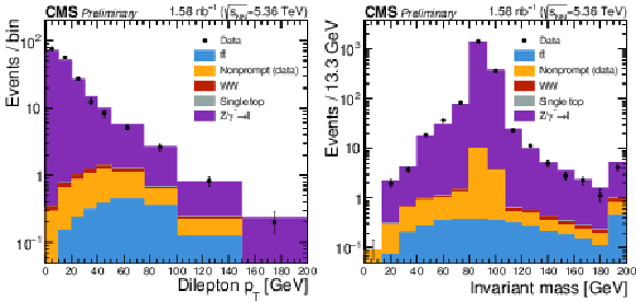
Figure 1:
Distributions of events in the $ p_{\mathrm{T}}(\ell\ell) $ (left) and $ m(\ell\ell) $ (right) variables in the same flavor ($ \ell\ell $) channels. The $ m(\ell\ell) $ distribution is shown prior to the veto of the Z boson resonant region. The data (black marker) is overlaid on top of the stacked contribution of the expectations for the $ \mathrm{t} \overline{\mathrm{t}} $ (blue), nonprompt (yellow), WW (red), single top (gray) and DY (violet) processes. Overflows are included in the last bin. |
png pdf |
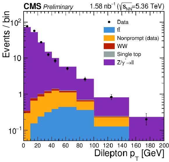
Figure 1-a:
Distributions of events in the $ p_{\mathrm{T}}(\ell\ell) $ (left) and $ m(\ell\ell) $ (right) variables in the same flavor ($ \ell\ell $) channels. The $ m(\ell\ell) $ distribution is shown prior to the veto of the Z boson resonant region. The data (black marker) is overlaid on top of the stacked contribution of the expectations for the $ \mathrm{t} \overline{\mathrm{t}} $ (blue), nonprompt (yellow), WW (red), single top (gray) and DY (violet) processes. Overflows are included in the last bin. |
png pdf |
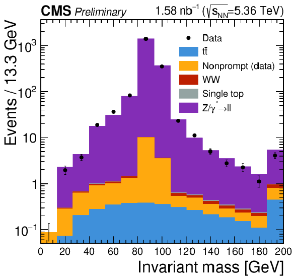
Figure 1-b:
Distributions of events in the $ p_{\mathrm{T}}(\ell\ell) $ (left) and $ m(\ell\ell) $ (right) variables in the same flavor ($ \ell\ell $) channels. The $ m(\ell\ell) $ distribution is shown prior to the veto of the Z boson resonant region. The data (black marker) is overlaid on top of the stacked contribution of the expectations for the $ \mathrm{t} \overline{\mathrm{t}} $ (blue), nonprompt (yellow), WW (red), single top (gray) and DY (violet) processes. Overflows are included in the last bin. |
png pdf |
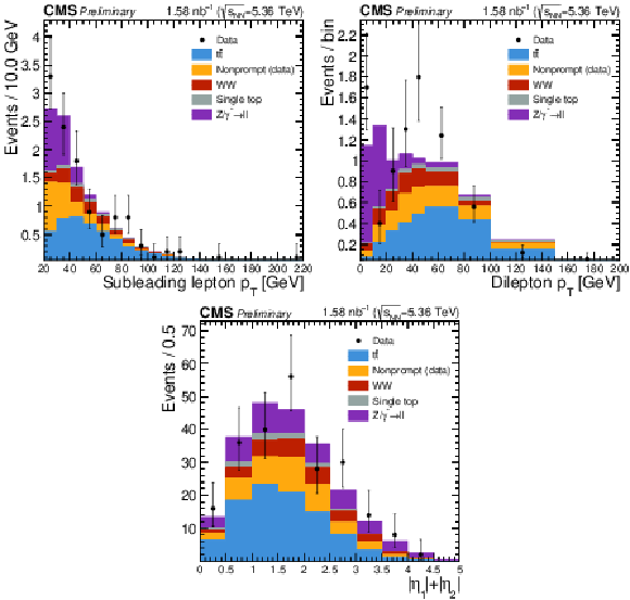
Figure 2:
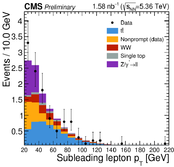
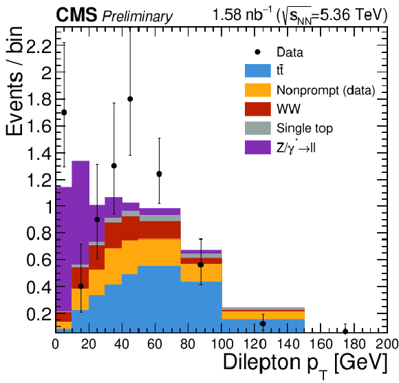
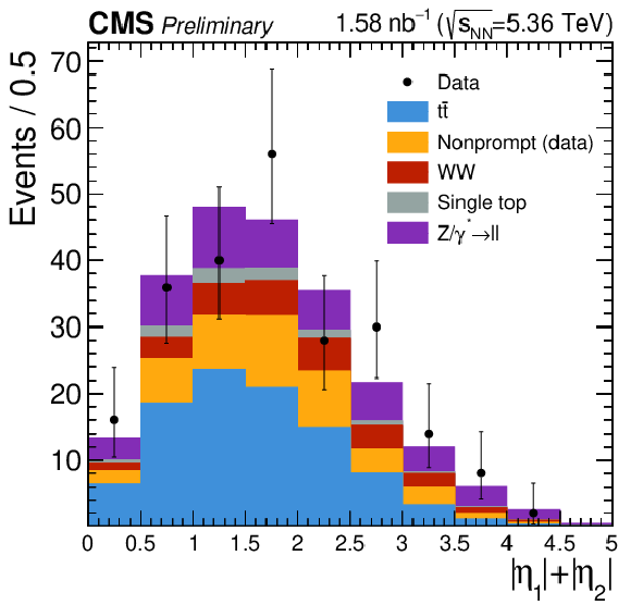
Distributions of events in the $ p_{\mathrm{T}}(\ell_2) $ (upper-left), $ p_{\mathrm{T}}(\ell\ell) $ (upper-right) and $ \sum |\eta_\ell| $ (lower) variables in the opposite flavor ($ \mathrm{e}\mu $) channel. The data (black marker) is overlaid on top of the stacked contribution of the expectations for the $ \mathrm{t} \overline{\mathrm{t}} $ (blue), nonprompt (yellow), WW (red), single top (gray) and DY (violet) processes. Overflows are included in the last bin. |
png pdf |
Figure 2-a:
Distributions of events in the $ p_{\mathrm{T}}(\ell_2) $ (upper-left), $ p_{\mathrm{T}}(\ell\ell) $ (upper-right) and $ \sum |\eta_\ell| $ (lower) variables in the opposite flavor ($ \mathrm{e}\mu $) channel. The data (black marker) is overlaid on top of the stacked contribution of the expectations for the $ \mathrm{t} \overline{\mathrm{t}} $ (blue), nonprompt (yellow), WW (red), single top (gray) and DY (violet) processes. Overflows are included in the last bin. |
png pdf |
Figure 2-b:
Distributions of events in the $ p_{\mathrm{T}}(\ell_2) $ (upper-left), $ p_{\mathrm{T}}(\ell\ell) $ (upper-right) and $ \sum |\eta_\ell| $ (lower) variables in the opposite flavor ($ \mathrm{e}\mu $) channel. The data (black marker) is overlaid on top of the stacked contribution of the expectations for the $ \mathrm{t} \overline{\mathrm{t}} $ (blue), nonprompt (yellow), WW (red), single top (gray) and DY (violet) processes. Overflows are included in the last bin. |
png pdf |
Figure 2-c:
Distributions of events in the $ p_{\mathrm{T}}(\ell_2) $ (upper-left), $ p_{\mathrm{T}}(\ell\ell) $ (upper-right) and $ \sum |\eta_\ell| $ (lower) variables in the opposite flavor ($ \mathrm{e}\mu $) channel. The data (black marker) is overlaid on top of the stacked contribution of the expectations for the $ \mathrm{t} \overline{\mathrm{t}} $ (blue), nonprompt (yellow), WW (red), single top (gray) and DY (violet) processes. Overflows are included in the last bin. |
png pdf |
Figure 3:
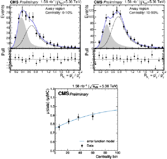
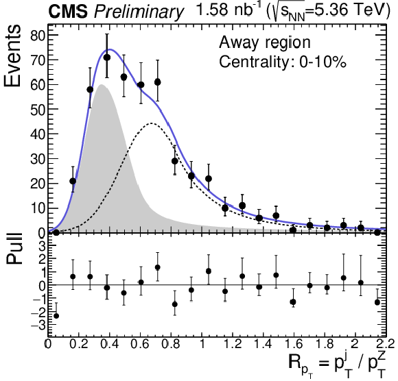
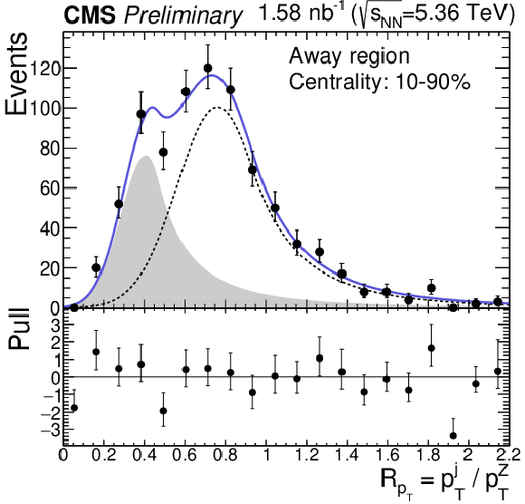
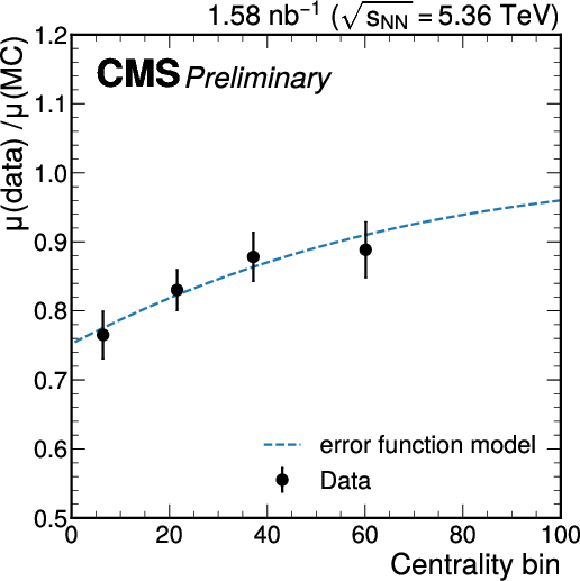
Results of the fits to the $ R_{p_{\mathrm{T}}}=p_{\mathrm{T}}({\rm jet})/p_{\mathrm{T}}(\mathrm{Z}) $ in $ \text{Z+jet} $ events in centrality bins of 0 -10% (upper-left) and 10-90% (upper-right). The upper panels show the estimated contribution from the underlying event jets (gray histogram) and the signal (black dashed line) stacked. The lower panel displays the pull distribution. The lower panel shows the ratio of the average $ R_{p_{\mathrm{T}}} $ in data over the $ R_{p_{\mathrm{T}}} $ in simulation as a function of the collision centrality. A fit to an error function (blue dashed line) is superimposed. |
png pdf |
Figure 3-a:
Results of the fits to the $ R_{p_{\mathrm{T}}}=p_{\mathrm{T}}({\rm jet})/p_{\mathrm{T}}(\mathrm{Z}) $ in $ \text{Z+jet} $ events in centrality bins of 0 -10% (upper-left) and 10-90% (upper-right). The upper panels show the estimated contribution from the underlying event jets (gray histogram) and the signal (black dashed line) stacked. The lower panel displays the pull distribution. The lower panel shows the ratio of the average $ R_{p_{\mathrm{T}}} $ in data over the $ R_{p_{\mathrm{T}}} $ in simulation as a function of the collision centrality. A fit to an error function (blue dashed line) is superimposed. |
png pdf |
Figure 3-b:
Results of the fits to the $ R_{p_{\mathrm{T}}}=p_{\mathrm{T}}({\rm jet})/p_{\mathrm{T}}(\mathrm{Z}) $ in $ \text{Z+jet} $ events in centrality bins of 0 -10% (upper-left) and 10-90% (upper-right). The upper panels show the estimated contribution from the underlying event jets (gray histogram) and the signal (black dashed line) stacked. The lower panel displays the pull distribution. The lower panel shows the ratio of the average $ R_{p_{\mathrm{T}}} $ in data over the $ R_{p_{\mathrm{T}}} $ in simulation as a function of the collision centrality. A fit to an error function (blue dashed line) is superimposed. |
png pdf |
Figure 3-c:
Results of the fits to the $ R_{p_{\mathrm{T}}}=p_{\mathrm{T}}({\rm jet})/p_{\mathrm{T}}(\mathrm{Z}) $ in $ \text{Z+jet} $ events in centrality bins of 0 -10% (upper-left) and 10-90% (upper-right). The upper panels show the estimated contribution from the underlying event jets (gray histogram) and the signal (black dashed line) stacked. The lower panel displays the pull distribution. The lower panel shows the ratio of the average $ R_{p_{\mathrm{T}}} $ in data over the $ R_{p_{\mathrm{T}}} $ in simulation as a function of the collision centrality. A fit to an error function (blue dashed line) is superimposed. |
png pdf |
Figure 4:
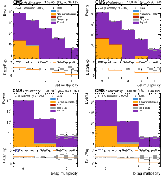
Jet (upper row) and b jet (lower row) counting in Z boson candidate events. The left (right) plots correspond to events in the 0-10% (10-90%) centrality bin. Overflows are included in the last bin. The upper panels display the post-fit stacked model of the $ \mathrm{t} \overline{\mathrm{t}} $ (blue), nonprompt (yellow), WW (red), single top (gray) and DY (violet) processes, and the data (black marker). The bottom panels show the data-to-expectation ratios before (yellow line) and after (black marker) the fit. The dashed band represents the post-fit uncertainty of the model in each bin. |
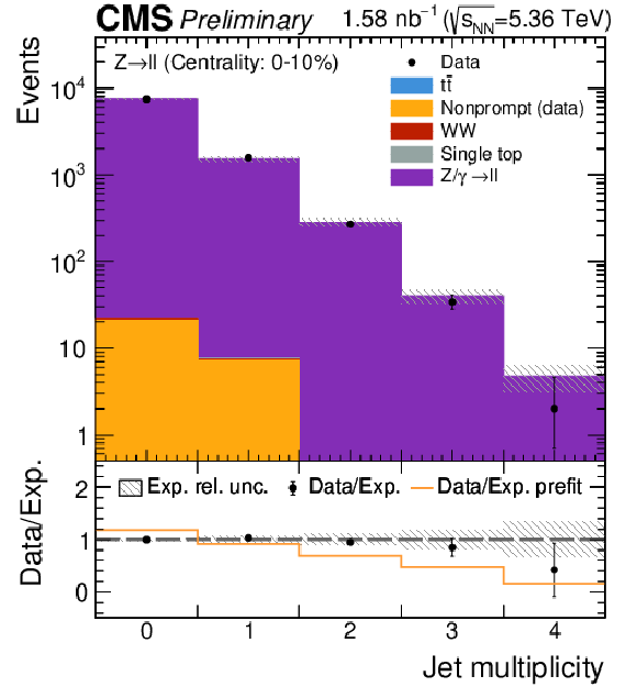
png pdf |
Figure 4-a:
Jet (upper row) and b jet (lower row) counting in Z boson candidate events. The left (right) plots correspond to events in the 0-10% (10-90%) centrality bin. Overflows are included in the last bin. The upper panels display the post-fit stacked model of the $ \mathrm{t} \overline{\mathrm{t}} $ (blue), nonprompt (yellow), WW (red), single top (gray) and DY (violet) processes, and the data (black marker). The bottom panels show the data-to-expectation ratios before (yellow line) and after (black marker) the fit. The dashed band represents the post-fit uncertainty of the model in each bin. |
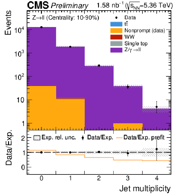
png pdf |
Figure 4-b:
Jet (upper row) and b jet (lower row) counting in Z boson candidate events. The left (right) plots correspond to events in the 0-10% (10-90%) centrality bin. Overflows are included in the last bin. The upper panels display the post-fit stacked model of the $ \mathrm{t} \overline{\mathrm{t}} $ (blue), nonprompt (yellow), WW (red), single top (gray) and DY (violet) processes, and the data (black marker). The bottom panels show the data-to-expectation ratios before (yellow line) and after (black marker) the fit. The dashed band represents the post-fit uncertainty of the model in each bin. |
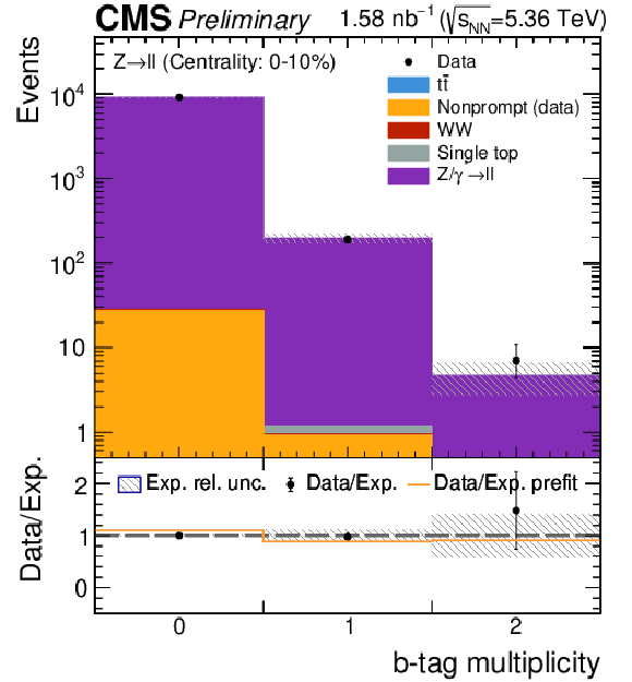
png pdf |
Figure 4-c:
Jet (upper row) and b jet (lower row) counting in Z boson candidate events. The left (right) plots correspond to events in the 0-10% (10-90%) centrality bin. Overflows are included in the last bin. The upper panels display the post-fit stacked model of the $ \mathrm{t} \overline{\mathrm{t}} $ (blue), nonprompt (yellow), WW (red), single top (gray) and DY (violet) processes, and the data (black marker). The bottom panels show the data-to-expectation ratios before (yellow line) and after (black marker) the fit. The dashed band represents the post-fit uncertainty of the model in each bin. |
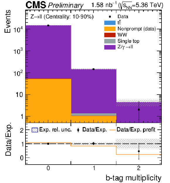
png pdf |
Figure 4-d:
Jet (upper row) and b jet (lower row) counting in Z boson candidate events. The left (right) plots correspond to events in the 0-10% (10-90%) centrality bin. Overflows are included in the last bin. The upper panels display the post-fit stacked model of the $ \mathrm{t} \overline{\mathrm{t}} $ (blue), nonprompt (yellow), WW (red), single top (gray) and DY (violet) processes, and the data (black marker). The bottom panels show the data-to-expectation ratios before (yellow line) and after (black marker) the fit. The dashed band represents the post-fit uncertainty of the model in each bin. |
png pdf |
Figure 5:
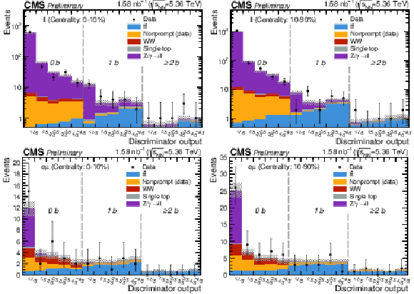
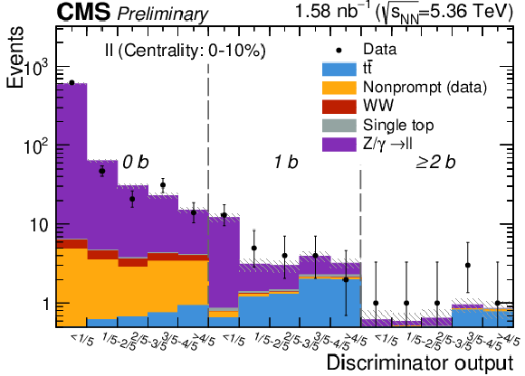
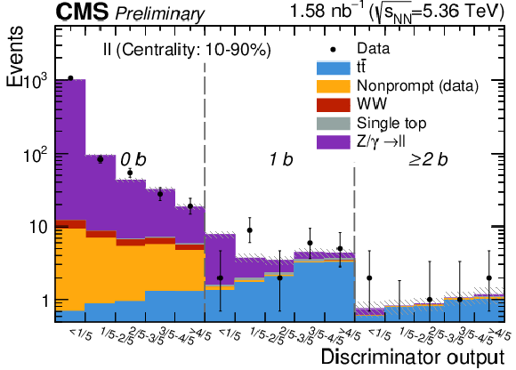
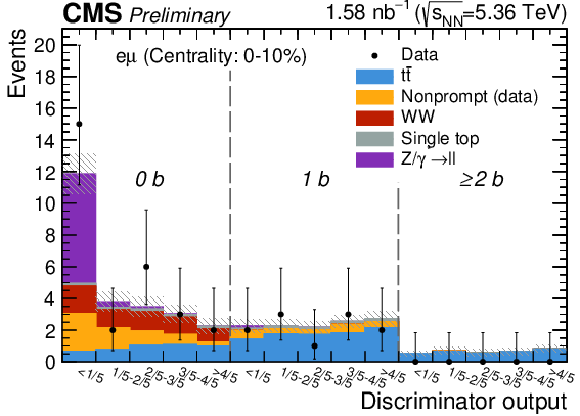
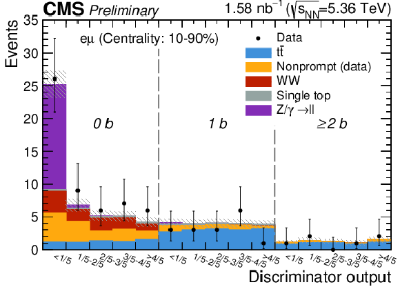
Distributions of the final discriminator after the fit for the same flavor $ \ell\ell $ (upper row) and opposite flavor $ \mathrm{e}\mu $ (lower row) channels. The discriminator output is shown for 0, 1 and $ \geq $ 2 b-tag jet events. The left (right) figure corresponds to events reconstructed in the 0-10% (10-90%) centrality bins. The panels display the stacked contributions of the $ \mathrm{t} \overline{\mathrm{t}} $ (blue), nonprompt (yellow), WW (red), single top (gray) and DY (violet) processes normalized to the post-fit expectations and the data (black marker). The gray band shows the total uncertainty in the predicted yields after the fit is performed. |
png pdf |
Figure 5-a:
Distributions of the final discriminator after the fit for the same flavor $ \ell\ell $ (upper row) and opposite flavor $ \mathrm{e}\mu $ (lower row) channels. The discriminator output is shown for 0, 1 and $ \geq $ 2 b-tag jet events. The left (right) figure corresponds to events reconstructed in the 0-10% (10-90%) centrality bins. The panels display the stacked contributions of the $ \mathrm{t} \overline{\mathrm{t}} $ (blue), nonprompt (yellow), WW (red), single top (gray) and DY (violet) processes normalized to the post-fit expectations and the data (black marker). The gray band shows the total uncertainty in the predicted yields after the fit is performed. |
png pdf |
Figure 5-b:
Distributions of the final discriminator after the fit for the same flavor $ \ell\ell $ (upper row) and opposite flavor $ \mathrm{e}\mu $ (lower row) channels. The discriminator output is shown for 0, 1 and $ \geq $ 2 b-tag jet events. The left (right) figure corresponds to events reconstructed in the 0-10% (10-90%) centrality bins. The panels display the stacked contributions of the $ \mathrm{t} \overline{\mathrm{t}} $ (blue), nonprompt (yellow), WW (red), single top (gray) and DY (violet) processes normalized to the post-fit expectations and the data (black marker). The gray band shows the total uncertainty in the predicted yields after the fit is performed. |
png pdf |
Figure 5-c:
Distributions of the final discriminator after the fit for the same flavor $ \ell\ell $ (upper row) and opposite flavor $ \mathrm{e}\mu $ (lower row) channels. The discriminator output is shown for 0, 1 and $ \geq $ 2 b-tag jet events. The left (right) figure corresponds to events reconstructed in the 0-10% (10-90%) centrality bins. The panels display the stacked contributions of the $ \mathrm{t} \overline{\mathrm{t}} $ (blue), nonprompt (yellow), WW (red), single top (gray) and DY (violet) processes normalized to the post-fit expectations and the data (black marker). The gray band shows the total uncertainty in the predicted yields after the fit is performed. |
png pdf |
Figure 5-d:
Distributions of the final discriminator after the fit for the same flavor $ \ell\ell $ (upper row) and opposite flavor $ \mathrm{e}\mu $ (lower row) channels. The discriminator output is shown for 0, 1 and $ \geq $ 2 b-tag jet events. The left (right) figure corresponds to events reconstructed in the 0-10% (10-90%) centrality bins. The panels display the stacked contributions of the $ \mathrm{t} \overline{\mathrm{t}} $ (blue), nonprompt (yellow), WW (red), single top (gray) and DY (violet) processes normalized to the post-fit expectations and the data (black marker). The gray band shows the total uncertainty in the predicted yields after the fit is performed. |
png pdf |
Figure 6:
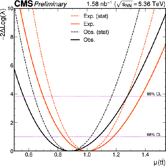
Scan of the profile likelihood as a function of the $ \mathrm{t} \overline{\mathrm{t}} $ signal strength. The expected and observed scans are overlaid. In each case, two additional curves corresponding to the scan resulting from freezing the systematic uncertainties are overlaid. The horizontal dashed lines represent the likelihood values (confidence level - CL) used to extract the 68% and 95% confidence intervals on the parameter of interest. |
png pdf |
Figure 7:
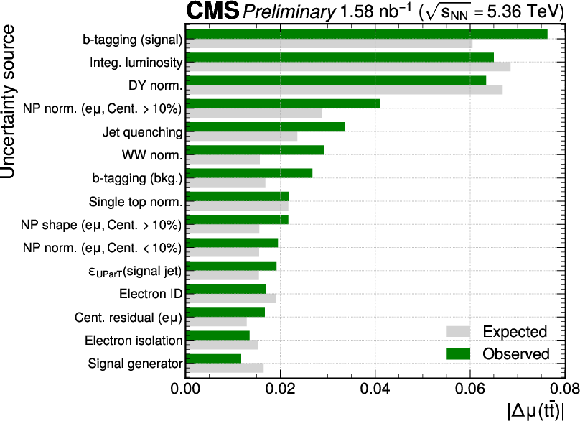
Impact of systematic uncertainties on the fitted $ \mathrm{t} \overline{\mathrm{t}} $ strength parameter. The systematic uncertainties are listed in decreasing order of their impact on the strength parameter in the vertical axis. |
png pdf |
Figure 8:
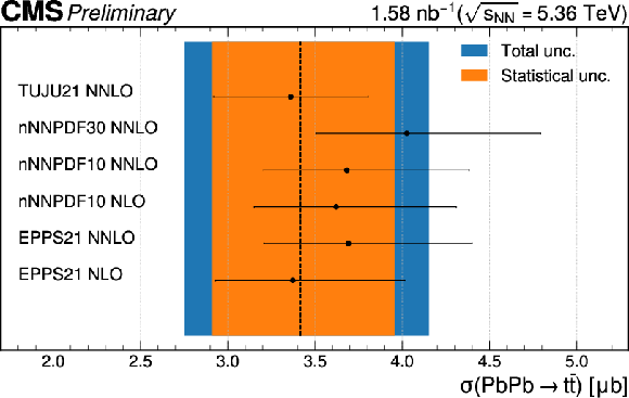
Comparison between the measured $ \mathrm{t} \overline{\mathrm{t}} $ cross section (shaded area) and the SM theory predictions (black markers) employing the TUJU21 [53], nNNPDF30 [54], nNNPDF10 [55] and EPPS21 [21] nuclear PDF sets. The error bars represent the uncertainties of the theory calculations while the blue (orange) area shows the total (statistical) uncertainties of the measured $ \mathrm{t} \overline{\mathrm{t}} $ cross section. |
png pdf |
Figure 9:
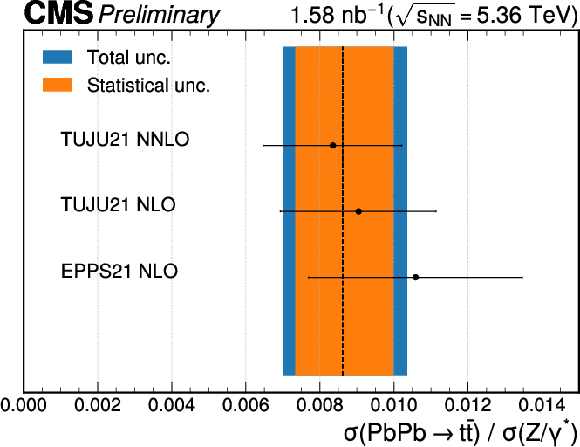
Comparison between the measured ratio of $ \mathrm{t} \overline{\mathrm{t}} $ over DY cross sections (shaded area) and the Standard Model theory predictions (black markers) employing the TUJU21 [53] and EPPS21 [21] nuclear PDF sets. The error bars represent the uncertainties of the theory calculations while the blue (orange) area shows the total (statistical) uncertainties of the measured $ \mathrm{t} \overline{\mathrm{t}} $ over DY ratio. |
png pdf |
Figure 10:
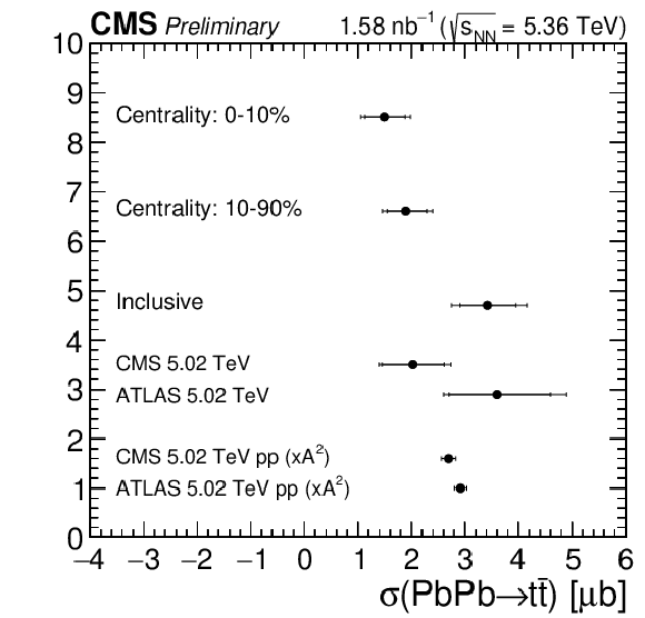
Comparison between the measured $ \mathrm{t} \overline{\mathrm{t}} $ cross section in PbPb at 5.36 TeV and the past measurements performed by the ATLAS and CMS collaborations in PbPb at 5.02 TeV and pp at 5.02 TeV scaled by the Pb mass number (A) squared. The error bars on each marker represent the statistical and total uncertainties. |
| Summary |
| We have presented the first measurement of the production cross section of top quark pairs in lead-lead collisions, $ \sigma(\mathrm{Pb}\mathrm{Pb}\rightarrow{\mathrm{t}\overline{\mathrm{t}}} ) $, at $ \sqrt{\smash[b]{s_{_{\mathrm{NN}}}}}= $ 5.36 TeV. Using dilepton events, selected in the 2023 data set recorded by the CMS experiment, the $ \sigma(\mathrm{Pb}\mathrm{Pb}\rightarrow{\mathrm{t}\overline{\mathrm{t}}} ) $, along with its ratio to the Drell-Yan cross section, are measured with total uncertainties of approximately 21%, and are both found to be in agreement with the standard model. New techniques used in this analysis, such as the electron identification criteria, the lepton isolation criteria, the calibration of the jet energy scale, and the identification of heavy-flavor jets, lead to a significant improvement in precision compared to previous $ \sigma(\mathrm{Pb}\mathrm{Pb}\rightarrow{\mathrm{t}\overline{\mathrm{t}}} ) $ measurements at the LHC. Combined with the increased center-of-mass energy and integrated luminosity expected for the remainder of Run 3, these advances establish top quark physics as a precision tool for studying the formation and properties of the quark-gluon plasma in heavy ion collisions. |
| References | ||||
| 1 | CMS Collaboration | Stairway to discovery: A report on the CMS programme of cross section measurements from millibarns to femtobarns | Phys. Rept. 1115 (2025) 3 | CMS-SMP-23-004 2405.18661 |
| 2 | ATLAS Collaboration | Climbing to the Top of the ATLAS 13 TeV data | Phys. Rept. 1116 (2025) 127 | 2404.10674 |
| 3 | Particle Data Group Collaboration | Review of particle physics | PRD 110 (2024) 30001 | |
| 4 | CMS Collaboration | Measurement of the $ \mathrm{t} \overline{\mathrm{t}} $ production cross section, the top quark mass, and the strong coupling constant using dilepton events in pp collisions at $ \sqrt{s} = $ 13 TeV | EPJC 79 (2019) 368 | CMS-TOP-17-001 1812.10505 |
| 5 | CMS Collaboration | Measurement of differential $ \mathrm{t} \overline{\mathrm{t}} $ production cross sections in the full kinematic range using lepton+jets events from proton-proton collisions at $ \sqrt {s} = $ 13 TeV | PRD 104 (2021) 92013 | CMS-TOP-20-001 2108.02803 |
| 6 | D. d'Enterria, K. Krajczar, and H. Paukkunen | Top-quark production in proton-nucleus and nucleus-nucleus collisions at LHC energies and beyond | PLB 746 (2015) 64 | 1501.05879 |
| 7 | L. Apolinario, J. G. Milhano, G. P. Salam, and C. A. Salgado | Probing the time structure of the quark-gluon plasma with top quarks | PRL 120 (2018) 232301 | 1711.03105 |
| 8 | CMS Collaboration | Observation of top quark production in proton-nucleus collisions | PRL 119 (2017) 242001 | CMS-HIN-17-002 1709.07411 |
| 9 | ATLAS Collaboration | Observation of $ t\overline{t} $ production in the lepton+jets and dilepton channels in p+Pb collisions at $ \sqrt{s_{\textrm{NN}}} = $ 8.16 TeV with the ATLAS detector | JHEP 11 (2024) 101 | 2405.05078 |
| 10 | CMS Collaboration | Evidence for Top Quark Production in Nucleus-Nucleus Collisions | PRL 125 (2020) 222001 | CMS-HIN-19-001 2006.11110 |
| 11 | ATLAS Collaboration | Observation of $ \mathrm{t} \overline{\mathrm{t}} $ production in Pb+Pb Collisions at $ \sqrt{\smash[b]{s_{_{\mathrm{NN}}}}} = $ 5.02 TeV with the ATLAS detector | PRL 134 (2025) 142301 | 2411.10186 |
| 12 | CMS Collaboration | The CMS experiment at the CERN LHC | JINST 3 (2008) S08004 | |
| 13 | CMS Collaboration | Development of the CMS detector for the CERN LHC Run 3 | JINST 19 (2024) P05064 | |
| 14 | CMS Collaboration | Performance of the CMS Level-1 trigger in proton-proton collisions at $ \sqrt{s} = $ 13 TeV | JINST 15 (2020) P10017 | CMS-TRG-17-001 2006.10165 |
| 15 | CMS Collaboration | The CMS trigger system | JINST 12 (2017) P01020 | CMS-TRG-12-001 1609.02366 |
| 16 | CMS Collaboration | Performance of the CMS high-level trigger during LHC run 2 | JINST 19 (2024) P11021 | CMS-TRG-19-001 2410.17038 |
| 17 | CMS Collaboration | Electron and photon reconstruction and identification with the CMS experiment at the CERN LHC | JINST 16 (2021) P05014 | CMS-EGM-17-001 2012.06888 |
| 18 | CMS Collaboration | Performance of the CMS muon detector and muon reconstruction with proton-proton collisions at $ \sqrt{s}= $ 13 TeV | JINST 13 (2018) P06015 | CMS-MUO-16-001 1804.04528 |
| 19 | CMS Collaboration | Description and performance of track and primary-vertex reconstruction with the CMS tracker | JINST 9 (2014) P10009 | CMS-TRK-11-001 1405.6569 |
| 20 | CMS Collaboration | Particle-flow reconstruction and global event description with the CMS detector | JINST 12 (2017) P10003 | CMS-PRF-14-001 1706.04965 |
| 21 | K. J. Eskola, P. Paakkinen, H. Paukkunen, and C. A. Salgado | EPPS21: a global QCD analysis of nuclear PDFs | EPJC 82 (2022) 413 | 2112.12462 |
| 22 | T. Sjöstrand et al. | An introduction to PYTHIA 8.2 | Comput. Phys. Commun. 191 (2015) 159 | 1410.3012 |
| 23 | I. P. Lokhtin et al. | Heavy ion event generator HYDJET++ (HYDrodynamics plus JETs) | Comput. Phys. Commun. 180 (2009) 779 | 0809.2708 |
| 24 | CMS Collaboration | Extraction and validation of a new set of CMS PYTHIA8 tunes from underlying-event measurements | EPJC 80 (2020) 4 | CMS-GEN-17-001 1903.12179 |
| 25 | D. d'Enterria and C. Loizides | Progress in the Glauber Model at Collider Energies | Ann. Rev. Nucl. Part. Sci. 71 (2021) 315 | 2011.14909 |
| 26 | GEANT4 Collaboration | GEANT4--a simulation toolkit | NIM A 506 (2003) 250 | |
| 27 | J. Alwall et al. | The automated computation of tree-level and next-to-leading order differential cross sections, and their matching to parton shower simulations | JHEP 07 (2014) 079 | 1405.0301 |
| 28 | S. Frixione, P. Nason, and G. Ridolfi | A Positive-weight next-to-leading-order Monte Carlo for heavy flavour hadroproduction | JHEP 09 (2007) 126 | 0707.3088 |
| 29 | R. Frederix and S. Frixione | Merging meets matching in MC@NLO | JHEP 12 (2012) 61 | 1209.6215 |
| 30 | M. Czakon, P. Fiedler, and A. Mitov | Total Top-Quark Pair-Production Cross Section at Hadron Colliders Through $ O(\alpha^4_S) $ | PRL 110 (2013) 252004 | 1303.6254 |
| 31 | E. Re | Single-top Wt-channel production matched with parton showers using the POWHEG method | EPJC 71 (2011) 1547 | 1009.2450 |
| 32 | T. Chen and C. Guestrin | Xgboost: A scalable tree boosting system | 02754, 2016 CoRR 160 (2016) 3 |
1603.02754 |
| 33 | F. Pedregosa et al. | Scikit-learn: Machine learning in python | CoRR abs/1201.0490, 2012 link |
1201.0490 |
| 34 | M. Cacciari, G. P. Salam, and G. Soyez | SoftKiller, a particle-level pileup removal method | EPJC 75 (2015) 59 | 1407.0408 |
| 35 | R. Pezoa, L. Salinas, and C. Torres | Explainability of High Energy Physics events classification using SHAP | J. Phys. Conf. Ser. 2438 (2023) 12082 | |
| 36 | T. Akiba et al. | Optuna: A next-generation hyperparameter optimization framework | in Proceedings of the 25th ACM SIGKDD International Conference on Knowledge Discovery and Data Mining. 2019 | |
| 37 | M. Cacciari, G. P. Salam, and G. Soyez | The anti-$ k_{\mathrm{T}} $ jet clustering algorithm | JHEP 04 (2008) 063 | 0802.1189 |
| 38 | M. Cacciari, G. P. Salam, and G. Soyez | FastJet User Manual | EPJC 72 (2012) 1896 | 1111.6097 |
| 39 | CMS Collaboration | A unified approach for jet tagging in Run 3 at $ \sqrt{s} = $ 13.6 TeV in CMS | CMS Detector Performance Summary CMS-DP-2024-066, 2024 CDS |
|
| 40 | CMS Collaboration | Jet tagging performance in Run 3 PbPb collisions at 5.36 TeV in CMS | CMS Detector Performance Summary CMS-DP-2024-088, 2024 CDS |
|
| 41 | CMS Collaboration | Performance of heavy-flavour jet identification in boosted topologies in proton-proton collisions at $ \sqrt{s} = $ 13 TeV | CMS Physics Analysis Summary, 2023 link |
CMS-PAS-BTV-22-001 |
| 42 | M. Oreglia | A Study of the Reactions $ \psi^\prime \to \gamma \gamma \psi $ | Phd thesis, Stanford University, 1980 | |
| 43 | R. Brun and F. Rademakers | ROOT: An object oriented data analysis framework | NIM A 389 (1997) 81 | |
| 44 | J. S. Conway | Incorporating Nuisance Parameters in Likelihoods for Multisource Spectra | in PHYSTAT 2011, p. 115. 2011 link |
1103.0354 |
| 45 | CMS Collaboration | The CMS statistical analysis and combination tool: Combine | Comput. Softw. Big Sci. 8 (2024) 19 | CMS-CAT-23-001 2404.06614 |
| 46 | W. Verkerke and D. Kirkby | The RooFit toolkit for data modeling | in Proc. 13th International Conference on Computing in High Energy and Nuclear Physics (CHEP 2003): La Jolla CA, United States, March 24--28, 2003. 2003 link |
physics/0306116 |
| 47 | L. Moneta et al. | The RooStats project | in Proc. 13th International Workshop on Advanced Computing and Analysis Techniques in Physics Research (ACAT 2010): Jaipur, India, February 22--27, 2010. 2010 link |
1009.1003 |
| 48 | S. van der Meer | Calibration of the Effective Beam Height in the ISR | ||
| 49 | R. J. Barlow and C. Beeston | Fitting using finite Monte Carlo samples | Comput. Phys. Commun. 77 (1993) 219 | |
| 50 | J. Butterworth et al. | PDF4LHC recommendations for LHC Run II | JPG 43 (2016) 23001 | 1510.03865 |
| 51 | CMS Collaboration | Differential cross section measurements for the production of top quark pairs and of additional jets using dilepton events from pp collisions at $ \sqrt{s} = $ 13 TeV | JHEP 02 (2025) 064 | CMS-TOP-20-006 2402.08486 |
| 52 | G. Cowan, K. Cranmer, E. Gross, and O. Vitells | Asymptotic formulae for likelihood-based tests of new physics | EPJC 71 (2011) 1554 | 1007.1727 |
| 53 | I. Helenius, M. Walt, and W. Vogelsang | NNLO nuclear parton distribution functions with electroweak-boson production data from the LHC | PRD 105 (2022) 94031 | 2112.11904 |
| 54 | R. Abdul Khalek et al. | nNNPDF3.0: evidence for a modified partonic structure in heavy nuclei | EPJC 82 (2022) 507 | 2201.12363 |
| 55 | NNPDF Collaboration | Nuclear parton distributions from lepton-nucleus scattering and the impact of an electron-ion collider | EPJC 79 (2019) 471 | 1904.00018 |

|
Compact Muon Solenoid LHC, CERN |

|

|

|

|

|

|