
Compact Muon Solenoid
LHC, CERN
 Visit us: CMS Public Website, CMS Physics ;
Contact us: CMS Publications Committee
| CMS-PAS-B2G-25-013 | ||
| Search for a light charged Higgs boson decaying to a W boson and a CP-odd Higgs boson in rare top quark decays in proton-proton collisions at $ \sqrt{s}= $ 13 and 13.6 TeV | ||
| CMS Collaboration | ||
| 2026-10-07 | ||
| Abstract: A search is presented for a light charged Higgs boson ($ \mathrm{H^+} $) and a CP-odd Higgs boson ($ \mathrm{A} $) in top quark pair production. The search targets the decay chain $ \mathrm{t} \to \mathrm{H^+}\mathrm{b} $, followed by $ \mathrm{H^+} \to \mathrm{W}^{+}\mathrm{A} \to \mathrm{W}^{+}\mu^{+}\mu^{-} $, with charge-conjugate processes implied. The analysis uses proton-proton collision data at $ \sqrt{s} = $ 13 and 13.6 TeV collected by the CMS experiment at the CERN LHC, corresponding to a total integrated luminosity of 200 fb$ ^{-1} $. Events with three leptons in the $ \mathrm{e}\mu\mu $ or $ \mu\mu\mu $ final state and at least two jets, including at least one jet identified as originating from a bottom quark, are selected. A graph-based deep neural network is used to suppress backgrounds containing a Z boson for signal hypotheses with $ m_{\mathrm{A}} $ near the Z boson mass. Mass hypotheses with $ m_{\mathrm{H^+}} $ between 70 and 160 GeV and $ m_{\mathrm{A}} $ between 15 GeV and $ (m_{\mathrm{H^+}} - 5 \mathrm{GeV}) $ are explored, covering for the first time the off-shell W boson regime. No significant excess over the standard model prediction is observed, and upper limits at 95% confidence level are set on the product of branching fractions $ \mathcal{B}(\mathrm{t} \to \mathrm{H^+}\mathrm{b}) \times \mathcal{B}(\mathrm{H^+} \to \mathrm{W}^{+}\mathrm{A}) \times \mathcal{B}(\mathrm{A} \to \mu^{+}\mu^{-}) $. The observed upper limits range from 0.5 $ \times 10^{-6} $ to 3.6 $ \times 10^{-6} $ away from the Z boson mass and from 0.8 $ \times 10^{-6} $ to 6.8 $ \times 10^{-6} $ near it. | ||
| Links: CDS record (PDF) ; CADI line (restricted) ; | ||
| Figures | |
png pdf |
Figure 1:
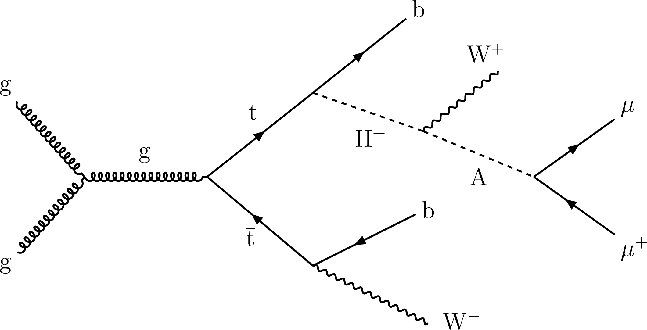
Representative Feynman diagram for the signal process $ \mathrm{g}\mathrm{g} \to \mathrm{t}\overline{\mathrm{t}} \to (\mathrm{H^+}\mathrm{b})(\mathrm{W^-}\overline{\mathrm{b}}) $ with $ \mathrm{H^+} \to \mathrm{W^+}\mathrm{A} \to \mathrm{W^+}\mu^{+}\mu^{-} $. |
png pdf |
Figure 2:
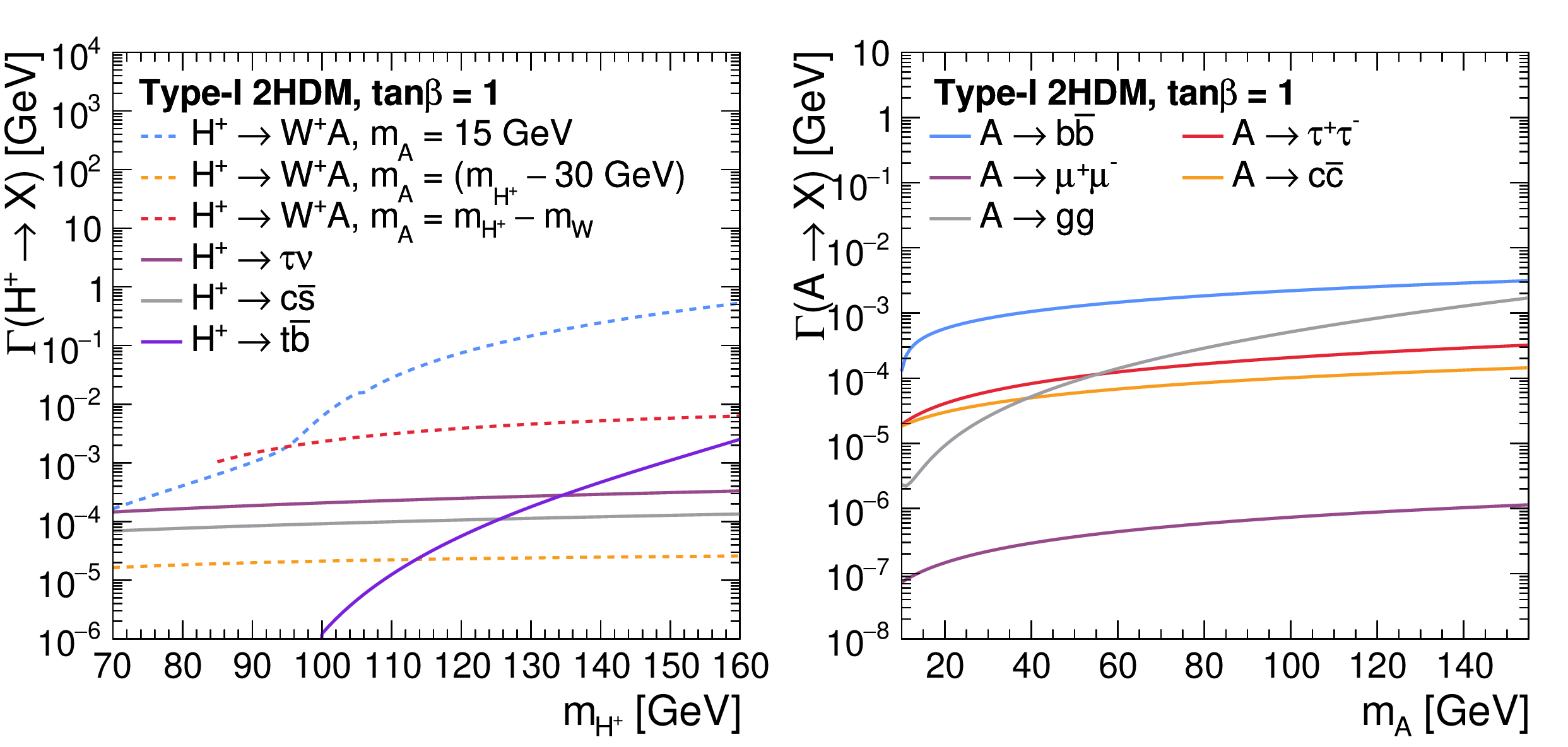
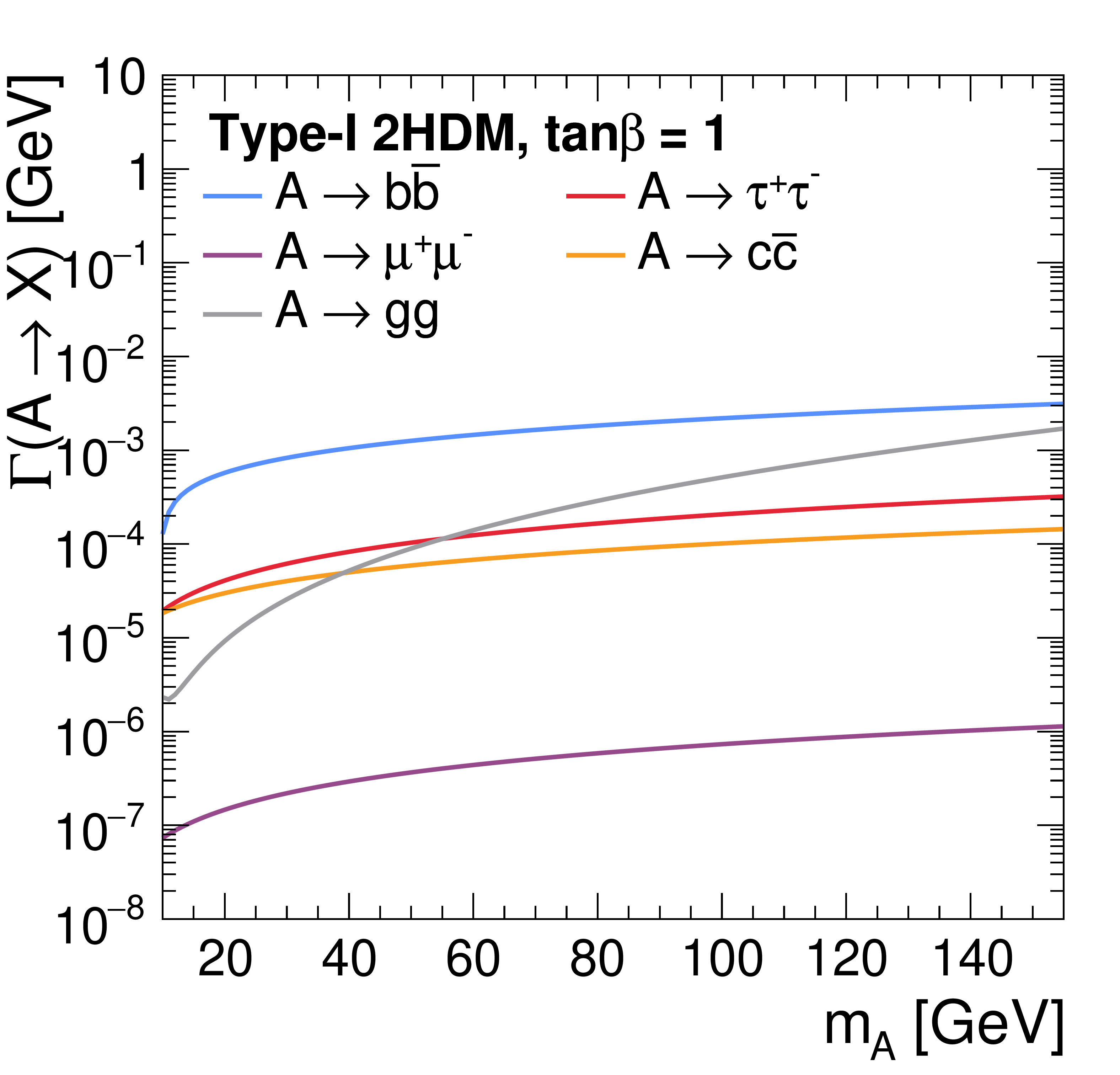
Partial decay widths of the charged Higgs boson (left) and of the CP-odd Higgs boson (right) in the Type-I 2HDM at $ \tan\beta = $ 1, calculated with 2HDMC. The left panel shows the widths as functions of $ \mathit{m}_{\mathrm{H^+}} $, for $ \mathrm{H^+} \to \mathrm{W^+}\mathrm{A} $ with $ \mathit{m}_{\mathrm{A}} = $ 15 GeV, $ (\mathit{m}_{\mathrm{H^+}} - 30 \text{GeV}) $, and $ \mathit{m}_{\mathrm{H^+}} - \mathit{m}_{\mathrm{W}} $, together with the fermionic modes $ \mathrm{H^+} \to \tau^{+}\nu $, $ \mathrm{c}\overline{\mathrm{s}} $, and $ \mathrm{t}\overline{\mathrm{b}} $. The right panel shows the widths as functions of $ \mathit{m}_{\mathrm{A}} $ for $ \mathrm{A} \to \mathrm{b}\overline{\mathrm{b}} $, $ \mathrm{g}\mathrm{g} $, $ \tau^{+}\tau^{-} $, $ \mathrm{c}\overline{\mathrm{c}} $, and $ \mu^{+}\mu^{-} $. |
png pdf |
Figure 2-a:
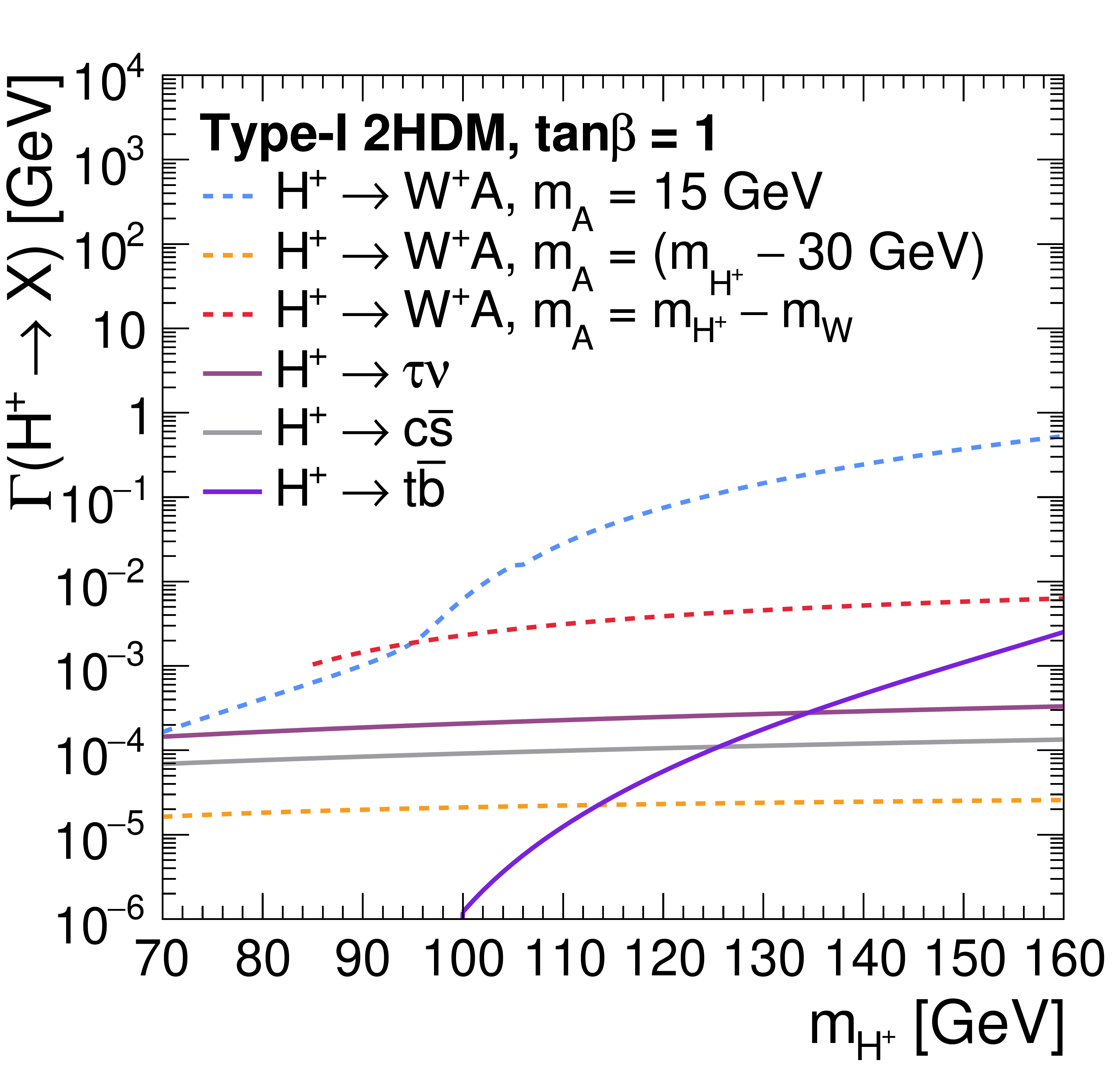
Partial decay widths of the charged Higgs boson (left) and of the CP-odd Higgs boson (right) in the Type-I 2HDM at $ \tan\beta = $ 1, calculated with 2HDMC. The left panel shows the widths as functions of $ \mathit{m}_{\mathrm{H^+}} $, for $ \mathrm{H^+} \to \mathrm{W^+}\mathrm{A} $ with $ \mathit{m}_{\mathrm{A}} = $ 15 GeV, $ (\mathit{m}_{\mathrm{H^+}} - 30 \text{GeV}) $, and $ \mathit{m}_{\mathrm{H^+}} - \mathit{m}_{\mathrm{W}} $, together with the fermionic modes $ \mathrm{H^+} \to \tau^{+}\nu $, $ \mathrm{c}\overline{\mathrm{s}} $, and $ \mathrm{t}\overline{\mathrm{b}} $. The right panel shows the widths as functions of $ \mathit{m}_{\mathrm{A}} $ for $ \mathrm{A} \to \mathrm{b}\overline{\mathrm{b}} $, $ \mathrm{g}\mathrm{g} $, $ \tau^{+}\tau^{-} $, $ \mathrm{c}\overline{\mathrm{c}} $, and $ \mu^{+}\mu^{-} $. |
png pdf |
Figure 2-b:
Partial decay widths of the charged Higgs boson (left) and of the CP-odd Higgs boson (right) in the Type-I 2HDM at $ \tan\beta = $ 1, calculated with 2HDMC. The left panel shows the widths as functions of $ \mathit{m}_{\mathrm{H^+}} $, for $ \mathrm{H^+} \to \mathrm{W^+}\mathrm{A} $ with $ \mathit{m}_{\mathrm{A}} = $ 15 GeV, $ (\mathit{m}_{\mathrm{H^+}} - 30 \text{GeV}) $, and $ \mathit{m}_{\mathrm{H^+}} - \mathit{m}_{\mathrm{W}} $, together with the fermionic modes $ \mathrm{H^+} \to \tau^{+}\nu $, $ \mathrm{c}\overline{\mathrm{s}} $, and $ \mathrm{t}\overline{\mathrm{b}} $. The right panel shows the widths as functions of $ \mathit{m}_{\mathrm{A}} $ for $ \mathrm{A} \to \mathrm{b}\overline{\mathrm{b}} $, $ \mathrm{g}\mathrm{g} $, $ \tau^{+}\tau^{-} $, $ \mathrm{c}\overline{\mathrm{c}} $, and $ \mu^{+}\mu^{-} $. |
png pdf |
Figure 3:
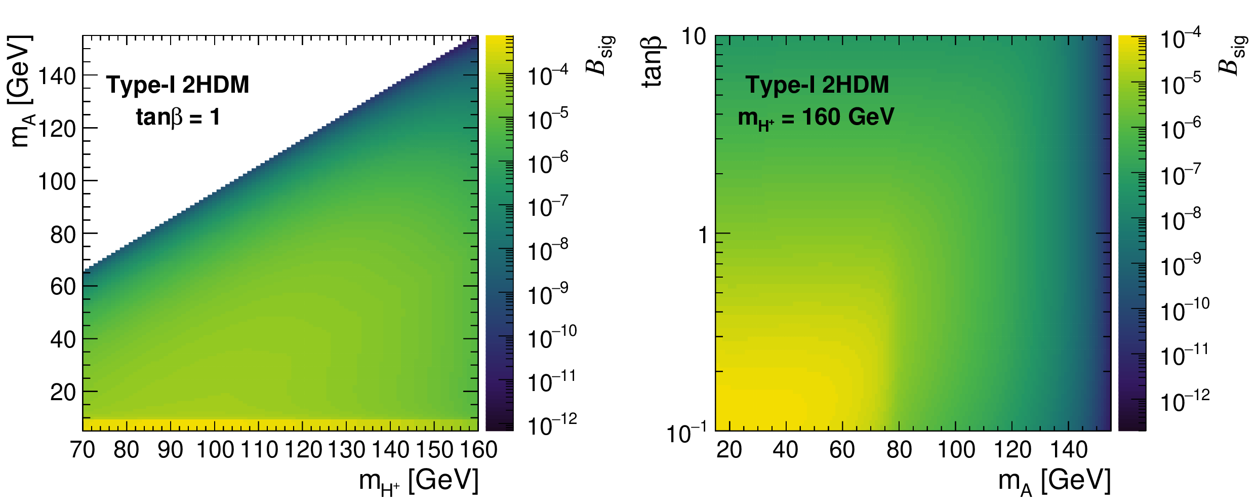
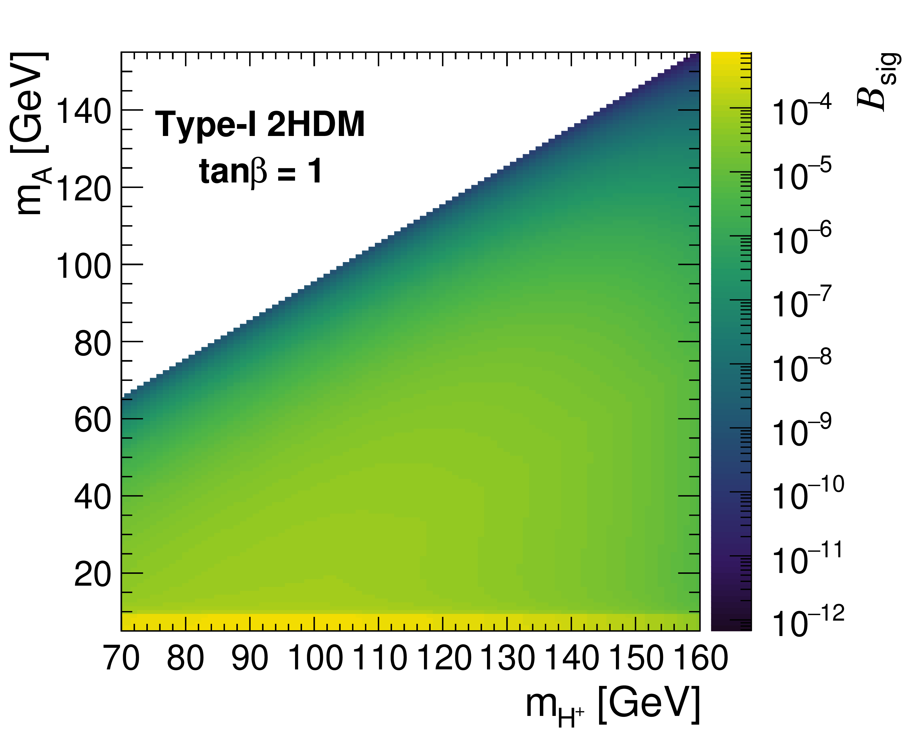
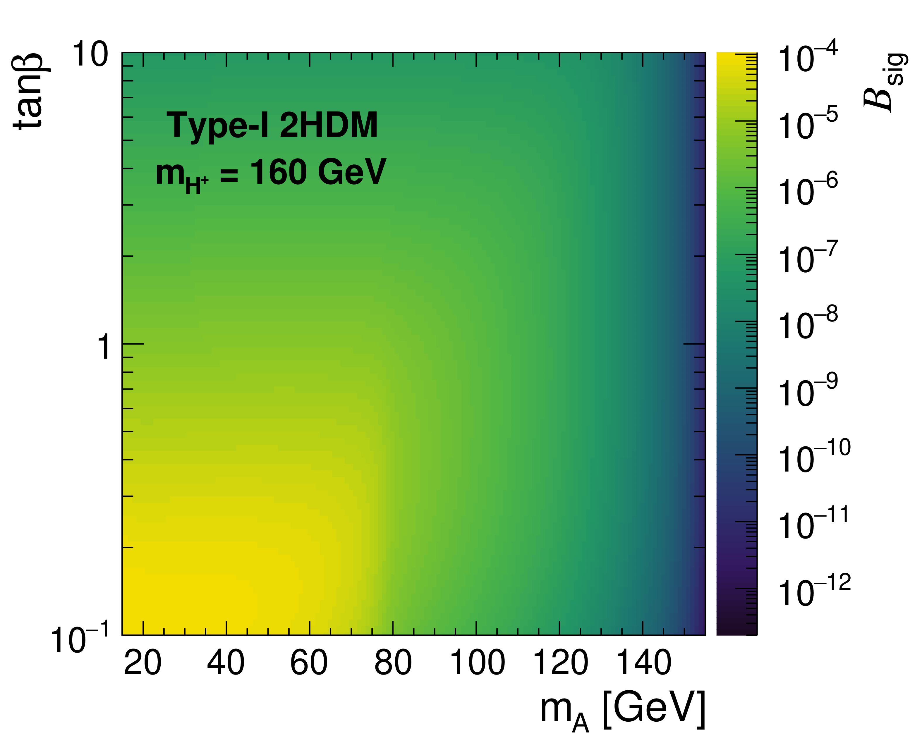
Predicted signal branching fraction $ \mathcal{B}_\text{sig} \equiv \mathcal{B}(\mathrm{t} \to \mathrm{H^+}\mathrm{b}) \times \mathcal{B}(\mathrm{H^+} \to \mathrm{W^+}\mathrm{A}) \times \mathcal{B}(\mathrm{A} \to \mu^{+}\mu^{-}) $ in the Type-I 2HDM, calculated with 2HDMC, in the $ (\mathit{m}_{\mathrm{H^+}}, \mathit{m}_{\mathrm{A}}) $ plane at $ \tan\beta = $ 1 (left) and in the $ (\mathit{m}_{\mathrm{A}}, \tan\beta) $ plane at $ \mathit{m}_{\mathrm{H^+}} = $ 160 GeV (right). |
png pdf |
Figure 3-a:
Predicted signal branching fraction $ \mathcal{B}_\text{sig} \equiv \mathcal{B}(\mathrm{t} \to \mathrm{H^+}\mathrm{b}) \times \mathcal{B}(\mathrm{H^+} \to \mathrm{W^+}\mathrm{A}) \times \mathcal{B}(\mathrm{A} \to \mu^{+}\mu^{-}) $ in the Type-I 2HDM, calculated with 2HDMC, in the $ (\mathit{m}_{\mathrm{H^+}}, \mathit{m}_{\mathrm{A}}) $ plane at $ \tan\beta = $ 1 (left) and in the $ (\mathit{m}_{\mathrm{A}}, \tan\beta) $ plane at $ \mathit{m}_{\mathrm{H^+}} = $ 160 GeV (right). |
png pdf |
Figure 3-b:
Predicted signal branching fraction $ \mathcal{B}_\text{sig} \equiv \mathcal{B}(\mathrm{t} \to \mathrm{H^+}\mathrm{b}) \times \mathcal{B}(\mathrm{H^+} \to \mathrm{W^+}\mathrm{A}) \times \mathcal{B}(\mathrm{A} \to \mu^{+}\mu^{-}) $ in the Type-I 2HDM, calculated with 2HDMC, in the $ (\mathit{m}_{\mathrm{H^+}}, \mathit{m}_{\mathrm{A}}) $ plane at $ \tan\beta = $ 1 (left) and in the $ (\mathit{m}_{\mathrm{A}}, \tan\beta) $ plane at $ \mathit{m}_{\mathrm{H^+}} = $ 160 GeV (right). |
png pdf |
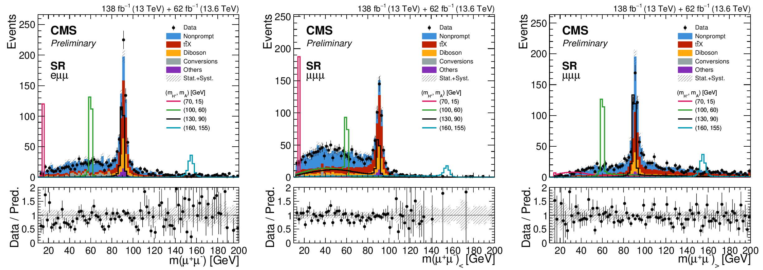
Figure 4:
Dimuon invariant mass distributions after the baseline selection. The left panel shows the OS dimuon mass in the $ \mathrm{e}\mu\mu $ channel, and the center and right panels show $ \mathit{m}(\mu^{+}\mu^{-})_ < $ and $ \mathit{m}(\mu^{+}\mu^{-})_ > $ in the $ \mu\mu\mu $ channel, respectively. The data are compared with the sum of the background predictions, which are grouped into the nonprompt lepton, photon conversion, $ {\mathrm{t}\overline{\mathrm{t}}} \mathrm{X} $, diboson, and other categories defined in Section 3, and the hatched band represents the combined statistical and systematic uncertainty in the prediction. Selected signal mass hypotheses with $ (\mathit{m}_{\mathrm{H^+}}, \mathit{m}_{\mathrm{A}}) = (70, 15) $, $ (100, 60) $, $ (130, 90) $, and $ (160, 155) \text{GeV} $ are overlaid, normalized to a signal cross section of 30 fb at 13 TeV and scaled by the ratio of $ \mathrm{t} \overline{\mathrm{t}} $ cross sections at 13.6 and 13 TeV for the Run 3 data. The lower panel of each distribution shows the ratio of the data to the total background prediction. |
png pdf |
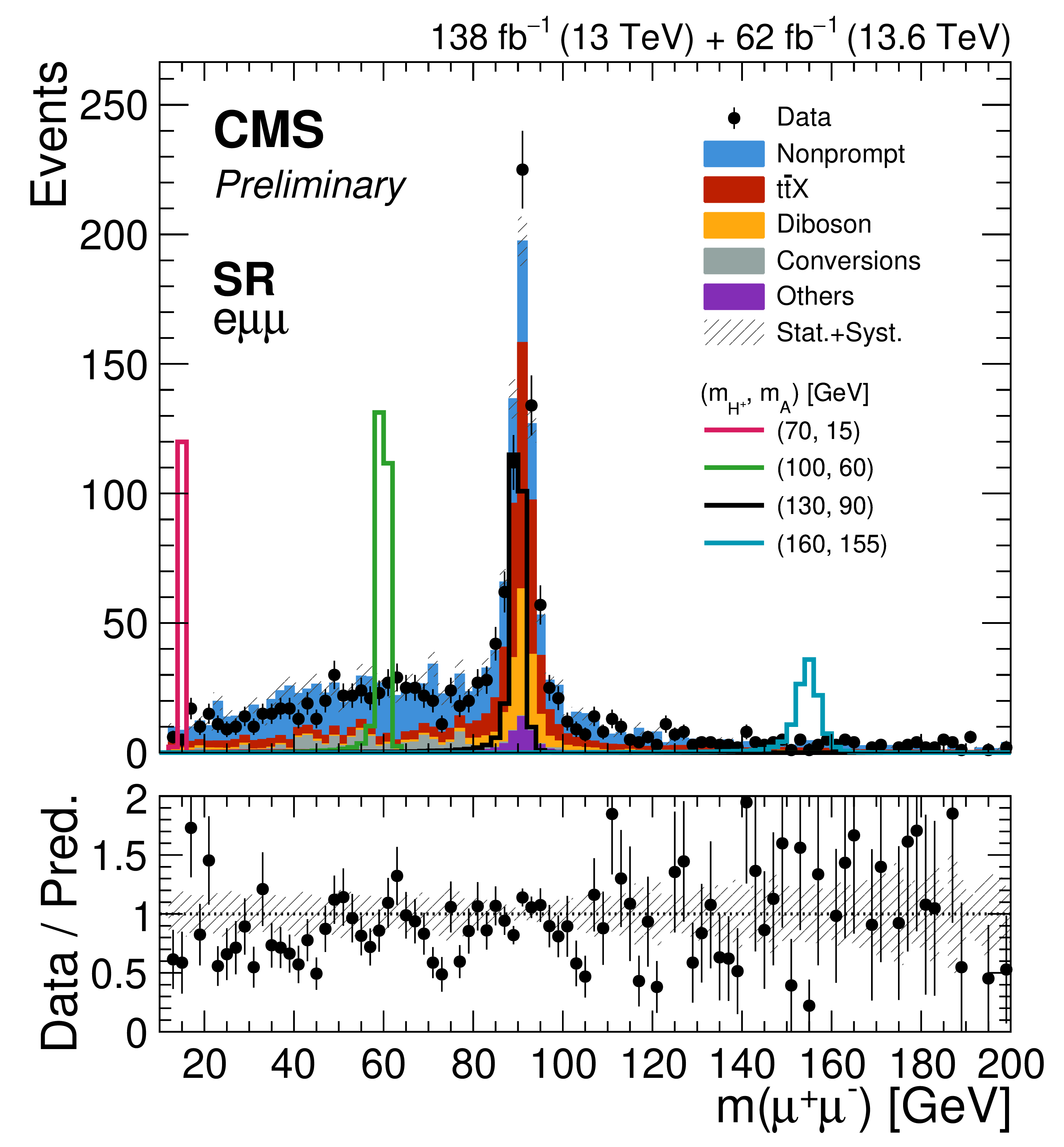
Figure 4-a:
Dimuon invariant mass distributions after the baseline selection. The left panel shows the OS dimuon mass in the $ \mathrm{e}\mu\mu $ channel, and the center and right panels show $ \mathit{m}(\mu^{+}\mu^{-})_ < $ and $ \mathit{m}(\mu^{+}\mu^{-})_ > $ in the $ \mu\mu\mu $ channel, respectively. The data are compared with the sum of the background predictions, which are grouped into the nonprompt lepton, photon conversion, $ {\mathrm{t}\overline{\mathrm{t}}} \mathrm{X} $, diboson, and other categories defined in Section 3, and the hatched band represents the combined statistical and systematic uncertainty in the prediction. Selected signal mass hypotheses with $ (\mathit{m}_{\mathrm{H^+}}, \mathit{m}_{\mathrm{A}}) = (70, 15) $, $ (100, 60) $, $ (130, 90) $, and $ (160, 155) \text{GeV} $ are overlaid, normalized to a signal cross section of 30 fb at 13 TeV and scaled by the ratio of $ \mathrm{t} \overline{\mathrm{t}} $ cross sections at 13.6 and 13 TeV for the Run 3 data. The lower panel of each distribution shows the ratio of the data to the total background prediction. |
png pdf |
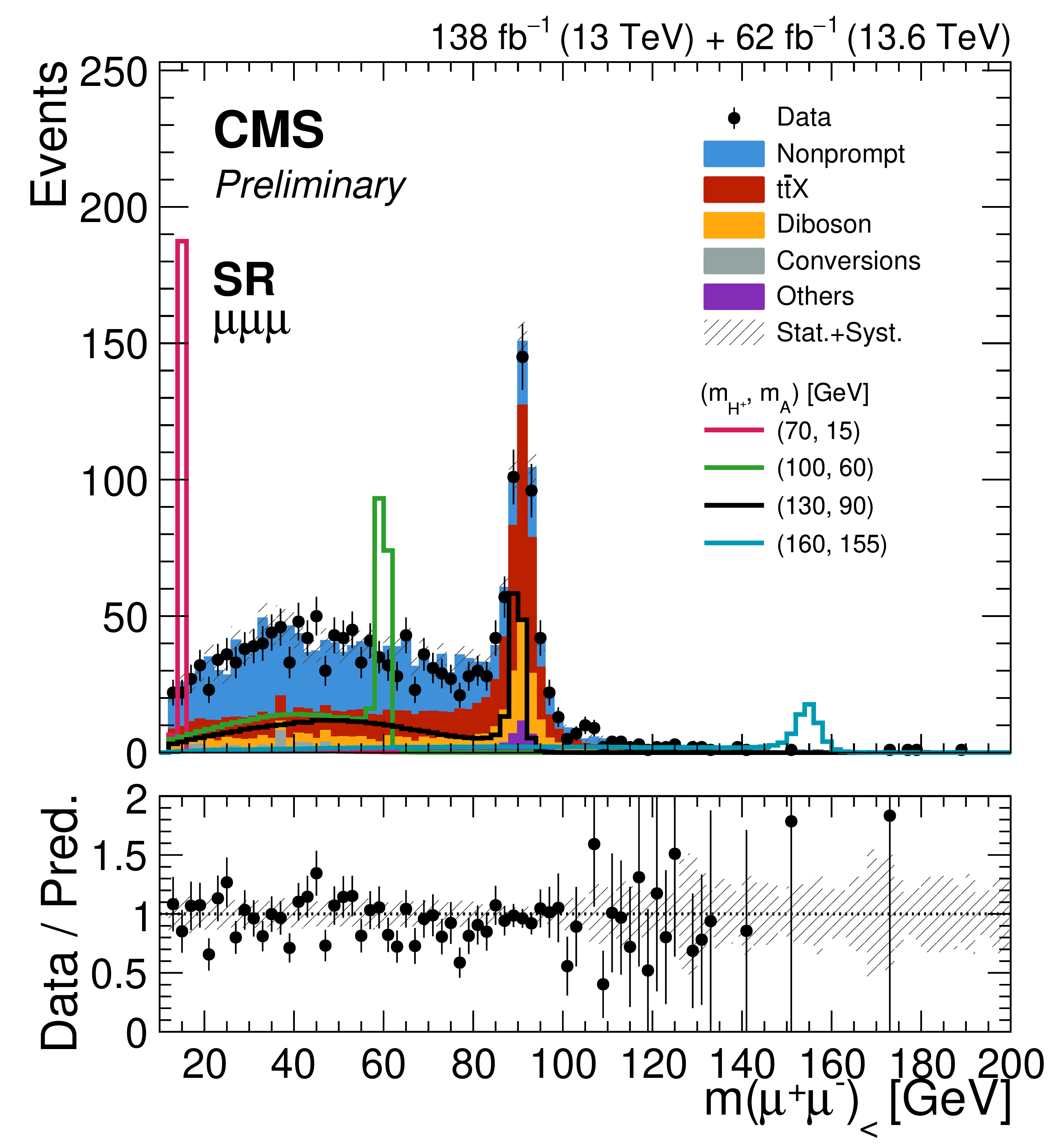
Figure 4-b:
Dimuon invariant mass distributions after the baseline selection. The left panel shows the OS dimuon mass in the $ \mathrm{e}\mu\mu $ channel, and the center and right panels show $ \mathit{m}(\mu^{+}\mu^{-})_ < $ and $ \mathit{m}(\mu^{+}\mu^{-})_ > $ in the $ \mu\mu\mu $ channel, respectively. The data are compared with the sum of the background predictions, which are grouped into the nonprompt lepton, photon conversion, $ {\mathrm{t}\overline{\mathrm{t}}} \mathrm{X} $, diboson, and other categories defined in Section 3, and the hatched band represents the combined statistical and systematic uncertainty in the prediction. Selected signal mass hypotheses with $ (\mathit{m}_{\mathrm{H^+}}, \mathit{m}_{\mathrm{A}}) = (70, 15) $, $ (100, 60) $, $ (130, 90) $, and $ (160, 155) \text{GeV} $ are overlaid, normalized to a signal cross section of 30 fb at 13 TeV and scaled by the ratio of $ \mathrm{t} \overline{\mathrm{t}} $ cross sections at 13.6 and 13 TeV for the Run 3 data. The lower panel of each distribution shows the ratio of the data to the total background prediction. |
png pdf |
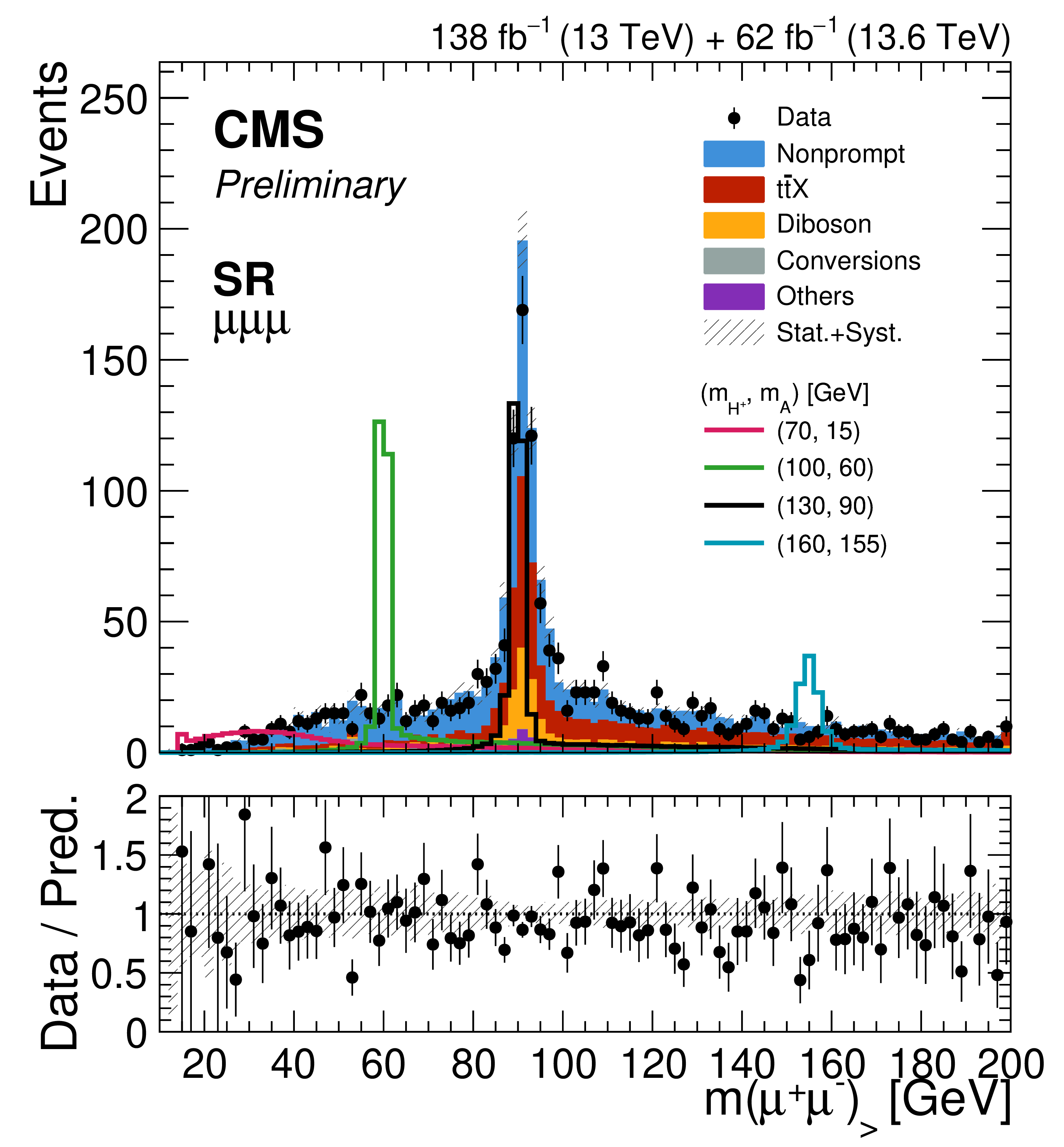
Figure 4-c:
Dimuon invariant mass distributions after the baseline selection. The left panel shows the OS dimuon mass in the $ \mathrm{e}\mu\mu $ channel, and the center and right panels show $ \mathit{m}(\mu^{+}\mu^{-})_ < $ and $ \mathit{m}(\mu^{+}\mu^{-})_ > $ in the $ \mu\mu\mu $ channel, respectively. The data are compared with the sum of the background predictions, which are grouped into the nonprompt lepton, photon conversion, $ {\mathrm{t}\overline{\mathrm{t}}} \mathrm{X} $, diboson, and other categories defined in Section 3, and the hatched band represents the combined statistical and systematic uncertainty in the prediction. Selected signal mass hypotheses with $ (\mathit{m}_{\mathrm{H^+}}, \mathit{m}_{\mathrm{A}}) = (70, 15) $, $ (100, 60) $, $ (130, 90) $, and $ (160, 155) \text{GeV} $ are overlaid, normalized to a signal cross section of 30 fb at 13 TeV and scaled by the ratio of $ \mathrm{t} \overline{\mathrm{t}} $ cross sections at 13.6 and 13 TeV for the Run 3 data. The lower panel of each distribution shows the ratio of the data to the total background prediction. |
png pdf |
Figure 5:
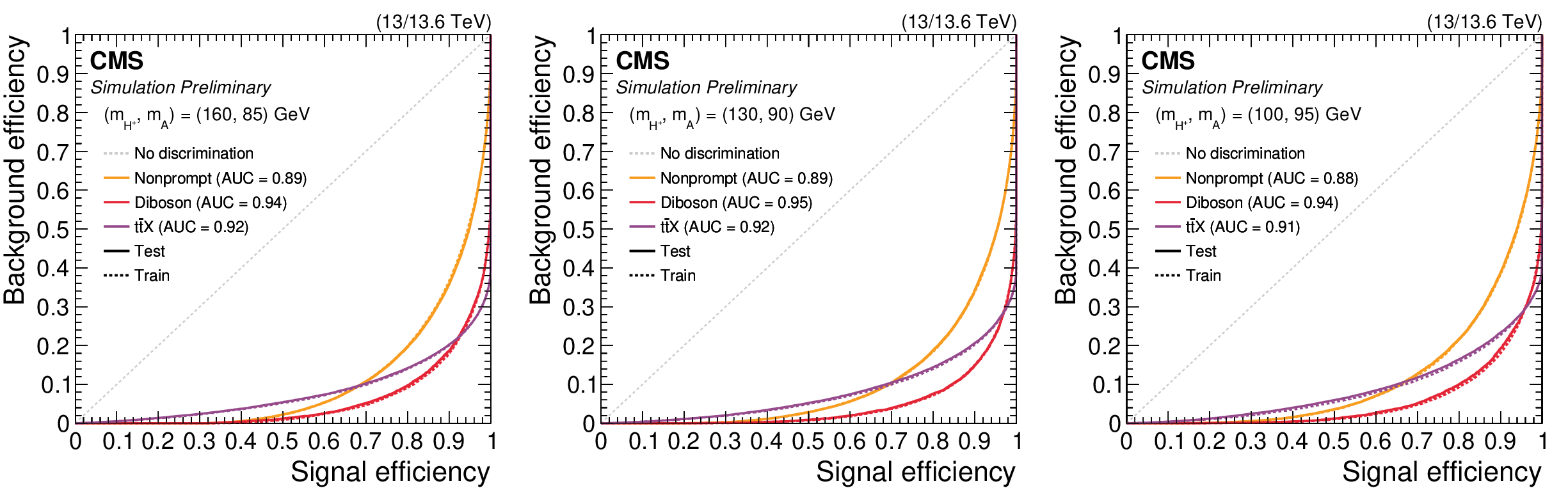
ROC curves for the ParticleNet classifiers for the signal mass hypotheses $ (\mathit{m}_{\mathrm{H^+}}, \mathit{m}_{\mathrm{A}}) = (160, 85) \text{GeV} $ (left), $ (130, 90) \text{GeV} $ (center), and $ (100, 95) \text{GeV} $ (right). Each panel shows the signal-versus-background curves for the three background classes, evaluated on the test data set (solid) and on the training data set (dotted), with the corresponding AUC values quoted in the panel. The diagonal line indicates the performance of a classifier with no discrimination power. |
png pdf |
Figure 5-a:
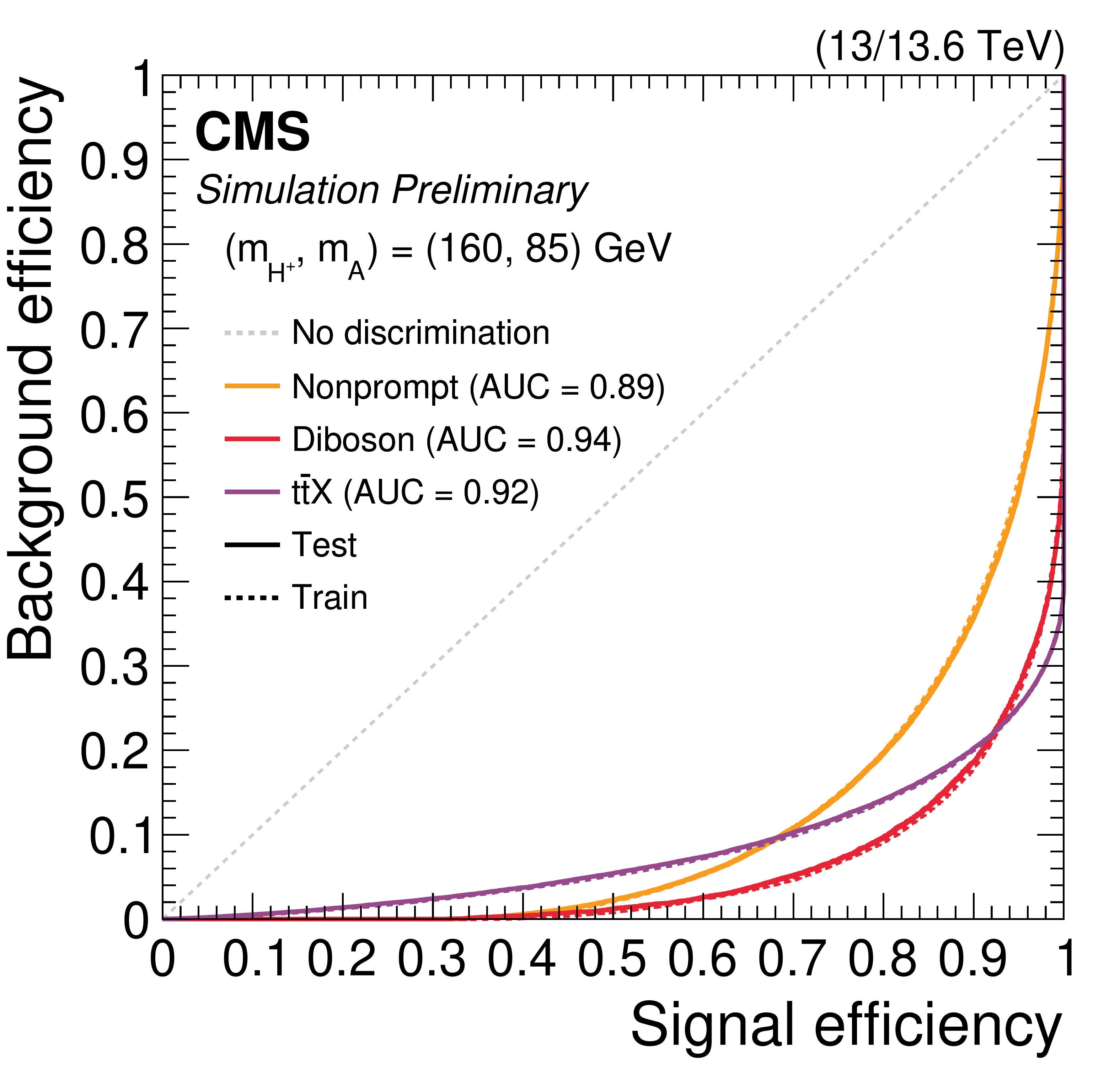
ROC curves for the ParticleNet classifiers for the signal mass hypotheses $ (\mathit{m}_{\mathrm{H^+}}, \mathit{m}_{\mathrm{A}}) = (160, 85) \text{GeV} $ (left), $ (130, 90) \text{GeV} $ (center), and $ (100, 95) \text{GeV} $ (right). Each panel shows the signal-versus-background curves for the three background classes, evaluated on the test data set (solid) and on the training data set (dotted), with the corresponding AUC values quoted in the panel. The diagonal line indicates the performance of a classifier with no discrimination power. |
png pdf |
Figure 5-b:
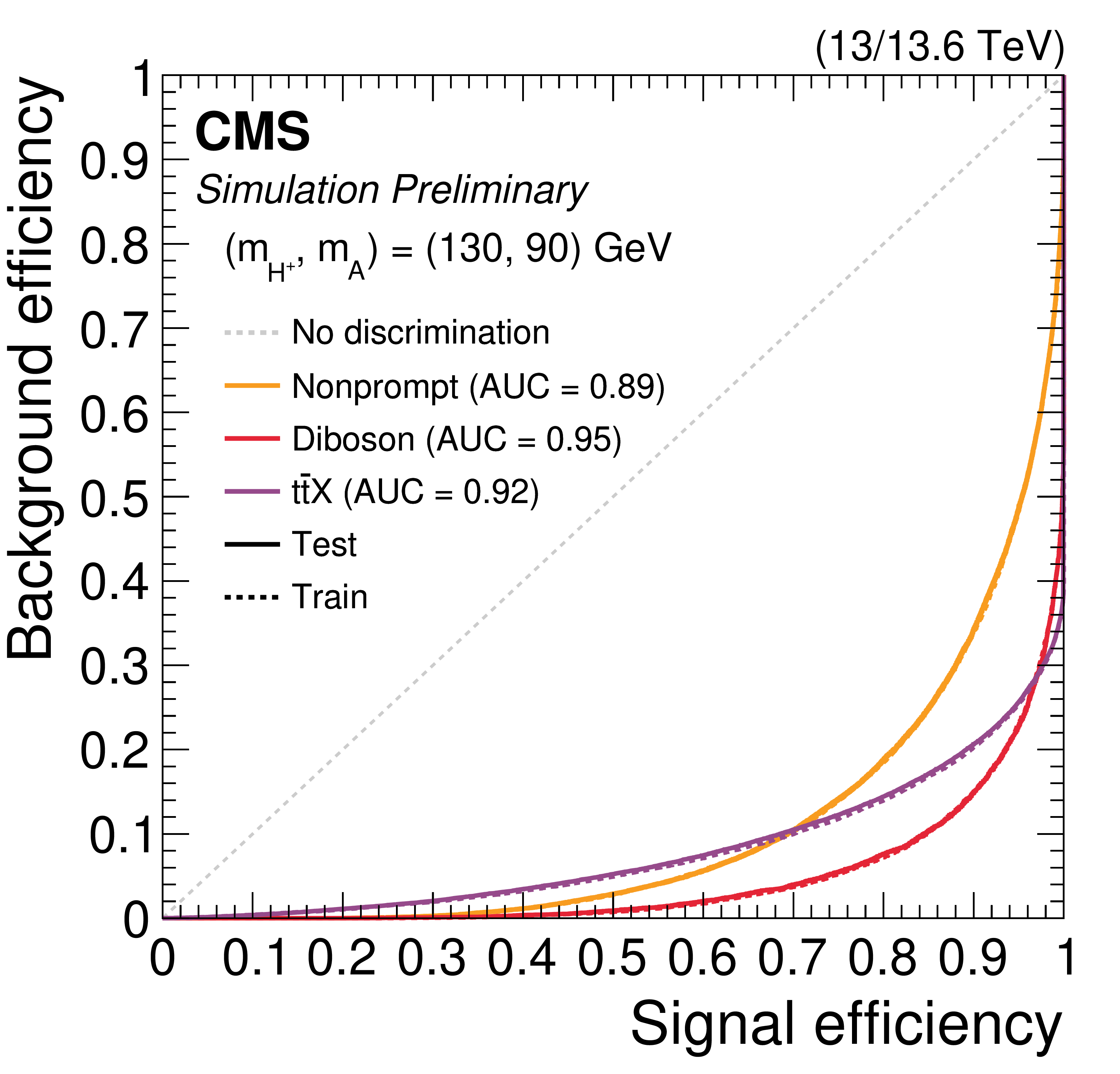
ROC curves for the ParticleNet classifiers for the signal mass hypotheses $ (\mathit{m}_{\mathrm{H^+}}, \mathit{m}_{\mathrm{A}}) = (160, 85) \text{GeV} $ (left), $ (130, 90) \text{GeV} $ (center), and $ (100, 95) \text{GeV} $ (right). Each panel shows the signal-versus-background curves for the three background classes, evaluated on the test data set (solid) and on the training data set (dotted), with the corresponding AUC values quoted in the panel. The diagonal line indicates the performance of a classifier with no discrimination power. |
png pdf |
Figure 5-c:
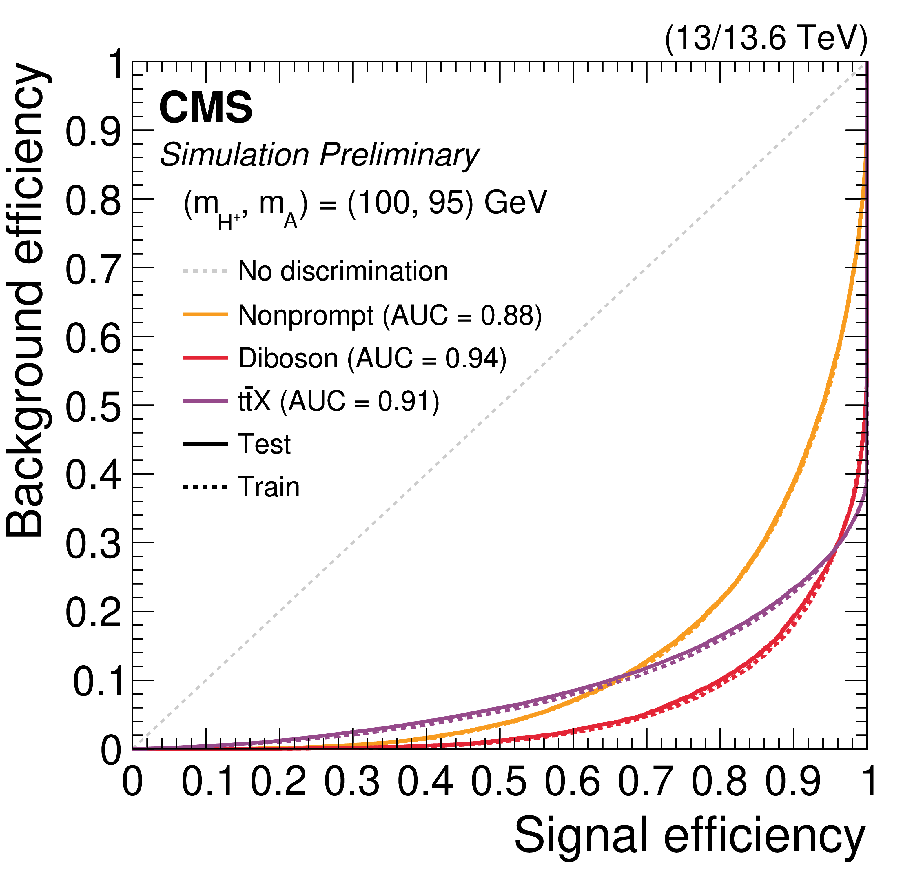
ROC curves for the ParticleNet classifiers for the signal mass hypotheses $ (\mathit{m}_{\mathrm{H^+}}, \mathit{m}_{\mathrm{A}}) = (160, 85) \text{GeV} $ (left), $ (130, 90) \text{GeV} $ (center), and $ (100, 95) \text{GeV} $ (right). Each panel shows the signal-versus-background curves for the three background classes, evaluated on the test data set (solid) and on the training data set (dotted), with the corresponding AUC values quoted in the panel. The diagonal line indicates the performance of a classifier with no discrimination power. |
png pdf |
Figure 6:
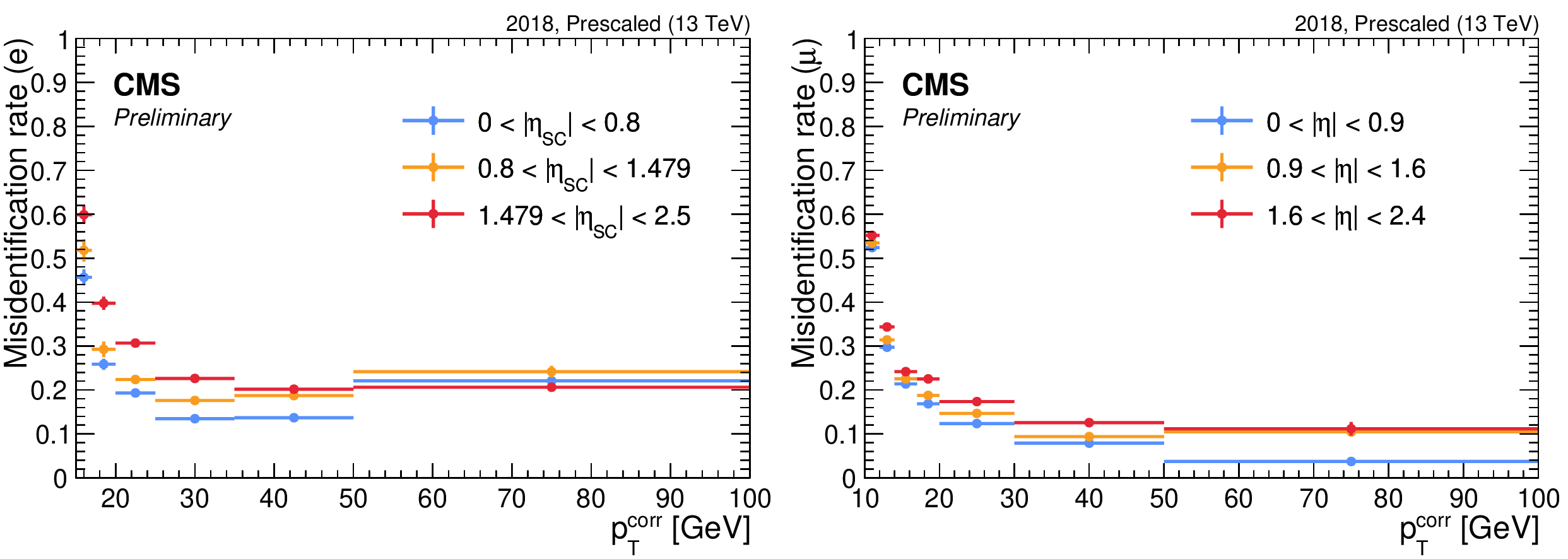
Measured nonprompt lepton misidentification rates as a function of the cone-corrected transverse momentum $ p_{\mathrm{T}}^{\text{corr}} $ and $ |\eta| $ in the 2018 data-taking period, for electrons (left) and muons (right). Only statistical uncertainties are shown. |
png pdf |
Figure 6-a:
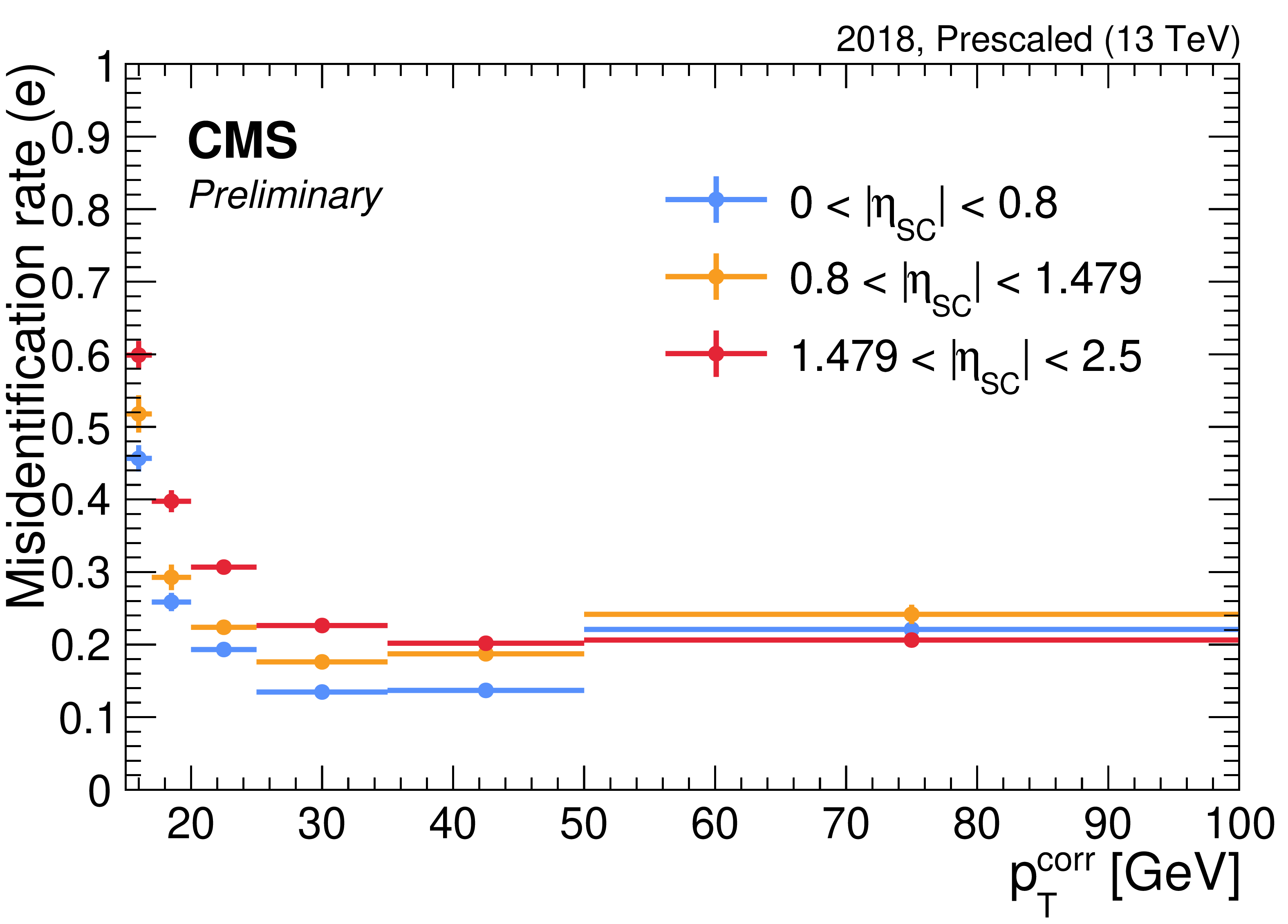
Measured nonprompt lepton misidentification rates as a function of the cone-corrected transverse momentum $ p_{\mathrm{T}}^{\text{corr}} $ and $ |\eta| $ in the 2018 data-taking period, for electrons (left) and muons (right). Only statistical uncertainties are shown. |
png pdf |
Figure 6-b:
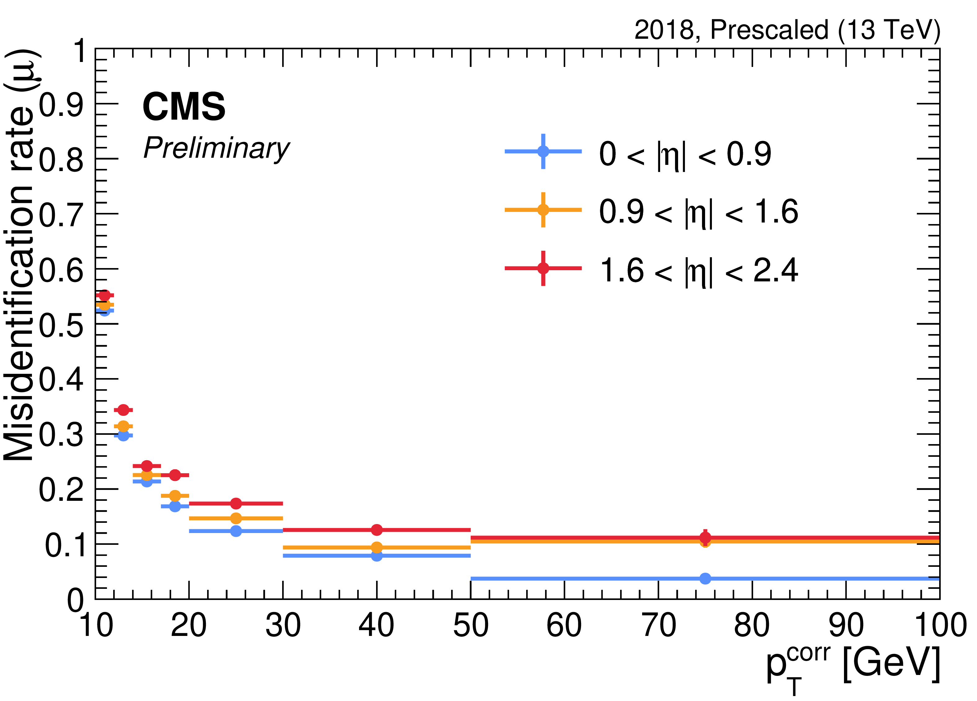
Measured nonprompt lepton misidentification rates as a function of the cone-corrected transverse momentum $ p_{\mathrm{T}}^{\text{corr}} $ and $ |\eta| $ in the 2018 data-taking period, for electrons (left) and muons (right). Only statistical uncertainties are shown. |
png pdf |
Figure 7:
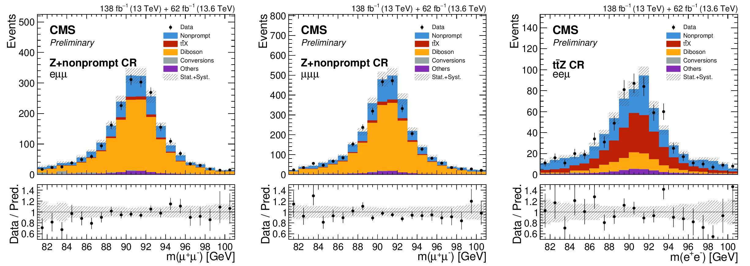
Distributions of the Z boson candidate invariant mass in the Z+nonprompt CR for the $ \mathrm{e}\mu\mu $ (left) and $ \mu\mu\mu $ (center) channels, and of the dielectron invariant mass in the $ {\mathrm{t}\overline{\mathrm{t}}} \mathrm{Z} $ CR (right), for the combined Run 2 and Run 3 data sets. The data are compared with the sum of the background predictions, which are grouped into the nonprompt lepton, photon conversion, $ {\mathrm{t}\overline{\mathrm{t}}} \mathrm{X} $, diboson, and other categories defined in Section 3, and the hatched band represents the combined statistical and systematic uncertainty in the prediction. The lower panel of each distribution shows the ratio of the data to the total background prediction. |
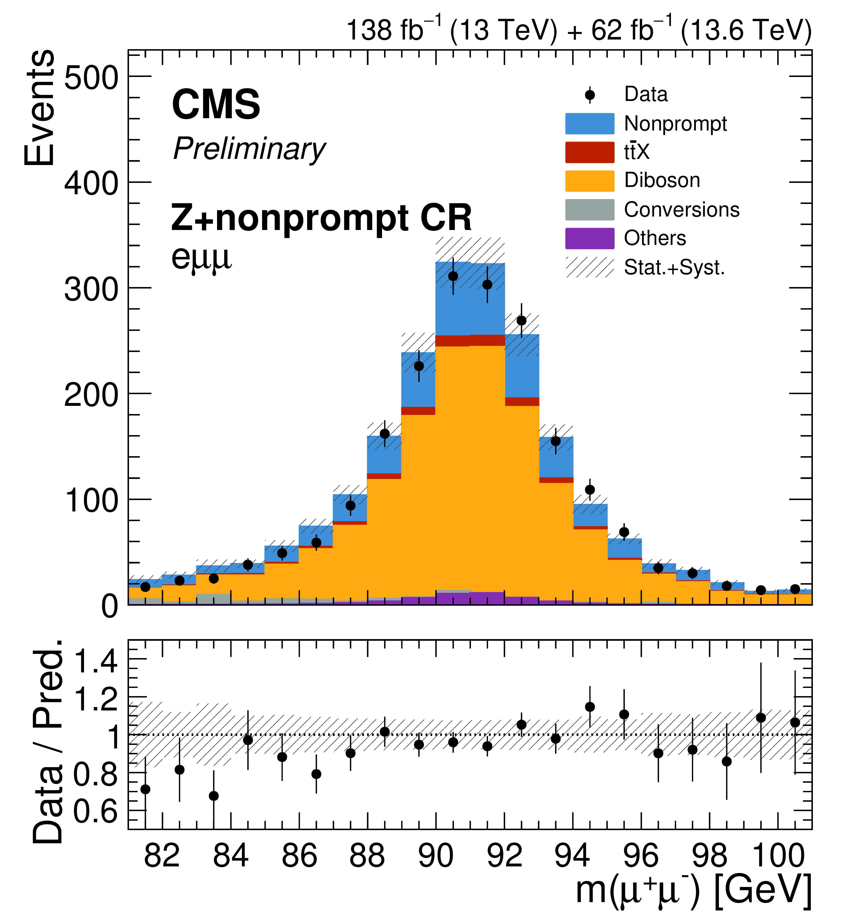
png pdf |
Figure 7-a:
Distributions of the Z boson candidate invariant mass in the Z+nonprompt CR for the $ \mathrm{e}\mu\mu $ (left) and $ \mu\mu\mu $ (center) channels, and of the dielectron invariant mass in the $ {\mathrm{t}\overline{\mathrm{t}}} \mathrm{Z} $ CR (right), for the combined Run 2 and Run 3 data sets. The data are compared with the sum of the background predictions, which are grouped into the nonprompt lepton, photon conversion, $ {\mathrm{t}\overline{\mathrm{t}}} \mathrm{X} $, diboson, and other categories defined in Section 3, and the hatched band represents the combined statistical and systematic uncertainty in the prediction. The lower panel of each distribution shows the ratio of the data to the total background prediction. |
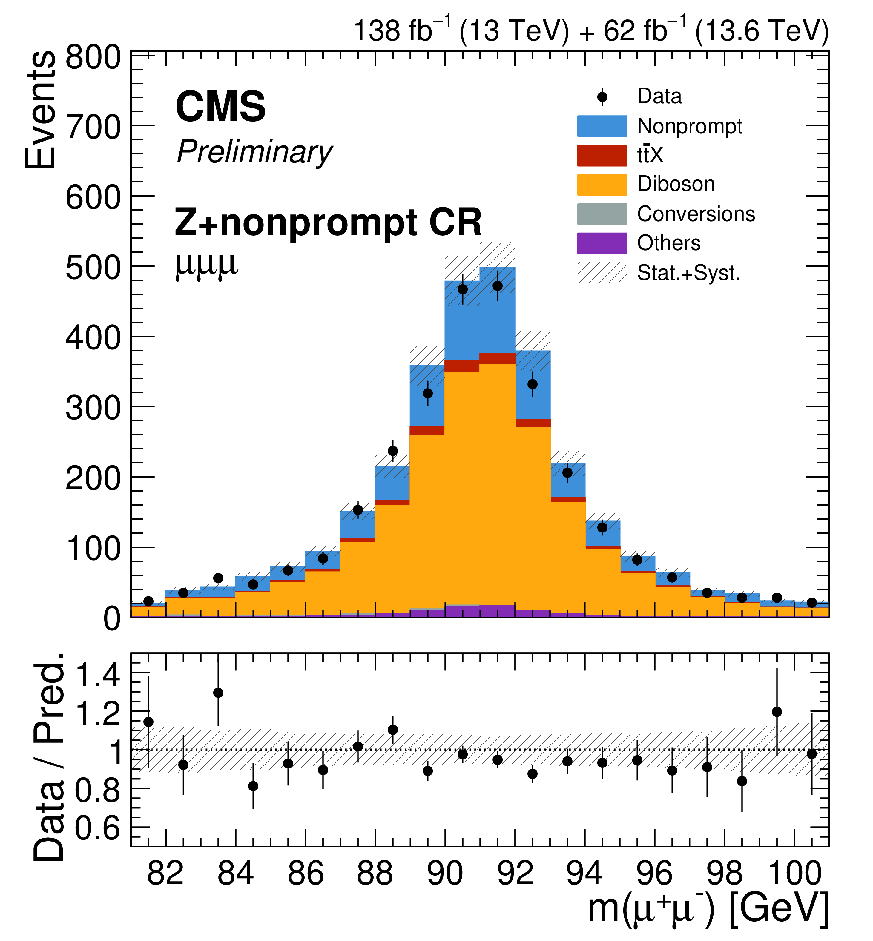
png pdf |
Figure 7-b:
Distributions of the Z boson candidate invariant mass in the Z+nonprompt CR for the $ \mathrm{e}\mu\mu $ (left) and $ \mu\mu\mu $ (center) channels, and of the dielectron invariant mass in the $ {\mathrm{t}\overline{\mathrm{t}}} \mathrm{Z} $ CR (right), for the combined Run 2 and Run 3 data sets. The data are compared with the sum of the background predictions, which are grouped into the nonprompt lepton, photon conversion, $ {\mathrm{t}\overline{\mathrm{t}}} \mathrm{X} $, diboson, and other categories defined in Section 3, and the hatched band represents the combined statistical and systematic uncertainty in the prediction. The lower panel of each distribution shows the ratio of the data to the total background prediction. |
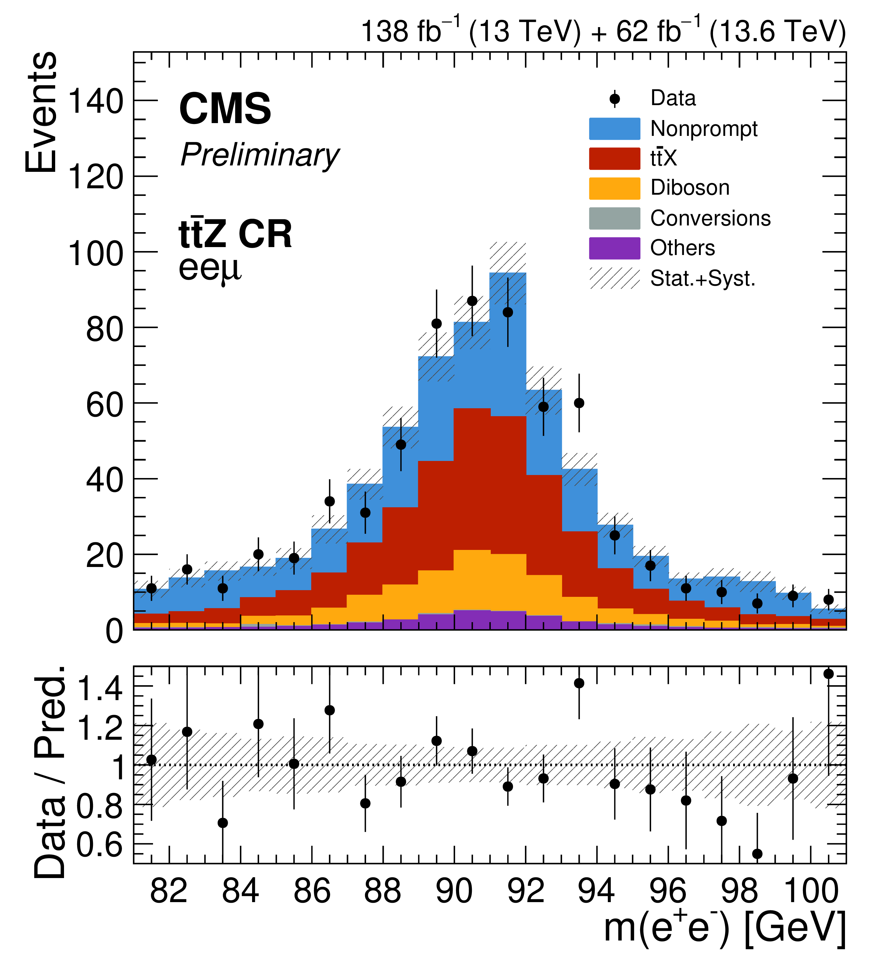
png pdf |
Figure 7-c:
Distributions of the Z boson candidate invariant mass in the Z+nonprompt CR for the $ \mathrm{e}\mu\mu $ (left) and $ \mu\mu\mu $ (center) channels, and of the dielectron invariant mass in the $ {\mathrm{t}\overline{\mathrm{t}}} \mathrm{Z} $ CR (right), for the combined Run 2 and Run 3 data sets. The data are compared with the sum of the background predictions, which are grouped into the nonprompt lepton, photon conversion, $ {\mathrm{t}\overline{\mathrm{t}}} \mathrm{X} $, diboson, and other categories defined in Section 3, and the hatched band represents the combined statistical and systematic uncertainty in the prediction. The lower panel of each distribution shows the ratio of the data to the total background prediction. |
png pdf |
Figure 8:
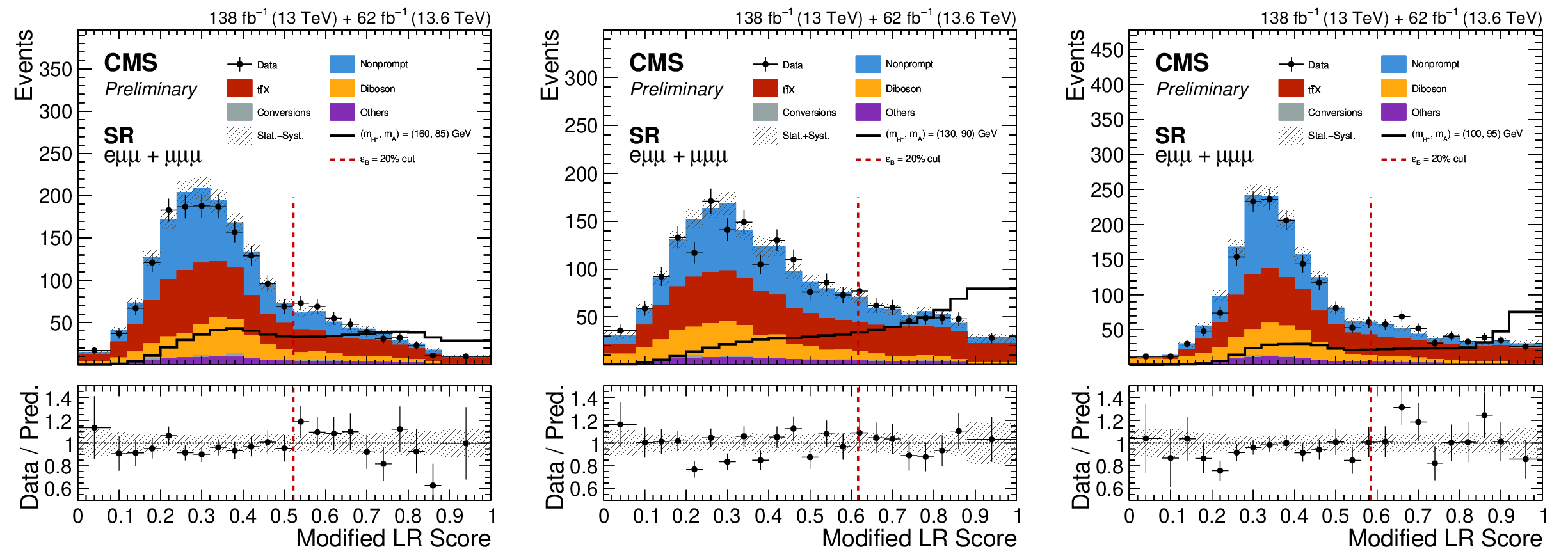
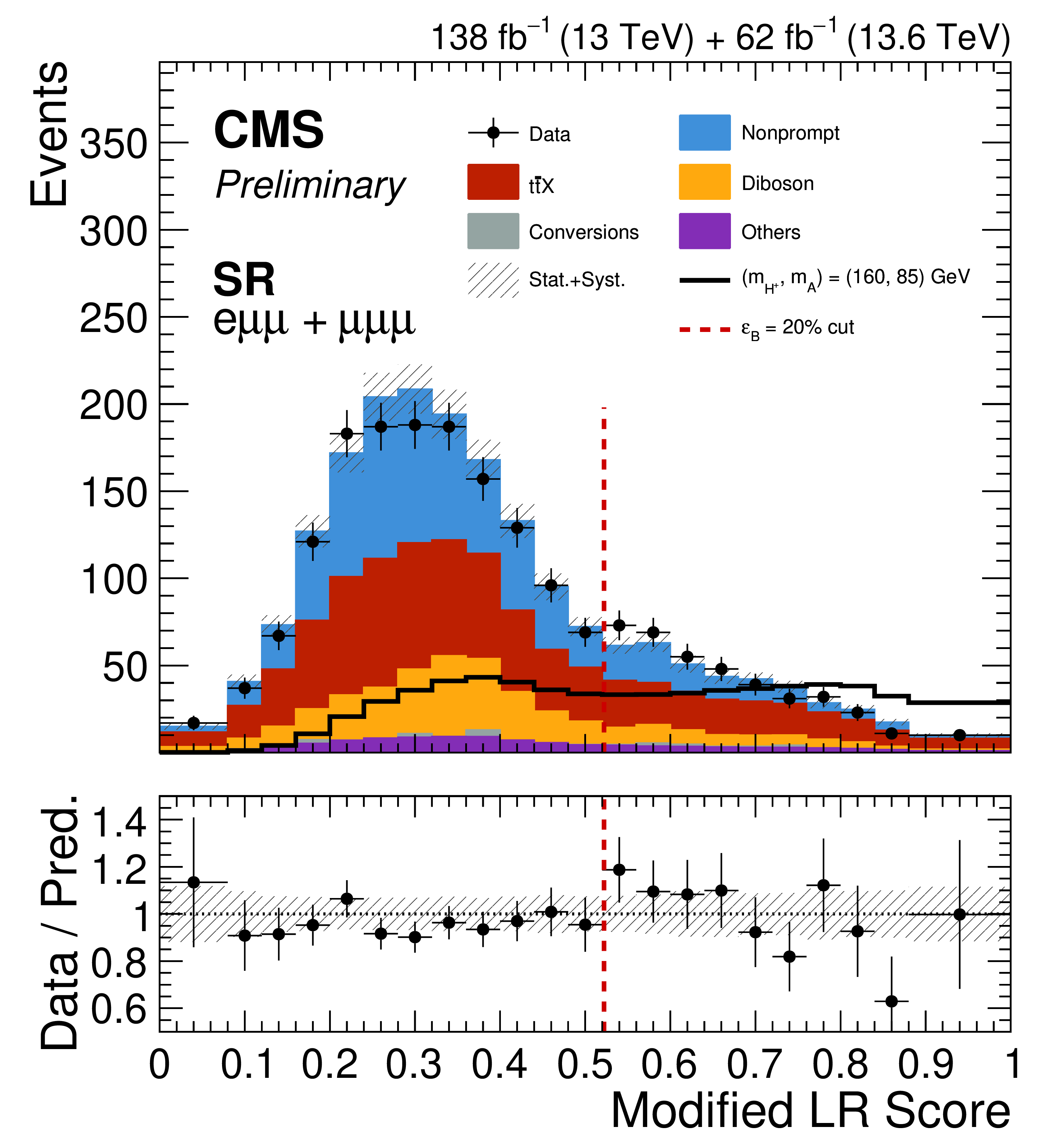
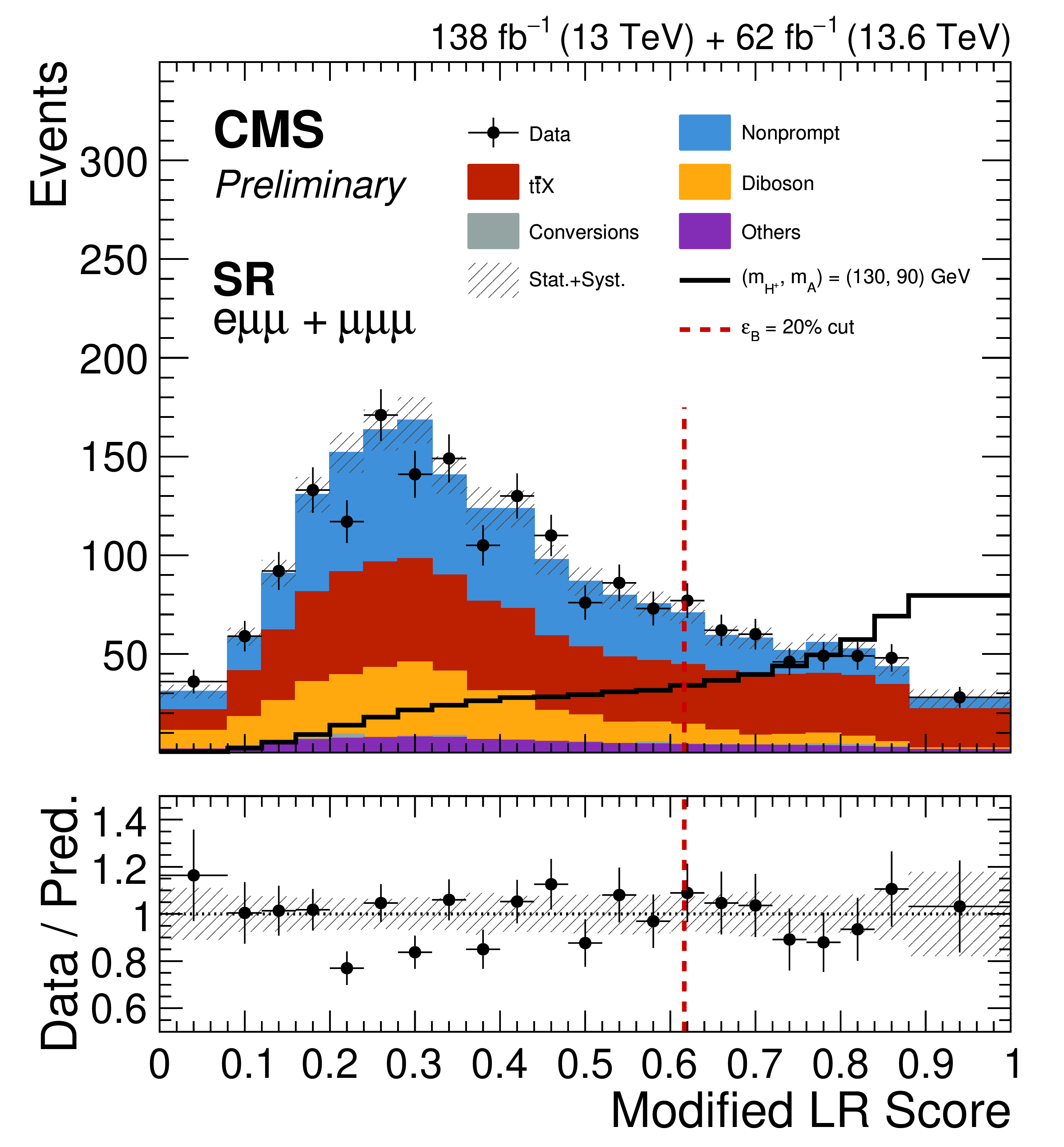
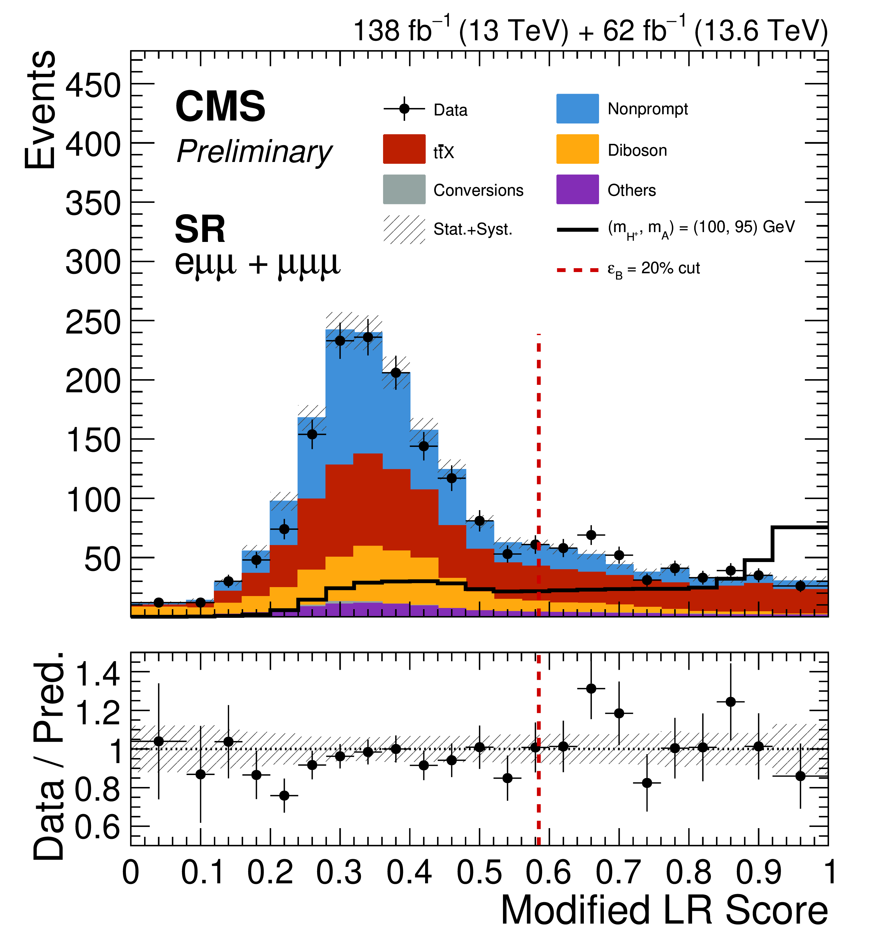
Distributions of the modified likelihood ratio $ \text{LR}_\text{modified} $ in the SR for the mass hypotheses $ (\mathit{m}_{\mathrm{H^+}}, \mathit{m}_{\mathrm{A}}) = (160, 85) \text{GeV} $ (left), $ (130, 90) \text{GeV} $ (center), and $ (100, 95) \text{GeV} $ (right). The data are compared with the sum of the background predictions, which are grouped into the nonprompt lepton, photon conversion, $ {\mathrm{t}\overline{\mathrm{t}}} \mathrm{X} $, diboson, and other categories defined in Section 3, and the hatched band represents the combined statistical and systematic uncertainty in the prediction. The signal distribution in each panel corresponds to the mass hypothesis indicated in that panel, normalized to a cross section of 30 fb in Run 2 and scaled by the ratio of $ \mathrm{t} \overline{\mathrm{t}} $ cross sections at 13.6 and 13 TeV for Run 3. The vertical dashed line indicates the working-point threshold, defined by a background efficiency of 20% as described in the text. The lower panel of each distribution shows the ratio of the data to the total background prediction. |
png pdf |
Figure 8-a:
Distributions of the modified likelihood ratio $ \text{LR}_\text{modified} $ in the SR for the mass hypotheses $ (\mathit{m}_{\mathrm{H^+}}, \mathit{m}_{\mathrm{A}}) = (160, 85) \text{GeV} $ (left), $ (130, 90) \text{GeV} $ (center), and $ (100, 95) \text{GeV} $ (right). The data are compared with the sum of the background predictions, which are grouped into the nonprompt lepton, photon conversion, $ {\mathrm{t}\overline{\mathrm{t}}} \mathrm{X} $, diboson, and other categories defined in Section 3, and the hatched band represents the combined statistical and systematic uncertainty in the prediction. The signal distribution in each panel corresponds to the mass hypothesis indicated in that panel, normalized to a cross section of 30 fb in Run 2 and scaled by the ratio of $ \mathrm{t} \overline{\mathrm{t}} $ cross sections at 13.6 and 13 TeV for Run 3. The vertical dashed line indicates the working-point threshold, defined by a background efficiency of 20% as described in the text. The lower panel of each distribution shows the ratio of the data to the total background prediction. |
png pdf |
Figure 8-b:
Distributions of the modified likelihood ratio $ \text{LR}_\text{modified} $ in the SR for the mass hypotheses $ (\mathit{m}_{\mathrm{H^+}}, \mathit{m}_{\mathrm{A}}) = (160, 85) \text{GeV} $ (left), $ (130, 90) \text{GeV} $ (center), and $ (100, 95) \text{GeV} $ (right). The data are compared with the sum of the background predictions, which are grouped into the nonprompt lepton, photon conversion, $ {\mathrm{t}\overline{\mathrm{t}}} \mathrm{X} $, diboson, and other categories defined in Section 3, and the hatched band represents the combined statistical and systematic uncertainty in the prediction. The signal distribution in each panel corresponds to the mass hypothesis indicated in that panel, normalized to a cross section of 30 fb in Run 2 and scaled by the ratio of $ \mathrm{t} \overline{\mathrm{t}} $ cross sections at 13.6 and 13 TeV for Run 3. The vertical dashed line indicates the working-point threshold, defined by a background efficiency of 20% as described in the text. The lower panel of each distribution shows the ratio of the data to the total background prediction. |
png pdf |
Figure 8-c:
Distributions of the modified likelihood ratio $ \text{LR}_\text{modified} $ in the SR for the mass hypotheses $ (\mathit{m}_{\mathrm{H^+}}, \mathit{m}_{\mathrm{A}}) = (160, 85) \text{GeV} $ (left), $ (130, 90) \text{GeV} $ (center), and $ (100, 95) \text{GeV} $ (right). The data are compared with the sum of the background predictions, which are grouped into the nonprompt lepton, photon conversion, $ {\mathrm{t}\overline{\mathrm{t}}} \mathrm{X} $, diboson, and other categories defined in Section 3, and the hatched band represents the combined statistical and systematic uncertainty in the prediction. The signal distribution in each panel corresponds to the mass hypothesis indicated in that panel, normalized to a cross section of 30 fb in Run 2 and scaled by the ratio of $ \mathrm{t} \overline{\mathrm{t}} $ cross sections at 13.6 and 13 TeV for Run 3. The vertical dashed line indicates the working-point threshold, defined by a background efficiency of 20% as described in the text. The lower panel of each distribution shows the ratio of the data to the total background prediction. |
png pdf |
Figure 9:
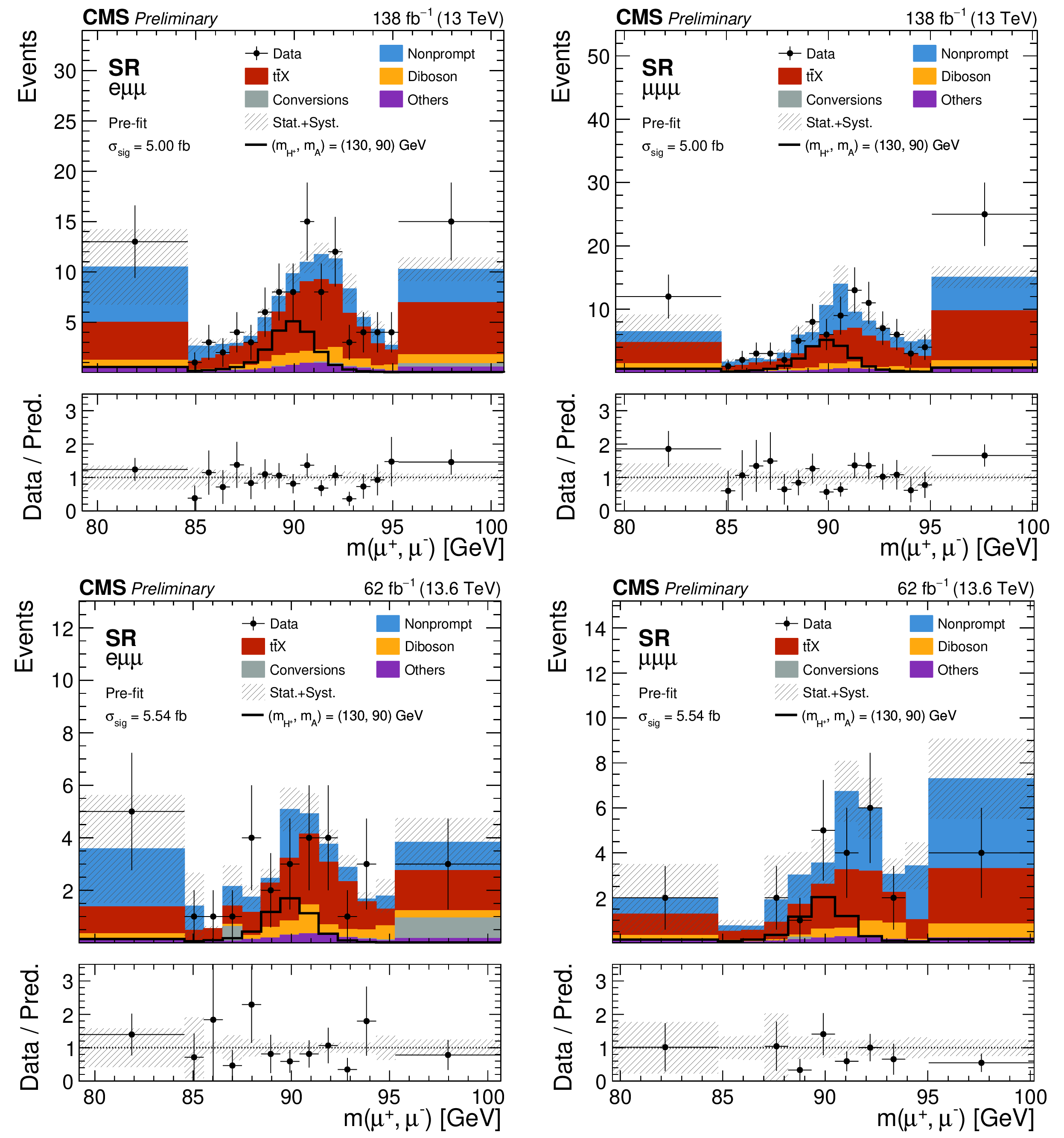
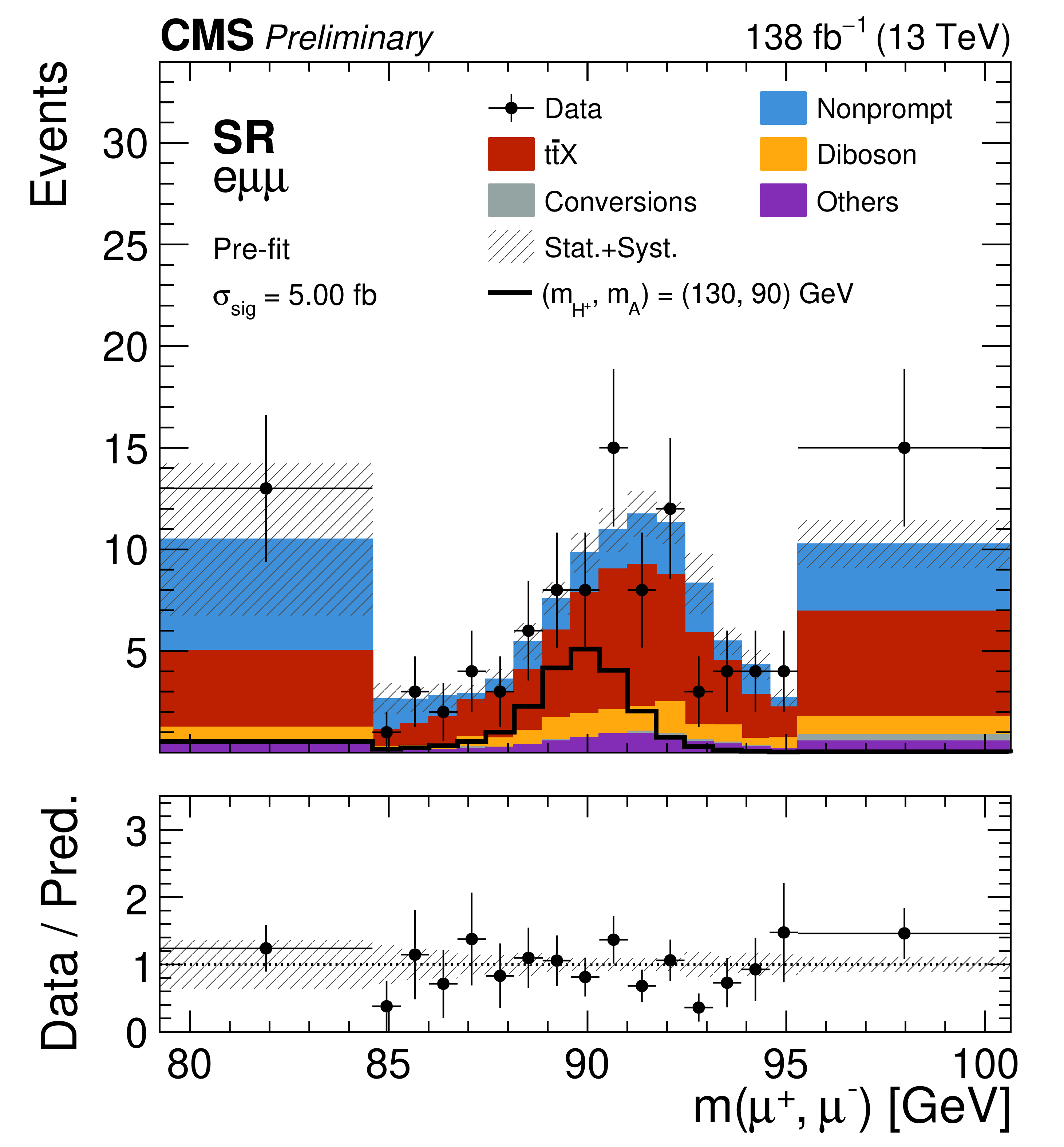
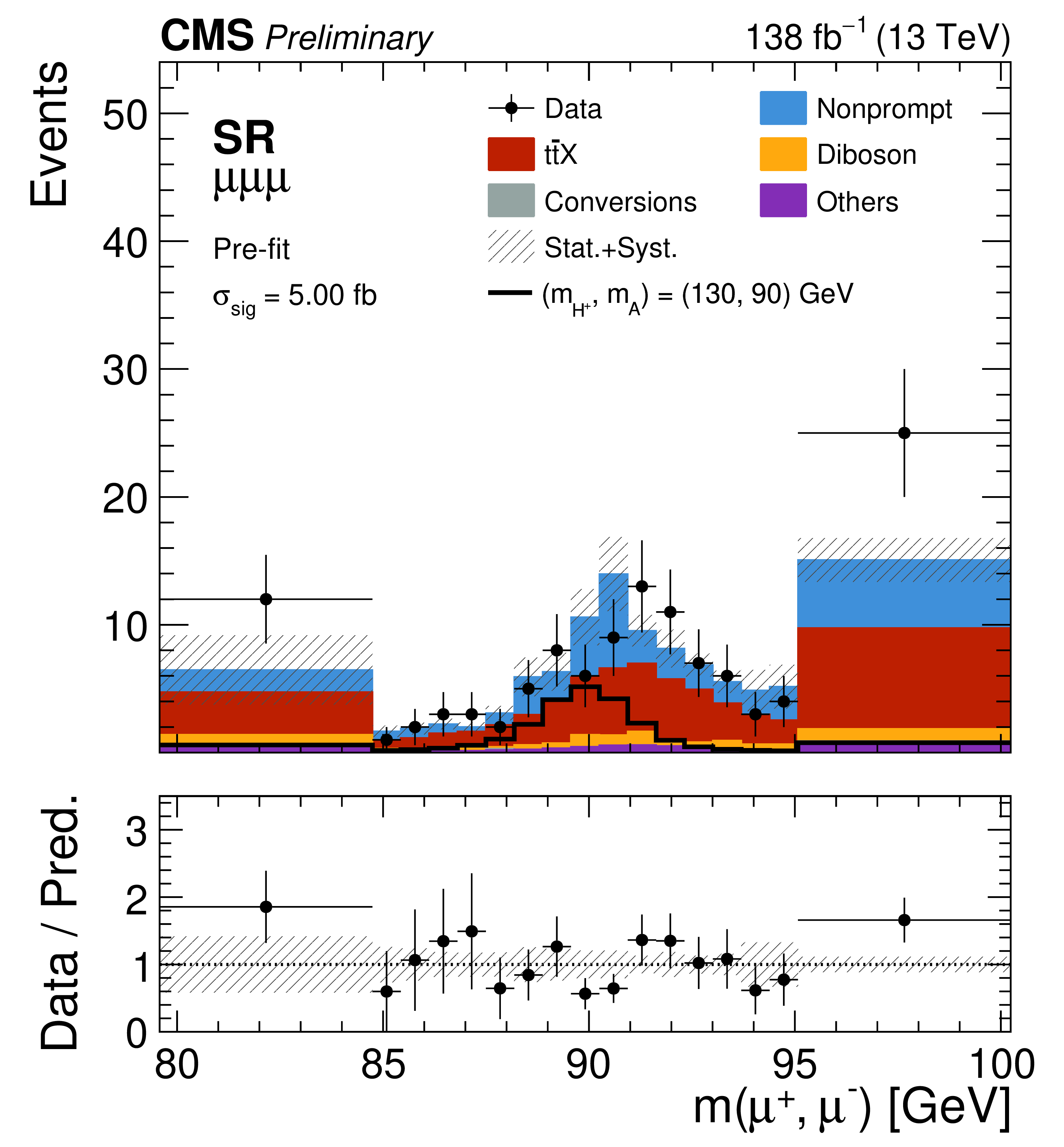
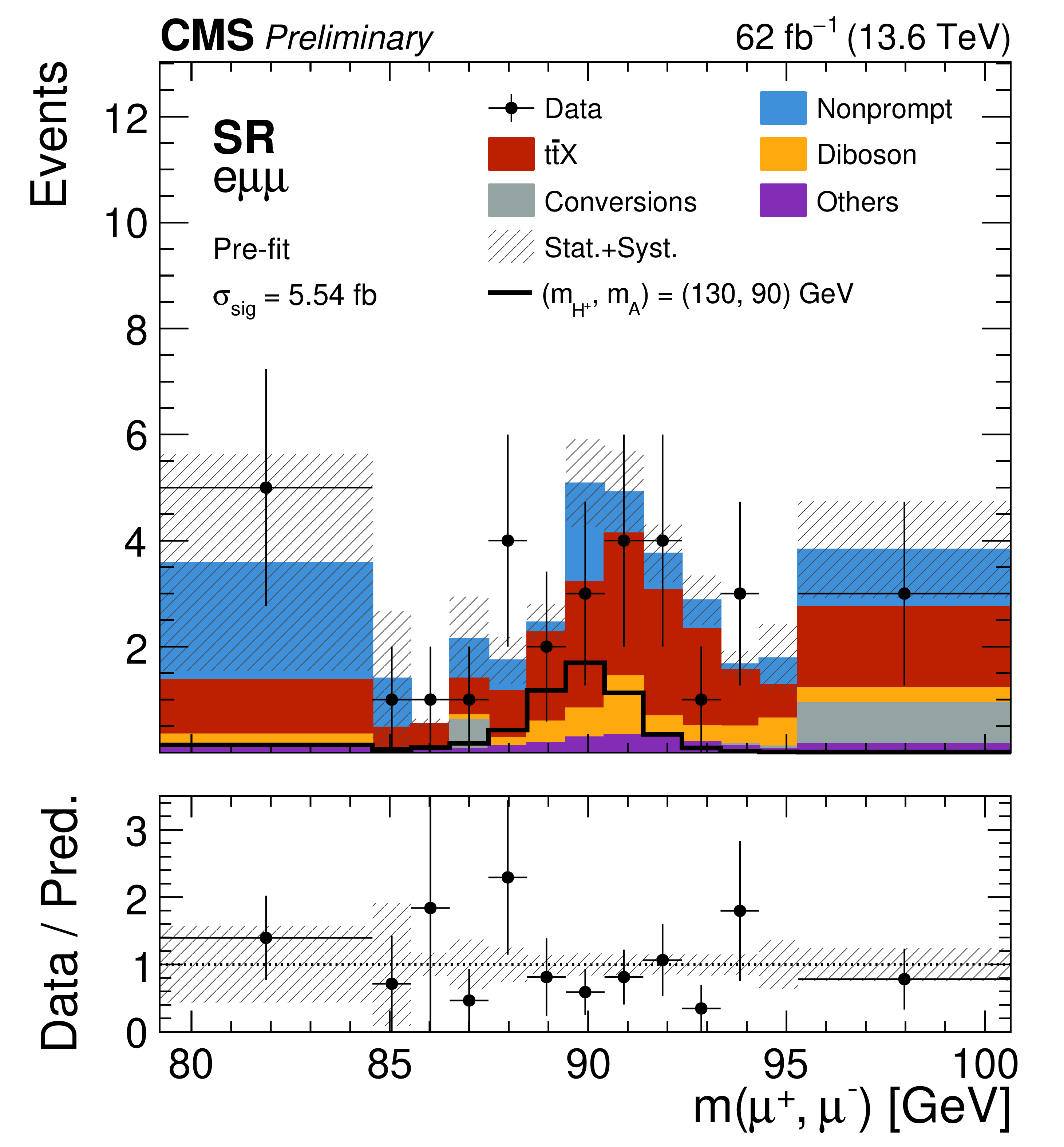
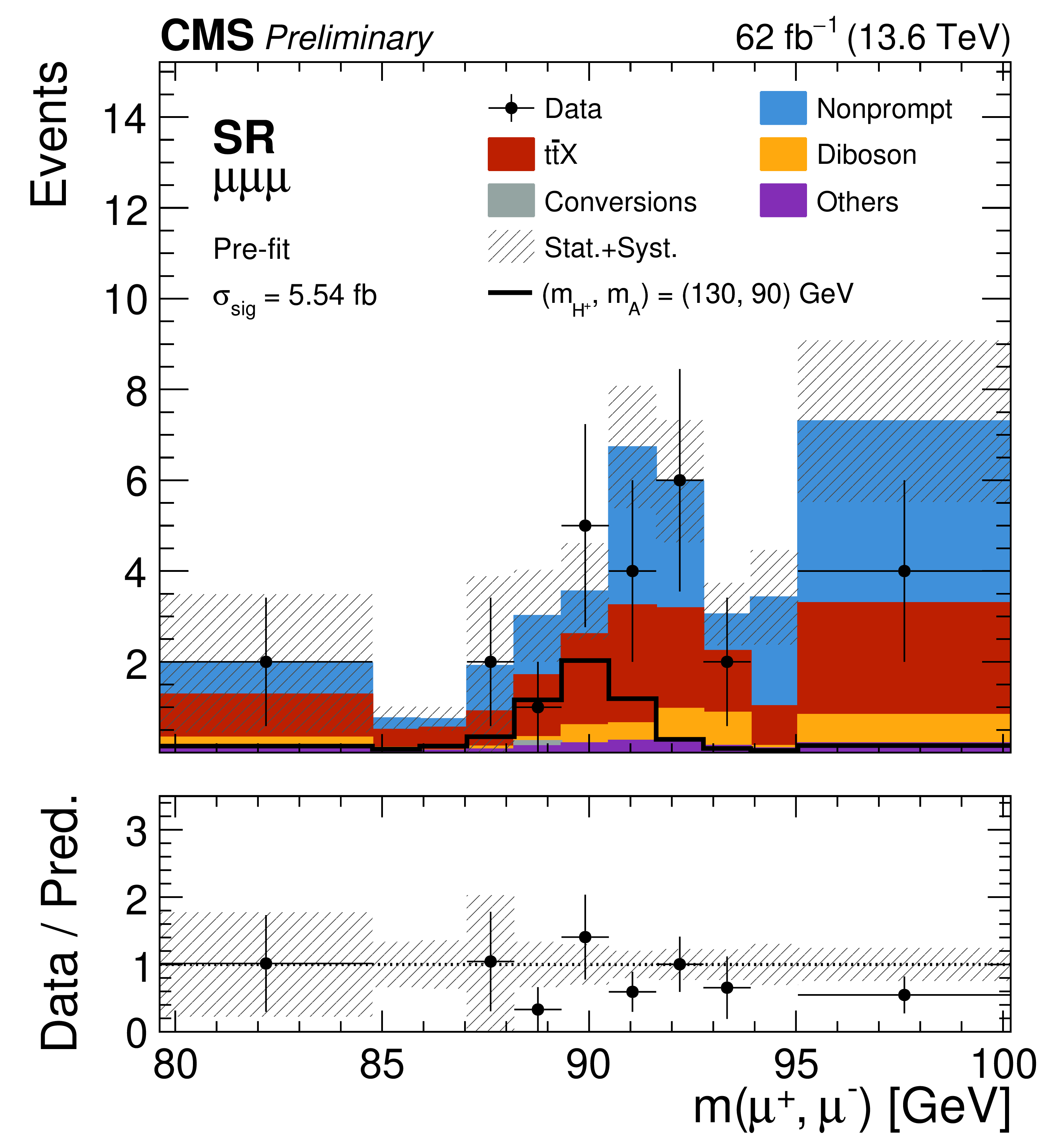
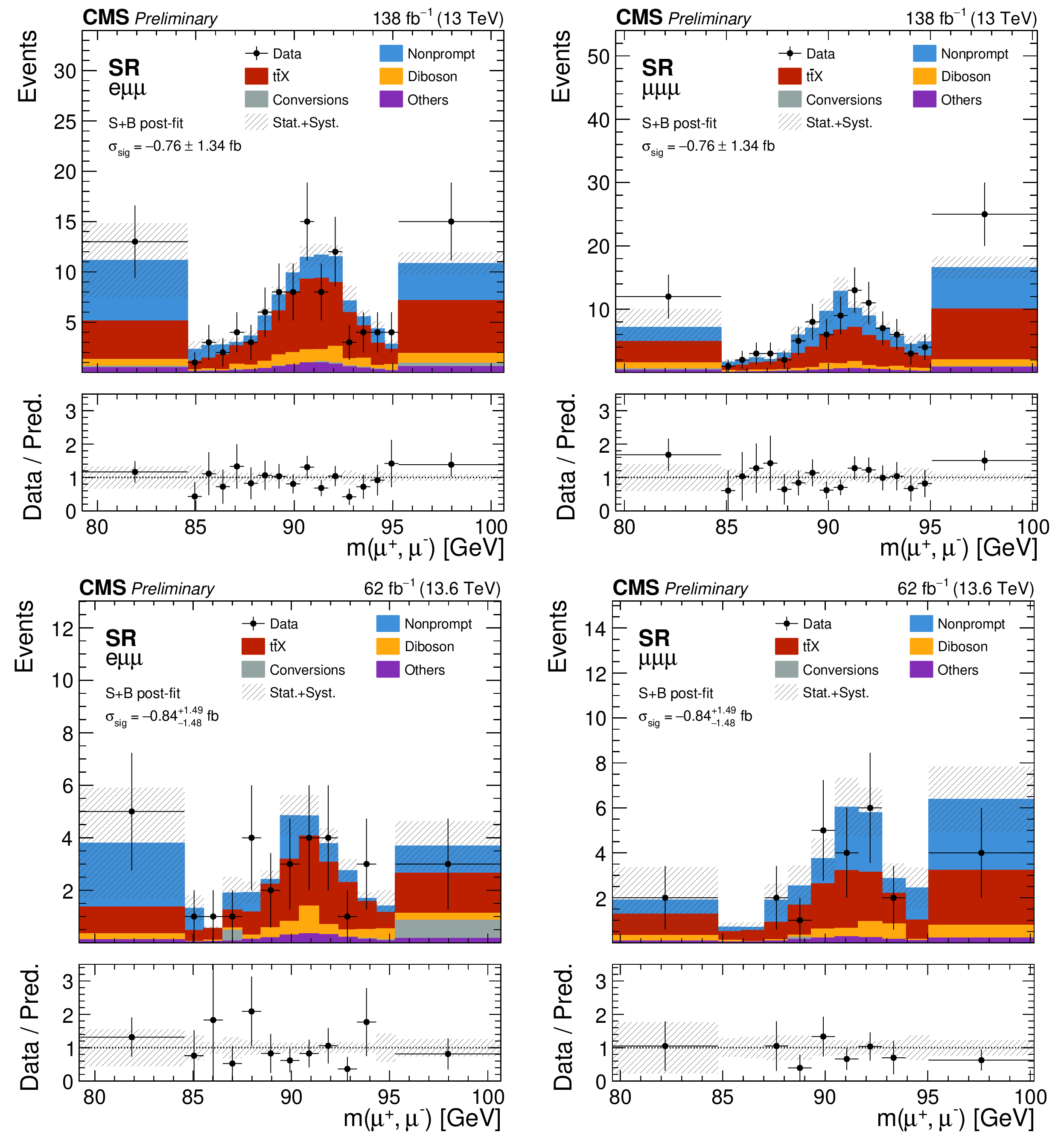
The ParticleNet-selected $ \mathit{m}(\mu^{+}\mu^{-}) $ templates before the fit, for the $ (\mathit{m}_{\mathrm{H^+}}, \mathit{m}_{\mathrm{A}}) = (130, 90) \text{GeV} $ mass hypothesis, for the $ \mathrm{e}\mu\mu $ (left column) and $ \mu\mu\mu $ (right column) channels in the Run 2 (upper row, 138 fb$^{-1}$, $ \sqrt{s} = $ 13 TeV) and Run 3 (lower row, 62 fb$^{-1}$, $ \sqrt{s} = $ 13.6 TeV) data-taking periods. The data are compared with the sum of the background predictions, which are grouped into the nonprompt lepton, photon conversion, $ {\mathrm{t}\overline{\mathrm{t}}} \mathrm{X} $, diboson, and other categories defined in Section 3, and the hatched band represents the combined statistical and systematic uncertainty in the prediction. The signal template, normalized to a signal cross section of 5 fb, is overlaid. The lower panel of each distribution shows the ratio of the data to the total background prediction. |
png pdf |
Figure 9-a:
The ParticleNet-selected $ \mathit{m}(\mu^{+}\mu^{-}) $ templates before the fit, for the $ (\mathit{m}_{\mathrm{H^+}}, \mathit{m}_{\mathrm{A}}) = (130, 90) \text{GeV} $ mass hypothesis, for the $ \mathrm{e}\mu\mu $ (left column) and $ \mu\mu\mu $ (right column) channels in the Run 2 (upper row, 138 fb$^{-1}$, $ \sqrt{s} = $ 13 TeV) and Run 3 (lower row, 62 fb$^{-1}$, $ \sqrt{s} = $ 13.6 TeV) data-taking periods. The data are compared with the sum of the background predictions, which are grouped into the nonprompt lepton, photon conversion, $ {\mathrm{t}\overline{\mathrm{t}}} \mathrm{X} $, diboson, and other categories defined in Section 3, and the hatched band represents the combined statistical and systematic uncertainty in the prediction. The signal template, normalized to a signal cross section of 5 fb, is overlaid. The lower panel of each distribution shows the ratio of the data to the total background prediction. |
png pdf |
Figure 9-b:
The ParticleNet-selected $ \mathit{m}(\mu^{+}\mu^{-}) $ templates before the fit, for the $ (\mathit{m}_{\mathrm{H^+}}, \mathit{m}_{\mathrm{A}}) = (130, 90) \text{GeV} $ mass hypothesis, for the $ \mathrm{e}\mu\mu $ (left column) and $ \mu\mu\mu $ (right column) channels in the Run 2 (upper row, 138 fb$^{-1}$, $ \sqrt{s} = $ 13 TeV) and Run 3 (lower row, 62 fb$^{-1}$, $ \sqrt{s} = $ 13.6 TeV) data-taking periods. The data are compared with the sum of the background predictions, which are grouped into the nonprompt lepton, photon conversion, $ {\mathrm{t}\overline{\mathrm{t}}} \mathrm{X} $, diboson, and other categories defined in Section 3, and the hatched band represents the combined statistical and systematic uncertainty in the prediction. The signal template, normalized to a signal cross section of 5 fb, is overlaid. The lower panel of each distribution shows the ratio of the data to the total background prediction. |
png pdf |
Figure 9-c:
The ParticleNet-selected $ \mathit{m}(\mu^{+}\mu^{-}) $ templates before the fit, for the $ (\mathit{m}_{\mathrm{H^+}}, \mathit{m}_{\mathrm{A}}) = (130, 90) \text{GeV} $ mass hypothesis, for the $ \mathrm{e}\mu\mu $ (left column) and $ \mu\mu\mu $ (right column) channels in the Run 2 (upper row, 138 fb$^{-1}$, $ \sqrt{s} = $ 13 TeV) and Run 3 (lower row, 62 fb$^{-1}$, $ \sqrt{s} = $ 13.6 TeV) data-taking periods. The data are compared with the sum of the background predictions, which are grouped into the nonprompt lepton, photon conversion, $ {\mathrm{t}\overline{\mathrm{t}}} \mathrm{X} $, diboson, and other categories defined in Section 3, and the hatched band represents the combined statistical and systematic uncertainty in the prediction. The signal template, normalized to a signal cross section of 5 fb, is overlaid. The lower panel of each distribution shows the ratio of the data to the total background prediction. |
png pdf |
Figure 9-d:
The ParticleNet-selected $ \mathit{m}(\mu^{+}\mu^{-}) $ templates before the fit, for the $ (\mathit{m}_{\mathrm{H^+}}, \mathit{m}_{\mathrm{A}}) = (130, 90) \text{GeV} $ mass hypothesis, for the $ \mathrm{e}\mu\mu $ (left column) and $ \mu\mu\mu $ (right column) channels in the Run 2 (upper row, 138 fb$^{-1}$, $ \sqrt{s} = $ 13 TeV) and Run 3 (lower row, 62 fb$^{-1}$, $ \sqrt{s} = $ 13.6 TeV) data-taking periods. The data are compared with the sum of the background predictions, which are grouped into the nonprompt lepton, photon conversion, $ {\mathrm{t}\overline{\mathrm{t}}} \mathrm{X} $, diboson, and other categories defined in Section 3, and the hatched band represents the combined statistical and systematic uncertainty in the prediction. The signal template, normalized to a signal cross section of 5 fb, is overlaid. The lower panel of each distribution shows the ratio of the data to the total background prediction. |
png pdf |
Figure 10:
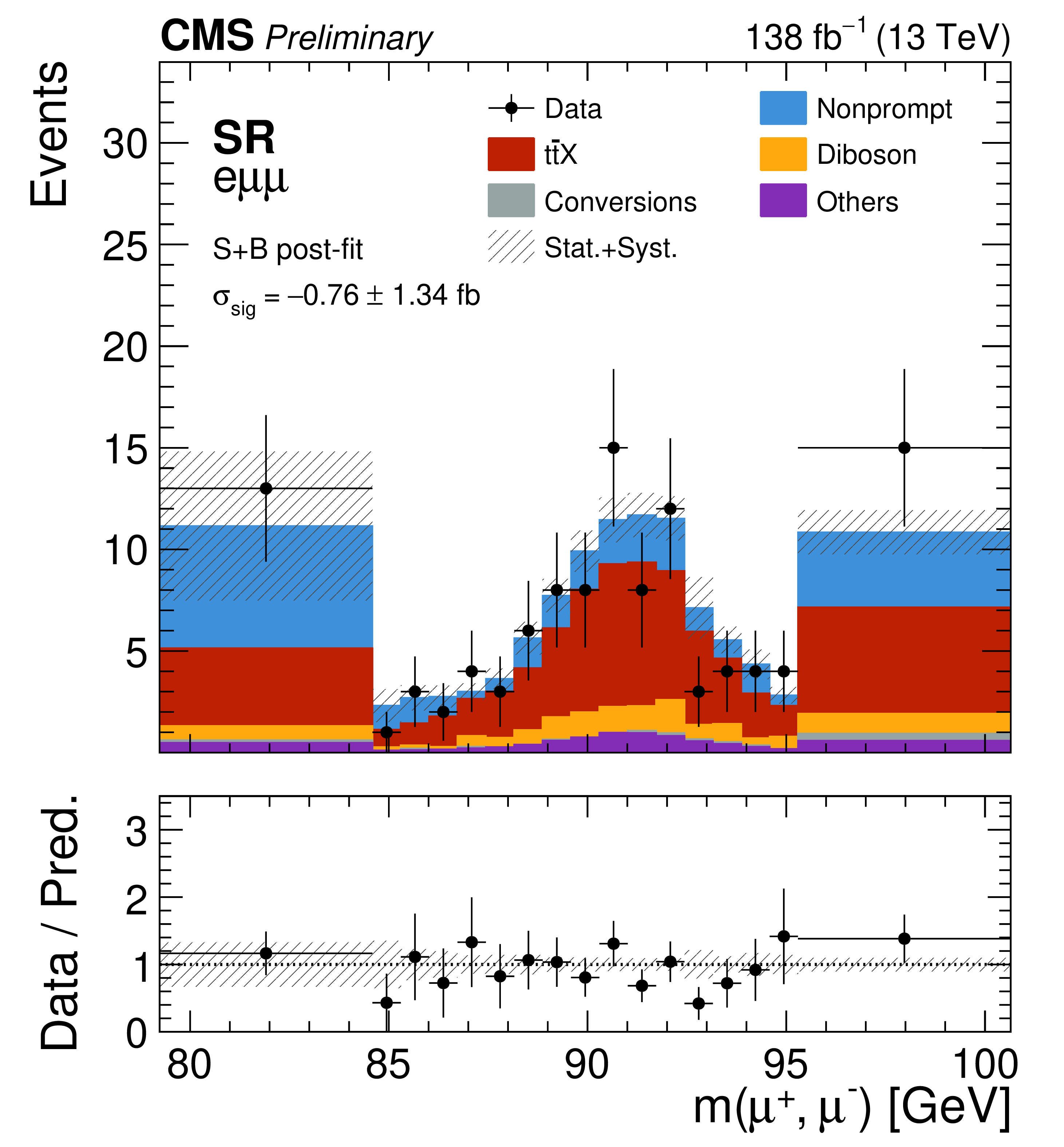
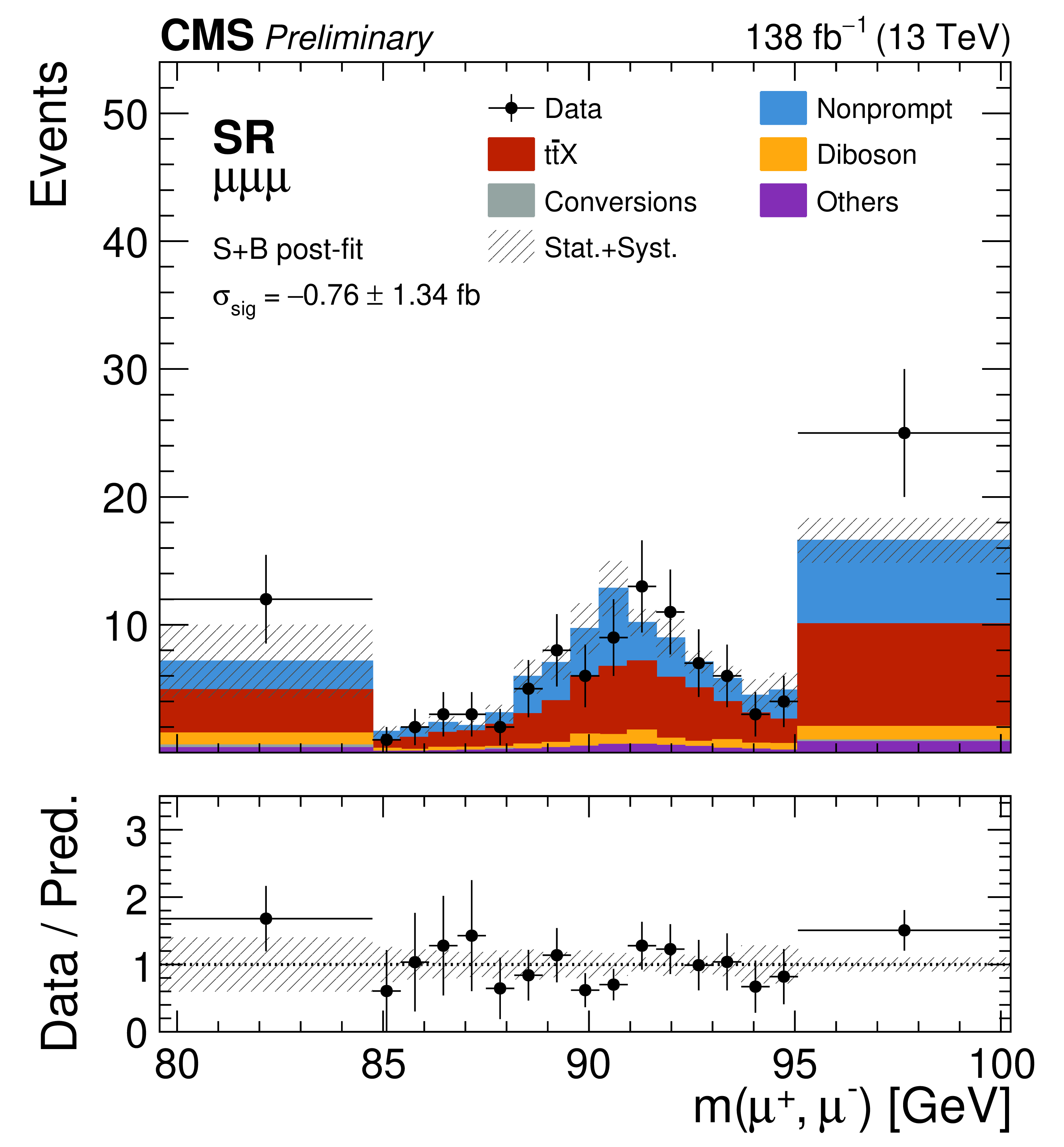
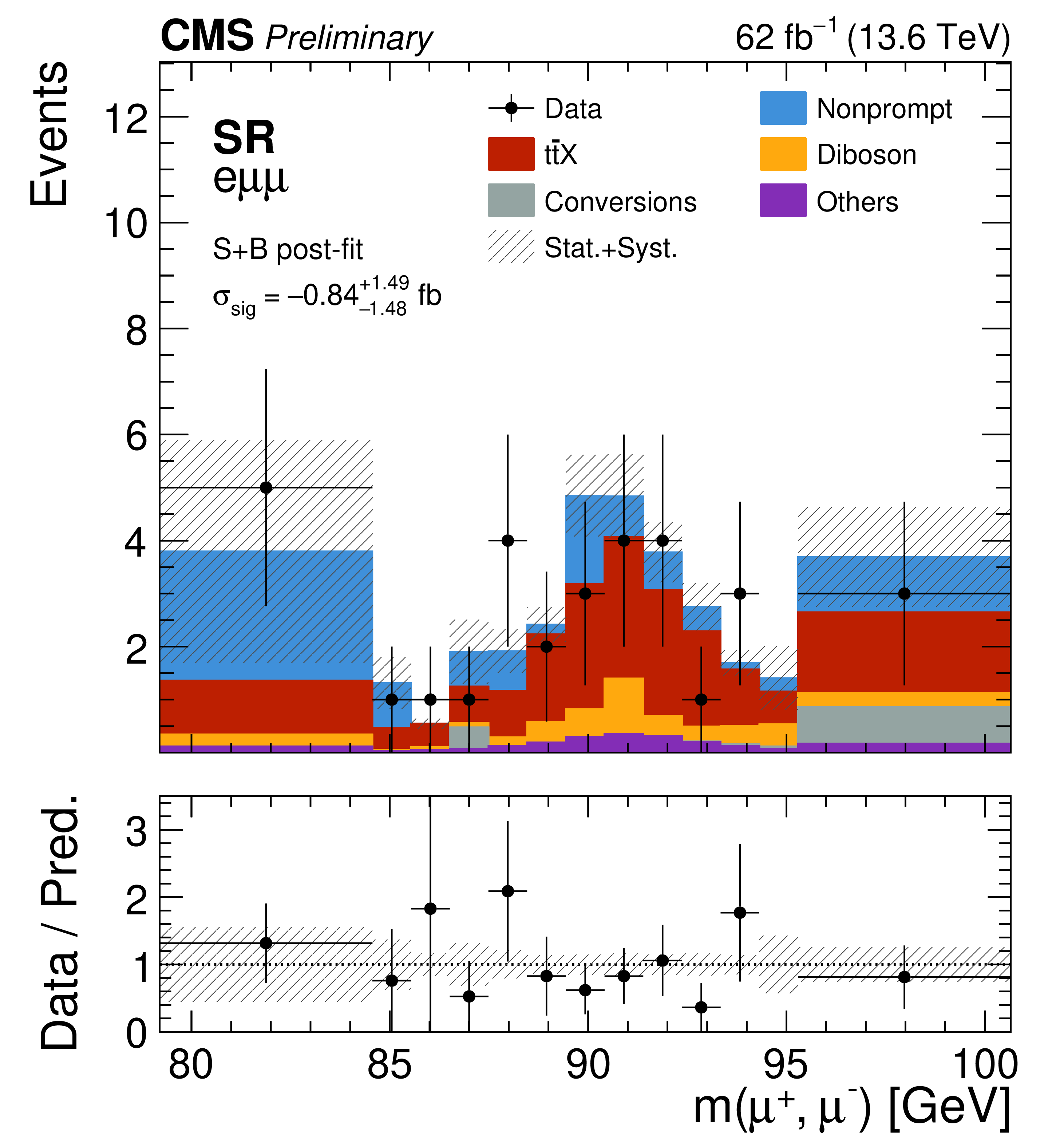
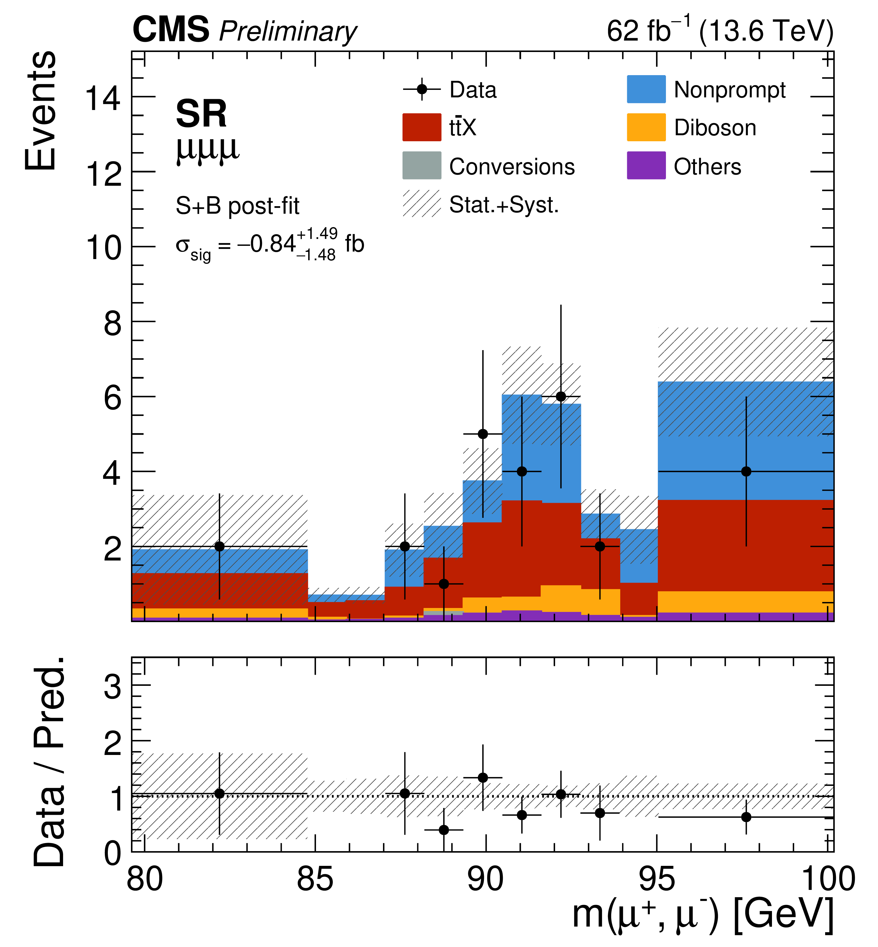
The ParticleNet-selected $ \mathit{m}(\mu^{+}\mu^{-}) $ templates after the signal-plus-background fit, for the $ (\mathit{m}_{\mathrm{H^+}}, \mathit{m}_{\mathrm{A}}) = (130, 90) \text{GeV} $ mass hypothesis, for the $ \mathrm{e}\mu\mu $ (left column) and $ \mu\mu\mu $ (right column) channels in the Run 2 (upper row, 138 fb$^{-1}$, $ \sqrt{s} = $ 13 TeV) and Run 3 (lower row, 62 fb$^{-1}$, $ \sqrt{s} = $ 13.6 TeV) data-taking periods. The fitted signal cross section $ \sigma_\text{sig} $ is given in each panel. The hatched band indicates the total uncertainty after the fit. |
png pdf |
Figure 10-a:
The ParticleNet-selected $ \mathit{m}(\mu^{+}\mu^{-}) $ templates after the signal-plus-background fit, for the $ (\mathit{m}_{\mathrm{H^+}}, \mathit{m}_{\mathrm{A}}) = (130, 90) \text{GeV} $ mass hypothesis, for the $ \mathrm{e}\mu\mu $ (left column) and $ \mu\mu\mu $ (right column) channels in the Run 2 (upper row, 138 fb$^{-1}$, $ \sqrt{s} = $ 13 TeV) and Run 3 (lower row, 62 fb$^{-1}$, $ \sqrt{s} = $ 13.6 TeV) data-taking periods. The fitted signal cross section $ \sigma_\text{sig} $ is given in each panel. The hatched band indicates the total uncertainty after the fit. |
png pdf |
Figure 10-b:
The ParticleNet-selected $ \mathit{m}(\mu^{+}\mu^{-}) $ templates after the signal-plus-background fit, for the $ (\mathit{m}_{\mathrm{H^+}}, \mathit{m}_{\mathrm{A}}) = (130, 90) \text{GeV} $ mass hypothesis, for the $ \mathrm{e}\mu\mu $ (left column) and $ \mu\mu\mu $ (right column) channels in the Run 2 (upper row, 138 fb$^{-1}$, $ \sqrt{s} = $ 13 TeV) and Run 3 (lower row, 62 fb$^{-1}$, $ \sqrt{s} = $ 13.6 TeV) data-taking periods. The fitted signal cross section $ \sigma_\text{sig} $ is given in each panel. The hatched band indicates the total uncertainty after the fit. |
png pdf |
Figure 10-c:
The ParticleNet-selected $ \mathit{m}(\mu^{+}\mu^{-}) $ templates after the signal-plus-background fit, for the $ (\mathit{m}_{\mathrm{H^+}}, \mathit{m}_{\mathrm{A}}) = (130, 90) \text{GeV} $ mass hypothesis, for the $ \mathrm{e}\mu\mu $ (left column) and $ \mu\mu\mu $ (right column) channels in the Run 2 (upper row, 138 fb$^{-1}$, $ \sqrt{s} = $ 13 TeV) and Run 3 (lower row, 62 fb$^{-1}$, $ \sqrt{s} = $ 13.6 TeV) data-taking periods. The fitted signal cross section $ \sigma_\text{sig} $ is given in each panel. The hatched band indicates the total uncertainty after the fit. |
png pdf |
Figure 10-d:
The ParticleNet-selected $ \mathit{m}(\mu^{+}\mu^{-}) $ templates after the signal-plus-background fit, for the $ (\mathit{m}_{\mathrm{H^+}}, \mathit{m}_{\mathrm{A}}) = (130, 90) \text{GeV} $ mass hypothesis, for the $ \mathrm{e}\mu\mu $ (left column) and $ \mu\mu\mu $ (right column) channels in the Run 2 (upper row, 138 fb$^{-1}$, $ \sqrt{s} = $ 13 TeV) and Run 3 (lower row, 62 fb$^{-1}$, $ \sqrt{s} = $ 13.6 TeV) data-taking periods. The fitted signal cross section $ \sigma_\text{sig} $ is given in each panel. The hatched band indicates the total uncertainty after the fit. |
png pdf |
Figure 11:
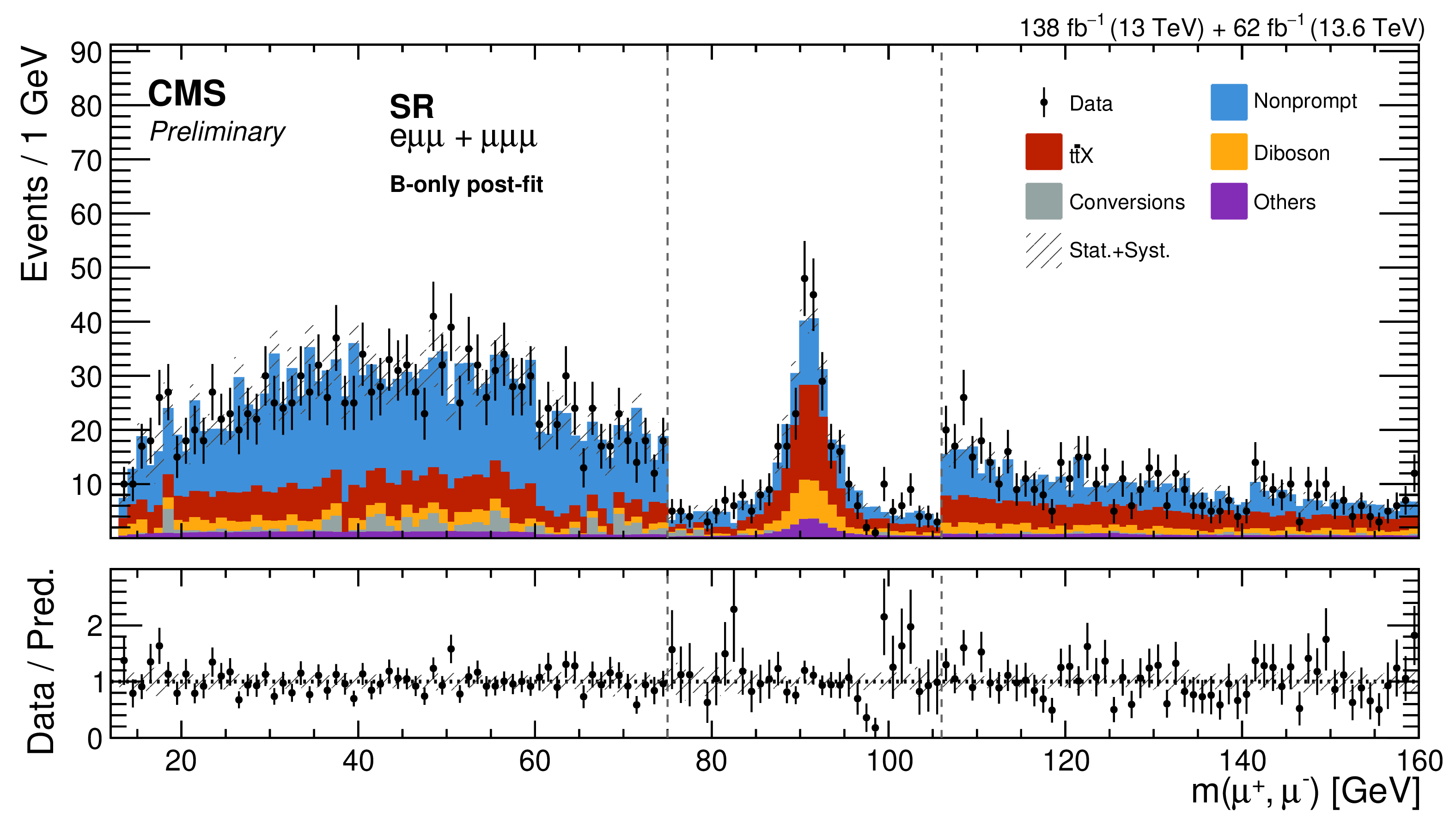
The $ \mathit{m}(\mu^{+}\mu^{-}) $ distribution after the background-only fit, assembled from the fits at the seed hypotheses with $ \mathit{m}_{\mathrm{H^+}} = $ 160 GeV as described in the text and shown in bins of 1 GeV. The interval between the vertical dashed lines is taken from the ParticleNet-selected fits, in which the $ \text{LR}_\text{modified} $ requirement is applied, and the rest of the distribution from the dimuon-mass-only fits. The hatched band indicates the total uncertainty after the fit, and the lower panel shows the ratio of the data to the fitted background. |
png pdf |
Figure 12:
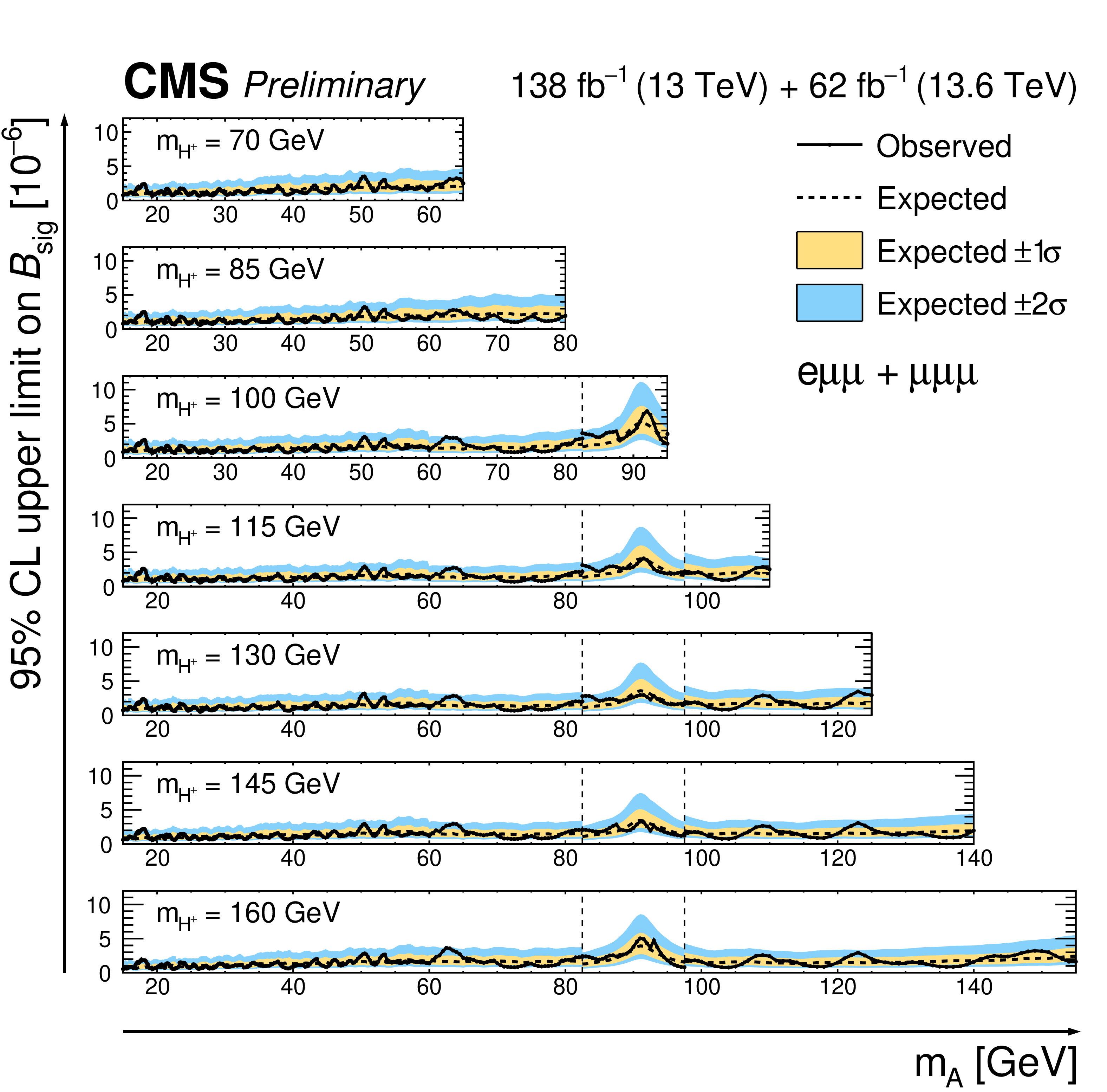
Expected and observed upper limits at 95% CL on the signal branching fraction $ \mathcal{B}_\text{sig} $ as a function of $ \mathit{m}_{\mathrm{A}} $, shown in a separate panel for each signal mass hypothesis, from the uppermost to the lowest panel $ \mathit{m}_{\mathrm{H^+}} = $ 70, 85, 100, 115, 130, 145, and 160 GeV, combining the Run 2 (138 fb$^{-1}$, $ \sqrt{s} = $ 13 TeV) and Run 3 (62 fb$^{-1}$, $ \sqrt{s} = $ 13.6 TeV) data sets. The limits are evaluated at every mass hypothesis of the scan in $ \mathit{m}_{\mathrm{A}} $. For $ \mathit{m}_{\mathrm{H^+}} \ge $ 100 GeV, the vertical dashed lines delimit the region 82.5 $ \le \mathit{m}_{\mathrm{A}} \le $ 97.5 GeV, in which the ParticleNet-selected templates are used. Outside this region the dimuon-mass-only templates are used. |
png pdf |
Figure 13:
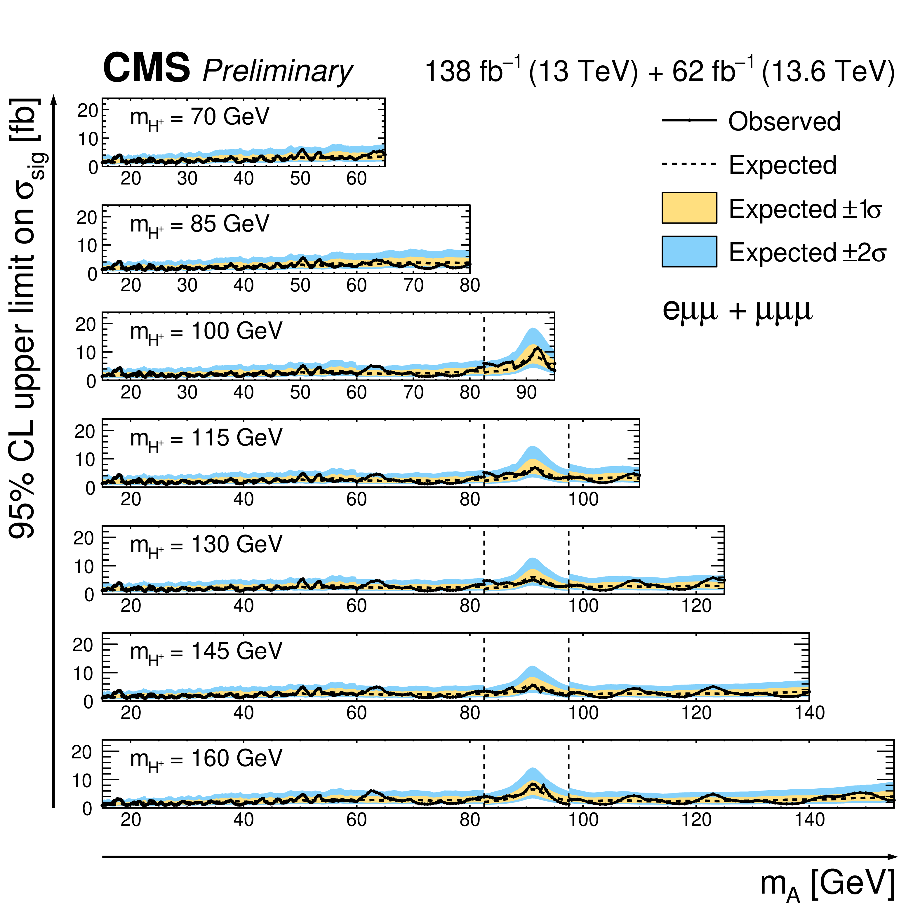
Expected and observed upper limits at 95% CL on the signal cross section $ \sigma_\text{sig} $ at $ \sqrt{s} = $ 13 TeV as a function of $ \mathit{m}_{\mathrm{A}} $, shown in a separate panel for each signal mass hypothesis, from the uppermost to the lowest panel $ \mathit{m}_{\mathrm{H^+}} = $ 70, 85, 100, 115, 130, 145, and 160 GeV, combining the Run 2 (138 fb$^{-1}$, $ \sqrt{s} = $ 13 TeV) and Run 3 (62 fb$^{-1}$, $ \sqrt{s} = $ 13.6 TeV) data sets. The conversion from $ \mathcal{B}_\text{sig} $ to $ \sigma_\text{sig} $ uses the $ \mathrm{t}\overline{\mathrm{t}} $ production cross section at 13 TeV given in Section 3. The limits are evaluated at every mass hypothesis of the scan in $ \mathit{m}_{\mathrm{A}} $. For $ \mathit{m}_{\mathrm{H^+}} \ge $ 100 GeV, the vertical dashed lines delimit the region 82.5 $ \le \mathit{m}_{\mathrm{A}} \le $ 97.5 GeV, in which the ParticleNet-selected templates are used. Outside this region the dimuon-mass-only templates are used. |
| Tables | |
png pdf |
Table 1:
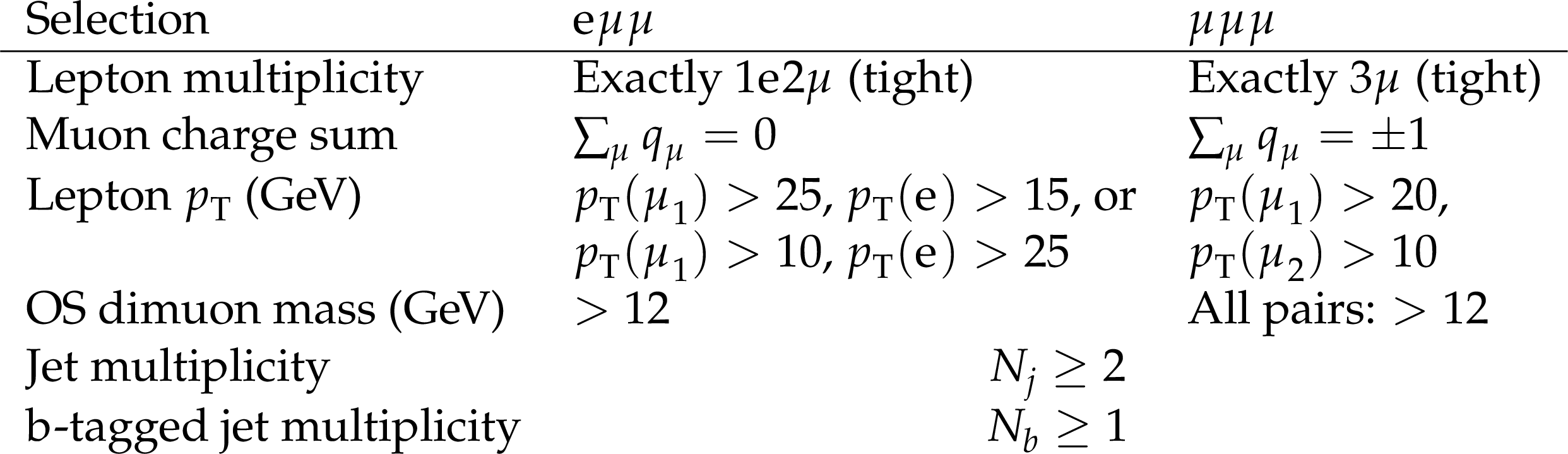
Event selection criteria for the $ \mathrm{e}\mu\mu $ and $ \mu\mu\mu $ signal channels. The muons are ordered by decreasing $ p_{\mathrm{T}} $, with $ \mu_1 $ and $ \mu_2 $ denoting the highest- and second-highest-$ p_{\mathrm{T}} $ muon, respectively, and $ q_\mu $ is the muon electric charge in units of the elementary charge. |
png pdf |
Table 2:
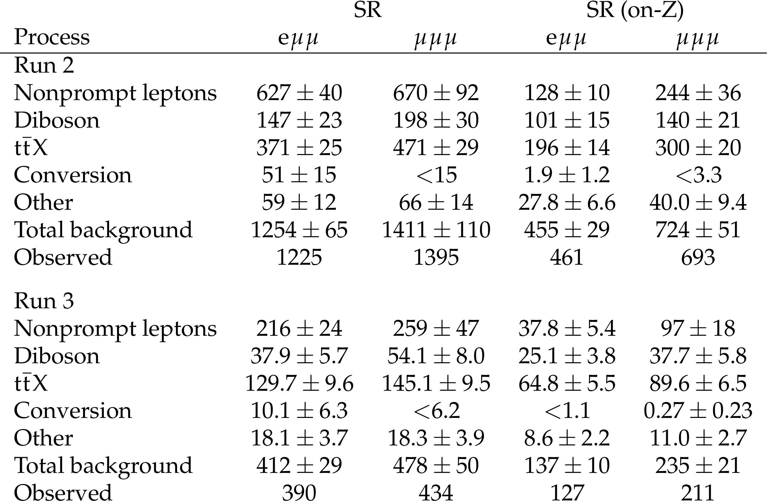
Expected background yields, before the maximum likelihood fit, in the SRs for the Run 2 (2016--2018, 138 fb$^{-1}$, $ \sqrt{s} = $ 13 TeV) and Run 3 (2022--2023, 62 fb$^{-1}$, $ \sqrt{s} = $ 13.6 TeV) data-taking periods, together with the observed event counts. The on-Z columns count the subset of events with a dimuon mass within 85 $ < \mathit{m}(\mu^{+}\mu^{-}) < $ 95 GeV, for either OS dimuon pair in the $ \mu\mu\mu $ channel. The uncertainties in the background yields include the statistical and systematic contributions. For yields whose uncertainty exceeds the expected value, an upper bound given by the expected yield plus one standard deviation is quoted, while the total background includes the expected yield. |
png pdf |
Table 3:
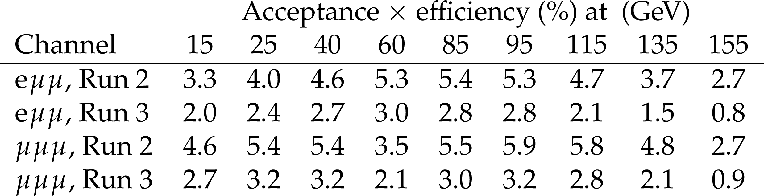
Product of signal acceptance and selection efficiency, in percent, for signal mass hypotheses with $ \mathit{m}_{\mathrm{H^+}} = $ 160 GeV, determined from simulation. The values include the generator-level requirement that at least one W boson decays leptonically and the requirement that the dimuon mass lies within $ \pm 5\sigma_{\mu\mu} $ of the fitted peak position, and are luminosity-weighted averages over the data-taking years of the Run 2 ($ \sqrt{s} = $ 13 TeV) and Run 3 ($ \sqrt{s} = $ 13.6 TeV) periods. |
png pdf |
Table 4:
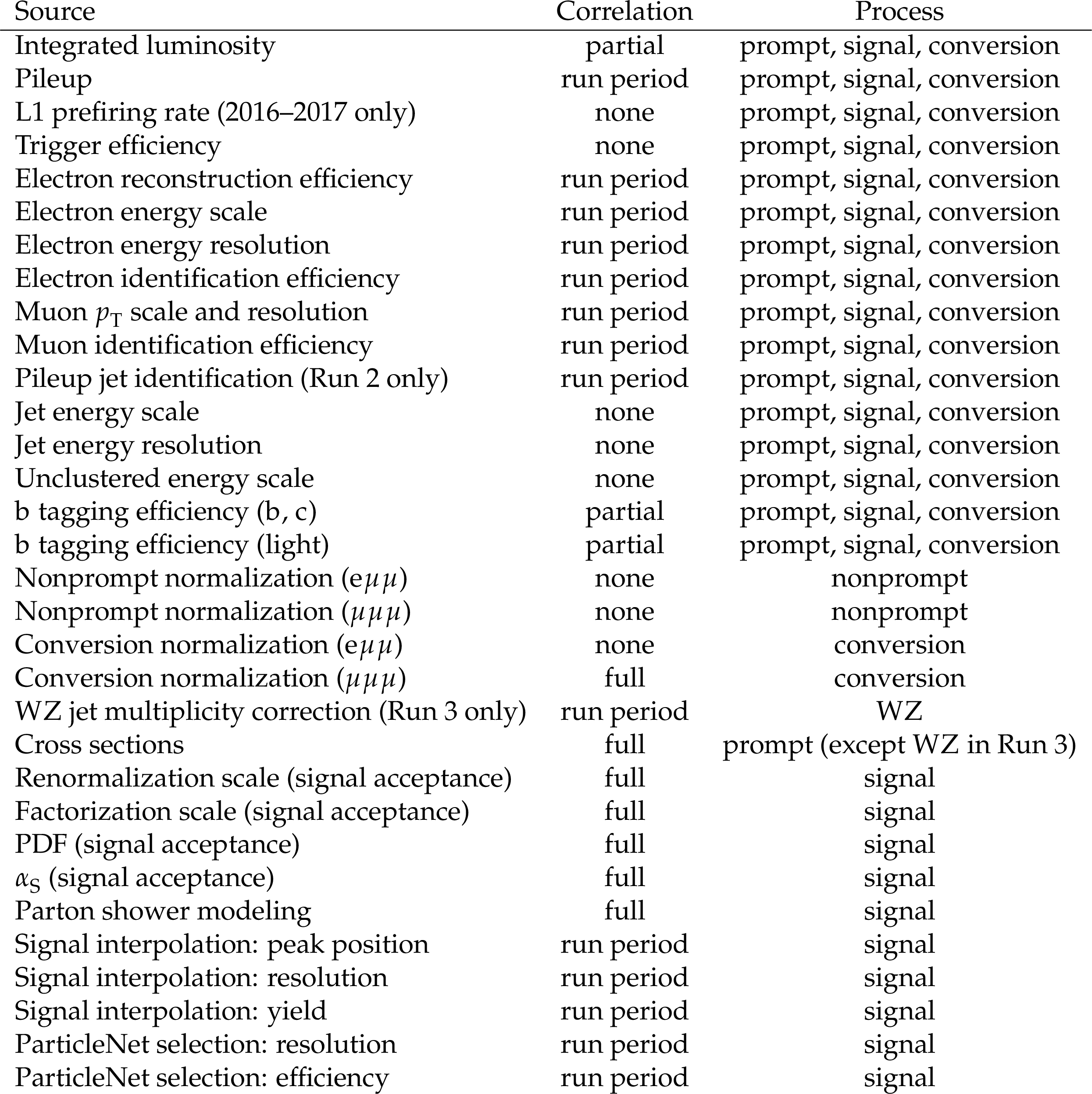
Summary of systematic uncertainty sources, their correlation across data-taking years, and the processes to which they apply. In the correlation column, ``none'' denotes that an independent uncertainty is assigned to each data-taking year, ``run period'' denotes uncertainties correlated across the data-taking years of the same run period but uncorrelated between Run 2 and Run 3, ``full'' denotes a single uncertainty shared by Run 2 and Run 3, and ``partial'' indicates that only some components are correlated, as described in the text. The last two rows apply only to the ParticleNet-selected templates, for which the resolution term replaces the signal interpolation resolution term. |
| Summary |
| A search for a light charged Higgs boson in the decay chain $ \mathrm{H^+} \to \mathrm{W^+}\mathrm{A} \to \mathrm{W^+}\mu^{+}\mu^{-} $, produced via $ \mathrm{t} \to \mathrm{H^+}\mathrm{b} $ in top quark pair production, is presented using proton-proton collision data collected by the CMS experiment at the CERN LHC, corresponding to 138 fb$^{-1}$ at $ \sqrt{s} = $ 13 TeV and 62 fb$^{-1}$ at $ \sqrt{s} = $ 13.6 TeV, for a total of 200 fb$^{-1}$. Events with three leptons in the $ \mathrm{e}\mu\mu $ or $ \mu\mu\mu $ final state and at least two jets, of which at least one is identified as originating from a bottom quark, are selected, and the signal is searched for as a narrow peak in the dimuon invariant mass distribution. Mass hypotheses with $ \mathit{m}_{\mathrm{H^+}} $ from 70 to 160 GeV and $ \mathit{m}_{\mathrm{A}} $ from 15 GeV up to $ (\mathit{m}_{\mathrm{H^+}} - 5 \text{GeV}) $ are explored. No significant excess over the standard model prediction is observed. Model-independent upper limits at 95% confidence level are set on the branching fraction $ \mathcal{B}_\text{sig} \equiv \mathcal{B}(\mathrm{t} \to \mathrm{H^+}\mathrm{b}) \times \mathcal{B}(\mathrm{H^+} \to \mathrm{W^+}\mathrm{A}) \times \mathcal{B}(\mathrm{A} \to \mu^{+}\mu^{-}) $ in the range $ ( $ 0.5--6.8 $) \times 10^{-6} $, depending on the mass hypothesis, and on the corresponding signal cross section $ \sigma_\text{sig} = 2\sigma(\mathrm{p}\mathrm{p} \to \mathrm{t}\overline{\mathrm{t}}) \times \mathcal{B}_\text{sig} $ at $ \sqrt{s} = $ 13 TeV. These results provide the first constraints in the off-shell W boson regime. The sensitivity is limited by the statistical uncertainty in the data and is expected to improve with the data of the ongoing LHC run and of the High-Luminosity LHC. |
| References | ||||
| 1 | S. L. Glashow | Partial Symmetries of Weak Interactions | NP 22 (1961) 579 | |
| 2 | S. Weinberg | A Model of Leptons | PRL 19 (1967) 1264 | |
| 3 | A. Salam | Weak and Electromagnetic Interactions | in Elementary Particle Theory: at Lerum, Sweden, N. Svartholm, ed., Almqvist and Wiksell, Stockholm, 1968 Proceedings of the Nobel Symposium Held 196 (1968) 367 |
|
| 4 | ATLAS Collaboration | Observation of a new particle in the search for the Standard Model Higgs boson with the ATLAS detector at the LHC | PLB 716 (2012) 1 | 1207.7214 |
| 5 | CMS Collaboration | Observation of a new boson at a mass of 125 GeV with the CMS experiment at the LHC | PLB 716 (2012) 30 | CMS-HIG-12-028 1207.7235 |
| 6 | CMS Collaboration | A portrait of the Higgs boson by the CMS experiment ten years after the discovery | Nature 607 (2022) 60 | CMS-HIG-22-001 2207.00043 |
| 7 | ATLAS Collaboration | A detailed map of Higgs boson interactions by the ATLAS experiment ten years after the discovery | Nature 607 (2022) 52 | 2207.00092 |
| 8 | S. P. Martin | A Supersymmetry primer | Adv. Ser. Direct. High Energy Phys. 18 (1998) 1 | hep-ph/9709356 |
| 9 | A. D. Sakharov | Violation of CP Invariance, C Asymmetry, and Baryon Asymmetry of the Universe | [Sov. Phys. Usp. 34 () 392], 1967 JETP Lett. 5 (1967) 24 |
|
| 10 | R. D. Peccei and H. R. Quinn | CP Conservation in the Presence of Instantons | PRL 38 (1977) 1440 | |
| 11 | R. D. Peccei and H. R. Quinn | Constraints Imposed by CP Conservation in the Presence of Instantons | PRD 16 (1977) 1791 | |
| 12 | G. C. Branco et al. | Theory and phenomenology of two-Higgs-doublet models | Phys. Rept. 516 (2012) 1 | 1106.0034 |
| 13 | M. Misiak and M. Steinhauser | Weak radiative decays of the B meson and bounds on $ M_{H^\pm} $ in the two-Higgs-doublet model | EPJC 77 (2017) 201 | 1702.04571 |
| 14 | P. Sikivie, L. Susskind, M. B. Voloshin, and V. I. Zakharov | Isospin Breaking in Technicolor Models | NPB 173 (1980) 189 | |
| 15 | CMS Collaboration | Performance of the CMS muon detector and muon reconstruction with proton-proton collisions at $ \sqrt{s} = $ 13 TeV | JINST 13 (2018) P06015 | CMS-MUO-16-001 1804.04528 |
| 16 | H. Qu and L. Gouskos | ParticleNet: Jet Tagging via Particle Clouds | PRD 101 (2020) 056019 | 1902.08570 |
| 17 | D. Eriksson, J. Rathsman, and O. Staal | 2HDMC: Two-Higgs-Doublet Model Calculator physics and manual | Comput. Phys. Commun. 181 (2010) 189 | 0902.0851 |
| 18 | ALEPH, DELPHI, L3, OPAL Collaborations | Search for charged Higgs bosons: combined results using LEP data | EPJC 73 (2013) 2463 | 1301.6065 |
| 19 | DELPHI Collaboration | Search for charged Higgs bosons at LEP in general two Higgs doublet models | EPJC 34 (2004) 399 | hep-ex/0404012 |
| 20 | OPAL Collaboration | Search for charged Higgs bosons in $ e^{+}e^{-} $ collisions at $ \sqrt{s} = 189- $ 209 GeV | EPJC 72 (2012) 2076 | 0812.0267 |
| 21 | CDF Collaboration | Search for charged Higgs bosons from top quark decays in $ p\bar{p} $ collisions at $ \sqrt{s}= $ 1.96 TeV | PRL 96 (2006) 042003 | hep-ex/0510065 |
| 22 | CMS Collaboration | Search for charged Higgs bosons in the $ \mathrm{H}^{\pm} \to \tau^{\pm}\nu_{\tau} $ decay channel in proton-proton collisions at $ \sqrt{s}= $ 13 TeV | JHEP 07 (2019) 142 | CMS-HIG-18-014 1903.04560 |
| 23 | ATLAS Collaboration | Search for charged Higgs bosons decaying via $ H^{\pm} \to \tau^{\pm}\nu_{\tau} $ in the $ \tau $+jets and $ \tau $+lepton final states with 36 fb$^{-1}$ of pp collision data recorded at $ \sqrt{s}= $ 13 TeV with the ATLAS experiment | JHEP 09 (2018) 139 | 1807.07915 |
| 24 | CMS Collaboration | Search for charged Higgs bosons decaying into a top and a bottom quark in the all-jet final state of pp collisions at $ \sqrt{s}= $ 13 TeV | JHEP 07 (2020) 126 | CMS-HIG-18-015 2001.07763 |
| 25 | CMS Collaboration | Search for a light charged Higgs boson in the $ \mathrm{H}^{\pm} \to \mathrm{cs} $ channel in proton-proton collisions at $ \sqrt{s}= $ 13 TeV | PRD 102 (2020) 072001 | CMS-HIG-18-021 2005.08900 |
| 26 | ATLAS Collaboration | Search for a light charged Higgs boson in $ t \to H^{\pm}b $ decays, with $ H^{\pm} \to cs $, in pp collisions at $ \sqrt{s}= $ 13 TeV with the ATLAS detector | EPJC 85 (2025) 153 | 2407.10096 |
| 27 | ATLAS Collaboration | Search for a light charged Higgs boson in $ t \to H^{\pm}b $ decays, with $ H^{\pm} \to cb $, in the lepton+jets final state in proton-proton collisions at $ \sqrt{s}= $ 13 TeV with the ATLAS detector | JHEP 09 (2023) 004 | 2302.11739 |
| 28 | CMS Collaboration | Search for a light charged Higgs boson decaying to a $ W $ boson and a $ CP $-odd Higgs boson in final states with $ e\mu\mu $ or $ \mu\mu\mu $ in proton-proton collisions at $ \sqrt{s} = $ 13 TeV | PRL 123 (2019) 131802 | CMS-HIG-18-020 1905.07453 |
| 29 | ATLAS Collaboration | Search for a new pseudoscalar decaying into a pair of muons in events with a top-quark pair at $ \sqrt{s} = $ 13 TeV with the ATLAS detector | PRD 108 (2023) 092007 | 2304.14247 |
| 30 | CMS Collaboration | The CMS experiment at the CERN LHC | JINST 3 (2008) S08004 | |
| 31 | CMS Collaboration | Performance of the CMS Level-1 trigger in proton-proton collisions at $ \sqrt{s} = $ 13 TeV | JINST 15 (2020) P10017 | CMS-TRG-17-001 2006.10165 |
| 32 | CMS Collaboration | The CMS trigger system | JINST 12 (2017) P01020 | CMS-TRG-12-001 1609.02366 |
| 33 | CMS Collaboration | Development of the CMS detector for the CERN LHC Run 3 | JINST 19 (2024) P05064 | CMS-PRF-21-001 2309.05466 |
| 34 | CMS BRIL Collaboration | The pixel luminosity telescope: a detector for luminosity measurement at CMS using silicon pixel sensors | EPJC 83 (2023) 673 | 2206.08870 |
| 35 | CMS Collaboration | Particle-flow reconstruction and global event description with the CMS detector | JINST 12 (2017) P10003 | CMS-PRF-14-001 1706.04965 |
| 36 | CMS Collaboration | Description and performance of track and primary-vertex reconstruction with the CMS tracker | JINST 9 (2014) P10009 | CMS-TRK-11-001 1405.6569 |
| 37 | CMS Collaboration | Electron and photon reconstruction and identification with the CMS experiment at the CERN LHC | JINST 16 (2021) P05014 | CMS-EGM-17-001 2012.06888 |
| 38 | M. Cacciari, G. P. Salam, and G. Soyez | The anti-$ k_{\mathrm{T}} $ jet clustering algorithm | JHEP 04 (2008) 063 | 0802.1189 |
| 39 | M. Cacciari, G. P. Salam, and G. Soyez | FastJet user manual | EPJC 72 (2012) 1896 | 1111.6097 |
| 40 | D. Bertolini, P. Harris, M. Low, and N. Tran | Pileup per particle identification | JHEP 10 (2014) 059 | 1407.6013 |
| 41 | CMS Collaboration | Pileup mitigation at CMS in 13 TeV data | JINST 15 (2020) P09018 | CMS-JME-18-001 2003.00503 |
| 42 | CMS Collaboration | Jet energy scale and resolution in the CMS experiment in pp collisions at 8 TeV | JINST 12 (2017) P02014 | CMS-JME-13-004 1607.03663 |
| 43 | CMS Collaboration | Jet energy scale and resolution performance with 13 TeV data collected by CMS in 2016--2018 | Technical Report CMS-DP-2020-019, CERN, 2020 CDS |
|
| 44 | CMS Collaboration | Precision luminosity measurement in proton-proton collisions at $ \sqrt{s} = $ 13 TeV in 2015 and 2016 at CMS | EPJC 81 (2021) 800 | CMS-LUM-17-003 2104.01927 |
| 45 | CMS Collaboration | Precision luminosity measurement in proton-proton collisions at a center-of-mass energy of 13 TeV with the CMS detector at the Large Hadron Collider | Submitted to Phys. Rev. X | CMS-LUM-20-001 2606.26832 |
| 46 | CMS Collaboration | Luminosity measurement in proton-proton collisions at 13.6 TeV in 2022 at CMS | CMS Physics Analysis Summary, CERN, 2024 CMS-PAS-LUM-22-001 |
CMS-PAS-LUM-22-001 |
| 47 | CMS Collaboration | Measurement of the offline integrated luminosity for the CMS proton-proton collision dataset recorded in 2023 | Technical Report CMS-DP-2024-068, CERN, 2024 CDS |
|
| 48 | CMS Collaboration | Performance of the CMS muon trigger system in proton-proton collisions at $ \sqrt{s} = $ 13 TeV | JINST 16 (2021) P07001 | CMS-MUO-19-001 2102.04790 |
| 49 | P. Nason | A new method for combining NLO QCD with shower Monte Carlo algorithms | JHEP 11 (2004) 040 | hep-ph/0409146 |
| 50 | S. Frixione, P. Nason, and C. Oleari | Matching NLO QCD computations with parton shower simulations: the POWHEG method | JHEP 11 (2007) 070 | 0709.2092 |
| 51 | S. Alioli, P. Nason, C. Oleari, and E. Re | A general framework for implementing NLO calculations in shower Monte Carlo programs: the POWHEG BOX | JHEP 06 (2010) 043 | 1002.2581 |
| 52 | J. Alwall et al. | The automated computation of tree-level and next-to-leading order differential cross sections, and their matching to parton shower simulations | JHEP 07 (2014) 079 | 1405.0301 |
| 53 | NNPDF Collaboration | Parton distributions from high-precision collider data | EPJC 77 (2017) 663 | 1706.00428 |
| 54 | T. Sjöstrand et al. | An introduction to PYTHIA 8.2 | Comput. Phys. Commun. 191 (2015) 159 | 1410.3012 |
| 55 | CMS Collaboration | Extraction and validation of a new set of CMS PYTHIA 8 tunes from underlying-event measurements | EPJC 80 (2020) 4 | CMS-GEN-17-001 1903.12179 |
| 56 | \GEANTfour Collaboration | $ GEANT $ 4 --- a simulation toolkit | NIM A 506 (2003) 250 | |
| 57 | R. Frederix and S. Frixione | Merging meets matching in MC@NLO | JHEP 12 (2012) 061 | 1209.6215 |
| 58 | M. Grazzini, S. Kallweit, D. Rathlev, and M. Wiesemann | $ W^\pm Z $ production at hadron colliders in NNLO QCD | PLB 761 (2016) 179 | 1604.08576 |
| 59 | F. Cascioli et al. | ZZ production at hadron colliders in NNLO QCD | PLB 735 (2014) 311 | 1405.2219 |
| 60 | N. Kidonakis and C. Foster | Soft-gluon corrections in $ t\bar{t}W $ production | PLB 854 (2024) 138708 | 2312.00861 |
| 61 | N. Kidonakis and C. Foster | Higher-order soft-gluon corrections for $ t\bar{t}Z $ cross sections | PLB 860 (2025) 139146 | 2410.01214 |
| 62 | H. B. Hartanto, B. Jager, L. Reina, and D. Wackeroth | Higgs boson production in association with top quarks in the POWHEG BOX | PRD 91 (2015) 094003 | 1501.04498 |
| 63 | D. de Florian et al. | Handbook of LHC Higgs cross sections: 4. Deciphering the nature of the Higgs sector | CERN Yellow Rep. Monogr. 2 (2017) | 1610.07922 |
| 64 | E. Bagnaschi, G. Degrassi, P. Slavich, and A. Vicini | Higgs production via gluon fusion in the POWHEG approach in the SM and in the MSSM | JHEP 02 (2012) 088 | 1111.2854 |
| 65 | P. Nason and C. Oleari | NLO Higgs boson production via vector-boson fusion matched with shower in POWHEG | JHEP 02 (2010) 037 | 0911.5299 |
| 66 | Y. Gao et al. | Spin determination of single-produced resonances at hadron colliders | PRD 81 (2010) 075022 | 1001.3396 |
| 67 | Y. Li and F. Petriello | Combining QCD and electroweak corrections to dilepton production in the framework of the FEWZ simulation code | PRD 86 (2012) 094034 | 1208.5967 |
| 68 | M. Cacciari et al. | Top-pair production at hadron colliders with next-to-next-to-leading logarithmic soft-gluon resummation | PLB 710 (2012) 612 | 1111.5869 |
| 69 | P. B ä rnreuther, M. Czakon, and A. Mitov | Percent level precision physics at the Tevatron: first genuine NNLO QCD corrections to $ q\bar{q} \to t\bar{t} + X $ | PRL 109 (2012) 132001 | 1204.5201 |
| 70 | M. Czakon and A. Mitov | NNLO corrections to top-pair production at hadron colliders: the all-fermionic scattering channels | JHEP 12 (2012) 054 | 1207.0236 |
| 71 | M. Czakon and A. Mitov | NNLO corrections to top pair production at hadron colliders: the quark-gluon reaction | JHEP 01 (2013) 080 | 1210.6832 |
| 72 | M. Czakon, P. Fiedler, and A. Mitov | Total top-quark pair-production cross section at hadron colliders through $ \mathcal{O}(\alpha_s^4) $ | PRL 110 (2013) 252004 | 1303.6254 |
| 73 | S. Catani et al. | Top-quark pair hadroproduction at next-to-next-to-leading order in QCD | PRD 99 (2019) 051501 | 1901.04005 |
| 74 | M. Czakon and A. Mitov | Top++: a program for the calculation of the top-pair cross-section at hadron colliders | Comput. Phys. Commun. 185 (2014) 2930 | 1112.5675 |
| 75 | R. D. Ball et al. | The PDF4LHC21 combination of global PDF fits for the LHC Run III | JPG 49 (2022) 080501 | 2203.05506 |
| 76 | N. Kidonakis | Two-loop soft anomalous dimensions for single top quark associated production with a $ W^- $ or $ H^- $ | PRD 82 (2010) 054018 | 1005.4451 |
| 77 | N. Kidonakis and N. Yamanaka | Higher-order corrections for $ tW $ production at high-energy hadron colliders | JHEP 05 (2021) 278 | 2102.11300 |
| 78 | P. Artoisenet, R. Frederix, O. Mattelaer, and R. Rietkerk | Automatic spin-entangled decays of heavy resonances in Monte Carlo simulations | JHEP 03 (2013) 015 | 1212.3460 |
| 79 | N. Kidonakis | NNLL resummation for $ s $-channel single top quark production | PRD 81 (2010) 054028 | 1001.5034 |
| 80 | N. Kidonakis | Next-to-next-to-leading-order collinear and soft gluon corrections for $ t $-channel single top quark production | PRD 83 (2011) 091503 | 1103.2792 |
| 81 | Z. L. Liu and J. Gao | $ s $-channel single top quark production and decay at next-to-next-to-leading-order in QCD | PRD 98 (2018) 071501 | 1807.03835 |
| 82 | J. Campbell, T. Neumann, and Z. Sullivan | Single-top-quark production in the $ t $-channel at NNLO | JHEP 02 (2021) 040 | 2012.01574 |
| 83 | M. Grazzini, S. Kallweit, and M. Wiesemann | Fully differential NNLO computations with MATRIX | EPJC 78 (2018) 537 | 1711.06631 |
| 84 | C. Degrande | Automatic evaluation of UV and R2 terms for beyond the Standard Model Lagrangians: a proof-of-principle | Comput. Phys. Commun. 197 (2015) 239 | 1406.3030 |
| 85 | K. Rehermann and B. Tweedie | Efficient Identification of Boosted Semileptonic Top Quarks at the LHC | JHEP 03 (2011) 059 | 1007.2221 |
| 86 | CMS Collaboration | Search for supersymmetry in pp collisions at $ \sqrt{s}= $ 13 TeV in the single-lepton final state using the sum of masses of large-radius jets | JHEP 08 (2016) 122 | CMS-SUS-15-007 1605.04608 |
| 87 | W. Adam et al. | The CMS Phase-1 pixel detector upgrade | JINST 16 (2021) P02027 | 2012.14304 |
| 88 | E. Bols et al. | Jet Flavour Classification Using DeepJet | JINST 15 (2020) P12012 | 2008.10519 |
| 89 | CMS Collaboration | Performance summary of AK4 jet b tagging with data from proton-proton collisions at 13 TeV with the CMS detector | Technical Report CMS-DP-2023-005, CERN, 2023 CDS |
|
| 90 | CMS Collaboration | A first look at early 2022 proton-proton collisions at $ \sqrt{s} = $ 13.6 TeV for heavy-flavor jet tagging | Technical Report CMS-DP-2023-012, CERN, 2023 CDS |
|
| 91 | CMS Collaboration | Performance of missing transverse momentum reconstruction in proton-proton collisions at $ \sqrt{s} = $ 13 TeV using the CMS detector | JINST 14 (2019) P07004 | CMS-JME-17-001 1903.06078 |
| 92 | Y. Wang et al. | Dynamic graph CNN for learning on point clouds | ACM Trans. Graph. 38 (2019) 146 | 1801.07829 |
| 93 | G. J. Székely, M. L. Rizzo, and N. K. Bakirov | Measuring and testing dependence by correlation of distances | The Annals of Statistics 35 (2007) 2769 | |
| 94 | J. H. Holland | Adaptation in Natural and Artificial Systems: An Introductory Analysis with Applications to Biology, Control, and Artificial Intelligence | MIT Press, Cambridge, MA,, ISBN 978-0-262-08213-6, 1992 link |
|
| 95 | D0 Collaboration | Extraction of the width of the $ W $ boson from measurements of $ \sigma(p\bar{p} \to W + X) \times B(W \to e \nu) $ and $ \sigma(p\bar{p} \to Z + X) \times B(Z \to e e) $ and their ratio | PRD 61 (2000) 072001 | hep-ex/9906025 |
| 96 | M. J. Oreglia | A study of the reactions $ \psi^\prime \to \gamma \gamma \psi $ | PhD thesis, Stanford University, SLAC Report SLAC-R-236, see Appendix D, 1980 link |
|
| 97 | R. J. Barlow and C. Beeston | Fitting using finite Monte Carlo samples | Comput. Phys. Commun. 77 (1993) 219 | |
| 98 | J. S. Conway | Incorporating nuisance parameters in likelihoods for multisource spectra | in orkshop on Statistical Issues Related to Discovery Claims in Search Experiments and Unfolding, CERN, Geneva, Switzerland, 2011 Proceedings of the PHYSTAT 2011 (2011) 115 |
1103.0354 |
| 99 | G. Cowan, K. Cranmer, E. Gross, and O. Vitells | Asymptotic formulae for likelihood-based tests of new physics | EPJC 71 (2011) 1554 | 1007.1727 |
| 100 | J. Butterworth et al. | PDF4LHC recommendations for LHC Run II | JPG 43 (2016) 023001 | 1510.03865 |
| 101 | R. Frederix, D. Pagani, and M. Zaro | Large NLO corrections in $ t\bar{t}W^{\pm} $ and $ t\bar{t}t\bar{t} $ hadroproduction from supposedly subleading EW contributions | JHEP 02 (2018) 031 | 1711.02116 |
| 102 | C. Degrande et al. | Single-top associated production with a $ Z $ or $ H $ boson at the LHC: the SMEFT interpretation | JHEP 10 (2018) 005 | 1804.07773 |
| 103 | CMS Collaboration | The CMS Statistical Analysis and Combination Tool: Combine | Comput. Softw. Big Sci. 8 (2024) 19 | CMS-CAT-23-001 2404.06614 |
| 104 | T. Junk | Confidence level computation for combining searches with small statistics | NIM A 434 (1999) 435 | hep-ex/9902006 |
| 105 | A. L. Read | Presentation of search results: the CL$ _{\text{s}} $ technique | JPG 28 (2002) 2693 | |
| 106 | E. Gross and O. Vitells | Trial factors for the look elsewhere effect in high energy physics | EPJC 70 (2010) 525 | 1005.1891 |
|
|
Compact Muon Solenoid LHC, CERN |

|
|
|
|
|
|