
Compact Muon Solenoid
LHC, CERN
 Visit us: CMS Public Website, CMS Physics ;
Contact us: CMS Publications Committee
Visit us: CMS Public Website, CMS Physics ;
Contact us: CMS Publications Committee
| CMS-PAS-B2G-24-019 | ||
| Search for a heavy resonance decaying into a Higgs boson and a new scalar boson using the $ \gamma\gamma\mathrm{b}\bar{\mathrm{b}} $ final state in proton-proton collisions at $ \sqrt{s} = $ 13 TeV | ||
| CMS Collaboration | ||
| 2026-07-28 | ||
| Abstract: A search is presented for a heavy resonance $ \mathrm{X} $ decaying into a Higgs boson (H) and a new scalar particle ($ \mathrm{Y} $) through the process $ \mathrm{X} \to \mathrm{H}\mathrm{Y} $. The Higgs boson is reconstructed in the diphoton decay channel, while the $ \mathrm{Y} $ particle is reconstructed in its decay to a bottom quark-antiquark pair, resulting in the distinctive $ \gamma\gamma\mathrm{b}\bar{\mathrm{b}} $ final state. The analysis uses proton-proton collision data collected with the CMS detector at a centre-of-mass energy of 13 TeV during 2016--2018, corresponding to an integrated luminosity of 138 fb$ ^{-1} $. The search explores the mass ranges 1.0 $ \leq m_{\mathrm{X}} \leq $ 4.0 TeV and 0.06 $ \leq m_{\mathrm{Y}} \leq $ 2.8 TeV. No statistically significant excess above the background expectation is observed. Model-independent upper limits at 95% confidence level are set on the production cross section times the branching fraction for $ \mathrm{X} \to \mathrm{H}\mathrm{Y} \to \gamma\gamma\mathrm{b}\bar{\mathrm{b}} $, ranging from 0.26 $ \mathrm{fb} $ at $ m_{\mathrm{X}} = $ 1 TeV to 0.046 $ \mathrm{fb} $ at $ m_{\mathrm{X}} = $ 4 TeV. | ||
| Links: CDS record (PDF) ; CADI line (restricted) ; | ||
| Figures | |
png pdf |
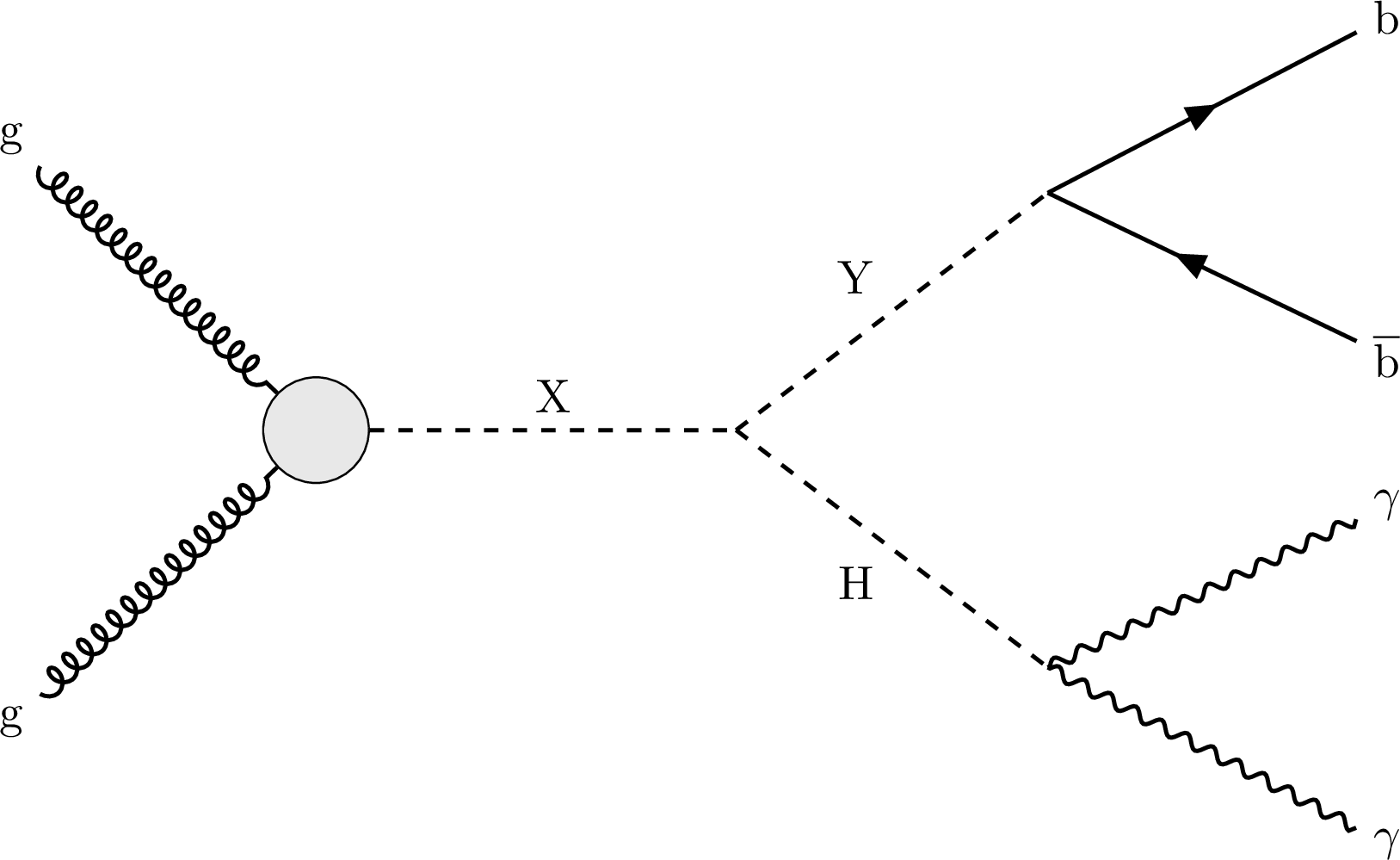
Figure 1:
Feynman diagram for the production of a resonance $ \mathrm{X} $ via gluon-gluon fusion and its decay $ \mathrm{X}\to\mathrm{H}\mathrm{Y} $, with $ \mathrm{H}\to\gamma\gamma $ and $ \mathrm{Y}\to\mathrm{b}\bar{\mathrm{b}} $. |
png pdf |
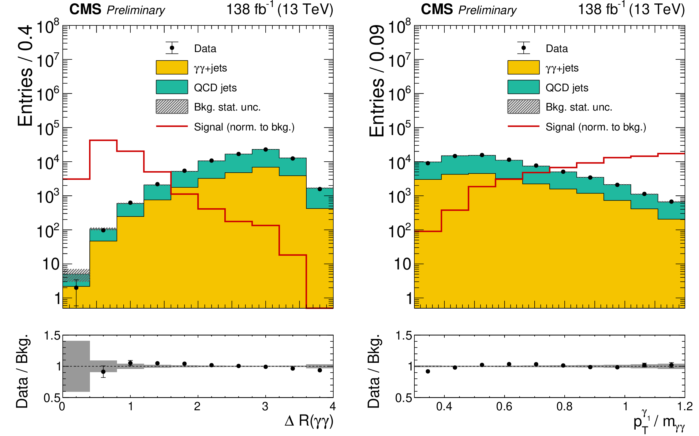
Figure 2:
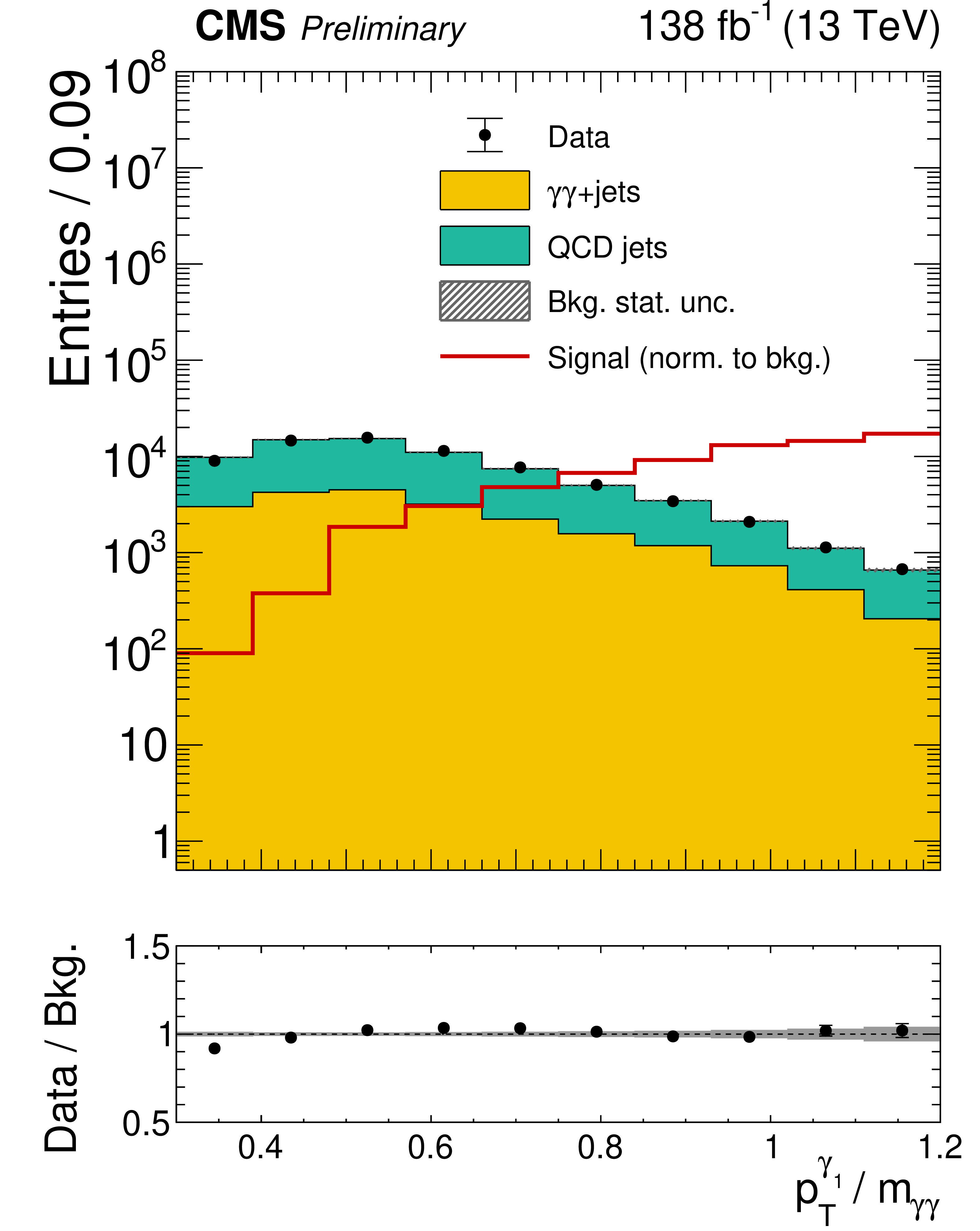
Distributions of $ \Delta R(\gamma\gamma) $ (left) and $ p_{\mathrm{T}}^{\gamma_1}/m_{\gamma\gamma} $ (right), where $ \gamma_1 $ is the leading photon. The points show data, and the stacked histograms show the simulated prompt diphoton and data-driven misidentified-photon backgrounds. The vertical bars and hatched bands show the statistical uncertainties in the data and total background, respectively. The red line shows the signal for $ m_{\mathrm{X}}= $ 1 TeV and $ m_{\mathrm{Y}}= $ 100 GeV, normalized to the total background yield. The lower panels show the ratio of data to the total background. |
png pdf |
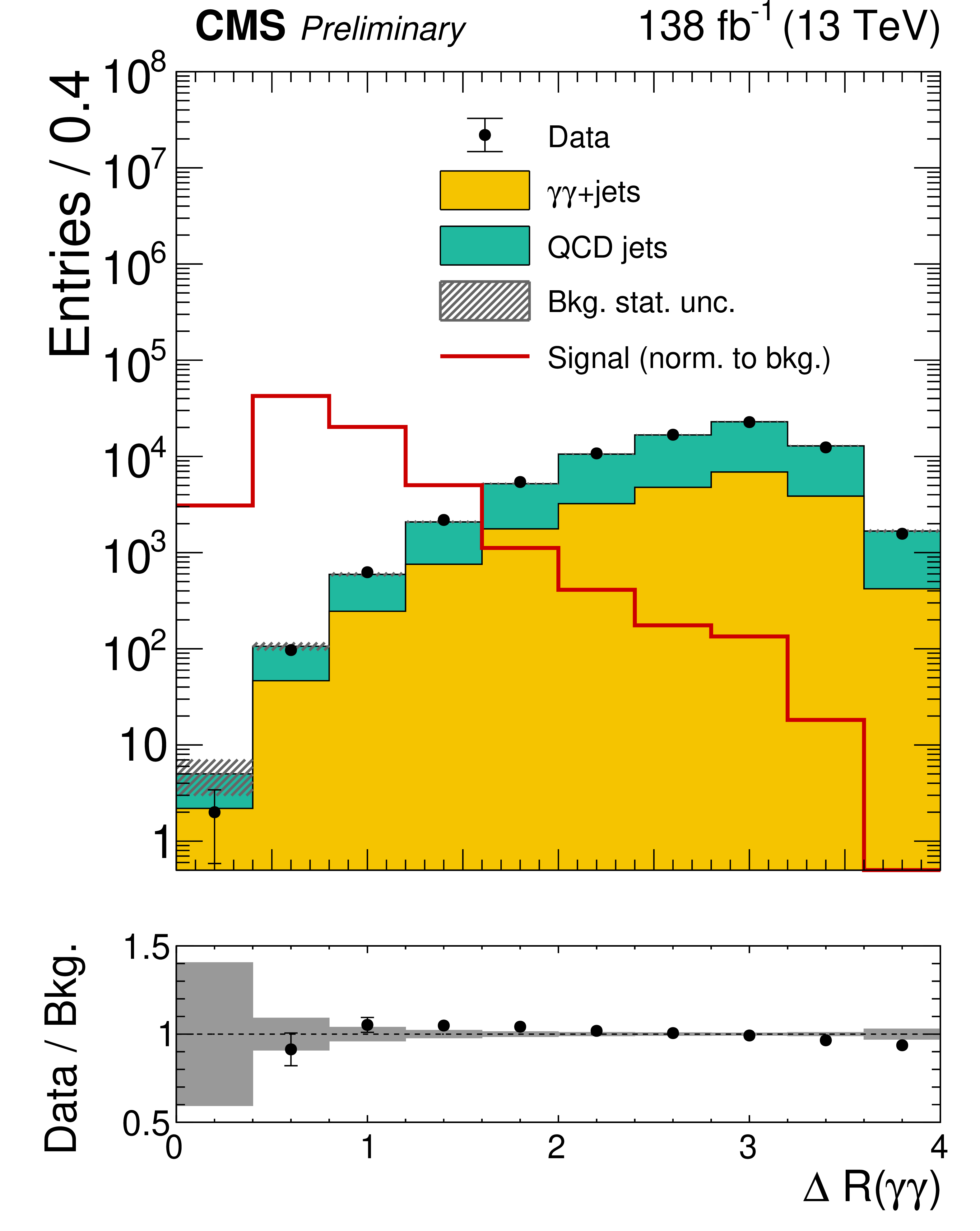
Figure 2-a:
Distributions of $ \Delta R(\gamma\gamma) $ (left) and $ p_{\mathrm{T}}^{\gamma_1}/m_{\gamma\gamma} $ (right), where $ \gamma_1 $ is the leading photon. The points show data, and the stacked histograms show the simulated prompt diphoton and data-driven misidentified-photon backgrounds. The vertical bars and hatched bands show the statistical uncertainties in the data and total background, respectively. The red line shows the signal for $ m_{\mathrm{X}}= $ 1 TeV and $ m_{\mathrm{Y}}= $ 100 GeV, normalized to the total background yield. The lower panels show the ratio of data to the total background. |
png pdf |
Figure 2-b:
Distributions of $ \Delta R(\gamma\gamma) $ (left) and $ p_{\mathrm{T}}^{\gamma_1}/m_{\gamma\gamma} $ (right), where $ \gamma_1 $ is the leading photon. The points show data, and the stacked histograms show the simulated prompt diphoton and data-driven misidentified-photon backgrounds. The vertical bars and hatched bands show the statistical uncertainties in the data and total background, respectively. The red line shows the signal for $ m_{\mathrm{X}}= $ 1 TeV and $ m_{\mathrm{Y}}= $ 100 GeV, normalized to the total background yield. The lower panels show the ratio of data to the total background. |
png pdf |
Figure 3:
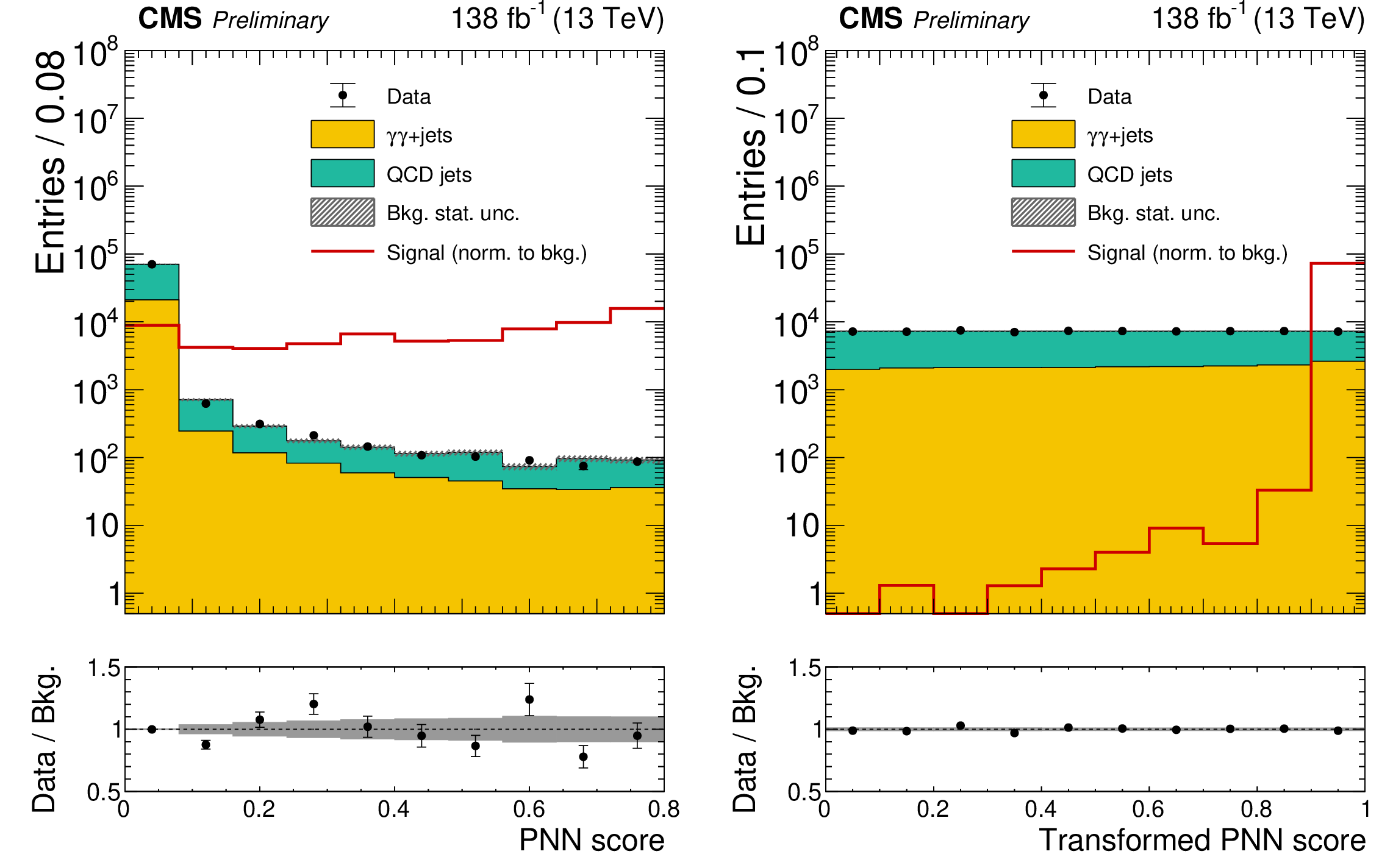
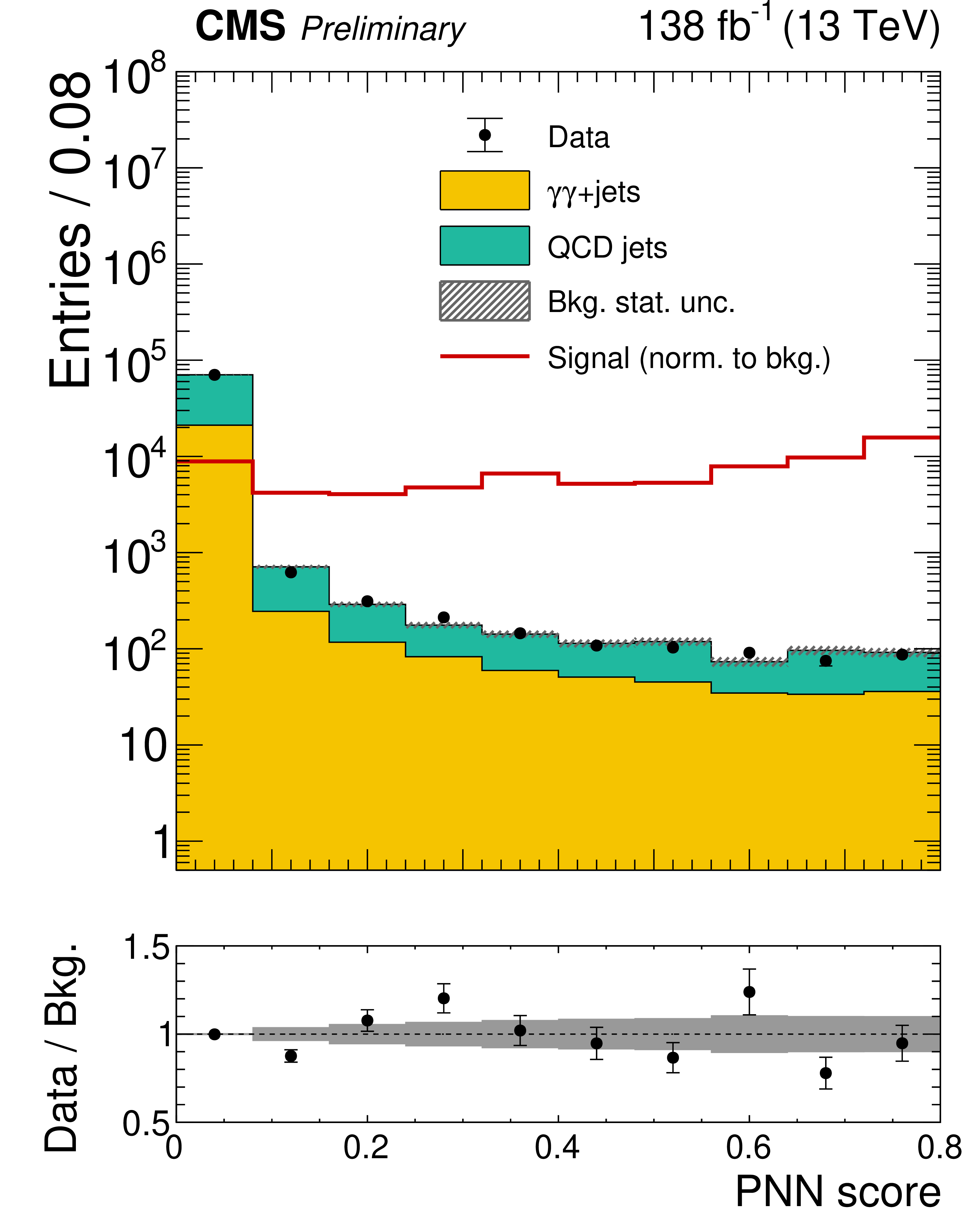
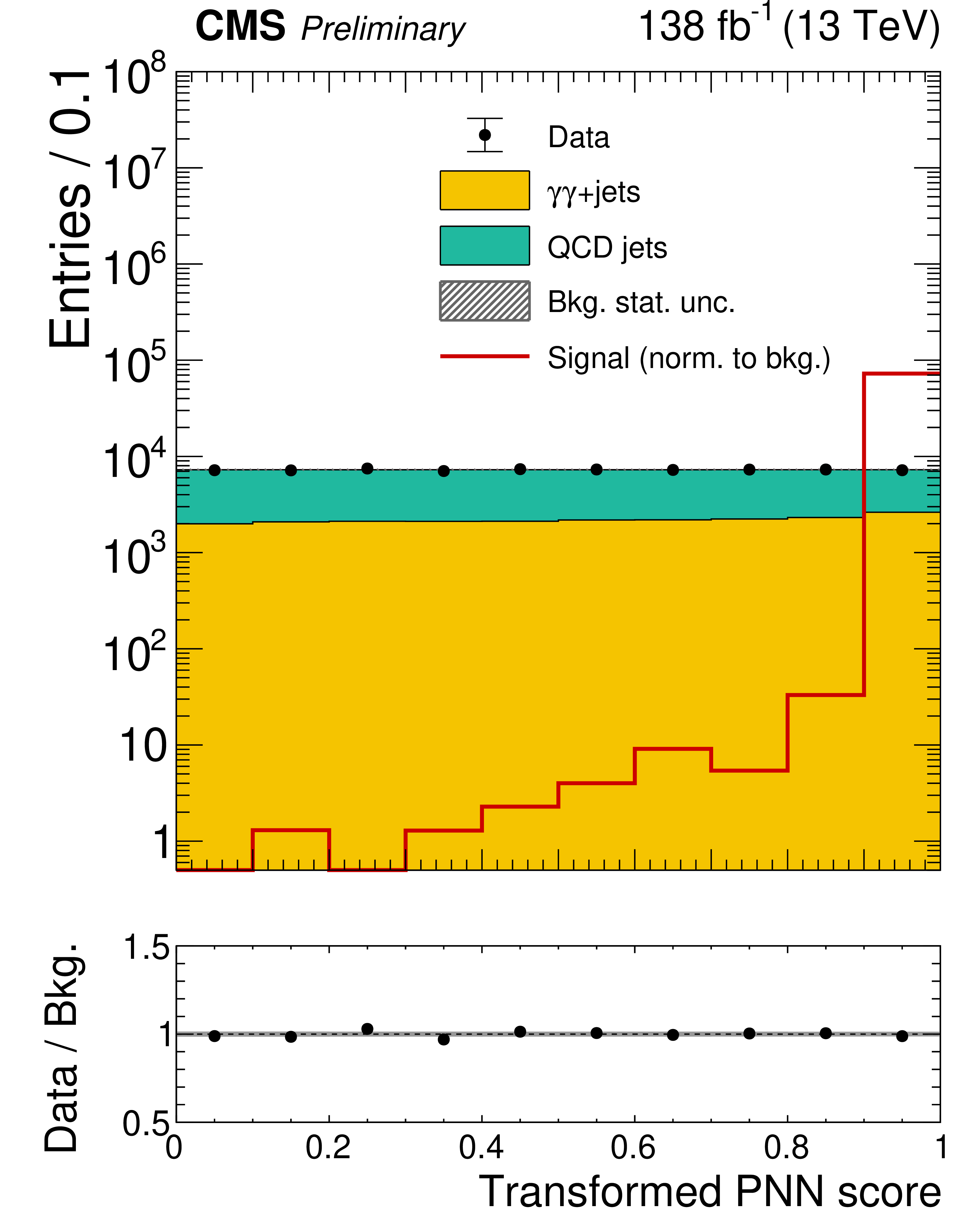
Distributions of the PNN output before (left) and after (right) the background-flattening transformation. The points show data, and the stacked histograms show the simulated prompt diphoton and data-driven misidentified-photon backgrounds. The vertical bars and hatched bands show the statistical uncertainties in the data and total background, respectively. The red line shows the signal for $ m_{\mathrm{X}}= $ 1 TeV and $ m_{\mathrm{Y}}= $ 100 GeV, normalized to the total background yield. The lower panels show the ratio of data to the total background. The different band widths reflect the event populations in the transformed bins. |
png pdf |
Figure 3-a:
Distributions of the PNN output before (left) and after (right) the background-flattening transformation. The points show data, and the stacked histograms show the simulated prompt diphoton and data-driven misidentified-photon backgrounds. The vertical bars and hatched bands show the statistical uncertainties in the data and total background, respectively. The red line shows the signal for $ m_{\mathrm{X}}= $ 1 TeV and $ m_{\mathrm{Y}}= $ 100 GeV, normalized to the total background yield. The lower panels show the ratio of data to the total background. The different band widths reflect the event populations in the transformed bins. |
png pdf |
Figure 3-b:
Distributions of the PNN output before (left) and after (right) the background-flattening transformation. The points show data, and the stacked histograms show the simulated prompt diphoton and data-driven misidentified-photon backgrounds. The vertical bars and hatched bands show the statistical uncertainties in the data and total background, respectively. The red line shows the signal for $ m_{\mathrm{X}}= $ 1 TeV and $ m_{\mathrm{Y}}= $ 100 GeV, normalized to the total background yield. The lower panels show the ratio of data to the total background. The different band widths reflect the event populations in the transformed bins. |
png pdf |
Figure 4:
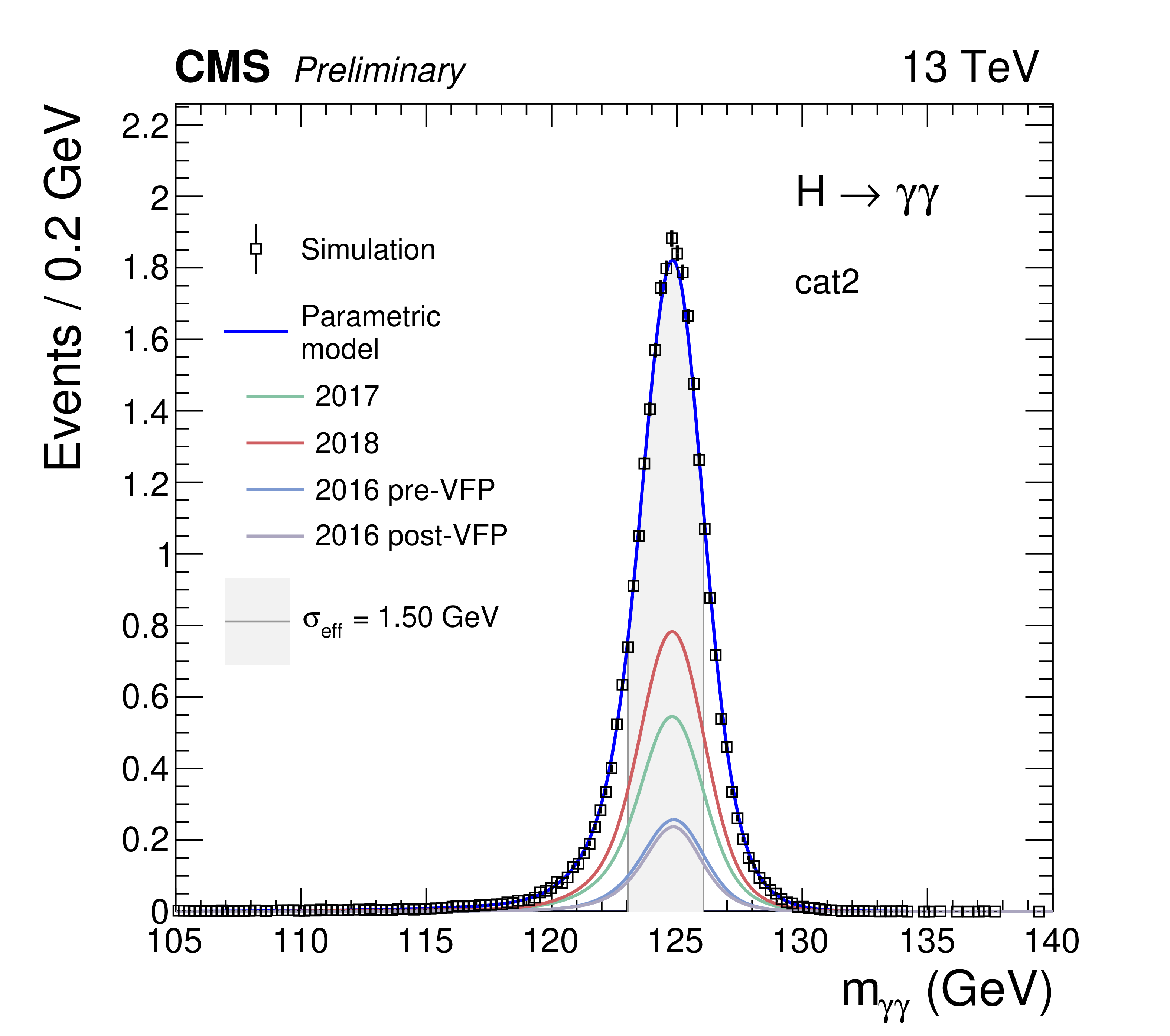
Simulated $ m_{\gamma\gamma} $ distribution for $ m_{\mathrm{X}}= $ 1 TeV and $ m_{\mathrm{Y}}= $ 170 GeV in resolved category 2. The points show signal events, and the blue curve shows the parametric fit. The other curves show the 2016 pre-VFP, 2016 post-VFP, 2017, and 2018 components. The vertical bars show statistical uncertainties. The effective standard deviation $ \sigma_{\mathrm{eff}} $ is half the width of the narrowest interval containing 68.3% of the distribution. |
png pdf |
Figure 5:
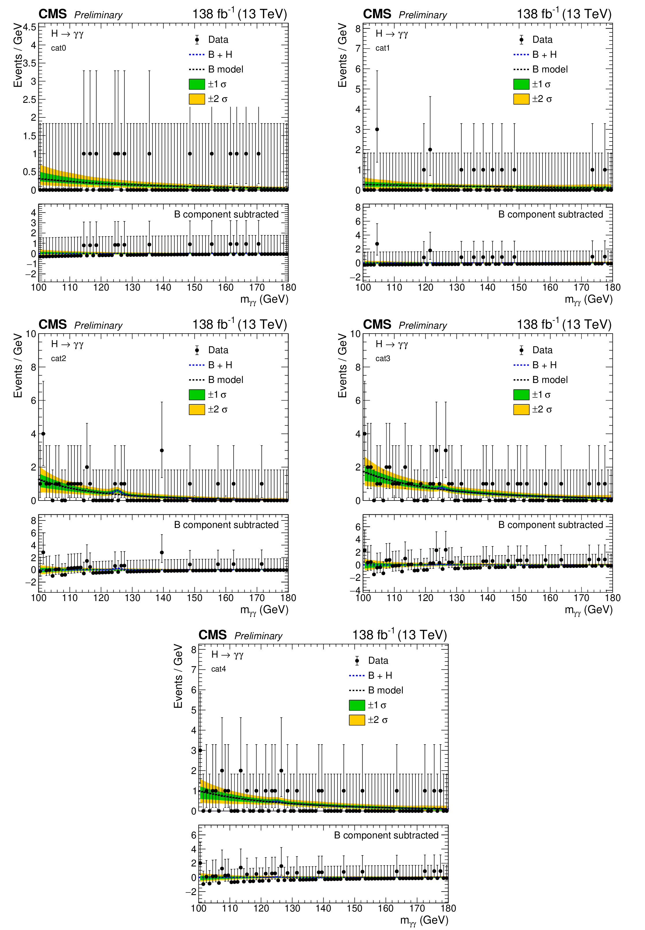
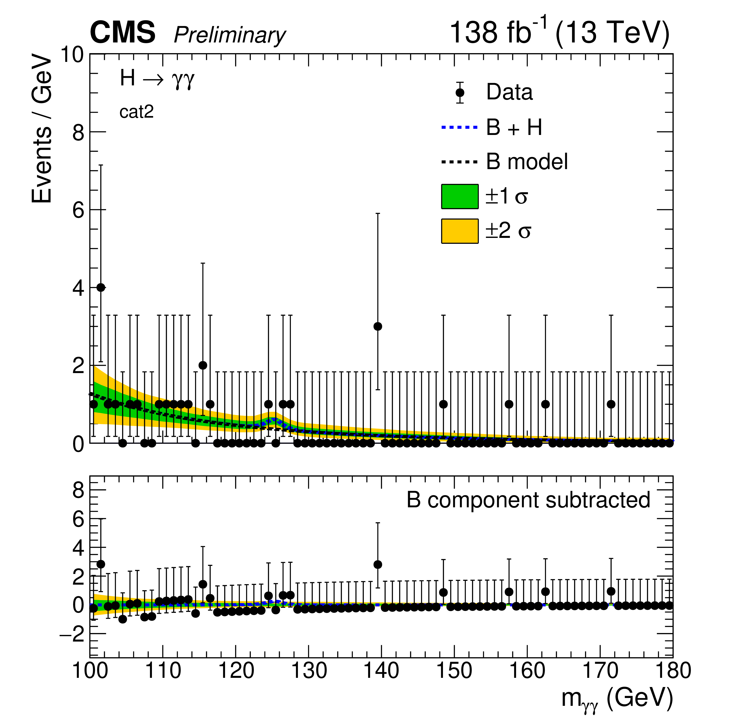
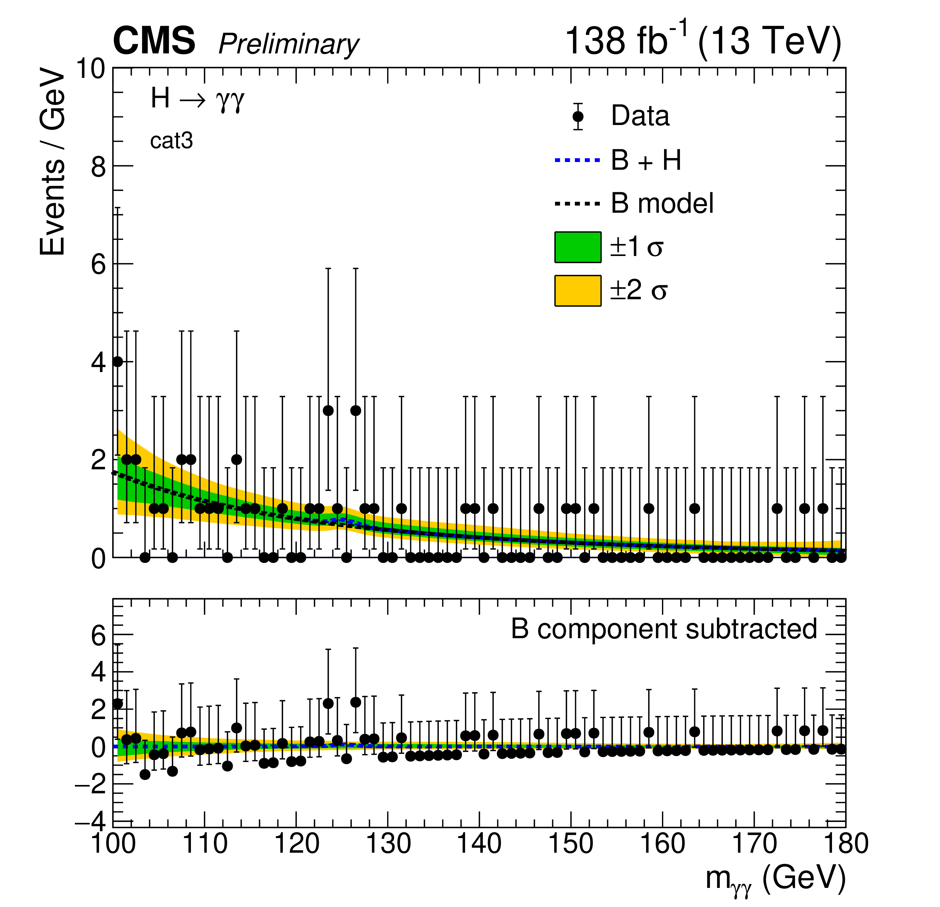
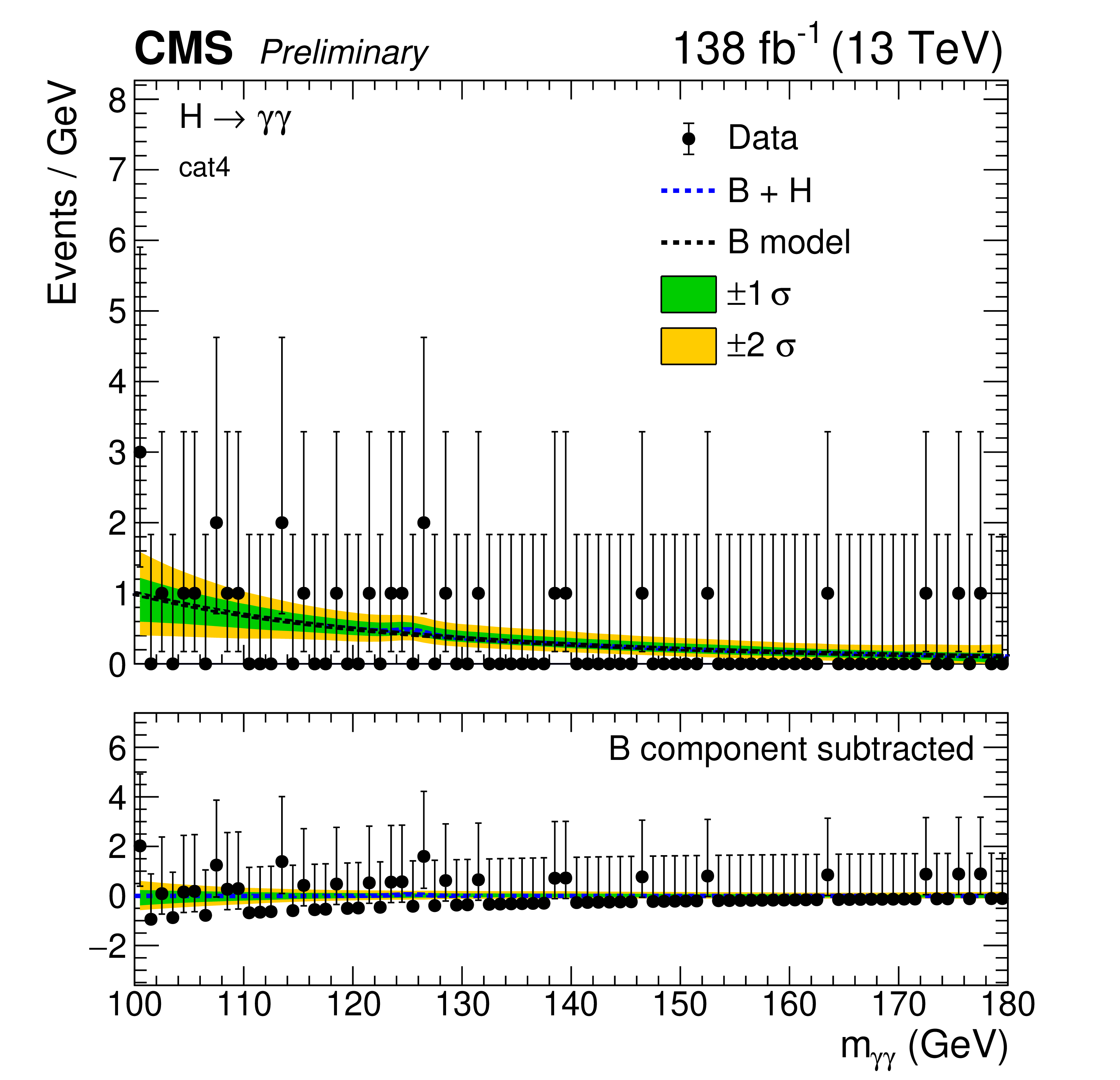
Diphoton invariant mass distributions in the five event categories for $ m_{\mathrm{X}}= $ 1 TeV and $ m_{\mathrm{Y}}= $ 100 GeV. The points show data, with vertical bars indicating statistical uncertainties. The green and yellow bands show the one and two standard deviation uncertainties in the fitted background, respectively. The dashed blue and black curves show the single Higgs boson plus nonresonant background (B+H) and the nonresonant background (B), respectively. The lower panels show the data after subtraction of the B component. |
png pdf |
Figure 5-a:
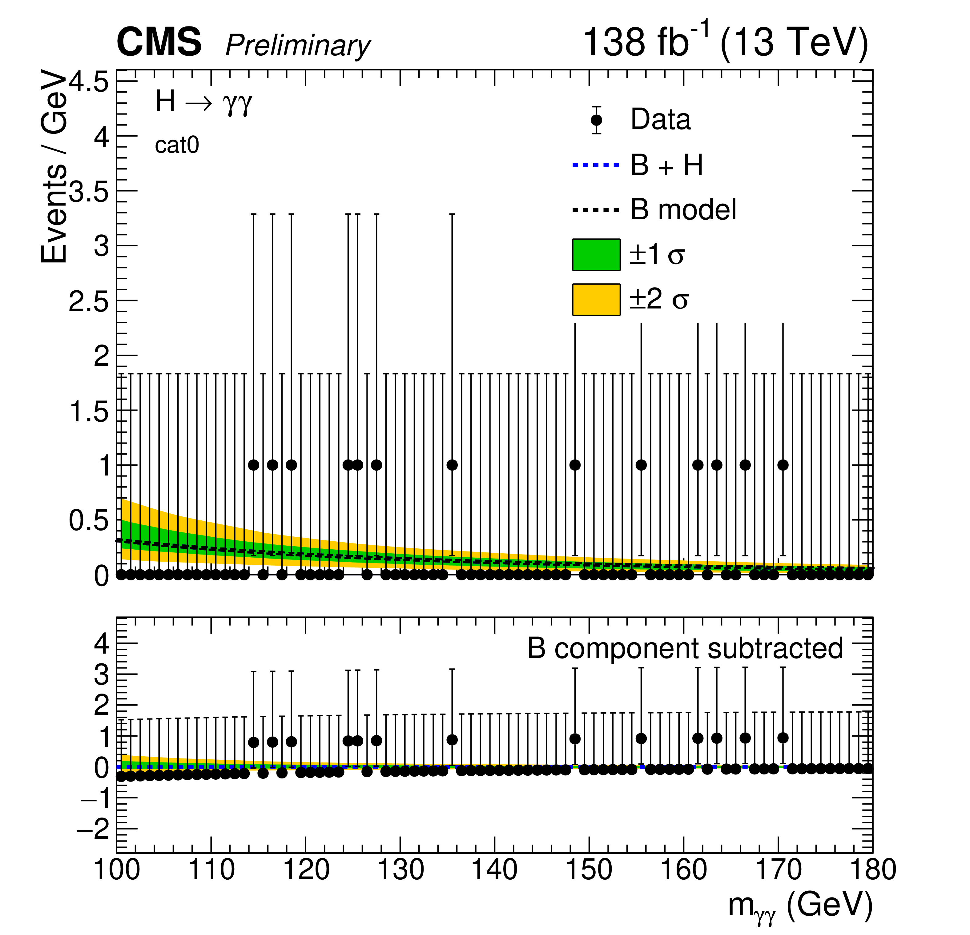
Diphoton invariant mass distributions in the five event categories for $ m_{\mathrm{X}}= $ 1 TeV and $ m_{\mathrm{Y}}= $ 100 GeV. The points show data, with vertical bars indicating statistical uncertainties. The green and yellow bands show the one and two standard deviation uncertainties in the fitted background, respectively. The dashed blue and black curves show the single Higgs boson plus nonresonant background (B+H) and the nonresonant background (B), respectively. The lower panels show the data after subtraction of the B component. |
png pdf |
Figure 5-b:
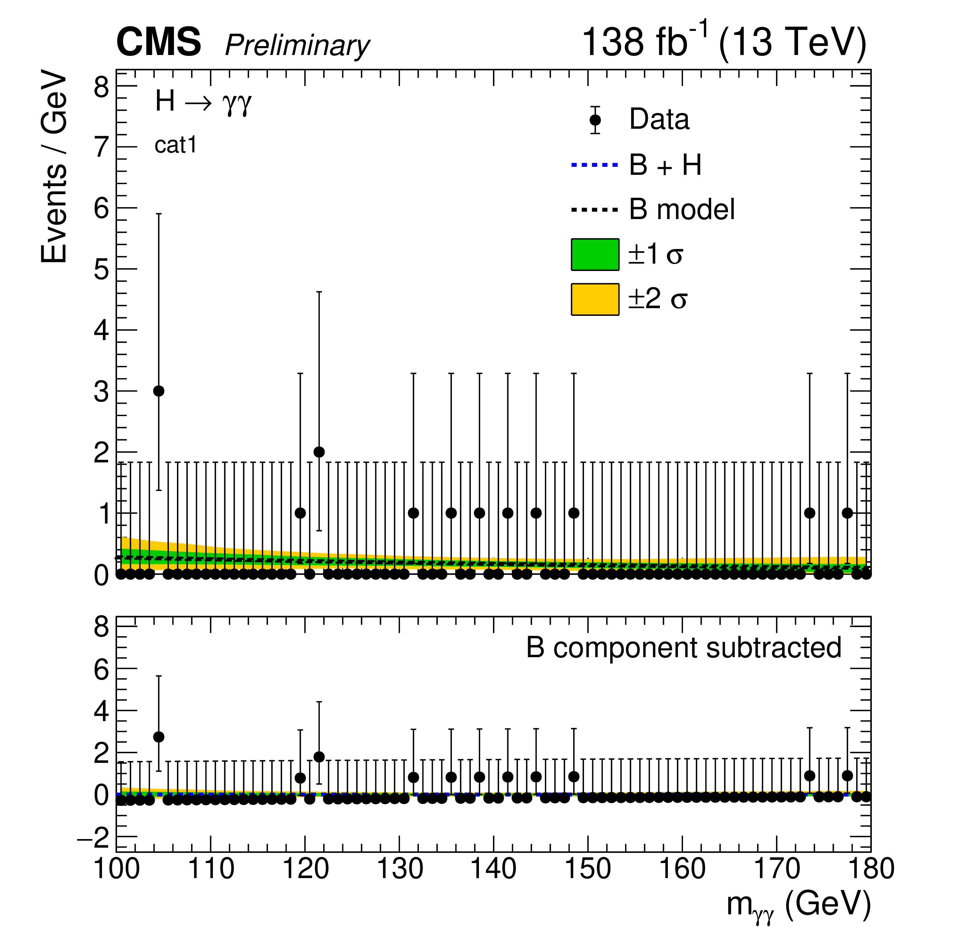
Diphoton invariant mass distributions in the five event categories for $ m_{\mathrm{X}}= $ 1 TeV and $ m_{\mathrm{Y}}= $ 100 GeV. The points show data, with vertical bars indicating statistical uncertainties. The green and yellow bands show the one and two standard deviation uncertainties in the fitted background, respectively. The dashed blue and black curves show the single Higgs boson plus nonresonant background (B+H) and the nonresonant background (B), respectively. The lower panels show the data after subtraction of the B component. |
png pdf |
Figure 5-c:
Diphoton invariant mass distributions in the five event categories for $ m_{\mathrm{X}}= $ 1 TeV and $ m_{\mathrm{Y}}= $ 100 GeV. The points show data, with vertical bars indicating statistical uncertainties. The green and yellow bands show the one and two standard deviation uncertainties in the fitted background, respectively. The dashed blue and black curves show the single Higgs boson plus nonresonant background (B+H) and the nonresonant background (B), respectively. The lower panels show the data after subtraction of the B component. |
png pdf |
Figure 5-d:
Diphoton invariant mass distributions in the five event categories for $ m_{\mathrm{X}}= $ 1 TeV and $ m_{\mathrm{Y}}= $ 100 GeV. The points show data, with vertical bars indicating statistical uncertainties. The green and yellow bands show the one and two standard deviation uncertainties in the fitted background, respectively. The dashed blue and black curves show the single Higgs boson plus nonresonant background (B+H) and the nonresonant background (B), respectively. The lower panels show the data after subtraction of the B component. |
png pdf |
Figure 5-e:
Diphoton invariant mass distributions in the five event categories for $ m_{\mathrm{X}}= $ 1 TeV and $ m_{\mathrm{Y}}= $ 100 GeV. The points show data, with vertical bars indicating statistical uncertainties. The green and yellow bands show the one and two standard deviation uncertainties in the fitted background, respectively. The dashed blue and black curves show the single Higgs boson plus nonresonant background (B+H) and the nonresonant background (B), respectively. The lower panels show the data after subtraction of the B component. |
png pdf |
Figure 6:
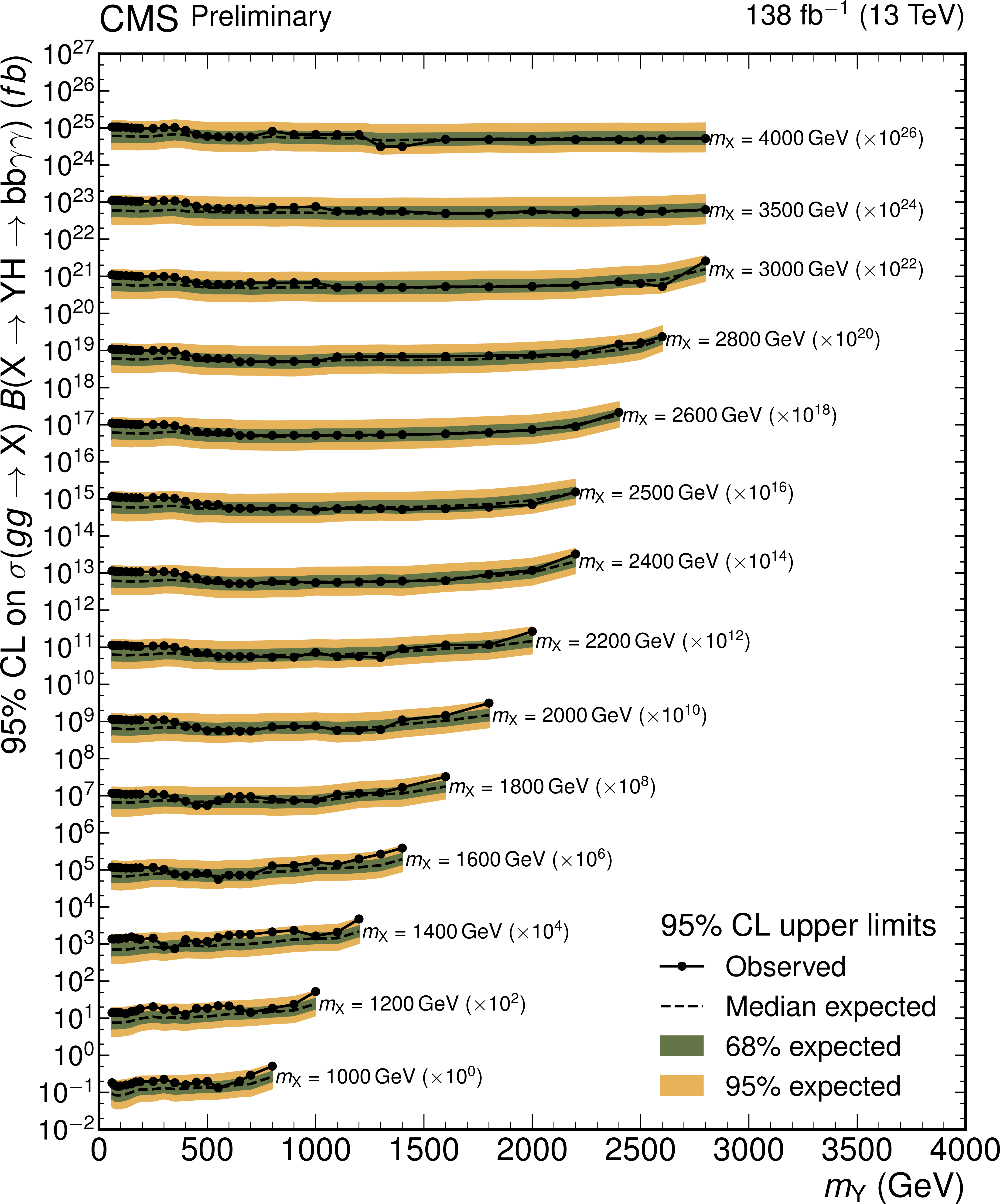
Observed (solid black) and expected (dashed black) 95% CL upper limits on the product of the $ \mathrm{X} $ production cross section and the $ \mathrm{X}\to\mathrm{H}\mathrm{Y}\to\gamma\gamma\mathrm{b}\bar{\mathrm{b}} $ branching fractions, as a function of $ m_{\mathrm{Y}} $. Results are shown for 1.0 $ \leq m_{\mathrm{X}} \leq $ 4.0 TeV and scaled by the factors indicated. The green and yellow bands show the 68 and 95% expected intervals, respectively. |
png pdf |
Figure 7:
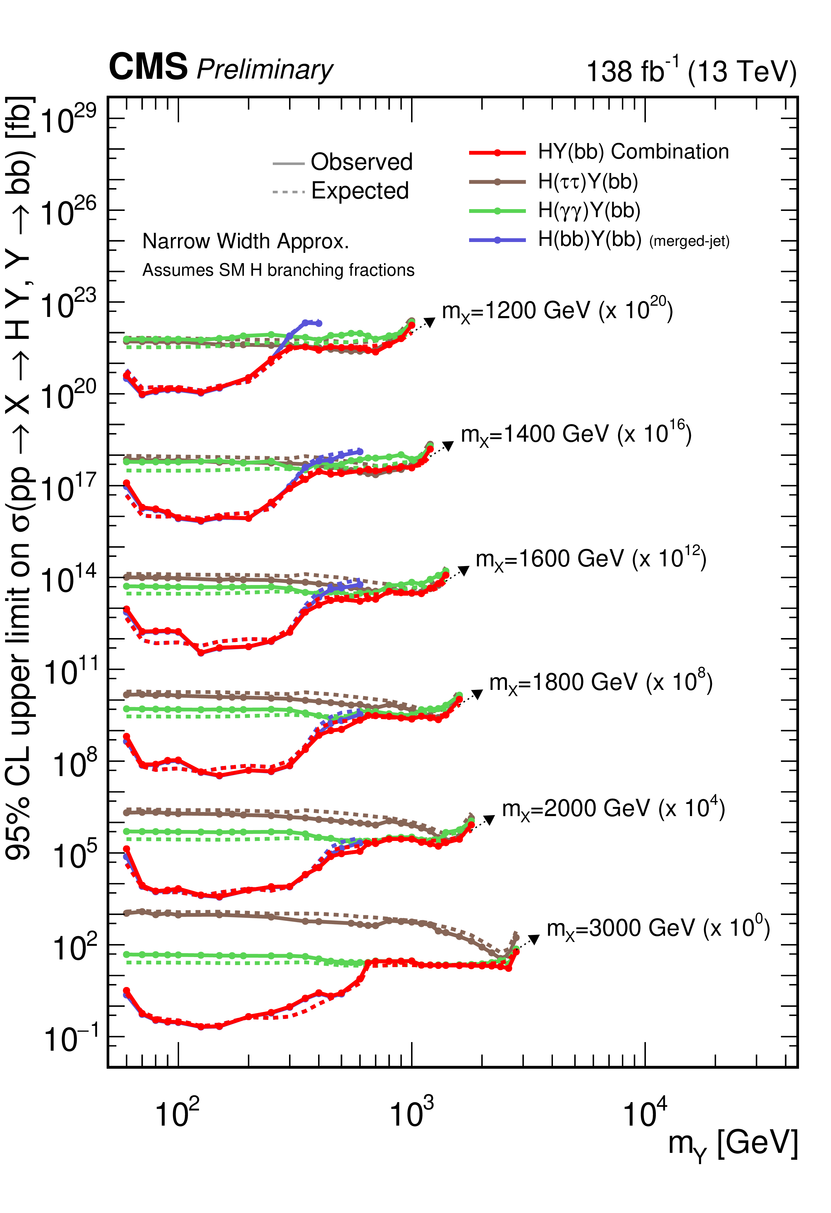
Observed and expected 95% CL upper limits on $ \sigma(\mathrm{p}\mathrm{p}\to\mathrm{X}) \mathcal{B}(\mathrm{X}\to\mathrm{H}\mathrm{Y}) \mathcal{B}(\mathrm{Y}\to\mathrm{b}\bar{\mathrm{b}}) $ as functions of $ m_{\mathrm{Y}} $ for the indicated $ m_{\mathrm{X}} $ hypotheses. SM branching fractions are assumed for the Higgs boson decays. Results are shown for the individual $ \mathrm{H}(\gamma\gamma)\mathrm{Y}(\mathrm{b}\bar{\mathrm{b}}) $, $ \mathrm{H}(\mathrm{b}\bar{\mathrm{b}})\mathrm{Y}(\mathrm{b}\bar{\mathrm{b}}) $, and $ \mathrm{H}(\tau\tau)\mathrm{Y}(\mathrm{b}\bar{\mathrm{b}}) $ channels and their combination. Observed and expected limits are indicated by solid and dashed lines, respectively. The curves are scaled by the factors shown; arrows identify the corresponding $ m_{\mathrm{X}} $ values. |
| Tables | |

png pdf |
Table 1:
The selection requirements for photon candidates. |
| Summary |
| The first search for the production of a new scalar resonance $ \mathrm{X} $ in the mass range 1 $ \leq m_{\mathrm{X}}\leq $ 4 TeV decaying into a Higgs boson (H) and another new scalar particle $ \mathrm{Y} $ in the photon-pair and bottom-quark-pair ($ \gamma\gamma\mathrm{b}\bar{\mathrm{b}} $) final state is presented. The search is based on proton-proton collisions at the LHC collected with the CMS detector during 2016--2018 at a centre-of-mass energy of 13 TeV and corresponding to an integrated luminosity of 138 fb$ ^{-1} $. The analysis is motivated by theoretical extensions of the standard model (SM), such as the next-to-minimal supersymmetric SM, which predict enhanced production rates for such processes. \beginsloppypar The analysis probes 0.06 $ \leq m_{\mathrm{Y}}\leq $ 2.8 TeV. No significant deviation from the background expectation is observed. The resulting 95% confidence level upper limits on the product of the production cross section and branching fraction for $ \mathrm{X}\to\mathrm{H}\mathrm{Y}\to\gamma\gamma\mathrm{b}\bar{\mathrm{b}} $ range from 0.26 fb for $ m_{\mathrm{X}}= $ 1 TeV to 0.046 fb for $ m_{\mathrm{X}}= $ 4 TeV. These results provide an important input to combinations with other $ \mathrm{H}\mathrm{Y} $ final states, improving the expected sensitivity in the high-mass region and extending the overall coverage of resonant scalar-pair searches. \endsloppypar |
| References | ||||
| 1 | ATLAS Collaboration | Observation of a new particle in the search for the Standard Model Higgs boson with the ATLAS detector at the LHC | PLB 716 (2012) 1 | 1207.7214 |
| 2 | CMS Collaboration | Observation of a new boson at a mass of 125 GeV with the CMS experiment at the LHC | PLB 716 (2012) 30 | CMS-HIG-12-028 1207.7235 |
| 3 | CMS Collaboration | Observation of a new boson with mass near 125 GeV in pp collisions at $ \sqrt{s} = $ 7 and 8 TeV | JHEP 06 (2013) 081 | CMS-HIG-12-036 1303.4571 |
| 4 | N. Arkani-Hamed, S. Dimopoulos, and G. Dvali | The hierarchy problem and new dimensions at a millimeter | PLB 429 (1998) 263 | hep-ph/9803315 |
| 5 | A. Djouadi | The anatomy of electroweak symmetry breaking tome ii: The Higgs bosons in the minimal supersymmetric model | Phys. Rept. 459 (2008) 1 | hep-ph/0503173 |
| 6 | U. Ellwanger, C. Hugonie, and A. M. Teixeira | The next-to-minimal supersymmetric standard model | Phys. Rept. 496 (2010) 1 | 0910.1785 |
| 7 | J. F. Gunion and H. E. Haber | CP-conserving two-Higgs-doublet model: The approach to the decoupling limit | PRD 67 (2003) 075019 | hep-ph/0207010 |
| 8 | T. Robens, T. Stefaniak, and J. Wittbrodt | Two-real-scalar-singlet extension of the SM: LHC phenomenology and benchmark scenarios | EPJC 80 (2020) 151 | 1908.08554 |
| 9 | H. Abouabid et al. | Benchmarking di-Higgs production in various extended Higgs sector models | JHEP 09 (2022) 011 | 2112.12515 |
| 10 | CMS Collaboration | Search for a heavy Higgs boson decaying into two lighter Higgs bosons in the $ \tau\tau\mathrm{b}\bar{\mathrm{b}} $ final state at 13 TeV | JHEP 11 (2021) 057 | CMS-HIG-20-014 2106.10361 |
| 11 | CMS Collaboration | Search for a new heavy scalar resonance decaying into the Higgs boson and a new scalar particle in the $ \mathrm{b}\bar{\mathrm{b}}\mathrm{b}\bar{\mathrm{b}} $ final state using proton-proton collisions at $ \sqrt{s} = $ 13 TeV | Submitted to Phys. Rev. D, 2026 | CMS-HIG-20-012 2605.02848 |
| 12 | ATLAS Collaboration | Search for a resonance decaying into a scalar particle and a Higgs boson in final states with leptons and two photons in proton-proton collisions at $ \sqrt{s} = $ 13 TeV with the ATLAS detector | JHEP 10 (2024) 104 | 2405.20926 |
| 13 | CMS Collaboration | Search for a massive scalar resonance decaying to a light scalar and a Higgs boson in the four b quarks final state with boosted topology | PLB 842 (2023) 137392 | 2204.12413 |
| 14 | CMS Collaboration | Search for a new resonance decaying into two spin-0 bosons in a final state with two photons and two bottom quarks in proton-proton collisions at $ \sqrt{s} = $ 13 TeV | JHEP 05 (2024) 316 | CMS-HIG-21-011 2310.01643 |
| 15 | ATLAS Collaboration | Search for a resonance decaying into a scalar particle and a Higgs boson in the final state with two bottom quarks and two photons in proton-proton collisions at $ \sqrt{s} = $ 13 TeV with the ATLAS detector | JHEP 11 (2024) 047 | 2404.12915 |
| 16 | ATLAS Collaboration | Search for a resonance decaying into a scalar particle and a Higgs boson in the final state with two bottom quarks and two photons with 199 fb$ ^{-1} $ of data collected at s=13 and 13.6 TeV with the ATLAS detector | PLB 877 (2026) 140425 | 2510.02857 |
| 17 | CMS Collaboration | The CMS experiment at the CERN LHC | JINST 3 (2008) S08004 | 0809.3129 |
| 18 | CMS Collaboration | Development of the CMS detector for the CERN LHC Run 3 | JINST 19 (2024) P05064 | CMS-PRF-21-001 2309.05466 |
| 19 | CMS Collaboration | Performance of the CMS Level-1 trigger in proton-proton collisions at $ \sqrt{s} = $ 13 TeV | JINST 15 (2020) P10017 | CMS-TRG-17-001 2006.10165 |
| 20 | CMS Collaboration | The CMS trigger system | JINST 12 (2017) P01020 | CMS-TRG-12-001 1609.02366 |
| 21 | CMS Collaboration | Performance of the CMS high-level trigger during LHC Run 2 | JINST 19 (2024) P11021 | CMS-TRG-19-001 2410.17038 |
| 22 | CMS Collaboration | Description and performance of track and primary-vertex reconstruction with the CMS tracker | JINST 9 (2014) P10009 | CMS-TRK-11-001 1405.6569 |
| 23 | CMS Collaboration | Particle-flow reconstruction and global event description with the CMS detector | JINST 12 (2017) P10003 | CMS-PRF-14-001 1706.04965 |
| 24 | CMS Collaboration | Performance of photon reconstruction and identification with the CMS detector in proton-proton collisions at $ \sqrt{s} = $ 8 TeV | JINST 10 (2015) P08010 | CMS-EGM-14-001 1502.02702 |
| 25 | CMS Collaboration | A measurement of the Higgs boson mass in the diphoton decay channel | PLB 805 (2020) 135425 | CMS-HIG-19-004 2002.06398 |
| 26 | M. Cacciari, G. P. Salam, and G. Soyez | The anti-$ k_{\mathrm{T}} $ jet clustering algorithm | JHEP 04 (2008) 063 | 0802.1189 |
| 27 | M. Cacciari, G. P. Salam, and G. Soyez | FastJet user manual | EPJC 72 (2012) 1896 | 1111.6097 |
| 28 | CMS Collaboration | Jet energy scale and resolution in the CMS experiment in pp collisions at 8 TeV | JINST 12 (2017) P02014 | CMS-JME-13-004 1607.03663 |
| 29 | CMS Collaboration | Pileup mitigation at CMS in 13 TeV data | JINST 15 (2020) P09018 | CMS-JME-18-001 2003.00503 |
| 30 | CMS Collaboration | Identification of heavy-flavour jets with the CMS detector in pp collisions at 13 TeV | JINST 13 (2018) P05011 | CMS-BTV-16-002 1712.07158 |
| 31 | CMS Collaboration | Performance of the DeepJet b tagging algorithm using 41.9 fb$ ^{-1} $ of data from proton-proton collisions at 13 TeV with Phase 1 CMS detector | CMS Detector Performance Note CMS-DP-2018-058, 2018 CDS |
|
| 32 | E. Bols et al. | Jet flavour classification using DeepJet | JINST 15 (2020) P12012 | 2008.10519 |
| 33 | CMS Collaboration | Performance summary of AK4 jet b tagging with data from proton-proton collisions at 13 TeV with the CMS detector | CMS Detector Performance Note CMS-DP-2023-005, 2023 CDS |
|
| 34 | H. Qu and L. Gouskos | ParticleNet: Jet Tagging via Particle Clouds | PRD 101 (2020) 056019 | 1902.08570 |
| 35 | CMS Collaboration | Identification of highly Lorentz-boosted heavy particles using graph neural networks and new mass decorrelation techniques | CMS Detector Performance Note CMS-DP-2020-002, 2020 CDS |
|
| 36 | CMS Collaboration | Calibration of the mass-decorrelated ParticleNet tagger for boosted $ \mathrm{b}\bar{\mathrm{b}} $ and $ \mathrm{c}\bar{\mathrm{c}} $ jets using LHC Run 2 data | CMS Detector Performance Note CMS-DP-2022-005, 2022 CDS |
|
| 37 | J. Alwall et al. | The automated computation of tree-level and next-to-leading order differential cross sections, and their matching to parton shower simulations | JHEP 07 (2014) 079 | 1405.0301 |
| 38 | R. Frederix et al. | The automation of next-to-leading order electroweak calculations | JHEP 07 (2018) 185 | 1804.10017 |
| 39 | D. de Florian et al. | Handbook of LHC Higgs cross sections: 4. Deciphering the nature of the Higgs sector | CERN Report CERN-2017-002-M, 2016 link |
1610.07922 |
| 40 | Sherpa Collaboration | Event Generation with Sherpa 2.2 | SciPost Phys. 7 (2019) 034 | 1905.09127 |
| 41 | T. Sjöstrand et al. | An introduction to PYTHIA 8.2 | Comput. Phys. Commun. 191 (2015) 159 | 1410.3012 |
| 42 | CMS Collaboration | Event generator tunes obtained from underlying event and multiparton scattering measurements | EPJC 76 (2016) 155 | CMS-GEN-14-001 1512.00815 |
| 43 | CMS Collaboration | Extraction and validation of a new set of CMS PYTHIA8 tunes from underlying-event measurements | EPJC 80 (2020) 4 | CMS-GEN-17-001 1903.12179 |
| 44 | NNPDF Collaboration | Parton distributions from high-precision collider data | EPJC 77 (2017) 663 | 1706.00428 |
| 45 | \GEANTfour Collaboration | GEANT 4 --- a simulation toolkit | NIM A 506 (2003) 250 | |
| 46 | CMS Collaboration | Precision luminosity measurement in proton-proton collisions at $ \sqrt{s} = $ 13 TeV in 2015 and 2016 at CMS | EPJC 81 (2021) 800 | CMS-LUM-17-003 2104.01927 |
| 47 | CMS Collaboration | CMS luminosity measurement for the 2017 data-taking period at $ \sqrt{s} = $ 13 TeV | CMS Physics Analysis Summary, 2018 CMS-PAS-LUM-17-004 |
CMS-PAS-LUM-17-004 |
| 48 | CMS Collaboration | CMS luminosity measurement for the 2018 data-taking period at $ \sqrt{s} = $ 13 TeV | CMS Physics Analysis Summary, 2019 CMS-PAS-LUM-18-002 |
CMS-PAS-LUM-18-002 |
| 49 | CMS Collaboration | Measurements of Higgs boson properties in the diphoton decay channel in proton-proton collisions at $ \sqrt{s} = $ 13 TeV | JHEP 11 (2018) 185 | CMS-HIG-16-040 1804.02716 |
| 50 | E. Spyromitros-Xioufis, G. Tsoumakas, W. Groves, and I. Vlahavas | Multi-target regression via input space expansion: treating targets as inputs | Mach. Learn. 104 (2016) 55 | 1211.6581 |
| 51 | A. J. Larkoski, S. Marzani, G. Soyez, and J. Thaler | Soft drop | JHEP 05 (2014) 146 | 1402.2657 |
| 52 | M. Abadi et al. | TensorFlow: A system for large-scale machine learning | 1605.08695 | |
| 53 | D. P. Kingma and J. Ba | Adam: A Method for Stochastic Optimization | 1412.6980 | |
| 54 | J. Collins and D. Soper | Angular distribution of dileptons in high-energy hadron collisions | PRD 16 (1977) 2219 | |
| 55 | R. A. Fisher | On the interpretation of $ \chi^{2} $ from contingency tables, and the calculation of P | J. R. Stat. Soc. A 85 (1922) 87 | |
| 56 | P. D. Dauncey, M. Kenzie, N. Wardle, and G. J. Davies | Handling uncertainties in background shapes | JINST 10 (2015) P04015 | 1408.6865 |
| 57 | T. Adams et al. | Beam test evaluation of electromagnetic calorimeter modules made from proton-damaged PbWO$ _4 $ crystals | JINST 11 (2016) P04012 | |
| 58 | F.-X. Gentit | Litrani: a general purpose Monte Carlo program simulating light propagation in isotropic or anisotropic media | NIM A 486 (2002) 35 | |
| 59 | T. Junk | Confidence level computation for combining searches with small statistics | NIM A 434 (1999) 435 | hep-ex/9902006 |
| 60 | A. L. Read | Presentation of search results: the CL$ _s $ technique | JPG 28 (2002) 2693 | |
| 61 | G. Cowan, K. Cranmer, E. Gross, and O. Vitells | Asymptotic formulae for likelihood-based tests of new physics | [Erratum: Eur. Phys. J. C 73 () 2501, doi:10.1140/epjc/s2-013-2501-z], 2011 EPJC 71 (2011) 1554 |
1007.1727 |
| 62 | ATLAS and CMS Collaborations | Procedure for the LHC Higgs boson search combination in summer 2011 | Technical Report CMS-NOTE-2011-005, ATL-PHYS-PUB-2011-11, 2011 link |
|
| 63 | CMS Collaboration | The CMS statistical analysis and combination tool: COMBINE | Comput. Softw. Big Sci. 8 (2024) 19 | CMS-CAT-23-001 2404.06614 |
| 64 | CMS Collaboration | Searches for Higgs boson production through decays of heavy resonances | Phys. Rept. 1115 (2025) 368 | 2403.16926 |
|
|
Compact Muon Solenoid LHC, CERN |

|
|
|
|
|
|