CMS-PAS-B2G-22-006

CMS-PAS-B2G-22-006
Search for new particles decaying into top quark-antiquark pairs in events with one lepton and jets in proton-proton collisions at 13 TeV
CMS Collaboration
3 April 2025

Abstract: A search for new particles decaying to top quark-antiquark pairs is performed using proton-proton collisions at a centre-of-mass energy of 13 TeV. The data recorded with the CMS detector between 2016 and 2018 are used, corresponding to an integrated luminosity of 138 fb $^{-1}$ . Events containing exactly one muon or one electron, at least two jets, and missing transverse momentum in the final state are considered. Different models of new physics are probed. No significant deviation from the prediction is observed and upper limits are set on the production cross section for heavy resonances. A Z' boson with 1%, 10%, and 30% relative width is excluded for masses in the range 0.4-4.3, 0.4-5.3, and 0.4-6.7 TeV, respectively. A Kaluza-Klein gluon in the Randall-Sundrum model and a dark matter mediator are excluded for masses between 0.5-4.7 TeV and 1.0-3.2 TeV, respectively. Moreover, upper limits are set on the coupling strength modifier for scalar and pseudoscalar Higgs bosons in the two-Higgs-doublet models for 2.5%, 10%, and 25% relative widths in the mass range 0.5-1 TeV.
Links: CDS record (PDF) ; CADI line (restricted) ;

Figures & Tables	Summary	References	CMS Publications

Figures
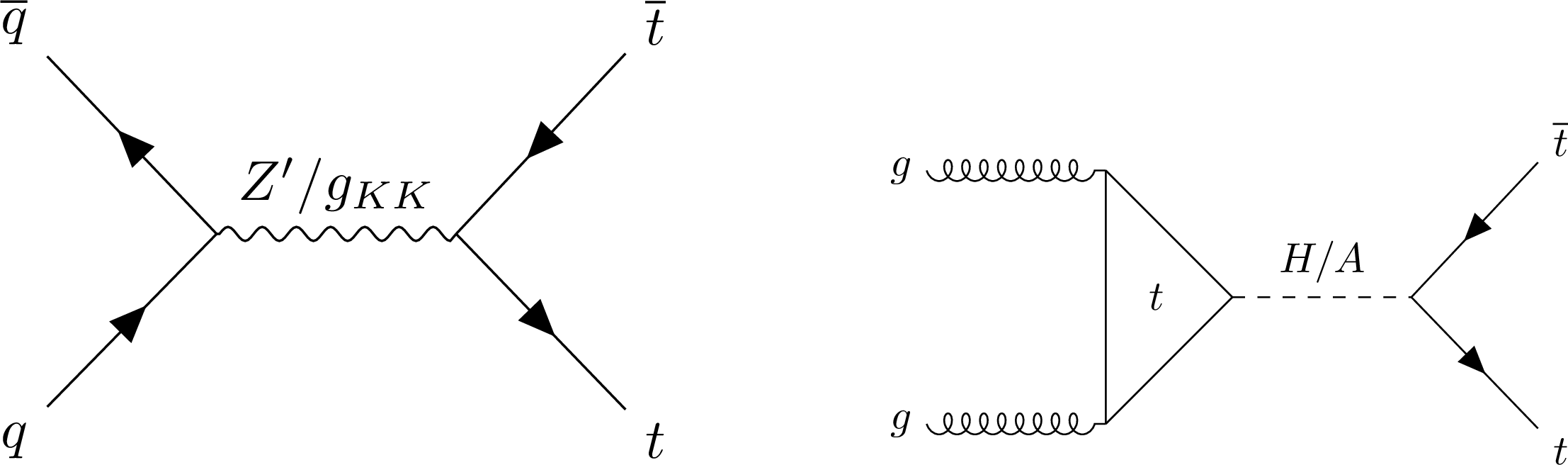
png pdf	Figure 1: Example Feynman diagrams at leading order for the production and decay of a Z'/ $\mathrm{ g_{KK} }$ (left) and a scalar H or pseudoscalar A resonance (right).
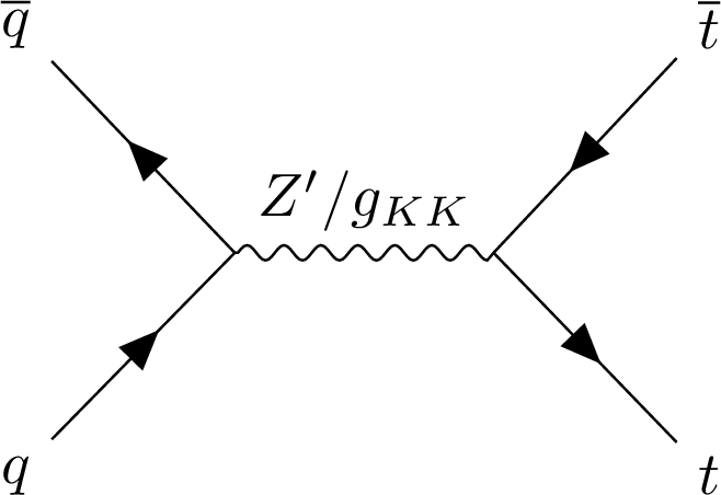
png pdf	Figure 1-a: Example Feynman diagrams at leading order for the production and decay of a Z'/ $\mathrm{ g_{KK} }$ (left) and a scalar H or pseudoscalar A resonance (right).
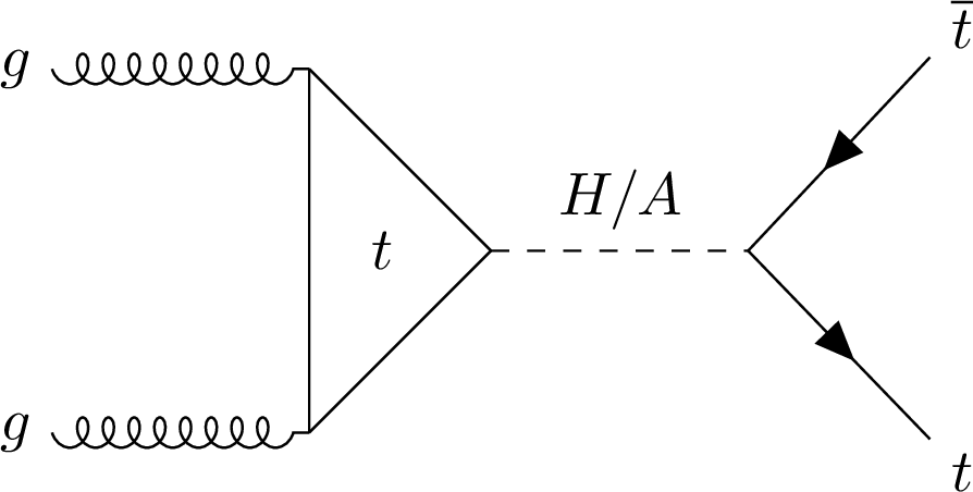
png pdf	Figure 1-b: Example Feynman diagrams at leading order for the production and decay of a Z'/ $\mathrm{ g_{KK} }$ (left) and a scalar H or pseudoscalar A resonance (right).
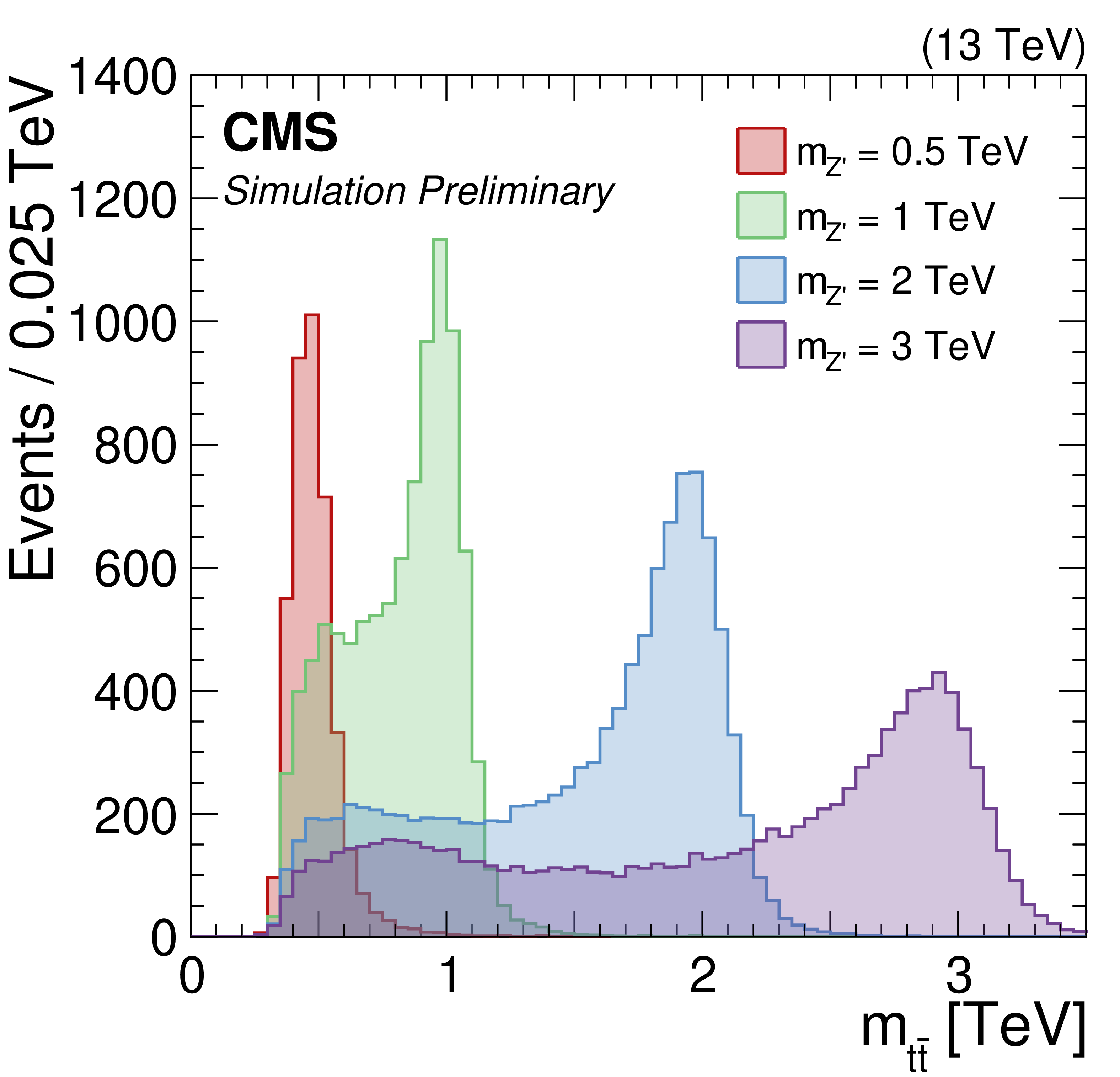
png pdf	Figure 2: Reconstructed invariant mass distribution for Z' bosons for different mass hypotheses. Each distribution corresponds to a production cross section of 1\unitpb.
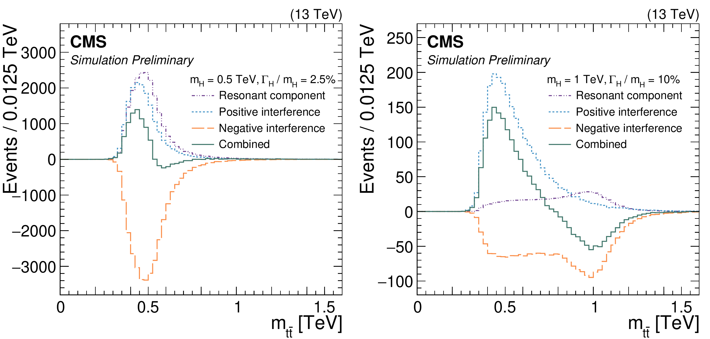
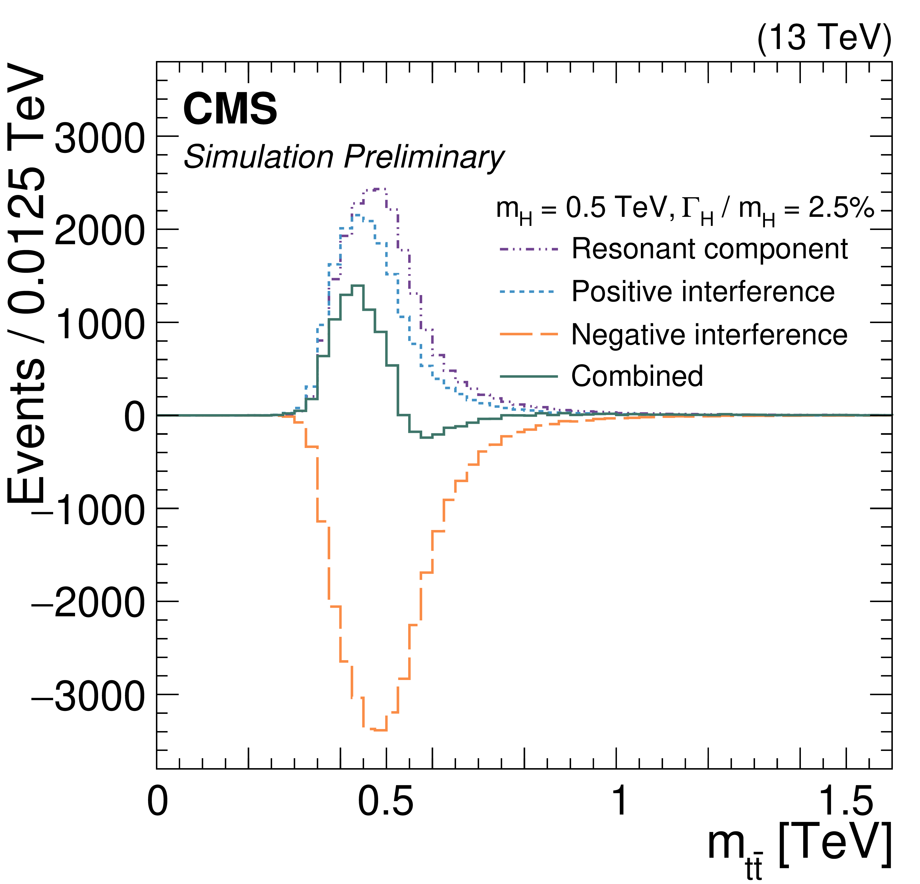
png pdf	Figure 3: Different contributions to the $m_{{\mathrm{t}\overline{\mathrm{t}}} }$ distribution for scalar Higgs bosons with masses of 0.5 TeV (left) and 1 TeV (right), and corresponding total widths of 2.5% and 10%, respectively. Each distribution is normalized to the corresponding production cross section.
png pdf	Figure 3-a: Different contributions to the $m_{{\mathrm{t}\overline{\mathrm{t}}} }$ distribution for scalar Higgs bosons with masses of 0.5 TeV (left) and 1 TeV (right), and corresponding total widths of 2.5% and 10%, respectively. Each distribution is normalized to the corresponding production cross section.
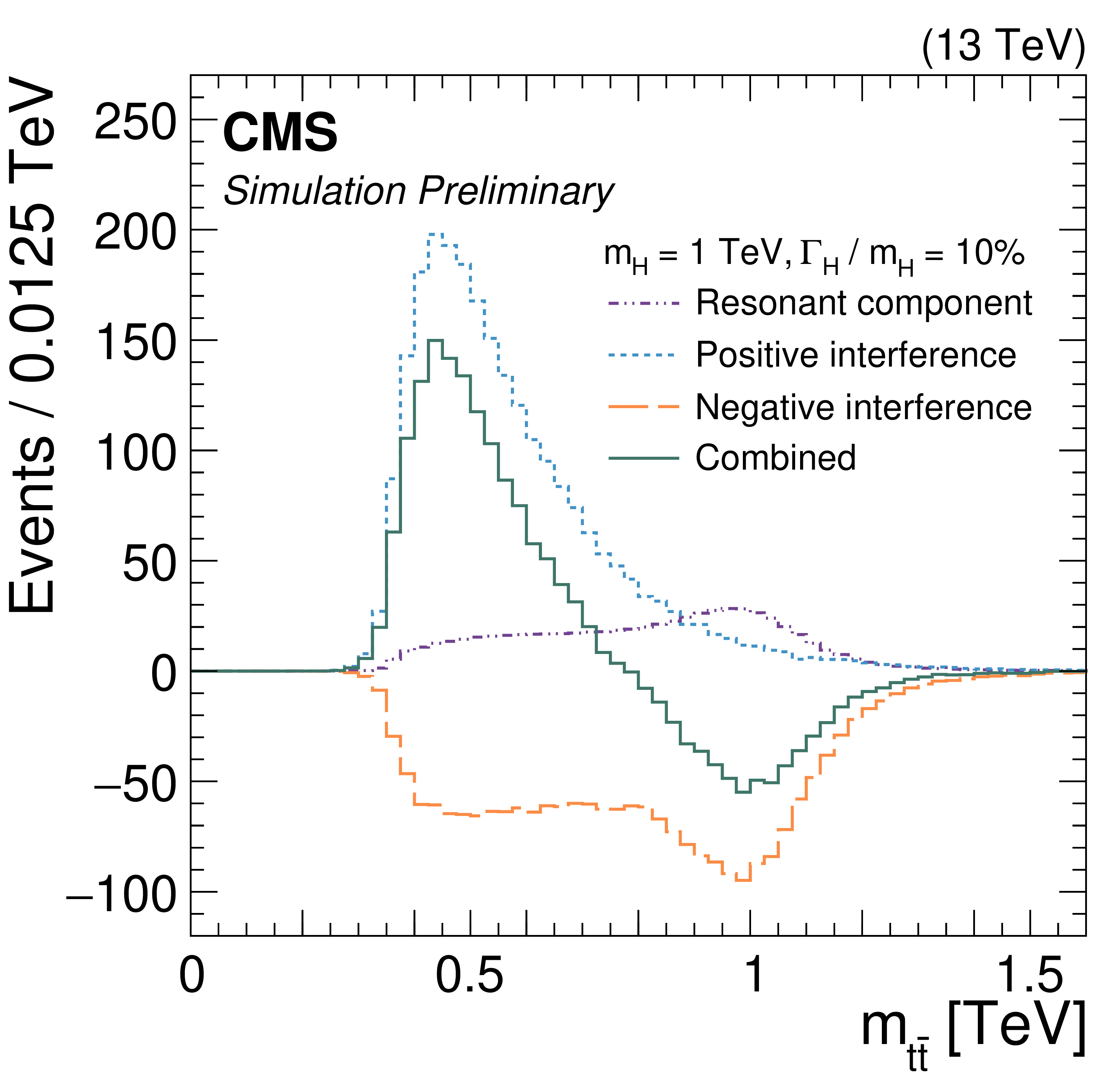
png pdf	Figure 3-b: Different contributions to the $m_{{\mathrm{t}\overline{\mathrm{t}}} }$ distribution for scalar Higgs bosons with masses of 0.5 TeV (left) and 1 TeV (right), and corresponding total widths of 2.5% and 10%, respectively. Each distribution is normalized to the corresponding production cross section.
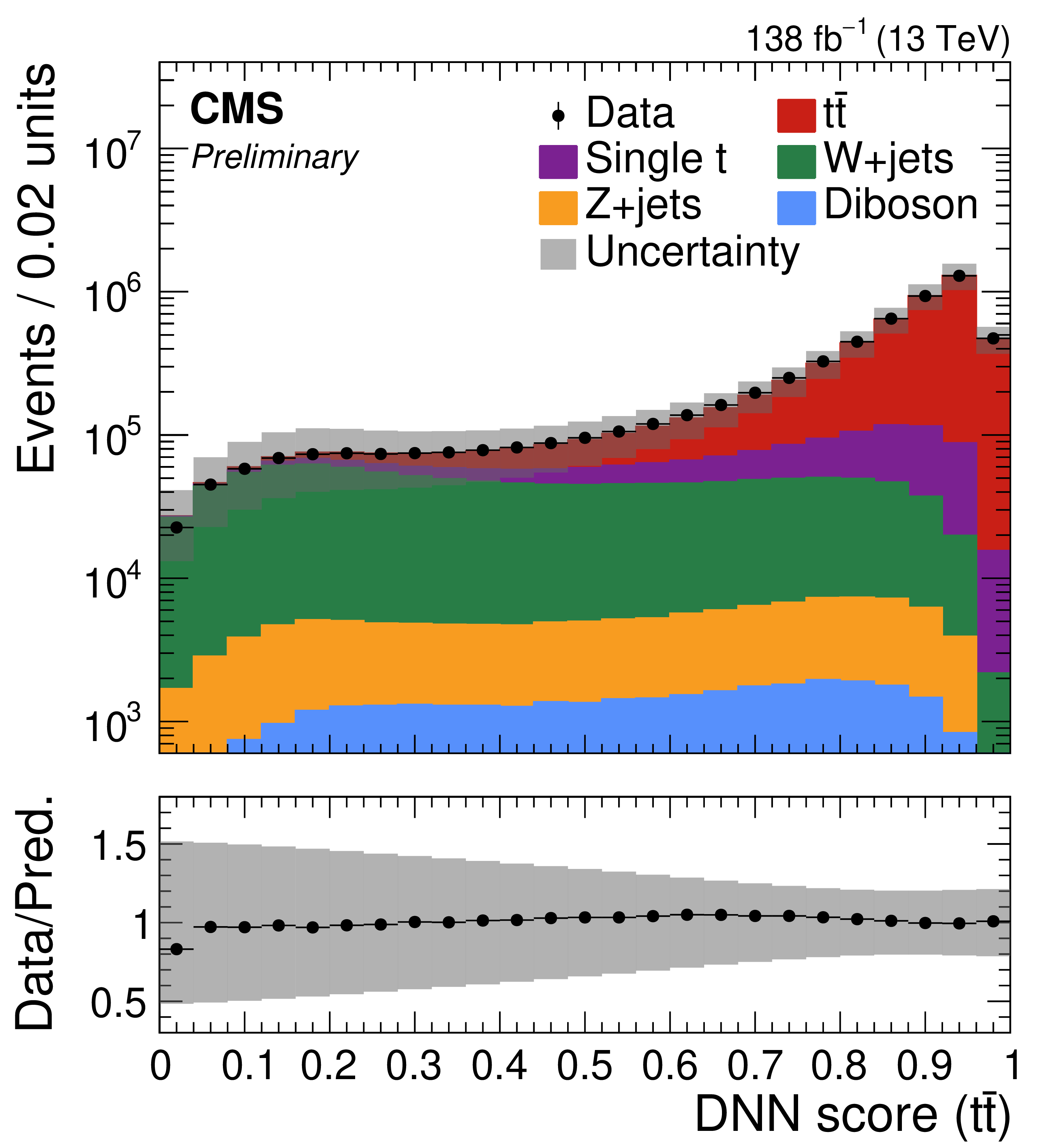
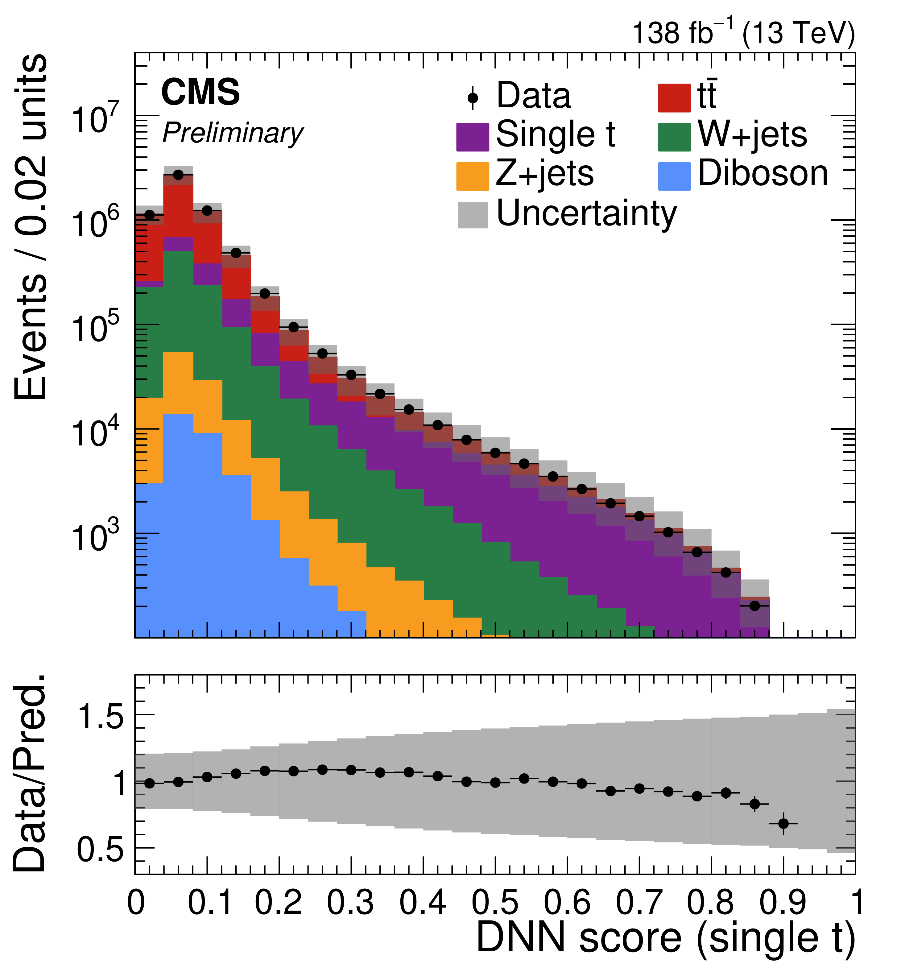
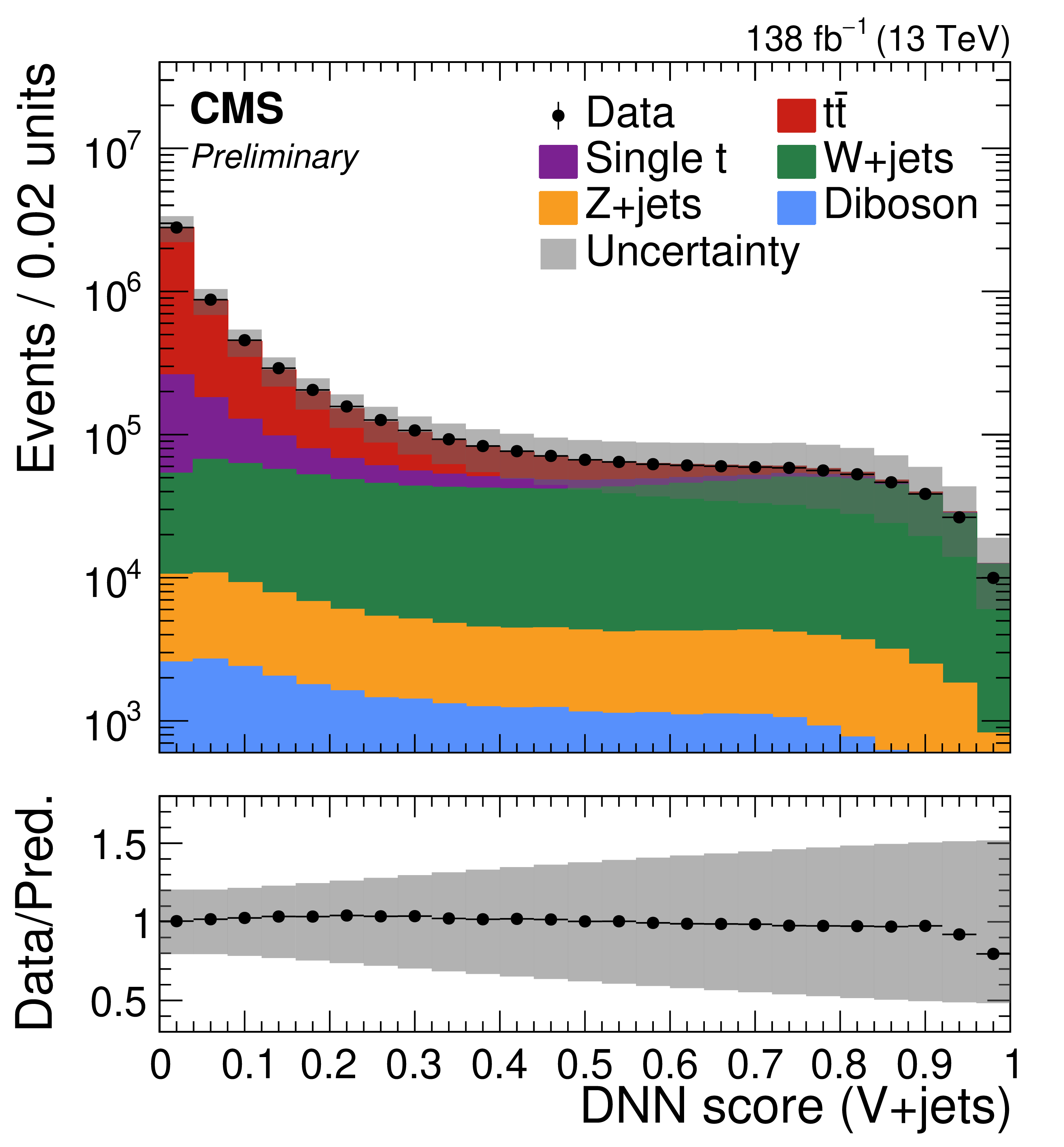
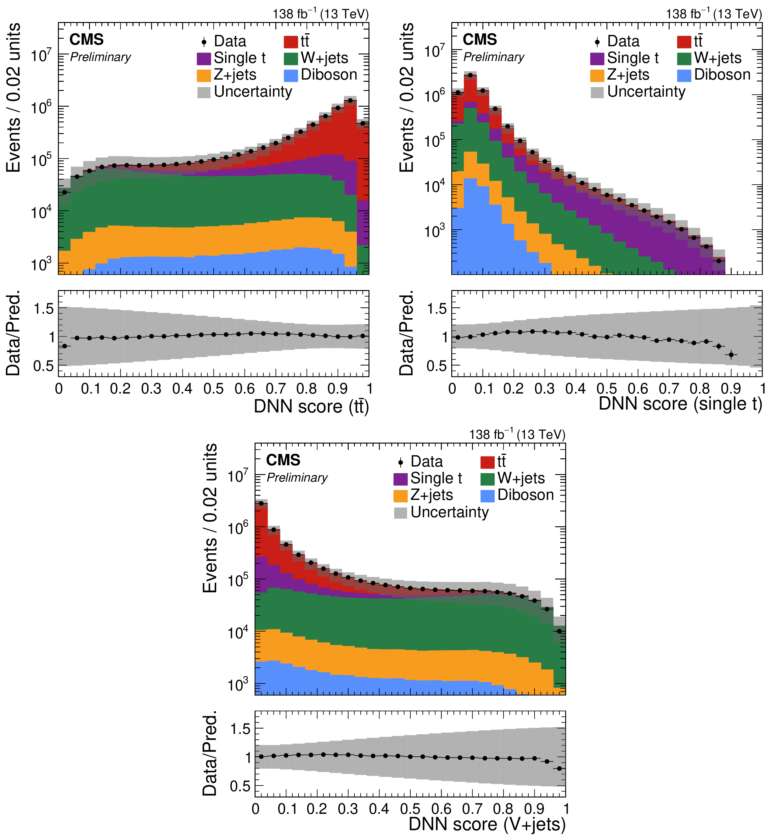
png pdf	Figure 4: DNN score distributions for the combined electron and muon channels: $\mathrm{t} \overline{\mathrm{t}}$ score (top left), single t score (top right), and V+jets} score (lower). The lower panels show the ratio of the data to the total SM background prediction. The gray bands represent the uncertainty, computed by summing in quadrature the statistical uncertainty and the systematic uncertainties affecting the normalization of each process.
png pdf	Figure 4-a: DNN score distributions for the combined electron and muon channels: $\mathrm{t} \overline{\mathrm{t}}$ score (top left), single t score (top right), and V+jets} score (lower). The lower panels show the ratio of the data to the total SM background prediction. The gray bands represent the uncertainty, computed by summing in quadrature the statistical uncertainty and the systematic uncertainties affecting the normalization of each process.
png pdf	Figure 4-b: DNN score distributions for the combined electron and muon channels: $\mathrm{t} \overline{\mathrm{t}}$ score (top left), single t score (top right), and V+jets} score (lower). The lower panels show the ratio of the data to the total SM background prediction. The gray bands represent the uncertainty, computed by summing in quadrature the statistical uncertainty and the systematic uncertainties affecting the normalization of each process.
png pdf	Figure 4-c: DNN score distributions for the combined electron and muon channels: $\mathrm{t} \overline{\mathrm{t}}$ score (top left), single t score (top right), and V+jets} score (lower). The lower panels show the ratio of the data to the total SM background prediction. The gray bands represent the uncertainty, computed by summing in quadrature the statistical uncertainty and the systematic uncertainties affecting the normalization of each process.
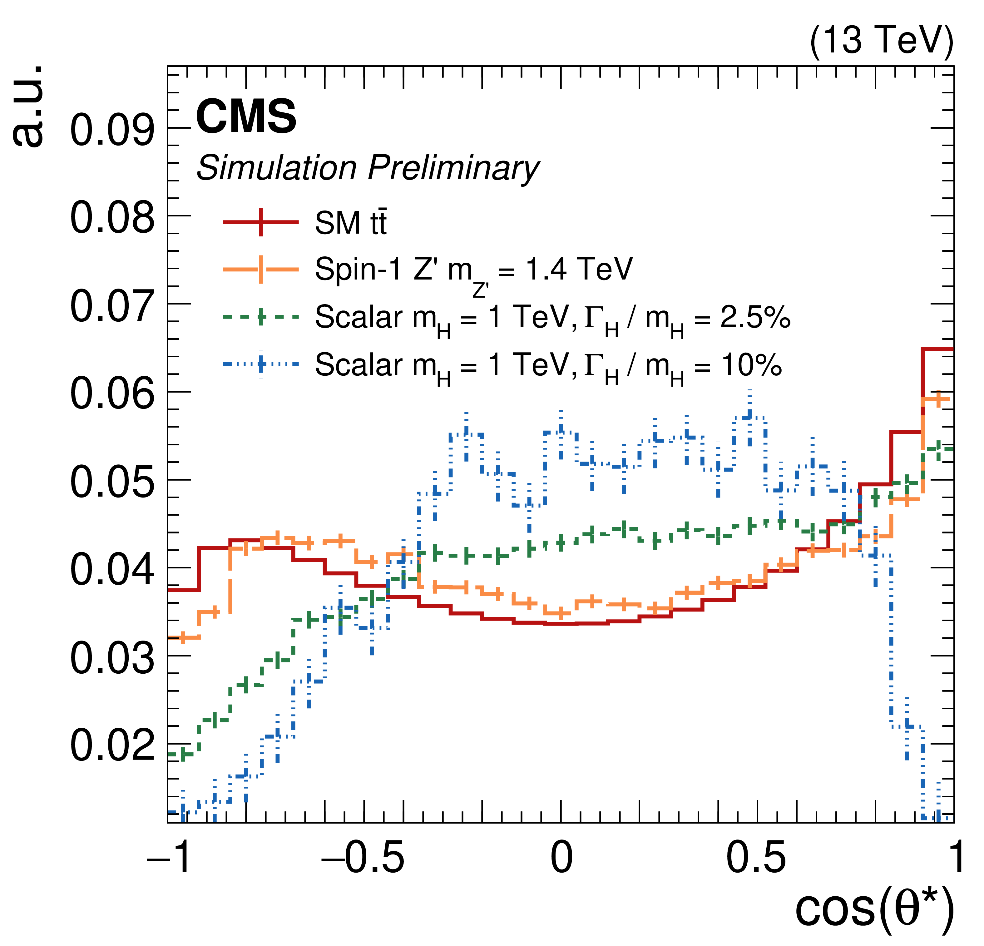
png pdf	Figure 5: Distribution of $\cos(\theta^*)$ for different processes: SM $\mathrm{t} \overline{\mathrm{t}}$ (solid red), Z' with $m_{{\mathrm{t}\overline{\mathrm{t}}} }=$ 1.4 TeV (long-dashed orange), scalar H with $m_{\mathrm{H}}=$ 1 TeV and 2.5% relative width (short-dashed green), and scalar H with $m_{\mathrm{H}}=$ 1 TeV and 10% relative width (dash-dotted blue). The fluctuations observed in the scalar signal samples, particularly for larger relative widths, arise from the interplay between the resonant and interference components. All distributions are normalized to unit area.
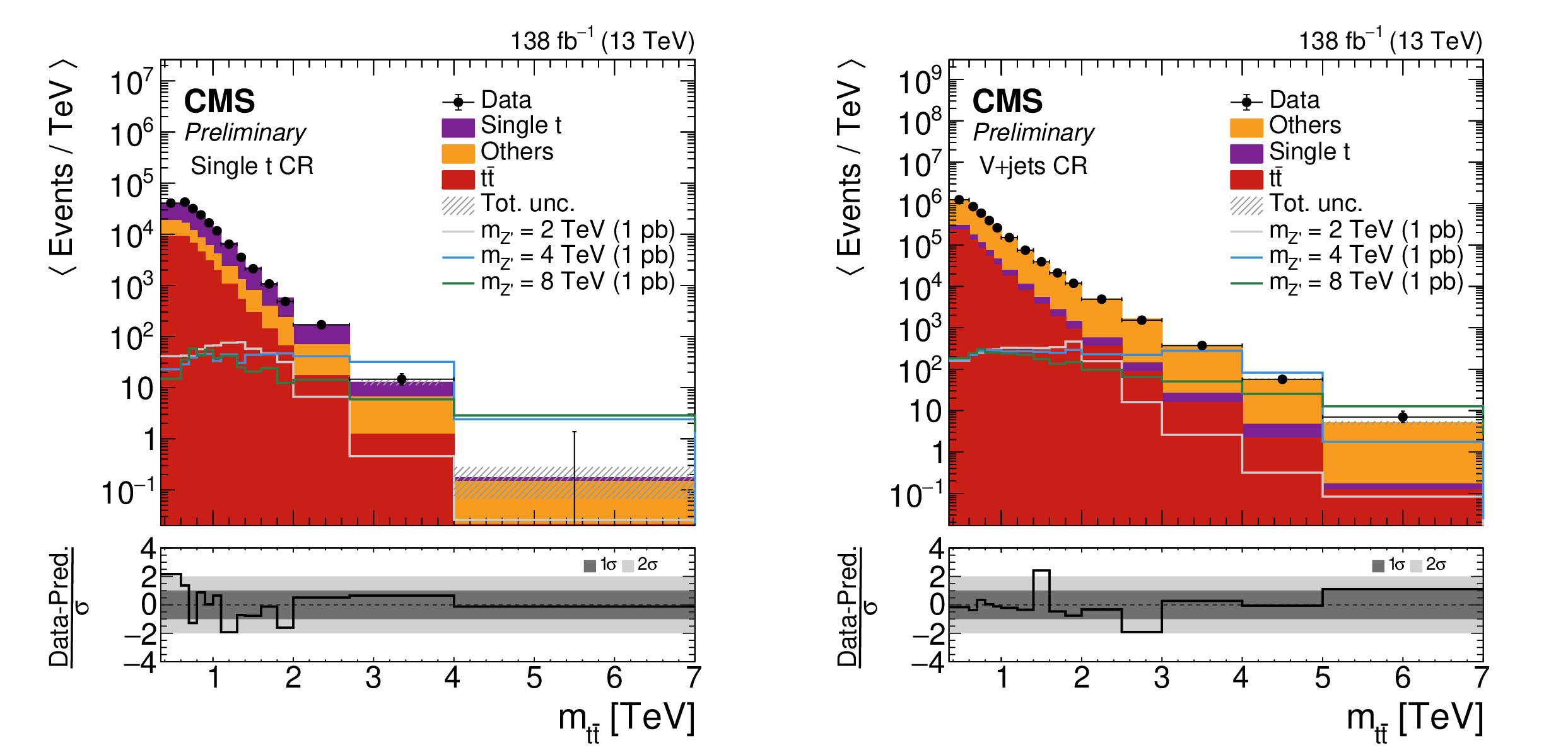
png pdf	Figure 6: Postfit distributions in $m_{{\mathrm{t}\overline{\mathrm{t}}} }$ for data and simulation in the single t (left) and V+jets} (right) CRs. The lower panels show the pull of each bin relative to the SM prediction, defined as (Data-Pred.)/ $\sigma$ , where $\sigma$ denotes the total uncertainty. The dark (light) gray band represents a pull of one (two) standard deviations from the predicted value.
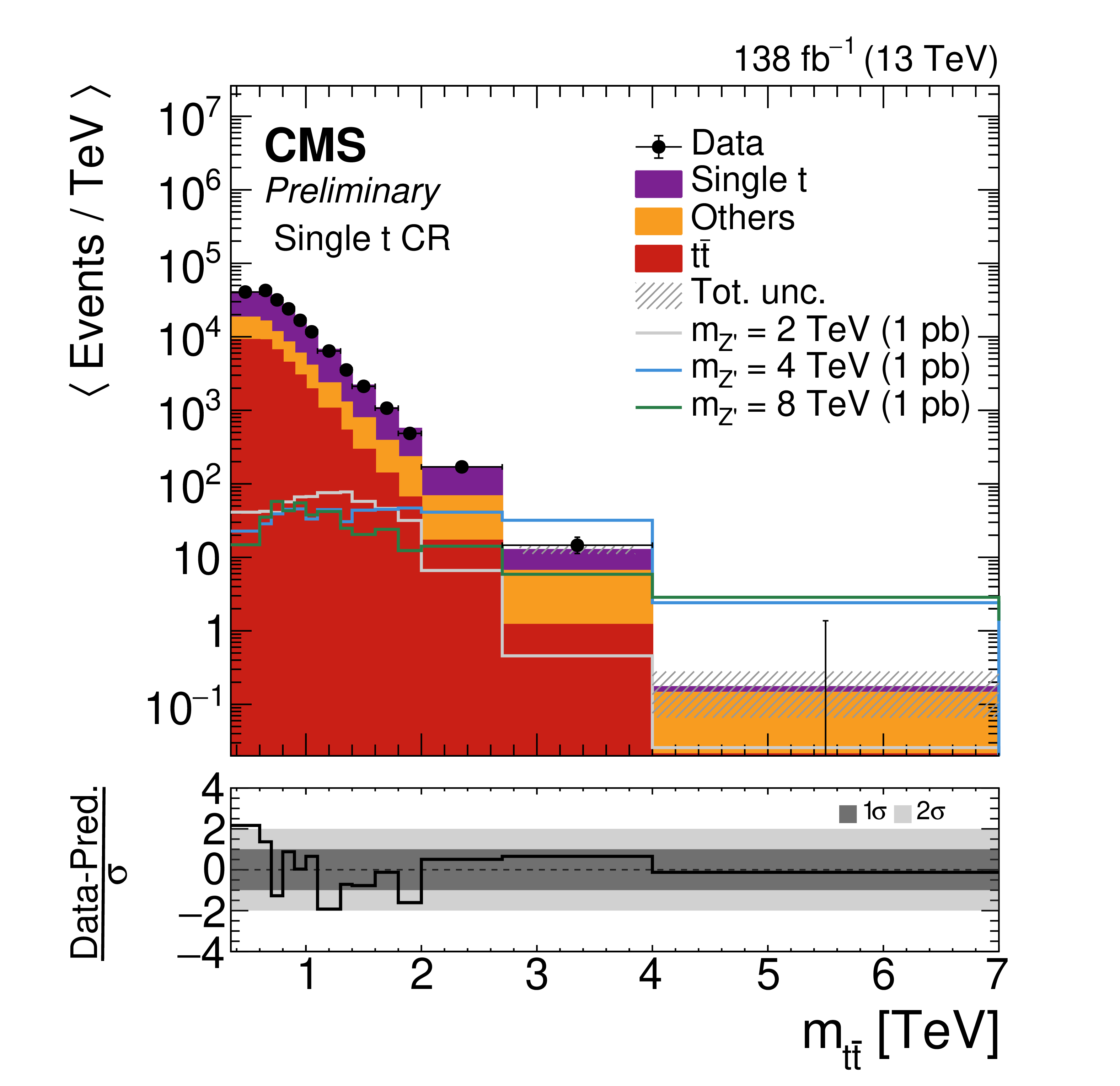
png pdf	Figure 6-a: Postfit distributions in $m_{{\mathrm{t}\overline{\mathrm{t}}} }$ for data and simulation in the single t (left) and V+jets} (right) CRs. The lower panels show the pull of each bin relative to the SM prediction, defined as (Data-Pred.)/ $\sigma$ , where $\sigma$ denotes the total uncertainty. The dark (light) gray band represents a pull of one (two) standard deviations from the predicted value.
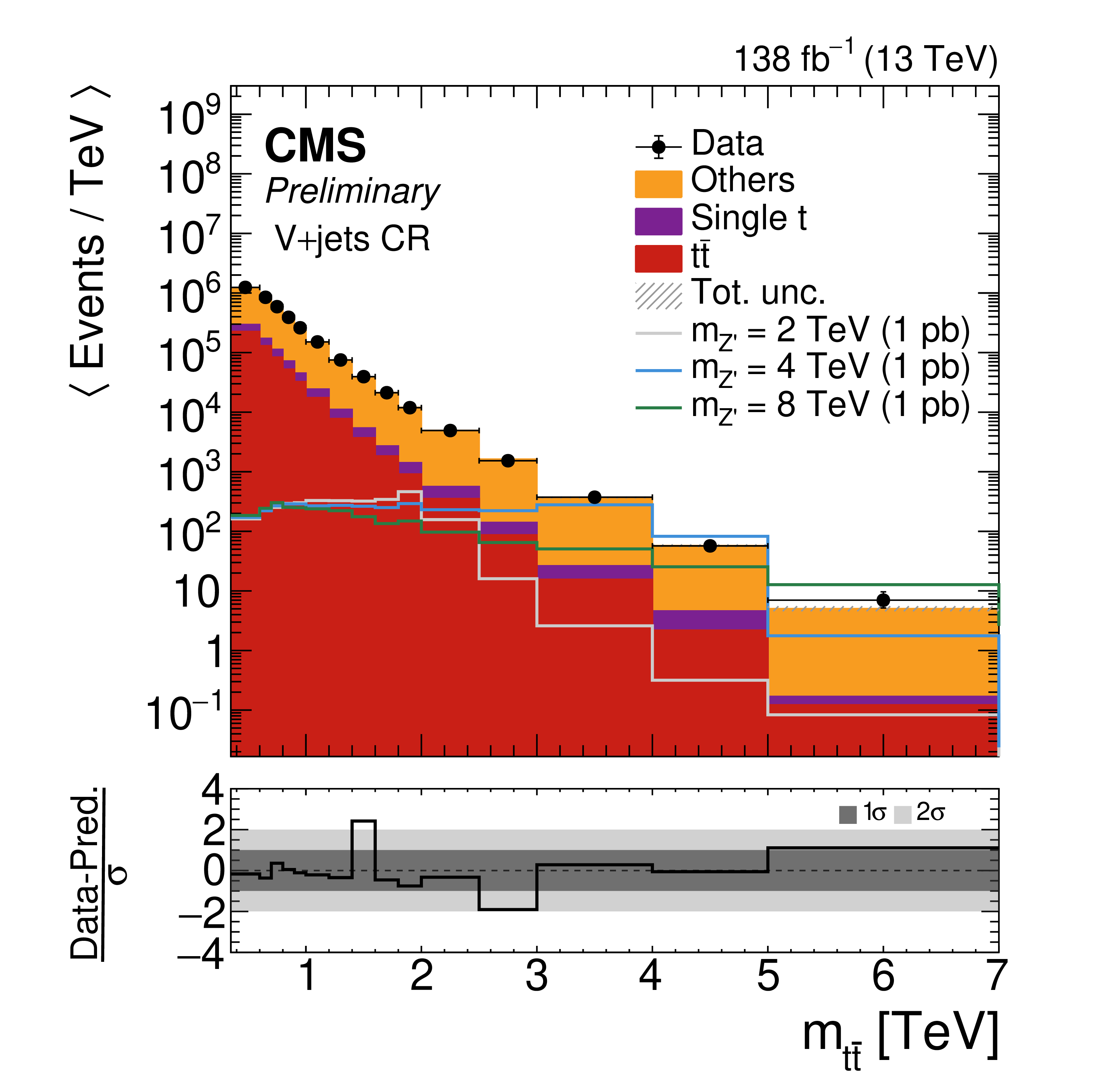
png pdf	Figure 6-b: Postfit distributions in $m_{{\mathrm{t}\overline{\mathrm{t}}} }$ for data and simulation in the single t (left) and V+jets} (right) CRs. The lower panels show the pull of each bin relative to the SM prediction, defined as (Data-Pred.)/ $\sigma$ , where $\sigma$ denotes the total uncertainty. The dark (light) gray band represents a pull of one (two) standard deviations from the predicted value.
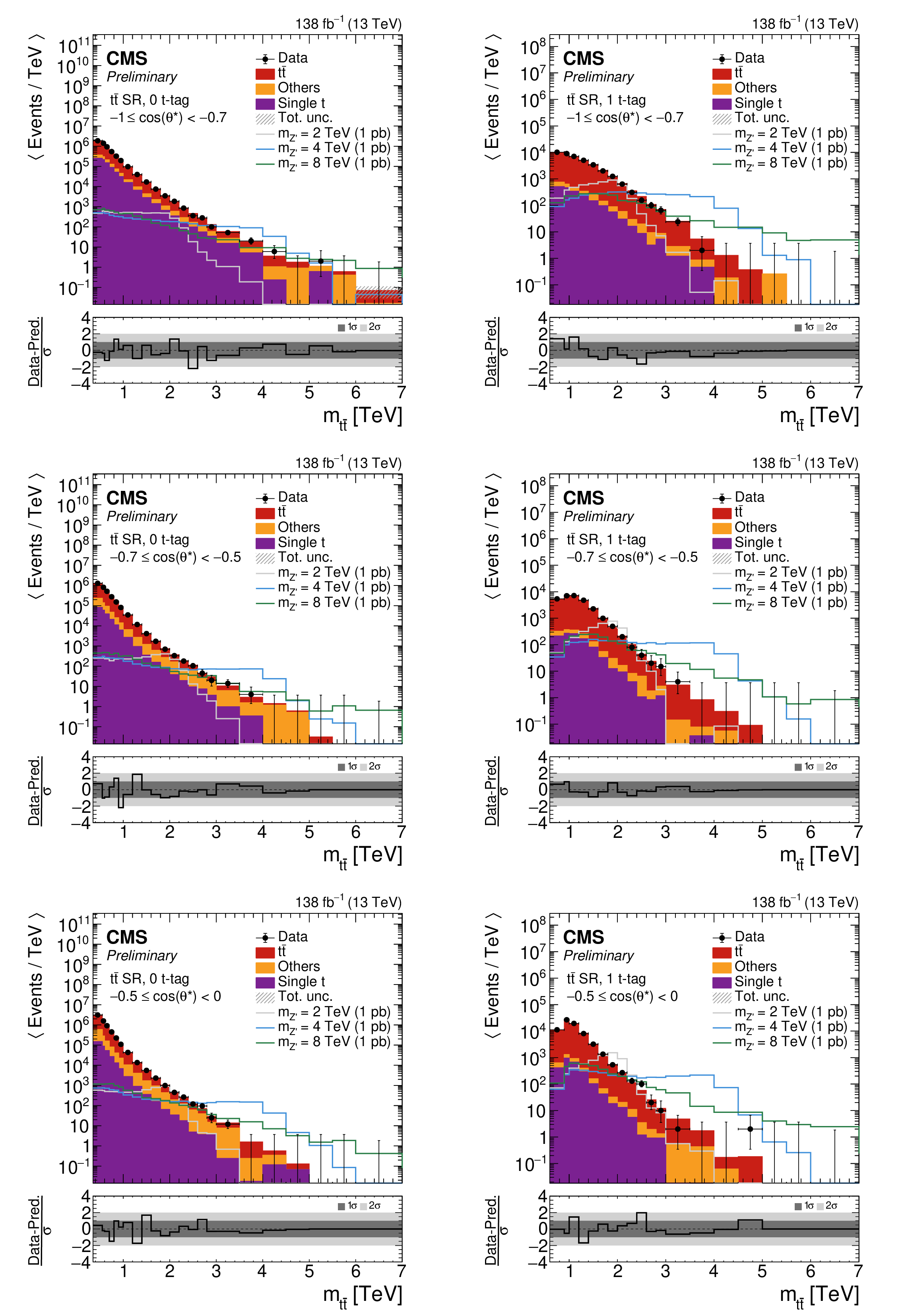
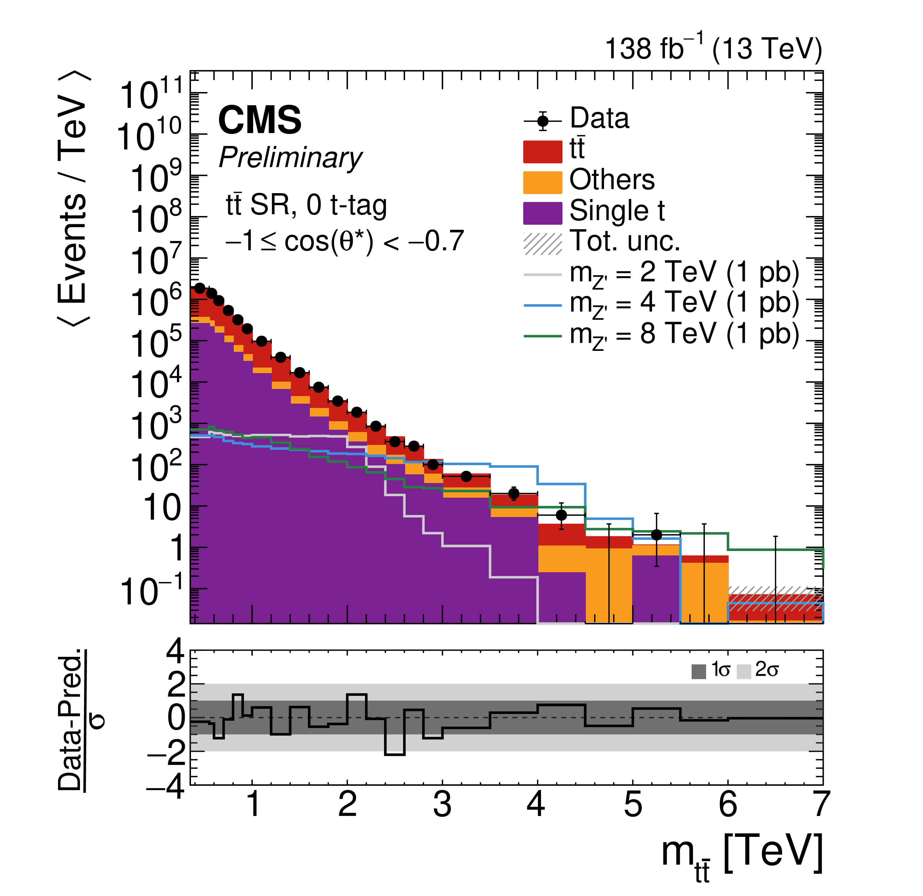
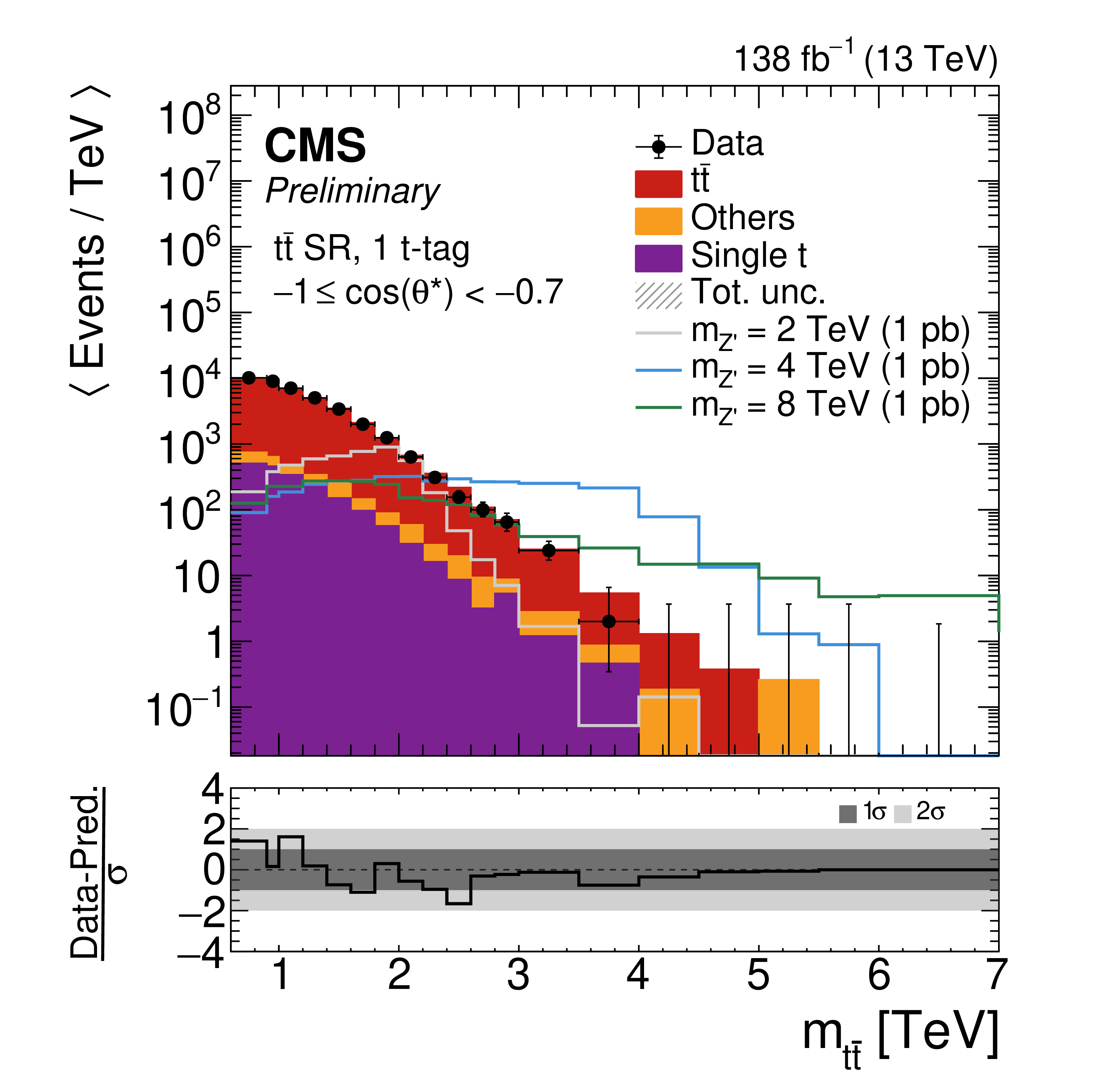
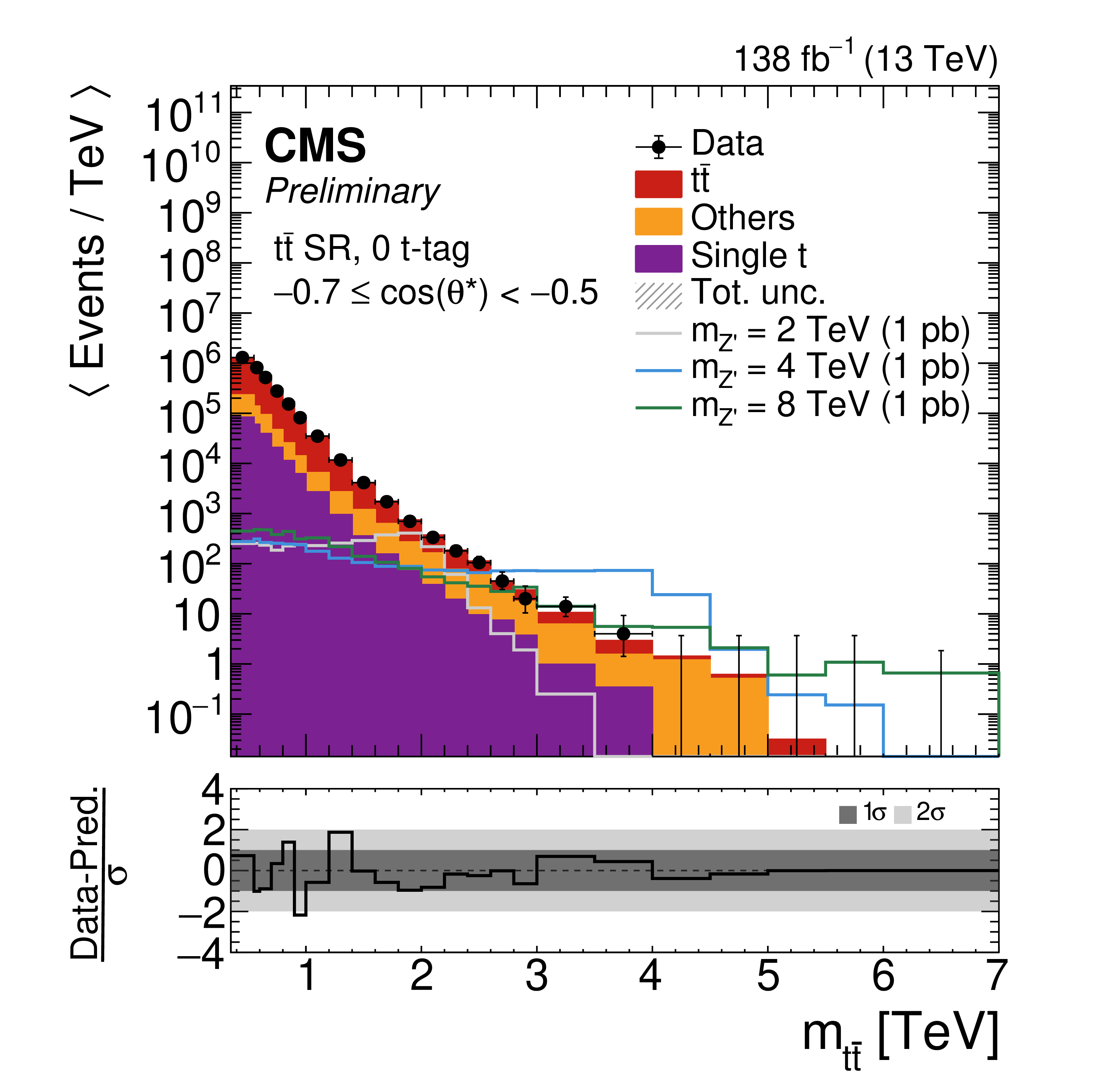
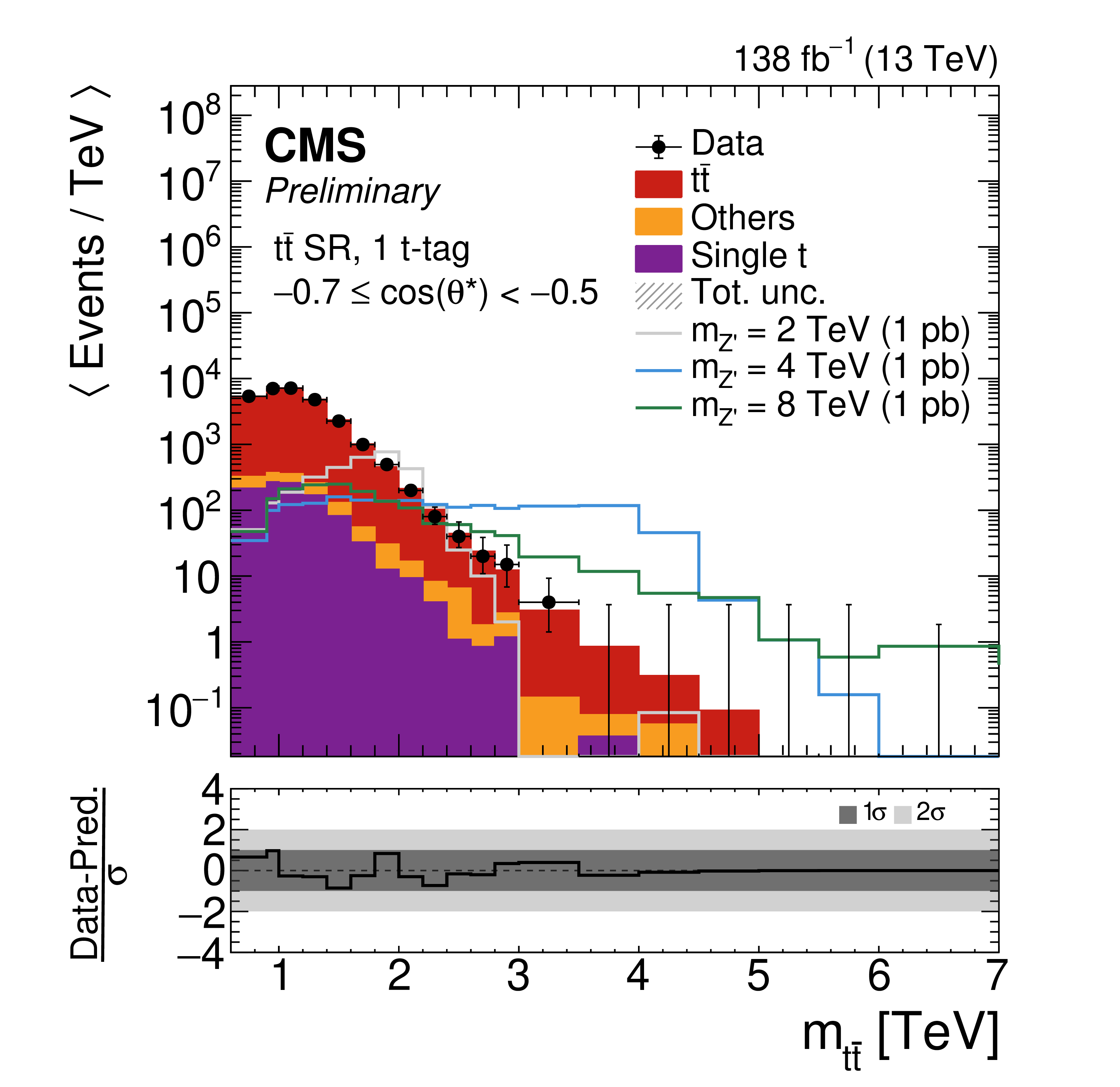
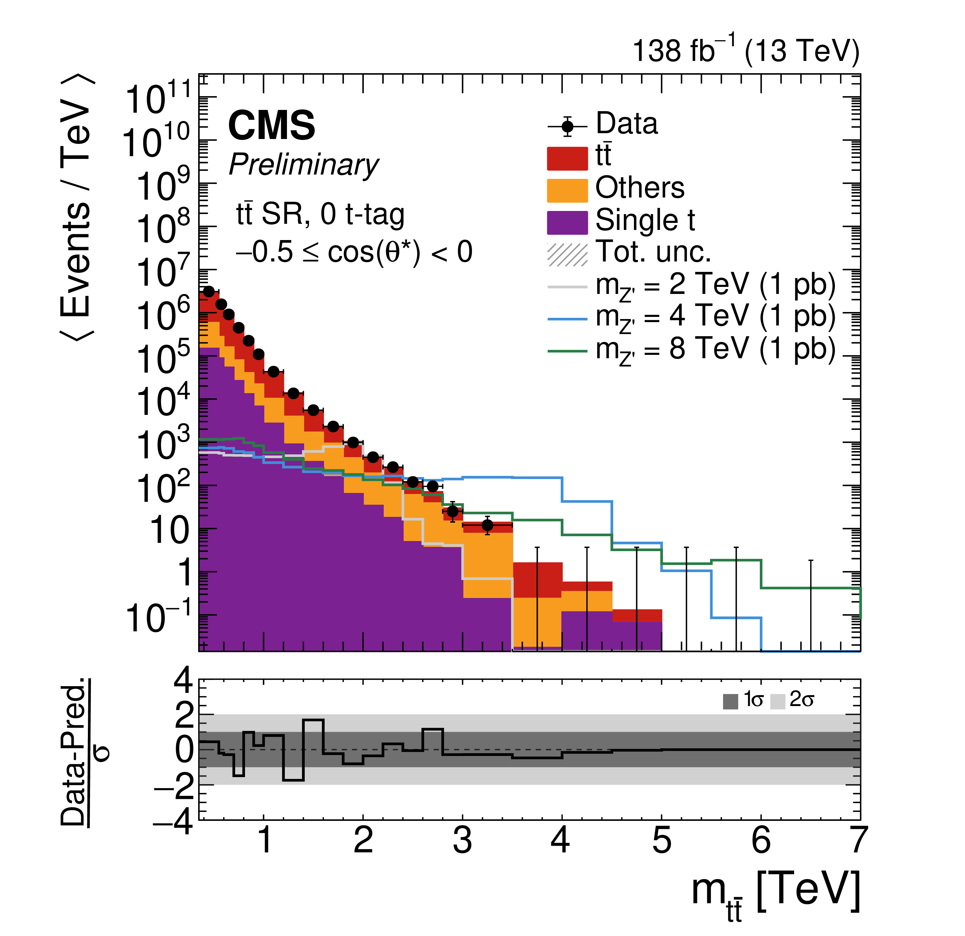
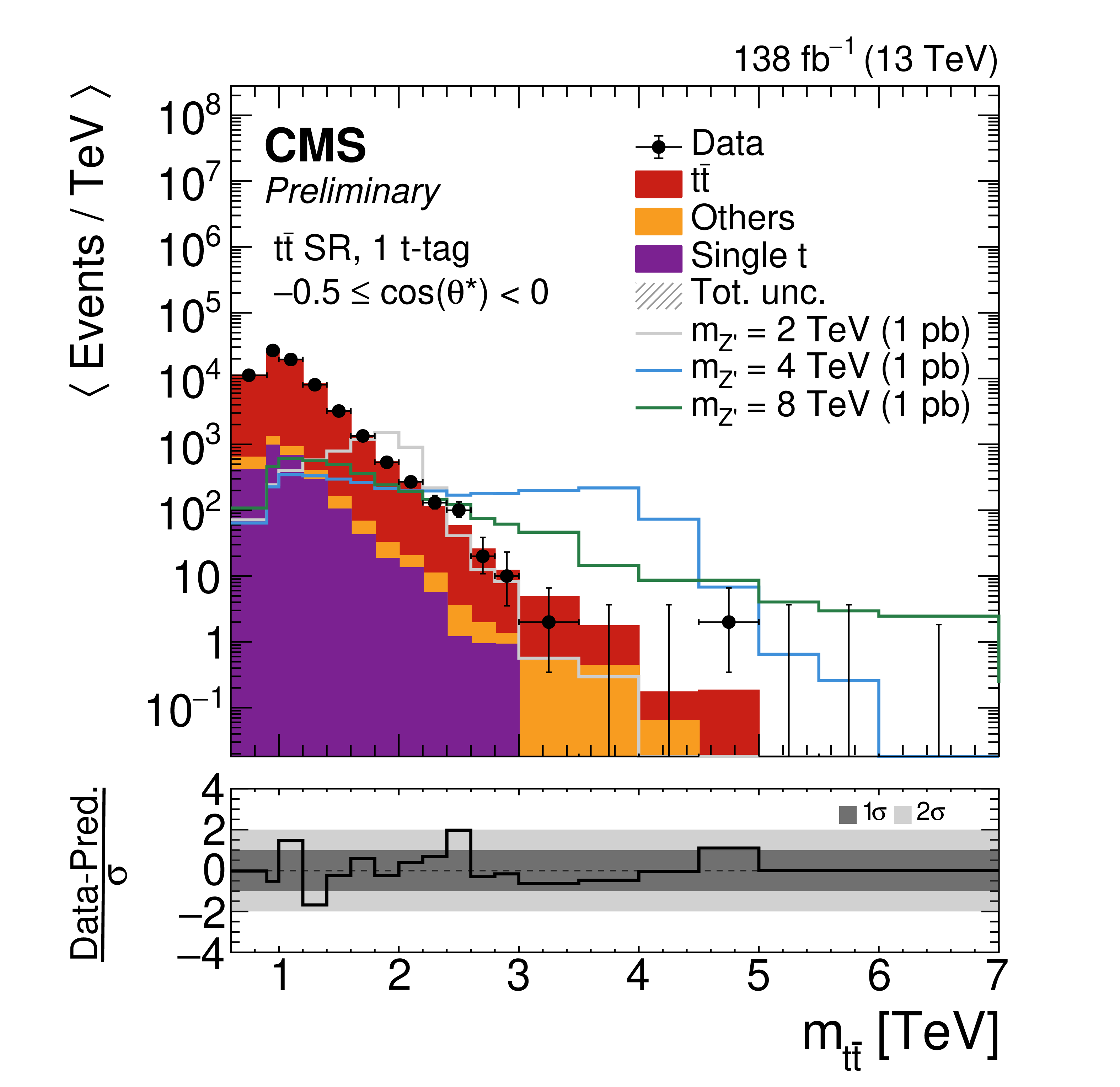
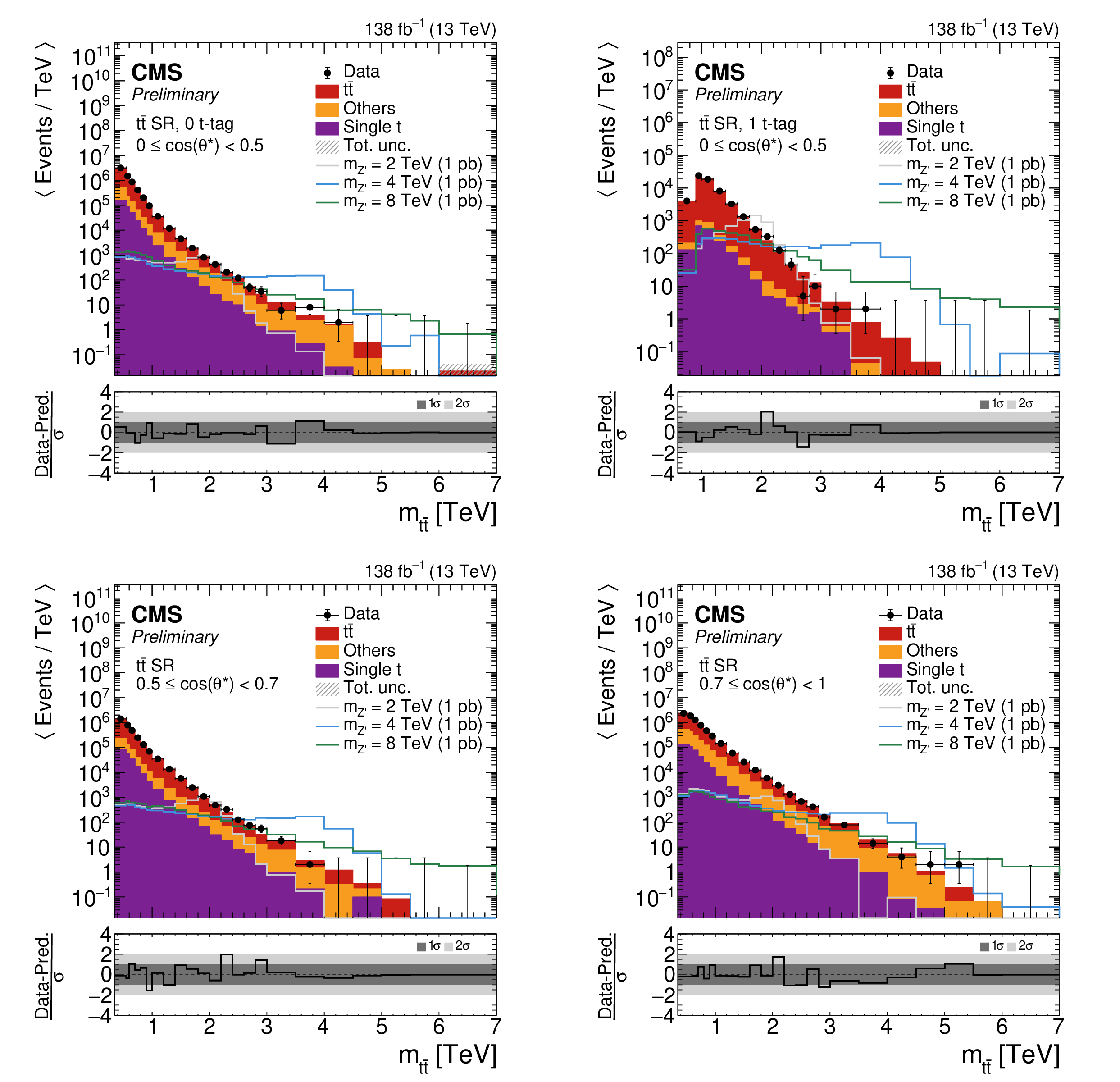
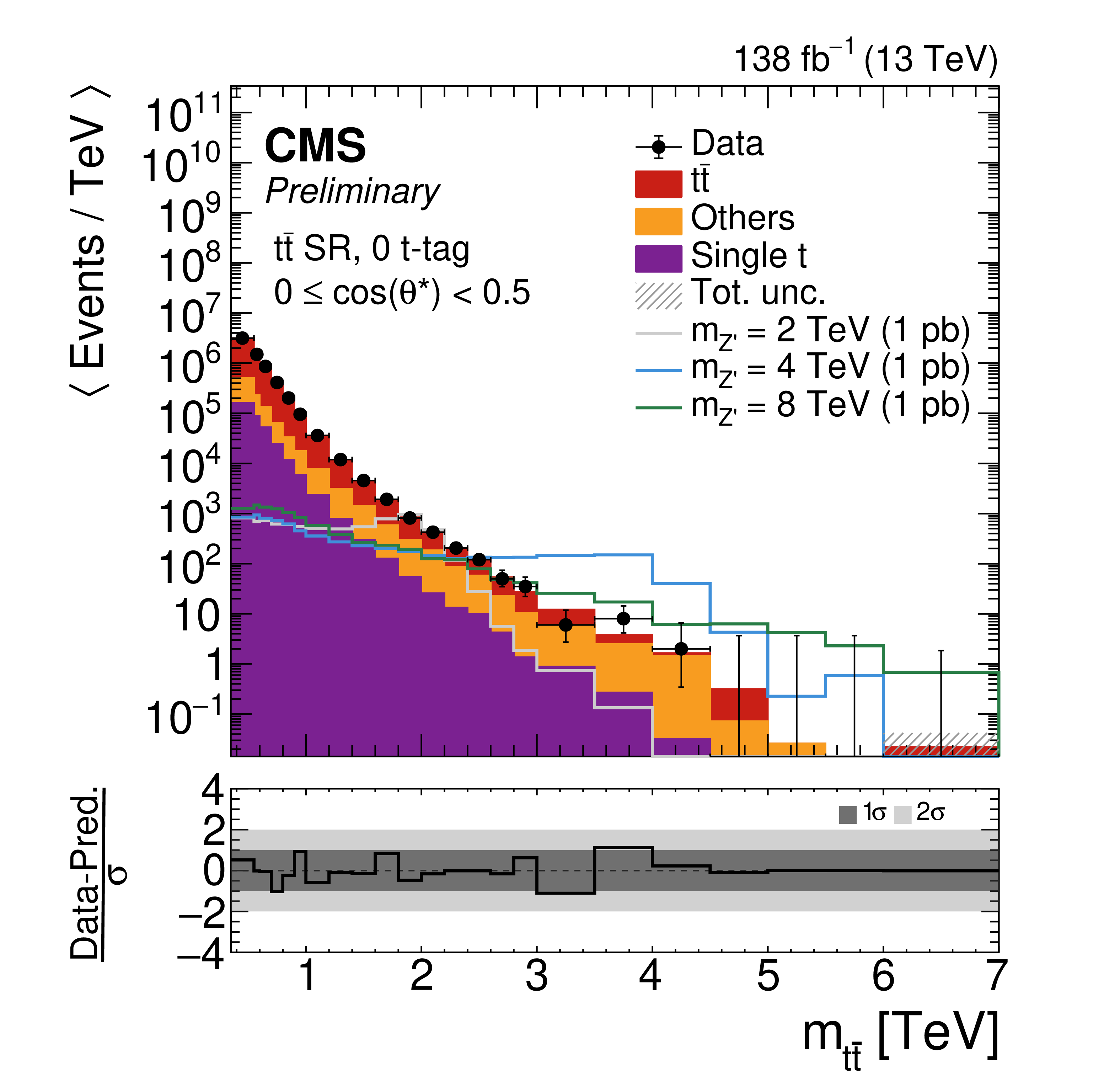
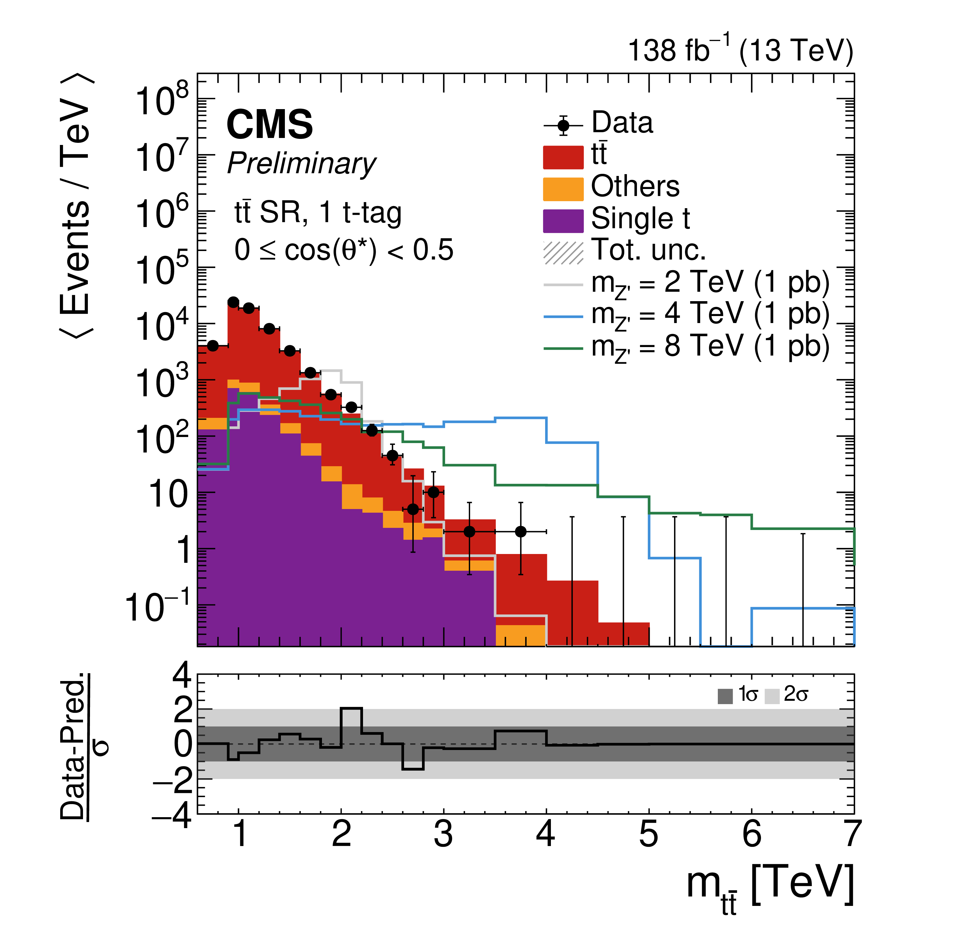
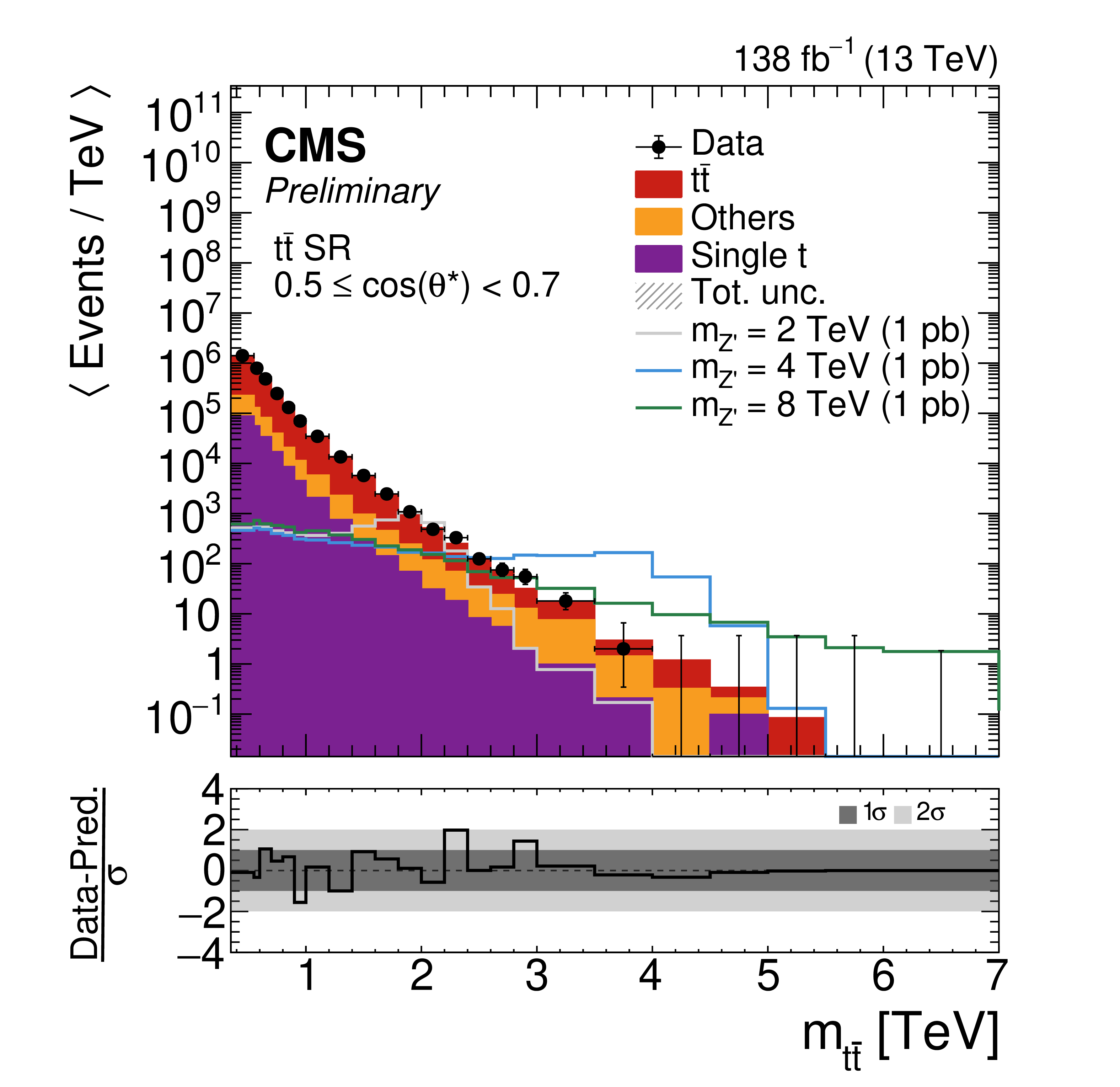
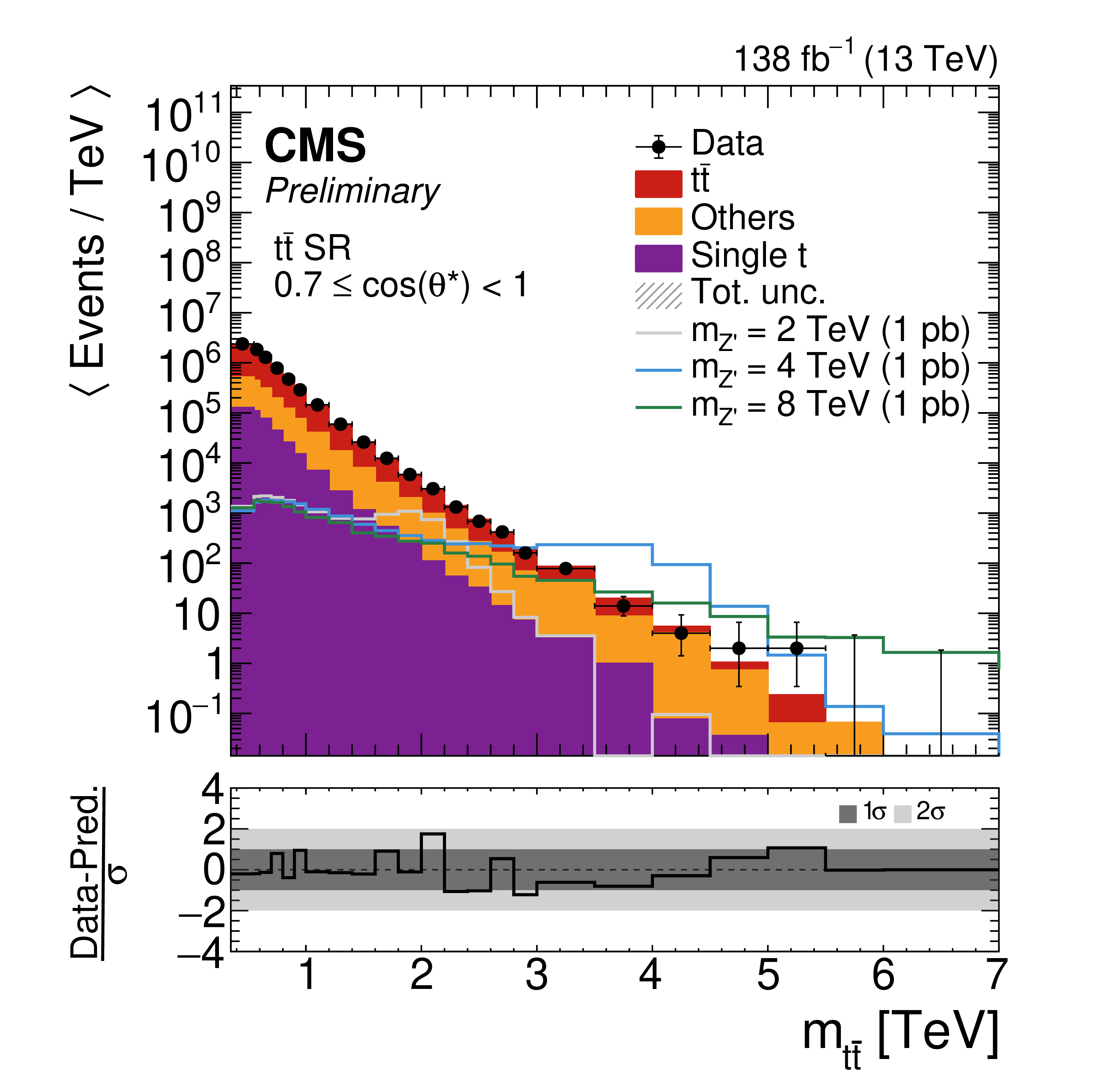
png pdf	Figure 7: Postfit distributions in $m_{{\mathrm{t}\overline{\mathrm{t}}} }$ for data and simulation in the first three bins of $\cos(\theta^*)$ in the $\mathrm{t} \overline{\mathrm{t}}$ SR, shown for the resolved (0 t-tag, left) and boosted (1 t-tag, right) categories. The lower panels show the pull of each bin relative to the SM prediction, defined as (Data-Pred.)/ $\sigma$ , where $\sigma$ denotes the total uncertainty. The dark (light) gray band represents a pull of one (two) standard deviations from the predicted value.
png pdf	Figure 7-a: Postfit distributions in $m_{{\mathrm{t}\overline{\mathrm{t}}} }$ for data and simulation in the first three bins of $\cos(\theta^*)$ in the $\mathrm{t} \overline{\mathrm{t}}$ SR, shown for the resolved (0 t-tag, left) and boosted (1 t-tag, right) categories. The lower panels show the pull of each bin relative to the SM prediction, defined as (Data-Pred.)/ $\sigma$ , where $\sigma$ denotes the total uncertainty. The dark (light) gray band represents a pull of one (two) standard deviations from the predicted value.
png pdf	Figure 7-b: Postfit distributions in $m_{{\mathrm{t}\overline{\mathrm{t}}} }$ for data and simulation in the first three bins of $\cos(\theta^*)$ in the $\mathrm{t} \overline{\mathrm{t}}$ SR, shown for the resolved (0 t-tag, left) and boosted (1 t-tag, right) categories. The lower panels show the pull of each bin relative to the SM prediction, defined as (Data-Pred.)/ $\sigma$ , where $\sigma$ denotes the total uncertainty. The dark (light) gray band represents a pull of one (two) standard deviations from the predicted value.
png pdf	Figure 7-c: Postfit distributions in $m_{{\mathrm{t}\overline{\mathrm{t}}} }$ for data and simulation in the first three bins of $\cos(\theta^*)$ in the $\mathrm{t} \overline{\mathrm{t}}$ SR, shown for the resolved (0 t-tag, left) and boosted (1 t-tag, right) categories. The lower panels show the pull of each bin relative to the SM prediction, defined as (Data-Pred.)/ $\sigma$ , where $\sigma$ denotes the total uncertainty. The dark (light) gray band represents a pull of one (two) standard deviations from the predicted value.
png pdf	Figure 7-d: Postfit distributions in $m_{{\mathrm{t}\overline{\mathrm{t}}} }$ for data and simulation in the first three bins of $\cos(\theta^*)$ in the $\mathrm{t} \overline{\mathrm{t}}$ SR, shown for the resolved (0 t-tag, left) and boosted (1 t-tag, right) categories. The lower panels show the pull of each bin relative to the SM prediction, defined as (Data-Pred.)/ $\sigma$ , where $\sigma$ denotes the total uncertainty. The dark (light) gray band represents a pull of one (two) standard deviations from the predicted value.
png pdf	Figure 7-e: Postfit distributions in $m_{{\mathrm{t}\overline{\mathrm{t}}} }$ for data and simulation in the first three bins of $\cos(\theta^*)$ in the $\mathrm{t} \overline{\mathrm{t}}$ SR, shown for the resolved (0 t-tag, left) and boosted (1 t-tag, right) categories. The lower panels show the pull of each bin relative to the SM prediction, defined as (Data-Pred.)/ $\sigma$ , where $\sigma$ denotes the total uncertainty. The dark (light) gray band represents a pull of one (two) standard deviations from the predicted value.
png pdf	Figure 7-f: Postfit distributions in $m_{{\mathrm{t}\overline{\mathrm{t}}} }$ for data and simulation in the first three bins of $\cos(\theta^*)$ in the $\mathrm{t} \overline{\mathrm{t}}$ SR, shown for the resolved (0 t-tag, left) and boosted (1 t-tag, right) categories. The lower panels show the pull of each bin relative to the SM prediction, defined as (Data-Pred.)/ $\sigma$ , where $\sigma$ denotes the total uncertainty. The dark (light) gray band represents a pull of one (two) standard deviations from the predicted value.
png pdf	Figure 8: Postfit distributions in $m_{{\mathrm{t}\overline{\mathrm{t}}} }$ for data and simulation in the last three bins of $\cos(\theta^*)$ in the $\mathrm{t} \overline{\mathrm{t}}$ SR, shown for the resolved (0 t-tag, left) and boosted (1 t-tag, right) categories. The lower panels show the pull of each bin relative to the SM prediction, defined as (Data-Pred.)/ $\sigma$ , where $\sigma$ denotes the total uncertainty. The dark (light) gray band represents a pull of one (two) standard deviations from the predicted value.
png pdf	Figure 8-a: Postfit distributions in $m_{{\mathrm{t}\overline{\mathrm{t}}} }$ for data and simulation in the last three bins of $\cos(\theta^*)$ in the $\mathrm{t} \overline{\mathrm{t}}$ SR, shown for the resolved (0 t-tag, left) and boosted (1 t-tag, right) categories. The lower panels show the pull of each bin relative to the SM prediction, defined as (Data-Pred.)/ $\sigma$ , where $\sigma$ denotes the total uncertainty. The dark (light) gray band represents a pull of one (two) standard deviations from the predicted value.
png pdf	Figure 8-b: Postfit distributions in $m_{{\mathrm{t}\overline{\mathrm{t}}} }$ for data and simulation in the last three bins of $\cos(\theta^*)$ in the $\mathrm{t} \overline{\mathrm{t}}$ SR, shown for the resolved (0 t-tag, left) and boosted (1 t-tag, right) categories. The lower panels show the pull of each bin relative to the SM prediction, defined as (Data-Pred.)/ $\sigma$ , where $\sigma$ denotes the total uncertainty. The dark (light) gray band represents a pull of one (two) standard deviations from the predicted value.
png pdf	Figure 8-c: Postfit distributions in $m_{{\mathrm{t}\overline{\mathrm{t}}} }$ for data and simulation in the last three bins of $\cos(\theta^*)$ in the $\mathrm{t} \overline{\mathrm{t}}$ SR, shown for the resolved (0 t-tag, left) and boosted (1 t-tag, right) categories. The lower panels show the pull of each bin relative to the SM prediction, defined as (Data-Pred.)/ $\sigma$ , where $\sigma$ denotes the total uncertainty. The dark (light) gray band represents a pull of one (two) standard deviations from the predicted value.
png pdf	Figure 8-d: Postfit distributions in $m_{{\mathrm{t}\overline{\mathrm{t}}} }$ for data and simulation in the last three bins of $\cos(\theta^*)$ in the $\mathrm{t} \overline{\mathrm{t}}$ SR, shown for the resolved (0 t-tag, left) and boosted (1 t-tag, right) categories. The lower panels show the pull of each bin relative to the SM prediction, defined as (Data-Pred.)/ $\sigma$ , where $\sigma$ denotes the total uncertainty. The dark (light) gray band represents a pull of one (two) standard deviations from the predicted value.
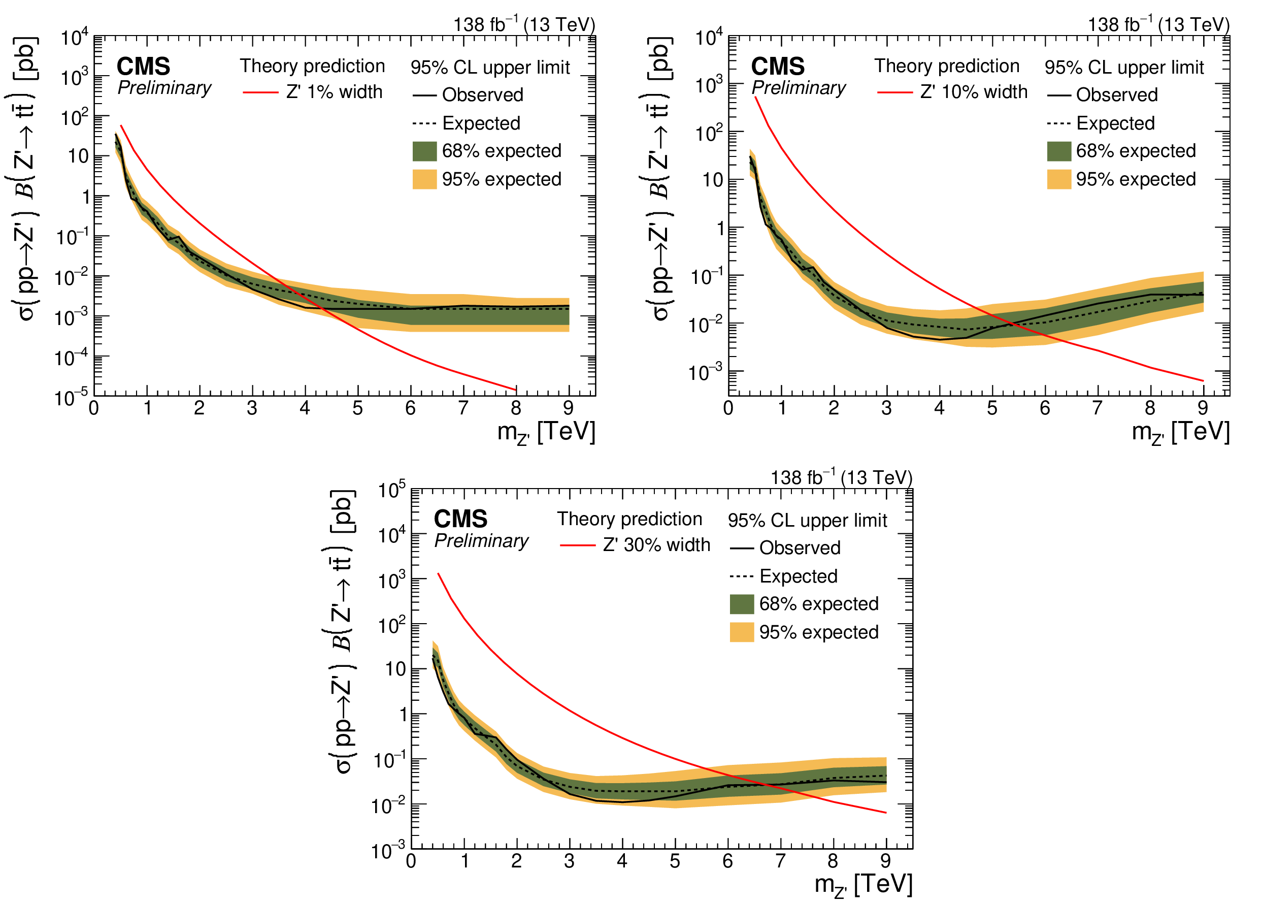
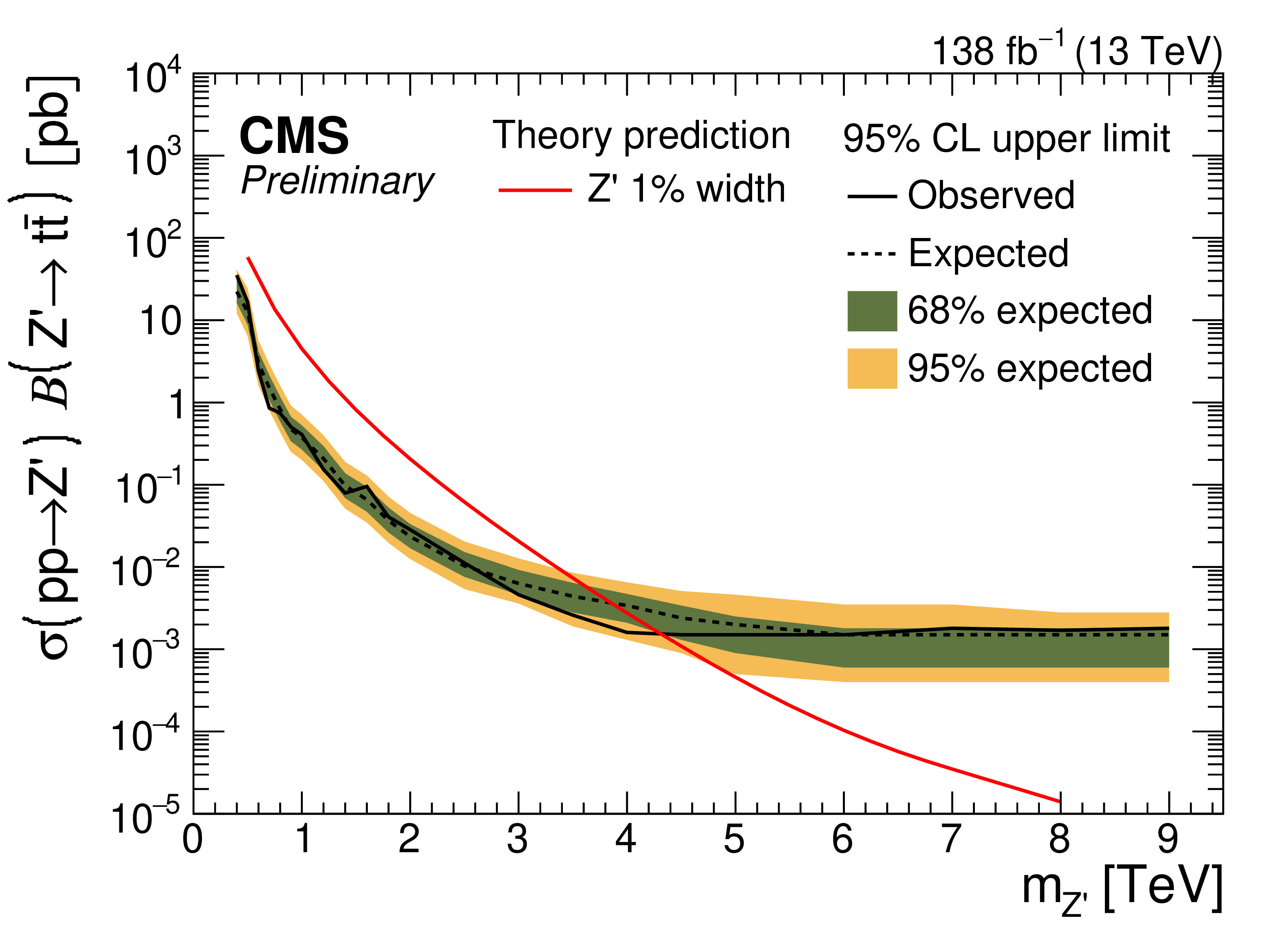
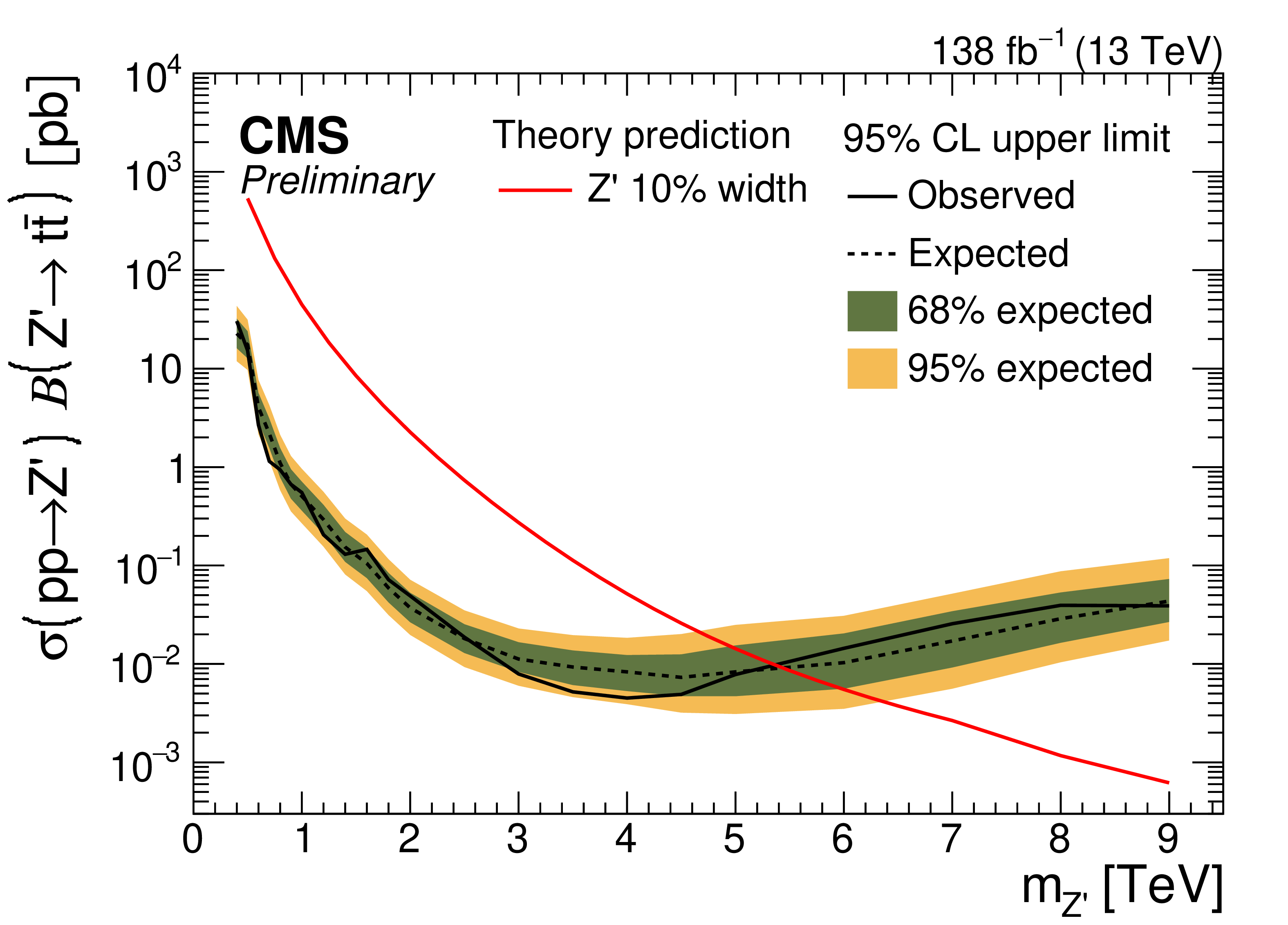
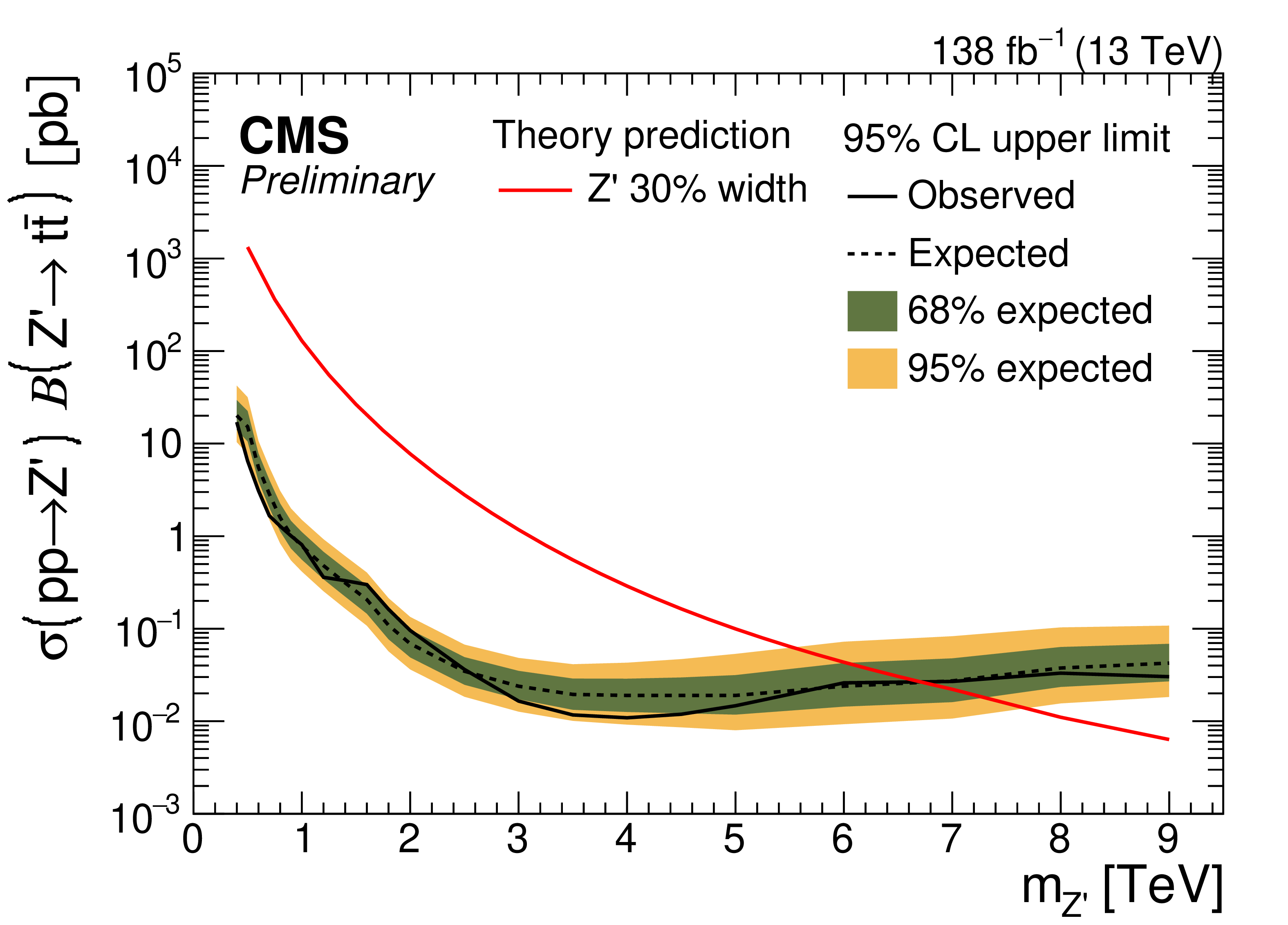
png pdf	Figure 9: Expected and observed upper limits at 95% CL on the product of the production cross section and the branching fraction as functions of the resonance mass. The limits are shown for Z' bosons with 1% (upper left), 10% (upper right) and 30% (lower) relative widths. The limits are compared with the respective theory predictions shown by red curves.
png pdf	Figure 9-a: Expected and observed upper limits at 95% CL on the product of the production cross section and the branching fraction as functions of the resonance mass. The limits are shown for Z' bosons with 1% (upper left), 10% (upper right) and 30% (lower) relative widths. The limits are compared with the respective theory predictions shown by red curves.
png pdf	Figure 9-b: Expected and observed upper limits at 95% CL on the product of the production cross section and the branching fraction as functions of the resonance mass. The limits are shown for Z' bosons with 1% (upper left), 10% (upper right) and 30% (lower) relative widths. The limits are compared with the respective theory predictions shown by red curves.
png pdf	Figure 9-c: Expected and observed upper limits at 95% CL on the product of the production cross section and the branching fraction as functions of the resonance mass. The limits are shown for Z' bosons with 1% (upper left), 10% (upper right) and 30% (lower) relative widths. The limits are compared with the respective theory predictions shown by red curves.
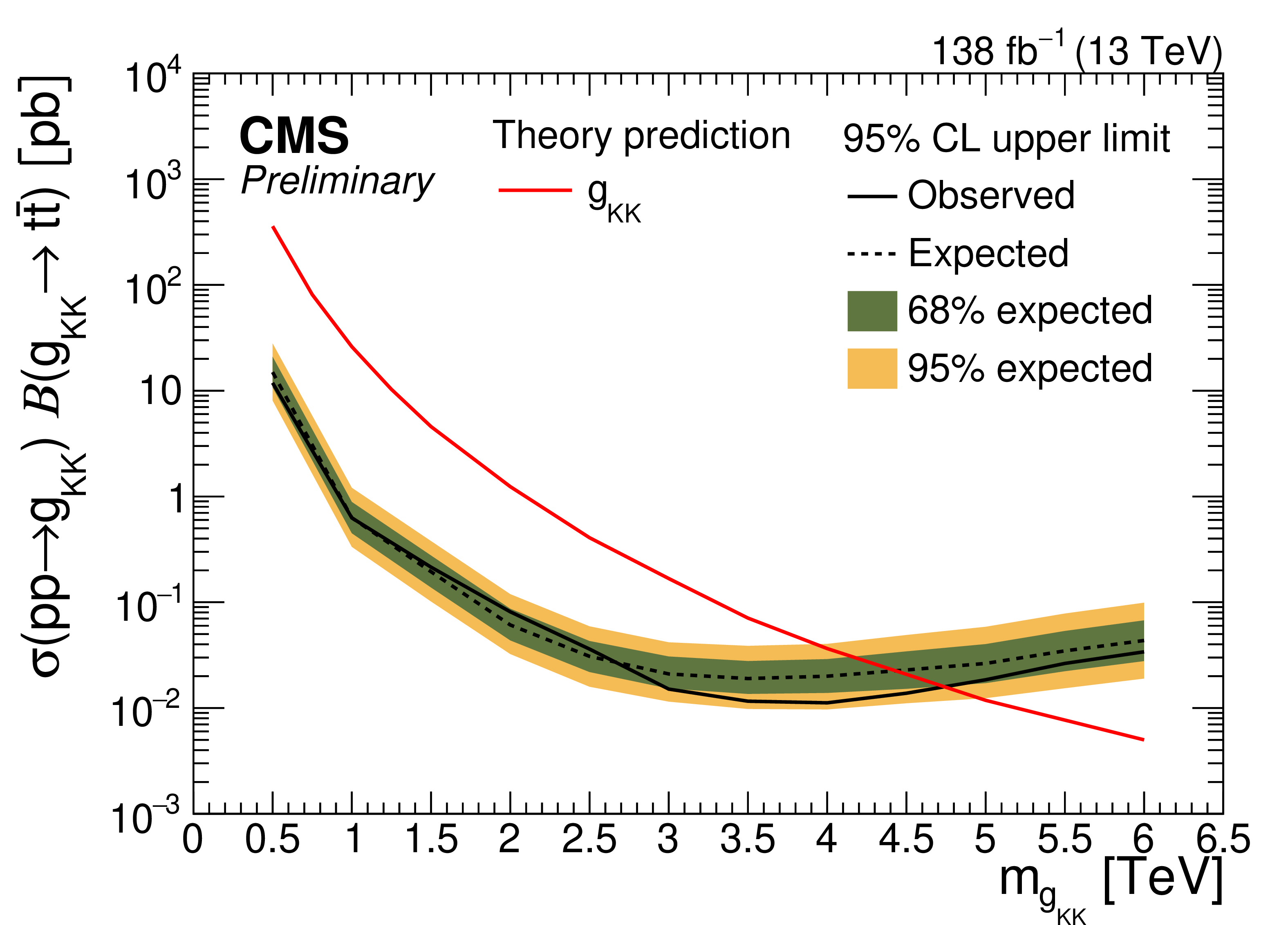
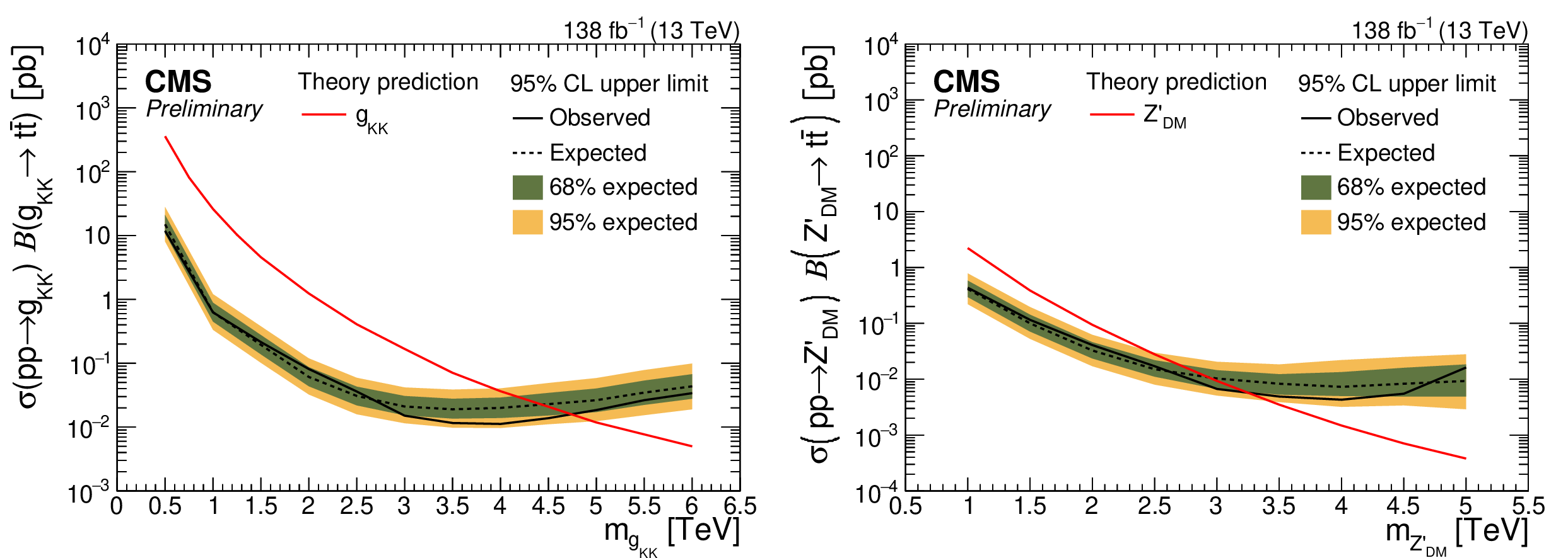
png pdf	Figure 10: Expected and observed upper limits at 95% CL on the product of the production cross section and the branching fraction as functions of the resonance mass. The limits are shown for the Kaluza-Klein gluon (left) and dark matter (right) scenarios. The limits are compared with the respective theory predictions shown by red curves.
png pdf	Figure 10-a: Expected and observed upper limits at 95% CL on the product of the production cross section and the branching fraction as functions of the resonance mass. The limits are shown for the Kaluza-Klein gluon (left) and dark matter (right) scenarios. The limits are compared with the respective theory predictions shown by red curves.
png pdf	Figure 10-b: Expected and observed upper limits at 95% CL on the product of the production cross section and the branching fraction as functions of the resonance mass. The limits are shown for the Kaluza-Klein gluon (left) and dark matter (right) scenarios. The limits are compared with the respective theory predictions shown by red curves.
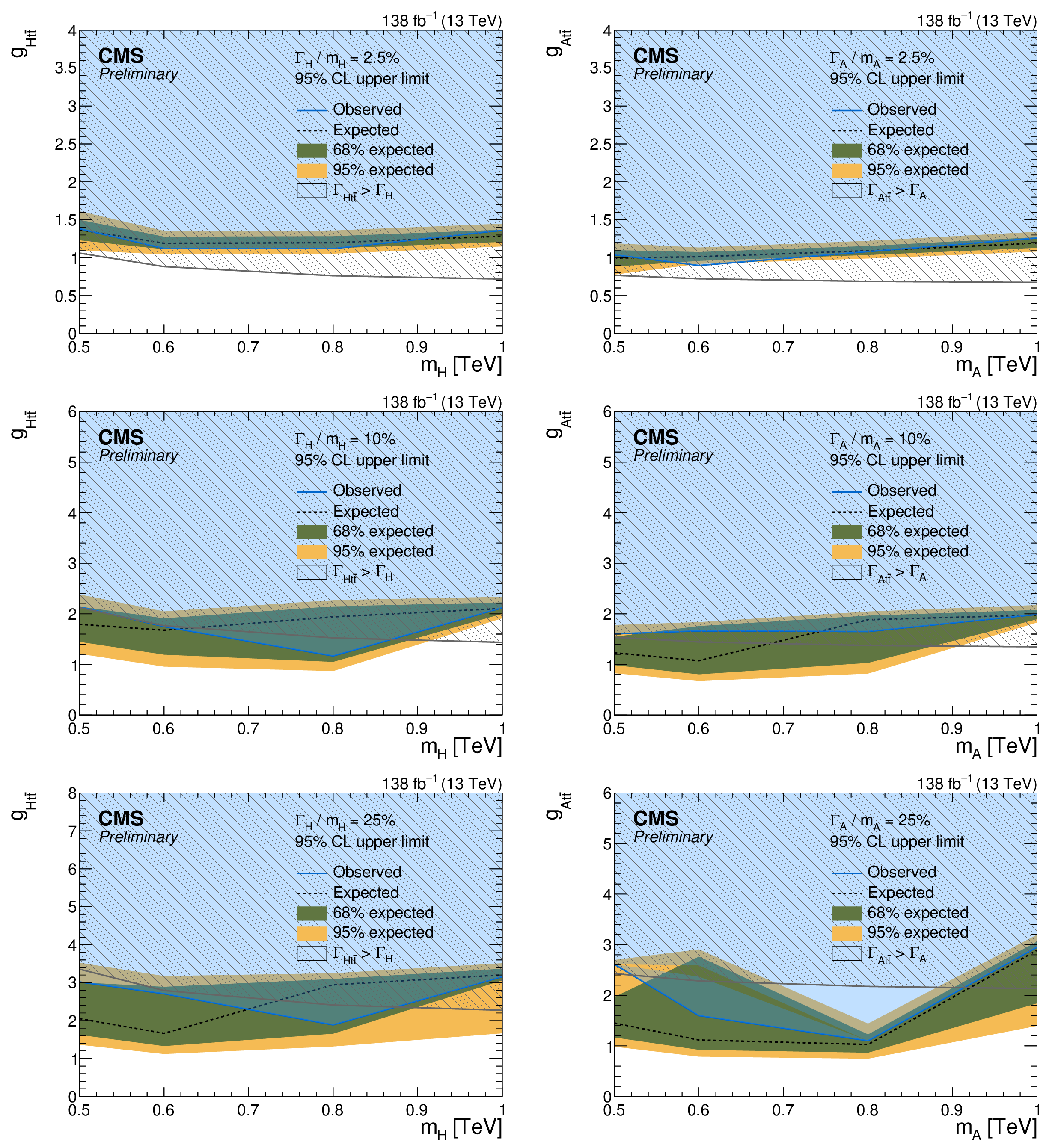
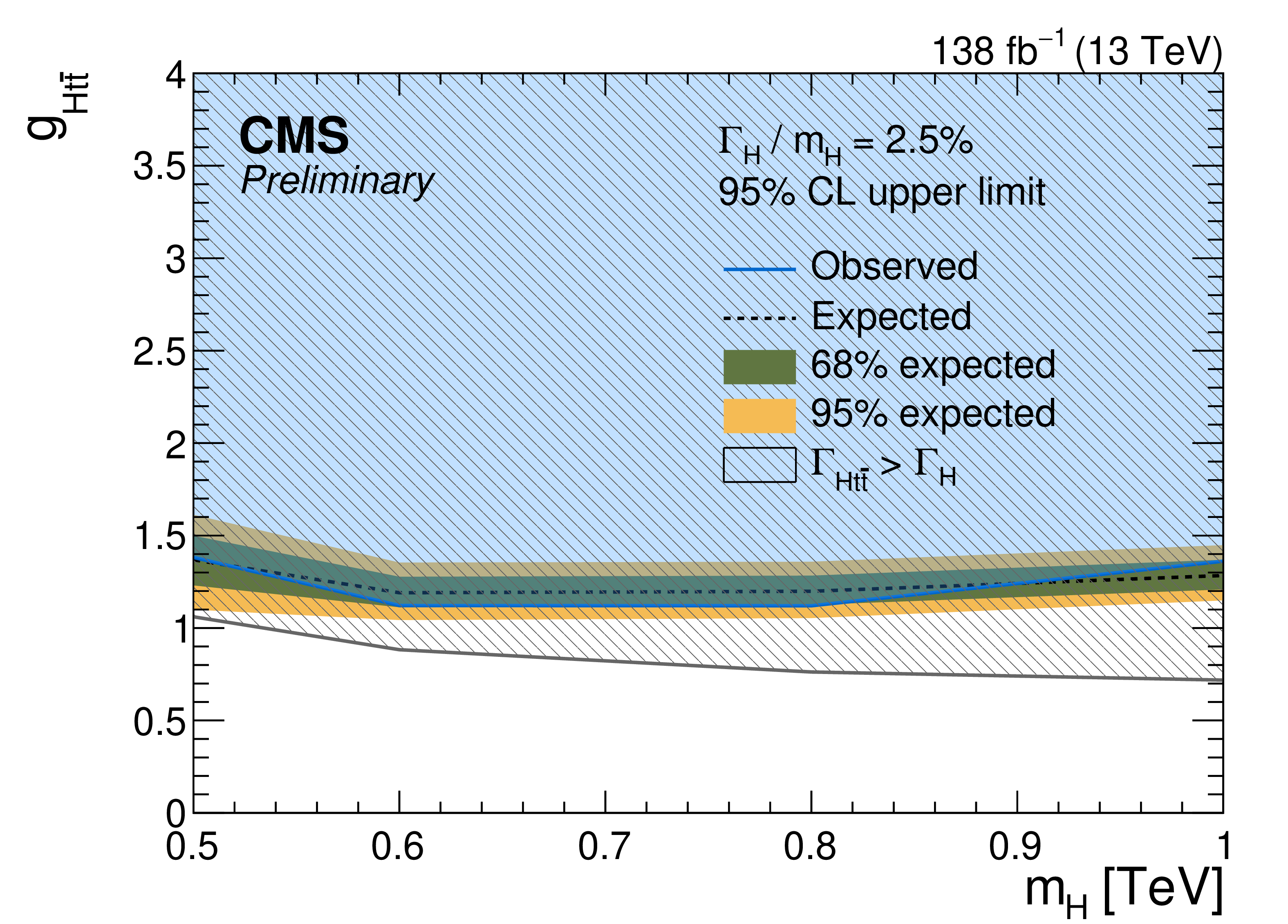
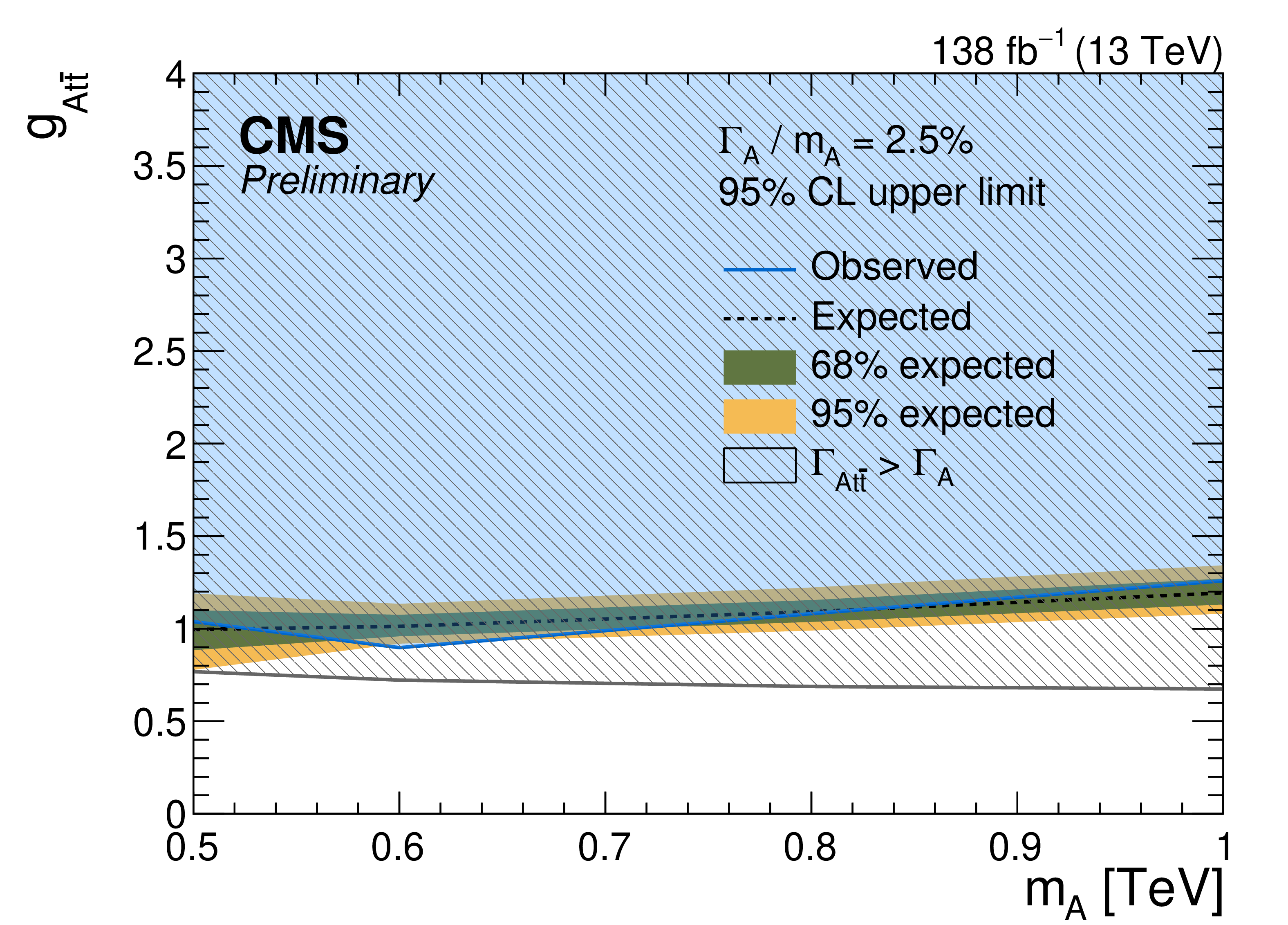
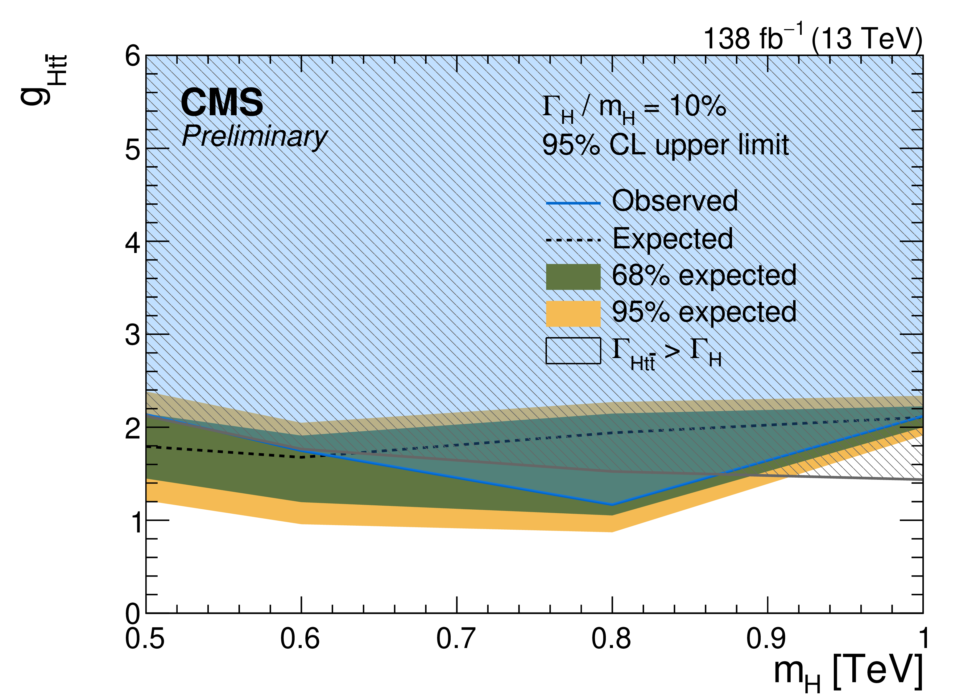
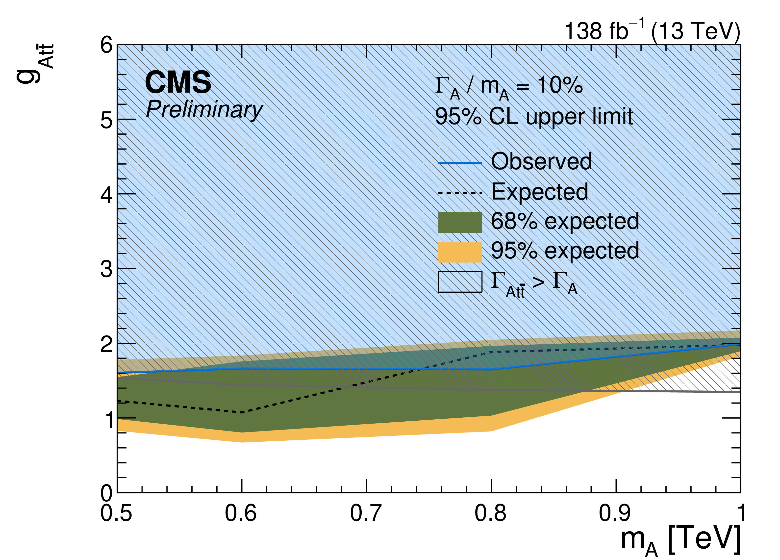
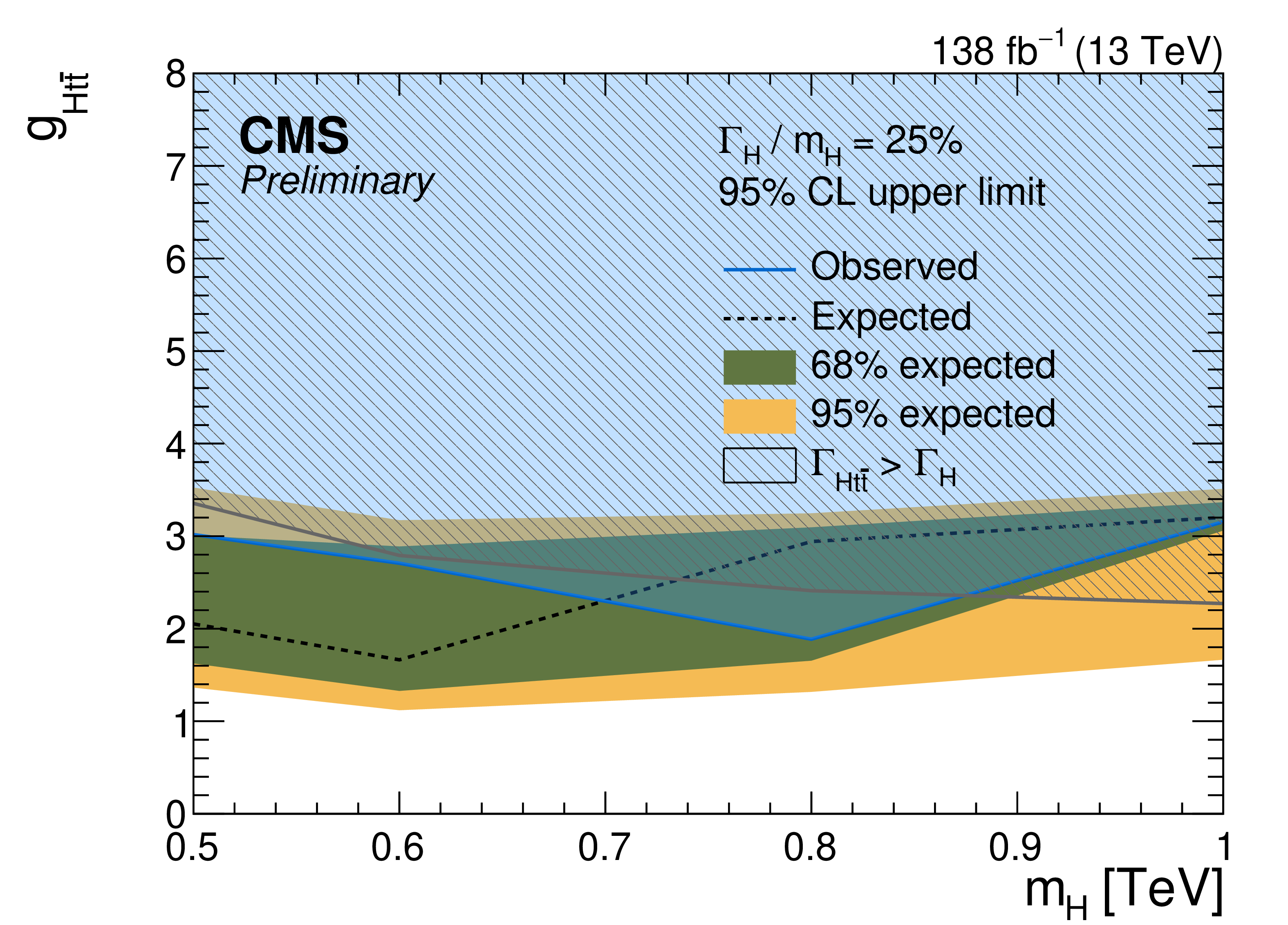
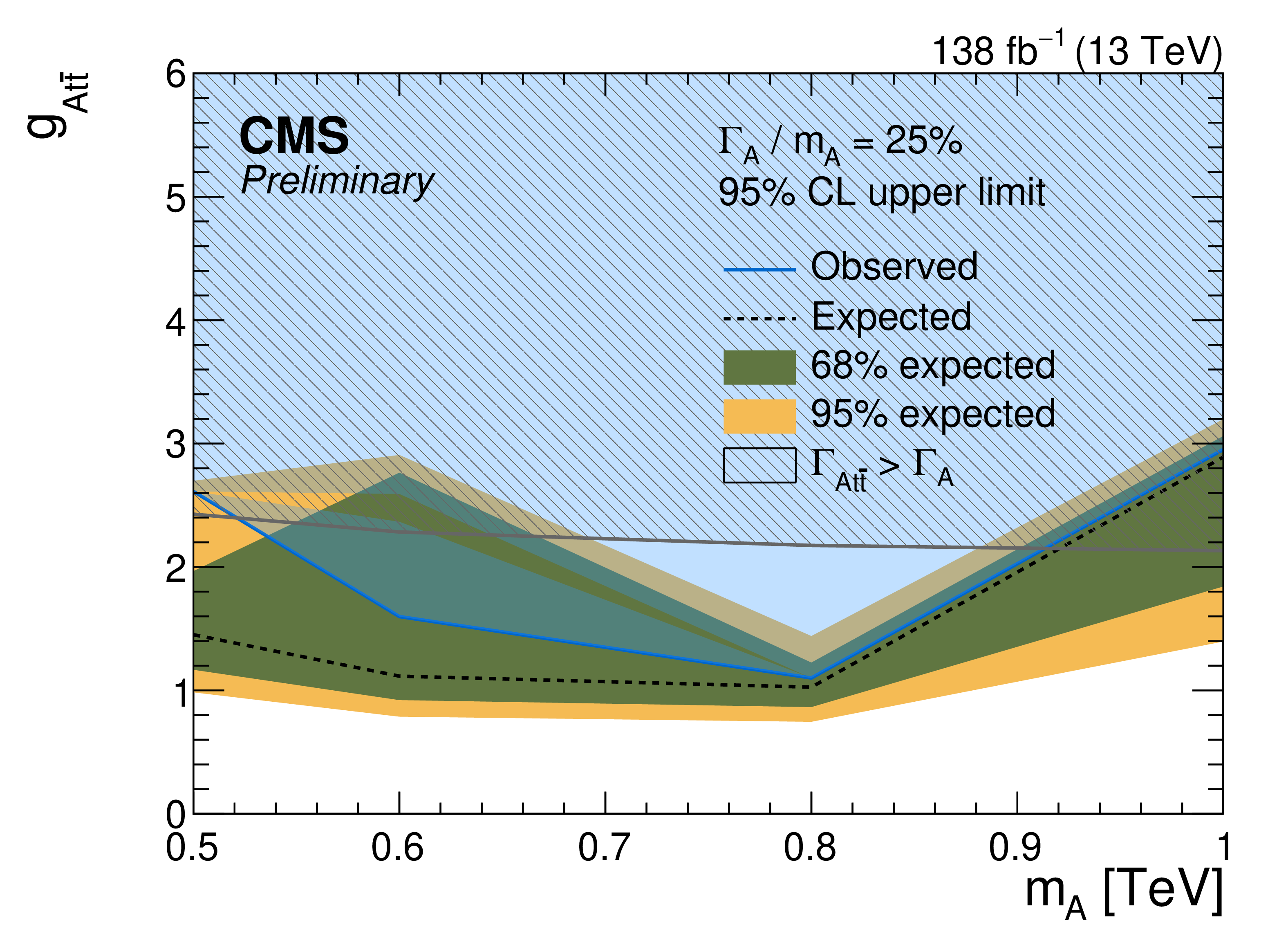
png pdf	Figure 11: Expected and observed upper limits at 95% CL on the coupling strength modifier for scalar (H, left) and pseudoscalar (A, right) heavy Higgs bosons with relative widths of 2.5% (upper), 10% (centre) and 25% (lower), respectively. The solid blue shaded area denotes the parameter space excluded by this search. The non-continuous shape of the excluded region, observed for the 25% width pseudoscalar signals with masses below 0.8 TeV, arises from the behavior of the $\text{CL}_\text{s}$ scan and reflects fluctuations in the limit calculation. The gray hatched area indicates the unphysical parameter space where the partial width $\Gamma_{\Phi{\mathrm{t}\overline{\mathrm{t}}} }$ exceeds the total width $\Gamma_{\Phi}$ .
png pdf	Figure 11-a: Expected and observed upper limits at 95% CL on the coupling strength modifier for scalar (H, left) and pseudoscalar (A, right) heavy Higgs bosons with relative widths of 2.5% (upper), 10% (centre) and 25% (lower), respectively. The solid blue shaded area denotes the parameter space excluded by this search. The non-continuous shape of the excluded region, observed for the 25% width pseudoscalar signals with masses below 0.8 TeV, arises from the behavior of the $\text{CL}_\text{s}$ scan and reflects fluctuations in the limit calculation. The gray hatched area indicates the unphysical parameter space where the partial width $\Gamma_{\Phi{\mathrm{t}\overline{\mathrm{t}}} }$ exceeds the total width $\Gamma_{\Phi}$ .
png pdf	Figure 11-b: Expected and observed upper limits at 95% CL on the coupling strength modifier for scalar (H, left) and pseudoscalar (A, right) heavy Higgs bosons with relative widths of 2.5% (upper), 10% (centre) and 25% (lower), respectively. The solid blue shaded area denotes the parameter space excluded by this search. The non-continuous shape of the excluded region, observed for the 25% width pseudoscalar signals with masses below 0.8 TeV, arises from the behavior of the $\text{CL}_\text{s}$ scan and reflects fluctuations in the limit calculation. The gray hatched area indicates the unphysical parameter space where the partial width $\Gamma_{\Phi{\mathrm{t}\overline{\mathrm{t}}} }$ exceeds the total width $\Gamma_{\Phi}$ .
png pdf	Figure 11-c: Expected and observed upper limits at 95% CL on the coupling strength modifier for scalar (H, left) and pseudoscalar (A, right) heavy Higgs bosons with relative widths of 2.5% (upper), 10% (centre) and 25% (lower), respectively. The solid blue shaded area denotes the parameter space excluded by this search. The non-continuous shape of the excluded region, observed for the 25% width pseudoscalar signals with masses below 0.8 TeV, arises from the behavior of the $\text{CL}_\text{s}$ scan and reflects fluctuations in the limit calculation. The gray hatched area indicates the unphysical parameter space where the partial width $\Gamma_{\Phi{\mathrm{t}\overline{\mathrm{t}}} }$ exceeds the total width $\Gamma_{\Phi}$ .
png pdf	Figure 11-d: Expected and observed upper limits at 95% CL on the coupling strength modifier for scalar (H, left) and pseudoscalar (A, right) heavy Higgs bosons with relative widths of 2.5% (upper), 10% (centre) and 25% (lower), respectively. The solid blue shaded area denotes the parameter space excluded by this search. The non-continuous shape of the excluded region, observed for the 25% width pseudoscalar signals with masses below 0.8 TeV, arises from the behavior of the $\text{CL}_\text{s}$ scan and reflects fluctuations in the limit calculation. The gray hatched area indicates the unphysical parameter space where the partial width $\Gamma_{\Phi{\mathrm{t}\overline{\mathrm{t}}} }$ exceeds the total width $\Gamma_{\Phi}$ .
png pdf	Figure 11-e: Expected and observed upper limits at 95% CL on the coupling strength modifier for scalar (H, left) and pseudoscalar (A, right) heavy Higgs bosons with relative widths of 2.5% (upper), 10% (centre) and 25% (lower), respectively. The solid blue shaded area denotes the parameter space excluded by this search. The non-continuous shape of the excluded region, observed for the 25% width pseudoscalar signals with masses below 0.8 TeV, arises from the behavior of the $\text{CL}_\text{s}$ scan and reflects fluctuations in the limit calculation. The gray hatched area indicates the unphysical parameter space where the partial width $\Gamma_{\Phi{\mathrm{t}\overline{\mathrm{t}}} }$ exceeds the total width $\Gamma_{\Phi}$ .
png pdf	Figure 11-f: Expected and observed upper limits at 95% CL on the coupling strength modifier for scalar (H, left) and pseudoscalar (A, right) heavy Higgs bosons with relative widths of 2.5% (upper), 10% (centre) and 25% (lower), respectively. The solid blue shaded area denotes the parameter space excluded by this search. The non-continuous shape of the excluded region, observed for the 25% width pseudoscalar signals with masses below 0.8 TeV, arises from the behavior of the $\text{CL}_\text{s}$ scan and reflects fluctuations in the limit calculation. The gray hatched area indicates the unphysical parameter space where the partial width $\Gamma_{\Phi{\mathrm{t}\overline{\mathrm{t}}} }$ exceeds the total width $\Gamma_{\Phi}$ .

Tables
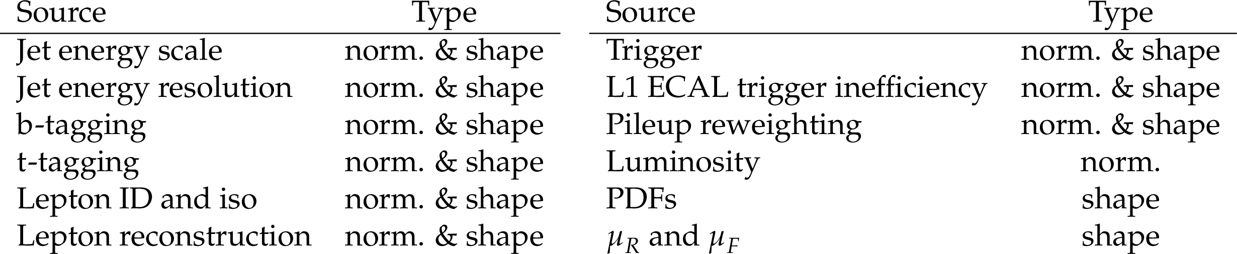
png pdf	Table 1: Sources of systematic uncertainties considered in this analysis affecting the $m_{{\mathrm{t}\overline{\mathrm{t}}} }$ distributions.

Summary

A search for new particles decaying to

$\mathrm{t} \overline{\mathrm{t}}$ in the lepton+jets channel has been presented. The analysis uses 138 fb

$^{-1}$ of data collected during 2016-2018 by the CMS experiment at a centre-of-mass energy of 13 TeV. The analysis performs a model-independent search and is sensitive both to the resolved and the boosted regimes. Upper limits at 95% confidence level are placed for different benchmark models. Heavy Z' bosons in the leptophobic topcolor model with relative widths of 1%, 10%, and 30% are excluded for mass ranges of 0.4-4.3, 0.4-5.3, and 0.4-6.7 TeV, respectively. Additionally, Kaluza-Klein gluon in the Randall-Sundrum model and dark matter mediators are excluded for masses between 0.5-4.7 TeV and 1-3.2 TeV, respectively. Limits on the coupling strength modifier are set for scalar and pseudoscalar heavy Higgs bosons in the 2HDM for 2.5%, 10%, and 25% relative widths in the mass range 0.5-1 TeV.

References
1	J. L. Rosner	Prominent decay modes of a leptophobic ${Z}^\prime$	PLB 387 (1996) 113	hep-ph/9607207
2	K. R. Lynch, S. Mrenna, M. Narain, and E. H. Simmons	Finding ${Z}^\prime$ bosons coupled preferentially to the third family at CERN LEP and the Fermilab Tevatron	PRD 63 (2001) 035006	hep-ph/0007286
3	M. Carena, A. Daleo, B. A. Dobrescu, and T. M. P. Tait	Z $^\prime$ gauge bosons at the Fermilab Tevatron	PRD 70 (2004) 093009	hep-ph/0408098
4	C. T. Hill	Topcolor: top quark condensation in a gauge extension of the standard model	PLB 266 (1991) 419
5	R. M. Harris and S. Jain	Cross sections for leptophobic topcolor ${Z}^\prime$ decaying to top-antitop	EPJC 72 (2012) 2072	hep-ph/1112.4928
6	C. T. Hill and S. J. Parke	Top quark production: Sensitivity to new physics	PRD 49 (1994) 4454	hep-ph/9312324
7	C. T. Hill	Topcolor assisted technicolor	PLB 345 (1995) 483	hep-ph/9411426
8	P. H. Frampton and S. L. Glashow	Chiral color: An alternative to the standard model	PLB 190 (1987) 157
9	D. Choudhury, R. M. Godbole, R. K. Singh, and K. Wagh	Top production at the Tevatron/LHC and nonstandard, strongly interacting spin one particles	PLB 657 (2007) 69	0810.3635
10	D. Dicus, A. Stange, and S. Willenbrock	Higgs decay to top quarks at hadron colliders	PLB 333 (1994) 126	hep-ph/9404359
11	K. Agashe et al.	CERN LHC signals from warped extra dimensions	PRD 77 (2008) 015003	hep-ph/0612015
12	H. Davoudiasl, J. L. Hewett, and T. G. Rizzo	Phenomenology of the Randall-Sundrum Gauge Hierarchy Model	PRL 84 (2000) 2080	hep-ph/9909255
13	L. Randall and R. Sundrum	A Large mass hierarchy from a small extra dimension	PRL 83 (1999) 3370	hep-ph/9905221
14	ATLAS Collaboration	Search for $t\overline{t}$ resonances in fully hadronic final states in $pp$ collisions at $\sqrt{s} =$ 13 TeV with the ATLAS detector	JHEP 10 (2020) 061	2005.05138
15	CMS Collaboration	Search for resonant ${\mathrm{t}\overline{\mathrm{t}}}$ production in proton-proton collisions at $\sqrt{s} =$ 13 TeV	JHEP 19 (2019) 031	1810.05905
16	CMS Collaboration	Search for heavy pseudoscalar and scalar bosons decaying to top quark pairs in proton-proton collisions at $\sqrt{s}=$ 13 TeV	CMS Physics Analysis Summary, 2025 CMS-PAS-HIG-22-013	CMS-PAS-HIG-22-013
17	CMS Collaboration	Observation of a pseudoscalar excess at the top quark pair production threshold	Submitted to Reports on Progress in Physics	CMS-TOP-24-007 2503.22382
18	V. D. Barger, W. Keung, and E. Ma	A Gauge Model With Light $W$ and $Z$ Bosons	PRD 22 (1980) 727
19	B. Bellazzini, C. Csáki, and J. Serra	Composite Higgses	EPJC 74 (2014) 2766	1401.2457
20	R. Contino, D. Marzocca, D. Pappadopulo, and R. Rattazzi	On the effect of resonances in composite Higgs phenomenology	JHEP 10 (2011) 081	1109.1570
21	A. Albert et al.	Recommendations of the LHC Dark Matter Working Group: Comparing LHC searches for dark matter mediators in visible and invisible decay channels and calculations of the thermal relic density	Phys. Dark Univ. 26 (2019) 100377	1703.05703
22	R. Bonciani et al.	Electroweak top-quark pair production at the LHC with $Z'$ bosons to NLO QCD in POWHEG	JHEP 02 (2016) 141	1511.08185
23	T. D. Lee	A Theory of Spontaneous T Violation	PRD 8 (1973) 1226
24	G. C. Branco et al.	Theory and phenomenology of two-Higgs-doublet models	Phys. Rept. 516 (2012) 1	1106.0034
25	H. E. Haber and O. Stral	New LHC benchmarks for the $\mathcal{CP}$ -conserving two-Higgs-doublet model	EPJC 75 (2015) 491	1507.04281
26	F. Kling, J. M. No, and S. Su	Anatomy of exotic Higgs decays in 2HDM	JHEP 09 (2016) 093	1604.01406
27	CMS Collaboration	The CMS experiment at the CERN LHC	JINST 3 (2008) S08004
28	CMS Collaboration	Electron and photon reconstruction and identification with the CMS experiment at the CERN LHC	JINST 16 (2021) P05014	CMS-EGM-17-001 2012.06888
29	CMS Collaboration	Performance of the CMS muon detector and muon reconstruction with proton--proton collisions at $\sqrt{s}=$ 13 TeV	JINST 13 (2018) P06015	CMS-MUO-16-001 1804.04528
30	CMS Collaboration	Description and performance of track and primary-vertex reconstruction with the CMS tracker	JINST 9 (2014) P10009	CMS-TRK-11-001 1405.6569
31	CMS Collaboration	Particle-flow reconstruction and global event description with the CMS detector	JINST 12 (2017) P10003	CMS-PRF-14-001 1706.04965
32	CMS Collaboration	Jet energy scale and resolution in the CMS experiment in pp collisions at 8 TeV	JINST 12 (2017) P02014	CMS-JME-13-004 1607.03663
33	CMS Collaboration	Performance of reconstruction and identification of $\tau$ leptons decaying to hadrons and $\nu_\tau$ in pp collisions at $\sqrt{s}=$ 13 TeV	JINST 13 (2018) P10005	CMS-TAU-16-003 1809.02816
34	CMS Collaboration	Performance of missing transverse momentum reconstruction in proton-proton collisions at $\sqrt{s} =$ 13 TeV using the CMS detector	JINST 14 (2019) P07004	CMS-JME-17-001 1903.06078
35	CMS Collaboration	Performance of the CMS Level-1 trigger in proton-proton collisions at $\sqrt{s} =$ 13 TeV	JINST 15 (2020) P10017	CMS-TRG-17-001 2006.10165
36	CMS Collaboration	The CMS trigger system	JINST 12 (2017) P01020	CMS-TRG-12-001 1609.02366
37	CMS Collaboration	Technical proposal for the Phase-II upgrade of the Compact Muon Solenoid	CMS Technical Proposal CERN-LHCC-2015-010, CMS-TDR-15-02, 2015 CDS
38	M. Cacciari, G. P. Salam, and G. Soyez	FastJet user manual	EPJC 72 (2012) 1896	1111.6097
39	M. Cacciari, G. P. Salam, and G. Soyez	The anti- $k_{\mathrm{T}}$ jet clustering algorithm	JHEP 04 (2008) 063	0802.1189
40	CMS Collaboration	Pileup mitigation at CMS in 13 TeV data	JINST 15 (2020) P09018	CMS-JME-18-001 2003.00503
41	D. Bertolini, P. Harris, M. Low, and N. Tran	Pileup per particle identification	JHEP 10 (2014) 059	1407.6013
42	A. J. Larkoski, S. Marzani, G. Soyez, and J. Thaler	Soft drop	JHEP 05 (2014) 146	1402.2657
43	M. Dasgupta, A. Fregoso, S. Marzani, and G. P. Salam	Towards an understanding of jet substructure	JHEP 09 (2013) 029	1307.0007
44	Y. L. Dokshitzer, G. D. Leder, S. Moretti, and B. R. Webber	Better jet clustering algorithms	JHEP 08 (1997) 001	hep-ph/9707323
45	M. Wobisch and T. Wengler	Hadronization corrections to jet cross-sections in deep inelastic scattering	in Proceedings of the Workshop on Monte Carlo Generators for HERA Physics, Hamburg, Germany, 1998 link	hep-ph/9907280
46	CMS Collaboration	Identification of heavy-flavour jets with the CMS detector in pp collisions at 13 TeV	JINST 13 (2018) P05011	CMS-BTV-16-002 1712.07158
47	E. Bols et al.	Jet Flavour Classification Using DeepJet	JINST 15 (2020) P12012	2008.10519
48	CMS Collaboration	Identification of heavy, energetic, hadronically decaying particles using machine-learning techniques	JINST 15 (2020) P06005	CMS-JME-18-002 2004.08262
49	P. Nason	A new method for combining NLO QCD with shower Monte Carlo algorithms	JHEP 11 (2004) 040	hep-ph/0409146
50	S. Frixione, P. Nason, and C. Oleari	Matching NLO QCD computations with parton shower simulations: The POWHEG method	JHEP 11 (2007) 070	0709.2092
51	S. Frixione, P. Nason, and G. Ridolfi	A positive-weight next-to-leading-order Monte Carlo for heavy flavour hadroproduction	JHEP 09 (2007) 126	0707.3088
52	S. Alioli, P. Nason, C. Oleari, and E. Re	A general framework for implementing NLO calculations in shower Monte Carlo programs: The POWHEG BOX	JHEP 06 (2010) 043	1002.2581
53	E. Re	Single-top ${\mathrm{W}}{\mathrm{t}}$ -channel production matched with parton showers using the POWHEG method	EPJC 71 (2011) 1547	1009.2450
54	M. Czakon and A. Mitov	Top++: A program for the calculation of the top-pair cross-section at hadron colliders	Comput. Phys. Commun. 185 (2014) 2930	1112.5675
55	Alwall, J. and Hoeche, S. and Krauss, F. and Lavesson, N. and Loennblad, L. and Maltoni, F. and Mangano, M. L. and Moretti, M. and Papadopoulos, C. G. and Piccinini, F. and Schumann, S. and Treccani, M. and Winter, J. and Worek, M.	Comparative study of various algorithms for the merging of parton showers and matrix elements in hadronic collisions	EPJC 53 (2008) 473	0706.2569
56	J. Alwall et al.	The automated computation of tree-level and next-to-leading order differential cross sections, and their matching to parton shower simulations	JHEP 07 (2014) 079	1405.0301
57	T. Sjöstrand et al.	An introduction to PYTHIA 8.2	Comput. Phys. Commun. 191 (2015) 159	1410.3012
58	J. M. Lindert et al.	Precise predictions for v+jets dark matter backgrounds	EPJC 77 (2017) 829	1705.04664
59	J. Gao et al.	Next-to-leading order QCD corrections to the heavy resonance production and decay into top quark pair at the LHC	PRD 82 (2010) 014020	1004.0876
60	B. Hespel, F. Maltoni, and E. Vryonidou	Signal background interference effects in heavy scalar production and decay to a top-anti-top pair	JHEP 10 (2016) 016	1606.04149
61	CMS Collaboration	Extraction and validation of a new set of CMS PYTHIA8 tunes from underlying-event measurements	EPJC 80 (2020) 4	CMS-GEN-17-001 1903.12179
62	NNPDF Collaboration	Parton distributions from high-precision collider data	EPJC 77 (2017) 663	1706.00428
63	GEANT4 Collaboration	GEANT 4 --- A simulation toolkit	NIM A 506 (2003) 250
64	CMS Collaboration	Measurement of the inelastic proton-proton cross section at $\sqrt{s}=$ 13 TeV	JHEP 07 (2018) 161	CMS-FSQ-15-005 1802.02613
65	CMS Collaboration	Measurement of the tt charge asymmetry in events with highly Lorentz-boosted top quarks in pp collisions at s=13 TeV	PLB 846 (2023) 137703	CMS-TOP-21-014 2208.02751
66	M. Carena and Z. Liu	Challenges and opportunities for heavy scalar searches in the $\mathrm{t} \overline{\mathrm{t}}$ channel at the LHC	JHEP 11 (2016) 159	1608.07282
67	A. Djouadi, J. Ellis, A. Popov, and J. Quevillon	Interference effects in $\mathrm{t} \overline{\mathrm{t}}$ production at the LHC as a window on new physics	JHEP 03 (2019) 119	1901.03417
68	F. Chollet et al.	Keras	link
69	J. Thaler and K. Van Tilburg	Identifying boosted objects with N-subjettiness	JHEP 03 (2011) 015	1011.2268
70	J. Thaler and K. Van Tilburg	Maximizing Boosted Top Identification by Minimizing N-subjettiness	JHEP 02 (2012) 093	1108.2701
71	CMS Collaboration	Search for heavy Higgs bosons decaying to a top quark pair in proton-proton collisions at $\sqrt{s} =$ 13 TeV	JHEP 04 (2020) 171	CMS-HIG-17-027 1908.01115
72	J. Butterworth et al.	PDF4LHC recommendations for LHC Run II	JPG 43 (2016) 023001	1510.03865
73	CMS Collaboration	Precision luminosity measurement in proton-proton collisions at $\sqrt{s}=$ 13 TeV in 2015 and 2016 at CMS	EPJC 81 (2021) 800	CMS-LUM-17-003 2104.01927
74	CMS Collaboration	CMS luminosity measurement for the 2017 data-taking period at $\sqrt{s}=$ 13 TeV	CMS Physics Analysis Summary, 2018 CMS-PAS-LUM-17-004	CMS-PAS-LUM-17-004
75	CMS Collaboration	CMS luminosity measurement for the 2018 data-taking period at $\sqrt{s}=$ 13 TeV	CMS Physics Analysis Summary, 2019 CMS-PAS-LUM-18-002	CMS-PAS-LUM-18-002
76	ATLAS and CMS Collaborations, and LHC Higgs Combination Group	Procedure for the LHC Higgs boson search combination in Summer 2011	CMS Note CMS-NOTE-2011-005, ATL-PHYS-PUB-2011-11, 2011
77	T. Junk	Confidence level computation for combining searches with small statistics	NIM A 434 (1999) 435	hep-ex/9902006
78	A. L. Read	Presentation of search results: The CL $_{\text{s}}$ technique	JPG 28 (2002) 2693
79	G. Cowan, K. Cranmer, E. Gross, and O. Vitells	Asymptotic formulae for likelihood-based tests of new physics	EPJC 71 (2011) 1554	1007.1727
80	CMS Collaboration	The CMS statistical analysis and combination tool: Combine	Accepted by Comput. Softw. Big Sci, 2024	CMS-CAT-23-001 2404.06614
81	W. Verkerke and D. P. Kirkby	The RooFit toolkit for data modeling	in Proc. Int. Conf. on Computing in High Energy and Nuclear Physics (CHEP03), L. Lyons and M. Karagoz, eds., 2003	physics/0306116
82	L. Moneta et al.	The RooStats project	in Proc. 13th Int. Workshop on Advanced Computing and Analysis Techniques in Physics Research, T. Speer et al., eds., 2010 link	1009.1003