

Compact Muon Solenoid
LHC, CERN
| CMS-PAS-TOP-22-010 | ||
| Search for new Higgs bosons through same-sign top quark pair production in association with a jet in proton-proton collisions at $ \sqrt{s}= $ 13 TeV | ||
| CMS Collaboration | ||
| 21 August 2023 | ||
| Abstract: A search is presented for new Higgs bosons in proton-proton collision events in which a same-sign top quark pair is produced in association with a jet, via the $ \mathrm{cg}\rightarrow\mathrm{tH/A}\rightarrow\mathrm{tt\overline{c}} $ and $ \mathrm{cg}\rightarrow\mathrm{tH/A}\rightarrow\mathrm{tt\overline{u}} $ processes. Here H and A represent the extra scalar and pseudoscalar boson, respectively, of the second Higgs doublet in the generalized two-Higgs-doublet model (g2HDM). The search is based on proton-proton collision data collected at a center-of-mass energy of 13 TeV with the CMS detector at the LHC, corresponding to an integrated luminosity of 138 fb$ ^{-1} $. Final states with a same-sign lepton pair in association with a charm or up quark are considered. New Higgs bosons in the 200-1000 GeV mass range are targeted in the search, for scenarios in which either H or A appear alone, or in which they coexist and interfere. No significant excess above the standard model prediction is observed, and exclusion limits are derived in the context of the g2HDM. Depending on the g2HDM signal assumptions, the mass of a new Higgs boson below 1 TeV and corresponding new Yukawa couplings between 0.4 and 1 are excluded at the 95% confidence level. | ||
|
Links:
CDS record (PDF) ;
Physics Briefing ;
CADI line (restricted) ;
These preliminary results are superseded in this paper, PLB 850 (2024) 138478. The superseded preliminary plots can be found here. |
||
| Figures | |
png pdf |
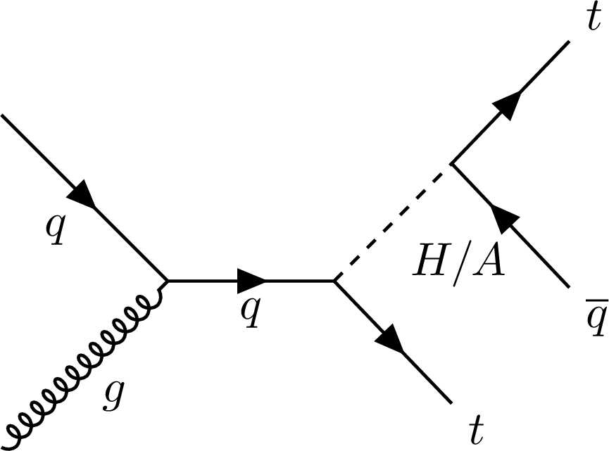
Figure 1:
Representative Feynman diagram for $ \mathrm{t}\mathrm{t}\overline{\mathrm{q}} $ ($ \mathrm{q} $ = u,c) production through a new scalar (H) or pseudoscalar (A) Higgs boson. |
png pdf |
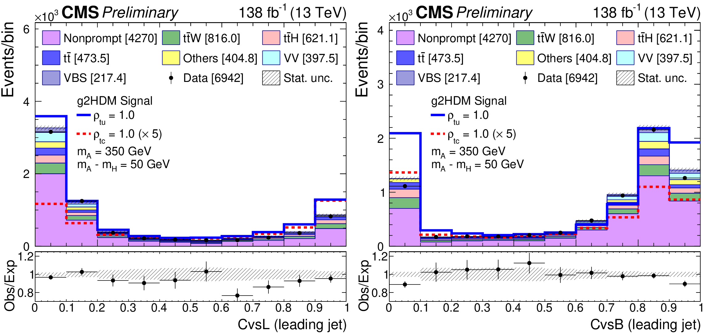
Figure 2:
The pre-fit CvsL (left panel) and CvsB (right panel) distributions for the selected highest-$ p_{\mathrm{T}} $ jet using the full Run 2 data. The predictions for $ m_{\mathrm{A}} = $ 350 GeV with A--H interference assuming $ m_{\mathrm{A}} -m_{\mathrm{H}}= $ 50 GeV for $ \rho_{\mathrm{t}\mathrm{u}}= $ 1.0 (solid blue line) and $ \rho_{\mathrm{t}\mathrm{c}}= $ 1.0 (dashed red line) are also displayed. The number in square brackets represents the yields for each sample. The error bars on the points and the hatched bands represent the statistical uncertainties in the data and in the background predictions, respectively. Beneath each plot is shown the ratio of data to predictions. The error bars in the ratio plots consider statistical uncertainties in the data and in the background predictions. |
png pdf |
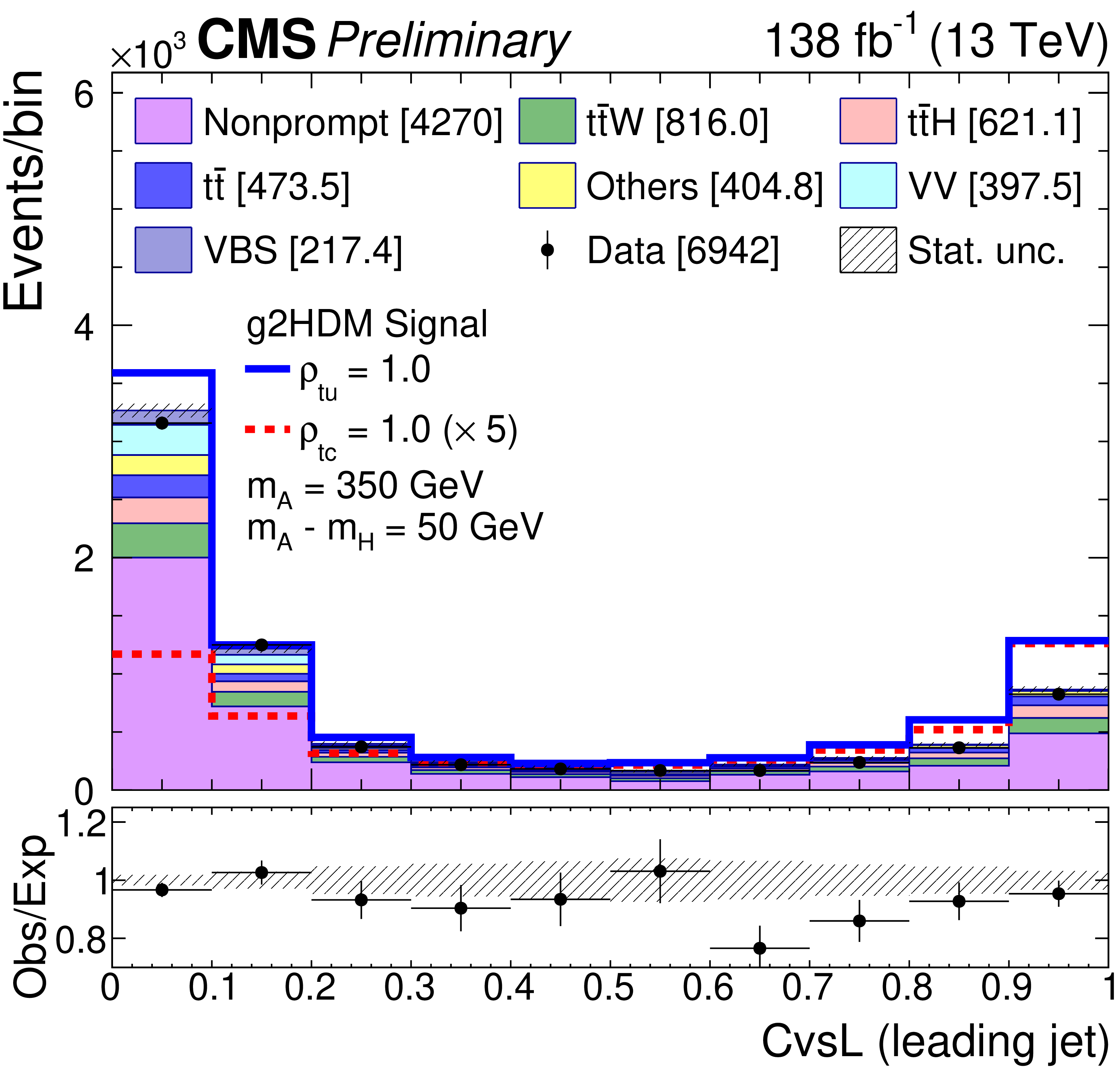
Figure 2-a:
The pre-fit CvsL (left panel) and CvsB (right panel) distributions for the selected highest-$ p_{\mathrm{T}} $ jet using the full Run 2 data. The predictions for $ m_{\mathrm{A}} = $ 350 GeV with A--H interference assuming $ m_{\mathrm{A}} -m_{\mathrm{H}}= $ 50 GeV for $ \rho_{\mathrm{t}\mathrm{u}}= $ 1.0 (solid blue line) and $ \rho_{\mathrm{t}\mathrm{c}}= $ 1.0 (dashed red line) are also displayed. The number in square brackets represents the yields for each sample. The error bars on the points and the hatched bands represent the statistical uncertainties in the data and in the background predictions, respectively. Beneath each plot is shown the ratio of data to predictions. The error bars in the ratio plots consider statistical uncertainties in the data and in the background predictions. |
png pdf |
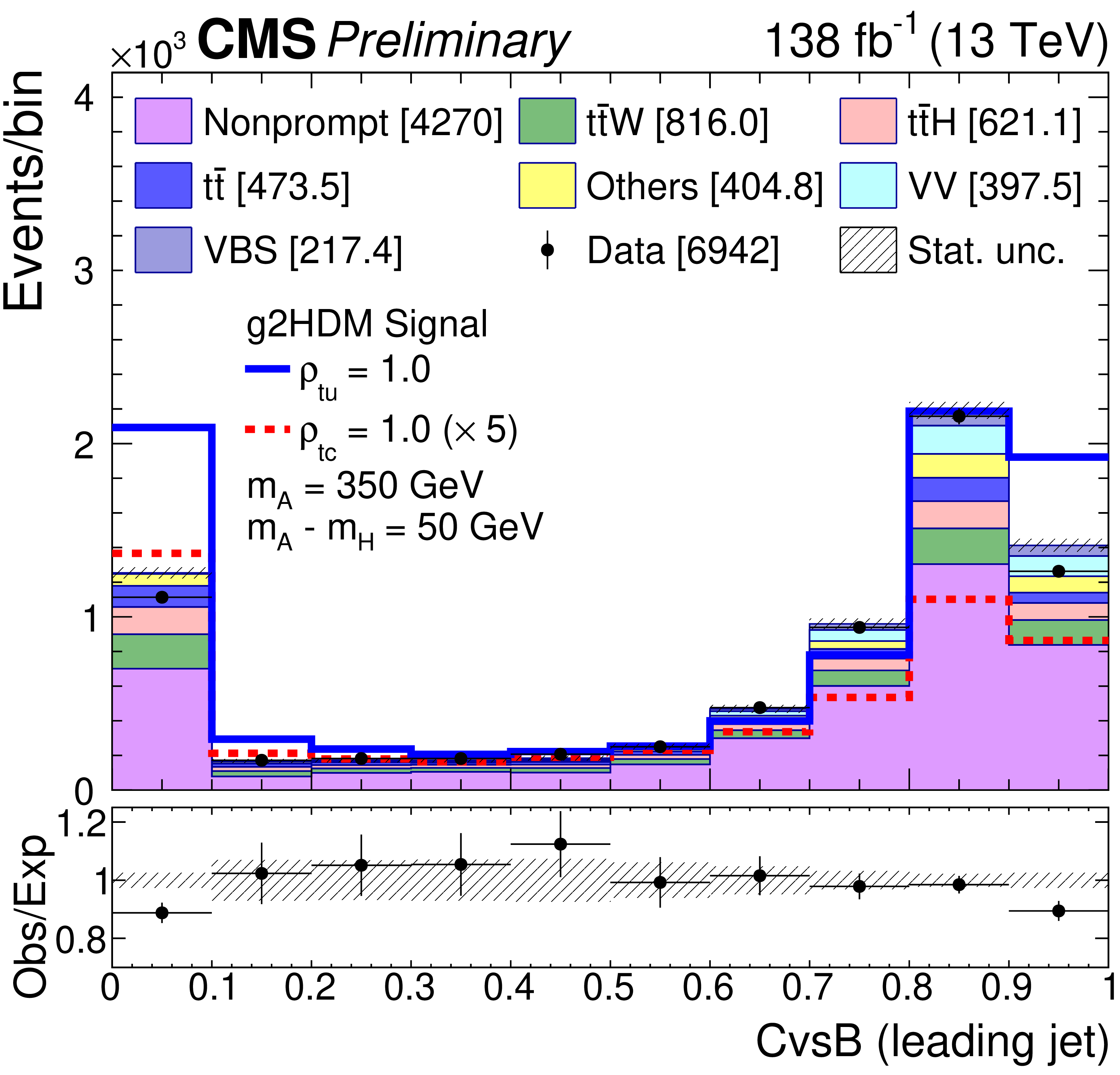
Figure 2-b:
The pre-fit CvsL (left panel) and CvsB (right panel) distributions for the selected highest-$ p_{\mathrm{T}} $ jet using the full Run 2 data. The predictions for $ m_{\mathrm{A}} = $ 350 GeV with A--H interference assuming $ m_{\mathrm{A}} -m_{\mathrm{H}}= $ 50 GeV for $ \rho_{\mathrm{t}\mathrm{u}}= $ 1.0 (solid blue line) and $ \rho_{\mathrm{t}\mathrm{c}}= $ 1.0 (dashed red line) are also displayed. The number in square brackets represents the yields for each sample. The error bars on the points and the hatched bands represent the statistical uncertainties in the data and in the background predictions, respectively. Beneath each plot is shown the ratio of data to predictions. The error bars in the ratio plots consider statistical uncertainties in the data and in the background predictions. |
png pdf |
Figure 3:
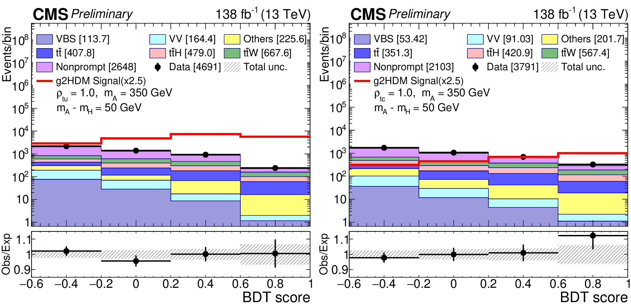
Post-fit distributions of the BDT discriminants combining the categories $ \mathrm{e}^\pm\mathrm{e}^\pm $, $ \mu^\pm\mu^\pm $, and $ \mathrm{e}^\pm\mu^\pm $ using the full Run 2 data set, for $ m_{\mathrm{A}}= $ 350 GeV with $ \rho_{\mathrm{t}\mathrm{u}}= $ 1.0 (left panel), and $ \rho_{\mathrm{t}\mathrm{c}}= $ 1.0 (right panel) with A--H interference. The number in square brackets represents the yields for each sample. The error bars on the points represent the statistical uncertainties in the data, and the hatched bands represent the total uncertainty in the background predictions. Beneath each plot the ratio of data to predictions is shown. The error bars in the ratio plots consider statistical uncertainties in the data and the total uncertainty in the background predictions. |
png pdf |
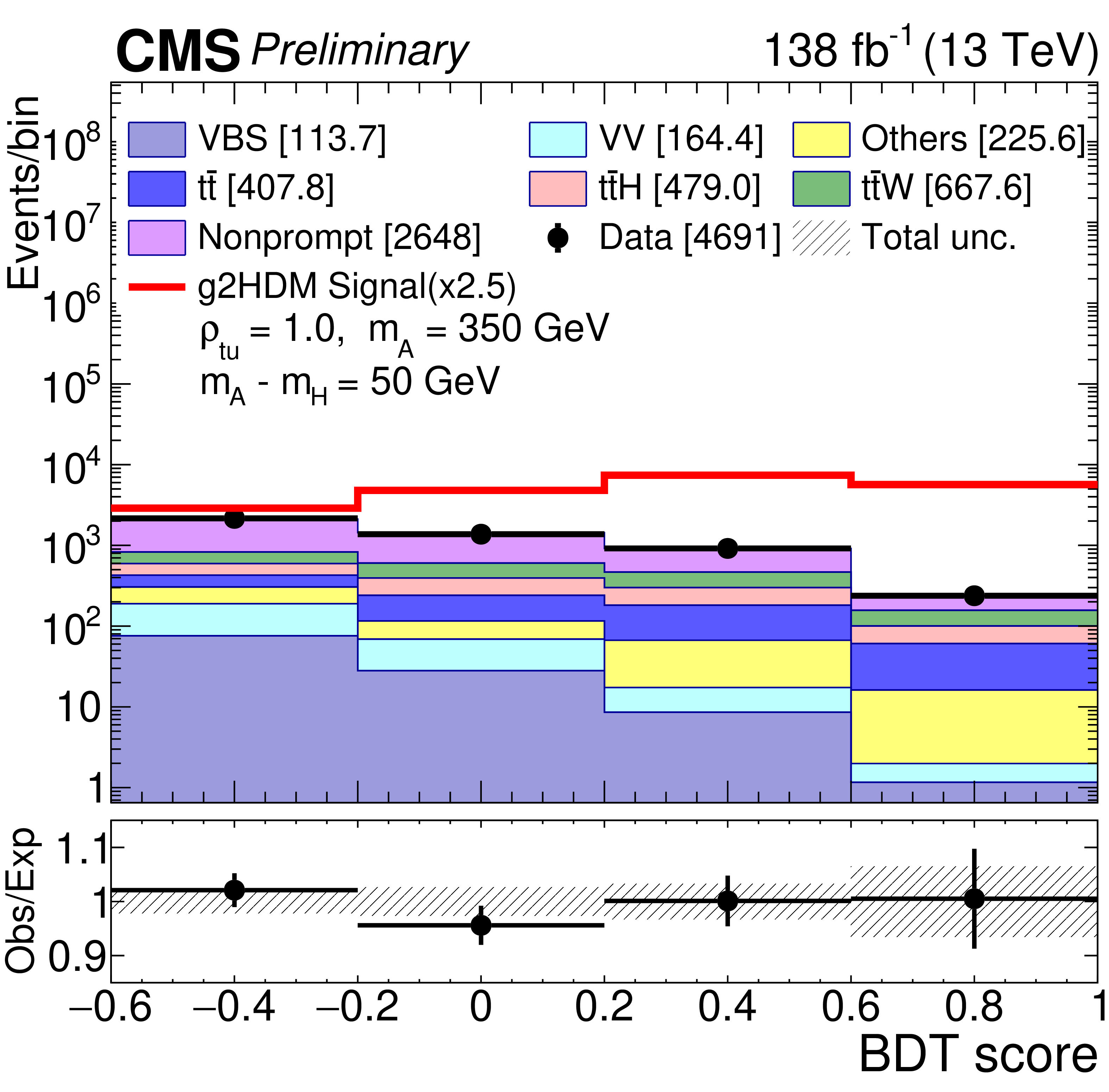
Figure 3-a:
Post-fit distributions of the BDT discriminants combining the categories $ \mathrm{e}^\pm\mathrm{e}^\pm $, $ \mu^\pm\mu^\pm $, and $ \mathrm{e}^\pm\mu^\pm $ using the full Run 2 data set, for $ m_{\mathrm{A}}= $ 350 GeV with $ \rho_{\mathrm{t}\mathrm{u}}= $ 1.0 (left panel), and $ \rho_{\mathrm{t}\mathrm{c}}= $ 1.0 (right panel) with A--H interference. The number in square brackets represents the yields for each sample. The error bars on the points represent the statistical uncertainties in the data, and the hatched bands represent the total uncertainty in the background predictions. Beneath each plot the ratio of data to predictions is shown. The error bars in the ratio plots consider statistical uncertainties in the data and the total uncertainty in the background predictions. |
png pdf |
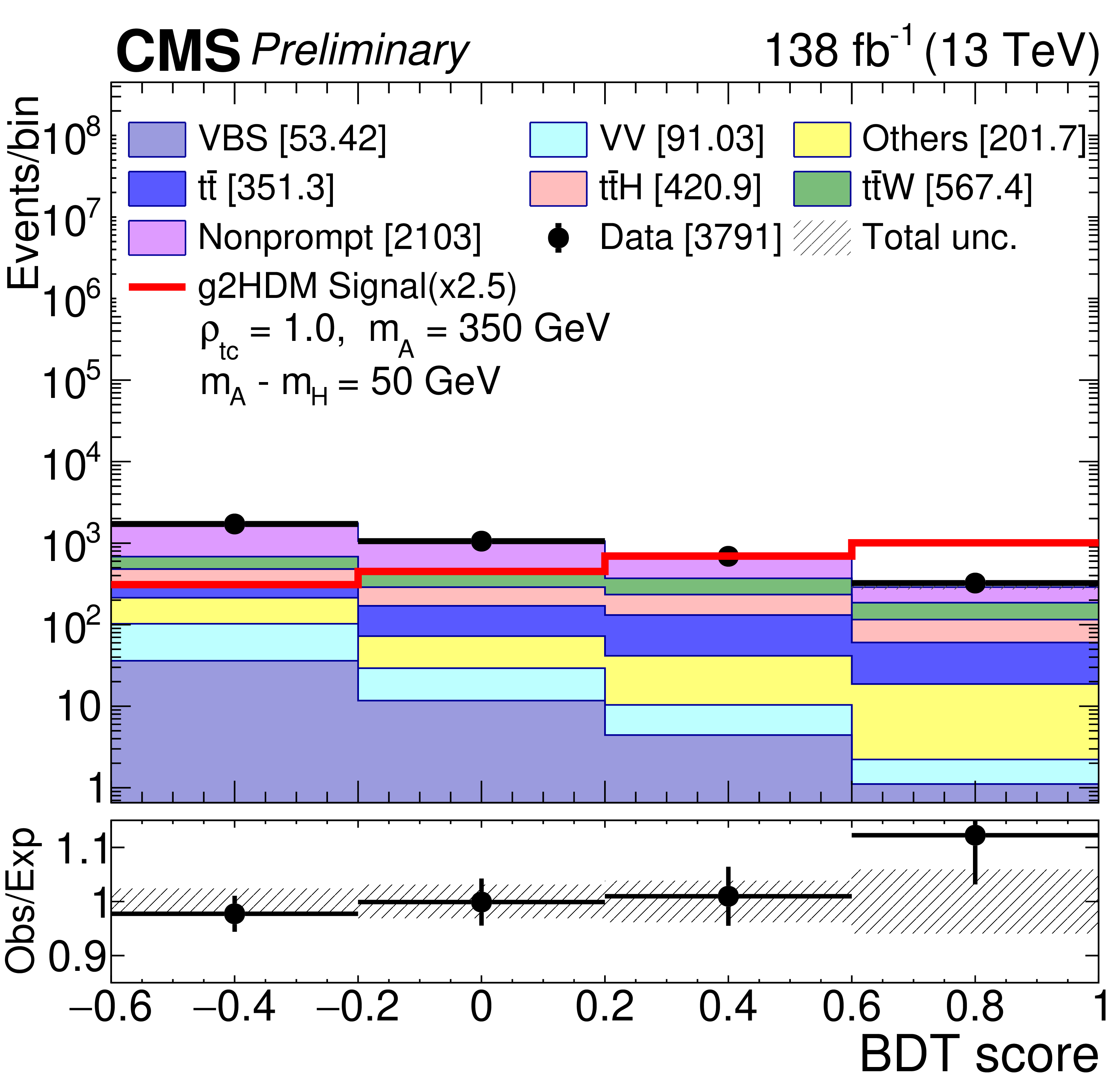
Figure 3-b:
Post-fit distributions of the BDT discriminants combining the categories $ \mathrm{e}^\pm\mathrm{e}^\pm $, $ \mu^\pm\mu^\pm $, and $ \mathrm{e}^\pm\mu^\pm $ using the full Run 2 data set, for $ m_{\mathrm{A}}= $ 350 GeV with $ \rho_{\mathrm{t}\mathrm{u}}= $ 1.0 (left panel), and $ \rho_{\mathrm{t}\mathrm{c}}= $ 1.0 (right panel) with A--H interference. The number in square brackets represents the yields for each sample. The error bars on the points represent the statistical uncertainties in the data, and the hatched bands represent the total uncertainty in the background predictions. Beneath each plot the ratio of data to predictions is shown. The error bars in the ratio plots consider statistical uncertainties in the data and the total uncertainty in the background predictions. |
png pdf |
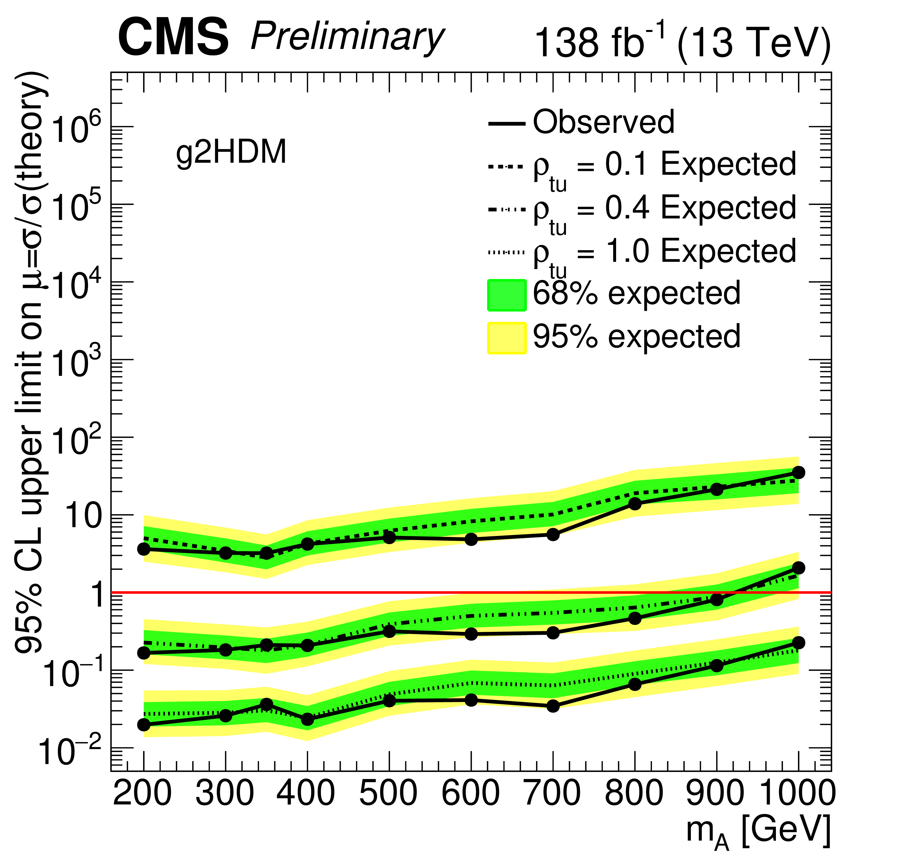
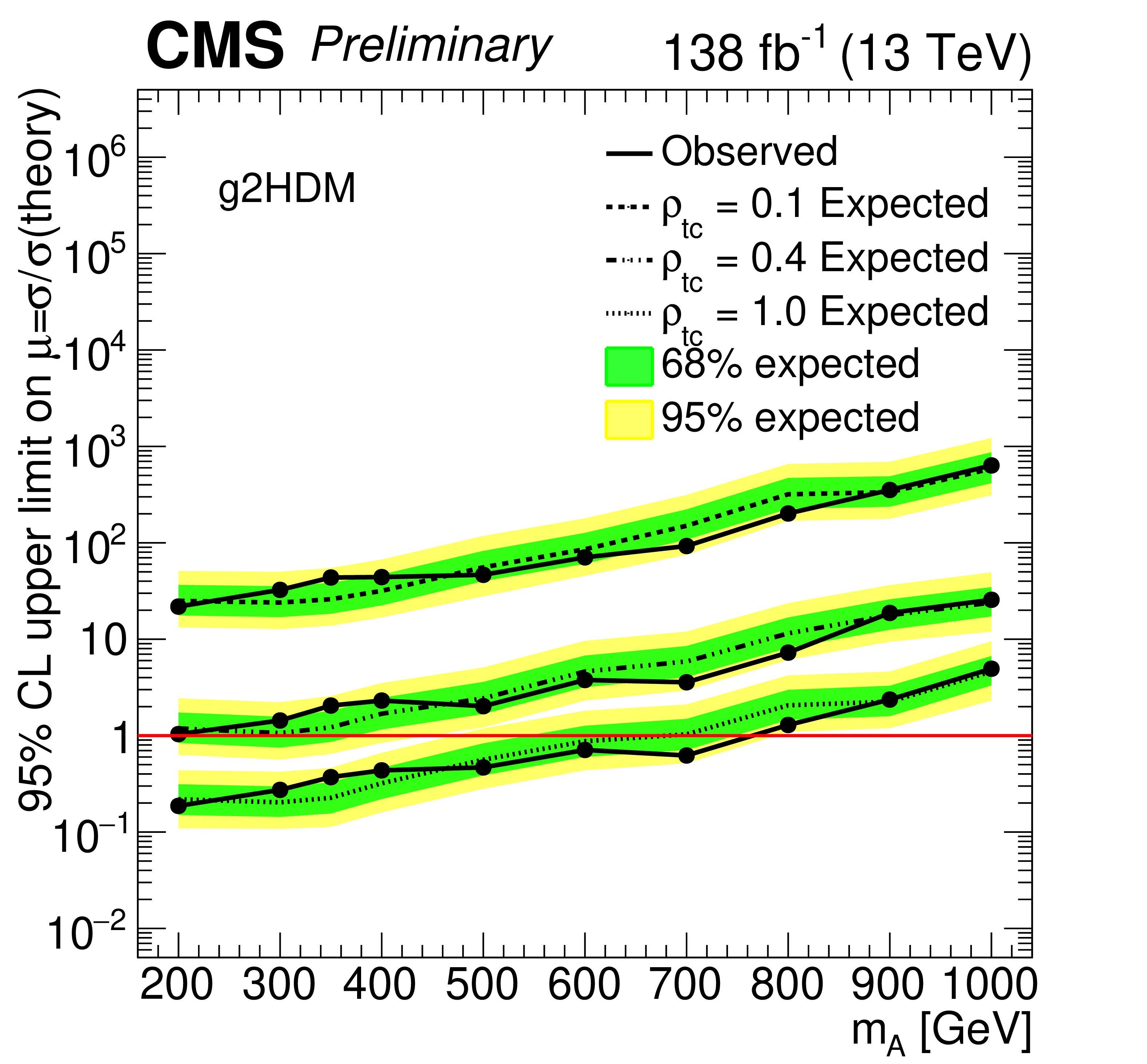
Figure 4:
Observed and expected 95% CL upper limits on the signal strength as a function of $ m_{\mathrm{A}} $ for the g2HDM signal model using different coupling assumptions: $ \rho_{\mathrm{t}\mathrm{u}} $ = 0.1, 0.4, 1.0 (left panel) and $ \rho_{\mathrm{t}\mathrm{c}} $ = 0.1, 0.4, 1.0 (right panel) without interference using the full Run 2 data set for a combination of $ \mathrm{e}^\pm\mathrm{e}^\pm $, $ \mu^\pm\mu^\pm $, and $ \mathrm{e}^\pm\mu^\pm $ categories. The inner (green) band and the outer (yellow) band indicate the regions containing 68 and 95%, respectively, of the distribution of limits expected under the background-only hypothesis. |
png pdf |
Figure 4-a:
Observed and expected 95% CL upper limits on the signal strength as a function of $ m_{\mathrm{A}} $ for the g2HDM signal model using different coupling assumptions: $ \rho_{\mathrm{t}\mathrm{u}} $ = 0.1, 0.4, 1.0 (left panel) and $ \rho_{\mathrm{t}\mathrm{c}} $ = 0.1, 0.4, 1.0 (right panel) without interference using the full Run 2 data set for a combination of $ \mathrm{e}^\pm\mathrm{e}^\pm $, $ \mu^\pm\mu^\pm $, and $ \mathrm{e}^\pm\mu^\pm $ categories. The inner (green) band and the outer (yellow) band indicate the regions containing 68 and 95%, respectively, of the distribution of limits expected under the background-only hypothesis. |
png pdf |
Figure 4-b:
Observed and expected 95% CL upper limits on the signal strength as a function of $ m_{\mathrm{A}} $ for the g2HDM signal model using different coupling assumptions: $ \rho_{\mathrm{t}\mathrm{u}} $ = 0.1, 0.4, 1.0 (left panel) and $ \rho_{\mathrm{t}\mathrm{c}} $ = 0.1, 0.4, 1.0 (right panel) without interference using the full Run 2 data set for a combination of $ \mathrm{e}^\pm\mathrm{e}^\pm $, $ \mu^\pm\mu^\pm $, and $ \mathrm{e}^\pm\mu^\pm $ categories. The inner (green) band and the outer (yellow) band indicate the regions containing 68 and 95%, respectively, of the distribution of limits expected under the background-only hypothesis. |
png pdf |
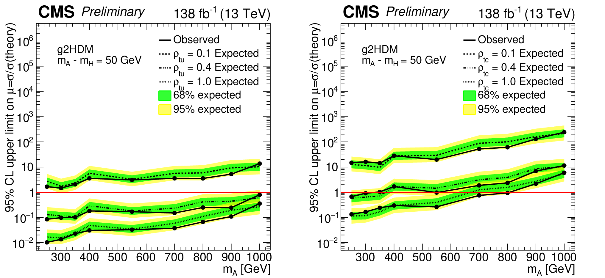
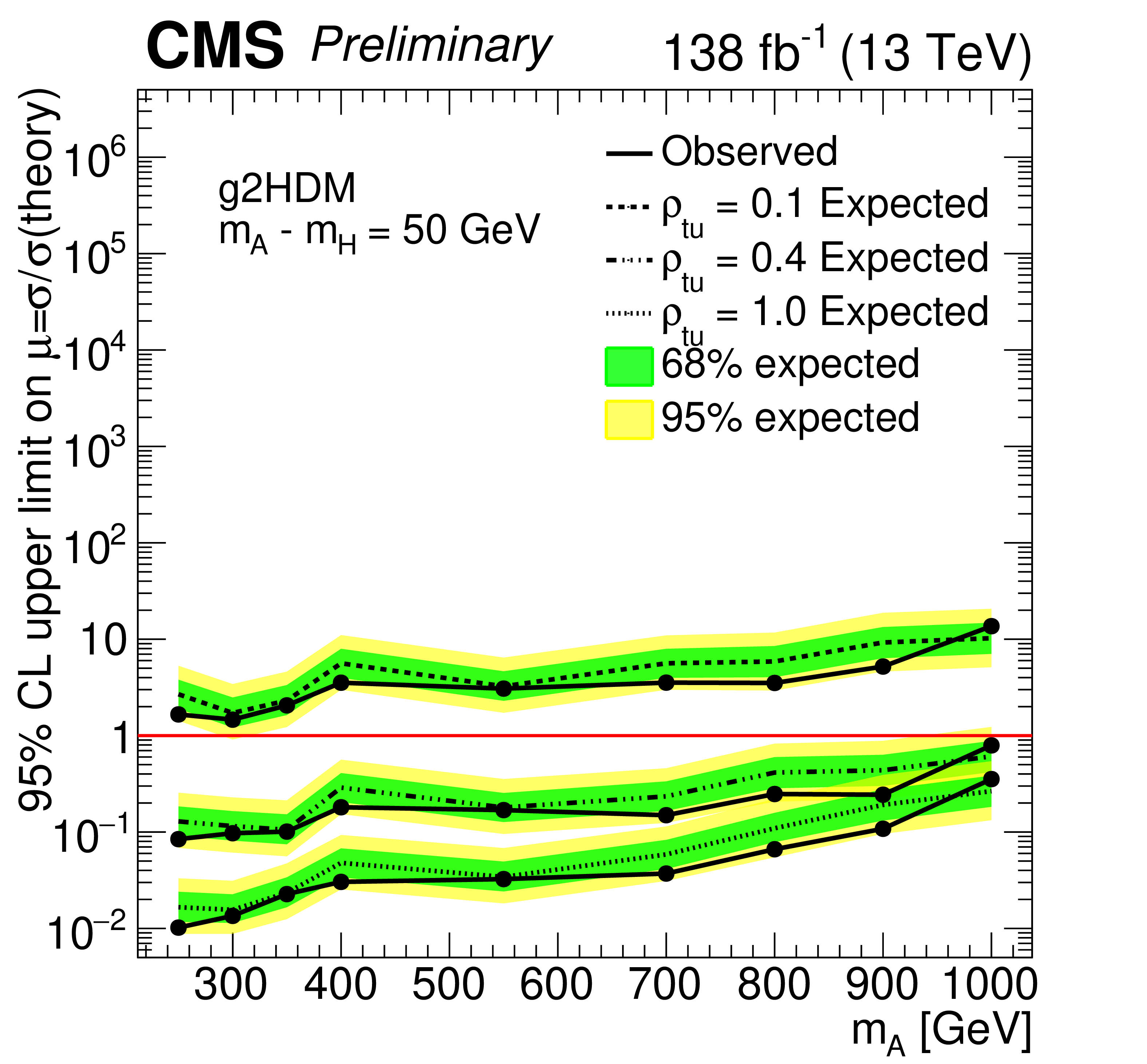
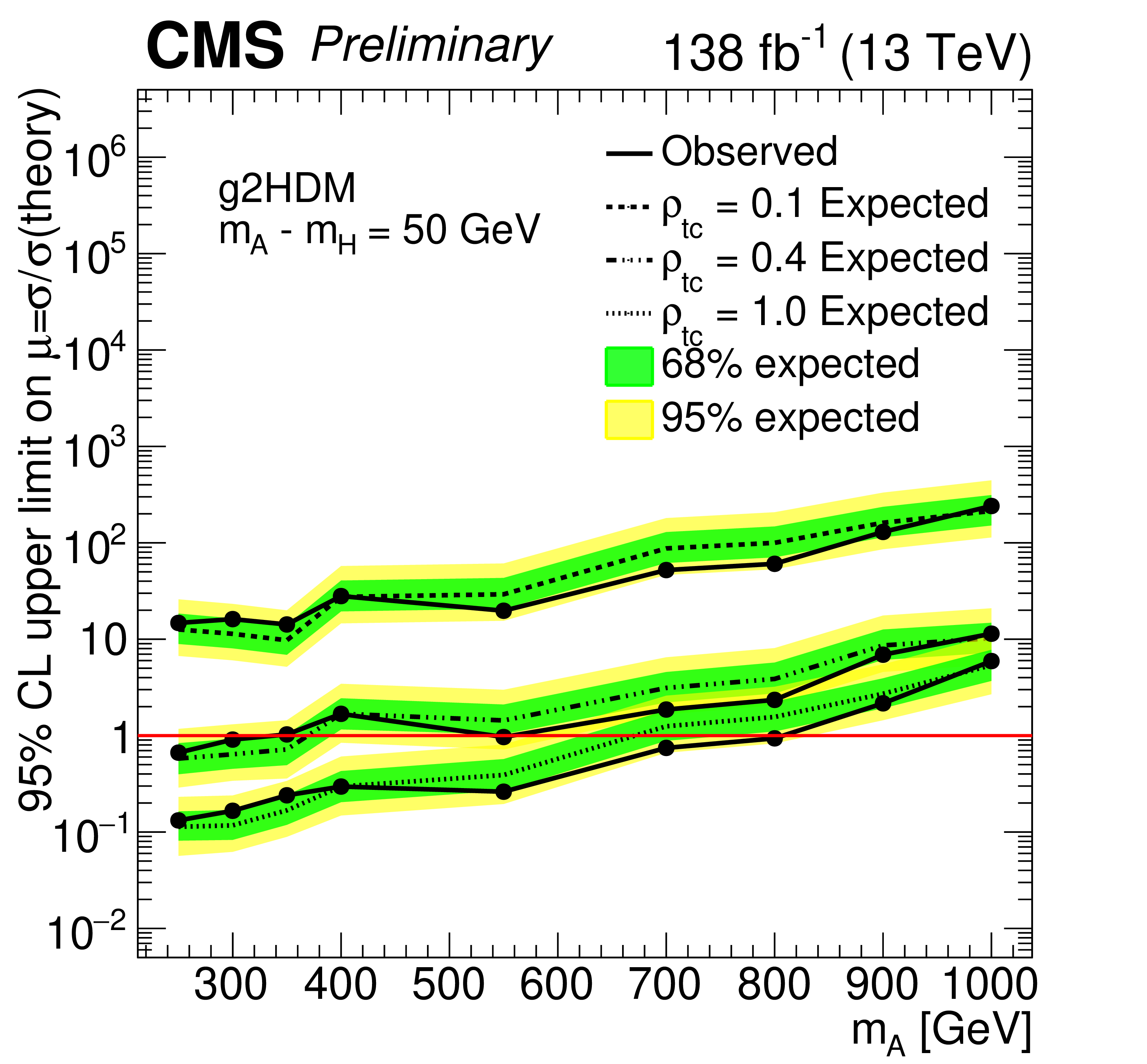
Figure 5:
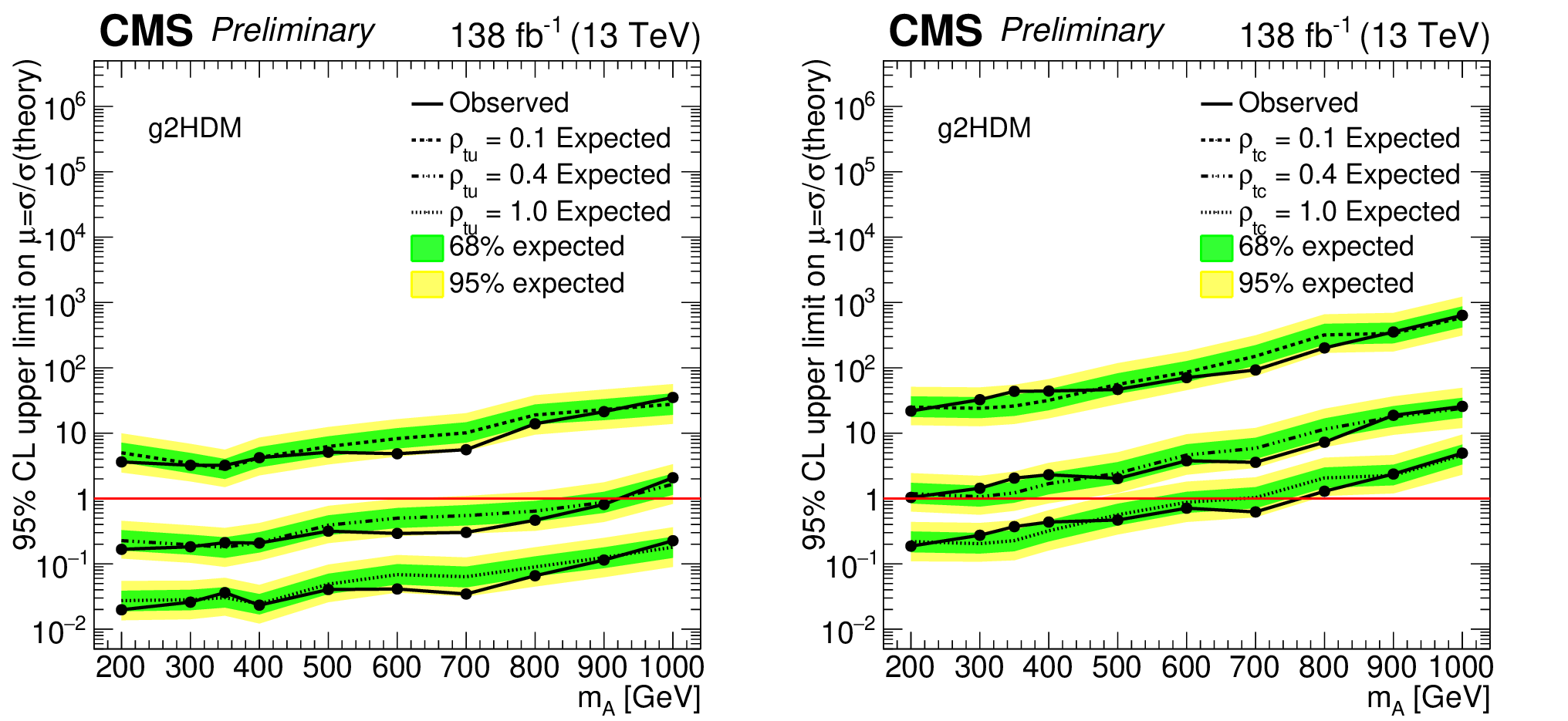
Observed and expected 95% CL upper limit on the signal strength as a function of $ m_{\mathrm{A}} $ for the g2HDM signal model using different coupling assumptions: $ \rho_{\mathrm{t}\mathrm{u}} $ = 0.1, 0.4, 1.0 (left panel) and $ \rho_{\mathrm{t}\mathrm{c}} $ = 0.1,0.4,1.0 (right panel) with A--H interference assuming $ m_{\mathrm{A}} - m_{\mathrm{H}} = $ 50 GeV, using the full Run 2 data set for the combination of $ \mathrm{e}^\pm\mathrm{e}^\pm $, $ \mu^\pm\mu^\pm $, and $ \mathrm{e}^\pm\mu^\pm $ categories. The inner (green) band and the outer (yellow) band indicate the regions containing 68 and 95%, respectively, of the distribution of limits expected under the background-only hypothesis. |
png pdf |
Figure 5-a:
Observed and expected 95% CL upper limit on the signal strength as a function of $ m_{\mathrm{A}} $ for the g2HDM signal model using different coupling assumptions: $ \rho_{\mathrm{t}\mathrm{u}} $ = 0.1, 0.4, 1.0 (left panel) and $ \rho_{\mathrm{t}\mathrm{c}} $ = 0.1,0.4,1.0 (right panel) with A--H interference assuming $ m_{\mathrm{A}} - m_{\mathrm{H}} = $ 50 GeV, using the full Run 2 data set for the combination of $ \mathrm{e}^\pm\mathrm{e}^\pm $, $ \mu^\pm\mu^\pm $, and $ \mathrm{e}^\pm\mu^\pm $ categories. The inner (green) band and the outer (yellow) band indicate the regions containing 68 and 95%, respectively, of the distribution of limits expected under the background-only hypothesis. |
png pdf |
Figure 5-b:
Observed and expected 95% CL upper limit on the signal strength as a function of $ m_{\mathrm{A}} $ for the g2HDM signal model using different coupling assumptions: $ \rho_{\mathrm{t}\mathrm{u}} $ = 0.1, 0.4, 1.0 (left panel) and $ \rho_{\mathrm{t}\mathrm{c}} $ = 0.1,0.4,1.0 (right panel) with A--H interference assuming $ m_{\mathrm{A}} - m_{\mathrm{H}} = $ 50 GeV, using the full Run 2 data set for the combination of $ \mathrm{e}^\pm\mathrm{e}^\pm $, $ \mu^\pm\mu^\pm $, and $ \mathrm{e}^\pm\mu^\pm $ categories. The inner (green) band and the outer (yellow) band indicate the regions containing 68 and 95%, respectively, of the distribution of limits expected under the background-only hypothesis. |
png pdf |
Figure 6:
Observed 95% CL upper limit on the signal strength as functions of $ m_{\mathrm{A}} $ and $ \rho_{\mathrm{t}\mathrm{u}} $ (left panel) and $ \rho_{\mathrm{t}\mathrm{c}} $ (right panel) for the g2HDM signal model without A--H interference, using the full Run 2 data set for the combination of $ \mathrm{e}^\pm\mathrm{e}^\pm $, $ \mu^\pm\mu^\pm $, and $ \mathrm{e}^\pm\mu^\pm $ categories. The color axis represents the observed upper limit on the signal strength. Expected (dashed lines) and observed (solid lines) exclusion contours are also shown. |
png pdf |
Figure 6-a:
Observed 95% CL upper limit on the signal strength as functions of $ m_{\mathrm{A}} $ and $ \rho_{\mathrm{t}\mathrm{u}} $ (left panel) and $ \rho_{\mathrm{t}\mathrm{c}} $ (right panel) for the g2HDM signal model without A--H interference, using the full Run 2 data set for the combination of $ \mathrm{e}^\pm\mathrm{e}^\pm $, $ \mu^\pm\mu^\pm $, and $ \mathrm{e}^\pm\mu^\pm $ categories. The color axis represents the observed upper limit on the signal strength. Expected (dashed lines) and observed (solid lines) exclusion contours are also shown. |
png pdf |
Figure 6-b:
Observed 95% CL upper limit on the signal strength as functions of $ m_{\mathrm{A}} $ and $ \rho_{\mathrm{t}\mathrm{u}} $ (left panel) and $ \rho_{\mathrm{t}\mathrm{c}} $ (right panel) for the g2HDM signal model without A--H interference, using the full Run 2 data set for the combination of $ \mathrm{e}^\pm\mathrm{e}^\pm $, $ \mu^\pm\mu^\pm $, and $ \mathrm{e}^\pm\mu^\pm $ categories. The color axis represents the observed upper limit on the signal strength. Expected (dashed lines) and observed (solid lines) exclusion contours are also shown. |
png pdf |
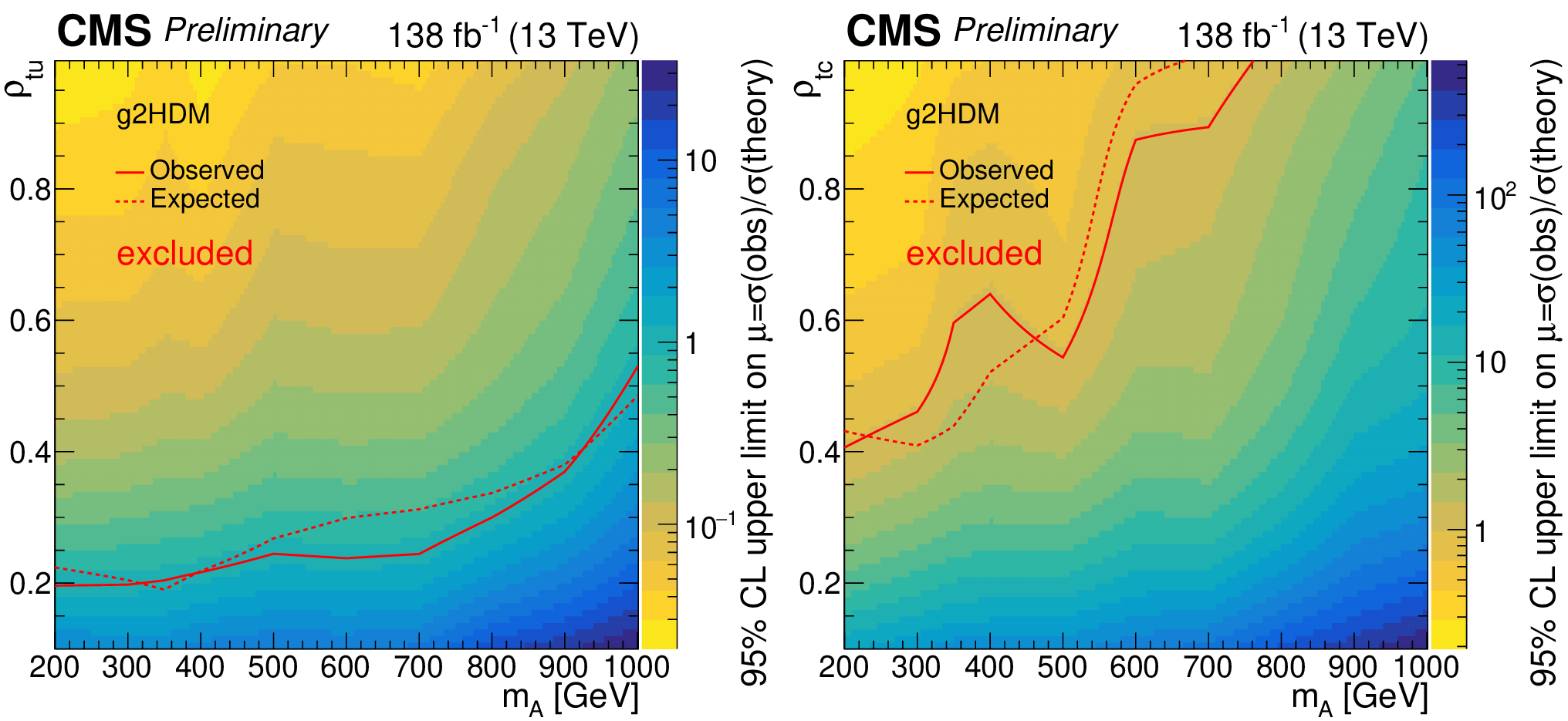
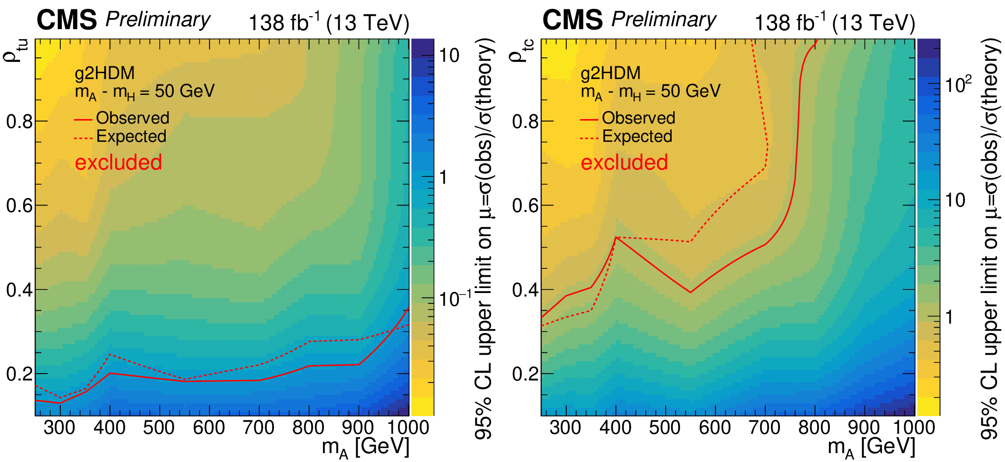
Figure 7:
Observed 95% CL upper limit on the signal strength as functions of $ m_{\mathrm{A}} $ and $ \rho_{\mathrm{t}\mathrm{u}} $ (left panel) and $ \rho_{\mathrm{t}\mathrm{c}} $ (right panel) for the g2HDM signal model with A--H interference, using the full Run 2 data set for the combination of $ \mathrm{e}^\pm\mathrm{e}^\pm $, $ \mu^\pm\mu^\pm $, and $ \mathrm{e}^\pm\mu^\pm $ categories. The color axis represents the observed upper limit on the signal strength. Expected (dashed lines) and observed (solid lines) exclusion contours are also shown. |
png pdf |
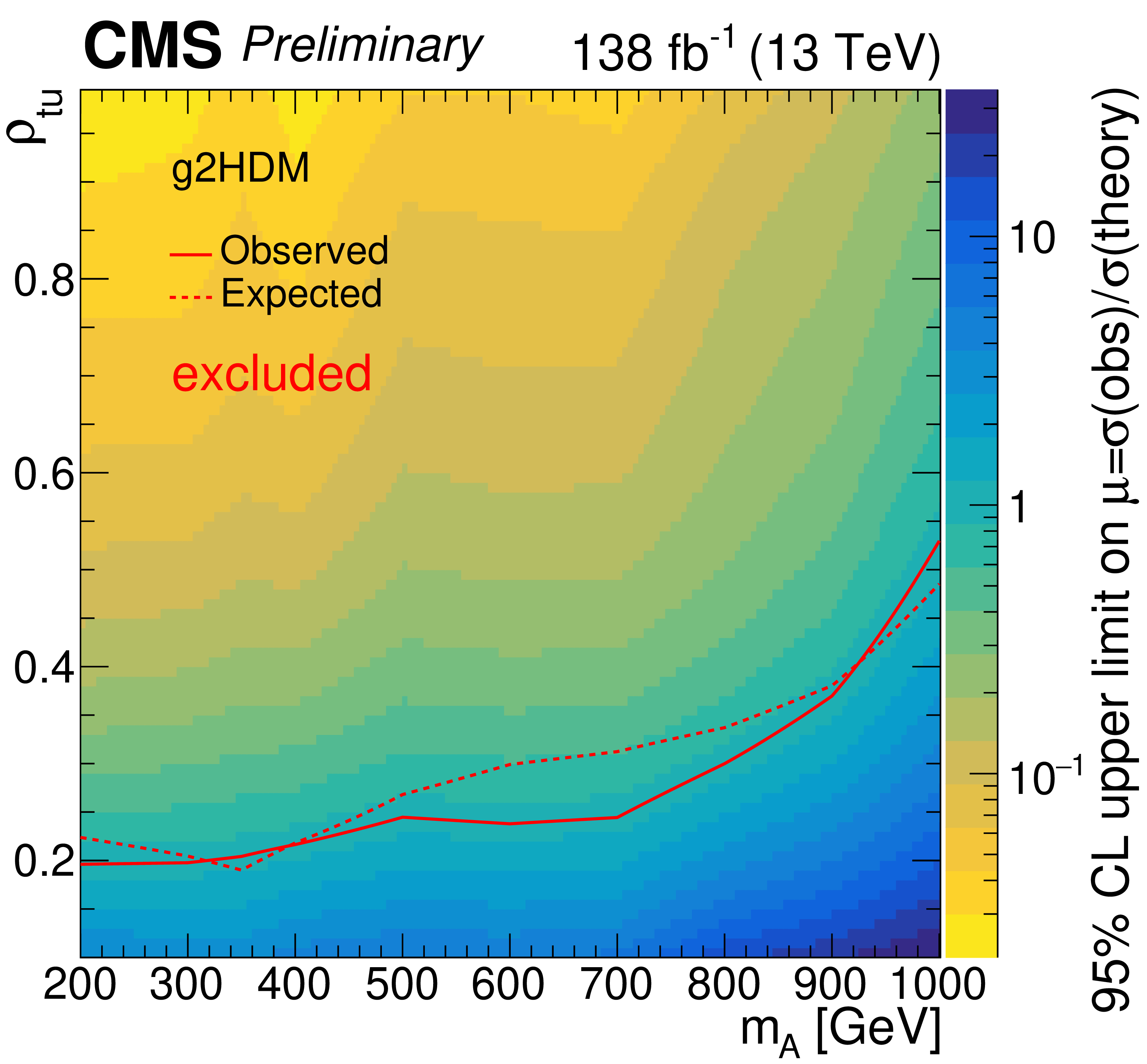
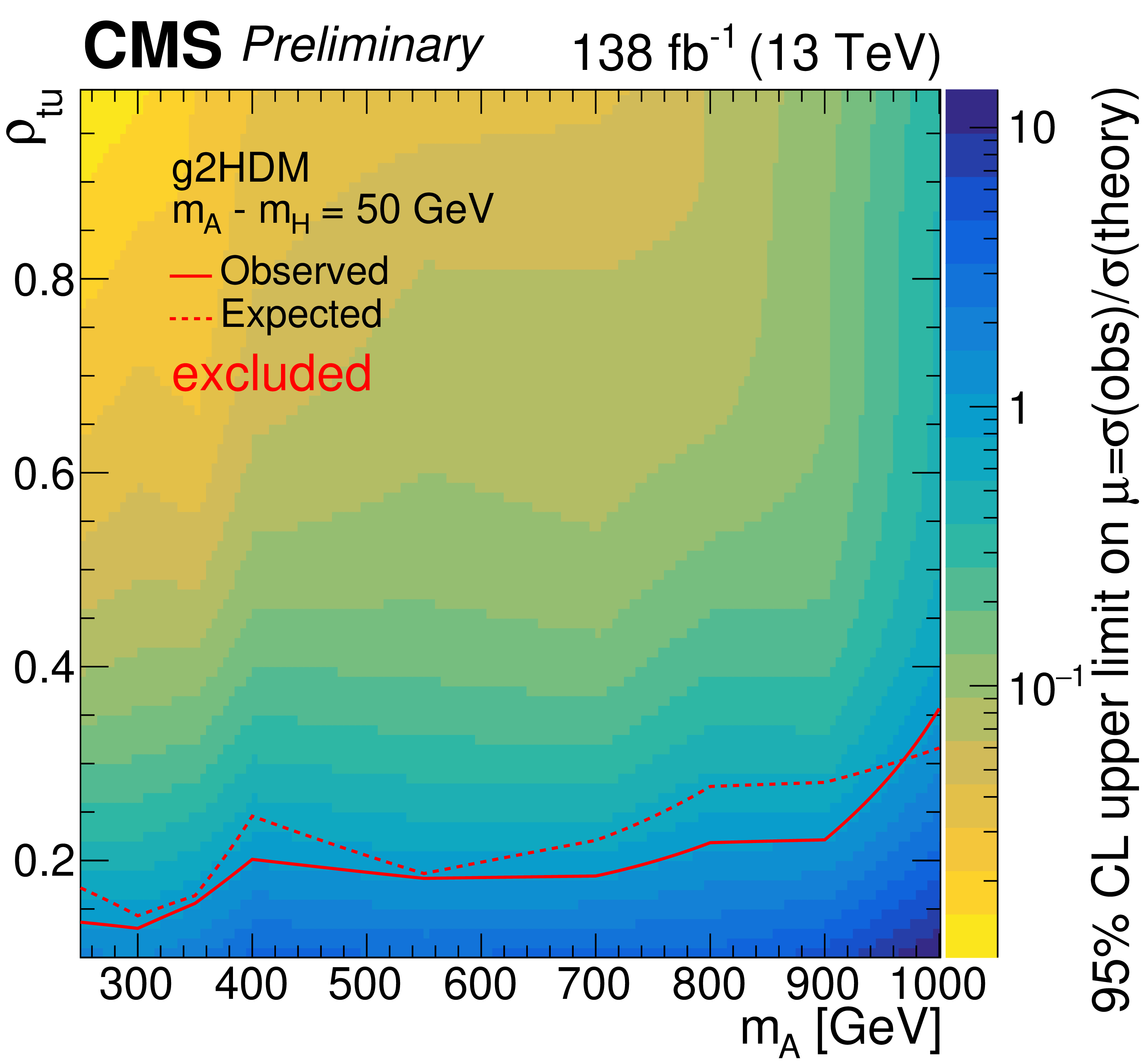
Figure 7-a:
Observed 95% CL upper limit on the signal strength as functions of $ m_{\mathrm{A}} $ and $ \rho_{\mathrm{t}\mathrm{u}} $ (left panel) and $ \rho_{\mathrm{t}\mathrm{c}} $ (right panel) for the g2HDM signal model with A--H interference, using the full Run 2 data set for the combination of $ \mathrm{e}^\pm\mathrm{e}^\pm $, $ \mu^\pm\mu^\pm $, and $ \mathrm{e}^\pm\mu^\pm $ categories. The color axis represents the observed upper limit on the signal strength. Expected (dashed lines) and observed (solid lines) exclusion contours are also shown. |
png pdf |
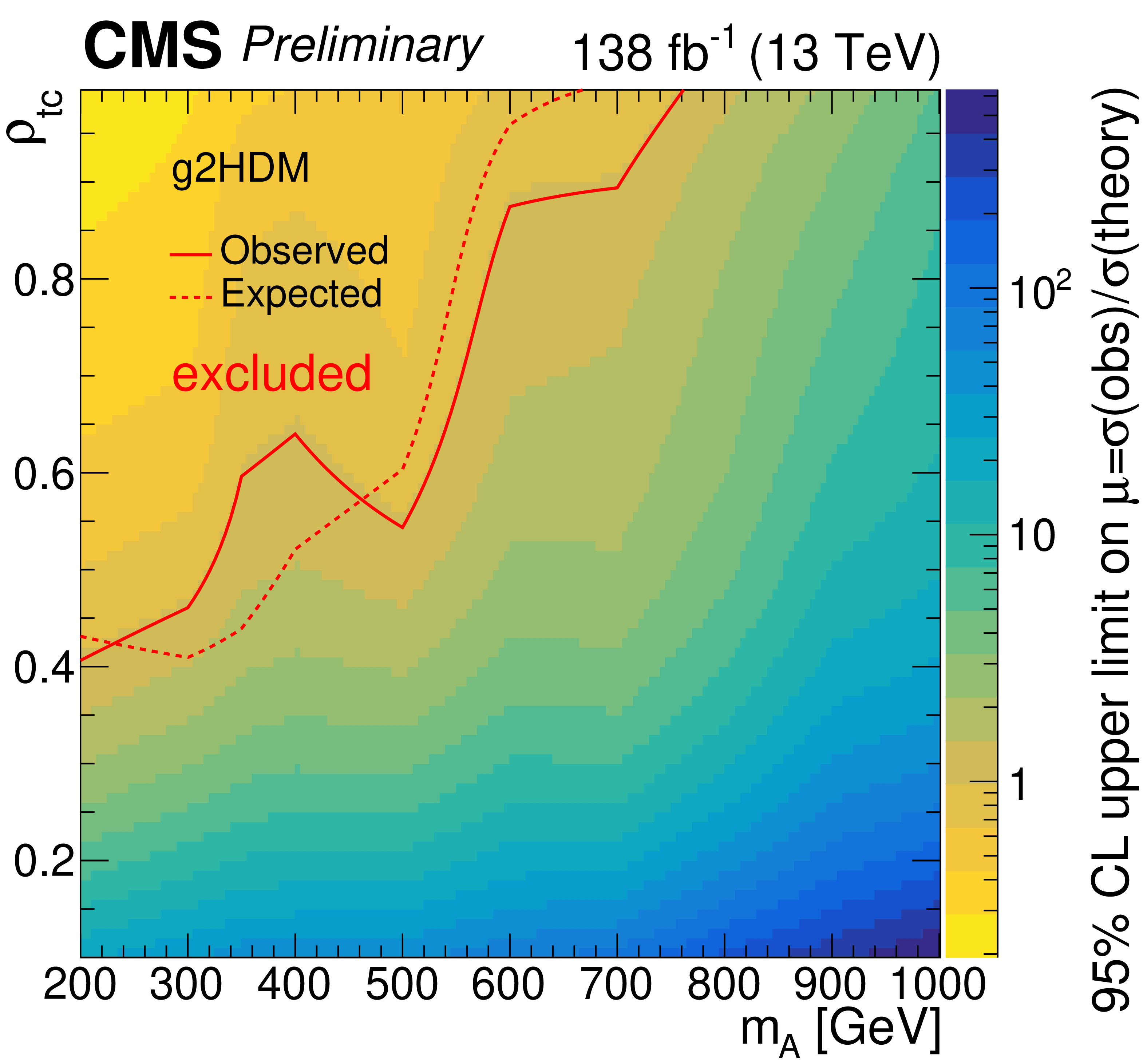
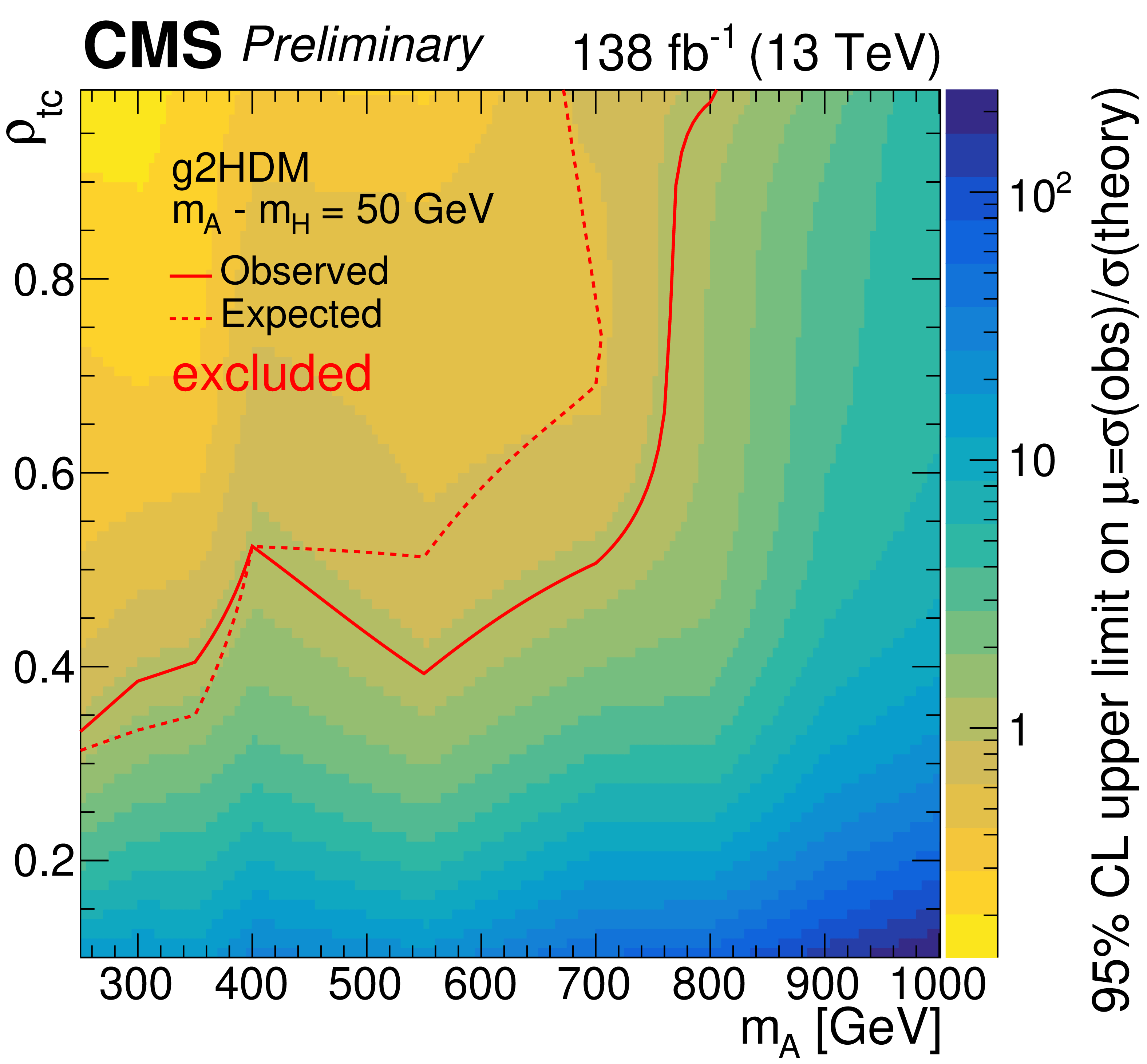
Figure 7-b:
Observed 95% CL upper limit on the signal strength as functions of $ m_{\mathrm{A}} $ and $ \rho_{\mathrm{t}\mathrm{u}} $ (left panel) and $ \rho_{\mathrm{t}\mathrm{c}} $ (right panel) for the g2HDM signal model with A--H interference, using the full Run 2 data set for the combination of $ \mathrm{e}^\pm\mathrm{e}^\pm $, $ \mu^\pm\mu^\pm $, and $ \mathrm{e}^\pm\mu^\pm $ categories. The color axis represents the observed upper limit on the signal strength. Expected (dashed lines) and observed (solid lines) exclusion contours are also shown. |
| Tables | |
png pdf |
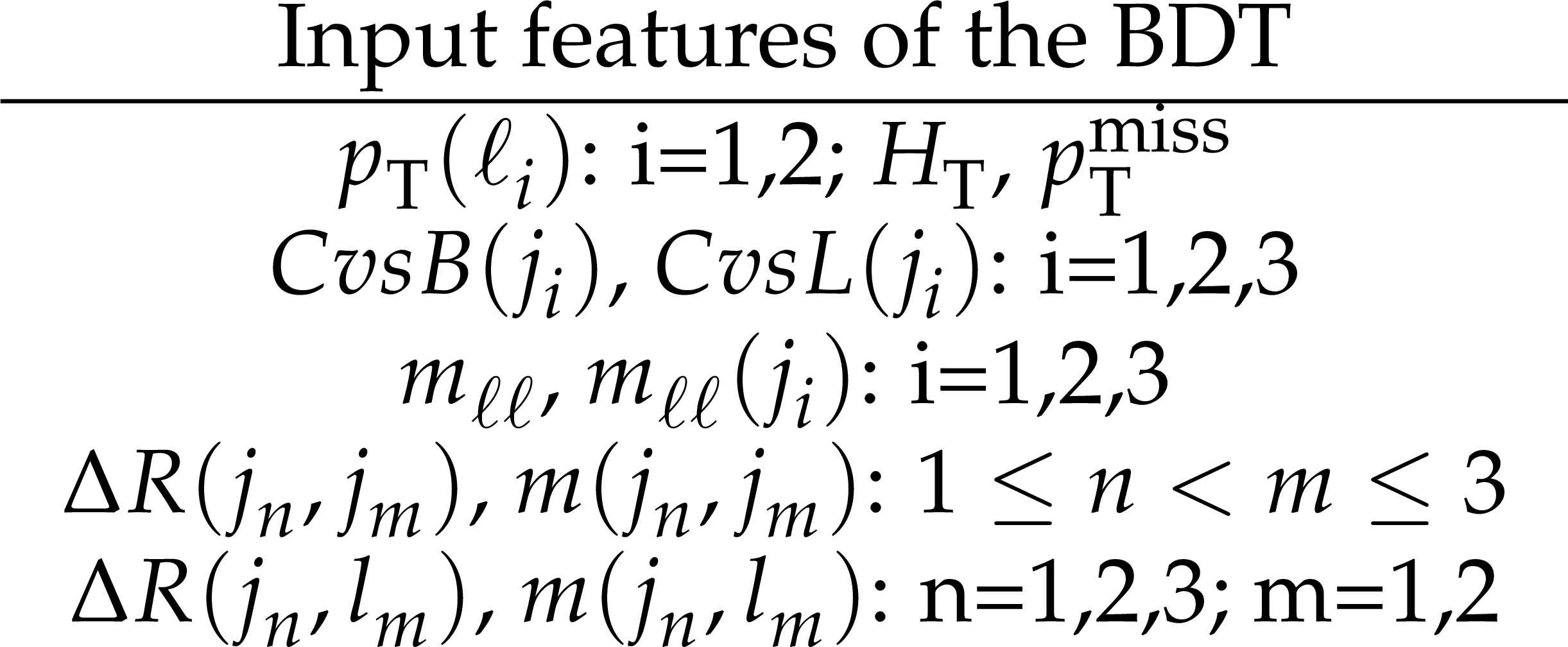
Table 1:
Input features of the BDT. Jets and leptons are ordered by $ p_{\mathrm{T}} $. The transverse momenta of the selected leptons are represented by $ p_{\mathrm{T}}(\ell_i) $. The invariant mass of the two selected leptons is denoted by $ m_{\ell\ell} $, and the invariant mass of the two selected leptons along with the $ i^{th} $ highest-$ p_{\mathrm{T}} $ jet by $ m_{\ell\ell}(j_i) $. The observable $ H_{\mathrm{T}} $ represents the scalar sum of the $ p_{\mathrm{T}} $ of the jets. |
png pdf |
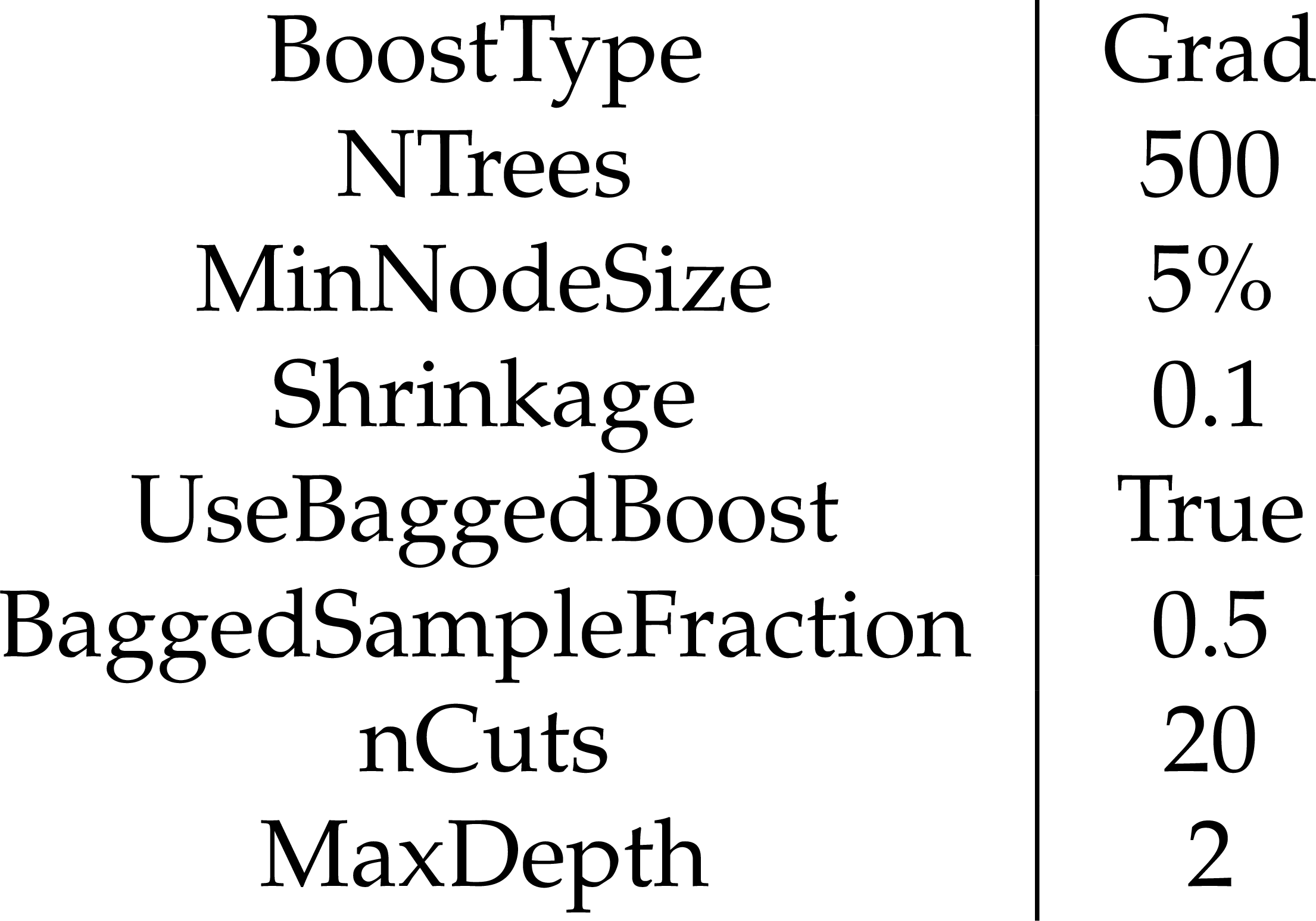
Table 2:
The BDT hyperparameters, as defined in the TMVA package, used in the analysis. |

png pdf |
Table 3:
Contributions of the dominant uncertainty sources with respect to the total uncertainty, given in percentages. The total background modeling contains the uncertainties due to the normalization of $ \mathrm{t} \overline{\mathrm{t}} $, VV, VBS, $ {\mathrm{t}\overline{\mathrm{t}}} \mathrm{H} $, $ {\mathrm{t}\overline{\mathrm{t}}} \mathrm{W} $, and other backgrounds. The total experimental uncertainty covers the uncertainties related to the integrated luminosity, pileup, L1 trigger inefficiency, nonprompt lepton background estimation, jet energy scale and resolution, reconstruction of $ {\vec p}_{\mathrm{T}}^{\kern1pt\text{miss}} $, lepton identification and isolation and trigger efficiencies, charge misidentification, muon momentum scale, and heavy quark and light quark jet identification. |
png pdf |
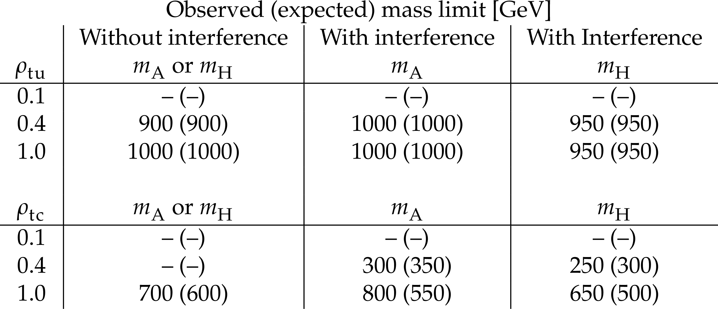
Table 4:
Observed (expected) lower limits on $ m_{\mathrm{A}} $ at 95% CL. For the scenario without interference, the limits on $ m_{\mathrm{H}} $ and $ m_{\mathrm{A}} $ are equivalent. |
| Summary |
| In summary, a search for new Yukawa couplings of the top quark with additional Higgs bosons in proton-proton collisions at a center-of-mass energy of 13 TeV is presented. The process considered is the production of same-sign top quark pairs associated with an up or a charm quark. No significant excess above the background prediction is observed. When no interference between the pseudoscalar (A) and scalar (H) Higgs bosons is assumed, A or H bosons with masses below 900 GeV and 1 TeV, are excluded at the 95% confidence level (CL) for coupling values $ \rho_{\mathrm{t}\mathrm{u}} = $ 0.4 and 1.0, respectively. Similarly, without interference between H and A, and assuming a coupling value of $ \rho_{\mathrm{t}\mathrm{c}} = $ 1.0, A or H bosons with masses below approximately 700 GeV are excluded at the 95% CL. In the assumption that A and H interfere in the scenario with a mass difference of $ m_{\mathrm{A}} - m_{\mathrm{H}} = $ 50 GeV, the pseudoscalar Higgs boson, A, is excluded for $ m_{\mathrm{A}} $ values below 1 TeV when considering coupling values ranging from $ \rho_{\mathrm{t}\mathrm{u}} = $ 0.4 to 1.0. Furthermore, assuming $ \rho_{\mathrm{t}\mathrm{c}} = $ 0.4, the exclusion limit for A is $ m_{\mathrm{A}} = $ 300 GeV, whereas assuming $ \rho_{\mathrm{t}\mathrm{c}} = $ 1.0, the limit extends to $ m_{\mathrm{A}} = $ 800 GeV at the 95% CL. These results represent the first search based on the generalized two-Higgs-doublet model considering the new Yukawa couplings $ \rho_{\mathrm{t}\mathrm{u}} $ and $ \rho_{\mathrm{t}\mathrm{c}} $ independently, and the first search to consider $ m_{\mathrm{A}} $-$ m_{\mathrm{H}} $ interference at the LHC. |
| References | ||||
| 1 | ATLAS Collaboration | Observation of a new particle in the search for the Standard Model Higgs boson with the ATLAS detector at the LHC | PLB 716 (2012) 1 | 1207.7214 |
| 2 | CMS Collaboration | Observation of a New Boson at a Mass of 125 GeV with the CMS Experiment at the LHC | PLB 716 (2012) 30 | CMS-HIG-12-028 1207.7235 |
| 3 | ATLAS and CMS Collaborations | Measurements of the Higgs boson production and decay rates and constraints on its couplings from a combined ATLAS and CMS analysis of the LHC pp collision data at $ \sqrt{s}= $ 7 and 8 TeV | JHEP 08 (2016) 045 | 1606.02266 |
| 4 | E. da Silva Almeida et al. | Electroweak Sector Under Scrutiny: A Combined Analysis of LHC and Electroweak Precision Data | PRD 99 (2019) 033001 | 1812.01009 |
| 5 | E. da Silva Almeida et al. | Electroweak legacy of the LHC Run II | PRD 105 (2022) 013006 | 2108.04828 |
| 6 | ATLAS Collaboration | A detailed map of Higgs boson interactions by the ATLAS experiment ten years after the discovery | Nature 607 (2022) 52 | 2207.00092 |
| 7 | CMS Collaboration | A portrait of the Higgs boson by the CMS experiment ten years after the discovery | Nature 607 (2022) 60 | CMS-HIG-22-001 2207.00043 |
| 8 | G. C. Branco et al. | Theory and phenomenology of two-Higgs-doublet models | Phys. Rept. 516 (2012) 1 | 1106.0034 |
| 9 | M. Kohda, T. Modak, and W.-S. Hou | Searching for new scalar bosons via triple-top signature in $ cg \to tS^0 \to tt\bar t $ | PLB 776 (2018) 379 | 1710.07260 |
| 10 | W.-S. Hou | Tree level t ---\ensuremath> c h or h ---\ensuremath> t anti-c decays | PLB 296 (1992) 179 | |
| 11 | W.-S. Hou and M. Kikuchi | Approximate Alignment in Two Higgs Doublet Model with Extra Yukawa Couplings | EPL 123 (2018) 11001 | 1706.07694 |
| 12 | J. F. Gunion and H. E. Haber | The CP conserving two Higgs doublet model: The Approach to the decoupling limit | PRD 67 (2003) 075019 | hep-ph/0207010 |
| 13 | M. Carena, I. Low, N. R. Shah, and C. E. M. Wagner | Impersonating the Standard Model Higgs Boson: Alignment without Decoupling | JHEP 04 (2014) 015 | 1310.2248 |
| 14 | P. S. Bhupal Dev and A. Pilaftsis | Maximally Symmetric Two Higgs Doublet Model with Natural Standard Model Alignment | JHEP 12 (2014) 024 | 1408.3405 |
| 15 | T. D. Lee | A Theory of Spontaneous T Violation | PRD 8 (1973) 1226 | |
| 16 | K. Fuyuto, W.-S. Hou, and E. Senaha | Electroweak baryogenesis driven by extra top Yukawa couplings | PLB 776 (2018) 402 | 1705.05034 |
| 17 | K. Fuyuto, W.-S. Hou, and E. Senaha | Cancellation mechanism for the electron electric dipole moment connected with the baryon asymmetry of the Universe | PRD 101 (2020) 011901 | 1910.12404 |
| 18 | Muon g-2 Collaboration | Measurement of the Positive Muon Anomalous Magnetic Moment to 0.46 ppm | PRL 126 (2021) 141801 | 2104.03281 |
| 19 | ATLAS Collaboration | Search for heavy Higgs bosons with flavour-violating couplings in multi-lepton plus $ b $-jets final states in $ pp $ collisions at 13 TeV with the ATLAS detector | 2307.14759 | |
| 20 | CMS Collaboration | The CMS experiment at the CERN LHC | JINST 3 (2008) S08004 | |
| 21 | CMS Collaboration | Performance of the CMS Level-1 trigger in proton-proton collisions at $ \sqrt{s} = $ 13\,TeV | JINST 15 (2020) P10017 | CMS-TRG-17-001 2006.10165 |
| 22 | CMS Collaboration | The CMS trigger system | JINST 12 (2017) P01020 | CMS-TRG-12-001 1609.02366 |
| 23 | CMS Collaboration | Electron and photon reconstruction and identification with the CMS experiment at the CERN LHC | JINST 16 (2021) P05014 | CMS-EGM-17-001 2012.06888 |
| 24 | CMS Collaboration | Performance of the CMS muon detector and muon reconstruction with proton-proton collisions at $ \sqrt{s} = $ 13 TeV | JINST 13 (2018) P06015 | CMS-MUO-16-001 1804.04528 |
| 25 | CMS Collaboration | Description and performance of track and primary-vertex reconstruction with the CMS tracker | JINST 9 (2014) P10009 | CMS-TRK-11-001 1405.6569 |
| 26 | CMS Collaboration | Particle-flow reconstruction and global event description with the CMS detector | JINST 12 (2017) P10003 | CMS-PRF-14-001 1706.04965 |
| 27 | CMS Collaboration | Performance of reconstruction and identification of $ \tau $ leptons decaying to hadrons and $ \nu_\tau $ in pp collisions at $ \sqrt{s}= $ 13 TeV | JINST 13 (2018) P10005 | CMS-TAU-16-003 1809.02816 |
| 28 | CMS Collaboration | Jet energy scale and resolution in the CMS experiment in pp collisions at 8 TeV | JINST 12 (2017) P02014 | CMS-JME-13-004 1607.03663 |
| 29 | CMS Collaboration | Performance of missing transverse momentum reconstruction in proton-proton collisions at $ \sqrt{s} = $ 13\,TeV using the CMS detector | JINST 14 (2019) P07004 | CMS-JME-17-001 1903.06078 |
| 30 | CMS Collaboration | Technical proposal for the phase-II upgrade of the Compact Muon Solenoid | CMS Technical proposal CERN-LHCC-2015-010, CMS-TDR-15-02, 2015 CDS |
|
| 31 | M. Cacciari, G. P. Salam, and G. Soyez | The anti-$ k_t $ jet clustering algorithm | JHEP 04 (2008) 063 | 0802.1189 |
| 32 | M. Cacciari, G. P. Salam, and G. Soyez | FastJet user manual | EPJC 72 (2012) 1896 | 1111.6097 |
| 33 | J. Alwall et al. | The automated computation of tree-level and next-to-leading order differential cross sections, and their matching to parton shower simulations | JHEP 07 (2014) 079 | 1405.0301 |
| 34 | J. Alwall et al. | Comparative study of various algorithms for the merging of parton showers and matrix elements in hadronic collisions | EPJC 53 (2008) 473 | 0706.2569 |
| 35 | W.-S. Hou and T. Modak | Probing Top Changing Neutral Higgs Couplings at Colliders | Mod. Phys. Lett. A 36 (2021) 2130006 | 2012.05735 |
| 36 | R. Frederix and S. Frixione | Merging meets matching in MC@NLO | JHEP 12 (2012) 061 | 1209.6215 |
| 37 | P. Nason | A New method for combining NLO QCD with shower Monte Carlo algorithms | JHEP 11 (2004) 040 | hep-ph/0409146 |
| 38 | S. Frixione, P. Nason, and C. Oleari | Matching NLO QCD computations with Parton Shower simulations: the POWHEG method | JHEP 11 (2007) 070 | 0709.2092 |
| 39 | S. Alioli, P. Nason, C. Oleari, and E. Re | A general framework for implementing NLO calculations in shower Monte Carlo programs: the POWHEG BOX | JHEP 06 (2010) 043 | 1002.2581 |
| 40 | S. Frixione, P. Nason, and G. Ridolfi | A Positive-weight next-to-leading-order Monte Carlo for heavy flavour hadroproduction | JHEP 09 (2007) 126 | 0707.3088 |
| 41 | T. Melia, P. Nason, R. Rontsch, and G. Zanderighi | W+W-, WZ and ZZ production in the POWHEG BOX | JHEP 11 (2011) 078 | 1107.5051 |
| 42 | E. Re | Single-top Wt-channel production matched with parton showers using the POWHEG method | EPJC 71 (2011) 1547 | 1009.2450 |
| 43 | S. Alioli, P. Nason, C. Oleari, and E. Re | NLO single-top production matched with shower in POWHEG: s- and t-channel contributions | JHEP 09 (2009) 111 | 0907.4076 |
| 44 | H. B. Hartanto, B. Jager, L. Reina, and D. Wackeroth | Higgs boson production in association with top quarks in the POWHEG BOX | PRD 91 (2015) 094003 | 1501.04498 |
| 45 | T. Sjöstrand et al. | An introduction to PYTHIA 8.2 | Comput. Phys. Commun. 191 (2015) 159 | 1410.3012 |
| 46 | CMS Collaboration | Extraction and validation of a new set of CMS PYTHIA8 tunes from underlying-event measurements | EPJC 80 (2020) 4 | CMS-GEN-17-001 1903.12179 |
| 47 | NNPDF Collaboration | Parton distributions from high-precision collider data | EPJC 77 (2017) 663 | 1706.00428 |
| 48 | GEANT4 Collaboration | GEANT 4 --- a simulation toolkit | NIM A 506 (2003) 250 | |
| 49 | CMS Collaboration | Measurement of the inclusive W and Z production cross sections in pp collisions at $ \sqrt{s}= $ 7 TeV | JHEP 10 (2011) 132 | CMS-EWK-10-005 1107.4789 |
| 50 | CMS Collaboration | Measurement of the Higgs boson production rate in association with top quarks in final states with electrons, muons, and hadronically decaying tau leptons at $ \sqrt{s} = $ 13 TeV | EPJC 81 (2021) 378 | CMS-HIG-19-008 2011.03652 |
| 51 | CMS Collaboration | Measurement of the cross section of top quark-antiquark pair production in association with a W boson in proton-proton collisions at $ \sqrt{s} $ = 13 TeV | CMS-TOP-21-011 2208.06485 |
|
| 52 | CMS Collaboration | Performance of electron reconstruction and selection with the CMS detector in proton-proton collisions at $ \sqrt{s} = $ 8 TeV | JINST 10 (2015) P06005 | CMS-EGM-13-001 1502.02701 |
| 53 | K. Rehermann and B. Tweedie | Efficient identification of boosted semileptonic top quarks at the LHC | JHEP 03 (2011) 059 | 1007.2221 |
| 54 | E. Bols et al. | Jet flavour classification using DeepJet | JINST 15 (2020) P12012 | 2008.10519 |
| 55 | CMS Collaboration | Performance summary of AK4 jet b tagging with data from proton-proton collisions at 13 TeV with the CMS detector | CMS Detector Performance Note CMS-DP-2023-005, 2023 CDS |
|
| 56 | CMS Collaboration | Identification of heavy-flavour jets with the CMS detector in pp collisions at 13 TeV | JINST 13 (2018) P05011 | CMS-BTV-16-002 1712.07158 |
| 57 | CMS Collaboration | A new calibration method for charm jet identification validated with proton-proton collision events at $ \sqrt{s} $ =13 TeV | JINST 17 (2022) P03014 | CMS-BTV-20-001 2111.03027 |
| 58 | CMS Collaboration | Performance summary of AK4 jet charm tagging with the CMS Run2 Legacy dataset | CMS Detector Performance Note CMS-DP-2023-006, 2023 CDS |
|
| 59 | CMS Collaboration | Evidence for associated production of a Higgs boson with a top quark pair in final states with electrons, muons, and hadronically decaying $ \tau $ leptons at $ \sqrt{s} = $ 13 TeV | JHEP 08 (2018) 066 | CMS-HIG-17-018 1803.05485 |
| 60 | A. Hocker et al. | TMVA - Toolkit for Multivariate Data Analysis | physics/0703039 | |
| 61 | The ATLAS and CMS Collaborations and the LHC Higgs Combination Group | Procedure for the LHC Higgs boson search combination in Summer 2011 | Technical Report CMS-NOTE-2011-005, ATL-PHYS-PUB-2011-11, CERN, Geneva, 2011 | |
| 62 | R. J. Barlow and C. Beeston | Fitting using finite Monte Carlo samples | Comput. Phys. Commun. 77 (1993) 219 | |
| 63 | CMS Collaboration | Precision luminosity measurement in proton-proton collisions at $ \sqrt{s} = $ 13 TeV in 2015 and 2016 at CMS | EPJC 81 (2021) 800 | CMS-LUM-17-003 2104.01927 |
| 64 | CMS Collaboration | CMS luminosity measurement for the 2017 data-taking period at $ \sqrt{s} = $ 13 TeV | CMS Physics Analysis Summary , CERN, Geneva, 2018 CMS-PAS-LUM-17-004 |
CMS-PAS-LUM-17-004 |
| 65 | CMS Collaboration | CMS luminosity measurement for the 2018 data-taking period at $ \sqrt{s} = $ 13 TeV | CMS Physics Analysis Summary , CERN, Geneva, 2019 CMS-PAS-LUM-18-002 |
CMS-PAS-LUM-18-002 |
| 66 | S. Heinemeyer et al. | Handbook of LHC Higgs cross sections: 3. Higgs properties | CERN Report CERN-2013-004, 2013 link |
1307.1347 |
| 67 | A. L. Read | Presentation of search results: the CL$ _s $ technique | JPG 28 (2002) 2693 | |
| 68 | T. Junk | Confidence level computation for combining searches with small statistics | NIM A 434 (1999) 435 | hep-ex/9902006 |
| 69 | G. Cowan, K. Cranmer, E. Gross, and O. Vitells | Asymptotic formulae for likelihood-based tests of new physics | EPJC 71 (2011) 1554 | 1007.1727 |
|
|
Compact Muon Solenoid LHC, CERN |
|

|

|

|

|

|