

Compact Muon Solenoid
LHC, CERN
| CMS-PAS-TOP-22-006 | ||
| Search for new physics in top quark production with additional leptons in the context of effective field theory using 138 fb$ ^{-1} $ of proton-proton collisions at $ \sqrt{s} $ = 13 TeV | ||
| CMS Collaboration | ||
| 7 March 2023 | ||
| Abstract: A search for new physics in top quark production with additional final-state leptons is performed with 138 fb$^{-1}$ of proton-proton collisions at $ \sqrt{s} = $ 13 TeV at the LHC, collected by the CMS detector during 2016, 2017, and 2018. Using the framework of effective field theory (EFT), potential new physics effects are parametrized in terms of 26 dimension-six EFT operators. EFT effects are incorporated into the event weights of the simulated samples, allowing detector-level predictions that account for correlations and interference effects among EFT operators and between EFT operators and standard model processes. The data are divided into several categories based on lepton multiplicity, total lepton charge, jet multiplicities, and b tagged jet multiplicities. Kinematic variables corresponding to the transverse momentum ($ p_{\mathrm{T}} $) of the leading pair of leptons and jets as well as the $ p_{\mathrm{T}} $ of on-shell Z bosons are used to extract the 95% confidence intervals of the 26 dimension-six EFT operators. No significant deviation with respect to the standard model prediction was found. | ||
|
Links:
CDS record (PDF) ;
Physics Briefing ;
CADI line (restricted) ;
These preliminary results are superseded in this paper, JHEP 12 (2023) 068. The superseded preliminary plots can be found here. |
||
| Figures | |
png pdf |
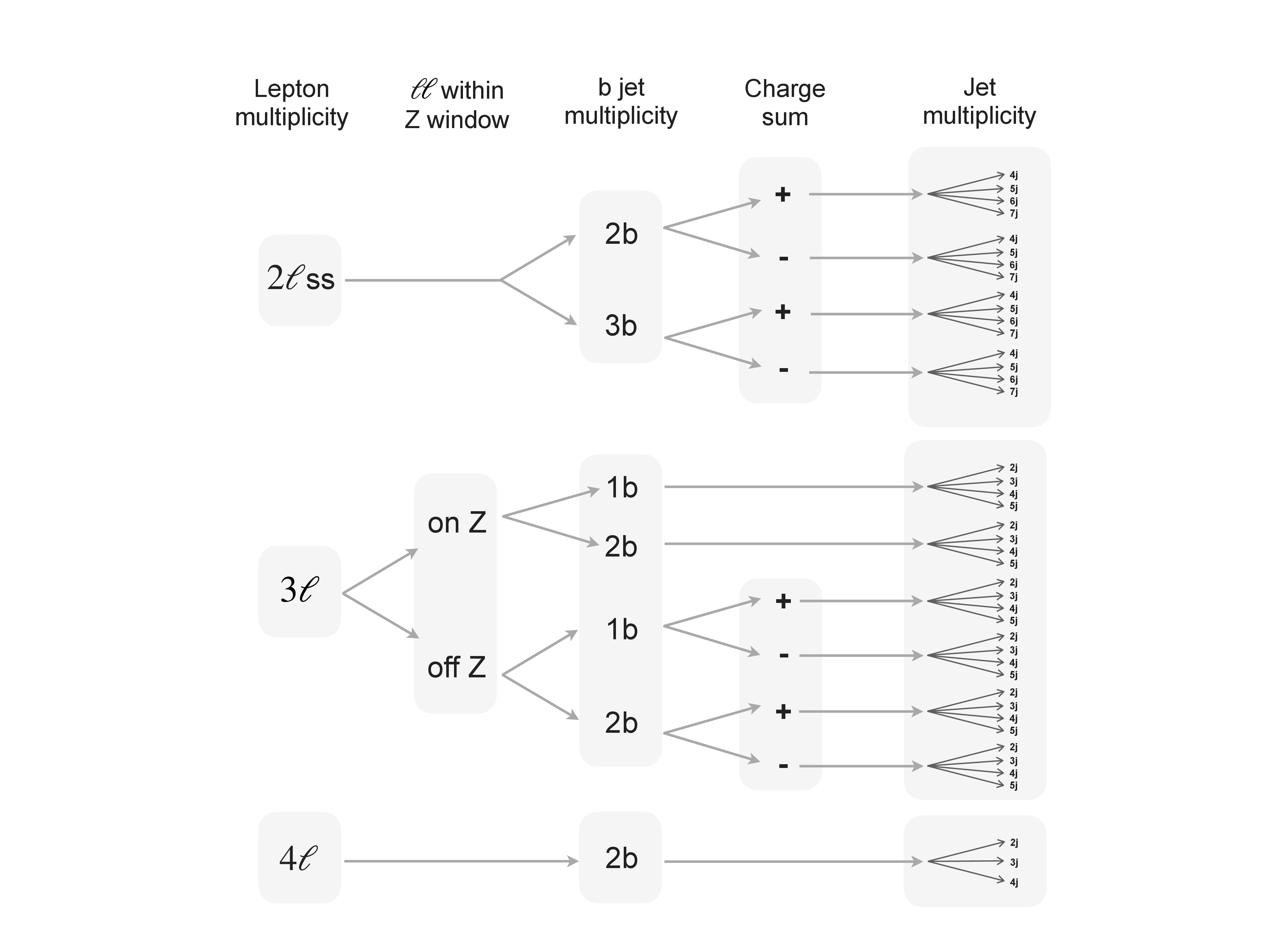
Figure 1:
Summary of the event selection categorization. The details for the selection requirements are described in Sections 5.1, 5.2, and 5.3. |
png pdf |
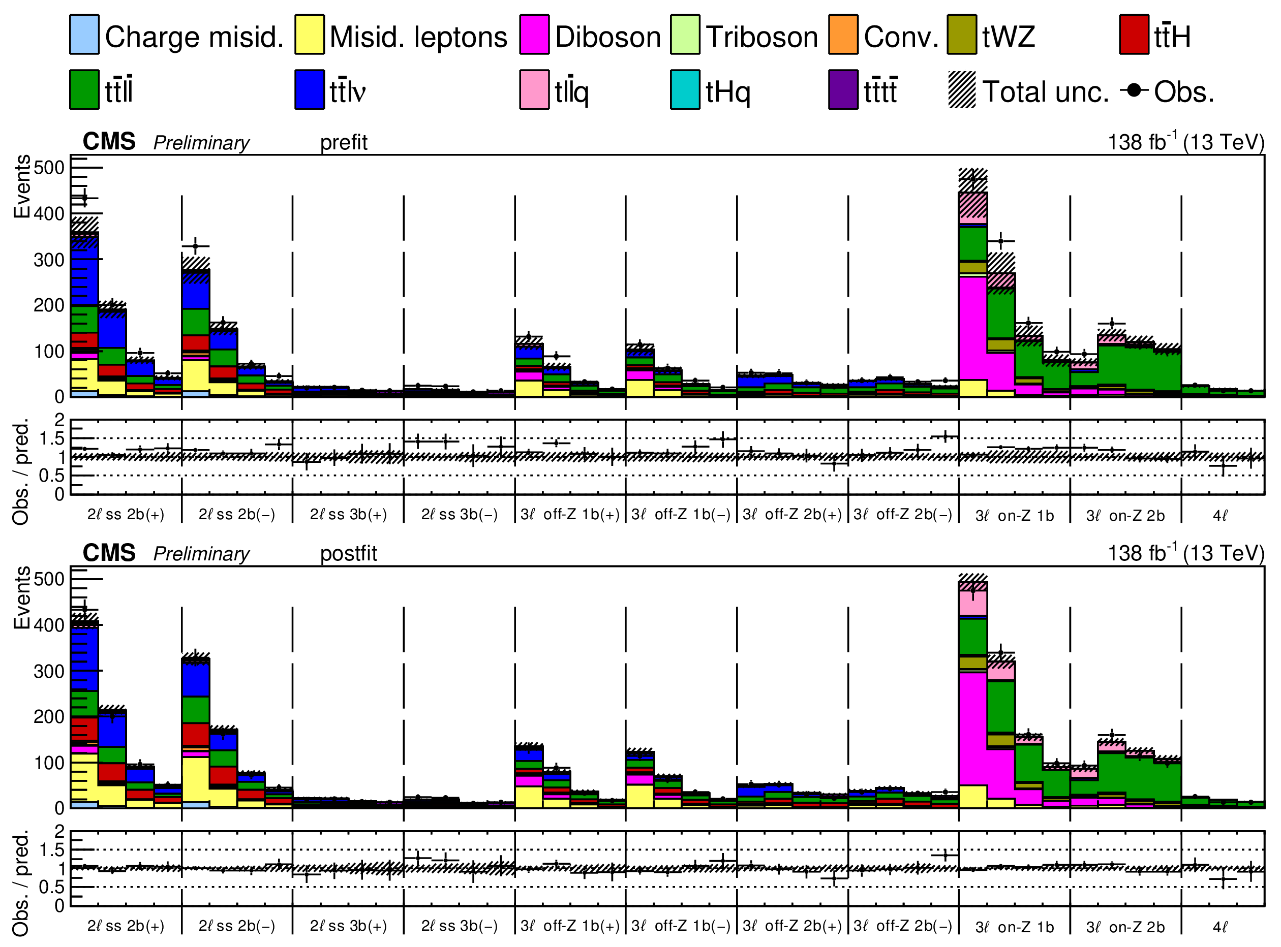
Figure 2:
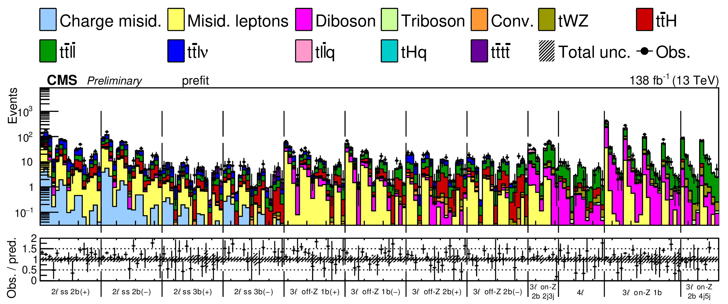
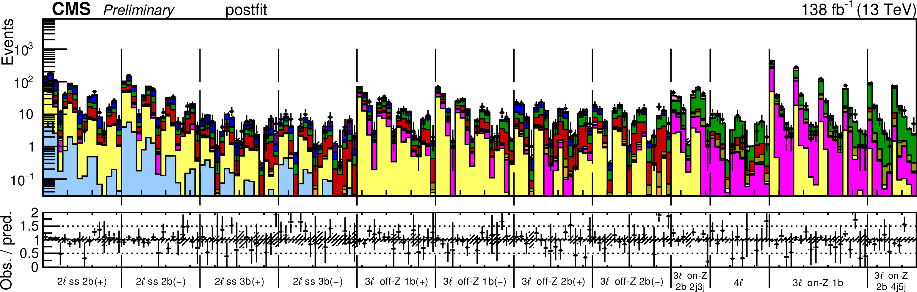
Expected yields prefit (top) and postfit (bottom). All kinematic variables and b jets categories have been combined, resulting in distributions for the jet multiplicity only. The postfit values are obtained by simultaneously fitting all 26 WCs and the NPs. The process labeled ``Conv." corresponds to the photon conversion background, ``Misid. leptons" corresponds to misidentified leptons, and ``Charge misid." corresponds to leptons with a mismeasured charge. The lower panel contains the ratios of the observed yields over the expected. The error bands correspond to NP and WC uncertainties added in quadrature. |

png pdf |
Figure 2-a:
Expected yields prefit (top) and postfit (bottom). All kinematic variables and b jets categories have been combined, resulting in distributions for the jet multiplicity only. The postfit values are obtained by simultaneously fitting all 26 WCs and the NPs. The process labeled ``Conv." corresponds to the photon conversion background, ``Misid. leptons" corresponds to misidentified leptons, and ``Charge misid." corresponds to leptons with a mismeasured charge. The lower panel contains the ratios of the observed yields over the expected. The error bands correspond to NP and WC uncertainties added in quadrature. |
png pdf |
Figure 2-b:
Expected yields prefit (top) and postfit (bottom). All kinematic variables and b jets categories have been combined, resulting in distributions for the jet multiplicity only. The postfit values are obtained by simultaneously fitting all 26 WCs and the NPs. The process labeled ``Conv." corresponds to the photon conversion background, ``Misid. leptons" corresponds to misidentified leptons, and ``Charge misid." corresponds to leptons with a mismeasured charge. The lower panel contains the ratios of the observed yields over the expected. The error bands correspond to NP and WC uncertainties added in quadrature. |
png pdf |
Figure 2-c:
Expected yields prefit (top) and postfit (bottom). All kinematic variables and b jets categories have been combined, resulting in distributions for the jet multiplicity only. The postfit values are obtained by simultaneously fitting all 26 WCs and the NPs. The process labeled ``Conv." corresponds to the photon conversion background, ``Misid. leptons" corresponds to misidentified leptons, and ``Charge misid." corresponds to leptons with a mismeasured charge. The lower panel contains the ratios of the observed yields over the expected. The error bands correspond to NP and WC uncertainties added in quadrature. |
png pdf |
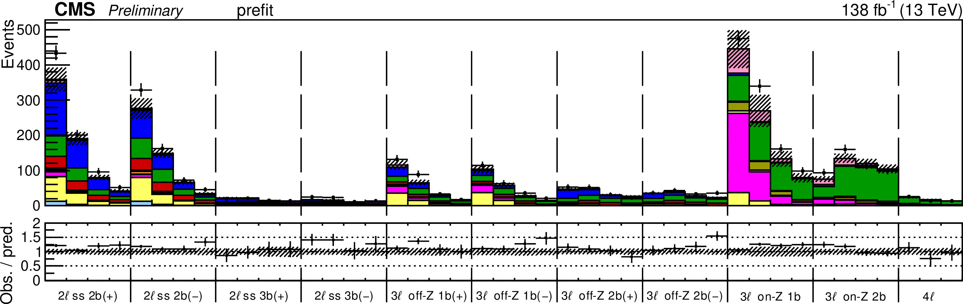
Figure 3:
Expected yields prefit. All kinematic variables are shown. Each event category (e.g. 2$ \ell $ss) is sub-divided into its jet multiplcity components. For example, the first four sub-bins of the 2$ \ell $ss bin are the $ {p_{\mathrm{T}}}\mathrm{(\ell j 0)} $ variable for four jets, the next four sub-bins are the $ {p_{\mathrm{T}}}\mathrm{(\ell j 0)} $ variable for 5 jets, etc. The postfit values are obtained by simultaneously fitting all 26 WCs and the NPs. The process labeled ``Conv." corresponds to the photon conversion background, ``Misid. leptons" corresponds to misidentified leptons, and ``Charge misid." corresponds to leptons with a mismeasured charge. The lower panel contains the ratios of the observed yields over the expected. The error bands correspond to NP and WC uncertainties added in quadrature. All yields are plotted on a log scale. |

png pdf |
Figure 3-a:
Expected yields prefit. All kinematic variables are shown. Each event category (e.g. 2$ \ell $ss) is sub-divided into its jet multiplcity components. For example, the first four sub-bins of the 2$ \ell $ss bin are the $ {p_{\mathrm{T}}}\mathrm{(\ell j 0)} $ variable for four jets, the next four sub-bins are the $ {p_{\mathrm{T}}}\mathrm{(\ell j 0)} $ variable for 5 jets, etc. The postfit values are obtained by simultaneously fitting all 26 WCs and the NPs. The process labeled ``Conv." corresponds to the photon conversion background, ``Misid. leptons" corresponds to misidentified leptons, and ``Charge misid." corresponds to leptons with a mismeasured charge. The lower panel contains the ratios of the observed yields over the expected. The error bands correspond to NP and WC uncertainties added in quadrature. All yields are plotted on a log scale. |

png pdf |
Figure 3-b:
Expected yields prefit. All kinematic variables are shown. Each event category (e.g. 2$ \ell $ss) is sub-divided into its jet multiplcity components. For example, the first four sub-bins of the 2$ \ell $ss bin are the $ {p_{\mathrm{T}}}\mathrm{(\ell j 0)} $ variable for four jets, the next four sub-bins are the $ {p_{\mathrm{T}}}\mathrm{(\ell j 0)} $ variable for 5 jets, etc. The postfit values are obtained by simultaneously fitting all 26 WCs and the NPs. The process labeled ``Conv." corresponds to the photon conversion background, ``Misid. leptons" corresponds to misidentified leptons, and ``Charge misid." corresponds to leptons with a mismeasured charge. The lower panel contains the ratios of the observed yields over the expected. The error bands correspond to NP and WC uncertainties added in quadrature. All yields are plotted on a log scale. |

png pdf |
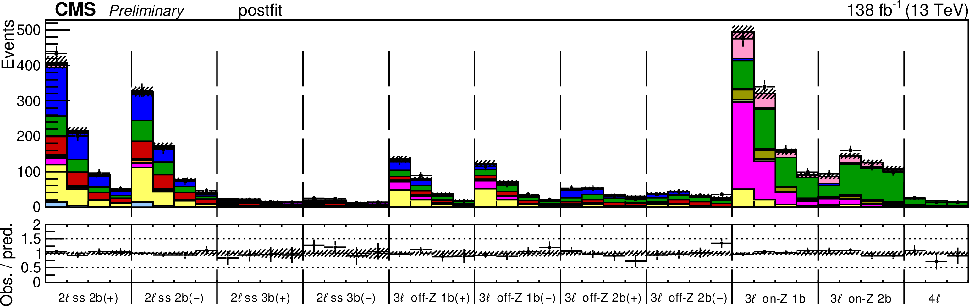
Figure 4:
Expected yields postfit. All kinematic variables are shown. Each event category (e.g. 2$ \ell $ss) is sub-divided into its jet multiplcity components. For example, the first four sub-bins of the 2$ \ell $ss bin are the $ {p_{\mathrm{T}}}\mathrm{(\ell j 0)} $ variable for four jets, the next four sub-bins are the $ {p_{\mathrm{T}}}\mathrm{(\ell j 0)} $ variable for 5 jets, etc. The postfit values are obtained by simultaneously fitting all 26 WCs and the NPs. The process labeled ``Conv." corresponds to the photon conversion background, ``Misid. leptons" corresponds to misidentified leptons, and ``Charge misid." corresponds to leptons with a mismeasured charge. The lower panel contains the ratios of the observed yields over the expected. The error bands correspond to NP and WC uncertainties added in quadrature. All yields are plotted on a log scale. |

png pdf |
Figure 4-a:
Expected yields postfit. All kinematic variables are shown. Each event category (e.g. 2$ \ell $ss) is sub-divided into its jet multiplcity components. For example, the first four sub-bins of the 2$ \ell $ss bin are the $ {p_{\mathrm{T}}}\mathrm{(\ell j 0)} $ variable for four jets, the next four sub-bins are the $ {p_{\mathrm{T}}}\mathrm{(\ell j 0)} $ variable for 5 jets, etc. The postfit values are obtained by simultaneously fitting all 26 WCs and the NPs. The process labeled ``Conv." corresponds to the photon conversion background, ``Misid. leptons" corresponds to misidentified leptons, and ``Charge misid." corresponds to leptons with a mismeasured charge. The lower panel contains the ratios of the observed yields over the expected. The error bands correspond to NP and WC uncertainties added in quadrature. All yields are plotted on a log scale. |
png pdf |
Figure 4-b:
Expected yields postfit. All kinematic variables are shown. Each event category (e.g. 2$ \ell $ss) is sub-divided into its jet multiplcity components. For example, the first four sub-bins of the 2$ \ell $ss bin are the $ {p_{\mathrm{T}}}\mathrm{(\ell j 0)} $ variable for four jets, the next four sub-bins are the $ {p_{\mathrm{T}}}\mathrm{(\ell j 0)} $ variable for 5 jets, etc. The postfit values are obtained by simultaneously fitting all 26 WCs and the NPs. The process labeled ``Conv." corresponds to the photon conversion background, ``Misid. leptons" corresponds to misidentified leptons, and ``Charge misid." corresponds to leptons with a mismeasured charge. The lower panel contains the ratios of the observed yields over the expected. The error bands correspond to NP and WC uncertainties added in quadrature. All yields are plotted on a log scale. |
png pdf |
Figure 5:
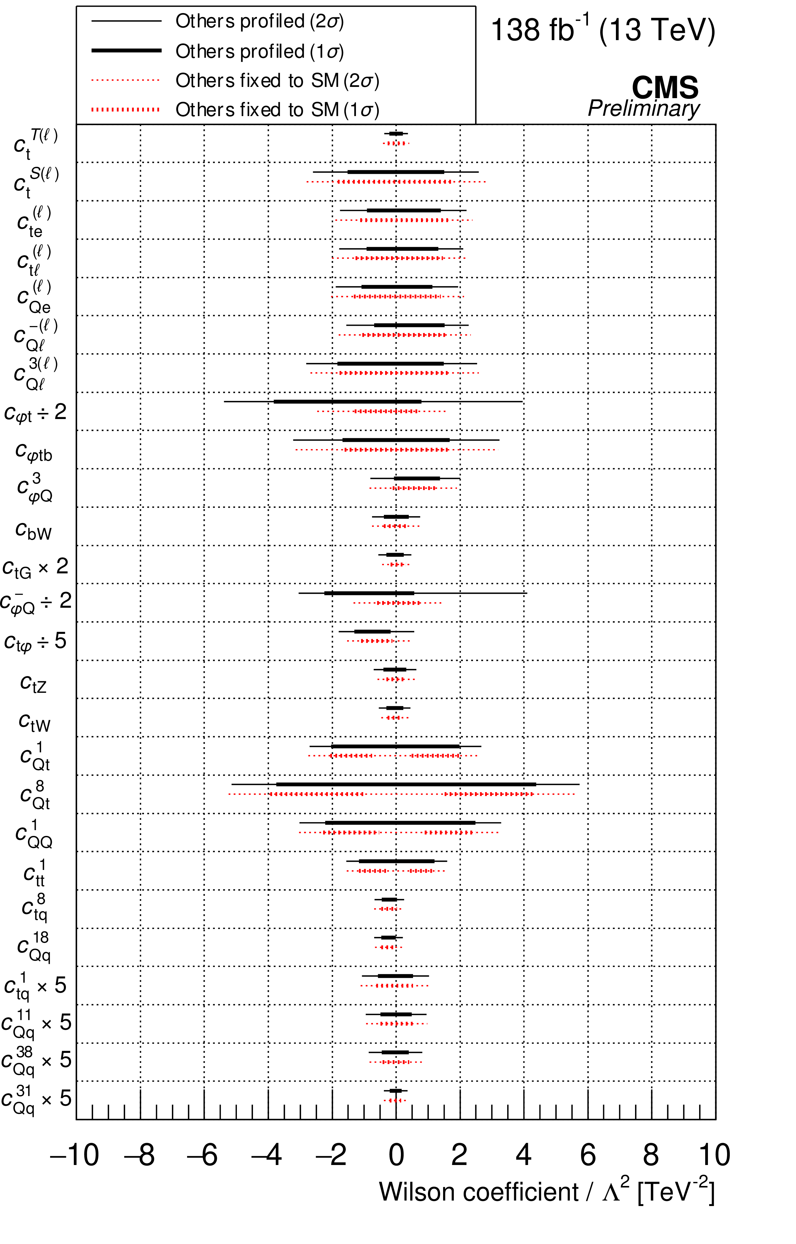
Summary of CIs extracted from the likelihood fits described in Section 7. WC 1 $ \sigma $ (thick line) and 2 $ \sigma $ (thin line) uncertainty intervals are shown for the case where the other WCs are profiled (in black), and the case where the other WCs are fixed to their SM values of zero (in red). To make the figure more readable, the intervals for $c_{\mathrm{t}\varphi}$ were scaled by 1/5, the intervals for $c_{\varphi\mathrm{t}}$ and $c^{-}_{\varphi\mathrm{Q}}$ were scaled by 1/2, the intervals for $c_{\mathrm{tG}}$ were scaled by 2, and the intervals for $c^{1}_{\mathrm{tq}}$, $c^{11}_{\mathrm{Qq}}$, $c^{38}_{\mathrm{Qq}}$, and $c^{31}_{\mathrm{Qq}}$ were all scaled by 5. |

png pdf |
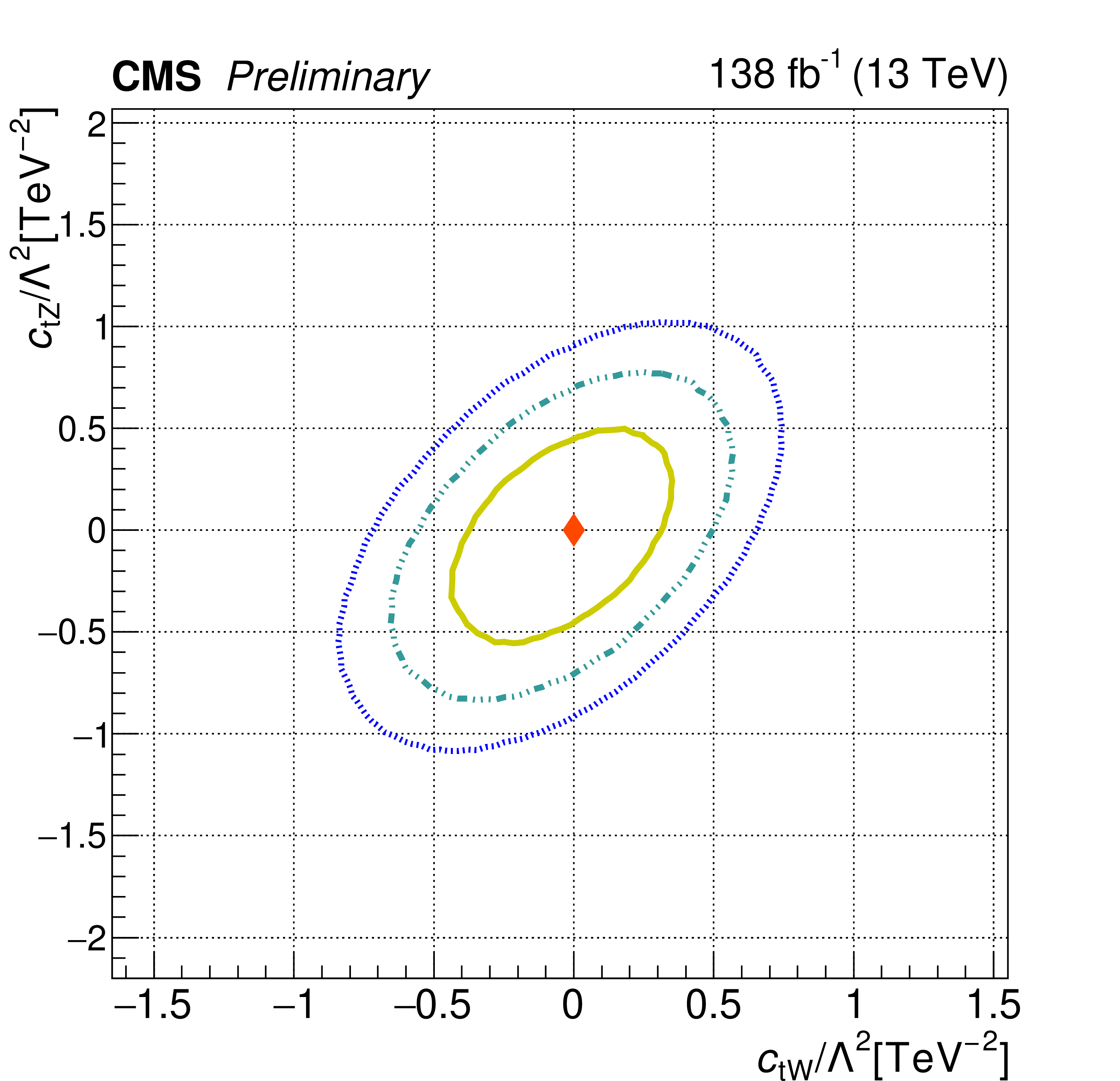
Figure 6:
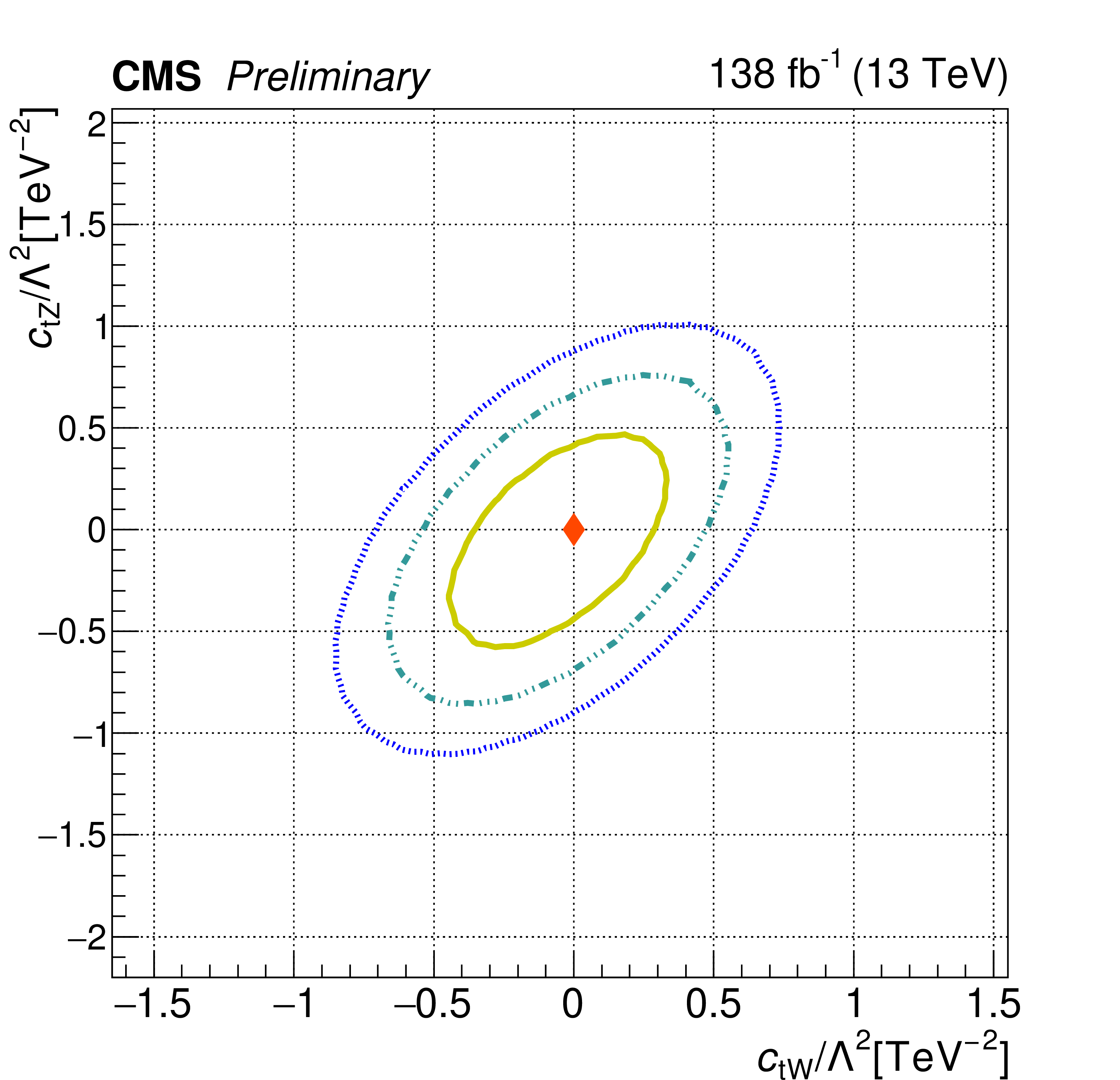
The observed 68.3%, 95.5%, and 99.7% confidence contours of a 2D scan for $c_{\mathrm{tW}}$ and $c_{\mathrm{tZ}}$ with the other WCs profiled (left), and fixed to their SM values (right). Diamond markers show the SM prediction. |

png pdf |
Figure 6-a:
The observed 68.3%, 95.5%, and 99.7% confidence contours of a 2D scan for $c_{\mathrm{tW}}$ and $c_{\mathrm{tZ}}$ with the other WCs profiled (left), and fixed to their SM values (right). Diamond markers show the SM prediction. |
png pdf |
Figure 6-b:
The observed 68.3%, 95.5%, and 99.7% confidence contours of a 2D scan for $c_{\mathrm{tW}}$ and $c_{\mathrm{tZ}}$ with the other WCs profiled (left), and fixed to their SM values (right). Diamond markers show the SM prediction. |
png pdf |
Figure 6-c:
The observed 68.3%, 95.5%, and 99.7% confidence contours of a 2D scan for $c_{\mathrm{tW}}$ and $c_{\mathrm{tZ}}$ with the other WCs profiled (left), and fixed to their SM values (right). Diamond markers show the SM prediction. |
png pdf |
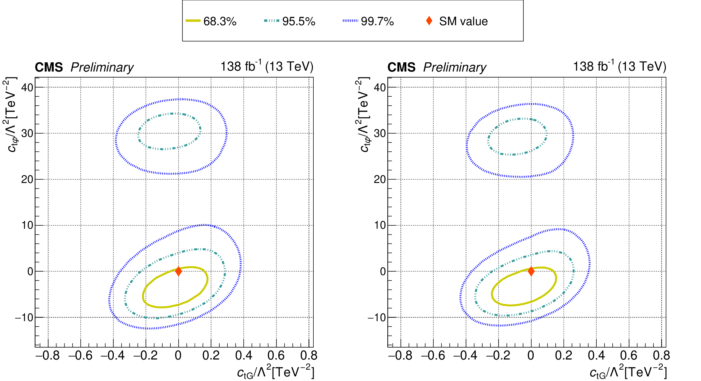
Figure 7:
The observed 68.3%, 95.5%, and 99.7% confidence contours of a 2D scan for $c_{\mathrm{tG}}$ and $c_{\mathrm{t}\varphi}$ with the other WCs profiled (left), and fixed to their SM values (right). Diamond markers show the SM prediction. |

png pdf |
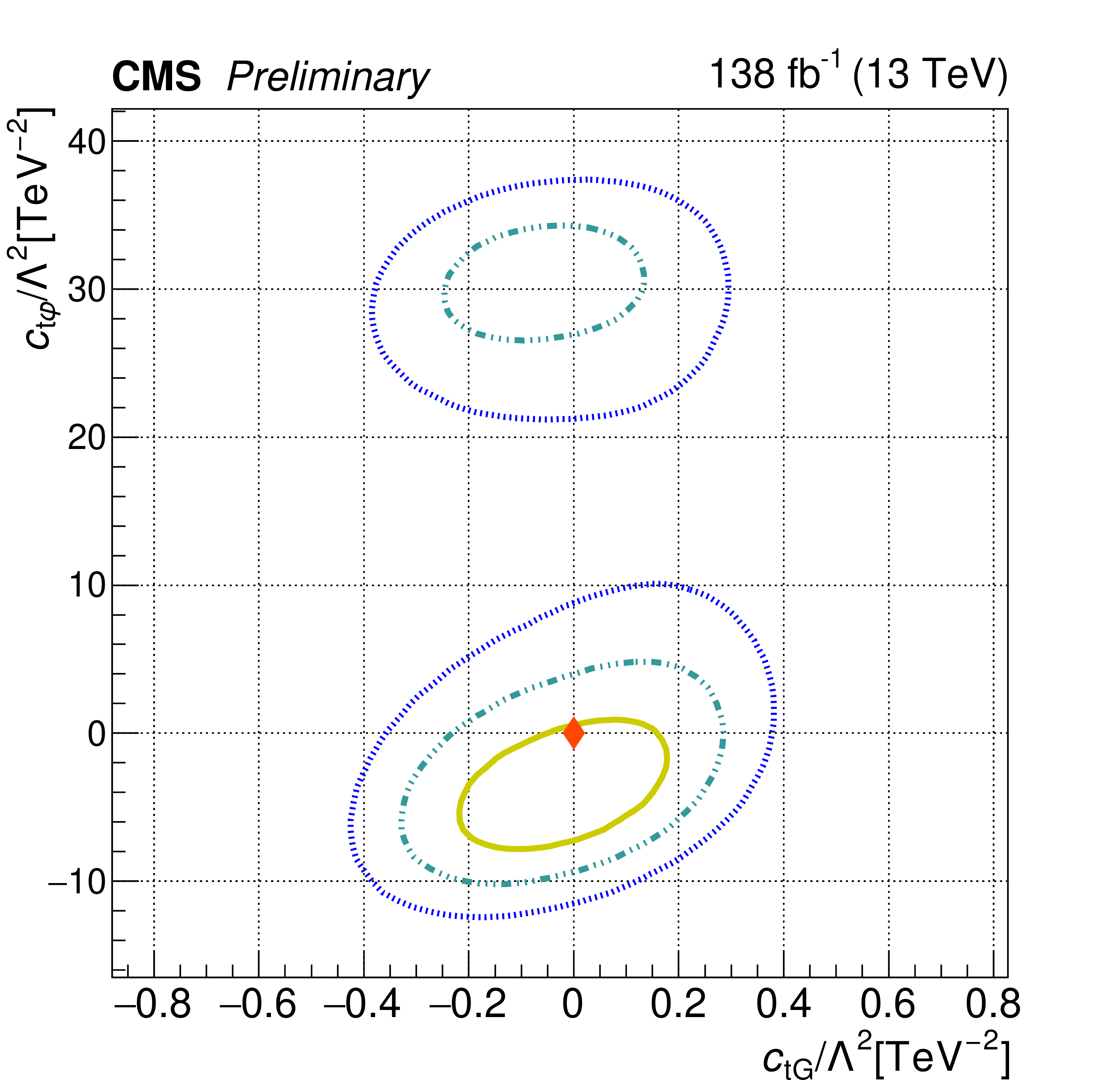
Figure 7-a:
The observed 68.3%, 95.5%, and 99.7% confidence contours of a 2D scan for $c_{\mathrm{tG}}$ and $c_{\mathrm{t}\varphi}$ with the other WCs profiled (left), and fixed to their SM values (right). Diamond markers show the SM prediction. |
png pdf |
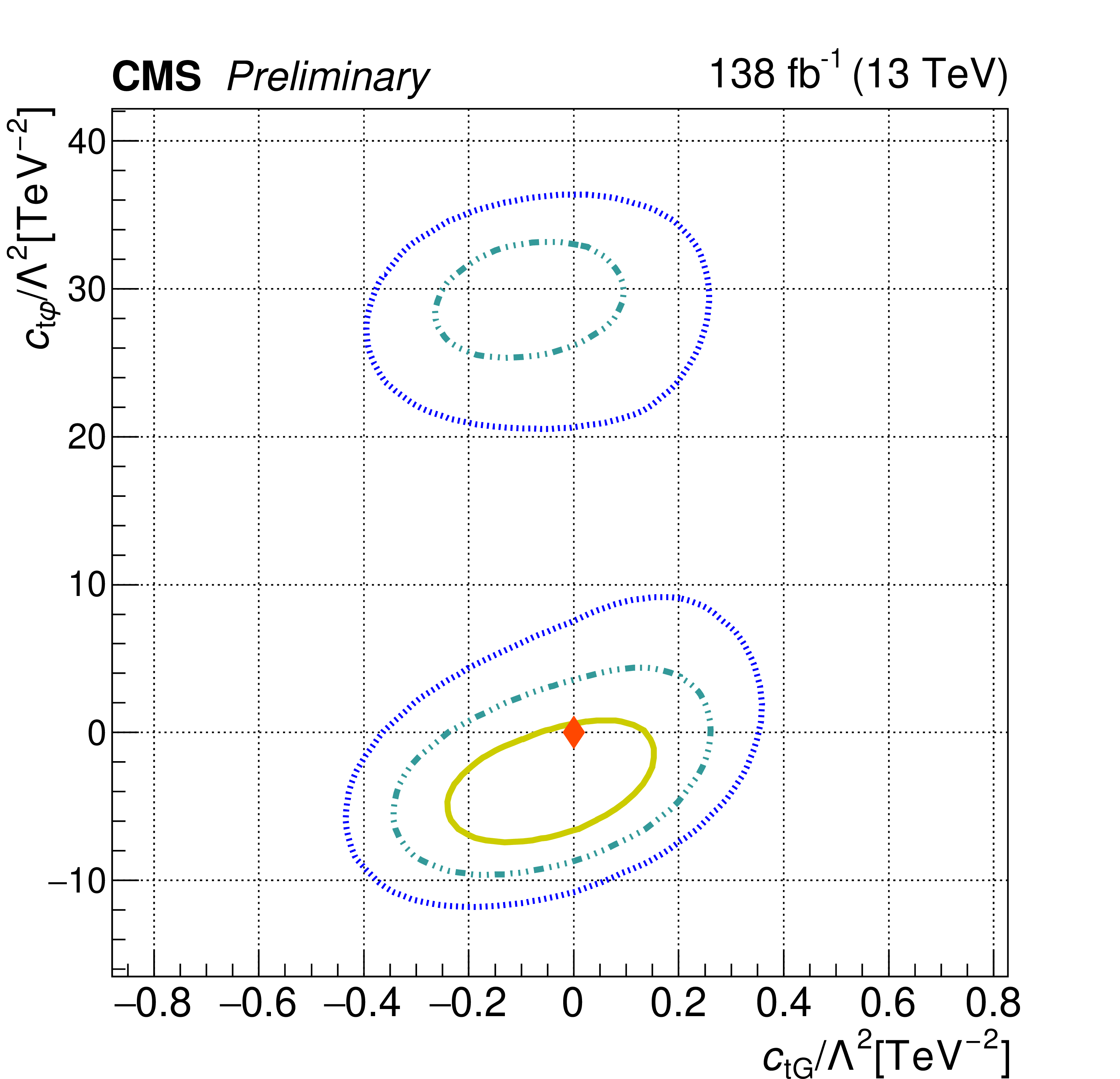
Figure 7-b:
The observed 68.3%, 95.5%, and 99.7% confidence contours of a 2D scan for $c_{\mathrm{tG}}$ and $c_{\mathrm{t}\varphi}$ with the other WCs profiled (left), and fixed to their SM values (right). Diamond markers show the SM prediction. |
png pdf |
Figure 7-c:
The observed 68.3%, 95.5%, and 99.7% confidence contours of a 2D scan for $c_{\mathrm{tG}}$ and $c_{\mathrm{t}\varphi}$ with the other WCs profiled (left), and fixed to their SM values (right). Diamond markers show the SM prediction. |
png pdf |
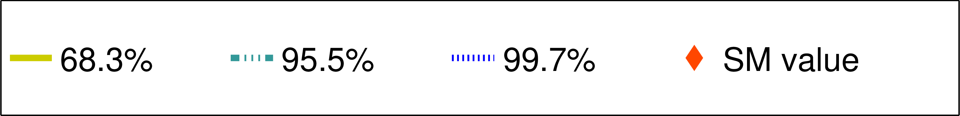
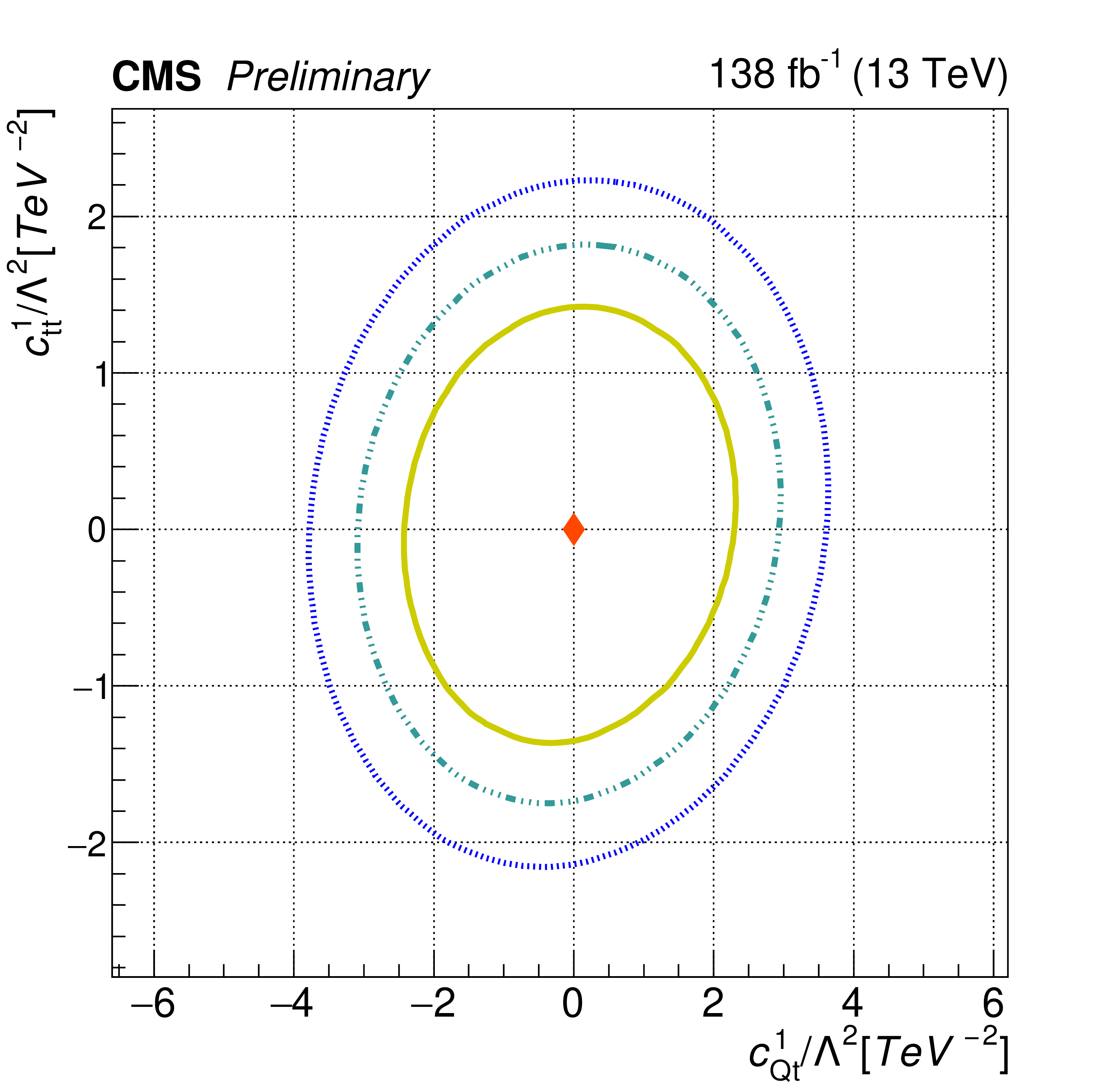
Figure 8:
The observed 68.3%, 95.5%, and 99.7% confidence contours of a 2D scan for $c^{1}_{\mathrm{Qt}}$ and \eftOp1$ \mathrm{t} \mathrm{t} ${c} with the other WCs profiled (left), and fixed to their SM values (right). Diamond markers show the SM prediction. |
png pdf |
Figure 8-a:
The observed 68.3%, 95.5%, and 99.7% confidence contours of a 2D scan for $c^{1}_{\mathrm{Qt}}$ and \eftOp1$ \mathrm{t} \mathrm{t} ${c} with the other WCs profiled (left), and fixed to their SM values (right). Diamond markers show the SM prediction. |

png pdf |
Figure 8-b:
The observed 68.3%, 95.5%, and 99.7% confidence contours of a 2D scan for $c^{1}_{\mathrm{Qt}}$ and \eftOp1$ \mathrm{t} \mathrm{t} ${c} with the other WCs profiled (left), and fixed to their SM values (right). Diamond markers show the SM prediction. |
png pdf |
Figure 8-c:
The observed 68.3%, 95.5%, and 99.7% confidence contours of a 2D scan for $c^{1}_{\mathrm{Qt}}$ and \eftOp1$ \mathrm{t} \mathrm{t} ${c} with the other WCs profiled (left), and fixed to their SM values (right). Diamond markers show the SM prediction. |
png pdf |
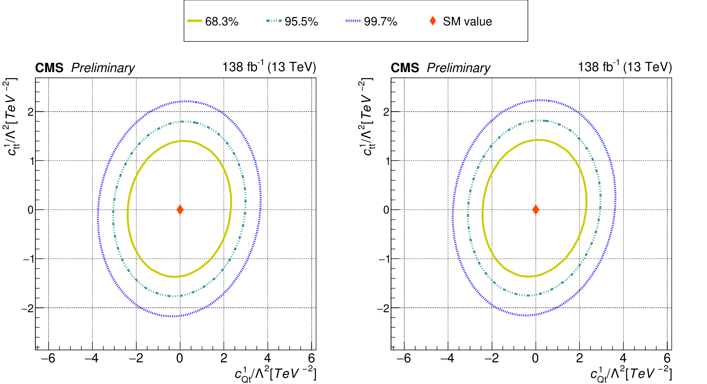
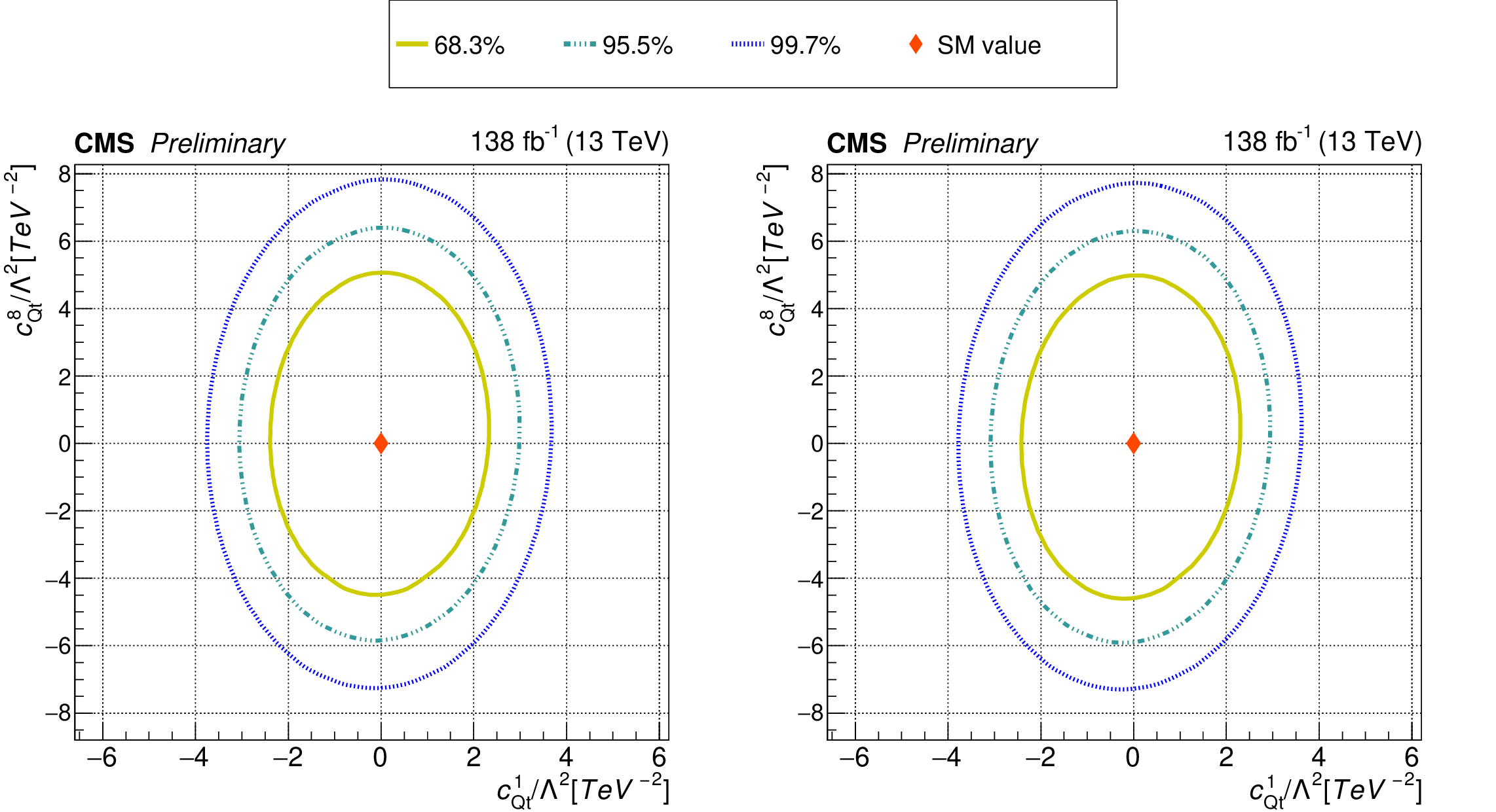
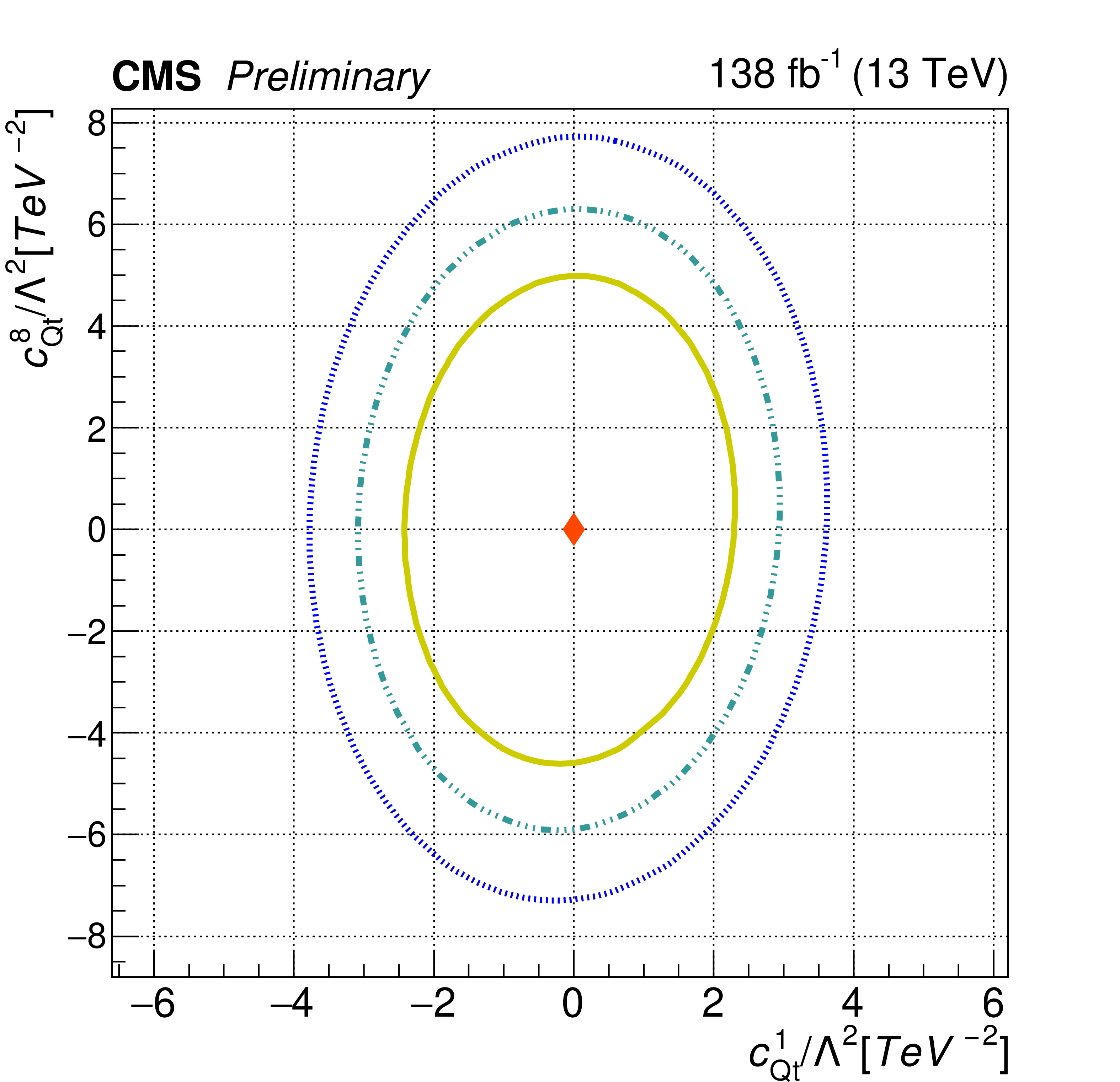
Figure 9:
The observed 68.3%, 95.5%, and 99.7% confidence contours of a 2D scan for $c^{1}_{\mathrm{Qt}}$ and $c^{8}_{\mathrm{Qt}}$ with the other WCs profiled (left), and fixed to their SM values (right). Diamond markers show the SM prediction. |

png pdf |
Figure 9-a:
The observed 68.3%, 95.5%, and 99.7% confidence contours of a 2D scan for $c^{1}_{\mathrm{Qt}}$ and $c^{8}_{\mathrm{Qt}}$ with the other WCs profiled (left), and fixed to their SM values (right). Diamond markers show the SM prediction. |

png pdf |
Figure 9-b:
The observed 68.3%, 95.5%, and 99.7% confidence contours of a 2D scan for $c^{1}_{\mathrm{Qt}}$ and $c^{8}_{\mathrm{Qt}}$ with the other WCs profiled (left), and fixed to their SM values (right). Diamond markers show the SM prediction. |
png pdf |
Figure 9-c:
The observed 68.3%, 95.5%, and 99.7% confidence contours of a 2D scan for $c^{1}_{\mathrm{Qt}}$ and $c^{8}_{\mathrm{Qt}}$ with the other WCs profiled (left), and fixed to their SM values (right). Diamond markers show the SM prediction. |
png pdf |
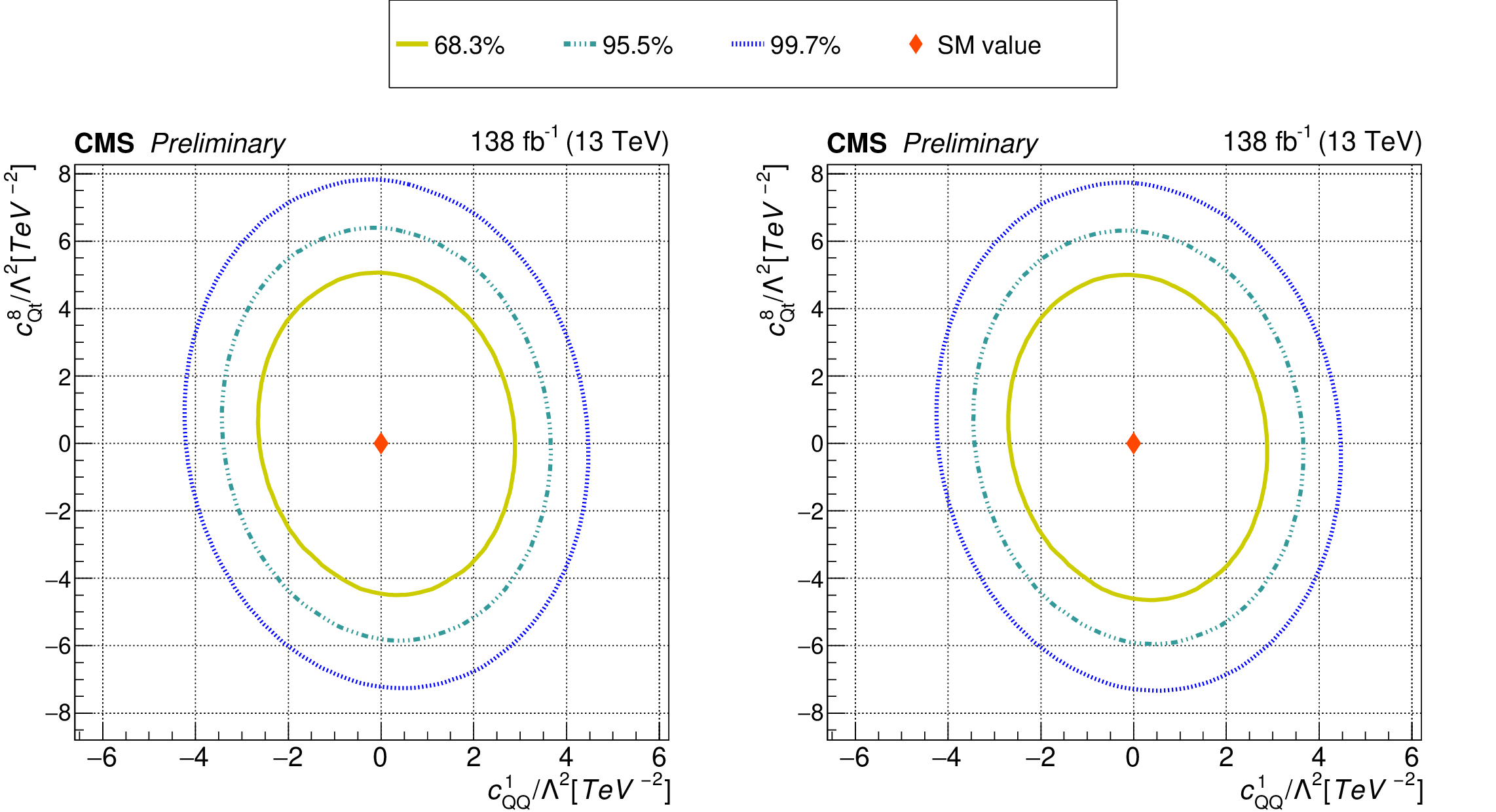
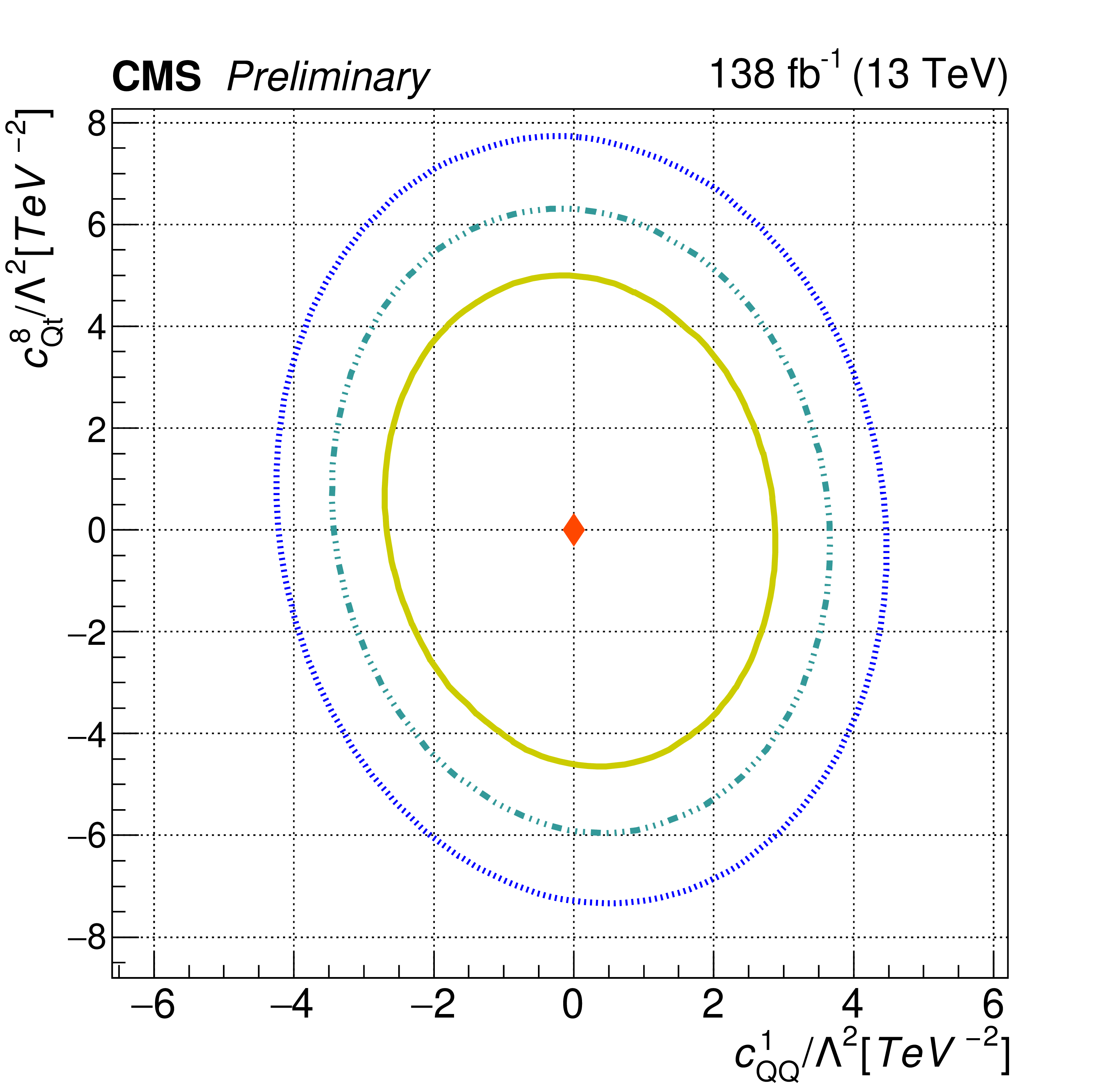
Figure 10:
The observed 68.3%, 95.5%, and 99.7% confidence contours of a 2D scan for $c^{1}_{\mathrm{QQ}}$ and $c^{8}_{\mathrm{Qt}}$ with the other WCs profiled (left), and fixed to their SM values (right). Diamond markers show the SM prediction. |

png pdf |
Figure 10-a:
The observed 68.3%, 95.5%, and 99.7% confidence contours of a 2D scan for $c^{1}_{\mathrm{QQ}}$ and $c^{8}_{\mathrm{Qt}}$ with the other WCs profiled (left), and fixed to their SM values (right). Diamond markers show the SM prediction. |

png pdf |
Figure 10-b:
The observed 68.3%, 95.5%, and 99.7% confidence contours of a 2D scan for $c^{1}_{\mathrm{QQ}}$ and $c^{8}_{\mathrm{Qt}}$ with the other WCs profiled (left), and fixed to their SM values (right). Diamond markers show the SM prediction. |
png pdf |
Figure 10-c:
The observed 68.3%, 95.5%, and 99.7% confidence contours of a 2D scan for $c^{1}_{\mathrm{QQ}}$ and $c^{8}_{\mathrm{Qt}}$ with the other WCs profiled (left), and fixed to their SM values (right). Diamond markers show the SM prediction. |
png pdf |
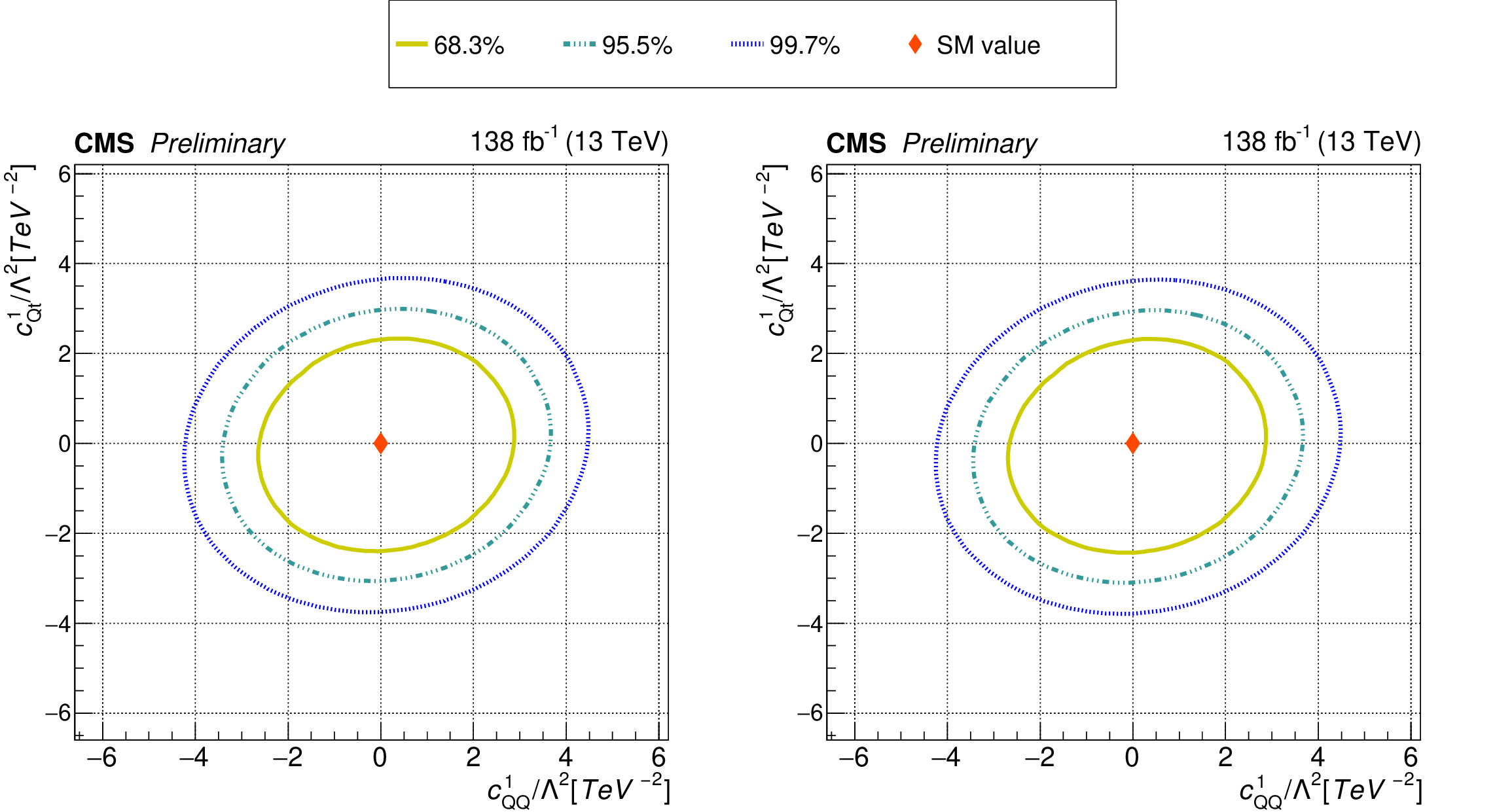
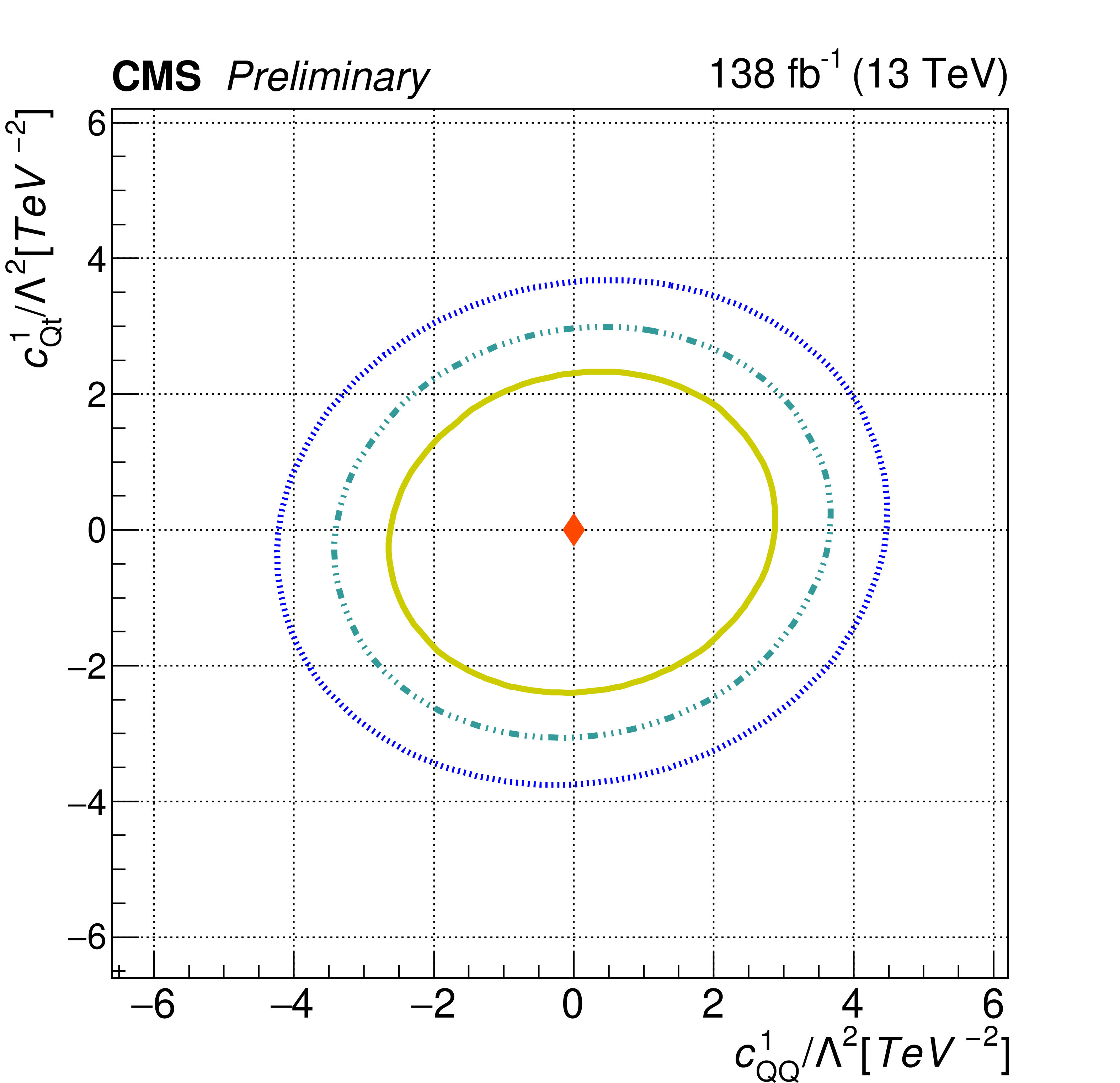
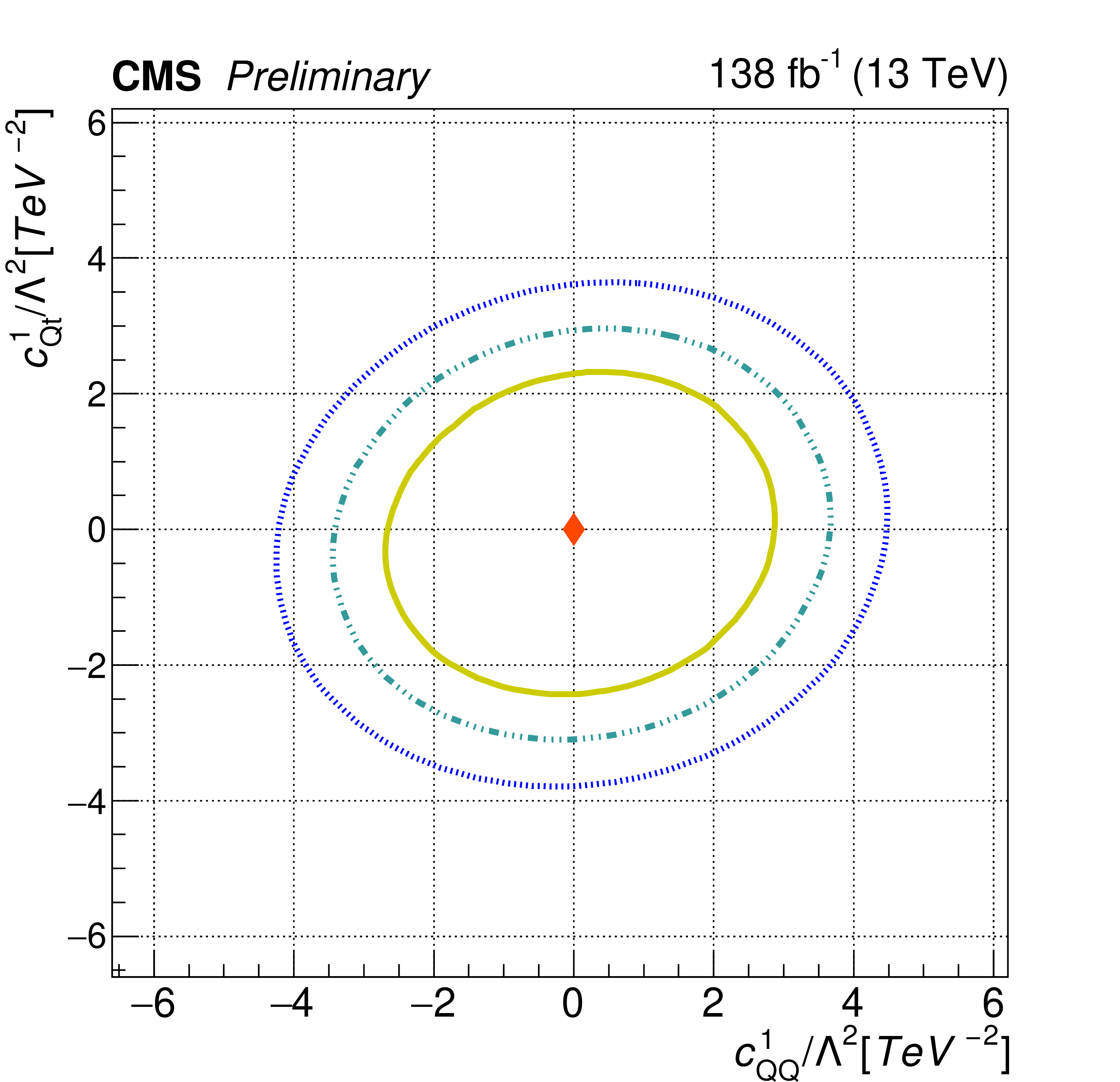
Figure 11:
The observed 68.3%, 95.5%, and 99.7% confidence contours of a 2D scan for $c^{1}_{\mathrm{QQ}}$ and $c^{1}_{\mathrm{Qt}}$ with the other WCs profiled (left), and fixed to their SM values (right). Diamond markers show the SM prediction. |

png pdf |
Figure 11-a:
The observed 68.3%, 95.5%, and 99.7% confidence contours of a 2D scan for $c^{1}_{\mathrm{QQ}}$ and $c^{1}_{\mathrm{Qt}}$ with the other WCs profiled (left), and fixed to their SM values (right). Diamond markers show the SM prediction. |
png pdf |
Figure 11-b:
The observed 68.3%, 95.5%, and 99.7% confidence contours of a 2D scan for $c^{1}_{\mathrm{QQ}}$ and $c^{1}_{\mathrm{Qt}}$ with the other WCs profiled (left), and fixed to their SM values (right). Diamond markers show the SM prediction. |
png pdf |
Figure 11-c:
The observed 68.3%, 95.5%, and 99.7% confidence contours of a 2D scan for $c^{1}_{\mathrm{QQ}}$ and $c^{1}_{\mathrm{Qt}}$ with the other WCs profiled (left), and fixed to their SM values (right). Diamond markers show the SM prediction. |
png pdf |
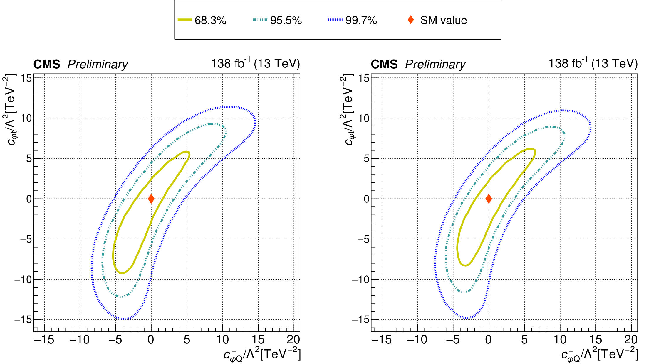
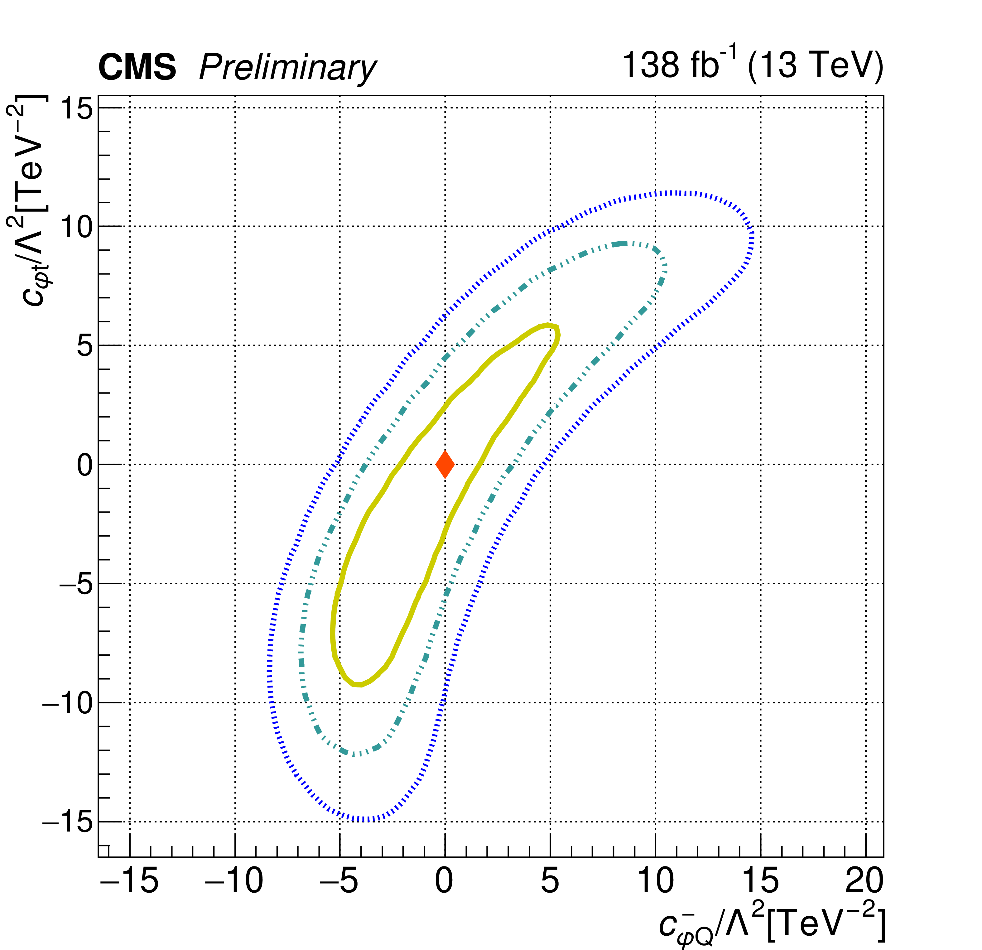
Figure 12:
The observed 68.3%, 95.5%, and 99.7% confidence contours of a 2D scan for $c^{-}_{\varphi\mathrm{Q}}$ and $c_{\varphi\mathrm{t}}$ with the other WCs profiled (left), and fixed to their SM values (right). Diamond markers show the SM prediction. |

png pdf |
Figure 12-a:
The observed 68.3%, 95.5%, and 99.7% confidence contours of a 2D scan for $c^{-}_{\varphi\mathrm{Q}}$ and $c_{\varphi\mathrm{t}}$ with the other WCs profiled (left), and fixed to their SM values (right). Diamond markers show the SM prediction. |
png pdf |
Figure 12-b:
The observed 68.3%, 95.5%, and 99.7% confidence contours of a 2D scan for $c^{-}_{\varphi\mathrm{Q}}$ and $c_{\varphi\mathrm{t}}$ with the other WCs profiled (left), and fixed to their SM values (right). Diamond markers show the SM prediction. |

png pdf |
Figure 12-c:
The observed 68.3%, 95.5%, and 99.7% confidence contours of a 2D scan for $c^{-}_{\varphi\mathrm{Q}}$ and $c_{\varphi\mathrm{t}}$ with the other WCs profiled (left), and fixed to their SM values (right). Diamond markers show the SM prediction. |
| Tables | |
png pdf |
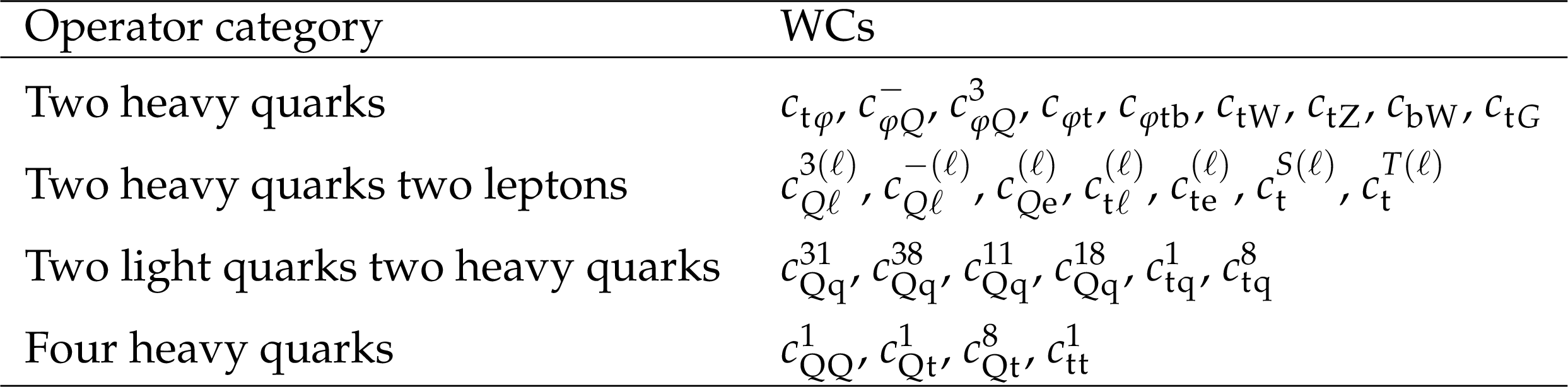
Table 1:
List of WCs included in this analysis. The definitions of the WCs and the definitions of the corresponding operators can be found in Table 1 of Ref. [18]. Note that in order to allow MadGraph-5\_aMC@NLO to properly handle the emission of gluons from the vertices involving the $c_{\mathrm{tG}}$ WC, an extra factor of the strong coupling is applied to the $c_{\mathrm{tG}}$ coefficients. |

png pdf |
Table 2:
NLO theoretical cross sections used for normalizing the signal simulation samples. |
png pdf |
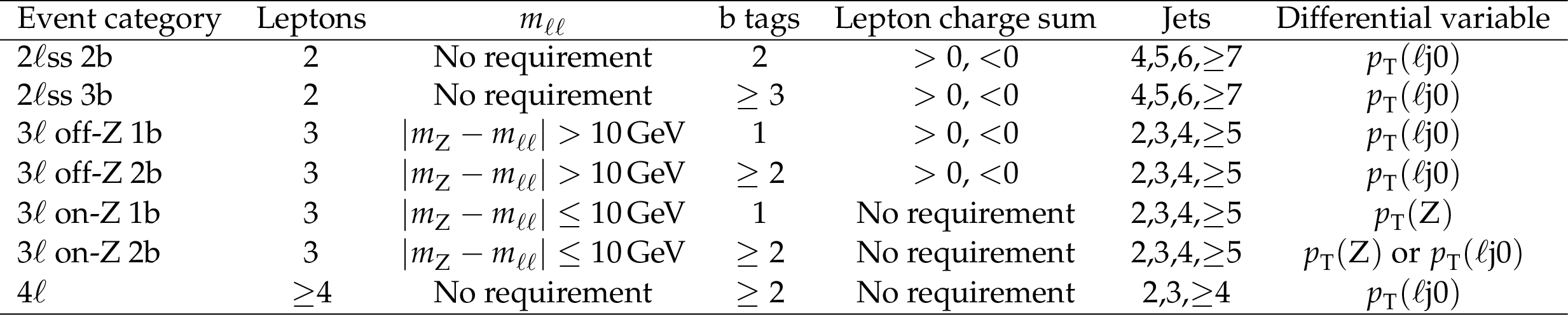
Table 3:
Object requirements for the 43 event selection categories. Requirements separated by commas indicate a division into subcategories. The kinematical variable that is used in the event category is also listed (Section 5.4 provides further details regarding the kinematical distributions). |
png pdf |
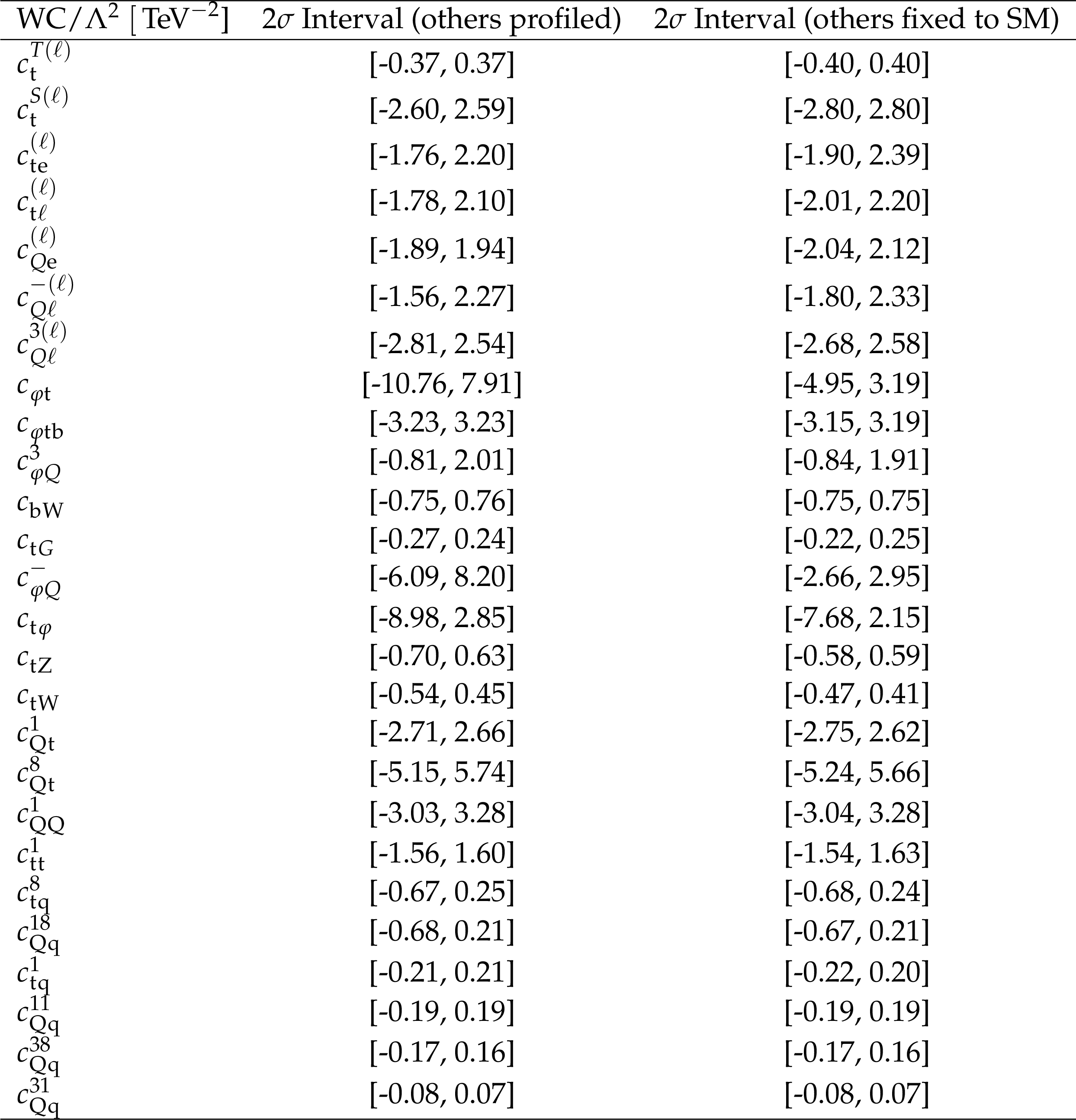
Table 4:
The 2 $ \sigma $ uncertainty intervals extracted from the likelihood fits described in Section 7. The intervals are shown for the case where the other WCs are profiled, and the case where the other WCs are fixed to their SM values of zero. |
png pdf |
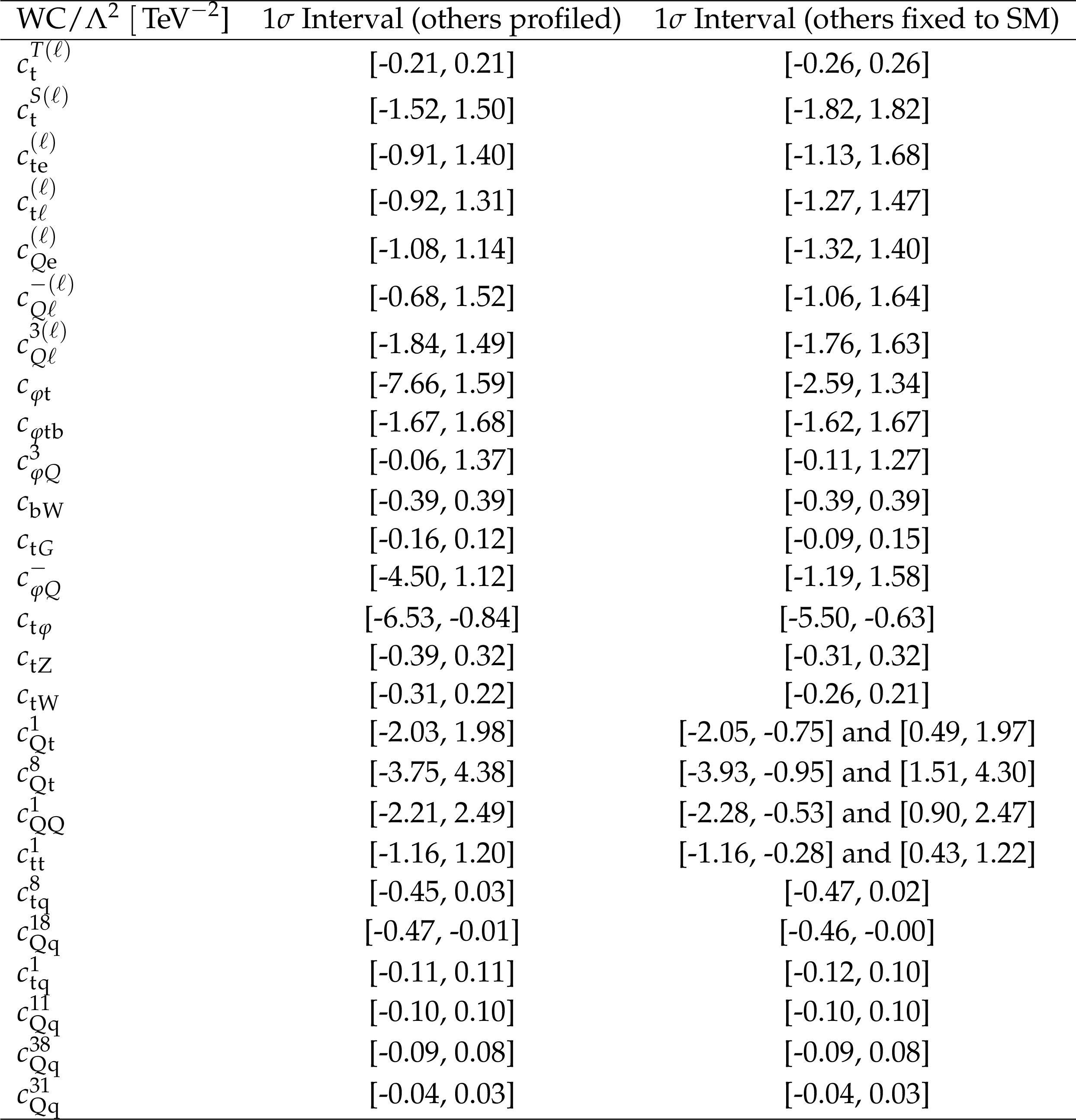
Table 5:
The 1 $ \sigma $ uncertainty intervals extracted from the likelihood fits described in Section 7. The intervals are shown for the case where the other WCs are profiled, and the case where the other WCs are fixed to their SM values of zero. |
png pdf |
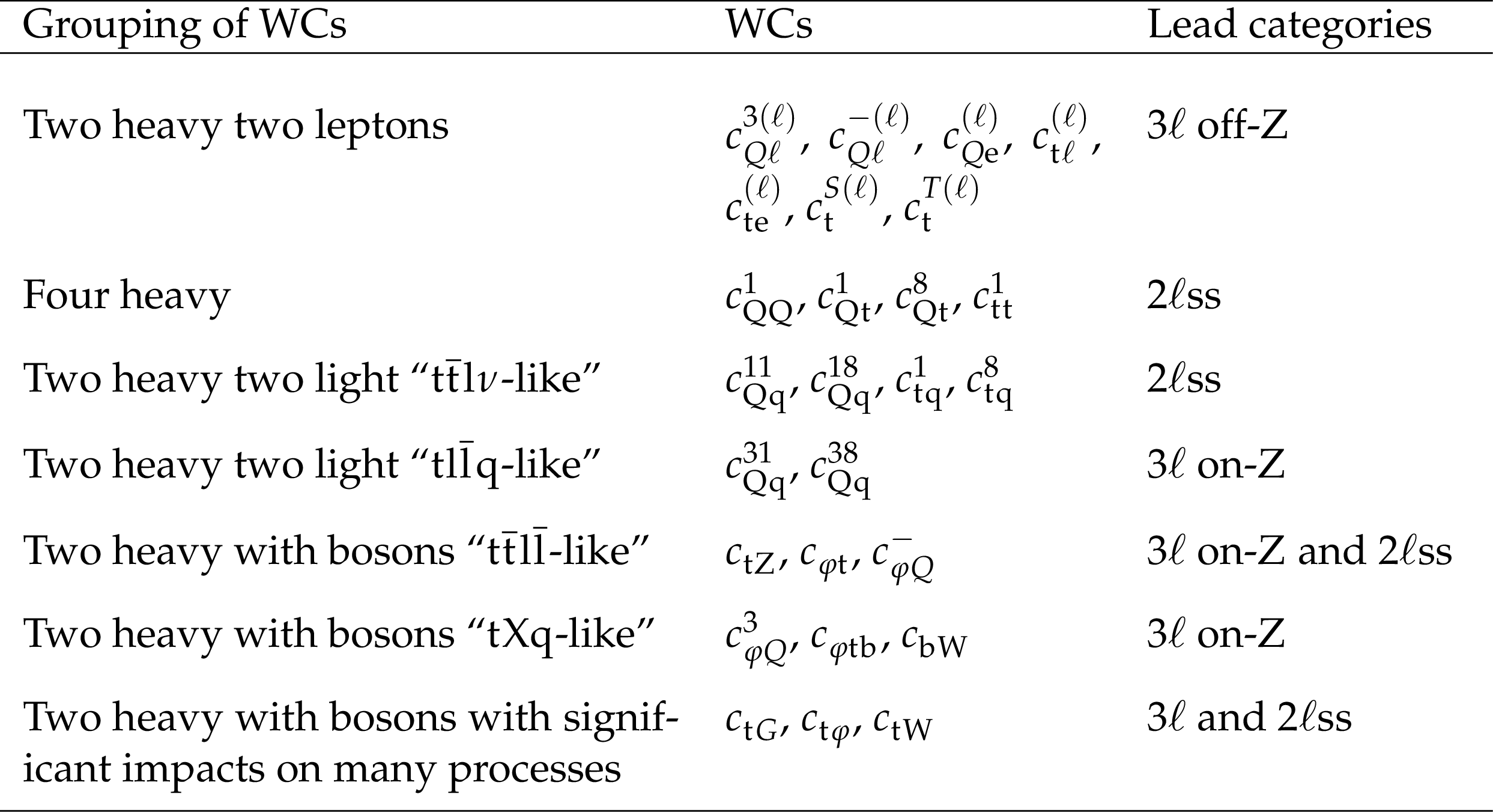
Table 6:
Summary of categories that provide leading contributions to the sensitivity for subsets of the WCs. |
| Summary |
| A search for new physics in the production of one or more top quarks with additional leptons, jets, and b jets in the context of effective field theory (EFT) has been performed. The events come from proton-proton collisions with a center-of-mass-energy of 13TeV corresponding to an integrated luminosity of 138 fb$^{-1}$. The expected yields were parameterized in terms of 26 Wilson coefficients (WCs) corresponding to different EFT operators. EFT effects are incorporated into the event weights of the simulated samples, allowing detector-level predictions that account for correlations and interference effects among EFT operators and between EFT operators and standard model (SM) processes. The WCs were simultaneously fit to the data. Confidence intervals were extracted for the WCs either individually or in pairs by scanning the likelihood with the other WCs either profiled or held at their SM values of zero. In all cases, the data are found to be consistent with the SM expectations. |
| References | ||||
| 1 | J. L. Feng | Dark matter candidates from particle physics and methods of detection | Ann. Rev. Astron. Astrophys. 48 (2010) 495 | 1003.0904 |
| 2 | T. A. Porter, R. P. Johnson, and P. W. Graham | Dark matter searches with astroparticle data | Ann. Rev. Astron. Astrophys. 49 (2011) 155 | 1104.2836 |
| 3 | P. J. E. Peebles and B. Ratra | The Cosmological Constant and Dark Energy | Rev. Mod. Phys. 75 (2003) 559 | astro-ph/0207347 |
| 4 | C. Degrande et al. | Effective Field Theory: A Modern Approach to Anomalous Couplings | Annals Phys. 335 (2013) 21 | 1205.4231 |
| 5 | CDF Collaboration | Observation of top quark production in $ \bar{p}p $ collisions | PRL 74 (1995) 2626 | hep-ex/9503002 |
| 6 | D0 Collaboration | Observation of the top quark | PRL 74 (1995) 2632 | hep-ex/9503003 |
| 7 | Particle Data Group | Review of particle physics | PTEP 2020 (2020) 083C01 | |
| 8 | CMS Collaboration | Search for new physics in top quark production with additional leptons in proton-proton collisions at $ \sqrt{s} = $ 13 TeV using effective field theory | JHEP 03 (2021) 095 | CMS-TOP-19-001 2012.04120 |
| 9 | CMS Collaboration | The CMS experiment at the CERN LHC | JINST 3 (2008) S08004 | |
| 10 | CMS Collaboration | Performance of the CMS Level-1 trigger in proton-proton collisions at $ \sqrt{s} = $ 13\,TeV | JINST 15 (2020) P10017 | CMS-TRG-17-001 2006.10165 |
| 11 | CMS Collaboration | The CMS trigger system | JINST 12 (2017) P01020 | CMS-TRG-12-001 1609.02366 |
| 12 | CMS Collaboration | Precision luminosity measurement in proton-proton collisions at $ \sqrt{s} = $ 13 TeV in 2015 and 2016 at CMS | EPJC 81 (2021) 800 | CMS-LUM-17-003 2104.01927 |
| 13 | CMS Collaboration | CMS luminosity measurement for the 2017 data-taking period at $ \sqrt{s} $ = 13 TeV | CMS Physics Analysis Summary, 2018 link |
CMS-PAS-LUM-17-004 |
| 14 | CMS Collaboration | CMS luminosity measurement for the 2018 data-taking period at $ \sqrt{s} $ = 13 TeV | CMS Physics Analysis Summary, 2019 link |
CMS-PAS-LUM-18-002 |
| 15 | J. Alwall et al. | The automated computation of tree-level and next-to-leading order differential cross sections, and their matching to parton shower simulations | JHEP 07 (2014) 079 | 1405.0301 |
| 16 | R. Frederix and S. Frixione | Merging meets matching in MC@NLO | JHEP 12 (2012) 061 | 1209.6215 |
| 17 | J. Alwall et al. | Comparative study of various algorithms for the merging of parton showers and matrix elements in hadronic collisions | EPJC 53 (2008) 473 | 0706.2569 |
| 18 | D. Barducci et al. | Interpreting top-quark LHC measurements in the standard-model effective field theory | 1802.07237 | |
| 19 | B. Grzadkowski, M. Iskrzynski, M. Misiak, and J. Rosiek | Dimension-Six Terms in the Standard Model Lagrangian | JHEP 10 (2010) 085 | 1008.4884 |
| 20 | LHC Higgs Cross Section Working Group | Handbook of LHC Higgs cross sections: 4. deciphering the nature of the Higgs sector | link | 1610.07922 |
| 21 | R. Frederix and I. Tsinikos | On improving NLO merging for $ \mathrm{t}\overline{\mathrm{t}}\mathrm{W} $ production | JHEP 11 (2021) 029 | 2108.07826 |
| 22 | CMS Collaboration | Search for production of four top quarks in final states with same-sign or multiple leptons in proton-proton collisions at $ \sqrt{s}= $ 13 TeV | EPJC 80 (2020) 75 | CMS-TOP-18-003 1908.06463 |
| 23 | O. Mattelaer | On the maximal use of Monte Carlo samples: re-weighting events at NLO accuracy | EPJC 76 (2016) 674 | 1607.00763 |
| 24 | R. Goldouzian et al. | Matching in $ pp\to t\overline{t}W/Z/h+ $ jet SMEFT studies | JHEP 06 (2021) 151 | 2012.06872 |
| 25 | CMS Collaboration | Particle-flow reconstruction and global event description with the CMS detector | JINST 12 (2017) P10003 | CMS-PRF-14-001 1706.04965 |
| 26 | CMS Collaboration | Electron and photon reconstruction and identification with the CMS experiment at the CERN LHC | JINST 16 (2021) P05014 | CMS-EGM-17-001 2012.06888 |
| 27 | CMS Collaboration | ECAL 2016 refined calibration and Run2 summary plots | CMS Detector Performance Summary CMS-DP-2020-021, 2020 CDS |
|
| 28 | CMS Collaboration | Performance of the CMS muon detector and muon reconstruction with proton-proton collisions at $ \sqrt{s}= $ 13 TeV | JINST 13 (2018) P06015 | CMS-MUO-16-001 1804.04528 |
| 29 | CMS Collaboration | Measurement of the Higgs boson production rate in association with top quarks in final states with electrons, muons, and hadronically decaying tau leptons at $ \sqrt{s} = $ 13 TeV | no.~4, 378, 2021 EPJC 81 (2021) |
CMS-HIG-19-008 2011.03652 |
| 30 | M. Cacciari, G. P. Salam, and G. Soyez | The anti-$ k_{\mathrm{t}} $ jet clustering algorithm | JHEP 04 (2008) 063 | 0802.1189 |
| 31 | M. Cacciari, G. P. Salam, and G. Soyez | FastJet user manual | EPJC 72 (2012) 1896 | 1111.6097 |
| 32 | CMS Collaboration | Jet energy scale and resolution in the CMS experiment in pp collisions at 8 TeV | JINST 12 (2017) P02014 | CMS-JME-13-004 1607.03663 |
| 33 | CMS Collaboration | Identification of heavy-flavour jets with the CMS detector in pp collisions at 13 TeV | JINST 13 (2018) P05011 | CMS-BTV-16-002 1712.07158 |
| 34 | E. Bols et al. | Jet Flavour Classification Using DeepJet | JINST 15 (2020) P1 | 2008.10519 |
| 35 | CMS Collaboration | Performance of the DeepJet b tagging algorithm using 41.9/fb of data from proton-proton collisions at 13 TeV with Phase 1 CMS detector | CMS Detector Performance Note CMS-DP-2018-058, 2018 CDS |
|
| 36 | M. Grazzini et al. | NNLO QCD + NLO EW with Matrix+OpenLoops: precise predictions for vector-boson pair production | JHEP 02 (2020) 087 | 1912.00068 |
| 37 | P. Nason | A new method for combining NLO QCD with shower Monte Carlo algorithms | JHEP 11 (2004) 040 | hep-ph/0409146 |
| 38 | S. Frixione, P. Nason, and C. Oleari | Matching NLO QCD computations with parton shower simulations: the POWHEG method | JHEP 11 (2007) 070 | 0709.2092 |
| 39 | F. Caola, K. Melnikov, R. Röntsch, and L. Tancredi | QCD corrections to ZZ production in gluon fusion at the LHC | PRD 92 (2015) 094028 | 1509.06734 |
| 40 | CMS Collaboration | Measurements of inclusive W and Z cross sections in pp collisions at $ \sqrt{s}= $ 7 TeV | JHEP 01 (2011) 080 | CMS-EWK-10-002 1012.2466 |
|
|
Compact Muon Solenoid LHC, CERN |
|

|

|

|

|

|