

Compact Muon Solenoid
LHC, CERN
| CMS-PAS-SUS-21-008 | ||
| Combined search for electroweak production of winos, binos, higgsinos, and sleptons in proton-proton collisions at $ \sqrt{s}= $ 13 TeV | ||
| CMS Collaboration | ||
| 24 March 2023 | ||
| Abstract: A combination of several searches for the electroweak production of winos, binos, higgsinos, and sleptons is presented. All searches use proton-proton collision data at $ \sqrt{s}= $ 13 TeV recorded with the CMS detector at the LHC during years 2016-2018. The analyzed data set corresponds to an integrated luminosity of 137 fb$ ^{-1} $. The results are interpreted in simplified models of chargino-neutralino, neutralino, or slepton pair production. In addition to the previously published searches, the combination includes results from an updated version of the search targeting events with two low-momentum leptons and missing transverse momentum. A parametric signal extraction is introduced that enhances the sensitivity to each signal hypothesis, along with a signal selection optimized to search for slepton pair production in models with compressed spectra. In addition to the models previously considered, the results of the combination are interpreted in a scenario where neutralinos and charginos in a mass-degenerate higgsino triplet are produced and decay to SM bosons and a bino-like LSP. The results are consistent with expectations from the standard model. The combination provides a more comprehensive coverage of the model parameter space than the individual searches, and adds sensitivity in the compressed mass parameter regions. | ||
|
Links:
CDS record (PDF) ;
CADI line (restricted) ;
These preliminary results are superseded in this paper, Submitted to PRD. The superseded preliminary plots can be found here. |
||
| Figures | |
png pdf |
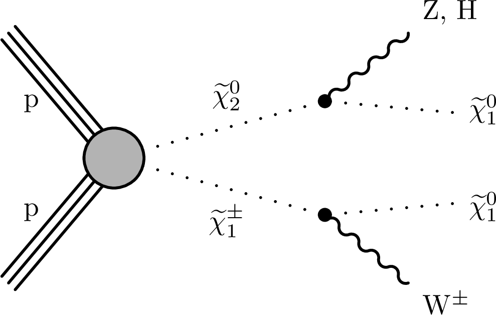
Figure 1:
Production of $ \tilde{\chi}_{1}^{\pm} $ and $ \tilde{\chi}_{2}^{0} $, with the $ \tilde{\chi}_{1}^{\pm} $ decaying to a W boson and a $ \tilde{\chi}_{1}^{0} $, and the $ \tilde{\chi}_{2}^{0} $ decaying to either a Z or H boson and a $ \tilde{\chi}_{1}^{0} $. |
png pdf |
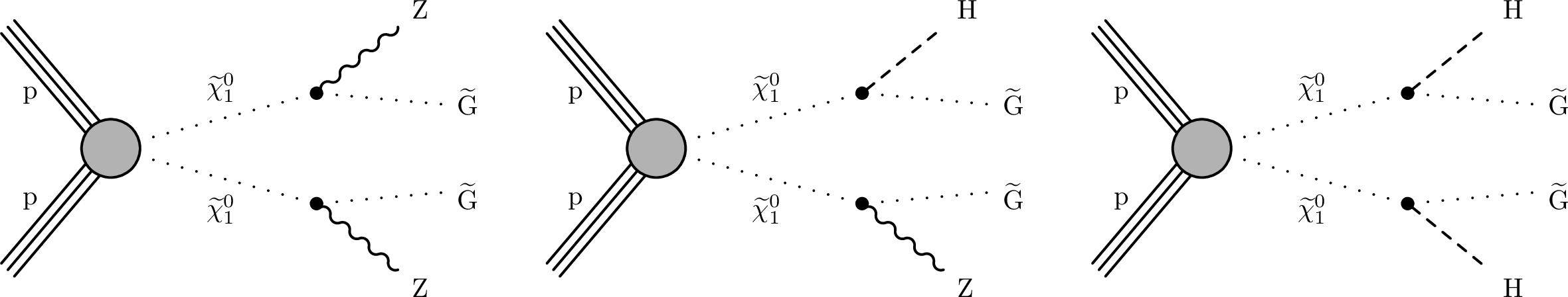
Figure 2:
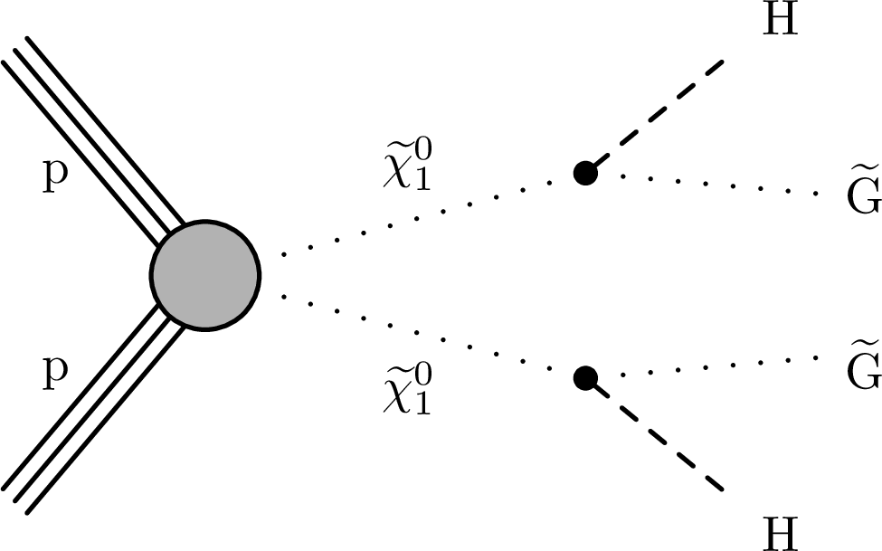
Pair production of $ \tilde{\chi}_{1}^{0} \tilde{\chi}_{1}^{0} $ assuming the GMSB quasi-degenerate higgsino model. The $ \tilde{\chi}_{1}^{0} $ particles each decay to a $ \tilde{\mathrm{G}} $ with the emission of an SM gauge boson: (left) both Z, (center) one Z and the other H, or (right) both H. Soft fermions from decays of nearly degenerate neutralinos and charginos are omitted. |
png pdf |
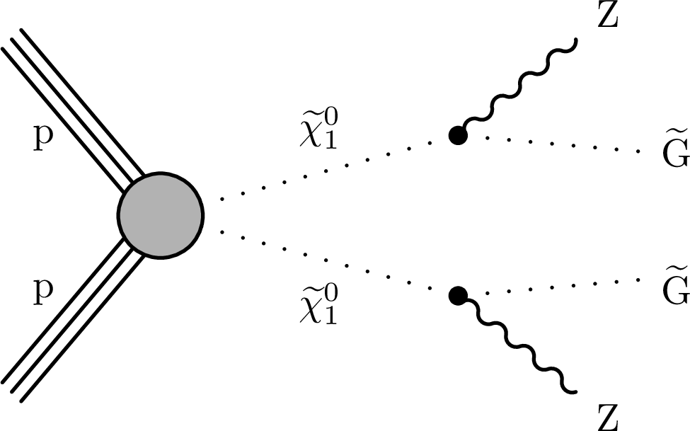
Figure 2-a:
Pair production of $ \tilde{\chi}_{1}^{0} \tilde{\chi}_{1}^{0} $ assuming the GMSB quasi-degenerate higgsino model. The $ \tilde{\chi}_{1}^{0} $ particles each decay to a $ \tilde{\mathrm{G}} $ with the emission of an SM gauge boson: (left) both Z, (center) one Z and the other H, or (right) both H. Soft fermions from decays of nearly degenerate neutralinos and charginos are omitted. |
png pdf |
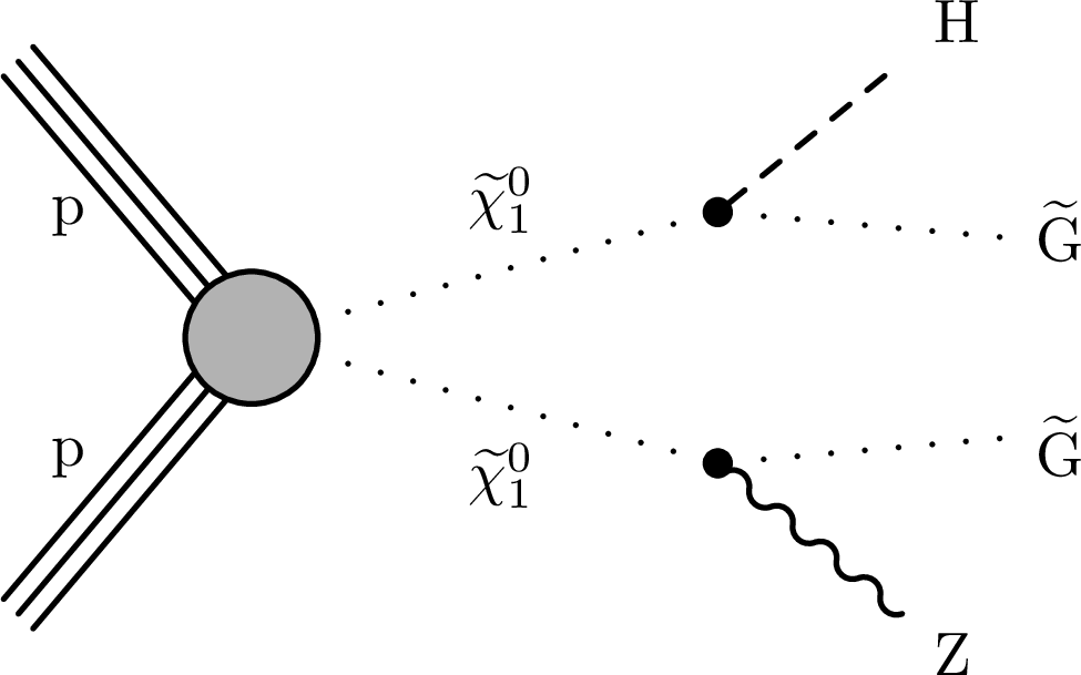
Figure 2-b:
Pair production of $ \tilde{\chi}_{1}^{0} \tilde{\chi}_{1}^{0} $ assuming the GMSB quasi-degenerate higgsino model. The $ \tilde{\chi}_{1}^{0} $ particles each decay to a $ \tilde{\mathrm{G}} $ with the emission of an SM gauge boson: (left) both Z, (center) one Z and the other H, or (right) both H. Soft fermions from decays of nearly degenerate neutralinos and charginos are omitted. |
png pdf |
Figure 2-c:
Pair production of $ \tilde{\chi}_{1}^{0} \tilde{\chi}_{1}^{0} $ assuming the GMSB quasi-degenerate higgsino model. The $ \tilde{\chi}_{1}^{0} $ particles each decay to a $ \tilde{\mathrm{G}} $ with the emission of an SM gauge boson: (left) both Z, (center) one Z and the other H, or (right) both H. Soft fermions from decays of nearly degenerate neutralinos and charginos are omitted. |
png pdf |
Figure 3:
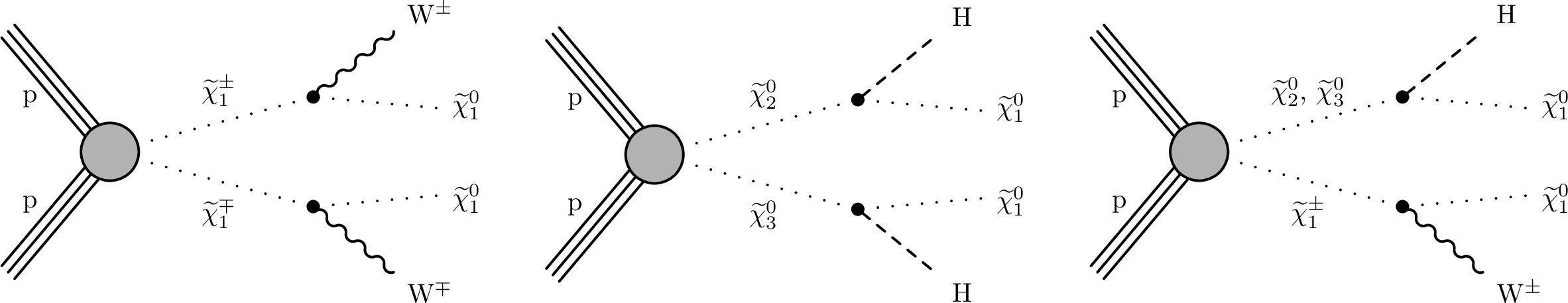
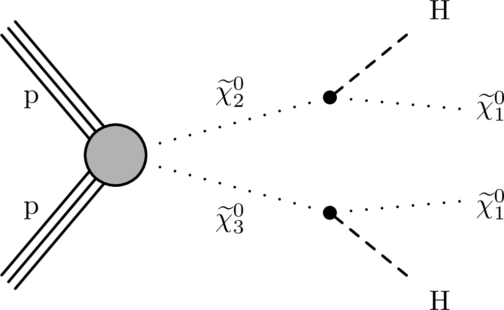
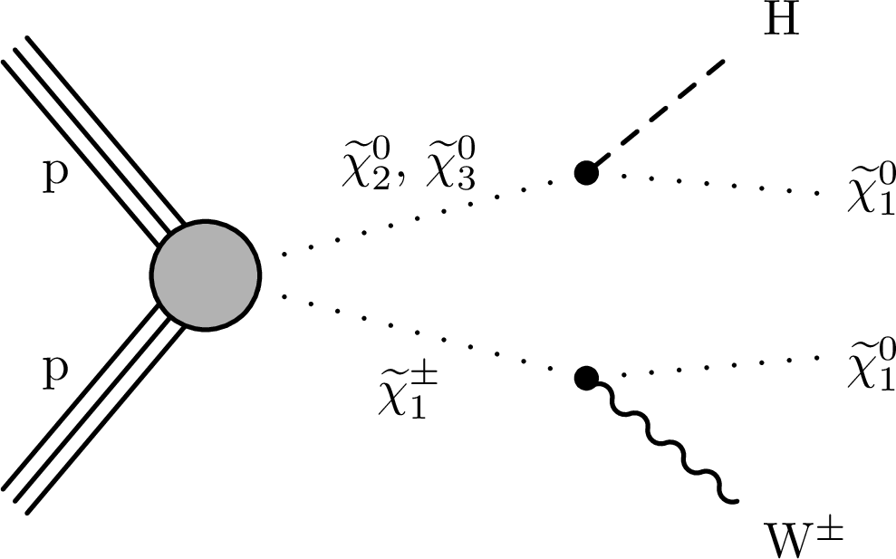
Production and decay modes used for the higgsino-bino interpretations, showing (left) the production of a pair of charginos followed by their decays to W bosons and the LSP, (middle) the production of a pair of neutralinos followed by decays to H bosons and the LSP and (right) the production of chargino-neutralino pairs followed by decays of the charginos (neutralinos) to a W (H) boson and the LSP. |

png pdf |
Figure 3-a:
Production and decay modes used for the higgsino-bino interpretations, showing (left) the production of a pair of charginos followed by their decays to W bosons and the LSP, (middle) the production of a pair of neutralinos followed by decays to H bosons and the LSP and (right) the production of chargino-neutralino pairs followed by decays of the charginos (neutralinos) to a W (H) boson and the LSP. |
png pdf |
Figure 3-b:
Production and decay modes used for the higgsino-bino interpretations, showing (left) the production of a pair of charginos followed by their decays to W bosons and the LSP, (middle) the production of a pair of neutralinos followed by decays to H bosons and the LSP and (right) the production of chargino-neutralino pairs followed by decays of the charginos (neutralinos) to a W (H) boson and the LSP. |
png pdf |
Figure 3-c:
Production and decay modes used for the higgsino-bino interpretations, showing (left) the production of a pair of charginos followed by their decays to W bosons and the LSP, (middle) the production of a pair of neutralinos followed by decays to H bosons and the LSP and (right) the production of chargino-neutralino pairs followed by decays of the charginos (neutralinos) to a W (H) boson and the LSP. |
png pdf |
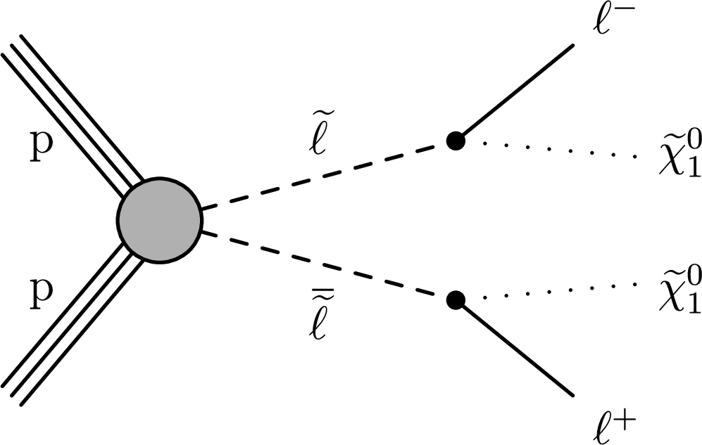
Figure 4:
Direct slepton pair production, with each slepton decaying into a lepton and a $ \tilde{\chi}_{1}^{0} $ LSP. |
png pdf |
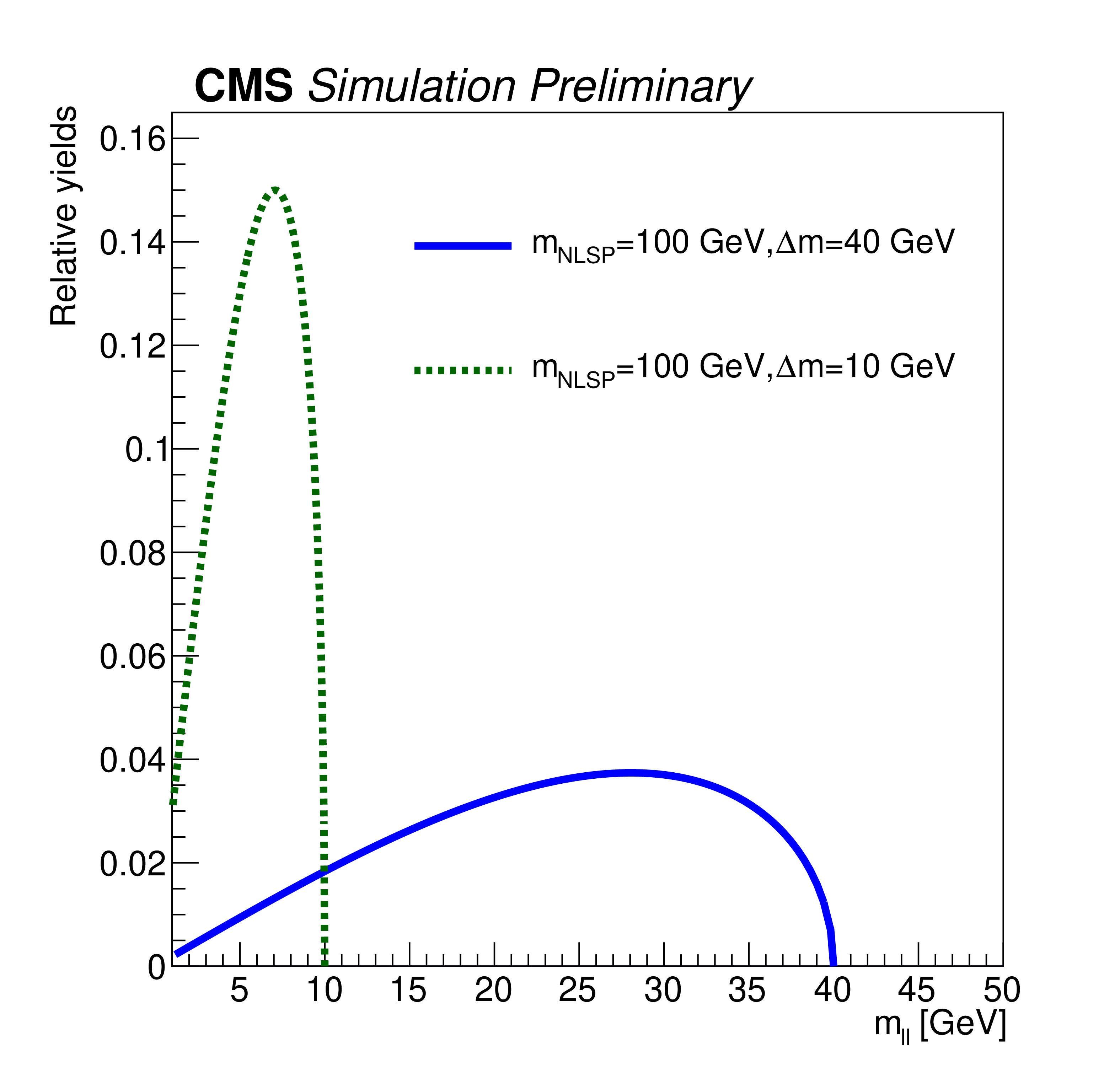
Figure 5:
The ``2/3$\ell $ soft'' dilepton mass spectrum for two mass hypotheses with the same NLSP mass (100 GeV) and different mass splittings $ \Delta m $ (40 or 10 GeV), both corresponding to analytical phase space only calculations. The distributions have a kinematic endpoint at the mass splitting. |

png pdf |
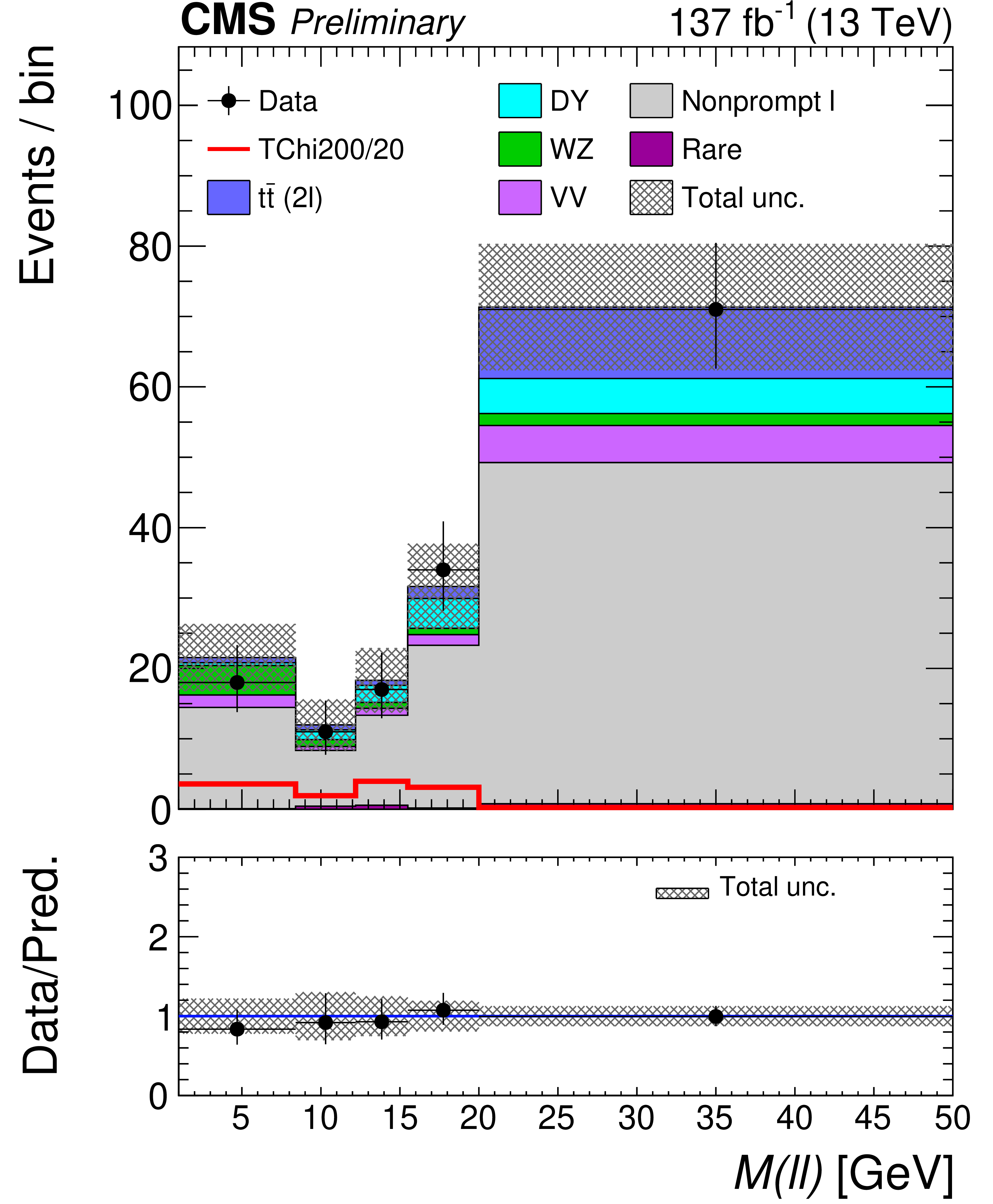
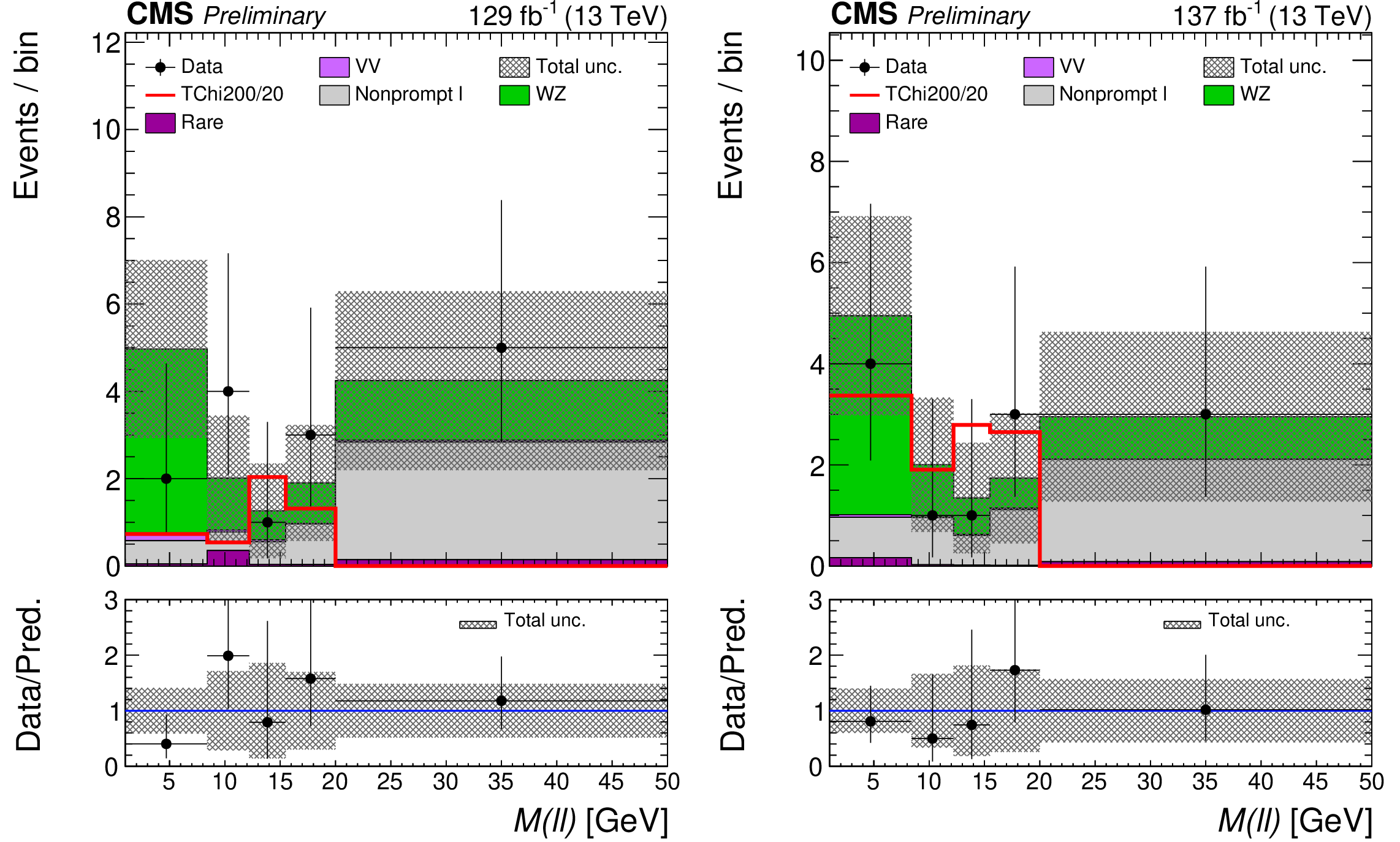
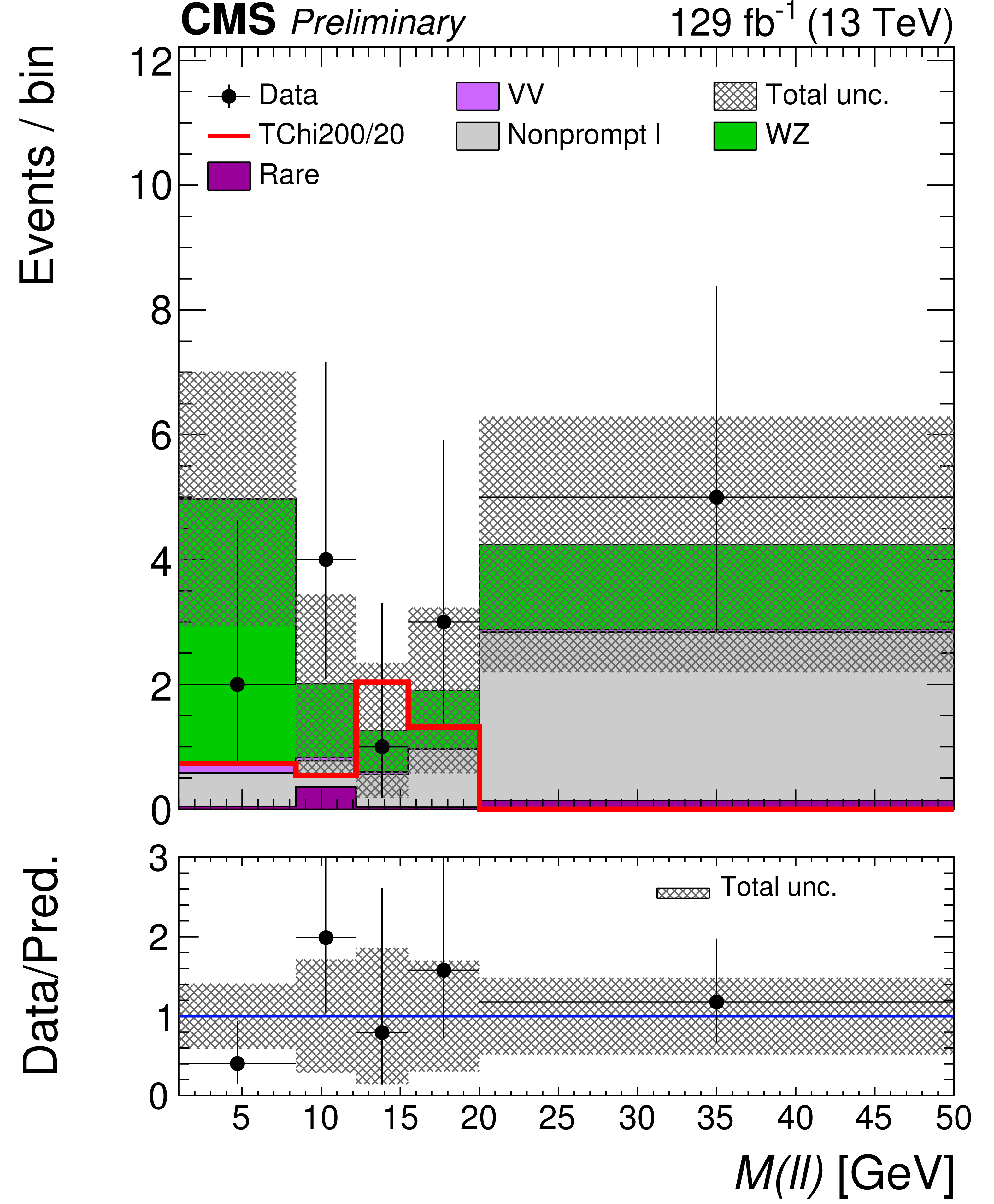
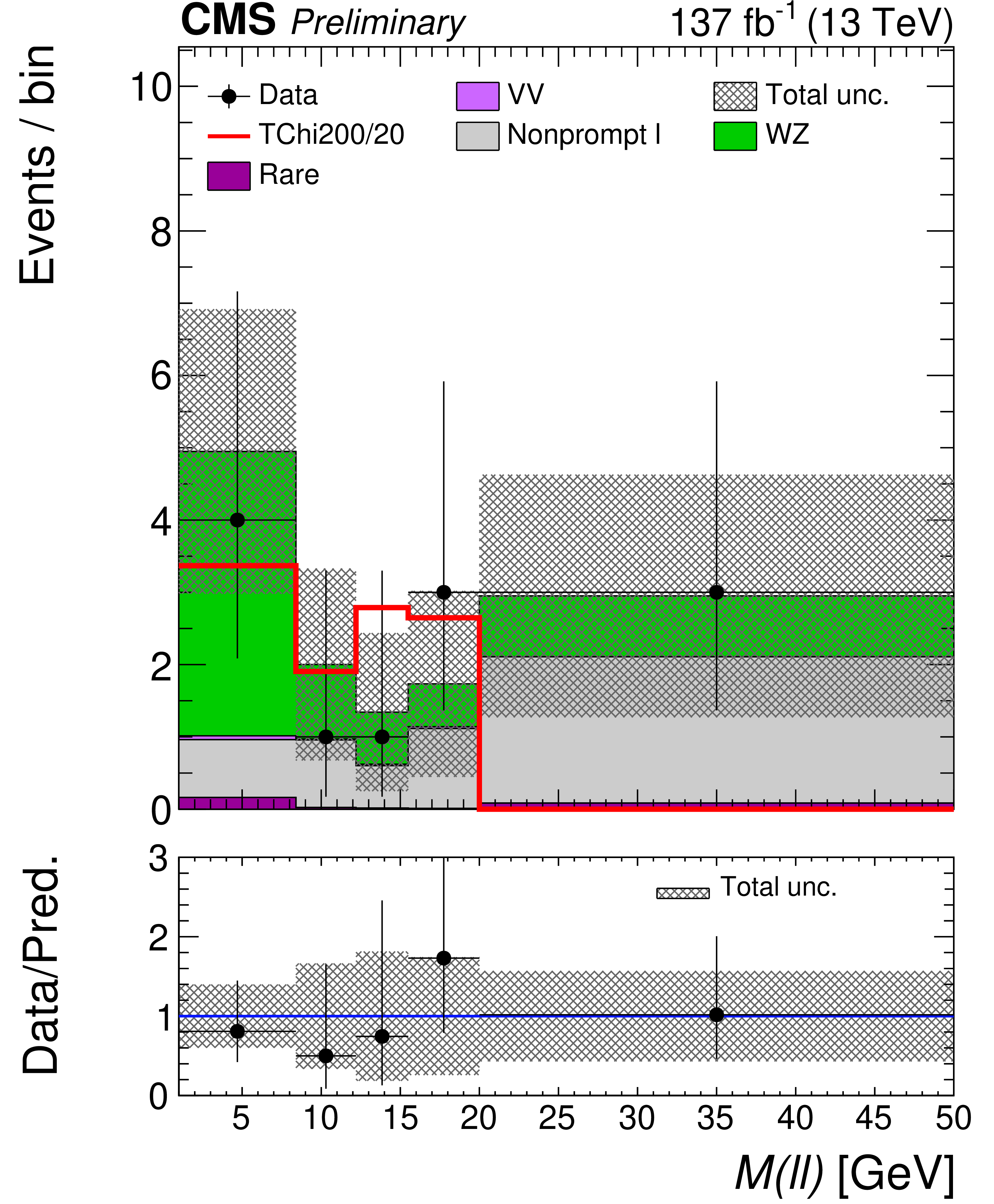
Figure 6:
Post-fit distributions of the $ m_{\ell\ell} $ variable for the low- (upper left), medium- (upper right), high- (bottom left) and ultra- (bottom right) $ p_{\mathrm{T}}^\text{miss} $ bins in the ``2$\ell $ soft'' signal region of Ref. [17]. These distributions are based on the parametric binnings derived for signal mass points with $ \Delta m $ = 20 GeV. The pre-fit signal distribution is overlaid for illustration. |

png pdf |
Figure 6-a:
Post-fit distributions of the $ m_{\ell\ell} $ variable for the low- (upper left), medium- (upper right), high- (bottom left) and ultra- (bottom right) $ p_{\mathrm{T}}^\text{miss} $ bins in the ``2$\ell $ soft'' signal region of Ref. [17]. These distributions are based on the parametric binnings derived for signal mass points with $ \Delta m $ = 20 GeV. The pre-fit signal distribution is overlaid for illustration. |
png pdf |
Figure 6-b:
Post-fit distributions of the $ m_{\ell\ell} $ variable for the low- (upper left), medium- (upper right), high- (bottom left) and ultra- (bottom right) $ p_{\mathrm{T}}^\text{miss} $ bins in the ``2$\ell $ soft'' signal region of Ref. [17]. These distributions are based on the parametric binnings derived for signal mass points with $ \Delta m $ = 20 GeV. The pre-fit signal distribution is overlaid for illustration. |

png pdf |
Figure 6-c:
Post-fit distributions of the $ m_{\ell\ell} $ variable for the low- (upper left), medium- (upper right), high- (bottom left) and ultra- (bottom right) $ p_{\mathrm{T}}^\text{miss} $ bins in the ``2$\ell $ soft'' signal region of Ref. [17]. These distributions are based on the parametric binnings derived for signal mass points with $ \Delta m $ = 20 GeV. The pre-fit signal distribution is overlaid for illustration. |
png pdf |
Figure 6-d:
Post-fit distributions of the $ m_{\ell\ell} $ variable for the low- (upper left), medium- (upper right), high- (bottom left) and ultra- (bottom right) $ p_{\mathrm{T}}^\text{miss} $ bins in the ``2$\ell $ soft'' signal region of Ref. [17]. These distributions are based on the parametric binnings derived for signal mass points with $ \Delta m $ = 20 GeV. The pre-fit signal distribution is overlaid for illustration. |
png pdf |
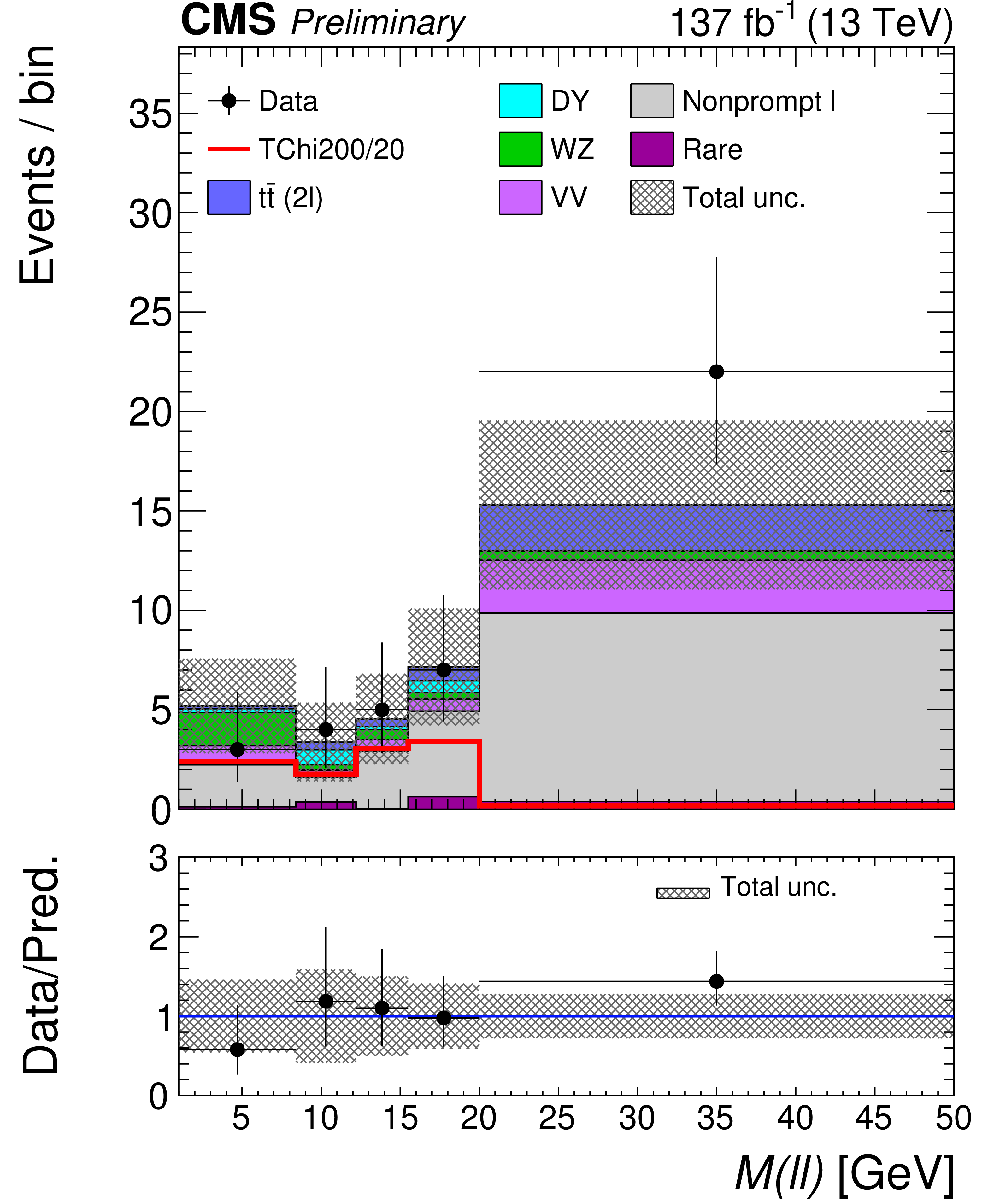
Figure 7:
Post-fit distributions of the $ m_{\ell\ell} $ variable for the low- (left) and medium- (right) $ p_{\mathrm{T}}^\text{miss} $ bins in the ``3 $ \ell $ soft'' signal region of Ref. [17]. These distributions are based on the parametric binnings derived for signal mass points with $ \Delta m $ = 20 GeV. The pre-fit signal distribution is overlaid for illustration. |
png pdf |
Figure 7-a:
Post-fit distributions of the $ m_{\ell\ell} $ variable for the low- (left) and medium- (right) $ p_{\mathrm{T}}^\text{miss} $ bins in the ``3 $ \ell $ soft'' signal region of Ref. [17]. These distributions are based on the parametric binnings derived for signal mass points with $ \Delta m $ = 20 GeV. The pre-fit signal distribution is overlaid for illustration. |
png pdf |
Figure 7-b:
Post-fit distributions of the $ m_{\ell\ell} $ variable for the low- (left) and medium- (right) $ p_{\mathrm{T}}^\text{miss} $ bins in the ``3 $ \ell $ soft'' signal region of Ref. [17]. These distributions are based on the parametric binnings derived for signal mass points with $ \Delta m $ = 20 GeV. The pre-fit signal distribution is overlaid for illustration. |
png pdf |
Figure 8:
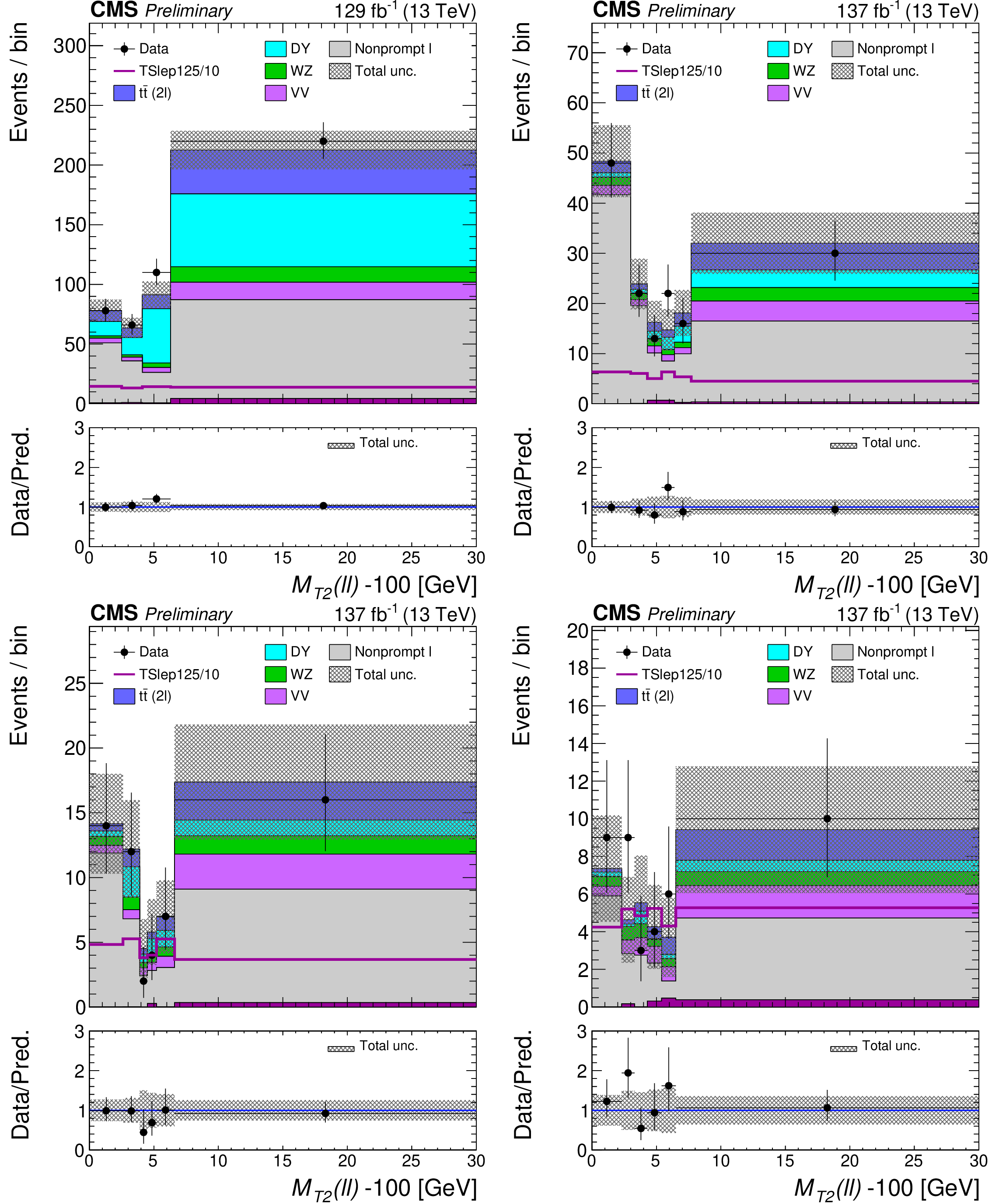
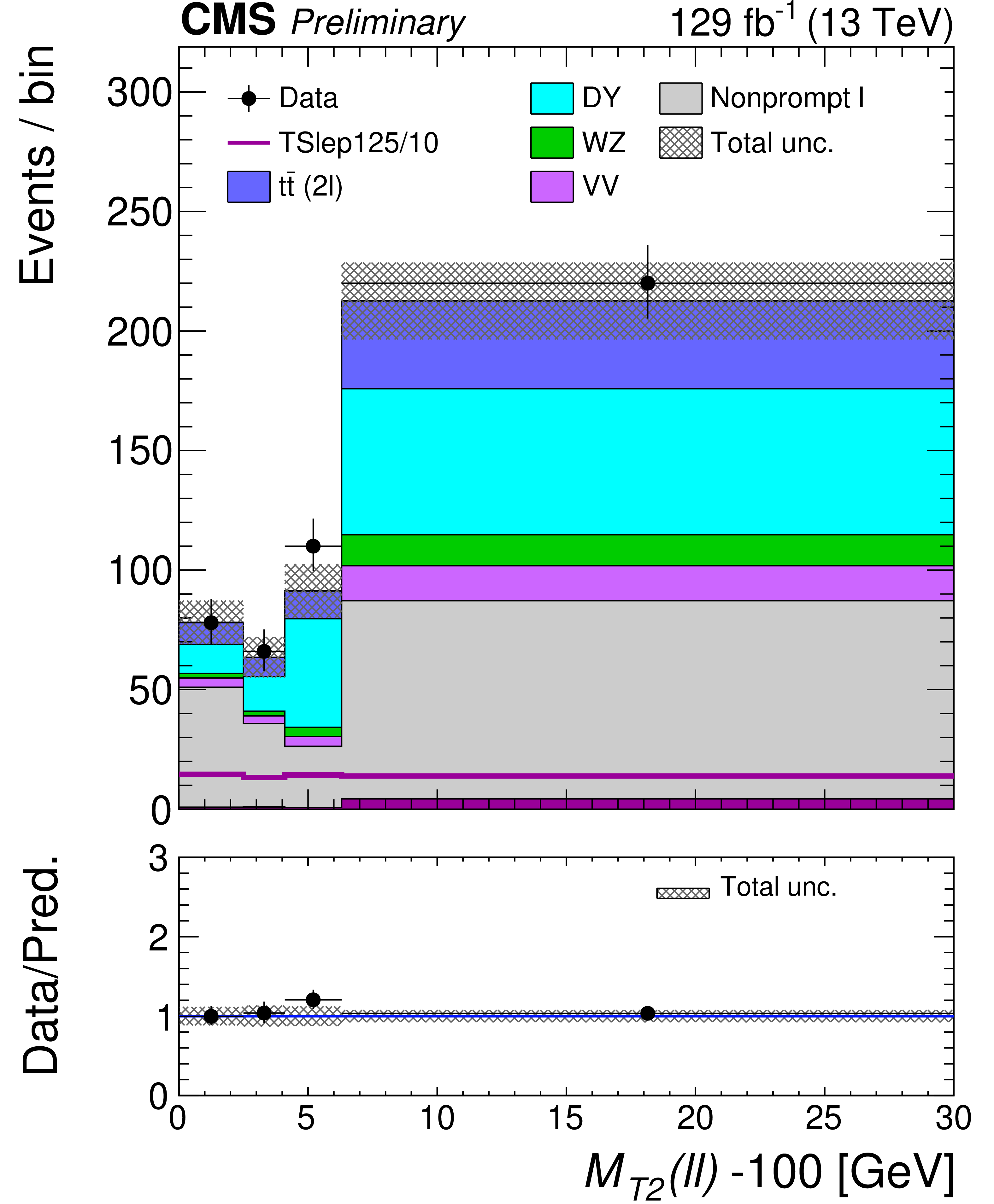
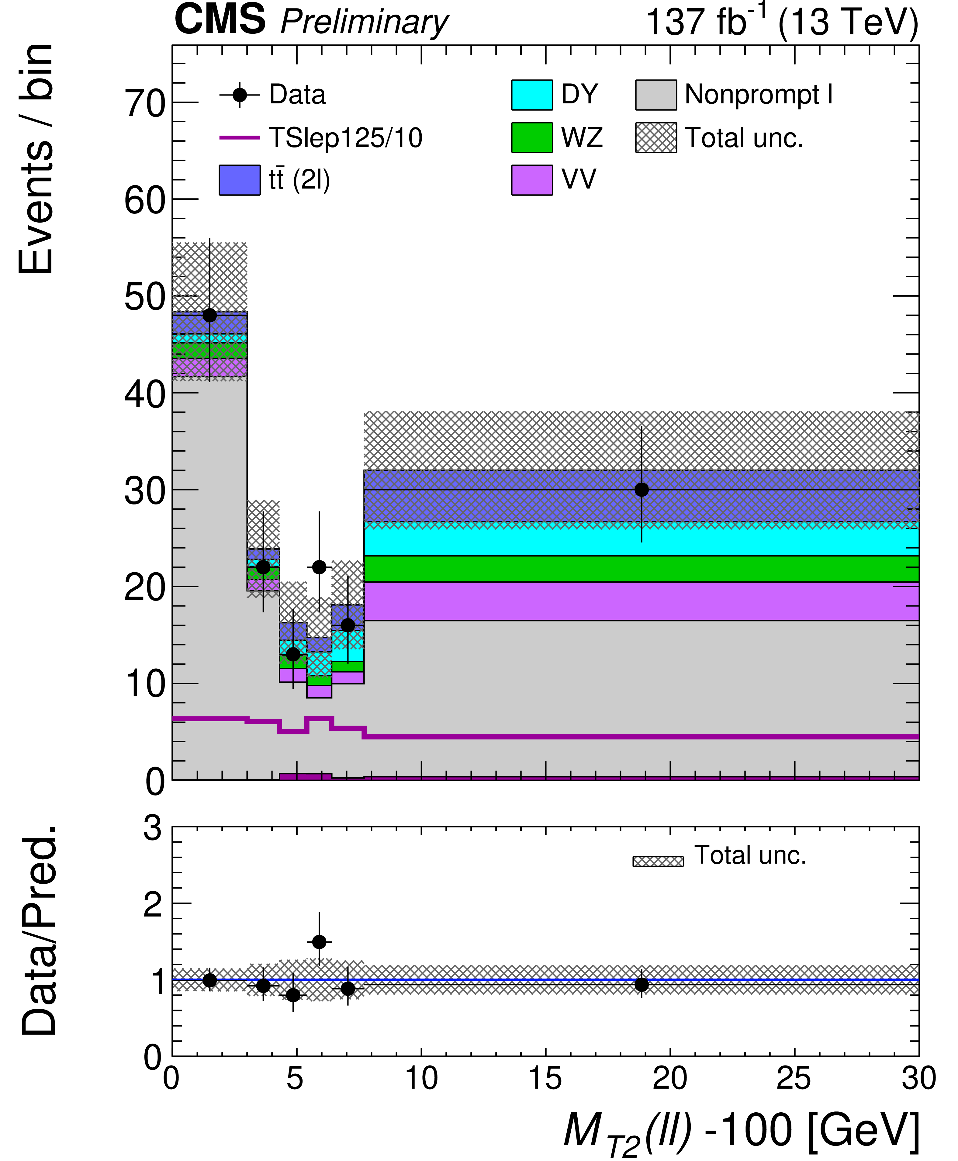
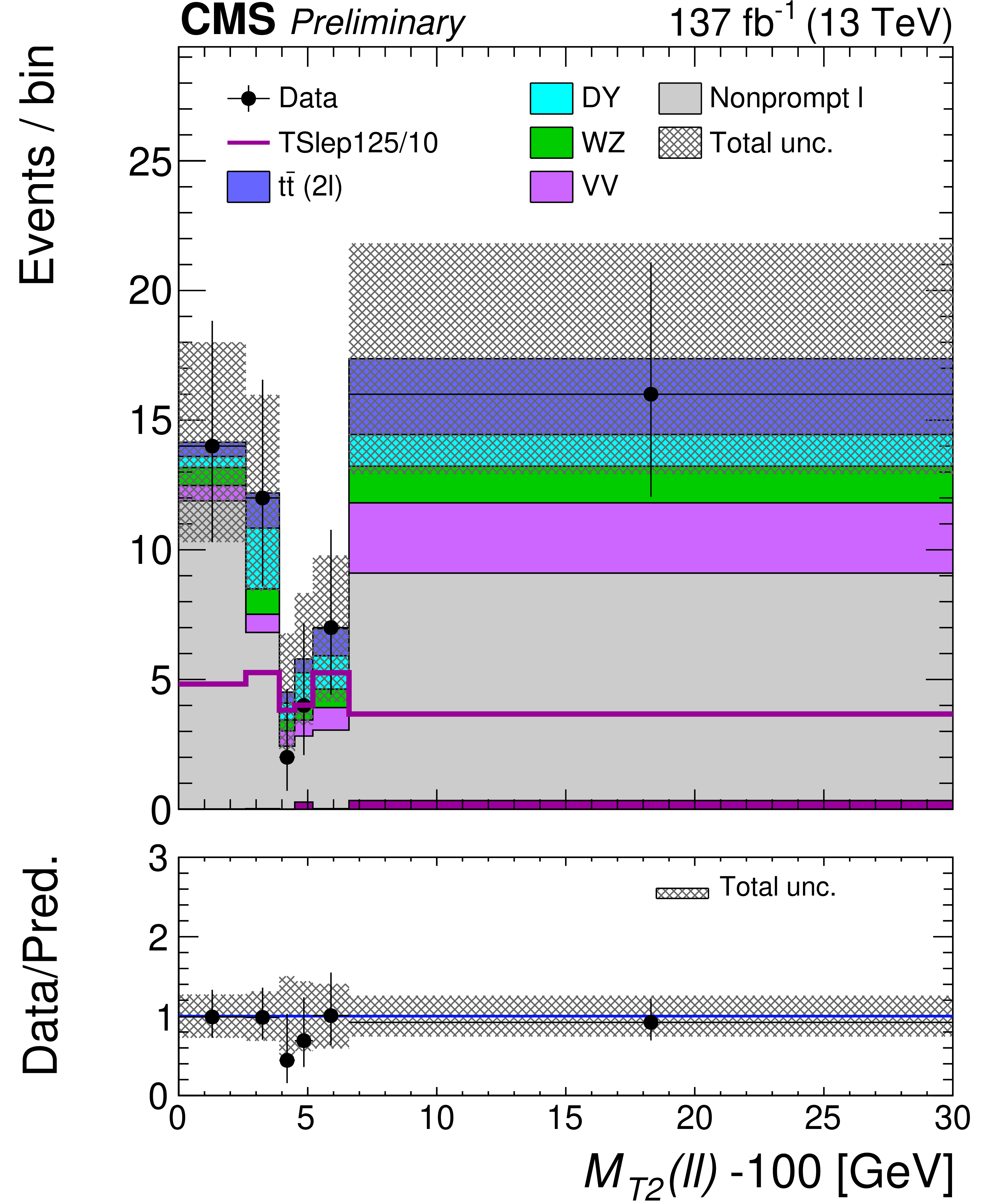
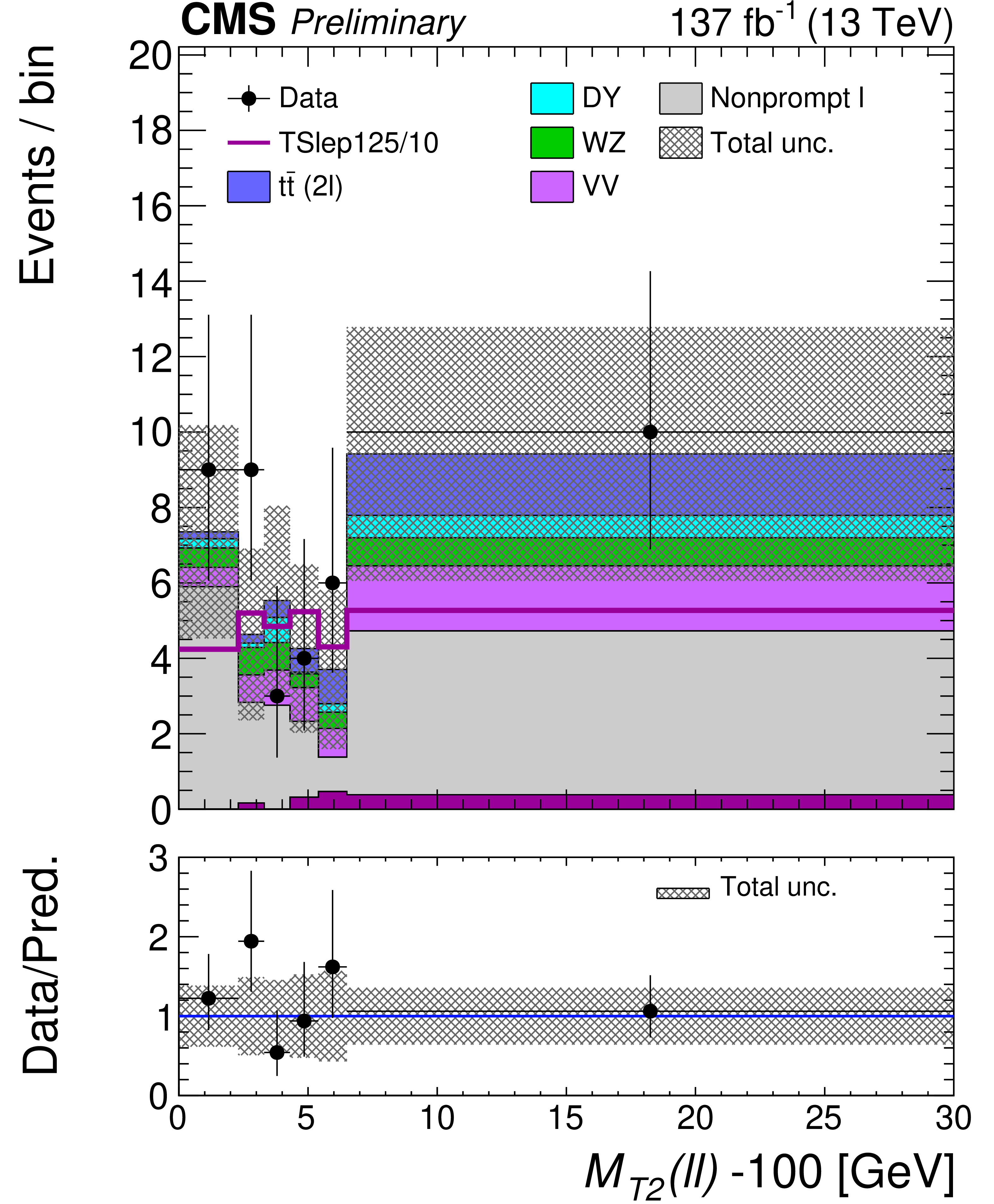
Post-fit distributions of the $ m_{\mathrm{T2}}(\ell\ell) $ variable are shown for the low- (upper left), medium- (upper right), high- (bottom left) and ultra- (bottom right) $ p_{\mathrm{T}}^\text{miss} $ bins in the ``2$\ell $ soft'' signal region of Ref. [17]. These distributions are based on the parametric binnings derived for the mass-point $ m_{\mathrm{NLSP}}=$ 125 GeV, $m_{\mathrm{LSP}}= $ 115 GeV. The pre-fit signal distribution is overlaid for illustration. Note that the signal distribution (purple line) is approximately flat across $ m_{\mathrm{T2}}(\ell\ell) $, by construction of the parametric binning procedure. The minimum value of $ m_{\mathrm{T2}}(\ell\ell) $, $ m_\chi = $ 100 GeV, is subtracted for the abscissa of the plot. |
png pdf |
Figure 8-a:
Post-fit distributions of the $ m_{\mathrm{T2}}(\ell\ell) $ variable are shown for the low- (upper left), medium- (upper right), high- (bottom left) and ultra- (bottom right) $ p_{\mathrm{T}}^\text{miss} $ bins in the ``2$\ell $ soft'' signal region of Ref. [17]. These distributions are based on the parametric binnings derived for the mass-point $ m_{\mathrm{NLSP}}=$ 125 GeV, $m_{\mathrm{LSP}}= $ 115 GeV. The pre-fit signal distribution is overlaid for illustration. Note that the signal distribution (purple line) is approximately flat across $ m_{\mathrm{T2}}(\ell\ell) $, by construction of the parametric binning procedure. The minimum value of $ m_{\mathrm{T2}}(\ell\ell) $, $ m_\chi = $ 100 GeV, is subtracted for the abscissa of the plot. |
png pdf |
Figure 8-b:
Post-fit distributions of the $ m_{\mathrm{T2}}(\ell\ell) $ variable are shown for the low- (upper left), medium- (upper right), high- (bottom left) and ultra- (bottom right) $ p_{\mathrm{T}}^\text{miss} $ bins in the ``2$\ell $ soft'' signal region of Ref. [17]. These distributions are based on the parametric binnings derived for the mass-point $ m_{\mathrm{NLSP}}=$ 125 GeV, $m_{\mathrm{LSP}}= $ 115 GeV. The pre-fit signal distribution is overlaid for illustration. Note that the signal distribution (purple line) is approximately flat across $ m_{\mathrm{T2}}(\ell\ell) $, by construction of the parametric binning procedure. The minimum value of $ m_{\mathrm{T2}}(\ell\ell) $, $ m_\chi = $ 100 GeV, is subtracted for the abscissa of the plot. |
png pdf |
Figure 8-c:
Post-fit distributions of the $ m_{\mathrm{T2}}(\ell\ell) $ variable are shown for the low- (upper left), medium- (upper right), high- (bottom left) and ultra- (bottom right) $ p_{\mathrm{T}}^\text{miss} $ bins in the ``2$\ell $ soft'' signal region of Ref. [17]. These distributions are based on the parametric binnings derived for the mass-point $ m_{\mathrm{NLSP}}=$ 125 GeV, $m_{\mathrm{LSP}}= $ 115 GeV. The pre-fit signal distribution is overlaid for illustration. Note that the signal distribution (purple line) is approximately flat across $ m_{\mathrm{T2}}(\ell\ell) $, by construction of the parametric binning procedure. The minimum value of $ m_{\mathrm{T2}}(\ell\ell) $, $ m_\chi = $ 100 GeV, is subtracted for the abscissa of the plot. |
png pdf |
Figure 8-d:
Post-fit distributions of the $ m_{\mathrm{T2}}(\ell\ell) $ variable are shown for the low- (upper left), medium- (upper right), high- (bottom left) and ultra- (bottom right) $ p_{\mathrm{T}}^\text{miss} $ bins in the ``2$\ell $ soft'' signal region of Ref. [17]. These distributions are based on the parametric binnings derived for the mass-point $ m_{\mathrm{NLSP}}=$ 125 GeV, $m_{\mathrm{LSP}}= $ 115 GeV. The pre-fit signal distribution is overlaid for illustration. Note that the signal distribution (purple line) is approximately flat across $ m_{\mathrm{T2}}(\ell\ell) $, by construction of the parametric binning procedure. The minimum value of $ m_{\mathrm{T2}}(\ell\ell) $, $ m_\chi = $ 100 GeV, is subtracted for the abscissa of the plot. |
png pdf |
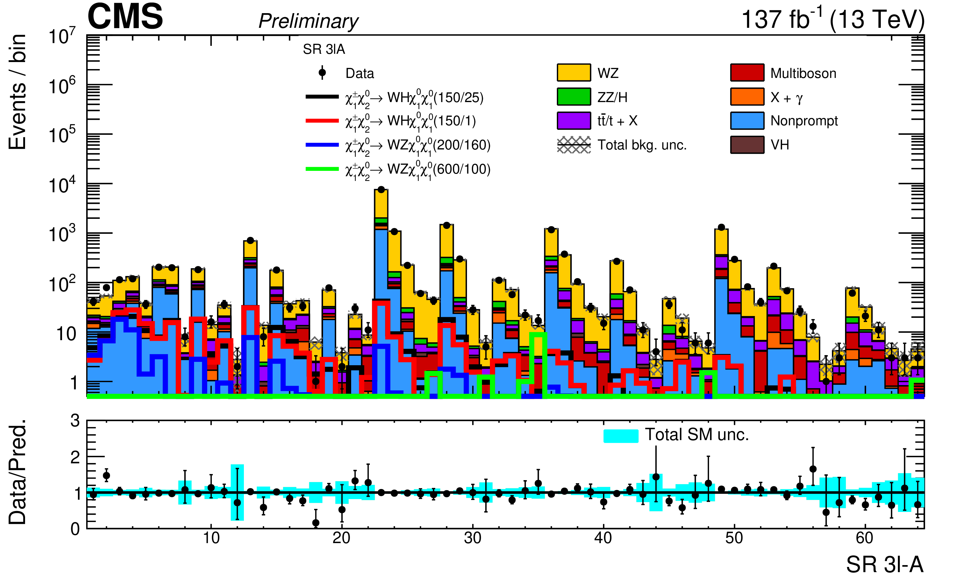
Figure 9:
Observed and expected yields across the search regions in the ``$ \geq$ 3$\ell $" search in category A, events with three light leptons at least two of which form an OSSF pair, after the requirement on the leading lepton $ p_{\mathrm{T}} $ to be greater than 30 GeV is applied. |
png pdf |
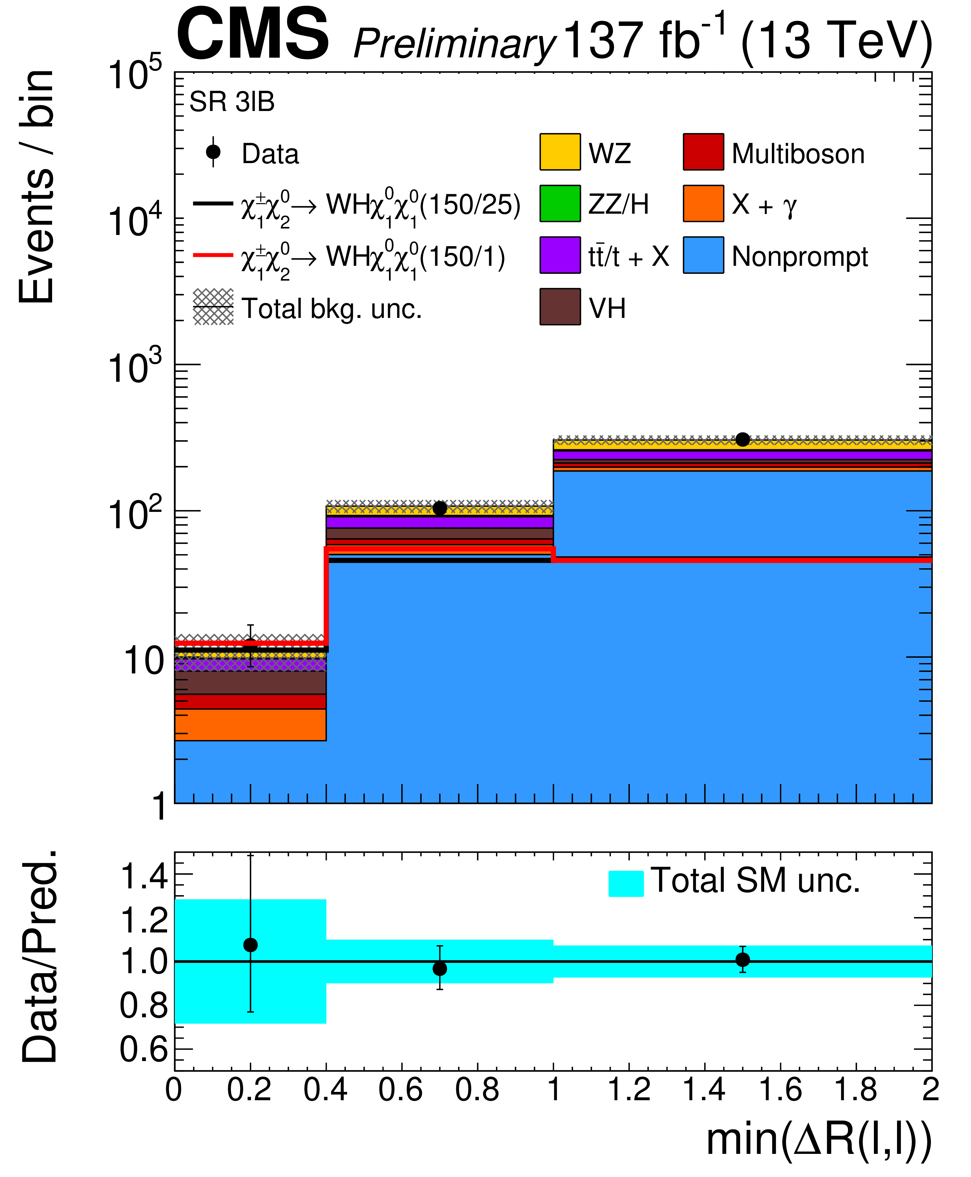
Figure 10:
Observed and expected yields across the SRs of the ``$ \geq$ 3$\ell $" search in category B, events with three light leptons and no OSSF pair, after the requirement on the leading lepton $ p_{\mathrm{T}} $ to be greater than 30 GeV is applied. |
png pdf |
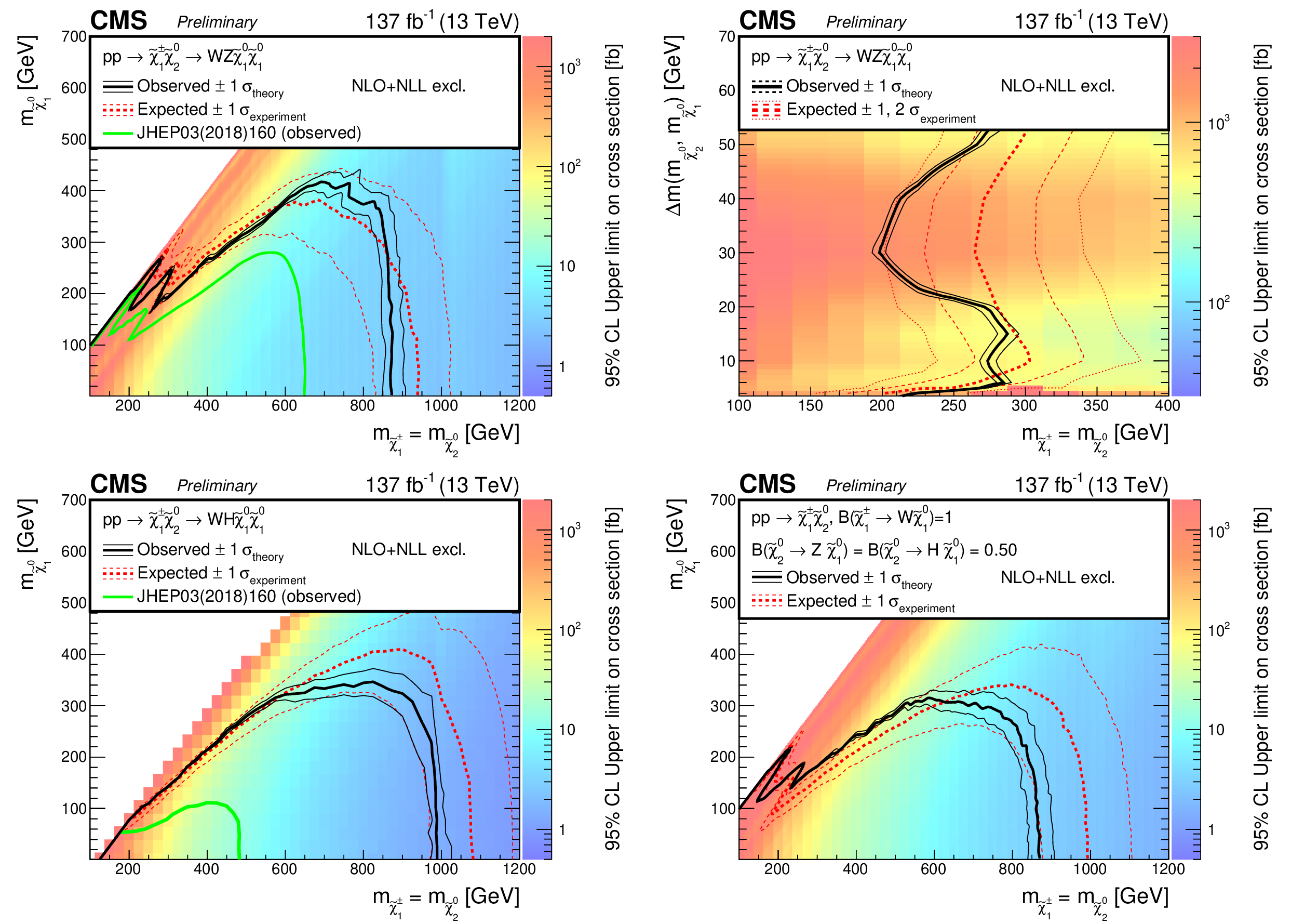
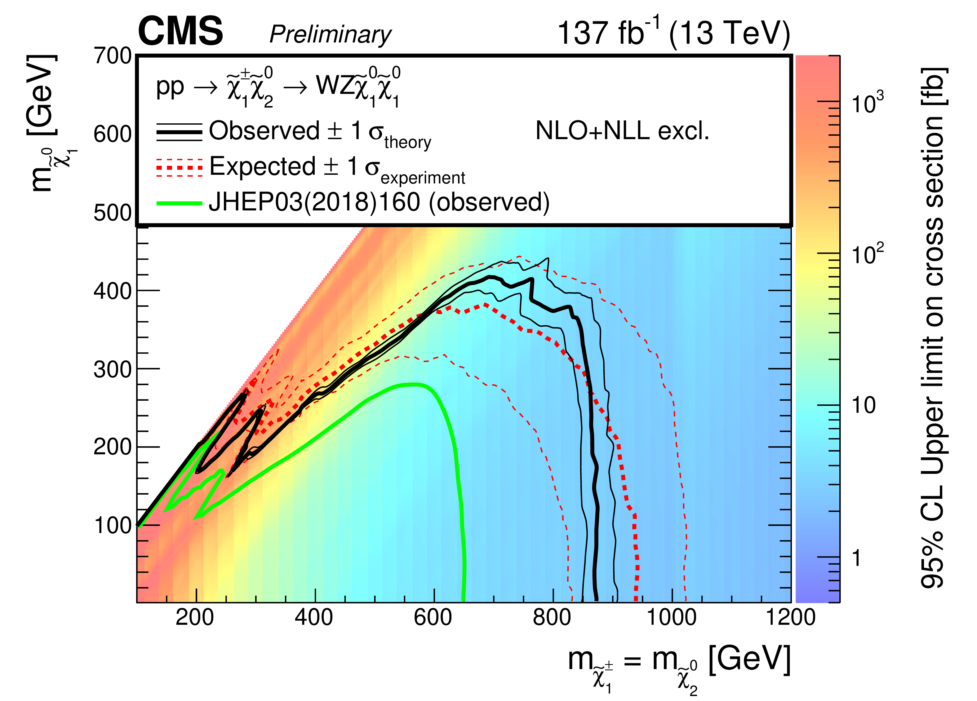
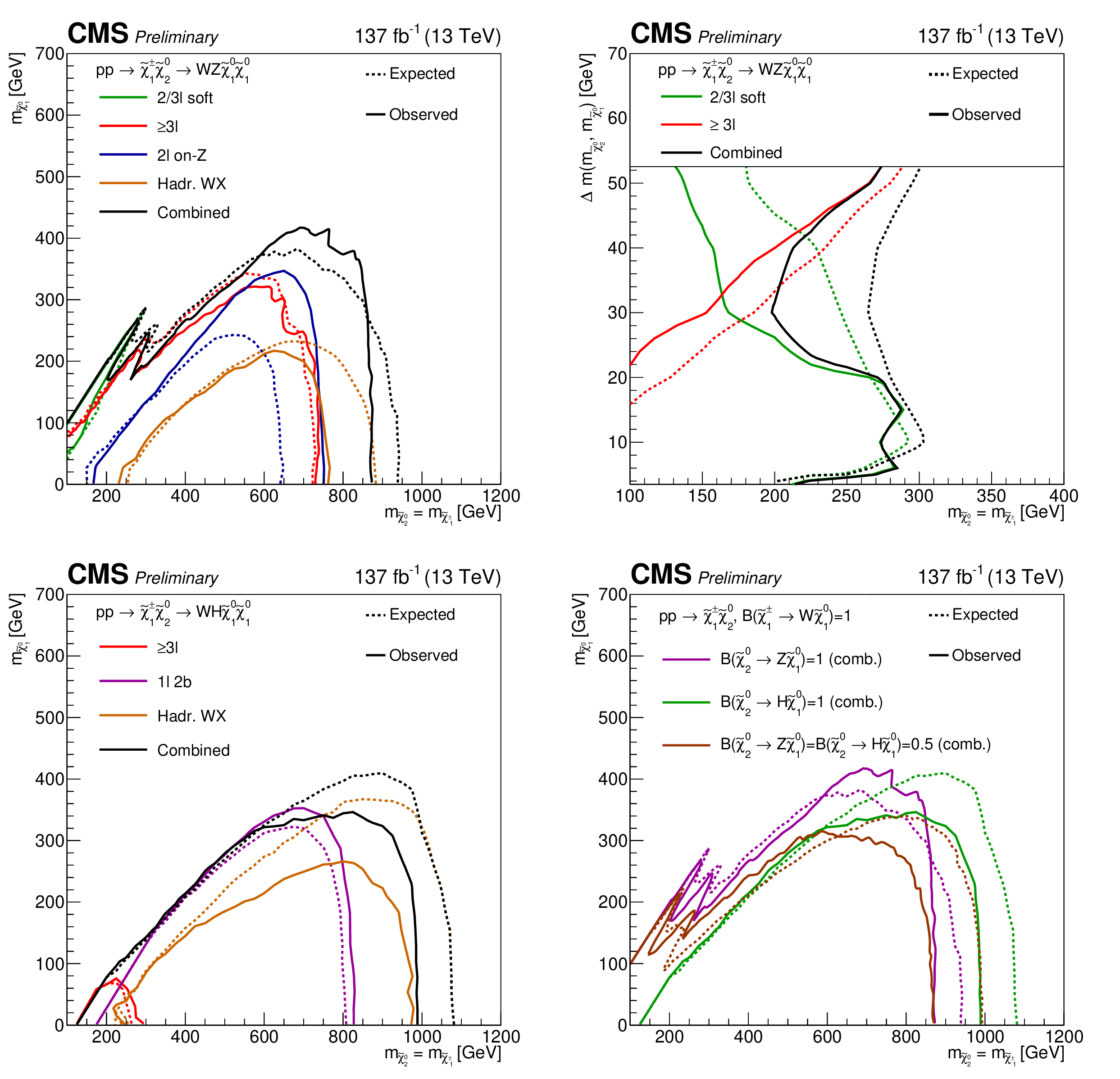
Figure 11:
Cross section limits with expected and observed exclusion boundaries in the model parameter space, for neutralino-chargino production in the WZ topology for the full parameter space (upper left) as well as the compressed region (upper right), the WH topology (lower left), and the mixed topology with 50% branching fraction to WZ and WH (lower right). |
png pdf |
Figure 11-a:
Cross section limits with expected and observed exclusion boundaries in the model parameter space, for neutralino-chargino production in the WZ topology for the full parameter space (upper left) as well as the compressed region (upper right), the WH topology (lower left), and the mixed topology with 50% branching fraction to WZ and WH (lower right). |

png pdf |
Figure 11-b:
Cross section limits with expected and observed exclusion boundaries in the model parameter space, for neutralino-chargino production in the WZ topology for the full parameter space (upper left) as well as the compressed region (upper right), the WH topology (lower left), and the mixed topology with 50% branching fraction to WZ and WH (lower right). |

png pdf |
Figure 11-c:
Cross section limits with expected and observed exclusion boundaries in the model parameter space, for neutralino-chargino production in the WZ topology for the full parameter space (upper left) as well as the compressed region (upper right), the WH topology (lower left), and the mixed topology with 50% branching fraction to WZ and WH (lower right). |
png pdf |
Figure 11-d:
Cross section limits with expected and observed exclusion boundaries in the model parameter space, for neutralino-chargino production in the WZ topology for the full parameter space (upper left) as well as the compressed region (upper right), the WH topology (lower left), and the mixed topology with 50% branching fraction to WZ and WH (lower right). |
png pdf |
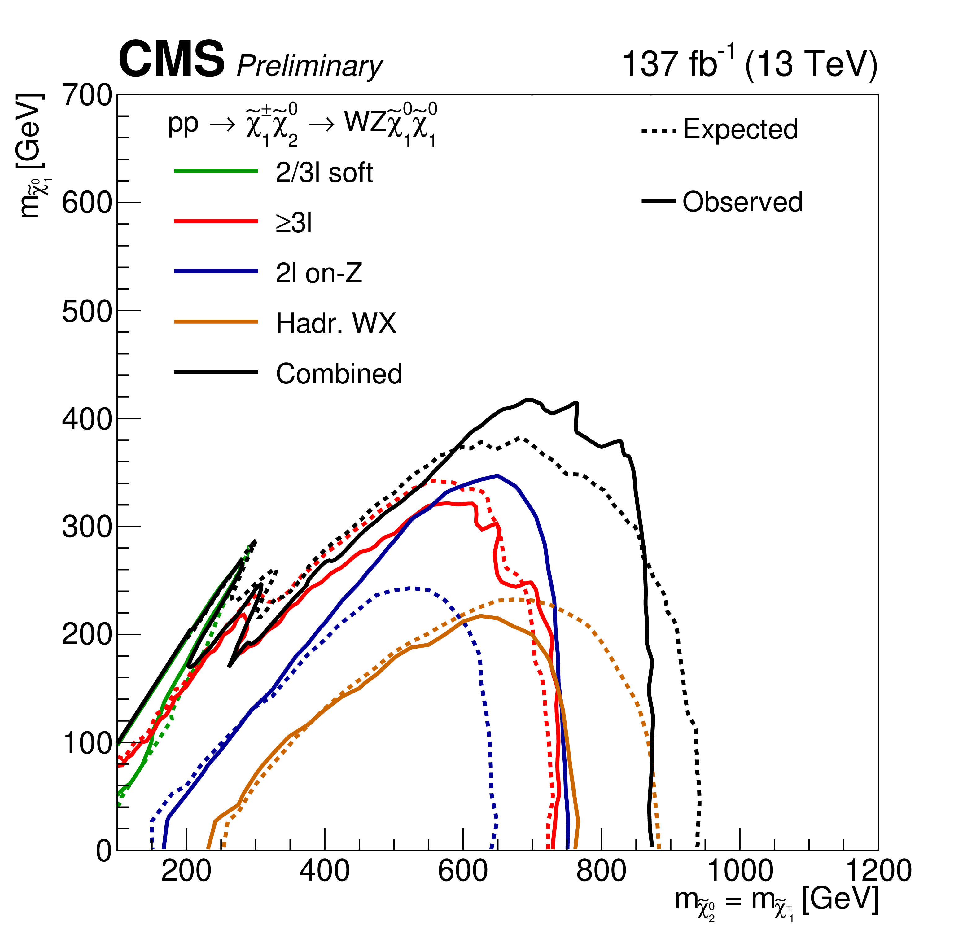
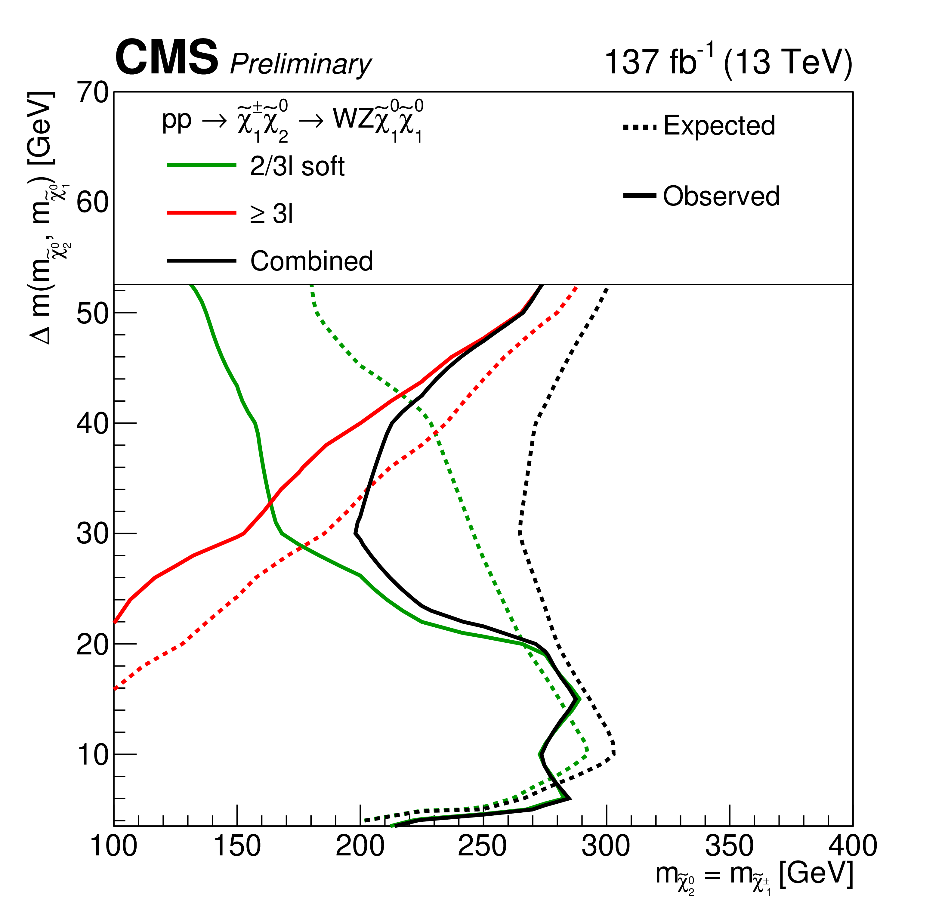
Figure 12:
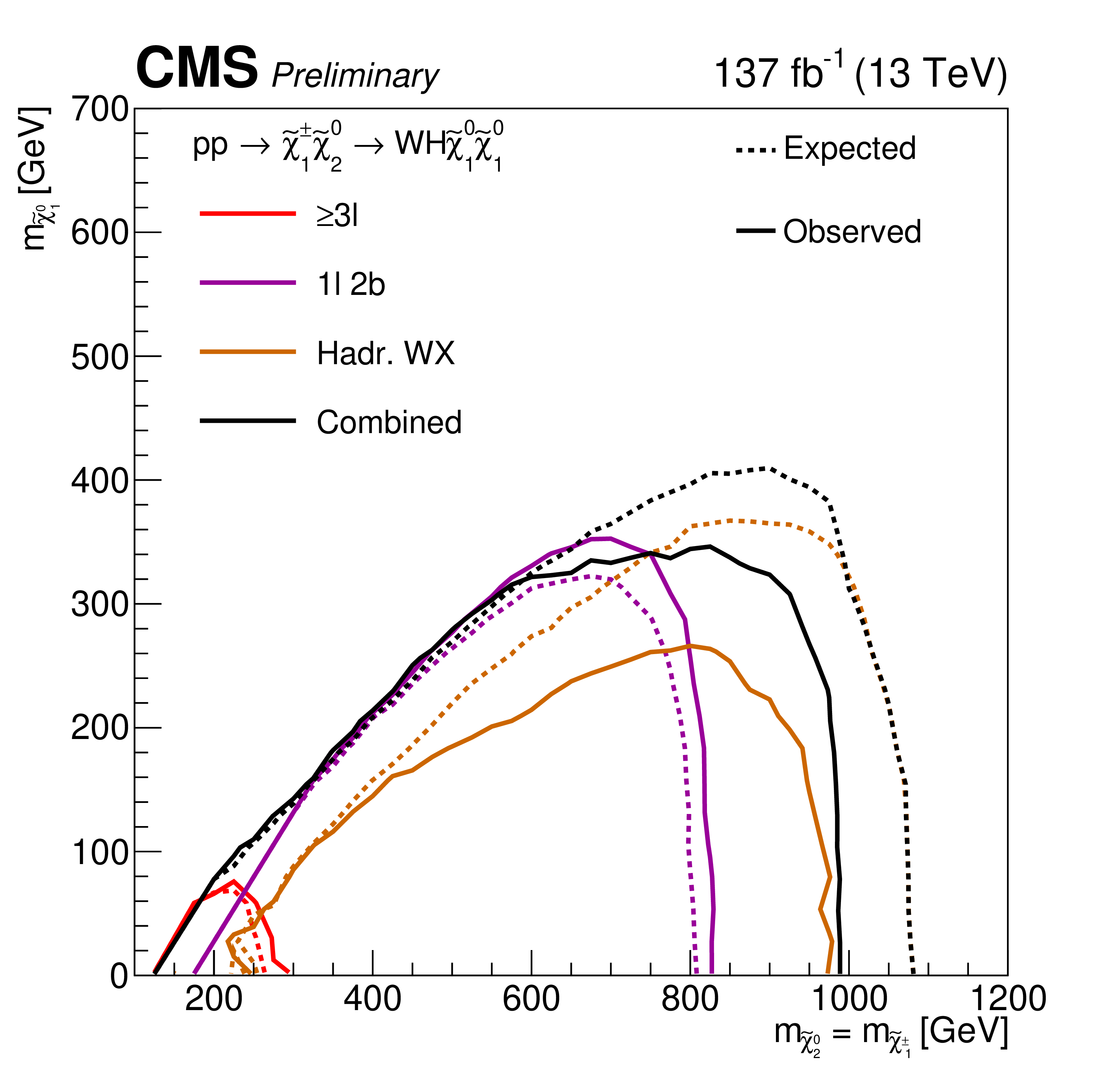
Exclusion contours for the individual analyses targeting the WZ topology for the full parameter space (upper left) the corresponding compressed region (upper right), and the WH topology (lower left). The combined contours for these two topologies are also shown. The combined contours for these and the mixed topology are overlaid in the lower right plot. The decay modes assumed for each contour are given in the legends. |
png pdf |
Figure 12-a:
Exclusion contours for the individual analyses targeting the WZ topology for the full parameter space (upper left) the corresponding compressed region (upper right), and the WH topology (lower left). The combined contours for these two topologies are also shown. The combined contours for these and the mixed topology are overlaid in the lower right plot. The decay modes assumed for each contour are given in the legends. |
png pdf |
Figure 12-b:
Exclusion contours for the individual analyses targeting the WZ topology for the full parameter space (upper left) the corresponding compressed region (upper right), and the WH topology (lower left). The combined contours for these two topologies are also shown. The combined contours for these and the mixed topology are overlaid in the lower right plot. The decay modes assumed for each contour are given in the legends. |
png pdf |
Figure 12-c:
Exclusion contours for the individual analyses targeting the WZ topology for the full parameter space (upper left) the corresponding compressed region (upper right), and the WH topology (lower left). The combined contours for these two topologies are also shown. The combined contours for these and the mixed topology are overlaid in the lower right plot. The decay modes assumed for each contour are given in the legends. |

png pdf |
Figure 12-d:
Exclusion contours for the individual analyses targeting the WZ topology for the full parameter space (upper left) the corresponding compressed region (upper right), and the WH topology (lower left). The combined contours for these two topologies are also shown. The combined contours for these and the mixed topology are overlaid in the lower right plot. The decay modes assumed for each contour are given in the legends. |
png pdf |
Figure 13:
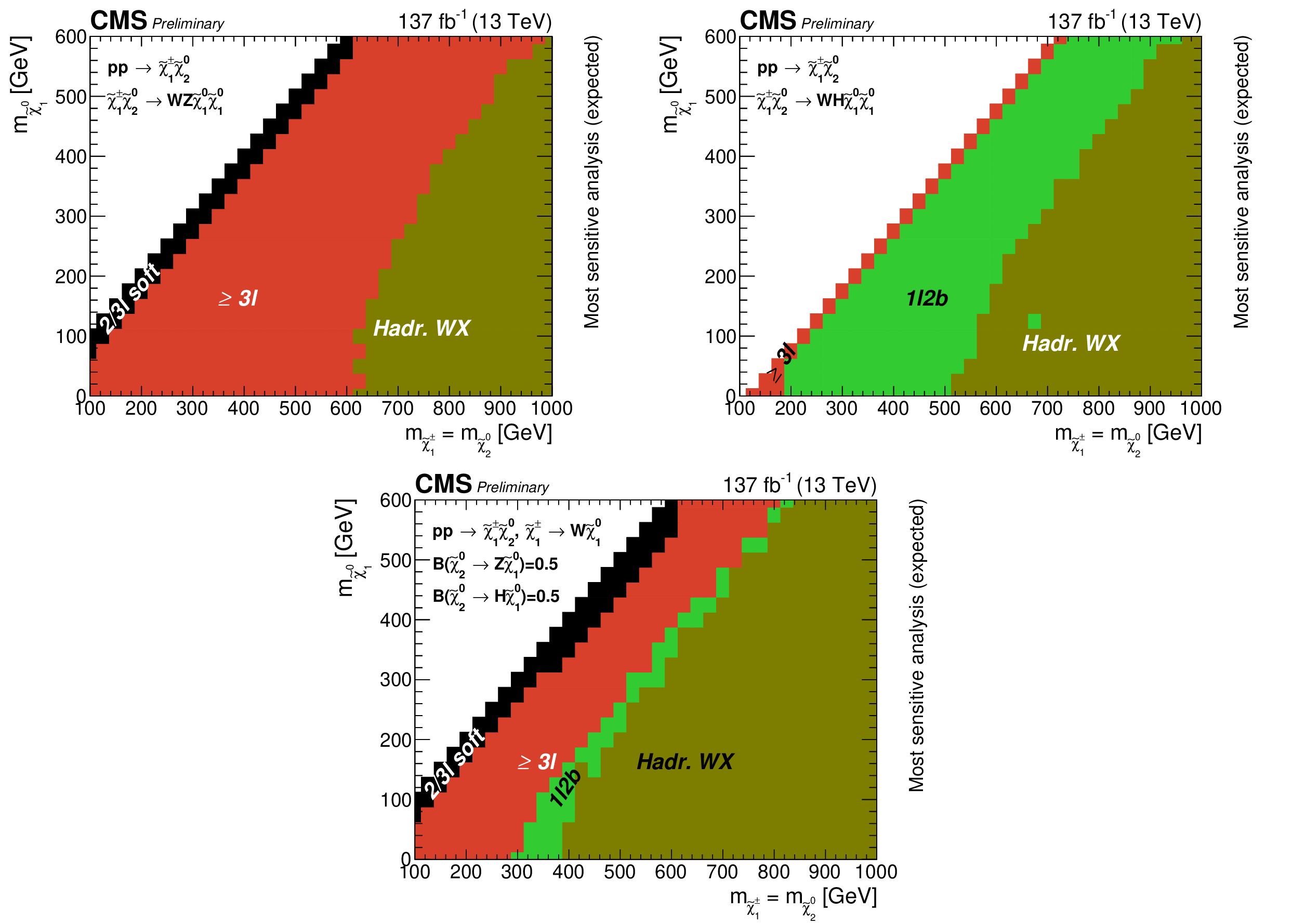
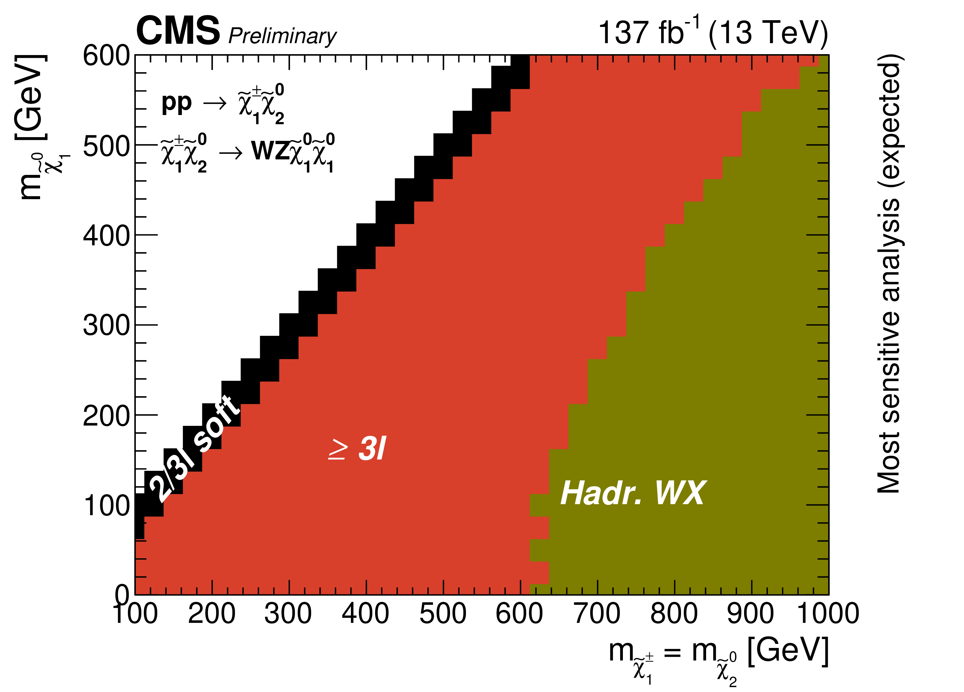
The analysis with the best exclusion limit for each point in the plane for the WZ topology (upper left), the WH topology (upper right), and the mixed topology with 50% branching fraction to WZ and WH (bottom). |
png pdf |
Figure 13-a:
The analysis with the best exclusion limit for each point in the plane for the WZ topology (upper left), the WH topology (upper right), and the mixed topology with 50% branching fraction to WZ and WH (bottom). |

png pdf |
Figure 13-b:
The analysis with the best exclusion limit for each point in the plane for the WZ topology (upper left), the WH topology (upper right), and the mixed topology with 50% branching fraction to WZ and WH (bottom). |

png pdf |
Figure 13-c:
The analysis with the best exclusion limit for each point in the plane for the WZ topology (upper left), the WH topology (upper right), and the mixed topology with 50% branching fraction to WZ and WH (bottom). |

png pdf |
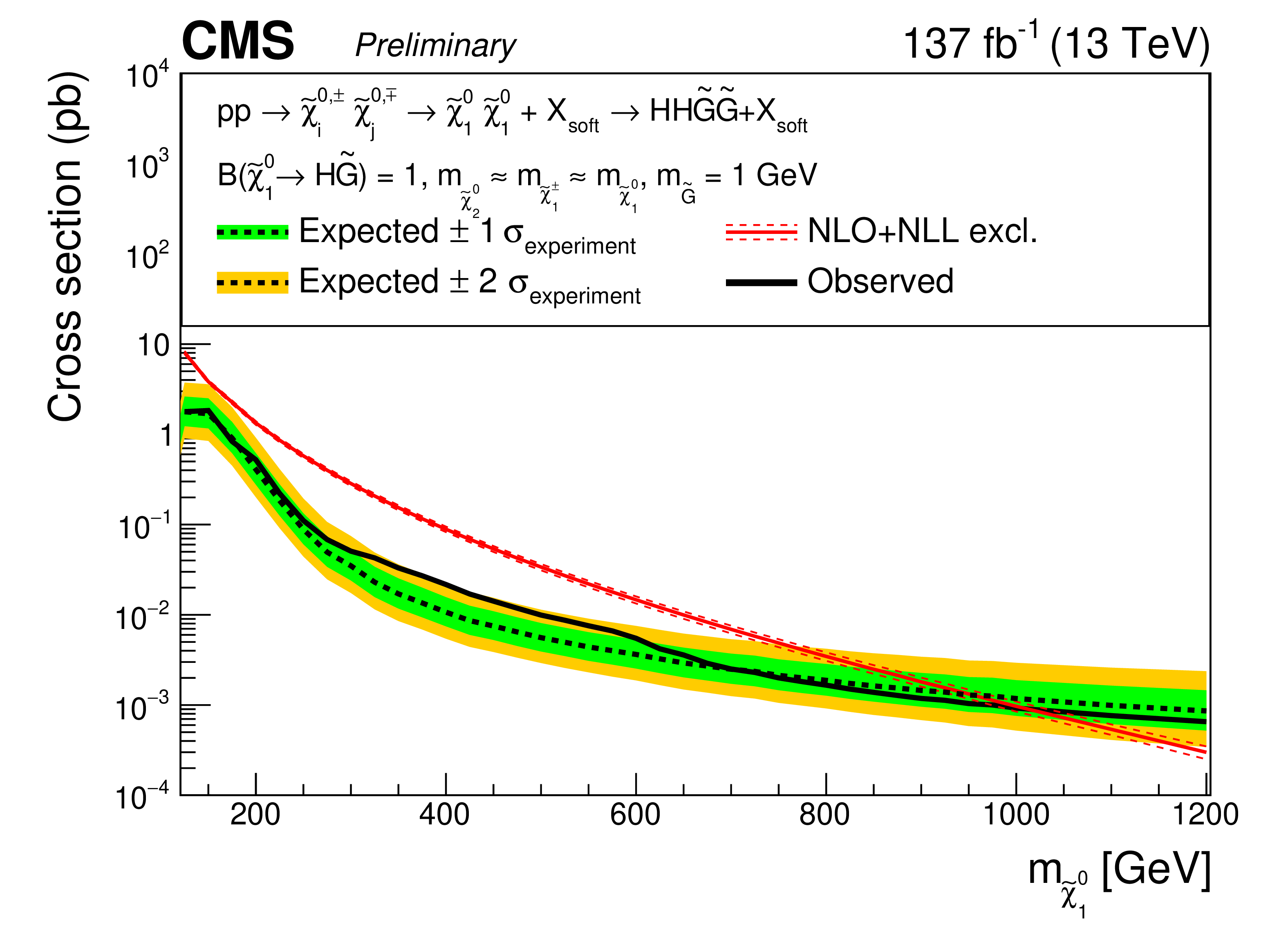
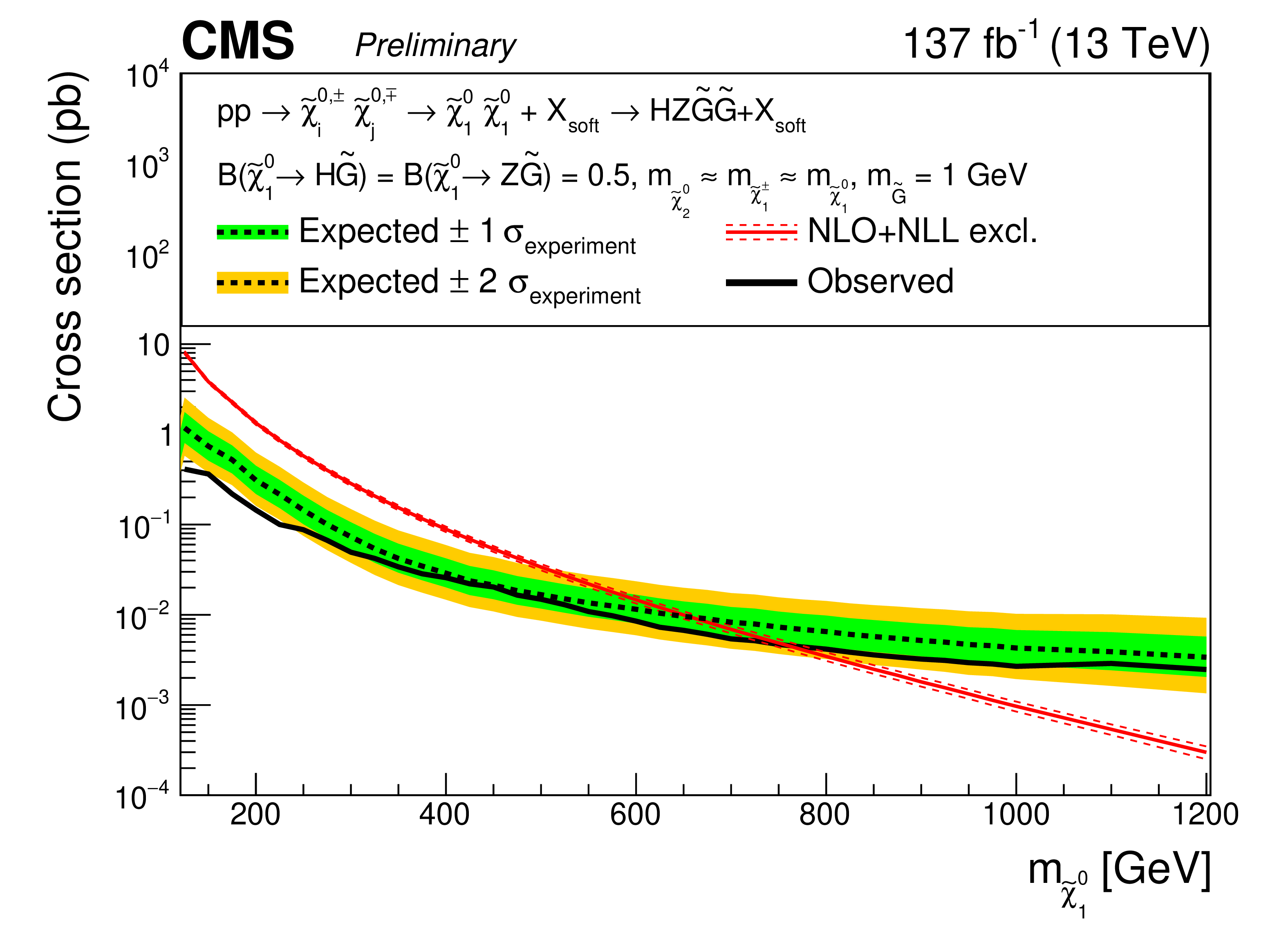
Figure 14:
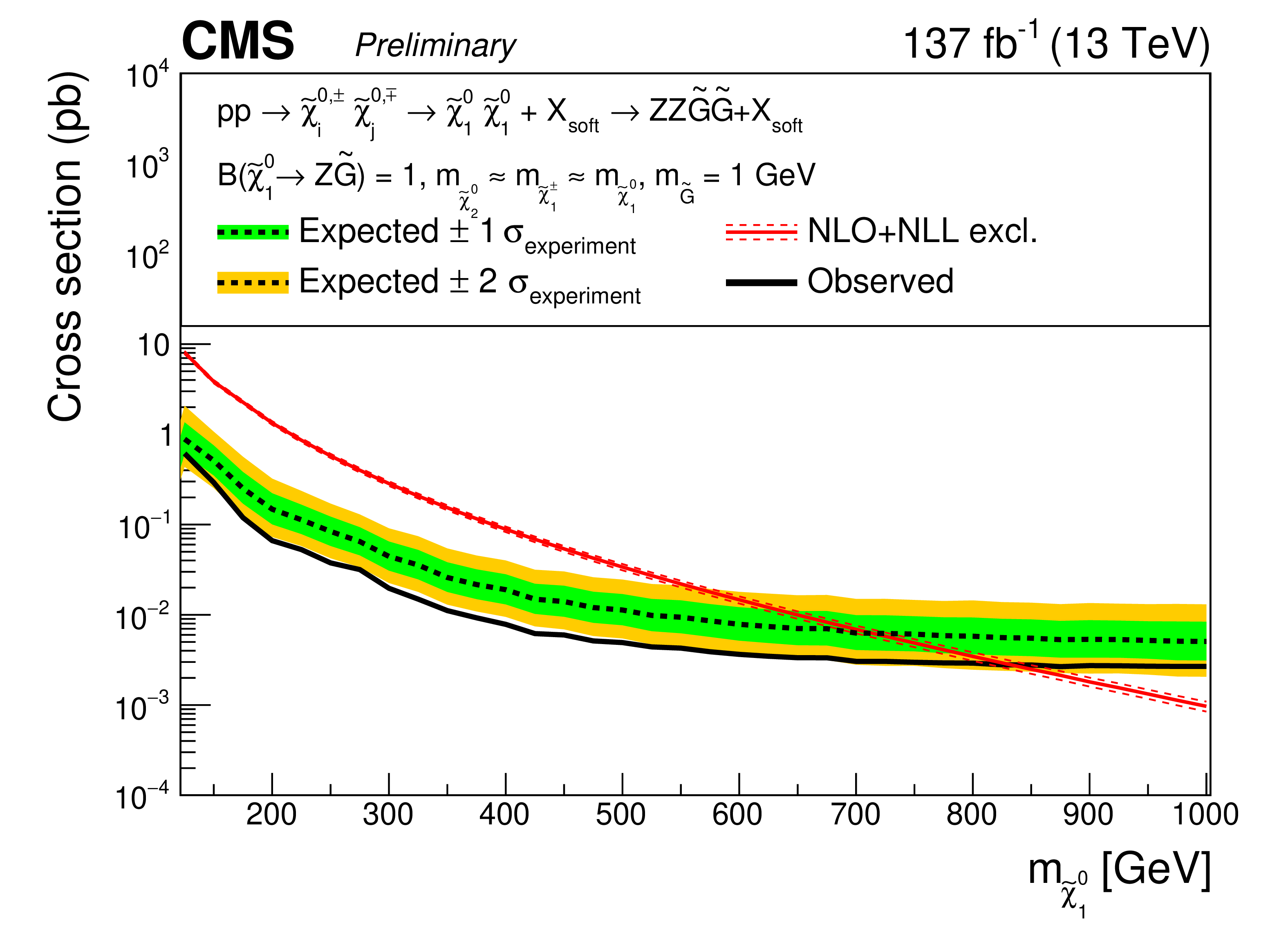
Expected and observed exclusion limits for the neutralino-neutralino production for the ZZ topology (upper left), the HH topology (upper right), and the mixed topology with 50% branching fraction to H and Z (lower). |
png pdf |
Figure 14-a:
Expected and observed exclusion limits for the neutralino-neutralino production for the ZZ topology (upper left), the HH topology (upper right), and the mixed topology with 50% branching fraction to H and Z (lower). |
png pdf |
Figure 14-b:
Expected and observed exclusion limits for the neutralino-neutralino production for the ZZ topology (upper left), the HH topology (upper right), and the mixed topology with 50% branching fraction to H and Z (lower). |
png pdf |
Figure 14-c:
Expected and observed exclusion limits for the neutralino-neutralino production for the ZZ topology (upper left), the HH topology (upper right), and the mixed topology with 50% branching fraction to H and Z (lower). |
png pdf |
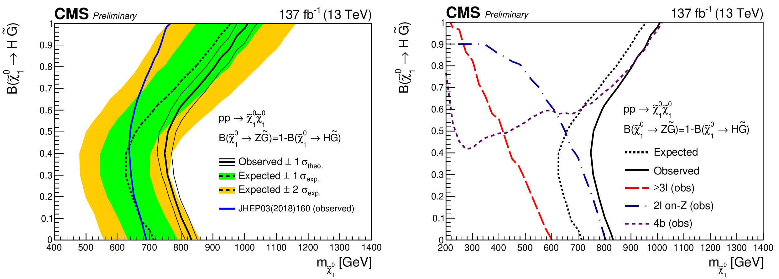
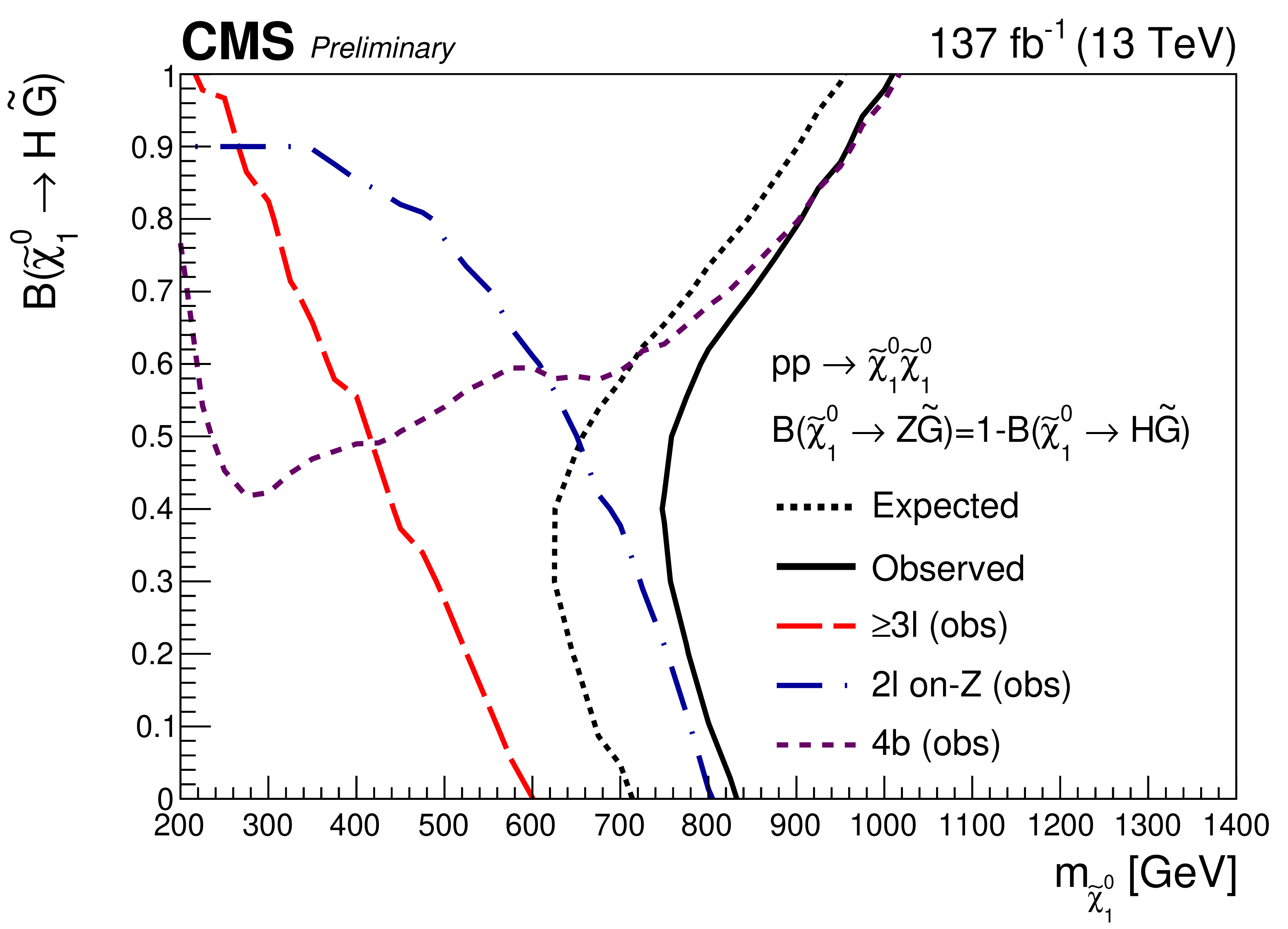
Figure 15:
NLSP-mass exclusion limit for neutralino-neutralino production as a function of the branching fraction to the H boson. Left: expected and observed limits for the combination of the searches, shown together with the observed limits of the combination [25] based on the 2016 CMS data. Right: expected and observed exclusion limits for the combination in comparison with those of the input searches. |

png pdf |
Figure 15-a:
NLSP-mass exclusion limit for neutralino-neutralino production as a function of the branching fraction to the H boson. Left: expected and observed limits for the combination of the searches, shown together with the observed limits of the combination [25] based on the 2016 CMS data. Right: expected and observed exclusion limits for the combination in comparison with those of the input searches. |
png pdf |
Figure 15-b:
NLSP-mass exclusion limit for neutralino-neutralino production as a function of the branching fraction to the H boson. Left: expected and observed limits for the combination of the searches, shown together with the observed limits of the combination [25] based on the 2016 CMS data. Right: expected and observed exclusion limits for the combination in comparison with those of the input searches. |

png pdf |
Figure 16:
The analysis with the best limit exclusion for each point in the branching fraction-$ m_{\tilde{\chi}_{1}^{0}} $ plane for neutralino-neutralino production. |

png pdf |
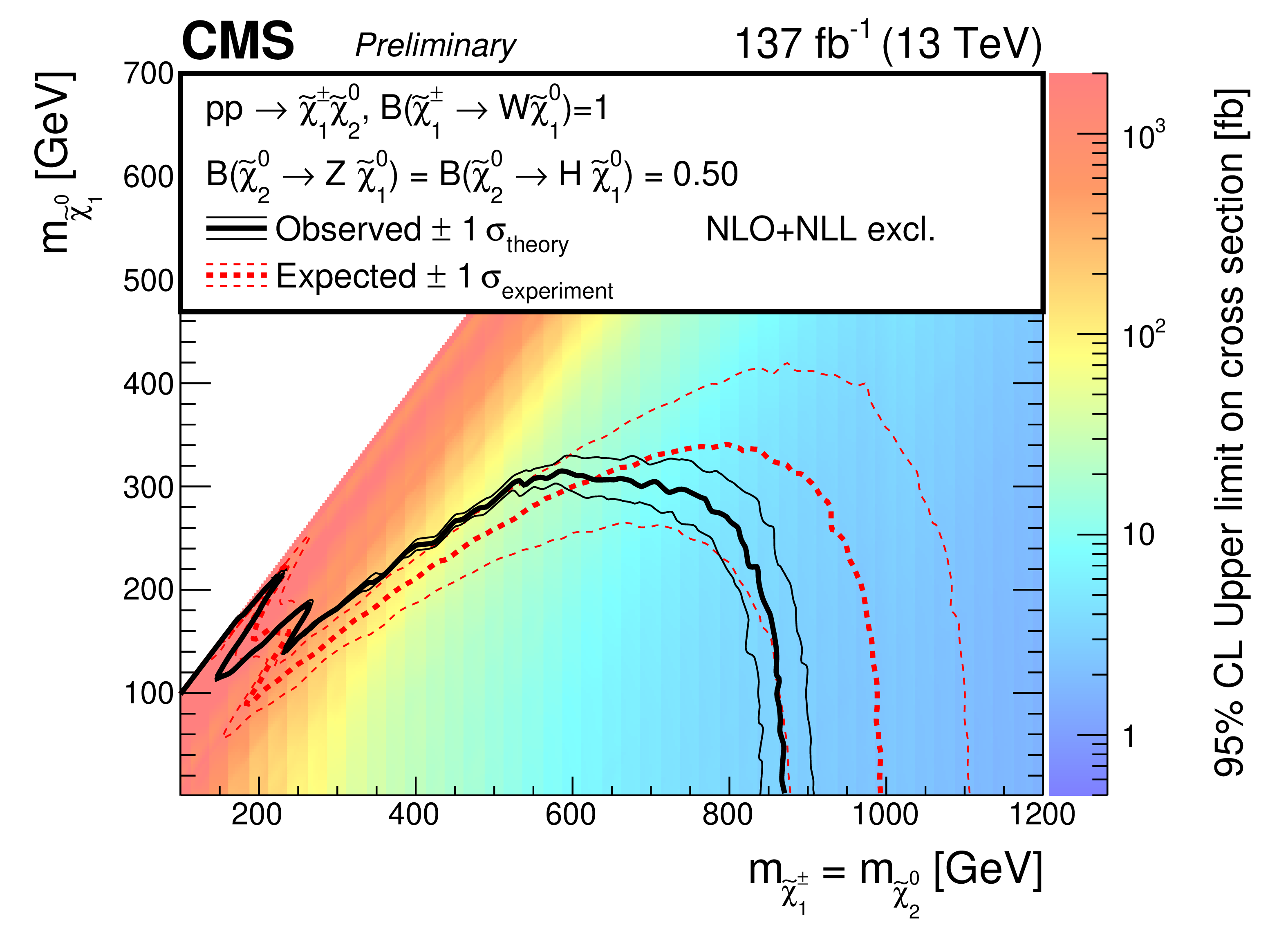
Figure 17:
Cross section upper limit in the mass plane of the higgsino-bino model, and the expected and observed exclusion limits. The model assumes mass-degenerate higgsino-like $ \tilde{\chi}_{2}^{0} $, $ \tilde{\chi}_{3}^{0} $, and $ \tilde{\chi}_{1}^{\pm} $ that decay to a bino-like $ \tilde{\chi}_{1}^{0} $ and an SM boson. |
png pdf |
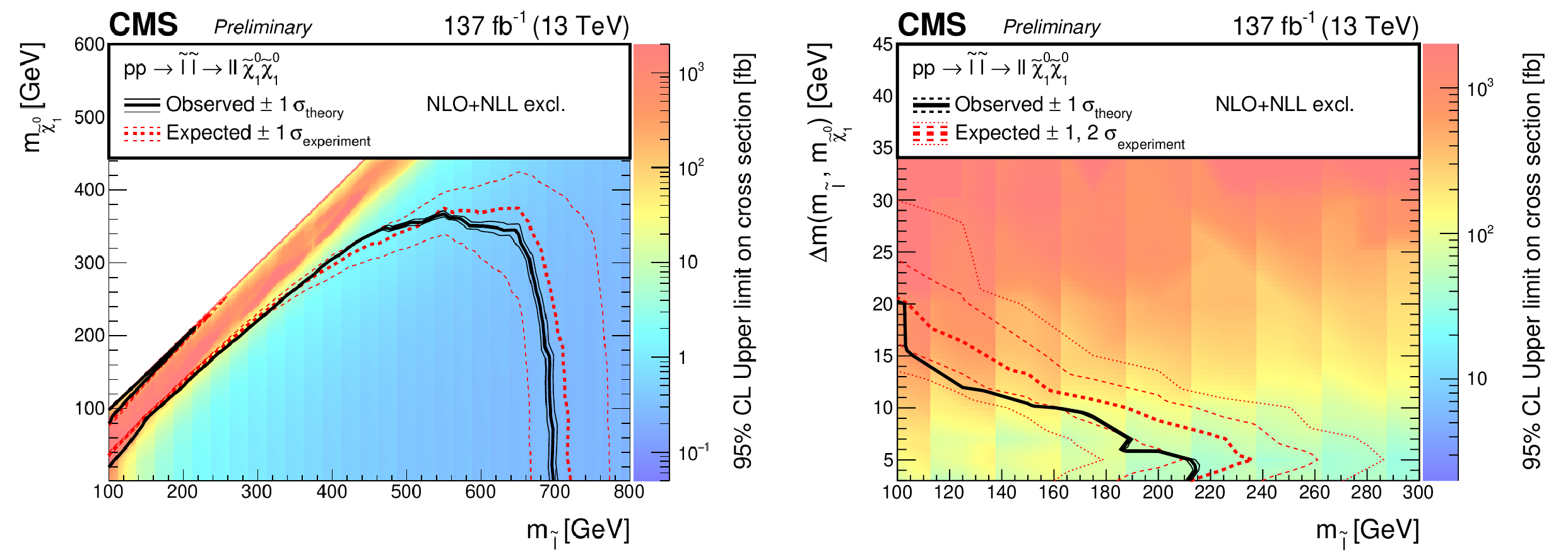
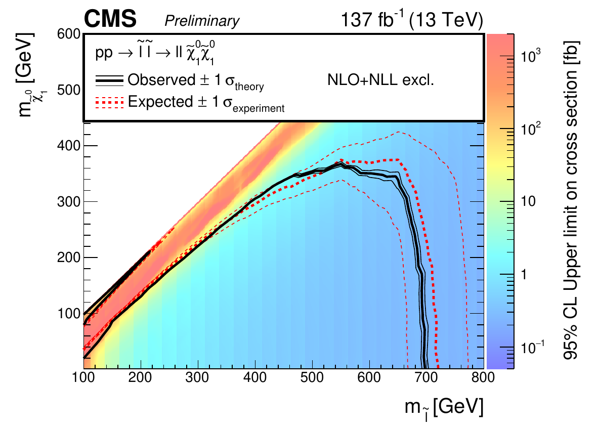
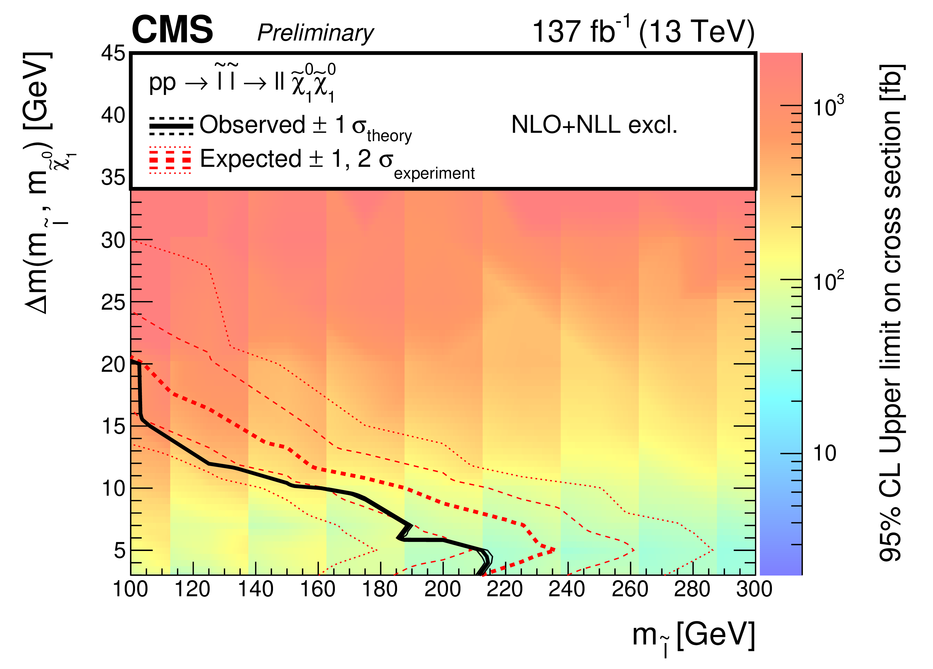
Figure 18:
Mass-plane cross section upper limit for direct slepton pair production, with observed and expected exclusion limits: (left) the full mass plane from the combination, and (right) the compressed region, obtained by the ``2/3$\ell $ soft'' search. |
png |
Figure 18-a:
Mass-plane cross section upper limit for direct slepton pair production, with observed and expected exclusion limits: (left) the full mass plane from the combination, and (right) the compressed region, obtained by the ``2/3$\ell $ soft'' search. |
png pdf |
Figure 18-b:
Mass-plane cross section upper limit for direct slepton pair production, with observed and expected exclusion limits: (left) the full mass plane from the combination, and (right) the compressed region, obtained by the ``2/3$\ell $ soft'' search. |
| Tables | |
png pdf |
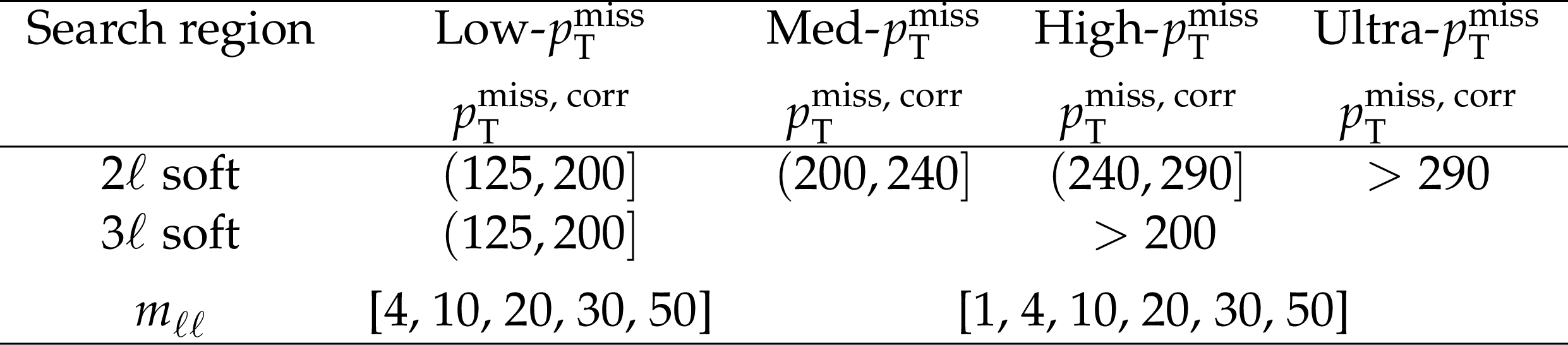
Table 1:
Definition of the lepton multiplicity and $ p_{\mathrm{T}}^\text{miss, corr} $ SRs of the ``2/3$\ell $ soft'' search. The last line shows the $ m_{\ell\ell} $ binning used in Ref. [17]. The boundaries are indicated in GeVns. Events in the Low-$ p_{\mathrm{T}}^\text{miss} $ SR must additionally have $ p_{\mathrm{T}}^\text{miss} > $ 125 GeV. |

png pdf |
Table 2:
Definitions of the SRs in category A, on-Z. |
png pdf |
Table 3:
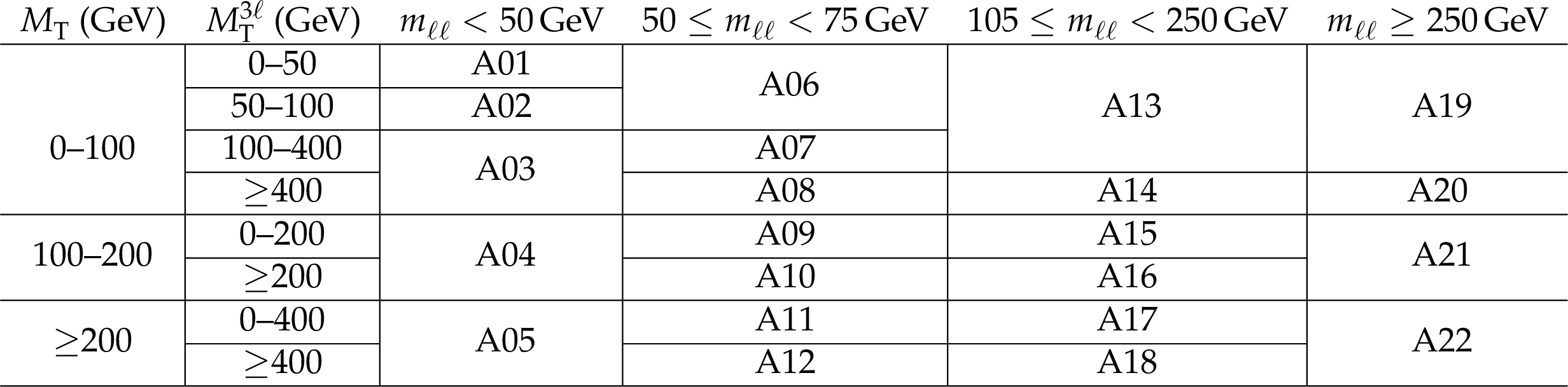
Definitions of the SRs in category A, off-Z. |
png pdf |
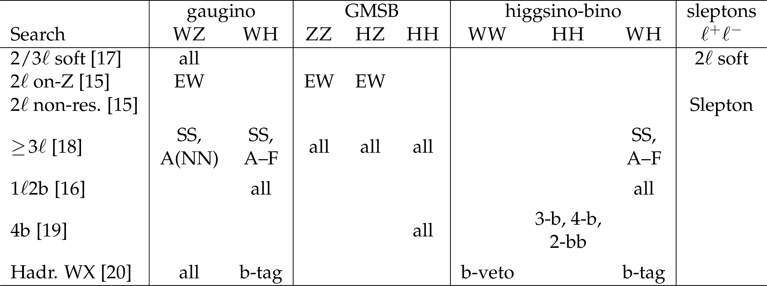
Table 4:
Summary of the searches considered in the combination and the SRs that contribute to the interpretation of each signal model and topology. The abbreviation 2$\ell $ non-res. refers to the ``2$\ell $ non-resonant'' search. For the ``2$\ell $ on-Z'' analysis, EW refers to the resolved and boosted VZ SRs and the HZ SR. For the ``2$\ell $ non-resonant'' search, Slepton refers to the two dedicated slepton SRs, those requiring $ N_{\text{jet}}= $ 0 and $ N_{\text{jet}} > $ 0. For the ``$ \geq$ 3\ell $'' search, A(NN) indicates SR A with the parametric neural network signal extraction. |
png pdf |
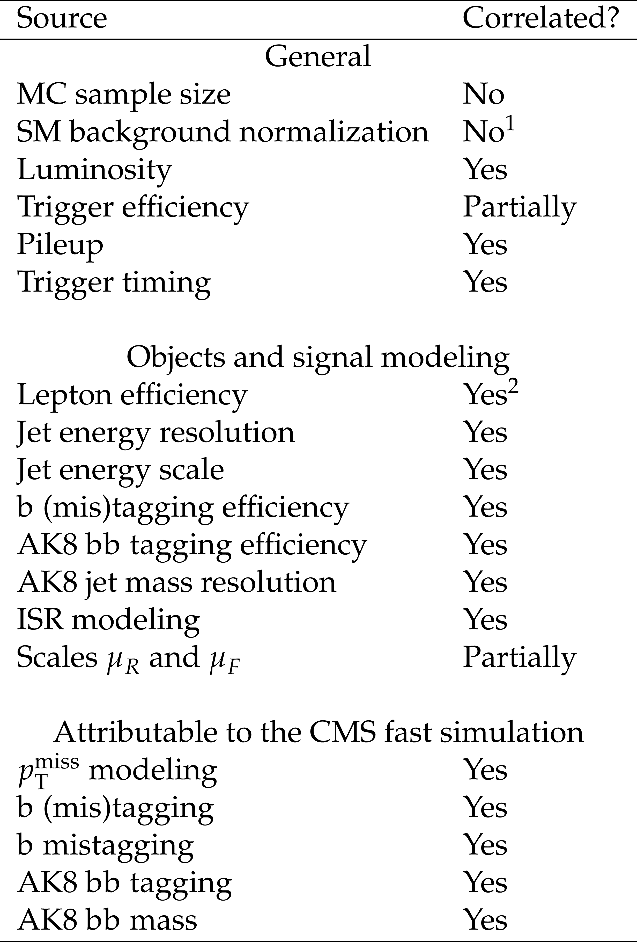
Table 5:
Sources of systematic uncertainties and the level of correlation between analyses. [4pt] Notes: 1. The WZ background normalization is correlated between the ``$ \geq$ 3$\ell $" [18] and the ``2/3$\ell $ soft'' [17] searches. 2. Except for slepton pair production, for which the two contributing searches, ``2/3$\ell $ soft'' [17] and ``2$\ell $ non-resonant'' [15], cover disjoint regions of the model parameter space. |
| Summary |
| A number of searches for new physics have been optimized and combined in different final states in proton-proton collision data at $ \sqrt{s}= $ 13 TeV, recorded with the CMS detector at the Large Hadron Collider and corresponding to an integrated luminosity of 137 fb$ ^{-1} $. No significant deviation from the standard model expectation has been observed. Limits are set on a variety of simplified models of supersymmetry (SUSY) that involve the electroweak production of supersymmetric partners of electroweak gauge or Higgs bosons. Specifically, limits are set on the production of gaugino-like chargino-neutralino pairs, higgsino-like neutralino pair production in a gauge-mediated SUSY breaking inspired scenario, a higgsino-bino interpretation, and slepton pair production. In the case of chargino-neutralino pair production, for an LSP $ \tilde{\chi}_{1}^{0} $ with a mass up to 50 GeV, the combined result gives an observed (expected) limit in $ m_{\tilde{\chi}_{1}^{\pm}} $ of about 875 (950) GeV for the WZ final state, 990 (1075) GeV for the WH final state, and 875 (1000) GeV for a mixed topology, extending the previous CMS result [25] by 225 GeV, 510 GeV, and 340 GeV, respectively, for the three topologies. For the higgsino pair production, the expected mass exclusion limit varies between about 600 and 950 GeV, being least stringent around $ \mathcal{B}(\tilde{\chi}_{1}^{0} \to \mathrm{H}\tilde{\mathrm{G}}) = $ 0.4. The observed limit ranges between about 750 and 1025 GeV, allowing the exclusion of masses below 750 GeV independent of this branching fraction. This extends the previous result [25] by 100 GeV. A higgsino-bino model that assumes mass degenerate higgsino-like $ \tilde{\chi}_{2}^{0} $, $ \tilde{\chi}_{3}^{0} $, and $ \tilde{\chi}_{1}^{\pm} $ decaying to a bino-like $ \tilde{\chi}_{1}^{0} $ and an SM boson is excluded for $ m_{\tilde{\chi}_{1}^{\pm}}=m_{\tilde{\chi}_{2}^{0}} $ between 225 and 800 GeV for a $ \tilde{\chi}_{1}^{0} $ mass below 50 GeV. In general for the models considered in this combination, chargino masses are excluded up to 990 GeV, while higgsino masses are excluded up to 1000 GeV. The improvement is between 100--510 GeV with respect to the previously set exclusion limits [25]. Additionally, the results presented here set limits on direct slepton pair production. A dedicated search added for this note explores the parameter space in the most compressed region. For $ \Delta m({\tilde{\ell}},\tilde{\chi}_{1}^{0})= $ 5 GeV slepton masses up to 215 GeV are excluded. The combination yields an observed (expected) exclusion in the slepton mass of about 130--700 (110--720) GeV, for $ m_{\tilde{\chi}_{1}^{0}} < $ 50 GeV. |
| References | ||||
| 1 | J. Wess and B. Zumino | Supergauge transformations in four dimensions | NPB 70 (1974) 39 | |
| 2 | H. P. Nilles | Supersymmetry, supergravity and particle physics | Phys. Rept. 110 (1984) 1 | |
| 3 | H. E. Haber and G. L. Kane | The search for supersymmetry: Probing physics beyond the standard model | Phys. Rept. 117 (1985) 75 | |
| 4 | R. Barbieri, S. Ferrara, and C. A. Savoy | Gauge models with spontaneously broken local supersymmetry | PLB 119 (1982) 343 | |
| 5 | S. Dawson, E. Eichten, and C. Quigg | Search for supersymmetric particles in hadron-hadron collisions | PRD 31 (1985) 1581 | |
| 6 | S. Dimopoulos and G. F. Giudice | Naturalness constraints in supersymmetric theories with nonuniversal soft terms | PLB 357 (1995) 573 | hep-ph/9507282 |
| 7 | R. Barbieri and D. Pappadopulo | S-particles at their naturalness limits | JHEP 10 (2009) 061 | 0906.4546 |
| 8 | M. Papucci, J. T. Ruderman, and A. Weiler | Natural SUSY endures | JHEP 09 (2012) 035 | 1110.6926 |
| 9 | A. J. Buras, J. Ellis, M. K. Gaillard, and D. V. Nanopoulos | Aspects of the grand unification of strong, weak and electromagnetic interactions | NP B 135 (1978) 66 | |
| 10 | G. R. Farrar and P. Fayet | Phenomenology of the Production, Decay, and Detection of New Hadronic States Associated with Supersymmetry | PLB 76 (1978) 575 | |
| 11 | H. Goldberg | Constraint on the photino mass from cosmology | PRL 50 (1983) 1419 | |
| 12 | J. R. Ellis et al. | Supersymmetric relics from the big bang | NPB 238 (1984) 453 | |
| 13 | S. Dimopoulos, M. Dine, S. Raby, and S. D. Thomas | Experimental signatures of low-energy gauge mediated supersymmetry breaking | PRL 76 (1996) 3494 | hep-ph/9601367 |
| 14 | K. T. Matchev and S. D. Thomas | Higgs and Z boson signatures of supersymmetry | PRD 62 (2000) 077702 | hep-ph/9908482 |
| 15 | CMS Collaboration | Search for supersymmetry in final states with two oppositely charged same-flavor leptons and missing transverse momentum in proton-proton collisions at $ \sqrt{s} = $ 13 TeV | JHEP 04 (2021) 123 | CMS-SUS-20-001 2012.08600 |
| 16 | CMS Collaboration | Search for chargino-neutralino production in events with Higgs and W bosons using 137 fb$ ^{-1} $ of proton-proton collisions at $ \sqrt{s} = $ 13 TeV | JHEP 10 (2021) 045 | CMS-SUS-20-003 2107.12553 |
| 17 | CMS Collaboration | Search for supersymmetry in final states with two or three soft leptons and missing transverse momentum in proton-proton collisions at $ \sqrt{s} = $ 13 TeV | JHEP 04 (2022) 091 | CMS-SUS-18-004 2111.06296 |
| 18 | CMS Collaboration | Search for electroweak production of charginos and neutralinos in proton-proton collisions at $ \sqrt{s} = $ 13 TeV | JHEP 04 (2022) 147 | CMS-SUS-19-012 2106.14246 |
| 19 | CMS Collaboration | Search for higgsinos decaying to two Higgs bosons and missing transverse momentum in proton-proton collisions at $ \sqrt{s} = $ 13 TeV | JHEP 05 (2022) 014 | CMS-SUS-20-004 2201.04206 |
| 20 | CMS Collaboration | Search for electroweak production of charginos and neutralinos at $ \sqrt{s} = $ 13 TeV in final states containing hadronic decays of WW, WZ, or WH and missing transverse momentum | Submitted to PLB | CMS-SUS-21-002 2205.09597 |
| 21 | N. Arkani-Hamed et al. | MARMOSET: The path from LHC data to the new standard model via on-shell effective theories | hep-ph/0703088 | |
| 22 | J. Alwall, P. Schuster, and N. Toro | Simplified models for a first characterization of new physics at the LHC | PRD 79 (2009) 075020 | 0810.3921 |
| 23 | J. Alwall, M.-P. Le, M. Lisanti, and J. G. Wacker | Model-independent jets plus missing energy searches | PRD 79 (2009) 015005 | 0809.3264 |
| 24 | D. Alves et al. | Simplified models for LHC new physics searches | JPG 39 (2012) 105005 | 1105.2838 |
| 25 | CMS Collaboration | Combined search for electroweak production of charginos and neutralinos in proton-proton collisions at $ \sqrt{s} = $ 13 TeV | JHEP 03 (2018) 160 | CMS-SUS-17-004 1801.03957 |
| 26 | ATLAS Collaboration | Search for direct production of electroweakinos in final states with one lepton, missing transverse momentum and a Higgs boson decaying into two $ b $-jets in pp collisions at $ \sqrt{s}= $ 13 TeV with the ATLAS detector | EPJC 80 (2020) 691 | 1909.09226 |
| 27 | ATLAS Collaboration | Searches for electroweak production of supersymmetric particles with compressed mass spectra in $ \sqrt{s}= $ 13 TeV pp collisions with the ATLAS detector | PRD 101 (2020) 052005 | 1911.12606 |
| 28 | ATLAS Collaboration | Search for electroweak production of charginos and sleptons decaying into final states with two leptons and missing transverse momentum in $ \sqrt{s}= $ 13 TeV pp collisions using the ATLAS detector | EPJC 80 (2020) 123 | 1908.08215 |
| 29 | ATLAS Collaboration | Search for chargino-neutralino pair production in final states with three leptons and missing transverse momentum in $ \sqrt{s} = $ 13 TeV pp collisions with the ATLAS detector | EPJC 81 (2021) 1118 | 2106.01676 |
| 30 | ATLAS Collaboration | Search for supersymmetry in events with four or more charged leptons in 139 fb$^{-1}$ of $ \sqrt{s}= $ 13 TeV pp collisions with the ATLAS detector | JHEP 07 (2021) 167 | 2103.11684 |
| 31 | ATLAS Collaboration | Search for charginos and neutralinos in final states with two boosted hadronically decaying bosons and missing transverse momentum in pp collisions at $ \sqrt{s}= $ 13 TeV with the ATLAS detector | PRD 104 (2021) 112010 | 2108.07586 |
| 32 | ATLAS Collaboration | Searches for new phenomena in events with two leptons, jets, and missing transverse momentum in 139 fb$^{-1}$ of $ \sqrt{s}=$ 13 TeV pp collisions with the ATLAS detector | Submitted to EPJC | 2204.13072 |
| 33 | ATLAS Collaboration | Search for direct pair production of sleptons and charginos decaying to two leptons and neutralinos with mass splittings near the $ W $-boson mass in $ {\sqrt{s}=13\,} $TeV pp collisions with the ATLAS detector | Submitted to JHEP | 2209.13935 |
| 34 | H. Baer et al. | Natural SUSY with a bino- or wino-like LSP | PRD 91 (2015) 075005 | 1501.06357 |
| 35 | CMS Collaboration | The CMS experiment at the CERN LHC | JINST 3 (2008) S08004 | |
| 36 | CMS Collaboration | Performance of the CMS Level-1 trigger in proton-proton collisions at $ \sqrt{s} = $ 13\,TeV | JINST 15 (2020) P10017 | CMS-TRG-17-001 2006.10165 |
| 37 | CMS Collaboration | The CMS trigger system | JINST 12 (2017) P01020 | CMS-TRG-12-001 1609.02366 |
| 38 | CMS Collaboration | Precision luminosity measurement in proton-proton collisions at $ \sqrt{s} = $ 13 TeV in 2015 and 2016 at CMS | EPJC 81 (2021) 800 | CMS-LUM-17-003 2104.01927 |
| 39 | CMS Collaboration | CMS luminosity measurement for the 2017 data-taking period at $ \sqrt{s} = $ 13 TeV | CMS Physics Analysis Summary, 2018 link |
CMS-PAS-LUM-17-004 |
| 40 | CMS Collaboration | CMS luminosity measurement for the 2018 data-taking period at $ \sqrt{s} = $ 13 TeV | CMS Physics Analysis Summary, 2019 link |
CMS-PAS-LUM-18-002 |
| 41 | CMS Collaboration | Particle-flow reconstruction and global event description with the CMS detector | JINST 12 (2017) P10003 | CMS-PRF-14-001 1706.04965 |
| 42 | CMS Collaboration | Reconstruction and identification of $ \tau $ lepton decays to hadrons and $ \nu_\tau $ at CMS. Reconstruction and identification of tau lepton decays to hadrons and tau neutrino at CMS | JINST 11 (2016) P01019 | CMS-TAU-14-001 1510.07488 |
| 43 | CMS Collaboration | Technical proposal for the Phase-II upgrade of the Compact Muon Solenoid | CMS Technical Proposal CERN-LHCC-2015-010, CMS-TDR-15-02, 2015 CDS |
|
| 44 | M. Cacciari, G. P. Salam, and G. Soyez | The anti-$ k_{\mathrm{T}} $ jet clustering algorithm | JHEP 04 (2008) 063 | 0802.1189 |
| 45 | M. Cacciari, G. P. Salam, and G. Soyez | FastJet User Manual | EPJC 72 (2012) 1896 | 1111.6097 |
| 46 | CMS Collaboration | Jet energy scale and resolution in the CMS experiment in pp collisions at 8 TeV | JINST 12 (2017) P02014 | CMS-JME-13-004 1607.03663 |
| 47 | CMS Collaboration | Identification of heavy-flavour jets with the CMS detector in pp collisions at 13 TeV | JINST 13 (2018) P05011 | CMS-BTV-16-002 1712.07158 |
| 48 | CMS Collaboration | Performance of deep tagging algorithms for boosted double quark jet topology in proton-proton collisions at 13 tev with the phase-0 cms detector | CMS Detector Performance Note CMS-DP-2018-046, CERN, 2018 link |
|
| 49 | G. Louppe, M. Kagan, and K. Cranmer | Learning to pivot with adversarial networks | in Advances in Neural Information Processing Systems, volume 30, 2017 link |
1611.01046 |
| 50 | CMS Collaboration | Identification of heavy, energetic, hadronically decaying particles using machine-learning techniques | JINST 15 (2020) P06005 | CMS-JME-18-002 2004.08262 |
| 51 | CMS Collaboration | Performance of missing transverse momentum reconstruction in proton-proton collisions at $ \sqrt{s} = $ 13\,TeV using the CMS detector | JINST 14 (2019) P07004 | CMS-JME-17-001 1903.06078 |
| 52 | J. Alwall et al. | The automated computation of tree-level and next-to-leading order differential cross sections, and their matching to parton shower simulations | JHEP 07 (2014) 079 | 1405.0301 |
| 53 | R. Frederix and S. Frixione | Merging meets matching in MC@NLO | JHEP 12 (2012) 061 | 1209.6215 |
| 54 | W. Beenakker et al. | Production of charginos, neutralinos, and sleptons at hadron colliders | PRL 83 (1999) 3780 | hep-ph/9906298 |
| 55 | B. Fuks, M. Klasen, D. R. Lamprea, and M. Rothering | Gaugino production in proton-proton collisions at a center-of-mass energy of 8 TeV | JHEP 10 (2012) 081 | 1207.2159 |
| 56 | B. Fuks, M. Klasen, D. R. Lamprea, and M. Rothering | Precision predictions for electroweak superpartner production at hadron colliders with \sc resummino | EPJC 73 (2013) 2480 | 1304.0790 |
| 57 | P. Nason | A new method for combining NLO QCD with shower Monte Carlo algorithms | JHEP 11 (2004) 040 | hep-ph/0409146 |
| 58 | S. Frixione, P. Nason, and C. Oleari | Matching NLO QCD computations with parton shower simulations: the POWHEG method | JHEP 11 (2007) 070 | 0709.2092 |
| 59 | S. Alioli, P. Nason, C. Oleari, and E. Re | NLO single-top production matched with shower in POWHEG: $ s $- and $ t $-channel contributions | JHEP 09 (2009) 111 | 0907.4076 |
| 60 | J. M. Campbell and R. K. Ellis | An update on vector boson pair production at hadron colliders | PRD 60 (1999) 113006 | hep-ph/9905386 |
| 61 | J. M. Campbell, R. K. Ellis, and C. Williams | Vector boson pair production at the LHC | JHEP 07 (2011) 018 | 1105.0020 |
| 62 | J. M. Campbell, R. K. Ellis, and W. T. Giele | A multi-threaded version of MCFM | EPJC 75 (2015) 246 | 1503.06182 |
| 63 | T. Sjöstrand et al. | An Introduction to PYTHIA 8.2 | Comput. Phys. Commun. 191 (2015) 159 | 1410.3012 |
| 64 | CMS Collaboration | Event generator tunes obtained from underlying event and multiparton scattering measurements | EPJC 76 (2016) 155 | CMS-GEN-14-001 1512.00815 |
| 65 | CMS Collaboration | Extraction and validation of a new set of CMS PYTHIA8 tunes from underlying-event measurements | EPJC 80 (2020) 4 | CMS-GEN-17-001 1903.12179 |
| 66 | NNPDF Collaboration | Parton distributions for the LHC Run II | JHEP 04 (2015) 040 | 1410.8849 |
| 67 | NNPDF Collaboration | Parton distributions from high-precision collider data | EPJC 77 (2017) 663 | 1706.00428 |
| 68 | S. Abdullin et al. | The fast simulation of the CMS detector at LHC | J. Phys. Conf. Ser. 331 (2011) 032049 | |
| 69 | A. Giammanco | The fast simulation of the CMS experiment | J. Phys. Conf. Ser. 513 (2014) 022012 | |
| 70 | GEANT4 Collaboration | GEANT 4---a simulation toolkit | NIM A 506 (2003) 250 | |
| 71 | U. De Sanctis, T. Lari, S. Montesano, and C. Troncon | Perspectives for the detection and measurement of supersymmetry in the focus point region of mSUGRA models with the ATLAS detector at LHC | EPJC 52 (2007) 743 | 0704.2515 |
| 72 | C. G. Lester and D. J. Summers | Measuring masses of semiinvisibly decaying particles pair produced at hadron colliders | PLB 463 (1999) 99 | hep-ph/9906349 |
| 73 | A. Barr, C. Lester, and P. Stephens | m(T2): The Truth behind the glamour | JPG 29 (2003) 2343 | hep-ph/0304226 |
| 74 | Particle Data Group | Review of particle physics | PTEP 2020 (2020) 083C01 | |
| 75 | A. L. Read | Presentation of search results: The $ \text{CL}_{\text{S}} $ technique | JPG 28 (2002) 2693 | |
| 76 | T. Junk | Confidence level computation for combining searches with small statistics | NIM A 434 (1999) 435 | hep-ex/9902006 |
| 77 | G. Cowan, K. Cranmer, E. Gross, and O. Vitells | Asymptotic formulae for likelihood-based tests of new physics | EPJC 71 (2011) 1554 | 1007.1727 |
| 78 | ATLAS Collaboration, CMS Collaboration, LHC Higgs Combination Group | Procedure for the LHC Higgs boson search combination in Summer 2011 | Technical Report CMS-NOTE-2011-005, ATL-PHYS-PUB-2011-11, CERN, 2011 link |
|
|
|
Compact Muon Solenoid LHC, CERN |
|

|

|

|

|

|