

Compact Muon Solenoid
LHC, CERN
| CMS-PAS-SMP-24-005 | ||
| Measurement of the inclusive WZ production cross section in pp collisions at $ \sqrt{s}= $ 13.6 TeV with the CMS experiment | ||
| CMS Collaboration | ||
| 19 July 2024 | ||
| Abstract: The inclusive WZ cross section is measured in proton-proton collisions at a centre-of-mass energy of 13.6 TeV, using 34.7 fb$ ^{-1} $ of data collected during 2022 with the CMS detector. The measurement is performed in multileptonic final states by performing a simultaneous likelihood fit to the number of events in four different lepton flavour categories: $ \mathrm{eee} $, $ \mathrm{ee}{\mu} $, $ {\mu}{\mu}\mathrm{e} $, $ {\mu}{\mu}{\mu} $. The selection is optimized to minimize the number of background events thanks to the usage of an efficient prompt lepton discrimination strategy. The WZ production cross section is measured in a phase space, defined around a 30 GeV window around the Z mass, as $ \sigma_{\text{total}} (pp \rightarrow \mathrm{WZ}) = $ 55.2 $ \pm $ 1.2 (stat) $ \pm $ 1.2 (syst) $ \pm $ 0.8 (lumi) $ \pm $ 0.1 (theo) pb. In addition, the cross section is also measured in a fiducial phase space, closer to the detector level requirements, as $ \sigma_{\text{fiducial}} (pp \rightarrow \mathrm{WZ}) = $ 297.6 $ \pm $ 6.4 (stat) $ \pm $ 6.4 (syst) $ \pm $ 4.2 (lumi) $ \pm $ 0.5 (theo) pb. | ||
|
Links:
CDS record (PDF) ;
Physics Briefing ;
CADI line (restricted) ;
These preliminary results are superseded in this paper, Submitted to JHEP. The superseded preliminary plots can be found here. |
||
| Figures | |

png pdf |
Figure 1:
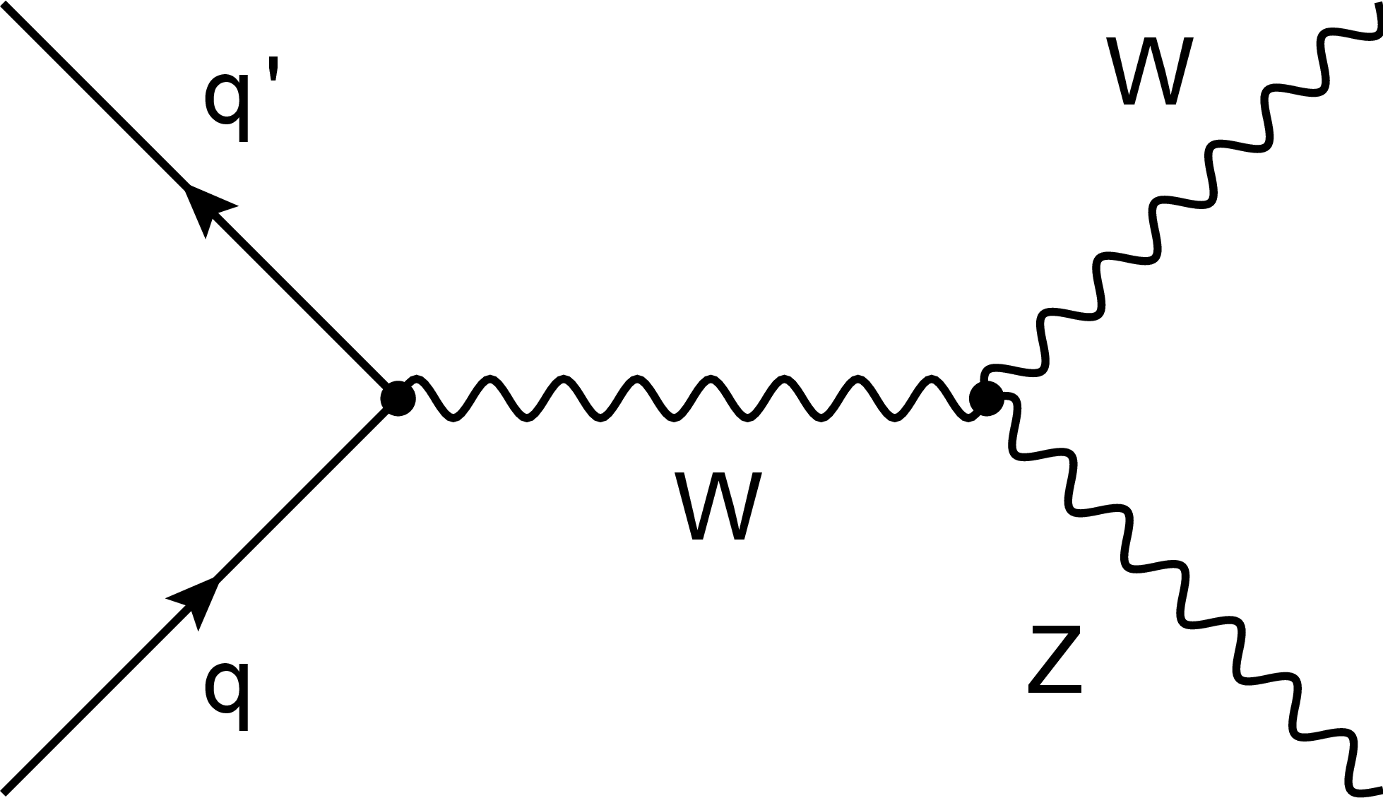
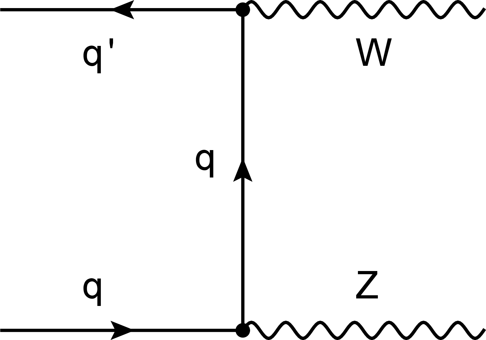
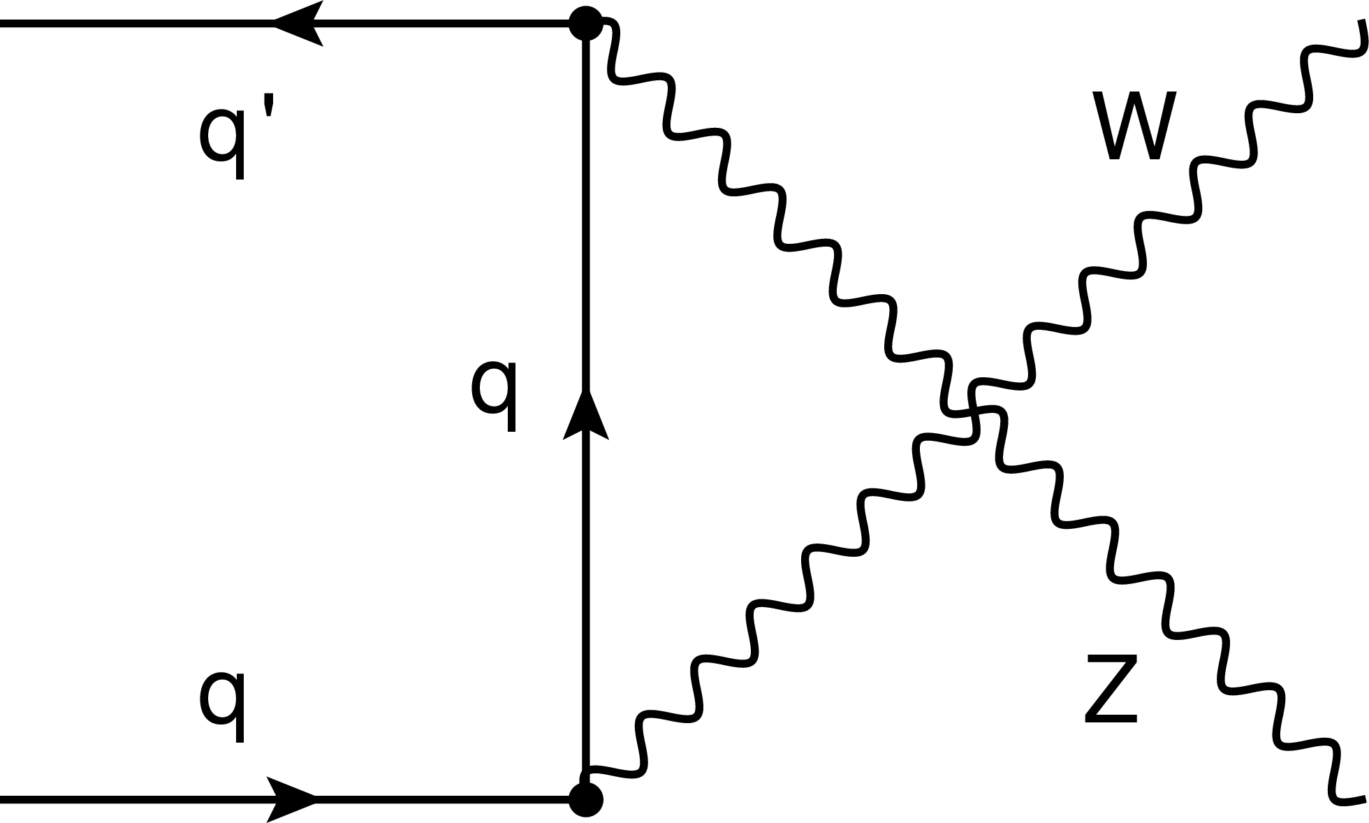
Feynman diagrams for WZ production at leading order in pp collisions. The contributions from the $ s $ channel (left), $ t $ channel (middle), and $ u $ channel (right) are shown. |
png pdf |
Figure 1-a:
Feynman diagrams for WZ production at leading order in pp collisions. The contributions from the $ s $ channel (left), $ t $ channel (middle), and $ u $ channel (right) are shown. |
png pdf |
Figure 1-b:
Feynman diagrams for WZ production at leading order in pp collisions. The contributions from the $ s $ channel (left), $ t $ channel (middle), and $ u $ channel (right) are shown. |
png pdf |
Figure 1-c:
Feynman diagrams for WZ production at leading order in pp collisions. The contributions from the $ s $ channel (left), $ t $ channel (middle), and $ u $ channel (right) are shown. |

png pdf |
Figure 2:
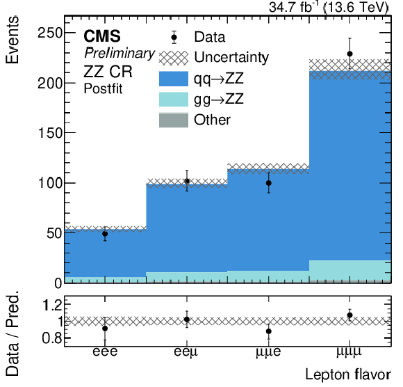
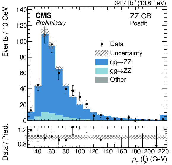
Distribution of observables in the ZZ CR after the fit to the data, described in Section 8. From top left to bottom right: flavour composition, $ p_{\mathrm{T}} $ of the $ \ell^1_{\mathrm{Z}} $, $ p_{\mathrm{T}} $ of the $ \ell^2_{\mathrm{Z}} $, and $ p_{\mathrm{T}} $ of the $ \ell_{\mathrm{W}} $. The shaded bands show the total uncertainty on the MC prediction. The vertical bars of the data account for the statistical uncertainty. When present, underflow and overflow events are included in the first and last bin of the observables. The ``Other" category groups all processes that have an small contribution to this region. |
png pdf |
Figure 2-a:
Distribution of observables in the ZZ CR after the fit to the data, described in Section 8. From top left to bottom right: flavour composition, $ p_{\mathrm{T}} $ of the $ \ell^1_{\mathrm{Z}} $, $ p_{\mathrm{T}} $ of the $ \ell^2_{\mathrm{Z}} $, and $ p_{\mathrm{T}} $ of the $ \ell_{\mathrm{W}} $. The shaded bands show the total uncertainty on the MC prediction. The vertical bars of the data account for the statistical uncertainty. When present, underflow and overflow events are included in the first and last bin of the observables. The ``Other" category groups all processes that have an small contribution to this region. |
png pdf |
Figure 2-b:
Distribution of observables in the ZZ CR after the fit to the data, described in Section 8. From top left to bottom right: flavour composition, $ p_{\mathrm{T}} $ of the $ \ell^1_{\mathrm{Z}} $, $ p_{\mathrm{T}} $ of the $ \ell^2_{\mathrm{Z}} $, and $ p_{\mathrm{T}} $ of the $ \ell_{\mathrm{W}} $. The shaded bands show the total uncertainty on the MC prediction. The vertical bars of the data account for the statistical uncertainty. When present, underflow and overflow events are included in the first and last bin of the observables. The ``Other" category groups all processes that have an small contribution to this region. |

png pdf |
Figure 2-c:
Distribution of observables in the ZZ CR after the fit to the data, described in Section 8. From top left to bottom right: flavour composition, $ p_{\mathrm{T}} $ of the $ \ell^1_{\mathrm{Z}} $, $ p_{\mathrm{T}} $ of the $ \ell^2_{\mathrm{Z}} $, and $ p_{\mathrm{T}} $ of the $ \ell_{\mathrm{W}} $. The shaded bands show the total uncertainty on the MC prediction. The vertical bars of the data account for the statistical uncertainty. When present, underflow and overflow events are included in the first and last bin of the observables. The ``Other" category groups all processes that have an small contribution to this region. |

png pdf |
Figure 2-d:
Distribution of observables in the ZZ CR after the fit to the data, described in Section 8. From top left to bottom right: flavour composition, $ p_{\mathrm{T}} $ of the $ \ell^1_{\mathrm{Z}} $, $ p_{\mathrm{T}} $ of the $ \ell^2_{\mathrm{Z}} $, and $ p_{\mathrm{T}} $ of the $ \ell_{\mathrm{W}} $. The shaded bands show the total uncertainty on the MC prediction. The vertical bars of the data account for the statistical uncertainty. When present, underflow and overflow events are included in the first and last bin of the observables. The ``Other" category groups all processes that have an small contribution to this region. |

png pdf |
Figure 3:
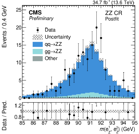
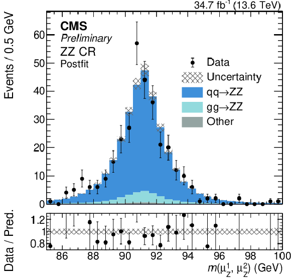
Distribution of the invariant mass of $ \ell^1_{\mathrm{Z}} $ and $ \ell^2_{\mathrm{Z}} $ in the ZZ CR after the fit to the data. The left (right) distribution shows the case in which both leptons are electrons (muons). The vertical bars of the data account for the statistical uncertainty. The ``Other" category groups all processes that have an small contribution to this region. |
png pdf |
Figure 3-a:
Distribution of the invariant mass of $ \ell^1_{\mathrm{Z}} $ and $ \ell^2_{\mathrm{Z}} $ in the ZZ CR after the fit to the data. The left (right) distribution shows the case in which both leptons are electrons (muons). The vertical bars of the data account for the statistical uncertainty. The ``Other" category groups all processes that have an small contribution to this region. |
png pdf |
Figure 3-b:
Distribution of the invariant mass of $ \ell^1_{\mathrm{Z}} $ and $ \ell^2_{\mathrm{Z}} $ in the ZZ CR after the fit to the data. The left (right) distribution shows the case in which both leptons are electrons (muons). The vertical bars of the data account for the statistical uncertainty. The ``Other" category groups all processes that have an small contribution to this region. |
png pdf |
Figure 4:
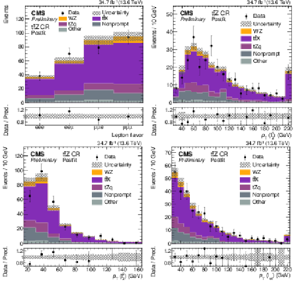
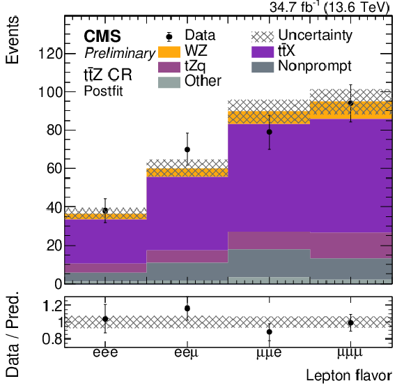
Distribution of observables in the $ {\mathrm{t}\overline{\mathrm{t}}} \mathrm{Z} $ CR after the fit to the data, described in Section 8. From top left to bottom right: flavour composition, $ p_{\mathrm{T}} $ of the $ \ell^1_{\mathrm{Z}} $, $ p_{\mathrm{T}} $ of the $ \ell^2_{\mathrm{Z}} $, and $ p_{\mathrm{T}} $ of the $ \ell_{\mathrm{W}} $. The shaded bands show the total uncertainty on the MC prediction. The vertical bars of the data account for the statistical uncertainty. When present, underflow and overflow events are included in the first and last bin of the observables. The ``Other" category groups all process that have an small contribution to this region. |
png pdf |
Figure 4-a:
Distribution of observables in the $ {\mathrm{t}\overline{\mathrm{t}}} \mathrm{Z} $ CR after the fit to the data, described in Section 8. From top left to bottom right: flavour composition, $ p_{\mathrm{T}} $ of the $ \ell^1_{\mathrm{Z}} $, $ p_{\mathrm{T}} $ of the $ \ell^2_{\mathrm{Z}} $, and $ p_{\mathrm{T}} $ of the $ \ell_{\mathrm{W}} $. The shaded bands show the total uncertainty on the MC prediction. The vertical bars of the data account for the statistical uncertainty. When present, underflow and overflow events are included in the first and last bin of the observables. The ``Other" category groups all process that have an small contribution to this region. |

png pdf |
Figure 4-b:
Distribution of observables in the $ {\mathrm{t}\overline{\mathrm{t}}} \mathrm{Z} $ CR after the fit to the data, described in Section 8. From top left to bottom right: flavour composition, $ p_{\mathrm{T}} $ of the $ \ell^1_{\mathrm{Z}} $, $ p_{\mathrm{T}} $ of the $ \ell^2_{\mathrm{Z}} $, and $ p_{\mathrm{T}} $ of the $ \ell_{\mathrm{W}} $. The shaded bands show the total uncertainty on the MC prediction. The vertical bars of the data account for the statistical uncertainty. When present, underflow and overflow events are included in the first and last bin of the observables. The ``Other" category groups all process that have an small contribution to this region. |
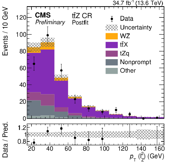
png pdf |
Figure 4-c:
Distribution of observables in the $ {\mathrm{t}\overline{\mathrm{t}}} \mathrm{Z} $ CR after the fit to the data, described in Section 8. From top left to bottom right: flavour composition, $ p_{\mathrm{T}} $ of the $ \ell^1_{\mathrm{Z}} $, $ p_{\mathrm{T}} $ of the $ \ell^2_{\mathrm{Z}} $, and $ p_{\mathrm{T}} $ of the $ \ell_{\mathrm{W}} $. The shaded bands show the total uncertainty on the MC prediction. The vertical bars of the data account for the statistical uncertainty. When present, underflow and overflow events are included in the first and last bin of the observables. The ``Other" category groups all process that have an small contribution to this region. |

png pdf |
Figure 4-d:
Distribution of observables in the $ {\mathrm{t}\overline{\mathrm{t}}} \mathrm{Z} $ CR after the fit to the data, described in Section 8. From top left to bottom right: flavour composition, $ p_{\mathrm{T}} $ of the $ \ell^1_{\mathrm{Z}} $, $ p_{\mathrm{T}} $ of the $ \ell^2_{\mathrm{Z}} $, and $ p_{\mathrm{T}} $ of the $ \ell_{\mathrm{W}} $. The shaded bands show the total uncertainty on the MC prediction. The vertical bars of the data account for the statistical uncertainty. When present, underflow and overflow events are included in the first and last bin of the observables. The ``Other" category groups all process that have an small contribution to this region. |
png pdf |
Figure 5:
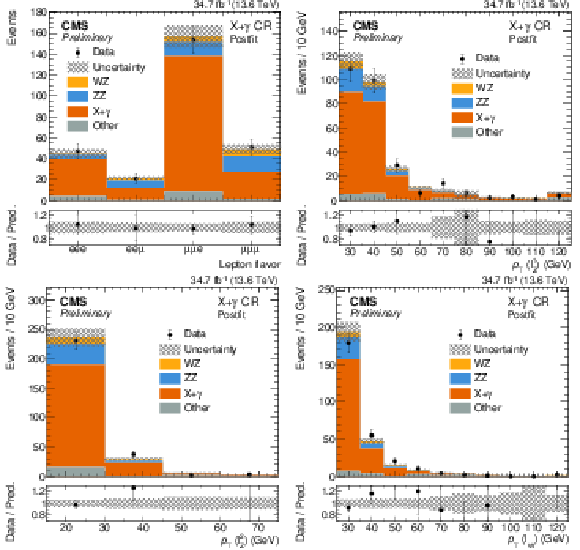
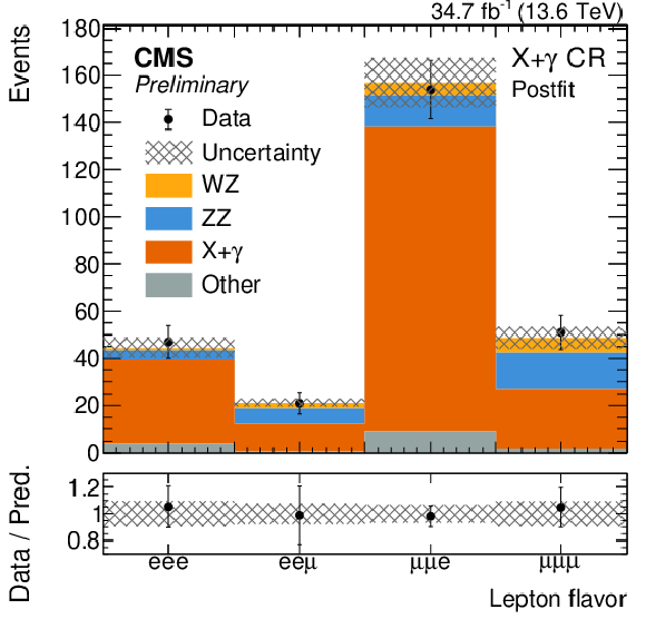
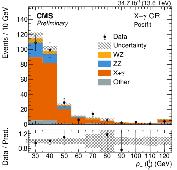
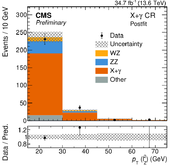
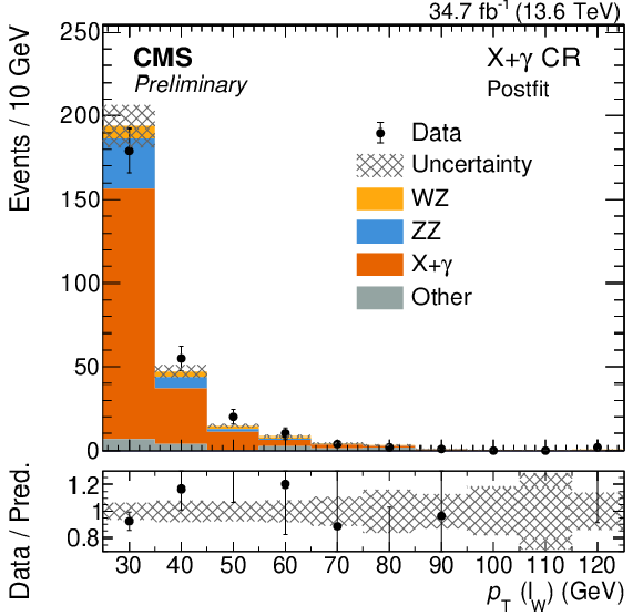
Distribution of observables in the $ \mbox{X}+\gamma $ CR after the fit to the data, described in Section 8. From top left to bottom right: flavour composition, $ p_{\mathrm{T}} $ of the $ \ell^1_{\mathrm{Z}} $, $ p_{\mathrm{T}} $ of the $ \ell^2_{\mathrm{Z}} $, and $ p_{\mathrm{T}} $ of the $ \ell_{\mathrm{W}} $. The shaded bands show the total uncertainty on the MC prediction. The vertical bars of the data account for the statistical uncertainty. When present, underflow and overflow events are included in the first and last bin of the observables. The ``Other" category groups all process that have an small contribution to this region. |
png pdf |
Figure 5-a:
Distribution of observables in the $ \mbox{X}+\gamma $ CR after the fit to the data, described in Section 8. From top left to bottom right: flavour composition, $ p_{\mathrm{T}} $ of the $ \ell^1_{\mathrm{Z}} $, $ p_{\mathrm{T}} $ of the $ \ell^2_{\mathrm{Z}} $, and $ p_{\mathrm{T}} $ of the $ \ell_{\mathrm{W}} $. The shaded bands show the total uncertainty on the MC prediction. The vertical bars of the data account for the statistical uncertainty. When present, underflow and overflow events are included in the first and last bin of the observables. The ``Other" category groups all process that have an small contribution to this region. |
png pdf |
Figure 5-b:
Distribution of observables in the $ \mbox{X}+\gamma $ CR after the fit to the data, described in Section 8. From top left to bottom right: flavour composition, $ p_{\mathrm{T}} $ of the $ \ell^1_{\mathrm{Z}} $, $ p_{\mathrm{T}} $ of the $ \ell^2_{\mathrm{Z}} $, and $ p_{\mathrm{T}} $ of the $ \ell_{\mathrm{W}} $. The shaded bands show the total uncertainty on the MC prediction. The vertical bars of the data account for the statistical uncertainty. When present, underflow and overflow events are included in the first and last bin of the observables. The ``Other" category groups all process that have an small contribution to this region. |
png pdf |
Figure 5-c:
Distribution of observables in the $ \mbox{X}+\gamma $ CR after the fit to the data, described in Section 8. From top left to bottom right: flavour composition, $ p_{\mathrm{T}} $ of the $ \ell^1_{\mathrm{Z}} $, $ p_{\mathrm{T}} $ of the $ \ell^2_{\mathrm{Z}} $, and $ p_{\mathrm{T}} $ of the $ \ell_{\mathrm{W}} $. The shaded bands show the total uncertainty on the MC prediction. The vertical bars of the data account for the statistical uncertainty. When present, underflow and overflow events are included in the first and last bin of the observables. The ``Other" category groups all process that have an small contribution to this region. |
png pdf |
Figure 5-d:
Distribution of observables in the $ \mbox{X}+\gamma $ CR after the fit to the data, described in Section 8. From top left to bottom right: flavour composition, $ p_{\mathrm{T}} $ of the $ \ell^1_{\mathrm{Z}} $, $ p_{\mathrm{T}} $ of the $ \ell^2_{\mathrm{Z}} $, and $ p_{\mathrm{T}} $ of the $ \ell_{\mathrm{W}} $. The shaded bands show the total uncertainty on the MC prediction. The vertical bars of the data account for the statistical uncertainty. When present, underflow and overflow events are included in the first and last bin of the observables. The ``Other" category groups all process that have an small contribution to this region. |
png pdf |
Figure 6:
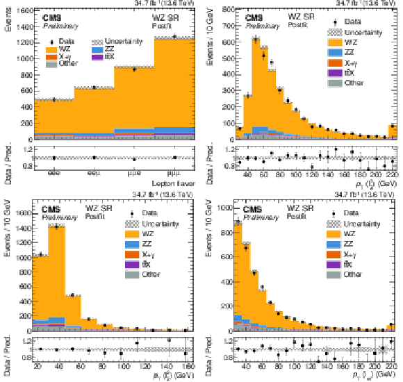
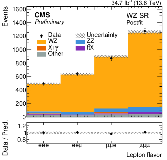
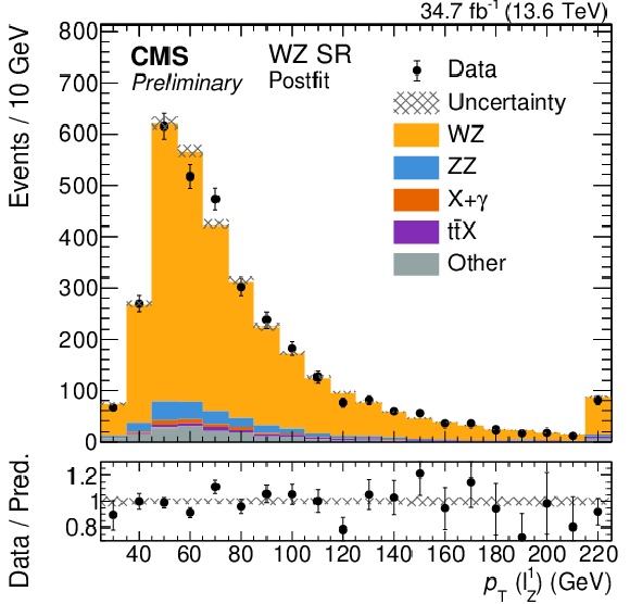
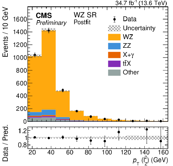
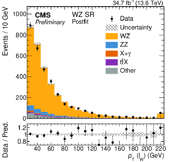
Distributions of several observables in the SR after the fit. From top left to bottom right: flavour composition, $ p_{\mathrm{T}} $ of the $ \ell^1_{\mathrm{Z}} $, $ p_{\mathrm{T}} $ of the $ \ell^2_{\mathrm{Z}} $, and $ p_{\mathrm{T}} $ of the $ \ell_{\mathrm{W}} $ (bottom right). The shaded band in the ratio includes all systematic uncertainties. |
png pdf |
Figure 6-a:
Distributions of several observables in the SR after the fit. From top left to bottom right: flavour composition, $ p_{\mathrm{T}} $ of the $ \ell^1_{\mathrm{Z}} $, $ p_{\mathrm{T}} $ of the $ \ell^2_{\mathrm{Z}} $, and $ p_{\mathrm{T}} $ of the $ \ell_{\mathrm{W}} $ (bottom right). The shaded band in the ratio includes all systematic uncertainties. |
png pdf |
Figure 6-b:
Distributions of several observables in the SR after the fit. From top left to bottom right: flavour composition, $ p_{\mathrm{T}} $ of the $ \ell^1_{\mathrm{Z}} $, $ p_{\mathrm{T}} $ of the $ \ell^2_{\mathrm{Z}} $, and $ p_{\mathrm{T}} $ of the $ \ell_{\mathrm{W}} $ (bottom right). The shaded band in the ratio includes all systematic uncertainties. |
png pdf |
Figure 6-c:
Distributions of several observables in the SR after the fit. From top left to bottom right: flavour composition, $ p_{\mathrm{T}} $ of the $ \ell^1_{\mathrm{Z}} $, $ p_{\mathrm{T}} $ of the $ \ell^2_{\mathrm{Z}} $, and $ p_{\mathrm{T}} $ of the $ \ell_{\mathrm{W}} $ (bottom right). The shaded band in the ratio includes all systematic uncertainties. |
png pdf |
Figure 6-d:
Distributions of several observables in the SR after the fit. From top left to bottom right: flavour composition, $ p_{\mathrm{T}} $ of the $ \ell^1_{\mathrm{Z}} $, $ p_{\mathrm{T}} $ of the $ \ell^2_{\mathrm{Z}} $, and $ p_{\mathrm{T}} $ of the $ \ell_{\mathrm{W}} $ (bottom right). The shaded band in the ratio includes all systematic uncertainties. |
png pdf |
Figure 7:
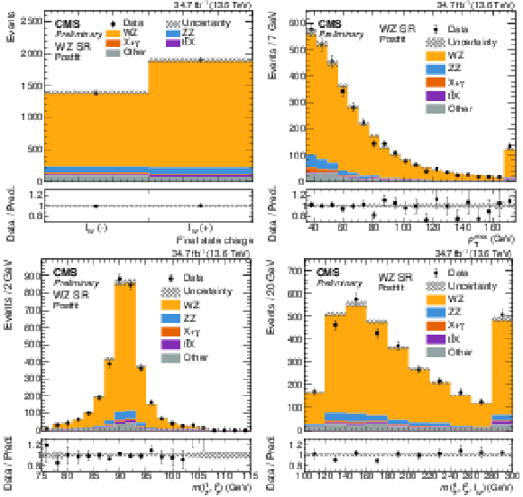
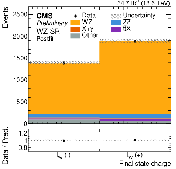
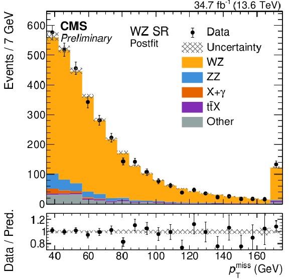
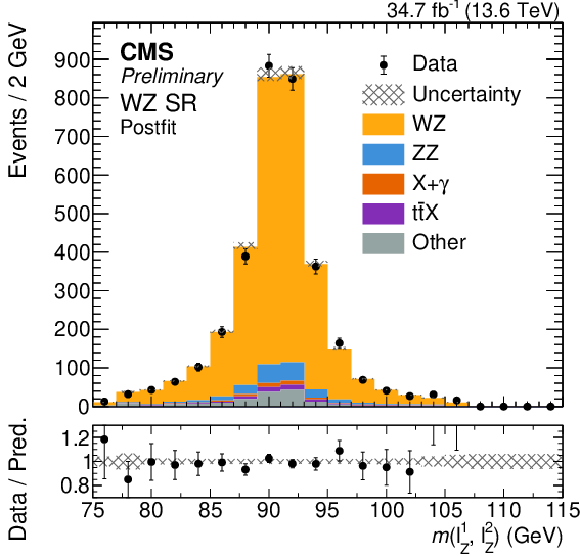
Distributions of several observables in the SR after the fit. From top left to bottom right: sum of charge of the final state leptons, missing transverse momentum, invariant mass of the two leptons assigned to the Z decay and invariant mass of the trileptonic system. The shaded band in the ratio includes all systematic uncertainties. |
png pdf |
Figure 7-a:
Distributions of several observables in the SR after the fit. From top left to bottom right: sum of charge of the final state leptons, missing transverse momentum, invariant mass of the two leptons assigned to the Z decay and invariant mass of the trileptonic system. The shaded band in the ratio includes all systematic uncertainties. |
png pdf |
Figure 7-b:
Distributions of several observables in the SR after the fit. From top left to bottom right: sum of charge of the final state leptons, missing transverse momentum, invariant mass of the two leptons assigned to the Z decay and invariant mass of the trileptonic system. The shaded band in the ratio includes all systematic uncertainties. |
png pdf |
Figure 7-c:
Distributions of several observables in the SR after the fit. From top left to bottom right: sum of charge of the final state leptons, missing transverse momentum, invariant mass of the two leptons assigned to the Z decay and invariant mass of the trileptonic system. The shaded band in the ratio includes all systematic uncertainties. |

png pdf |
Figure 7-d:
Distributions of several observables in the SR after the fit. From top left to bottom right: sum of charge of the final state leptons, missing transverse momentum, invariant mass of the two leptons assigned to the Z decay and invariant mass of the trileptonic system. The shaded band in the ratio includes all systematic uncertainties. |
png pdf |
Figure 8:
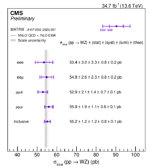
Total WZ production cross section for each of the flavour-exclusive and flavour-inclusive categories. The solid vertical band shows the theoretical prediction from MATRIX. For each of the measurements, the best fit value is denoted with a purple point and three main groups of uncertainties (statistical, systematic and theoretical) are presented with delimiters on the error bars. |
png pdf |
Figure 9:
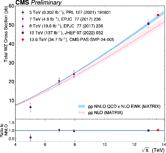
Measurement obtained in this analysis together with other WZ production cross section measurements at different center-of-mass energies by the CMS [5,36,6] Collaboration, compared to the NNLO QCD $ \times $ NLO EW predictions, as well as the pure NLO prediction; computed in all cases with MATRIX. |
| Tables | |

png pdf |
Table 1:
Requirements for the definition of the signal and control regions of the analysis. |
png pdf |
Table 2:
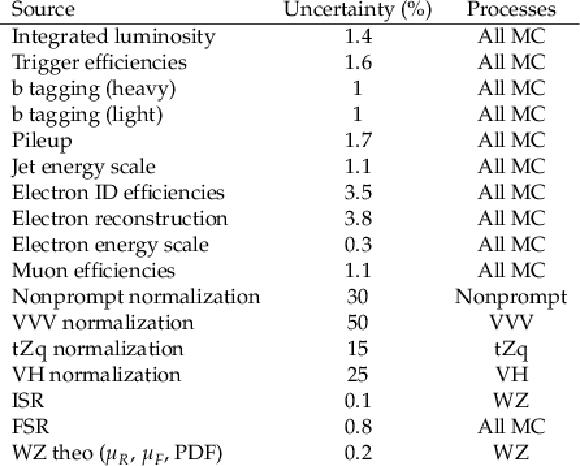
Summary of the input relative uncertainties for the WZ measurement. Numbers are presented in percentages over the total yields of the associated process they have an effect on. All uncertainties are treated as shape variations on the templates used for the fit, with the exception of the normalization uncertainties on the backgrounds that are treated as flat variations of the corresponding yield. |
png pdf |
Table 3:
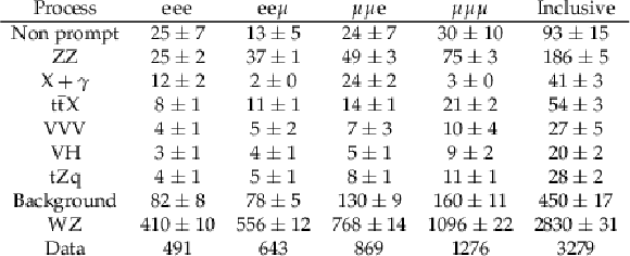
Number of selected events (by flavor channel) for the relevant processes in the signal region of the analysis after the fit. |
png pdf |
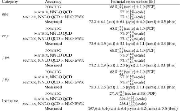
Table 4:
Measured fiducial cross sections and their corresponding uncertainties for the flavour-exclusive and flavour-inclusive categories. The predictions from both POWHEG at NLO in QCD and LO EWK as well as several ones obtained from MATRIX (NNLO QCD, NNLO QCD $ \times $ NLO EWK) are also included. |

png pdf |
Table 5:
Measured total cross sections and their corresponding uncertainties for the flavour-exclusive and flavour-inclusive categories. The predictions from both POWHEG at NLO in QCD and LO EWK as well as several ones obtained from MATRIX (NNLO QCD, NNLO QCD $ \times $ NLO EWK) are also included. |

png pdf |
Table 6:
Breakdown of different sources of systematic and their relative impact in each channel, as well as in the combined measurement. |
| Summary |
| The $ \mathrm{pp}\to\mathrm{W}\mathrm{Z} $ production is studied in the trilepton final state at a new energy regime of $ \sqrt{s}= $ 13.6 TeV, using the 2022 data set with a total integrated luminosity of 34.7 fb$ ^{-1} $. The production cross section in the total and fiducial phase spaces are measured in the inclusive case as well as up to four different combinations of final state flavour composition. The cross section is measured to be $ \sigma_{\text{total}}(\mathrm{p}\mathrm{p} \rightarrow \mathrm{W}\mathrm{Z}) = $ 55.2 $ \pm $ 1.2 (stat) $ \pm $ 1.4 (syst) $ \pm $ 0.1 (theo) pb. The observed accuracy that is achieved is shown to be competitive with previous measurements in terms of systematic uncertainty. This measurement is an addition to the set of LHC WZ cross section measurements, shown in Fig. 9, where the different results at different $ \sqrt{s} $ are also included. |
| References | ||||
| 1 | ATLAS Collaboration | Measurements of $ W^\pm Z $ production cross sections in $ pp $ collisions at $ \sqrt{s} = $ 8 TeV with the ATLAS detector and limits on anomalous gauge boson self-couplings | PRD 93 (2016) 092004 | 1603.02151 |
| 2 | CMS Collaboration | Measurement of the WZ production cross section in pp collisions at $ \sqrt{s} = $ 13 TeV | PLB 766 (2017) 268 | CMS-SMP-16-002 1607.06943 |
| 3 | ATLAS Collaboration | Measurement of the $ \mathrm{W}^{\pm}\mathrm{Z} $ boson pair-production cross section in pp collisions at $ \sqrt{s}= $ 13 TeV with the ATLAS Detector | PLB 762 (2016) 1 | 1606.04017 |
| 4 | ATLAS Collaboration | Measurement of $ W^{\pm}Z $ production cross sections and gauge boson polarisation in $ pp $ collisions at $ \sqrt{s} = $ 13 TeV with the ATLAS detector | EPJC 79 (2019) 535 | 1902.05759 |
| 5 | CMS Collaboration | Measurements of the electroweak diboson production cross sections in proton-proton collisions at $ \sqrt{s} = $ 5.02 TeV using leptonic decays | PRL 127 (2021) 191801 | CMS-SMP-20-012 2107.01137 |
| 6 | CMS Collaboration | Measurement of the inclusive and differential WZ production cross sections, polarization angles, and triple gauge couplings in pp collisions at $ \sqrt{s} = $ 13 TeV | JHEP 07 (2022) 032 | CMS-SMP-20-014 2110.11231 |
| 7 | CMS Collaboration | The CMS experiment at the CERN LHC | JINST 3 (2008) S08004 | |
| 8 | CMS Collaboration | Performance of the CMS Level-1 trigger in proton-proton collisions at $ \sqrt{s} = $ 13 TeV | JINST 15 (2020) P10017 | CMS-TRG-17-001 2006.10165 |
| 9 | CMS Collaboration | The CMS trigger system | JINST 12 (2017) P01020 | CMS-TRG-12-001 1609.02366 |
| 10 | P. Nason | A New method for combining NLO QCD with shower Monte Carlo algorithms | JHEP 11 (2004) 040 | hep-ph/0409146 |
| 11 | S. Frixione, P. Nason, and C. Oleari | Matching NLO QCD computations with Parton Shower simulations: the POWHEG method | JHEP 11 (2007) 070 | 0709.2092 |
| 12 | S. Alioli, P. Nason, C. Oleari, and E. Re | A general framework for implementing NLO calculations in shower Monte Carlo programs: the POWHEG BOX | JHEP 06 (2010) 043 | 1002.2581 |
| 13 | T. Melia, P. Nason, R. Rontsch, and G. Zanderighi | $ \mathrm{W}^+ \mathrm{W}^- $, $\mathrm{WZ}$ and $\mathrm{ZZ}$ production in the POWHEG BOX | JHEP 11 (2011) 078 | 1107.5051 |
| 14 | P. Nason and G. Zanderighi | $ \mathrm{W}^+ \mathrm{W}^- $, $\mathrm{WZ}$ and $\mathrm{ZZ}$ production in the POWHEG-BOX-V2 | EPJC 74 (2014) 2702 | 1311.1365 |
| 15 | J. Alwall et al. | The automated computation of tree-level and next-to-leading order differential cross sections, and their matching to parton shower simulations | JHEP 07 (2014) 079 | 1405.0301 |
| 16 | NNPDF Collaboration | Parton distributions from high-precision collider data | EPJC 77 (2017) 663 | 1706.00428 |
| 17 | C. Bierlich et al. | A comprehensive guide to the physics and usage of PYTHIA 8.3 | SciPost Phys. Codeb. 2022 (2022) 8 | 2203.11601 |
| 18 | CMS Collaboration | Extraction and validation of a new set of CMS PYTHIA8 tunes from underlying-event measurements | EPJC 80 (2020) 4 | CMS-GEN-17-001 1903.12179 |
| 19 | GEANT4 Collaboration | GEANT 4---a simulation toolkit | NIM A 506 (2003) 250 | |
| 20 | CMS Collaboration | Particle-flow reconstruction and global event description with the CMS detector | JINST 12 (2017) P10003 | CMS-PRF-14-001 1706.04965 |
| 21 | CMS Collaboration | Technical proposal for the Phase-II upgrade of the Compact Muon Solenoid | CMS Technical Proposal CERN-LHCC-2015-010, CMS-TDR-15-02, 2015 CDS |
|
| 22 | CMS Collaboration | Electron and photon reconstruction and identification with the CMS experiment at the CERN LHC | JINST 16 (2021) P05014 | CMS-EGM-17-001 2012.06888 |
| 23 | CMS Collaboration | Performance of the CMS muon detector and muon reconstruction with proton-proton collisions at $ \sqrt{s}= $ 13 TeV | JINST 13 (2018) P06015 | CMS-MUO-16-001 1804.04528 |
| 24 | M. Cacciari, G. P. Salam, and G. Soyez | The anti-$ k_{\mathrm{T}} $ jet clustering algorithm | JHEP 04 (2008) 063 | 0802.1189 |
| 25 | M. Cacciari, G. P. Salam, and G. Soyez | FastJet user manual | EPJC 72 (2012) 1896 | 1111.6097 |
| 26 | CMS Collaboration | Pileup mitigation at CMS in 13 TeV data | JINST 15 (2020) P09018 | CMS-JME-18-001 2003.00503 |
| 27 | D. Bertolini, P. Harris, M. Low, and N. Tran | Pileup per particle identification | JHEP 10 (2014) 059 | 1407.6013 |
| 28 | CMS Collaboration | Identification of heavy-flavour jets with the CMS detector in pp collisions at 13 TeV | JINST 13 (2018) P05011 | CMS-BTV-16-002 1712.07158 |
| 29 | E. Bols et al. | Jet flavour classification using DeepJet | JINST 15 (2020) P12012 | 2008.10519 |
| 30 | CMS Collaboration | Performance of missing transverse momentum reconstruction in proton-proton collisions at $ \sqrt{s} = $ 13 TeV using the CMS detector | JINST 14 (2019) P07004 | CMS-JME-17-001 1903.06078 |
| 31 | ATLAS Collaboration | Measurement of the inelastic proton-proton cross section at $ \sqrt{s} = $ 13 TeV with the ATLAS detector at the LHC | PRL 117 (2016) 182002 | 1606.02625 |
| 32 | CMS Collaboration | Luminosity measurement in proton-proton collisions at 13.6 TeV in 2022 at CMS | CMS Physics Analysis Summary, 2024 CMS-PAS-LUM-22-001 |
CMS-PAS-LUM-22-001 |
| 33 | R. J. Barlow and C. Beeston | Fitting using finite Monte Carlo samples | Comput. Phys. Commun. 77 (1993) 219 | |
| 34 | CMS Collaboration | The CMS statistical analysis and combination tool: \textscCombine | Accepted by Comput. Softw. Big Sci, 2024 | CMS-CAT-23-001 2404.06614 |
| 35 | M. Grazzini et al. | NNLO QCD + NLO EW with Matrix+OpenLoops: precise predictions for vector-boson pair production | JHEP 02 (2020) 087 | 1912.00068 |
| 36 | CMS Collaboration | Measurement of the WZ production cross section in pp collisions at $ \sqrt{s} = $ 7 and 8 TeV and search for anomalous triple gauge couplings at $ \sqrt{s} = $ 8 TeV | EPJC 77 (2017) 236 | CMS-SMP-14-014 1609.05721 |

|
Compact Muon Solenoid LHC, CERN |

|

|

|

|

|

|