

Compact Muon Solenoid
LHC, CERN
| CMS-PAS-HIG-20-015 | ||
| Measurement of the inclusive and differential Higgs boson production cross sections in the decay mode to a pair of $\tau$ leptons | ||
| CMS Collaboration | ||
| June 2021 | ||
| Abstract: Measurements of the inclusive and differential fiducial cross sections of the Higgs boson are presented, using the $\tau$ lepton decay channel. The differential cross sections are measured as a function of the Higgs boson transverse momentum, jet multiplicity, and transverse momentum of the leading jet in the event if any. The analysis is performed using proton-proton data collected by the CMS detector at a center-of-mass energy of 13 TeV and amounting to an integrated luminosity of 138 fb$^{-1}$. These are the first differential measurements of the Higgs boson cross section in the final state of two $\tau$ leptons, and they constitute a significant improvement over measurements in other final states in parts of the phase space, namely in events with a large jet multiplicity or with Lorentz-boosted Higgs bosons. | ||
|
Links:
CDS record (PDF) ;
inSPIRE record ;
CADI line (restricted) ;
These preliminary results are superseded in this paper, PRL 128 (2022) 081805. The superseded preliminary plots can be found here. |
||
| Figures & Tables | Summary | Additional Figures | References | CMS Publications |
|---|
| Figures | |
png pdf |
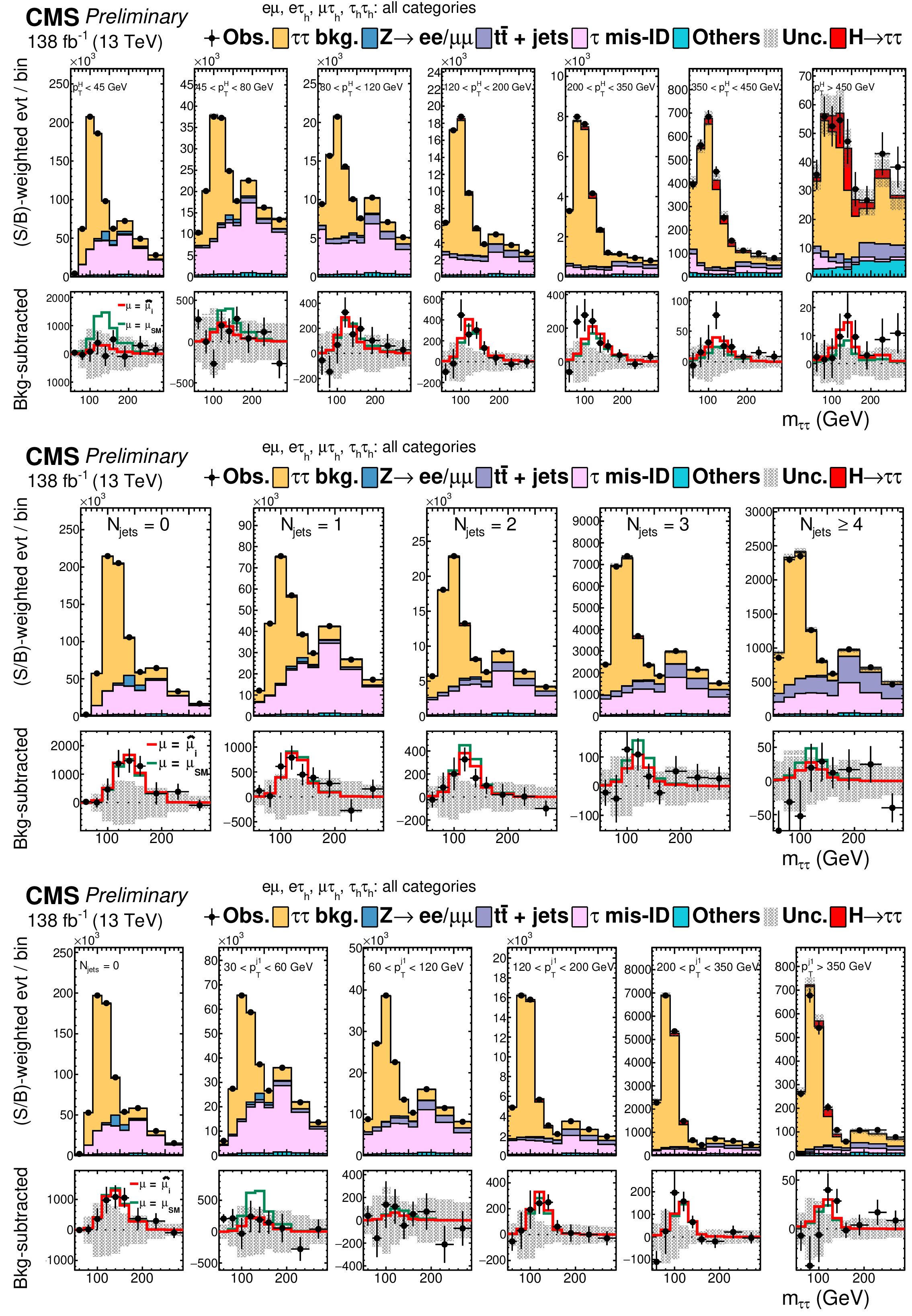
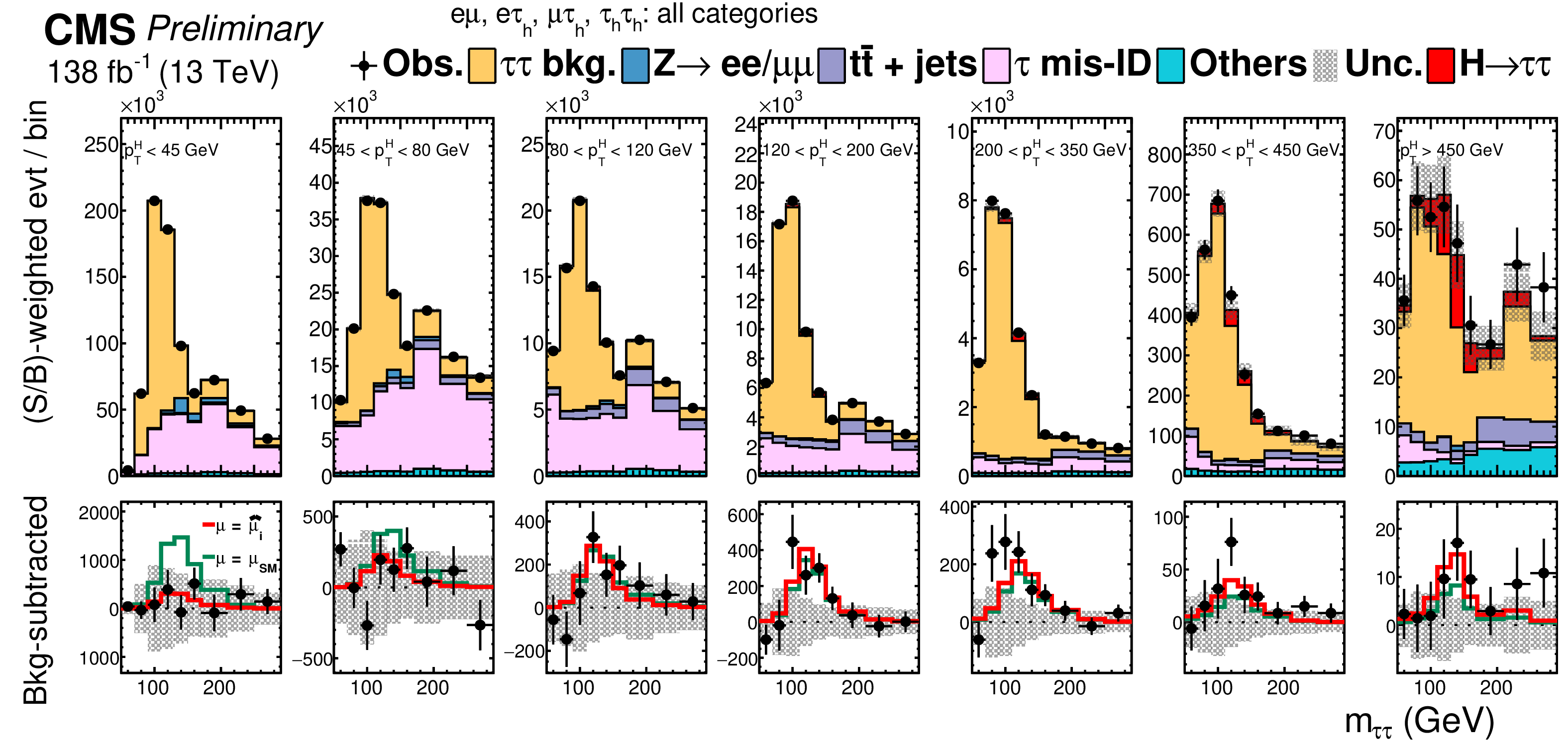
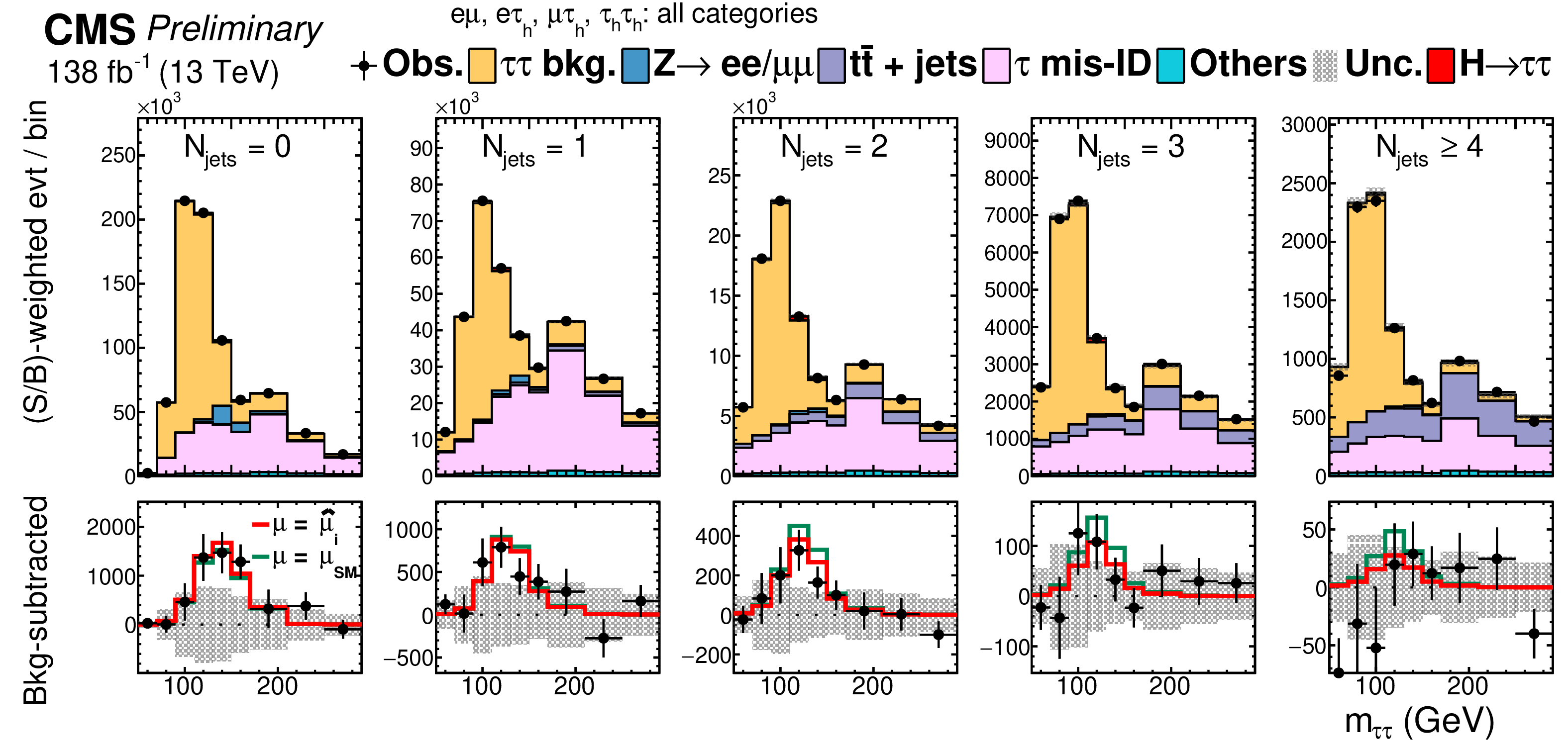
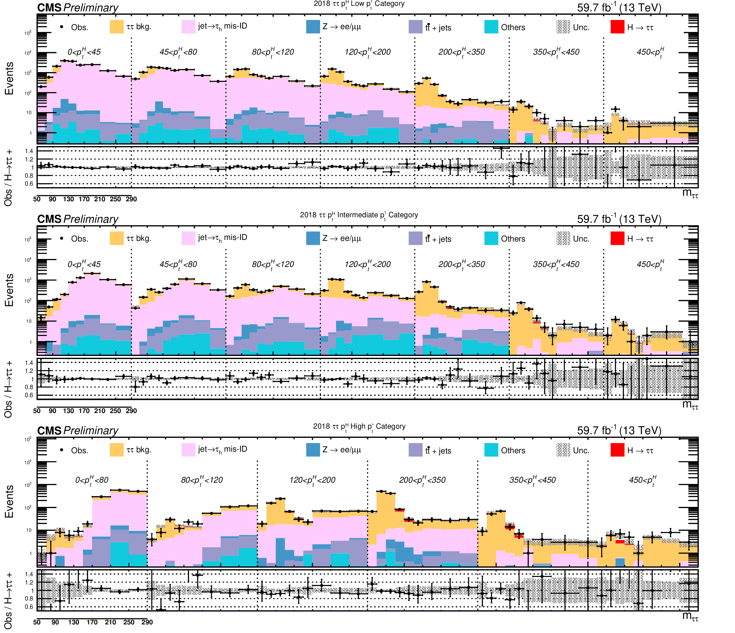
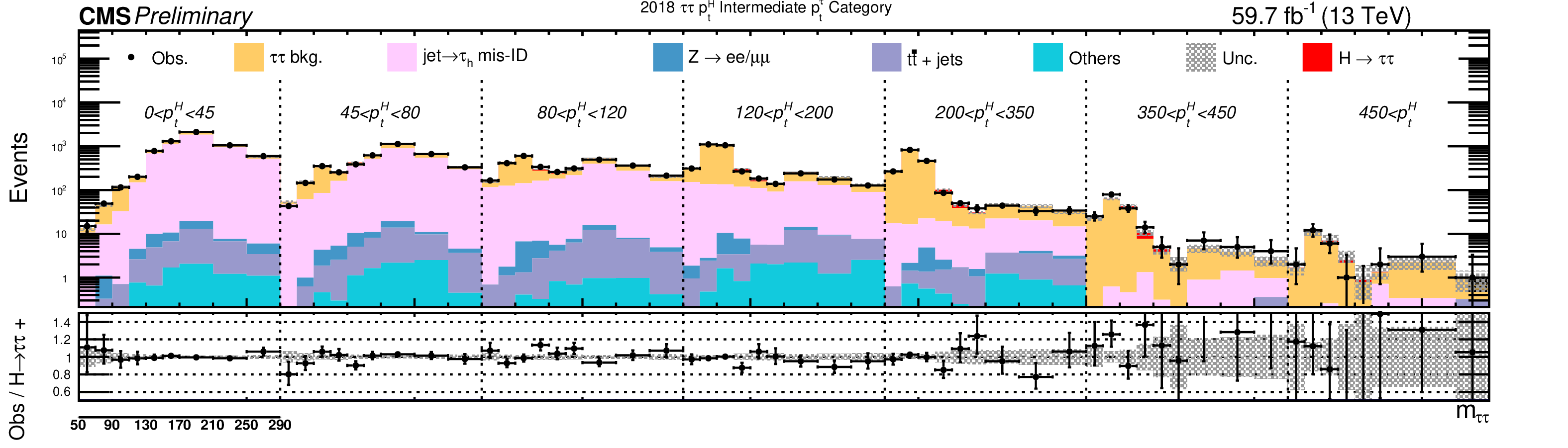
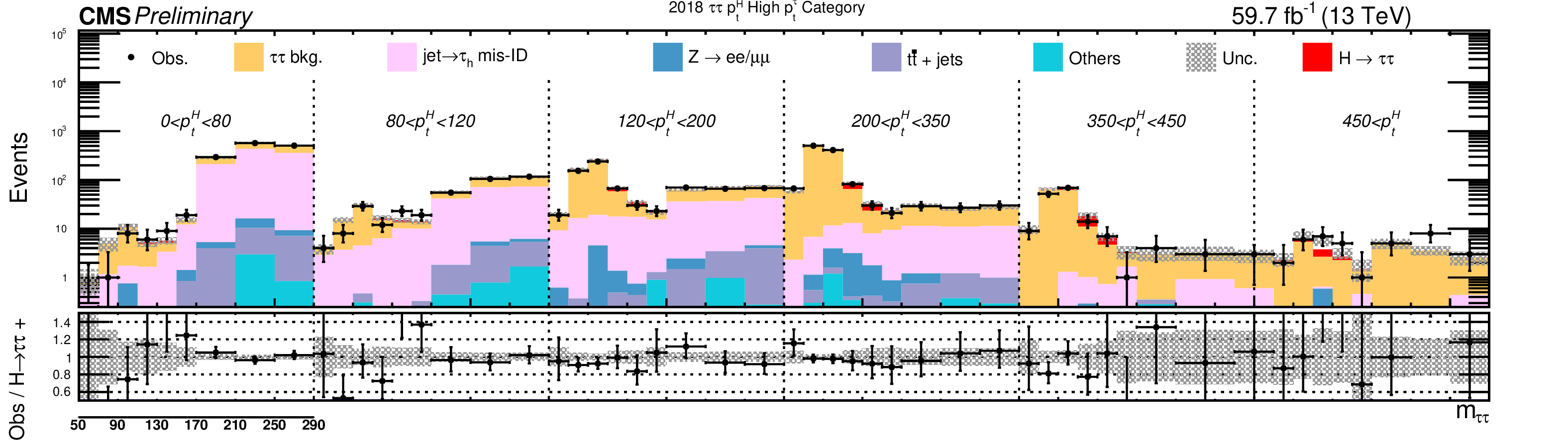
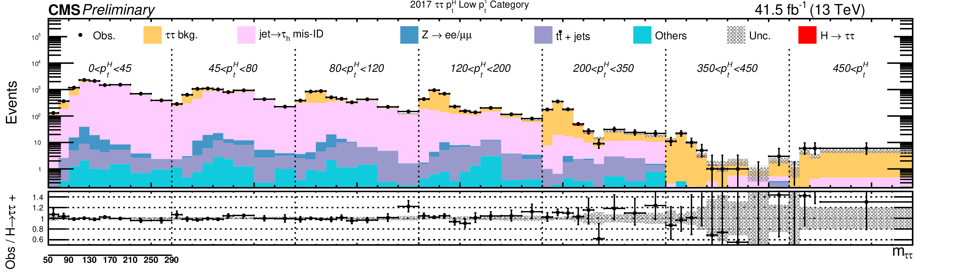
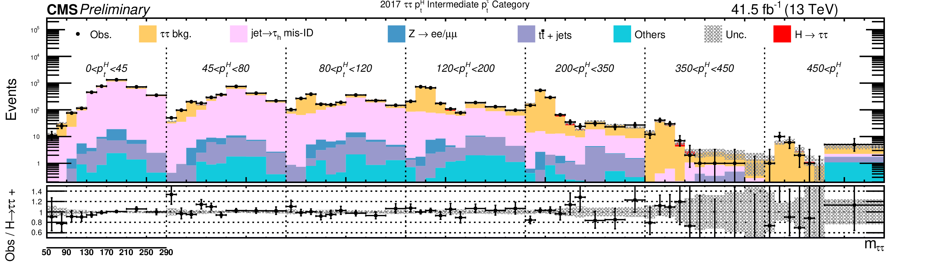
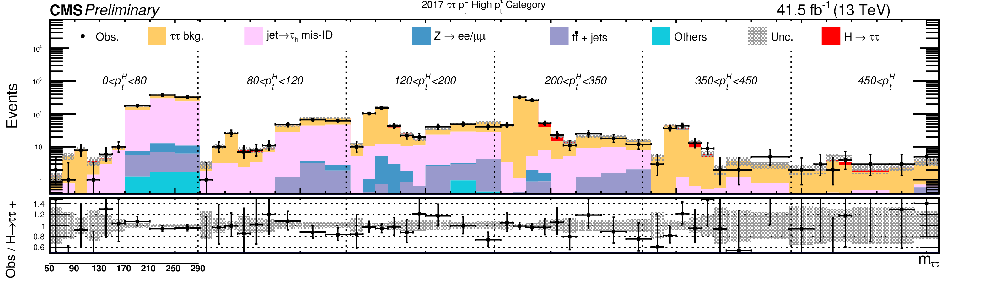
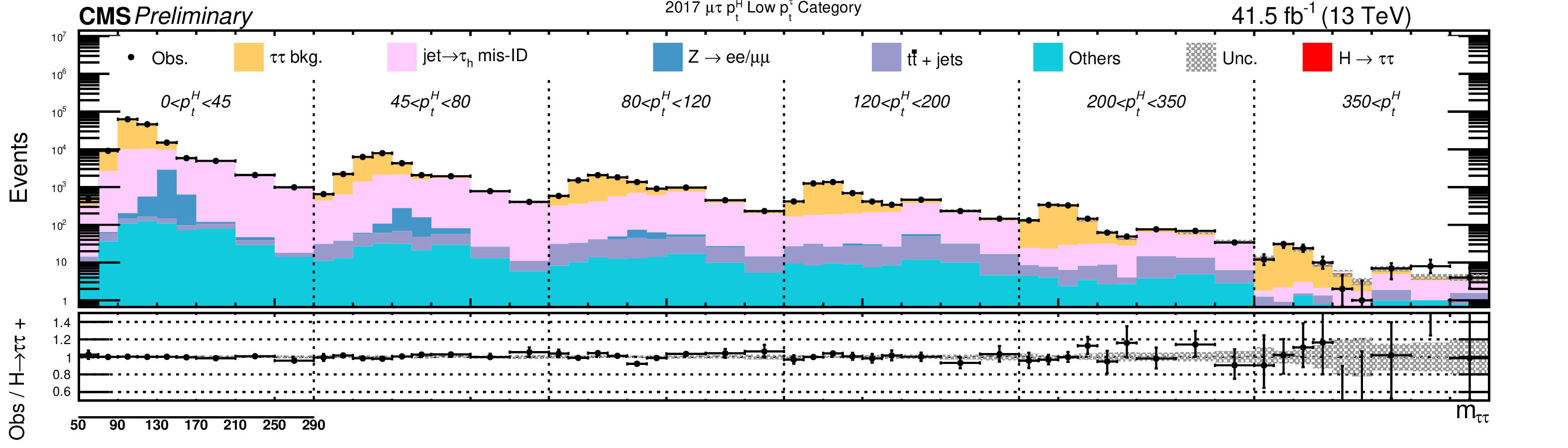
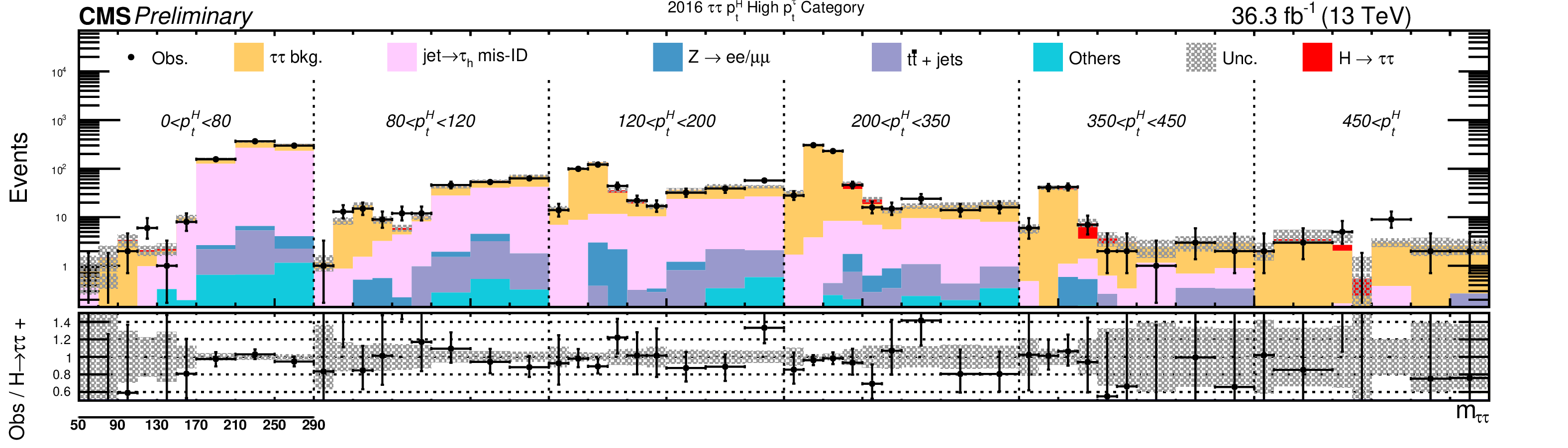
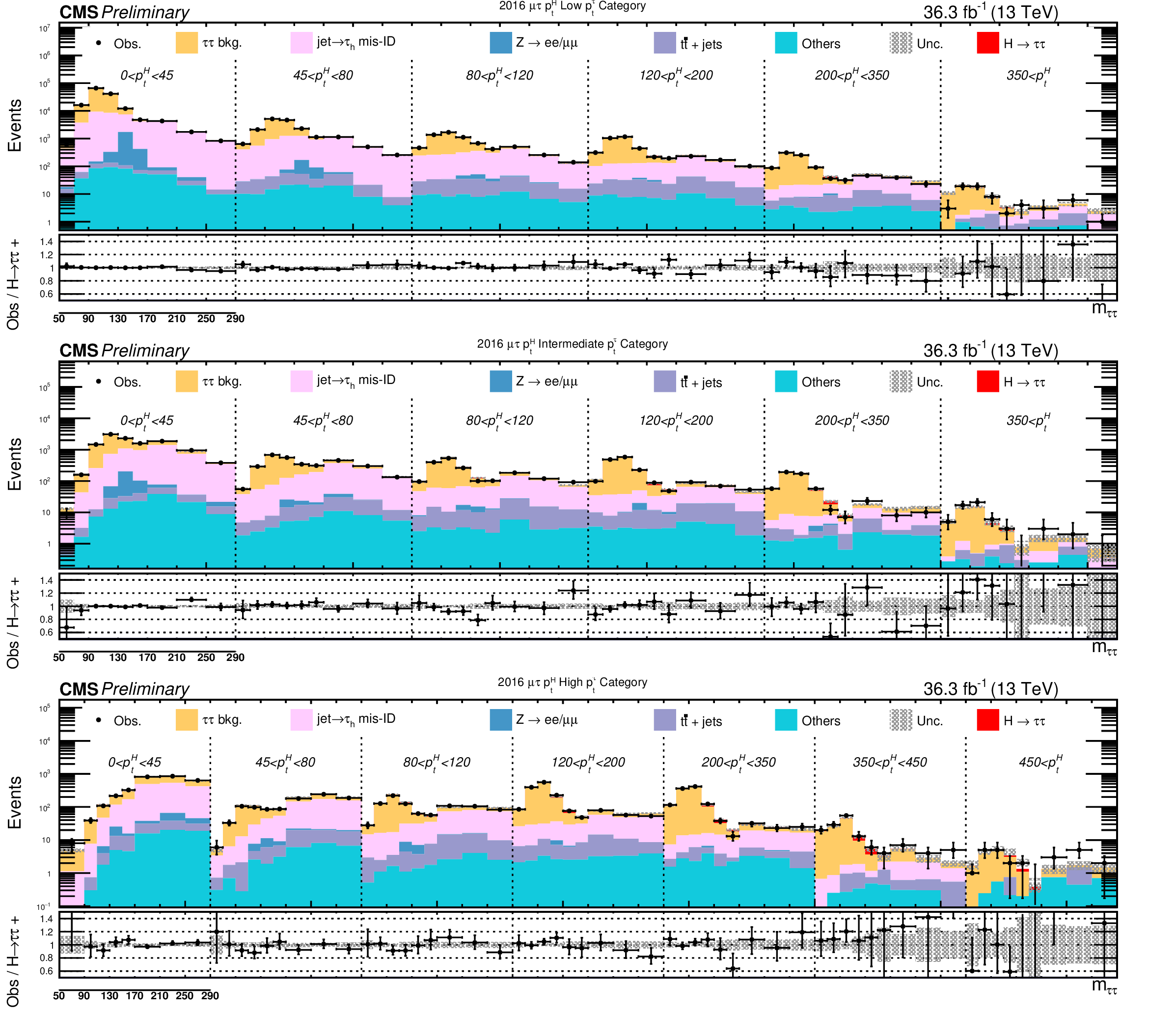
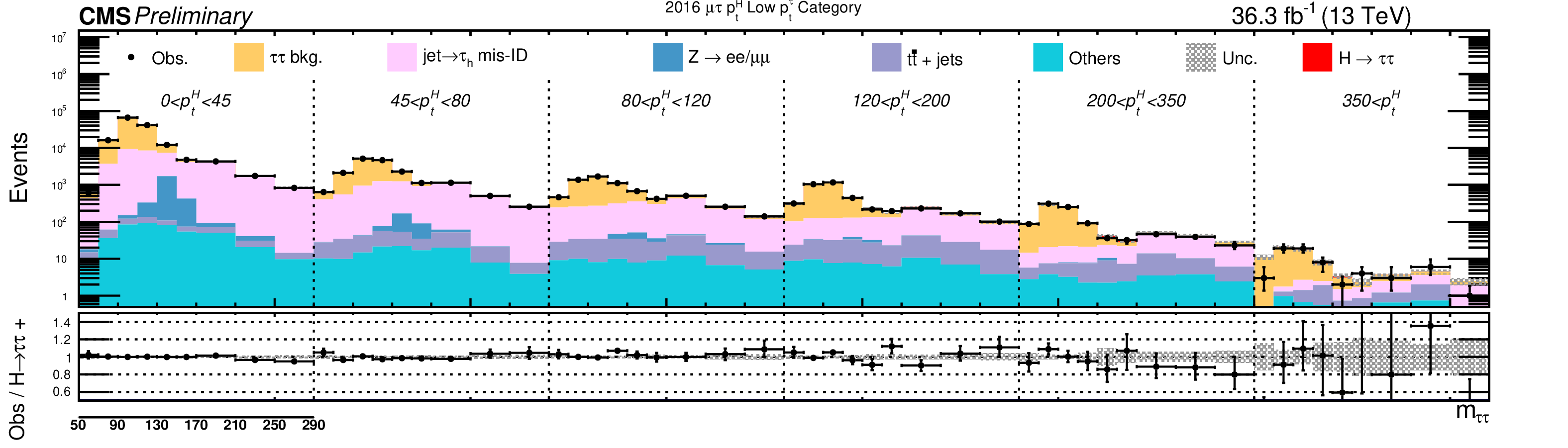
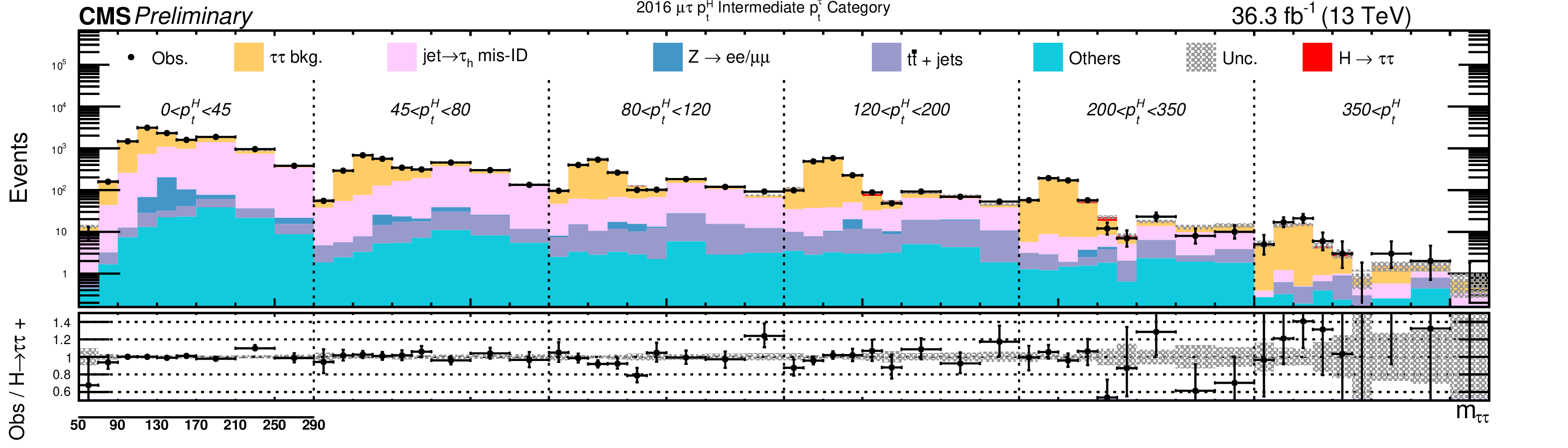
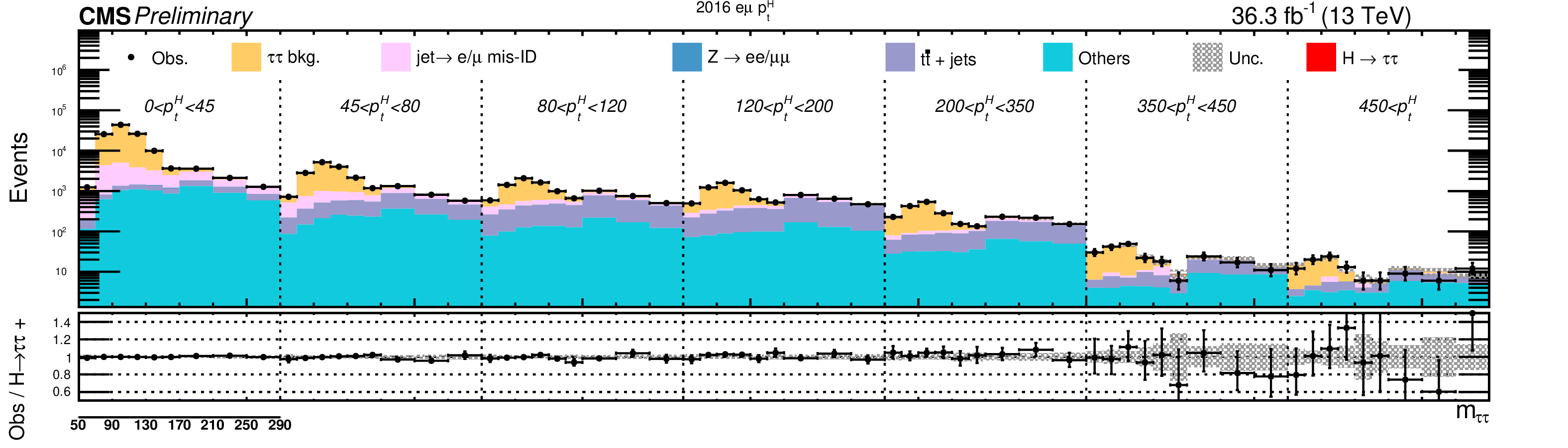
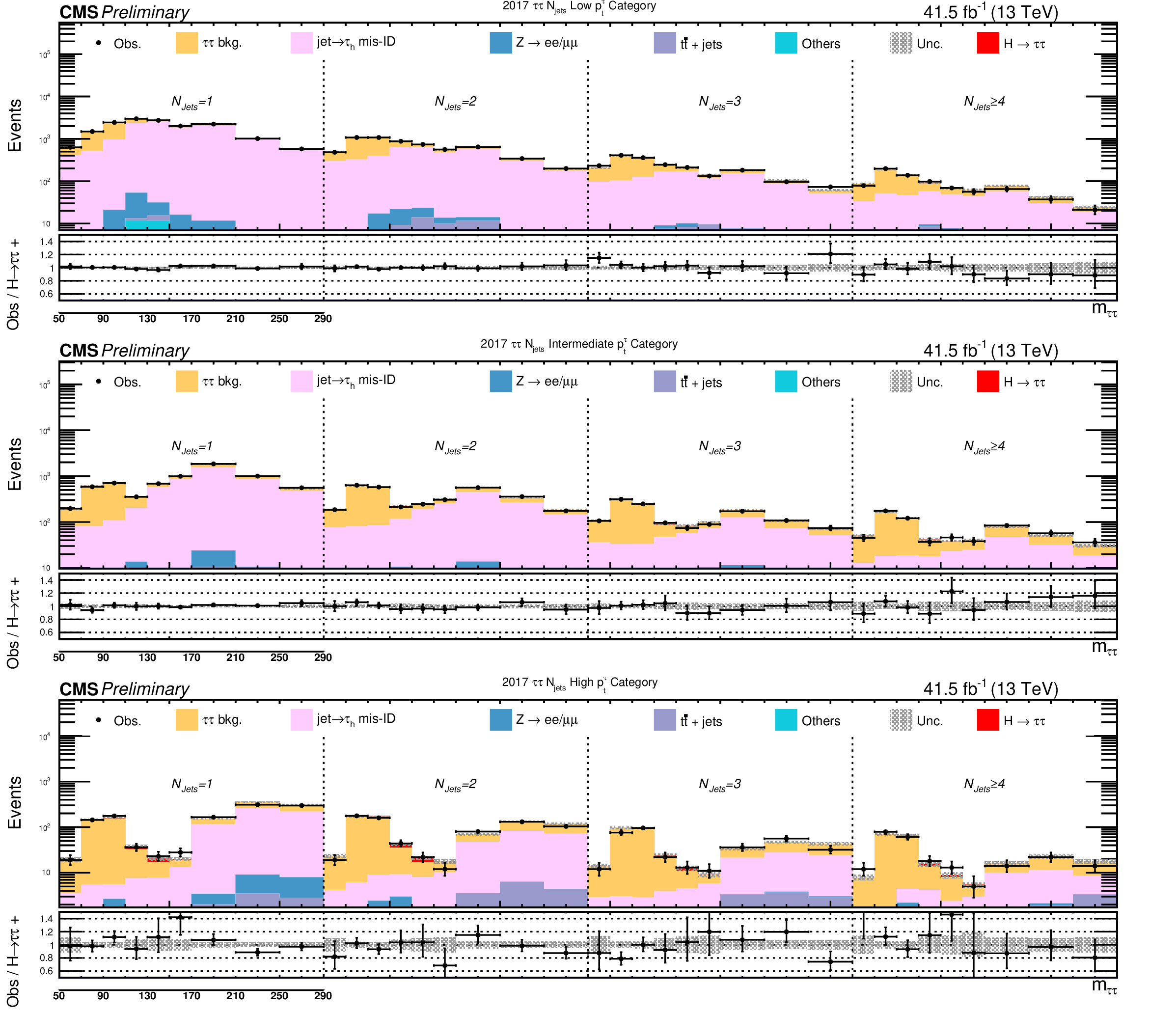
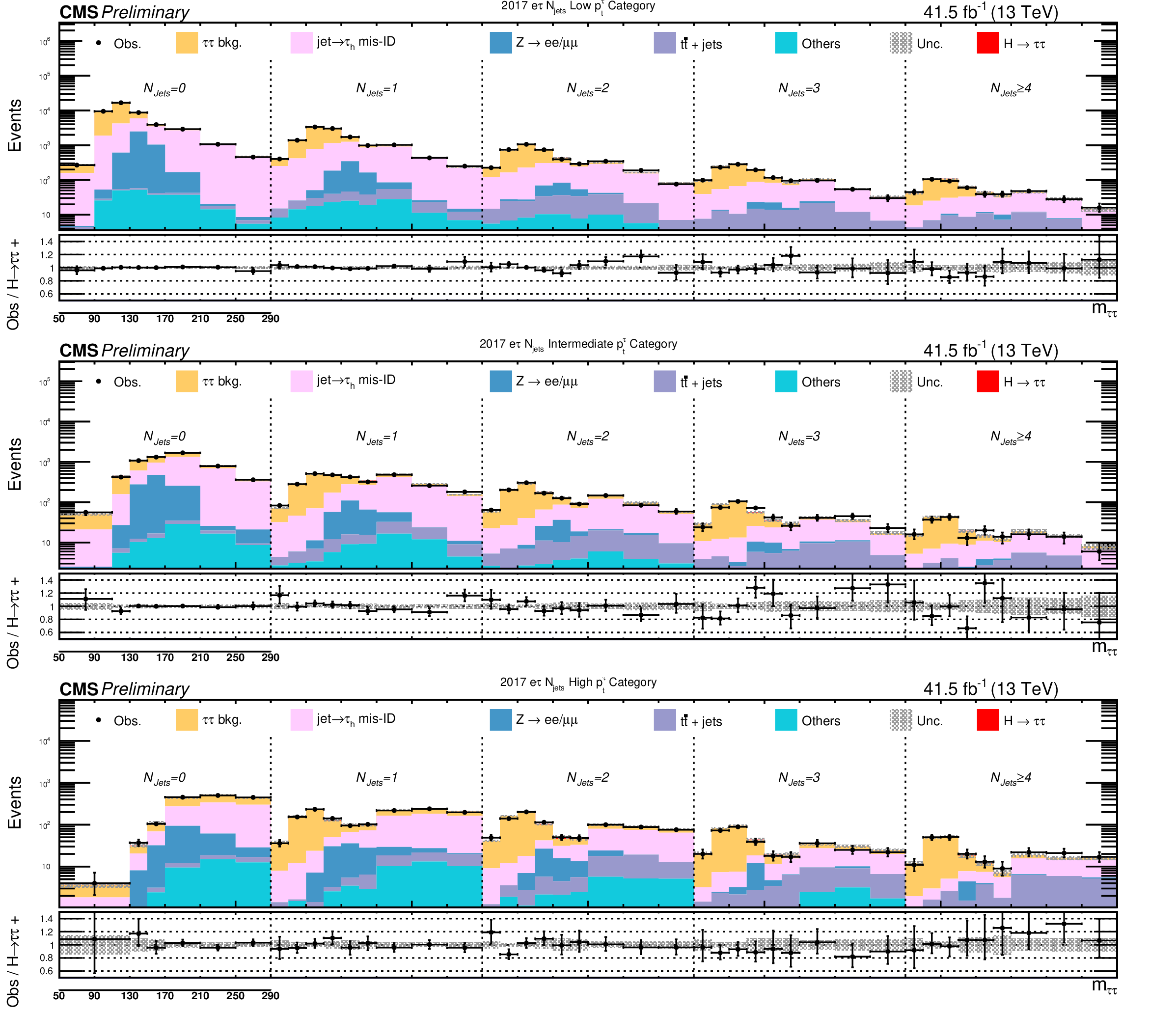
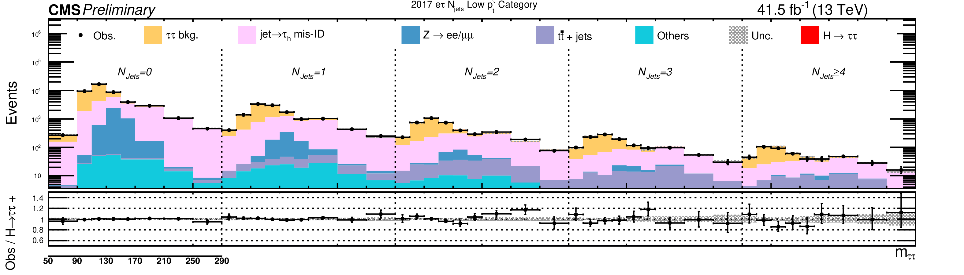
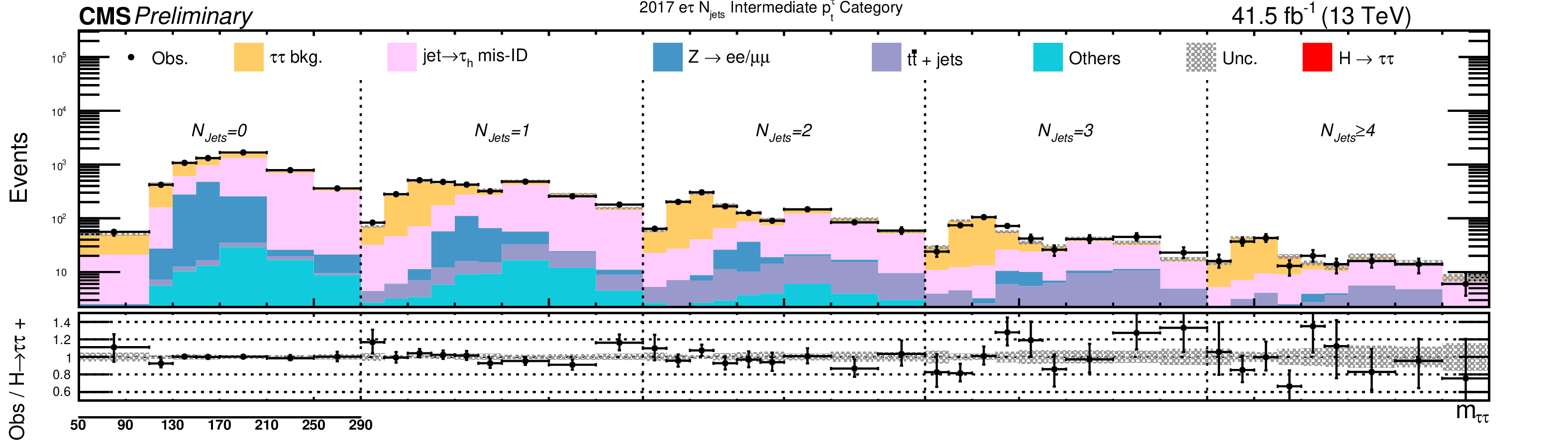
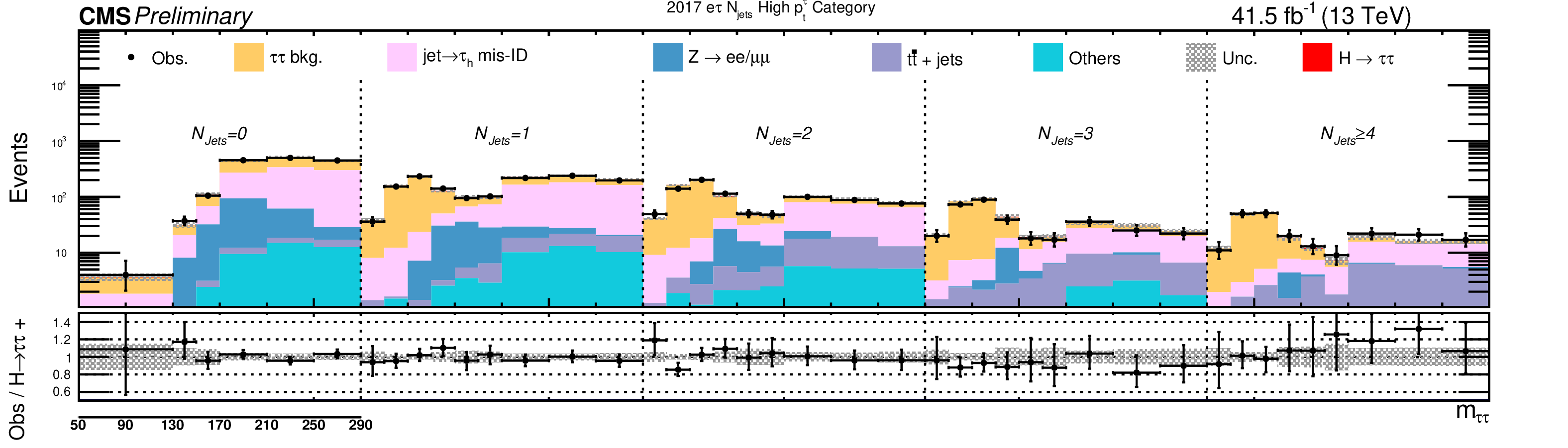
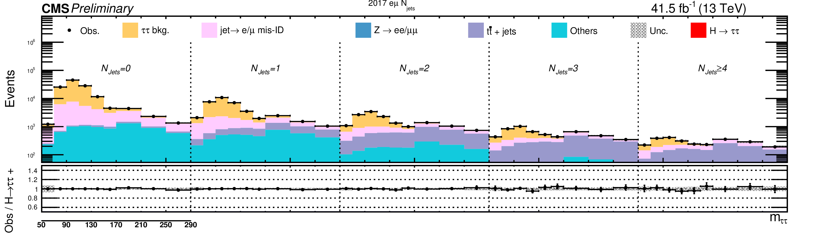
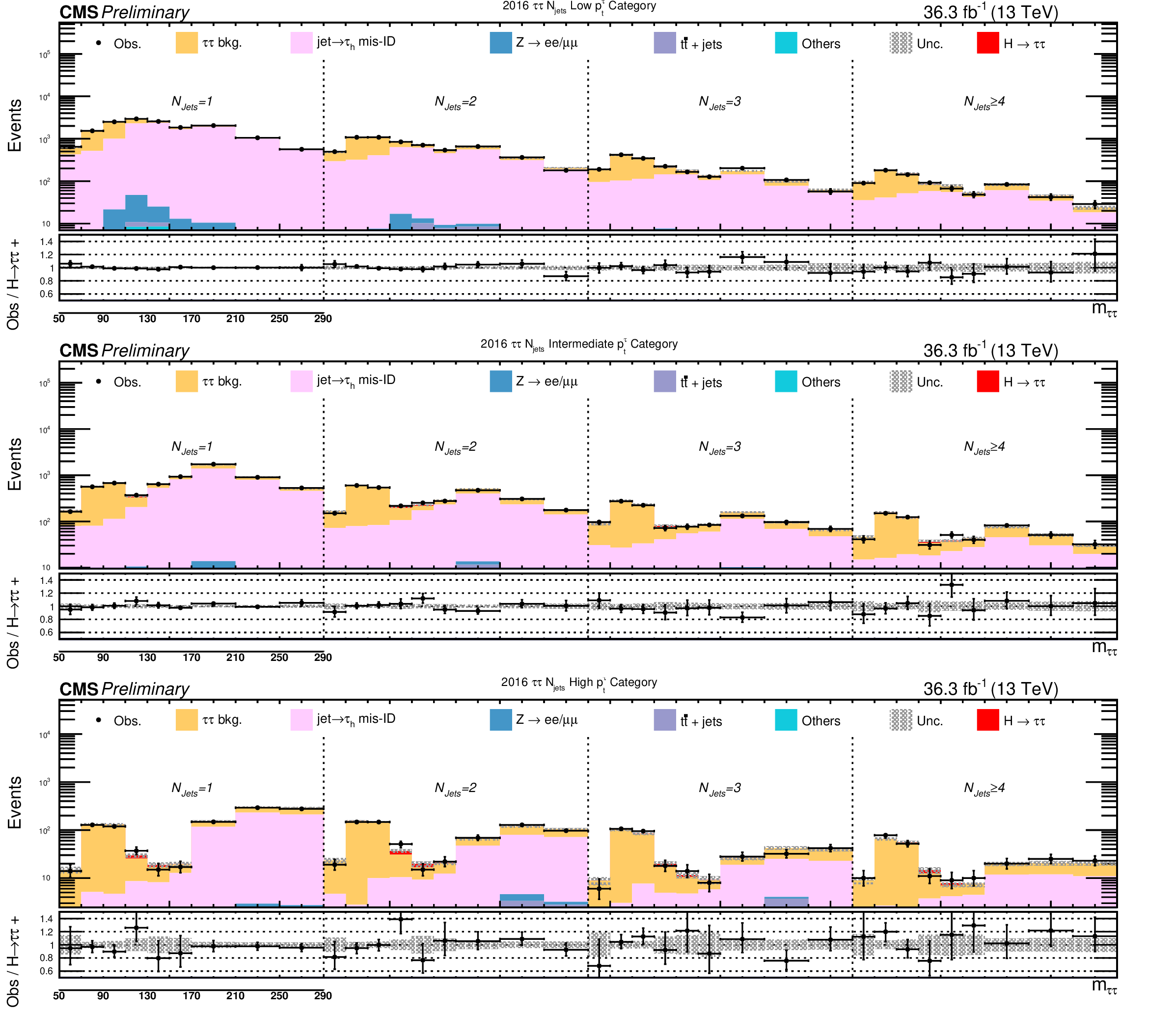
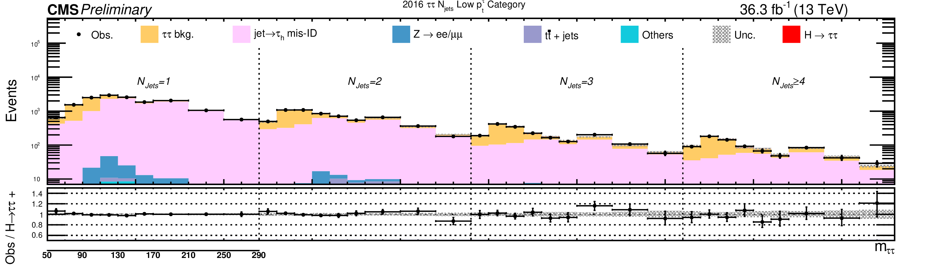
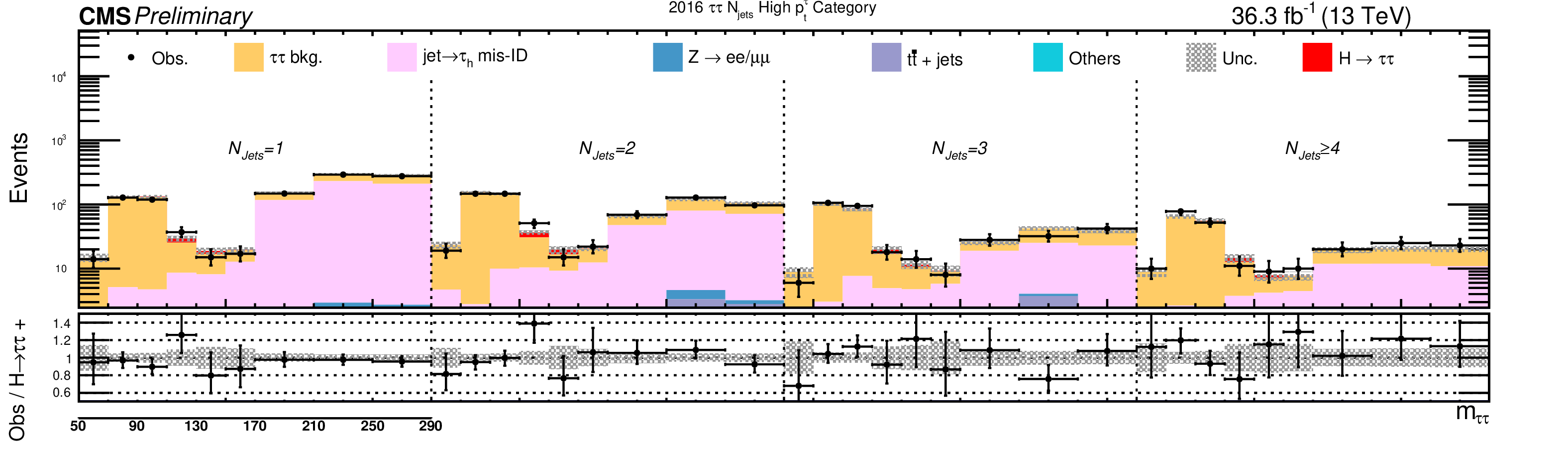
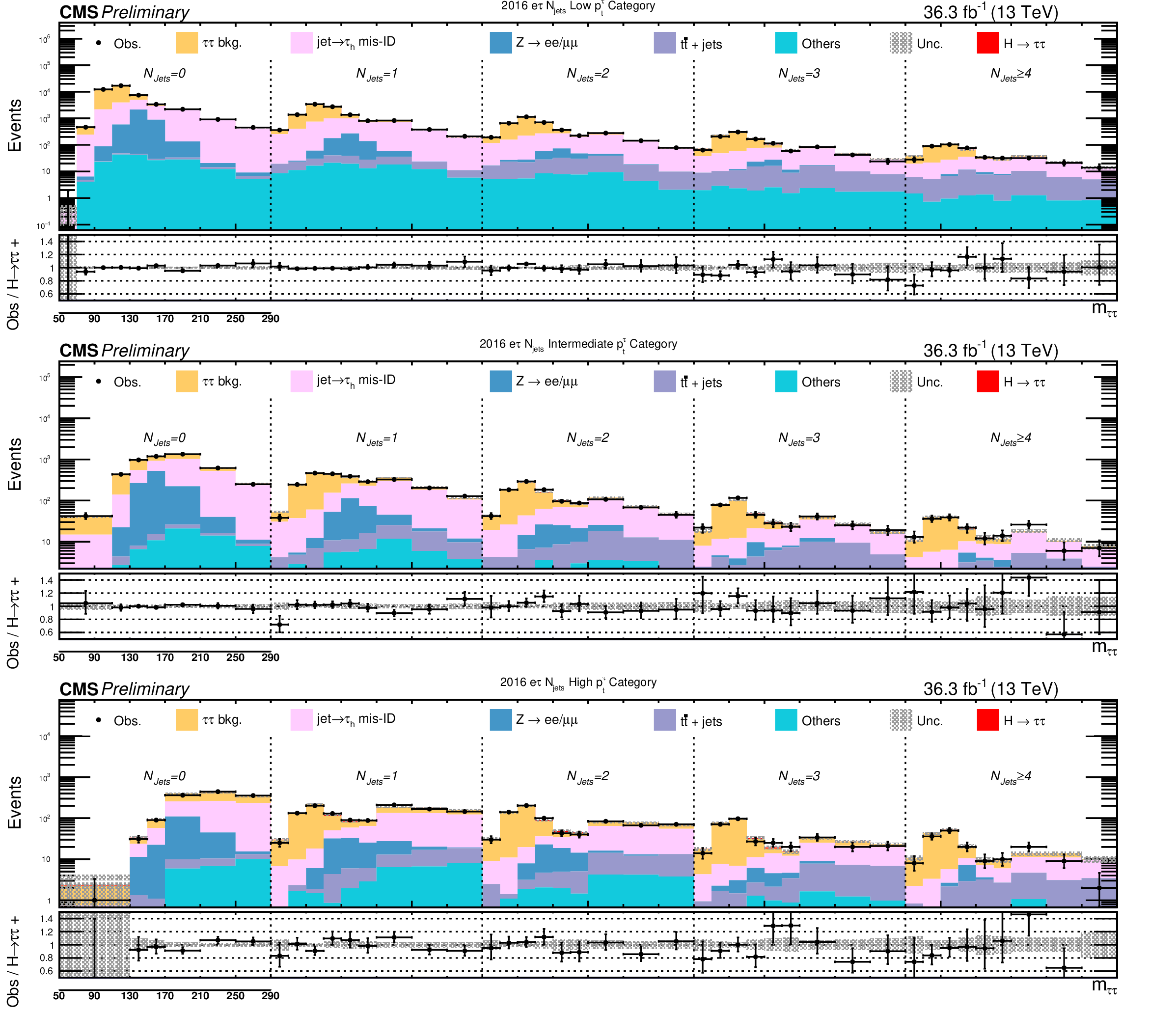
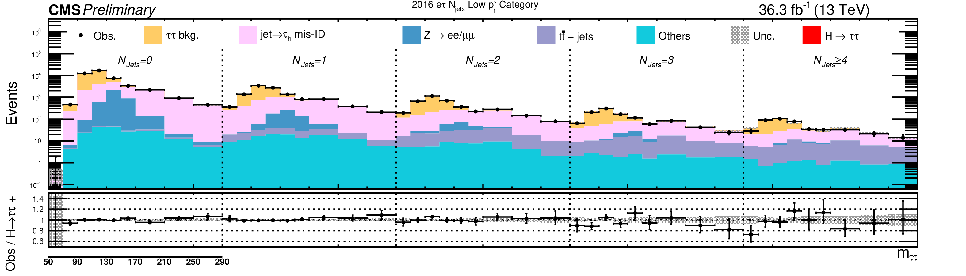
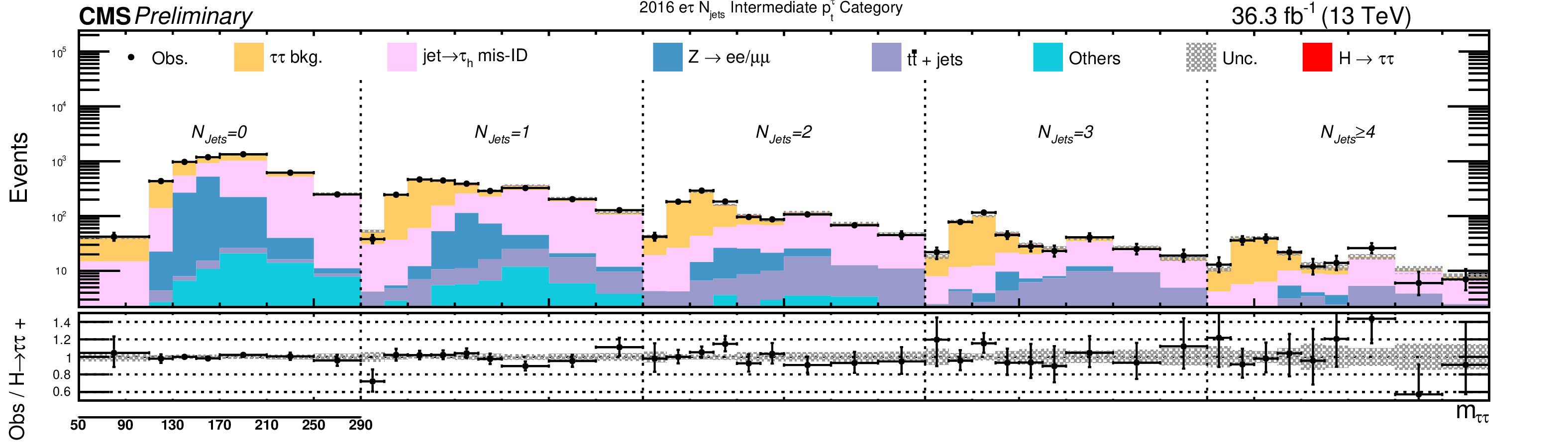
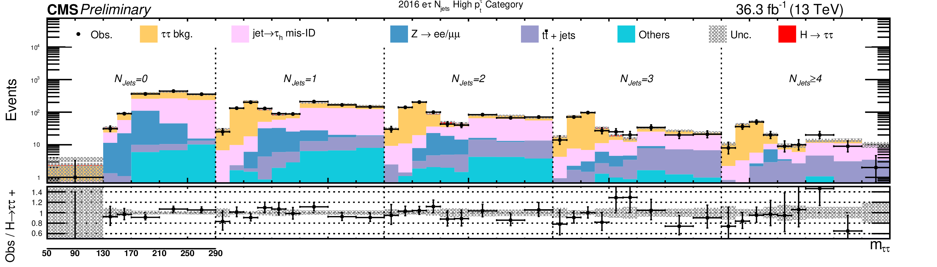
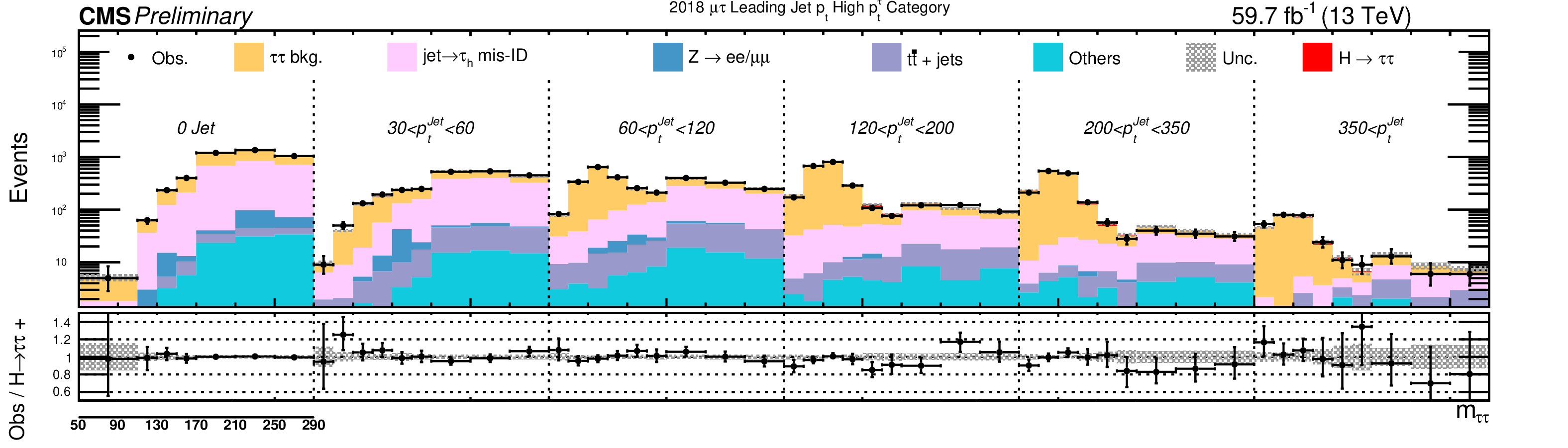
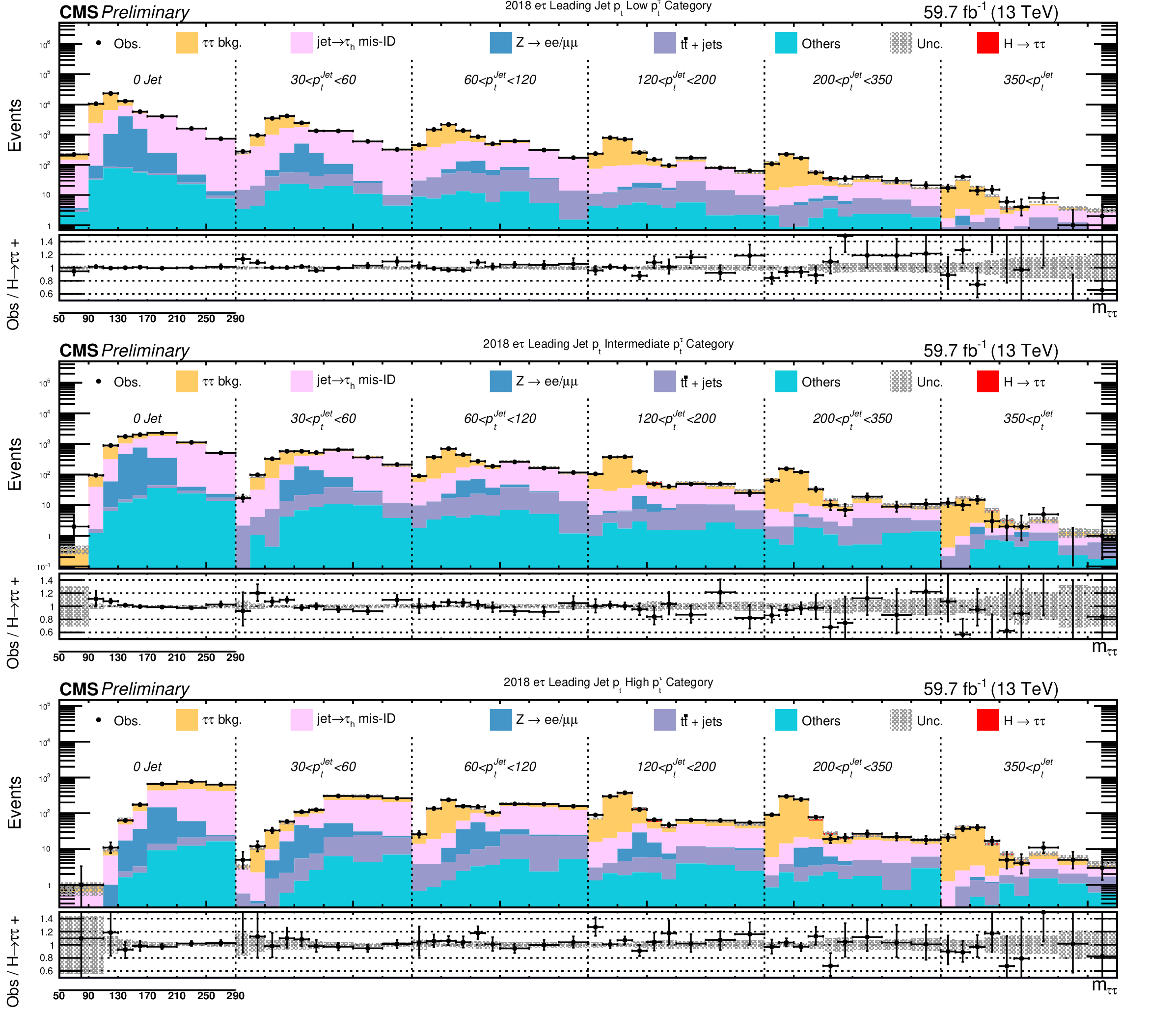
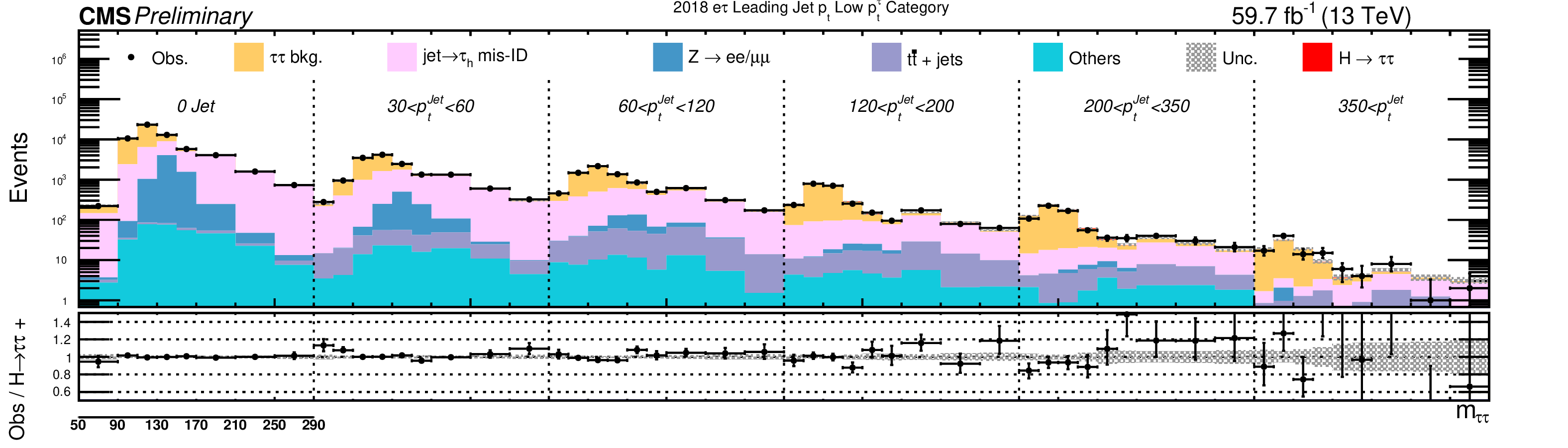
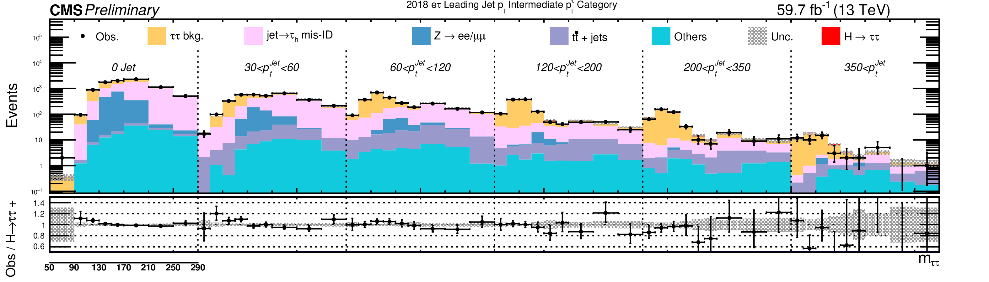
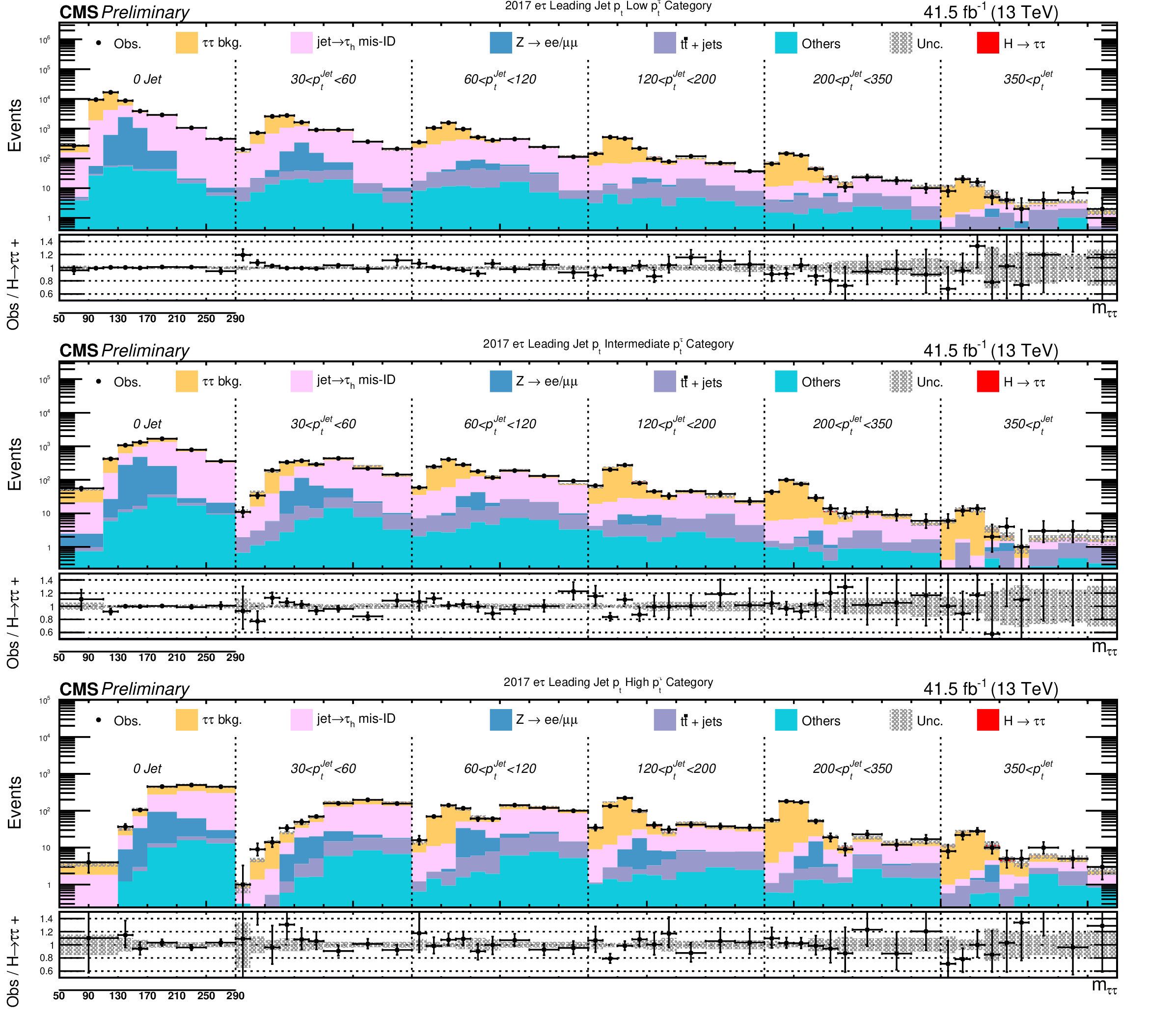
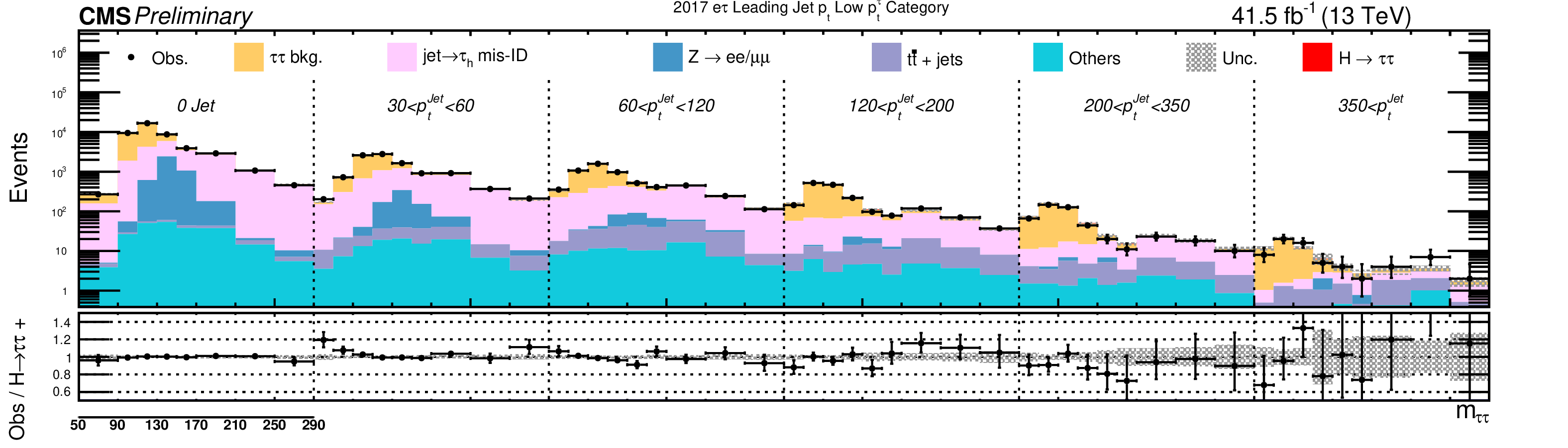
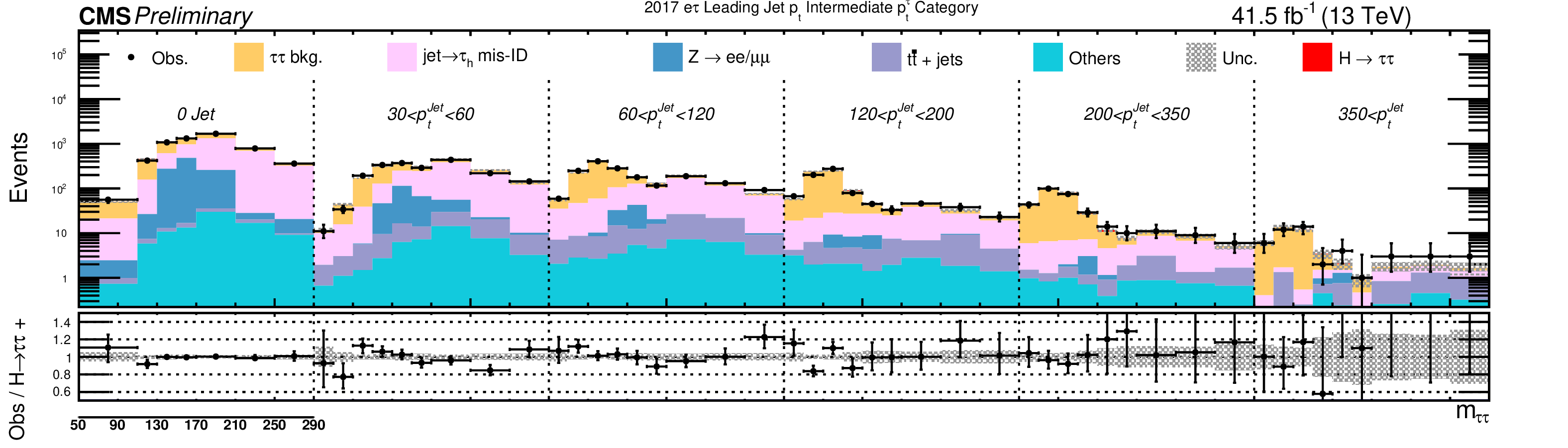
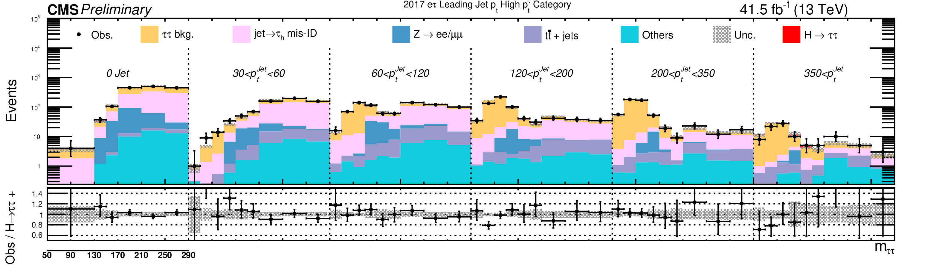
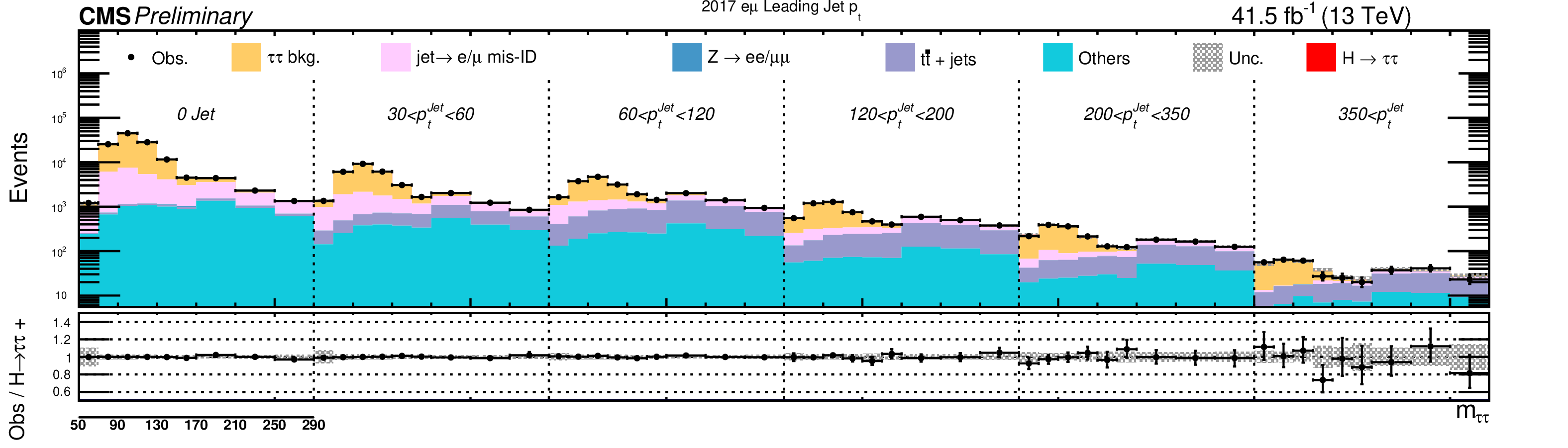
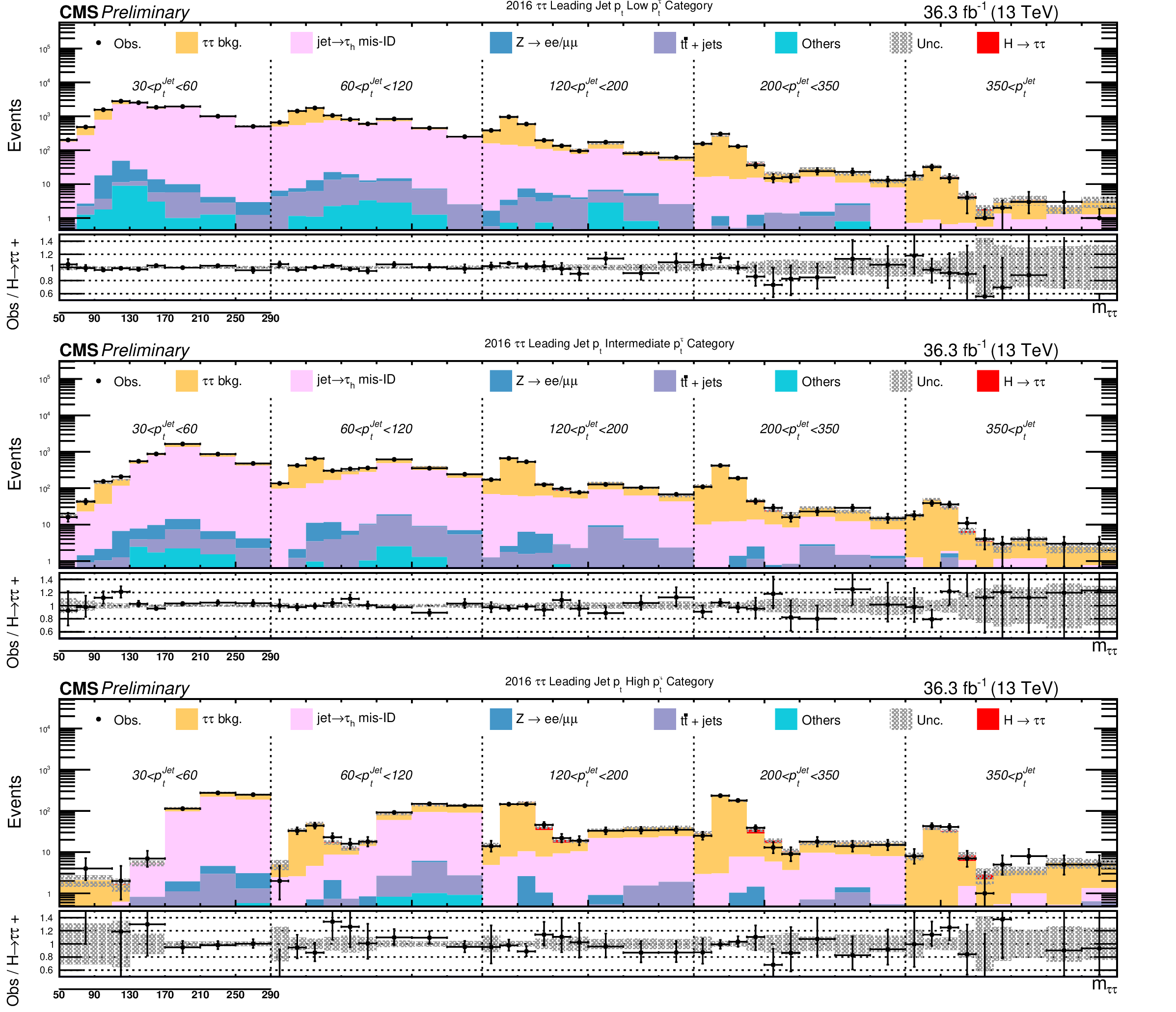
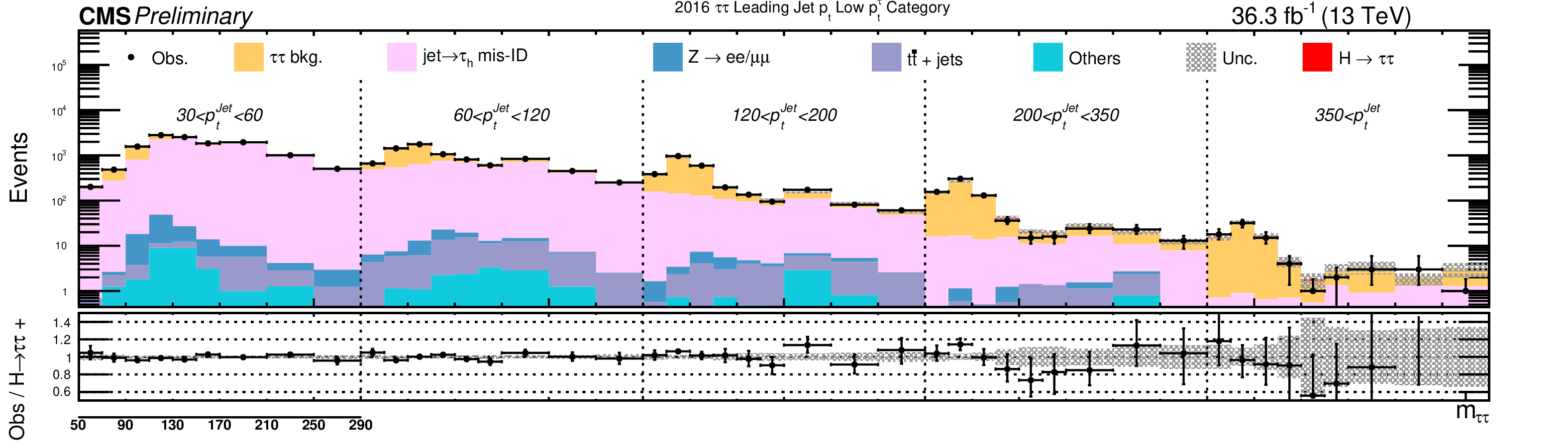
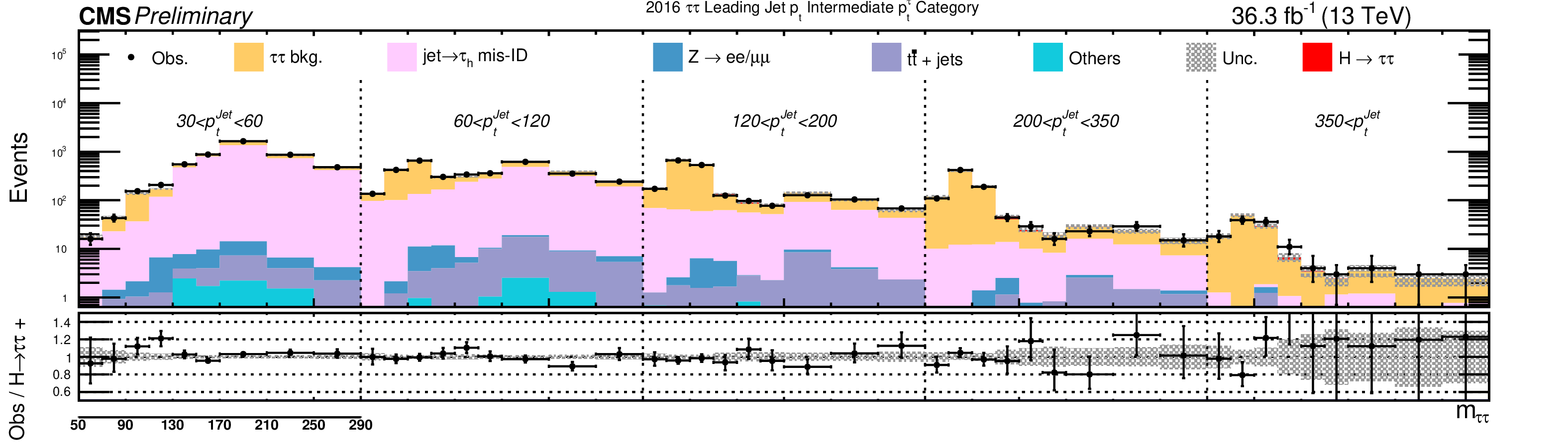
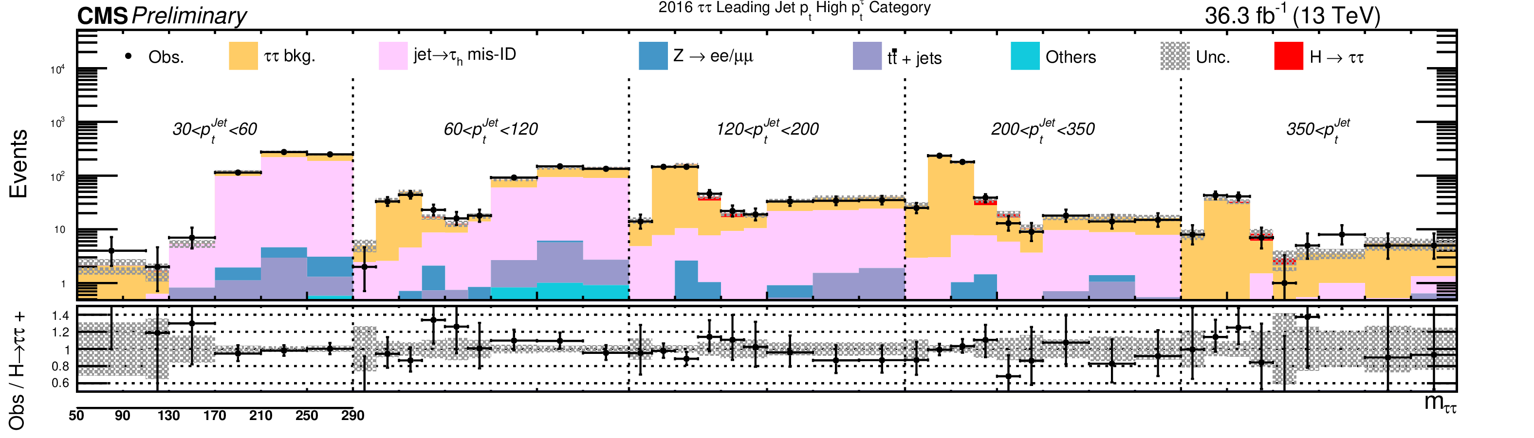
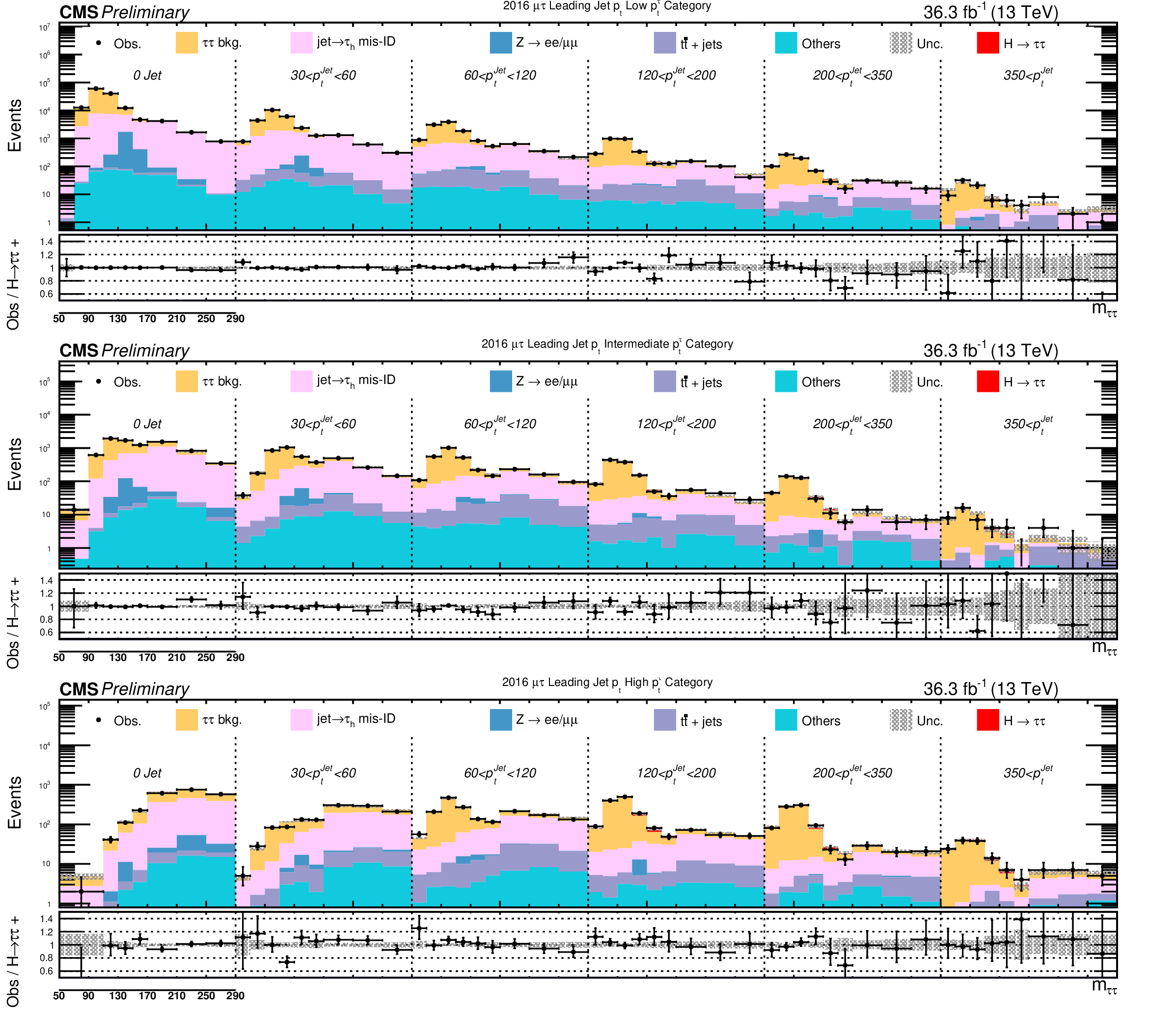
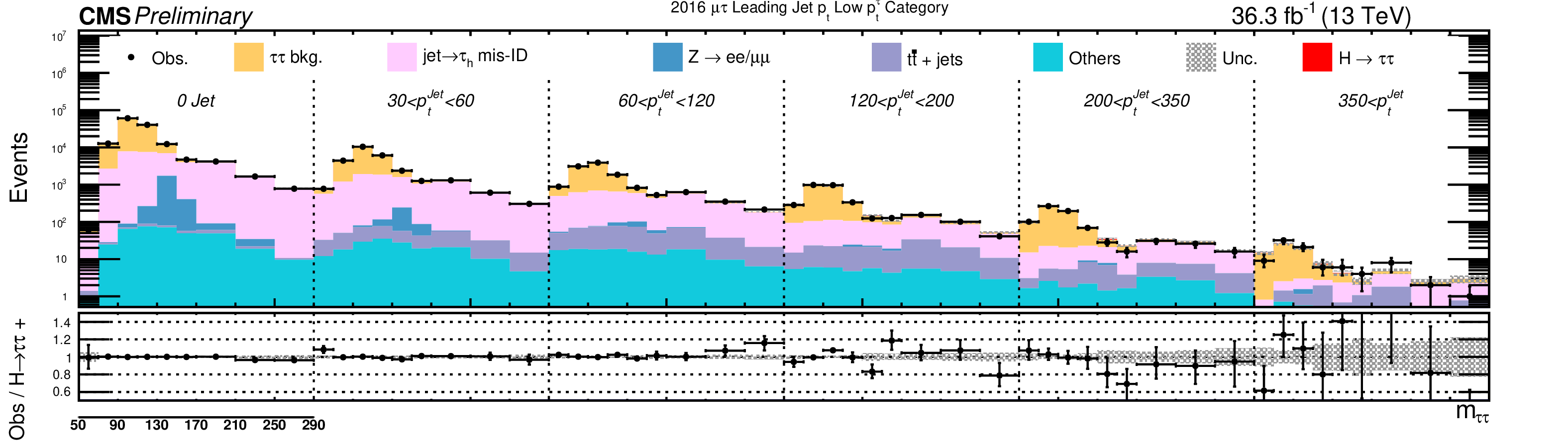
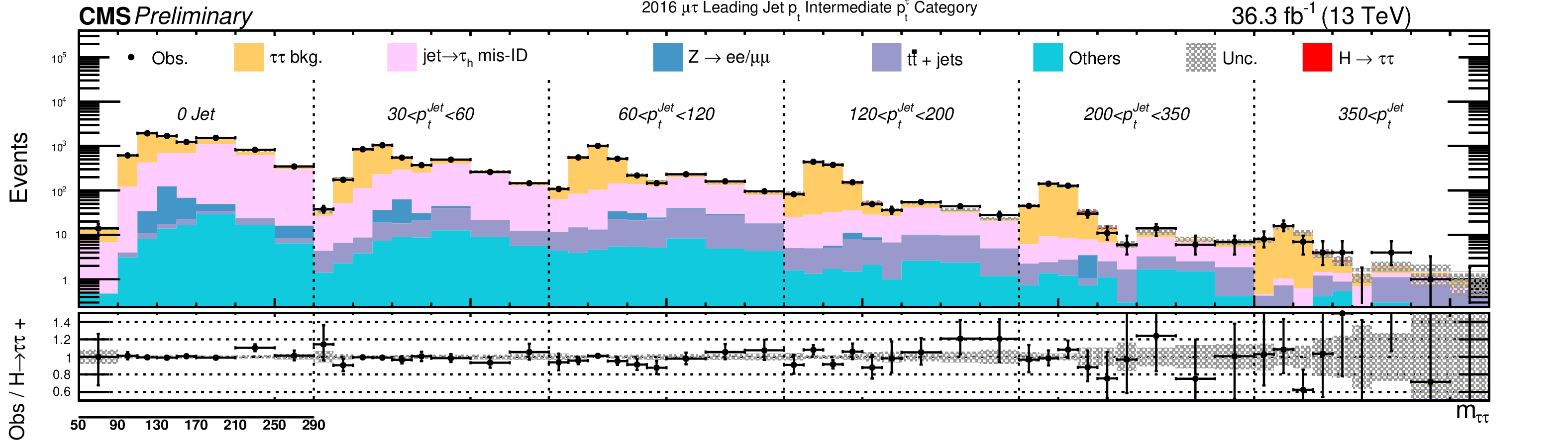
Figure 1:
Observed and expected $ {m_{\tau \tau}} $ distributions in the different reconstructed ranges of the differential observable, obtained by reweighting every $ {m_{\tau \tau}} $ distribution of each category, year, and final state by a factor proportional to the ratio between the signal and background yields in bins with 90 $ < {m_{\tau \tau}} < $ 150 GeV. The reweighting is such that the signal normalization is conserved. The signal and background distributions are the results of a multidimensional maximum likelihood regularized fit. The green line in the ratio plot corresponds to the SM signal expectation. The contribution "Others" include the diboson and single top quark productions, as well as the Higgs boson events outside of the fiducial region. |
png pdf |
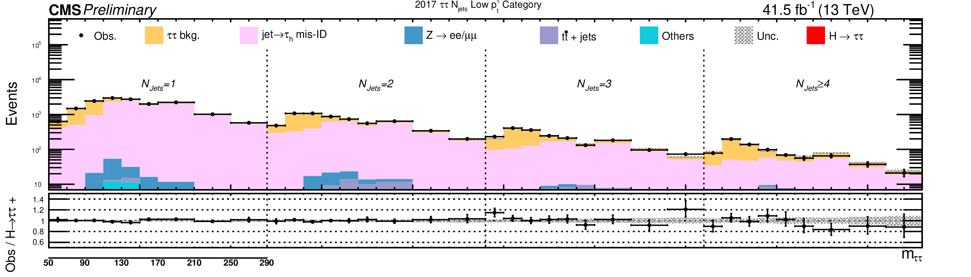
Figure 1-a:
Observed and expected $ {m_{\tau \tau}} $ distributions in the different reconstructed ranges of the differential observable, obtained by reweighting every $ {m_{\tau \tau}} $ distribution of each category, year, and final state by a factor proportional to the ratio between the signal and background yields in bins with 90 $ < {m_{\tau \tau}} < $ 150 GeV. The reweighting is such that the signal normalization is conserved. The signal and background distributions are the results of a multidimensional maximum likelihood regularized fit. The green line in the ratio plot corresponds to the SM signal expectation. The contribution "Others" include the diboson and single top quark productions, as well as the Higgs boson events outside of the fiducial region. |
png pdf |
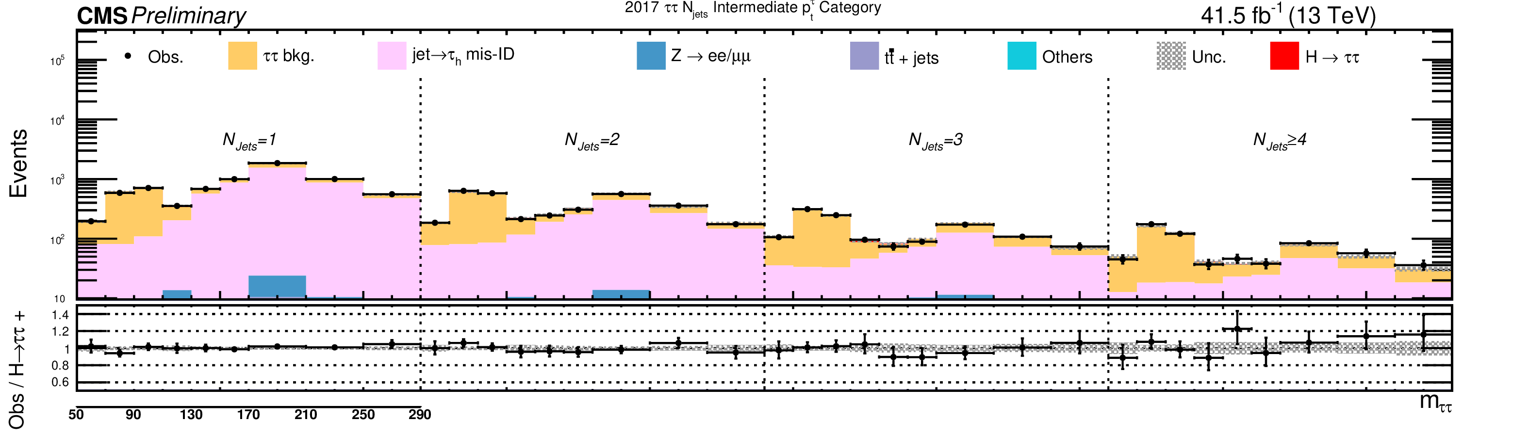
Figure 1-b:
Observed and expected $ {m_{\tau \tau}} $ distributions in the different reconstructed ranges of the differential observable, obtained by reweighting every $ {m_{\tau \tau}} $ distribution of each category, year, and final state by a factor proportional to the ratio between the signal and background yields in bins with 90 $ < {m_{\tau \tau}} < $ 150 GeV. The reweighting is such that the signal normalization is conserved. The signal and background distributions are the results of a multidimensional maximum likelihood regularized fit. The green line in the ratio plot corresponds to the SM signal expectation. The contribution "Others" include the diboson and single top quark productions, as well as the Higgs boson events outside of the fiducial region. |
png pdf |
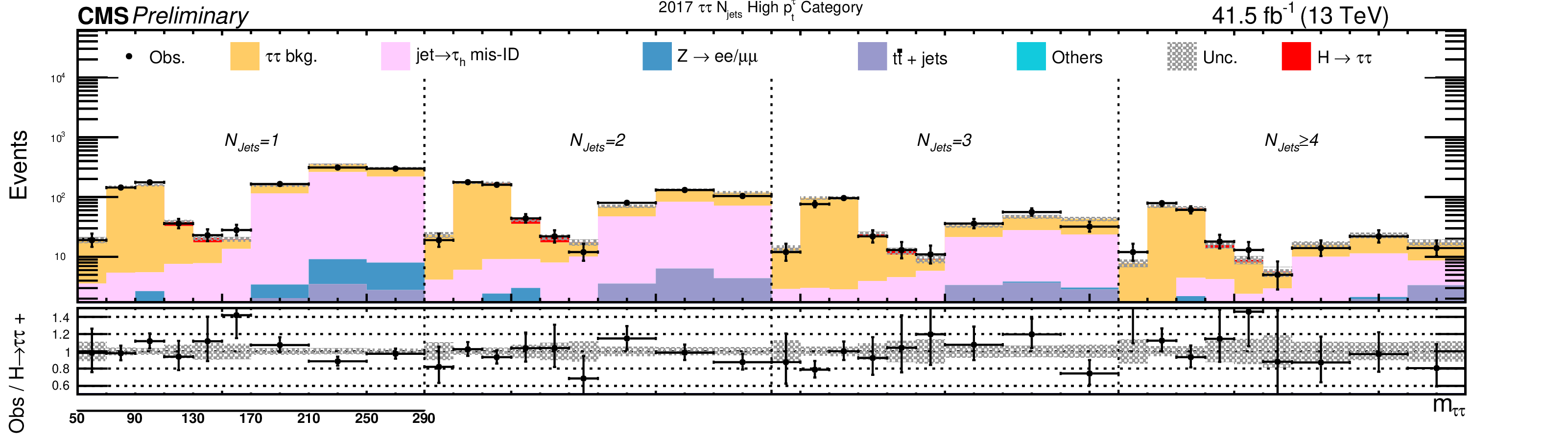
Figure 1-c:
Observed and expected $ {m_{\tau \tau}} $ distributions in the different reconstructed ranges of the differential observable, obtained by reweighting every $ {m_{\tau \tau}} $ distribution of each category, year, and final state by a factor proportional to the ratio between the signal and background yields in bins with 90 $ < {m_{\tau \tau}} < $ 150 GeV. The reweighting is such that the signal normalization is conserved. The signal and background distributions are the results of a multidimensional maximum likelihood regularized fit. The green line in the ratio plot corresponds to the SM signal expectation. The contribution "Others" include the diboson and single top quark productions, as well as the Higgs boson events outside of the fiducial region. |
png pdf |
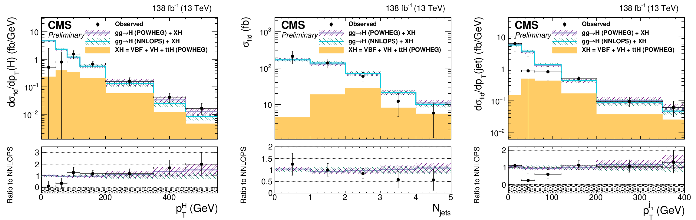
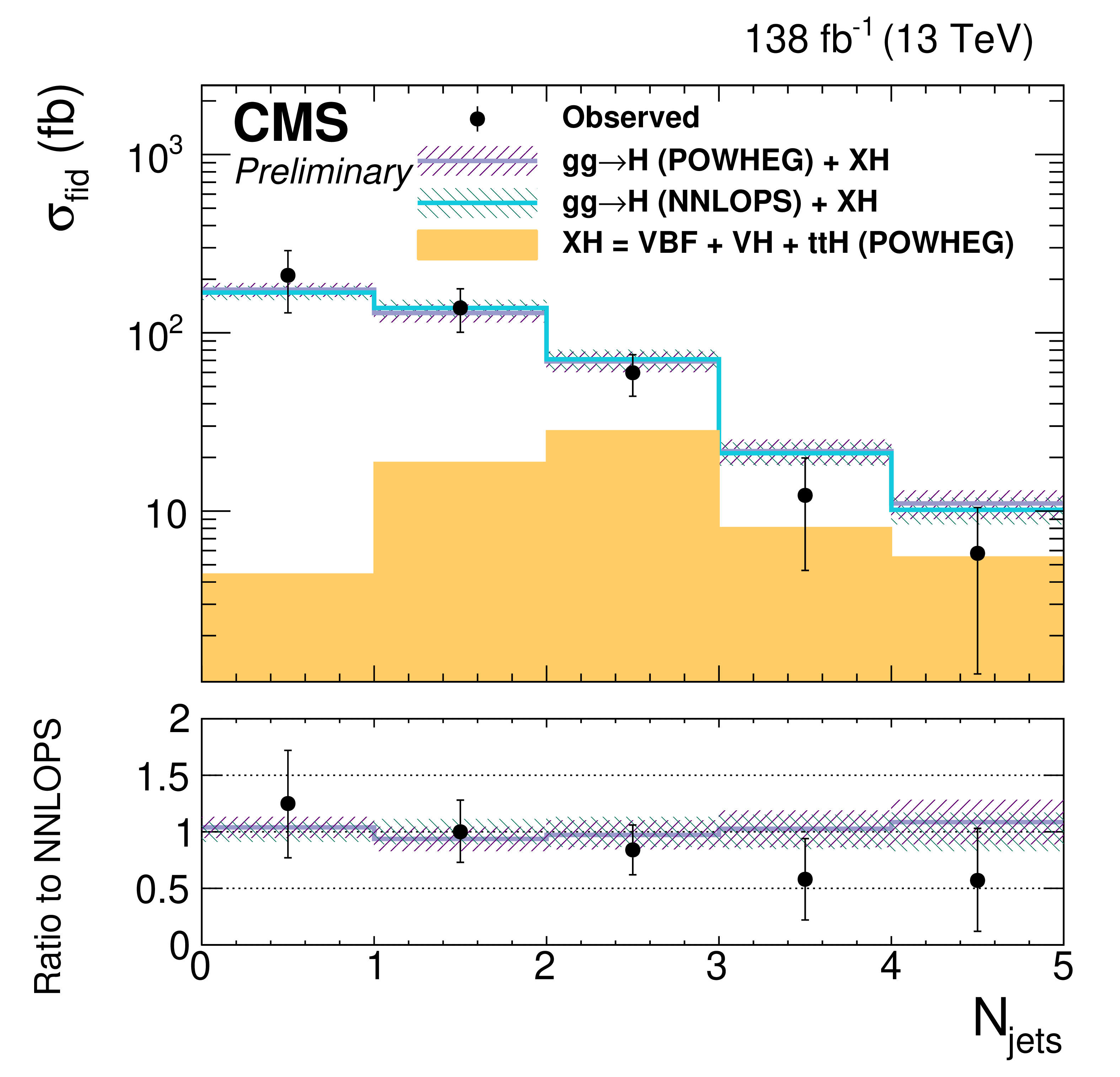
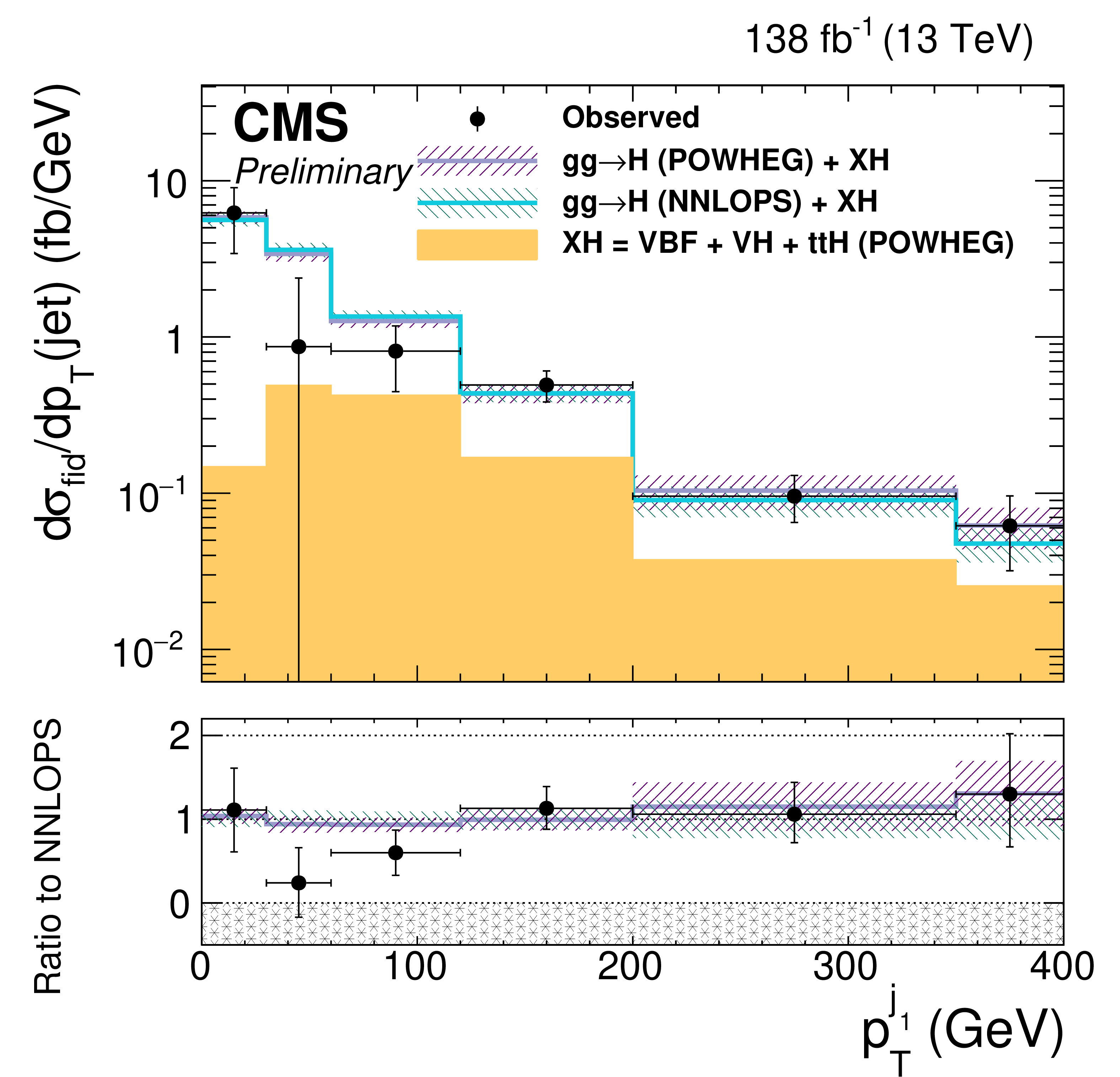
Figure 2:
Observed and expected differential fiducial cross section in bins of $ {{p_{\mathrm {T}}} ^{\mathrm{H}}} $ (left), $ {N_\textrm {jets}} $ (center), and $ {{p_{\mathrm {T}}} ^{\mathrm {j}_1}} $ (right). The signal samples are generated using POWHEG, and the predictions from NNLOPS are also shown as nominal model. The uncertainty bands in the theoretical predictions include uncertainties from the following sources: PDF, renormalization and factorization scale, underlying event and parton showering, and $\mathcal {B}(\mathrm{H} \to \tau \tau)$. The last bins include the overflow. |

png pdf |
Figure 2-a:
Observed and expected differential fiducial cross section in bins of $ {{p_{\mathrm {T}}} ^{\mathrm{H}}} $ (left), $ {N_\textrm {jets}} $ (center), and $ {{p_{\mathrm {T}}} ^{\mathrm {j}_1}} $ (right). The signal samples are generated using POWHEG, and the predictions from NNLOPS are also shown as nominal model. The uncertainty bands in the theoretical predictions include uncertainties from the following sources: PDF, renormalization and factorization scale, underlying event and parton showering, and $\mathcal {B}(\mathrm{H} \to \tau \tau)$. The last bins include the overflow. |
png pdf |
Figure 2-b:
Observed and expected differential fiducial cross section in bins of $ {{p_{\mathrm {T}}} ^{\mathrm{H}}} $ (left), $ {N_\textrm {jets}} $ (center), and $ {{p_{\mathrm {T}}} ^{\mathrm {j}_1}} $ (right). The signal samples are generated using POWHEG, and the predictions from NNLOPS are also shown as nominal model. The uncertainty bands in the theoretical predictions include uncertainties from the following sources: PDF, renormalization and factorization scale, underlying event and parton showering, and $\mathcal {B}(\mathrm{H} \to \tau \tau)$. The last bins include the overflow. |
png pdf |
Figure 2-c:
Observed and expected differential fiducial cross section in bins of $ {{p_{\mathrm {T}}} ^{\mathrm{H}}} $ (left), $ {N_\textrm {jets}} $ (center), and $ {{p_{\mathrm {T}}} ^{\mathrm {j}_1}} $ (right). The signal samples are generated using POWHEG, and the predictions from NNLOPS are also shown as nominal model. The uncertainty bands in the theoretical predictions include uncertainties from the following sources: PDF, renormalization and factorization scale, underlying event and parton showering, and $\mathcal {B}(\mathrm{H} \to \tau \tau)$. The last bins include the overflow. |
| Tables | |
png pdf |
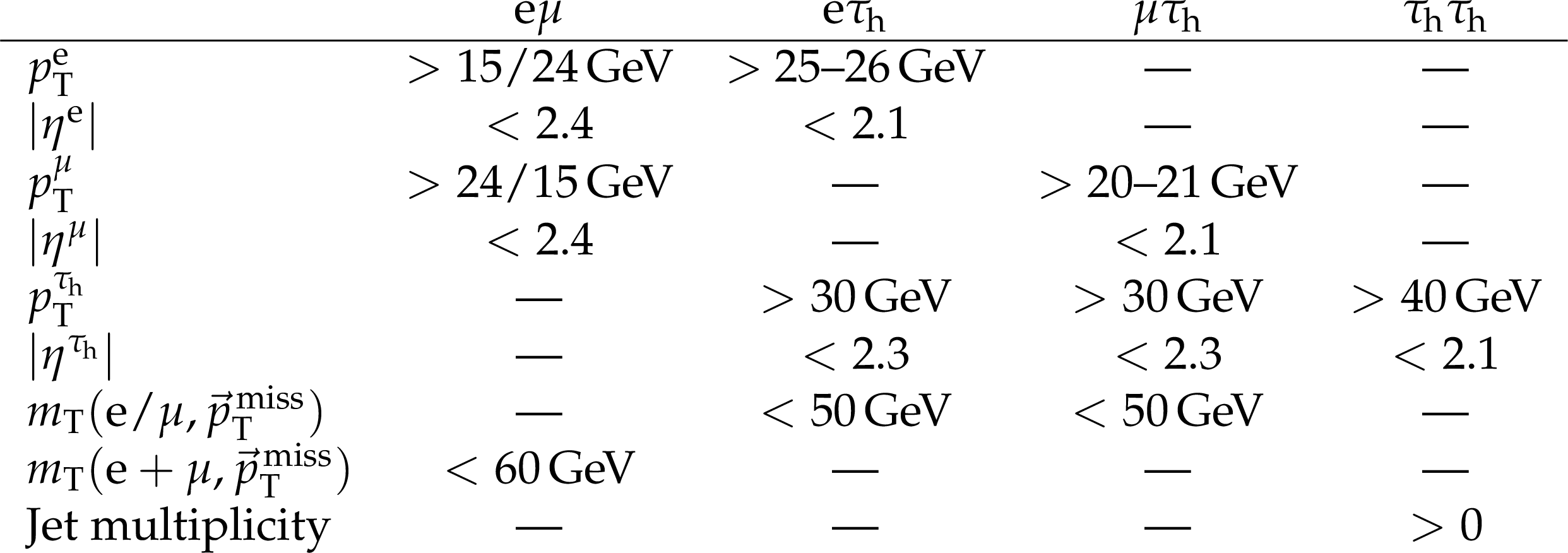
Table 1:
Selection criteria in the four di-$\tau $ final states. The ${p_{\mathrm {T}}}$ ranges are related to different triggers used during different data-taking periods. The symbol $m_T$ denotes the transverse mass between two objects [10]. In events collected in 2016 in the $\mu {\tau _\mathrm {h}} $ channel, $ {\tau _\mathrm {h}} $ candidates with 0.2 $ < {| \eta |} < $ 0.3 are discarded because of a significantly larger misidentification rate of muons as $ {\tau _\mathrm {h}} $ objects. |

png pdf |
Table 2:
Observed and expected fiducial cross sections in $ {N_\textrm {jets}} $, $ {{p_{\mathrm {T}}} ^{\mathrm{H}}} $, and $ {{p_{\mathrm {T}}} ^{\mathrm {j}_1}} $ bins. The signal strengths obtained from the regularized and unregularized fits are indicated. The observed cross section corresponds to the result of the regularized fit. The signal strengths do not include yield uncertainties in the predictions of the SM Higgs boson production cross sections nor branching fractions. Results for $ {N_\textrm {jets}} =$ 0 are given twice in the table: the first occurence is related to the fit of $ {N_\textrm {jets}} $-based categories, while the second occurence corresponds to the fit of $ {{p_{\mathrm {T}}} ^{\mathrm {j}_1}} $-based categories. |
| Summary |
| In summary, measurements of the differential fiducial cross sections of the Higgs boson have been performed for the first time at the LHC in the decay channel of two $\tau$ leptons. The differential cross section as a function of the jet multiplicity, Higgs boson transverse momentum, and tranverse momentum of the leading jet, are in agreement with the expectations of the standard model, with a competitive precision with respect to measurements in other final states in the phase spaces with a large jet multiplicity, or with a Higgs boson transverse momentum between 120 and 600 GeV. In addition, the fiducial inclusive cross section has been measured to be 426 $\pm$ 102 fb, for a standard-model expectation of 408 $\pm$ 27 fb. |
| Additional Figures | |
png pdf |
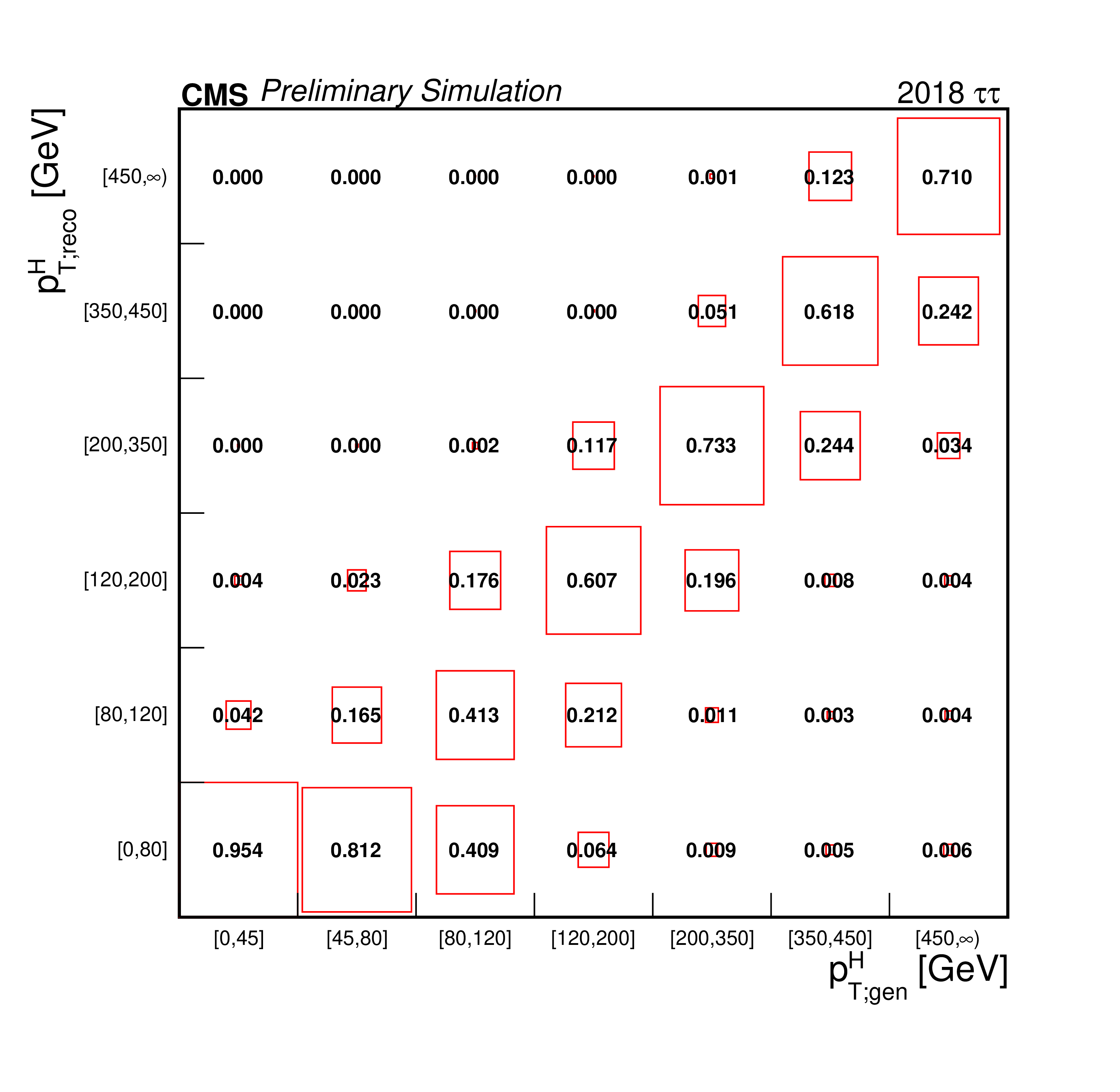
Additional Figure 1:
Response matrices for the reconstructed vs. generated Higgs $ {p_{\mathrm {T}}} $ in the $ {{\tau} _\mathrm {h}} {{\tau} _\mathrm {h}} $ channel for 2018. The horizontal axis represents the generator-level Higgs $ {p_{\mathrm {T}}} $ bins and the vertical axis represents the reconstruction-level Higgs $ {p_{\mathrm {T}}} $ bins. Each column is normalized so that event yield in the column adds up to unity. |
png pdf |
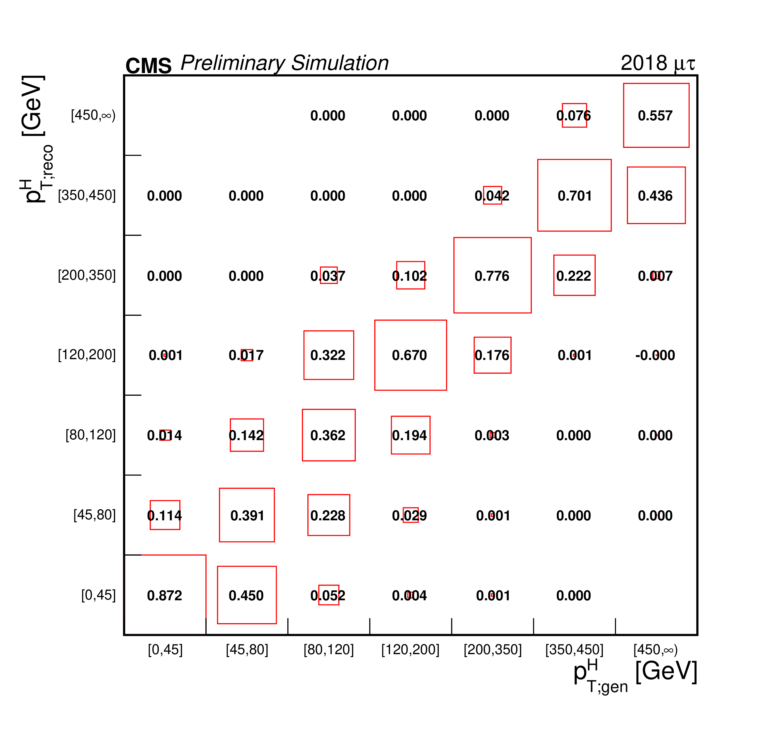
Additional Figure 2:
Response matrices for the reconstructed vs. generated Higgs $ {p_{\mathrm {T}}} $ in the $\mu {{\tau} _\mathrm {h}} $ channel for 2018. The horizontal axis represents the generator-level Higgs $ {p_{\mathrm {T}}} $ bins and the vertical axis represents the reconstruction-level Higgs $ {p_{\mathrm {T}}} $ bins. Each column is normalized so that event yield in the column adds up to unity. |
png pdf |
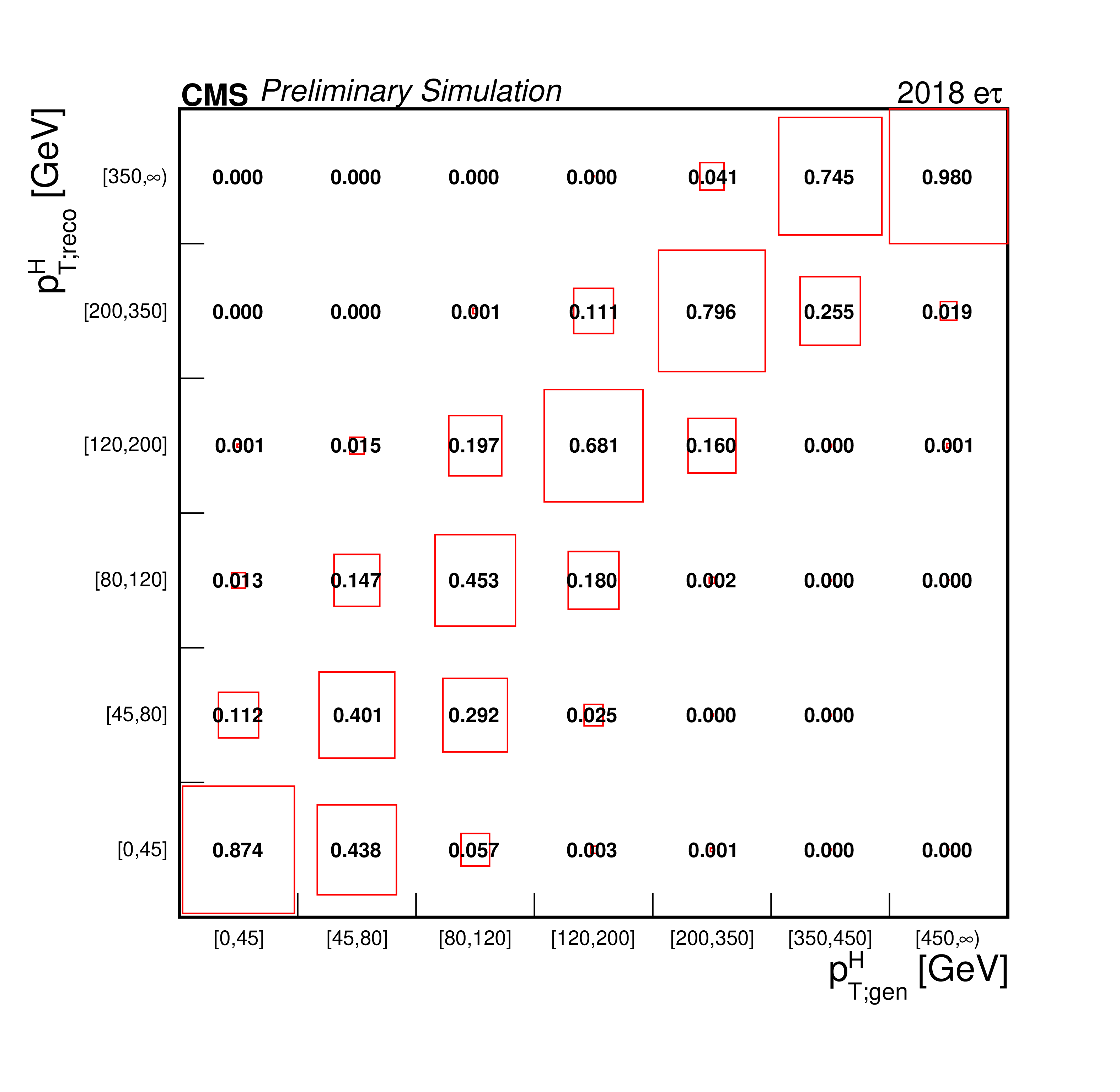
Additional Figure 3:
Response matrices for the reconstructed vs. generated Higgs $ {p_{\mathrm {T}}} $ in the $ {\mathrm {e}} {{\tau} _\mathrm {h}} $ channel for 2018. The horizontal axis represents the generator-level Higgs $ {p_{\mathrm {T}}} $ bins and the vertical axis represents the reconstruction-level Higgs $ {p_{\mathrm {T}}} $ bins. Each column is normalized so that event yield in the column adds up to unity. |
png pdf |
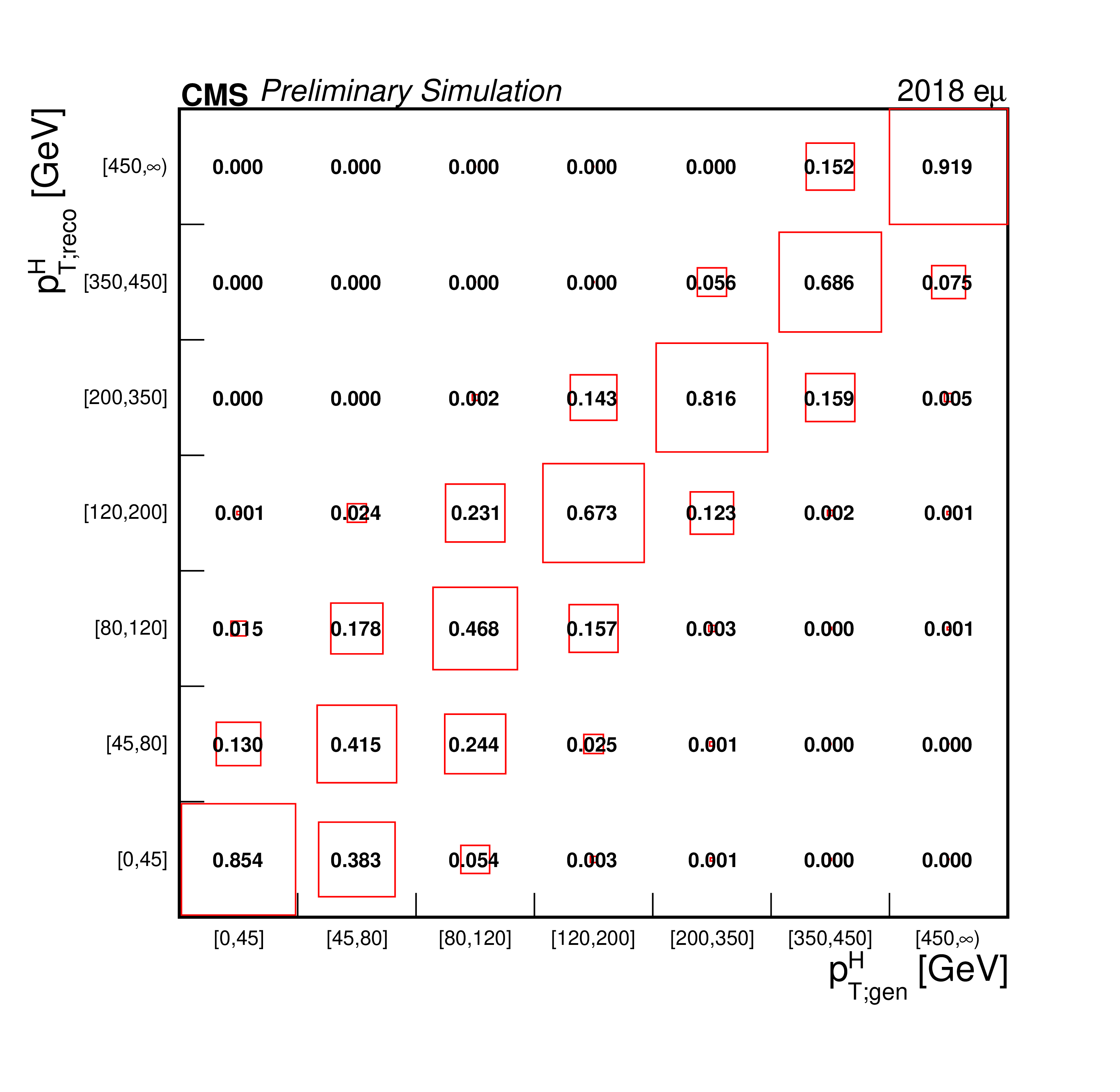
Additional Figure 4:
Response matrices for the reconstructed vs. generated Higgs $ {p_{\mathrm {T}}} $ in the $ {\mathrm {e}}\mu $ channel for 2018. The horizontal axis represents the generator-level Higgs $ {p_{\mathrm {T}}} $ bins and the vertical axis represents the reconstruction-level Higgs $ {p_{\mathrm {T}}} $ bins. Each column is normalized so that event yield in the column adds up to unity. |
png pdf |
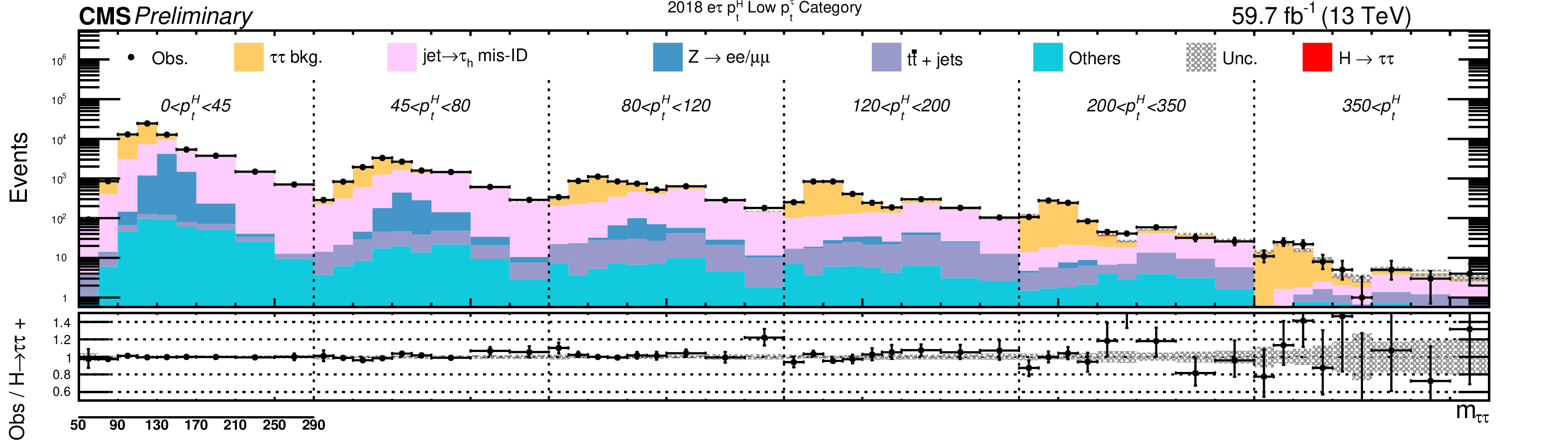
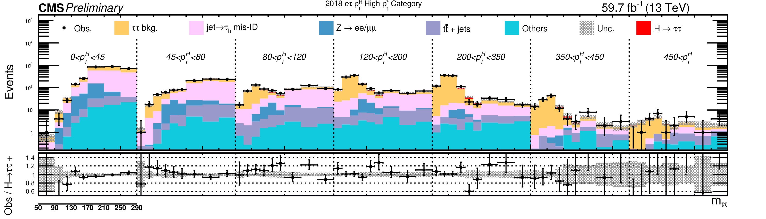
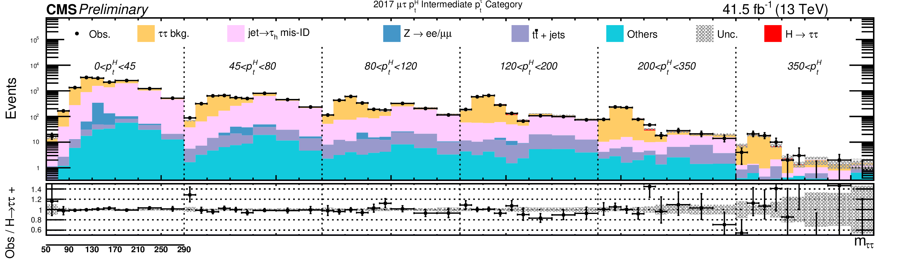
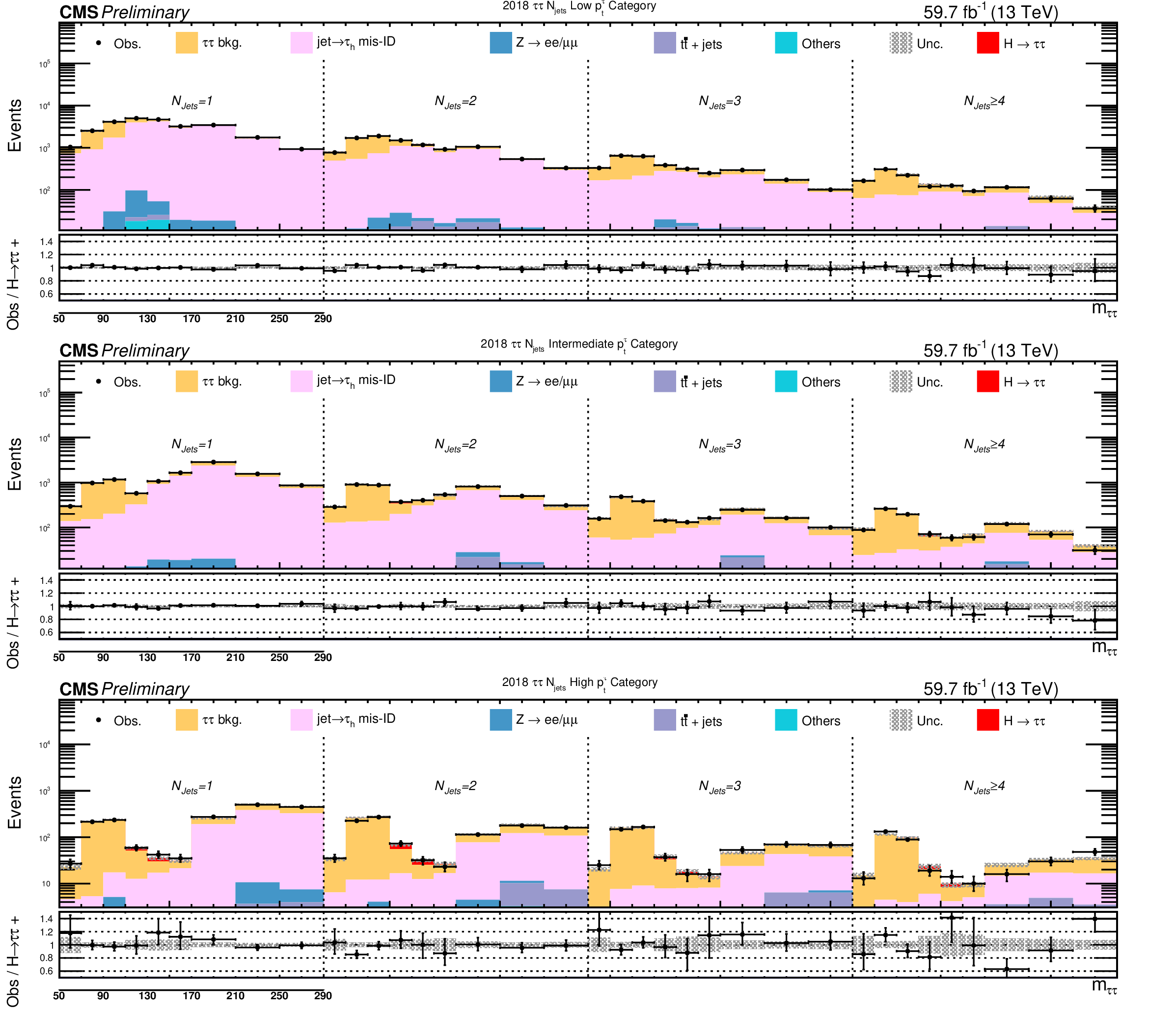
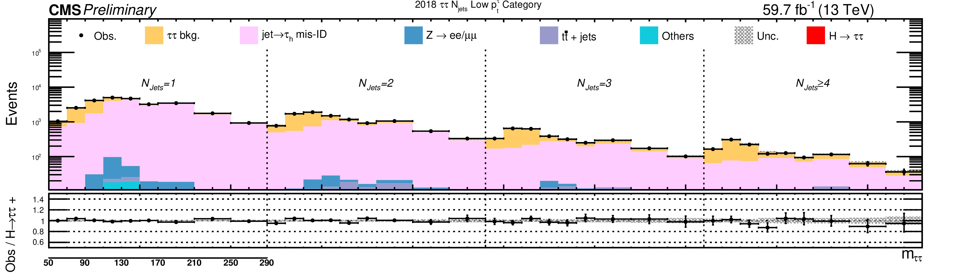
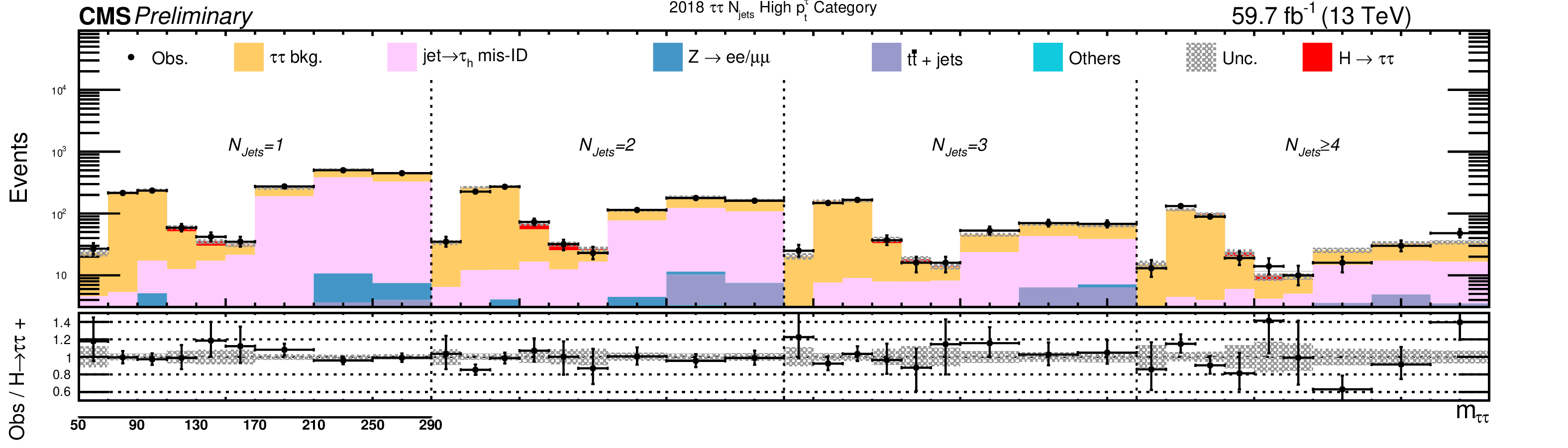
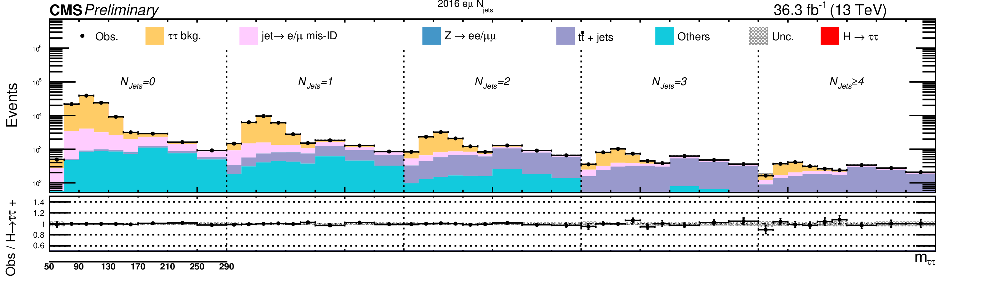
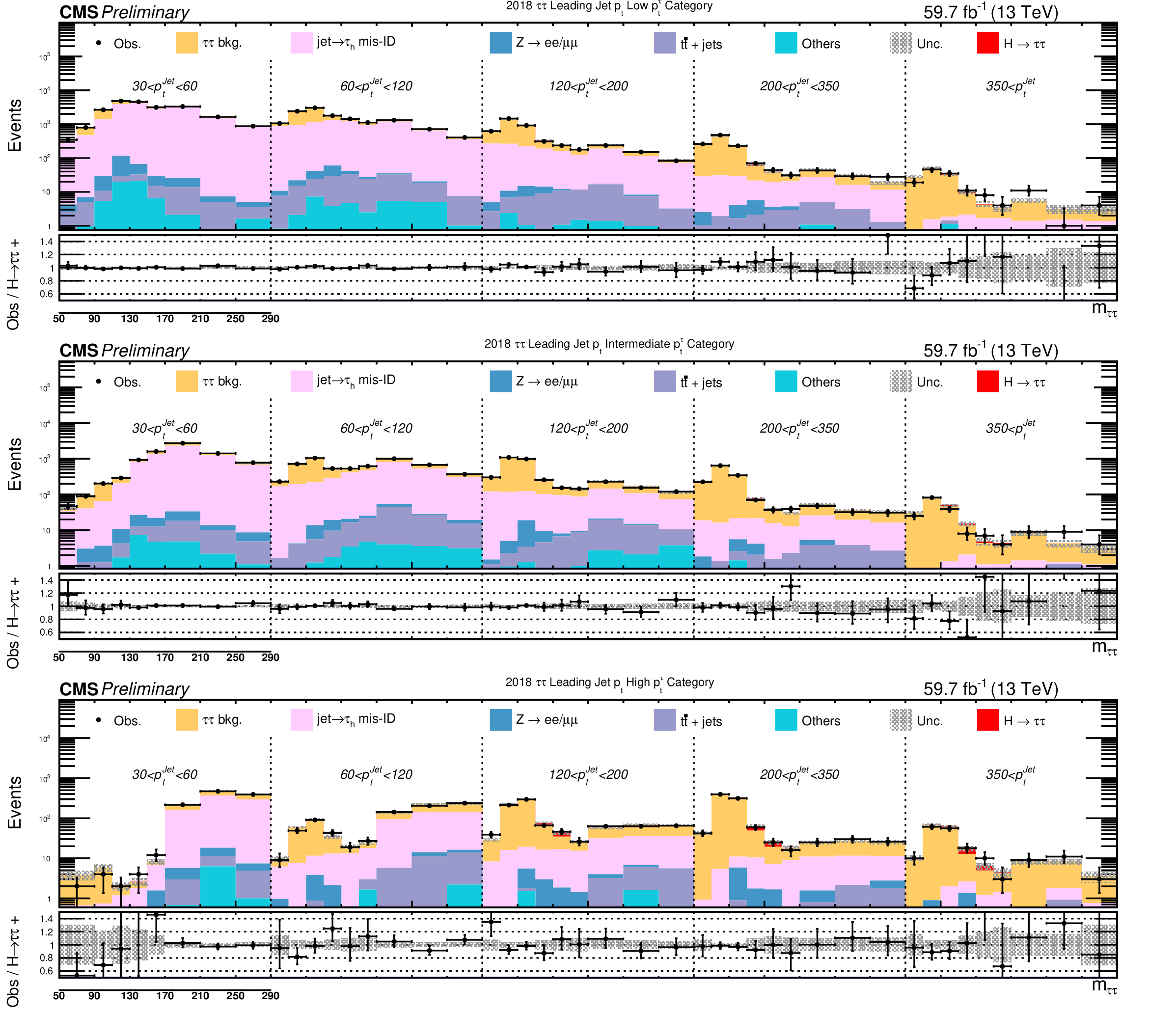
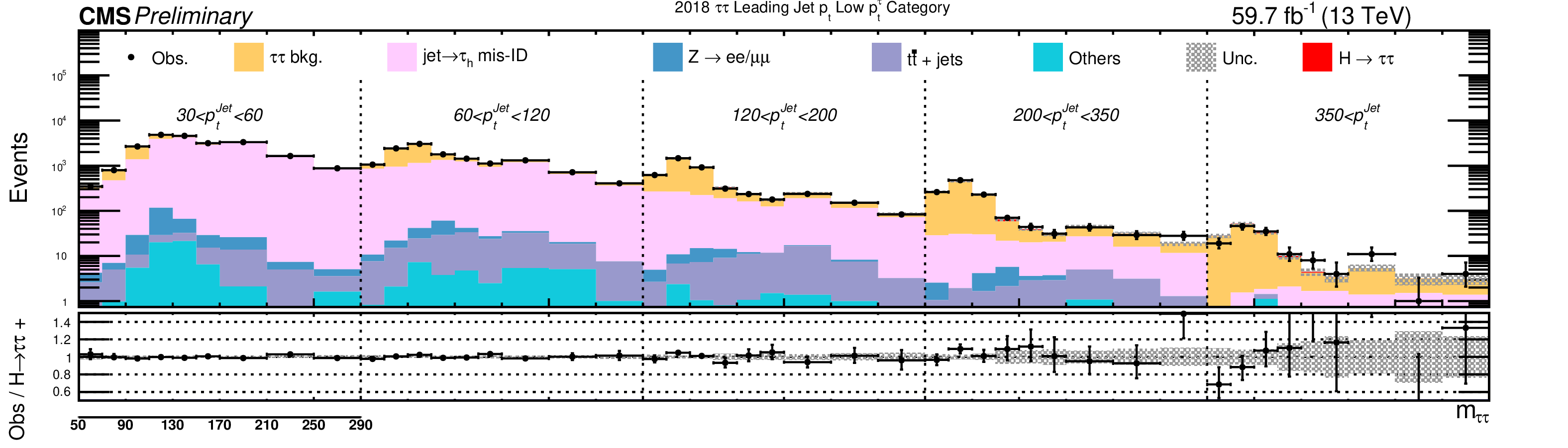
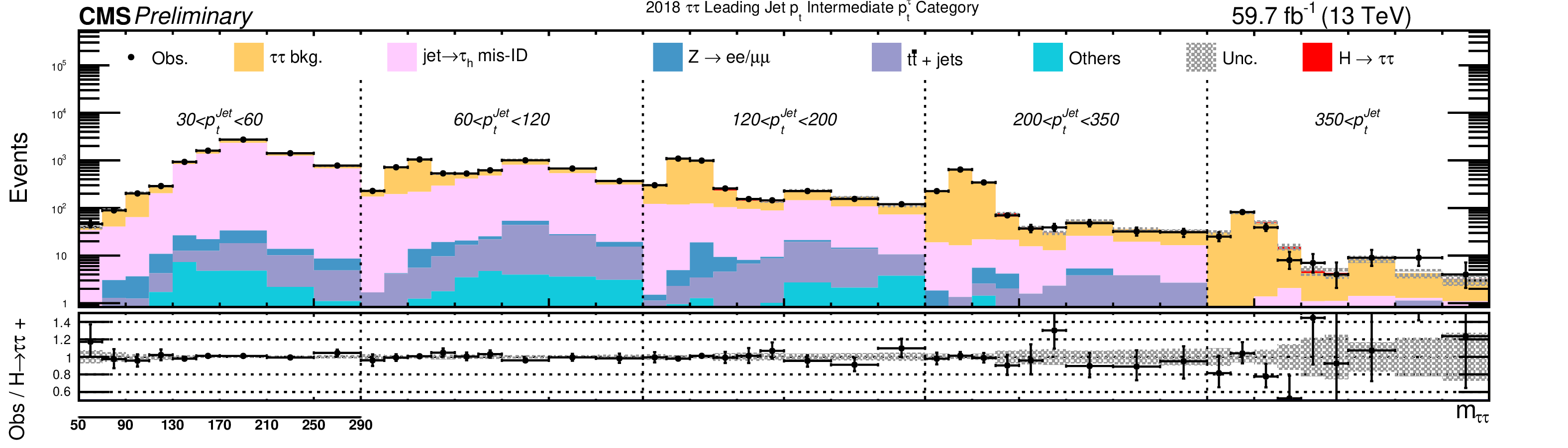
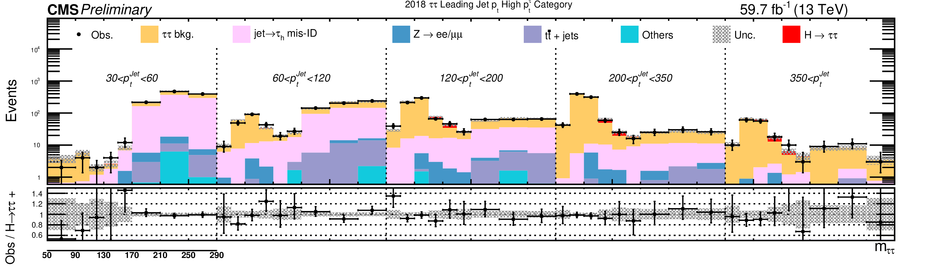
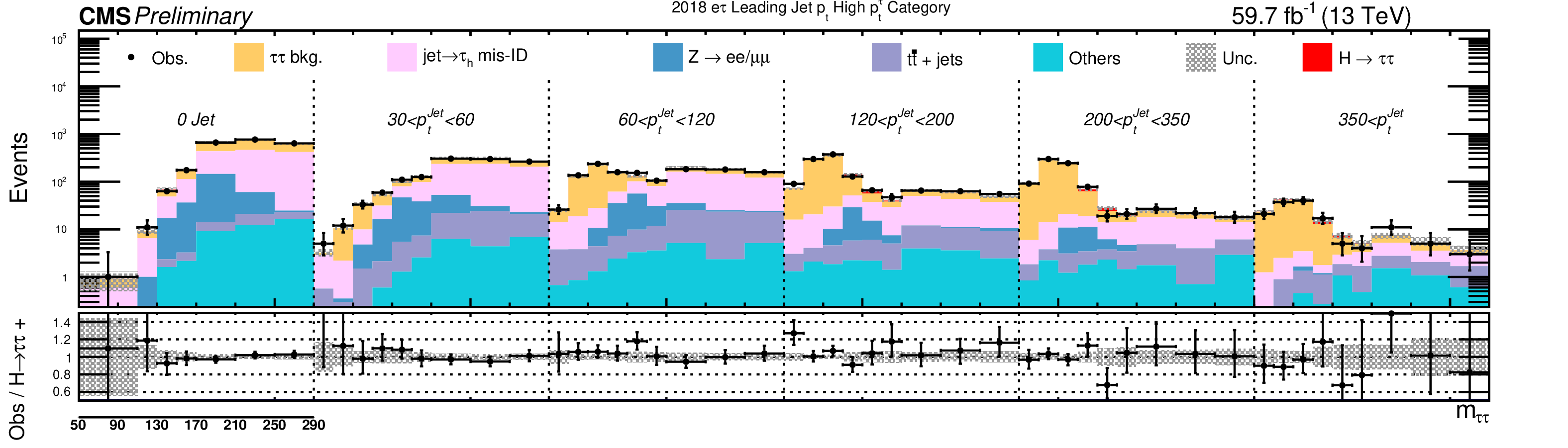
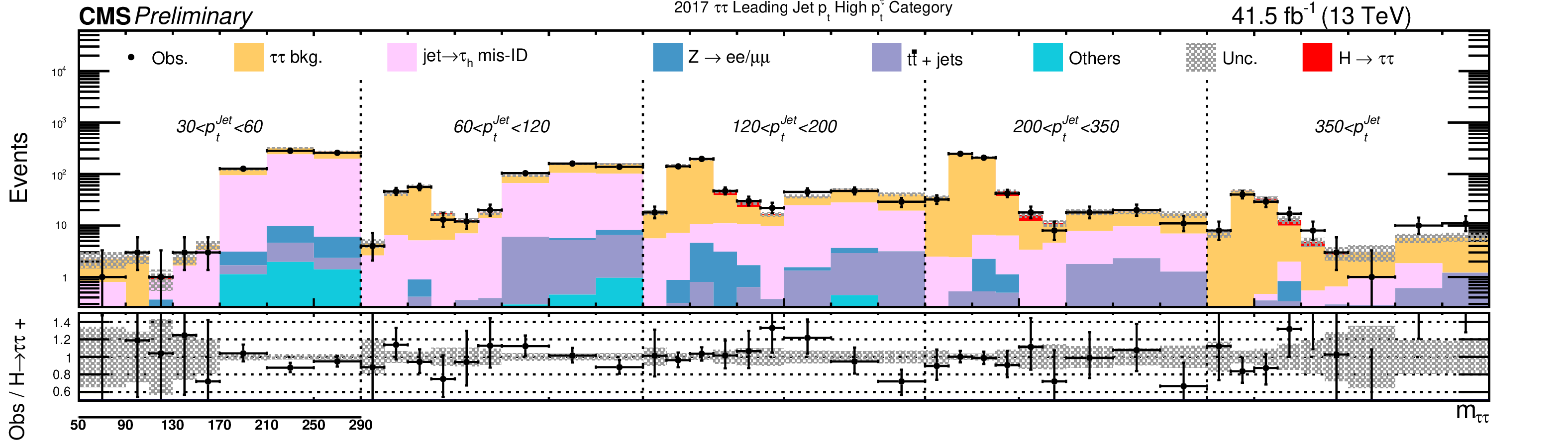
Additional Figure 5:
Postfit distributions in the $ {{\tau} _\mathrm {h}} {{\tau} _\mathrm {h}} $ final state in 2018. This represents a fit to data with all years and final states. |

png pdf |
Additional Figure 5-a:
Postfit distributions in the $ {{\tau} _\mathrm {h}} {{\tau} _\mathrm {h}} $ final state in 2018. This represents a fit to data with all years and final states. |
png pdf |
Additional Figure 5-b:
Postfit distributions in the $ {{\tau} _\mathrm {h}} {{\tau} _\mathrm {h}} $ final state in 2018. This represents a fit to data with all years and final states. |
png pdf |
Additional Figure 5-c:
Postfit distributions in the $ {{\tau} _\mathrm {h}} {{\tau} _\mathrm {h}} $ final state in 2018. This represents a fit to data with all years and final states. |
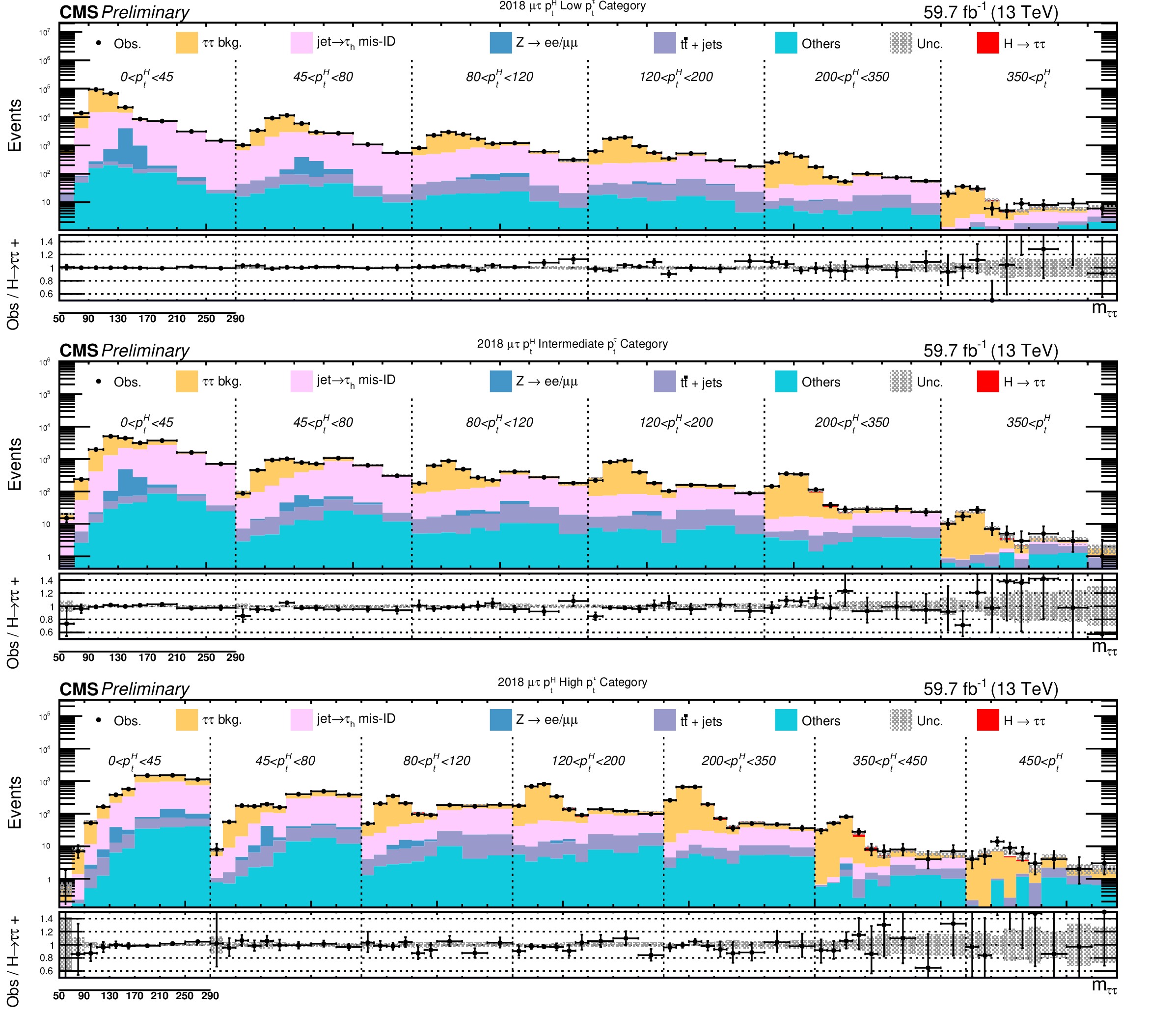
png pdf |
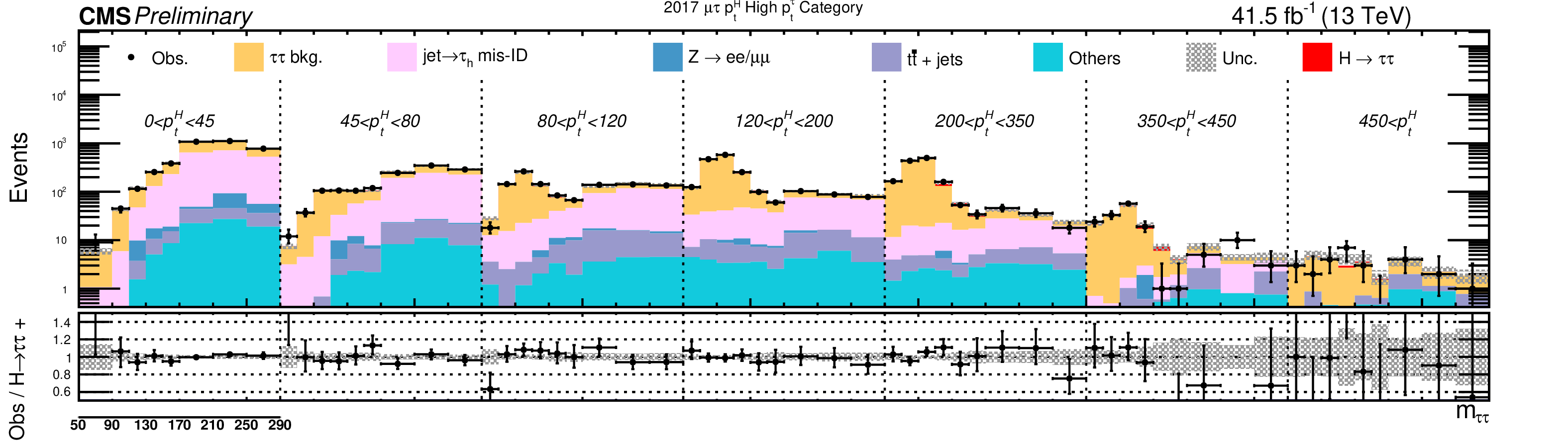
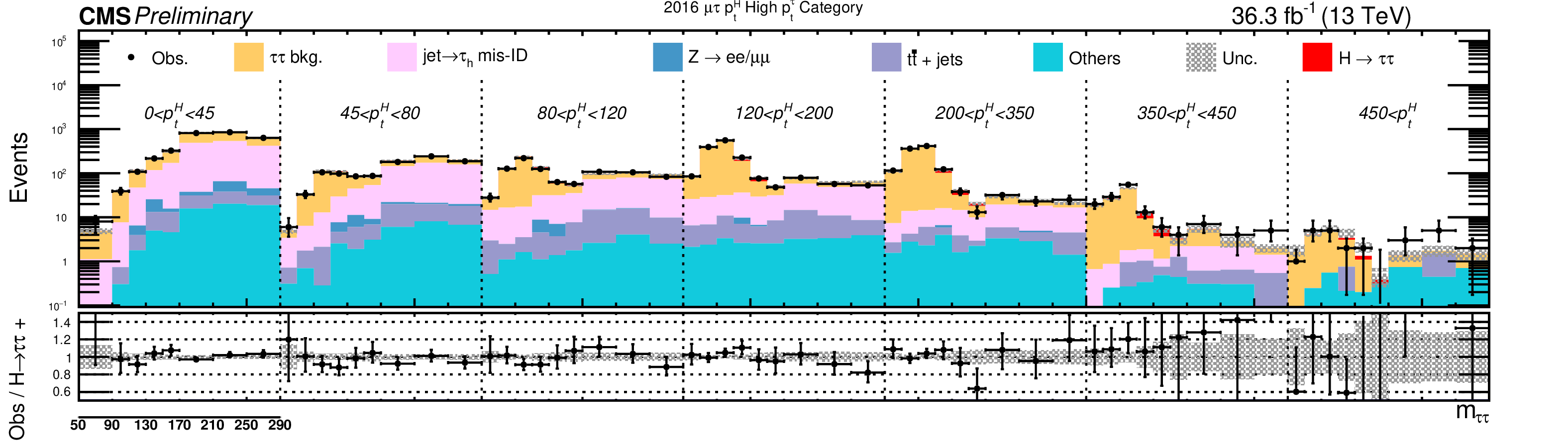
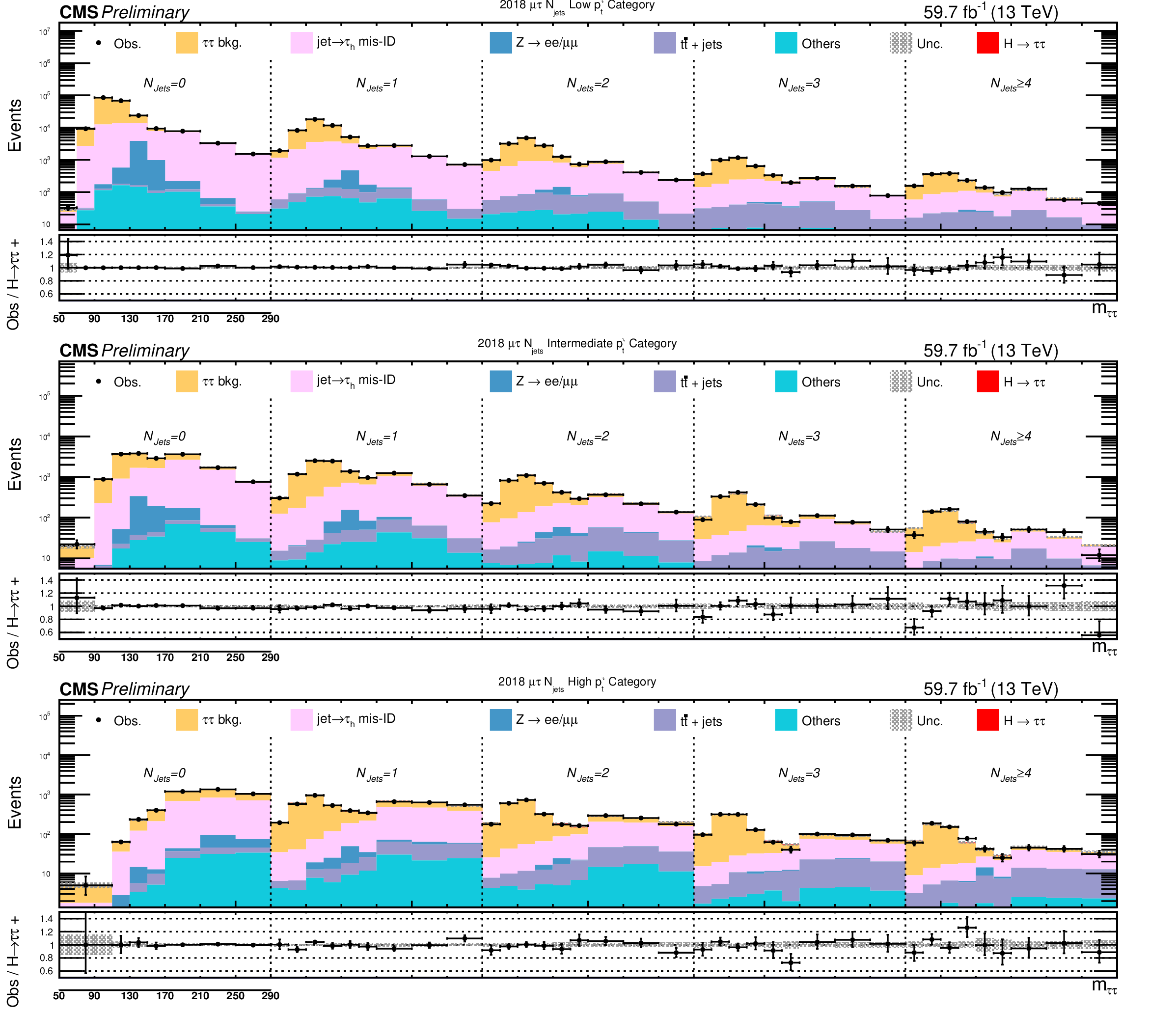
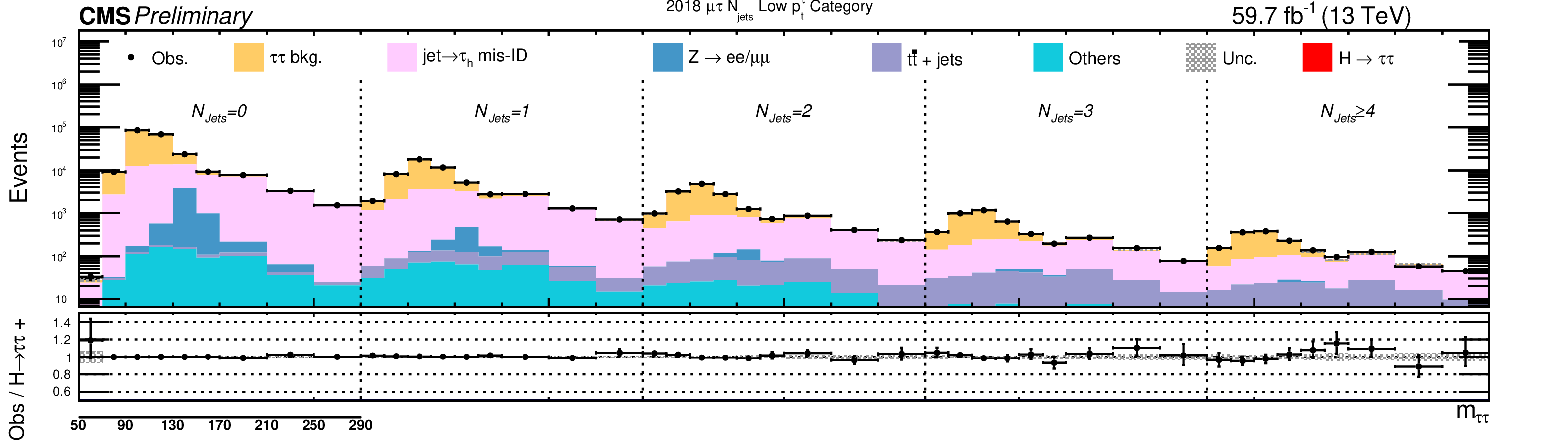
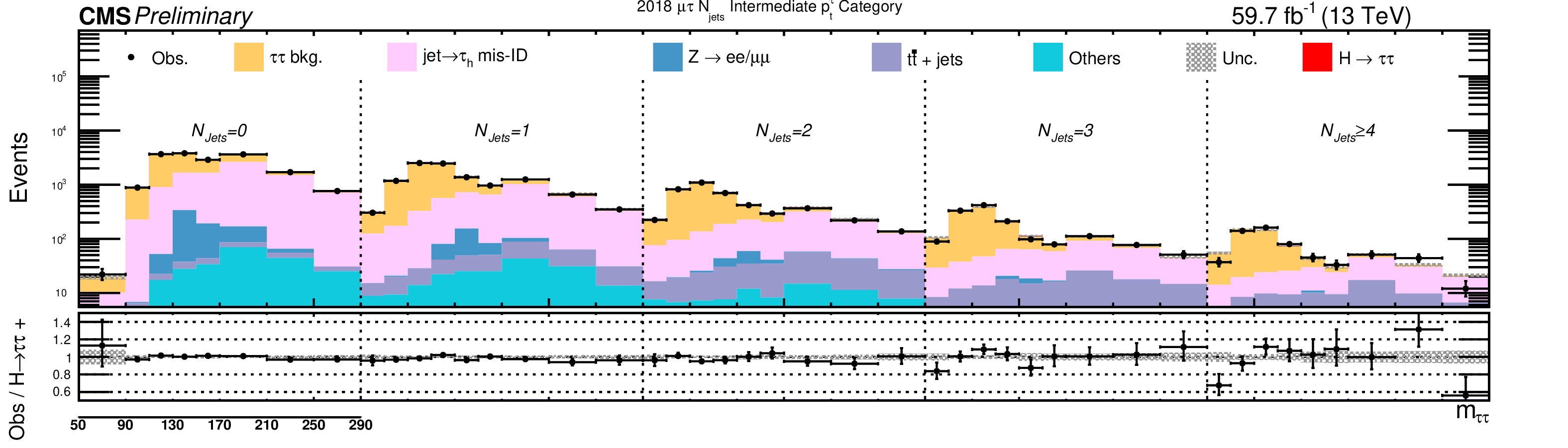
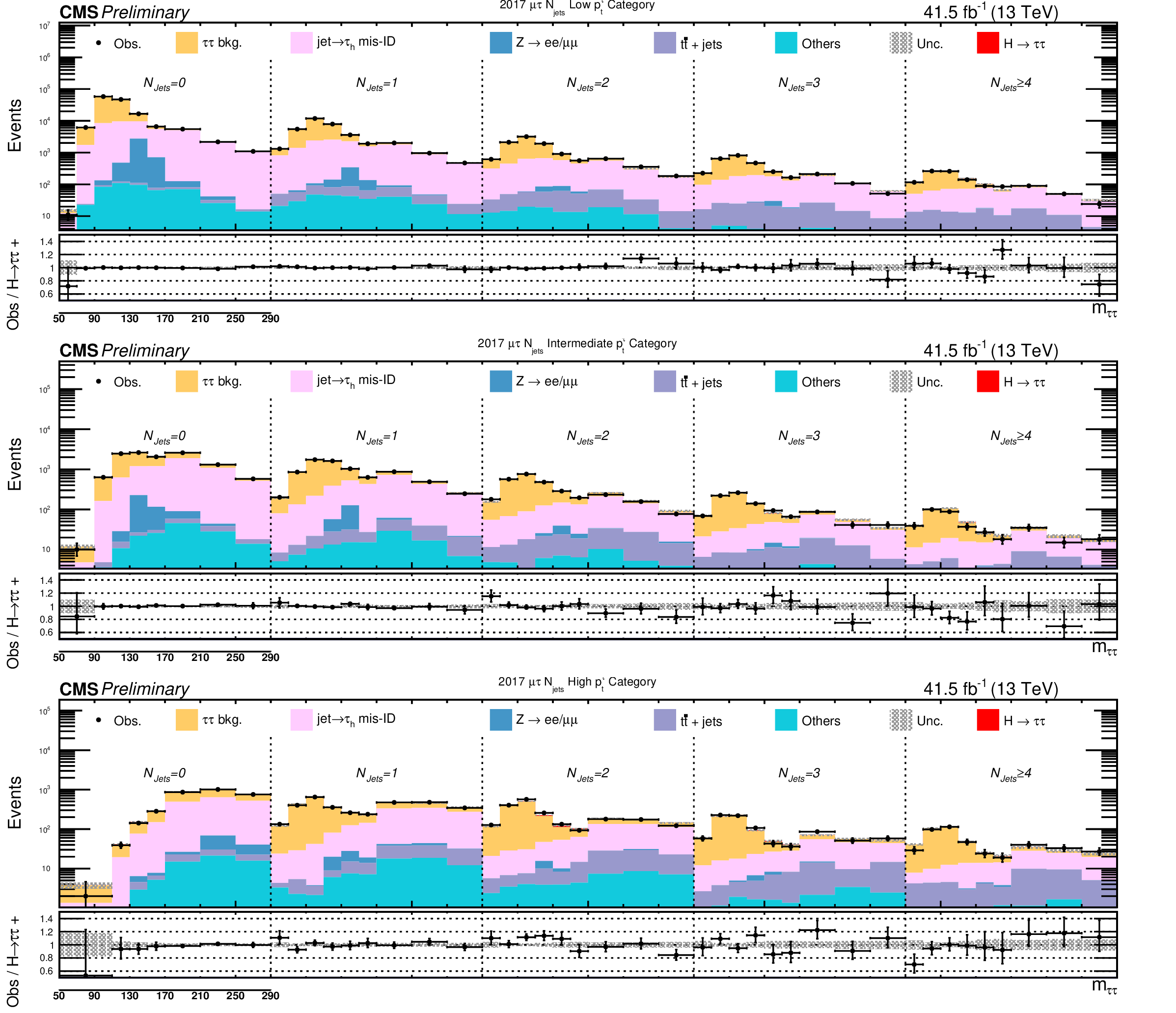
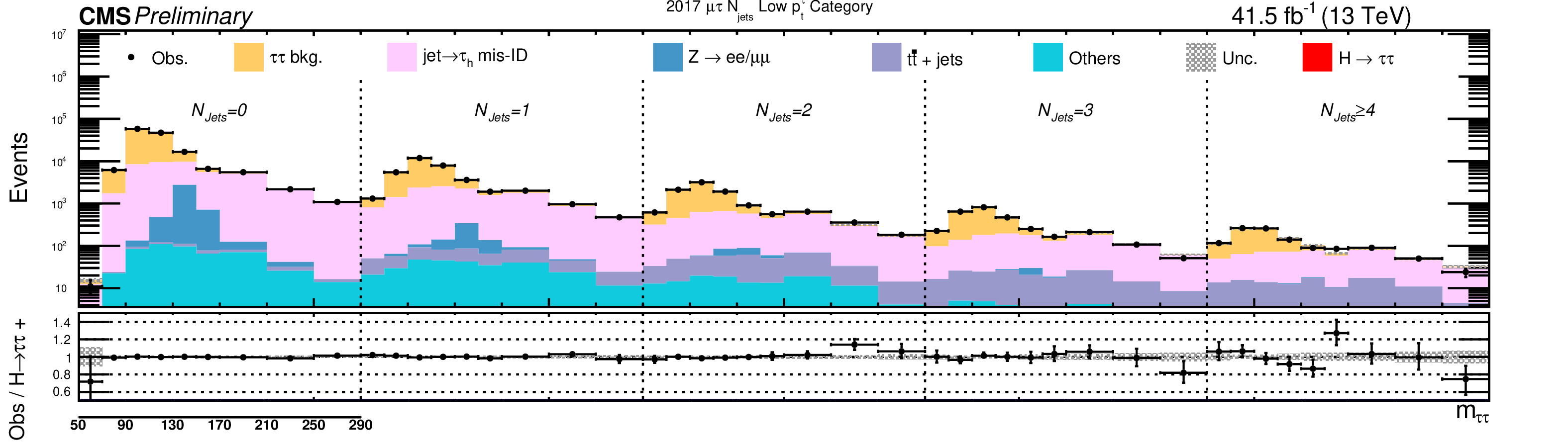
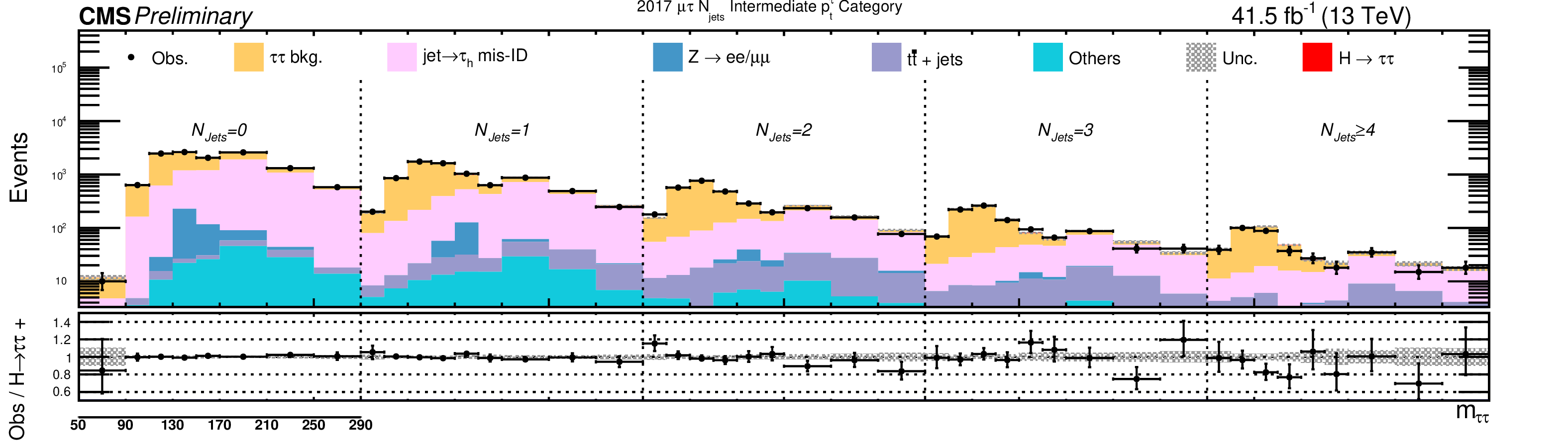
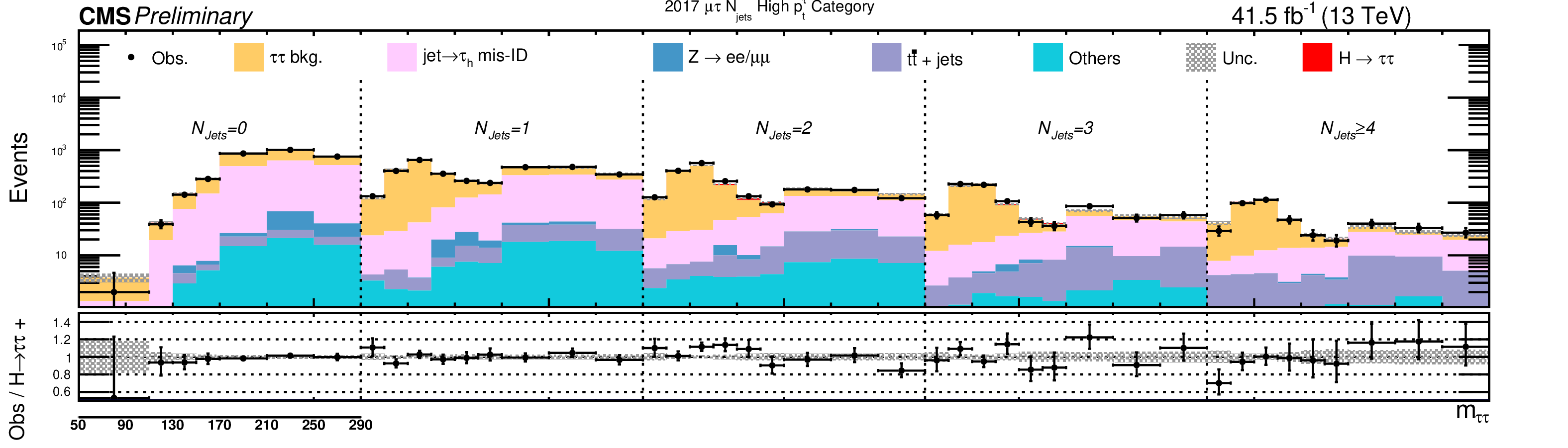
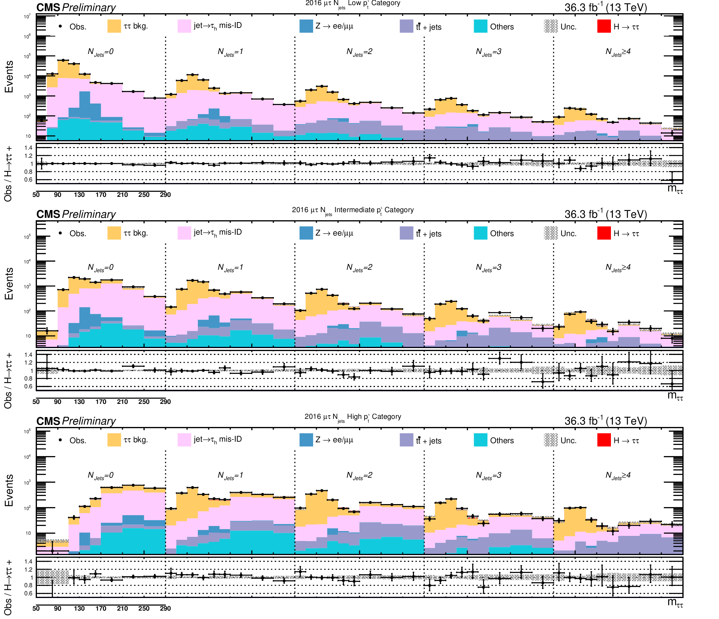
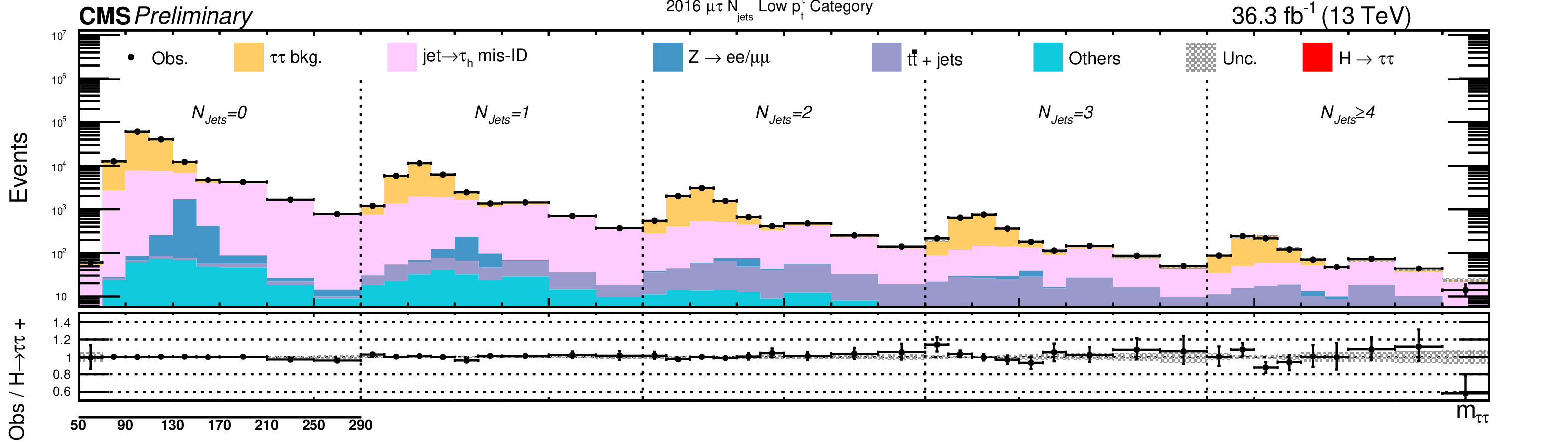
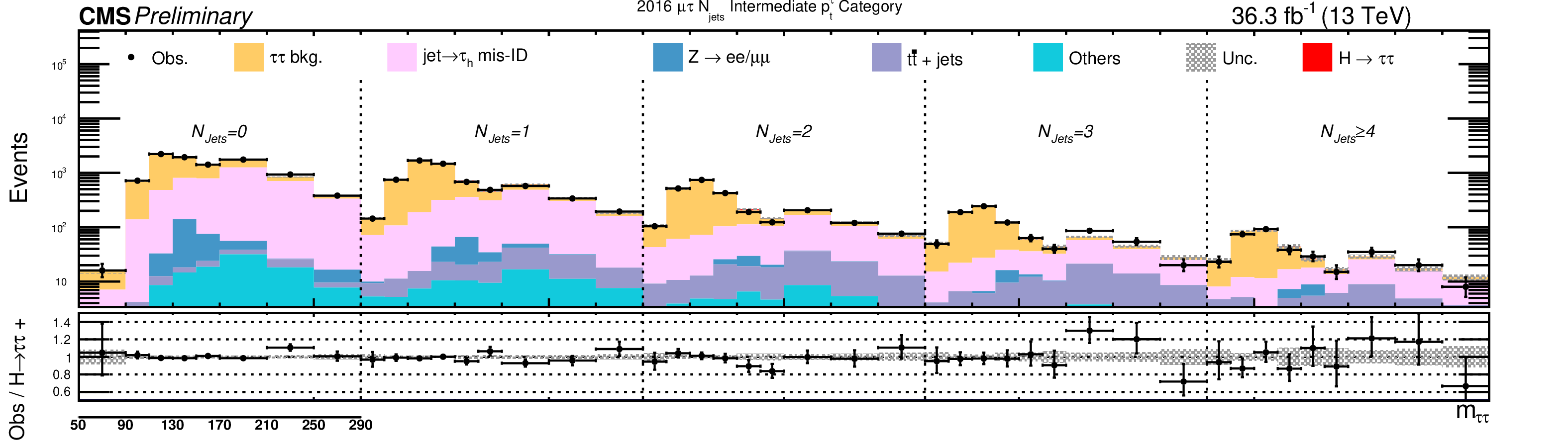
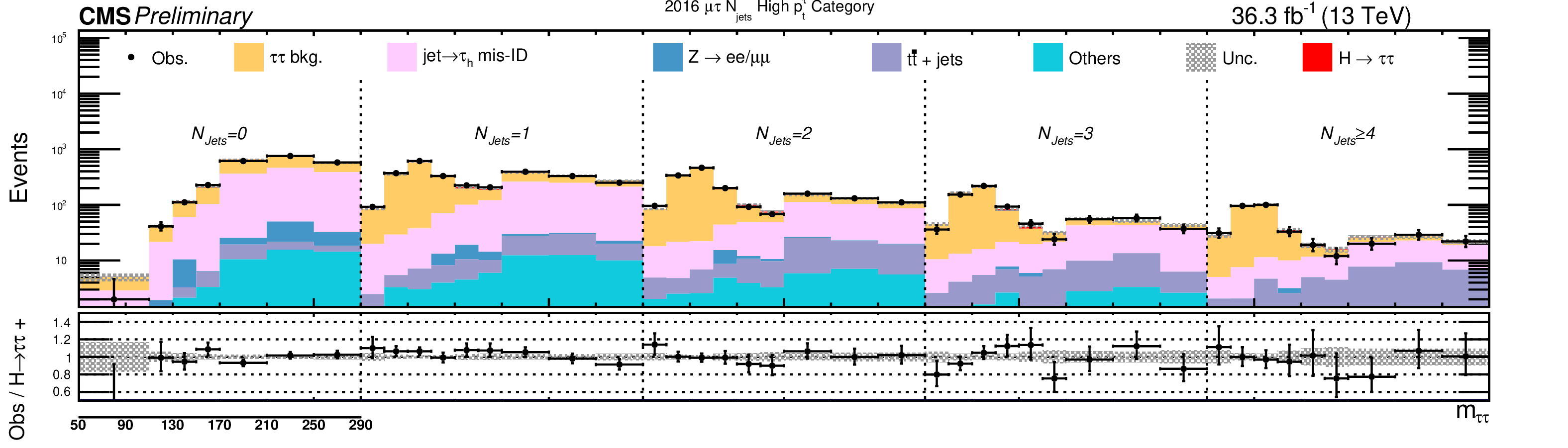
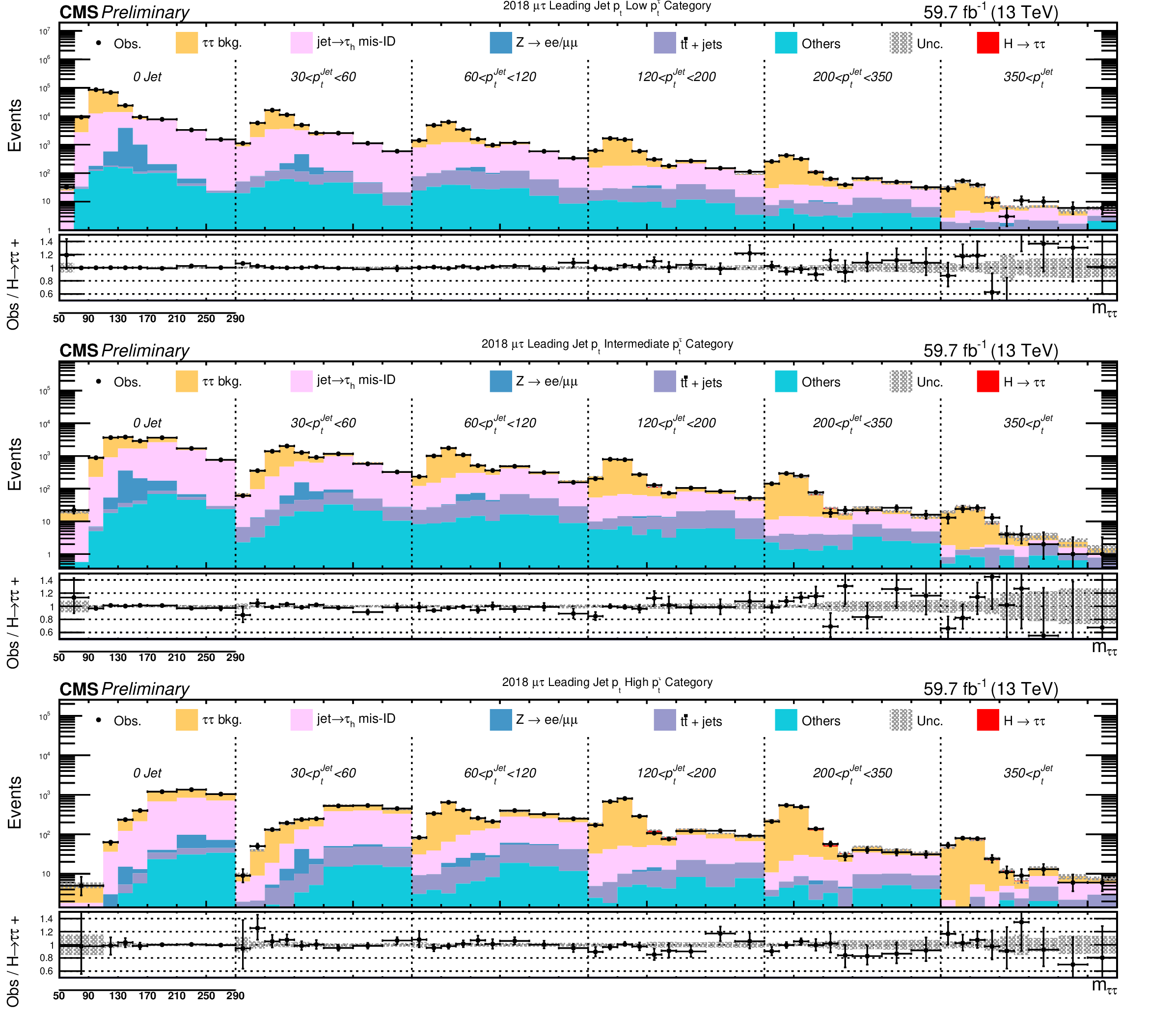
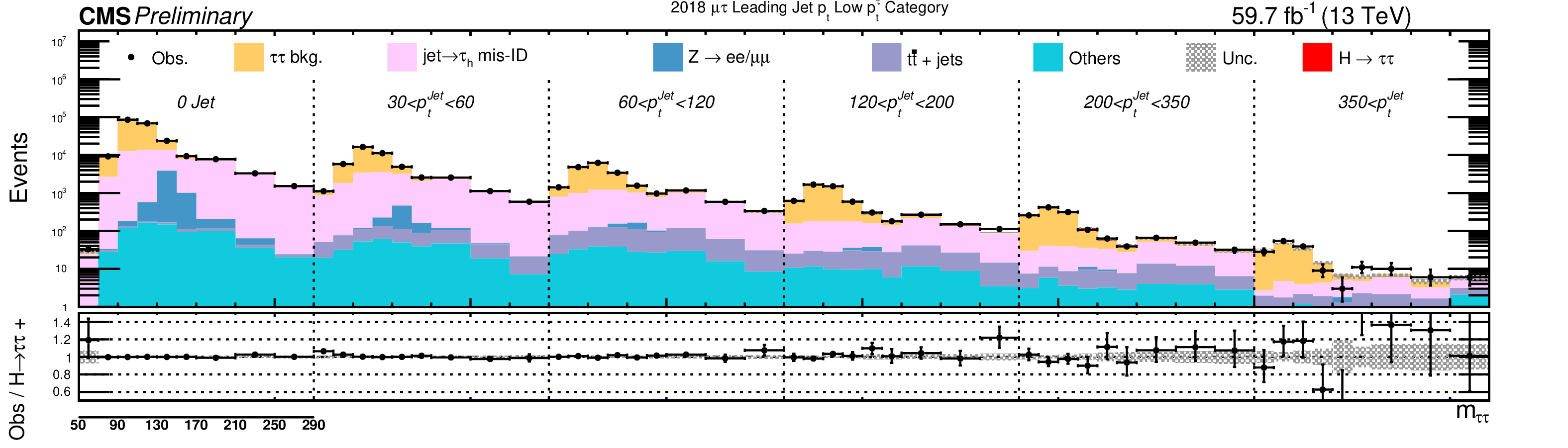
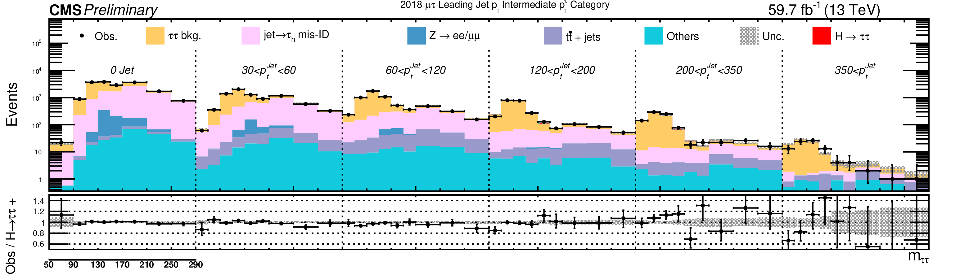
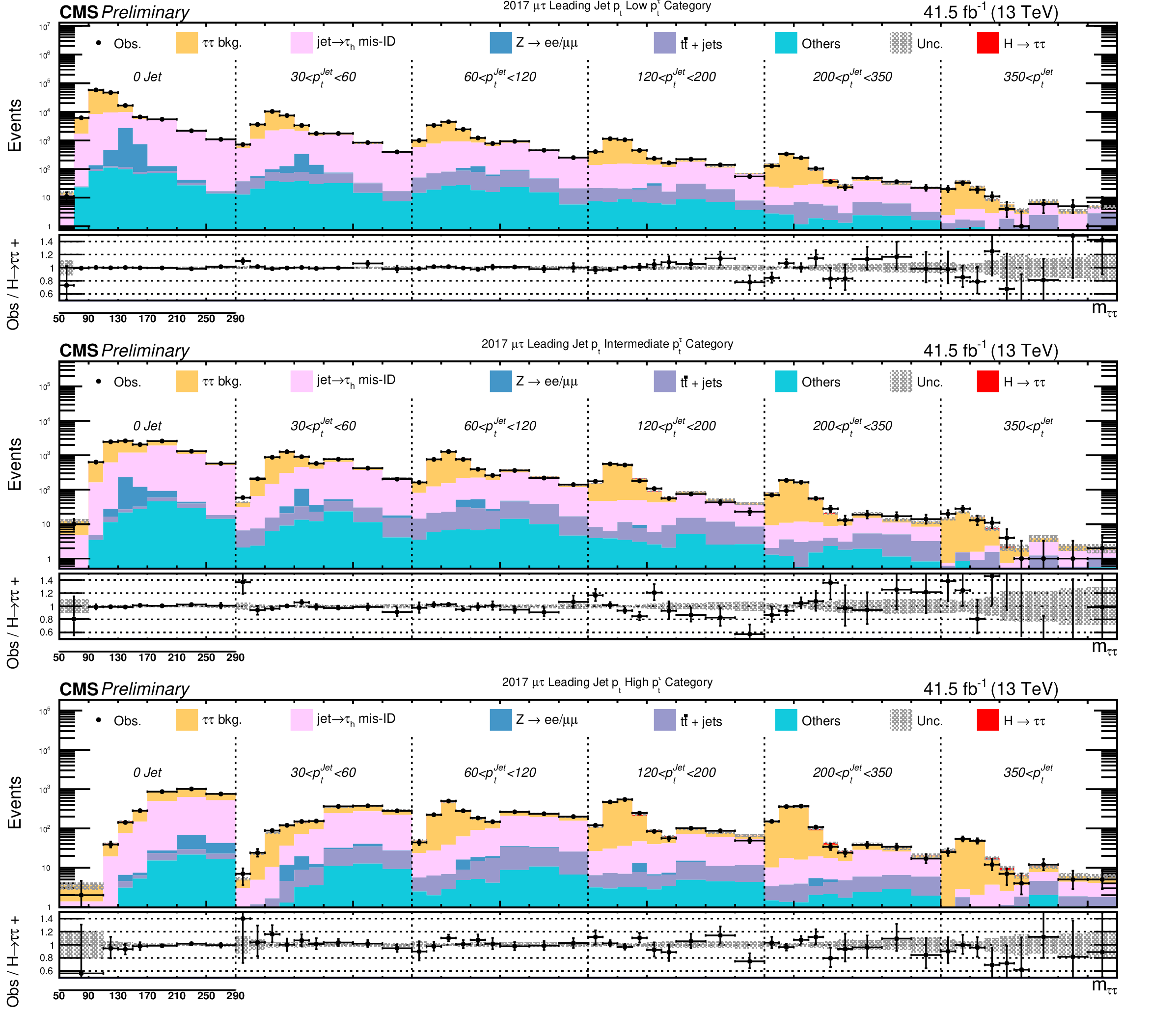
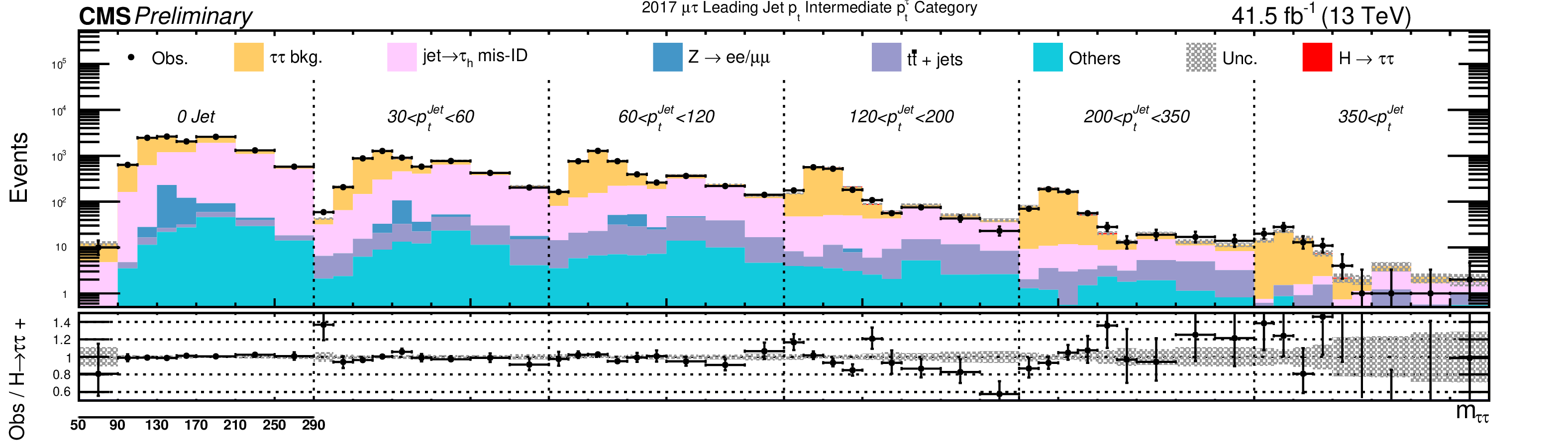
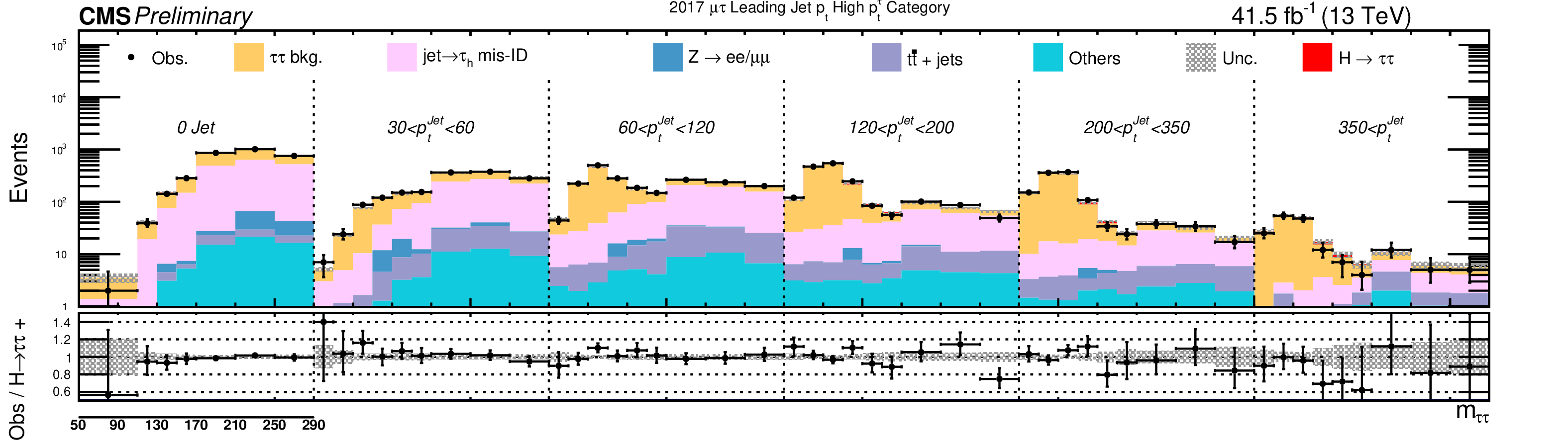
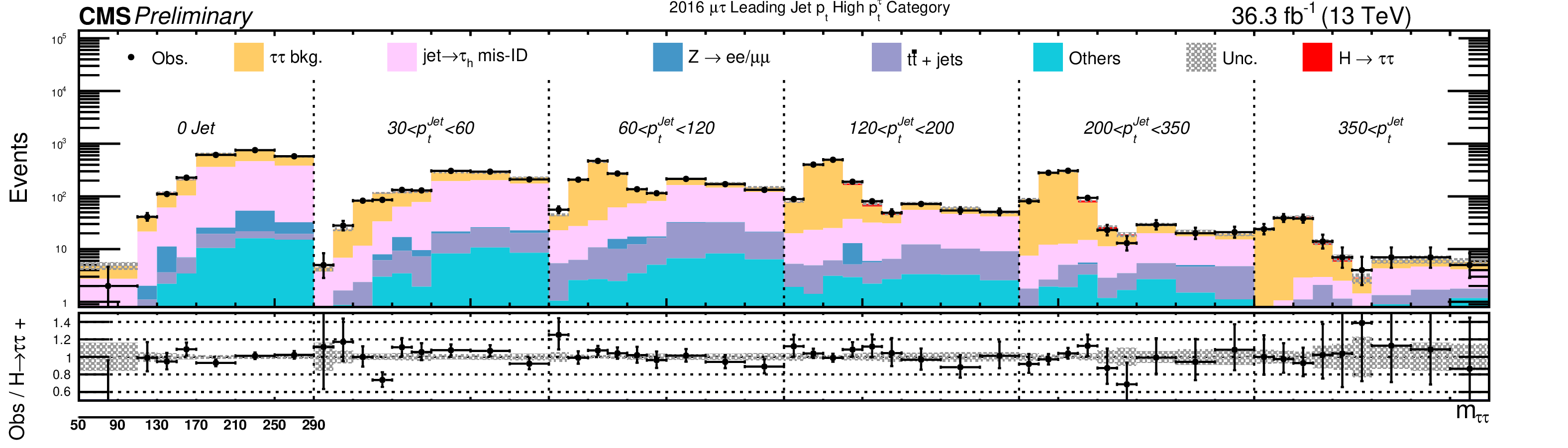
Additional Figure 6:
Postfit distributions in the $\mu {{\tau} _\mathrm {h}} $ final state in 2018. This represents a fit to data with all years and final states. |
png pdf |
Additional Figure 6-a:
Postfit distributions in the $\mu {{\tau} _\mathrm {h}} $ final state in 2018. This represents a fit to data with all years and final states. |
png pdf |
Additional Figure 6-b:
Postfit distributions in the $\mu {{\tau} _\mathrm {h}} $ final state in 2018. This represents a fit to data with all years and final states. |
png pdf |
Additional Figure 6-c:
Postfit distributions in the $\mu {{\tau} _\mathrm {h}} $ final state in 2018. This represents a fit to data with all years and final states. |
png pdf |
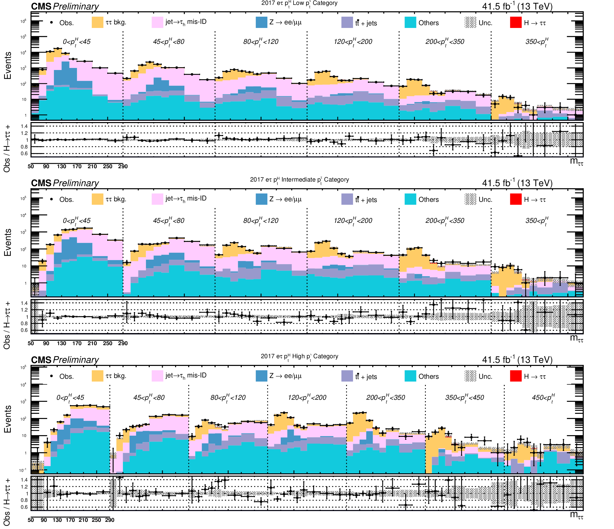
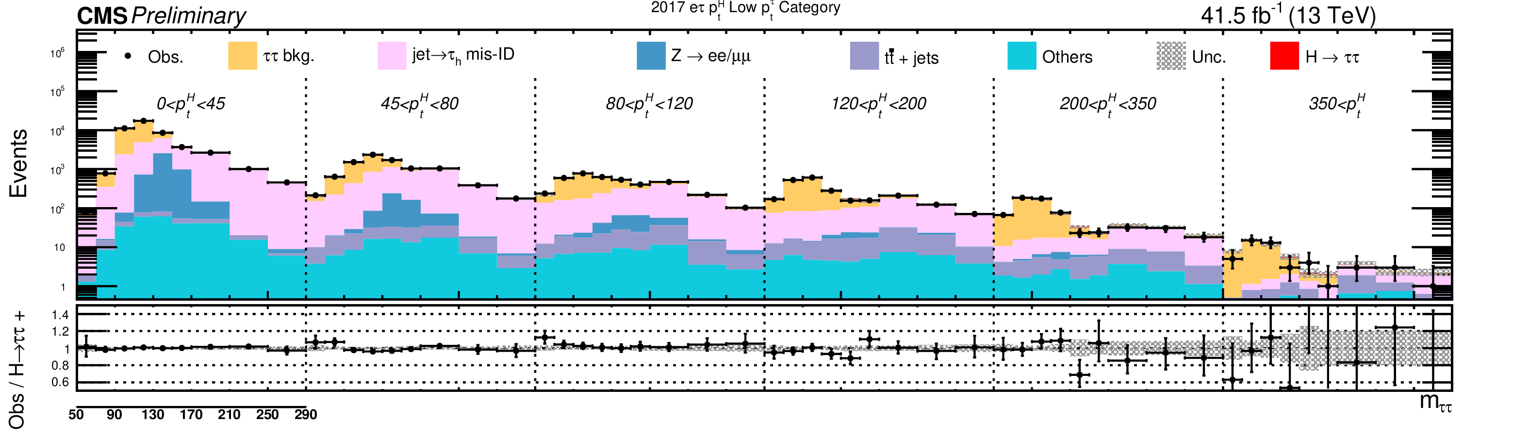
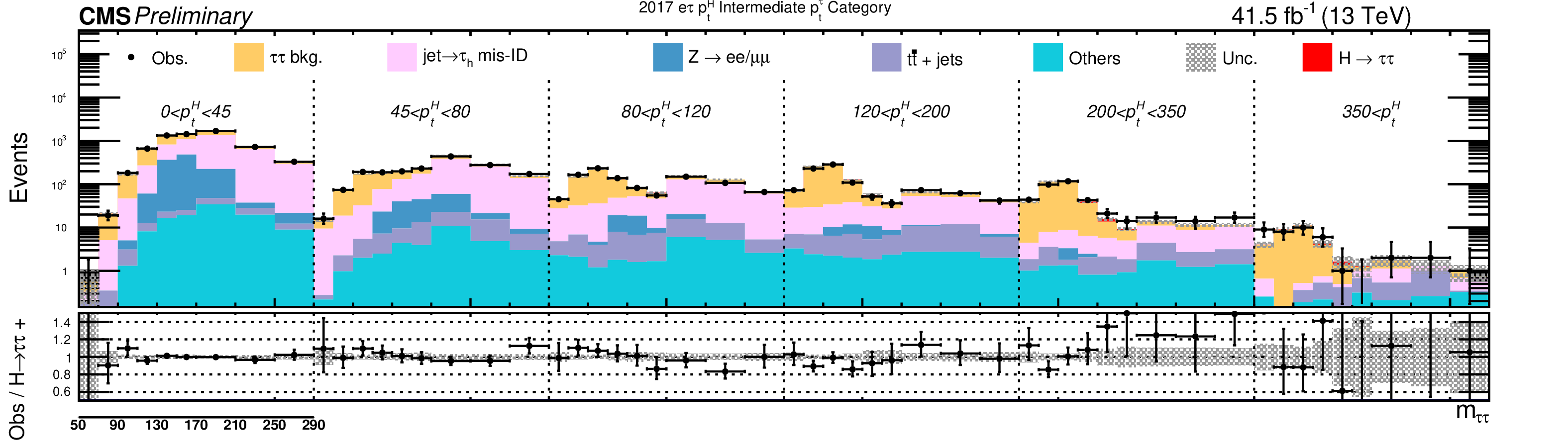
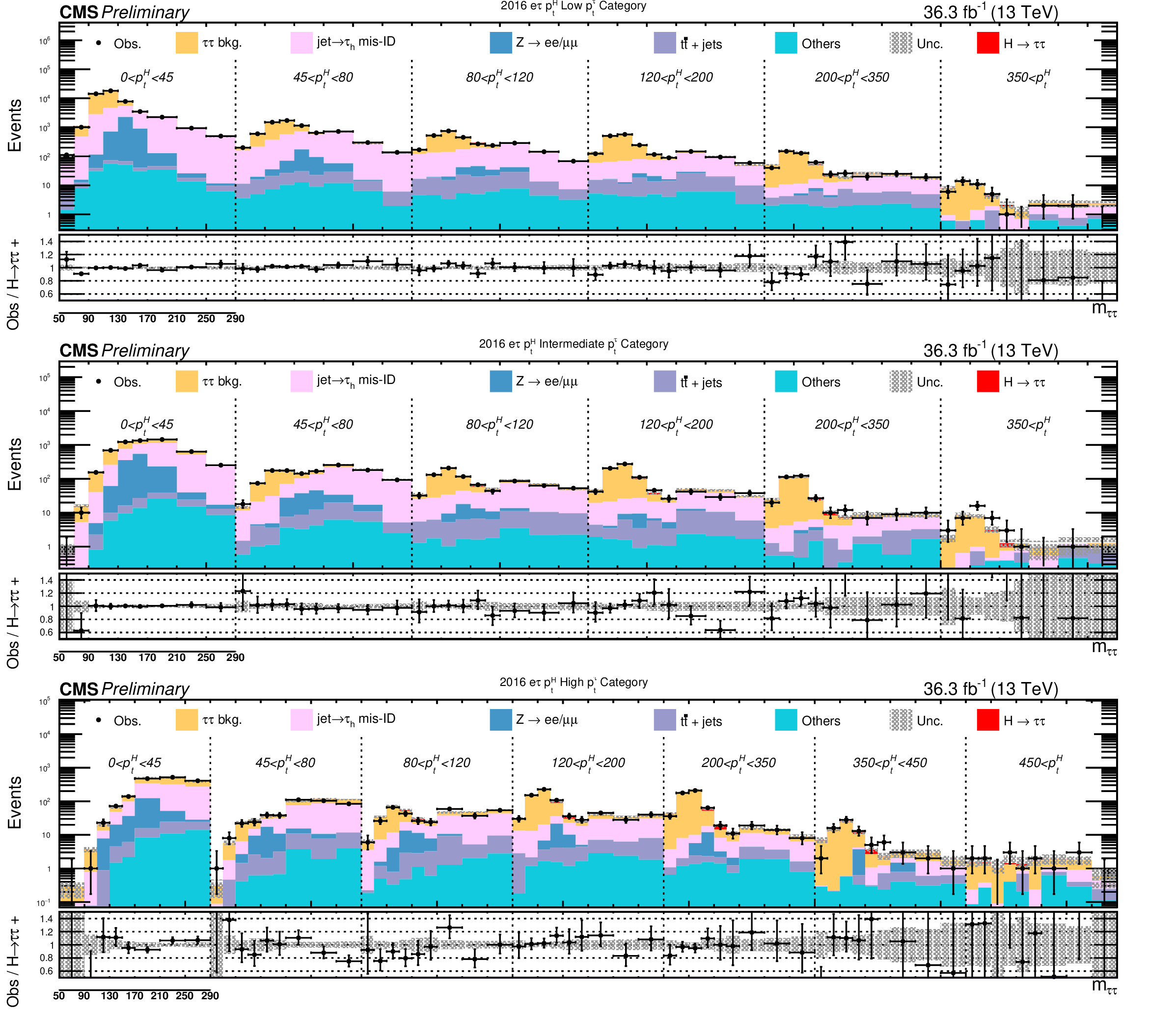
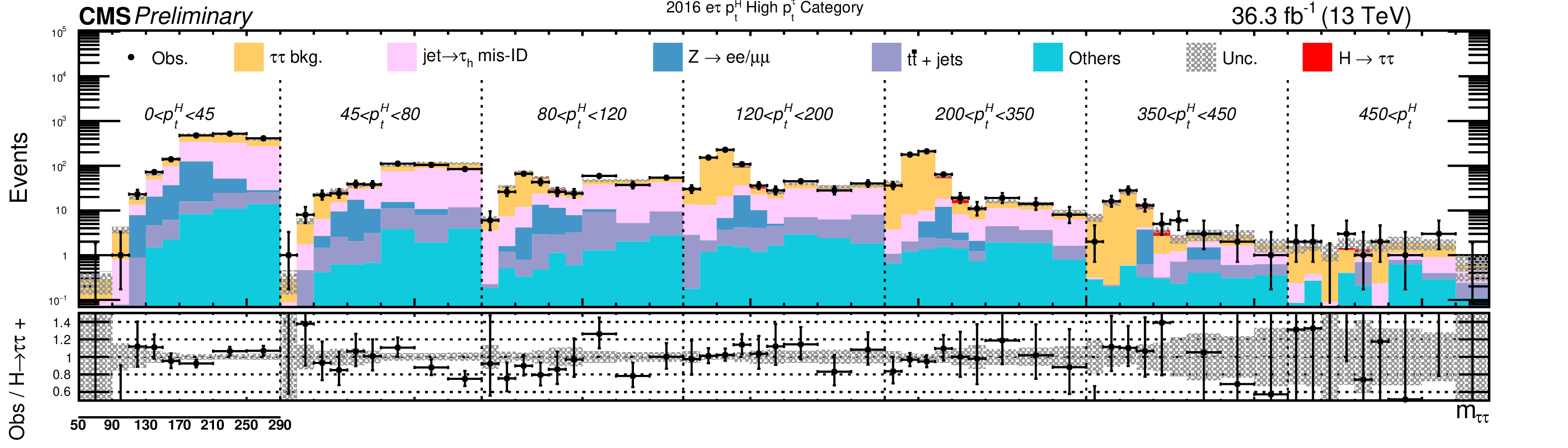
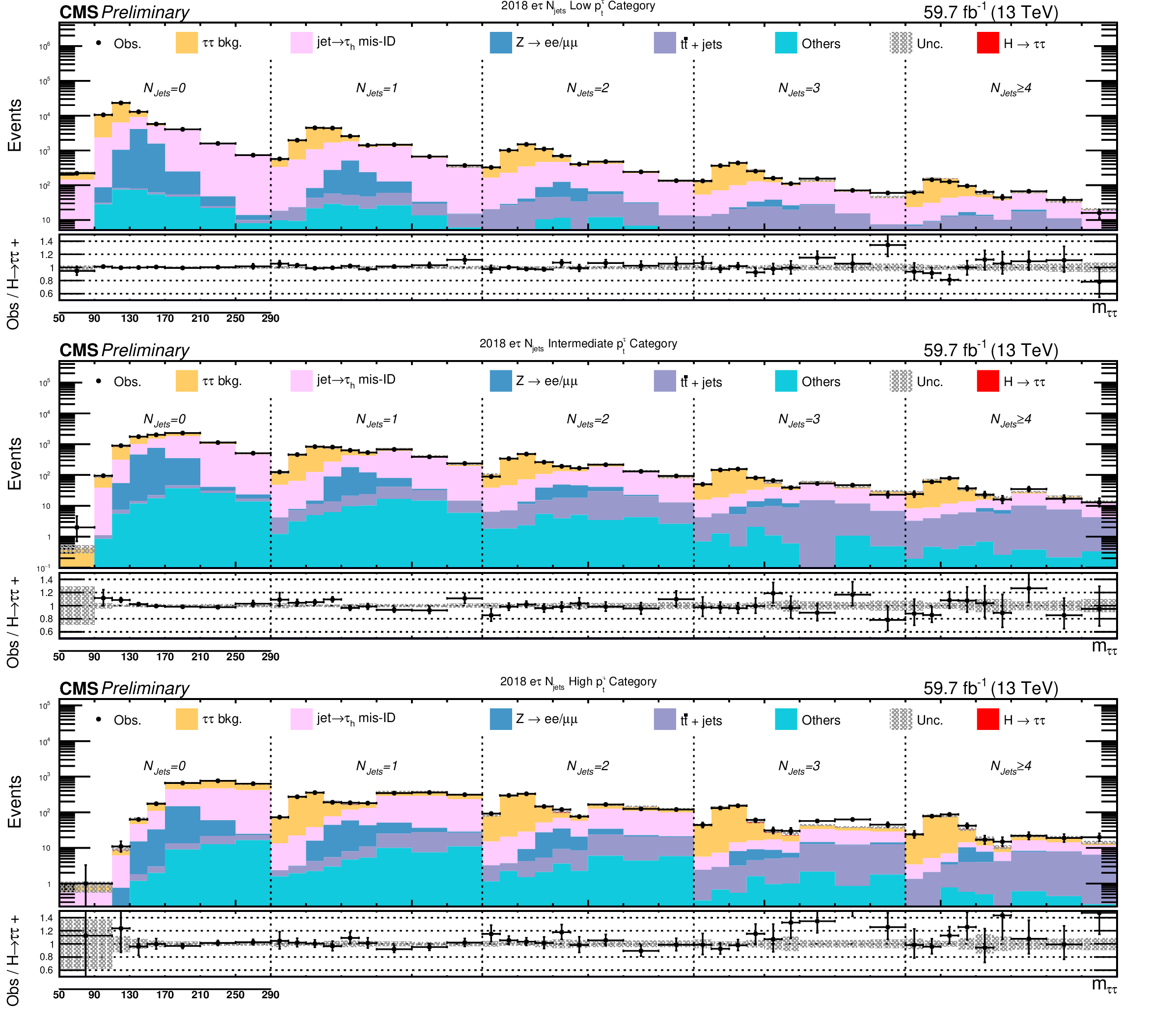
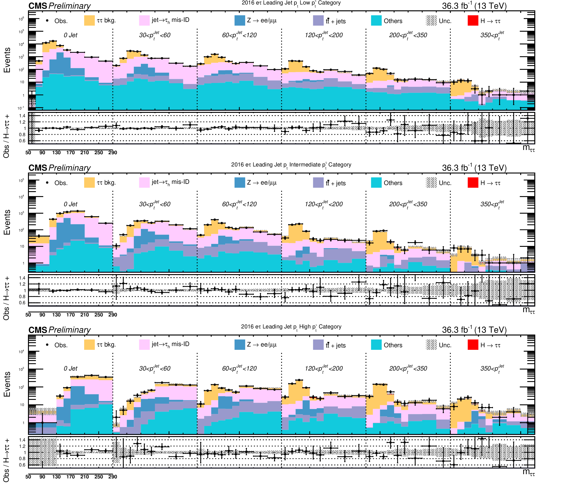
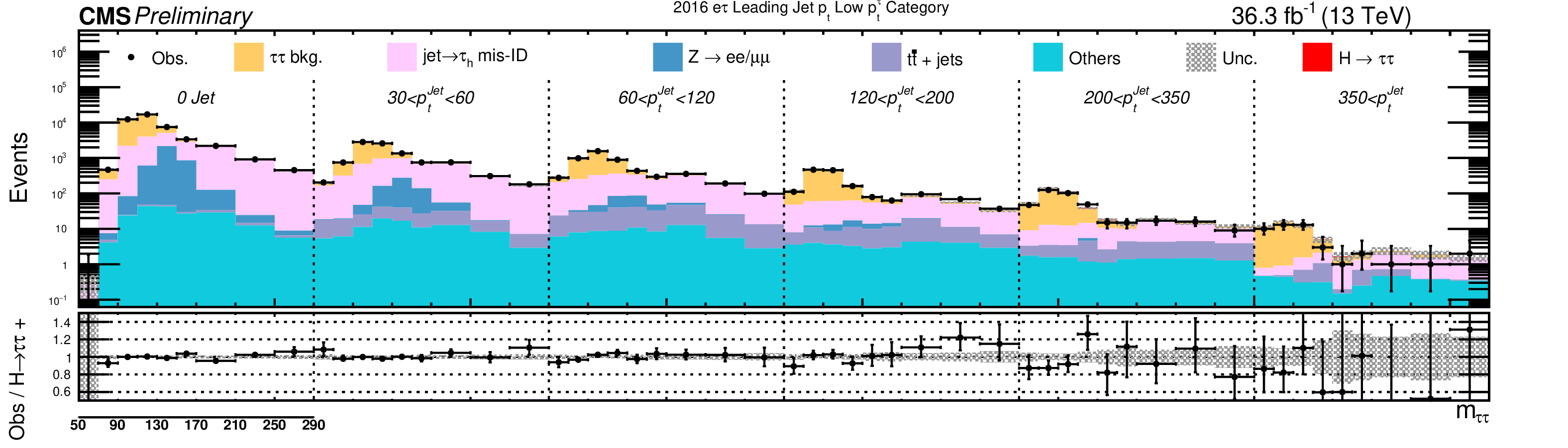
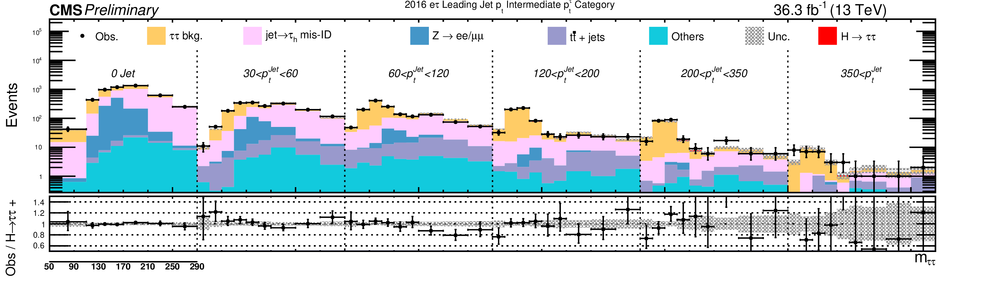
Additional Figure 7:
Postfit distributions in the $ {\mathrm {e}} {{\tau} _\mathrm {h}} $ final state in 2018. This represents a fit to data with all years and final states. |
png pdf |
Additional Figure 7-a:
Postfit distributions in the $ {\mathrm {e}} {{\tau} _\mathrm {h}} $ final state in 2018. This represents a fit to data with all years and final states. |

png pdf |
Additional Figure 7-b:
Postfit distributions in the $ {\mathrm {e}} {{\tau} _\mathrm {h}} $ final state in 2018. This represents a fit to data with all years and final states. |
png pdf |
Additional Figure 7-c:
Postfit distributions in the $ {\mathrm {e}} {{\tau} _\mathrm {h}} $ final state in 2018. This represents a fit to data with all years and final states. |
png pdf |
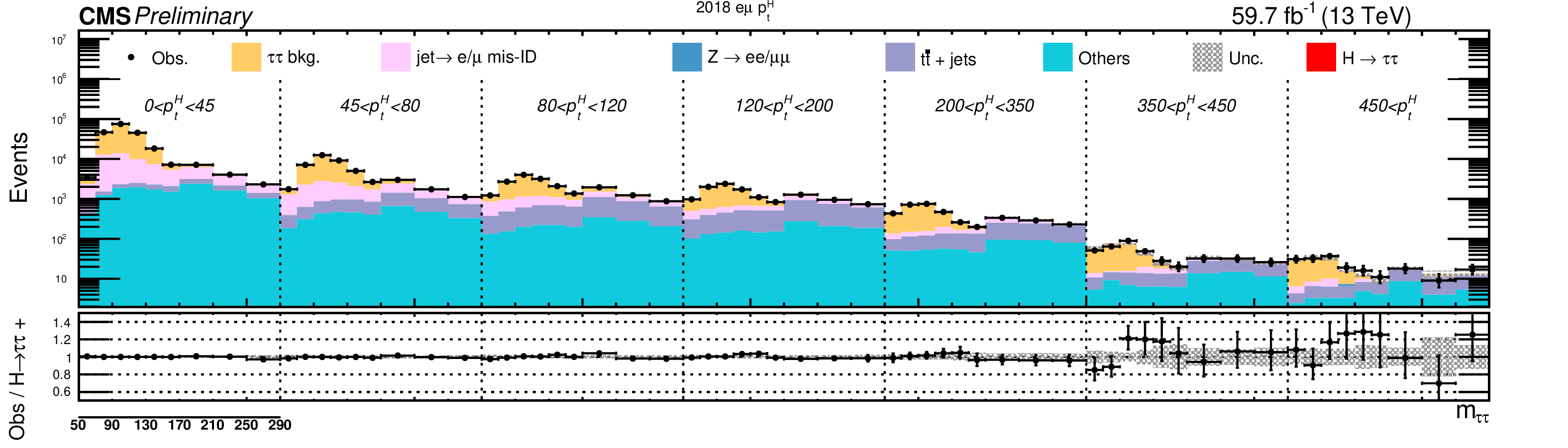
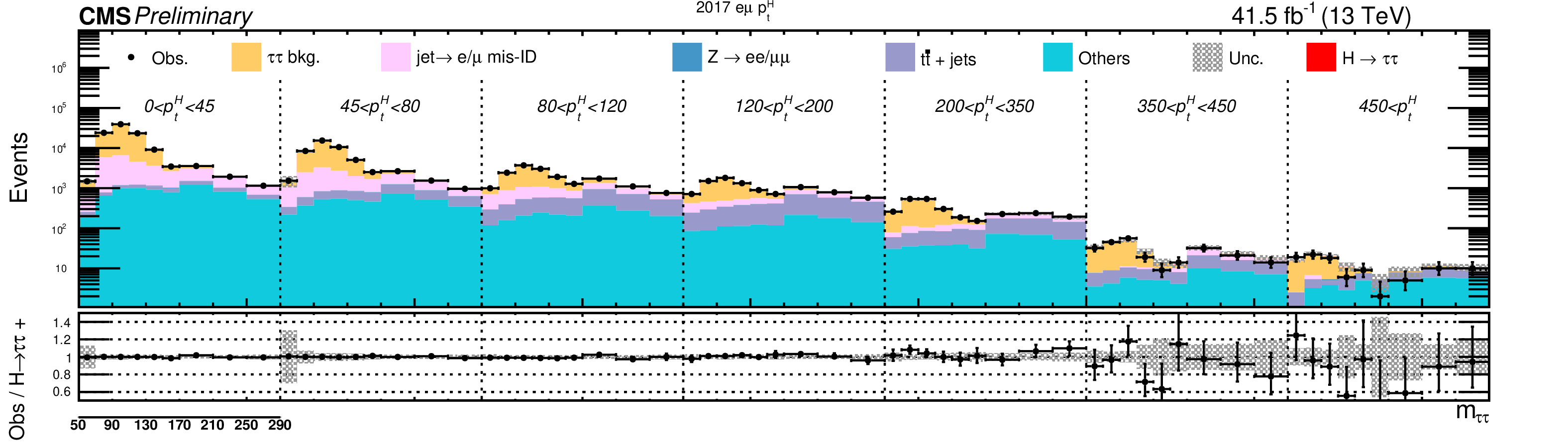
Additional Figure 8:
Postfit distributions in the $ {\mathrm {e}}\mu $ final state in 2018. This represents a fit to data with all years and final states. |
png pdf |
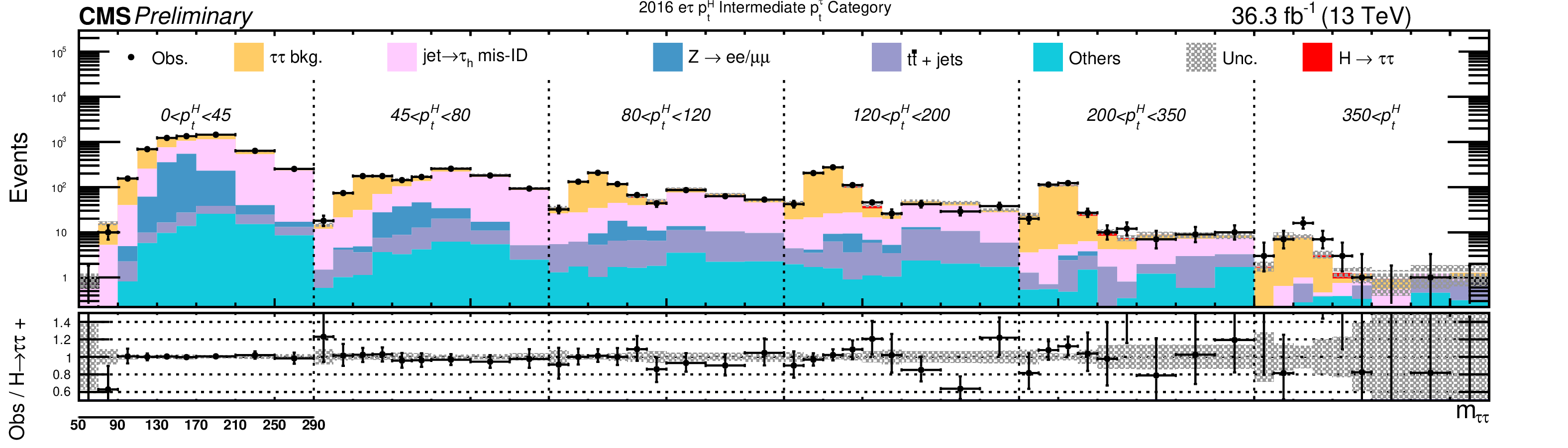
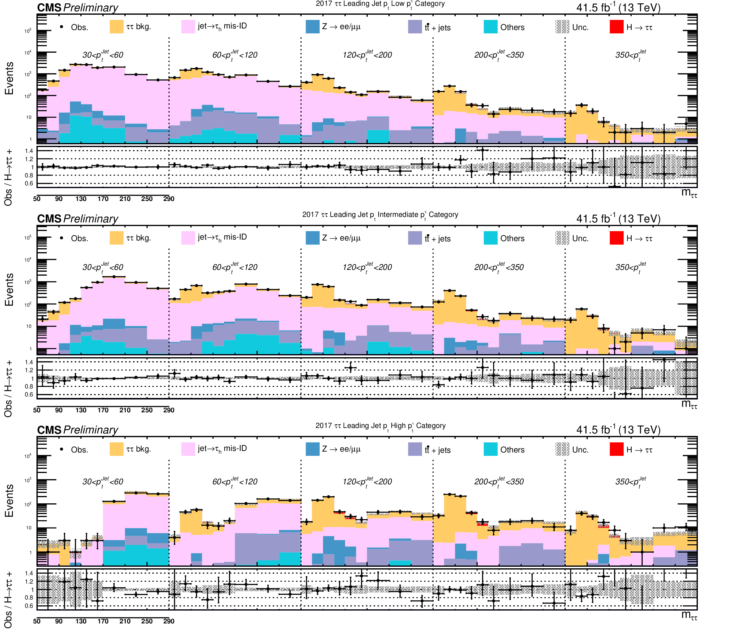
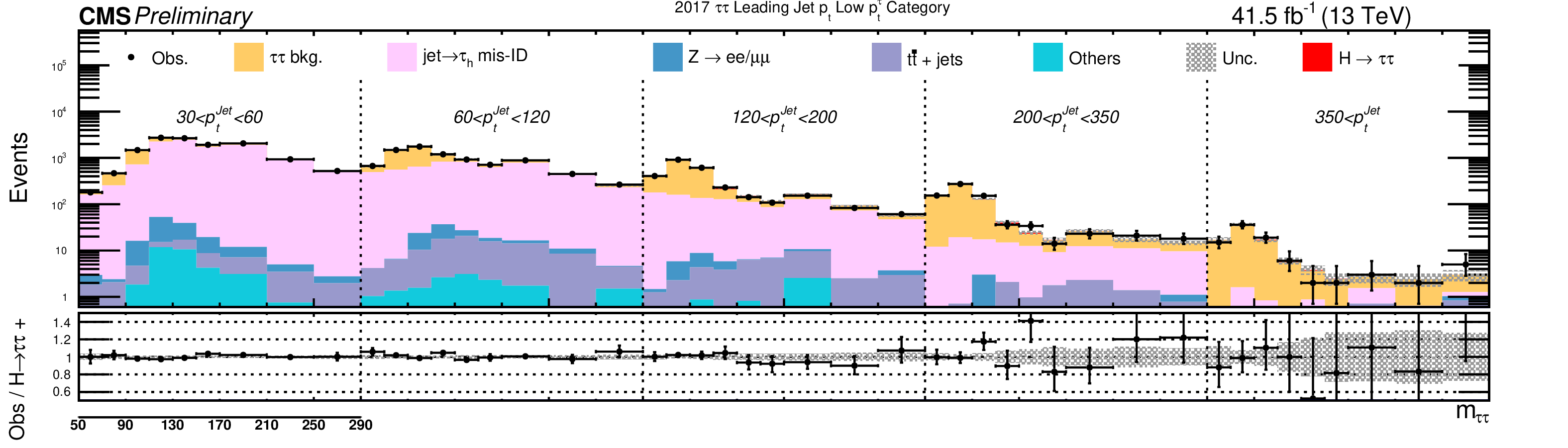
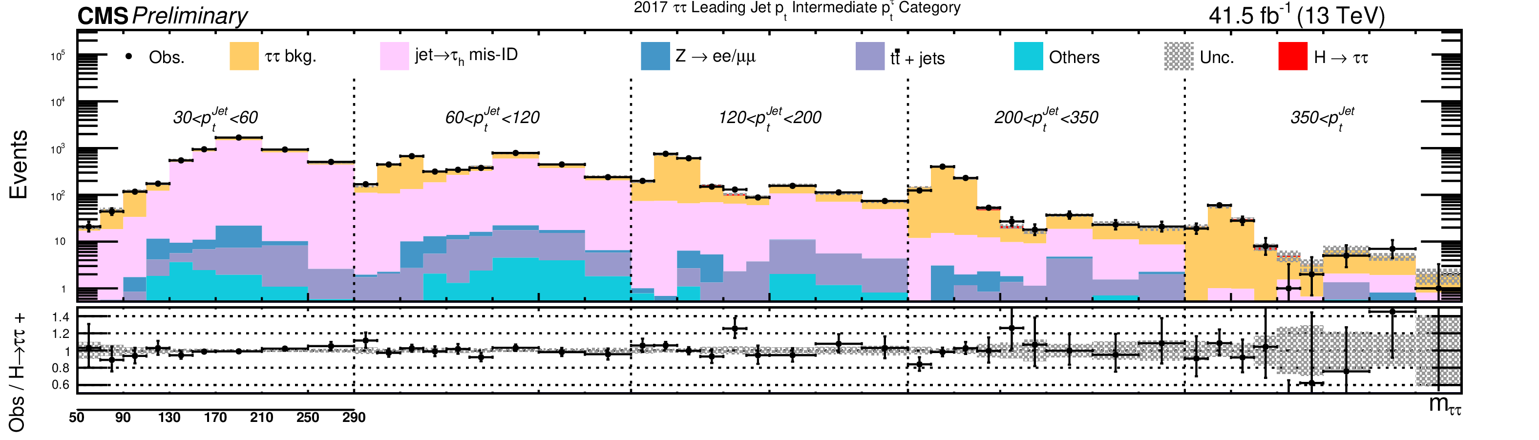
Additional Figure 9:
Postfit distributions in the $ {{\tau} _\mathrm {h}} {{\tau} _\mathrm {h}} $ final state in 2017. This represents a fit to data with all years and final states. |
png pdf |
Additional Figure 9-a:
Postfit distributions in the $ {{\tau} _\mathrm {h}} {{\tau} _\mathrm {h}} $ final state in 2017. This represents a fit to data with all years and final states. |
png pdf |
Additional Figure 9-b:
Postfit distributions in the $ {{\tau} _\mathrm {h}} {{\tau} _\mathrm {h}} $ final state in 2017. This represents a fit to data with all years and final states. |
png pdf |
Additional Figure 9-c:
Postfit distributions in the $ {{\tau} _\mathrm {h}} {{\tau} _\mathrm {h}} $ final state in 2017. This represents a fit to data with all years and final states. |

png pdf |
Additional Figure 10:
Postfit distributions in the $\mu {{\tau} _\mathrm {h}} $ final state in 2017. This represents a fit to data with all years and final states. |
png pdf |
Additional Figure 10-a:
Postfit distributions in the $\mu {{\tau} _\mathrm {h}} $ final state in 2017. This represents a fit to data with all years and final states. |
png pdf |
Additional Figure 10-b:
Postfit distributions in the $\mu {{\tau} _\mathrm {h}} $ final state in 2017. This represents a fit to data with all years and final states. |
png pdf |
Additional Figure 10-c:
Postfit distributions in the $\mu {{\tau} _\mathrm {h}} $ final state in 2017. This represents a fit to data with all years and final states. |
png pdf |
Additional Figure 11:
Postfit distributions in the $ {\mathrm {e}} {{\tau} _\mathrm {h}} $ final state in 2017. This represents a fit to data with all years and final states. |
png pdf |
Additional Figure 11-a:
Postfit distributions in the $ {\mathrm {e}} {{\tau} _\mathrm {h}} $ final state in 2017. This represents a fit to data with all years and final states. |
png pdf |
Additional Figure 11-b:
Postfit distributions in the $ {\mathrm {e}} {{\tau} _\mathrm {h}} $ final state in 2017. This represents a fit to data with all years and final states. |

png pdf |
Additional Figure 11-c:
Postfit distributions in the $ {\mathrm {e}} {{\tau} _\mathrm {h}} $ final state in 2017. This represents a fit to data with all years and final states. |
png pdf |
Additional Figure 12:
Postfit distributions in the $ {\mathrm {e}}\mu $ final state in 2017. This represents a fit to data with all years and final states. |

png pdf |
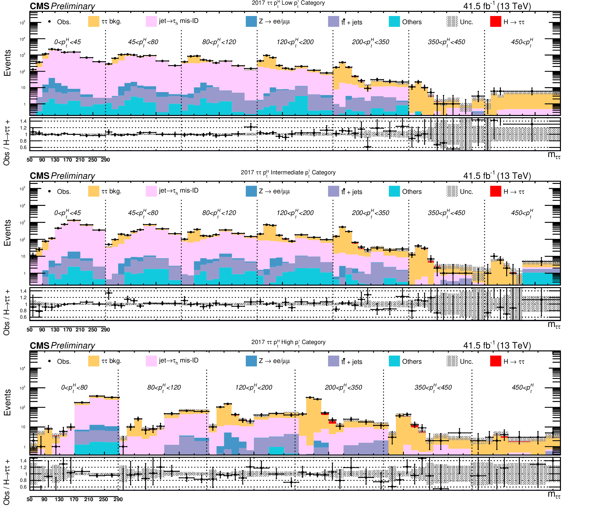
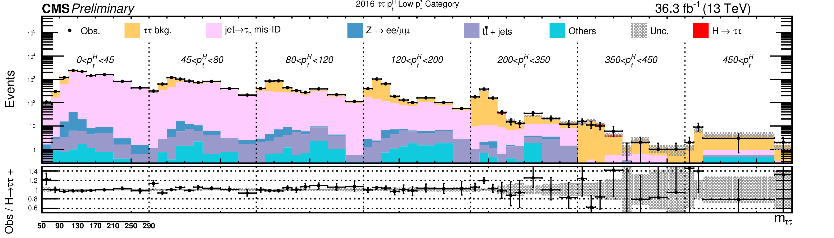
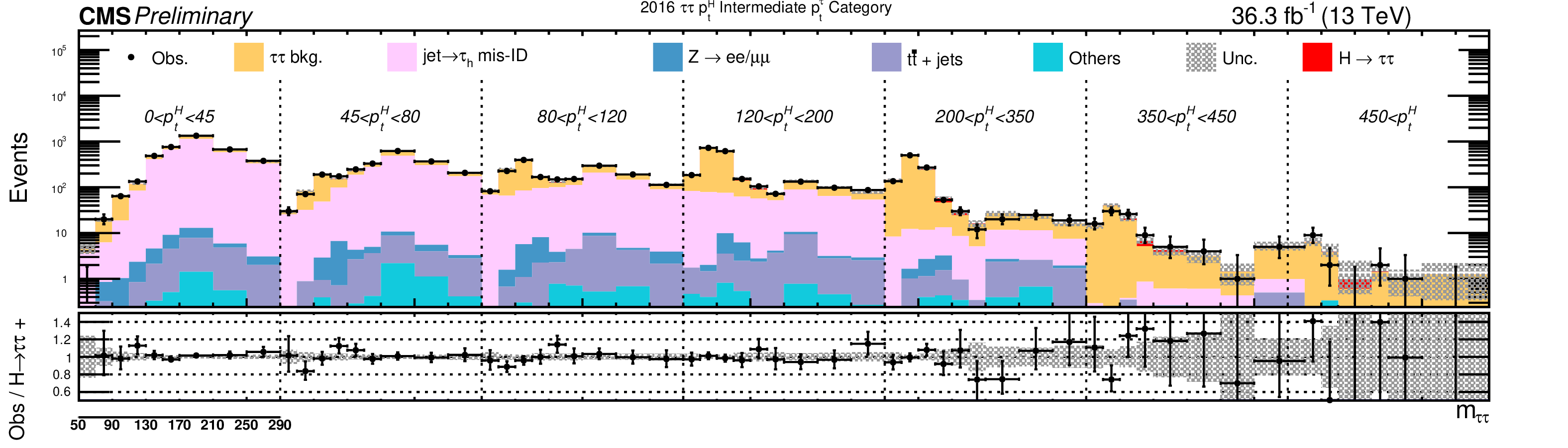
Additional Figure 13:
Postfit distributions in the $ {{\tau} _\mathrm {h}} {{\tau} _\mathrm {h}} $ final state in 2016. This represents a fit to data with all years and final states. |
png pdf |
Additional Figure 13-a:
Postfit distributions in the $ {{\tau} _\mathrm {h}} {{\tau} _\mathrm {h}} $ final state in 2016. This represents a fit to data with all years and final states. |
png pdf |
Additional Figure 13-b:
Postfit distributions in the $ {{\tau} _\mathrm {h}} {{\tau} _\mathrm {h}} $ final state in 2016. This represents a fit to data with all years and final states. |
png pdf |
Additional Figure 13-c:
Postfit distributions in the $ {{\tau} _\mathrm {h}} {{\tau} _\mathrm {h}} $ final state in 2016. This represents a fit to data with all years and final states. |
png pdf |
Additional Figure 14:
Postfit distributions in the $\mu {{\tau} _\mathrm {h}} $ final state in 2016. This represents a fit to data with all years and final states. |
png pdf |
Additional Figure 14-a:
Postfit distributions in the $\mu {{\tau} _\mathrm {h}} $ final state in 2016. This represents a fit to data with all years and final states. |
png pdf |
Additional Figure 14-b:
Postfit distributions in the $\mu {{\tau} _\mathrm {h}} $ final state in 2016. This represents a fit to data with all years and final states. |
png pdf |
Additional Figure 14-c:
Postfit distributions in the $\mu {{\tau} _\mathrm {h}} $ final state in 2016. This represents a fit to data with all years and final states. |
png pdf |
Additional Figure 15:
Postfit distributions in the $ {\mathrm {e}} {{\tau} _\mathrm {h}} $ final state in 2016. This represents a fit to data with all years and final states. |

png pdf |
Additional Figure 15-a:
Postfit distributions in the $ {\mathrm {e}} {{\tau} _\mathrm {h}} $ final state in 2016. This represents a fit to data with all years and final states. |
png pdf |
Additional Figure 15-b:
Postfit distributions in the $ {\mathrm {e}} {{\tau} _\mathrm {h}} $ final state in 2016. This represents a fit to data with all years and final states. |
png pdf |
Additional Figure 15-c:
Postfit distributions in the $ {\mathrm {e}} {{\tau} _\mathrm {h}} $ final state in 2016. This represents a fit to data with all years and final states. |
png pdf |
Additional Figure 16:
Postfit distributions in the $ {\mathrm {e}}\mu $ final state in 2016. This represents a fit to data with all years and final states. |
png pdf |
Additional Figure 17:
Postfit distributions in the $ {{\tau} _\mathrm {h}} {{\tau} _\mathrm {h}} $ final state in 2018. This represents a fit to data with all years and final states. |
png pdf |
Additional Figure 17-a:
Postfit distributions in the $ {{\tau} _\mathrm {h}} {{\tau} _\mathrm {h}} $ final state in 2018. This represents a fit to data with all years and final states. |

png pdf |
Additional Figure 17-b:
Postfit distributions in the $ {{\tau} _\mathrm {h}} {{\tau} _\mathrm {h}} $ final state in 2018. This represents a fit to data with all years and final states. |
png pdf |
Additional Figure 17-c:
Postfit distributions in the $ {{\tau} _\mathrm {h}} {{\tau} _\mathrm {h}} $ final state in 2018. This represents a fit to data with all years and final states. |
png pdf |
Additional Figure 18:
Postfit distributions in the $\mu {{\tau} _\mathrm {h}} $ final state in 2018. This represents a fit to data with all years and final states. |
png pdf |
Additional Figure 18-a:
Postfit distributions in the $\mu {{\tau} _\mathrm {h}} $ final state in 2018. This represents a fit to data with all years and final states. |
png pdf |
Additional Figure 18-b:
Postfit distributions in the $\mu {{\tau} _\mathrm {h}} $ final state in 2018. This represents a fit to data with all years and final states. |

png pdf |
Additional Figure 18-c:
Postfit distributions in the $\mu {{\tau} _\mathrm {h}} $ final state in 2018. This represents a fit to data with all years and final states. |
png pdf |
Additional Figure 19:
Postfit distributions in the $ {\mathrm {e}} {{\tau} _\mathrm {h}} $ final state in 2018. This represents a fit to data with all years and final states. |
png pdf |
Additional Figure 19-a:
Postfit distributions in the $ {\mathrm {e}} {{\tau} _\mathrm {h}} $ final state in 2018. This represents a fit to data with all years and final states. |
png pdf |
Additional Figure 19-b:
Postfit distributions in the $ {\mathrm {e}} {{\tau} _\mathrm {h}} $ final state in 2018. This represents a fit to data with all years and final states. |
png pdf |
Additional Figure 19-c:
Postfit distributions in the $ {\mathrm {e}} {{\tau} _\mathrm {h}} $ final state in 2018. This represents a fit to data with all years and final states. |
png pdf |
Additional Figure 20:
Postfit distributions in the $ {\mathrm {e}}\mu $ final state in 2018. This represents a fit to data with all years and final states. |
png pdf |
Additional Figure 21:
Postfit distributions in the $ {{\tau} _\mathrm {h}} {{\tau} _\mathrm {h}} $ final state in 2017. This represents a fit to data with all years and final states. |
png pdf |
Additional Figure 21-a:
Postfit distributions in the $ {{\tau} _\mathrm {h}} {{\tau} _\mathrm {h}} $ final state in 2017. This represents a fit to data with all years and final states. |
png pdf |
Additional Figure 21-b:
Postfit distributions in the $ {{\tau} _\mathrm {h}} {{\tau} _\mathrm {h}} $ final state in 2017. This represents a fit to data with all years and final states. |
png pdf |
Additional Figure 21-c:
Postfit distributions in the $ {{\tau} _\mathrm {h}} {{\tau} _\mathrm {h}} $ final state in 2017. This represents a fit to data with all years and final states. |
png pdf |
Additional Figure 22:
Postfit distributions in the $\mu {{\tau} _\mathrm {h}} $ final state in 2017. This represents a fit to data with all years and final states. |
png pdf |
Additional Figure 22-a:
Postfit distributions in the $\mu {{\tau} _\mathrm {h}} $ final state in 2017. This represents a fit to data with all years and final states. |
png pdf |
Additional Figure 22-b:
Postfit distributions in the $\mu {{\tau} _\mathrm {h}} $ final state in 2017. This represents a fit to data with all years and final states. |
png pdf |
Additional Figure 22-c:
Postfit distributions in the $\mu {{\tau} _\mathrm {h}} $ final state in 2017. This represents a fit to data with all years and final states. |
png pdf |
Additional Figure 23:
Postfit distributions in the $ {\mathrm {e}} {{\tau} _\mathrm {h}} $ final state in 2017. This represents a fit to data with all years and final states. |
png pdf |
Additional Figure 23-a:
Postfit distributions in the $ {\mathrm {e}} {{\tau} _\mathrm {h}} $ final state in 2017. This represents a fit to data with all years and final states. |
png pdf |
Additional Figure 23-b:
Postfit distributions in the $ {\mathrm {e}} {{\tau} _\mathrm {h}} $ final state in 2017. This represents a fit to data with all years and final states. |
png pdf |
Additional Figure 23-c:
Postfit distributions in the $ {\mathrm {e}} {{\tau} _\mathrm {h}} $ final state in 2017. This represents a fit to data with all years and final states. |
png pdf |
Additional Figure 24:
Postfit distributions in the $ {\mathrm {e}}\mu $ final state in 2017. This represents a fit to data with all years and final states. |
png pdf |
Additional Figure 25:
Postfit distributions in the $ {{\tau} _\mathrm {h}} {{\tau} _\mathrm {h}} $ final state in 2016. This represents a fit to data with all years and final states. |
png pdf |
Additional Figure 25-a:
Postfit distributions in the $ {{\tau} _\mathrm {h}} {{\tau} _\mathrm {h}} $ final state in 2016. This represents a fit to data with all years and final states. |

png pdf |
Additional Figure 25-b:
Postfit distributions in the $ {{\tau} _\mathrm {h}} {{\tau} _\mathrm {h}} $ final state in 2016. This represents a fit to data with all years and final states. |
png pdf |
Additional Figure 25-c:
Postfit distributions in the $ {{\tau} _\mathrm {h}} {{\tau} _\mathrm {h}} $ final state in 2016. This represents a fit to data with all years and final states. |
png pdf |
Additional Figure 26:
Postfit distributions in the $\mu {{\tau} _\mathrm {h}} $ final state in 2016. This represents a fit to data with all years and final states. |
png pdf |
Additional Figure 26-a:
Postfit distributions in the $\mu {{\tau} _\mathrm {h}} $ final state in 2016. This represents a fit to data with all years and final states. |
png pdf |
Additional Figure 26-b:
Postfit distributions in the $\mu {{\tau} _\mathrm {h}} $ final state in 2016. This represents a fit to data with all years and final states. |
png pdf |
Additional Figure 26-c:
Postfit distributions in the $\mu {{\tau} _\mathrm {h}} $ final state in 2016. This represents a fit to data with all years and final states. |
png pdf |
Additional Figure 27:
Postfit distributions in the $ {\mathrm {e}} {{\tau} _\mathrm {h}} $ final state in 2016. This represents a fit to data with all years and final states. |
png pdf |
Additional Figure 27-a:
Postfit distributions in the $ {\mathrm {e}} {{\tau} _\mathrm {h}} $ final state in 2016. This represents a fit to data with all years and final states. |
png pdf |
Additional Figure 27-b:
Postfit distributions in the $ {\mathrm {e}} {{\tau} _\mathrm {h}} $ final state in 2016. This represents a fit to data with all years and final states. |
png pdf |
Additional Figure 27-c:
Postfit distributions in the $ {\mathrm {e}} {{\tau} _\mathrm {h}} $ final state in 2016. This represents a fit to data with all years and final states. |
png pdf |
Additional Figure 28:
Postfit distributions in the $ {\mathrm {e}}\mu $ final state in 2016. This represents a fit to data with all years and final states. |
png pdf |
Additional Figure 29:
Postfit distributions in the $ {{\tau} _\mathrm {h}} {{\tau} _\mathrm {h}} $ final state in 2018. This represents a fit to data with all years and final states. |
png pdf |
Additional Figure 29-a:
Postfit distributions in the $ {{\tau} _\mathrm {h}} {{\tau} _\mathrm {h}} $ final state in 2018. This represents a fit to data with all years and final states. |
png pdf |
Additional Figure 29-b:
Postfit distributions in the $ {{\tau} _\mathrm {h}} {{\tau} _\mathrm {h}} $ final state in 2018. This represents a fit to data with all years and final states. |
png pdf |
Additional Figure 29-c:
Postfit distributions in the $ {{\tau} _\mathrm {h}} {{\tau} _\mathrm {h}} $ final state in 2018. This represents a fit to data with all years and final states. |
png pdf |
Additional Figure 30:
Postfit distributions in the $\mu {{\tau} _\mathrm {h}} $ final state in 2018. This represents a fit to data with all years and final states. |
png pdf |
Additional Figure 30-a:
Postfit distributions in the $\mu {{\tau} _\mathrm {h}} $ final state in 2018. This represents a fit to data with all years and final states. |
png pdf |
Additional Figure 30-b:
Postfit distributions in the $\mu {{\tau} _\mathrm {h}} $ final state in 2018. This represents a fit to data with all years and final states. |
png pdf |
Additional Figure 30-c:
Postfit distributions in the $\mu {{\tau} _\mathrm {h}} $ final state in 2018. This represents a fit to data with all years and final states. |
png pdf |
Additional Figure 31:
Postfit distributions in the $ {\mathrm {e}} {{\tau} _\mathrm {h}} $ final state in 2018. This represents a fit to data with all years and final states. |
png pdf |
Additional Figure 31-a:
Postfit distributions in the $ {\mathrm {e}} {{\tau} _\mathrm {h}} $ final state in 2018. This represents a fit to data with all years and final states. |
png pdf |
Additional Figure 31-b:
Postfit distributions in the $ {\mathrm {e}} {{\tau} _\mathrm {h}} $ final state in 2018. This represents a fit to data with all years and final states. |
png pdf |
Additional Figure 31-c:
Postfit distributions in the $ {\mathrm {e}} {{\tau} _\mathrm {h}} $ final state in 2018. This represents a fit to data with all years and final states. |

png pdf |
Additional Figure 32:
Postfit distributions in the $ {\mathrm {e}}\mu $ final state in 2018. This represents a fit to data with all years and final states. |
png pdf |
Additional Figure 33:
Postfit distributions in the $ {{\tau} _\mathrm {h}} {{\tau} _\mathrm {h}} $ final state in 2017. This represents a fit to data with all years and final states. |
png pdf |
Additional Figure 33-a:
Postfit distributions in the $ {{\tau} _\mathrm {h}} {{\tau} _\mathrm {h}} $ final state in 2017. This represents a fit to data with all years and final states. |
png pdf |
Additional Figure 33-b:
Postfit distributions in the $ {{\tau} _\mathrm {h}} {{\tau} _\mathrm {h}} $ final state in 2017. This represents a fit to data with all years and final states. |
png pdf |
Additional Figure 33-c:
Postfit distributions in the $ {{\tau} _\mathrm {h}} {{\tau} _\mathrm {h}} $ final state in 2017. This represents a fit to data with all years and final states. |
png pdf |
Additional Figure 34:
Postfit distributions in the $\mu {{\tau} _\mathrm {h}} $ final state in 2017. This represents a fit to data with all years and final states. |

png pdf |
Additional Figure 34-a:
Postfit distributions in the $\mu {{\tau} _\mathrm {h}} $ final state in 2017. This represents a fit to data with all years and final states. |
png pdf |
Additional Figure 34-b:
Postfit distributions in the $\mu {{\tau} _\mathrm {h}} $ final state in 2017. This represents a fit to data with all years and final states. |
png pdf |
Additional Figure 34-c:
Postfit distributions in the $\mu {{\tau} _\mathrm {h}} $ final state in 2017. This represents a fit to data with all years and final states. |
png pdf |
Additional Figure 35:
Postfit distributions in the $ {\mathrm {e}} {{\tau} _\mathrm {h}} $ final state in 2017. This represents a fit to data with all years and final states. |
png pdf |
Additional Figure 35-a:
Postfit distributions in the $ {\mathrm {e}} {{\tau} _\mathrm {h}} $ final state in 2017. This represents a fit to data with all years and final states. |
png pdf |
Additional Figure 35-b:
Postfit distributions in the $ {\mathrm {e}} {{\tau} _\mathrm {h}} $ final state in 2017. This represents a fit to data with all years and final states. |
png pdf |
Additional Figure 35-c:
Postfit distributions in the $ {\mathrm {e}} {{\tau} _\mathrm {h}} $ final state in 2017. This represents a fit to data with all years and final states. |
png pdf |
Additional Figure 36:
Postfit distributions in the $ {\mathrm {e}}\mu $ final state in 2017. This represents a fit to data with all years and final states. |
png pdf |
Additional Figure 37:
Postfit distributions in the $ {{\tau} _\mathrm {h}} {{\tau} _\mathrm {h}} $ final state in 2016. This represents a fit to data with all years and final states. |
png pdf |
Additional Figure 37-a:
Postfit distributions in the $ {{\tau} _\mathrm {h}} {{\tau} _\mathrm {h}} $ final state in 2016. This represents a fit to data with all years and final states. |
png pdf |
Additional Figure 37-b:
Postfit distributions in the $ {{\tau} _\mathrm {h}} {{\tau} _\mathrm {h}} $ final state in 2016. This represents a fit to data with all years and final states. |
png pdf |
Additional Figure 37-c:
Postfit distributions in the $ {{\tau} _\mathrm {h}} {{\tau} _\mathrm {h}} $ final state in 2016. This represents a fit to data with all years and final states. |
png pdf |
Additional Figure 38:
Postfit distributions in the $\mu {{\tau} _\mathrm {h}} $ final state in 2016. This represents a fit to data with all years and final states. |
png pdf |
Additional Figure 38-a:
Postfit distributions in the $\mu {{\tau} _\mathrm {h}} $ final state in 2016. This represents a fit to data with all years and final states. |
png pdf |
Additional Figure 38-b:
Postfit distributions in the $\mu {{\tau} _\mathrm {h}} $ final state in 2016. This represents a fit to data with all years and final states. |
png pdf |
Additional Figure 38-c:
Postfit distributions in the $\mu {{\tau} _\mathrm {h}} $ final state in 2016. This represents a fit to data with all years and final states. |
png pdf |
Additional Figure 39:
Postfit distributions in the $ {\mathrm {e}} {{\tau} _\mathrm {h}} $ final state in 2016. This represents a fit to data with all years and final states. |
png pdf |
Additional Figure 39-a:
Postfit distributions in the $ {\mathrm {e}} {{\tau} _\mathrm {h}} $ final state in 2016. This represents a fit to data with all years and final states. |
png pdf |
Additional Figure 39-b:
Postfit distributions in the $ {\mathrm {e}} {{\tau} _\mathrm {h}} $ final state in 2016. This represents a fit to data with all years and final states. |
png pdf |
Additional Figure 39-c:
Postfit distributions in the $ {\mathrm {e}} {{\tau} _\mathrm {h}} $ final state in 2016. This represents a fit to data with all years and final states. |
png pdf |
Additional Figure 40:
Postfit distributions in the $ {\mathrm {e}}\mu $ final state in 2016. This represents a fit to data with all years and final states. |
png pdf |
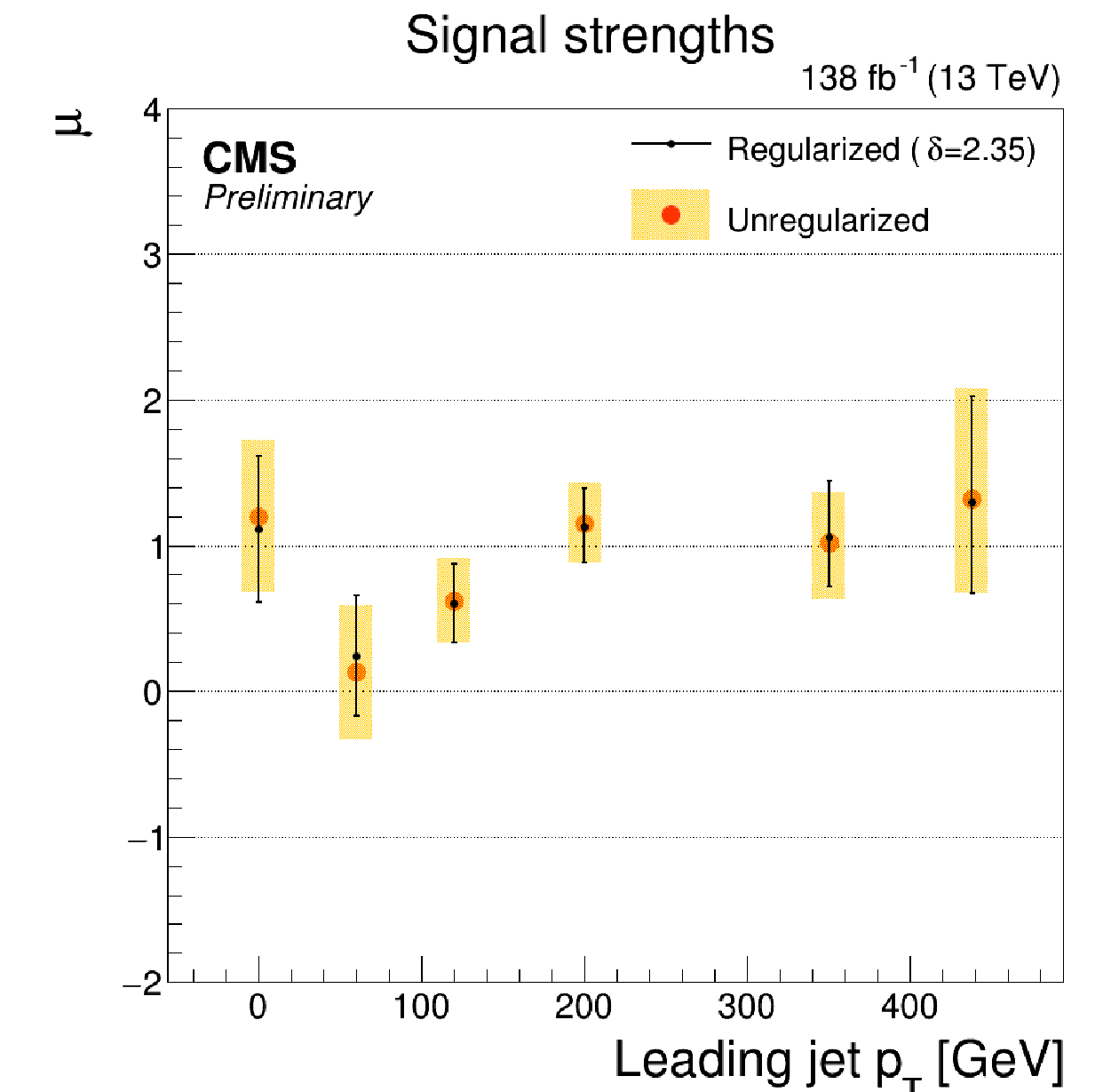
Additional Figure 41:
Observed signal strength modifiers in $ {p_{\mathrm {T}}} ^{H}$ bins. |
png pdf |
Additional Figure 42:
Observed signal strength modifiers in $N_{jets}$ bins. |
png pdf |
Additional Figure 43:
Observed signal strength modifiers in $ {p_{\mathrm {T}}} ^{jet1}$ bins. |
png pdf |
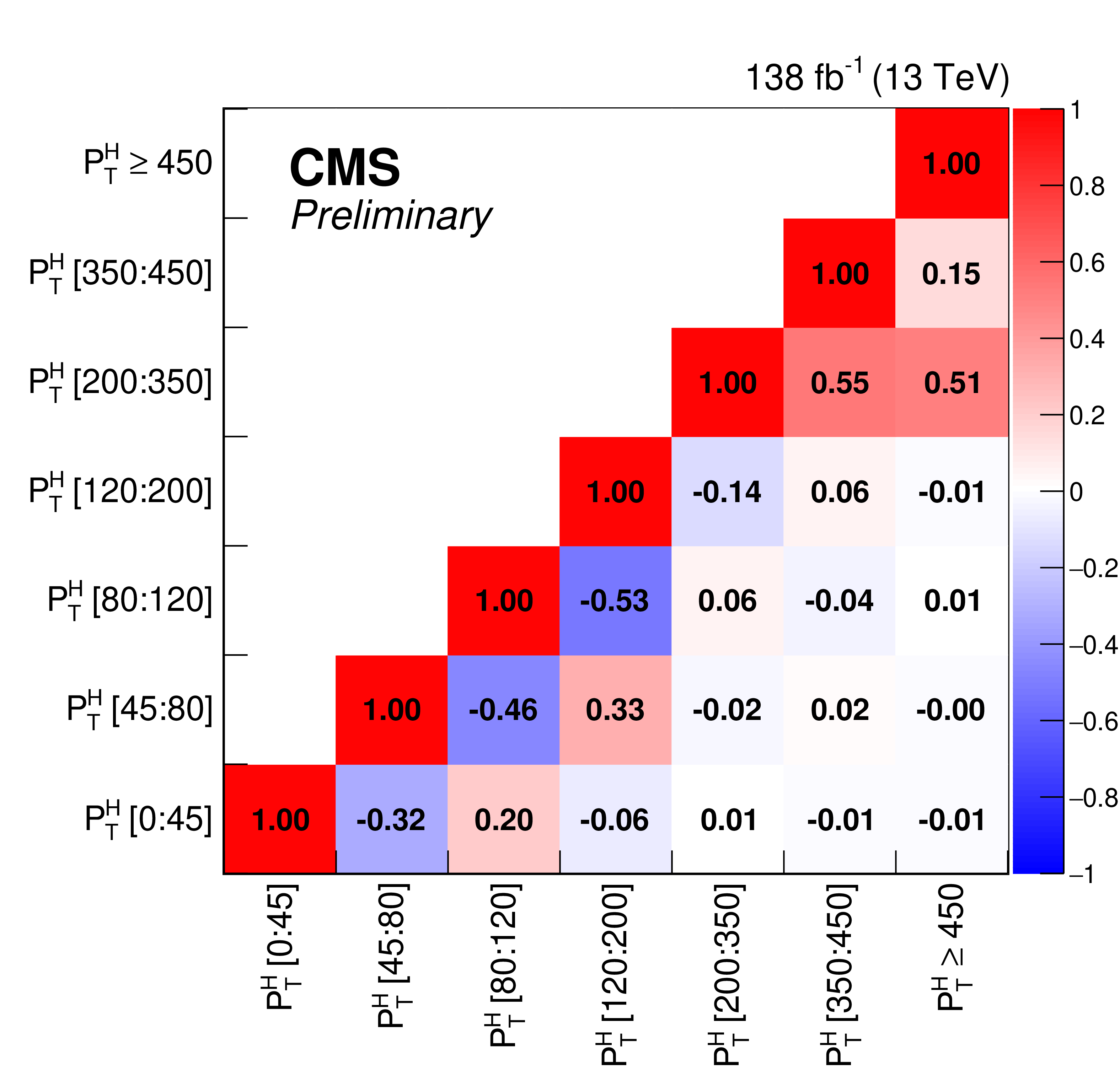
Additional Figure 44:
Correlation between signal strength modifiers in fiducial $ {p_{\mathrm {T}}} ^{H}$ bins obtained from fits to data without regularization. |
png pdf |
Additional Figure 45:
Correlation between signal strength modifiers in fiducial $ {p_{\mathrm {T}}} ^{H}$ bins obtained from fits to data with regularization. |
png pdf |
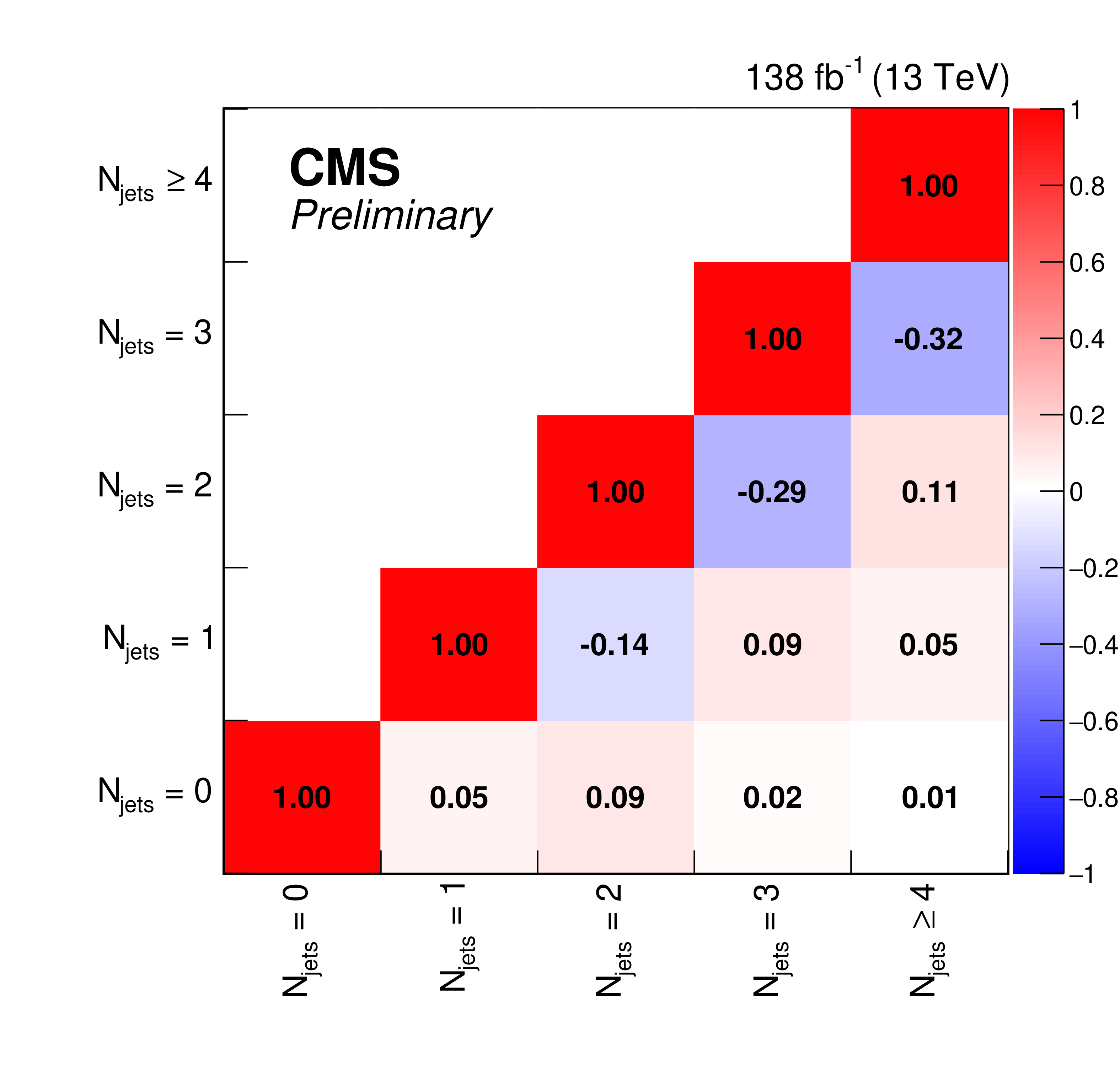
Additional Figure 46:
Correlation between signal strength modifiers in fiducial $N_{jets}$ bins obtained from fits to data without regularization. |
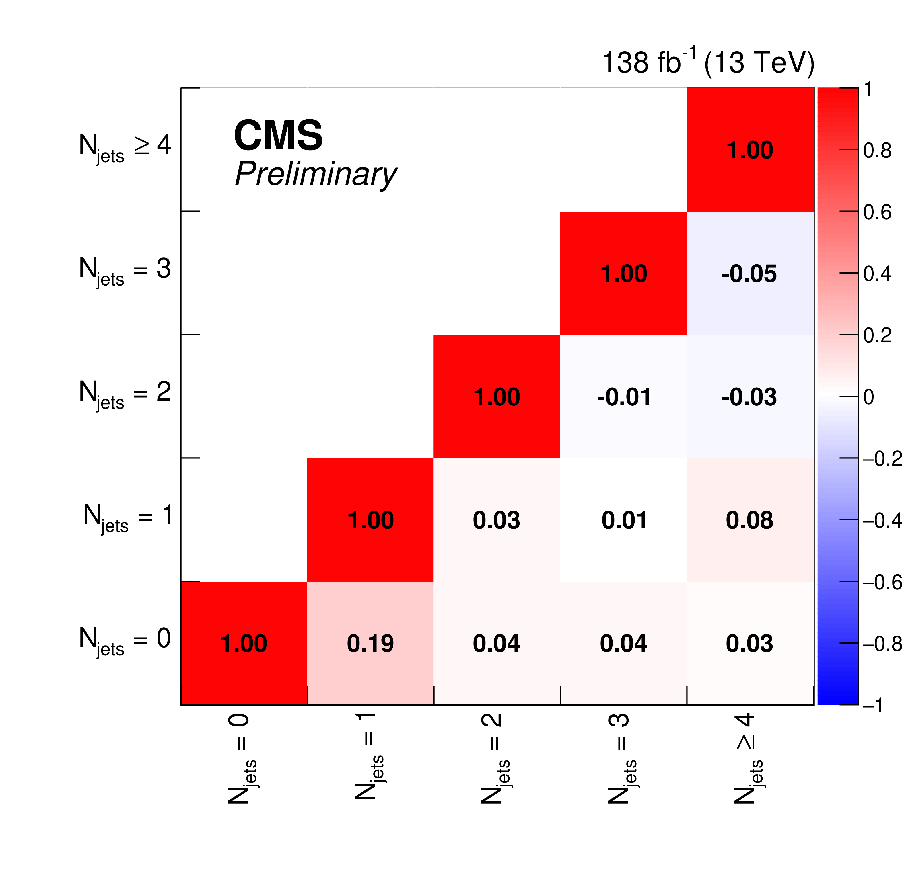
png pdf |
Additional Figure 47:
Correlation between signal strength modifiers in fiducial $N_{jets}$ bins obtained from fits to data with regularization. |
png pdf |
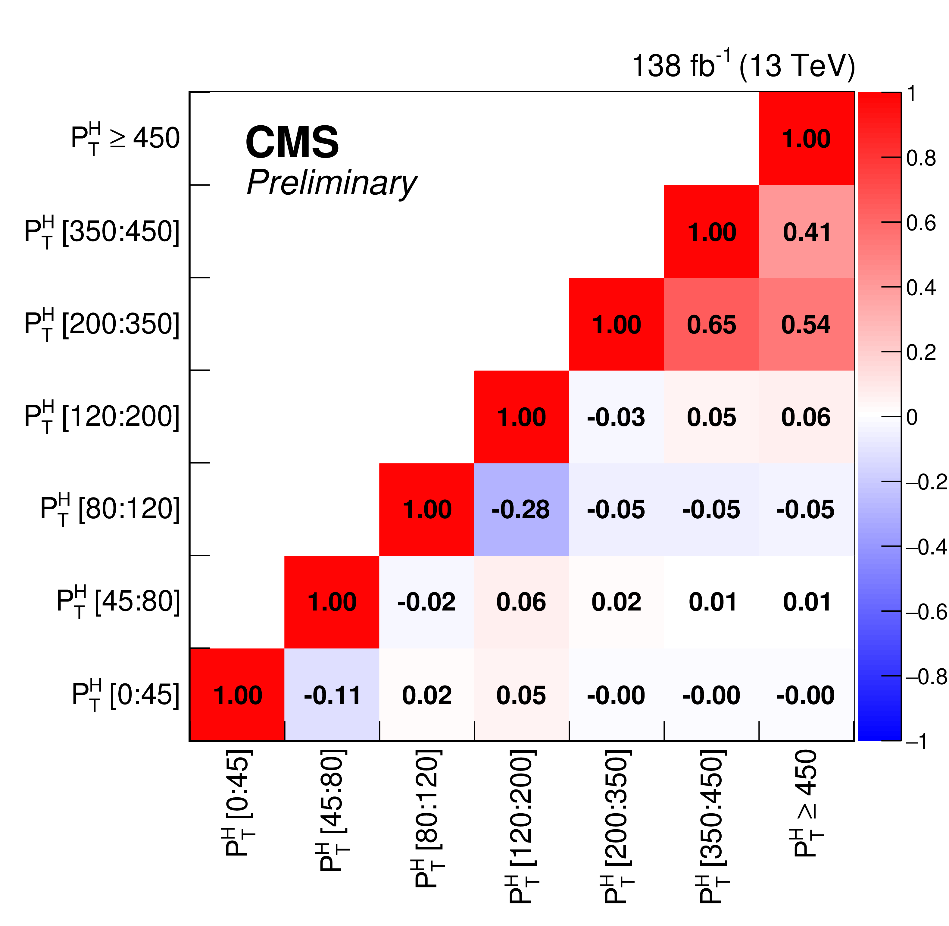
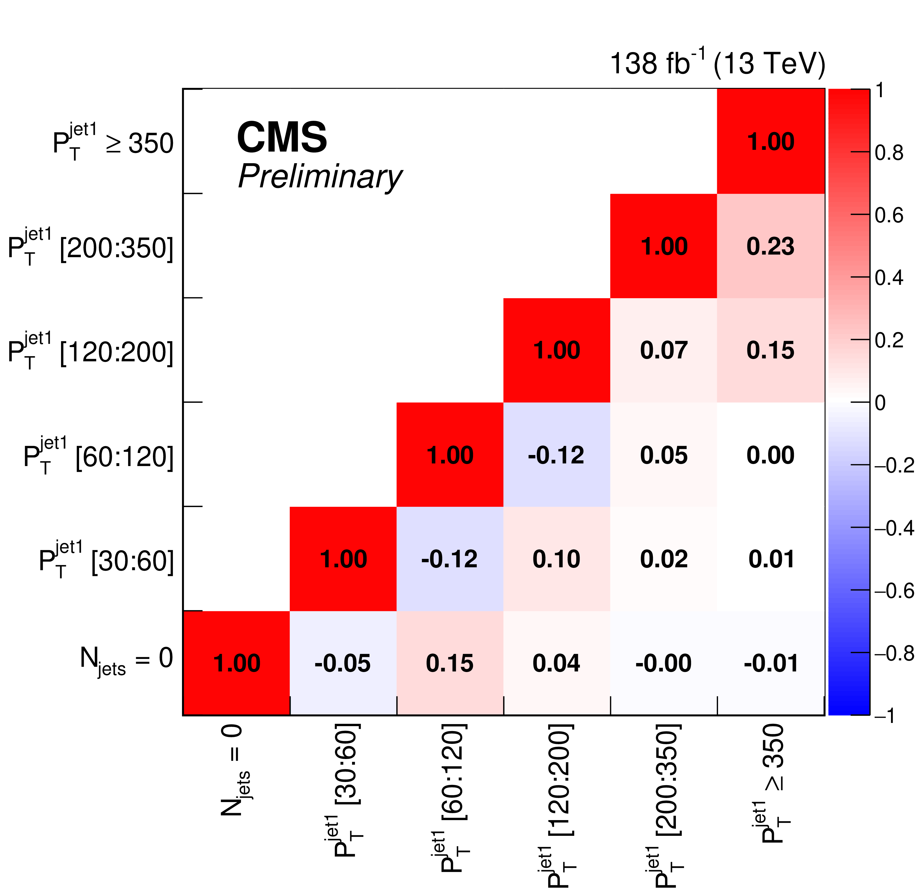
Additional Figure 48:
Correlation between signal strength modifiers in fiducial $ {p_{\mathrm {T}}} ^{jet1}$ bins obtained from fits to data without regularization. |
png pdf |
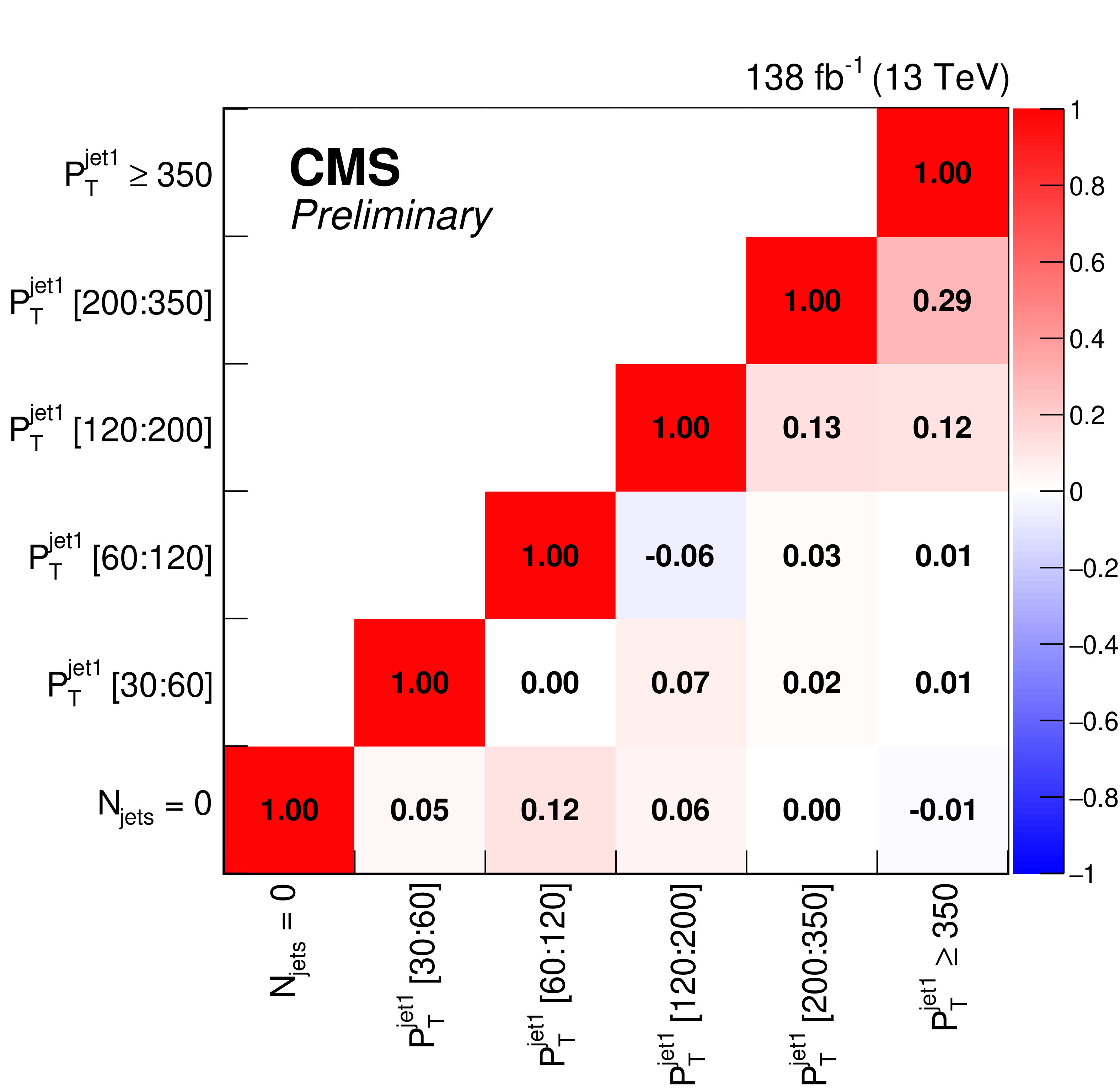
Additional Figure 49:
Correlation between signal strength modifiers in fiducial $ {p_{\mathrm {T}}} ^{jet1}$ bins obtained from fits to data with regularization. |
| References | ||||
| 1 | S. Alioli et al. | Higgsstrahlung at NNLL' + NaNLO matched to parton showers in GENEVA | PRD 100 (2019) 096016 | 1909.02026 |
| 2 | M. Grazzini, A. Ilnicka, M. Spira, and M. Wiesemann | Modeling BSM effects on the Higgs transverse-momentum spectrum in an EFT approach | JHEP 03 (2017) 115 | 1612.00283 |
| 3 | F. Bishara, U. Haisch, P. F. Monni, and E. Re | Constraining light-quark Yukawa couplings from Higgs distributions | PRL 118 (2017) 121801 | 1606.09253 |
| 4 | CMS Collaboration | Measurement of the transverse momentum spectrum of the Higgs boson produced in pp collisions at $ \sqrt{s}= $ 8 TeV using $ H \rightarrow WW $ decays | JHEP 03 (2017) 032 | CMS-HIG-15-010 1606.01522 |
| 5 | ATLAS Collaboration | Combined measurement of differential and total cross sections in the $ H \rightarrow \gamma \gamma $ and the $ H \rightarrow ZZ^* \rightarrow 4\ell $ decay channels at $ \sqrt{s} = $ 13 TeV with the ATLAS detector | PLB 786 (2018) 114 | 1805.10197 |
| 6 | CMS Collaboration | Measurement and interpretation of differential cross sections for Higgs boson production at $ \sqrt{s} = $ 13 TeV | PLB 792 (2019) 369 | CMS-HIG-17-028 1812.06504 |
| 7 | CMS Collaboration | Measurement of inclusive and differential Higgs boson production cross sections in the diphoton decay channel in proton-proton collisions at $ \sqrt{s} = $ 13 TeV | JHEP 01 (2019) 183 | CMS-HIG-17-025 1807.03825 |
| 8 | CMS Collaboration | Measurement of the inclusive and differential Higgs boson production cross sections in the leptonic WW decay mode at $ \sqrt{s} = $ 13 TeV | JHEP 03 (2021) 003 | CMS-HIG-19-002 2007.01984 |
| 9 | ATLAS Collaboration | Measurements of the Higgs boson inclusive and differential fiducial cross sections in the 4$ \ell $ decay channel at $ \sqrt{s} = $ 13 TeV | EPJC 80 (2020) 942 | 2004.03969 |
| 10 | CMS Collaboration | Observation of the Higgs boson decay to a pair of $ \tau $ leptons with the CMS detector | PLB 779 (2018) 283 | CMS-HIG-16-043 1708.00373 |
| 11 | CMS Collaboration | The CMS experiment at the CERN LHC | JINST 3 (2008) S08004 | CMS-00-001 |
| 12 | P. Nason | A new method for combining NLO QCD with shower Monte Carlo algorithms | JHEP 11 (2004) 040 | hep-ph/0409146 |
| 13 | S. Frixione, P. Nason, and C. Oleari | Matching NLO QCD computations with parton shower simulations: the POWHEG method | JHEP 11 (2007) 070 | 0709.2092 |
| 14 | S. Alioli, P. Nason, C. Oleari, and E. Re | A general framework for implementing NLO calculations in shower Monte Carlo programs: the POWHEG BOX | JHEP 06 (2010) 043 | 1002.2581 |
| 15 | S. Alioli et al. | Jet pair production in POWHEG | JHEP 04 (2011) 081 | 1012.3380 |
| 16 | S. Alioli, P. Nason, C. Oleari, and E. Re | NLO Higgs boson production via gluon fusion matched with shower in POWHEG | JHEP 04 (2009) 002 | 0812.0578 |
| 17 | K. Hamilton, P. Nason, E. Re, and G. Zanderighi | NNLOPS simulation of Higgs boson production | JHEP 10 (2013) 222 | 1309.0017 |
| 18 | K. Hamilton, P. Nason, and G. Zanderighi | Finite quark-mass effects in the NNLOPS POWHEG+MiNLO Higgs generator | JHEP 05 (2015) 140 | 1501.04637 |
| 19 | CMS Collaboration | A measurement of the Higgs boson mass in the diphoton decay channel | PLB 805 (2020) 135425 | CMS-HIG-19-004 2002.06398 |
| 20 | J. Alwall et al. | The automated computation of tree-level and next-to-leading order differential cross sections, and their matching to parton shower simulations | JHEP 07 (2014) 079 | 1405.0301 |
| 21 | J. Alwall et al. | Comparative study of various algorithms for the merging of parton showers and matrix elements in hadronic collisions | EPJC 53 (2008) 473 | 0706.2569 |
| 22 | J. M. Campbell, R. K. Ellis, and C. Williams | Vector boson pair production at the LHC | JHEP 07 (2011) 018 | 1105.0020 |
| 23 | T. Gehrmann et al. | $ W^+W^- $ production at hadron colliders in next to next to leading order QCD | PRL 113 (2014) 212001 | 1408.5243 |
| 24 | K. Melnikov and F. Petriello | Electroweak gauge boson production at hadron colliders through $ O(\alpha_s^2) $ | PRD 74 (2006) 114017 | hep-ph/0609070 |
| 25 | M. Czakon and A. Mitov | Top++: A program for the calculation of the top-pair cross-section at hadron colliders | CPC 185 (2014) 2930 | 1112.5675 |
| 26 | T. Sjostrand et al. | An introduction to PYTHIA 8.2 | CPC 191 (2015) 159 | 1410.3012 |
| 27 | CMS Collaboration | Event generator tunes obtained from underlying event and multiparton scattering measurements | EPJC 76 (2016) 155 | CMS-GEN-14-001 1512.00815 |
| 28 | GEANT4 Collaboration | GEANT4 --- a simulation toolkit | NIMA 506 (2003) 250 | |
| 29 | CMS Collaboration | Particle-flow reconstruction and global event description with the CMS detector | JINST 12 (2017) P10003 | CMS-PRF-14-001 1706.04965 |
| 30 | CMS Collaboration | Performance of CMS muon reconstruction in pp collision events at $ \sqrt{s} = $ 7 TeV | JINST 7 (2012) P10002 | CMS-MUO-10-004 1206.4071 |
| 31 | CMS Collaboration | Performance of electron reconstruction and selection with the CMS detector in proton-proton collisions at $ \sqrt{s} = $ 8 TeV | JINST 10 (2015) P06005 | CMS-EGM-13-001 1502.02701 |
| 32 | M. Cacciari, G. P. Salam, and G. Soyez | The anti-$ k_t $ jet clustering algorithm | JHEP 04 (2008) 063 | 0802.1189 |
| 33 | CMS Collaboration | Jet algorithms performance in 13 TeV data | CMS-PAS-JME-16-003 | CMS-PAS-JME-16-003 |
| 34 | CMS Collaboration | Identification of heavy-flavour jets with the CMS detector in pp collisions at 13 TeV | JINST 13 (2018) P05011 | CMS-BTV-16-002 1712.07158 |
| 35 | CMS Collaboration | Performance of the CMS missing transverse momentum reconstruction in pp data at $ \sqrt{s} = $ 8 TeV | JINST 10 (2015) P02006 | CMS-JME-13-003 1411.0511 |
| 36 | CMS Collaboration | Performance of reconstruction and identification of $ \tau $ leptons decaying to hadrons and $ \nu_\tau $ in pp collisions at $ \sqrt{s}= $ 13 TeV | JINST 13 (2018) P10005 | CMS-TAU-16-003 1809.02816 |
| 37 | CMS Collaboration | An embedding technique to determine $ \tau\tau $ backgrounds in proton-proton collision data | JINST 14 (2019) P06032 | CMS-TAU-18-001 1903.01216 |
| 38 | CMS Collaboration | Precision luminosity measurement in proton-proton collisions at $ \sqrt{s} = $ 13 TeV in 2015 and 2016 at CMS | Submitted to EPJC | CMS-LUM-17-003 2104.01927 |
| 39 | CMS Collaboration | CMS luminosity measurement for the 2017 data-taking period at $ \sqrt{s} = $ 13 TeV | CMS-PAS-LUM-17-004 | CMS-PAS-LUM-17-004 |
| 40 | CMS Collaboration | Jet energy scale and resolution performance with 13 TeV data collected by CMS in 2016-2018 | CDS | |
| 41 | LHC Higgs Cross Section Working Group Collaboration | Handbook of LHC Higgs cross sections: 4. deciphering the nature of the Higgs sector | 1610.07922 | |
| 42 | L. Bianchini, J. Conway, E. K. Friis, and C. Veelken | Reconstruction of the Higgs mass in $ H \to \tau\tau $ events by dynamical likelihood techniques | J. Phys. Conf. Ser. 513 (2014) 022035 | |
| 43 | C. Bierlich et al. | Robust independent validation of experiment and theory: Rivet version 3 | SciPost Phys. 8 (2020) 026 | 1912.05451 |
| 44 | A. N. Tikhonov | Solution of incorrectly formulated problems and the regularization method | Soviet Math. Dokl. 4 (1963) 1035 | |
| 45 | A. Hocker and V. Kartvelishvili | SVD approach to data unfolding | NIMA 372 (1996) 469 | hep-ph/9509307 |
| 46 | S. Schmitt | TUnfold: an algorithm for correcting migration effects in high energy physics | JINST 7 (2012) T10003 | 1205.6201 |
|
|
Compact Muon Solenoid LHC, CERN |
|

|

|

|

|

|