

Compact Muon Solenoid
LHC, CERN
| CMS-PAS-BPH-22-001 | ||
| Measurement of the $ \mathrm{B}^0_\mathrm{s} $ effective lifetime in the decay $ \mathrm{B}^0_\mathrm{s}\to\mathrm{J}/\psi\,\mathrm{K}^0_\mathrm{S} $ from pp collisions at $ \sqrt{s} = $ 13 TeV | ||
| CMS Collaboration | ||
| 28 March 2024 | ||
| Abstract: The effective lifetime of the $ \mathrm{B}^0_\mathrm{s} $ meson in the decay $ \mathrm{B}^0_\mathrm{s}\to\mathrm{J}/\psi \, \mathrm{K}^0_\mathrm{S} $ is measured using data collected during 2016-2018 with the CMS detector in $ \sqrt{s}= $ 13 TeV proton-proton collisions at the LHC, corresponding to an integrated luminosity of 140 fb$ ^{-1} $. The effective lifetime is determined by performing a two-dimensional unbinned maximum likelihood fit to the $ \mathrm{B}^0_\mathrm{s}\to\mathrm{J}/\psi\, \mathrm{K}^0_\mathrm{S} $ meson invariant mass and proper decay time distributions. The resulting value is 1.59 $ \pm $ 0.07 (stat) $ \pm $ 0.03 (syst) ps, where the first uncertainty represents the statistical uncertainty and the latter corresponds to the systematic uncertainty. | ||
|
Links:
CDS record (PDF) ;
CADI line (restricted) ;
These preliminary results are superseded in this paper, Submitted to JHEP. The superseded preliminary plots can be found here. |
||
| Figures | |

png pdf |
Figure 1:
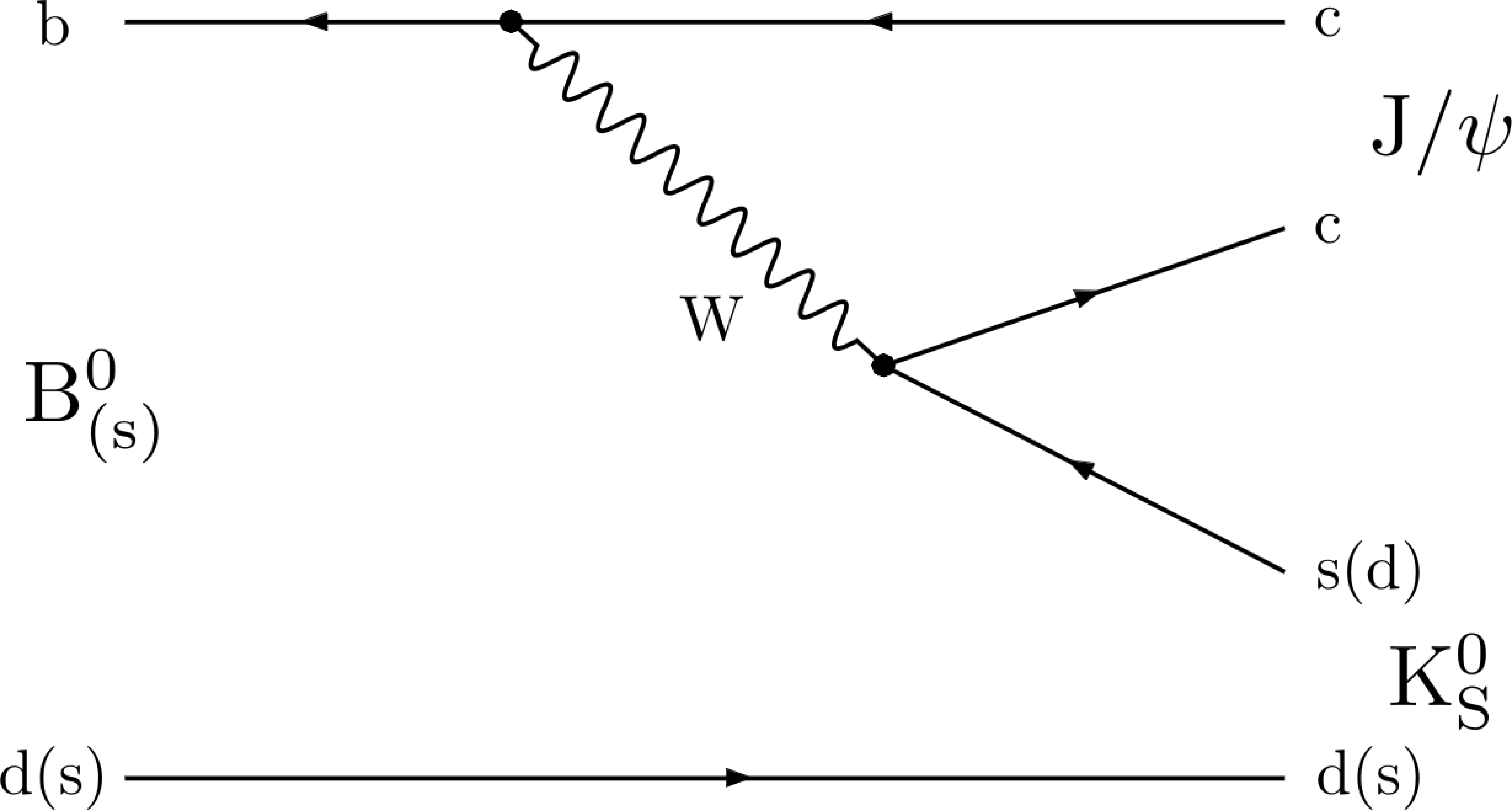
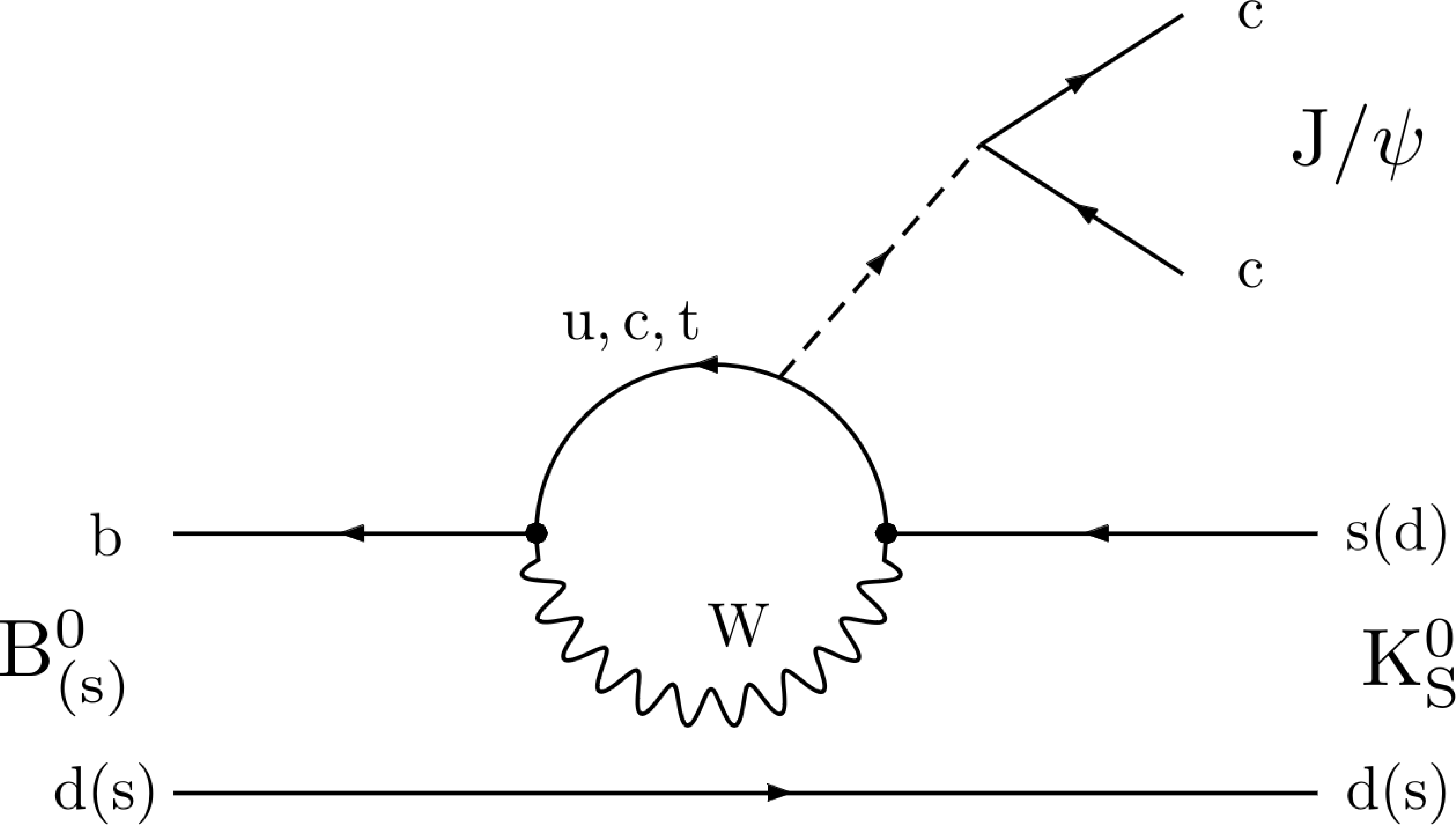
The tree-level (left) and penguin (right) diagrams for the decay $ \mathrm{B}_{s}^{0} \to \mathrm{J}/\psi\mathrm{K^0_S} $. |
png pdf |
Figure 1-a:
The tree-level (left) and penguin (right) diagrams for the decay $ \mathrm{B}_{s}^{0} \to \mathrm{J}/\psi\mathrm{K^0_S} $. |
png pdf |
Figure 1-b:
The tree-level (left) and penguin (right) diagrams for the decay $ \mathrm{B}_{s}^{0} \to \mathrm{J}/\psi\mathrm{K^0_S} $. |

png pdf |
Figure 2:
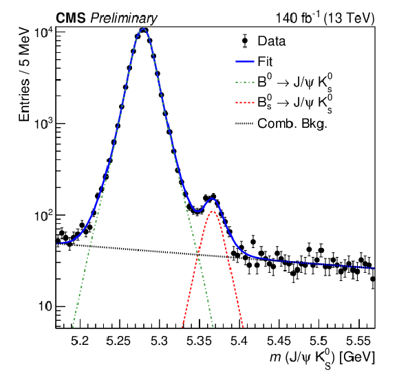
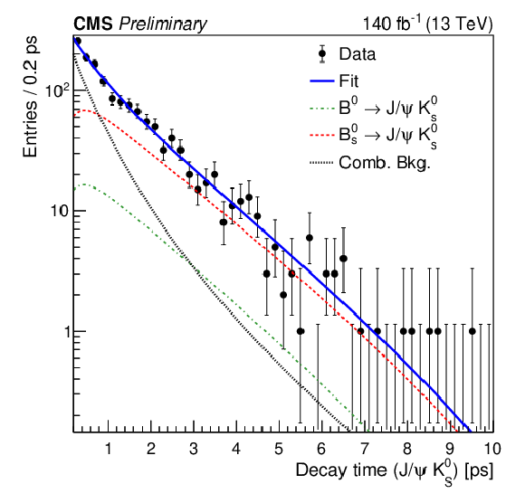
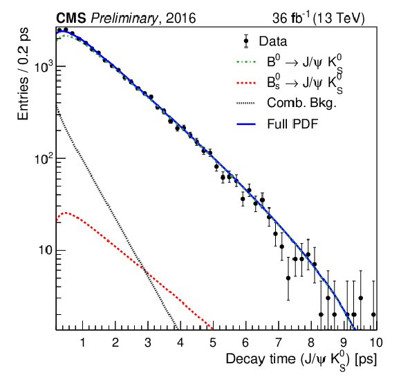
Distributions of the $ \mathrm{J}/\psi\mathrm{K^0_S} $ invariant mass (left) and proper decay time (right) from data (points) and the results from the 2D UML fit. The plots show the complete data set from 2016-2018. The vertical bars on the data points indicate the statistical uncertainty. The dashed, dotted-dashed, dotted lines and solid lines show the $ \mathrm{B}_{s}^{0} $ signal, $ {\mathrm{B}^0} $ control channel, combinatorial background, and total fit contributions, respectively. |
png pdf |
Figure 2-a:
Distributions of the $ \mathrm{J}/\psi\mathrm{K^0_S} $ invariant mass (left) and proper decay time (right) from data (points) and the results from the 2D UML fit. The plots show the complete data set from 2016-2018. The vertical bars on the data points indicate the statistical uncertainty. The dashed, dotted-dashed, dotted lines and solid lines show the $ \mathrm{B}_{s}^{0} $ signal, $ {\mathrm{B}^0} $ control channel, combinatorial background, and total fit contributions, respectively. |

png pdf |
Figure 2-b:
Distributions of the $ \mathrm{J}/\psi\mathrm{K^0_S} $ invariant mass (left) and proper decay time (right) from data (points) and the results from the 2D UML fit. The plots show the complete data set from 2016-2018. The vertical bars on the data points indicate the statistical uncertainty. The dashed, dotted-dashed, dotted lines and solid lines show the $ \mathrm{B}_{s}^{0} $ signal, $ {\mathrm{B}^0} $ control channel, combinatorial background, and total fit contributions, respectively. |
png pdf |
Figure 3:
The proper decay time distribution from data (points) for events in the $ \mathrm{B}_{s}^{0} $ signal region with $ \mathrm{J}/\psi\mathrm{K^0_S} $ invariant mass in the range 5.34-5.42 GeV. The vertical bars on the data points indicate the statistical uncertainty. The dashed, dotted-dashed, dotted lines and solid lines show the $ \mathrm{B}_{s}^{0} $ signal, $ {\mathrm{B}^0} $ control channel, combinatorial background, and total fit contributions, respectively. |

png pdf |
Figure 4:
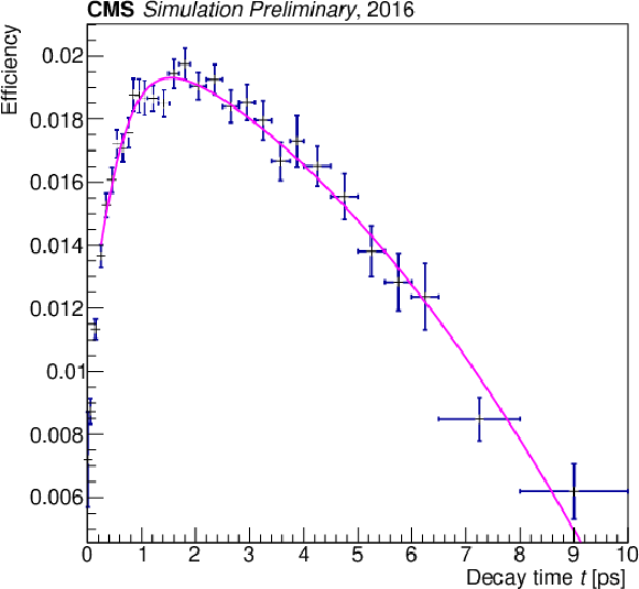
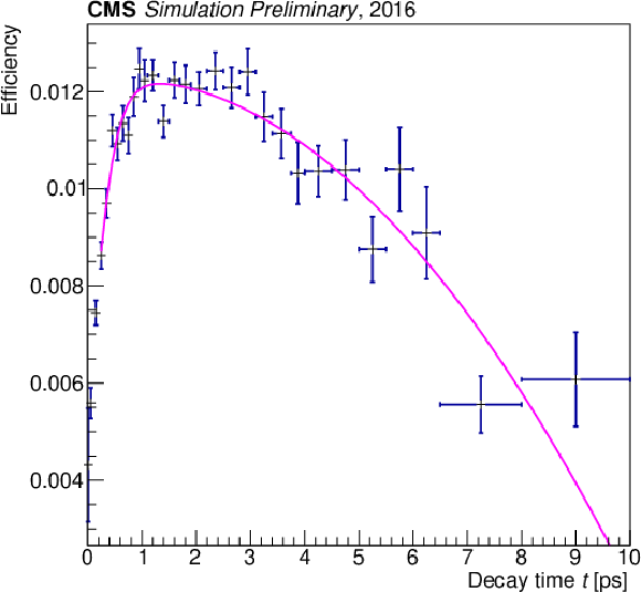
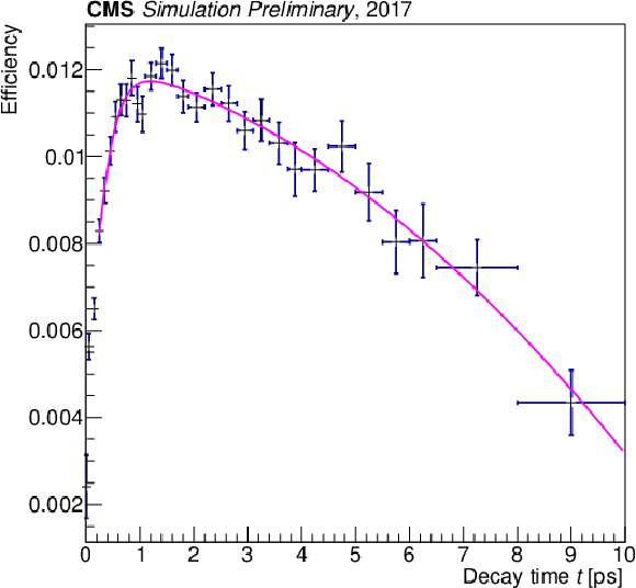
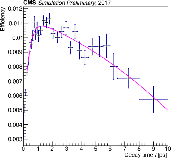
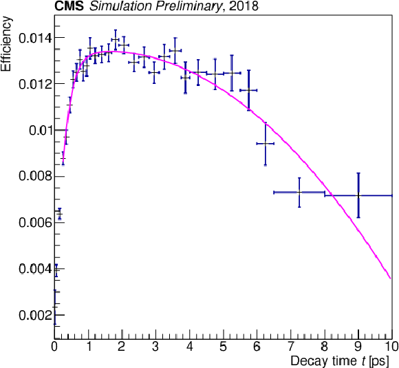
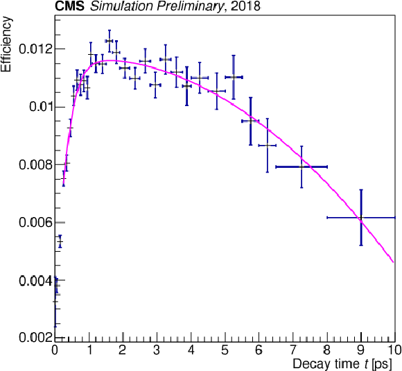
The signal efficiency as a function of the decay time for the $ {\mathrm{B}^0} \to \mathrm{J}/\psi\mathrm{K^0_S} $ (left) and $ \mathrm{B}_{s}^{0} \to \mathrm{J}/\psi\mathrm{K^0_S} $ (right) decays from simulation for each of the three data-taking years. The vertical bars indicate the statistical uncertainty, and the horizontal bars give the bin width. The curves show the projections of the fit to the simulated event samples. |
png pdf |
Figure 4-a:
The signal efficiency as a function of the decay time for the $ {\mathrm{B}^0} \to \mathrm{J}/\psi\mathrm{K^0_S} $ (left) and $ \mathrm{B}_{s}^{0} \to \mathrm{J}/\psi\mathrm{K^0_S} $ (right) decays from simulation for each of the three data-taking years. The vertical bars indicate the statistical uncertainty, and the horizontal bars give the bin width. The curves show the projections of the fit to the simulated event samples. |
png pdf |
Figure 4-b:
The signal efficiency as a function of the decay time for the $ {\mathrm{B}^0} \to \mathrm{J}/\psi\mathrm{K^0_S} $ (left) and $ \mathrm{B}_{s}^{0} \to \mathrm{J}/\psi\mathrm{K^0_S} $ (right) decays from simulation for each of the three data-taking years. The vertical bars indicate the statistical uncertainty, and the horizontal bars give the bin width. The curves show the projections of the fit to the simulated event samples. |
png pdf |
Figure 4-c:
The signal efficiency as a function of the decay time for the $ {\mathrm{B}^0} \to \mathrm{J}/\psi\mathrm{K^0_S} $ (left) and $ \mathrm{B}_{s}^{0} \to \mathrm{J}/\psi\mathrm{K^0_S} $ (right) decays from simulation for each of the three data-taking years. The vertical bars indicate the statistical uncertainty, and the horizontal bars give the bin width. The curves show the projections of the fit to the simulated event samples. |
png pdf |
Figure 4-d:
The signal efficiency as a function of the decay time for the $ {\mathrm{B}^0} \to \mathrm{J}/\psi\mathrm{K^0_S} $ (left) and $ \mathrm{B}_{s}^{0} \to \mathrm{J}/\psi\mathrm{K^0_S} $ (right) decays from simulation for each of the three data-taking years. The vertical bars indicate the statistical uncertainty, and the horizontal bars give the bin width. The curves show the projections of the fit to the simulated event samples. |
png pdf |
Figure 4-e:
The signal efficiency as a function of the decay time for the $ {\mathrm{B}^0} \to \mathrm{J}/\psi\mathrm{K^0_S} $ (left) and $ \mathrm{B}_{s}^{0} \to \mathrm{J}/\psi\mathrm{K^0_S} $ (right) decays from simulation for each of the three data-taking years. The vertical bars indicate the statistical uncertainty, and the horizontal bars give the bin width. The curves show the projections of the fit to the simulated event samples. |
png pdf |
Figure 4-f:
The signal efficiency as a function of the decay time for the $ {\mathrm{B}^0} \to \mathrm{J}/\psi\mathrm{K^0_S} $ (left) and $ \mathrm{B}_{s}^{0} \to \mathrm{J}/\psi\mathrm{K^0_S} $ (right) decays from simulation for each of the three data-taking years. The vertical bars indicate the statistical uncertainty, and the horizontal bars give the bin width. The curves show the projections of the fit to the simulated event samples. |
png pdf |
Figure 5:
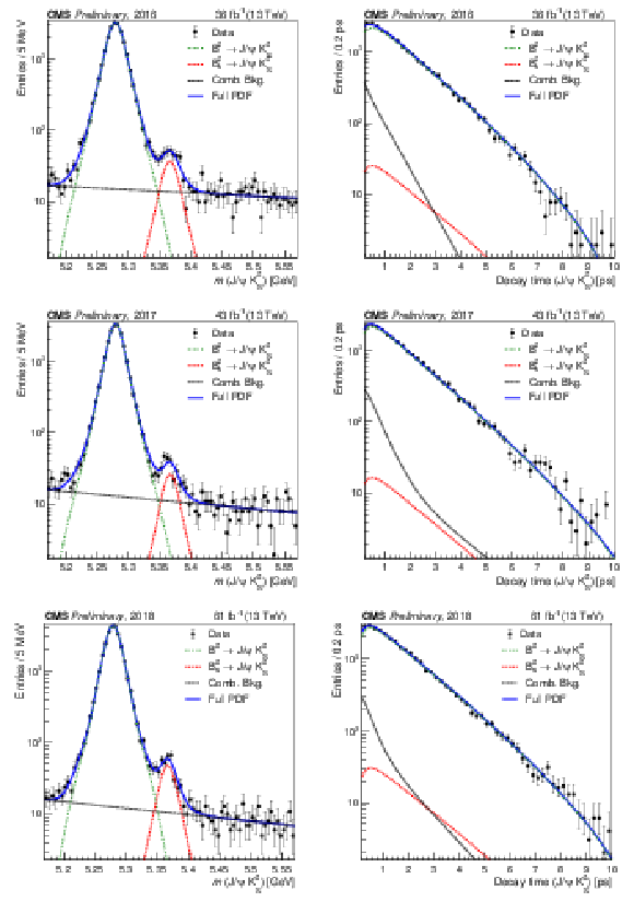
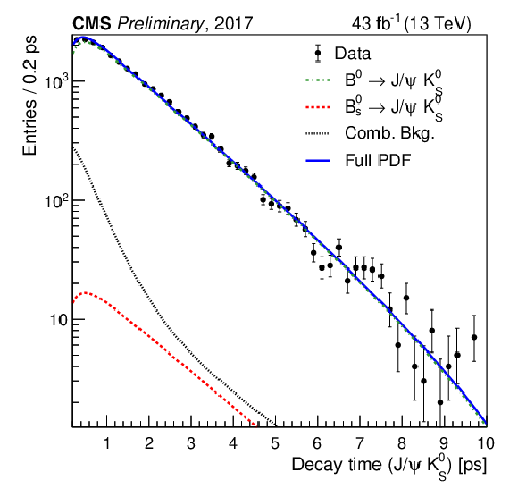
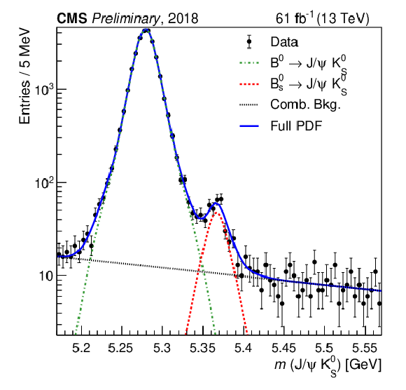
Distributions of the $ \mathrm{J}/\psi\mathrm{K^0_S} $ invariant mass (left) and decay time (right) from data (points), along with the projections from the 2D UML fit for each year of data taking. The vertical bars on the data points indicate the statistical uncertainty. The dashed, dotted-dashed, dotted and solid lines represent the signal, control channel, combinational background, and total fit contributions respectively. |

png pdf |
Figure 5-a:
Distributions of the $ \mathrm{J}/\psi\mathrm{K^0_S} $ invariant mass (left) and decay time (right) from data (points), along with the projections from the 2D UML fit for each year of data taking. The vertical bars on the data points indicate the statistical uncertainty. The dashed, dotted-dashed, dotted and solid lines represent the signal, control channel, combinational background, and total fit contributions respectively. |
png pdf |
Figure 5-b:
Distributions of the $ \mathrm{J}/\psi\mathrm{K^0_S} $ invariant mass (left) and decay time (right) from data (points), along with the projections from the 2D UML fit for each year of data taking. The vertical bars on the data points indicate the statistical uncertainty. The dashed, dotted-dashed, dotted and solid lines represent the signal, control channel, combinational background, and total fit contributions respectively. |

png pdf |
Figure 5-c:
Distributions of the $ \mathrm{J}/\psi\mathrm{K^0_S} $ invariant mass (left) and decay time (right) from data (points), along with the projections from the 2D UML fit for each year of data taking. The vertical bars on the data points indicate the statistical uncertainty. The dashed, dotted-dashed, dotted and solid lines represent the signal, control channel, combinational background, and total fit contributions respectively. |
png pdf |
Figure 5-d:
Distributions of the $ \mathrm{J}/\psi\mathrm{K^0_S} $ invariant mass (left) and decay time (right) from data (points), along with the projections from the 2D UML fit for each year of data taking. The vertical bars on the data points indicate the statistical uncertainty. The dashed, dotted-dashed, dotted and solid lines represent the signal, control channel, combinational background, and total fit contributions respectively. |
png pdf |
Figure 5-e:
Distributions of the $ \mathrm{J}/\psi\mathrm{K^0_S} $ invariant mass (left) and decay time (right) from data (points), along with the projections from the 2D UML fit for each year of data taking. The vertical bars on the data points indicate the statistical uncertainty. The dashed, dotted-dashed, dotted and solid lines represent the signal, control channel, combinational background, and total fit contributions respectively. |

png pdf |
Figure 5-f:
Distributions of the $ \mathrm{J}/\psi\mathrm{K^0_S} $ invariant mass (left) and decay time (right) from data (points), along with the projections from the 2D UML fit for each year of data taking. The vertical bars on the data points indicate the statistical uncertainty. The dashed, dotted-dashed, dotted and solid lines represent the signal, control channel, combinational background, and total fit contributions respectively. |

png pdf |
Figure 6:
The 2D UML fit projection on the decay time axis for mass range 5.17 $ < m < $ 5.22 GeV for 2016, 2017 and 2018 respectively. |

png pdf |
Figure 6-a:
The 2D UML fit projection on the decay time axis for mass range 5.17 $ < m < $ 5.22 GeV for 2016, 2017 and 2018 respectively. |
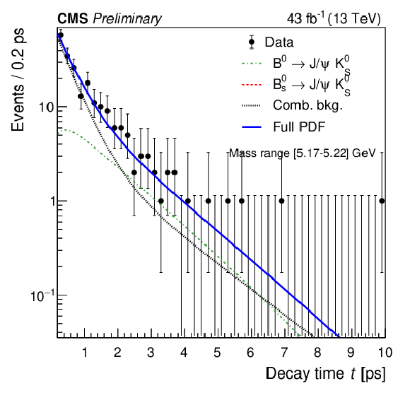
png pdf |
Figure 6-b:
The 2D UML fit projection on the decay time axis for mass range 5.17 $ < m < $ 5.22 GeV for 2016, 2017 and 2018 respectively. |
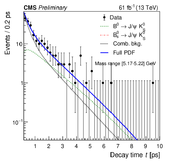
png pdf |
Figure 6-c:
The 2D UML fit projection on the decay time axis for mass range 5.17 $ < m < $ 5.22 GeV for 2016, 2017 and 2018 respectively. |

png pdf |
Figure 7:
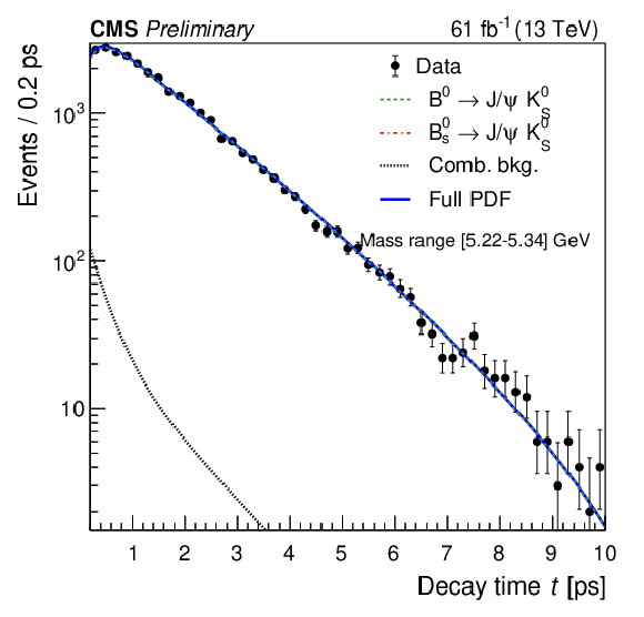
The 2D UML fit projection on the decay time axis for mass range 5.22 $ < m < $ 5.34 GeV for 2016, 2017 and 2018 respectively. |

png pdf |
Figure 7-a:
The 2D UML fit projection on the decay time axis for mass range 5.22 $ < m < $ 5.34 GeV for 2016, 2017 and 2018 respectively. |

png pdf |
Figure 7-b:
The 2D UML fit projection on the decay time axis for mass range 5.22 $ < m < $ 5.34 GeV for 2016, 2017 and 2018 respectively. |
png pdf |
Figure 7-c:
The 2D UML fit projection on the decay time axis for mass range 5.22 $ < m < $ 5.34 GeV for 2016, 2017 and 2018 respectively. |

png pdf |
Figure 8:
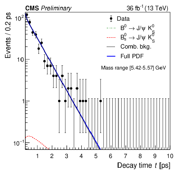
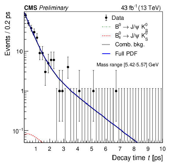
The 2D UML fit projection on the decay time axis for mass range 5.42 $ < m < $ 5.57 GeV for 2016, 2017 and 2018 respectively. |
png pdf |
Figure 8-a:
The 2D UML fit projection on the decay time axis for mass range 5.42 $ < m < $ 5.57 GeV for 2016, 2017 and 2018 respectively. |
png pdf |
Figure 8-b:
The 2D UML fit projection on the decay time axis for mass range 5.42 $ < m < $ 5.57 GeV for 2016, 2017 and 2018 respectively. |

png pdf |
Figure 8-c:
The 2D UML fit projection on the decay time axis for mass range 5.42 $ < m < $ 5.57 GeV for 2016, 2017 and 2018 respectively. |

png pdf |
Figure 9:
The 2D UML fit projection plots on the mass axis for decay time range 0.2 $ < t < $ 2.5 ps for 2016, 2017 and 2018 respectively. |

png pdf |
Figure 9-a:
The 2D UML fit projection plots on the mass axis for decay time range 0.2 $ < t < $ 2.5 ps for 2016, 2017 and 2018 respectively. |

png pdf |
Figure 9-b:
The 2D UML fit projection plots on the mass axis for decay time range 0.2 $ < t < $ 2.5 ps for 2016, 2017 and 2018 respectively. |

png pdf |
Figure 9-c:
The 2D UML fit projection plots on the mass axis for decay time range 0.2 $ < t < $ 2.5 ps for 2016, 2017 and 2018 respectively. |

png pdf |
Figure 10:
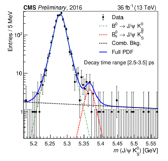
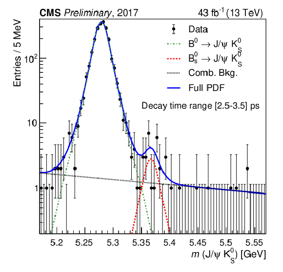
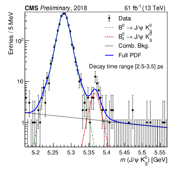
The 2D UML fit projection plots on the mass axis for decay time range 2.5 $ < t < $ 3.5 ps for 2016, 2017 and 2018 respectively. |
png pdf |
Figure 10-a:
The 2D UML fit projection plots on the mass axis for decay time range 2.5 $ < t < $ 3.5 ps for 2016, 2017 and 2018 respectively. |
png pdf |
Figure 10-b:
The 2D UML fit projection plots on the mass axis for decay time range 2.5 $ < t < $ 3.5 ps for 2016, 2017 and 2018 respectively. |
png pdf |
Figure 10-c:
The 2D UML fit projection plots on the mass axis for decay time range 2.5 $ < t < $ 3.5 ps for 2016, 2017 and 2018 respectively. |

png pdf |
Figure 11:
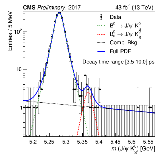
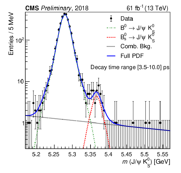
The 2D UML fit projection plots on the mass axis for decay time range 3.5 $ < t < $ 10 ps for 2016, 2017 and 2018 respectively. |
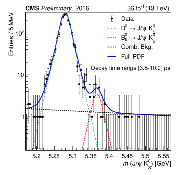
png pdf |
Figure 11-a:
The 2D UML fit projection plots on the mass axis for decay time range 3.5 $ < t < $ 10 ps for 2016, 2017 and 2018 respectively. |
png pdf |
Figure 11-b:
The 2D UML fit projection plots on the mass axis for decay time range 3.5 $ < t < $ 10 ps for 2016, 2017 and 2018 respectively. |
png pdf |
Figure 11-c:
The 2D UML fit projection plots on the mass axis for decay time range 3.5 $ < t < $ 10 ps for 2016, 2017 and 2018 respectively. |
| Tables | |
png pdf |
Table 1:
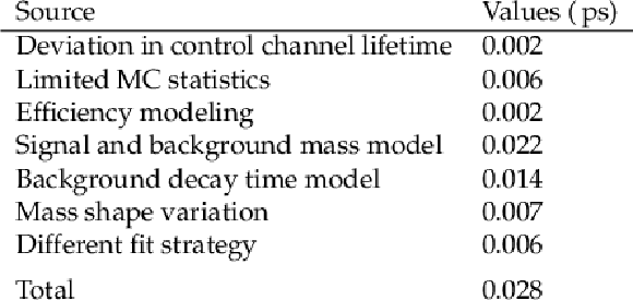
Sources of systematic uncertainties in the $ \mathrm{B}_{s}^{0} \to \mathrm{J}/\psi\mathrm{K^0_S} $ effective lifetime measurement and their estimated values, along with the total systematic uncertainty. |
| Summary |
| The effective lifetime of the $ \mathrm{B}_{s}^{0} $ meson in the $ \mathrm{J}/\psi\mathrm{K^0_S} $ decay channel is measured using the data collected during 2016-2018 by the CMS detector in proton-proton collision events at a center-of-mass energy of 13 TeV, corresponding to an integrated luminosity of 140 fb$ ^{-1} $. Throughout the analysis, the decay $ {\mathrm{B}^0} \to \mathrm{J}/\psi\mathrm{K^0_S} $ with larger event yield is used as a reference at multiple stages validating analysis method. The measured effective lifetime is found to be 1.59 $ \pm $ 0.07 (stat) $ \pm $ 0.03 (syst) ps. This measurement is compatible within 2.1$ \sigma $ with a previous measurement conducted by the LHCb experiment and shows strong agreement with the SM prediction of 1.62 $ \pm $ 0.02 ps. |
| References | ||||
| 1 | K. De Bruyn et al. | Branching ratio measurements of $ \mathrm{B}_{s}^{0} $ decays | PRD 86 (2012) 014027 | |
| 2 | CMS Collaboration | Measurement of the B$ ^0_\mathrm{S} \to \mu^+\mu^- $ decay properties and search for the B$ ^0 \to \mu^+\mu^- $ decay in proton-proton collisions at $ \sqrt{s} $ = 13 TeV | PLB 842 (2023) 137955 | CMS-BPH-21-006 2212.10311 |
| 3 | CMS Collaboration | Measurement of properties of B$ ^0_\mathrm{s}\to\mu^+\mu^- $ decays and search for B$ ^0\to\mu^+\mu^- $ with the CMS experiment | JHEP 04 (2020) 188 | CMS-BPH-16-004 1910.12127 |
| 4 | CMS Collaboration | Combination of the ATLAS, CMS and LHCb results on the B$ ^0_\mathrm{s}\to\mu^+\mu^- $ decays | LHCb-CONF-2020-002, ATLAS-CONF-2020-049, 2020 | CMS-PAS-BPH-20-003 |
| 5 | LHCb Collaboration | Measurement of the B$ ^0_\mathrm{s}\to\mu^+\mu^- $ decay properties and search for the B$ ^0\to\mu^+\mu^- $ and B$ ^0_\mathrm{s}\to\mu^+\mu^-\gamma $ decays | PRD 105 (2022) 012010 | 2108.09283 |
| 6 | ATLAS Collaboration | Study of the rare decays of $ B^0_s $ and $ B^0 $ mesons into muon pairs using data collected during 2015 and 2016 with the ATLAS detector | JHEP 04 (2019) 098 | 1812.03017 |
| 7 | LHCb Collaboration | Measurement of the $ B_s $ effective lifetime in the $ J/\psi f_0(980) $ final state | PRL 109 (2012) 152002 | 1207.0878 |
| 8 | LHCb Collaboration | Measurement of the effective $ B_s^0 \rightarrow K^+ K^- $ lifetime | PLB 716 (2012) 393 | 1207.5993 |
| 9 | K. De Bruyn, R. Fleischer, and P. Koppenburg | Extracting $ \gamma $ and penguin topologies through CP violation in $ \mathrm{B}_{s}^{0} \to \mathrm{J}/\psi\mathrm{K^0_S} $ | EPJC 70 (2010) | 1010.0089 |
| 10 | R. Fleischer | Extracting $ \gamma $ from $ {\mathrm{B}^0} $ (s/d) $ \to \mathrm{J}/\psi\mathrm{K^0_S} $ and $ {\mathrm{B}^0} $ (d/s) $ \to $ D$ ^+ $(d/s) D$ ^- $(d/s) | EPJC 10 (1999) | hep-ph/9903455 |
| 11 | Particle Data Group Collaboration | Review of particle physics | Prog. Theor. Exp. Phys. 2022 (2022) 083C01 | |
| 12 | LHCb Collaboration | Measurement of the effective $ \mathrm{B}_{s}^{0} \to \mathrm{J}/\psi\mathrm{K^0_S} $ lifetime | NPB 873 (2013) | 1304.4500 |
| 13 | CMS Collaboration | Description and performance of track and primary-vertex reconstruction with the CMS tracker | JINST 9 (2014) P10009 | CMS-TRK-11-001 1405.6569 |
| 14 | CMS Tracker Group Collaboration | The CMS phase-1 pixel detector upgrade | JINST 16 (2021) P02027 | 2012.14304 |
| 15 | CMS Collaboration | Track impact parameter resolution for the full pseudo rapidity coverage in the 2017 dataset with the CMS phase-1 pixel detector | CMS Detector Performance Summary CMS-DP-2020-049, 2020 CDS |
|
| 16 | CMS Collaboration | The CMS experiment at the CERN LHC | JINST 3 (2008) S08004 | |
| 17 | CMS Collaboration | Performance of the CMS Level-1 trigger in proton-proton collisions at $ \sqrt{s} = $ 13 TeV | JINST 15 (2020) P10017 | CMS-TRG-17-001 2006.10165 |
| 18 | CMS Collaboration | The CMS trigger system | JINST 12 (2017) P01020 | CMS-TRG-12-001 1609.02366 |
| 19 | CMS Collaboration | Precision luminosity measurement in proton-proton collisions at $ \sqrt{s}= $ 13 TeV in 2015 and 2016 at CMS | EPJC 81 (2021) 800 | CMS-LUM-17-003 2104.01927 |
| 20 | CMS Collaboration | CMS luminosity measurement for the 2017 data-taking period at $ \sqrt{s} = $ 13 TeV | CMS Physics Analysis Summary, 2018 link |
CMS-PAS-LUM-17-004 |
| 21 | CMS Collaboration | CMS luminosity measurement for the 2018 data-taking period at $ \sqrt{s} = $ 13 TeV | CMS Physics Analysis Summary, 2019 link |
CMS-PAS-LUM-18-002 |
| 22 | T. Sjöstrand et al. | An introduction to PYTHIA 8.2 | Comput. Phys. Commun. 191 (2015) 159 | 1410.3012 |
| 23 | D. J. Lange | The EvtGen particle decay simulation package | NIM A 462 (2001) 152 | |
| 24 | GEANT4 Collaboration | GEANT 4 --- a simulation toolkit | NIM A 506 (2003) 250 | |
| 25 | CMS Collaboration | Performance of the CMS muon detector and muon reconstruction with proton-proton collisions at $ \sqrt{s}= $ 13 TeV | JINST 13 (2018) | CMS-MUO-16-001 1804.04528 |
| 26 | P. B. Rodríguez et al. | Calibration of the momentum scale of a particle physics detector using the Armenteros-Podolanski plot | JINST 16 (2021) | 2012.03620 |
| 27 | L.-G. Xia | Understanding the boosted decision tree methods with the weak-learner approximation | ||
| 28 | N. L. Johnson | Systems of frequency curves generated by methods of translation | Biometrika 36 (1949) 149 | |
| 29 | S. Jackman | Bayesian analysis for the social sciences | John Wiley & Sons, New Jersey, USA, 2009 link |
|

|
Compact Muon Solenoid LHC, CERN |

|

|

|

|

|

|