CMS-BPH-22-001

CMS-BPH-22-001 ; CERN-EP-2024-172
Measurement of the $\mathrm{B}_{s}^{0} \to \mathrm{J}/\psi\mathrm{K^0_S}$ effective lifetime from proton-proton collisions at $\sqrt{s} =$ 13 TeV
CMS Collaboration
18 July 2024
JHEP 10 (2024) 247
Abstract: The effective lifetime of the $\mathrm{B}_{s}^{0}$ meson in the decay $\mathrm{B}_{s}^{0} \to \mathrm{J}/\psi\mathrm{K^0_S}$ is measured using data collected during 2016-2018 with the CMS detector in $\sqrt{s}=$ 13 TeV proton-proton collisions at the LHC, corresponding to an integrated luminosity of 140 fb $^{-1}$ . The effective lifetime is determined by performing a two-dimensional unbinned maximum likelihood fit to the $\mathrm{B}_{s}^{0}$ meson invariant mass and proper decay time distributions. The resulting value of 1.59 $\pm$ 0.07 (stat) $\pm$ 0.03 (syst) ps is the most precise measurement to date and is in good agreement with the expected value.
Links: e-print arXiv:2407.13441 [hep-ex] (PDF) ; CDS record ; inSPIRE record ; HepData record ; CADI line (restricted) ;

Figures & Tables	Summary	References	CMS Publications

Figures
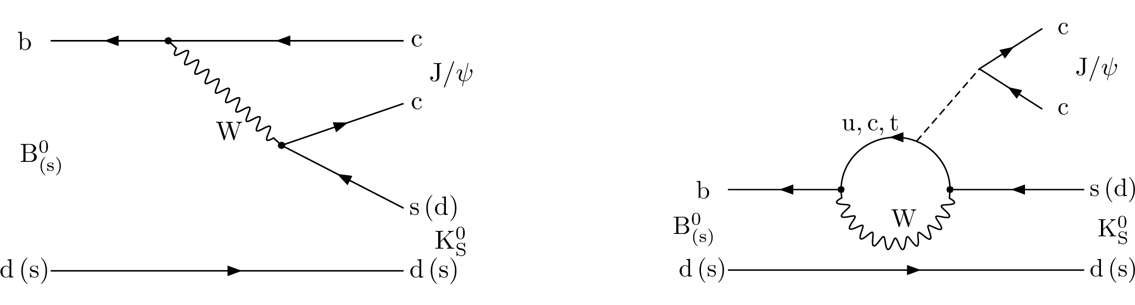
png pdf	Figure 1: The tree-level (left) and penguin (right) Feynman diagrams for the decays ${\mathrm{B}^0} \to \mathrm{J}/\psi\mathrm{K^0_S}$ and $\mathrm{B}_{s}^{0} \to \mathrm{J}/\psi\mathrm{K^0_S}$ .
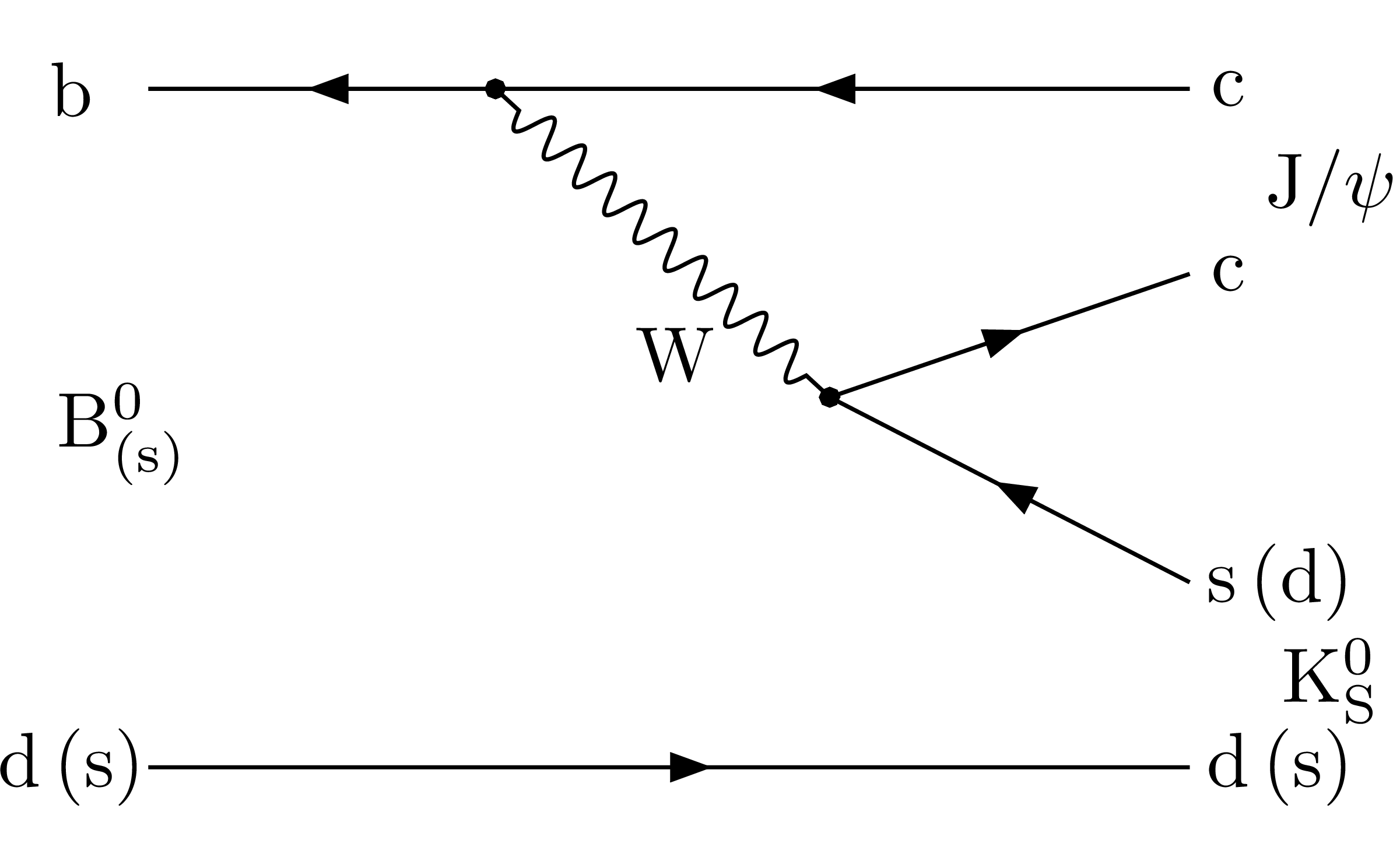
png pdf	Figure 1-a: The tree-level (left) and penguin (right) Feynman diagrams for the decays ${\mathrm{B}^0} \to \mathrm{J}/\psi\mathrm{K^0_S}$ and $\mathrm{B}_{s}^{0} \to \mathrm{J}/\psi\mathrm{K^0_S}$ .
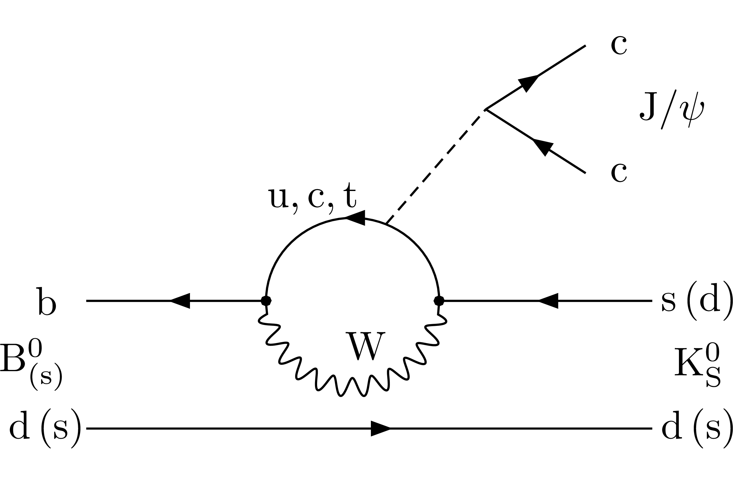
png pdf	Figure 1-b: The tree-level (left) and penguin (right) Feynman diagrams for the decays ${\mathrm{B}^0} \to \mathrm{J}/\psi\mathrm{K^0_S}$ and $\mathrm{B}_{s}^{0} \to \mathrm{J}/\psi\mathrm{K^0_S}$ .
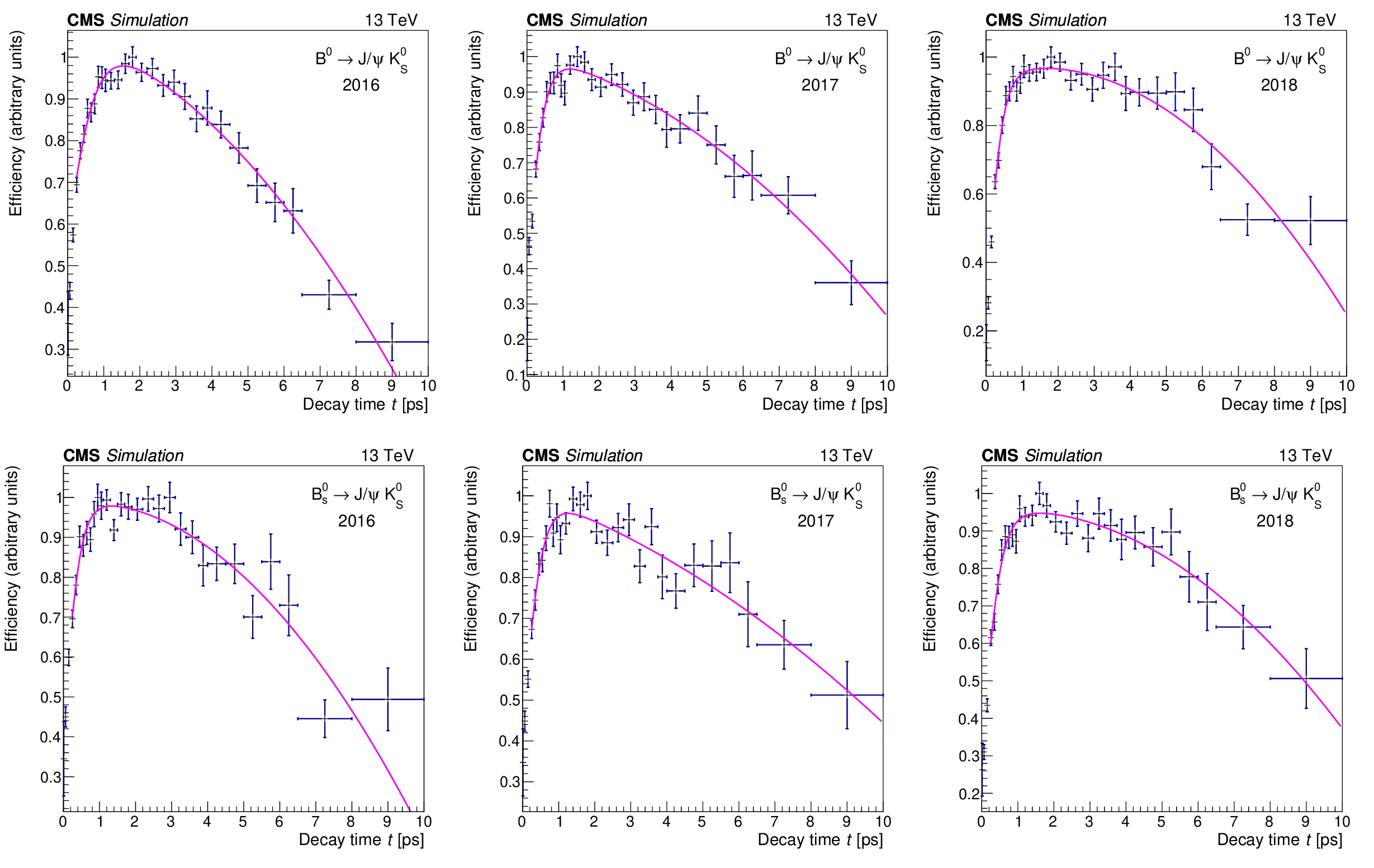
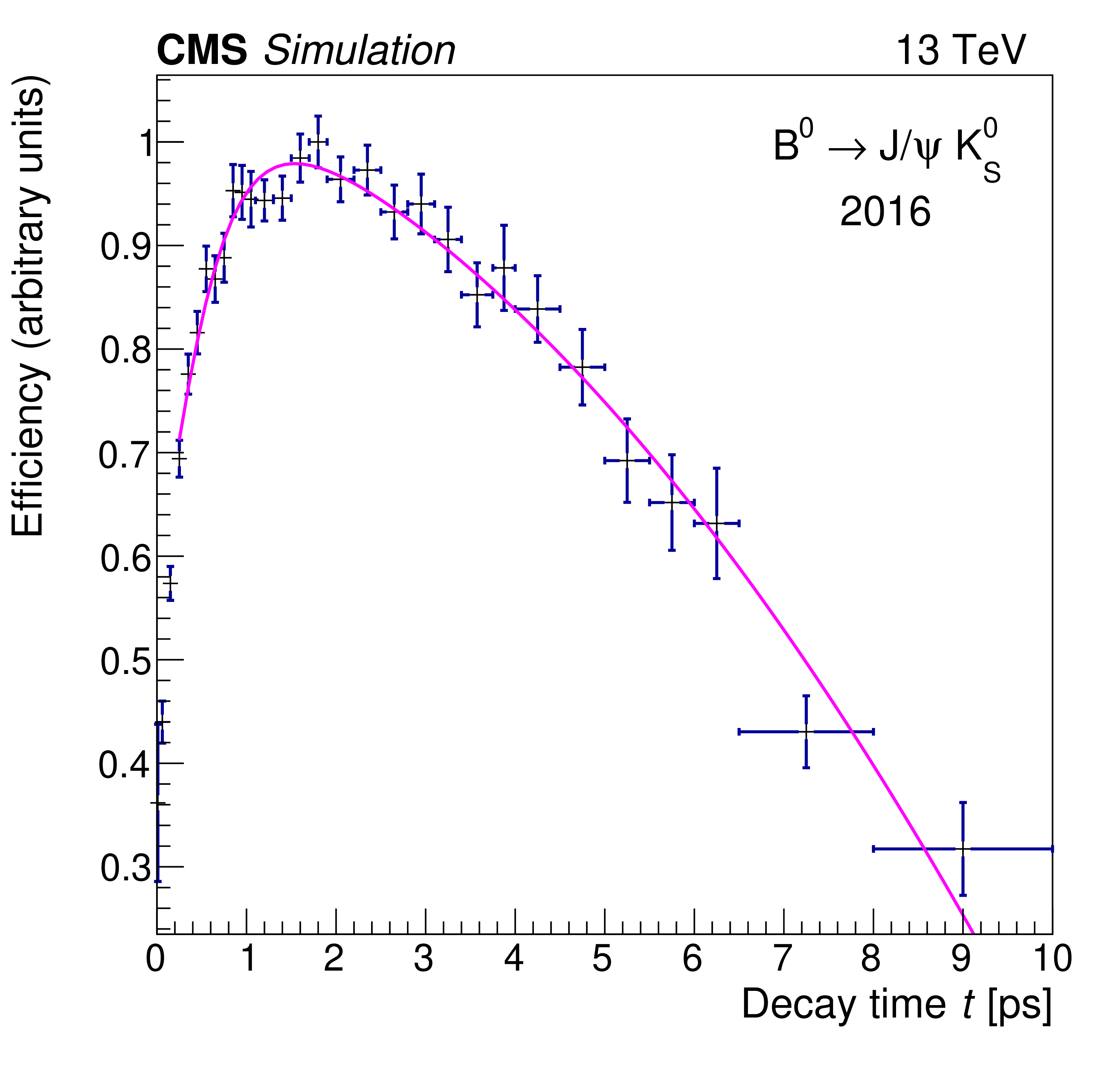
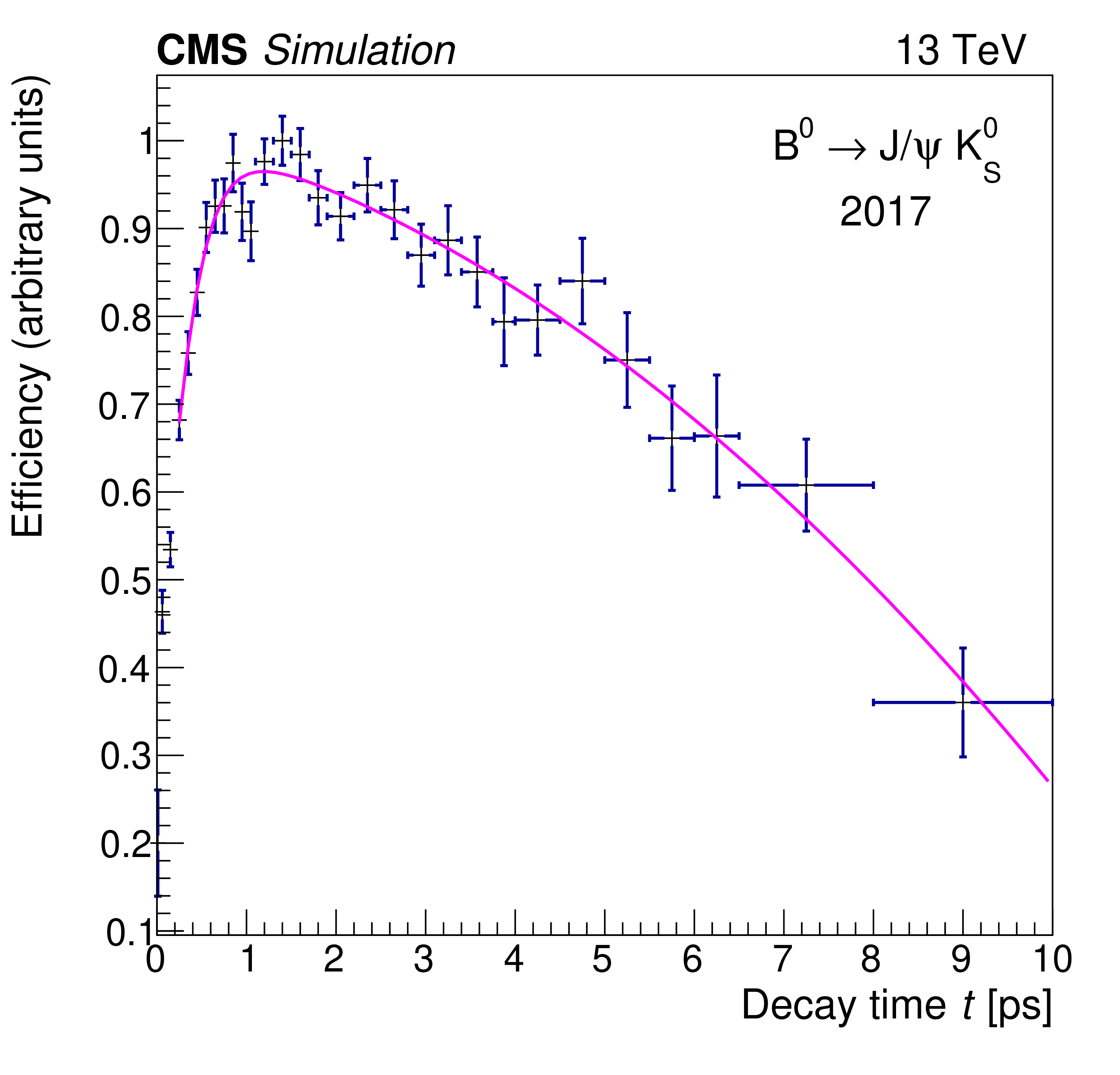
png pdf	Figure 2: The signal efficiency as a function of the decay time for the ${\mathrm{B}^0} \to \mathrm{J}/\psi\mathrm{K^0_S}$ (upper) and $\mathrm{B}_{s}^{0} \to \mathrm{J}/\psi\mathrm{K^0_S}$ (lower) decays from simulation for each of the three data-taking years. The vertical bars indicate the statistical uncertainty, and the horizontal bars give bin widths. The curves show the fit results.
png pdf	Figure 2-a: The signal efficiency as a function of the decay time for the ${\mathrm{B}^0} \to \mathrm{J}/\psi\mathrm{K^0_S}$ (upper) and $\mathrm{B}_{s}^{0} \to \mathrm{J}/\psi\mathrm{K^0_S}$ (lower) decays from simulation for each of the three data-taking years. The vertical bars indicate the statistical uncertainty, and the horizontal bars give bin widths. The curves show the fit results.
png pdf	Figure 2-b: The signal efficiency as a function of the decay time for the ${\mathrm{B}^0} \to \mathrm{J}/\psi\mathrm{K^0_S}$ (upper) and $\mathrm{B}_{s}^{0} \to \mathrm{J}/\psi\mathrm{K^0_S}$ (lower) decays from simulation for each of the three data-taking years. The vertical bars indicate the statistical uncertainty, and the horizontal bars give bin widths. The curves show the fit results.
png pdf	Figure 2-c: The signal efficiency as a function of the decay time for the ${\mathrm{B}^0} \to \mathrm{J}/\psi\mathrm{K^0_S}$ (upper) and $\mathrm{B}_{s}^{0} \to \mathrm{J}/\psi\mathrm{K^0_S}$ (lower) decays from simulation for each of the three data-taking years. The vertical bars indicate the statistical uncertainty, and the horizontal bars give bin widths. The curves show the fit results.
png pdf	Figure 2-d: The signal efficiency as a function of the decay time for the ${\mathrm{B}^0} \to \mathrm{J}/\psi\mathrm{K^0_S}$ (upper) and $\mathrm{B}_{s}^{0} \to \mathrm{J}/\psi\mathrm{K^0_S}$ (lower) decays from simulation for each of the three data-taking years. The vertical bars indicate the statistical uncertainty, and the horizontal bars give bin widths. The curves show the fit results.
png pdf	Figure 2-e: The signal efficiency as a function of the decay time for the ${\mathrm{B}^0} \to \mathrm{J}/\psi\mathrm{K^0_S}$ (upper) and $\mathrm{B}_{s}^{0} \to \mathrm{J}/\psi\mathrm{K^0_S}$ (lower) decays from simulation for each of the three data-taking years. The vertical bars indicate the statistical uncertainty, and the horizontal bars give bin widths. The curves show the fit results.
png pdf	Figure 2-f: The signal efficiency as a function of the decay time for the ${\mathrm{B}^0} \to \mathrm{J}/\psi\mathrm{K^0_S}$ (upper) and $\mathrm{B}_{s}^{0} \to \mathrm{J}/\psi\mathrm{K^0_S}$ (lower) decays from simulation for each of the three data-taking years. The vertical bars indicate the statistical uncertainty, and the horizontal bars give bin widths. The curves show the fit results.
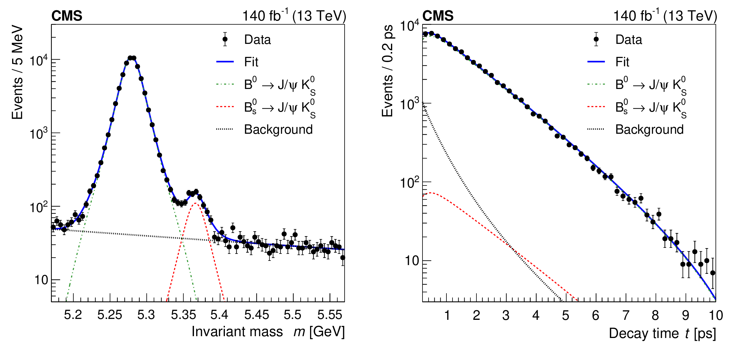
png pdf	Figure 3: Distributions of the $\mathrm{J}/\psi\mathrm{K^0_S}$ invariant mass (left) and proper decay time (right) from data (points) and the results from the 2D UML fit projections (lines) for the 2016-2018 data set. The vertical bars on the data points indicate the statistical uncertainty. The solid, dotted-dashed, dashed, and dotted lines show the total fit, ${\mathrm{B}^0}$ control channel, $\mathrm{B}_{s}^{0}$ signal, and background contributions, respectively.
png pdf	Figure 3-a: Distributions of the $\mathrm{J}/\psi\mathrm{K^0_S}$ invariant mass (left) and proper decay time (right) from data (points) and the results from the 2D UML fit projections (lines) for the 2016-2018 data set. The vertical bars on the data points indicate the statistical uncertainty. The solid, dotted-dashed, dashed, and dotted lines show the total fit, ${\mathrm{B}^0}$ control channel, $\mathrm{B}_{s}^{0}$ signal, and background contributions, respectively.
png pdf	Figure 3-b: Distributions of the $\mathrm{J}/\psi\mathrm{K^0_S}$ invariant mass (left) and proper decay time (right) from data (points) and the results from the 2D UML fit projections (lines) for the 2016-2018 data set. The vertical bars on the data points indicate the statistical uncertainty. The solid, dotted-dashed, dashed, and dotted lines show the total fit, ${\mathrm{B}^0}$ control channel, $\mathrm{B}_{s}^{0}$ signal, and background contributions, respectively.
png pdf	Figure 4: The proper decay time distribution from data (points) for events in the $\mathrm{B}_{s}^{0}$ signal region with $\mathrm{J}/\psi\mathrm{K^0_S}$ invariant mass in the range 5.34-5.42 GeV and the results from the 2D UML fit projections (lines) for the 2016-2018 data set. The vertical bars on the data points indicate the statistical uncertainty. The dashed, dotted-dashed, dotted, and solid lines show the $\mathrm{B}_{s}^{0}$ signal, ${\mathrm{B}^0}$ control channel, background, and total fit contributions, respectively.
png pdf	Figure 5: Distributions of the $\mathrm{J}/\psi\mathrm{K^0_S}$ invariant mass (upper) and decay time (lower) from data (points), along with the projections from the 2D UML fit for each year of data taking. The vertical bars on the data points indicate the statistical uncertainty. The dashed, dotted-dashed, dotted, and solid lines represent the signal, control channel, background, and total fit contributions, respectively.
png pdf	Figure 5-a: Distributions of the $\mathrm{J}/\psi\mathrm{K^0_S}$ invariant mass (upper) and decay time (lower) from data (points), along with the projections from the 2D UML fit for each year of data taking. The vertical bars on the data points indicate the statistical uncertainty. The dashed, dotted-dashed, dotted, and solid lines represent the signal, control channel, background, and total fit contributions, respectively.
png pdf	Figure 5-b: Distributions of the $\mathrm{J}/\psi\mathrm{K^0_S}$ invariant mass (upper) and decay time (lower) from data (points), along with the projections from the 2D UML fit for each year of data taking. The vertical bars on the data points indicate the statistical uncertainty. The dashed, dotted-dashed, dotted, and solid lines represent the signal, control channel, background, and total fit contributions, respectively.
png pdf	Figure 5-c: Distributions of the $\mathrm{J}/\psi\mathrm{K^0_S}$ invariant mass (upper) and decay time (lower) from data (points), along with the projections from the 2D UML fit for each year of data taking. The vertical bars on the data points indicate the statistical uncertainty. The dashed, dotted-dashed, dotted, and solid lines represent the signal, control channel, background, and total fit contributions, respectively.
png pdf	Figure 5-d: Distributions of the $\mathrm{J}/\psi\mathrm{K^0_S}$ invariant mass (upper) and decay time (lower) from data (points), along with the projections from the 2D UML fit for each year of data taking. The vertical bars on the data points indicate the statistical uncertainty. The dashed, dotted-dashed, dotted, and solid lines represent the signal, control channel, background, and total fit contributions, respectively.
png pdf	Figure 5-e: Distributions of the $\mathrm{J}/\psi\mathrm{K^0_S}$ invariant mass (upper) and decay time (lower) from data (points), along with the projections from the 2D UML fit for each year of data taking. The vertical bars on the data points indicate the statistical uncertainty. The dashed, dotted-dashed, dotted, and solid lines represent the signal, control channel, background, and total fit contributions, respectively.
png pdf	Figure 5-f: Distributions of the $\mathrm{J}/\psi\mathrm{K^0_S}$ invariant mass (upper) and decay time (lower) from data (points), along with the projections from the 2D UML fit for each year of data taking. The vertical bars on the data points indicate the statistical uncertainty. The dashed, dotted-dashed, dotted, and solid lines represent the signal, control channel, background, and total fit contributions, respectively.
png pdf	Figure 6: The decay time distribution for events with $\mathrm{J}/\psi\mathrm{K^0_S}$ invariant mass in the range 5.17 $< m <$ 5.22 (upper), 5.22 $< m <$ 5.34 (center), and 5.42 $< m <$ 5.57 (lower) GeV and the fit results for the 2016 (left), 2017 (middle), and 2018 (right) data-taking years.
png pdf	Figure 6-a: The decay time distribution for events with $\mathrm{J}/\psi\mathrm{K^0_S}$ invariant mass in the range 5.17 $< m <$ 5.22 (upper), 5.22 $< m <$ 5.34 (center), and 5.42 $< m <$ 5.57 (lower) GeV and the fit results for the 2016 (left), 2017 (middle), and 2018 (right) data-taking years.
png pdf	Figure 6-b: The decay time distribution for events with $\mathrm{J}/\psi\mathrm{K^0_S}$ invariant mass in the range 5.17 $< m <$ 5.22 (upper), 5.22 $< m <$ 5.34 (center), and 5.42 $< m <$ 5.57 (lower) GeV and the fit results for the 2016 (left), 2017 (middle), and 2018 (right) data-taking years.
png pdf	Figure 6-c: The decay time distribution for events with $\mathrm{J}/\psi\mathrm{K^0_S}$ invariant mass in the range 5.17 $< m <$ 5.22 (upper), 5.22 $< m <$ 5.34 (center), and 5.42 $< m <$ 5.57 (lower) GeV and the fit results for the 2016 (left), 2017 (middle), and 2018 (right) data-taking years.
png pdf	Figure 6-d: The decay time distribution for events with $\mathrm{J}/\psi\mathrm{K^0_S}$ invariant mass in the range 5.17 $< m <$ 5.22 (upper), 5.22 $< m <$ 5.34 (center), and 5.42 $< m <$ 5.57 (lower) GeV and the fit results for the 2016 (left), 2017 (middle), and 2018 (right) data-taking years.
png pdf	Figure 6-e: The decay time distribution for events with $\mathrm{J}/\psi\mathrm{K^0_S}$ invariant mass in the range 5.17 $< m <$ 5.22 (upper), 5.22 $< m <$ 5.34 (center), and 5.42 $< m <$ 5.57 (lower) GeV and the fit results for the 2016 (left), 2017 (middle), and 2018 (right) data-taking years.
png pdf	Figure 6-f: The decay time distribution for events with $\mathrm{J}/\psi\mathrm{K^0_S}$ invariant mass in the range 5.17 $< m <$ 5.22 (upper), 5.22 $< m <$ 5.34 (center), and 5.42 $< m <$ 5.57 (lower) GeV and the fit results for the 2016 (left), 2017 (middle), and 2018 (right) data-taking years.
png pdf	Figure 6-g: The decay time distribution for events with $\mathrm{J}/\psi\mathrm{K^0_S}$ invariant mass in the range 5.17 $< m <$ 5.22 (upper), 5.22 $< m <$ 5.34 (center), and 5.42 $< m <$ 5.57 (lower) GeV and the fit results for the 2016 (left), 2017 (middle), and 2018 (right) data-taking years.
png pdf	Figure 6-h: The decay time distribution for events with $\mathrm{J}/\psi\mathrm{K^0_S}$ invariant mass in the range 5.17 $< m <$ 5.22 (upper), 5.22 $< m <$ 5.34 (center), and 5.42 $< m <$ 5.57 (lower) GeV and the fit results for the 2016 (left), 2017 (middle), and 2018 (right) data-taking years.
png pdf	Figure 6-i: The decay time distribution for events with $\mathrm{J}/\psi\mathrm{K^0_S}$ invariant mass in the range 5.17 $< m <$ 5.22 (upper), 5.22 $< m <$ 5.34 (center), and 5.42 $< m <$ 5.57 (lower) GeV and the fit results for the 2016 (left), 2017 (middle), and 2018 (right) data-taking years.
png pdf	Figure 7: The invariant mass distribution for events with $\mathrm{J}/\psi\mathrm{K^0_S}$ decay time in the range 0.2 $< t <$ 2.5 (upper), 2.5 $< t <$ 3.5 (center), and 3.5 $< t <$ 10.0 (lower)\unitps and the fit results for the 2016 (left), 2017 (middle), and 2018 (right) data-taking years.
png pdf	Figure 7-a: The invariant mass distribution for events with $\mathrm{J}/\psi\mathrm{K^0_S}$ decay time in the range 0.2 $< t <$ 2.5 (upper), 2.5 $< t <$ 3.5 (center), and 3.5 $< t <$ 10.0 (lower)\unitps and the fit results for the 2016 (left), 2017 (middle), and 2018 (right) data-taking years.
png pdf	Figure 7-b: The invariant mass distribution for events with $\mathrm{J}/\psi\mathrm{K^0_S}$ decay time in the range 0.2 $< t <$ 2.5 (upper), 2.5 $< t <$ 3.5 (center), and 3.5 $< t <$ 10.0 (lower)\unitps and the fit results for the 2016 (left), 2017 (middle), and 2018 (right) data-taking years.
png pdf	Figure 7-c: The invariant mass distribution for events with $\mathrm{J}/\psi\mathrm{K^0_S}$ decay time in the range 0.2 $< t <$ 2.5 (upper), 2.5 $< t <$ 3.5 (center), and 3.5 $< t <$ 10.0 (lower)\unitps and the fit results for the 2016 (left), 2017 (middle), and 2018 (right) data-taking years.
png pdf	Figure 7-d: The invariant mass distribution for events with $\mathrm{J}/\psi\mathrm{K^0_S}$ decay time in the range 0.2 $< t <$ 2.5 (upper), 2.5 $< t <$ 3.5 (center), and 3.5 $< t <$ 10.0 (lower)\unitps and the fit results for the 2016 (left), 2017 (middle), and 2018 (right) data-taking years.
png pdf	Figure 7-e: The invariant mass distribution for events with $\mathrm{J}/\psi\mathrm{K^0_S}$ decay time in the range 0.2 $< t <$ 2.5 (upper), 2.5 $< t <$ 3.5 (center), and 3.5 $< t <$ 10.0 (lower)\unitps and the fit results for the 2016 (left), 2017 (middle), and 2018 (right) data-taking years.
png pdf	Figure 7-f: The invariant mass distribution for events with $\mathrm{J}/\psi\mathrm{K^0_S}$ decay time in the range 0.2 $< t <$ 2.5 (upper), 2.5 $< t <$ 3.5 (center), and 3.5 $< t <$ 10.0 (lower)\unitps and the fit results for the 2016 (left), 2017 (middle), and 2018 (right) data-taking years.
png pdf	Figure 7-g: The invariant mass distribution for events with $\mathrm{J}/\psi\mathrm{K^0_S}$ decay time in the range 0.2 $< t <$ 2.5 (upper), 2.5 $< t <$ 3.5 (center), and 3.5 $< t <$ 10.0 (lower)\unitps and the fit results for the 2016 (left), 2017 (middle), and 2018 (right) data-taking years.
png pdf	Figure 7-h: The invariant mass distribution for events with $\mathrm{J}/\psi\mathrm{K^0_S}$ decay time in the range 0.2 $< t <$ 2.5 (upper), 2.5 $< t <$ 3.5 (center), and 3.5 $< t <$ 10.0 (lower)\unitps and the fit results for the 2016 (left), 2017 (middle), and 2018 (right) data-taking years.
png pdf	Figure 7-i: The invariant mass distribution for events with $\mathrm{J}/\psi\mathrm{K^0_S}$ decay time in the range 0.2 $< t <$ 2.5 (upper), 2.5 $< t <$ 3.5 (center), and 3.5 $< t <$ 10.0 (lower)\unitps and the fit results for the 2016 (left), 2017 (middle), and 2018 (right) data-taking years.

Tables
png pdf	Table 1: Sources of systematic uncertainties in the $\mathrm{B}_{s}^{0} \to \mathrm{J}/\psi\mathrm{K^0_S}$ effective lifetime measurement and their estimated values, along with the total systematic uncertainty.

Summary

In this paper, a measurement of the effective lifetime of the

$\mathrm{B}_{s}^{0}$ meson in the

$\mathrm{J}/\psi\mathrm{K^0_S}$ decay channel is presented. The analysis is performed using data collected by the CMS detector during proton-proton collisions at a center-of-mass energy of 13 TeV from 2016 to 2018, corresponding to an integrated luminosity of 140 fb

$^{-1}$ . The effective lifetime is extracted using a two-dimensional unbinned maximum likelihood fit to the invariant mass and proper decay time distributions of the

$\mathrm{B}_{s}^{0}$ meson. The decay

${\mathrm{B}^0} \to \mathrm{J}/\psi\mathrm{K^0_S}$ , which has a much larger event yield than the corresponding

$\mathrm{B}_{s}^{0}$ decay, is used as a control channel for estimating resolutions and systematic uncertainties. The measured value of the effective lifetime is

$\tau(\mathrm{B}_{s}^{0} \to \mathrm{J}/\psi\mathrm{K^0_S}) =$ 1.59

$\pm$ 0.07 (stat)

$\pm$ 0.03 (syst) ps, which is the most precise result to date. This measurement can be used to constrain the parameters that govern mixing and CP violation in the

$\mathrm{B}_{s}^{0}$ system and also to better understand the penguin contributions in measurements of

$\sin{(2\beta)}$ from

${\mathrm{B}^0} \to \mathrm{J}/\psi\mathrm{K^0_S}$ decays.

References
1	J. Albrecht, F. Bernlochner, A. Lenz, and A. Rusov	Lifetimes of b-hadrons and mixing of neutral B-mesons: theoretical and experimental status	Eur. Phys. J. ST 233 (2024) 359	2402.04224
2	N. Cabibbo	Unitary symmetry and leptonic decays	PRL 10 (1963) 531
3	M. Kobayashi and T. Maskawa	$C\hspace{-.08em}P$ violation in the renormalizable theory of weak interaction	Prog. Theor. Phys. 49 (1973) 652
4	M. Ciuchini, M. Pierini, and L. Silvestrini	Effect of penguin operators in the ${\mathrm{B}^0} \to \mathrm{J}/\psi \mathrm{K}^0 C\hspace{-.08em}P$ asymmetry	PRL 95 (2005) 221804	hep-ph/0507290
5	S. Faller, M. Jung, R. Fleischer, and T. Mannel	The golden modes ${\mathrm{B}^0} \to \mathrm{J}/\psi \mathrm{K}_\mathrm{S,L}$ in the era of precision flavour physics	PRD 79 (2009) 014030	0809.0842
6	M. Jung	Determining weak phases from $\mathrm{B} \to \mathrm{J}/\psi P$ decays	PRD 86 (2012) 053008	1206.2050
7	P. Frings, U. Nierste, and M. Wiebusch	Penguin contributions to $C\hspace{-.08em}P$ phases in $\mathrm{B}_\mathrm{d,s}$ decays to charmonium	PRL 115 (2015) 061802	1503.00859
8	LHCb Collaboration	Measurement of $C\hspace{-.08em}P$ violation in ${\mathrm{B}^0} \to \psi( \to l^{+}l^{-}) \mathrm{K^0_S}( \to \pi^{+}\pi^{-})$ decays	PRL 132 (2024) 021801	2309.09728
9	R. Fleischer	Recent theoretical developments in $C\hspace{-.08em}P$ violation in the B system	NIM A 446 (2000) 1	hep-ph/9908340
10	K. De Bruyn, R. Fleischer, and P. Koppenburg	Extracting $\gamma$ and penguin topologies through $C\hspace{-.08em}P$ violation in $\mathrm{B}_{s}^{0} \to \mathrm{J}/\psi\mathrm{K^0_S}$	EPJC 70 (2010) 1025	1010.0089
11	K. De Bruyn and R. Fleischer	A roadmap to control penguin effects in $\mathrm{B}_\mathrm{d}^0 \to \mathrm{J}/\psi\mathrm{K^0_S}$ and $\mathrm{B}_{s}^{0} \to \mathrm{J}/\psi \phi$	JHEP 03 (2015) 145	1412.6834
12	M. Z. Barel, K. De Bruyn, R. Fleischer, and E. Malami	In pursuit of new physics with $\mathrm{B}_\mathrm{d}^0 \to \mathrm{J}/\psi {\mathrm{k}^0}$ and $\mathrm{B}_{s}^{0} \to \mathrm{J}/\psi \phi$ decays at the high-precision frontier	JPG 48 (2021) 065002	2010.14423
13	M. Z. Barel, K. De Bruyn, R. Fleischer, and E. Malami	Penguin effects in $\mathrm{B}_\mathrm{d}^0 \to \mathrm{J}/\psi\mathrm{K^0_S}$ and $\mathrm{B}_{s}^{0} \to \mathrm{J}/\psi \phi$	PoS CKM 111, 2023 link	2203.14652
14	K. De Bruyn et al.	Branching ratio measurements of $\mathrm{B}_{s}^{0}$ decays	PRD 86 (2012) 014027	1204.1735
15	CMS Collaboration	Measurement of the $\mathrm{B}_{s}^{0} \to \mu^{+}\mu^{-}$ decay properties and search for the ${\mathrm{B}^0} \to \mu^{+}\mu^{-}$ decay in proton-proton collisions at $\sqrt{s} =$ 13 TeV	PLB 842 (2023) 137955	CMS-BPH-21-006 2212.10311
16	CMS Collaboration	Measurement of properties of $\mathrm{B}_{s}^{0} \to \mu^{+}\mu^{-}$ decays and search for ${\mathrm{B}^0} \to \mu^{+}\mu^{-}$ with the CMS experiment	JHEP 04 (2020) 188	CMS-BPH-16-004 1910.12127
17	CMS Collaboration	Measurement of b hadron lifetimes in pp collisions at $\sqrt{s} =$ 8 TeV	EPJC 78 (2018) 457	CMS-BPH-13-008 1710.08949
18	ATLAS Collaboration	Measurement of the $\mathrm{B}_{s}^{0} \to \mu^{+}\mu^{-}$ effective lifetime with the ATLAS detector	JHEP 09 (2023) 199	2308.01171
19	LHCb Collaboration	Measurement of $\tau_\mathrm{L}$ using the $\mathrm{B}_{s}^{0} \to \mathrm{J}/\psi \eta$ decay mode	EPJC 83 (2023) 629	2206.03088
20	LHCb Collaboration	Analysis of neutral B-meson decays into two muons	PRL 128 (2022) 041801	2108.09284
21	LHCb Collaboration	Measurement of the $\mathrm{B}_{s}^{0} \to \mu^{+}\mu^{-}$ decay properties and search for the ${\mathrm{B}^0} \to \mu^{+}\mu^{-}$ and $\mathrm{B}_{s}^{0} \to \mu^{+}\mu^{-}\gamma$ decays	PRD 105 (2022) 012010	2108.09283
22	LHCb Collaboration	Measurement of the $\mathrm{B}_{s}^{0} \to \mu^{+}\mu^{-}$ branching fraction and effective lifetime and search for ${\mathrm{B}^0} \to \mu^{+}\mu^{-}$ decays	PRL 118 (2017) 191801	1703.05747
23	LHCb Collaboration	Measurement of the $\mathrm{B}_{s}^{0} \to \mathrm{J}/\psi \eta$ lifetime	PLB 762 (2016) 484	1607.06314
24	LHCb Collaboration	Effective lifetime measurements in the $\mathrm{B}_{s}^{0} \to \mathrm{K}^+\mathrm{K}^-$ , ${\mathrm{B}^0} \to \mathrm{K}^+\pi^-$ and $\mathrm{B}_{s}^{0}\to \pi^+ \mathrm{K}^-$ decays	PLB 736 (2014) 446	1406.7204
25	LHCb Collaboration	Measurements of the $\mathrm{B}^+$ , $\mathrm{B}^0$ , $\mathrm{B}^0_\mathrm{s}$ meson and $\Lambda^0_\mathrm{b}$ baryon lifetimes	JHEP 04 (2014) 114	1402.2554
26	LHCb Collaboration	Measurement of the $\overline{\mathrm{B}}_{s}^{0}\to \mathrm{D}_\mathrm{s}^-\mathrm{D}_\mathrm{s}^+$ and $\overline{\mathrm{B}}_{s}^{0}\to \mathrm{D}^-\mathrm{D}_\mathrm{s}^+$ effective lifetimes	PRL 112 (2014) 111802	1312.1217
27	LHCb Collaboration	Measurement of the effective $\mathrm{B}_{s}^{0} \to \mathrm{J}/\psi\mathrm{K^0_S}$ lifetime	NPB 873 (2013) 275	1304.4500
28	LHCb Collaboration	Measurement of the effective $\mathrm{B}_{s}^{0}\to \mathrm{K}^+\mathrm{K}^-$ lifetime	PLB 707 (2012) 349	1111.0521
29	LHCb Collaboration	Measurement of the $\mathrm{B}_{s}^{0}$ effective lifetime in the $\mathrm{J}/\psi f_0$ final state	PRL 109 (2012) 152002	1207.0878
30	LHCb Collaboration	Measurement of the effective $\mathrm{B}_{s}^{0} \to \mathrm{K}^+\mathrm{K}^-$ lifetime	PLB 716 (2012) 393	1207.5993
31	Heavy Flavor Averaging Group	Averages of b-hadron, c-hadron, and $\tau$ -lepton properties as of 2021	PRD 107 (2023) 052008	2206.07501
32	CDF Collaboration	Observation of $B^0_s \to J/\psi K^{*0}(892)$ and $B^0_s \to J/\psi K^0_S$ decays	PRD 83 (2011) 052012	1102.1961
33	R. Fleischer and R. Knegjens	Effective lifetimes of $\mathrm{B}_{s}^{0}$ decays and their constraints on the $\mathrm{B}_{s}^{0}$ - $\overline{\mathrm{B}}_{s}^{0}$ mixing parameters	EPJC 71 (2011) 1789	1109.5115
34	Particle Data Group	Review of particle physics	PRD 110 (2024) 030001
35	CMS Collaboration	Description and performance of track and primary-vertex reconstruction with the CMS tracker	JINST 9 (2014) P10009	CMS-TRK-11-001 1405.6569
36	Tracker group of the CMS Collaboration	The CMS phase-1 pixel detector upgrade	JINST 16 (2021) P02027	2012.14304
37	CMS Collaboration	Track impact parameter resolution for the full pseudo rapidity coverage in the 2017 dataset with the CMS phase-1 pixel detector	CMS Detector Performance Note CMS-DP-2020-049, 2020 CDS
38	CMS Collaboration	The CMS experiment at the CERN LHC	JINST 3 (2008) S08004
39	CMS Collaboration	Performance of the CMS Level-1 trigger in proton-proton collisions at $\sqrt{s} =$ 13 TeV	JINST 15 (2020) P10017	CMS-TRG-17-001 2006.10165
40	CMS Collaboration	The CMS trigger system	JINST 12 (2017) P01020	CMS-TRG-12-001 1609.02366
41	CMS Collaboration	Precision luminosity measurement in proton-proton collisions at $\sqrt{s}=$ 13 TeV in 2015 and 2016 at CMS	EPJC 81 (2021) 800	CMS-LUM-17-003 2104.01927
42	CMS Collaboration	CMS luminosity measurement for the 2017 data-taking period at $\sqrt{s} =$ 13 TeV	CMS Physics Analysis Summary, 2018 link	CMS-PAS-LUM-17-004
43	CMS Collaboration	CMS luminosity measurement for the 2018 data-taking period at $\sqrt{s} =$ 13 TeV	CMS Physics Analysis Summary, 2019 link	CMS-PAS-LUM-18-002
44	T. Sjöstrand et al.	An introduction to PYTHIA 8.2	Comput. Phys. Commun. 191 (2015) 159	1410.3012
45	D. J. Lange	The EvtGen particle decay simulation package	NIM A 462 (2001) 152
46	E. Barberio and Z. Was	PHOTOS --- a universal Monte Carlo for QED radiative corrections: version 2.0	Comput. Phys. Commun. 79 (1994) 291
47	GEANT4 Collaboration	GEANT 4 --- a simulation toolkit	NIM A 506 (2003) 250
48	CMS Collaboration	Performance of the CMS muon detector and muon reconstruction with proton-proton collisions at $\sqrt{s}=$ 13 TeV	JINST 13 (2018) P06015	CMS-MUO-16-001 1804.04528
49	CMS Collaboration	CMS tracking performance results from early LHC operation	EPJC 70 (2010) 1165	CMS-TRK-10-001 1007.1988
50	R. Frühwirth	Application of Kalman filtering to track and vertex fitting	NIM A 262 (1987) 444
51	J. Podolanski and R. Armenteros	Analysis of V-events	Philosophical Magazine 45 (1954) 13
52	J. E. Gaiser	Charmonium spectroscopy from radiative decays of $\mathrm{J}/\psi$ and $\psi'$	PhD thesis, Stanford University, SLAC Report SLAC-R-255, 1982 link
53	N. L. Johnson	Systems of frequency curves generated by methods of translation	Biometrika 36 (1949) 149
54	S. Jackman	Bayesian analysis for the social sciences	John Wiley & Sons, New Jersey, USA, 2009 link
55	CMS Collaboration	HEPData record for this analysis	link