CMS-BPH-13-008

CMS-BPH-13-008 ; CERN-EP-2017-244
Measurement of b hadron lifetimes in pp collisions at $\sqrt{s} =$ 8 TeV
CMS Collaboration
24 October 2017
Eur. Phys. J. C 78 (2018) 457 [Erratum]
Abstract: Measurements are presented of the lifetimes of the $\mathrm{B}^{0}$ , $\mathrm{B}^{0}_{\mathrm{s}}$ , $\Lambda_\mathrm{b}^0$ , and $\mathrm{B}_{\mathrm{c}}^{+}$ hadrons using the decay channels ${\mathrm{B}^{0} \!\to\! \mathrm{J}/\psi {\mathrm{K^{}(892)}}^{0}}$ , ${\mathrm{B}^{0} \!\to\! \mathrm{J}/\psi {\mathrm{K^0_S}}}$ , ${\mathrm{B}^{0}_{\mathrm{s}} \!\to\! \mathrm{J}/\psi \pi^{+} \pi^{-}}$ , ${\mathrm{B}^{0}_{\mathrm{s}} \!\to\! \mathrm{J}/\psi \phi(1020)}$ , $\Lambda_{\mathrm{b}} \to \mathrm{J}/\psi \Lambda$ , and $\mathrm{B}_{\mathrm{c}}^{+} \to \mathrm{J}/\psi \pi^{+}$ . The data sample, corresponding to an integrated luminosity of 19.7 fb $^{-1}$ , was collected by the CMS detector at the LHC in proton-proton collisions at $\sqrt{s} =$ 8 TeV. The $\mathrm{B}^{0}$ lifetime is measured to be 453.0 $\pm$ 1.6 (stat) $\pm$ 1.5 (syst) $\mu$ m in ${\mathrm{J}/\psi {\mathrm{K^{}(892)}}^{0}}$ and 457.8 $\pm$ 2.7 (stat) $\pm$ 2.7 (syst) $\mu$ m in ${\mathrm{J}/\psi {\mathrm{K^0_S}}}$ , which results in a combined measurement of $c\tau_{\mathrm{B}^{0}} =$ 454.1 $\pm$ 1.4 (stat) $\pm$ 1.3 (syst) $\mu$ m. The effective lifetime of the $\mathrm{B}^{0}_{\mathrm{s}}$ meson is measured in two decay modes, with contributions from different amounts of the heavy and light eigenstates. This results in two different measured lifetimes: $c\tau_{\mathrm{B}^{0}_{\mathrm{s}} \to \mathrm{J}/\psi \pi^{+} \pi^{-}} =$ 502.7 $\pm$ 10.2 (stat) $\pm$ 3.2 (syst) $\mu$ m and $c\tau_{\mathrm{B}^{0}_{\mathrm{s}} \to \mathrm{J}/\psi \phi(1020)} =$ 443.9 $\pm$ 2.0 (stat) $\pm$ 1.2 (syst) $\mu$ m. The $\Lambda_\mathrm{b}^0$ lifetime is found to be 442.9 $\pm$ 8.2 (stat) $\pm$ 2.7 (syst) $\mu$ m. The precision from each of these channels is as good as or better than previous measurements. The $\mathrm{B}_{\mathrm{c}}^{+}$ lifetime, measured with respect to the $\mathrm{B^{+}}$ to reduce the systematic uncertainty, is 162.3 $\pm$ 8.2 (stat) $\pm$ 4.7 (syst) $\pm$ 0.1 ( $\tau_{\mathrm{B^{+}}}$ ) $\mu$ m. All results are in agreement with current world-average values.
Links: e-print arXiv:1710.08949 [hep-ex] (PDF) ; CDS record ; inSPIRE record ; HepData record ; CADI line (restricted) ;

Figures & Tables	Summary	References	CMS Publications

Figures
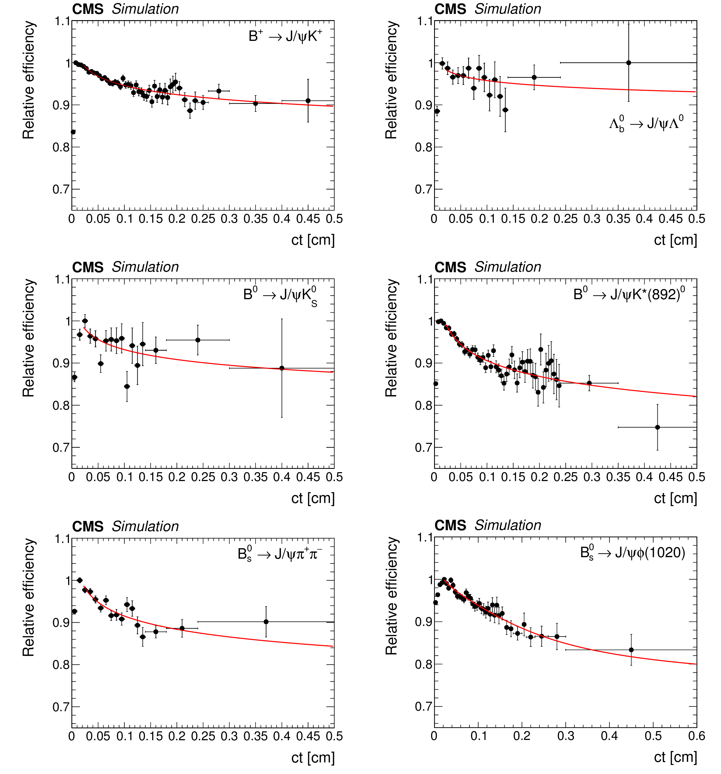
png pdf	Figure 1: The combined reconstruction and selection efficiency from simulation versus ${ct}$ with a superimposed fit to an inverse power function for ${\mathrm{B^{+}} \to \mathrm{J}/\psi \mathrm{K^{+}}}$ (upper left), ${\Lambda_{\mathrm{b}}^{0} \to \mathrm{J}/\psi \Lambda ^{0}}$ (upper right), ${\mathrm{B}^{0} \to \mathrm{J}/\psi {\mathrm{K^0_S}}}$ (centre left), ${\mathrm{B}^{0} \to \mathrm{J}/\psi {\mathrm{K^{*}(892)}} ^{0}}$ (centre right), ${\mathrm{B}^{0}_{\mathrm{s}} \to \mathrm{J}/\psi \pi^{+} \pi^{-}}$ (lower left), and ${\mathrm{B}^{0}_{\mathrm{s}} \to \mathrm{J}/\psi \phi (1020)}$ (lower right). The efficiency scale is arbitrary.
png pdf	Figure 1-a: The combined reconstruction and selection efficiency from simulation versus ${ct}$ with a superimposed fit to an inverse power function for ${\mathrm{B^{+}} \to \mathrm{J}/\psi \mathrm{K^{+}}}$ . The efficiency scale is arbitrary.
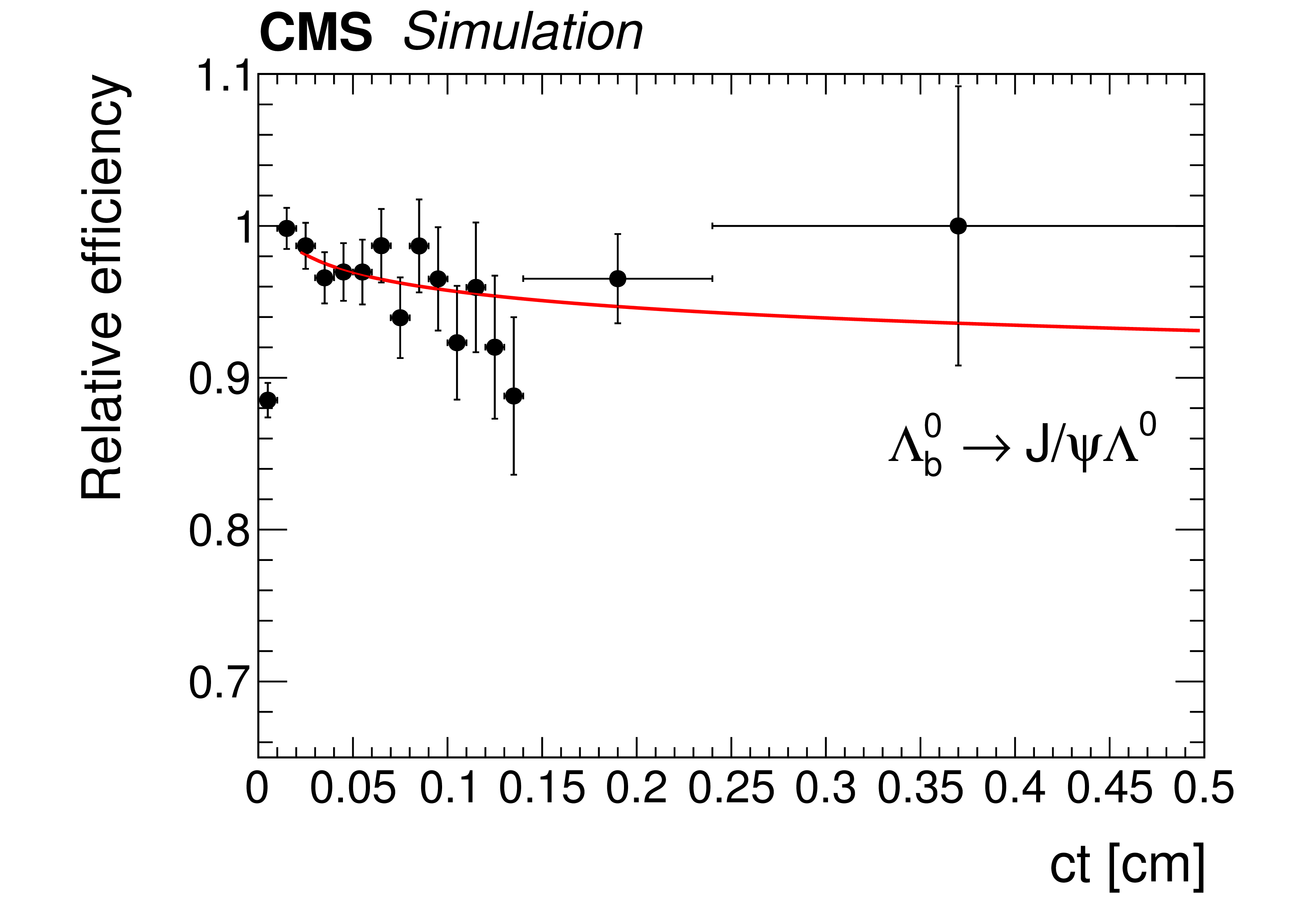
png pdf	Figure 1-b: The combined reconstruction and selection efficiency from simulation versus ${ct}$ with a superimposed fit to an inverse power function for ${\Lambda_{\mathrm{b}}^{0} \to \mathrm{J}/\psi \Lambda ^{0}}$ . The efficiency scale is arbitrary.
png pdf	Figure 1-c: The combined reconstruction and selection efficiency from simulation versus ${ct}$ with a superimposed fit to an inverse power function for ${\mathrm{B}^{0} \to \mathrm{J}/\psi {\mathrm{K^0_S}}}$ . The efficiency scale is arbitrary.
png pdf	Figure 1-d: The combined reconstruction and selection efficiency from simulation versus ${ct}$ with a superimposed fit to an inverse power function for ${\mathrm{B}^{0} \to \mathrm{J}/\psi {\mathrm{K^{*}(892)}} ^{0}}$ . The efficiency scale is arbitrary.
png pdf	Figure 1-e: The combined reconstruction and selection efficiency from simulation versus ${ct}$ with a superimposed fit to an inverse power function for ${\mathrm{B}^{0}_{\mathrm{s}} \to \mathrm{J}/\psi \pi^{+} \pi^{-}}$ . The efficiency scale is arbitrary.
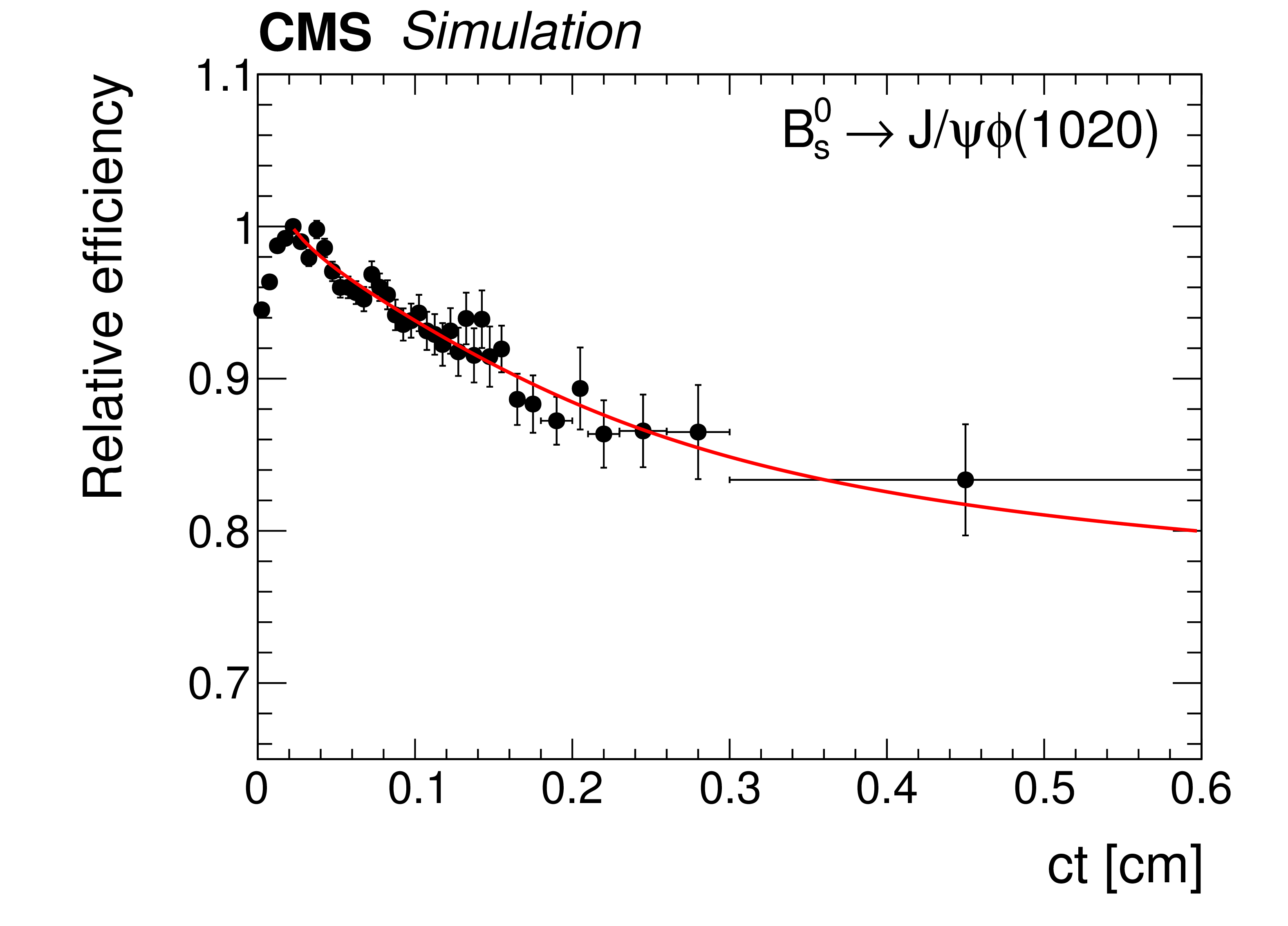
png pdf	Figure 1-f: The combined reconstruction and selection efficiency from simulation versus ${ct}$ with a superimposed fit to an inverse power function for ${\mathrm{B}^{0}_{\mathrm{s}} \to \mathrm{J}/\psi \phi (1020)}$ . The efficiency scale is arbitrary.
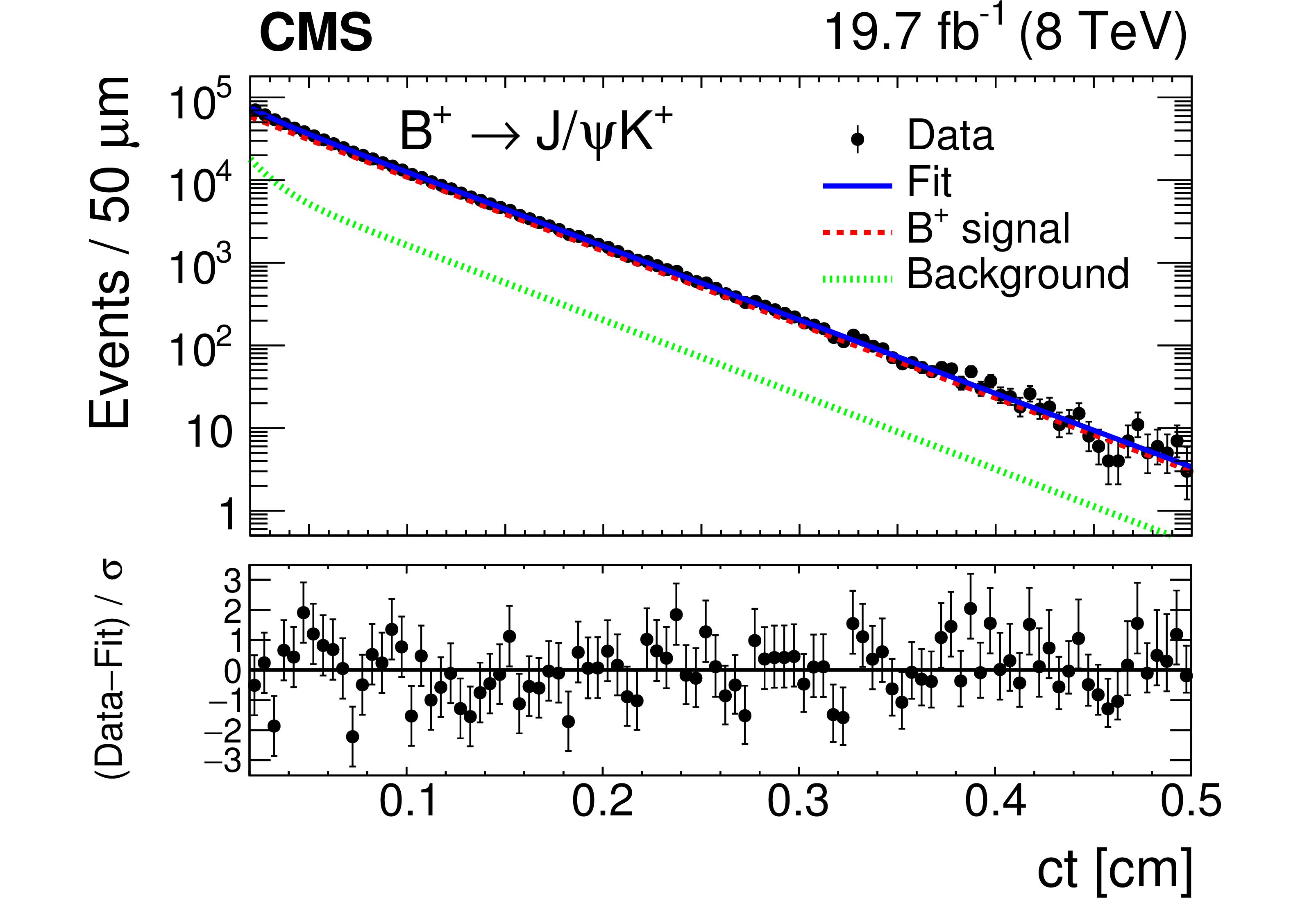
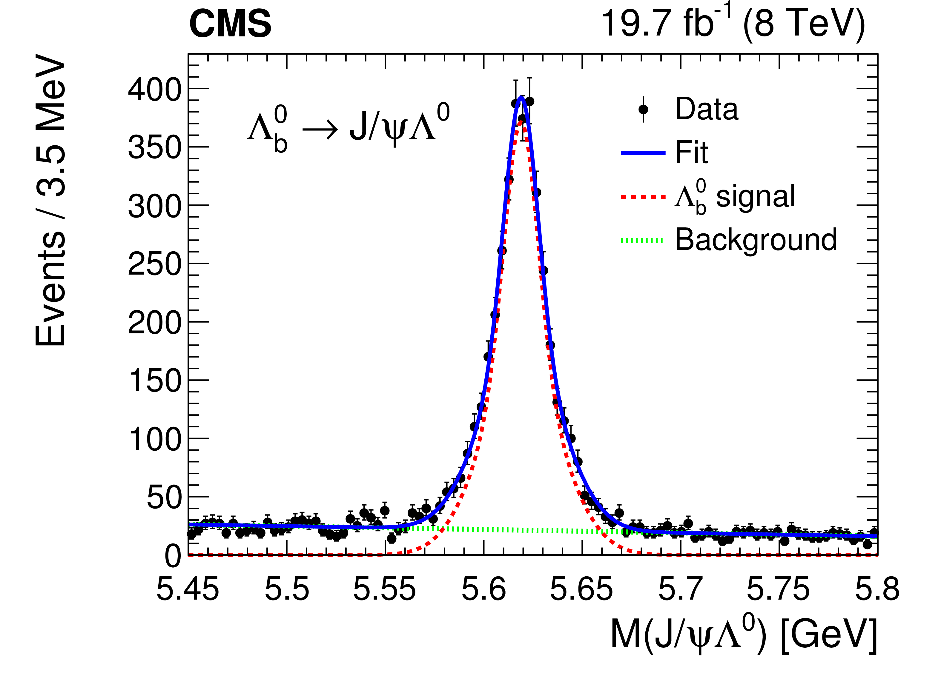
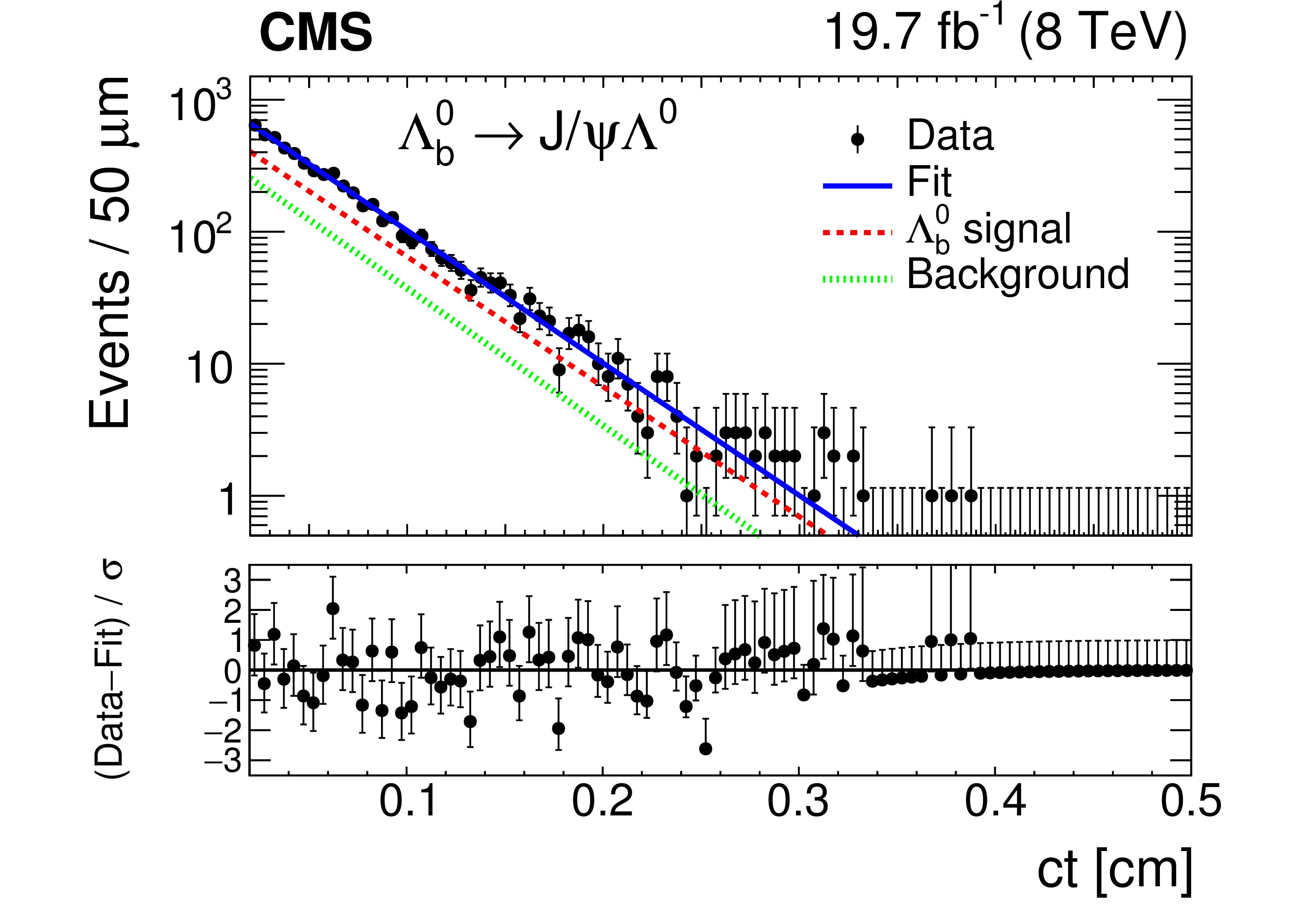
png pdf	Figure 2: Invariant mass (left) and $ct$ (right) distributions for ${\mathrm{B^{+}}}$ (upper) and for $\Lambda_{\mathrm{b}}^{0}$ (lower) candidates. The curves are projections of the fit to the data, with the contributions from signal (dashed), background (dotted), and the sum of signal and background (solid) shown. The bottom panels of the figures on the right show the difference between the observed data and the fit divided by the data uncertainty. The vertical bars on the data points represent the statistical uncertainties.
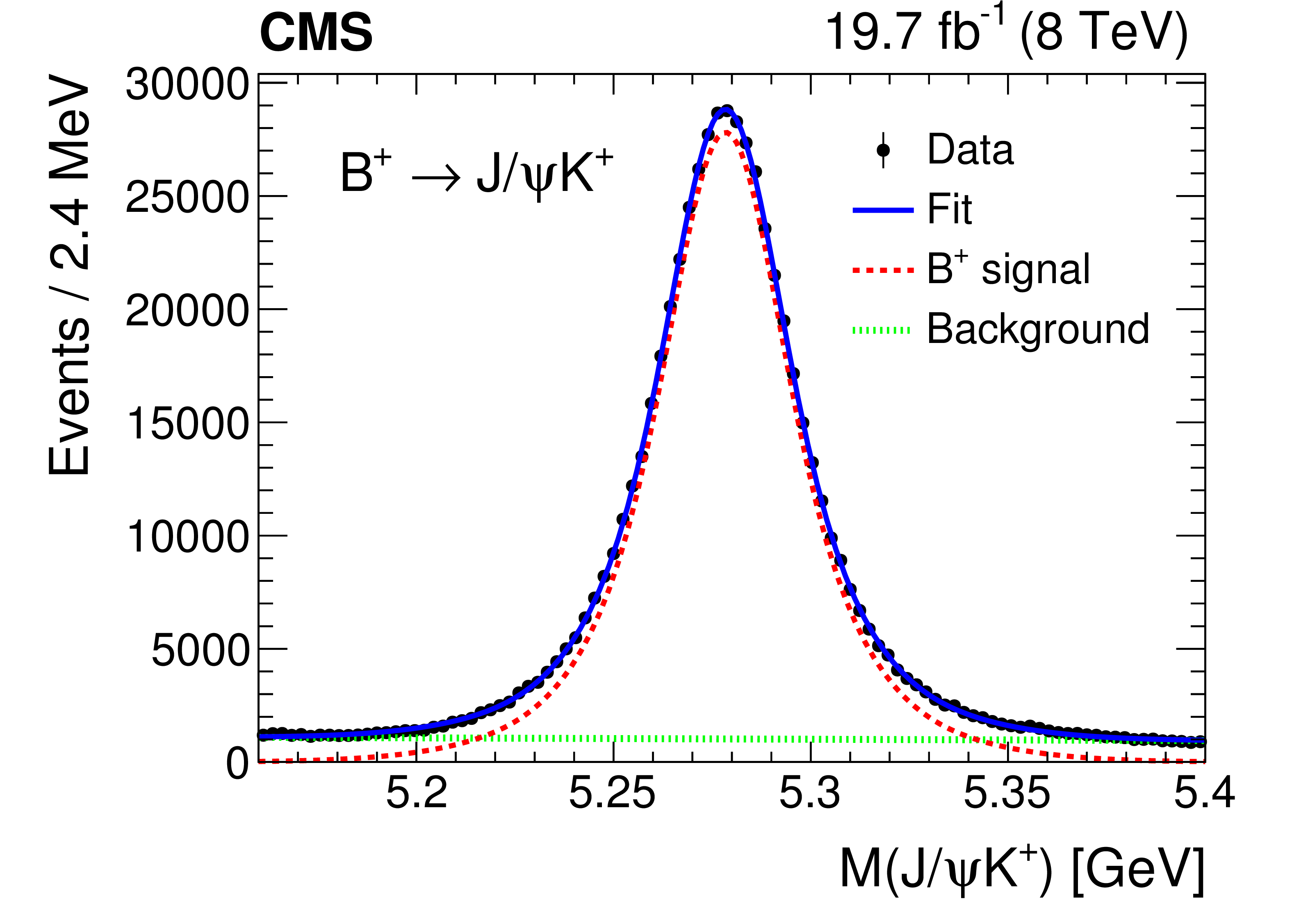
png pdf	Figure 2-a: Invariant mass distribution for ${\mathrm{B^{+}}}$ candidates. The curves are projections of the fit to the data, with the contributions from signal (dashed), background (dotted), and the sum of signal and background (solid) shown. The vertical bars on the data points represent the statistical uncertainties.
png pdf	Figure 2-b: $ct$ distribution for $\Lambda_{\mathrm{b}}^{0}$ candidates. The curves are projections of the fit to the data, with the contributions from signal (dashed), background (dotted), and the sum of signal and background (solid) shown. The bottom panel shows the difference between the observed data and the fit divided by the data uncertainty. The vertical bars on the data points represent the statistical uncertainties.
png pdf	Figure 2-c: Invariant mass distribution for ${\mathrm{B^{+}}}$ candidates. The curves are projections of the fit to the data, with the contributions from signal (dashed), background (dotted), and the sum of signal and background (solid) shown.The vertical bars on the data points represent the statistical uncertainties.
png pdf	Figure 2-d: $ct$ distribution for $\Lambda_{\mathrm{b}}^{0}$ candidates. The curves are projections of the fit to the data, with the contributions from signal (dashed), background (dotted), and the sum of signal and background (solid) shown. The bottom panel shows the difference between the observed data and the fit divided by the data uncertainty. The vertical bars on the data points represent the statistical uncertainties.
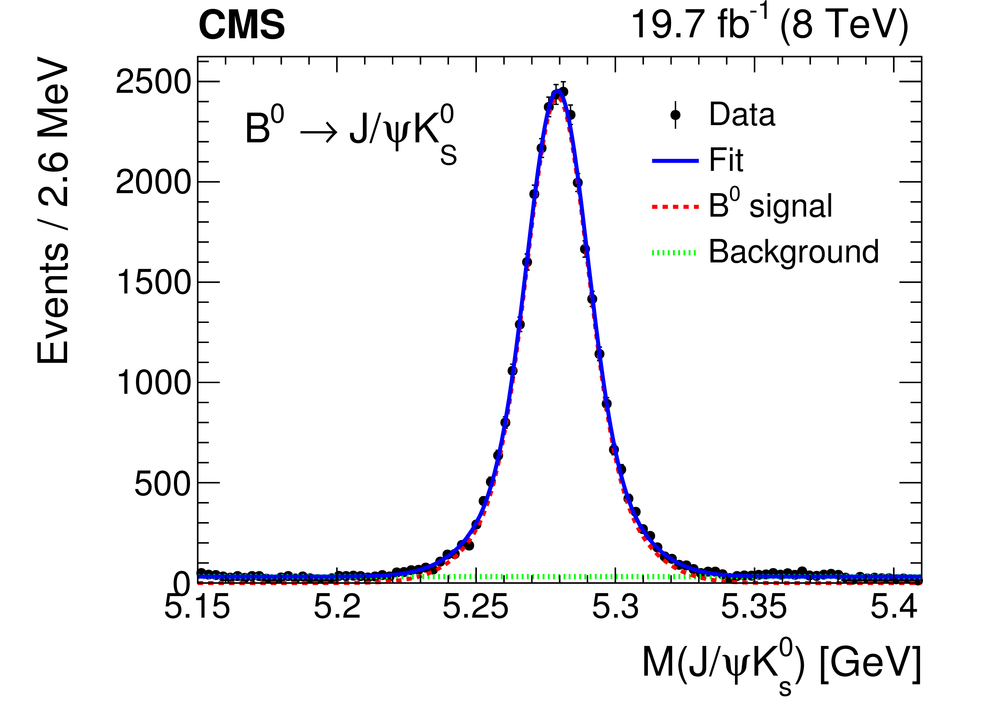
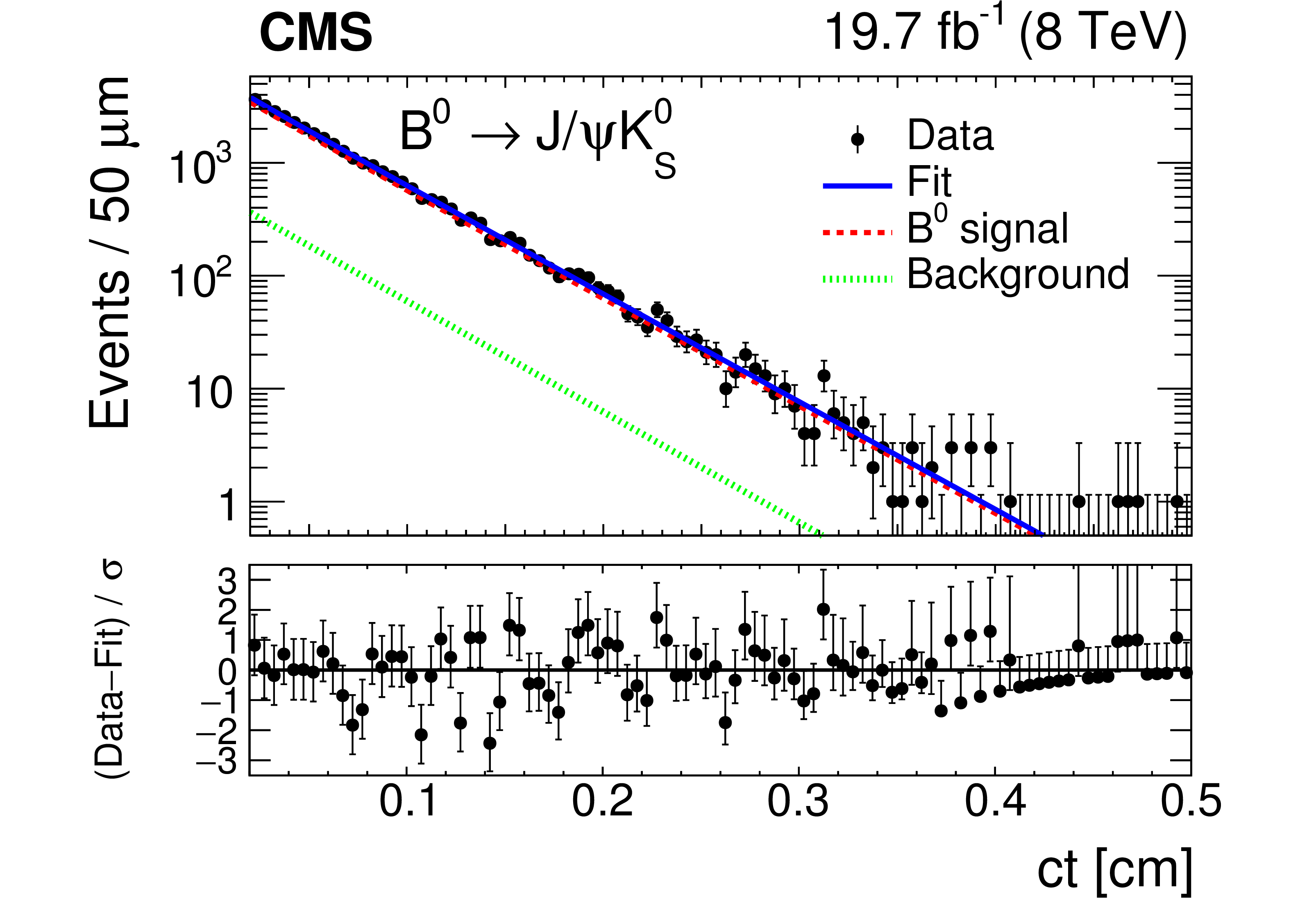
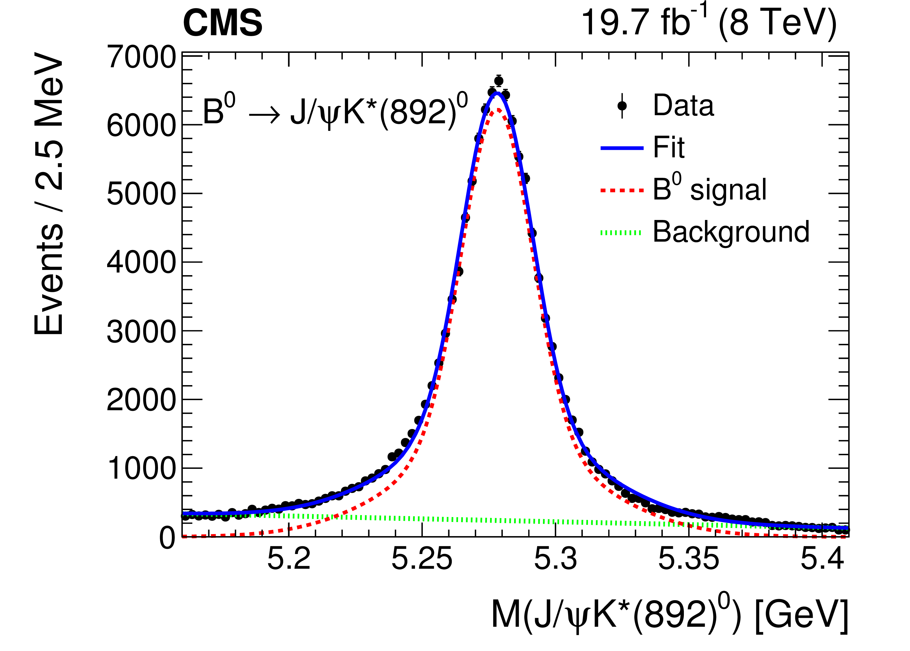
png pdf	Figure 3: Invariant mass (left) and $ct$ (right) distributions for $\mathrm{B}^{0}$ candidates reconstructed from ${\mathrm{J}/\psi {\mathrm{K^{*}(892)}} ^{0}}$ (upper) and ${\mathrm{J}/\psi {\mathrm{K^0_S}}}$ (lower) decays. The curves are projections of the fit to the data, with the contributions from signal (dashed), background (dotted), and the sum of signal and background (solid) shown. The bottom panels of the figures on the right show the difference between the observed data and the fit divided by the data uncertainty. The vertical bars on the data points represent the statistical uncertainties.
png pdf	Figure 3-a: Invariant mass distribution for $\mathrm{B}^{0}$ candidates reconstructed from ${\mathrm{J}/\psi {\mathrm{K^{*}(892)}} ^{0}}$ decays. The curves are projections of the fit to the data, with the contributions from signal (dashed), background (dotted), and the sum of signal and background (solid) shown. The vertical bars on the data points represent the statistical uncertainties.
png pdf	Figure 3-b: $ct$ distribution for $\mathrm{B}^{0}$ candidates reconstructed from ${\mathrm{J}/\psi {\mathrm{K^{*}(892)}} ^{0}}$ decays. The curves are projections of the fit to the data, with the contributions from signal (dashed), background (dotted), and the sum of signal and background (solid) shown. The bottom panel shows the difference between the observed data and the fit divided by the data uncertainty. The vertical bars on the data points represent the statistical uncertainties.
png pdf	Figure 3-c: Invariant mass distribution for $\mathrm{B}^{0}$ candidates reconstructed from ${\mathrm{J}/\psi {\mathrm{K^0_S}}}$ decays. The curves are projections of the fit to the data, with the contributions from signal (dashed), background (dotted), and the sum of signal and background (solid) shown. The vertical bars on the data points represent the statistical uncertainties.
png pdf	Figure 3-d: $ct$ distribution for $\mathrm{B}^{0}$ candidates reconstructed from ${\mathrm{J}/\psi {\mathrm{K^0_S}}}$ decays. The curves are projections of the fit to the data, with the contributions from signal (dashed), background (dotted), and the sum of signal and background (solid) shown. The bottom panel shows the difference between the observed data and the fit divided by the data uncertainty. The vertical bars on the data points represent the statistical uncertainties.
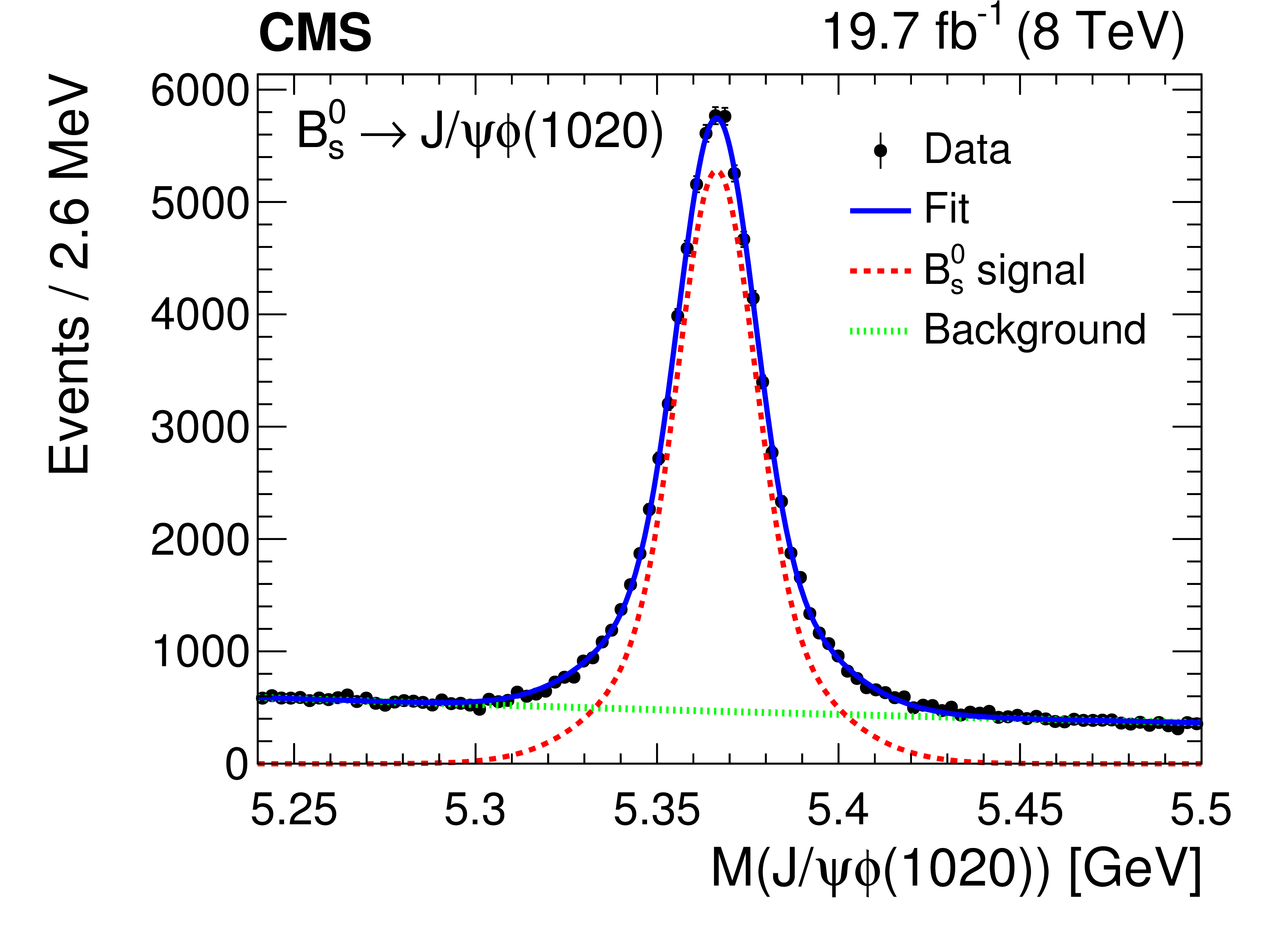
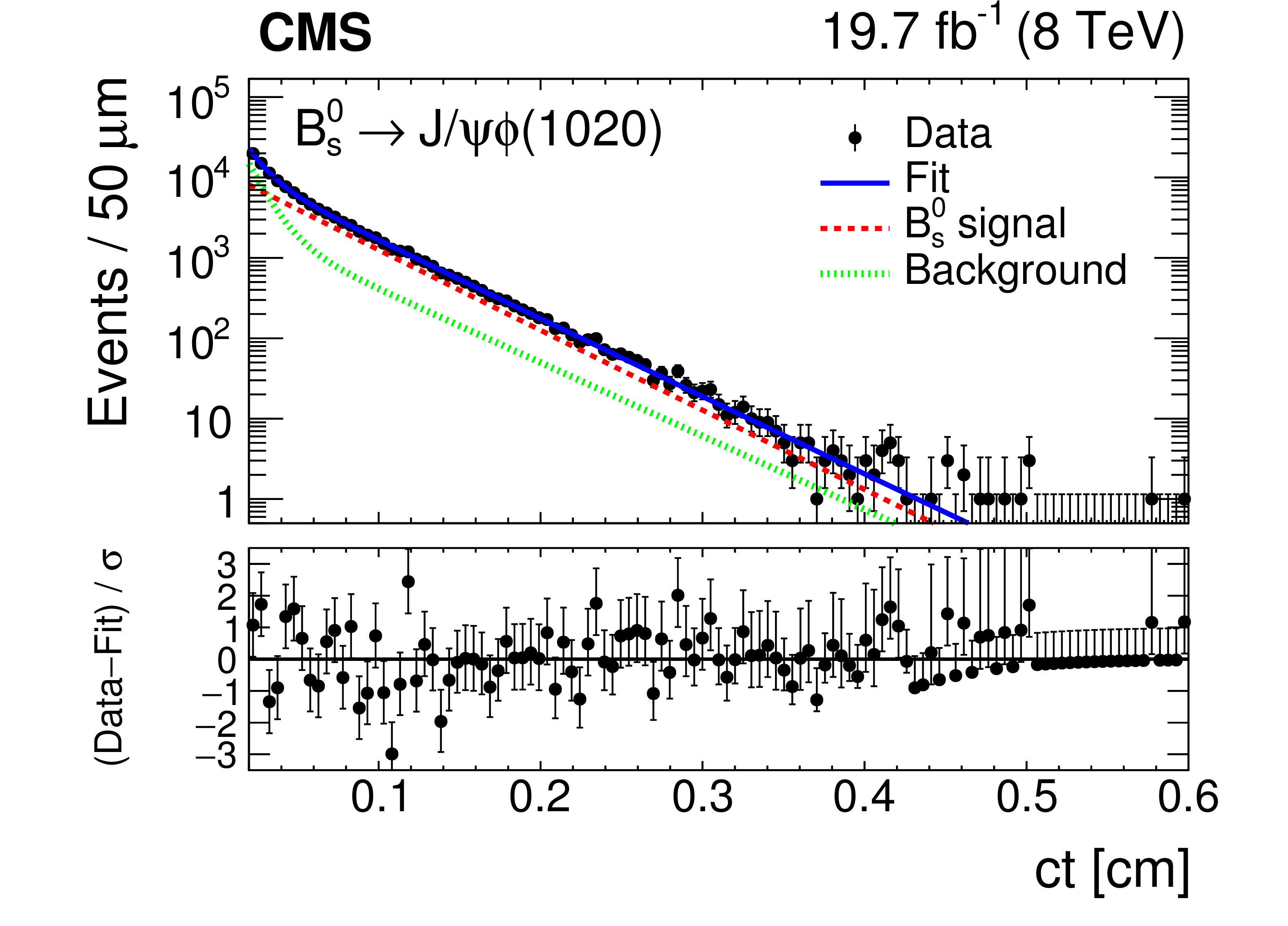
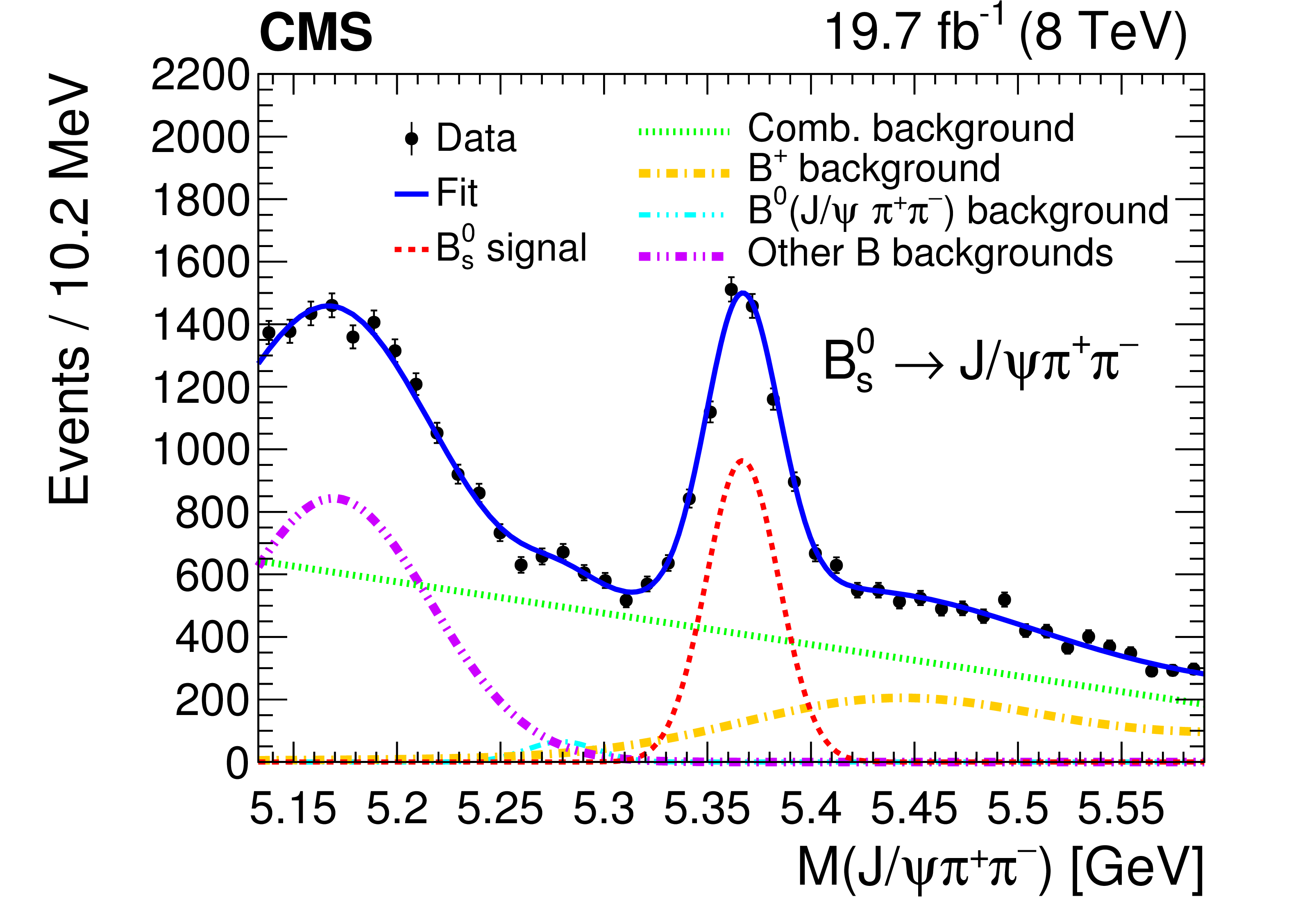
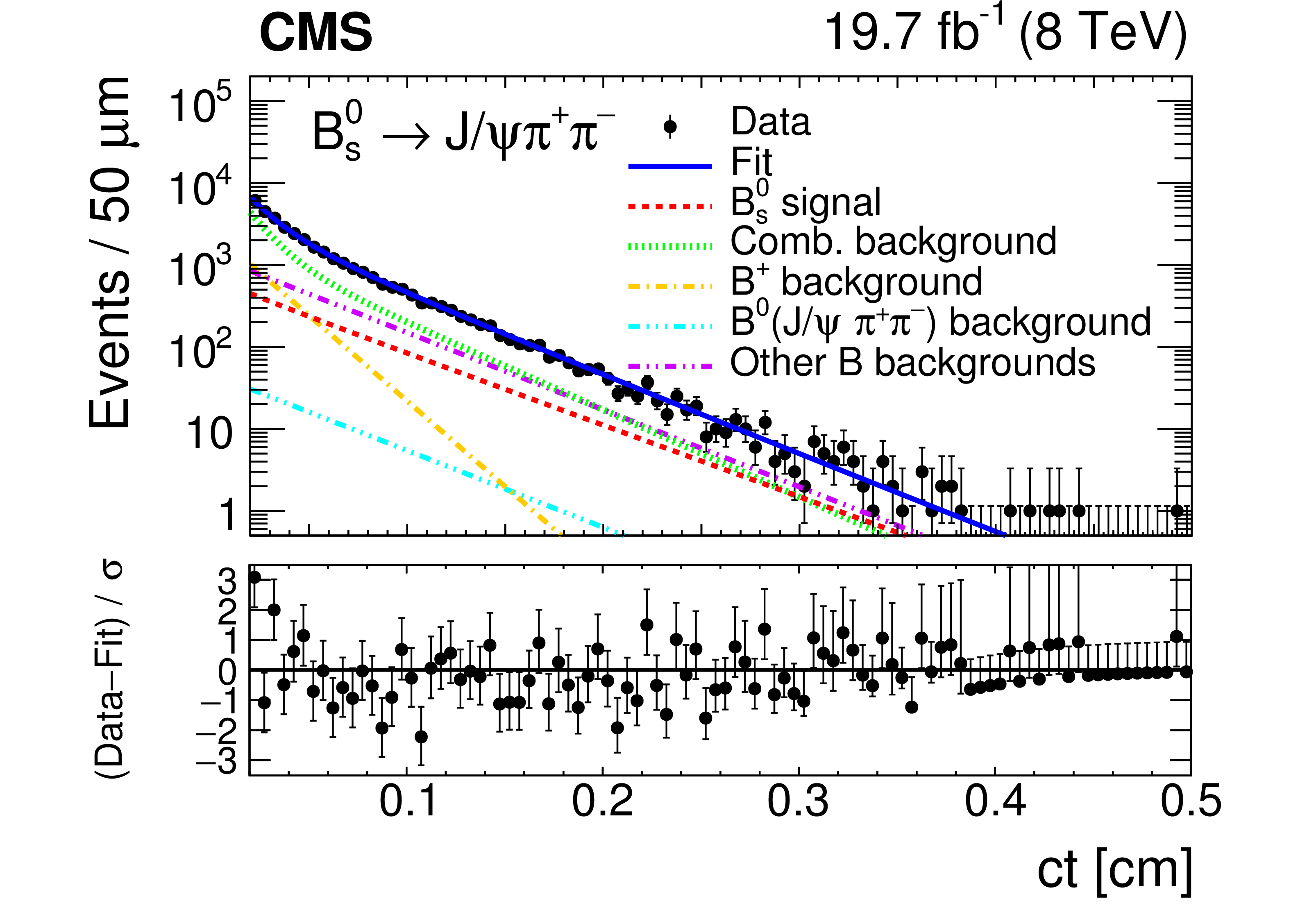
png pdf	Figure 4: Invariant mass (left) and $ct$ (right) distributions for ${ \mathrm{B}^{0}_{\mathrm{s}} }$ candidates reconstructed from ${\mathrm{J}/\psi \phi (1020)}$ (upper) and ${\mathrm{J}/\psi \pi^{+} \pi^{-}}$ (lower) decays. The curves are projections of the fit to the data, with the full fit function (solid) and signal (dashed) shown for both decays, the total background (dotted) shown for the upper plots, and the combinatorial background (dotted), misidentified ${\mathrm{B^{+}} \to \mathrm{J}/\psi \mathrm{K^{+}}}$ background (dashed-dotted), ${\mathrm{B}^{0} \to \mathrm{J}/\psi \pi^{+} \pi^{-}}$ contribution (dashed-dotted-dotted-dotted), and partially reconstructed and other misidentified B backgrounds (dashed-dotted-dotted) shown for the lower plots. The bottom panels of the figures on the right show the difference between the observed data and the fit divided by the data uncertainty. The vertical bars on the data points represent the statistical uncertainties.
png pdf	Figure 4-a: Invariant mass distribution for ${ \mathrm{B}^{0}_{\mathrm{s}} }$ candidates reconstructed from ${\mathrm{J}/\psi \phi (1020)}$ decays. The curves are projections of the fit to the data, with the full fit function (solid) and signal (dashed) shown for both decays, the total background (dotted) shown for the upper plots, and the combinatorial background (dotted), misidentified ${\mathrm{B^{+}} \to \mathrm{J}/\psi \mathrm{K^{+}}}$ background (dashed-dotted), ${\mathrm{B}^{0} \to \mathrm{J}/\psi \pi^{+} \pi^{-}}$ contribution (dashed-dotted-dotted-dotted), and partially reconstructed and other misidentified B backgrounds (dashed-dotted-dotted) shown for the lower plots. The vertical bars on the data points represent the statistical uncertainties.
png pdf	Figure 4-b: $ct$ distribution for ${ \mathrm{B}^{0}_{\mathrm{s}} }$ candidates reconstructed from ${\mathrm{J}/\psi \phi (1020)}$ decays. The curves are projections of the fit to the data, with the full fit function (solid) and signal (dashed) shown for both decays, the total background (dotted) shown for the upper plots, and the combinatorial background (dotted), misidentified ${\mathrm{B^{+}} \to \mathrm{J}/\psi \mathrm{K^{+}}}$ background (dashed-dotted), ${\mathrm{B}^{0} \to \mathrm{J}/\psi \pi^{+} \pi^{-}}$ contribution (dashed-dotted-dotted-dotted), and partially reconstructed and other misidentified B backgrounds (dashed-dotted-dotted) shown for the lower plots. The bottom panel shows the difference between the observed data and the fit divided by the data uncertainty. The vertical bars on the data points represent the statistical uncertainties.
png pdf	Figure 4-c: Invariant mass distribution for ${ \mathrm{B}^{0}_{\mathrm{s}} }$ candidates reconstructed from ${\mathrm{J}/\psi \pi^{+} \pi^{-}}$ decays. The curves are projections of the fit to the data, with the full fit function (solid) and signal (dashed) shown for both decays, the total background (dotted) shown for the upper plots, and the combinatorial background (dotted), misidentified ${\mathrm{B^{+}} \to \mathrm{J}/\psi \mathrm{K^{+}}}$ background (dashed-dotted), ${\mathrm{B}^{0} \to \mathrm{J}/\psi \pi^{+} \pi^{-}}$ contribution (dashed-dotted-dotted-dotted), and partially reconstructed and other misidentified B backgrounds (dashed-dotted-dotted) shown for the lower plots. The vertical bars on the data points represent the statistical uncertainties.
png pdf	Figure 4-d: $ct$ distribution for ${ \mathrm{B}^{0}_{\mathrm{s}} }$ candidates reconstructed from ${\mathrm{J}/\psi \pi^{+} \pi^{-}}$ decays. The curves are projections of the fit to the data, with the full fit function (solid) and signal (dashed) shown for both decays, the total background (dotted) shown for the upper plots, and the combinatorial background (dotted), misidentified ${\mathrm{B^{+}} \to \mathrm{J}/\psi \mathrm{K^{+}}}$ background (dashed-dotted), ${\mathrm{B}^{0} \to \mathrm{J}/\psi \pi^{+} \pi^{-}}$ contribution (dashed-dotted-dotted-dotted), and partially reconstructed and other misidentified B backgrounds (dashed-dotted-dotted) shown for the lower plots. The bottom panel shows the difference between the observed data and the fit divided by the data uncertainty. The vertical bars on the data points represent the statistical uncertainties.
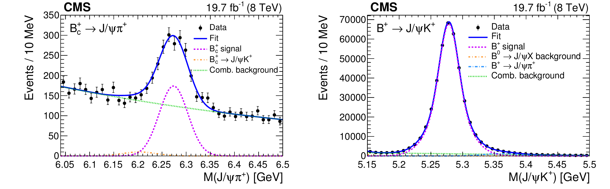
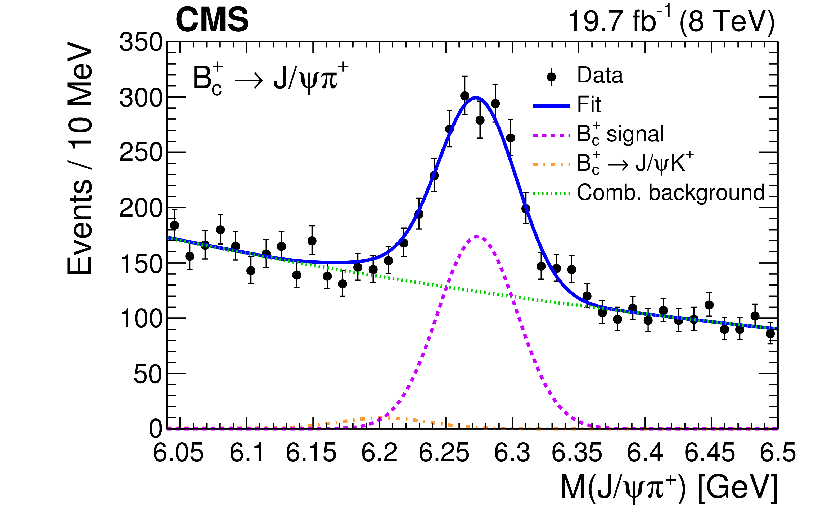
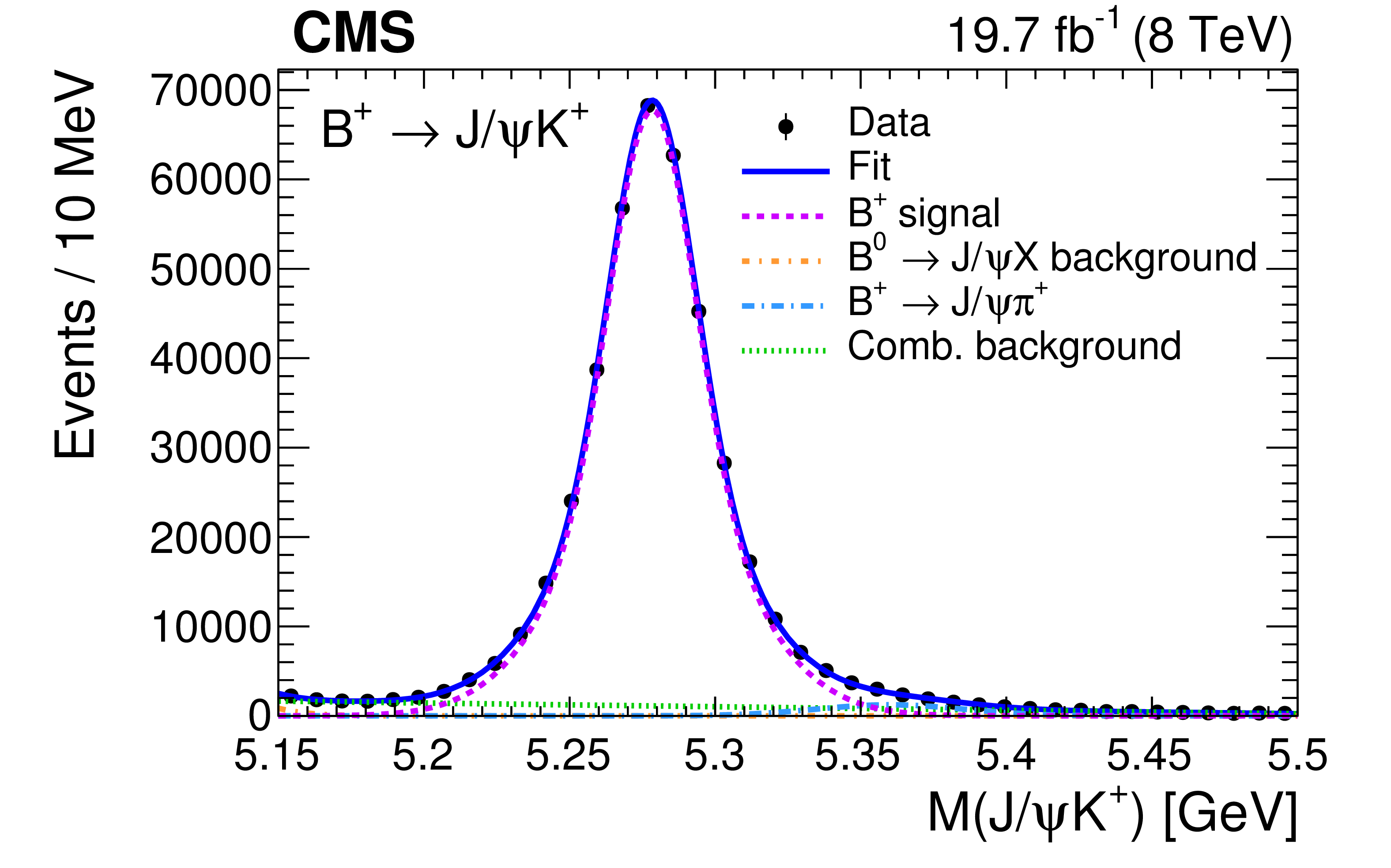
png pdf	Figure 5: The ${\mathrm{J}/\psi \pi^{+}}$ invariant mass distribution (left) with the solid line representing the total fit, the dashed line the signal component, the dotted line the combinatorial background, and the dashed-dotted line the contribution from ${\mathrm{B}_{\mathrm{c}}^{+} \to \mathrm{J}/\psi \mathrm{K^{+}}}$ decays. The ${\mathrm{J}/\psi \mathrm{K^{+}}}$ invariant mass distribution (right) with the solid line representing the total fit, the dashed line the signal component, the dotted-dashed curves the $\mathrm{B^{+}} \to {\mathrm{J}/\psi} \pi^{+}$ and $\mathrm{B}^{0}$ contributions, and the dotted curve the combinatorial background. The vertical bars on the data points represent the statistical uncertainties.
png pdf	Figure 5-a: The ${\mathrm{J}/\psi \pi^{+}}$ invariant mass distribution with the solid line representing the total fit, the dashed line the signal component, the dotted line the combinatorial background, and the dashed-dotted line the contribution from ${\mathrm{B}_{\mathrm{c}}^{+} \to \mathrm{J}/\psi \mathrm{K^{+}}}$ decays. The vertical bars on the data points represent the statistical uncertainties.
png pdf	Figure 5-b: The ${\mathrm{J}/\psi \mathrm{K^{+}}}$ invariant mass distribution (right) with the solid line representing the total fit, the dashed line the signal component, the dotted-dashed curves the $\mathrm{B^{+}} \to {\mathrm{J}/\psi} \pi^{+}$ and $\mathrm{B}^{0}$ contributions, and the dotted curve the combinatorial background. The vertical bars on the data points represent the statistical uncertainties.
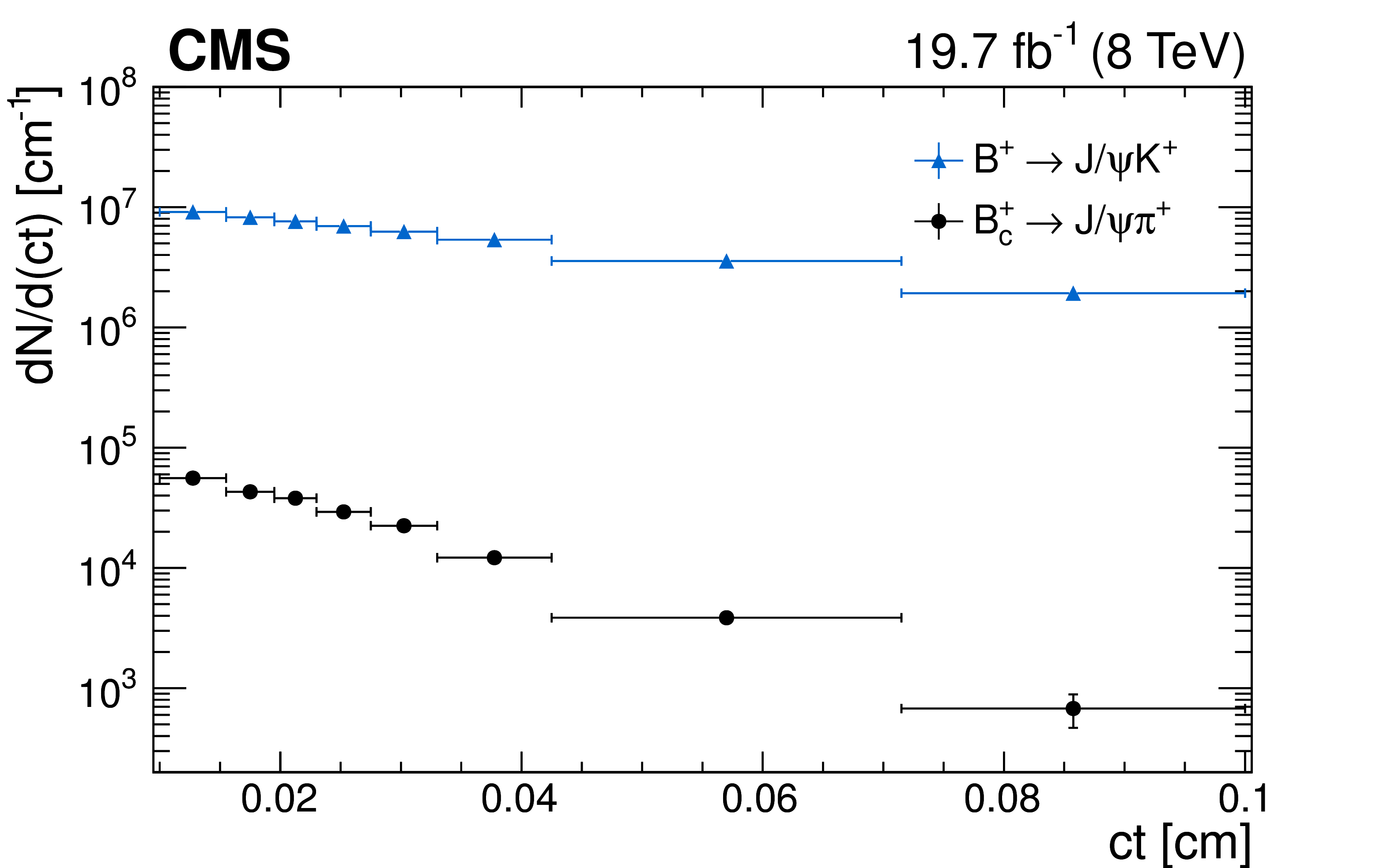
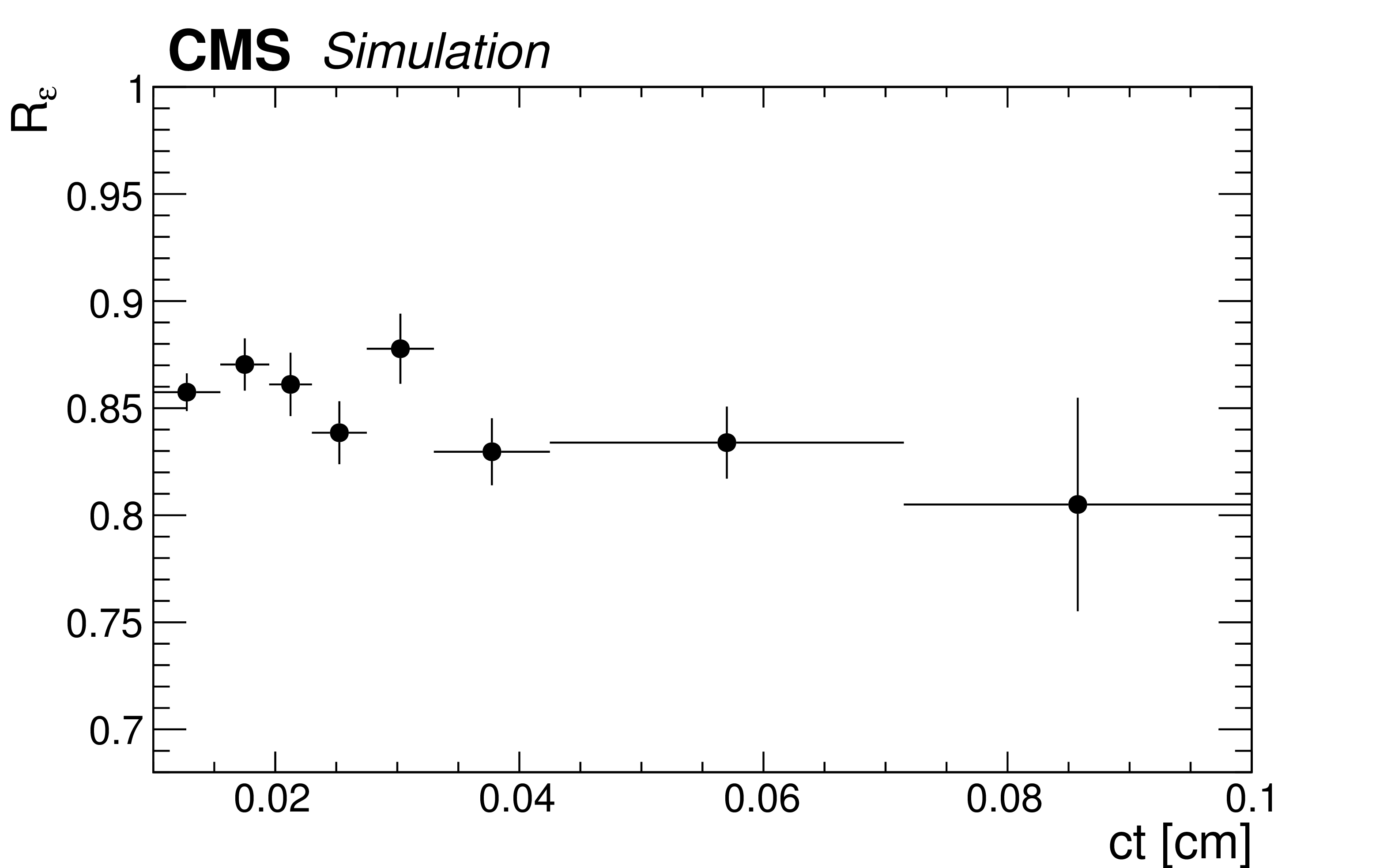
png pdf	Figure 6: Left: Yields of ${\mathrm{B}_{\mathrm{c}}^{+} \to \mathrm{J}/\psi \pi^{+}} and {\mathrm{B^{+}} \to \mathrm{J}/\psi \mathrm{K^{+}}}$ events as a function of ${ct}$ , normalized to the bin width, as determined from fits to the invariant mass distributions. Right: Ratio of the $\mathrm{B}_{\mathrm{c}}^{+}$ and $\mathrm{B^{+}}$ efficiency distributions as a function of ${ct}$ , as determined from simulated events. The vertical bars on the data points represent the statistical uncertainties, and the horizontal bars show the bin widths.
png pdf	Figure 6-a: Yields of ${\mathrm{B}_{\mathrm{c}}^{+} \to \mathrm{J}/\psi \pi^{+}} and {\mathrm{B^{+}} \to \mathrm{J}/\psi \mathrm{K^{+}}}$ events as a function of ${ct}$ , normalized to the bin width, as determined from fits to the invariant mass distributions. The vertical bars on the data points represent the statistical uncertainties, and the horizontal bars show the bin widths.
png pdf	Figure 6-b: Ratio of the $\mathrm{B}_{\mathrm{c}}^{+}$ and $\mathrm{B^{+}}$ efficiency distributions as a function of ${ct}$ , as determined from simulated events. The vertical bars on the data points represent the statistical uncertainties, and the horizontal bars show the bin widths.
png pdf	Figure 7: Ratio of the $\mathrm{B}_{\mathrm{c}}^{+} to \mathrm{B^{+}}$ efficiency-corrected ${ct}$ distributions, $R/R_{\varepsilon}$ , with a line showing the result of the fit to an exponential function. The vertical bars give the statistical uncertainty in the data, and the horizontal bars show the bin widths.

Tables
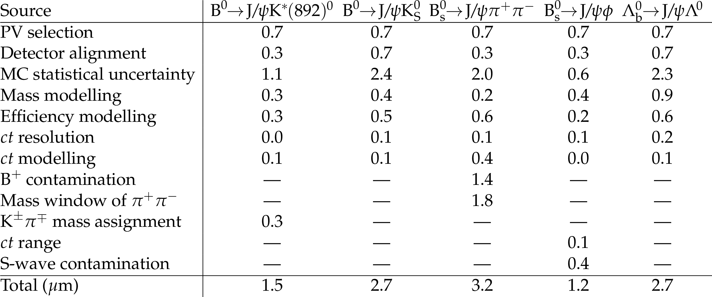
png pdf	Table 1: Summary of the sources and values of systematic uncertainties in the lifetime measurements (in $\mu$ m). The total systematic uncertainty is the sum in quadrature of the individual uncertainties.
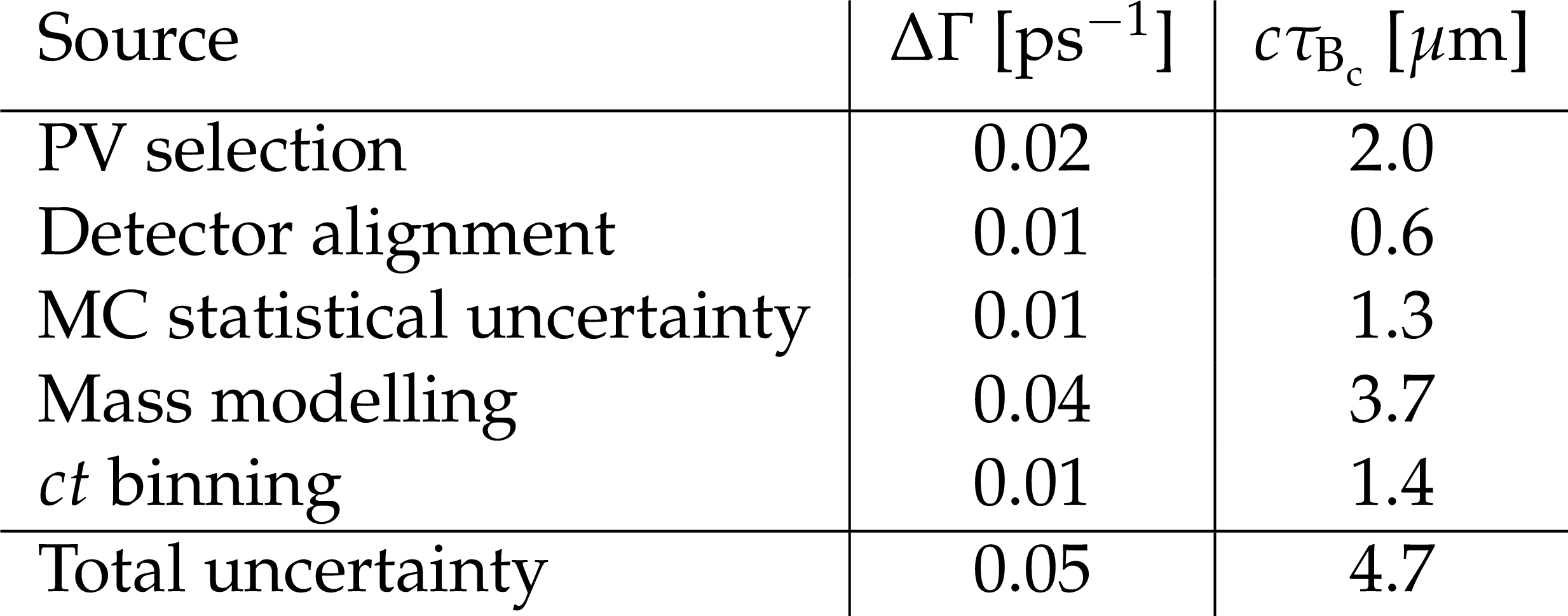
png pdf	Table 2: Summary of the systematic uncertainties in the $\Delta \Gamma$ and $c\tau _{\mathrm{B}_{\mathrm{c}}^{+}}$ measurements.

Summary

The lifetimes of the

$\mathrm{B}^{0}$ ,

$\mathrm{B}^{0}_{\mathrm{s}}$ ,

$\Lambda_{\mathrm{b}}^{0}$ , and

$\mathrm{B}_{\mathrm{c}}^{+}$ hadrons have been measured using fully reconstructed decays with a

${\mathrm{J}/\psi}$ meson. The data were collected by the CMS detector in proton-proton collision events at a centre-of-mass energy of 8 TeV, and correspond to an integrated luminosity of 19.7 fb

$^{-1}$ . The

$\mathrm{B}^{0}$ and

$\mathrm{B}^{0}_{\mathrm{s}}$ meson lifetimes have each been measured in two channels:

${\mathrm{J}/\psi {\mathrm{K^{*}(892)}}^{0}}$ ,

${\mathrm{J}/\psi {\mathrm{K^0_S}}}$ for

$\mathrm{B}^{0}$ and

${\mathrm{J}/\psi \pi^{+} \pi^{-}}$ ,

${\mathrm{J}/\psi \phi(1020)}$ for

$\mathrm{B}^{0}_{\mathrm{s}}$ . The precision from each channel is as good as or better than previous measurements in the respective channel. The

$\mathrm{B}^{0}_{\mathrm{s}}$ lifetime results are used to obtain the lifetimes of the heavy and light

$\mathrm{B}^{0}_{\mathrm{s}}$ mass eigenstates. The precision of the

$\Lambda_{\mathrm{b}}^{0}$ lifetime measurement is also as good as any previous measurement in the

${\mathrm{J}/\psi \Lambda^{0}}$ channel. The measurement of the

$\mathrm{B}_{\mathrm{c}}^{+}$ meson lifetime confirms a longer lifetime than found by the Tevatron experiments, in agreement with results from LHCb. All measured lifetimes are compatible with the current world-average values.

References
1	A. Lenz	Lifetimes and heavy quark expansion	Int. J. Mod. Phys. A 30 (2015) 1543005
2	Particle Data Group, C. Patrignani et al.	Review of particle physics	CPC 40 (2016) 100001
3	CMS Collaboration	The CMS experiment at the CERN LHC	JINST 3 (2008) S08004	CMS-00-001
4	R. Fleischer and R. Knegjens	Effective lifetimes of $\text{B}_\text{s}$ decays and their constraints on the $\mathrm{B}^{0}s$ -- ${\mathrm{\overline{B}}^0}s$ mixing parameters	EPJC 71 (2011) 1789	1109.5115
5	LHCb Collaboration	Analysis of the resonant components in ${\mathrm{\overline{B}}^0}s \to J/\psi \pi^+ \pi^-$	PRD 86 (2012) 052006	1301.5347
6	LHCb Collaboration	Measurement of resonant and CP components in ${\mathrm{\overline{B}}^0}s \to J/\psi \pi^+ \pi^-$	PRD 89 (2014) 092006	1402.6248
7	CMS Collaboration	Measurement of the CP-violating weak phase $\phi_s$ and the decay width difference $\Delta \Gamma_s$ using the $\mathrm{B}^{0}s \to J/\psi\phi$ (1020) decay channel in pp collisions at $\sqrt{s}=$ 8 TeV	PLB 757 (2016) 97	CMS-BPH-13-012 1507.07527
8	V. V. Kiselev	Exclusive decays and lifetime of $\mathrm{B_c}$ meson in QCD sum rules		hep-ph/0211021
9	LHCb Collaboration	Measurement of the $\mathrm{B}_{\mathrm{c}}$ meson lifetime using $\mathrm{B}_{\mathrm{c}} \to J\!/\!\psi \mu^+ \nu_{\mu} X$ decays	EPJC 74 (2014) 2839	1401.6932
10	LHCb Collaboration	Measurement of the lifetime of the $\mathrm{B}_{\mathrm{c}}$ meson using the $\mathrm{B}_{\mathrm{c}} \to J/\psi \pi^+$ decay mode	PLB 742 (2015) 29	1411.6899
11	CDF Collaboration	Observation of the $\text{B}_\text{c}$ meson in $\text{p}\overline{\text{p}}$ collisions at $\sqrt{s} =$ 1.8 TeV	PRL 81 (1998) 2432	hep-ex/9805034
12	CDF Collaboration	Measurement of the $\mathrm{B}_{\mathrm{c}}$ meson lifetime using the decay mode $\mathrm{B}_{\mathrm{c}}\to J/\psi \mathrm{e^{+}} \nu$	PRL 97 (2006) 012002	hep-ex/0603027
13	D0 Collaboration	Measurement of the lifetime of the $\text{B}^{\pm}_\text{c}$ meson in the semileptonic decay channel	PRL 102 (2009) 092001	0805.2614
14	CDF Collaboration	Measurement of the $\text{B}^-_\text{c}$ meson lifetime in the decay $\text{B}^-_\text{c} \to J/\psi \pi^-$	PRD 87 (2013) 011101	1210.2366
15	CMS Collaboration	Description and performance of track and primary-vertex reconstruction with the CMS tracker	JINST 9 (2014) P10009	CMS-TRK-11-001 1405.6569
16	CMS Collaboration	The CMS trigger system	JINST 12 (2017) P01020	CMS-TRG-12-001 1609.02366
17	T. Sjostrand, S. Mrenna, and P. Z. Skands	PYTHIA 6.4 physics and manual	JHEP 05 (2006) 026	hep-ph/0603175
18	C. Chang, C. Driouchi, P. Eerola, and X. Wu	BCVEGPY: an event generator for hadronic production of the $\mathrm{B_c}$ meson	CPC 159 (2004) 192	hep-ph/0309120
19	C. Chang, J. Wang, and X. Wu	BCVEGPY2.0: An upgraded version of the generator BCVEGPY with the addition of hadroproduction of the P-wave $\mathrm{B_c}$ states	CPC 174 (2006) 241	hep-ph/0504017
20	D. J. Lange	The EvtGen particle decay simulation package	NIMA 462 (2001) 152
21	P. Golonka and Z. W\cas	PHOTOS Monte Carlo: a precision tool for QED corrections in Z and W decays	EPJC 45 (2006) 97	hep-ph/0506026
22	GEANT4 Collaboration	GEANT4---a simulation toolkit	NIMA 506 (2003) 250
23	CMS Collaboration	Performance of CMS muon reconstruction in pp collision events at $\sqrt{s} =$ 7 TeV	JINST 7 (2012) P10002	CMS-MUO-10-004 1206.4071
24	A. S. Dighe, I. Dunietz, and R. Fleischer	Extracting CKM phases and $\text{B}_\text{s} - \overline{\text{B}}_\text{s}$ mixing parameters from angular distributions of non-leptonic $\text{B}$ decays	EPJC 6 (1999) 647	hep-ph/9804253
25	LHCb Collaboration	First observation of the decay $\mathrm{B^+_c}\to \mathrm{J}/\psi \mathrm{K^{+}}$	JHEP 09 (2013) 075	1306.6723
26	CMS Collaboration	Alignment of the CMS tracker with LHC and cosmic ray data	JINST 9 (2014) P06009	CMS-TRK-11-002 1403.2286
27	M. J. Oreglia	A study of the reactions $\psi' \to \gamma\gamma \psi$	PhD thesis, Stanford University, 1980 SLAC Report SLAC-R-236, see Appendix D
28	CDF Collaboration	Measurement of branching ratio and $\mathrm{B}^{0}s$ lifetime in the decay $\mathrm{B}^{0}s \to J/\psi \text{f}_0(980)$ at CDF	PRD 84 (2011) 052012	1106.3682
29	LHCb Collaboration	Measurement of CP violation and the $\mathrm{B}^{0}s$ meson decay width difference with $\mathrm{B}^{0}s \to J/\psi \mathrm{K^{+}} \mathrm{K^{-}}$ and $\mathrm{B}^{0}s \to J/\psi \pi^+\pi^-$ decays	PRD 87 (2013) 112010	1304.2600
30	D0 Collaboration	$\mathrm{B}^{0}s$ lifetime measurement in the CP-odd decay channel $\mathrm{B}^{0}s \to J/\psi \text{f}_0(980)$	PRD 94 (2016) 012001	1603.01302
31	C.-H. Chang, S.-L. Chen, T.-F. Feng, and X.-Q. Li	Lifetime of the $\mathrm{B}_{\mathrm{c}}$ meson and some relevant problems	PRD 64 (2001) 014003	hep-ph/0007162
32	M. Beneke and G. Buchalla	$\mathrm{B}_{\mathrm{c}}$ meson lifetime	PRD 53 (1996) 4991	hep-ph/9601249
33	A. Yu. Anisimov, I. M. Narodetskii, C. Semay, and B. Silvestre-Brac	The $\mathrm{B}_{\mathrm{c}}$ meson lifetime in the light-front constituent quark model	PLB 452 (1999) 129	hep-ph/9812514
34	V. V. Kiselev, A. E. Kovalsky, and A. K. Likhoded	Decays and lifetime of $\mathrm{B}_{\mathrm{c}}$ in QCD sum rules	in 5th International Workshop on Heavy Quark Physics, Dubna, Russia, April 6-8	hep-ph/0006104
35	R. Alonso, B. Grinstein, and J. Martin Camalich	Lifetime of $\mathrm{B}_{\mathrm{c}}^-$ constrains explanations for anomalies in $\mathrm{B} \to \mathrm{D}^{(*)}\tau\nu$	PRL 118 (2017) 081802	1611.06676