

Compact Muon Solenoid
LHC, CERN
| CMS-SMP-23-002 ; CERN-EP-2024-308 | ||
| High-precision measurement of the W boson mass with the CMS experiment | ||
| CMS Collaboration | ||
| 18 December 2024 | ||
| Nature 652, 321–327 (2026) | ||
| Abstract: In the standard model of particle physics, the masses of the W and Z bosons, the carriers of the weak interaction, are uniquely related. A precise determination of their masses is important because quantum loops of heavy, undiscovered particles could modify this relationship. Although the Z mass is known to the remarkable precision of 22 parts per million (2.0 MeV), the W mass is known much less precisely. A global fit to measured electroweak observables predicts the W mass with 6 MeV uncertainty [1,2,3]. Reaching a comparable experimental precision would be a sensitive and fundamental test of the standard model, made even more urgent by a recent challenge to the global fit prediction by a measurement from the CDF Collaboration at the Fermilab Tevatron collider [4]. Here we report the measurement of the W mass by the CMS Collaboration at the CERN LHC, based on a large data sample of $ \mathrm{W}\to\mu\nu $ events collected in 2016 at the proton-proton collision energy of 13 TeV. The measurement exploits a high-granularity maximum likelihood fit to the kinematic properties of muons produced in W decays. By combining an accurate determination of experimental effects with marked in situ constraints of theoretical inputs, we reach a precise measurement of the W mass, of 80 360.2 $ \pm $ 9.9 MeV, in agreement with the standard model prediction. | ||
| Links: e-print arXiv:2412.13872 [hep-ex] (PDF) ; CDS record ; inSPIRE record ; HepData record ; Physics Briefing ; CADI line (restricted) ; | ||
| Covariance matrices can be found here |
| Figures | |
png pdf |
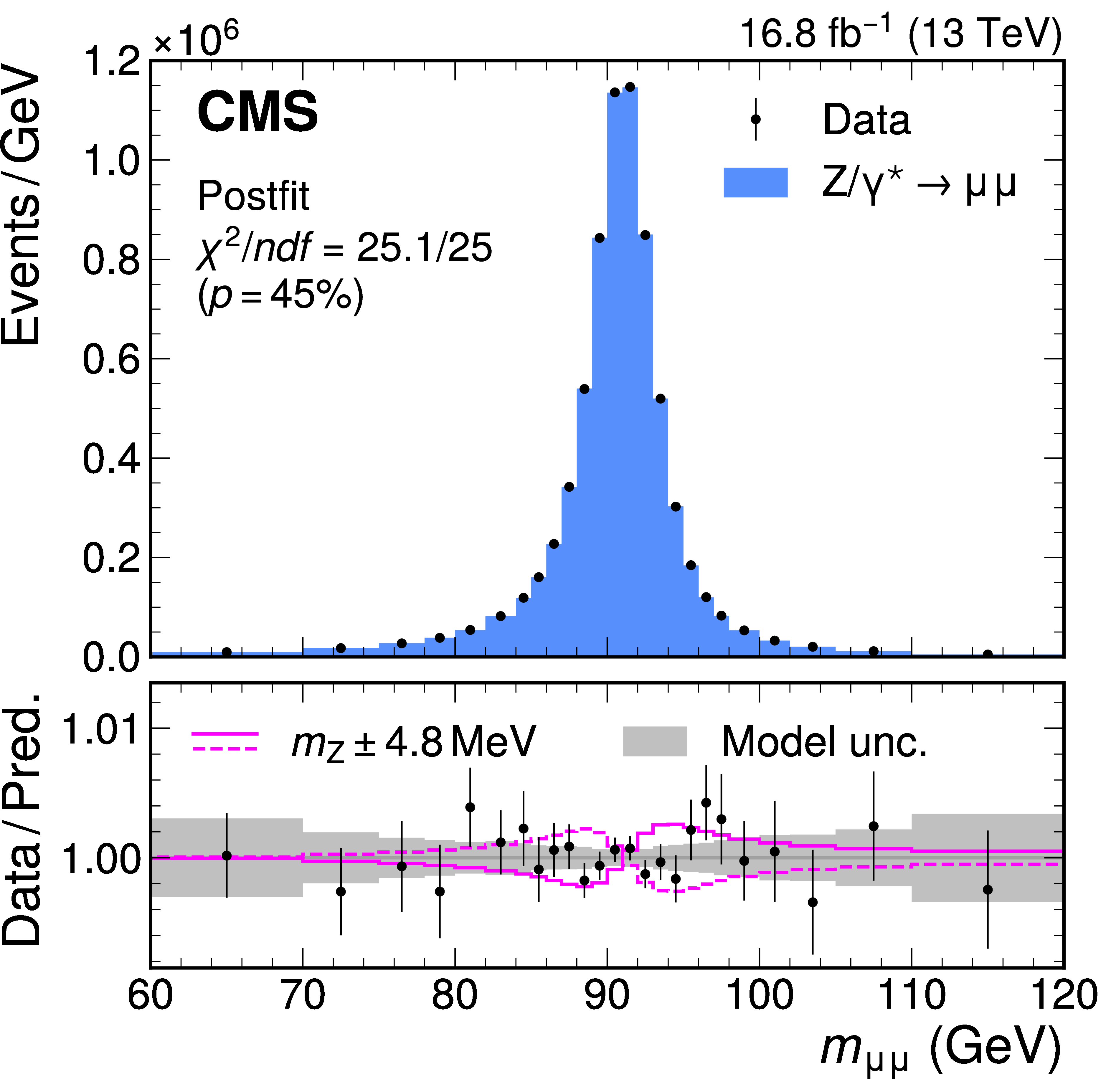
Figure 1:
The Z boson mass measurement. Measured and simulated $ \mathrm{Z}\to\mu\mu $ dimuon mass distributions. The postfit $ \mathrm{Z}\to\mu\mu $ distribution is shown in blue. The small contributions of other processes are included but not visible. The bottom panel shows the ratio between the number of events in data and the total nominal prediction. The vertical bars represent the statistical uncertainties in the data. The total uncertainty in the prediction after the uncertainty profiling procedure (gray band) and the effect of a $ \pm $4.8 MeV variation of $ m_{\mathrm{Z}} $ (magenta lines) are also shown, illustrating the precision of the achieved understanding of the distribution. |
png pdf |
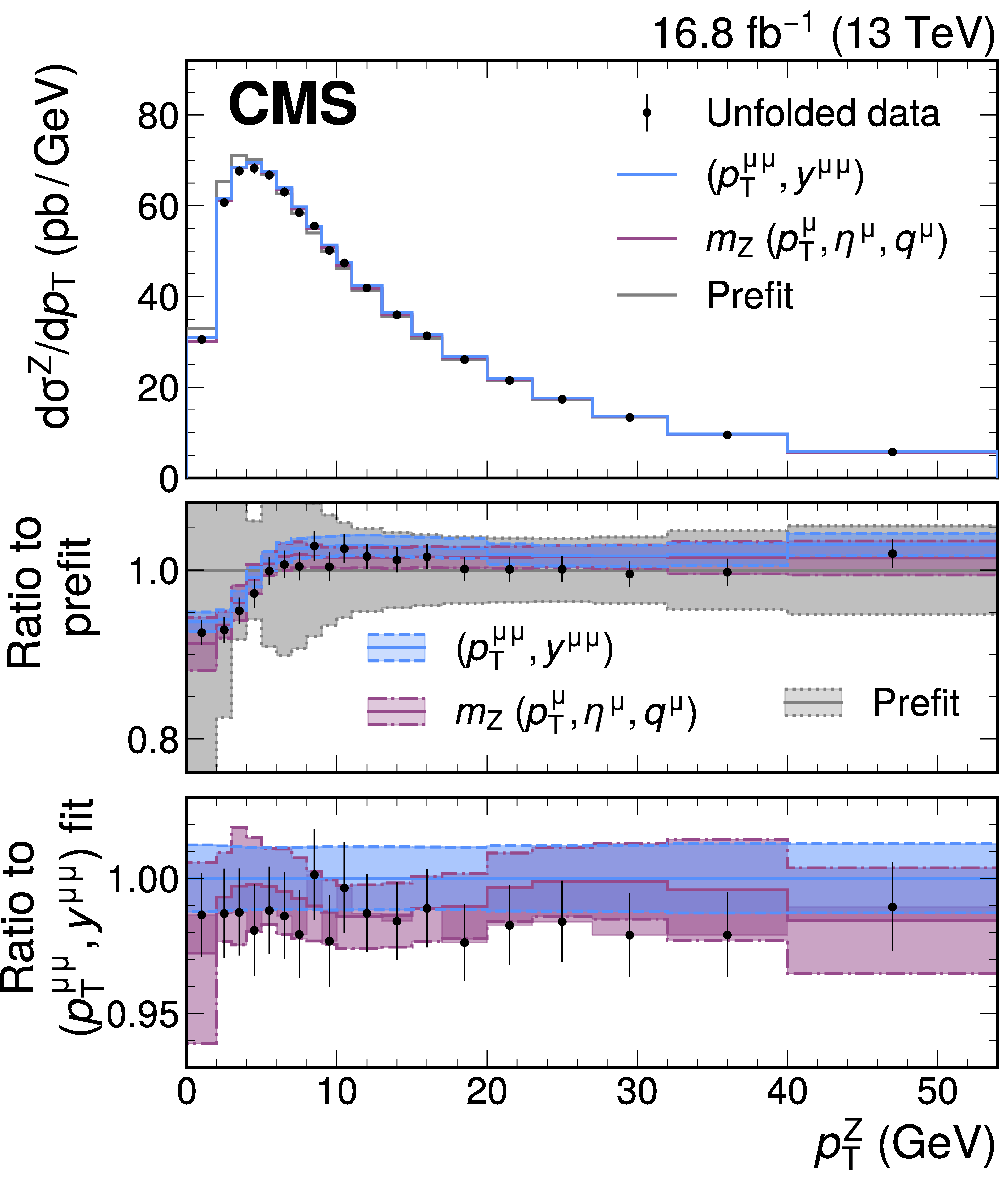
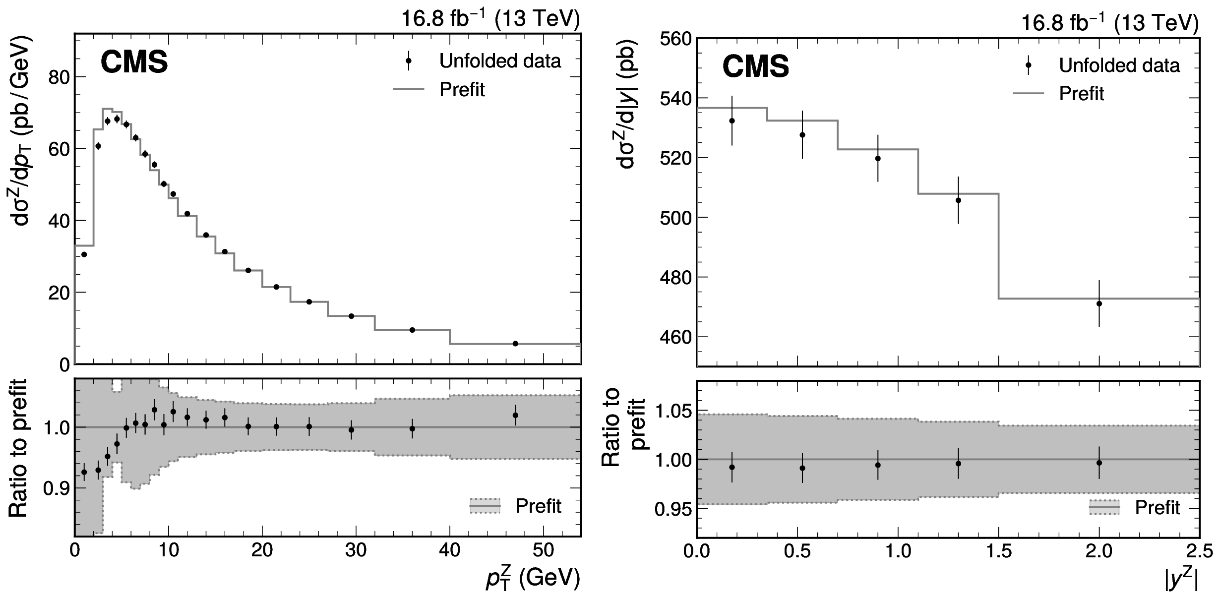
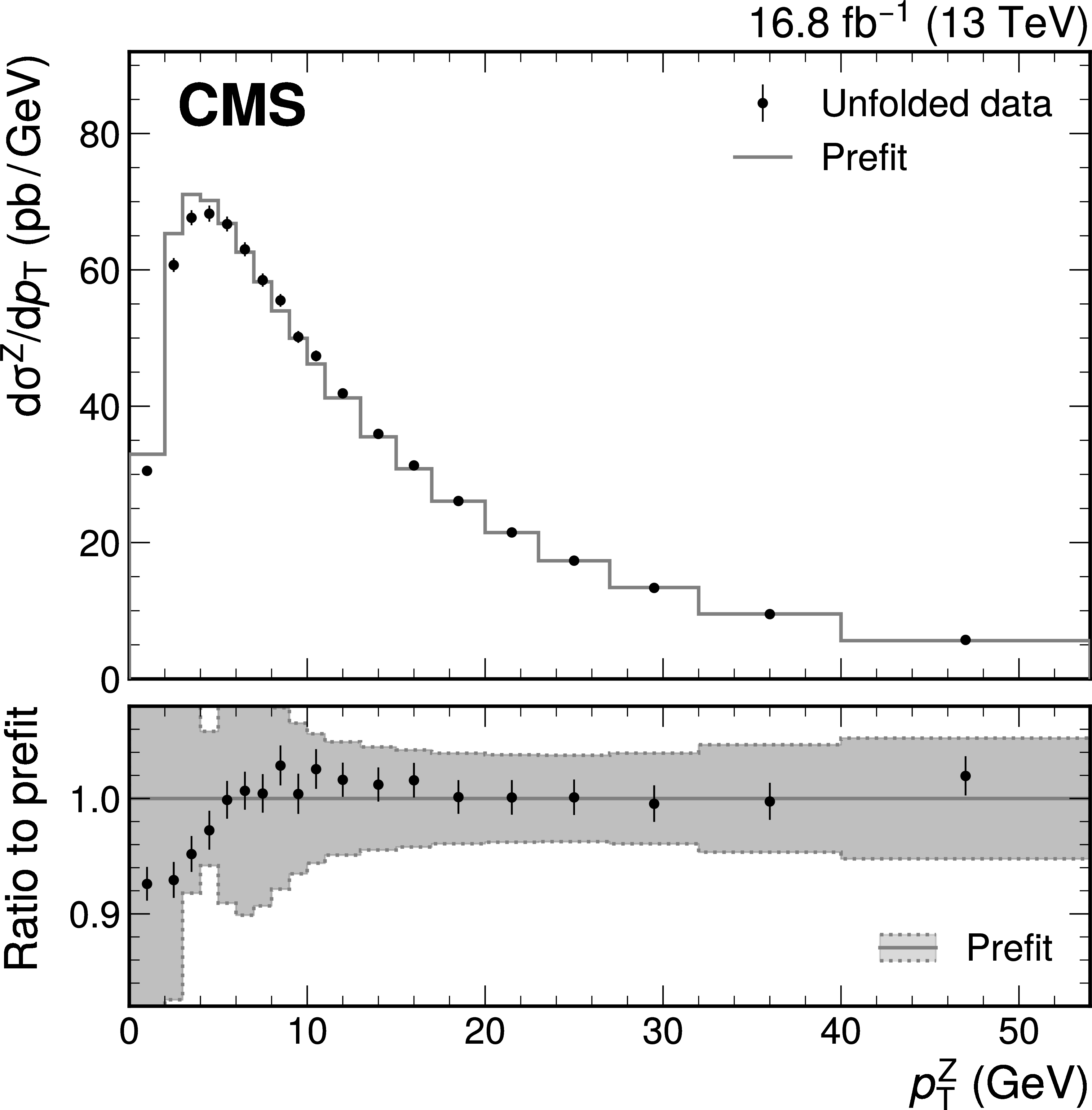
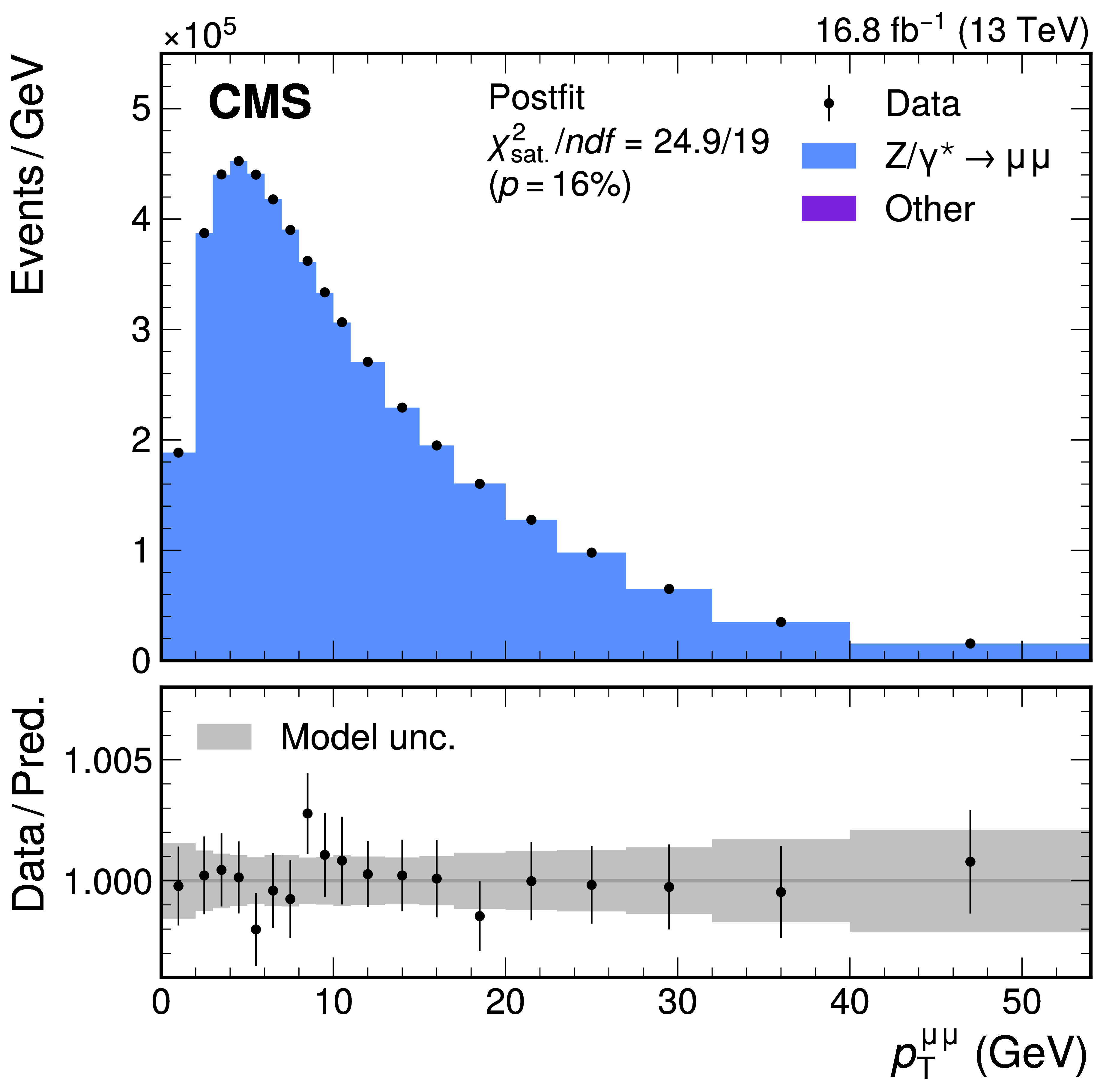
Figure 2:
Validation of the theory model. Unfolded measured $ p_{\mathrm{T}}^{\mathrm{Z}} $ distribution (points) compared with the generator-level SCETLIB $+$ MiNNLO$_{\text{PS}}$ predictions before (prefit, gray) and after adjusting the nuisance parameters to the best fit values obtained from the W-like $ m_{\mathrm{Z}} $ fit (magenta) or from the direct fit to the $ p_{\mathrm{T}}^{\mu\mu} $ distribution (blue). The center panel shows the ratio of the predictions and unfolded data to the prefit prediction. The uncertainty in the prefit prediction is shown by the shaded gray area. The bottom panel shows the ratio of the predictions and unfolded data to the postfit prediction from the fit to the $ (p_{\mathrm{T}}^{\mu\mu}, y^{\mu\mu}) $ distribution. The postfit uncertainties in the predictions are shown in the shaded magenta and blue bands. The vertical bars represent the total uncertainty in the unfolded data. |
png pdf |
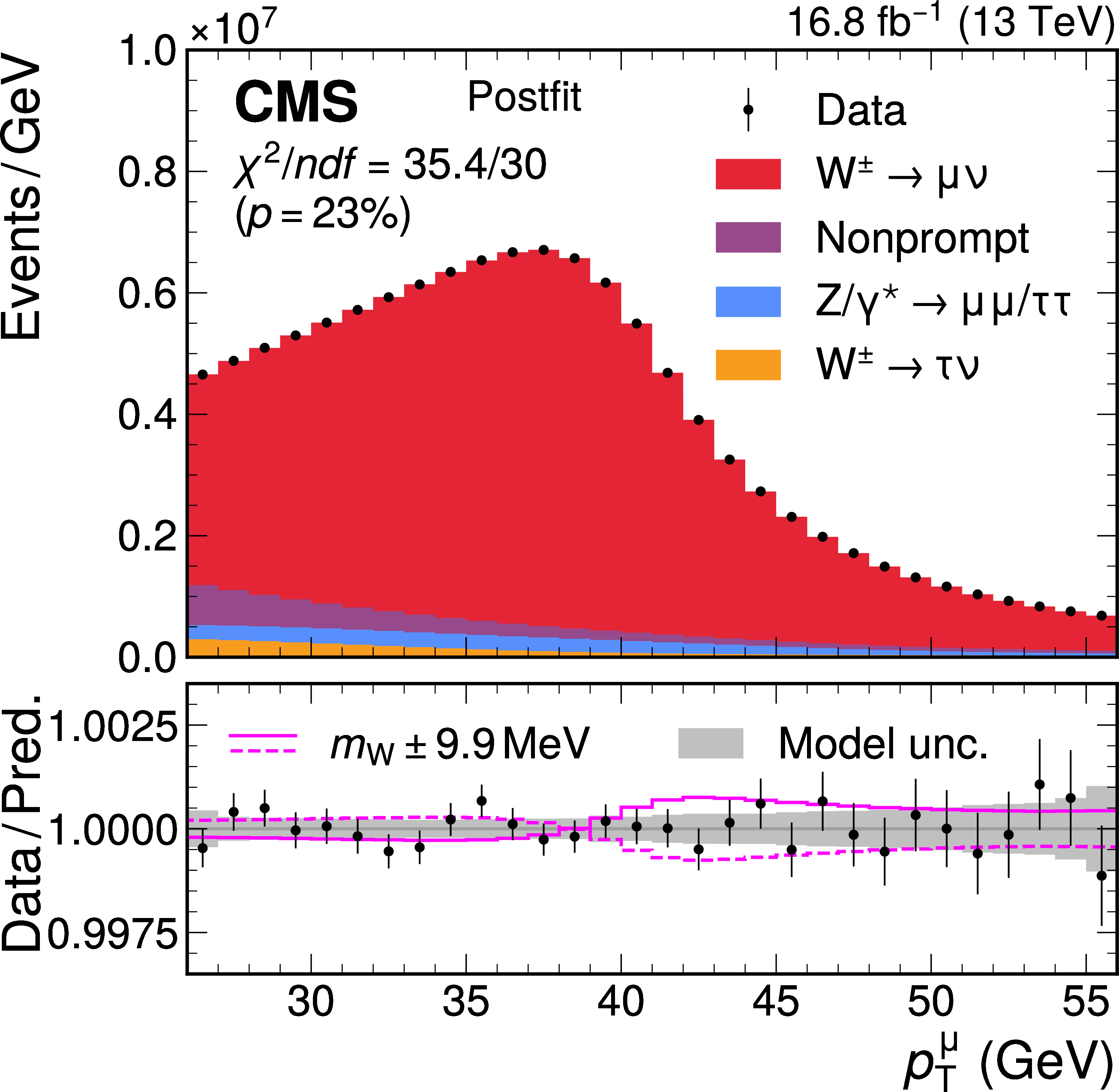
Figure 3:
The W boson mass measurement. Measured and postfit $ p_{\mathrm{T}}^{\mu} $ distributions, showing the sensitivity to $ m_{\mathrm{W}} $ from the characteristic peak at $ {\sim}m_{\mathrm{W}}/ $ 2. The predicted $ \mathrm{W}\to\mu\nu $ contribution, shown in red, reflects the measured value of $ m_{\mathrm{W}} $. The dominant background contributions are shown as colored filled histograms. The bottom panel shows the ratio between the number of events observed in data, including variations in the predictions, and the total nominal prediction. The vertical bars represent the statistical uncertainties in the data. A shift in the $ m_{\mathrm{W}} $ value shifts the peak of the distribution, as illustrated by the solid and dashed magenta lines, which show an increase or decrease of $ m_{\mathrm{W}} $ by 9.9 MeV. The total contribution of all theoretical and experimental uncertainties in the predictions, after the uncertainty profiling in the maximum likelihood fit, is shown by the gray band. |
png pdf |
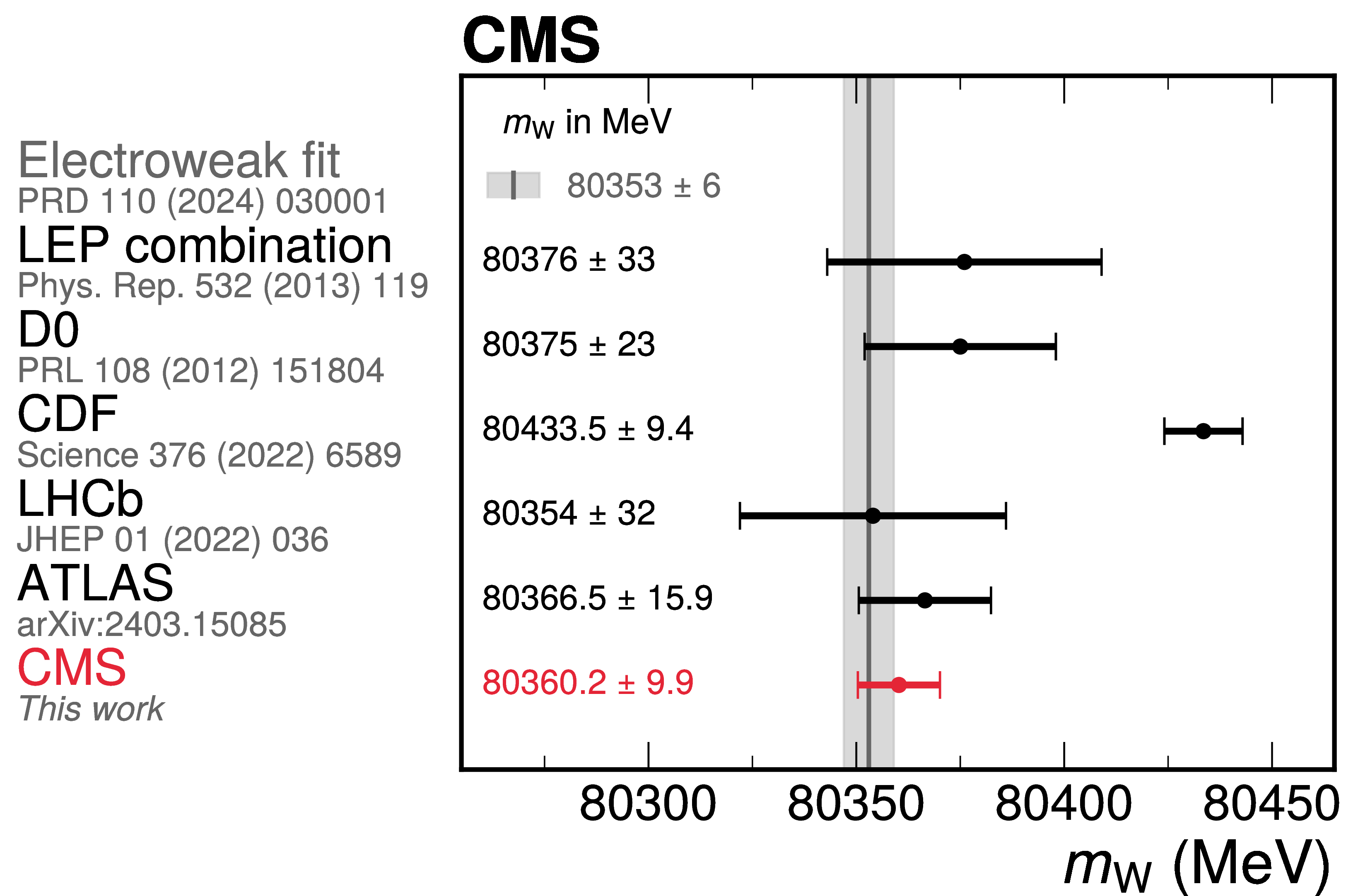
Figure 4:
Comparison with other experiments and the EW fit prediction. The $ m_{\mathrm{W}} $ measurement from this analysis (in red) is compared with the combined measurement of experiments at LEP [15], and with the measurements performed by the D0 [16], CDF [4], LHCb [18], and ATLAS [19] experiments. The global EW fit prediction [1,2,3] is represented by the gray vertical band, with the shaded band showing its uncertainty. |
png pdf |
Figure A1:
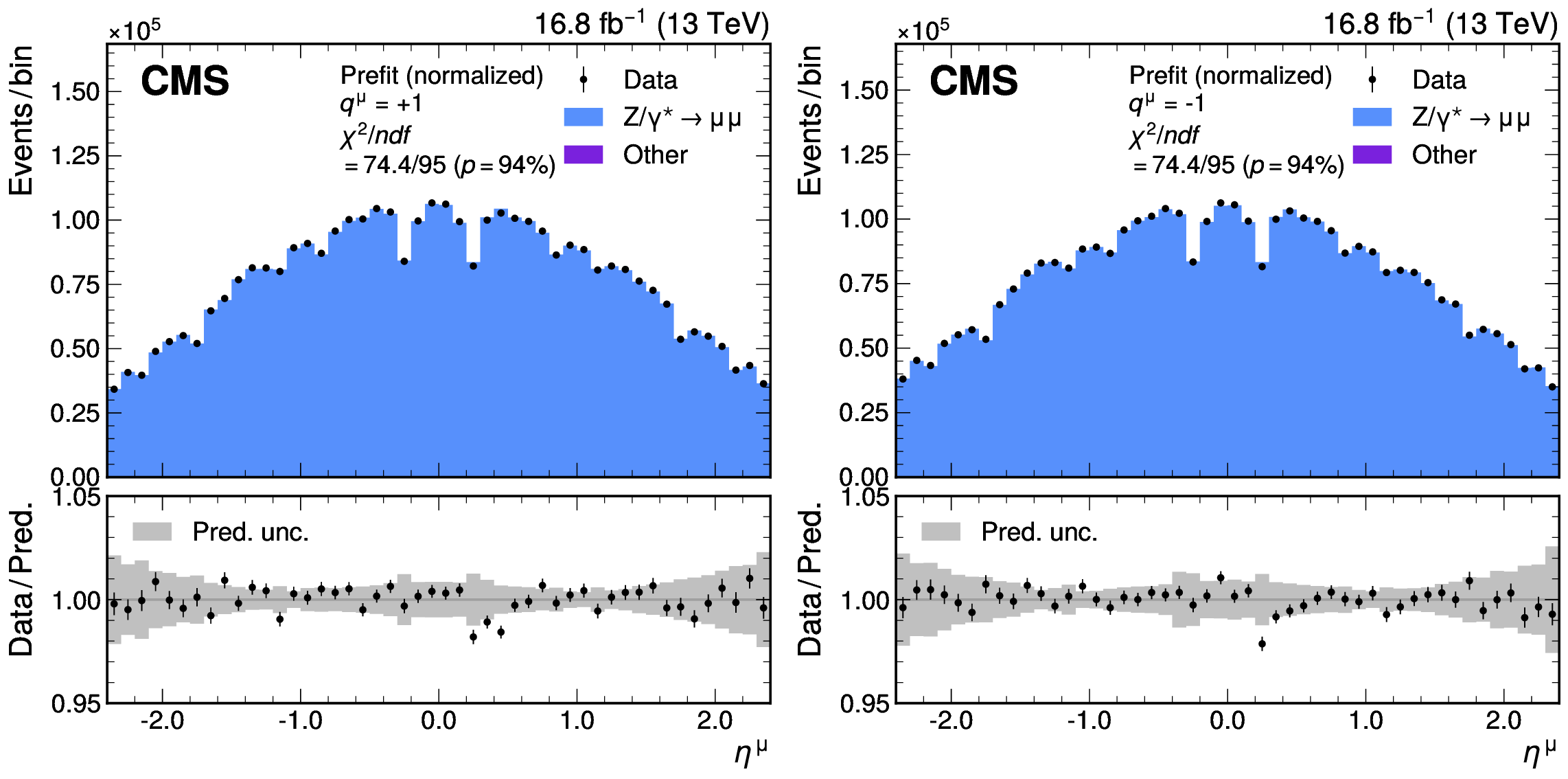
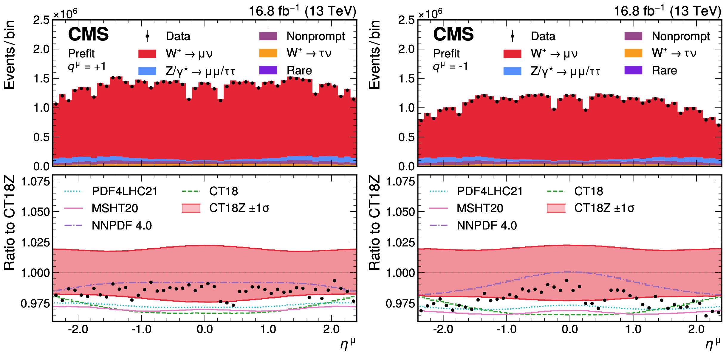
Measured and predicted $ \eta^{\mu} $ distributions in $ \mathrm{Z}\to\mu\mu $ events with the W-like Z boson selection for positively (left) and negatively (right) charged muons. The normalization of the simulated spectrum is scaled to the measured distribution to better illustrate the level of agreement between the two. The shaded bands correspond to the total (statistical and systematic) uncertainty on the normalized distributions. The normalization of the prediction is scaled by about 1%, which is less than the luminosity and total cross section uncertainties. The vertical bars represent the statistical uncertainties in the data. The bottom panel shows the ratio of the number of events observed in data and of normalized variations in the predictions to that of the total nominal prediction. |
png pdf |
Figure A1-a:
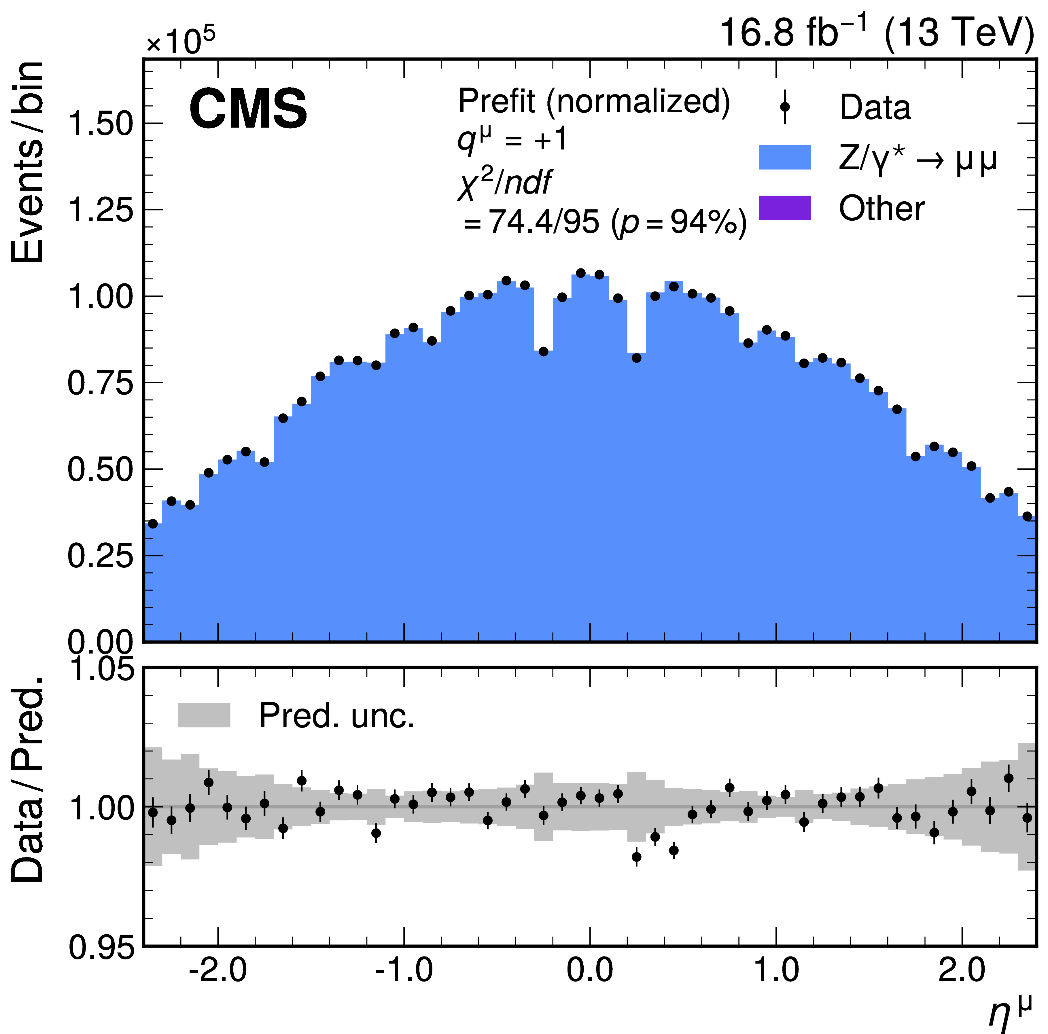
Measured and predicted $ \eta^{\mu} $ distributions in $ \mathrm{Z}\to\mu\mu $ events with the W-like Z boson selection for positively (left) and negatively (right) charged muons. The normalization of the simulated spectrum is scaled to the measured distribution to better illustrate the level of agreement between the two. The shaded bands correspond to the total (statistical and systematic) uncertainty on the normalized distributions. The normalization of the prediction is scaled by about 1%, which is less than the luminosity and total cross section uncertainties. The vertical bars represent the statistical uncertainties in the data. The bottom panel shows the ratio of the number of events observed in data and of normalized variations in the predictions to that of the total nominal prediction. |
png pdf |
Figure A1-b:
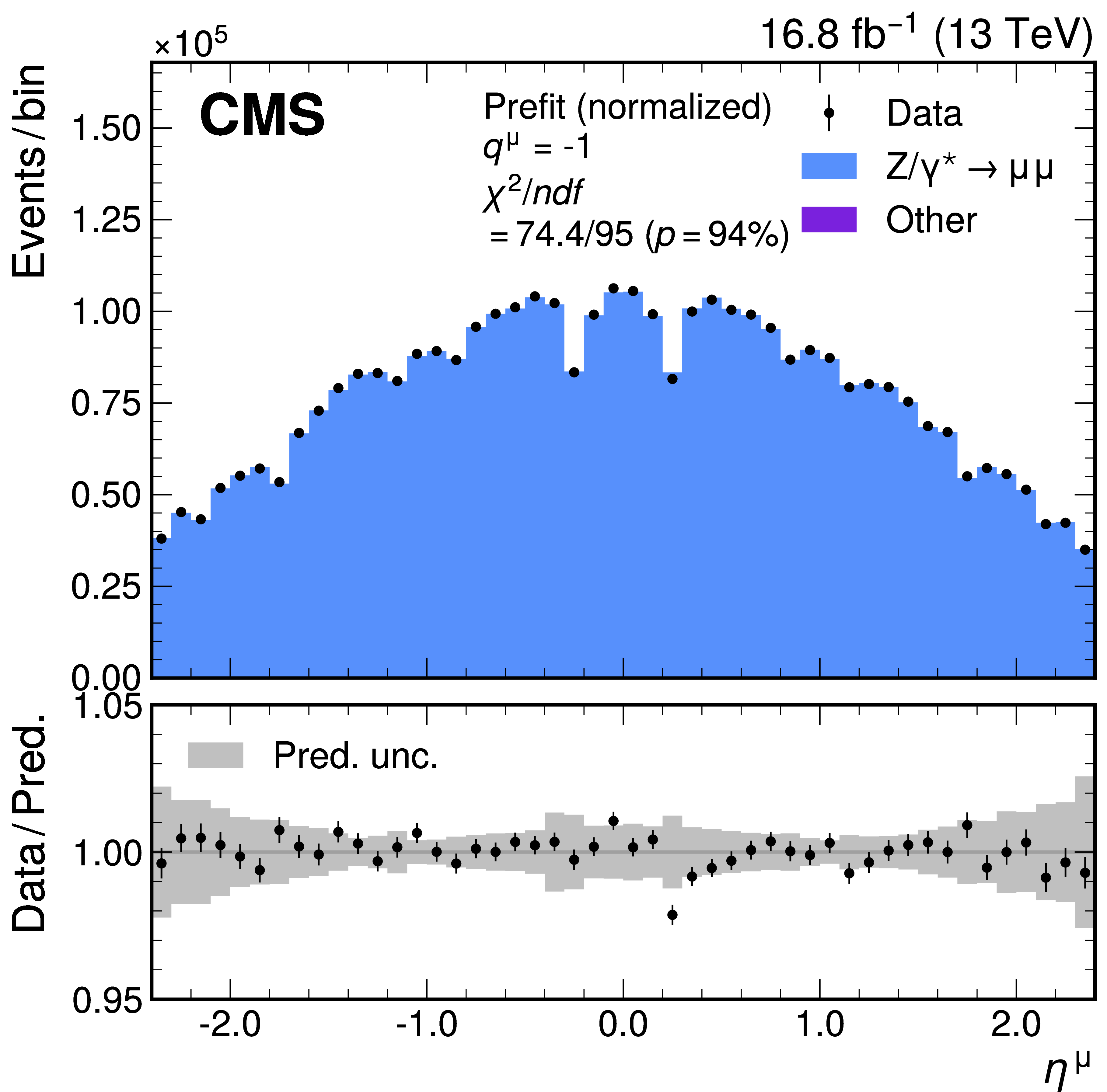
Measured and predicted $ \eta^{\mu} $ distributions in $ \mathrm{Z}\to\mu\mu $ events with the W-like Z boson selection for positively (left) and negatively (right) charged muons. The normalization of the simulated spectrum is scaled to the measured distribution to better illustrate the level of agreement between the two. The shaded bands correspond to the total (statistical and systematic) uncertainty on the normalized distributions. The normalization of the prediction is scaled by about 1%, which is less than the luminosity and total cross section uncertainties. The vertical bars represent the statistical uncertainties in the data. The bottom panel shows the ratio of the number of events observed in data and of normalized variations in the predictions to that of the total nominal prediction. |
png pdf |
Figure A2:
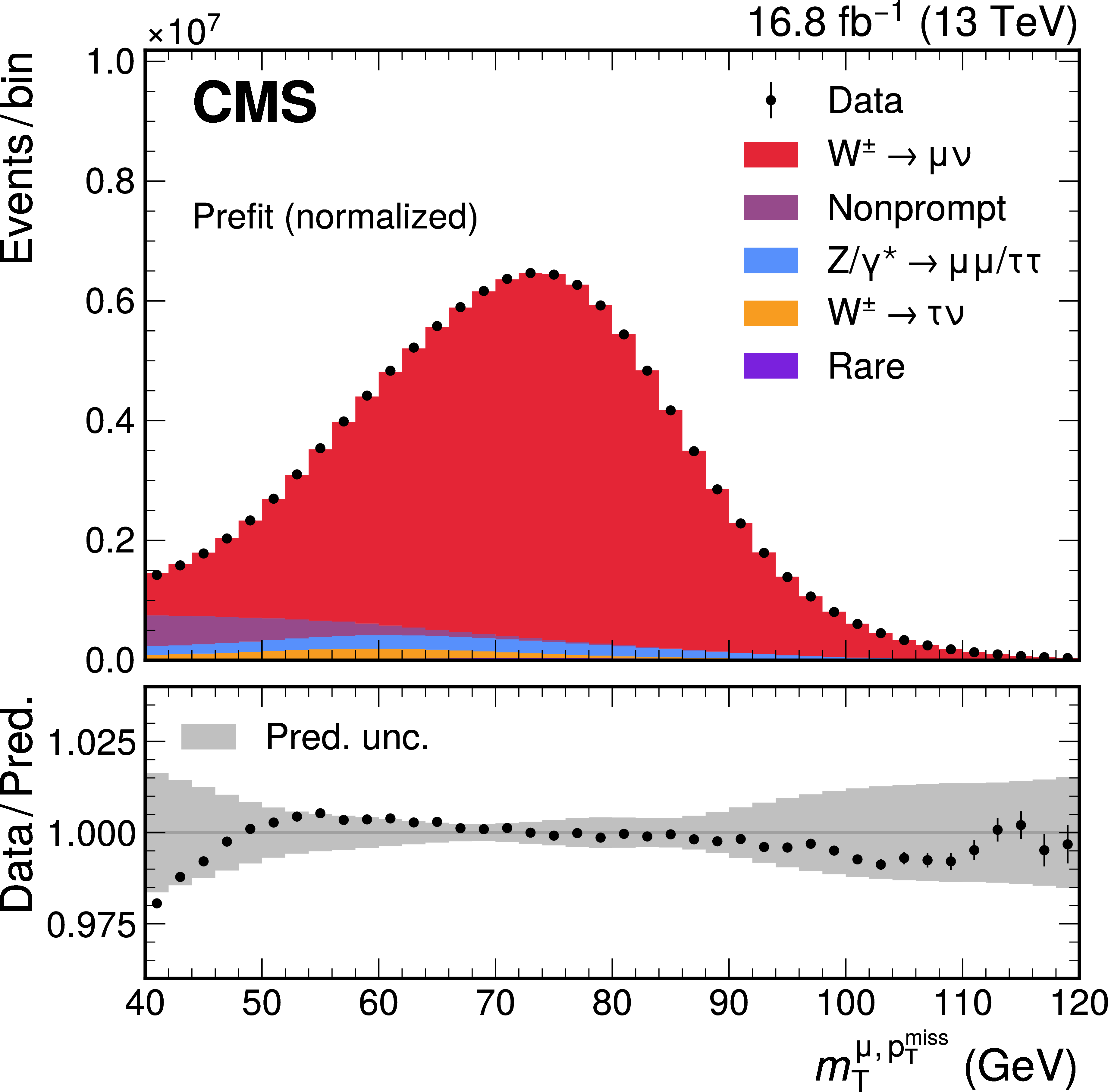
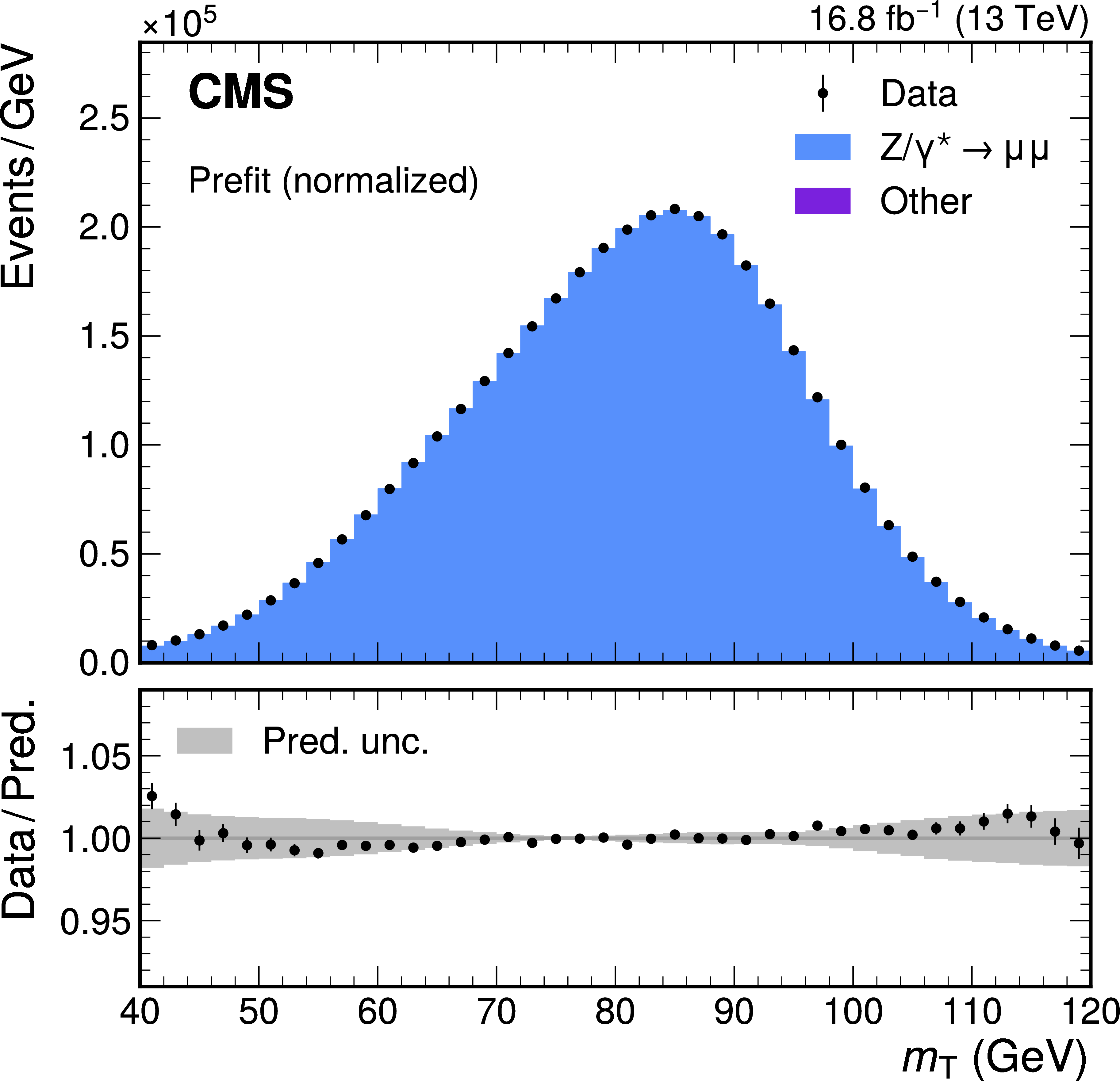
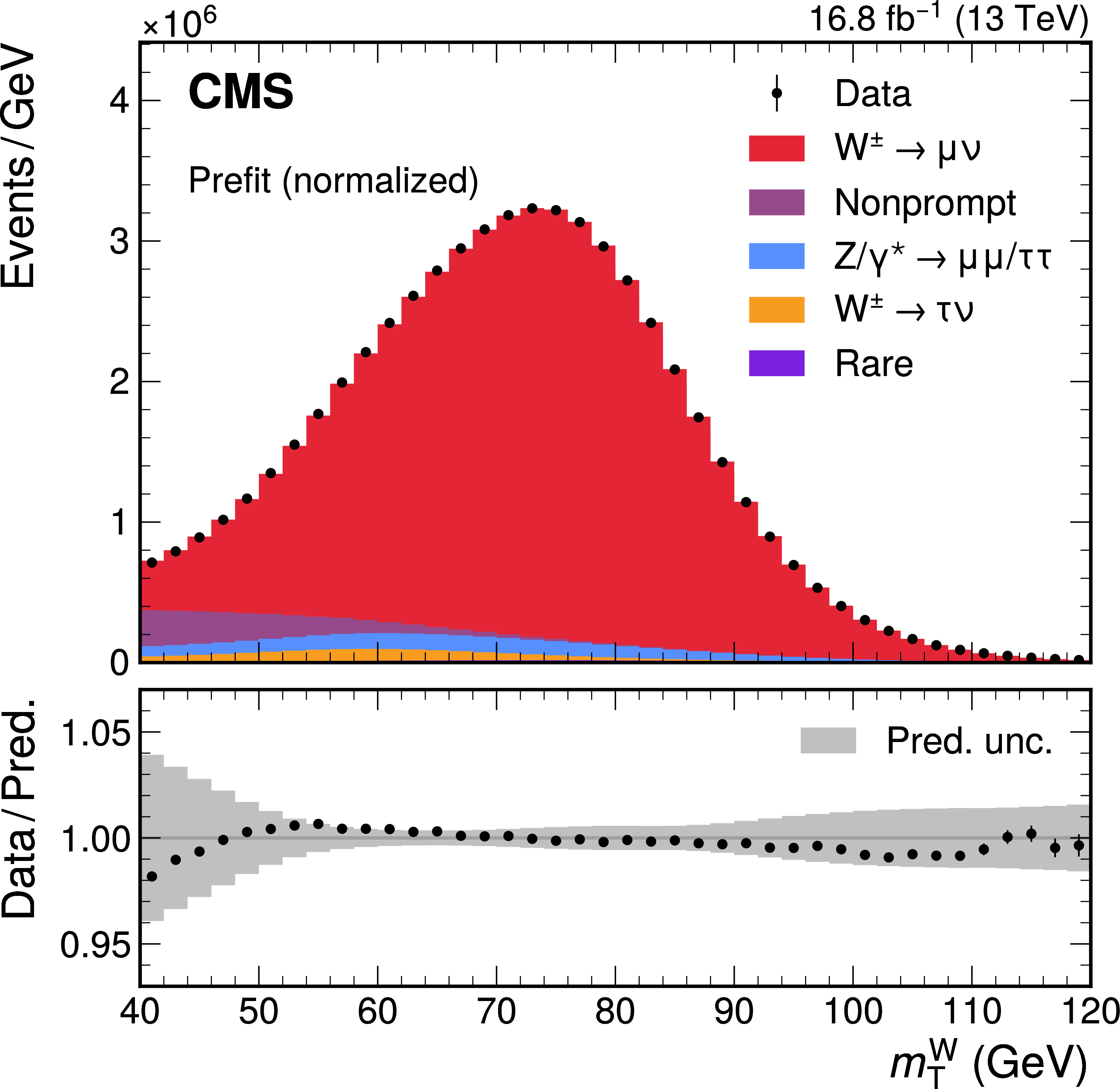
Measured and predicted $ m_{\mathrm{T}} $ distributions in $ \mathrm{Z}\to\mu\mu $ and $ \mathrm{W}\to\mu\nu $ events, after calibrating $ u_{\mathrm{T}} $. Given that $ m_{\mathrm{T}}^{\mathrm{W}} $ is an input variable, the extended ABCD method does not give suitable predictions for the $ m_{\mathrm{T}}^{\mathrm{W}} $ distribution. Therefore, the nonprompt background contribution to W boson production is estimated from the QCD multijet simulation. The predictions are those prior to the fit to data. The total uncertainties (statistical and systematic) are represented by the gray band and the normalization of the simulated spectrum is scaled to the measured distribution to better illustrate their agreement. The vertical bars represent the statistical uncertainties in the data. The bottom panel shows the ratio of the number of events observed in data and of variations in the predictions to that of the total nominal prediction. |
png pdf |
Figure A2-a:
Measured and predicted $ m_{\mathrm{T}} $ distributions in $ \mathrm{Z}\to\mu\mu $ and $ \mathrm{W}\to\mu\nu $ events, after calibrating $ u_{\mathrm{T}} $. Given that $ m_{\mathrm{T}}^{\mathrm{W}} $ is an input variable, the extended ABCD method does not give suitable predictions for the $ m_{\mathrm{T}}^{\mathrm{W}} $ distribution. Therefore, the nonprompt background contribution to W boson production is estimated from the QCD multijet simulation. The predictions are those prior to the fit to data. The total uncertainties (statistical and systematic) are represented by the gray band and the normalization of the simulated spectrum is scaled to the measured distribution to better illustrate their agreement. The vertical bars represent the statistical uncertainties in the data. The bottom panel shows the ratio of the number of events observed in data and of variations in the predictions to that of the total nominal prediction. |
png pdf |
Figure A2-b:
Measured and predicted $ m_{\mathrm{T}} $ distributions in $ \mathrm{Z}\to\mu\mu $ and $ \mathrm{W}\to\mu\nu $ events, after calibrating $ u_{\mathrm{T}} $. Given that $ m_{\mathrm{T}}^{\mathrm{W}} $ is an input variable, the extended ABCD method does not give suitable predictions for the $ m_{\mathrm{T}}^{\mathrm{W}} $ distribution. Therefore, the nonprompt background contribution to W boson production is estimated from the QCD multijet simulation. The predictions are those prior to the fit to data. The total uncertainties (statistical and systematic) are represented by the gray band and the normalization of the simulated spectrum is scaled to the measured distribution to better illustrate their agreement. The vertical bars represent the statistical uncertainties in the data. The bottom panel shows the ratio of the number of events observed in data and of variations in the predictions to that of the total nominal prediction. |
png pdf |
Figure A3:
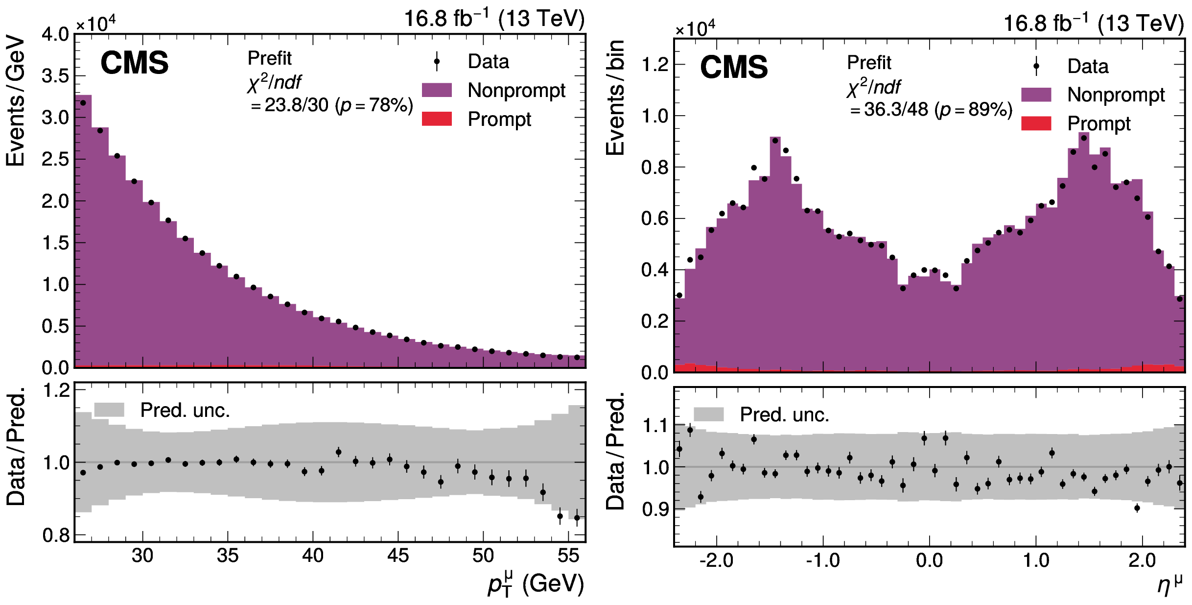
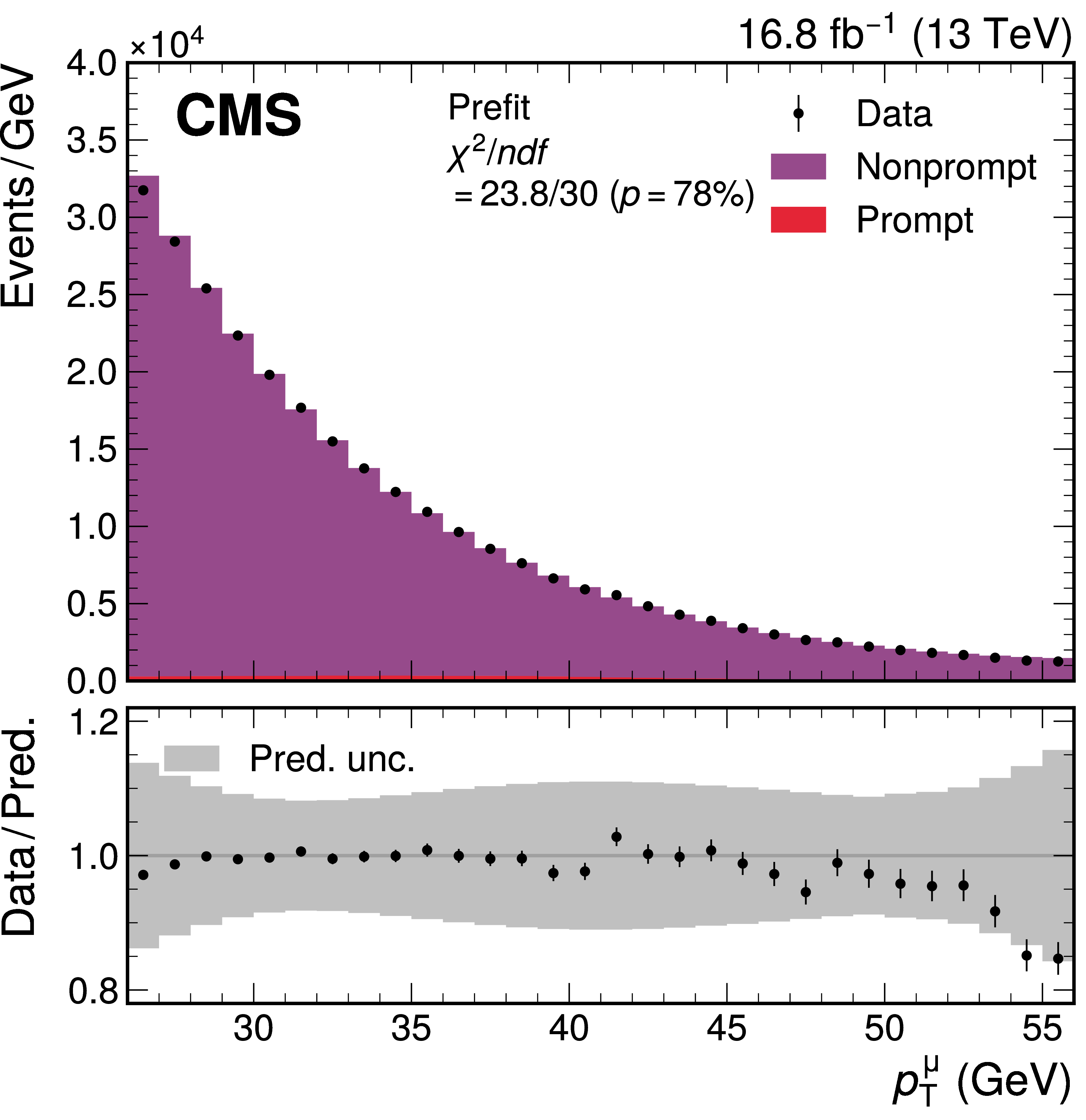
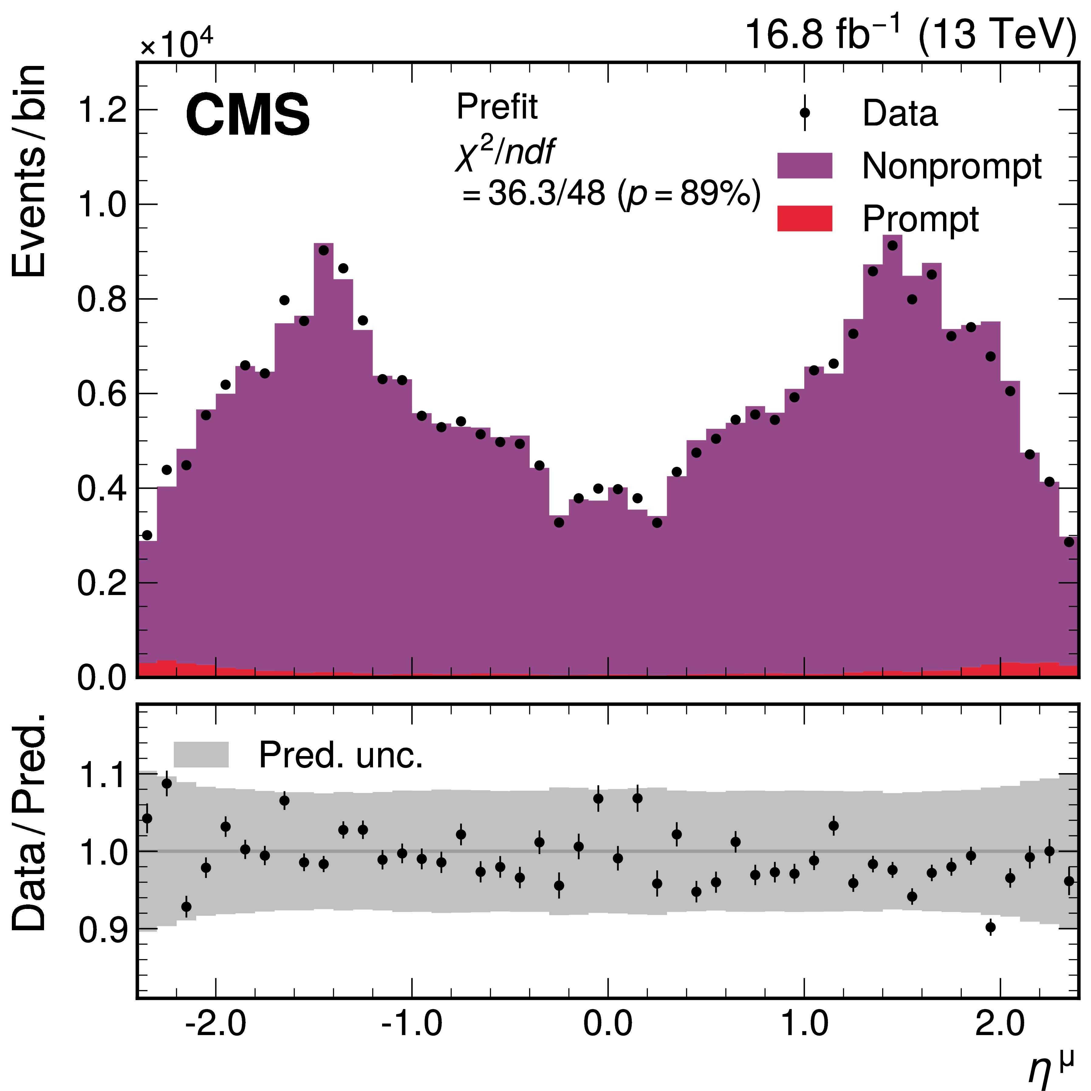
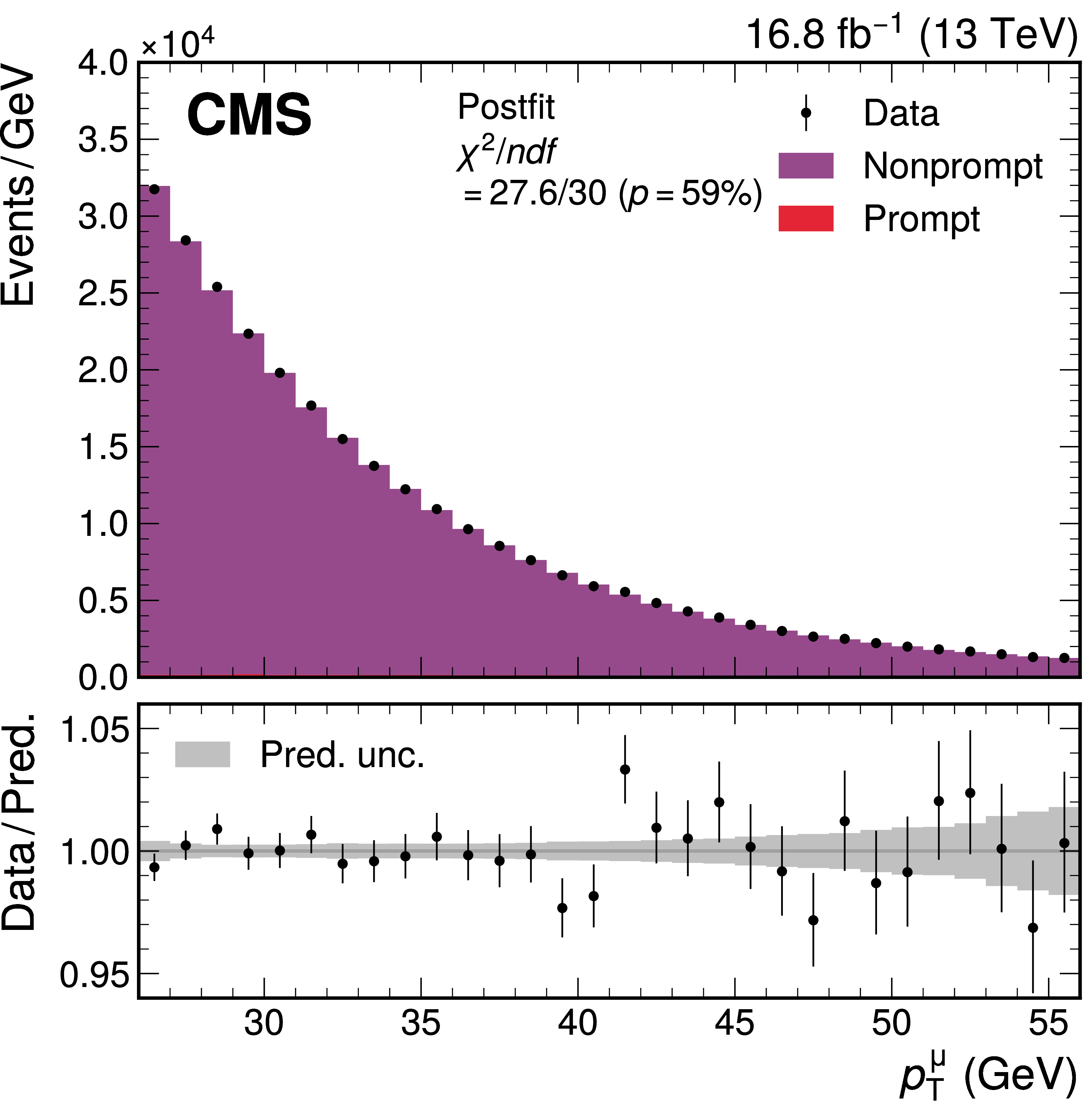
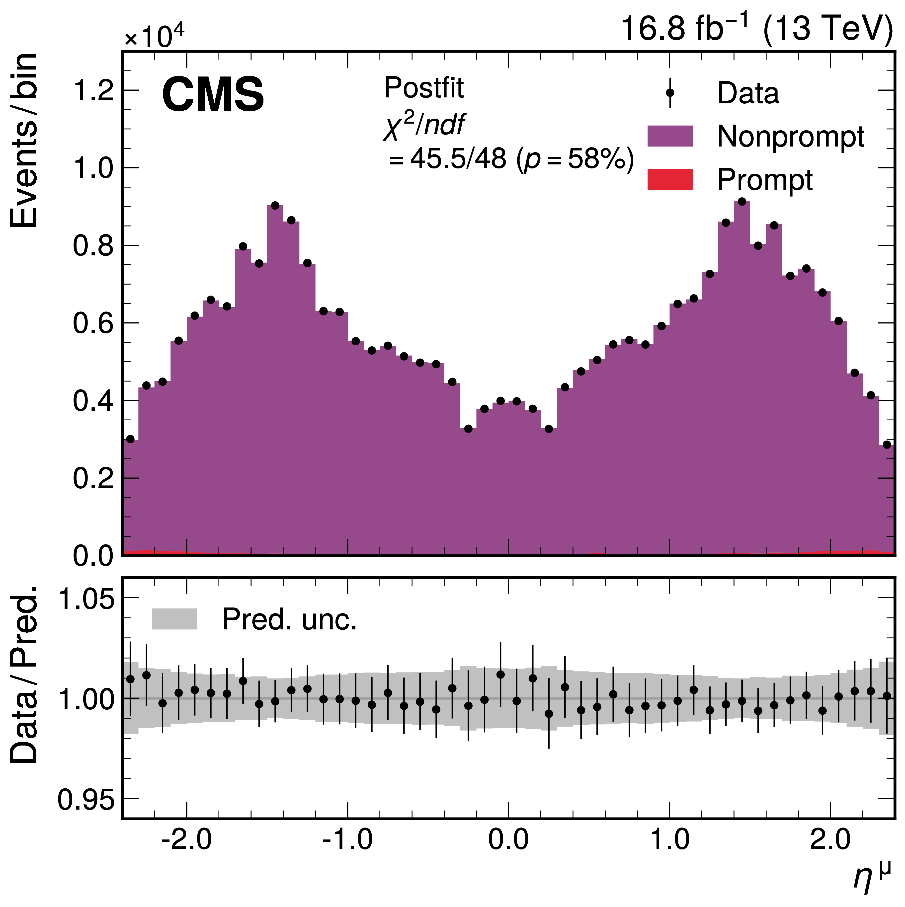
The observed data and the prediction of the extended ABCD method before (top) and after (bottom) the maximum likelihood fit, for the $ p_{\mathrm{T}}^{\mu} $ (left) and $ \eta^{\mu} $ (right) distributions, in a control region enriched in events with nonprompt muons matched to displaced secondary vertices. Small contributions from events with a prompt muon, evaluated using simulated samples, are shown by the red histogram. The total uncertainties (statistical and systematic) are represented by the gray bands. The vertical bars represent the statistical uncertainties in the data. The bottom panel shows the ratio of the number of events observed in data and of variations in the predictions to that of the total nominal prediction. |
png pdf |
Figure A3-a:
The observed data and the prediction of the extended ABCD method before (top) and after (bottom) the maximum likelihood fit, for the $ p_{\mathrm{T}}^{\mu} $ (left) and $ \eta^{\mu} $ (right) distributions, in a control region enriched in events with nonprompt muons matched to displaced secondary vertices. Small contributions from events with a prompt muon, evaluated using simulated samples, are shown by the red histogram. The total uncertainties (statistical and systematic) are represented by the gray bands. The vertical bars represent the statistical uncertainties in the data. The bottom panel shows the ratio of the number of events observed in data and of variations in the predictions to that of the total nominal prediction. |
png pdf |
Figure A3-b:
The observed data and the prediction of the extended ABCD method before (top) and after (bottom) the maximum likelihood fit, for the $ p_{\mathrm{T}}^{\mu} $ (left) and $ \eta^{\mu} $ (right) distributions, in a control region enriched in events with nonprompt muons matched to displaced secondary vertices. Small contributions from events with a prompt muon, evaluated using simulated samples, are shown by the red histogram. The total uncertainties (statistical and systematic) are represented by the gray bands. The vertical bars represent the statistical uncertainties in the data. The bottom panel shows the ratio of the number of events observed in data and of variations in the predictions to that of the total nominal prediction. |
png pdf |
Figure A3-c:
The observed data and the prediction of the extended ABCD method before (top) and after (bottom) the maximum likelihood fit, for the $ p_{\mathrm{T}}^{\mu} $ (left) and $ \eta^{\mu} $ (right) distributions, in a control region enriched in events with nonprompt muons matched to displaced secondary vertices. Small contributions from events with a prompt muon, evaluated using simulated samples, are shown by the red histogram. The total uncertainties (statistical and systematic) are represented by the gray bands. The vertical bars represent the statistical uncertainties in the data. The bottom panel shows the ratio of the number of events observed in data and of variations in the predictions to that of the total nominal prediction. |
png pdf |
Figure A3-d:
The observed data and the prediction of the extended ABCD method before (top) and after (bottom) the maximum likelihood fit, for the $ p_{\mathrm{T}}^{\mu} $ (left) and $ \eta^{\mu} $ (right) distributions, in a control region enriched in events with nonprompt muons matched to displaced secondary vertices. Small contributions from events with a prompt muon, evaluated using simulated samples, are shown by the red histogram. The total uncertainties (statistical and systematic) are represented by the gray bands. The vertical bars represent the statistical uncertainties in the data. The bottom panel shows the ratio of the number of events observed in data and of variations in the predictions to that of the total nominal prediction. |
png pdf |
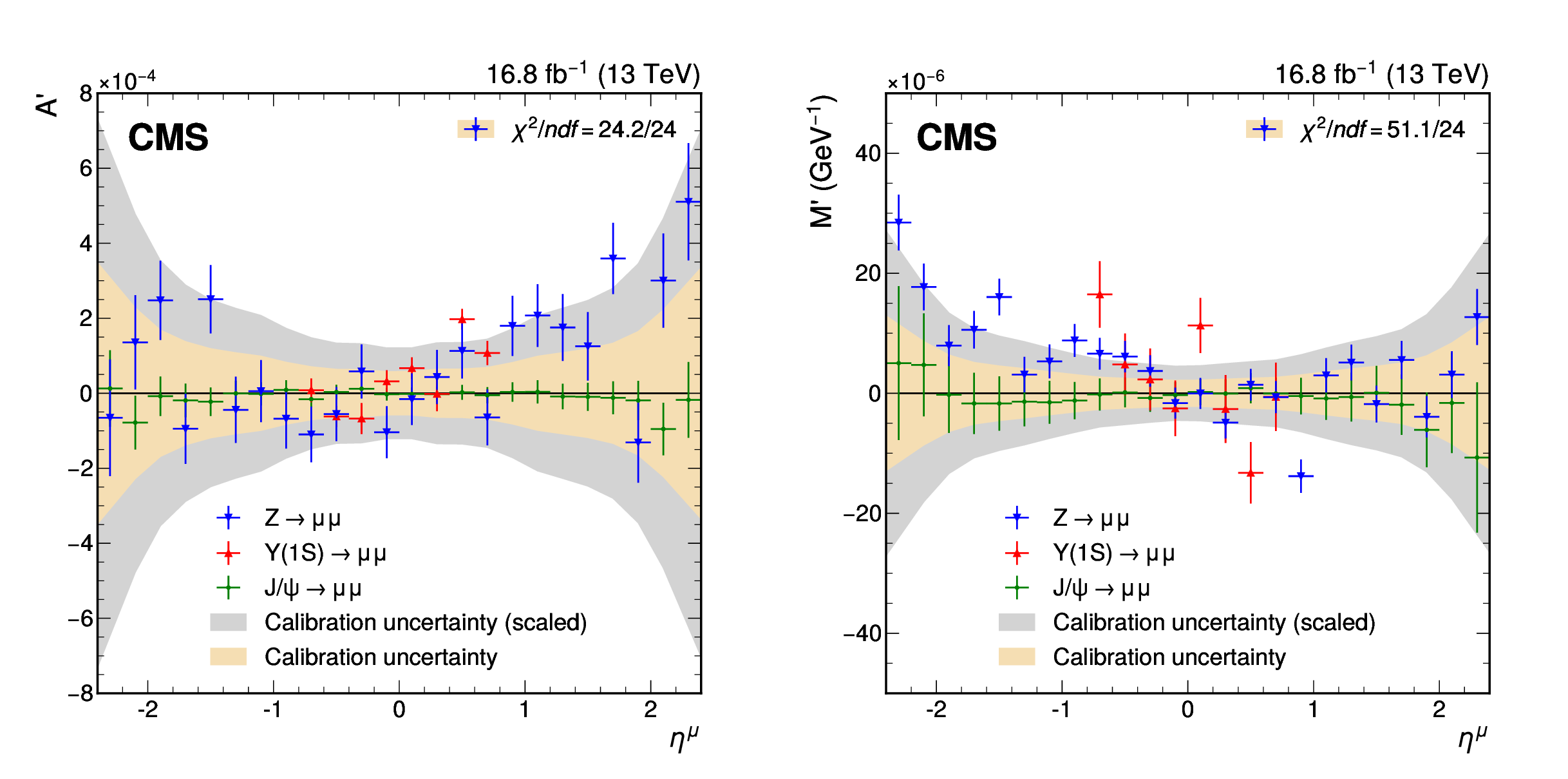
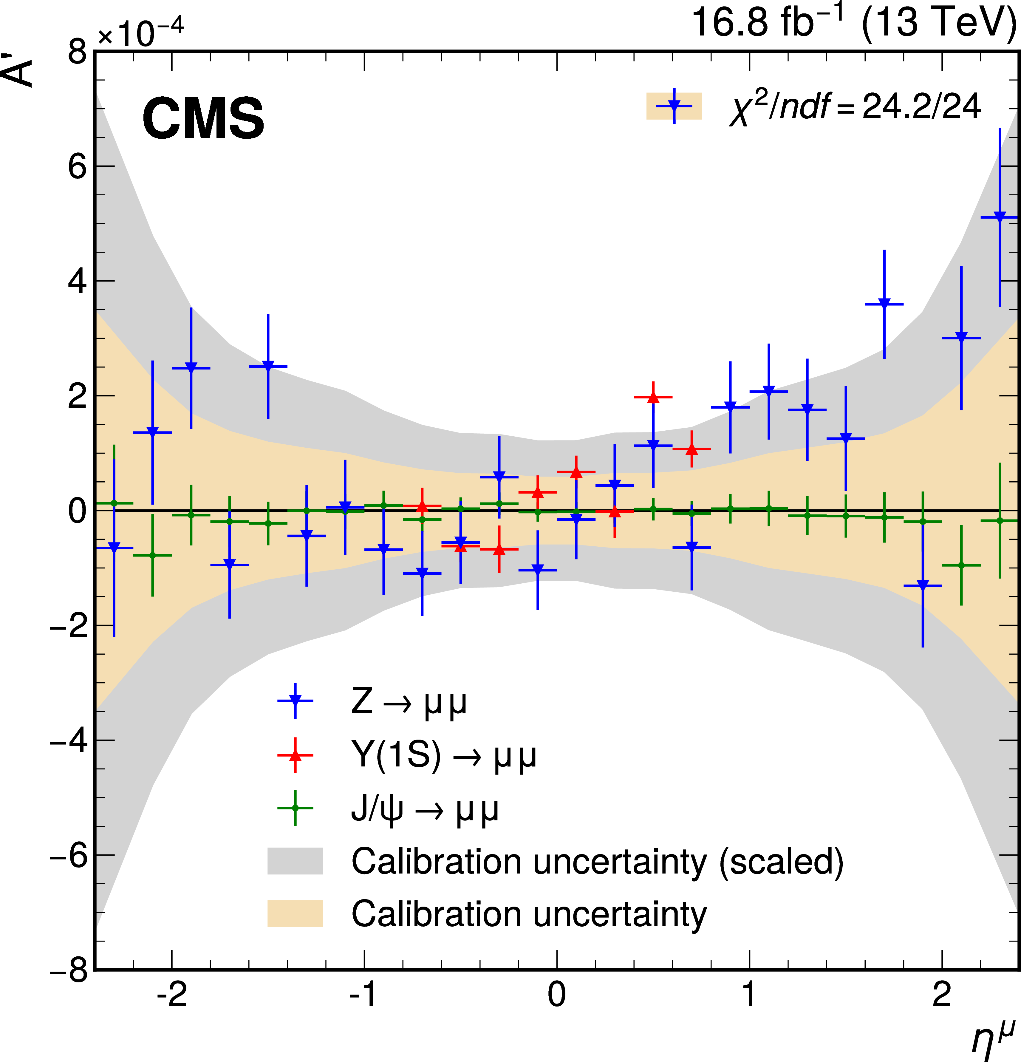
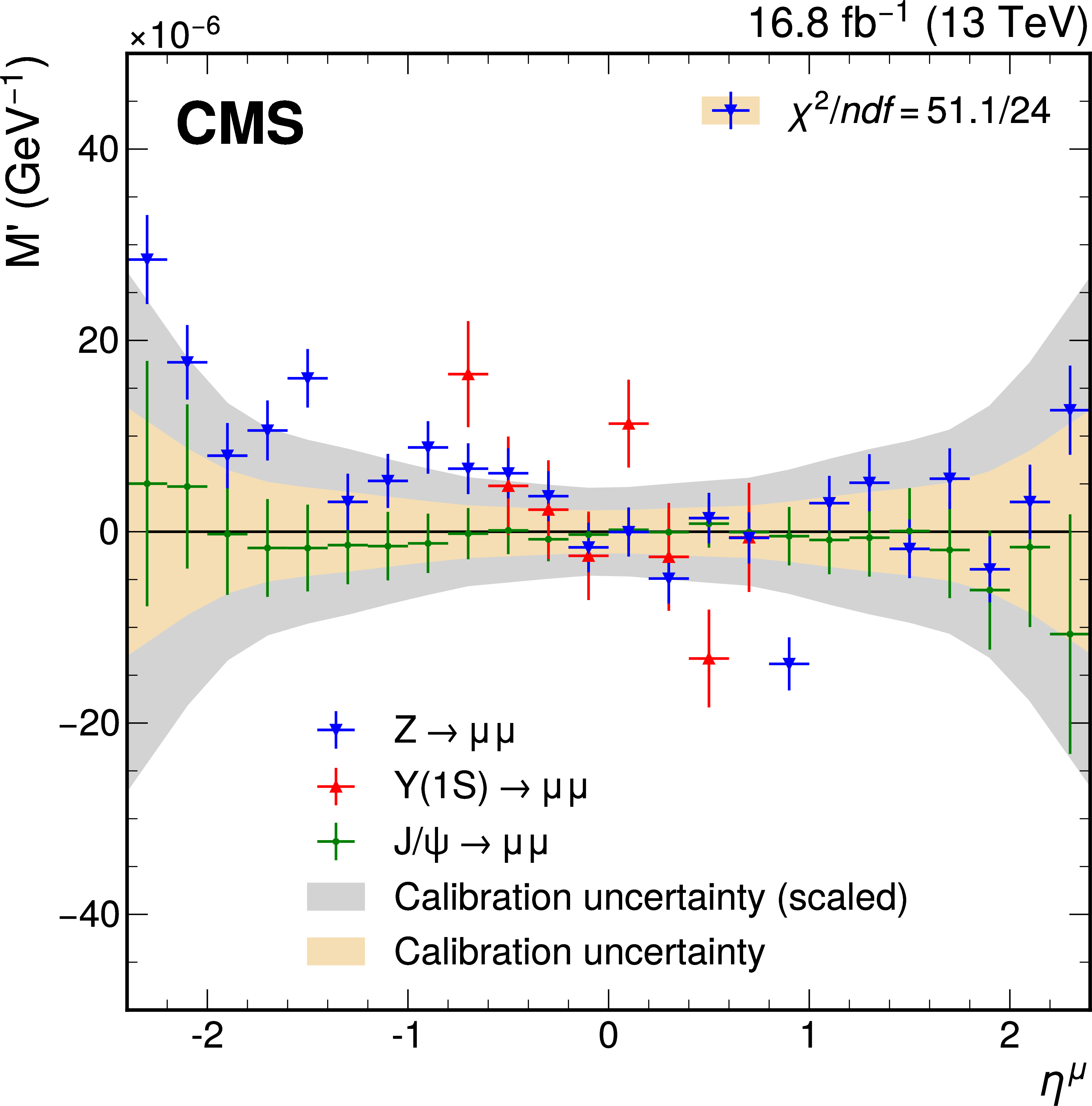
Figure A4:
Charge-independent ($ A^{\prime} $, left) and charge-dependent ($ M^{\prime} $, right) residual scale differences between data and simulation, after applying the corrections derived from the $ {\mathrm{J}/\psi} \to\mu\mu $ event sample. The scale differences are evaluated separately in $ {\mathrm{J}/\psi} \to\mu\mu $, $ \Upsilon{\textrm{(1S)}}\to\mu\mu $, and $ \mathrm{Z}\to\mu\mu $ events to assess the consistency of the muon momentum scale calibration in the different event samples. The charge-independent comparison probes a magnetic-field-like difference, whereas the charge-dependent comparison reflects a misalignment-like term. The points with error bars represent the scale parameters and statistical uncertainties associated with the closure test performed with $ {\mathrm{J}/\psi} \to\mu\mu $ (green), $ \Upsilon{\textrm{(1S)}}\to\mu\mu $ (red), and $ \mathrm{Z}\to\mu\mu $ (blue) events. The yellow band represents the corresponding statistical uncertainty in the calibration parameters derived from the $ \mathrm{J}/\psi $ calibration sample. The filled gray band shows this uncertainty scaled by a factor of 2.1, as described in the text. The $ \chi^2 $ values correspond to the compatibility of the scale parameters with zero for the closure test performed with $ \mathrm{Z}\to\mu\mu $ events. The statistical uncertainties for these parameters, as well as for the calibration parameters derived from the $ \mathrm{J}/\psi $ sample (without the 2.1 uncertainty scaling factor applied), are taken into account. The calibration parameter uncertainties are fully uncorrelated from the Z and $ \Upsilon{\textrm{(1S)}} $ closure test uncertainties, but very strongly correlated with the $ \mathrm{J}/\psi $ closure uncertainties, since they use the same data. |
png pdf |
Figure A4-a:
Charge-independent ($ A^{\prime} $, left) and charge-dependent ($ M^{\prime} $, right) residual scale differences between data and simulation, after applying the corrections derived from the $ {\mathrm{J}/\psi} \to\mu\mu $ event sample. The scale differences are evaluated separately in $ {\mathrm{J}/\psi} \to\mu\mu $, $ \Upsilon{\textrm{(1S)}}\to\mu\mu $, and $ \mathrm{Z}\to\mu\mu $ events to assess the consistency of the muon momentum scale calibration in the different event samples. The charge-independent comparison probes a magnetic-field-like difference, whereas the charge-dependent comparison reflects a misalignment-like term. The points with error bars represent the scale parameters and statistical uncertainties associated with the closure test performed with $ {\mathrm{J}/\psi} \to\mu\mu $ (green), $ \Upsilon{\textrm{(1S)}}\to\mu\mu $ (red), and $ \mathrm{Z}\to\mu\mu $ (blue) events. The yellow band represents the corresponding statistical uncertainty in the calibration parameters derived from the $ \mathrm{J}/\psi $ calibration sample. The filled gray band shows this uncertainty scaled by a factor of 2.1, as described in the text. The $ \chi^2 $ values correspond to the compatibility of the scale parameters with zero for the closure test performed with $ \mathrm{Z}\to\mu\mu $ events. The statistical uncertainties for these parameters, as well as for the calibration parameters derived from the $ \mathrm{J}/\psi $ sample (without the 2.1 uncertainty scaling factor applied), are taken into account. The calibration parameter uncertainties are fully uncorrelated from the Z and $ \Upsilon{\textrm{(1S)}} $ closure test uncertainties, but very strongly correlated with the $ \mathrm{J}/\psi $ closure uncertainties, since they use the same data. |
png pdf |
Figure A4-b:
Charge-independent ($ A^{\prime} $, left) and charge-dependent ($ M^{\prime} $, right) residual scale differences between data and simulation, after applying the corrections derived from the $ {\mathrm{J}/\psi} \to\mu\mu $ event sample. The scale differences are evaluated separately in $ {\mathrm{J}/\psi} \to\mu\mu $, $ \Upsilon{\textrm{(1S)}}\to\mu\mu $, and $ \mathrm{Z}\to\mu\mu $ events to assess the consistency of the muon momentum scale calibration in the different event samples. The charge-independent comparison probes a magnetic-field-like difference, whereas the charge-dependent comparison reflects a misalignment-like term. The points with error bars represent the scale parameters and statistical uncertainties associated with the closure test performed with $ {\mathrm{J}/\psi} \to\mu\mu $ (green), $ \Upsilon{\textrm{(1S)}}\to\mu\mu $ (red), and $ \mathrm{Z}\to\mu\mu $ (blue) events. The yellow band represents the corresponding statistical uncertainty in the calibration parameters derived from the $ \mathrm{J}/\psi $ calibration sample. The filled gray band shows this uncertainty scaled by a factor of 2.1, as described in the text. The $ \chi^2 $ values correspond to the compatibility of the scale parameters with zero for the closure test performed with $ \mathrm{Z}\to\mu\mu $ events. The statistical uncertainties for these parameters, as well as for the calibration parameters derived from the $ \mathrm{J}/\psi $ sample (without the 2.1 uncertainty scaling factor applied), are taken into account. The calibration parameter uncertainties are fully uncorrelated from the Z and $ \Upsilon{\textrm{(1S)}} $ closure test uncertainties, but very strongly correlated with the $ \mathrm{J}/\psi $ closure uncertainties, since they use the same data. |

png pdf |
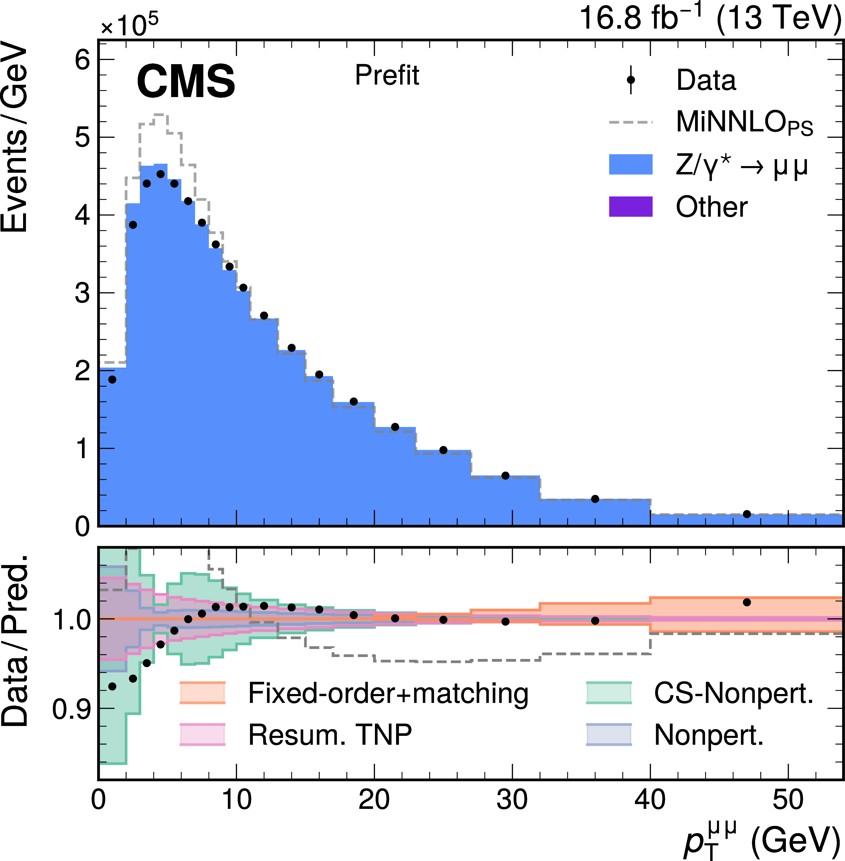
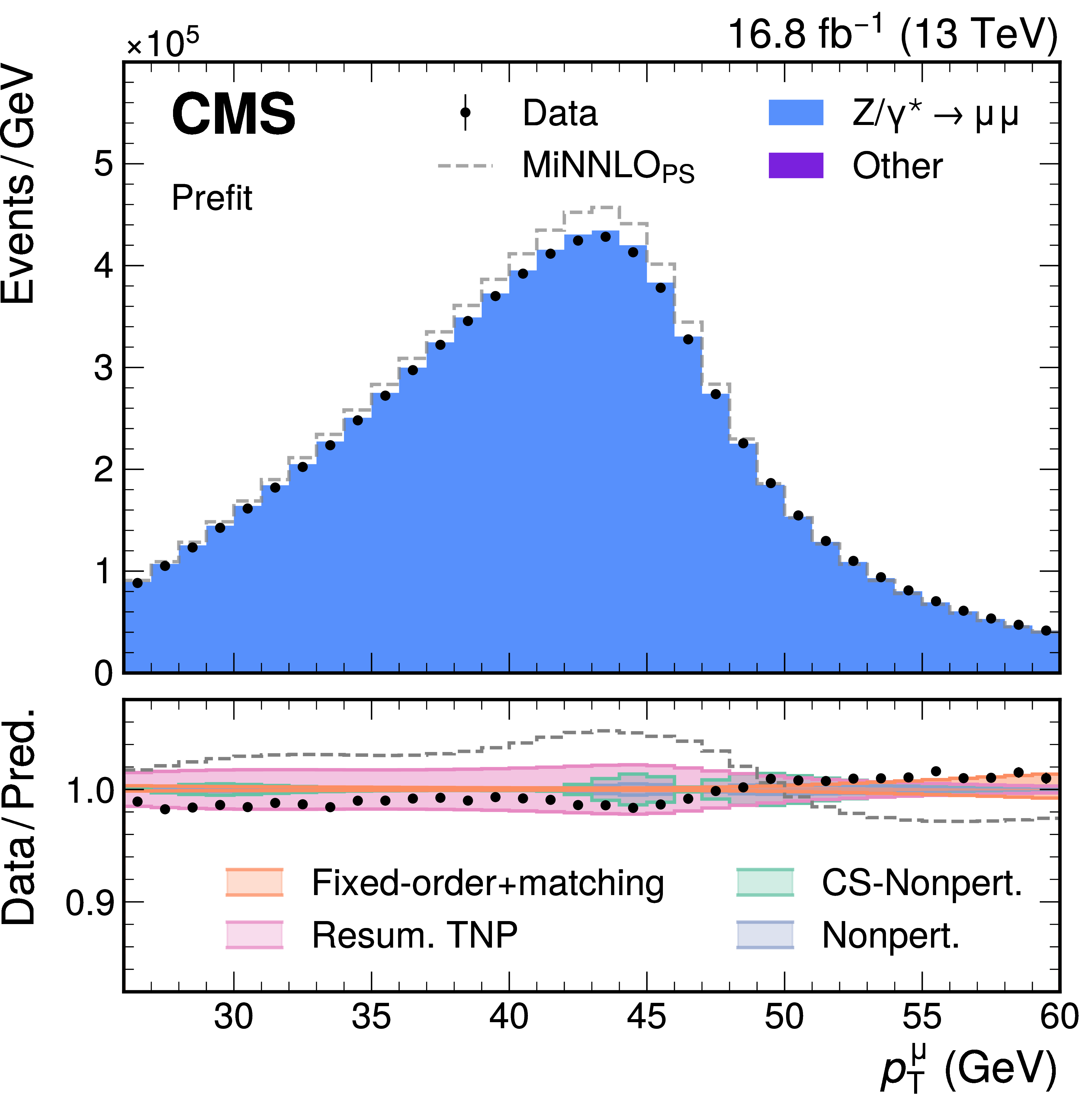
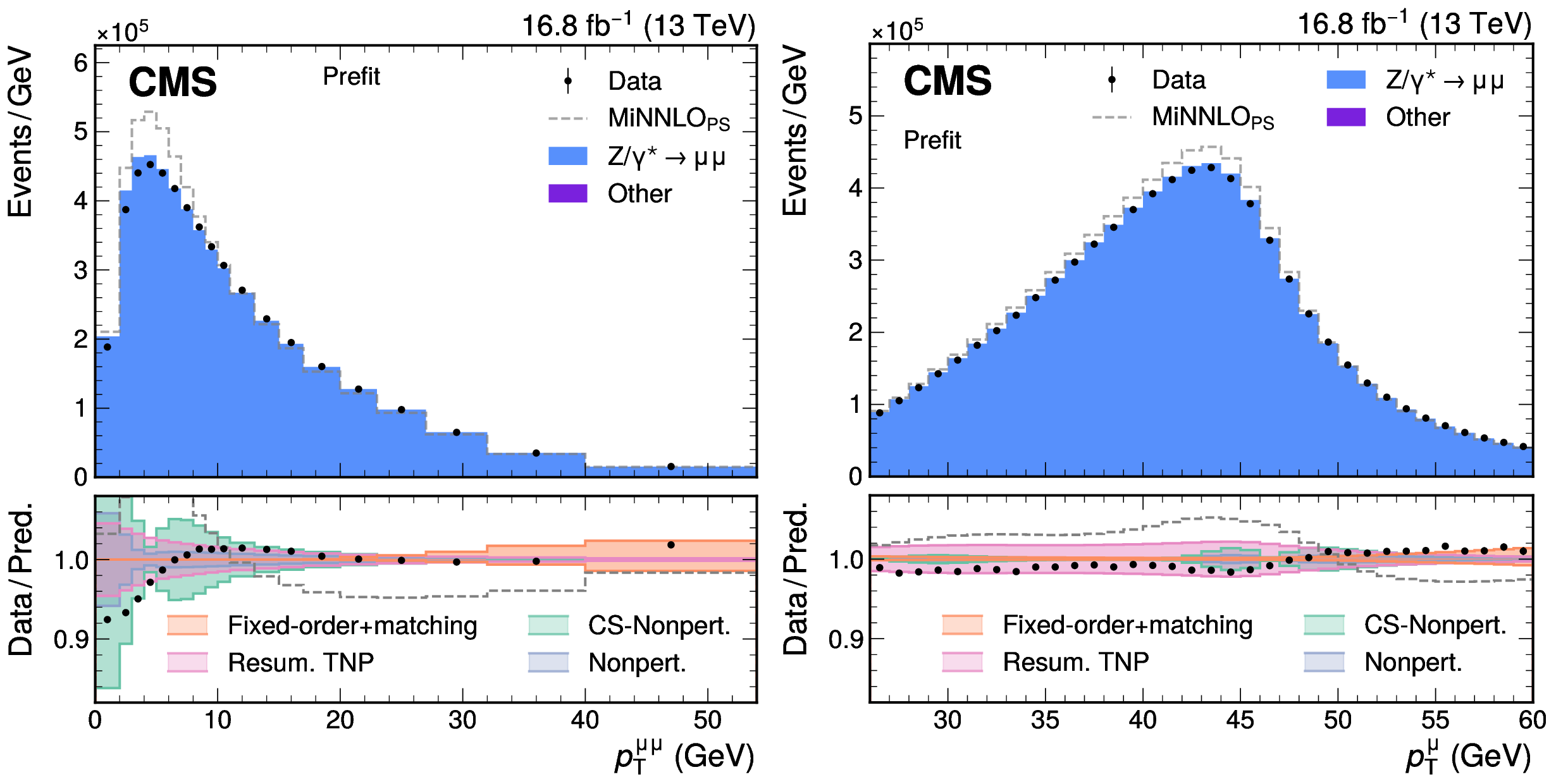
Figure A5:
Measured and simulated $ p_{\mathrm{T}}^{\mu\mu} $ (left) and $ p_{\mathrm{T}}^{\mu} $ (right) distributions in selected $ \mathrm{Z}\to\mu\mu $ events. The standalone uncorrected MINNLO} _\TEXT{PS predictions are shown by the dashed gray line. The nominal predictions (blue) correct the POWHEG MINNLO$_{\text{PS}}$ $p_{\mathrm{T}}^{\mathrm{V}} $ with SCETLIB $+$ DYTURBO at $ \mathrm{N}^{3}\mathrm{LL}{+}\mathrm{NNLO} $, as described in the text. The vertical bars represent the statistical uncertainties in the data. The bottom panel shows the ratio of the number of events observed in data to that of the total nominal prediction, as well as the relative impact of variations of the predictions. Different sources of uncertainty are shown as solid bands in the lower panel: the fixed-order uncertainty and the uncertainty in the resummation and fixed-order matching (orange), resummed prediction using TNPs (pink), the Collins--Soper (CS) kernel nonperturbative uncertainty (green), and other nonperturbative uncertainties (light blue). Additional sources of experimental and theoretical uncertainty that impact the agreement with the data are not shown. |
png pdf |
Figure A5-a:
Measured and simulated $ p_{\mathrm{T}}^{\mu\mu} $ (left) and $ p_{\mathrm{T}}^{\mu} $ (right) distributions in selected $ \mathrm{Z}\to\mu\mu $ events. The standalone uncorrected MINNLO} _\TEXT{PS predictions are shown by the dashed gray line. The nominal predictions (blue) correct the POWHEG MINNLO$_{\text{PS}}$ $p_{\mathrm{T}}^{\mathrm{V}} $ with SCETLIB $+$ DYTURBO at $ \mathrm{N}^{3}\mathrm{LL}{+}\mathrm{NNLO} $, as described in the text. The vertical bars represent the statistical uncertainties in the data. The bottom panel shows the ratio of the number of events observed in data to that of the total nominal prediction, as well as the relative impact of variations of the predictions. Different sources of uncertainty are shown as solid bands in the lower panel: the fixed-order uncertainty and the uncertainty in the resummation and fixed-order matching (orange), resummed prediction using TNPs (pink), the Collins--Soper (CS) kernel nonperturbative uncertainty (green), and other nonperturbative uncertainties (light blue). Additional sources of experimental and theoretical uncertainty that impact the agreement with the data are not shown. |
png pdf |
Figure A5-b:
Measured and simulated $ p_{\mathrm{T}}^{\mu\mu} $ (left) and $ p_{\mathrm{T}}^{\mu} $ (right) distributions in selected $ \mathrm{Z}\to\mu\mu $ events. The standalone uncorrected MINNLO} _\TEXT{PS predictions are shown by the dashed gray line. The nominal predictions (blue) correct the POWHEG MINNLO$_{\text{PS}}$ $p_{\mathrm{T}}^{\mathrm{V}} $ with SCETLIB $+$ DYTURBO at $ \mathrm{N}^{3}\mathrm{LL}{+}\mathrm{NNLO} $, as described in the text. The vertical bars represent the statistical uncertainties in the data. The bottom panel shows the ratio of the number of events observed in data to that of the total nominal prediction, as well as the relative impact of variations of the predictions. Different sources of uncertainty are shown as solid bands in the lower panel: the fixed-order uncertainty and the uncertainty in the resummation and fixed-order matching (orange), resummed prediction using TNPs (pink), the Collins--Soper (CS) kernel nonperturbative uncertainty (green), and other nonperturbative uncertainties (light blue). Additional sources of experimental and theoretical uncertainty that impact the agreement with the data are not shown. |
png pdf |
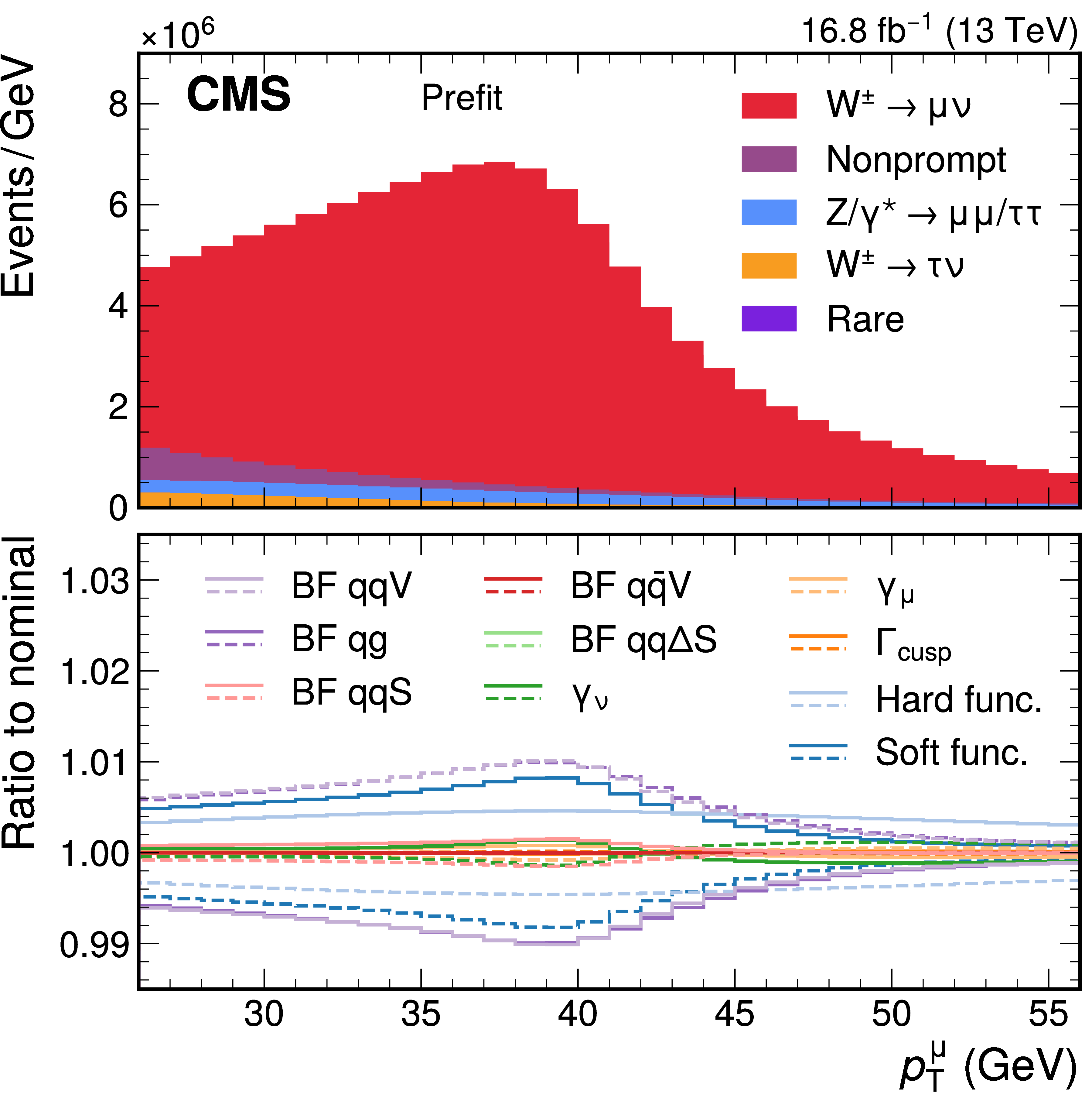
Figure A6:
The predicted $ p_{\mathrm{T}}^{\mu} $ distribution for selected $ \mathrm{W}\to\mu\nu $ events, before the maximum likelihood fit. The lower panel shows the ratio of the ten TNP variations described in the text to the nominal prediction, illustrating their impact on the spectrum. |
png pdf |
Figure A7:
The generator-level $ p_{\mathrm{T}}^{\mathrm{W}} $ distribution, with three instances of the prediction and their uncertainty: before the maximum likelihood fit (``prefit"), and reflecting the results of the two fits described in the text. The distribution and uncertainties obtained from the combined $ (p_{\mathrm{T}}^{\mu}, \eta^{\mu}, q^{\mu}) $ and $ (p_{\mathrm{T}}^{\mu\mu}, y^{\mu\mu}) $ fit is shown in red, whereas the blue band shows the distribution obtained from the nominal $ (p_{\mathrm{T}}^{\mu}, \eta^{\mu}, q^{\mu}) $ fit. The generator-level distribution predicted by SCETLIB $+$ DYTURBO before incorporating in situ constraints is shown in gray. The ratio of the postfit predictions to the prefit prediction (in gray), as well as their uncertainties, are shown by the shaded bands in the lower panel. |

png pdf |
Figure A8:
The W boson mass measured with the helicity fit for different scaling scenarios of the prefit helicity cross section uncertainties, denoted by $ \Delta_{\sigma_3} $ and $ \Delta_{\sigma_{\text{others}}} $ for the $ \sigma_3 $ and the other components, respectively. The points are grouped and colored according to the scaling of $ \sigma_3 $. The black line indicates the nominal result, with its uncertainties shown by the gray band. |
png pdf |
Figure A9:
Measured and predicted $ (p_{\mathrm{T}}^{\mu}, \eta^{\mu}) $ distributions used in the W-like $ m_{\mathrm{Z}} $ (upper two) and $ m_{\mathrm{W}} $ (lower two) measurements for positively (upper and second from bottom) and negatively (second from top and lower) charged muons. The two-dimensional distribution is ``unrolled" such that each bin on the $ x $-axis represents one $ (p_{\mathrm{T}}^{\mu}, \eta^{\mu}) $ cell. The gray band represents the uncertainty in the prediction, before the fit to the data. The bottom panel shows the ratio of the number of events observed in data to the nominal prediction. The vertical bars represent the statistical uncertainties in the data. |
png pdf |
Figure A9-a:
Measured and predicted $ (p_{\mathrm{T}}^{\mu}, \eta^{\mu}) $ distributions used in the W-like $ m_{\mathrm{Z}} $ (upper two) and $ m_{\mathrm{W}} $ (lower two) measurements for positively (upper and second from bottom) and negatively (second from top and lower) charged muons. The two-dimensional distribution is ``unrolled" such that each bin on the $ x $-axis represents one $ (p_{\mathrm{T}}^{\mu}, \eta^{\mu}) $ cell. The gray band represents the uncertainty in the prediction, before the fit to the data. The bottom panel shows the ratio of the number of events observed in data to the nominal prediction. The vertical bars represent the statistical uncertainties in the data. |
png pdf |
Figure A9-b:
Measured and predicted $ (p_{\mathrm{T}}^{\mu}, \eta^{\mu}) $ distributions used in the W-like $ m_{\mathrm{Z}} $ (upper two) and $ m_{\mathrm{W}} $ (lower two) measurements for positively (upper and second from bottom) and negatively (second from top and lower) charged muons. The two-dimensional distribution is ``unrolled" such that each bin on the $ x $-axis represents one $ (p_{\mathrm{T}}^{\mu}, \eta^{\mu}) $ cell. The gray band represents the uncertainty in the prediction, before the fit to the data. The bottom panel shows the ratio of the number of events observed in data to the nominal prediction. The vertical bars represent the statistical uncertainties in the data. |
png pdf |
Figure A9-c:
Measured and predicted $ (p_{\mathrm{T}}^{\mu}, \eta^{\mu}) $ distributions used in the W-like $ m_{\mathrm{Z}} $ (upper two) and $ m_{\mathrm{W}} $ (lower two) measurements for positively (upper and second from bottom) and negatively (second from top and lower) charged muons. The two-dimensional distribution is ``unrolled" such that each bin on the $ x $-axis represents one $ (p_{\mathrm{T}}^{\mu}, \eta^{\mu}) $ cell. The gray band represents the uncertainty in the prediction, before the fit to the data. The bottom panel shows the ratio of the number of events observed in data to the nominal prediction. The vertical bars represent the statistical uncertainties in the data. |
png pdf |
Figure A9-d:
Measured and predicted $ (p_{\mathrm{T}}^{\mu}, \eta^{\mu}) $ distributions used in the W-like $ m_{\mathrm{Z}} $ (upper two) and $ m_{\mathrm{W}} $ (lower two) measurements for positively (upper and second from bottom) and negatively (second from top and lower) charged muons. The two-dimensional distribution is ``unrolled" such that each bin on the $ x $-axis represents one $ (p_{\mathrm{T}}^{\mu}, \eta^{\mu}) $ cell. The gray band represents the uncertainty in the prediction, before the fit to the data. The bottom panel shows the ratio of the number of events observed in data to the nominal prediction. The vertical bars represent the statistical uncertainties in the data. |
png pdf |
Figure B1:
Measured and simulated $ \mathrm{Z}\to\mu\mu $ dimuon mass distributions, after applying the muon momentum scale and resolution corrections. The simulated predictions and uncertainties are scaled to match the number of observed data events. The vertical bars represent the statistical uncertainties in the data. The bottom panel shows the ratio of the number of events observed in data and of variations in the predictions to that of the total nominal prediction. |
png pdf |
Figure B2:
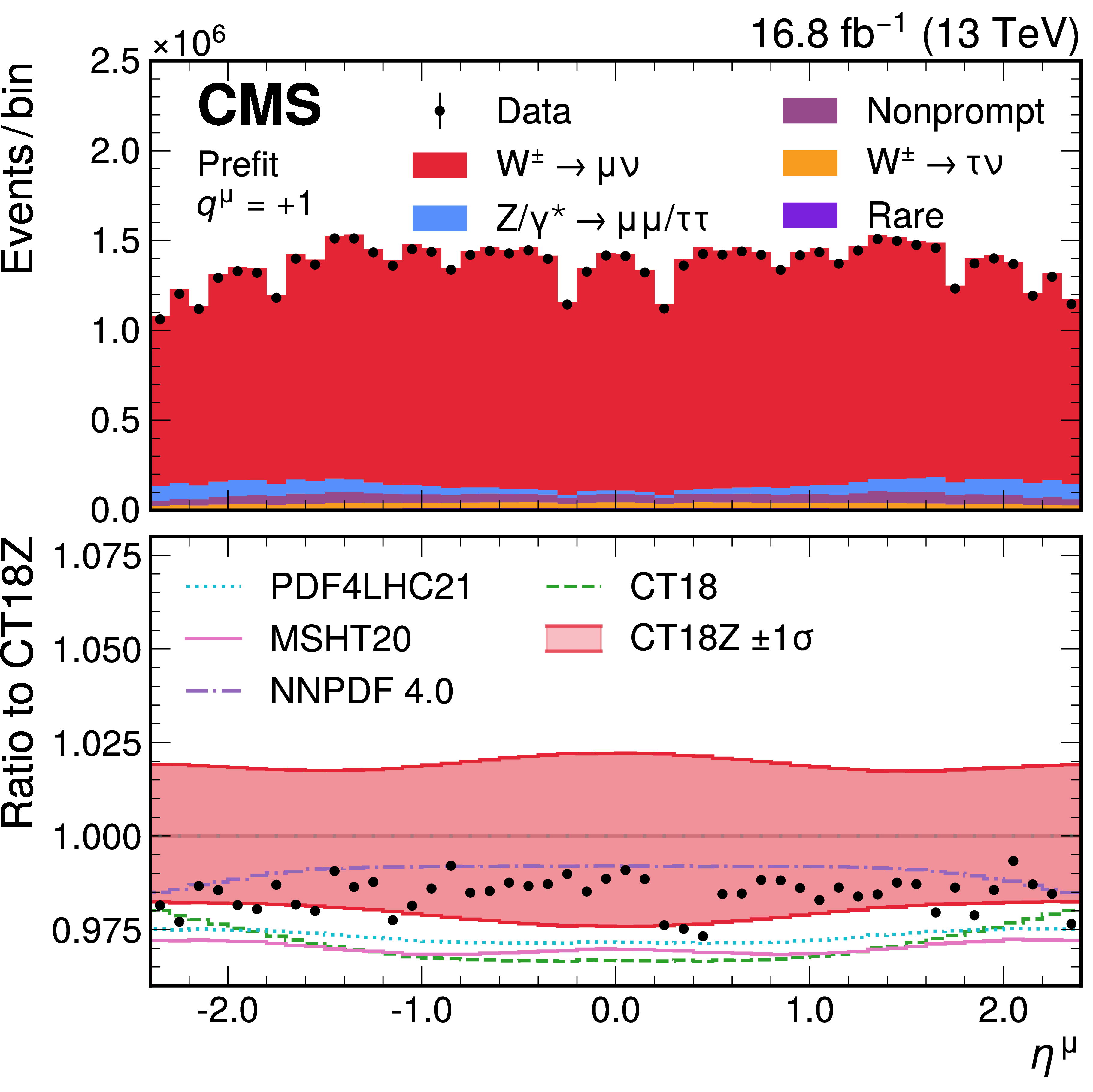
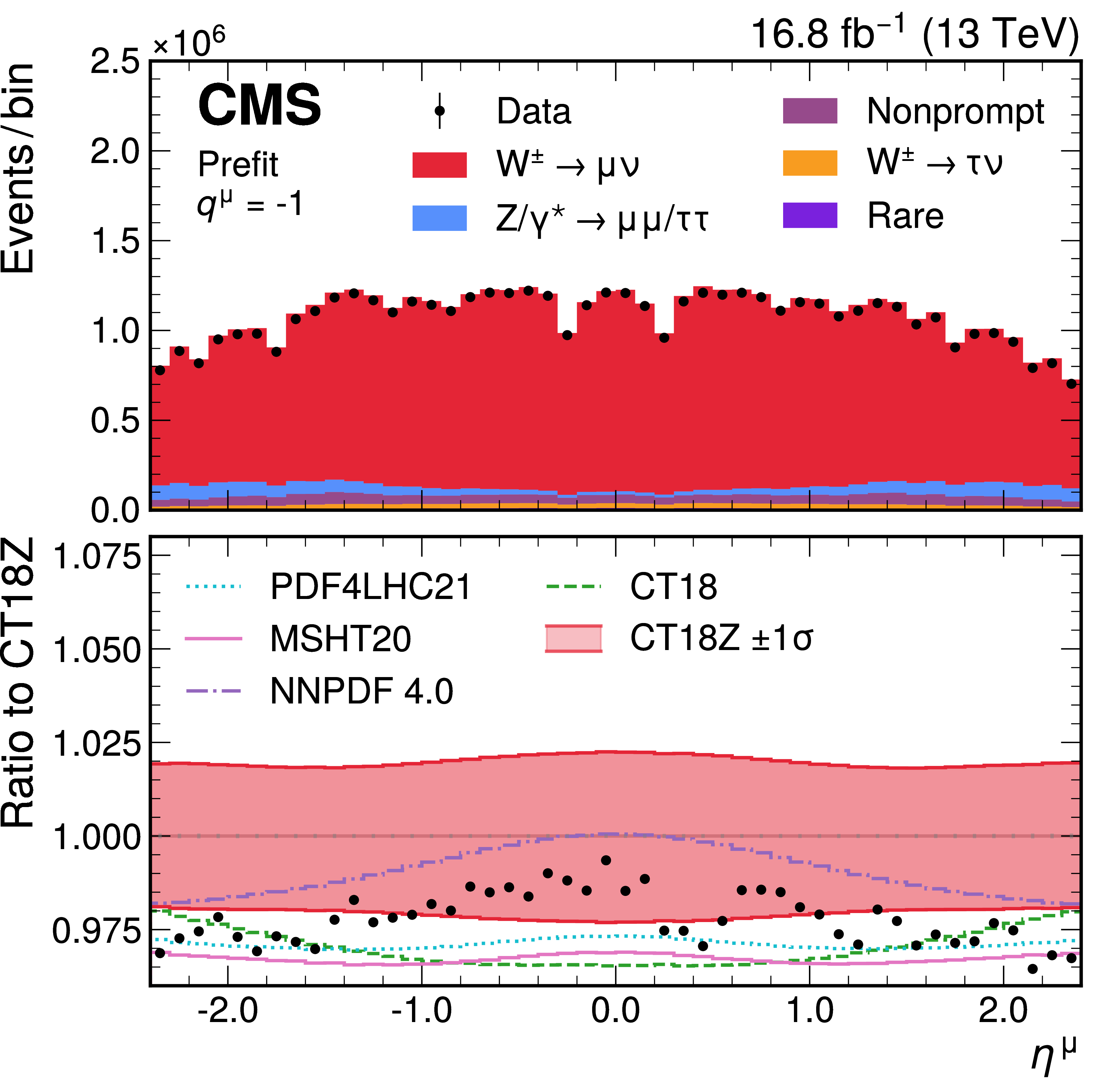
Measured and predicted $ \eta^{\mu} $ distributions for positively (left) and negatively (right) charged muons. The nominal prediction, obtained with the CT18Z PDF set, is shown in filled red. The uncertainty, evaluated as the sum of the eigenvector variation sets, is represented by the filled band in the lower panel. The predictions using the PDF4LHC21, MSHT20, NNPDF4.0, and CT18 sets are also shown (without uncertainty bands). The vertical bars represent the statistical uncertainties in the data. The bottom panel shows the ratio of the number of events observed in data and of variations in the predictions to that of the nominal prediction. |
png pdf |
Figure B2-a:
Measured and predicted $ \eta^{\mu} $ distributions for positively (left) and negatively (right) charged muons. The nominal prediction, obtained with the CT18Z PDF set, is shown in filled red. The uncertainty, evaluated as the sum of the eigenvector variation sets, is represented by the filled band in the lower panel. The predictions using the PDF4LHC21, MSHT20, NNPDF4.0, and CT18 sets are also shown (without uncertainty bands). The vertical bars represent the statistical uncertainties in the data. The bottom panel shows the ratio of the number of events observed in data and of variations in the predictions to that of the nominal prediction. |
png pdf |
Figure B2-b:
Measured and predicted $ \eta^{\mu} $ distributions for positively (left) and negatively (right) charged muons. The nominal prediction, obtained with the CT18Z PDF set, is shown in filled red. The uncertainty, evaluated as the sum of the eigenvector variation sets, is represented by the filled band in the lower panel. The predictions using the PDF4LHC21, MSHT20, NNPDF4.0, and CT18 sets are also shown (without uncertainty bands). The vertical bars represent the statistical uncertainties in the data. The bottom panel shows the ratio of the number of events observed in data and of variations in the predictions to that of the nominal prediction. |
png pdf |
Figure B3:
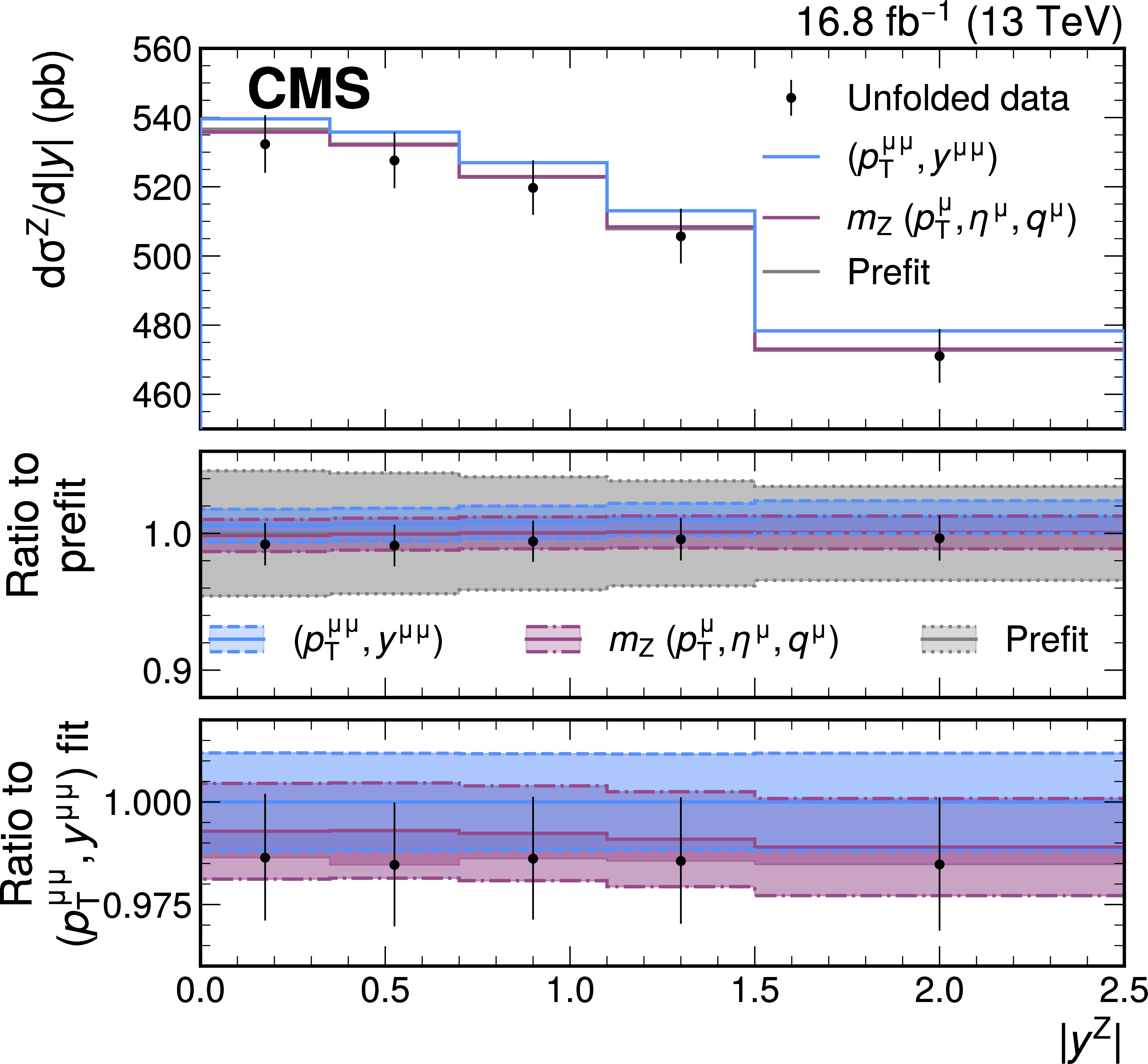
Unfolded measured $ |y^{\mathrm{Z}}| $ distribution (points) compared with the generator-level SCETLIB+MINNLO$_{PS}$ predictions before (prefit, gray) and after adjusting the nuisance parameters to the best fit values obtained from the W-like $ m_{\mathrm{Z}} $ fit (magenta) or from the direct fit to the $ p_{\mathrm{T}}^{\mu\mu} $ distribution (blue). The results are obtained with the selection $ |y^{\mathrm{Z}}| < $ 2.5 and $ p_{\mathrm{T}}^{\mathrm{Z}} < $ 54 GeV. The center panel shows the ratio of the predictions and unfolded data to the prefit prediction. The uncertainty in the prefit prediction is shown by the shaded gray area. The bottom panel shows the ratio of the predictions and unfolded data to the postfit prediction from the fit to the $ (p_{\mathrm{T}}^{\mu\mu}, y^{\mu\mu}) $ distribution. The postfit uncertainties in the predictions are shown in the shaded magenta and blue bands. The vertical bars represent the total uncertainty in the unfolded data. |
png pdf |
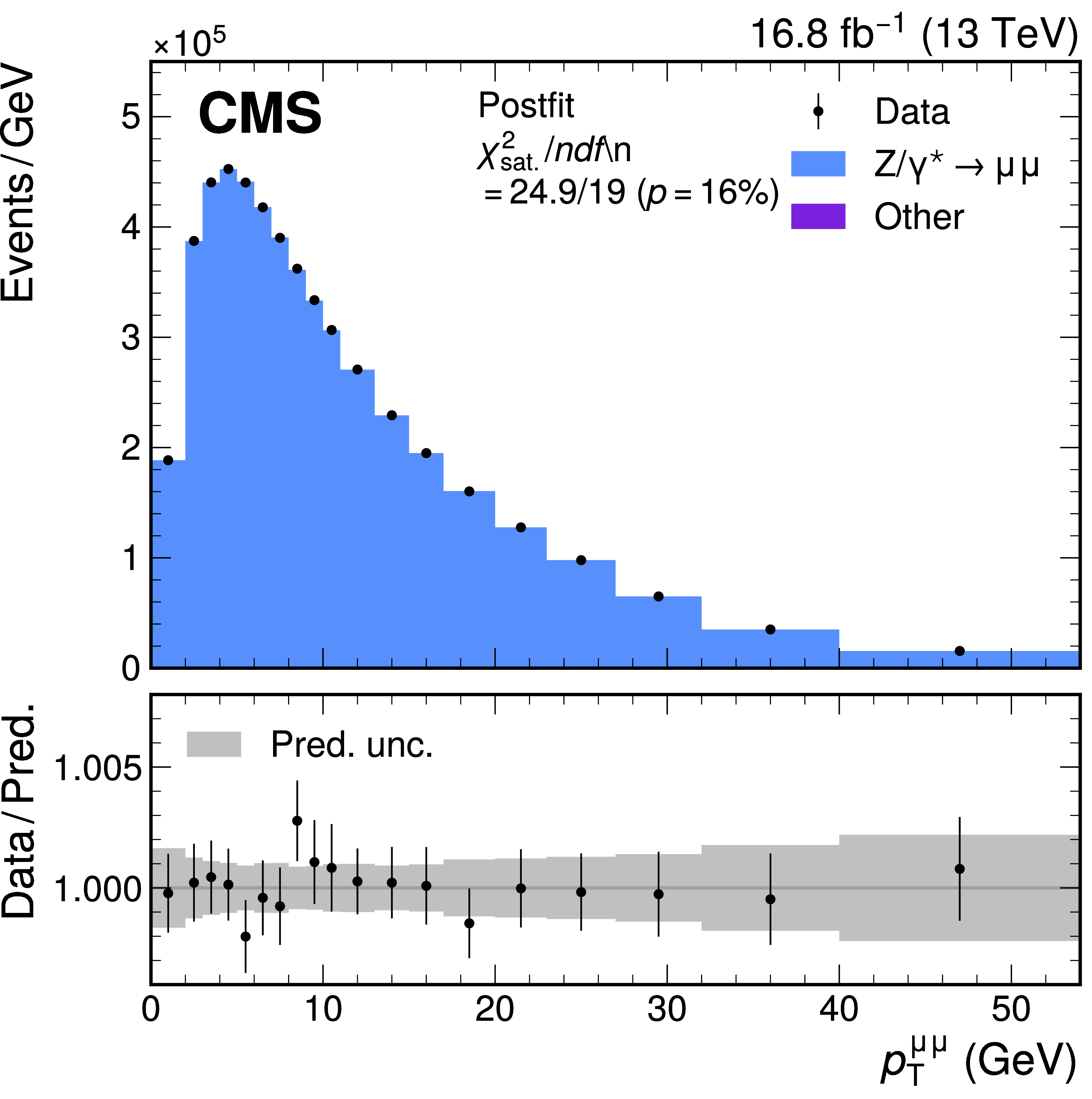
Figure B4:
Measured and simulated $ p_{\mathrm{T}}^{\mu\mu} $ distributions in selected $ \mathrm{Z}\to\mu\mu $ events, with the normalization and uncertainties of the prediction set to the postfit values. The gray band represents the total systematic uncertainty. The vertical bars represent the statistical uncertainties in the data. The bottom panel shows the ratio between the number of events observed in data, including variations in the predictions, and the nominal prediction. |
png pdf |
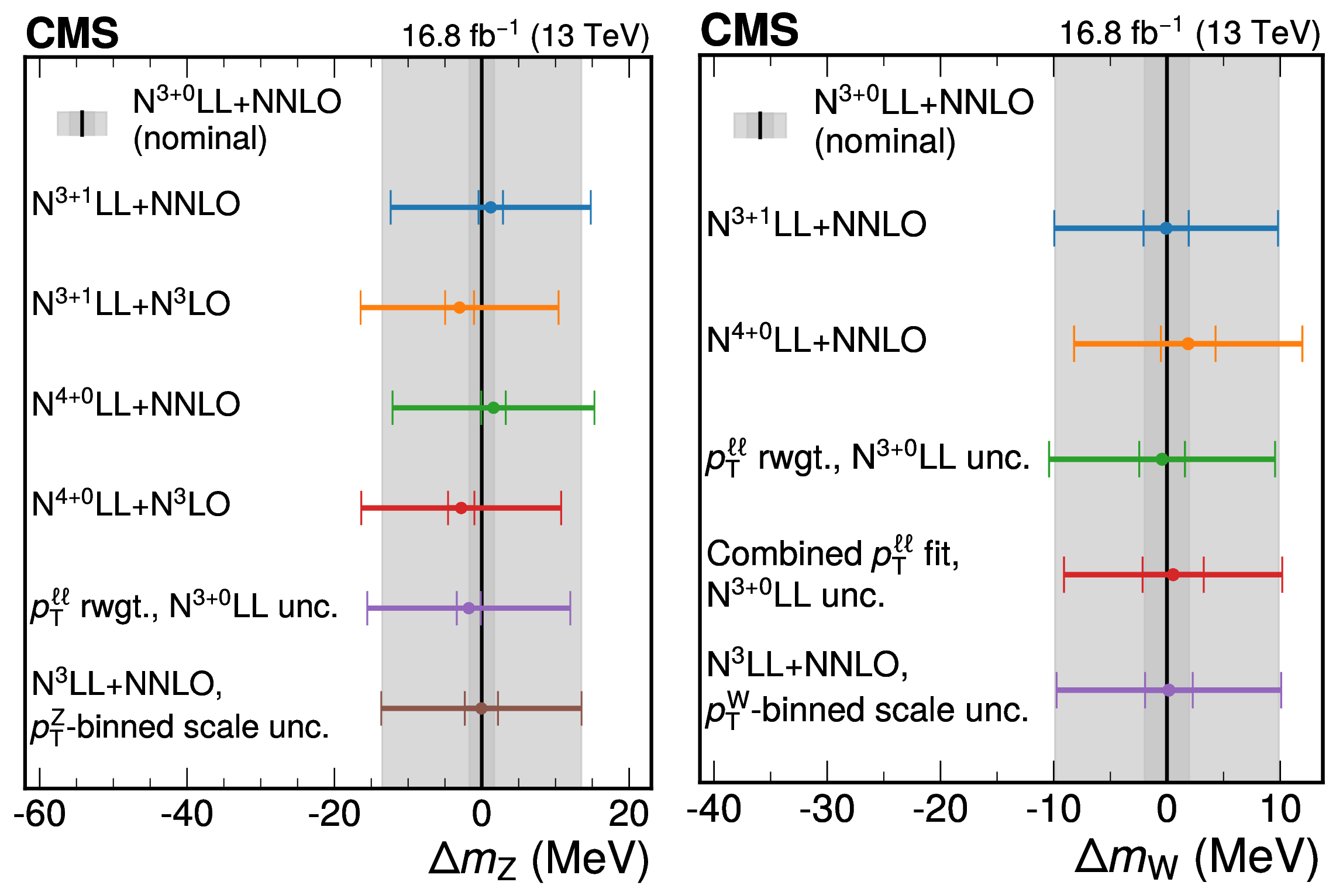
Figure B5:
Comparison of the nominal result and its theory uncertainty for the W-like $ m_{\mathrm{Z}} $ measurement (left) and the $ m_{\mathrm{W}} $ measurement (right), using SCETLIB+DYTURBO at $ \mathrm{N}^{3+0}\mathrm{LL}{+}\mathrm{NNLO} $, with the difference in $ m_{\mathrm{V}} $ measured when using alternative approaches to the $ p_{\mathrm{T}}^{\mathrm{V}} $ modeling and its uncertainty. The results from alternative approaches to the $ p_{\mathrm{T}}^{\mathrm{V}} $ modeling and uncertainty are shown as points. The solid black line represents the nominal result, the inner shaded gray band shows the $ p_{\mathrm{T}}^{\mathrm{V}} $ modeling uncertainty, and the outer shaded gray band shows the total uncertainty in the nominal result. The $ p_{\mathrm{T}}^{\mathrm{V}} $ modeling uncertainties are shown as the inner bars while the outer bars denote the total uncertainties. |
png pdf |
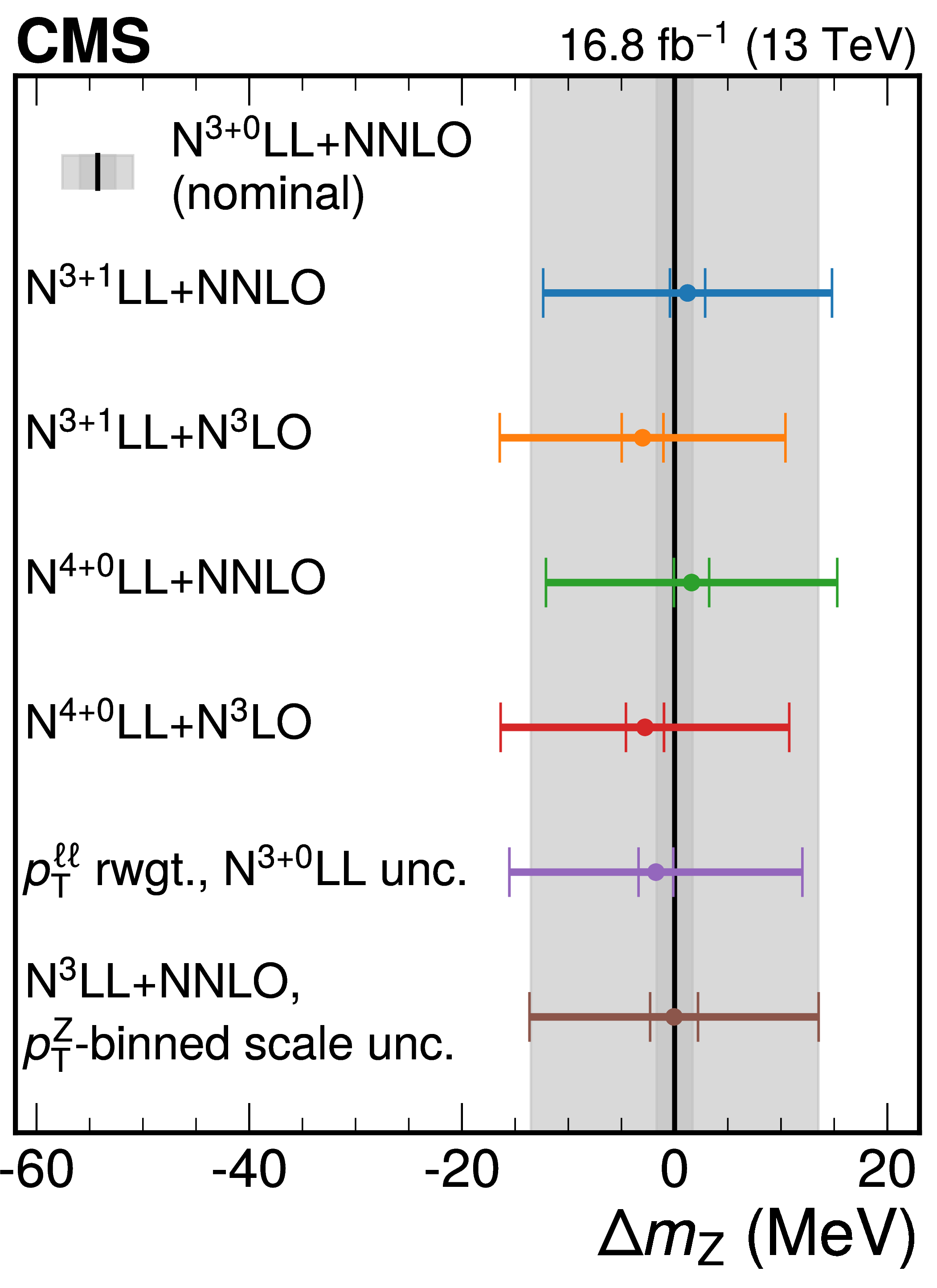
Figure B5-a:
Comparison of the nominal result and its theory uncertainty for the W-like $ m_{\mathrm{Z}} $ measurement (left) and the $ m_{\mathrm{W}} $ measurement (right), using SCETLIB+DYTURBO at $ \mathrm{N}^{3+0}\mathrm{LL}{+}\mathrm{NNLO} $, with the difference in $ m_{\mathrm{V}} $ measured when using alternative approaches to the $ p_{\mathrm{T}}^{\mathrm{V}} $ modeling and its uncertainty. The results from alternative approaches to the $ p_{\mathrm{T}}^{\mathrm{V}} $ modeling and uncertainty are shown as points. The solid black line represents the nominal result, the inner shaded gray band shows the $ p_{\mathrm{T}}^{\mathrm{V}} $ modeling uncertainty, and the outer shaded gray band shows the total uncertainty in the nominal result. The $ p_{\mathrm{T}}^{\mathrm{V}} $ modeling uncertainties are shown as the inner bars while the outer bars denote the total uncertainties. |
png pdf |
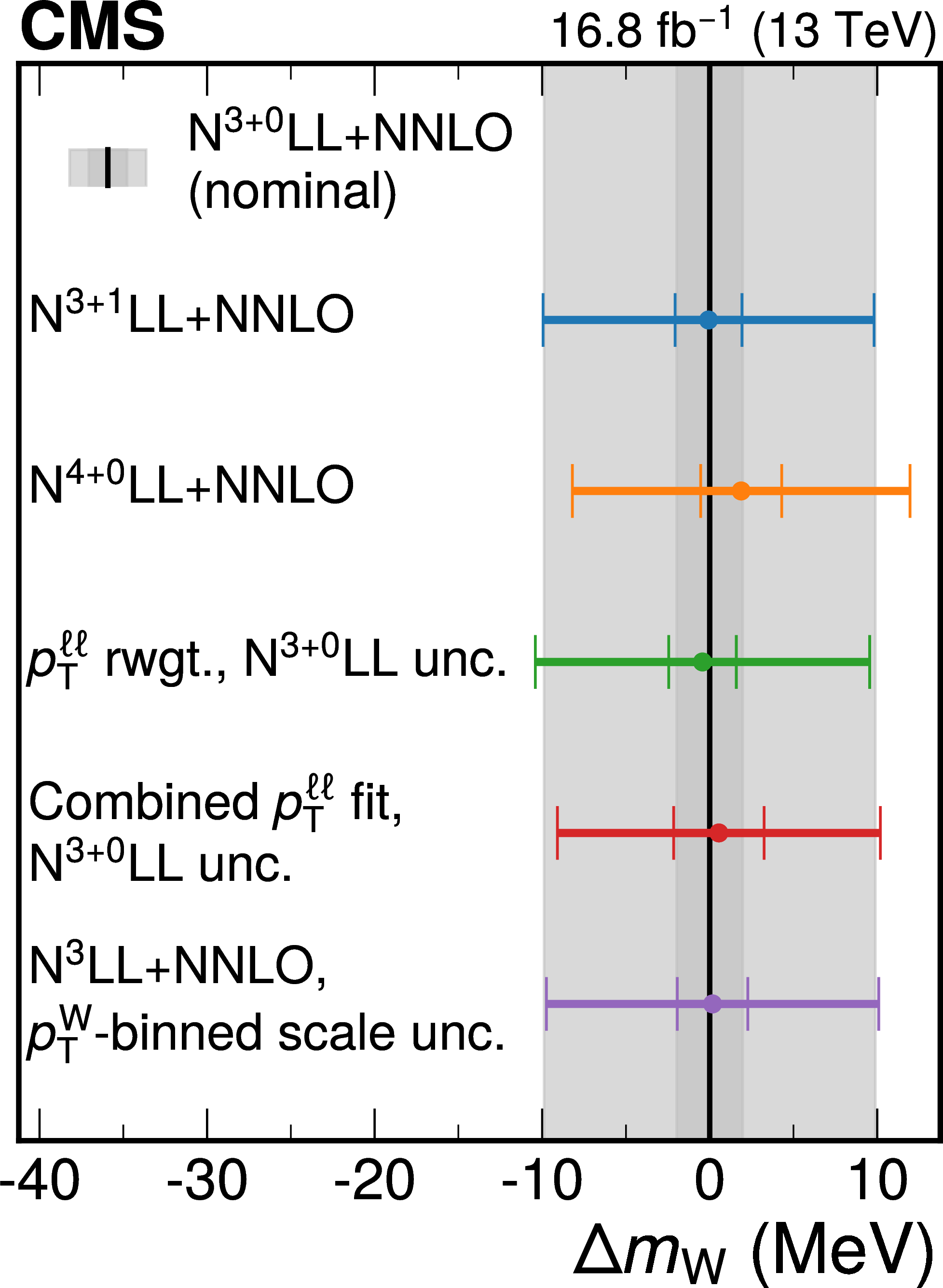
Figure B5-b:
Comparison of the nominal result and its theory uncertainty for the W-like $ m_{\mathrm{Z}} $ measurement (left) and the $ m_{\mathrm{W}} $ measurement (right), using SCETLIB+DYTURBO at $ \mathrm{N}^{3+0}\mathrm{LL}{+}\mathrm{NNLO} $, with the difference in $ m_{\mathrm{V}} $ measured when using alternative approaches to the $ p_{\mathrm{T}}^{\mathrm{V}} $ modeling and its uncertainty. The results from alternative approaches to the $ p_{\mathrm{T}}^{\mathrm{V}} $ modeling and uncertainty are shown as points. The solid black line represents the nominal result, the inner shaded gray band shows the $ p_{\mathrm{T}}^{\mathrm{V}} $ modeling uncertainty, and the outer shaded gray band shows the total uncertainty in the nominal result. The $ p_{\mathrm{T}}^{\mathrm{V}} $ modeling uncertainties are shown as the inner bars while the outer bars denote the total uncertainties. |
png pdf |
Figure B6:
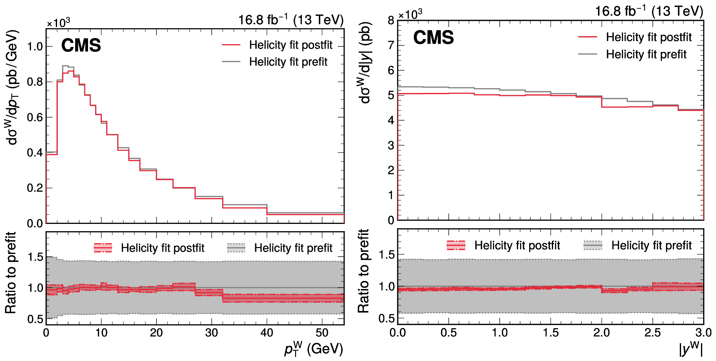
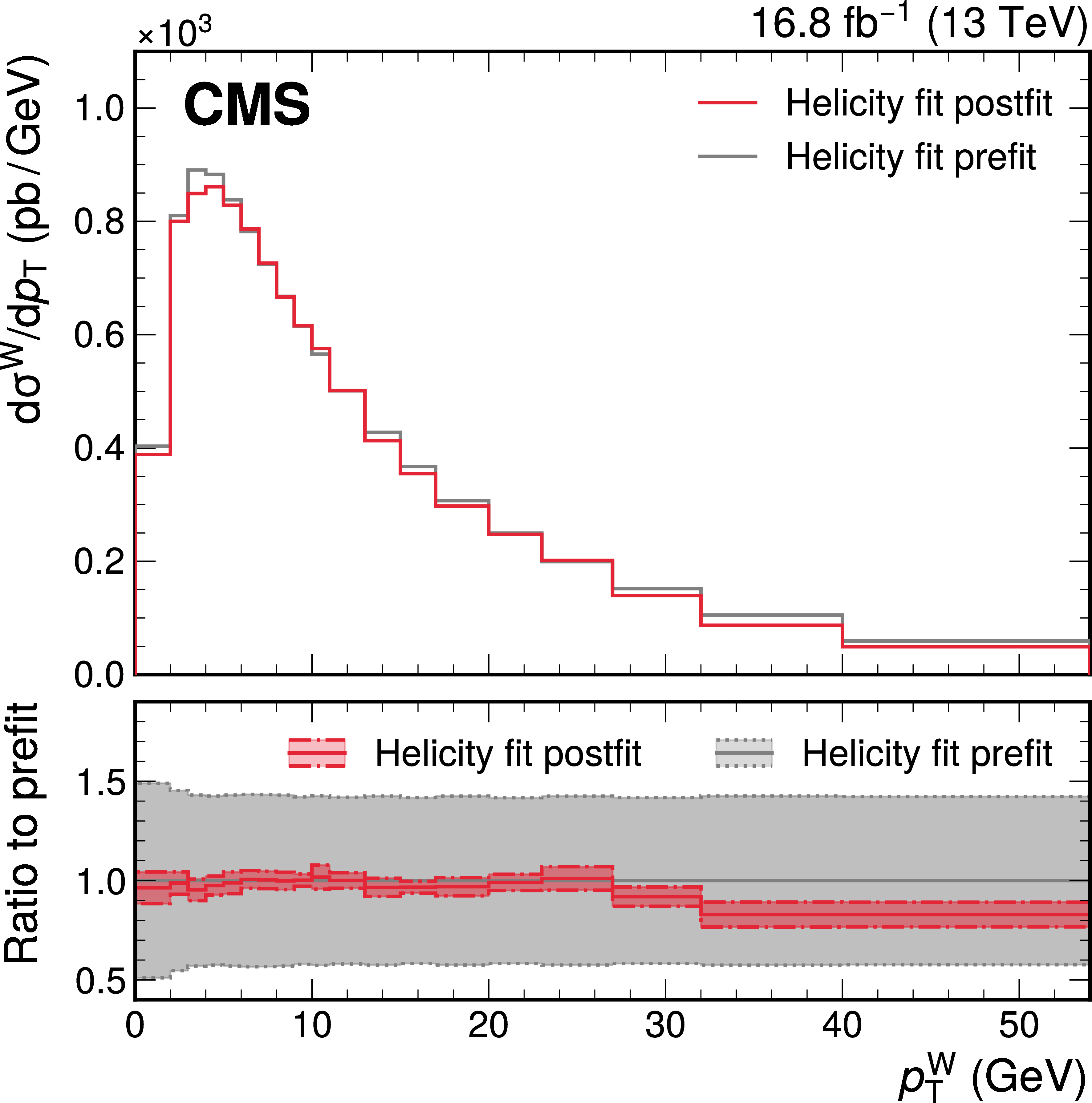
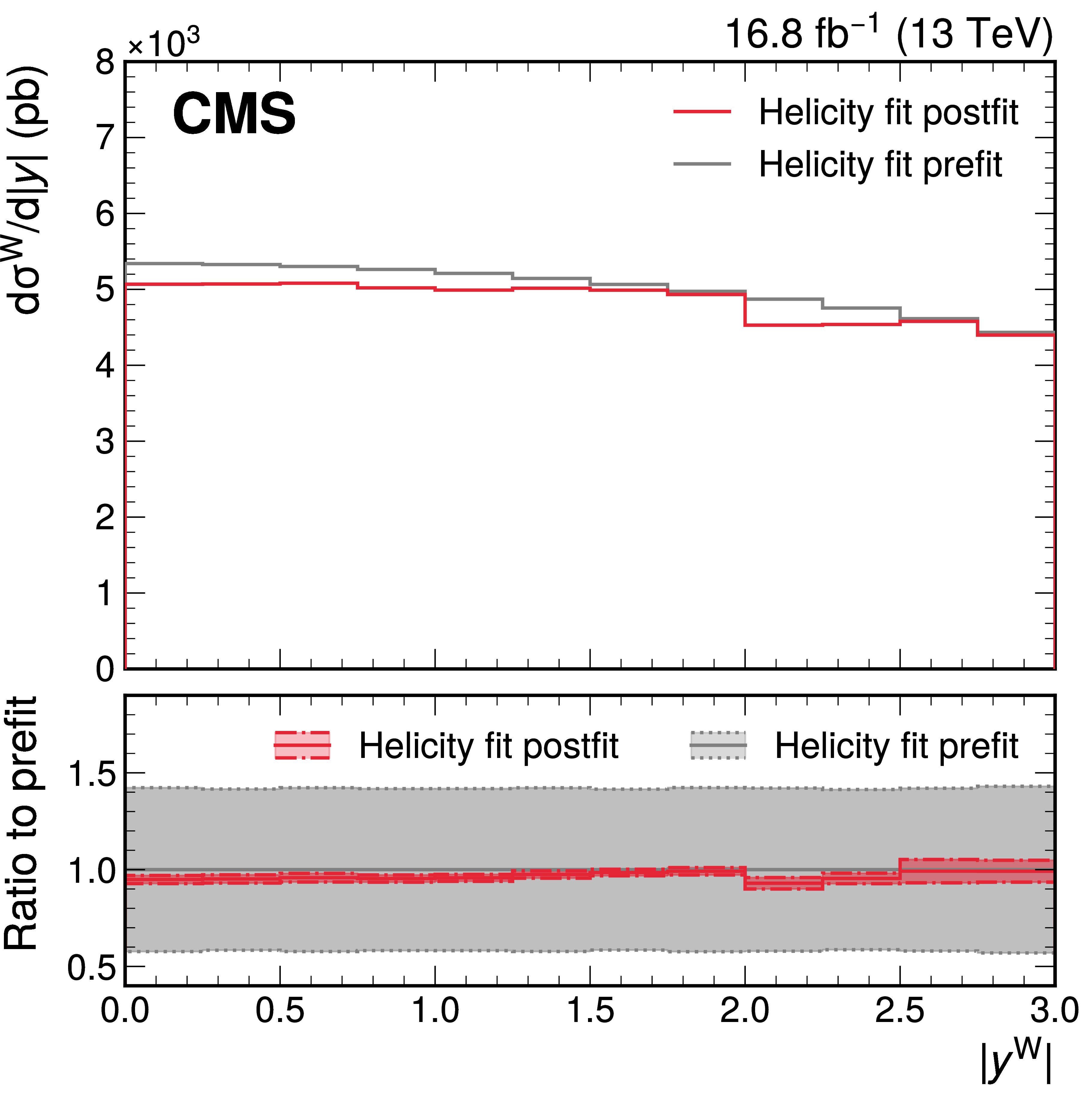
Differential W boson production cross section, in the $ \mathrm{W}\to\mu\nu $ decay channel, in $ p_{\mathrm{T}}^{\mathrm{W}} $ (left) and $ |y^{\mathrm{W}}| $ (right), measured from the $ (p_{\mathrm{T}}^{\mu}, \eta^{\mu}, q^{\mu}) $ distributions using the helicity fit approach (in red). The SCETLIB+DYTURBO generator-level predictions, before incorporating in situ constraints, are also shown (in gray). The results are shown for the selection $ |y^{\mathrm{W}}| < $ 3.0 and $ p_{\mathrm{T}}^{\mathrm{W}} < $ 54 GeV. The lower panel shows the ratio between the postfit and prefit spectra. |
png pdf |
Figure B6-a:
Differential W boson production cross section, in the $ \mathrm{W}\to\mu\nu $ decay channel, in $ p_{\mathrm{T}}^{\mathrm{W}} $ (left) and $ |y^{\mathrm{W}}| $ (right), measured from the $ (p_{\mathrm{T}}^{\mu}, \eta^{\mu}, q^{\mu}) $ distributions using the helicity fit approach (in red). The SCETLIB+DYTURBO generator-level predictions, before incorporating in situ constraints, are also shown (in gray). The results are shown for the selection $ |y^{\mathrm{W}}| < $ 3.0 and $ p_{\mathrm{T}}^{\mathrm{W}} < $ 54 GeV. The lower panel shows the ratio between the postfit and prefit spectra. |
png pdf |
Figure B6-b:
Differential W boson production cross section, in the $ \mathrm{W}\to\mu\nu $ decay channel, in $ p_{\mathrm{T}}^{\mathrm{W}} $ (left) and $ |y^{\mathrm{W}}| $ (right), measured from the $ (p_{\mathrm{T}}^{\mu}, \eta^{\mu}, q^{\mu}) $ distributions using the helicity fit approach (in red). The SCETLIB+DYTURBO generator-level predictions, before incorporating in situ constraints, are also shown (in gray). The results are shown for the selection $ |y^{\mathrm{W}}| < $ 3.0 and $ p_{\mathrm{T}}^{\mathrm{W}} < $ 54 GeV. The lower panel shows the ratio between the postfit and prefit spectra. |
png pdf |
Figure B7:
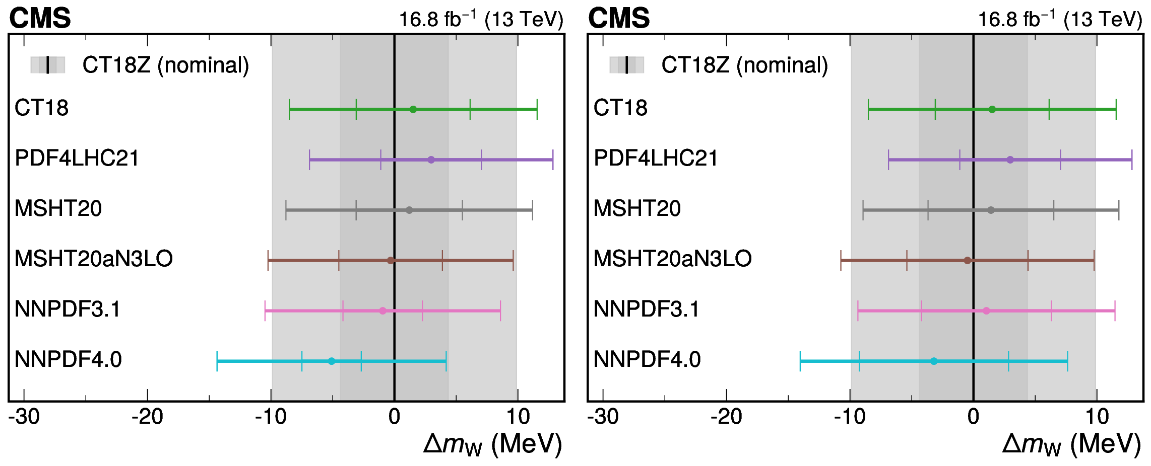
Difference in $ m_{\mathrm{W}} $ values for six alternative recent PDF sets, when using the original uncertainty for the given set (left) and when the uncertainties are scaled to accommodate the central prediction of the other sets (right). Each point corresponds to the result obtained when using the indicated PDF set and its uncertainty for the simulated predictions. The inner bar shows the uncertainty from the PDF and the outer bar the total uncertainty. The nominal result, using CT18Z, is shown by the black line, with the CT18Z PDF and total uncertainty shown in dark and light gray, respectively. The uncertainty scaling procedure described in \insuppSection of 8 the Methods section in the main workSection 7.8 improves the consistency of the $ m_{\mathrm{W}} $ values across the PDF sets and with the nominal result. |
png pdf |
Figure B7-a:
Difference in $ m_{\mathrm{W}} $ values for six alternative recent PDF sets, when using the original uncertainty for the given set (left) and when the uncertainties are scaled to accommodate the central prediction of the other sets (right). Each point corresponds to the result obtained when using the indicated PDF set and its uncertainty for the simulated predictions. The inner bar shows the uncertainty from the PDF and the outer bar the total uncertainty. The nominal result, using CT18Z, is shown by the black line, with the CT18Z PDF and total uncertainty shown in dark and light gray, respectively. The uncertainty scaling procedure described in \insuppSection of 8 the Methods section in the main workSection 7.8 improves the consistency of the $ m_{\mathrm{W}} $ values across the PDF sets and with the nominal result. |
png pdf |
Figure B7-b:
Difference in $ m_{\mathrm{W}} $ values for six alternative recent PDF sets, when using the original uncertainty for the given set (left) and when the uncertainties are scaled to accommodate the central prediction of the other sets (right). Each point corresponds to the result obtained when using the indicated PDF set and its uncertainty for the simulated predictions. The inner bar shows the uncertainty from the PDF and the outer bar the total uncertainty. The nominal result, using CT18Z, is shown by the black line, with the CT18Z PDF and total uncertainty shown in dark and light gray, respectively. The uncertainty scaling procedure described in \insuppSection of 8 the Methods section in the main workSection 7.8 improves the consistency of the $ m_{\mathrm{W}} $ values across the PDF sets and with the nominal result. |
png pdf |
Figure B8:
The postfit $ (p_{\mathrm{T}}^{\mu}, \eta^{\mu}) $ distribution compared to the observed data for the W-like $ m_{\mathrm{Z}} $ (upper two) and $ m_{\mathrm{W}} $ (lower two) measurements for positively (upper and second from bottom) and negatively (second from top and lower) charged muons. The predictions and their uncertainties are adjusted to the best fit values obtained from the maximum likelihood fit. The two-dimensional distribution is ``unrolled" such that each bin on the $ x $-axis represents one $ (p_{\mathrm{T}}^{\mu}, \eta^{\mu}) $ cell. The gray band represents the uncertainty in the prediction, before the fit to the data. The bottom panel shows the ratio of the number of events observed in data to the nominal prediction. The vertical bars represent the statistical uncertainties in the data. |
png pdf |
Figure B8-a:
The postfit $ (p_{\mathrm{T}}^{\mu}, \eta^{\mu}) $ distribution compared to the observed data for the W-like $ m_{\mathrm{Z}} $ (upper two) and $ m_{\mathrm{W}} $ (lower two) measurements for positively (upper and second from bottom) and negatively (second from top and lower) charged muons. The predictions and their uncertainties are adjusted to the best fit values obtained from the maximum likelihood fit. The two-dimensional distribution is ``unrolled" such that each bin on the $ x $-axis represents one $ (p_{\mathrm{T}}^{\mu}, \eta^{\mu}) $ cell. The gray band represents the uncertainty in the prediction, before the fit to the data. The bottom panel shows the ratio of the number of events observed in data to the nominal prediction. The vertical bars represent the statistical uncertainties in the data. |

png pdf |
Figure B8-b:
The postfit $ (p_{\mathrm{T}}^{\mu}, \eta^{\mu}) $ distribution compared to the observed data for the W-like $ m_{\mathrm{Z}} $ (upper two) and $ m_{\mathrm{W}} $ (lower two) measurements for positively (upper and second from bottom) and negatively (second from top and lower) charged muons. The predictions and their uncertainties are adjusted to the best fit values obtained from the maximum likelihood fit. The two-dimensional distribution is ``unrolled" such that each bin on the $ x $-axis represents one $ (p_{\mathrm{T}}^{\mu}, \eta^{\mu}) $ cell. The gray band represents the uncertainty in the prediction, before the fit to the data. The bottom panel shows the ratio of the number of events observed in data to the nominal prediction. The vertical bars represent the statistical uncertainties in the data. |
png pdf |
Figure B8-c:
The postfit $ (p_{\mathrm{T}}^{\mu}, \eta^{\mu}) $ distribution compared to the observed data for the W-like $ m_{\mathrm{Z}} $ (upper two) and $ m_{\mathrm{W}} $ (lower two) measurements for positively (upper and second from bottom) and negatively (second from top and lower) charged muons. The predictions and their uncertainties are adjusted to the best fit values obtained from the maximum likelihood fit. The two-dimensional distribution is ``unrolled" such that each bin on the $ x $-axis represents one $ (p_{\mathrm{T}}^{\mu}, \eta^{\mu}) $ cell. The gray band represents the uncertainty in the prediction, before the fit to the data. The bottom panel shows the ratio of the number of events observed in data to the nominal prediction. The vertical bars represent the statistical uncertainties in the data. |
png pdf |
Figure B8-d:
The postfit $ (p_{\mathrm{T}}^{\mu}, \eta^{\mu}) $ distribution compared to the observed data for the W-like $ m_{\mathrm{Z}} $ (upper two) and $ m_{\mathrm{W}} $ (lower two) measurements for positively (upper and second from bottom) and negatively (second from top and lower) charged muons. The predictions and their uncertainties are adjusted to the best fit values obtained from the maximum likelihood fit. The two-dimensional distribution is ``unrolled" such that each bin on the $ x $-axis represents one $ (p_{\mathrm{T}}^{\mu}, \eta^{\mu}) $ cell. The gray band represents the uncertainty in the prediction, before the fit to the data. The bottom panel shows the ratio of the number of events observed in data to the nominal prediction. The vertical bars represent the statistical uncertainties in the data. |
png pdf |
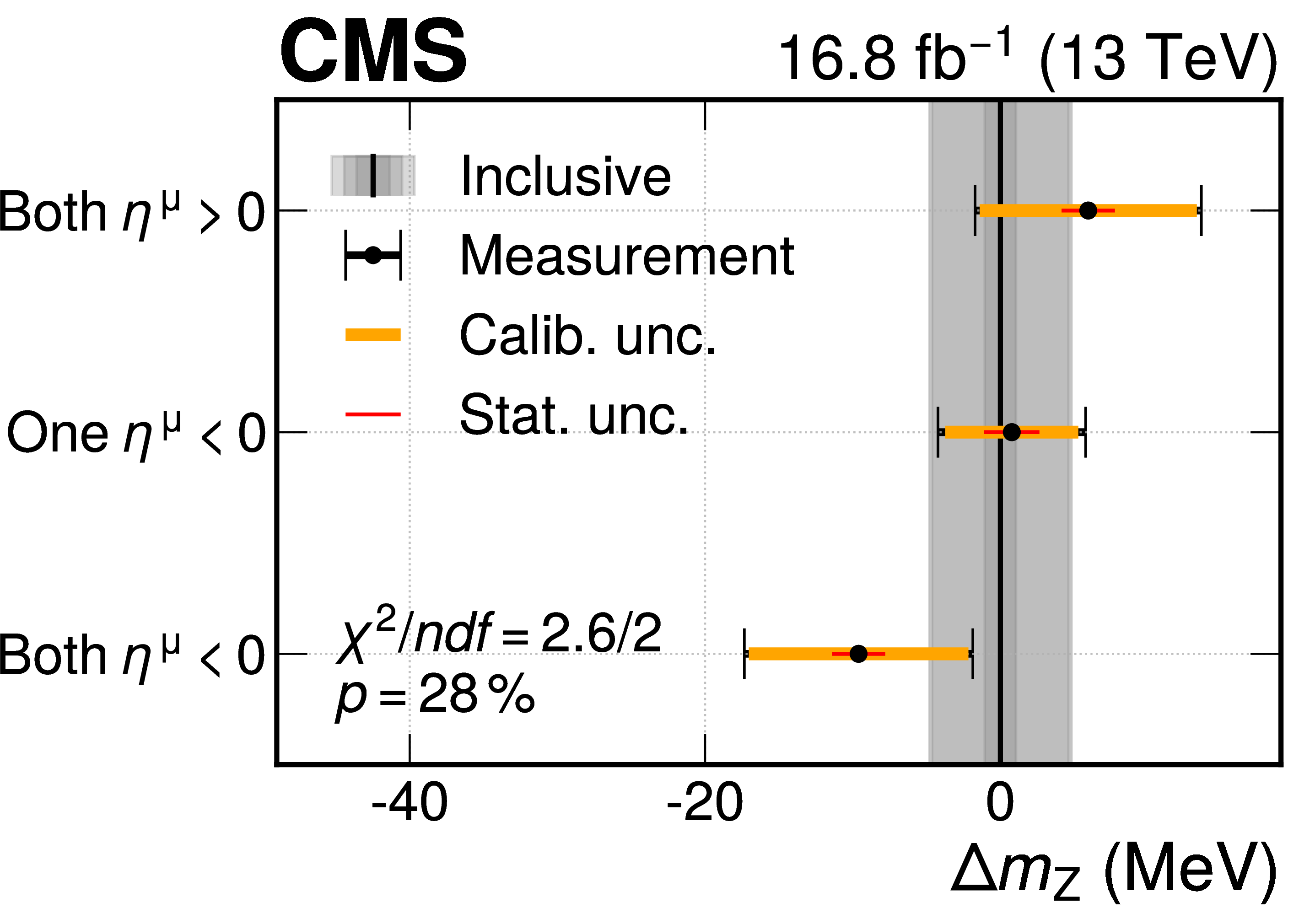
Figure B9:
The difference between the nominal $ m_{\mathrm{Z}} $ value measured from the $ \mathrm{Z}\to\mu\mu $ events and the result when $ m_{\mathrm{Z}} $ is allowed to vary, in three regions of the $ \eta^{\mu} $ of the two muons. The results binned in $ |\eta^{\mu}| $ (both central, one central and one forward, and both forward) are shown on the left and results binned in $ \eta^{\mu} $ (both negative, one positive and one negative, and both positive) are shown on the right. The result of a fit with three $ m_{\mathrm{Z}} $ parameters is compared with the result with a single $ m_{\mathrm{Z}} $ parameter and the compatibility of the results is also shown, as assessed via the saturated goodness-of-fit test. The points show the $ m_{\mathrm{Z}} $ result for the indicated $ \eta^{\mu} $ region and the horizontal bars represent the calibration (orange line), statistical (red line), and total (black line) uncertainties. The black vertical line represents the result with a single $ m_{\mathrm{Z}} $ parameter, with the three shaded gray bands representing the statistical (dark grey), calibration (intermediate grey), and total (light grey) uncertainties. |
png pdf |
Figure B9-a:
The difference between the nominal $ m_{\mathrm{Z}} $ value measured from the $ \mathrm{Z}\to\mu\mu $ events and the result when $ m_{\mathrm{Z}} $ is allowed to vary, in three regions of the $ \eta^{\mu} $ of the two muons. The results binned in $ |\eta^{\mu}| $ (both central, one central and one forward, and both forward) are shown on the left and results binned in $ \eta^{\mu} $ (both negative, one positive and one negative, and both positive) are shown on the right. The result of a fit with three $ m_{\mathrm{Z}} $ parameters is compared with the result with a single $ m_{\mathrm{Z}} $ parameter and the compatibility of the results is also shown, as assessed via the saturated goodness-of-fit test. The points show the $ m_{\mathrm{Z}} $ result for the indicated $ \eta^{\mu} $ region and the horizontal bars represent the calibration (orange line), statistical (red line), and total (black line) uncertainties. The black vertical line represents the result with a single $ m_{\mathrm{Z}} $ parameter, with the three shaded gray bands representing the statistical (dark grey), calibration (intermediate grey), and total (light grey) uncertainties. |
png pdf |
Figure B9-b:
The difference between the nominal $ m_{\mathrm{Z}} $ value measured from the $ \mathrm{Z}\to\mu\mu $ events and the result when $ m_{\mathrm{Z}} $ is allowed to vary, in three regions of the $ \eta^{\mu} $ of the two muons. The results binned in $ |\eta^{\mu}| $ (both central, one central and one forward, and both forward) are shown on the left and results binned in $ \eta^{\mu} $ (both negative, one positive and one negative, and both positive) are shown on the right. The result of a fit with three $ m_{\mathrm{Z}} $ parameters is compared with the result with a single $ m_{\mathrm{Z}} $ parameter and the compatibility of the results is also shown, as assessed via the saturated goodness-of-fit test. The points show the $ m_{\mathrm{Z}} $ result for the indicated $ \eta^{\mu} $ region and the horizontal bars represent the calibration (orange line), statistical (red line), and total (black line) uncertainties. The black vertical line represents the result with a single $ m_{\mathrm{Z}} $ parameter, with the three shaded gray bands representing the statistical (dark grey), calibration (intermediate grey), and total (light grey) uncertainties. |
png pdf |
Figure A10:
Measured and simulated $ p_{\mathrm{T}}^{\mu} $ distributions, with the prediction adjusted according to the best fit values of nuisance parameters and of $ m_{\mathrm{Z}} $ obtained from the maximum likelihood fit of the W-like $ m_{\mathrm{Z}} $ analysis. The vertical bars represent the statistical uncertainties in the data. The bottom panel shows the ratio of the number of events observed in data to the nominal prediction. The solid and dashed purple lines represent, respectively, the relative impact of an increase and decrease of $ m_{\mathrm{Z}} $ by 14 MeV. The uncertainties in the predictions, after the systematic uncertainty profiling in the maximum likelihood fit, are shown by the shaded band. |
png pdf |
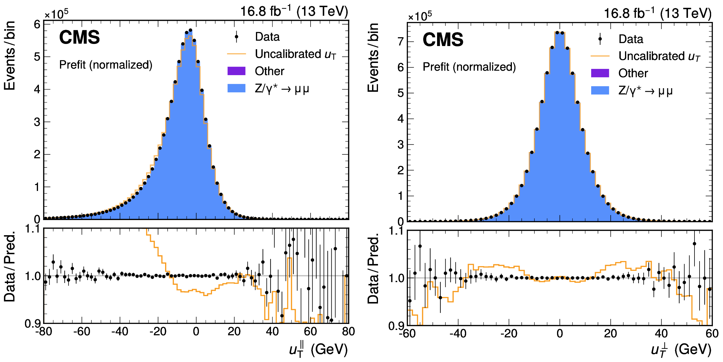
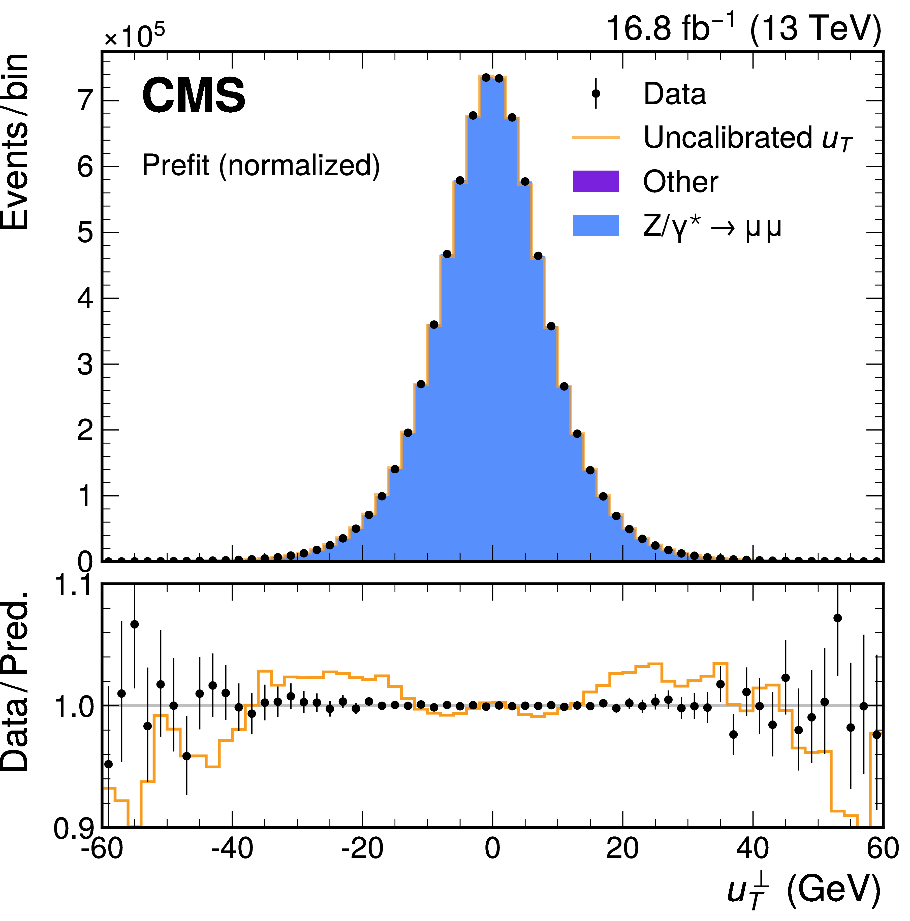
Figure B10:
Comparison of the prediction and observed data for the parallel ($ u_{\mathrm{T}}^{\parallel} $, left) and perpendicular ($ u_{\mathrm{T}}^{\perp} $, right) components of the hadronic recoil. The filled histograms show the simulation with the hadronic recoil corrected according to the procedure described in the text. The orange line shows the predicted distribution before the hadronic recoil corrections. The uncertainties in the predictions are not shown. The bottom panel shows the ratio of the number of events observed in data (black point) and the uncorrected prediction (orange line) to the recoil-corrected prediction. |
png pdf |
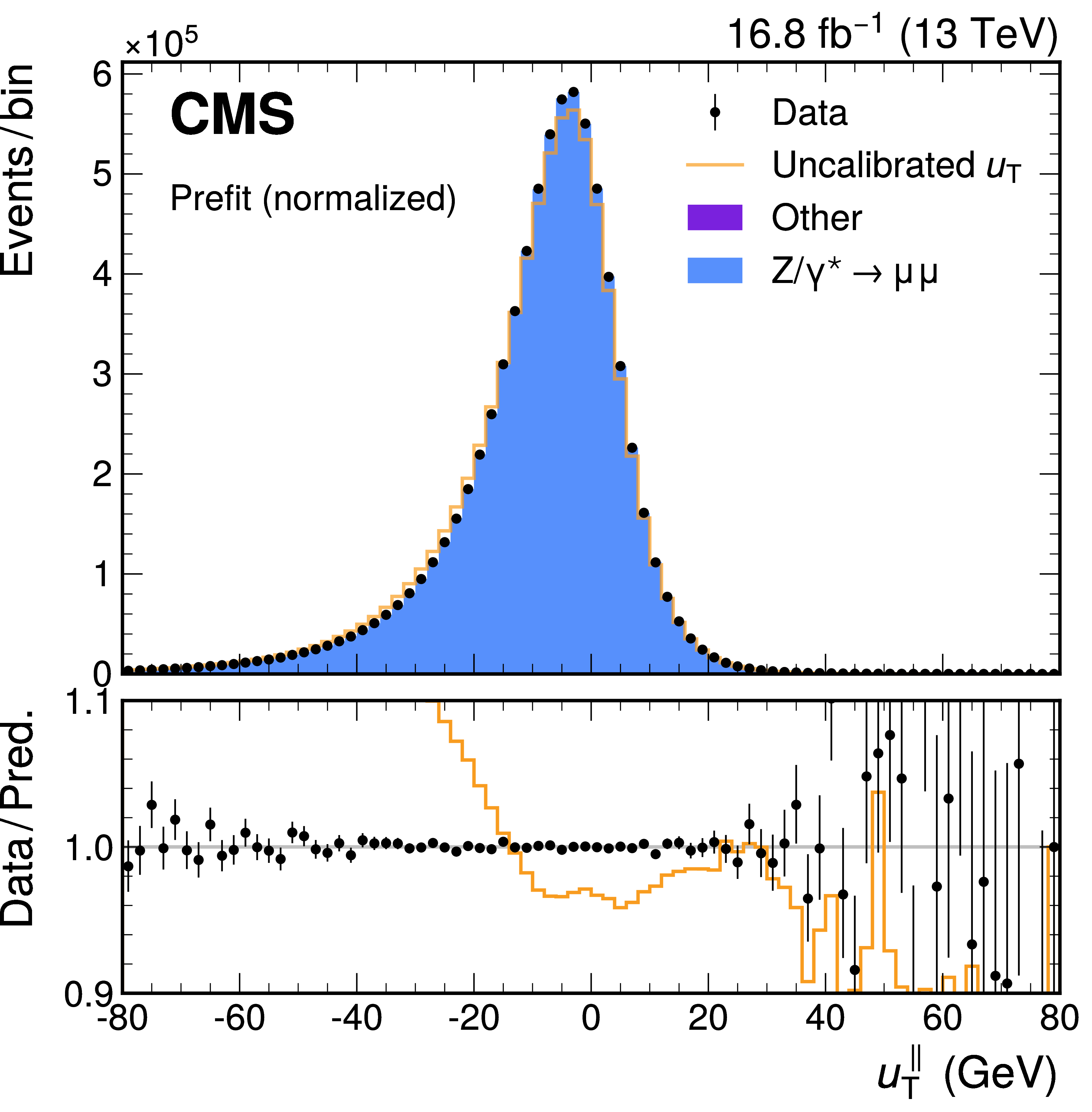
Figure B10-a:
Comparison of the prediction and observed data for the parallel ($ u_{\mathrm{T}}^{\parallel} $, left) and perpendicular ($ u_{\mathrm{T}}^{\perp} $, right) components of the hadronic recoil. The filled histograms show the simulation with the hadronic recoil corrected according to the procedure described in the text. The orange line shows the predicted distribution before the hadronic recoil corrections. The uncertainties in the predictions are not shown. The bottom panel shows the ratio of the number of events observed in data (black point) and the uncorrected prediction (orange line) to the recoil-corrected prediction. |
png pdf |
Figure B10-b:
Comparison of the prediction and observed data for the parallel ($ u_{\mathrm{T}}^{\parallel} $, left) and perpendicular ($ u_{\mathrm{T}}^{\perp} $, right) components of the hadronic recoil. The filled histograms show the simulation with the hadronic recoil corrected according to the procedure described in the text. The orange line shows the predicted distribution before the hadronic recoil corrections. The uncertainties in the predictions are not shown. The bottom panel shows the ratio of the number of events observed in data (black point) and the uncorrected prediction (orange line) to the recoil-corrected prediction. |
png pdf |
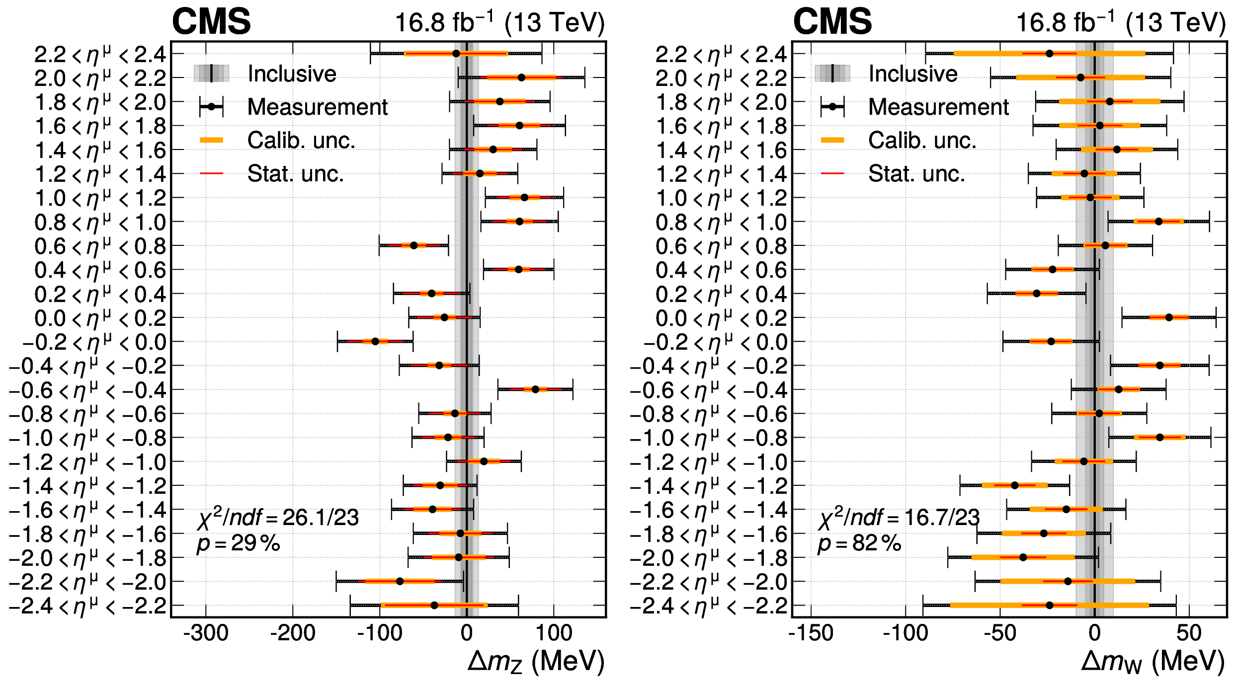
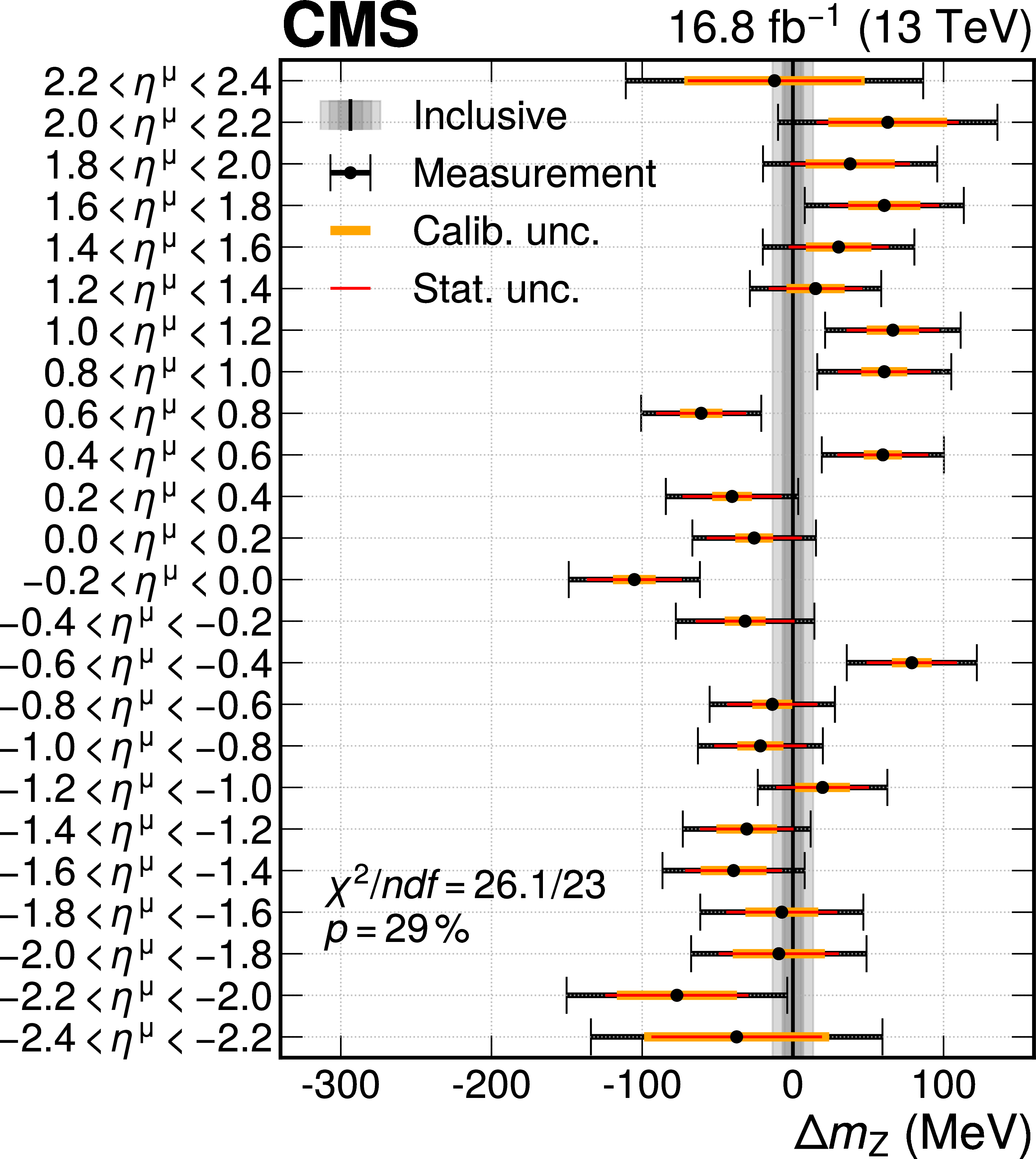
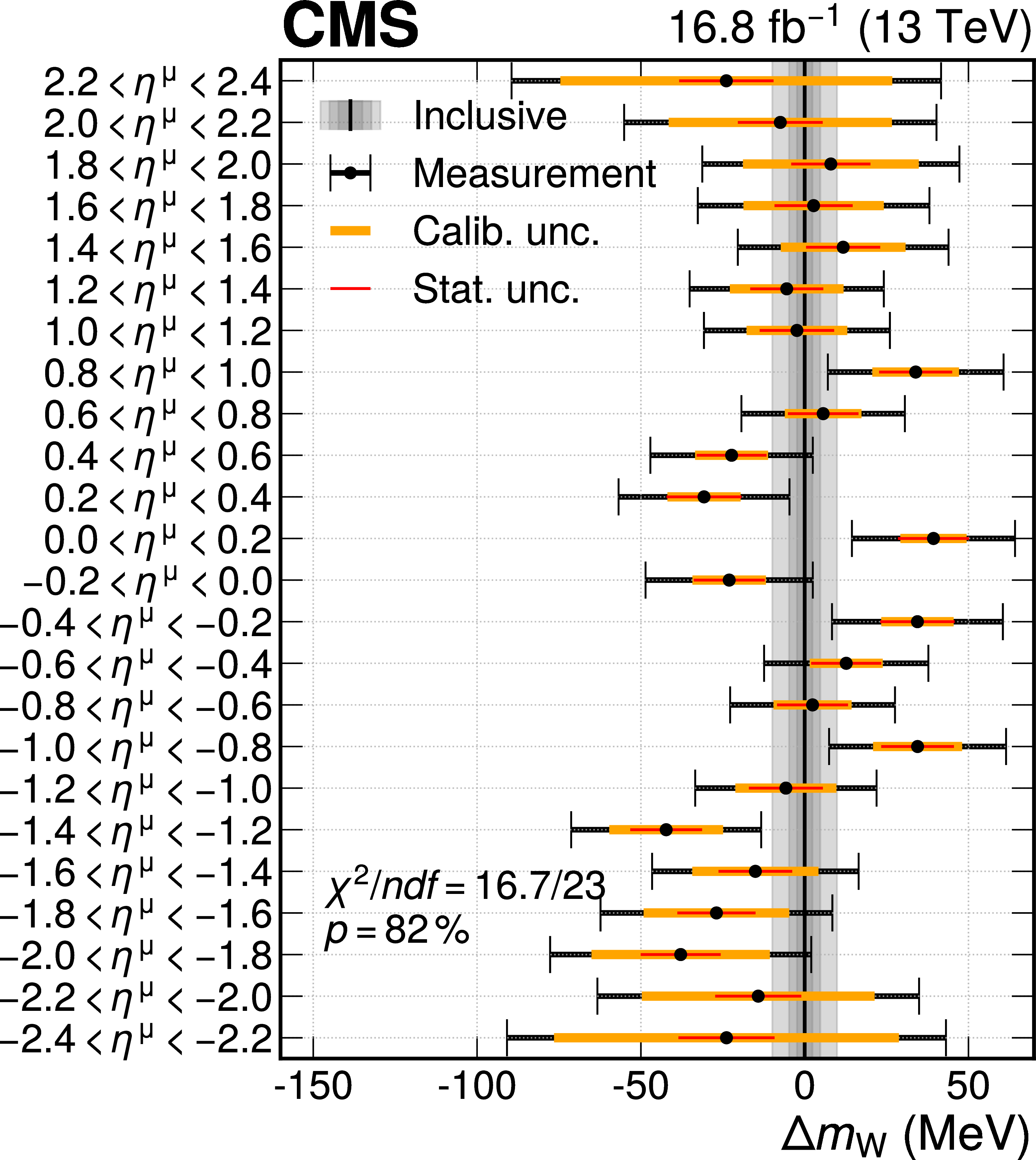
Figure B11:
For the W-like $ m_{\mathrm{Z}} $ analysis (left) and the $ m_{\mathrm{W}} $ measurement (right) the result of a fit with 24 $ m_{\mathrm{V}} $ parameters corresponding to different $ \eta^{\mu} $ ranges is compared with the nominal $ m_{\mathrm{V}} $ fit result. The $ \chi^2 $-like compatibility of the two fits is also shown, assessed via the saturated goodness-of-fit test. The points show $ m_{\mathrm{V}} $ result for the indicated $ \eta^{\mu} $ region, and the horizontal bars represent the calibration (orange line), statistical (red line), and total (black line) uncertainties. The black vertical line shows the result with a single $ m_{\mathrm{V}} $ parameter, with the shaded gray bands representing its statistical, calibration, and total uncertainties. |
png pdf |
Figure B11-a:
For the W-like $ m_{\mathrm{Z}} $ analysis (left) and the $ m_{\mathrm{W}} $ measurement (right) the result of a fit with 24 $ m_{\mathrm{V}} $ parameters corresponding to different $ \eta^{\mu} $ ranges is compared with the nominal $ m_{\mathrm{V}} $ fit result. The $ \chi^2 $-like compatibility of the two fits is also shown, assessed via the saturated goodness-of-fit test. The points show $ m_{\mathrm{V}} $ result for the indicated $ \eta^{\mu} $ region, and the horizontal bars represent the calibration (orange line), statistical (red line), and total (black line) uncertainties. The black vertical line shows the result with a single $ m_{\mathrm{V}} $ parameter, with the shaded gray bands representing its statistical, calibration, and total uncertainties. |
png pdf |
Figure B11-b:
For the W-like $ m_{\mathrm{Z}} $ analysis (left) and the $ m_{\mathrm{W}} $ measurement (right) the result of a fit with 24 $ m_{\mathrm{V}} $ parameters corresponding to different $ \eta^{\mu} $ ranges is compared with the nominal $ m_{\mathrm{V}} $ fit result. The $ \chi^2 $-like compatibility of the two fits is also shown, assessed via the saturated goodness-of-fit test. The points show $ m_{\mathrm{V}} $ result for the indicated $ \eta^{\mu} $ region, and the horizontal bars represent the calibration (orange line), statistical (red line), and total (black line) uncertainties. The black vertical line shows the result with a single $ m_{\mathrm{V}} $ parameter, with the shaded gray bands representing its statistical, calibration, and total uncertainties. |
png pdf |
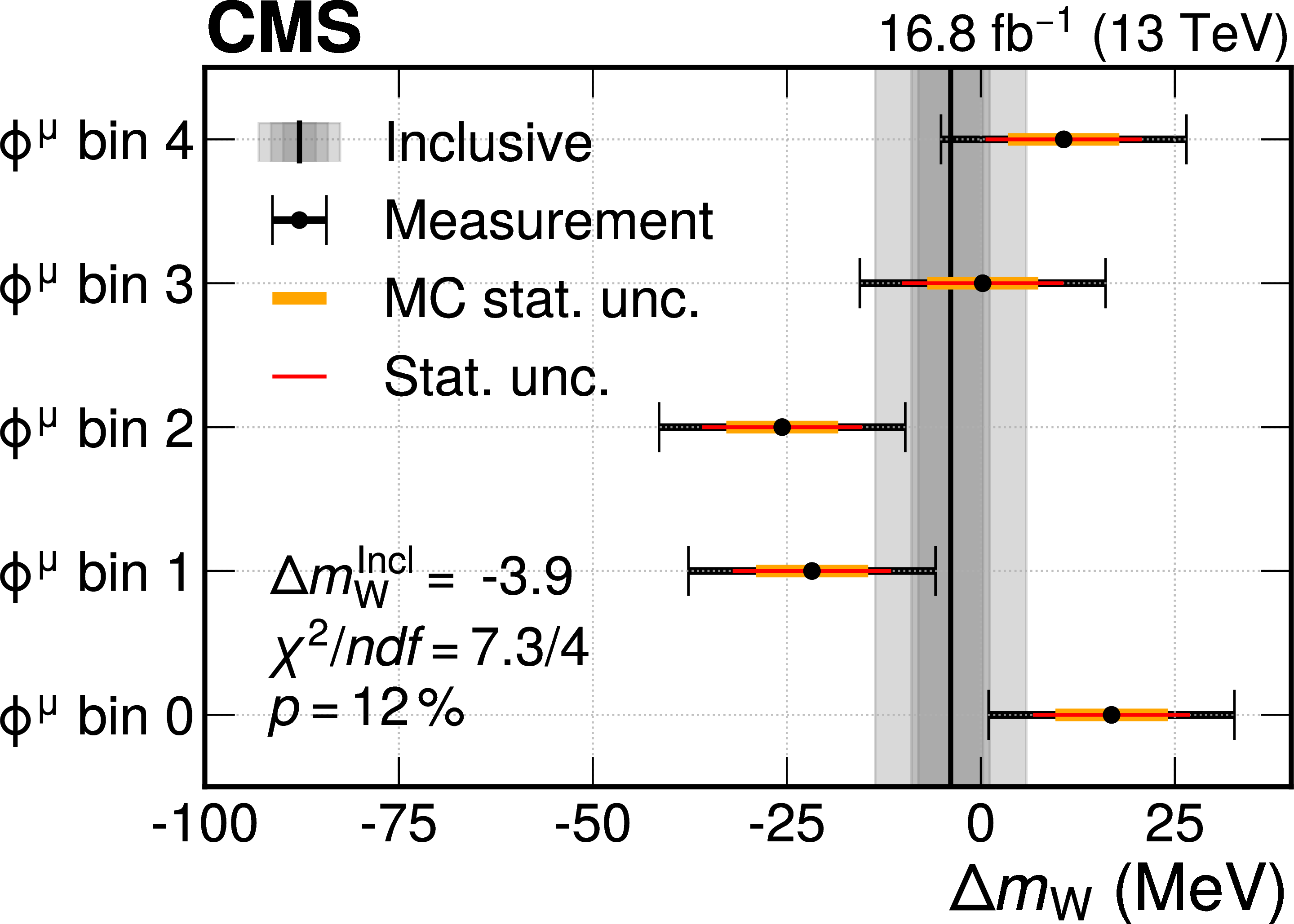
Figure B12:
Measured value of $ m_{\mathrm{W}} $ after splitting the analyzed data and simulated samples in five uniformly spaced bins of muon $ \phi^{\mu} $ from $ -\pi $ to $ \pi $. The points show the $ m_{\mathrm{W}} $ measurement for the indicated bin, and the horizontal bars represent the MC (orange line), data statistical (red line), and total (black line) uncertainties. The $ \chi^2 $-like compatibility of the measurements is also shown, assessed via the saturated goodness-of-fit test. The mutual correlation of the five measurements is accounted for in the $ \chi^2 $, and is about 30% accounting for the common theoretical uncertainties. Most of the experimental uncertainties are uncorrelated across the five bins. The black vertical line shows the combined result from a simultaneous fit of the five bins with a single $ m_{\mathrm{W}} $ parameter, with the shaded gray bands representing its data or MC statistical uncertainty and the total uncertainty. The zero of the horizontal axis corresponds to the nominal measured value. The partial uncertainties are defined using the ``global'' impacts. |
png pdf |
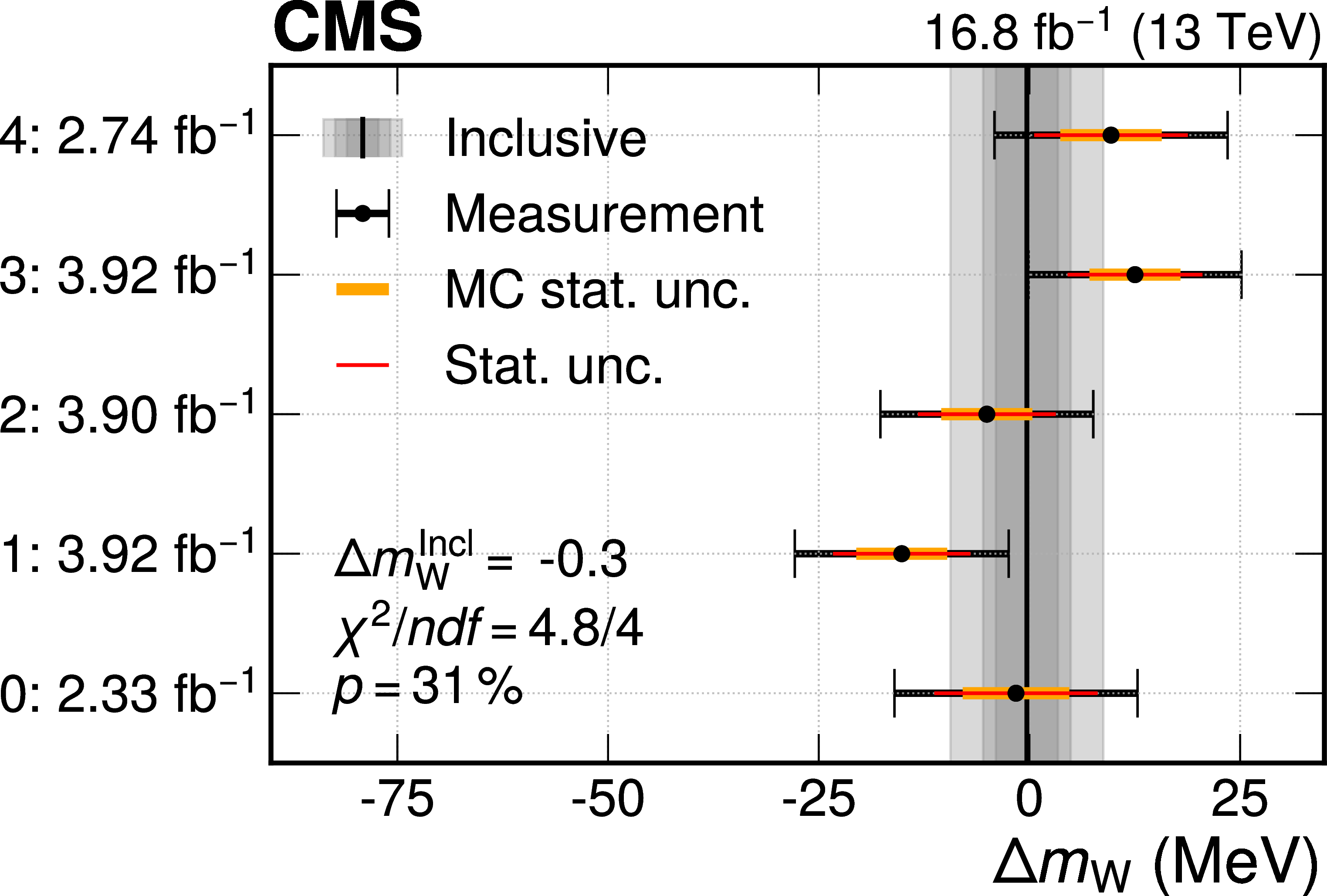
Figure B13:
Measured value of $ m_{\mathrm{W}} $ after splitting the analyzed data and simulated samples in five independent subsets. The points show the $ m_{\mathrm{W}} $ measurement for the indicated integrated luminosity, and the horizontal bars represent the MC (orange line), data statistical (red line), and total (black line) uncertainties. The integrated luminosity of each bin follows the discrete pattern of the data-taking runs. The five bins gather data collected from the beginning to the end of the data taking from bottom to top. Since the average pileup increased with time during 2016, this splitting approximately corresponds to a categorization in bins of pileup as well. The $ \chi^2 $-like compatibility of the measurements is also shown, assessed via the saturated goodness-of-fit test. The mutual correlation of the five measurements is accounted for in the $ \chi^2 $, and is about 30% accounting for the common theoretical uncertainties. Most of the experimental uncertainties are treated as uncorrelated across the five bins. The black vertical line shows the combined result from a simultaneous fit of the five bins with a single $ m_{\mathrm{W}} $ parameter, with the shaded gray bands representing its data or MC statistical uncertainty and the total uncertainty. The zero of the horizontal axis corresponds to the nominal measured value. The partial uncertainties are defined using the ``global'' impacts. |
png pdf |
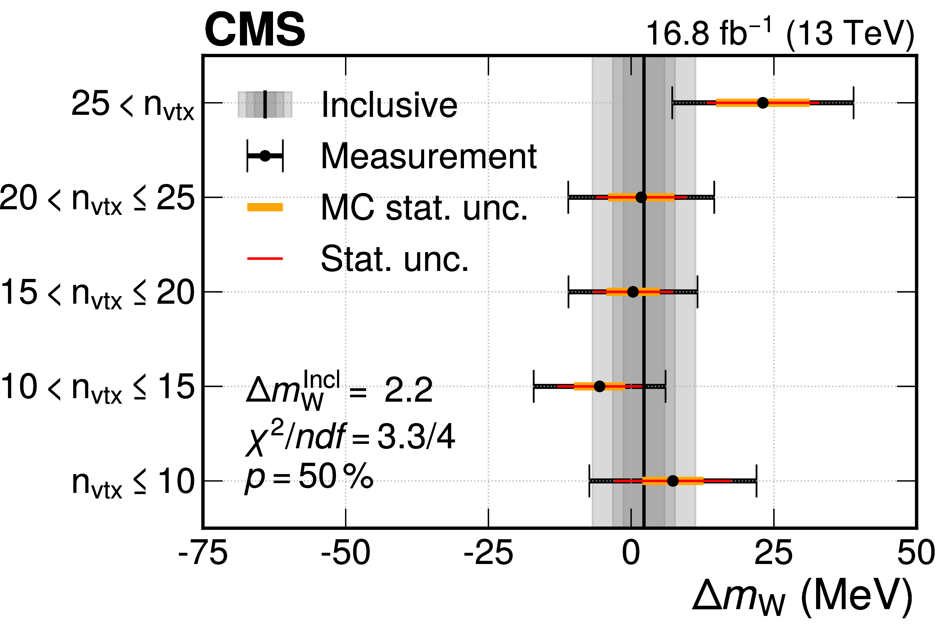
Figure B14:
Measured value of $ m_{\mathrm{W}} $ after splitting the analyzed data and simulated samples in five independent subsets based on the number of reconstructed vertices ($ n_{\text{vtx}} $). The points show the $ m_{\mathrm{W}} $ measurement for the indicated $ n_{\text{vtx}} $ region, and the horizontal bars represent the MC (orange line), data statistical (red line), and total (black line) uncertainties. The $ \chi^2 $-like compatibility of the measurements is also shown, assessed via the saturated goodness-of-fit test. The mutual correlation of the five measurements is accounted for in the $ \chi^2 $, and is about 30%, accounting for the common theoretical uncertainties. The black vertical line shows the combined result from a simultaneous fit of the five bins with a single $ m_{\mathrm{W}} $ parameter, with the shaded gray bands representing its data or MC statistical uncertainty and the total uncertainty. The zero of the horizontal axis corresponds to the nominal measured value, $ m_{\mathrm{W}} = 80 $ 360.2 MeV. The partial uncertainties are defined using the ``global'' impacts. |
png pdf |
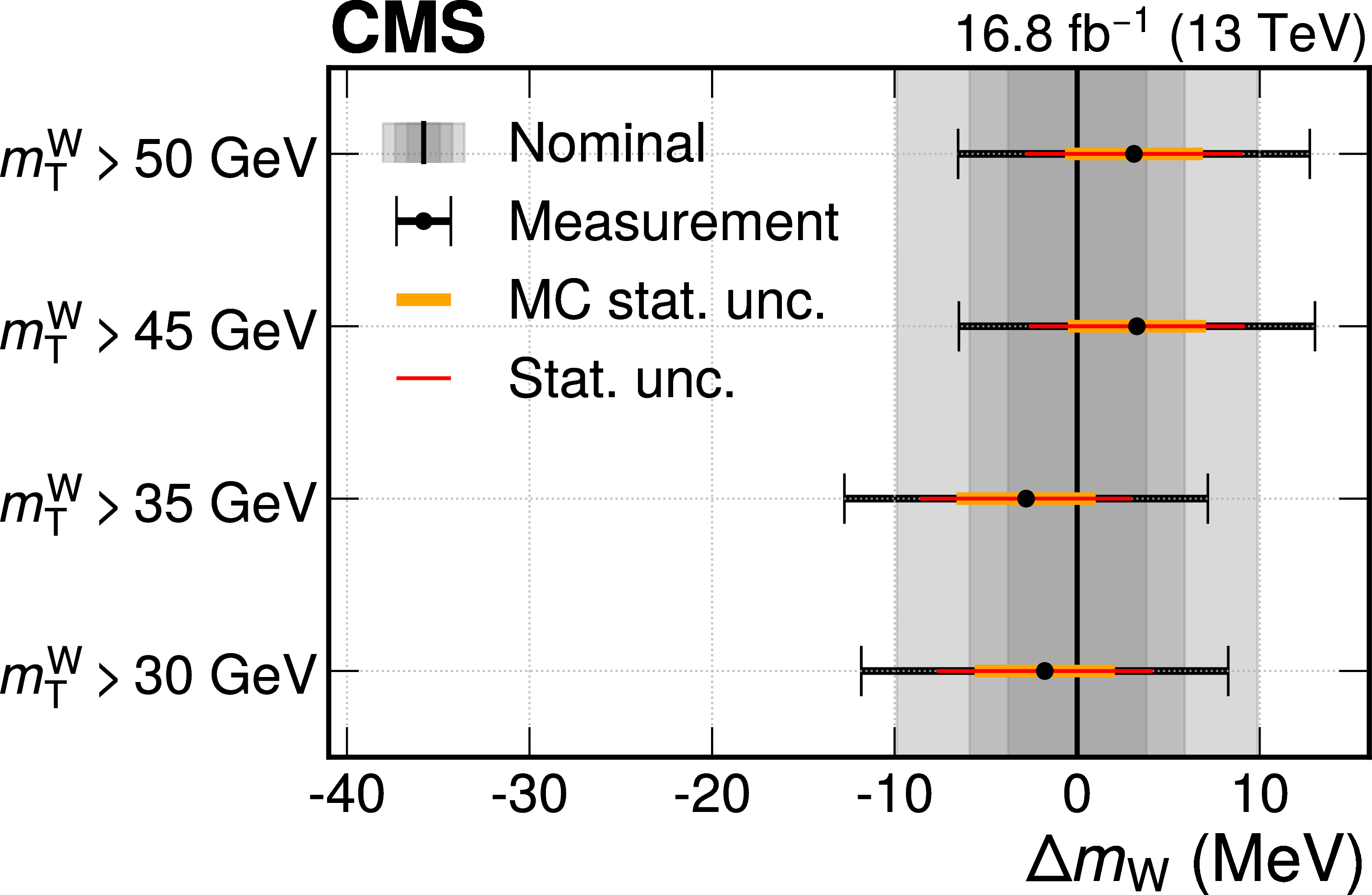
Figure B15:
Measured value of $ m_{\mathrm{W}} $ after modifying the threshold in the transverse mass $ m_{\mathrm{T}} $. The points show the $ m_{\mathrm{W}} $ measurement for the indicated threshold, and the horizontal bars represent the MC (orange line), data statistical (red line), and total (black line) uncertainties. The partial uncertainties are defined using the ``global'' impacts. The black vertical line shows the nominal measured value, for which the $ m_{\mathrm{T}} $ threshold is 40 GeV. The measurements are not statistically independent. |
png pdf |
Figure B16:
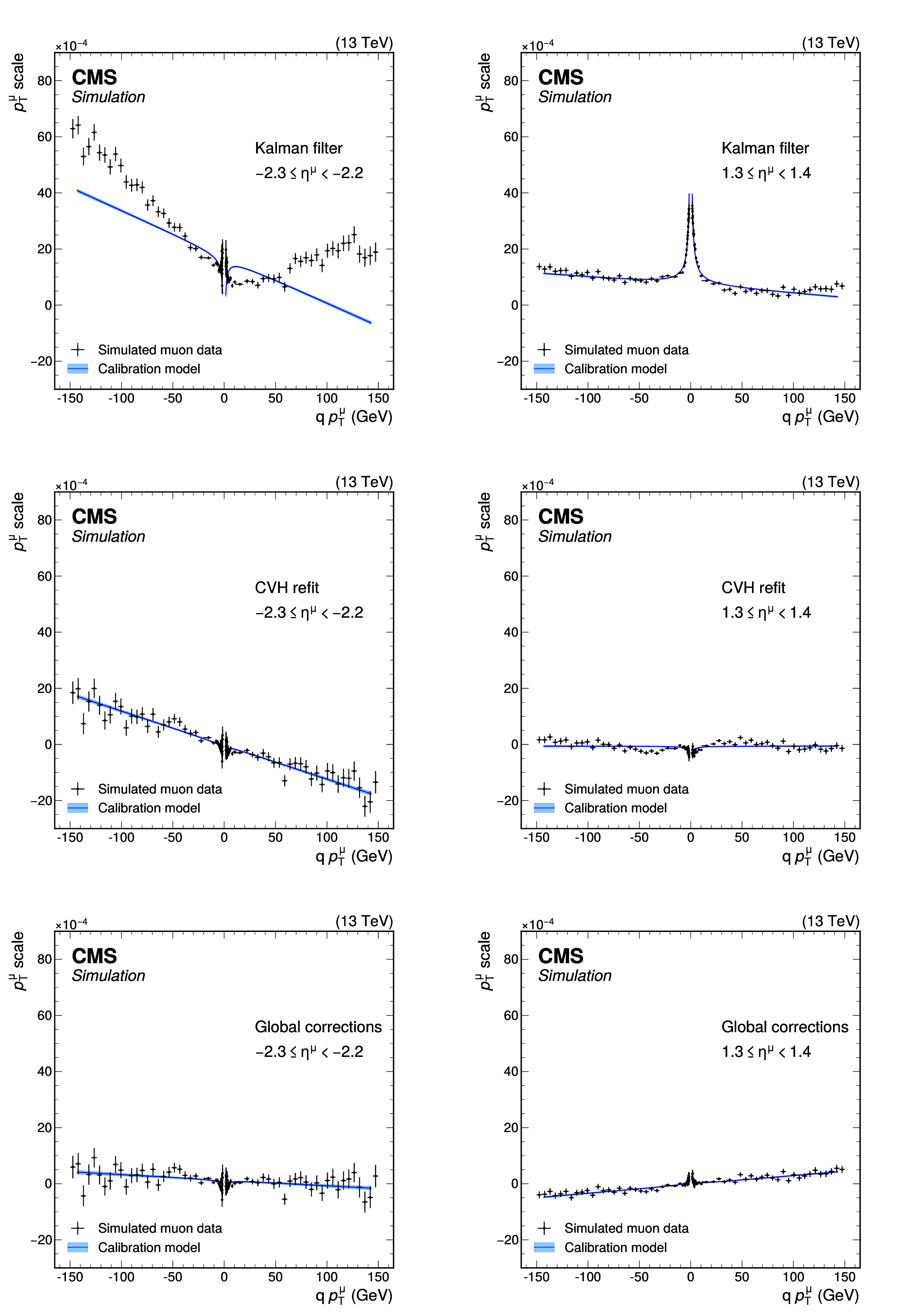
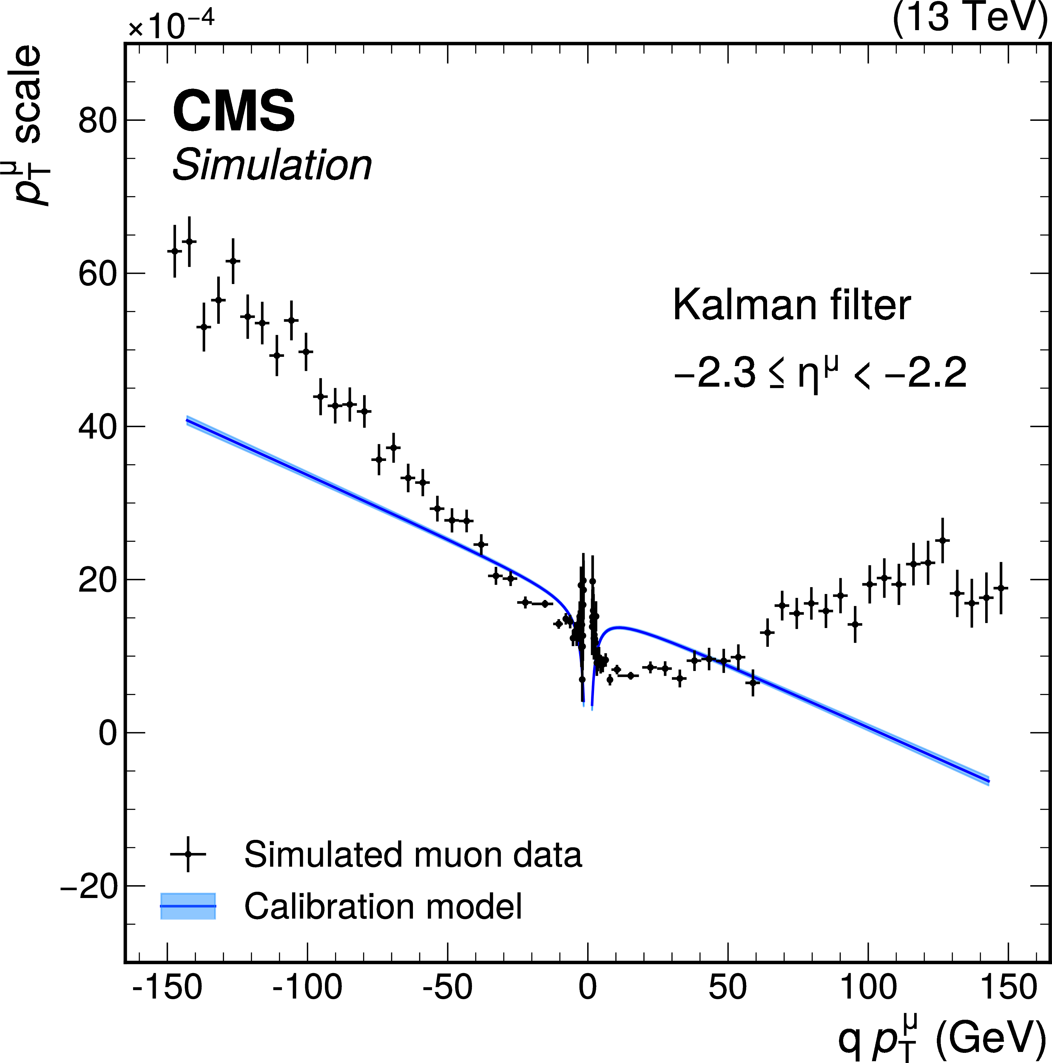
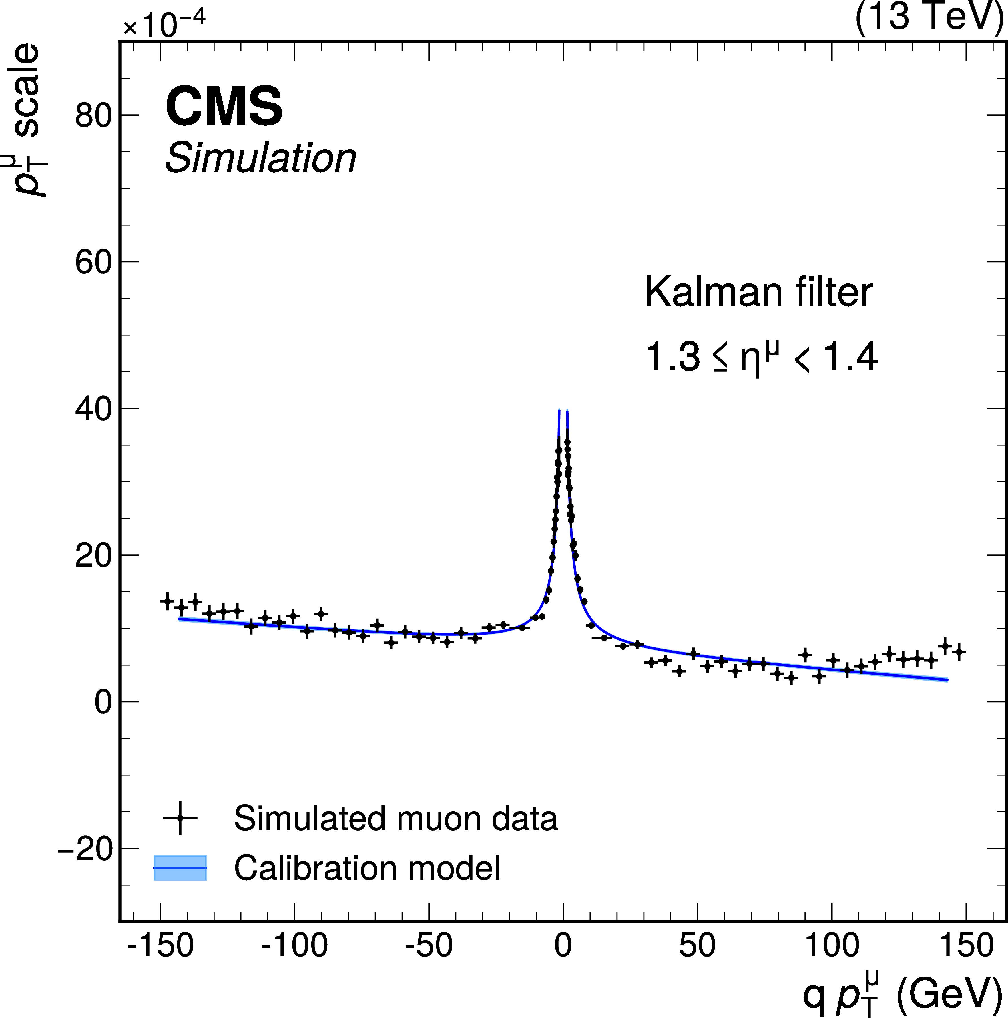
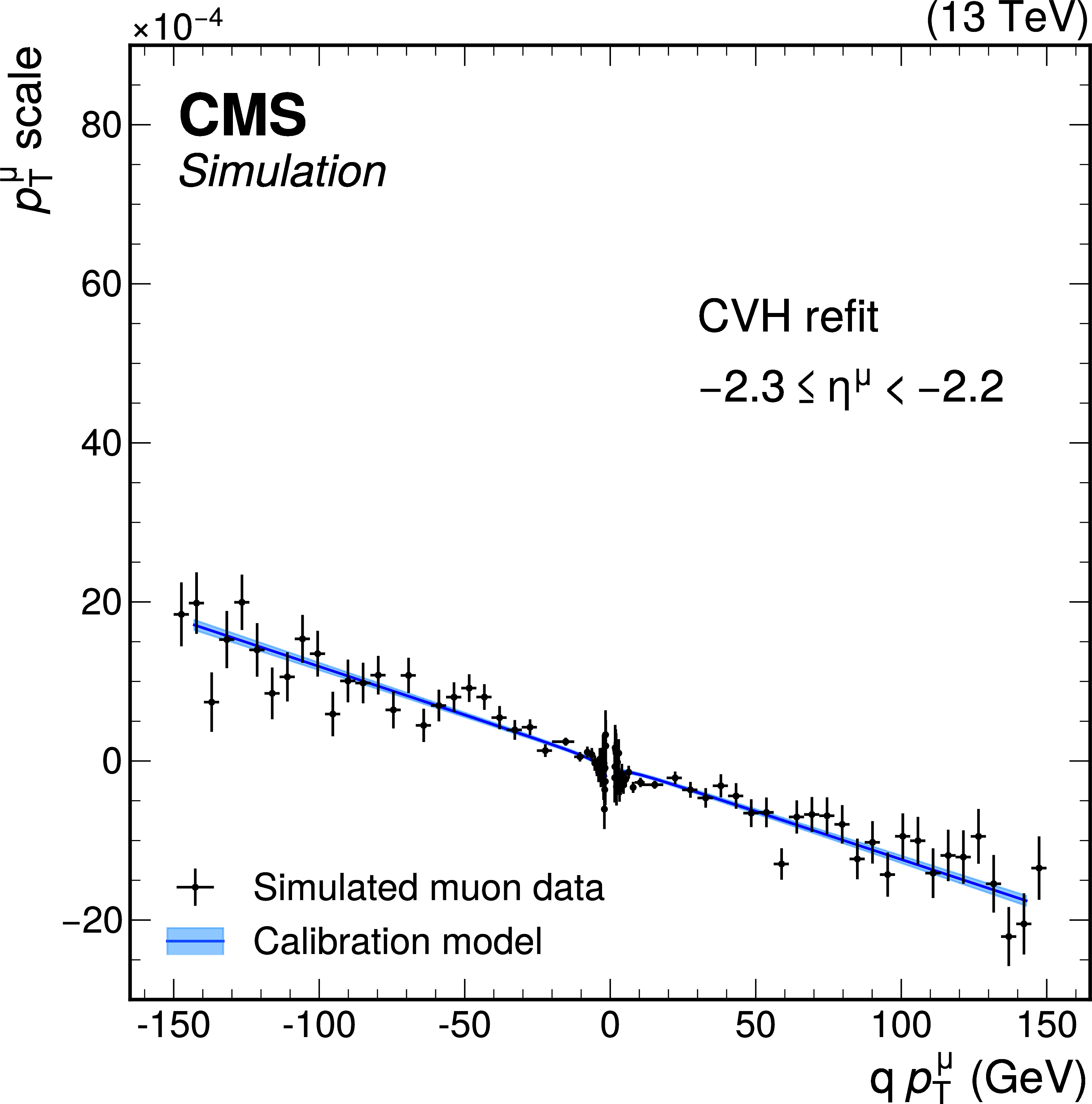
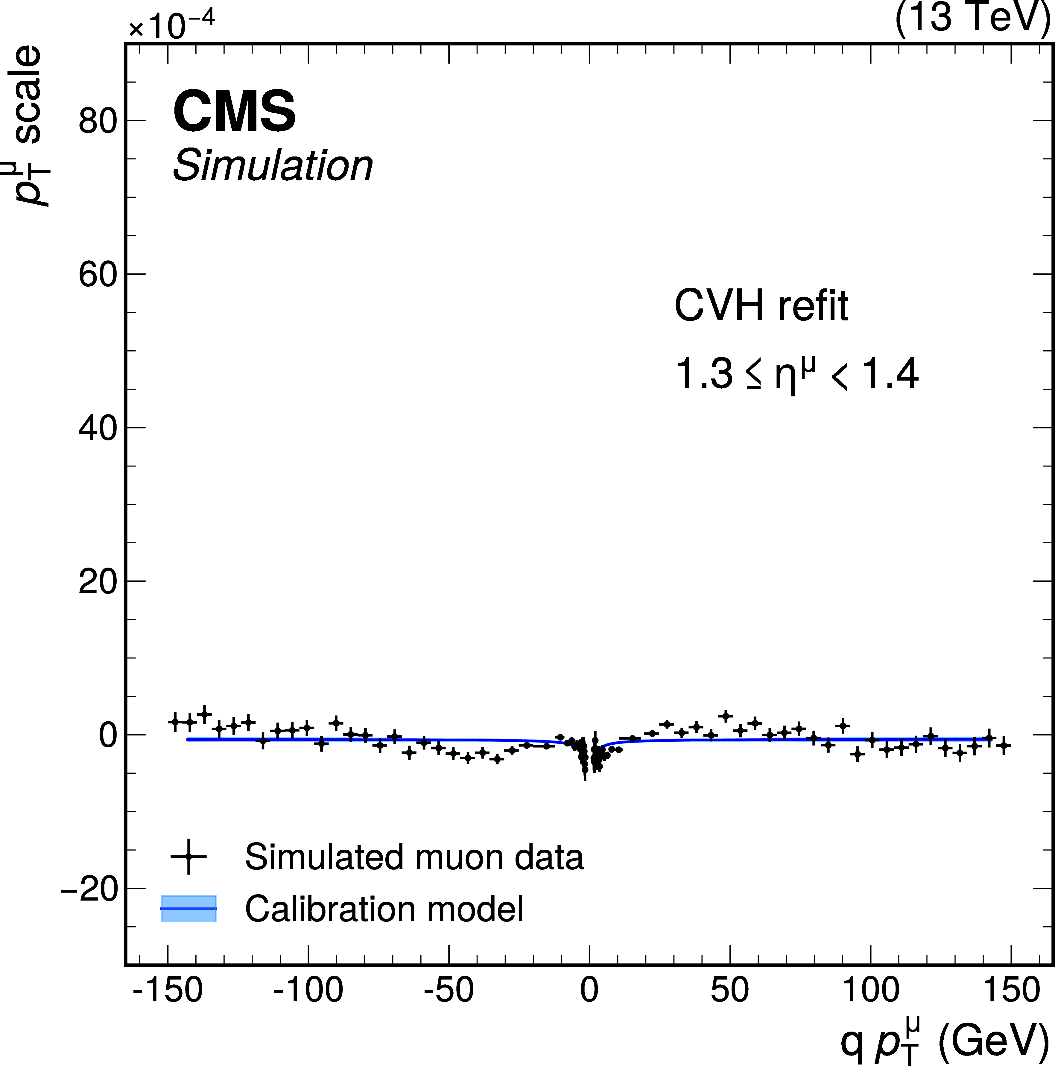
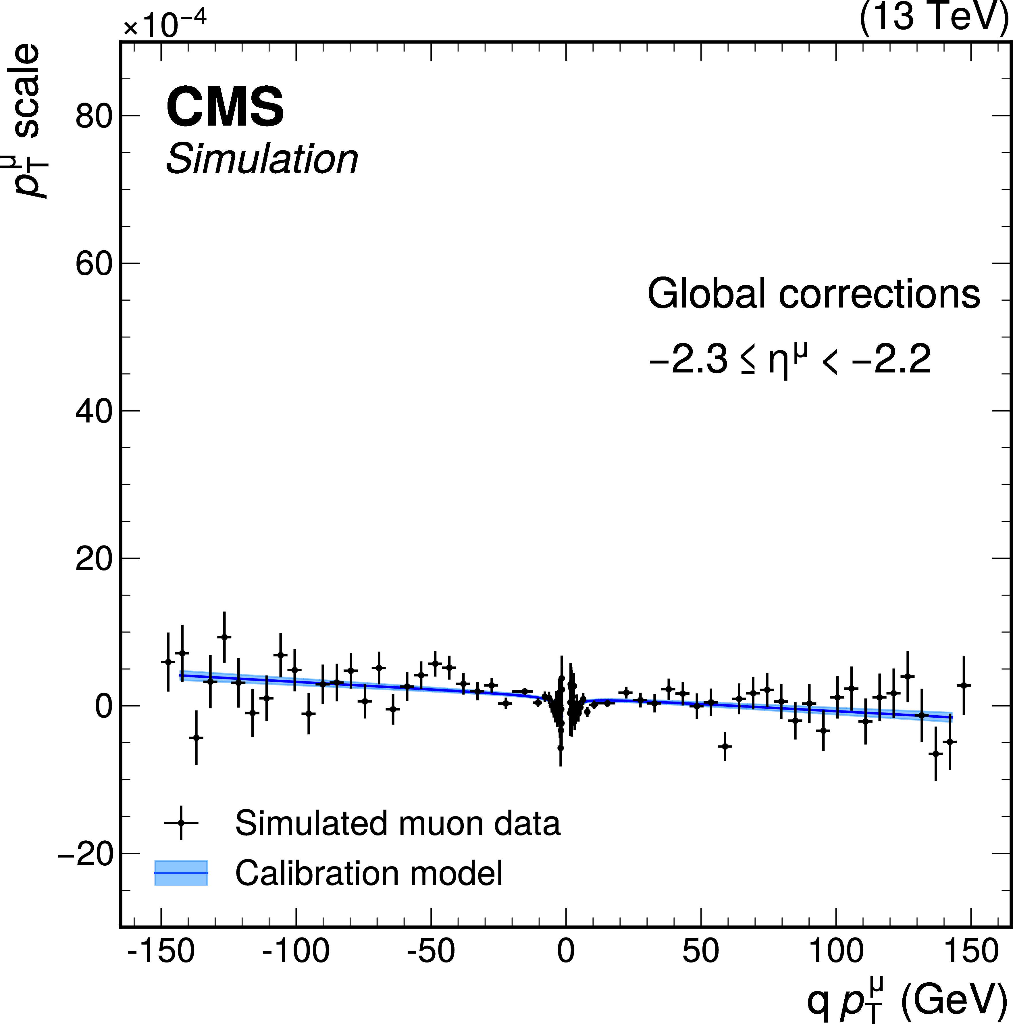
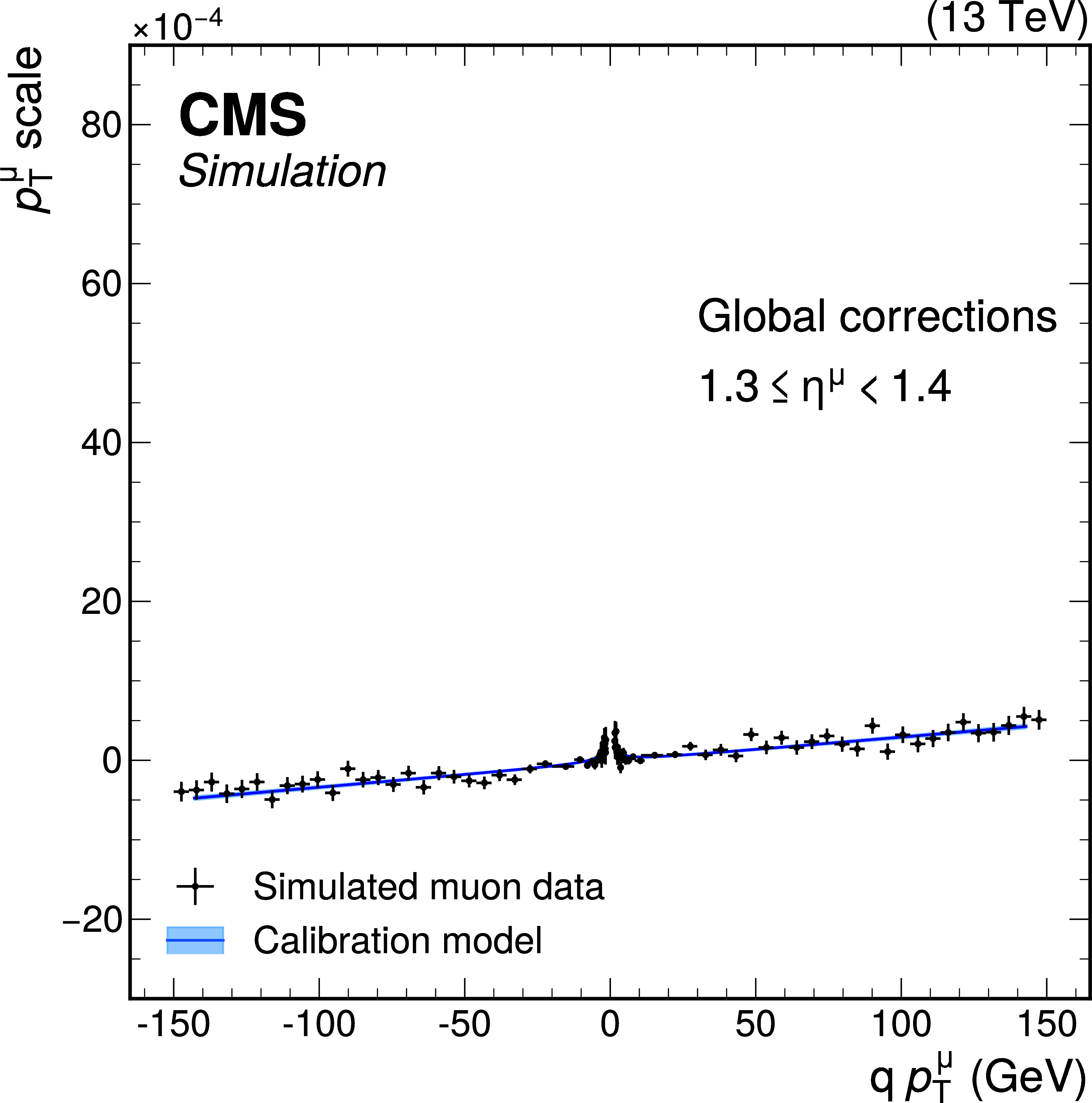
Muon momentum scale bias evaluated in simulated events as a function of $ p_{\mathrm{T}}^{\mu} $ times the muon charge $ q $. The black dots represent simulated data, while the solid line is a fit of the calibration model. The bias is shown after the Kalman filter track fit (top), the CVH refit (middle), and the generalized global corrections applied on top of the CVH refit (bottom). The comparison is performed in two $ \eta^{\mu} $ bins in the forward (left) and central (right) regions of the tracker. |
png pdf |
Figure B16-a:
Muon momentum scale bias evaluated in simulated events as a function of $ p_{\mathrm{T}}^{\mu} $ times the muon charge $ q $. The black dots represent simulated data, while the solid line is a fit of the calibration model. The bias is shown after the Kalman filter track fit (top), the CVH refit (middle), and the generalized global corrections applied on top of the CVH refit (bottom). The comparison is performed in two $ \eta^{\mu} $ bins in the forward (left) and central (right) regions of the tracker. |
png pdf |
Figure B16-b:
Muon momentum scale bias evaluated in simulated events as a function of $ p_{\mathrm{T}}^{\mu} $ times the muon charge $ q $. The black dots represent simulated data, while the solid line is a fit of the calibration model. The bias is shown after the Kalman filter track fit (top), the CVH refit (middle), and the generalized global corrections applied on top of the CVH refit (bottom). The comparison is performed in two $ \eta^{\mu} $ bins in the forward (left) and central (right) regions of the tracker. |
png pdf |
Figure B16-c:
Muon momentum scale bias evaluated in simulated events as a function of $ p_{\mathrm{T}}^{\mu} $ times the muon charge $ q $. The black dots represent simulated data, while the solid line is a fit of the calibration model. The bias is shown after the Kalman filter track fit (top), the CVH refit (middle), and the generalized global corrections applied on top of the CVH refit (bottom). The comparison is performed in two $ \eta^{\mu} $ bins in the forward (left) and central (right) regions of the tracker. |
png pdf |
Figure B16-d:
Muon momentum scale bias evaluated in simulated events as a function of $ p_{\mathrm{T}}^{\mu} $ times the muon charge $ q $. The black dots represent simulated data, while the solid line is a fit of the calibration model. The bias is shown after the Kalman filter track fit (top), the CVH refit (middle), and the generalized global corrections applied on top of the CVH refit (bottom). The comparison is performed in two $ \eta^{\mu} $ bins in the forward (left) and central (right) regions of the tracker. |
png pdf |
Figure B16-e:
Muon momentum scale bias evaluated in simulated events as a function of $ p_{\mathrm{T}}^{\mu} $ times the muon charge $ q $. The black dots represent simulated data, while the solid line is a fit of the calibration model. The bias is shown after the Kalman filter track fit (top), the CVH refit (middle), and the generalized global corrections applied on top of the CVH refit (bottom). The comparison is performed in two $ \eta^{\mu} $ bins in the forward (left) and central (right) regions of the tracker. |
png pdf |
Figure B16-f:
Muon momentum scale bias evaluated in simulated events as a function of $ p_{\mathrm{T}}^{\mu} $ times the muon charge $ q $. The black dots represent simulated data, while the solid line is a fit of the calibration model. The bias is shown after the Kalman filter track fit (top), the CVH refit (middle), and the generalized global corrections applied on top of the CVH refit (bottom). The comparison is performed in two $ \eta^{\mu} $ bins in the forward (left) and central (right) regions of the tracker. |
png pdf |
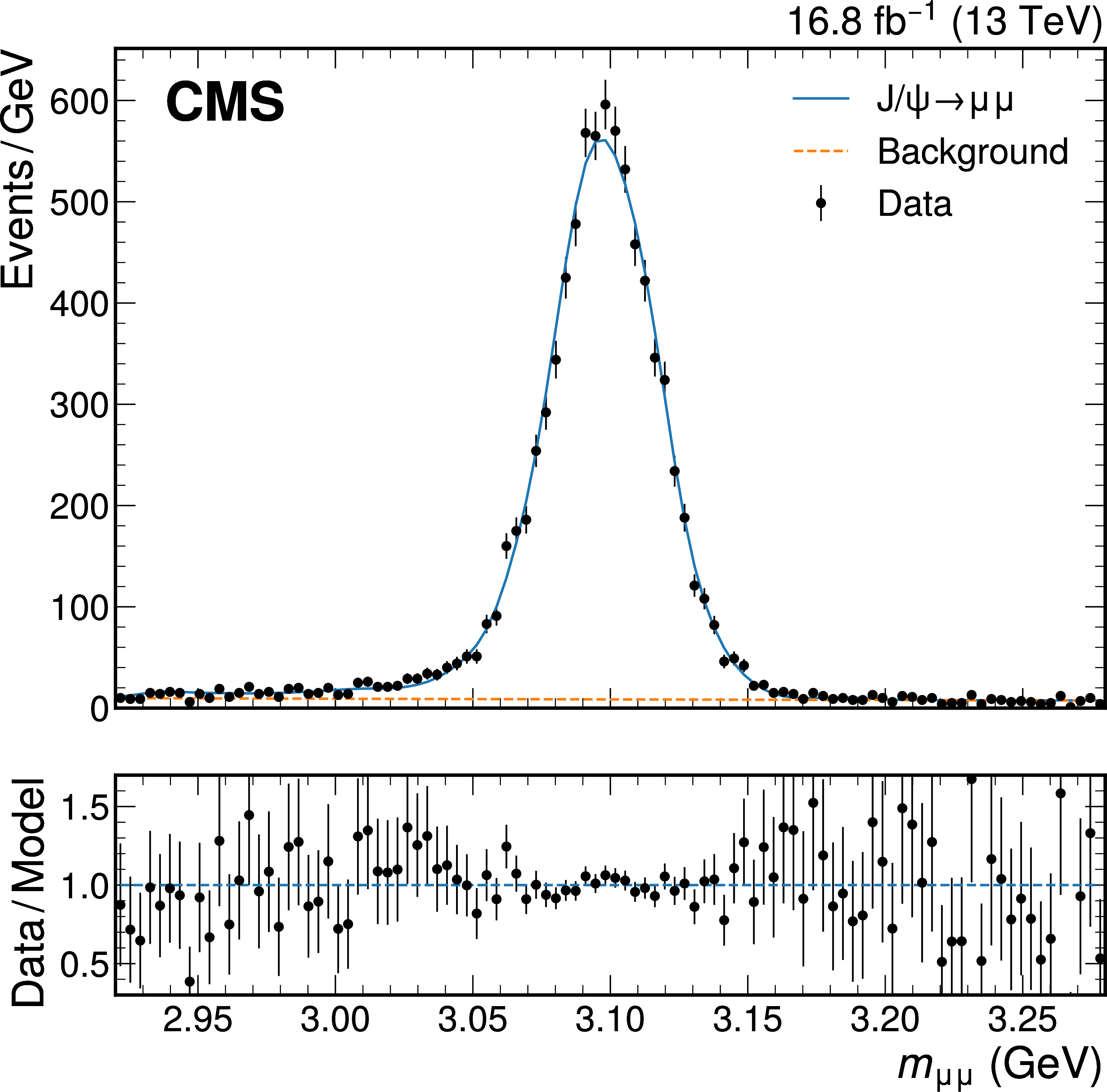
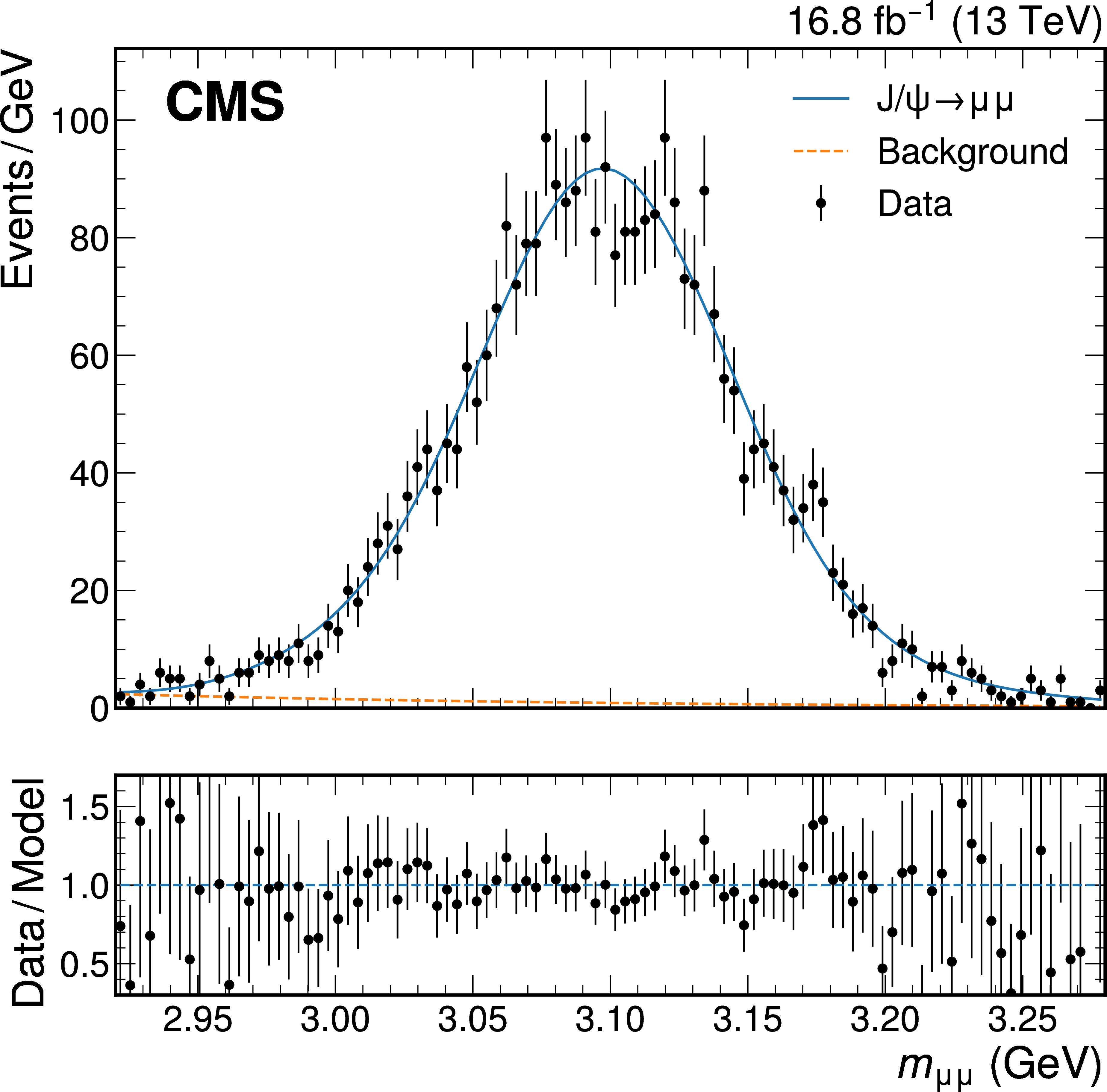
Figure B17:
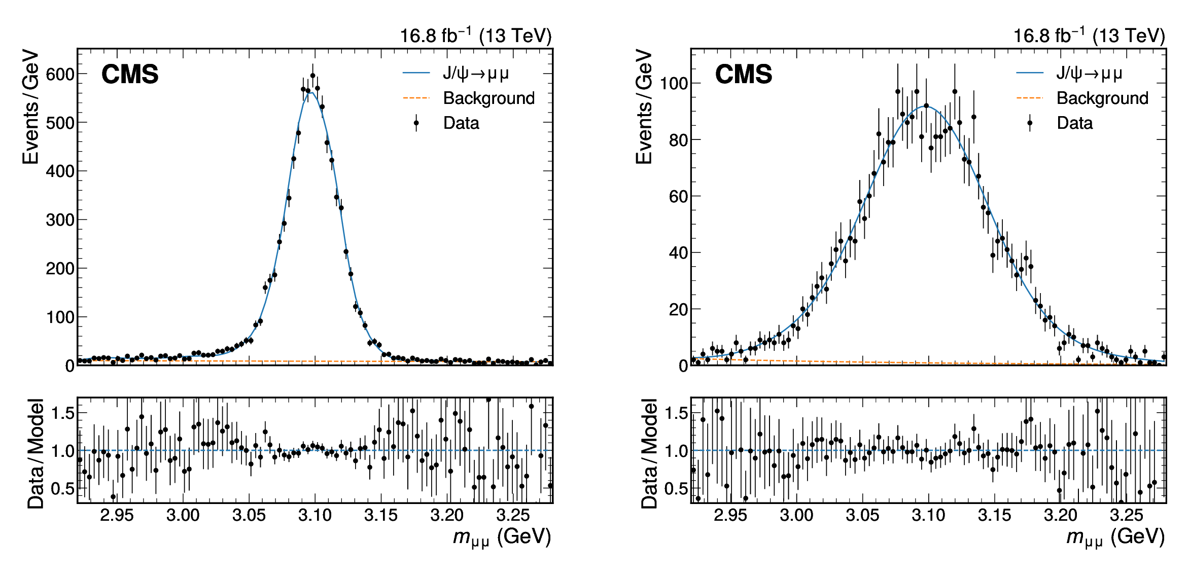
Dimuon invariant mass distributions in $ {\mathrm{J}/\psi} \to\mu\mu $ decays reconstructed in data (black points) in two representative $ \eta^{\mu} $ bins in the central (left) and forward (right) regions of the tracker. The blue line represents a fit to the distribution. The small background component is shown as a dashed orange line. |
png pdf |
Figure B17-a:
Dimuon invariant mass distributions in $ {\mathrm{J}/\psi} \to\mu\mu $ decays reconstructed in data (black points) in two representative $ \eta^{\mu} $ bins in the central (left) and forward (right) regions of the tracker. The blue line represents a fit to the distribution. The small background component is shown as a dashed orange line. |
png pdf |
Figure B17-b:
Dimuon invariant mass distributions in $ {\mathrm{J}/\psi} \to\mu\mu $ decays reconstructed in data (black points) in two representative $ \eta^{\mu} $ bins in the central (left) and forward (right) regions of the tracker. The blue line represents a fit to the distribution. The small background component is shown as a dashed orange line. |
png pdf |
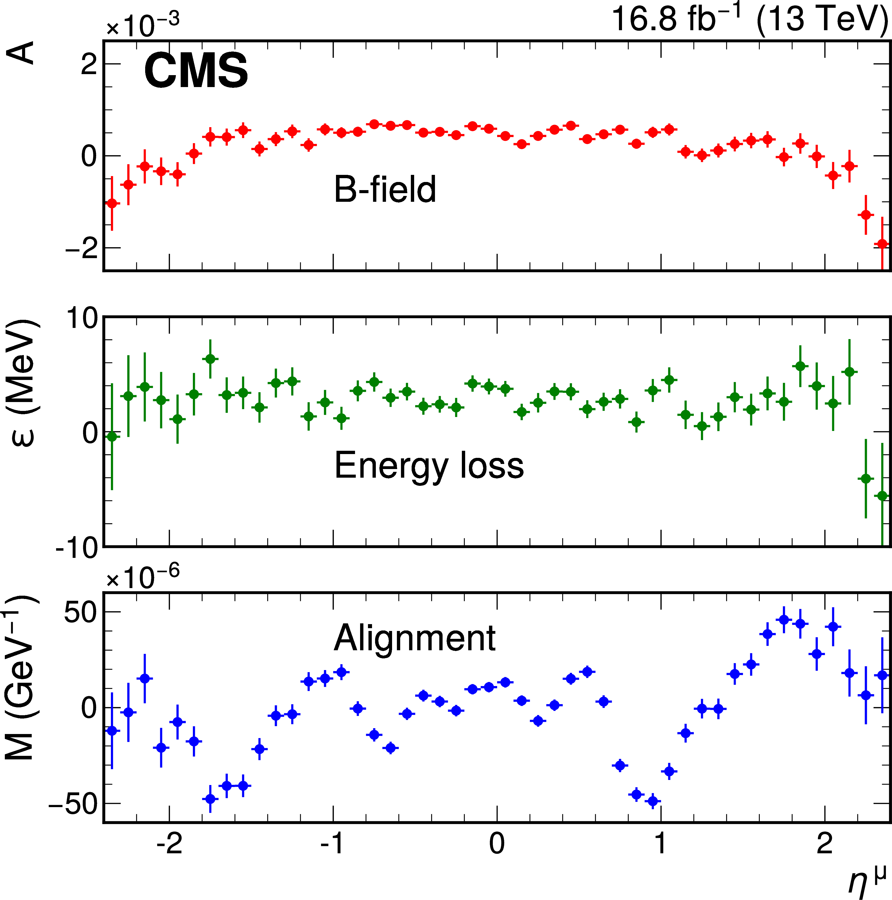
Figure B18:
Parameters of the calibration model as functions of $ \eta^{\mu} $, extracted from $ {\mathrm{J}/\psi} \to\mu\mu $ events. |
| Tables | |
png pdf |
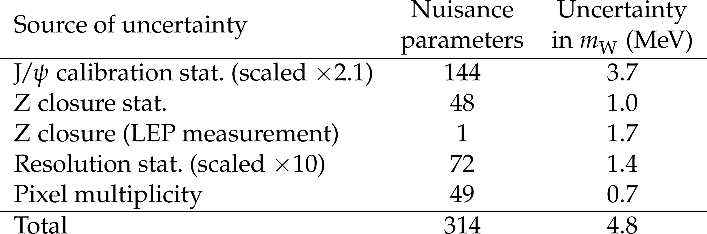
Table A1:
Breakdown of muon momentum calibration uncertainties. |
png pdf |
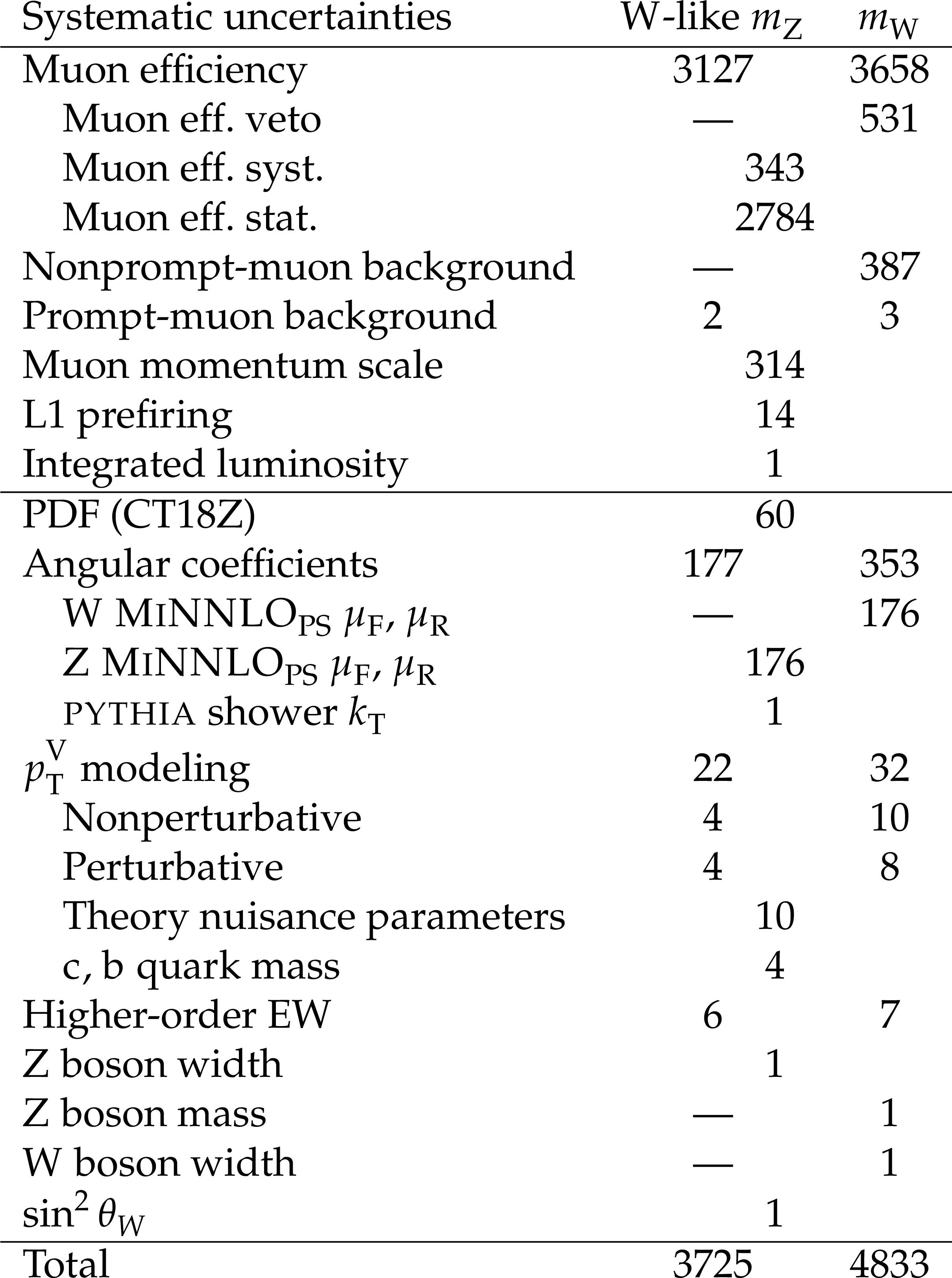
Table A2:
Uncertainties in the W-like $ m_{\mathrm{Z}} $ and $ m_{\mathrm{W}} $ measurements, with contributions to the total uncertainty from individual sources separated according to the ``nominal'' [none-none-none] and ``global'' [105] definitions of the impacts. |
png pdf |
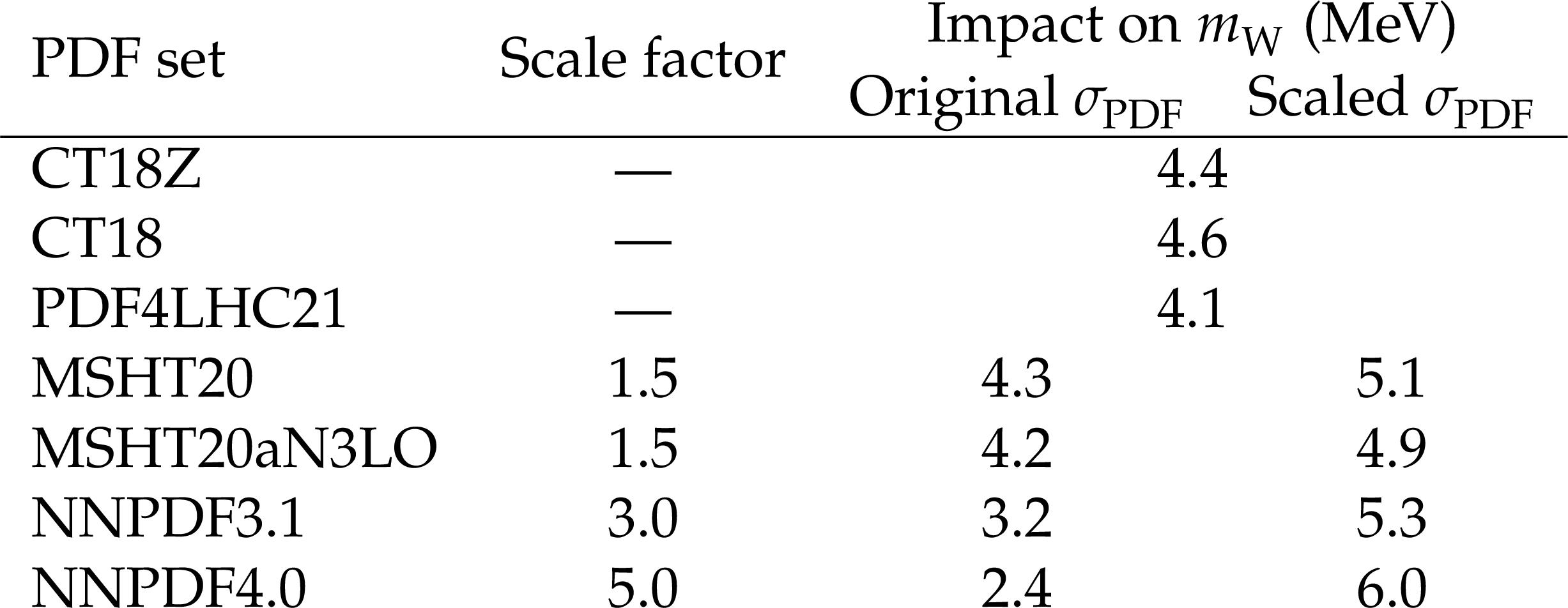
Table A3:
The $ m_{\mathrm{W}} $ values measured for different PDF sets. The second column indicates the prefit uncertainty scaling factors required to cover the central predictions of the considered PDF sets, as described in the text. The observed values, with uncertainties scaled following the procedure described in Section 7.8 and with the default unscaled uncertainties, are shown in the last two columns. The uncertainty in $ m_{\mathrm{W}} $ from the PDF is indicated in parenthesis following the total uncertainty. |
png pdf |
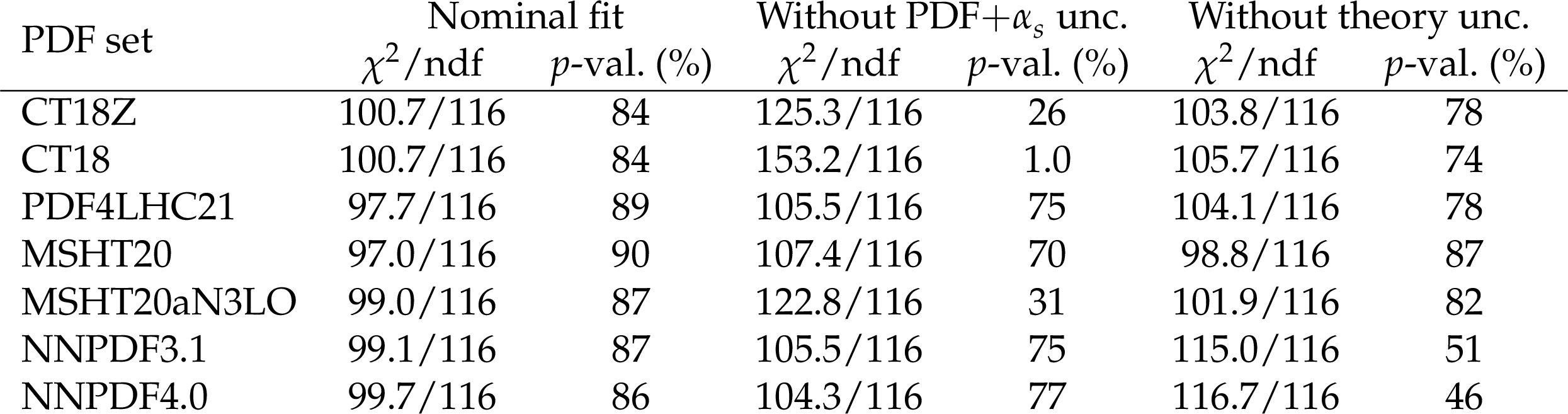
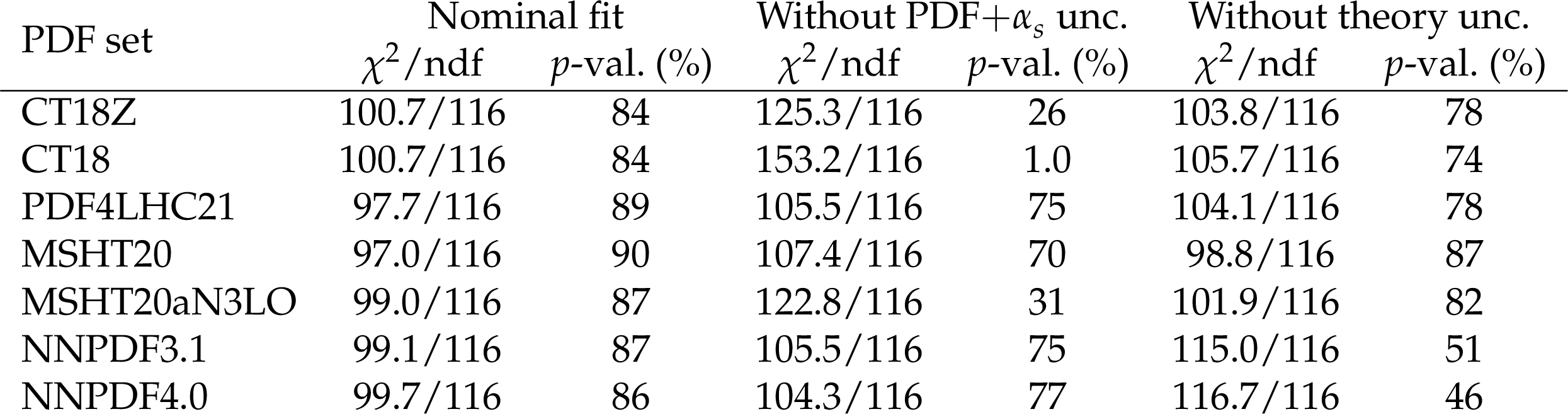
Table B1:
Goodness-of-fit test statistic for different PDF sets when fitting simultaneously the $ \eta^{\mu} $ distributions for selected $ \mathrm{W^+} $ ($ \mathrm{W^-} $) events and the $ y^{\mu\mu} $ distribution for $ \mathrm{Z}\to\mu\mu $ events. Both the saturated likelihood ratios, which are expected to follow a $ \chi^2 $ distribution with ndf degrees of freedom if the model is an accurate representation of the data, and the associated $ p $-value are shown. The fit is performed in the nominal configuration with all uncertainties (left column), nominal configuration without PDF and $ \alpha_{s} $ uncertainties (middle column), and nominal configuration without theory uncertainties (right column). |
png pdf |
Table B2:
Number of nuisance parameters for the main groups of systematic uncertainties, for the W-like $ m_{\mathrm{Z}} $ and $ m_{\mathrm{W}} $ fits. The number of parameters is displayed only once when it is the same for both fits, while ``$ \text{-} $'' means that this source is not relevant. For completeness, subgroups of parameters are also reported as indented labels for a few groups. |
png pdf |
Table B3:
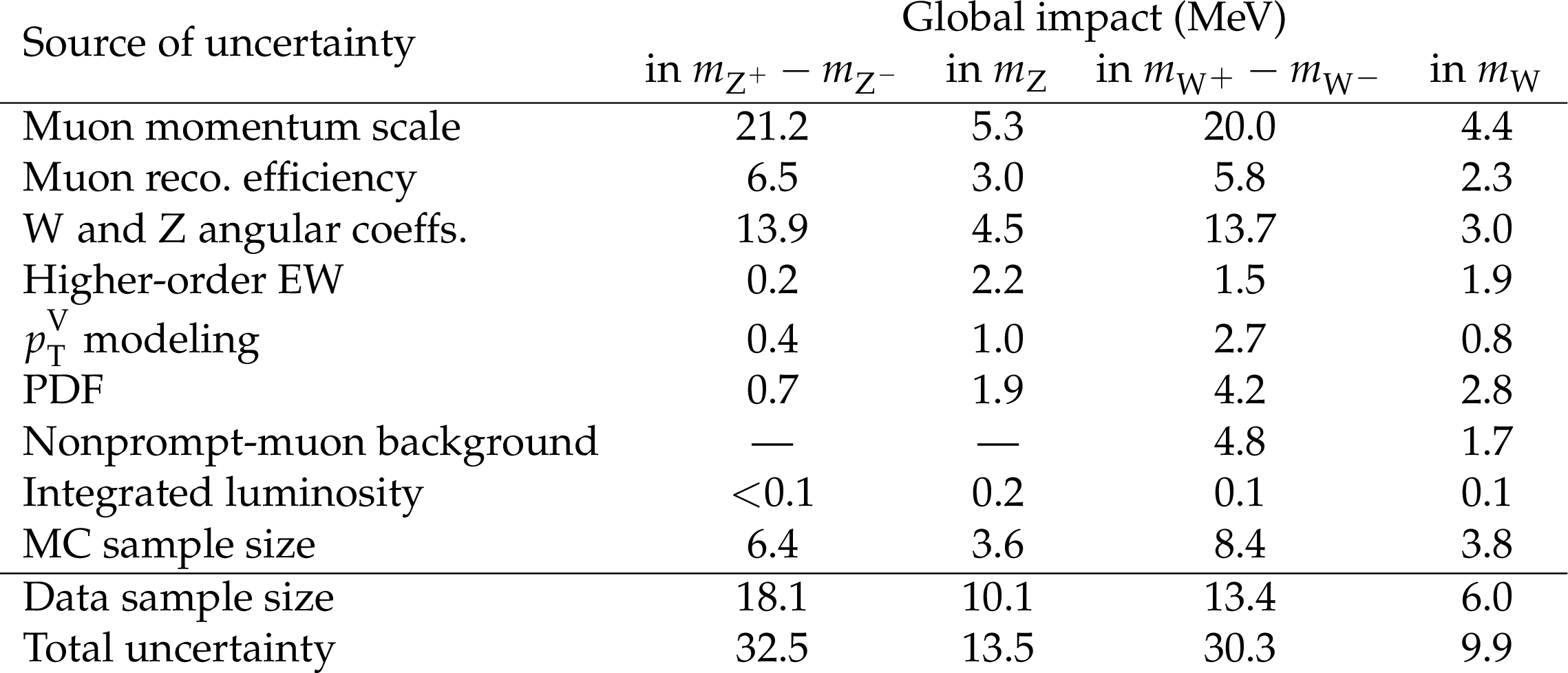
Uncertainties in the W-like $ m_{\mathrm{Z}} $ and $ m_{\mathrm{W}} $ measurements, comparing the mass difference between charges and the nominal charge combination, using nominal (upper) and global (lower) impacts. |
| Summary |
| In this paper we report the first W boson mass measurement by the CMS Collaboration at the CERN LHC. The result is markedly more precise than previous LHC measurements. The W boson mass is extracted from a sample of 117 million selected $ \mathrm{W}\to\mu\nu $ events, collected in 2016 at the proton-proton collision energy of 13 TeV, via a highly granular binned maximum likelihood fit to the three-dimensional distribution of the muon $ p_{\mathrm{T}}^{\mu} $, $ \eta^{\mu} $, and electric charge. Novel experimental techniques have been used, together with state-of-the-art theoretical models, to improve the measurement accuracy. The muon momentum calibration, based on $ {\mathrm{J}/\psi} \to\mu\mu $ decays, as well as the data analysis methods and the treatment of the theory calculations used in the $ m_{\mathrm{W}} $ measurement have been extensively validated by extracting $ m_{\mathrm{Z}} $ and $ p_{\mathrm{T}}^{\mathrm{Z}} $ both from a direct $ \mathrm{Z}\to\mu\mu $ dimuon analysis and from a W-like analysis of the Z boson data. As shown in Fig. 4, the measured value, $m_{\mathrm{W}} = 80\,360.2 \pm 9.9$ MeV, agrees with the standard model expectation from the electroweak fit and is in disagreement with the measurement reported by the CDF Collaboration. Our result has similar precision to the CDF Collaboration measurement and is significantly more precise than all other measurements. The dominant sources of uncertainty are the muon momentum calibration and the parton distribution functions. Uncertainties in the modeling of W boson production are subdominant due to novel approaches used to parameterize and constrain the predictions and their corresponding uncertainties in situ with the data. This result constitutes a significant step towards achieving an experimental measurement of $ m_{\mathrm{W}} $ with a precision matching that of the EW fit. |
| Covariance Matrices |
|
We provide seven covariance matrices:
|
| References | ||||
| 1 | Particle Data Group , S. Navas et al. | Review of particle physics | PRD 110 (2024) 030001 | |
| 2 | J. Haller et al. | Update of the global electroweak fit and constraints on two-Higgs-doublet models | EPJC 78 (2018) 675 | 1803.01853 |
| 3 | J. de Blas et al. | Global analysis of electroweak data in the standard model | PRD 106 (2022) 033003 | |
| 4 | CDF Collaboration | High-precision measurement of the W boson mass with the CDF II detector | Science 376 (2022) 170 | |
| 5 | ATLAS Collaboration | Observation of a new particle in the search for the Standard Model Higgs boson with the ATLAS detector at the LHC | PLB 716 (2012) 1 | 1207.7214 |
| 6 | CMS Collaboration | Observation of a new boson at a mass of 125 GeV with the CMS experiment at the LHC | PLB 716 (2012) 30 | CMS-HIG-12-028 1207.7235 |
| 7 | CMS Collaboration | Observation of a new boson with mass near 125 GeV in pp collisions at $ \sqrt{s} = $ 7 and 8 TeV | JHEP 06 (2013) 081 | CMS-HIG-12-036 1303.4571 |
| 8 | S. Heinemeyer, W. Hollik, G. Weiglein, and L. Zeune | Implications of LHC search results on the W boson mass prediction in the MSSM | JHEP 12 (2013) 084 | 1311.1663 |
| 9 | D. L \'o pez-Val and T. Robens | $ \Delta $r and the W-boson mass in the singlet extension of the standard model | PRD 90 (2014) 114018 | 1406.1043 |
| 10 | UA1 Collaboration | Experimental observation of isolated large transverse energy electrons with associated missing energy at $ \sqrt{s} = $ 540 GeV | PLB 122 (1983) 103 | |
| 11 | UA2 Collaboration | Observation of single isolated electrons of high transverse momentum in events with missing transverse energy at the $ \overline{\mathrm{p}}\mathrm{p} $ collider | PLB 122 (1983) 476 | |
| 12 | UA1 Collaboration | Experimental observation of lepton pairs of invariant mass around 95 GeV/c2 at the CERN SPS collider | PLB 126 (1983) 398 | |
| 13 | UA2 Collaboration | Evidence for Z0 --$ > $; e+e- at the CERN $ \overline{\mathrm{p}}\mathrm{p} $ collider | PLB 129 (1983) 130 | |
| 14 | ALEPH, DELPHI, L3, OPAL, SLD, LEP Electroweak Working Group, SLD Electroweak Group, SLD Heavy Flavour Group Collaboration | Precision electroweak measurements on the Z resonance | Phys. Rept. 427 (2006) 257 | hep-ex/0509008 |
| 15 | ALEPH, DELPHI, L3, OPAL, LEP Electroweak Working Group , S. Schael et al. | Electroweak measurements in electron-positron collisions at W-boson-pair energies at LEP | Phys. Rept. 532 (2013) 119 | 1302.3415 |
| 16 | D0 Collaboration | Measurement of the W boson mass with the D0 detector | PRL 108 (2012) 151804 | 1203.0293 |
| 17 | ATLAS Collaboration | Measurement of the W-boson mass in pp collisions at $ \sqrt{s} = $ 7 TeV with the ATLAS detector | EPJC 78 (2018) 110 | 1701.07240 |
| 18 | LHCb Collaboration | Measurement of the W boson mass | JHEP 01 (2022) 036 | 2109.01113 |
| 19 | ATLAS Collaboration | Measurement of the W-boson mass and width with the ATLAS detector using proton-proton collisions at $ \sqrt{s} = $ 7 TeV | EPJC 84 (2024) 1309 | 2403.15085 |
| 20 | LHC-TeV MW Working Group , S. Amoroso et al. | Compatibility and combination of world W-boson mass measurements | EPJC 84 (2024) 451 | 2308.09417 |
| 21 | CMS Collaboration | The CMS experiment at the CERN LHC | JINST 3 (2008) S08004 | |
| 22 | CMS Collaboration | Performance of the CMS Level-1 trigger in proton-proton collisions at $ \sqrt{s} = $ 13 TeV | JINST 15 (2020) P10017 | CMS-TRG-17-001 2006.10165 |
| 23 | CMS Collaboration | Performance of the CMS high-level trigger during LHC Run 2 | JINST 19 (2024) P11021 | CMS-TRG-19-001 2410.17038 |
| 24 | CMS Collaboration | The CMS trigger system | JINST 12 (2017) P01020 | CMS-TRG-12-001 1609.02366 |
| 25 | CMS Collaboration | Electron and photon reconstruction and identification with the CMS experiment at the CERN LHC | JINST 16 (2021) P05014 | CMS-EGM-17-001 2012.06888 |
| 26 | CMS Collaboration | Performance of the CMS muon detector and muon reconstruction with proton-proton collisions at $ \sqrt{s} = $ 13 TeV | JINST 13 (2018) P06015 | CMS-MUO-16-001 1804.04528 |
| 27 | CMS Collaboration | Description and performance of track and primary-vertex reconstruction with the CMS tracker | JINST 9 (2014) P10009 | CMS-TRK-11-001 1405.6569 |
| 28 | CMS Collaboration | Particle-flow reconstruction and global event description with the CMS detector | JINST 12 (2017) P10003 | CMS-PRF-14-001 1706.04965 |
| 29 | E. Manca, O. Cerri, N. Foppiani, and G. Rolandi | About the rapidity and helicity distributions of the W bosons produced at LHC | JHEP 12 (2017) 130 | 1707.09344 |
| 30 | M. A. Ebert, J. K. L. Michel, I. W. Stewart, and F. J. Tackmann | Drell--Yan $ q_{\mathrm{T}} $ resummation of fiducial power corrections at N$ ^{3} $LL | JHEP 04 (2021) 102 | 2006.11382 |
| 31 | G. Billis, J. K. L. Michel, and F. J. Tackmann | Drell-Yan transverse-momentum spectra at N$ ^{3} $LL$ ^{\prime} $ and approximate N$ ^{4} $LL with SCETlib | JHEP 02 (2025) 170 | 2411.16004 |
| 32 | F. J. Tackmann | Beyond scale variations: perturbative theory uncertainties from nuisance parameters | JHEP 08 (2025) 098 | 2411.18606 |
| 33 | CMS Collaboration | Measurements of the W boson rapidity, helicity, double-differential cross sections, and charge asymmetry in $ {\mathrm{p}\mathrm{p}} $ collisions at 13 TeV | PRD 102 (2020) 092012 | CMS-SMP-18-012 2008.04174 |
| 34 | E. Mirkes | Angular decay distribution of leptons from W bosons at NLO in hadronic collisions | NPB 387 (1992) 3 | |
| 35 | D. Y. Bardin, A. Leike, T. Riemann, and M. Sachwitz | Energy dependent width effects in $ \mathrm{e}^+\mathrm{e}^- $ annihilation near the Z boson pole | PLB 206 (1988) 539 | |
| 36 | J. R. Klein and A. Roodman | Blind analysis in nuclear and particle physics | Ann. Rev. Nucl. Part. Sci. 55 (2005) 141 | |
| 37 | CMS Collaboration | Precision luminosity measurement in proton-proton collisions at $ \sqrt{s} = $ 13 TeV in 2015 and 2016 at CMS | EPJC 81 (2021) 800 | CMS-LUM-17-003 2104.01927 |
| 38 | CMS Collaboration | DeepMET: Improving missing transverse momentum estimation with a deep neural network | Submitted to Phys. Rev. D, 2025 | CMS-JME-24-001 2509.12012 |
| 39 | CMS Collaboration | Performance of missing transverse momentum reconstruction in proton-proton collisions at $ \sqrt{s} = $ 13 TeV using the CMS detector | JINST 14 (2019) P07004 | CMS-JME-17-001 1903.06078 |
| 40 | P. F. Monni et al. | MiNNLO$ _\mathrm{PS} $: a new method to match NNLO QCD to parton showers | JHEP 05 (2020) 143 | 1908.06987 |
| 41 | P. F. Monni, E. Re, and M. Wiesemann | MiNNLO$ _{\mathrm{PS}} $: optimizing 2 $ \to $ 1 hadronic processes | EPJC 80 (2020) 1075 | 2006.04133 |
| 42 | T. Sjöstrand et al. | An introduction to PYTHIA 8.2 | Comput. Phys. Commun. 191 (2015) 159 | 1410.3012 |
| 43 | G. Billis, M. A. Ebert, J. K. L. Michel, and F. J. Tackmann | A toolbox for $ q_{\mathrm{T}} $ and 0-jettiness subtractions at N$ ^3 $LO | Eur. Phys. J. Plus 136 (2021) 214 | 1909.00811 |
| 44 | T.-J. Hou et al. | New CTEQ global analysis of quantum chromodynamics with high-precision data from the LHC | PRD 103 (2021) 014013 | 1912.10053 |
| 45 | GEANT4 Collaboration | GEANT 4---a simulation toolkit | NIM A 506 (2003) 250 | |
| 46 | S. Choi and H. Oh | Improved extrapolation methods of data-driven background estimations in high energy physics | EPJC 81 (2021) 643 | 1906.10831 |
| 47 | CMS Collaboration | Strategies and performance of the CMS silicon tracker alignment during LHC Run 2 | NIM A 1037 (2022) 166795 | CMS-TRK-20-001 2111.08757 |
| 48 | W. Bizon et al. | The transverse momentum spectrum of weak gauge bosons at N$ ^3 $LL+NNLO | EPJC 79 (2019) 868 | 1905.05171 |
| 49 | T. Cridge, G. Marinelli, and F. J. Tackmann | Theory uncertainties in the extraction of $ \alpha_s $ from Drell-Yan at small transverse momentum | 2506.13874 | |
| 50 | S. Camarda et al. | DYTurbo: Fast predictions for Drell--Yan processes | EPJC 80 (2020) 251 | 1910.07049 |
| 51 | J. Campbell and T. Neumann | Precision phenomenology with MCFM | JHEP 12 (2019) 034 | 1909.09117 |
| 52 | J. Butterworth et al. | PDF4LHC recommendations for LHC Run II | JPG 43 (2016) 023001 | 1510.03865 |
| 53 | J. S. Conway | Incorporating nuisance parameters in likelihoods for multisource spectra | in: Workshop on statistical issues related to discovery claims in search experiments and unfolding, H. B. Prosper and L. Lyons, eds., CERN Yellow Reports: Conf.\ Proc., CERN, Geneva, 2011 PHYSTAT 201 (2011) 115 |
1103.0354 |
| 54 | M. Abadi et al. | TensorFlow: Large-scale machine learning on heterogeneous distributed systems | Software available from tensorflow.org, 2016 | 1603.04467 |
| 55 | A. G. Baydin, B. A. Pearlmutter, A. A. Radul, and J. M. Siskind | Automatic differentiation in machine learning: a survey | Journal of Machine Learning Research 18 () 1, 2018 link |
1502.05767 |
| 56 | J. K. Lindsey | Parametric Statistical Inference | Oxford University Press,, ISBN 978023598, 1996 link |
|
| 57 | P. Nason | A new method for combining NLO QCD with shower Monte Carlo algorithms | JHEP 11 (2004) 040 | hep-ph/0409146 |
| 58 | S. Frixione, P. Nason, and C. Oleari | Matching NLO QCD computations with parton shower simulations: the POWHEG method | JHEP 11 (2007) 070 | 0709.2092 |
| 59 | S. Alioli, P. Nason, C. Oleari, and E. Re | A general framework for implementing NLO calculations in shower Monte Carlo programs: the POWHEG BOX | JHEP 06 (2010) 043 | 1002.2581 |
| 60 | P. Golonka and Z. W \c a s | PHOTOS Monte Carlo: a precision tool for QED corrections in Z and W decays | EPJC 45 (2006) 97 | hep-ph/0506026 |
| 61 | N. Davidson, T. Przedzinski, and Z. W \c a s | PHOTOS interface in C++: Technical and physics documentation | Comput. Phys. Commun. 199 (2016) 86 | 1011.0937 |
| 62 | CMS Collaboration | Extraction and validation of a new set of CMS PYTHIA8 tunes from underlying-event measurements | EPJC 80 (2020) 4 | CMS-GEN-17-001 1903.12179 |
| 63 | CMS Collaboration | Measurements of differential Z boson production cross sections in proton-proton collisions at $ \sqrt{s} = $ 13 TeV | JHEP 12 (2019) 061 | CMS-SMP-17-010 1909.04133 |
| 64 | NNPDF Collaboration | Parton distributions from high-precision collider data | EPJC 77 (2017) 663 | 1706.00428 |
| 65 | NNPDF Collaboration | The path to proton structure at 1\% accuracy | EPJC 82 (2022) 428 | 2109.02653 |
| 66 | S. Bailey et al. | Parton distributions from LHC, HERA, Tevatron and fixed target data: MSHT20 PDFs | EPJC 81 (2021) 341 | 2012.04684 |
| 67 | PDF4LHC Working Group Collaboration | The PDF4LHC21 combination of global PDF fits for the LHC Run III | JPG 49 (2022) 080501 | 2203.05506 |
| 68 | T. Cridge, L. A. Harland-Lang, and R. S. Thorne | Combining QED and approximate N$ ^3 $LO QCD corrections in a global PDF fit: MSHT20qed\_an3lo PDFs | SciPost Phys. 17 (2024) 026 | 2312.07665 |
| 69 | NNPDF Collaboration | Illuminating the photon content of the proton within a global PDF analysis | SciPost Phys. 5 (2018) 008 | 1712.07053 |
| 70 | J. Alwall et al. | The automated computation of tree-level and next-to-leading order differential cross sections, and their matching to parton shower simulations | JHEP 07 (2014) 079 | 1405.0301 |
| 71 | T. Melia, P. Nason, R. Rontsch, and G. Zanderighi | $ \text{W}^{+}\text{W}^{-} $, WZ and ZZ production in the POWHEG BOX | JHEP 11 (2011) 078 | 1107.5051 |
| 72 | CMS Collaboration | Technical proposal for the Phase-II upgrade of the Compact Muon Solenoid | CMS Technical Proposal CERN-LHCC-2015-010, CMS-TDR-15-02, 2015 CDS |
|
| 73 | CMS Collaboration | Measurements of inclusive W and Z cross sections in pp collisions at $ \sqrt{s} = $ 7 TeV | JHEP 01 (2011) 080 | CMS-EWK-10-002 1012.2466 |
| 74 | CMS Collaboration | Performance of the CMS muon trigger system in proton-proton collisions at $ \sqrt{s} = $ 13 TeV | JINST 16 (2021) P07001 | CMS-MUO-19-001 2102.04790 |
| 75 | V. Blobel, C. Kleinwort, and F. Meier | Fast alignment of a complex tracking detector using advanced track models | Comput. Phys. Commun. 182 (2011) 1760 | 1103.3909 |
| 76 | V. Blobel | A new fast track-fit algorithm based on broken lines | NIM A 566 (2006) 14 | |
| 77 | CMS Collaboration | Precision measurement of the structure of the CMS inner tracking system using nuclear interactions | JINST 13 (2018) P10034 | CMS-TRK-17-001 1807.03289 |
| 78 | J. Allison et al. | GEANT 4 developments and applications | IEEE Trans. Nucl. Sci. 53 (2006) 270 | |
| 79 | J. Allison et al. | Recent developments in GEANT 4 | NIM A 835 (2016) 186 | |
| 80 | V. Klyukhin et al. | The CMS magnetic field measuring and monitoring systems | Symmetry 14 (2022) 169 | 2202.02562 |
| 81 | CMS Collaboration | Alignment of the CMS tracker with LHC and cosmic ray data | JINST 9 (2014) P06009 | CMS-TRK-11-002 1403.2286 |
| 82 | C. W. Bauer, S. Fleming, D. Pirjol, and I. W. Stewart | An effective field theory for collinear and soft gluons: Heavy to light decays | PRD 63 (2001) 114020 | hep-ph/0011336 |
| 83 | C. W. Bauer, D. Pirjol, and I. W. Stewart | Soft collinear factorization in effective field theory | PRD 65 (2002) 054022 | hep-ph/0109045 |
| 84 | J.-Y. Chiu, A. Jain, D. Neill, and I. Z. Rothstein | A formalism for the systematic treatment of rapidity logarithms in quantum field theory | JHEP 05 (2012) 084 | 1202.0814 |
| 85 | S. Camarda, L. Cieri, and G. Ferrera | Drell--Yan lepton-pair production: $ q_{\mathrm{T}} $ resummation at N$ ^3 $LL accuracy and fiducial cross sections at N$ ^3 $LO | PRD 104 (2021) L111503 | 2103.04974 |
| 86 | M. Grazzini, S. Kallweit, and M. Wiesemann | Fully differential NNLO computations with MATRIX | EPJC 78 (2018) 537 | 1711.06631 |
| 87 | T. Becher and T. Neumann | Fiducial $ q_{\mathrm{T}} $ resummation of color-singlet processes at N$ ^3 $LL+NNLO | JHEP 03 (2021) 199 | 2009.11437 |
| 88 | J. C. Collins and D. E. Soper | Back-to-back jets in QCD | NPB 193 (1981) 381 | |
| 89 | M. A. Ebert, J. K. L. Michel, I. W. Stewart, and Z. Sun | Disentangling long and short distances in momentum-space TMDs | JHEP 07 (2022) 129 | 2201.07237 |
| 90 | T. Cridge, L. A. Harland-Lang, A. D. Martin, and R. S. Thorne | An investigation of the $ \alpha_S $ and heavy quark mass dependence in the MSHT20 global PDF analysis | EPJC 81 (2021) 744 | 2106.10289 |
| 91 | J. C. Collins and D. E. Soper | Angular distribution of dileptons in high-energy hadron collisions | PRD 16 (1977) 2219 | |
| 92 | ATLAS Collaboration | Measurement of the W-boson angular coefficients and transverse momentum in pp collisions at $ \sqrt{s}= $ 13 TeV with the ATLAS detector | Submitted to EPJC, 2025 | 2509.13759 |
| 93 | C. M. Carloni Calame, G. Montagna, O. Nicrosini, and M. Treccani | Higher order QED corrections to W boson mass determination at hadron colliders | PRD 69 (2004) 037301 | hep-ph/0303102 |
| 94 | C. M. Carloni Calame, G. Montagna, O. Nicrosini, and M. Treccani | Multiple photon corrections to the neutral-current Drell--Yan process | JHEP 05 (2005) 019 | hep-ph/0502218 |
| 95 | L. Barze et al. | Neutral current Drell--Yan with combined QCD and electroweak corrections in the POWHEG BOX | EPJC 73 (2013) 2474 | 1302.4606 |
| 96 | M. Chiesa, C. L. Del Pio, and F. Piccinini | On electroweak corrections to neutral current Drell--Yan with the POWHEG BOX | EPJC 84 (2024) 539 | 2402.14659 |
| 97 | S. Bondarenko et al. | Hadron-hadron collision mode in ReneSANCe-v1.3.0 | Comput. Phys. Commun. 285 (2023) 108646 | 2207.04332 |
| 98 | L. Barze et al. | Implementation of electroweak corrections in the POWHEG BOX: single W production | JHEP 04 (2012) 037 | 1202.0465 |
| 99 | S. Alioli et al. | Precision studies of observables in $ \mathrm{p}\mathrm{p} \to \mathrm{W} \to l\nu_l $ and $ \mathrm{p}\mathrm{p} \to \gamma,Z \to l^+ l^- $ processes at the LHC | EPJC 77 (2017) 280 | 1606.02330 |
| 100 | A. Huss et al. | NNLOJET: a parton-level event generator for jet cross sections at NNLO QCD accuracy | Submitted to SciPost Physics Codebases, 2025 | 2503.22804 |
| 101 | A. Gehrmann-De Ridder et al. | Next-to-next-to-leading-order QCD corrections to the transverse momentum distribution of weak gauge bosons | PRL 120 (2018) 122001 | 1712.07543 |
| 102 | C.-A. Alexe, J. L. Bendavid, L. Bianchini, and D. Bruschini | Undercoverage in high-statistics counting experiments with finite MC samples | 2401.10542 | |
| 103 | R. J. Barlow and C. Beeston | Fitting using finite Monte Carlo samples | Comput. Phys. Commun. 77 (1993) 219 | |
| 104 | B. Efron | Bootstrap methods: another look at the jackknife | in Breakthroughs in statistics: methodology and distribution, S. Kotz and N. L. Johnson, eds., Springer New York, New York, NY, 1992 link |
|
| 105 | A. Pinto et al. | Uncertainty components in profile likelihood fits | EPJC 84 (2024) 593 | 2307.04007 |
| 106 | A. V. Kotwal | The precision measurement of the W boson mass and its impact on physics | Nature Rev. Phys. 6 (2024) 180 | 2409.08244 |
| 107 | CMS Collaboration | The CMS statistical analysis and combination tool: Combine | Comput. Softw. Big Sci. 8 (2024) 19 | CMS-CAT-23-001 2404.06614 |
| 108 | CMSnoop | HEPData record for this analysis | \href,, 2024 link |
|
| 109 | M. Peruzzi, G. Petrucciani, A. Rizzi, and for the CMS Collaboration | The NanoAOD event data format in CMS | Journal of Physics:, 2020 Conference Series 1525 (2020) 012038 |
|
|
|
Compact Muon Solenoid LHC, CERN |
|

|

|

|

|

|