

Compact Muon Solenoid
LHC, CERN
| CMS-HIG-22-004 ; CERN-EP-2024-313 | ||
| Search for a heavy pseudoscalar Higgs boson decaying to a 125 GeV Higgs boson and a Z boson in final states with two tau and two light leptons in proton-proton collisions at $ \sqrt{s} = $ 13 TeV | ||
| CMS Collaboration | ||
| 22 January 2025 | ||
| JHEP 10 (2025) 074 | ||
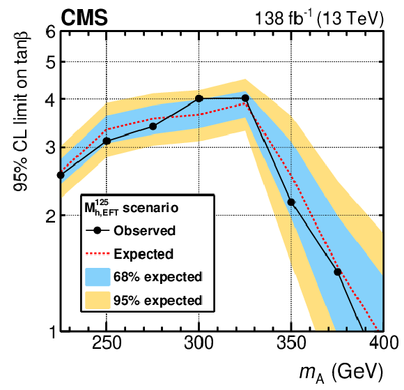
| Abstract: A search for a heavy pseudoscalar Higgs boson, A, decaying to a 125 GeV Higgs boson $ \mathrm{h} $ and a Z boson is presented. The $ \mathrm{h} $ boson is identified via its decay to a pair of tau leptons, while the Z boson is identified via its decay to a pair of electrons or muons. The search targets the production of the A boson via the gluon-gluon fusion process, $ \mathrm{g}\mathrm{g}\to\mathrm{A} $, and in association with bottom quarks, $ \mathrm{b}\overline{\mathrm{b}}\mathrm{A} $. The analysis uses a data sample corresponding to an integrated luminosity of 138 fb$ ^{-1} $ collected with the CMS detector at the CERN LHC in proton-proton collisions at a centre-of-mass energy of $ \sqrt{s} = $ 13 TeV. Constraints are set on the product of the cross sections of the A production mechanisms and the $ \mathrm{A}\to\mathrm{Z}\mathrm{h} $ decay branching fraction. The observed (expected) upper limit at 95% confidence level ranges from 0.049 (0.060) pb to 1.02 (0.79) pb for the $ \mathrm{g}\mathrm{g}\to\mathrm{A} $ process and from 0.053 (0.059) pb to 0.79 (0.61) pb for the $ \mathrm{b}\overline{\mathrm{b}}\mathrm{A} $ process in the probed range of the A boson mass, $ m_{\mathrm{A}} $, from 225 GeV to 1 TeV. The results of the search are used to constrain parameters within the $ {\text{M}_{\text{h,EFT}}^{\text{125}}} $ benchmark scenario of the minimal supersymmetric extension of the standard model. Values of $ \tan\beta $ below 2.2 are excluded in this scenario at 95% confidence level for all $ m_{\mathrm{A}} $ values in the range from 225 to 350 GeV. | ||
| Links: e-print arXiv:2501.14825 [hep-ex] (PDF) ; CDS record ; inSPIRE record ; HepData record ; CADI line (restricted) ; | ||
| Figures | |
png pdf |
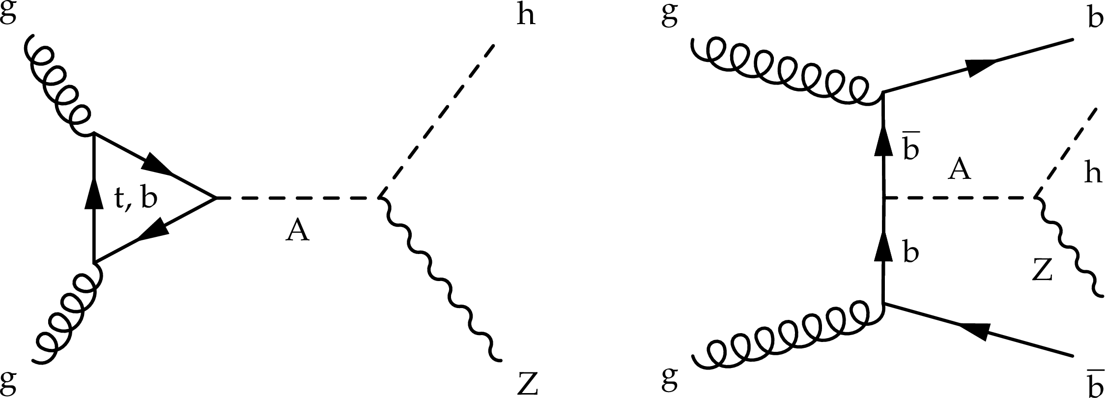
Figure 1:
Feynman diagrams representing the production of the pseudoscalar A boson via gluon-gluon $ m_{\mathrm{A}}-\tan\beta $ fusion (left) and associated production with a bottom quark-antiquark pair (right). In each case, the A boson decays to an SM-like $ \mathrm{h} $ boson and a Z boson. |
png pdf |
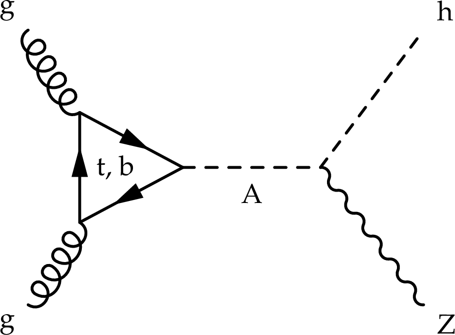
Figure 1-a:
Feynman diagrams representing the production of the pseudoscalar A boson via gluon-gluon $ m_{\mathrm{A}}-\tan\beta $ fusion (left) and associated production with a bottom quark-antiquark pair (right). In each case, the A boson decays to an SM-like $ \mathrm{h} $ boson and a Z boson. |
png pdf |
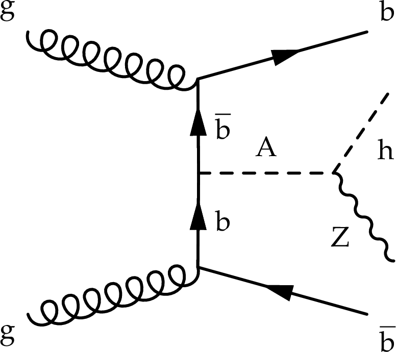
Figure 1-b:
Feynman diagrams representing the production of the pseudoscalar A boson via gluon-gluon $ m_{\mathrm{A}}-\tan\beta $ fusion (left) and associated production with a bottom quark-antiquark pair (right). In each case, the A boson decays to an SM-like $ \mathrm{h} $ boson and a Z boson. |
png pdf |
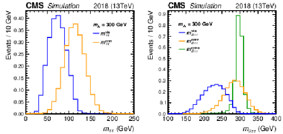
Figure 2:
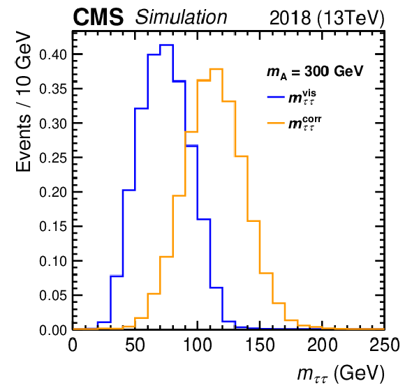
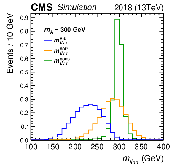
The distribution of the reconstructed mass of the $ \mathrm{h}\to\tau\tau $ candidate (left plot) and of the $ \mathrm{A}\to\mathrm{Z}\mathrm{h}\to(\ell\ell)(\tau\tau) $ candidate (right plot) in a 2018 simulated sample of $ \mathrm{g}\mathrm{g}\to\mathrm{A} $ events with $ m_{\mathrm{A}}= $ 300 GeV. Several methods of mass reconstruction are compared: 1) using only the visible decay products of $ \tau $ lepton ($ m_{\tau\tau}^{\text{vis}} $ in the left plot and $ m_{\ell\ell\tau\tau}^{\text{vis}} $ in the right plot, blue histograms), 2) using the FastMTT algorithm to correct for missing momentum carried away by neutrinos in the $ \tau $ lepton decays ($ m_{\tau\tau}^{\text{corr}} $ in the left plot and $ m_{\ell\ell\tau\tau}^{\text{corr}} $ in the right plot, orange histograms), and 3) using the FastMTT algorithm with a mass constraint of 125 GeV for the $ \mathrm{h}\to\tau\tau $ candidate ($ m_{\ell\ell\tau\tau}^{\text{cons}} $ in the right plot, green histogram). |
png pdf |
Figure 2-a:
The distribution of the reconstructed mass of the $ \mathrm{h}\to\tau\tau $ candidate (left plot) and of the $ \mathrm{A}\to\mathrm{Z}\mathrm{h}\to(\ell\ell)(\tau\tau) $ candidate (right plot) in a 2018 simulated sample of $ \mathrm{g}\mathrm{g}\to\mathrm{A} $ events with $ m_{\mathrm{A}}= $ 300 GeV. Several methods of mass reconstruction are compared: 1) using only the visible decay products of $ \tau $ lepton ($ m_{\tau\tau}^{\text{vis}} $ in the left plot and $ m_{\ell\ell\tau\tau}^{\text{vis}} $ in the right plot, blue histograms), 2) using the FastMTT algorithm to correct for missing momentum carried away by neutrinos in the $ \tau $ lepton decays ($ m_{\tau\tau}^{\text{corr}} $ in the left plot and $ m_{\ell\ell\tau\tau}^{\text{corr}} $ in the right plot, orange histograms), and 3) using the FastMTT algorithm with a mass constraint of 125 GeV for the $ \mathrm{h}\to\tau\tau $ candidate ($ m_{\ell\ell\tau\tau}^{\text{cons}} $ in the right plot, green histogram). |
png pdf |
Figure 2-b:
The distribution of the reconstructed mass of the $ \mathrm{h}\to\tau\tau $ candidate (left plot) and of the $ \mathrm{A}\to\mathrm{Z}\mathrm{h}\to(\ell\ell)(\tau\tau) $ candidate (right plot) in a 2018 simulated sample of $ \mathrm{g}\mathrm{g}\to\mathrm{A} $ events with $ m_{\mathrm{A}}= $ 300 GeV. Several methods of mass reconstruction are compared: 1) using only the visible decay products of $ \tau $ lepton ($ m_{\tau\tau}^{\text{vis}} $ in the left plot and $ m_{\ell\ell\tau\tau}^{\text{vis}} $ in the right plot, blue histograms), 2) using the FastMTT algorithm to correct for missing momentum carried away by neutrinos in the $ \tau $ lepton decays ($ m_{\tau\tau}^{\text{corr}} $ in the left plot and $ m_{\ell\ell\tau\tau}^{\text{corr}} $ in the right plot, orange histograms), and 3) using the FastMTT algorithm with a mass constraint of 125 GeV for the $ \mathrm{h}\to\tau\tau $ candidate ($ m_{\ell\ell\tau\tau}^{\text{cons}} $ in the right plot, green histogram). |
png pdf |
Figure 3:
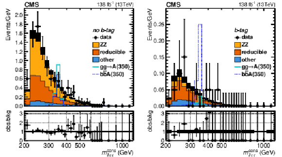
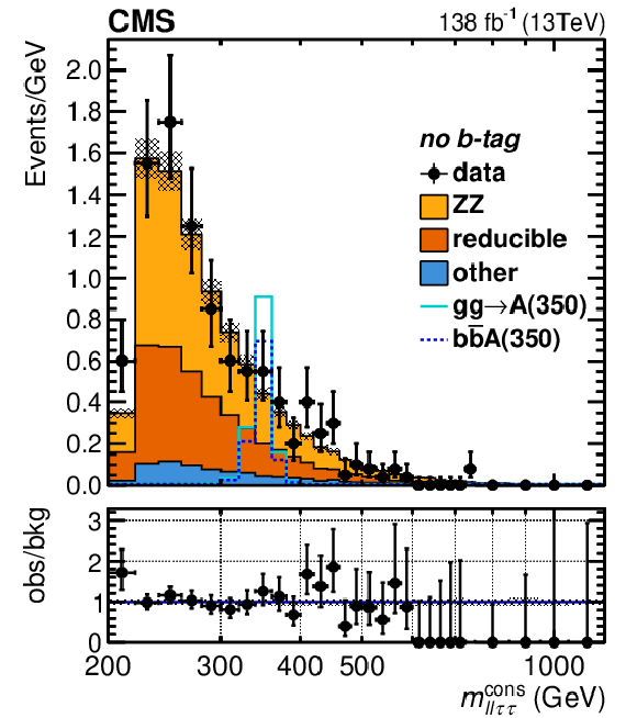
The reconstructed four-lepton mass, $ m_{\ell\ell\tau\tau}^{\text{cons}} $, in the no b-tag (left plot) and b-tag (right plot) categories. Background distributions are shown after performing a maximum likelihood fit to the data under a background-only hypothesis. Signal samples corresponding to the $ \mathrm{g}\mathrm{g}\to\mathrm{A} $ and $ \mathrm{b}\overline{\mathrm{b}}\mathrm{A} $ production modes of a pseudoscalar Higgs boson with a mass of $ m_{\mathrm{A}} = $ 350 GeV, are overlaid to illustrate the expected signal contribution. Signal yields are computed by setting $ \sigma{\mathcal{B}}(\mathrm{A}\to\mathrm{Z}\mathrm{h}) $ to a benchmark value of 1 pb for both $ \mathrm{g}\mathrm{g}\to\mathrm{A} $ and $ \mathrm{b}\overline{\mathrm{b}}\mathrm{A} $ processes. Hatched bands indicate uncertainties in the total background. Contents of each bin, along with the corresponding uncertainties, are divided by the bin width. |
png pdf |
Figure 3-a:
The reconstructed four-lepton mass, $ m_{\ell\ell\tau\tau}^{\text{cons}} $, in the no b-tag (left plot) and b-tag (right plot) categories. Background distributions are shown after performing a maximum likelihood fit to the data under a background-only hypothesis. Signal samples corresponding to the $ \mathrm{g}\mathrm{g}\to\mathrm{A} $ and $ \mathrm{b}\overline{\mathrm{b}}\mathrm{A} $ production modes of a pseudoscalar Higgs boson with a mass of $ m_{\mathrm{A}} = $ 350 GeV, are overlaid to illustrate the expected signal contribution. Signal yields are computed by setting $ \sigma{\mathcal{B}}(\mathrm{A}\to\mathrm{Z}\mathrm{h}) $ to a benchmark value of 1 pb for both $ \mathrm{g}\mathrm{g}\to\mathrm{A} $ and $ \mathrm{b}\overline{\mathrm{b}}\mathrm{A} $ processes. Hatched bands indicate uncertainties in the total background. Contents of each bin, along with the corresponding uncertainties, are divided by the bin width. |
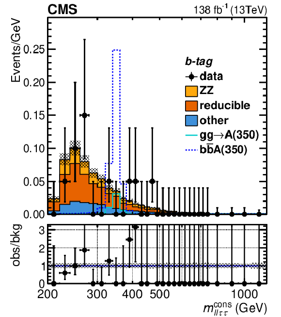
png pdf |
Figure 3-b:
The reconstructed four-lepton mass, $ m_{\ell\ell\tau\tau}^{\text{cons}} $, in the no b-tag (left plot) and b-tag (right plot) categories. Background distributions are shown after performing a maximum likelihood fit to the data under a background-only hypothesis. Signal samples corresponding to the $ \mathrm{g}\mathrm{g}\to\mathrm{A} $ and $ \mathrm{b}\overline{\mathrm{b}}\mathrm{A} $ production modes of a pseudoscalar Higgs boson with a mass of $ m_{\mathrm{A}} = $ 350 GeV, are overlaid to illustrate the expected signal contribution. Signal yields are computed by setting $ \sigma{\mathcal{B}}(\mathrm{A}\to\mathrm{Z}\mathrm{h}) $ to a benchmark value of 1 pb for both $ \mathrm{g}\mathrm{g}\to\mathrm{A} $ and $ \mathrm{b}\overline{\mathrm{b}}\mathrm{A} $ processes. Hatched bands indicate uncertainties in the total background. Contents of each bin, along with the corresponding uncertainties, are divided by the bin width. |
png pdf |
Figure 4:
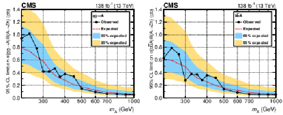
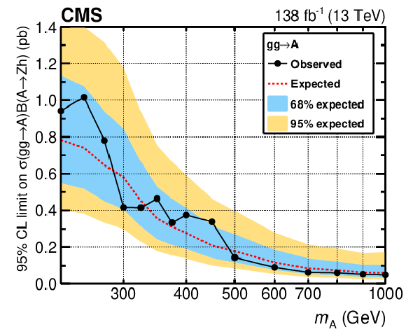
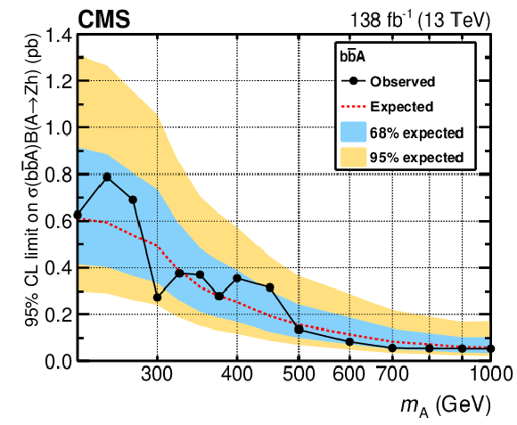
The expected and observed upper limits at 95% CL on the production cross section times branching fraction of the $ \mathrm{A}\to\mathrm{Z}\mathrm{h} $ decay for $ \mathrm{g}\mathrm{g}\to\mathrm{A} $ (left plot) and $ \mathrm{b}\overline{\mathrm{b}}\mathrm{A} $ (right plot) processes as functions of $ m_{\mathrm{A}} $. The limits for the $ \mathrm{g}\mathrm{g}\to\mathrm{A} $ ($ \mathrm{b}\overline{\mathrm{b}}\mathrm{A} $) process are derived with the rate of other process fixed to zero. The branching fraction of the $ \mathrm{h}\to\tau\tau $ decay is set to the value predicted in the SM, $ {\mathcal{B}}(\mathrm{h}\to\tau\tau)= $ 0.062 [55]. |
png pdf |
Figure 4-a:
The expected and observed upper limits at 95% CL on the production cross section times branching fraction of the $ \mathrm{A}\to\mathrm{Z}\mathrm{h} $ decay for $ \mathrm{g}\mathrm{g}\to\mathrm{A} $ (left plot) and $ \mathrm{b}\overline{\mathrm{b}}\mathrm{A} $ (right plot) processes as functions of $ m_{\mathrm{A}} $. The limits for the $ \mathrm{g}\mathrm{g}\to\mathrm{A} $ ($ \mathrm{b}\overline{\mathrm{b}}\mathrm{A} $) process are derived with the rate of other process fixed to zero. The branching fraction of the $ \mathrm{h}\to\tau\tau $ decay is set to the value predicted in the SM, $ {\mathcal{B}}(\mathrm{h}\to\tau\tau)= $ 0.062 [55]. |
png pdf |
Figure 4-b:
The expected and observed upper limits at 95% CL on the production cross section times branching fraction of the $ \mathrm{A}\to\mathrm{Z}\mathrm{h} $ decay for $ \mathrm{g}\mathrm{g}\to\mathrm{A} $ (left plot) and $ \mathrm{b}\overline{\mathrm{b}}\mathrm{A} $ (right plot) processes as functions of $ m_{\mathrm{A}} $. The limits for the $ \mathrm{g}\mathrm{g}\to\mathrm{A} $ ($ \mathrm{b}\overline{\mathrm{b}}\mathrm{A} $) process are derived with the rate of other process fixed to zero. The branching fraction of the $ \mathrm{h}\to\tau\tau $ decay is set to the value predicted in the SM, $ {\mathcal{B}}(\mathrm{h}\to\tau\tau)= $ 0.062 [55]. |
png pdf |
Figure 5:
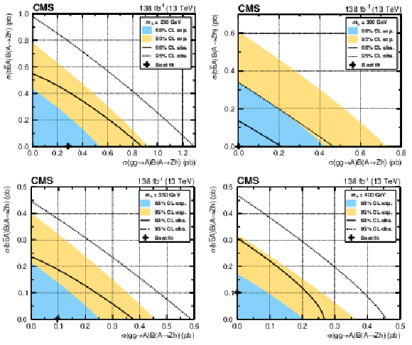
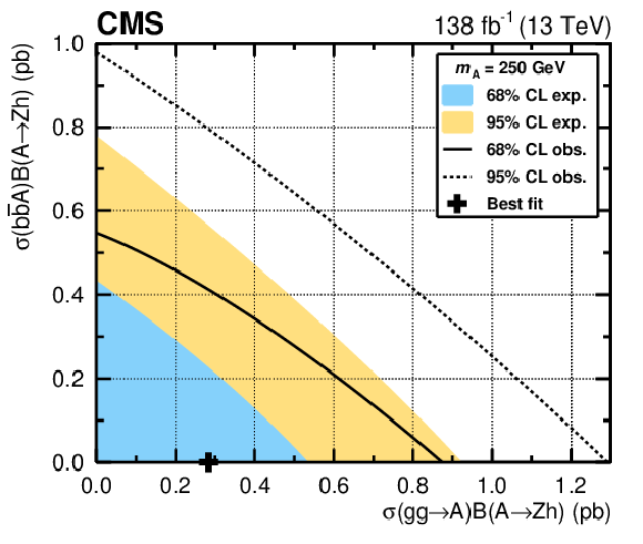
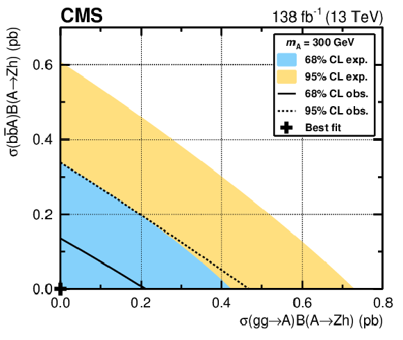
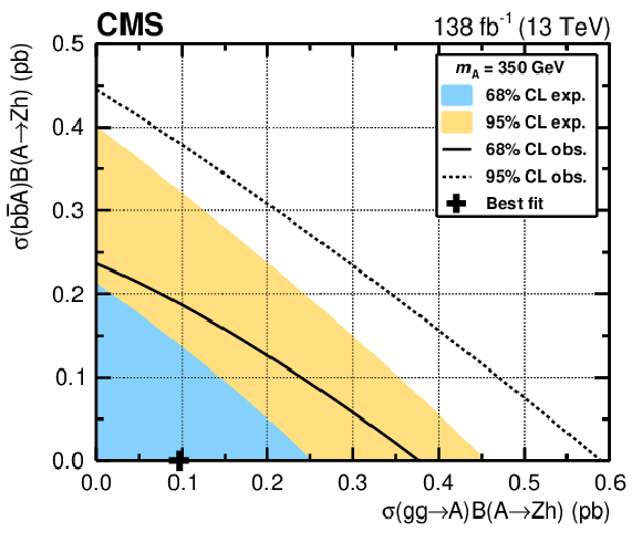
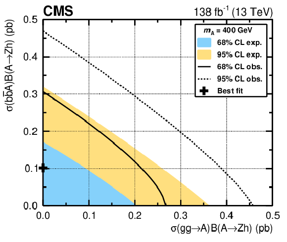
Two-dimensional constraints on the cross section times branching fraction for the two production mechanisms. The confidence level intervals are derived for mass hypotheses of $ m_\mathrm{A}= $ 250 (upper left plot), 300 (upper right plot), 350 (lower left plot), and 400 GeV (lower right plot). The branching fraction of the $ \mathrm{h}\to\tau\tau $ decay is set to the value predicted in the SM, $ {\mathcal{B}}(\mathrm{h}\to\tau\tau)= $ 0.062 [55]. Computation of the best fit point and determination of the observed and expected 68% and 95% CL contours are described in the text. |
png pdf |
Figure 5-a:
Two-dimensional constraints on the cross section times branching fraction for the two production mechanisms. The confidence level intervals are derived for mass hypotheses of $ m_\mathrm{A}= $ 250 (upper left plot), 300 (upper right plot), 350 (lower left plot), and 400 GeV (lower right plot). The branching fraction of the $ \mathrm{h}\to\tau\tau $ decay is set to the value predicted in the SM, $ {\mathcal{B}}(\mathrm{h}\to\tau\tau)= $ 0.062 [55]. Computation of the best fit point and determination of the observed and expected 68% and 95% CL contours are described in the text. |
png pdf |
Figure 5-b:
Two-dimensional constraints on the cross section times branching fraction for the two production mechanisms. The confidence level intervals are derived for mass hypotheses of $ m_\mathrm{A}= $ 250 (upper left plot), 300 (upper right plot), 350 (lower left plot), and 400 GeV (lower right plot). The branching fraction of the $ \mathrm{h}\to\tau\tau $ decay is set to the value predicted in the SM, $ {\mathcal{B}}(\mathrm{h}\to\tau\tau)= $ 0.062 [55]. Computation of the best fit point and determination of the observed and expected 68% and 95% CL contours are described in the text. |
png pdf |
Figure 5-c:
Two-dimensional constraints on the cross section times branching fraction for the two production mechanisms. The confidence level intervals are derived for mass hypotheses of $ m_\mathrm{A}= $ 250 (upper left plot), 300 (upper right plot), 350 (lower left plot), and 400 GeV (lower right plot). The branching fraction of the $ \mathrm{h}\to\tau\tau $ decay is set to the value predicted in the SM, $ {\mathcal{B}}(\mathrm{h}\to\tau\tau)= $ 0.062 [55]. Computation of the best fit point and determination of the observed and expected 68% and 95% CL contours are described in the text. |
png pdf |
Figure 5-d:
Two-dimensional constraints on the cross section times branching fraction for the two production mechanisms. The confidence level intervals are derived for mass hypotheses of $ m_\mathrm{A}= $ 250 (upper left plot), 300 (upper right plot), 350 (lower left plot), and 400 GeV (lower right plot). The branching fraction of the $ \mathrm{h}\to\tau\tau $ decay is set to the value predicted in the SM, $ {\mathcal{B}}(\mathrm{h}\to\tau\tau)= $ 0.062 [55]. Computation of the best fit point and determination of the observed and expected 68% and 95% CL contours are described in the text. |
png pdf |
Figure 6:
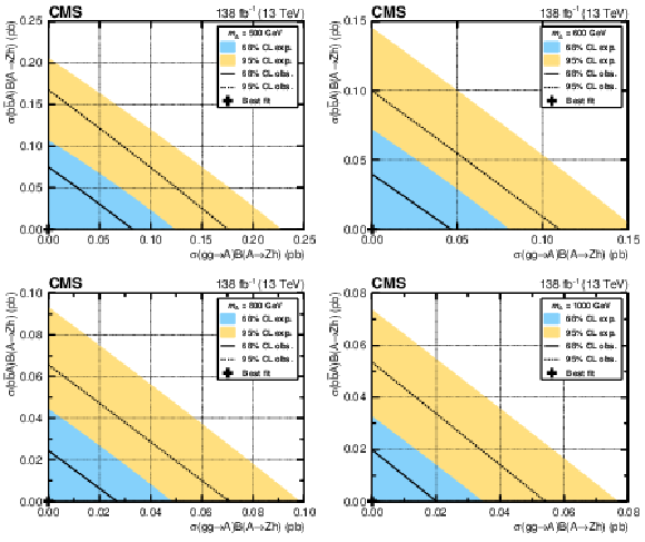
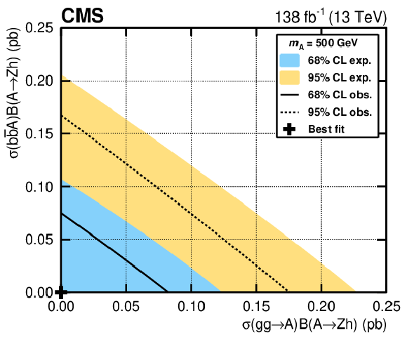
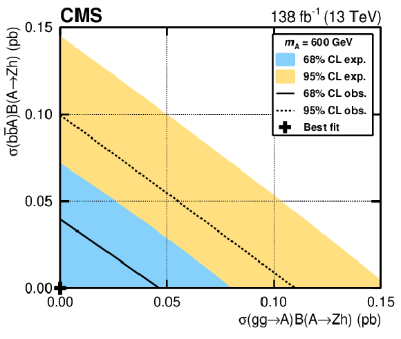
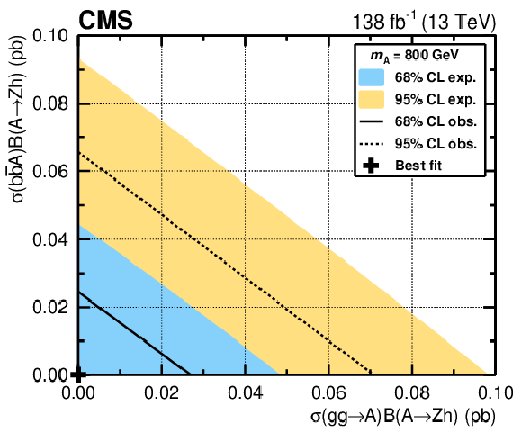
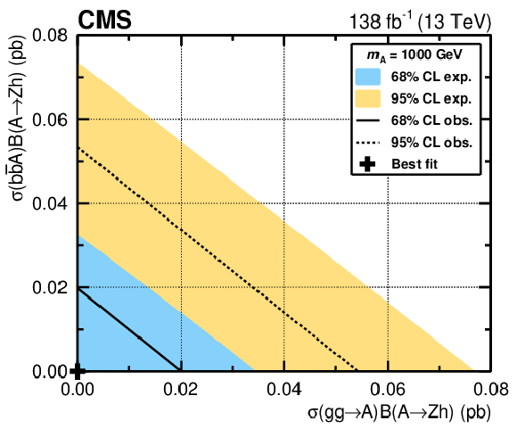
Same as Fig. 5 but for mass hypotheses of $ m_{\mathrm{A}}= $ 500 (upper left plot), 600 (upper right plot), 800 (lower left plot) and 1000 GeV (lower right plot). The branching fraction of the $ \mathrm{h}\to\tau\tau $ decay is set to the value predicted in the SM, $ {\mathcal{B}}(\mathrm{h}\to\tau\tau)= $ 0.062 [55]. Computation of the best-fit point and determination of the observed and expected 68% and 95% CL contours are described in the text. |
png pdf |
Figure 6-a:
Same as Fig. 5 but for mass hypotheses of $ m_{\mathrm{A}}= $ 500 (upper left plot), 600 (upper right plot), 800 (lower left plot) and 1000 GeV (lower right plot). The branching fraction of the $ \mathrm{h}\to\tau\tau $ decay is set to the value predicted in the SM, $ {\mathcal{B}}(\mathrm{h}\to\tau\tau)= $ 0.062 [55]. Computation of the best-fit point and determination of the observed and expected 68% and 95% CL contours are described in the text. |
png pdf |
Figure 6-b:
Same as Fig. 5 but for mass hypotheses of $ m_{\mathrm{A}}= $ 500 (upper left plot), 600 (upper right plot), 800 (lower left plot) and 1000 GeV (lower right plot). The branching fraction of the $ \mathrm{h}\to\tau\tau $ decay is set to the value predicted in the SM, $ {\mathcal{B}}(\mathrm{h}\to\tau\tau)= $ 0.062 [55]. Computation of the best-fit point and determination of the observed and expected 68% and 95% CL contours are described in the text. |
png pdf |
Figure 6-c:
Same as Fig. 5 but for mass hypotheses of $ m_{\mathrm{A}}= $ 500 (upper left plot), 600 (upper right plot), 800 (lower left plot) and 1000 GeV (lower right plot). The branching fraction of the $ \mathrm{h}\to\tau\tau $ decay is set to the value predicted in the SM, $ {\mathcal{B}}(\mathrm{h}\to\tau\tau)= $ 0.062 [55]. Computation of the best-fit point and determination of the observed and expected 68% and 95% CL contours are described in the text. |
png pdf |
Figure 6-d:
Same as Fig. 5 but for mass hypotheses of $ m_{\mathrm{A}}= $ 500 (upper left plot), 600 (upper right plot), 800 (lower left plot) and 1000 GeV (lower right plot). The branching fraction of the $ \mathrm{h}\to\tau\tau $ decay is set to the value predicted in the SM, $ {\mathcal{B}}(\mathrm{h}\to\tau\tau)= $ 0.062 [55]. Computation of the best-fit point and determination of the observed and expected 68% and 95% CL contours are described in the text. |
png pdf |
Figure 7:
Lower 95% CL limit on $ \tan\beta $ as a function of $ m_{\mathrm{A}} $ in the $ \text{M}_{\text{h,EFT}}^{\text{125}} $ MSSM scenario. Values below the black solid line are excluded at 95% CL. |
| Tables | |

png pdf |
Table 1:
Efficiencies for the identification of $ \tau_\mathrm{h} $ decays and corresponding misidentification rates (given in parentheses) for the working points of $ D_{\mathrm{e}} $, $ D_{\mu} $, and $ D_{\text{jet}} $, chosen for the $ \mathrm{h}\to\tau\tau $ selection, depending on the $ \tau\tau $ final state. The numbers are given as percentages. Efficiencies and misidentification rates are determined from dedicated studies [26]. |
png pdf |
Table 2:
Summary of Monte Carlo programs and their purposes. |
png pdf |
Table 3:
Summary of regions used in the misidentification factor method. |

png pdf |
Table 4:
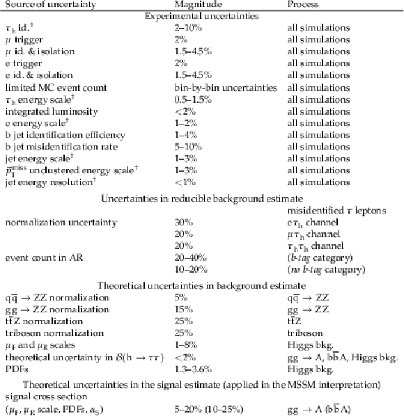
Dominant sources of systematic uncertainty are considered in this analysis. The symbol $ \dagger $ indicates uncertainties that affect both the shape and normalization of the final $ m_{\ell\ell\tau\tau}^\mathrm{cons} $ distributions. Uncertainties without $ \dagger $ affect only normalization. The magnitude column indicates an approximation of the associated change in normalization. The uncertainties in each group are listed in descending order of their impact on the analysis sensitivity. |

png pdf |
Table 5:
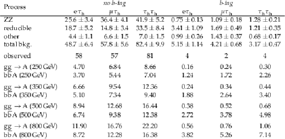
Expected and observed yields in the final selected sample. The $ \mathrm{Z}\to\mathrm{e}\mathrm{e} $ and $ \mathrm{Z}\to\mu\mu $ samples and all three data-taking periods are combined for the final results. Numbers are reported individually for no b-tag and b-tag categories and three analyzed di-$ \tau $ decay modes: $ \mathrm{e}\tau_\mathrm{h} $, $ \mu\tau_\mathrm{h} $, and $ \tau_\mathrm{h}\tau_\mathrm{h} $, combining $ \mathrm{Z}\to \mathrm{ee},\mu\mu $ channels and three data-taking years. Background yields and related uncertainties are obtained after performing a maximum likelihood fit to the data under a background-only hypothesis. Signal yields are computed for representative chosen mass hypotheses of $ m_{\mathrm{A}} = $ 250, 350, 500, and 800 GeV, by setting $ \sigma{\mathcal{B}}(\mathrm{A}\to\mathrm{Z}\mathrm{h}) $ to a benchmark value of 1 pb for both the $ \mathrm{g}\mathrm{g}\to\mathrm{A} $ and $ \mathrm{b}\overline{\mathrm{b}}\mathrm{A} $ processes. |
| Summary |
| A search is presented for the decay of a heavy pseudoscalar boson A to a Z boson and a 125 GeV Higgs boson, $ \mathrm{h} $, in final states with two $ \tau $ leptons and two light leptons ($ \mathrm{e}\mathrm{e} $, $ \mu\mu $). The study is based on proton-proton collision data collected by the CMS experiment at $ \sqrt{s}= $ 13 TeV, corresponding to an integrated luminosity of 138 fb$ ^{-1} $. The analysis probes the gluon-gluon fusion process, $ \mathrm{g}\mathrm{g}\to\mathrm{A} $, and bottom quark associated production, $ \mathrm{b}\overline{\mathrm{b}}\mathrm{A} $. No evidence for a signal is found in the data. Upper limits at 95% confidence level are derived on the product of the cross section and branching fraction of the $ \mathrm{A}\to\mathrm{Z}\mathrm{h} $ decay under the assumption that the scalar state $ \mathrm{h} $ has the properties of the 125 GeV SM Higgs boson. Observed limits range from 0.049 (0.053) pb at $ m_{\mathrm{A}}= $ 1 TeV to 1.02 (0.79) pb at $ m_{\mathrm{A}}= $ 250 GeV for the $ \mathrm{g}\mathrm{g}\to\mathrm{A} $ ($ \mathrm{b}\overline{\mathrm{b}}\mathrm{A} $) process. The results of the search are also interpreted in terms of constraints on $ \tan\beta $ as a function of $ m_{\mathrm{A}} $ within the $ \text{M}_{\text{h,EFT}}^{\text{125}} $ MSSM benchmark scenario. Values of $ \tan\beta $ below 2.2 are excluded at 95% CL in the mass range of 225 $ < m_{\mathrm{A}} < $ 350 GeV. The present analysis supersedes the previous search for the $ \mathrm{A}\to\mathrm{Z}\mathrm{h} $ decay carried out by the CMS Collaboration in the $ (\mathrm{Z}\to\nu\overline{\nu}/\ell\ell)(\mathrm{h}\to\mathrm{b}\overline{\mathrm{b}}) $ and $ (\mathrm{Z}\to\ell\ell)(\mathrm{h}\to\tau\tau) $ channels (where $ \ell=\mathrm{e},\mu $) [22,20] on proton-proton collision data collected at $ \sqrt{s}= $ 13 TeV and corresponding to an integrated luminosity of 36 fb$ ^{-1} $. |
| References | ||||
| 1 | ATLAS Collaboration | Observation of a new particle in the search for the standard model Higgs boson with the ATLAS detector at the LHC | PLB 716 (2012) 1 | 1207.7214 |
| 2 | CMS Collaboration | Observation of a new boson at a mass of 125 GeV with the CMS experiment at the LHC | PLB 716 (2012) 30 | CMS-HIG-12-028 1207.7235 |
| 3 | CMS Collaboration | Observation of a new boson with mass near 125 GeV in pp collisions at $ \sqrt{s} = $ 7 and 8 TeV | JHEP 06 (2013) 081 | CMS-HIG-12-036 1303.4571 |
| 4 | ATLAS Collaboration | A detailed map of Higgs boson interactions by the ATLAS experiment ten years after the discovery | Nature 607 (2022) 52 | 2207.00092 |
| 5 | CMS Collaboration | A portrait of the Higgs boson by the CMS experiment ten years after the discovery. | Nature 607 (2022) 60 | CMS-HIG-22-001 2207.00043 |
| 6 | ATLAS and CMS Collaborations | Measurements of the Higgs boson production and decay rates and constraints on its couplings from a combined ATLAS and CMS analysis of the LHC pp collision data at $ \sqrt{s}= $ 7 and 8 TeV | JHEP 08 (2016) 045 | 1606.02266 |
| 7 | CMS Collaboration | Combined measurements of Higgs boson couplings in proton-proton collisions at $ \sqrt{s}= $ 13 TeV | EPJC 79 (2019) 421 | CMS-HIG-17-031 1809.10733 |
| 8 | ATLAS Collaboration | Combined measurements of Higgs boson production and decay using up to 80 fb$ ^{-1} $ of proton-proton collision data at $ \sqrt{s}= $ 13 TeV collected with the ATLAS experiment | PRD 101 (2020) 012002 | 1909.02845 |
| 9 | CMS Collaboration | Measurements of the Higgs boson width and anomalous $ \mathrm{H}\mathrm{V}\mathrm{V} $ couplings from on-shell and off-shell production in the four-lepton final state | PRD 99 (2019) 112003 | CMS-HIG-18-002 1901.00174 |
| 10 | CMS Collaboration | A measurement of the Higgs boson mass in the diphoton decay channel | PLB 805 (2020) 135425 | CMS-HIG-19-004 2002.06398 |
| 11 | T. D. Lee | A theory of spontaneous T violation | PRD 8 (1973) 1226 | |
| 12 | G. C. Branco et al. | Theory and phenomenology of two-Higgs-doublet models | Phys. Rept. 516 (2012) 1 | 1106.0034 |
| 13 | L. Fromme, S. J. Huber, and M. Seniuch | Baryogenesis in the two-Higgs doublet model | JHEP 11 (2006) 038 | hep-ph/0605242 |
| 14 | P. Fayet | Supergauge invariant extension of the Higgs mechanism and a model for the electron and its neutrino | NPB 90 (1975) 104 | |
| 15 | P. Fayet | Spontaneously broken supersymmetric theories of weak, electromagnetic and strong interactions | PLB 69 (1977) 489 | |
| 16 | H. E. Haber and G. L. Kane | The search for Supersymmetry: probing physics beyond the Standard Model | Phys. Rept. 117 (1985) 75 | |
| 17 | H. Bahl, S. Liebler, and T. Stefaniak | MSSM Higgs benchmark scenarios for Run 2 and beyond: the low $ \tan\beta $ region | EPJC 79 (2019) 279 | 1901.05933 |
| 18 | ATLAS Collaboration | Search for a CP-odd Higgs boson decaying to Zh in pp collisions at $ \sqrt{s} = $ 8 TeV with the ATLAS detector | PLB 744 (2015) 163 | 1502.04478 |
| 19 | CMS Collaboration | Searches for a heavy scalar boson H decaying to a pair of 125 GeV Higgs bosons hh or for a heavy pseudoscalar boson A decaying to Zh, in the final states with $ h \to \tau \tau $ | PLB 755 (2016) 217 | CMS-HIG-14-034 1510.01181 |
| 20 | CMS Collaboration | Search for a heavy pseudoscalar Higgs boson decaying into a 125 GeV Higgs boson and a Z boson in final states with two tau and two light leptons at $ \sqrt{s}= $ 13 TeV | JHEP 03 (2020) 065 | CMS-HIG-18-023 1910.11634 |
| 21 | ATLAS Collaboration | Search for heavy resonances decaying into a $ W $ or $ Z $ boson and a Higgs boson in final states with leptons and $ b $-jets in 36 fb$ ^{-1} $ of $ \sqrt s = $ 13 TeV $ pp $ collisions with the ATLAS detector | JHEP 03 (2018) 174 | 1712.06518 |
| 22 | CMS Collaboration | Search for a heavy pseudoscalar boson decaying to a Z and a Higgs boson at $ \sqrt{s} = $ 13 TeV | EPJC 79 (2019) 564 | CMS-HIG-18-005 1903.00941 |
| 23 | ATLAS Collaboration | Search for heavy resonances decaying into a $ Z $ or $ W $ boson and a Higgs boson in final states with leptons and $ b $-jets in 139 $ $fb$ ^{-1} $ of $ pp $ collisions at $ \sqrt{s}=13 $TeV with the ATLAS detector | JHEP 06 (2023) 016 | 2207.00230 |
| 24 | L. Bianchini et al. | Reconstruction of the Higgs mass in events with Higgs bosons decaying into a pair of $ \tau $ leptons using matrix element techniques | NIM A 862 (2017) 54 | 1603.05910 |
| 25 | W. Matyszkiewicz and A. Kalinowski | Tau-pair invariant mass estimation using maximum likelihood estimation and collinear approximation | Acta Phys. Polon. Supp. 18 (2025) 5--A21 | |
| 26 | CMS Collaboration | Identification of hadronic tau lepton decays using a deep neural network | JINST 17 (2022) P07023 | CMS-TAU-20-001 2201.08458 |
| 27 | E. Bols et al. | Jet flavour classification using DeepJet | JINST 15 (2020) P12012 | 2008.10519 |
| 28 | CMS Collaboration | HEPData record for this analysis | link | |
| 29 | CMS Collaboration | Performance of the CMS Level-1 trigger in proton-proton collisions at $ \sqrt{s} = $ 13 TeV | JINST 15 (2020) P10017 | CMS-TRG-17-001 2006.10165 |
| 30 | CMS Collaboration | The CMS trigger system | JINST 12 (2017) P01020 | CMS-TRG-12-001 1609.02366 |
| 31 | CMS Collaboration | The CMS experiment at the CERN LHC | JINST 3 (2008) S08004 | |
| 32 | CMS Collaboration | Particle-flow reconstruction and global event description with the CMS detector | JINST 12 (2017) P10003 | CMS-PRF-14-001 1706.04965 |
| 33 | CMS Collaboration | Technical proposal for the Phase-II upgrade of the Compact Muon Solenoid | CMS Technical Proposal CERN-LHCC-2015-010, CMS-TDR-15-02, 2015 CDS |
|
| 34 | CMS Collaboration | Electron and photon reconstruction and identification with the CMS experiment at the CERN LHC | JINST 16 (2021) P05014 | CMS-EGM-17-001 2012.06888 |
| 35 | CMS Collaboration | Performance of the CMS muon detector and muon reconstruction with proton-proton collisions at $ \sqrt{s}= $ 13 TeV | JINST 13 (2018) P06015 | CMS-MUO-16-001 1804.04528 |
| 36 | M. Cacciari, G. P. Salam, and G. Soyez | The anti-$ k_{\mathrm{T}} $ jet clustering algorithm | JHEP 04 (2008) 063 | 0802.1189 |
| 37 | M. Cacciari, G. P. Salam, and G. Soyez | FastJet user manual | EPJC 72 (2012) 1896 | 1111.6097 |
| 38 | CMS Collaboration | Jet energy scale and resolution in the CMS experiment in pp collisions at 8 TeV | JINST 12 (2017) P02014 | CMS-JME-13-004 1607.03663 |
| 39 | CMS Collaboration | Identification of heavy-flavour jets with the CMS detector in pp collisions at 13 TeV | JINST 13 (2018) P05011 | CMS-BTV-16-002 1712.07158 |
| 40 | CMS Collaboration | Performance of the DeepJet b tagging algorithm using 41.9 $ \mathrm{fb^{-1}} $ of data from proton-proton collisions at 13 TeV with Phase 1 CMS detector | CMS Detector Performance Summary CMS-DP-2020-021, 2018 CDS |
|
| 41 | CMS Collaboration | Performance of reconstruction and identification of $ \tau $ leptons decaying to hadrons and $ \nu_\tau $ in pp collisions at $ \sqrt{s}= $ 13 TeV | JINST 13 (2018) P10005 | CMS-TAU-16-003 1809.02816 |
| 42 | CMS Collaboration | Performance of missing transverse momentum reconstruction in proton-proton collisions at $ \sqrt{s} = $ 13 TeV using the CMS detector | JINST 14 (2019) P07004 | CMS-JME-17-001 1903.06078 |
| 43 | J. Alwall et al. | The automated computation of tree-level and next-to-leading order differential cross sections, and their matching to parton shower simulations | JHEP 07 (2014) 079 | 1405.0301 |
| 44 | P. Artoisenet, R. Frederix, O. Mattelaer, and R. Rietkerk | Automatic spin-entangled decays of heavy resonances in Monte Carlo simulations | JHEP 03 (2013) 015 | 1212.3460 |
| 45 | J. Alwall et al. | Comparative study of various algorithms for the merging of parton showers and matrix elements in hadronic collisions | EPJC 53 (2008) 473 | 0706.2569 |
| 46 | S. P. Martin | A Supersymmetry primer | Adv. Ser. Direct. HEP 21 (2010) 1 | hep-ph/9709356 |
| 47 | P. Nason | A new method for combining NLO QCD with shower Monte Carlo algorithms | JHEP 11 (2004) 040 | hep-ph/0409146 |
| 48 | S. Frixione, P. Nason, and C. Oleari | Matching NLO QCD computations with parton shower simulations: the POWHEG method | JHEP 11 (2007) 070 | 0709.2092 |
| 49 | S. Alioli, P. Nason, C. Oleari, and E. Re | A general framework for implementing NLO calculations in shower Monte Carlo programs: the POWHEG BOX | JHEP 06 (2010) 043 | 1002.2581 |
| 50 | G. Luisoni, P. Nason, C. Oleari, and F. Tramontano | $ \text{HW}^{\pm} $/HZ + 0 and 1 jet at NLO with the POWHEG BOX interfaced to GoSam and their merging within MiNLO | JHEP 10 (2013) 083 | 1306.2542 |
| 51 | F. Granata, J. M. Lindert, C. Oleari, and S. Pozzorini | NLO QCD+EW predictions for HV and HV+jet production including parton-shower effects | JHEP 09 (2017) 012 | 1706.03522 |
| 52 | H. B. Hartanto, B. Jager, L. Reina, and D. Wackeroth | Higgs boson production in association with top quarks in the POWHEG BOX | PRD 91 (2015) 094003 | 1501.04498 |
| 53 | S. Bolognesi et al. | On the spin and parity of a single-produced resonance at the LHC | PRD 86 (2012) 095031 | 1208.4018 |
| 54 | LHC Higgs Cross Section Working Group | Handbook of LHC Higgs cross sections: 4. Deciphering the nature of the Higgs sector | CERN Report CERN-2017-002-M, 2016 link |
1610.07922 |
| 55 | J. M. Campbell, R. K. Ellis, and C. Williams | Vector boson pair production at the LHC | JHEP 07 (2011) 018 | 1105.0020 |
| 56 | P. Nason and G. Zanderighi | $ W^+ W^- $, $ W Z $ and $ Z Z $ production in the POWHEG-BOX-V2 | EPJC 74 (2014) 2702 | 1311.1365 |
| 57 | R. Frederix and S. Frixione | Merging meets matching in MC@NLO | JHEP 12 (2012) 061 | 1209.6215 |
| 58 | S. Alioli, S.-O. Moch, and P. Uwer | Hadronic top-quark pair-production with one jet and parton showering | JHEP 01 (2012) 137 | 1110.5251 |
| 59 | F. Caola et al. | QCD corrections to vector boson pair production in gluon fusion including interference effects with off-shell Higgs at the LHC | JHEP 07 (2016) 087 | 1605.04610 |
| 60 | T. Gehrmann et al. | $ W^+ W^- $ production at hadron colliders in next to next to leading order QCD | PRL 113 (2014) 212001 | 1408.5243 |
| 61 | K. Melnikov and F. Petriello | Electroweak gauge boson production at hadron colliders through $ \mathcal{O}(\alpha_\text{s}^{2}) $ | PRD 74 (2006) 114017 | hep-ph/0609070 |
| 62 | M. Czakon and A. Mitov | Top++: A program for the calculation of the top-pair cross-section at hadron colliders | Comput. Phys. Commun. 185 (2014) 2930 | 1112.5675 |
| 63 | J. M. Campbell and R. K. Ellis | $ t\bar{t} W^{\pm} $ production and decay at NLO | JHEP 07 (2012) 052 | 1204.5678 |
| 64 | M. V. Garzelli, A. Kardos, C. G. Papadopoulos, and Z. Trocsanyi | $ t\bar{t} W^{\pm} $ and $ t\bar{t} Z $ hadroproduction at NLO accuracy in QCD with parton shower and hadronization effects | JHEP 11 (2012) 056 | 1208.2665 |
| 65 | NNPDF Collaboration | Parton distributions from high-precision collider data | EPJC 77 (2017) 663 | 1706.00428 |
| 66 | T. Sjöstrand et al. | An introduction to PYTHIA 8.2 | Comput. Phys. Commun. 191 (2015) 159 | 1410.3012 |
| 67 | CMS Collaboration | Extraction and validation of a new set of CMS PYTHIA8 tunes from underlying-event measurements | EPJC 80 (2020) 4 | CMS-GEN-17-001 1903.12179 |
| 68 | GEANT4 Collaboration | GEANT 4---a simulation toolkit | NIM A 506 (2003) 250 | |
| 69 | R. D. Cousins | Lectures on statistics in theory: Prelude to statistics in practice | link | 1807.05996 |
| 70 | CMS Collaboration | The CMS statistical analysis and combination tool: \textscCombine | Comput. Softw. Big Sci. 8 (2024) 19 | CMS-CAT-23-001 2404.06614 |
| 71 | J. Butterworth et al. | PDF4LHC recommendations for LHC Run II | JPG 43 (2016) 023001 | 1510.03865 |
| 72 | CMS Collaboration | Measurement of the cross section for top quark pair production in association with a W or Z boson in proton-proton collisions at $ \sqrt{s} = $ 13 TeV | JHEP 08 (2018) 011 | CMS-TOP-17-005 1711.02547 |
| 73 | E. A. Bagnaschi et al. | Benchmark scenarios for MSSM Higgs boson searches at the LHC | CERN Report LHCHWG-2021-001, 2021 | |
| 74 | CMS Collaboration | Precision luminosity measurement in proton-proton collisions at $ \sqrt{s} = $ 13 TeV in 2015 and 2016 at CMS | EPJC 81 (2021) 800 | CMS-LUM-17-003 2104.01927 |
| 75 | CMS Collaboration | CMS luminosity measurement for the 2017 data-taking period at $ \sqrt{s} $ = 13 TeV | CMS Physics Analysis Summary, 2018 link |
CMS-PAS-LUM-17-004 |
| 76 | CMS Collaboration | CMS luminosity measurement for the 2018 data-taking period at $ \sqrt{s} $ = 13 TeV | CMS Physics Analysis Summary, 2019 link |
CMS-PAS-LUM-18-002 |
| 77 | R. J. Barlow and C. Beeston | Fitting using finite Monte Carlo samples | Comput. Phys. Commun. 77 (1993) 219 | |
| 78 | J. S. Conway | Incorporating nuisance parameters in likelihoods for multisource spectra | in, 2011 PHYSTAT 201 (2011) 115 |
1103.0354 |
| 79 | W. Verkerke and D. P. Kirkby | The RooFit toolkit for data modeling | in Statistical Problems in Particle Physics, Astrophysics and Cosmology, L. Lyons and M. Karagoz, eds., p.~MOLT007. . . eConf C0303241, 2003 Proc. PHYSTAT 200 (2003) 3 |
physics/0306116 |
| 80 | L. Moneta et al. | The RooStats project | in Proc. ACAT 2010, 13th International Workshop on Advanced Computing and Analysis Techniques in Physics Research Proc. ACAT 201 (2010) 057 |
1009.1003 |
| 81 | CMS Collaboration | Combined results of searches for the standard model Higgs boson in $ pp $ collisions at $ \sqrt{s}= $ 7 TeV | PLB 710 (2012) 26 | CMS-HIG-11-032 1202.1488 |
| 82 | T. Junk | Confidence level computation for combining searches with small statistics | NIM A 434 (1999) 435 | hep-ex/9902006 |
| 83 | A. L. Read | Presentation of search results: The $ CL_s $ technique | JPG 28 (2002) 2693 | |
| 84 | S. Heinemeyer, W. Hollik, and G. Weiglein | FeynHiggs: A program for the calculation of the masses of the neutral CP-even Higgs bosons in the MSSM | Comput. Phys. Commun. 124 (2000) 76 | hep-ph/9812320 |
| 85 | S. Heinemeyer, W. Hollik, and G. Weiglein | The masses of the neutral CP-even Higgs bosons in the MSSM: Accurate analysis at the two-loop level | EPJC 9 (1999) 343 | hep-ph/9812472 |
| 86 | G. Degrassi et al. | Towards high-precision predictions for the MSSM Higgs sector | EPJC 28 (2003) 133 | hep-ph/0212020 |
| 87 | M. Frank et al. | The Higgs boson masses and mixings of the complex MSSM in the Feynman-diagrammatic approach | JHEP 02 (2007) 047 | hep-ph/0611326 |
| 88 | T. Hahn et al. | High-precision predictions for the light CP-even Higgs boson mass of the minimal supersymmetric standard model | PRL 112 (2014) 141801 | 1312.4937 |
| 89 | H. Bahl and W. Hollik | Precise prediction for the light MSSM Higgs boson mass combining effective field theory and fixed-order calculations | EPJC 76 (2016) 499 | 1608.01880 |
| 90 | H. Bahl, S. Heinemeyer, W. Hollik, and G. Weiglein | Reconciling EFT and hybrid calculations of the light MSSM Higgs-boson mass | EPJC 78 (2018) 57 | 1706.00346 |
| 91 | H. Bahl et al. | Precision calculations in the MSSM Higgs-boson sector with FeynHiggs 2.14 | Comput. Phys. Commun. 249 (2020) 107099 | 1811.09073 |
| 92 | A. Djouadi, J. Kalinowski, M. Muehlleitner, and M. Spira | HDECAY: Twenty$ {++} $ years after | Comput. Phys. Commun. 238 (2019) 214 | 1801.09506 |
| 93 | LHC Higgs Cross Section Working Group | Handbook of LHC Higgs cross sections: 3. Higgs properties | CERN Report CERN-2013-004, 2013 link |
1307.1347 |
| 94 | A. Denner et al. | Standard model Higgs-boson branching ratios with uncertainties | EPJC 71 (2011) 1753 | 1107.5909 |
| 95 | R. V. Harlander, S. Liebler, and H. Mantler | SusHi: A program for the calculation of Higgs production in gluon fusion and bottom-quark annihilation in the standard model and the MSSM | Comput. Phys. Commun. 184 (2013) 1605 | 1212.3249 |
| 96 | R. V. Harlander, S. Liebler, and H. Mantler | SusHi Bento: Beyond NNLO and the heavy-top limit | Comput. Phys. Commun. 212 (2017) 239 | 1605.03190 |
| 97 | M. Spira, A. Djouadi, D. Graudenz, and P. M. Zerwas | Higgs boson production at the LHC | NPB 453 (1995) 17 | hep-ph/9504378 |
| 98 | R. Harlander and P. Kant | Higgs production and decay: analytic results at next-to-leading order QCD | JHEP 12 (2005) 015 | hep-ph/0509189 |
| 99 | R. V. Harlander and W. B. Kilgore | Next-to-next-to-leading order Higgs production at hadron colliders | PRL 88 (2002) 201801 | hep-ph/0201206 |
| 100 | C. Anastasiou and K. Melnikov | Higgs boson production at hadron colliders in NNLO QCD | NPB 646 (2002) 220 | hep-ph/0207004 |
| 101 | V. Ravindran, J. Smith, and W. L. van Neerven | NNLO corrections to the total cross-section for Higgs boson production in hadron-hadron collisions | NPB 665 (2003) 325 | hep-ph/0302135 |
| 102 | R. V. Harlander and W. B. Kilgore | Production of a pseudo-scalar Higgs boson at hadron colliders at next-to-next-to leading order | JHEP 10 (2002) 017 | hep-ph/0208096 |
| 103 | C. Anastasiou and K. Melnikov | Pseudoscalar Higgs boson production at hadron colliders in next-to-next-to-leading order QCD | PRD 67 (2003) 037501 | hep-ph/0208115 |
| 104 | C. Anastasiou et al. | Higgs boson gluon-fusion production beyond threshold in N$ ^{3} $LO QCD | JHEP 03 (2015) 091 | 1411.3584 |
| 105 | C. Anastasiou et al. | Soft expansion of double-real-virtual corrections to Higgs production at N$ ^{3} $LO | JHEP 08 (2015) 051 | 1505.04110 |
| 106 | C. Anastasiou et al. | High precision determination of the gluon fusion Higgs boson cross-section at the LHC | JHEP 05 (2016) 058 | 1602.00695 |
| 107 | U. Aglietti, R. Bonciani, G. Degrassi, and A. Vicini | Two-loop light fermion contribution to Higgs production and decays | PLB 595 (2004) 432 | hep-ph/0404071 |
| 108 | R. Bonciani, G. Degrassi, and A. Vicini | On the generalized harmonic polylogarithms of one complex variable | Comput. Phys. Commun. 182 (2011) 1253 | 1007.1891 |
| 109 | M. Bonvini, A. S. Papanastasiou, and F. J. Tackmann | Resummation and matching of b-quark mass effects in $ \mathrm{b}\overline{\mathrm{b}}\mathrm{H} $ production | JHEP 11 (2015) 196 | 1508.03288 |
| 110 | M. Bonvini, A. S. Papanastasiou, and F. J. Tackmann | Matched predictions for the $ \mathrm{b}\overline{\mathrm{b}}\mathrm{H} $ cross section at the 13 TeV LHC | JHEP 10 (2016) 053 | 1605.01733 |
| 111 | S. Forte, D. Napoletano, and M. Ubiali | Higgs production in bottom-quark fusion in a matched scheme | PLB 751 (2015) 331 | 1508.01529 |
| 112 | S. Forte, D. Napoletano, and M. Ubiali | Higgs production in bottom-quark fusion: matching beyond leading order | PLB 763 (2016) 190 | 1607.00389 |
| 113 | R. V. Harlander and W. B. Kilgore | Higgs boson production in bottom quark fusion at next-to-next-to leading order | PRD 68 (2003) 013001 | hep-ph/0304035 |
| 114 | S. Dittmaier, M. Kr ä mer, and M. Spira | Higgs radiation off bottom quarks at the Fermilab Tevatron and the CERN LHC | PRD 70 (2004) 074010 | hep-ph/0309204 |
| 115 | S. Dawson, C. B. Jackson, L. Reina, and D. Wackeroth | Exclusive Higgs boson production with bottom quarks at hadron colliders | PRD 69 (2004) 074027 | hep-ph/0311067 |

|
Compact Muon Solenoid LHC, CERN |

|

|

|

|

|

|