

Compact Muon Solenoid
LHC, CERN
| CMS-PAS-TOP-25-002 | ||
| Observation of a pseudoscalar excess at the top quark pair production threshold in the single lepton channel | ||
| CMS Collaboration | ||
| 2026-03-22 | ||
| Abstract: A search is presented for top quark-antiquark ($ \mathrm{t\bar{t}} $) bound states near the $ \mathrm{t\bar{t}} $ production threshold, in final states with a single electron or muon and jets. The study uses proton-proton collision data at $ \sqrt{s} = $ 13 TeV, collected by the CMS experiment at the CERN LHC, corresponding to an integrated luminosity of 138 fb$ ^{-1} $. The analysis examines the relative velocity between the top quark and antiquark, along with two angular observables sensitive to the parity and spin of the $ \mathrm{t\bar{t}} $ system. A significant excess of events is observed relative to the standard model prediction for $ \mathrm{t\bar{t}} $ production calculated at next-to-next-to-leading order in perturbative quantum chromodynamics. The excess corresponds to an observed cross section of 5.1 $ \pm $ 0.9 $ \mathrm{pb} $ and is consistent with a simplified model of a color-singlet pseudoscalar toponium motivated by nonrelativistic quantum chromodynamics. The result provides an independent confirmation of the excess reported in the dilepton channel. | ||
| Links: CDS record (PDF) ; Physics Briefing ; CADI line (restricted) ; | ||
| Figures | |
png pdf |
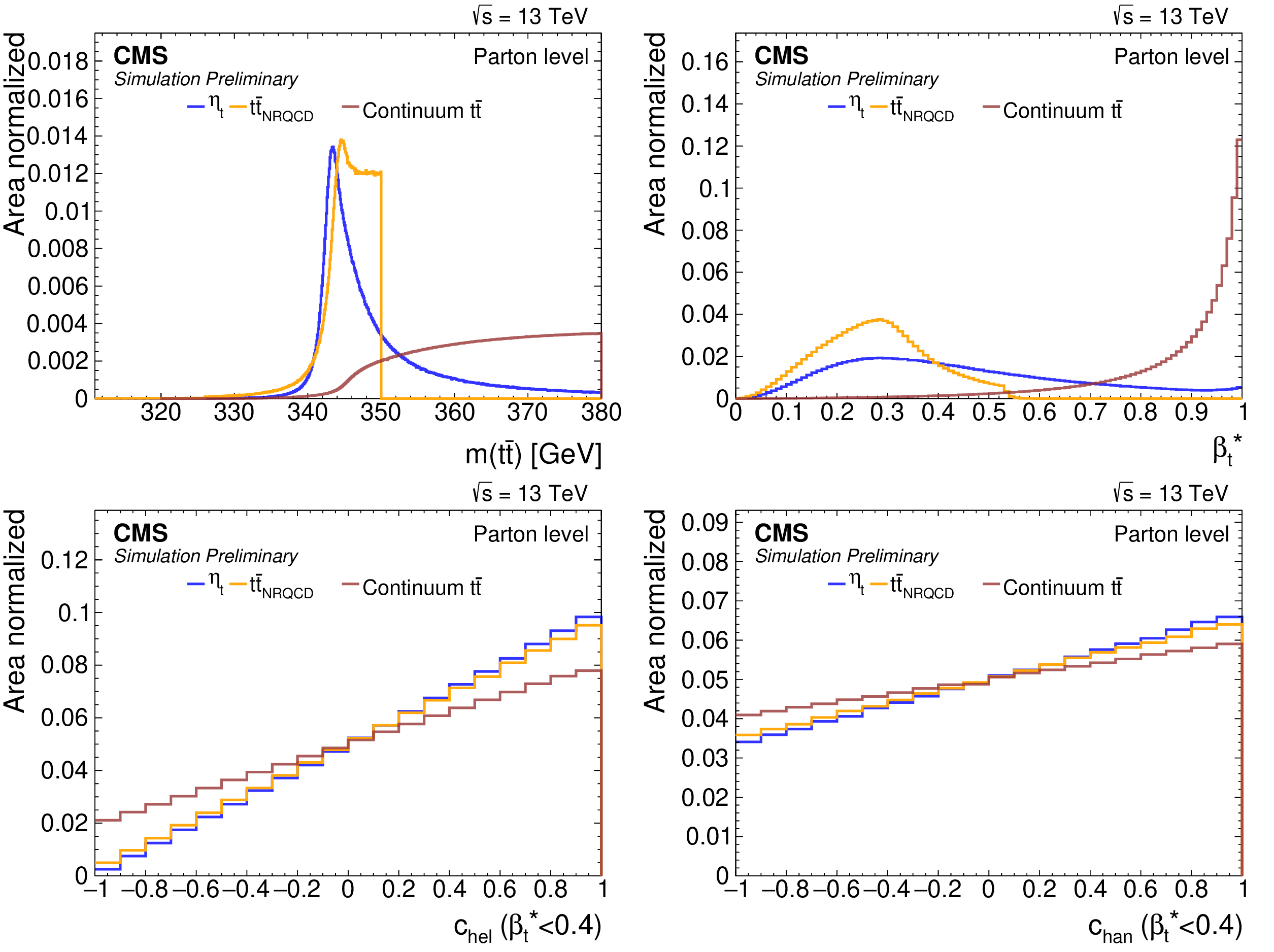
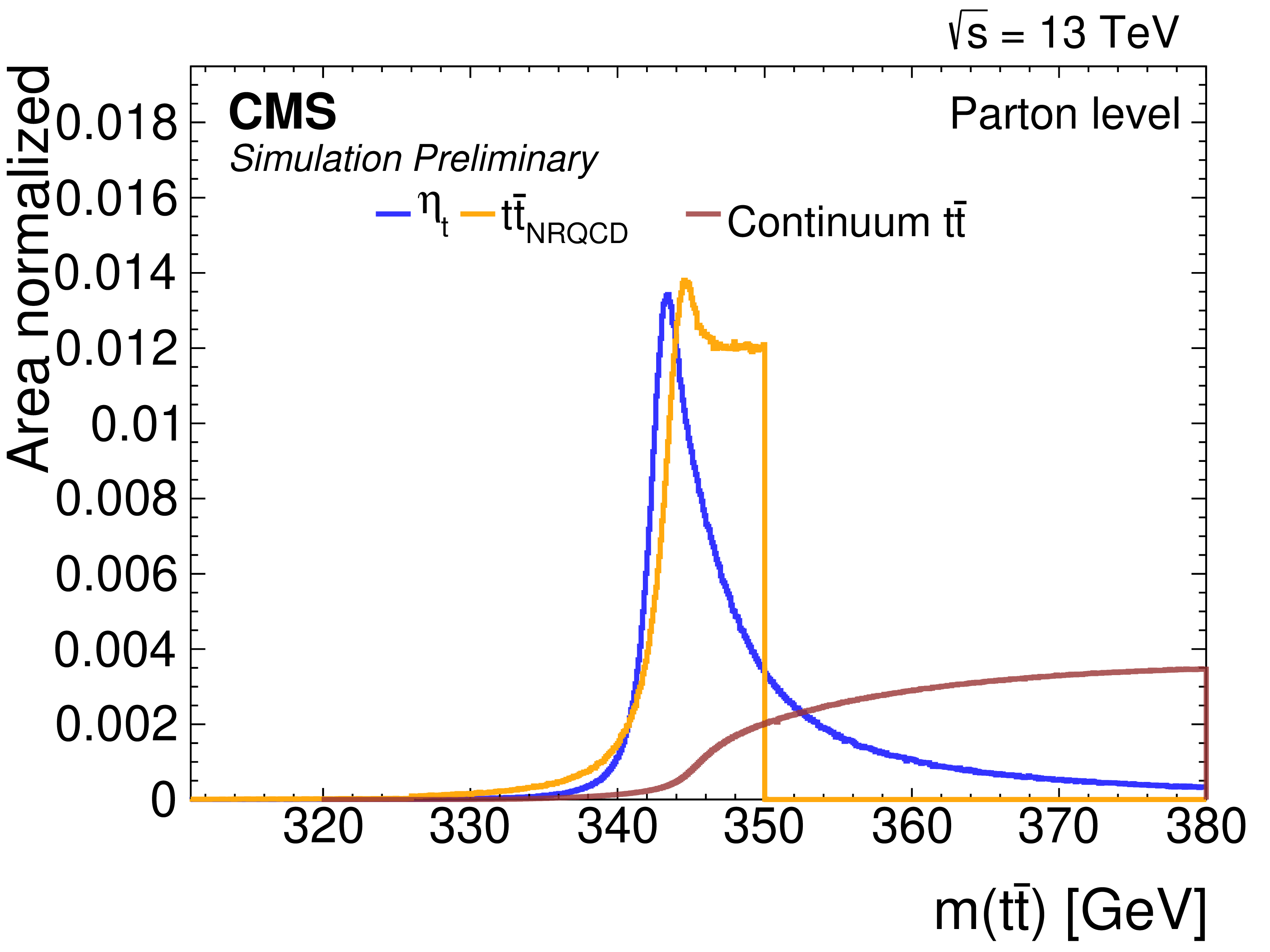
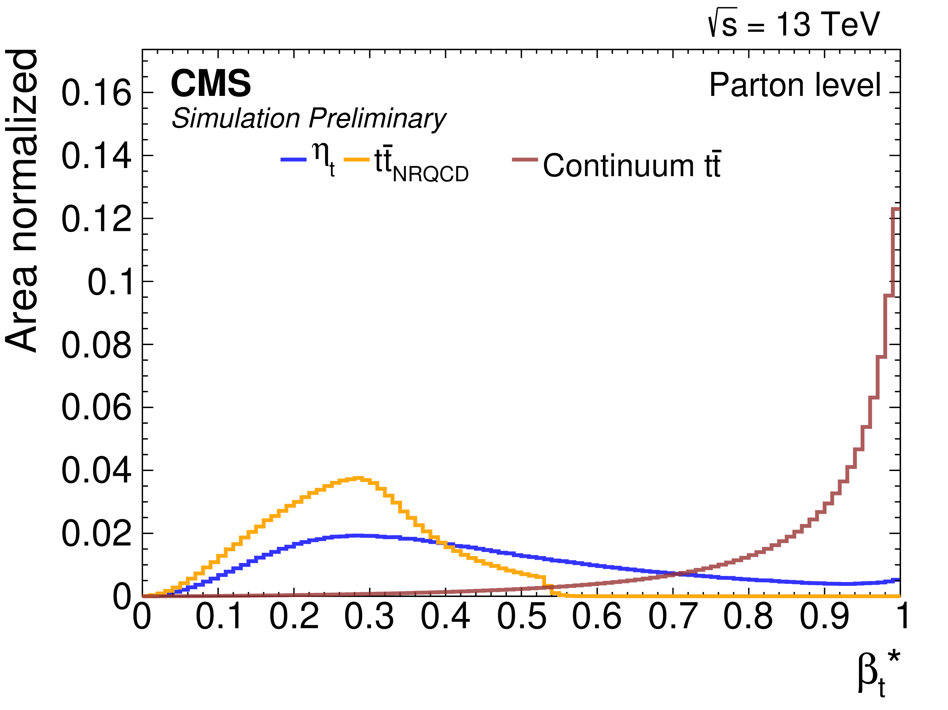
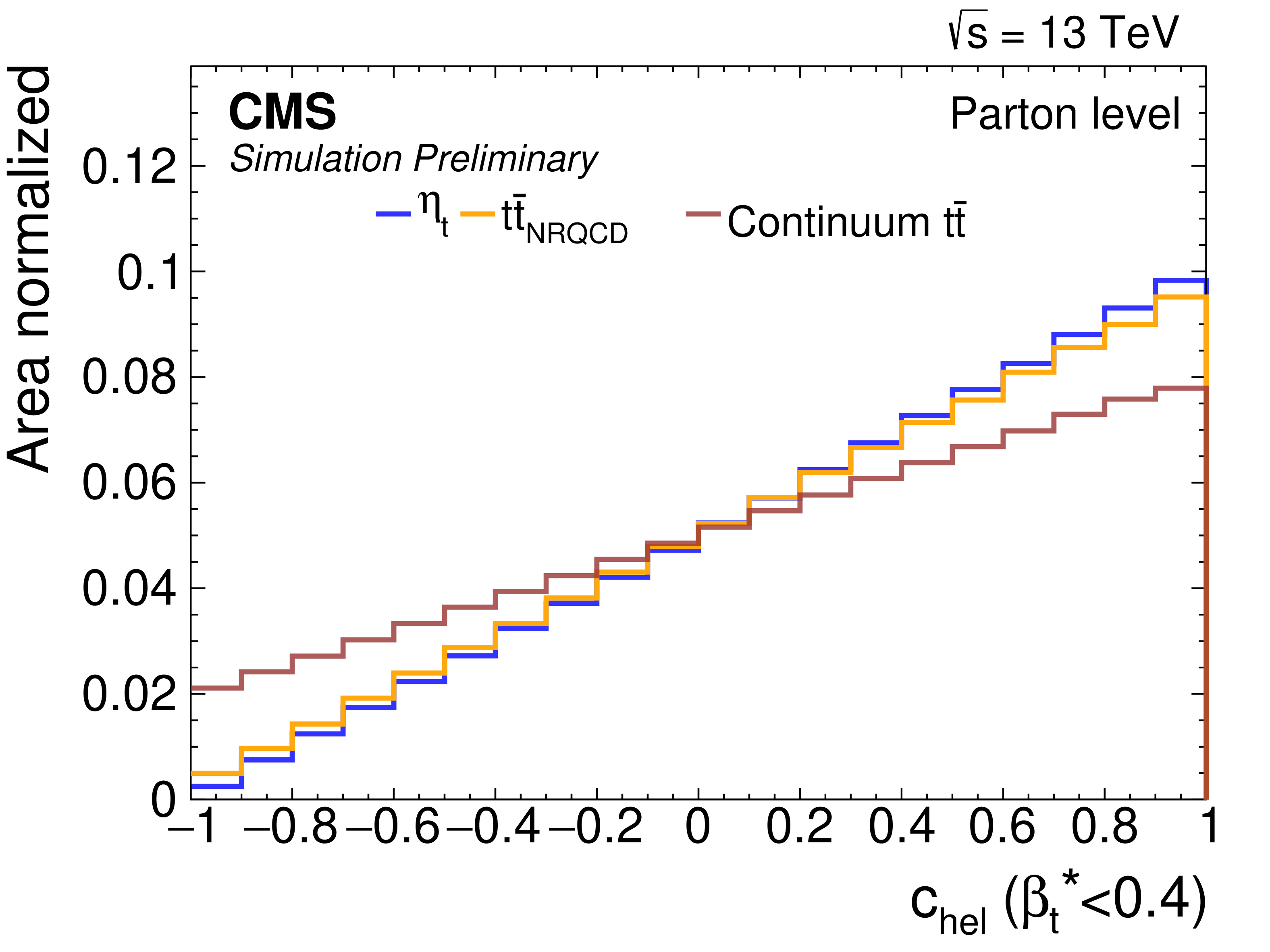
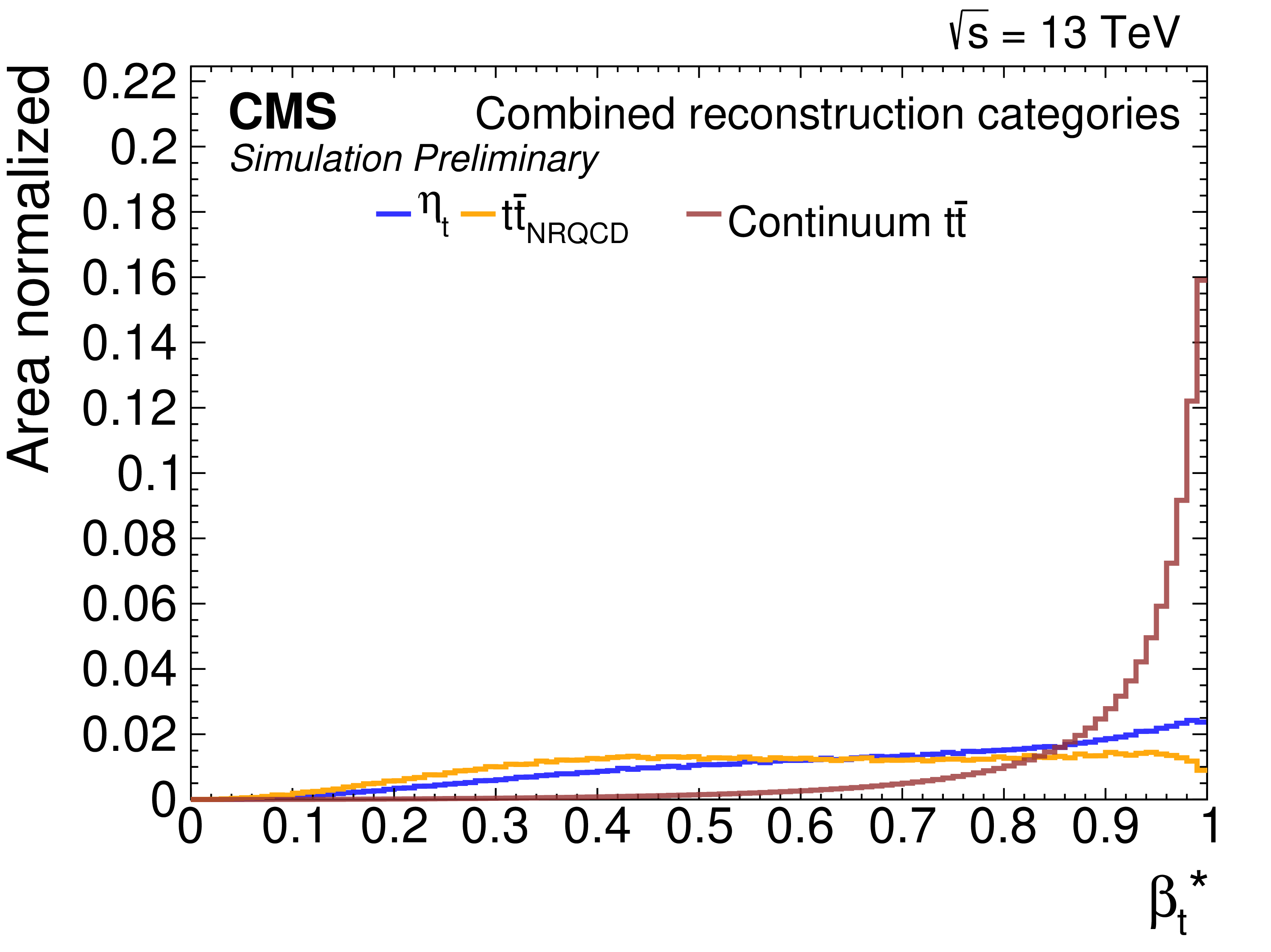
Figure 1:
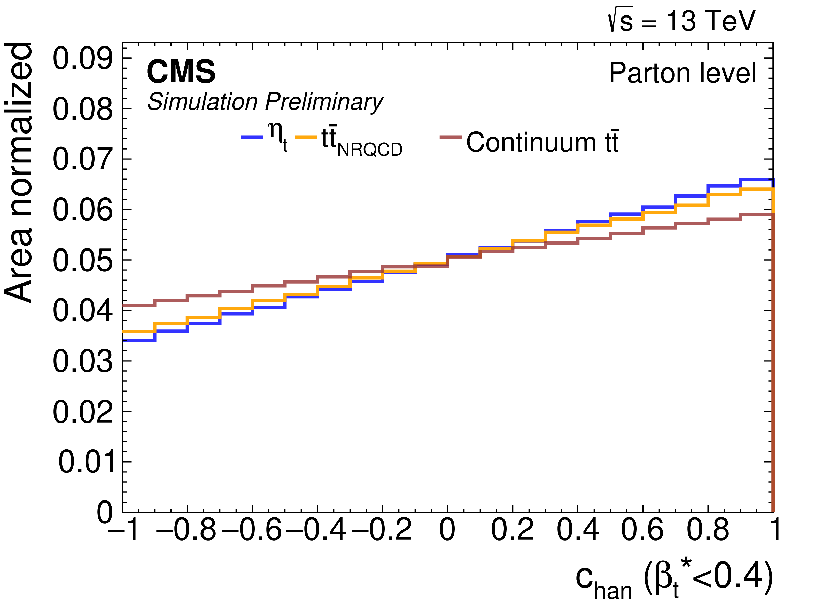
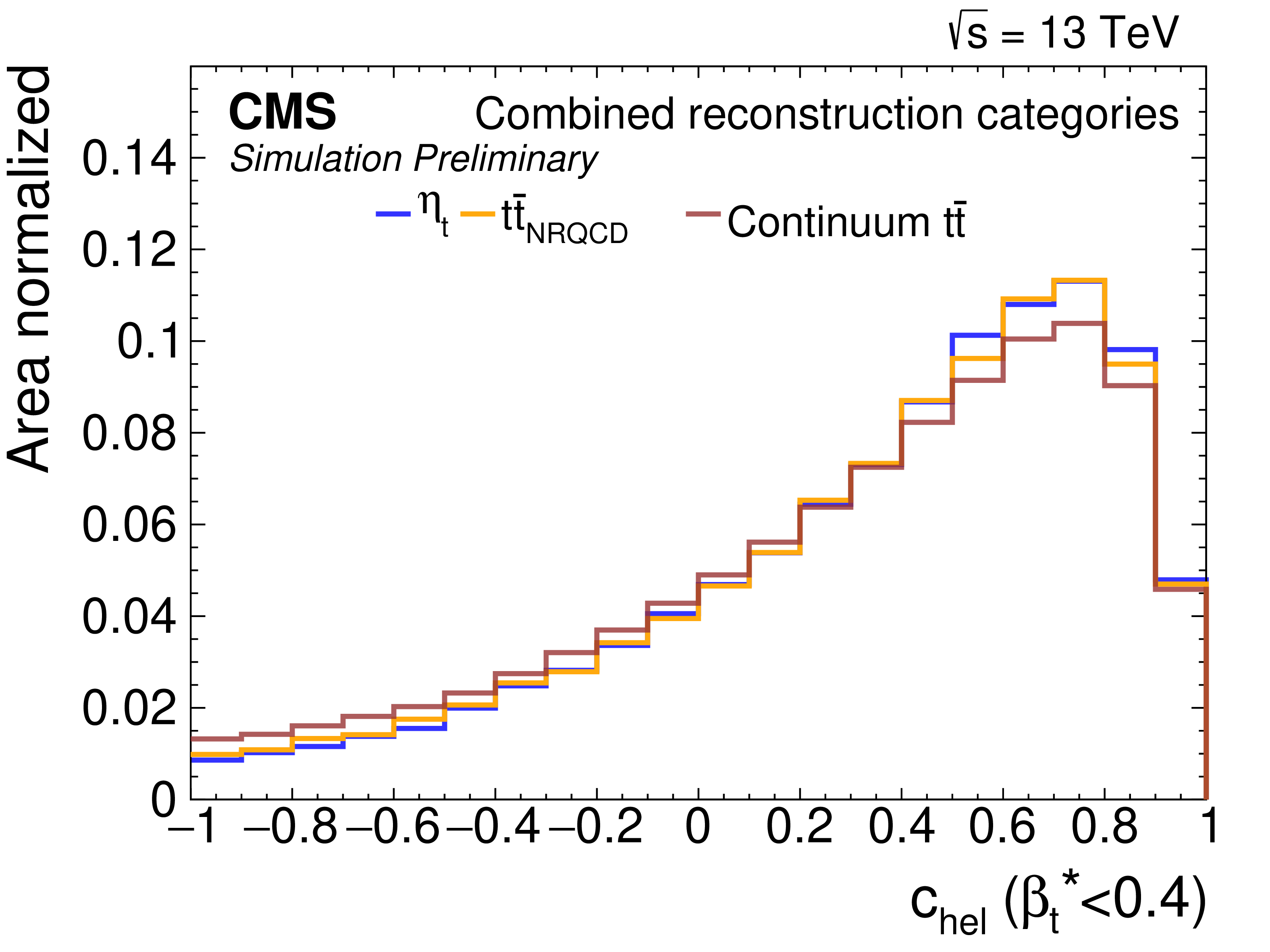
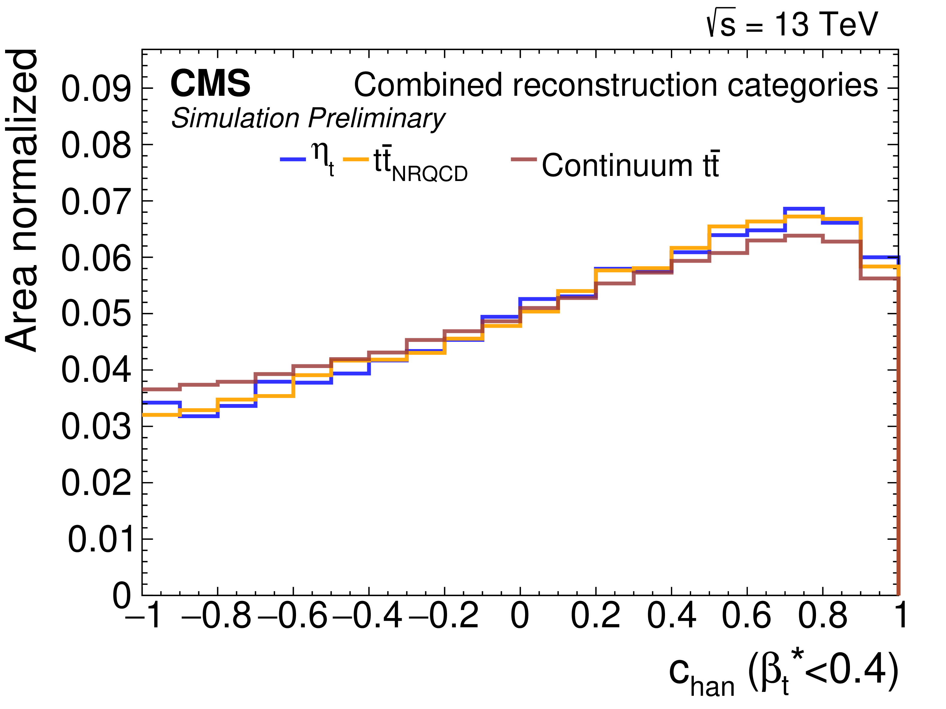
Parton-level distributions of $ m({\mathrm{t}\overline{\mathrm{t}}} ) $ (upper left), $ \beta_{\mathrm{t}}^{*} $ (upper right), $ c_\mathrm{hel} $ (lower left), and $ c_\mathrm{han} $ (lower right) for the $ \eta \mathrm{t} $ model (blue), the $ {\mathrm{t}\overline{\mathrm{t}}} _{\text{NRQCD}} $ model (orange), and the continuum $ \mathrm{t} \overline{\mathrm{t}} $ background (red). The distributions for the continuum $ \mathrm{t} \overline{\mathrm{t}} $ background include the NNLO QCD reweighting and the EW corrections. All distributions are normalized to unit area. |
png pdf |
Figure 1-a:
Parton-level distributions of $ m({\mathrm{t}\overline{\mathrm{t}}} ) $ (upper left), $ \beta_{\mathrm{t}}^{*} $ (upper right), $ c_\mathrm{hel} $ (lower left), and $ c_\mathrm{han} $ (lower right) for the $ \eta \mathrm{t} $ model (blue), the $ {\mathrm{t}\overline{\mathrm{t}}} _{\text{NRQCD}} $ model (orange), and the continuum $ \mathrm{t} \overline{\mathrm{t}} $ background (red). The distributions for the continuum $ \mathrm{t} \overline{\mathrm{t}} $ background include the NNLO QCD reweighting and the EW corrections. All distributions are normalized to unit area. |
png pdf |
Figure 1-b:
Parton-level distributions of $ m({\mathrm{t}\overline{\mathrm{t}}} ) $ (upper left), $ \beta_{\mathrm{t}}^{*} $ (upper right), $ c_\mathrm{hel} $ (lower left), and $ c_\mathrm{han} $ (lower right) for the $ \eta \mathrm{t} $ model (blue), the $ {\mathrm{t}\overline{\mathrm{t}}} _{\text{NRQCD}} $ model (orange), and the continuum $ \mathrm{t} \overline{\mathrm{t}} $ background (red). The distributions for the continuum $ \mathrm{t} \overline{\mathrm{t}} $ background include the NNLO QCD reweighting and the EW corrections. All distributions are normalized to unit area. |
png pdf |
Figure 1-c:
Parton-level distributions of $ m({\mathrm{t}\overline{\mathrm{t}}} ) $ (upper left), $ \beta_{\mathrm{t}}^{*} $ (upper right), $ c_\mathrm{hel} $ (lower left), and $ c_\mathrm{han} $ (lower right) for the $ \eta \mathrm{t} $ model (blue), the $ {\mathrm{t}\overline{\mathrm{t}}} _{\text{NRQCD}} $ model (orange), and the continuum $ \mathrm{t} \overline{\mathrm{t}} $ background (red). The distributions for the continuum $ \mathrm{t} \overline{\mathrm{t}} $ background include the NNLO QCD reweighting and the EW corrections. All distributions are normalized to unit area. |
png pdf |
Figure 1-d:
Parton-level distributions of $ m({\mathrm{t}\overline{\mathrm{t}}} ) $ (upper left), $ \beta_{\mathrm{t}}^{*} $ (upper right), $ c_\mathrm{hel} $ (lower left), and $ c_\mathrm{han} $ (lower right) for the $ \eta \mathrm{t} $ model (blue), the $ {\mathrm{t}\overline{\mathrm{t}}} _{\text{NRQCD}} $ model (orange), and the continuum $ \mathrm{t} \overline{\mathrm{t}} $ background (red). The distributions for the continuum $ \mathrm{t} \overline{\mathrm{t}} $ background include the NNLO QCD reweighting and the EW corrections. All distributions are normalized to unit area. |
png pdf |
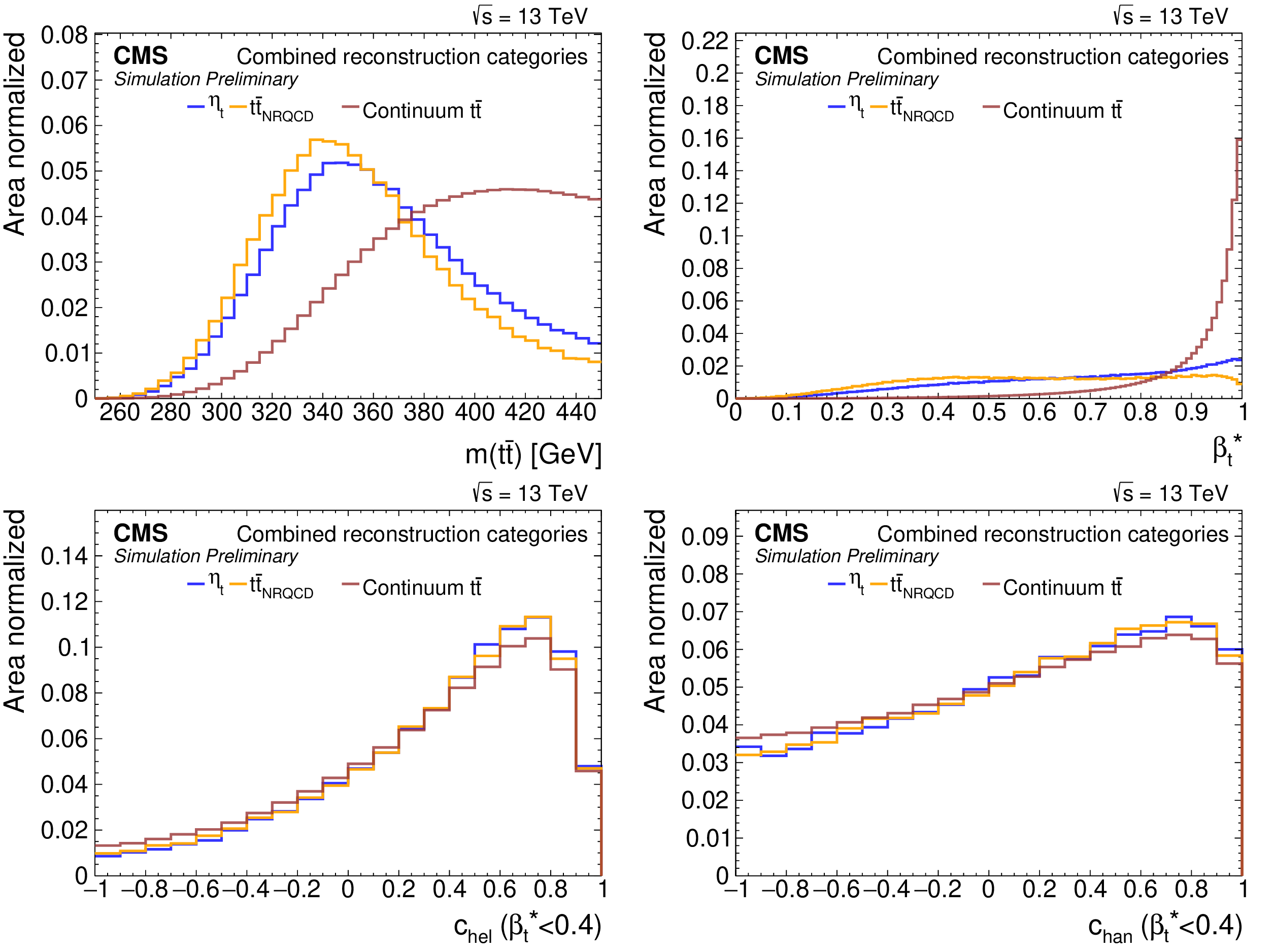
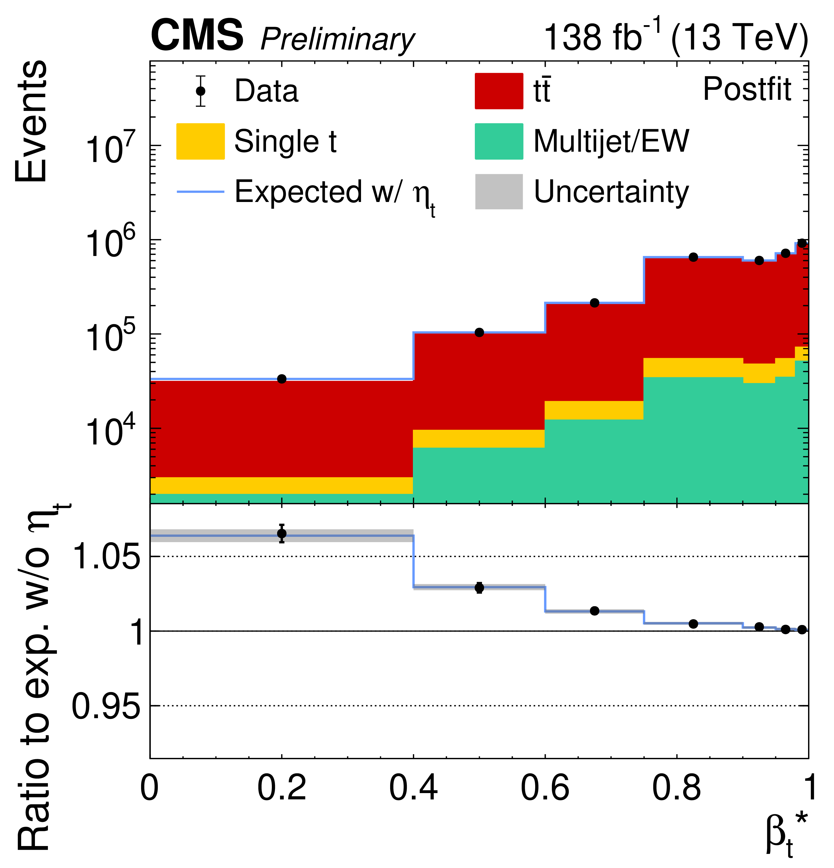
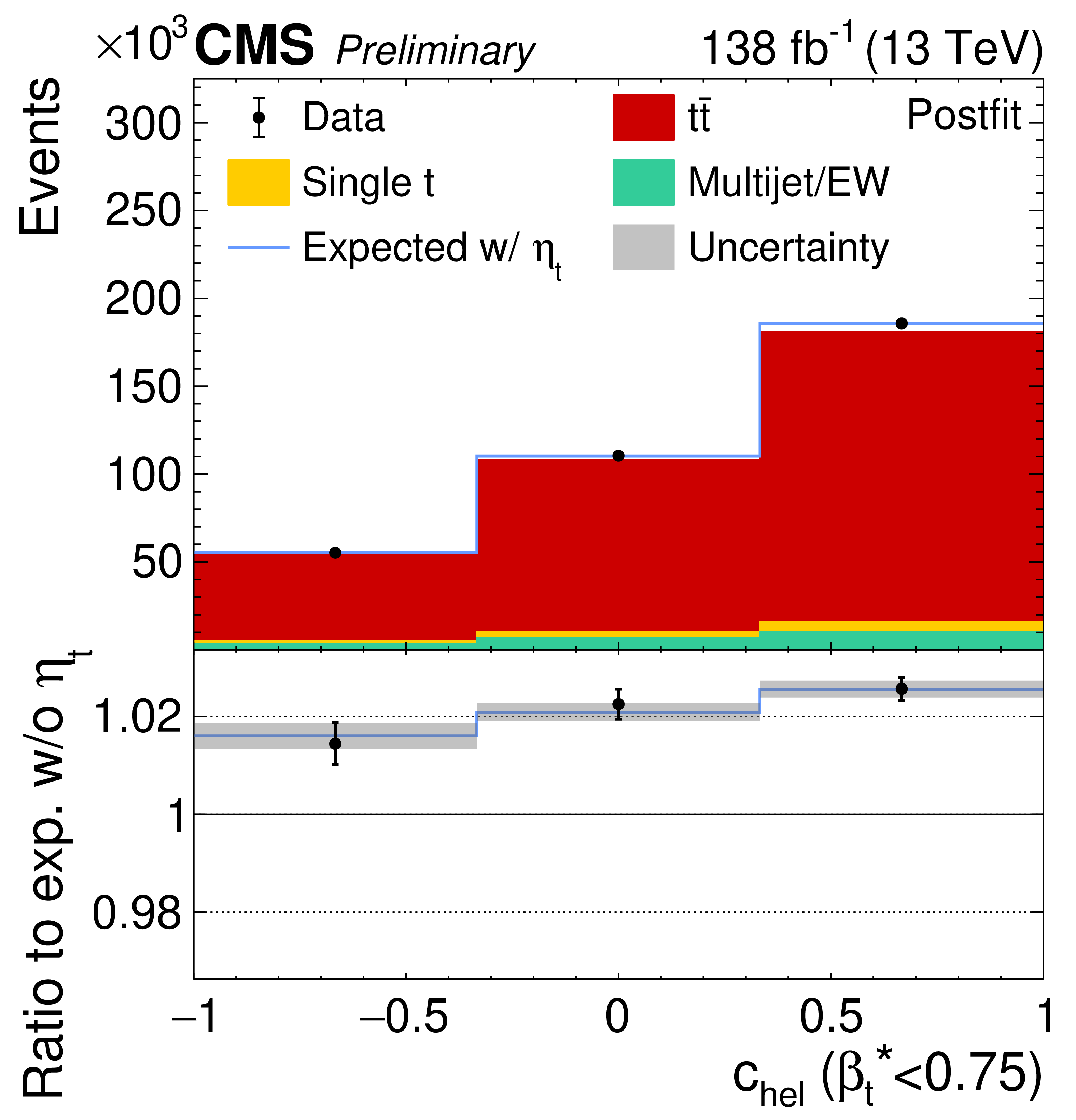
Figure 2:
Detector-level distributions of $ m({\mathrm{t}\overline{\mathrm{t}}} ) $ (upper left), $ \beta_{\mathrm{t}}^{*} $ (upper right), $ c_\mathrm{hel} $ (lower left), and $ c_\mathrm{han} $ (lower right) for the $ \eta \mathrm{t} $ model (blue), the $ {\mathrm{t}\overline{\mathrm{t}}} _{\text{NRQCD}} $ model (orange), and the continuum $ \mathrm{t} \overline{\mathrm{t}} $ background (red). The distributions are shown for all signal categories defined in Section 6 combined. The distributions for the continuum $ \mathrm{t} \overline{\mathrm{t}} $ background include the NNLO QCD reweighting and the EW corrections. All distributions are normalized to unit area. |
png pdf |
Figure 2-a:
Detector-level distributions of $ m({\mathrm{t}\overline{\mathrm{t}}} ) $ (upper left), $ \beta_{\mathrm{t}}^{*} $ (upper right), $ c_\mathrm{hel} $ (lower left), and $ c_\mathrm{han} $ (lower right) for the $ \eta \mathrm{t} $ model (blue), the $ {\mathrm{t}\overline{\mathrm{t}}} _{\text{NRQCD}} $ model (orange), and the continuum $ \mathrm{t} \overline{\mathrm{t}} $ background (red). The distributions are shown for all signal categories defined in Section 6 combined. The distributions for the continuum $ \mathrm{t} \overline{\mathrm{t}} $ background include the NNLO QCD reweighting and the EW corrections. All distributions are normalized to unit area. |
png pdf |
Figure 2-b:
Detector-level distributions of $ m({\mathrm{t}\overline{\mathrm{t}}} ) $ (upper left), $ \beta_{\mathrm{t}}^{*} $ (upper right), $ c_\mathrm{hel} $ (lower left), and $ c_\mathrm{han} $ (lower right) for the $ \eta \mathrm{t} $ model (blue), the $ {\mathrm{t}\overline{\mathrm{t}}} _{\text{NRQCD}} $ model (orange), and the continuum $ \mathrm{t} \overline{\mathrm{t}} $ background (red). The distributions are shown for all signal categories defined in Section 6 combined. The distributions for the continuum $ \mathrm{t} \overline{\mathrm{t}} $ background include the NNLO QCD reweighting and the EW corrections. All distributions are normalized to unit area. |
png pdf |
Figure 2-c:
Detector-level distributions of $ m({\mathrm{t}\overline{\mathrm{t}}} ) $ (upper left), $ \beta_{\mathrm{t}}^{*} $ (upper right), $ c_\mathrm{hel} $ (lower left), and $ c_\mathrm{han} $ (lower right) for the $ \eta \mathrm{t} $ model (blue), the $ {\mathrm{t}\overline{\mathrm{t}}} _{\text{NRQCD}} $ model (orange), and the continuum $ \mathrm{t} \overline{\mathrm{t}} $ background (red). The distributions are shown for all signal categories defined in Section 6 combined. The distributions for the continuum $ \mathrm{t} \overline{\mathrm{t}} $ background include the NNLO QCD reweighting and the EW corrections. All distributions are normalized to unit area. |
png pdf |
Figure 2-d:
Detector-level distributions of $ m({\mathrm{t}\overline{\mathrm{t}}} ) $ (upper left), $ \beta_{\mathrm{t}}^{*} $ (upper right), $ c_\mathrm{hel} $ (lower left), and $ c_\mathrm{han} $ (lower right) for the $ \eta \mathrm{t} $ model (blue), the $ {\mathrm{t}\overline{\mathrm{t}}} _{\text{NRQCD}} $ model (orange), and the continuum $ \mathrm{t} \overline{\mathrm{t}} $ background (red). The distributions are shown for all signal categories defined in Section 6 combined. The distributions for the continuum $ \mathrm{t} \overline{\mathrm{t}} $ background include the NNLO QCD reweighting and the EW corrections. All distributions are normalized to unit area. |
png pdf |
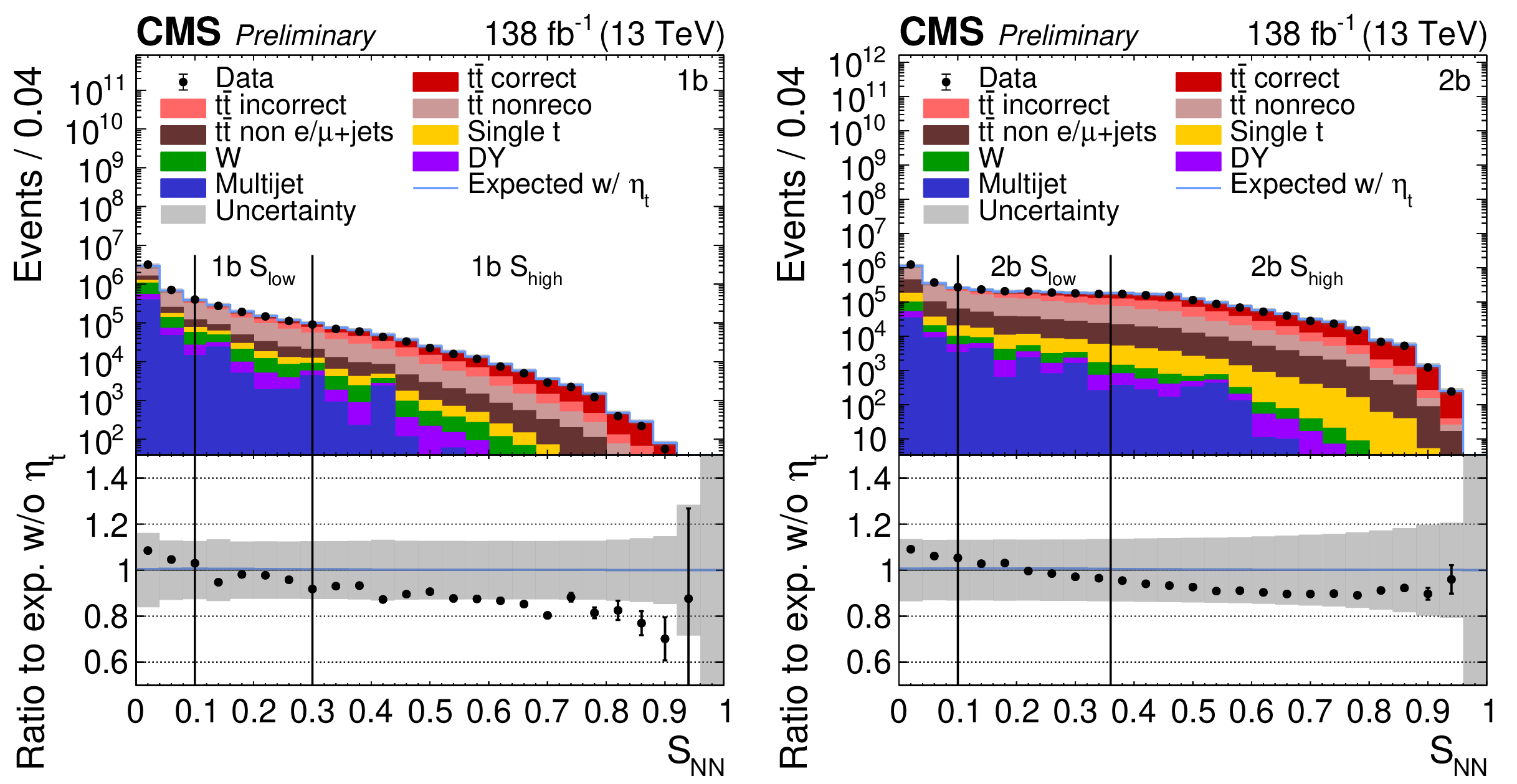
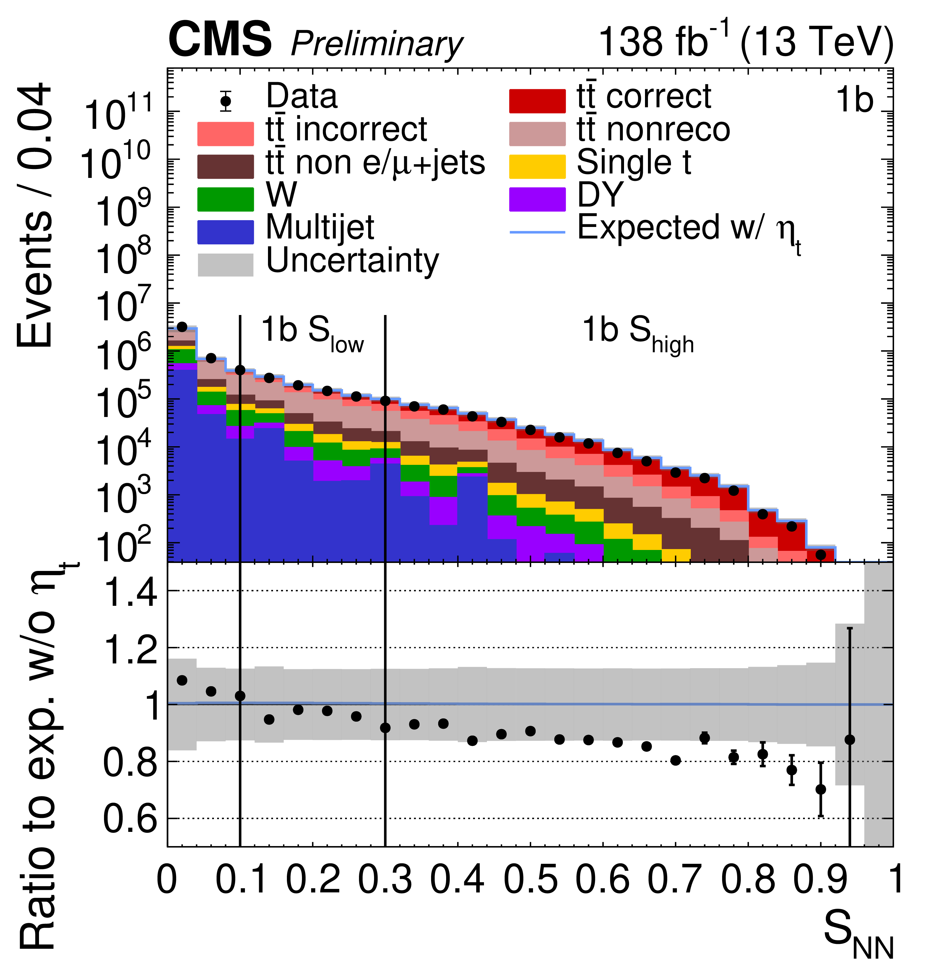
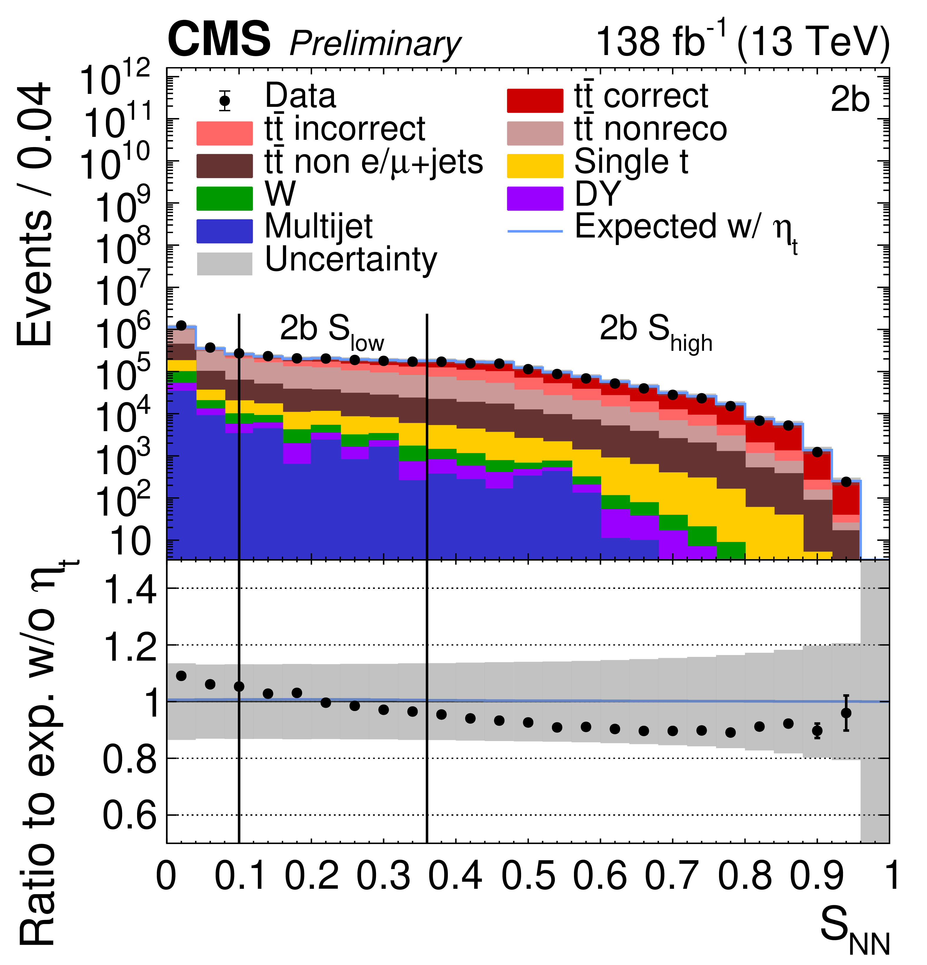
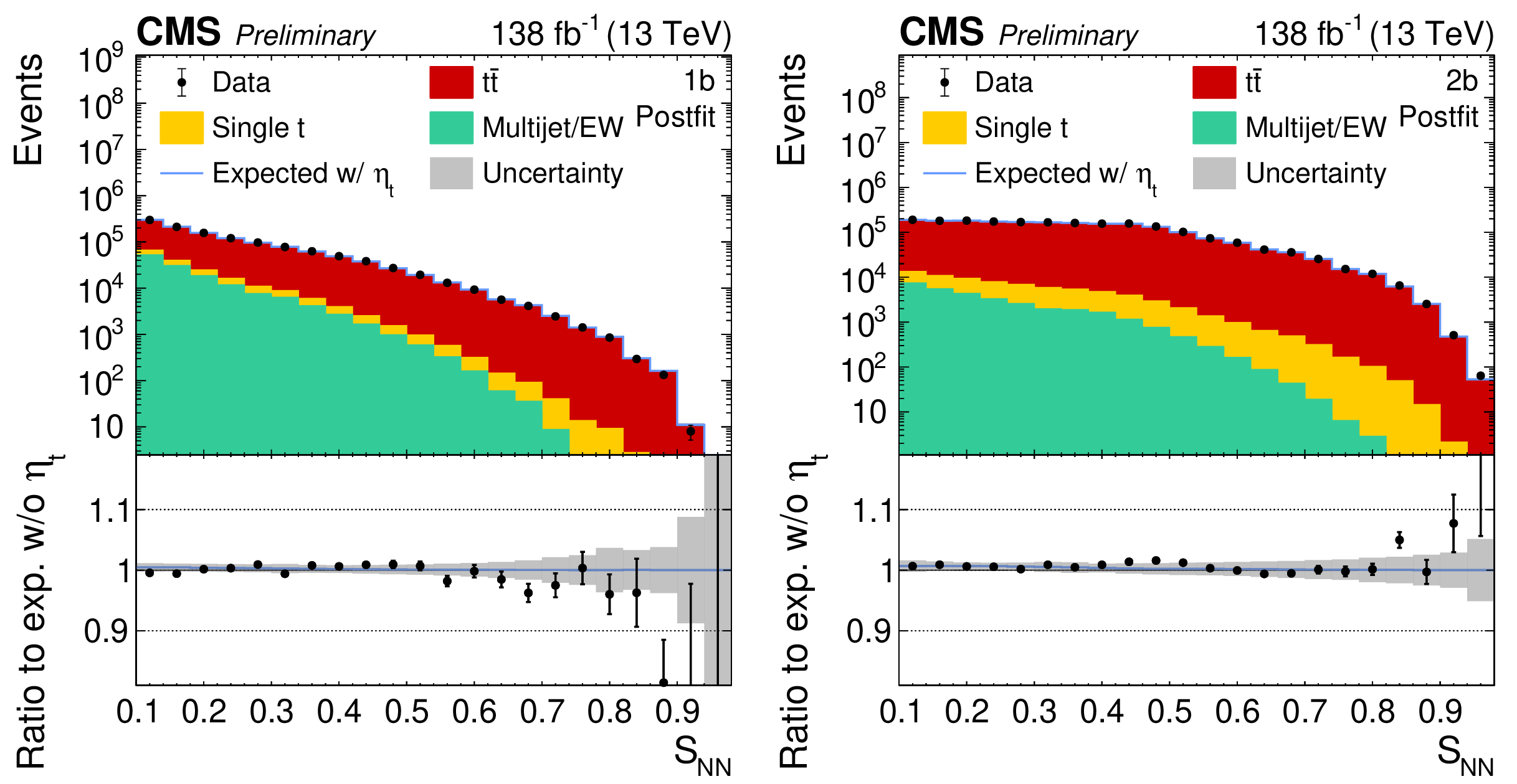
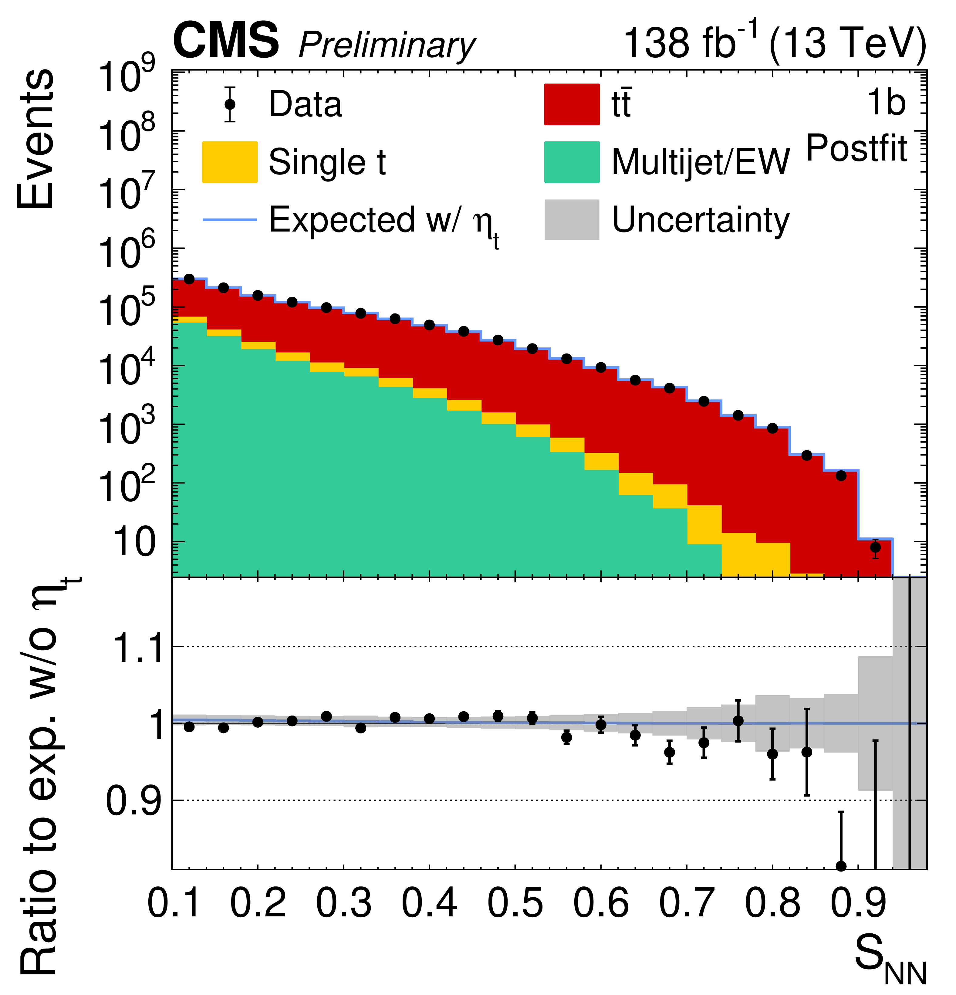
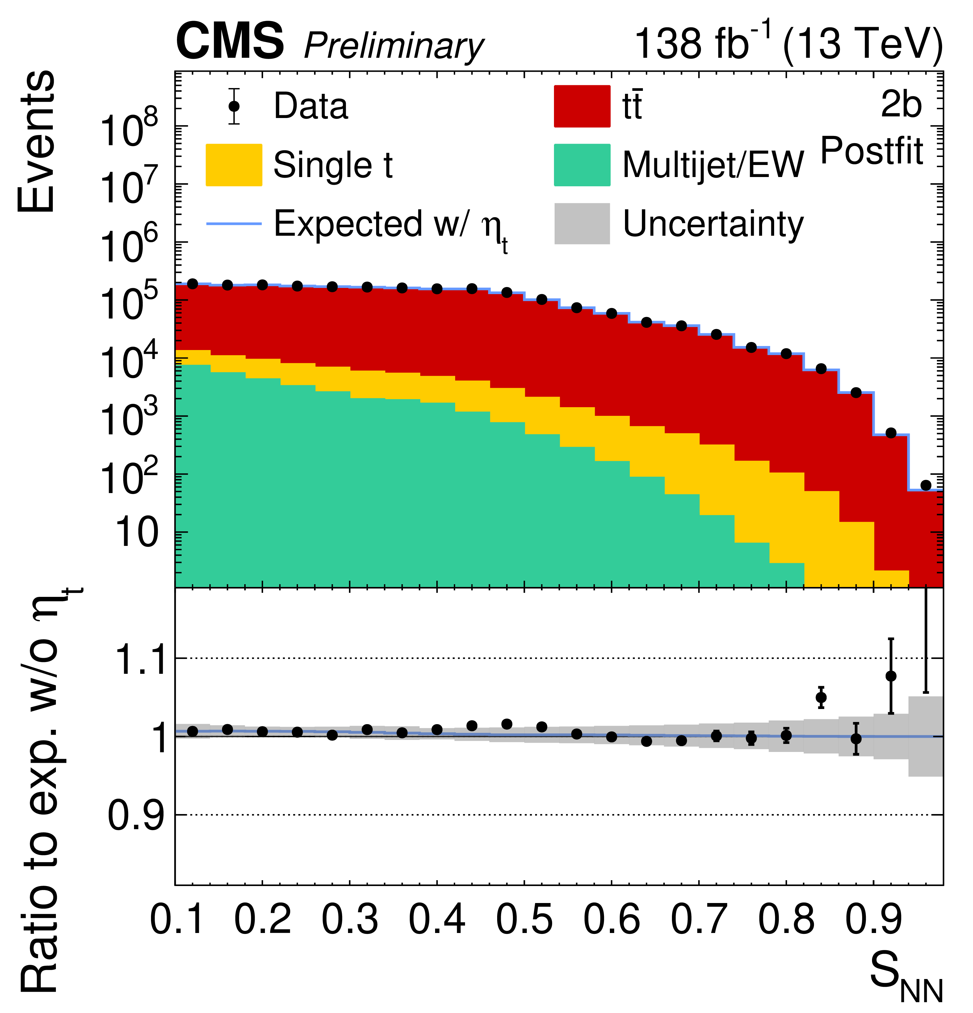
Figure 3:
The $ S_{\text{NN}} $ distribution before the mass window selections is presented for the 1b (left) and 2b (right) categories, with data points compared against the predictions without $ \eta \mathrm{t} $ (stacked histograms) and those including it (blue line). The $ \mathrm{t} \overline{\mathrm{t}} $ component is categorized into correctly reconstructed, incorrectly reconstructed, ``nonreconstructible'', and non $ \mathrm{e}/\mu $+jets events. The gray band represents the total statistical and systematic uncertainties in the prediction, while the vertical error bars on the data points indicate the statistical uncertainties of the data. The lower panels illustrate the ratio of observed data to predicted yields. |
png pdf |
Figure 3-a:
The $ S_{\text{NN}} $ distribution before the mass window selections is presented for the 1b (left) and 2b (right) categories, with data points compared against the predictions without $ \eta \mathrm{t} $ (stacked histograms) and those including it (blue line). The $ \mathrm{t} \overline{\mathrm{t}} $ component is categorized into correctly reconstructed, incorrectly reconstructed, ``nonreconstructible'', and non $ \mathrm{e}/\mu $+jets events. The gray band represents the total statistical and systematic uncertainties in the prediction, while the vertical error bars on the data points indicate the statistical uncertainties of the data. The lower panels illustrate the ratio of observed data to predicted yields. |
png pdf |
Figure 3-b:
The $ S_{\text{NN}} $ distribution before the mass window selections is presented for the 1b (left) and 2b (right) categories, with data points compared against the predictions without $ \eta \mathrm{t} $ (stacked histograms) and those including it (blue line). The $ \mathrm{t} \overline{\mathrm{t}} $ component is categorized into correctly reconstructed, incorrectly reconstructed, ``nonreconstructible'', and non $ \mathrm{e}/\mu $+jets events. The gray band represents the total statistical and systematic uncertainties in the prediction, while the vertical error bars on the data points indicate the statistical uncertainties of the data. The lower panels illustrate the ratio of observed data to predicted yields. |
png pdf |
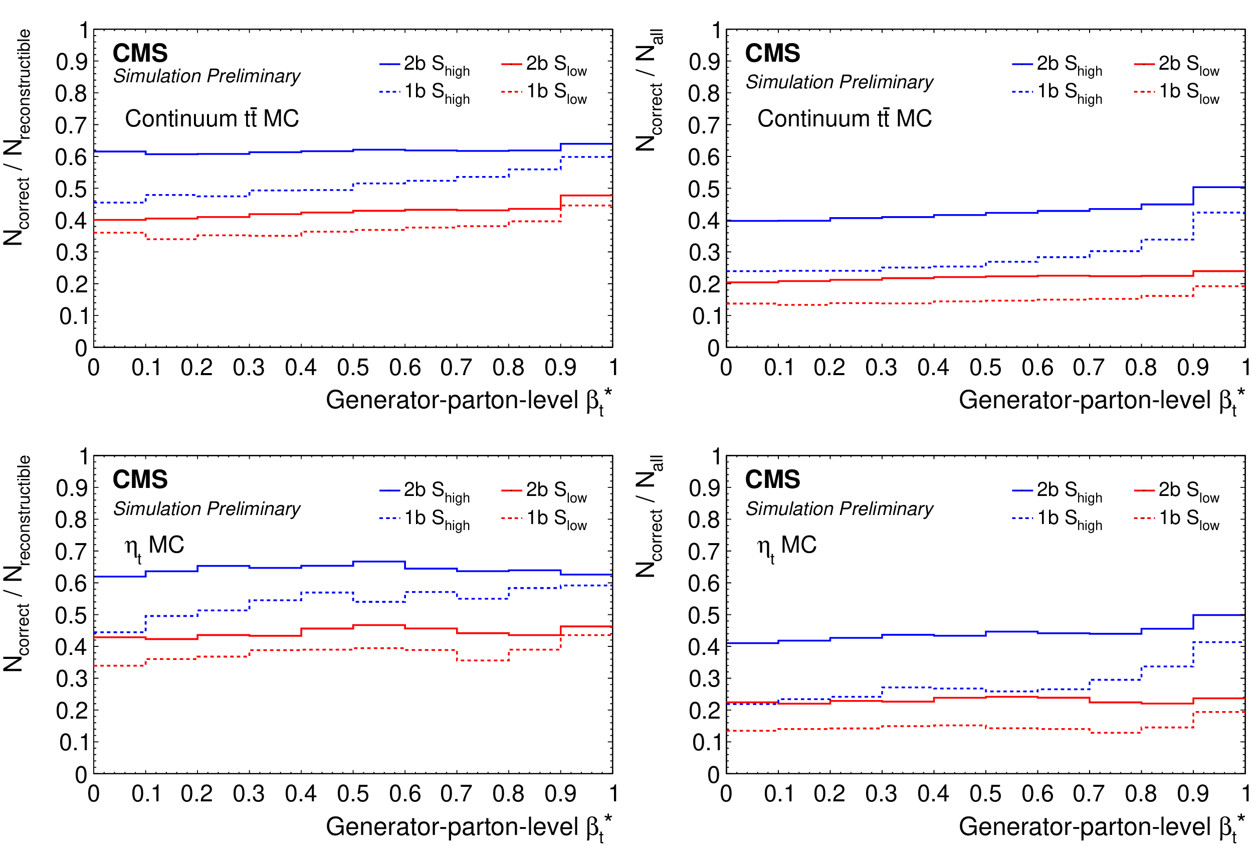
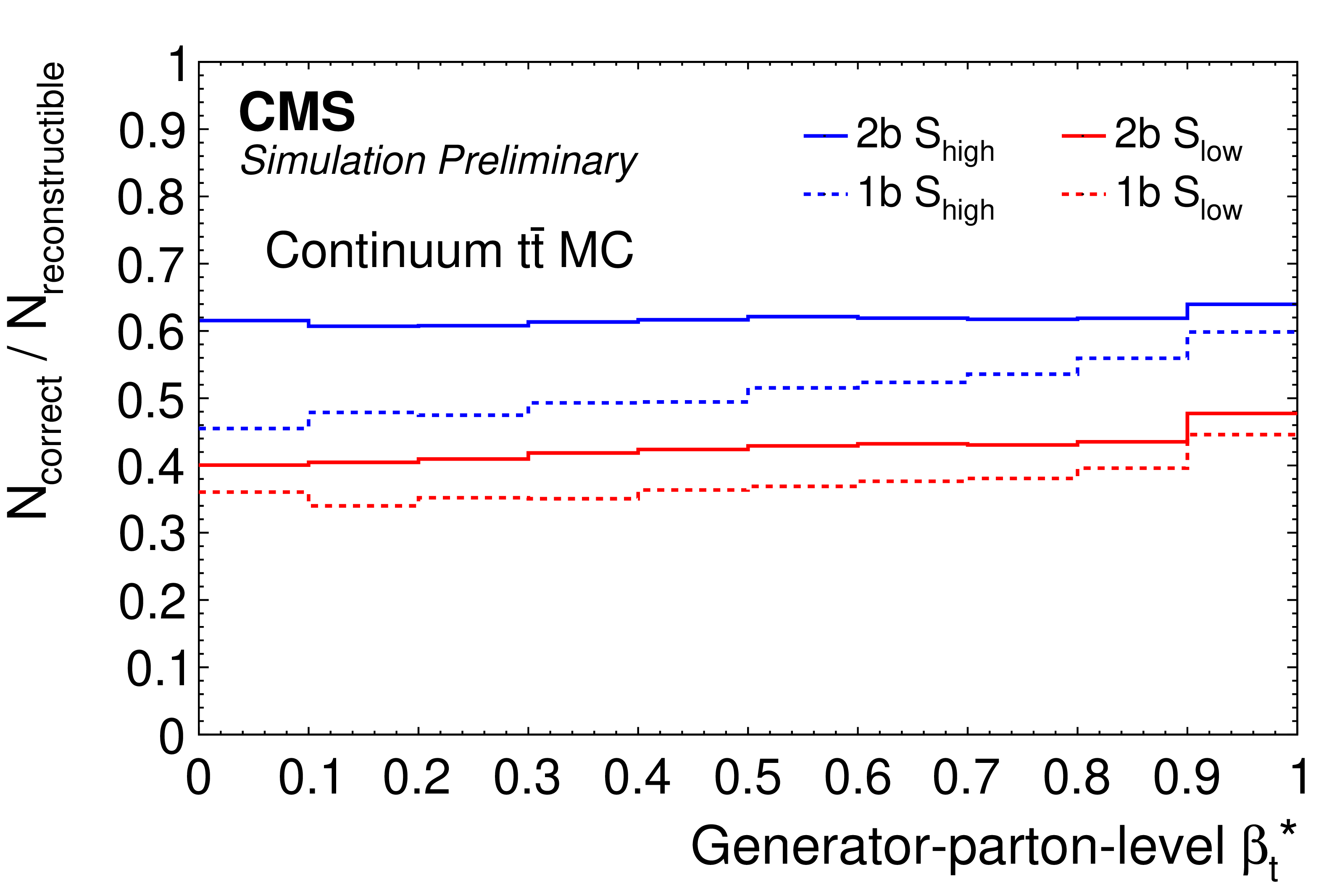
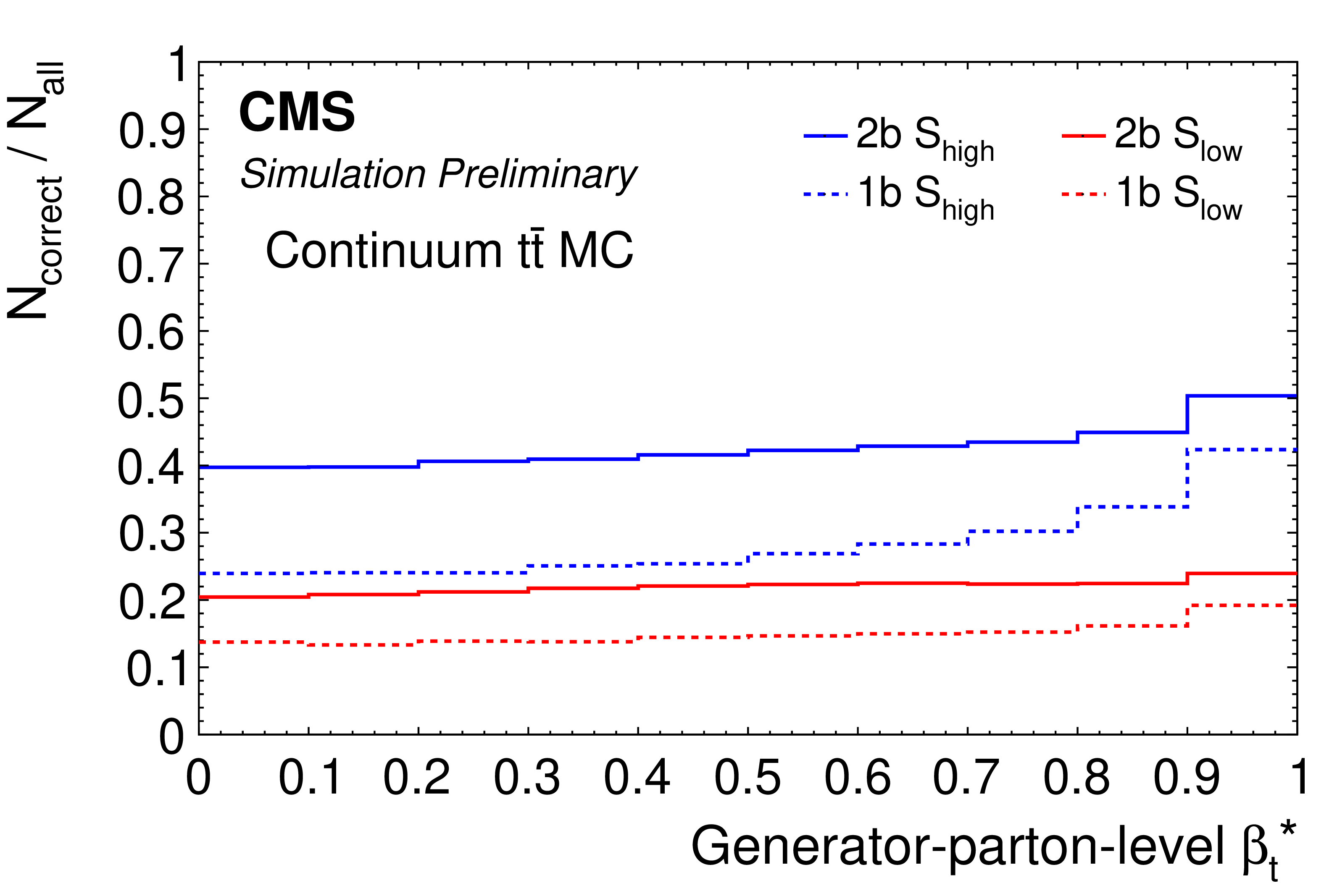
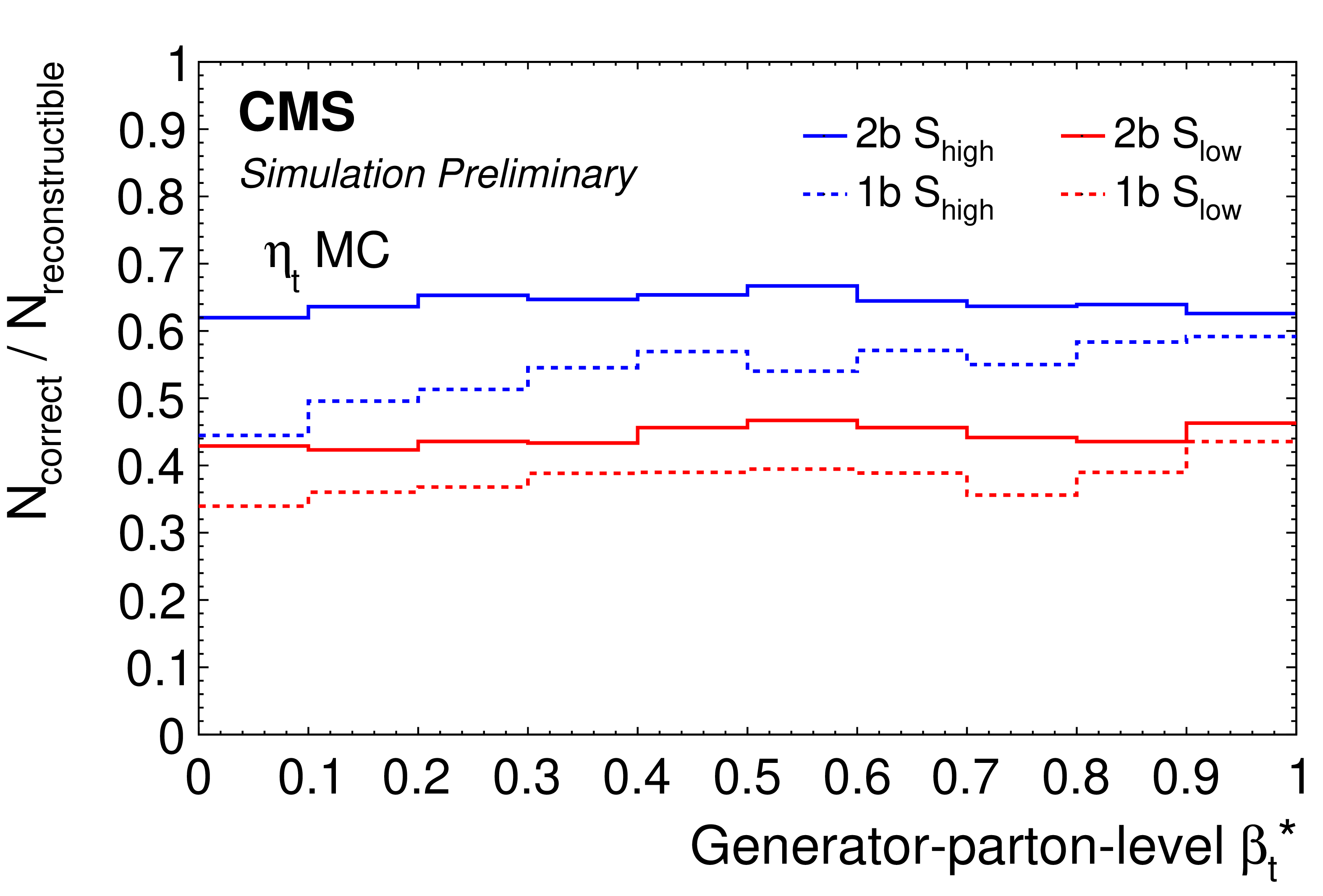
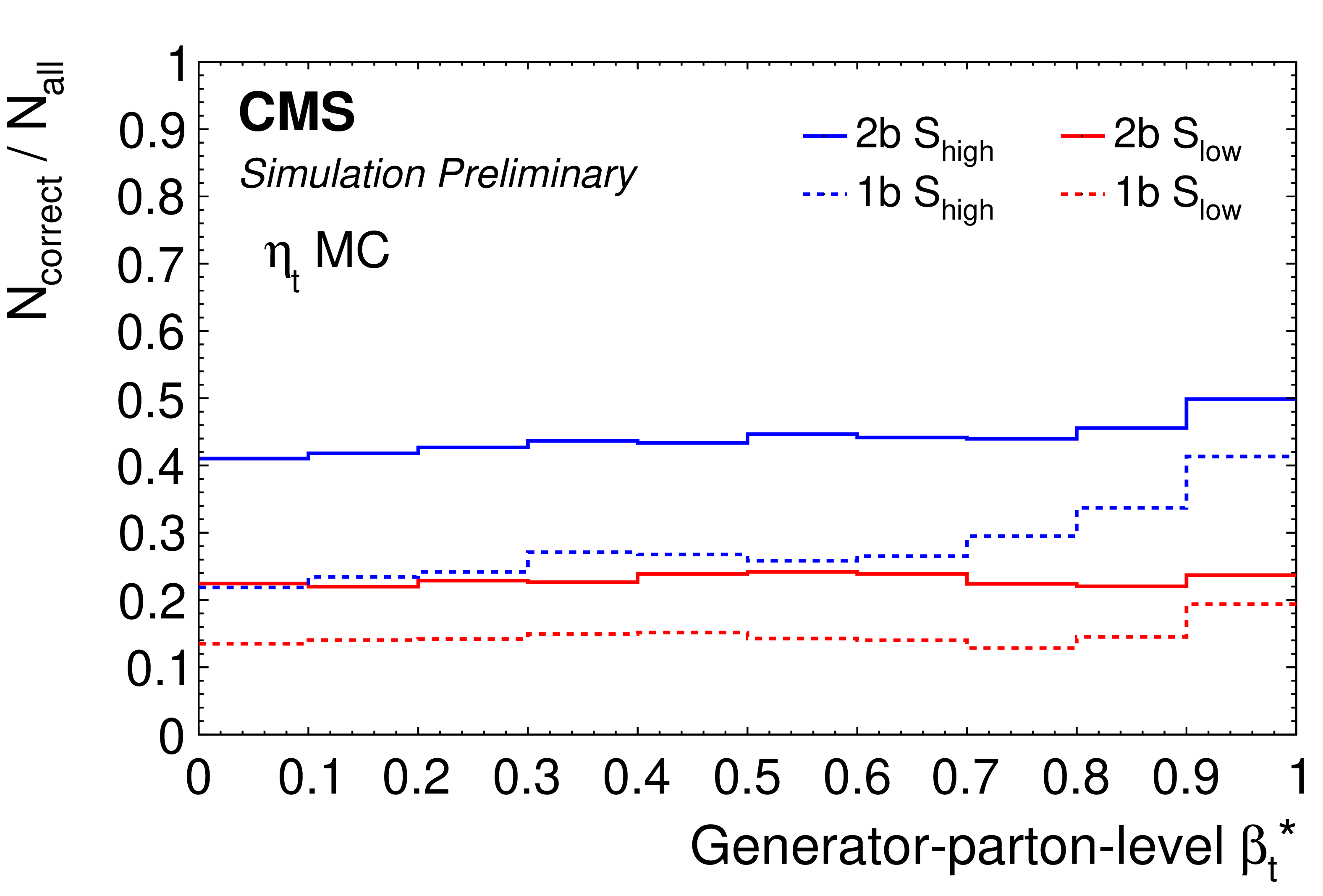
Figure 4:
Reconstruction performance as a function of $ \beta_{\mathrm{t}}^{*} $ at the parton level. The plots in the left column show the fraction of correctly reconstructed events ($ N_\mathrm{correct} $) relative to the reconstructible events ($ N_\mathrm{reconstructible} $), while the plots in the right column display those relative to all generated events for each respective process ($ N_\mathrm{all} $). The plots in the upper row are based on the continuum $ \mathrm{t} \overline{\mathrm{t}} $ simulation, while those in the lower row use the $ \eta \mathrm{t} $ simulation. Results are presented separately for the 1b and 2b categories under the $ S_{\text{low}} $ and $ S_{\text{high}} $ selections. |
png pdf |
Figure 4-a:
Reconstruction performance as a function of $ \beta_{\mathrm{t}}^{*} $ at the parton level. The plots in the left column show the fraction of correctly reconstructed events ($ N_\mathrm{correct} $) relative to the reconstructible events ($ N_\mathrm{reconstructible} $), while the plots in the right column display those relative to all generated events for each respective process ($ N_\mathrm{all} $). The plots in the upper row are based on the continuum $ \mathrm{t} \overline{\mathrm{t}} $ simulation, while those in the lower row use the $ \eta \mathrm{t} $ simulation. Results are presented separately for the 1b and 2b categories under the $ S_{\text{low}} $ and $ S_{\text{high}} $ selections. |
png pdf |
Figure 4-b:
Reconstruction performance as a function of $ \beta_{\mathrm{t}}^{*} $ at the parton level. The plots in the left column show the fraction of correctly reconstructed events ($ N_\mathrm{correct} $) relative to the reconstructible events ($ N_\mathrm{reconstructible} $), while the plots in the right column display those relative to all generated events for each respective process ($ N_\mathrm{all} $). The plots in the upper row are based on the continuum $ \mathrm{t} \overline{\mathrm{t}} $ simulation, while those in the lower row use the $ \eta \mathrm{t} $ simulation. Results are presented separately for the 1b and 2b categories under the $ S_{\text{low}} $ and $ S_{\text{high}} $ selections. |
png pdf |
Figure 4-c:
Reconstruction performance as a function of $ \beta_{\mathrm{t}}^{*} $ at the parton level. The plots in the left column show the fraction of correctly reconstructed events ($ N_\mathrm{correct} $) relative to the reconstructible events ($ N_\mathrm{reconstructible} $), while the plots in the right column display those relative to all generated events for each respective process ($ N_\mathrm{all} $). The plots in the upper row are based on the continuum $ \mathrm{t} \overline{\mathrm{t}} $ simulation, while those in the lower row use the $ \eta \mathrm{t} $ simulation. Results are presented separately for the 1b and 2b categories under the $ S_{\text{low}} $ and $ S_{\text{high}} $ selections. |
png pdf |
Figure 4-d:
Reconstruction performance as a function of $ \beta_{\mathrm{t}}^{*} $ at the parton level. The plots in the left column show the fraction of correctly reconstructed events ($ N_\mathrm{correct} $) relative to the reconstructible events ($ N_\mathrm{reconstructible} $), while the plots in the right column display those relative to all generated events for each respective process ($ N_\mathrm{all} $). The plots in the upper row are based on the continuum $ \mathrm{t} \overline{\mathrm{t}} $ simulation, while those in the lower row use the $ \eta \mathrm{t} $ simulation. Results are presented separately for the 1b and 2b categories under the $ S_{\text{low}} $ and $ S_{\text{high}} $ selections. |
png pdf |
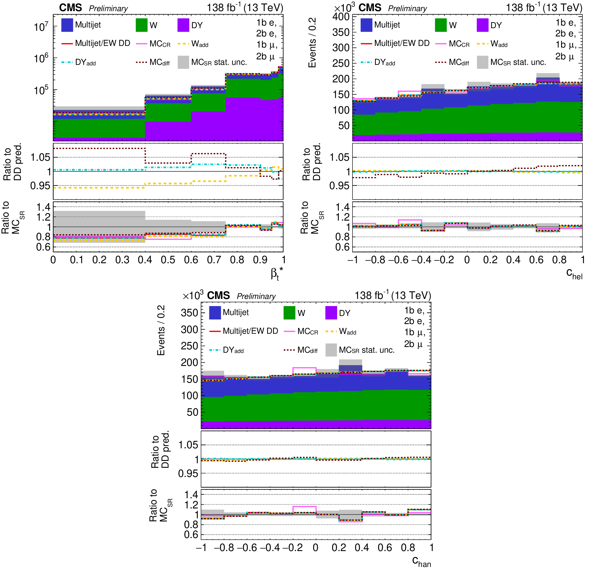
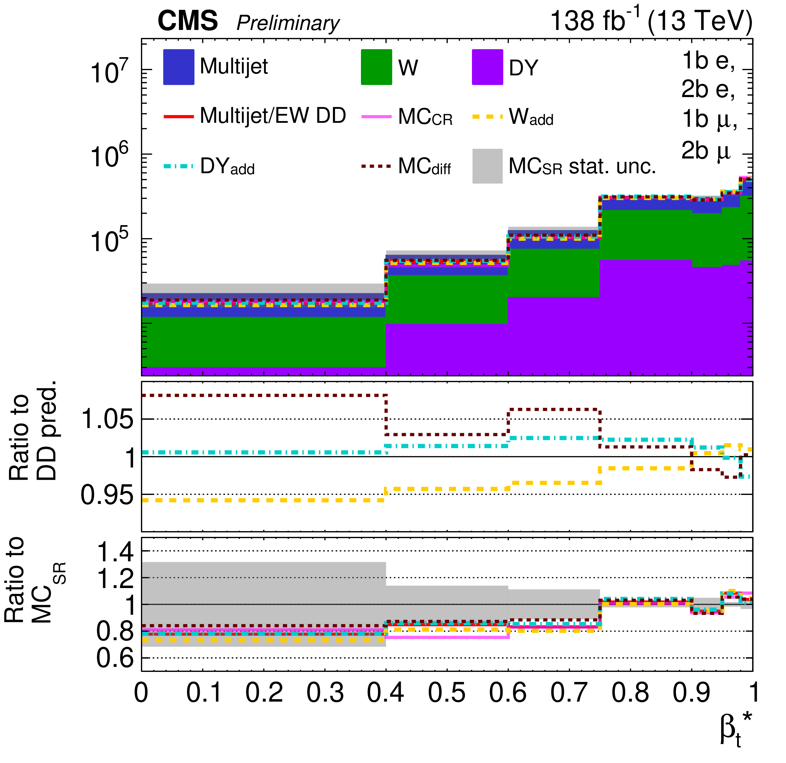
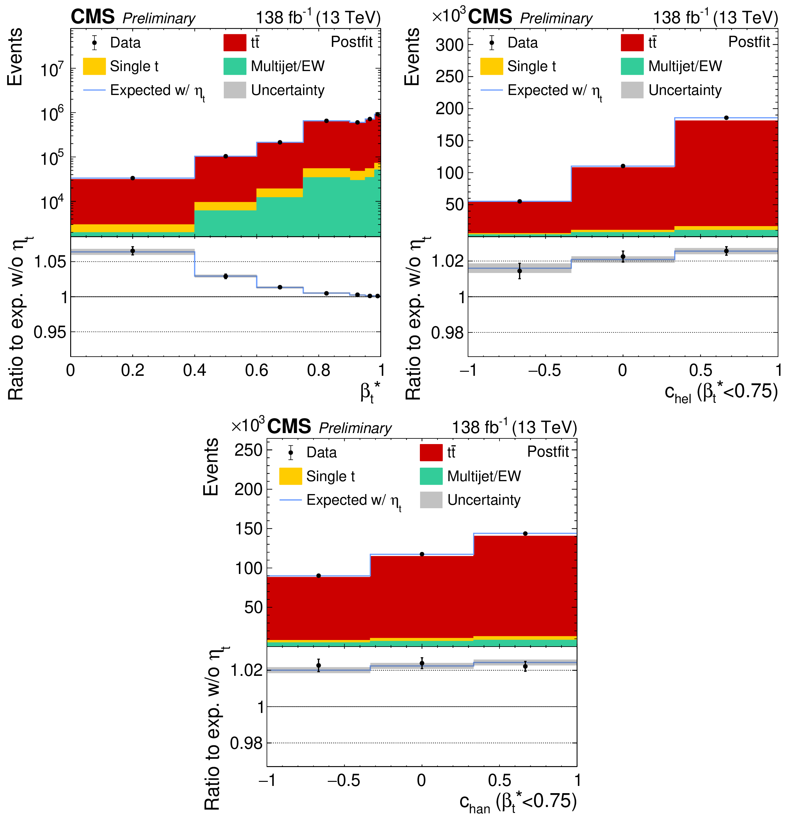
Figure 5:
Comparison of multijet/EW $ \beta_{\mathrm{t}}^{*} $ (upper, left), $ c_\mathrm{hel} $ (upper, right) and $ c_\mathrm{han} $ (lower) distributions from different sources. The top panels show the distributions for the DD prediction (Multijet/EW DD, red line), the CR simulation ($ \mathrm{MC}_\mathrm{CR} $, pink line), and the SR simulation (stacked histogram). The gray shaded band represents the statistical uncertainty of the SR simulation. Systematic uncertainties on the DD prediction are shown as dotted lines for $ \mathrm{W}_\mathrm{add} $ (yellow), $ \mathrm{DY}_\mathrm{add} $ (turquoise), and $ \mathrm{MC}_\mathrm{diff} $ (dark red). All distributions are normalized to the SR MC event yield. The middle panels display the ratios of these systematic variations to the DD prediction, while the lower panels show the ratios of all distributions to the SR MC. To reduce statistical fluctuations, the $ S_{\text{NN}} $ and invariant-mass requirements are not applied. |
png pdf |
Figure 5-a:
Comparison of multijet/EW $ \beta_{\mathrm{t}}^{*} $ (upper, left), $ c_\mathrm{hel} $ (upper, right) and $ c_\mathrm{han} $ (lower) distributions from different sources. The top panels show the distributions for the DD prediction (Multijet/EW DD, red line), the CR simulation ($ \mathrm{MC}_\mathrm{CR} $, pink line), and the SR simulation (stacked histogram). The gray shaded band represents the statistical uncertainty of the SR simulation. Systematic uncertainties on the DD prediction are shown as dotted lines for $ \mathrm{W}_\mathrm{add} $ (yellow), $ \mathrm{DY}_\mathrm{add} $ (turquoise), and $ \mathrm{MC}_\mathrm{diff} $ (dark red). All distributions are normalized to the SR MC event yield. The middle panels display the ratios of these systematic variations to the DD prediction, while the lower panels show the ratios of all distributions to the SR MC. To reduce statistical fluctuations, the $ S_{\text{NN}} $ and invariant-mass requirements are not applied. |
png pdf |
Figure 5-b:
Comparison of multijet/EW $ \beta_{\mathrm{t}}^{*} $ (upper, left), $ c_\mathrm{hel} $ (upper, right) and $ c_\mathrm{han} $ (lower) distributions from different sources. The top panels show the distributions for the DD prediction (Multijet/EW DD, red line), the CR simulation ($ \mathrm{MC}_\mathrm{CR} $, pink line), and the SR simulation (stacked histogram). The gray shaded band represents the statistical uncertainty of the SR simulation. Systematic uncertainties on the DD prediction are shown as dotted lines for $ \mathrm{W}_\mathrm{add} $ (yellow), $ \mathrm{DY}_\mathrm{add} $ (turquoise), and $ \mathrm{MC}_\mathrm{diff} $ (dark red). All distributions are normalized to the SR MC event yield. The middle panels display the ratios of these systematic variations to the DD prediction, while the lower panels show the ratios of all distributions to the SR MC. To reduce statistical fluctuations, the $ S_{\text{NN}} $ and invariant-mass requirements are not applied. |
png pdf |
Figure 5-c:
Comparison of multijet/EW $ \beta_{\mathrm{t}}^{*} $ (upper, left), $ c_\mathrm{hel} $ (upper, right) and $ c_\mathrm{han} $ (lower) distributions from different sources. The top panels show the distributions for the DD prediction (Multijet/EW DD, red line), the CR simulation ($ \mathrm{MC}_\mathrm{CR} $, pink line), and the SR simulation (stacked histogram). The gray shaded band represents the statistical uncertainty of the SR simulation. Systematic uncertainties on the DD prediction are shown as dotted lines for $ \mathrm{W}_\mathrm{add} $ (yellow), $ \mathrm{DY}_\mathrm{add} $ (turquoise), and $ \mathrm{MC}_\mathrm{diff} $ (dark red). All distributions are normalized to the SR MC event yield. The middle panels display the ratios of these systematic variations to the DD prediction, while the lower panels show the ratios of all distributions to the SR MC. To reduce statistical fluctuations, the $ S_{\text{NN}} $ and invariant-mass requirements are not applied. |
png pdf |
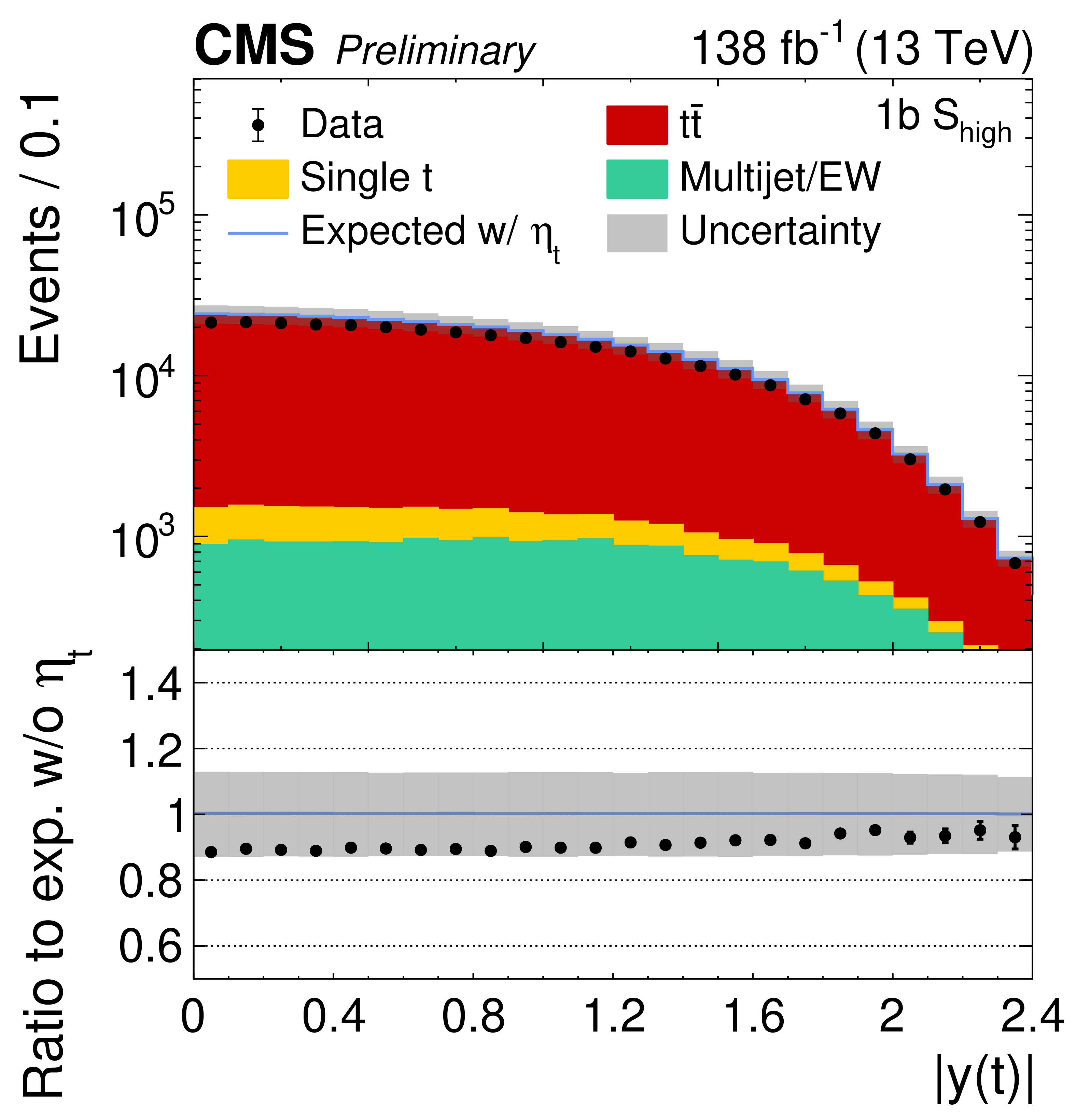
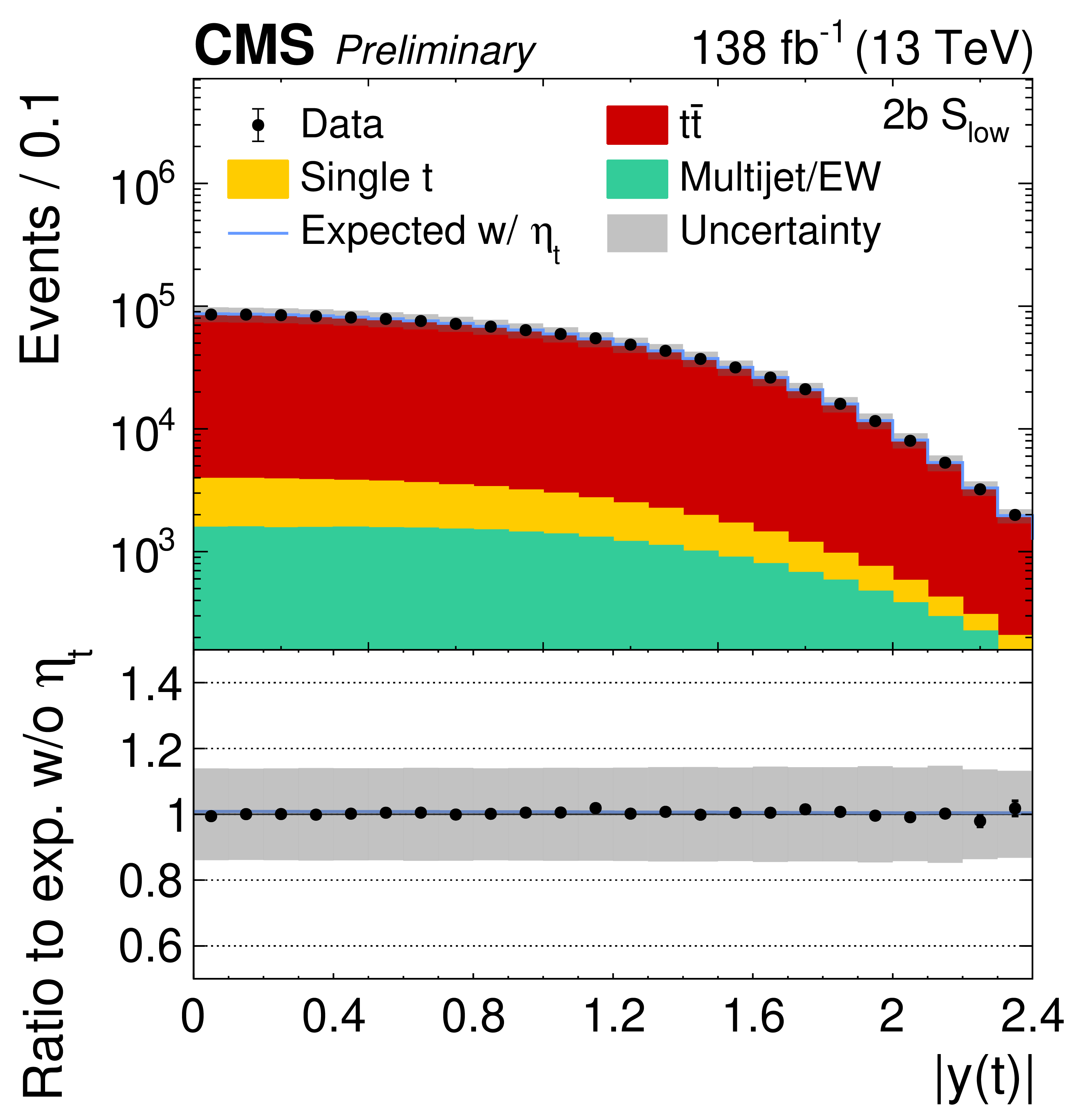
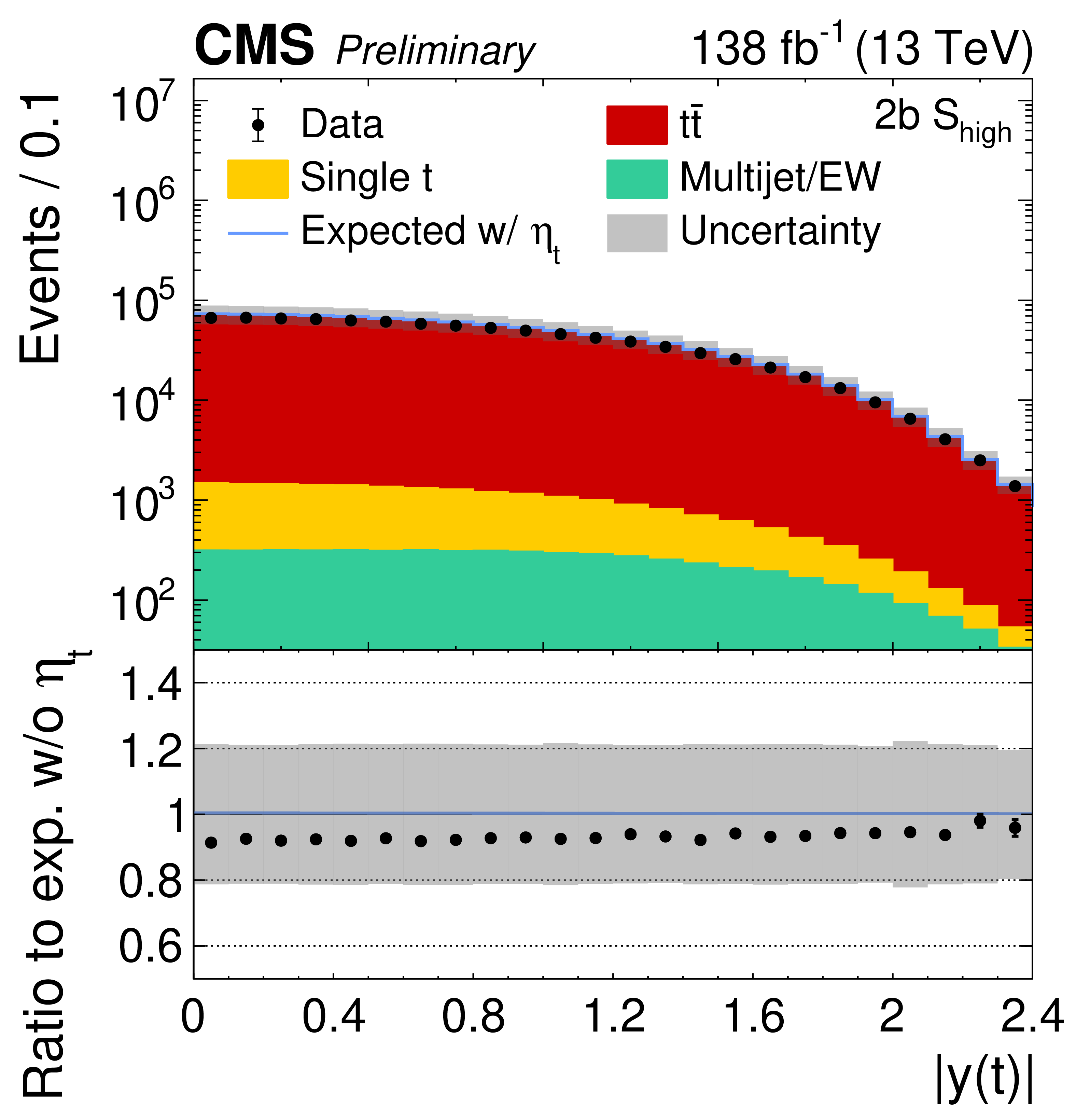
Figure 6:
Pre-fit distributions of $ |y(\mathrm{t})| $ in all four categories. The data (points) are compared to the predictions without $ \eta \mathrm{t} $ (stacked histograms) and those including it (blue line). The $ \mathrm{t} \overline{\mathrm{t}} $ and single top quark contributions are taken from simulation, while the multijet+EW background is derived from the CR. The gray uncertainty band represents the combined statistical and systematic uncertainties in the predictions, while the vertical bars on the data points indicate their statistical uncertainties. The ratios to the predicted yields excluding $ \eta \mathrm{t} $ are shown in the lower panels. |
png pdf |
Figure 6-a:
Pre-fit distributions of $ |y(\mathrm{t})| $ in all four categories. The data (points) are compared to the predictions without $ \eta \mathrm{t} $ (stacked histograms) and those including it (blue line). The $ \mathrm{t} \overline{\mathrm{t}} $ and single top quark contributions are taken from simulation, while the multijet+EW background is derived from the CR. The gray uncertainty band represents the combined statistical and systematic uncertainties in the predictions, while the vertical bars on the data points indicate their statistical uncertainties. The ratios to the predicted yields excluding $ \eta \mathrm{t} $ are shown in the lower panels. |
png pdf |
Figure 6-b:
Pre-fit distributions of $ |y(\mathrm{t})| $ in all four categories. The data (points) are compared to the predictions without $ \eta \mathrm{t} $ (stacked histograms) and those including it (blue line). The $ \mathrm{t} \overline{\mathrm{t}} $ and single top quark contributions are taken from simulation, while the multijet+EW background is derived from the CR. The gray uncertainty band represents the combined statistical and systematic uncertainties in the predictions, while the vertical bars on the data points indicate their statistical uncertainties. The ratios to the predicted yields excluding $ \eta \mathrm{t} $ are shown in the lower panels. |
png pdf |
Figure 6-c:
Pre-fit distributions of $ |y(\mathrm{t})| $ in all four categories. The data (points) are compared to the predictions without $ \eta \mathrm{t} $ (stacked histograms) and those including it (blue line). The $ \mathrm{t} \overline{\mathrm{t}} $ and single top quark contributions are taken from simulation, while the multijet+EW background is derived from the CR. The gray uncertainty band represents the combined statistical and systematic uncertainties in the predictions, while the vertical bars on the data points indicate their statistical uncertainties. The ratios to the predicted yields excluding $ \eta \mathrm{t} $ are shown in the lower panels. |
png pdf |
Figure 6-d:
Pre-fit distributions of $ |y(\mathrm{t})| $ in all four categories. The data (points) are compared to the predictions without $ \eta \mathrm{t} $ (stacked histograms) and those including it (blue line). The $ \mathrm{t} \overline{\mathrm{t}} $ and single top quark contributions are taken from simulation, while the multijet+EW background is derived from the CR. The gray uncertainty band represents the combined statistical and systematic uncertainties in the predictions, while the vertical bars on the data points indicate their statistical uncertainties. The ratios to the predicted yields excluding $ \eta \mathrm{t} $ are shown in the lower panels. |
png pdf |
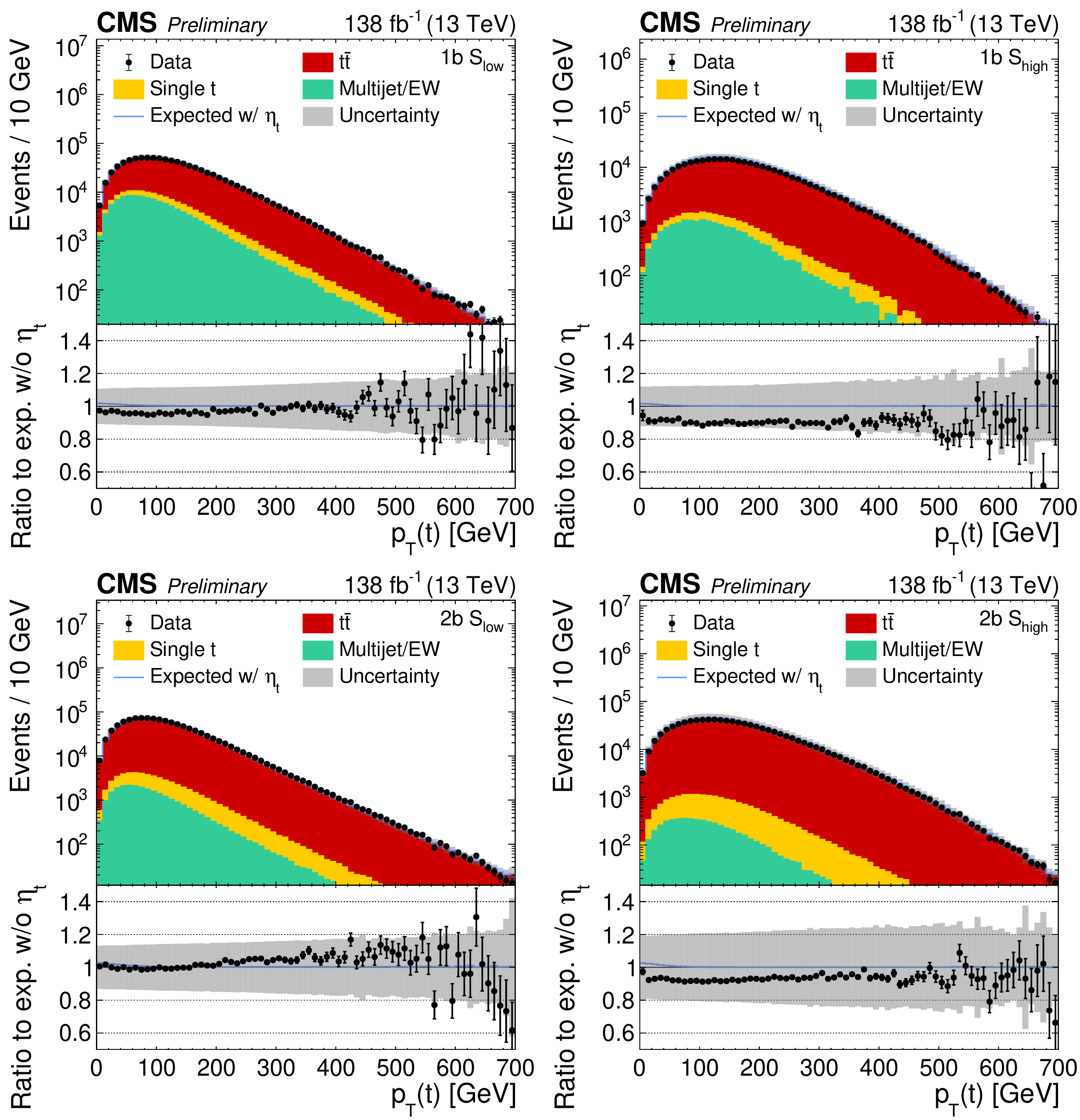
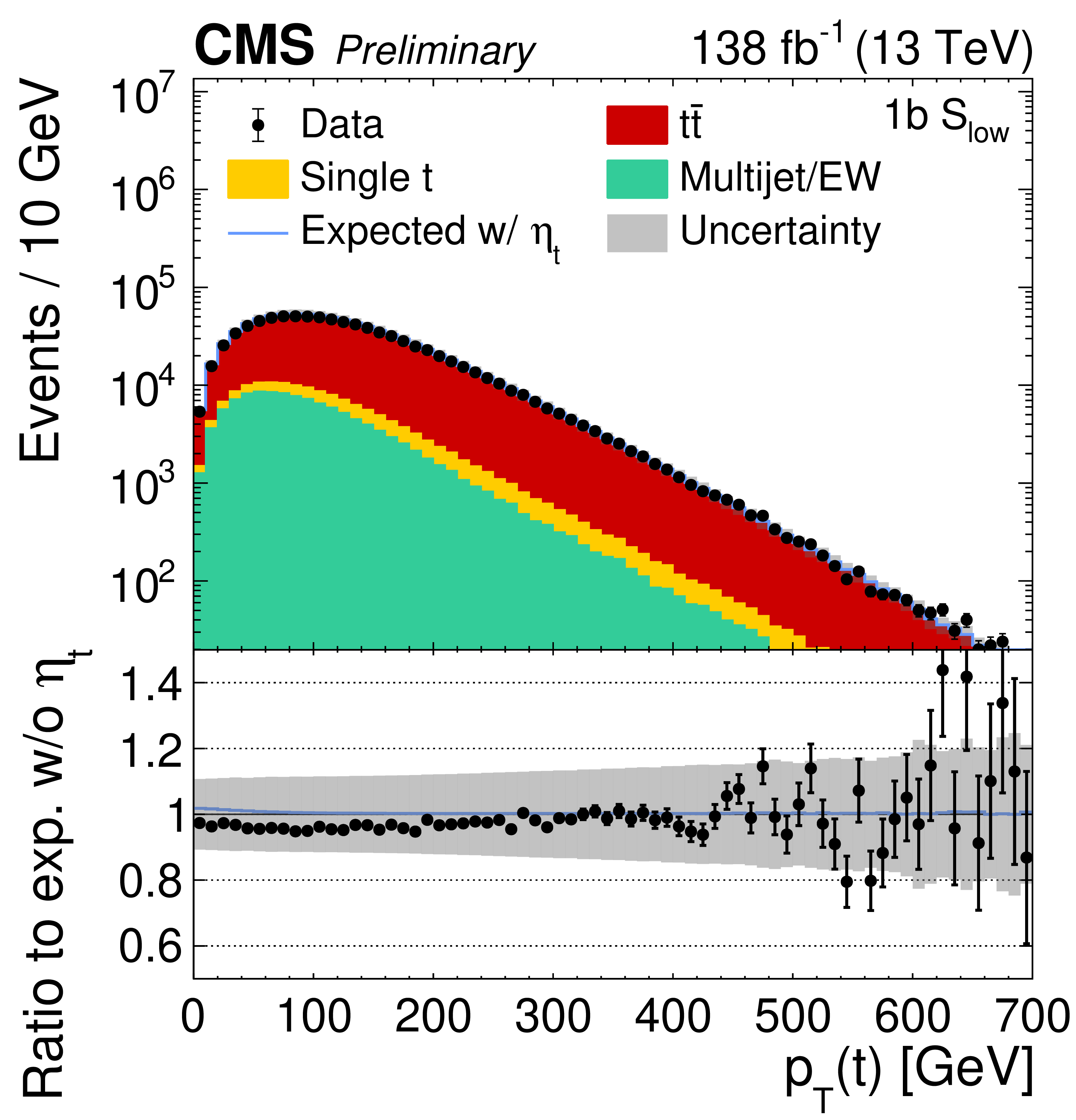
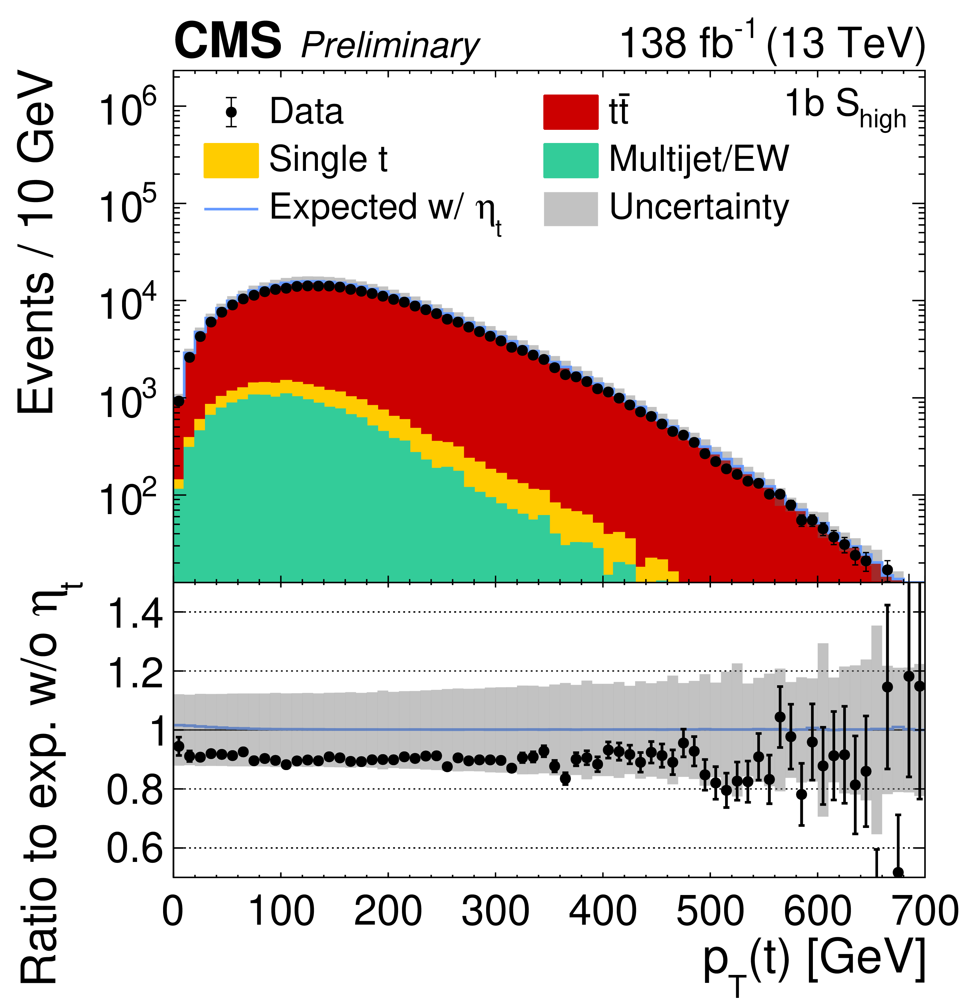
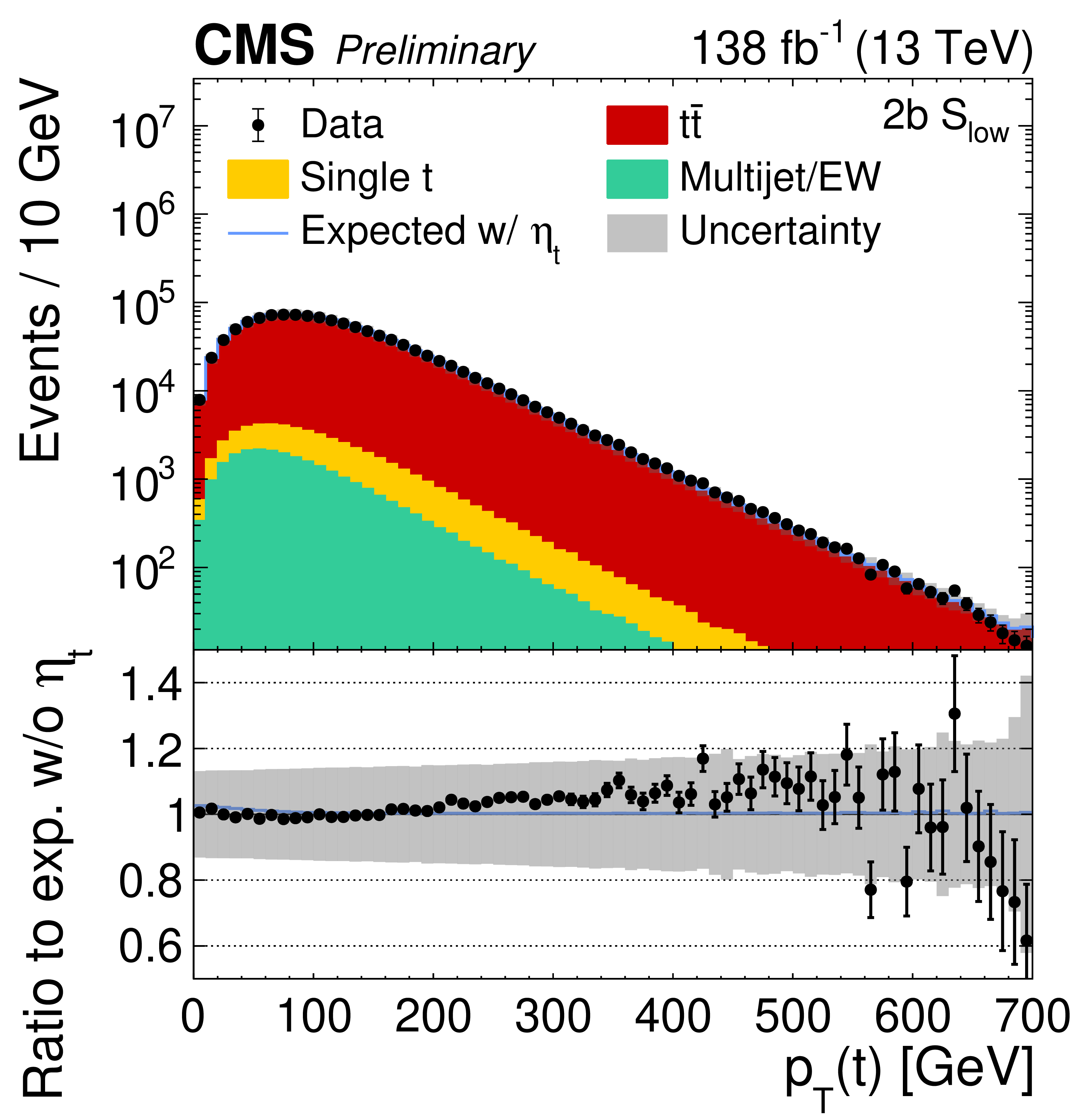
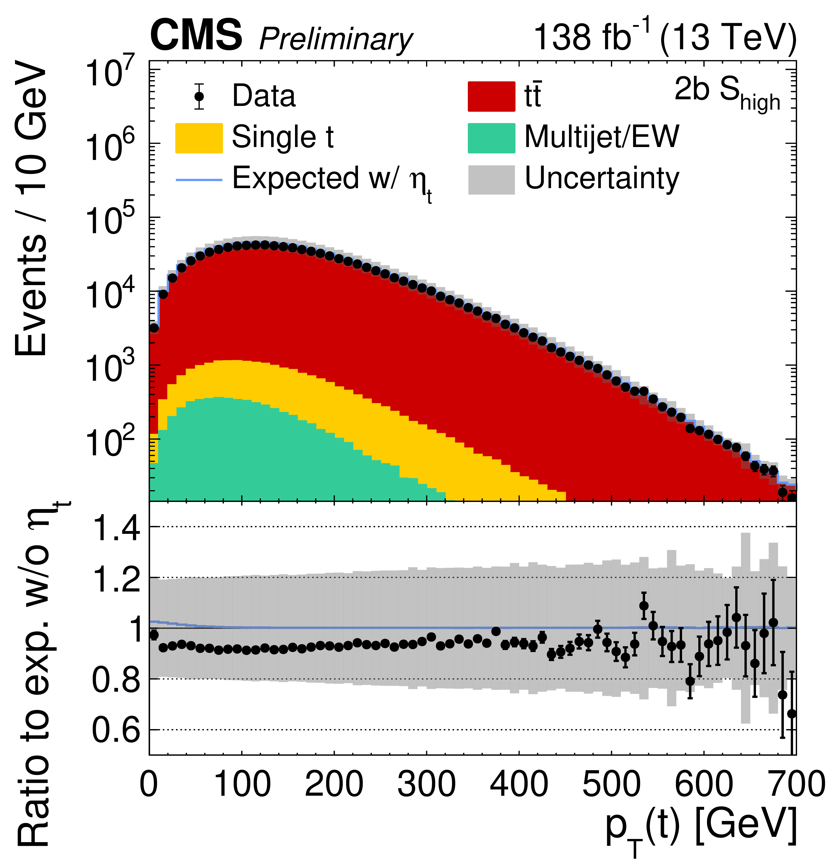
Figure 7:
Pre-fit distributions of $ p_{\mathrm{T}}(\mathrm{t}) $ in all four categories. The data (points) are compared to the predictions without $ \eta \mathrm{t} $ (stacked histograms) and those including it (blue line). The $ \mathrm{t} \overline{\mathrm{t}} $ and single top quark contributions are taken from simulation, while the multijet+EW background is derived from the CR. The gray uncertainty band represents the combined statistical and systematic uncertainties in the predictions, while the vertical bars on the data points indicate their statistical uncertainties. The ratios to the predicted yields excluding $ \eta \mathrm{t} $ are shown in the lower panels. |
png pdf |
Figure 7-a:
Pre-fit distributions of $ p_{\mathrm{T}}(\mathrm{t}) $ in all four categories. The data (points) are compared to the predictions without $ \eta \mathrm{t} $ (stacked histograms) and those including it (blue line). The $ \mathrm{t} \overline{\mathrm{t}} $ and single top quark contributions are taken from simulation, while the multijet+EW background is derived from the CR. The gray uncertainty band represents the combined statistical and systematic uncertainties in the predictions, while the vertical bars on the data points indicate their statistical uncertainties. The ratios to the predicted yields excluding $ \eta \mathrm{t} $ are shown in the lower panels. |
png pdf |
Figure 7-b:
Pre-fit distributions of $ p_{\mathrm{T}}(\mathrm{t}) $ in all four categories. The data (points) are compared to the predictions without $ \eta \mathrm{t} $ (stacked histograms) and those including it (blue line). The $ \mathrm{t} \overline{\mathrm{t}} $ and single top quark contributions are taken from simulation, while the multijet+EW background is derived from the CR. The gray uncertainty band represents the combined statistical and systematic uncertainties in the predictions, while the vertical bars on the data points indicate their statistical uncertainties. The ratios to the predicted yields excluding $ \eta \mathrm{t} $ are shown in the lower panels. |
png pdf |
Figure 7-c:
Pre-fit distributions of $ p_{\mathrm{T}}(\mathrm{t}) $ in all four categories. The data (points) are compared to the predictions without $ \eta \mathrm{t} $ (stacked histograms) and those including it (blue line). The $ \mathrm{t} \overline{\mathrm{t}} $ and single top quark contributions are taken from simulation, while the multijet+EW background is derived from the CR. The gray uncertainty band represents the combined statistical and systematic uncertainties in the predictions, while the vertical bars on the data points indicate their statistical uncertainties. The ratios to the predicted yields excluding $ \eta \mathrm{t} $ are shown in the lower panels. |
png pdf |
Figure 7-d:
Pre-fit distributions of $ p_{\mathrm{T}}(\mathrm{t}) $ in all four categories. The data (points) are compared to the predictions without $ \eta \mathrm{t} $ (stacked histograms) and those including it (blue line). The $ \mathrm{t} \overline{\mathrm{t}} $ and single top quark contributions are taken from simulation, while the multijet+EW background is derived from the CR. The gray uncertainty band represents the combined statistical and systematic uncertainties in the predictions, while the vertical bars on the data points indicate their statistical uncertainties. The ratios to the predicted yields excluding $ \eta \mathrm{t} $ are shown in the lower panels. |
png pdf |
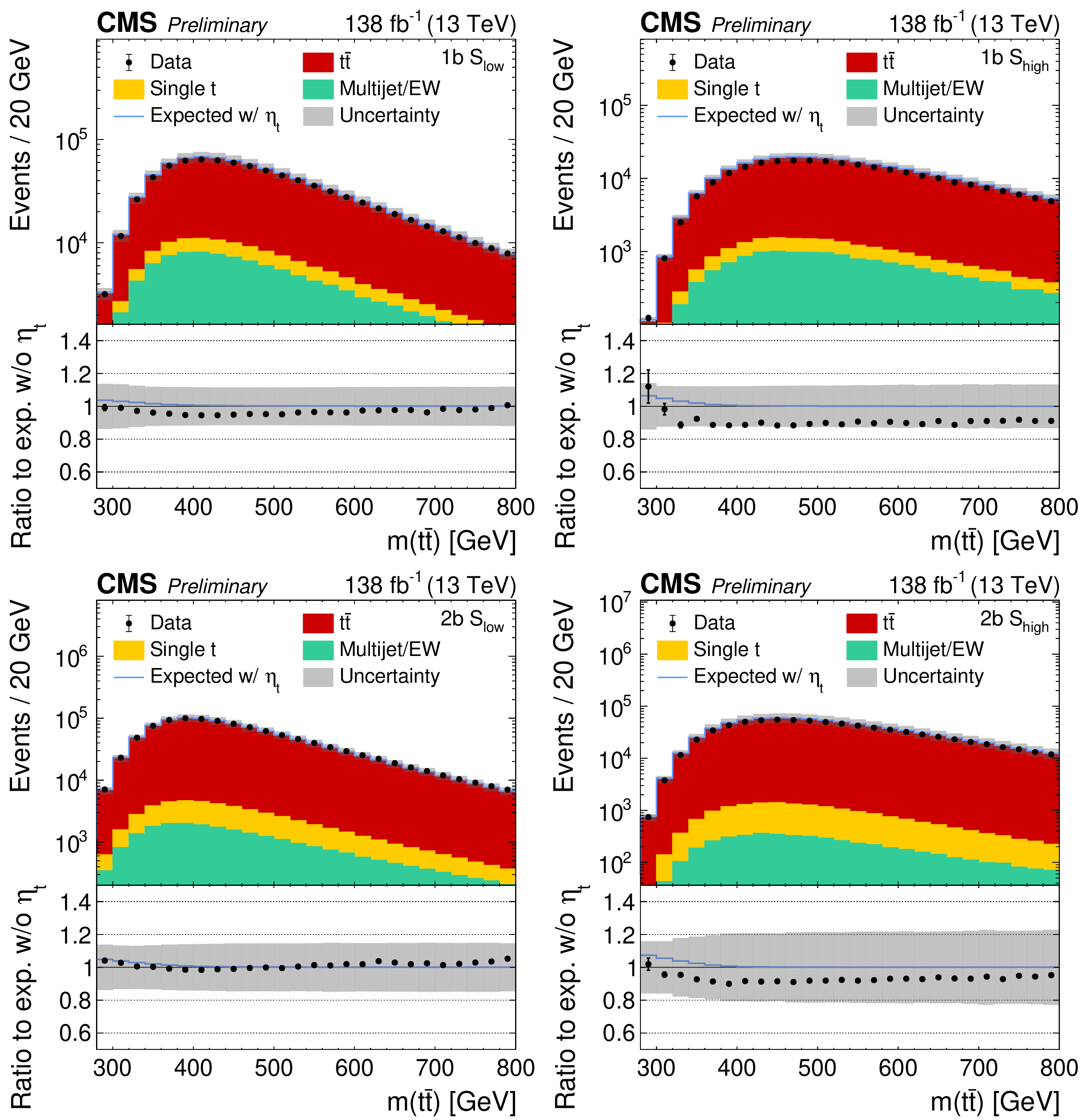
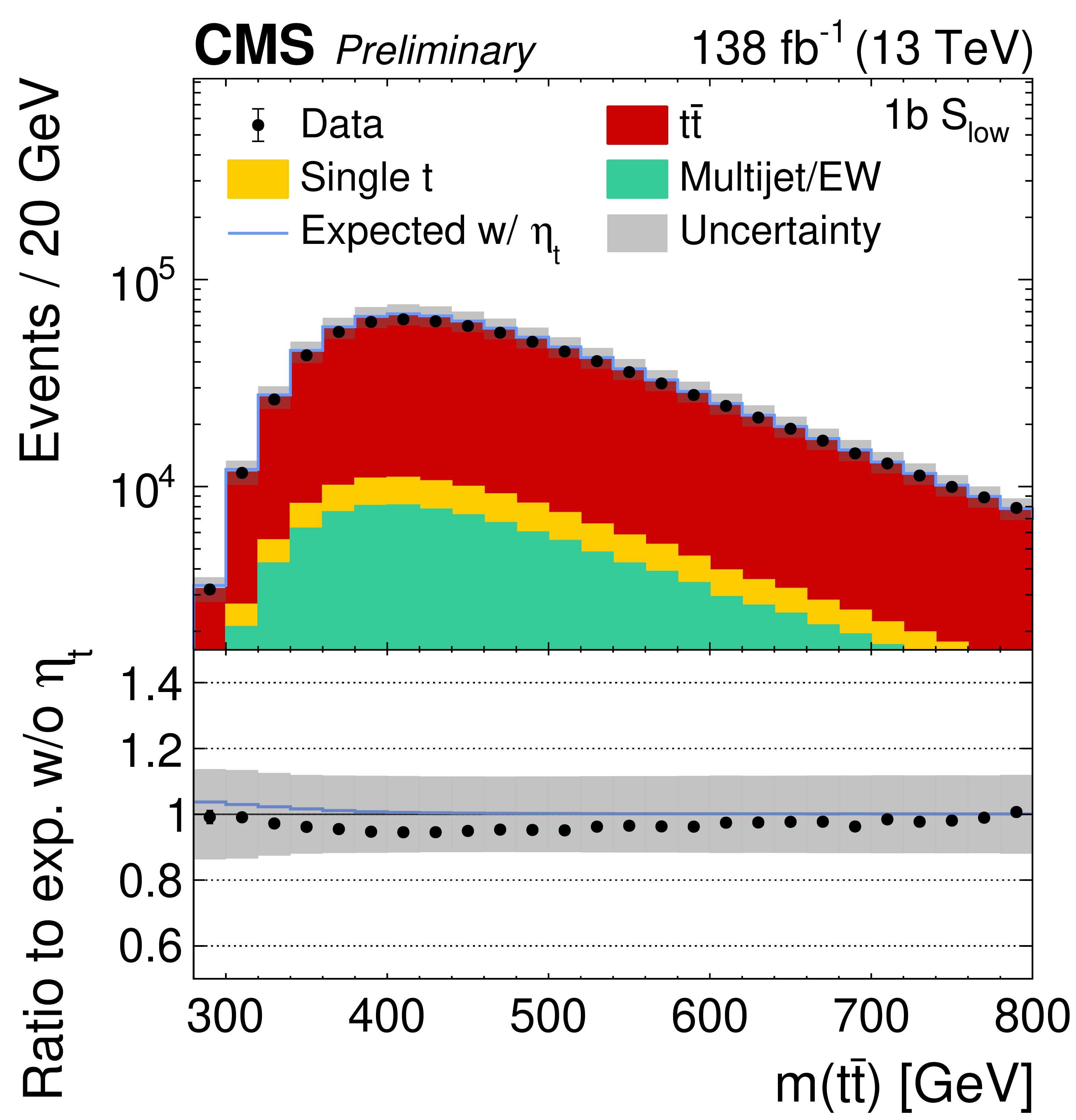
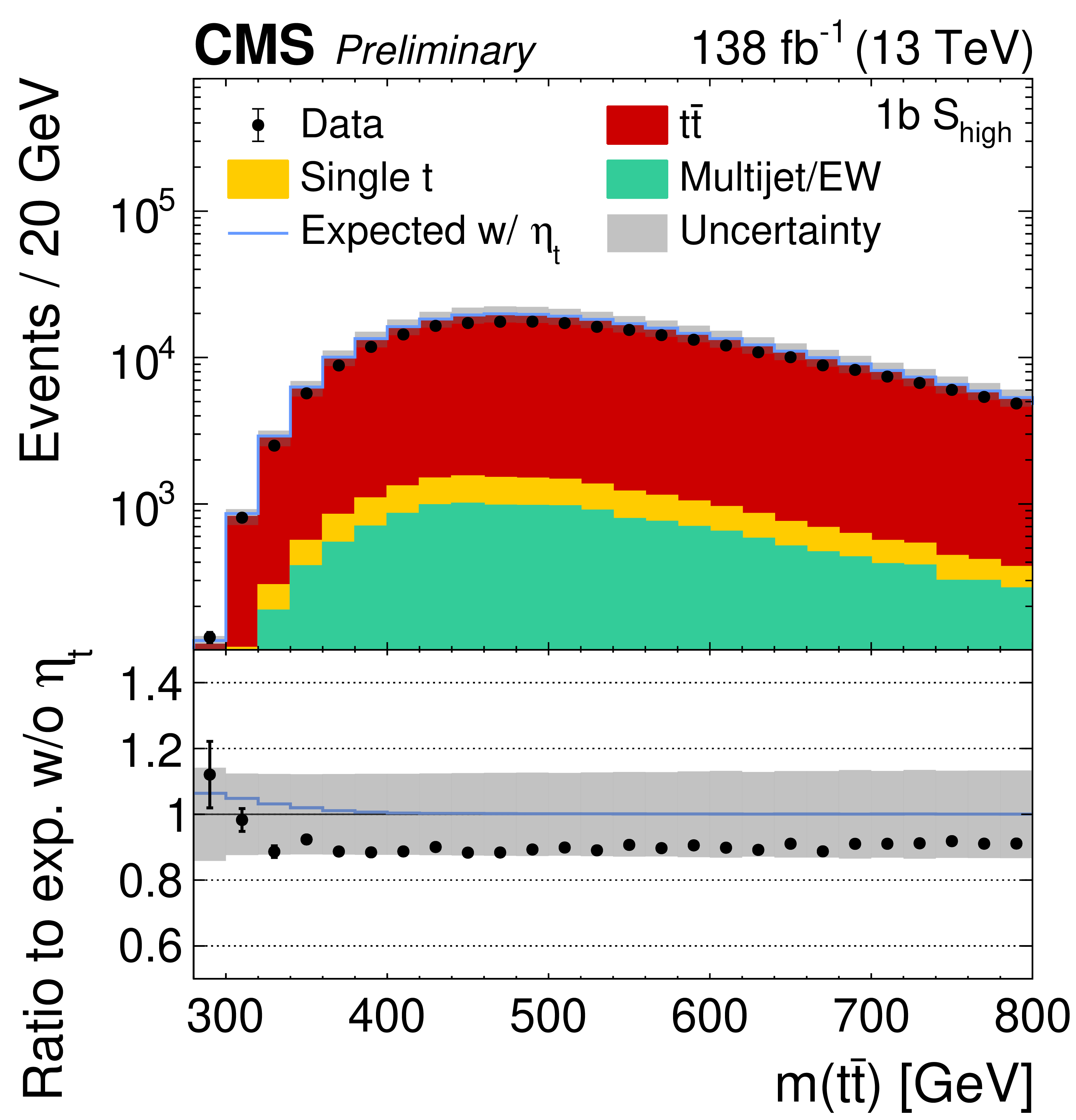
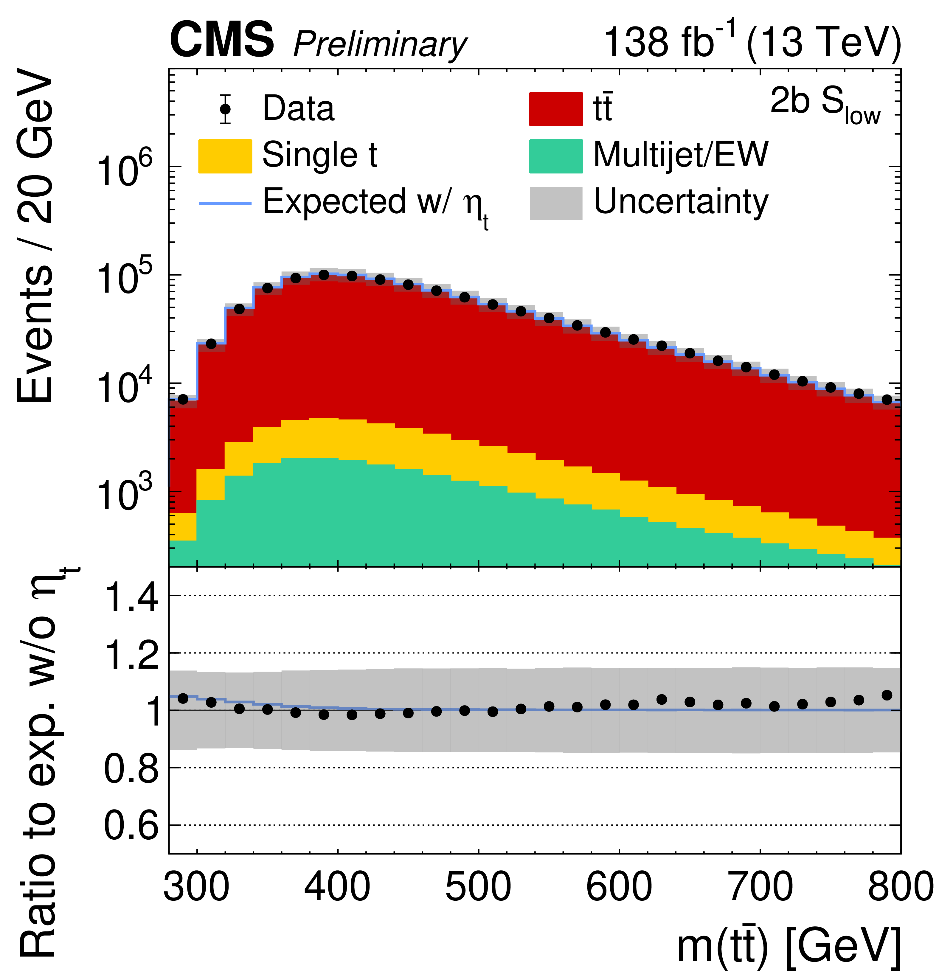
Figure 8:
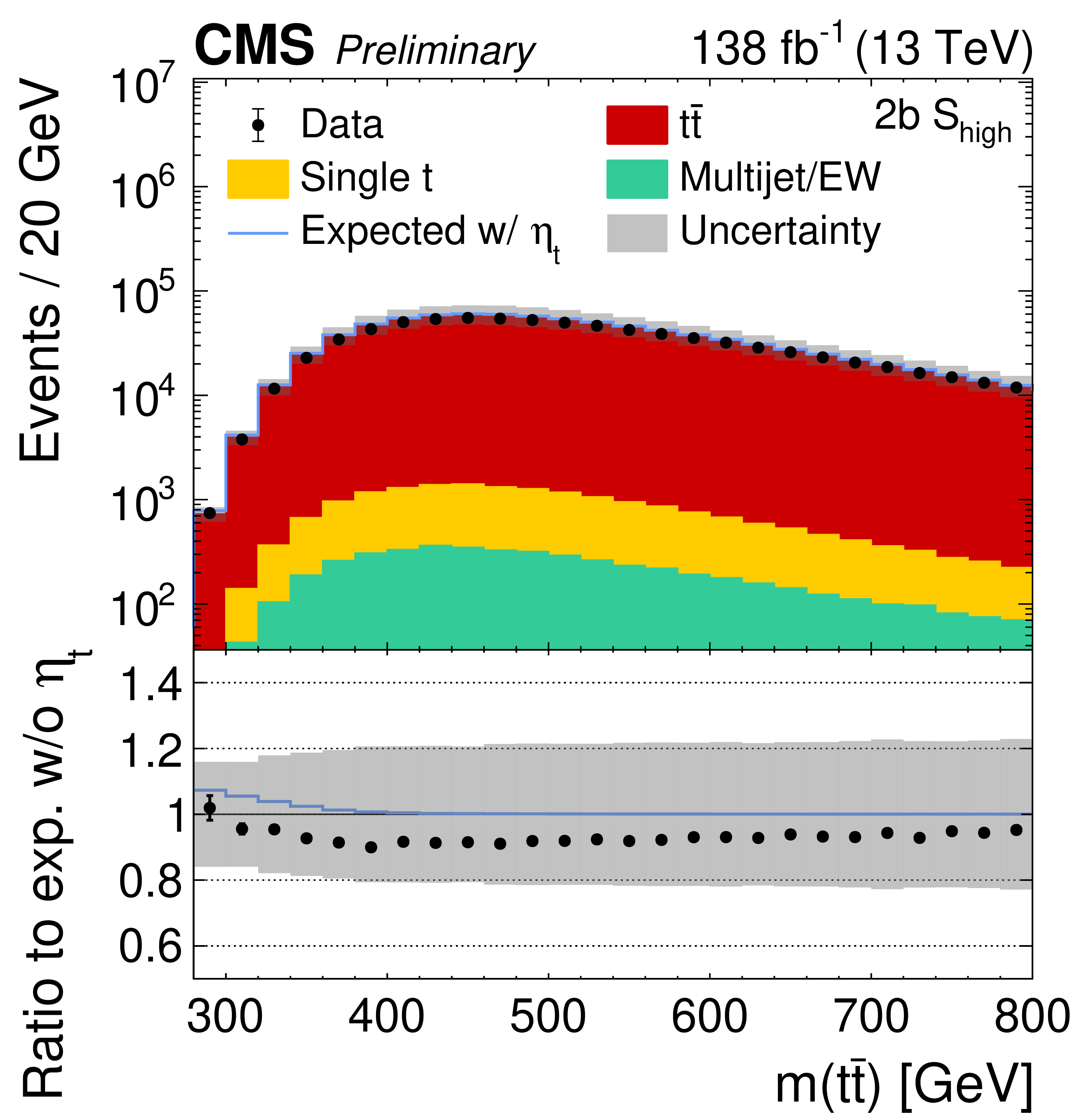
Pre-fit distributions of $ m({\mathrm{t}\overline{\mathrm{t}}} ) $ in all four categories. The data (points) are compared to the predictions without $ \eta \mathrm{t} $ (stacked histograms) and those including it (blue line). The $ \mathrm{t} \overline{\mathrm{t}} $ and single top quark contributions are taken from simulation, while the multijet+EW background is derived from the CR. The gray uncertainty band represents the combined statistical and systematic uncertainties in the predictions, while the vertical bars on the data points indicate their statistical uncertainties. The ratios to the predicted yields excluding $ \eta \mathrm{t} $ are shown in the lower panels. |
png pdf |
Figure 8-a:
Pre-fit distributions of $ m({\mathrm{t}\overline{\mathrm{t}}} ) $ in all four categories. The data (points) are compared to the predictions without $ \eta \mathrm{t} $ (stacked histograms) and those including it (blue line). The $ \mathrm{t} \overline{\mathrm{t}} $ and single top quark contributions are taken from simulation, while the multijet+EW background is derived from the CR. The gray uncertainty band represents the combined statistical and systematic uncertainties in the predictions, while the vertical bars on the data points indicate their statistical uncertainties. The ratios to the predicted yields excluding $ \eta \mathrm{t} $ are shown in the lower panels. |
png pdf |
Figure 8-b:
Pre-fit distributions of $ m({\mathrm{t}\overline{\mathrm{t}}} ) $ in all four categories. The data (points) are compared to the predictions without $ \eta \mathrm{t} $ (stacked histograms) and those including it (blue line). The $ \mathrm{t} \overline{\mathrm{t}} $ and single top quark contributions are taken from simulation, while the multijet+EW background is derived from the CR. The gray uncertainty band represents the combined statistical and systematic uncertainties in the predictions, while the vertical bars on the data points indicate their statistical uncertainties. The ratios to the predicted yields excluding $ \eta \mathrm{t} $ are shown in the lower panels. |
png pdf |
Figure 8-c:
Pre-fit distributions of $ m({\mathrm{t}\overline{\mathrm{t}}} ) $ in all four categories. The data (points) are compared to the predictions without $ \eta \mathrm{t} $ (stacked histograms) and those including it (blue line). The $ \mathrm{t} \overline{\mathrm{t}} $ and single top quark contributions are taken from simulation, while the multijet+EW background is derived from the CR. The gray uncertainty band represents the combined statistical and systematic uncertainties in the predictions, while the vertical bars on the data points indicate their statistical uncertainties. The ratios to the predicted yields excluding $ \eta \mathrm{t} $ are shown in the lower panels. |
png pdf |
Figure 8-d:
Pre-fit distributions of $ m({\mathrm{t}\overline{\mathrm{t}}} ) $ in all four categories. The data (points) are compared to the predictions without $ \eta \mathrm{t} $ (stacked histograms) and those including it (blue line). The $ \mathrm{t} \overline{\mathrm{t}} $ and single top quark contributions are taken from simulation, while the multijet+EW background is derived from the CR. The gray uncertainty band represents the combined statistical and systematic uncertainties in the predictions, while the vertical bars on the data points indicate their statistical uncertainties. The ratios to the predicted yields excluding $ \eta \mathrm{t} $ are shown in the lower panels. |
png pdf |
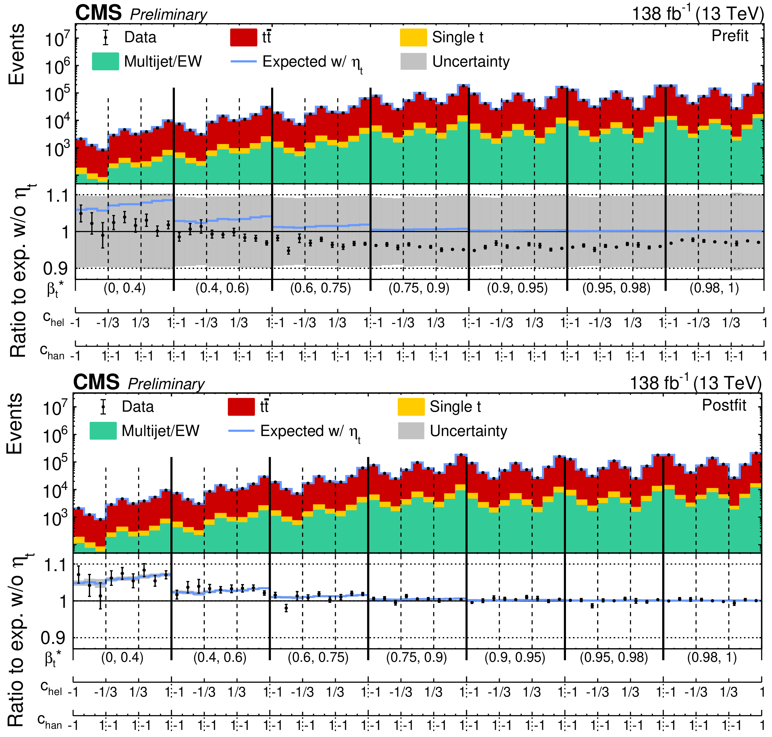
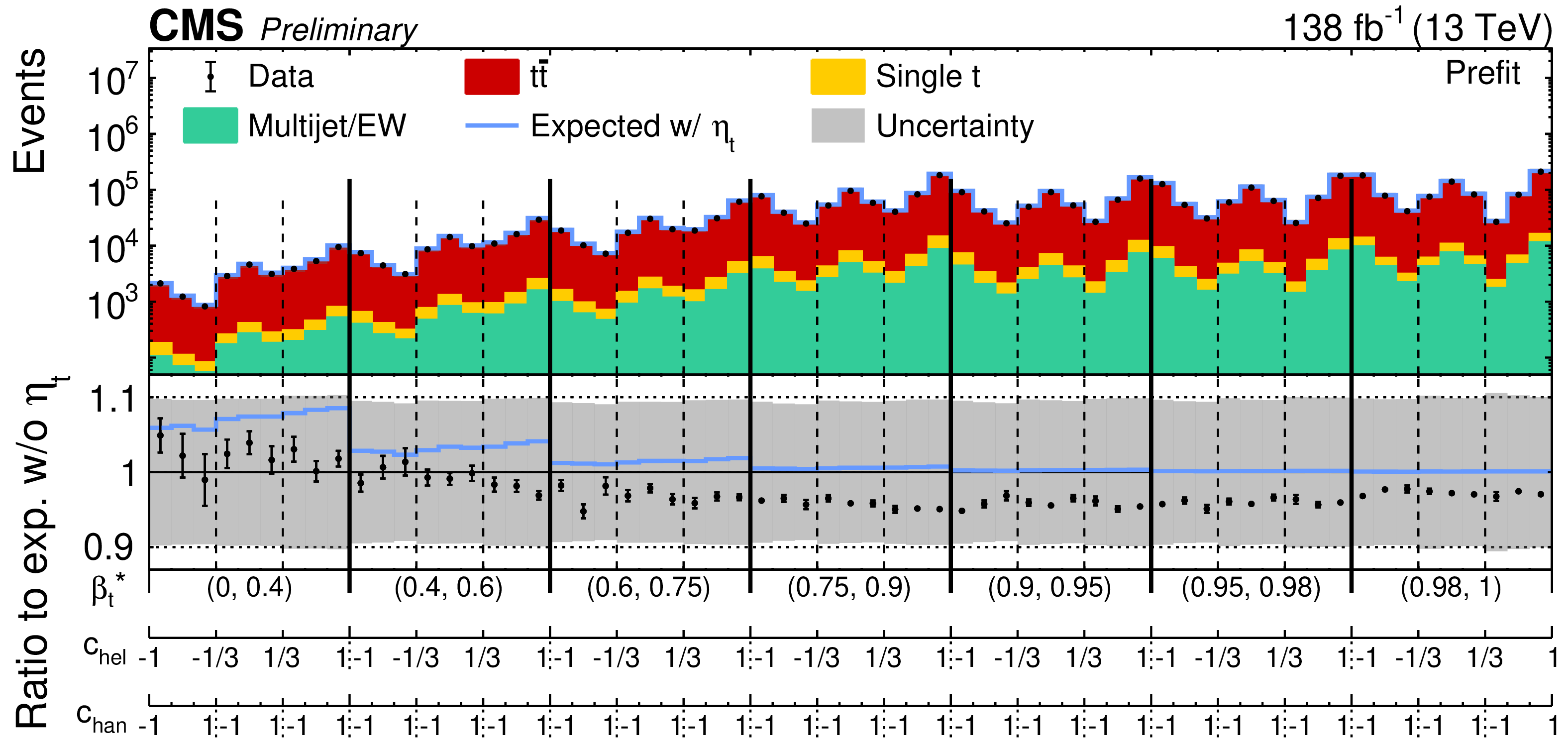
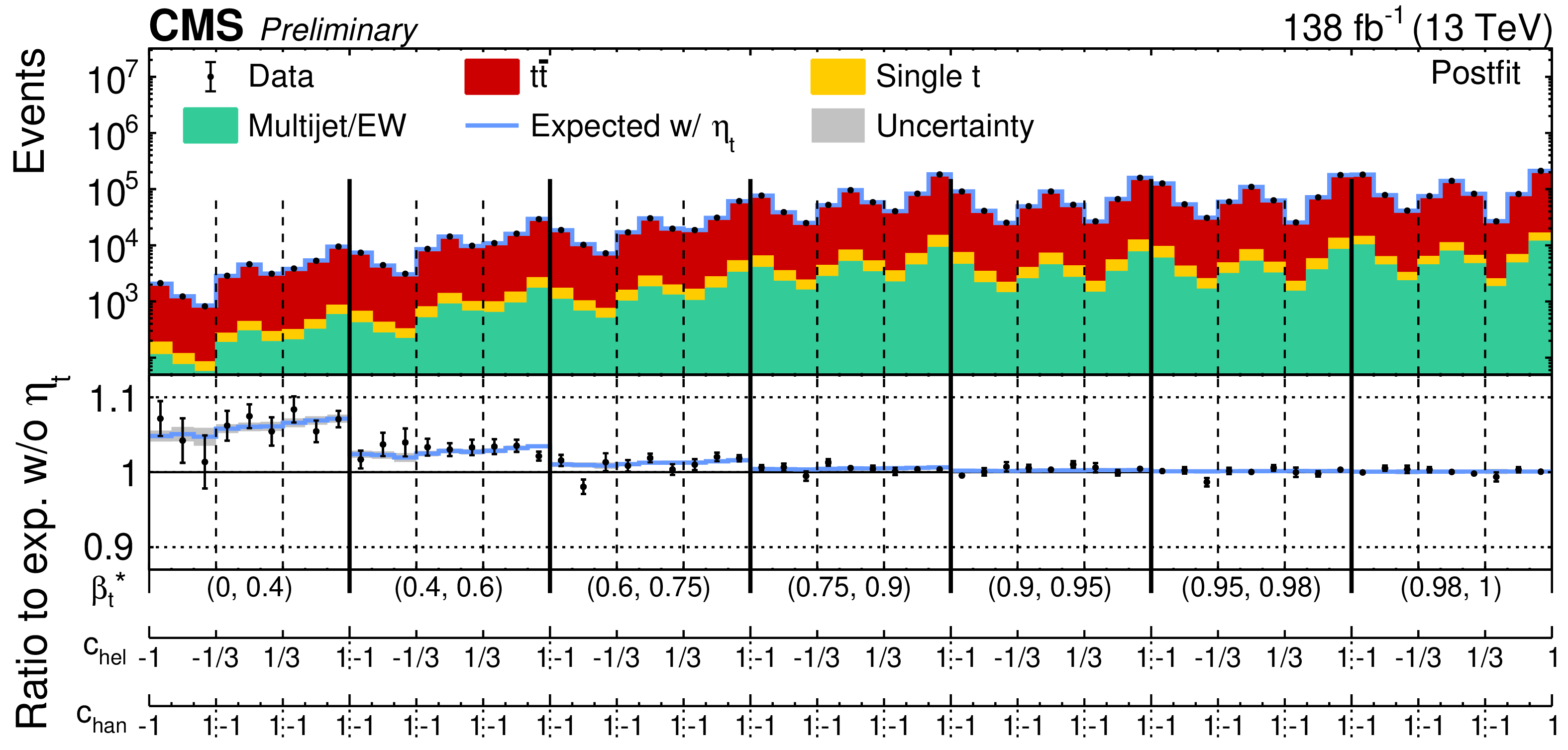
Figure 9:
Pre-fit (upper) and post-fit (lower) $ \beta_{\mathrm{t}}^{*} \times c_\mathrm{hel} \times c_\mathrm{han} $ distributions with all signal categories and data-taking periods combined. The data (points) are compared with the predictions without $ \eta \mathrm{t} $ (stacked histograms) and those including it (blue line). The $ x $-axis shows bins of the unrolled three-dimensional distribution. The gray uncertainty band represents the combined statistical and systematic uncertainties in the predictions, while the vertical bars on the points indicate the statistical uncertainties in the data. The ratios to the predicted yields excluding $ \eta \mathrm{t} $ are shown in the lower panels. |
png pdf |
Figure 9-a:
Pre-fit (upper) and post-fit (lower) $ \beta_{\mathrm{t}}^{*} \times c_\mathrm{hel} \times c_\mathrm{han} $ distributions with all signal categories and data-taking periods combined. The data (points) are compared with the predictions without $ \eta \mathrm{t} $ (stacked histograms) and those including it (blue line). The $ x $-axis shows bins of the unrolled three-dimensional distribution. The gray uncertainty band represents the combined statistical and systematic uncertainties in the predictions, while the vertical bars on the points indicate the statistical uncertainties in the data. The ratios to the predicted yields excluding $ \eta \mathrm{t} $ are shown in the lower panels. |
png pdf |
Figure 9-b:
Pre-fit (upper) and post-fit (lower) $ \beta_{\mathrm{t}}^{*} \times c_\mathrm{hel} \times c_\mathrm{han} $ distributions with all signal categories and data-taking periods combined. The data (points) are compared with the predictions without $ \eta \mathrm{t} $ (stacked histograms) and those including it (blue line). The $ x $-axis shows bins of the unrolled three-dimensional distribution. The gray uncertainty band represents the combined statistical and systematic uncertainties in the predictions, while the vertical bars on the points indicate the statistical uncertainties in the data. The ratios to the predicted yields excluding $ \eta \mathrm{t} $ are shown in the lower panels. |
png pdf |
Figure 10:
Post-fit $ S_{\text{NN}} $ distributions for the 1b (left) and 2b (right) categories. The data (points) are compared with the predictions without $ \eta \mathrm{t} $ (stacked histograms) and those including it (blue line). The gray uncertainty band represents the post-fit combined statistical and systematic uncertainties in the predictions, while the vertical bars on the points indicate the statistical uncertainties in the data. The ratios to the predicted yields excluding $ \eta \mathrm{t} $ are shown in the lower panels. |
png pdf |
Figure 10-a:
Post-fit $ S_{\text{NN}} $ distributions for the 1b (left) and 2b (right) categories. The data (points) are compared with the predictions without $ \eta \mathrm{t} $ (stacked histograms) and those including it (blue line). The gray uncertainty band represents the post-fit combined statistical and systematic uncertainties in the predictions, while the vertical bars on the points indicate the statistical uncertainties in the data. The ratios to the predicted yields excluding $ \eta \mathrm{t} $ are shown in the lower panels. |
png pdf |
Figure 10-b:
Post-fit $ S_{\text{NN}} $ distributions for the 1b (left) and 2b (right) categories. The data (points) are compared with the predictions without $ \eta \mathrm{t} $ (stacked histograms) and those including it (blue line). The gray uncertainty band represents the post-fit combined statistical and systematic uncertainties in the predictions, while the vertical bars on the points indicate the statistical uncertainties in the data. The ratios to the predicted yields excluding $ \eta \mathrm{t} $ are shown in the lower panels. |
png pdf |
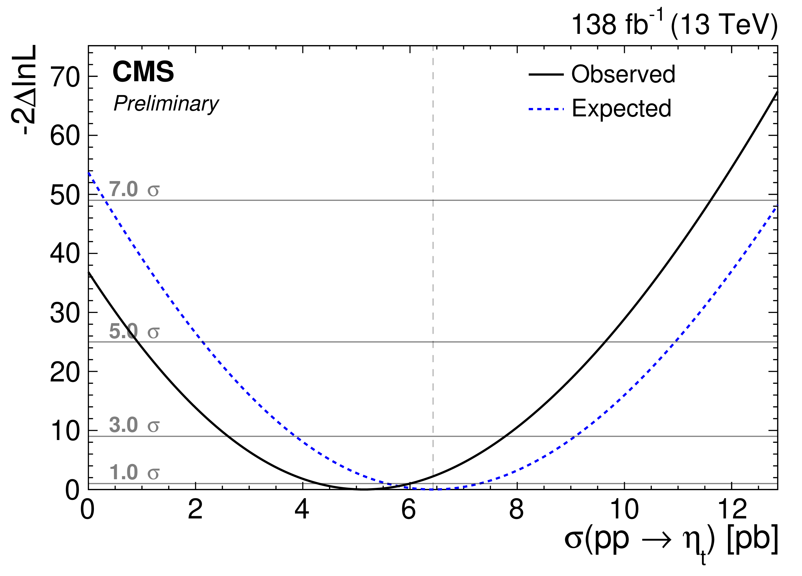
Figure 11:
Observed (black solid line) and expected (blue dashed line) negative log-likelihood ratio scan as a function of the total $ \eta \mathrm{t} $ cross section. The gray horizontal lines represent the confidence intervals at the indicated standard deviation ($ \sigma $) levels. The vertical dashed line marks the nominal signal hypothesis $ (\mu=1) $, corresponding to a cross section of 6.43\unitpb. |
png pdf |
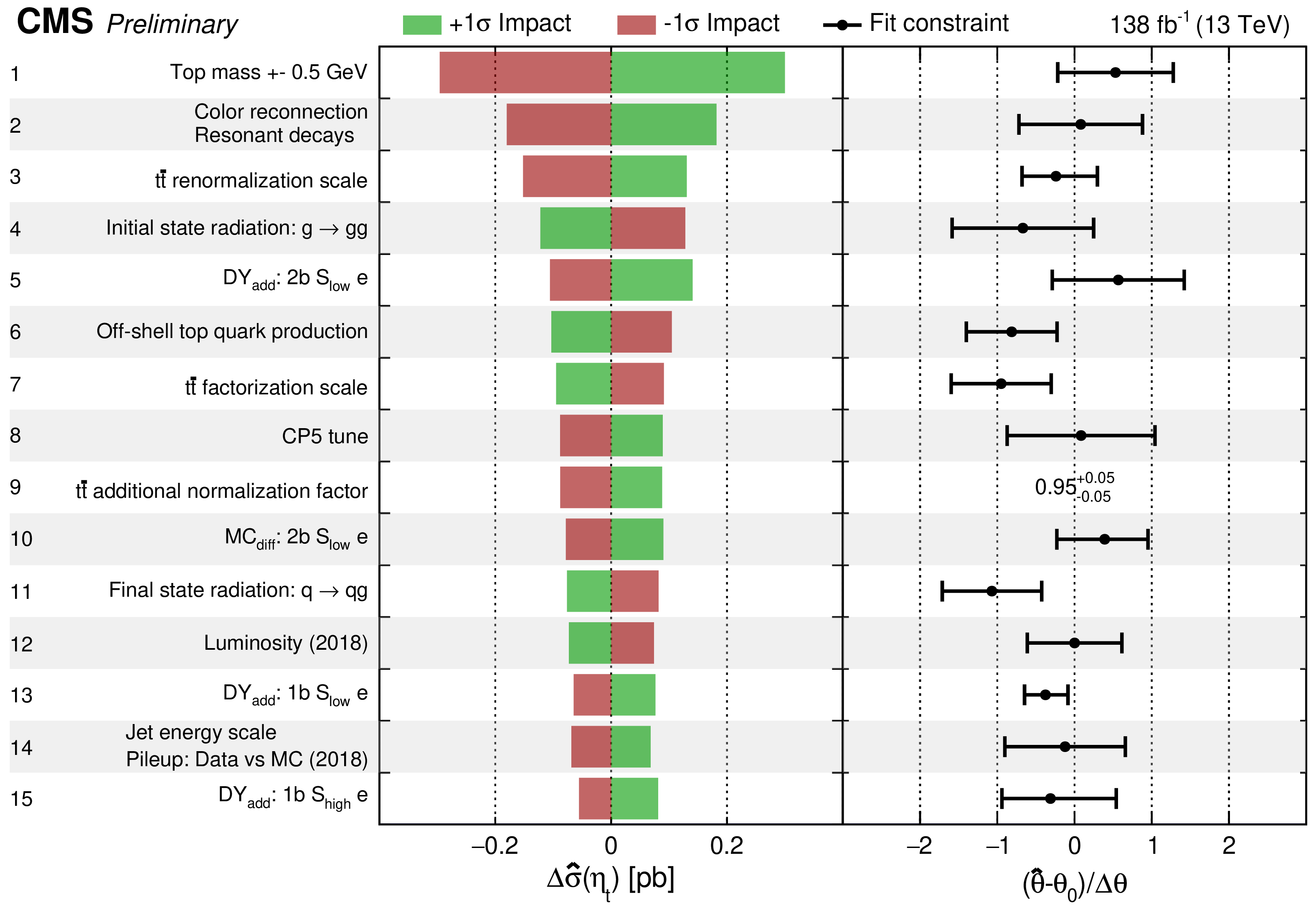
Figure 12:
Impact of the 15 most significant systematic uncertainties on the measured $ \eta \mathrm{t} $ cross section $ \hat{\sigma}({\eta}{\mathrm{t}} ) $. The left panel shows the impact $ \Delta\hat{\sigma}({\eta}{\mathrm{t}} ) $ on the measurement when varying each nuisance parameter by $ +1\sigma $ and $ -1\sigma $ of its pre-fit uncertainty, represented by green and red bars, respectively. The right panel displays the pulls of the nuisance parameters, defined as $ (\hat{\theta} - \theta_{0})/\Delta\theta $, where $ \hat{\theta} $ is the post-fit value, $ \theta_{0} $ is the pre-fit value, and $ \Delta\theta $ is the pre-fit uncertainty. |
png pdf |
Figure 13:
Post-fit distributions of $ \beta_{\mathrm{t}}^{*} $ (upper left), $ c_\mathrm{hel} $ (upper right), and $ c_\mathrm{han} $ (lower) for all four signal categories combined. The $ \beta_{\mathrm{t}}^{*} $ distribution is integrated over $ c_\mathrm{hel} $ and $ c_\mathrm{han} $, while the $ c_\mathrm{hel} $ ($ c_\mathrm{han} $) distribution is integrated over $ c_\mathrm{han} $ ($ c_\mathrm{hel} $) and the first three bins of $ \beta_{\mathrm{t}}^{*} $ ($ \beta_{\mathrm{t}}^{*} < $ 0.75). The data (points) are compared to the predictions without $ \eta \mathrm{t} $ (stacked histograms) and those including it (blue line). The gray uncertainty band represents the combined statistical and systematic uncertainties in the prediction. The vertical bars on the points indicate the statistical uncertainty in the data. The ratios to predicted yields excluding $ \eta \mathrm{t} $ are shown in the lower panels. |
png pdf |
Figure 13-a:
Post-fit distributions of $ \beta_{\mathrm{t}}^{*} $ (upper left), $ c_\mathrm{hel} $ (upper right), and $ c_\mathrm{han} $ (lower) for all four signal categories combined. The $ \beta_{\mathrm{t}}^{*} $ distribution is integrated over $ c_\mathrm{hel} $ and $ c_\mathrm{han} $, while the $ c_\mathrm{hel} $ ($ c_\mathrm{han} $) distribution is integrated over $ c_\mathrm{han} $ ($ c_\mathrm{hel} $) and the first three bins of $ \beta_{\mathrm{t}}^{*} $ ($ \beta_{\mathrm{t}}^{*} < $ 0.75). The data (points) are compared to the predictions without $ \eta \mathrm{t} $ (stacked histograms) and those including it (blue line). The gray uncertainty band represents the combined statistical and systematic uncertainties in the prediction. The vertical bars on the points indicate the statistical uncertainty in the data. The ratios to predicted yields excluding $ \eta \mathrm{t} $ are shown in the lower panels. |
png pdf |
Figure 13-b:
Post-fit distributions of $ \beta_{\mathrm{t}}^{*} $ (upper left), $ c_\mathrm{hel} $ (upper right), and $ c_\mathrm{han} $ (lower) for all four signal categories combined. The $ \beta_{\mathrm{t}}^{*} $ distribution is integrated over $ c_\mathrm{hel} $ and $ c_\mathrm{han} $, while the $ c_\mathrm{hel} $ ($ c_\mathrm{han} $) distribution is integrated over $ c_\mathrm{han} $ ($ c_\mathrm{hel} $) and the first three bins of $ \beta_{\mathrm{t}}^{*} $ ($ \beta_{\mathrm{t}}^{*} < $ 0.75). The data (points) are compared to the predictions without $ \eta \mathrm{t} $ (stacked histograms) and those including it (blue line). The gray uncertainty band represents the combined statistical and systematic uncertainties in the prediction. The vertical bars on the points indicate the statistical uncertainty in the data. The ratios to predicted yields excluding $ \eta \mathrm{t} $ are shown in the lower panels. |
png pdf |
Figure 13-c:
Post-fit distributions of $ \beta_{\mathrm{t}}^{*} $ (upper left), $ c_\mathrm{hel} $ (upper right), and $ c_\mathrm{han} $ (lower) for all four signal categories combined. The $ \beta_{\mathrm{t}}^{*} $ distribution is integrated over $ c_\mathrm{hel} $ and $ c_\mathrm{han} $, while the $ c_\mathrm{hel} $ ($ c_\mathrm{han} $) distribution is integrated over $ c_\mathrm{han} $ ($ c_\mathrm{hel} $) and the first three bins of $ \beta_{\mathrm{t}}^{*} $ ($ \beta_{\mathrm{t}}^{*} < $ 0.75). The data (points) are compared to the predictions without $ \eta \mathrm{t} $ (stacked histograms) and those including it (blue line). The gray uncertainty band represents the combined statistical and systematic uncertainties in the prediction. The vertical bars on the points indicate the statistical uncertainty in the data. The ratios to predicted yields excluding $ \eta \mathrm{t} $ are shown in the lower panels. |
png pdf |
Figure 14:
Pre-fit comparison of the $ \eta \mathrm{t} $ (blue) and $ {\mathrm{t}\overline{\mathrm{t}}} _{\text{NRQCD}} $ (orange) models in the $ \beta_{\mathrm{t}}^{*} \times c_\mathrm{hel} \times c_\mathrm{han} $ binning used for the signal extraction for all four signal categories combined, shown as ratios to the continuum $ \mathrm{t} \overline{\mathrm{t}} $ at NNLO QCD accuracy. The continuum $ \mathrm{t} \overline{\mathrm{t}} $ at NLO QCD accuracy normalized to the NNLO total cross section (red) is also shown for reference. |
| Summary |
| A search for the color-singlet pseudoscalar toponium quasi-bound-state was conducted using pp collision data collected by the CMS experiment from 2016 to 2018 at $ \sqrt{s} = $ 13 TeV. While previous studies utilized the \text{dilepton} channel, this analysis performs the search in the $ \mathrm{e}/\mu $+jets channel for the first time. The strategy leverages the variables $ c_\mathrm{hel} $, $ c_\mathrm{han} $, and $ \beta_{\mathrm{t}}^{*} $, the latter of which is more sensitive to the $ \eta \mathrm{t} $ signal and more robust against certain uncertainties. The background-only hypothesis is excluded with an observed (expected) significance of 6.1(7.3) $ \sigma $. The total $ \eta \mathrm{t} $ production cross section is measured to be 5.1 $ \pm $ 0.9 pb with main uncertainties from the modeling of the $ \mathrm{t} \overline{\mathrm{t}} $ background. This result provides an independent confirmation of the excess reported in the dilepton channel. It is important to note that this study relies solely on a simplified model, and further theoretical investigations are needed to accurately model the $ \mathrm{t} \overline{\mathrm{t}} $ threshold region. |
| References | ||||
| 1 | Particle Data Group , S. Navas et al. | Review of particle physics | PRD 110 (2024) 030001 | |
| 2 | I. Bigi et al. | Production and decay properties of ultra-heavy quarks | PLB 181 (1986) 157 | |
| 3 | V. S. Fadin, V. A. Khoze, and T. Sjöstrand | On the threshold behaviour of heavy top production | Z. Phys. C 48 (1990) 613 | |
| 4 | Y. Kiyo et al. | Top-quark pair production near threshold at LHC | EPJC 60 (2009) 375 | 0812.0919 |
| 5 | K. Hagiwara, Y. Sumino, and H. Yokoya | Bound-state effects on top quark production at hadron colliders | PLB 666 (2008) 71 | 0804.1014 |
| 6 | Y. Sumino and H. Yokoya | Bound-state effects on kinematical distributions of top quarks at hadron colliders | JHEP 09 (2010) 034 | 1007.0075 |
| 7 | W.-L. Ju et al. | Top quark pair production near threshold: single/double distributions and mass determination | JHEP 06 (2020) 158 | 2004.03088 |
| 8 | B. Fuks, K. Hagiwara, K. Ma, and Y.-J. Zheng | Signatures of toponium formation in LHC run 2 data | PRD 104 (2021) 034023 | 2102.11281 |
| 9 | M. V. Garzelli et al. | Updated predictions for toponium production at the LHC | PLB 866 (2025) 139532 | 2412.16685 |
| 10 | B. Fuks, K. Hagiwara, K. Ma, and Y.-J. Zheng | Simulating toponium formation signals at the LHC | EPJC 85 (2025) 157 | 2411.18962 |
| 11 | CMS Collaboration | Observation of a pseudoscalar excess at the top quark pair production threshold | Reports on Progress in Physics 88 (2025) 087801 | CMS-TOP-24-007 2503.22382 |
| 12 | ATLAS Collaboration | Observation of a cross-section enhancement near the $ {\mathrm{t}\overline{\mathrm{t}}} $ production threshold in $ \sqrt{s}= $ 13 tev $ {\mathrm{p}\mathrm{p}} $ collisions with the ATLAS detector | Technical Report ATLAS-CONF-2025-008, 2025 | |
| 13 | CMS Collaboration | Search for heavy pseudoscalar and scalar bosons decaying to top quark pairs in proton-proton collisions at $ \sqrt{s}= $ 13 TeV | CMS Physics Analysis Summary, 2024 CMS-PAS-HIG-22-013 |
CMS-PAS-HIG-22-013 |
| 14 | W. Bernreuther, D. Heisler, and Z.-G. Si | A set of top quark spin correlation and polarization observables for the LHC: Standard model predictions and new physics contributions | JHEP 12 (2015) 026 | 1508.05271 |
| 15 | A. Brandenburg, Z. G. Si, and P. Uwer | QCD corrected spin analyzing power of jets in decays of polarized top quarks | PLB 539 (2002) 235 | hep-ph/0205023 |
| 16 | CMS Collaboration | The CMS experiment at the CERN LHC | JINST 3 (2008) S08004 | |
| 17 | CMS Collaboration | Performance of the CMS Level-1 trigger in proton-proton collisions at $ \sqrt{s}= $ 13 TeV | JINST 15 (2020) P10017 | CMS-TRG-17-001 2006.10165 |
| 18 | CMS Collaboration | The CMS trigger system | JINST 12 (2017) P01020 | CMS-TRG-12-001 1609.02366 |
| 19 | CMS Collaboration | Particle-flow reconstruction and global event description with the CMS detector | JINST 12 (2017) P10003 | CMS-PRF-14-001 1706.04965 |
| 20 | CMS Collaboration | Technical proposal for the Phase-II upgrade of the Compact Muon Solenoid | CMS Technical Proposal CERN-LHCC-2015-010, CMS-TDR-15-02, 2015 link |
|
| 21 | J. Alwall et al. | The automated computation of tree-level and next-to-leading order differential cross sections, and their matching to parton shower simulations | JHEP 07 (2014) 079 | 1405.0301 |
| 22 | T. Sjöstrand et al. | An introduction to PYTHIA8.2 | Comput. Phys. Commun. 191 (2015) 159 | 1410.3012 |
| 23 | CMS Collaboration | Extraction and validation of a new set of CMS PYTHIA8 tunes from underlying-event measurements | EPJC 80 (2020) 4 | CMS-GEN-17-001 1903.12179 |
| 24 | P. Nason | A new method for combining NLO QCD with shower Monte Carlo algorithms | JHEP 11 (2004) 040 | hep-ph/0409146 |
| 25 | S. Frixione, P. Nason, and C. Oleari | Matching NLO QCD computations with parton shower simulations: the POWHEG method | JHEP 11 (2007) 070 | 0709.2092 |
| 26 | S. Frixione, G. Ridolfi, and P. Nason | A positive-weight next-to-leading-order Monte Carlo for heavy flavour hadroproduction | JHEP 09 (2007) 126 | 0707.3088 |
| 27 | A. Andreassen and B. Nachman | Neural networks for full phase-space reweighting and parameter tuning | PRD 101 (2020) 091901 | 1907.08209 |
| 28 | CMS Collaboration | Machine learning approaches for parameter reweighting in MC samples of top quark production in CMS | CMS Detector Performance Note CMS-DP-2023-031, 2023 CDS |
|
| 29 | J. Mazzitelli et al. | Next-to-next-to-leading order event generation for top-quark pair production | PRL 127 (2021) 062001 | 2012.14267 |
| 30 | M. Aliev et al. | hathor: Hadronic top and heavy quarks cross section calculator | Comput. Phys. Commun. 182 (2011) 1034 | 1007.1327 |
| 31 | M. Czakon and A. Mitov | top++: a program for the calculation of the top-pair cross-section at hadron colliders | Comput. Phys. Commun. 185 (2014) 2930 | 1112.5675 |
| 32 | CMS Collaboration | Measurement of the top quark mass using proton-proton data at $ \sqrt{s}= $ 7 and 8 TeV | PRD 93 (2016) 072004 | CMS-TOP-14-022 1509.04044 |
| 33 | M. Czakon, D. Heymes, and A. Mitov | Dynamical scales for multi-tev top-pair production at the lhc | JHEP 04 (2017) 71 | 1606.03350 |
| 34 | M. L. Mangano, M. Moretti, F. Piccinini, and M. Treccani | Matching matrix elements and shower evolution for top-pair production in hadronic collisions | JHEP 01 (2007) 013 | hep-ph/0611129 |
| 35 | J. Alwall et al. | Comparative study of various algorithms for the merging of parton showers and matrix elements in hadronic collisions | EPJC 53 (2008) 473 | 0706.2569 |
| 36 | Y. Li and F. Petriello | Combining QCD and electroweak corrections to dilepton production in FEWZ | PRD 86 (2012) 094034 | 1208.5967 |
| 37 | P. Kant et al. | hathor for single top-quark production: Updated predictions and uncertainty estimates for single top-quark production in hadronic collisions | Comput. Phys. Commun. 191 (2015) 74 | 1406.4403 |
| 38 | N. Kidonakis | NNLL threshold resummation for top-pair and single-top production | Phys. Part. Nucl. 45 (2014) 714 | 1210.7813 |
| 39 | NNPDF Collaboration | Parton distributions from high-precision collider data | EPJC 77 (2017) 663 | 1706.00428 |
| 40 | GEANT4 Collaboration | GEANT 4---a simulation toolkit | NIM A 506 (2003) 250 | |
| 41 | CMS Collaboration | Measurement of the inelastic proton-proton cross section at $ \sqrt{s}= $ 13 TeV | JHEP 07 (2018) 161 | CMS-FSQ-15-005 1802.02613 |
| 42 | CMS Collaboration | Electron and photon reconstruction and identification with the CMS experiment at the CERN LHC | JINST 16 (2021) P05014 | CMS-EGM-17-001 2012.06888 |
| 43 | CMS Collaboration | Performance of the CMS muon detector and muon reconstruction with proton-proton collisions at $ \sqrt{s}= $ 13 TeV | JINST 13 (2018) P06015 | CMS-MUO-16-001 1804.04528 |
| 44 | CMS Collaboration | Measurements of inclusive W and Z cross sections in $ {\mathrm{p}\mathrm{p}} $ collisions at $ \sqrt{s}= $ 7 TeV | JHEP 01 (2011) 080 | CMS-EWK-10-002 1012.2466 |
| 45 | M. Cacciari, G. P. Salam, and G. Soyez | The anti-$ k_{\mathrm{T}} $ jet clustering algorithm | JHEP 04 (2008) 063 | 0802.1189 |
| 46 | M. Cacciari, G. P. Salam, and G. Soyez | FASTJET user manual | EPJC 72 (2012) 1896 | 1111.6097 |
| 47 | CMS Collaboration | Pileup mitigation at CMS in 13 TeV data | JINST 15 (2020) P09018 | CMS-JME-18-001 2003.00503 |
| 48 | CMS Collaboration | Jet energy scale and resolution in the CMS experiment in $ {\mathrm{p}\mathrm{p}} $ collisions at 8 TeV | JINST 12 (2017) P02014 | CMS-JME-13-004 1607.03663 |
| 49 | E. Bols et al. | Jet flavour classification using DeepJet | JINST 15 (2020) P12012 | 2008.10519 |
| 50 | CMS Collaboration | Identification of heavy-flavour jets with the CMS detector in $ {\mathrm{p}\mathrm{p}} $ collisions at 13 TeV | JINST 13 (2018) P05011 | CMS-BTV-16-002 1712.07158 |
| 51 | CMS Collaboration | Performance of missing transverse momentum reconstruction in proton-proton collisions at $ \sqrt{s}= $ 13 TeV using the CMS detector | JINST 14 (2019) P07004 | CMS-JME-17-001 1903.06078 |
| 52 | CMS Collaboration | Measurements of polarization and spin correlation and observation of entanglement in top quark pairs using lepton+jets events from proton-proton collisions at $ \sqrt{s}= $ 13 TeV | PRD 110 (2024) 112016 | CMS-TOP-23-007 2409.11067 |
| 53 | D. P. Kingma and J. Ba | adam: a method for stochastic optimization | in Proc. 3rd Int. Conf. on Learning Representations (): San Diego CA, USA, May 7--9,, 2015 ICLR 201 (2015) 5 |
1412.6980 |
| 54 | M. Bähr et al. | HERWIG++ physics and manual | EPJC 58 (2008) 639 | 0803.0883 |
| 55 | CMS Collaboration | Development and validation of HERWIG 7 tunes from CMS underlying-event measurements | EPJC 81 (2021) 312 | CMS-GEN-19-001 2011.03422 |
| 56 | M. Czakon, P. Fiedler, and A. Mitov | Total top-quark pair-production cross section at hadron colliders through $ \mathcal{O}({\alpha_\mathrm{S}}^4) $ | PRL 110 (2013) 252004 | 1303.6254 |
| 57 | CMS Collaboration | A portrait of the Higgs boson by the CMS experiment ten years after the discovery | Nature 607 (2022) 60 | CMS-HIG-22-001 2207.00043 |
| 58 | CMS Collaboration | Measurement of the top quark yukawa coupling from $ \mathrm{t} \overline{\mathrm{t}} $ kinematic distributions in the dilepton final state in proton-proton collisions at $ \sqrt{s}= $ 13 TeV | PRD 102 (2020) 092013 | CMS-TOP-19-008 2009.07123 |
| 59 | S. Argyropoulos and T. Sjöstrand | Effects of color reconnection on $ \mathrm{t} \overline{\mathrm{t}} $ final states at the LHC | JHEP 11 (2014) 043 | 1407.6653 |
| 60 | J. R. Christiansen and P. Z. Skands | String formation beyond leading colour | JHEP 08 (2015) 003 | 1505.01681 |
| 61 | ATLAS Collaboration | Measurement of the top-quark mass using a leptonic invariant mass in $ {\mathrm{p}\mathrm{p}} $ collisions at $ \sqrt{s}= $ 13 tev with the ATLAS detector | JHEP 06 (2023) 19 | 2209.00583 |
| 62 | CMS Collaboration | Precision luminosity measurement in proton-proton collisions at $ \sqrt{s}= $ 13 TeV in 2015 and 2016 at CMS | EPJC 81 (2021) 800 | CMS-LUM-17-003 2104.01927 |
| 63 | CMS Collaboration | CMS luminosity measurement for the 2017 data-taking period at $ \sqrt{s}= $ 13 TeV | CMS Physics Analysis Summary, 2018 CMS-PAS-LUM-17-004 |
CMS-PAS-LUM-17-004 |
| 64 | CMS Collaboration | CMS luminosity measurement for the 2018 data-taking period at $ \sqrt{s}= $ 13 TeV | CMS Physics Analysis Summary, 2019 CMS-PAS-LUM-18-002 |
CMS-PAS-LUM-18-002 |
| 65 | CMS Collaboration | Performance summary of AK4 jet b tagging with data from proton-proton collisions at 13 TeV with the CMS detector | CMS Detector Performance Note CMS-DP-2023-005, 2023 CDS |
|
| 66 | J. S. Conway | Incorporating nuisance parameters in likelihoods for multisource spectra | in Proceedings of orkshop on Statistical Issues Related to Discovery Claims in Search Experiments and Unfolding, H. Propser and L. Lyons, eds., CERN, 2011 PHYSTAT 2011 (2011) 115 |
|
| 67 | W. S. Cleveland | Robust locally weighted regression and smoothing scatterplots | J. Am. Stat. Assoc. 74 (1979) 829 | |
| 68 | S. Baker and R. D. Cousins | Clarification of the use of chi-square and likelihood functions in fits to histograms | Nuclear Instruments and Methods in Physics Research 221 (1984) | |
| 69 | G. Cowan, K. Cranmer, E. Gross, and O. Vitells | Asymptotic formulae for likelihood-based tests of new physics | EPJC 71 (2011) 1554 | 1007.1727 |
|
|
Compact Muon Solenoid LHC, CERN |
|

|

|

|

|

|