Compact Muon Solenoid
LHC, CERN

Visit us: CMS Public Website, CMS Physics ; Contact us: CMS Publications Committee

CMS-PAS-SUS-16-051

Search for top squark pair production in the single lepton final state in pp collisions at $\sqrt{s}=$ 13 TeV

CMS Collaboration

March 2017

Abstract: A search for top squark pair production in pp collisions at $\sqrt{s}=$ 13 TeV is performed using events with a single isolated electron or muon, jets, and large transverse momentum imbalance. Results are based on a study of data from proton-proton collisions collected in 2016 with the CMS detector at the LHC corresponding to an integrated luminosity of 35.9 fb$^{-1}$. No significant excess of events is observed above the expectation from standard model processes. Exclusion limits are set in the context of supersymmetric models of pair production of top squarks that decay either to a top quark and a neutralino or to a bottom quark and a chargino.

Links: CDS record (PDF) ; inSPIRE record ; CADI line (restricted) ; These preliminary results are superseded in this paper, JHEP 10 (2017) 019. The superseded preliminary plots can be found here.

Additional information on efficiencies needed for reinterpretation of these results are available here and additional figures for speakers can be found here.

Figures
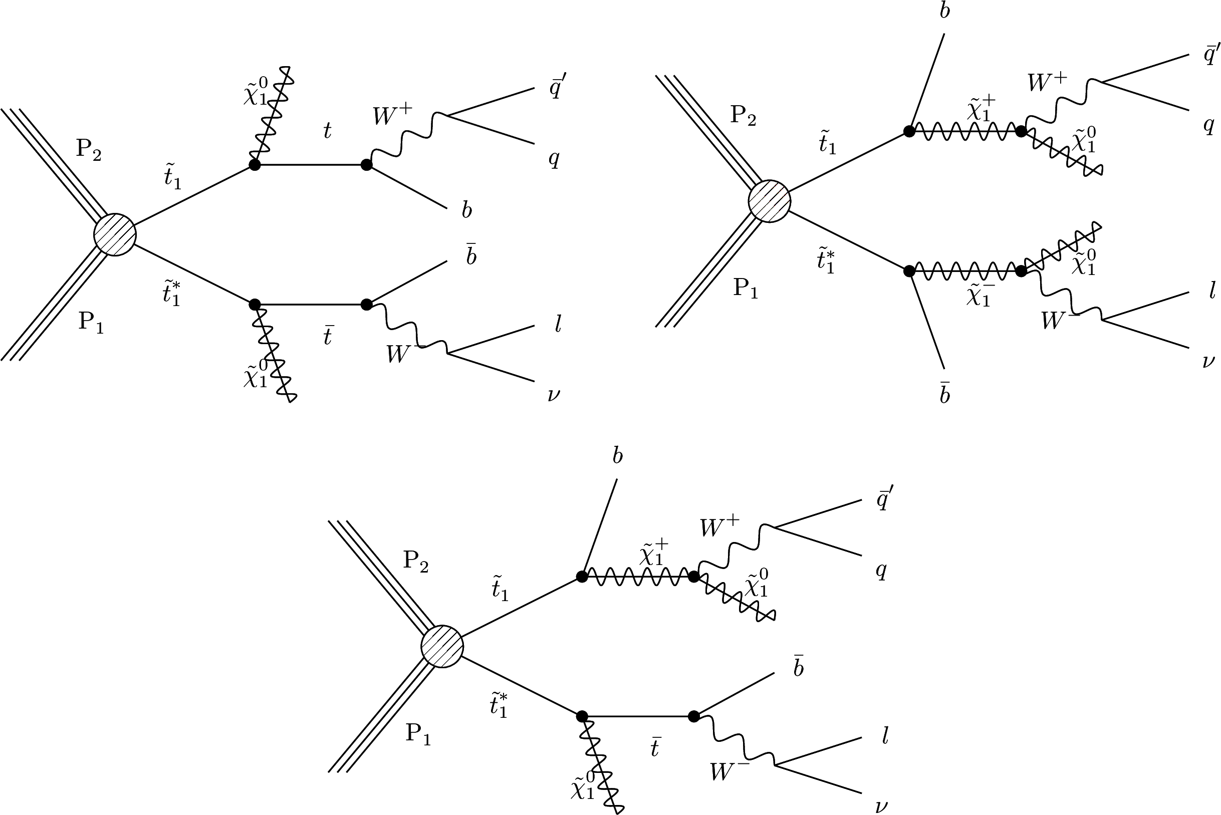
png pdf	Figure 1: Diagrams corresponding to top squark pair production, followed by the specific decay modes targeted in this note. Top left: $pp\rightarrow \tilde{t_1}\tilde{t_1}^*\rightarrow t^{(*)}\chi ^0_1\bar{t}^{(*)}\chi ^0_1$; top right: $pp\rightarrow \tilde{t_1}\tilde{t_1}^*\rightarrow b\chi ^+_1\bar{b}\chi ^-_1$; bottom: $pp\rightarrow \tilde{t_1}\tilde{t_1}^*\rightarrow t^{(*)}\chi ^0_1b\chi ^+_1$.
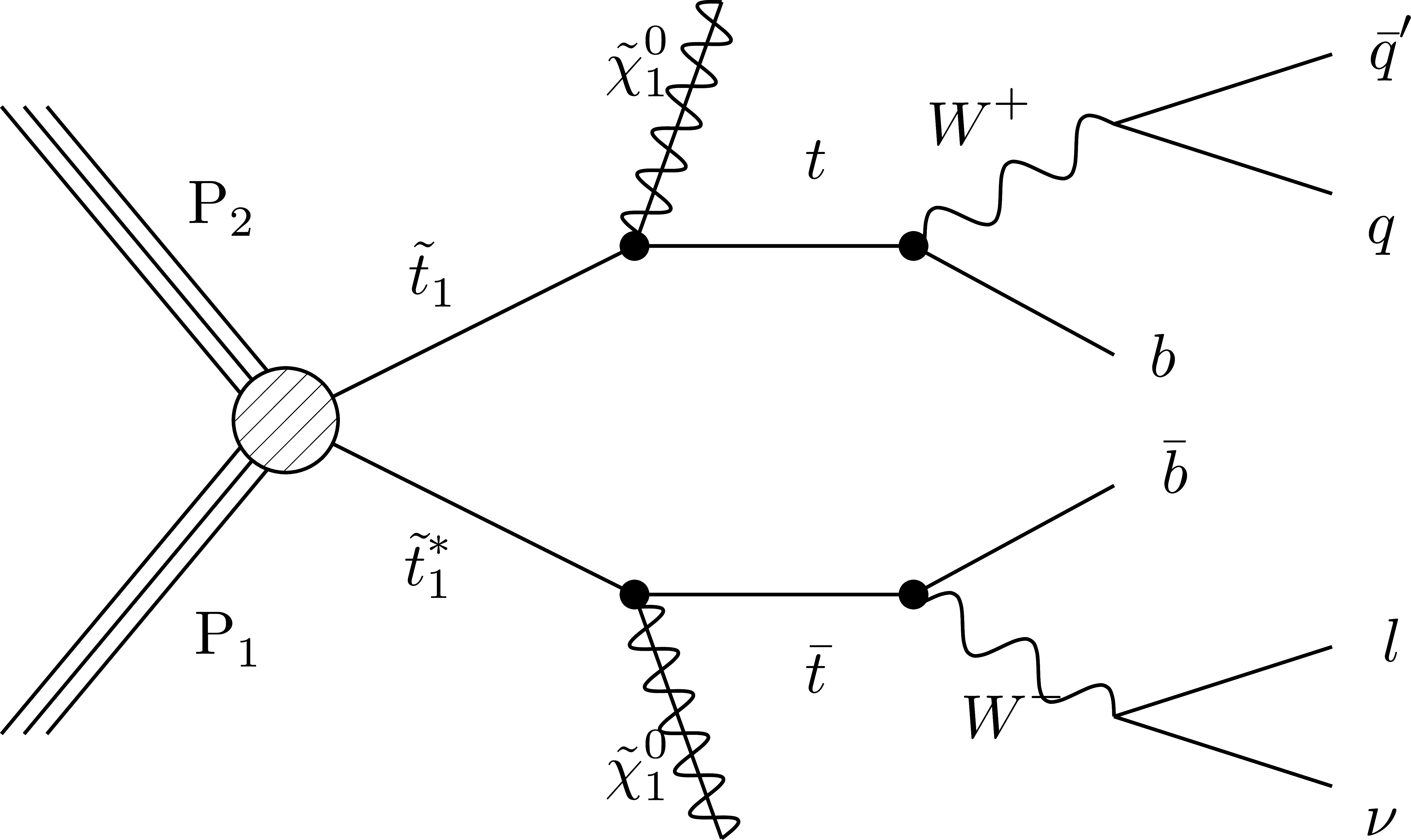
png pdf	Figure 1-a: Diagram corresponding to top squark pair production and decay targeted in this note: $pp\rightarrow \tilde{t_1}\tilde{t_1}^*\rightarrow t^{(*)}\chi ^0_1\bar{t}^{(*)}\chi ^0_1$.
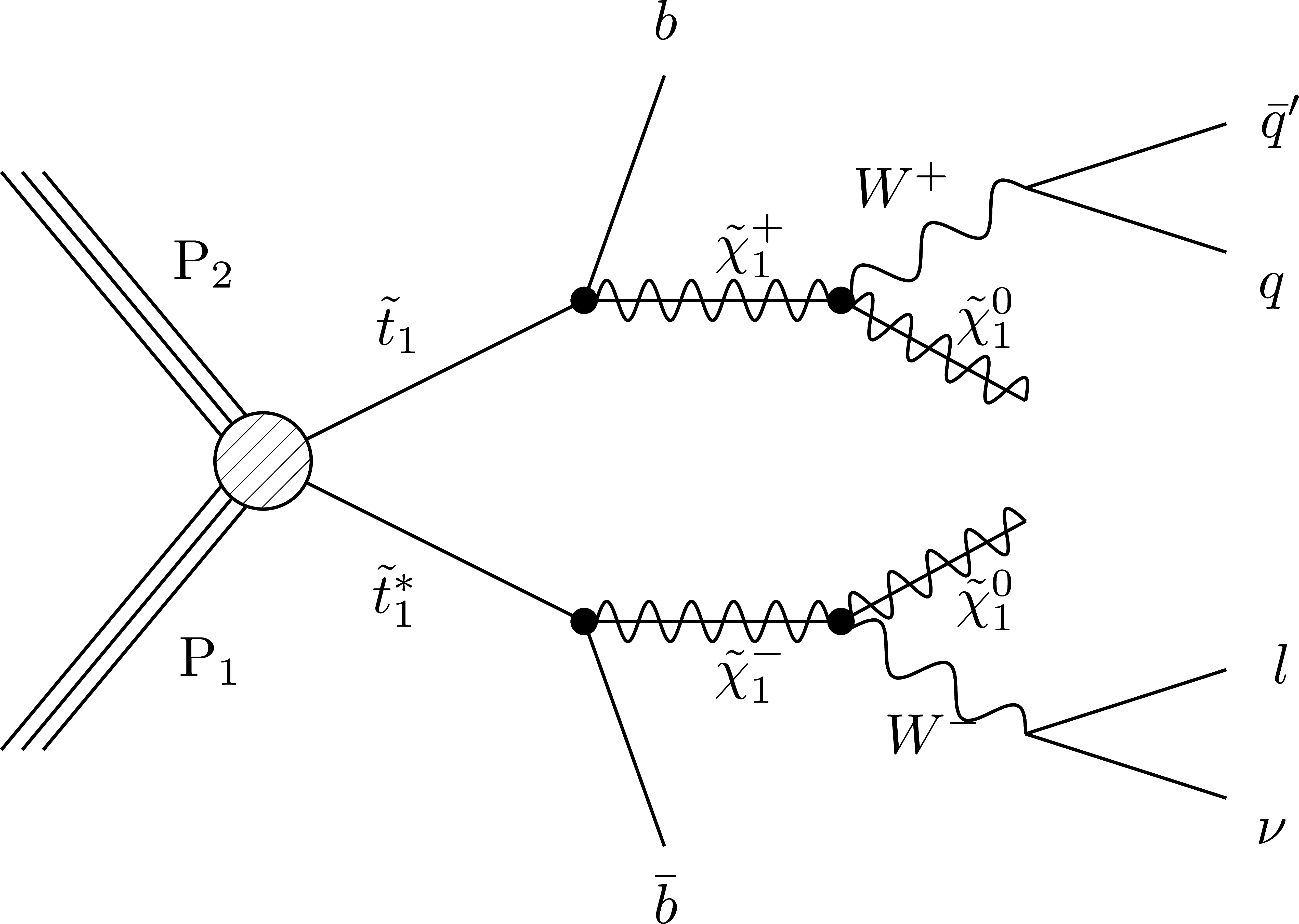
png pdf	Figure 1-b: Diagram corresponding to top squark pair production and decay targeted in this note: $pp\rightarrow \tilde{t_1}\tilde{t_1}^*\rightarrow b\chi ^+_1\bar{b}\chi ^-_1$.
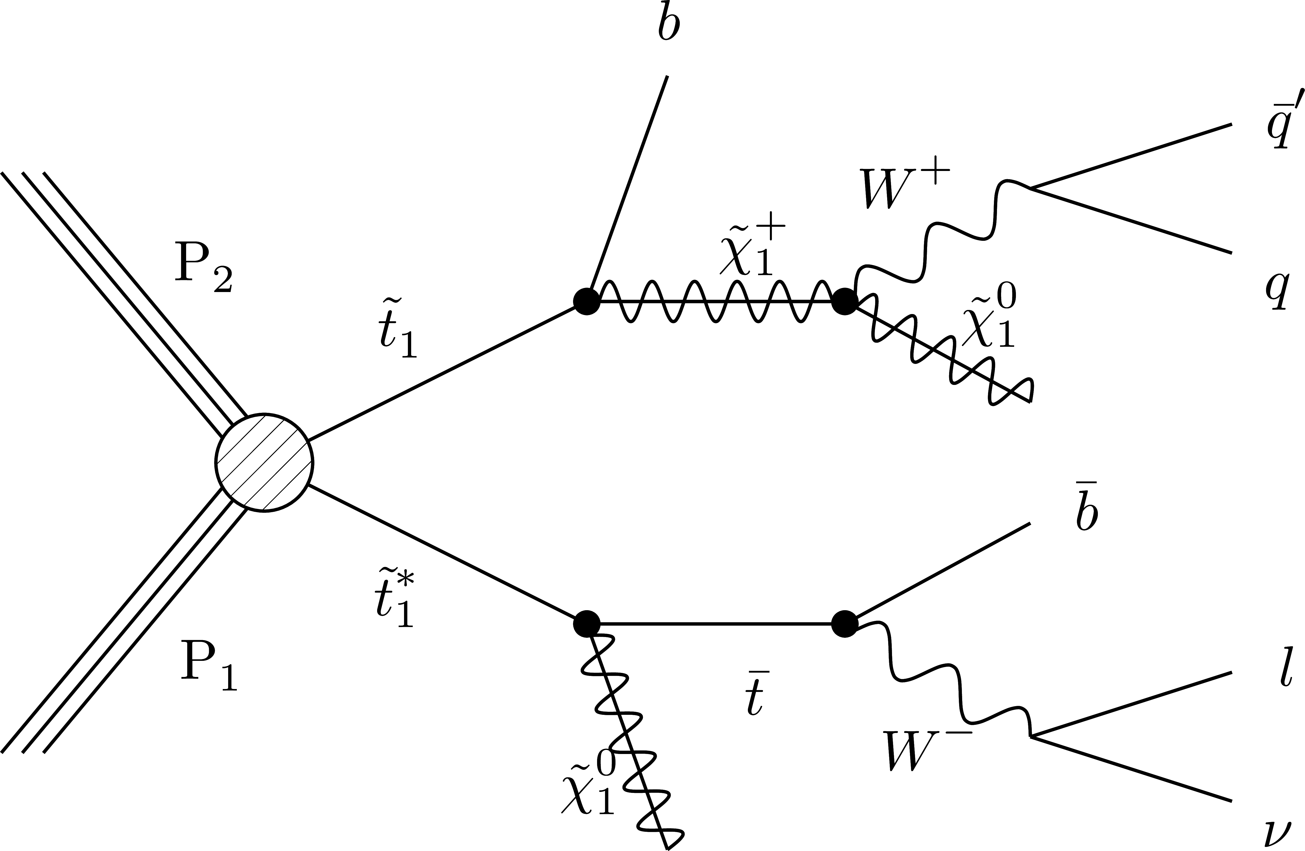
png pdf	Figure 1-c: Diagram corresponding to top squark pair production and decay targeted in this note: $pp\rightarrow \tilde{t_1}\tilde{t_1}^*\rightarrow t^{(*)}\chi ^0_1b\chi ^+_1$.
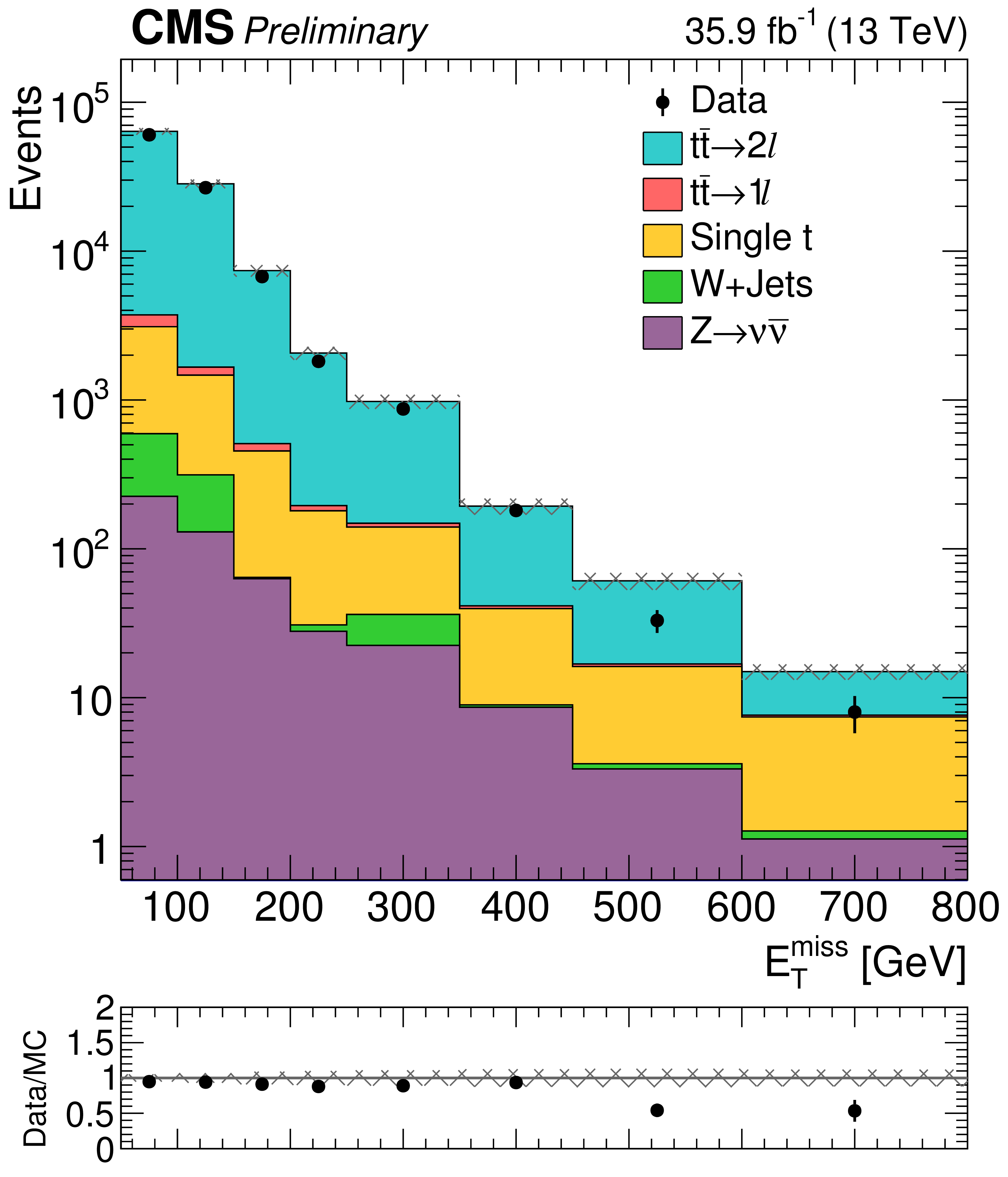
png pdf	Figure 2: Distributions of ${E_{\mathrm {T}}^{\text {miss}}}$ for a top-enriched control region of $\mathrm{ e } \mu$ events with at least one b tagged jet.
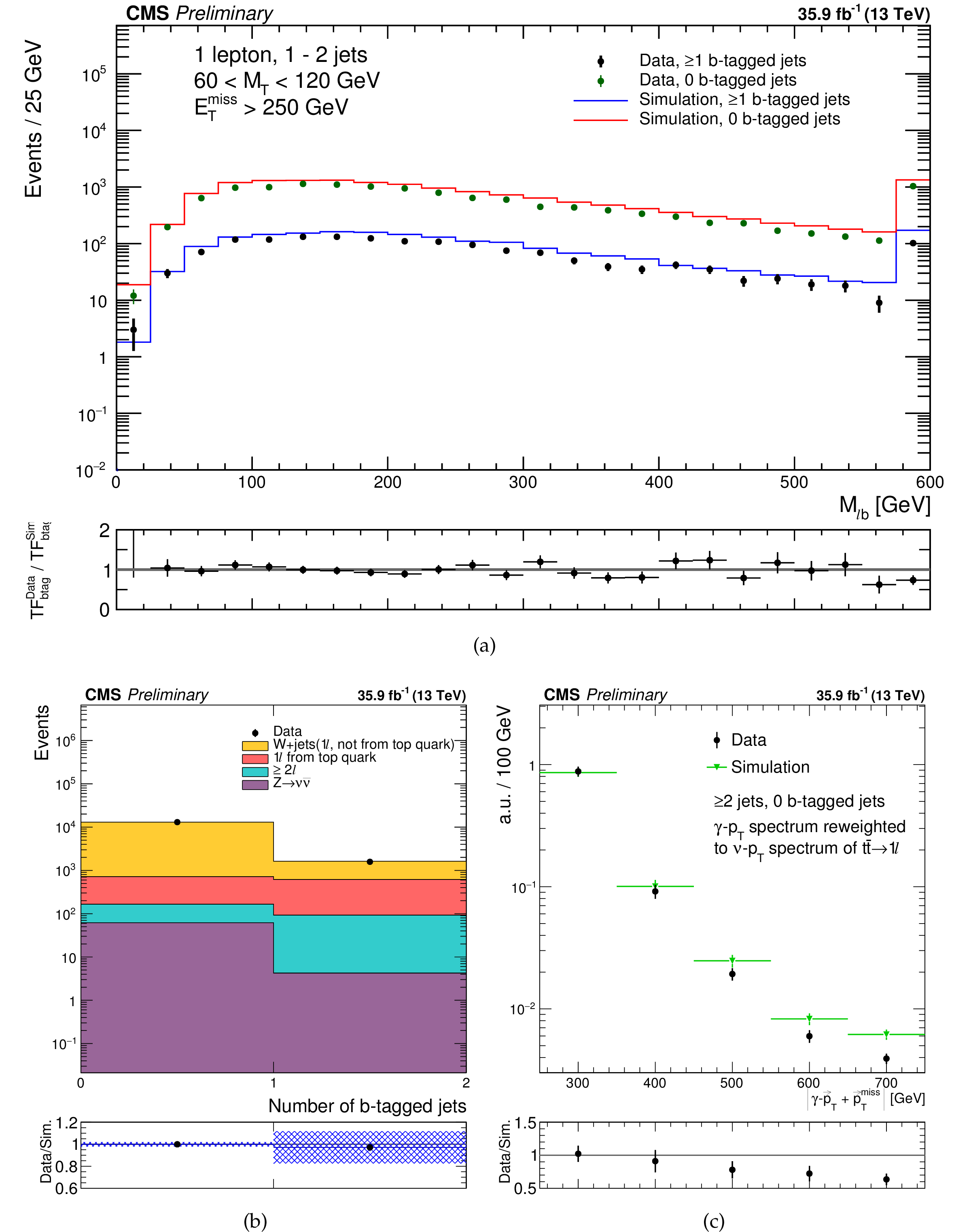
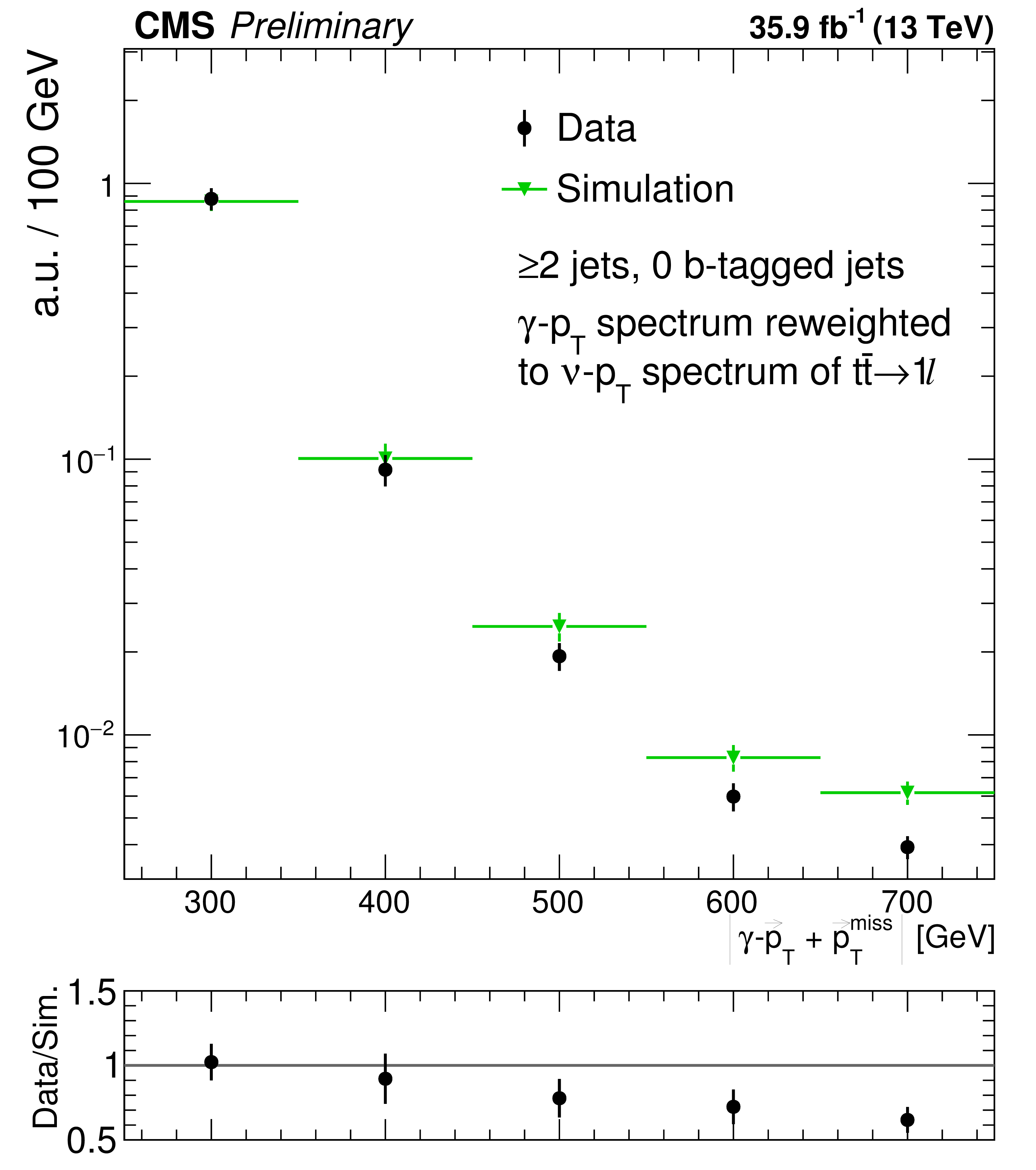
png pdf	Figure 3: Comparison of the modeling of kinematic distributions in data and simulation relevant for the estimate of the single lepton backgrounds. (a) Comparison of the ${M_{\mathrm {\ell b}}}$ distribution in a control sample with 1 or 2 jets, with 60 $< {M_{\mathrm {T}}} <$ 120 GeV. The distribution is shown separately for events with 0 and $\geq$1 jet passing the medium b-tagging working point. The lower panel shows the ratio of the the transfer factors (TF) in data and simulation from the 0 tags to the $\geq 1$ tags samples. (b) The distribution of the number of b-tagged jets in the same control sample after tightening the ${E_{\mathrm {T}}^{\text {miss}}}$ requirement to 250 GeV. The shaded band shows the uncertainty resulting from a 50% systematic uncertainty on the heavy flavor component of the W+jets sample. (c) Comparison of the ${E_{\mathrm {T}}^{\text {miss}}}$ distribution between data and simulation in the $\gamma$+jets control region. The uncertainty shown is statistical-only.
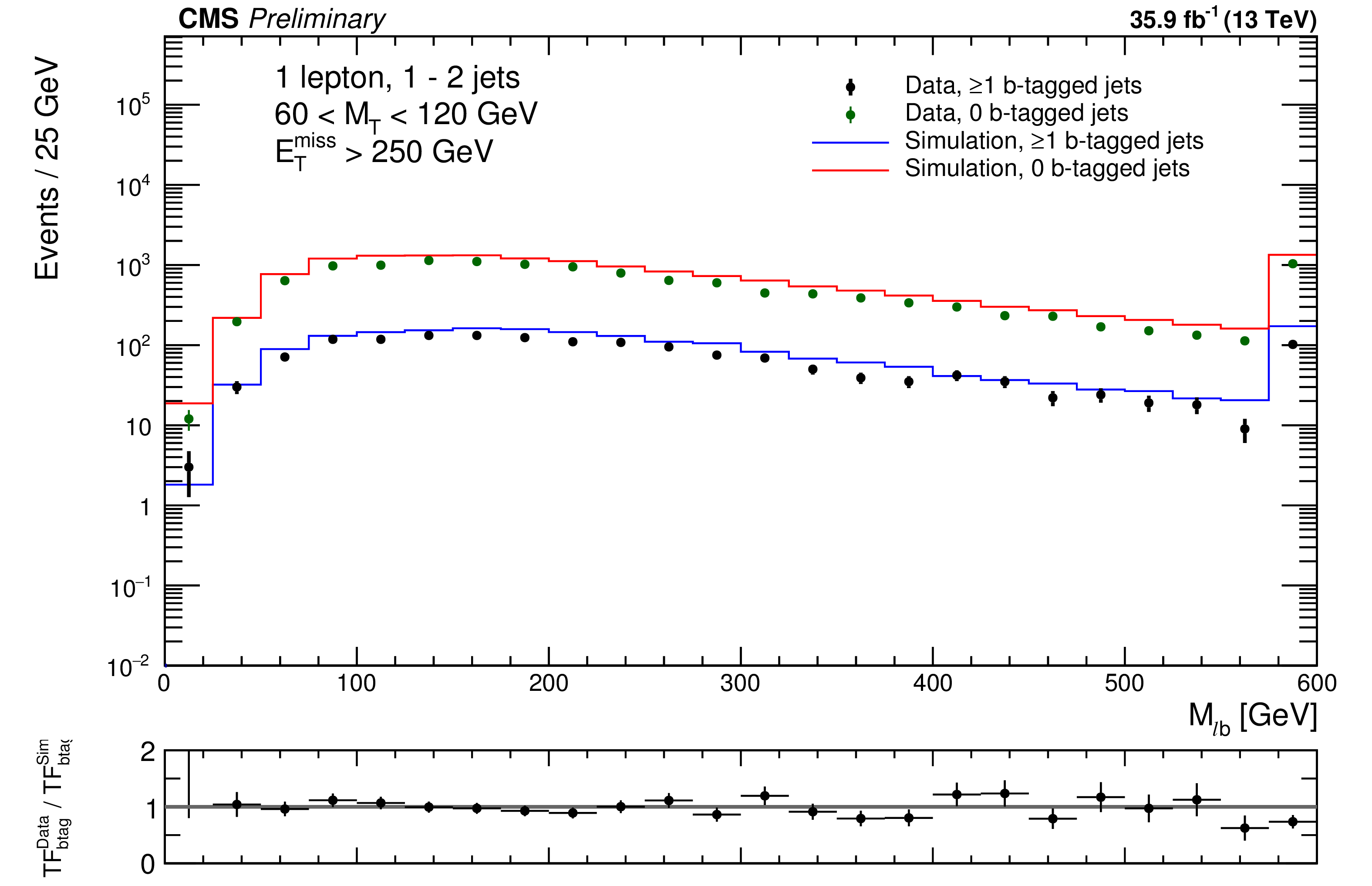
png pdf	Figure 3-a: Comparison of the ${M_{\mathrm {\ell b}}}$ distribution in a control sample with 1 or 2 jets, with 60 $< {M_{\mathrm {T}}} <$ 120 GeV. The distribution is shown separately for events with 0 and $\geq$1 jet passing the medium b-tagging working point. The lower panel shows the ratio of the the transfer factors (TF) in data and simulation from the 0 tags to the $\geq 1$ tags samples.
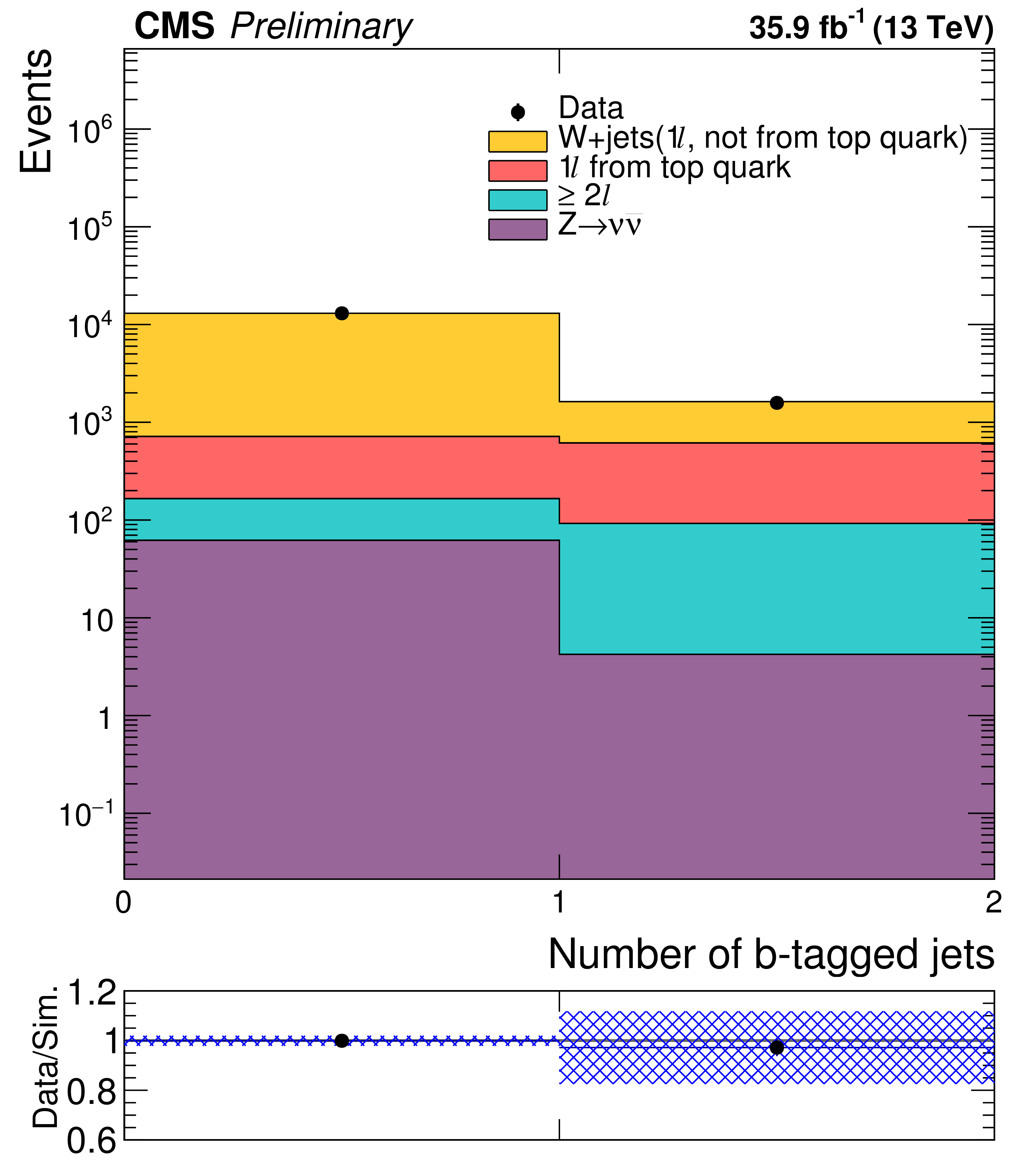
png pdf	Figure 3-b: The distribution of the number of b-tagged jets in the same control sample after tightening the ${E_{\mathrm {T}}^{\text {miss}}}$ requirement to 250 GeV. The shaded band shows the uncertainty resulting from a 50% systematic uncertainty on the heavy flavor component of the W+jets sample.
png pdf	Figure 3-c: Comparison of the ${E_{\mathrm {T}}^{\text {miss}}}$ distribution between data and simulation in the $\gamma$+jets control region. The uncertainty shown is statistical-only.
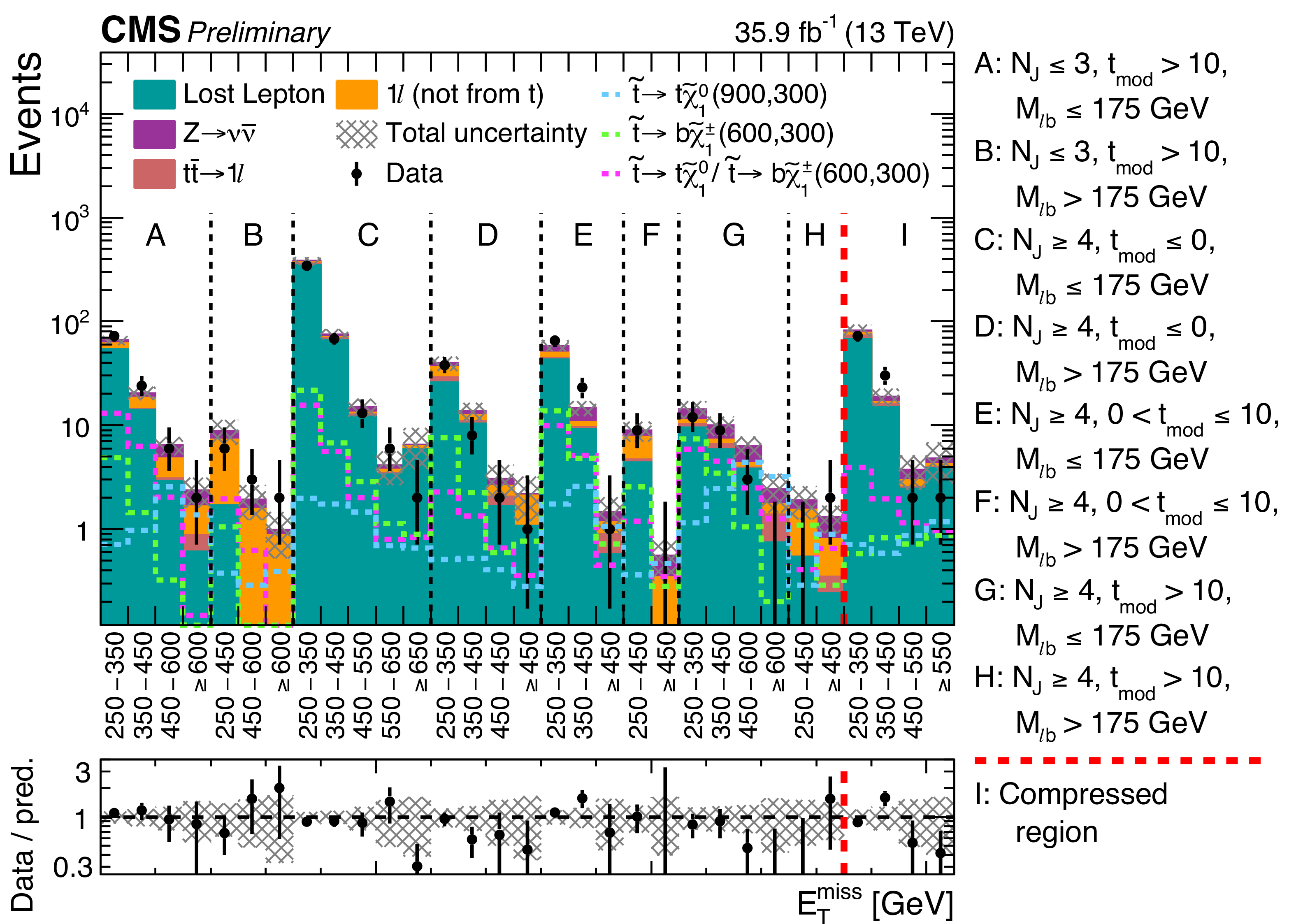
png pdf	Figure 4: Observed data yields compared with SM background estimations for the 31 signal regions of Table 2 and 3. The uncertainties, which are the quadratic sums of statistical and systematic uncertainties, are shown as shaded bands. The expectations for three signal hypotheses are overlaid. The corresponding numbers in parentheses in the legend refer to the masses of the top squark and neutralino, respectively.
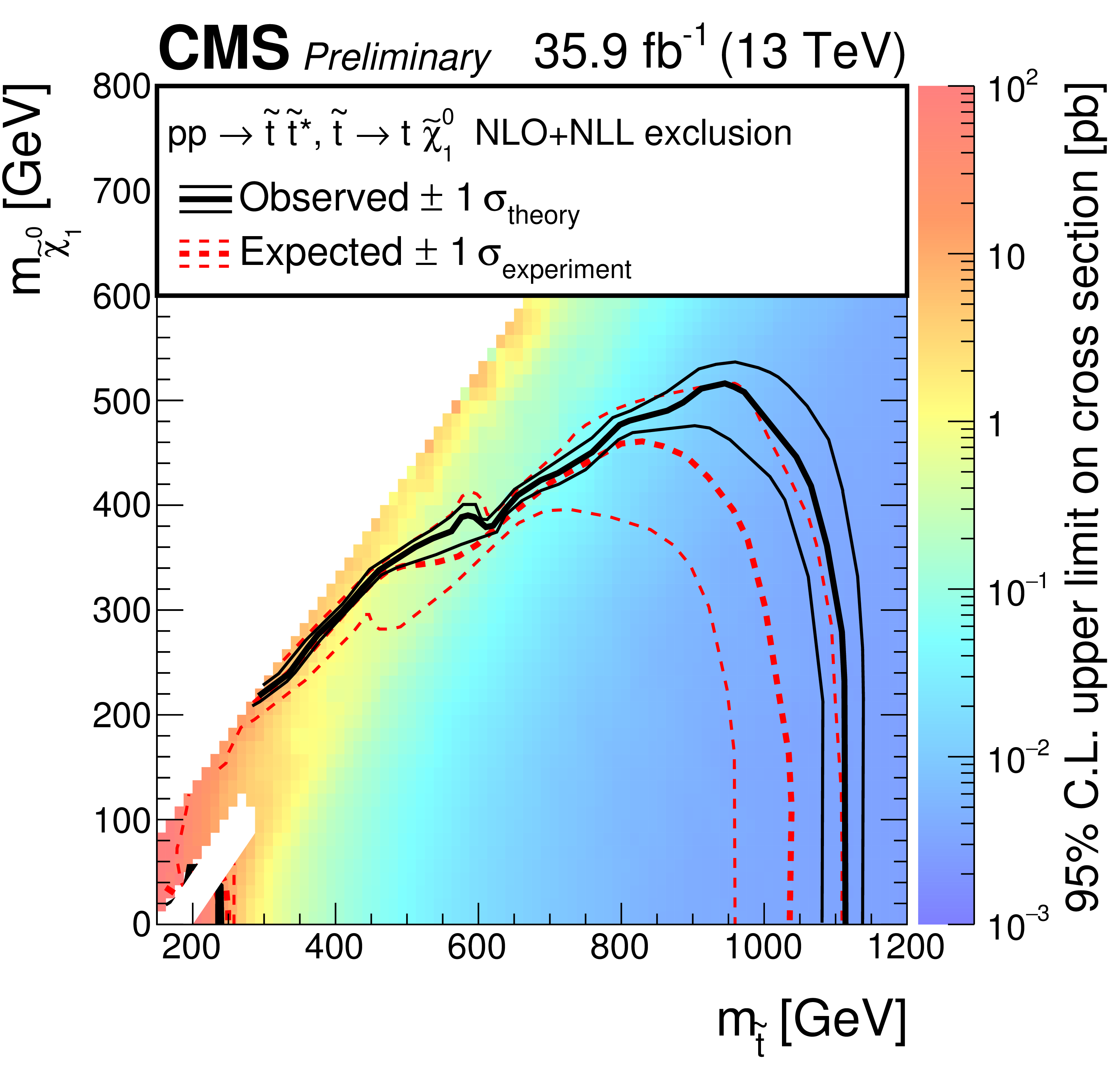
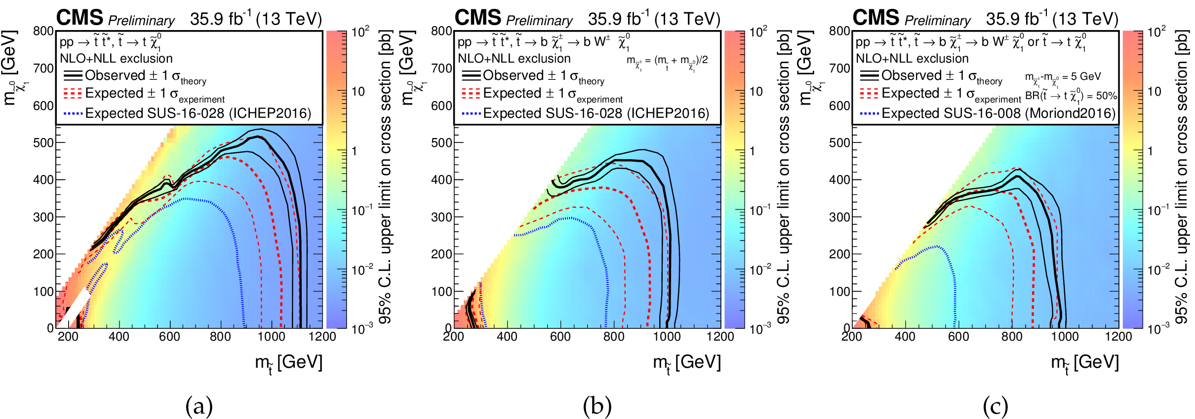
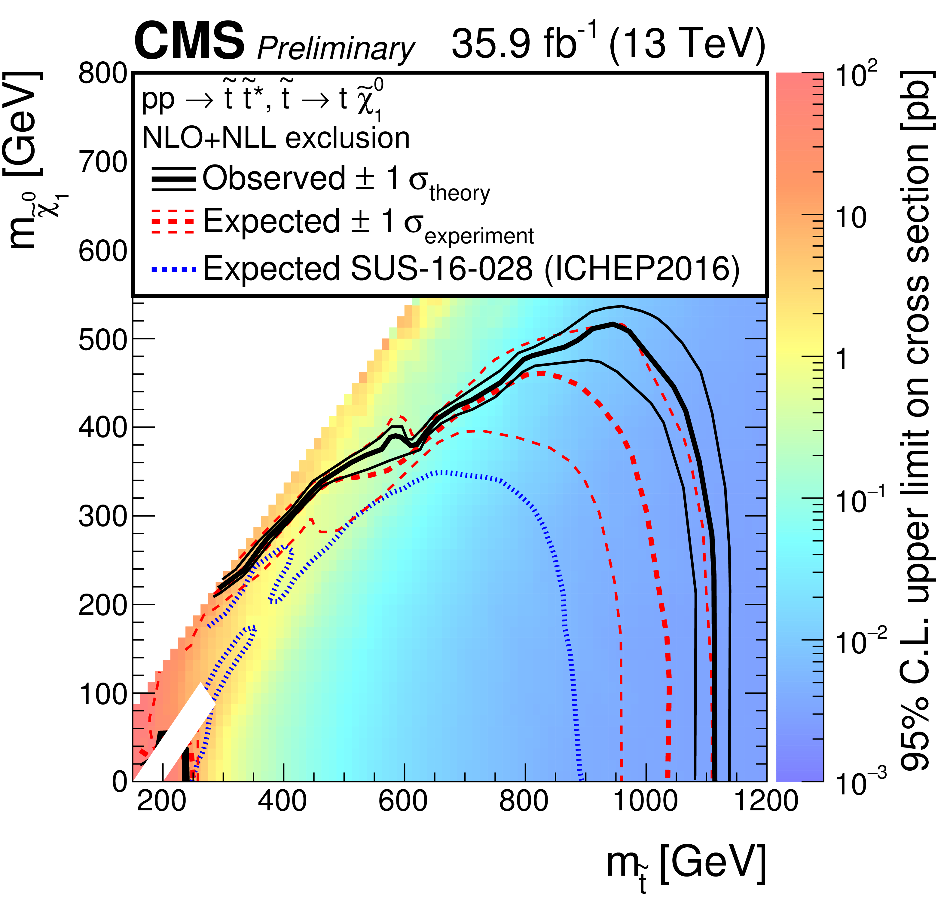
png pdf root	Figure 5: The exclusion limits at 95% CL for direct top-squark production with decay $\tilde{ \mathrm{ t } }_1 \to \mathrm{ t } \tilde{\chi}^0_1$. The interpretation is done in the two dimensional space of $m_{\tilde{ \mathrm{ t } } }$ vs. $m_{\tilde{\chi}^0_1 }$. The color indicates the 95% CL upper limit on the cross section times branching fraction at each point in the $m_{\tilde{ \mathrm{ t } }_1 }$ vs. $m_{\tilde{\chi}^0_1 }$ plane. The area to the left of and below the thick black curve represents the observed exclusion region at 95% CL, while the dashed red lines indicate the expected limit at 95% CL and their $\pm$1$\sigma$ experiment standard deviation uncertainties. The thin black lines show the effect of the theoretical uncertainties ($\sigma _\mathrm {theory}$) on the signal cross section. The whited out region is discussed in Sec. 7.
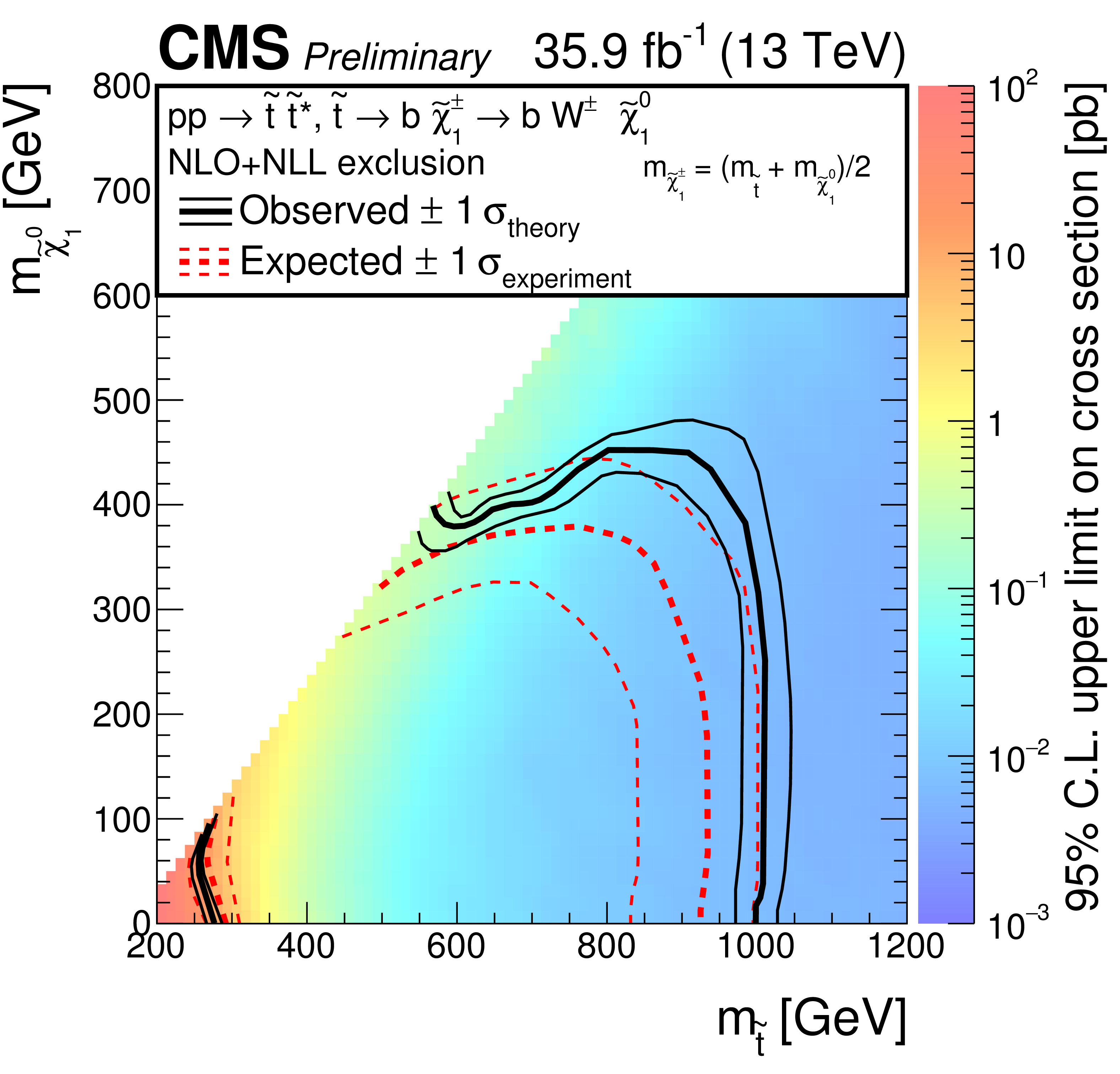
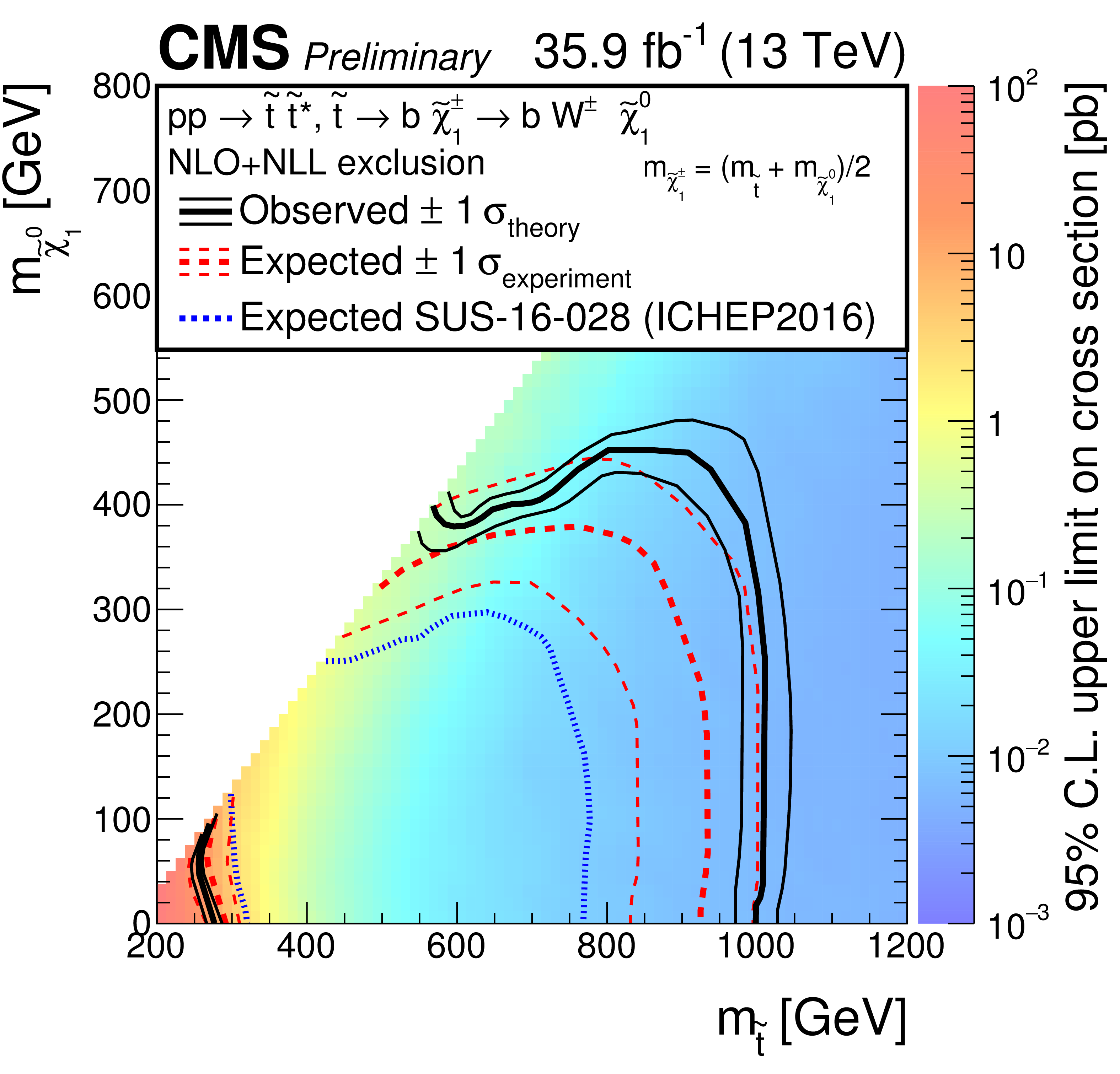
png pdf root	Figure 6: The exclusion limit at 95% CL for direct top-squark production with decay $\mathrm{ p } \mathrm{ p } \to \tilde{ \mathrm{ t } }_1 \tilde{ \mathrm{ t } }_1 ^*\to \mathrm{ b \bar{b} } \tilde{\chi}^{\pm}_1 \tilde{\chi}^{\pm}_1$, $\tilde{\chi}^{\pm}_1 \to \mathrm{ W } \tilde{\chi}^0_1$. The mass of the chargino is chosen to be $(m_{\tilde{ \mathrm{ t } }_1 } + m_{\tilde{\chi}^0_1 })/2$. The interpretation is done in the two dimensional space of $m_{\tilde{ \mathrm{ t } }_1 }$ vs. $m_{\tilde{\chi}^0_1 }$. The color indicates the 95% CL upper limit on the cross section times branching fraction at each point in the $m_{\tilde{ \mathrm{ t } }_1 }$ vs. $m_{\tilde{\chi}^0_1 }$ plane. The area to the left of and below the thick black curve represents the observed exclusion region at 95% CL, while the dashed red lines indicate the expected limit at 95% CL and their $\pm$1$\sigma$ experiment standard deviation uncertainties. The thin black lines show the effect of the theoretical uncertainties ($\sigma _\mathrm {theory}$) on the signal cross section.
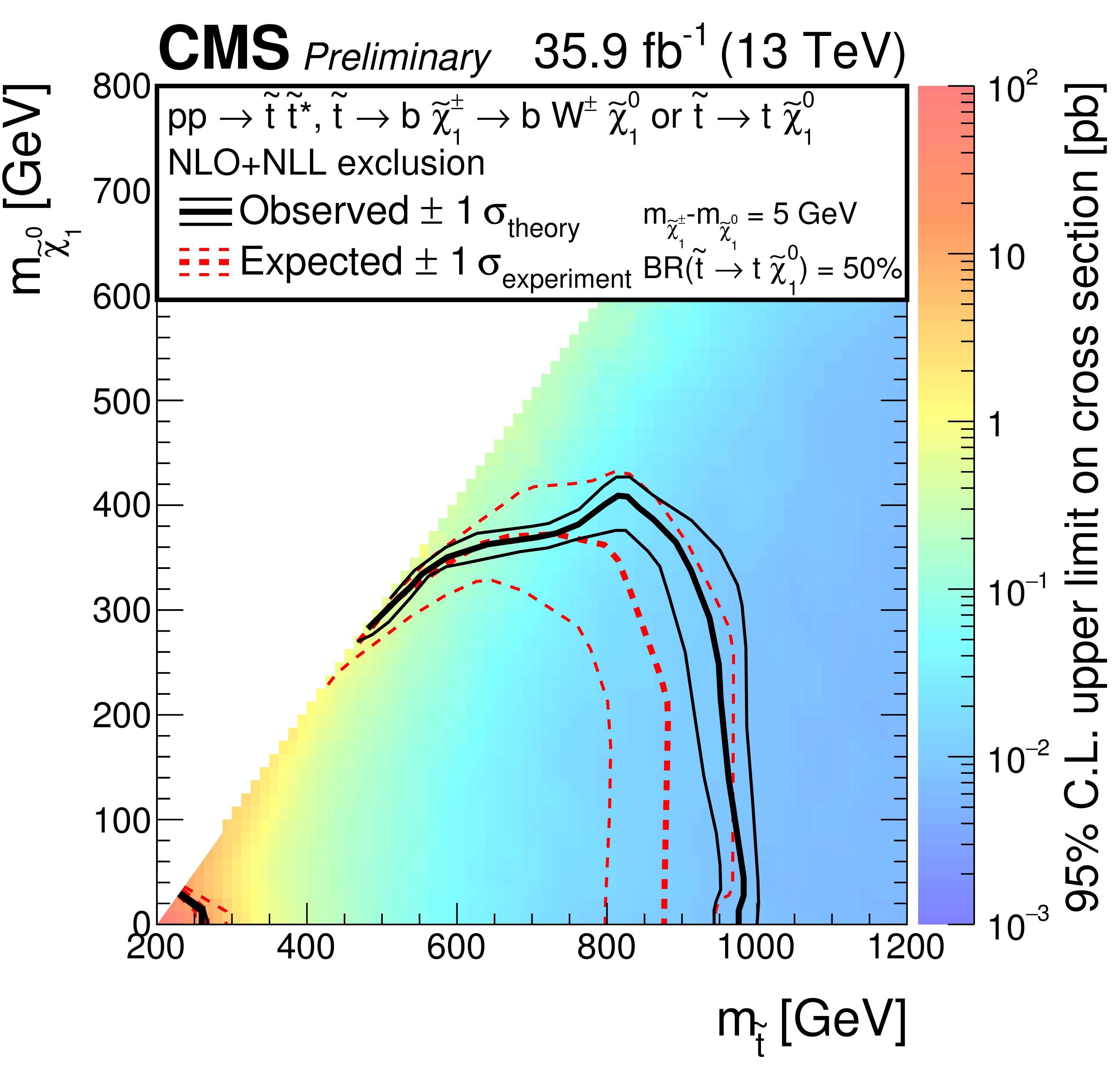
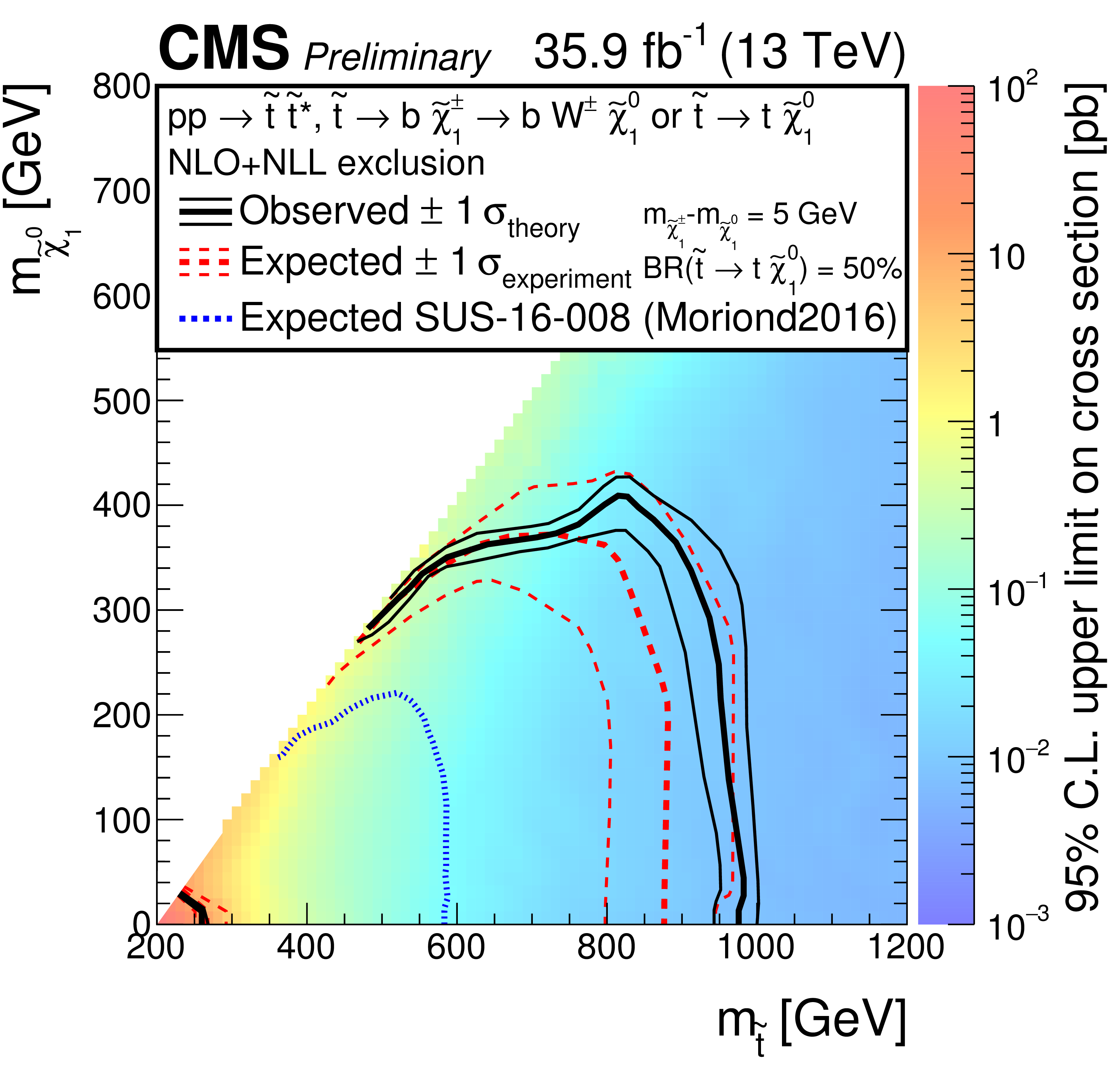
png pdf root	Figure 7: The exclusion limit at 95% CL for direct top-squark production with decay $\mathrm{ p } \mathrm{ p } \to \tilde{ \mathrm{ t } }_1 \tilde{ \mathrm{ t } }_1 ^*\to \mathrm{ t } \mathrm{ b } \tilde{\chi}^{\pm}_1 \tilde{\chi}^0_1$, $\tilde{\chi}^{\pm}_1 \to \mathrm{ W } ^{*}\tilde{\chi}^0_1$. The mass splitting of the chargino and neutralino is fixed to 5 GeV. The interpretation is done in the two dimensional space of $m_{\tilde{ \mathrm{ t } }_1 }$ vs. $m_{\tilde{\chi}^0_1 }$. The color indicates the 95% CL upper limit on the cross section times branching fraction at each point in the $m_{\tilde{ \mathrm{ t } }_1 }$ vs. $m_{\tilde{\chi}^0_1 }$ plane. The area to the left of and below the thick black curve represents the observed exclusion region at 95% CL, while the dashed red lines indicate the expected limit at 95% CL and their $\pm$1$\sigma$ experiment standard deviation uncertainties. The thin black lines show the effect of the theoretical uncertainties ($\sigma _\mathrm {theory}$) on the signal cross section.
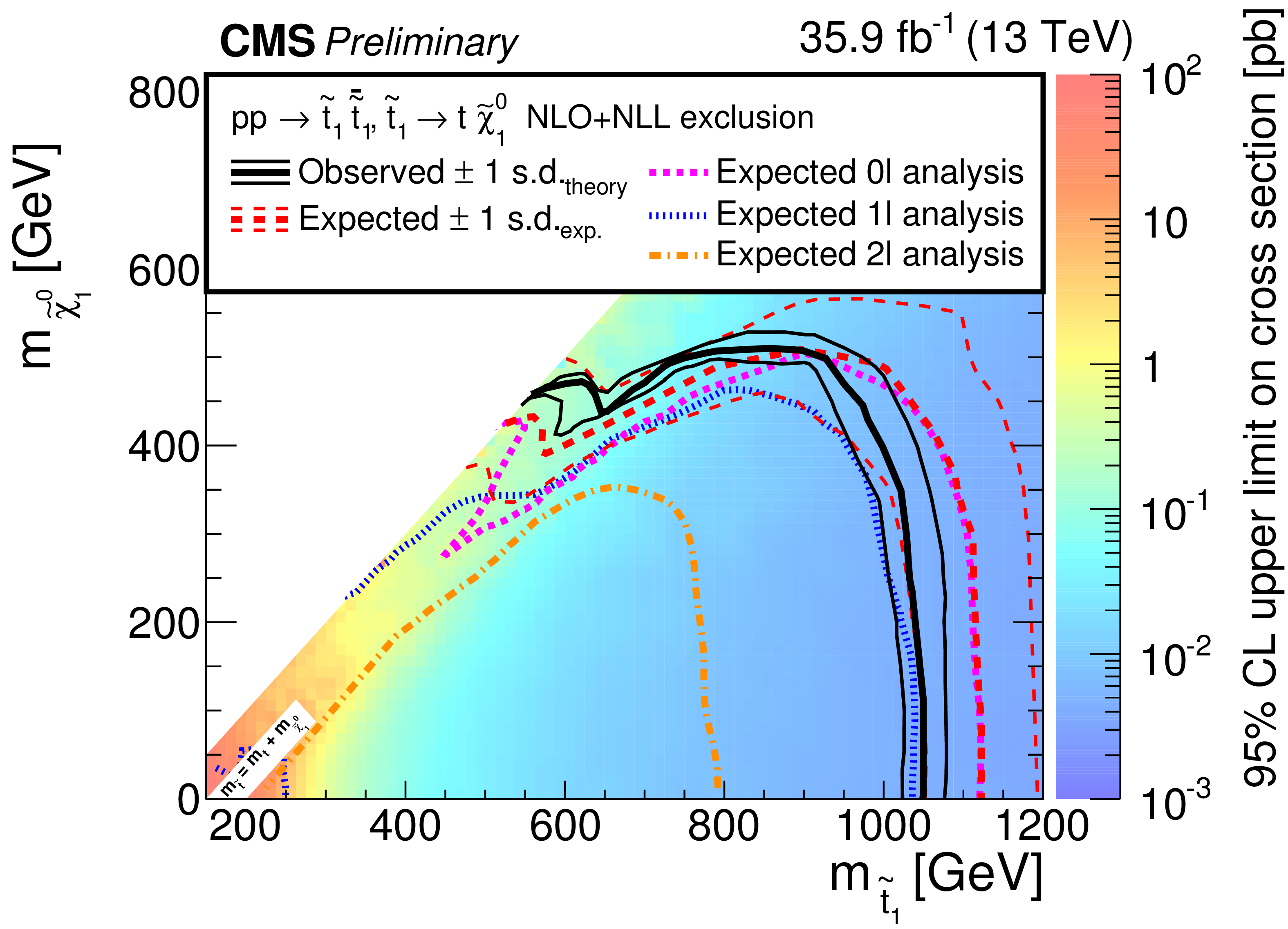
png pdf	Figure 8: Exclusion limits at 95% CL for direct top squark pair production for the decay mode $\tilde{ \mathrm{ t } }_1 \to \mathrm{ t } \tilde{\chi}^0_1$. The color indicates the 95% CL upper limit on the cross section times branching fraction at each point in the $m_{\tilde{ \mathrm{ t } }_1 }-m_{\tilde{\chi}^0_1 }$ plane. The area to the left of and below the thick black curve represents the observed exclusion region at 95% CL, while the dashed red lines indicate the expected limits at 95% CL and their $\pm$1$\sigma$ experiment standard deviation uncertainties. The thin black lines show the effect of the theoretical uncertainties $\sigma _\mathrm {theory}$ on the signal cross section. The magenta short-dashed, blue dotted, and long-short-dashed orange curves show the expected limits for the fully-hdaronic [27], single-lepton and dilepton [28] analyses, respectively.
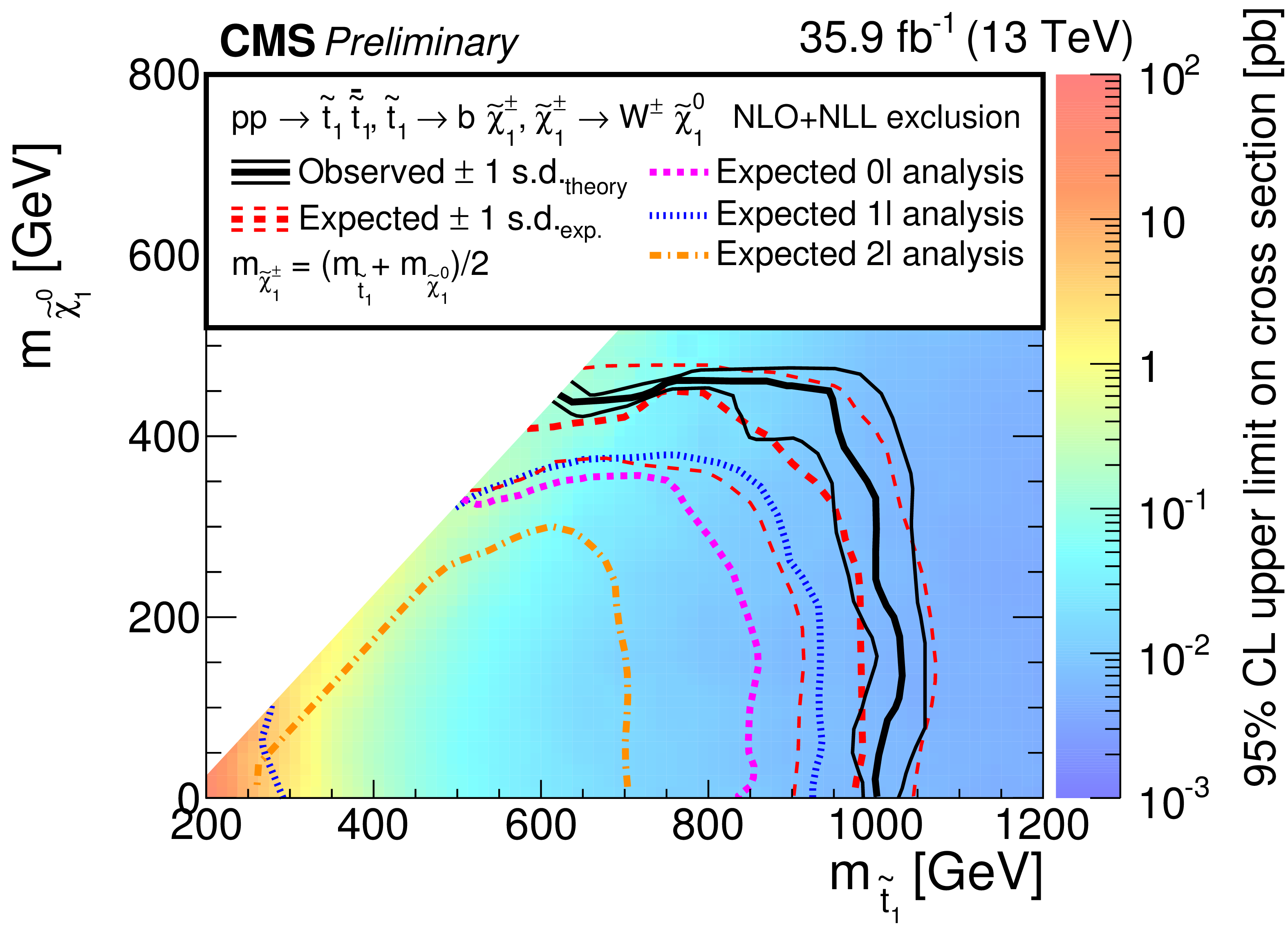
png pdf	Figure 9: Exclusion limits at 95% CL for direct top squark pair production for the decay mode $\tilde{ \mathrm{ t } }_1 \to \mathrm{ b } \tilde{ \chi }^{+}_1$, $\tilde{ \chi }^{+}_1 \to \mathrm{ W } ^{+}\tilde{\chi}^0_1$. The mass of the chargino is chosen to be $(m_{\tilde{ \mathrm{ t } }_1 } + m_{\tilde{\chi}^0_1 })/2$. The color indicates the 95% CL upper limit on the cross section times branching fraction at each point in the $m_{\tilde{ \mathrm{ t } }_1 }-m_{\tilde{\chi}^0_1 }$ plane. The area to the left of and below the thick black curve represents the observed exclusion region at 95% CL, while the dashed red lines indicate the expected limits at 95% CL and their $\pm$1$\sigma$ experiment standard deviation uncertainties. The thin black lines show the effect of the theoretical uncertainties $\sigma _\mathrm {theory}$ on the signal cross section. The magenta short-dashed, blue dotted, and long-short-dashed orange curves show the expected limits for the fully-hdaronic [27], single-lepton and dilepton [28] analyses, respectively.
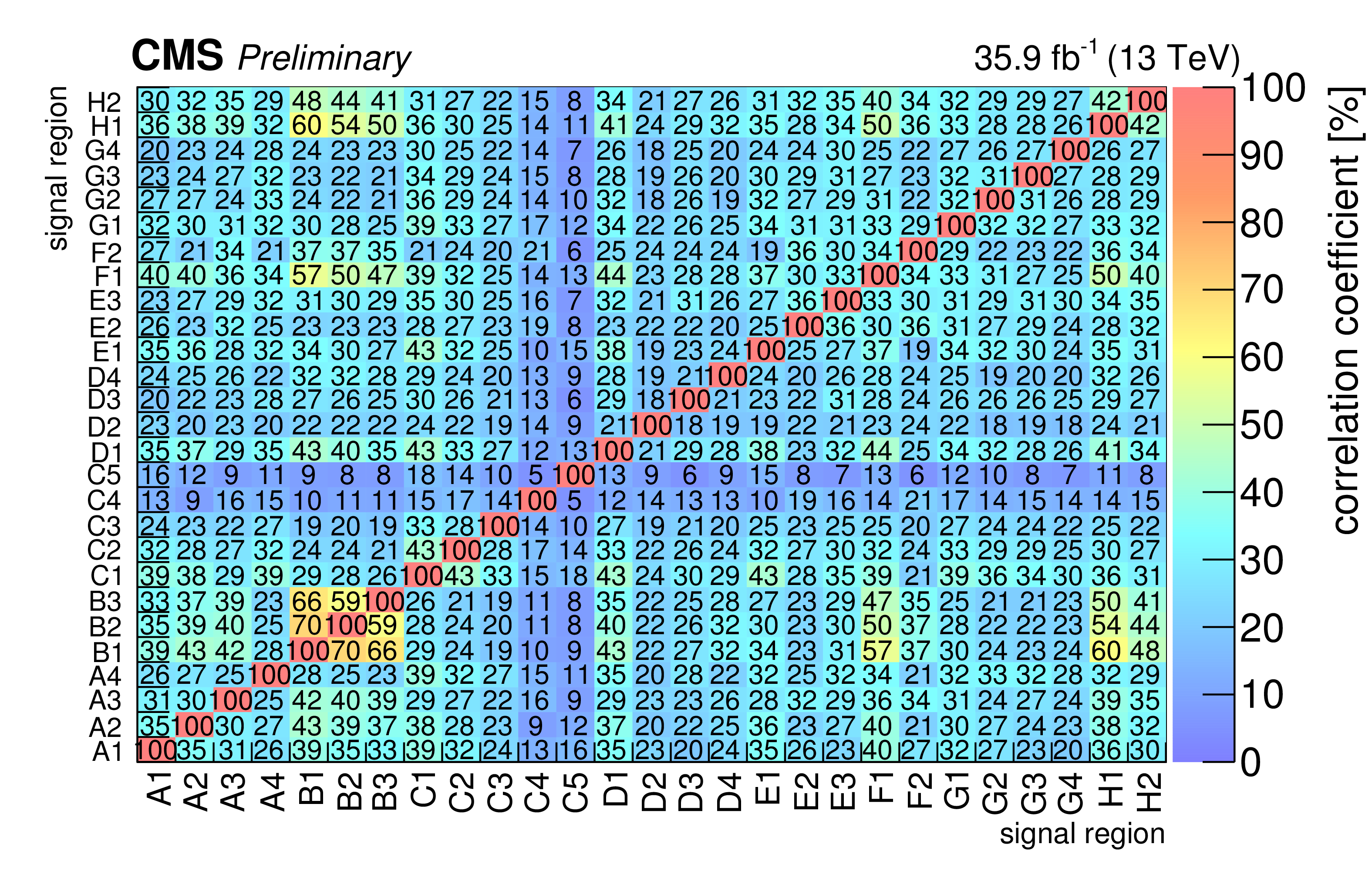
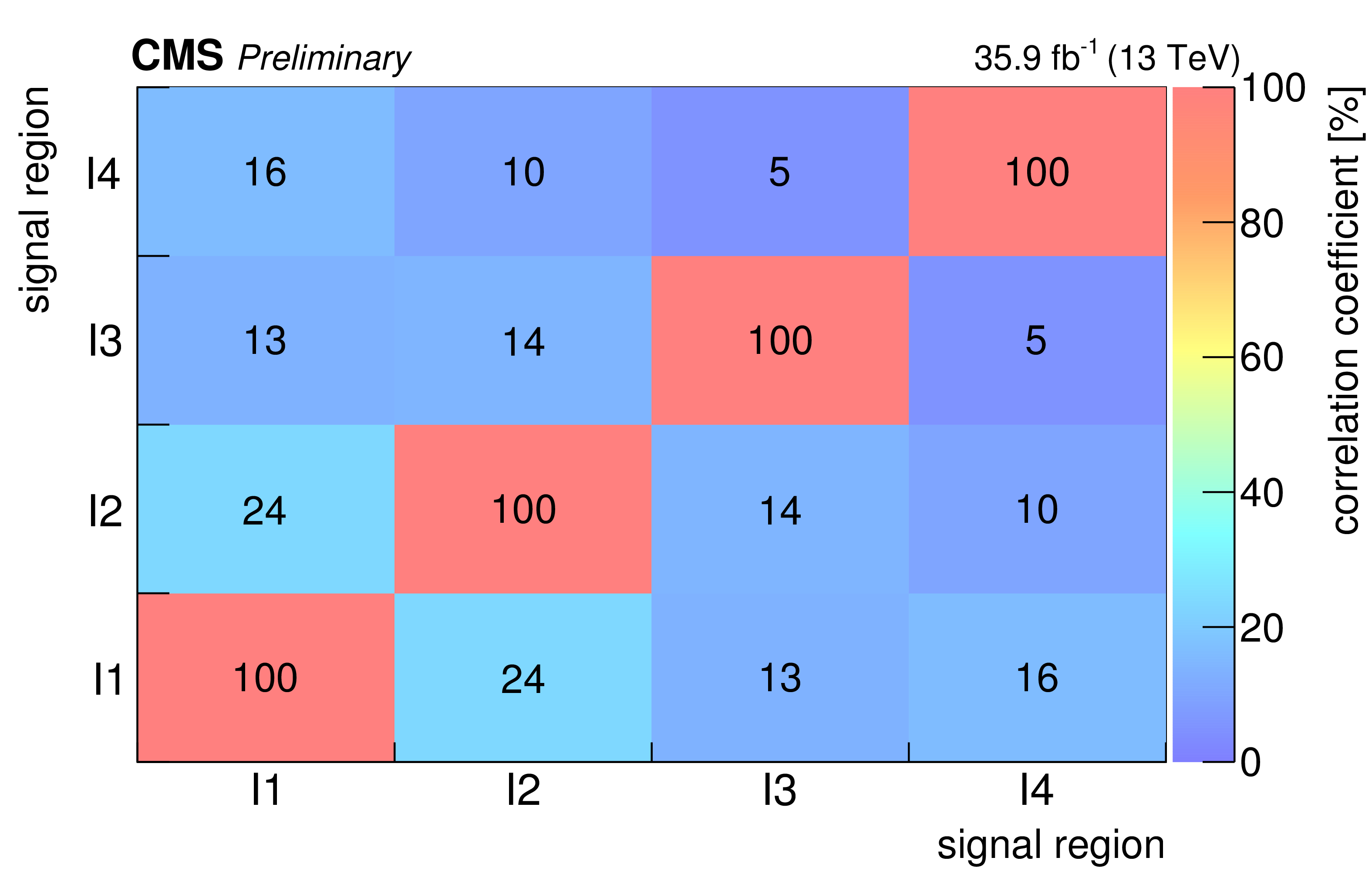
png pdf root	Figure 10: Correlation matrix for the background predictions for the signal regions for the standard selection (in percent). The labelling of the regions follows the convention of Fig. {fig:results}.
png pdf root	Figure 11: Correlation matrix for the background predictions for the signal regions for the compressed selection (in percent). The labelling of the regions follows the convention of Fig. {fig:results}.

Tables
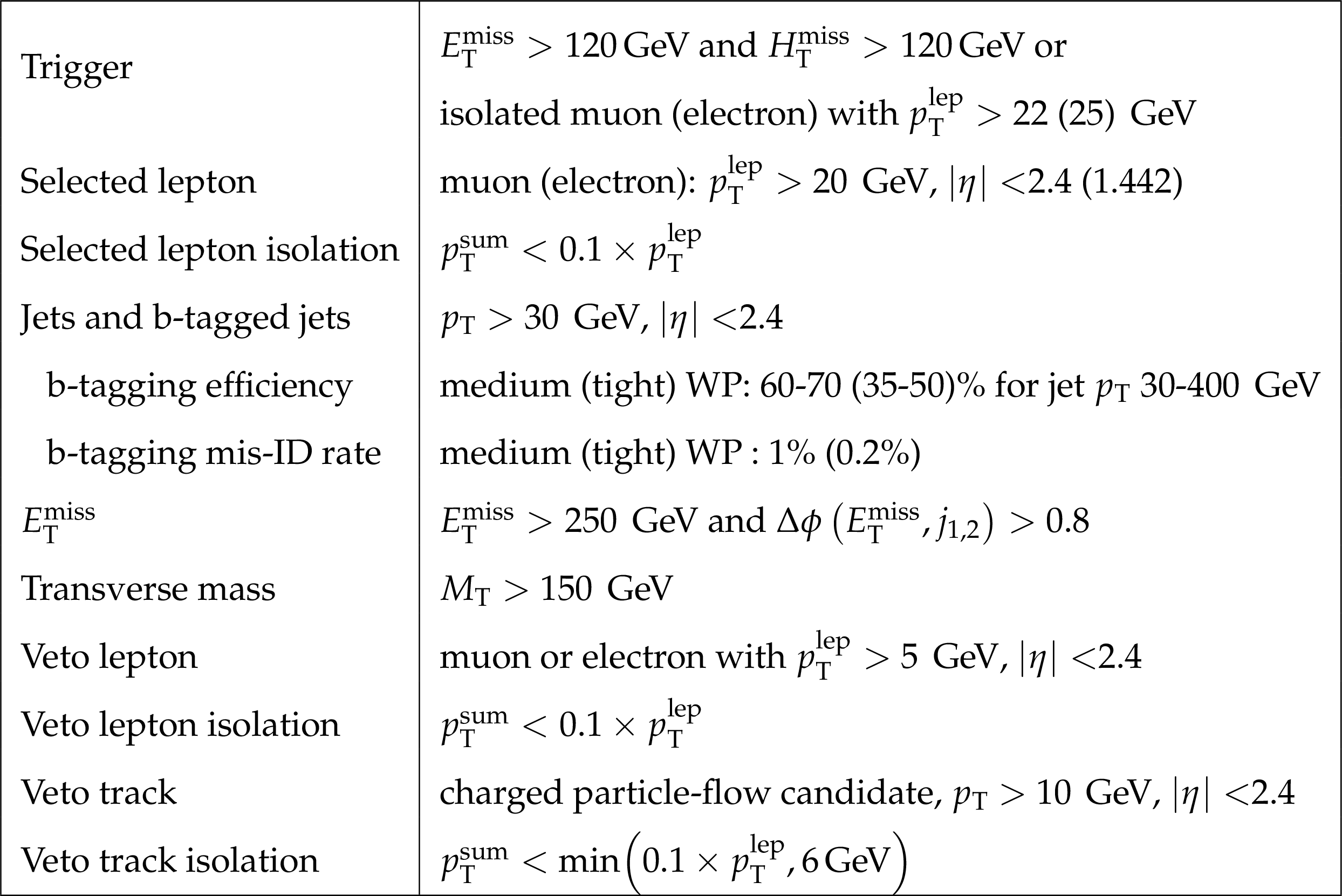
png pdf	Table 1: Summary of the preselection. ${H_{\mathrm {T}}^{\mathrm {miss}}}$ is the magnitude of the vector sum of the transverse momenta of all jets and leptons in the event. The symbol ${p_{\mathrm {T}}} ^{\mathrm {lep}}$ denotes the transverse momentum of the lepton, while ${p_{\mathrm {T}}} ^{\mathrm {sum}}$ is the scalar sum of the transverse momenta of all PF candidates in a cone around the lepton but excluding the lepton. The radius of the cone is $\Delta R =$ 0.2 for ${p_{\mathrm {T}}} ^{\mathrm {lep}} \le$ 50 GeV , and $\Delta R =$ Max(0.05, 10 GeV/${p_{\mathrm {T}}} ^{\mathrm {lep}}$) at higher values of lepton transverse momentum.
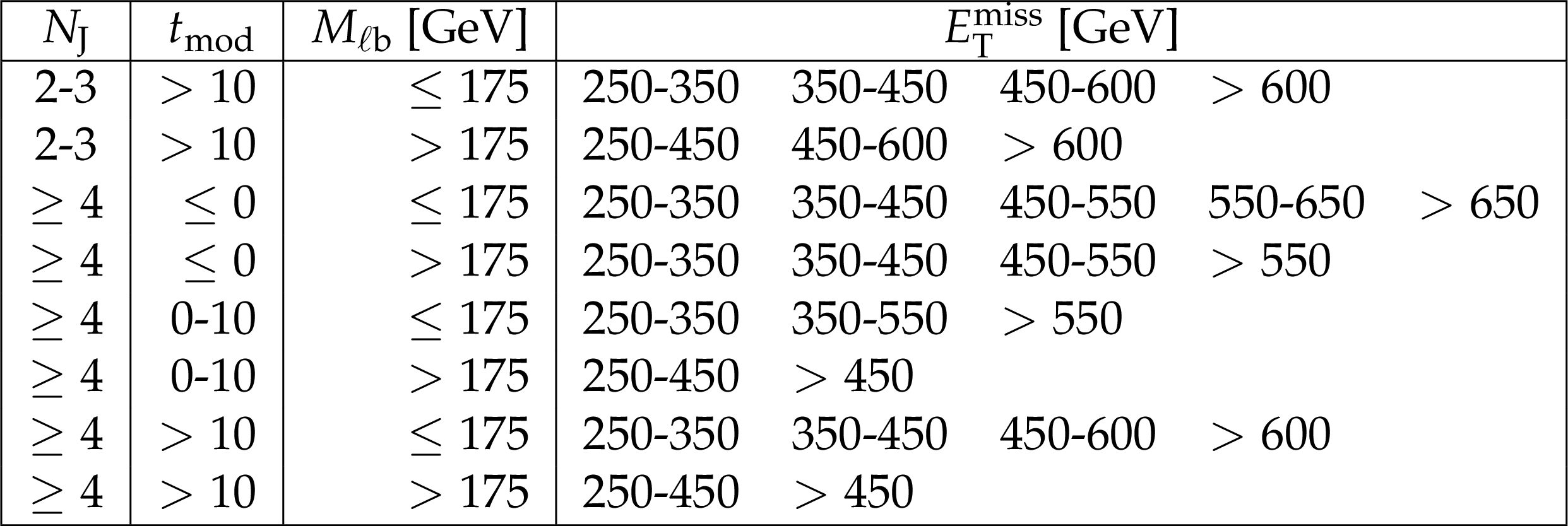
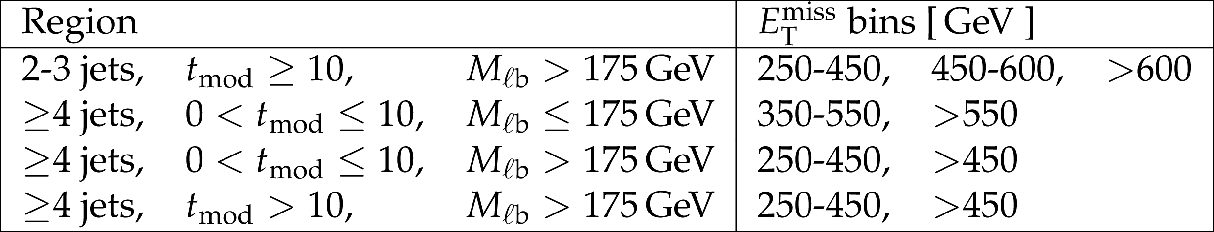
png pdf	Table 2: Definitions for the 27 signal regions of the standard selection. At least one b-tagged jet (medium WP) is required in all search regions. To suppress the W+jets background in signal regions with ${M_{\mathrm {\ell b}}} >$ 175 GeV, a more strict requirement that at least one jet satisfies the tight b-tagging WP is made.
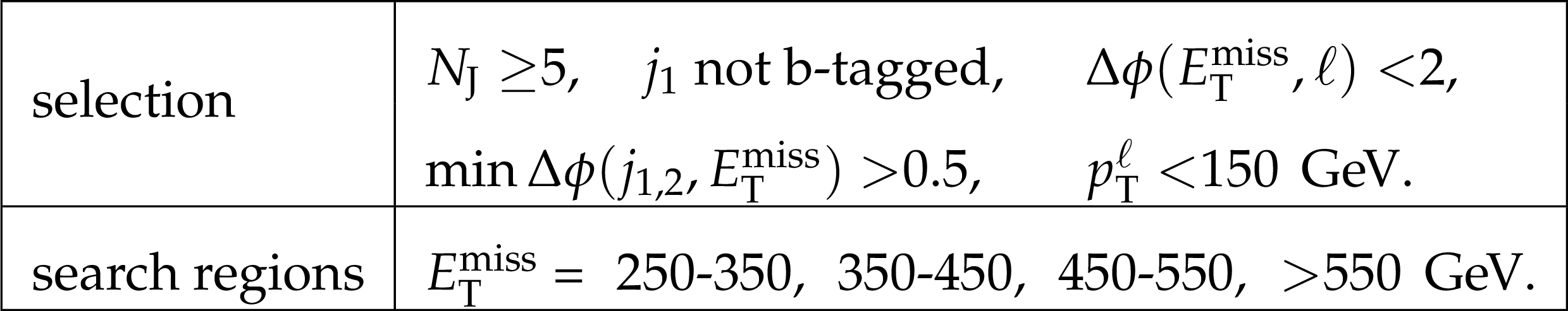
png pdf	Table 3: Summary of the compressed selection and the requirements for the four corresponding signal regions. The symbol $\Delta \phi ( {E_{\mathrm {T}}^{\text {miss}}} ,\ell )$ denotes the angle between $E_{\mathrm{T}}^{\text{miss}}$ and the $\vec{p}_{\mathrm{T}}$ of the lepton.
png pdf	Table 4: Dilepton control regions that are combined when estimating the LL background.
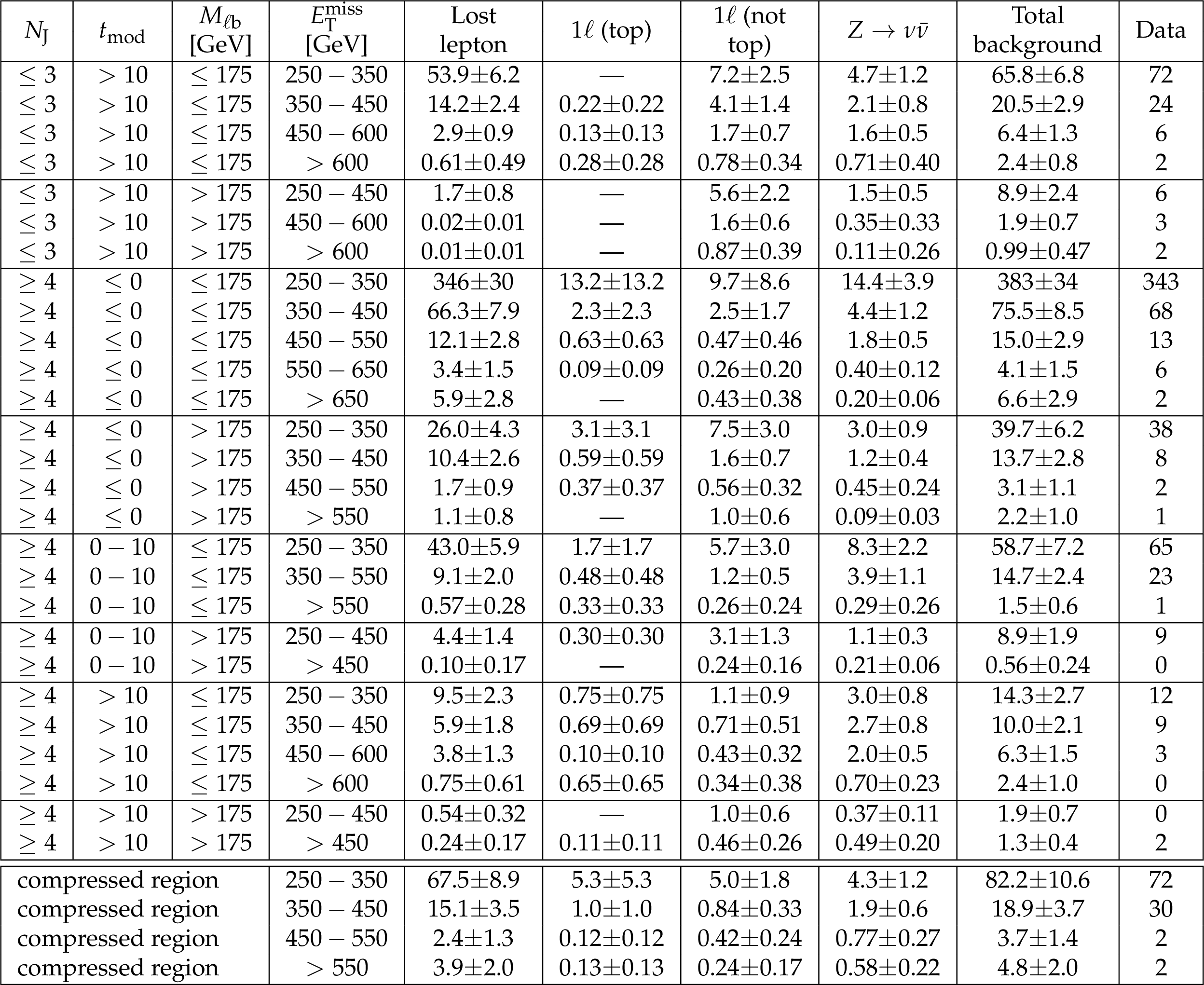
png pdf	Table 5: Result of the background estimates and signal region yields corresponding to 35.9 fb${^{-1}}$.
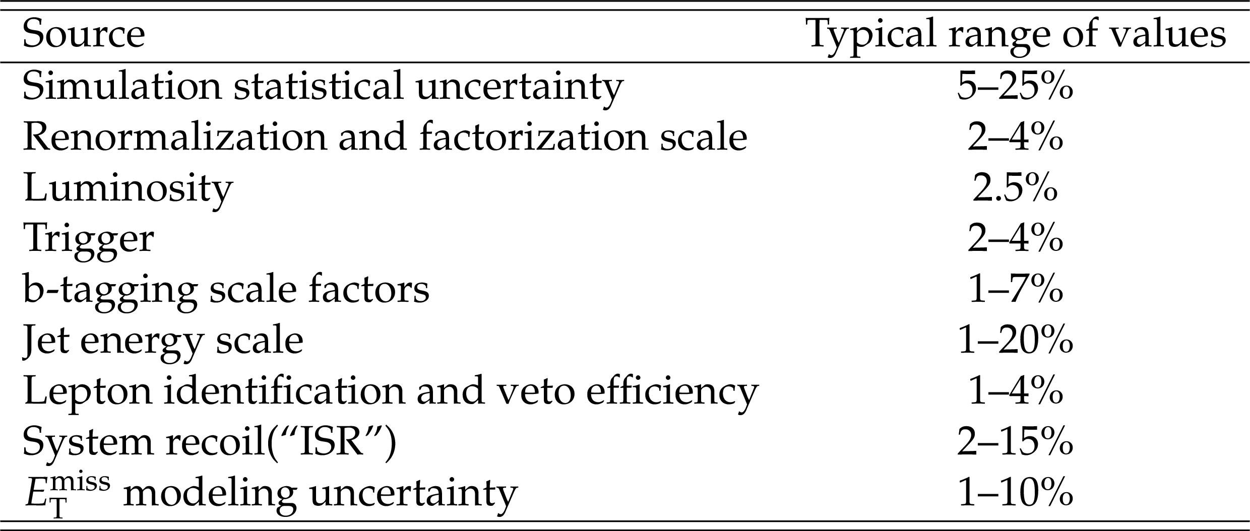
png pdf	Table 6: Summary of the systematic uncertainties for the signal efficiency with their typical values in individual signal regions.
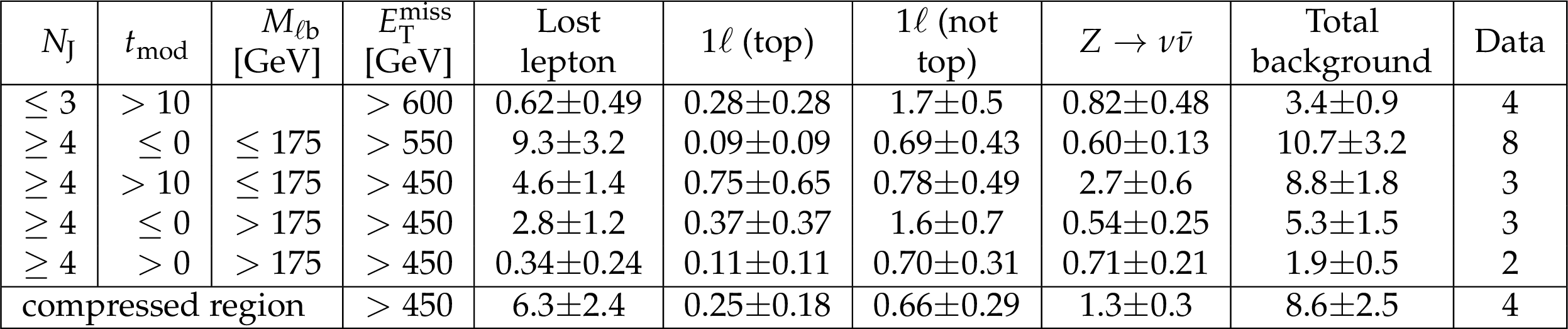
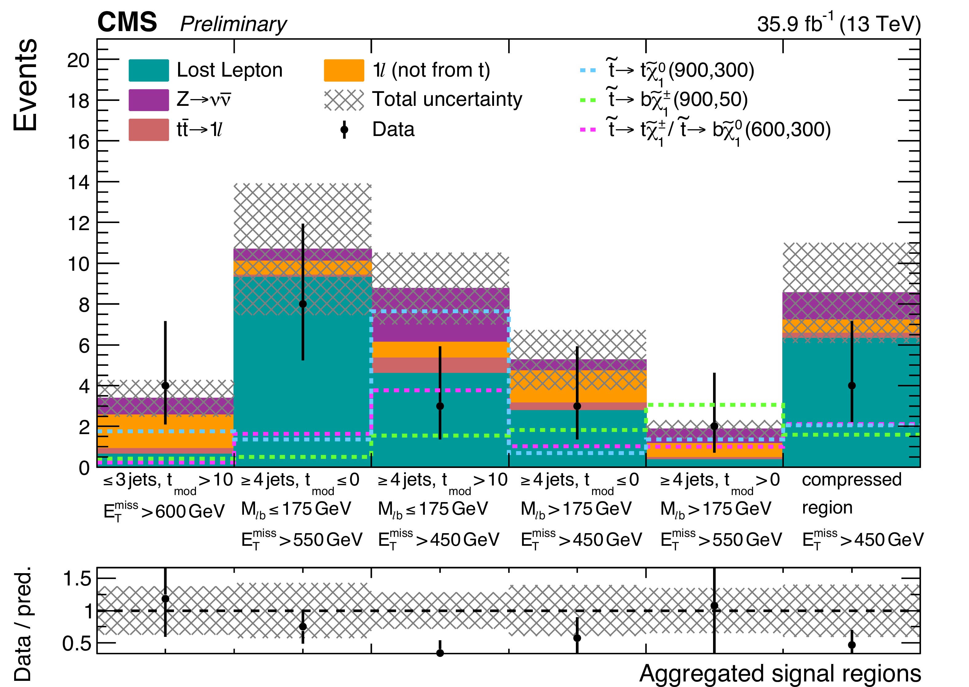
png pdf	Table 7: Background predictions and data for aggregated signal regions.

Summary

We have reported on a search for top squark pair production in pp collisions at $\sqrt{s} =$ 13 TeV in events with a single isolated electron or muon, jets, and large $E_{\mathrm{T}}^{\text{miss}}$ using 35.9 fb${^{-1}}$ of data collected with the CMS detector during the 2016 run of the LHC. The event data counts are consistent with expectations from SM processes. The results are interpreted as exclusion limits in the context of supersymmetric models with pair production of top squarks that decay either to a top quark and a neutralino or to a bottom quark and a chargino. Assuming both top squarks decay to a top quark and a neutralino, we exclude at the 95% confidence level top squark masses up to 1120 GeV for a massless neutralino and neutralino masses up to 515 GeV for a 950 GeV top squark mass.

Additional Figures
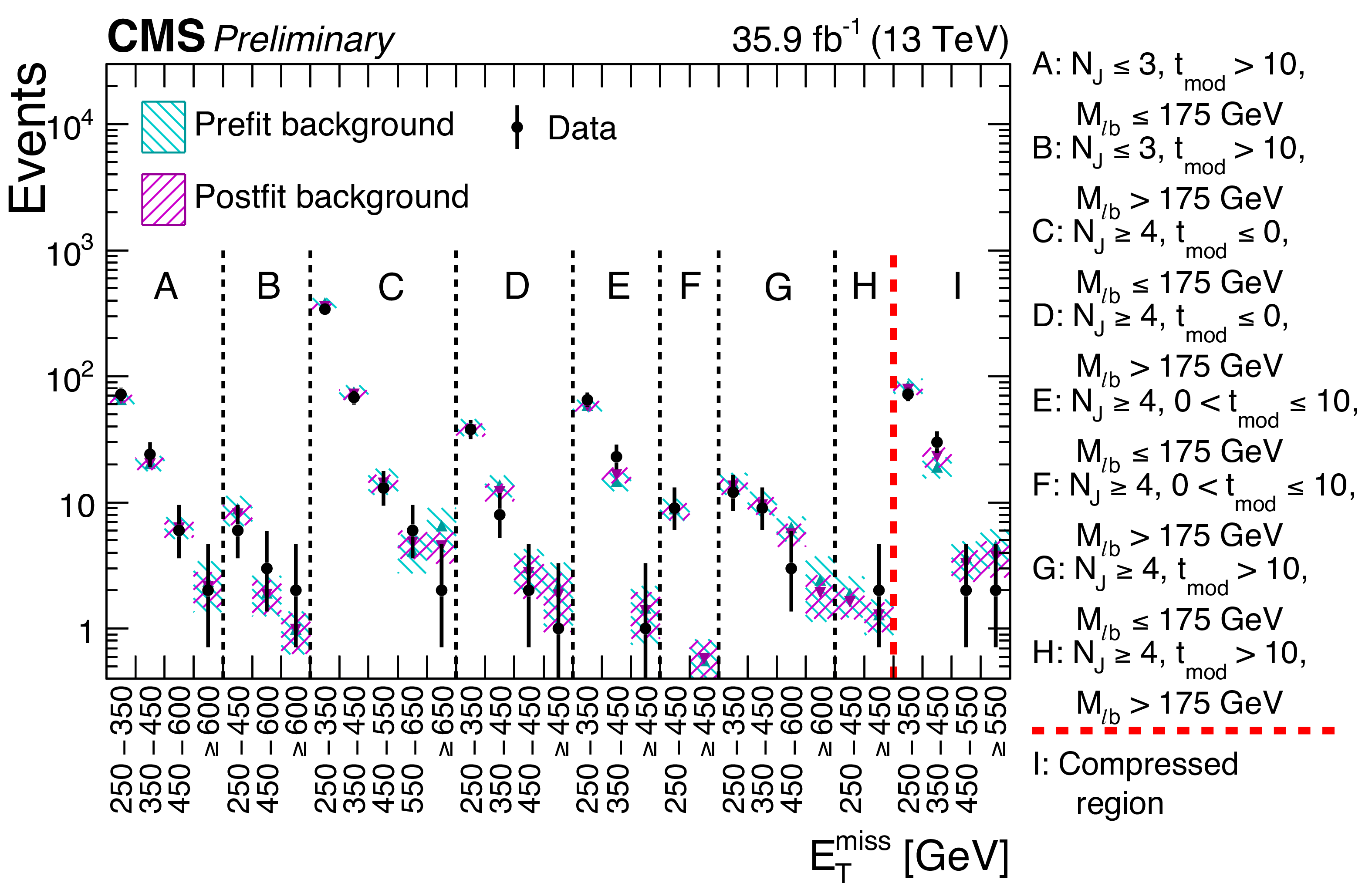
png pdf root	Additional Figure 1: Comparison between postfit and prefit background predictions and data for 35.9 fb$^{-1}$ collected during 2016 pp collisions.
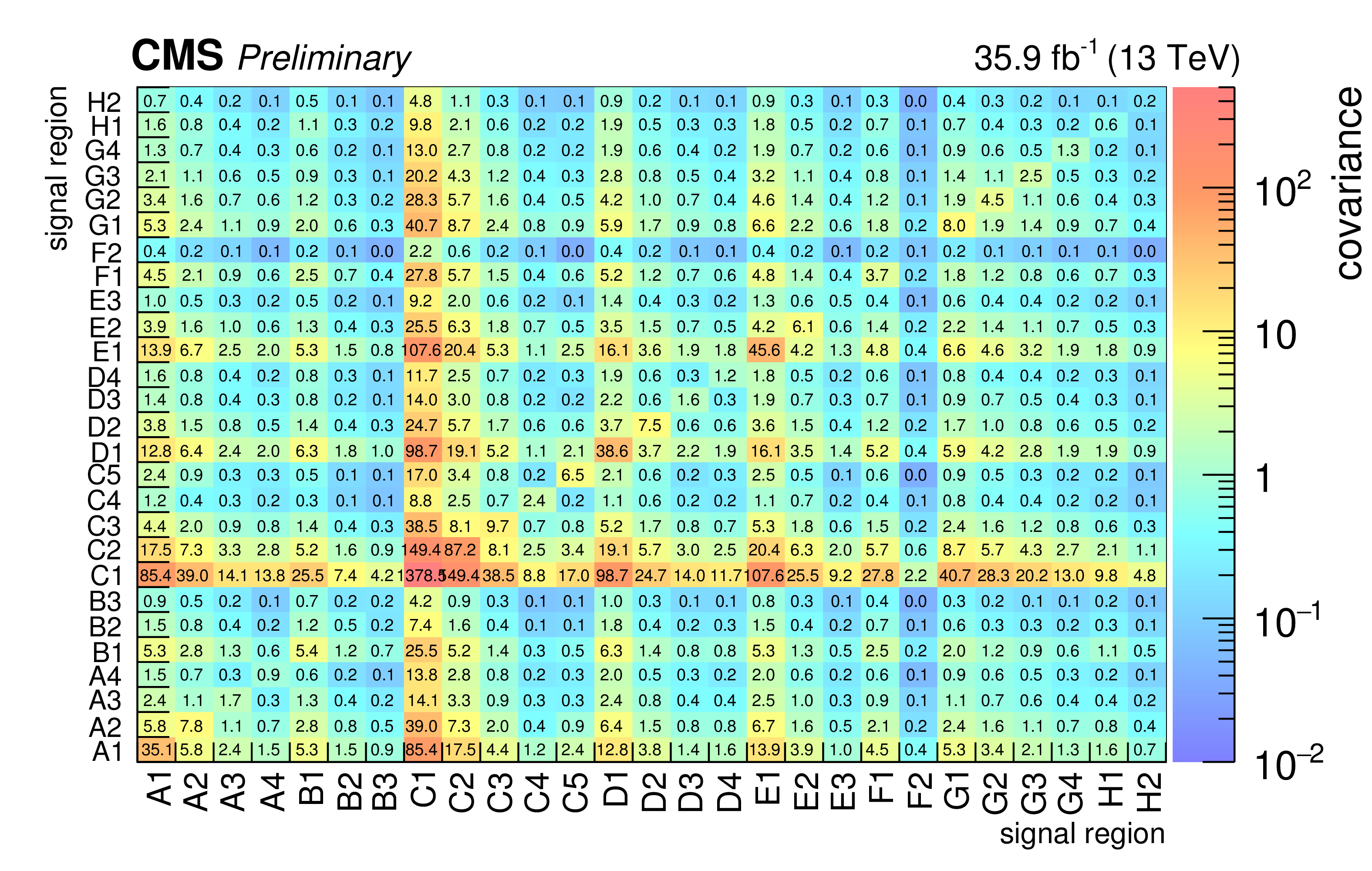
png pdf root	Additional Figure 2: Covariance matrix for the background predictions for the signal regions for the standard selection. The labelling of the regions follows the convention of correlation matrices in the appendix of the note.
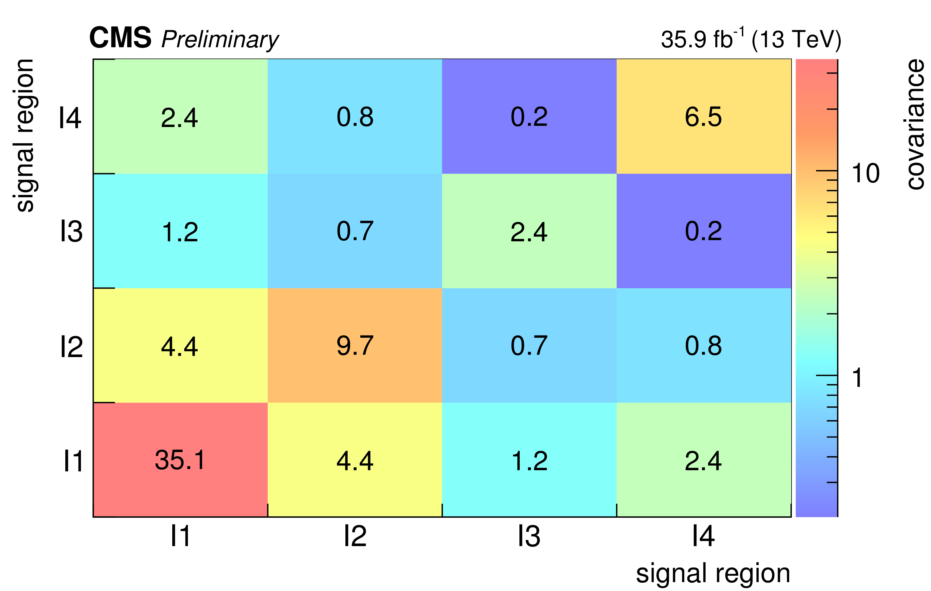
png pdf root	Additional Figure 3: Covariance matrix for the background predictions for the signal regions for the compressed selection. The labelling of the regions follows the convention of correlation matrices in the appendix of the note.
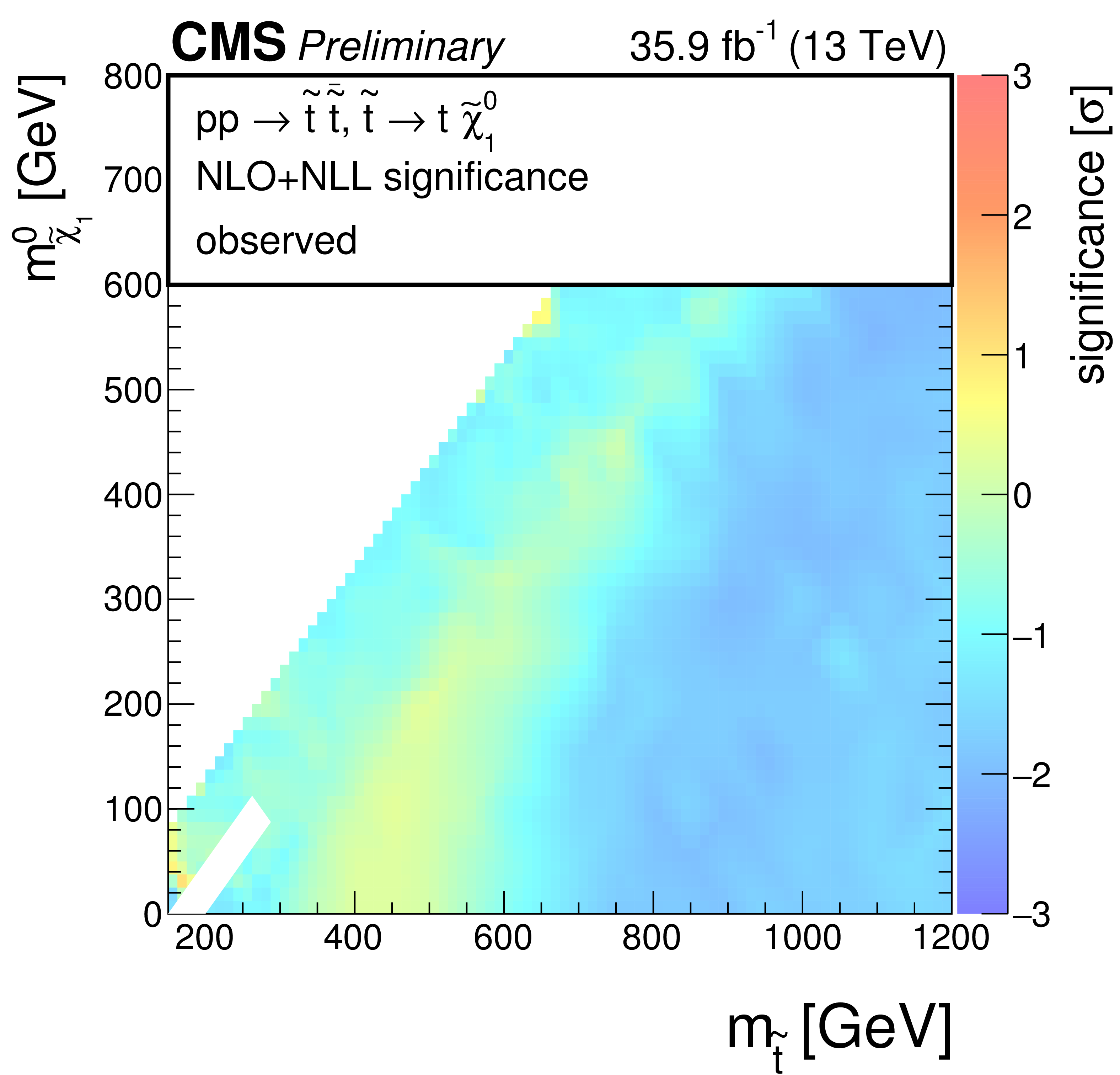
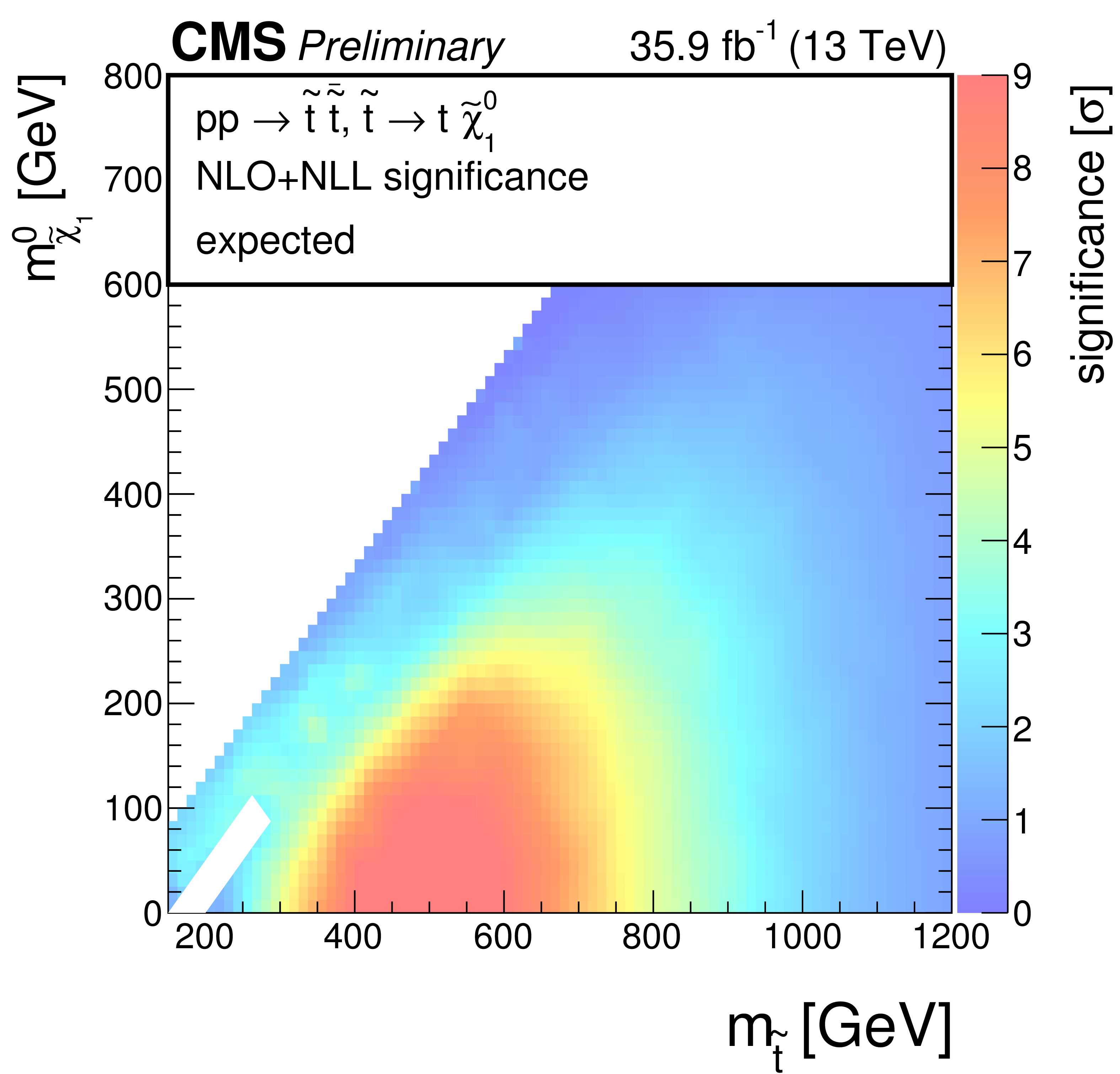
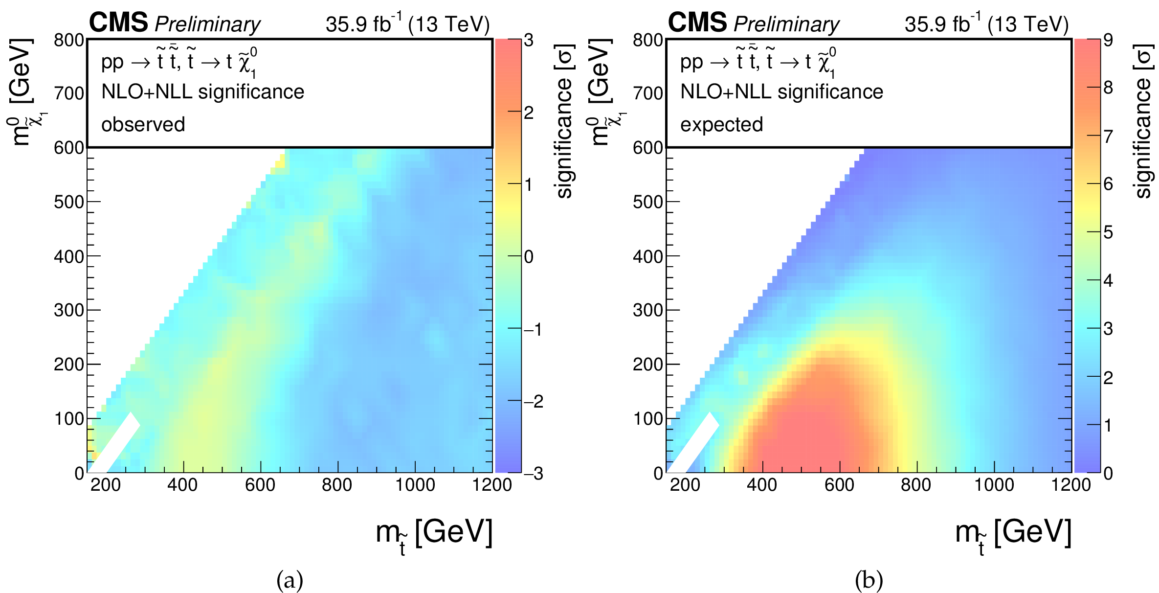
png pdf	Additional Figure 4: Significances for a model of direct top-squark production with decay $\mathrm{ p } \mathrm{ p } \to \tilde{ \mathrm{ t } } \overline{\tilde{\mathrm{t}}}$, $\tilde{ \mathrm{ t } } \to \mathrm{ t } ^{(*)}\tilde{\chi}^0_1$ as a function of $M_{\tilde{ \mathrm{ t } } }$ and $M_{\tilde{\chi}^0_1 }$. (a) Observed, (b) expected.
png pdf	Additional Figure 4-a: Observed significance for a model of direct top-squark production with decay $\mathrm{ p } \mathrm{ p } \to \tilde{ \mathrm{ t } } \overline{\tilde{\mathrm{t}}}$, $\tilde{ \mathrm{ t } } \to \mathrm{ t } ^{(*)}\tilde{\chi}^0_1$ as a function of $M_{\tilde{ \mathrm{ t } } }$ and $M_{\tilde{\chi}^0_1 }$.
png pdf	Additional Figure 4-b: Expected significance for a model of direct top-squark production with decay $\mathrm{ p } \mathrm{ p } \to \tilde{ \mathrm{ t } } \overline{\tilde{\mathrm{t}}}$, $\tilde{ \mathrm{ t } } \to \mathrm{ t } ^{(*)}\tilde{\chi}^0_1$ as a function of $M_{\tilde{ \mathrm{ t } } }$ and $M_{\tilde{\chi}^0_1 }$.
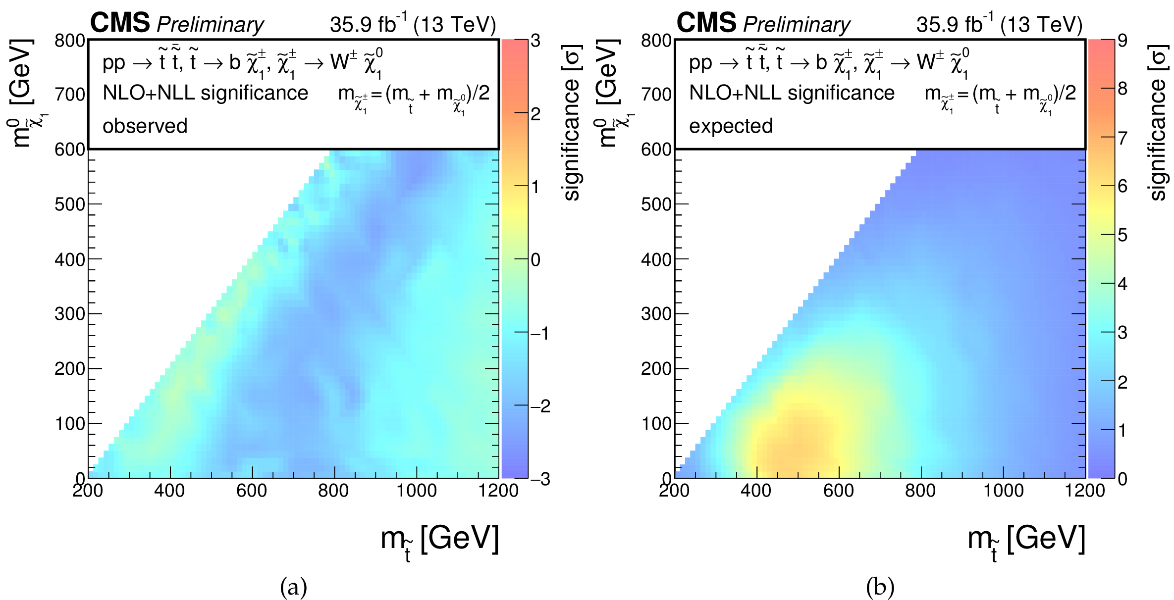
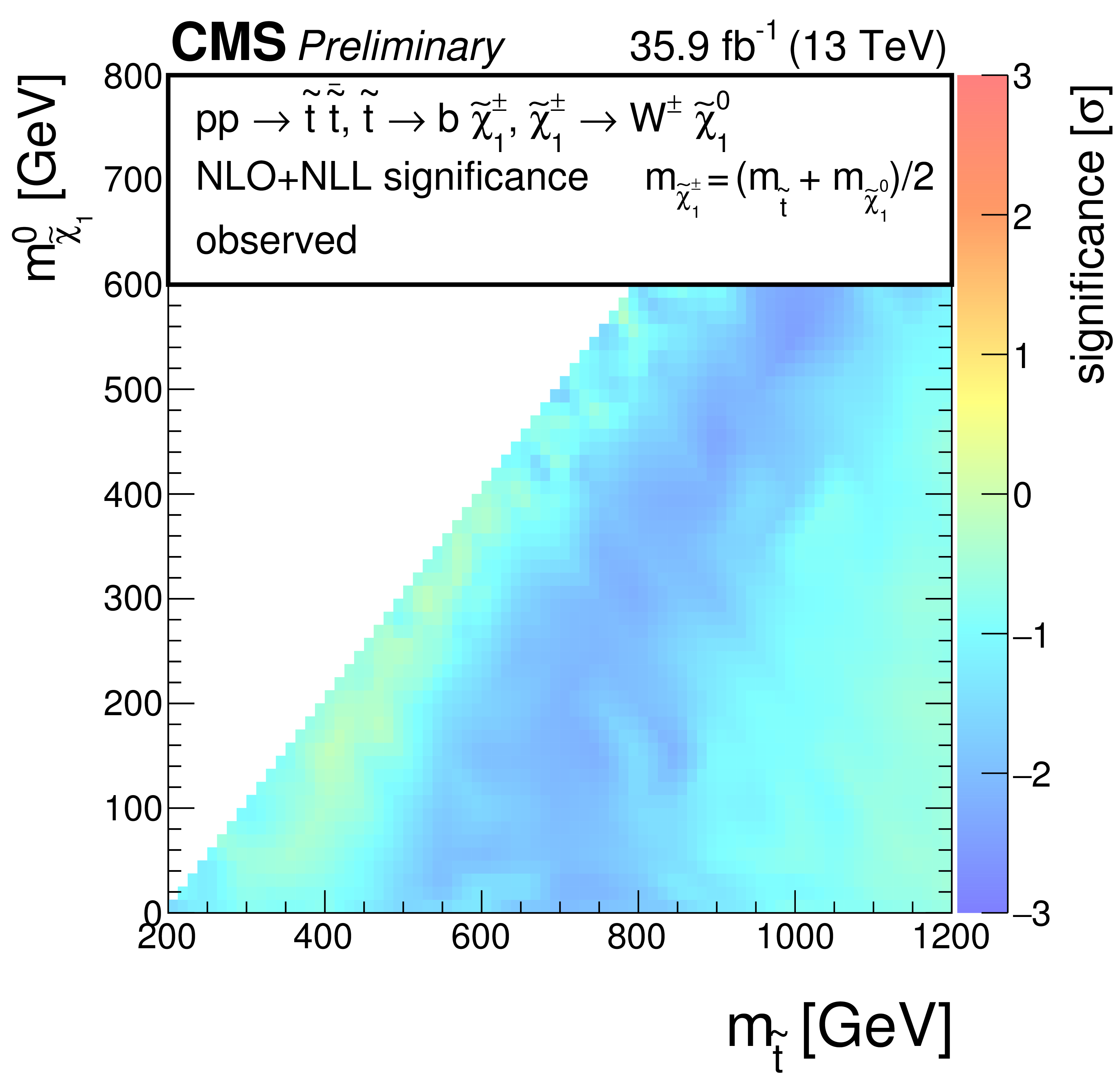
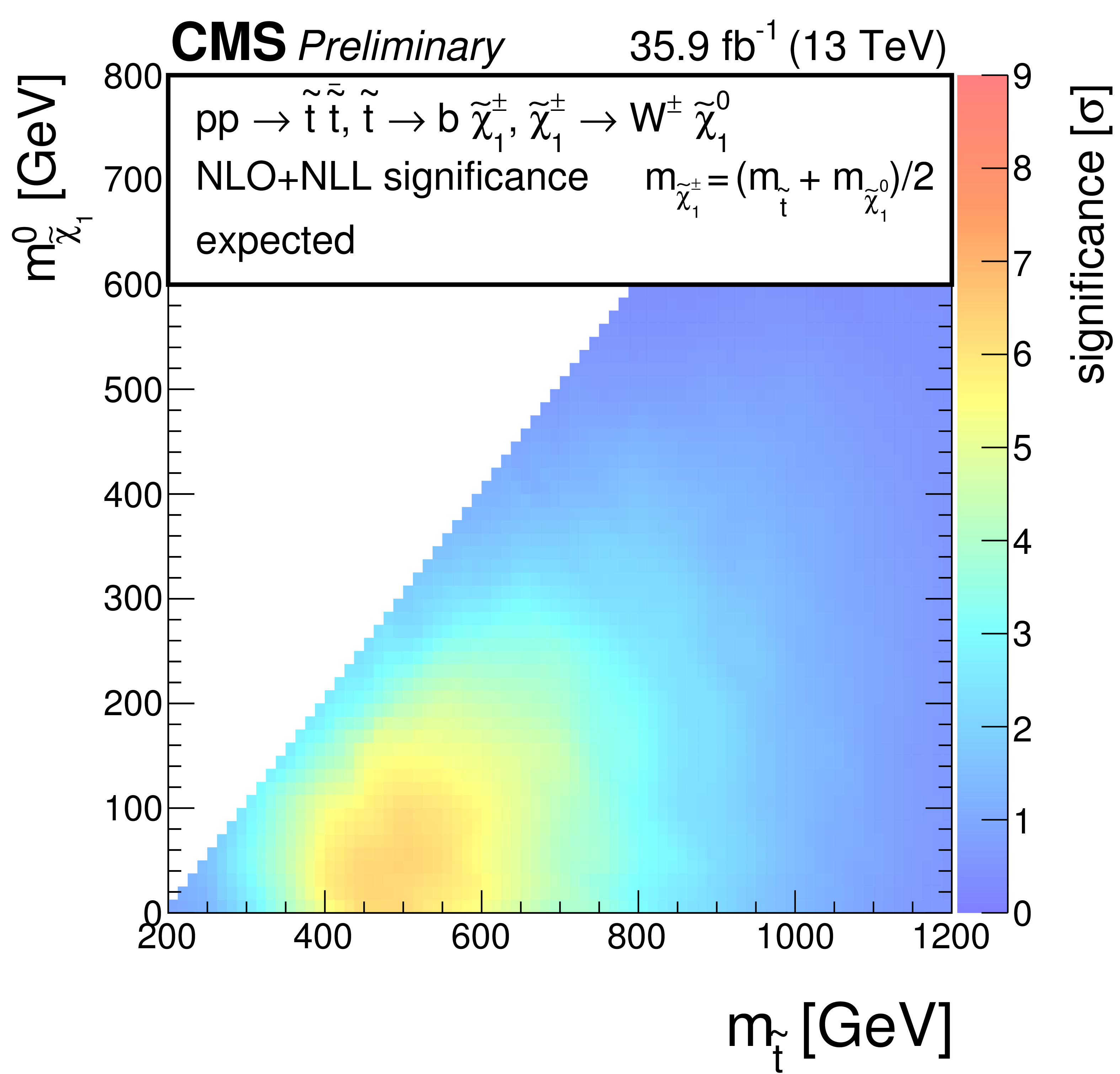
png pdf	Additional Figure 5: Significances for a model of direct top-squark production with decay $\mathrm{ p } \mathrm{ p } \to \tilde{ \mathrm{ t } } \overline{\tilde{\mathrm{t}}} \to \mathrm{ b \bar{b} } \tilde{\chi}^{\pm}_1 \tilde{\chi}^{\pm}_1$, $\tilde{\chi}^{\pm}_1 \to \mathrm{ W } \tilde{\chi}^0_1$ as a function of $M_{\tilde{ \mathrm{ t } } }$ and $M_{\tilde{\chi}^0_1 }$. The mass of the chargino is chosen to be $(M_{\tilde{ \mathrm{ t } } } + M_{\tilde{\chi}^0_1 })/2$. (a) Observed, (b) expected.
png pdf	Additional Figure 5-a: Observed significance for a model of direct top-squark production with decay $\mathrm{ p } \mathrm{ p } \to \tilde{ \mathrm{ t } } \overline{\tilde{\mathrm{t}}} \to \mathrm{ b \bar{b} } \tilde{\chi}^{\pm}_1 \tilde{\chi}^{\pm}_1$, $\tilde{\chi}^{\pm}_1 \to \mathrm{ W } \tilde{\chi}^0_1$ as a function of $M_{\tilde{ \mathrm{ t } } }$ and $M_{\tilde{\chi}^0_1 }$. The mass of the chargino is chosen to be $(M_{\tilde{ \mathrm{ t } } } + M_{\tilde{\chi}^0_1 })/2$.
png pdf	Additional Figure 5-b: Expected significance for a model of direct top-squark production with decay $\mathrm{ p } \mathrm{ p } \to \tilde{ \mathrm{ t } } \overline{\tilde{\mathrm{t}}} \to \mathrm{ b \bar{b} } \tilde{\chi}^{\pm}_1 \tilde{\chi}^{\pm}_1$, $\tilde{\chi}^{\pm}_1 \to \mathrm{ W } \tilde{\chi}^0_1$ as a function of $M_{\tilde{ \mathrm{ t } } }$ and $M_{\tilde{\chi}^0_1 }$. The mass of the chargino is chosen to be $(M_{\tilde{ \mathrm{ t } } } + M_{\tilde{\chi}^0_1 })/2$.
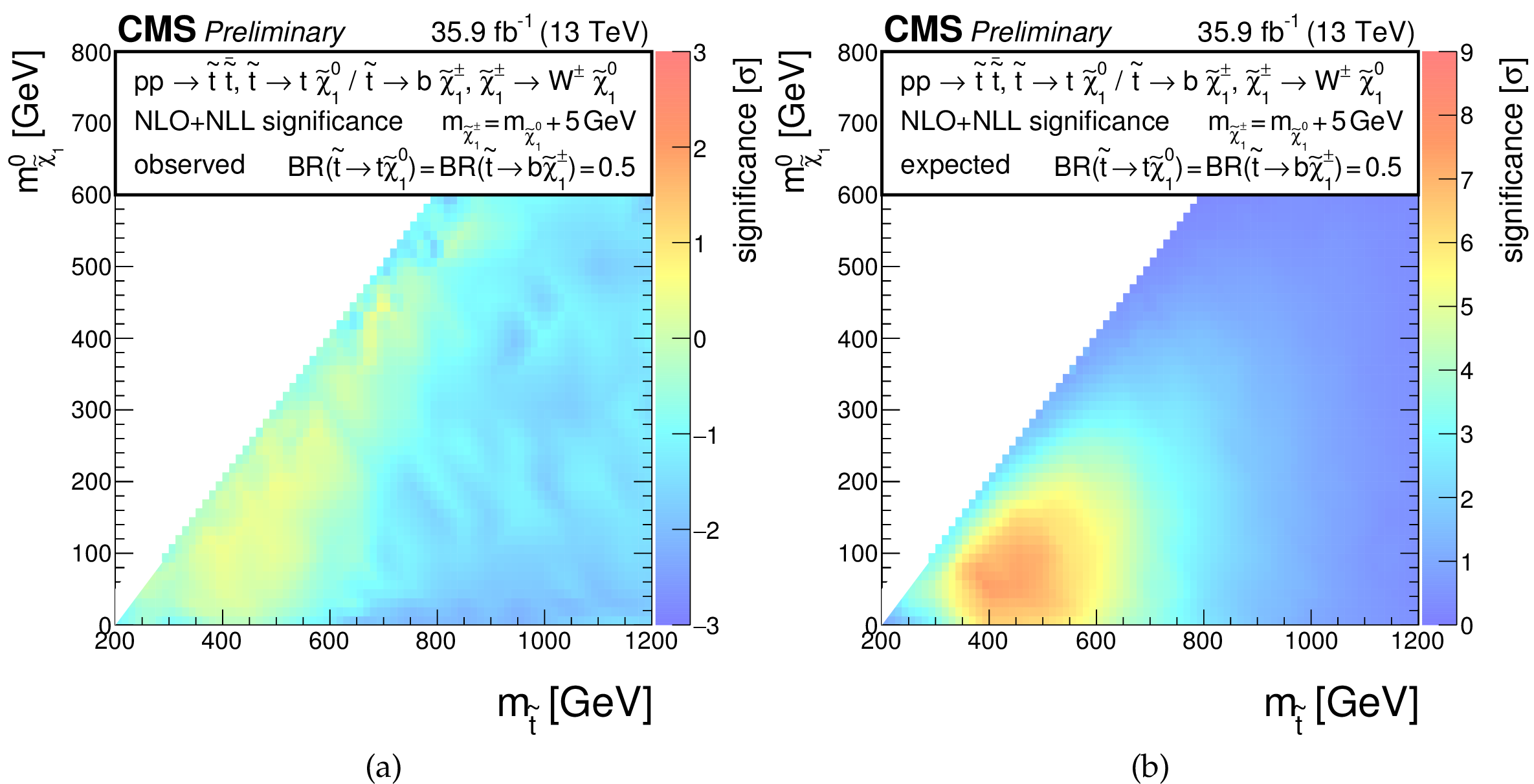
png pdf	Additional Figure 6: Significances for a model of direct top-squark production with decay $\mathrm{ p } \mathrm{ p } \to \tilde{ \mathrm{ t } } \overline{\tilde{\mathrm{t}}}$, $\tilde{ \mathrm{ t } } \to \mathrm{ b } \tilde{\chi}^{\pm}_1 / \mathrm{ t } \tilde{\chi}^0_1$, $\tilde{\chi}^{\pm}_1 \to \mathrm{ W } \tilde{\chi}^0_1$, $m_{\tilde{\chi}^{\pm}_1 } = m_{\tilde{\chi}^0_1 }+$ 5 GeV, BR($\tilde{ \mathrm{ t } } \to \mathrm{ b } \tilde{\chi}^{\pm}_1$) = BR($\tilde{ \mathrm{ t } } \to \mathrm{ t } \tilde{\chi}^0_1$) = 0.5 as a function of $M_{\tilde{ \mathrm{ t } } }$ and $M_{\tilde{\chi}^0_1 }$. (a) Observed, (b) expected.
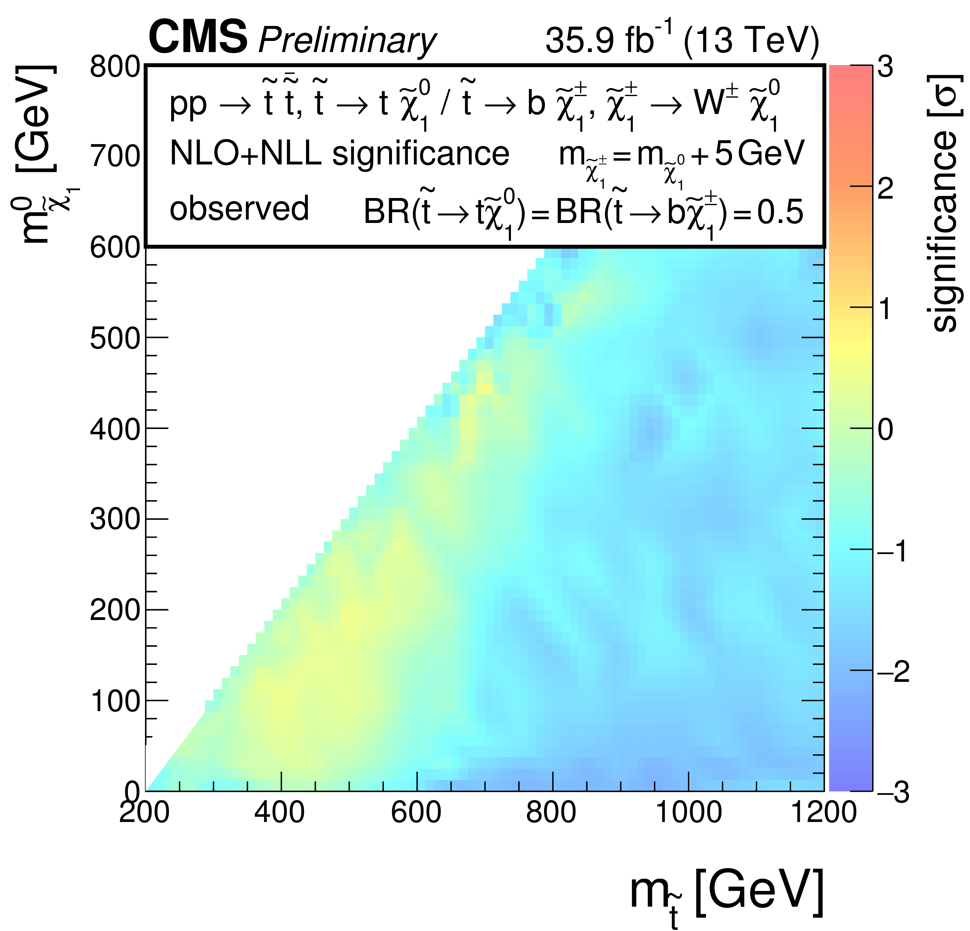
png pdf	Additional Figure 6-a: Observed significance for a model of direct top-squark production with decay $\mathrm{ p } \mathrm{ p } \to \tilde{ \mathrm{ t } } \overline{\tilde{\mathrm{t}}}$, $\tilde{ \mathrm{ t } } \to \mathrm{ b } \tilde{\chi}^{\pm}_1 / \mathrm{ t } \tilde{\chi}^0_1$, $\tilde{\chi}^{\pm}_1 \to \mathrm{ W } \tilde{\chi}^0_1$, $m_{\tilde{\chi}^{\pm}_1 } = m_{\tilde{\chi}^0_1 }+$ 5 GeV, BR($\tilde{ \mathrm{ t } } \to \mathrm{ b } \tilde{\chi}^{\pm}_1$) = BR($\tilde{ \mathrm{ t } } \to \mathrm{ t } \tilde{\chi}^0_1$) = 0.5 as a function of $M_{\tilde{ \mathrm{ t } } }$ and $M_{\tilde{\chi}^0_1 }$.
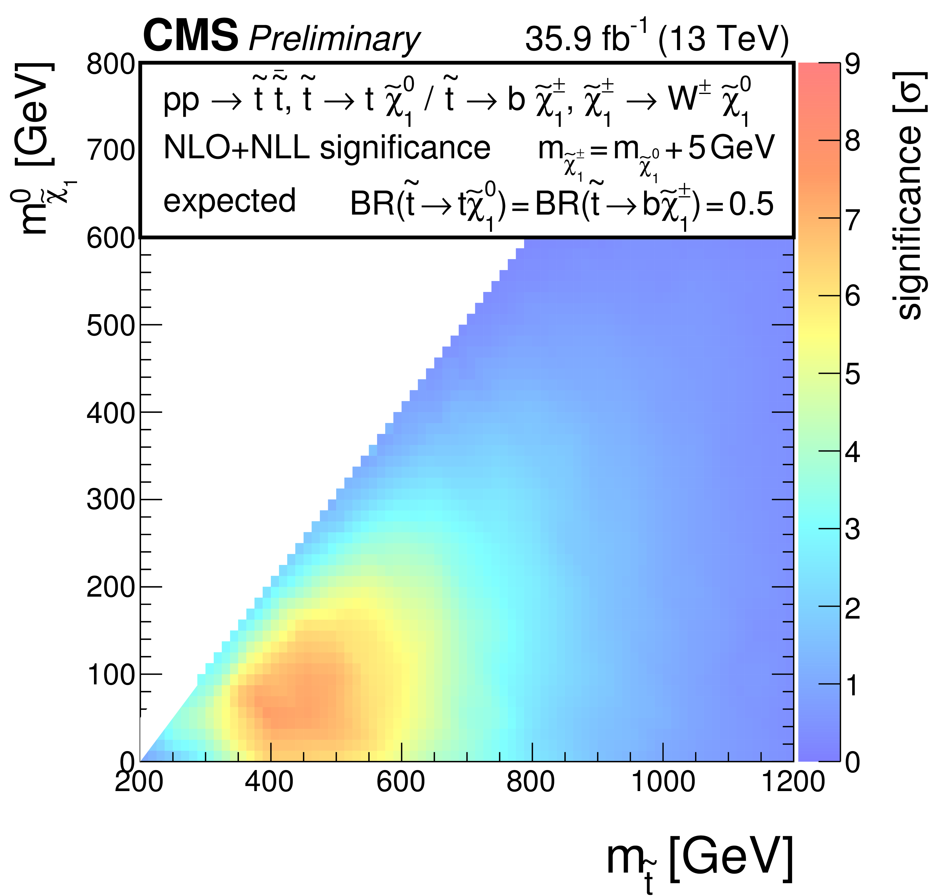
png pdf	Additional Figure 6-b: Expected significance for a model of direct top-squark production with decay $\mathrm{ p } \mathrm{ p } \to \tilde{ \mathrm{ t } } \overline{\tilde{\mathrm{t}}}$, $\tilde{ \mathrm{ t } } \to \mathrm{ b } \tilde{\chi}^{\pm}_1 / \mathrm{ t } \tilde{\chi}^0_1$, $\tilde{\chi}^{\pm}_1 \to \mathrm{ W } \tilde{\chi}^0_1$, $m_{\tilde{\chi}^{\pm}_1 } = m_{\tilde{\chi}^0_1 }+$ 5 GeV, BR($\tilde{ \mathrm{ t } } \to \mathrm{ b } \tilde{\chi}^{\pm}_1$) = BR($\tilde{ \mathrm{ t } } \to \mathrm{ t } \tilde{\chi}^0_1$) = 0.5 as a function of $M_{\tilde{ \mathrm{ t } } }$ and $M_{\tilde{\chi}^0_1 }$.
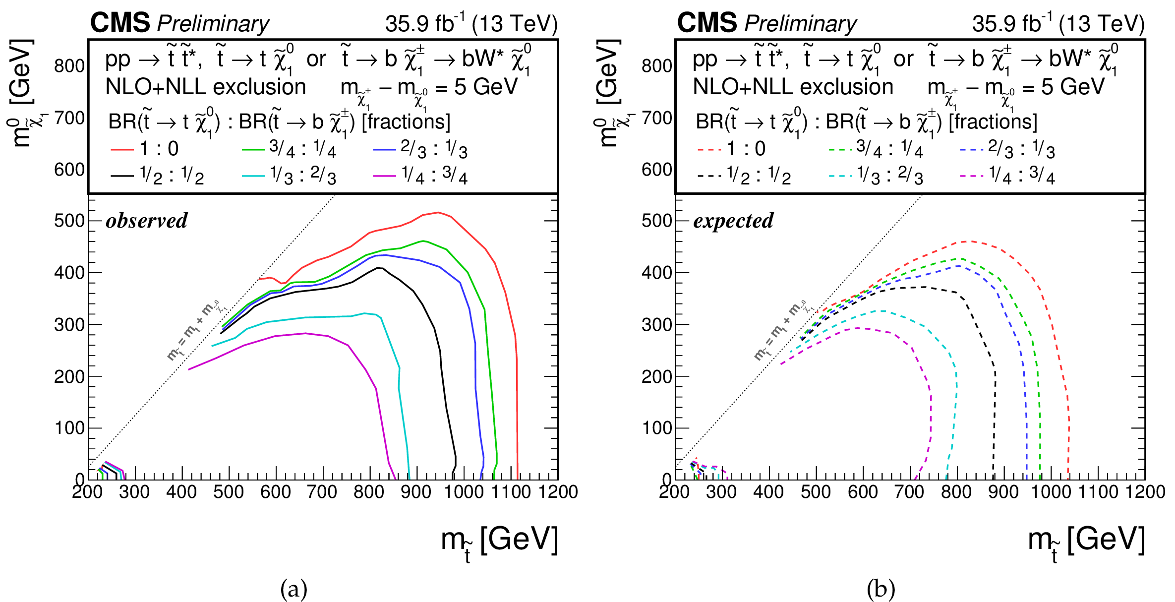
png pdf root	Additional Figure 7: Exclusion limit for the model of direct top-squark production with decay $\mathrm{ p } \mathrm{ p } \to \tilde{ \mathrm{ t } } \overline{\tilde{\mathrm{t}}}$, $\tilde{ \mathrm{ t } } \to \mathrm{ b } \tilde{\chi}^{\pm}_1 / \mathrm{ t } \tilde{\chi}^0_1$, $\tilde{\chi}^{\pm}_1 \to \mathrm{ W } \tilde{\chi}^0_1$, $m_{\tilde{\chi}^{\pm}_1 } = m_{\tilde{\chi}^0_1 }+$ 5 GeV as a function of $M_{\tilde{ \mathrm{ t } } }$ and $M_{\tilde{\chi}^0_1 }$ for various choices of the branching fraction between the two decays. (a) Observed, (b) expected.
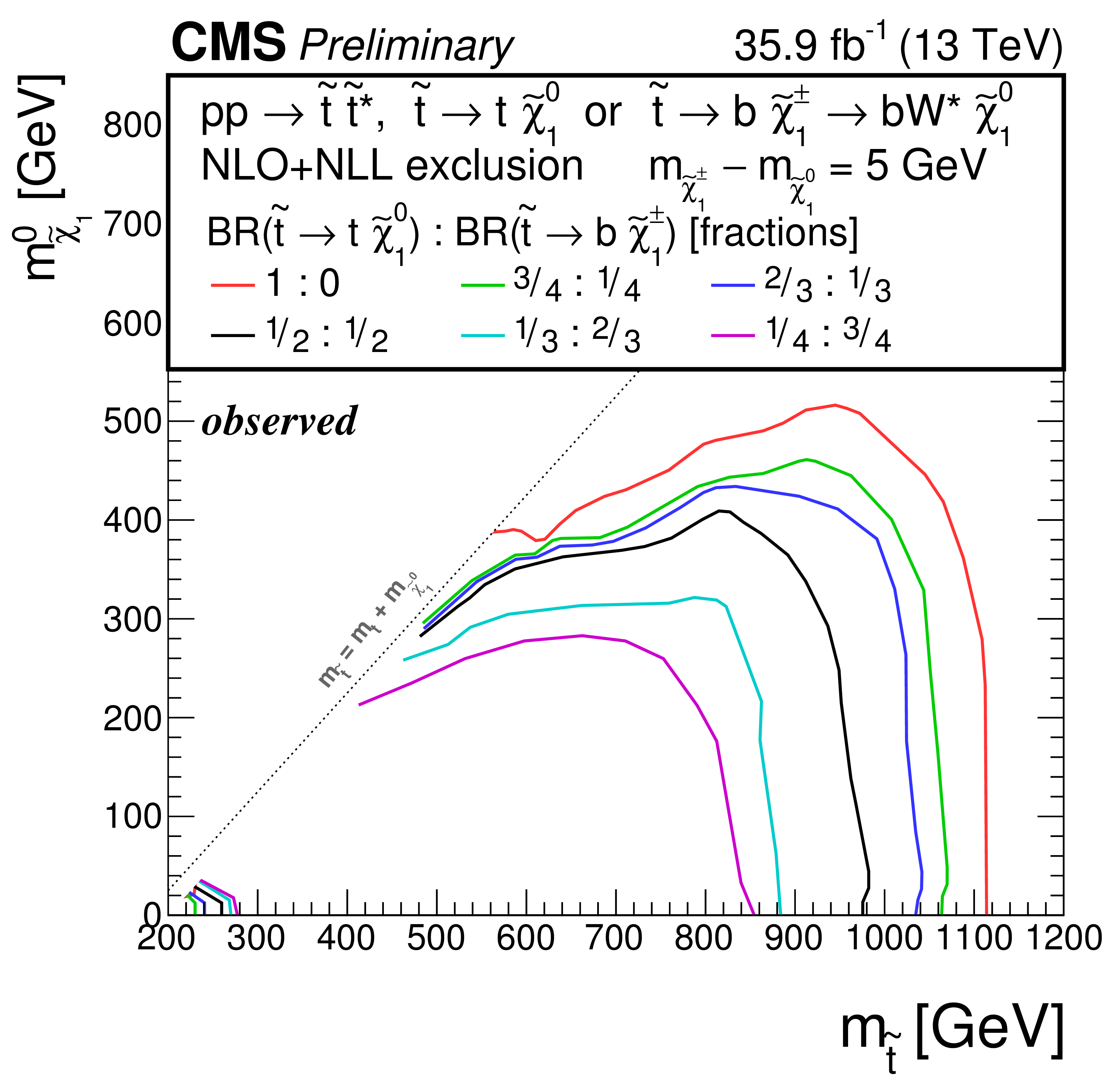
png pdf root	Additional Figure 7-a: Observed exclusion limit for the model of direct top-squark production with decay $\mathrm{ p } \mathrm{ p } \to \tilde{ \mathrm{ t } } \overline{\tilde{\mathrm{t}}}$, $\tilde{ \mathrm{ t } } \to \mathrm{ b } \tilde{\chi}^{\pm}_1 / \mathrm{ t } \tilde{\chi}^0_1$, $\tilde{\chi}^{\pm}_1 \to \mathrm{ W } \tilde{\chi}^0_1$, $m_{\tilde{\chi}^{\pm}_1 } = m_{\tilde{\chi}^0_1 }+$ 5 GeV as a function of $M_{\tilde{ \mathrm{ t } } }$ and $M_{\tilde{\chi}^0_1 }$ for various choices of the branching fraction between the two decays.
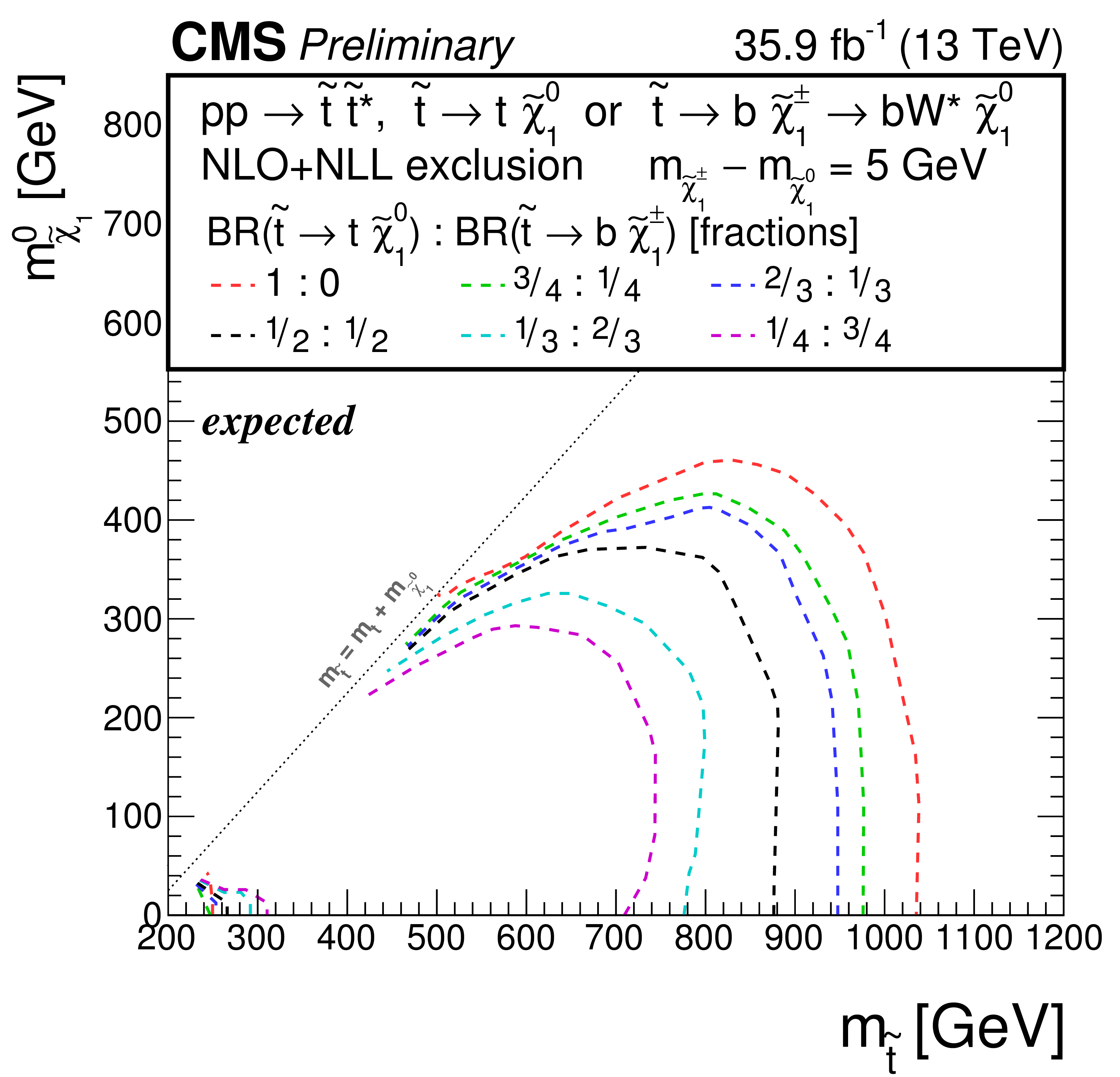
png pdf root	Additional Figure 7-b: Expected exclusion limit for the model of direct top-squark production with decay $\mathrm{ p } \mathrm{ p } \to \tilde{ \mathrm{ t } } \overline{\tilde{\mathrm{t}}}$, $\tilde{ \mathrm{ t } } \to \mathrm{ b } \tilde{\chi}^{\pm}_1 / \mathrm{ t } \tilde{\chi}^0_1$, $\tilde{\chi}^{\pm}_1 \to \mathrm{ W } \tilde{\chi}^0_1$, $m_{\tilde{\chi}^{\pm}_1 } = m_{\tilde{\chi}^0_1 }+$ 5 GeV as a function of $M_{\tilde{ \mathrm{ t } } }$ and $M_{\tilde{\chi}^0_1 }$ for various choices of the branching fraction between the two decays.
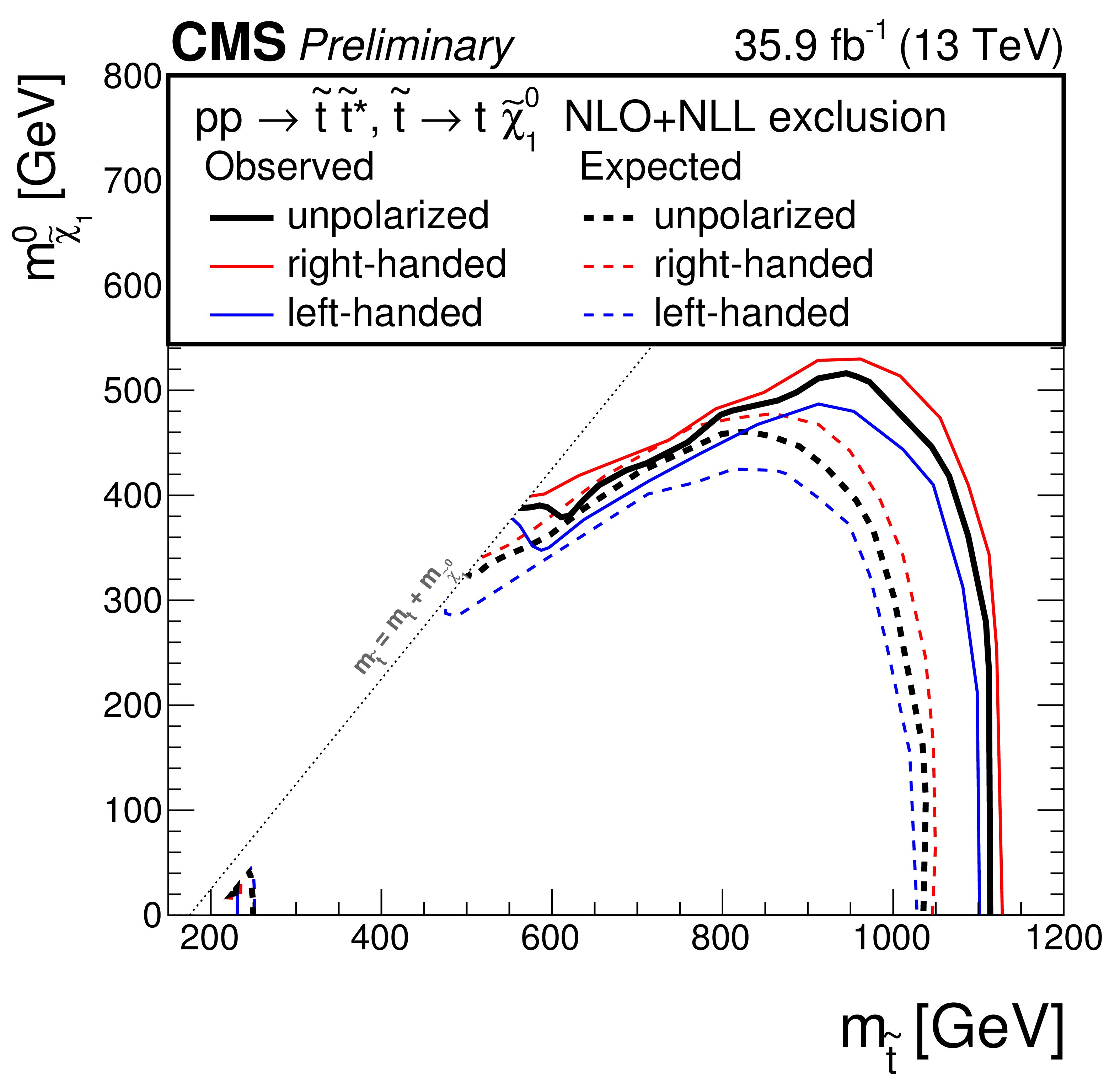
png pdf root	Additional Figure 8: Exclusion limit for the model of direct top-squark production with decay $\mathrm{ p } \mathrm{ p } \to \tilde{ \mathrm{ t } } \overline{\tilde{\mathrm{t}}}$, $\tilde{ \mathrm{ t } } \to \mathrm{ t } ^{(*)}\tilde{\chi}^0_1$ as a function of $M_{\tilde{ \mathrm{ t } } }$ and $M_{\tilde{\chi}^0_1 }$ for unpolarized top quarks (black lines), right-handed top quarks (red lines), and left-handed top quarks (blue lines).
png pdf	Additional Figure 9: Exclusion limits as presented in the note, with the addition of the most recent previous limits as presented during ICHEP 2016 or Moriond 2015. (a): for the model of direct top-squark production with decay $\mathrm{ p } \mathrm{ p } \to \tilde{ \mathrm{ t } } \overline{\tilde{\mathrm{t}}}$, $\tilde{ \mathrm{ t } } \to \mathrm{ t } ^{(*)}\tilde{\chi}^0_1$, (b): for the model of direct top-squark production with decay $\mathrm{ p } \mathrm{ p } \to \tilde{ \mathrm{ t } } \overline{\tilde{\mathrm{t}}} \to \mathrm{ b \bar{b} } \tilde{\chi}^{\pm}_1 \tilde{\chi}^{\pm}_1$, $\tilde{\chi}^{\pm}_1 \to \mathrm{ W } \tilde{\chi}^0_1$ as a function of $M_{\tilde{ \mathrm{ t } } }$ and $M_{\tilde{\chi}^0_1 }$. The mass of the chargino is chosen to be $(M_{\tilde{ \mathrm{ t } } } + M_{\tilde{\chi}^0_1 })/2$, (c): for the model of direct top-squark production with decay $\mathrm{ p } \mathrm{ p } \to \tilde{ \mathrm{ t } } \overline{\tilde{\mathrm{t}}}$, $\tilde{ \mathrm{ t } } \to \mathrm{ b } \tilde{\chi}^{\pm}_1 / \mathrm{ t } \tilde{\chi}^0_1$, $\tilde{\chi}^{\pm}_1 \to \mathrm{ W } \tilde{\chi}^0_1$, $m_{\tilde{\chi}^{\pm}_1 } = m_{\tilde{\chi}^0_1 }+$ 5 GeV, BR($\tilde{ \mathrm{ t } } \to \mathrm{ b } \tilde{\chi}^{\pm}_1$) = BR($\tilde{ \mathrm{ t } } \to \mathrm{ t } \tilde{\chi}^0_1$) = 0.5.
png pdf	Additional Figure 9-a: Exclusion limits as presented in the note, with the addition of the most recent previous limits as presented during ICHEP 2016 or Moriond 2015, for the model of direct top-squark production with decay $\mathrm{ p } \mathrm{ p } \to \tilde{ \mathrm{ t } } \overline{\tilde{\mathrm{t}}}$, $\tilde{ \mathrm{ t } } \to \mathrm{ t } ^{(*)}\tilde{\chi}^0_1$.
png pdf	Additional Figure 9-b: Exclusion limits as presented in the note, with the addition of the most recent previous limits as presented during ICHEP 2016 or Moriond 2015, for the model of direct top-squark production with decay $\mathrm{ p } \mathrm{ p } \to \tilde{ \mathrm{ t } } \overline{\tilde{\mathrm{t}}} \to \mathrm{ b \bar{b} } \tilde{\chi}^{\pm}_1 \tilde{\chi}^{\pm}_1$, $\tilde{\chi}^{\pm}_1 \to \mathrm{ W } \tilde{\chi}^0_1$ as a function of $M_{\tilde{ \mathrm{ t } } }$ and $M_{\tilde{\chi}^0_1 }$. The mass of the chargino is chosen to be $(M_{\tilde{ \mathrm{ t } } } + M_{\tilde{\chi}^0_1 })/2$.
png pdf	Additional Figure 9-c: Exclusion limits as presented in the note, with the addition of the most recent previous limits as presented during ICHEP 2016 or Moriond 2015, for the model of direct top-squark production with decay $\mathrm{ p } \mathrm{ p } \to \tilde{ \mathrm{ t } } \overline{\tilde{\mathrm{t}}}$, $\tilde{ \mathrm{ t } } \to \mathrm{ b } \tilde{\chi}^{\pm}_1 / \mathrm{ t } \tilde{\chi}^0_1$, $\tilde{\chi}^{\pm}_1 \to \mathrm{ W } \tilde{\chi}^0_1$, $m_{\tilde{\chi}^{\pm}_1 } = m_{\tilde{\chi}^0_1 }+$ 5 GeV, BR($\tilde{ \mathrm{ t } } \to \mathrm{ b } \tilde{\chi}^{\pm}_1$) = BR($\tilde{ \mathrm{ t } } \to \mathrm{ t } \tilde{\chi}^0_1$) = 0.5.
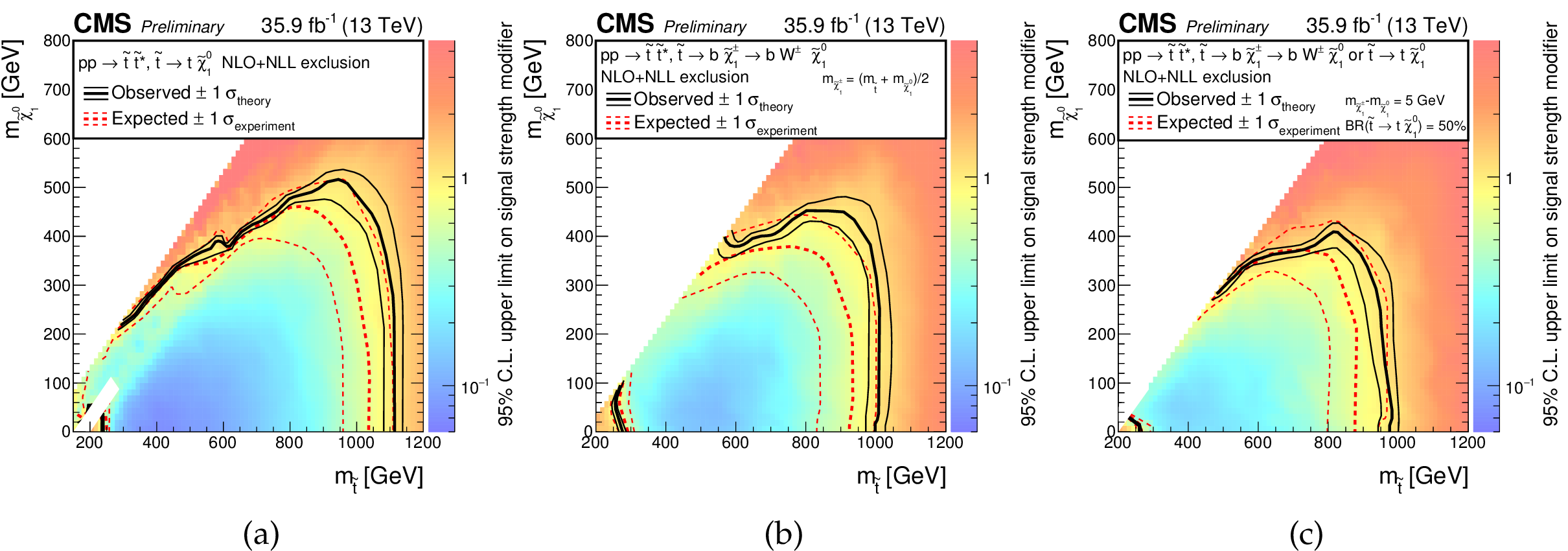
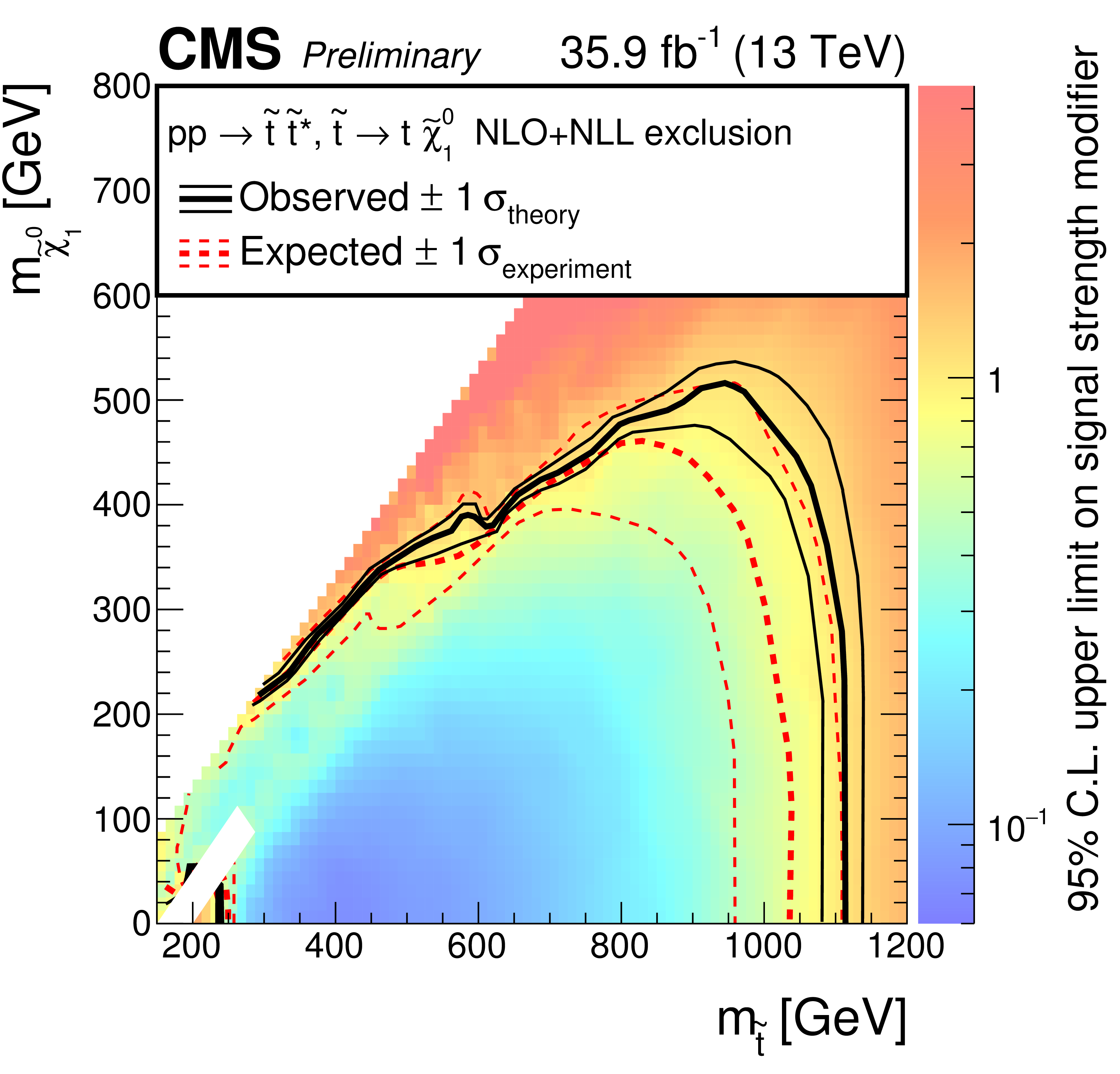
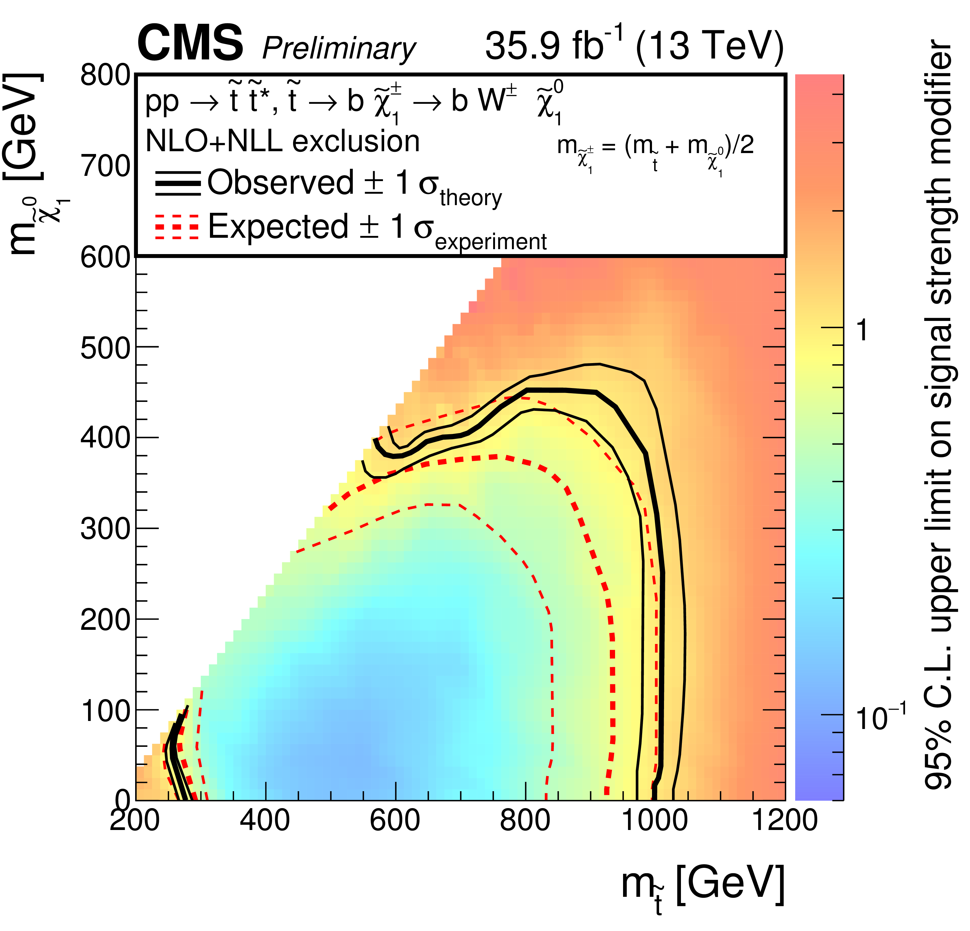
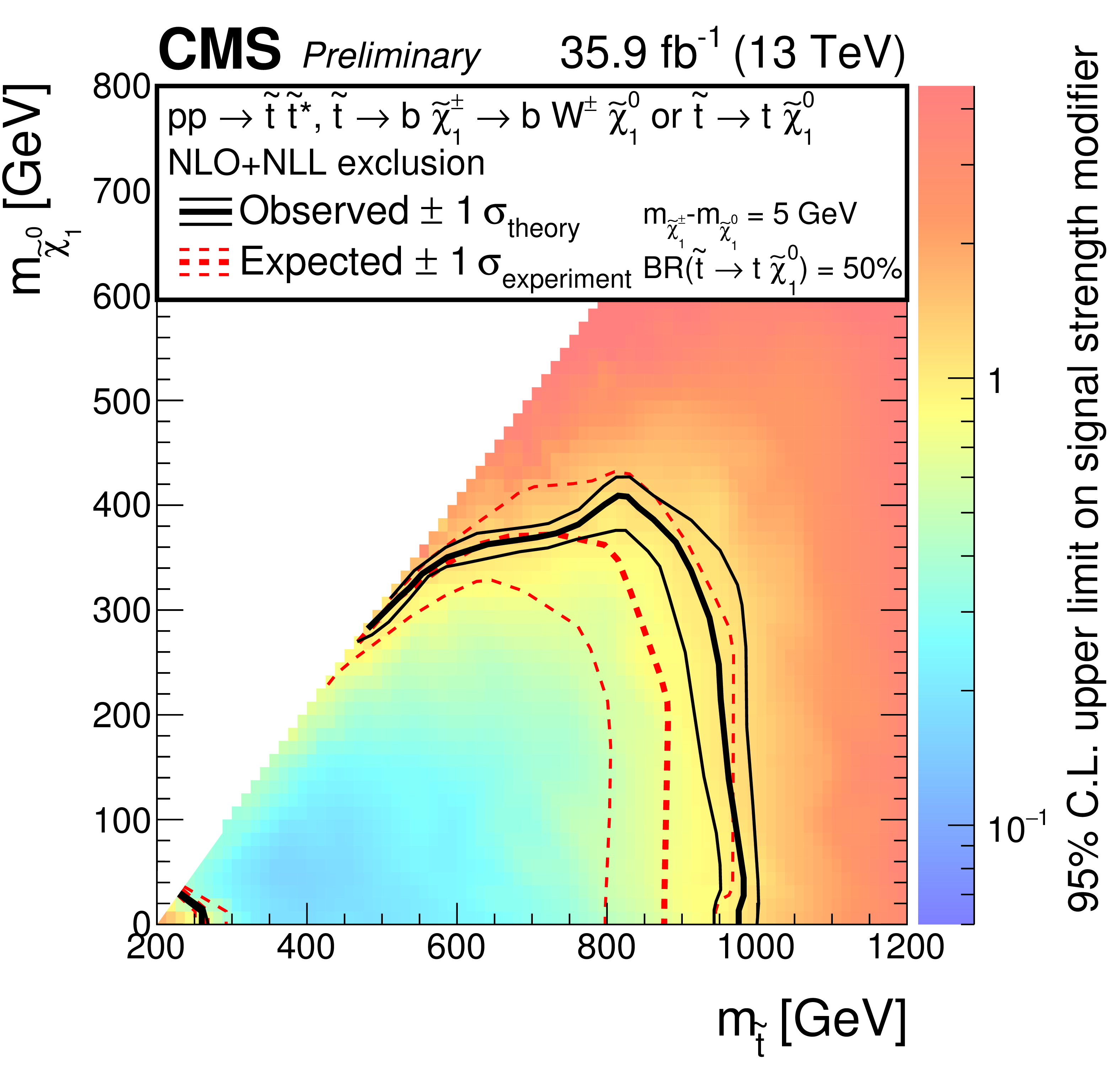
png pdf	Additional Figure 10: Exclusion limits as presented in the note, however the color map is showing the 95% confidence level on the signal strength modifier. (a): for the model of direct top-squark production with decay $\mathrm{ p } \mathrm{ p } \to \tilde{ \mathrm{ t } } \overline{\tilde{\mathrm{t}}}$, $\tilde{ \mathrm{ t } } \to \mathrm{ t } ^{(*)}\tilde{\chi}^0_1$, (b): for the model of direct top-squark production with decay $\mathrm{ p } \mathrm{ p } \to \tilde{ \mathrm{ t } } \overline{\tilde{\mathrm{t}}} \to \mathrm{ b \bar{b} } \tilde{\chi}^{\pm}_1 \tilde{\chi}^{\pm}_1$, $\tilde{\chi}^{\pm}_1 \to \mathrm{ W } \tilde{\chi}^0_1$ as a function of $M_{\tilde{ \mathrm{ t } } }$ and $M_{\tilde{\chi}^0_1 }$. The mass of the chargino is chosen to be $(M_{\tilde{ \mathrm{ t } } } + M_{\tilde{\chi}^0_1 })/2$, (c): for the model of direct top-squark production with decay $\mathrm{ p } \mathrm{ p } \to \tilde{ \mathrm{ t } } \overline{\tilde{\mathrm{t}}}$, $\tilde{ \mathrm{ t } } \to \mathrm{ b } \tilde{\chi}^{\pm}_1 / \mathrm{ t } \tilde{\chi}^0_1$, $\tilde{\chi}^{\pm}_1 \to \mathrm{ W } \tilde{\chi}^0_1$, $m_{\tilde{\chi}^{\pm}_1 } = m_{\tilde{\chi}^0_1 }+$ 5 GeV, BR($\tilde{ \mathrm{ t } } \to \mathrm{ b } \tilde{\chi}^{\pm}_1$) = BR($\tilde{ \mathrm{ t } } \to \mathrm{ t } \tilde{\chi}^0_1$) = 0.5.
png pdf	Additional Figure 10-a: Exclusion limits as presented in the note, however the color map is showing the 95% confidence level on the signal strength modifier, for the model of direct top-squark production with decay $\mathrm{ p } \mathrm{ p } \to \tilde{ \mathrm{ t } } \overline{\tilde{\mathrm{t}}}$, $\tilde{ \mathrm{ t } } \to \mathrm{ t } ^{(*)}\tilde{\chi}^0_1$,
png pdf	Additional Figure 10-b: Exclusion limits as presented in the note, however the color map is showing the 95% confidence level on the signal strength modifier, for the model of direct top-squark production with decay $\mathrm{ p } \mathrm{ p } \to \tilde{ \mathrm{ t } } \overline{\tilde{\mathrm{t}}} \to \mathrm{ b \bar{b} } \tilde{\chi}^{\pm}_1 \tilde{\chi}^{\pm}_1$, $\tilde{\chi}^{\pm}_1 \to \mathrm{ W } \tilde{\chi}^0_1$ as a function of $M_{\tilde{ \mathrm{ t } } }$ and $M_{\tilde{\chi}^0_1 }$. The mass of the chargino is chosen to be $(M_{\tilde{ \mathrm{ t } } } + M_{\tilde{\chi}^0_1 })/2$,
png pdf	Additional Figure 10-c: Exclusion limits as presented in the note, however the color map is showing the 95% confidence level on the signal strength modifier, for the model of direct top-squark production with decay $\mathrm{ p } \mathrm{ p } \to \tilde{ \mathrm{ t } } \overline{\tilde{\mathrm{t}}}$, $\tilde{ \mathrm{ t } } \to \mathrm{ b } \tilde{\chi}^{\pm}_1 / \mathrm{ t } \tilde{\chi}^0_1$, $\tilde{\chi}^{\pm}_1 \to \mathrm{ W } \tilde{\chi}^0_1$, $m_{\tilde{\chi}^{\pm}_1 } = m_{\tilde{\chi}^0_1 }+$ 5 GeV, BR($\tilde{ \mathrm{ t } } \to \mathrm{ b } \tilde{\chi}^{\pm}_1$) = BR($\tilde{ \mathrm{ t } } \to \mathrm{ t } \tilde{\chi}^0_1$) = 0.5.
png pdf	Additional Figure 11: Background predictions and data for the aggregated signal regions using 35.9 fb$^{-1}$collected during 2016 pp collisions.

Additional Tables
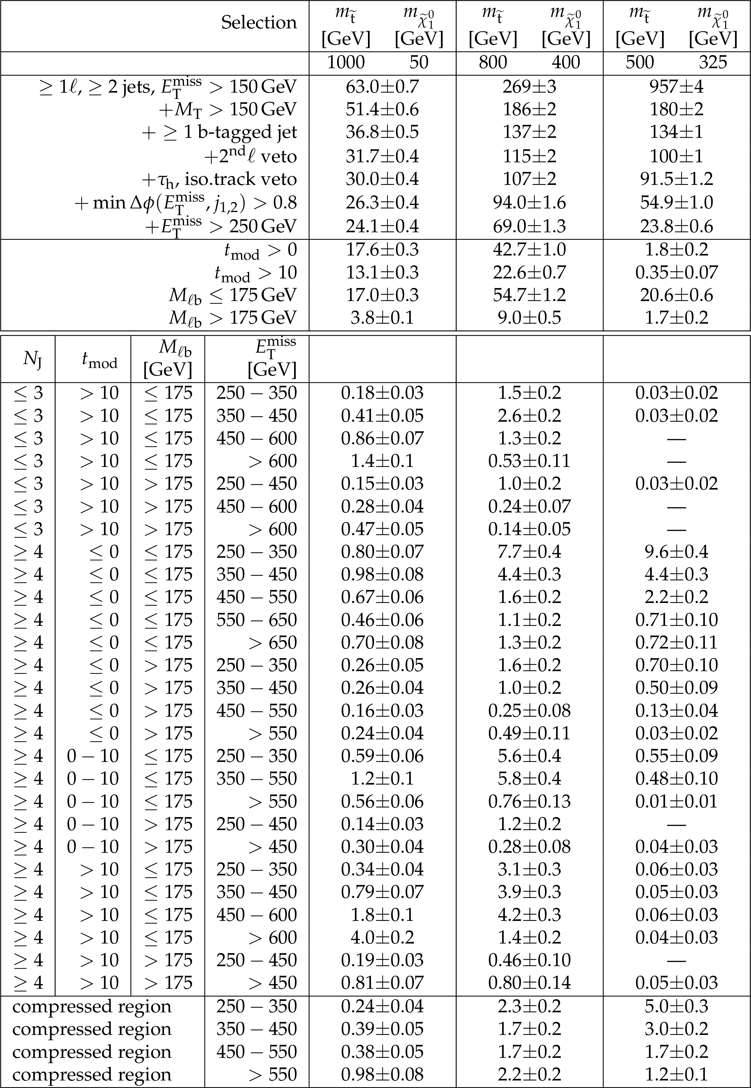
png pdf	Additional Table 1: Cutflow table for $\mathrm{ p } \mathrm{ p } \to \tilde{ \mathrm{ t } } \tilde{ \mathrm{ t } } ^{*}\to \mathrm{ t \bar{t} } \tilde{\chi}^0_1 \tilde{\chi}^0_1$ signals for an integrated luminosity of 35.9 fb$^{-1}$. The uncertainties are purely statistical. No correction for signal contamination in data control regions are applied.
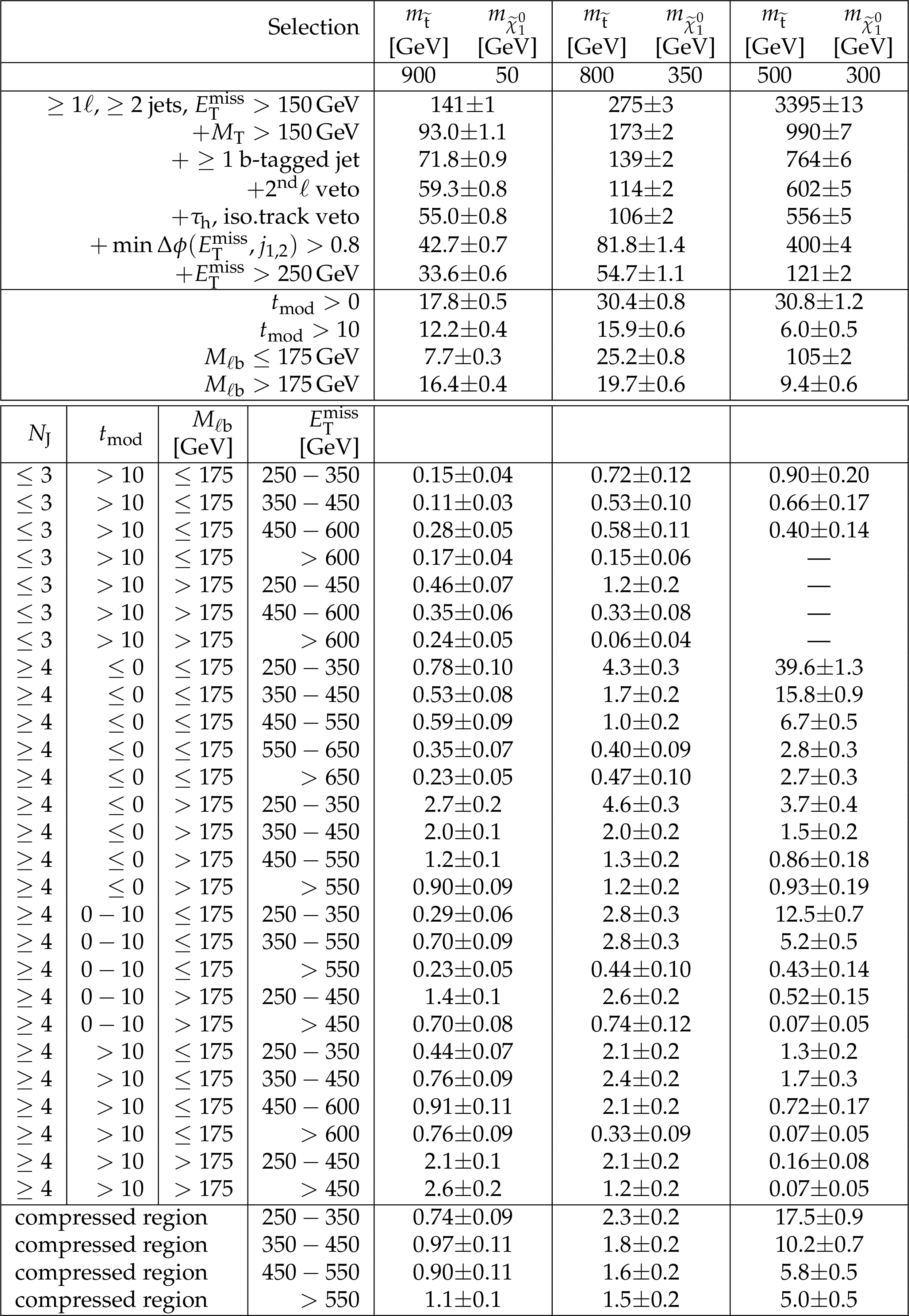
png pdf	Additional Table 2: Cutflow table for $\mathrm{ p } \mathrm{ p } \to \tilde{ \mathrm{ t } } \tilde{ \mathrm{ t } } ^{*}, \tilde{ \mathrm{ t } } \to \mathrm{ t } \tilde{\chi}^0_1 / \mathrm{ b } \tilde{\chi}^{\pm}_1$ signals for an integrated luminosity of 35.9 fb$^{-1}$. The branching fraction for this model is BR($\tilde{ \mathrm{ t } } \to \mathrm{ t } \tilde{\chi}^0_1$) = BR($\tilde{ \mathrm{ t } } \to \mathrm{ b } \tilde{\chi}^{\pm}_1$) = 0.5, and $M_{\tilde{\chi}^{\pm}_1 } = M_{\tilde{\chi}^0_1 } + 5 GeV$. The uncertainties are purely statistical. No correction for signal contamination in data control regions are applied.
png pdf	Additional Table 3: Cutflow table for $\mathrm{ p } \mathrm{ p } \to \tilde{ \mathrm{ t } } \tilde{ \mathrm{ t } } ^{*}\to \mathrm{ b \bar{b} } \tilde{\chi}^{\pm}_1 \tilde{\chi}^{\pm}_1$, $\tilde{\chi}^{\pm}_1 \to \mathrm{ W } \tilde{\chi}^0_1$ signals with $M_{\tilde{\chi}^{\pm}_1 } = (M_{\tilde{ \mathrm{ t } } }+M_{\tilde{\chi}^0_1 })/2$ for an integrated luminosity of 35.9 fb$^{-1}$. The uncertainties are purely statistical. No correction for signal contamination in data control regions are applied.

Electronic version of the limit curves can be found as three rootfiles here, here, and here. The correlation and covariance matrices can be found as two rootfiles here, and here. A code snippet to calculate the tmod variables together with an example how to use it is provided here.

References
1	ATLAS Collaboration	Search for top squarks in final states with one isolated lepton, jets, and missing transverse momentum in $\sqrt{s}=13$ TeV $pp$ collisions with the ATLAS detector	PRD 94 (2016), no. 5, 052009	1606.03903
2	CMS Collaboration	Searches for pair production for third-generation squarks in sqrt(s)=13 TeV pp collisions		CMS-SUS-16-008 1612.03877
3	CMS Collaboration	Search for supersymmetry in the all-hadronic final state using top quark tagging in pp collisions at $\sqrt{s}$ = 13 TeV		CMS-SUS-16-009 1701.01954
4	CMS Collaboration	The CMS experiment at the CERN LHC	JINST 3 (2008) S08004	CMS-00-001
5	J. Alwall et al.	The automated computation of tree-level and next-to-leading order differential cross sections, and their matching to parton shower simulations	JHEP 07 (2014) 079	1405.0301
6	NNPDF Collaboration	Parton distributions for the LHC Run II	JHEP 04 (2015) 040	1410.8849
7	P. Nason	A new method for combining NLO QCD with shower Monte Carlo algorithms	JHEP 11 (2004) 040	hep-ph/0409146
8	S. Frixione, P. Nason, and C. Oleari	Matching NLO QCD computations with parton shower simulations: the $POWHEG$ method	JHEP 11 (2007) 070	0709.2092
9	S. Alioli, P. Nason, C. Oleari, and E. Re	A general framework for implementing NLO calculations in shower Monte Carlo programs: the $POWHEG$ BOX	JHEP 06 (2010) 043	1002.2581
10	E. Re	Single-top $Wt$-channel production matched with parton showers using the POWHEG method	EPJC 71 (2011) 1547	1009.2450
11	T. Sj\"ostrand et al.	An introduction to PYTHIA 8.2	CPC 191 (2015) 159	1410.3012
12	GEANT4 Collaboration	GEANT4---a simulation toolkit	NIMA 506 (2003) 250
13	S. Abdullin et al.	The fast simulation of the CMS detector at LHC	J. Phys. Conf. Ser. 331 (2011) 032049
14	CMS Collaboration	Particle-Flow Event Reconstruction in CMS and Performance for Jets, Taus, and $E_{\mathrm{T}}^{\text{miss}}$	CDS
15	CMS Collaboration	Commissioning of the Particle-flow Event Reconstruction with the first LHC collisions recorded in the CMS detector	CDS
16	CMS Collaboration	Performance of electron reconstruction and selection with the CMS detector in proton-proton collisions at $\sqrt{s} = 8$~TeV	JINST 10 (2015) P06005	CMS-EGM-13-001 1502.02701
17	CMS Collaboration	Performance of CMS muon reconstruction in pp collision events at $\sqrt{s}=7$ TeV	JINST 7 (2012) P10002	CMS-MUO-10-004 1206.4071
18	M. Cacciari, G. P. Salam, and G. Soyez	The anti-$k_\mathrm{T}$ jet clustering algorithm	JHEP 04 (2008) 063	0802.1189
19	M. Cacciari and G. P. Salam	Pileup subtraction using jet areas	PLB 659 (2008) 119	0707.1378
20	CMS Collaboration	Identification of b-quark jets with the CMS experiment	JINST 8 (2013) P04013	CMS-BTV-12-001 1211.4462
21	CMS Collaboration	Missing transverse energy performance of the CMS detector	JINST 6 (2011) P09001	CMS-JME-10-009 1106.5048
22	M. L. Graesser and J. Shelton	Hunting Mixed Top Squark Decays	PRL 111 (2013) 121802	1212.4495
23	A. L. Read	Presentation of search results: the $CL_{S}$ technique	JPG 28 (2002) 2693
24	T. Junk	Confidence level computation for combining searches with small statistics	NIMA 434 (1999) 435	hep-ex/9902006
25	G. Cowan, K. Cranmer, E. Gross, and O. Vitells	Asymptotic formulae for likelihood-based tests of new physics	EPJC 71 (2011) 1554, , [Erratum: Eur. Phys. J.C73,2501(2013)]	1007.1727
26	ATLAS and CMS Collaborations, LHC Higgs Combination Group	Procedure for the LHC Higgs boson search combination in Summer 2011	Technical Report ATL-PHYS-PUB 2011-11, CMS NOTE 2011/005
27	CMS Collaboration	Search for direct top squark pair production in the fully hadronic final state at $13 \mathrm{TeV}$	Technical Report CMS-PAS-SUS-16-049, CERN, Geneva
28	CMS Collaboration	Search for direct top squark pair production in the dilepton final state at $13 \mathrm{TeV}$	Technical Report CMS-PAS-SUS-17-001, CERN, Geneva
29	CMS Collaboration	Simplified likelihood for the re-interpretation of public CMS results	CDS

Compact Muon Solenoid LHC, CERN

© Copyright CERN 2018 for the benefit of the CMS Collaboration