

Compact Muon Solenoid
LHC, CERN
| CMS-PAS-HIG-25-007 | ||
| A search for HH$ \rightarrow $bb$ \gamma\gamma $ production in proton-proton collisions at $ \sqrt{s}= $ 13.6 TeV with a partial CMS Run 3 dataset. | ||
| CMS Collaboration | ||
| 2025-10-02 | ||
| Abstract: A search is conducted for the nonresonant production of a pair of Higgs bosons, where one decays into two photons and the other into two bottom quarks. The analysis is based on proton-proton collision data from the LHC at $ \sqrt{s}= $ 13.6 TeV, recorded by the CMS detector in 2022 and 2023, corresponding to an integrated luminosity of 61.9 fb$ ^{-1} $. We present two complementary approaches; the more sensitive version of the analysis relies on a 2-dimensional fit to the diphoton and dijet mass observables and yields an observed (expected) 95% confidence level (CL) upper limit of 11.0 (7.3) times the standard model prediction of $ \sigma(\mathrm{pp} \rightarrow \mathrm{HH}) \times \mathcal{B}(\mathrm{HH} \rightarrow \mathrm{b\bar{b}}\gamma\gamma) $. An alternative version, which does not rely on a fit to the dijet mass and gives an observed (expected) 95% confidence level upper limit of 7.4 (8.7) times the standard model prediction. We place constraints on the effective Higgs boson self-coupling modifier $ \kappa_{\lambda} $, excluding values outside the range $ -$5 $< \kappa_{\lambda} < $ 12 for the 2D approach and the range $ -$3.9 $< \kappa_{\lambda} < $ 10.4 for the 1D approach, assuming all other Higgs couplings follow the SM prediction. | ||
| Links: CDS record (PDF) ; CADI line (restricted) ; | ||
| Figures | |
png pdf |
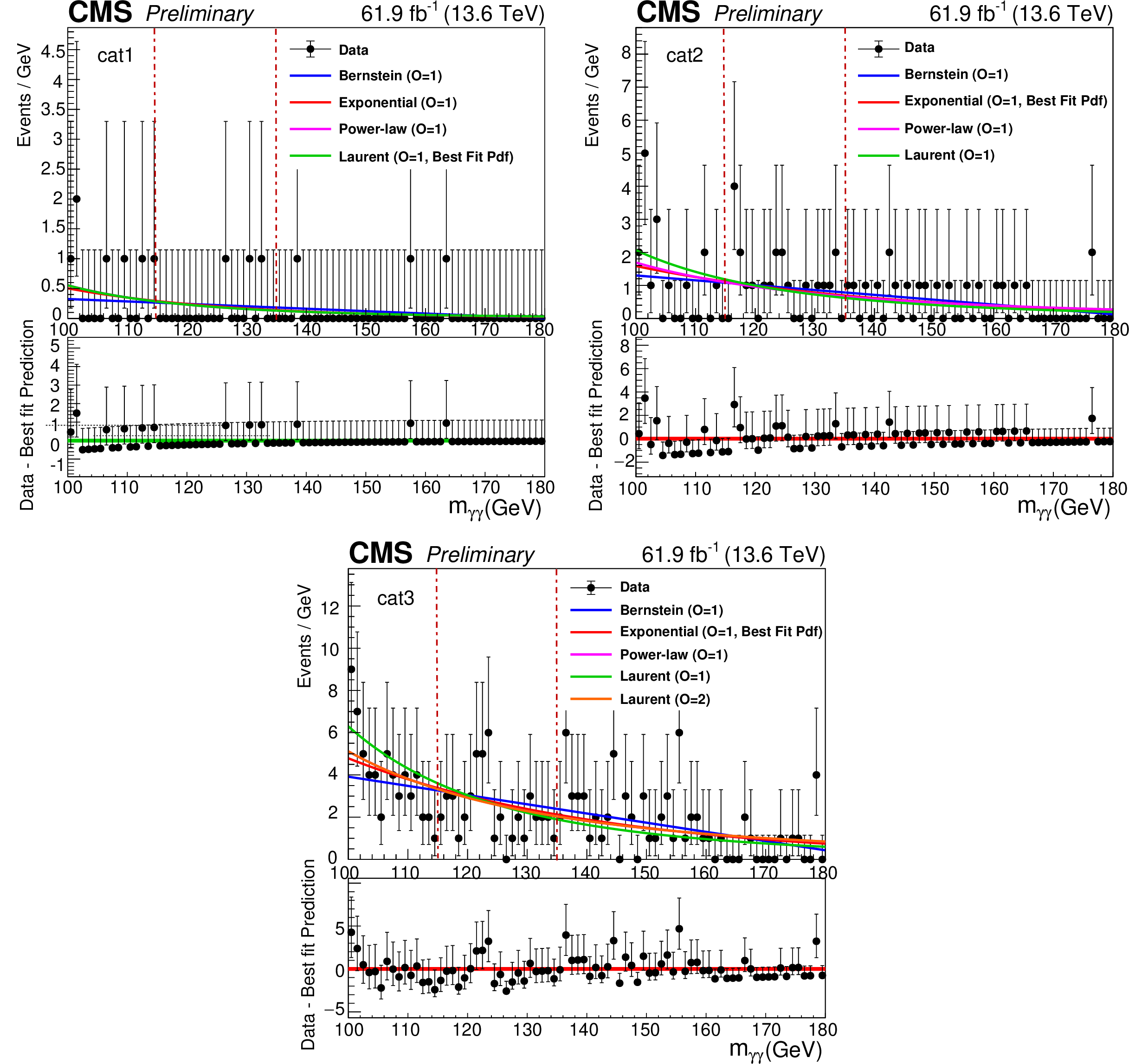
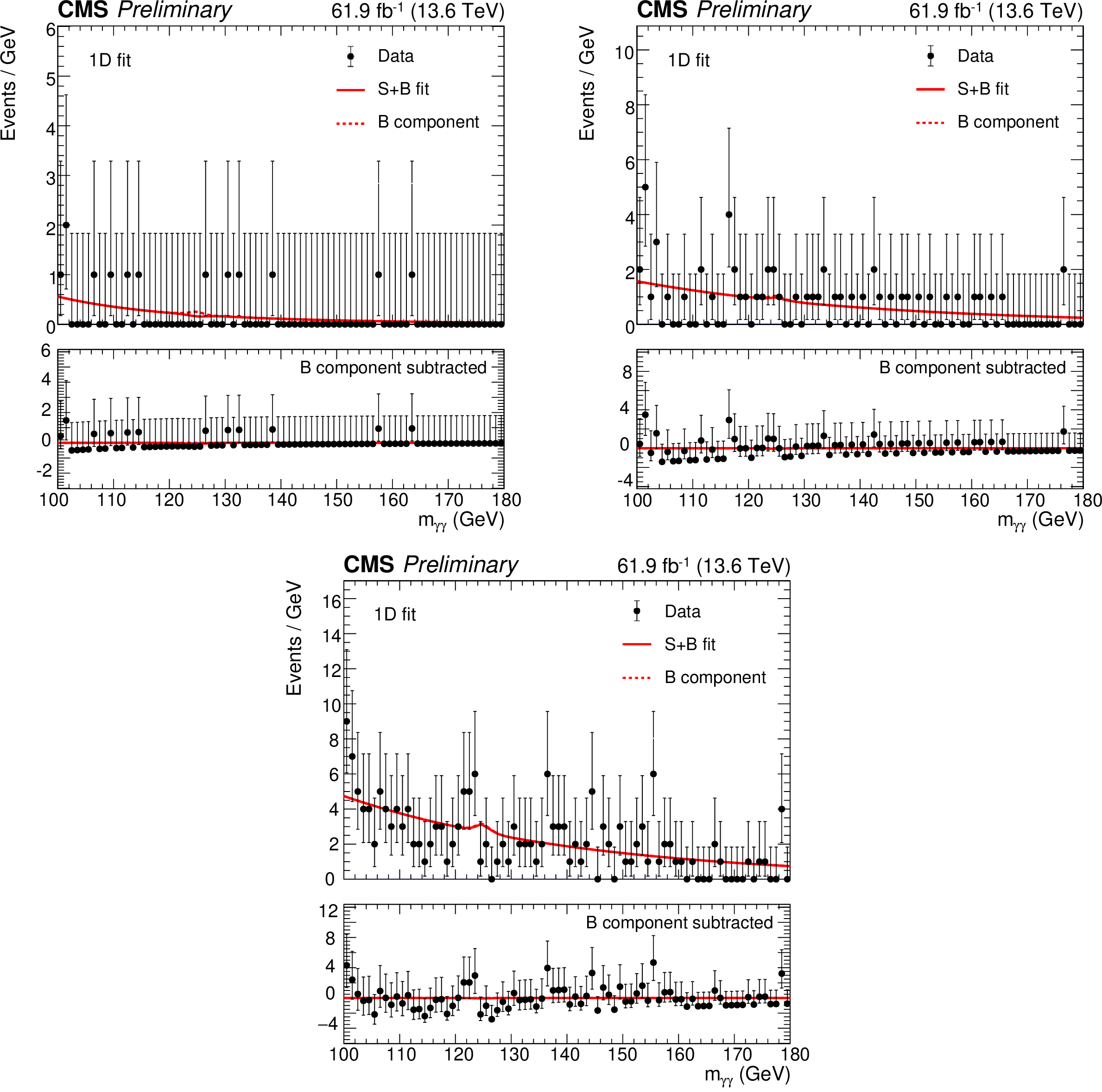
Figure 1:
Results from sideband F-test fits to the diphoton mass distribution in data, excluding the (115, 135) GeV region, to obtain the nonresonant background used for the 1D fit strategy for categories 1 (upper left), 2 (upper right), and 3 (bottom). The result of the F-test is used to determine the best order for each class of background functions considered. The fits are performed separately for each event category. The dotted lines indicate the 115 to 135 GeV blinded region which was explicitly excluded from the sideband fits and F-test. |

png pdf |
Figure 1-a:
Results from sideband F-test fits to the diphoton mass distribution in data, excluding the (115, 135) GeV region, to obtain the nonresonant background used for the 1D fit strategy for categories 1 (upper left), 2 (upper right), and 3 (bottom). The result of the F-test is used to determine the best order for each class of background functions considered. The fits are performed separately for each event category. The dotted lines indicate the 115 to 135 GeV blinded region which was explicitly excluded from the sideband fits and F-test. |
png pdf |
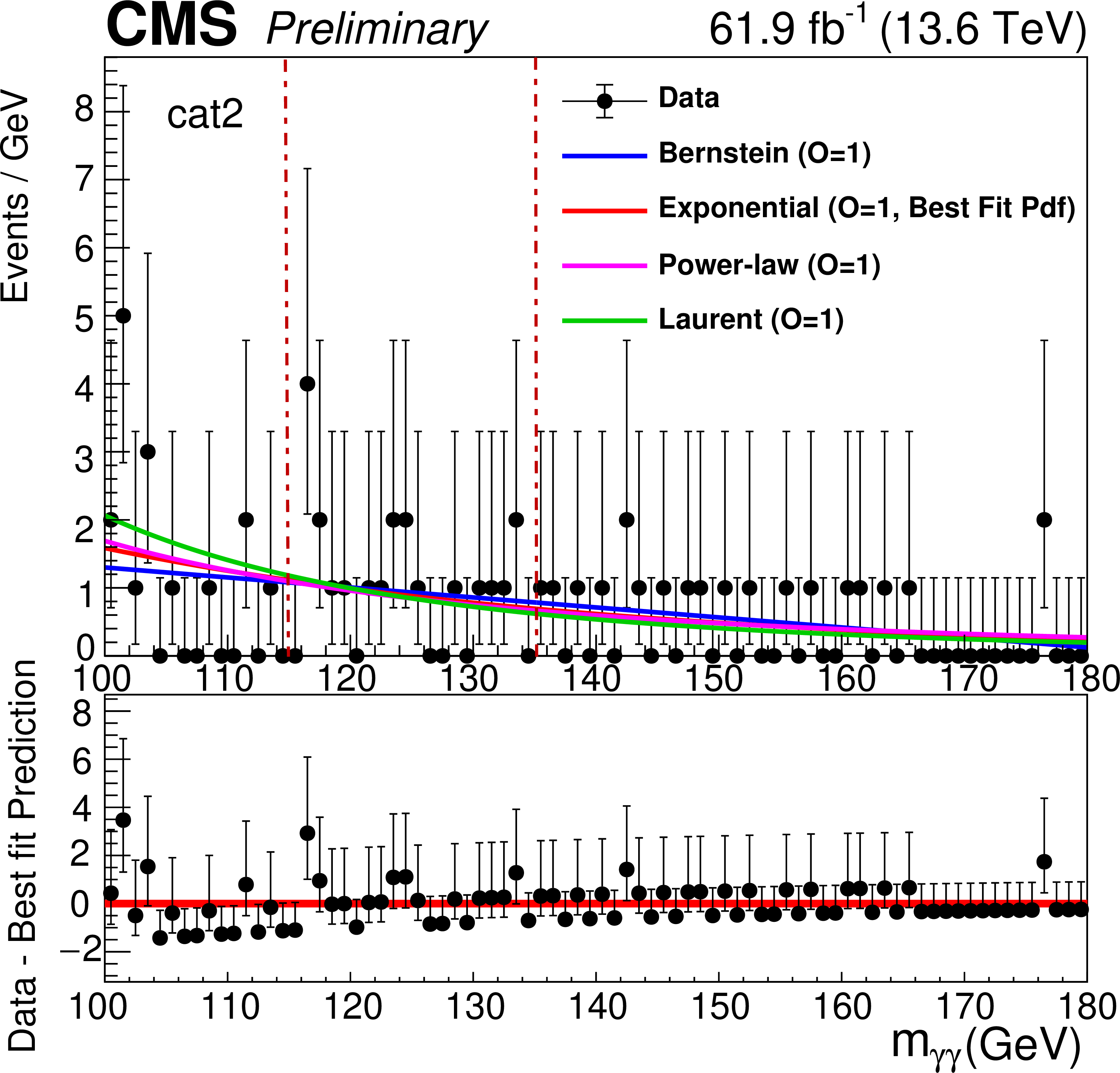
Figure 1-b:
Results from sideband F-test fits to the diphoton mass distribution in data, excluding the (115, 135) GeV region, to obtain the nonresonant background used for the 1D fit strategy for categories 1 (upper left), 2 (upper right), and 3 (bottom). The result of the F-test is used to determine the best order for each class of background functions considered. The fits are performed separately for each event category. The dotted lines indicate the 115 to 135 GeV blinded region which was explicitly excluded from the sideband fits and F-test. |
png pdf |
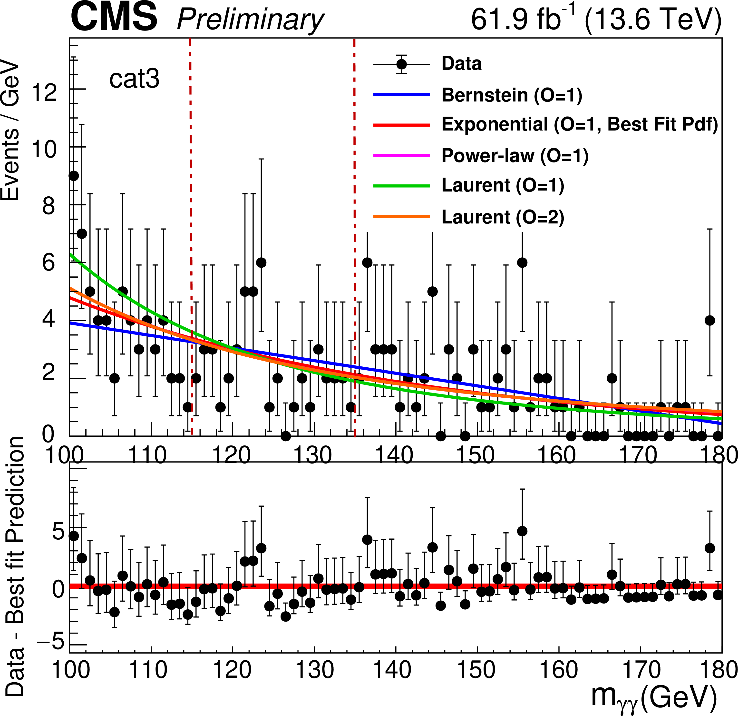
Figure 1-c:
Results from sideband F-test fits to the diphoton mass distribution in data, excluding the (115, 135) GeV region, to obtain the nonresonant background used for the 1D fit strategy for categories 1 (upper left), 2 (upper right), and 3 (bottom). The result of the F-test is used to determine the best order for each class of background functions considered. The fits are performed separately for each event category. The dotted lines indicate the 115 to 135 GeV blinded region which was explicitly excluded from the sideband fits and F-test. |
png pdf |
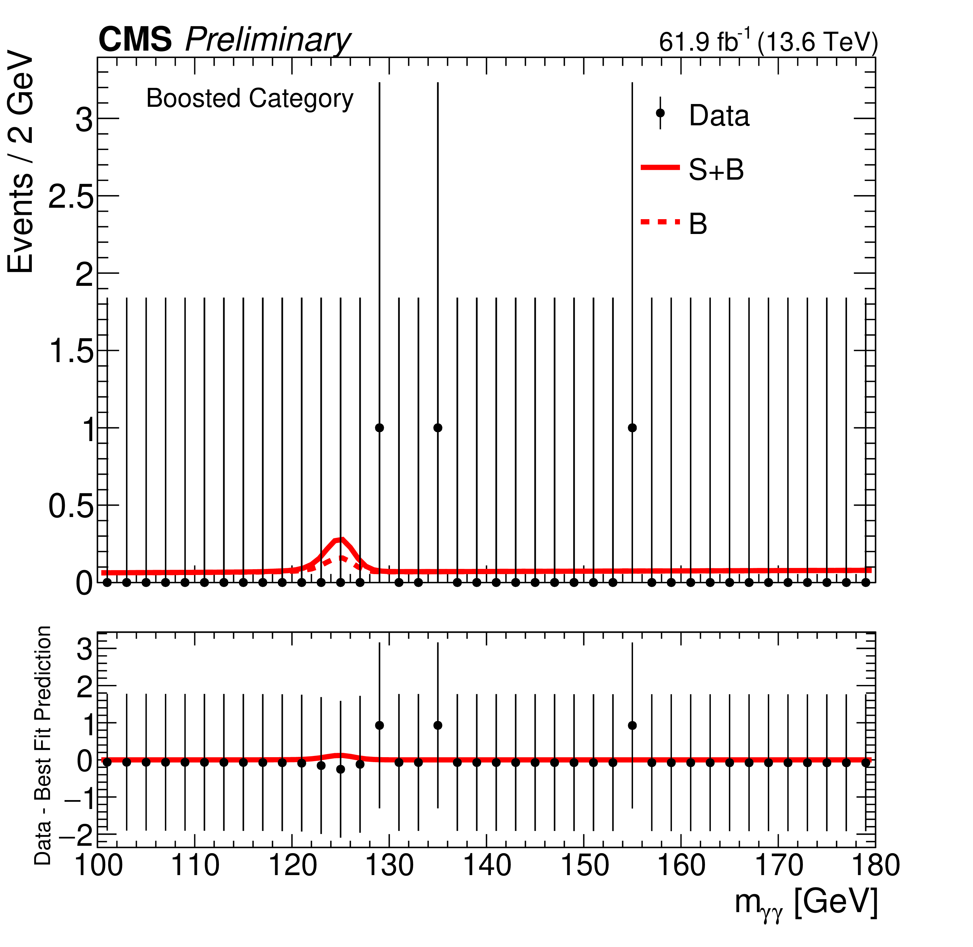
Figure 2:
The signal plus background and background fits to data for the boosted category, which is combined with the 1D and 2D resolved categories. In both 1D and 2D approaches, $ m_{\gamma \gamma} $ is fit. |
png pdf |
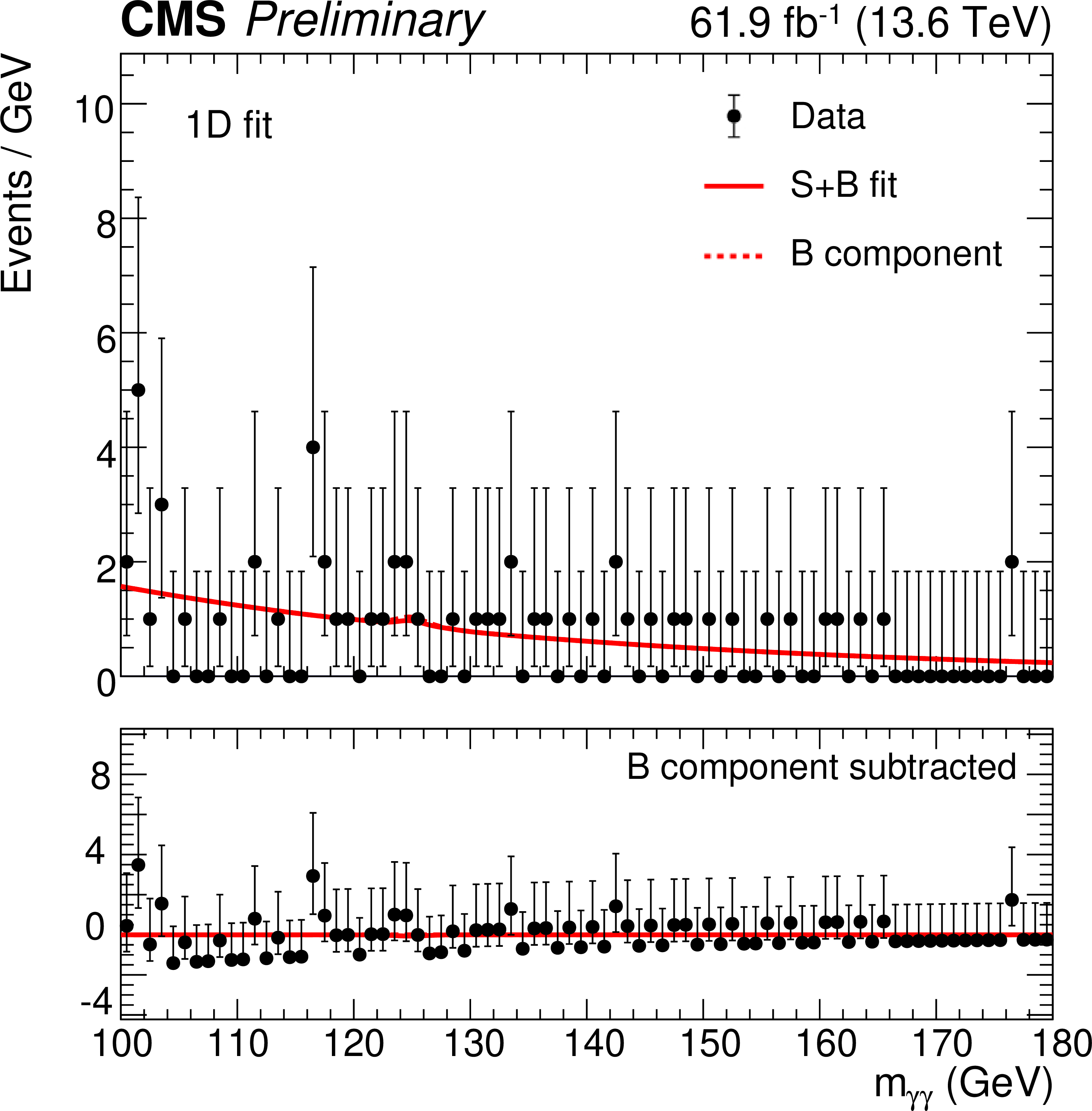
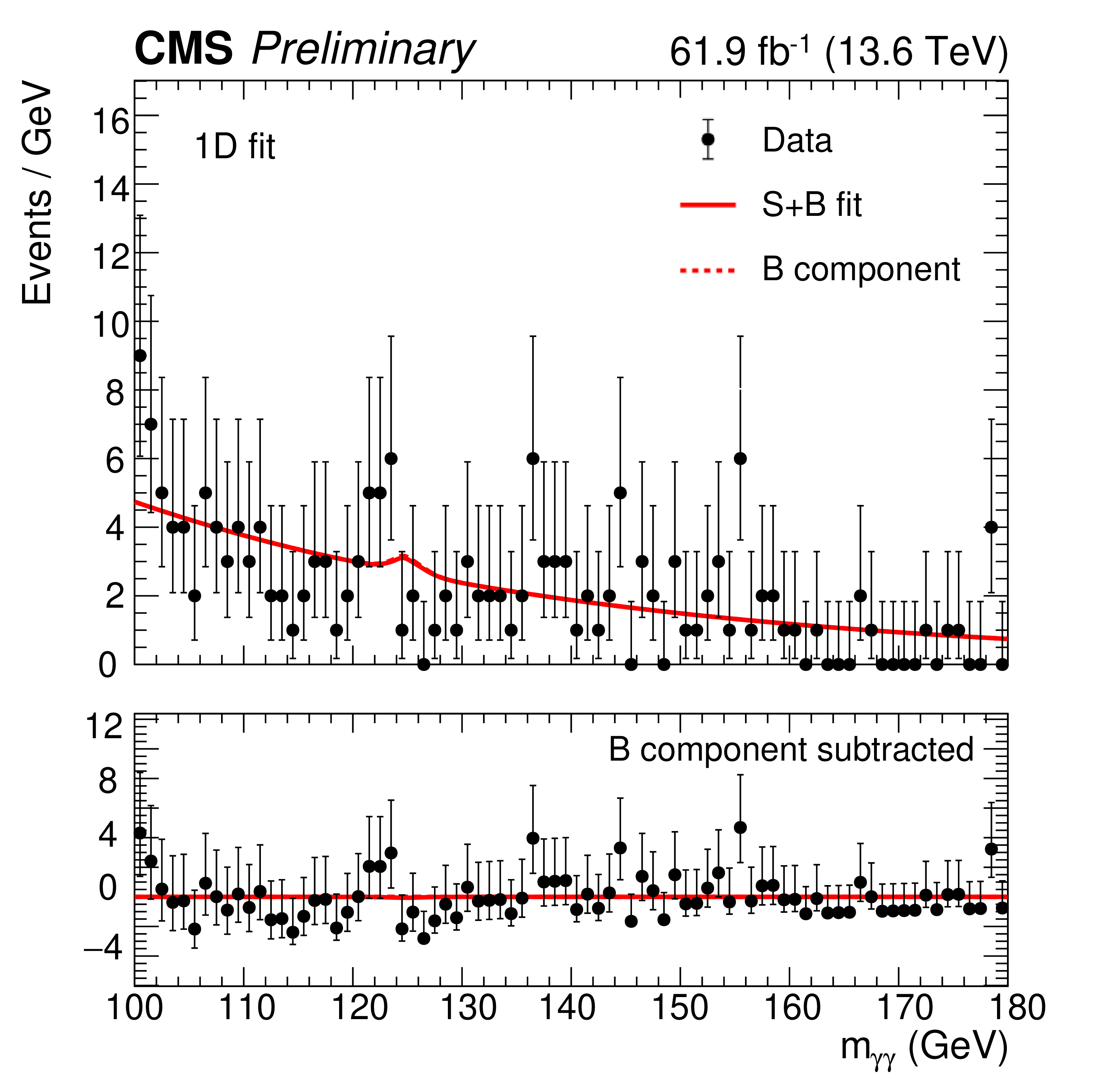
Figure 3:
The signal plus background fits to the diphoton mass distribution is shown for the 1D fit strategy. Categories 1, 2, and 3, are shown on the upper left, upper right, and bottom, respectively. |

png pdf |
Figure 3-a:
The signal plus background fits to the diphoton mass distribution is shown for the 1D fit strategy. Categories 1, 2, and 3, are shown on the upper left, upper right, and bottom, respectively. |
png pdf |
Figure 3-b:
The signal plus background fits to the diphoton mass distribution is shown for the 1D fit strategy. Categories 1, 2, and 3, are shown on the upper left, upper right, and bottom, respectively. |
png pdf |
Figure 3-c:
The signal plus background fits to the diphoton mass distribution is shown for the 1D fit strategy. Categories 1, 2, and 3, are shown on the upper left, upper right, and bottom, respectively. |
png pdf |
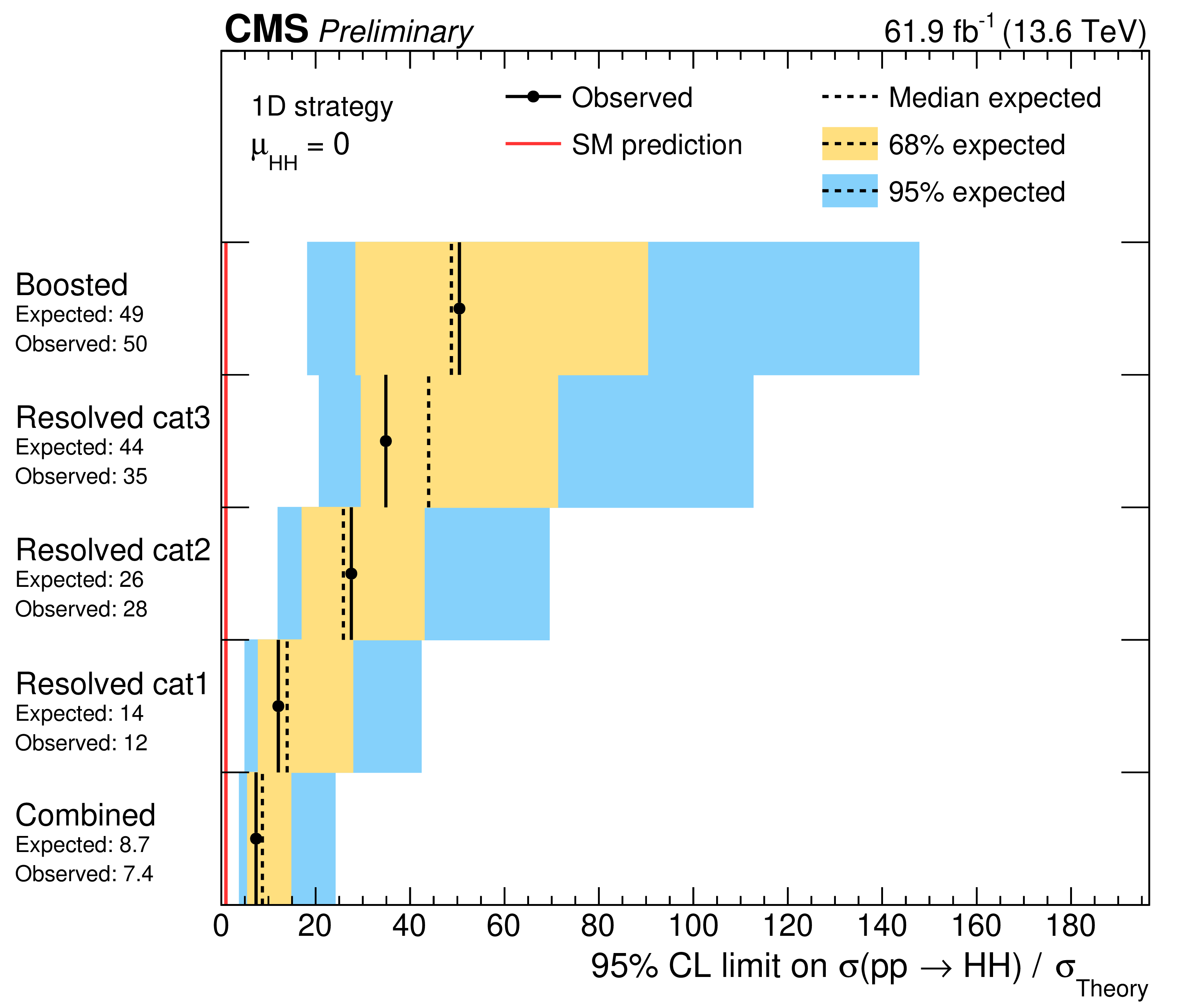
Figure 4:
Expected and observed limits at 95% CL on the signal strength resulting from the 1D analysis for the boosted and resolved categories. The categories 1, 2, and 3 are defined based on requirements on the multivariate discriminator with decreasing signal-to-background ratio. |
png pdf |
Figure 5:
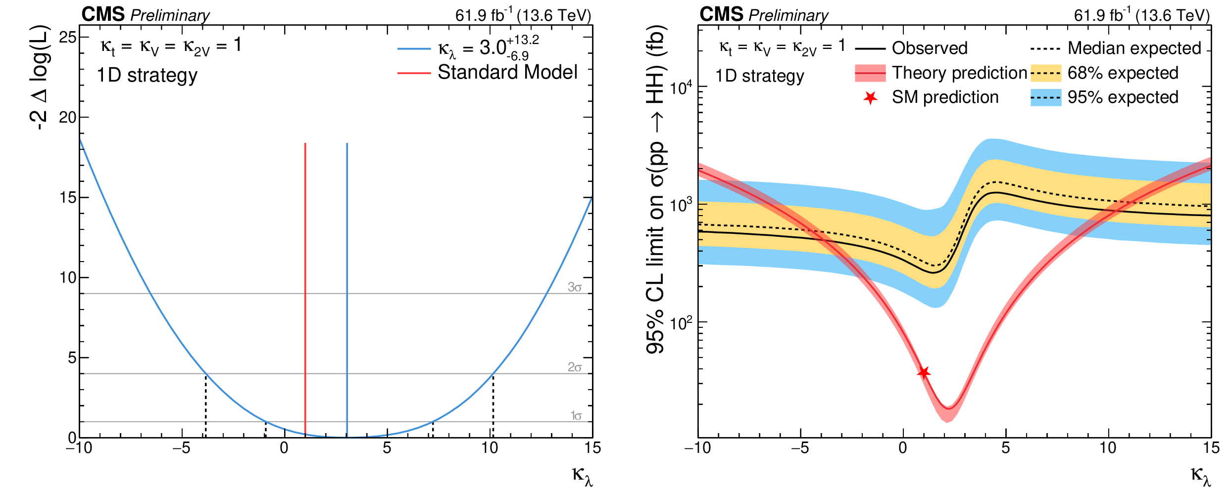
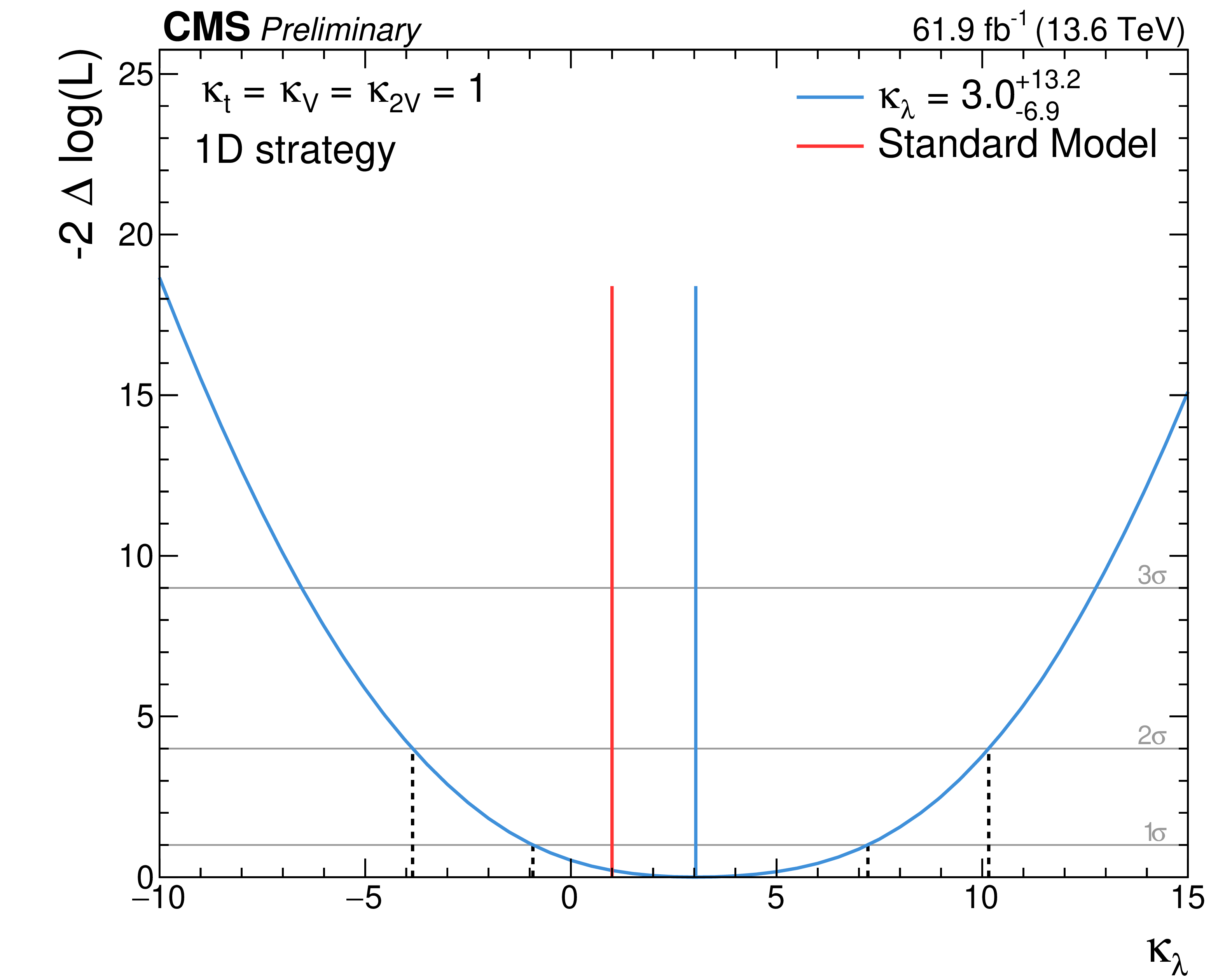
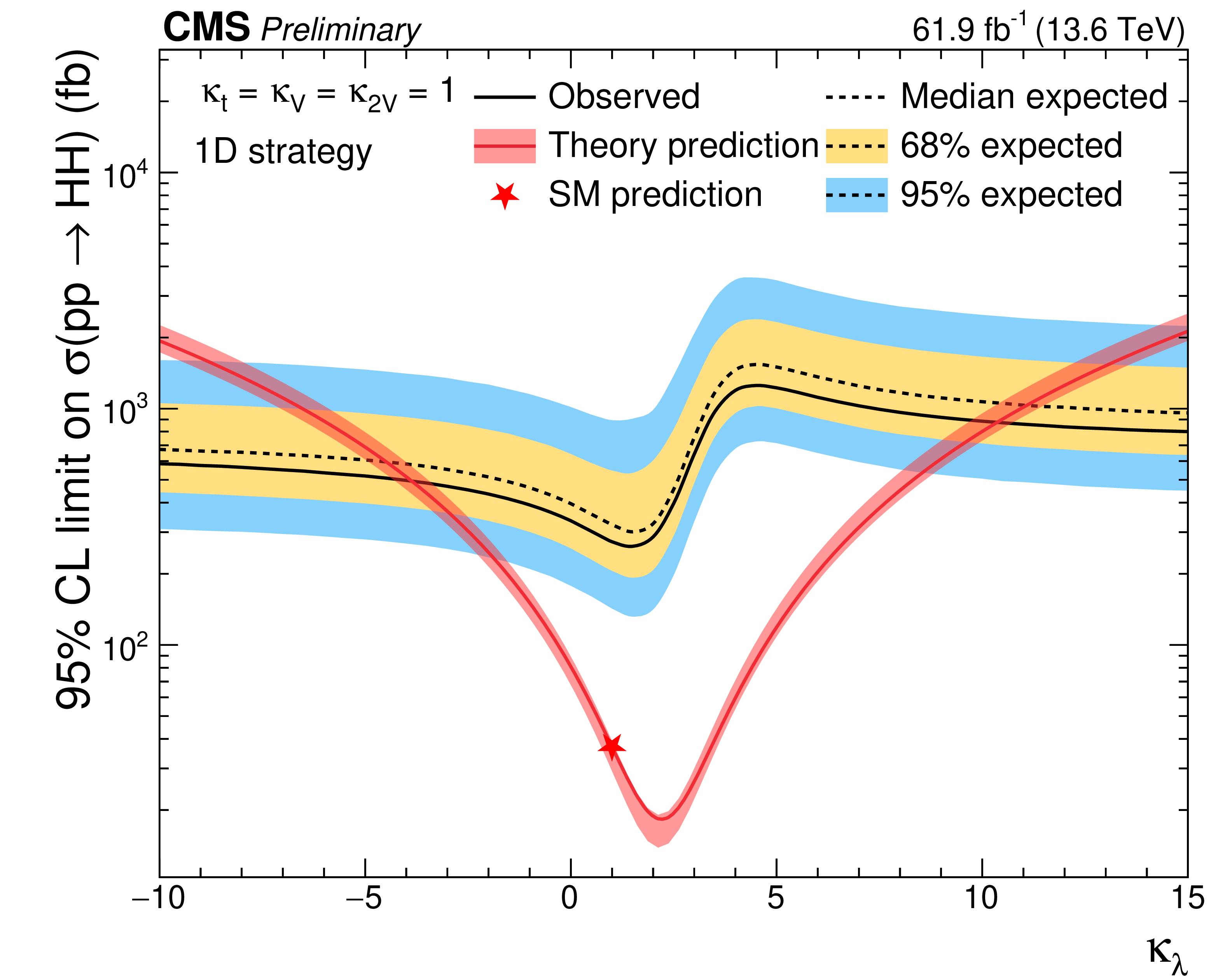
Left: the $ -2\Delta\log(L) $ scan as a function of $ \kappa_{\lambda} $ for the 1D fit strategy, where L is the likelihood function for the 1D analysis. Right: the 95% CL upper limits on the $ {\mathrm{H}\mathrm{H}} $ production cross section as a function of the assumed $ \kappa_{\lambda} $ value. |
png pdf |
Figure 5-a:
Left: the $ -2\Delta\log(L) $ scan as a function of $ \kappa_{\lambda} $ for the 1D fit strategy, where L is the likelihood function for the 1D analysis. Right: the 95% CL upper limits on the $ {\mathrm{H}\mathrm{H}} $ production cross section as a function of the assumed $ \kappa_{\lambda} $ value. |
png pdf |
Figure 5-b:
Left: the $ -2\Delta\log(L) $ scan as a function of $ \kappa_{\lambda} $ for the 1D fit strategy, where L is the likelihood function for the 1D analysis. Right: the 95% CL upper limits on the $ {\mathrm{H}\mathrm{H}} $ production cross section as a function of the assumed $ \kappa_{\lambda} $ value. |
png pdf |
Figure 6:
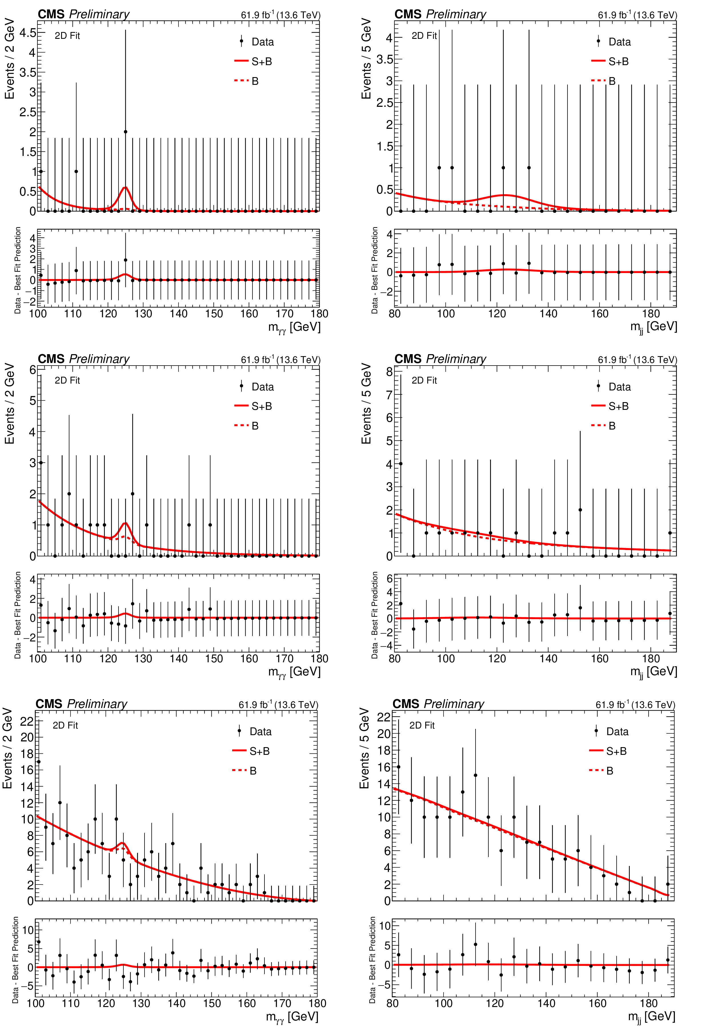
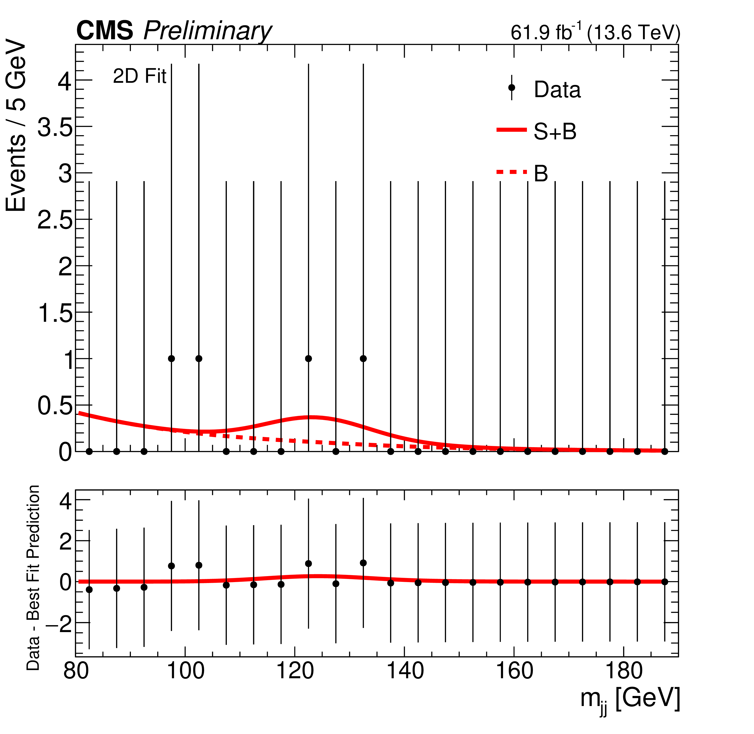
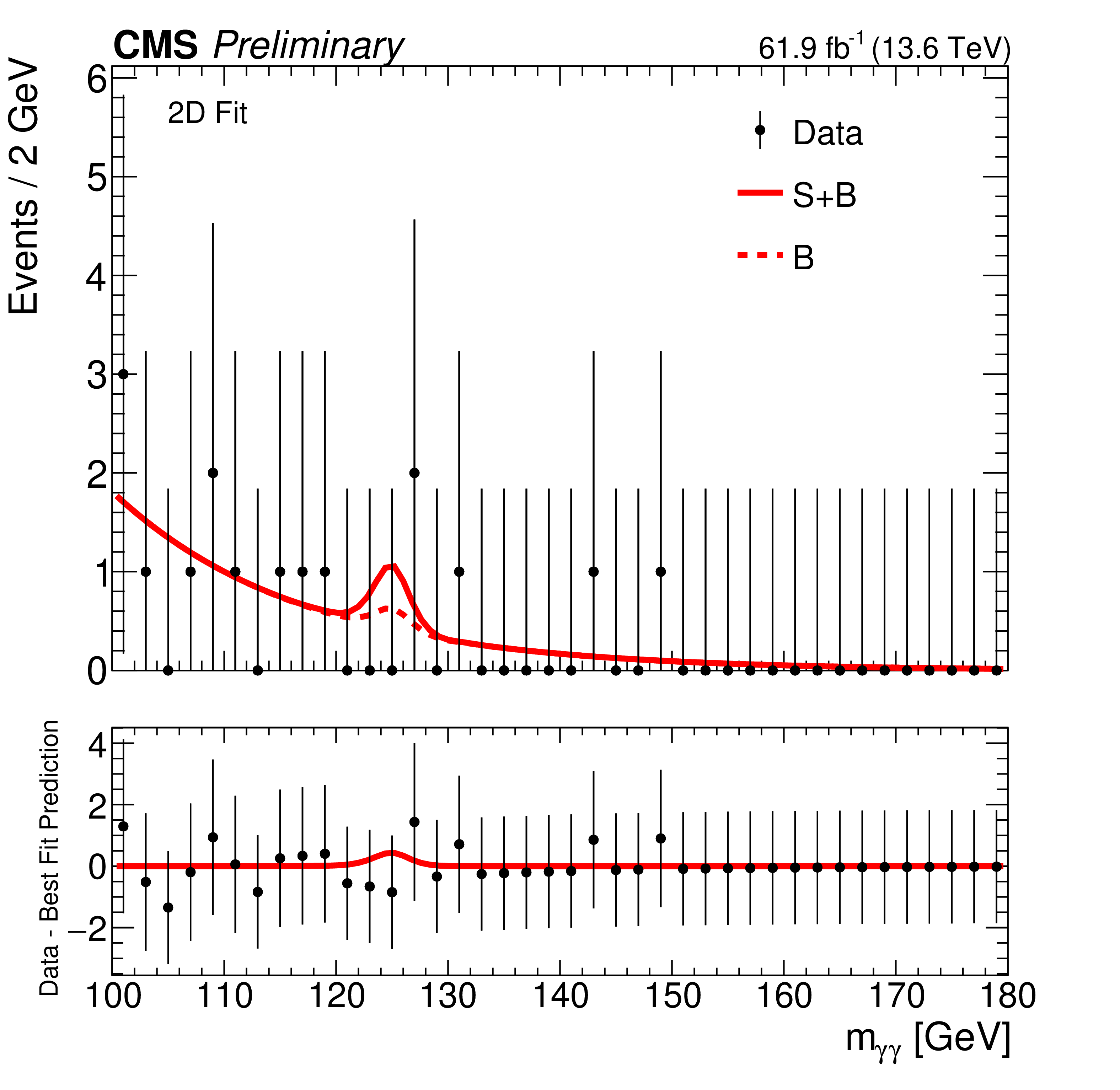
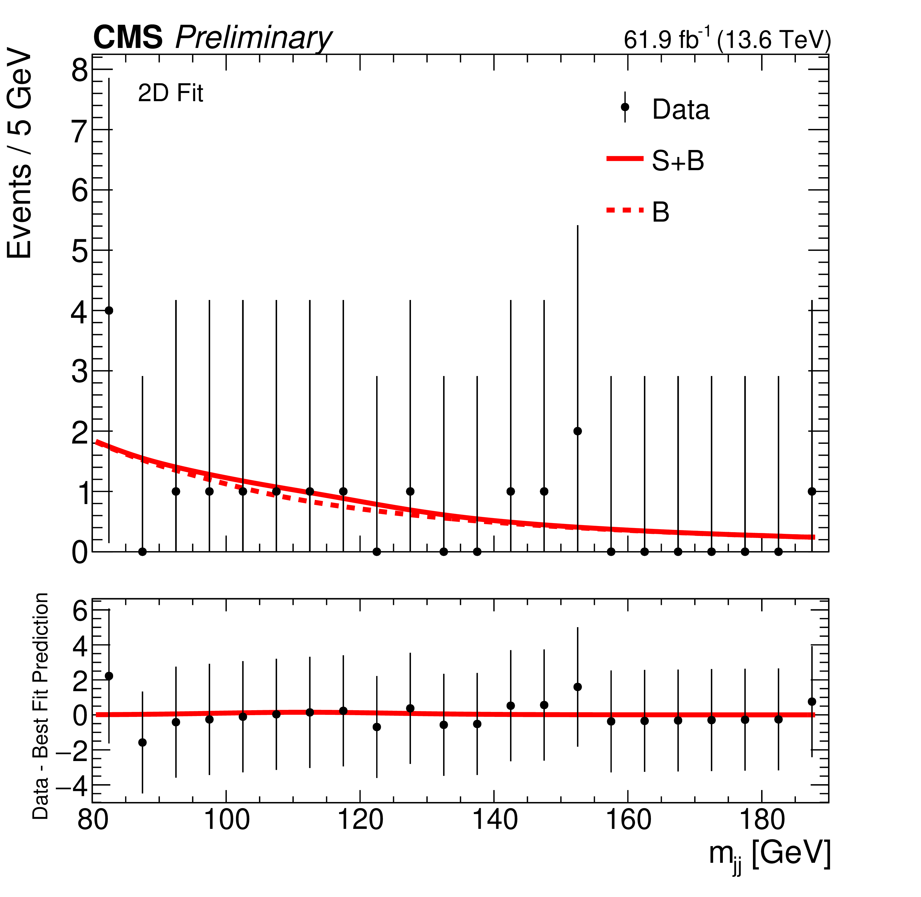
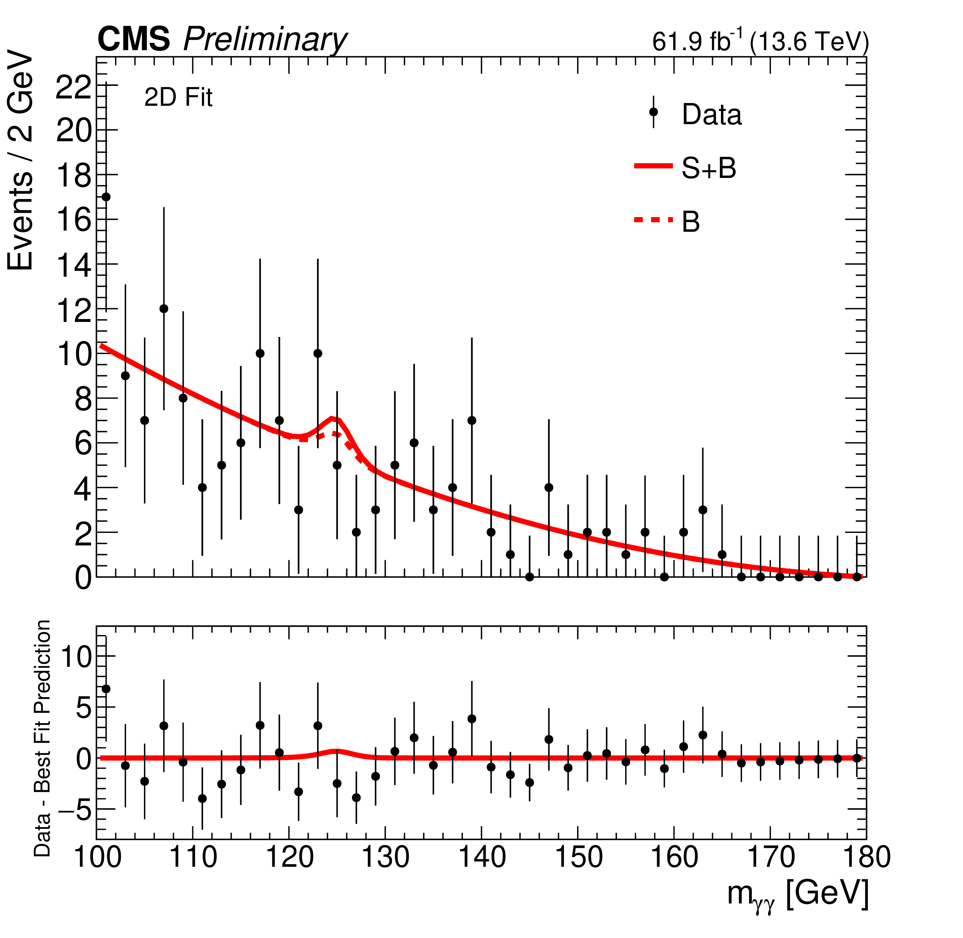
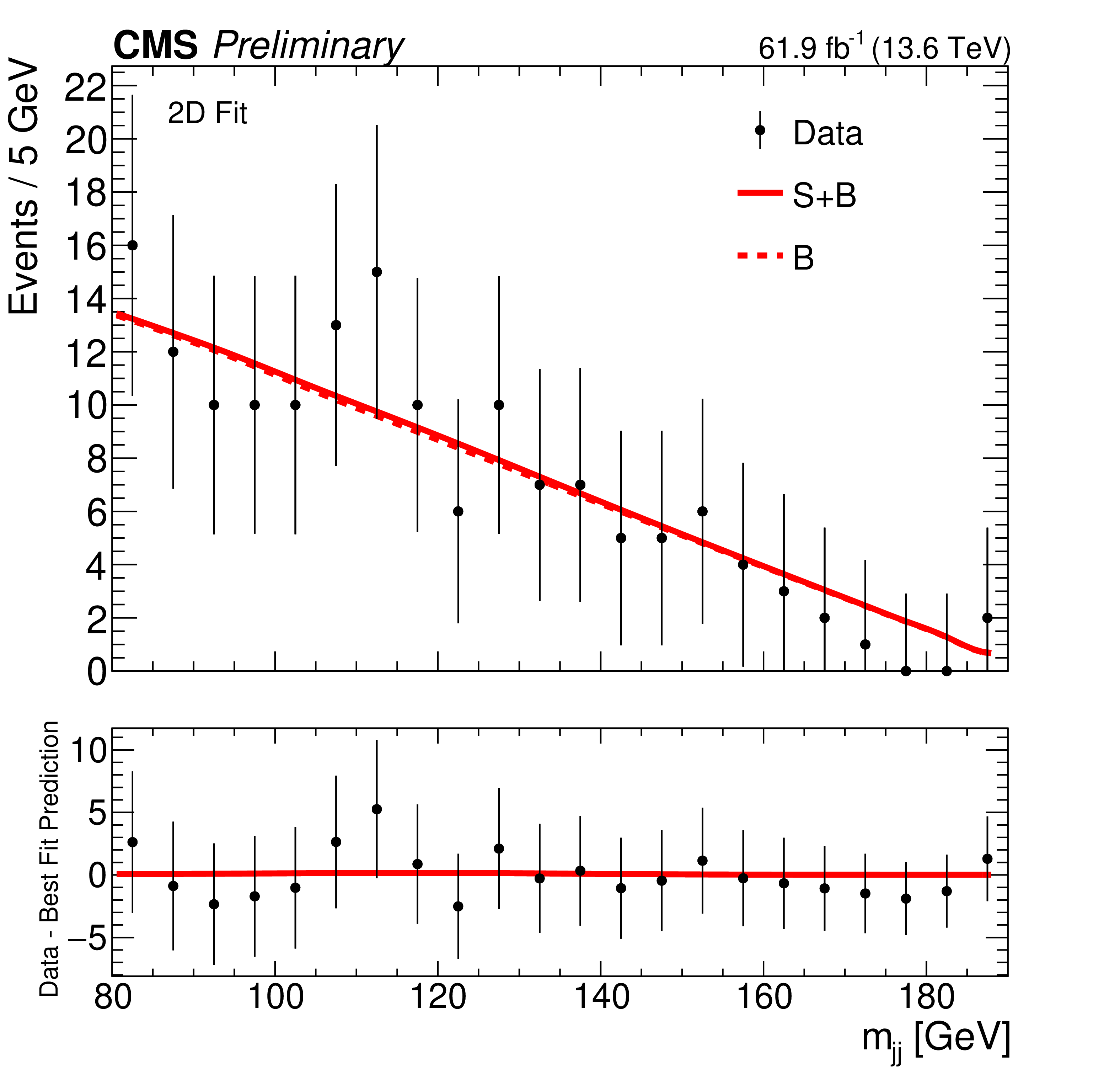
The signal plus background and background fits to data for the 2D fit strategy. The $ m_{\gamma \gamma} $ distributions are shown in the first column, with $ {m_\mathrm{jj}} $ in the second, while the first, second, and third categories are shown top to bottom. |

png pdf |
Figure 6-a:
The signal plus background and background fits to data for the 2D fit strategy. The $ m_{\gamma \gamma} $ distributions are shown in the first column, with $ {m_\mathrm{jj}} $ in the second, while the first, second, and third categories are shown top to bottom. |
png pdf |
Figure 6-b:
The signal plus background and background fits to data for the 2D fit strategy. The $ m_{\gamma \gamma} $ distributions are shown in the first column, with $ {m_\mathrm{jj}} $ in the second, while the first, second, and third categories are shown top to bottom. |
png pdf |
Figure 6-c:
The signal plus background and background fits to data for the 2D fit strategy. The $ m_{\gamma \gamma} $ distributions are shown in the first column, with $ {m_\mathrm{jj}} $ in the second, while the first, second, and third categories are shown top to bottom. |
png pdf |
Figure 6-d:
The signal plus background and background fits to data for the 2D fit strategy. The $ m_{\gamma \gamma} $ distributions are shown in the first column, with $ {m_\mathrm{jj}} $ in the second, while the first, second, and third categories are shown top to bottom. |
png pdf |
Figure 6-e:
The signal plus background and background fits to data for the 2D fit strategy. The $ m_{\gamma \gamma} $ distributions are shown in the first column, with $ {m_\mathrm{jj}} $ in the second, while the first, second, and third categories are shown top to bottom. |
png pdf |
Figure 6-f:
The signal plus background and background fits to data for the 2D fit strategy. The $ m_{\gamma \gamma} $ distributions are shown in the first column, with $ {m_\mathrm{jj}} $ in the second, while the first, second, and third categories are shown top to bottom. |
png pdf |
Figure 7:
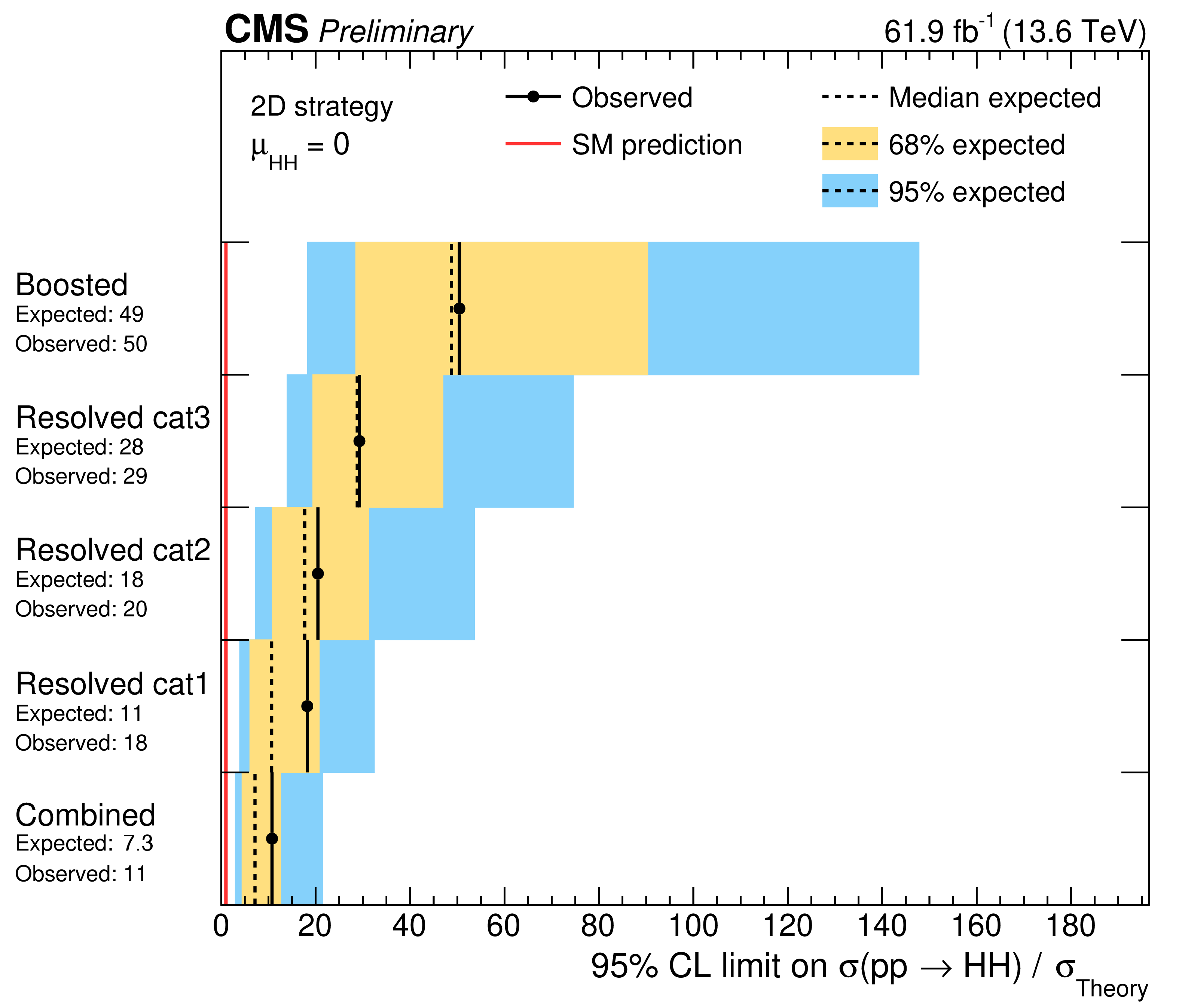
Expected and observed limits at 95% CL on the signal strength resulting from the two-dimensional fit of $ m_{\gamma\gamma} $ and $ {m_\mathrm{jj}} $ of 2022+2023 data for boosted and resolved categories. The categories 1, 2, and 3 are defined based on requirements on the multivariate discriminator with decreasing signal-to-background ratio. |
png pdf |
Figure 8:
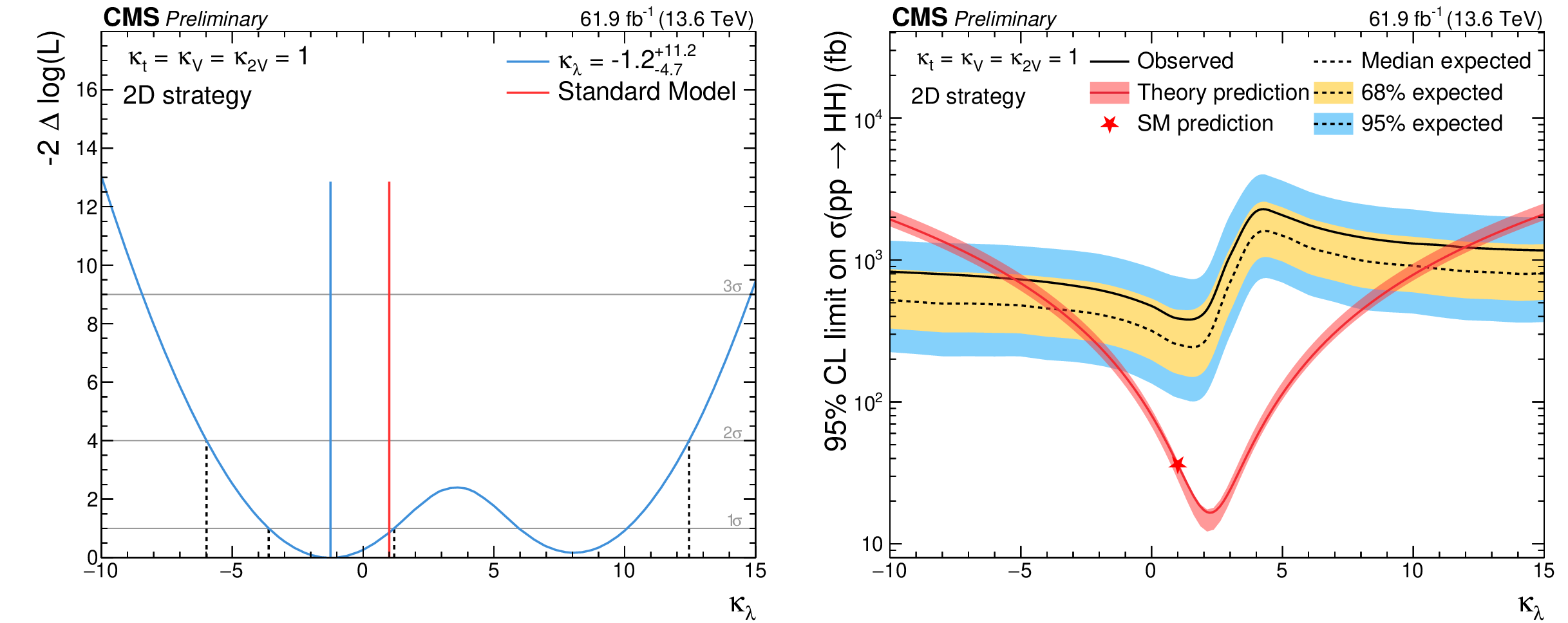
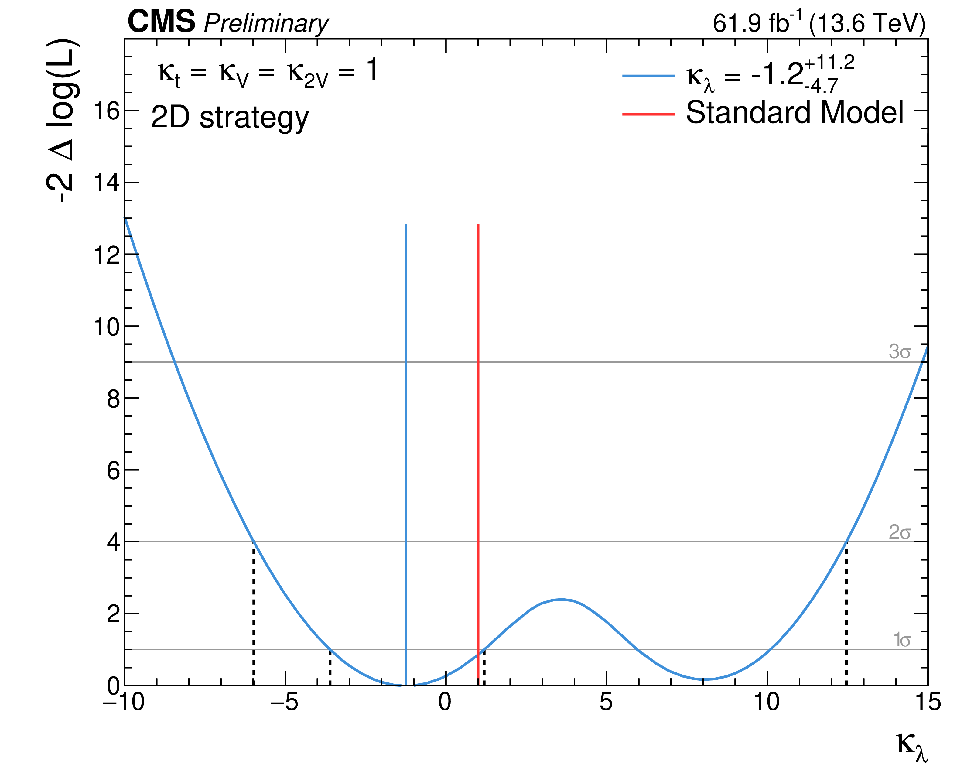
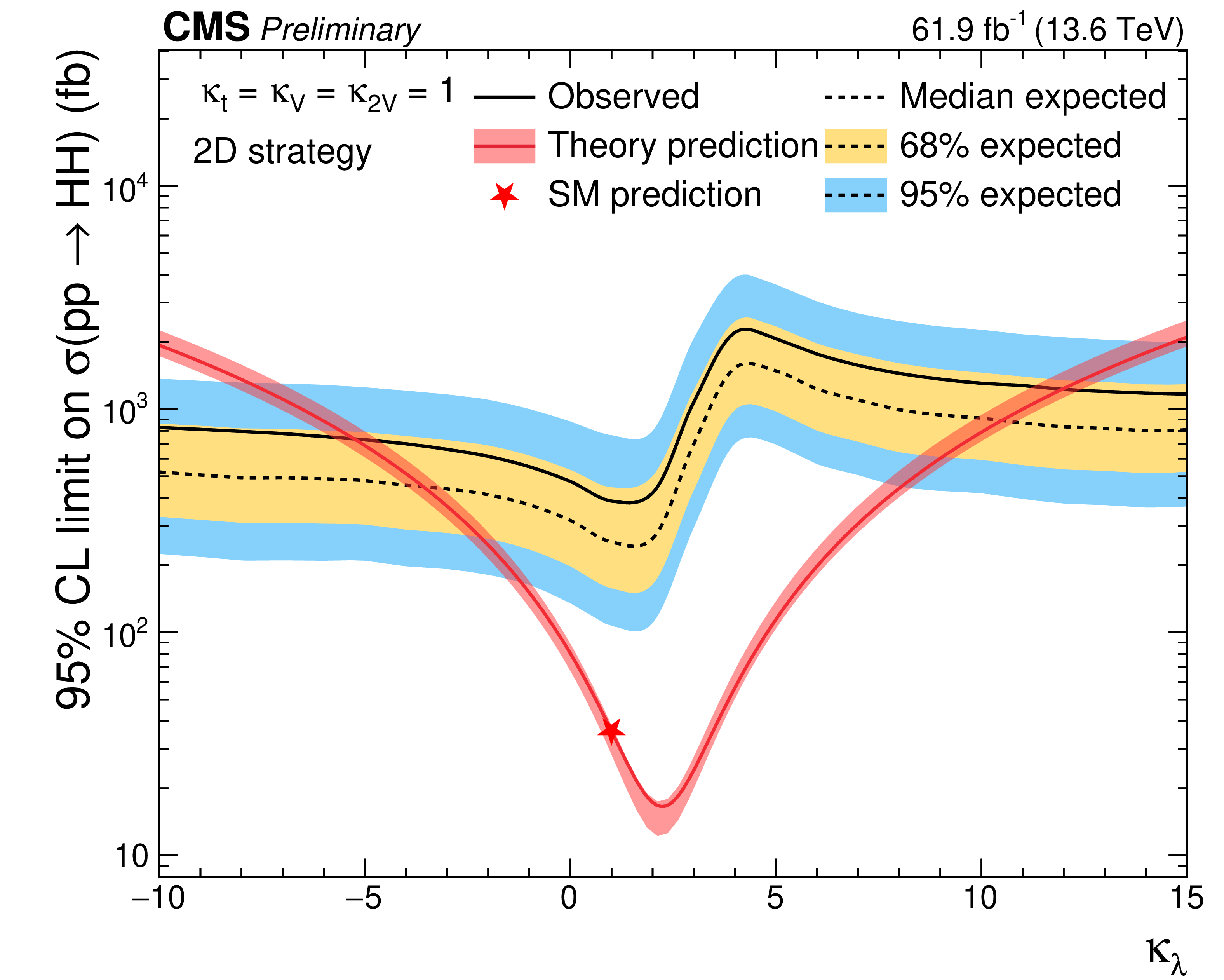
Left: the $ -2\Delta\log(L) $ scan as a function of $ \kappa_{\lambda} $ for the 2D fit strategy, where L is the likelihood function for the 2D analysis. Right: the 95% CL upper limits on the $ {\mathrm{H}\mathrm{H}} $ production cross section as a function of the assumed $ \kappa_{\lambda} $ value is shown on the right. |
png pdf |
Figure 8-a:
Left: the $ -2\Delta\log(L) $ scan as a function of $ \kappa_{\lambda} $ for the 2D fit strategy, where L is the likelihood function for the 2D analysis. Right: the 95% CL upper limits on the $ {\mathrm{H}\mathrm{H}} $ production cross section as a function of the assumed $ \kappa_{\lambda} $ value is shown on the right. |
png pdf |
Figure 8-b:
Left: the $ -2\Delta\log(L) $ scan as a function of $ \kappa_{\lambda} $ for the 2D fit strategy, where L is the likelihood function for the 2D analysis. Right: the 95% CL upper limits on the $ {\mathrm{H}\mathrm{H}} $ production cross section as a function of the assumed $ \kappa_{\lambda} $ value is shown on the right. |
| Tables | |

png pdf |
Table 1:
A summary of the systematic uncertainty and their fractional effect on the signal and background yields. The last three columns explain how each uncertainty source is implemented for the 1D fit, 2D fit, and boosted categories. The term ``norm'' indicates that the systematic uncertainty only affects the normalization of the signal or background yield prediction, while the term ``shape'' indicates that the systematic uncertainty affects the shape of the $ m_{\gamma\gamma} $ and/or $ {m_\mathrm{jj}} $ shapes used for the signal extraction fit. |
| Summary |
| The CMS Collaboration has conducted a search for nonresonant production of Higgs boson pairs in the decay channel $ {\mathrm{H}\mathrm{H}} \rightarrow \mathrm{b}\overline{\mathrm{b}}\gamma\gamma $. The analysis is based on a partial dataset of LHC Run-3 proton-proton collisions at a center-of-mass energy of $ \sqrt{s}= $ 13.6 TeV, corresponding to an integrated luminosity of 61.9 fb$^{-1}$ collected in 2022 and 2023. Two different and complementary analysis strategies are presented resulting in consistent results, thereby strengthening the robustness of the studies presented in this note. The more sensitive version of the analysis relies on a 2-dimensional (2D) fit to the diphoton and dijet mass observables and yields an observed (expected) 95% confidence level (CL) upper limit of 11.0 (7.3) times the standard model prediction of $ \sigma(pp \rightarrow {\mathrm{H}\mathrm{H}}) \times \mathcal{B}({\mathrm{H}\mathrm{H}} \rightarrow \mathrm{b}\overline{\mathrm{b}}\gamma\gamma) $. An alternative version that does not rely on a fit the dijet mass, the 1-dimensional (1D) approach, gives an observed (expected) 95% confidence level (CL) upper limit of 7.4 (8.7) times the standard model prediction. We place constraints on the effective Higgs boson self-coupling modifier $ \kappa_{\lambda} $, excluding values outside the range $ -$5 $< \kappa_{\lambda} < $ 12 for the 2D approach and $ -$3.9 $< \kappa_{\lambda} < $ 10.4 for the 1-dimensional (1D) approach, assuming all other Higgs boson couplings follow the SM prediction. |
| References | ||||
| 1 | ATLAS Collaboration | Observation of a new particle in the search for the Standard Model Higgs boson with the ATLAS detector at the LHC | PLB 716 (2012) 1 | 1207.7214 |
| 2 | CMS Collaboration | Observation of a new boson at a mass of 125 GeV with the CMS experiment at the LHC | PLB 716 (2012) 30 | CMS-HIG-12-028 1207.7235 |
| 3 | F. Englert and R. Brout | Broken Symmetry and the Mass of Gauge Vector Mesons | PRL 13 (1964) 321 | |
| 4 | P. W. Higgs | Broken symmetries, massless particles and gauge fields | PL 12 (1964) 132 | |
| 5 | CMS Collaboration | Combination of searches for Higgs boson pair production in proton-proton collisions at $ \sqrt{s} = $ 13 TeV | PRL 122 (2019) 121803 | CMS-HIG-17-030 1811.09689 |
| 6 | ATLAS Collaboration | Combination of searches for Higgs boson pair production in pp collisions at $ \sqrt{s}= $ 13 TeV with the ATLAS detector | PRL 133 (2024) 101801 | 2406.09971 |
| 7 | M. Grazzini et al. | Higgs boson pair production at NNLO with top quark mass effects | JHEP 05 (2018) 059 | 1803.02463 |
| 8 | LHC Higgs Working Group 4 (formerly LHC-HH subgroup) | Current recommendations for HH cross sections | technical report, 2024 link |
|
| 9 | A. Karlberg et al. | Ad Interim recommendations for the Higgs boson production cross sections at $ \sqrt{s} = $ 13.6 TeV | 2, 2024 | 2402.09955 |
| 10 | F. A. Dreyer, A. Karlberg, J.-N. Lang, and M. Pellen | Precise predictions for double-Higgs production via vector-boson fusion | EPJC 80 (2020) 1037 | 2005.13341 |
| 11 | F. A. Dreyer and A. Karlberg | Vector-Boson Fusion Higgs Pair Production at N$ ^3 $LO | PRD 98 (2018) 114016 | 1811.07906 |
| 12 | LHC Higgs Working Group 1 | SM Higgs branching ratios and total decay widths (update in CERN Report4 2016) | technical report, 2016 link |
|
| 13 | P. Nason | A new method for combining NLO QCD with shower Monte Carlo algorithms | JHEP 11 (2004) 040 | hep-ph/0409146 |
| 14 | S. Frixione, P. Nason, and C. Oleari | Matching NLO QCD computations with Parton Shower simulations: the POWHEG method | JHEP 11 (2007) 070 | 0709.2092 |
| 15 | S. Alioli, P. Nason, C. Oleari, and E. Re | A general framework for implementing NLO calculations in shower Monte Carlo programs: the POWHEG BOX | JHEP 06 (2010) 043 | 1002.2581 |
| 16 | C. Bierlich et al. | A comprehensive guide to the physics and usage of PYTHIA 8.3 | SciPost Phys. Codeb. 2022 (2022) 8 | 2203.11601 |
| 17 | C. Bierlich et al. | Codebase release 8.3 for PYTHIA | SciPost Phys. Codebases 8--r8.3, 2022 link |
|
| 18 | J. Alwall et al. | The automated computation of tree-level and next-to-leading order differential cross sections, and their matching to parton shower simulations | JHEP 07 (2014) 079 | 1405.0301 |
| 19 | R. Frederix et al. | The automation of next-to-leading order electroweak calculations | JHEP 07 (2018) 185 | 1804.10017 |
| 20 | LHC Higgs Cross Section Working Group | Handbook of LHC Higgs Cross Sections: 4. Deciphering the Nature of the Higgs Sector | 10, 2016 link |
|
| 21 | Sherpa Collaboration | Event Generation with Sherpa 2.2 | SciPost Phys. 7 (2019) 034 | 1905.09127 |
| 22 | CMS Collaboration | Technical proposal for the Phase-II upgrade of the Compact Muon Solenoid | CMS Technical Proposal CERN-LHCC-2015-010, CMS-TDR-15-02, 2015 CDS |
|
| 23 | CMS Collaboration | Electron and photon reconstruction and identification performance at CMS in 2022 and 2023 | CMS Detector Performance Summary CMS-DP-2024-052, 2024 CDS |
|
| 24 | M. Cacciari, G. P. Salam, and G. Soyez | The anti-$ k_{\mathrm{T}} $ jet clustering algorithm | JHEP 04 (2008) 063 | 0802.1189 |
| 25 | H. Qu and L. Gouskos | Jet tagging via particle clouds | PRD 101 (2020) 056019 | 1902.08570 |
| 26 | CMS Collaboration | Performance of missing transverse momentum reconstruction in proton-proton collisions at $ \sqrt{s} = $ 13 TeV using the CMS detector | JINST 14 (2019) P07004 | CMS-JME-17-001 1903.06078 |
| 27 | M. Abadi et al. | Tensorflow: A system for large-scale machine learning | link | |
| 28 | M. Dasgupta, A. Fregoso, S. Marzani, and G. P. Salam | Towards an understanding of jet substructure | JHEP 09 (2013) 029 | 1307.0007 |
| 29 | CMS Collaboration | Search for nonresonant Higgs boson pair production in final states with two bottom quarks and two photons in proton-proton collisions at $ \sqrt{s} = $ 13 TeV | JHEP 03 (2021) 257 | CMS-HIG-19-018 2011.12373 |
| 30 | R. A. Fisher | On the interpretation of $ \chi^2 $ from contingency tables, and the calculation of p | J. Royal Statistical Society 85 (1922) 87 | |
| 31 | P. D. Dauncey, M. Kenzie, N. Wardle, and G. J. Davies | Handling uncertainties in background shapes: the discrete profiling method | JINST 10 (2015) P04015 | 1408.6865 |
| 32 | CMS Collaboration | Luminosity measurement in proton-proton collisions at 13.6 TeV in 2022 at CMS | CMS Physics Analysis Summary, 2024 CMS-PAS-LUM-22-001 |
CMS-PAS-LUM-22-001 |
| 33 | CMS Collaboration | Precision luminosity measurement in proton-proton collisions at $ \sqrt{s} = $ 13 TeV in 2015 and 2016 at CMS | EPJC 81 (2021) 800 | CMS-LUM-17-003 2104.01927 |
| 34 | CMS Collaboration | CMS luminosity measurement for the 2017 data-taking period at $ \sqrt{s} = $ 13 TeV | CMS Physics Analysis Summary, 2018 link |
CMS-PAS-LUM-17-004 |
| 35 | CMS Collaboration | CMS luminosity measurement for the 2018 data-taking period at $ \sqrt{s} = $ 13 TeV | CMS Physics Analysis Summary, 2019 link |
CMS-PAS-LUM-18-002 |
| 36 | G. Cowan, K. Cranmer, E. Gross, and O. Vitells | Asymptotic formulae for likelihood-based tests of new physics | EPJC 71 (2011) 1554 | 1007.1727 |
| 37 | CMS Collaboration | Combination of searches for nonresonant Higgs boson pair production in proton-proton collisions at $ \sqrt{s} = $ 13 TeV | CMS Physics Analysis Summary, 2024 CMS-PAS-HIG-20-011 |
CMS-PAS-HIG-20-011 |
|
|
Compact Muon Solenoid LHC, CERN |
|

|

|

|

|

|