

Compact Muon Solenoid
LHC, CERN
| CMS-PAS-HIG-24-006 | ||
| Constraints on anomalous Higgs boson couplings to vector bosons and fermions in the $ \gamma\gamma $ final state | ||
| CMS Collaboration | ||
| 2025-07-11 | ||
| Abstract: Possible anomalous couplings of the Higgs boson to vector bosons and fermions are studied in this document. The data are recorded by the CMS experiment at the LHC and corresponds to an integrated luminosity of 138 fb$ ^{-1} $ at a center-of-mass energy of 13 TeV. These measurements use Higgs boson candidates produced mainly in gluon fusion, electroweak vector boson fusion (VBF) and the associated production with a vector boson (VH) that subsequently decay to a pair of photons. Events are categorized based on matrix element techniques and multivariate discriminants. The CP properties in the Higgs boson couplings to gluons through a loop of heavy particles are studied, as well as the tensor structure of the interactions with two electroweak bosons, analyzing VBF and VH associated production. The results, interpreted as fractional contribution of each anomalous Higgs boson coupling to the total cross section of a process, are found consistent with the standard model expectations. | ||
| Links: CDS record (PDF) ; CADI line (restricted) ; | ||
| Figures | |

png pdf |
Figure 1:
Leading-order Feynman diagrams for the gluon fusion (a), VBF (b), and VH (c) production modes and for $ \mathrm{H}\to\gamma\gamma $ decay (d). |

png pdf |
Figure 1-a:
Leading-order Feynman diagrams for the gluon fusion (a), VBF (b), and VH (c) production modes and for $ \mathrm{H}\to\gamma\gamma $ decay (d). |

png pdf |
Figure 1-b:
Leading-order Feynman diagrams for the gluon fusion (a), VBF (b), and VH (c) production modes and for $ \mathrm{H}\to\gamma\gamma $ decay (d). |

png pdf |
Figure 1-c:
Leading-order Feynman diagrams for the gluon fusion (a), VBF (b), and VH (c) production modes and for $ \mathrm{H}\to\gamma\gamma $ decay (d). |

png pdf |
Figure 1-d:
Leading-order Feynman diagrams for the gluon fusion (a), VBF (b), and VH (c) production modes and for $ \mathrm{H}\to\gamma\gamma $ decay (d). |

png pdf |
Figure 2:
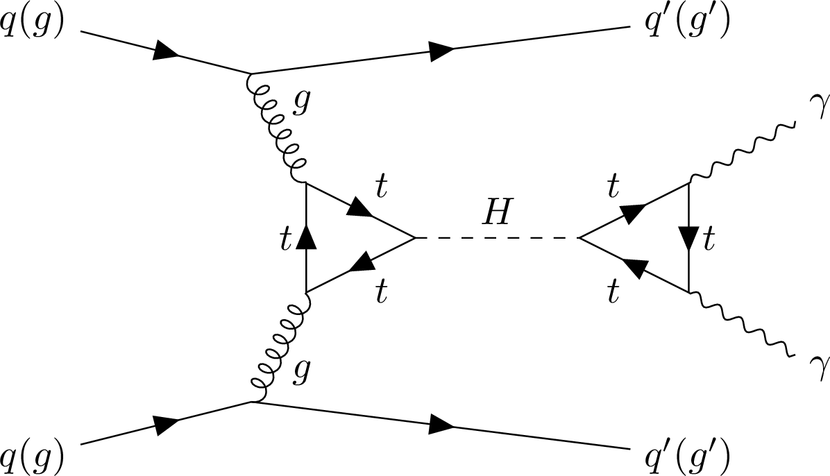
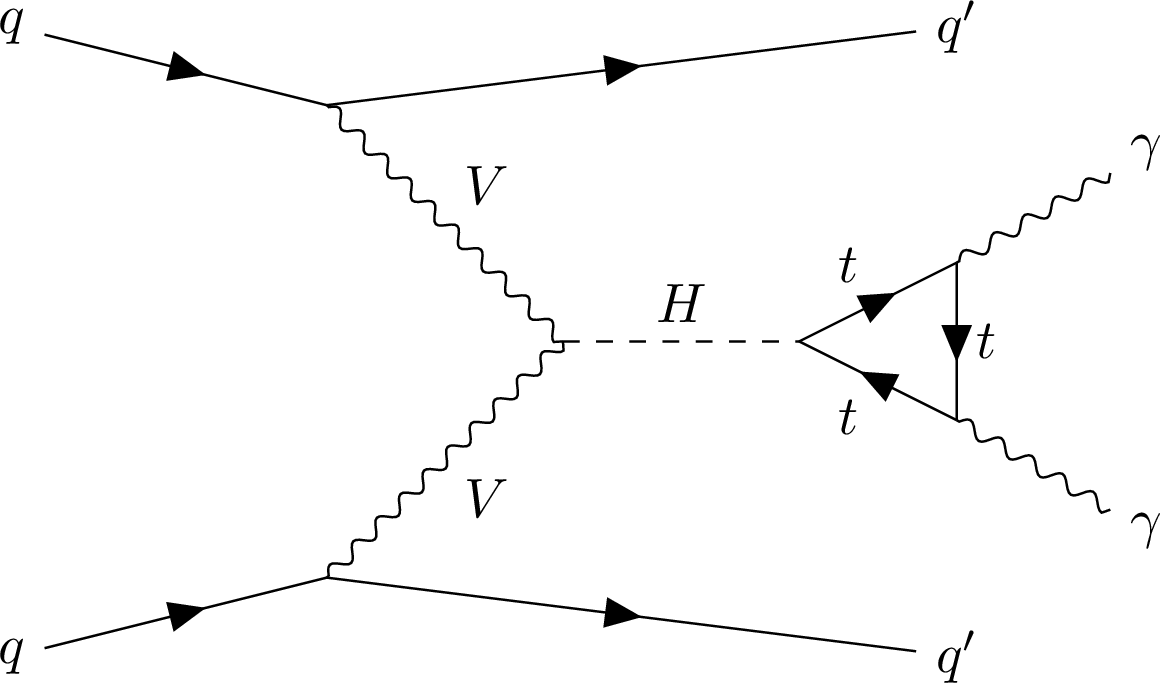
Example of diagrams for the process in which a Higgs boson decaying into a pair of photons is produced via gluon fusion in association with two jets (left) and via vector boson fusion (right). |
png pdf |
Figure 2-a:
Example of diagrams for the process in which a Higgs boson decaying into a pair of photons is produced via gluon fusion in association with two jets (left) and via vector boson fusion (right). |
png pdf |
Figure 2-b:
Example of diagrams for the process in which a Higgs boson decaying into a pair of photons is produced via gluon fusion in association with two jets (left) and via vector boson fusion (right). |
png pdf |
Figure 3:
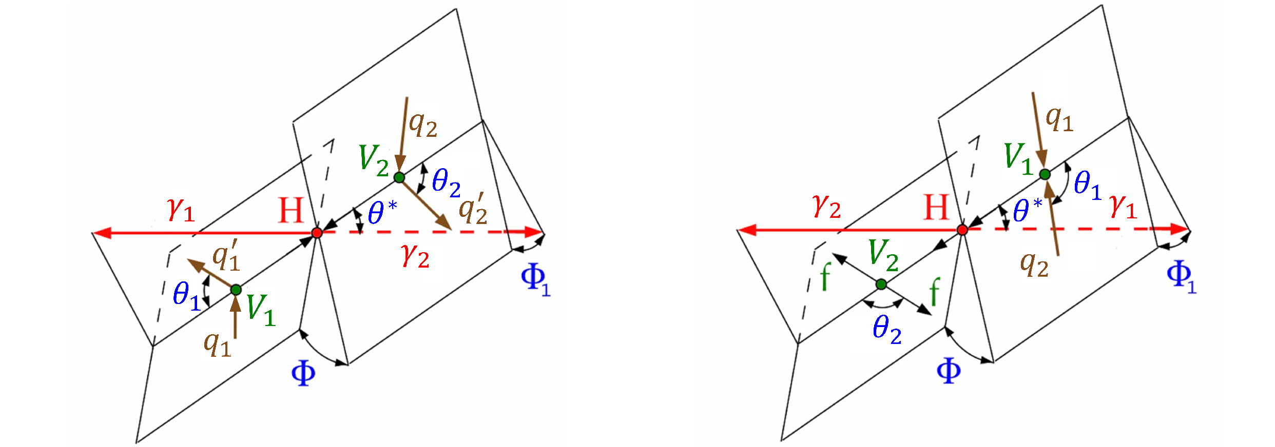
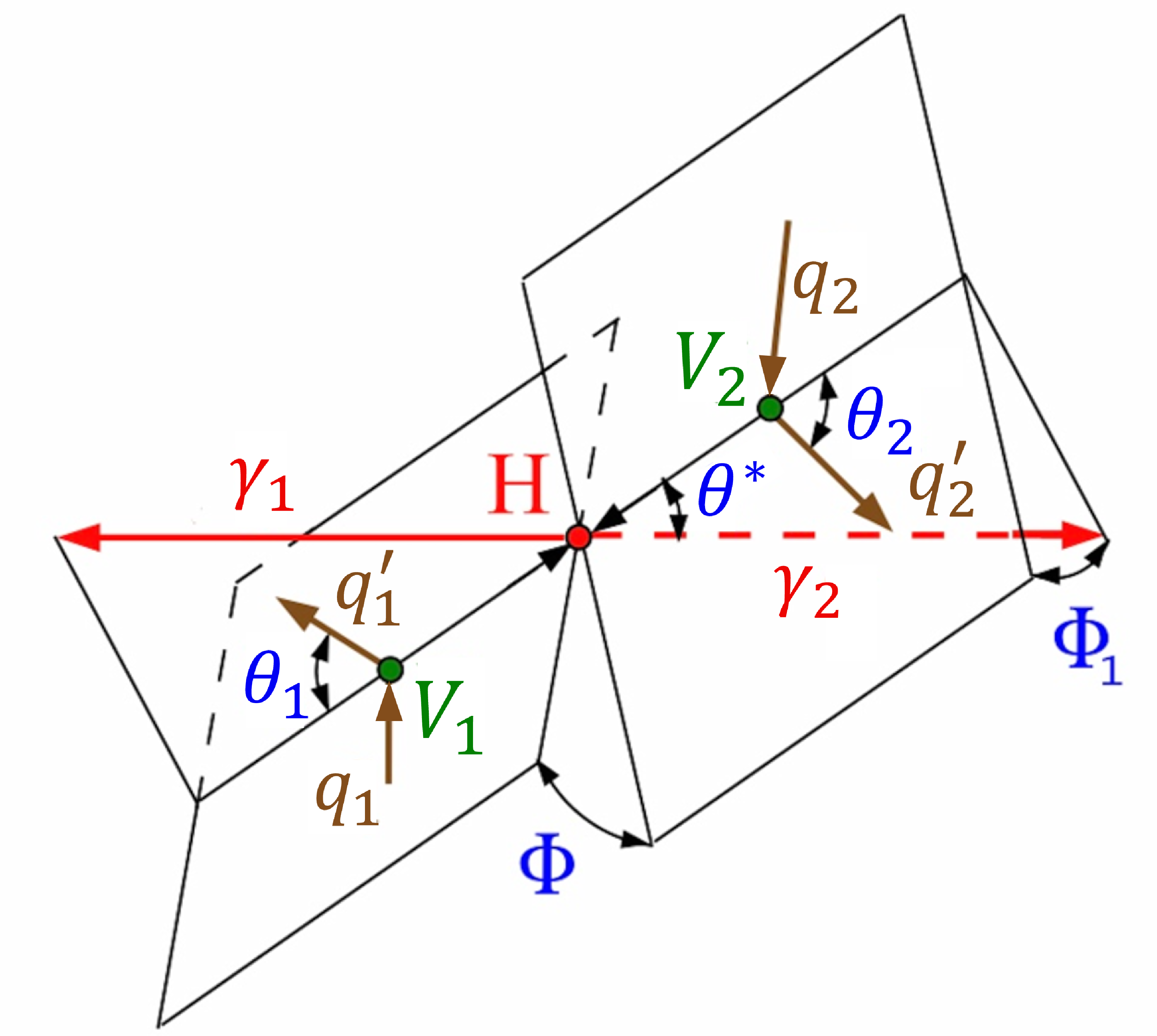
Topologies of the H production and decay, useful for the measurement of $ \mathrm{H}\mathrm{V}\mathrm{V} $ couplings: EW vector boson fusion $ q_1 q_2\to \mathrm{V}_1\mathrm{V}_2 + q_1^{'}q_2^{'} \to \mathrm{H} + q_1^{'}q_2^{'} \to \gamma_1\gamma_2 + q_1^{'}q_2^{'} $ (left); associated production $ q_1 q_2\to \mathrm{V}_1 \to \mathrm{V}_2\mathrm{H} \to \gamma_1\gamma_2 +\mathrm{ff} $ (right). The figure on the left is also valid to describe gluon fusion events in association with two jets, useful for the measurement of $ \mathrm{H}\mathrm{g}\mathrm{g} $ couplings, when $ \mathrm{V} = \mathrm{g} $. The incoming partons are shown in brown and the intermediate or final-state particles are shown in red and green. The angles characterizing kinematic distributions are shown in blue and are defined in the respective rest frames [39,44,47]. |
png pdf |
Figure 3-a:
Topologies of the H production and decay, useful for the measurement of $ \mathrm{H}\mathrm{V}\mathrm{V} $ couplings: EW vector boson fusion $ q_1 q_2\to \mathrm{V}_1\mathrm{V}_2 + q_1^{'}q_2^{'} \to \mathrm{H} + q_1^{'}q_2^{'} \to \gamma_1\gamma_2 + q_1^{'}q_2^{'} $ (left); associated production $ q_1 q_2\to \mathrm{V}_1 \to \mathrm{V}_2\mathrm{H} \to \gamma_1\gamma_2 +\mathrm{ff} $ (right). The figure on the left is also valid to describe gluon fusion events in association with two jets, useful for the measurement of $ \mathrm{H}\mathrm{g}\mathrm{g} $ couplings, when $ \mathrm{V} = \mathrm{g} $. The incoming partons are shown in brown and the intermediate or final-state particles are shown in red and green. The angles characterizing kinematic distributions are shown in blue and are defined in the respective rest frames [39,44,47]. |
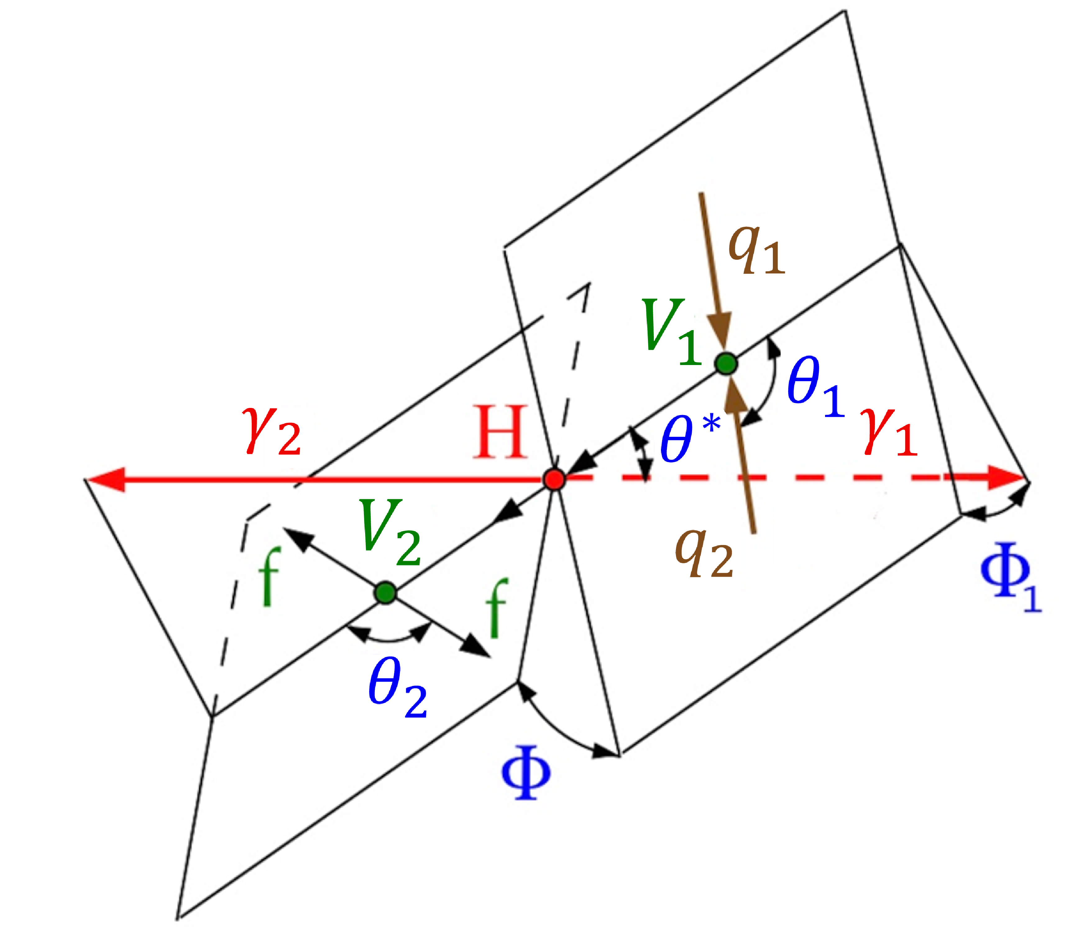
png pdf |
Figure 3-b:
Topologies of the H production and decay, useful for the measurement of $ \mathrm{H}\mathrm{V}\mathrm{V} $ couplings: EW vector boson fusion $ q_1 q_2\to \mathrm{V}_1\mathrm{V}_2 + q_1^{'}q_2^{'} \to \mathrm{H} + q_1^{'}q_2^{'} \to \gamma_1\gamma_2 + q_1^{'}q_2^{'} $ (left); associated production $ q_1 q_2\to \mathrm{V}_1 \to \mathrm{V}_2\mathrm{H} \to \gamma_1\gamma_2 +\mathrm{ff} $ (right). The figure on the left is also valid to describe gluon fusion events in association with two jets, useful for the measurement of $ \mathrm{H}\mathrm{g}\mathrm{g} $ couplings, when $ \mathrm{V} = \mathrm{g} $. The incoming partons are shown in brown and the intermediate or final-state particles are shown in red and green. The angles characterizing kinematic distributions are shown in blue and are defined in the respective rest frames [39,44,47]. |
png pdf |
Figure 4:
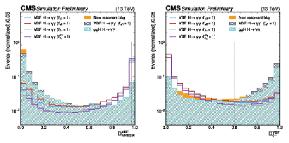
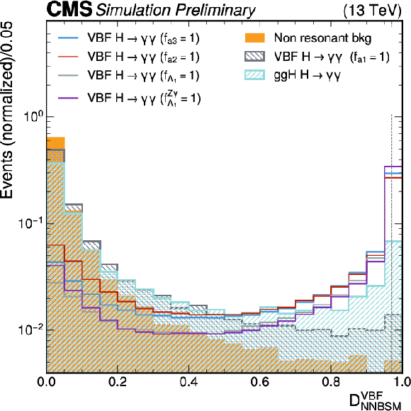
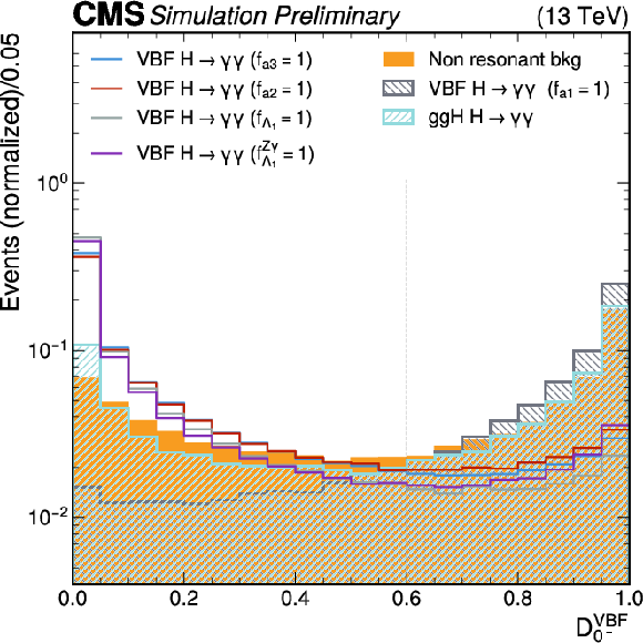
Distribution of the $ \mathcal{D}^\mathrm{VBF}_\mathrm{NNBSM} $ (left) and $ \mathcal{D}^\mathrm{VBF}_\mathrm{0-} $ (right) discriminant for the SM $ \mathrm{VBF} $ signal and for four anomalous coupling hypotheses, shown together with the main resonant background (SM $ \mathrm{g}\mathrm{g}\mathrm{H} $ production), and the continuous diphoton background. The distributions are shown after the VBF preselection described in the text and are normalized to the unit area. The vertical dashed lines indicate the category boundaries applied in the analysis. |
png pdf |
Figure 4-a:
Distribution of the $ \mathcal{D}^\mathrm{VBF}_\mathrm{NNBSM} $ (left) and $ \mathcal{D}^\mathrm{VBF}_\mathrm{0-} $ (right) discriminant for the SM $ \mathrm{VBF} $ signal and for four anomalous coupling hypotheses, shown together with the main resonant background (SM $ \mathrm{g}\mathrm{g}\mathrm{H} $ production), and the continuous diphoton background. The distributions are shown after the VBF preselection described in the text and are normalized to the unit area. The vertical dashed lines indicate the category boundaries applied in the analysis. |
png pdf |
Figure 4-b:
Distribution of the $ \mathcal{D}^\mathrm{VBF}_\mathrm{NNBSM} $ (left) and $ \mathcal{D}^\mathrm{VBF}_\mathrm{0-} $ (right) discriminant for the SM $ \mathrm{VBF} $ signal and for four anomalous coupling hypotheses, shown together with the main resonant background (SM $ \mathrm{g}\mathrm{g}\mathrm{H} $ production), and the continuous diphoton background. The distributions are shown after the VBF preselection described in the text and are normalized to the unit area. The vertical dashed lines indicate the category boundaries applied in the analysis. |
png pdf |
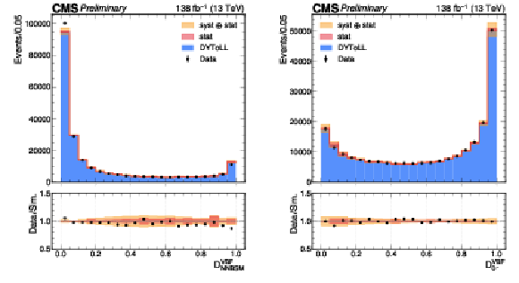
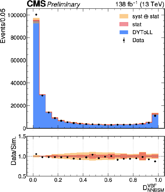
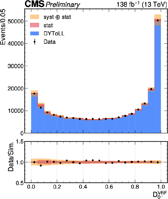
Figure 5:
The comparison between simulation (blue filled histograms, normalized to the data integral) and Z($ \rightarrow ee $) + jets data events (black markers) is shown, along with the corresponding ratio plots for the $ \mathcal{D}^\mathrm{VBF}_\mathrm{NNBSM} $ (left) and $ \mathcal{D}^\mathrm{VBF}_\mathrm{0-} $ (right) outputs. The systematic uncertainty is estimated by comparing NLO and LO Drell-Yan simulations, and is treated as a shape uncertainty. |
png pdf |
Figure 5-a:
The comparison between simulation (blue filled histograms, normalized to the data integral) and Z($ \rightarrow ee $) + jets data events (black markers) is shown, along with the corresponding ratio plots for the $ \mathcal{D}^\mathrm{VBF}_\mathrm{NNBSM} $ (left) and $ \mathcal{D}^\mathrm{VBF}_\mathrm{0-} $ (right) outputs. The systematic uncertainty is estimated by comparing NLO and LO Drell-Yan simulations, and is treated as a shape uncertainty. |
png pdf |
Figure 5-b:
The comparison between simulation (blue filled histograms, normalized to the data integral) and Z($ \rightarrow ee $) + jets data events (black markers) is shown, along with the corresponding ratio plots for the $ \mathcal{D}^\mathrm{VBF}_\mathrm{NNBSM} $ (left) and $ \mathcal{D}^\mathrm{VBF}_\mathrm{0-} $ (right) outputs. The systematic uncertainty is estimated by comparing NLO and LO Drell-Yan simulations, and is treated as a shape uncertainty. |
png pdf |
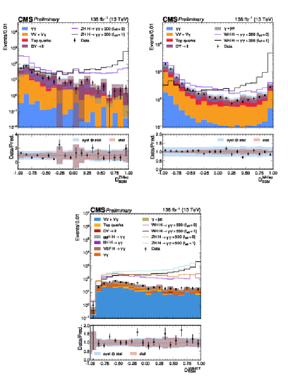
Figure 6:
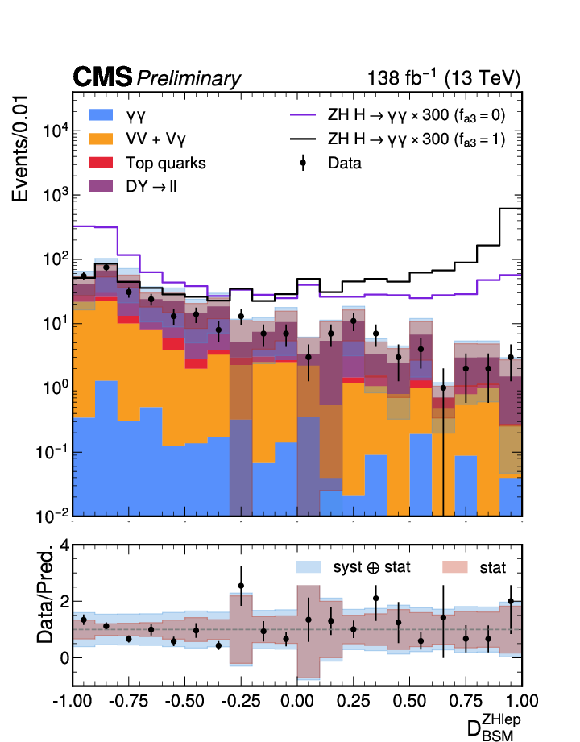
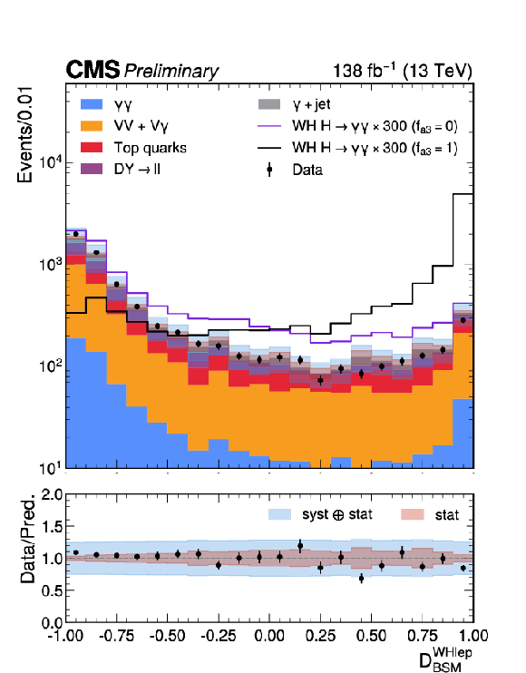
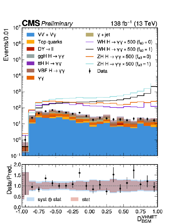
Stacked distributions of the output scores for the V(lep)H BDTs, $ \mathcal{D}^\mathrm{\mathrm{Z}\mathrm{H} lep}_\mathrm{BSM} $ (top left), $ \mathcal{D}^\mathrm{\mathrm{W}\mathrm{H} lep}_\mathrm{BSM} $ (top right), $ \mathcal{D}^\mathrm{\mathrm{V}\mathrm{H} MET}_\mathrm{BSM} $ (bottom) trained to separate the SM H from $ CP $-odd $ (f_{a3}=1) $ sample. The statistical uncertainty in the data points is denoted as vertical bars and that on the background simulation by the gray/blue bars. The simulated signal and background distributions are normalized to the luminosity of the data. To increase its visibility, the signal is scaled by a factor of either 300 or 500 for the different discriminants. For the $ \mathcal{D}^\mathrm{\mathrm{V}\mathrm{H} MET}_\mathrm{BSM} $ distribution, a requirement of $ \mathcal{D}^\mathrm{\mathrm{V}\mathrm{H} MET}_\mathrm{STXS} > $ 0.619 is applied to exclude events not used in the analysis. A systematic uncertainty is assigned to the data-driven component of the non-resonant background, to account for discrepancies between data and simulation. |
png pdf |
Figure 6-a:
Stacked distributions of the output scores for the V(lep)H BDTs, $ \mathcal{D}^\mathrm{\mathrm{Z}\mathrm{H} lep}_\mathrm{BSM} $ (top left), $ \mathcal{D}^\mathrm{\mathrm{W}\mathrm{H} lep}_\mathrm{BSM} $ (top right), $ \mathcal{D}^\mathrm{\mathrm{V}\mathrm{H} MET}_\mathrm{BSM} $ (bottom) trained to separate the SM H from $ CP $-odd $ (f_{a3}=1) $ sample. The statistical uncertainty in the data points is denoted as vertical bars and that on the background simulation by the gray/blue bars. The simulated signal and background distributions are normalized to the luminosity of the data. To increase its visibility, the signal is scaled by a factor of either 300 or 500 for the different discriminants. For the $ \mathcal{D}^\mathrm{\mathrm{V}\mathrm{H} MET}_\mathrm{BSM} $ distribution, a requirement of $ \mathcal{D}^\mathrm{\mathrm{V}\mathrm{H} MET}_\mathrm{STXS} > $ 0.619 is applied to exclude events not used in the analysis. A systematic uncertainty is assigned to the data-driven component of the non-resonant background, to account for discrepancies between data and simulation. |
png pdf |
Figure 6-b:
Stacked distributions of the output scores for the V(lep)H BDTs, $ \mathcal{D}^\mathrm{\mathrm{Z}\mathrm{H} lep}_\mathrm{BSM} $ (top left), $ \mathcal{D}^\mathrm{\mathrm{W}\mathrm{H} lep}_\mathrm{BSM} $ (top right), $ \mathcal{D}^\mathrm{\mathrm{V}\mathrm{H} MET}_\mathrm{BSM} $ (bottom) trained to separate the SM H from $ CP $-odd $ (f_{a3}=1) $ sample. The statistical uncertainty in the data points is denoted as vertical bars and that on the background simulation by the gray/blue bars. The simulated signal and background distributions are normalized to the luminosity of the data. To increase its visibility, the signal is scaled by a factor of either 300 or 500 for the different discriminants. For the $ \mathcal{D}^\mathrm{\mathrm{V}\mathrm{H} MET}_\mathrm{BSM} $ distribution, a requirement of $ \mathcal{D}^\mathrm{\mathrm{V}\mathrm{H} MET}_\mathrm{STXS} > $ 0.619 is applied to exclude events not used in the analysis. A systematic uncertainty is assigned to the data-driven component of the non-resonant background, to account for discrepancies between data and simulation. |
png pdf |
Figure 6-c:
Stacked distributions of the output scores for the V(lep)H BDTs, $ \mathcal{D}^\mathrm{\mathrm{Z}\mathrm{H} lep}_\mathrm{BSM} $ (top left), $ \mathcal{D}^\mathrm{\mathrm{W}\mathrm{H} lep}_\mathrm{BSM} $ (top right), $ \mathcal{D}^\mathrm{\mathrm{V}\mathrm{H} MET}_\mathrm{BSM} $ (bottom) trained to separate the SM H from $ CP $-odd $ (f_{a3}=1) $ sample. The statistical uncertainty in the data points is denoted as vertical bars and that on the background simulation by the gray/blue bars. The simulated signal and background distributions are normalized to the luminosity of the data. To increase its visibility, the signal is scaled by a factor of either 300 or 500 for the different discriminants. For the $ \mathcal{D}^\mathrm{\mathrm{V}\mathrm{H} MET}_\mathrm{BSM} $ distribution, a requirement of $ \mathcal{D}^\mathrm{\mathrm{V}\mathrm{H} MET}_\mathrm{STXS} > $ 0.619 is applied to exclude events not used in the analysis. A systematic uncertainty is assigned to the data-driven component of the non-resonant background, to account for discrepancies between data and simulation. |
png pdf |
Figure 7:
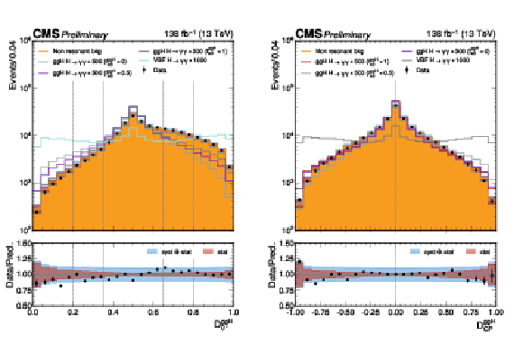
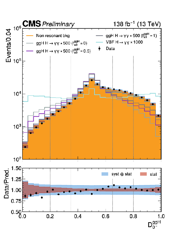
Signal and background distributions for MELA discriminants $ \mathcal{D}_{0-}^{\mathrm{g}\mathrm{g}\mathrm{H}} $ (right) and $ \mathcal{D}_\mathrm{CP}^{\mathrm{g}\mathrm{g}\mathrm{H}} $ (left) used in the $ \mathrm{H}\mathrm{g}\mathrm{g} $ analysis. Events are requested to have two jets with $ p_{\mathrm{T}} > $ 30 GeV. The non-resonant background is normalized to the data integral. The dashed lines indicate the bin boundaries applied in the analysis. A 10% systematic uncertainty is assigned to the data-driven component of the non-resonant background, to account for discrepancies between data and simulation. |
png pdf |
Figure 7-a:
Signal and background distributions for MELA discriminants $ \mathcal{D}_{0-}^{\mathrm{g}\mathrm{g}\mathrm{H}} $ (right) and $ \mathcal{D}_\mathrm{CP}^{\mathrm{g}\mathrm{g}\mathrm{H}} $ (left) used in the $ \mathrm{H}\mathrm{g}\mathrm{g} $ analysis. Events are requested to have two jets with $ p_{\mathrm{T}} > $ 30 GeV. The non-resonant background is normalized to the data integral. The dashed lines indicate the bin boundaries applied in the analysis. A 10% systematic uncertainty is assigned to the data-driven component of the non-resonant background, to account for discrepancies between data and simulation. |
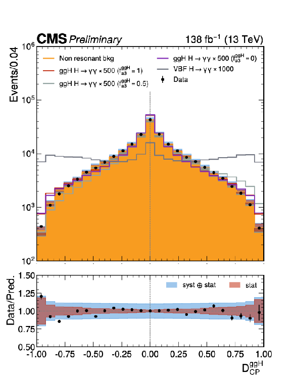
png pdf |
Figure 7-b:
Signal and background distributions for MELA discriminants $ \mathcal{D}_{0-}^{\mathrm{g}\mathrm{g}\mathrm{H}} $ (right) and $ \mathcal{D}_\mathrm{CP}^{\mathrm{g}\mathrm{g}\mathrm{H}} $ (left) used in the $ \mathrm{H}\mathrm{g}\mathrm{g} $ analysis. Events are requested to have two jets with $ p_{\mathrm{T}} > $ 30 GeV. The non-resonant background is normalized to the data integral. The dashed lines indicate the bin boundaries applied in the analysis. A 10% systematic uncertainty is assigned to the data-driven component of the non-resonant background, to account for discrepancies between data and simulation. |
png pdf |
Figure 8:
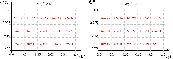
Definition of the $ \mathrm{H}\mathrm{g}\mathrm{g} $ analysis categories defined in bins of $ \mathcal{D}_{0-}^{\mathrm{g}\mathrm{g}\mathrm{H}} $ and $ \mathcal{D}^\mathrm{\mathrm{g}\mathrm{g}\mathrm{H}}_\mathrm{STXS} $, for negative (left) and positive (right) values of $ \mathcal{D}_\mathrm{CP}^{\mathrm{g}\mathrm{g}\mathrm{H}} $. |
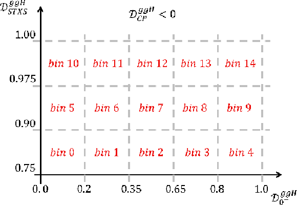
png pdf |
Figure 8-a:
Definition of the $ \mathrm{H}\mathrm{g}\mathrm{g} $ analysis categories defined in bins of $ \mathcal{D}_{0-}^{\mathrm{g}\mathrm{g}\mathrm{H}} $ and $ \mathcal{D}^\mathrm{\mathrm{g}\mathrm{g}\mathrm{H}}_\mathrm{STXS} $, for negative (left) and positive (right) values of $ \mathcal{D}_\mathrm{CP}^{\mathrm{g}\mathrm{g}\mathrm{H}} $. |
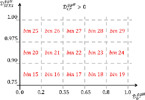
png pdf |
Figure 8-b:
Definition of the $ \mathrm{H}\mathrm{g}\mathrm{g} $ analysis categories defined in bins of $ \mathcal{D}_{0-}^{\mathrm{g}\mathrm{g}\mathrm{H}} $ and $ \mathcal{D}^\mathrm{\mathrm{g}\mathrm{g}\mathrm{H}}_\mathrm{STXS} $, for negative (left) and positive (right) values of $ \mathcal{D}_\mathrm{CP}^{\mathrm{g}\mathrm{g}\mathrm{H}} $. |
png pdf |
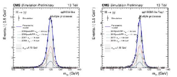
Figure 9:
Examples of fits to the $ m_{\gamma\gamma} $ distribution for SM signal samples with $ m_\mathrm{H} = $ 125 GeV are shown for the luminosity-weighted average of the three Run 2 data-taking years, in two categories targeting $ \mathrm{VBF} $ production: one dominated by BSM-like events and the other by SM-like events. Different Higgs production modes are summed according to their expected SM cross sections. The points represent simulation events weighted by their respective event weights, while the blue lines show the corresponding signal models. Colored lines represent the individual signal models for each data-taking year. The effective mass resolution ($ \sigma_{\text{eff}} $) of the $ m_{\gamma\gamma} $ distribution is also indicated in the figure. |
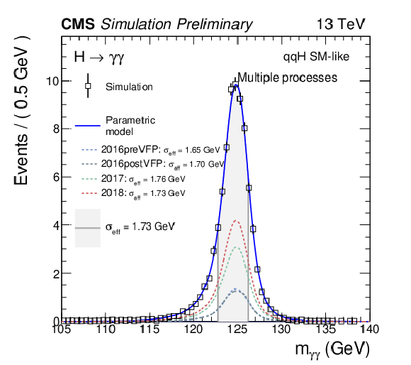
png pdf |
Figure 9-a:
Examples of fits to the $ m_{\gamma\gamma} $ distribution for SM signal samples with $ m_\mathrm{H} = $ 125 GeV are shown for the luminosity-weighted average of the three Run 2 data-taking years, in two categories targeting $ \mathrm{VBF} $ production: one dominated by BSM-like events and the other by SM-like events. Different Higgs production modes are summed according to their expected SM cross sections. The points represent simulation events weighted by their respective event weights, while the blue lines show the corresponding signal models. Colored lines represent the individual signal models for each data-taking year. The effective mass resolution ($ \sigma_{\text{eff}} $) of the $ m_{\gamma\gamma} $ distribution is also indicated in the figure. |
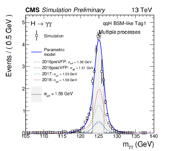
png pdf |
Figure 9-b:
Examples of fits to the $ m_{\gamma\gamma} $ distribution for SM signal samples with $ m_\mathrm{H} = $ 125 GeV are shown for the luminosity-weighted average of the three Run 2 data-taking years, in two categories targeting $ \mathrm{VBF} $ production: one dominated by BSM-like events and the other by SM-like events. Different Higgs production modes are summed according to their expected SM cross sections. The points represent simulation events weighted by their respective event weights, while the blue lines show the corresponding signal models. Colored lines represent the individual signal models for each data-taking year. The effective mass resolution ($ \sigma_{\text{eff}} $) of the $ m_{\gamma\gamma} $ distribution is also indicated in the figure. |
png pdf |
Figure 10:
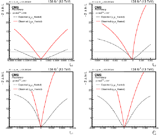
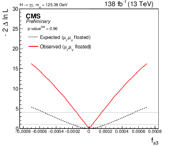
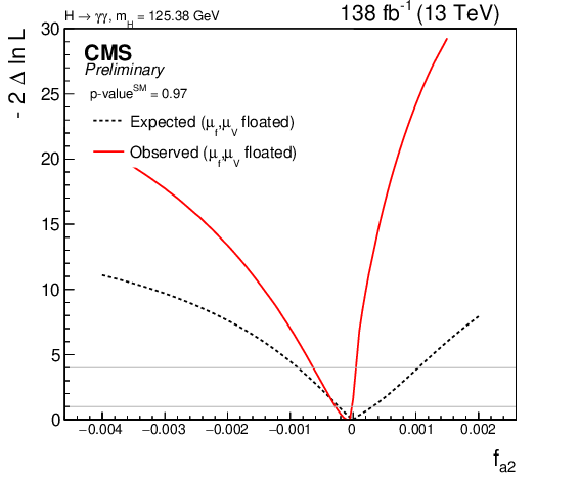
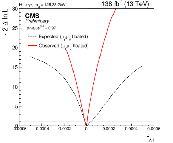
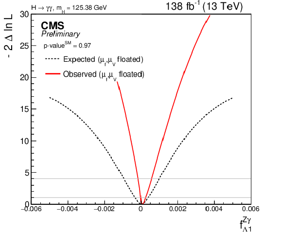
Likelihood scan for the expected and observed constraints of the $ \mathrm{H}\mathrm{V}\mathrm{V} $ coupling parameters: $ f_{a3} $ (top left, p-$ \mathrm{value^{SM}} = $ 0.96), $ f_{a2} $ (top right, p-$ \mathrm{value^{SM}} = $ 0.97), $ f_{\Lambda1} $ (bottom left, p-$ \mathrm{value^{SM}} = $ 0.97), $ f_{\Lambda1}^{Z\gamma} $ (bottom right, p-$ \mathrm{value^{SM}} = $ 0.97). |
png pdf |
Figure 10-a:
Likelihood scan for the expected and observed constraints of the $ \mathrm{H}\mathrm{V}\mathrm{V} $ coupling parameters: $ f_{a3} $ (top left, p-$ \mathrm{value^{SM}} = $ 0.96), $ f_{a2} $ (top right, p-$ \mathrm{value^{SM}} = $ 0.97), $ f_{\Lambda1} $ (bottom left, p-$ \mathrm{value^{SM}} = $ 0.97), $ f_{\Lambda1}^{Z\gamma} $ (bottom right, p-$ \mathrm{value^{SM}} = $ 0.97). |
png pdf |
Figure 10-b:
Likelihood scan for the expected and observed constraints of the $ \mathrm{H}\mathrm{V}\mathrm{V} $ coupling parameters: $ f_{a3} $ (top left, p-$ \mathrm{value^{SM}} = $ 0.96), $ f_{a2} $ (top right, p-$ \mathrm{value^{SM}} = $ 0.97), $ f_{\Lambda1} $ (bottom left, p-$ \mathrm{value^{SM}} = $ 0.97), $ f_{\Lambda1}^{Z\gamma} $ (bottom right, p-$ \mathrm{value^{SM}} = $ 0.97). |
png pdf |
Figure 10-c:
Likelihood scan for the expected and observed constraints of the $ \mathrm{H}\mathrm{V}\mathrm{V} $ coupling parameters: $ f_{a3} $ (top left, p-$ \mathrm{value^{SM}} = $ 0.96), $ f_{a2} $ (top right, p-$ \mathrm{value^{SM}} = $ 0.97), $ f_{\Lambda1} $ (bottom left, p-$ \mathrm{value^{SM}} = $ 0.97), $ f_{\Lambda1}^{Z\gamma} $ (bottom right, p-$ \mathrm{value^{SM}} = $ 0.97). |
png pdf |
Figure 10-d:
Likelihood scan for the expected and observed constraints of the $ \mathrm{H}\mathrm{V}\mathrm{V} $ coupling parameters: $ f_{a3} $ (top left, p-$ \mathrm{value^{SM}} = $ 0.96), $ f_{a2} $ (top right, p-$ \mathrm{value^{SM}} = $ 0.97), $ f_{\Lambda1} $ (bottom left, p-$ \mathrm{value^{SM}} = $ 0.97), $ f_{\Lambda1}^{Z\gamma} $ (bottom right, p-$ \mathrm{value^{SM}} = $ 0.97). |
png pdf |
Figure 11:
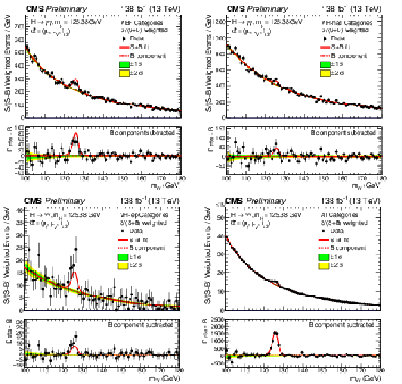
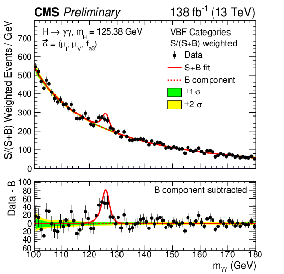
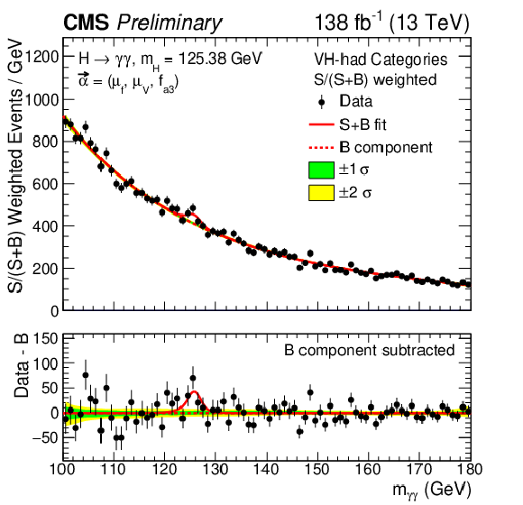
The best fit signal-plus-background model is shown overlaid on the S/(S+B)-weighted distribution of the data points (black) from the fit to the $ f_{a3} $ anomalous coupling parameter. The distributions are presented separately for categories optimized for VBF production (upper left), V(had)H (upper right), and V(lep)H (lower left). The lower right panel shows the combined distribution across all categories. S and B represent the fitted number of Higgs boson candidates and background events in the mass peak region. The green and yellow bands correspond to the one and two standard deviation uncertainties in the background component of the fit. The solid red line indicates the total signal-plus-background prediction, while the dashed red line represents the background-only contribution. The lower panel in each plot displays the residuals obtained by subtracting the background component from the data. |
png pdf |
Figure 11-a:
The best fit signal-plus-background model is shown overlaid on the S/(S+B)-weighted distribution of the data points (black) from the fit to the $ f_{a3} $ anomalous coupling parameter. The distributions are presented separately for categories optimized for VBF production (upper left), V(had)H (upper right), and V(lep)H (lower left). The lower right panel shows the combined distribution across all categories. S and B represent the fitted number of Higgs boson candidates and background events in the mass peak region. The green and yellow bands correspond to the one and two standard deviation uncertainties in the background component of the fit. The solid red line indicates the total signal-plus-background prediction, while the dashed red line represents the background-only contribution. The lower panel in each plot displays the residuals obtained by subtracting the background component from the data. |
png pdf |
Figure 11-b:
The best fit signal-plus-background model is shown overlaid on the S/(S+B)-weighted distribution of the data points (black) from the fit to the $ f_{a3} $ anomalous coupling parameter. The distributions are presented separately for categories optimized for VBF production (upper left), V(had)H (upper right), and V(lep)H (lower left). The lower right panel shows the combined distribution across all categories. S and B represent the fitted number of Higgs boson candidates and background events in the mass peak region. The green and yellow bands correspond to the one and two standard deviation uncertainties in the background component of the fit. The solid red line indicates the total signal-plus-background prediction, while the dashed red line represents the background-only contribution. The lower panel in each plot displays the residuals obtained by subtracting the background component from the data. |
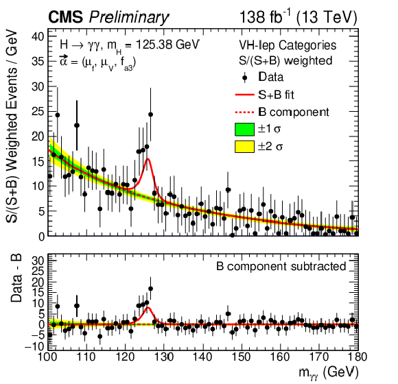
png pdf |
Figure 11-c:
The best fit signal-plus-background model is shown overlaid on the S/(S+B)-weighted distribution of the data points (black) from the fit to the $ f_{a3} $ anomalous coupling parameter. The distributions are presented separately for categories optimized for VBF production (upper left), V(had)H (upper right), and V(lep)H (lower left). The lower right panel shows the combined distribution across all categories. S and B represent the fitted number of Higgs boson candidates and background events in the mass peak region. The green and yellow bands correspond to the one and two standard deviation uncertainties in the background component of the fit. The solid red line indicates the total signal-plus-background prediction, while the dashed red line represents the background-only contribution. The lower panel in each plot displays the residuals obtained by subtracting the background component from the data. |
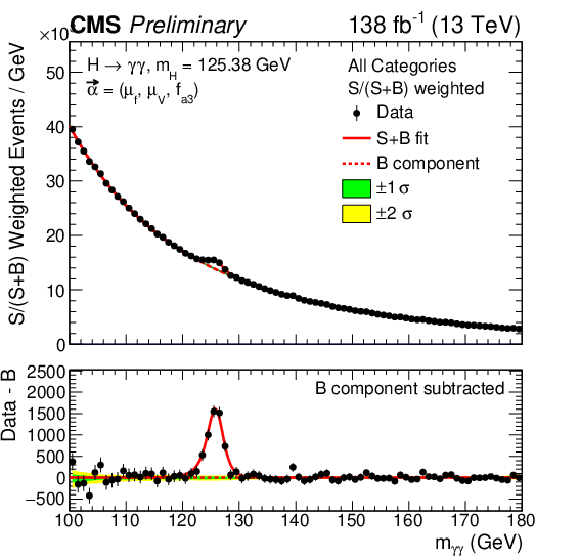
png pdf |
Figure 11-d:
The best fit signal-plus-background model is shown overlaid on the S/(S+B)-weighted distribution of the data points (black) from the fit to the $ f_{a3} $ anomalous coupling parameter. The distributions are presented separately for categories optimized for VBF production (upper left), V(had)H (upper right), and V(lep)H (lower left). The lower right panel shows the combined distribution across all categories. S and B represent the fitted number of Higgs boson candidates and background events in the mass peak region. The green and yellow bands correspond to the one and two standard deviation uncertainties in the background component of the fit. The solid red line indicates the total signal-plus-background prediction, while the dashed red line represents the background-only contribution. The lower panel in each plot displays the residuals obtained by subtracting the background component from the data. |
png pdf |
Figure 12:
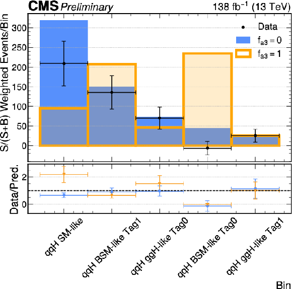
Distribution of events weighted by S/(S+B), using the bins optimized for the VBF production mode. S denotes the sum of all resonant signal events and B represents the non-resonant background. The plot shows the event yields in each bin within the mass window $ m_H - \sigma_{\text{eff}} < m_{\gamma\gamma} < m_H + \sigma_{\text{eff}} $, where $ \sigma_{\text{eff}} $ is defined as the smallest interval containing 68.3% of the $ m_{\gamma\gamma} $ distribution in each bin, for both the full BSM hypothesis (orange) and the SM hypothesis (blue). The data points (black dots) indicate the observed events in the same mass window, after background subtraction, and include statistical uncertainties. |
png pdf |
Figure 13:
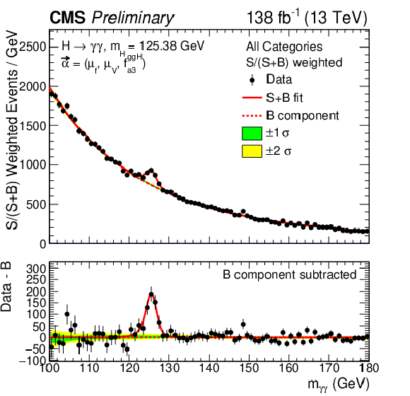
The best fit signal-plus-background model is shown overlaid on the S/(S+B)-weighted distribution of the data points (black) from the fit to the $ f_{a3}^{\mathrm{g}\mathrm{g}\mathrm{H}} $ anomalous coupling parameter, for the sum of all the $ \mathrm{H}\mathrm{g}\mathrm{g} $ analysis categories. S and B represent the fitted number of Higgs boson candidates and background events in the mass peak region. The green and yellow bands correspond to the one and two standard deviation uncertainties on the background component of the fit. The solid red line indicates the total signal-plus-background prediction, while the dashed red line represents the background-only contribution. The lower panel displays the residuals obtained by subtracting the background component from the data. |
png pdf |
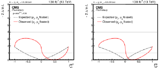
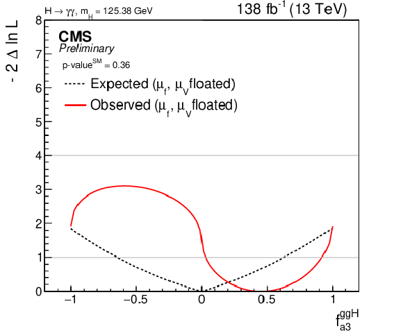
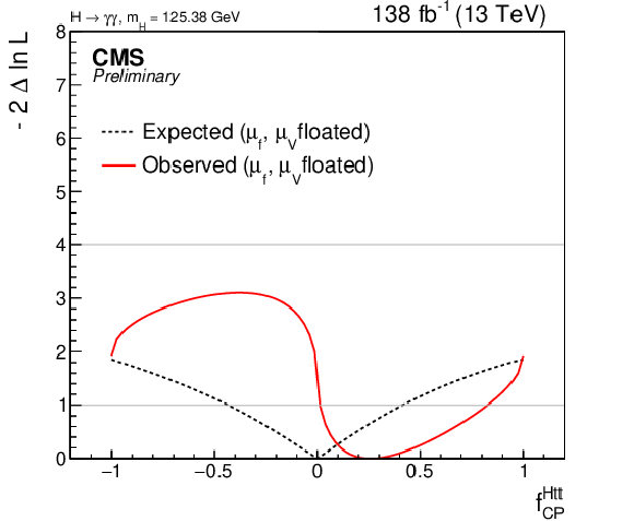
Figure 14:
Likelihood profile for the observed and expected CP-odd anomalous coupling parameters: $ f_{a3}^{\mathrm{g}\mathrm{g}\mathrm{H}} $ (left, p-$ \mathrm{value^{SM}} $ = 0.36) and $ f_{\rm CP}^{Htt} $ (right). |
png pdf |
Figure 14-a:
Likelihood profile for the observed and expected CP-odd anomalous coupling parameters: $ f_{a3}^{\mathrm{g}\mathrm{g}\mathrm{H}} $ (left, p-$ \mathrm{value^{SM}} $ = 0.36) and $ f_{\rm CP}^{Htt} $ (right). |
png pdf |
Figure 14-b:
Likelihood profile for the observed and expected CP-odd anomalous coupling parameters: $ f_{a3}^{\mathrm{g}\mathrm{g}\mathrm{H}} $ (left, p-$ \mathrm{value^{SM}} $ = 0.36) and $ f_{\rm CP}^{Htt} $ (right). |
| Tables | |

png pdf |
Table 1:
List of the $ \mathrm{H}\to\gamma\gamma $ preselection requirements. EB is the ECAL barrel region, with $ |\eta| < $ 1.442, while EE is the ECAL endcap region, with $ |\eta| > $ 1.566. |

png pdf |
Table 2:
List of discriminants for separating anomalous couplings from the SM contribution in the $ \mathrm{H}\mathrm{V}\mathrm{V} $ analysis. The third column indicates the targeted discrimination for that specific observable. Discriminants in this table are only used for event categorization. |

png pdf |
Table 3:
List of discriminants for separating anomalous couplings from the SM contribution in the $ \mathrm{H}\mathrm{g}\mathrm{g} $ analysis. The third column indicates the targeted discrimination for that specific observable. For the $ \mathcal{D}_{0-}^{\mathrm{g}\mathrm{g}\mathrm{H}} $ discriminant, the ``$ \mathrm{g}\mathrm{g}\mathrm{H} $" label indicates that this observable is constructed using matrix elements computed for the $ \mathrm{g}\mathrm{g}\mathrm{H} $ production process to differentiate it from the equivalent discriminant for the VBF process ($ \mathcal{D}^\mathrm{VBF}_\mathrm{0-} $). Discriminants in this table are only used for event categorization. |
png pdf |
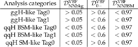
Table 4:
Definition of the $ \mathrm{VBF} $ categories based on the values of the discriminants $ \mathcal{D}^\mathrm{VBF}_\mathrm{NNbkg} $, $ \mathcal{D}^\mathrm{VBF}_\mathrm{0-} $ and $ \mathcal{D}^\mathrm{VBF}_\mathrm{NNBSM} $. |

png pdf |
Table 5:
The expected number of signal events in the case of SM H with $ m_\mathrm{H}= $ 125 GeV in analysis categories targeting $ \mathrm{VBF} $ associated production, shown for an integrated luminosity of 138 fb$ ^{-1} $. The fraction of the total number of events arising from the $ \mathrm{VBF} $ production mode in each analysis category is provided. Entries with values less than 0.1% are not shown. The $ \sigma_{\text{eff}} $, defined as the smallest interval containing 68.3% of the $ m_{\gamma\gamma} $ distribution, is listed for each analysis category. The final column shows the expected ratio of signal to signal-plus-background, S/(S+B), where S and B are the numbers of expected signal and background events in a $ \pm1\sigma_{\text{eff}} $ window centered on $ m_\mathrm{H} $. |

png pdf |
Table 6:
Definition of the V(had)H categories (i.e. VH events where the vector boson decays hadronically) based on the values of the discriminants $ \mathcal{D}^\mathrm{\mathrm{V}\mathrm{H} had}_\mathrm{bkg} $ and $ \mathcal{D}^\mathrm{\mathrm{V}\mathrm{H} had}_\mathrm{BSM} $. |
png pdf |
Table 7:
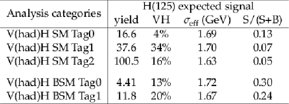
The expected number of signal events in the case of SM H with $ m_\mathrm{H}= $ 125 GeV in analysis categories targeting VH associated production in which the vector boson decays hadronically, shown for an integrated luminosity of 138 fb$ ^{-1} $. The fraction of the total number of events arising from the VH production mode in each analysis category is provided. Entries with values less than 0.1% are not shown. The $ \sigma_{\text{eff}} $, defined as the smallest interval containing 68.3% of the $ m_{\gamma\gamma} $ distribution, is listed for each analysis category. The final column shows the expected ratio of signal to signal-plus-background, S/(S+B), where S and B are the numbers of expected signal and background events in a $ \pm1\sigma_{\text{eff}} $ window centered on $ m_\mathrm{H} $. |
png pdf |
Table 8:
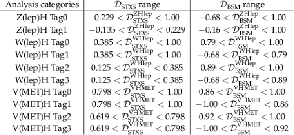
Definition of the V(lep)H categories based on the values of the discriminants $ \mathcal{D}_\mathrm{STXS} $ and $ \mathcal{D}_\mathrm{BSM} $. |
png pdf |
Table 9:
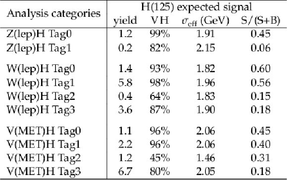
The expected number of signal events in the case of SM H with $ m_\mathrm{H}= $ 125 GeV in analysis categories targeting VH associated production in which the vector boson decays leptonically, shown for an integrated luminosity of 138 fb$ ^{-1} $. The fraction of the total number of events arising from the VH production mode in each analysis category is provided. Entries with values less than 0.1% are not shown. The $ \sigma_{\text{eff}} $, defined as the smallest interval containing 68.3% of the $ m_{\gamma\gamma} $ distribution, is listed for each analysis category. The final column shows the expected ratio of signal to signal-plus-background, S/(S+B), where S and B are the numbers of expected signal and background events in a $ \pm1\sigma_{\text{eff}} $ window centered on $ m_\mathrm{H} $. |
png pdf |
Table 10:
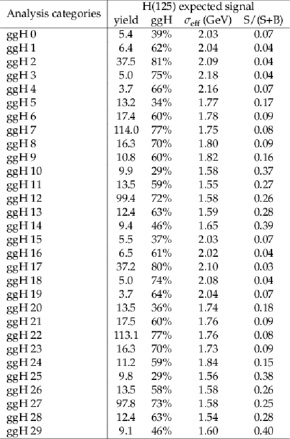
The expected number of signal events in the case of SM H with $ m_\mathrm{H}= $ 125 GeV in analysis categories targeting $ \mathrm{g}\mathrm{g}\mathrm{H} $ production associated with two jets, shown for an integrated luminosity of 138 fb$ ^{-1} $. The fraction of the total number of events arising from the $ \mathrm{g}\mathrm{g}\mathrm{H} $ production mode in each analysis category is provided. The $ \sigma_{\text{eff}} $, defined as the smallest interval containing 68.3% of the $ m_{\gamma\gamma} $ distribution, is listed for each analysis category. The final column shows the expected ratio of signal to signal-plus-background, S/(S+B), where S and B are the numbers of expected signal and background events in a $ \pm1\sigma_{\text{eff}} $ window centered on $ m_\mathrm{H} $. |

png pdf |
Table 11:
Summary of expected and observed allowed 68% CL intervals on $ \mathrm{H}\mathrm{V}\mathrm{V} $ anomalous coupling parameters, for the $ \mathrm{H}\mathrm{V}\mathrm{V} $ analysis described in this document and, for comparison, for the combination of $ \mathrm{H}\to4\ell $ + $ \mathrm{H}\to\tau\tau $ channels in [none-none-none]. |
png pdf |
Table 12:
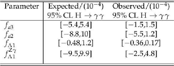
Summary of expected and observed allowed 95% CL intervals on $ \mathrm{H}\mathrm{V}\mathrm{V} $ anomalous coupling parameters for the $ \mathrm{H}\mathrm{V}\mathrm{V} $ analysis. |
png pdf |
Table 13:
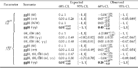
Constraints on the $ f_{a3}^{\mathrm{g}\mathrm{g}\mathrm{H}} $ and $ f_{\rm CP}^{Htt} $ parameters with the best fit values and allowed 68% CL (quoted uncertainties) and 95% CL (within square brackets) intervals, limited to the physical range of $ [-1, 1] $. The $ f_{a3}^{\mathrm{g}\mathrm{g}\mathrm{H}} $ constraints obtained in this work are compared to those obtained in the $ \mathrm{t}\mathrm{H} $ and $ \mathrm{t}\overline{\mathrm{t}}\mathrm{H} \mathrm{H}\to\gamma\gamma $ channel [20], the ggH $ \mathrm{H}\to4\ell $ [none-none-none-none], $ \mathrm{H}\to\tau\tau $ [19], and $ \mathrm{H}\to\mathrm{W}\mathrm{W} $ [34] channels respectively. The interpretation of the $ f_{a3}^{\mathrm{g}\mathrm{g}\mathrm{H}} $ result under the assumption of the top quark dominance in the gluon fusion loop are presented in terms of the $ f_{\rm CP}^{Htt} $ parameter, where either $ \mathrm{g}\mathrm{g}\mathrm{H} $ or its combination with $ \mathrm{t}\mathrm{H} $ and $ \mathrm{t}\overline{\mathrm{t}}\mathrm{H} $ results are shown. |
| Summary |
| An investigation of anomalous interactions between the Higgs boson (H) and vector bosons and gluons, including potential $ CP $-violating effects, is presented. The study is based on Higgs boson production via vector boson fusion ($ \mathrm{VBF} $), associated production with a vector boson (VH), and gluon fusion in association with two jets ($ \mathrm{g}\mathrm{g}\mathrm{H} $). Higgs boson candidates are selected through their decay into a pair of photons. The analysis uses proton-proton collision data collected by the CMS experiment at the LHC, corresponding to an integrated luminosity of 138 fb$ ^{-1} $ at a center-of-mass energy of 13 TeV. To enhance sensitivity in the $ \mathrm{H}\mathrm{g}\mathrm{g} $ channel, which shares a topology similar to $ \mathrm{VBF} $ production, the extraction of $ \mathrm{H}\mathrm{V}\mathrm{V} $ and $ \mathrm{H}\mathrm{g}\mathrm{g} $ anomalous coupling parameters is performed separately. Both analyses employ matrix element techniques and multivariate discriminants to optimize event categorization. The effective cross section ratios $ \vec{f} = \left(f_{a2}, f_{a3}, f_{\Lambda 1}, f_{\Lambda 1}^{\mathrm{Z}\gamma}\right) $ and $ f_{a3}^{\mathrm{g}\mathrm{g}\mathrm{H}} $ are extracted via a simultaneous fit to the $ m_{\gamma\gamma} $ distributions across all categories. In the $ \mathrm{H}\mathrm{V}\mathrm{V} $ analysis, constraints are placed on the $ CP $-violating parameter $ f_{a3} $ and on the $ CP $-conserving parameters $ f_{a2} $, $ f_{\Lambda 1} $, and $ f_{\Lambda 1}^{\mathrm{Z}\gamma} $. The resulting 68% confidence level (CL) limits are: $ f_{a3} = ( $ 0.00 $ ^{+0.39}_{-0.39} $) $\times $ 10$^-4$, $ f_{a2} = (-0.81_{-2.0}^{+0.65}$) $\times $ 10$^{-4} $, $ f_{\Lambda 1} = (-0.014_{-0.14}^{+0.032}$) $\times $ 10$^{-4} $, $ f_{\Lambda 1}^{\mathrm{Z}\gamma} = (0.83_{-0.92}^{+1.5}$) $\times $ 10$^{-4} $. These represent some of the most stringent limits to date. In the $ \mathrm{H}\mathrm{g}\mathrm{g} $ analysis, constraints are set in terms of the effective cross section ratio $ f_{a3}^{\mathrm{g}\mathrm{g}\mathrm{H}} $, or equivalently in terms of $ f_{\rm CP}^{Htt} $. The observed one-dimensional constraints at 68% CL are found to be respectively $ f_{a3}^{\mathrm{g}\mathrm{g}\mathrm{H}} = $ 0.45 $ ^{+0.46}_{-0.42} $ (stat.) $ ^{+0.10}_{-0.08} $ (syst.) and $ f_{\rm CP}^{Htt} = $ 0.26 $ ^{+0.57}_{-0.25} $. The observed limits on $ CP $-violating parameters in $ \mathrm{g}\mathrm{g}\mathrm{H} $, $ \mathrm{VBF} $ and VH production modes are consistent with results obtained in other Higgs decay channels [33,34]. As systematic uncertainties largely cancel in ratios, all measurements are currently limited by the statistical precision and are expected to improve with additional LHC data. |
| References | ||||
| 1 | ATLAS Collaboration | Observation of a new particle in the search for the standard model Higgs boson with the ATLAS detector at the LHC | PLB 716 (2012) 1 | 1207.7214 |
| 2 | CMS Collaboration | Observation of a new boson at a mass of 125 GeV with the CMS experiment at the LHC | PLB 716 (2012) 30 | CMS-HIG-12-028 1207.7235 |
| 3 | CMS Collaboration | Observation of a new boson with mass near 125 GeV in pp collisions at $ \sqrt{s} $ = 7 and 8 TeV | JHEP 06 (2013) 081 | CMS-HIG-12-036 1303.4571 |
| 4 | S. L. Glashow | Partial-symmetries of weak interactions | NP 22 (1961) 579 | |
| 5 | F. Englert and R. Brout | Broken symmetry and the mass of gauge vector mesons | PRL 13 (1964) 321 | |
| 6 | P. W. Higgs | Broken symmetries, massless particles and gauge fields | PL 12 (1964) 132 | |
| 7 | P. W. Higgs | Broken symmetries and the masses of gauge bosons | PRL 13 (1964) 508 | |
| 8 | G. S. Guralnik, C. R. Hagen, and T. W. B. Kibble | Global conservation laws and massless particles | PRL 13 (1964) 585 | |
| 9 | S. Weinberg | A model of leptons | PRL 19 (1967) 1264 | |
| 10 | A. Salam | Weak and electromagnetic interactions | Conf. Proc. C 680519 (1968) 367 | |
| 11 | CMS Collaboration | Constraints on the spin-parity and anomalous HVV couplings of the Higgs boson in proton collisions at 7 and 8 TeV | PRD 92 (2015) 012004 | CMS-HIG-14-018 1411.3441 |
| 12 | ATLAS Collaboration | Study of the spin and parity of the Higgs boson in diboson decays with the ATLAS detector | EPJC 75 (2015) 476 | 1506.05669 |
| 13 | CMS Collaboration | Study of the mass and spin-parity of the Higgs boson candidate via its decays to Z boson pairs | PRL 110 (2013) 081803 | CMS-HIG-12-041 1212.6639 |
| 14 | CMS Collaboration | Measurement of the properties of a Higgs boson in the four-lepton final state | PRD 89 (2014) 092007 | CMS-HIG-13-002 1312.5353 |
| 15 | CMS Collaboration | Limits on the Higgs boson lifetime and width from its decay to four charged leptons | PRD 92 (2015) 072010 | CMS-HIG-14-036 1507.06656 |
| 16 | CMS Collaboration | Combined search for anomalous pseudoscalar HVV couplings in VH production and H $ \to $ VV decay | PLB 759 (2016) 672 | CMS-HIG-14-035 1602.04305 |
| 17 | CMS Collaboration | Constraints on anomalous Higgs boson couplings using production and decay information in the four-lepton final state | PLB 775 (2017) 1 | CMS-HIG-17-011 1707.00541 |
| 18 | CMS Collaboration | Measurements of the Higgs boson width and anomalous HVV couplings from on-shell and off-shell production in the four-lepton final state | PRD 99 (2019) 112003 | CMS-HIG-18-002 1901.00174 |
| 19 | CMS Collaboration | Constraints on anomalous HVV couplings from the production of Higgs bosons decaying to $ \tau $ lepton pairs | PRD 100 (2019) 112002 | CMS-HIG-17-034 1903.06973 |
| 20 | CMS Collaboration | Measurements of $ \text{t}\bar{\text{t}}\mathrm{H} $ production and the CP structure of the Yukawa interaction between the Higgs boson and top quark in the diphoton decay channel | PRL 125 (2020) 061801 | CMS-HIG-19-013 2003.10866 |
| 21 | CMS Collaboration | Constraints on anomalous Higgs boson couplings to vector bosons and fermions in its production and decay using the four-lepton final state | PRD 104 (2021) 052004 | CMS-HIG-19-009 2104.12152 |
| 22 | CMS Collaboration | Analysis of the $ CP $ structure of the Yukawa coupling between the Higgs boson and $ \tau $ leptons in proton-proton collisions at $ \sqrt{s} $ = 13 TeV | JHEP 06 (2022) 012 | CMS-HIG-20-006 2110.04836 |
| 23 | CMS Collaboration | Measurement of the Higgs boson width and evidence of its off-shell contributions to ZZ production | Nature Phys. 18 (2022) 1329--1334 | CMS-HIG-21-013 2202.06923 |
| 24 | ATLAS Collaboration | Evidence for the spin-0 nature of the Higgs boson using ATLAS data | PLB 726 (2013) 120 | 1307.1432 |
| 25 | ATLAS Collaboration | Test of CP invariance in vector-boson fusion production of the Higgs boson using the optimal observable method in the ditau decay channel with the ATLAS detector | EPJC 76 (2016) 658 | 1602.04516 |
| 26 | ATLAS Collaboration | Measurement of inclusive and differential cross sections in the $ H \rightarrow ZZ^* \rightarrow 4\ell $ decay channel in pp collisions at $ \sqrt{s}= $ 13 TeV with the ATLAS detector | JHEP 10 (2017) 132 | 1708.02810 |
| 27 | ATLAS Collaboration | Measurement of the Higgs boson coupling properties in the $ H\rightarrow ZZ^{*} \rightarrow 4\ell $ decay channel at $ \sqrt{s} $ = 13 TeV with the ATLAS detector | JHEP 03 (2018) 095 | 1712.02304 |
| 28 | ATLAS Collaboration | Measurements of Higgs boson properties in the diphoton decay channel with 36 fb$ ^{-1} $ of pp collision data at $ \sqrt{s} = $ 13 TeV with the ATLAS detector | PRD 98 (2018) 052005 | 1802.04146 |
| 29 | ATLAS Collaboration | Test of CP invariance in vector-boson fusion production of the Higgs boson in the $ H\rightarrow\tau\tau $ channel in proton-proton collisions at $ \sqrt{s} $ = 13 TeV with the ATLAS detector | PLB 805 (2020) 135426 | 2002.05315 |
| 30 | ATLAS Collaboration | CP properties of Higgs boson interactions with top quarks in the $ t\bar{t}H $ and $ tH $ processes using $ H \rightarrow \gamma\gamma $ with the ATLAS detector | PRL 125 (2020) 061802 | 2004.04545 |
| 31 | ATLAS Collaboration | Constraints on Higgs boson properties using $ WW^{*}(\rightarrow e\nu \mu \nu )jj $ production in 36.1 fb$ ^{-1} $ of $ \sqrt{s}= $ 13 TeV pp collisions with the ATLAS detector | EPJC 82 (2022) 622 | 2109.13808 |
| 32 | ATLAS Collaboration | Probing the Higgs boson CP properties in vector-boson fusion production in the $ H\to \tau^{+}\tau^{-} $ channel with the ATLAS detector | technical report, 2025 link |
2506.19395 |
| 33 | CMS Collaboration | Constraints on anomalous Higgs boson couplings to vector bosons and fermions from the production of Higgs bosons using the \ensuremath\tau\ensuremath\tau final state | PRD 108 (2023) 032013 | CMS-HIG-20-007 2205.05120 |
| 34 | CMS Collaboration | Constraints on anomalous Higgs boson couplings from its production and decay using the WW channel in proton-proton collisions at $ \sqrt{s} = 13 \text {TeV} $ | EPJC 84 (2024) 779 | CMS-HIG-22-008 2403.00657 |
| 35 | T. Plehn, D. L. Rainwater, and D. Zeppenfeld | Determining the structure of Higgs couplings at the LHC | PRL 88 (2002) 051801 | hep-ph/0105325 |
| 36 | V. Hankele, G. Klamke, D. Zeppenfeld, and T. Figy | Anomalous Higgs boson couplings in vector boson fusion at the CERN LHC | PRD 74 (2006) 095001 | hep-ph/0609075 |
| 37 | E. Accomando et al. | CP Studies and Non-Standard Higgs Physics | link | hep-ph/0608079 |
| 38 | K. Hagiwara, Q. Li, and K. Mawatari | Jet angular correlation in vector-boson fusion processes at hadron colliders | JHEP 07 (2009) 101 | 0905.4314 |
| 39 | Y. Gao et al. | Spin determination of single-produced resonances at hadron colliders | PRD 81 (2010) 075022 | 1001.3396 |
| 40 | A. De Rujula et al. | Higgs look-alikes at the LHC | PRD 82 (2010) 013003 | 1001.5300 |
| 41 | S. Bolognesi et al. | Spin and parity of a single-produced resonance at the LHC | PRD 86 (2012) 095031 | 1208.4018 |
| 42 | J. Ellis, D. S. Hwang, V. Sanz, and T. You | A fast track towards the 'Higgs' spin and parity | JHEP 11 (2012) 134 | 1208.6002 |
| 43 | P. Artoisenet et al. | A framework for Higgs characterisation | JHEP 11 (2013) 043 | 1306.6464 |
| 44 | I. Anderson et al. | Constraining anomalous HVV interactions at proton and lepton colliders | PRD 89 (2014) 035007 | 1309.4819 |
| 45 | M. J. Dolan, P. Harris, M. Jankowiak, and M. Spannowsky | Constraining CP-violating Higgs sectors at the LHC using gluon fusion | PRD 90 (2014) 073008 | 1406.3322 |
| 46 | A. Greljo, G. Isidori, J. M. Lindert, and D. Marzocca | Pseudo-observables in electroweak Higgs production | EPJC 76 (2016) 158 | 1512.06135 |
| 47 | A. V. Gritsan, R. R ö ntsch, M. Schulze, and M. Xiao | Constraining anomalous Higgs boson couplings to the heavy flavor fermions using matrix element techniques | PRD 94 (2016) 055023 | 1606.03107 |
| 48 | J. Davis et al. | Constraining anomalous Higgs boson couplings to virtual photons | PRD 105 (2022) 096027 | 2109.13363 |
| 49 | A. V. Gritsan et al. | New features in the JHU generator framework: constraining Higgs boson properties from on-shell and off-shell production | PRD 102 (2020) 056022 | 2002.09888 |
| 50 | K. Hamilton, P. Nason, and G. Zanderighi | Finite quark-mass effects in the NNLOPS POWHEG+MiNLO Higgs generator | JHEP 05 (2015) 140 | 1501.04637 |
| 51 | CMS Collaboration | Measurements of Higgs boson production cross sections and couplings in the diphoton decay channel at $ \sqrt{\mathrm{s}} $ = 13 TeV | JHEP 07 (2021) 027 | CMS-HIG-19-015 2103.06956 |
| 52 | CMS Collaboration | The CMS experiment at the CERN LHC | JINST 3 (2008) S08004 | |
| 53 | CMS Collaboration | The CMS trigger system | JINST 12 (2017) P01020 | CMS-TRG-12-001 1609.02366 |
| 54 | CMS Collaboration | CMS luminosity measurements for the 2016 data taking period | CMS Physics Analysis Summary, 2017 CMS-PAS-LUM-17-001 |
CMS-PAS-LUM-17-001 |
| 55 | CMS Collaboration | CMS luminosity measurement for the 2017 data-taking period at $ \sqrt{s} = $ 13 TeV | CMS Physics Analysis Summary, 2018 CMS-PAS-LUM-17-004 |
CMS-PAS-LUM-17-004 |
| 56 | CMS Collaboration | CMS luminosity measurement for the 2018 data-taking period at $ \sqrt{s} = $ 13 TeV | CMS Physics Analysis Summary, 2019 CMS-PAS-LUM-18-002 |
CMS-PAS-LUM-18-002 |
| 57 | CMS Collaboration | Measurement of the Inclusive W and Z Production Cross Sections in pp Collisions at $ \sqrt{s} = $ 7 TeV | JHEP 10 (2011) 132 | |
| 58 | T. Sjöstrand et al. | An introduction to PYTHIA 8.2 | Comput. Phys. Commun. 191 (2015) 159 | 1410.3012 |
| 59 | CMS Collaboration | Event generator tunes obtained from underlying event and multiparton scattering measurements | EPJC 76 (2016) 155 | CMS-GEN-14-001 1512.00815 |
| 60 | CMS Collaboration | Extraction and validation of a new set of CMS PYTHIA8 tunes from underlying-event measurements | EPJC 80 (2020) 4 | CMS-GEN-17-001 1903.12179 |
| 61 | NNPDF Collaboration | Parton distributions for the LHC Run II | JHEP 04 (2015) 040 | 1410.8849 |
| 62 | NNPDF Collaboration | Parton distributions from high-precision collider data | EPJC 77 (2017) 663 | 1706.00428 |
| 63 | LHC Higgs Cross Section Working Group | Handbook of LHC Higgs cross sections: 4. deciphering the nature of the Higgs sector | CERN, 2016 link |
1610.07922 |
| 64 | GEANT4 Collaboration | GEANT 4---a simulation toolkit | NIM A 506 (2003) 250 | |
| 65 | J. Alwall et al. | The automated computation of tree-level and next-to-leading order differential cross sections, and their matching to parton shower simulations | JHEP 07 (2014) 079 | 1405.0301 |
| 66 | P. Nason | A new method for combining NLO QCD with shower Monte Carlo algorithms | JHEP 11 (2004) 040 | hep-ph/0409146 |
| 67 | S. Frixione, P. Nason, and C. Oleari | Matching NLO QCD computations with parton shower simulations: the POWHEG method | JHEP 11 (2007) 070 | 0709.2092 |
| 68 | S. Alioli, P. Nason, C. Oleari, and E. Re | NLO Higgs boson production via gluon fusion matched with shower in POWHEG | JHEP 04 (2009) 002 | 0812.0578 |
| 69 | P. Nason and C. Oleari | NLO Higgs boson production via vector-boson fusion matched with shower in POWHEG | JHEP 02 (2010) 037 | 0911.5299 |
| 70 | S. Alioli, P. Nason, C. Oleari, and E. Re | A general framework for implementing NLO calculations in shower Monte Carlo programs: the POWHEG BOX | JHEP 06 (2010) 043 | 1002.2581 |
| 71 | H. B. Hartanto, B. Jager, L. Reina, and D. Wackeroth | Higgs boson production in association with top quarks in the POWHEG BOX | PRD 91 (2015) 094003 | 1501.04498 |
| 72 | G. Luisoni, P. Nason, C. Oleari, and F. Tramontano | $ HW^{\pm} $/HZ + 0 and 1 jet at NLO with the POWHEG BOX interfaced to GoSam and their merging within MiNLO | JHEP 10 (2013) 083 | 1306.2542 |
| 73 | T. Gleisberg et al. | Event generation with SHERPA 1.1 | JHEP 02 (2009) 007 | 0811.4622 |
| 74 | CMS Collaboration | Particle-flow reconstruction and global event description with the CMS detector | JINST 12 (2017) P10003 | CMS-PRF-14-001 1706.04965 |
| 75 | M. Cacciari, G. P. Salam, and G. Soyez | The anti-$ k_{\mathrm{T}} $ jet clustering algorithm | JHEP 04 (2008) 063 | 0802.1189 |
| 76 | M. Cacciari, G. P. Salam, and G. Soyez | FastJet user manual | EPJC 72 (2012) 1896 | 1111.6097 |
| 77 | CMS Collaboration | Jet energy scale and resolution in the CMS experiment in pp collisions at 8 TeV | JINST 12 (2017) P02014 | CMS-JME-13-004 1607.03663 |
| 78 | CMS Collaboration | Performance of missing transverse momentum reconstruction in proton-proton collisions at $ \sqrt{s} = $ 13\,TeV using the CMS detector | JINST 14 (2019) P07004 | CMS-JME-17-001 1903.06078 |
| 79 | CMS Collaboration | A measurement of the Higgs boson mass in the diphoton decay channel | PLB 805 (2020) 135425 | CMS-HIG-19-004 2002.06398 |
| 80 | CMS Collaboration | Precise determination of the mass of the Higgs boson and tests of compatibility of its couplings with the standard model predictions using proton collisions at 7 and 8 $ \,\text {TeV} $ | EPJC 75 (2015) 212 | CMS-HIG-14-009 1412.8662 |
| 81 | CMS Collaboration | The CMS Statistical Analysis and Combination Tool: Combine | Comput Softw Big Sci 8 (2024) 19 | |
| 82 | R. J. Barlow | Extended maximum likelihood | NIM A 297 (1990) 496 | |
| 83 | G. Cowan, K. Cranmer, E. Gross, and O. Vitells | Asymptotic formulae for likelihood-based tests of new physics | EPJC 71 (2011) 1554 | 1007.1727 |
| 84 | R. A. Fisher | On the interpretation of $ \chi^2 $ from contingency tables, and the calculation of p | J. Royal Stat. Soc. 85 (1922) 87 | |
| 85 | P. D. Dauncey, M. Kenzie, N. Wardle, and G. J. Davies | Handling uncertainties in background shapes: the discrete profiling method | JINST 10 (2015) P04015 | 1408.6865 |

|
Compact Muon Solenoid LHC, CERN |

|

|

|

|

|

|