
Compact Muon Solenoid
LHC, CERN
 Visit us: CMS Public Website, CMS Physics ;
Contact us: CMS Publications Committee
Visit us: CMS Public Website, CMS Physics ;
Contact us: CMS Publications Committee
| CMS-PAS-EXO-24-036 | ||
| Search for inelastic dark matter with low-momentum displaced electrons in proton-proton collisions at $ \sqrt{s} = $ 13 TeV | ||
| CMS Collaboration | ||
| 2026-07-15 | ||
| Abstract: A search for inelastic dark matter in events with missing transverse momentum and a nonresonant pair of low-momentum, displaced electrons is presented. The analysis is performed using a sample of proton-proton (pp) collision data collected by the CMS experiment at the CERN LHC corresponding to an integrated luminosity of 138 fb$ ^{-1} $ recorded in 2016--2018 at a center-of-mass energy of 13 TeV. A dedicated algorithm for reconstructing low-$ p_{\mathrm{T}} $ electrons is used to improve the search sensitivity, marking its first application to displaced electrons in CMS. No significant deviation from the standard model expectation is observed, and upper limits at 95% confidence level are set on the product of the inelastic dark matter production cross section $ \sigma(\mathrm{pp} \to A^{'} \to \chi_{1}\chi_{2}) $ and the decay branching fraction $ \mathcal{B}(\chi_{2} \to \chi_{1}\mathrm{e}^{+}\mathrm{e}^{-}) $, where $ A^{'} $ is a dark photon and $ \chi_{1} $ and $ \chi_{2} $ are states in the dark sector with small mass splitting, the lightest of which is the stable dark matter. Stringent constraints are placed on benchmark inelastic dark matter scenarios with mass splitting of 10% and 20% of the dark matter particle over the range from 3 to 100 GeV, providing the first collider constraints on inelastic dark matter in the electron final state. | ||
| Links: CDS record (PDF) ; CADI line (restricted) ; | ||
| Figures | |
png pdf |
Figure 1:
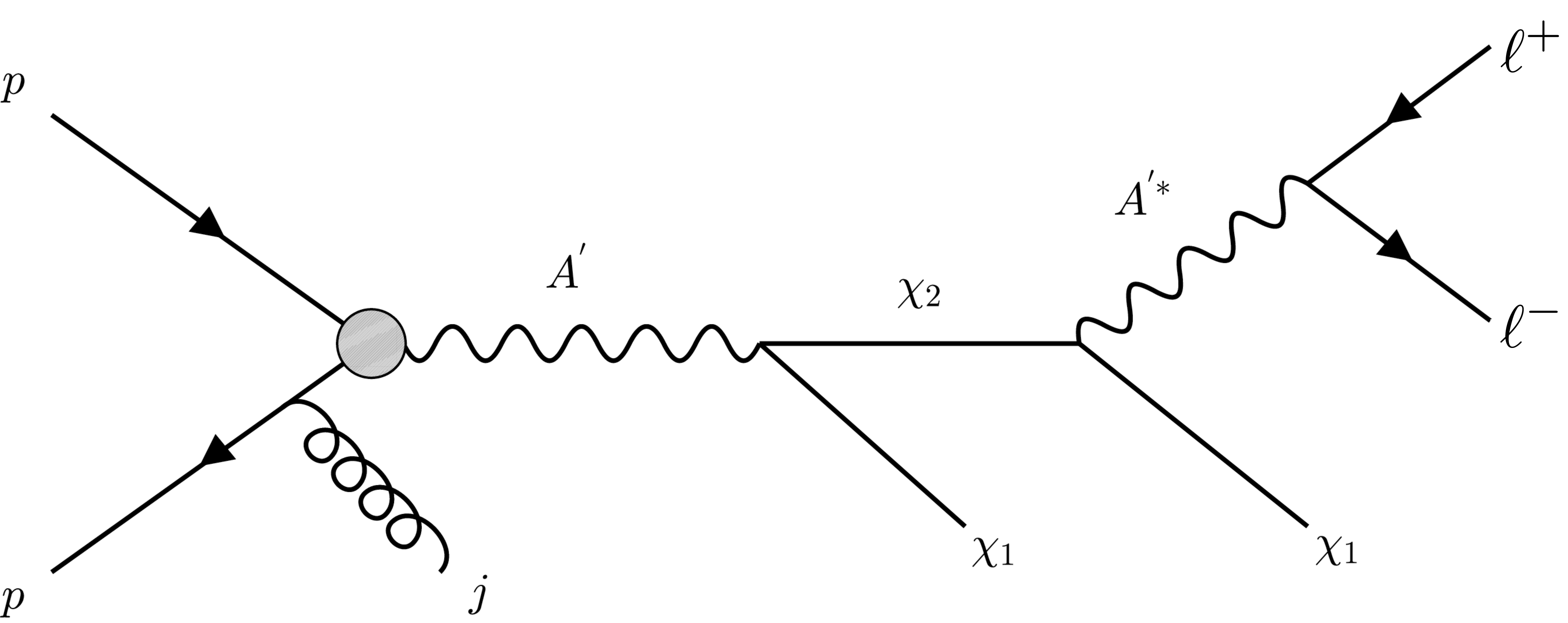
Feynman diagram for the IDM collider signature, showing the cascade decay of a dark photon A' into a pair of charged leptons and DM particles $ \chi_{1} $ and $ \chi_{2} $. |
png pdf |
Figure 2:
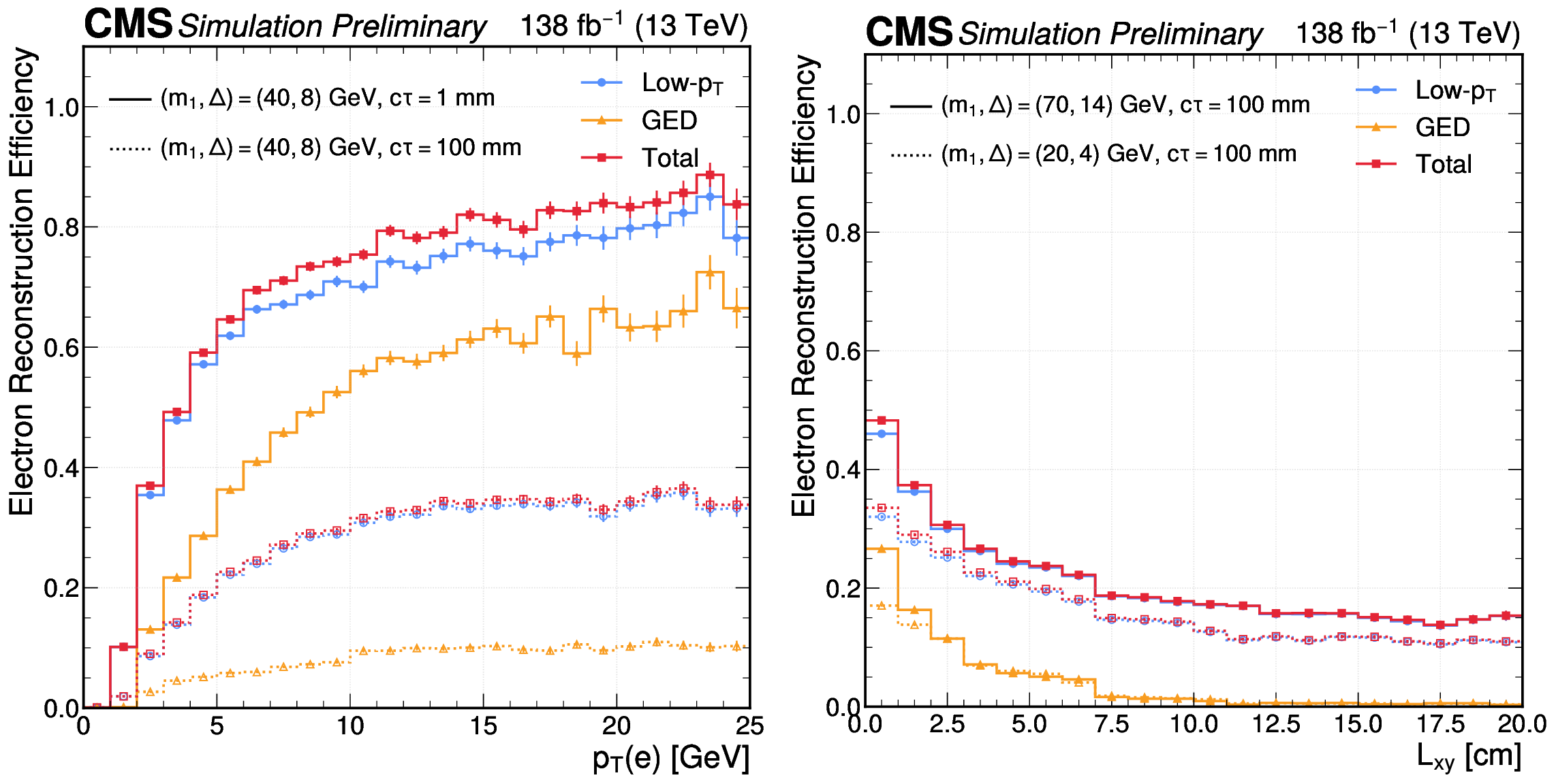
Fraction of reconstructed IDM signal electrons compared across different electron reconstruction algorithms, as a function of generator-level electron $ p_{\mathrm{T}} $ (left) and $ L_{xy} $ (right), derived from simulated IDM samples with selected signal benchmarks. The different signal benchmarks are labeled by the mass $m_{1}$ of the stable DM state, the proper decay length $ c\tau $ of the heavier state $ \chi_{2} $, and the mass splitting $ \Delta \equiv m_2 - m_1 $ between the two states. |
png pdf |
Figure 2-a:
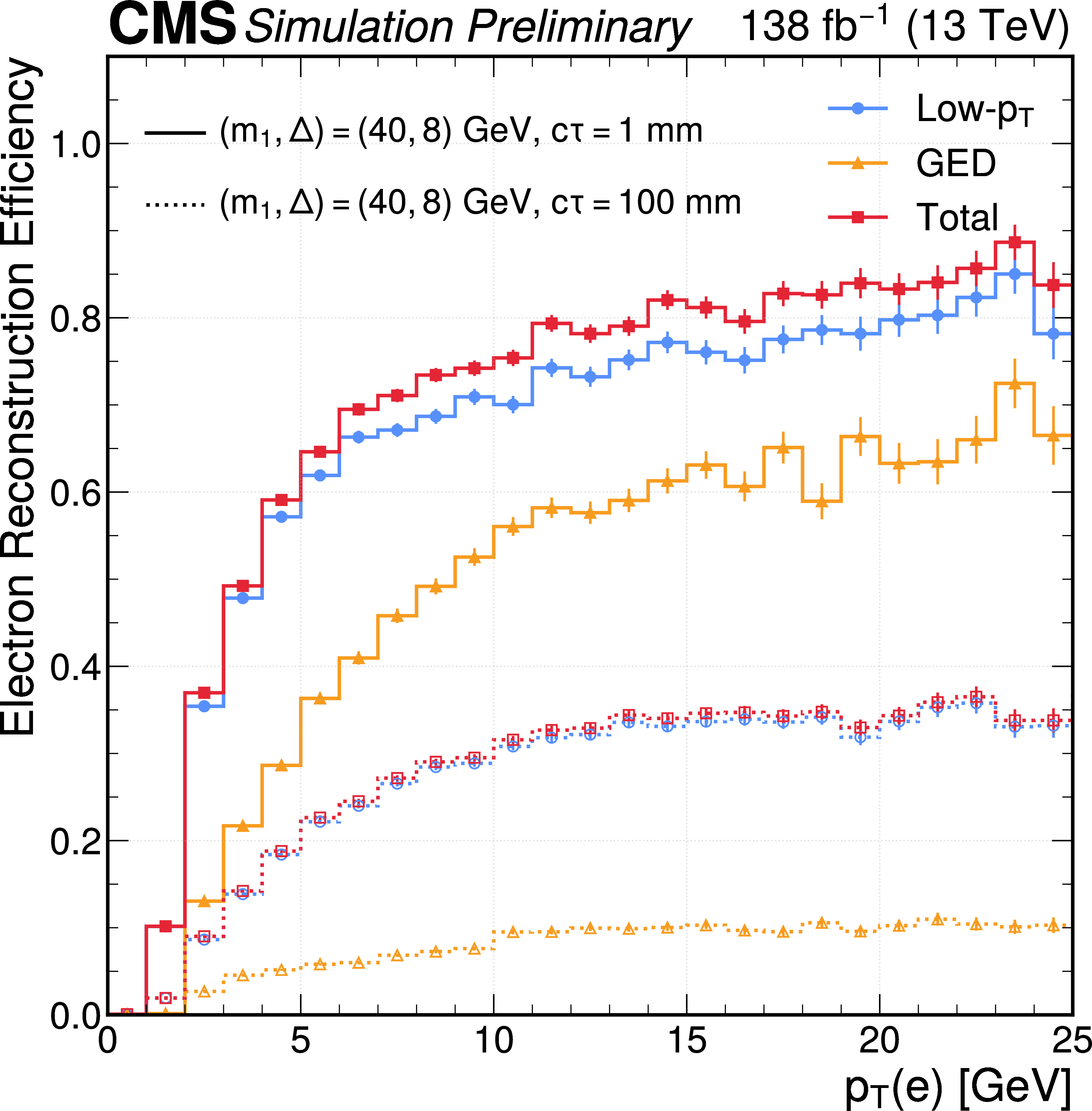
Fraction of reconstructed IDM signal electrons compared across different electron reconstruction algorithms, as a function of generator-level electron $ p_{\mathrm{T}} $ (left) and $ L_{xy} $ (right), derived from simulated IDM samples with selected signal benchmarks. The different signal benchmarks are labeled by the mass $m_{1}$ of the stable DM state, the proper decay length $ c\tau $ of the heavier state $ \chi_{2} $, and the mass splitting $ \Delta \equiv m_2 - m_1 $ between the two states. |
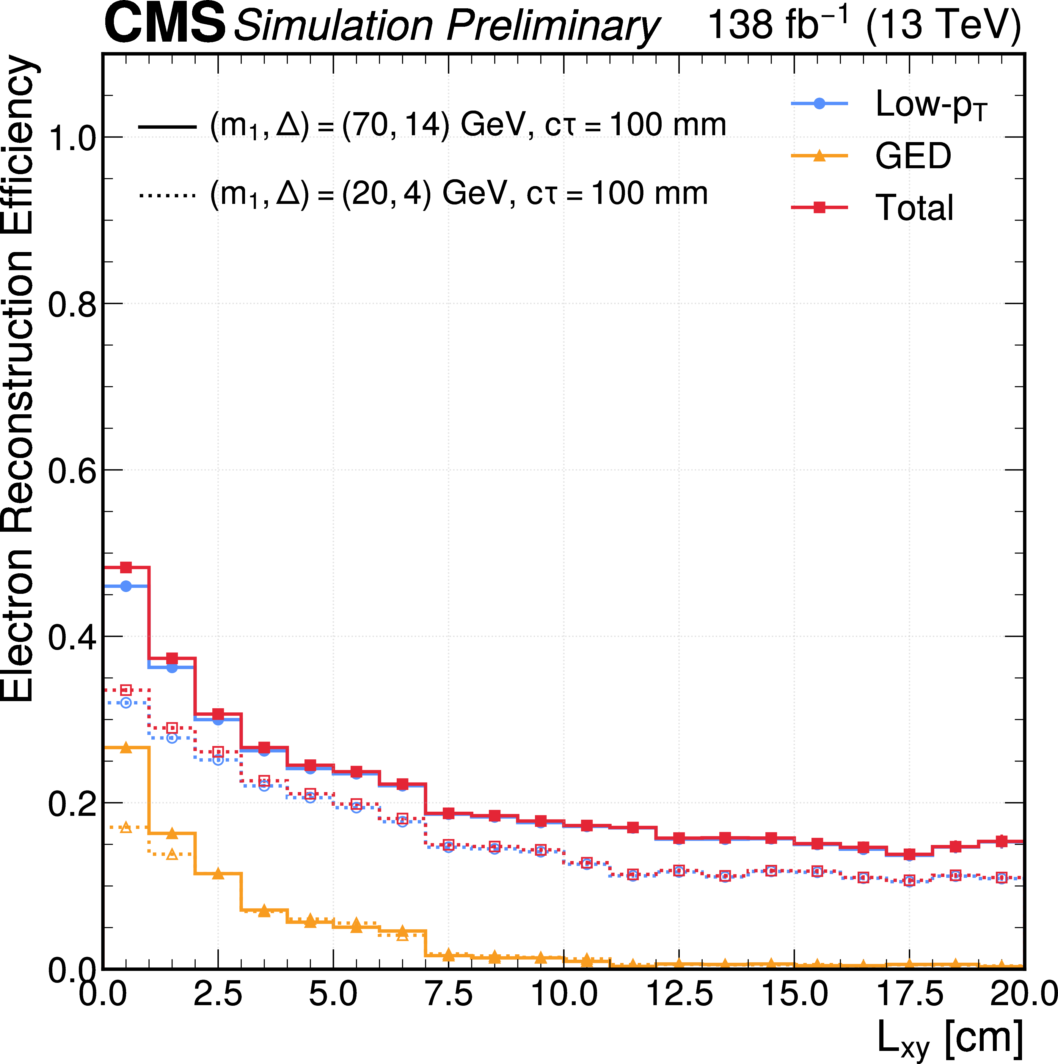
png pdf |
Figure 2-b:
Fraction of reconstructed IDM signal electrons compared across different electron reconstruction algorithms, as a function of generator-level electron $ p_{\mathrm{T}} $ (left) and $ L_{xy} $ (right), derived from simulated IDM samples with selected signal benchmarks. The different signal benchmarks are labeled by the mass $m_{1}$ of the stable DM state, the proper decay length $ c\tau $ of the heavier state $ \chi_{2} $, and the mass splitting $ \Delta \equiv m_2 - m_1 $ between the two states. |
png pdf |
Figure 3:
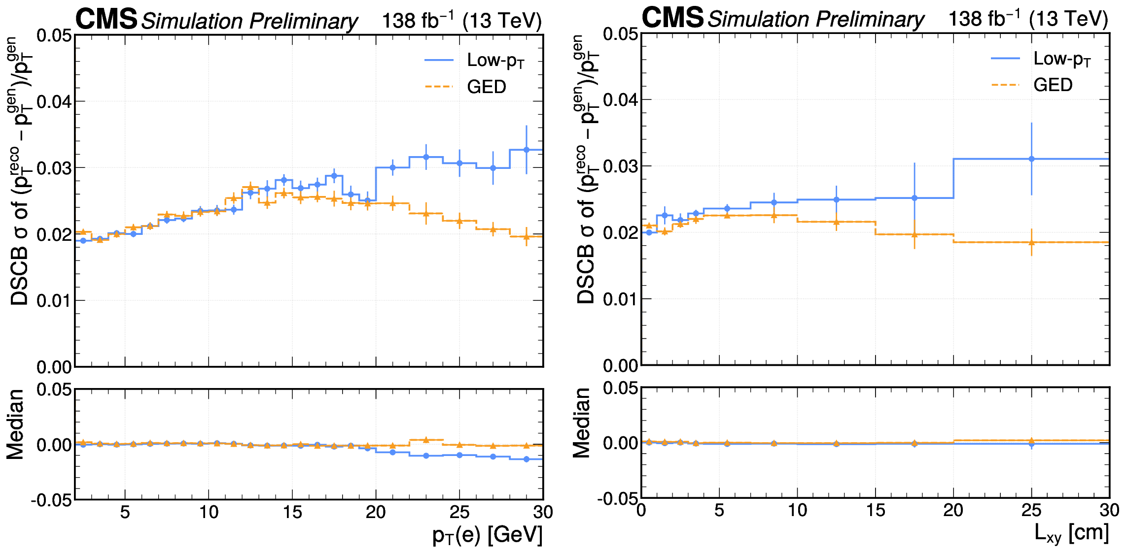
Electron transverse momentum resolution compared across different electron reconstruction algorithms, as a function of generator-level electron $ p_{\mathrm{T}} $ (left) and $ L_{xy} $ (right). The values plotted are the averages of results obtained from the full set of IDM samples simulated for this analysis. The resolution shown in the upper panels is quantified by a fit of the relative residual $ (p_{\mathrm{T}}^{\mathrm{reco}}-p_{\mathrm{T}}^{\mathrm{gen}})/p_{\mathrm{T}}^{\mathrm{gen}} $ using a Double Side Crystal Ball (DSCB) function [27,28], which has a width parameter $ \sigma $. The median residual shown in the lower panels demonstrates that the reconstructed $ p_{\mathrm{T}} $ has minimal bias. |
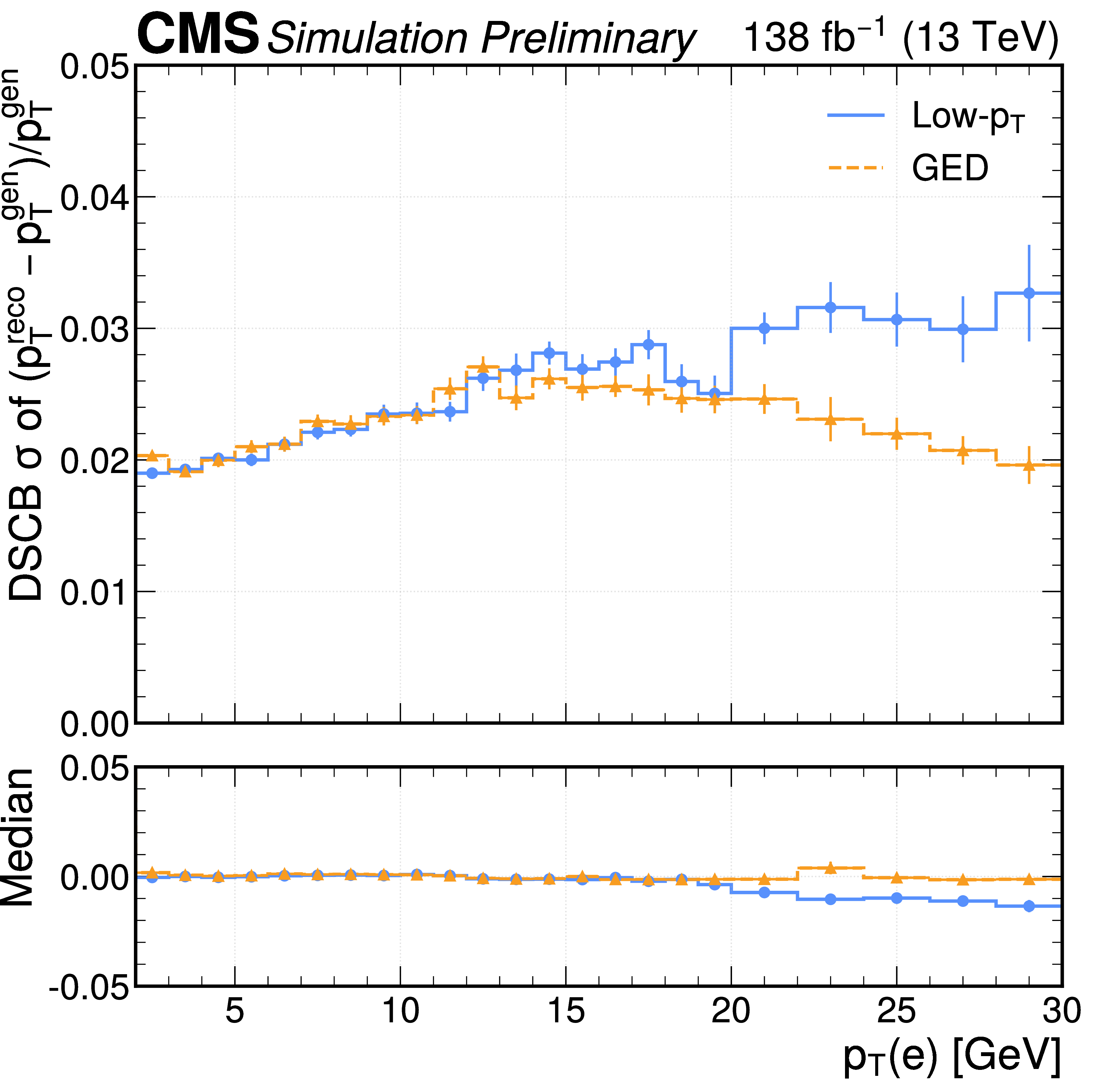
png pdf |
Figure 3-a:
Electron transverse momentum resolution compared across different electron reconstruction algorithms, as a function of generator-level electron $ p_{\mathrm{T}} $ (left) and $ L_{xy} $ (right). The values plotted are the averages of results obtained from the full set of IDM samples simulated for this analysis. The resolution shown in the upper panels is quantified by a fit of the relative residual $ (p_{\mathrm{T}}^{\mathrm{reco}}-p_{\mathrm{T}}^{\mathrm{gen}})/p_{\mathrm{T}}^{\mathrm{gen}} $ using a Double Side Crystal Ball (DSCB) function [27,28], which has a width parameter $ \sigma $. The median residual shown in the lower panels demonstrates that the reconstructed $ p_{\mathrm{T}} $ has minimal bias. |
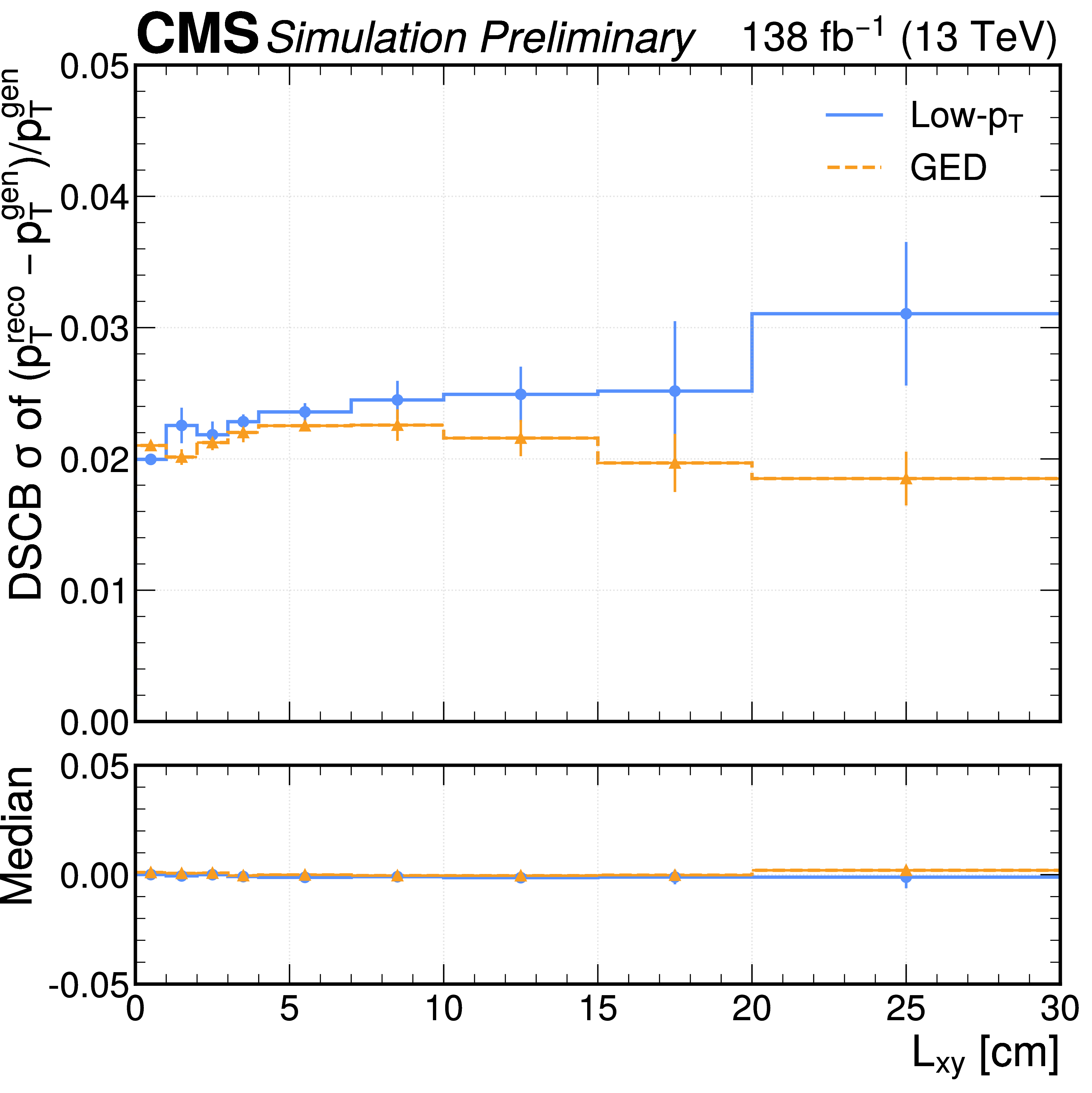
png pdf |
Figure 3-b:
Electron transverse momentum resolution compared across different electron reconstruction algorithms, as a function of generator-level electron $ p_{\mathrm{T}} $ (left) and $ L_{xy} $ (right). The values plotted are the averages of results obtained from the full set of IDM samples simulated for this analysis. The resolution shown in the upper panels is quantified by a fit of the relative residual $ (p_{\mathrm{T}}^{\mathrm{reco}}-p_{\mathrm{T}}^{\mathrm{gen}})/p_{\mathrm{T}}^{\mathrm{gen}} $ using a Double Side Crystal Ball (DSCB) function [27,28], which has a width parameter $ \sigma $. The median residual shown in the lower panels demonstrates that the reconstructed $ p_{\mathrm{T}} $ has minimal bias. |
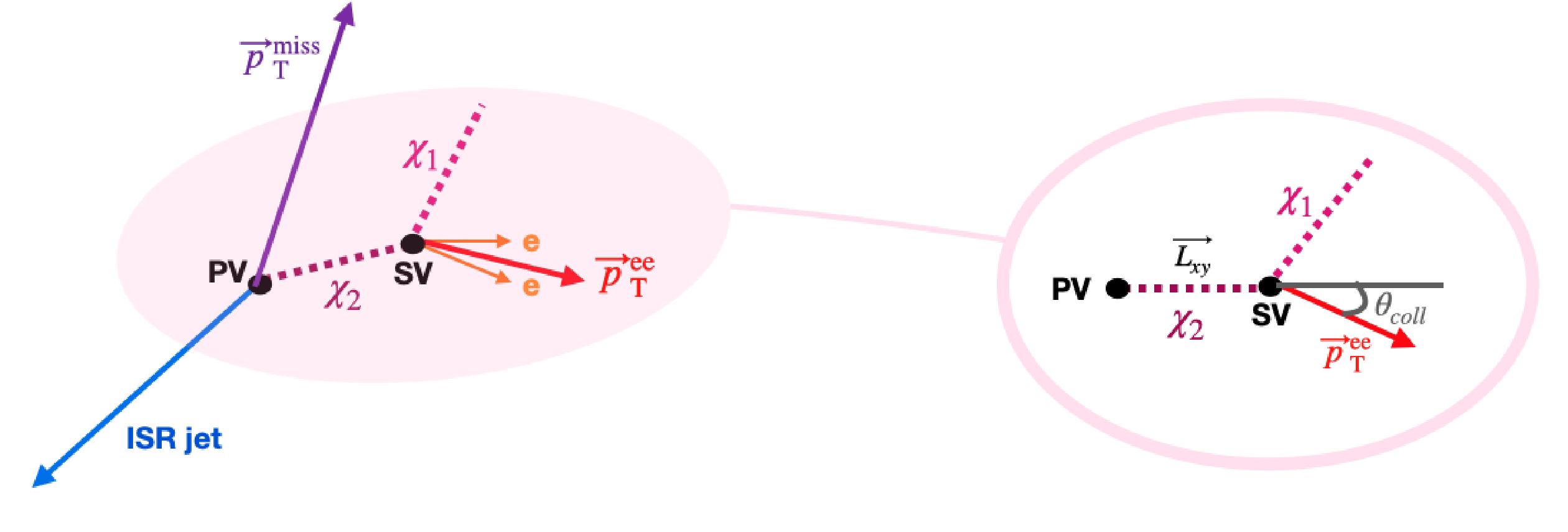
png pdf |
Figure 4:
Illustration of the expected signal event topology and definition of $ \theta_\text{coll} $. |
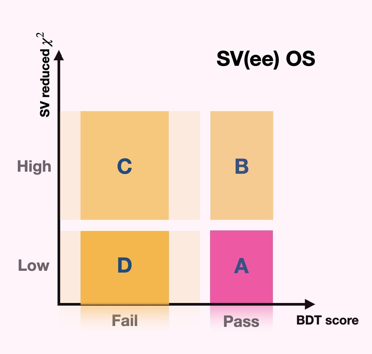
png pdf |
Figure 5:
Illustration of the ABCD plane in which region A is the SR. |
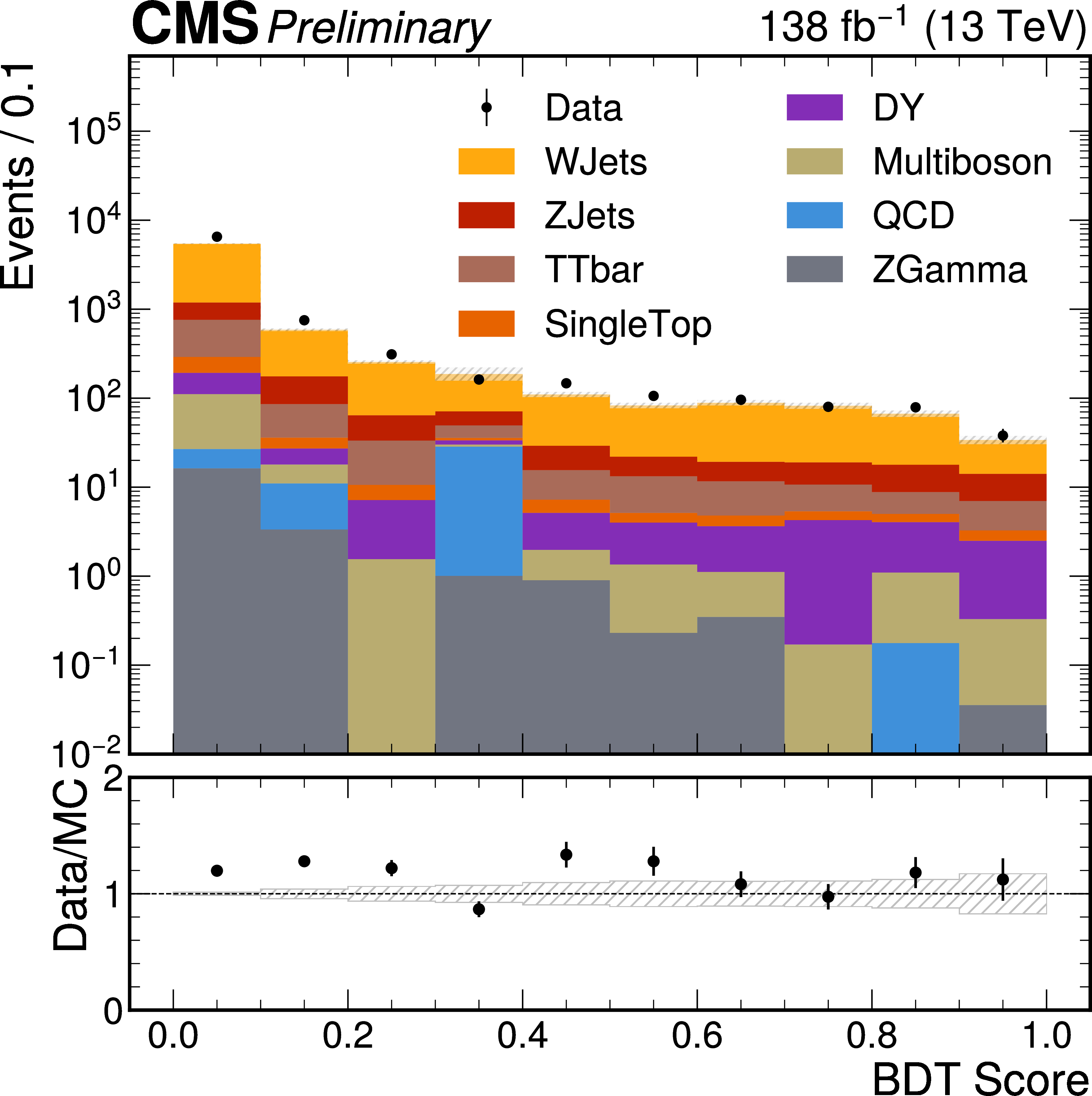
png pdf |
Figure 6:
Distribution of the BDT score in data and simulation in the SS validation region $ \mathrm{VR^{SS}} $. |
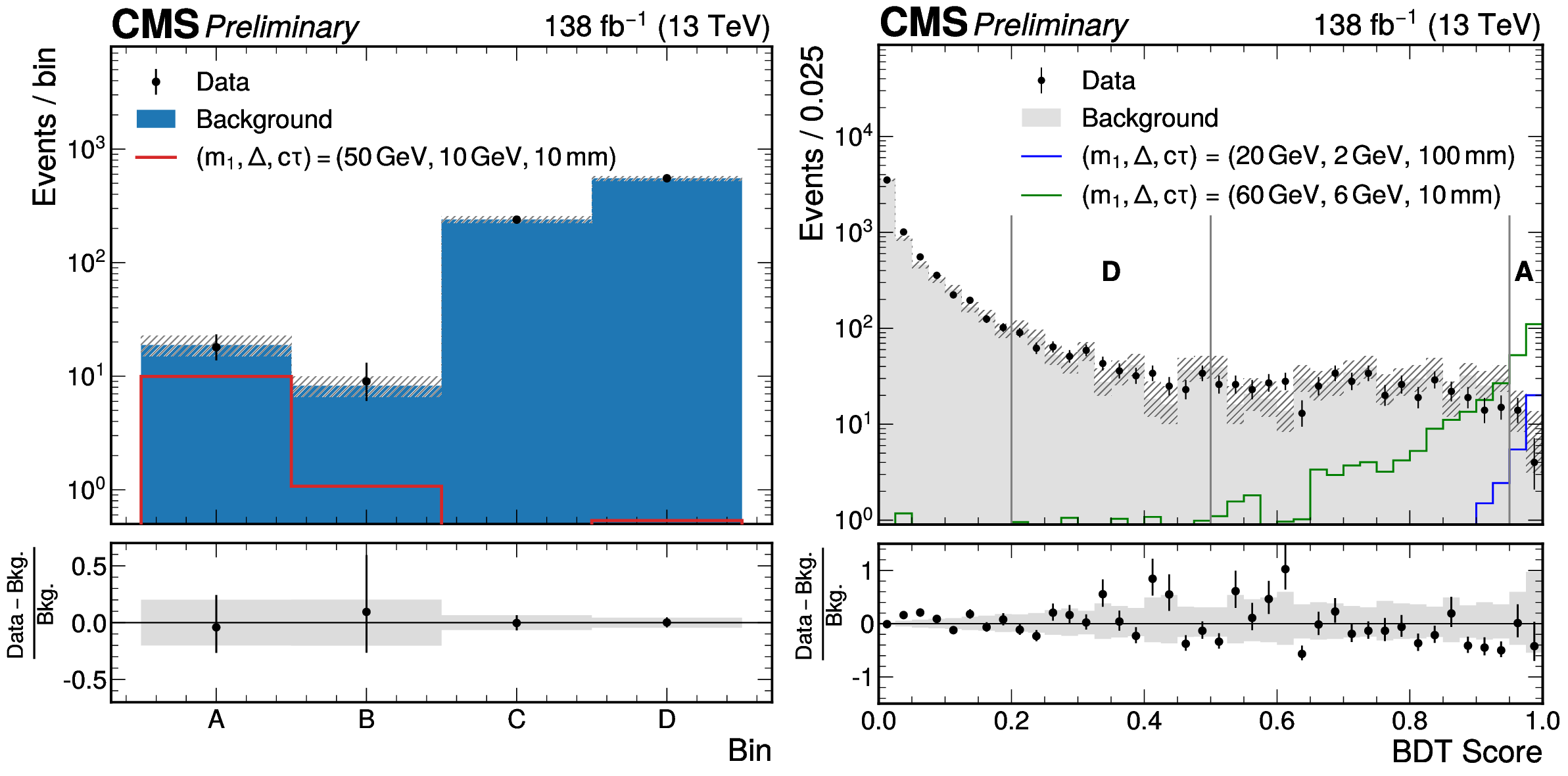
png pdf |
Figure 7:
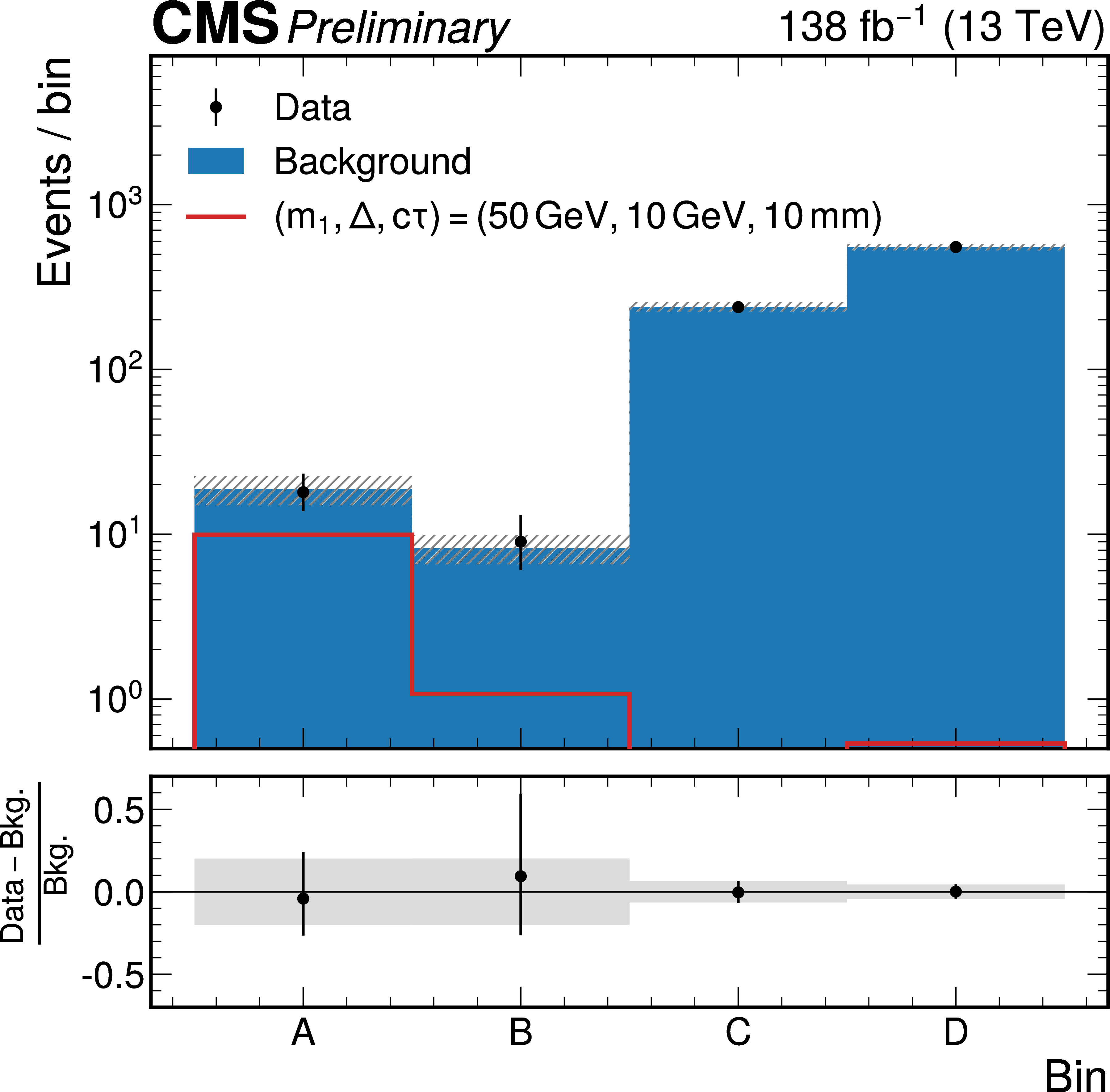
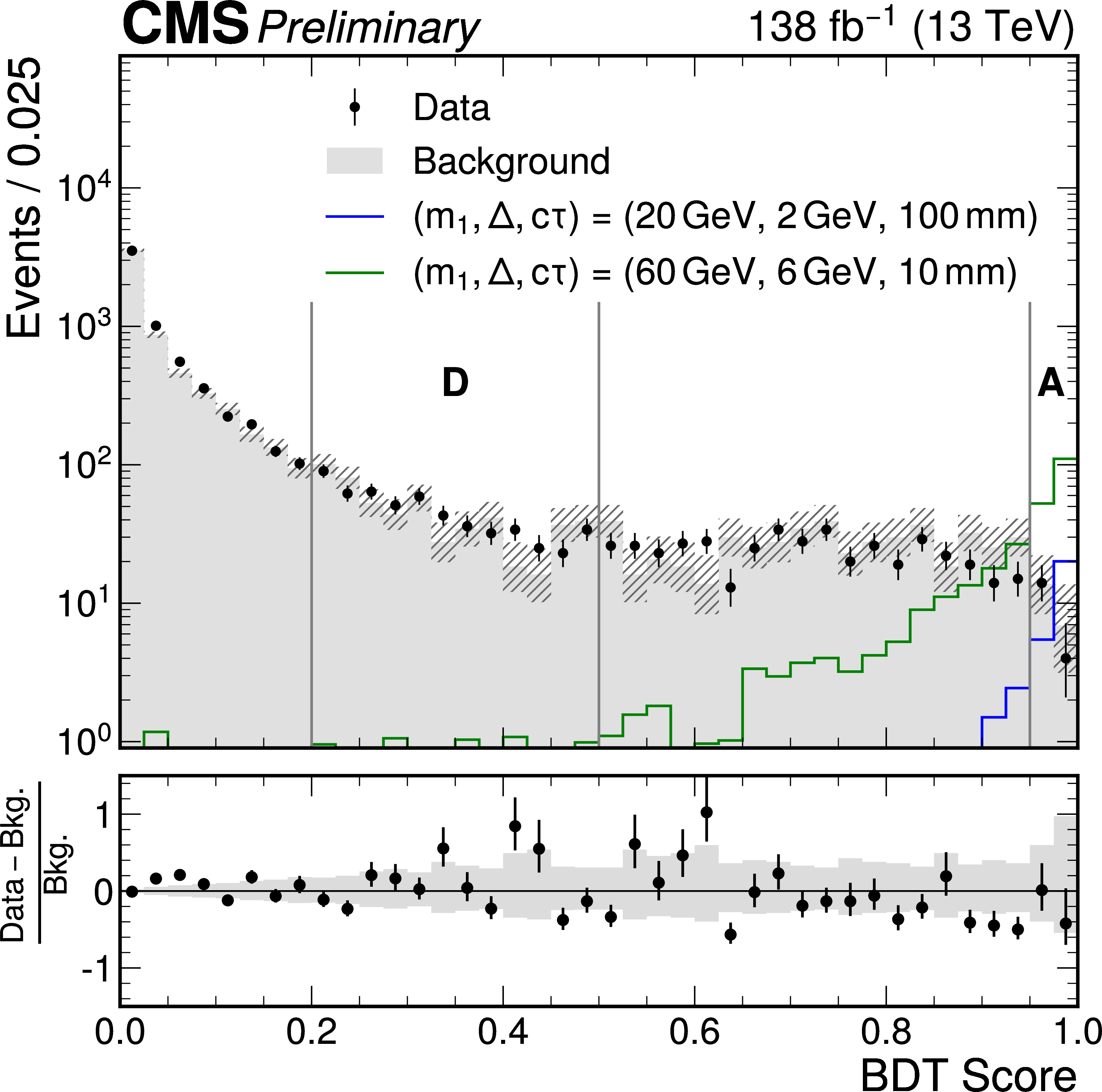
Shown in the left panel are observed data yields in the ABCD regions, with region A corresponding to the signal region. The background prediction is obtained from the post-fit ABCD background estimate. The panel on the right shows the distribution of the BDT score for the observed data and the predicted background. The background template is constructed from data events normalized to the post-fit background prediction. Representative signal benchmarks are overlaid for comparison. |
png pdf |
Figure 7-a:
Shown in the left panel are observed data yields in the ABCD regions, with region A corresponding to the signal region. The background prediction is obtained from the post-fit ABCD background estimate. The panel on the right shows the distribution of the BDT score for the observed data and the predicted background. The background template is constructed from data events normalized to the post-fit background prediction. Representative signal benchmarks are overlaid for comparison. |
png pdf |
Figure 7-b:
Shown in the left panel are observed data yields in the ABCD regions, with region A corresponding to the signal region. The background prediction is obtained from the post-fit ABCD background estimate. The panel on the right shows the distribution of the BDT score for the observed data and the predicted background. The background template is constructed from data events normalized to the post-fit background prediction. Representative signal benchmarks are overlaid for comparison. |
png pdf |
Figure 8:
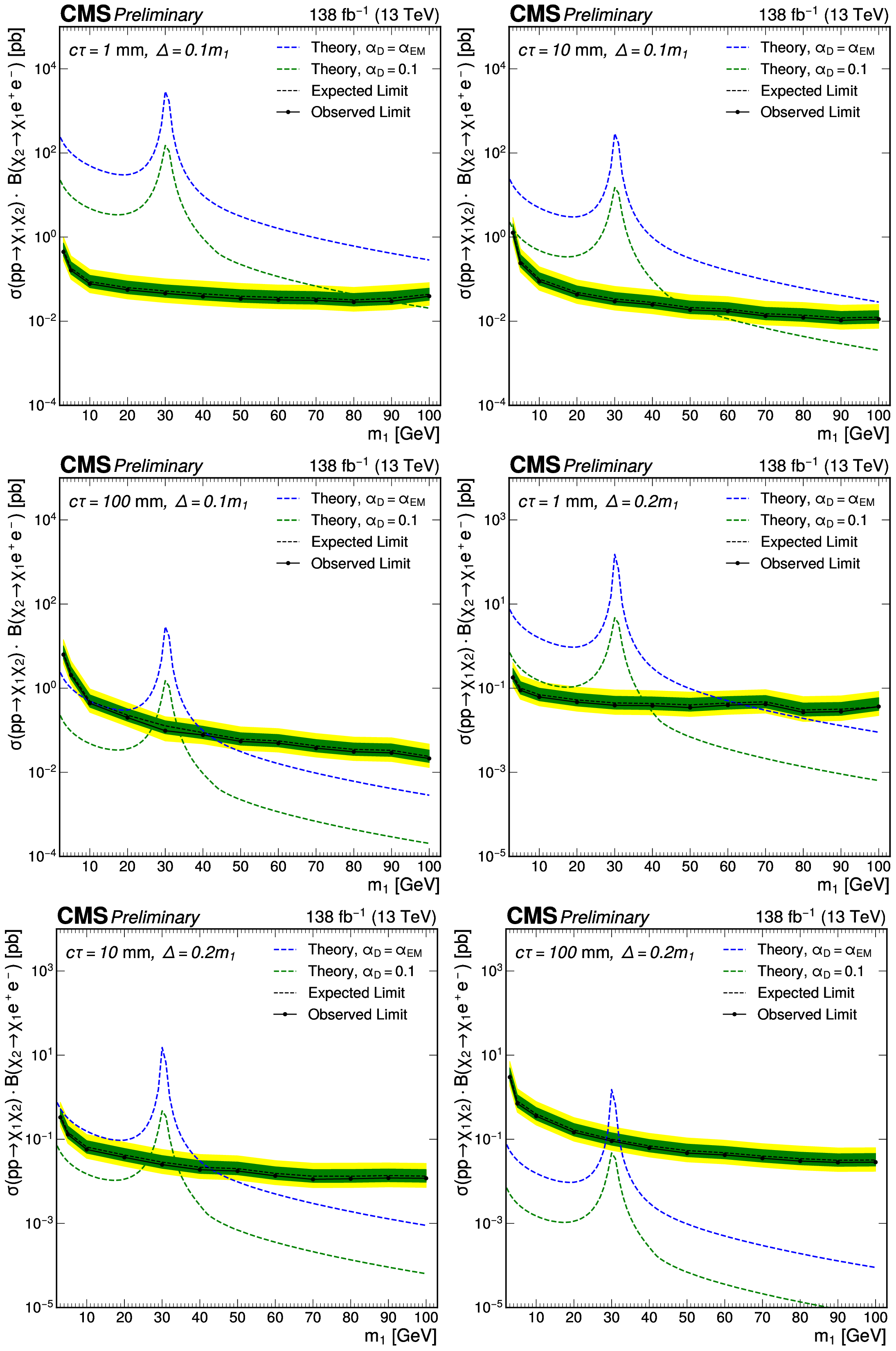
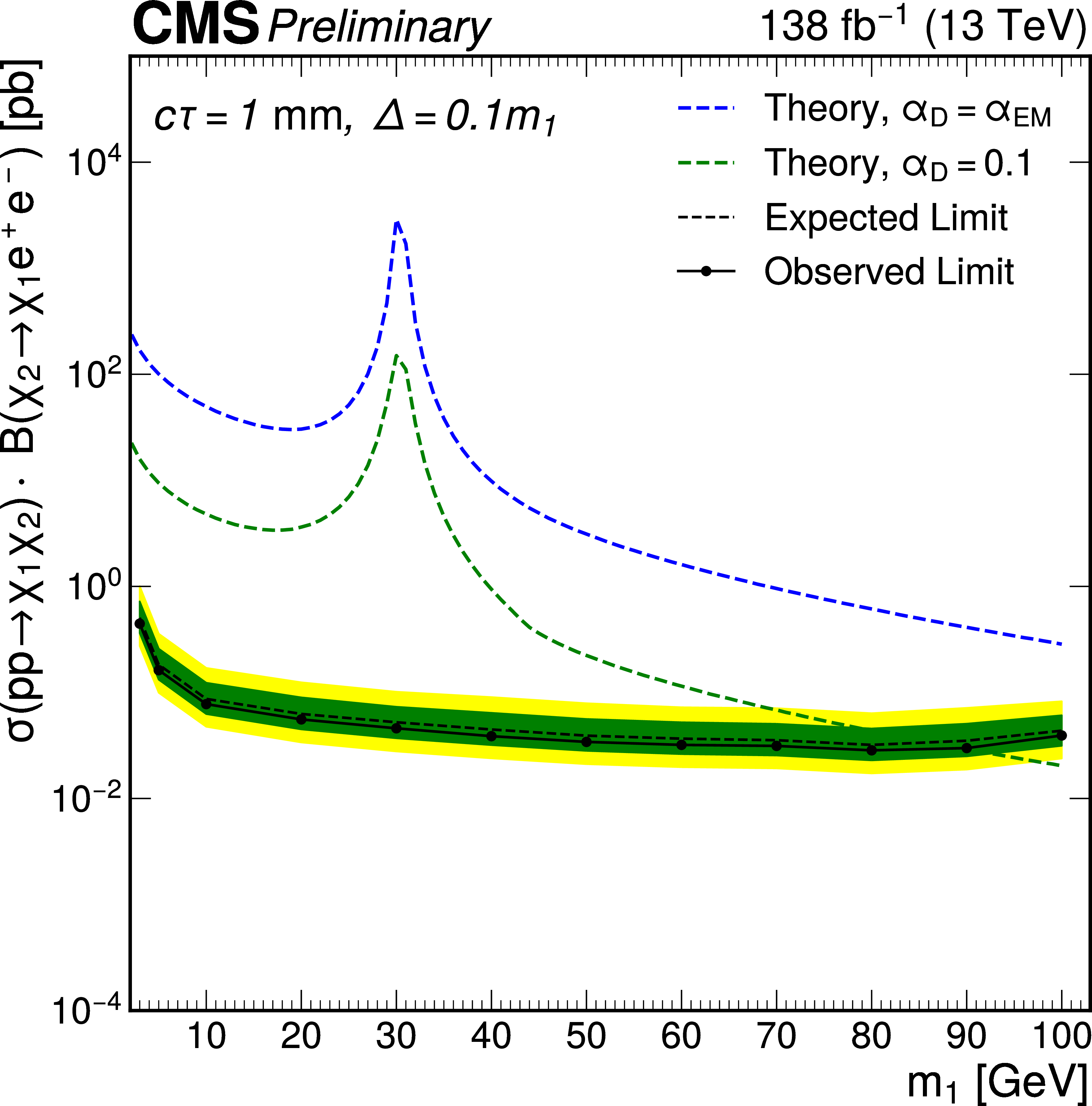
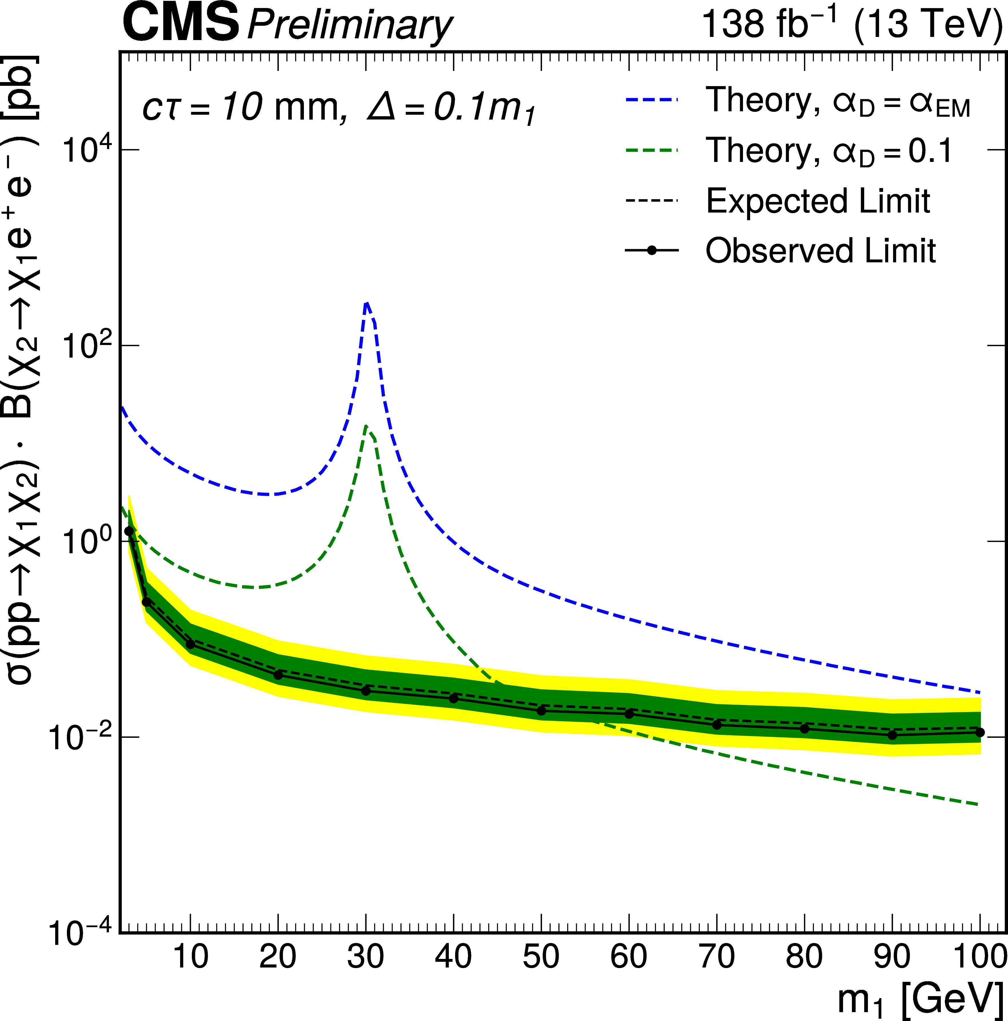
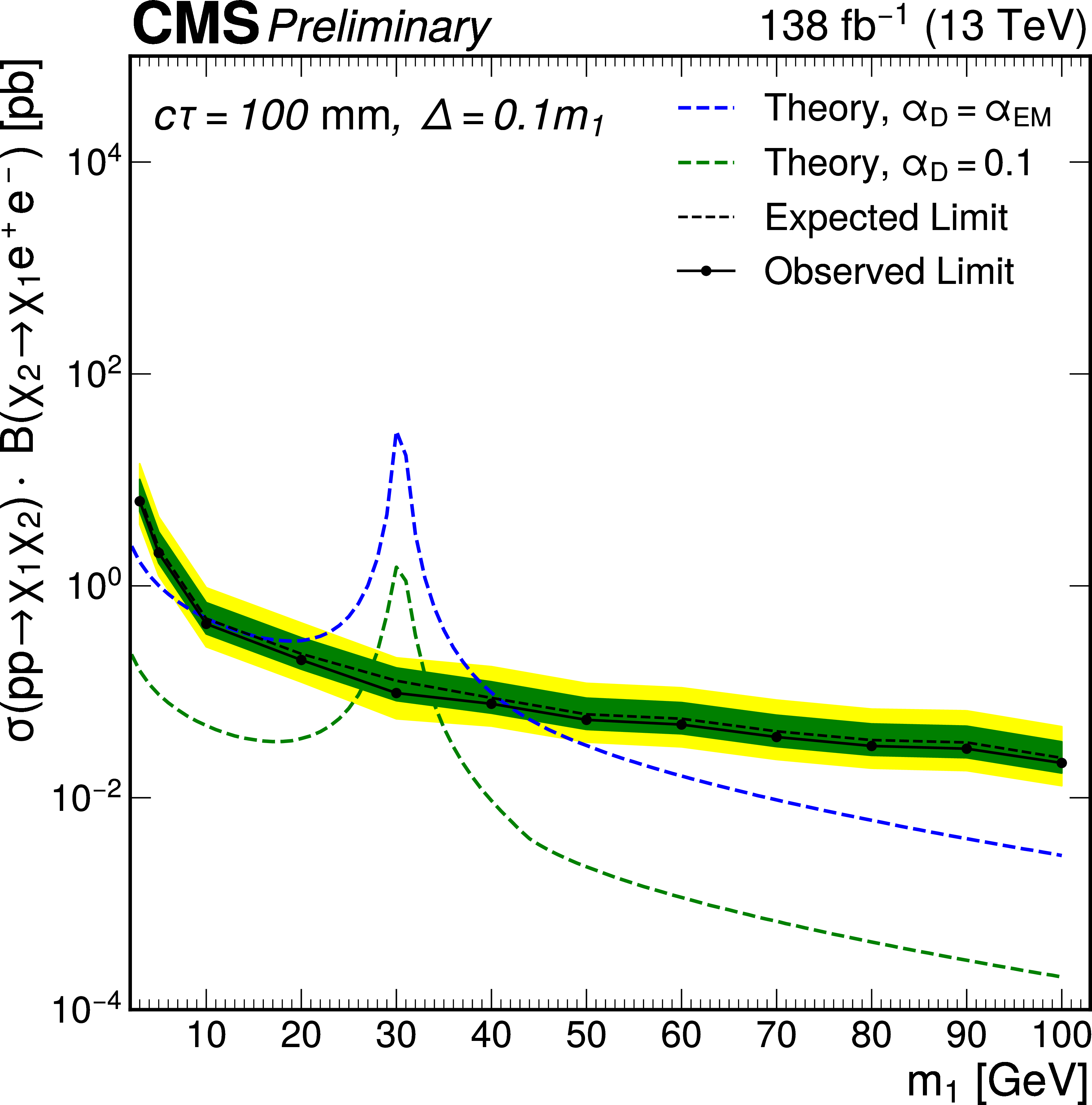
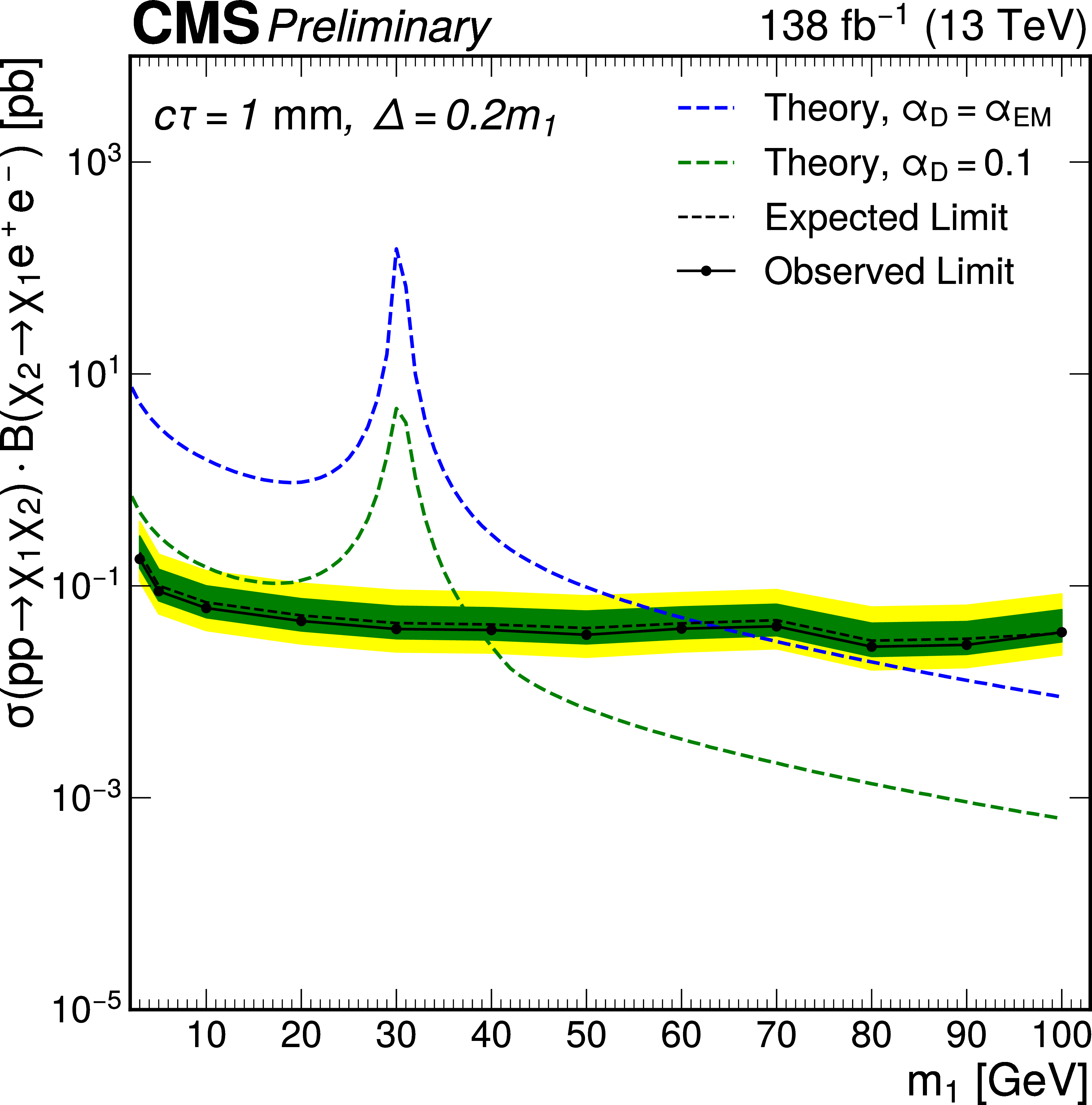
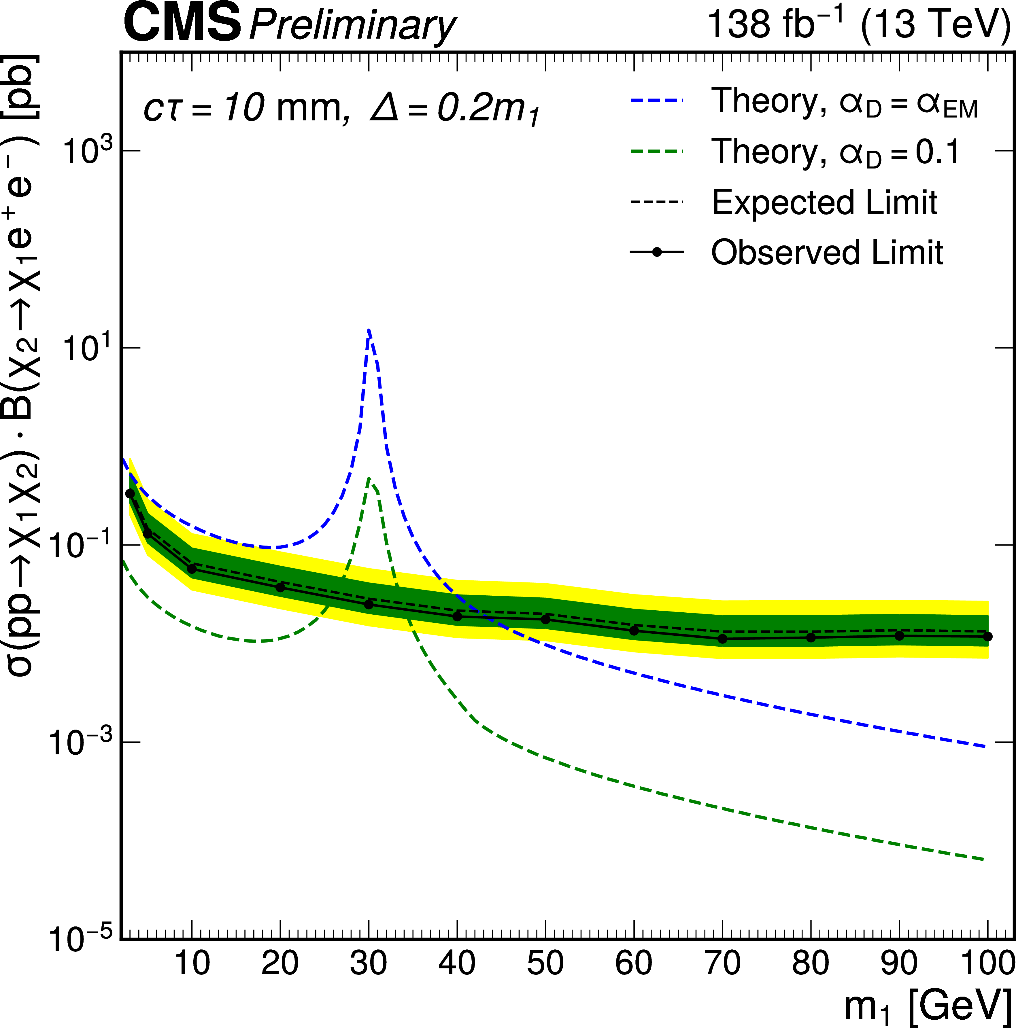
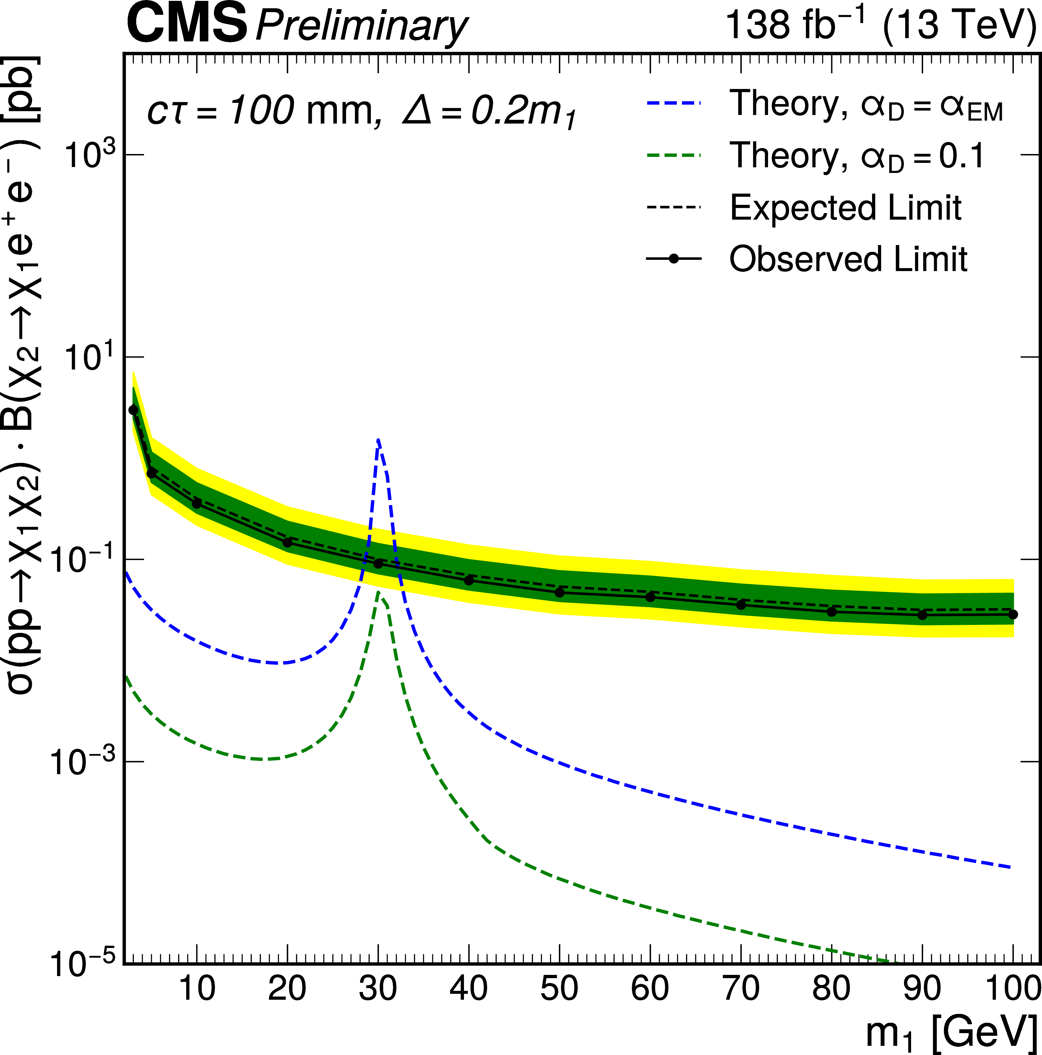
Expected and observed limits on the product of the cross section $ \sigma(\mathrm{p}\mathrm{p} \to A' \to \chi_{1} \chi_{2} ) $ and the branching ratio, where $ \mathcal{B}( \chi_{2} \to \chi_{1} \mathrm{e}^+\mathrm{e}^-) $ is assumed to be 100%. We plot the limits as a function of $ m_1 $ for IDM signals with 10% (left) and 20% (right) mass splittings and 1mm (top), 10 mm (middle), and 100 mm (bottom) $ \chi_{2} $ mean lifetimes. The expected theoretical cross section is overlaid. The peaking structure near $ m_1 = $ 30 GeV is due to resonant effects when the A' mass is near that of the SM Z boson. |
png pdf |
Figure 8-a:
Expected and observed limits on the product of the cross section $ \sigma(\mathrm{p}\mathrm{p} \to A' \to \chi_{1} \chi_{2} ) $ and the branching ratio, where $ \mathcal{B}( \chi_{2} \to \chi_{1} \mathrm{e}^+\mathrm{e}^-) $ is assumed to be 100%. We plot the limits as a function of $ m_1 $ for IDM signals with 10% (left) and 20% (right) mass splittings and 1mm (top), 10 mm (middle), and 100 mm (bottom) $ \chi_{2} $ mean lifetimes. The expected theoretical cross section is overlaid. The peaking structure near $ m_1 = $ 30 GeV is due to resonant effects when the A' mass is near that of the SM Z boson. |
png pdf |
Figure 8-b:
Expected and observed limits on the product of the cross section $ \sigma(\mathrm{p}\mathrm{p} \to A' \to \chi_{1} \chi_{2} ) $ and the branching ratio, where $ \mathcal{B}( \chi_{2} \to \chi_{1} \mathrm{e}^+\mathrm{e}^-) $ is assumed to be 100%. We plot the limits as a function of $ m_1 $ for IDM signals with 10% (left) and 20% (right) mass splittings and 1mm (top), 10 mm (middle), and 100 mm (bottom) $ \chi_{2} $ mean lifetimes. The expected theoretical cross section is overlaid. The peaking structure near $ m_1 = $ 30 GeV is due to resonant effects when the A' mass is near that of the SM Z boson. |
png pdf |
Figure 8-c:
Expected and observed limits on the product of the cross section $ \sigma(\mathrm{p}\mathrm{p} \to A' \to \chi_{1} \chi_{2} ) $ and the branching ratio, where $ \mathcal{B}( \chi_{2} \to \chi_{1} \mathrm{e}^+\mathrm{e}^-) $ is assumed to be 100%. We plot the limits as a function of $ m_1 $ for IDM signals with 10% (left) and 20% (right) mass splittings and 1mm (top), 10 mm (middle), and 100 mm (bottom) $ \chi_{2} $ mean lifetimes. The expected theoretical cross section is overlaid. The peaking structure near $ m_1 = $ 30 GeV is due to resonant effects when the A' mass is near that of the SM Z boson. |
png pdf |
Figure 8-d:
Expected and observed limits on the product of the cross section $ \sigma(\mathrm{p}\mathrm{p} \to A' \to \chi_{1} \chi_{2} ) $ and the branching ratio, where $ \mathcal{B}( \chi_{2} \to \chi_{1} \mathrm{e}^+\mathrm{e}^-) $ is assumed to be 100%. We plot the limits as a function of $ m_1 $ for IDM signals with 10% (left) and 20% (right) mass splittings and 1mm (top), 10 mm (middle), and 100 mm (bottom) $ \chi_{2} $ mean lifetimes. The expected theoretical cross section is overlaid. The peaking structure near $ m_1 = $ 30 GeV is due to resonant effects when the A' mass is near that of the SM Z boson. |
png pdf |
Figure 8-e:
Expected and observed limits on the product of the cross section $ \sigma(\mathrm{p}\mathrm{p} \to A' \to \chi_{1} \chi_{2} ) $ and the branching ratio, where $ \mathcal{B}( \chi_{2} \to \chi_{1} \mathrm{e}^+\mathrm{e}^-) $ is assumed to be 100%. We plot the limits as a function of $ m_1 $ for IDM signals with 10% (left) and 20% (right) mass splittings and 1mm (top), 10 mm (middle), and 100 mm (bottom) $ \chi_{2} $ mean lifetimes. The expected theoretical cross section is overlaid. The peaking structure near $ m_1 = $ 30 GeV is due to resonant effects when the A' mass is near that of the SM Z boson. |
png pdf |
Figure 8-f:
Expected and observed limits on the product of the cross section $ \sigma(\mathrm{p}\mathrm{p} \to A' \to \chi_{1} \chi_{2} ) $ and the branching ratio, where $ \mathcal{B}( \chi_{2} \to \chi_{1} \mathrm{e}^+\mathrm{e}^-) $ is assumed to be 100%. We plot the limits as a function of $ m_1 $ for IDM signals with 10% (left) and 20% (right) mass splittings and 1mm (top), 10 mm (middle), and 100 mm (bottom) $ \chi_{2} $ mean lifetimes. The expected theoretical cross section is overlaid. The peaking structure near $ m_1 = $ 30 GeV is due to resonant effects when the A' mass is near that of the SM Z boson. |
png pdf |
Figure 9:
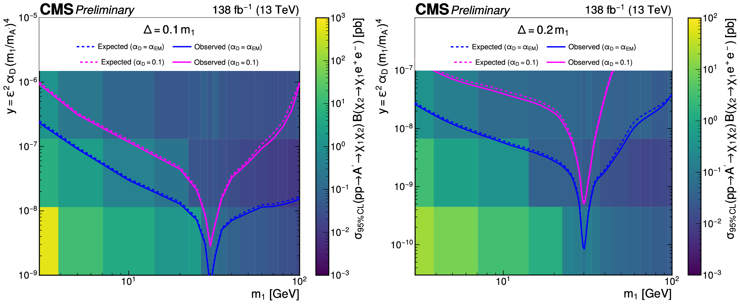
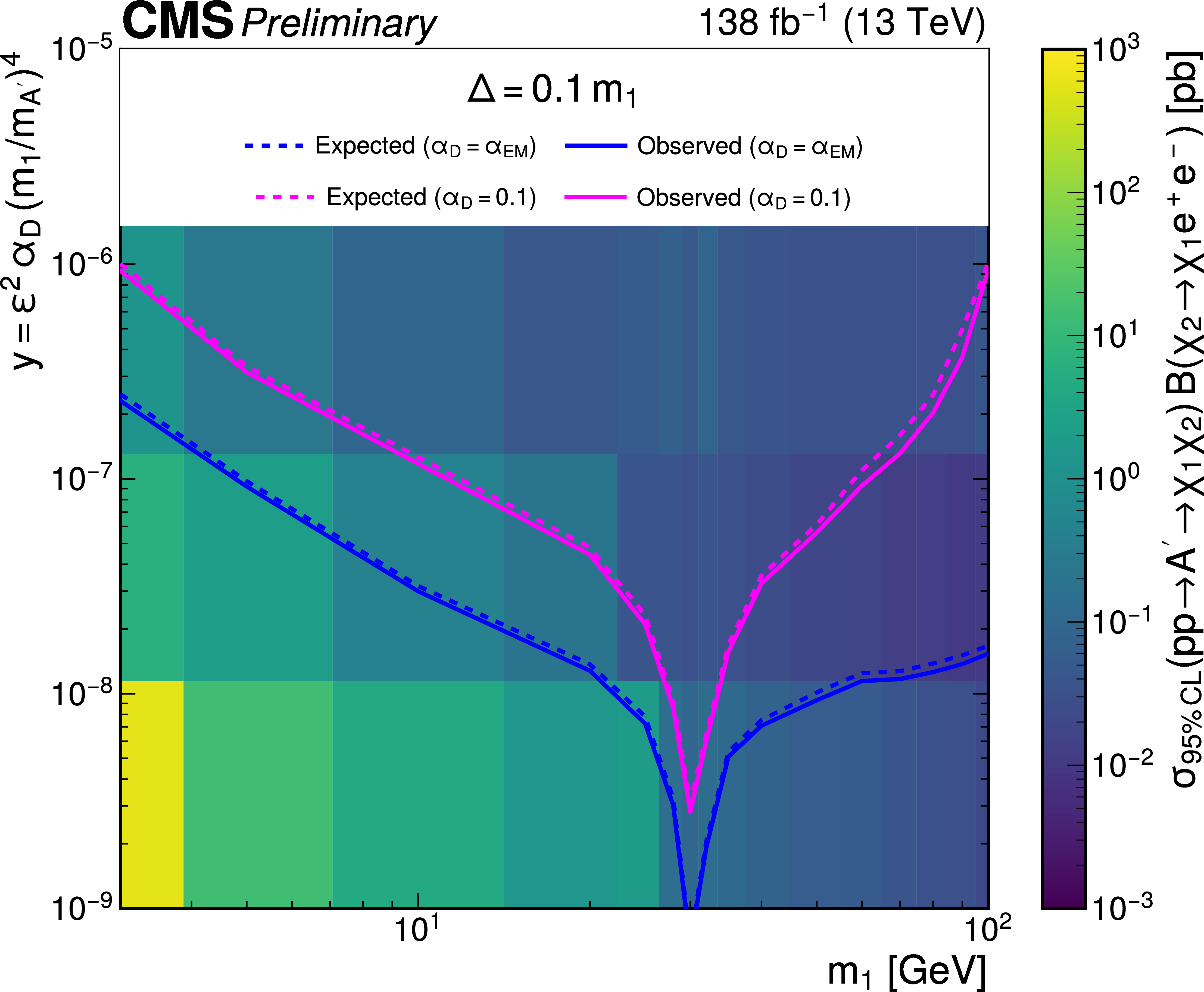
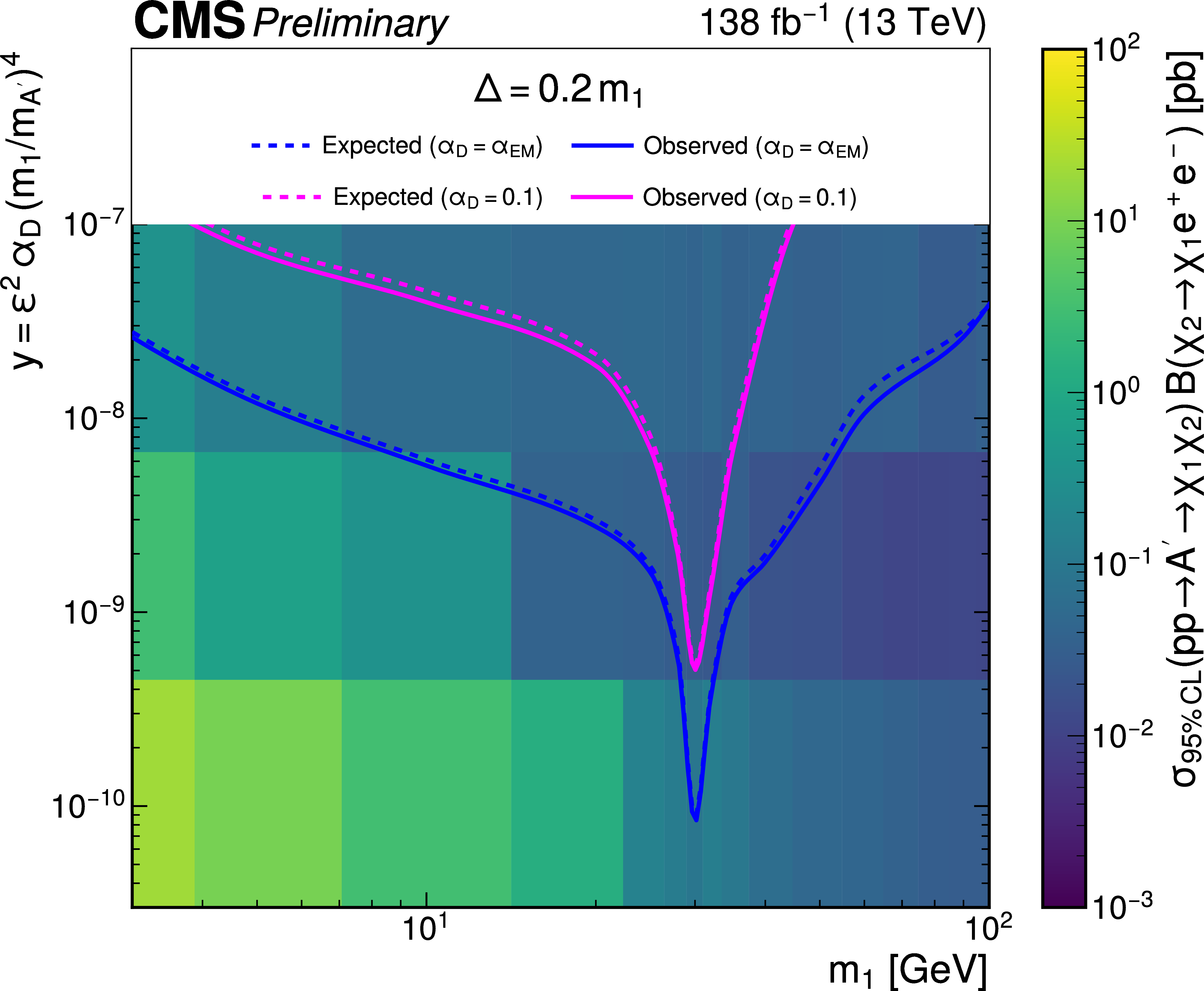
Observed two-dimensional exclusion contours in the $ ( m_{1} ,y) $ plane for the 10% (left) and 20% (right) mass splitting scenarios, where $ y \equiv \epsilon^2 \alpha_D ( m_{1} /m_{A'})^4 $. The color fill denotes the upper limit on the product of the production cross section and branching fraction, with $ \mathcal{B}( \chi_{2} \to \chi_{1} \mathrm{e}^+\mathrm{e}^-) $ assumed to be 100%. The exclusion contours trace the signal strength $ \mu = $ 1 boundary, excluding the region of parameter space above them. The increased sensitivity near $ m_{1} = $ 30 GeV is due to resonant effects when the A' mass is near that of the SM Z boson. |
png pdf |
Figure 9-a:
Observed two-dimensional exclusion contours in the $ ( m_{1} ,y) $ plane for the 10% (left) and 20% (right) mass splitting scenarios, where $ y \equiv \epsilon^2 \alpha_D ( m_{1} /m_{A'})^4 $. The color fill denotes the upper limit on the product of the production cross section and branching fraction, with $ \mathcal{B}( \chi_{2} \to \chi_{1} \mathrm{e}^+\mathrm{e}^-) $ assumed to be 100%. The exclusion contours trace the signal strength $ \mu = $ 1 boundary, excluding the region of parameter space above them. The increased sensitivity near $ m_{1} = $ 30 GeV is due to resonant effects when the A' mass is near that of the SM Z boson. |
png pdf |
Figure 9-b:
Observed two-dimensional exclusion contours in the $ ( m_{1} ,y) $ plane for the 10% (left) and 20% (right) mass splitting scenarios, where $ y \equiv \epsilon^2 \alpha_D ( m_{1} /m_{A'})^4 $. The color fill denotes the upper limit on the product of the production cross section and branching fraction, with $ \mathcal{B}( \chi_{2} \to \chi_{1} \mathrm{e}^+\mathrm{e}^-) $ assumed to be 100%. The exclusion contours trace the signal strength $ \mu = $ 1 boundary, excluding the region of parameter space above them. The increased sensitivity near $ m_{1} = $ 30 GeV is due to resonant effects when the A' mass is near that of the SM Z boson. |
png pdf |
Figure 10:
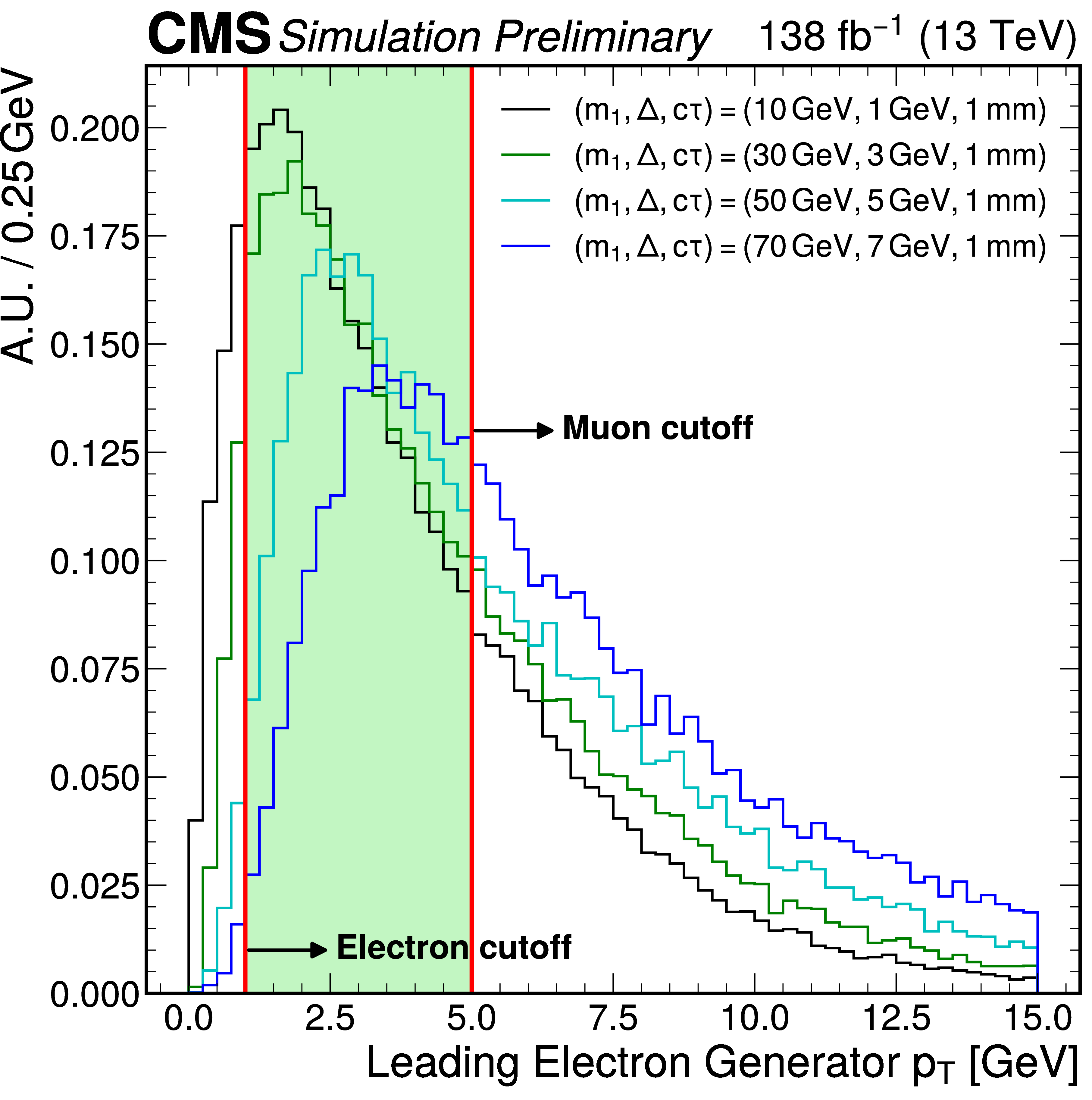
Leading electron $ p_{\mathrm{T}} $ at generator level, highlighting the $ p_{\mathrm{T}} $ cutoff differences between the previous muon analysis [5] and this electron analysis. |
png pdf |
Figure 11:
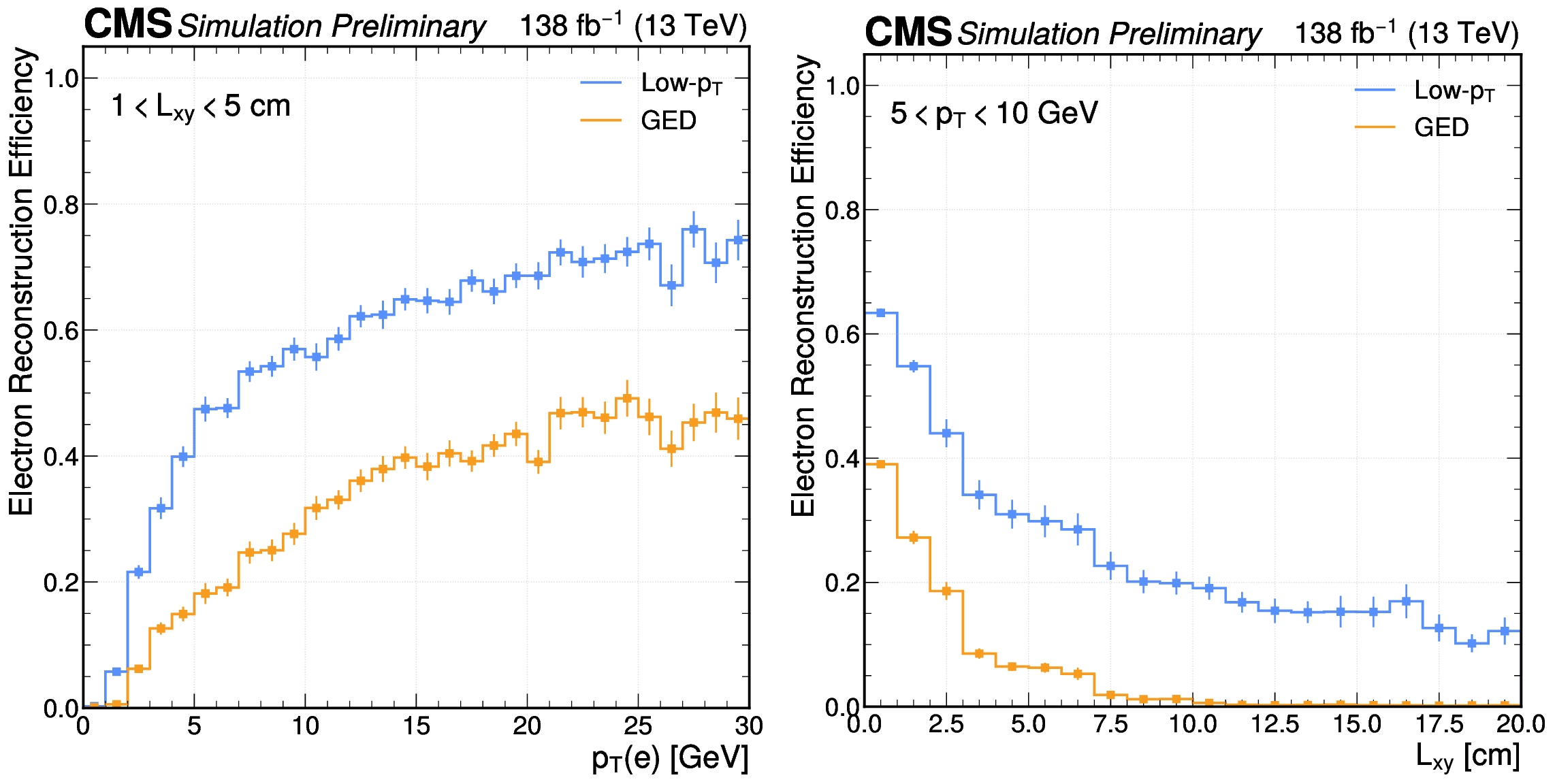
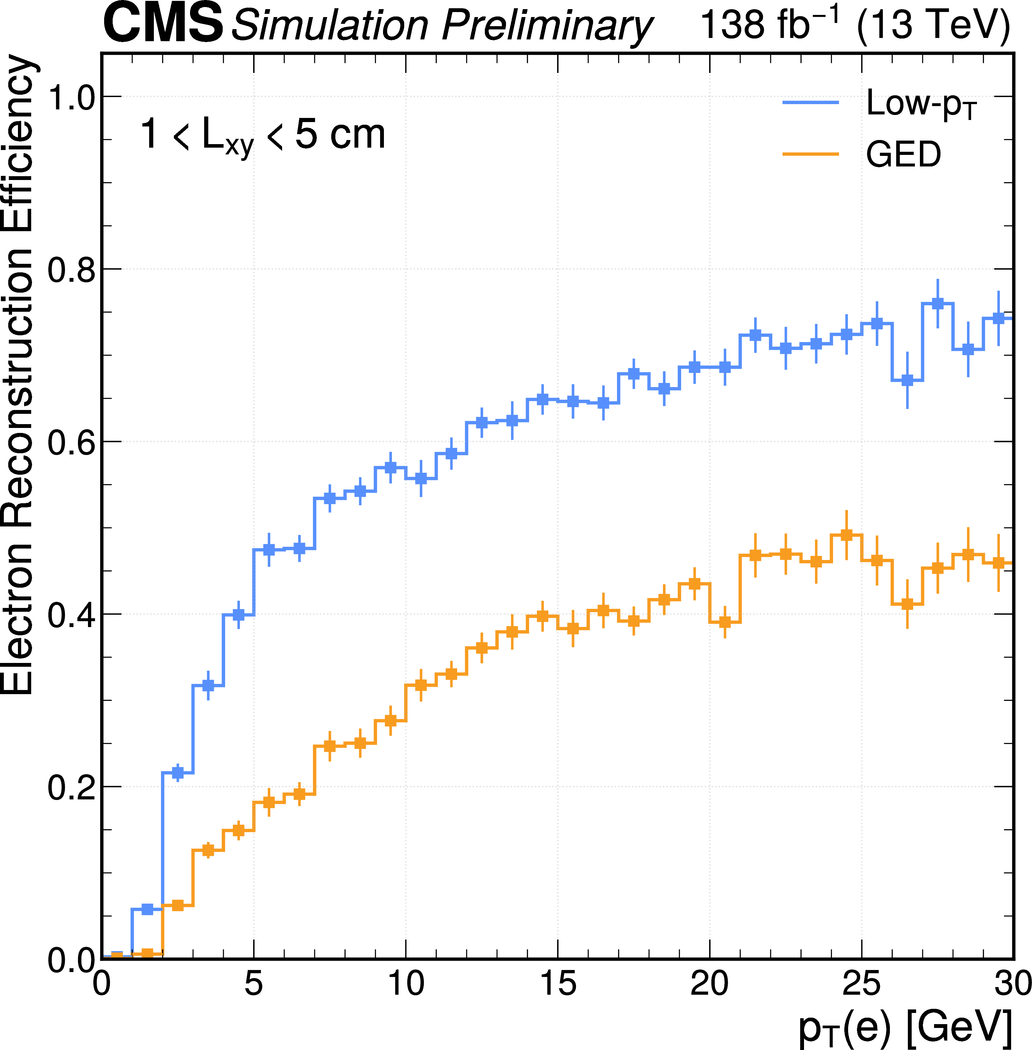
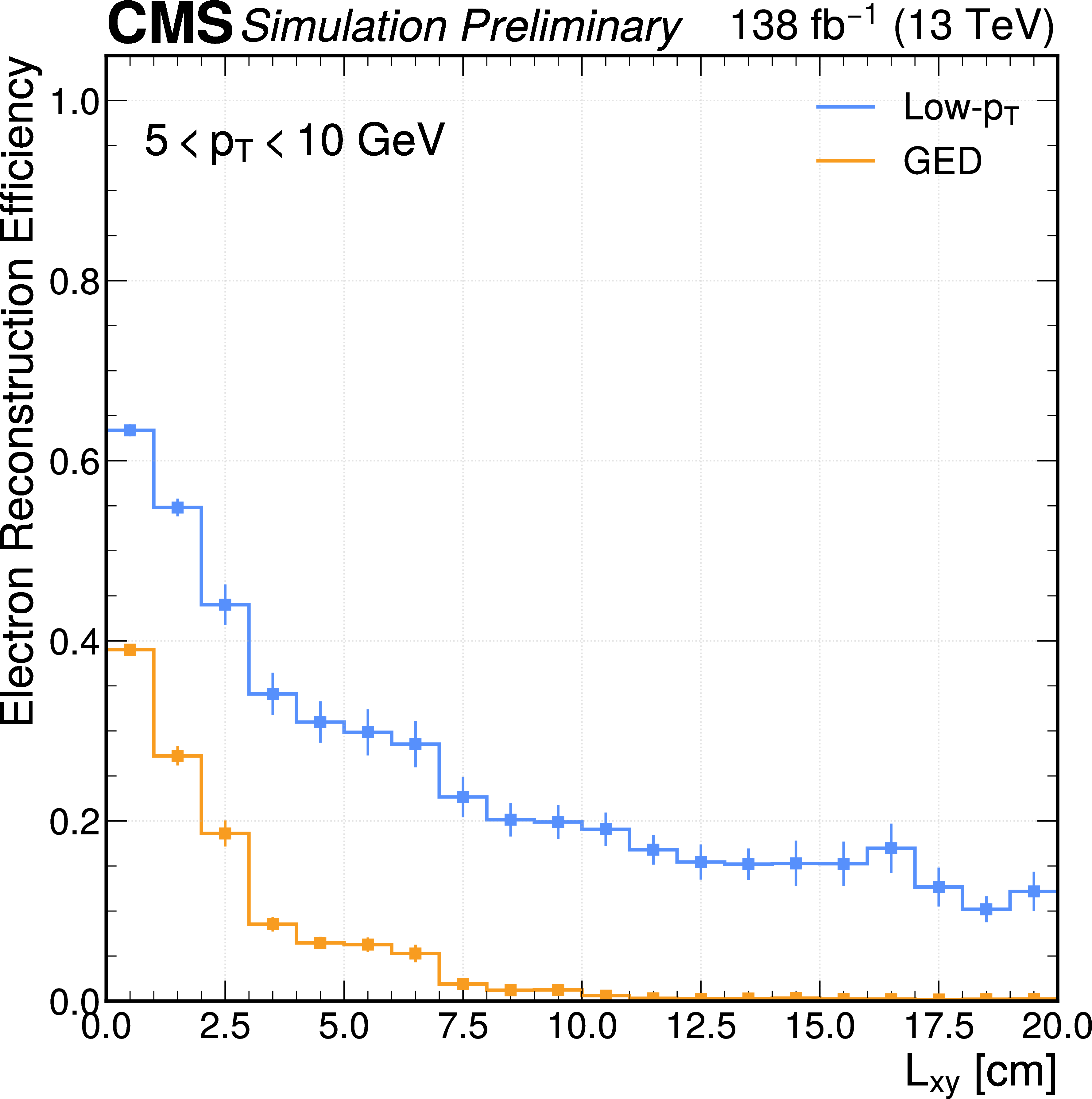
(Left) Electron reconstruction efficiency as a function of $ p_{\mathrm{T}} $ for a fixed $ L_{xy} $ bin. (Right) Electron reconstruction efficiency as a function of $ L_{xy} $ for a fixed $ p_{\mathrm{T}} $ bin. In both panels, the efficiencies are averaged over signal samples with mean proper lifetimes ranging from 1 to 100 mm and dark matter masses between 5 and 100 GeV. The performance of the low-$ p_{\mathrm{T}} $ electron reconstruction is compared with that of the GED electron reconstruction. |
png pdf |
Figure 11-a:
(Left) Electron reconstruction efficiency as a function of $ p_{\mathrm{T}} $ for a fixed $ L_{xy} $ bin. (Right) Electron reconstruction efficiency as a function of $ L_{xy} $ for a fixed $ p_{\mathrm{T}} $ bin. In both panels, the efficiencies are averaged over signal samples with mean proper lifetimes ranging from 1 to 100 mm and dark matter masses between 5 and 100 GeV. The performance of the low-$ p_{\mathrm{T}} $ electron reconstruction is compared with that of the GED electron reconstruction. |
png pdf |
Figure 11-b:
(Left) Electron reconstruction efficiency as a function of $ p_{\mathrm{T}} $ for a fixed $ L_{xy} $ bin. (Right) Electron reconstruction efficiency as a function of $ L_{xy} $ for a fixed $ p_{\mathrm{T}} $ bin. In both panels, the efficiencies are averaged over signal samples with mean proper lifetimes ranging from 1 to 100 mm and dark matter masses between 5 and 100 GeV. The performance of the low-$ p_{\mathrm{T}} $ electron reconstruction is compared with that of the GED electron reconstruction. |
png pdf |
Figure 12:
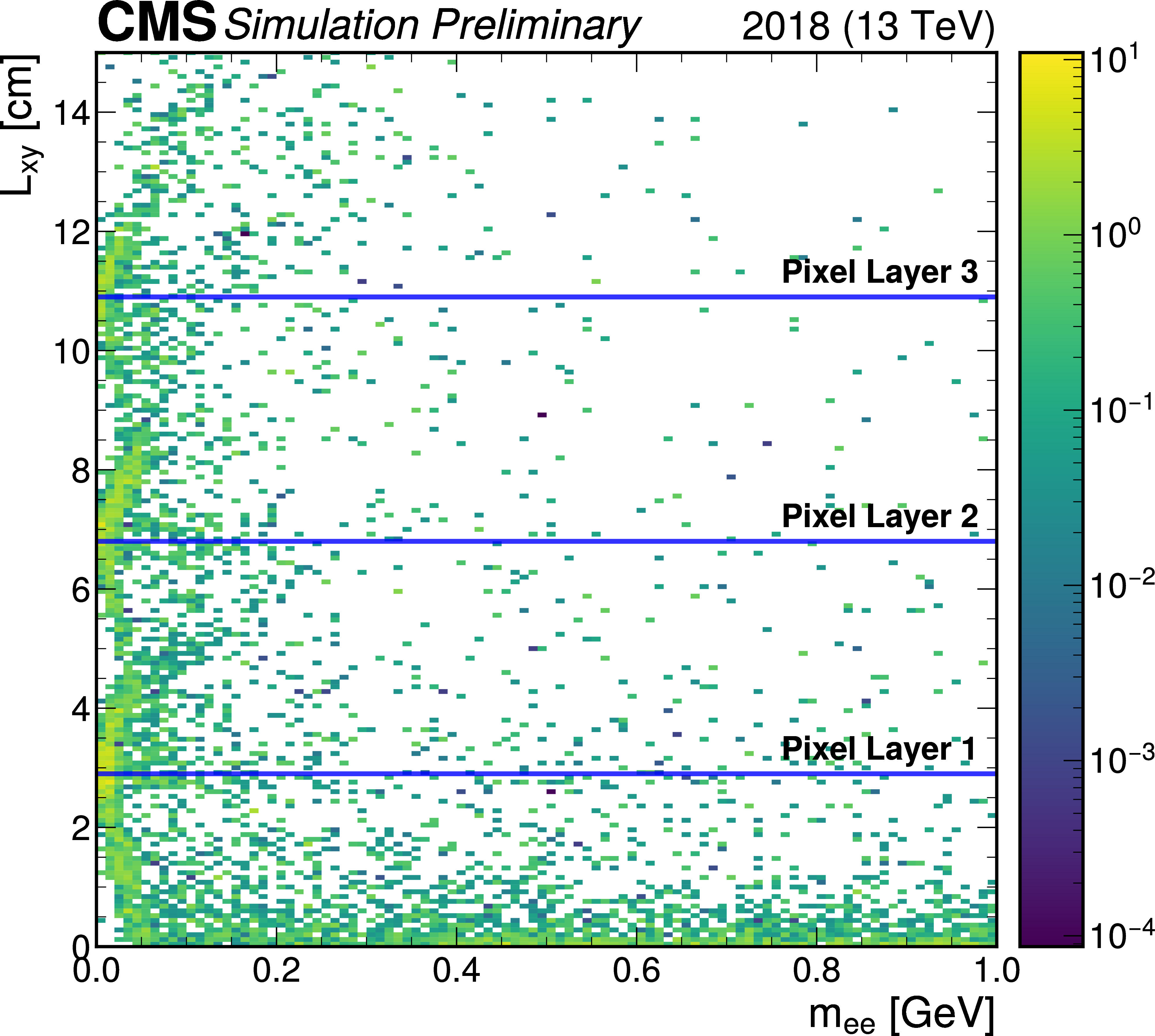
Two-dimensional distribution of the di-electron invariant mass $ m_{ee} $ and $ L_{xy} $ for background events, before the dedicated conversion rejection cuts are applied with $ m_{ee} > $ 0.1 GeV. |
png pdf |
Figure 13:
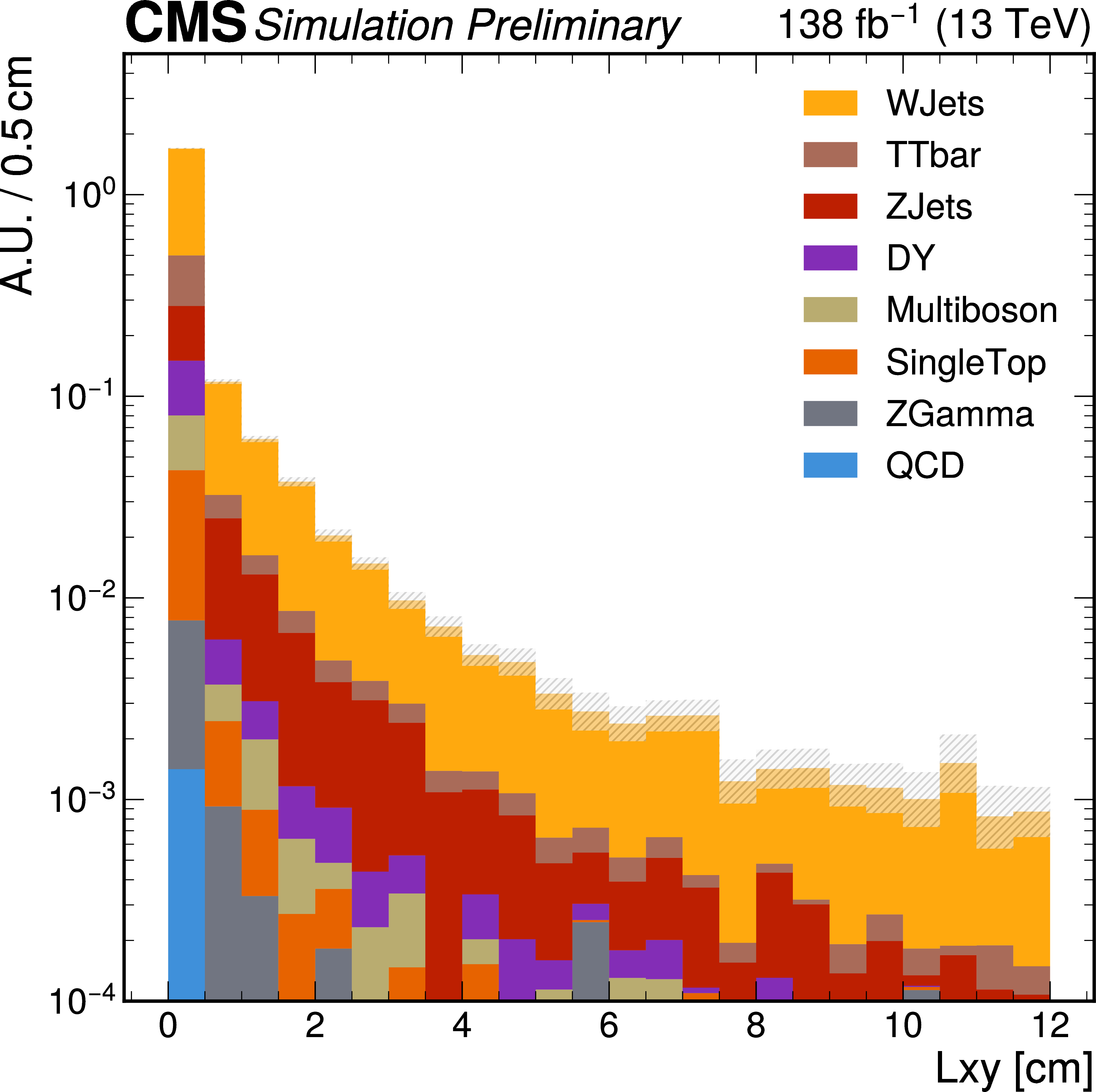
Distribution of $ L_{xy} $ for simulated background events, after the dedicated conversion rejection cuts are applied with $ m_{ee}> $ 0.1 GeV. |
png pdf |
Figure 14:
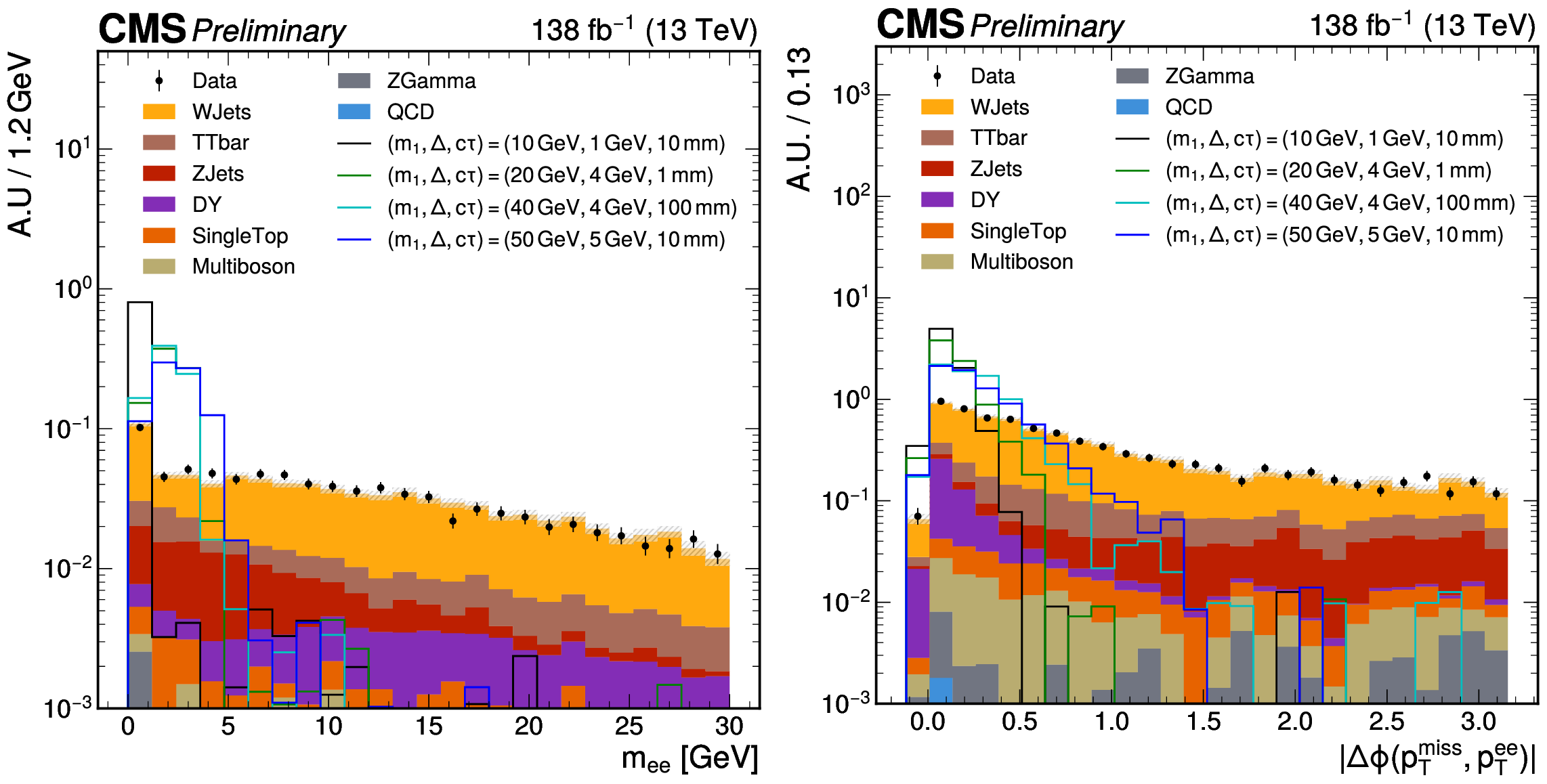
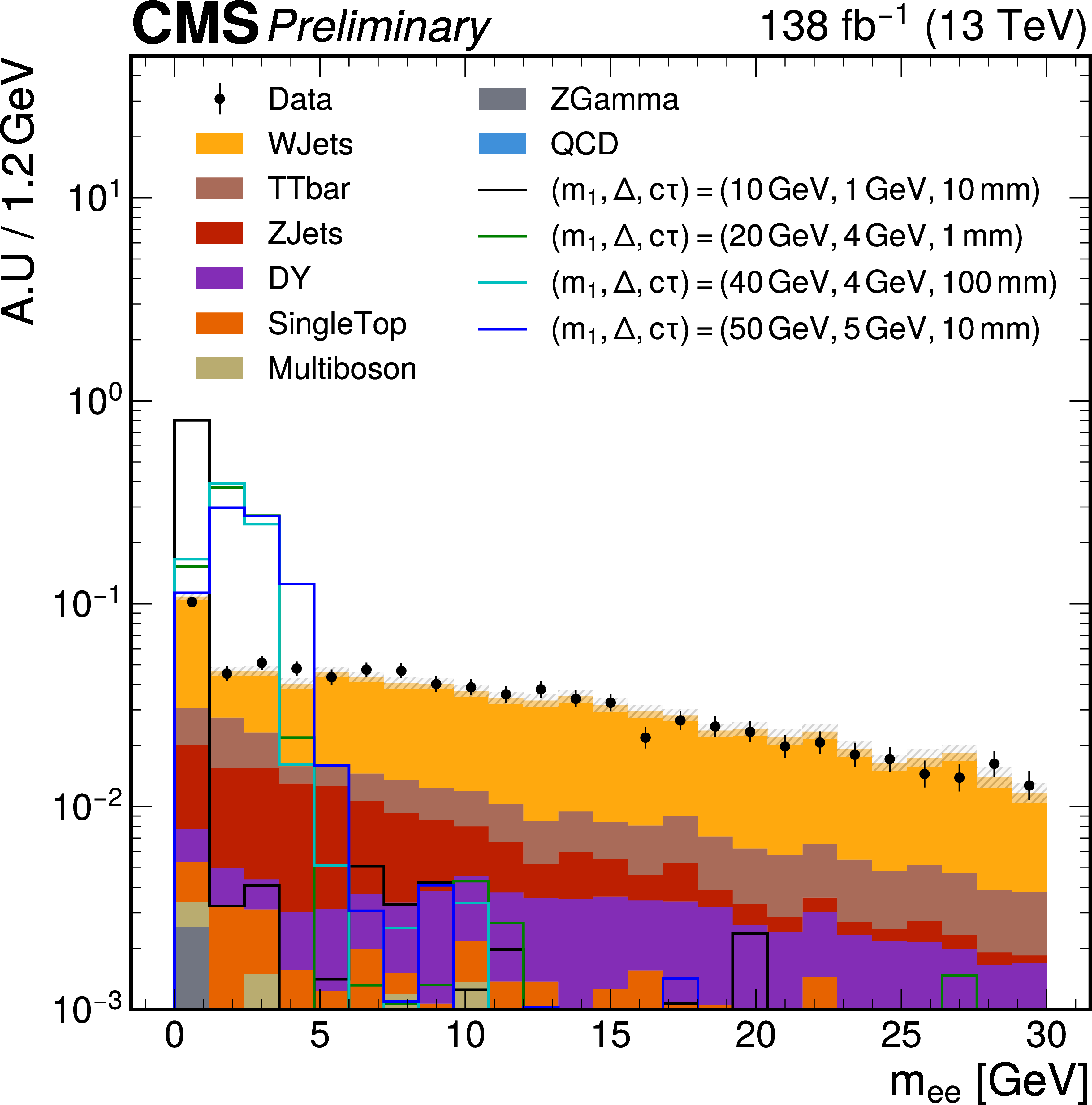
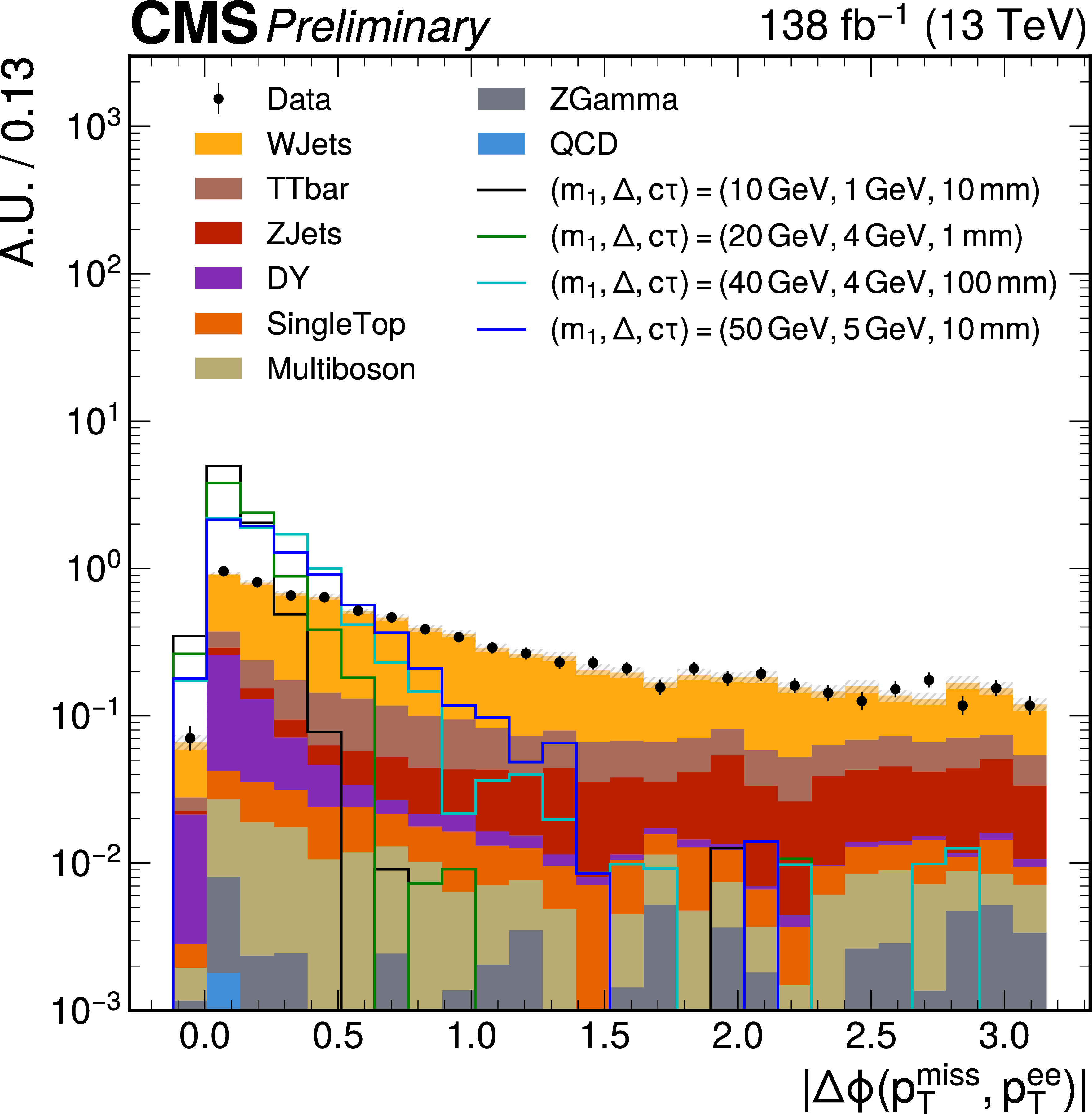
Subset of input variables for the BDT model, in both data and simulation, in the phase space with OS electron pair vertices. |
png pdf |
Figure 14-a:
Subset of input variables for the BDT model, in both data and simulation, in the phase space with OS electron pair vertices. |
png pdf |
Figure 14-b:
Subset of input variables for the BDT model, in both data and simulation, in the phase space with OS electron pair vertices. |
png pdf |
Figure 15:
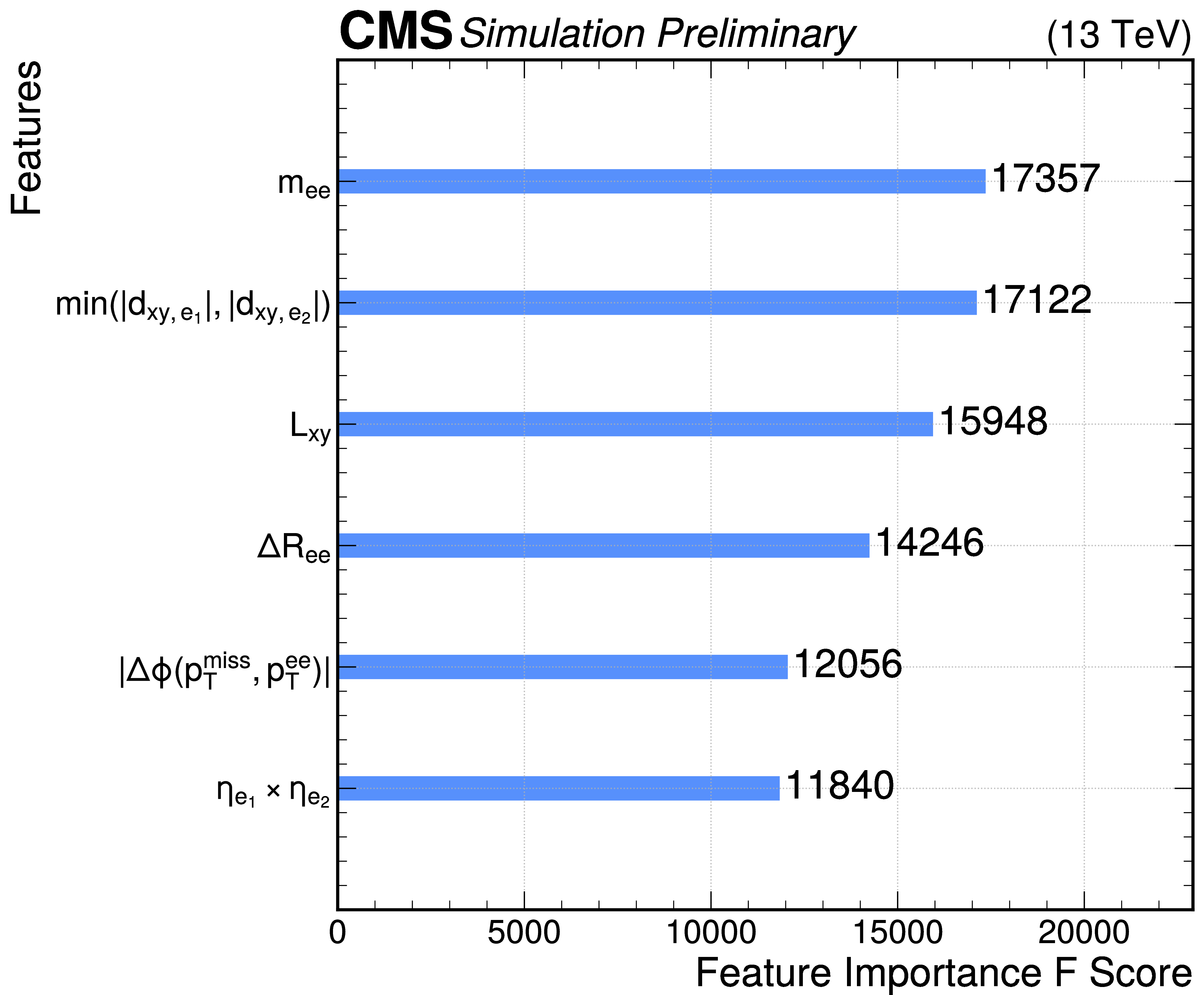
Feature importance ranking of BDT input variables after the training. |
png pdf |
Figure 16:
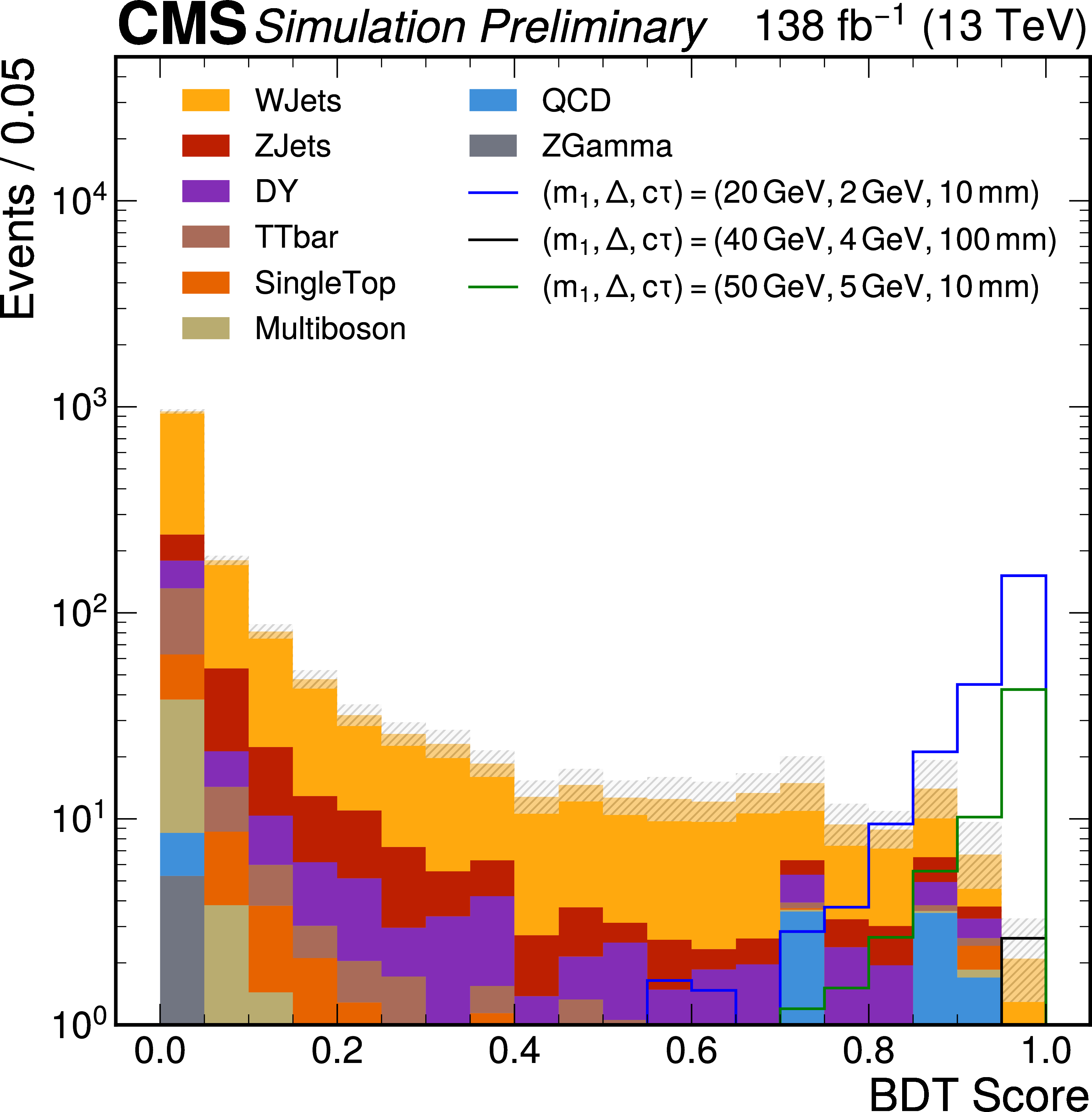
BDT output score distribution in signal and background simulation, in the phase space with OS electron pair vertices. |
png pdf |
Figure 17:
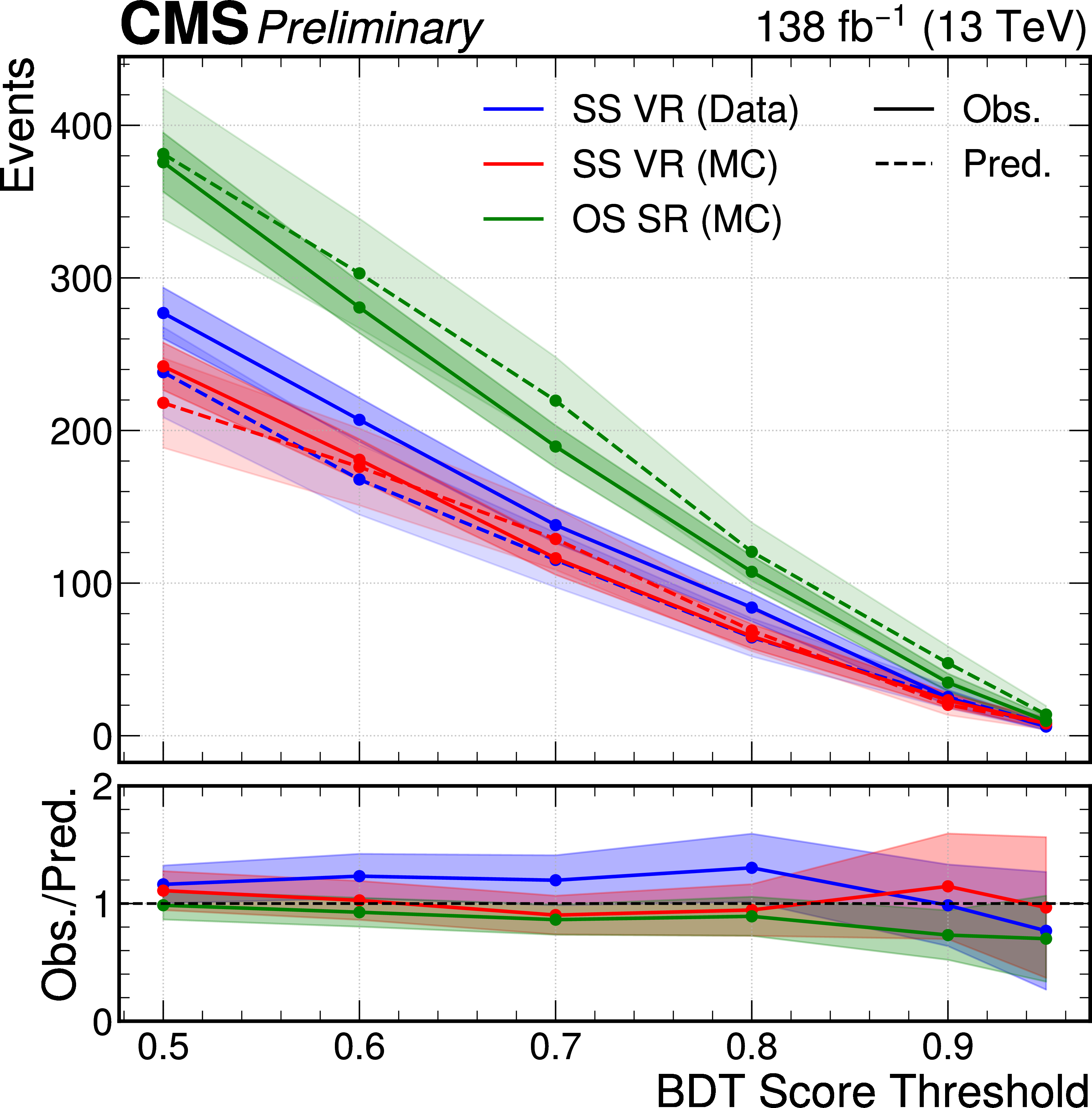
Closure test for ABCD background estimation in OS SR with MC simulation, as well as in SS VR with data and simulation, with varying BDT thresholds. |
| Tables | |
png pdf |
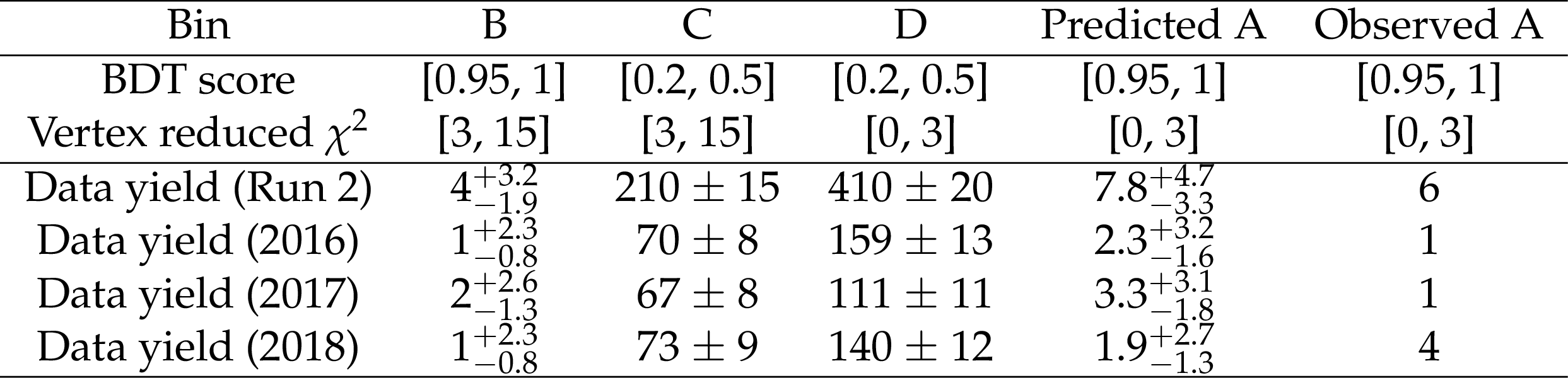
Table 1:
Background prediction validation tests in $ \mathrm{VR^{SS}} $, the region containing events with a pair of same-sign electrons. Only statistical uncertainties are considered. |
png pdf |
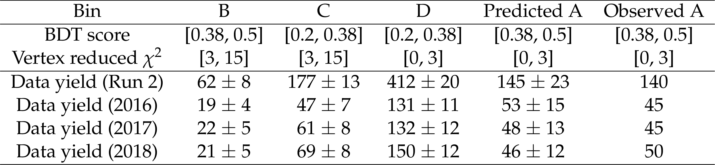
Table 2:
Background prediction validation tests in $ \mathrm{VR^{OS}} $, defined as the subset of events with opposite-sign electron pairs with ``medium'' BDT score. Only statistical uncertainties are considered. |
png pdf |
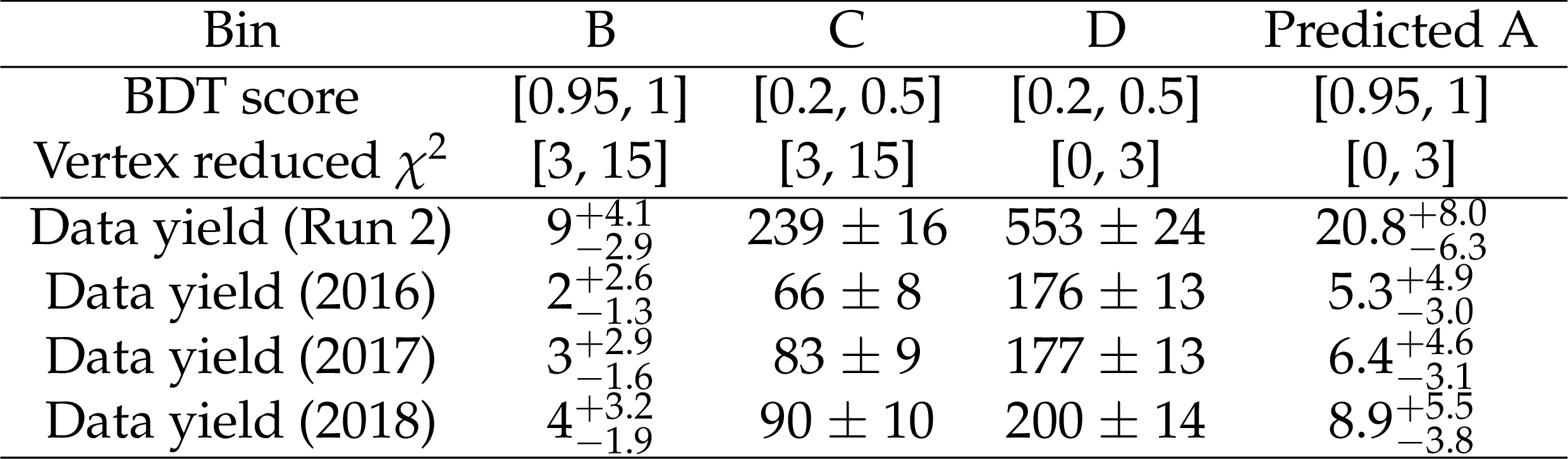
Table 3:
Summary of pre-fit background prediction in SR from the ABCD method. Only statistical uncertainties are considered. |
png pdf |
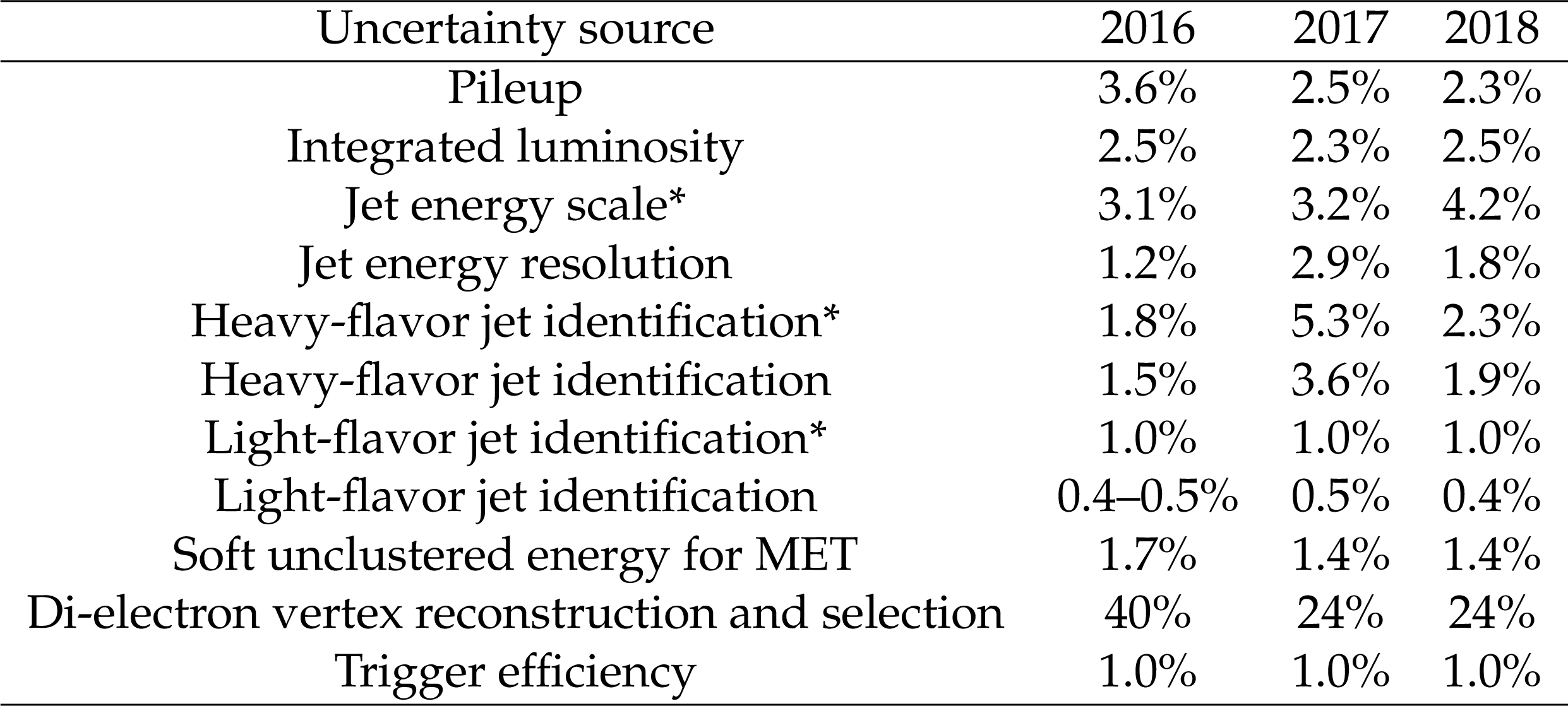
Table 4:
Summary of systematic uncertainties, shown as the average variation in the yield of simulated signal events during each data-taking period. Note that the estimated background and observation are derived solely from data and are not subject to systematic uncertainties. Uncertainty sources noted with an * are treated as fully correlated across data-taking periods, while all others are treated as fully uncorrelated. |
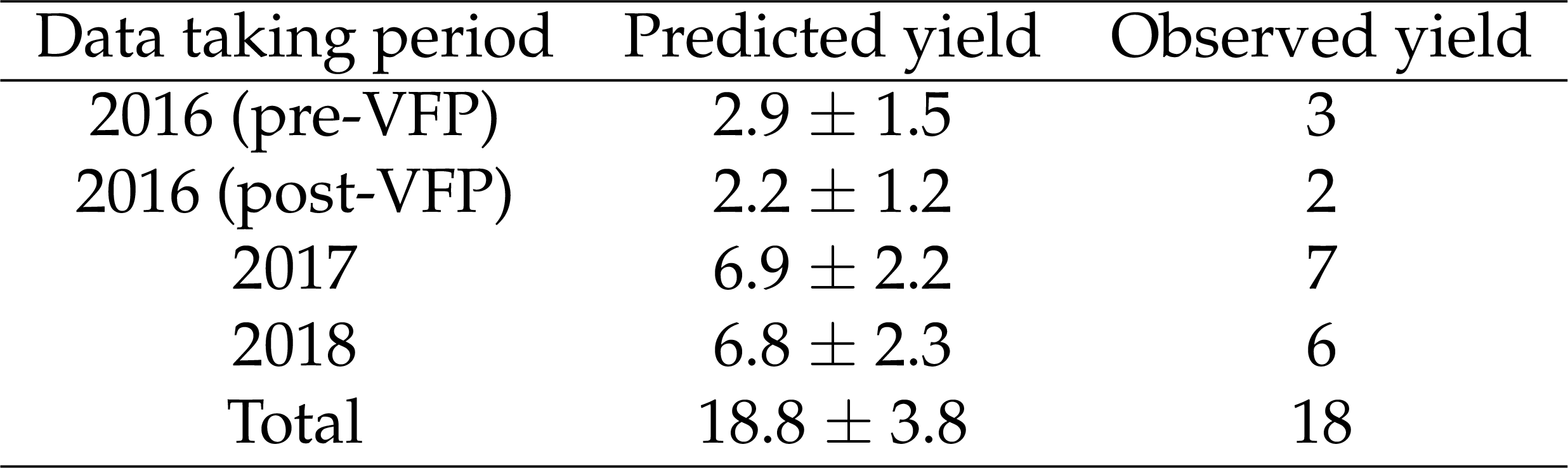
png pdf |
Table 5:
Summary of post-fit background prediction and observed data yield in SR. |
| Summary |
| The first collider search for inelastic dark matter with low-momentum, displaced electrons in the final state has been performed, using proton-proton (pp) collision data collected by the CMS experiment at $ \sqrt{s} = $ 13 TeV corresponding to an integrated luminosity of 138 fb$ ^{-1} $. A dedicated electron reconstruction algorithm, developed for the flavor physics program in CMS, was employed to enhance the sensitivity of the search in the low-momentum and displaced regime. A machine learning algorithm is trained to optimally separate signal and background events, using collimated and displaced electron pair vertex distributions. No significant deviation from the standard model predictions is observed. Upper limits at 95% confidence level are set on the product of the inelastic dark matter production cross section $ \sigma(\mathrm{p}\mathrm{p} \to A' \to $ \chi_{1} $$ \chi_{2} $) $ and the decay branching fraction $ \mathcal{B}($ \chi_{2} $ \to $ \chi_{1} $\mathrm{e}^+\mathrm{e}^-) $, where A' is a dark photon and $ \chi_{1} $ and $ \chi_{2} $ are states in the dark sector with small mass splitting, the lightest of which is the stable dark matter. Stringent constraints are placed on benchmark scenarios with 10% and 20% mass splitting of the dark matter mass range of 3 to 100 GeV, extending the sensitivity of collider searches to inelastic dark matter models. |
| References | ||||
| 1 | CMS Collaboration | Dark sector searches with the CMS experiment | Physics Reports 1115 (2025) 448 | CMS-EXO-23-005 2405.13778 |
| 2 | D. Tucker-Smith and N. Weiner | Inelastic dark matter | PRD 64 (2001) 043502 | hep-ph/0101138 |
| 3 | E. Izaguirre, G. Krnjaic, and B. Shuve | Discovering Inelastic Thermal-Relic Dark Matter at Colliders | PRD 93 (2016) no. 6 | 1508.03050 |
| 4 | A. Berlin and F. Kling | Inelastic Dark Matter at the LHC Lifetime Frontier: ATLAS, CMS, LHCb, CODEX-b, FASER, and MATHUSLA | PRD 99 (2019) no. 1 | 1810.01879 |
| 5 | CMS Collaboration | Search for Inelastic Dark Matter in Events with Two Displaced Muons and Missing Transverse Momentum in Proton-Proton Collisions at $ \sqrt{s}= $13 TeV | PRL 132 (2024) no. 4 | CMS-EXO-20-010 2305.11649 |
| 6 | CMS Collaboration | Recording and reconstructing 10 billion unbiased b hadron decays in CMS | EPJ Web Conf. 245 (2020) 01025 | |
| 7 | CMS Collaboration | The CMS Experiment at the CERN LHC | JINST 3 (2008) S08004 | |
| 8 | CMS Collaboration | Development of the CMS detector for the CERN LHC Run 3 | JINST 19 (2024) P05064 | CMS-PRF-21-001 2309.05466 |
| 9 | CMS Collaboration | Performance of the CMS Level-1 trigger in proton-proton collisions at $ \sqrt{s} = $ 13 TeV | JINST 15 (2020) no. 10 | CMS-TRG-17-001 2006.10165 |
| 10 | CMS Collaboration | The CMS trigger system | JINST 12 (2017) no. 01 | CMS-TRG-12-001 1609.02366 |
| 11 | CMS Collaboration | Performance of the CMS high-level trigger during LHC Run 2 | JINST 19 (2024) P11021 | CMS-TRG-19-001 2410.17038 |
| 12 | CMS Collaboration | Electron and photon reconstruction and identification with the CMS experiment at the CERN LHC | JINST 16 (2021) no. 05 | CMS-EGM-17-001 2012.06888 |
| 13 | CMS Collaboration | Performance of the CMS muon detector and muon reconstruction with proton-proton collisions at $ \sqrt{s}= $ 13 TeV | JINST 13 (2018) P06015 | CMS-MUO-16-001 1804.04528 |
| 14 | CMS Collaboration | Description and performance of track and primary-vertex reconstruction with the CMS tracker | JINST 9 (2014) no. 10 | CMS-TRK-11-001 1405.6569 |
| 15 | CMS Collaboration | Technical Proposal for the Phase-II Upgrade of the CMS Detector | CMS Technical Proposal CERN-LHCC-2015-010, CMS-TDR-15-02, 6, 2015 link |
|
| 16 | CMS Tracker Group Collaboration | The CMS Phase-1 pixel detector upgrade | JINST 16 (2021) P02027 | 2012.14304 |
| 17 | CMS Collaboration | Track impact parameter resolution for the full pseudo rapidity coverage in the 2017 dataset with the CMS Phase-1 pixel detector | CMS Detector Performance Summary CMS-DP-2020-049, 2020 CDS |
|
| 18 | CMS Collaboration | 2017 tracking performance plots | CMS Detector Performance Summary CMS-DP-2017-015, 2017 CDS |
|
| 19 | CMS Collaboration | Particle-flow reconstruction and global event description with the CMS detector | JINST 12 (2017) no. 10 | CMS-PRF-14-001 1706.04965 |
| 20 | M. Cacciari, G. P. Salam, and G. Soyez | The anti-$ k_t $ jet clustering algorithm | JHEP 04 (2008) 063 | 0802.1189 |
| 21 | M. Cacciari, G. P. Salam, and G. Soyez | FastJet User Manual | EPJC 72 (2012) 1896 | 1111.6097 |
| 22 | CMS Collaboration | Pileup mitigation at CMS in 13 TeV data | JINST 15 (2020) P09018 | CMS-JME-18-001 2003.00503 |
| 23 | D. Bertolini, P. Harris, M. Low, and N. Tran | Pileup Per Particle Identification | JHEP 10 (2014) 059 | 1407.6013 |
| 24 | CMS Collaboration | Identification of heavy-flavour jets with the CMS detector in pp collisions at 13 TeV | JINST 13 (2018) no. 05 | CMS-BTV-16-002 1712.07158 |
| 25 | E. Bols et al. | Jet Flavour Classification Using DeepJet | JINST 15 (2020) no. 12 | 2008.10519 |
| 26 | CMS Collaboration | Performance of missing transverse momentum reconstruction in proton-proton collisions at $ \sqrt{s} = $ 13 TeV using the CMS detector | JINST 14 (2019) no. 07 | CMS-JME-17-001 1903.06078 |
| 27 | M. J. Oreglia | A study of the reactions $ \psi^\prime \to \gamma \gamma \psi $ | PhD thesis, Stanford University, SLAC Report SLAC-R-236, 1980 link |
|
| 28 | J. E. Gaiser | Charmonium spectroscopy from radiative decays of the $ J/\psi $ and $ \psi^\prime $ | PhD thesis, Stanford University, SLAC Report SLAC-R-255, 1982 link |
|
| 29 | CMS Collaboration | Precision luminosity measurement in proton-proton collisions at $ \sqrt{s} = $ 13 TeV in 2015 and 2016 at CMS | EPJC 81 (2021) 800 | CMS-LUM-17-003 2104.01927 |
| 30 | CMS Collaboration | Precision luminosity measurement in proton-proton collisions at 13 tev with the CMS detector | CMS Physics Analysis Summary, 2025 CMS-PAS-LUM-20-001 |
CMS-PAS-LUM-20-001 |
| 31 | J. Alwall et al. | The automated computation of tree-level and next-to-leading order differential cross sections, and their matching to parton shower simulations | JHEP 07 (2014) 079 | 1405.0301 |
| 32 | T. Sjöstrand, S. Ask, J. R. Christiansen et al. | An introduction to PYTHIA 8.2 | Comput Phys Commun 191 (2015) 159 | |
| 33 | NNPDF Collaboration | Parton distributions for the LHC Run II | JHEP 04 (2015) 040 | 1410.8849 |
| 34 | NNPDF Collaboration | Parton distributions from high-precision collider data | EPJC 77 (2017) no. 10 | 1706.00428 |
| 35 | GEANT4 Collaboration | GEANT4--a simulation toolkit | NIM A 506 (2003) 250 | |
| 36 | J. Alwall et al. | MadGraph 5: Going Beyond | JHEP 06 (2011) 128 | 1106.0522 |
| 37 | J. Alwall et al. | Comparative study of various algorithms for the merging of parton showers and matrix elements in hadronic collisions | EPJC 53 (2008) 473 | 0706.2569 |
| 38 | P. Nason | A New method for combining NLO QCD with shower Monte Carlo algorithms | JHEP 11 (2004) 040 | hep-ph/0409146 |
| 39 | S. Frixione, P. Nason, and C. Oleari | Matching NLO QCD computations with Parton Shower simulations: the POWHEG method | JHEP 11 (2007) 070 | 0709.2092 |
| 40 | S. Alioli, P. Nason, C. Oleari, and E. Re | A general framework for implementing NLO calculations in shower Monte Carlo programs: the POWHEG BOX | JHEP 06 (2010) 043 | 1002.2581 |
| 41 | C. Bierlich et al. | A comprehensive guide to the physics and usage of PYTHIA 8.3 | SciPost Phys. Codeb. 2022 (2022) 8 | 2203.11601 |
| 42 | CMS Collaboration | Extraction and validation of a new set of CMS PYTHIA8 tunes from underlying-event measurements | EPJC 80 (2020) no. 1 | CMS-GEN-17-001 1903.12179 |
| 43 | CMS Collaboration | Performance summary of AK4 jet b tagging with data from proton-proton collisions at 13 TeV with the CMS detector | CDS | |
| 44 | R. Fruhwirth | Application of Kalman filtering to track and vertex fitting | NIM A 262 (1987) 444 | |
| 45 | L. Breiman, J. Friedman, C. Stone, and R. Olshen | Classification and Regression Trees | Taylor & Francis, ISBN 978041418, 1984 | |
| 46 | J. H. Friedman | Greedy function approximation: a gradient boosting machine | Annals of statistics 118 (2001) 9 | |
| 47 | J. H. Friedman | Stochastic gradient boosting | Computational statistics \& data analysis 38, no. 4, 367--378, 2002 | |
| 48 | T. Chen and C. Guestrin | XGBoost: A scalable tree boosting system | in nd ACM SIGKDD International Conference on Knowledge Discovery and Data Mining, 2016 Proceedings of the 2 (2016) 785 |
|
| 49 | CMS Collaboration | The CMS statistical analysis and combination tool: Combine | Submitted to Comput. Softw. Big Sci, 2024 | CMS-CAT-23-001 2404.06614 |
| 50 | T. Junk | Confidence level computation for combining searches with small statistics | NIM A 434 (1999) 435 | hep-ex/9902006 |
| 51 | A. L. Read | Presentation of search results: The $ CL_s $ technique | JPG 28 (2002) 2693 | |
| 52 | G. Cowan, K. Cranmer, E. Gross, and O. Vitells | Asymptotic formulae for likelihood-based tests of new physics | [Erratum: Eur.Phys.J.C 73, 2501 ()] EPJC 71 (2011) 1554 |
1007.1727 |
|
|
Compact Muon Solenoid LHC, CERN |

|
|
|
|
|
|