
Compact Muon Solenoid
LHC, CERN
 Visit us: CMS Public Website, CMS Physics ;
Contact us: CMS Publications Committee
Visit us: CMS Public Website, CMS Physics ;
Contact us: CMS Publications Committee
| CMS-PAS-B2G-24-023 | ||
| Search for heavy neutral leptons in top quark decays with same-sign dilepton final states in proton-proton collisions at $ \sqrt{s}= $ 13 TeV | ||
| CMS Collaboration | ||
| 2026-05-18 | ||
| Abstract: The first search for a Majorana$ \text{-} $type heavy neutral lepton (N) produced in top quark decays with the CMS detector is reported. In type$ \text{-} $I seesaw models, where the N mixes with the first two generations of neutrinos, these heavy leptons lead to novel top quark decay modes that violate lepton number conservation. We therefore search for top quark pair production in proton$ \text{-} $proton collisions, followed by a top quark decay to a bottom quark and a W boson, decaying further into a charged lepton (electron or muon), and N. Here, the Majorana N decays to a W boson and a charged lepton with the same sign as the charged lepton produced with N. The experimental signature of this process is characterized by the presence of same$ \text{-} $sign and same$ \text{-} $flavor lepton pairs and jets. We use proton$ \text{-} $proton collision data corresponding to an integrated luminosity of 138 $ \text{fb}^{-1} $ at a center$ \text{-} $of$ \text{-} $mass energy of 13 TeV, collected during 2016--2018 with the CMS detector at the LHC. The search is performed for N masses between 20 and 100 GeV. Depending on the mass of N, the observed (expected) upper limits at the 95% CL on the branching ratio of the top quark decay to N, charged lepton, and bottom quark vary between 1.1 $ \times10^{-5} $ (6.8 $ \times10^{-6} $) and 4.7 $ \times10^{-5} $ (3.0 $ \times 10^{-5} $) in the dielectron final state and between 3.8 $ \times10^{-6} $ (3.4 $ \times 10^{-6} $) and 2.4 $ \times10^{-5} $ (1.3 $ \times 10^{-5} $) in the dimuon final state. | ||
| Links: CDS record (PDF) ; CADI line (restricted) ; | ||
| Figures | |
png pdf |
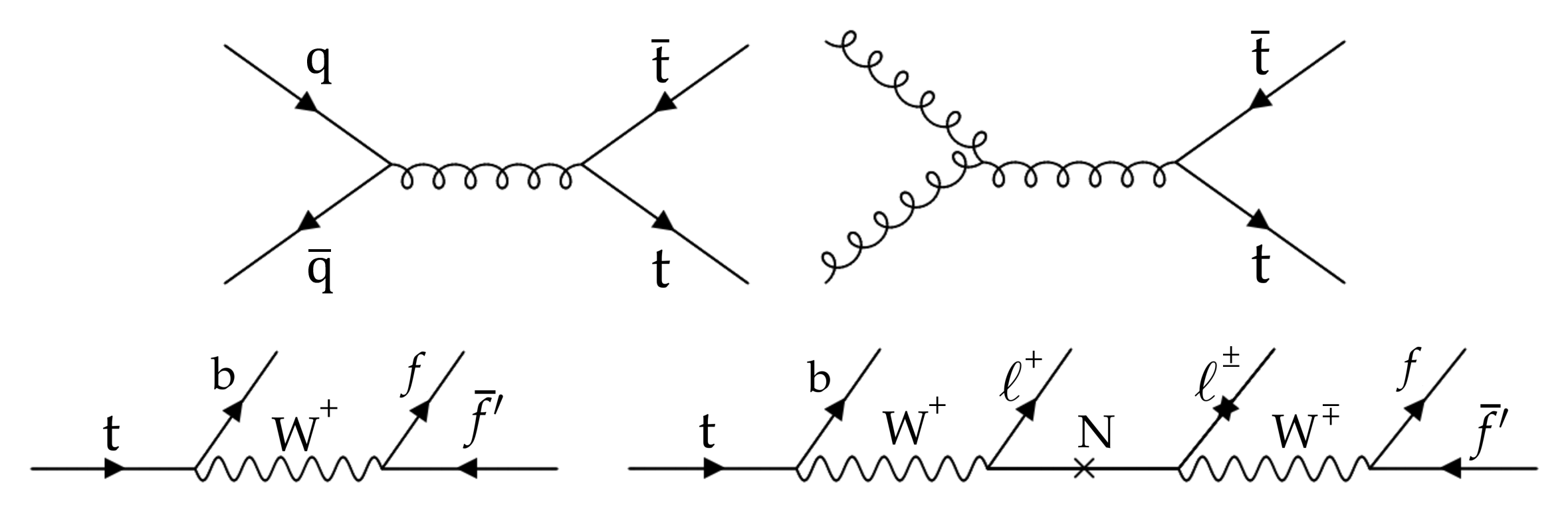
Figure 1:
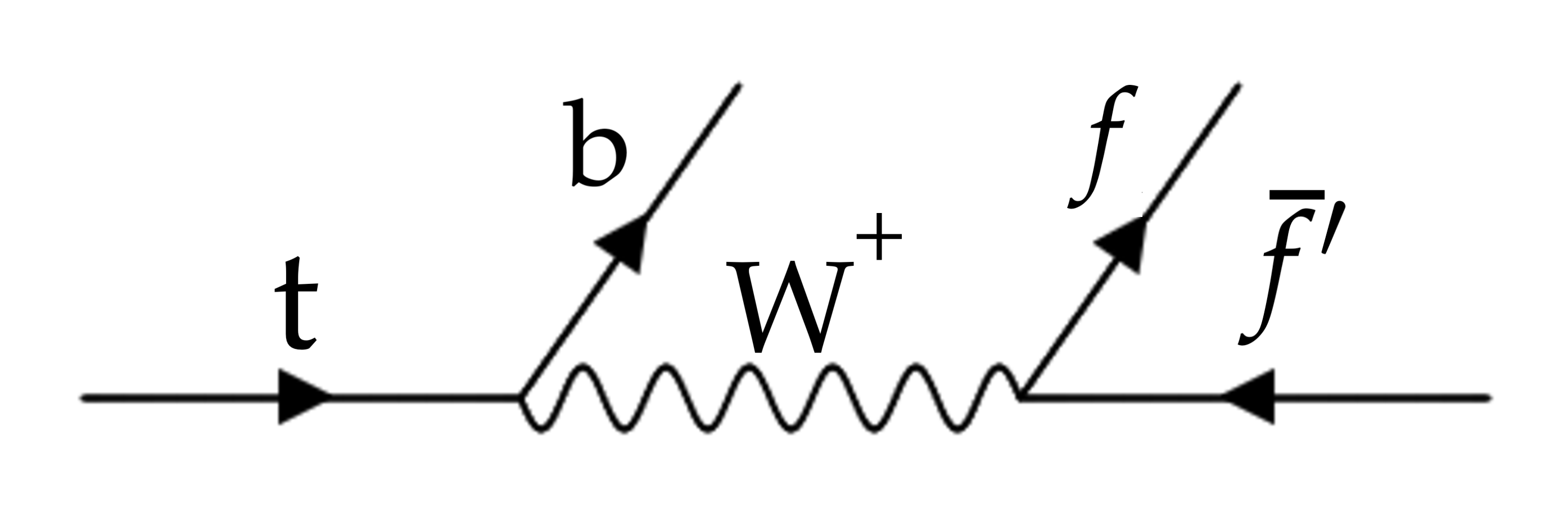
Representative Feynman diagrams of $ \mathrm{t} \overline{\mathrm{t}} $ production (upper) and SM top quark decays (lower left) and BSM decays involving $ \mathrm{N} $s (lower right), where $ \ell $ represents e or $ \mu $, and $ \text{f},\text{f}^\prime $ represent SM fermions. |
png pdf |
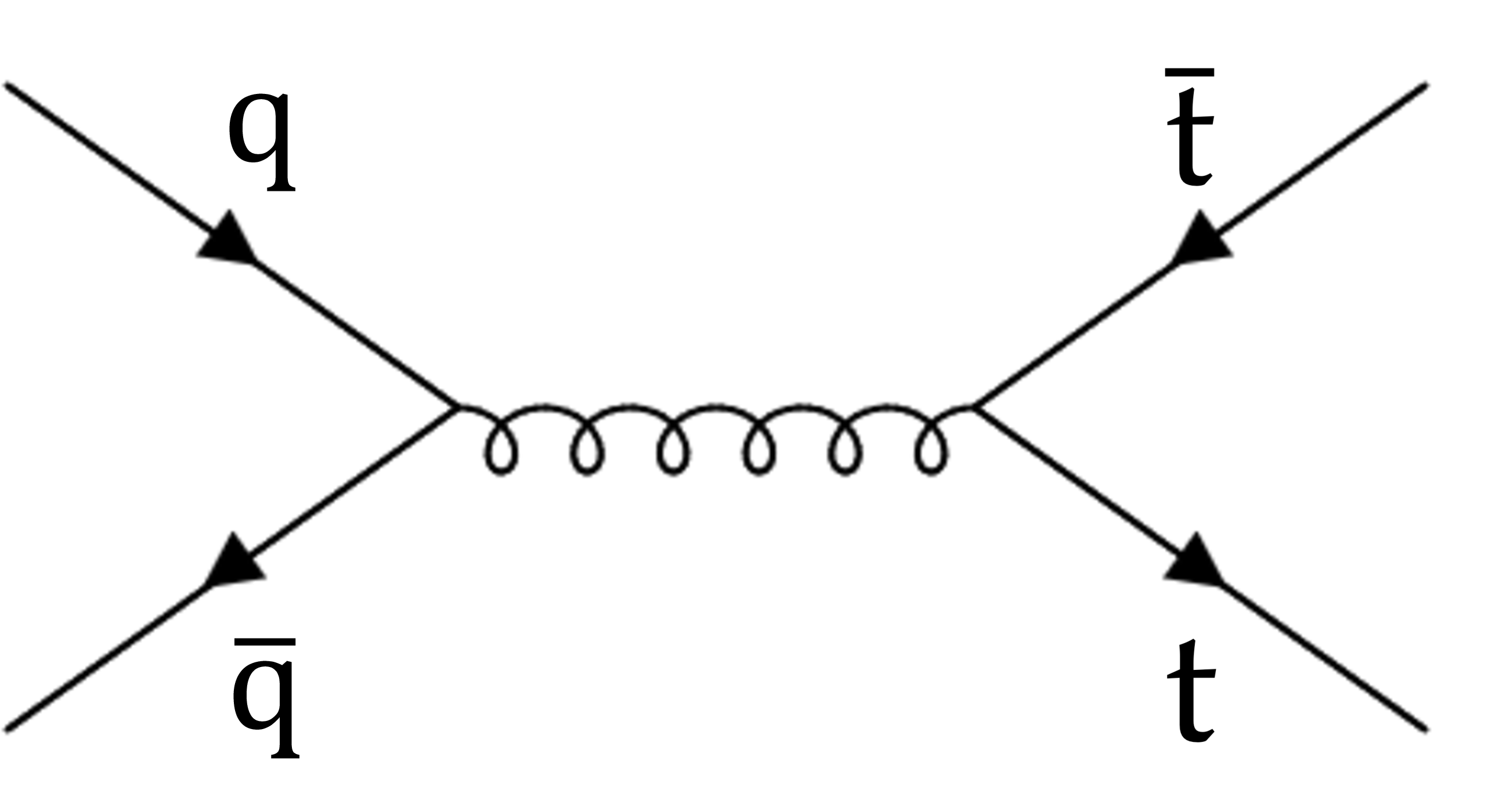
Figure 1-a:
Representative Feynman diagrams of $ \mathrm{t} \overline{\mathrm{t}} $ production (upper) and SM top quark decays (lower left) and BSM decays involving $ \mathrm{N} $s (lower right), where $ \ell $ represents e or $ \mu $, and $ \text{f},\text{f}^\prime $ represent SM fermions. |
png pdf |
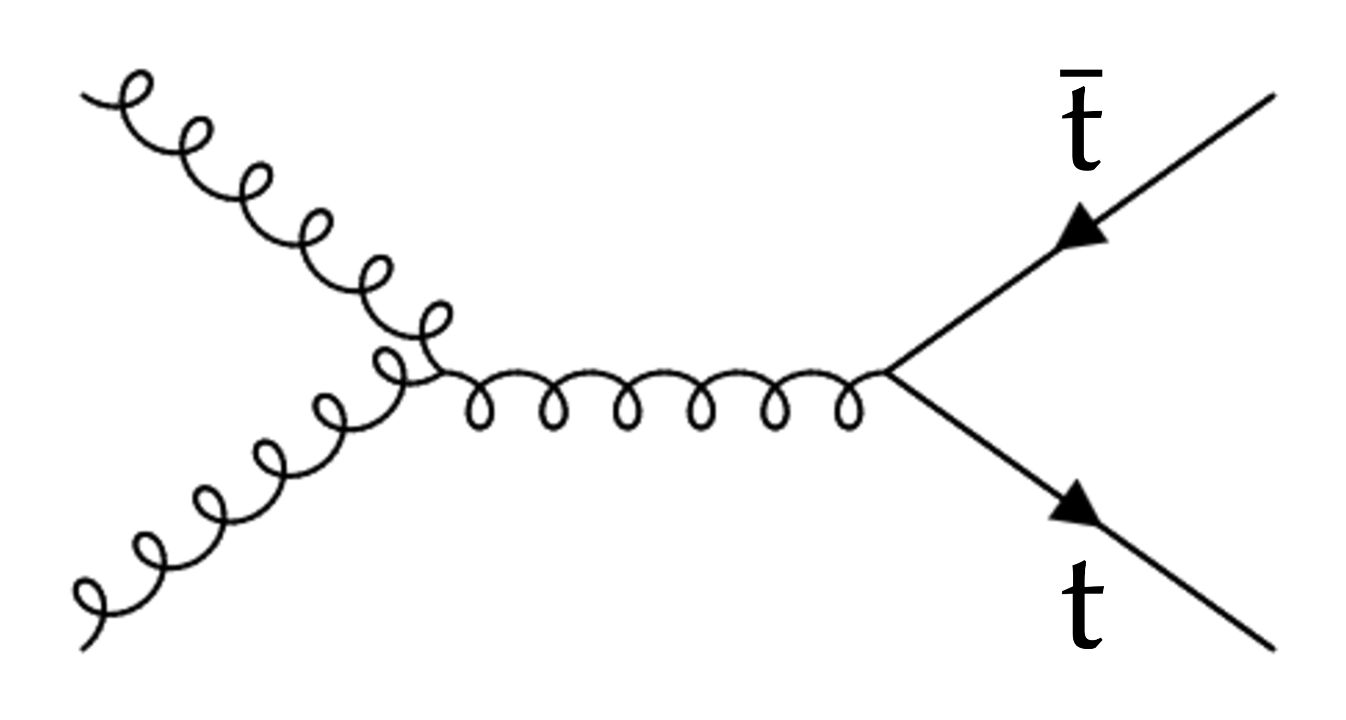
Figure 1-b:
Representative Feynman diagrams of $ \mathrm{t} \overline{\mathrm{t}} $ production (upper) and SM top quark decays (lower left) and BSM decays involving $ \mathrm{N} $s (lower right), where $ \ell $ represents e or $ \mu $, and $ \text{f},\text{f}^\prime $ represent SM fermions. |
png pdf |
Figure 1-c:
Representative Feynman diagrams of $ \mathrm{t} \overline{\mathrm{t}} $ production (upper) and SM top quark decays (lower left) and BSM decays involving $ \mathrm{N} $s (lower right), where $ \ell $ represents e or $ \mu $, and $ \text{f},\text{f}^\prime $ represent SM fermions. |

png pdf |
Figure 1-d:
Representative Feynman diagrams of $ \mathrm{t} \overline{\mathrm{t}} $ production (upper) and SM top quark decays (lower left) and BSM decays involving $ \mathrm{N} $s (lower right), where $ \ell $ represents e or $ \mu $, and $ \text{f},\text{f}^\prime $ represent SM fermions. |
png pdf |
Figure 2:
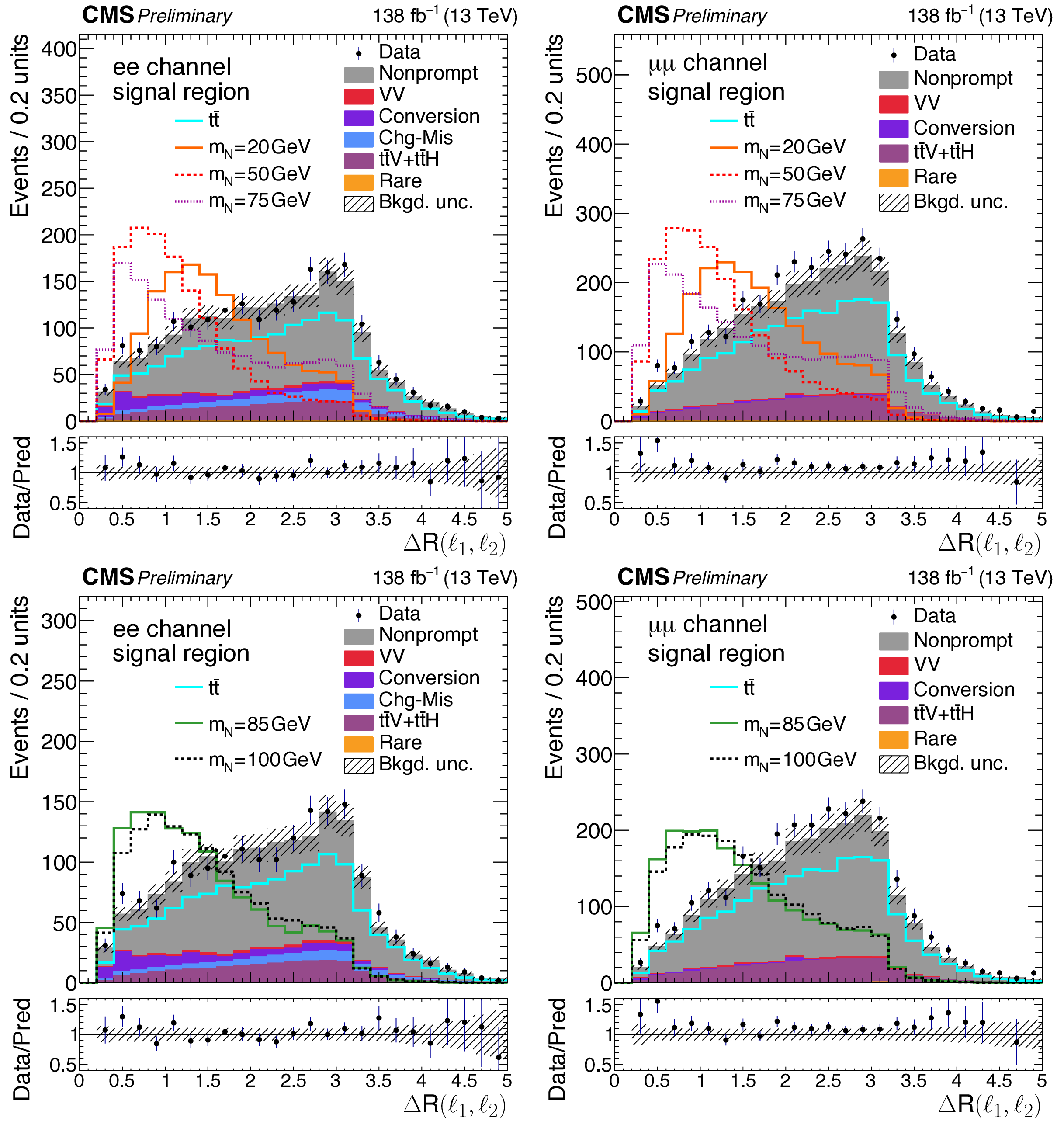
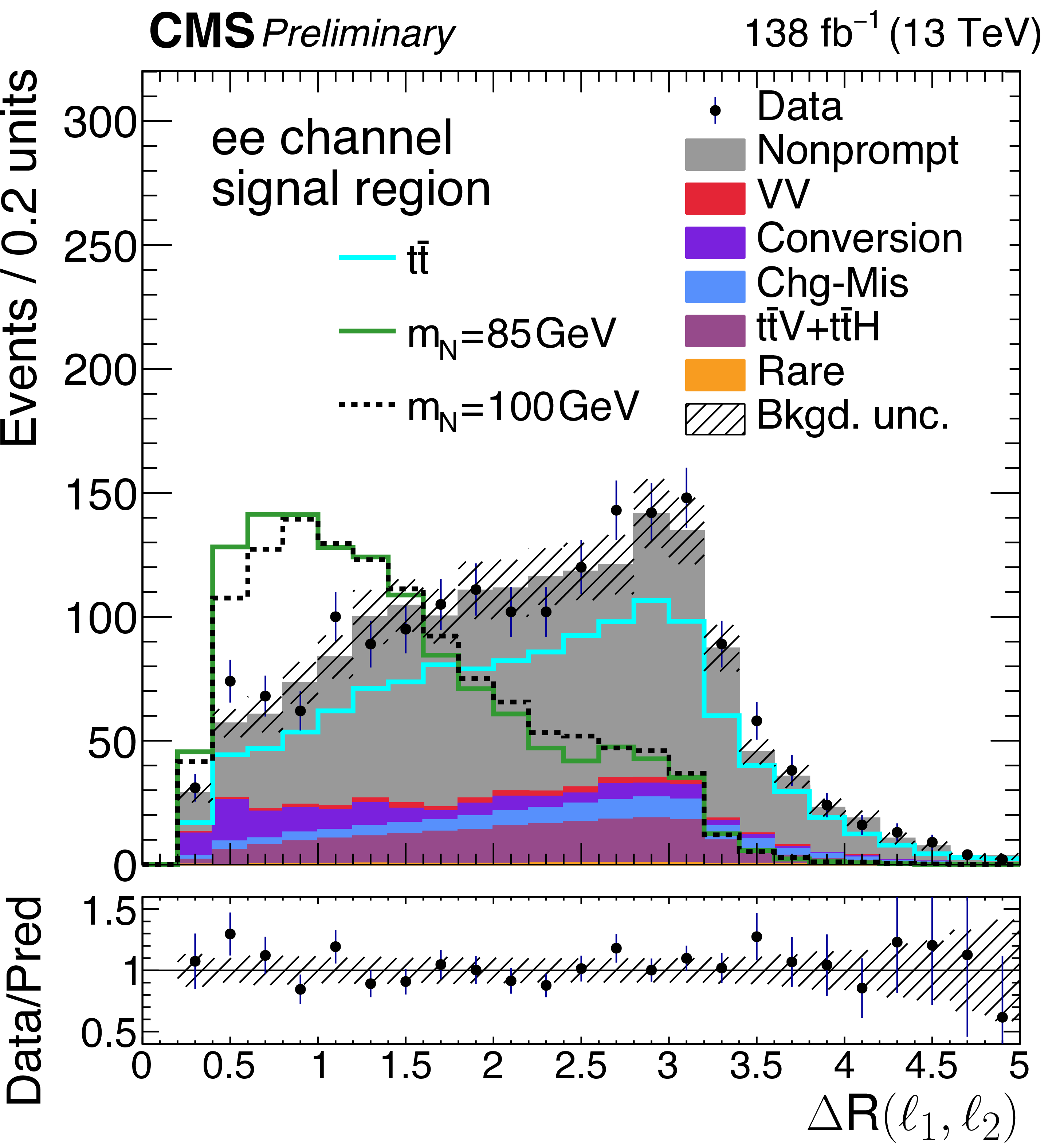
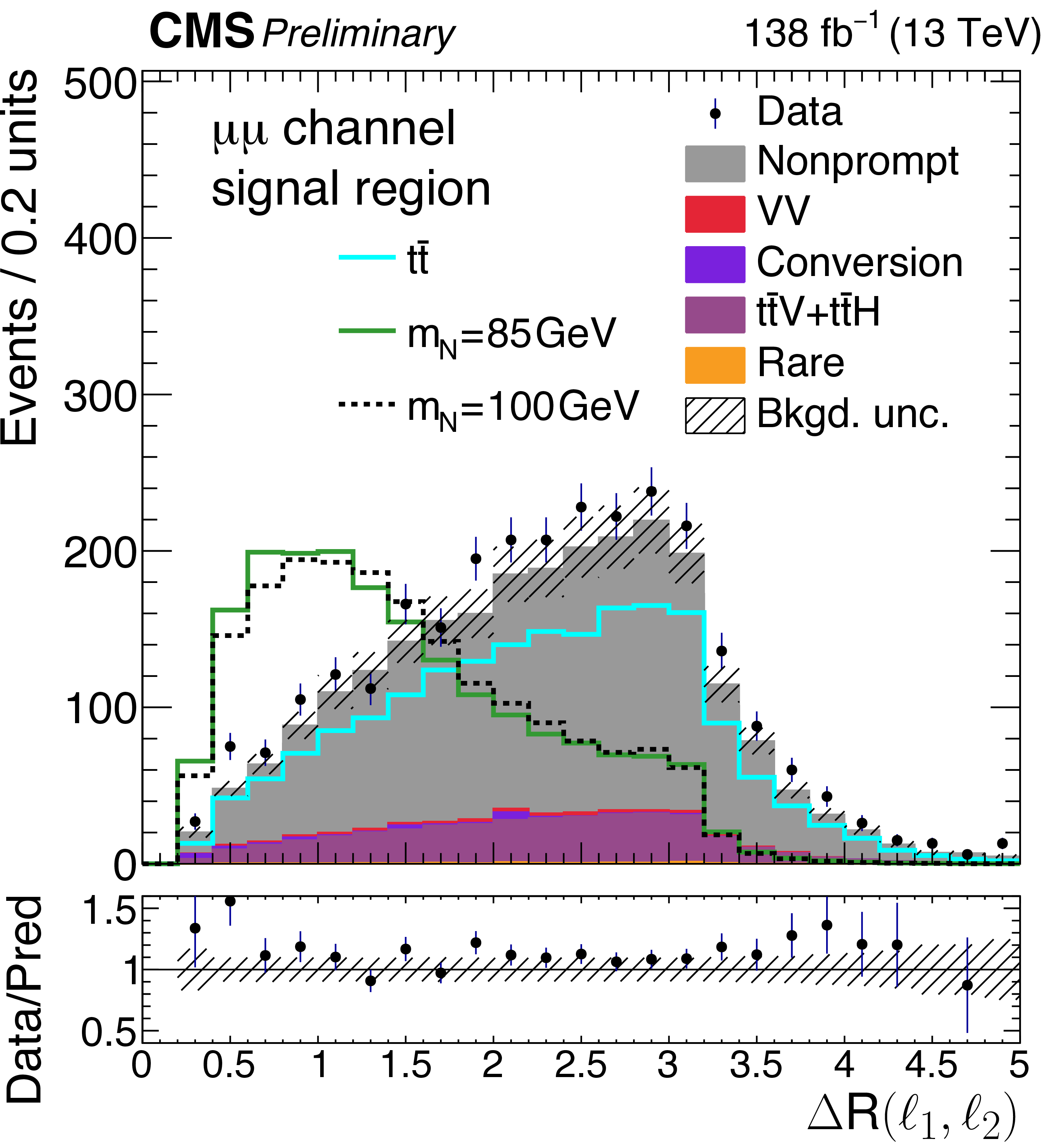
Pre$ \text{-} $fit distributions of the $ \Delta R $ between two leptons are shown in dielectron (left) and dimuon (right) events as examples of the input variables for the training. Within the two rows for each variable, the top row and the bottom row correspond to the $ m_{\mathrm{N}} < m_{\mathrm{W}} $ selection and the $ m_{\mathrm{N}} > m_{\mathrm{W}} $ selection, respectively, which differ in the required number of untagged jets. The cyan line is the $ \mathrm{t} \overline{\mathrm{t}} $ simulation used for the training background. Signal distributions are normalized to the background rate. The background uncertainty band shows the total uncertainty including systematics. |
png pdf |
Figure 2-a:
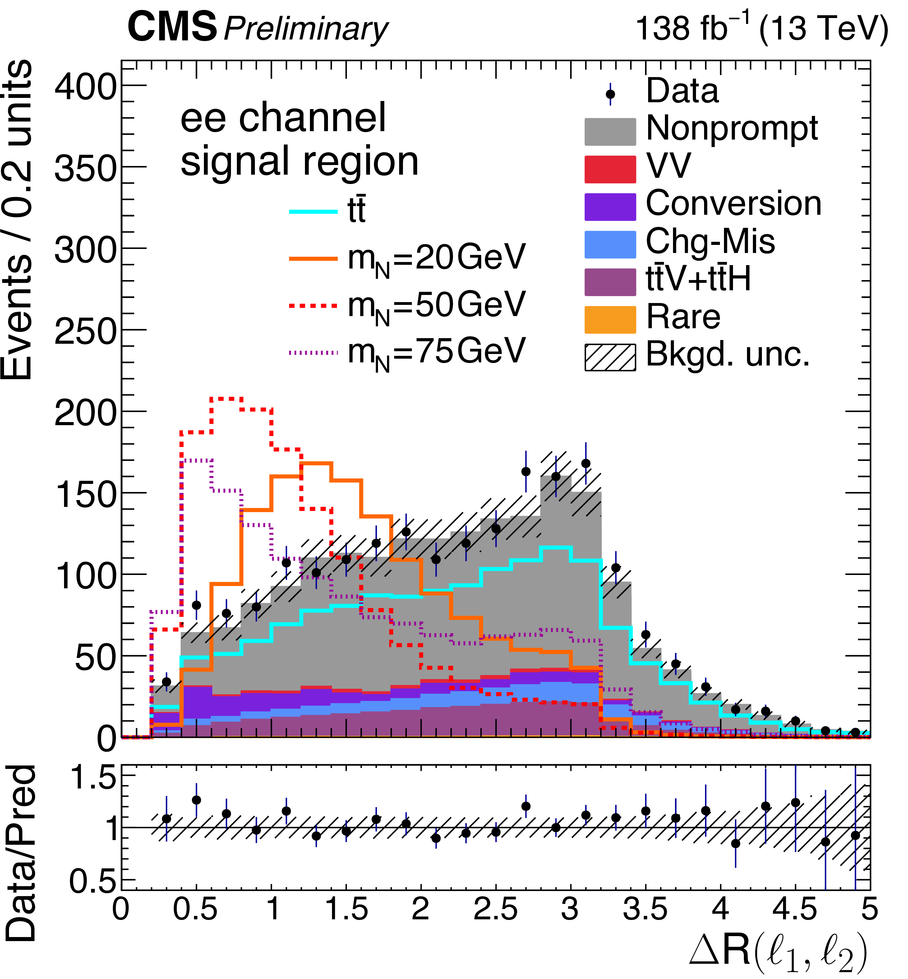
Pre$ \text{-} $fit distributions of the $ \Delta R $ between two leptons are shown in dielectron (left) and dimuon (right) events as examples of the input variables for the training. Within the two rows for each variable, the top row and the bottom row correspond to the $ m_{\mathrm{N}} < m_{\mathrm{W}} $ selection and the $ m_{\mathrm{N}} > m_{\mathrm{W}} $ selection, respectively, which differ in the required number of untagged jets. The cyan line is the $ \mathrm{t} \overline{\mathrm{t}} $ simulation used for the training background. Signal distributions are normalized to the background rate. The background uncertainty band shows the total uncertainty including systematics. |
png pdf |
Figure 2-b:
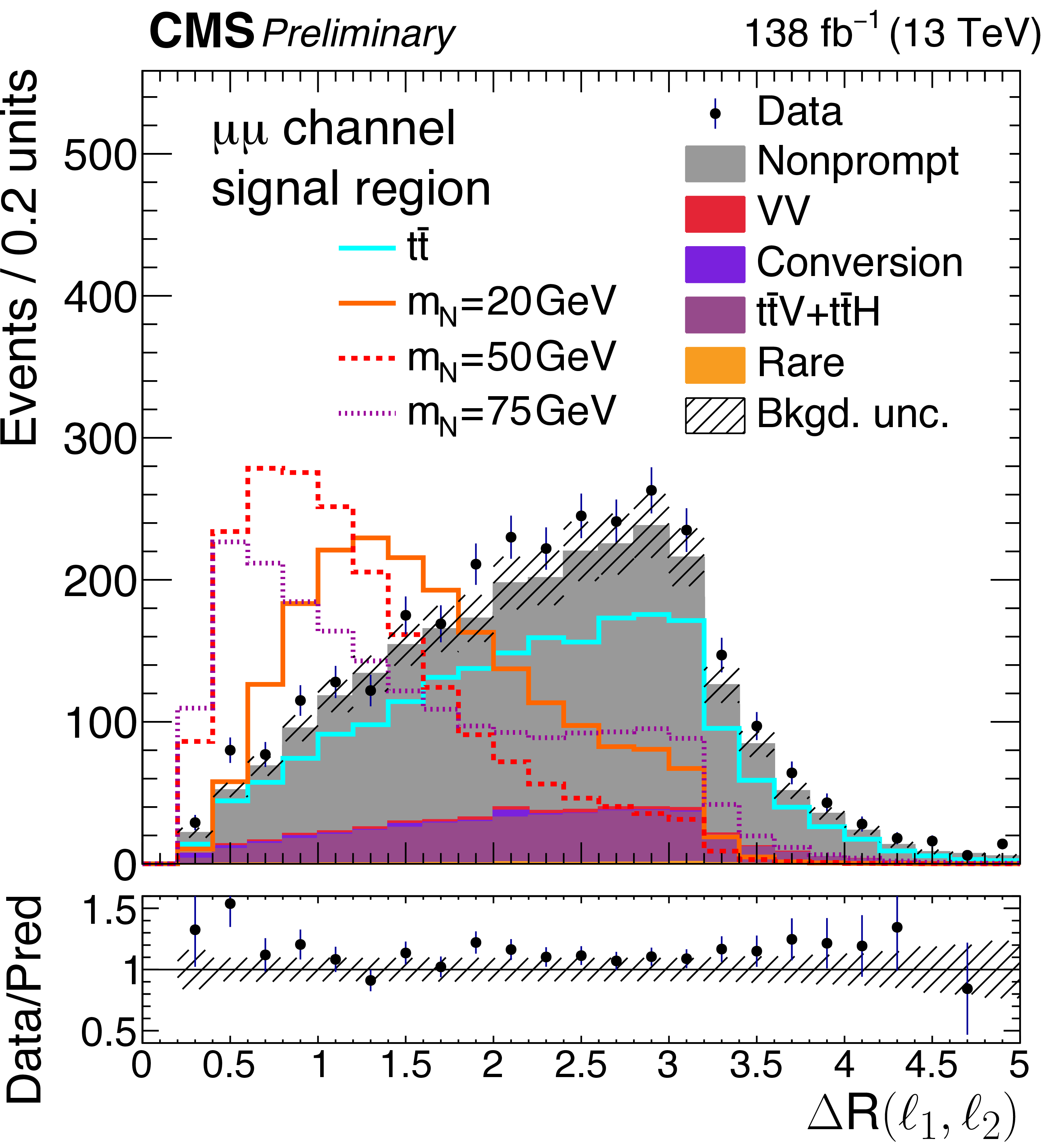
Pre$ \text{-} $fit distributions of the $ \Delta R $ between two leptons are shown in dielectron (left) and dimuon (right) events as examples of the input variables for the training. Within the two rows for each variable, the top row and the bottom row correspond to the $ m_{\mathrm{N}} < m_{\mathrm{W}} $ selection and the $ m_{\mathrm{N}} > m_{\mathrm{W}} $ selection, respectively, which differ in the required number of untagged jets. The cyan line is the $ \mathrm{t} \overline{\mathrm{t}} $ simulation used for the training background. Signal distributions are normalized to the background rate. The background uncertainty band shows the total uncertainty including systematics. |
png pdf |
Figure 2-c:
Pre$ \text{-} $fit distributions of the $ \Delta R $ between two leptons are shown in dielectron (left) and dimuon (right) events as examples of the input variables for the training. Within the two rows for each variable, the top row and the bottom row correspond to the $ m_{\mathrm{N}} < m_{\mathrm{W}} $ selection and the $ m_{\mathrm{N}} > m_{\mathrm{W}} $ selection, respectively, which differ in the required number of untagged jets. The cyan line is the $ \mathrm{t} \overline{\mathrm{t}} $ simulation used for the training background. Signal distributions are normalized to the background rate. The background uncertainty band shows the total uncertainty including systematics. |
png pdf |
Figure 2-d:
Pre$ \text{-} $fit distributions of the $ \Delta R $ between two leptons are shown in dielectron (left) and dimuon (right) events as examples of the input variables for the training. Within the two rows for each variable, the top row and the bottom row correspond to the $ m_{\mathrm{N}} < m_{\mathrm{W}} $ selection and the $ m_{\mathrm{N}} > m_{\mathrm{W}} $ selection, respectively, which differ in the required number of untagged jets. The cyan line is the $ \mathrm{t} \overline{\mathrm{t}} $ simulation used for the training background. Signal distributions are normalized to the background rate. The background uncertainty band shows the total uncertainty including systematics. |
png pdf |
Figure 3:
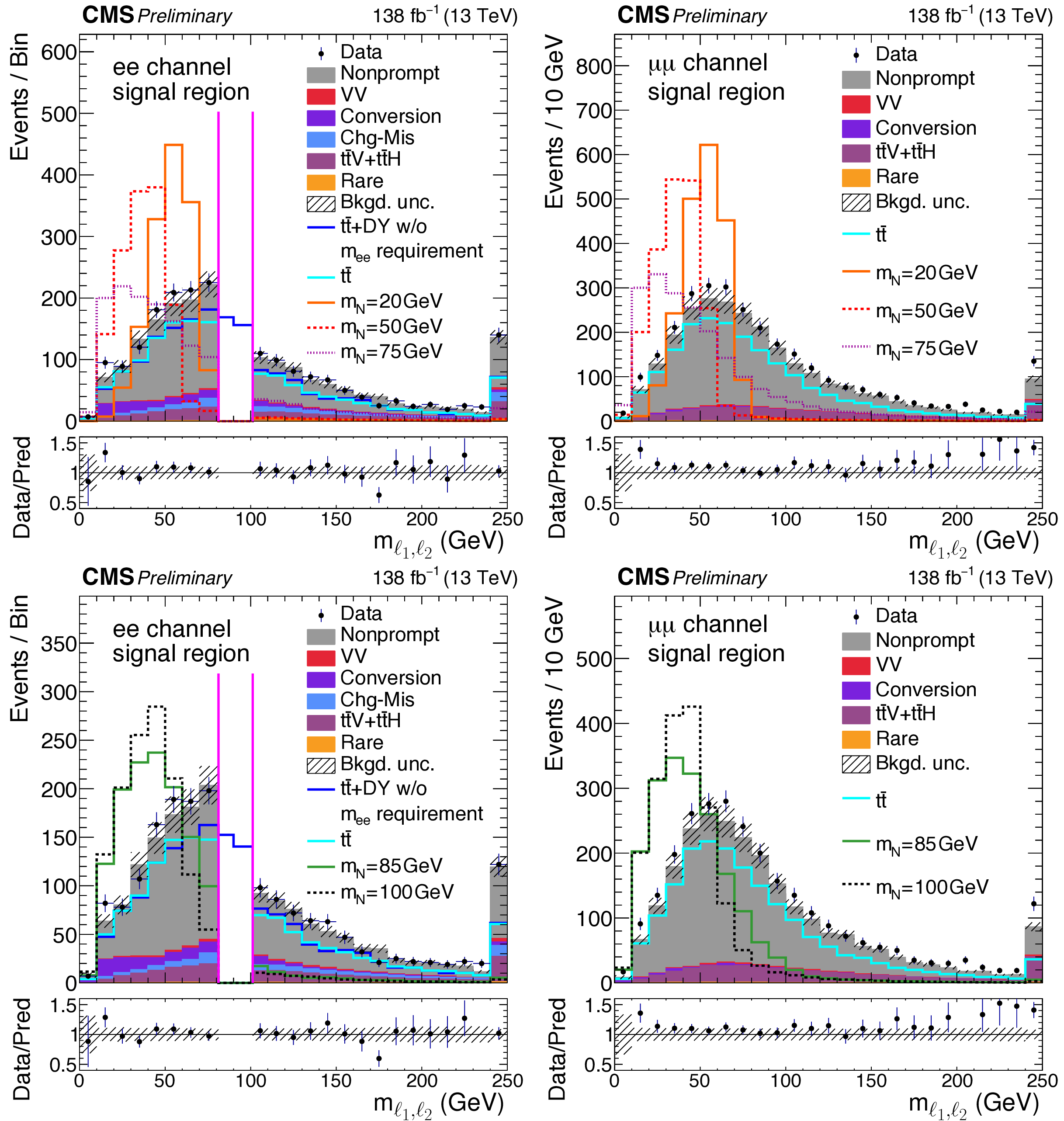
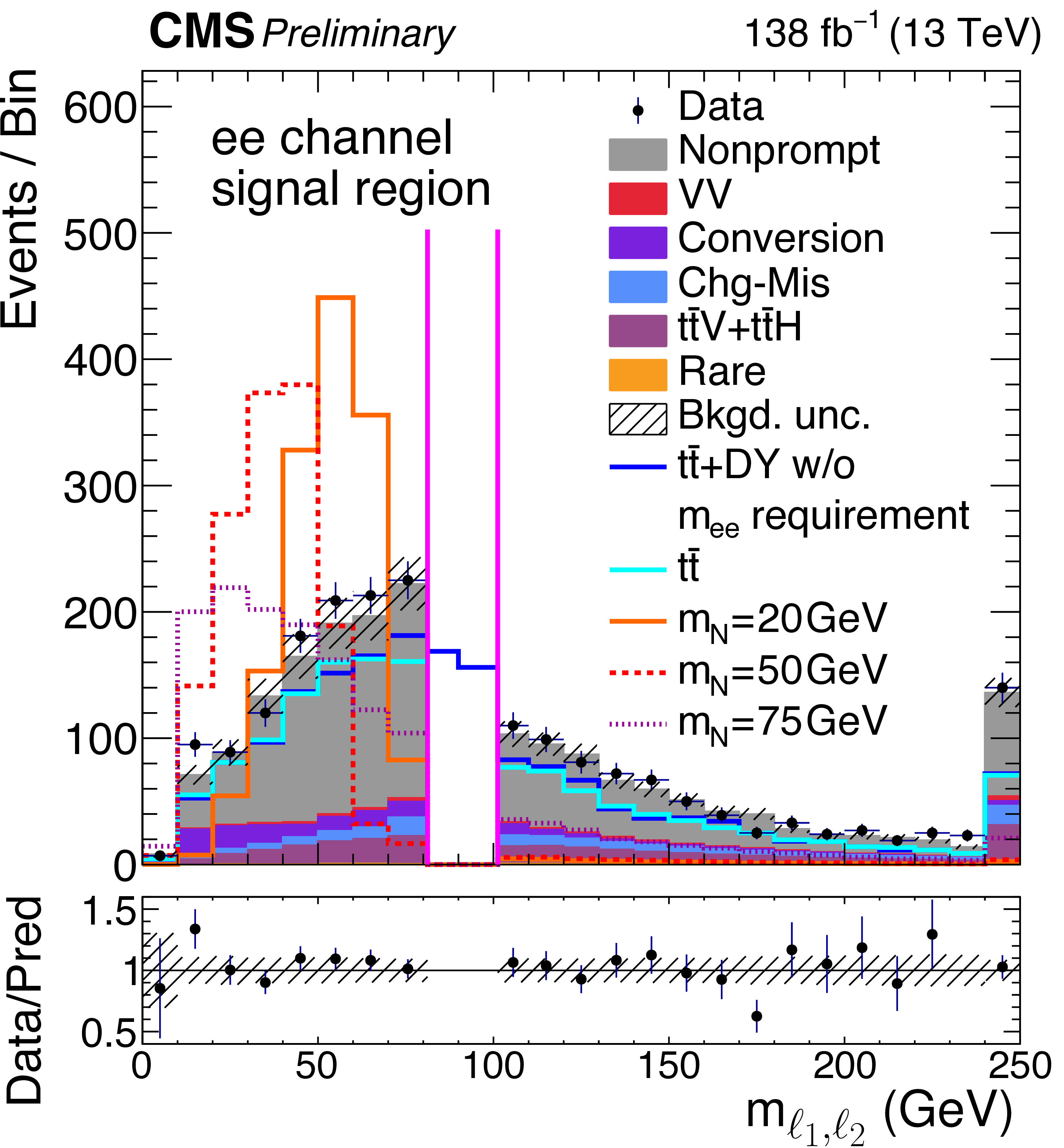
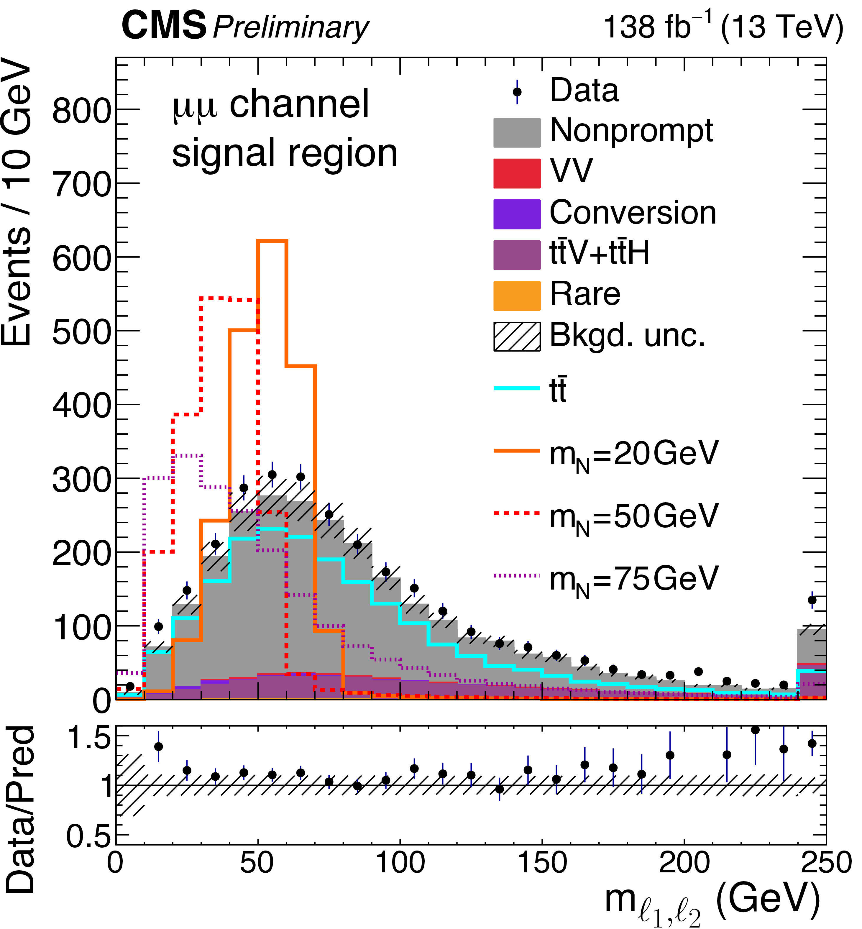
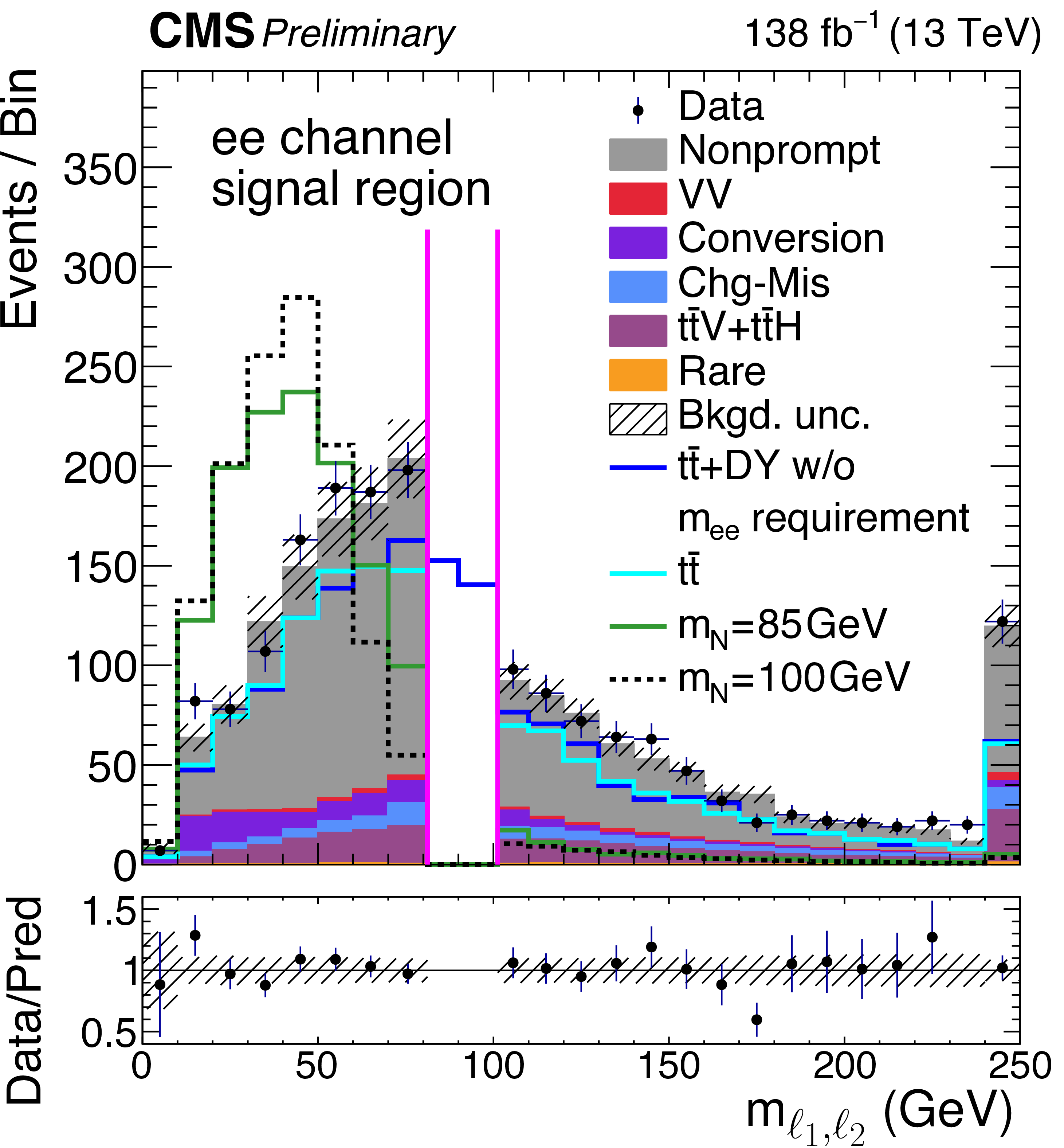
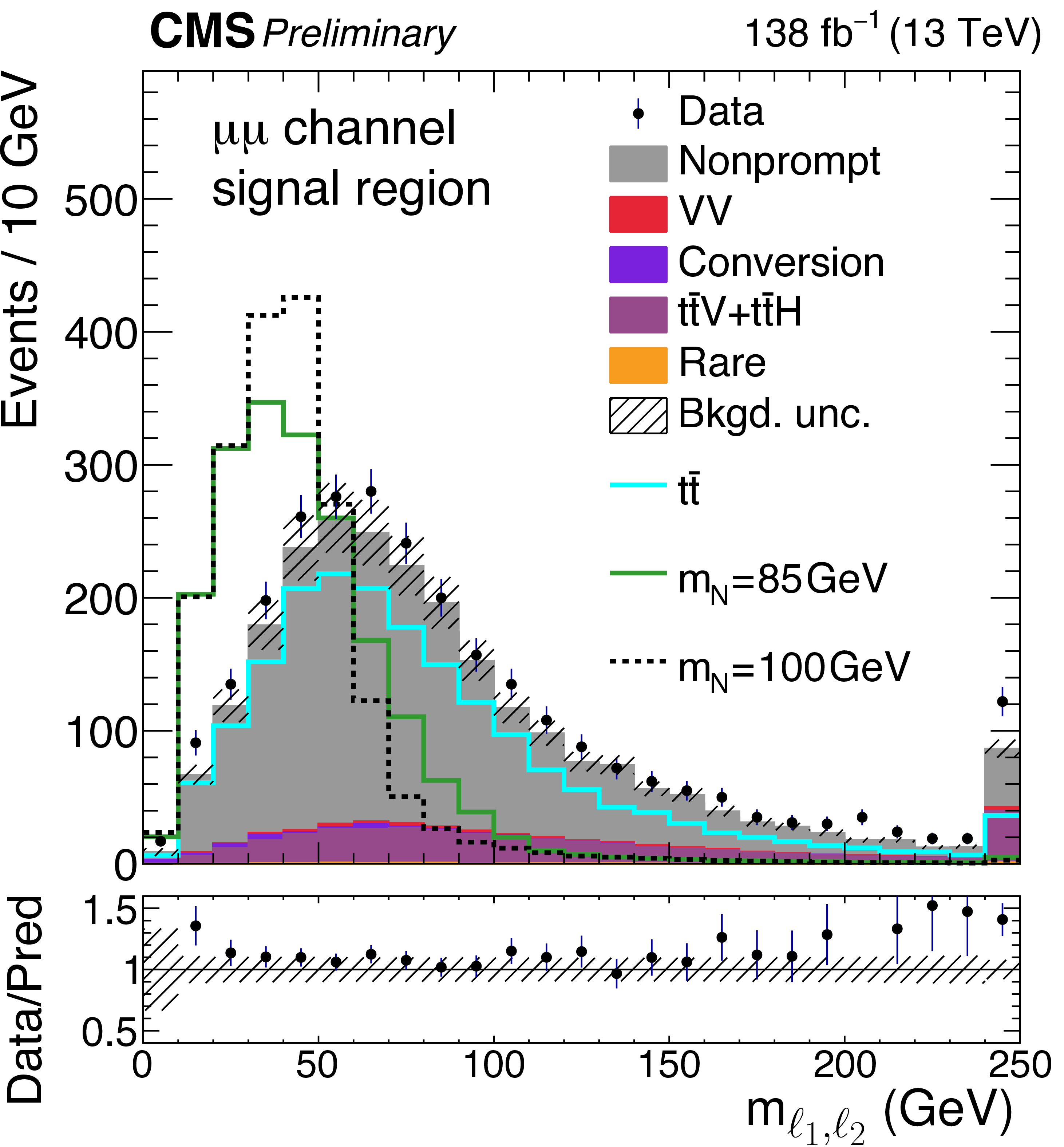
Pre$ \text{-} $fit distributions of theinvariant mass of two leptons are shown in dielectron (left) and dimuon (right) events as examples of the input variables for the training. The top row and the bottom row correspond to the $ m_{\mathrm{N}} < m_{\mathrm{W}} $ selection and the $ m_{\mathrm{N}} > m_{\mathrm{W}} $ selection, respectively, which differ in the required number of untagged jets. The cyan line is the $ \mathrm{t} \overline{\mathrm{t}} $ simulation used for the training background. Signal distributions are normalized to the background rate. The region between two magenta lines depicts what is removed from $ |m_{\mathrm{e}\mathrm{e}}-91.2| > $ 10 GeV requirement in the dielectron channel. The blue line is the $ \mathrm{t} \overline{\mathrm{t}} $ simulation and DY simulation combined without $ |m_{\mathrm{e}\mathrm{e}}-91.2| > $ 10 GeV requirement. In order to match the $ |m_{\mathrm{e}\mathrm{e}}-91.2| > $ 10 GeV requirement to the bin edges, the plots on the left have the bin size of 10 GeV, except for the [70,81.2] and [101.2,110] GeV bins. The background uncertainty band shows the total uncertainty including systematics. |
png pdf |
Figure 3-a:
Pre$ \text{-} $fit distributions of theinvariant mass of two leptons are shown in dielectron (left) and dimuon (right) events as examples of the input variables for the training. The top row and the bottom row correspond to the $ m_{\mathrm{N}} < m_{\mathrm{W}} $ selection and the $ m_{\mathrm{N}} > m_{\mathrm{W}} $ selection, respectively, which differ in the required number of untagged jets. The cyan line is the $ \mathrm{t} \overline{\mathrm{t}} $ simulation used for the training background. Signal distributions are normalized to the background rate. The region between two magenta lines depicts what is removed from $ |m_{\mathrm{e}\mathrm{e}}-91.2| > $ 10 GeV requirement in the dielectron channel. The blue line is the $ \mathrm{t} \overline{\mathrm{t}} $ simulation and DY simulation combined without $ |m_{\mathrm{e}\mathrm{e}}-91.2| > $ 10 GeV requirement. In order to match the $ |m_{\mathrm{e}\mathrm{e}}-91.2| > $ 10 GeV requirement to the bin edges, the plots on the left have the bin size of 10 GeV, except for the [70,81.2] and [101.2,110] GeV bins. The background uncertainty band shows the total uncertainty including systematics. |
png pdf |
Figure 3-b:
Pre$ \text{-} $fit distributions of theinvariant mass of two leptons are shown in dielectron (left) and dimuon (right) events as examples of the input variables for the training. The top row and the bottom row correspond to the $ m_{\mathrm{N}} < m_{\mathrm{W}} $ selection and the $ m_{\mathrm{N}} > m_{\mathrm{W}} $ selection, respectively, which differ in the required number of untagged jets. The cyan line is the $ \mathrm{t} \overline{\mathrm{t}} $ simulation used for the training background. Signal distributions are normalized to the background rate. The region between two magenta lines depicts what is removed from $ |m_{\mathrm{e}\mathrm{e}}-91.2| > $ 10 GeV requirement in the dielectron channel. The blue line is the $ \mathrm{t} \overline{\mathrm{t}} $ simulation and DY simulation combined without $ |m_{\mathrm{e}\mathrm{e}}-91.2| > $ 10 GeV requirement. In order to match the $ |m_{\mathrm{e}\mathrm{e}}-91.2| > $ 10 GeV requirement to the bin edges, the plots on the left have the bin size of 10 GeV, except for the [70,81.2] and [101.2,110] GeV bins. The background uncertainty band shows the total uncertainty including systematics. |
png pdf |
Figure 3-c:
Pre$ \text{-} $fit distributions of theinvariant mass of two leptons are shown in dielectron (left) and dimuon (right) events as examples of the input variables for the training. The top row and the bottom row correspond to the $ m_{\mathrm{N}} < m_{\mathrm{W}} $ selection and the $ m_{\mathrm{N}} > m_{\mathrm{W}} $ selection, respectively, which differ in the required number of untagged jets. The cyan line is the $ \mathrm{t} \overline{\mathrm{t}} $ simulation used for the training background. Signal distributions are normalized to the background rate. The region between two magenta lines depicts what is removed from $ |m_{\mathrm{e}\mathrm{e}}-91.2| > $ 10 GeV requirement in the dielectron channel. The blue line is the $ \mathrm{t} \overline{\mathrm{t}} $ simulation and DY simulation combined without $ |m_{\mathrm{e}\mathrm{e}}-91.2| > $ 10 GeV requirement. In order to match the $ |m_{\mathrm{e}\mathrm{e}}-91.2| > $ 10 GeV requirement to the bin edges, the plots on the left have the bin size of 10 GeV, except for the [70,81.2] and [101.2,110] GeV bins. The background uncertainty band shows the total uncertainty including systematics. |
png pdf |
Figure 3-d:
Pre$ \text{-} $fit distributions of theinvariant mass of two leptons are shown in dielectron (left) and dimuon (right) events as examples of the input variables for the training. The top row and the bottom row correspond to the $ m_{\mathrm{N}} < m_{\mathrm{W}} $ selection and the $ m_{\mathrm{N}} > m_{\mathrm{W}} $ selection, respectively, which differ in the required number of untagged jets. The cyan line is the $ \mathrm{t} \overline{\mathrm{t}} $ simulation used for the training background. Signal distributions are normalized to the background rate. The region between two magenta lines depicts what is removed from $ |m_{\mathrm{e}\mathrm{e}}-91.2| > $ 10 GeV requirement in the dielectron channel. The blue line is the $ \mathrm{t} \overline{\mathrm{t}} $ simulation and DY simulation combined without $ |m_{\mathrm{e}\mathrm{e}}-91.2| > $ 10 GeV requirement. In order to match the $ |m_{\mathrm{e}\mathrm{e}}-91.2| > $ 10 GeV requirement to the bin edges, the plots on the left have the bin size of 10 GeV, except for the [70,81.2] and [101.2,110] GeV bins. The background uncertainty band shows the total uncertainty including systematics. |
png pdf |
Figure 4:
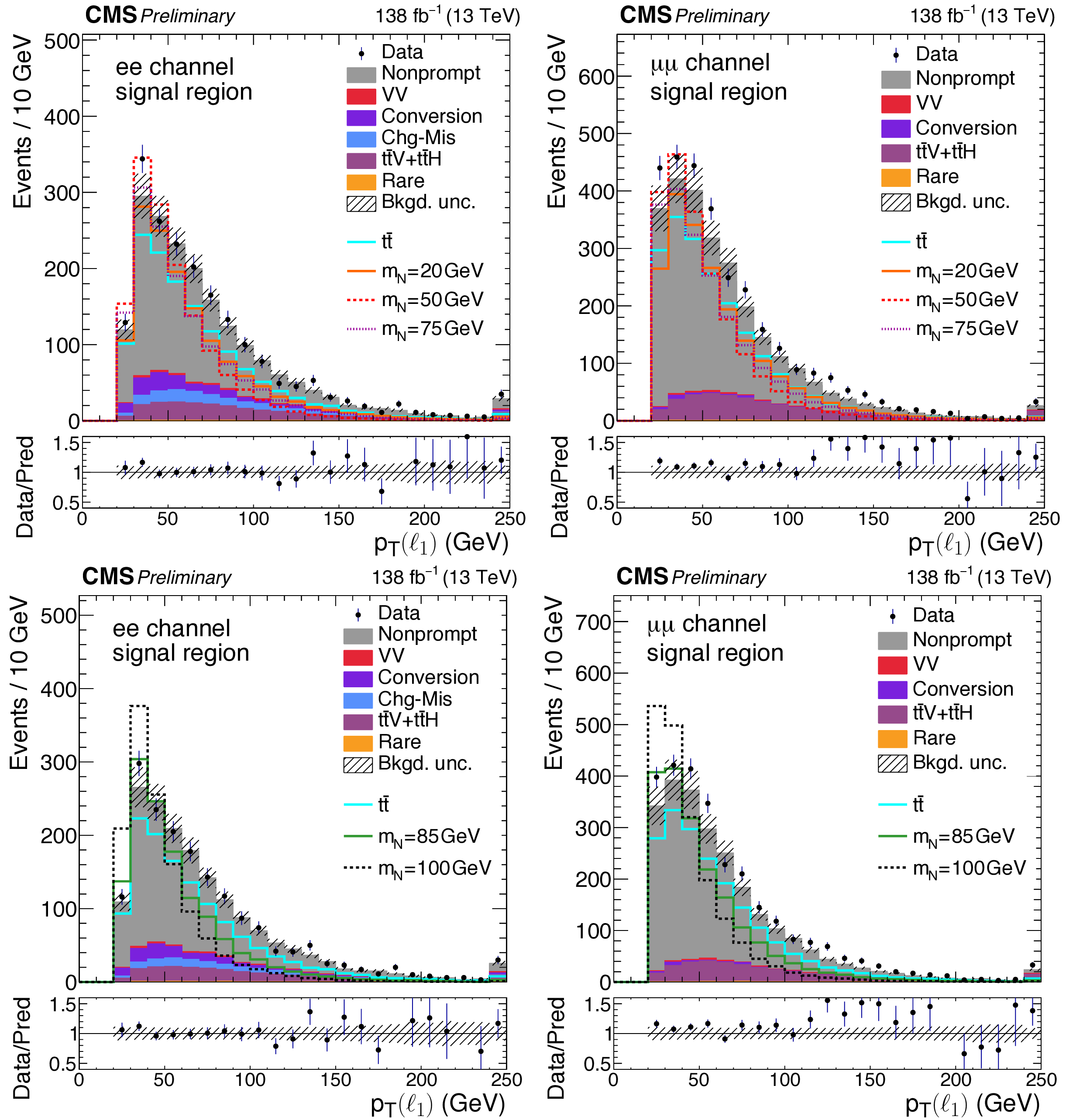
Pre$ \text{-} $fit distributions of the leading lepton transverse momentum are shown in dielectron (left) and dimuon (right) events as examples of the input variables for the training. The top row and the bottom row correspond to the $ m_{\mathrm{N}} < m_{\mathrm{W}} $ selection and the $ m_{\mathrm{N}} > m_{\mathrm{W}} $ selection, respectively, which differ in the required number of untagged jets. The cyan line is the $ \mathrm{t} \overline{\mathrm{t}} $ simulation used for the training background. Signal distributions are normalized to the background rate. The background uncertainty band shows the total uncertainty including systematics. |
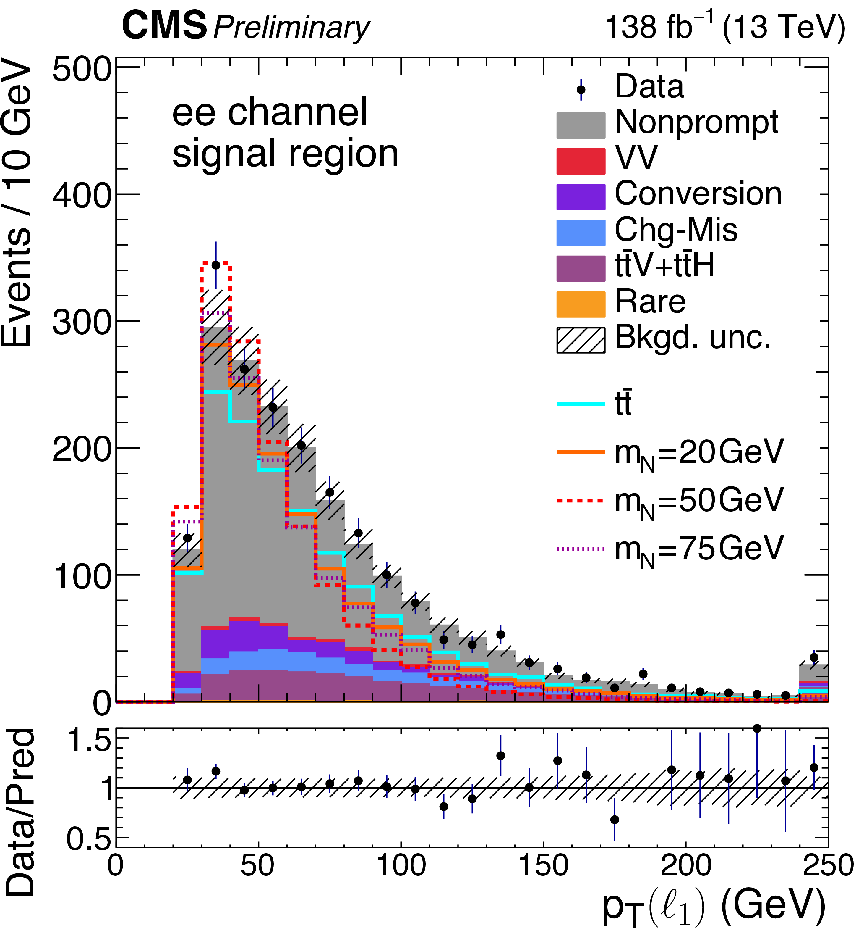
png pdf |
Figure 4-a:
Pre$ \text{-} $fit distributions of the leading lepton transverse momentum are shown in dielectron (left) and dimuon (right) events as examples of the input variables for the training. The top row and the bottom row correspond to the $ m_{\mathrm{N}} < m_{\mathrm{W}} $ selection and the $ m_{\mathrm{N}} > m_{\mathrm{W}} $ selection, respectively, which differ in the required number of untagged jets. The cyan line is the $ \mathrm{t} \overline{\mathrm{t}} $ simulation used for the training background. Signal distributions are normalized to the background rate. The background uncertainty band shows the total uncertainty including systematics. |
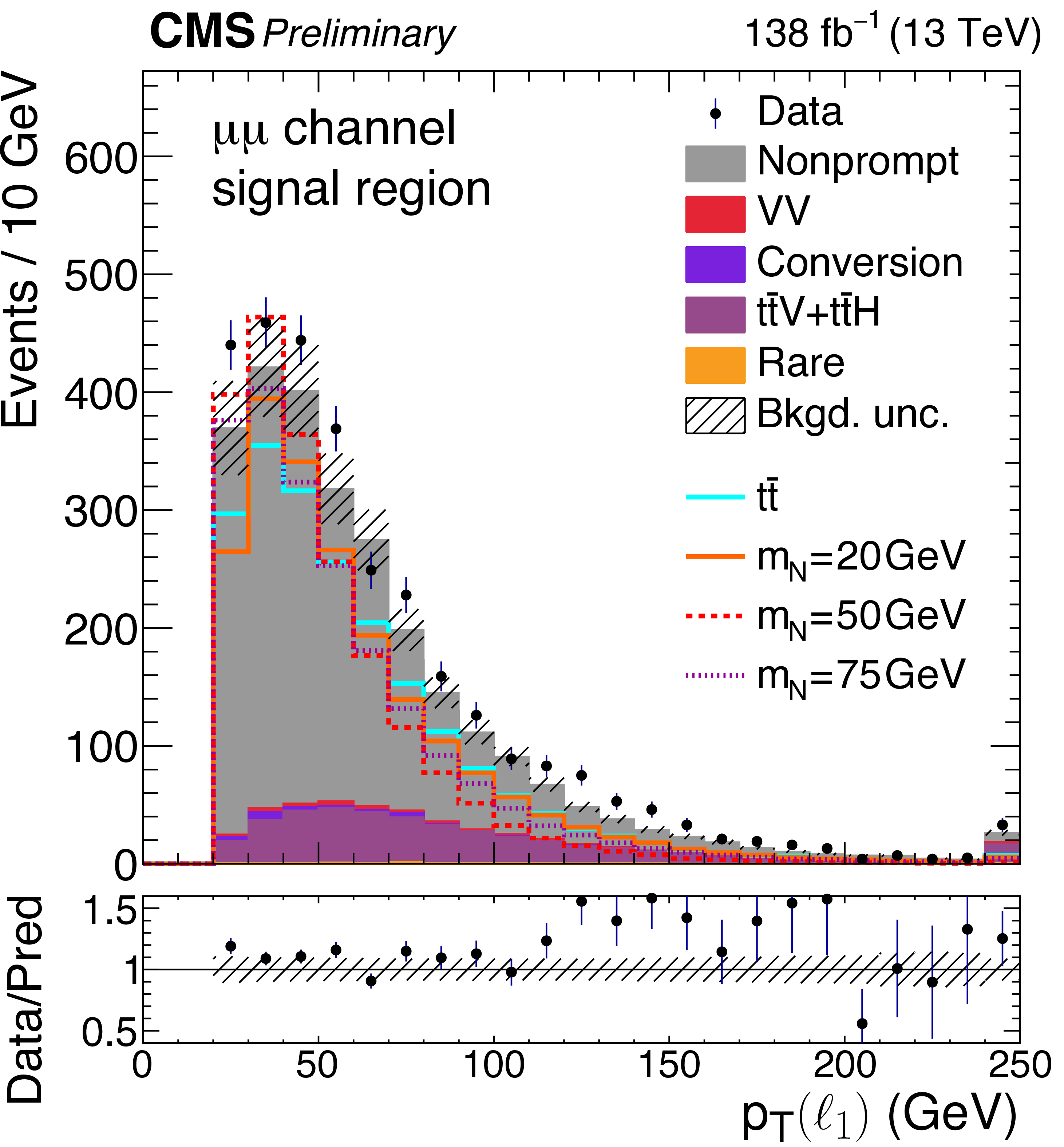
png pdf |
Figure 4-b:
Pre$ \text{-} $fit distributions of the leading lepton transverse momentum are shown in dielectron (left) and dimuon (right) events as examples of the input variables for the training. The top row and the bottom row correspond to the $ m_{\mathrm{N}} < m_{\mathrm{W}} $ selection and the $ m_{\mathrm{N}} > m_{\mathrm{W}} $ selection, respectively, which differ in the required number of untagged jets. The cyan line is the $ \mathrm{t} \overline{\mathrm{t}} $ simulation used for the training background. Signal distributions are normalized to the background rate. The background uncertainty band shows the total uncertainty including systematics. |
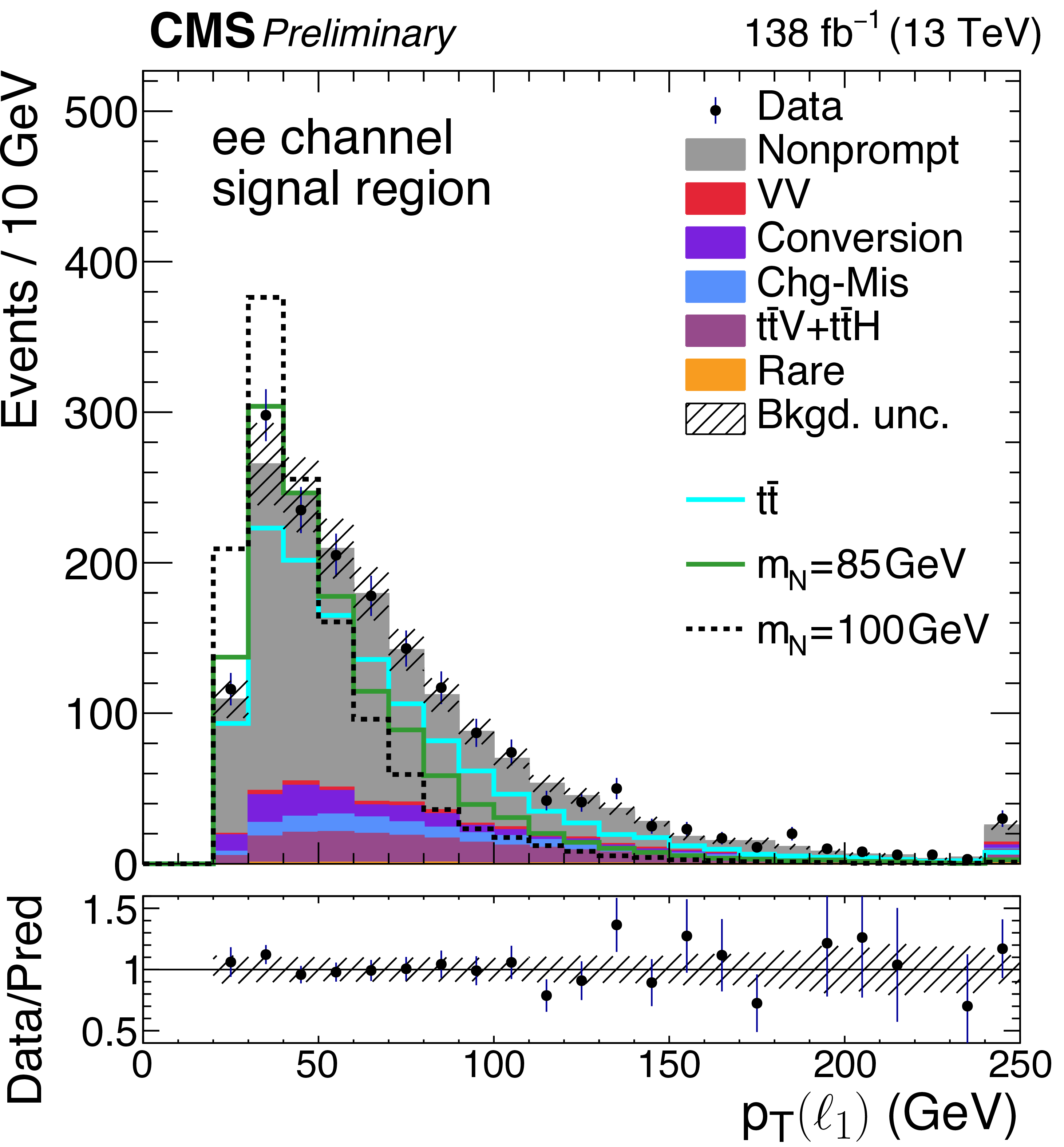
png pdf |
Figure 4-c:
Pre$ \text{-} $fit distributions of the leading lepton transverse momentum are shown in dielectron (left) and dimuon (right) events as examples of the input variables for the training. The top row and the bottom row correspond to the $ m_{\mathrm{N}} < m_{\mathrm{W}} $ selection and the $ m_{\mathrm{N}} > m_{\mathrm{W}} $ selection, respectively, which differ in the required number of untagged jets. The cyan line is the $ \mathrm{t} \overline{\mathrm{t}} $ simulation used for the training background. Signal distributions are normalized to the background rate. The background uncertainty band shows the total uncertainty including systematics. |
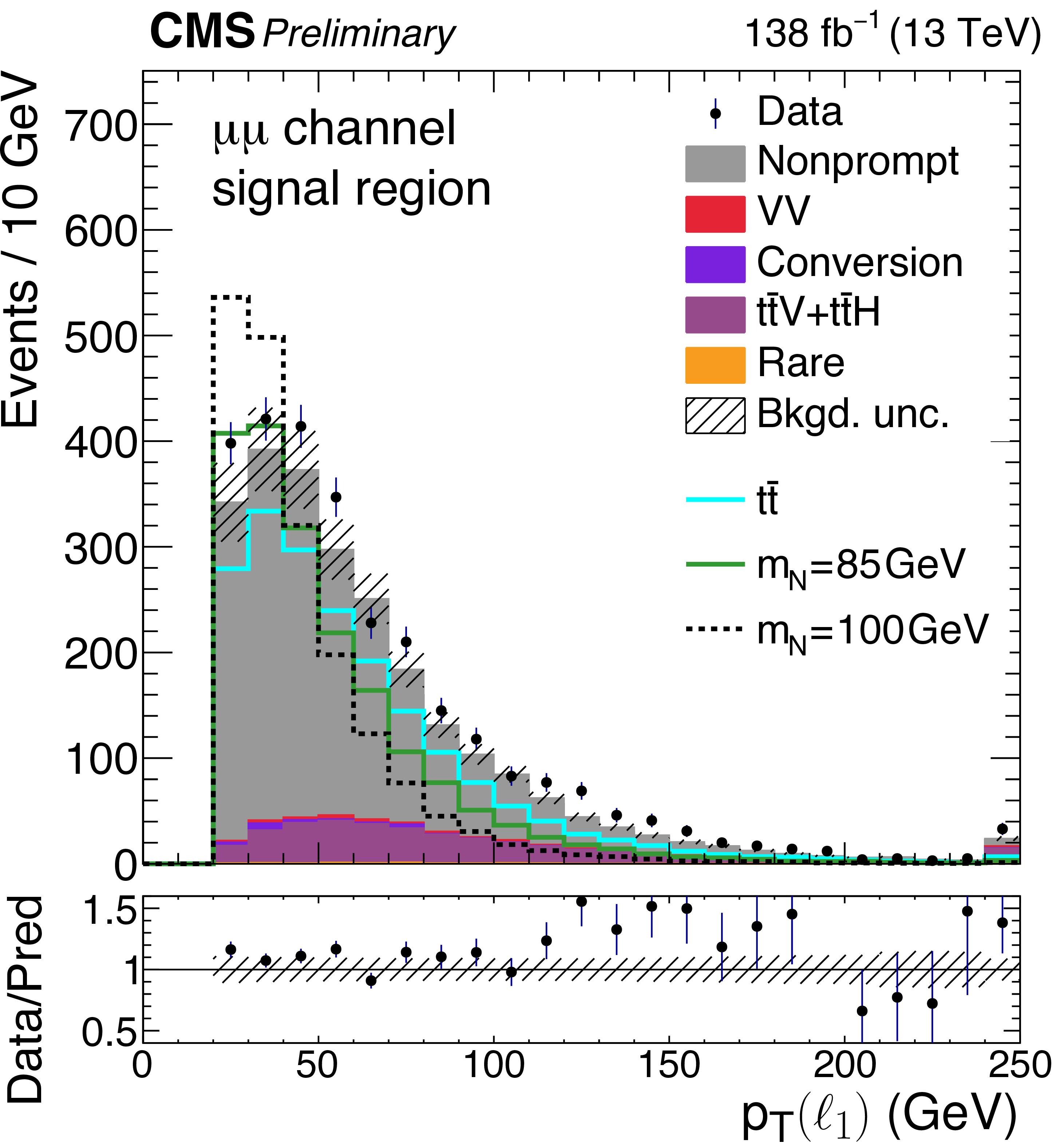
png pdf |
Figure 4-d:
Pre$ \text{-} $fit distributions of the leading lepton transverse momentum are shown in dielectron (left) and dimuon (right) events as examples of the input variables for the training. The top row and the bottom row correspond to the $ m_{\mathrm{N}} < m_{\mathrm{W}} $ selection and the $ m_{\mathrm{N}} > m_{\mathrm{W}} $ selection, respectively, which differ in the required number of untagged jets. The cyan line is the $ \mathrm{t} \overline{\mathrm{t}} $ simulation used for the training background. Signal distributions are normalized to the background rate. The background uncertainty band shows the total uncertainty including systematics. |
png pdf |
Figure 5:
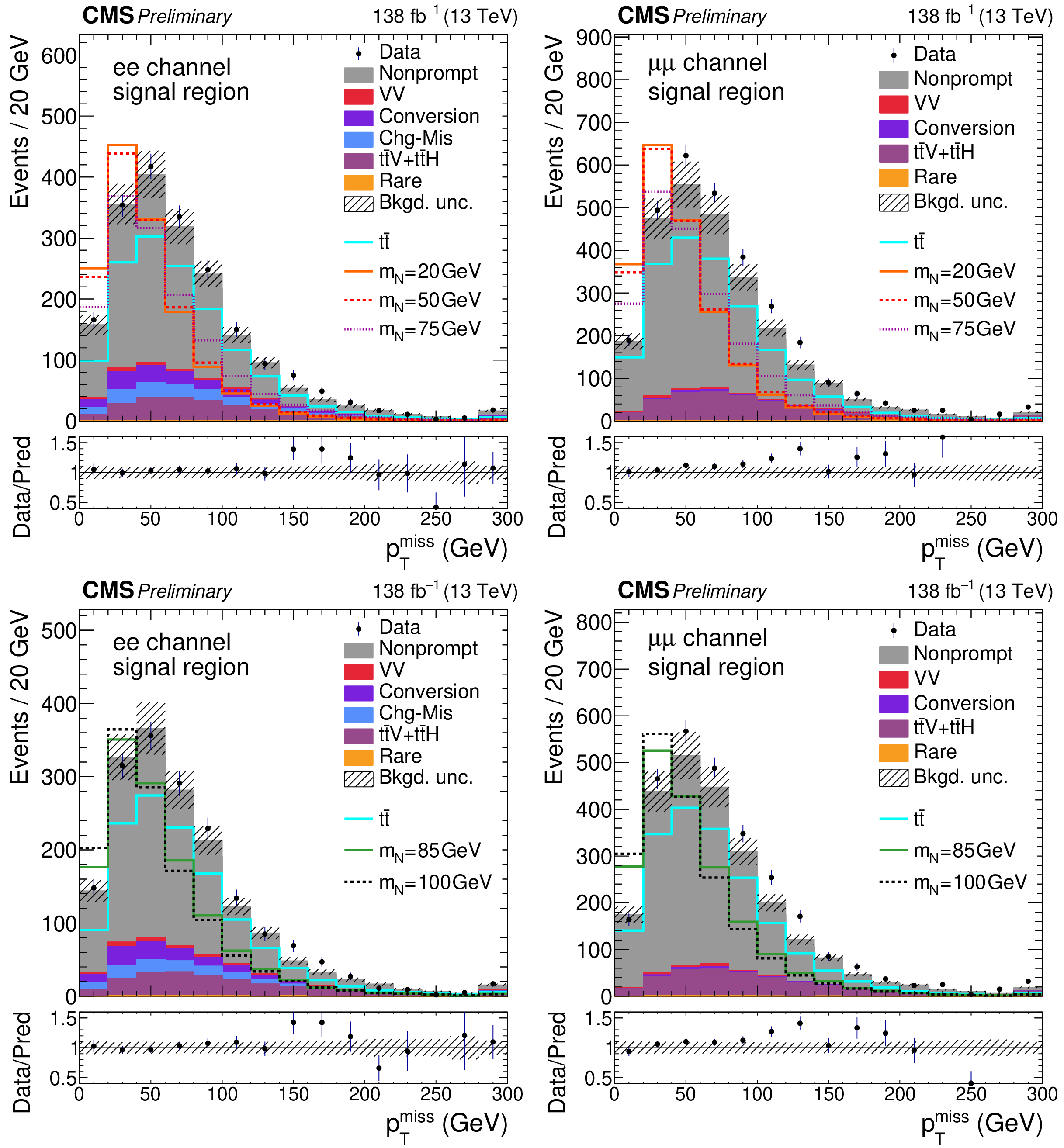
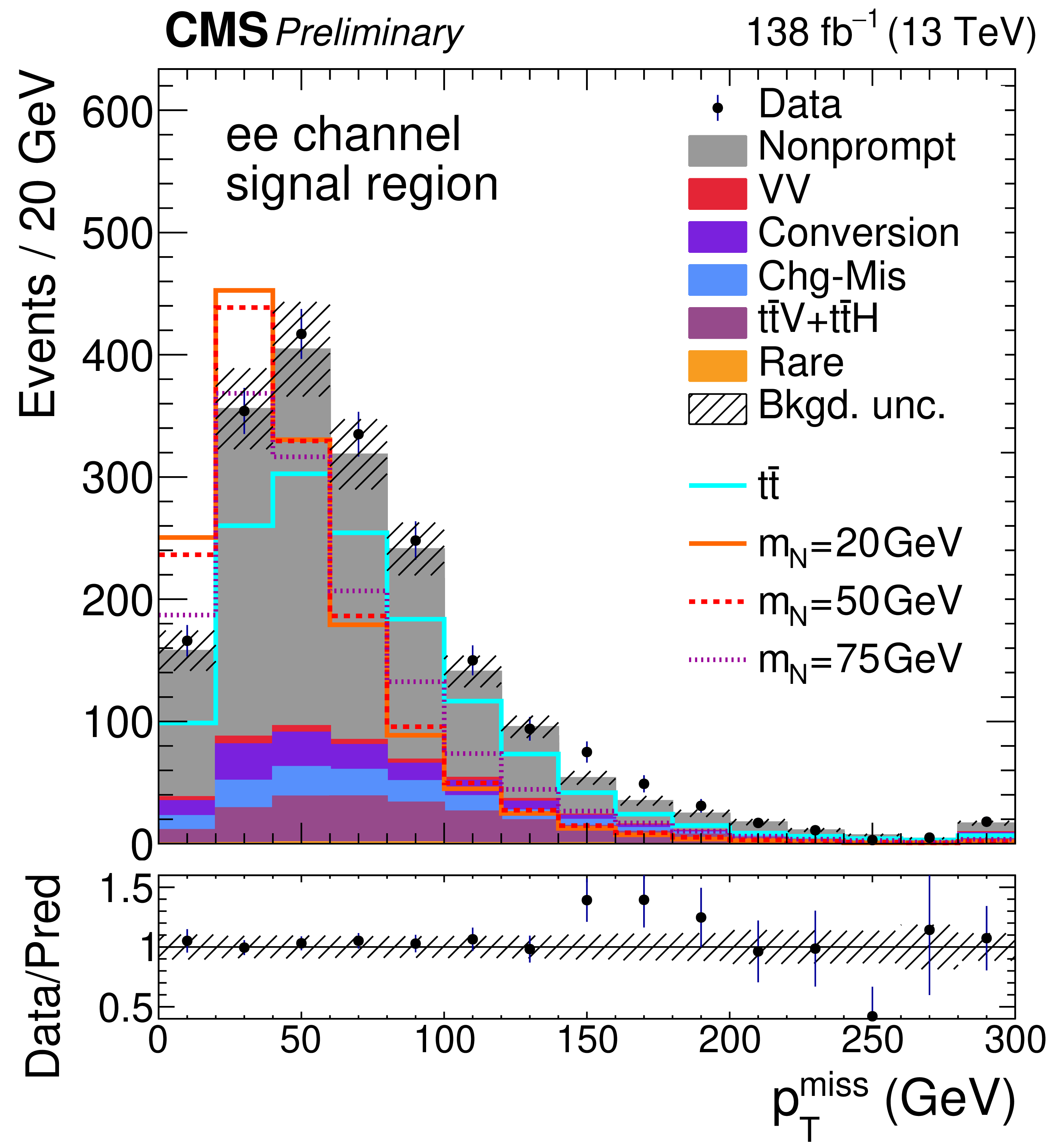
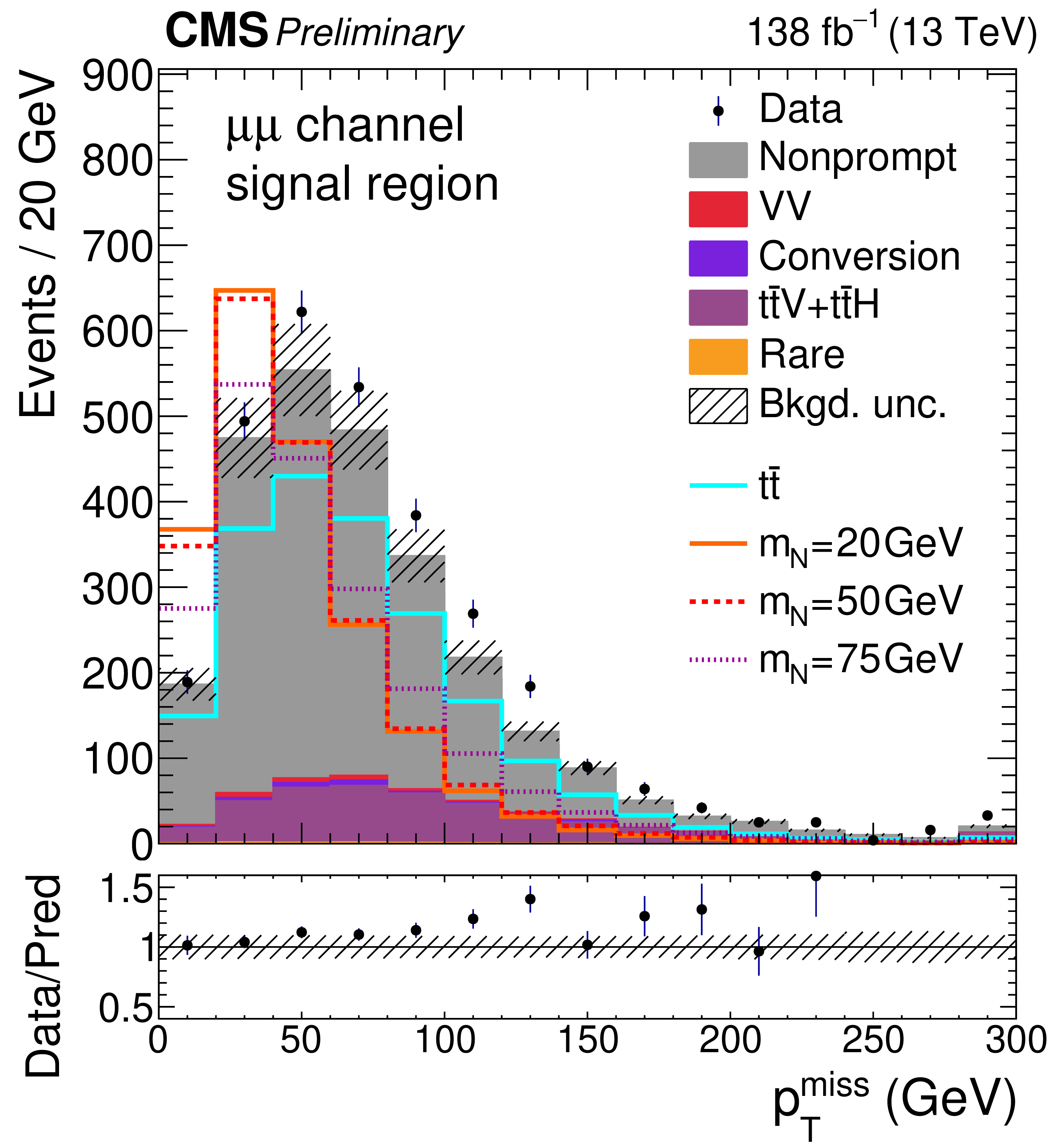
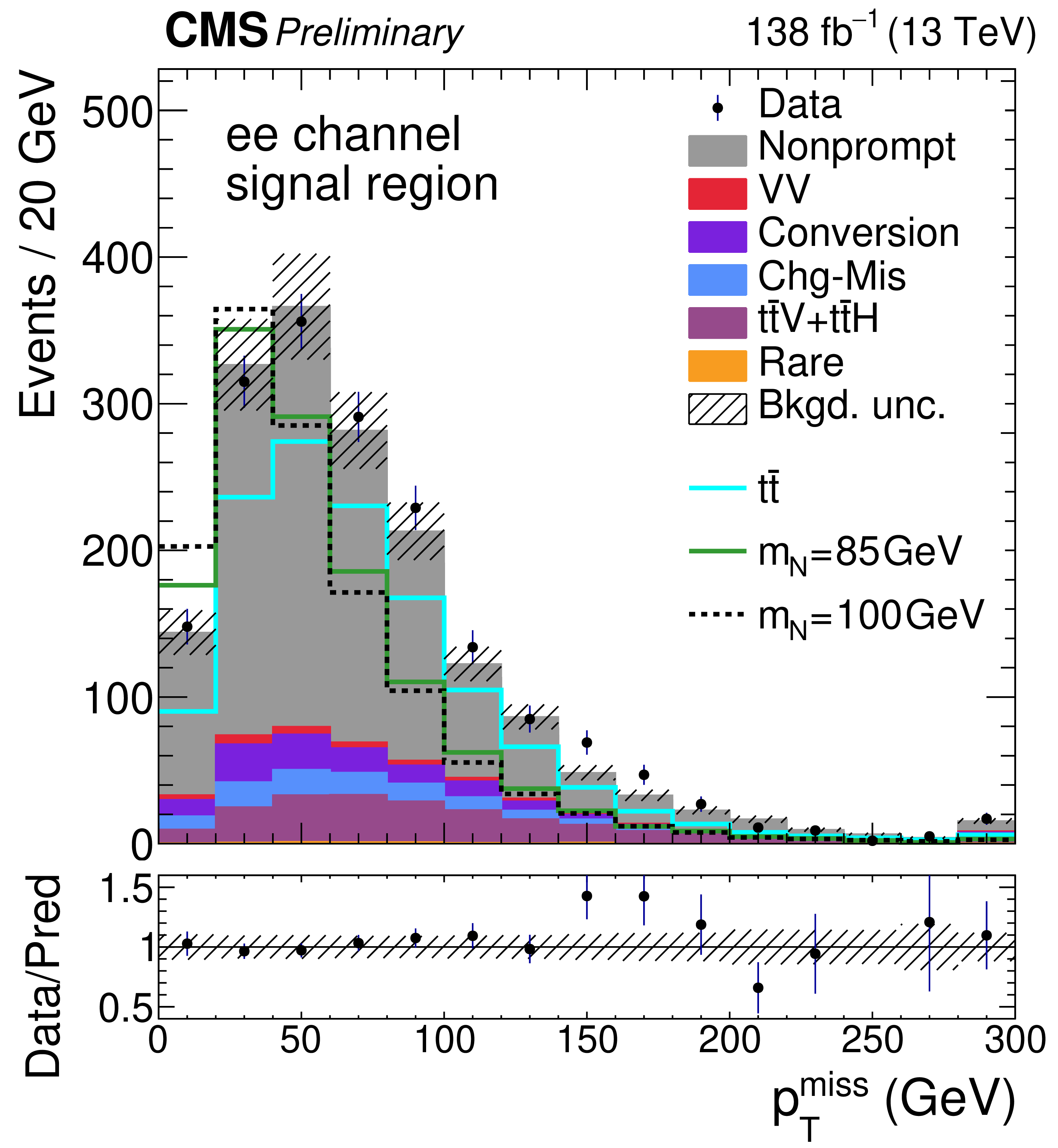
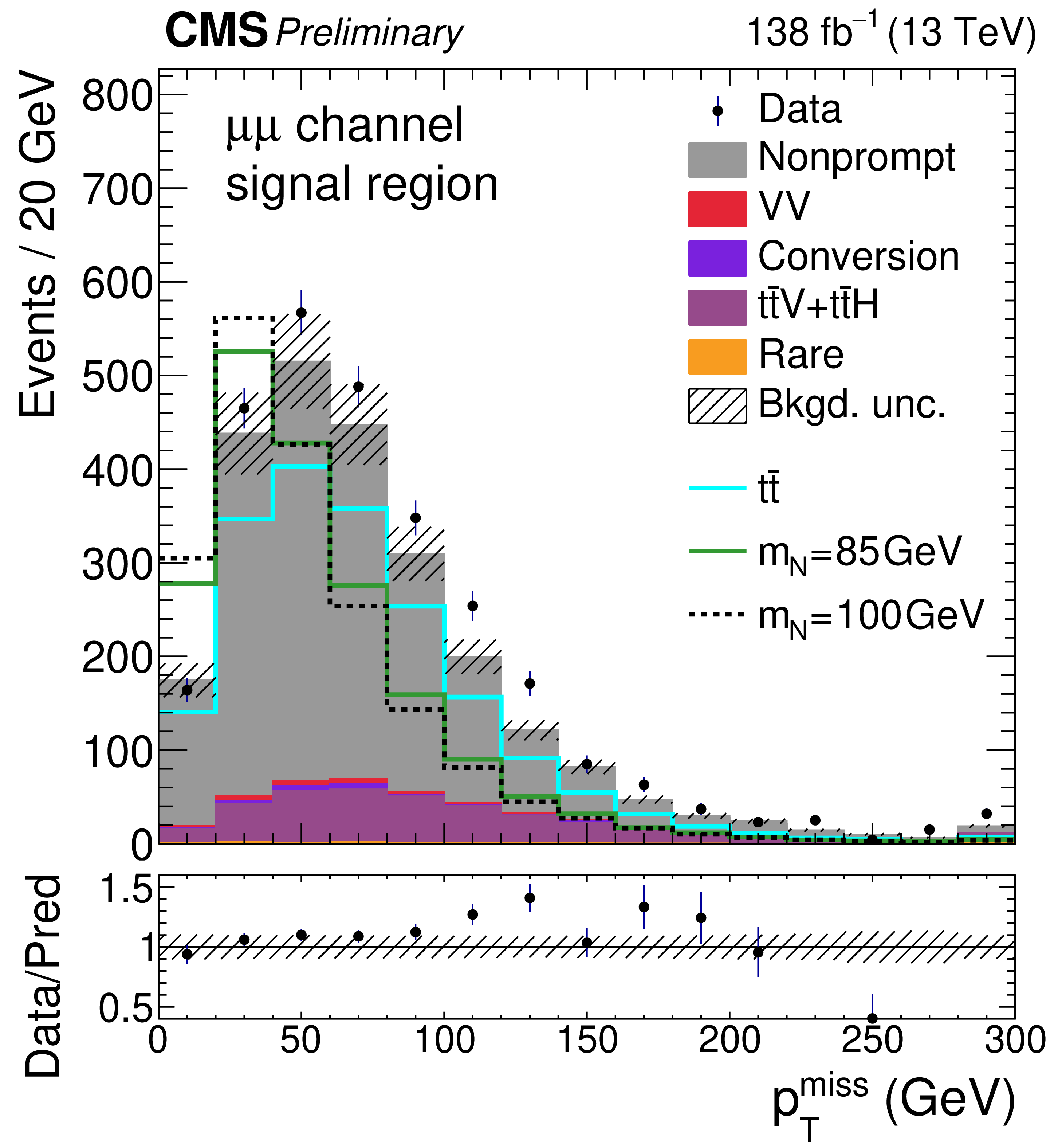
Pre$ \text{-} $fit distributions of themissing transverse momentum are shown in dielectron (left) and dimuon (right) events as examples of the input variables for the training. The top row and the bottom row correspond to the $ m_{\mathrm{N}} < m_{\mathrm{W}} $ selection and the $ m_{\mathrm{N}} > m_{\mathrm{W}} $ selection, respectively, which differ in the required number of untagged jets. The cyan line is the $ \mathrm{t} \overline{\mathrm{t}} $ simulation used for the training background. Signal distributions are normalized to the background rate. The background uncertainty band shows the total uncertainty including systematics. |
png pdf |
Figure 5-a:
Pre$ \text{-} $fit distributions of themissing transverse momentum are shown in dielectron (left) and dimuon (right) events as examples of the input variables for the training. The top row and the bottom row correspond to the $ m_{\mathrm{N}} < m_{\mathrm{W}} $ selection and the $ m_{\mathrm{N}} > m_{\mathrm{W}} $ selection, respectively, which differ in the required number of untagged jets. The cyan line is the $ \mathrm{t} \overline{\mathrm{t}} $ simulation used for the training background. Signal distributions are normalized to the background rate. The background uncertainty band shows the total uncertainty including systematics. |
png pdf |
Figure 5-b:
Pre$ \text{-} $fit distributions of themissing transverse momentum are shown in dielectron (left) and dimuon (right) events as examples of the input variables for the training. The top row and the bottom row correspond to the $ m_{\mathrm{N}} < m_{\mathrm{W}} $ selection and the $ m_{\mathrm{N}} > m_{\mathrm{W}} $ selection, respectively, which differ in the required number of untagged jets. The cyan line is the $ \mathrm{t} \overline{\mathrm{t}} $ simulation used for the training background. Signal distributions are normalized to the background rate. The background uncertainty band shows the total uncertainty including systematics. |
png pdf |
Figure 5-c:
Pre$ \text{-} $fit distributions of themissing transverse momentum are shown in dielectron (left) and dimuon (right) events as examples of the input variables for the training. The top row and the bottom row correspond to the $ m_{\mathrm{N}} < m_{\mathrm{W}} $ selection and the $ m_{\mathrm{N}} > m_{\mathrm{W}} $ selection, respectively, which differ in the required number of untagged jets. The cyan line is the $ \mathrm{t} \overline{\mathrm{t}} $ simulation used for the training background. Signal distributions are normalized to the background rate. The background uncertainty band shows the total uncertainty including systematics. |
png pdf |
Figure 5-d:
Pre$ \text{-} $fit distributions of themissing transverse momentum are shown in dielectron (left) and dimuon (right) events as examples of the input variables for the training. The top row and the bottom row correspond to the $ m_{\mathrm{N}} < m_{\mathrm{W}} $ selection and the $ m_{\mathrm{N}} > m_{\mathrm{W}} $ selection, respectively, which differ in the required number of untagged jets. The cyan line is the $ \mathrm{t} \overline{\mathrm{t}} $ simulation used for the training background. Signal distributions are normalized to the background rate. The background uncertainty band shows the total uncertainty including systematics. |
png pdf |
Figure 6:
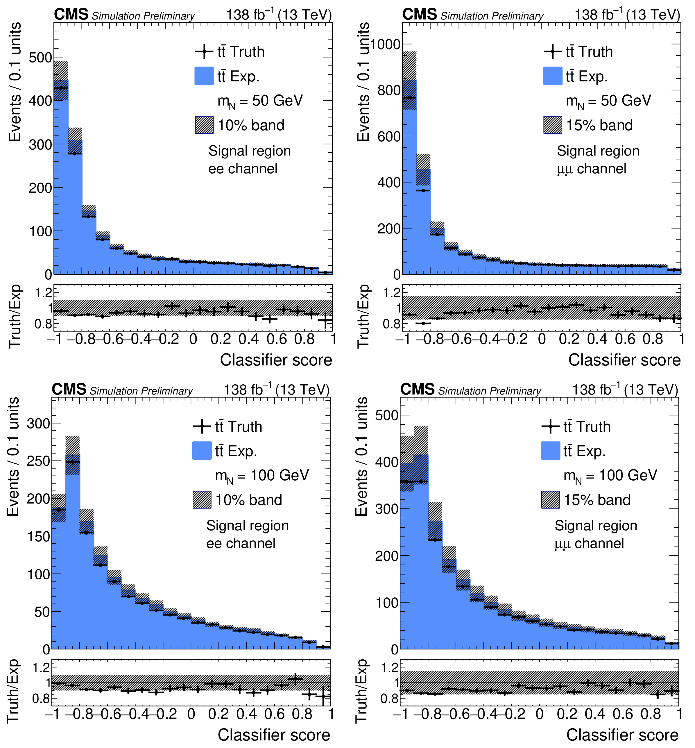
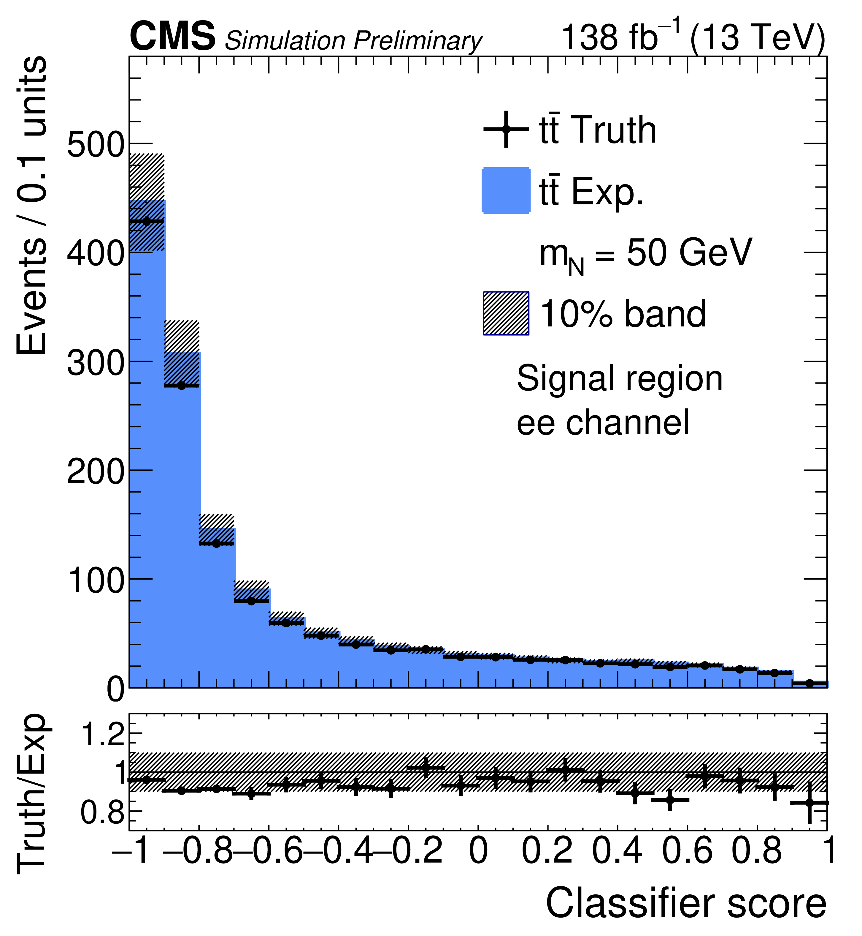
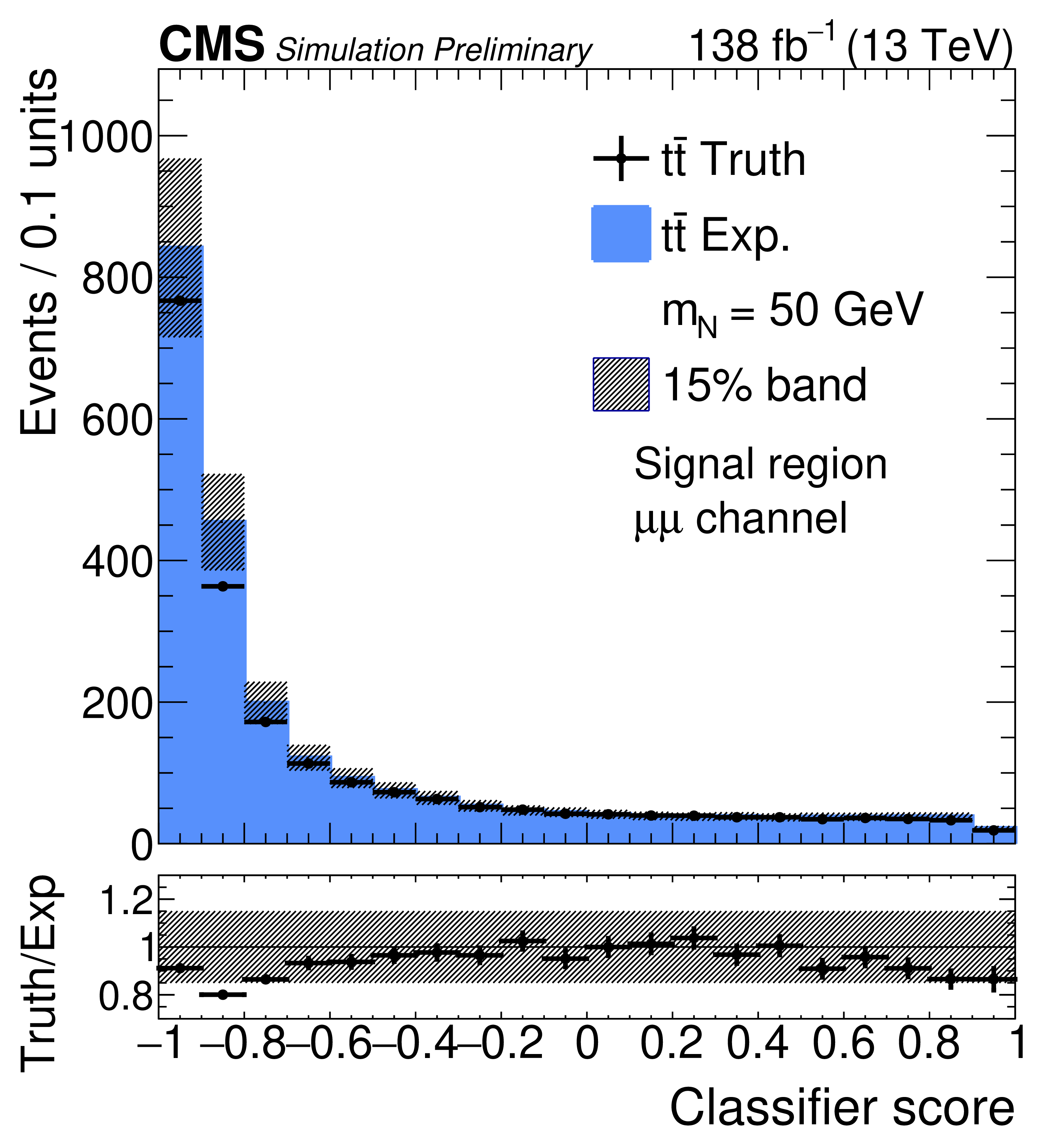
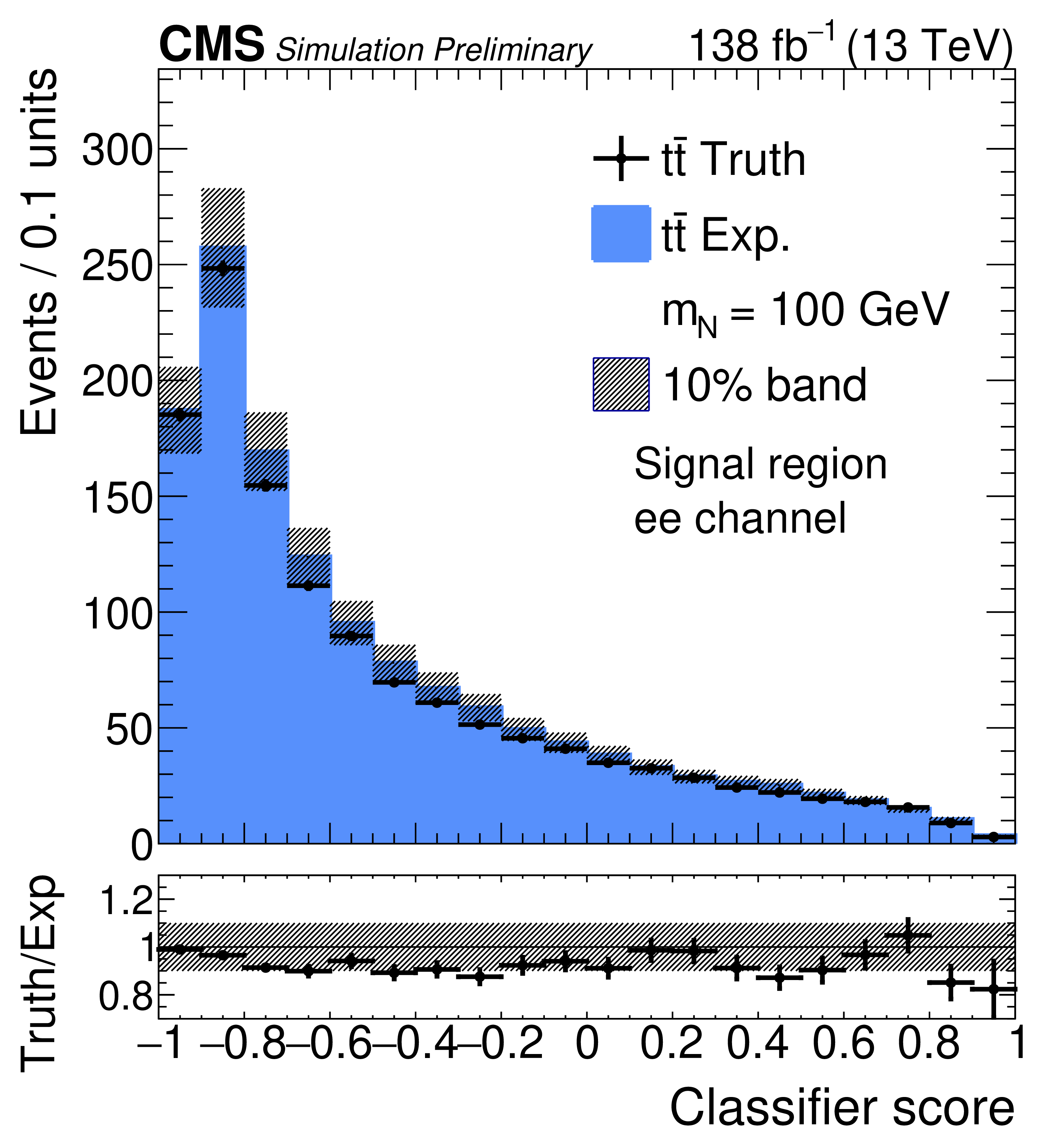
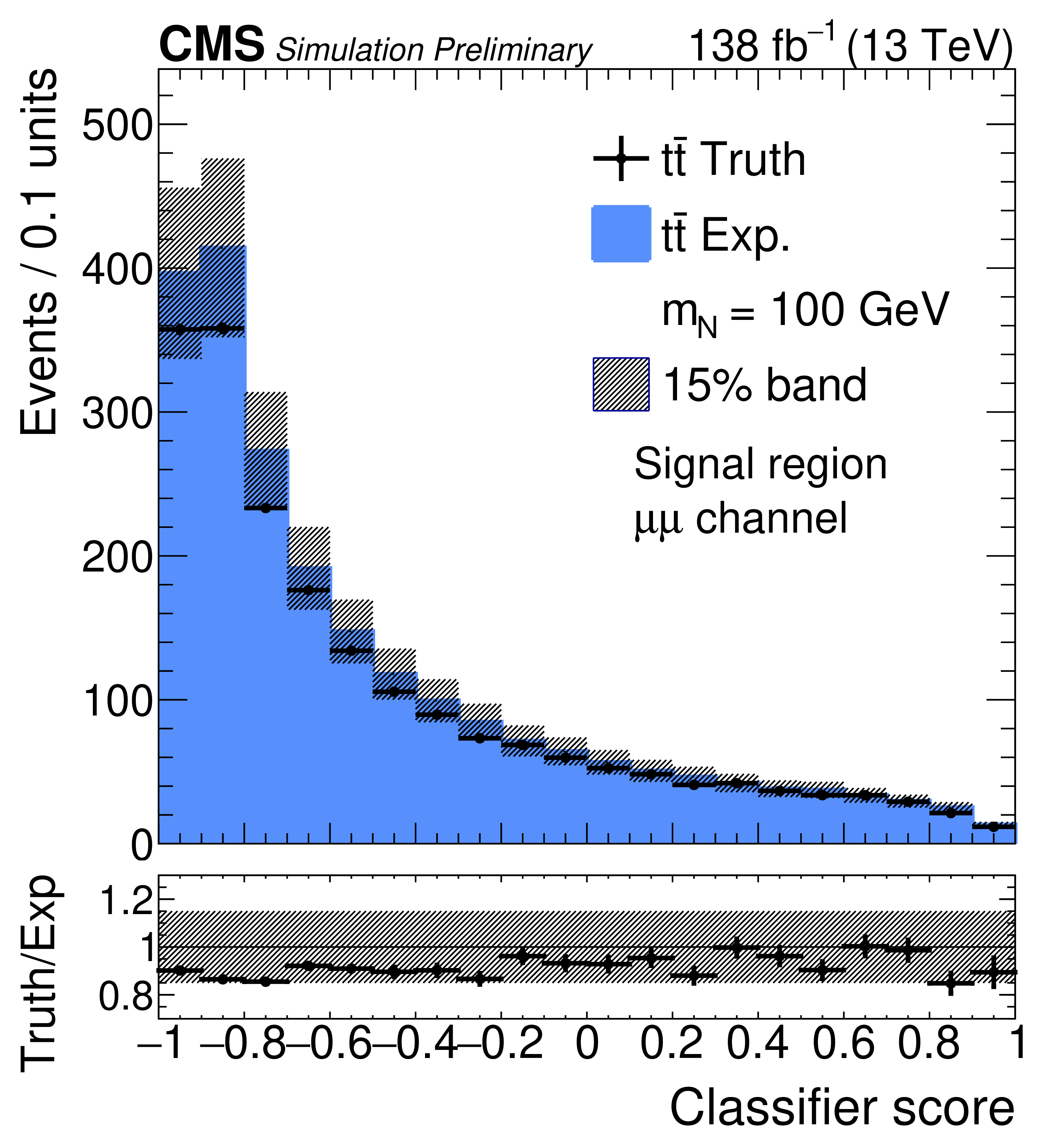
Comparison of BDTG classifier distributions between actual distribution of $ {\mathrm{t}\overline{\mathrm{t}}} $ simulation passing tight ID and expected distribution from $ {\mathrm{t}\overline{\mathrm{t}}} $ simulation dielectron (left) and dimuon (right) events in the sideband region and misidentification rate of QCD simulation with BDT model for $ m_{\mathrm{N}}= $ 50 GeV (top) and for $ m_{\mathrm{N}}= $ 100 GeV (bottom). Error bands include 10$ % $ (15$ % $) uncertainty for dielectron (dimuon) events. |
png pdf |
Figure 6-a:
Comparison of BDTG classifier distributions between actual distribution of $ {\mathrm{t}\overline{\mathrm{t}}} $ simulation passing tight ID and expected distribution from $ {\mathrm{t}\overline{\mathrm{t}}} $ simulation dielectron (left) and dimuon (right) events in the sideband region and misidentification rate of QCD simulation with BDT model for $ m_{\mathrm{N}}= $ 50 GeV (top) and for $ m_{\mathrm{N}}= $ 100 GeV (bottom). Error bands include 10$ % $ (15$ % $) uncertainty for dielectron (dimuon) events. |
png pdf |
Figure 6-b:
Comparison of BDTG classifier distributions between actual distribution of $ {\mathrm{t}\overline{\mathrm{t}}} $ simulation passing tight ID and expected distribution from $ {\mathrm{t}\overline{\mathrm{t}}} $ simulation dielectron (left) and dimuon (right) events in the sideband region and misidentification rate of QCD simulation with BDT model for $ m_{\mathrm{N}}= $ 50 GeV (top) and for $ m_{\mathrm{N}}= $ 100 GeV (bottom). Error bands include 10$ % $ (15$ % $) uncertainty for dielectron (dimuon) events. |
png pdf |
Figure 6-c:
Comparison of BDTG classifier distributions between actual distribution of $ {\mathrm{t}\overline{\mathrm{t}}} $ simulation passing tight ID and expected distribution from $ {\mathrm{t}\overline{\mathrm{t}}} $ simulation dielectron (left) and dimuon (right) events in the sideband region and misidentification rate of QCD simulation with BDT model for $ m_{\mathrm{N}}= $ 50 GeV (top) and for $ m_{\mathrm{N}}= $ 100 GeV (bottom). Error bands include 10$ % $ (15$ % $) uncertainty for dielectron (dimuon) events. |
png pdf |
Figure 6-d:
Comparison of BDTG classifier distributions between actual distribution of $ {\mathrm{t}\overline{\mathrm{t}}} $ simulation passing tight ID and expected distribution from $ {\mathrm{t}\overline{\mathrm{t}}} $ simulation dielectron (left) and dimuon (right) events in the sideband region and misidentification rate of QCD simulation with BDT model for $ m_{\mathrm{N}}= $ 50 GeV (top) and for $ m_{\mathrm{N}}= $ 100 GeV (bottom). Error bands include 10$ % $ (15$ % $) uncertainty for dielectron (dimuon) events. |
png pdf |
Figure 7:
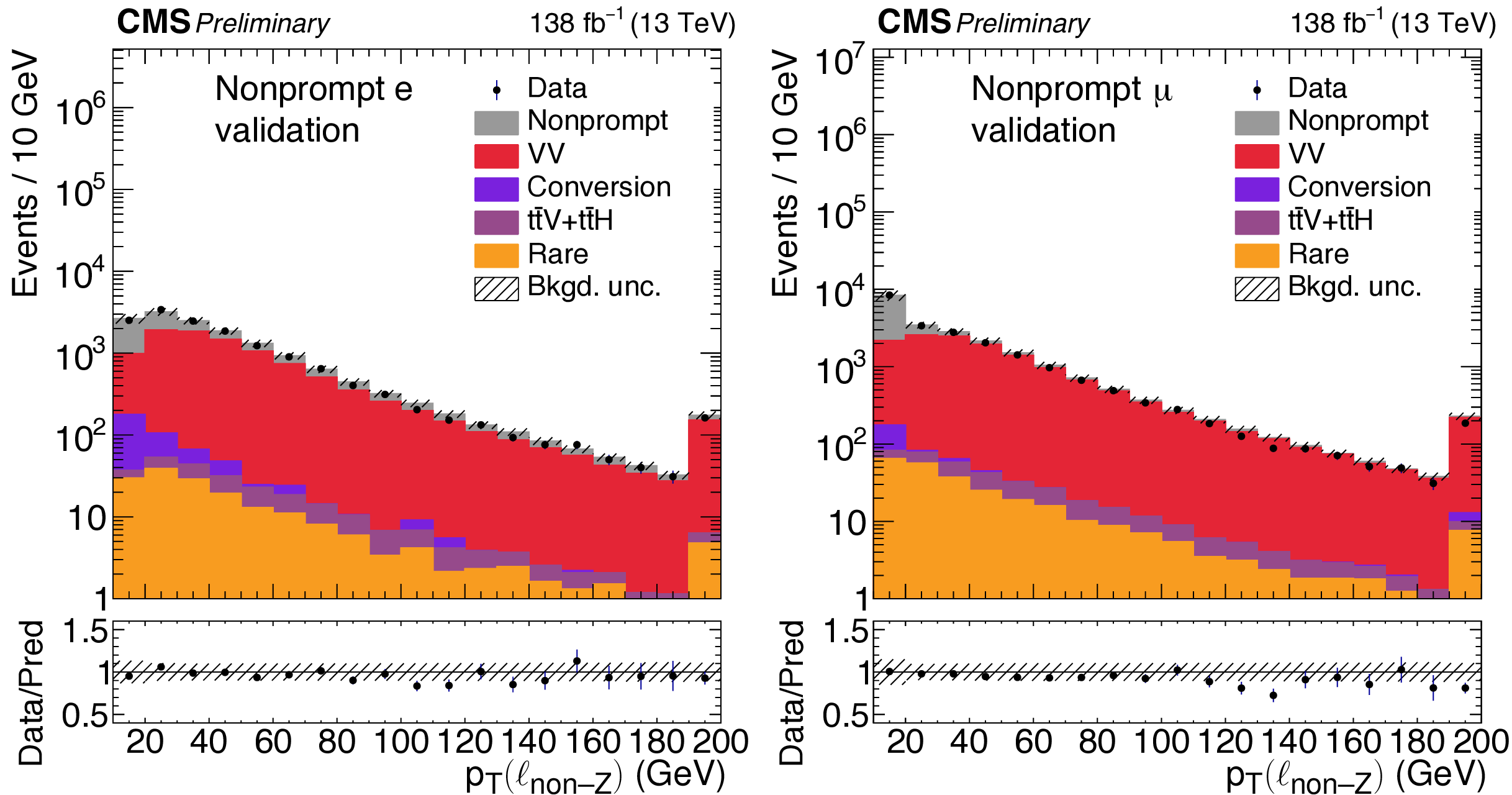
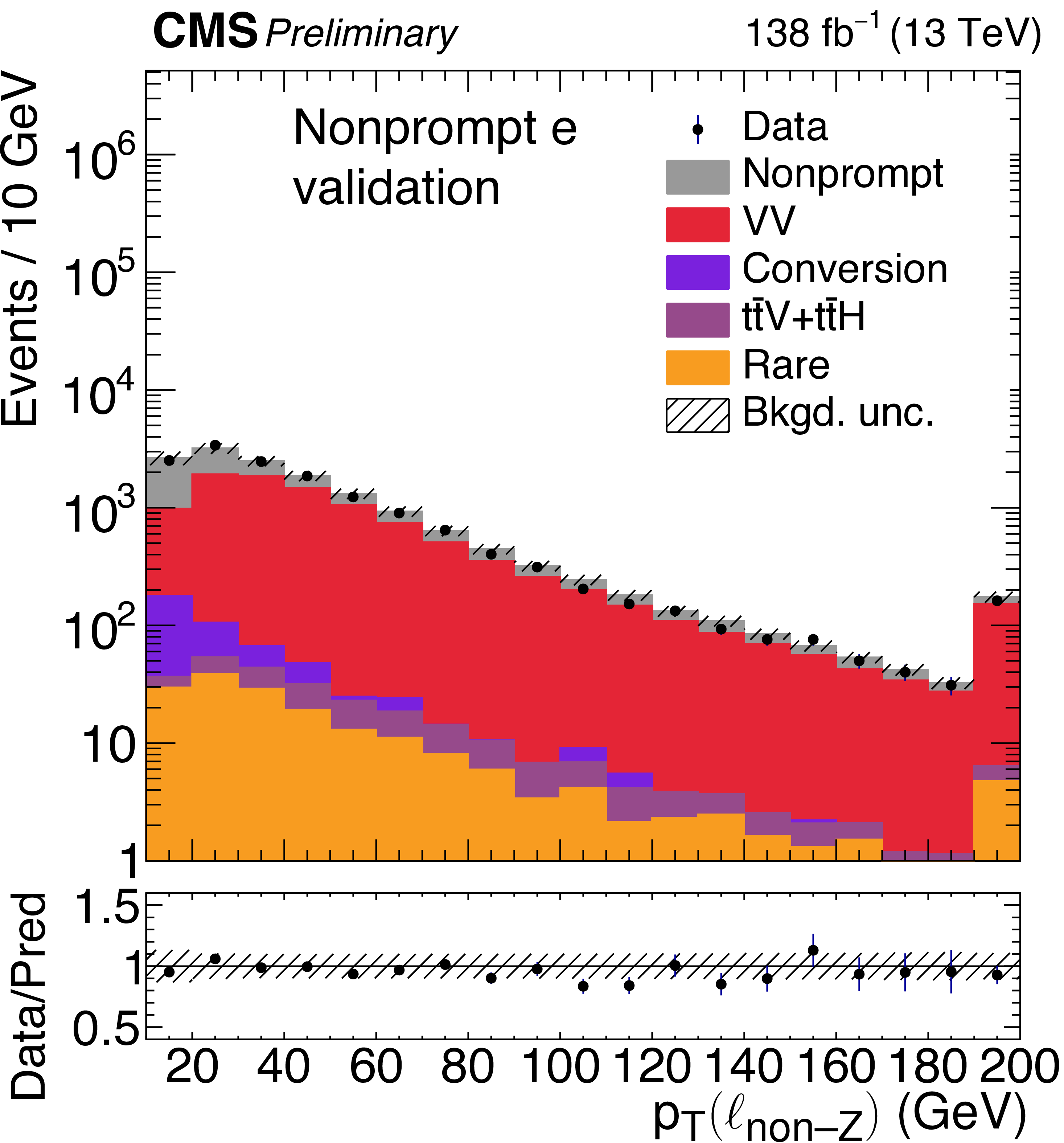
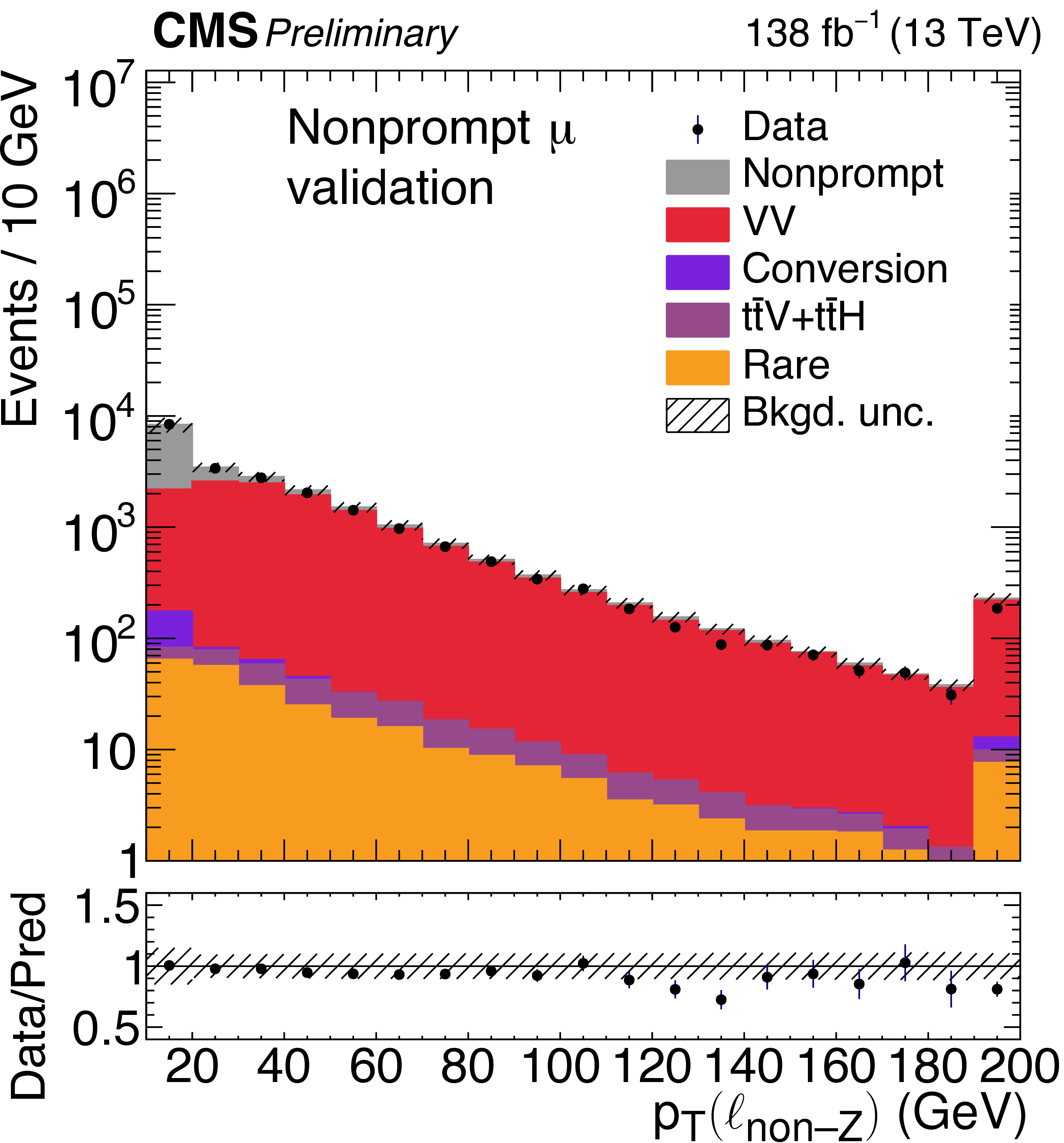
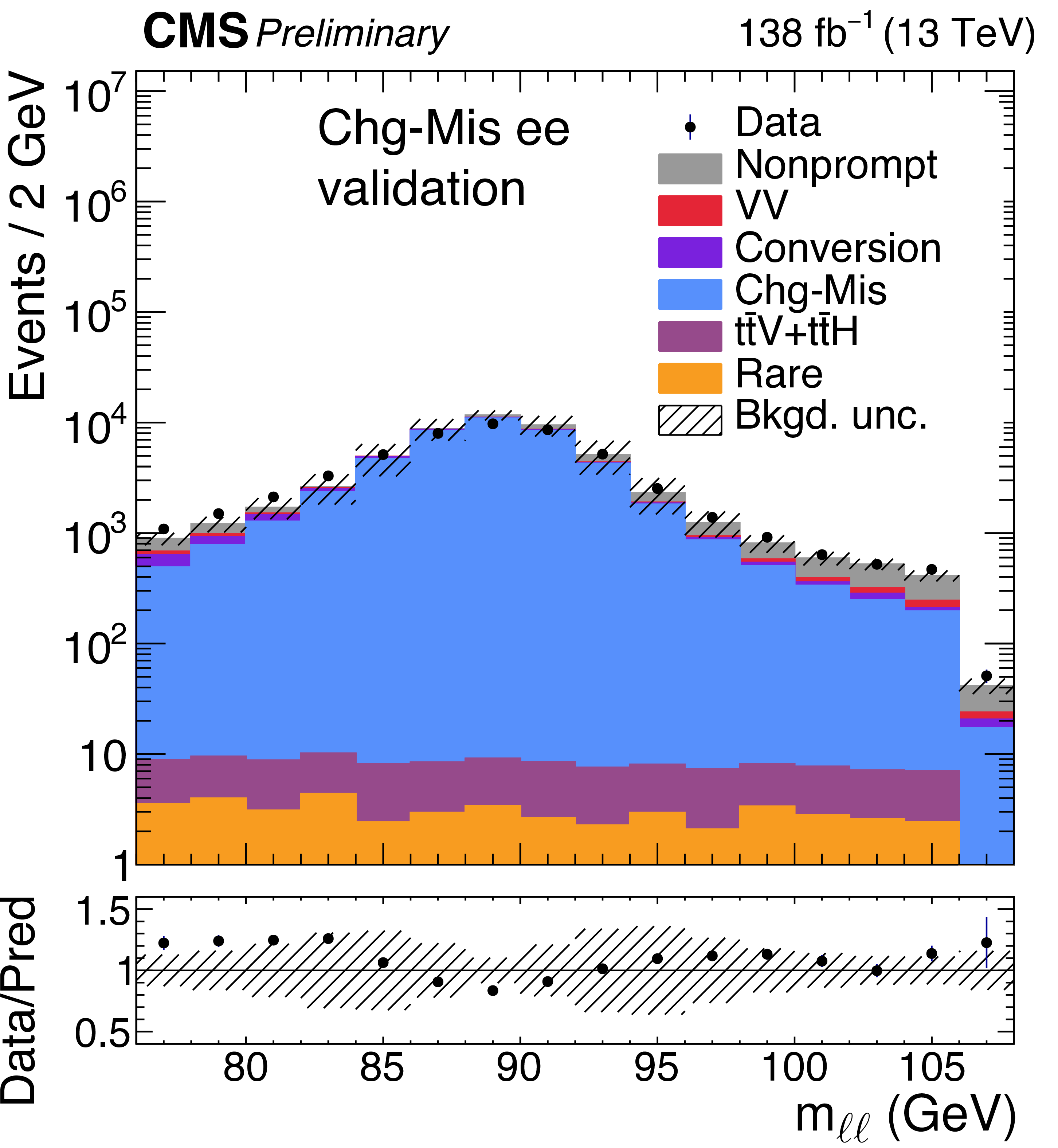
Validation of nonprompt background in the trilepton validation region. Plots of $ p_{\mathrm{T}} $ of the electron (left) or muon (right) not from the Z boson decay are shown. The last bin includes the overflow bins. The background uncertainty band shows the total uncertainty including systematics. |
png pdf |
Figure 7-a:
Validation of nonprompt background in the trilepton validation region. Plots of $ p_{\mathrm{T}} $ of the electron (left) or muon (right) not from the Z boson decay are shown. The last bin includes the overflow bins. The background uncertainty band shows the total uncertainty including systematics. |
png pdf |
Figure 7-b:
Validation of nonprompt background in the trilepton validation region. Plots of $ p_{\mathrm{T}} $ of the electron (left) or muon (right) not from the Z boson decay are shown. The last bin includes the overflow bins. The background uncertainty band shows the total uncertainty including systematics. |
png pdf |
Figure 8:
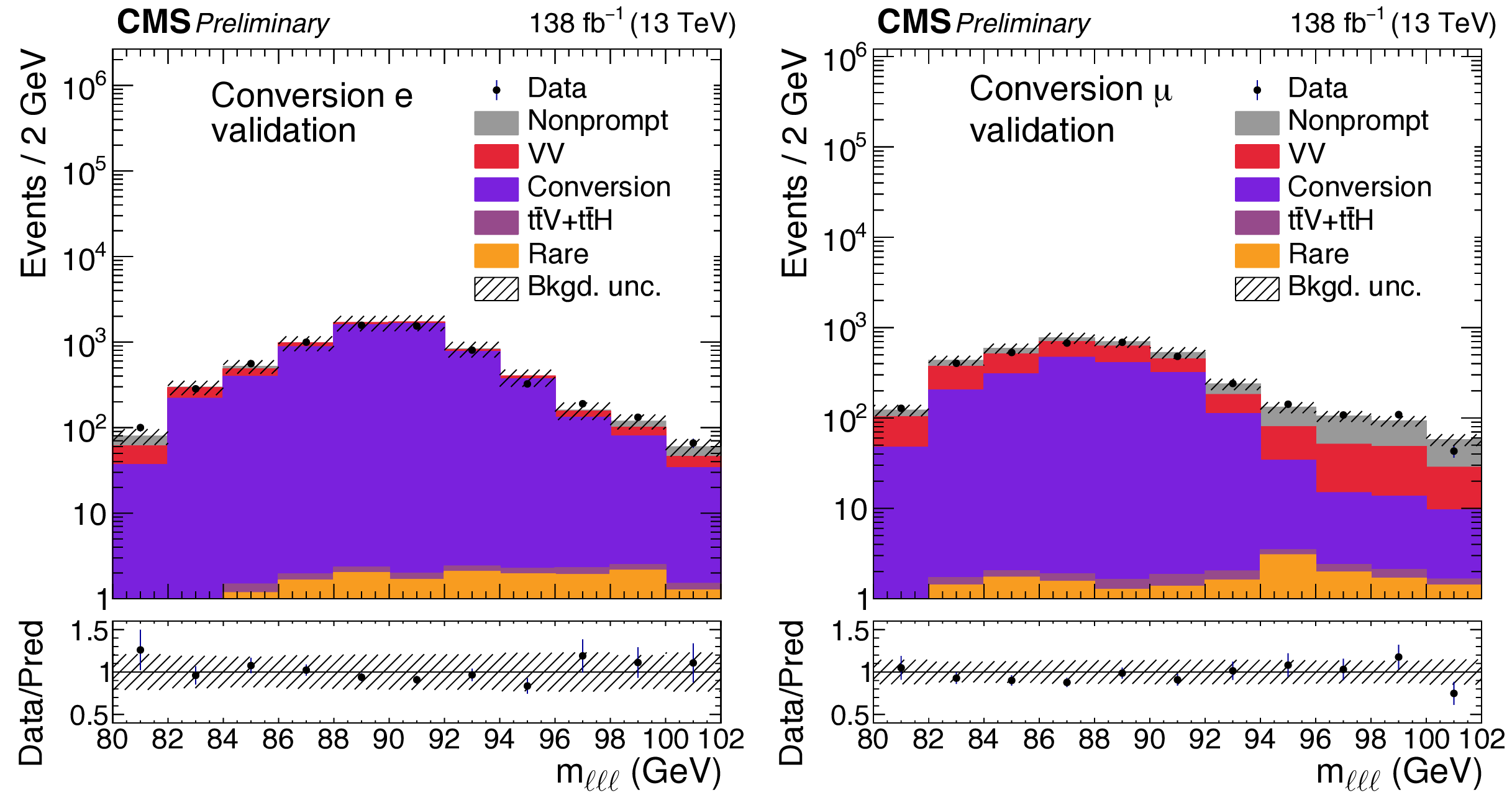
The invariant mass of SS electron pair in charge mismeasurement validation region. The background uncertainty band shows the total uncertainty including systematics. |
png pdf |
Figure 9:
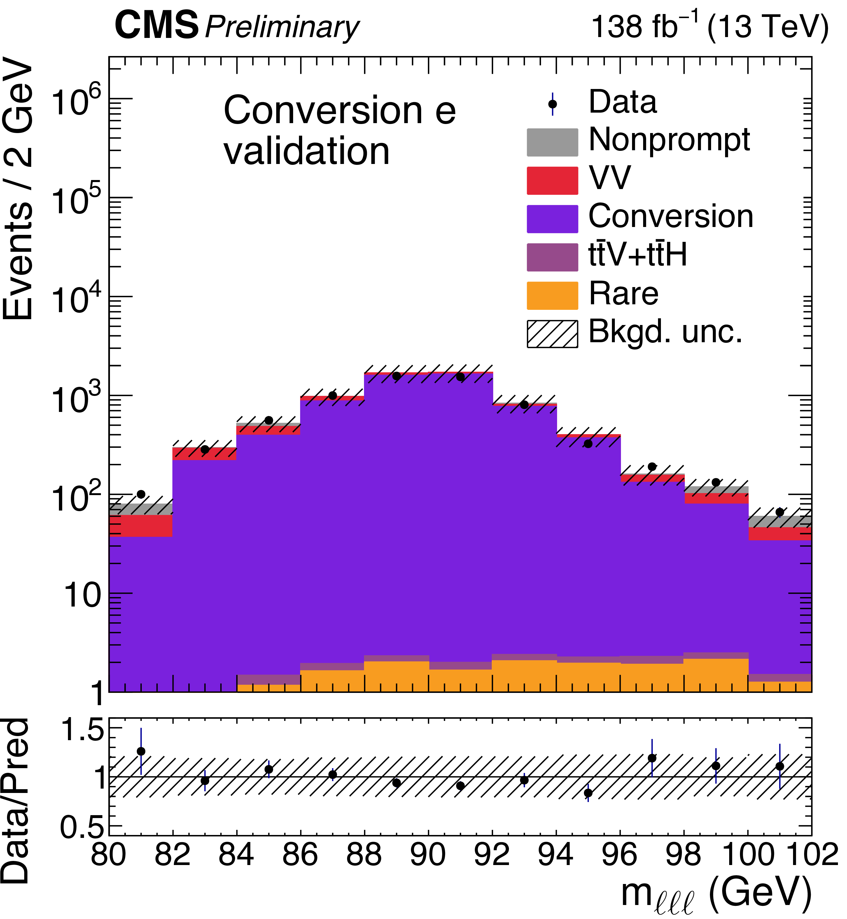
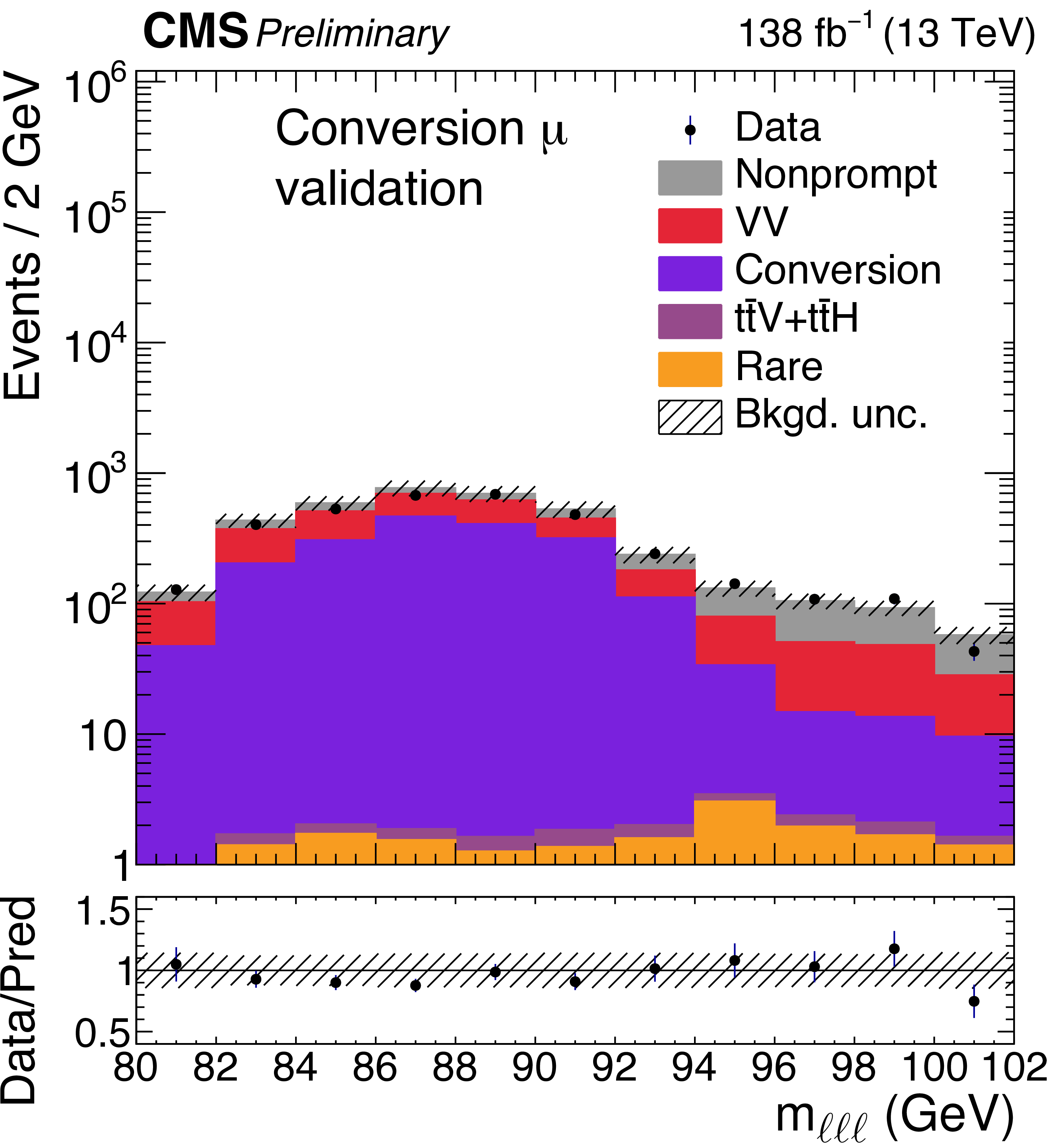
The invariant mass of three leptons are shown for the conversion electron (left) events and for the conversion muon (right) events for the conversion background validation. The background uncertainty band shows the total uncertainty including systematics. |
png pdf |
Figure 9-a:
The invariant mass of three leptons are shown for the conversion electron (left) events and for the conversion muon (right) events for the conversion background validation. The background uncertainty band shows the total uncertainty including systematics. |
png pdf |
Figure 9-b:
The invariant mass of three leptons are shown for the conversion electron (left) events and for the conversion muon (right) events for the conversion background validation. The background uncertainty band shows the total uncertainty including systematics. |
png pdf |
Figure 10:
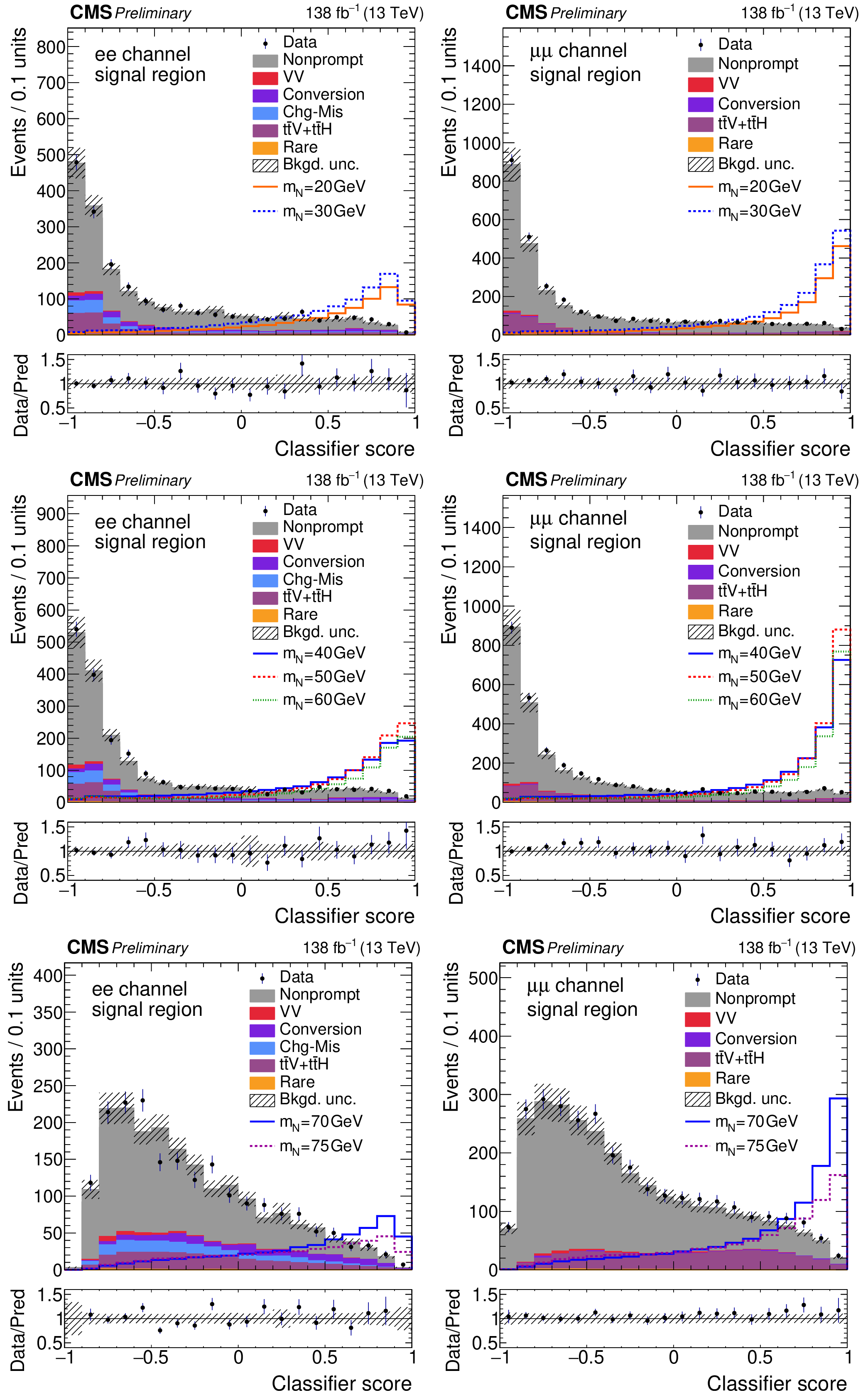
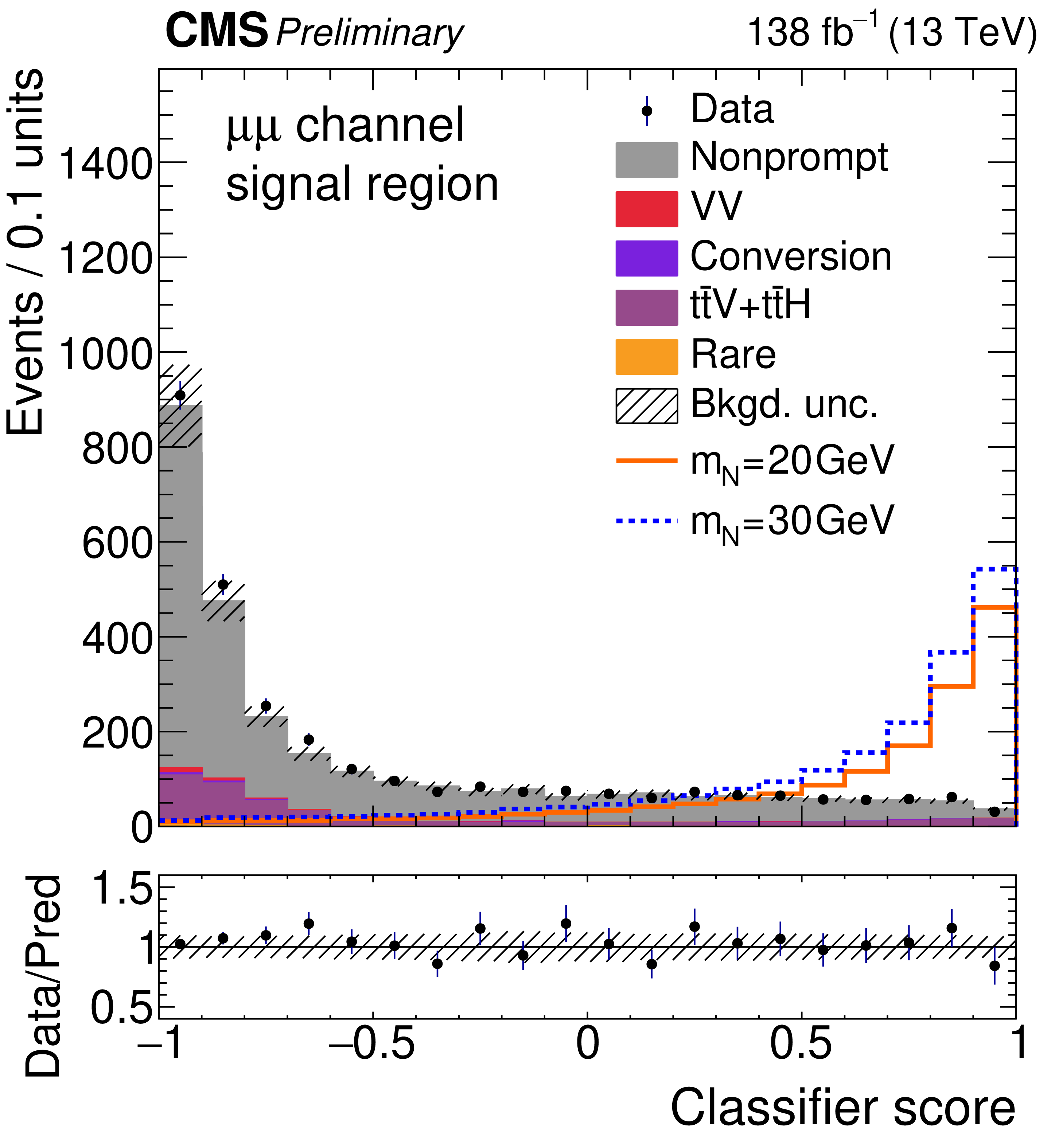
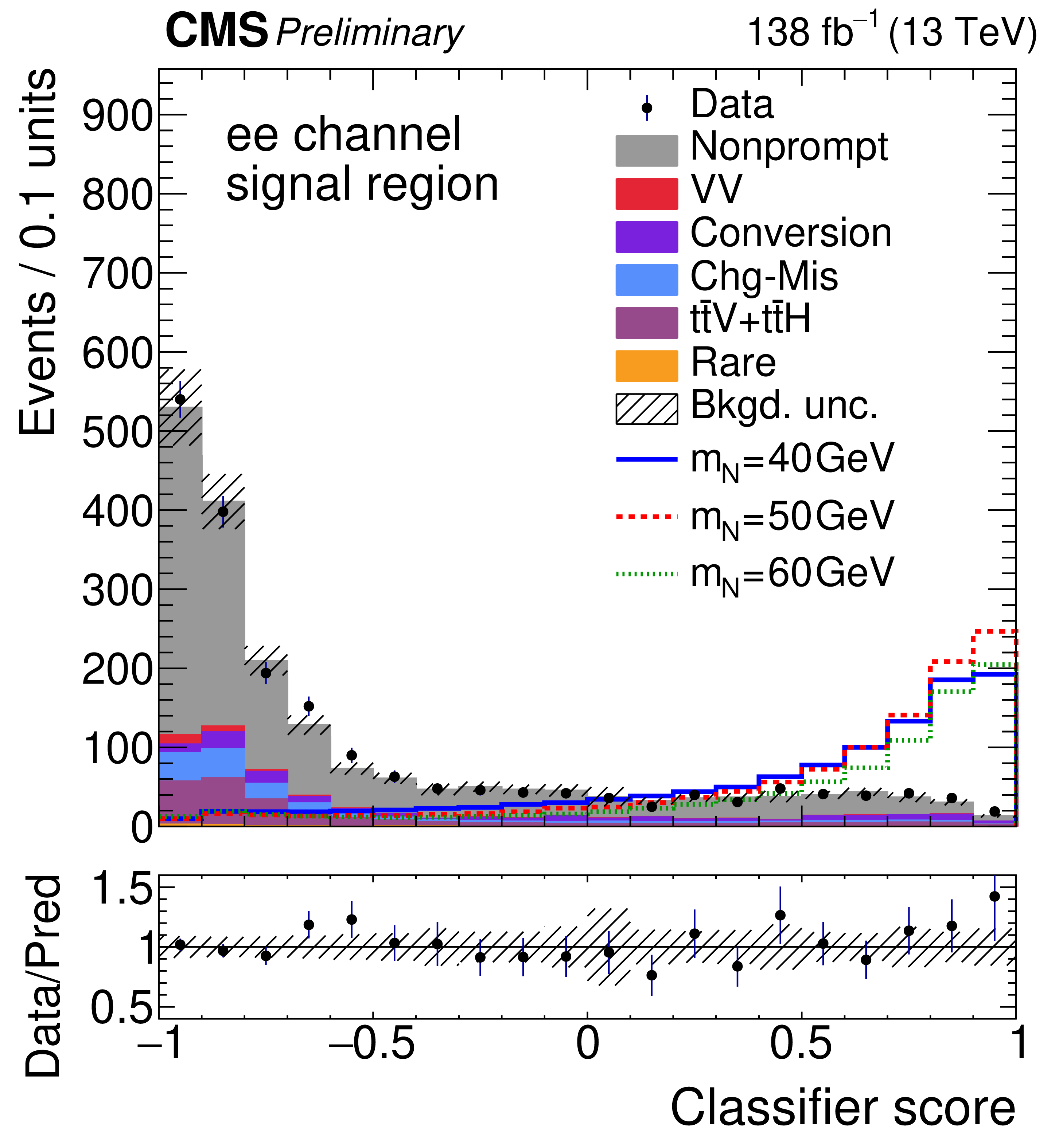
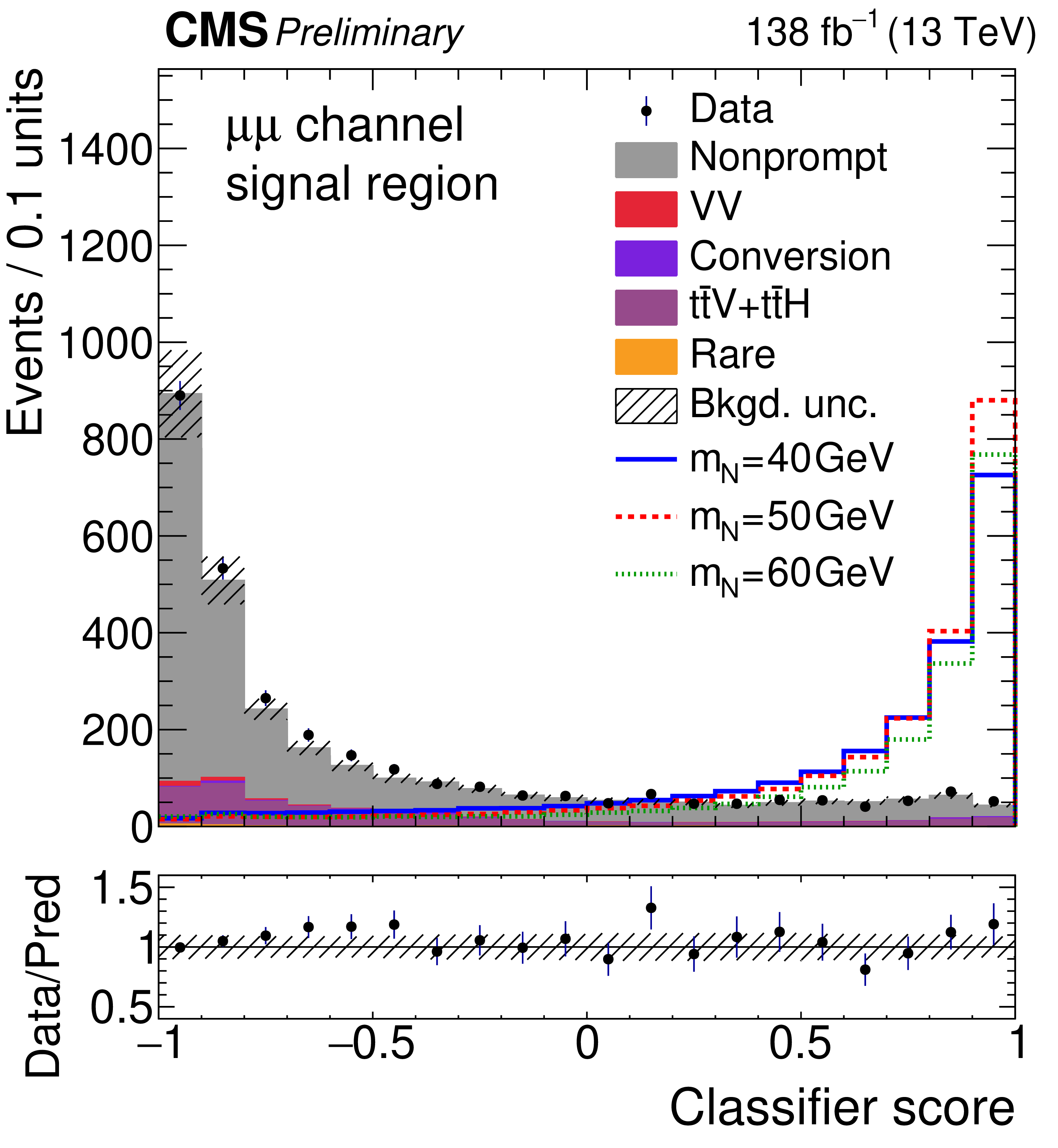
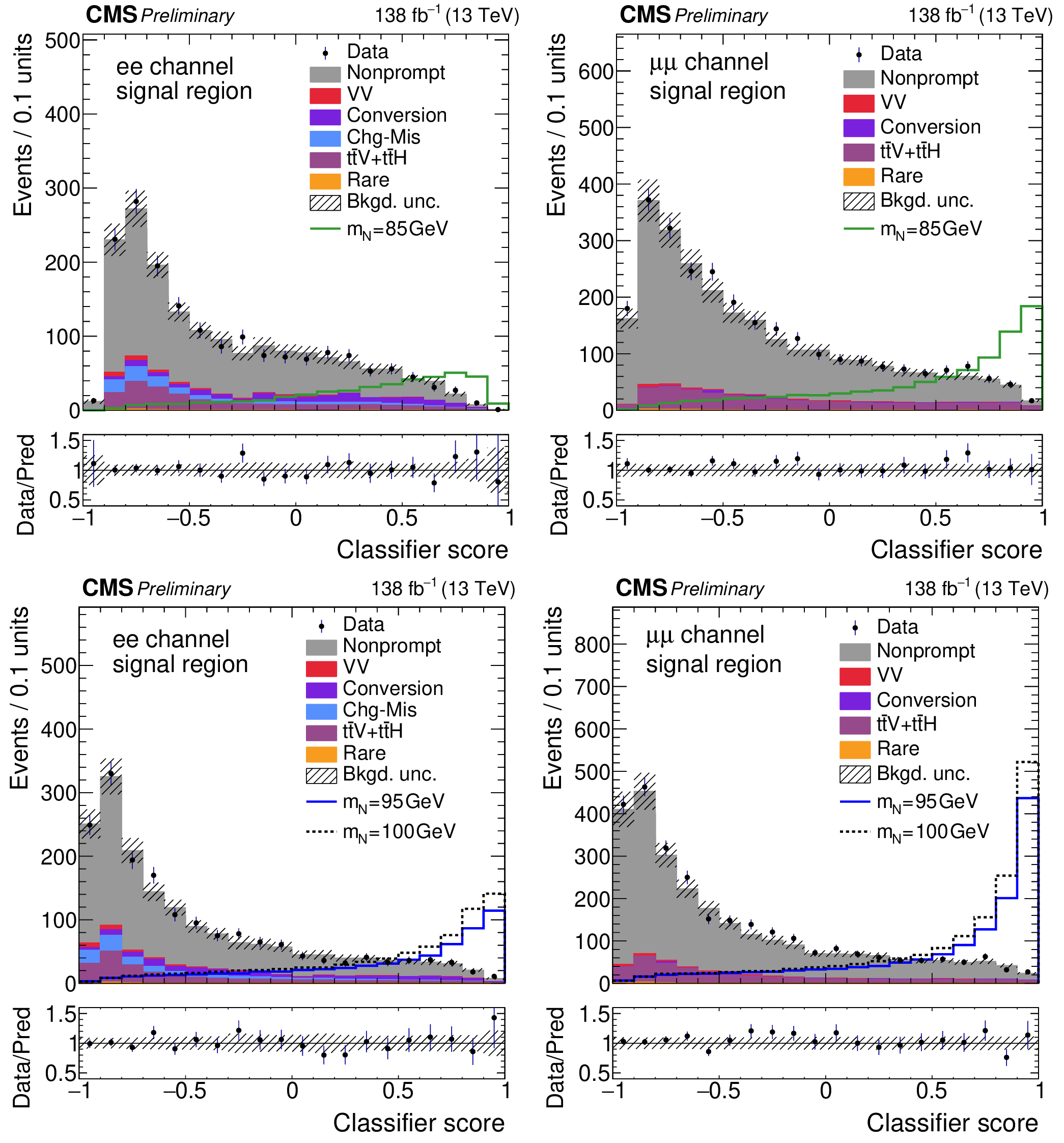
Comparison of the observed (points) and predicted (filled histograms) post$ \text{-} $fit BDTG score distributions in the dielectron (left) and dimuon (right) channels. The BDTG score distributions correspond to classifiers trained with signal mass hypotheses of 20 (top), 50 (middle), and 75 (bottom) GeV. The expected signal distributions extracted with the same classifier are overlaid on the figures, assuming a $ \mathcal{B}(\mathrm{t}\to\mathrm{b}\ell\mathrm{N}) $ value of 2.4 $ \times10^{-4} $. The background uncertainty band shows the total uncertainty including systematics. |
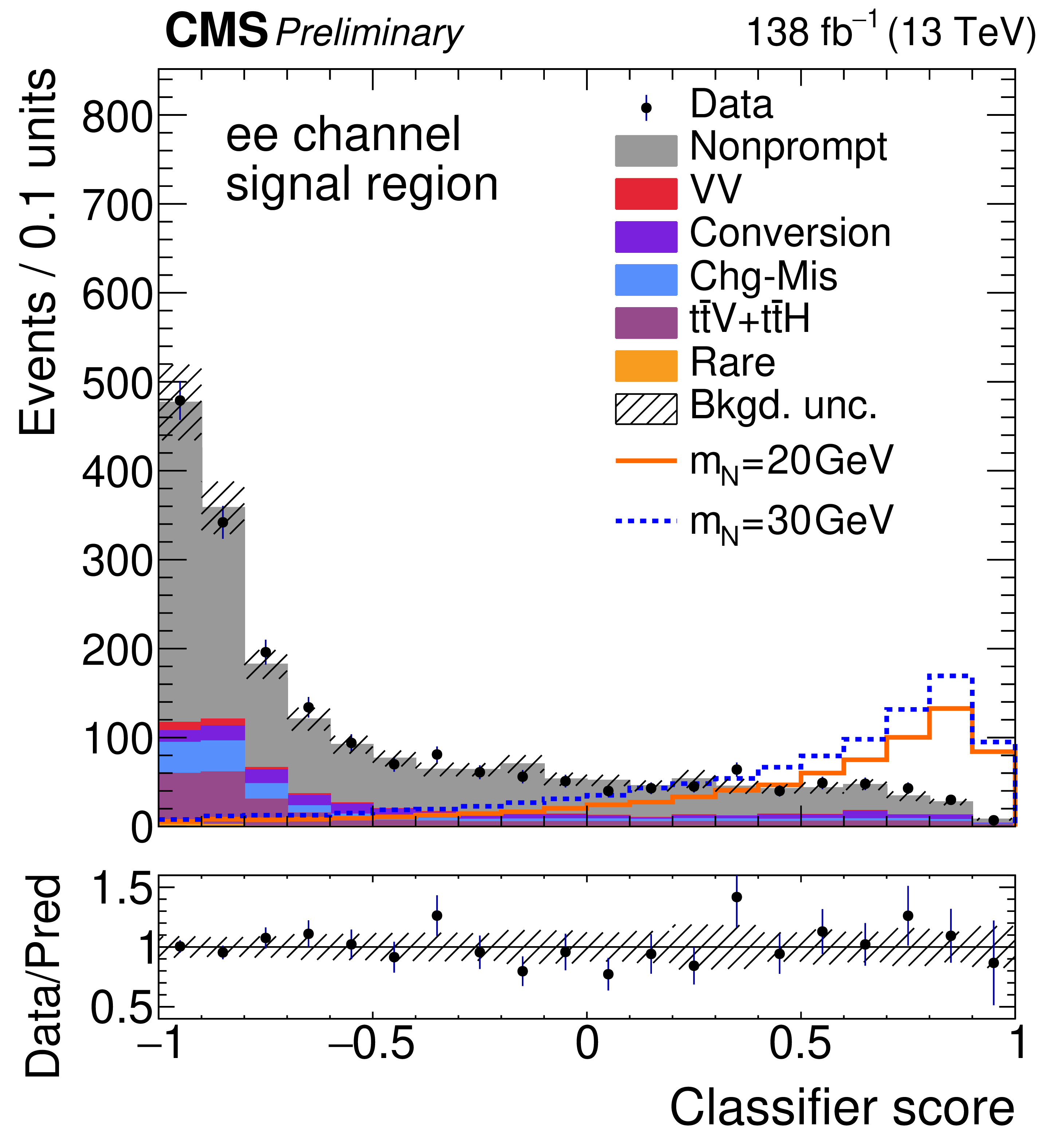
png pdf |
Figure 10-a:
Comparison of the observed (points) and predicted (filled histograms) post$ \text{-} $fit BDTG score distributions in the dielectron (left) and dimuon (right) channels. The BDTG score distributions correspond to classifiers trained with signal mass hypotheses of 20 (top), 50 (middle), and 75 (bottom) GeV. The expected signal distributions extracted with the same classifier are overlaid on the figures, assuming a $ \mathcal{B}(\mathrm{t}\to\mathrm{b}\ell\mathrm{N}) $ value of 2.4 $ \times10^{-4} $. The background uncertainty band shows the total uncertainty including systematics. |
png pdf |
Figure 10-b:
Comparison of the observed (points) and predicted (filled histograms) post$ \text{-} $fit BDTG score distributions in the dielectron (left) and dimuon (right) channels. The BDTG score distributions correspond to classifiers trained with signal mass hypotheses of 20 (top), 50 (middle), and 75 (bottom) GeV. The expected signal distributions extracted with the same classifier are overlaid on the figures, assuming a $ \mathcal{B}(\mathrm{t}\to\mathrm{b}\ell\mathrm{N}) $ value of 2.4 $ \times10^{-4} $. The background uncertainty band shows the total uncertainty including systematics. |
png pdf |
Figure 10-c:
Comparison of the observed (points) and predicted (filled histograms) post$ \text{-} $fit BDTG score distributions in the dielectron (left) and dimuon (right) channels. The BDTG score distributions correspond to classifiers trained with signal mass hypotheses of 20 (top), 50 (middle), and 75 (bottom) GeV. The expected signal distributions extracted with the same classifier are overlaid on the figures, assuming a $ \mathcal{B}(\mathrm{t}\to\mathrm{b}\ell\mathrm{N}) $ value of 2.4 $ \times10^{-4} $. The background uncertainty band shows the total uncertainty including systematics. |
png pdf |
Figure 10-d:
Comparison of the observed (points) and predicted (filled histograms) post$ \text{-} $fit BDTG score distributions in the dielectron (left) and dimuon (right) channels. The BDTG score distributions correspond to classifiers trained with signal mass hypotheses of 20 (top), 50 (middle), and 75 (bottom) GeV. The expected signal distributions extracted with the same classifier are overlaid on the figures, assuming a $ \mathcal{B}(\mathrm{t}\to\mathrm{b}\ell\mathrm{N}) $ value of 2.4 $ \times10^{-4} $. The background uncertainty band shows the total uncertainty including systematics. |
png pdf |
Figure 10-e:
Comparison of the observed (points) and predicted (filled histograms) post$ \text{-} $fit BDTG score distributions in the dielectron (left) and dimuon (right) channels. The BDTG score distributions correspond to classifiers trained with signal mass hypotheses of 20 (top), 50 (middle), and 75 (bottom) GeV. The expected signal distributions extracted with the same classifier are overlaid on the figures, assuming a $ \mathcal{B}(\mathrm{t}\to\mathrm{b}\ell\mathrm{N}) $ value of 2.4 $ \times10^{-4} $. The background uncertainty band shows the total uncertainty including systematics. |
png pdf |
Figure 10-f:
Comparison of the observed (points) and predicted (filled histograms) post$ \text{-} $fit BDTG score distributions in the dielectron (left) and dimuon (right) channels. The BDTG score distributions correspond to classifiers trained with signal mass hypotheses of 20 (top), 50 (middle), and 75 (bottom) GeV. The expected signal distributions extracted with the same classifier are overlaid on the figures, assuming a $ \mathcal{B}(\mathrm{t}\to\mathrm{b}\ell\mathrm{N}) $ value of 2.4 $ \times10^{-4} $. The background uncertainty band shows the total uncertainty including systematics. |
png pdf |
Figure 11:
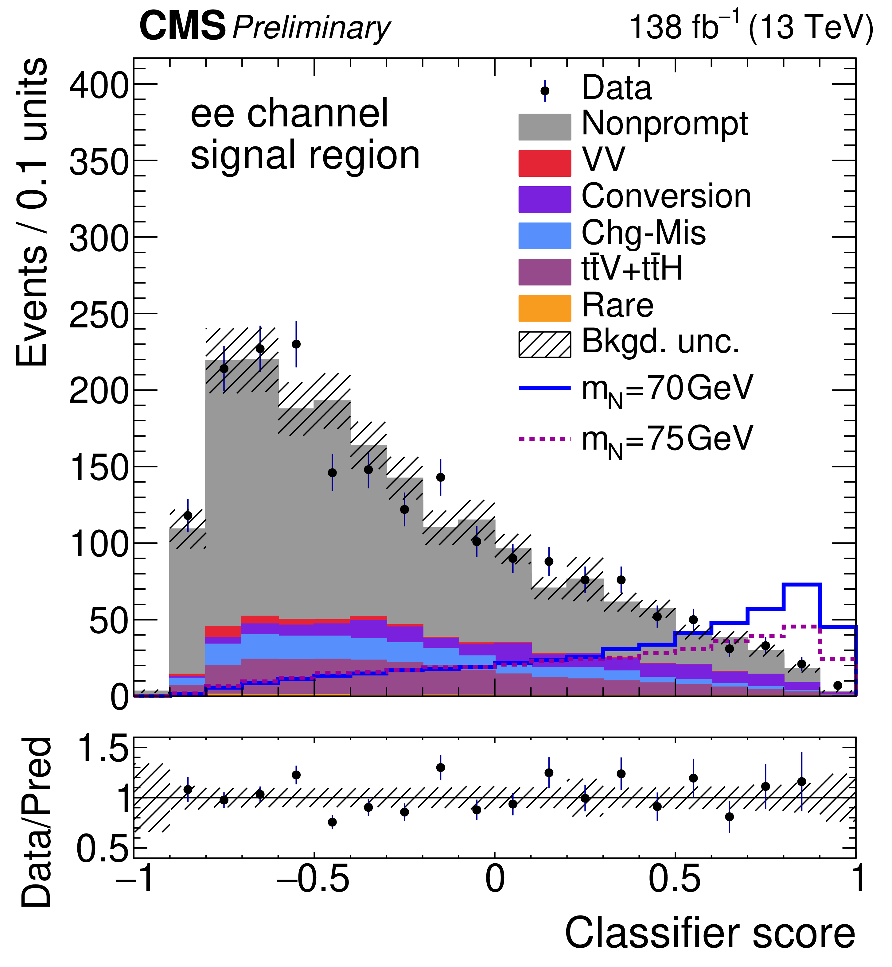
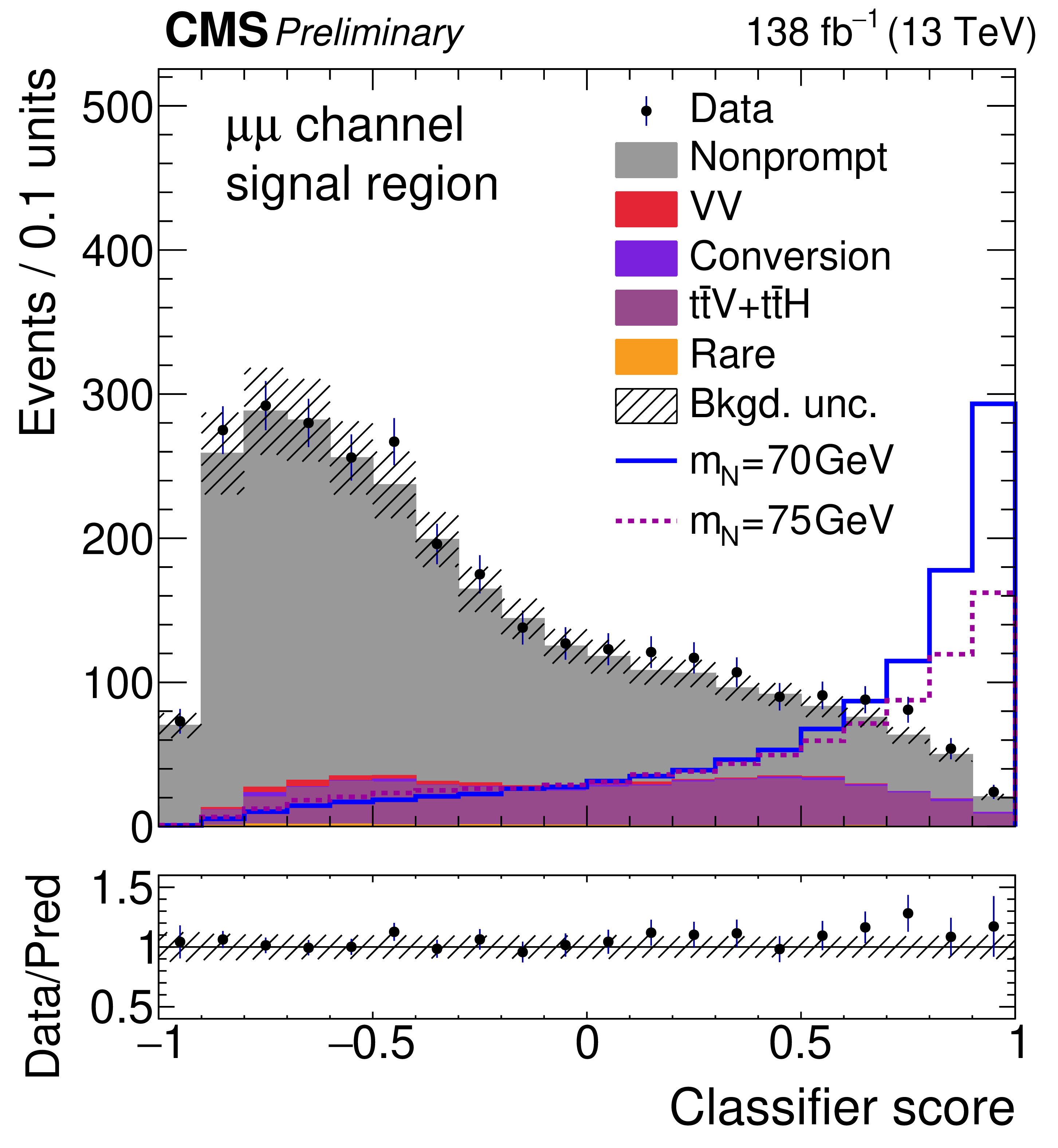
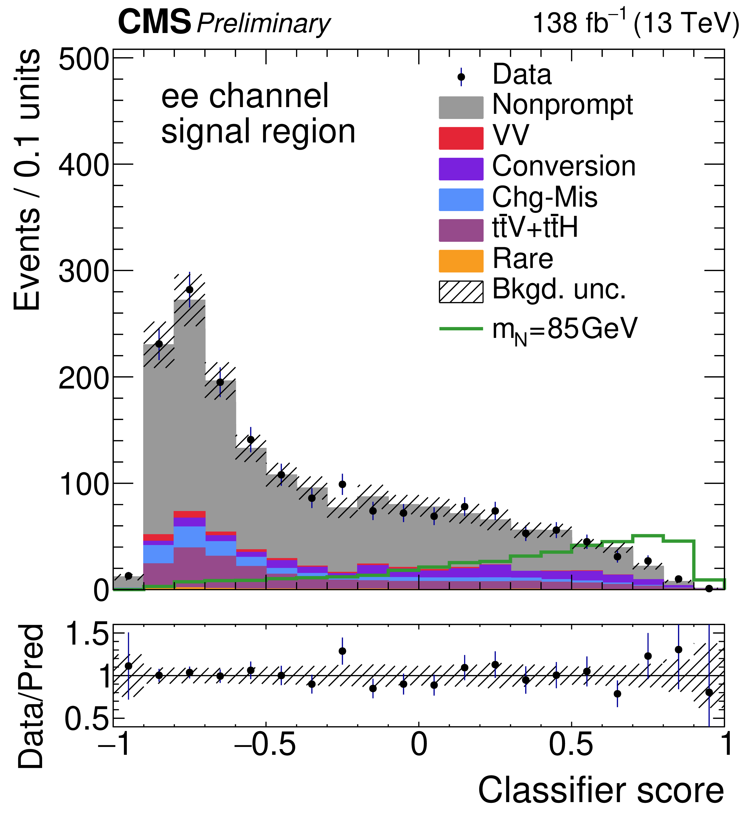
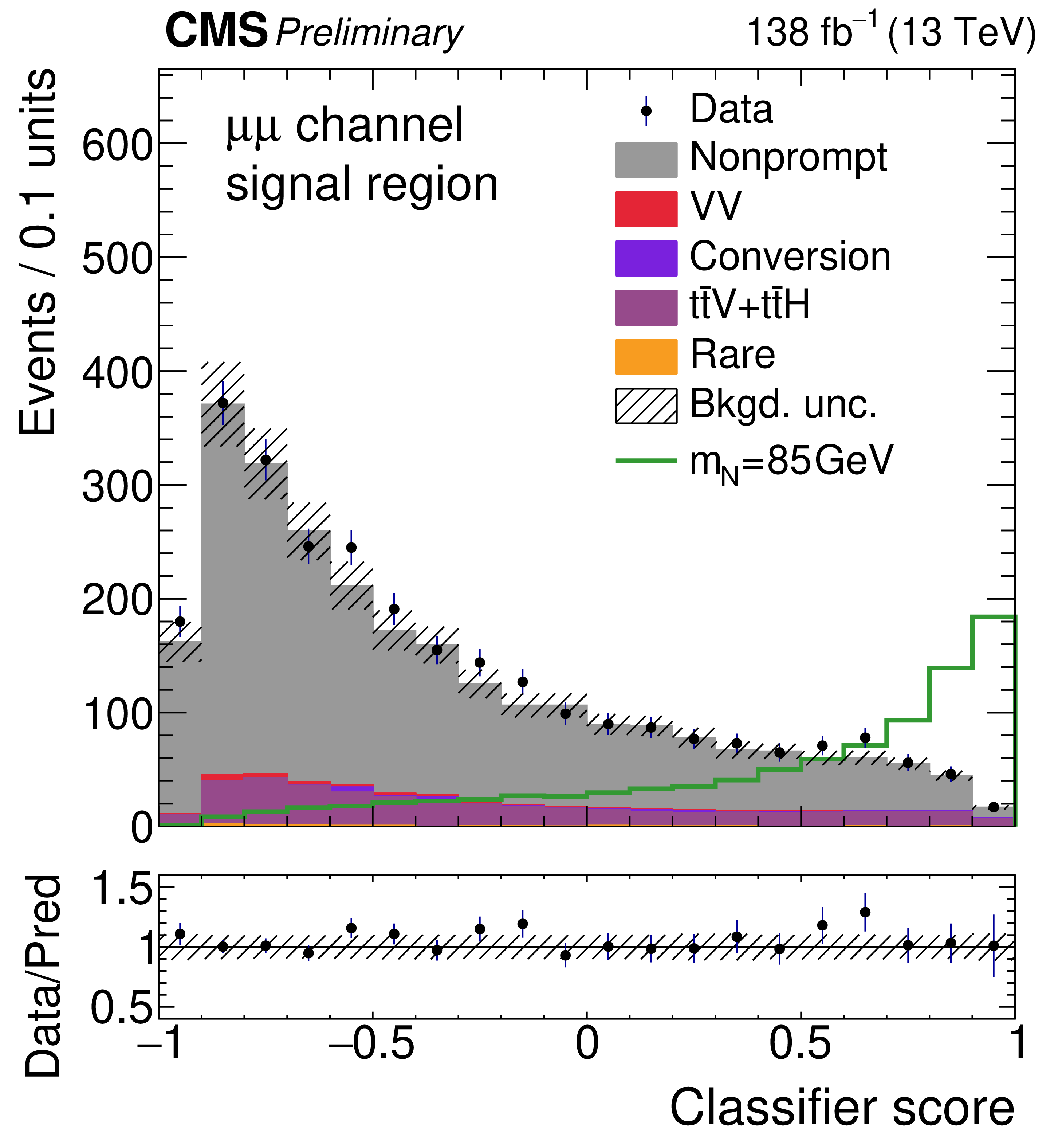
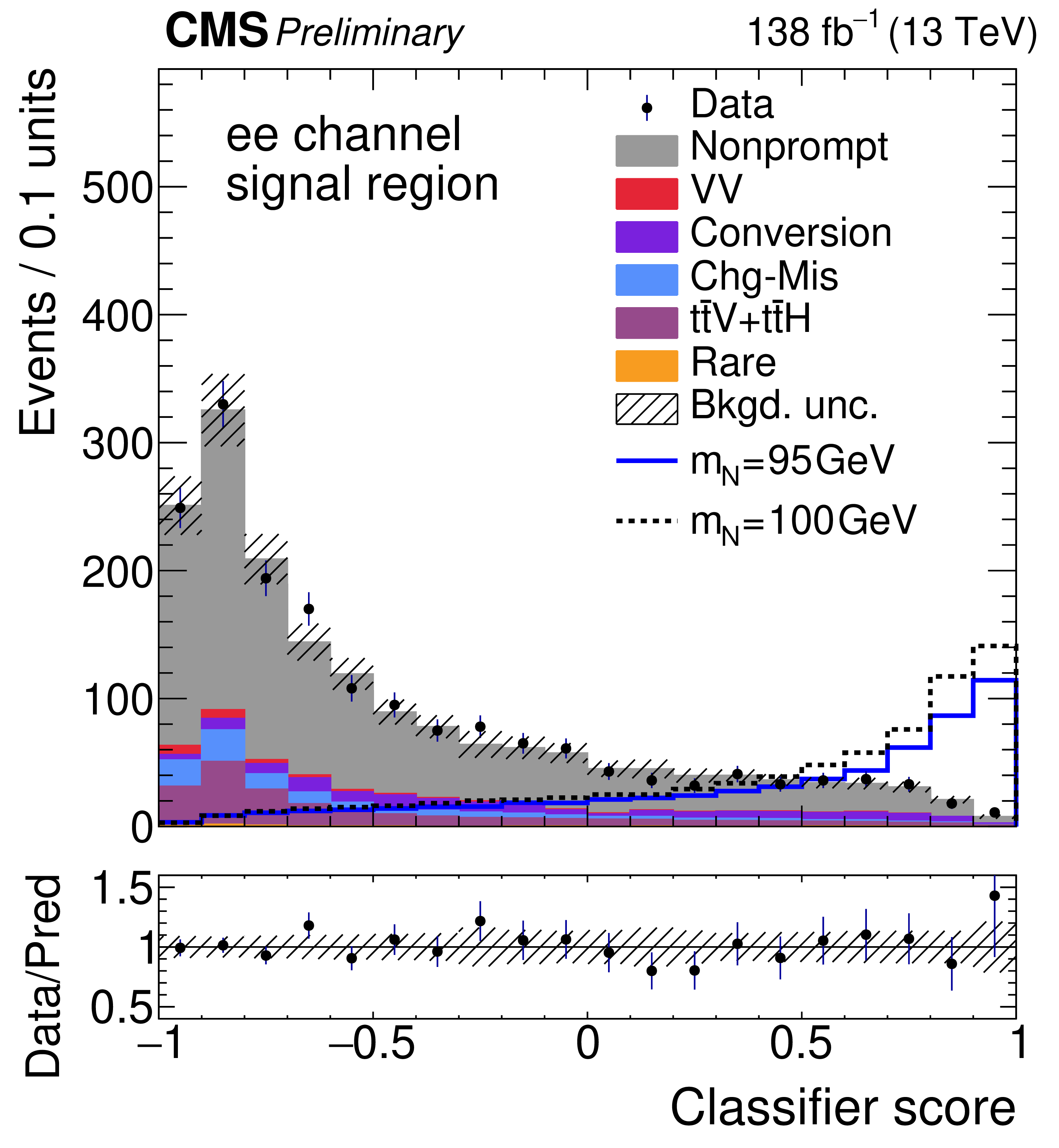
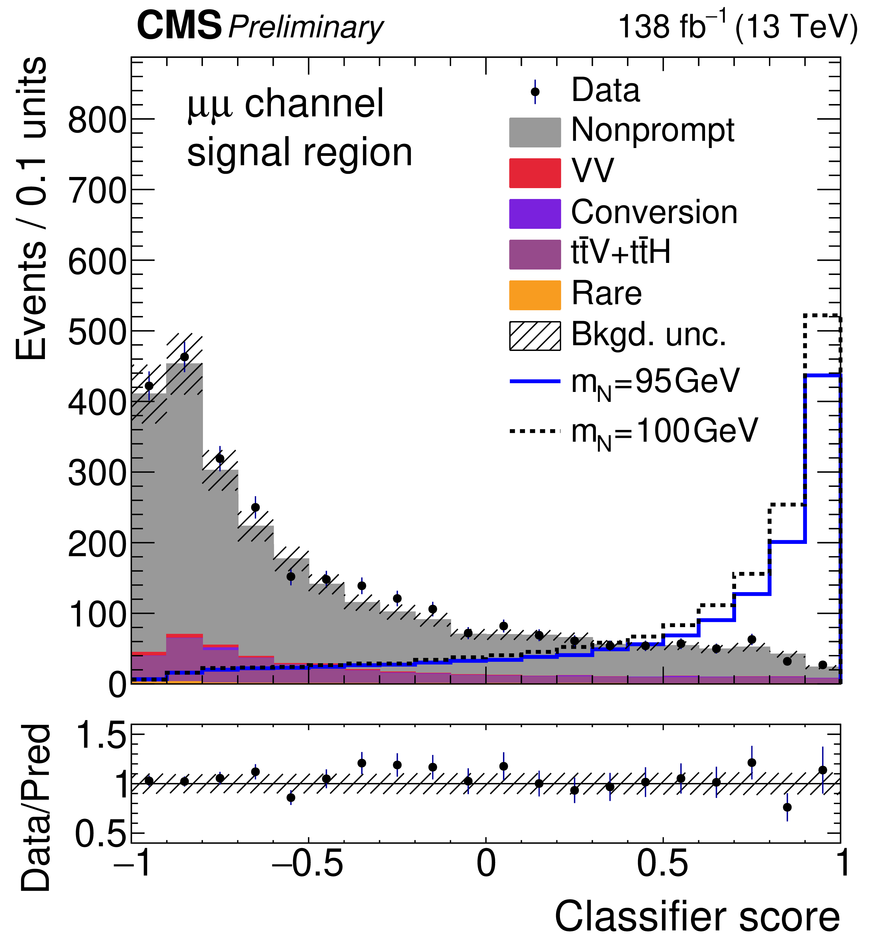
Comparison of the observed (points) and predicted (filled histograms) post$ \text{-} $fit BDTG score distributions in the dielectron (left) and dimuon (right) channels. The BDTG score distributions correspond to classifiers trained with signal mass hypotheses of 85 (top) and 100 (bottom) GeV. The expected signal distributions extracted with the same classifier are overlaid on the figures, assuming a $ \mathcal{B}(\mathrm{t}\to\mathrm{b}\ell\mathrm{N}) $ value of 2.4 $ \times10^{-4} $. The background uncertainty band shows the total uncertainty including systematics. |
png pdf |
Figure 11-a:
Comparison of the observed (points) and predicted (filled histograms) post$ \text{-} $fit BDTG score distributions in the dielectron (left) and dimuon (right) channels. The BDTG score distributions correspond to classifiers trained with signal mass hypotheses of 85 (top) and 100 (bottom) GeV. The expected signal distributions extracted with the same classifier are overlaid on the figures, assuming a $ \mathcal{B}(\mathrm{t}\to\mathrm{b}\ell\mathrm{N}) $ value of 2.4 $ \times10^{-4} $. The background uncertainty band shows the total uncertainty including systematics. |
png pdf |
Figure 11-b:
Comparison of the observed (points) and predicted (filled histograms) post$ \text{-} $fit BDTG score distributions in the dielectron (left) and dimuon (right) channels. The BDTG score distributions correspond to classifiers trained with signal mass hypotheses of 85 (top) and 100 (bottom) GeV. The expected signal distributions extracted with the same classifier are overlaid on the figures, assuming a $ \mathcal{B}(\mathrm{t}\to\mathrm{b}\ell\mathrm{N}) $ value of 2.4 $ \times10^{-4} $. The background uncertainty band shows the total uncertainty including systematics. |
png pdf |
Figure 11-c:
Comparison of the observed (points) and predicted (filled histograms) post$ \text{-} $fit BDTG score distributions in the dielectron (left) and dimuon (right) channels. The BDTG score distributions correspond to classifiers trained with signal mass hypotheses of 85 (top) and 100 (bottom) GeV. The expected signal distributions extracted with the same classifier are overlaid on the figures, assuming a $ \mathcal{B}(\mathrm{t}\to\mathrm{b}\ell\mathrm{N}) $ value of 2.4 $ \times10^{-4} $. The background uncertainty band shows the total uncertainty including systematics. |
png pdf |
Figure 11-d:
Comparison of the observed (points) and predicted (filled histograms) post$ \text{-} $fit BDTG score distributions in the dielectron (left) and dimuon (right) channels. The BDTG score distributions correspond to classifiers trained with signal mass hypotheses of 85 (top) and 100 (bottom) GeV. The expected signal distributions extracted with the same classifier are overlaid on the figures, assuming a $ \mathcal{B}(\mathrm{t}\to\mathrm{b}\ell\mathrm{N}) $ value of 2.4 $ \times10^{-4} $. The background uncertainty band shows the total uncertainty including systematics. |
png pdf |
Figure 12:
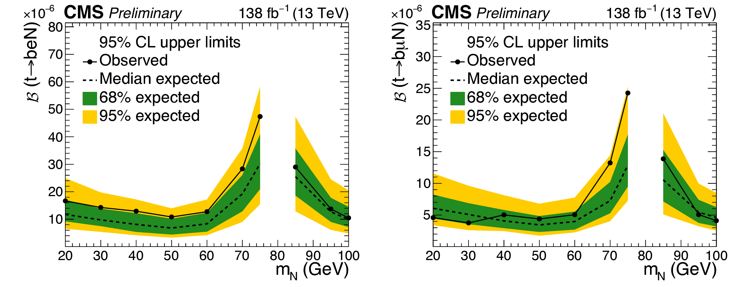
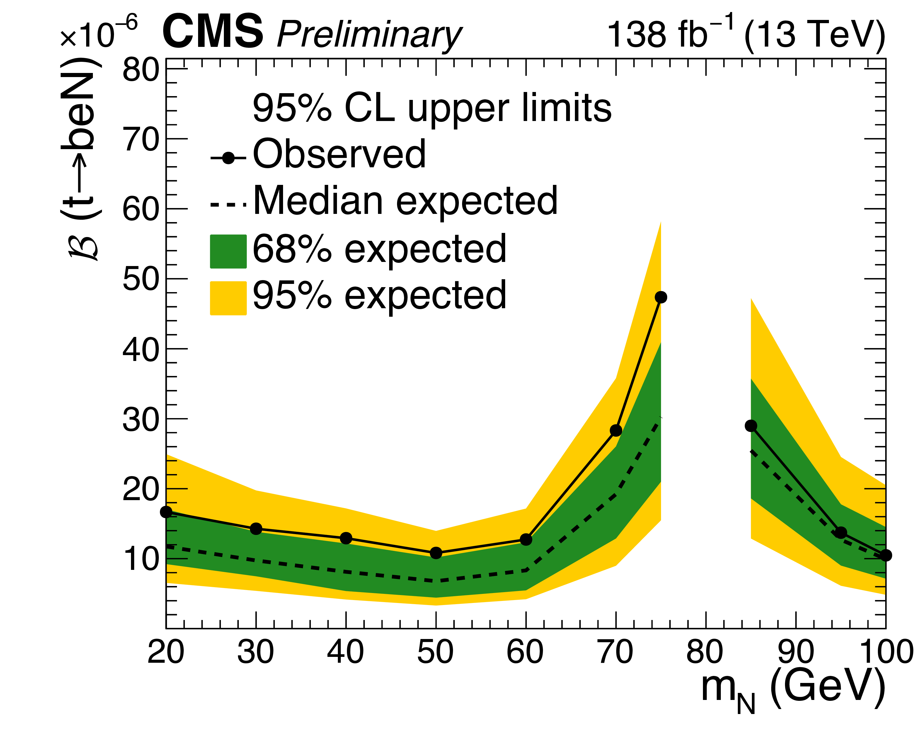
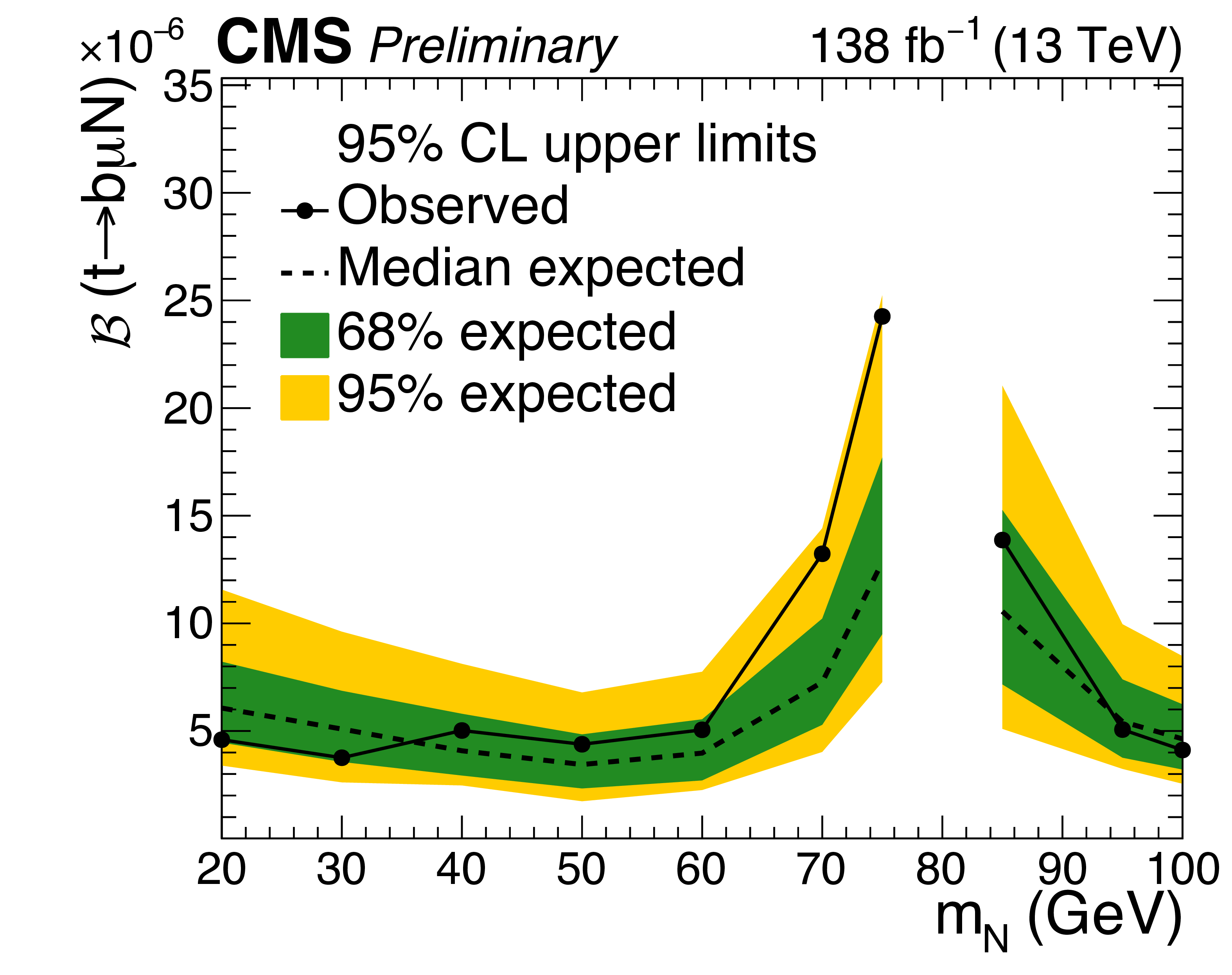
The expected and observed upper limits at 95$ % $ CL on the branching fraction, $ \mathcal{B} $ (t}\rightarrow\textb\ell\text{N), at the $ m_{\mathrm{N}} $ values considered in the search. The left and right figures correspond to the electron and muon mixing scenarios. The uncertainty includes statistical and systematic uncertainties. |
png pdf |
Figure 12-a:
The expected and observed upper limits at 95$ % $ CL on the branching fraction, $ \mathcal{B} $ (t}\rightarrow\textb\ell\text{N), at the $ m_{\mathrm{N}} $ values considered in the search. The left and right figures correspond to the electron and muon mixing scenarios. The uncertainty includes statistical and systematic uncertainties. |
png pdf |
Figure 12-b:
The expected and observed upper limits at 95$ % $ CL on the branching fraction, $ \mathcal{B} $ (t}\rightarrow\textb\ell\text{N), at the $ m_{\mathrm{N}} $ values considered in the search. The left and right figures correspond to the electron and muon mixing scenarios. The uncertainty includes statistical and systematic uncertainties. |
png pdf |
Figure 13:
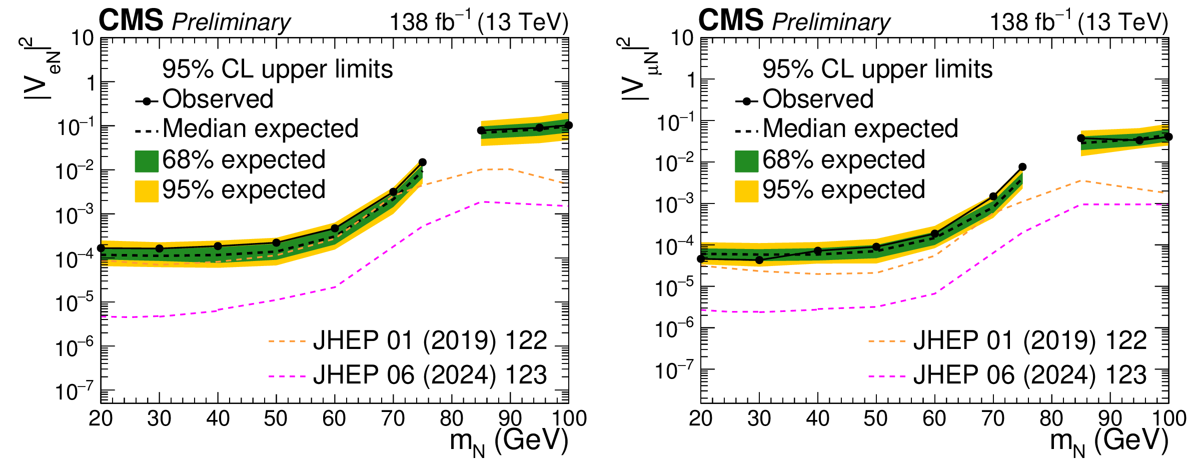
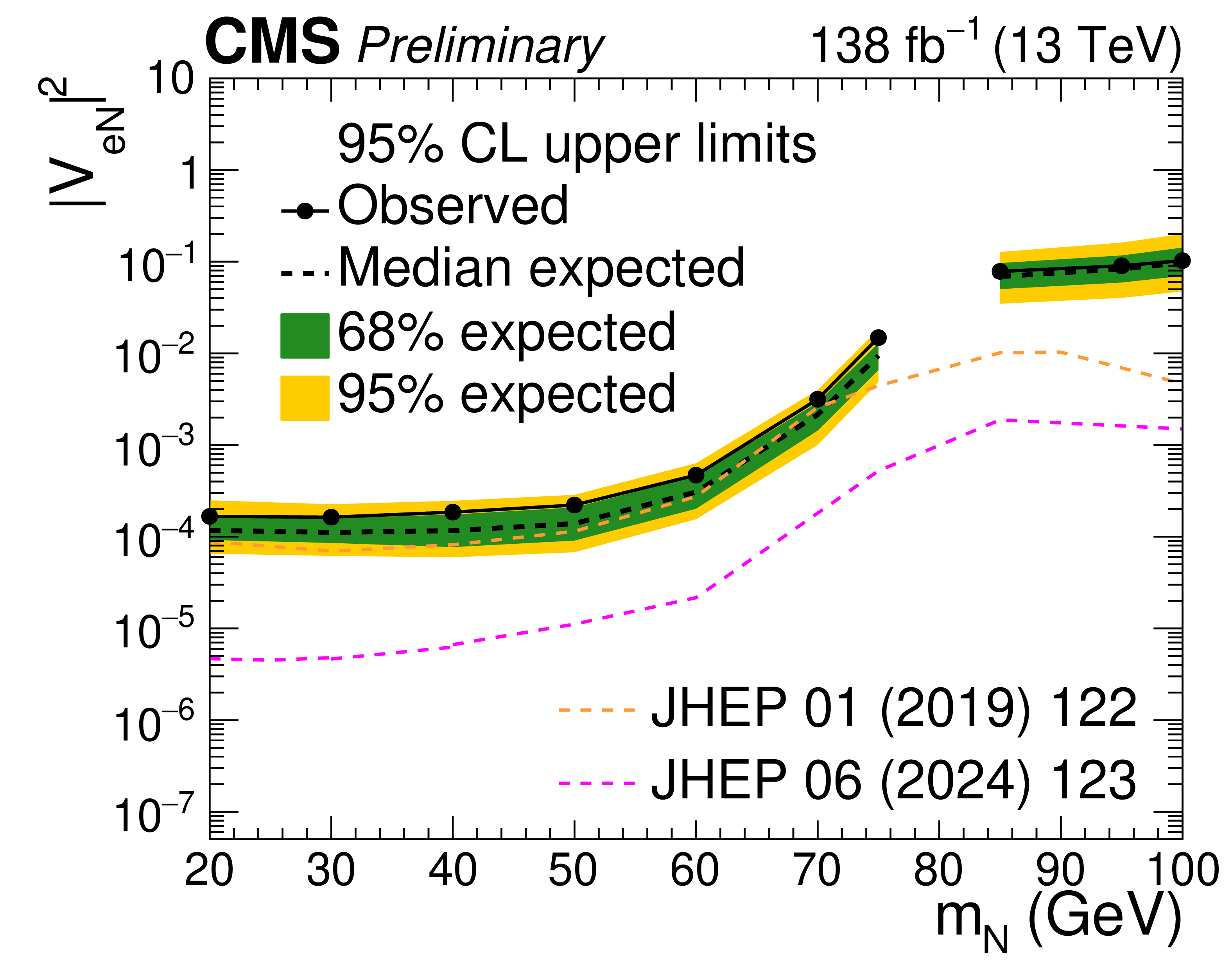
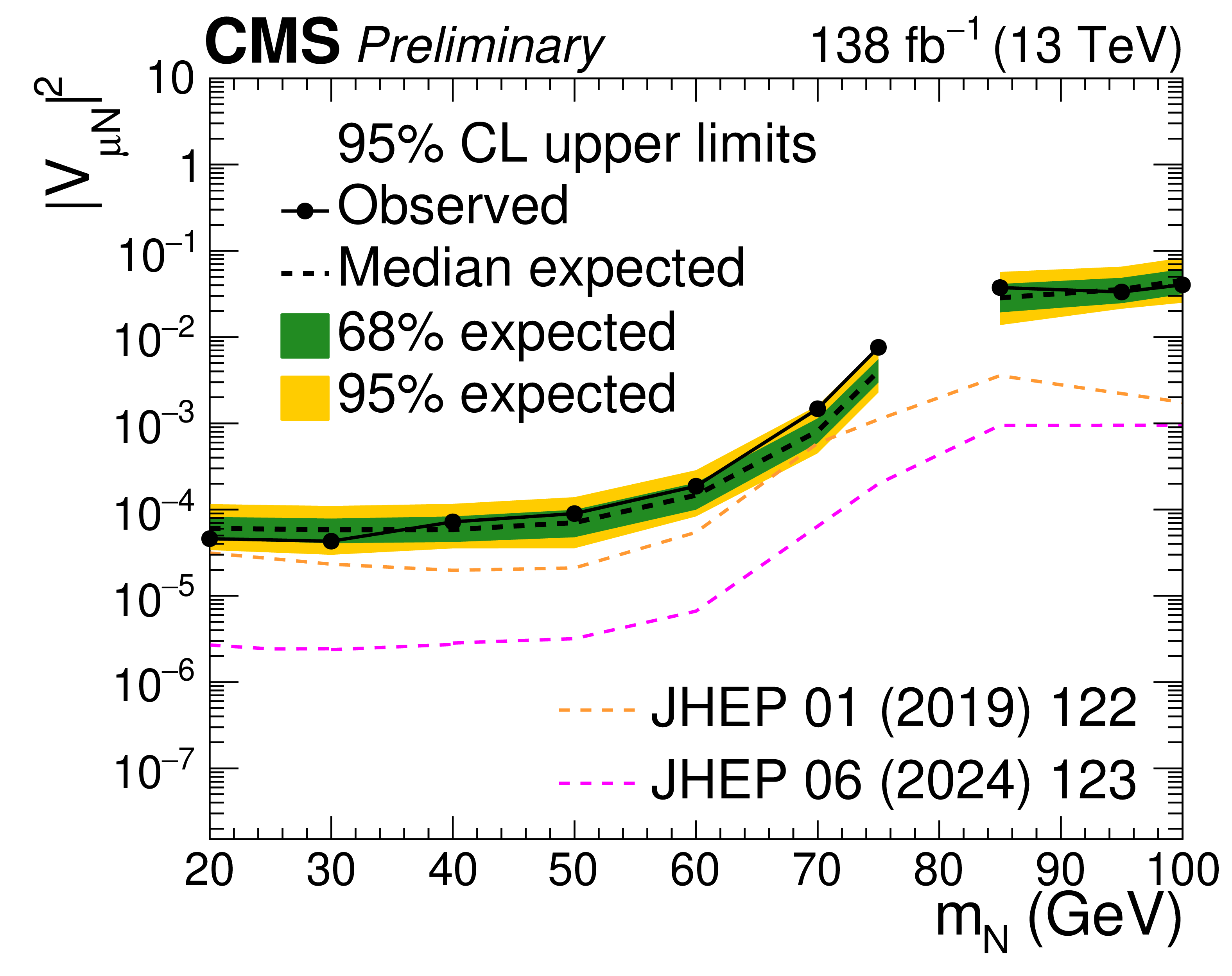
The expected and observed upper limits at 95$ % $ CL on the model parameters, $ |\mathrm{V}_{\mathrm{e}\mathrm{N}}|^{2} $ and $ |\mathrm{V}_{\mu\mathrm{N}}|^{2} $, at the $ m_{\mathrm{N}} $ values considered in the search. The left and right figures correspond to the electron and muon mixing scenarios. For comparison, observed limits from DY channels are overlaid on the figure [9,10]. |
png pdf |
Figure 13-a:
The expected and observed upper limits at 95$ % $ CL on the model parameters, $ |\mathrm{V}_{\mathrm{e}\mathrm{N}}|^{2} $ and $ |\mathrm{V}_{\mu\mathrm{N}}|^{2} $, at the $ m_{\mathrm{N}} $ values considered in the search. The left and right figures correspond to the electron and muon mixing scenarios. For comparison, observed limits from DY channels are overlaid on the figure [9,10]. |
png pdf |
Figure 13-b:
The expected and observed upper limits at 95$ % $ CL on the model parameters, $ |\mathrm{V}_{\mathrm{e}\mathrm{N}}|^{2} $ and $ |\mathrm{V}_{\mu\mathrm{N}}|^{2} $, at the $ m_{\mathrm{N}} $ values considered in the search. The left and right figures correspond to the electron and muon mixing scenarios. For comparison, observed limits from DY channels are overlaid on the figure [9,10]. |
| Tables | |
png pdf |
Table 1:
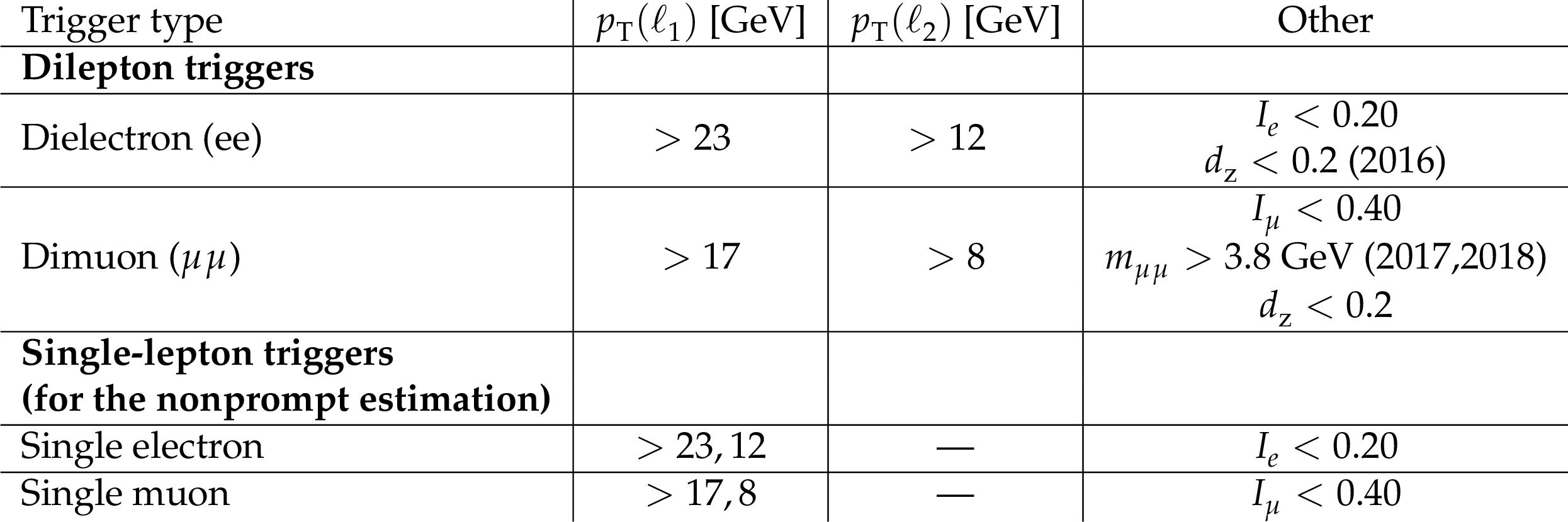
Summary of trigger $ p_{\mathrm{T}} $ thresholds and additional selection requirements for dielectron and dimuon channels. |
png pdf |
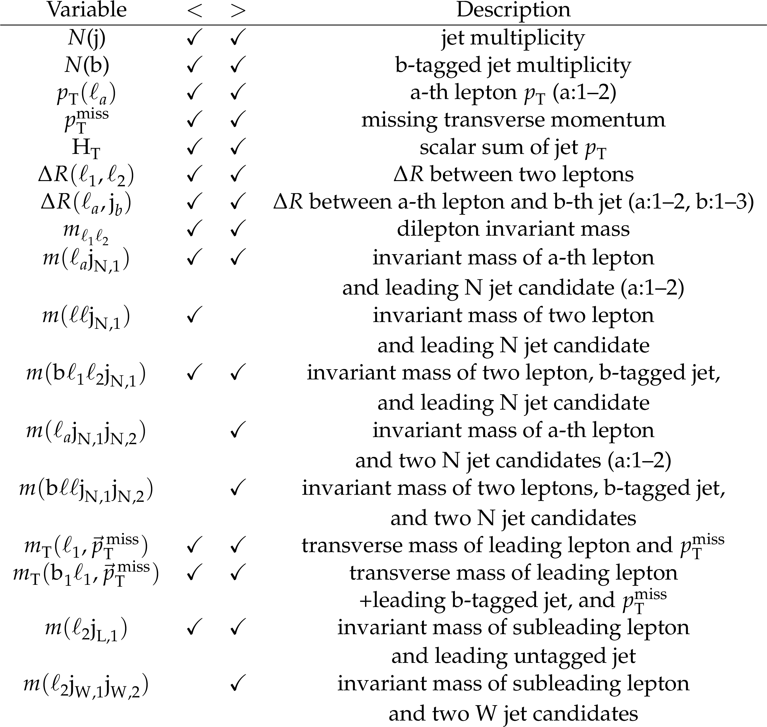
Table 2:
Input variables used for the training of classifiers. The usage in the low and high mass scenarios ($ m_{\mathrm{N}} < m_{\mathrm{W}} $ and $ m_{\mathrm{N}} > m_{\mathrm{W}} $) is shown in the second and third columns. Subscript "a" indices for leptons, and subscript "b" indexes for jets. $ \text{j}_{L} $ denotes the non$ \text{-} $b$ \text{-} $tagged jet. The check marks below $ m_{\mathrm{N}} $ conditions indicate the corresponding input variable is used for the training. |
png pdf |
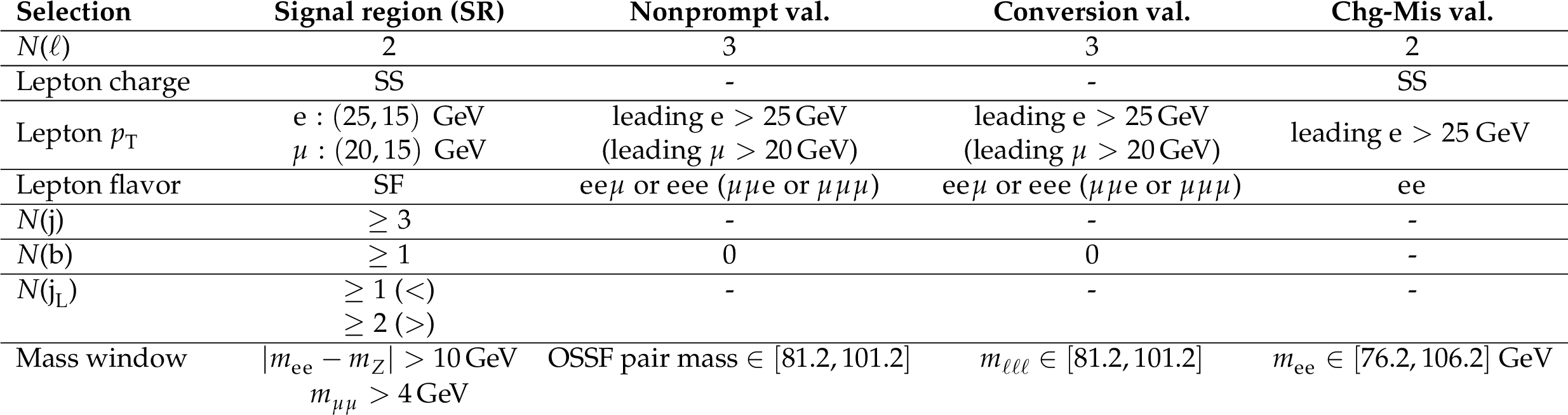
Table 3:
Summary of event selection criteria for the SR and background validation regions. |
png pdf |
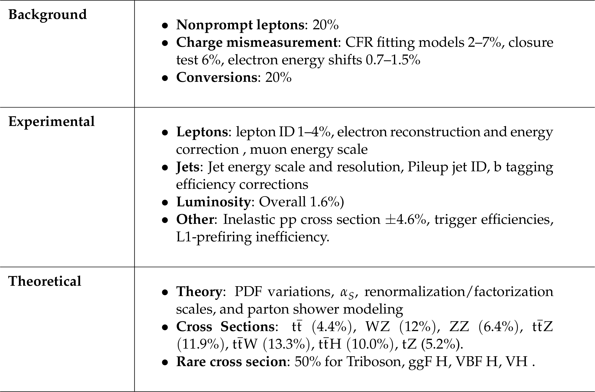
Table 4:
Summary of systematic uncertainties |
| Summary |
| This note presents the first CMS search for heavy neutral leptons ($ \mathrm{N} $) produced in top quark decays using same$ \text{-} $sign dilepton final states in proton$ \text{-} $proton collisions at $ \sqrt{s}= $ 13 TeV, corresponding to an integrated luminosity of 138 $ \text{fb}^{-1} $ collected with the CMS detector. The analysis targeted top quark decays via a $ \mathrm{N} $, predicted by type$ \text{-} $I seesaw models, exploring $ \mathrm{N} $ masses between 20 and 100 GeV. Events are selected using a same$ \text{-} $sign requirement for dileptons and the presence of jets, and a multivariate classifier to enhance the sensitivity. The result of this analysis shows the sensitivity to the branching fraction of the top quark decaying to $ \mathrm{N} $ of order $ 10^{-6} $ to $ 10^{-5} $. Converting into model parameters of the type$ \text{-} $I seesaw model, the mixing angle between $ \mathrm{N} $ and the standard model neutrino, the search shows that this channel is sensitive to those parameters at the order of $ 10^{-4} $ and 0.1 for the mass of $ \mathrm{N} $ values lower and higher than the W boson mass. |
| References | ||||
| 1 | Particle Data Group Collaboration | Review of particle physics | PRD 110 (2024) 030001 | |
| 2 | P. Minkowski | $ \mu \to e\gamma $ at a rate of one out of $ 10^{9} $ muon decays? | PLB 67 (1977) | |
| 3 | M. Gell-Mann, P. Ramond, and R. Slansky | Complex spinors and unified theories | Conf. Proc. C 790927 (1979) 315 | 1306.4669 |
| 4 | T. Yanagida | Horizontal symmetry and masses of neutrinos | Prog. Theor. Phys. 64 (1980) 1103 | |
| 5 | R. N. Mohapatra and G. Senjanovic | Neutrino mass and spontaneous parity nonconservation | PRL 44 (1980) 912 | |
| 6 | A. M. Abdullahi et al. | The present and future status of heavy neutral leptons | JPG 50 (2023) 020501 | 2203.08039 |
| 7 | M. Galeazzi, F. Fontanelli, F. Gatti, and S. Vitale | Limits on the existence of heavy neutrinos in the range 50--1000 eV from the study of the $ ^{187}\mathrm{Re} $ beta decay | PRL 86 (2001) 1978 | |
| 8 | K. H. Hiddemann, H. Daniel, and O. Schwentker | Limits on neutrino masses from the tritium beta spectrum | JPG 21 (1995) 639 | |
| 9 | CMS Collaboration | Search for heavy Majorana neutrinos in same-sign dilepton channels in proton-proton collisions at $ \sqrt{s}= $ 13 TeV | JHEP 01 (2019) 122 | CMS-EXO-17-028 1806.10905 |
| 10 | CMS Collaboration | Search for heavy neutral leptons in final states with electrons, muons, and hadronically decaying tau leptons in proton-proton collisions at $ \sqrt{s} = $ 13 TeV | JHEP 06 (2024) 123 | CMS-EXO-22-011 2403.00100 |
| 11 | ATLAS Collaboration | Search for heavy neutral leptons in decays of $ W $ bosons produced in 13 TeV $ pp $ collisions using prompt and displaced signatures with the ATLAS detector | JHEP 10 (2019) 265 | 1905.09787 |
| 12 | S. Bar-Shalom et al. | Majorana neutrinos and lepton--number--violating signals in top-quark and W-boson rare decays | PLB 643 (2006) 342 | hep-ph/0608309 |
| 13 | Z. Si and K. Wang | GeV Majorana neutrinos in top-quark decay at the LHC | PRD 79 (2009) 014034 | 0810.5266 |
| 14 | N. Quintero, G. Lopez Castro, and D. Delepine | Lepton number violation in top quark and neutral B meson decays | [Erratum: 10.1103/PhysRevD.86.079905] PRD 84 (2011) 096011 |
1108.6009 |
| 15 | N. Liu et al. | Top quark as a probe of heavy Majorana neutrino at the LHC and future colliders | PRD 101 (2020) 071701 | 1910.00749 |
| 16 | P.-C. Lu, Z.-G. Si, Z. Wang, and X.-H. Yang | CP violation in top quark decay via heavy Majorana neutrinos at the LHC | PRD 104 (2021) 115003 | 2110.10463 |
| 17 | CMS Collaboration | The CMS experiment at the CERN LHC | JINST 3 (2008) S08004 | |
| 18 | CMS Collaboration | Development of the CMS detector for the CERN LHC Run 3 | JINST 19 (2024) P05064 | CMS-PRF-21-001 2309.05466 |
| 19 | CMS Collaboration | Performance of the CMS Level-1 trigger in proton-proton collisions at $ \sqrt{s} = $ 13 TeV | JINST 15 (2020) P10017 | CMS-TRG-17-001 2006.10165 |
| 20 | CMS Collaboration | The CMS trigger system | JINST 12 (2017) P01020 | CMS-TRG-12-001 1609.02366 |
| 21 | CMS Collaboration | Performance of the CMS high-level trigger during LHC Run 2 | JINST 19 (2024) P11021 | CMS-TRG-19-001 2410.17038 |
| 22 | CMS Collaboration | Electron and photon reconstruction and identification with the CMS experiment at the CERN LHC | JINST 16 (2021) P05014 | CMS-EGM-17-001 2012.06888 |
| 23 | CMS Collaboration | Performance of the CMS muon detector and muon reconstruction with proton-proton collisions at $ \sqrt{s}= $ 13 TeV | JINST 13 (2018) P06015 | CMS-MUO-16-001 1804.04528 |
| 24 | CMS Collaboration | Description and performance of track and primary-vertex reconstruction with the CMS tracker | JINST 9 (2014) P10009 | CMS-TRK-11-001 1405.6569 |
| 25 | CMS Collaboration | Particle-flow reconstruction and global event description with the CMS detector | JINST 12 (2017) P10003 | CMS-PRF-14-001 1706.04965 |
| 26 | CMS Collaboration | Performance of reconstruction and identification of $ \tau $ leptons decaying to hadrons and $ \nu_\tau $ in pp collisions at $ \sqrt{s}= $ 13 TeV | JINST 13 (2018) P10005 | CMS-TAU-16-003 1809.02816 |
| 27 | CMS Collaboration | Jet energy scale and resolution in the CMS experiment in pp collisions at 8 TeV | JINST 12 (2017) P02014 | CMS-JME-13-004 1607.03663 |
| 28 | CMS Collaboration | Performance of missing transverse momentum reconstruction in proton-proton collisions at $ \sqrt{s} = $ 13 TeV using the CMS detector | JINST 14 (2019) P07004 | CMS-JME-17-001 1903.06078 |
| 29 | CMS Collaboration | Technical proposal for the Phase-II upgrade of the Compact Muon Solenoid | CMS Technical Proposal CERN-LHCC-2015-010, CMS-TDR-15-02, 2015 CDS |
|
| 30 | CMS Collaboration | ECAL 2016 refined calibration and Run 2 summary plots | CMS Detector Performance Summary CMS-DP-2020-021, 2020 CDS |
|
| 31 | M. Cacciari, G. P. Salam, and G. Soyez | The anti-$ k_{\mathrm{T}} $ jet clustering algorithm | JHEP 04 (2008) 063 | 0802.1189 |
| 32 | M. Cacciari, G. P. Salam, and G. Soyez | FastJet user manual | EPJC 72 (2012) 1896 | 1111.6097 |
| 33 | CMS Collaboration | Pileup mitigation at CMS in 13 TeV data | JINST 15 (2020) P09018 | CMS-JME-18-001 2003.00503 |
| 34 | CMS Collaboration | Performance of the pile up jet identification in CMS for Run 2 | CMS Detector Performance Summary CMS-DP-2020-020, 2020 CDS |
|
| 35 | E. Bols et al. | Jet flavour classification using DeepJet | JINST 15 (2020) P12012 | 2008.10519 |
| 36 | CMS Collaboration | Performance of the DeepJet b tagging algorithm using 41.9/fb of data from proton-proton collisions at 13 TeV with Phase 1 CMS detector | CMS Detector Performance Summary CMS-DP-2018-058, 2018 CDS |
|
| 37 | CMS Collaboration | Precision luminosity measurement in proton-proton collisions at $ \sqrt{s} = $ 13 TeV in 2015 and 2016 at CMS | EPJC 81 (2021) 800 | CMS-LUM-17-003 2104.01927 |
| 38 | CMS Collaboration | CMS luminosity measurement for the 2017 data-taking period at $ \sqrt{s} = $ 13 TeV | CMS Physics Analysis Summary, 2018 link |
CMS-PAS-LUM-17-004 |
| 39 | CMS Collaboration | CMS luminosity measurement for the 2018 data-taking period at $ \sqrt{s} = $ 13 TeV | CMS Physics Analysis Summary, 2019 link |
CMS-PAS-LUM-18-002 |
| 40 | J. Alwall et al. | The automated computation of tree-level and next-to-leading order differential cross sections, and their matching to parton shower simulations | JHEP 07 (2014) 079 | 1405.0301 |
| 41 | D. Alva, T. Han, and R. Ruiz | Heavy Majorana neutrinos from $ W\gamma $ fusion at hadron colliders | JHEP 02 (2015) 072 | 1411.7305 |
| 42 | C. Degrande, O. Mattelaer, R. Ruiz, and J. Turner | Fully-automated precision predictions for heavy neutrino production mechanisms at hadron colliders | PRD 94 (2016) 053002 | 1602.06957 |
| 43 | A. Alloul et al. | FeynRules 2.0 -- a complete toolbox for tree-level phenomenology | Comput. Phys. Commun. 185 (2014) 2250 | 1310.1921 |
| 44 | S. Hoeche et al. | Matching parton showers and matrix elements | in HERA and the LHC: A Workshop on the Implications of HERA for LHC Physics: CERN - / (Midterm Meeting, CERN, 11-13 October; Final Meeting, DESY, 17-21 January ), 2005 DESY Workshop 200 (2005) 288 |
hep-ph/0602031 |
| 45 | P. Artoisenet, R. Frederix, O. Mattelaer, and R. Rietkerk | Automatic spin-entangled decays of heavy resonances in Monte Carlo simulations | JHEP 03 (2013) 015 | 1212.3460 |
| 46 | P. Nason | A new method for combining NLO QCD with shower Monte Carlo algorithms | JHEP 11 (2004) 040 | hep-ph/0409146 |
| 47 | S. Frixione, P. Nason, and C. Oleari | Matching NLO QCD computations with parton shower simulations: the POWHEG method | JHEP 11 (2007) 070 | 0709.2092 |
| 48 | S. Alioli, P. Nason, C. Oleari, and E. Re | A general framework for implementing NLO calculations in shower Monte Carlo programs: the POWHEG BOX | JHEP 06 (2010) 043 | 1002.2581 |
| 49 | T. Melia, P. Nason, R. Rontsch, and G. Zanderighi | W+W-, WZ and ZZ production in the POWHEG BOX | JHEP 11 (2011) 078 | 1107.5051 |
| 50 | H. B. Hartanto, B. Jager, L. Reina, and D. Wackeroth | Higgs boson production in association with top quarks in the POWHEG BOX | PRD 91 (2015) 094003 | 1501.04498 |
| 51 | E. Bagnaschi, G. Degrassi, P. Slavich, and A. Vicini | Higgs production via gluon fusion in the POWHEG approach in the SM and in the MSSM | JHEP 02 (2012) 088 | 1111.2854 |
| 52 | P. Nason and C. Oleari | NLO Higgs boson production via vector-boson fusion matched with shower in POWHEG | JHEP 02 (2010) 037 | 0911.5299 |
| 53 | E. Re | Single-top Wt-channel production matched with parton showers using the POWHEG method | EPJC 71 (2011) 1547 | 1009.2450 |
| 54 | S. Frixione, P. Nason, and G. Ridolfi | A positive-weight next-to-leading-order Monte Carlo for heavy flavour hadroproduction | JHEP 09 (2007) 126 | 0707.3088 |
| 55 | F. Cascioli et al. | ZZ production at hadron colliders in NNLO QCD | PLB 735 (2014) 311 | 1405.2219 |
| 56 | Y. Gao et al. | Spin determination of single-produced resonances at hadron colliders | PRD 81 (2010) 075022 | 1001.3396 |
| 57 | T. Sjöstrand et al. | An introduction to PYTHIA 8.2 | Comput. Phys. Commun. 191 (2015) 159 | 1410.3012 |
| 58 | CMS Collaboration | Extraction and validation of a new set of CMS PYTHIA8 tunes from underlying-event measurements | EPJC 80 (2020) 4 | CMS-GEN-17-001 1903.12179 |
| 59 | NNPDF Collaboration | Parton distributions from high-precision collider data | EPJC 77 (2017) 663 | 1706.00428 |
| 60 | GEANT4 Collaboration | Geant4 -- a simulation toolkit | NIM A 506 (2003) 250 | |
| 61 | CMS Collaboration | Search for new physics with same-sign isolated dilepton events with jets and missing transverse energy at the LHC | JHEP 06 (2011) 077 | CMS-SUS-10-004 1104.3168 |
| 62 | R. C. Gray et al. | Backgrounds to Higgs boson searches from $ W \gamma^* - > l \nu l (l) $ asymmetric internal conversion | 1110.1368 | |
| 63 | ATLAS, CMS, LHC Higgs Combination Group Collaboration | Procedure for the LHC Higgs boson search combination in summer 2011 | Technical Report CMS-NOTE-2011-005, ATL-PHYS-PUB-2011-11, 2011 | |
| 64 | CMS Collaboration | Measurement of tracking efficiency | CMS Physics Analysis Summary, 2010 CMS-PAS-TRK-10-002 |
|
| 65 | CMS Collaboration | Electron and photon reconstruction and identification with the CMS experiment at the CERN LHC | JINST 16 (2021) P05014 | CMS-EGM-17-001 2012.06888 |
| 66 | CMS Collaboration | Measurement of the inelastic proton-proton cross section at $ \sqrt{s}= $ 13TeV | JHEP 07 (2018) 161 | CMS-FSQ-15-005 1802.02613 |
| 67 | CMS Collaboration | Performance of the CMS electromagnetic calorimeter in pp collisions at \ensuremath\sqrt$ _{s} = $ 13 TeV | JINST 19 (2024) P09004 | CMS-EGM-18-002 2403.15518 |
| 68 | R. J. Barlow and C. Beeston | Fitting using finite Monte Carlo samples | Comput. Phys. Commun. 77 (1993) 219 | |
| 69 | ATLAS Collaboration | Measurement of the $ t\bar{t} $ production cross-section using $ e\mu $ events with b-tagged jets in pp collisions at $ \sqrt{s} = $ 13 TeV with the ATLAS detector | [Erratum: 10./j.physletb..09.027] PLB 761 (2016) 136 |
1606.02699 |
| 70 | J. Butterworth et al. | PDF4LHC recommendations for LHC Run II | JPG 43 (2016) 023001 | |
| 71 | M. Grazzini, S. Kallweit, D. Rathlev, and M. Wiesemann | $ W^{\pm}Z $ production at hadron colliders in NNLO QCD | PLB 761 (2016) 179 | 1604.08576 |
| 72 | LHC Higgs Cross Section Working Group | Handbook of lhc higgs cross sections: 4. deciphering the nature of the higgs sector | CERN Yellow Rep. Monogr. 2 (2017) 1 | 1610.07922 |
| 73 | C. Degrande et al. | Single--top associated production with a $ Z $ or $ H $ boson at the LHC: the SMEFT interpretation | JHEP 10 (2018) 005 | 1804.07773 |
| 74 | CMS Collaboration | The CMS statistical analysis and combination tool: Combine | Comput. Softw. Big Sci. 8 (2024) 19 | CMS-CAT-23-001 2404.06614 |
| 75 | W. Verkerke and D. P. Kirkby | The RooFit toolkit for data modeling | volume 0303241, p. MOLT007, 2003 | physics/0306116 |
| 76 | L. Moneta et al. | The RooStats project | in the Int. Workshop on Advanced Computing and Analysis Techniques in Physics Research (ACAT ): Jaipur, India, February 22--27, 2010 Proc. 1 (2010) 3 |
1009.1003 |
| 77 | T. Junk | Confidence level computation for combining searches with small statistics | NIM A 434 (1999) 435 | hep-ex/9902006 |
| 78 | A. L. Read | Presentation of search results: The $ CL_s $ technique | JPG 28 (2002) 2693 | |
|
|
Compact Muon Solenoid LHC, CERN |

|
|
|
|
|
|