

Compact Muon Solenoid
LHC, CERN
| CMS-PAS-TOP-19-008 | ||
| Measurement of the top quark Yukawa coupling from $\mathrm{t}\bar{\mathrm{t}}$ kinematic distributions in the dilepton final state at $\sqrt{s}= $ 13 TeV | ||
| CMS Collaboration | ||
| May 2020 | ||
| Abstract: An indirect measurement of the Higgs Yukawa coupling to the top quark is presented using pp collision at $\sqrt{s}= $ 13 TeV with an integrated luminosity of 137 fb$^{-1}$ recorded by the CMS detector. The coupling strength with respect to the standard model value, $Y_\mathrm{t}$, is determined from kinematic distributions in $\mathrm{t\bar{t}}$ production final states containing ee, $\mu\mu$, or e$\mu$ pairs. Sensitivity to the Yukawa coupling originates from altered distributions of $\mathrm{t\bar{t}}$ production in the presence of virtual Higgs boson exchange. In particular the distributions of the mass of the $\mathrm{t\bar{t}}$ system and the rapidity difference of the top quark and antiquark are sensitive to the value of $Y_\mathrm{t}$. The measurement yields a best-fit value of $Y_\mathrm{t}=$ 1.16$^{+0.24}_{-0.35}$ and a 95% confidence interval of $Y_\mathrm{t}\in[0,1.62]$. | ||
|
Links:
CDS record (PDF) ;
CADI line (restricted) ;
These preliminary results are superseded in this paper, PRD 102 (2020) 092013. The superseded preliminary plots can be found here. |
||
| Figures | |
png pdf |
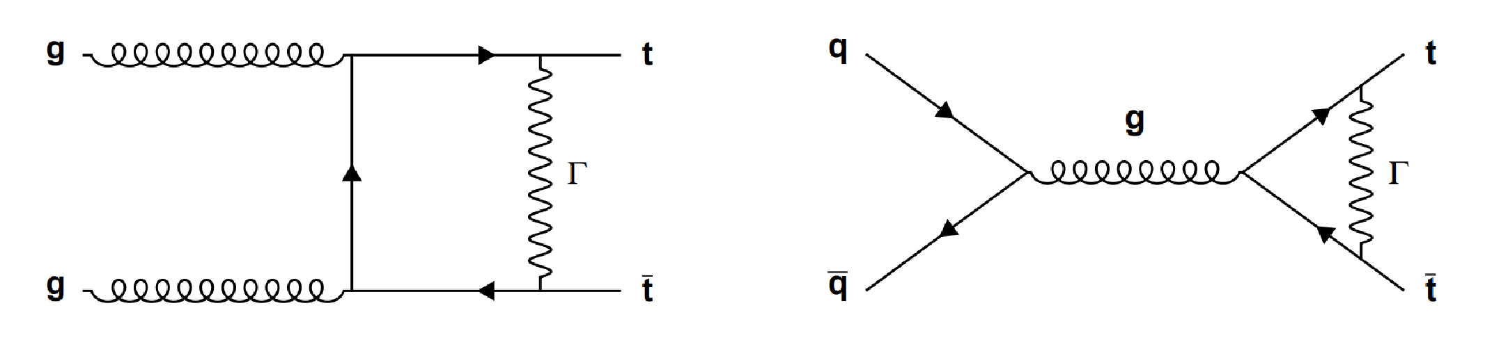
Figure 1:
Sample diagrams for weak contributions to gluon-induced and quark-induced top quark pair production, where $\Gamma $ stands for neutral gauge bosons, Higgs boson and pseudo-Goldstone bosons. |
png pdf |
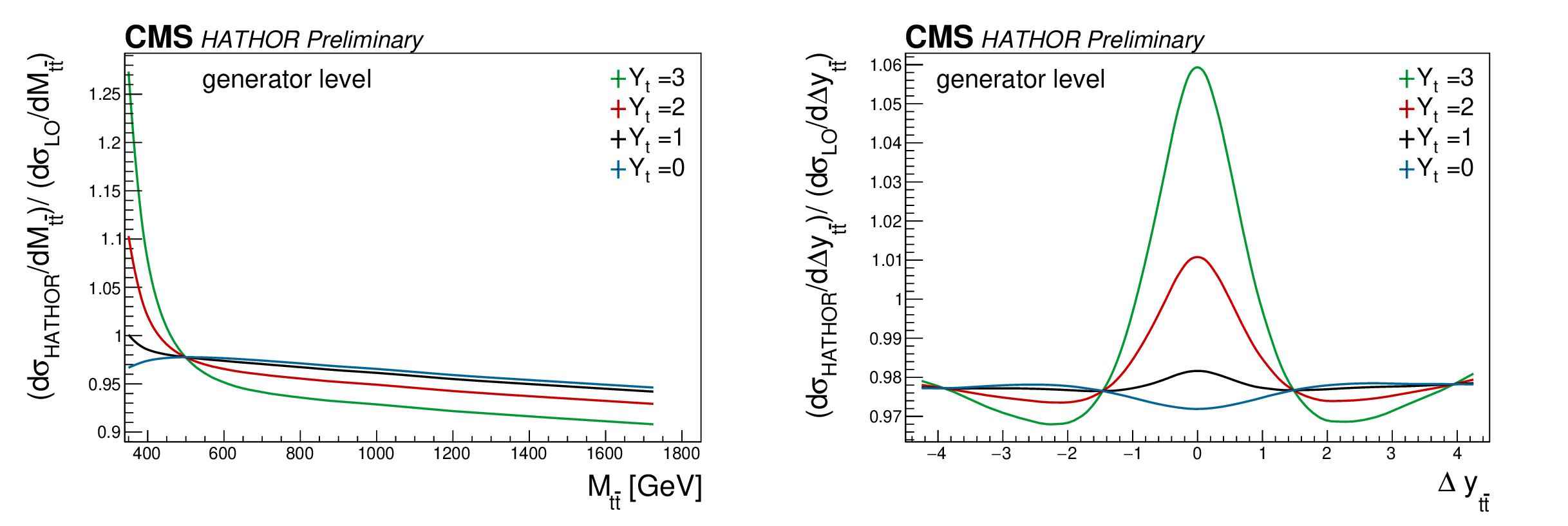
Figure 2:
Effect of the weak corrections on ${\mathrm{t} {}\mathrm{\bar{t}}}$ differential kinematic distributions for different values of $ {Y_\mathrm {t}} $, after reweighting of simulated events. |
png pdf |
Figure 2-a:
Effect of the weak corrections on ${\mathrm{t} {}\mathrm{\bar{t}}}$ differential kinematic distributions for different values of $ {Y_\mathrm {t}} $, after reweighting of simulated events. |
png pdf |
Figure 2-b:
Effect of the weak corrections on ${\mathrm{t} {}\mathrm{\bar{t}}}$ differential kinematic distributions for different values of $ {Y_\mathrm {t}} $, after reweighting of simulated events. |
png pdf |
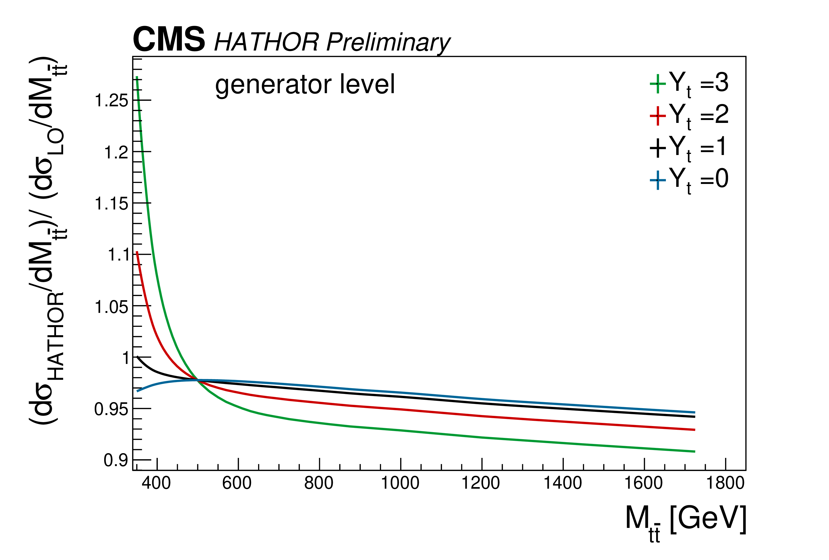
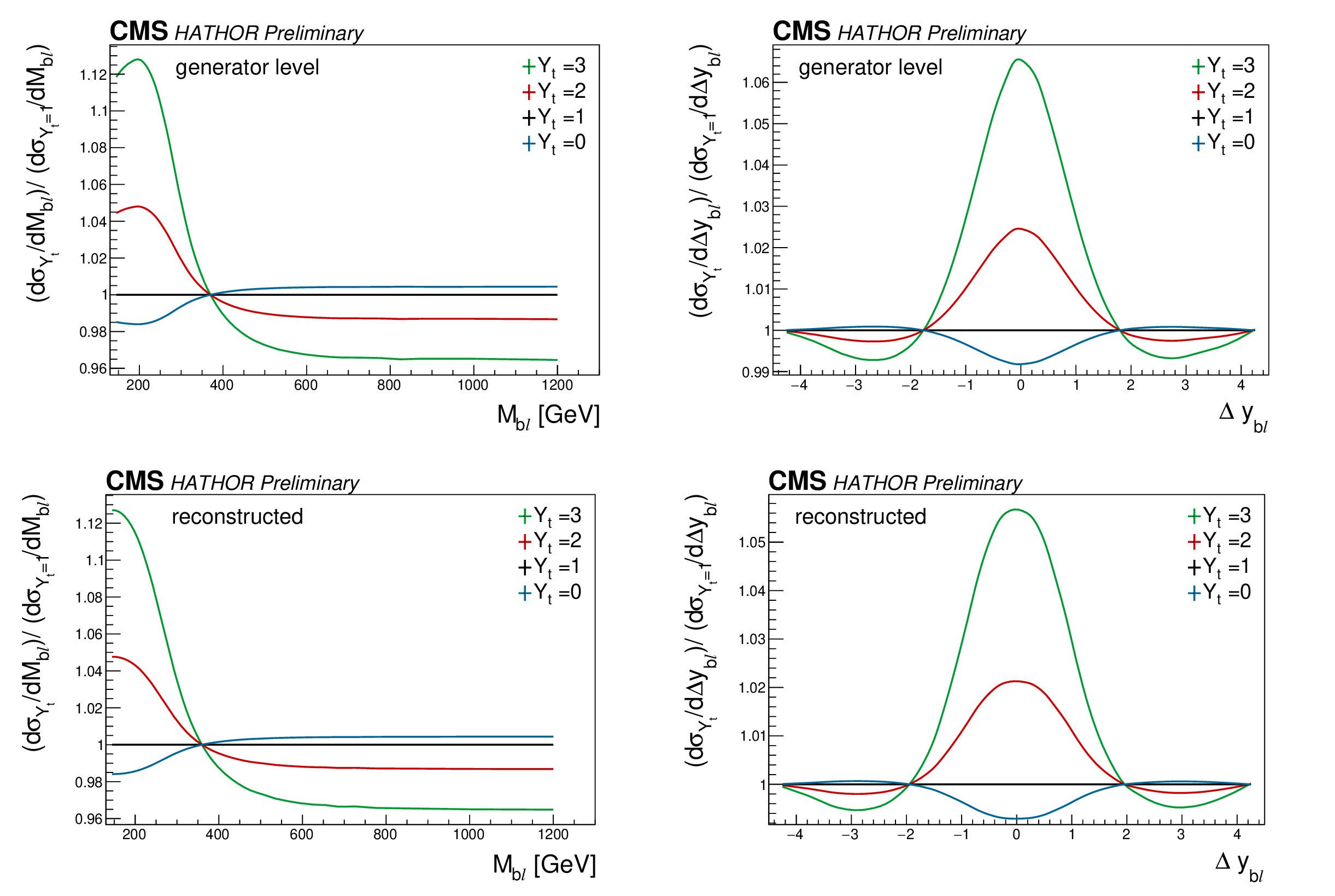
Figure 3:
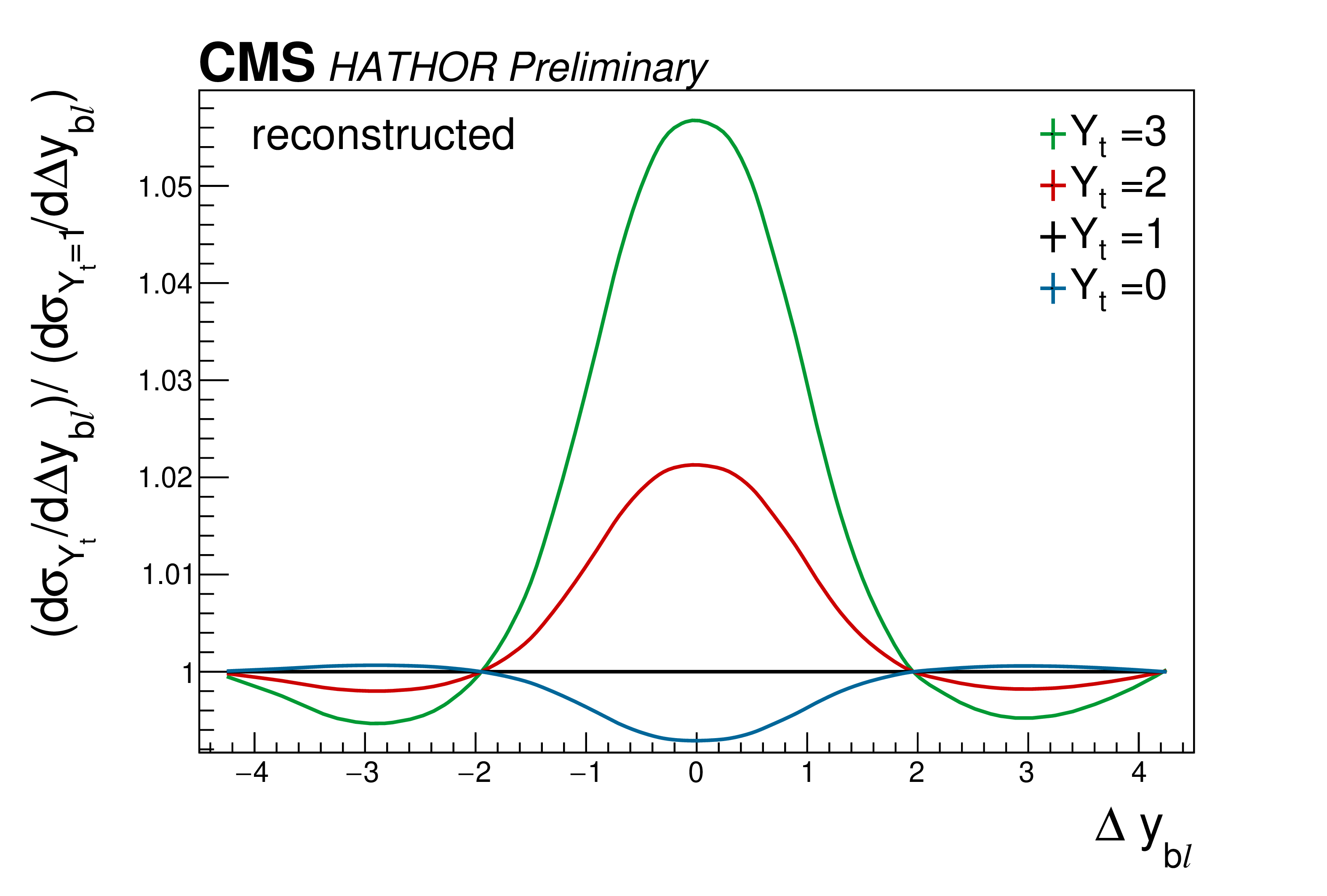
The ratio of reconstructed kinematic distributions with weak corrections (evaluated for various values of ${Y_\mathrm {t}}$) to the SM kinematic distribution is shown, demonstrating the sensitivity of these distributions to the Yukawa coupling. The upper figures show the information at generator level, while the lower figures are obtained from reconstructed events. |
png pdf |
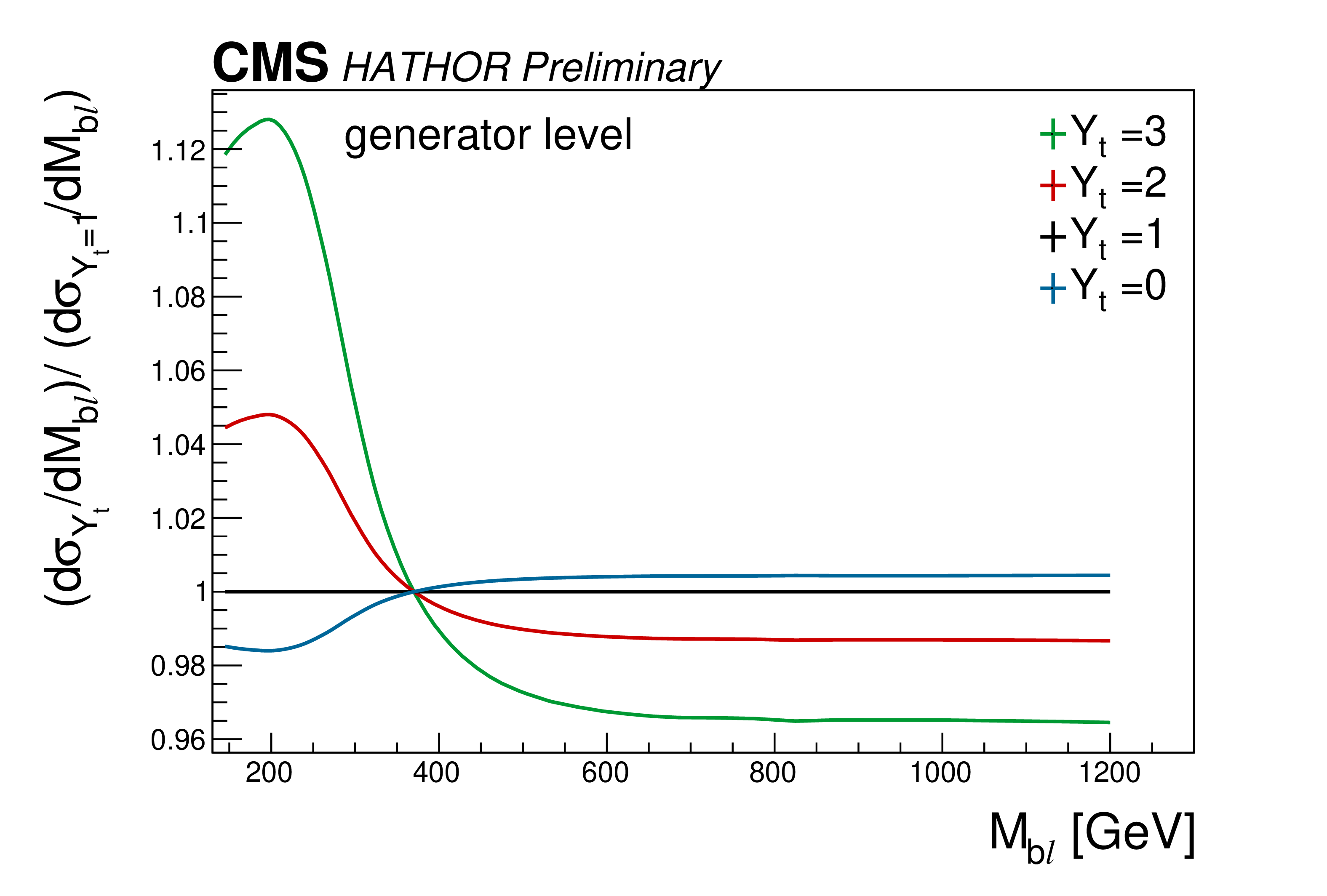
Figure 3-a:
The ratio of reconstructed kinematic distributions with weak corrections (evaluated for various values of ${Y_\mathrm {t}}$) to the SM kinematic distribution is shown, demonstrating the sensitivity of these distributions to the Yukawa coupling. The upper figures show the information at generator level, while the lower figures are obtained from reconstructed events. |
png pdf |
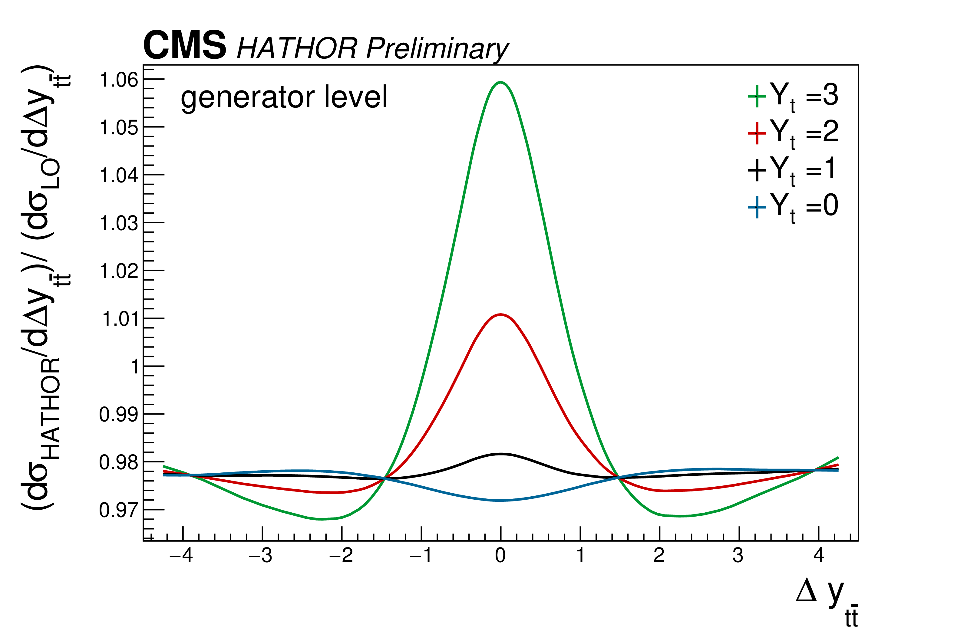
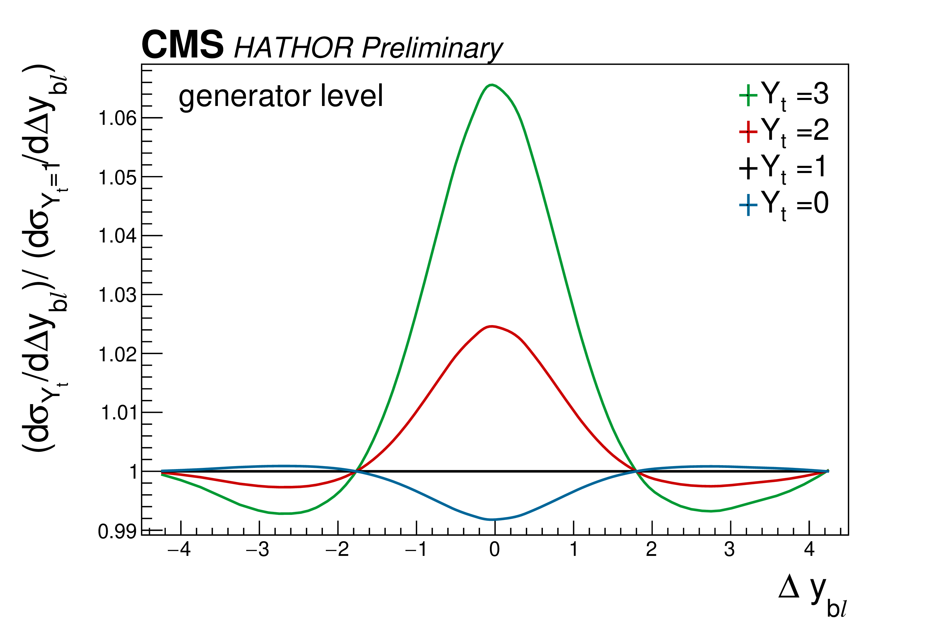
Figure 3-b:
The ratio of reconstructed kinematic distributions with weak corrections (evaluated for various values of ${Y_\mathrm {t}}$) to the SM kinematic distribution is shown, demonstrating the sensitivity of these distributions to the Yukawa coupling. The upper figures show the information at generator level, while the lower figures are obtained from reconstructed events. |
png pdf |
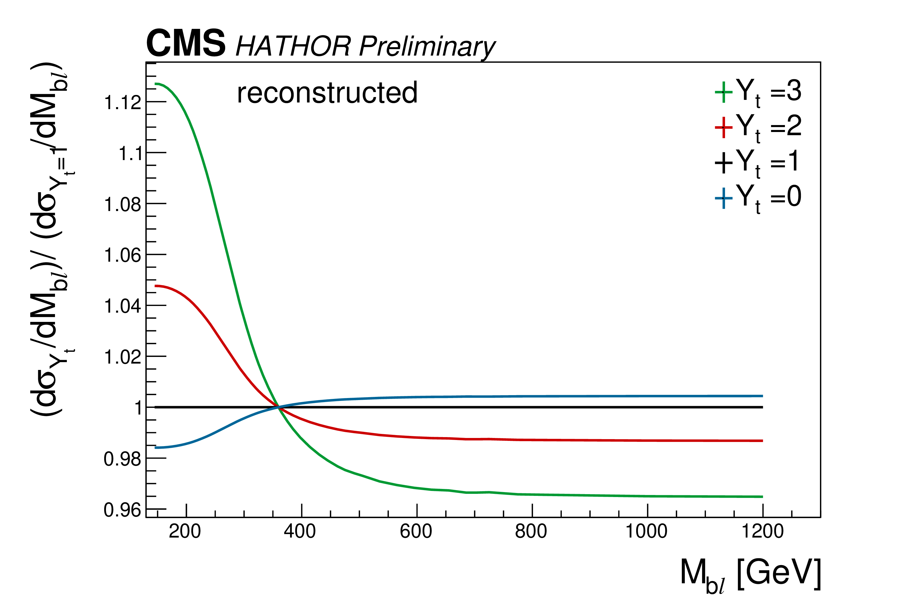
Figure 3-c:
The ratio of reconstructed kinematic distributions with weak corrections (evaluated for various values of ${Y_\mathrm {t}}$) to the SM kinematic distribution is shown, demonstrating the sensitivity of these distributions to the Yukawa coupling. The upper figures show the information at generator level, while the lower figures are obtained from reconstructed events. |
png pdf |
Figure 3-d:
The ratio of reconstructed kinematic distributions with weak corrections (evaluated for various values of ${Y_\mathrm {t}}$) to the SM kinematic distribution is shown, demonstrating the sensitivity of these distributions to the Yukawa coupling. The upper figures show the information at generator level, while the lower figures are obtained from reconstructed events. |
png pdf |
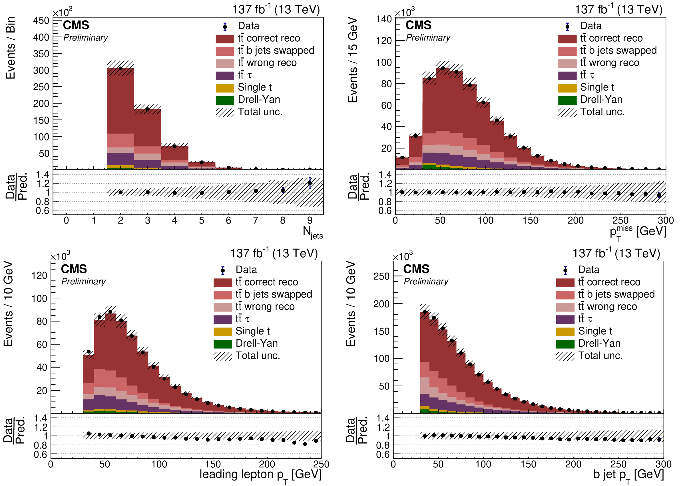
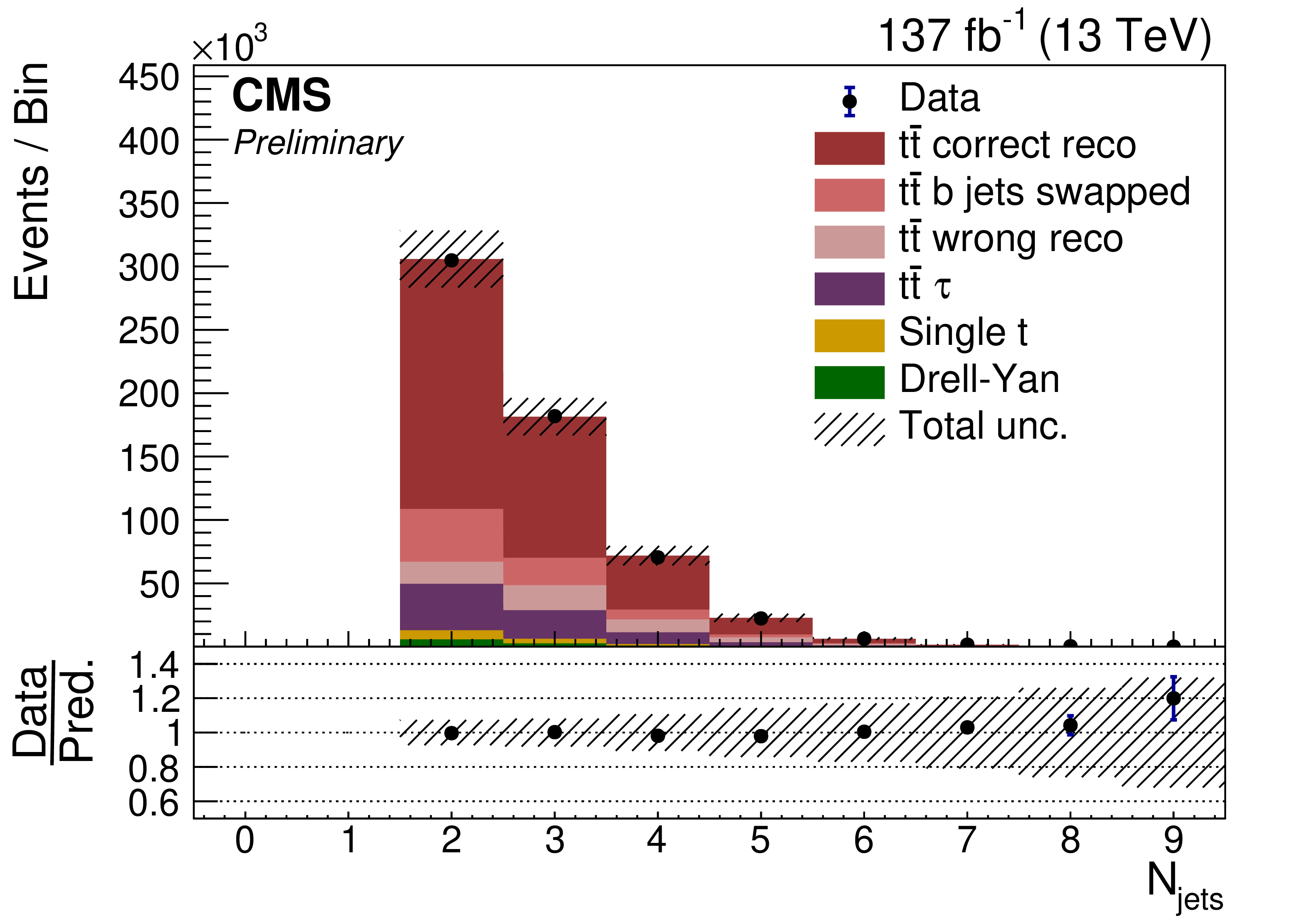
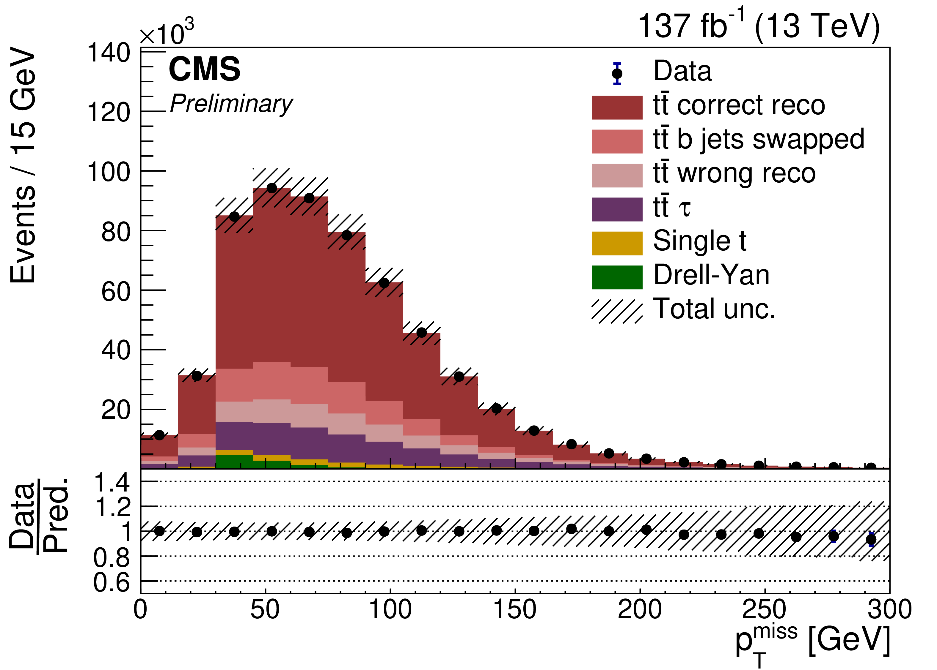
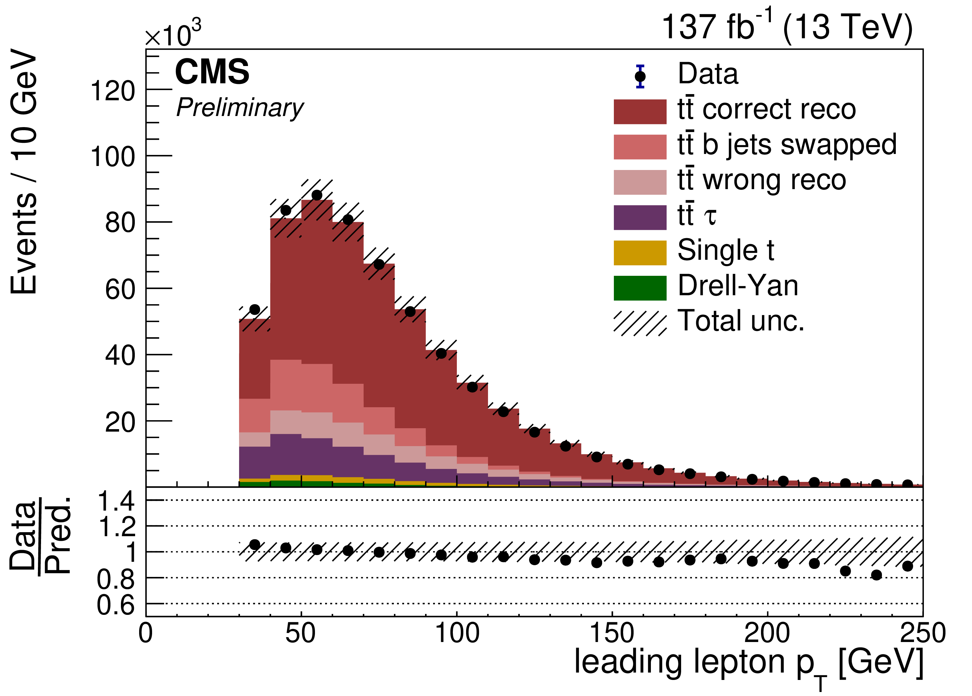
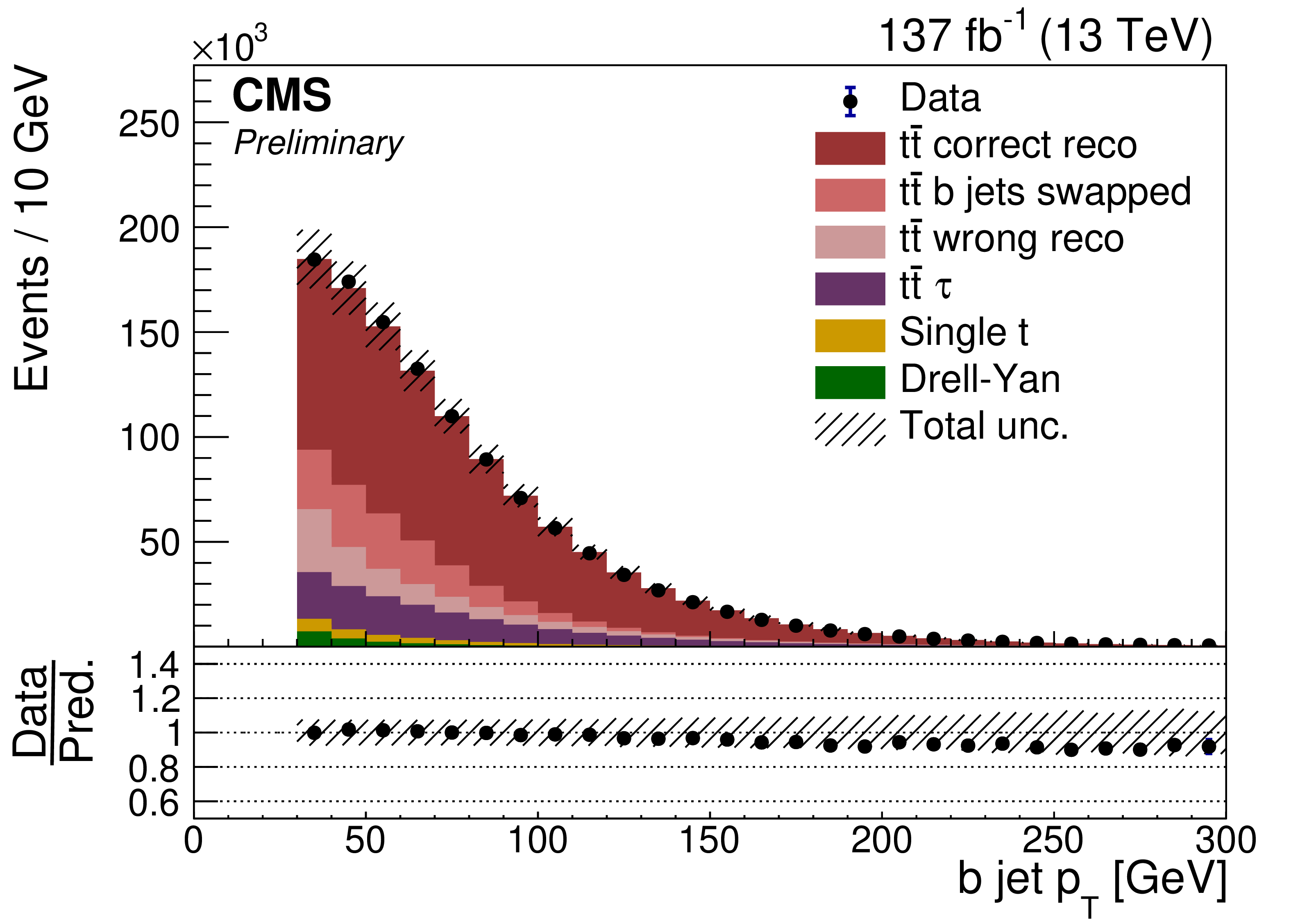
Figure 4:
Data to MC simulation comparison is shown for jet multiplicity, ${{p_{\mathrm {T}}} ^\text {miss}}$, lepton ${p_{\mathrm {T}}}$, and b jet ${p_{\mathrm {T}}}$. Uncertainty bands are derived by varying each known uncertainty source up and down across the full data-taking run, and summing the effects in quadrature. Here the signal simulation is divided into the following categories: correctly reconstructed events (${\mathrm{t} {}\mathrm{\bar{t}}}$ correct reco), events with correctly reconstructed leptons and b jets but incorrect pairing of b jets and leptons (${\mathrm{t} {}\mathrm{\bar{t}}}$ b jets swapped), events with incorrectly reconstructed b jets or leptons including non-dilepton ${\mathrm{t} {}\mathrm{\bar{t}}}$ decays (${\mathrm{t} {}\mathrm{\bar{t}}}$ wrong reco), and a separate category for incorrectly reconstructed dilepton events which have a $\tau $ lepton in the final state (${\mathrm{t} {}\mathrm{\bar{t}}}$ $\tau $). |
png pdf |
Figure 4-a:
Data to MC simulation comparison is shown for jet multiplicity, ${{p_{\mathrm {T}}} ^\text {miss}}$, lepton ${p_{\mathrm {T}}}$, and b jet ${p_{\mathrm {T}}}$. Uncertainty bands are derived by varying each known uncertainty source up and down across the full data-taking run, and summing the effects in quadrature. Here the signal simulation is divided into the following categories: correctly reconstructed events (${\mathrm{t} {}\mathrm{\bar{t}}}$ correct reco), events with correctly reconstructed leptons and b jets but incorrect pairing of b jets and leptons (${\mathrm{t} {}\mathrm{\bar{t}}}$ b jets swapped), events with incorrectly reconstructed b jets or leptons including non-dilepton ${\mathrm{t} {}\mathrm{\bar{t}}}$ decays (${\mathrm{t} {}\mathrm{\bar{t}}}$ wrong reco), and a separate category for incorrectly reconstructed dilepton events which have a $\tau $ lepton in the final state (${\mathrm{t} {}\mathrm{\bar{t}}}$ $\tau $). |
png pdf |
Figure 4-b:
Data to MC simulation comparison is shown for jet multiplicity, ${{p_{\mathrm {T}}} ^\text {miss}}$, lepton ${p_{\mathrm {T}}}$, and b jet ${p_{\mathrm {T}}}$. Uncertainty bands are derived by varying each known uncertainty source up and down across the full data-taking run, and summing the effects in quadrature. Here the signal simulation is divided into the following categories: correctly reconstructed events (${\mathrm{t} {}\mathrm{\bar{t}}}$ correct reco), events with correctly reconstructed leptons and b jets but incorrect pairing of b jets and leptons (${\mathrm{t} {}\mathrm{\bar{t}}}$ b jets swapped), events with incorrectly reconstructed b jets or leptons including non-dilepton ${\mathrm{t} {}\mathrm{\bar{t}}}$ decays (${\mathrm{t} {}\mathrm{\bar{t}}}$ wrong reco), and a separate category for incorrectly reconstructed dilepton events which have a $\tau $ lepton in the final state (${\mathrm{t} {}\mathrm{\bar{t}}}$ $\tau $). |
png pdf |
Figure 4-c:
Data to MC simulation comparison is shown for jet multiplicity, ${{p_{\mathrm {T}}} ^\text {miss}}$, lepton ${p_{\mathrm {T}}}$, and b jet ${p_{\mathrm {T}}}$. Uncertainty bands are derived by varying each known uncertainty source up and down across the full data-taking run, and summing the effects in quadrature. Here the signal simulation is divided into the following categories: correctly reconstructed events (${\mathrm{t} {}\mathrm{\bar{t}}}$ correct reco), events with correctly reconstructed leptons and b jets but incorrect pairing of b jets and leptons (${\mathrm{t} {}\mathrm{\bar{t}}}$ b jets swapped), events with incorrectly reconstructed b jets or leptons including non-dilepton ${\mathrm{t} {}\mathrm{\bar{t}}}$ decays (${\mathrm{t} {}\mathrm{\bar{t}}}$ wrong reco), and a separate category for incorrectly reconstructed dilepton events which have a $\tau $ lepton in the final state (${\mathrm{t} {}\mathrm{\bar{t}}}$ $\tau $). |
png pdf |
Figure 4-d:
Data to MC simulation comparison is shown for jet multiplicity, ${{p_{\mathrm {T}}} ^\text {miss}}$, lepton ${p_{\mathrm {T}}}$, and b jet ${p_{\mathrm {T}}}$. Uncertainty bands are derived by varying each known uncertainty source up and down across the full data-taking run, and summing the effects in quadrature. Here the signal simulation is divided into the following categories: correctly reconstructed events (${\mathrm{t} {}\mathrm{\bar{t}}}$ correct reco), events with correctly reconstructed leptons and b jets but incorrect pairing of b jets and leptons (${\mathrm{t} {}\mathrm{\bar{t}}}$ b jets swapped), events with incorrectly reconstructed b jets or leptons including non-dilepton ${\mathrm{t} {}\mathrm{\bar{t}}}$ decays (${\mathrm{t} {}\mathrm{\bar{t}}}$ wrong reco), and a separate category for incorrectly reconstructed dilepton events which have a $\tau $ lepton in the final state (${\mathrm{t} {}\mathrm{\bar{t}}}$ $\tau $). |
png pdf |
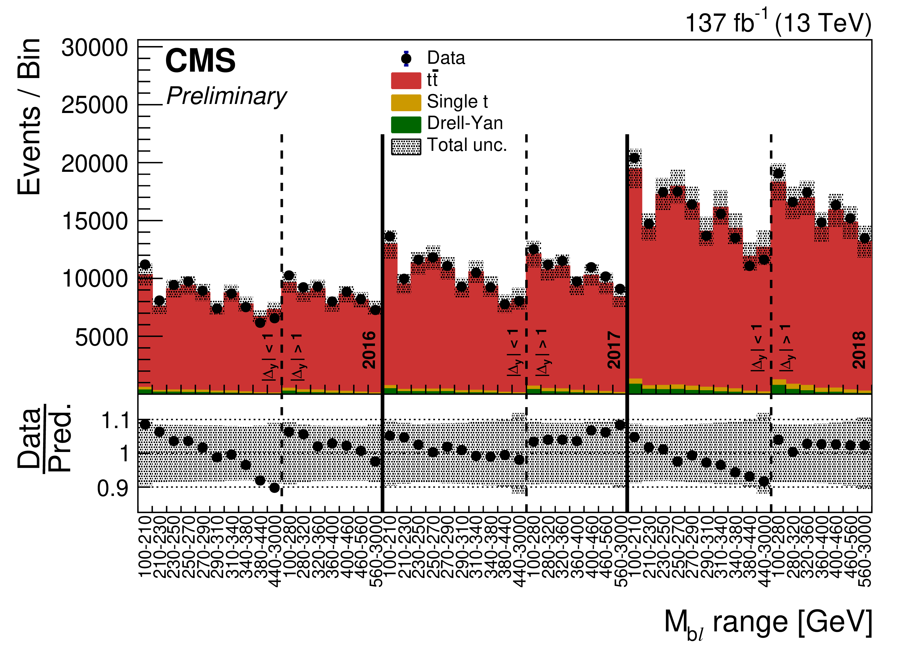
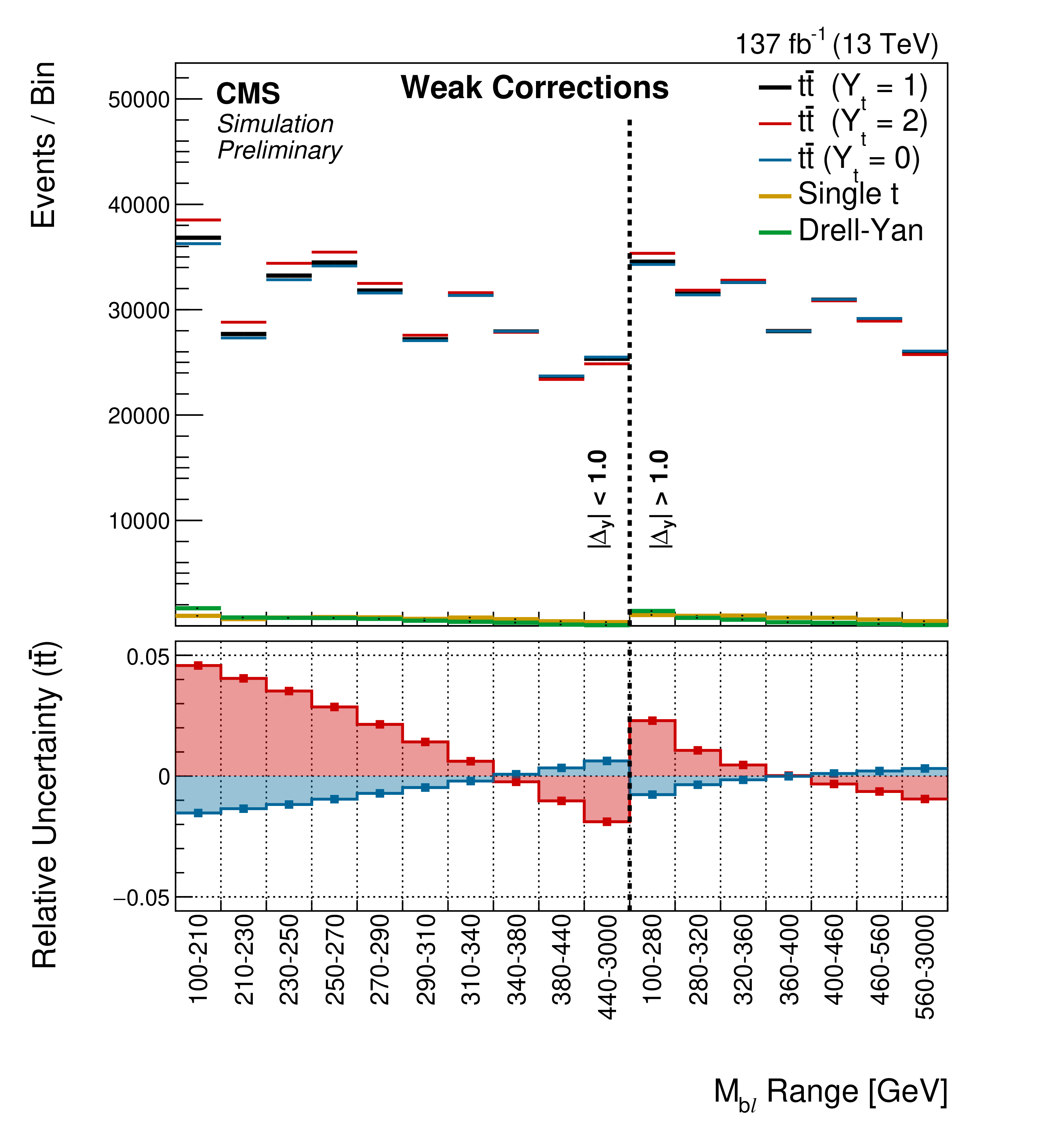
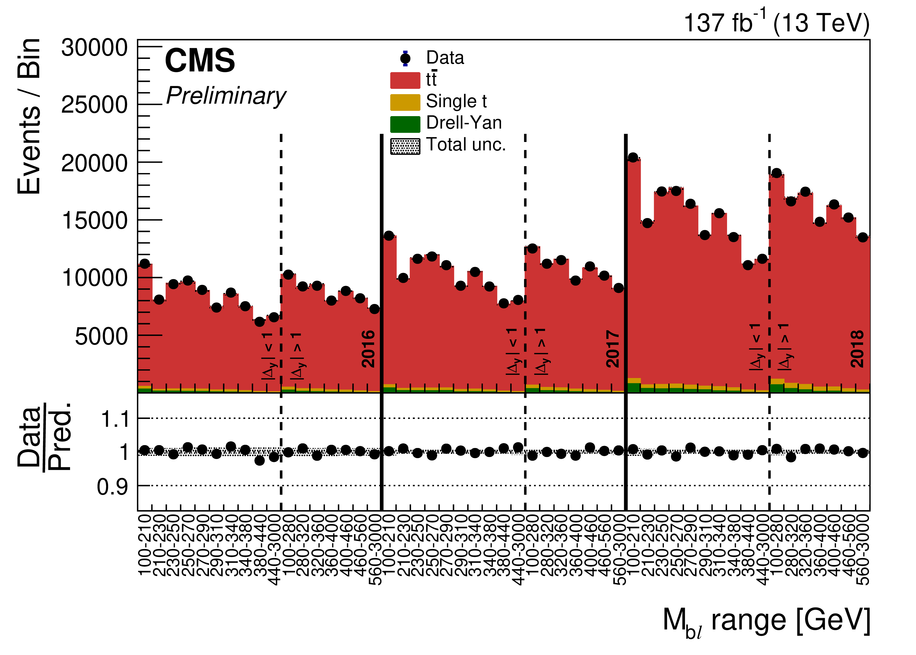
Figure 5:
Binned data and simulated events prior to performing the fit. The solid lines divide the three datataking periods, while the dashed lines divide the two ${|\Delta y|_\mathrm {b\ell}}$ bins in each datataking period, with ${M_\mathrm {b\ell}}$ bin ranges displayed on the $x$ axis. |
png pdf |
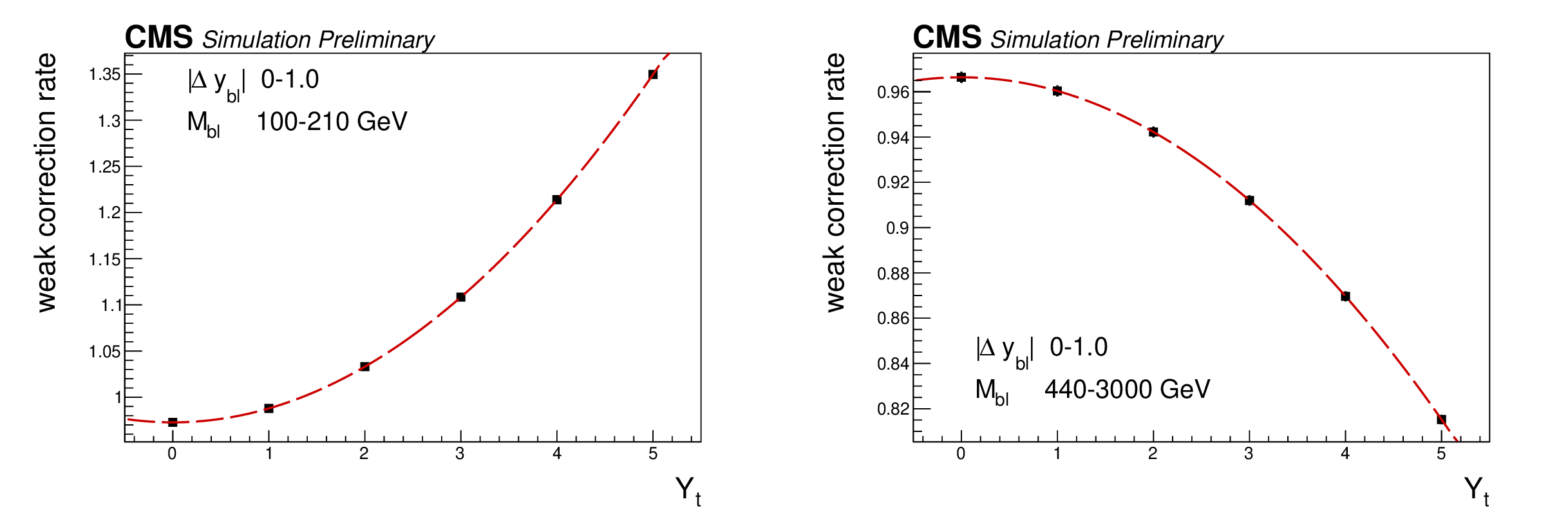
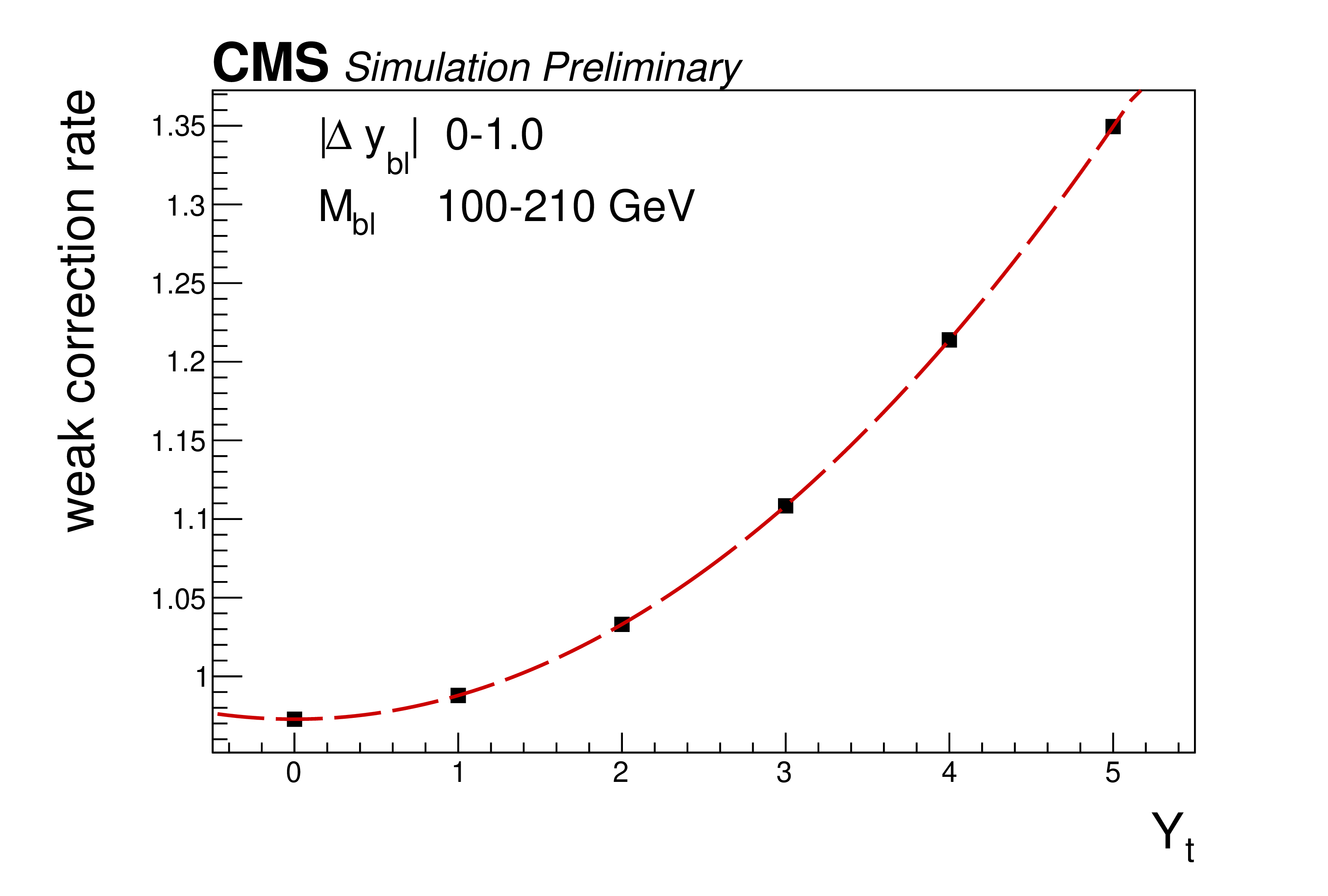
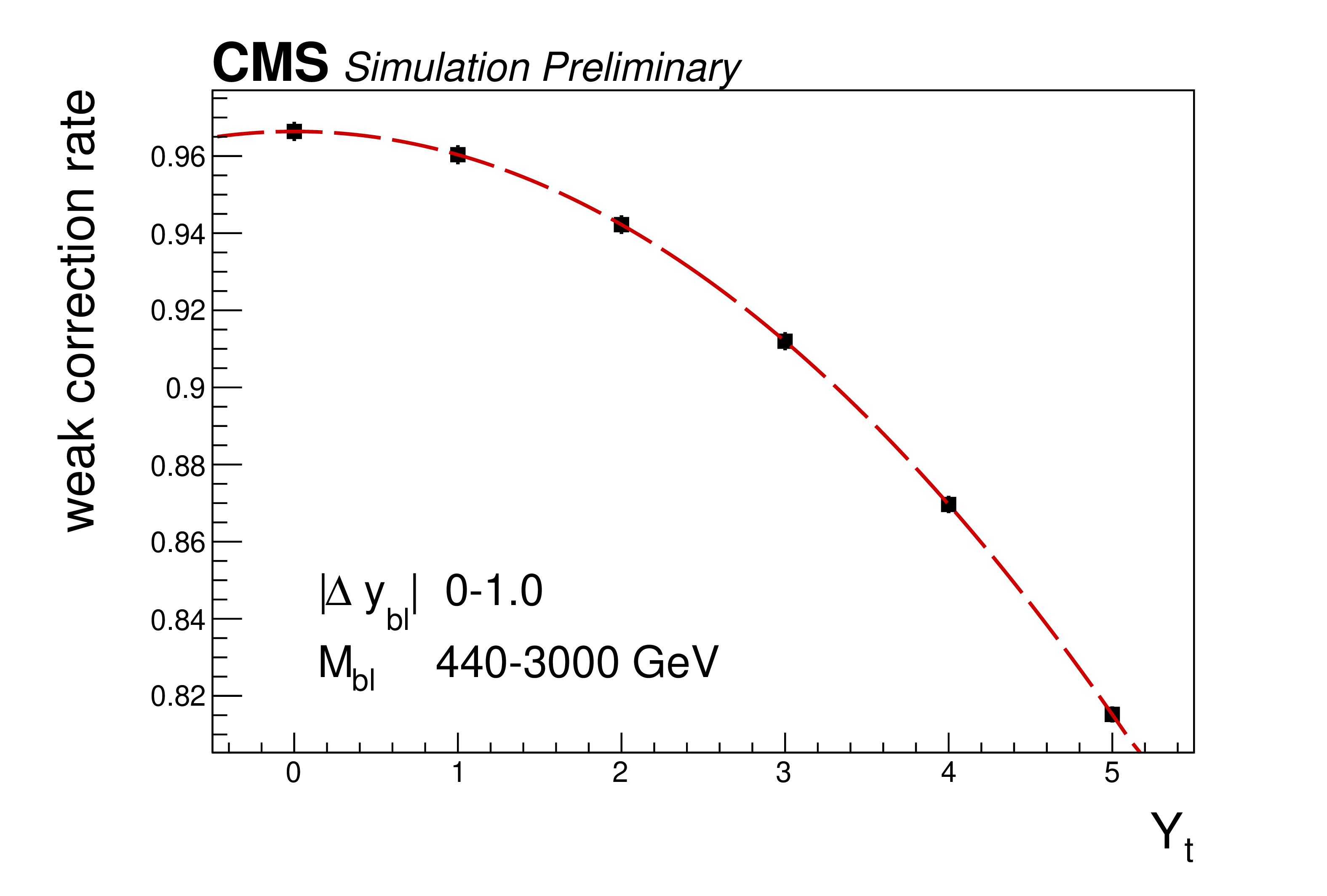
Figure 6:
The weak correction rate modifier $R_\mathrm {W}^\mathrm {bin}$ in two separate [$ {M_\mathrm {b\ell}}$, ${\Delta y_\mathrm {b\ell}} $] bins from 2017 data, demonstrating the quadratic dependence on ${Y_\mathrm {t}}$. All bins will have an increasing or decreasing quadratic yield function, with the steepest dependence on ${Y_\mathrm {t}}$ found at lower values of ${M_\mathrm {b\ell}}$. |
png pdf |
Figure 6-a:
The weak correction rate modifier $R_\mathrm {W}^\mathrm {bin}$ in two separate [$ {M_\mathrm {b\ell}}$, ${\Delta y_\mathrm {b\ell}} $] bins from 2017 data, demonstrating the quadratic dependence on ${Y_\mathrm {t}}$. All bins will have an increasing or decreasing quadratic yield function, with the steepest dependence on ${Y_\mathrm {t}}$ found at lower values of ${M_\mathrm {b\ell}}$. |
png pdf |
Figure 6-b:
The weak correction rate modifier $R_\mathrm {W}^\mathrm {bin}$ in two separate [$ {M_\mathrm {b\ell}}$, ${\Delta y_\mathrm {b\ell}} $] bins from 2017 data, demonstrating the quadratic dependence on ${Y_\mathrm {t}}$. All bins will have an increasing or decreasing quadratic yield function, with the steepest dependence on ${Y_\mathrm {t}}$ found at lower values of ${M_\mathrm {b\ell}}$. |
png pdf |
Figure 7:
The effect of the Yukawa parameter ${Y_\mathrm {t}}$ on reconstructed events in the final binning. The POI induces a shape distortion on the kinematic distributions. |
png pdf |
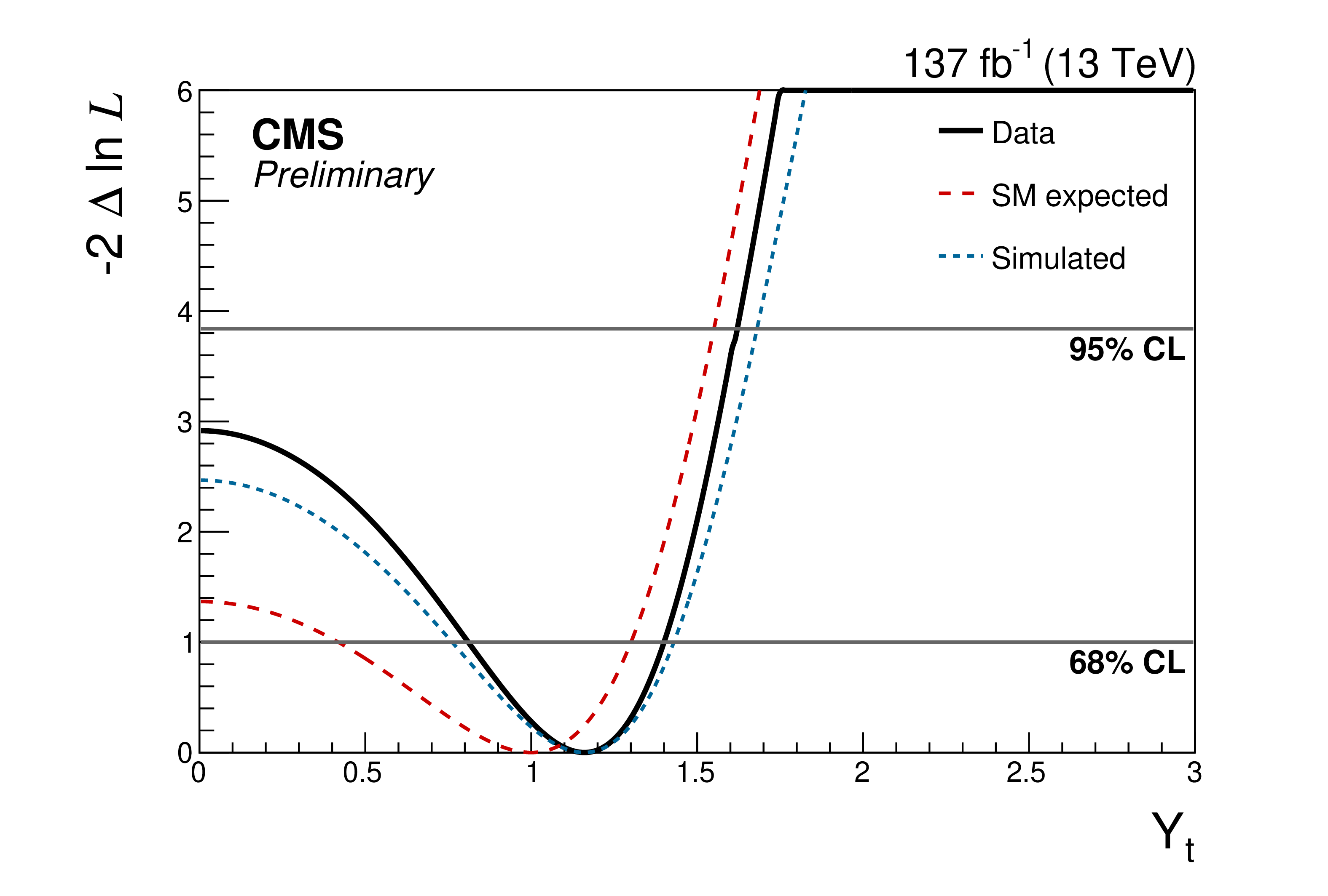
Figure 8:
The result of a likelihood scan, performed by fixing the value of $ {Y_\mathrm {t}} $ at values over the interval [0, 3]. Expected curves from fits on simulated data are shown produced at the SM value $ {Y_\mathrm {t}} =$ 1.0 (red, dashed) and at the final best-fit value of $ {Y_\mathrm {t}} =$ 1.16 (blue, dashed). |
png pdf |
Figure 9:
The agreement between data and MC simulation at the best fit value of $ {Y_\mathrm {t}} =$ 1.16 after performing the likelihood maximization, with shaded bands displaying the post-fit uncertainty. The solid lines divide the three datataking periods, while the dashed lines divide the two ${|\Delta y|_\mathrm {b\ell}}$ bins in each datataking period, with ${M_\mathrm {b\ell}}$ bin ranges displayed on the x axis. |
png pdf |
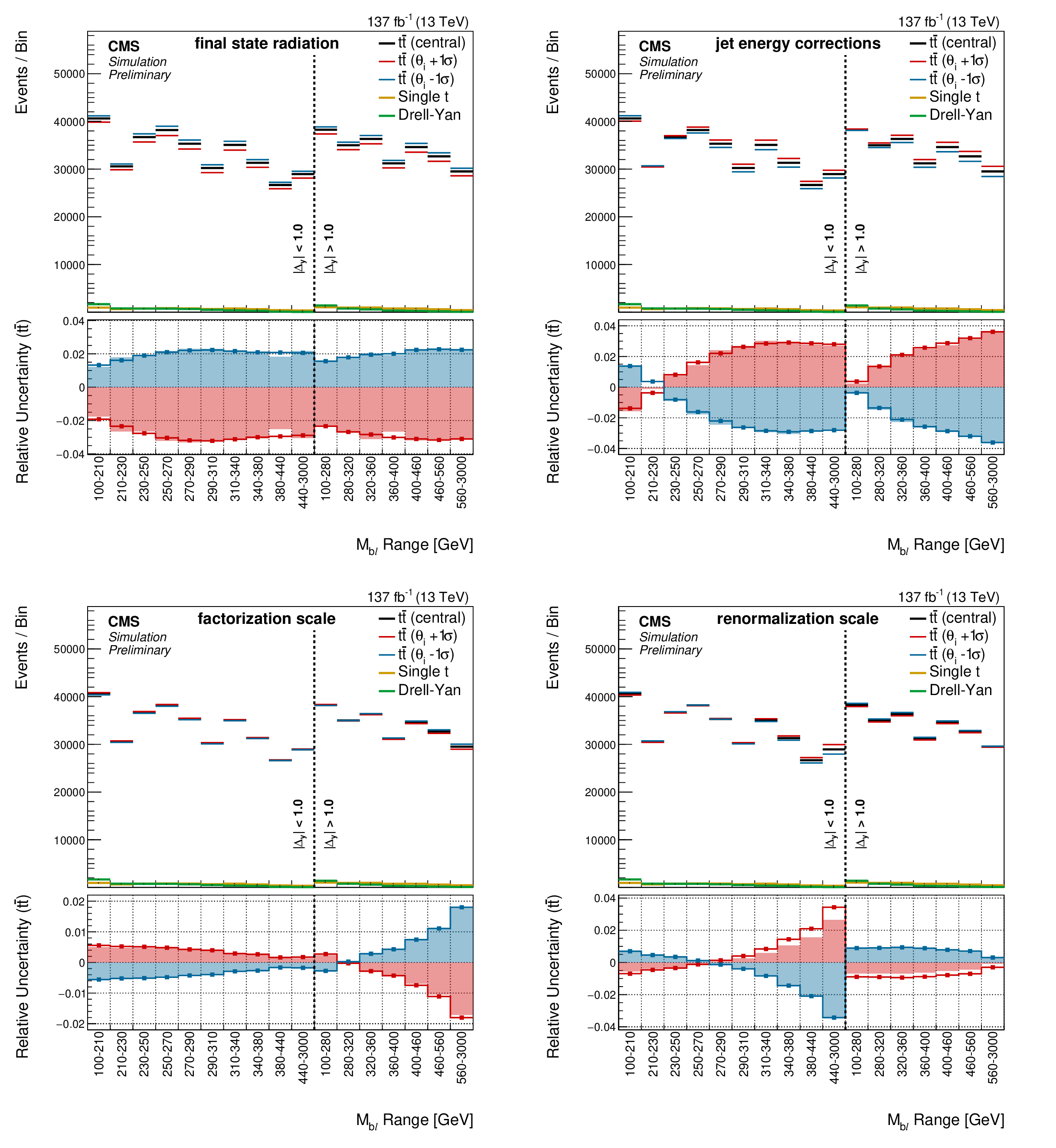
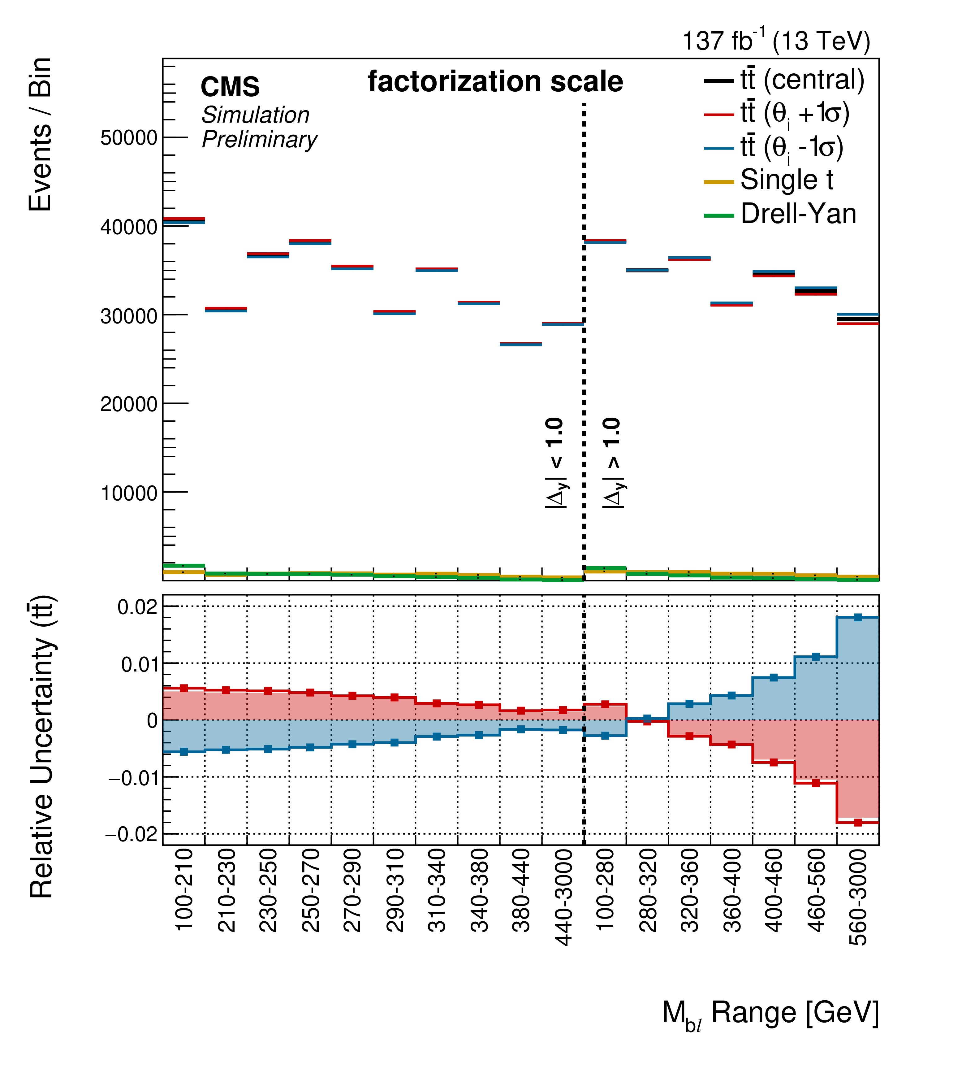
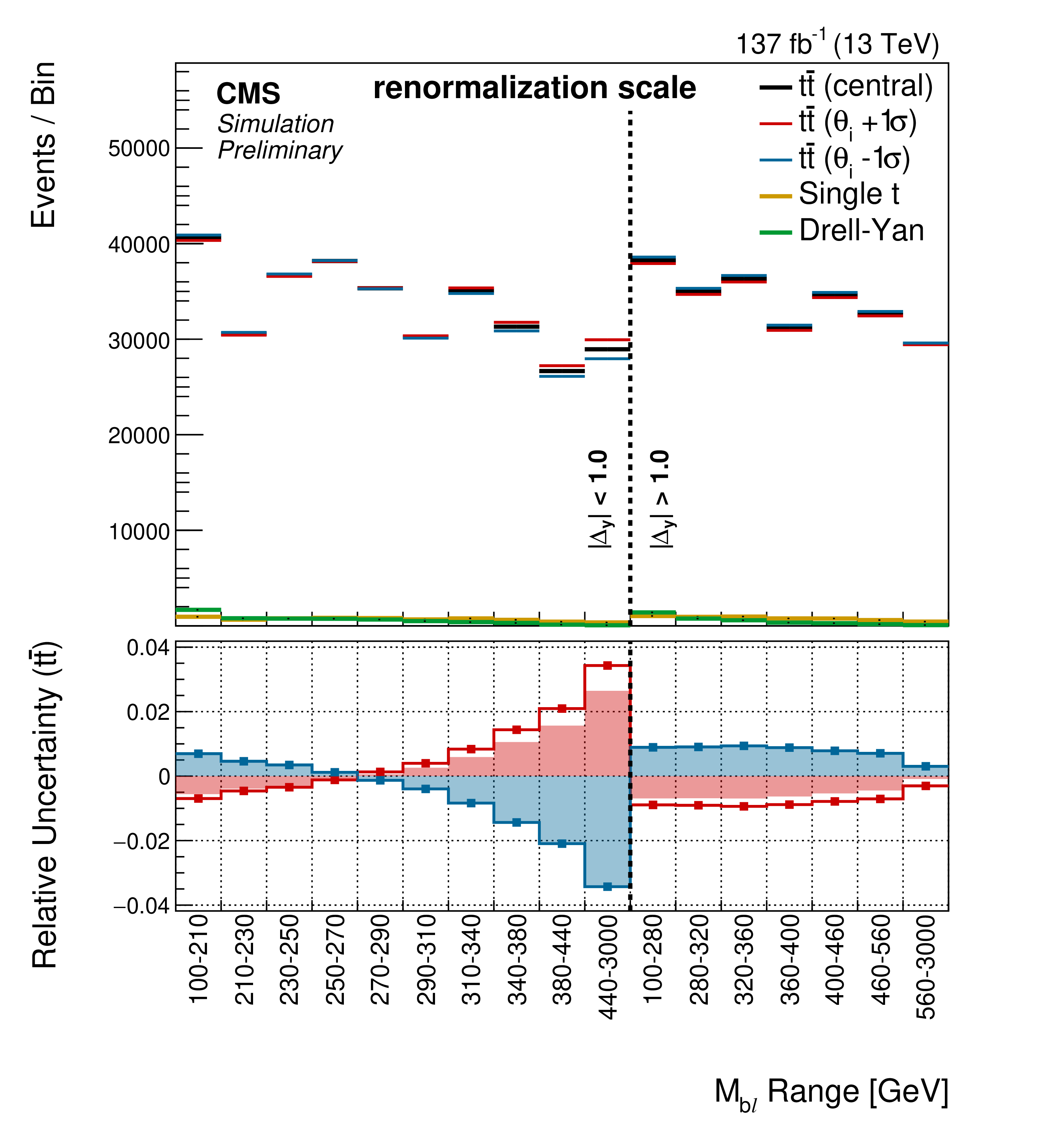
Figure 10:
Shape templates are shown for the uncertainties associated with the final-state radiation in PYTHIA8, the jet energy corrections, the factorization scale, and the renormalization scale. Along with the intrinsic uncertainty included on the weak corrections, these are seen to be the dominant uncertainties in the fit. The shaded bars represent the raw template information, while the lines show the shapes after smoothing and symmetrization procedures have been applied. In the fit, the jet energy corrections are split into 26 different components, but for brevity only the total uncertainty is shown here. Variation between years is minimal for each of these uncertainties, though they are treated separately in the fit. |
png pdf |
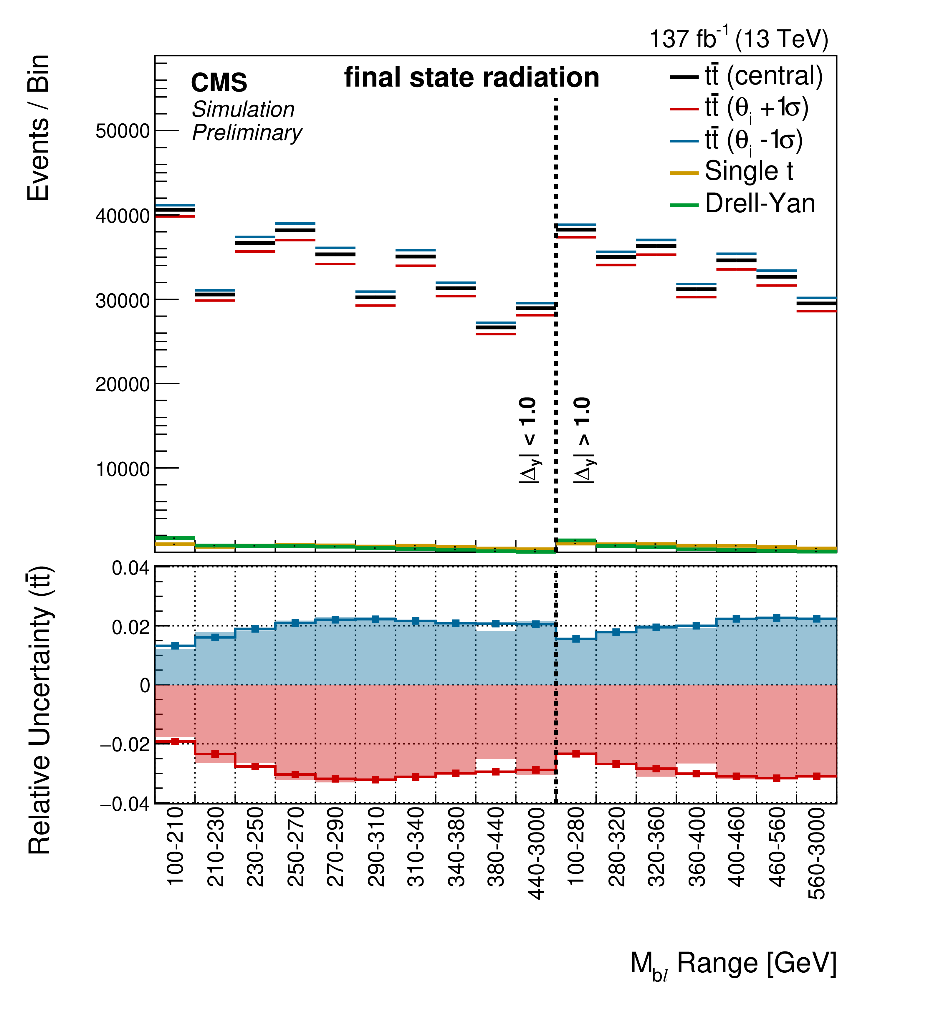
Figure 10-a:
Shape templates are shown for the uncertainties associated with the final-state radiation in PYTHIA8, the jet energy corrections, the factorization scale, and the renormalization scale. Along with the intrinsic uncertainty included on the weak corrections, these are seen to be the dominant uncertainties in the fit. The shaded bars represent the raw template information, while the lines show the shapes after smoothing and symmetrization procedures have been applied. In the fit, the jet energy corrections are split into 26 different components, but for brevity only the total uncertainty is shown here. Variation between years is minimal for each of these uncertainties, though they are treated separately in the fit. |
png pdf |
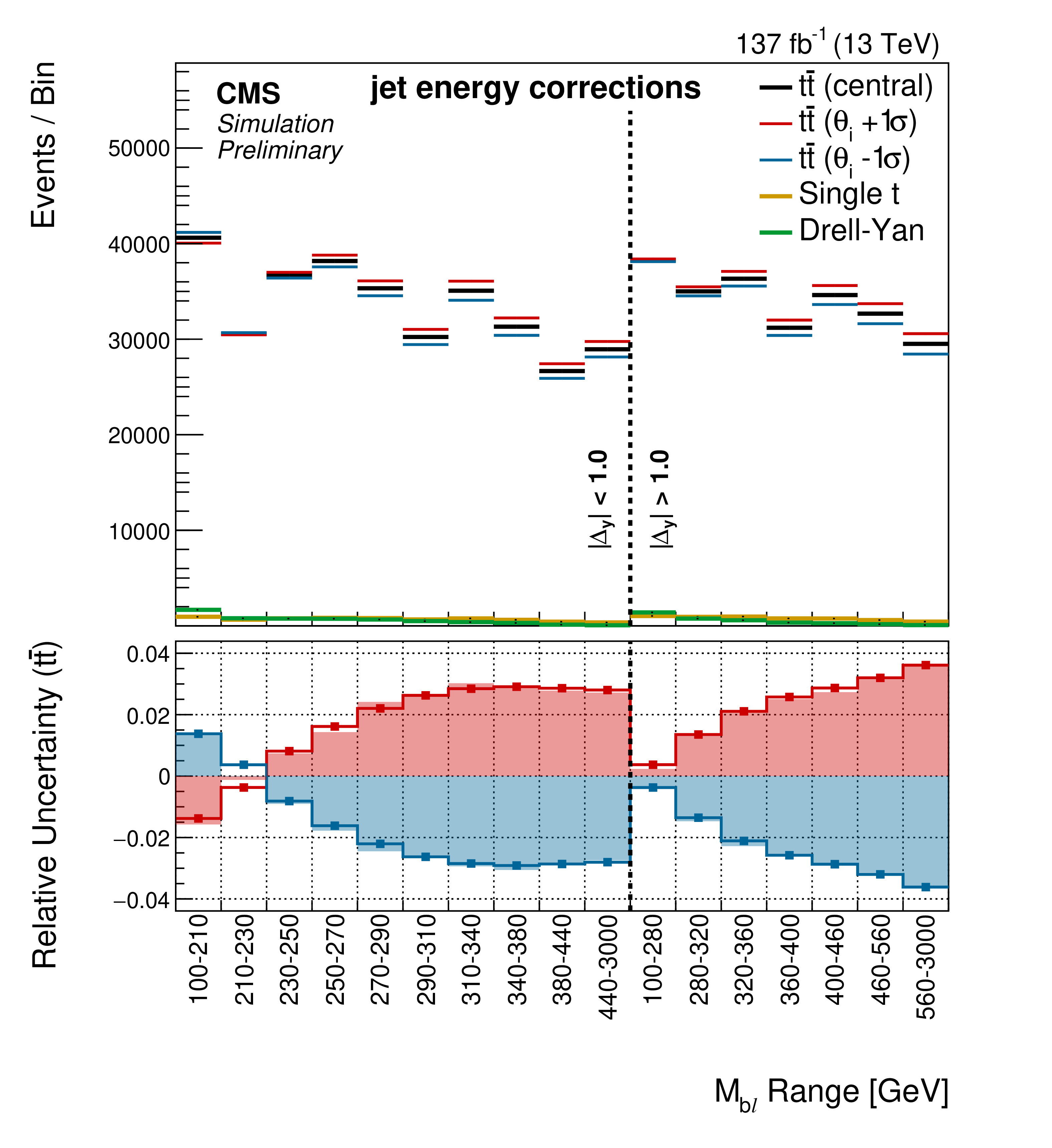
Figure 10-b:
Shape templates are shown for the uncertainties associated with the final-state radiation in PYTHIA8, the jet energy corrections, the factorization scale, and the renormalization scale. Along with the intrinsic uncertainty included on the weak corrections, these are seen to be the dominant uncertainties in the fit. The shaded bars represent the raw template information, while the lines show the shapes after smoothing and symmetrization procedures have been applied. In the fit, the jet energy corrections are split into 26 different components, but for brevity only the total uncertainty is shown here. Variation between years is minimal for each of these uncertainties, though they are treated separately in the fit. |
png pdf |
Figure 10-c:
Shape templates are shown for the uncertainties associated with the final-state radiation in PYTHIA8, the jet energy corrections, the factorization scale, and the renormalization scale. Along with the intrinsic uncertainty included on the weak corrections, these are seen to be the dominant uncertainties in the fit. The shaded bars represent the raw template information, while the lines show the shapes after smoothing and symmetrization procedures have been applied. In the fit, the jet energy corrections are split into 26 different components, but for brevity only the total uncertainty is shown here. Variation between years is minimal for each of these uncertainties, though they are treated separately in the fit. |
png pdf |
Figure 10-d:
Shape templates are shown for the uncertainties associated with the final-state radiation in PYTHIA8, the jet energy corrections, the factorization scale, and the renormalization scale. Along with the intrinsic uncertainty included on the weak corrections, these are seen to be the dominant uncertainties in the fit. The shaded bars represent the raw template information, while the lines show the shapes after smoothing and symmetrization procedures have been applied. In the fit, the jet energy corrections are split into 26 different components, but for brevity only the total uncertainty is shown here. Variation between years is minimal for each of these uncertainties, though they are treated separately in the fit. |
| Tables | |
png pdf |
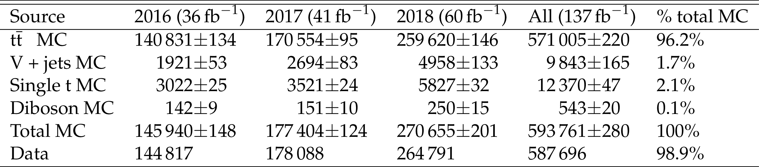
Table 1:
MC simulation and data event yields for each of the three years and their combination. Drell-Yan decays are included in V + jets samples, where V stands for a W or Z vector boson. The rightmost column shows the fraction of each component relative to the total simulated sample yield across the full data set. The statistical uncertainty in the simulated event counts is given. |
| Summary |
| A measurement of the Higgs Yukawa coupling to the top quark is presented, based on data from proton-proton collisions at the CMS experiment, deriving a best fit value of ${Y_\mathrm{t}} =$ 1.16$^{+0.24}_{-0.35}$ and a 95% confidence interval (CI) of ${Y_\mathrm{t}} \in\,{[0, \,1.62]} $. Data at a center-of-mass energy 13 TeV is analyzed from the full LHC Run 2, collected from 2016-2018, yielding an integrated luminosity of 137 fb$^{-1}$. This measurement uses the effects of virtual Higgs boson exchange on $\mathrm{t\bar{t}}$ kinematic properties to extract information about the coupling from kinematic distributions. Although the sensitivity is lower compared to constraints obtained from studying processes involving Higgs boson production in Refs. [7] and [9], this measurement avoids dependence on other Yukawa coupling values through additional branching assumptions, making it a compelling orthogonal measurement. This measurement also achieves a slightly higher precision than the only other ${Y_\mathrm{t}} $ measurement that does not make additional branching fraction assumptions, performed in the search for production of four top quarks. The four top quark search places a 95% CI of ${Y_\mathrm{t}} < $ 1.7 [10] while this measurement achieves a 95% CI of ${Y_\mathrm{t}} < $ 1.62. |
| References | ||||
| 1 | CMS Collaboration | Observation of a New Boson at a Mass of 125 GeV with the CMS Experiment at the LHC | PLB 716 (2012) 30 | CMS-HIG-12-028 1207.7235 |
| 2 | ATLAS Collaboration | Observation of a new particle in the search for the Standard Model Higgs boson with the ATLAS detector at the LHC | PLB 716 (2012) 1 | 1207.7214 |
| 3 | LHC Higgs Cross Section Working Group | Handbook of LHC Higgs Cross Sections: 3. Higgs Properties | 1307.1347 | |
| 4 | CMS Collaboration | Measurement of the top quark mass using proton-proton data at $ \sqrt{s} $~= 7 and 8 TeV | PRD 93 (2016) 072004 | CMS-TOP-14-022 1509.04044 |
| 5 | G. C. Branco et al. | Theory and phenomenology of two-Higgs-doublet models | PR 516 (2012) 1 | 1106.0034 |
| 6 | K. Agashe, R. Contino, and A. Pomarol | The Minimal composite Higgs model | NPB 719 (2005) 165 | hep-ph/0412089 |
| 7 | CMS Collaboration | Observation of $ \mathrm{t\overline{t}} $H production | PRL 120 (2018) 231801 | CMS-HIG-17-035 1804.02610 |
| 8 | ATLAS Collaboration | Observation of Higgs boson production in association with a top quark pair at the LHC with the ATLAS detector | PLB 784 (2018) 173 | 1806.00425 |
| 9 | CMS Collaboration | Combined measurements of Higgs boson couplings in proton-proton collisions at $ \sqrt{s}= $ 13 TeV | EPJC 79 (2019) 421 | CMS-HIG-17-031 1809.10733 |
| 10 | CMS Collaboration | Search for standard model production of four top quarks with same-sign and multilepton final states in proton-proton collisions at $ \sqrt{s} = $ 13 TeV | EPJC 78 (2018) 140 | CMS-TOP-17-009 1710.10614 |
| 11 | CMS Collaboration | Measurement of the top quark Yukawa coupling from $ \mathrm{t\bar{t}} $ kinematic distributions in the lepton+jets final state in proton-proton collisions at $ \sqrt{s} = $ 13 TeV | PRD 100 (2019) 072007 | CMS-TOP-17-004 1907.01590 |
| 12 | J. H. Kuhn, A. Scharf, and P. Uwer | Weak interactions in top-quark pair production at hadron colliders: an update | PRD 91 (2015) 014020 | 1305.5773 |
| 13 | CMS Collaboration | Measurement of differential cross sections for the production of top quark pairs and of additional jets in lepton+jets events from pp collisions at $ \sqrt{s} = $ 13 TeV | PRD 97 (2018) 112003 | CMS-TOP-17-002 1803.08856 |
| 14 | P. Nason | A new method for combining NLO QCD with shower Monte Carlo algorithms | JHEP 11 (2004) 040 | hep-ph/0409146 |
| 15 | S. Frixione, P. Nason, and C. Oleari | Matching NLO QCD computations with parton shower simulations: the POWHEG method | JHEP 11 (2007) 070 | 0709.2092 |
| 16 | S. Alioli, P. Nason, C. Oleari, and E. Re | A general framework for implementing NLO calculations in shower Monte Carlo programs: the POWHEG BOX | JHEP 06 (2010) 043 | 1002.2581 |
| 17 | J. M. Campbell, R. K. Ellis, P. Nason, and E. Re | Top-pair production and decay at NLO matched with parton showers | JHEP 04 (2015) 114 | 1412.1828 |
| 18 | T. Sjostrand, S. Mrenna, and P. Skands | PYTHIA 6.4 physics and manual | JHEP 05 (2006) 026 | hep-ph/0603175 |
| 19 | T. Sjostrand, S. Mrenna, and P. Z. Skands | A brief introduction to PYTHIA 8.1 | CPC 178 (2008) 852 | 0710.3820 |
| 20 | R. Frederix and S. Frixione | Merging meets matching in MC@NLO | JHEP 12 (2012) 061 | 1209.6215 |
| 21 | P. Skands, S. Carrazza, and J. Rojo | Tuning PYTHIA 8.1: the Monash 2013 tune | EPJC 74 (2014) 3024 | 1404.5630 |
| 22 | CMS Collaboration | Extraction and validation of a new set of CMS PYTHIA8 tunes from underlying-event measurements | EPJC 80 (2020) 4 | CMS-GEN-17-001 1903.12179 |
| 23 | NNPDF Collaboration | Parton distributions for the LHC Run II | JHEP 04 (2015) 040 | 1410.8849 |
| 24 | NNPDF Collaboration | Parton distributions from high-precision collider data | EPJC 77 (2017) 663 | 1706.00428 |
| 25 | M. Czakon and A. Mitov | Top++: A program for the calculation of the top-pair cross-section at hadron colliders | CPC 185 (2014) 2930 | 1112.5675 |
| 26 | J. Alwall et al. | The automated computation of tree-level and next-to-leading order differential cross sections, and their matching to parton shower simulations | JHEP 07 (2014) 079 | 1405.0301 |
| 27 | J. Alwall et al. | Comparative study of various algorithms for the merging of parton showers and matrix elements in hadronic collisions | EPJC 53 (2008) 473 | 0706.2569 |
| 28 | GEANT4 Collaboration | GEANT4--a simulation toolkit | NIMA 506 (2003) 250 | |
| 29 | M. Aliev et al. | HATHOR: HAdronic Top and Heavy quarks crOss section calculatoR | CPC 182 (2011) 1034 | 1007.1327 |
| 30 | W. Hollik and M. Kollar | NLO QED contributions to top-pair production at hadron collider | PRD 77 (2008) 014008 | 0708.1697 |
| 31 | M. Czakon et al. | Top-pair production at the LHC through NNLO QCD and NLO EW | JHEP 10 (2017) 186 | 1705.04105 |
| 32 | M. Cacciari, G. P. Salam, and G. Soyez | The anti-$ k_\mathrm{t} $ jet clustering algorithm | JHEP 04 (2008) 063 | 0802.1189 |
| 33 | M. Cacciari, G. P. Salam, and G. Soyez | FastJet user manual | EPJC 72 (2012) 1896 | 1111.6097 |
| 34 | CMS Collaboration | Jet energy scale and resolution in the CMS experiment in pp collisions at 8 TeV | JINST 12 (2017) P02014 | CMS-JME-13-004 1607.03663 |
| 35 | CMS Collaboration | Identification of heavy-flavour jets with the CMS detector in pp collisions at 13 TeV | JINST 13 (2018) P05011 | CMS-BTV-16-002 1712.07158 |
| 36 | B. A. Betchart, R. Demina, and A. Harel | Analytic solutions for neutrino momenta in decay of top quarks | NIMA 736 (2014) 169 | 1305.1878 |
| 37 | M. Czakon, D. Heymes, and A. Mitov | Dynamical scales for multi-TeV top-pair production at the LHC | JHEP 04 (2017) 071 | 1606.03350 |
| 38 | CMS Collaboration | CMS Luminosity Measurements for the 2016 Data Taking Period | CMS-PAS-LUM-17-001 | CMS-PAS-LUM-17-001 |
| 39 | CMS Collaboration | CMS luminosity measurement for the 2017 data-taking period at $ \sqrt{s} = $ 13 TeV | CMS-PAS-LUM-17-004 | CMS-PAS-LUM-17-004 |
| 40 | CMS Collaboration | CMS luminosity measurement for the 2018 data-taking period at $ \sqrt{s} = $ 13 TeV | CMS-PAS-LUM-18-002 | CMS-PAS-LUM-18-002 |
| 41 | ATLAS Collaboration | Measurement of the inelastic proton-proton cross section at $ \sqrt{s} = $ 13 TeV with the ATLAS detector at the LHC | PRL 117 (2016) 182002 | 1606.02625 |
| 42 | CMS Collaboration | Performance of the CMS muon detector and muon reconstruction with proton-proton collisions at $ \sqrt{s}= $ 13 TeV | JINST 13 (2018) P06015 | CMS-MUO-16-001 1804.04528 |
| 43 | CMS Collaboration | Performance of electron reconstruction and selection with the CMS detector in proton-proton collisions at $ \sqrt{s} = $ 8 TeV | JINST 10 (2015) P06005 | CMS-EGM-13-001 1502.02701 |
| 44 | M. Czakon, D. Heymes, and A. Mitov | fastNLO tables for NNLO top-quark pair differential distributions | 1704.08551 | |
| 45 | M. Czakon, D. Heymes, and A. Mitov | High-precision differential predictions for top-quark pairs at the LHC | PRL 116 (2016) 082003 | 1511.00549 |
| 46 | M. Czakon et al. | A study of the impact of double-differential top distributions from CMS on parton distribution functions | 1912.08801 | |
| 47 | Particle Data Group, C. Patrignani et al. | Review of particle physics | CPC 40 (2016) 100001 | |
| 48 | M. G. Bowler | $ {\rm e}^{+}{\rm e}^{-} $ Production of heavy quarks in the string model | Z. Phys. C 11 (1981) 169 | |
| 49 | W. S. Cleveland | Robust locally weighted regression and smoothing scatterplots | Journal of the American Statistical Association 74 (1979) 829 | |
|
|
Compact Muon Solenoid LHC, CERN |
|

|

|

|

|

|