

Compact Muon Solenoid
LHC, CERN
| CMS-PAS-TOP-19-006 | ||
| Search for charged lepton flavor violation in top quark production and decay in proton-proton collisions at $\sqrt{s}= $ 13 TeV | ||
| CMS Collaboration | ||
| June 2021 | ||
| Abstract: The result of a search for charged lepton flavor violation (CLFV) through top quark production and decay in proton-proton collisions at a center-of-mass energy of 13 TeV is presented. The search is performed in events with an oppositely charged electron-muon pair in the final state along with at least one jet identified as originating from a bottom quark. The data correspond to an integrated luminosity of 137 fb$^{-1}$, collected by the CMS experiment at the CERN LHC in 2016-2018. The CLFV interactions of top quarks are parametrized using an effective field theory (EFT) approach. In this analysis, we emphasize the importance of single top quark production via CLFV interactions, in addition to the $ \mathrm{t}\rightarrow \mathrm{e}\mu \mathrm{q}$ (q = u, c) decays. No significant excess over the standard model expectation is observed. The results are interpreted in terms of scalar-, vector- and tensor-like CLFV four-fermion EFT interactions. Exclusion limits at 95% confidence level on the branching fractions of a top quark decaying to an e$\mu$ pair and an up (a charm) quark are found to be 0.12 $\times$ 10$^{-6}$ (1.59 $\times$ 10$^{-6}$), 0.24 $\times$ 10$^{-6}$ (2.55 $\times $ 10$^{-6}$), 0.46 $\times$ 10$^{-6}$ (4.62 $\times $ 10$^{-6}$) for the scalar, vector and tensor CLFV interaction types, respectively. | ||
|
Links:
CDS record (PDF) ;
inSPIRE record ;
CADI line (restricted) ;
These preliminary results are superseded in this paper, JHEP 06 (2022) 082. The superseded preliminary plots can be found here. |
||
| Figures | |

png pdf |
Figure 1:
Feynman diagrams for single top quark production (left and middle) and top quark decays in ${\mathrm{t} {}\mathrm{\bar{t}}}$ events (right) via CLFV interactions. The CLFV vertex is marked as a filled circle. |
png pdf |
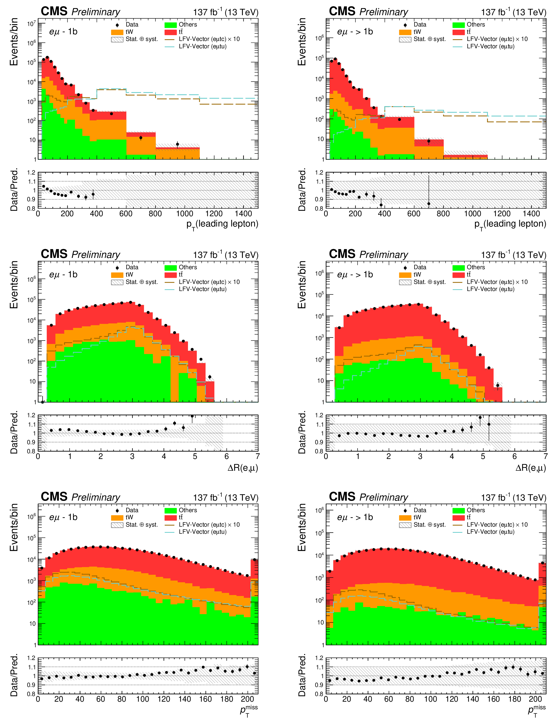
Figure 2:
The distributions of leading lepton ${p_{\mathrm {T}}}$ (upper row), $\Delta $R($\ell _1,\, \ell _2$) (middle row), and ${{p_{\mathrm {T}}} ^\text {miss}}$ (lower row) are shown for data (points) and simulation (histograms). Events with one (more than one) b-tagged jet are shown in the left (right) column. The hatched band indicates the total uncertainty (statistical and systematic) for the SM background predictions. Overflow events are added to the last bin. Examples of the predicted signal contribution for the vector type CLFV via $\mathrm{e} \mu \mathrm{t} \mathrm{u} $ and $\mathrm{e} \mu \mathrm{t} \mathrm{c} $ vertices are shown, assuming $\text {C}_x/\Lambda ^2 = $ 1 TeV$^{-2}$. The $\mathrm{e} \mu \mathrm{t} \mathrm{c} $ signal cross section is scaled by a factor of 10 for improved visualization. The lower panels show the ratio of data over the prediction with the total uncertainty. |

png pdf |
Figure 2-a:
The distributions of leading lepton ${p_{\mathrm {T}}}$ (upper row), $\Delta $R($\ell _1,\, \ell _2$) (middle row), and ${{p_{\mathrm {T}}} ^\text {miss}}$ (lower row) are shown for data (points) and simulation (histograms). Events with one (more than one) b-tagged jet are shown in the left (right) column. The hatched band indicates the total uncertainty (statistical and systematic) for the SM background predictions. Overflow events are added to the last bin. Examples of the predicted signal contribution for the vector type CLFV via $\mathrm{e} \mu \mathrm{t} \mathrm{u} $ and $\mathrm{e} \mu \mathrm{t} \mathrm{c} $ vertices are shown, assuming $\text {C}_x/\Lambda ^2 = $ 1 TeV$^{-2}$. The $\mathrm{e} \mu \mathrm{t} \mathrm{c} $ signal cross section is scaled by a factor of 10 for improved visualization. The lower panels show the ratio of data over the prediction with the total uncertainty. |
png pdf |
Figure 2-b:
The distributions of leading lepton ${p_{\mathrm {T}}}$ (upper row), $\Delta $R($\ell _1,\, \ell _2$) (middle row), and ${{p_{\mathrm {T}}} ^\text {miss}}$ (lower row) are shown for data (points) and simulation (histograms). Events with one (more than one) b-tagged jet are shown in the left (right) column. The hatched band indicates the total uncertainty (statistical and systematic) for the SM background predictions. Overflow events are added to the last bin. Examples of the predicted signal contribution for the vector type CLFV via $\mathrm{e} \mu \mathrm{t} \mathrm{u} $ and $\mathrm{e} \mu \mathrm{t} \mathrm{c} $ vertices are shown, assuming $\text {C}_x/\Lambda ^2 = $ 1 TeV$^{-2}$. The $\mathrm{e} \mu \mathrm{t} \mathrm{c} $ signal cross section is scaled by a factor of 10 for improved visualization. The lower panels show the ratio of data over the prediction with the total uncertainty. |

png pdf |
Figure 2-c:
The distributions of leading lepton ${p_{\mathrm {T}}}$ (upper row), $\Delta $R($\ell _1,\, \ell _2$) (middle row), and ${{p_{\mathrm {T}}} ^\text {miss}}$ (lower row) are shown for data (points) and simulation (histograms). Events with one (more than one) b-tagged jet are shown in the left (right) column. The hatched band indicates the total uncertainty (statistical and systematic) for the SM background predictions. Overflow events are added to the last bin. Examples of the predicted signal contribution for the vector type CLFV via $\mathrm{e} \mu \mathrm{t} \mathrm{u} $ and $\mathrm{e} \mu \mathrm{t} \mathrm{c} $ vertices are shown, assuming $\text {C}_x/\Lambda ^2 = $ 1 TeV$^{-2}$. The $\mathrm{e} \mu \mathrm{t} \mathrm{c} $ signal cross section is scaled by a factor of 10 for improved visualization. The lower panels show the ratio of data over the prediction with the total uncertainty. |
png pdf |
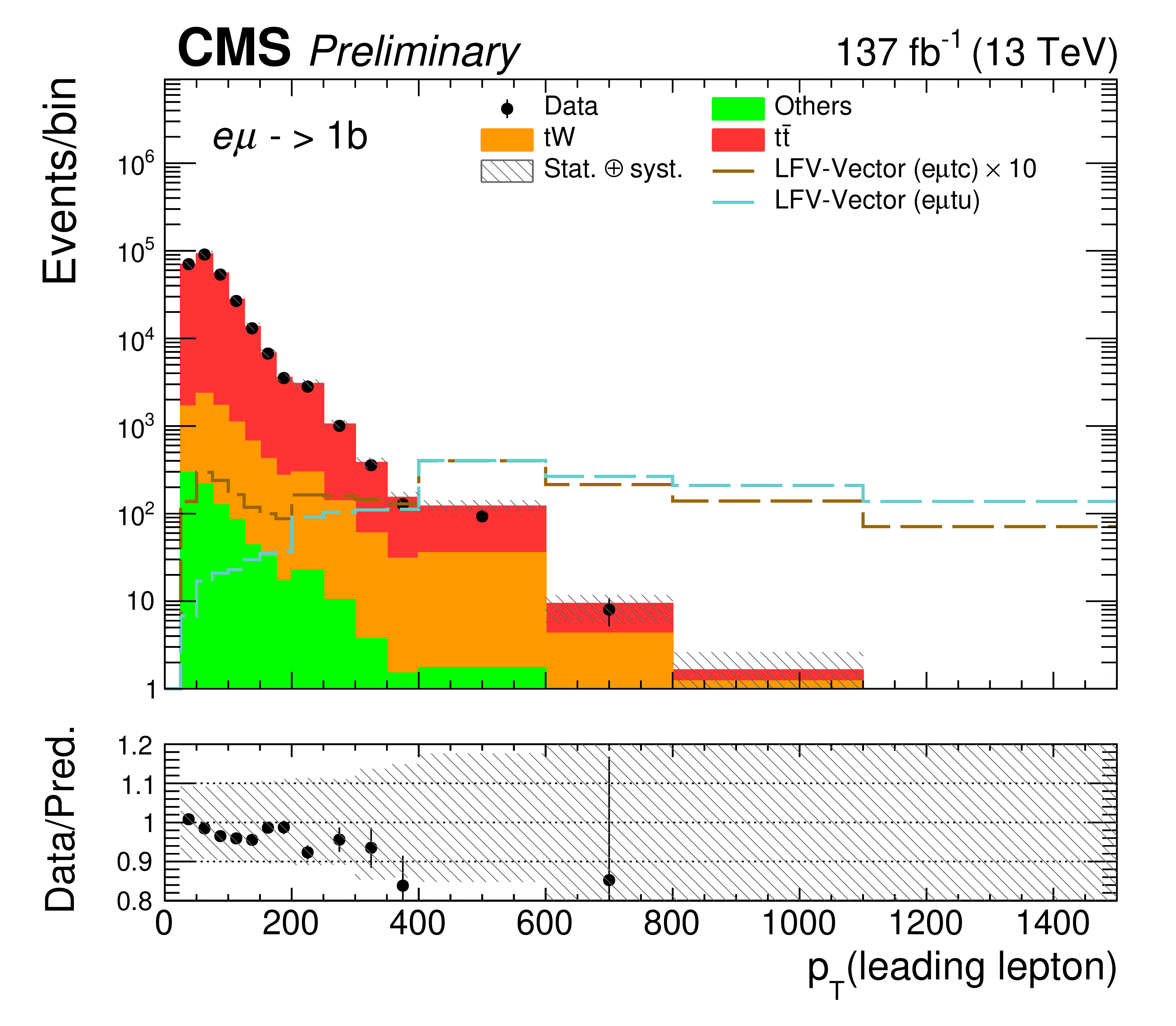
Figure 2-d:
The distributions of leading lepton ${p_{\mathrm {T}}}$ (upper row), $\Delta $R($\ell _1,\, \ell _2$) (middle row), and ${{p_{\mathrm {T}}} ^\text {miss}}$ (lower row) are shown for data (points) and simulation (histograms). Events with one (more than one) b-tagged jet are shown in the left (right) column. The hatched band indicates the total uncertainty (statistical and systematic) for the SM background predictions. Overflow events are added to the last bin. Examples of the predicted signal contribution for the vector type CLFV via $\mathrm{e} \mu \mathrm{t} \mathrm{u} $ and $\mathrm{e} \mu \mathrm{t} \mathrm{c} $ vertices are shown, assuming $\text {C}_x/\Lambda ^2 = $ 1 TeV$^{-2}$. The $\mathrm{e} \mu \mathrm{t} \mathrm{c} $ signal cross section is scaled by a factor of 10 for improved visualization. The lower panels show the ratio of data over the prediction with the total uncertainty. |
png pdf |
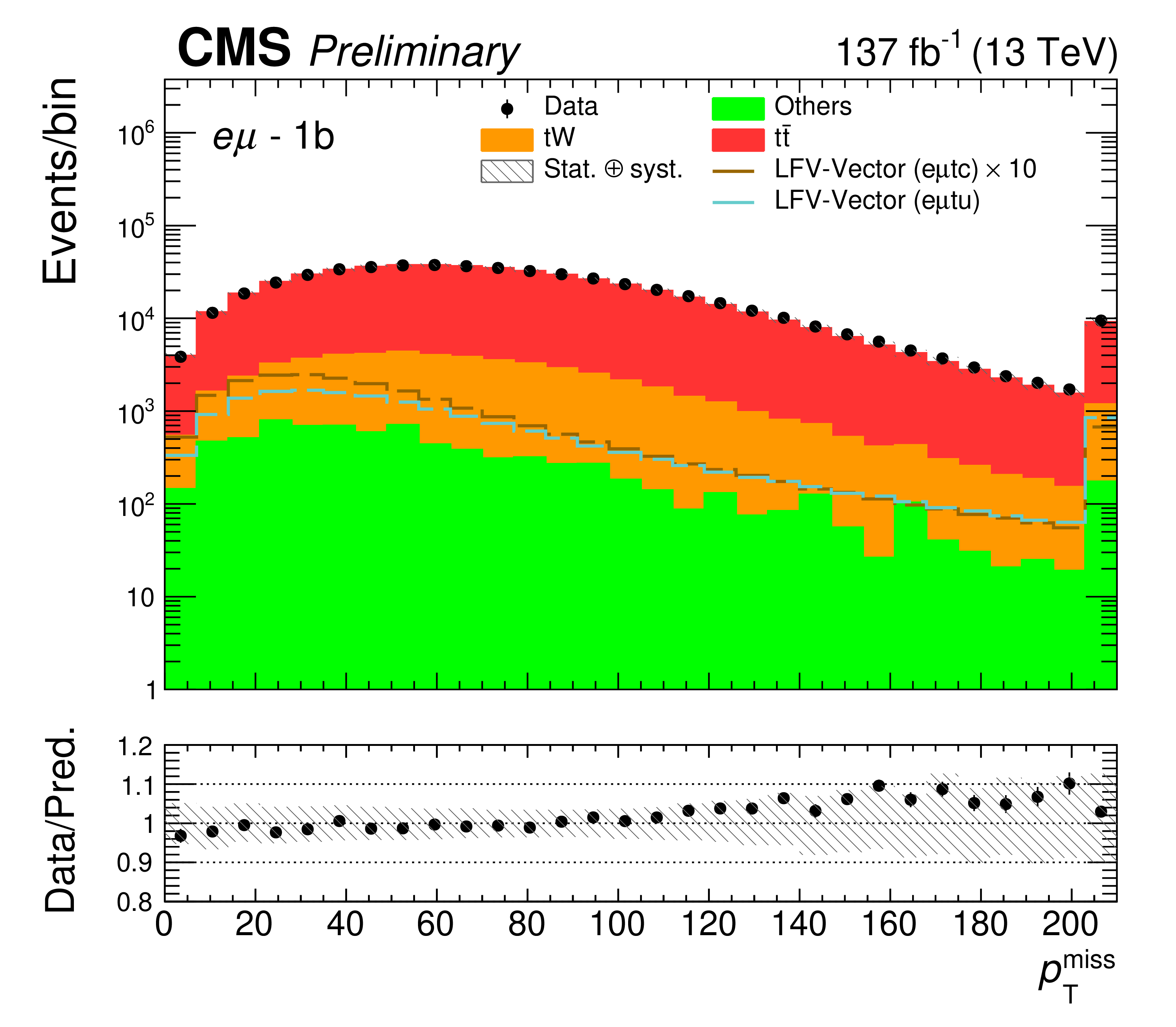
Figure 2-e:
The distributions of leading lepton ${p_{\mathrm {T}}}$ (upper row), $\Delta $R($\ell _1,\, \ell _2$) (middle row), and ${{p_{\mathrm {T}}} ^\text {miss}}$ (lower row) are shown for data (points) and simulation (histograms). Events with one (more than one) b-tagged jet are shown in the left (right) column. The hatched band indicates the total uncertainty (statistical and systematic) for the SM background predictions. Overflow events are added to the last bin. Examples of the predicted signal contribution for the vector type CLFV via $\mathrm{e} \mu \mathrm{t} \mathrm{u} $ and $\mathrm{e} \mu \mathrm{t} \mathrm{c} $ vertices are shown, assuming $\text {C}_x/\Lambda ^2 = $ 1 TeV$^{-2}$. The $\mathrm{e} \mu \mathrm{t} \mathrm{c} $ signal cross section is scaled by a factor of 10 for improved visualization. The lower panels show the ratio of data over the prediction with the total uncertainty. |

png pdf |
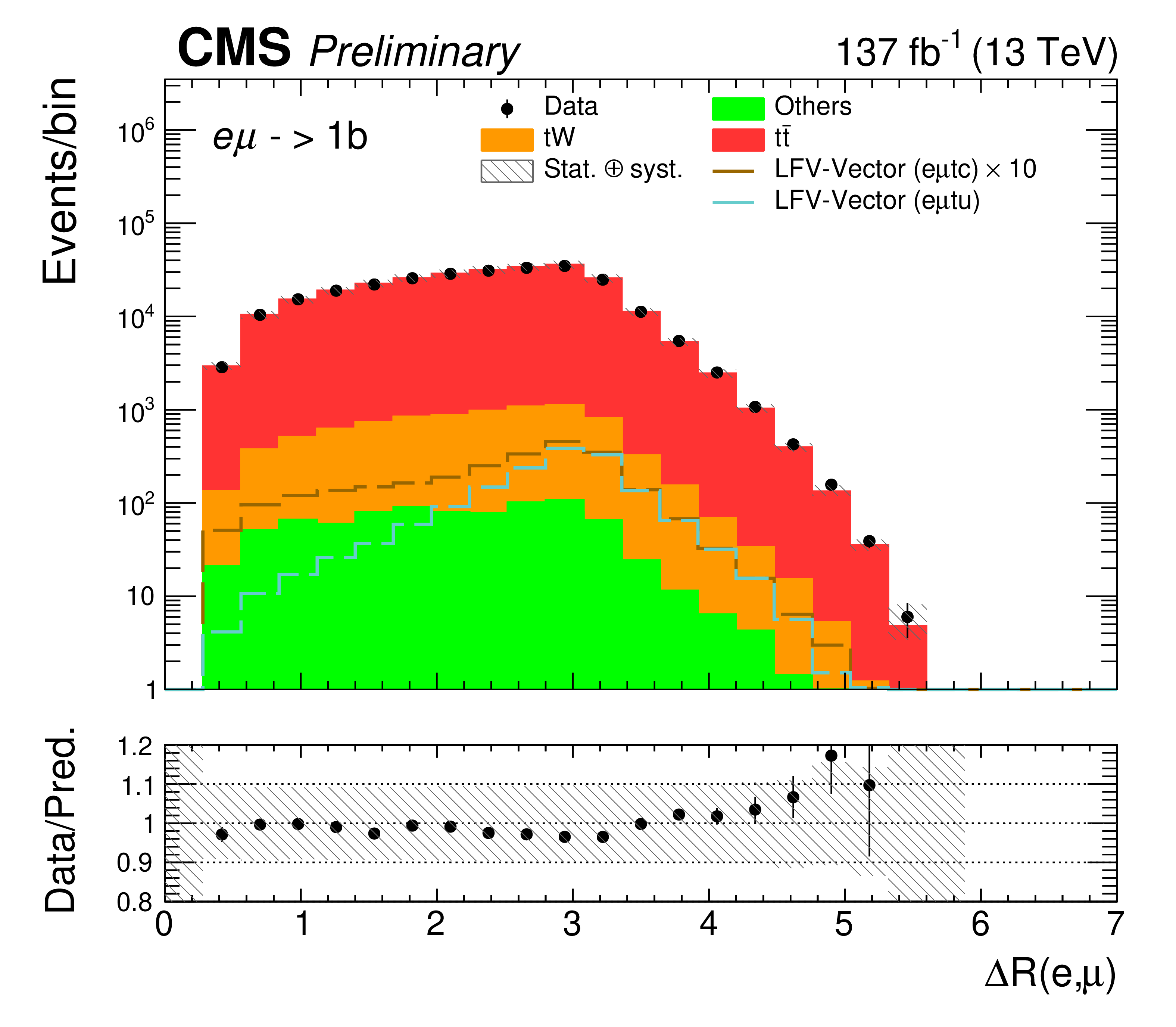
Figure 2-f:
The distributions of leading lepton ${p_{\mathrm {T}}}$ (upper row), $\Delta $R($\ell _1,\, \ell _2$) (middle row), and ${{p_{\mathrm {T}}} ^\text {miss}}$ (lower row) are shown for data (points) and simulation (histograms). Events with one (more than one) b-tagged jet are shown in the left (right) column. The hatched band indicates the total uncertainty (statistical and systematic) for the SM background predictions. Overflow events are added to the last bin. Examples of the predicted signal contribution for the vector type CLFV via $\mathrm{e} \mu \mathrm{t} \mathrm{u} $ and $\mathrm{e} \mu \mathrm{t} \mathrm{c} $ vertices are shown, assuming $\text {C}_x/\Lambda ^2 = $ 1 TeV$^{-2}$. The $\mathrm{e} \mu \mathrm{t} \mathrm{c} $ signal cross section is scaled by a factor of 10 for improved visualization. The lower panels show the ratio of data over the prediction with the total uncertainty. |

png pdf |
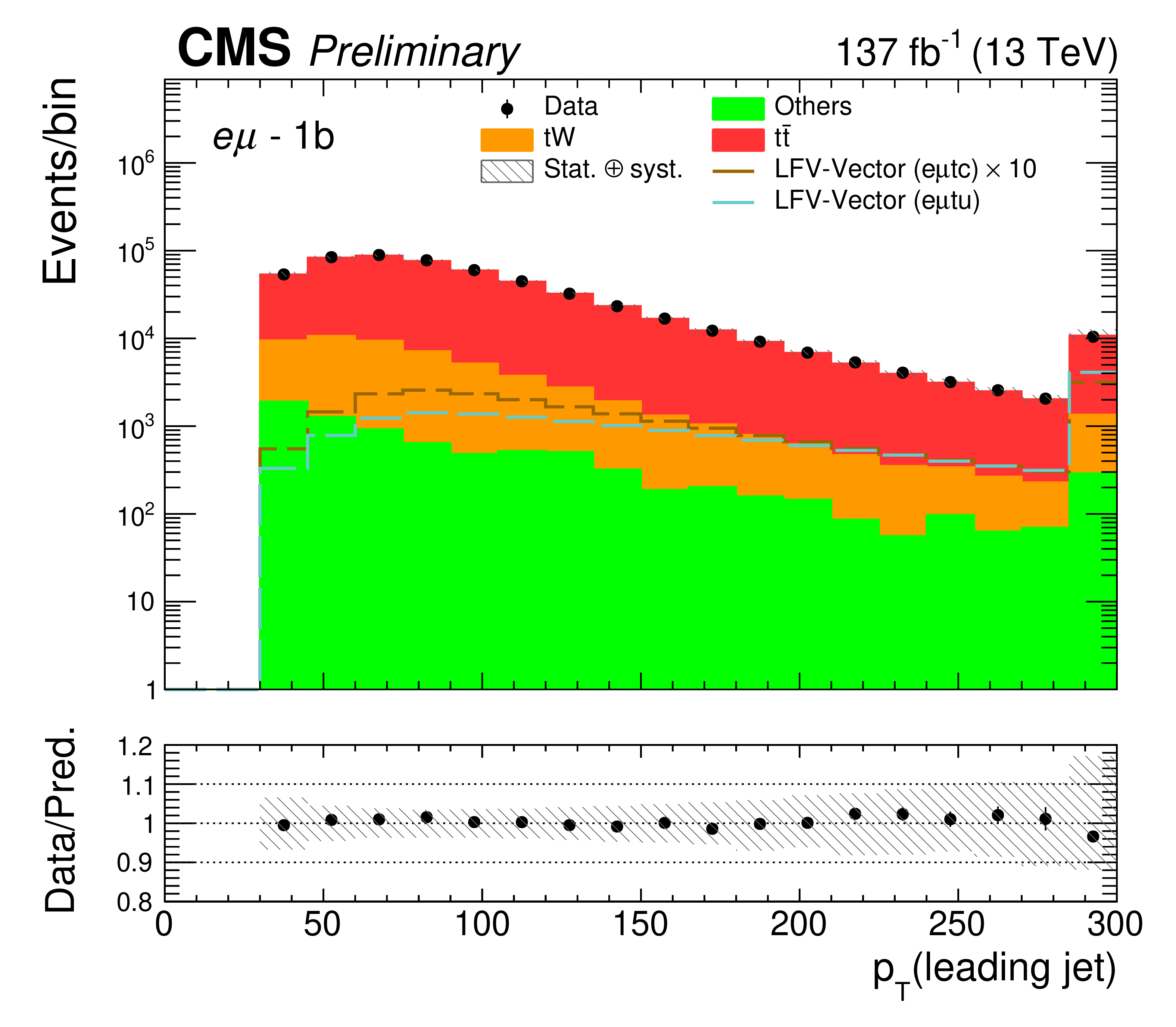
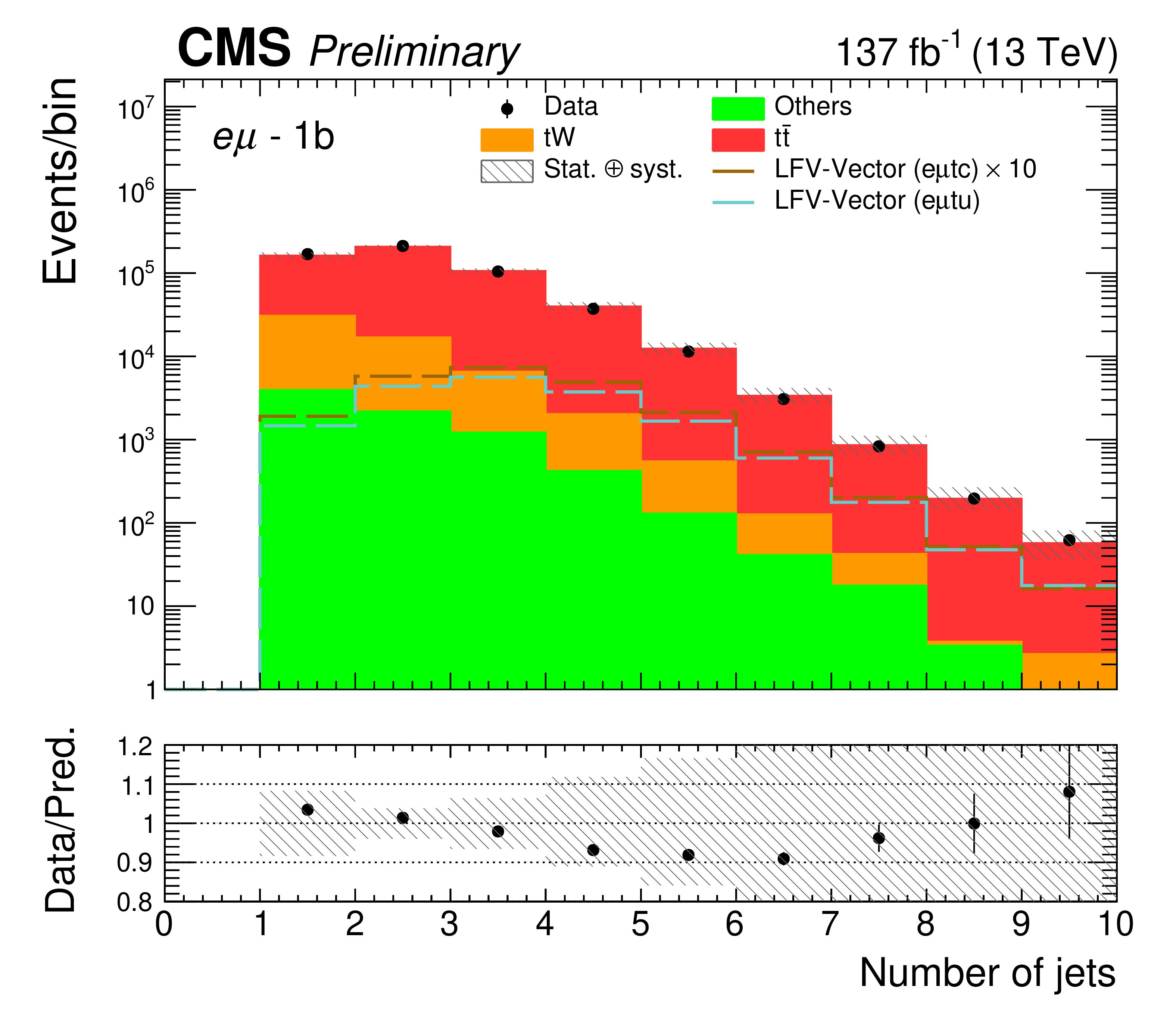
Figure 3:
The distributions of leading jet ${p_{\mathrm {T}}}$ (upper row), and the number of jets (lower row) are shown for data (points) and simulation (histograms). Events with one (more than one) b-tagged jet are shown in the left (right) column. The hatched band indicates the total uncertainty (statistical and systematic) for the SM background predictions. Overflow events are added to the last bin. Examples of the predicted signal contribution for the vector type CLFV via $\mathrm{e} \mu \mathrm{t} \mathrm{u} $ and $\mathrm{e} \mu \mathrm{t} \mathrm{c} $ vertices are shown, assuming $\text {C}_x/\Lambda ^2 = $ 1 TeV$^{-2}$. The $\mathrm{e} \mu \mathrm{t} \mathrm{c} $ signal cross section is scaled by a factor of 10 for improved visualization. The lower panels show the ratio of data over the prediction with the total uncertainty. |
png pdf |
Figure 3-a:
The distributions of leading jet ${p_{\mathrm {T}}}$ (upper row), and the number of jets (lower row) are shown for data (points) and simulation (histograms). Events with one (more than one) b-tagged jet are shown in the left (right) column. The hatched band indicates the total uncertainty (statistical and systematic) for the SM background predictions. Overflow events are added to the last bin. Examples of the predicted signal contribution for the vector type CLFV via $\mathrm{e} \mu \mathrm{t} \mathrm{u} $ and $\mathrm{e} \mu \mathrm{t} \mathrm{c} $ vertices are shown, assuming $\text {C}_x/\Lambda ^2 = $ 1 TeV$^{-2}$. The $\mathrm{e} \mu \mathrm{t} \mathrm{c} $ signal cross section is scaled by a factor of 10 for improved visualization. The lower panels show the ratio of data over the prediction with the total uncertainty. |
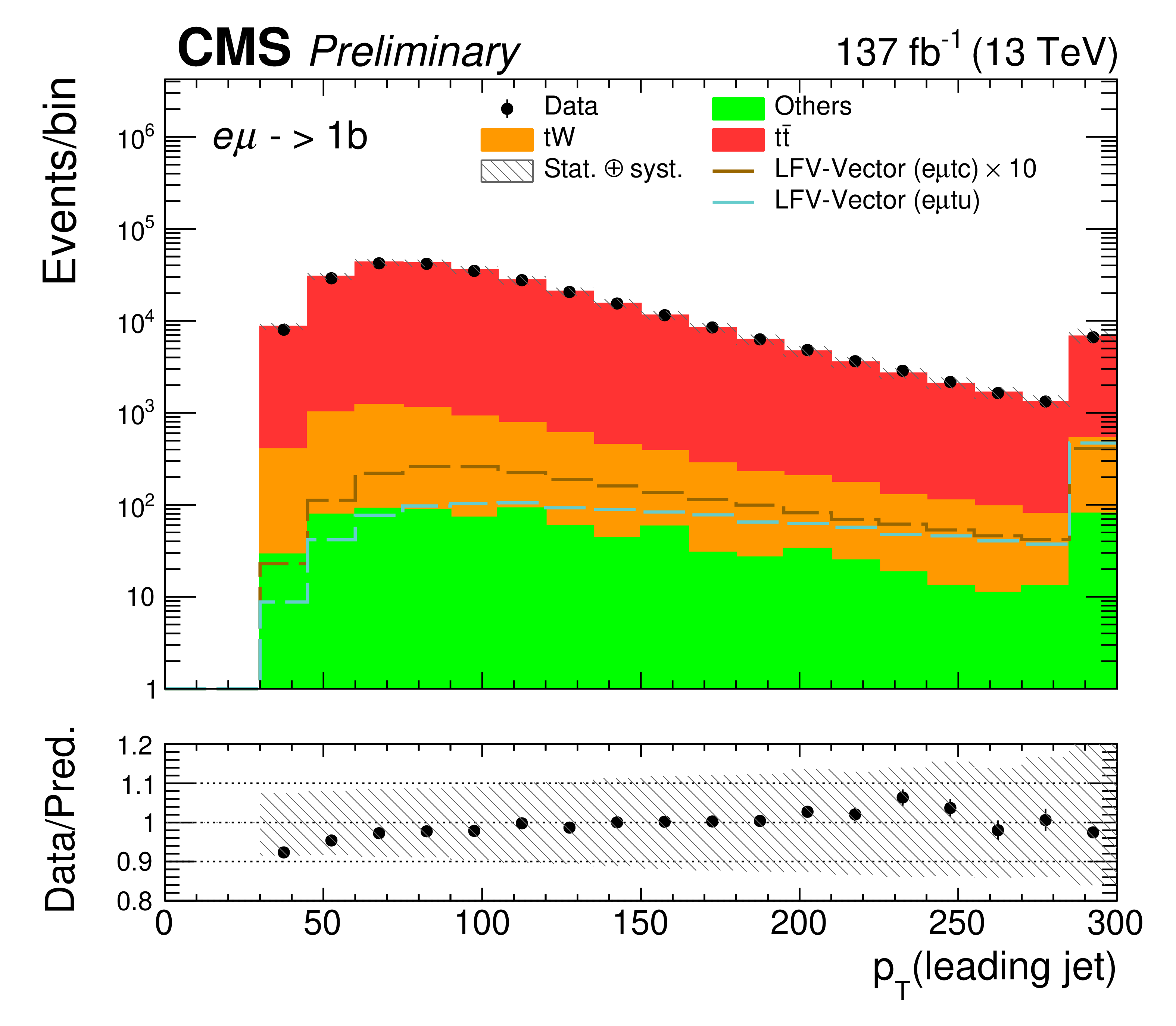
png pdf |
Figure 3-b:
The distributions of leading jet ${p_{\mathrm {T}}}$ (upper row), and the number of jets (lower row) are shown for data (points) and simulation (histograms). Events with one (more than one) b-tagged jet are shown in the left (right) column. The hatched band indicates the total uncertainty (statistical and systematic) for the SM background predictions. Overflow events are added to the last bin. Examples of the predicted signal contribution for the vector type CLFV via $\mathrm{e} \mu \mathrm{t} \mathrm{u} $ and $\mathrm{e} \mu \mathrm{t} \mathrm{c} $ vertices are shown, assuming $\text {C}_x/\Lambda ^2 = $ 1 TeV$^{-2}$. The $\mathrm{e} \mu \mathrm{t} \mathrm{c} $ signal cross section is scaled by a factor of 10 for improved visualization. The lower panels show the ratio of data over the prediction with the total uncertainty. |
png pdf |
Figure 3-c:
The distributions of leading jet ${p_{\mathrm {T}}}$ (upper row), and the number of jets (lower row) are shown for data (points) and simulation (histograms). Events with one (more than one) b-tagged jet are shown in the left (right) column. The hatched band indicates the total uncertainty (statistical and systematic) for the SM background predictions. Overflow events are added to the last bin. Examples of the predicted signal contribution for the vector type CLFV via $\mathrm{e} \mu \mathrm{t} \mathrm{u} $ and $\mathrm{e} \mu \mathrm{t} \mathrm{c} $ vertices are shown, assuming $\text {C}_x/\Lambda ^2 = $ 1 TeV$^{-2}$. The $\mathrm{e} \mu \mathrm{t} \mathrm{c} $ signal cross section is scaled by a factor of 10 for improved visualization. The lower panels show the ratio of data over the prediction with the total uncertainty. |

png pdf |
Figure 3-d:
The distributions of leading jet ${p_{\mathrm {T}}}$ (upper row), and the number of jets (lower row) are shown for data (points) and simulation (histograms). Events with one (more than one) b-tagged jet are shown in the left (right) column. The hatched band indicates the total uncertainty (statistical and systematic) for the SM background predictions. Overflow events are added to the last bin. Examples of the predicted signal contribution for the vector type CLFV via $\mathrm{e} \mu \mathrm{t} \mathrm{u} $ and $\mathrm{e} \mu \mathrm{t} \mathrm{c} $ vertices are shown, assuming $\text {C}_x/\Lambda ^2 = $ 1 TeV$^{-2}$. The $\mathrm{e} \mu \mathrm{t} \mathrm{c} $ signal cross section is scaled by a factor of 10 for improved visualization. The lower panels show the ratio of data over the prediction with the total uncertainty. |

png pdf |
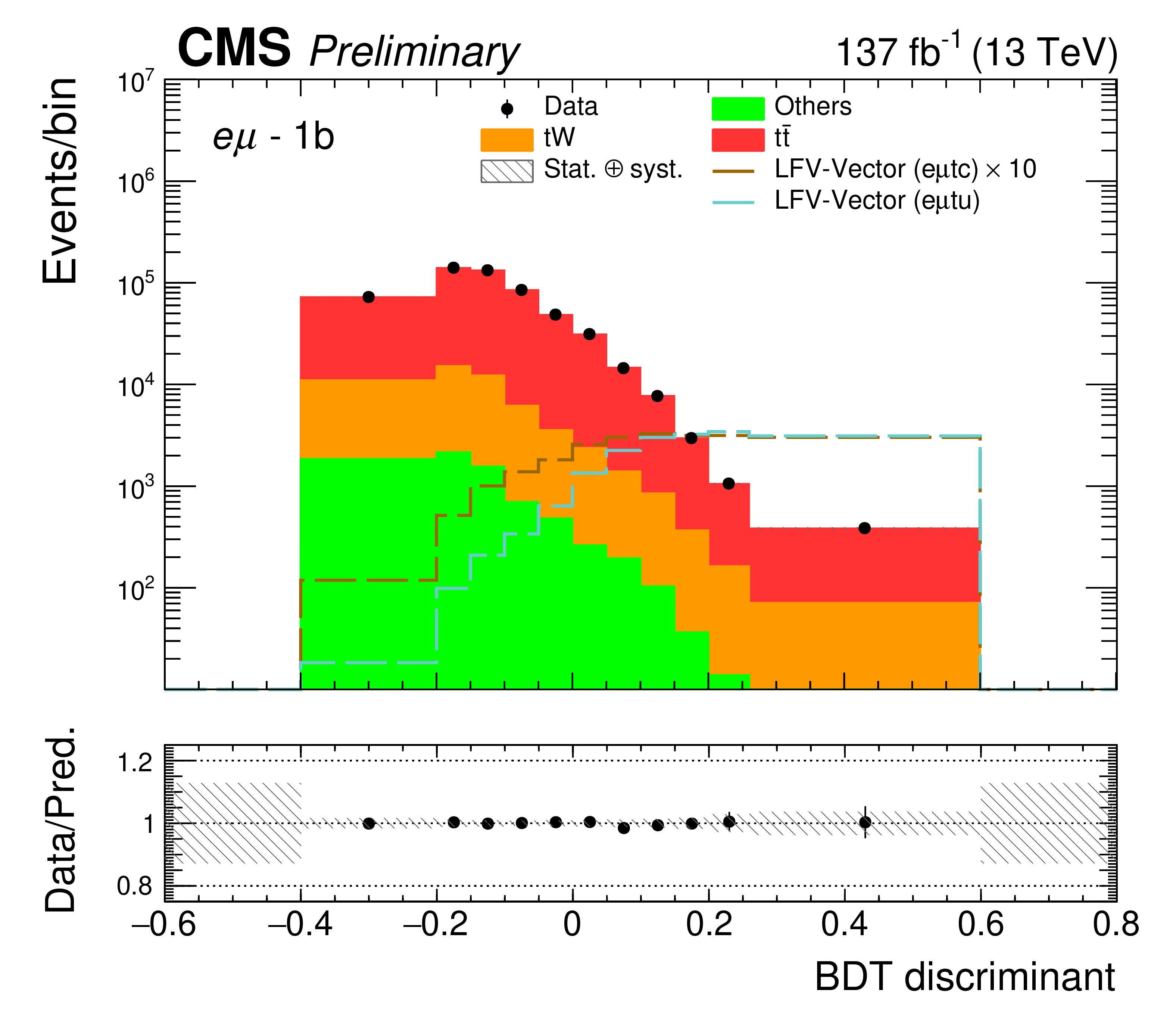
Figure 4:
BDT output distributions are shown for data (points) and simulation (histograms) with the pre-fit background prediction (upper row) and post-fit background prediction (lower row). Events with one (more than one) b-tagged jet are shown in the left (right) column. The hatched band indicates the total uncertainty (statistical and systematic) for the SM background predictions. Examples of the predicted signal contribution for the vector type CLFV via $\mathrm{e} \mu \mathrm{t} \mathrm{u} $ and $\mathrm{e} \mu \mathrm{t} \mathrm{c} $ vertices are shown, assuming $\text {C}_x/\Lambda ^2 = $ 1 TeV$^{-2}$. The $\mathrm{e} \mu \mathrm{t} \mathrm{c} $ signal cross section is scaled by a factor of 10 for improved visualization. The lower panels show the ratio of data over the prediction with the total uncertainty. |

png pdf |
Figure 4-a:
BDT output distributions are shown for data (points) and simulation (histograms) with the pre-fit background prediction (upper row) and post-fit background prediction (lower row). Events with one (more than one) b-tagged jet are shown in the left (right) column. The hatched band indicates the total uncertainty (statistical and systematic) for the SM background predictions. Examples of the predicted signal contribution for the vector type CLFV via $\mathrm{e} \mu \mathrm{t} \mathrm{u} $ and $\mathrm{e} \mu \mathrm{t} \mathrm{c} $ vertices are shown, assuming $\text {C}_x/\Lambda ^2 = $ 1 TeV$^{-2}$. The $\mathrm{e} \mu \mathrm{t} \mathrm{c} $ signal cross section is scaled by a factor of 10 for improved visualization. The lower panels show the ratio of data over the prediction with the total uncertainty. |

png pdf |
Figure 4-b:
BDT output distributions are shown for data (points) and simulation (histograms) with the pre-fit background prediction (upper row) and post-fit background prediction (lower row). Events with one (more than one) b-tagged jet are shown in the left (right) column. The hatched band indicates the total uncertainty (statistical and systematic) for the SM background predictions. Examples of the predicted signal contribution for the vector type CLFV via $\mathrm{e} \mu \mathrm{t} \mathrm{u} $ and $\mathrm{e} \mu \mathrm{t} \mathrm{c} $ vertices are shown, assuming $\text {C}_x/\Lambda ^2 = $ 1 TeV$^{-2}$. The $\mathrm{e} \mu \mathrm{t} \mathrm{c} $ signal cross section is scaled by a factor of 10 for improved visualization. The lower panels show the ratio of data over the prediction with the total uncertainty. |
png pdf |
Figure 4-c:
BDT output distributions are shown for data (points) and simulation (histograms) with the pre-fit background prediction (upper row) and post-fit background prediction (lower row). Events with one (more than one) b-tagged jet are shown in the left (right) column. The hatched band indicates the total uncertainty (statistical and systematic) for the SM background predictions. Examples of the predicted signal contribution for the vector type CLFV via $\mathrm{e} \mu \mathrm{t} \mathrm{u} $ and $\mathrm{e} \mu \mathrm{t} \mathrm{c} $ vertices are shown, assuming $\text {C}_x/\Lambda ^2 = $ 1 TeV$^{-2}$. The $\mathrm{e} \mu \mathrm{t} \mathrm{c} $ signal cross section is scaled by a factor of 10 for improved visualization. The lower panels show the ratio of data over the prediction with the total uncertainty. |

png pdf |
Figure 4-d:
BDT output distributions are shown for data (points) and simulation (histograms) with the pre-fit background prediction (upper row) and post-fit background prediction (lower row). Events with one (more than one) b-tagged jet are shown in the left (right) column. The hatched band indicates the total uncertainty (statistical and systematic) for the SM background predictions. Examples of the predicted signal contribution for the vector type CLFV via $\mathrm{e} \mu \mathrm{t} \mathrm{u} $ and $\mathrm{e} \mu \mathrm{t} \mathrm{c} $ vertices are shown, assuming $\text {C}_x/\Lambda ^2 = $ 1 TeV$^{-2}$. The $\mathrm{e} \mu \mathrm{t} \mathrm{c} $ signal cross section is scaled by a factor of 10 for improved visualization. The lower panels show the ratio of data over the prediction with the total uncertainty. |

png pdf |
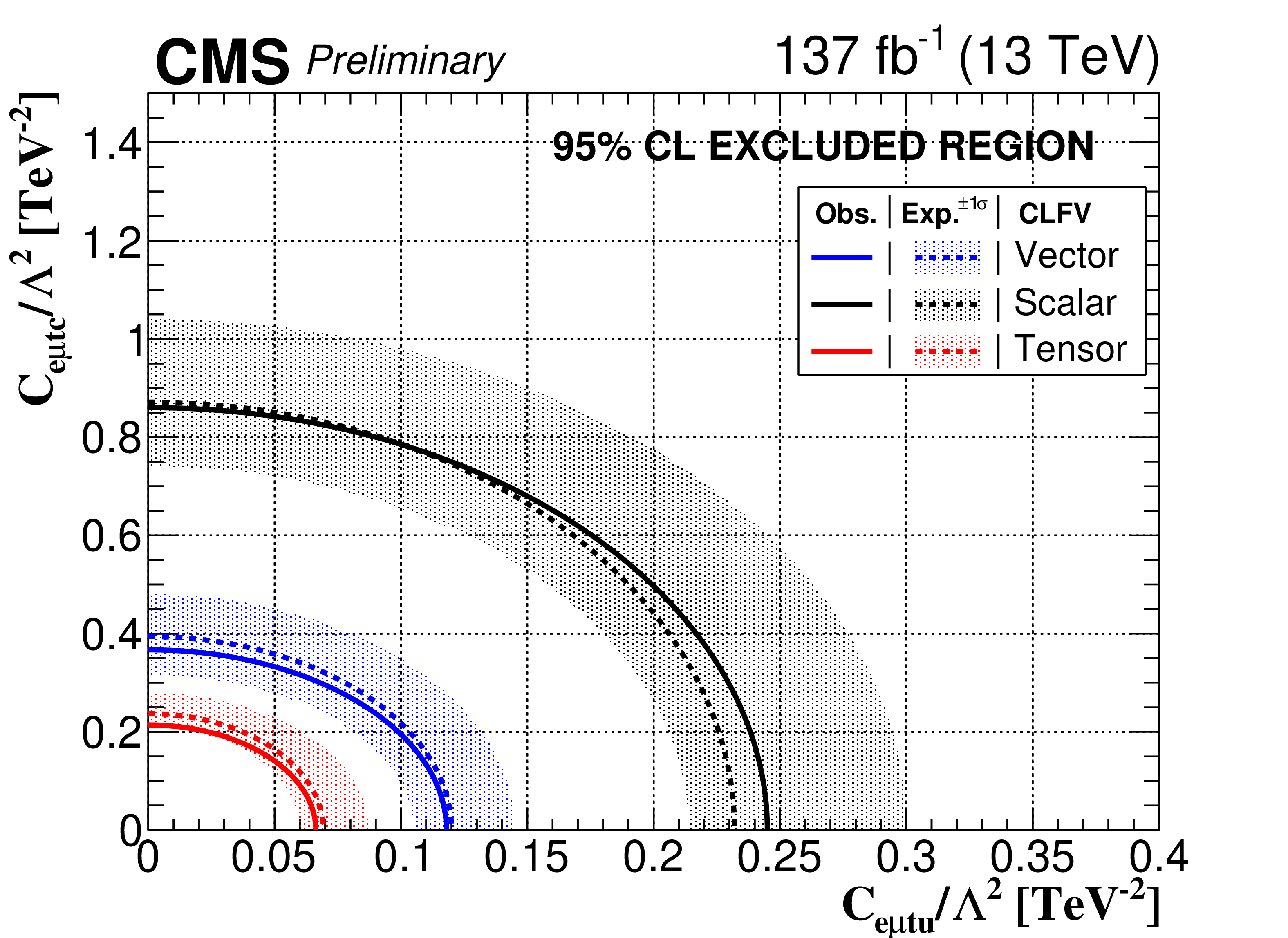
Figure 5:
The observed 95% exclusion limits on $\mathrm{e} \mu \mathrm{t} \mathrm{c} $ Wilson coefficient as a function of $\mathrm{e} \mu \mathrm{t} \mathrm{u} $ Wilson coefficient (left) and $\mathcal {B}(\mathrm{t} \to \mathrm{e} \mu \mathrm{c})$ as a function of $\mathcal {B}(\mathrm{t} \to \mathrm{e} \mu \mathrm{u})$ (right) for the scalar, vector and tensor like CLFV interactions. |
png pdf |
Figure 5-a:
The observed 95% exclusion limits on $\mathrm{e} \mu \mathrm{t} \mathrm{c} $ Wilson coefficient as a function of $\mathrm{e} \mu \mathrm{t} \mathrm{u} $ Wilson coefficient (left) and $\mathcal {B}(\mathrm{t} \to \mathrm{e} \mu \mathrm{c})$ as a function of $\mathcal {B}(\mathrm{t} \to \mathrm{e} \mu \mathrm{u})$ (right) for the scalar, vector and tensor like CLFV interactions. |

png pdf |
Figure 5-b:
The observed 95% exclusion limits on $\mathrm{e} \mu \mathrm{t} \mathrm{c} $ Wilson coefficient as a function of $\mathrm{e} \mu \mathrm{t} \mathrm{u} $ Wilson coefficient (left) and $\mathcal {B}(\mathrm{t} \to \mathrm{e} \mu \mathrm{c})$ as a function of $\mathcal {B}(\mathrm{t} \to \mathrm{e} \mu \mathrm{u})$ (right) for the scalar, vector and tensor like CLFV interactions. |
| Tables | |

png pdf |
Table 1:
The number of expected events from ${\mathrm{t} {}\mathrm{\bar{t}}}$, tW, and from the remaining backgrounds (other), the total background contribution and the observed events in data, collected during three years (2016, 2017, and 2018), after all selections for signal (1 b-tagged) and control ($ > $1 b-tagged) regions. The expected signal yields for single top quark production and top quark decays via the scalar, vector and tensor CLFV interactions, assuming $\text {C}_x/\Lambda ^2 = $ 1 TeV$ ^{-2}$ are also shown. The uncertainties correspond to the statistical contribution only. |

png pdf |
Table 2:
Summary of representative systematic uncertainties on the selection efficiency for the ${\mathrm{t} {}\mathrm{\bar{t}}}$ process and for the signal processes: single top quark production and top quark decays via vector $\mathrm{e} \mu \mathrm{t} \mathrm{u} $ CLFV interactions in the signal and ${\mathrm{t} {}\mathrm{\bar{t}}}$ control regions. |
png pdf |
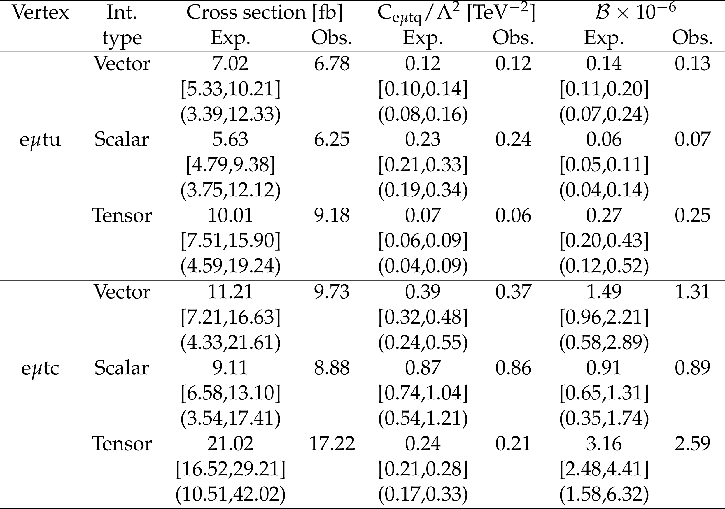
Table 3:
Expected/Observed upper limits on the signal cross sections (production + decay), CLFV Wilson coefficients, and top quark CLFV branching ratios are shown for all three years combined. For expected limits [$-1\sigma, +1\sigma $] and ($-2\sigma, +2\sigma $) ranges are shown. |
| Summary |
| The result of a search for charged lepton flavor violation (CLFV) in top quark production and decay has been presented. The search is performed using proton-proton collisions collected by the CMS detector at the LHC at a center-of-mass energy of 13 TeV, and corresponds to an integrated luminosity of 137 fb$^{-1}$. No significant excess over the SM prediction is observed. Within the effective field theory framework, upper limits are set on individual relevant Wilson coefficients. Limits on the Wilson coefficients are converted to limits on the branching fractions of the top quark $\mathcal{B}_{\text{scalar}}(\mathrm{t} \to \mathrm{e}\mu \mathrm{u} (\mathrm{c})) < $ 0.07 $\times$ 10$^{-6}$ (0.89 $\times$ 10$^{-6}$), $\mathcal{B}_{\text{vector}}(\mathrm{t} \to \mathrm{e}\mu \mathrm{u} (\mathrm{c})) < $ 0.135 $\times$ 10$^{-6}$ (1.3 $\times$ 10$^{-6}$), and $\mathcal{B}_{\text{tensor}}(\mathrm{t} \to \mathrm{e}\mu \mathrm{u} (\mathrm{c})) < $ 0.25 $\times$ 10$^{-6}$ (2.59 $\times$ 10$^{-6}$), which are the most restrictive bounds to date. |
| References | ||||
| 1 | S. Roy Choudhury and S. Choubey | Updated Bounds on Sum of Neutrino Masses in Various Cosmological Scenarios | JCAP 09 (2018) 017 | 1806.10832 |
| 2 | J. Diaz-Cruz and J. Toscano | Lepton flavor violating decays of Higgs bosons beyond the standard model | PRD 62 (2000) 116005 | hep-ph/9910233 |
| 3 | A. Crivellin et al. | Lepton flavour violation in the MSSM: exact diagonalization vs mass expansion | JHEP 06 (2018) 003 | 1802.06803 |
| 4 | M. Malinsky, T. Ohlsson, Z.-z. Xing, and H. Zhang | Non-unitary neutrino mixing and CP violation in the minimal inverse seesaw model | PLB 679 (2009) 242 | 0905.2889 |
| 5 | MEG Collaboration | New constraint on the existence of the $ \mu^{+} \rightarrow e^{+} \gamma $ decay | PRL 110 (2013) 201801 | 1303.0754 |
| 6 | S. Mihara, J. P. Miller, P. Paradisi, and G. Piredda | Charged Lepton Flavor Violation Experiments | Ann. Rev. Nucl. Part. Sci. 63 (2013) 531 | |
| 7 | ATLAS Collaboration | A search for lepton-flavor-violating decays of the $ Z $ boson into a $ \tau $-lepton and a light lepton with the ATLAS detector | PRD 98 (2018) 092010 | 1804.09568 |
| 8 | ATLAS Collaboration | Search for lepton-flavour-violating decays of the Higgs and $ Z $ bosons with the ATLAS detector | EPJC 77 (2017) 70 | 1604.07730 |
| 9 | CMS Collaboration | Search for lepton flavour violating decays of the Higgs boson to $ \mu\tau $ and e$ \tau $ in proton-proton collisions at $ \sqrt{s}= $ 13 TeV | JHEP 06 (2018) 001 | CMS-HIG-17-001 1712.07173 |
| 10 | ATLAS Collaboration | Search for charged lepton-flavour violation in top-quark decays at the LHC with the ATLAS detector | ATLAS-CONF-2018-044, CERN, Geneva, Sep | |
| 11 | LHCb Collaboration | Test of lepton universality using $ B^{+}\rightarrow K^{+}\ell^{+}\ell^{-} $ decays | PRL 113 (2014) 151601 | 1406.6482 |
| 12 | LHCb Collaboration | Measurement of the ratio of branching fractions $ \mathcal{B}(\bar{B}^0 \to D^{*+}\tau^{-}\bar{\nu}_{\tau})/\mathcal{B}(\bar{B}^0 \to D^{*+}\mu^{-}\bar{\nu}_{\mu}) $ | PRL 115 (2015) 111803 | 1506.08614 |
| 13 | LHCb Collaboration | Test of lepton universality with $ B^{0} \rightarrow K^{*0}\ell^{+}\ell^{-} $ decays | JHEP 08 (2017) 055 | 1705.05802 |
| 14 | S. L. Glashow, D. Guadagnoli, and K. Lane | Lepton Flavor Violation in $ B $ Decays? | PRL 114 (2015) 091801 | 1411.0565 |
| 15 | T. J. Kim et al. | Correlation between $ {R}_{D^{\left(\ast \right)}} $ and top quark FCNC decays in leptoquark models | JHEP 07 (2019) 025 | 1812.08484 |
| 16 | D. Barducci et al. | Interpreting top-quark LHC measurements in the standard-model effective field theory | 1802.07237 | |
| 17 | S. Davidson, M. L. Mangano, S. Perries, and V. Sordini | Lepton Flavour Violating top decays at the LHC | EPJC 75 (2015) 450 | 1507.07163 |
| 18 | C. Oleari | The POWHEG BOX | Nuclear Physics B - Proceedings Supplements 205 (2010) 36, Loops and Legs in Quantum Field Theory | |
| 19 | P. Nason | A new method for combining NLO QCD with shower Monte Carlo algorithms | JHEP 11 (2004) 040 | hep-ph/0409146 |
| 20 | S. Frixione, P. Nason, and C. Oleari | Matching NLO QCD computations with parton shower simulations: the POWHEG method | JHEP 11 (2007) 070 | 0709.2092 |
| 21 | S. Alioli, P. Nason, C. Oleari, and E. Re | A general framework for implementing NLO calculations in shower Monte Carlo programs: the POWHEG BOX | JHEP 06 (2010) 043 | 1002.2581 |
| 22 | S. Frixione, P. Nason, and G. Ridolfi | A positive-weight next-to-leading-order Monte Carlo for heavy flavour hadroproduction | JHEP 09 (2007) 126 | 0707.3088 |
| 23 | J. Alwall et al. | The automated computation of tree-level and next-to-leading order differential cross sections, and their matching to parton shower simulations | JHEP 07 (2014) 079 | 1405.0301 |
| 24 | NNPDF Collaboration | Parton distributions for the LHC Run II | JHEP 04 (2015) 040 | 1410.8849 |
| 25 | NNPDF Collaboration | Parton distributions from high-precision collider data | EPJC 77 (2017) 663 | 1706.00428 |
| 26 | T. Sjostrand et al. | An Introduction to PYTHIA 8.2 | CPC 191 (2015) 159 | 1410.3012 |
| 27 | CMS Collaboration | Event generator tunes obtained from underlying event and multiparton scattering measurements | EPJC 76 (2016) 155 | CMS-GEN-14-001 1512.00815 |
| 28 | CMS Collaboration | Extraction and validation of a new set of CMS PYTHIA8 tunes from underlying-event measurements | EPJC 80 (2020) 4 | CMS-GEN-17-001 1903.12179 |
| 29 | GEANT4 Collaboration | GEANT4--a simulation toolkit | NIMA 506 (2003) 250 | |
| 30 | M. Czakon and A. Mitov | Top++: A program for the calculation of the top-pair cross-section at hadron colliders | CPC 185 (2014) 2930 | 1112.5675 |
| 31 | M. Czakon et al. | Top-pair production at the LHC through NNLO QCD and NLO EW | JHEP 10 (2017) 186 | 1705.04105 |
| 32 | I. Brivio, Y. Jiang, and M. Trott | The SMEFTsim package, theory and tools | JHEP 12 (2017) 070 | 1709.06492 |
| 33 | A. Dedes et al. | SmeftFR -- Feynman rules generator for the Standard Model Effective Field Theory | CPC 247 (2020) 106931 | 1904.03204 |
| 34 | J. Kile and A. Soni | Model-Independent Constraints on Lepton-Flavor-Violating Decays of the Top Quark | PRD 78 (2008) 094008 | 0807.4199 |
| 35 | CMS Collaboration | Performance of the CMS Level-1 trigger in proton-proton collisions at $ \sqrt{s} = $ 13 TeV | JINST 15 (2020) P10017 | CMS-TRG-17-001 2006.10165 |
| 36 | CMS Collaboration | The CMS trigger system | JINST 12 (2017) P01020 | CMS-TRG-12-001 1609.02366 |
| 37 | CMS Collaboration | Particle-flow reconstruction and global event description with the CMS detector | JINST 12 (2017) P10003 | CMS-PRF-14-001 1706.04965 |
| 38 | CMS Collaboration | Performance of the CMS muon detector and muon reconstruction with proton-proton collisions at $ \sqrt{s}= $ 13 TeV | JINST 13 (2018) | CMS-MUO-16-001 1804.04528 |
| 39 | CMS Collaboration | Performance of the reconstruction and identification of high-momentum muons in proton-proton collisions at $ \sqrt{s} = $ 13 TeV | JINST 15 (2020) P02027 | CMS-MUO-17-001 1912.03516 |
| 40 | CMS Collaboration | Performance of electron reconstruction and selection with the CMS detector in proton-proton collisions at $ \sqrt{s} = $ 8 TeV | JINST 10 (2015) P06005 | CMS-EGM-13-001 1502.02701 |
| 41 | M. Cacciari, G. P. Salam, and G. Soyez | The anti-$ k_{\rm{T}} $ jet clustering algorithm | JHEP 04 (2008) 063 | 0802.1189 |
| 42 | CMS Collaboration | Jet energy scale and resolution in the CMS experiment in pp collisions at 8 TeV | JINST 12 (2017) P02014 | CMS-JME-13-004 1607.03663 |
| 43 | M. Cacciari and G. P. Salam | Pileup subtraction using jet areas | PLB 659 (2008) 119--126 | 0707.1378 |
| 44 | CMS Collaboration | Identification of heavy-flavour jets with the CMS detector in pp collisions at 13 TeV | JINST 13 (2018) P05011 | CMS-BTV-16-002 1712.07158 |
| 45 | TMVA Core Developer Team Collaboration | TMVA: Toolkit for multivariate data analysis | AIP Conf. Proc. 1504 (2012) | |
| 46 | CMS Collaboration | Measurements of $ \mathrm{t\overline{t}} $ differential cross sections in proton-proton collisions at $ \sqrt{s}= $ 13 TeV using events containing two leptons | JHEP 02 (2019) | CMS-TOP-17-014 1811.06625 |
| 47 | CMS Collaboration | Performance of CMS muon reconstruction in pp collision events at $ \sqrt{s}= $ 7 TeV | JINST 7 (2012) P10002 | CMS-MUO-10-004 1206.4071 |
| 48 | CMS Collaboration | Electron and photon reconstruction and identification with the CMS experiment at the CERN LHC | JINST 16 (2021) P05014 | CMS-EGM-17-001 2012.06888 |
| 49 | CMS Collaboration | Identification of heavy-flavour jets with the CMS detector in pp collisions at 13 TeV | JINST 13 (2018) P05011 | CMS-BTV-16-002 1712.07158 |
| 50 | CMS Collaboration | CMS luminosity measurements for the 2016 data-taking period | CMS-PAS-LUM-17-001 | CMS-PAS-LUM-17-001 |
| 51 | CMS Collaboration | CMS luminosity measurement for the 2017 data-taking period at $ \sqrt{s} = $ 13 TeV | CMS-PAS-LUM-17-004 | CMS-PAS-LUM-17-004 |
| 52 | CMS Collaboration | CMS luminosity measurement for the 2018 data-taking period at $ \sqrt{s} = $ 13 TeV | CMS-PAS-LUM-18-002 | CMS-PAS-LUM-18-002 |
| 53 | CMS Collaboration | Measurement of the inelastic proton-proton cross section at $ \sqrt{s}= $ 13 TeV | JHEP 07 (2018) 161 | CMS-FSQ-15-005 1802.02613 |
| 54 | A. Kalogeropoulos and J. Alwall | The SysCalc code: A tool to derive theoretical systematic uncertainties | 1801.08401 | |
| 55 | CMS Collaboration | Measurement of the production cross section for single top quarks in association with W bosons in proton-proton collisions at $ \sqrt{s}= $ 13 TeV | JHEP 10 (2018) 117 | CMS-TOP-17-018 1805.07399 |
| 56 | T. Junk | Confidence level computation for combining searches with small statistics | Nucl. Instrum. Meth A 434 (1999) 435 | |
| 57 | A. L. Read | Presentation of search results: the CLs technique | JPG 28 (2002) 2693 | |
| 58 | R. Barlow and C. Beeston | Fitting using finite monte carlo samples | CPC 77 (1993) 219 | |
|
|
Compact Muon Solenoid LHC, CERN |
|

|

|

|

|

|