

Compact Muon Solenoid
LHC, CERN
| CMS-PAS-TOP-17-011 | ||
| Measurement of the single top quark and antiquark production cross sections in the $t$ channel and their ratio in pp collisions at $\sqrt{s} = $ 13 TeV | ||
| CMS Collaboration | ||
| July 2018 | ||
| Abstract: The cross sections for the production of single top quarks and antiquarks in the $t$ channel, and their ratio, are measured in proton-proton collisions at a center-of-mass energy of 13 TeV. The full data set recorded in 2016 by the CMS detector at the LHC is analyzed, corresponding to an integrated luminosity of 35.9 fb$^{-1}$. Events with one muon or electron and two jets are selected, where one of the two jets is identified as originating from a bottom quark. A multivariate discriminator exploiting several kinematic variables is applied to separate signal from background events. The ratio $R_{t\mathrm{\text{-}ch.}}$ of the cross sections is measured to be 1.65 $\pm$ 0.02 (stat) $\pm$ 0.04 (syst). The total cross section for the production of single top quarks or antiquarks is measured to be 219.0 $\pm$ 1.5 (stat) $\pm$ 33.0 (syst) pb and the absolute value of the CKM matrix element $V_{\mathrm{tb}}$ is determined to be 1.00 $\pm$ 0.05 (exp) $\pm$ 0.02 (theo). All results are in agreement with the standard model predictions. | ||
|
Links:
CDS record (PDF) ;
CADI line (restricted) ;
These preliminary results are superseded in this paper, PLB 800 (2019) 135042. The superseded preliminary plots can be found here. |
||
| Figures | |

png pdf |
Figure 1:
Leading-order Feynman diagrams for the electroweak production of a single top quark (left) and a single top antiquark (right). The flavor of the light quark in the initial state - either up-type (u) or down-type (d) - defines whether a top quark or top antiquark is produced. |

png pdf |
Figure 1-a:
Leading-order Feynman diagrams for the electroweak production of a single top quark (left) and a single top antiquark (right). The flavor of the light quark in the initial state - either up-type (u) or down-type (d) - defines whether a top quark or top antiquark is produced. |

png pdf |
Figure 1-b:
Leading-order Feynman diagrams for the electroweak production of a single top quark (left) and a single top antiquark (right). The flavor of the light quark in the initial state - either up-type (u) or down-type (d) - defines whether a top quark or top antiquark is produced. |

png pdf |
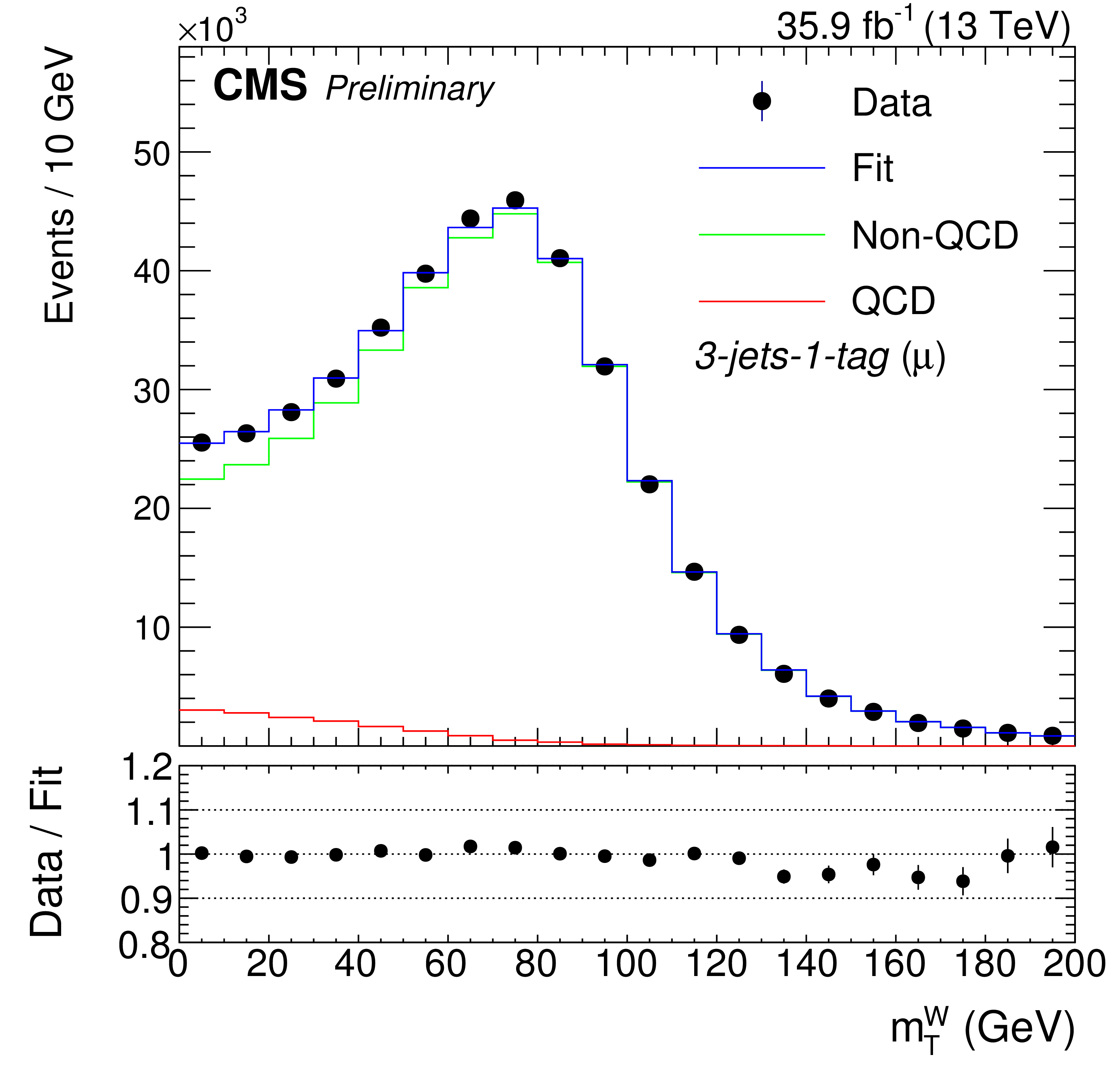
Figure 2:
Fit to the ${m_{\mathrm {T}}^{\mathrm {W}}}$ distribution for events with muons (left) and to the ${{p_{\mathrm {T}}} ^\text {miss}}$ distribution for events with electrons (right) in the 2-jets-1-tag (upper row), 3-jets-1-tag (middle row), and the 2-jets-0-tags categories. The QCD template is extracted from a sideband region in data. For the fit, only statistical uncertainties are considered. |

png pdf |
Figure 2-a:
Fit to the ${m_{\mathrm {T}}^{\mathrm {W}}}$ distribution for events with muons (left) and to the ${{p_{\mathrm {T}}} ^\text {miss}}$ distribution for events with electrons (right) in the 2-jets-1-tag (upper row), 3-jets-1-tag (middle row), and the 2-jets-0-tags categories. The QCD template is extracted from a sideband region in data. For the fit, only statistical uncertainties are considered. |

png pdf |
Figure 2-b:
Fit to the ${m_{\mathrm {T}}^{\mathrm {W}}}$ distribution for events with muons (left) and to the ${{p_{\mathrm {T}}} ^\text {miss}}$ distribution for events with electrons (right) in the 2-jets-1-tag (upper row), 3-jets-1-tag (middle row), and the 2-jets-0-tags categories. The QCD template is extracted from a sideband region in data. For the fit, only statistical uncertainties are considered. |
png pdf |
Figure 2-c:
Fit to the ${m_{\mathrm {T}}^{\mathrm {W}}}$ distribution for events with muons (left) and to the ${{p_{\mathrm {T}}} ^\text {miss}}$ distribution for events with electrons (right) in the 2-jets-1-tag (upper row), 3-jets-1-tag (middle row), and the 2-jets-0-tags categories. The QCD template is extracted from a sideband region in data. For the fit, only statistical uncertainties are considered. |

png pdf |
Figure 2-d:
Fit to the ${m_{\mathrm {T}}^{\mathrm {W}}}$ distribution for events with muons (left) and to the ${{p_{\mathrm {T}}} ^\text {miss}}$ distribution for events with electrons (right) in the 2-jets-1-tag (upper row), 3-jets-1-tag (middle row), and the 2-jets-0-tags categories. The QCD template is extracted from a sideband region in data. For the fit, only statistical uncertainties are considered. |

png pdf |
Figure 2-e:
Fit to the ${m_{\mathrm {T}}^{\mathrm {W}}}$ distribution for events with muons (left) and to the ${{p_{\mathrm {T}}} ^\text {miss}}$ distribution for events with electrons (right) in the 2-jets-1-tag (upper row), 3-jets-1-tag (middle row), and the 2-jets-0-tags categories. The QCD template is extracted from a sideband region in data. For the fit, only statistical uncertainties are considered. |

png pdf |
Figure 2-f:
Fit to the ${m_{\mathrm {T}}^{\mathrm {W}}}$ distribution for events with muons (left) and to the ${{p_{\mathrm {T}}} ^\text {miss}}$ distribution for events with electrons (right) in the 2-jets-1-tag (upper row), 3-jets-1-tag (middle row), and the 2-jets-0-tags categories. The QCD template is extracted from a sideband region in data. For the fit, only statistical uncertainties are considered. |

png pdf |
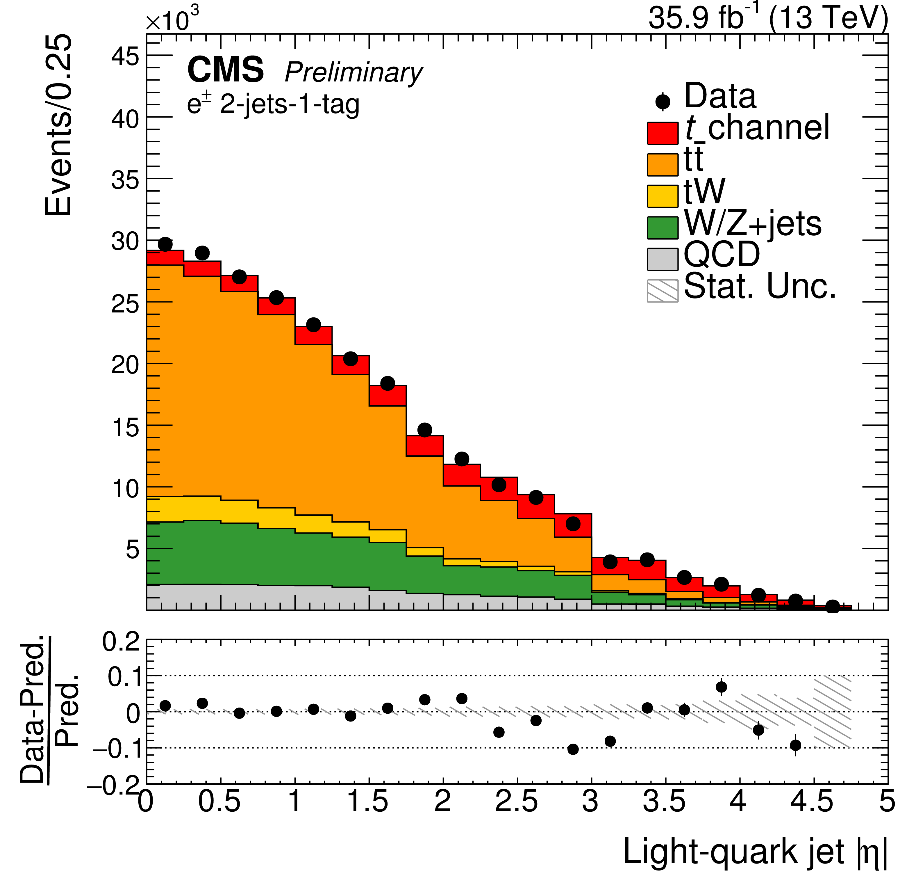
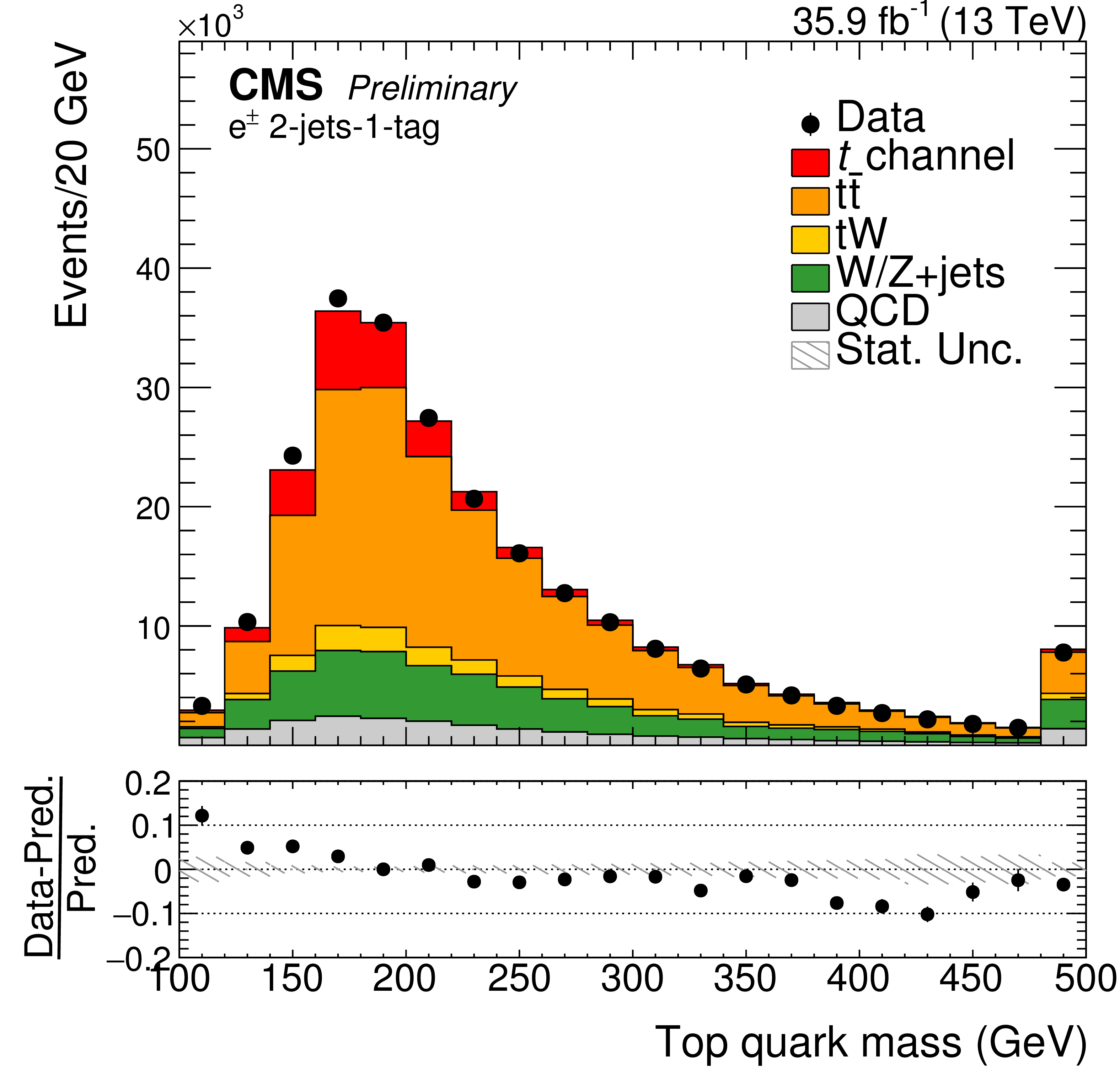
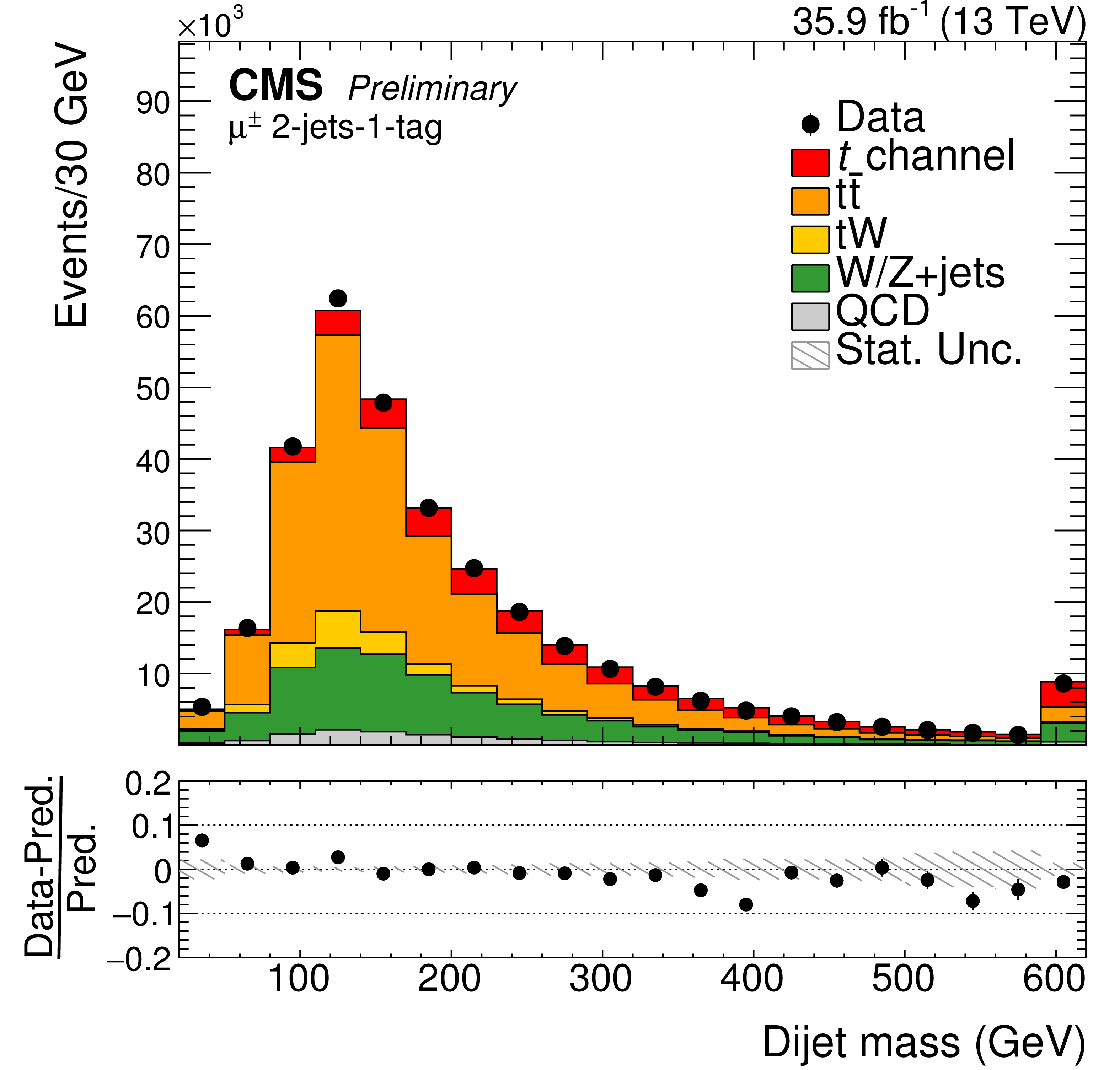
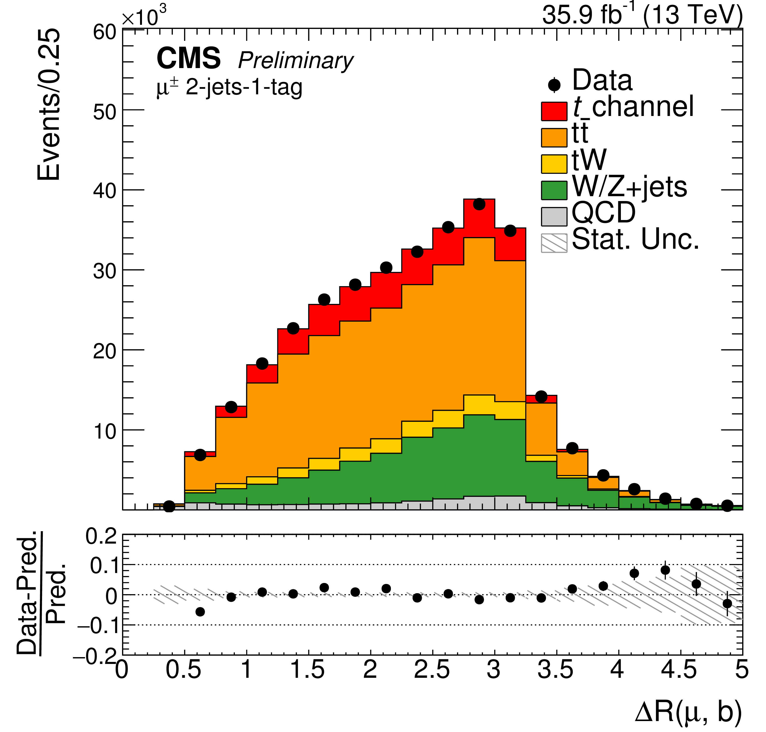
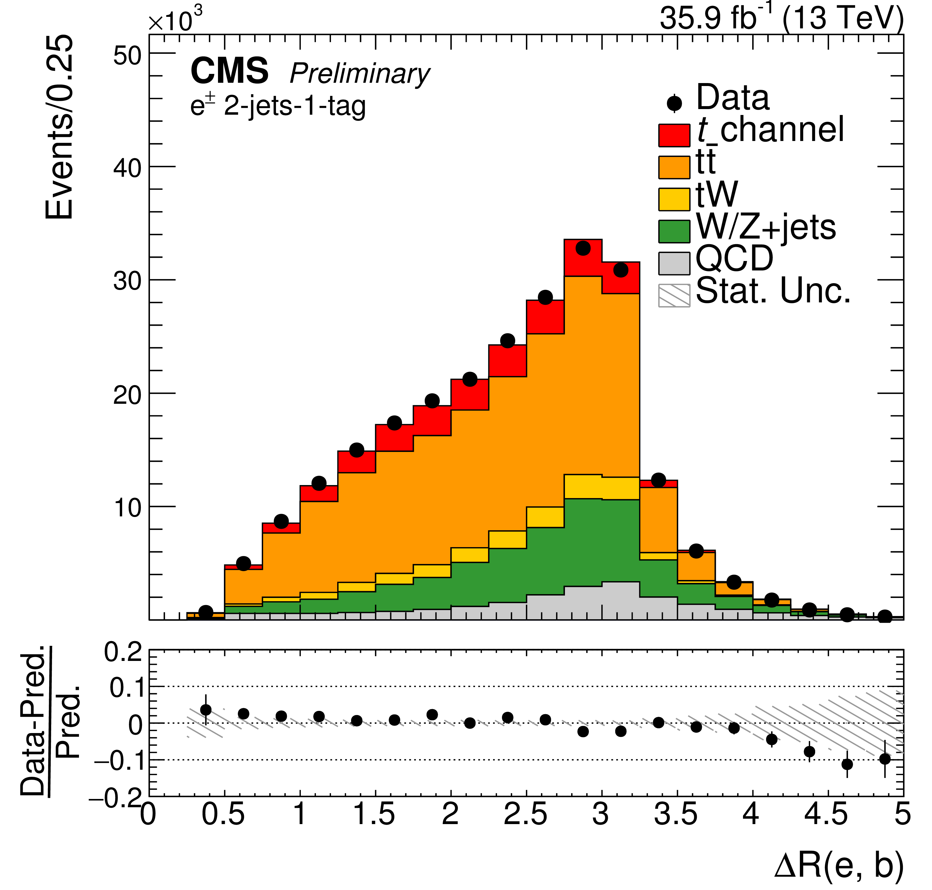
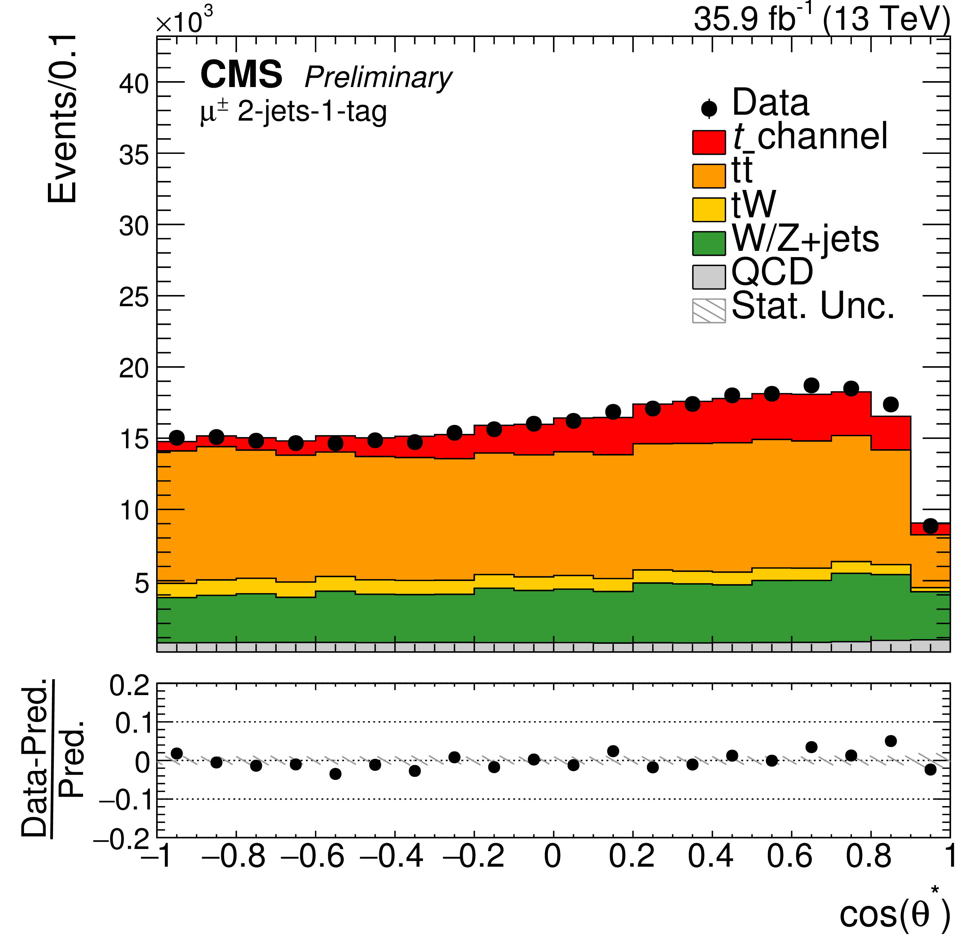
Figure 3:
The three most important input variables for the training of the BDTs in the muon channel (left) and in the electron channel (right). The variables are ordered by their importance in the training. The simulation is normalized to the amount of data. The shaded areas correspond to the statistical uncertainties. |

png pdf |
Figure 3-a:
The three most important input variables for the training of the BDTs in the muon channel (left) and in the electron channel (right). The variables are ordered by their importance in the training. The simulation is normalized to the amount of data. The shaded areas correspond to the statistical uncertainties. |
png pdf |
Figure 3-b:
The three most important input variables for the training of the BDTs in the muon channel (left) and in the electron channel (right). The variables are ordered by their importance in the training. The simulation is normalized to the amount of data. The shaded areas correspond to the statistical uncertainties. |

png pdf |
Figure 3-c:
The three most important input variables for the training of the BDTs in the muon channel (left) and in the electron channel (right). The variables are ordered by their importance in the training. The simulation is normalized to the amount of data. The shaded areas correspond to the statistical uncertainties. |
png pdf |
Figure 3-d:
The three most important input variables for the training of the BDTs in the muon channel (left) and in the electron channel (right). The variables are ordered by their importance in the training. The simulation is normalized to the amount of data. The shaded areas correspond to the statistical uncertainties. |
png pdf |
Figure 3-e:
The three most important input variables for the training of the BDTs in the muon channel (left) and in the electron channel (right). The variables are ordered by their importance in the training. The simulation is normalized to the amount of data. The shaded areas correspond to the statistical uncertainties. |

png pdf |
Figure 3-f:
The three most important input variables for the training of the BDTs in the muon channel (left) and in the electron channel (right). The variables are ordered by their importance in the training. The simulation is normalized to the amount of data. The shaded areas correspond to the statistical uncertainties. |

png pdf |
Figure 4:
The fourth and fifth most important input variables for the training of the BDTs in the muon channel (left) and in the electron channel (right). The simulation is normalized to the amount of data. The shaded areas correspond to the statistical uncertainties. |
png pdf |
Figure 4-a:
The fourth and fifth most important input variables for the training of the BDTs in the muon channel (left) and in the electron channel (right). The simulation is normalized to the amount of data. The shaded areas correspond to the statistical uncertainties. |
png pdf |
Figure 4-b:
The fourth and fifth most important input variables for the training of the BDTs in the muon channel (left) and in the electron channel (right). The simulation is normalized to the amount of data. The shaded areas correspond to the statistical uncertainties. |
png pdf |
Figure 4-c:
The fourth and fifth most important input variables for the training of the BDTs in the muon channel (left) and in the electron channel (right). The simulation is normalized to the amount of data. The shaded areas correspond to the statistical uncertainties. |

png pdf |
Figure 4-d:
The fourth and fifth most important input variables for the training of the BDTs in the muon channel (left) and in the electron channel (right). The simulation is normalized to the amount of data. The shaded areas correspond to the statistical uncertainties. |
png pdf |
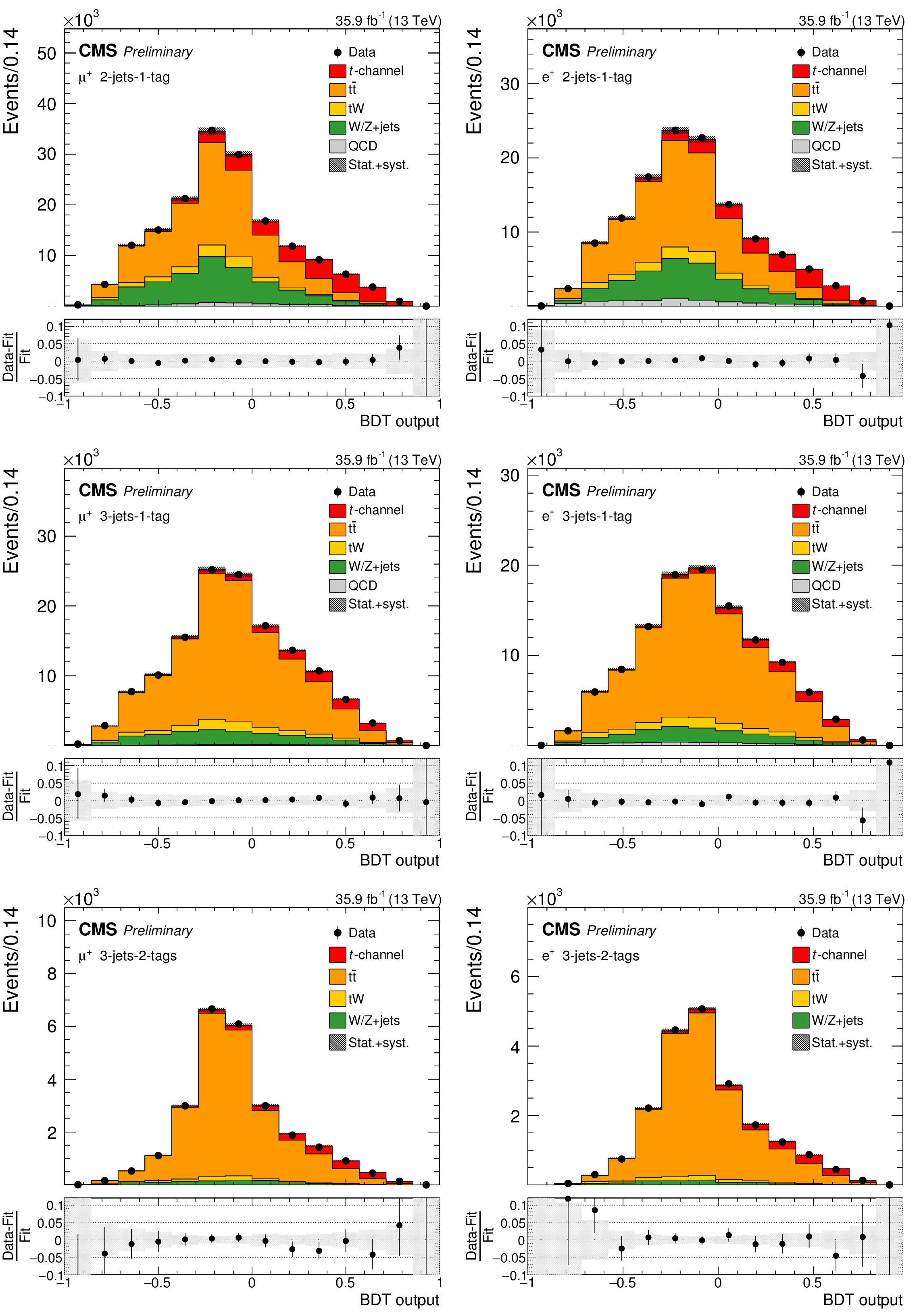
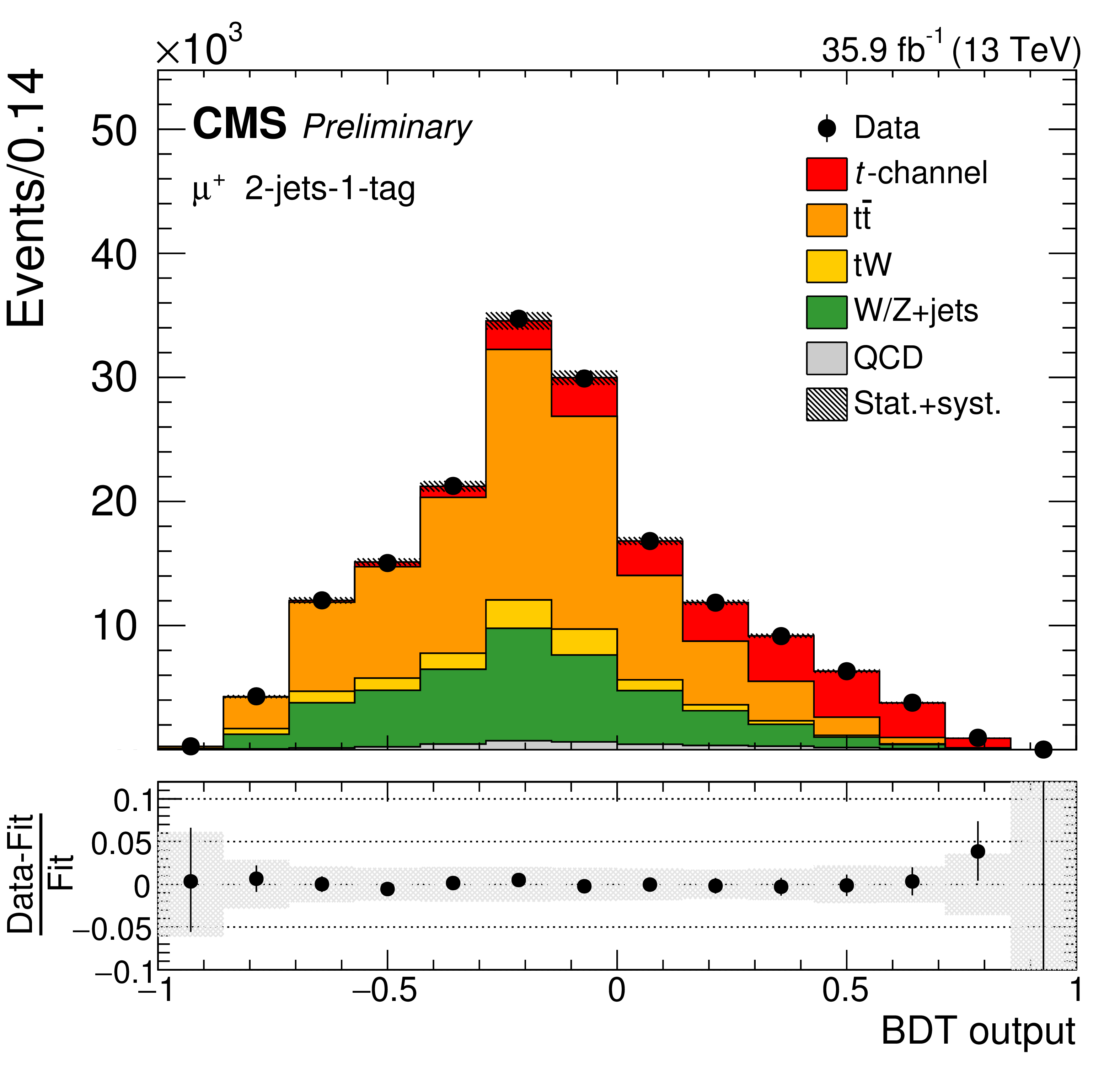
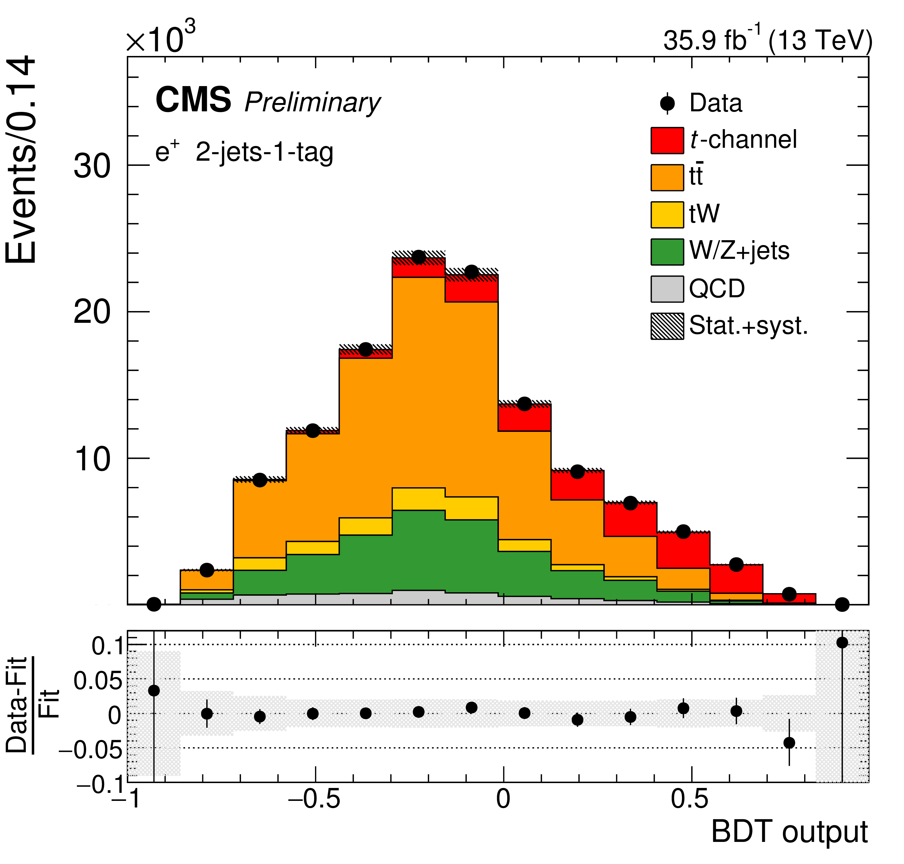
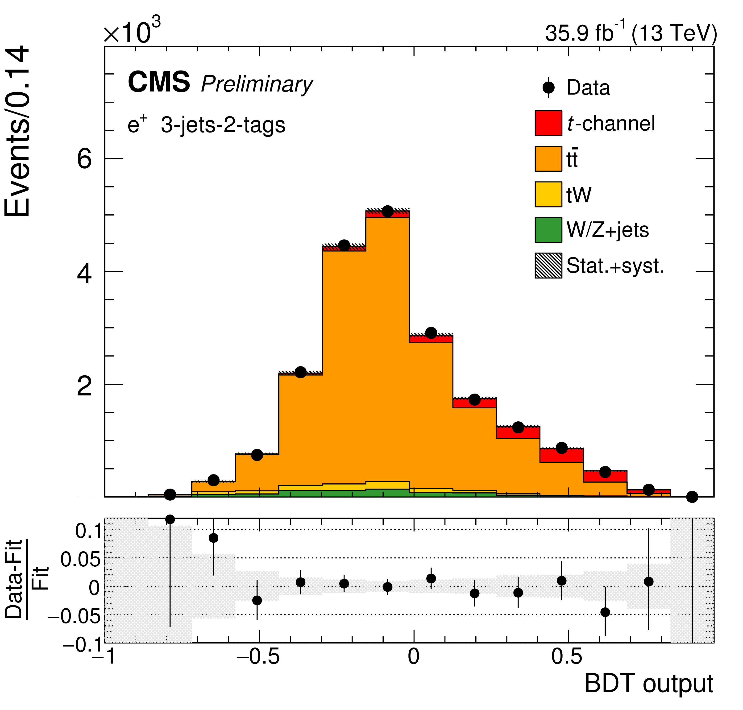
Figure 5:
BDT output distribution in the 2-jets-1-tag category (upper row), the 3-jets-1-tag category (middle row), and the 3-jets-2-tags category (lower row) for positively charged muons (left column) and electrons (right column). The different processes are scaled to the corresponding fit results. In each figure, the relative difference between the fitted distribution and the distribution in data is shown. The shaded areas correspond to the post-fit uncertainties. |
png pdf |
Figure 5-a:
BDT output distribution in the 2-jets-1-tag category (upper row), the 3-jets-1-tag category (middle row), and the 3-jets-2-tags category (lower row) for positively charged muons (left column) and electrons (right column). The different processes are scaled to the corresponding fit results. In each figure, the relative difference between the fitted distribution and the distribution in data is shown. The shaded areas correspond to the post-fit uncertainties. |
png pdf |
Figure 5-b:
BDT output distribution in the 2-jets-1-tag category (upper row), the 3-jets-1-tag category (middle row), and the 3-jets-2-tags category (lower row) for positively charged muons (left column) and electrons (right column). The different processes are scaled to the corresponding fit results. In each figure, the relative difference between the fitted distribution and the distribution in data is shown. The shaded areas correspond to the post-fit uncertainties. |

png pdf |
Figure 5-c:
BDT output distribution in the 2-jets-1-tag category (upper row), the 3-jets-1-tag category (middle row), and the 3-jets-2-tags category (lower row) for positively charged muons (left column) and electrons (right column). The different processes are scaled to the corresponding fit results. In each figure, the relative difference between the fitted distribution and the distribution in data is shown. The shaded areas correspond to the post-fit uncertainties. |

png pdf |
Figure 5-d:
BDT output distribution in the 2-jets-1-tag category (upper row), the 3-jets-1-tag category (middle row), and the 3-jets-2-tags category (lower row) for positively charged muons (left column) and electrons (right column). The different processes are scaled to the corresponding fit results. In each figure, the relative difference between the fitted distribution and the distribution in data is shown. The shaded areas correspond to the post-fit uncertainties. |

png pdf |
Figure 5-e:
BDT output distribution in the 2-jets-1-tag category (upper row), the 3-jets-1-tag category (middle row), and the 3-jets-2-tags category (lower row) for positively charged muons (left column) and electrons (right column). The different processes are scaled to the corresponding fit results. In each figure, the relative difference between the fitted distribution and the distribution in data is shown. The shaded areas correspond to the post-fit uncertainties. |
png pdf |
Figure 5-f:
BDT output distribution in the 2-jets-1-tag category (upper row), the 3-jets-1-tag category (middle row), and the 3-jets-2-tags category (lower row) for positively charged muons (left column) and electrons (right column). The different processes are scaled to the corresponding fit results. In each figure, the relative difference between the fitted distribution and the distribution in data is shown. The shaded areas correspond to the post-fit uncertainties. |
png pdf |
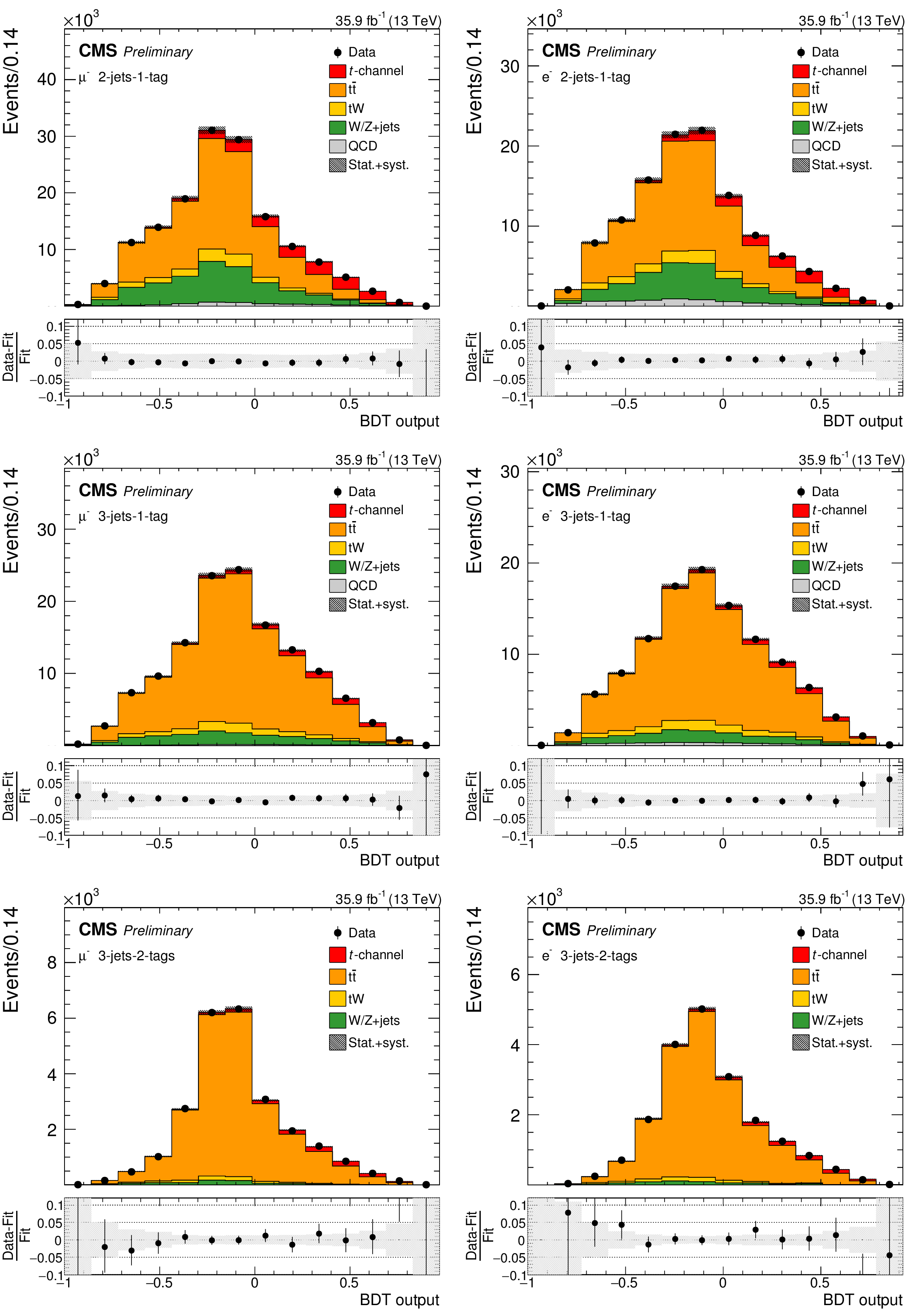
Figure 6:
BDT output distribution in the 2-jets-1-tag category (upper row), the 3-jets-1-tag category (middle row), and the 3-jets-2-tags category (lower row) for negatively charged muons (left column) and electrons (right column). The different processes are scaled to the corresponding fit results. In each figure, the relative difference between the fitted distribution and the distribution in data is shown. The shaded areas correspond to the post-fit uncertainties. |

png pdf |
Figure 6-a:
BDT output distribution in the 2-jets-1-tag category (upper row), the 3-jets-1-tag category (middle row), and the 3-jets-2-tags category (lower row) for negatively charged muons (left column) and electrons (right column). The different processes are scaled to the corresponding fit results. In each figure, the relative difference between the fitted distribution and the distribution in data is shown. The shaded areas correspond to the post-fit uncertainties. |

png pdf |
Figure 6-b:
BDT output distribution in the 2-jets-1-tag category (upper row), the 3-jets-1-tag category (middle row), and the 3-jets-2-tags category (lower row) for negatively charged muons (left column) and electrons (right column). The different processes are scaled to the corresponding fit results. In each figure, the relative difference between the fitted distribution and the distribution in data is shown. The shaded areas correspond to the post-fit uncertainties. |

png pdf |
Figure 6-c:
BDT output distribution in the 2-jets-1-tag category (upper row), the 3-jets-1-tag category (middle row), and the 3-jets-2-tags category (lower row) for negatively charged muons (left column) and electrons (right column). The different processes are scaled to the corresponding fit results. In each figure, the relative difference between the fitted distribution and the distribution in data is shown. The shaded areas correspond to the post-fit uncertainties. |

png pdf |
Figure 6-d:
BDT output distribution in the 2-jets-1-tag category (upper row), the 3-jets-1-tag category (middle row), and the 3-jets-2-tags category (lower row) for negatively charged muons (left column) and electrons (right column). The different processes are scaled to the corresponding fit results. In each figure, the relative difference between the fitted distribution and the distribution in data is shown. The shaded areas correspond to the post-fit uncertainties. |

png pdf |
Figure 6-e:
BDT output distribution in the 2-jets-1-tag category (upper row), the 3-jets-1-tag category (middle row), and the 3-jets-2-tags category (lower row) for negatively charged muons (left column) and electrons (right column). The different processes are scaled to the corresponding fit results. In each figure, the relative difference between the fitted distribution and the distribution in data is shown. The shaded areas correspond to the post-fit uncertainties. |

png pdf |
Figure 6-f:
BDT output distribution in the 2-jets-1-tag category (upper row), the 3-jets-1-tag category (middle row), and the 3-jets-2-tags category (lower row) for negatively charged muons (left column) and electrons (right column). The different processes are scaled to the corresponding fit results. In each figure, the relative difference between the fitted distribution and the distribution in data is shown. The shaded areas correspond to the post-fit uncertainties. |

png pdf |
Figure 7:
Estimated relative contributions of the listed uncertainty sources in% to the total uncertainties of the measured cross sections for top quark production and top antiquark production, and of the cross section ratio $R_{t\text {-ch.}}$. For the externalized signal modeling uncertainties, the values correspond to their relative uncertainties (first four entries). The other values are obtained by performing the fit again for each uncertainty source, with the corresponding nuisance parameter fixed to its optimal fit value and by calculating the resulting relative change in the cross sections, or cross section ratio, to the nominal ones. |
png pdf |
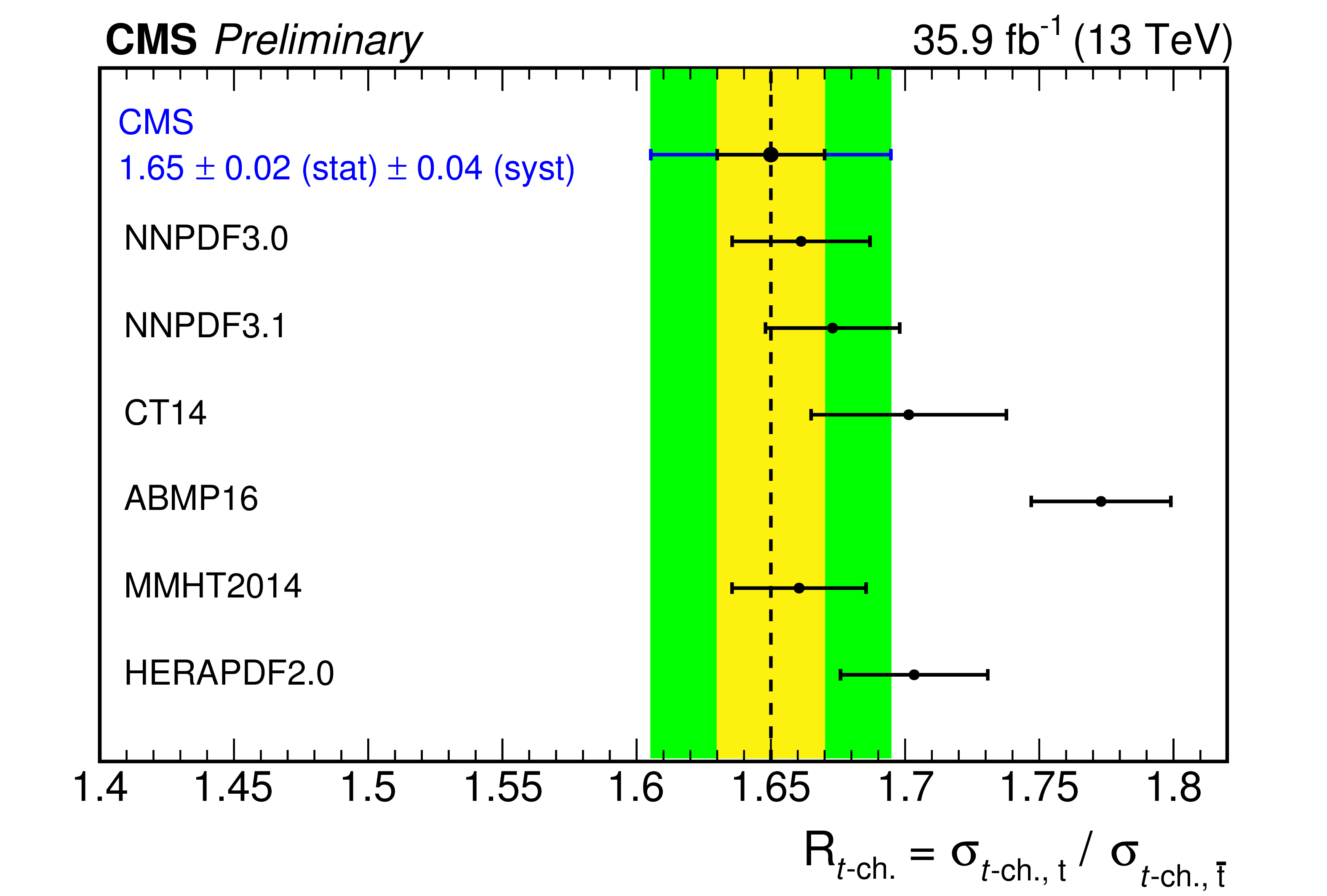
Figure 8:
Comparison of the measured $R_{\textit {t}\text {-ch.}}$ (dotted line) with the prediction from different PDF sets: NNPDF3.0 NLO [17], NNPDF3.1 NNLO [56], CT14 NLO [57], ABMP16 NNLO [58], MMHT2014 NLO [59], HERAPDF2.0 NLO [60]. The {powheg} 4FS calculation is used with a nominal value for the top quark mass of 172.5 GeV. The uncertainty bars for the different PDF sets include the statistical uncertainty, the uncertainty due to the factorization and renormalization scales, derived by varying both of them by a factor 0.5 and 2, and the uncertainty in the top quark mass, derived by varying the top quark mass between 171.5 and 173.5 GeV. For the measurement, the inner and outer uncertainty bars correspond to the statistical and total uncertainty, respectively. |
| Tables | |
png pdf |
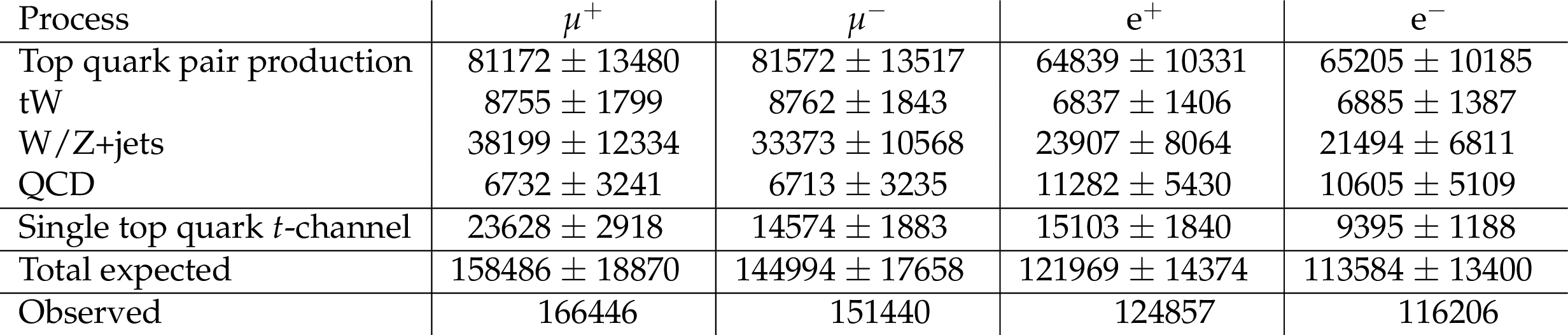
Table 1:
Event yields for the relevant processes in the 2-jets-1-tag category after applying the full event selection in the muon and electron channels for an integrated luminosity of 35.9 fb$^{-1}$. Statistical and systematic uncertainties are considered. The yields are obtained from simulation (using the 4FS prediction for the $t$-channel signal process and 5FS for the tW process), except for the QCD multijet contribution, which is derived from data (see Section xxxxx). |
png pdf |
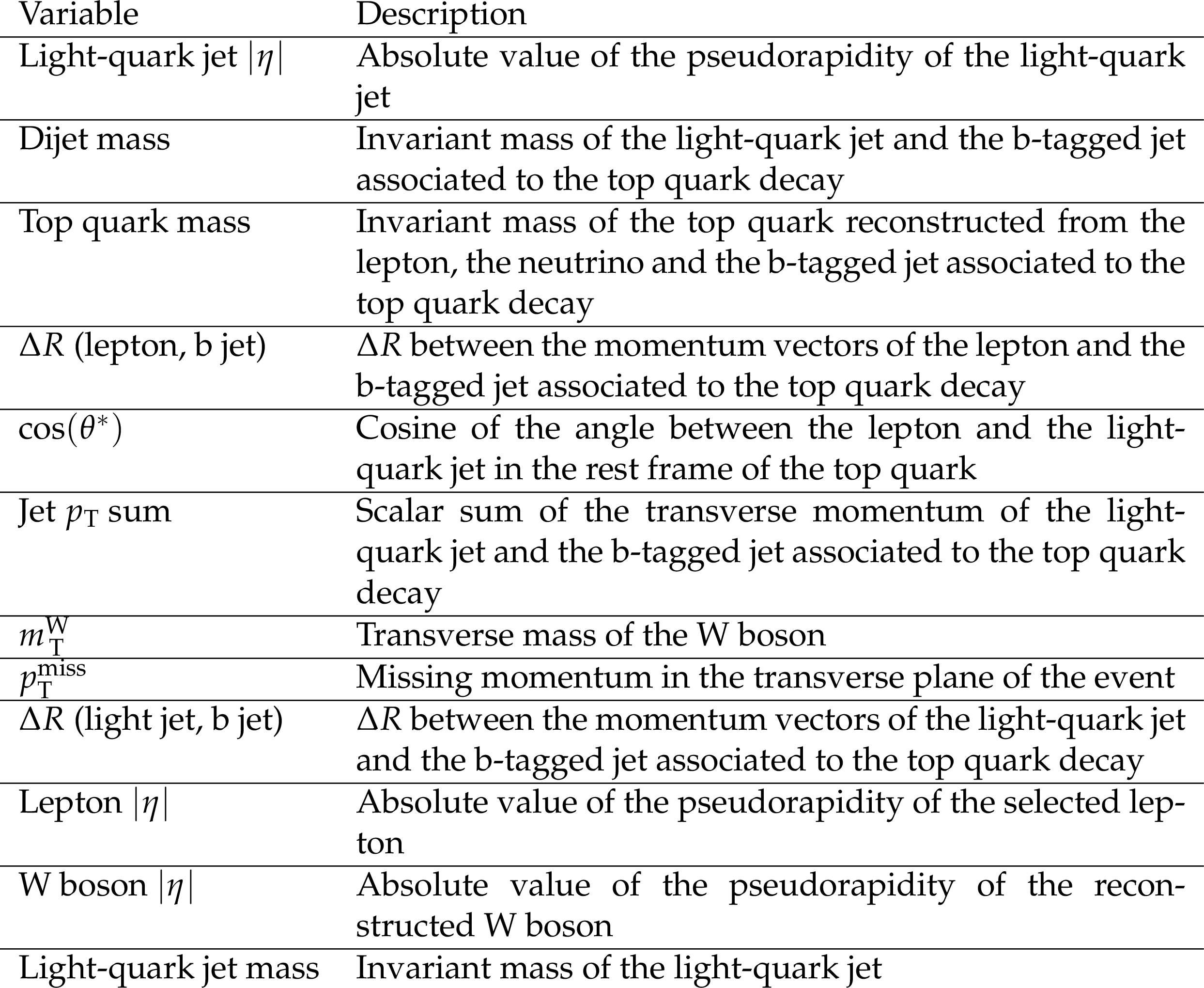
Table 2:
Input variables for the BDTs. The variables ${m_{\mathrm {T}}^{\mathrm {W}}}$ and lepton $|\eta |$ are only used in the training of events with a muon, while ${{p_{\mathrm {T}}} ^\text {miss}}$ is only used as input for events with an electron. |

png pdf |
Table 3:
Estimated relative contributions of the listed uncertainty sources in% to the total uncertainties of the measured cross sections for top quark production and top antiquark production, and of the cross section ratio $R_{t\text {-ch.}}$. For the externalized signal modeling uncertainties, the values correspond to their relative uncertainties (first four entries). The other values are obtained by performing the fit again for each uncertainty source, with the corresponding nuisance parameter fixed to its optimal fit value and by calculating the resulting relative change in the cross sections, or cross section ratio, to the nominal ones. |
| Summary |
| A measurement of the ratio of the cross sections for the $t$-channel single top quark and single top antiquark production has been presented. The analysis uses events with one muon or electron and multiple jets in the final state to measure the cross sections for the production of single top quarks and of single top antiquarks, along with the ratio of the two processes. The measured ratio of the cross sections of the two processes of $R_{t\mathrm{\text{-}ch.}}= 1.65 \pm 0.05 $ is compared to recent predictions using different parton distribution functions (PDFs) to describe the inner structure of the proton. Good agreement with most PDF sets is found within the uncertainties of the measurement. The measured cross sections are $\sigma_{t\mathrm{\text{-}ch.,t}} = $ 136.3 $\pm$ 20.0 pb for the production of single top quarks, $\sigma_{t\mathrm{\text{-}ch.,\bar{t}}} = $ 82.7 $\pm$ 13.1 pb for the production of single top antiquarks, and $\sigma_{t\mathrm{\text{-}ch.,t+\bar{t}}}= $ 219.0 $\pm$ 33.1 pb for the total cross section. The latter result is used to calculate the absolute value of the Cabibbo-Kobayashi-Maskawa matrix element $|\mathrm{f_{LV}}V_{\mathrm{tb}}| = $ 1.00 $\pm$ 0.05 (exp) $\pm$ 0.02 (theo). All results are, within the reported uncertainties, in agreement with recent standard model predictions. With the increased data set used in this analysis, the statistical uncertainty plays only a minor role for the achieved precision of the measurement, which is limited by the systematic uncertainties in the modeling of the signal process. Deeper understanding of these effects and improved procedures to estimate the uncertainty are therefore crucial to further decrease the systematic uncertainty. Because of the cancellation of systematic effects when measuring the ratio of cross sections, the precision of the measurement of $R_{t\mathrm{\text{-}ch.}}$ reported in this article is, however, significantly improved with respect to the results of previous measurements. The total uncertainty in the measured $R_{t\mathrm{\text{-}ch.}}$ is now only about two times the size of the uncertainty in the predictions from theory and the result can already be used to test the predictions from different PDF sets for their compatibility with measured data. |
| References | ||||
| 1 | N. Kidonakis | Differential and total cross sections for top pair and single top production | DESY-PROC 2012-02/251 (2012) | 1205.3453 |
| 2 | ATLAS Collaboration | Measurement of the $ t $-channel single top-quark production cross section in $ pp $ collisions at $ \sqrt{s}= $ 7 TeV with the ATLAS detector | PLB 717 (2012) 330 | 1205.3130 |
| 3 | ATLAS Collaboration | Comprehensive measurements of $ t $-channel single top-quark production cross sections at $ \sqrt{s} = $ 7 TeV with the ATLAS detector | PRD 90 (2014) 112006 | 1406.7844 |
| 4 | ATLAS Collaboration | Fiducial, total and differential cross-section measurements of $ t $-channel single top-quark production in $ pp $ collisions at 8 TeV using data collected by the ATLAS detector | EPJC 77 (2017) 531 | 1702.02859 |
| 5 | ATLAS Collaboration | Measurement of the inclusive cross-sections of single top-quark and top-antiquark $ t $-channel production in $ pp $ collisions at $ \sqrt{s} = $ 13 TeV with the ATLAS detector | JHEP 04 (2017) 086 | 1609.03920 |
| 6 | CMS Collaboration | Measurement of the $ t $-channel single top quark production cross section in $ pp $ collisions at $ \sqrt{s}= $ 7 TeV | PRL 107 (2011) 091802 | CMS-TOP-10-008 1106.3052 |
| 7 | CMS Collaboration | Measurement of the single-top-quark $ t $-channel cross section in $ pp $ collisions at $ \sqrt{s}= $ 7 TeV | JHEP 12 (2012) 035 | CMS-TOP-11-021 1209.4533 |
| 8 | CMS Collaboration | Measurement of the t-channel single-top-quark production cross section and of the $ \mid V_{tb} \mid $ CKM matrix element in pp collisions at $ \sqrt{s} = $ 8 TeV | JHEP 06 (2014) 090 | CMS-TOP-12-038 1403.7366 |
| 9 | CMS Collaboration | Cross section measurement of $ t $-channel single top quark production in pp collisions at $ \sqrt s = $ 13 TeV | PLB 772 (2017) 752 | CMS-TOP-16-003 1610.00678 |
| 10 | M. Aliev et al. | HATHOR: HAdronic Top and Heavy quarks crOss section calculatoR | CPC 182 (2011) 1034 | 1007.1327 |
| 11 | P. Kant et al. | HatHor for single top-quark production: Updated predictions and uncertainty estimates for single top-quark production in hadronic collisions | CPC 191 (2015) 74 | 1406.4403 |
| 12 | A. D. Martin, W. J. Stirling, R. S. Thorne, and G. Watt | Parton distributions for the LHC | EPJC 63 (2009) 189 | 0901.0002 |
| 13 | A. D. Martin, W. J. Stirling, R. S. Thorne, and G. Watt | Uncertainties on alpha(S) in global PDF analyses and implications for predicted hadronic cross sections | EPJC 64 (2009) 653 | 0905.3531 |
| 14 | H.-L. Lai et al. | New parton distributions for collider physics | PRD 82 (2010) 074024 | 1007.2241 |
| 15 | R. D. Ball et al. | Parton distributions with LHC data | NPB 867 (2013) 244 | 1207.1303 |
| 16 | M. Botje et al. | The PDF4LHC Working Group Interim Recommendations | 1101.0538 | |
| 17 | R. D. Ball et al. | Parton distributions for the LHC Run II | JHEP 04 (2015) 040 | 1410.8849 |
| 18 | CMS Collaboration | The CMS experiment at the CERN LHC | JINST 3 (2008) S08004 | CMS-00-001 |
| 19 | P. Nason | A New method for combining NLO QCD with shower Monte Carlo algorithms | JHEP 11 (2004) 040 | hep-ph/0409146 |
| 20 | S. Frixione, P. Nason, and C. Oleari | Matching NLO QCD computations with Parton Shower simulations: the POWHEG method | JHEP 11 (2007) 070 | 0709.2092 |
| 21 | S. Alioli, P. Nason, C. Oleari, and E. Re | A general framework for implementing NLO calculations in shower Monte Carlo programs: the POWHEG BOX | JHEP 06 (2010) 043 | 1002.2581 |
| 22 | S. Alioli, P. Nason, C. Oleari, and E. Re | NLO single-top production matched with shower in POWHEG: s- and t-channel contributions | JHEP 09 (2009) 111 | 0907.4076 |
| 23 | CMS Collaboration | Measurements of the differential cross section of single top-quark production in the $ t $ channel in proton-proton collisions at $ \sqrt{s}= $ 8 TeV | CMS-PAS-TOP-14-004 | CMS-PAS-TOP-14-004 |
| 24 | S. Alioli, S.-O. Moch, and P. Uwer | Hadronic top-quark pair-production with one jet and parton showering | JHEP 01 (2012) 137 | 1110.5251 |
| 25 | E. Re | Single-top Wt-channel production matched with parton showers using the POWHEG method | EPJC 71 (2011) 1547 | 1009.2450 |
| 26 | J. Alwall et al. | The automated computation of tree-level and next-to-leading order differential cross sections, and their matching to parton shower simulations | JHEP 07 (2014) 079 | 1405.0301 |
| 27 | R. Frederix and S. Frixione | Merging meets matching in MC@NLO | JHEP 12 (2012) 061 | 1209.6215 |
| 28 | T. Sjostrand et al. | An Introduction to PYTHIA 8.2 | CPC 191 (2015) 159 | 1410.3012 |
| 29 | P. Skands, S. Carrazza, and J. Rojo | Tuning PYTHIA 8.1: the Monash 2013 Tune | EPJC 74 (2014) 3024 | 1404.5630 |
| 30 | CMS Collaboration | Investigations of the impact of the parton shower tuning in Pythia 8 in the modelling of $ \mathrm{t\overline{t}} $ at $ \sqrt{s}= $ 8 and 13 TeV | ||
| 31 | GEANT4 Collaboration | GEANT4: A Simulation toolkit | NIMA 506 (2003) 250--303 | |
| 32 | CMS Collaboration | Particle-flow reconstruction and global event description with the CMS detector | JINST 12 (2017) P10003 | CMS-PRF-14-001 1706.04965 |
| 33 | W. Adam, R. Fruhwirth, A. Strandlie, and T. Todorov | Reconstruction of electrons with the Gaussian-sum filter in the CMS tracker at the LHC | JPG 31 (2005) 9 | physics/0306087 |
| 34 | M. Cacciari, G. P. Salam, and G. Soyez | The anti-$ k_t $ jet clustering algorithm | JHEP 04 (2008) 063 | 0802.1189 |
| 35 | M. Cacciari, G. P. Salam, and G. Soyez | FastJet User Manual | EPJC 72 (2012) 1896 | 1111.6097 |
| 36 | M. Cacciari and G. P. Salam | Pileup subtraction using jet areas | PLB 659 (2008) 119 | 0707.1378 |
| 37 | CMS Collaboration | Jet energy scale and resolution in the CMS experiment in pp collisions at 8 TeV | JINST 12 (2017) P02014 | CMS-JME-13-004 1607.03663 |
| 38 | CMS Collaboration | Identification of heavy-flavour jets with the CMS detector in pp collisions at 13 TeV | JINST 13 (2018) P05011 | CMS-BTV-16-002 1712.07158 |
| 39 | CMS Collaboration | Performance of missing energy reconstruction in 13 TeV pp collision data using the CMS detector | CMS-PAS-JME-16-004 | CMS-PAS-JME-16-004 |
| 40 | D0 Collaboration | Observation of single top-quark production | PRL 103 (2009) 092001 | 0903.0850 |
| 41 | CDF Collaboration | First observation of electroweak single top quark production | PRL 103 (2009) 092002 | 0903.0885 |
| 42 | A. Hocker et al. | TMVA - Toolkit for Multivariate Data Analysis | PoS ACAT (2007) 040 | physics/0703039 |
| 43 | CMS Collaboration | Determination of Jet Energy Calibration and Transverse Momentum Resolution in CMS | JINST 6 (2011) P11002 | CMS-JME-10-011 1107.4277 |
| 44 | CMS Collaboration | Performance of the CMS missing transverse momentum reconstruction in pp data at $ \sqrt{s} = $ 8 TeV | JINST 10 (2015) P02006 | CMS-JME-13-003 1411.0511 |
| 45 | CMS Collaboration | Measurements of Inclusive $ W $ and $ Z $ Cross Sections in $ pp $ Collisions at $ \sqrt{s}= $ 7 TeV | JHEP 01 (2011) 080 | CMS-EWK-10-002 1012.2466 |
| 46 | CMS Collaboration | Measurement of the inelastic proton-proton cross section at $ \sqrt{s}= $ 13 TeV | Submitted to: JHEP (2018) | CMS-FSQ-15-005 1802.02613 |
| 47 | R. Barlow and C. Beeston | Fitting using finite Monte Carlo samples | Comp. Phys. Commun. 77 (1993) 219 | |
| 48 | CMS Collaboration | Measurement of the $ t\bar{t} $ production cross section using events in the e$ \mu $ final state in pp collisions at $ \sqrt{s} = $ 13 TeV | EPJC 77 (2017) 172 | CMS-TOP-16-005 1611.04040 |
| 49 | CMS Collaboration | Measurement of the differential cross section for top quark pair production in pp collisions at $ \sqrt{s} = $ 8 TeV | EPJC 75 (2015) 542 | CMS-TOP-12-028 1505.04480 |
| 50 | CMS Collaboration | Measurement of differential cross sections for top quark pair production using the lepton+jets final state in proton-proton collisions at 13 TeV | PRD 95 (2017) 092001 | CMS-TOP-16-008 1610.04191 |
| 51 | CMS Collaboration | Measurement of normalized differential $ \mathrm{t}\overline{\mathrm{t}} $ cross sections in the dilepton channel from pp collisions at $ \sqrt{s}= $ 13 TeV | JHEP 04 (2018) 060 | CMS-TOP-16-007 1708.07638 |
| 52 | CMS Collaboration | Measurement of inclusive W and Z boson production cross sections in pp collisions at $ \sqrt s = $ 13 TeV | CMS-PAS-SMP-15-004 | CMS-PAS-SMP-15-004 |
| 53 | CMS Collaboration | Measurement of the production cross section for single top quarks in association with W bosons in proton-proton collisions at $ \sqrt{s}= $ 13 TeV | Submitted to: JHEP (2018) | CMS-TOP-17-018 1805.07399 |
| 54 | A. Kalogeropoulos and J. Alwall | The SysCalc code: A tool to derive theoretical systematic uncertainties | 1801.08401 | |
| 55 | CMS Collaboration | CMS Luminosity Measurements for the 2016 Data Taking Period | CMS-PAS-LUM-17-001 | CMS-PAS-LUM-17-001 |
| 56 | R. D. Ball et al. | Parton distributions from high-precision collider data | EPJC 77 (2017) 663 | 1706.00428 |
| 57 | S. Dulat et al. | New parton distribution functions from a global analysis of quantum chromodynamics | PRD 93 (2016) 033006 | 1506.07443 |
| 58 | S. Alekhin, J. Blumlein, S. Moch, and R. Placakyte | Parton distribution functions, $ \alpha_s $, and heavy-quark masses for LHC Run II | PRD 96 (2017) 014011 | 1701.05838 |
| 59 | L. A. Harland-Lang, A. D. Martin, P. Motylinski, and R. S. Thorne | Parton distributions in the LHC era: MMHT 2014 PDFs | EPJC 75 (2015) 204 | 1412.3989 |
| 60 | ZEUS, H1 Collaboration | Combined Measurement and QCD Analysis of the Inclusive e+- p Scattering Cross Sections at HERA | JHEP 01 (2010) 109 | 0911.0884 |
|
|
Compact Muon Solenoid LHC, CERN |
|

|

|

|

|

|