

Compact Muon Solenoid
LHC, CERN
| CMS-PAS-SMP-21-008 | ||
| Multi-differential measurement of the dijet cross section in proton-proton collisions at $ \sqrt{s}= $ 13 TeV | ||
| CMS Collaboration | ||
| 7 December 2022 | ||
| Abstract: A measurement of the dijet production cross section is reported based on an integrated luminosity of 36.3 fb$ ^{-1} $ of proton-proton collision data collected in 2016 at $ \sqrt{s}= $ 13 TeV by the CMS detector at the CERN LHC. Jets are reconstructed with the anti-$ k_{\text{T}} $ algorithm for distance parameters of $ R= $ 0.4 and $ R= $ 0.8 and differential cross sections are measured as a function of the kinematic properties of the two jets with largest transverse momenta. Double-differential (2D) measurements are presented as a function of the largest absolute rapidity $ |y|_{\text{max}} $ of the two jets and the dijet invariant mass $ m_{1,2} $. Triple-differential (3D) measurements are presented as a function of the dijet rapidity separation $ y^{*} $, the total boost $ y_{\text{b}} $ of the dijet system, and either $ m_{1,2} $ or the average dijet transverse momentum $ \langle p_{\text{T}} \rangle_{1,2} $ as the third variable. The measured cross sections are unfolded to correct for detector effects and are compared with fixed-order calculations derived at next-to-next-to-leading order in perturbative quantum chromodynamics. The impact of the 2D and 3D measurements on determinations of the parton distribution functions and the strong coupling constant is investigated, with the inclusion of the 3D cross sections yielding the more precise value of $ \alpha_{\text{s}}(m_{\text{Z}})= $ 0.1201 $ \pm $ 0.0020. | ||
|
Links:
CDS record (PDF) ;
CADI line (restricted) ;
These preliminary results are superseded in this paper, Submitted to EPJC. The superseded preliminary plots can be found here. |
||
| Figures | |
png pdf |
Figure 1:
Illustration of the dijet rapidity phase space, highlighting the relationship between the variables used for the 2D and 3D measurements. The colored triangles are suggestive of the orientation of the two jets in the different phase space regions in the laboratory frame, assuming that the beam line runs horizontally. |
png pdf |
Figure 2:
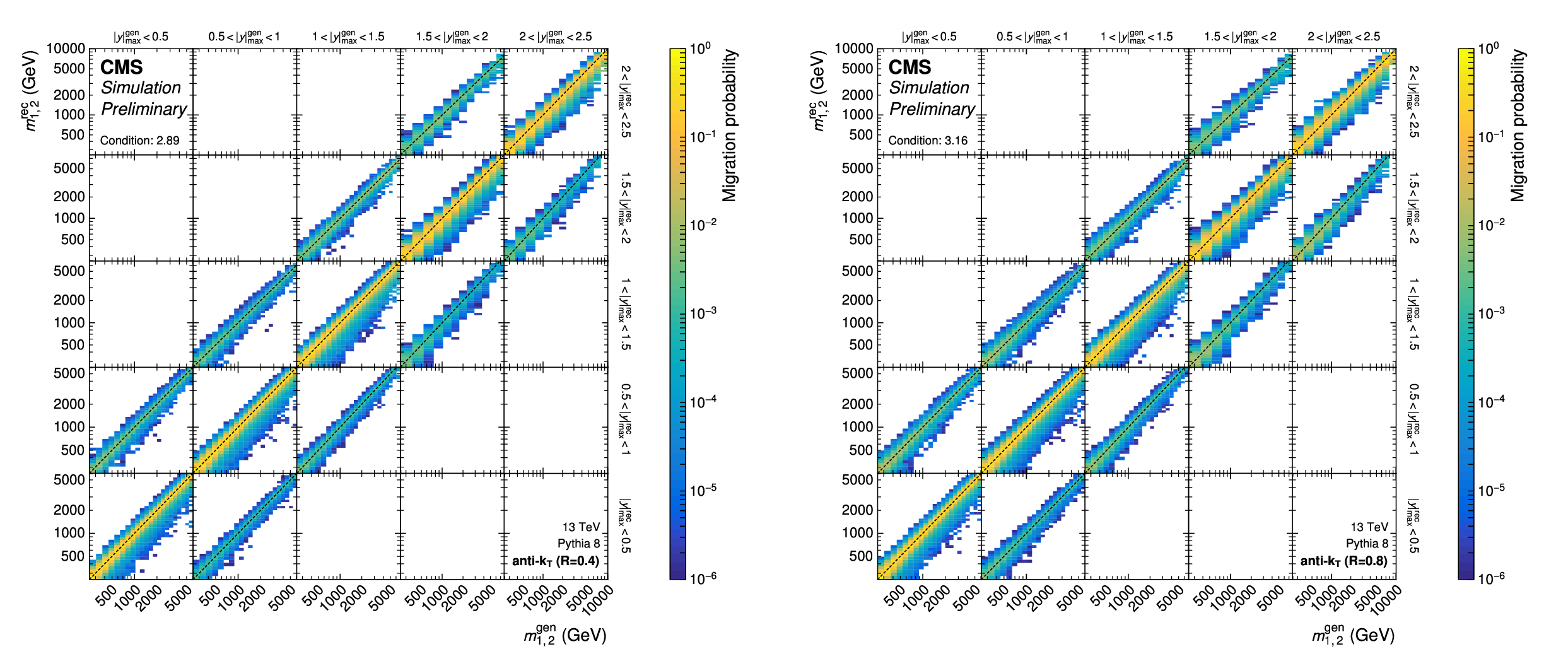
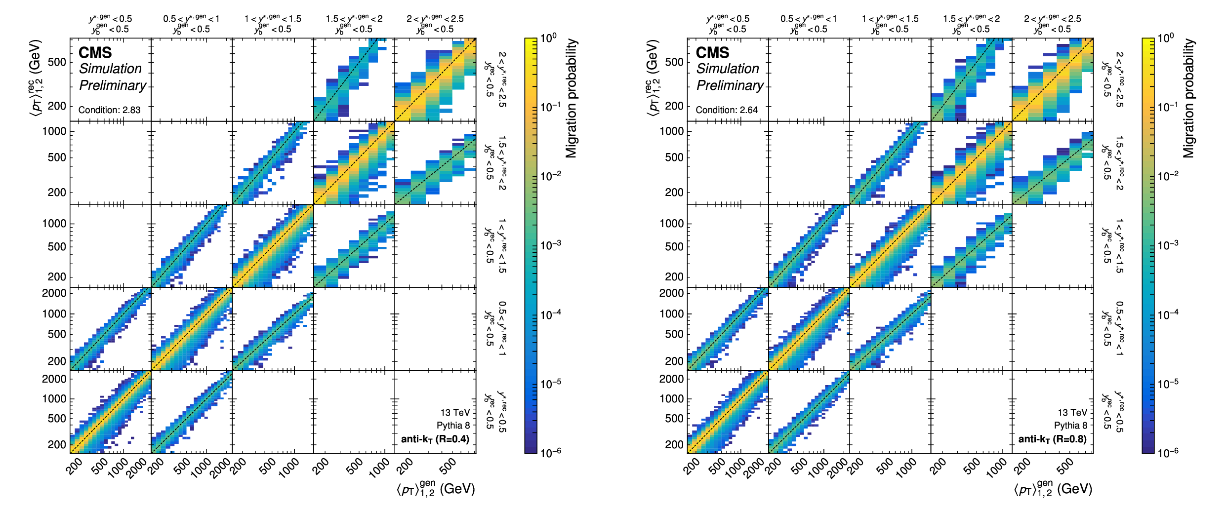
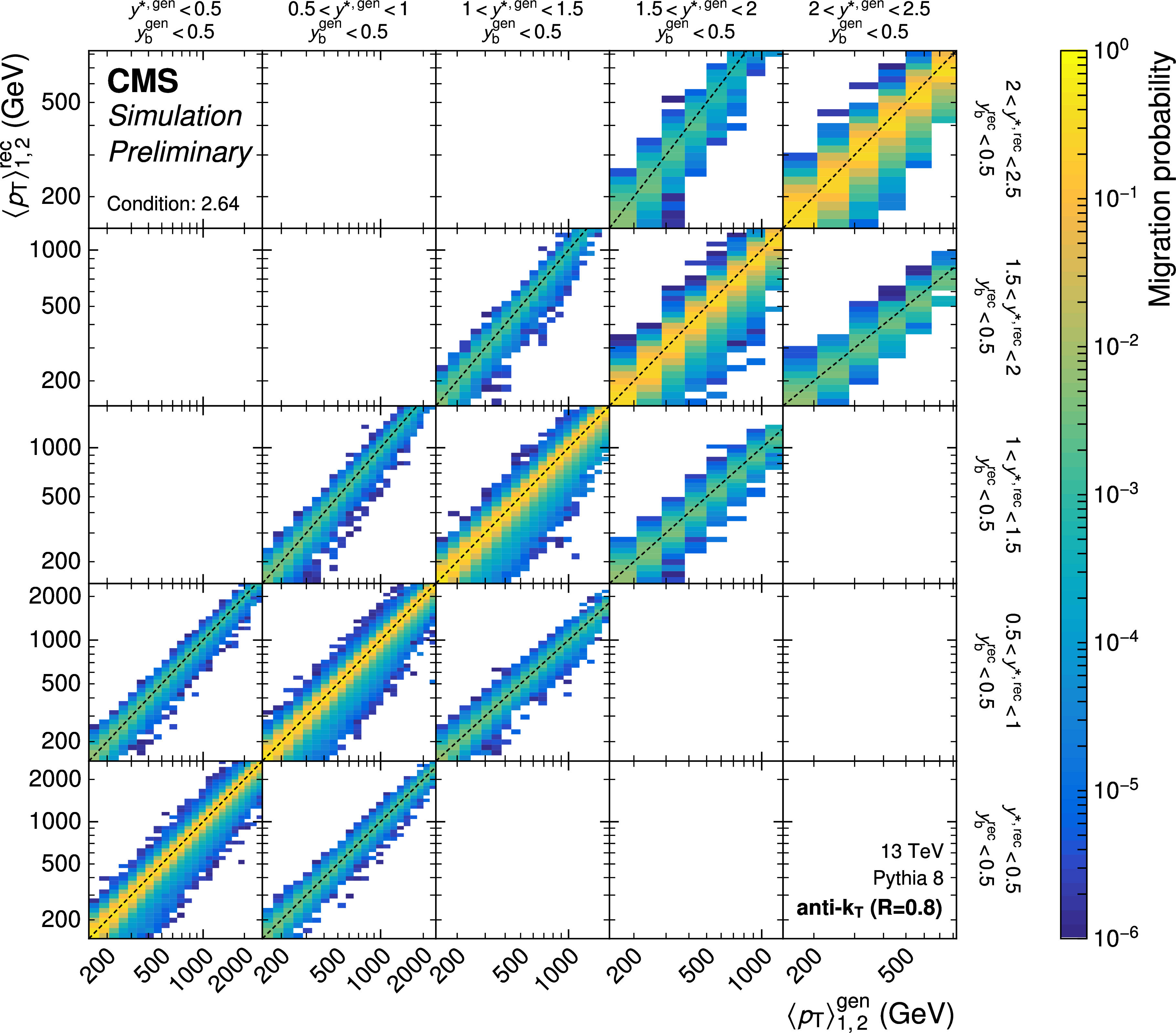
Response matrices for the 2D measurement as a function of $ m_{1,2} $ using jets with $ R = $ 0.8 (top), and for the 3D measurement as a function of $ \langle p_{\mathrm{T}} \rangle_{1,2} $ using jets with $ R = $ 0.4 (bottom). The former includes all five $ |y|_{\text{max}} $ regions while the latter only shows a subset of the full 3D response matrix, covering the five rapidity regions with $ y_{\text{b}} < $ 0.5. The entries represent the probability for a dijet event generated in the phase space region indicated on the $ x $ axis to be reconstructed in the phase space region indicated on the $ y $ axis. |
png pdf |
Figure 2-a:
Response matrix for the 2D measurement as a function of $ m_{1,2} $ using jets with $ R = $ 0.8. It includes all five $ |y|_{\text{max}} $ regions while the latter only shows a subset of the full 3D response matrix, covering the five rapidity regions with $ y_{\text{b}} < $ 0.5. The entries represent the probability for a dijet event generated in the phase space region indicated on the $ x $ axis to be reconstructed in the phase space region indicated on the $ y $ axis. |
png pdf |
Figure 2-b:
Response matrix for the 3D measurement as a function of $ \langle p_{\mathrm{T}} \rangle_{1,2} $ using jets with $ R = $ 0.4. The entries represent the probability for a dijet event generated in the phase space region indicated on the $ x $ axis to be reconstructed in the phase space region indicated on the $ y $ axis. |
png pdf |
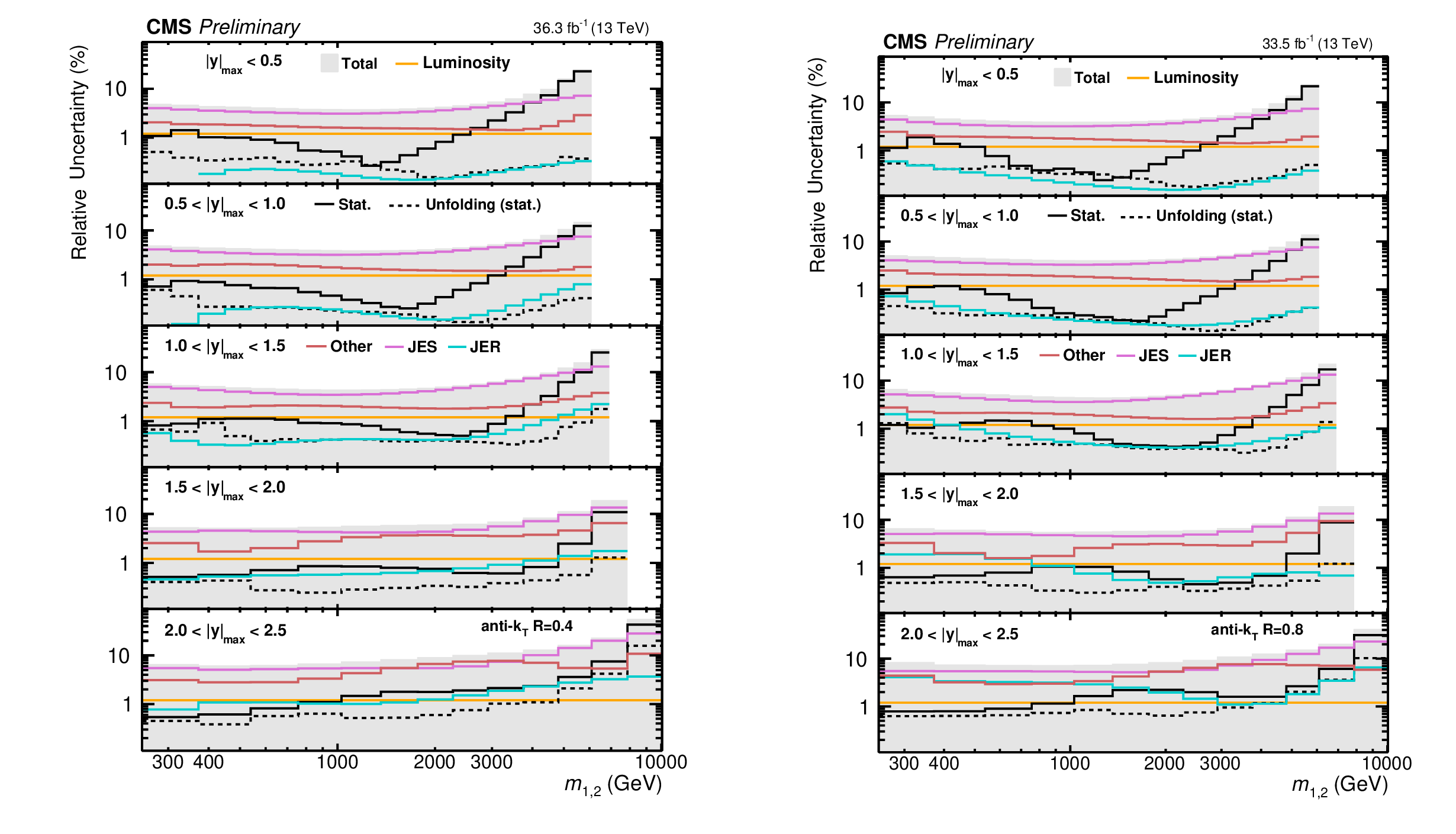
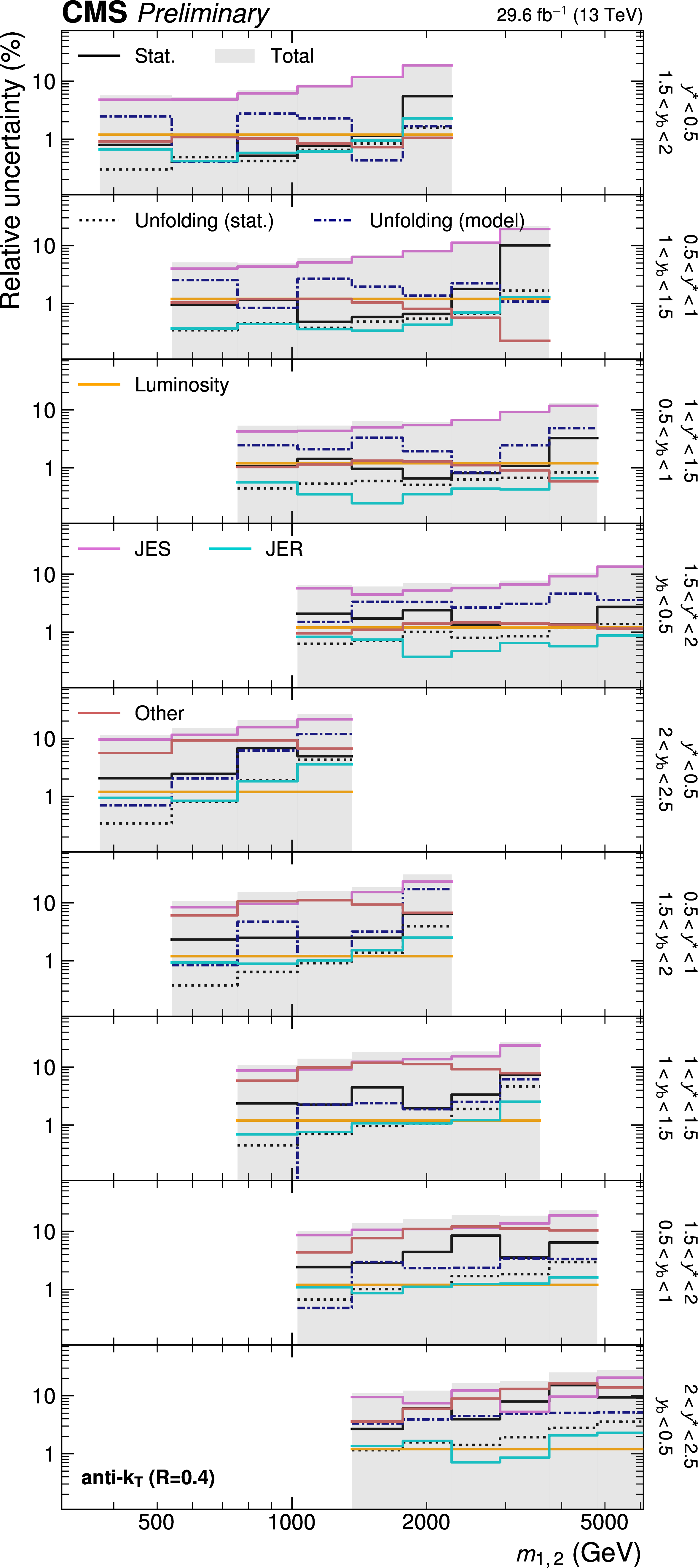
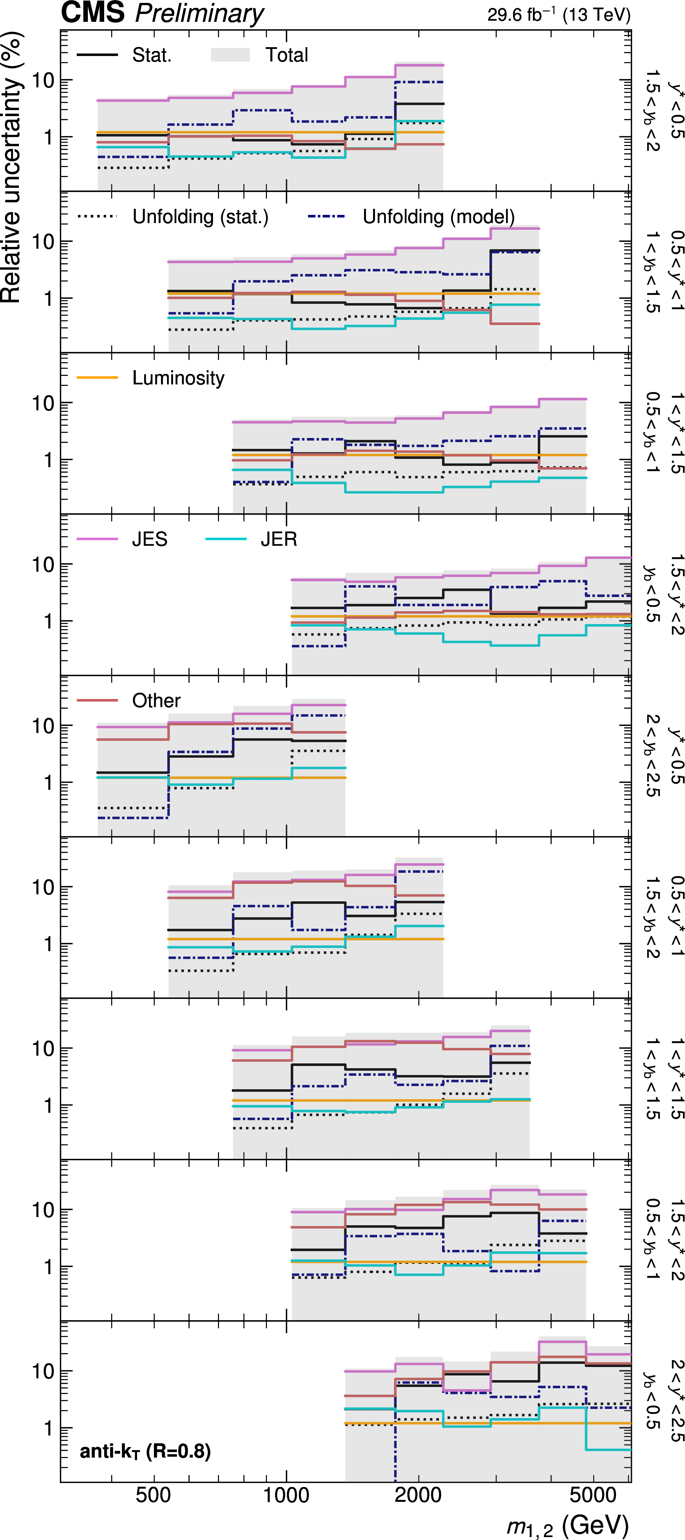
Figure 3:
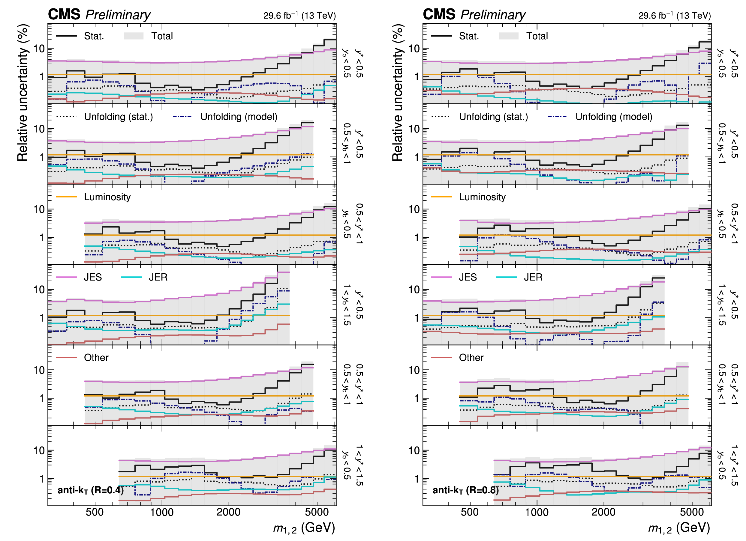
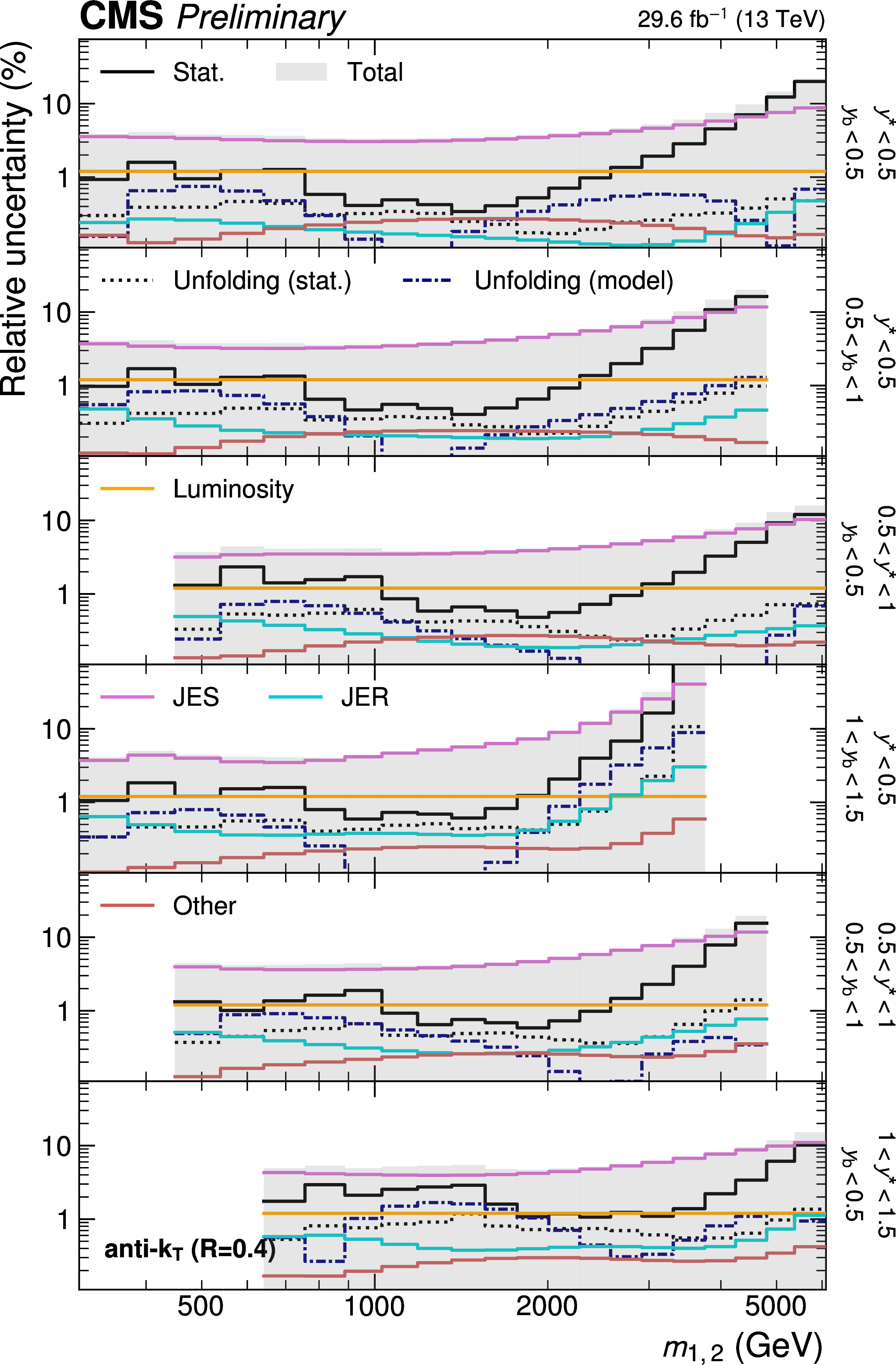
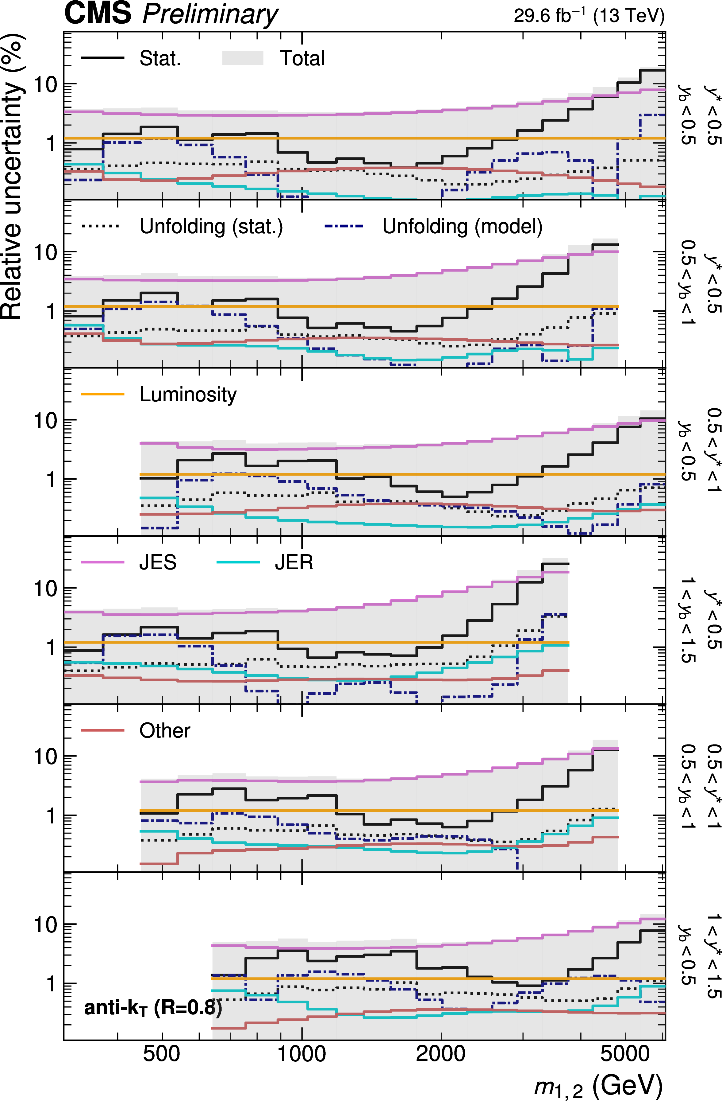
Breakdown of the experimental uncertainty for the 2D measurements as a function of $ m_{1,2} $ using jets with $ R = $ 0.4 (left) and $ R = $ 0.8 (right). The shaded area represents the sum in quadrature of the individual uncertainty components. |
png pdf |
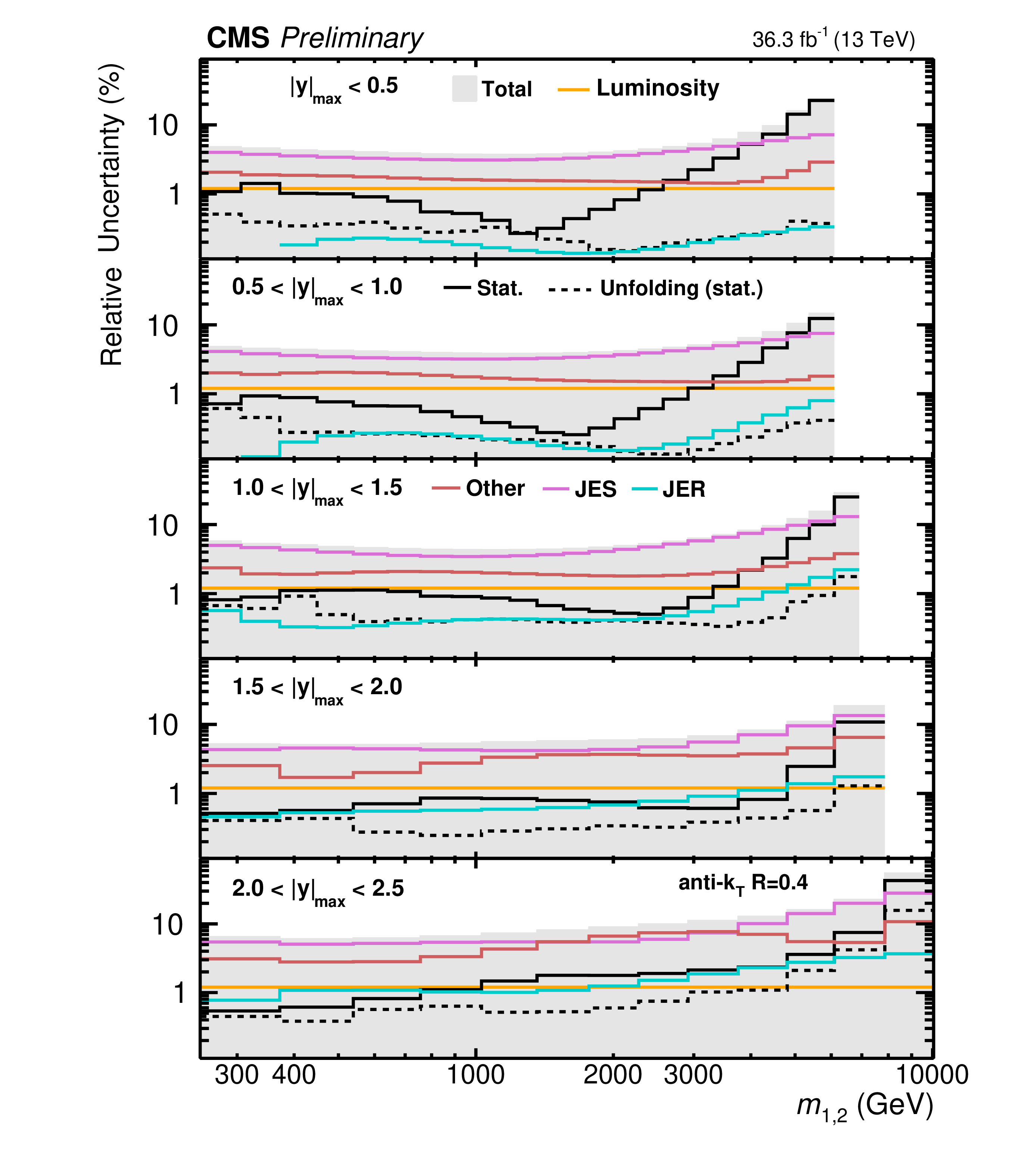
Figure 3-a:
Breakdown of the experimental uncertainty for the 2D measurements as a function of $ m_{1,2} $ using jets with $ R = $ 0.4. The shaded area represents the sum in quadrature of the individual uncertainty components. |
png pdf |
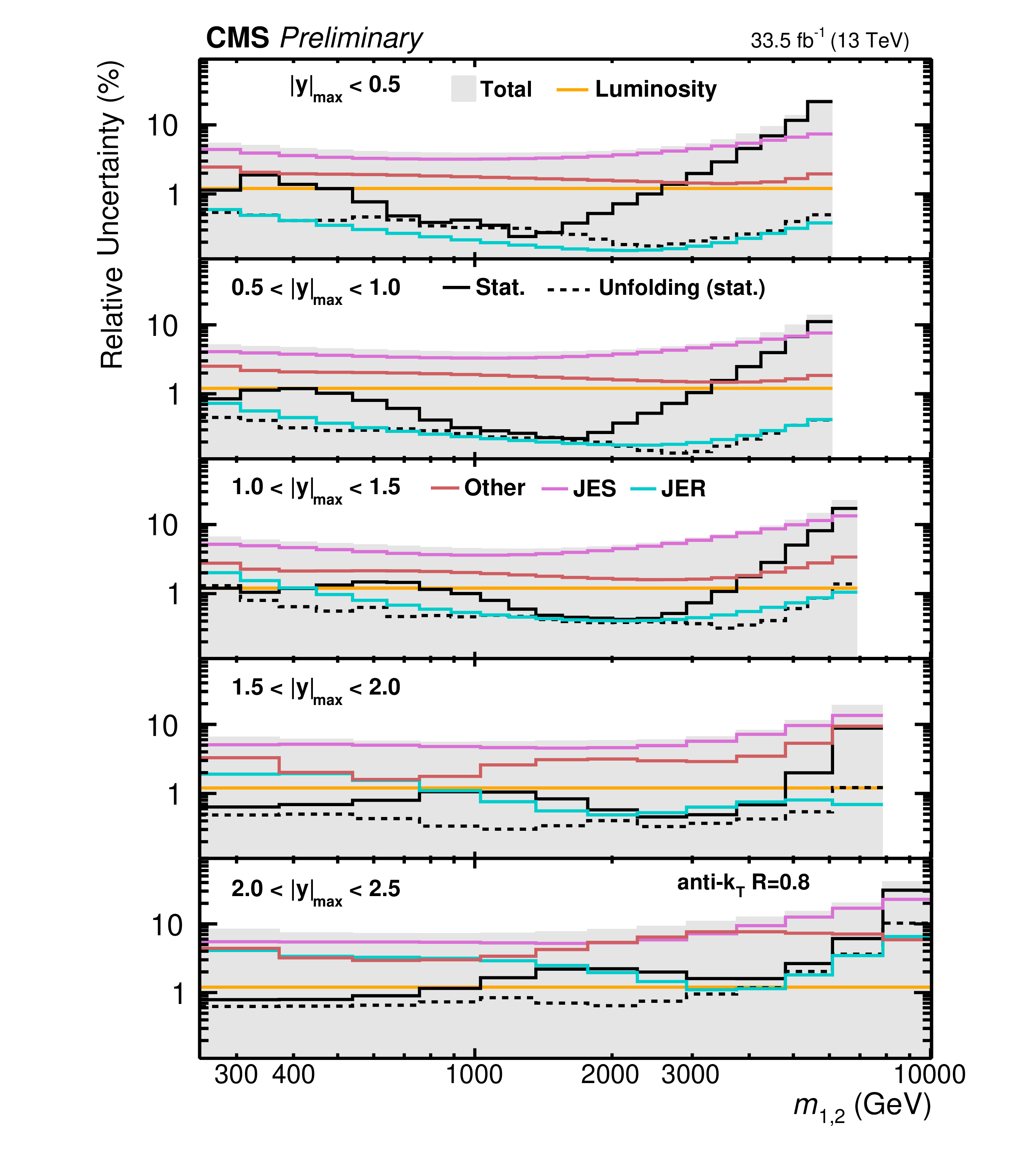
Figure 3-b:
Breakdown of the experimental uncertainty for the 2D measurements as a function of $ m_{1,2} $ using jets with $ R = $ 0.8. The shaded area represents the sum in quadrature of the individual uncertainty components. |
png pdf |
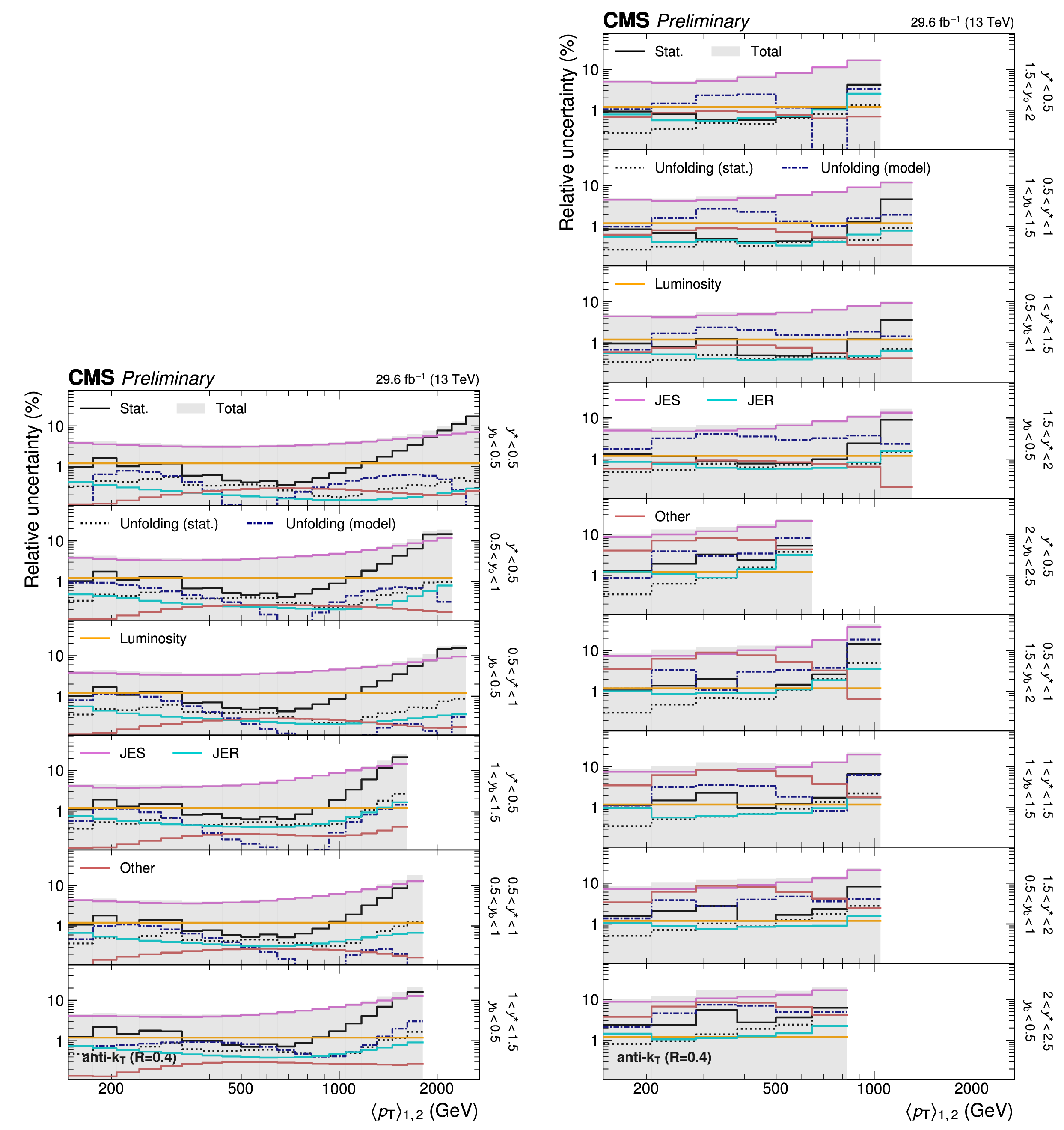
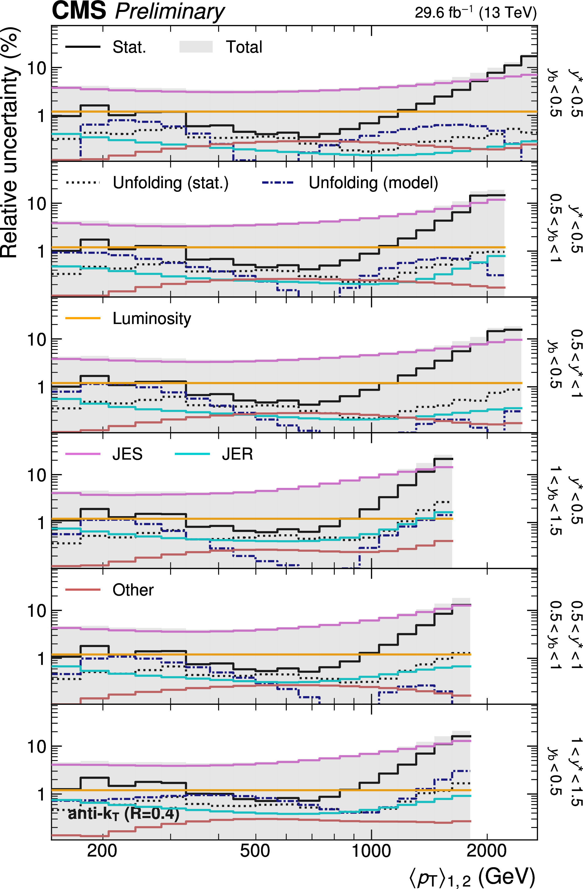
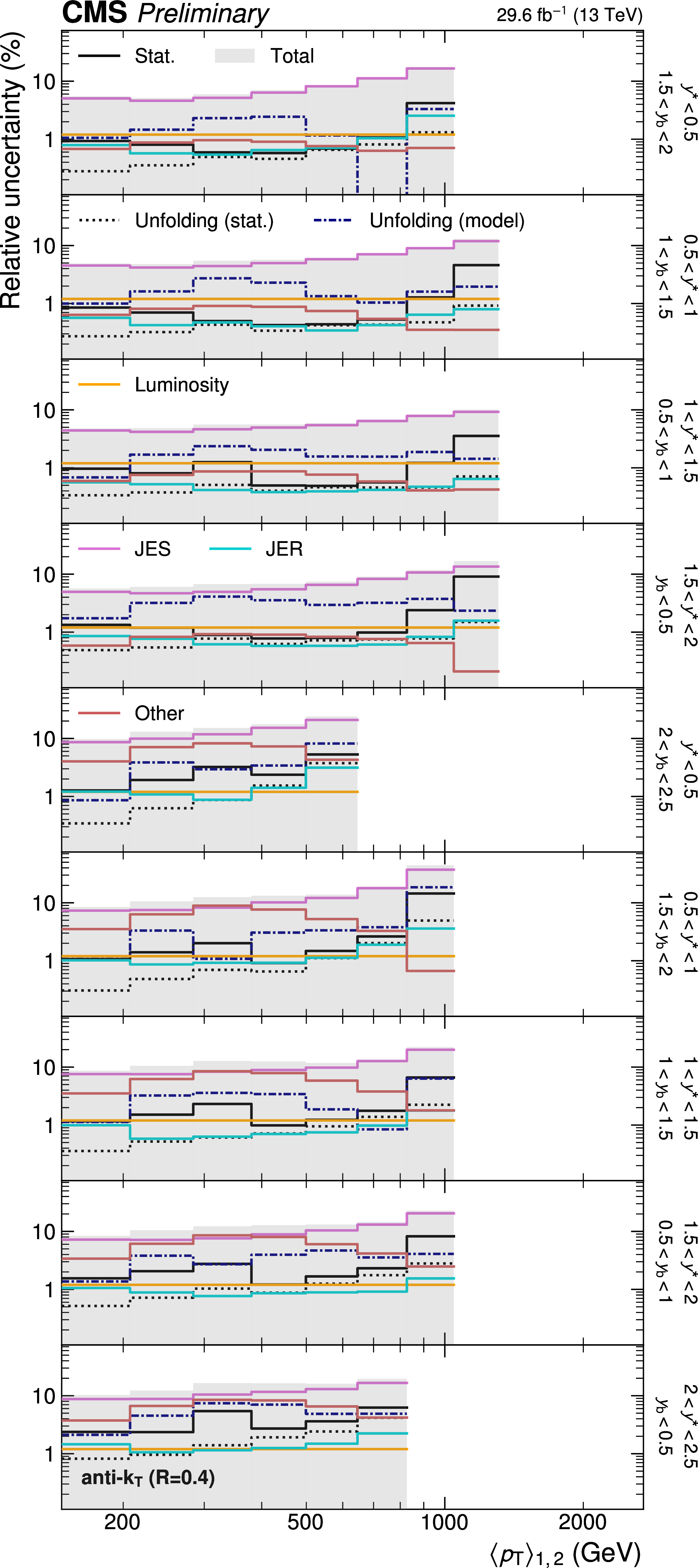
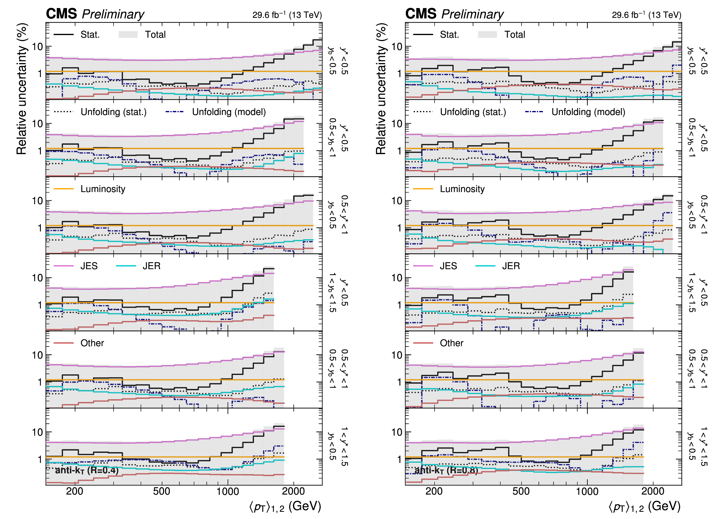
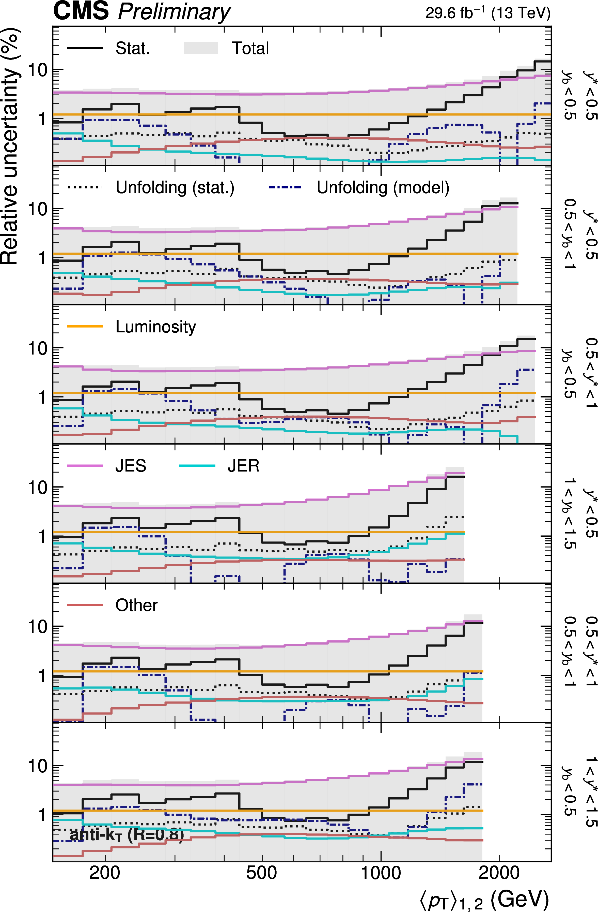
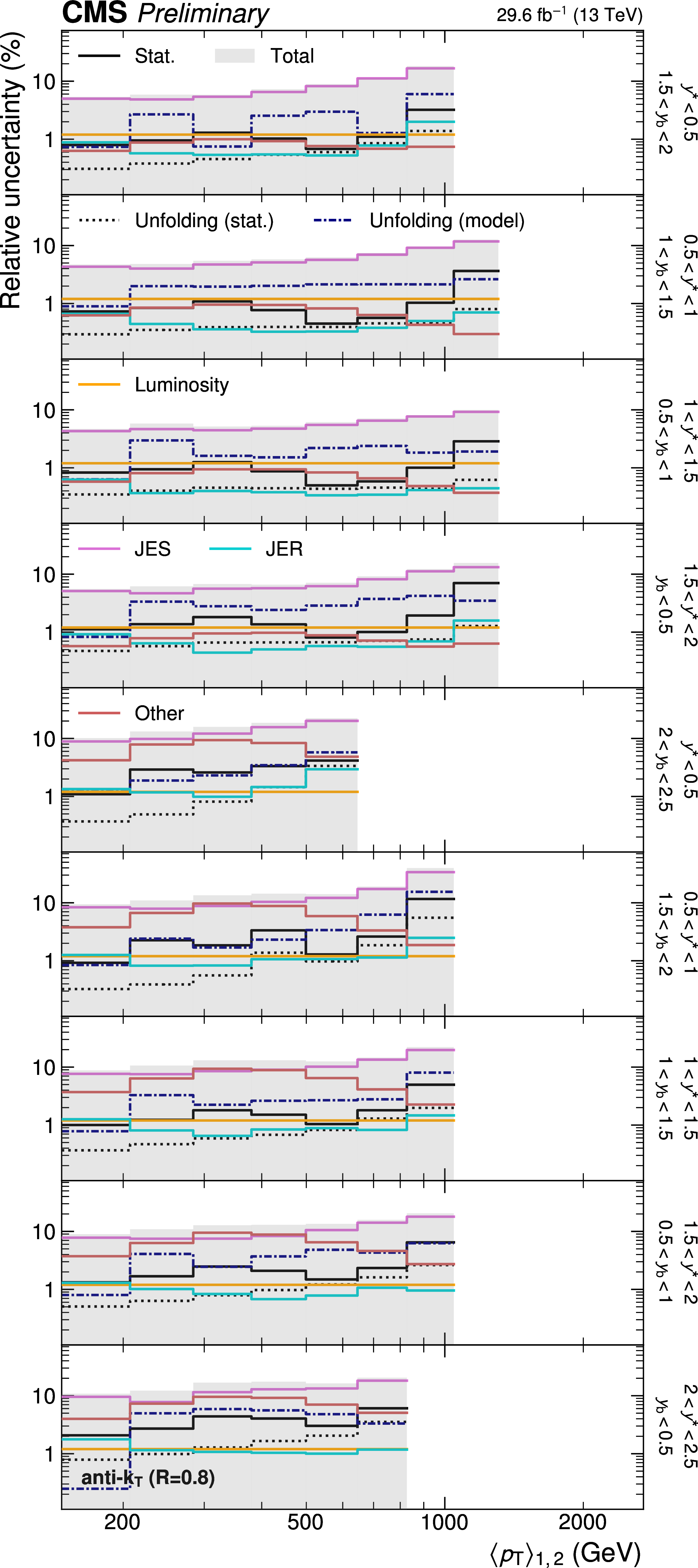
Figure 4:
Breakdown of the experimental uncertainty for the 3D measurement as a function of $ \langle p_{\mathrm{T}} \rangle_{1,2} $ using jets with $ R = $ 0.4. The shaded area represents the sum in quadrature of the individual uncertainty components. |
png pdf |
Figure 4-a:
Breakdown of the experimental uncertainty for the 3D measurement as a function of $ \langle p_{\mathrm{T}} \rangle_{1,2} $ using jets with $ R = $ 0.4. The shaded area represents the sum in quadrature of the individual uncertainty components. |
png pdf |
Figure 4-b:
Breakdown of the experimental uncertainty for the 3D measurement as a function of $ \langle p_{\mathrm{T}} \rangle_{1,2} $ using jets with $ R = $ 0.4. The shaded area represents the sum in quadrature of the individual uncertainty components. |
png pdf |
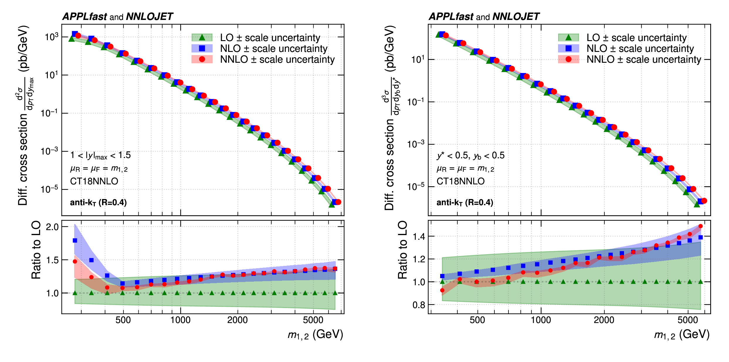
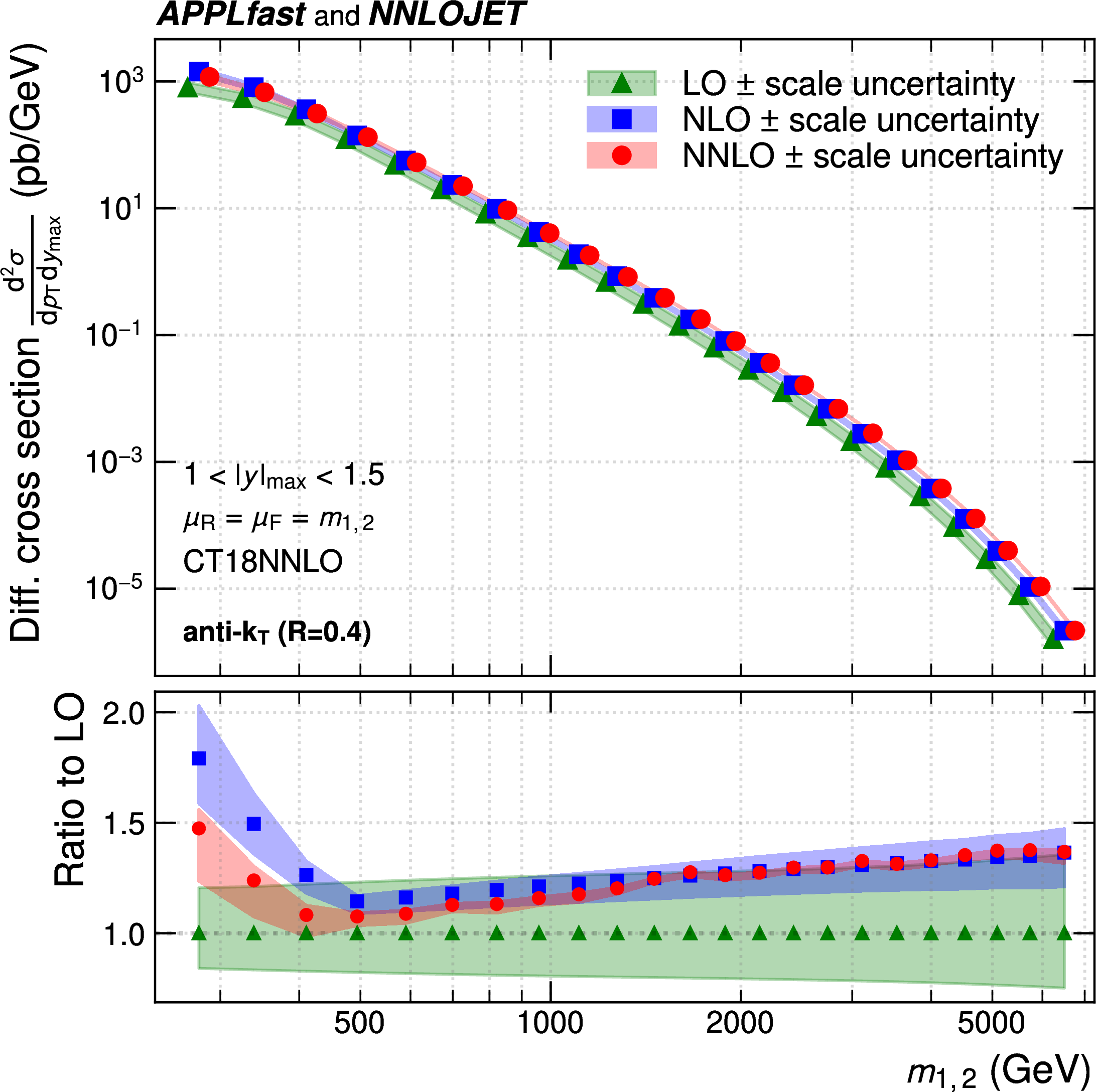
Figure 5:
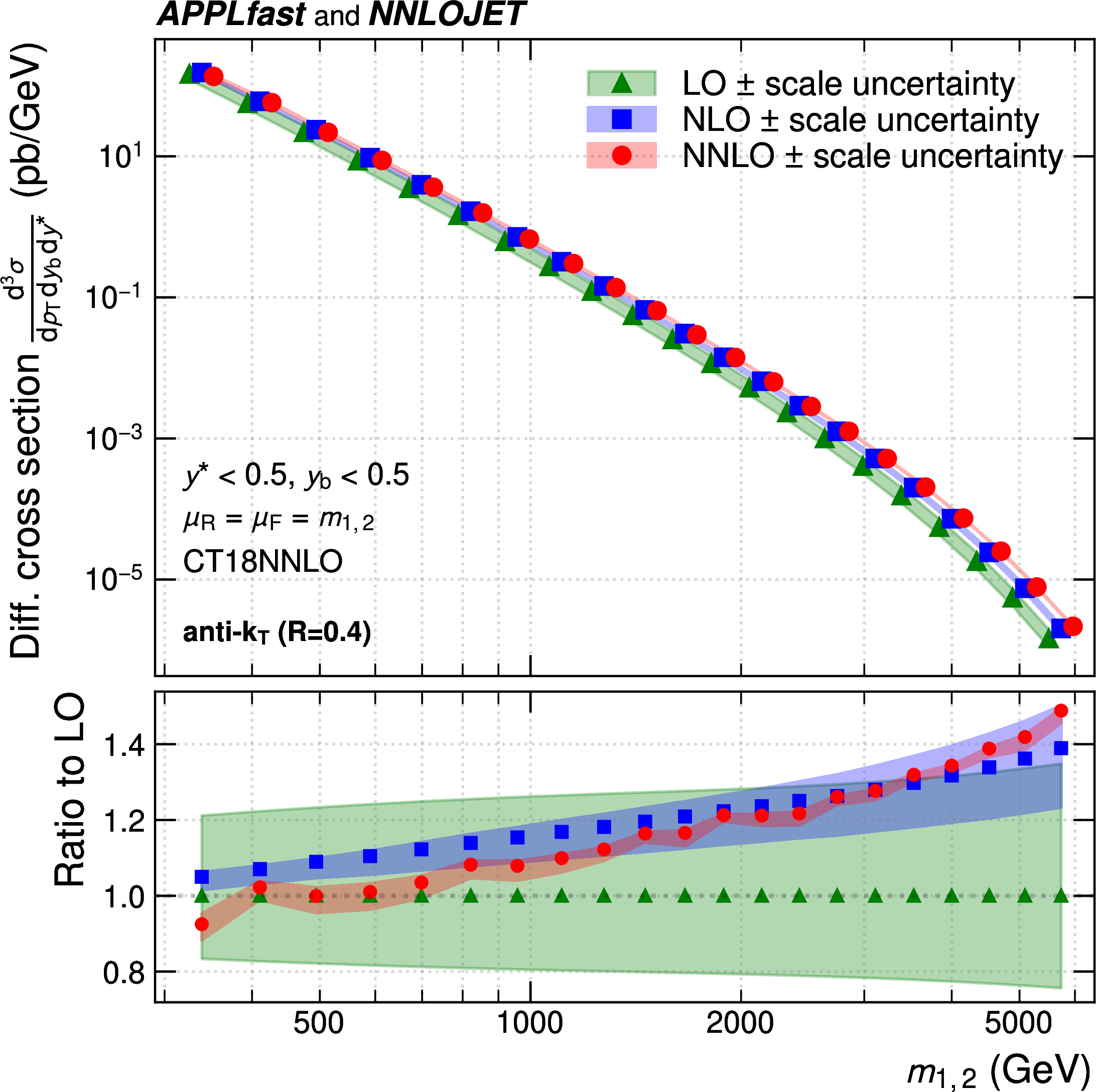
Theory predictions for the 2D (left) and 3D (right) cross sections, as a function of $ m_{1,2} $, illustrated here in the rapidity regions 1.0 $ < |y|_{\text{max}} < $ 1.5 and ($ y_{\text{b}} < $ 0.5, $ y^{*} < $ 0.5), together with the corresponding six-point scale uncertainty for $ \mu_{\mathrm{R}}=\mu_{\mathrm{F}}=m_{1,2} $ using the CT18 NNLO PDF set. In the upper panels, the curves and symbols are slightly shifted for better visibility. The lower panels show the ratio to the respective prediction at LO. |
png pdf |
Figure 5-a:
Theory predictions for the 2D cross sections, as a function of $ m_{1,2} $, illustrated here in the rapidity regions 1.0 $ < |y|_{\text{max}} < $ 1.5 and ($ y_{\text{b}} < $ 0.5, $ y^{*} < $ 0.5), together with the corresponding six-point scale uncertainty for $ \mu_{\mathrm{R}}=\mu_{\mathrm{F}}=m_{1,2} $ using the CT18 NNLO PDF set. In the upper panel, the curves and symbols are slightly shifted for better visibility. The lower panel shows the ratio to the respective prediction at LO. |
png pdf |
Figure 5-b:
Theory predictions for the 3D cross sections, as a function of $ m_{1,2} $, illustrated here in the rapidity regions 1.0 $ < |y|_{\text{max}} < $ 1.5 and ($ y_{\text{b}} < $ 0.5, $ y^{*} < $ 0.5), together with the corresponding six-point scale uncertainty for $ \mu_{\mathrm{R}}=\mu_{\mathrm{F}}=m_{1,2} $ using the CT18 NNLO PDF set. In the upper panel, the curves and symbols are slightly shifted for better visibility. The lower panel shows the ratio to the respective prediction at LO. |
png pdf |
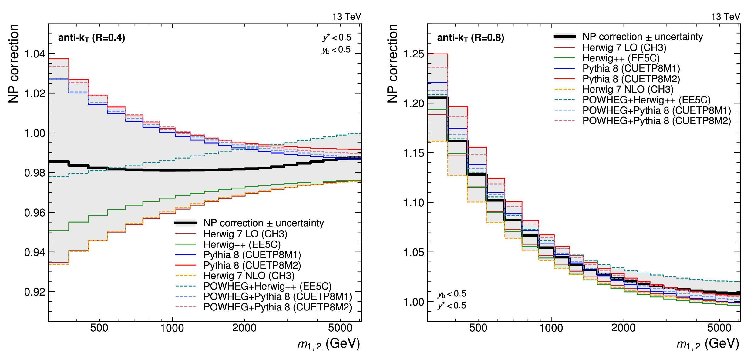
Figure 6:
Nonperturbative correction factors obtained for jets with $ R = $ 0.4 (left) and $ R = $ 0.8 (right) as a function of $ m_{1,2} $, illustrated here in the rapidity region ($ y_{\text{b}} < $ 0.5, $ y^{*} < $ 0.5). Individual correction factors are first derived from simulation using eight different MC configurations. The largest and smallest value obtained in each observable bin is then used to define the final correction factor and its associated uncertainty. The correction values are larger for jets with $ R = $ 0.8, increasing to over 20% in the lowest $ m_{1,2} $ bin. |
png pdf |
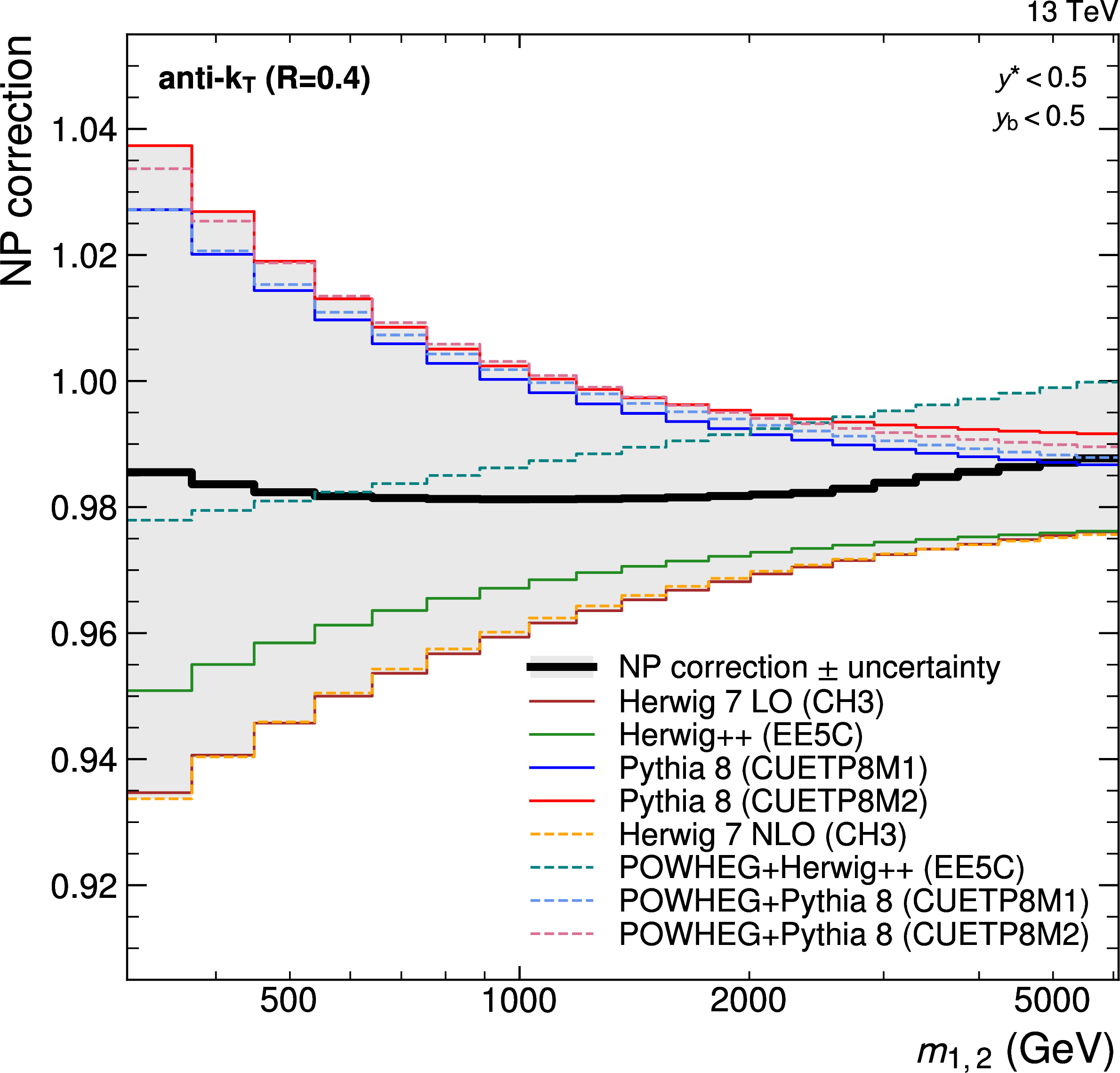
Figure 6-a:
Nonperturbative correction factors obtained for jets with $ R = $ 0.4 as a function of $ m_{1,2} $, illustrated here in the rapidity region ($ y_{\text{b}} < $ 0.5, $ y^{*} < $ 0.5). Individual correction factors are first derived from simulation using eight different MC configurations. The largest and smallest value obtained in each observable bin is then used to define the final correction factor and its associated uncertainty. |
png pdf |
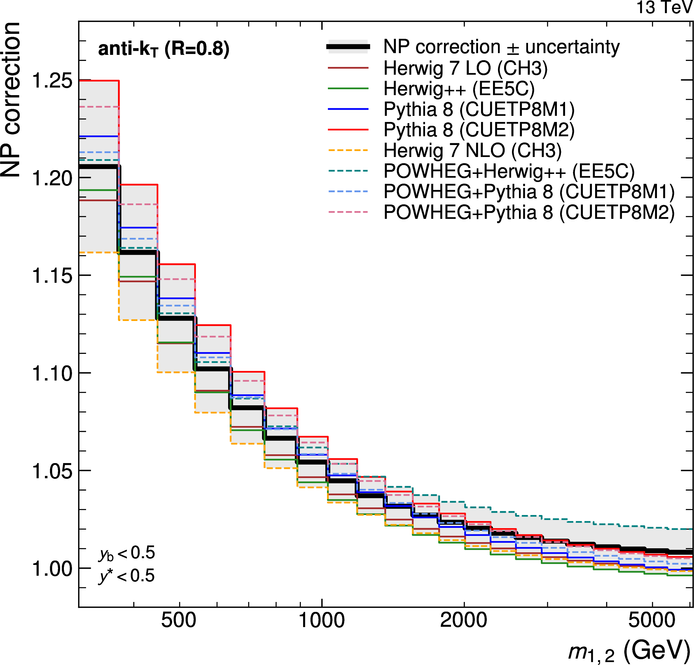
Figure 6-b:
Nonperturbative correction factors obtained for jets with $ R = $ 0.8 as a function of $ m_{1,2} $, illustrated here in the rapidity region ($ y_{\text{b}} < $ 0.5, $ y^{*} < $ 0.5). Individual correction factors are first derived from simulation using eight different MC configurations. The largest and smallest value obtained in each observable bin is then used to define the final correction factor and its associated uncertainty. The correction values are increasing to over 20% in the lowest $ m_{1,2} $ bin. |
png pdf |
Figure 7:
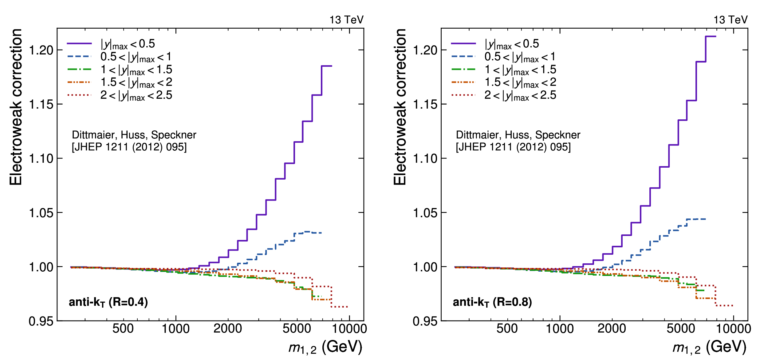
Electroweak correction factors obtained for jets with $ R = $ 0.4 (left) and $ R = $ 0.8 (right) as a function of $ m_{1,2} $ in the five different $ |y|_{\text{max}} $ regions. The corrections depend strongly on the kinematic properties of the jets and are observed to be largest at central rapidities for $ m_{1,2} > $ 1 TeV. |
png pdf |
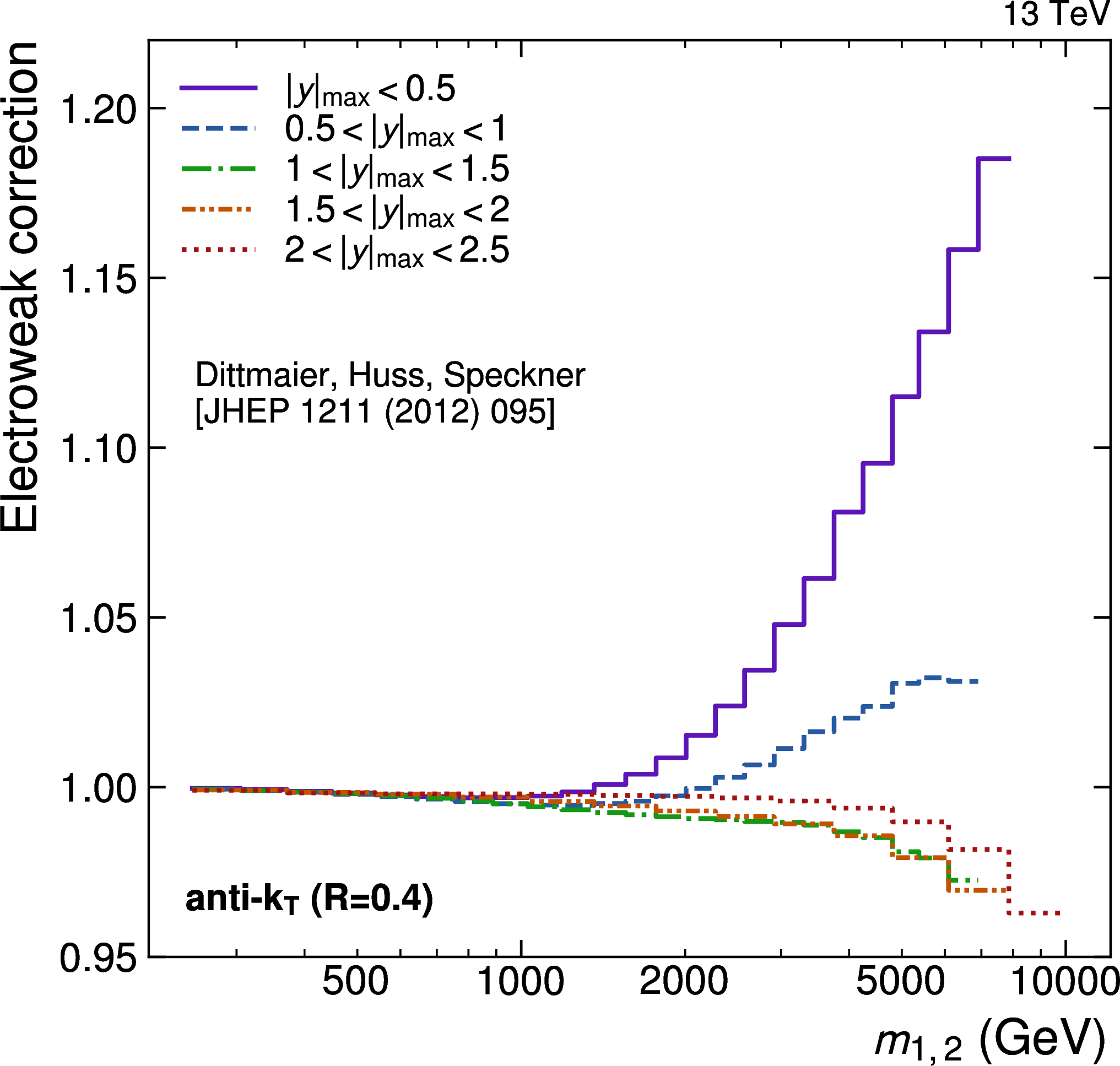
Figure 7-a:
Electroweak correction factors obtained for jets with $ R = $ 0.4 as a function of $ m_{1,2} $ in the five different $ |y|_{\text{max}} $ regions. The corrections depend strongly on the kinematic properties of the jets and are observed to be largest at central rapidities for $ m_{1,2} > $ 1 TeV. |
png pdf |
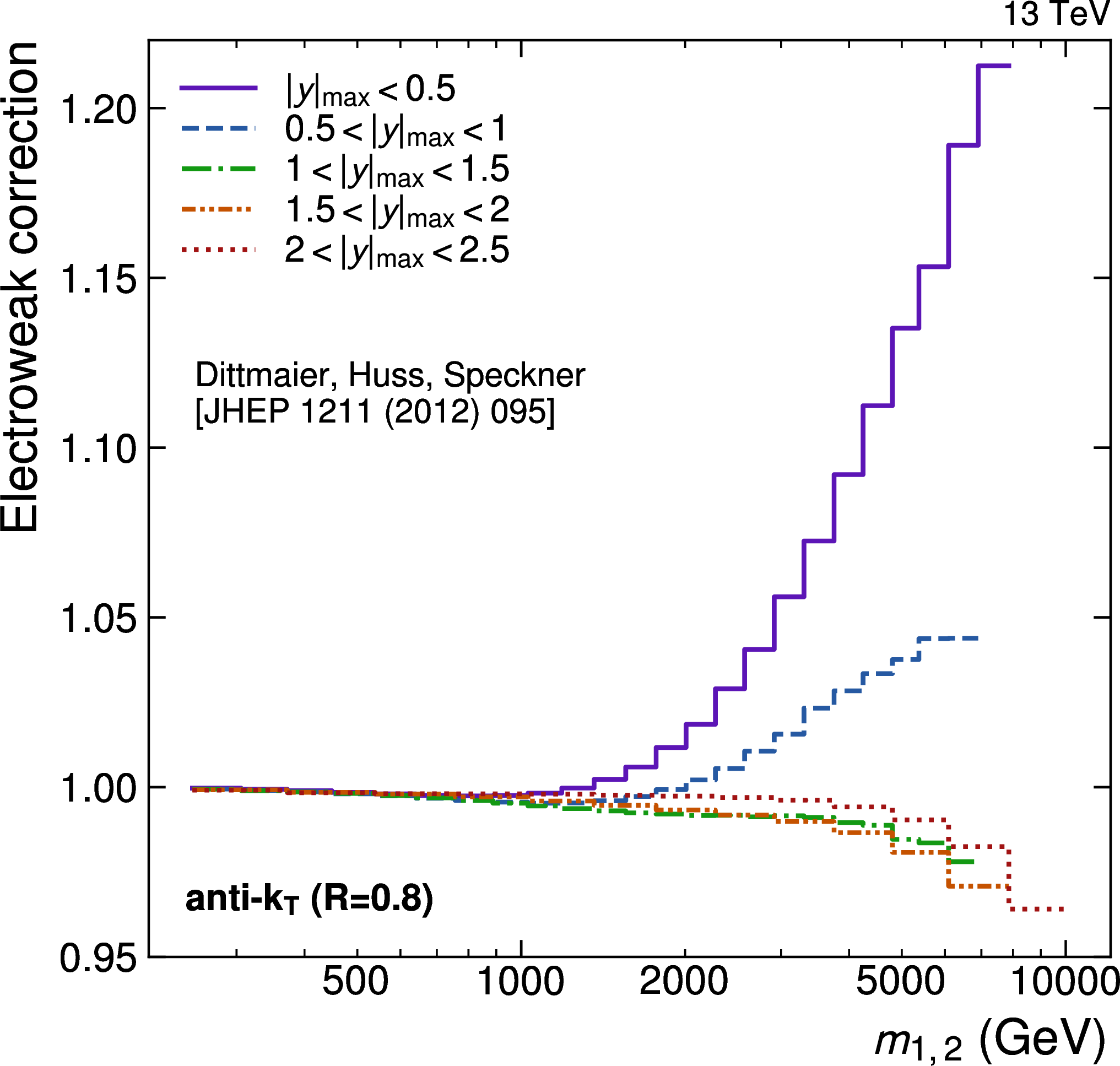
Figure 7-b:
Electroweak correction factors obtained for jets with $ R = $ 0.8 as a function of $ m_{1,2} $ in the five different $ |y|_{\text{max}} $ regions. The corrections depend strongly on the kinematic properties of the jets and are observed to be largest at central rapidities for $ m_{1,2} > $ 1 TeV. |

png pdf |
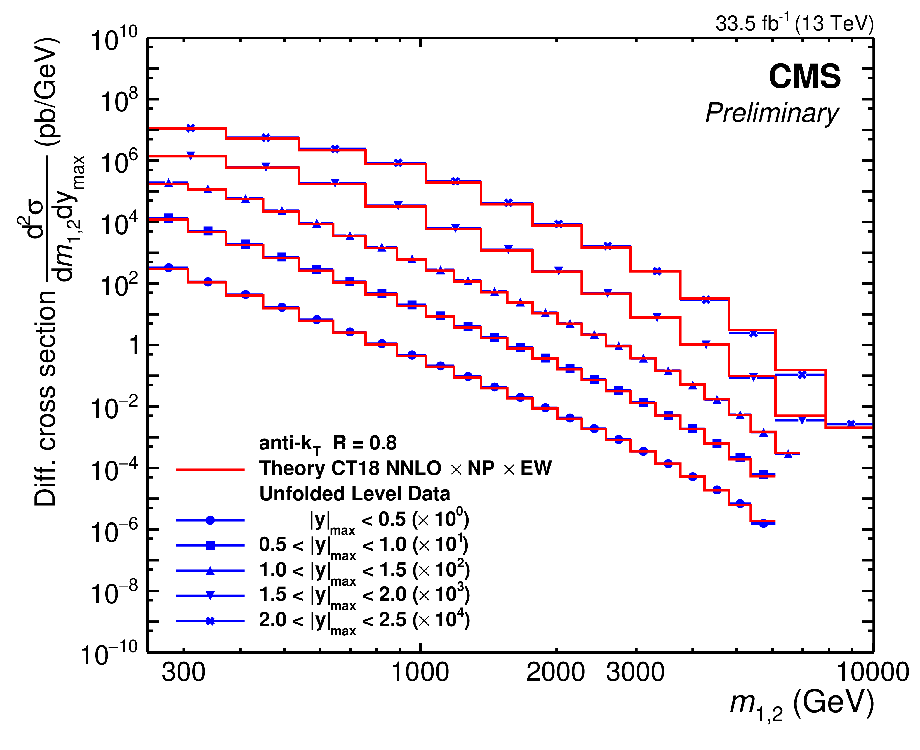
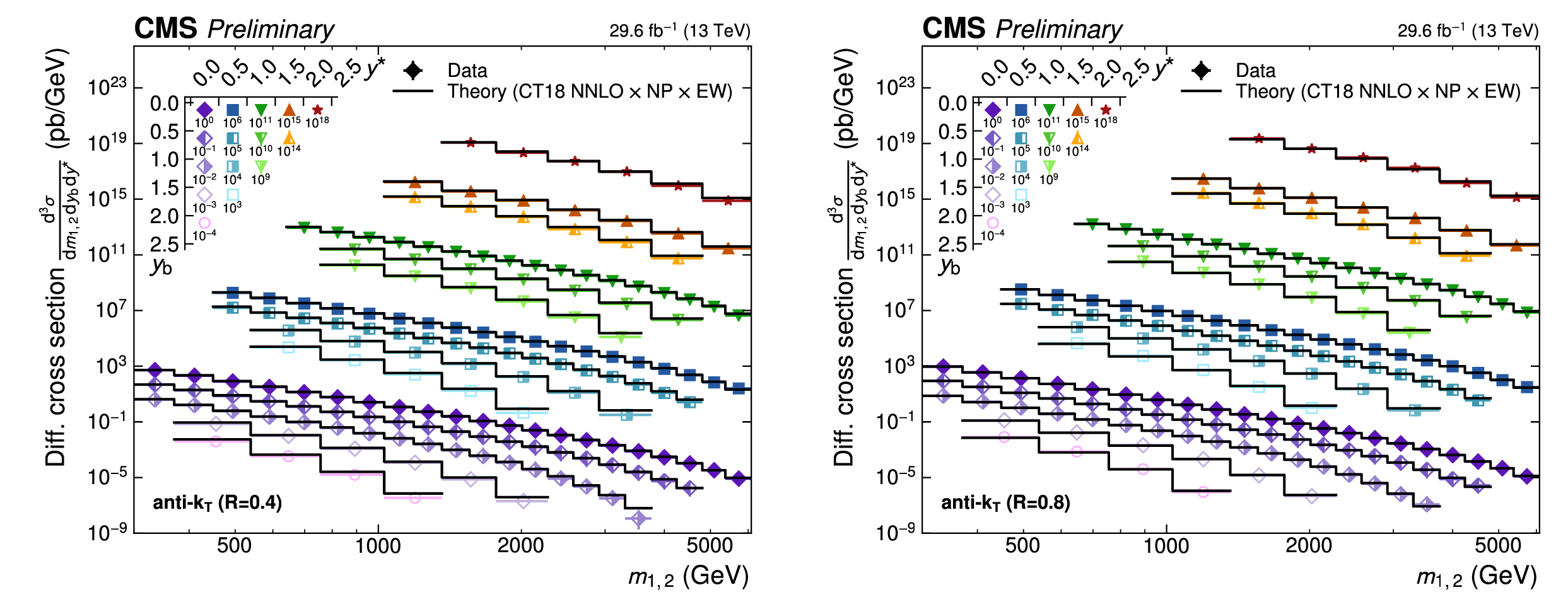
Figure 8:
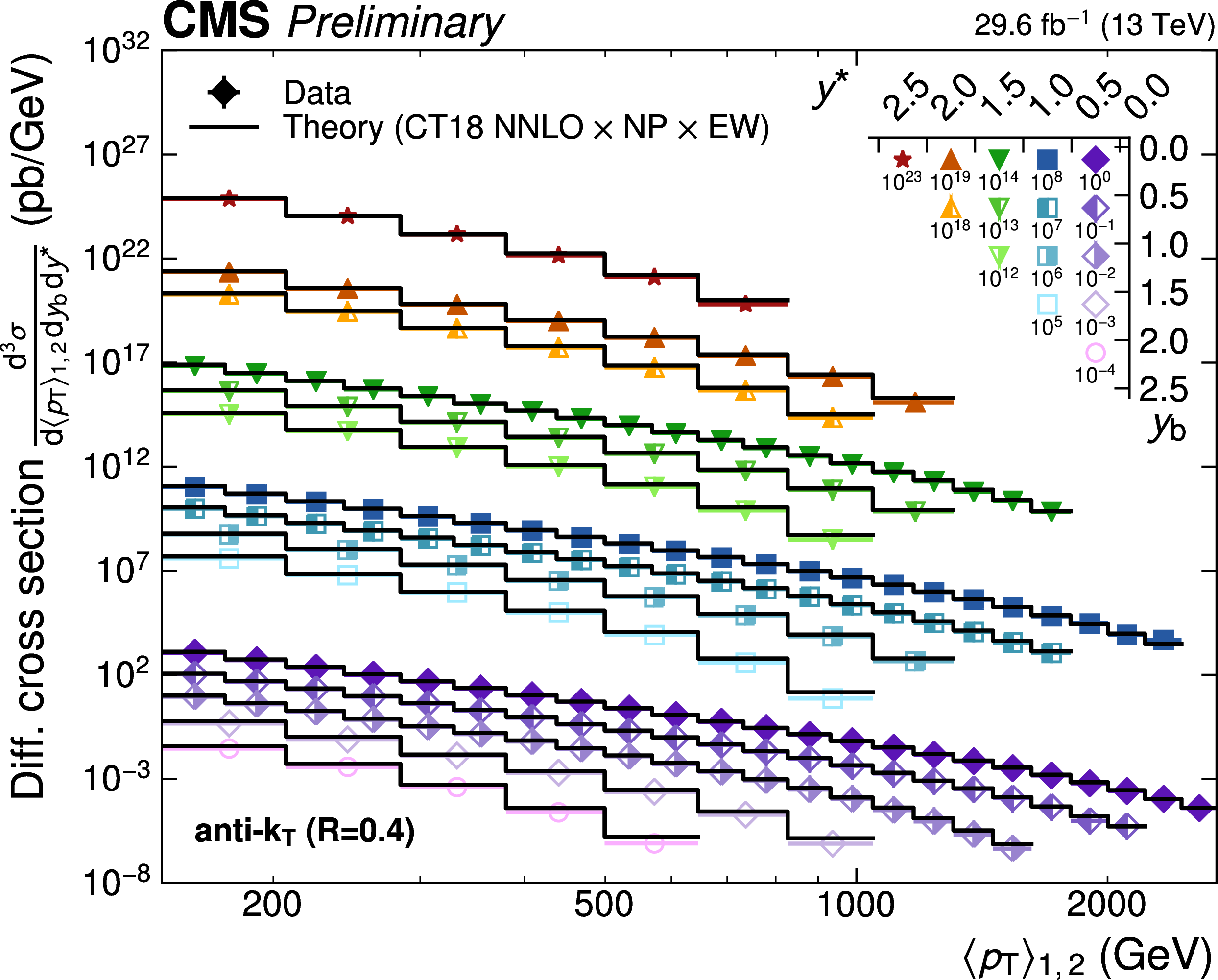
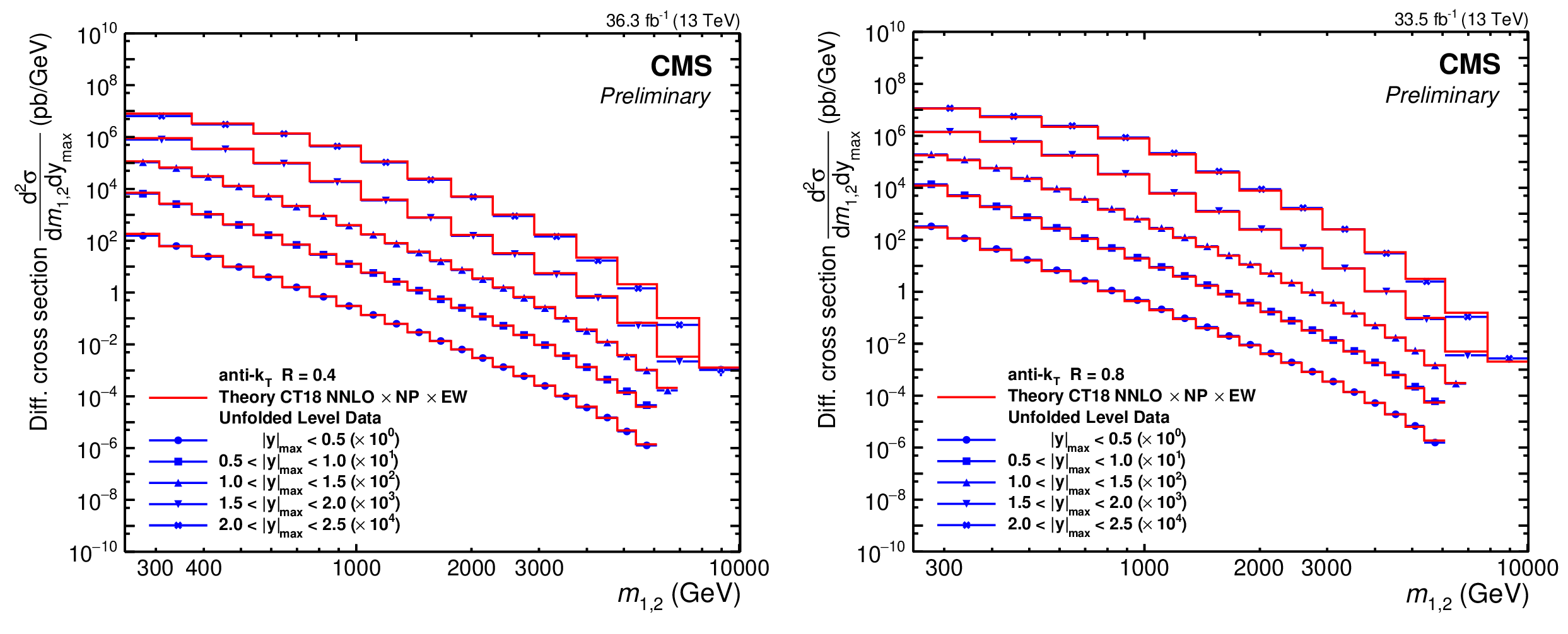
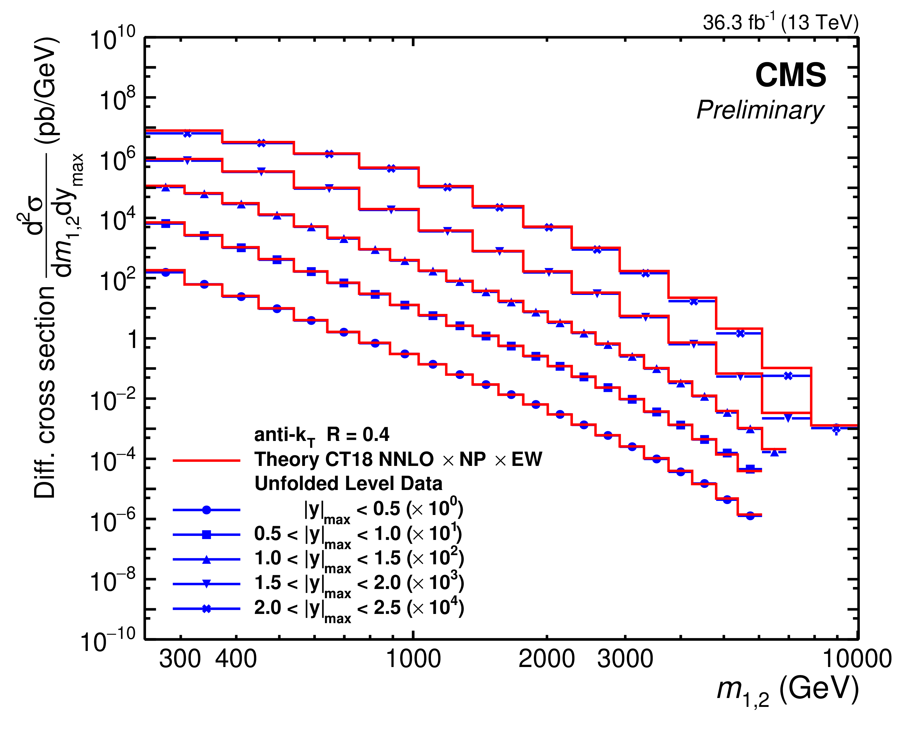
Overview of the dijet cross sections, illustrated here for the 2D measurement as a function of $ m_{1,2} $ using jets with $ R = $ 0.8 (left), and the 3D measurement as a function of $ \langle p_{\mathrm{T}} \rangle_{1,2} $ using jets with $ R = $ 0.4 (right). The markers and lines indicate the measured unfolded cross sections and the corresponding NNLO predictions, respectively. For better visibility, the values are scaled by a factor depending on the rapidity region, as indicated in the legend. |
png pdf |
Figure 8-a:
Overview of the dijet cross sections, illustrated here for the 2D measurement as a function of $ m_{1,2} $ using jets with $ R = $ 0.8. The markers and lines indicate the measured unfolded cross sections and the corresponding NNLO predictions, respectively. For better visibility, the values are scaled by a factor depending on the rapidity region, as indicated in the legend. |
png pdf |
Figure 8-b:
Overview of the 3D measurement as a function of $ \langle p_{\mathrm{T}} \rangle_{1,2} $ using jets with $ R = $ 0.4. The markers and lines indicate the measured unfolded cross sections and the corresponding NNLO predictions, respectively. For better visibility, the values are scaled by a factor depending on the rapidity region, as indicated in the legend. |
png pdf |
Figure 9:
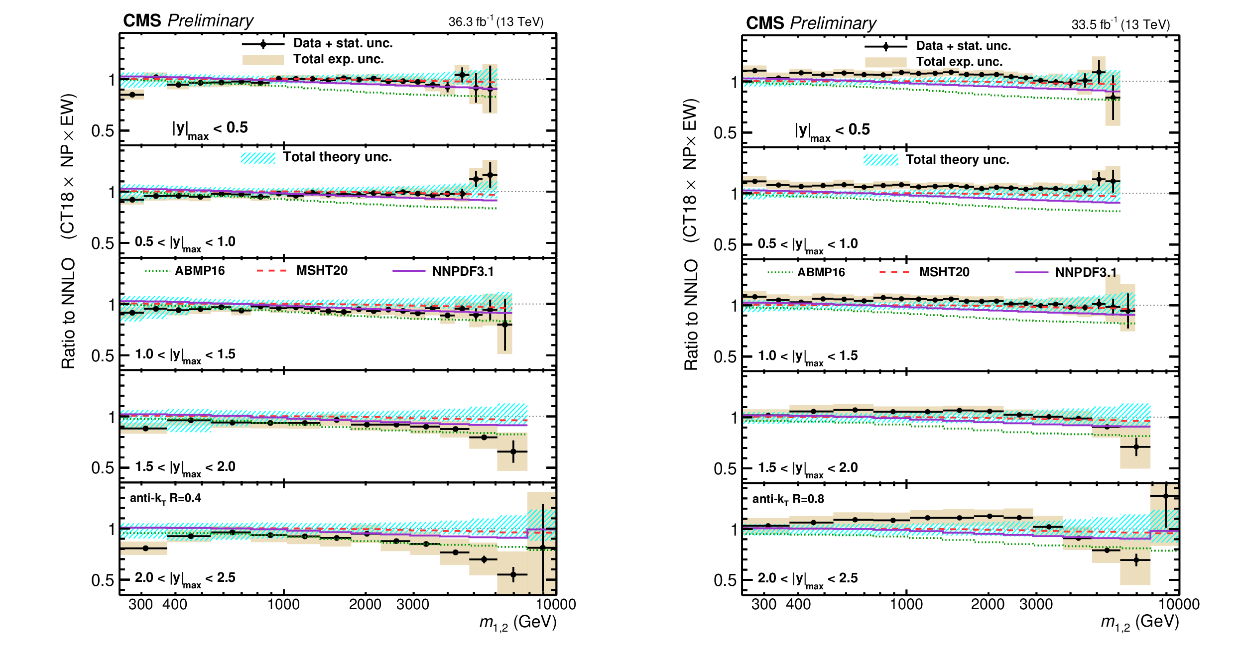
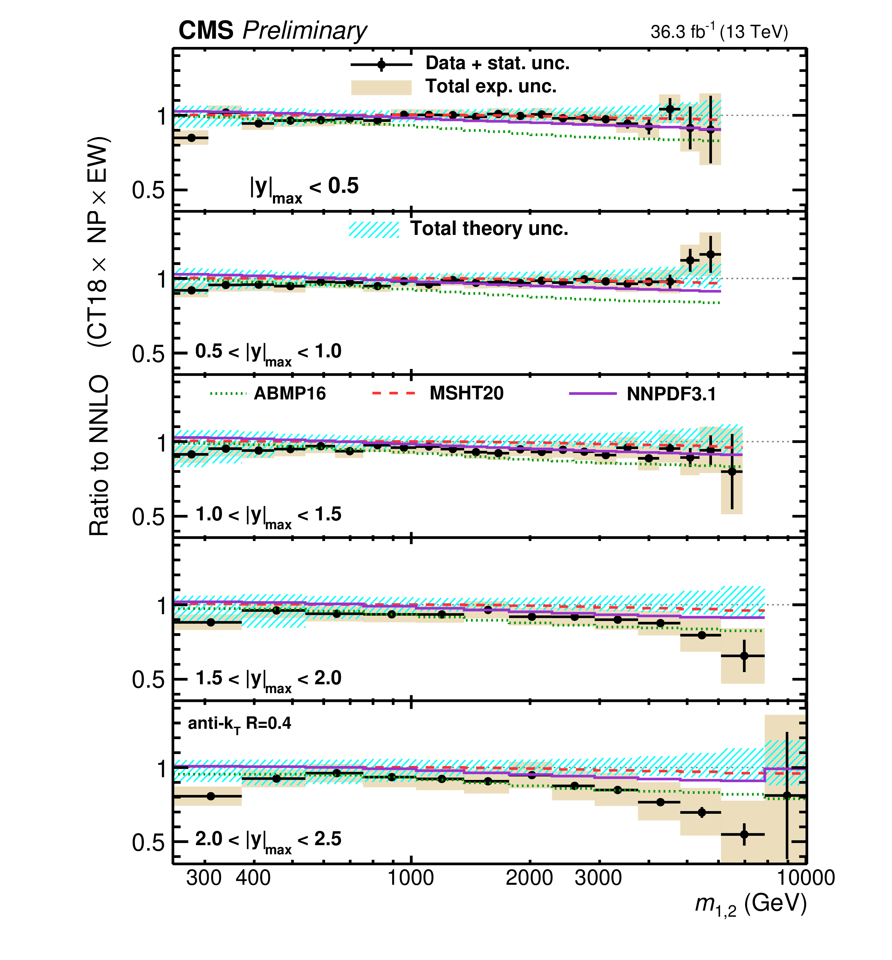
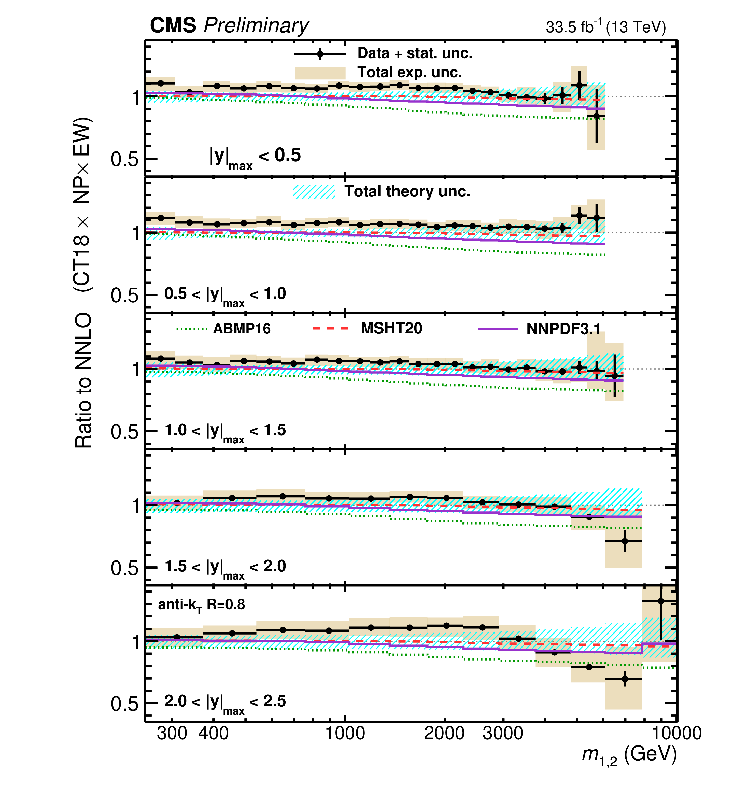
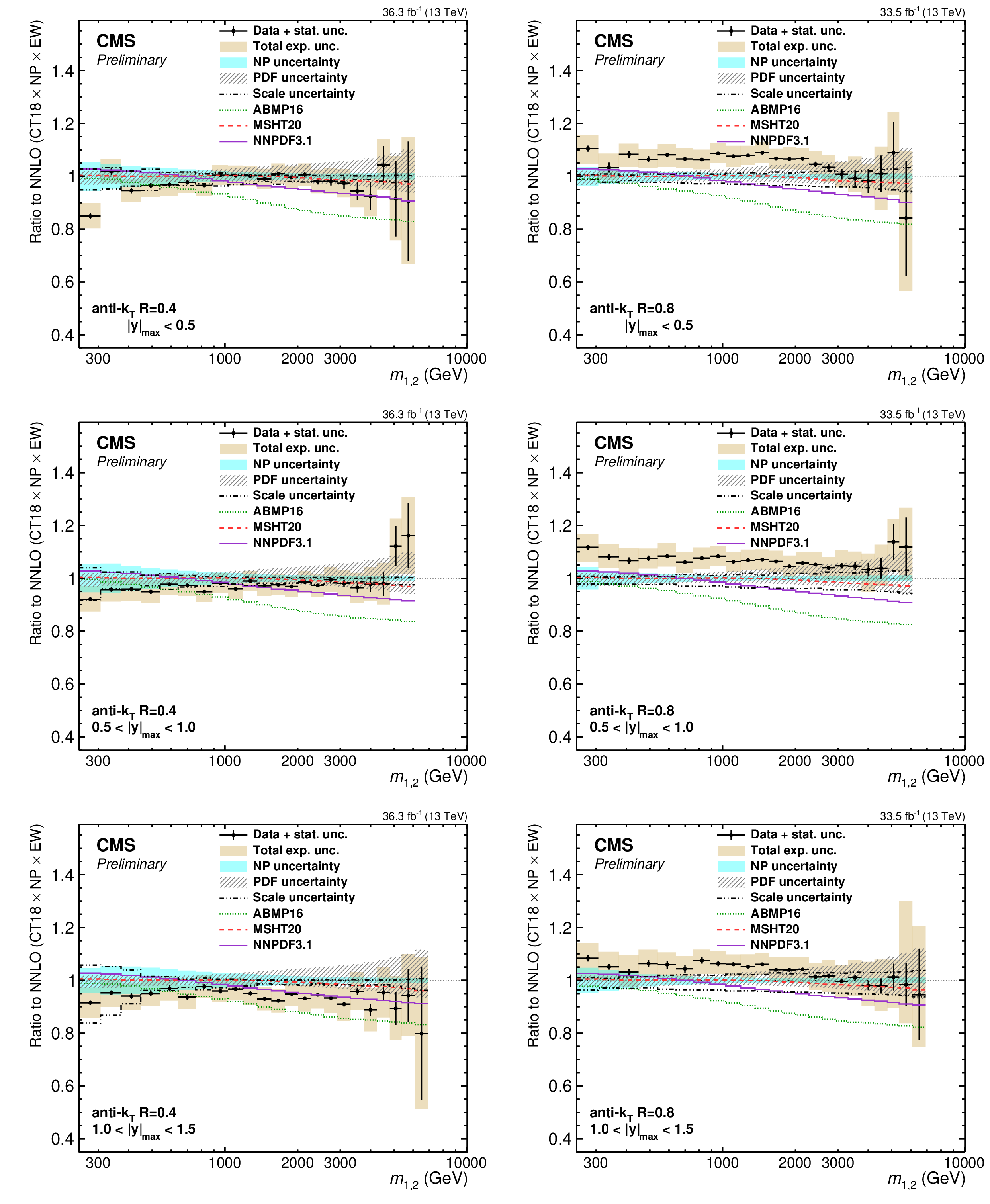
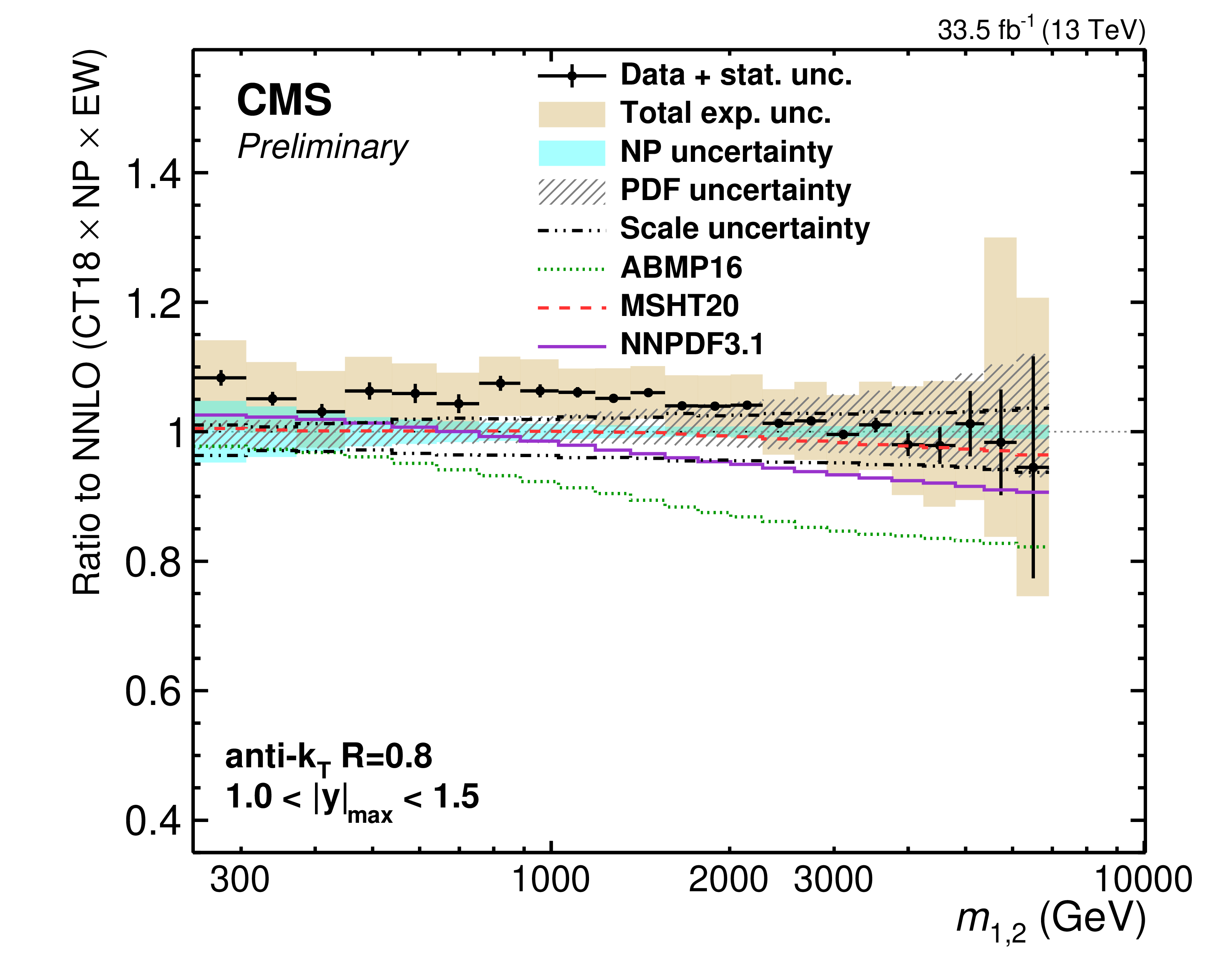
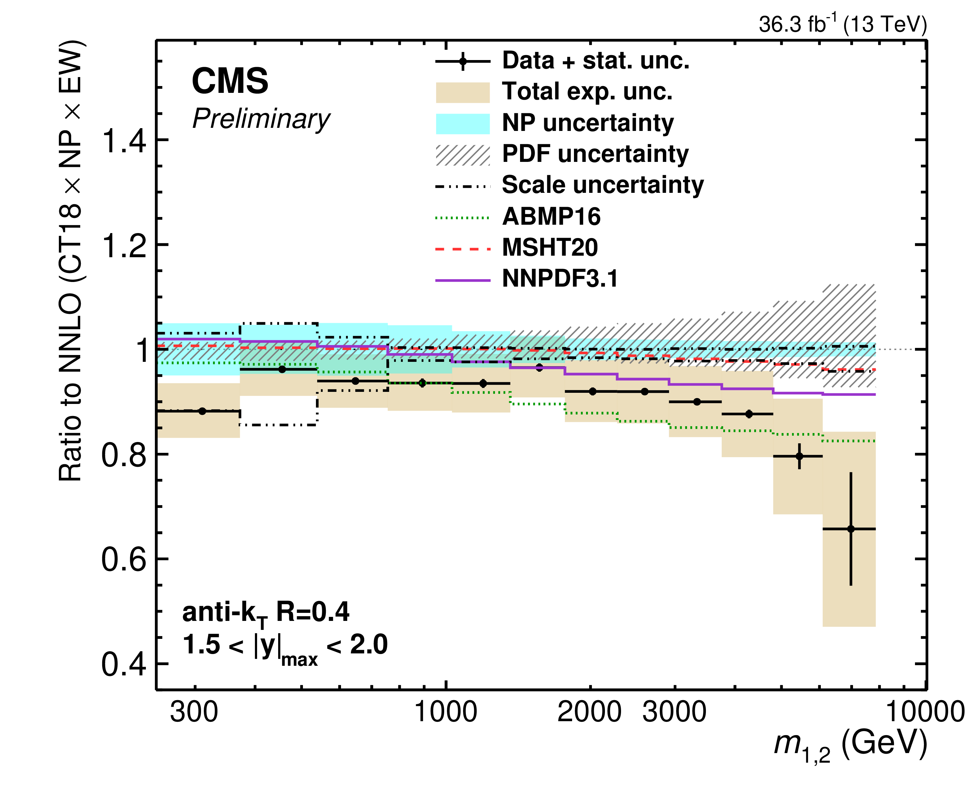
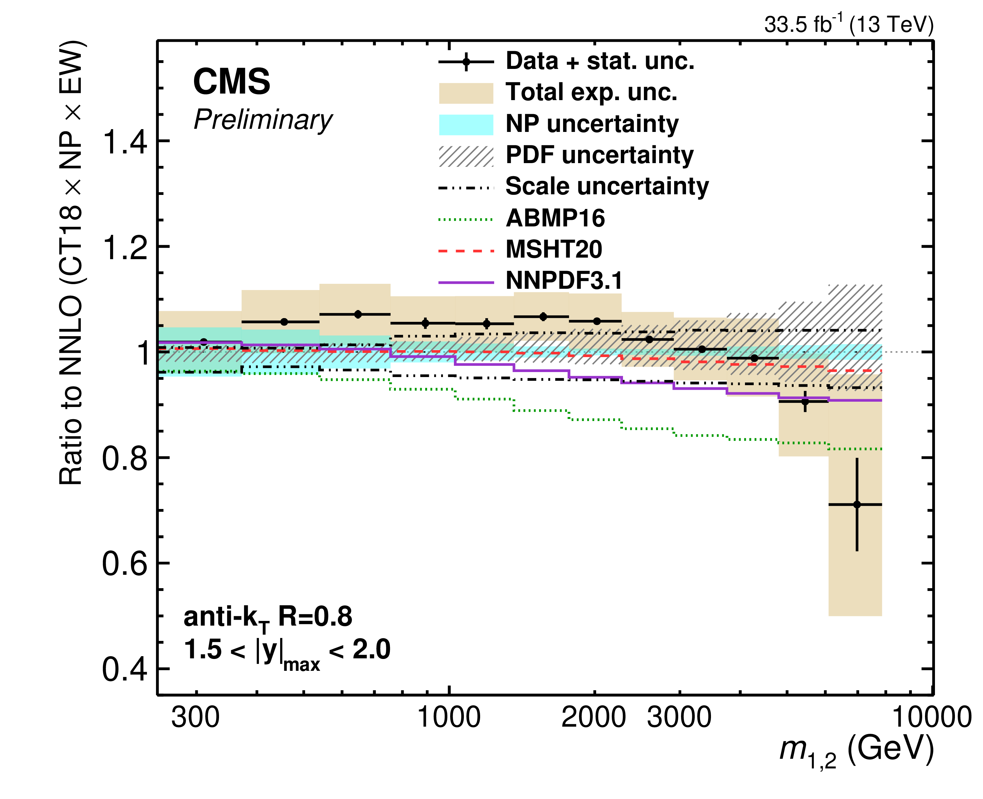
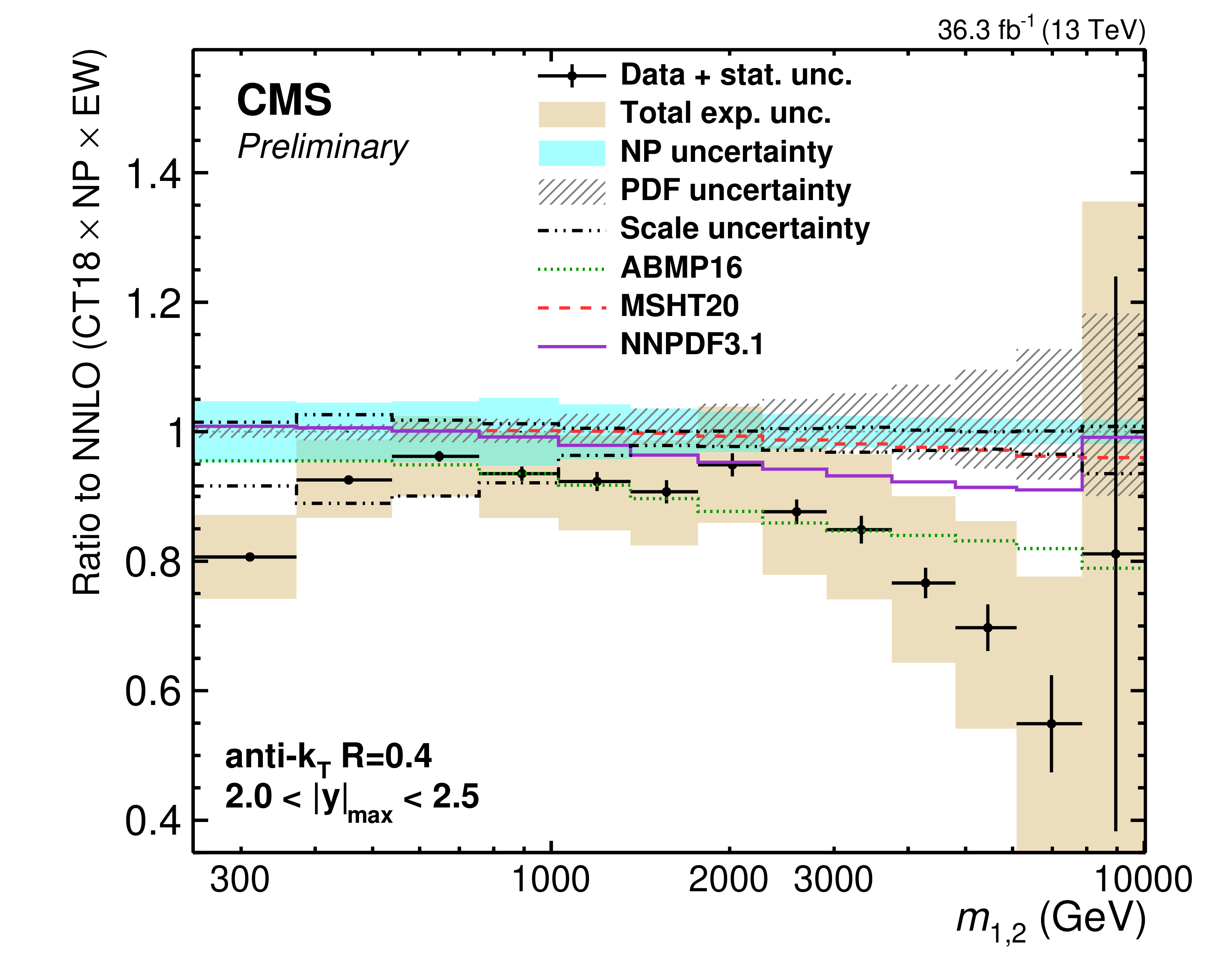
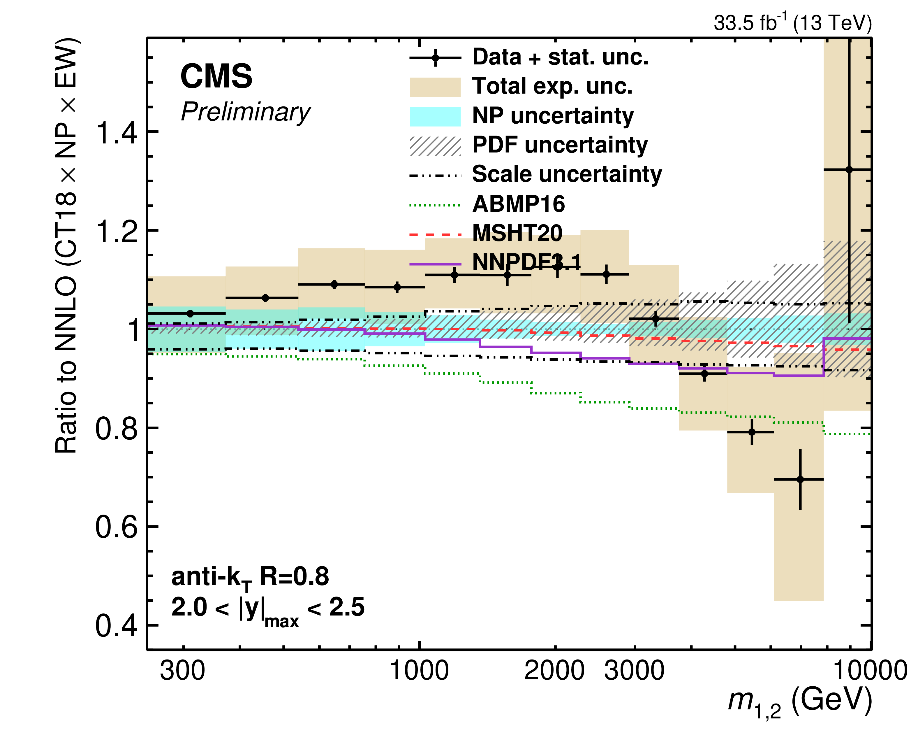
Comparison of the 2D dijet cross section as a function of $ m_{1,2} $ to fixed-order theory calculations at NNLO, using jets with $ R = $ 0.4 (left) and $ R = $ 0.8 (right). Shown are the ratios of the measured cross sections (markers) to predictions obtained using the CT18 NNLO PDF set. The error bars and shaded yellow regions indicate the statistical and the total experimental uncertainties of the data, respectively, and the hatched teal band indicates the total theory uncertainty. Alternative theory predictions obtained using other global PDF sets are shown as colored lines. |
png pdf |
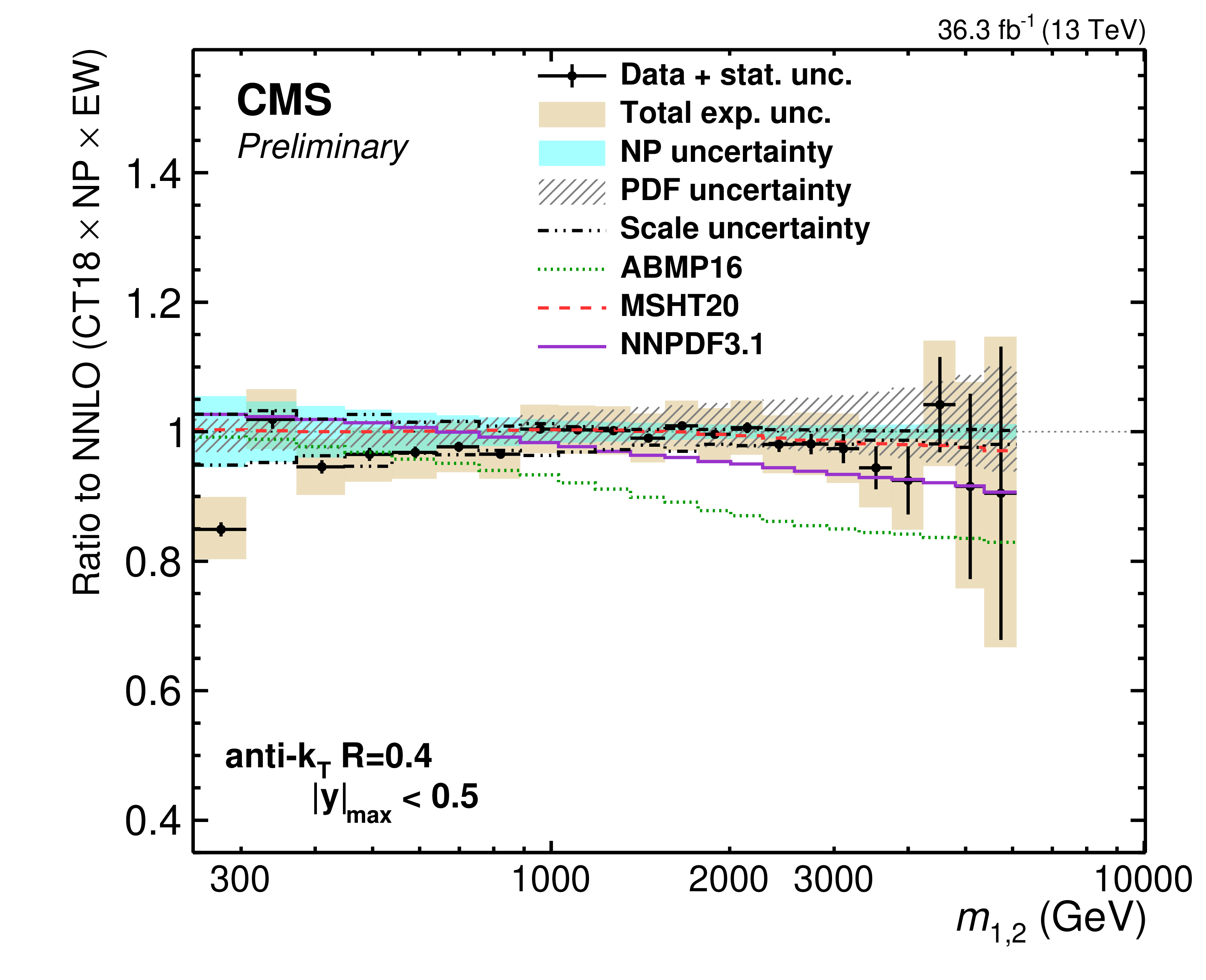
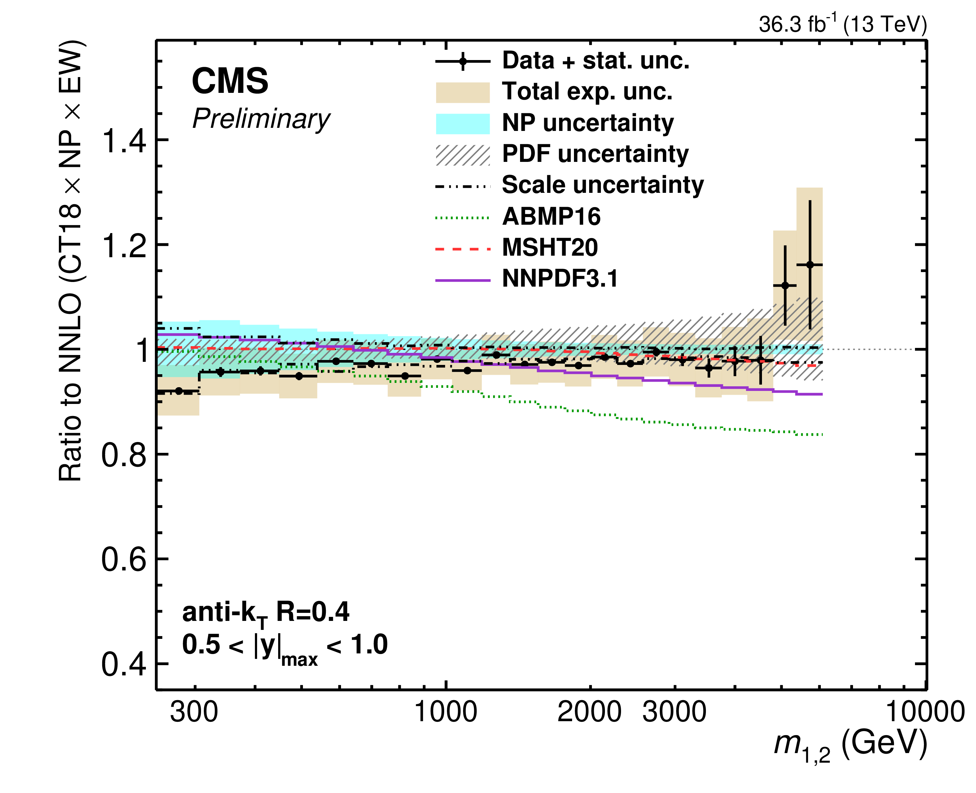
Figure 9-a:
Comparison of the 2D dijet cross section as a function of $ m_{1,2} $ to fixed-order theory calculations at NNLO, using jets with $ R = $ 0.4. Shown are the ratios of the measured cross sections (markers) to predictions obtained using the CT18 NNLO PDF set. The error bars and shaded yellow regions indicate the statistical and the total experimental uncertainties of the data, respectively, and the hatched teal band indicates the total theory uncertainty. Alternative theory predictions obtained using other global PDF sets are shown as colored lines. |
png pdf |
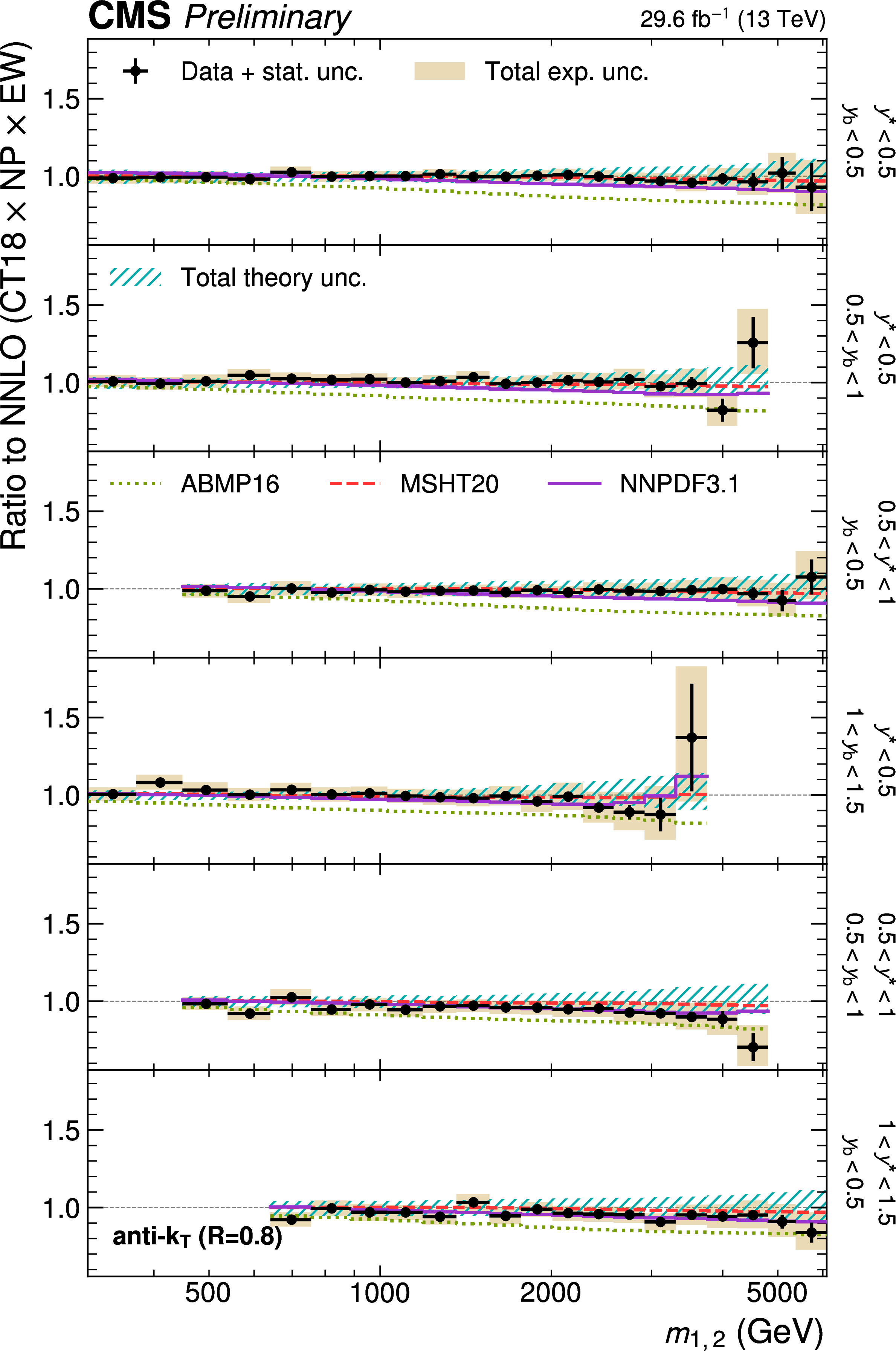
Figure 9-b:
Comparison of the 2D dijet cross section as a function of $ m_{1,2} $ to fixed-order theory calculations at NNLO, using jets with $ R = $ 0.8. Shown are the ratios of the measured cross sections (markers) to predictions obtained using the CT18 NNLO PDF set. The error bars and shaded yellow regions indicate the statistical and the total experimental uncertainties of the data, respectively, and the hatched teal band indicates the total theory uncertainty. Alternative theory predictions obtained using other global PDF sets are shown as colored lines. |
png pdf |
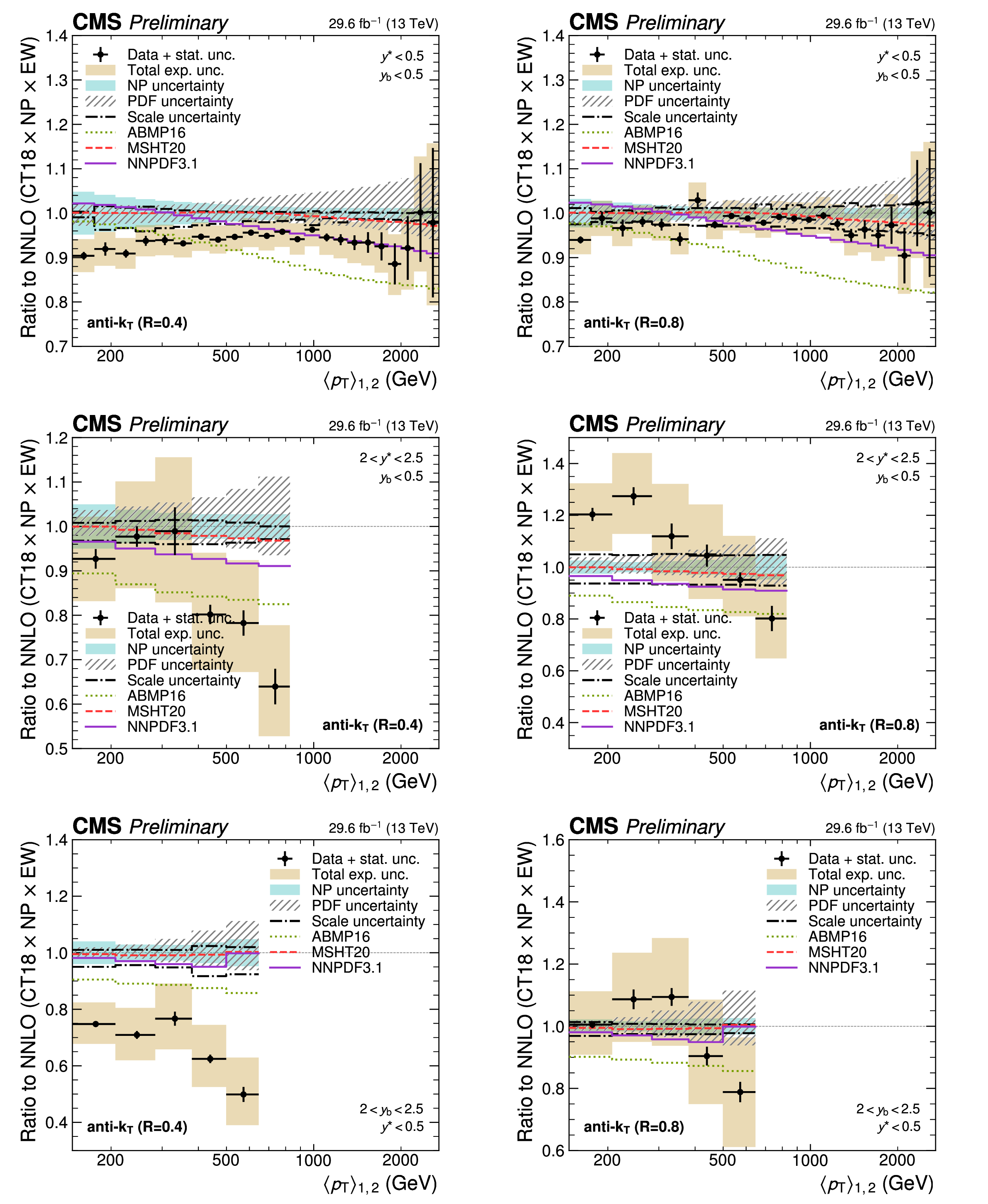
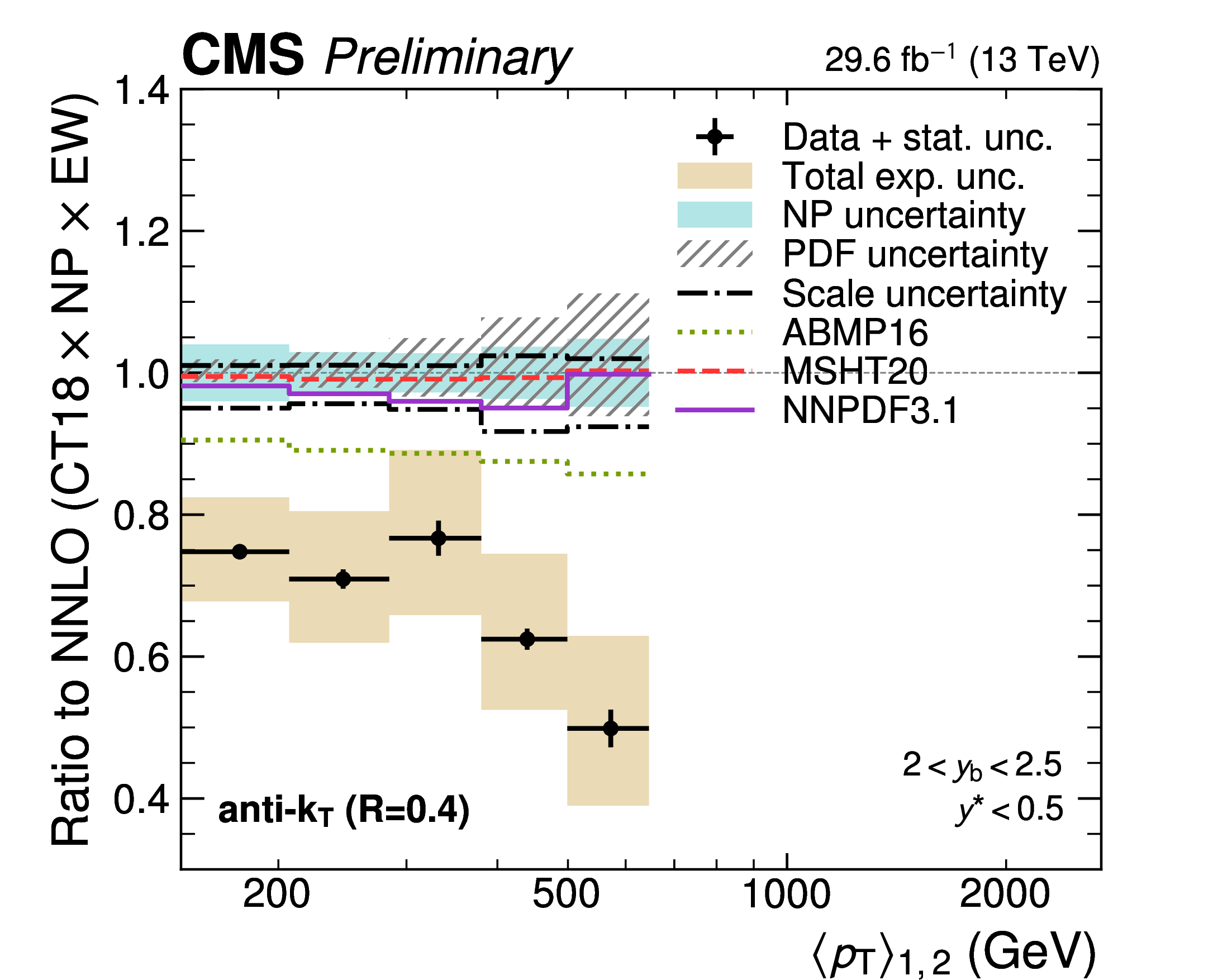
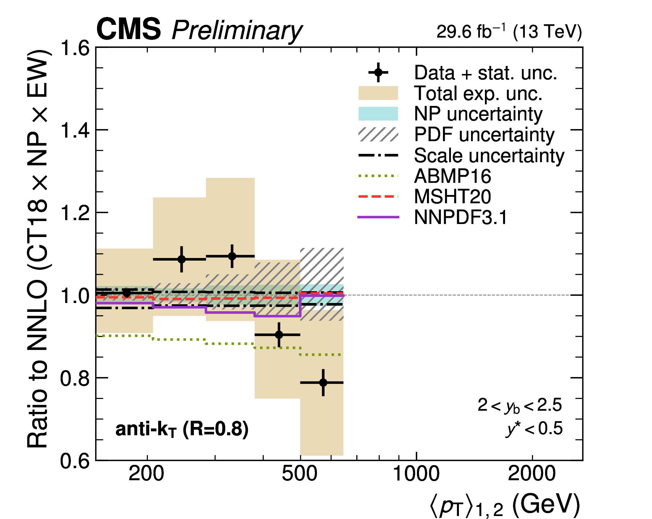
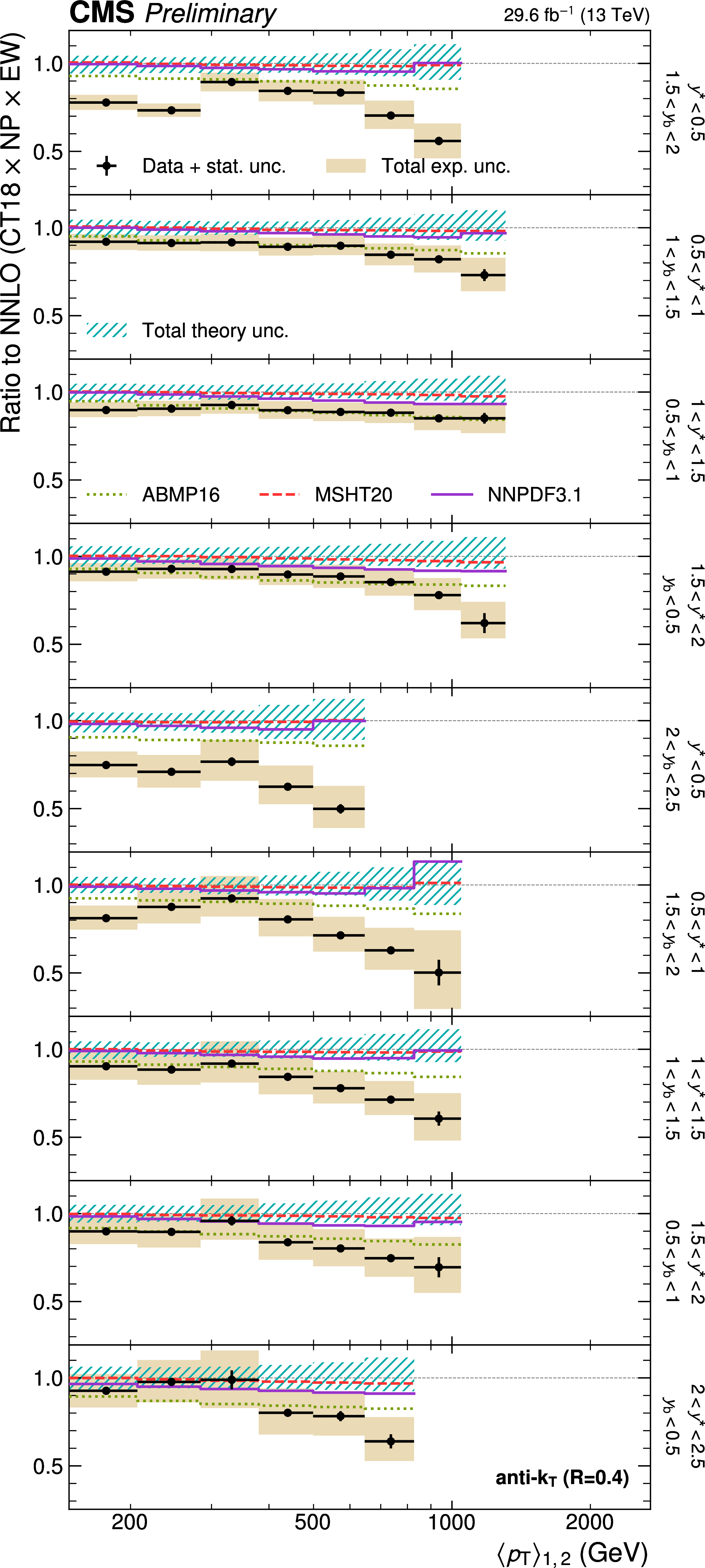
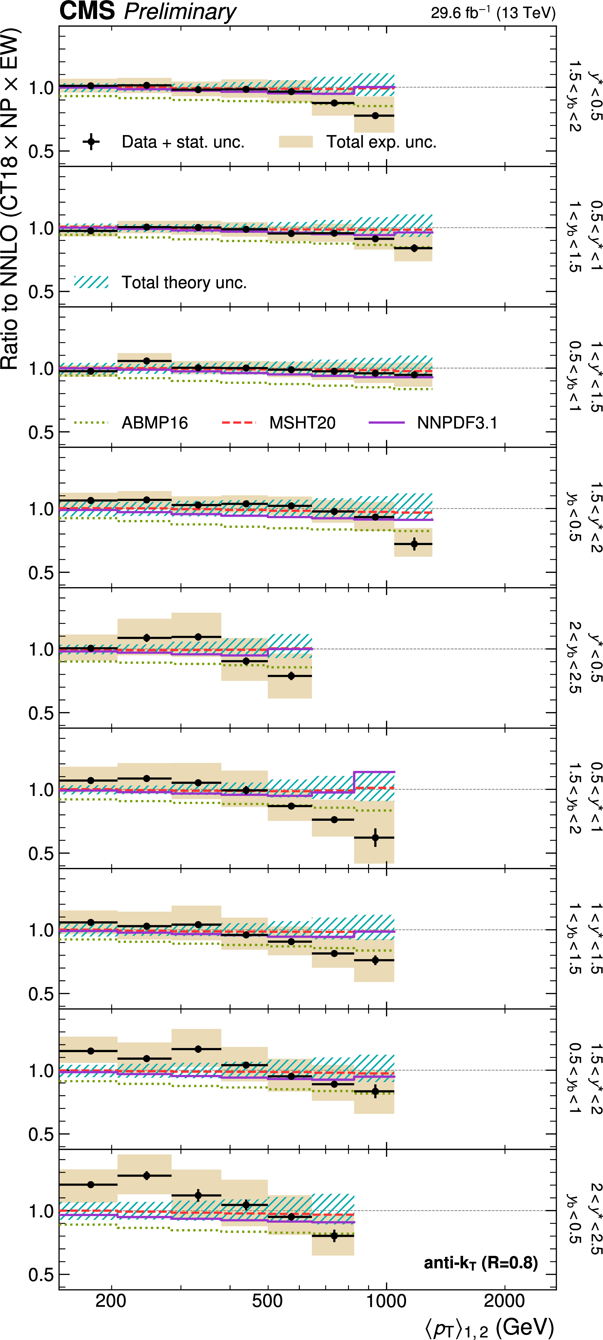
Figure 10:
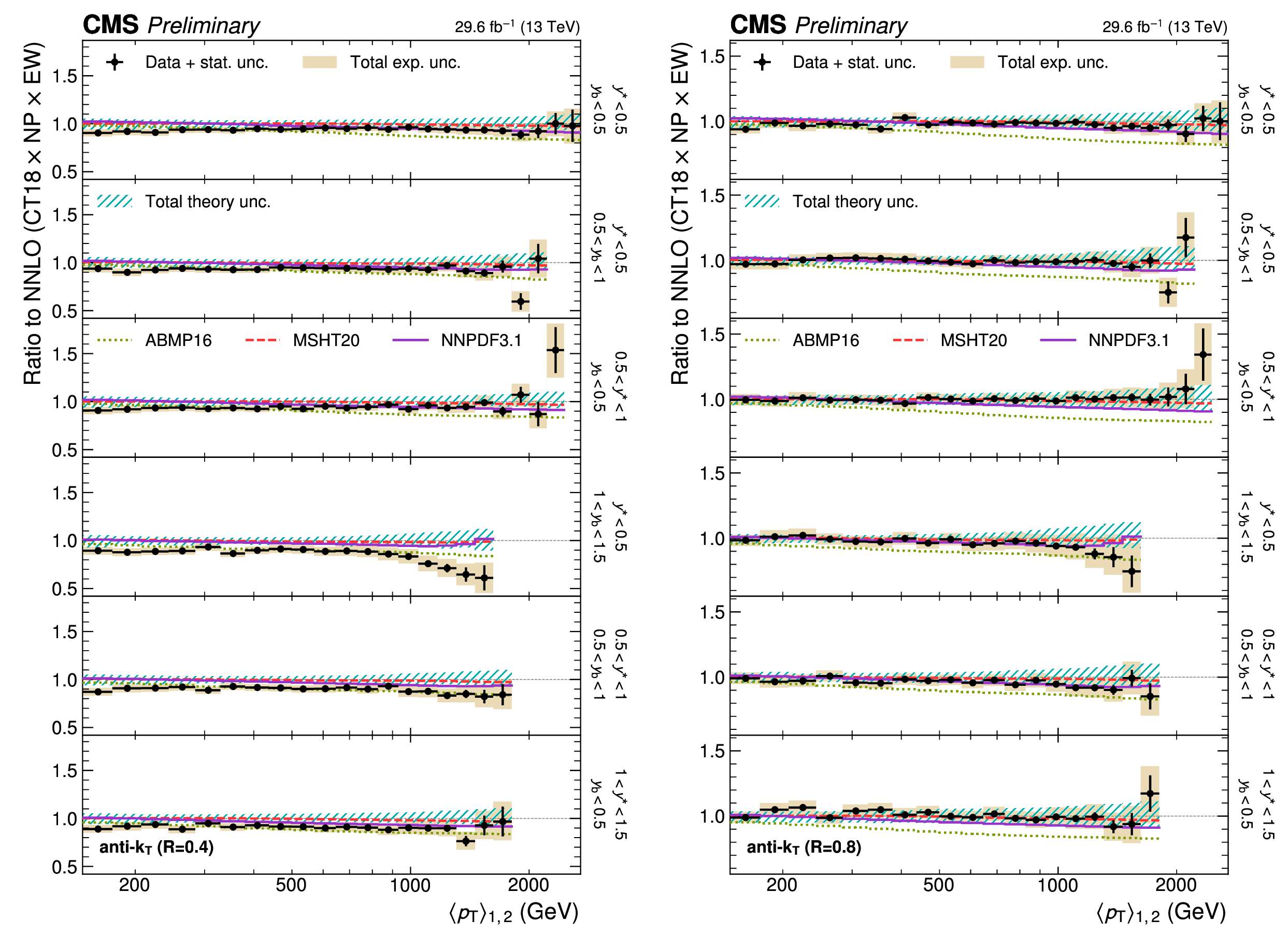
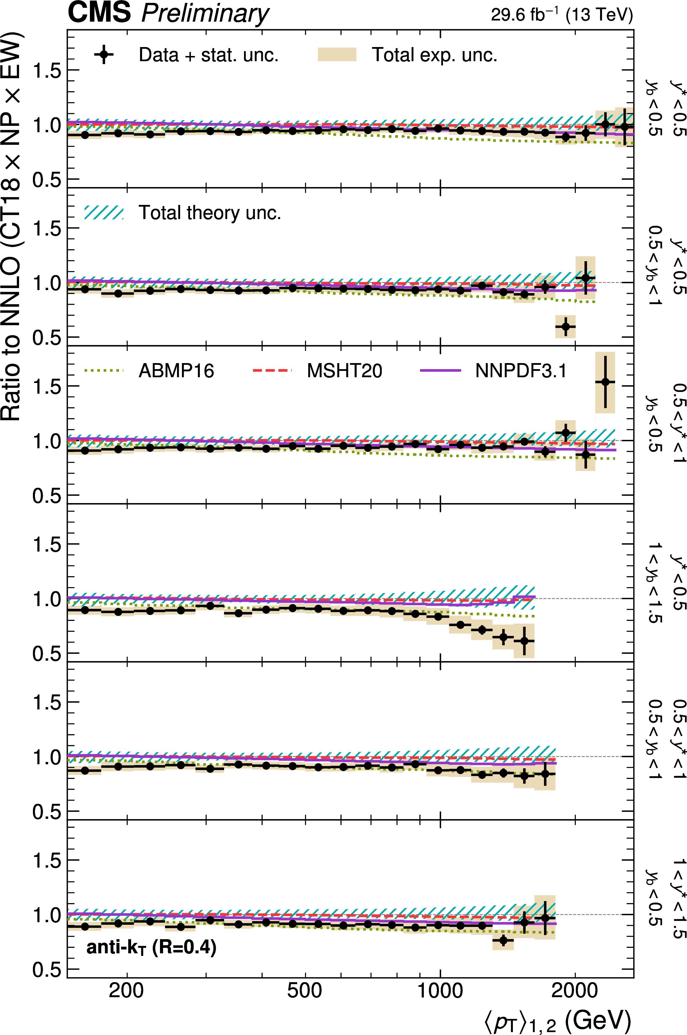
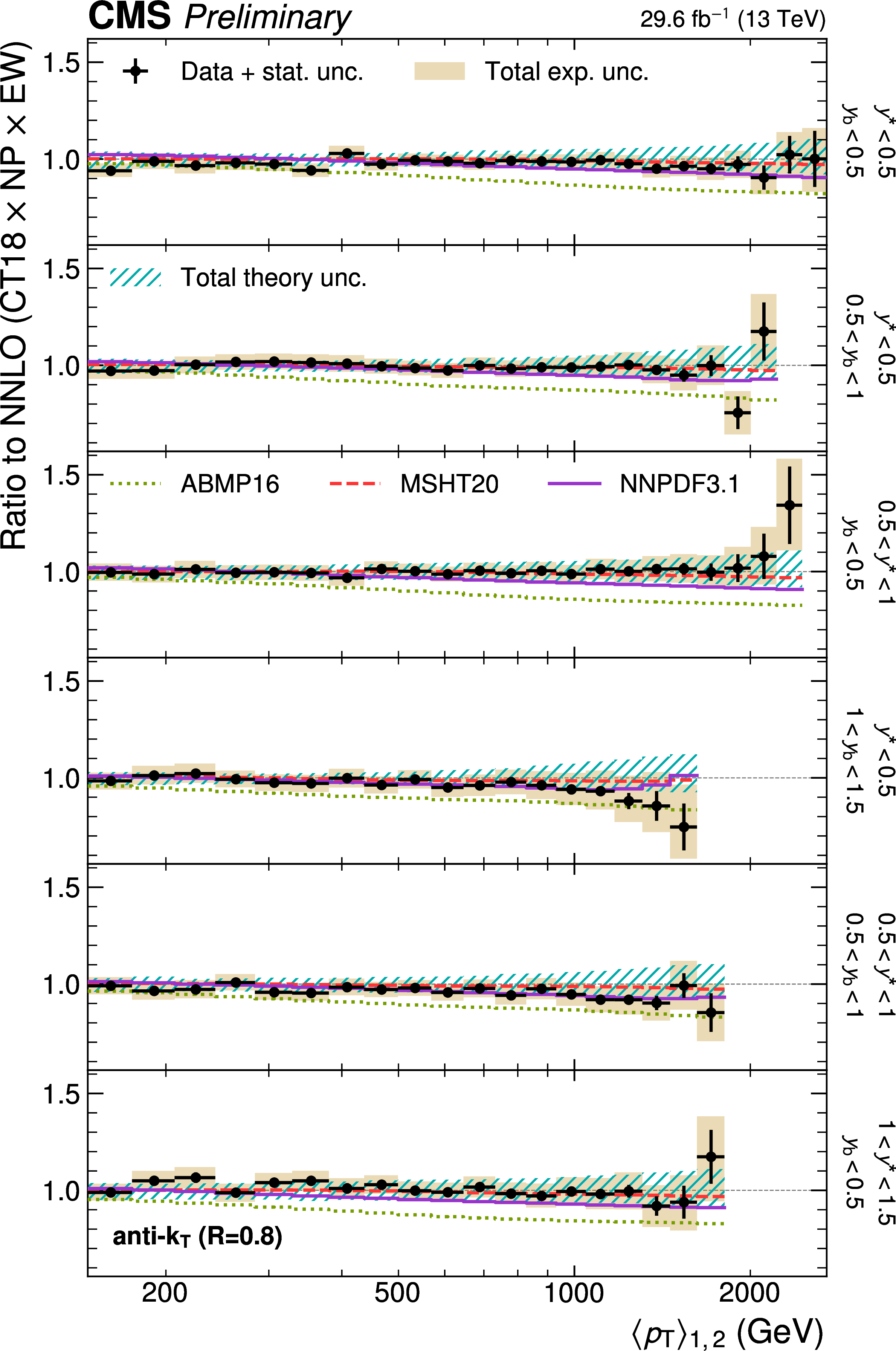
Comparison of the 3D dijet cross section for jets with $ R = $ 0.4 (left) and $ R = $ 0.8 (right) as a function of $ \langle p_{\mathrm{T}} \rangle_{1,2} $ to fixed-order theory calculations at NNLO, shown here for three out of the total of 15 rapidity regions. The data points and predictions for alternative PDFs are analogous to those in continuation. In addition, the separate contributions to the theory uncertainty due to the CT18 PDFs, NP corrections, and six-point scale variations are shown explicitly. |
png pdf |
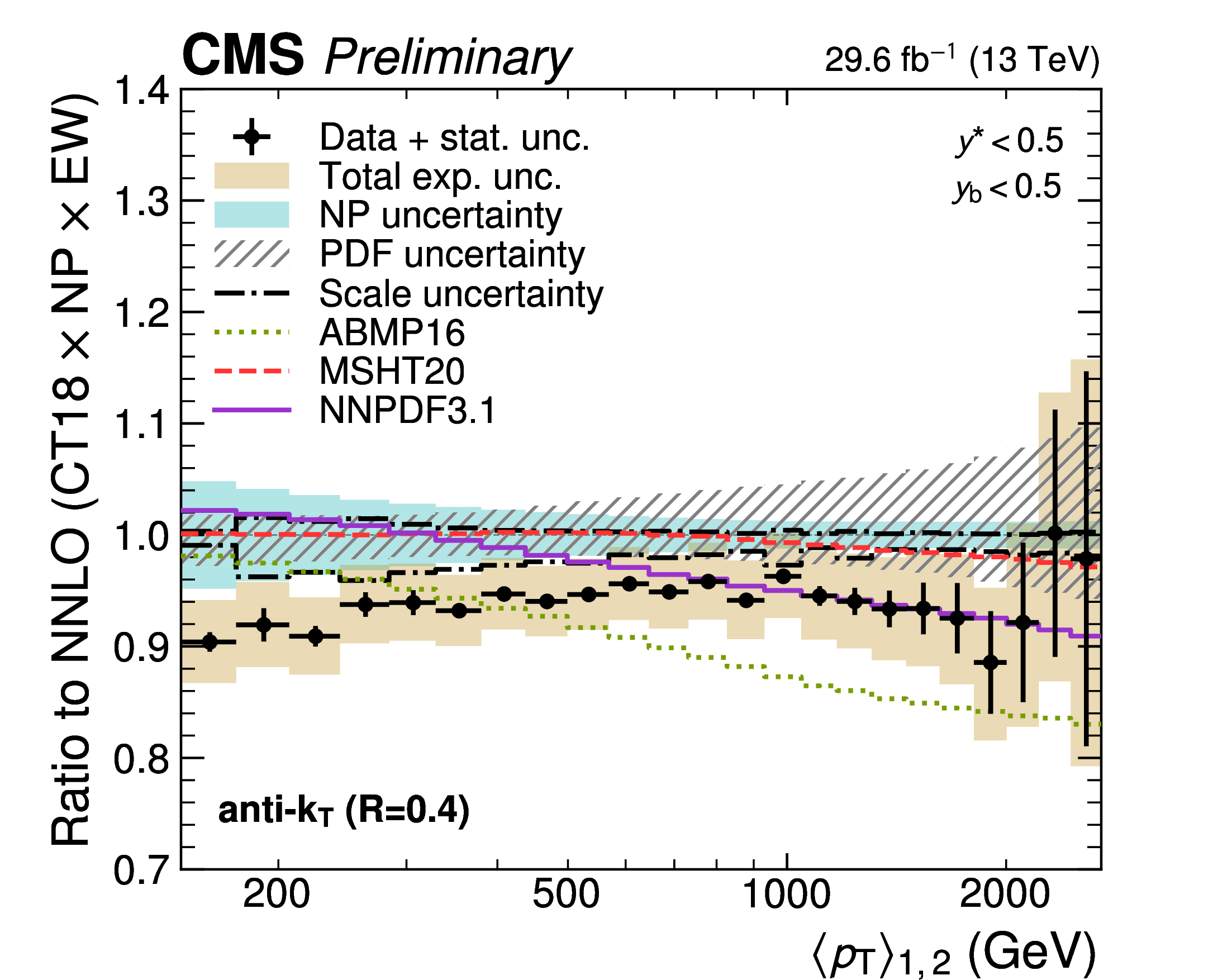
Figure 10-a:
Comparison of the 3D dijet cross section for jets with $ R = $ 0.4 as a function of $ \langle p_{\mathrm{T}} \rangle_{1,2} $ to fixed-order theory calculations at NNLO, shown here for one of the total of 15 rapidity regions. The data points and predictions for alternative PDFs are analogous to those in continuation. In addition, the separate contributions to the theory uncertainty due to the CT18 PDFs, NP corrections, and six-point scale variations are shown explicitly. |

png pdf |
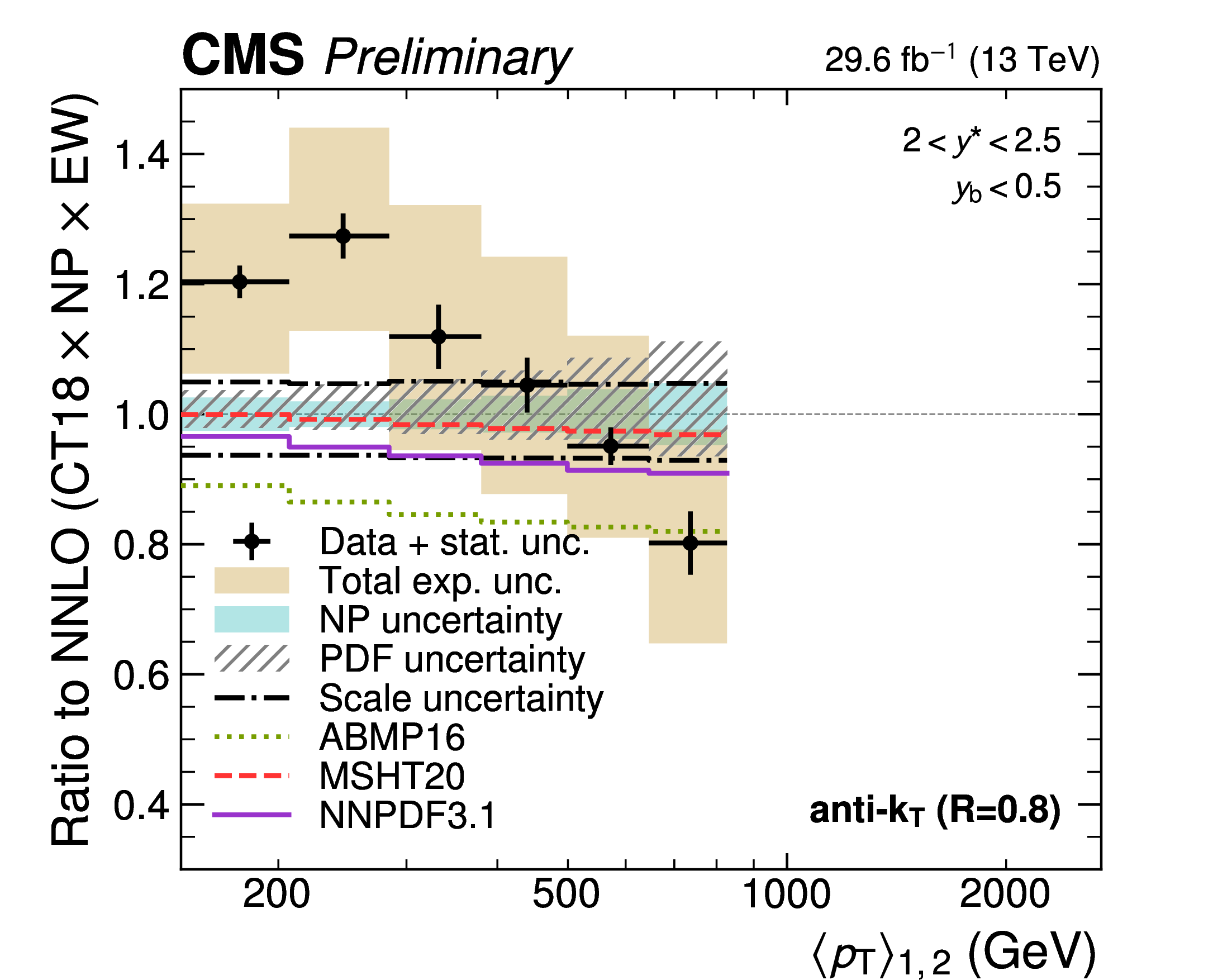
Figure 10-b:
Comparison of the 3D dijet cross section for jets with $ R = $ 0.8 as a function of $ \langle p_{\mathrm{T}} \rangle_{1,2} $ to fixed-order theory calculations at NNLO, shown here for one out of the total of 15 rapidity regions. The data points and predictions for alternative PDFs are analogous to those in continuation. In addition, the separate contributions to the theory uncertainty due to the CT18 PDFs, NP corrections, and six-point scale variations are shown explicitly. |
png pdf |
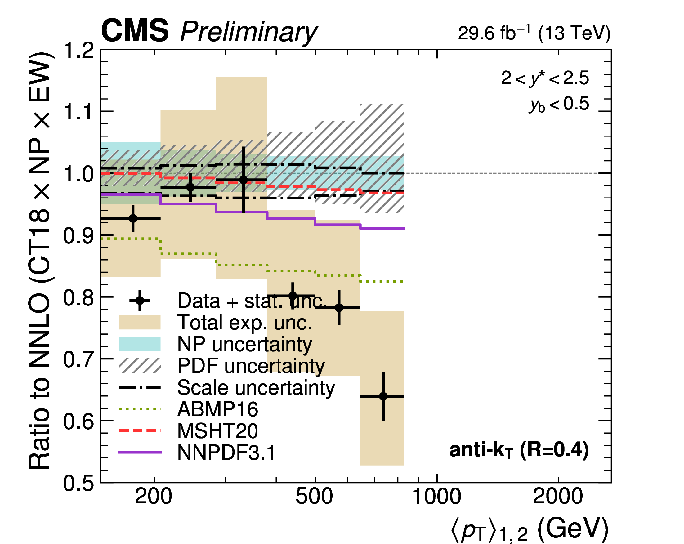
Figure 10-c:
Comparison of the 3D dijet cross section for jets with $ R = $ 0.4 as a function of $ \langle p_{\mathrm{T}} \rangle_{1,2} $ to fixed-order theory calculations at NNLO, shown here for one out of the total of 15 rapidity regions. The data points and predictions for alternative PDFs are analogous to those in continuation. In addition, the separate contributions to the theory uncertainty due to the CT18 PDFs, NP corrections, and six-point scale variations are shown explicitly. |
png pdf |
Figure 10-d:
Comparison of the 3D dijet cross section for jets with $ R = $ 0.8 as a function of $ \langle p_{\mathrm{T}} \rangle_{1,2} $ to fixed-order theory calculations at NNLO, shown here for one out of the total of 15 rapidity regions. The data points and predictions for alternative PDFs are analogous to those in continuation. In addition, the separate contributions to the theory uncertainty due to the CT18 PDFs, NP corrections, and six-point scale variations are shown explicitly. |
png pdf |
Figure 10-e:
Comparison of the 3D dijet cross section for jets with $ R = $ 0.4 as a function of $ \langle p_{\mathrm{T}} \rangle_{1,2} $ to fixed-order theory calculations at NNLO, shown here for one out of the total of 15 rapidity regions. The data points and predictions for alternative PDFs are analogous to those in continuation. In addition, the separate contributions to the theory uncertainty due to the CT18 PDFs, NP corrections, and six-point scale variations are shown explicitly. |
png pdf |
Figure 10-f:
Comparison of the 3D dijet cross section for jets with $ R = $ 0.8 as a function of $ \langle p_{\mathrm{T}} \rangle_{1,2} $ to fixed-order theory calculations at NNLO, shown here for one out of the total of 15 rapidity regions. The data points and predictions for alternative PDFs are analogous to those in continuation. In addition, the separate contributions to the theory uncertainty due to the CT18 PDFs, NP corrections, and six-point scale variations are shown explicitly. |
png pdf |
Figure 11:
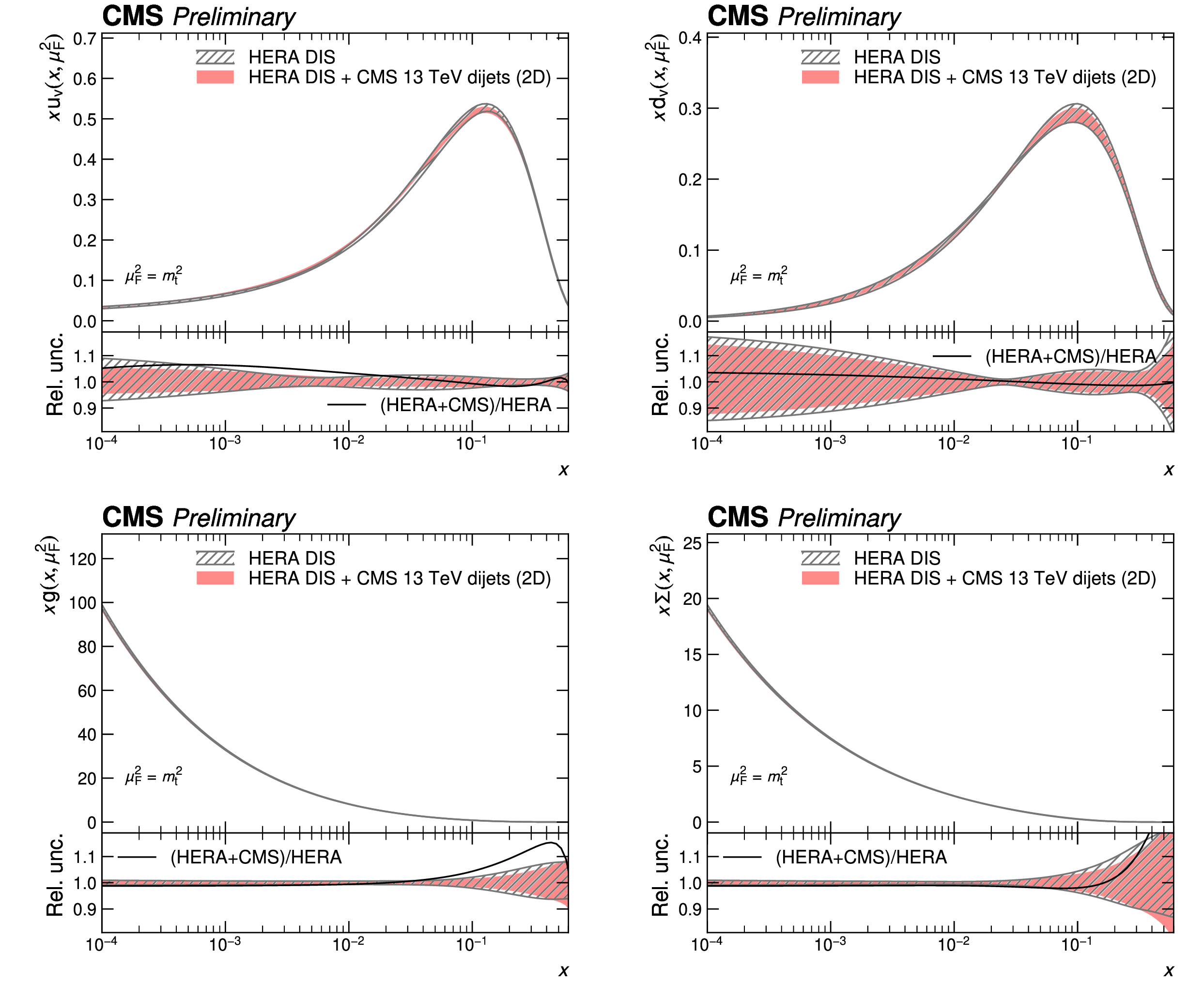
PDFs obtained in a fit to HERA DIS together with CMS 2D dijet data. Shown are the PDFs of the up and down valence quarks (top row), of the gluon (bottom left), and of the total sea quarks (bottom right) as a function of the fractional parton momentum $ x $ at a factorization scale equal to the top quark mass. The colored bands correspond to the individual contributions to the total PDF uncertainty. |
png pdf |
Figure 11-a:
PDFs obtained in a fit to HERA DIS together with CMS 2D dijet data. Shown are the PDFs of the up valence quark as a function of the fractional parton momentum $ x $ at a factorization scale equal to the top quark mass. The colored bands correspond to the individual contributions to the total PDF uncertainty. |
png pdf |
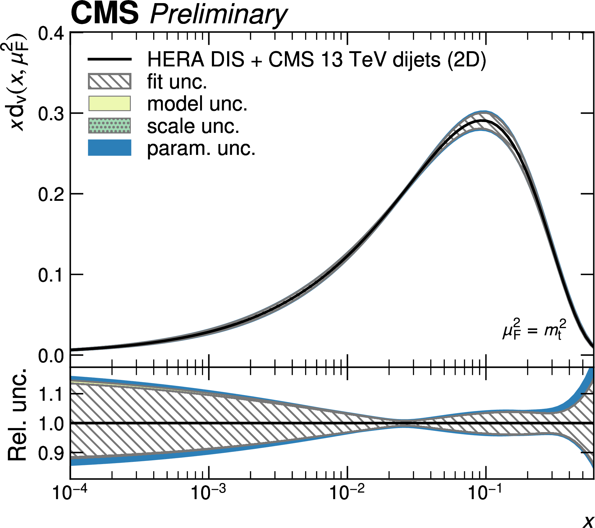
Figure 11-b:
PDFs obtained in a fit to HERA DIS together with CMS 2D dijet data. Shown are the PDFs of the down valence quark as a function of the fractional parton momentum $ x $ at a factorization scale equal to the top quark mass. The colored bands correspond to the individual contributions to the total PDF uncertainty. |
png pdf |
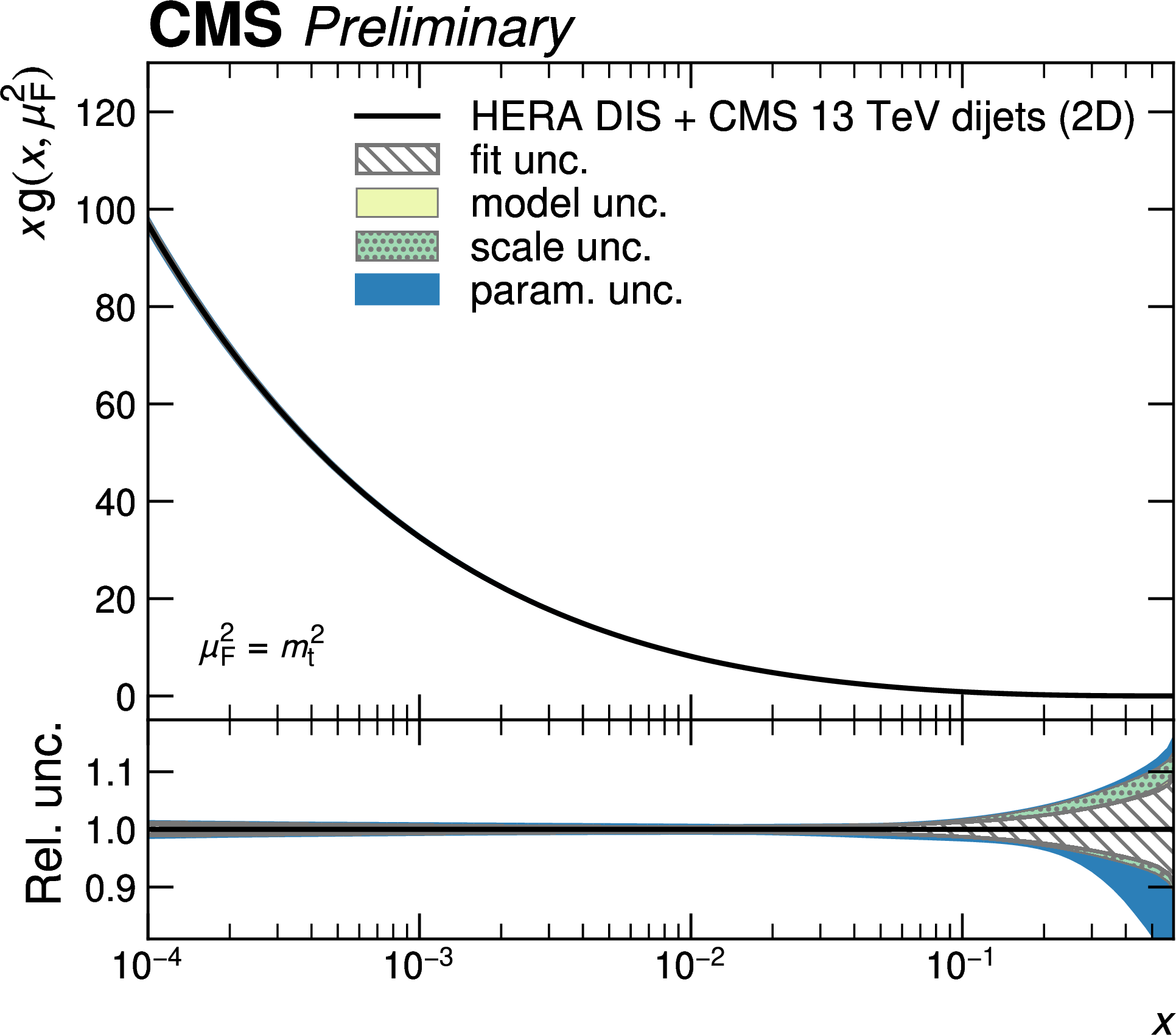
Figure 11-c:
PDFs obtained in a fit to HERA DIS together with CMS 2D dijet data. Shown are the PDFs of the gluon as a function of the fractional parton momentum $ x $ at a factorization scale equal to the top quark mass. The colored bands correspond to the individual contributions to the total PDF uncertainty. |
png pdf |
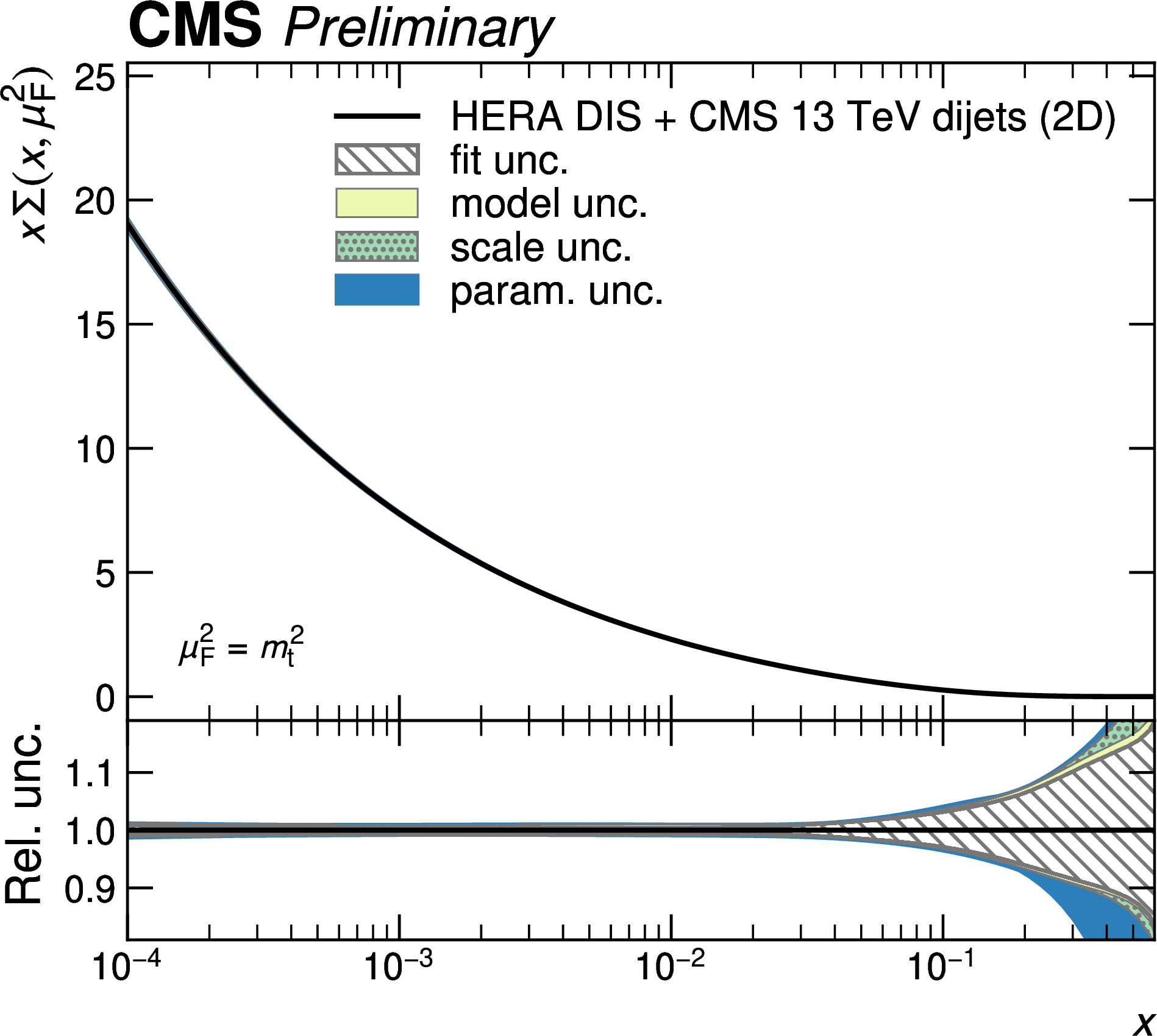
Figure 11-d:
PDFs obtained in a fit to HERA DIS together with CMS 2D dijet data. Shown are the PDFs of the total sea quarks as a function of the fractional parton momentum $ x $ at a factorization scale equal to the top quark mass. The colored bands correspond to the individual contributions to the total PDF uncertainty. |
png pdf |
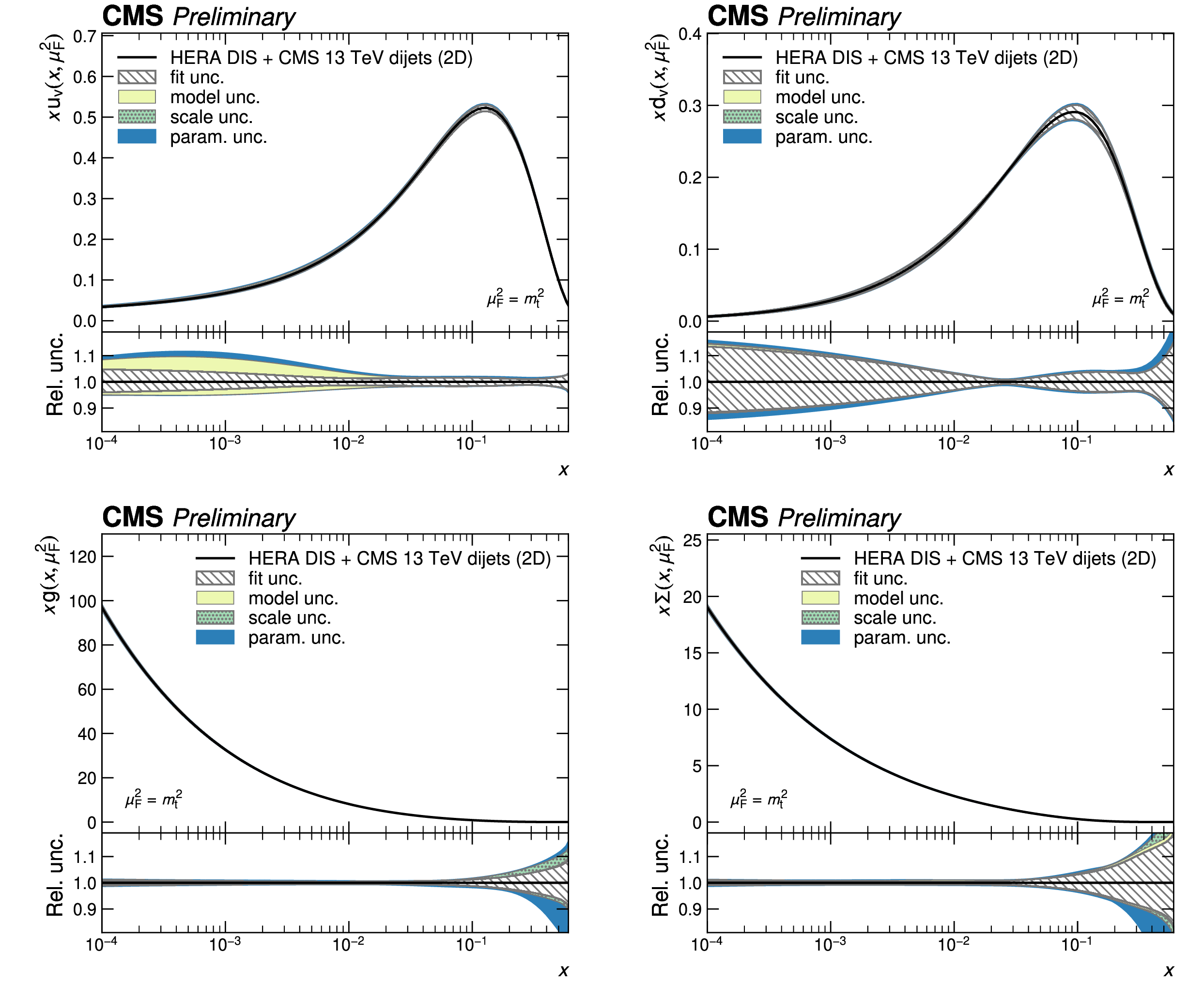
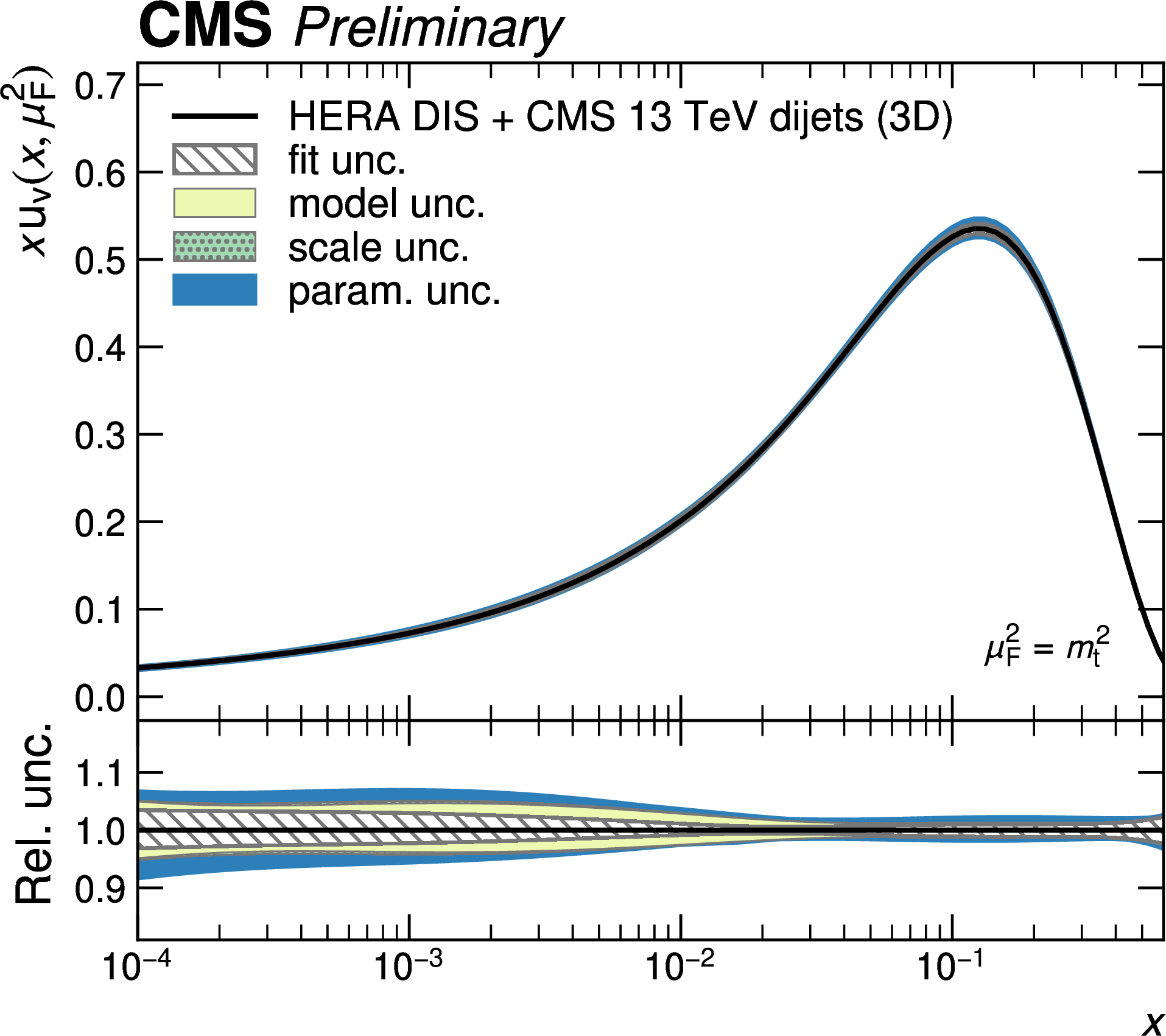
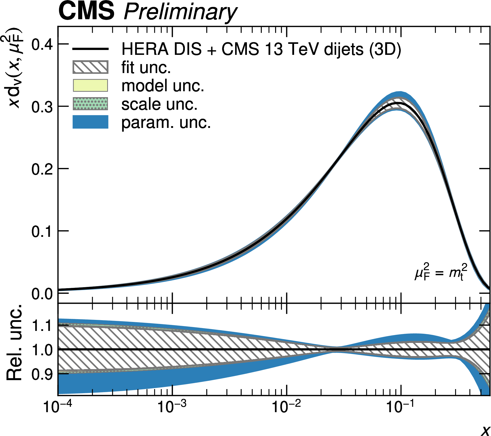
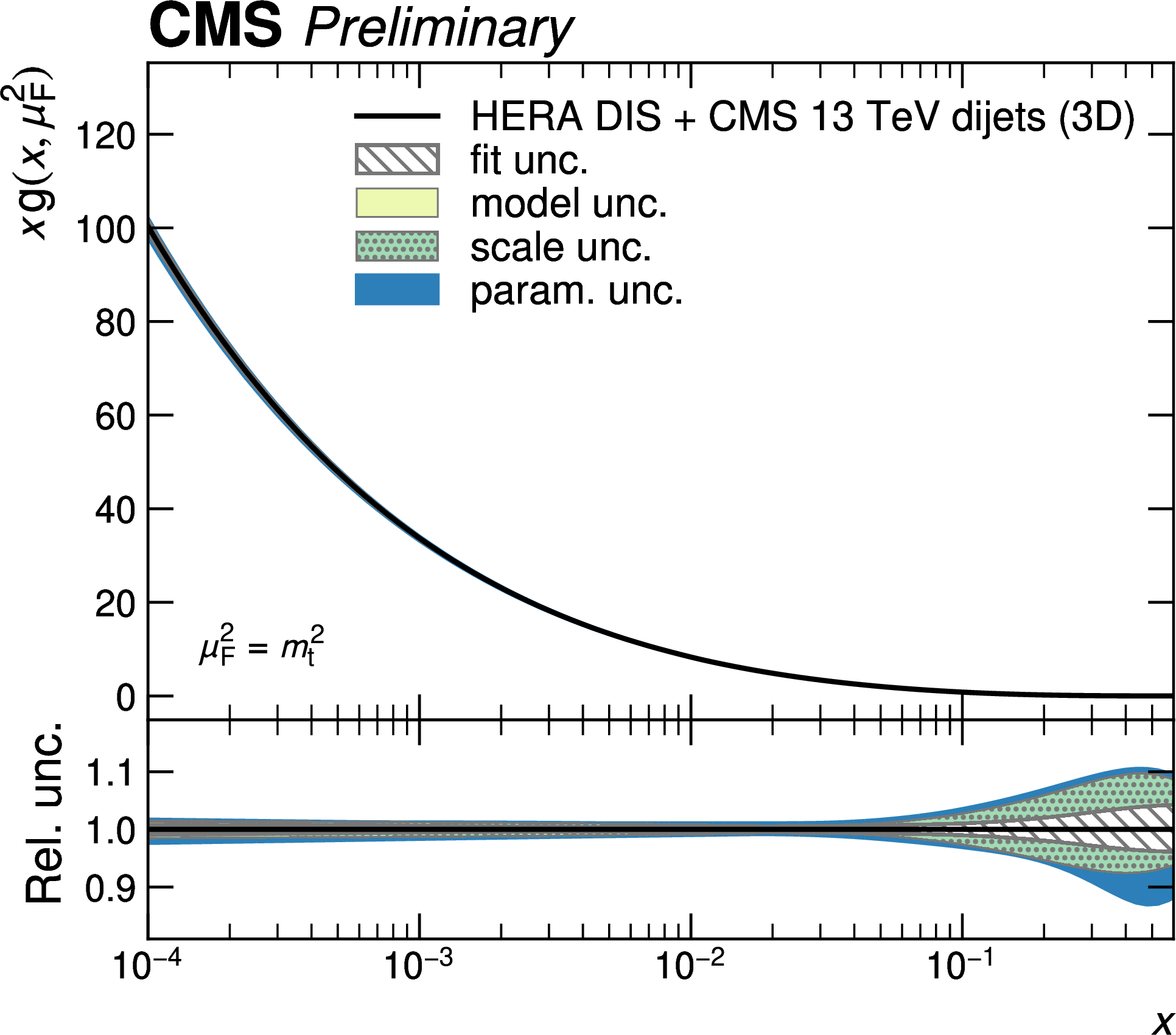
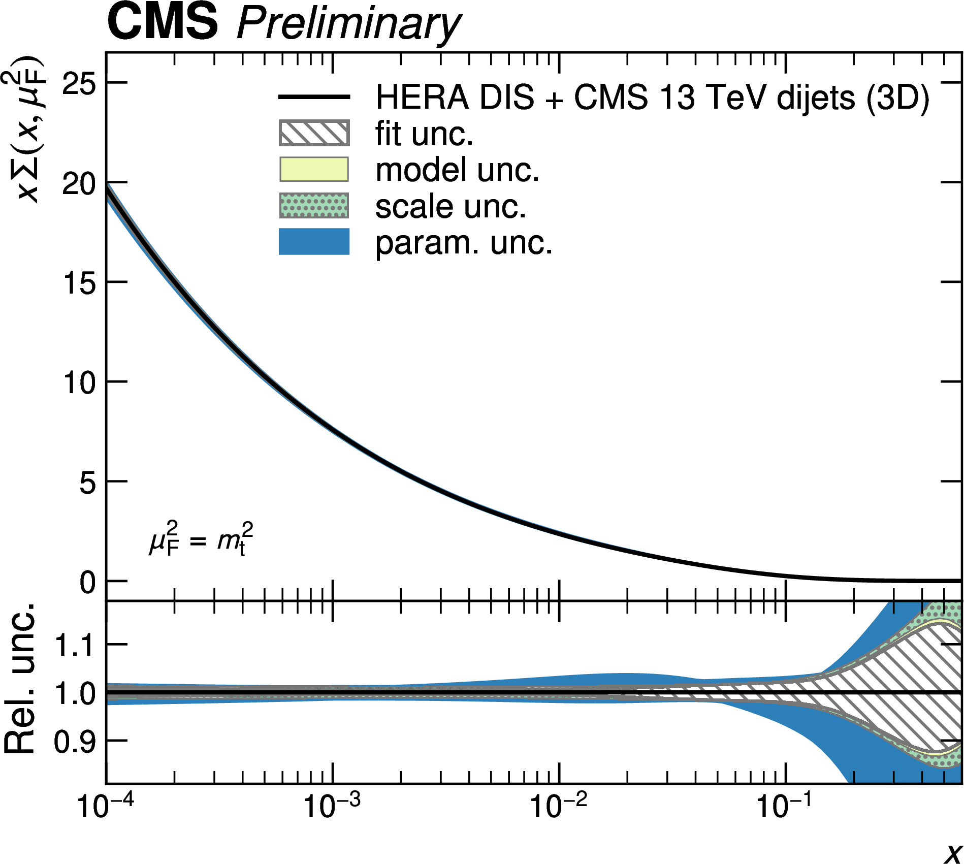
Figure 12:
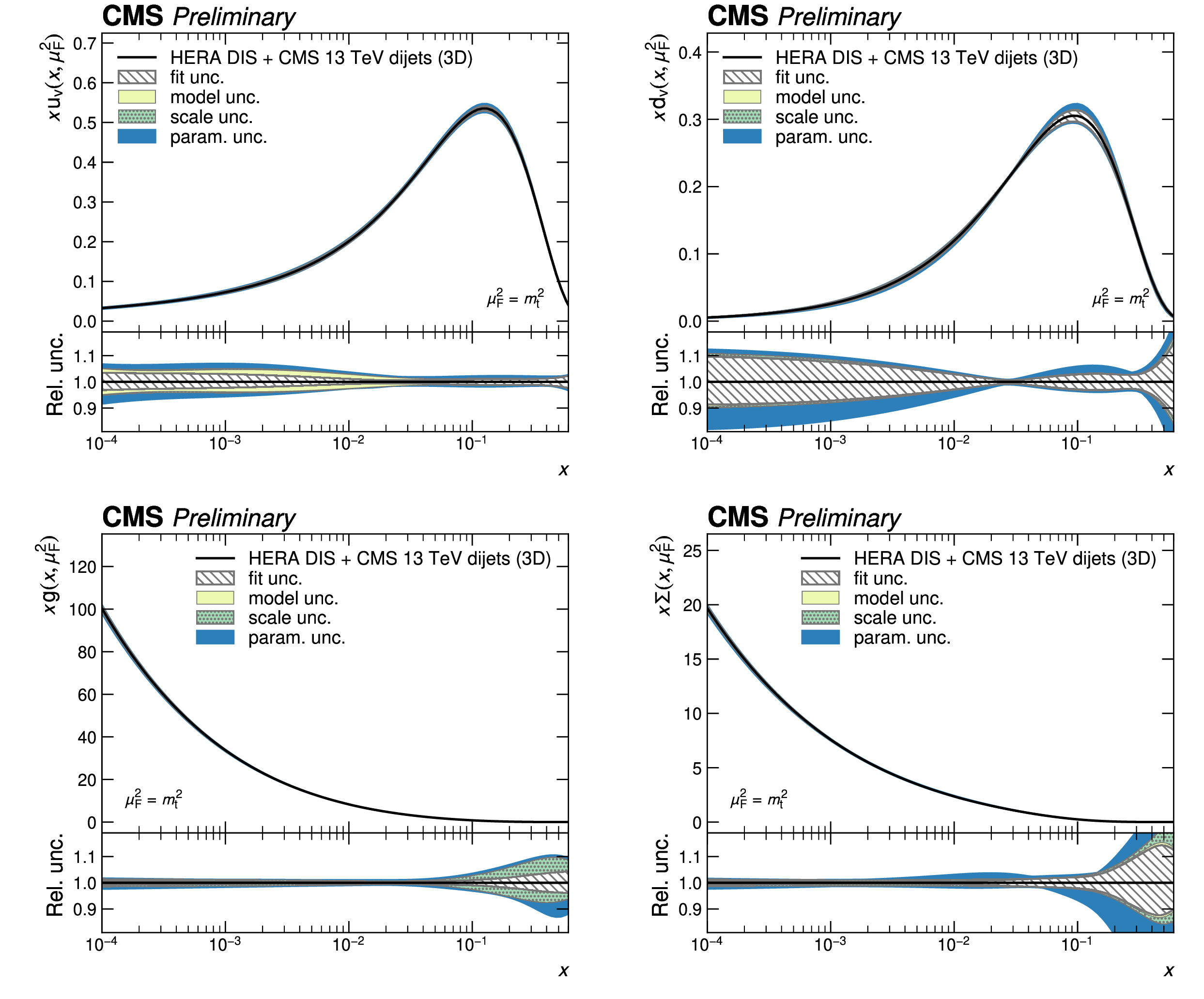
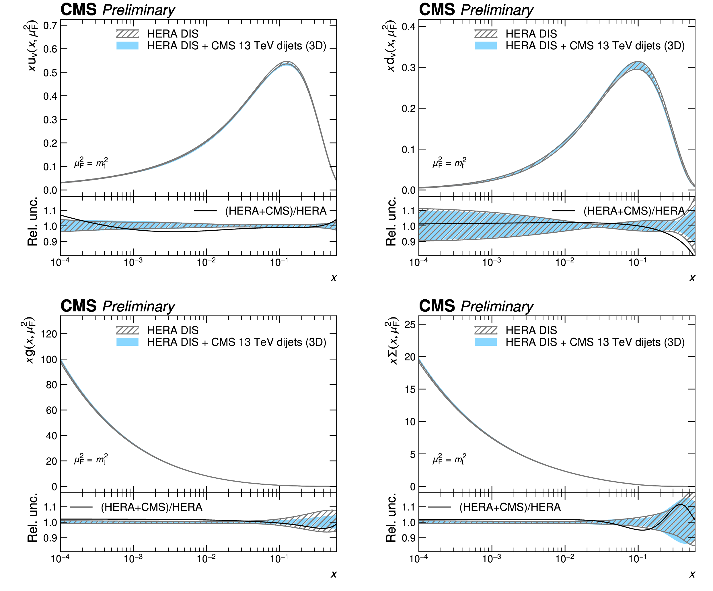
PDFs obtained in a fit to HERA DIS together with CMS 3D dijet data. Shown are the PDFs of the up and down valence quarks (top row), of the gluon (bottom left), and of the total sea quarks (bottom right) as a function of the fractional parton momentum $ x $ at a factorization scale equal to the top quark mass. The colored bands correspond to the individual contributions to the total PDF uncertainty. |
png pdf |
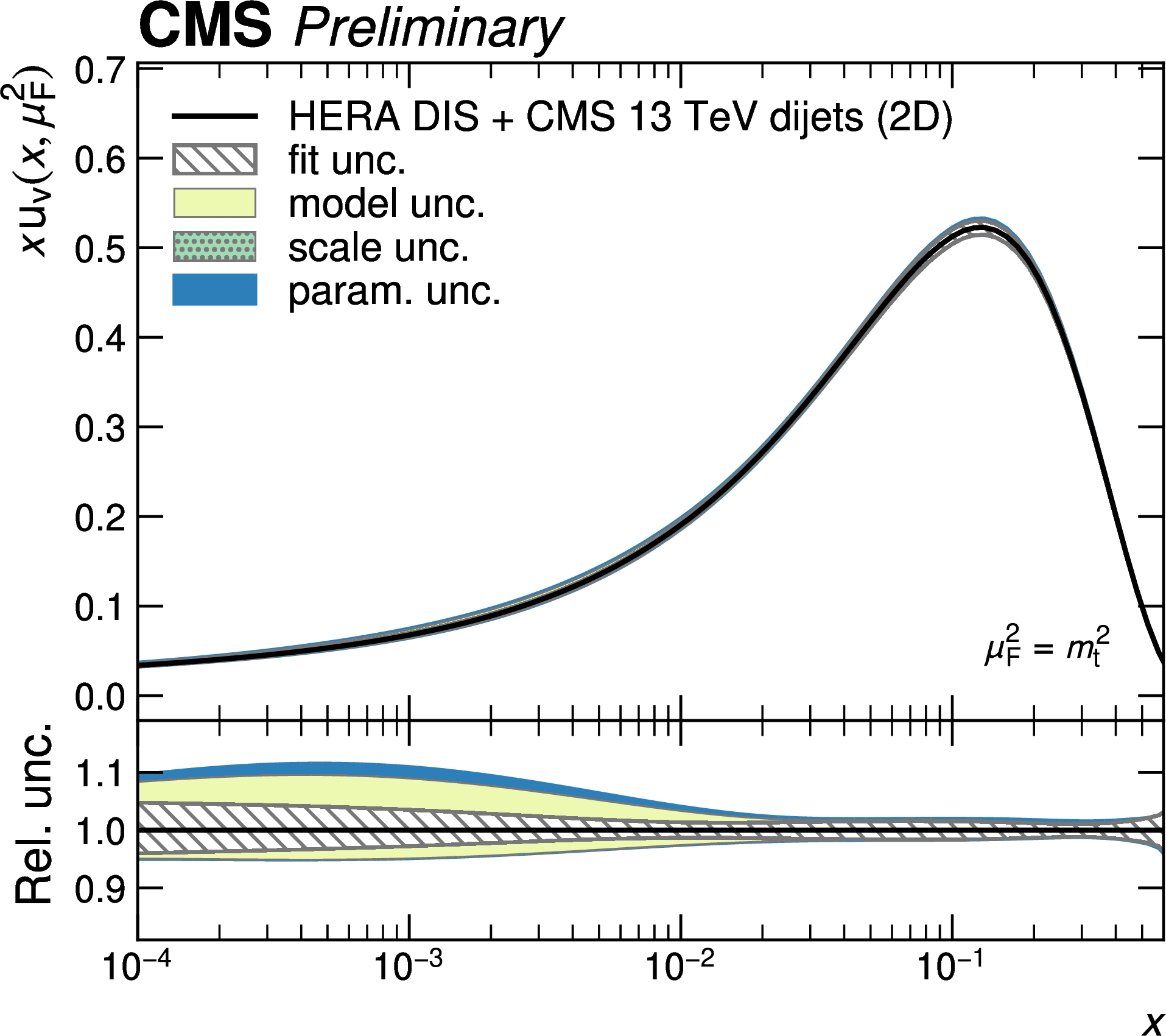
Figure 12-a:
PDFs obtained in a fit to HERA DIS together with CMS 3D dijet data. Shown are the PDFs of the up valence quark as a function of the fractional parton momentum $ x $ at a factorization scale equal to the top quark mass. The colored bands correspond to the individual contributions to the total PDF uncertainty. |
png pdf |
Figure 12-b:
PDFs obtained in a fit to HERA DIS together with CMS 3D dijet data. Shown are the PDFs of the down valence quark as a function of the fractional parton momentum $ x $ at a factorization scale equal to the top quark mass. The colored bands correspond to the individual contributions to the total PDF uncertainty. |
png pdf |
Figure 12-c:
PDFs obtained in a fit to HERA DIS together with CMS 3D dijet data. Shown are the PDFs of the gluon as a function of the fractional parton momentum $ x $ at a factorization scale equal to the top quark mass. The colored bands correspond to the individual contributions to the total PDF uncertainty. |
png pdf |
Figure 12-d:
PDFs obtained in a fit to HERA DIS together with CMS 3D dijet data. Shown are the PDFs of the total sea quarks as a function of the fractional parton momentum $ x $ at a factorization scale equal to the top quark mass. The colored bands correspond to the individual contributions to the total PDF uncertainty. |
png pdf |
Figure 13:
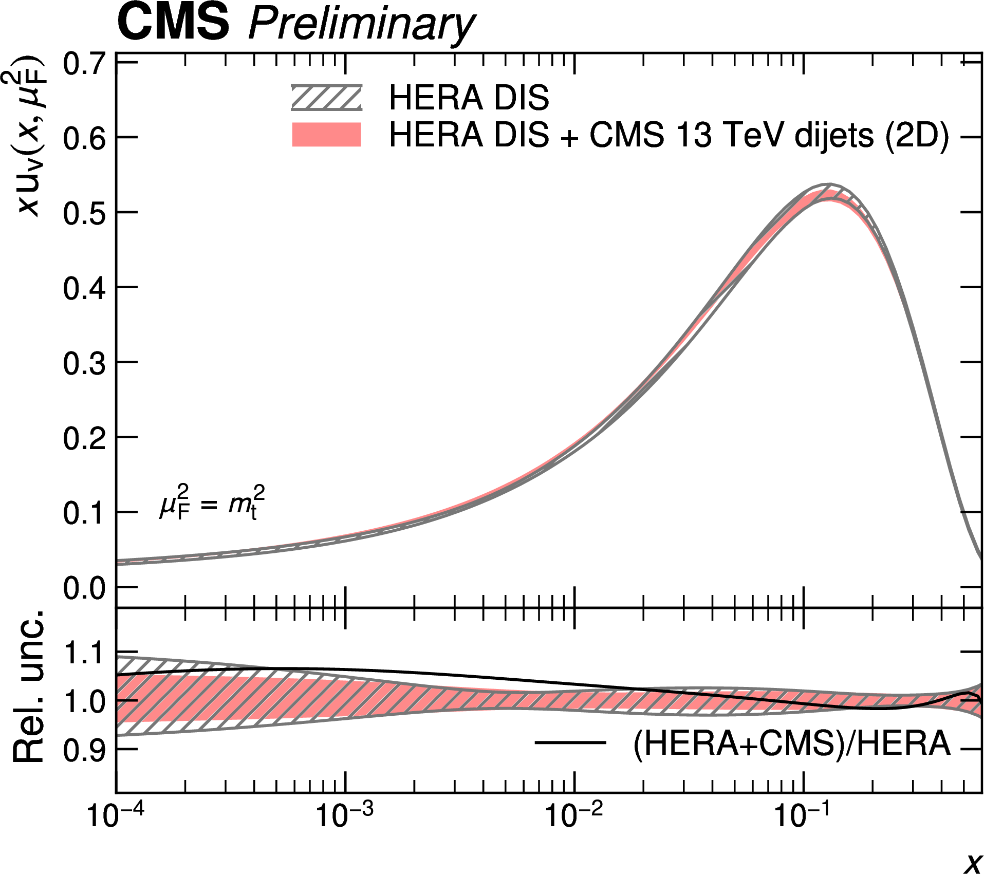
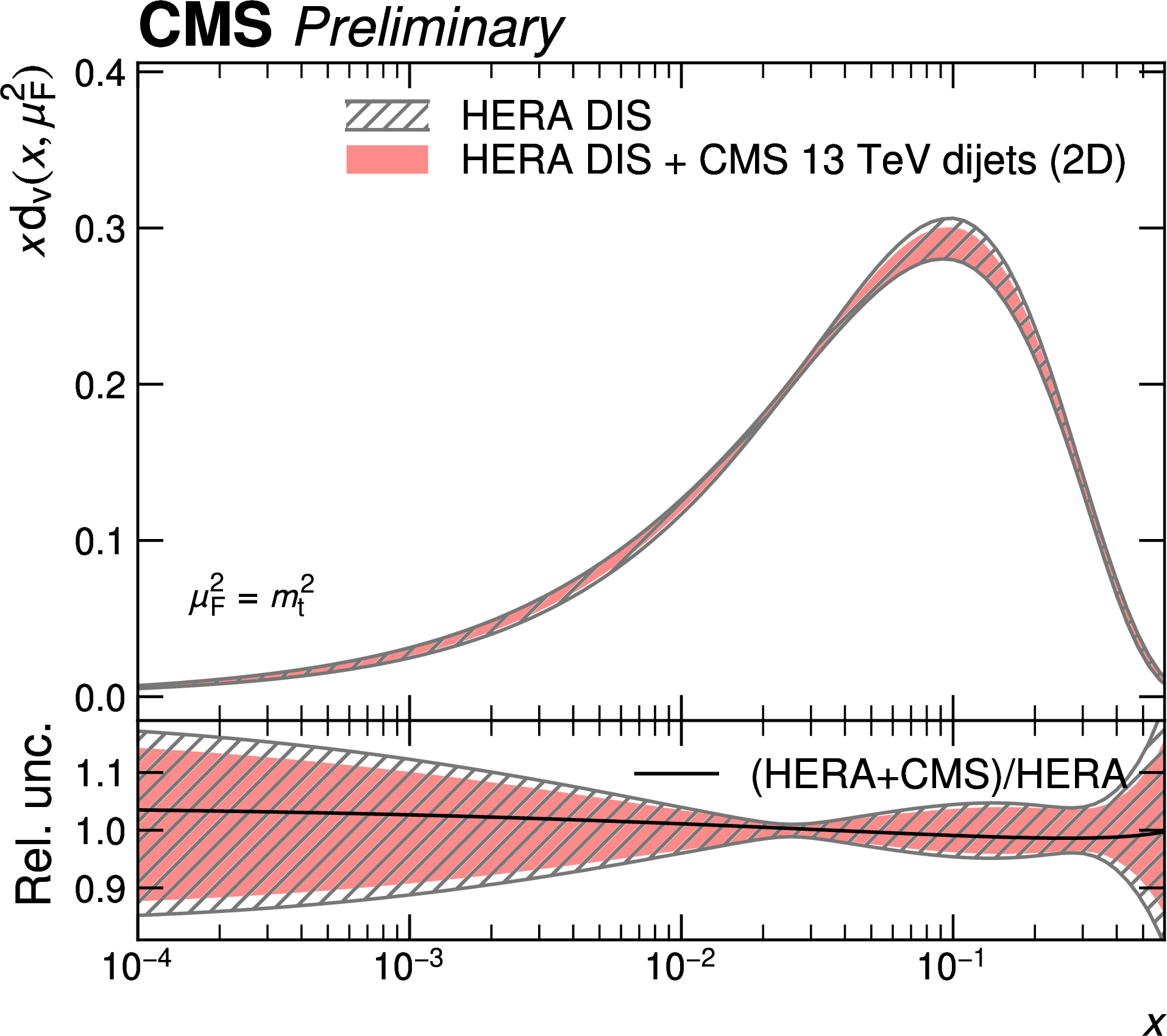
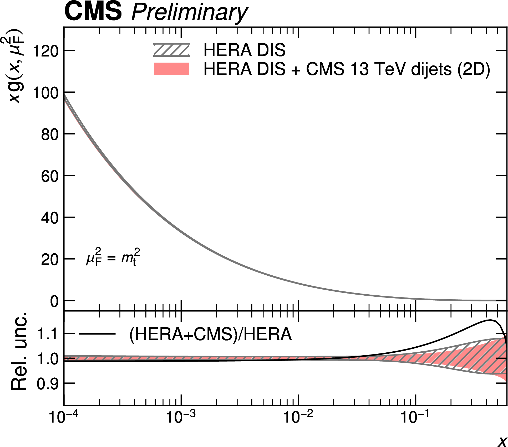
PDFs obtained in a fit to HERA DIS together with CMS 2D dijet data compared to a fit to HERA DIS data alone. Shown are the PDFs of the up and down valence quarks (top row), of the gluon (bottom left), and of the total sea quarks (bottom right) as a function of the fractional parton momentum $ x $ at a factorization scale equal to the top quark mass. The hatched bands indicate the Hessian fit uncertainty and are shown in the lower panels as a relative uncertainty with respect to the corresponding central values. The solid black line shows the ratio between the fitted central values. |
png pdf |
Figure 13-a:
PDFs obtained in a fit to HERA DIS together with CMS 2D dijet data compared to a fit to HERA DIS data alone. Shown are the PDFs of the up valence quark as a function of the fractional parton momentum $ x $ at a factorization scale equal to the top quark mass. The hatched bands indicate the Hessian fit uncertainty and are shown in the lower panels as a relative uncertainty with respect to the corresponding central values. The solid black line shows the ratio between the fitted central values. |
png pdf |
Figure 13-b:
PDFs obtained in a fit to HERA DIS together with CMS 2D dijet data compared to a fit to HERA DIS data alone. Shown are the PDFs of the down valence quark as a function of the fractional parton momentum $ x $ at a factorization scale equal to the top quark mass. The hatched bands indicate the Hessian fit uncertainty and are shown in the lower panels as a relative uncertainty with respect to the corresponding central values. The solid black line shows the ratio between the fitted central values. |
png pdf |
Figure 13-c:
PDFs obtained in a fit to HERA DIS together with CMS 2D dijet data compared to a fit to HERA DIS data alone. Shown are the PDFs of the gluon as a function of the fractional parton momentum $ x $ at a factorization scale equal to the top quark mass. The hatched bands indicate the Hessian fit uncertainty and are shown in the lower panels as a relative uncertainty with respect to the corresponding central values. The solid black line shows the ratio between the fitted central values. |

png pdf |
Figure 13-d:
PDFs obtained in a fit to HERA DIS together with CMS 2D dijet data compared to a fit to HERA DIS data alone. Shown are the PDFs of the total sea quarks as a function of the fractional parton momentum $ x $ at a factorization scale equal to the top quark mass. The hatched bands indicate the Hessian fit uncertainty and are shown in the lower panels as a relative uncertainty with respect to the corresponding central values. The solid black line shows the ratio between the fitted central values. |
png pdf |
Figure 14:
PDFs obtained in a fit to HERA DIS together with CMS 3D dijet data compared to a fit to HERA DIS data alone. Shown are the PDFs of the up and down valence quarks (top row), of the gluon (bottom left), and of the total sea quarks (bottom right) as a function of the fractional parton momentum $ x $ at a factorization scale equal to the top quark mass. The hatched bands indicate the Hessian fit uncertainty and are shown in the lower panels as a relative uncertainty with respect to the corresponding central values. The solid black line shows the ratio between the fitted central values. |
png pdf |
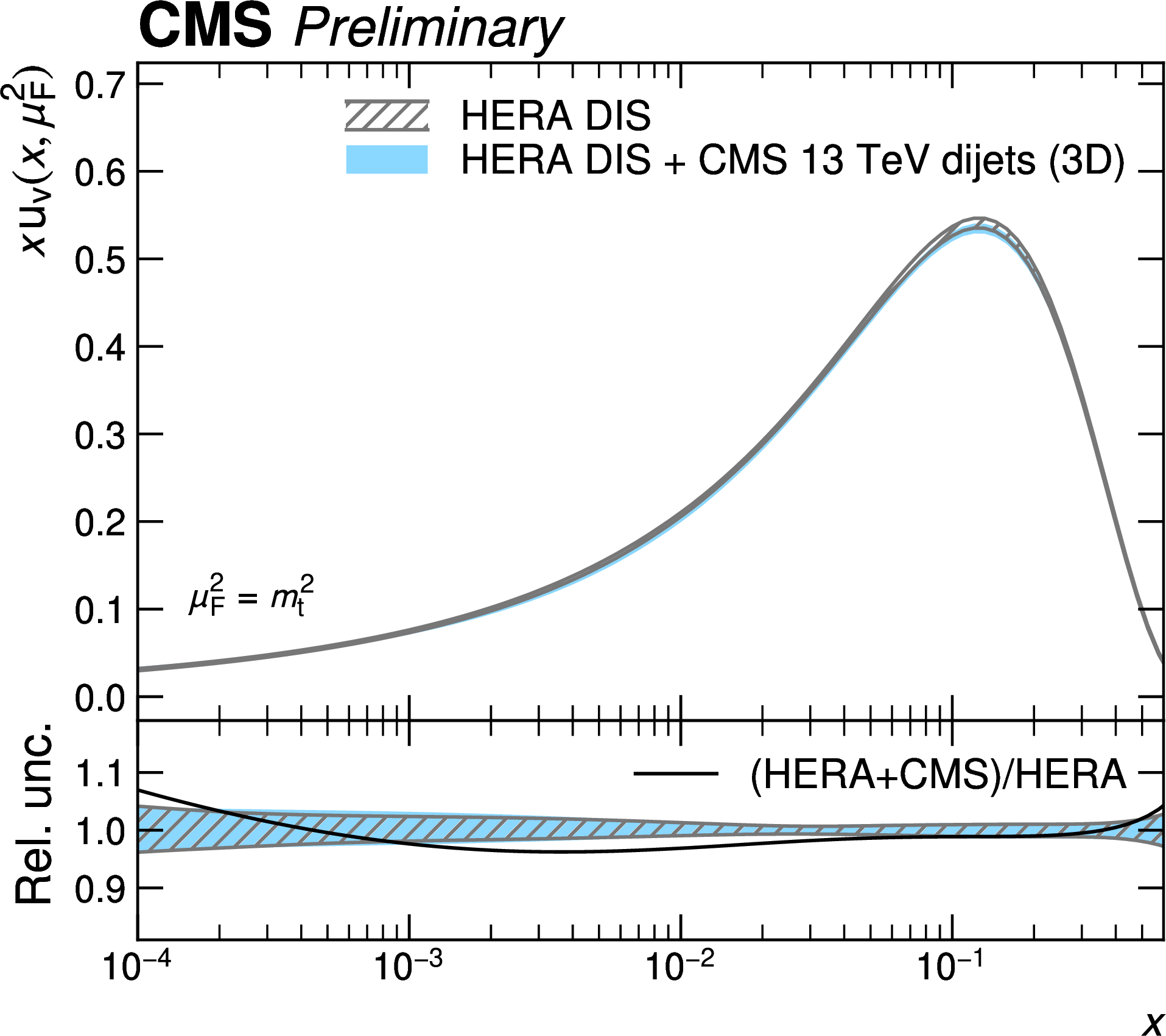
Figure 14-a:
PDFs obtained in a fit to HERA DIS together with CMS 3D dijet data compared to a fit to HERA DIS data alone. Shown are the PDFs of the up valence quark as a function of the fractional parton momentum $ x $ at a factorization scale equal to the top quark mass. The hatched bands indicate the Hessian fit uncertainty and are shown in the lower panels as a relative uncertainty with respect to the corresponding central values. The solid black line shows the ratio between the fitted central values. |
png pdf |
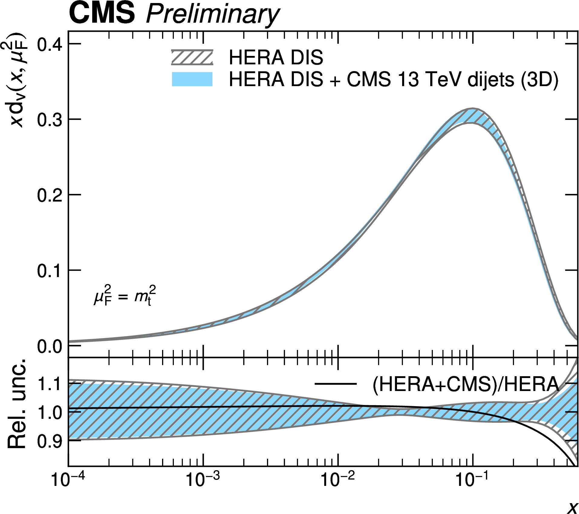
Figure 14-b:
PDFs obtained in a fit to HERA DIS together with CMS 3D dijet data compared to a fit to HERA DIS data alone. Shown are the PDFs of the down valence quark as a function of the fractional parton momentum $ x $ at a factorization scale equal to the top quark mass. The hatched bands indicate the Hessian fit uncertainty and are shown in the lower panels as a relative uncertainty with respect to the corresponding central values. The solid black line shows the ratio between the fitted central values. |
png pdf |
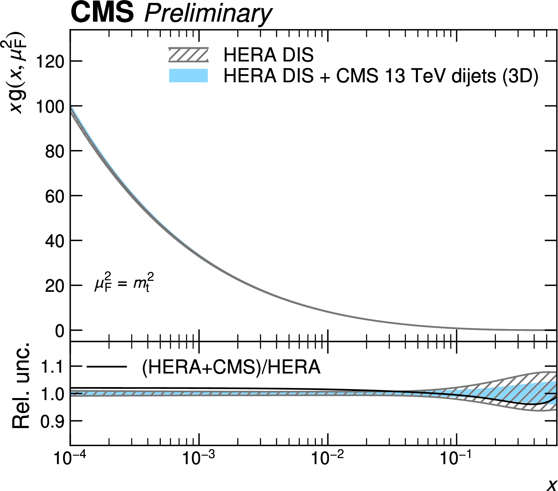
Figure 14-c:
PDFs obtained in a fit to HERA DIS together with CMS 3D dijet data compared to a fit to HERA DIS data alone. Shown are the PDFs of the gluon as a function of the fractional parton momentum $ x $ at a factorization scale equal to the top quark mass. The hatched bands indicate the Hessian fit uncertainty and are shown in the lower panels as a relative uncertainty with respect to the corresponding central values. The solid black line shows the ratio between the fitted central values. |

png pdf |
Figure 14-d:
PDFs obtained in a fit to HERA DIS together with CMS 3D dijet data compared to a fit to HERA DIS data alone. Shown are the PDFs of the total sea quarks as a function of the fractional parton momentum $ x $ at a factorization scale equal to the top quark mass. The hatched bands indicate the Hessian fit uncertainty and are shown in the lower panels as a relative uncertainty with respect to the corresponding central values. The solid black line shows the ratio between the fitted central values. |
png pdf |
Figure 15:
The response matrices for the 2D measurements as a function of $ |y|_{\text{max}} $ and $ m_{1,2} $ for jets with $ R = $ 0.4 (left) and $ R = $ 0.8 (right). The figure description corresponds to that of Fig. 2. |

png pdf |
Figure 15-a:
The response matrices for the 2D measurements as a function of $ |y|_{\text{max}} $ and $ m_{1,2} $ for jets with $ R = $ 0.4. The figure description corresponds to that of Fig. 2. |

png pdf |
Figure 15-b:
The response matrices for the 2D measurements as a function of $ |y|_{\text{max}} $ and $ m_{1,2} $ for jets with $ R = $ 0.8. The figure description corresponds to that of Fig. 2. |
png pdf |
Figure 16:
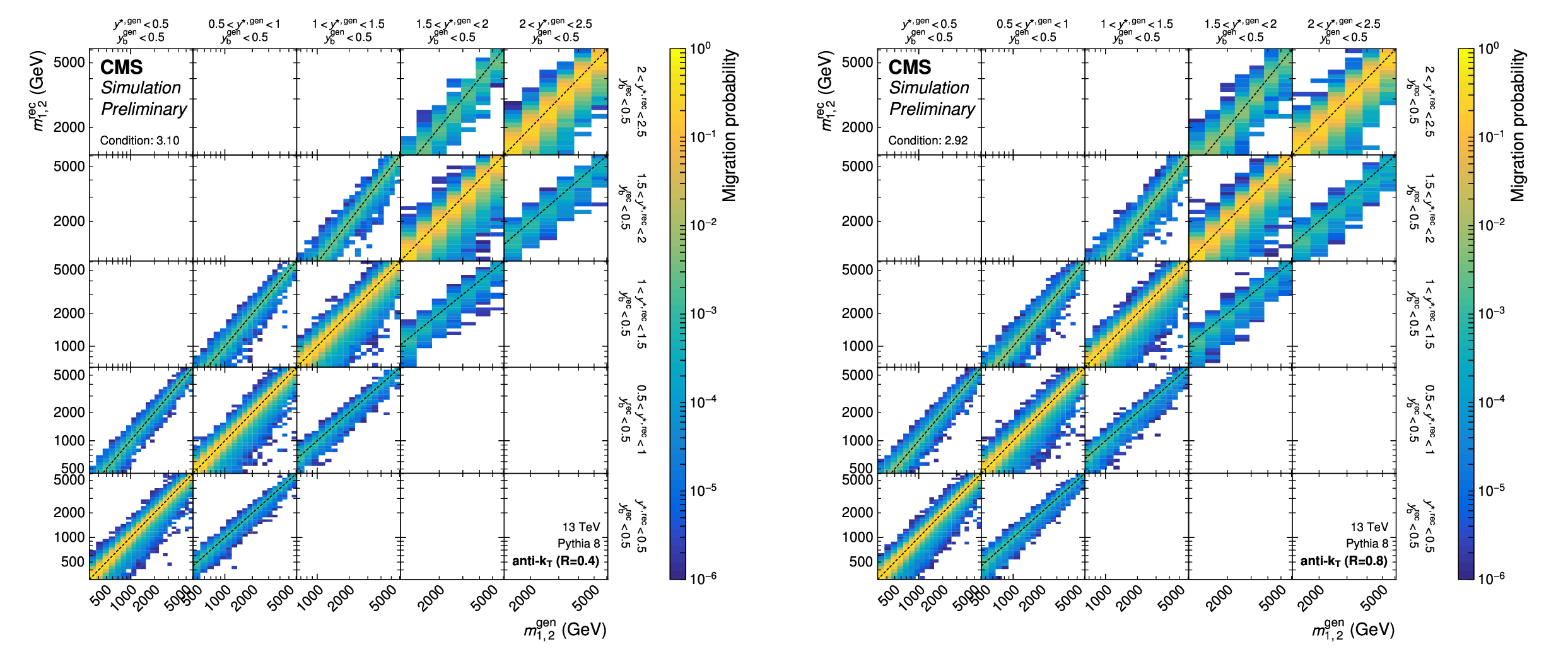
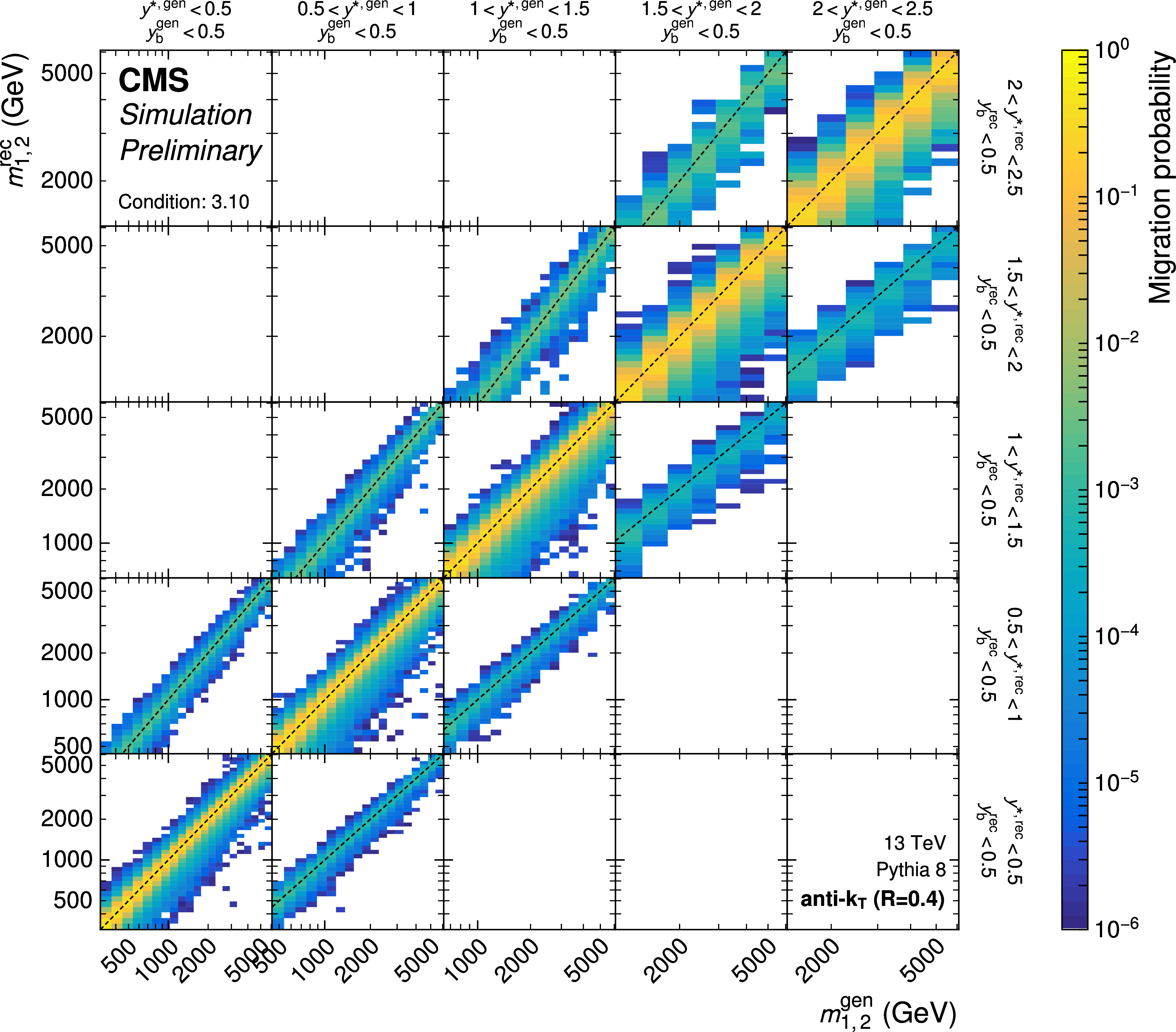
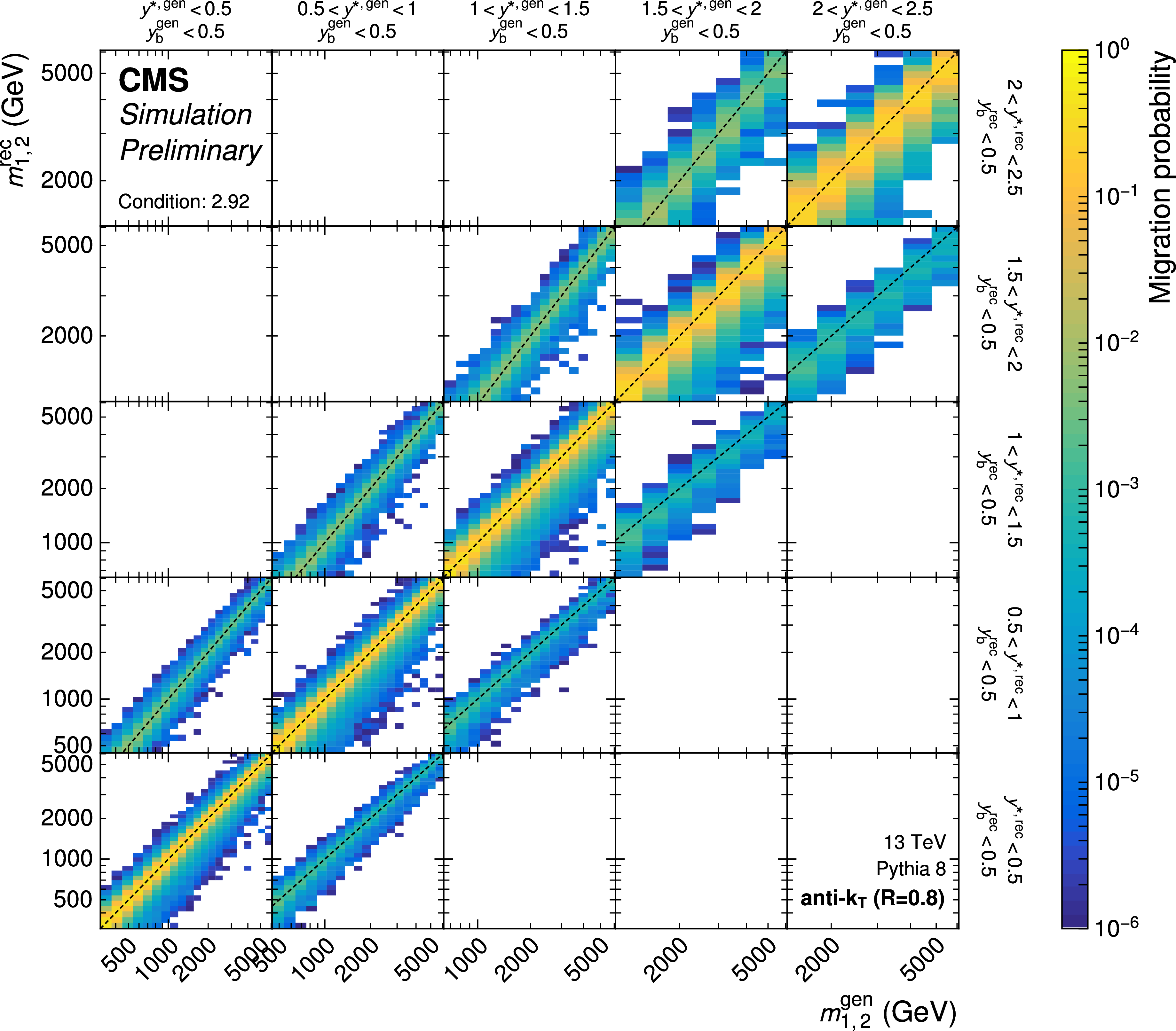
Partial response matrices for the 3D measurements as a function of $ m_{1,2} $ using jets with $ R = $ 0.4 (left) and $ R = $ 0.8 (right), shown here for the five rapidity regions with $ y_{\text{b}} < $ 0.5. The figure description corresponds to that of Fig. 2. |
png pdf |
Figure 16-a:
Partial response matrices for the 3D measurements as a function of $ m_{1,2} $ using jets with $ R = $ 0.4, shown here for the five rapidity regions with $ y_{\text{b}} < $ 0.5. The figure description corresponds to that of Fig. 2. |
png pdf |
Figure 16-b:
Partial response matrices for the 3D measurements as a function of $ m_{1,2} $ using jets with $ R = $ 0.8, shown here for the five rapidity regions with $ y_{\text{b}} < $ 0.5. The figure description corresponds to that of Fig. 2. |
png pdf |
Figure 17:
Partial response matrices for the 3D measurements as a function of $ \langle p_{\mathrm{T}} \rangle_{1,2} $ using jets with $ R = $ 0.4 (left) and $ R = $ 0.8 (right), shown here for the five rapidity regions with $ y_{\text{b}} < $ 0.5. The figure description corresponds to that of Fig. 2. |

png pdf |
Figure 17-a:
Partial response matrices for the 3D measurements as a function of $ \langle p_{\mathrm{T}} \rangle_{1,2} $ using jets with $ R = $ 0.4, shown here for the five rapidity regions with $ y_{\text{b}} < $ 0.5. The figure description corresponds to that of Fig. 2. |
png pdf |
Figure 17-b:
Partial response matrices for the 3D measurements as a function of $ \langle p_{\mathrm{T}} \rangle_{1,2} $ using jets with $ R = $ 0.8, shown here for the five rapidity regions with $ y_{\text{b}} < $ 0.5. The figure description corresponds to that of Fig. 2. |
png pdf |
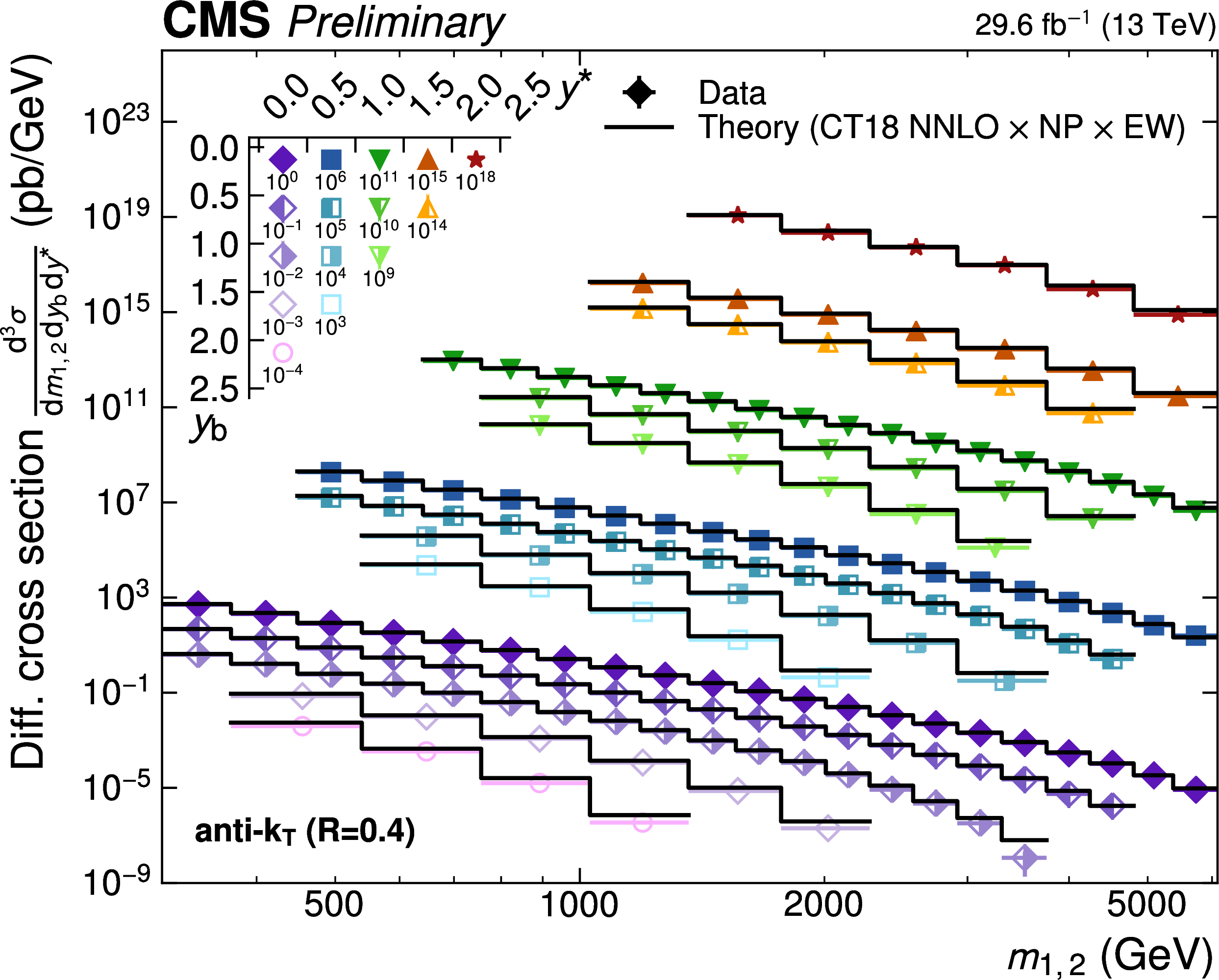
Figure 18:
Overview of the 2D dijet cross section as a function of $ m_{1,2} $ in all 5 $ |y|_{\text{max}} $ regions, using jets with $ R = $ 0.4 (left) and $ R = $ 0.8 (right). The figure description corresponds to that of Fig. 8. |
png pdf |
Figure 18-a:
Overview of the 2D dijet cross section as a function of $ m_{1,2} $ in all 5 $ |y|_{\text{max}} $ regions, using jets with $ R = $ 0.4. The figure description corresponds to that of Fig. 8. |

png pdf |
Figure 18-b:
Overview of the 2D dijet cross section as a function of $ m_{1,2} $ in all 5 $ |y|_{\text{max}} $ regions, using jets with $ R = $ 0.8. The figure description corresponds to that of Fig. 8. |
png pdf |
Figure 19:
Overview of the 3D dijet cross section as a function of $ m_{1,2} $ in all 15 $ {(y^{*}\!, y_{\text{b}})} $ regions, using jets with $ R = $ 0.4 (left) and $ R = $ 0.8 (right). The figure description corresponds to that of Fig. 8. |
png pdf |
Figure 19-a:
Overview of the 3D dijet cross section as a function of $ m_{1,2} $ in all 15 $ {(y^{*}\!, y_{\text{b}})} $ regions, using jets with $ R = $ 0.4. The figure description corresponds to that of Fig. 8. |

png pdf |
Figure 19-b:
Overview of the 3D dijet cross section as a function of $ m_{1,2} $ in all 15 $ {(y^{*}\!, y_{\text{b}})} $ regions, using jets with $ R = $ 0.8. The figure description corresponds to that of Fig. 8. |
png pdf |
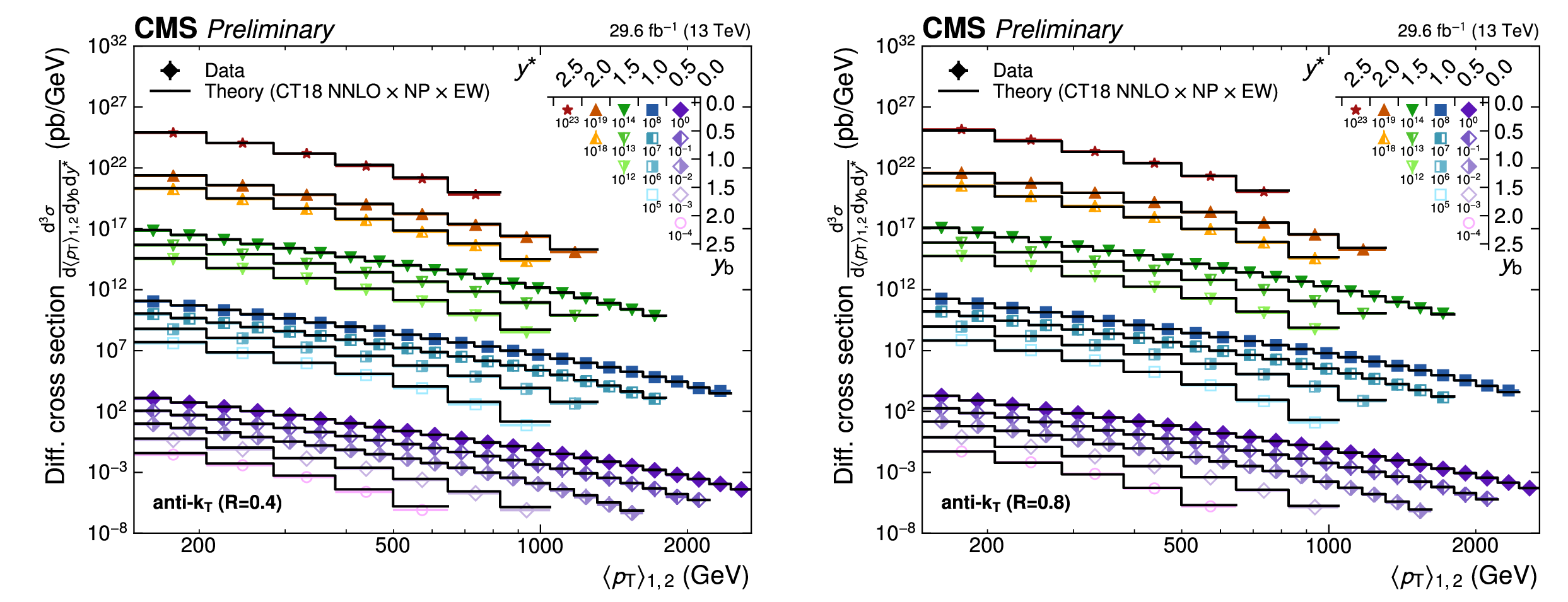
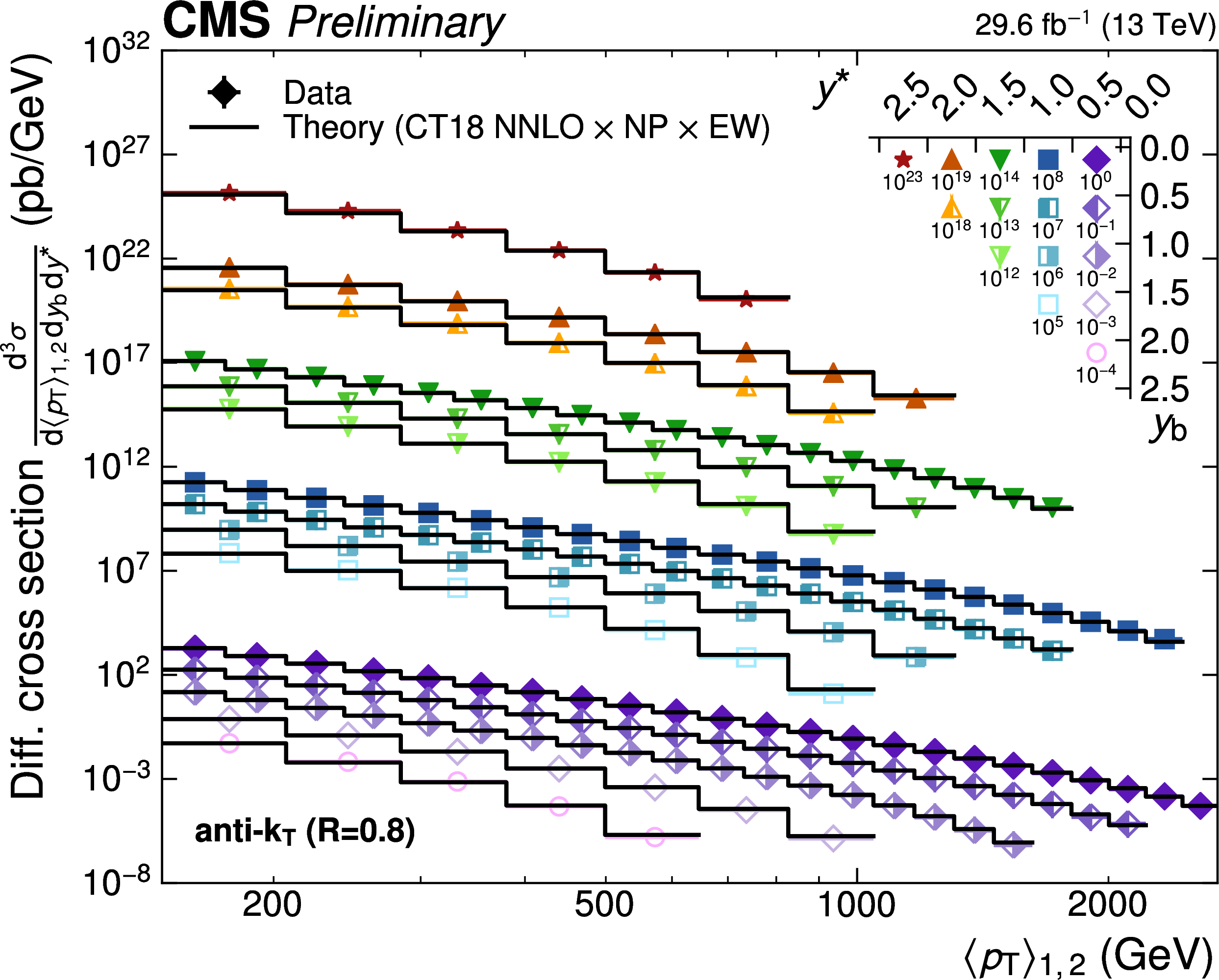
Figure 20:
Overview of the 3D dijet cross section as a function of $ \langle p_{\mathrm{T}} \rangle_{1,2} $ in all 15 $ {(y^{*}\!, y_{\text{b}})} $ regions, using jets with $ R = $ 0.4 (left) and $ R = $ 0.8 (right). The figure description corresponds to that of Fig. 8. |

png pdf |
Figure 20-a:
Overview of the 3D dijet cross section as a function of $ \langle p_{\mathrm{T}} \rangle_{1,2} $ in all 15 $ {(y^{*}\!, y_{\text{b}})} $ regions, using jets with $ R = $ 0.4. The figure description corresponds to that of Fig. 8. |
png pdf |
Figure 20-b:
Overview of the 3D dijet cross section as a function of $ \langle p_{\mathrm{T}} \rangle_{1,2} $ in all 15 $ {(y^{*}\!, y_{\text{b}})} $ regions, using jets with $ R = $ 0.8. The figure description corresponds to that of Fig. 8. |
png pdf |
Figure 21:
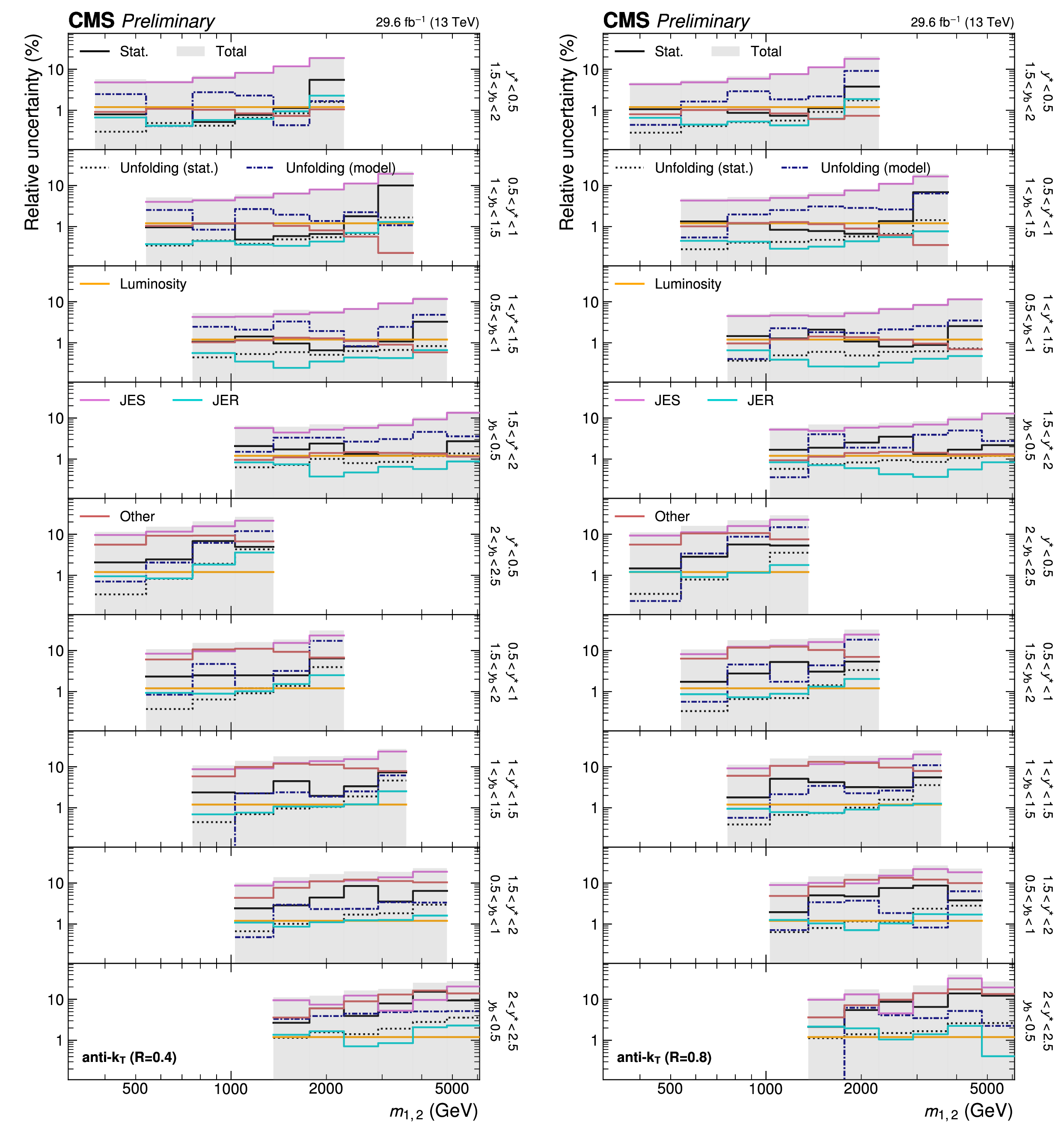
Detailed breakdown of the experimental uncertainty for the 3D measurements as a function of $ m_{1,2} $ using jets with $ R = $ 0.4 (left) and $ R = $ 0.8 (right), in six out of 15 $ {(y^{*}\!, y_{\text{b}})} $ bins. The figure description corresponds to that of Fig. 4. |
png pdf |
Figure 21-a:
Detailed breakdown of the experimental uncertainty for the 3D measurements as a function of $ m_{1,2} $ using jets with $ R = $ 0.4, in six out of 15 $ {(y^{*}\!, y_{\text{b}})} $ bins. The figure description corresponds to that of Fig. 4. |
png pdf |
Figure 21-b:
Detailed breakdown of the experimental uncertainty for the 3D measurements as a function of $ m_{1,2} $ using jets with $ R = $ 0.8, in six out of 15 $ {(y^{*}\!, y_{\text{b}})} $ bins. The figure description corresponds to that of Fig. 4. |
png pdf |
Figure 22:
(continuation of Fig. 21) Detailed breakdown of the experimental uncertainty for the 3D measurements as a function of $ m_{1,2} $ using jets with $ R = $ 0.4 (left) and $ R = $ 0.8 (right), in the remaining nine out of 15 $ {(y^{*}\!, y_{\text{b}})} $ bins. The figure description corresponds to that of Fig. 4. |
png pdf |
Figure 22-a:
(continuation of Fig. 21) Detailed breakdown of the experimental uncertainty for the 3D measurements as a function of $ m_{1,2} $ using jets with $ R = $ 0.4, in the remaining nine out of 15 $ {(y^{*}\!, y_{\text{b}})} $ bins. The figure description corresponds to that of Fig. 4. |
png pdf |
Figure 22-b:
(continuation of Fig. 21) Detailed breakdown of the experimental uncertainty for the 3D measurements as a function of $ m_{1,2} $ using jets with $ R = $ 0.8, in the remaining nine out of 15 $ {(y^{*}\!, y_{\text{b}})} $ bins. The figure description corresponds to that of Fig. 4. |
png pdf |
Figure 23:
Detailed breakdown of the experimental uncertainty for the 3D measurements as a function of $ \langle p_{\mathrm{T}} \rangle_{1,2} $ using jets with $ R = $ 0.4 (left) and $ R = $ 0.8 (right), in six out of 15 $ {(y^{*}\!, y_{\text{b}})} $ bins. The figure description corresponds to that of Fig. 4. |

png pdf |
Figure 23-a:
Detailed breakdown of the experimental uncertainty for the 3D measurements as a function of $ \langle p_{\mathrm{T}} \rangle_{1,2} $ using jets with $ R = $ 0.4, in six out of 15 $ {(y^{*}\!, y_{\text{b}})} $ bins. The figure description corresponds to that of Fig. 4. |
png pdf |
Figure 23-b:
Detailed breakdown of the experimental uncertainty for the 3D measurements as a function of $ \langle p_{\mathrm{T}} \rangle_{1,2} $ using jets with $ R = $ 0.8, in six out of 15 $ {(y^{*}\!, y_{\text{b}})} $ bins. The figure description corresponds to that of Fig. 4. |

png pdf |
Figure 24:
(continuation of Fig. 23) Detailed breakdown of the experimental uncertainty for the 3D measurements as a function of $ \langle p_{\mathrm{T}} \rangle_{1,2} $ using jets with $ R = $ 0.4 (left) and $ R = $ 0.8 (right), in the remaining nine out of 15 $ {(y^{*}\!, y_{\text{b}})} $ bins. The figure description corresponds to that of Fig. 4. |

png pdf |
Figure 24-a:
(continuation of Fig. 23) Detailed breakdown of the experimental uncertainty for the 3D measurements as a function of $ \langle p_{\mathrm{T}} \rangle_{1,2} $ using jets with $ R = $ 0.4, in the remaining nine out of 15 $ {(y^{*}\!, y_{\text{b}})} $ bins. The figure description corresponds to that of Fig. 4. |
png pdf |
Figure 24-b:
(continuation of Fig. 23) Detailed breakdown of the experimental uncertainty for the 3D measurements as a function of $ \langle p_{\mathrm{T}} \rangle_{1,2} $ using jets with $ R = $ 0.8, in the remaining nine out of 15 $ {(y^{*}\!, y_{\text{b}})} $ bins. The figure description corresponds to that of Fig. 4. |
png pdf |
Figure 25:
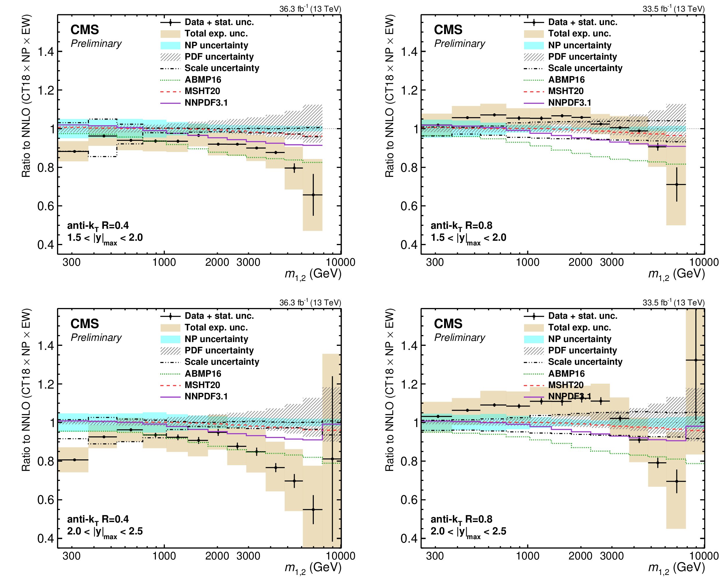
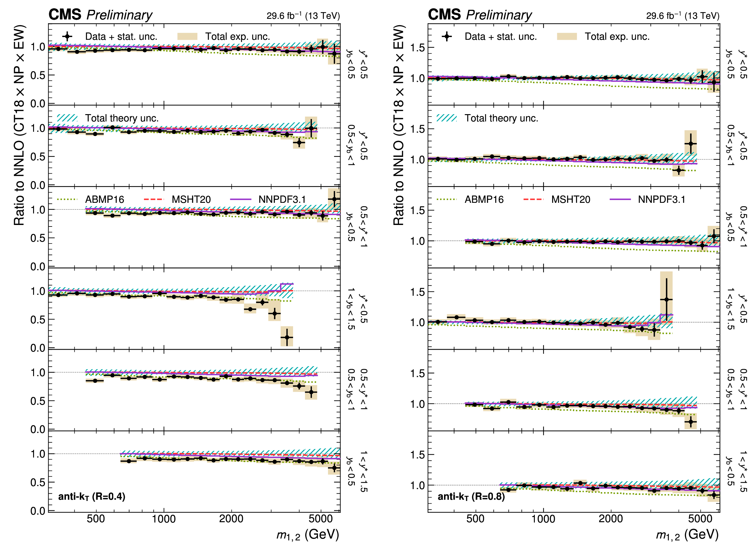
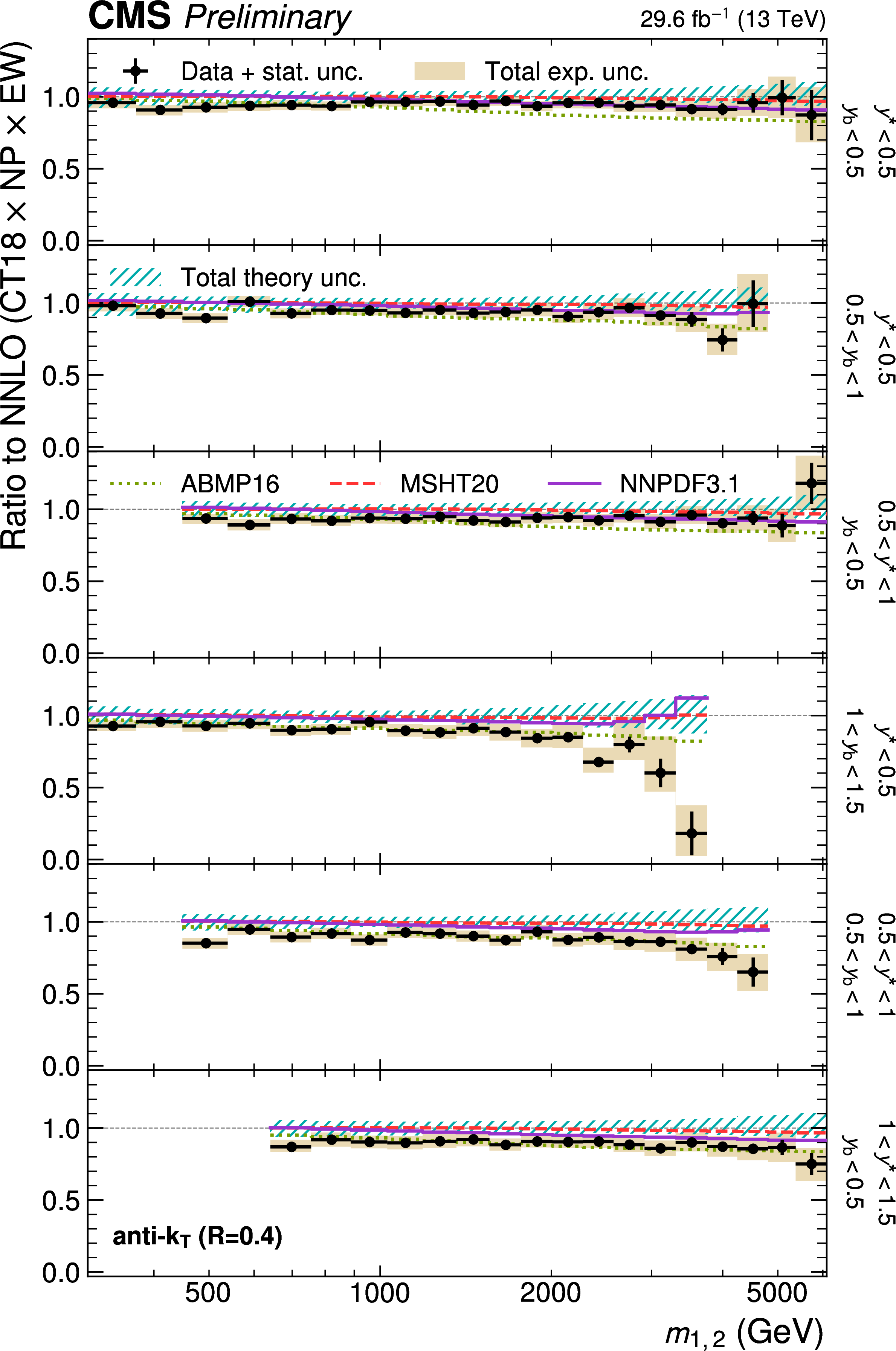
Comparison of the 2D dijet cross section for jets with $ R = $ 0.4 (left) and $ R = $ 0.8 (right) as a function of $ m_{1,2} $ to fixed-order theory calculations at NNLO, shown here for three inner $ |y|_{\text{max}} $ regions. The figure description corresponds to that of Fig. 9. |
png pdf |
Figure 25-a:
Comparison of the 2D dijet cross section for jets with $ R = $ 0.4, as a function of $ m_{1,2} $ to fixed-order theory calculations at NNLO, shown here for three inner $ |y|_{\text{max}} $ regions. The figure description corresponds to that of Fig. 9. |

png pdf |
Figure 25-b:
Comparison of the 2D dijet cross section for jets with $ R = $ 0.8, as a function of $ m_{1,2} $ to fixed-order theory calculations at NNLO, shown here for three inner $ |y|_{\text{max}} $ regions. The figure description corresponds to that of Fig. 9. |
png pdf |
Figure 25-c:
Comparison of the 2D dijet cross section for jets with $ R = $ 0.4 (left) and $ R = $ 0.8 (right) as a function of $ m_{1,2} $ to fixed-order theory calculations at NNLO, shown here for three inner $ |y|_{\text{max}} $ regions. The figure description corresponds to that of Fig. 9. -c |

png pdf |
Figure 25-d:
Comparison of the 2D dijet cross section for jets with $ R = $ 0.4 (left) and $ R = $ 0.8 (right) as a function of $ m_{1,2} $ to fixed-order theory calculations at NNLO, shown here for three inner $ |y|_{\text{max}} $ regions. The figure description corresponds to that of Fig. 9. -d |

png pdf |
Figure 25-e:
Comparison of the 2D dijet cross section for jets with $ R = $ 0.4 (left) and $ R = $ 0.8 (right) as a function of $ m_{1,2} $ to fixed-order theory calculations at NNLO, shown here for three inner $ |y|_{\text{max}} $ regions. The figure description corresponds to that of Fig. 9. -e |
png pdf |
Figure 25-f:
Comparison of the 2D dijet cross section for jets with $ R = $ 0.4 (left) and $ R = $ 0.8 (right) as a function of $ m_{1,2} $ to fixed-order theory calculations at NNLO, shown here for three inner $ |y|_{\text{max}} $ regions. The figure description corresponds to that of Fig. 9. -f |
png pdf |
Figure 26:
(continuation of Fig. 25) Comparison of the 2D dijet cross section for jets with $ R = $ 0.4 (left) and $ R = $ 0.8 (right) as a function of $ m_{1,2} $ to fixed-order theory calculations at NNLO, shown here for two outermost $ |y|_{\text{max}} $ regions. The figure description corresponds to that of Fig. 9. |
png pdf |
Figure 26-a:
(continuation of Fig. 25) Comparison of the 2D dijet cross section for jets with $ R = $ 0.4, as a function of $ m_{1,2} $ to fixed-order theory calculations at NNLO, shown here for two outermost $ |y|_{\text{max}} $ regions. The figure description corresponds to that of Fig. 9. |
png pdf |
Figure 26-b:
(continuation of Fig. 25) Comparison of the 2D dijet cross section for jets with $ R = $ 0.8, as a function of $ m_{1,2} $ to fixed-order theory calculations at NNLO, shown here for two outermost $ |y|_{\text{max}} $ regions. The figure description corresponds to that of Fig. 9. |
png pdf |
Figure 26-c:
(continuation of Fig. 25) Comparison of the 2D dijet cross section for jets with $ R = $ 0.4 (left) and $ R = $ 0.8 (right) as a function of $ m_{1,2} $ to fixed-order theory calculations at NNLO, shown here for two outermost $ |y|_{\text{max}} $ regions. The figure description corresponds to that of Fig. 9. -c |
png pdf |
Figure 26-d:
(continuation of Fig. 25) Comparison of the 2D dijet cross section for jets with $ R = $ 0.4 (left) and $ R = $ 0.8 (right) as a function of $ m_{1,2} $ to fixed-order theory calculations at NNLO, shown here for two outermost $ |y|_{\text{max}} $ regions. The figure description corresponds to that of Fig. 9. -d |
png pdf |
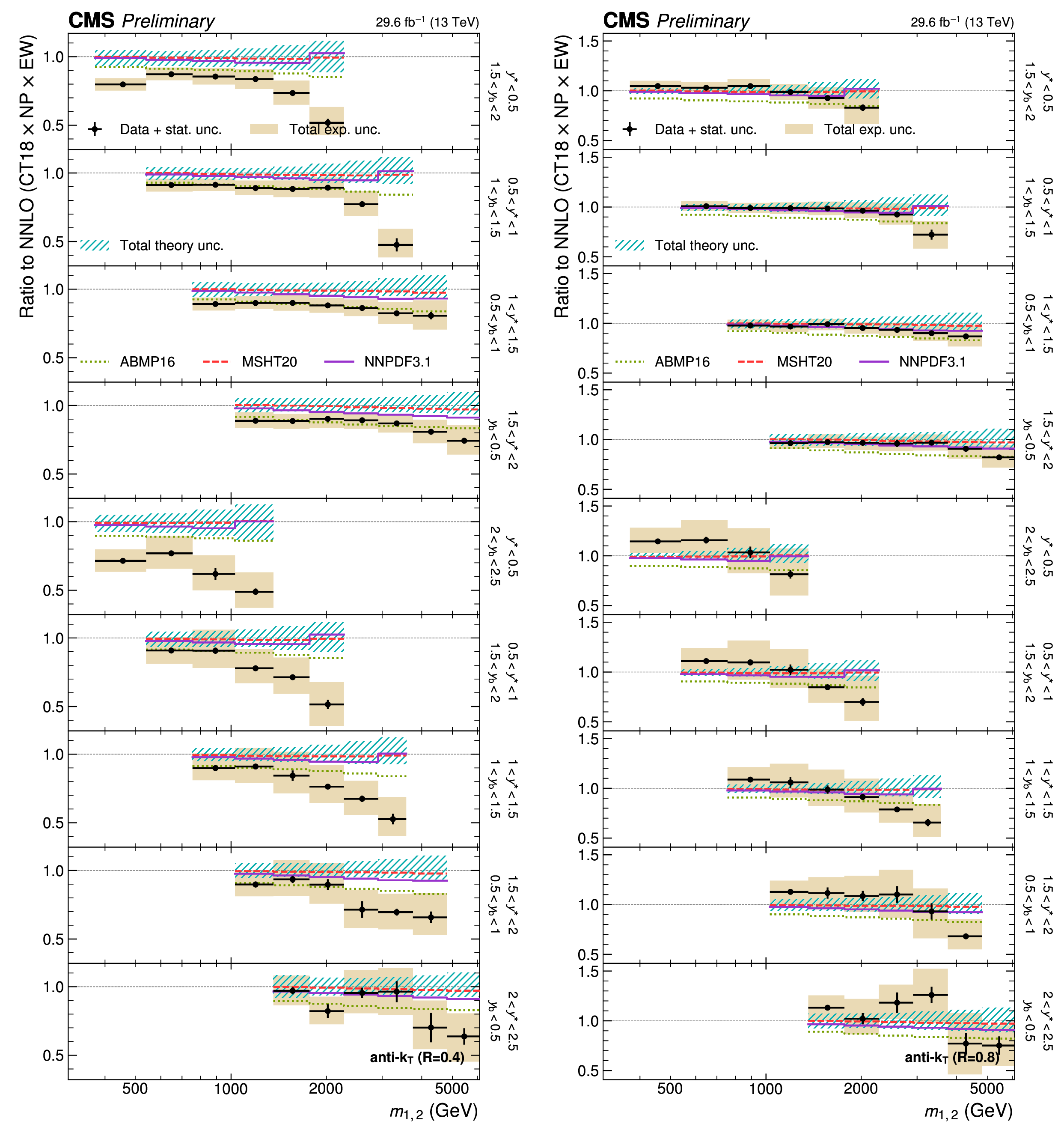
Figure 27:
Comparison of the 3D dijet cross section as a function of $ m_{1,2} $ to fixed-order theory calculations at NNLO, using jets with $ R = $ 0.4 (left) and $ R = $ 0.8 (right), in six out of the total 15 $ {(y^{*}\!, y_{\text{b}})} $ bins. The figure description corresponds to that of Fig. 10. |
png pdf |
Figure 27-a:
Comparison of the 3D dijet cross section as a function of $ m_{1,2} $ to fixed-order theory calculations at NNLO, using jets with $ R = $ 0.4, in six out of the total 15 $ {(y^{*}\!, y_{\text{b}})} $ bins. The figure description corresponds to that of Fig. 10. |
png pdf |
Figure 27-b:
Comparison of the 3D dijet cross section as a function of $ m_{1,2} $ to fixed-order theory calculations at NNLO, using jets with $ R = $ 0.8, in six out of the total 15 $ {(y^{*}\!, y_{\text{b}})} $ bins. The figure description corresponds to that of Fig. 10. |
png pdf |
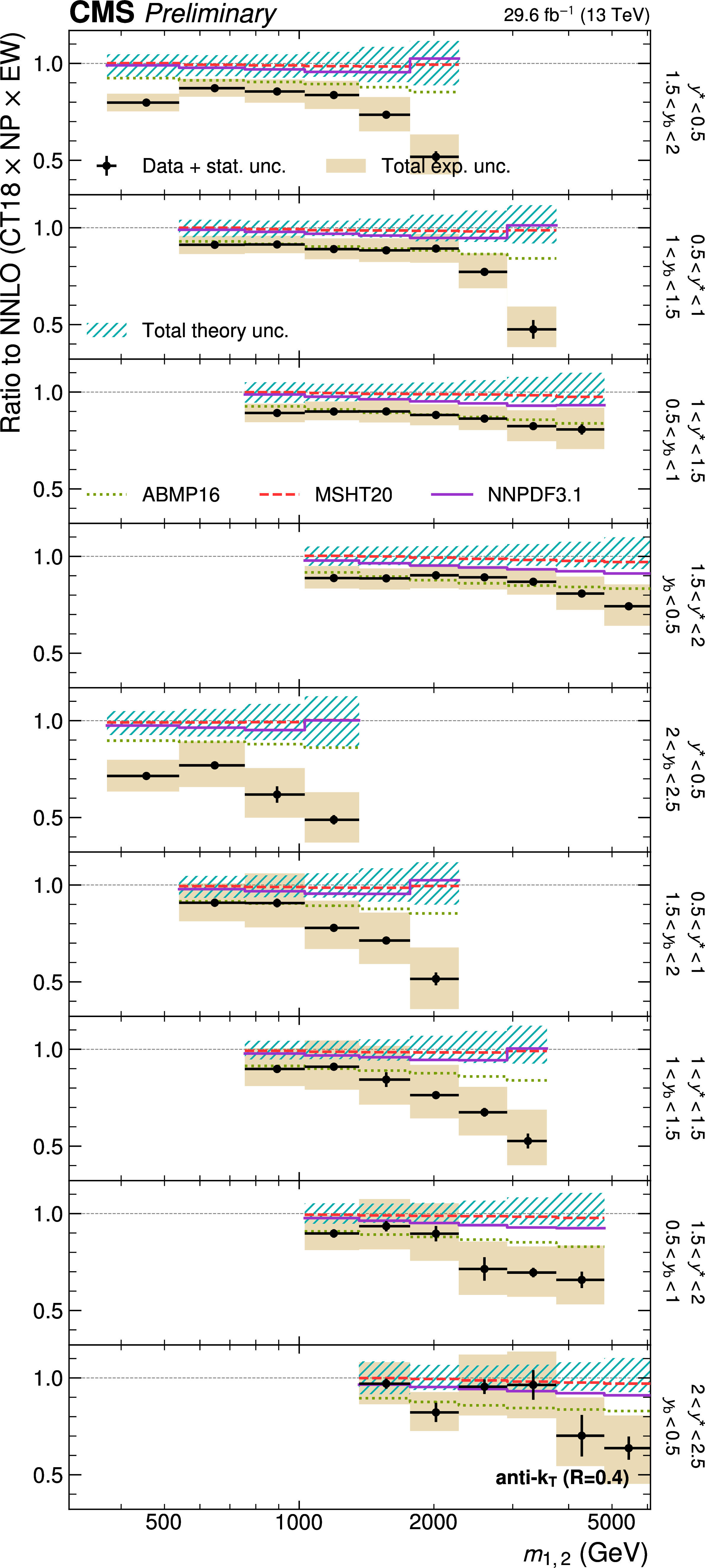
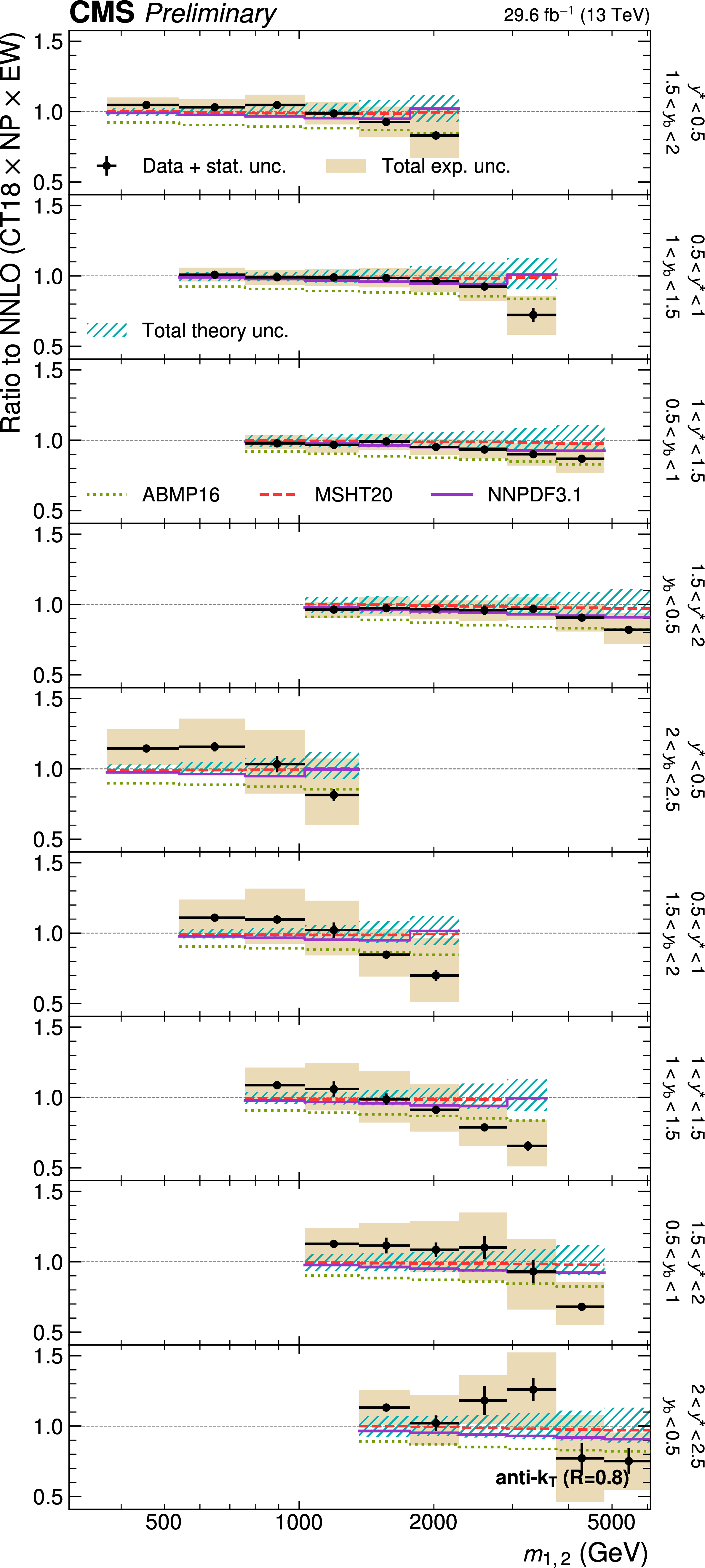
Figure 28:
(continuation of Fig. 27) Comparison of the 3D dijet cross section as a function of $ \langle p_{\mathrm{T}} \rangle_{1,2} $ to fixed-order theory calculations at NNLO, using jets with $ R = $ 0.4 (left) and $ R = $ 0.8 (right), in the remaining nine out of 15 $ {(y^{*}\!, y_{\text{b}})} $ bins. The figure description corresponds to that of Fig. 10. |
png pdf |
Figure 28-a:
(continuation of Fig. 27) Comparison of the 3D dijet cross section as a function of $ \langle p_{\mathrm{T}} \rangle_{1,2} $ to fixed-order theory calculations at NNLO, using jets with $ R = $ 0.4, in the remaining nine out of 15 $ {(y^{*}\!, y_{\text{b}})} $ bins. The figure description corresponds to that of Fig. 10. |
png pdf |
Figure 28-b:
(continuation of Fig. 27) Comparison of the 3D dijet cross section as a function of $ \langle p_{\mathrm{T}} \rangle_{1,2} $ to fixed-order theory calculations at NNLO, using jets with $ R = $ 0.8, in the remaining nine out of 15 $ {(y^{*}\!, y_{\text{b}})} $ bins. The figure description corresponds to that of Fig. 10. |
png pdf |
Figure 29:
Comparison of the 3D dijet cross section as a function of $ \langle p_{\mathrm{T}} \rangle_{1,2} $ to fixed-order theory calculations at NNLO, using jets with $ R = $ 0.4 (left) and $ R = $ 0.8 (right), in six out of the total 15 $ {(y^{*}\!, y_{\text{b}})} $ bins. The figure description corresponds to that of Fig. 10. |
png pdf |
Figure 29-a:
Comparison of the 3D dijet cross section as a function of $ \langle p_{\mathrm{T}} \rangle_{1,2} $ to fixed-order theory calculations at NNLO, using jets with $ R = $ 0.4, in six out of the total 15 $ {(y^{*}\!, y_{\text{b}})} $ bins. The figure description corresponds to that of Fig. 10. |
png pdf |
Figure 29-b:
Comparison of the 3D dijet cross section as a function of $ \langle p_{\mathrm{T}} \rangle_{1,2} $ to fixed-order theory calculations at NNLO, using jets with $ R = $ 0.8, in six out of the total 15 $ {(y^{*}\!, y_{\text{b}})} $ bins. The figure description corresponds to that of Fig. 10. |
png pdf |
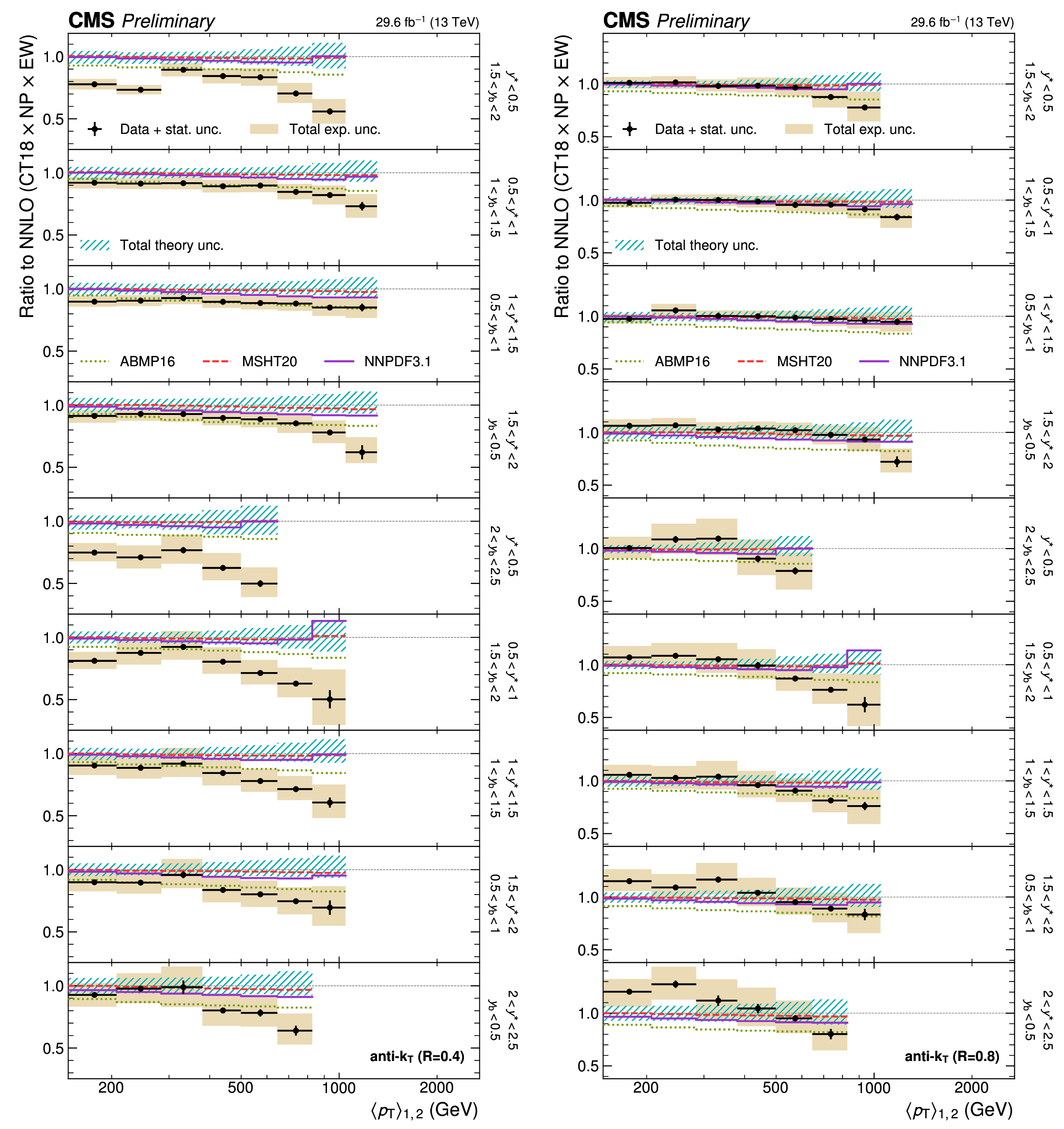
Figure 30:
(continuation of Fig. 29) Comparison of the 3D dijet cross section as a function of $ \langle p_{\mathrm{T}} \rangle_{1,2} $ to fixed-order theory calculations at NNLO, using jets with $ R = $ 0.4 (left) and $ R = $ 0.8 (right), in the remaining nine out of 15 $ {(y^{*}\!, y_{\text{b}})} $ bins. The figure description corresponds to that of Fig. 10. |
png pdf |
Figure 30-a:
(continuation of Fig. 29) Comparison of the 3D dijet cross section as a function of $ \langle p_{\mathrm{T}} \rangle_{1,2} $ to fixed-order theory calculations at NNLO, using jets with $ R = $ 0.4, in the remaining nine out of 15 $ {(y^{*}\!, y_{\text{b}})} $ bins. The figure description corresponds to that of Fig. 10. |
png pdf |
Figure 30-b:
(continuation of Fig. 29) Comparison of the 3D dijet cross section as a function of $ \langle p_{\mathrm{T}} \rangle_{1,2} $ to fixed-order theory calculations at NNLO, using jets with $ R = $ 0.8, in the remaining nine out of 15 $ {(y^{*}\!, y_{\text{b}})} $ bins. The figure description corresponds to that of Fig. 10. |
| Tables | |
png pdf |
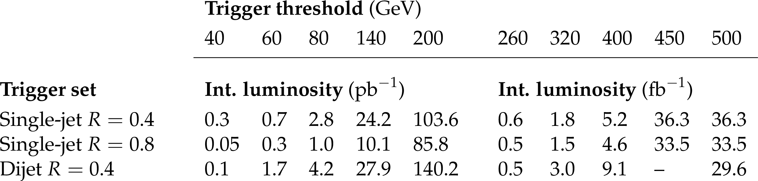
Table 1:
Overview of the single-jet (dijet) triggers deployed for the different $ p_{\mathrm{T}} $ ($ \langle p_{\mathrm{T}} \rangle $) thresholds at the HLT, and the corresponding integrated luminosities. |
png pdf |
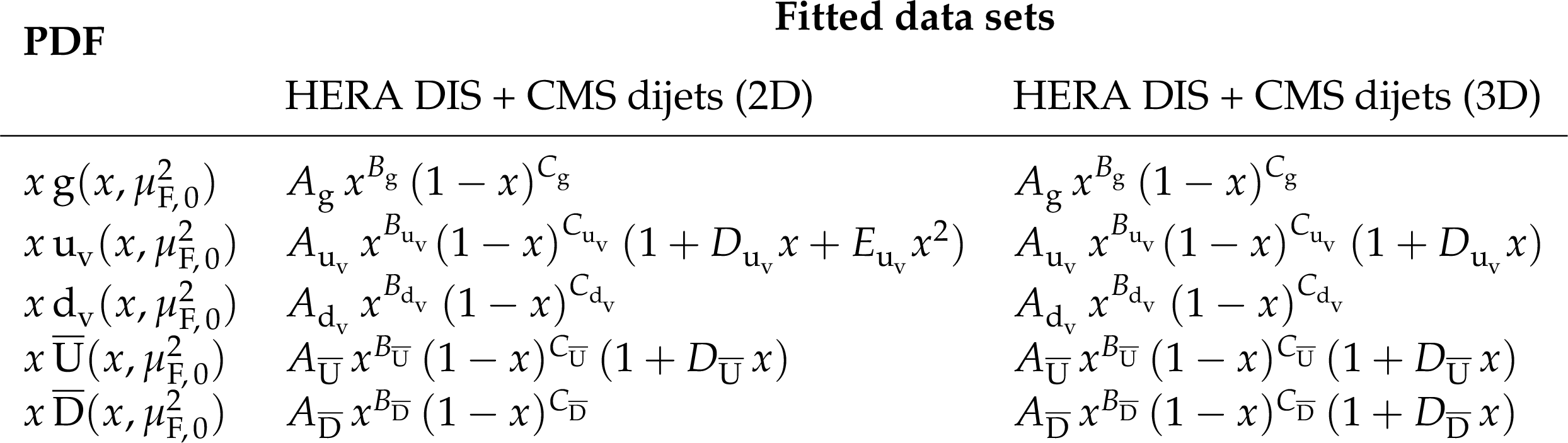
Table 2:
PDF parametrizations obtained after the $ \chi^2 $ scan for the fits of the HERA DIS data together with the CMS 2D or 3D dijet measurements. |
png pdf |
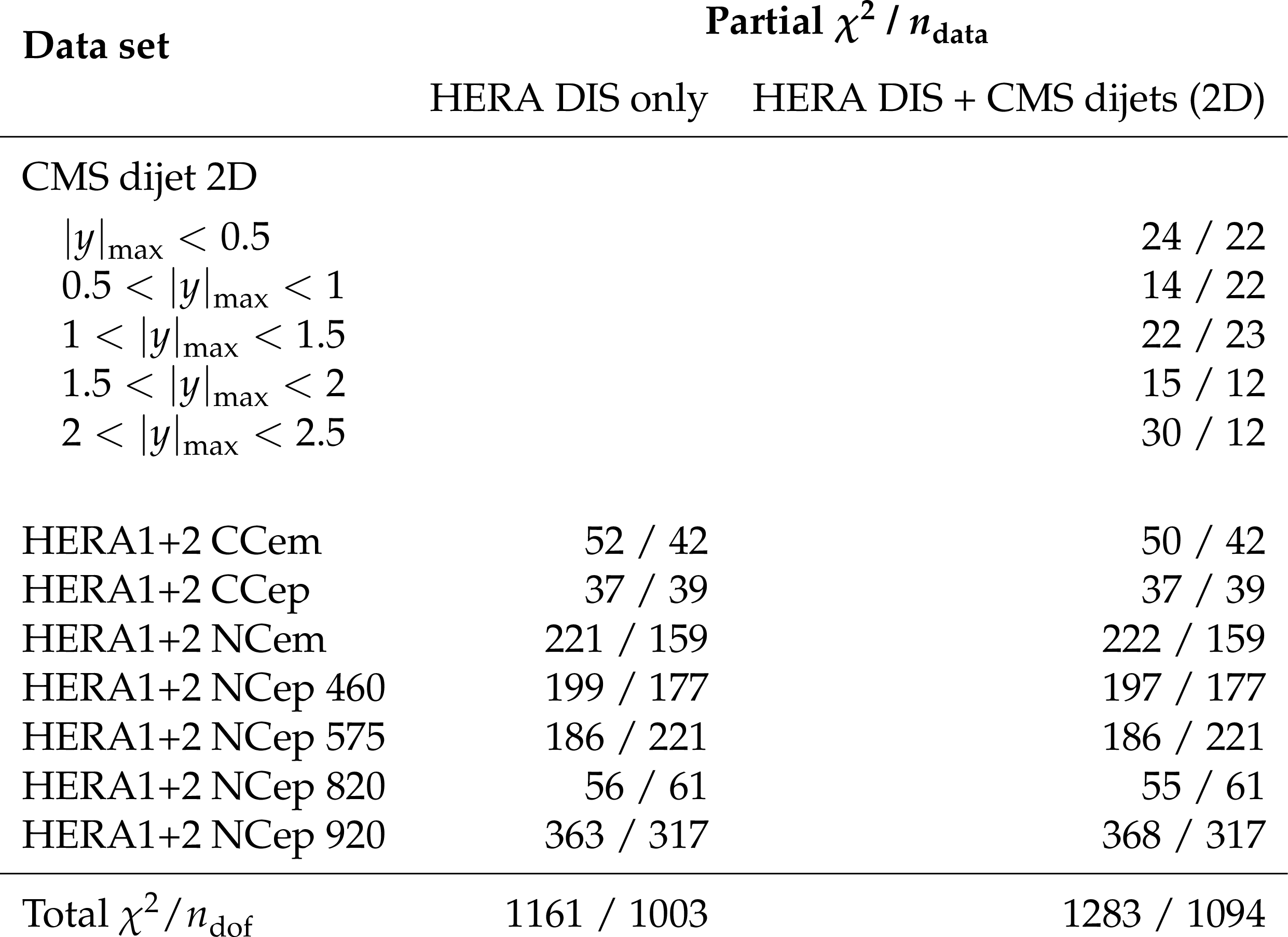
Table 3:
Goodness-of-fit values for the fits to the HERA DIS data alone and together with the CMS 2D dijet measurement, using the final PDF parametrization for the 2D fits. The table shows the partial $ \chi^2 $ values divided by the number of data points for the HERA DIS datasets and each of the dijet rapidity regions. The total $ \chi^2 $ value, divided by the number of degrees of freedom, is given at the bottom of the table. |

png pdf |
Table 4:
Goodness-of-fit values for the fits to the HERA DIS data alone and together with the CMS 3D dijet measurement, using the final PDF parametrization for the 3D fits. The table shows the partial $ \chi^2 $ values divided by the number of data points for the HERA DIS datasets and each of the dijet rapidity regions. The total $ \chi^2 $ value, divided by the number of degrees of freedom, is given at the bottom of the table. |
png pdf |
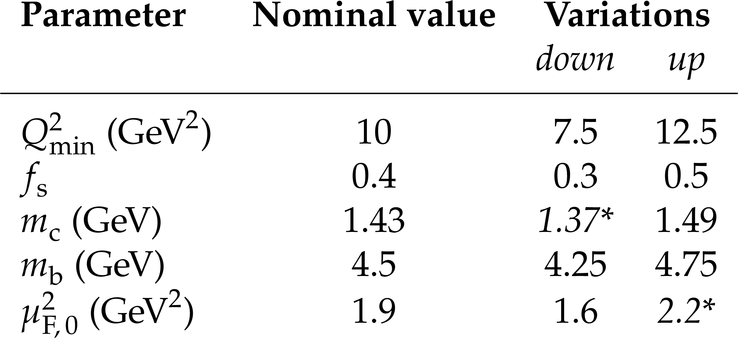
Table 5:
Nominal values and variations of parameters used to determine the PDF model uncertainty. Variations marked with an asterisk are in conflict with the requirement $ \mu_{\mathrm{F},\,0} < m_\text{c} $ and thus cannot be used directly for the uncertainty estimation. Following Ref. [56], the results obtained for the opposite variation are symmetrized in these cases. |
| Summary |
| Dijet production cross sections are presented double-differentially as a function of the dijet invariant mass $ m_{1,2} $ in five regions of the maximal absolute rapidity $ |y|_{\text{max}} $\ of the two leading-$ p_{\mathrm{T}} $ jets, and triple-differentially as a function of either $ m_{1,2} $ or the average transverse momentum $ \langle p_{\mathrm{T}} \rangle_{1,2} $ in 15 bins of the rapidity variables $ y^{*} $\ and $ y_{\text{b}} $. The latter correspond to the rapidity separation of the two jets, and the total boost of the dijet system, respectively. All measurements are performed for jets clustered using the anti-$ k_{\mathrm{T}} $ jet algorithm with distance parameters $ R= $ 0.4 and $ R= $ 0.8 and the cross sections are unfolded in all measurement dimensions simultaneously to correct for detector effects. The data are compared to fixed-order calculations at next-to-next-to-leading order in perturbative QCD, supplemented with electroweak and nonperturbative corrections. The theory is observed to describe the data better for the larger jet radius $ R = $ 0.8. Focusing on the larger jet radius and the dijet invariant mass $ m_{1,2} $ as an observable, the parton distribution functions (PDFs) of the proton are determined in fits to the dijet measurements together with deep-inelastic scattering data from the HERA experiments following the approach described in earlier HERAPDF analyses [54,55,56]. The inclusion of the presented measurements leads to an improved determination of the PDFs compared to fits to HERA data alone. In particular, the uncertainty in the gluon PDF at medium to large fractional momenta $ x $ of the proton is reduced. The results obtained from the double- and triple-differential measurements are shown to be compatible within the estimated uncertainties. Fits including the strong coupling constant $ \alpha_{\mathrm{s}}(m_{\mathrm{Z}}) $ as a free parameter yield consistent results between the double- and triple-differential dijet measurements, where the latter gives the slightly more precise value of $ \alpha_{\mathrm{s}}(m_{\mathrm{Z}}) = $ 0.1201 $ \pm $ 0.0020 at NNLO\@. The impact of subleading-color contributions to the leading-color NNLO calculation used here is not known yet [34]. Apart from being useful input to PDF fits or studies of jet size dependence, the presented double- and triple-differential measurements for two jet size parameters $ R= $ 0.4 and $ R= $ 0.8, and for the two dijet observables invariant mass $ m_{1,2} $ and average transverse momentum $ \langle p_{\mathrm{T}} \rangle_{1,2} $ provide an ideal testing ground for further investigations. |
| References | ||||
| 1 | J. Currie et al. | Precise predictions for dijet production at the LHC | PRL 119 (2017) 152001 | 1705.10271 |
| 2 | A. Gehrmann-De Ridder et al. | Triple differential dijet cross section at the LHC | PRL 123 (2019) 102001 | 1905.09047 |
| 3 | CMS Collaboration | Measurement of the triple-differential dijet cross section in proton-proton collisions at $ \sqrt{s}= $ 8 TeV and constraints on parton distribution functions | EPJC 77 (2017) 746 | CMS-SMP-16-011 1705.02628 |
| 4 | M. Cacciari, G. P. Salam, and G. Soyez | The anti-$ k_{\mathrm{T}} $ jet clustering algorithm | JHEP 04 (2008) 063 | 0802.1189 |
| 5 | M. Cacciari, G. P. Salam, and G. Soyez | FastJet user manual | EPJC 72 (2012) 1896 | 1111.6097 |
| 6 | ATLAS Collaboration | Measurement of inclusive jet and dijet cross sections in proton-proton collisions at 7 TeV centre-of-mass energy with the ATLAS detector | EPJC 71 (2011) 1512 | 1009.5908 |
| 7 | CMS Collaboration | Measurement of the differential dijet production cross section in proton-proton collisions at $ \sqrt{s}= $ 7 TeV | PLB 700 (2011) 187 | CMS-QCD-10-025 1104.1693 |
| 8 | CMS Collaboration | Measurements of differential jet cross sections in proton-proton collisions at $ \sqrt{s}= $ 7 TeV with the CMS detector | PRD 87 (2013) 112002 | CMS-QCD-11-004 1212.6660 |
| 9 | ATLAS Collaboration | Measurement of dijet cross sections in pp collisions at 7 TeV centre-of-mass energy using the ATLAS detector | JHEP 05 (2014) 059 | 1312.3524 |
| 10 | ATLAS Collaboration | Measurement of inclusive jet and dijet cross-sections in proton-proton collisions at $ \sqrt{s}= $ 13 TeV with the ATLAS detector | JHEP 05 (2018) 195 | 1711.02692 |
| 11 | CMS Collaboration | The CMS trigger system | JINST 12 (2017) P01020 | CMS-TRG-12-001 1609.02366 |
| 12 | CMS Collaboration | Performance of the CMS Level-1 trigger in proton-proton collisions at $ \sqrt{s}= $ 13 TeV | JINST 15 (2020) P10017 | CMS-TRG-17-001 2006.10165 |
| 13 | CMS Collaboration | The CMS experiment at the CERN LHC | JINST 3 (2008) S08004 | |
| 14 | T. Sjöstrand, S. Mrenna, and P. Z. Skands | A brief introduction to PYTHIA 8.1 | Comput. Phys. Commun. 178 (2008) 852 | 0710.3820 |
| 15 | CMS Collaboration | Event generator tunes obtained from underlying event and multiparton scattering measurements | EPJC 76 (2016) 155 | CMS-GEN-14-001 1512.00815 |
| 16 | J. Alwall et al. | The automated computation of tree-level and next-to-leading order differential cross sections, and their matching to parton shower simulations | JHEP 07 (2014) 079 | 1405.0301 |
| 17 | GEANT4 Collaboration | GEANT 4---a simulation toolkit | NIM A 506 (2003) 250 | |
| 18 | CMS Collaboration | Particle-flow reconstruction and global event description with the CMS detector | JINST 12 (2017) P10003 | CMS-PRF-14-001 1706.04965 |
| 19 | CMS Collaboration | Technical proposal for the Phase-II upgrade of the Compact Muon Solenoid | CMS Technical Proposal CERN-LHCC-2015-010, CMS-TDR-15-02, 2015 CDS |
|
| 20 | CMS Collaboration | Jet energy scale and resolution in the CMS experiment in pp collisions at 8 TeV | JINST 12 (2017) P02014 | CMS-JME-13-004 1607.03663 |
| 21 | CMS Collaboration | Performance of missing transverse momentum reconstruction in proton-proton collisions at $ \sqrt{s}= $ 13 TeV using the CMS detector | JINST 14 (2019) P07004 | CMS-JME-17-001 1903.06078 |
| 22 | S. Schmitt | TUnfold: an algorithm for correcting migration effects in high energy physics | JINST 7 (2012) T10003 | 1205.6201 |
| 23 | CMS Collaboration | Jet energy scale and resolution performance with 13 TeV data collected by CMS in 2016-2018 | CMS Detector Performance Note CMS-DP-2020-019, CERN, 2020 CDS |
|
| 24 | CMS Collaboration | Precision luminosity measurement in proton-proton collisions at $ \sqrt{s} = $ 13 TeV in 2015 and 2016 at CMS | EPJC 81 (2021) 800 | CMS-LUM-17-003 2104.01927 |
| 25 | T. Gehrmann et al. | Jet cross sections and transverse momentum distributions with NNLOJET | PoS RADCOR 074, 2018 link |
1801.06415 |
| 26 | T. Kluge, K. Rabbertz, and M. Wobisch | fastNLO: Fast pQCD calculations for PDF fits | in Proceedings, 14th International Workshop on Deep-Inelastic Scattering, Tsukuba, Japan, 2006 DIS 200 (2006) 483 |
hep-ph/0609285 |
| 27 | D. Britzger, K. Rabbertz, F. Stober, and M. Wobisch | New features in version 2 of the fastNLO project | in 20th International Workshop on Deep-Inelastic Scattering and Related Subjects, 2012 link |
1208.3641 |
| 28 | D. Britzger et al. | Calculations for deep inelastic scattering using fast interpolation grid techniques at NNLO in QCD and the extraction of $ \alpha_\text{s} $ from HERA data | EPJC 79 (2019) 845 | 1906.05303 |
| 29 | D. Britzger et al. | NNLO interpolation grids for jet production at the LHC | EPJC 82 (2022) 930 | 2207.13735 |
| 30 | J. Currie et al. | Jet cross sections at the LHC with NNLOJET | PoS LL 001, 2018 link |
1807.06057 |
| 31 | M. Cacciari et al. | The $ \mathrm{t} \overline{\mathrm{t}} $ cross-section at 1.8 TeV and 1.96 TeV: a study of the systematics due to parton densities and scale dependence | JHEP 04 (2004) 068 | hep-ph/0303085 |
| 32 | S. Catani, D. de Florian, M. Grazzini, and P. Nason | Soft gluon resummation for Higgs boson production at hadron colliders | JHEP 07 (2003) 028 | hep-ph/0306211 |
| 33 | A. Banfi, G. P. Salam, and G. Zanderighi | Phenomenology of event shapes at hadron colliders | JHEP 06 (2010) 038 | 1001.4082 |
| 34 | X. Chen et al. | NNLO QCD corrections in full colour for jet production observables at the LHC | JHEP 09 (2022) 025 | 2204.10173 |
| 35 | CMS Collaboration | Measurement of the double-differential inclusive jet cross section in proton-proton collisions at $ \sqrt{s} = $ 13 TeV | EPJC 76 (2016) 451 | CMS-SMP-15-007 1605.04436 |
| 36 | CMS Collaboration | Investigations of the impact of the parton shower tuning in Pythia 8 in the modelling of $ \mathrm{t\overline{t}} $ at $ \sqrt{s}= $ 8 and 13 TeV | CMS Physics Analysis Summary, 2016 CMS-PAS-TOP-16-021 |
CMS-PAS-TOP-16-021 |
| 37 | M. Bähr et al. | Herwig++ physics and manual | EPJC 58 (2008) 639 | 0803.0883 |
| 38 | M. H. Seymour and A. Siodmok | Constraining MPI models using $ \sigma_{\text{eff}} $ and recent Tevatron and LHC underlying event data | JHEP 10 (2013) 113 | 1307.5015 |
| 39 | P. Nason | A new method for combining NLO QCD with shower Monte Carlo algorithms | JHEP 11 (2004) 040 | hep-ph/0409146 |
| 40 | S. Frixione, P. Nason, and C. Oleari | Matching NLO QCD computations with parton shower simulations: the POWHEG method | JHEP 11 (2007) 070 | 0709.2092 |
| 41 | S. Alioli, P. Nason, C. Oleari, and E. Re | A general framework for implementing NLO calculations in shower Monte Carlo programs: the POWHEG BOX | JHEP 06 (2010) 043 | 1002.2581 |
| 42 | S. Alioli et al. | Jet pair production in POWHEG | JHEP 04 (2011) 081 | 1012.3380 |
| 43 | J. Bellm et al. | Herwig 7.0/Herwig++ 3.0 release note | EPJC 76 (2016) 196 | 1512.01178 |
| 44 | CMS Collaboration | Development and validation of HERWIG 7 tunes from CMS underlying-event measurements | EPJC 81 (2021) 312 | CMS-GEN-19-001 2011.03422 |
| 45 | S. Dittmaier, A. Huss, and C. Speckner | Weak radiative corrections to dijet production at hadron colliders | JHEP 11 (2012) 095 | 1210.0438 |
| 46 | A. Buckley et al. | LHAPDF6: parton density access in the LHC precision era | EPJC 75 (2015) 132 | 1412.7420 |
| 47 | S. Alekhin, J. Blümlein, S. Moch, and R. Placakyte | Parton distribution functions, $ \alpha_\text{s} $, and heavy-quark masses for LHC Run II | PRD 96 (2017) 014011 | 1701.05838 |
| 48 | T.-J. Hou et al. | New CTEQ global analysis of quantum chromodynamics with high-precision data from the LHC | PRD 103 (2021) 014013 | 1912.10053 |
| 49 | S. Bailey et al. | Parton distributions from LHC, HERA, Tevatron and fixed target data: MSHT20 PDFs | EPJC 81 (2021) 341 | 2012.04684 |
| 50 | NNPDF Collaboration | Parton distributions from high-precision collider data | EPJC 77 (2017) 663 | 1706.00428 |
| 51 | CMS Collaboration | Measurement of the ratio of inclusive jet cross sections using the anti-$ k_{\mathrm{T}} $ algorithm with radius parameters $ {R} = $ 0.5 and 0.7 in pp collisions at $ \sqrt{s} $ = 7 TeV | PRD 90 (2014) 072006 | CMS-SMP-13-002 1406.0324 |
| 52 | ATLAS Collaboration | Measurement of the inclusive jet cross-sections in proton--proton collisions at $ \sqrt{s}= $8 TeV with the ATLAS detector | JHEP 09 (2017) 020 | 1706.03192 |
| 53 | CMS Collaboration | Measurement and QCD analysis of double-differential inclusive jet cross sections in proton-proton collisions at $ \sqrt{s} $ = 13 TeV | JHEP 02 (2022) 142 | CMS-SMP-20-011 2111.10431 |
| 54 | H1 and ZEUS Collaborations | Combined measurement and QCD analysis of the inclusive $ {e^{\pm }p} $ scattering cross sections at HERA | JHEP 01 (2010) 109 | 0911.0884 |
| 55 | H1 and ZEUS Collaborations | Combination of measurements of inclusive deep inelastic $ \mathrm{e}^{\pm} \mathrm{p} $ scattering cross sections and QCD analysis of HERA data | EPJC 75 (2015) 580 | 1506.06042 |
| 56 | H1 and ZEUS Collaborations | Impact of jet-production data on the next-to-next-to-leading-order determination of HERAPDF2.0 parton distributions | EPJC 82 (2022) 243 | 2112.01120 |
| 57 | S. Alekhin et al. | HERAFitter: open source QCD fit project | EPJC 75 (2015) 304 | 1410.4412 |
| 58 | V. Bertone et al. | xFitter 2.0.0: An open source QCD fit framework | PoS DIS 203, 2018 link |
1709.01151 |
| 59 | Y. L. Dokshitzer | Calculation of the structure functions for deep inelastic scattering and e$ ^{+} $e$ ^{-} $ annihilation by perturbation theory in quantum chromodynamics | Sov. Phys. JETP 46 (1977) 641 | |
| 60 | V. N. Gribov and L. N. Lipatov | Deep inelastic $ \mathrm{e} \mathrm{p} $ scattering in perturbation theory | Sov. J. Nucl. Phys. 15 (1972) 438 | |
| 61 | G. Altarelli and G. Parisi | Asymptotic freedom in parton language | NPB 126 (1977) 298 | |
| 62 | M. Botje | QCDNUM: Fast QCD evolution and convolution | Comput. Phys. Commun. 182 (2011) 490 | 1005.1481 |
| 63 | R. S. Thorne and R. G. Roberts | An ordered analysis of heavy flavor production in deep inelastic scattering | PRD 57 (1998) 6871 | hep-ph/9709442 |
| 64 | R. S. Thorne | A variable-flavor number scheme for NNLO | PRD 73 (2006) 054019 | hep-ph/0601245 |
| 65 | R. S. Thorne | Effect of changes of variable flavor number scheme on parton distribution functions and predicted cross sections | PRD 86 (2012) 074017 | 1201.6180 |
| 66 | J. Pumplin et al. | Uncertainties of predictions from parton distribution functions. ii. the Hessian method | PRD 65 (2001) 014013 | hep-ph/0101032 |
| 67 | Particle Data Group , R. L. Workman et al. | Review of particle physics | Prog. Theor. Exp. Phys. 2022 (2022) 083C01 | |
|
|
Compact Muon Solenoid LHC, CERN |
|

|

|

|

|

|