

Compact Muon Solenoid
LHC, CERN
| CMS-PAS-HIN-19-001 | ||
| Evidence for top quark production in nucleus-nucleus collisions | ||
| CMS Collaboration | ||
| November 2019 | ||
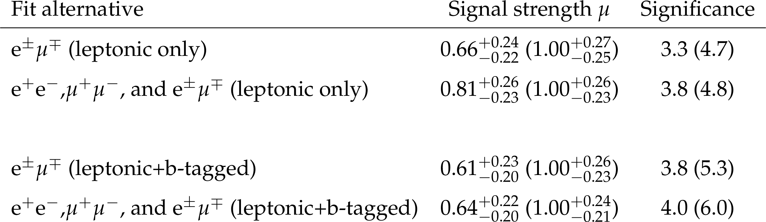
| Abstract: Evidence for the production of top quarks in heavy ion collisions is reported in a data sample of lead-lead collisions recorded in 2018 by the CMS experiment at a nucleon-nucleon center-of-mass energy of $\sqrt{\smash[b]{s_{_{\mathrm{NN}}}}} = $ 5.02 TeV, corresponding to an integrated luminosity of 1.7 $\pm$ 0.1 nb$^{-1}$. Top quark pair ($\mathrm{t\bar{t}}$) production is measured in events with two opposite-sign high-$p_{\mathrm{T}}$ isolated leptons ($\ell^\pm\ell^\mp =\,\mathrm{e}^{+} \mathrm{e}^{-},\,\mu^{+} \mu^{-}$ , and $\mathrm{e}^{\pm} \mu^{\mp}$). We test the sensitivity to the $\mathrm{t\bar{t}}$ signal process by requiring or not the additional presence of b-tagged jets, and hence the feasilibility to identify top quark decay products irrespective of interacting with the medium (bottom quarks) or not (leptonically decaying W bosons). To that end, the inclusive cross section ($\sigma_{\mathrm{t\bar{t}}}$) is derived from likelihood fits to a multivariate discriminator, which includes different leptonic kinematic variables, with and without the b-tagged jet multiplicity information. The observed (expected) significance of the $\mathrm{t\bar{t}}$ signal against the background-only hypothesis is 4.0 (6.0) and 3.8 (4.8) standard deviations, respectively, for the fits with and without the b-jet multiplicity input. After event reconstruction and background subtraction, the extracted cross sections are $\sigma_{\mathrm{t\bar{t}}} = $ 2.02 $\pm$ 0.69 and 2.56 $\pm$ 0.82 $\mu$b, respectively, which are consistent with each other and lower than, but still compatible with, the expectations from scaled proton-proton data as well as from perturbative quantum chromodynamics predictions. This measurement constitutes the first step towards using the top quark as a novel tool for probing strongly interacting matter. | ||
|
Links:
CDS record (PDF) ;
CADI line (restricted) ;
These preliminary results are superseded in this paper, PRL 125 (2020) 222001. The superseded preliminary plots can be found here. |
||
| Figures & Tables | Summary | Additional Figures & Tables | References | CMS Publications |
|---|
| Figures | |
png pdf |
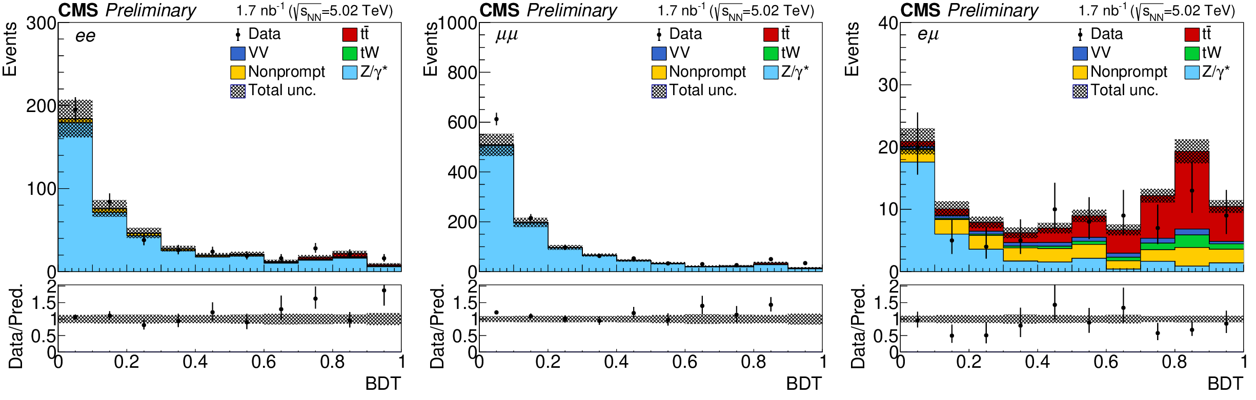
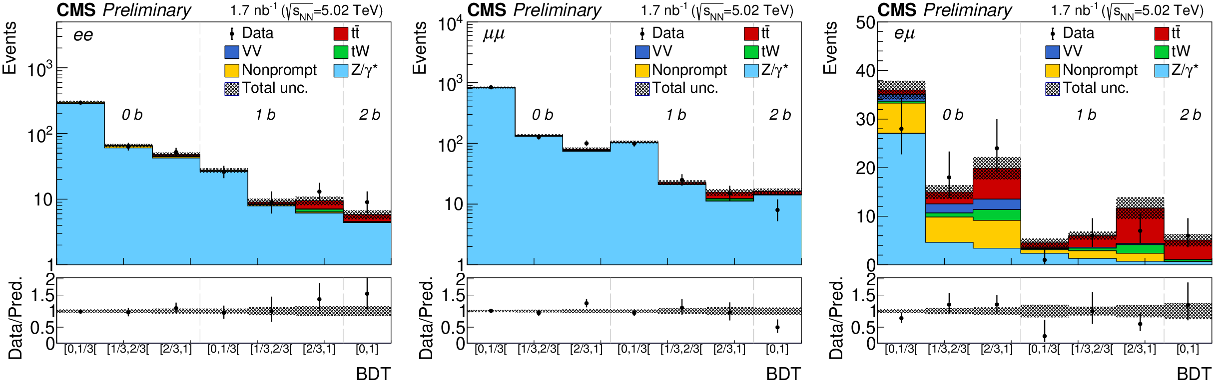
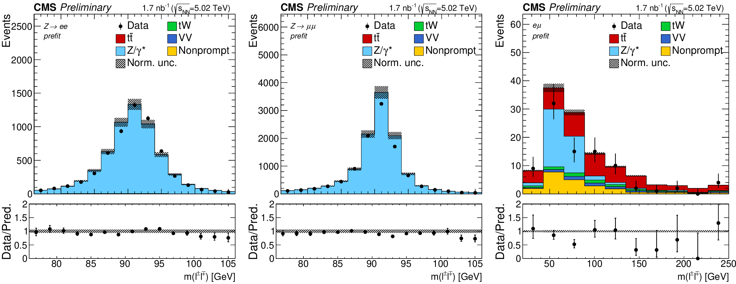
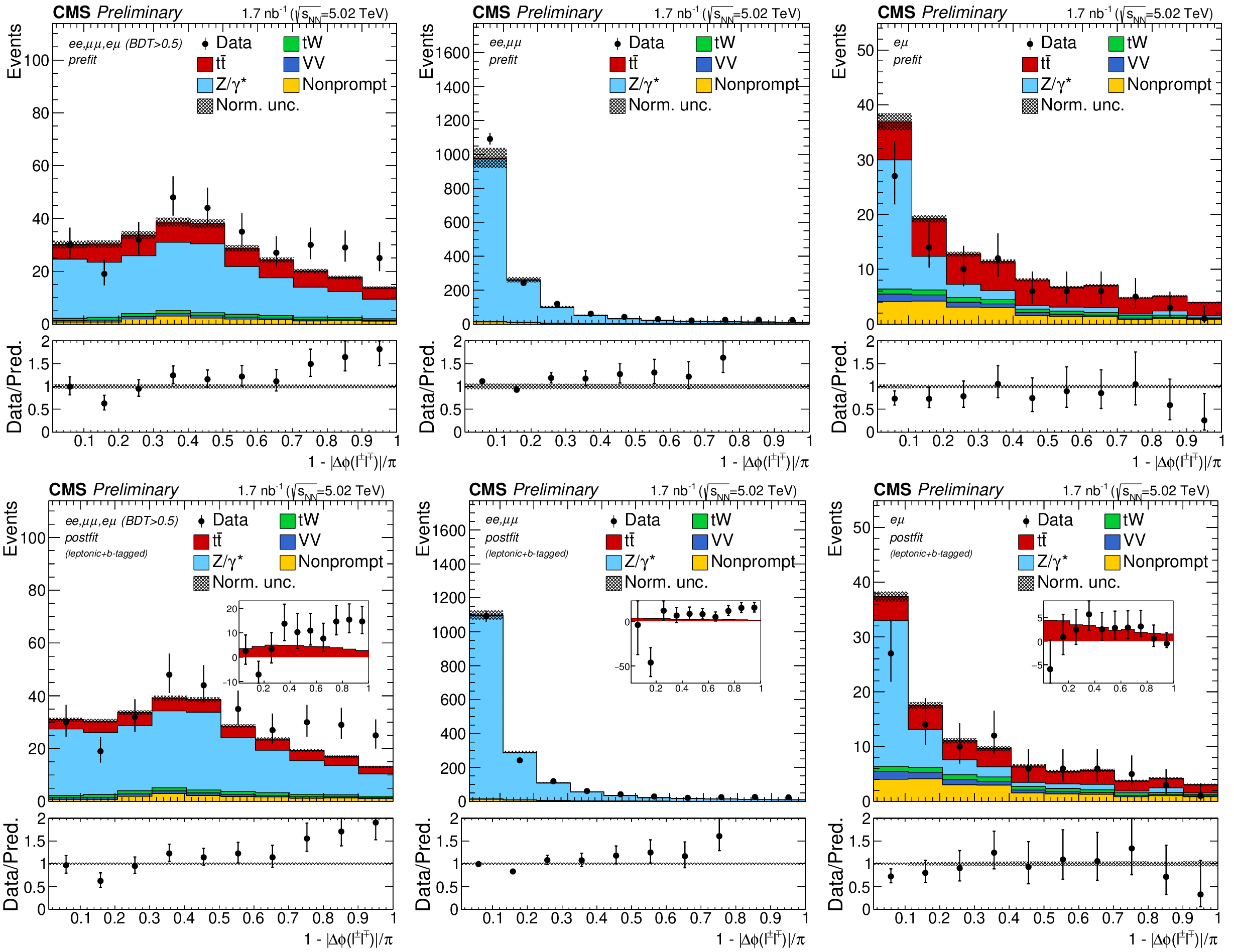
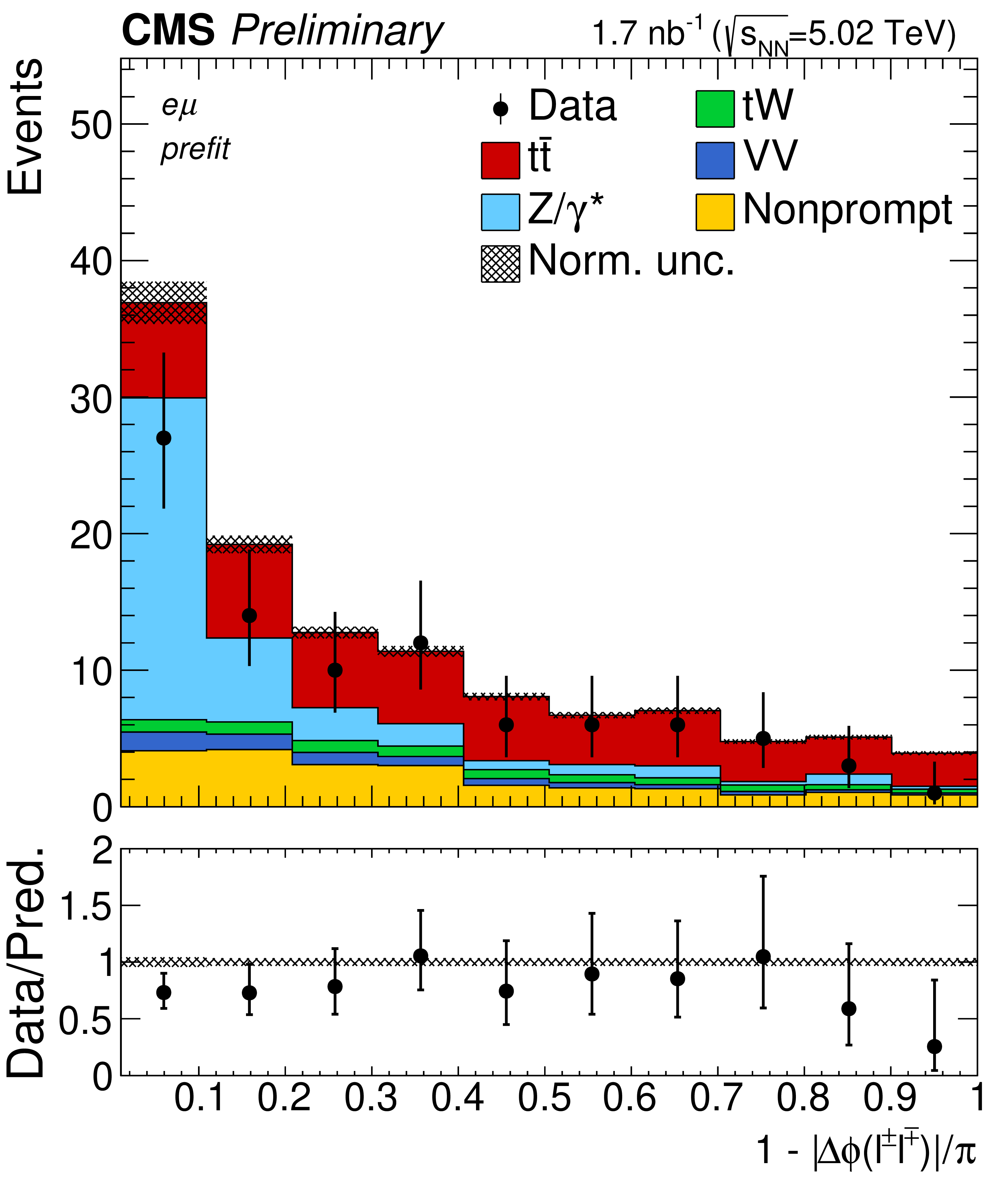
Figure 1:
Observed (markers) and prefit expected (filled histograms) BDT discriminator distributions in the ${\mathrm{e} ^+ \mathrm{e} ^-}$ (left), ${\mu ^+ \mu ^-}$ (middle), and ${\mathrm{e} ^\pm \mu ^\mp}$ (right) channels. The data are shown with markers, and the signal and background processes with filled histograms. The vertical bars on the markers represent the statistical uncertainties in data. The hatched regions show the prefit uncertainties in the sum of $ {\mathrm{t} \mathrm{\bar{t}}} $ signal and backgrounds. The lower panels display the ratio of the data to the predictions, including the $ {\mathrm{t} \mathrm{\bar{t}}} $ signal, with bands representing the prefit uncertainties in the predictions. |
png pdf |
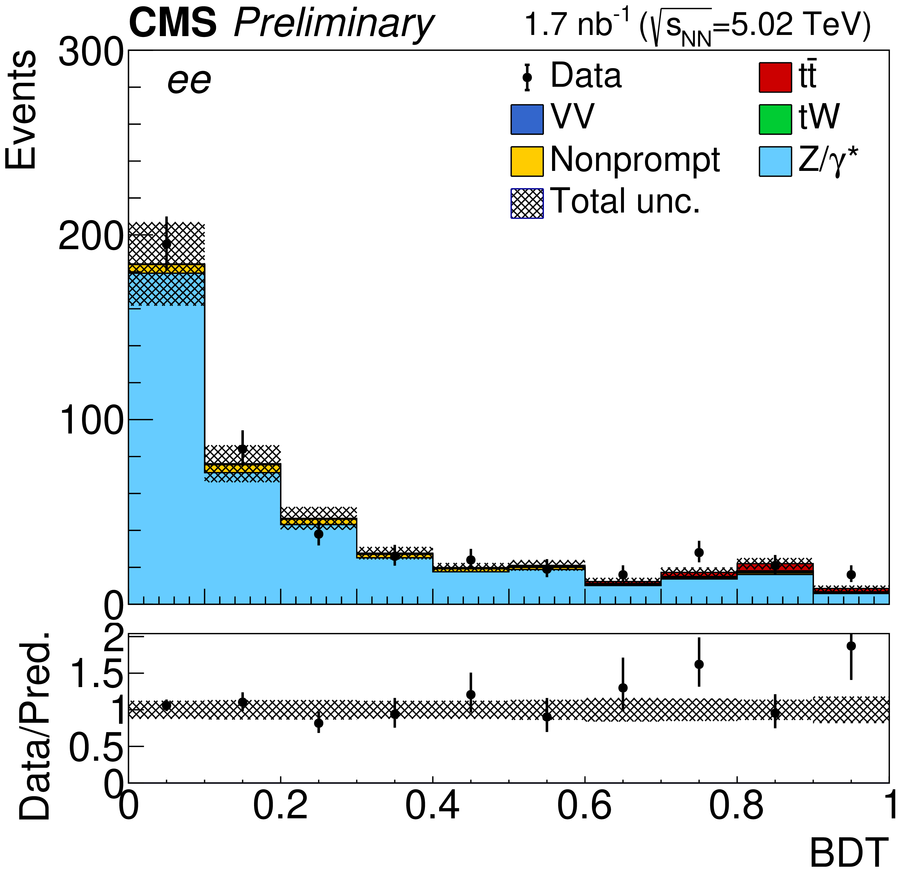
Figure 1-a:
Observed (markers) and prefit expected (filled histograms) BDT discriminator distributions in the ${\mathrm{e} ^+ \mathrm{e} ^-}$ channel. The data are shown with markers, and the signal and background processes with filled histograms. The vertical bars on the markers represent the statistical uncertainties in data. The hatched regions show the prefit uncertainties in the sum of $ {\mathrm{t} \mathrm{\bar{t}}} $ signal and backgrounds. The lower panel displays the ratio of the data to the predictions, including the $ {\mathrm{t} \mathrm{\bar{t}}} $ signal, with bands representing the prefit uncertainties in the predictions. |

png pdf |
Figure 1-b:
Observed (markers) and prefit expected (filled histograms) BDT discriminator distributions in the ${\mu ^+ \mu ^-}$ channel. The data are shown with markers, and the signal and background processes with filled histograms. The vertical bars on the markers represent the statistical uncertainties in data. The hatched regions show the prefit uncertainties in the sum of $ {\mathrm{t} \mathrm{\bar{t}}} $ signal and backgrounds. The lower panel displays the ratio of the data to the predictions, including the $ {\mathrm{t} \mathrm{\bar{t}}} $ signal, with bands representing the prefit uncertainties in the predictions. |
png pdf |
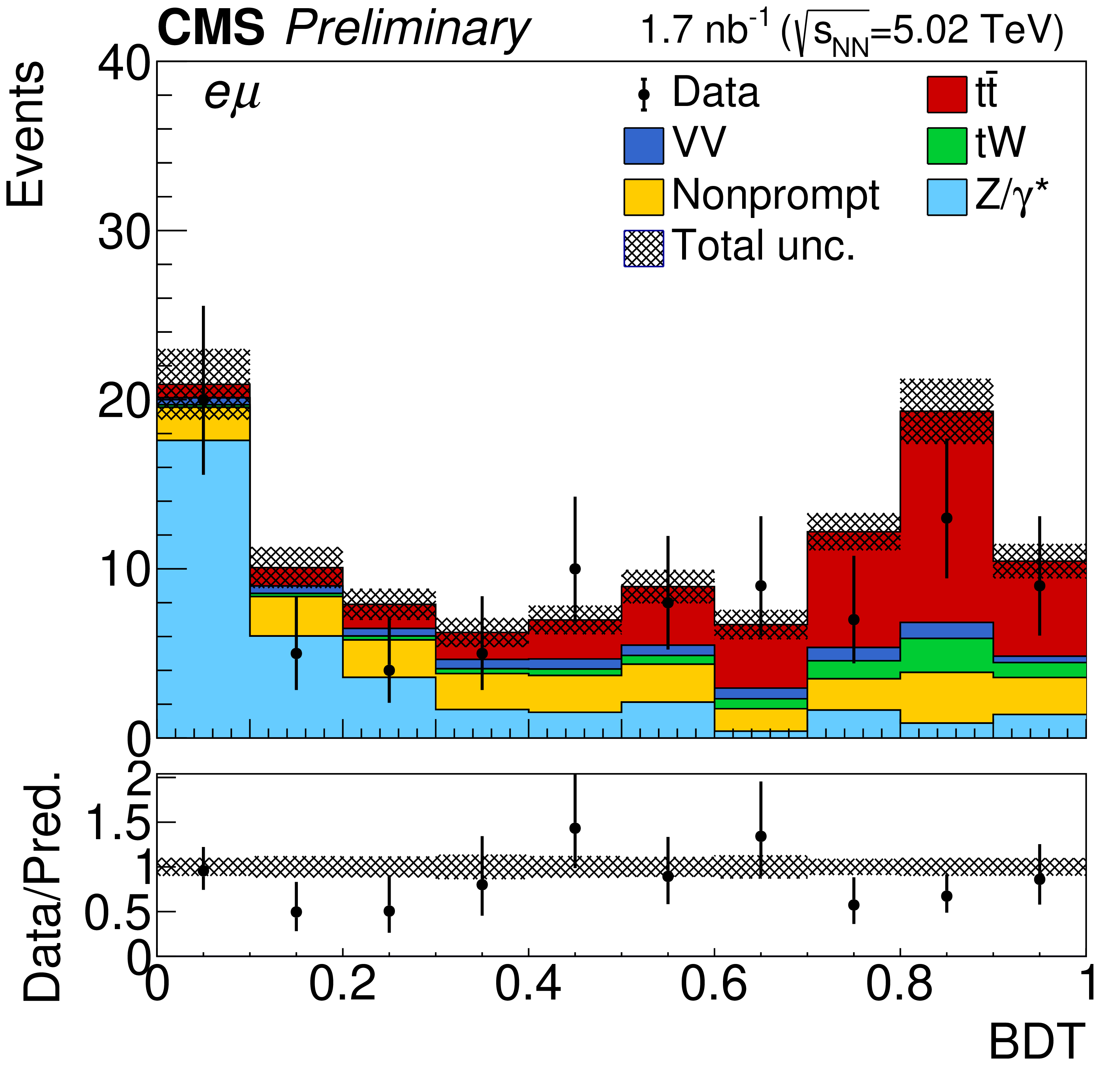
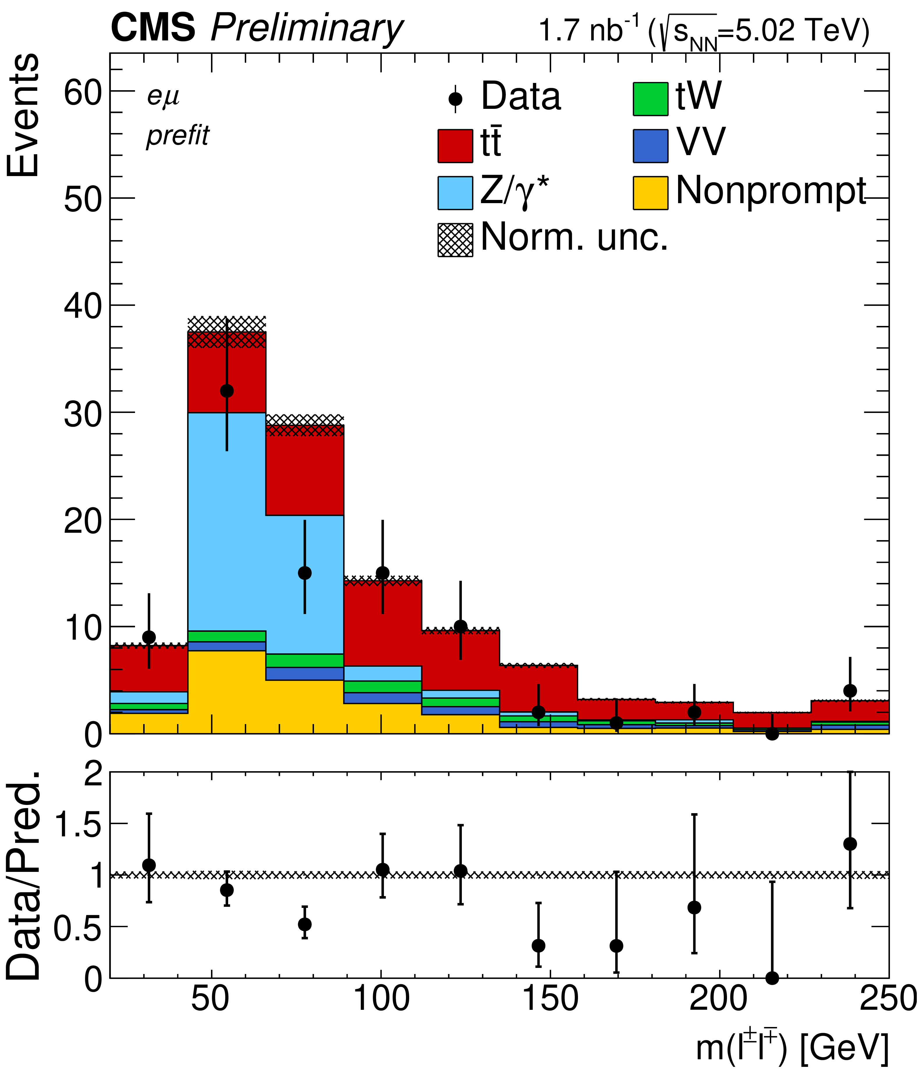
Figure 1-c:
Observed (markers) and prefit expected (filled histograms) BDT discriminator distributions in the ${\mathrm{e} ^\pm \mu ^\mp}$ channel. The data are shown with markers, and the signal and background processes with filled histograms. The vertical bars on the markers represent the statistical uncertainties in data. The hatched regions show the prefit uncertainties in the sum of $ {\mathrm{t} \mathrm{\bar{t}}} $ signal and backgrounds. The lower panel displays the ratio of the data to the predictions, including the $ {\mathrm{t} \mathrm{\bar{t}}} $ signal, with bands representing the prefit uncertainties in the predictions. |
png pdf |
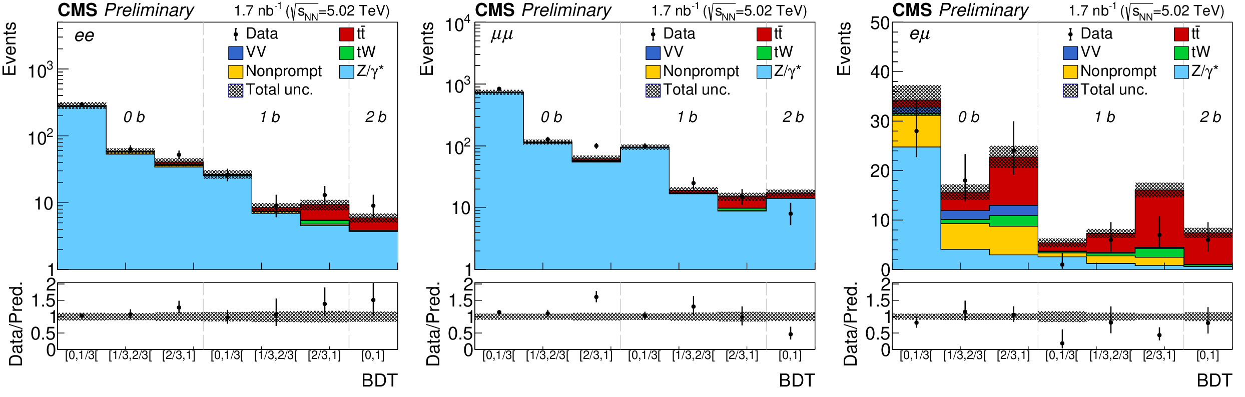
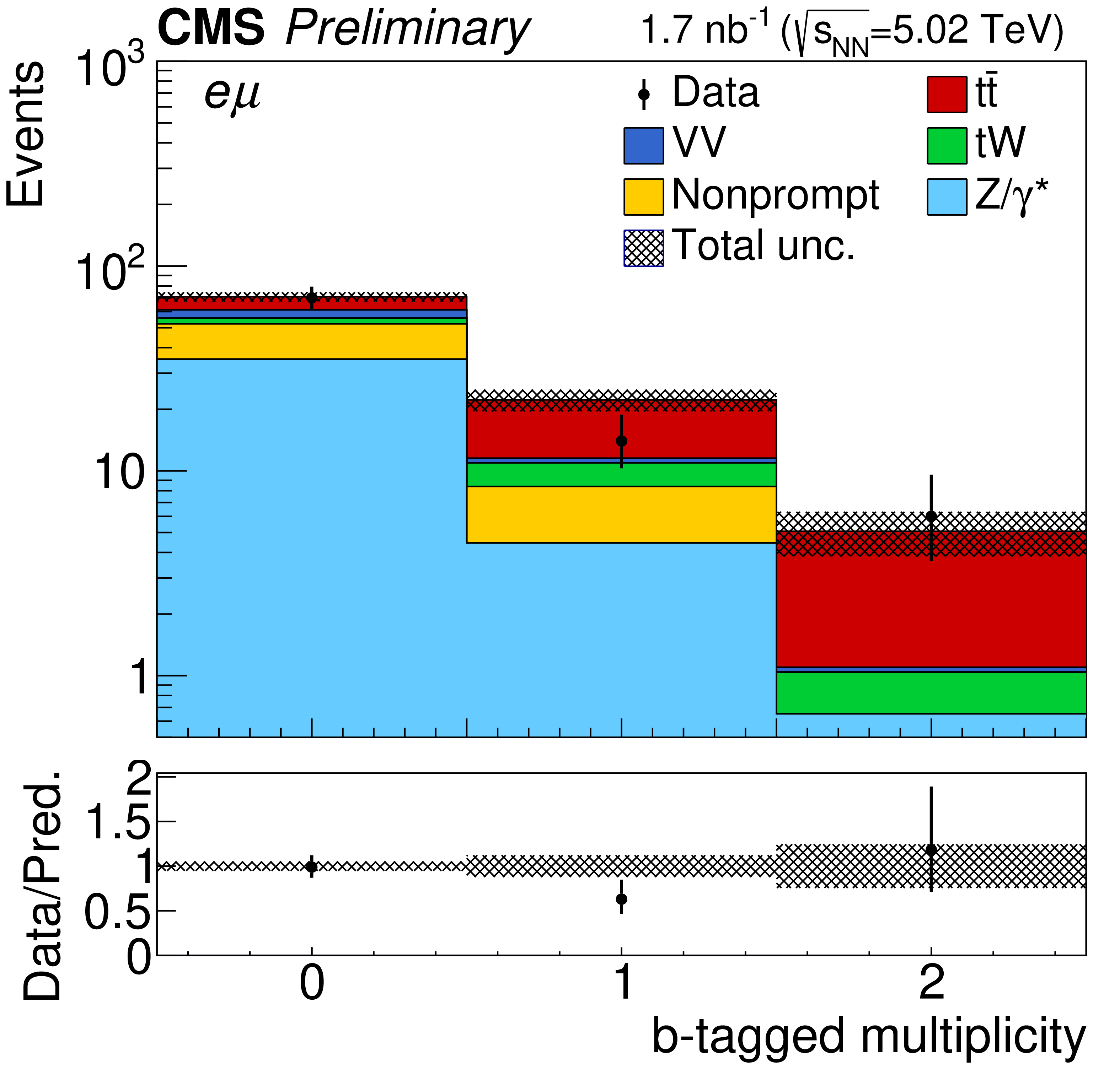
Figure 2:
Observed (markers) and prefit expected (filled histograms) BDT discriminator distributions in the ${\mathrm{e} ^+ \mathrm{e} ^-}$ (left), ${\mu ^+ \mu ^-}$ (middle), and ${\mathrm{e} ^\pm \mu ^\mp}$ (right) channels separately for the 0b-, 1b-, and 2b-jet multiplicity categories. The data are shown with markers, and the signal and background processes with filled histograms. The vertical bars on the markers represent the statistical uncertainties in data. The hatched regions show the prefit uncertainties in the sum of $ {\mathrm{t} \mathrm{\bar{t}}} $ signal and backgrounds. The lower panels display the ratio of the data to the predictions, including the $ {\mathrm{t} \mathrm{\bar{t}}} $ signal, with bands representing the prefit uncertainties in the predictions. |

png pdf |
Figure 2-a:
Observed (markers) and prefit expected (filled histograms) BDT discriminator distributions in the ${\mathrm{e} ^+ \mathrm{e} ^-}$ channel separately for the 0b-, 1b-, and 2b-jet multiplicity categories. The data are shown with markers, and the signal and background processes with filled histograms. The vertical bars on the markers represent the statistical uncertainties in data. The hatched regions show the prefit uncertainties in the sum of $ {\mathrm{t} \mathrm{\bar{t}}} $ signal and backgrounds. The lower panel displays the ratio of the data to the predictions, including the $ {\mathrm{t} \mathrm{\bar{t}}} $ signal, with bands representing the prefit uncertainties in the predictions. |
png pdf |
Figure 2-b:
Observed (markers) and prefit expected (filled histograms) BDT discriminator distributions in the ${\mu ^+ \mu ^-}$ channel separately for the 0b-, 1b-, and 2b-jet multiplicity categories. The data are shown with markers, and the signal and background processes with filled histograms. The vertical bars on the markers represent the statistical uncertainties in data. The hatched regions show the prefit uncertainties in the sum of $ {\mathrm{t} \mathrm{\bar{t}}} $ signal and backgrounds. The lower panel displays the ratio of the data to the predictions, including the $ {\mathrm{t} \mathrm{\bar{t}}} $ signal, with bands representing the prefit uncertainties in the predictions. |
png pdf |
Figure 2-c:
Observed (markers) and prefit expected (filled histograms) BDT discriminator distributions in the ${\mathrm{e} ^\pm \mu ^\mp}$ channel separately for the 0b-, 1b-, and 2b-jet multiplicity categories. The data are shown with markers, and the signal and background processes with filled histograms. The vertical bars on the markers represent the statistical uncertainties in data. The hatched regions show the prefit uncertainties in the sum of $ {\mathrm{t} \mathrm{\bar{t}}} $ signal and backgrounds. The lower panel displays the ratio of the data to the predictions, including the $ {\mathrm{t} \mathrm{\bar{t}}} $ signal, with bands representing the prefit uncertainties in the predictions. |

png pdf |
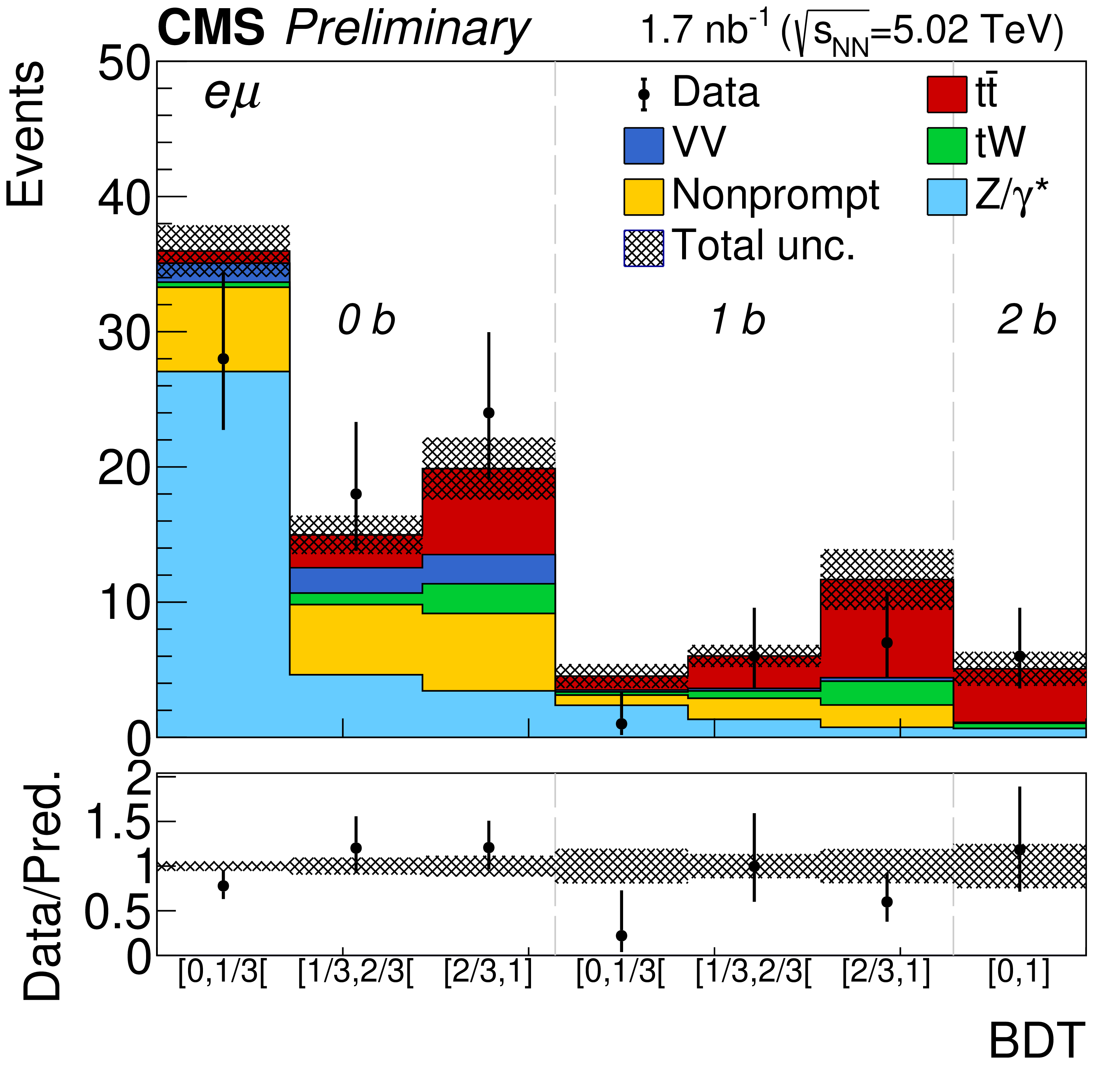
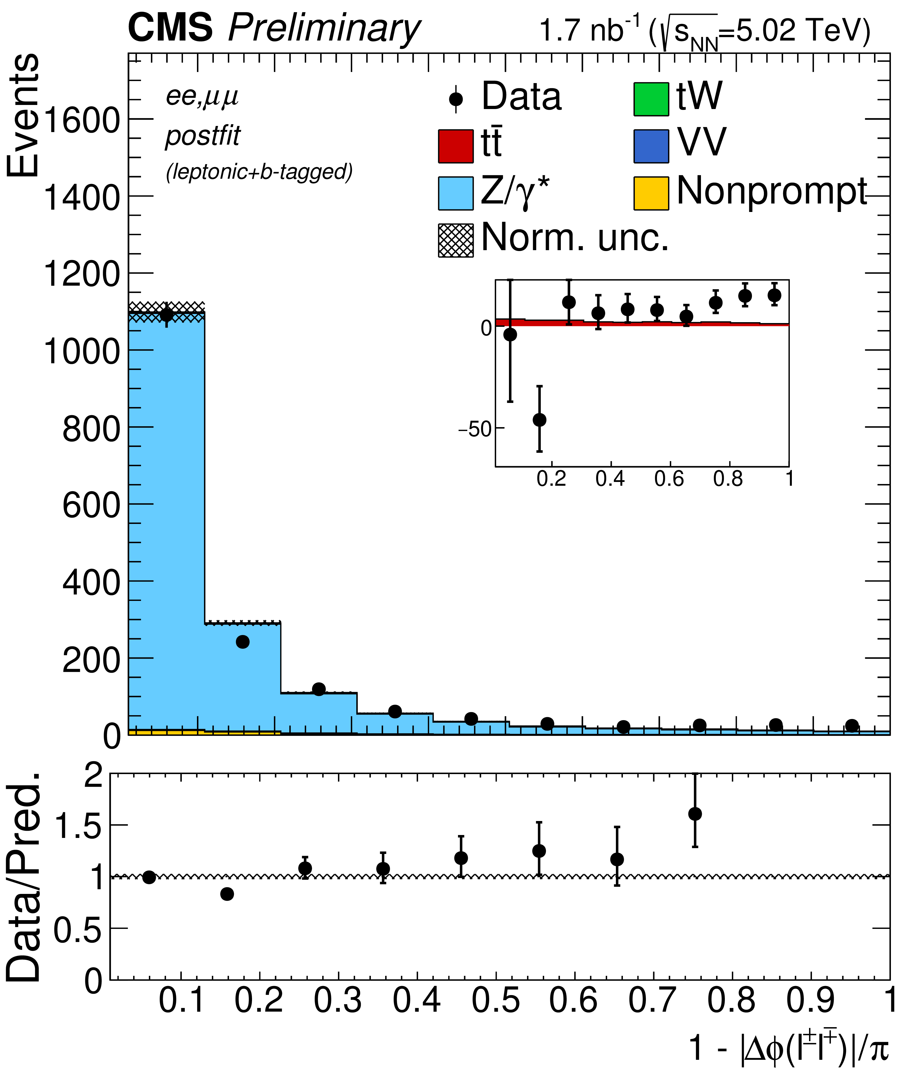
Figure 3:
Observed (markers) and postfit predicted (filled histograms) BDT discriminator distributions in the ${\mathrm{e} ^+ \mathrm{e} ^-}$ (left), ${\mu ^+ \mu ^-}$ (middle), and ${\mathrm{e} ^\pm \mu ^\mp}$ (right) channels. The data are shown with markers, and the signal and background processes with filled histograms. The vertical bars on the markers represent the statistical uncertainties in data. The hatched regions show the postfit uncertainties in the sum of $ {\mathrm{t} \mathrm{\bar{t}}} $ signal and backgrounds. The lower panels display the ratio of the data to the predictions, including the $ {\mathrm{t} \mathrm{\bar{t}}} $ signal, with bands representing the postfit uncertainties in the predictions. |
png pdf |
Figure 3-a:
Observed (markers) and postfit predicted (filled histograms) BDT discriminator distributions in the ${\mathrm{e} ^+ \mathrm{e} ^-}$ channel. The data are shown with markers, and the signal and background processes with filled histograms. The vertical bars on the markers represent the statistical uncertainties in data. The hatched regions show the postfit uncertainties in the sum of $ {\mathrm{t} \mathrm{\bar{t}}} $ signal and backgrounds. The lower panel displays the ratio of the data to the predictions, including the $ {\mathrm{t} \mathrm{\bar{t}}} $ signal, with bands representing the postfit uncertainties in the predictions. |

png pdf |
Figure 3-b:
Observed (markers) and postfit predicted (filled histograms) BDT discriminator distributions in the ${\mu ^+ \mu ^-}$ channel. The data are shown with markers, and the signal and background processes with filled histograms. The vertical bars on the markers represent the statistical uncertainties in data. The hatched regions show the postfit uncertainties in the sum of $ {\mathrm{t} \mathrm{\bar{t}}} $ signal and backgrounds. The lower panel displays the ratio of the data to the predictions, including the $ {\mathrm{t} \mathrm{\bar{t}}} $ signal, with bands representing the postfit uncertainties in the predictions. |
png pdf |
Figure 3-c:
Observed (markers) and postfit predicted (filled histograms) BDT discriminator distributions in the ${\mathrm{e} ^\pm \mu ^\mp}$ channel. The data are shown with markers, and the signal and background processes with filled histograms. The vertical bars on the markers represent the statistical uncertainties in data. The hatched regions show the postfit uncertainties in the sum of $ {\mathrm{t} \mathrm{\bar{t}}} $ signal and backgrounds. The lower panel displays the ratio of the data to the predictions, including the $ {\mathrm{t} \mathrm{\bar{t}}} $ signal, with bands representing the postfit uncertainties in the predictions. |
png pdf |
Figure 4:
Observed (markers) and postfit predicted (filled histograms) BDT discriminator distributions in the ${\mathrm{e} ^+ \mathrm{e} ^-}$ (left), ${\mu ^+ \mu ^-}$ (middle), and ${\mathrm{e} ^\pm \mu ^\mp}$ (right) channels separately for the 0b-, 1b-, and 2b-jet multiplicity categories. The data are shown with markers, and the signal and background processes with filled histograms. The vertical bars on the markers represent the statistical uncertainties in data. The hatched regions show the postfit uncertainties in the sum of $ {\mathrm{t} \mathrm{\bar{t}}} $ signal and backgrounds. The lower panels display the ratio of the data to the predictions, including the $ {\mathrm{t} \mathrm{\bar{t}}} $ signal, with bands representing the postfit uncertainties in the predictions. |

png pdf |
Figure 4-a:
Observed (markers) and postfit predicted (filled histograms) BDT discriminator distributions in the ${\mathrm{e} ^+ \mathrm{e} ^-}$ channel separately for the 0b-, 1b-, and 2b-jet multiplicity categories. The data are shown with markers, and the signal and background processes with filled histograms. The vertical bars on the markers represent the statistical uncertainties in data. The hatched regions show the postfit uncertainties in the sum of $ {\mathrm{t} \mathrm{\bar{t}}} $ signal and backgrounds. The lower panel displays the ratio of the data to the predictions, including the $ {\mathrm{t} \mathrm{\bar{t}}} $ signal, with bands representing the postfit uncertainties in the predictions. |

png pdf |
Figure 4-b:
Observed (markers) and postfit predicted (filled histograms) BDT discriminator distributions in the ${\mu ^+ \mu ^-}$ channel separately for the 0b-, 1b-, and 2b-jet multiplicity categories. The data are shown with markers, and the signal and background processes with filled histograms. The vertical bars on the markers represent the statistical uncertainties in data. The hatched regions show the postfit uncertainties in the sum of $ {\mathrm{t} \mathrm{\bar{t}}} $ signal and backgrounds. The lower panel displays the ratio of the data to the predictions, including the $ {\mathrm{t} \mathrm{\bar{t}}} $ signal, with bands representing the postfit uncertainties in the predictions. |
png pdf |
Figure 4-c:
Observed (markers) and postfit predicted (filled histograms) BDT discriminator distributions in the ${\mathrm{e} ^\pm \mu ^\mp}$ channel separately for the 0b-, 1b-, and 2b-jet multiplicity categories. The data are shown with markers, and the signal and background processes with filled histograms. The vertical bars on the markers represent the statistical uncertainties in data. The hatched regions show the postfit uncertainties in the sum of $ {\mathrm{t} \mathrm{\bar{t}}} $ signal and backgrounds. The lower panel displays the ratio of the data to the predictions, including the $ {\mathrm{t} \mathrm{\bar{t}}} $ signal, with bands representing the postfit uncertainties in the predictions. |

png pdf |
Figure 5:
Inclusive $ {\mathrm{t} \mathrm{\bar{t}}} $ cross sections measured in the combined ${\mathrm{e} ^+ \mathrm{e} ^-}$, ${\mu ^+ \mu ^-}$, and ${\mathrm{e} ^\pm \mu ^\mp}$ final states in PbPb collisions (divided by the mass number squared, $A^2$), compared to theoretical NNLO+NNLL predictions [32], and pp results at $ {\sqrt {\smash [b]{s_{_{\mathrm {NN}}}}}} =$ 5.02 TeV [17]. The total experimental error bars (theoretical error bands) include statistical and systematic (PDF and scale) uncertainties added in quadrature. |
| Tables | |
png pdf |
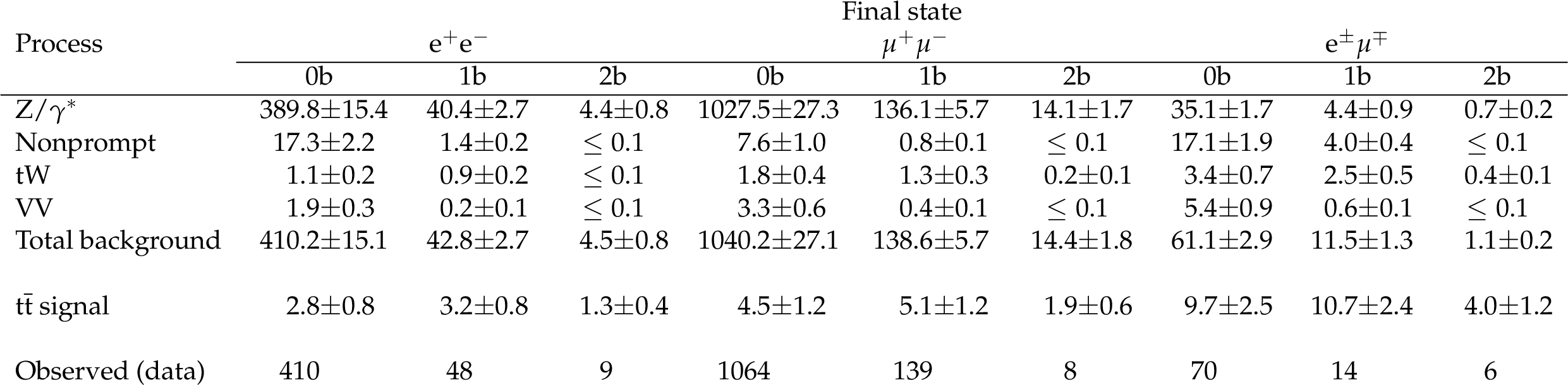
Table 1:
Number of expected background and signal events, and observed event yields in the $\mathrm{e} ^+\mathrm{e} ^-$, $\mu ^+\mu ^-$, and $\mathrm{e} ^\pm \mu ^\mp $ event categories for the three b jet multiplicities (0-b, 1-b, 2-b) after all selection criteria and the signal extraction fit. |
png pdf |
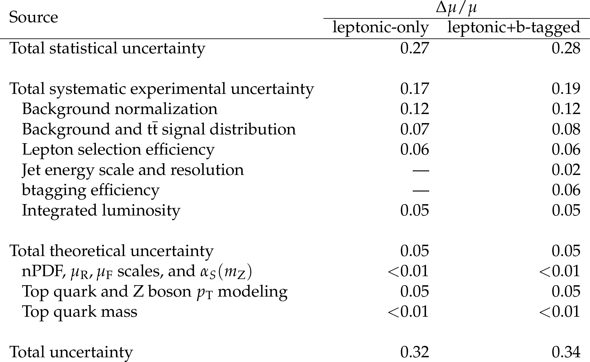
Table 2:
Observed impact of each source of uncertainty in the signal strength $\mu $, for the leptonic-only and leptonic+b-tagged analyses. The total uncertainty is obtained from the covariance matrix of the fits. The values quoted are symmetrized. |
| Summary |
| In summary, evidence for top quark pair production in nucleus-nucleus collisions has been presented for the first time, using lead-lead data at ${\sqrt {\smash [b]{s_{_{\mathrm {NN}}}}}} = $ 5.02 TeV with a total integrated luminosity of 1.7 $\pm$ 0.1 nb$^{-1}$. The measurement is performed analyzing events with at least one pair of isolated and oppositely charged leptons ($\ell^\pm\ell^\mp =\,\mathrm{e}^{+} \mathrm{e}^{-},\,\mu^{+} \mu^{-}$ , and $\mathrm{e}^{\pm} \mu^{\mp}$) with large transverse momenta, as well as adding the information on the number of jets tagged as originating from the hadronization of bottom quarks. The inclusive cross section (${\sigma_{\mathrm{t\bar{t}}}} $) is derived from likelihood fits to a multivariate discriminator, which includes different leptonic kinematic variables. Using the dilepton categories with and without the b-tagged jet multiplicity information, we demonstrate that top quark decay products are identified, irrespective of whether interacting with the medium or not. The measured cross sections are ${\sigma_{\mathrm{t\bar{t}}}} = $ 2.02 $\pm$ 0.69 (tot) and 2.56 $\pm$ 0.82 (tot) $\mu$b, respectively. These values are consistent with each other and lower, but still compatible, with respect to the expectations from scaled pp data as well as from perturbative quantum chromodynamics calculations. The observed (expected) significance of the $ \mathrm{t\bar{t}}$ signal against the background-only hypothesis are 4.0 (6.0) and 3.8 (4.8) standard deviations in the two cases, respectively. This first measurement paves the way for further detailed investigations of top quark production in nuclear interactions, providing, in particular, a new tool for studies of the strongly interacting matter created in nucleus-nucleus collisions. |
| Additional Figures | |
png pdf |
Additional Figure 1:
Invariant mass distributions of the lepton pairs in the ${{\mathrm {e}}^+ {\mathrm {e}}^-}$ (left), ${{{\mu}}^+ {{\mu}}^-}$ (middle), and ${{\mathrm {e}}^\pm {{\mu}}^\mp}$ (right) channels. Backgrounds and signal are shown with the filled histograms and data are shown with the markers. The vertical bars on the markers represent the statistical uncertainties in data. The hatched regions show the prefit uncertainties in the sum of ${{\mathrm {t}\overline {\mathrm {t}}}} $ signal and backgrounds. The lower panels display the ratio of the data to the predictions, including the ${{\mathrm {t}\overline {\mathrm {t}}}} $ signal, with bands representing the prefit uncertainties in the predictions. |

png pdf |
Additional Figure 1-a:
Invariant mass distributions of the lepton pairs in the ${{\mathrm {e}}^+ {\mathrm {e}}^-}$ (left), ${{{\mu}}^+ {{\mu}}^-}$ (middle), and ${{\mathrm {e}}^\pm {{\mu}}^\mp}$ (right) channels. Backgrounds and signal are shown with the filled histograms and data are shown with the markers. The vertical bars on the markers represent the statistical uncertainties in data. The hatched regions show the prefit uncertainties in the sum of ${{\mathrm {t}\overline {\mathrm {t}}}} $ signal and backgrounds. The lower panels display the ratio of the data to the predictions, including the ${{\mathrm {t}\overline {\mathrm {t}}}} $ signal, with bands representing the prefit uncertainties in the predictions. |

png pdf |
Additional Figure 1-b:
Invariant mass distributions of the lepton pairs in the ${{\mathrm {e}}^+ {\mathrm {e}}^-}$ (left), ${{{\mu}}^+ {{\mu}}^-}$ (middle), and ${{\mathrm {e}}^\pm {{\mu}}^\mp}$ (right) channels. Backgrounds and signal are shown with the filled histograms and data are shown with the markers. The vertical bars on the markers represent the statistical uncertainties in data. The hatched regions show the prefit uncertainties in the sum of ${{\mathrm {t}\overline {\mathrm {t}}}} $ signal and backgrounds. The lower panels display the ratio of the data to the predictions, including the ${{\mathrm {t}\overline {\mathrm {t}}}} $ signal, with bands representing the prefit uncertainties in the predictions. |
png pdf |
Additional Figure 1-c:
Invariant mass distributions of the lepton pairs in the ${{\mathrm {e}}^+ {\mathrm {e}}^-}$ (left), ${{{\mu}}^+ {{\mu}}^-}$ (middle), and ${{\mathrm {e}}^\pm {{\mu}}^\mp}$ (right) channels. Backgrounds and signal are shown with the filled histograms and data are shown with the markers. The vertical bars on the markers represent the statistical uncertainties in data. The hatched regions show the prefit uncertainties in the sum of ${{\mathrm {t}\overline {\mathrm {t}}}} $ signal and backgrounds. The lower panels display the ratio of the data to the predictions, including the ${{\mathrm {t}\overline {\mathrm {t}}}} $ signal, with bands representing the prefit uncertainties in the predictions. |
png pdf |
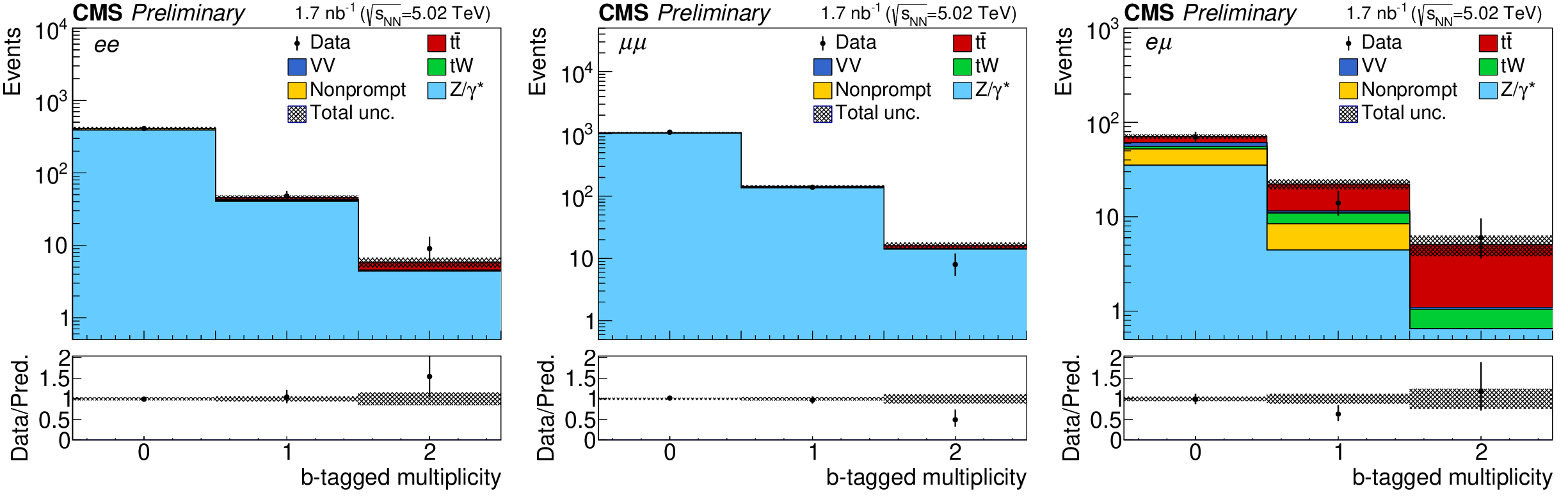
Additional Figure 2:
Postfit predicted multiplicity distributions of the b-tagged jets ($N_{\mathrm {b-tag}}$) in the ${{\mathrm {e}}^+ {\mathrm {e}}^-}$ (left), ${{{\mu}}^+ {{\mu}}^-}$ (middle), and ${{\mathrm {e}}^\pm {{\mu}}^\mp}$ (right) channels. The distribution of the Z/$\gamma ^{*}$ background is taken from the data. Backgrounds and signal are shown with the filled histograms and data are shown with the markers. The vertical bars on the markers represent the statistical uncertainties in data. The hatched regions show the postfit uncertainties in the sum of ${{\mathrm {t}\overline {\mathrm {t}}}} $ signal and backgrounds. The lower panels display the ratio of the data to the predictions, including the ${{\mathrm {t}\overline {\mathrm {t}}}} $ signal, with bands representing the postfit uncertainties in the predictions. |
png pdf |
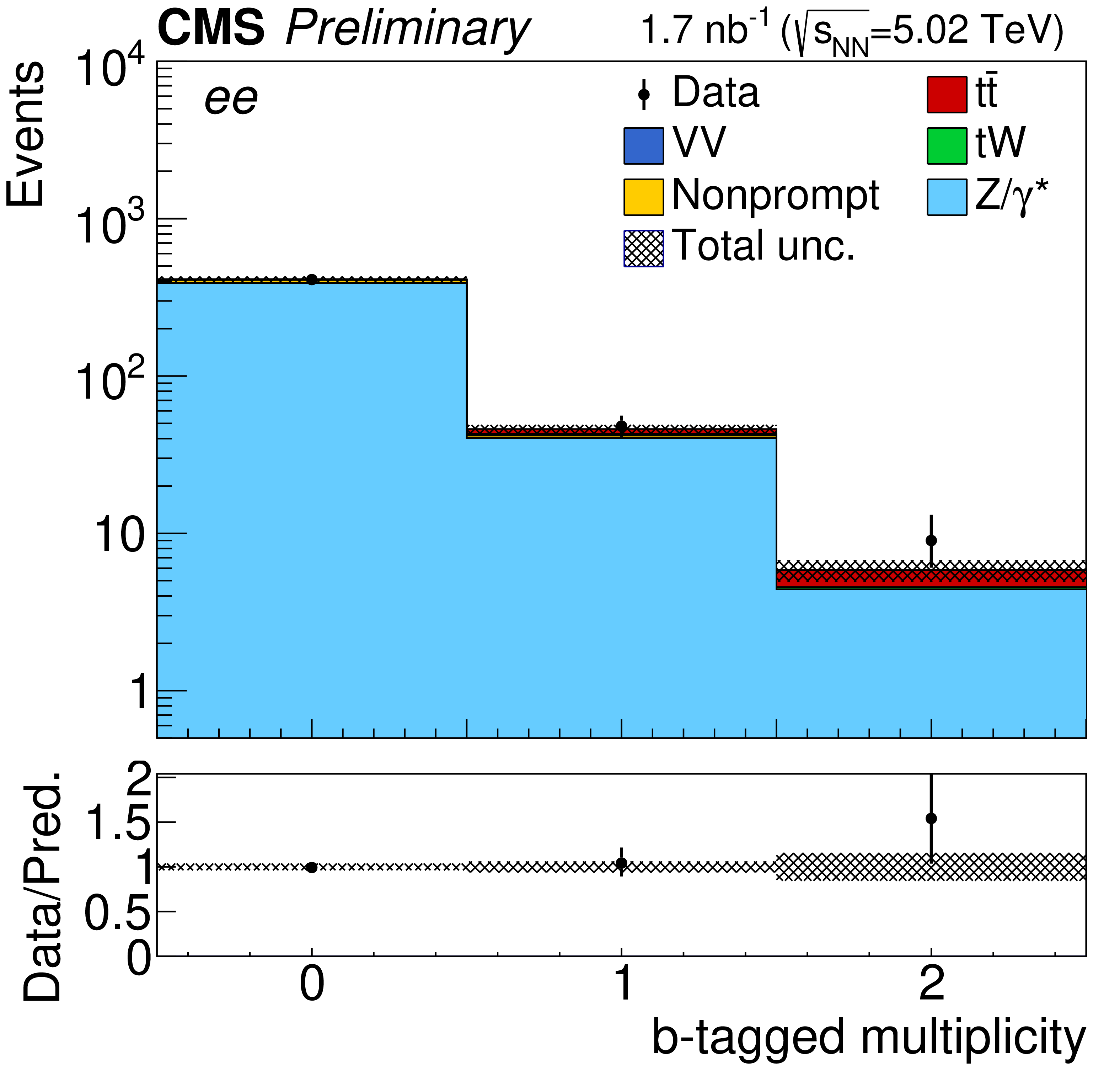
Additional Figure 2-a:
Postfit predicted multiplicity distributions of the b-tagged jets ($N_{\mathrm {b-tag}}$) in the ${{\mathrm {e}}^+ {\mathrm {e}}^-}$ (left), ${{{\mu}}^+ {{\mu}}^-}$ (middle), and ${{\mathrm {e}}^\pm {{\mu}}^\mp}$ (right) channels. The distribution of the Z/$\gamma ^{*}$ background is taken from the data. Backgrounds and signal are shown with the filled histograms and data are shown with the markers. The vertical bars on the markers represent the statistical uncertainties in data. The hatched regions show the postfit uncertainties in the sum of ${{\mathrm {t}\overline {\mathrm {t}}}} $ signal and backgrounds. The lower panels display the ratio of the data to the predictions, including the ${{\mathrm {t}\overline {\mathrm {t}}}} $ signal, with bands representing the postfit uncertainties in the predictions. |

png pdf |
Additional Figure 2-b:
Postfit predicted multiplicity distributions of the b-tagged jets ($N_{\mathrm {b-tag}}$) in the ${{\mathrm {e}}^+ {\mathrm {e}}^-}$ (left), ${{{\mu}}^+ {{\mu}}^-}$ (middle), and ${{\mathrm {e}}^\pm {{\mu}}^\mp}$ (right) channels. The distribution of the Z/$\gamma ^{*}$ background is taken from the data. Backgrounds and signal are shown with the filled histograms and data are shown with the markers. The vertical bars on the markers represent the statistical uncertainties in data. The hatched regions show the postfit uncertainties in the sum of ${{\mathrm {t}\overline {\mathrm {t}}}} $ signal and backgrounds. The lower panels display the ratio of the data to the predictions, including the ${{\mathrm {t}\overline {\mathrm {t}}}} $ signal, with bands representing the postfit uncertainties in the predictions. |
png pdf |
Additional Figure 2-c:
Postfit predicted multiplicity distributions of the b-tagged jets ($N_{\mathrm {b-tag}}$) in the ${{\mathrm {e}}^+ {\mathrm {e}}^-}$ (left), ${{{\mu}}^+ {{\mu}}^-}$ (middle), and ${{\mathrm {e}}^\pm {{\mu}}^\mp}$ (right) channels. The distribution of the Z/$\gamma ^{*}$ background is taken from the data. Backgrounds and signal are shown with the filled histograms and data are shown with the markers. The vertical bars on the markers represent the statistical uncertainties in data. The hatched regions show the postfit uncertainties in the sum of ${{\mathrm {t}\overline {\mathrm {t}}}} $ signal and backgrounds. The lower panels display the ratio of the data to the predictions, including the ${{\mathrm {t}\overline {\mathrm {t}}}} $ signal, with bands representing the postfit uncertainties in the predictions. |

png pdf |
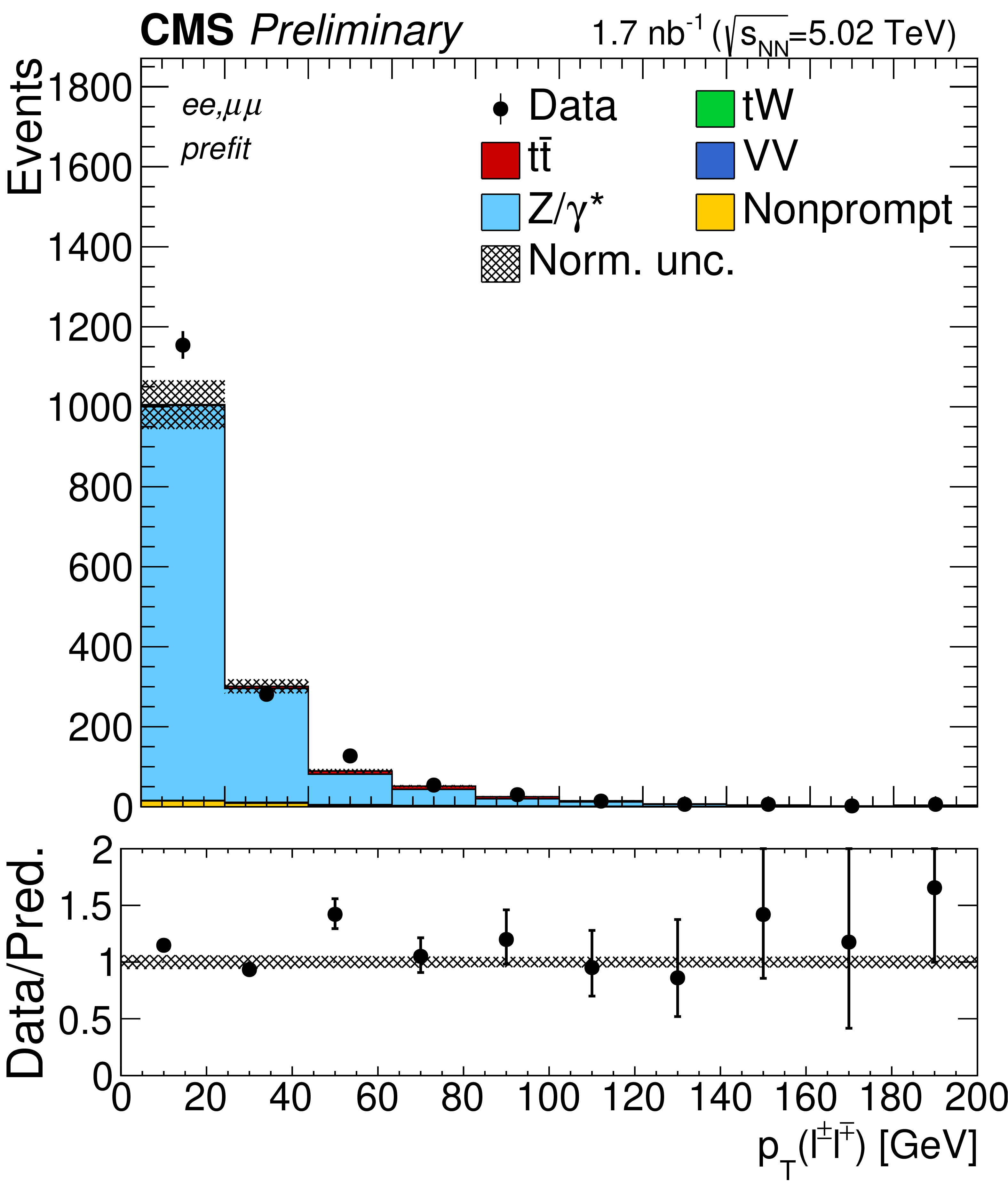
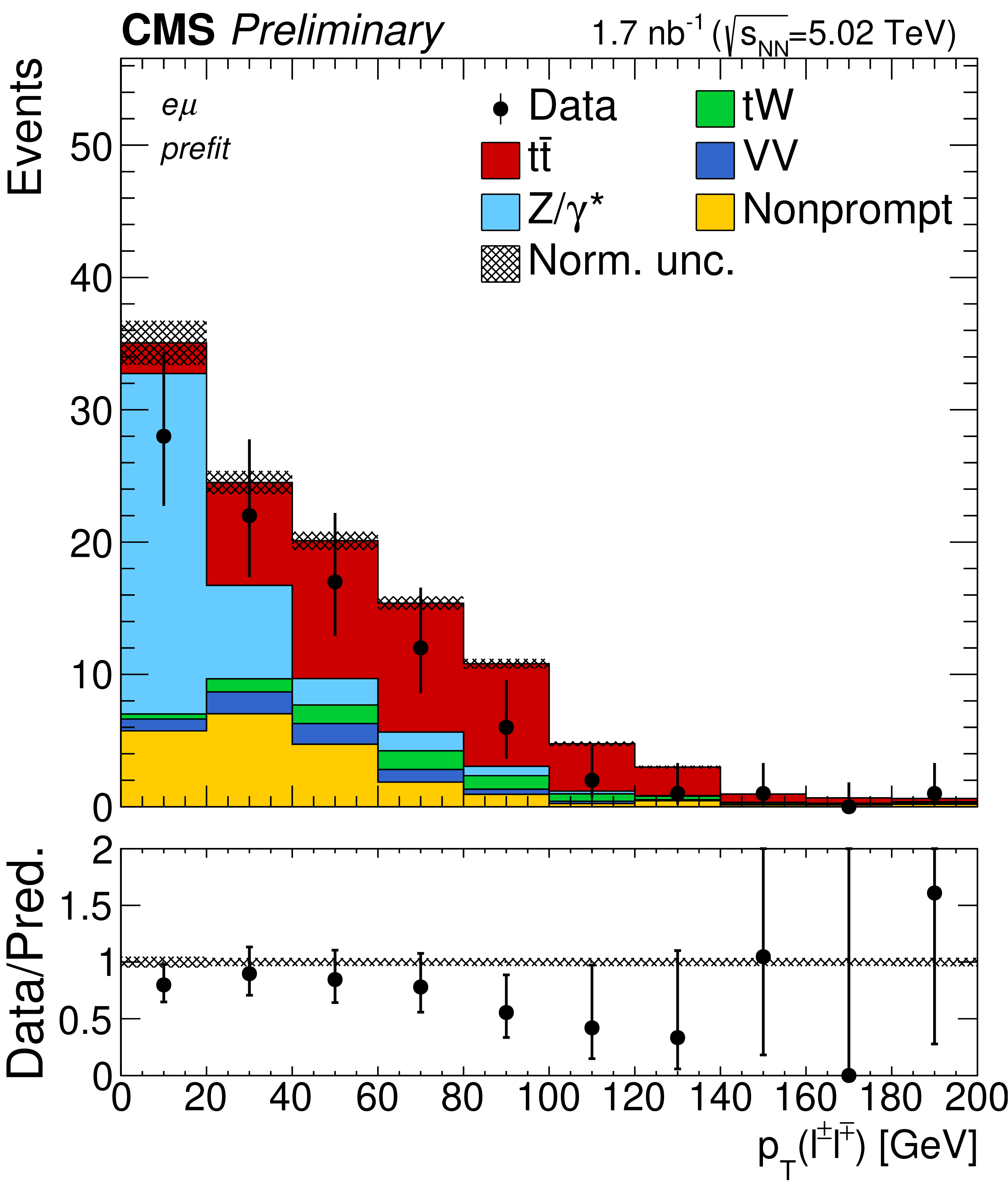
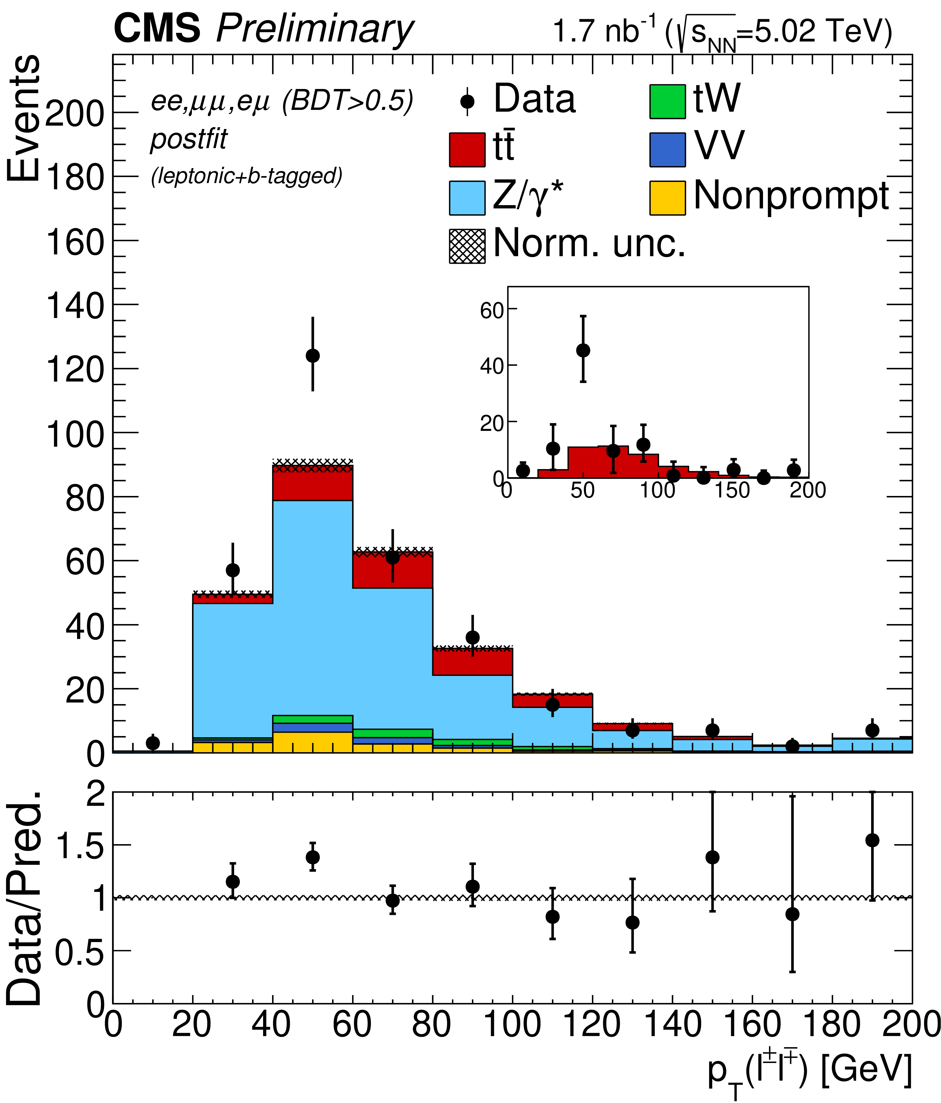
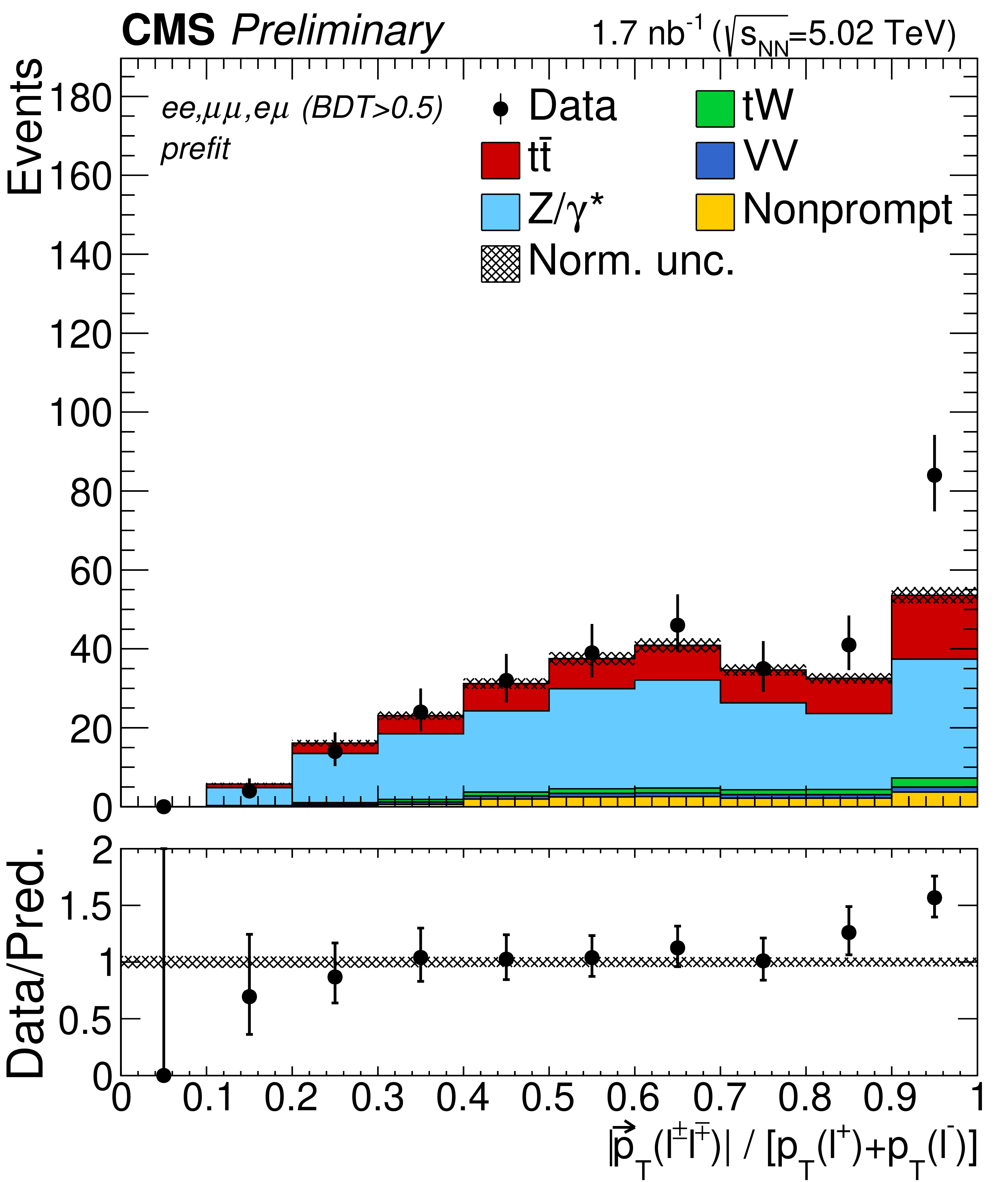
Additional Figure 3:
Transverse momentum distributions of the lepton pairs in the ${{\mathrm {e}}^+ {\mathrm {e}}^-}$, ${{{\mu}}^+ {{\mu}}^-}$, and ${{\mathrm {e}}^\pm {{\mu}}^\mp}$ ($\text {BDT} > 0.5$, left), ${{\mathrm {e}}^+ {\mathrm {e}}^-}$ and ${{{\mu}}^+ {{\mu}}^-}$(middle), and ${{\mathrm {e}}^\pm {{\mu}}^\mp}$ (right) channels. In the top (bottom) row the prefit (postfit) expectations (predictions) are compared to data. The comparison between the ${{\mathrm {t}\overline {\mathrm {t}}}} $ signal and the background-subtracted data is shown for the postfit distributions as inset panels. Backgrounds and signal are shown with the filled histograms and data are shown with the markers. The vertical bars on the markers represent the statistical uncertainties in data. The hatched regions show the postfit uncertainties in the sum of ${{\mathrm {t}\overline {\mathrm {t}}}} $ signal and backgrounds. The lower panels display the ratio of the data to the predictions, including the ${{\mathrm {t}\overline {\mathrm {t}}}} $ signal, with bands representing the postfit uncertainties in the predictions. |

png pdf |
Additional Figure 3-a:
Transverse momentum distributions of the lepton pairs in the ${{\mathrm {e}}^+ {\mathrm {e}}^-}$, ${{{\mu}}^+ {{\mu}}^-}$, and ${{\mathrm {e}}^\pm {{\mu}}^\mp}$ ($\text {BDT} > 0.5$, left), ${{\mathrm {e}}^+ {\mathrm {e}}^-}$ and ${{{\mu}}^+ {{\mu}}^-}$(middle), and ${{\mathrm {e}}^\pm {{\mu}}^\mp}$ (right) channels. In the top (bottom) row the prefit (postfit) expectations (predictions) are compared to data. The comparison between the ${{\mathrm {t}\overline {\mathrm {t}}}} $ signal and the background-subtracted data is shown for the postfit distributions as inset panels. Backgrounds and signal are shown with the filled histograms and data are shown with the markers. The vertical bars on the markers represent the statistical uncertainties in data. The hatched regions show the postfit uncertainties in the sum of ${{\mathrm {t}\overline {\mathrm {t}}}} $ signal and backgrounds. The lower panels display the ratio of the data to the predictions, including the ${{\mathrm {t}\overline {\mathrm {t}}}} $ signal, with bands representing the postfit uncertainties in the predictions. |
png pdf |
Additional Figure 3-b:
Transverse momentum distributions of the lepton pairs in the ${{\mathrm {e}}^+ {\mathrm {e}}^-}$, ${{{\mu}}^+ {{\mu}}^-}$, and ${{\mathrm {e}}^\pm {{\mu}}^\mp}$ ($\text {BDT} > 0.5$, left), ${{\mathrm {e}}^+ {\mathrm {e}}^-}$ and ${{{\mu}}^+ {{\mu}}^-}$(middle), and ${{\mathrm {e}}^\pm {{\mu}}^\mp}$ (right) channels. In the top (bottom) row the prefit (postfit) expectations (predictions) are compared to data. The comparison between the ${{\mathrm {t}\overline {\mathrm {t}}}} $ signal and the background-subtracted data is shown for the postfit distributions as inset panels. Backgrounds and signal are shown with the filled histograms and data are shown with the markers. The vertical bars on the markers represent the statistical uncertainties in data. The hatched regions show the postfit uncertainties in the sum of ${{\mathrm {t}\overline {\mathrm {t}}}} $ signal and backgrounds. The lower panels display the ratio of the data to the predictions, including the ${{\mathrm {t}\overline {\mathrm {t}}}} $ signal, with bands representing the postfit uncertainties in the predictions. |
png pdf |
Additional Figure 3-c:
Transverse momentum distributions of the lepton pairs in the ${{\mathrm {e}}^+ {\mathrm {e}}^-}$, ${{{\mu}}^+ {{\mu}}^-}$, and ${{\mathrm {e}}^\pm {{\mu}}^\mp}$ ($\text {BDT} > 0.5$, left), ${{\mathrm {e}}^+ {\mathrm {e}}^-}$ and ${{{\mu}}^+ {{\mu}}^-}$(middle), and ${{\mathrm {e}}^\pm {{\mu}}^\mp}$ (right) channels. In the top (bottom) row the prefit (postfit) expectations (predictions) are compared to data. The comparison between the ${{\mathrm {t}\overline {\mathrm {t}}}} $ signal and the background-subtracted data is shown for the postfit distributions as inset panels. Backgrounds and signal are shown with the filled histograms and data are shown with the markers. The vertical bars on the markers represent the statistical uncertainties in data. The hatched regions show the postfit uncertainties in the sum of ${{\mathrm {t}\overline {\mathrm {t}}}} $ signal and backgrounds. The lower panels display the ratio of the data to the predictions, including the ${{\mathrm {t}\overline {\mathrm {t}}}} $ signal, with bands representing the postfit uncertainties in the predictions. |
png pdf |
Additional Figure 3-d:
Transverse momentum distributions of the lepton pairs in the ${{\mathrm {e}}^+ {\mathrm {e}}^-}$, ${{{\mu}}^+ {{\mu}}^-}$, and ${{\mathrm {e}}^\pm {{\mu}}^\mp}$ ($\text {BDT} > 0.5$, left), ${{\mathrm {e}}^+ {\mathrm {e}}^-}$ and ${{{\mu}}^+ {{\mu}}^-}$(middle), and ${{\mathrm {e}}^\pm {{\mu}}^\mp}$ (right) channels. In the top (bottom) row the prefit (postfit) expectations (predictions) are compared to data. The comparison between the ${{\mathrm {t}\overline {\mathrm {t}}}} $ signal and the background-subtracted data is shown for the postfit distributions as inset panels. Backgrounds and signal are shown with the filled histograms and data are shown with the markers. The vertical bars on the markers represent the statistical uncertainties in data. The hatched regions show the postfit uncertainties in the sum of ${{\mathrm {t}\overline {\mathrm {t}}}} $ signal and backgrounds. The lower panels display the ratio of the data to the predictions, including the ${{\mathrm {t}\overline {\mathrm {t}}}} $ signal, with bands representing the postfit uncertainties in the predictions. |

png pdf |
Additional Figure 3-e:
Transverse momentum distributions of the lepton pairs in the ${{\mathrm {e}}^+ {\mathrm {e}}^-}$, ${{{\mu}}^+ {{\mu}}^-}$, and ${{\mathrm {e}}^\pm {{\mu}}^\mp}$ ($\text {BDT} > 0.5$, left), ${{\mathrm {e}}^+ {\mathrm {e}}^-}$ and ${{{\mu}}^+ {{\mu}}^-}$(middle), and ${{\mathrm {e}}^\pm {{\mu}}^\mp}$ (right) channels. In the top (bottom) row the prefit (postfit) expectations (predictions) are compared to data. The comparison between the ${{\mathrm {t}\overline {\mathrm {t}}}} $ signal and the background-subtracted data is shown for the postfit distributions as inset panels. Backgrounds and signal are shown with the filled histograms and data are shown with the markers. The vertical bars on the markers represent the statistical uncertainties in data. The hatched regions show the postfit uncertainties in the sum of ${{\mathrm {t}\overline {\mathrm {t}}}} $ signal and backgrounds. The lower panels display the ratio of the data to the predictions, including the ${{\mathrm {t}\overline {\mathrm {t}}}} $ signal, with bands representing the postfit uncertainties in the predictions. |

png pdf |
Additional Figure 3-f:
Transverse momentum distributions of the lepton pairs in the ${{\mathrm {e}}^+ {\mathrm {e}}^-}$, ${{{\mu}}^+ {{\mu}}^-}$, and ${{\mathrm {e}}^\pm {{\mu}}^\mp}$ ($\text {BDT} > 0.5$, left), ${{\mathrm {e}}^+ {\mathrm {e}}^-}$ and ${{{\mu}}^+ {{\mu}}^-}$(middle), and ${{\mathrm {e}}^\pm {{\mu}}^\mp}$ (right) channels. In the top (bottom) row the prefit (postfit) expectations (predictions) are compared to data. The comparison between the ${{\mathrm {t}\overline {\mathrm {t}}}} $ signal and the background-subtracted data is shown for the postfit distributions as inset panels. Backgrounds and signal are shown with the filled histograms and data are shown with the markers. The vertical bars on the markers represent the statistical uncertainties in data. The hatched regions show the postfit uncertainties in the sum of ${{\mathrm {t}\overline {\mathrm {t}}}} $ signal and backgrounds. The lower panels display the ratio of the data to the predictions, including the ${{\mathrm {t}\overline {\mathrm {t}}}} $ signal, with bands representing the postfit uncertainties in the predictions. |
png pdf |
Additional Figure 4:
Acoplanarity distributions of the lepton pairs in the ${{\mathrm {e}}^+ {\mathrm {e}}^-}$, ${{{\mu}}^+ {{\mu}}^-}$, and ${{\mathrm {e}}^\pm {{\mu}}^\mp}$ ($\text {BDT} > 0.5$, left), ${{\mathrm {e}}^+ {\mathrm {e}}^-}$ and ${{{\mu}}^+ {{\mu}}^-}$(middle), and ${{\mathrm {e}}^\pm {{\mu}}^\mp}$ (right) channels. In the top (bottom) row the prefit (postfit) expectations (predictions) are compared to data. The comparison between the ${{\mathrm {t}\overline {\mathrm {t}}}} $ signal and the background-subtracted data is shown for the postfit distributions as inset panels. Backgrounds and signal are shown with the filled histograms and data are shown with the markers. The vertical bars on the markers represent the statistical uncertainties in data. The hatched regions show the postfit uncertainties in the sum of ${{\mathrm {t}\overline {\mathrm {t}}}} $ signal and backgrounds. The lower panels display the ratio of the data to the predictions, including the ${{\mathrm {t}\overline {\mathrm {t}}}} $ signal, with bands representing the postfit uncertainties in the predictions. |

png pdf |
Additional Figure 4-a:
Acoplanarity distributions of the lepton pairs in the ${{\mathrm {e}}^+ {\mathrm {e}}^-}$, ${{{\mu}}^+ {{\mu}}^-}$, and ${{\mathrm {e}}^\pm {{\mu}}^\mp}$ ($\text {BDT} > 0.5$, left), ${{\mathrm {e}}^+ {\mathrm {e}}^-}$ and ${{{\mu}}^+ {{\mu}}^-}$(middle), and ${{\mathrm {e}}^\pm {{\mu}}^\mp}$ (right) channels. In the top (bottom) row the prefit (postfit) expectations (predictions) are compared to data. The comparison between the ${{\mathrm {t}\overline {\mathrm {t}}}} $ signal and the background-subtracted data is shown for the postfit distributions as inset panels. Backgrounds and signal are shown with the filled histograms and data are shown with the markers. The vertical bars on the markers represent the statistical uncertainties in data. The hatched regions show the postfit uncertainties in the sum of ${{\mathrm {t}\overline {\mathrm {t}}}} $ signal and backgrounds. The lower panels display the ratio of the data to the predictions, including the ${{\mathrm {t}\overline {\mathrm {t}}}} $ signal, with bands representing the postfit uncertainties in the predictions. |

png pdf |
Additional Figure 4-b:
Acoplanarity distributions of the lepton pairs in the ${{\mathrm {e}}^+ {\mathrm {e}}^-}$, ${{{\mu}}^+ {{\mu}}^-}$, and ${{\mathrm {e}}^\pm {{\mu}}^\mp}$ ($\text {BDT} > 0.5$, left), ${{\mathrm {e}}^+ {\mathrm {e}}^-}$ and ${{{\mu}}^+ {{\mu}}^-}$(middle), and ${{\mathrm {e}}^\pm {{\mu}}^\mp}$ (right) channels. In the top (bottom) row the prefit (postfit) expectations (predictions) are compared to data. The comparison between the ${{\mathrm {t}\overline {\mathrm {t}}}} $ signal and the background-subtracted data is shown for the postfit distributions as inset panels. Backgrounds and signal are shown with the filled histograms and data are shown with the markers. The vertical bars on the markers represent the statistical uncertainties in data. The hatched regions show the postfit uncertainties in the sum of ${{\mathrm {t}\overline {\mathrm {t}}}} $ signal and backgrounds. The lower panels display the ratio of the data to the predictions, including the ${{\mathrm {t}\overline {\mathrm {t}}}} $ signal, with bands representing the postfit uncertainties in the predictions. |
png pdf |
Additional Figure 4-c:
Acoplanarity distributions of the lepton pairs in the ${{\mathrm {e}}^+ {\mathrm {e}}^-}$, ${{{\mu}}^+ {{\mu}}^-}$, and ${{\mathrm {e}}^\pm {{\mu}}^\mp}$ ($\text {BDT} > 0.5$, left), ${{\mathrm {e}}^+ {\mathrm {e}}^-}$ and ${{{\mu}}^+ {{\mu}}^-}$(middle), and ${{\mathrm {e}}^\pm {{\mu}}^\mp}$ (right) channels. In the top (bottom) row the prefit (postfit) expectations (predictions) are compared to data. The comparison between the ${{\mathrm {t}\overline {\mathrm {t}}}} $ signal and the background-subtracted data is shown for the postfit distributions as inset panels. Backgrounds and signal are shown with the filled histograms and data are shown with the markers. The vertical bars on the markers represent the statistical uncertainties in data. The hatched regions show the postfit uncertainties in the sum of ${{\mathrm {t}\overline {\mathrm {t}}}} $ signal and backgrounds. The lower panels display the ratio of the data to the predictions, including the ${{\mathrm {t}\overline {\mathrm {t}}}} $ signal, with bands representing the postfit uncertainties in the predictions. |

png pdf |
Additional Figure 4-d:
Acoplanarity distributions of the lepton pairs in the ${{\mathrm {e}}^+ {\mathrm {e}}^-}$, ${{{\mu}}^+ {{\mu}}^-}$, and ${{\mathrm {e}}^\pm {{\mu}}^\mp}$ ($\text {BDT} > 0.5$, left), ${{\mathrm {e}}^+ {\mathrm {e}}^-}$ and ${{{\mu}}^+ {{\mu}}^-}$(middle), and ${{\mathrm {e}}^\pm {{\mu}}^\mp}$ (right) channels. In the top (bottom) row the prefit (postfit) expectations (predictions) are compared to data. The comparison between the ${{\mathrm {t}\overline {\mathrm {t}}}} $ signal and the background-subtracted data is shown for the postfit distributions as inset panels. Backgrounds and signal are shown with the filled histograms and data are shown with the markers. The vertical bars on the markers represent the statistical uncertainties in data. The hatched regions show the postfit uncertainties in the sum of ${{\mathrm {t}\overline {\mathrm {t}}}} $ signal and backgrounds. The lower panels display the ratio of the data to the predictions, including the ${{\mathrm {t}\overline {\mathrm {t}}}} $ signal, with bands representing the postfit uncertainties in the predictions. |
png pdf |
Additional Figure 4-e:
Acoplanarity distributions of the lepton pairs in the ${{\mathrm {e}}^+ {\mathrm {e}}^-}$, ${{{\mu}}^+ {{\mu}}^-}$, and ${{\mathrm {e}}^\pm {{\mu}}^\mp}$ ($\text {BDT} > 0.5$, left), ${{\mathrm {e}}^+ {\mathrm {e}}^-}$ and ${{{\mu}}^+ {{\mu}}^-}$(middle), and ${{\mathrm {e}}^\pm {{\mu}}^\mp}$ (right) channels. In the top (bottom) row the prefit (postfit) expectations (predictions) are compared to data. The comparison between the ${{\mathrm {t}\overline {\mathrm {t}}}} $ signal and the background-subtracted data is shown for the postfit distributions as inset panels. Backgrounds and signal are shown with the filled histograms and data are shown with the markers. The vertical bars on the markers represent the statistical uncertainties in data. The hatched regions show the postfit uncertainties in the sum of ${{\mathrm {t}\overline {\mathrm {t}}}} $ signal and backgrounds. The lower panels display the ratio of the data to the predictions, including the ${{\mathrm {t}\overline {\mathrm {t}}}} $ signal, with bands representing the postfit uncertainties in the predictions. |

png pdf |
Additional Figure 4-f:
Acoplanarity distributions of the lepton pairs in the ${{\mathrm {e}}^+ {\mathrm {e}}^-}$, ${{{\mu}}^+ {{\mu}}^-}$, and ${{\mathrm {e}}^\pm {{\mu}}^\mp}$ ($\text {BDT} > 0.5$, left), ${{\mathrm {e}}^+ {\mathrm {e}}^-}$ and ${{{\mu}}^+ {{\mu}}^-}$(middle), and ${{\mathrm {e}}^\pm {{\mu}}^\mp}$ (right) channels. In the top (bottom) row the prefit (postfit) expectations (predictions) are compared to data. The comparison between the ${{\mathrm {t}\overline {\mathrm {t}}}} $ signal and the background-subtracted data is shown for the postfit distributions as inset panels. Backgrounds and signal are shown with the filled histograms and data are shown with the markers. The vertical bars on the markers represent the statistical uncertainties in data. The hatched regions show the postfit uncertainties in the sum of ${{\mathrm {t}\overline {\mathrm {t}}}} $ signal and backgrounds. The lower panels display the ratio of the data to the predictions, including the ${{\mathrm {t}\overline {\mathrm {t}}}} $ signal, with bands representing the postfit uncertainties in the predictions. |

png pdf |
Additional Figure 5:
Sphericity distributions of the lepton pairs in the ${{\mathrm {e}}^+ {\mathrm {e}}^-}$, ${{{\mu}}^+ {{\mu}}^-}$, and ${{\mathrm {e}}^\pm {{\mu}}^\mp}$ ($\text {BDT} > 0.5$, left), ${{\mathrm {e}}^+ {\mathrm {e}}^-}$ and ${{{\mu}}^+ {{\mu}}^-}$(middle), and ${{\mathrm {e}}^\pm {{\mu}}^\mp}$ (right) channels. In the top (bottom) row the prefit (postfit) expectations (predictions) are compared to data. The comparison between the ${{\mathrm {t}\overline {\mathrm {t}}}} $ signal and the background-subtracted data is shown for the postfit distributions as inset panels. Backgrounds and signal are shown with the filled histograms and data are shown with the markers. The vertical bars on the markers represent the statistical uncertainties in data. The hatched regions show the postfit uncertainties in the sum of ${{\mathrm {t}\overline {\mathrm {t}}}} $ signal and backgrounds. The lower panels display the ratio of the data to the predictions, including the ${{\mathrm {t}\overline {\mathrm {t}}}} $ signal, with bands representing the postfit uncertainties in the predictions. |
png pdf |
Additional Figure 5-a:
Sphericity distributions of the lepton pairs in the ${{\mathrm {e}}^+ {\mathrm {e}}^-}$, ${{{\mu}}^+ {{\mu}}^-}$, and ${{\mathrm {e}}^\pm {{\mu}}^\mp}$ ($\text {BDT} > 0.5$, left), ${{\mathrm {e}}^+ {\mathrm {e}}^-}$ and ${{{\mu}}^+ {{\mu}}^-}$(middle), and ${{\mathrm {e}}^\pm {{\mu}}^\mp}$ (right) channels. In the top (bottom) row the prefit (postfit) expectations (predictions) are compared to data. The comparison between the ${{\mathrm {t}\overline {\mathrm {t}}}} $ signal and the background-subtracted data is shown for the postfit distributions as inset panels. Backgrounds and signal are shown with the filled histograms and data are shown with the markers. The vertical bars on the markers represent the statistical uncertainties in data. The hatched regions show the postfit uncertainties in the sum of ${{\mathrm {t}\overline {\mathrm {t}}}} $ signal and backgrounds. The lower panels display the ratio of the data to the predictions, including the ${{\mathrm {t}\overline {\mathrm {t}}}} $ signal, with bands representing the postfit uncertainties in the predictions. |

png pdf |
Additional Figure 5-b:
Sphericity distributions of the lepton pairs in the ${{\mathrm {e}}^+ {\mathrm {e}}^-}$, ${{{\mu}}^+ {{\mu}}^-}$, and ${{\mathrm {e}}^\pm {{\mu}}^\mp}$ ($\text {BDT} > 0.5$, left), ${{\mathrm {e}}^+ {\mathrm {e}}^-}$ and ${{{\mu}}^+ {{\mu}}^-}$(middle), and ${{\mathrm {e}}^\pm {{\mu}}^\mp}$ (right) channels. In the top (bottom) row the prefit (postfit) expectations (predictions) are compared to data. The comparison between the ${{\mathrm {t}\overline {\mathrm {t}}}} $ signal and the background-subtracted data is shown for the postfit distributions as inset panels. Backgrounds and signal are shown with the filled histograms and data are shown with the markers. The vertical bars on the markers represent the statistical uncertainties in data. The hatched regions show the postfit uncertainties in the sum of ${{\mathrm {t}\overline {\mathrm {t}}}} $ signal and backgrounds. The lower panels display the ratio of the data to the predictions, including the ${{\mathrm {t}\overline {\mathrm {t}}}} $ signal, with bands representing the postfit uncertainties in the predictions. |
png pdf |
Additional Figure 5-c:
Sphericity distributions of the lepton pairs in the ${{\mathrm {e}}^+ {\mathrm {e}}^-}$, ${{{\mu}}^+ {{\mu}}^-}$, and ${{\mathrm {e}}^\pm {{\mu}}^\mp}$ ($\text {BDT} > 0.5$, left), ${{\mathrm {e}}^+ {\mathrm {e}}^-}$ and ${{{\mu}}^+ {{\mu}}^-}$(middle), and ${{\mathrm {e}}^\pm {{\mu}}^\mp}$ (right) channels. In the top (bottom) row the prefit (postfit) expectations (predictions) are compared to data. The comparison between the ${{\mathrm {t}\overline {\mathrm {t}}}} $ signal and the background-subtracted data is shown for the postfit distributions as inset panels. Backgrounds and signal are shown with the filled histograms and data are shown with the markers. The vertical bars on the markers represent the statistical uncertainties in data. The hatched regions show the postfit uncertainties in the sum of ${{\mathrm {t}\overline {\mathrm {t}}}} $ signal and backgrounds. The lower panels display the ratio of the data to the predictions, including the ${{\mathrm {t}\overline {\mathrm {t}}}} $ signal, with bands representing the postfit uncertainties in the predictions. |

png pdf |
Additional Figure 5-d:
Sphericity distributions of the lepton pairs in the ${{\mathrm {e}}^+ {\mathrm {e}}^-}$, ${{{\mu}}^+ {{\mu}}^-}$, and ${{\mathrm {e}}^\pm {{\mu}}^\mp}$ ($\text {BDT} > 0.5$, left), ${{\mathrm {e}}^+ {\mathrm {e}}^-}$ and ${{{\mu}}^+ {{\mu}}^-}$(middle), and ${{\mathrm {e}}^\pm {{\mu}}^\mp}$ (right) channels. In the top (bottom) row the prefit (postfit) expectations (predictions) are compared to data. The comparison between the ${{\mathrm {t}\overline {\mathrm {t}}}} $ signal and the background-subtracted data is shown for the postfit distributions as inset panels. Backgrounds and signal are shown with the filled histograms and data are shown with the markers. The vertical bars on the markers represent the statistical uncertainties in data. The hatched regions show the postfit uncertainties in the sum of ${{\mathrm {t}\overline {\mathrm {t}}}} $ signal and backgrounds. The lower panels display the ratio of the data to the predictions, including the ${{\mathrm {t}\overline {\mathrm {t}}}} $ signal, with bands representing the postfit uncertainties in the predictions. |

png pdf |
Additional Figure 5-e:
Sphericity distributions of the lepton pairs in the ${{\mathrm {e}}^+ {\mathrm {e}}^-}$, ${{{\mu}}^+ {{\mu}}^-}$, and ${{\mathrm {e}}^\pm {{\mu}}^\mp}$ ($\text {BDT} > 0.5$, left), ${{\mathrm {e}}^+ {\mathrm {e}}^-}$ and ${{{\mu}}^+ {{\mu}}^-}$(middle), and ${{\mathrm {e}}^\pm {{\mu}}^\mp}$ (right) channels. In the top (bottom) row the prefit (postfit) expectations (predictions) are compared to data. The comparison between the ${{\mathrm {t}\overline {\mathrm {t}}}} $ signal and the background-subtracted data is shown for the postfit distributions as inset panels. Backgrounds and signal are shown with the filled histograms and data are shown with the markers. The vertical bars on the markers represent the statistical uncertainties in data. The hatched regions show the postfit uncertainties in the sum of ${{\mathrm {t}\overline {\mathrm {t}}}} $ signal and backgrounds. The lower panels display the ratio of the data to the predictions, including the ${{\mathrm {t}\overline {\mathrm {t}}}} $ signal, with bands representing the postfit uncertainties in the predictions. |

png pdf |
Additional Figure 5-f:
Sphericity distributions of the lepton pairs in the ${{\mathrm {e}}^+ {\mathrm {e}}^-}$, ${{{\mu}}^+ {{\mu}}^-}$, and ${{\mathrm {e}}^\pm {{\mu}}^\mp}$ ($\text {BDT} > 0.5$, left), ${{\mathrm {e}}^+ {\mathrm {e}}^-}$ and ${{{\mu}}^+ {{\mu}}^-}$(middle), and ${{\mathrm {e}}^\pm {{\mu}}^\mp}$ (right) channels. In the top (bottom) row the prefit (postfit) expectations (predictions) are compared to data. The comparison between the ${{\mathrm {t}\overline {\mathrm {t}}}} $ signal and the background-subtracted data is shown for the postfit distributions as inset panels. Backgrounds and signal are shown with the filled histograms and data are shown with the markers. The vertical bars on the markers represent the statistical uncertainties in data. The hatched regions show the postfit uncertainties in the sum of ${{\mathrm {t}\overline {\mathrm {t}}}} $ signal and backgrounds. The lower panels display the ratio of the data to the predictions, including the ${{\mathrm {t}\overline {\mathrm {t}}}} $ signal, with bands representing the postfit uncertainties in the predictions. |
png pdf |
Additional Figure 6:
Distributions for the two reconstructed jets with the highest b tagging discriminator value in the ${{\mathrm {t}\overline {\mathrm {t}}}} $ signal (red) and Z/$\gamma ^{*}$ (cyan) background MC simulation. The generator level transverse momentum is shown on the top, while the b tagging discriminator output on the bottom. The left (right) distributions correspond to the leading (subleading) in b tagging discriminator jet. |
png pdf |
Additional Figure 6-a:
Distributions for the two reconstructed jets with the highest b tagging discriminator value in the ${{\mathrm {t}\overline {\mathrm {t}}}} $ signal (red) and Z/$\gamma ^{*}$ (cyan) background MC simulation. The generator level transverse momentum is shown on the top, while the b tagging discriminator output on the bottom. The left (right) distributions correspond to the leading (subleading) in b tagging discriminator jet. |
png pdf |
Additional Figure 6-b:
Distributions for the two reconstructed jets with the highest b tagging discriminator value in the ${{\mathrm {t}\overline {\mathrm {t}}}} $ signal (red) and Z/$\gamma ^{*}$ (cyan) background MC simulation. The generator level transverse momentum is shown on the top, while the b tagging discriminator output on the bottom. The left (right) distributions correspond to the leading (subleading) in b tagging discriminator jet. |

png pdf |
Additional Figure 6-c:
Distributions for the two reconstructed jets with the highest b tagging discriminator value in the ${{\mathrm {t}\overline {\mathrm {t}}}} $ signal (red) and Z/$\gamma ^{*}$ (cyan) background MC simulation. The generator level transverse momentum is shown on the top, while the b tagging discriminator output on the bottom. The left (right) distributions correspond to the leading (subleading) in b tagging discriminator jet. |

png pdf |
Additional Figure 6-d:
Distributions for the two reconstructed jets with the highest b tagging discriminator value in the ${{\mathrm {t}\overline {\mathrm {t}}}} $ signal (red) and Z/$\gamma ^{*}$ (cyan) background MC simulation. The generator level transverse momentum is shown on the top, while the b tagging discriminator output on the bottom. The left (right) distributions correspond to the leading (subleading) in b tagging discriminator jet. |
png pdf |
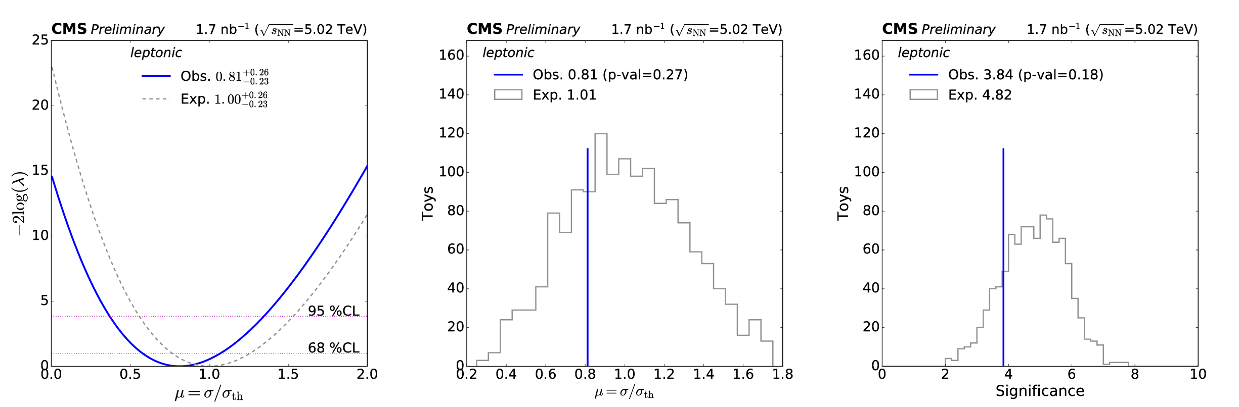
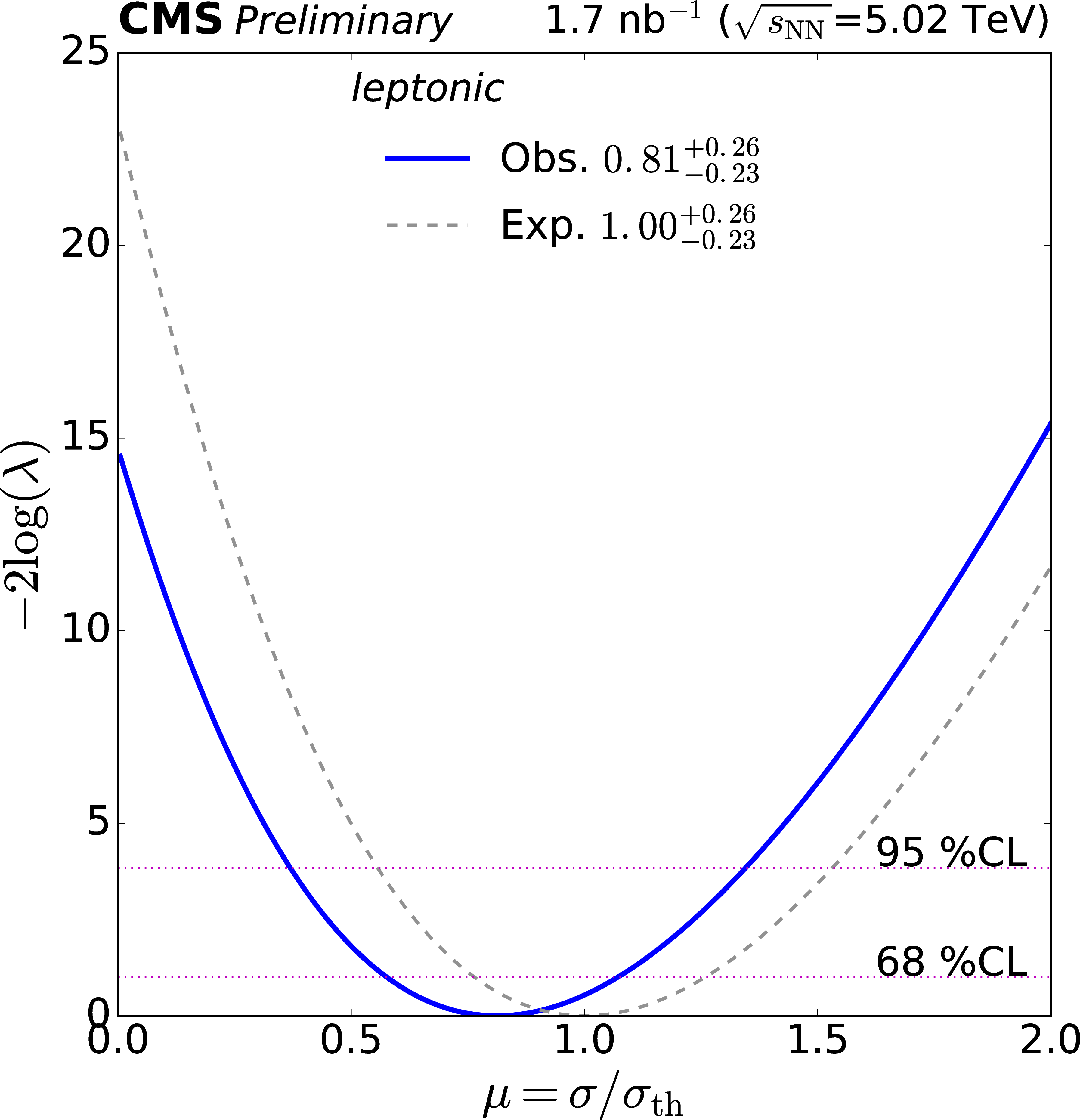
Additional Figure 7:
Scan of the profile likelihood (left), distribution of signal strength $\mu $ (middle), distribution of significances (right) expected in pseudo-experiments (blue curves and histograms) and observed in data (green curves and lines) for the signal extraction fit in the leptonic-only measurement. |
png pdf |
Additional Figure 7-a:
Scan of the profile likelihood (left), distribution of signal strength $\mu $ (middle), distribution of significances (right) expected in pseudo-experiments (blue curves and histograms) and observed in data (green curves and lines) for the signal extraction fit in the leptonic-only measurement. |

png pdf |
Additional Figure 7-b:
Scan of the profile likelihood (left), distribution of signal strength $\mu $ (middle), distribution of significances (right) expected in pseudo-experiments (blue curves and histograms) and observed in data (green curves and lines) for the signal extraction fit in the leptonic-only measurement. |

png pdf |
Additional Figure 7-c:
Scan of the profile likelihood (left), distribution of signal strength $\mu $ (middle), distribution of significances (right) expected in pseudo-experiments (blue curves and histograms) and observed in data (green curves and lines) for the signal extraction fit in the leptonic-only measurement. |

png pdf |
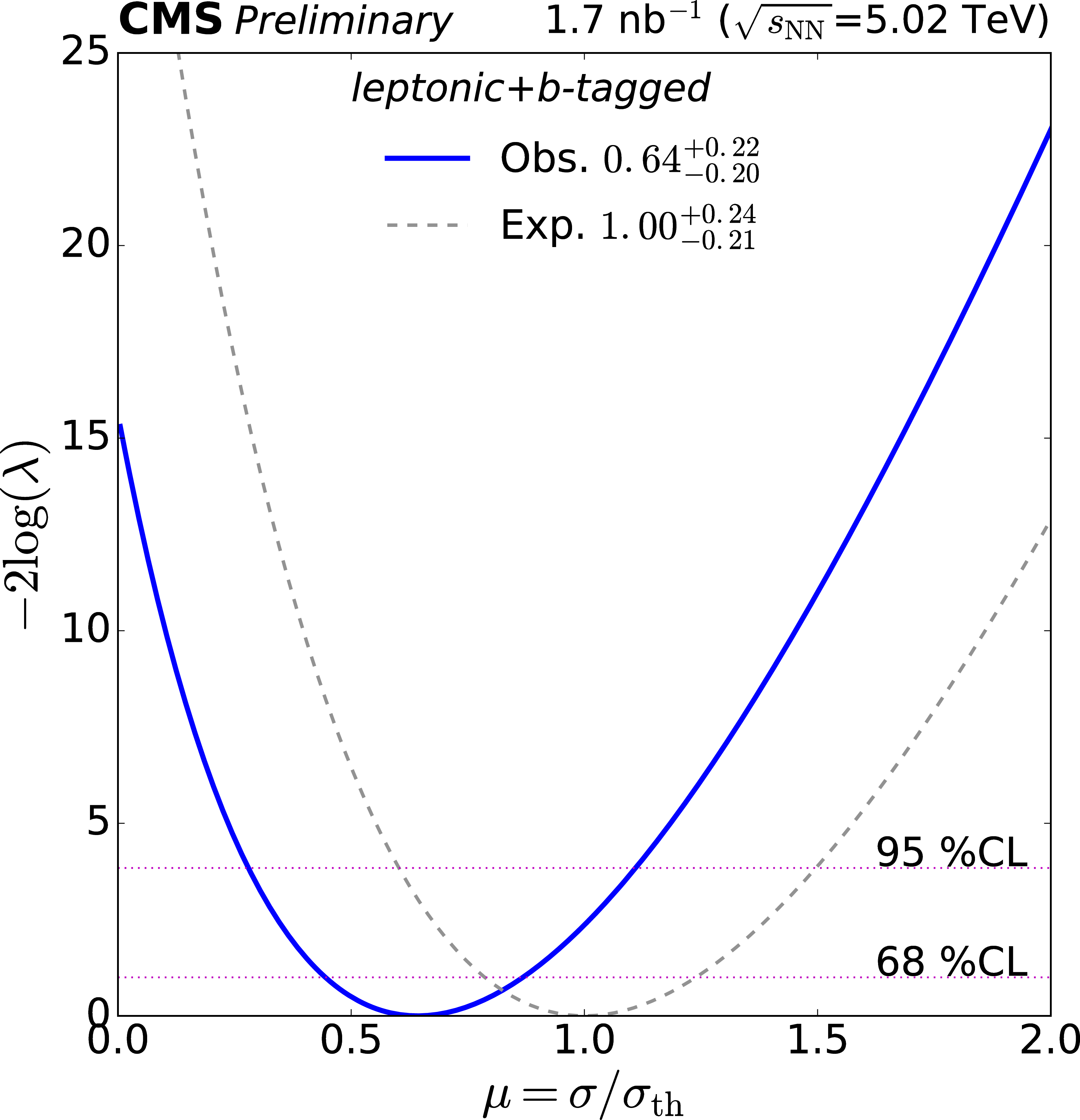
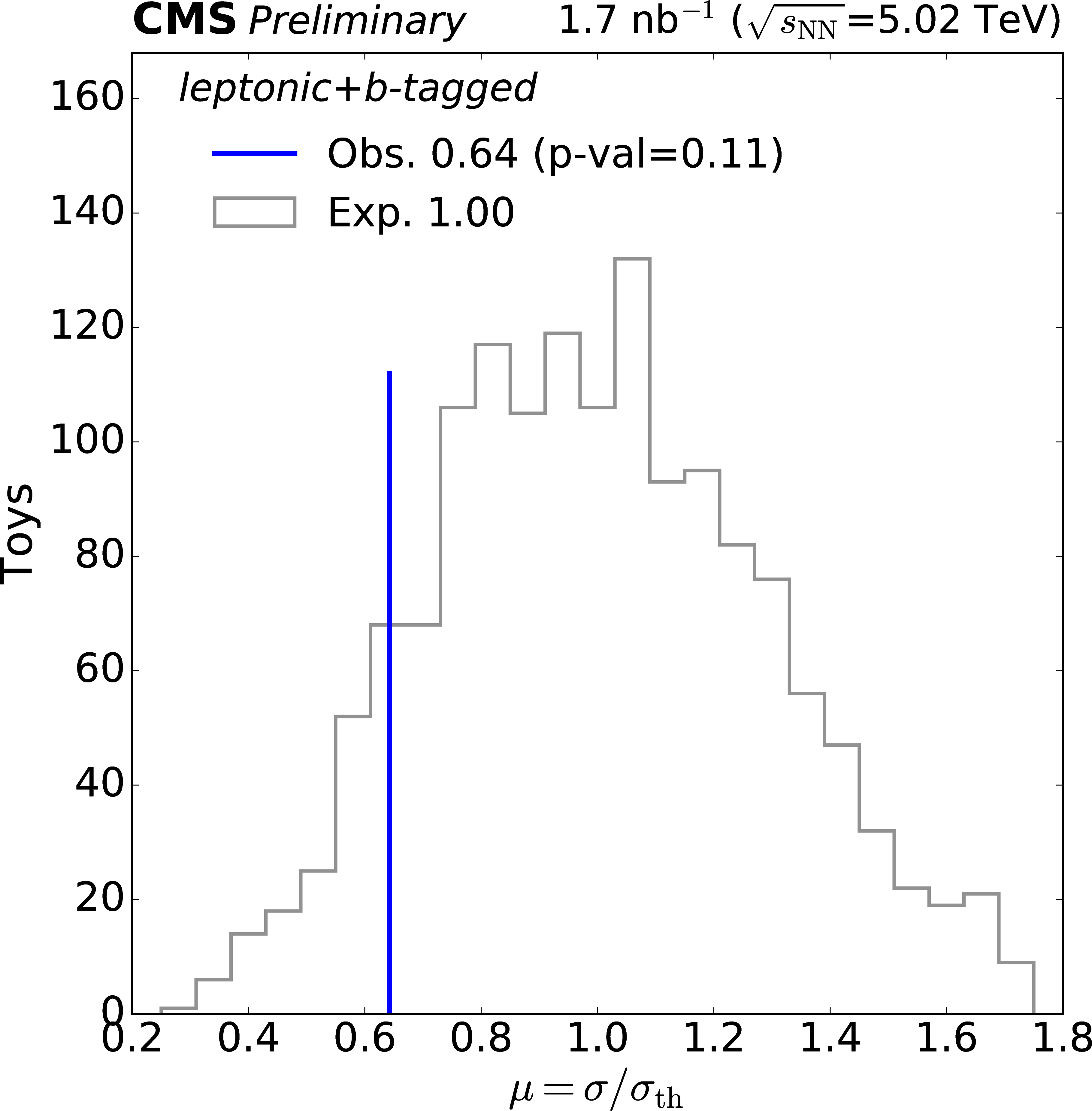
Additional Figure 8:
Scan of the profile likelihood (left), distribution of signal strength $\mu $ (middle), distribution of significances (right) expected in pseudo-experiments (blue curves and histograms) and observed in data (green curves and lines) for the signal extraction fit in the leptonic+b-tagged measurement. |
png pdf |
Additional Figure 8-a:
Scan of the profile likelihood (left), distribution of signal strength $\mu $ (middle), distribution of significances (right) expected in pseudo-experiments (blue curves and histograms) and observed in data (green curves and lines) for the signal extraction fit in the leptonic+b-tagged measurement. |
png pdf |
Additional Figure 8-b:
Scan of the profile likelihood (left), distribution of signal strength $\mu $ (middle), distribution of significances (right) expected in pseudo-experiments (blue curves and histograms) and observed in data (green curves and lines) for the signal extraction fit in the leptonic+b-tagged measurement. |

png pdf |
Additional Figure 8-c:
Scan of the profile likelihood (left), distribution of signal strength $\mu $ (middle), distribution of significances (right) expected in pseudo-experiments (blue curves and histograms) and observed in data (green curves and lines) for the signal extraction fit in the leptonic+b-tagged measurement. |
png pdf |
Additional Figure 9:
Impacts $\mu $ estimated after performing the fit to the data for the leptonic-only (left) and the leptonic+b-tagged (right) measurements. Only the 15 leading nuisance parameters are shown. |
png pdf |
Additional Figure 9-a:
Impacts $\mu $ estimated after performing the fit to the data for the leptonic-only (left) and the leptonic+b-tagged (right) measurements. Only the 15 leading nuisance parameters are shown. |

png pdf |
Additional Figure 9-b:
Impacts $\mu $ estimated after performing the fit to the data for the leptonic-only (left) and the leptonic+b-tagged (right) measurements. Only the 15 leading nuisance parameters are shown. |
png pdf |
Additional Figure 10:
Distribution of events as a function of the decimal logarithm of $S/B$, where $S$ and $B$ are the prefit expected ${{\mathrm {t}\overline {\mathrm {t}}}} $ signal (with $\mu =1$) and background yields, respectively, in BDT bins of similar prefit expected signal-to-background ratio. The shaded histogram shows the prefit expected background distribution. The red histogram, stacked on top of the background histogram, show the ${{\mathrm {t}\overline {\mathrm {t}}}} $ signal prefit expectation. The lower panel shows the ratios of the observed results and prefit expected $ {{\mathrm {t}\overline {\mathrm {t}}}}$ signal relative to the prefit expected background. The leptonic-only (leptonic+ b-tagged) measurement is shown on the left (right). |
png pdf |
Additional Figure 10-a:
Distribution of events as a function of the decimal logarithm of $S/B$, where $S$ and $B$ are the prefit expected ${{\mathrm {t}\overline {\mathrm {t}}}} $ signal (with $\mu =1$) and background yields, respectively, in BDT bins of similar prefit expected signal-to-background ratio. The shaded histogram shows the prefit expected background distribution. The red histogram, stacked on top of the background histogram, show the ${{\mathrm {t}\overline {\mathrm {t}}}} $ signal prefit expectation. The lower panel shows the ratios of the observed results and prefit expected $ {{\mathrm {t}\overline {\mathrm {t}}}}$ signal relative to the prefit expected background. The leptonic-only (leptonic+ b-tagged) measurement is shown on the left (right). |

png pdf |
Additional Figure 10-b:
Distribution of events as a function of the decimal logarithm of $S/B$, where $S$ and $B$ are the prefit expected ${{\mathrm {t}\overline {\mathrm {t}}}} $ signal (with $\mu =1$) and background yields, respectively, in BDT bins of similar prefit expected signal-to-background ratio. The shaded histogram shows the prefit expected background distribution. The red histogram, stacked on top of the background histogram, show the ${{\mathrm {t}\overline {\mathrm {t}}}} $ signal prefit expectation. The lower panel shows the ratios of the observed results and prefit expected $ {{\mathrm {t}\overline {\mathrm {t}}}}$ signal relative to the prefit expected background. The leptonic-only (leptonic+ b-tagged) measurement is shown on the left (right). |
| Additional Tables | |
png pdf |
Additional Table 1:
Signal strength $\mu $ and significance in standard deviations including only the ${{\mathrm {e}}^\pm {{\mu}}^\mp}$ channel in the fit and compared to the ${{\mathrm {e}}^+ {\mathrm {e}}^-}$, ${{{\mu}}^+ {{\mu}}^-}$, and ${{\mathrm {e}}^\pm {{\mu}}^\mp}$ measurements. The observed (expected) results of the fits are reported. |
| References | ||||
| 1 | CMS Collaboration | Study of W boson production in PbPb and pp collisions at $ \sqrt{\smash[b]{s_{_{\mathrm{NN}}}}}= $ 2.76 TeV | PLB 715 (2012) 66 | CMS-HIN-11-008 1205.6334 |
| 2 | ATLAS Collaboration | Measurement of the production and lepton charge asymmetry of W bosons in Pb+Pb collisions at $ \sqrt{\smash[b]{s_{_{\mathrm{NN}}}}}= $ 2.76 TeV with the ATLAS detector | EPJC 75 (2015) 23 | 1408.4674 |
| 3 | CMS Collaboration | Study of Z boson production in PbPb collisions at $ \sqrt{\smash[b]{s_{_{\mathrm{NN}}}}} = $ 2.76 TeV | PRL 106 (2011) 212301 | CMS-HIN-10-003 1102.5435 |
| 4 | ATLAS Collaboration | Measurement of Z boson production in Pb+Pb collisions at $ \sqrt{\smash[b]{s_{_{\mathrm{NN}}}}}= $ 2.76 TeV with the ATLAS detector | PRL 110 (2013) 022301 | 1210.6486 |
| 5 | ALICE Collaboration | Measurement of Z-boson production at large rapidities in Pb-Pb collisions at $ \sqrt{\smash[b]{s_{_{\mathrm{NN}}}}}= $ 5.02 TeV | PLB 780 (2018) 372 | 1711.10753 |
| 6 | D. d'Enterria | Top-quark and Higgs boson perspectives at heavy-ion colliders | Nucl. Part. Phys. Proc. 289 (2017) 237 | 1701.08047 |
| 7 | D. d'Enterria, K. Krajcz\'ar, and H. Paukkunen | Top-quark production in proton-nucleus and nucleus-nucleus collisions at LHC energies and beyond | PLB 746 (2015) 64 | 1501.05879 |
| 8 | L. Apolin\'ario, J. G. Milhano, G. P. Salam, and C. A. Salgado | Probing the time structure of the quark-gluon plasma with top quarks | PRL 120 (2018) 232301 | 1711.03105 |
| 9 | CMS Collaboration | Observation of top quark production in proton-nucleus collisions | PRL 119 (2017) 242001 | CMS-HIN-17-002 1709.07411 |
| 10 | M. Czakon, M. L. Mangano, A. Mitov, and J. Rojo | Constraints on the gluon PDF from top quark pair production at hadron colliders | JHEP 07 (2013) 167 | 1303.7215 |
| 11 | Particle Data Group Collaboration | Review of particle physics | PRD 98 (2018) 030001 | |
| 12 | CDF Collaboration | Observation of top quark production in $ {\mathrm{p}}\mathrm{\bar{p}} $ collisions | PRL 74 (1995) 2626 | hep-ex/9503002 |
| 13 | D0 Collaboration | Observation of the top quark | PRL 74 (1995) 2632 | hep-ex/9503003 |
| 14 | ATLAS Collaboration | Measurement of the $ \mathrm{t\bar{t}} $ production cross sections using $ \mathrm{e} \mu $ events with b-tagged jets in pp collisions at $ \sqrt{s} = $ 13 TeV with the ATLAS detector | PLB 761 (2016) 136 | 1606.02699 |
| 15 | LHCb Collaboration | Measurement of forward top pair production in the dilepton channel in pp collisions at $ \sqrt{s} = $ 13 TeV | JHEP 08 (2018) 174 | 1803.05188 |
| 16 | CMS Collaboration | Measurement of the $ \mathrm{t}\overline{\mathrm{t}} $ production cross section using events with one lepton and at least one jet in pp collisions at $ \sqrt{s}= $ 13 TeV | JHEP 09 (2017) 051 | CMS-TOP-16-006 1701.06228 |
| 17 | CMS Collaboration | Measurement of the inclusive $ \mathrm{t}\overline{\mathrm{t}} $ cross section in pp collisions at $ \sqrt{s}= $ 5.02 TeV using final states with at least one charged lepton | JHEP 03 (2018) 115 | CMS-TOP-16-023 1711.03143 |
| 18 | CMS Collaboration | Measurement of the $ \mathrm{t}\overline{\mathrm{t}} $ production cross section, the top quark mass, and the strong coupling constant using dilepton events in pp collisions at $ \sqrt{s}= $ 13 TeV | EPJC 79 (2019) 368 | CMS-TOP-17-001 1812.10505 |
| 19 | CMS Collaboration | Description and performance of track and primary-vertex reconstruction with the CMS tracker | JINST 9 (2014) P10009 | CMS-TRK-11-001 1405.6569 |
| 20 | CMS Collaboration | Performance of electron reconstruction and selection with the CMS detector in proton-proton collisions at $ \sqrt{s} = $ 8 TeV | JINST 10 (2015) P06005 | CMS-EGM-13-001 1502.02701 |
| 21 | CMS Collaboration | Performance of the CMS muon detector and muon reconstruction with proton-proton collisions at $ \sqrt{s}= $ 13 TeV | JINST 13 (2018) P06015 | CMS-MUO-16-001 1804.04528 |
| 22 | CMS Collaboration | Jet energy scale and resolution in the CMS experiment in pp collisions at 8 TeV | JINST 12 (2017) P02014 | CMS-JME-13-004 1607.03663 |
| 23 | CMS Collaboration | The CMS experiment at the CERN LHC | JINST 3 (2008) S08004 | CMS-00-001 |
| 24 | CMS Collaboration | CMS luminosity measurement using 2016 proton-nucleus collisions at nucleon-nucleon center-of-mass energy of 8.16 TeV | CMS-PAS-LUM-17-002 | CMS-PAS-LUM-17-002 |
| 25 | J. Alwall et al. | The automated computation of tree-level and next-to-leading order differential cross sections, and their matching to parton shower simulations | JHEP 07 (2014) 079 | 1405.0301 |
| 26 | S. Frixione, P. Nason, and C. Oleari | Matching NLO QCD computations with parton shower simulations: the POWHEG method | JHEP 11 (2007) 070 | 0709.2092 |
| 27 | S. Alioli, P. Nason, C. Oleari, and E. Re | A general framework for implementing NLO calculations in shower Monte Carlo programs: the POWHEG BOX | JHEP 06 (2010) 043 | 1002.2581 |
| 28 | K. J. Eskola, P. Paakkinen, H. Paukkunen, and C. A. Salgado | EPPS16: Nuclear parton distributions with LHC data | EPJC 77 (2017) 163 | 1612.05741 |
| 29 | S. Dulat et al. | New parton distribution functions from a global analysis of quantum chromodynamics | PRD 93 (2016) 033006 | 1506.07443 |
| 30 | CMS Collaboration | Measurement of the top quark mass in the all-jets final state at $ \sqrt{s} = $ 13 TeV and combination with the lepton+jets channel | EPJC 79 (2019) 313 | CMS-TOP-17-008 1812.10534 |
| 31 | M. Czakon and A. Mitov | Top++: a program for the calculation of the top-pair cross-section at hadron colliders | CPC 185 (2014) 2930 | 1112.5675 |
| 32 | M. Czakon, P. Fiedler, and A. Mitov | Total top quark pair production cross section at hadron colliders through $ \mathcal{O}({\alpha_S}^4) $ | PRL 110 (2013) 252004 | 1303.6254 |
| 33 | K. Melnikov and F. Petriello | Electroweak gauge boson production at hadron colliders through $ \mathcal{O}({\alpha_S}^2) $ | PRD 74 (2006) 114017 | hep-ph/0609070 |
| 34 | J. M. Campbell and R. K. Ellis | MCFM for the Tevatron and the LHC | NPPS 205 (2010) 10 | 1007.3492 |
| 35 | E. Re | Single-top Wt-channel production matched with parton showers using the POWHEG method | EPJC 71 (2011) 1547 | 1009.2450 |
| 36 | N. Kidonakis | Top quark production | in Proceedings, Helmholtz International Summer School on Physics of Heavy Quarks and Hadrons (HQ 2013), Hamburg | 1311.0283 |
| 37 | T. Sjostrand, S. Mrenna, and P. Skands | A brief introduction to $ PYTHIA $ 8.1 | CPC 178 (2008) 852 | 0710.3820 |
| 38 | T. Sjostrand et al. | An introduction to $ PYTHIA $ 8.2 | CPC 191 (2015) 159 | 1410.3012 |
| 39 | CMS Collaboration | Extraction and validation of a new set of CMS PYTHIA 8 tunes from underlying-event measurements | Submitted to EPJC | CMS-GEN-17-001 1903.12179 |
| 40 | I. P. Lokhtin and A. M. Snigirev | A model of jet quenching in ultrarelativistic heavy ion collisions and high-$ {p_{\mathrm{T}}} $ hadron spectra at RHIC | EPJC 45 (2016) 211 | hep-ph/0506189 |
| 41 | C. Loizides, J. Kamin, and D. d'Enterria | Improved Monte Carlo Glauber predictions at present and future nuclear colliders | PRC 97 (2018) 054910 | 1710.07098 |
| 42 | GEANT4 Collaboration | GEANT4 --- a simulation toolkit | NIMA 506 (2003) 250 | |
| 43 | CMS Collaboration | The CMS trigger system | JINST 12 (2017) P01020 | CMS-TRG-12-001 1609.02366 |
| 44 | A. J. Bell | Beam and radiation monitoring for CMS | in Proceedings of the 2008 IEEE Nuclear Science Symposium, Medical Imaging Conference and 16th International Workshop on Room-Temperature Semiconductor X-Ray and Gamma-Ray Detectors, Dresden | |
| 45 | CMS Collaboration | Particle-flow reconstruction and global-event description with the CMS detector | JINST 12 (2017) P10003 | CMS-PRF-14-001 1706.04965 |
| 46 | CMS Collaboration | Technical proposal for the Phase-II upgrade of the Compact Muon Solenoid | CMS-PAS-TDR-15-002 | CMS-PAS-TDR-15-002 |
| 47 | M. Cacciari, G. P. Salam, and G. Soyez | The anti-$ k_{\mathrm{t}} $ jet clustering algorithm | JHEP 04 (2008) 063 | 0802.1189 |
| 48 | M. Cacciari and G. P. Salam | Pileup subtraction using jet areas | PLB 659 (2008) 119 | 0707.1378 |
| 49 | M. Cacciari, G. P. Salam, and G. Soyez | FastJet user manual | EPJC 72 (2012) 1896 | 1111.6097 |
| 50 | CMS Collaboration | Measurements of inclusive W and Z cross sections in pp collisions at $ \sqrt{s} = $ 7 TeV | JHEP 01 (2011) 080 | CMS-EWK-10-002 1012.2466 |
| 51 | CMS Collaboration | Measurement of Higgs boson production and properties in the WW decay channel with leptonic final states | JHEP 01 (2014) 096 | CMS-HIG-13-023 1312.1129 |
| 52 | P. Berta, M. Spousta, D. W. Miller, and R. Leitner | Particle-level pileup subtraction for jets and jet shapes | JHEP 06 (2014) 092 | 1403.3108 |
| 53 | CMS Collaboration | Measurement of the splitting function in pp and PbPb collisions at $ \sqrt{\smash[b]{s_{_{\mathrm{NN}}}}} = $ 5.02 TeV | PRL 120 (2018) 142302 | CMS-HIN-16-006 1708.09429 |
| 54 | CMS Collaboration | Identification of heavy-flavour jets with the CMS detector in pp collisions at 13 TeV | JINST 13 (2018) P05011 | CMS-BTV-16-002 1712.07158 |
| 55 | CMS Collaboration | Measurement of the inclusive $ \mathrm{t\bar{t}} $ cross section in pp collisions at $ \sqrt{s} = $ 5.02 TeV using final states with at least one charged lepton | JHEP 03 (2018) 115 | CMS-TOP-16-023 1711.03143 |
| 56 | F. Pedregosa et al. | Scikit-learn: machine learning in Python | J. Mach. Learn. Res 12 (2011) 2825 | 1201.0490 |
| 57 | CMS Collaboration | Evidence of b-jet quenching in PbPb collisions at $ \sqrt{\smash[b]{s_{_{\mathrm{NN}}}}}= $ 2.76 TeV | PRL 113 (2014) 132301 | CMS-HIN-12-003 1312.4198 |
| 58 | H. Voss, A. Hocker, J. Stelzer, and F. Tegenfeldt | TMVA, the toolkit for multivariate data analysis with ROOT | in XIth International Workshop on Advanced Computing and Analysis Techniques in Physics Research (ACAT), p. 40 2007 [PoS(ACAT)040] | physics/0703039 |
| 59 | W. Verkerke and D. P. Kirkby | The RooFit toolkit for data modeling | eConf C 0303241 (2003) MOLT007, [,186(2003)] | physics/0306116 |
| 60 | L. Moneta et al. | The RooStats Project | PoS ACAT (2010) 057 | 1009.1003 |
| 61 | G. Cowan, K. Cranmer, E. Gross, and O. Vitells | Asymptotic formulae for likelihood-based tests of new physics | EPJC 71 (2011) 1554 | 1007.1727 |
| 62 | CMS Collaboration | Precise determination of the mass of the Higgs boson and tests of compatibility of its couplings with the standard model predictions using proton collisions at 7 and 8 TeV | EPJC 75 (2015) 212 | CMS-HIG-14-009 1412.8662 |
| 63 | ATLAS and CMS Collaborations | Procedure for the LHC Higgs boson search combination in summer 2011 | CMS-NOTE-2011-005 | |
| 64 | CMS Collaboration | Measurement of the $ \mathrm{t}\overline{\mathrm{t}} $ production cross section, the top quark mass, and the strong coupling constant using dilepton events in pp collisions at $ \sqrt{s} = $ 13 TeV | EPJC 79 (2019) 368 | CMS-TOP-17-001 1812.10505 |
| 65 | F. Arleo | Tomography of cold and hot QCD matter: tools and diagnosis | JHEP 11 (2002) 044 | hep-ph/0210104 |
| 66 | F. Arleo | Quenching of hadron spectra in heavy ion collisions at the LHC | PRL 119 (2017) 062302 | 1703.10852 |
| 67 | E. Todesco and J. Wenninger | Large Hadron Collider momentum calibration and accuracy | PRAccel. Beams 20 (2017) 081003 | |
| 68 | NNPDF Collaboration | Parton distributions for the LHC Run II | JHEP 04 (2015) 040 | 1410.8849 |
|
|
Compact Muon Solenoid LHC, CERN |
|

|

|

|

|

|