

Compact Muon Solenoid
LHC, CERN
| CMS-PAS-HIG-19-006 | ||
| Measurement of Higgs boson decay to a pair of muons in proton-proton collisions at $\sqrt{s}=$ 13 TeV | ||
| CMS Collaboration | ||
| July 2020 | ||
| Abstract: A measurement of the Higgs boson decay to a pair of muons is presented. This result combines searches in four exclusive categories targeting the production of the Higgs boson via gluon fusion, via vector boson fusion, in association with a weak vector boson, and in association with a pair of top quarks. The measurement is performed using $\sqrt{s}=$ 13 TeV proton-proton (pp) collision data, corresponding to an integrated luminosity of 137 fb$^{-1}$, recorded by the CMS experiment at the CERN LHC. An excess of events is observed in data with a significance of 3.0 standard deviations, where the expectation for the standard model (SM) Higgs boson with $ m_{\mathrm{H}} = $ 125.38 GeV is 2.5. The measured signal strength, relative to the SM expectation, is 1.19$^{+0.41}_{-0.39}$ (stat) $^{+0.17}_{-0.16}$ (syst). The combination of this result with that from data recorded at centre-of-mass energies of 7 and 8 TeV improves both expected and observed sensitivity by 1%. This result constitutes the first evidence for the Higgs boson decay to fermions of the second generation. | ||
|
Links:
CDS record (PDF) ;
CADI line (restricted) ;
These preliminary results are superseded in this paper, JHEP 01 (2021) 148. The superseded preliminary plots can be found here. |
||
| Figures & Tables | Summary | Additional Figures | References | CMS Publications |
|---|
| Figures | |

png pdf |
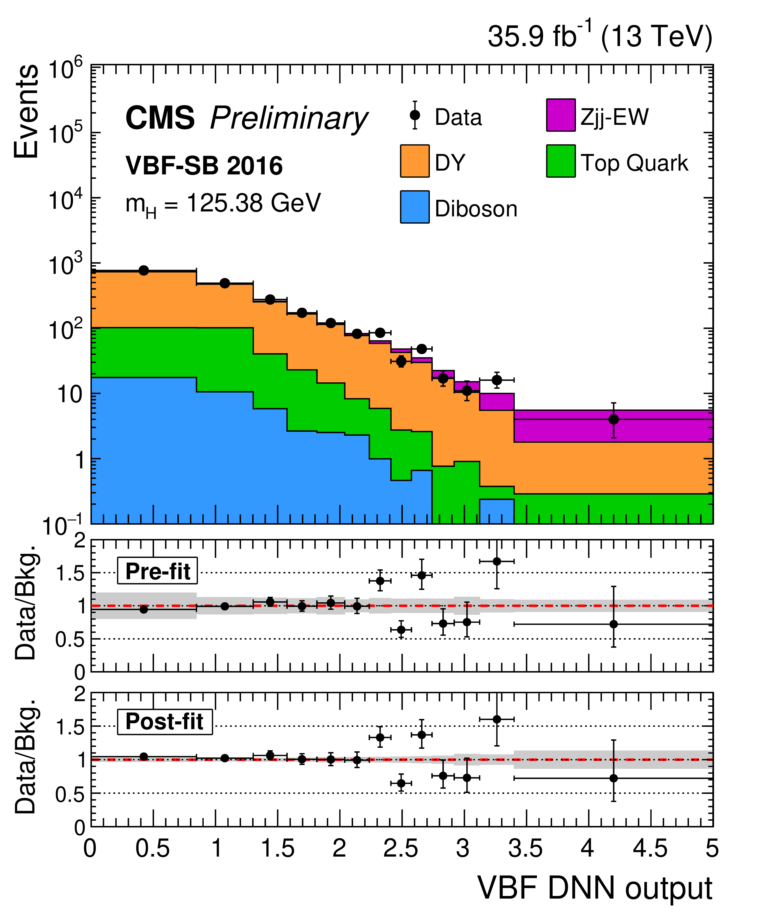
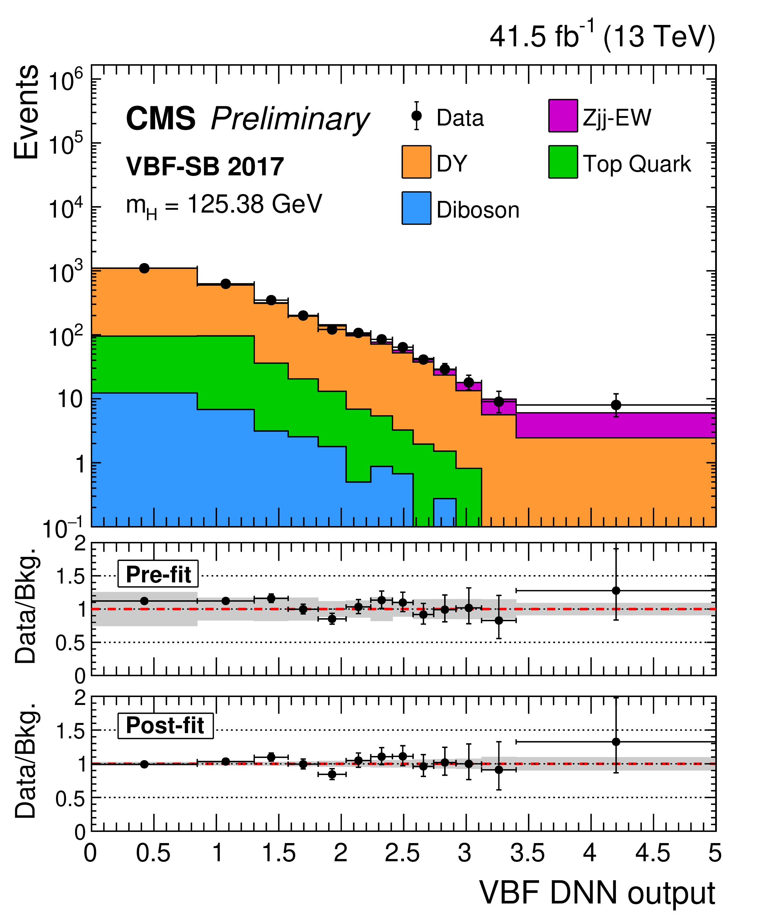
Figure 1:
The observed DNN output distribution for data collected in 2016 (left), 2017 (middle), and 2018 (right) in the VBF-SB region compared to the post-fit background estimate from SM processes. The predicted backgrounds are obtained from a signal-plus-background fit performed across analysis regions and years. In the second panel, the ratio between data and the pre-fit background prediction is shown. The grey band indicates the total pre-fit uncertainty obtained from the systematic sources previously described. The third panel shows the ratio between data and the post-fit background prediction from the signal-plus-background fit. The grey band indicates the total background uncertainty after performing the fit. |
png pdf |
Figure 1-a:
The observed DNN output distribution for data collected in 2016 in the VBF-SB region compared to the post-fit background estimate from SM processes. The predicted backgrounds are obtained from a signal-plus-background fit performed across analysis regions and years. In the second panel, the ratio between data and the pre-fit background prediction is shown. The grey band indicates the total pre-fit uncertainty obtained from the systematic sources previously described. The third panel shows the ratio between data and the post-fit background prediction from the signal-plus-background fit. The grey band indicates the total background uncertainty after performing the fit. |
png pdf |
Figure 1-b:
The observed DNN output distribution for data collected in 2017 in the VBF-SB region compared to the post-fit background estimate from SM processes. The predicted backgrounds are obtained from a signal-plus-background fit performed across analysis regions and years. In the second panel, the ratio between data and the pre-fit background prediction is shown. The grey band indicates the total pre-fit uncertainty obtained from the systematic sources previously described. The third panel shows the ratio between data and the post-fit background prediction from the signal-plus-background fit. The grey band indicates the total background uncertainty after performing the fit. |

png pdf |
Figure 1-c:
The observed DNN output distribution for data collected in 2018 in the VBF-SB region compared to the post-fit background estimate from SM processes. The predicted backgrounds are obtained from a signal-plus-background fit performed across analysis regions and years. In the second panel, the ratio between data and the pre-fit background prediction is shown. The grey band indicates the total pre-fit uncertainty obtained from the systematic sources previously described. The third panel shows the ratio between data and the post-fit background prediction from the signal-plus-background fit. The grey band indicates the total background uncertainty after performing the fit. |
png pdf |
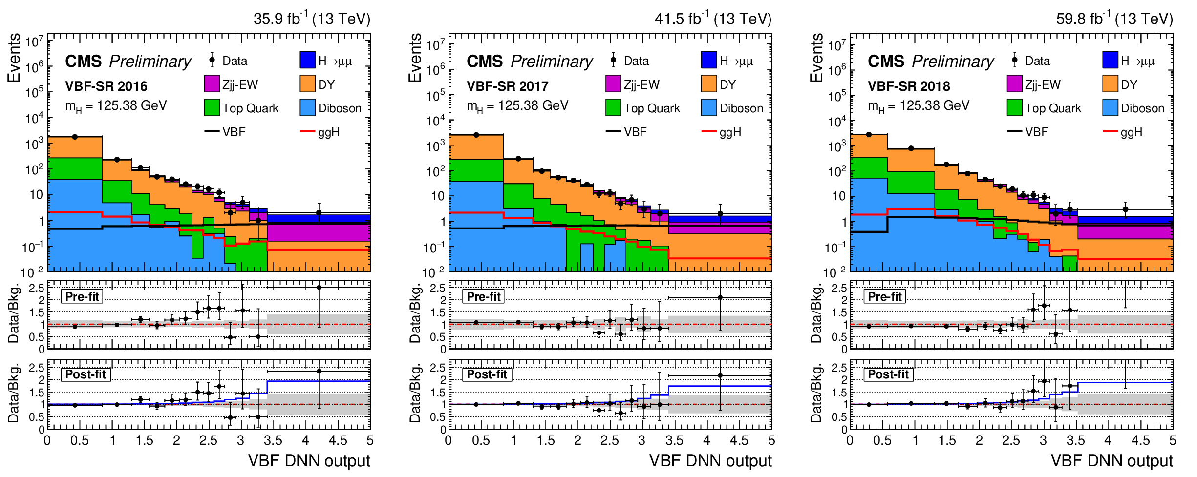
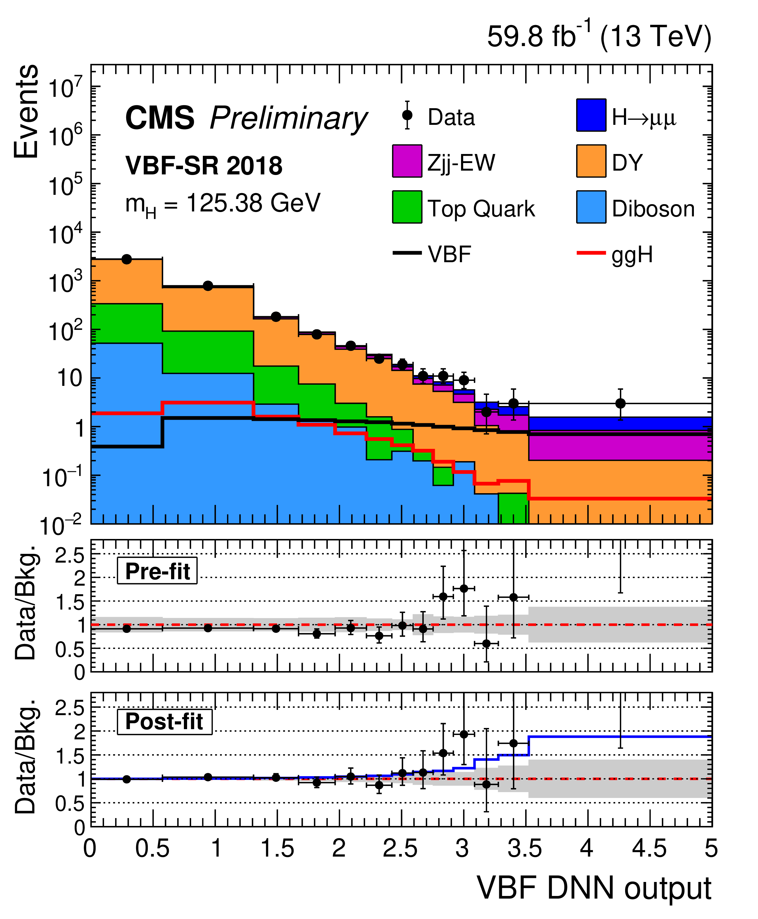
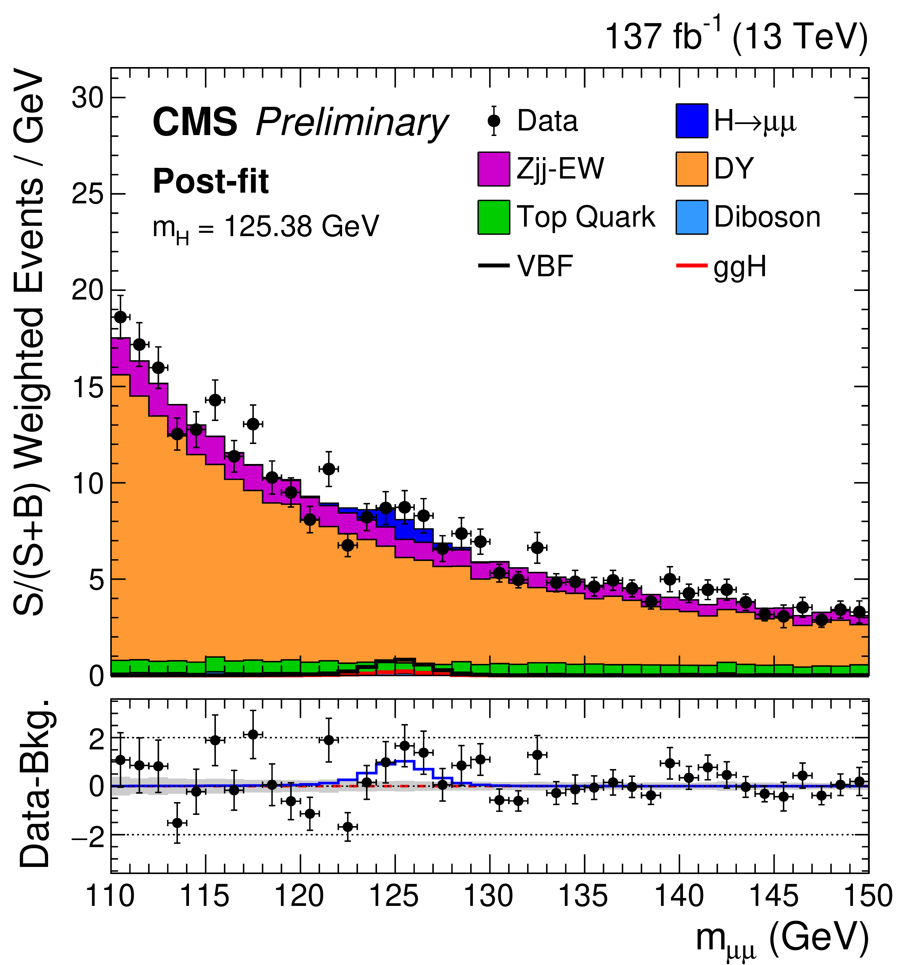
Figure 2:
The observed DNN output distribution in the VBF-SR region compared to the post-fit background estimate for the contributing SM processes. The post-fit distributions for the Higgs boson signal produced via $\mathrm{g} \mathrm{g} \mathrm{H} $ and VBF modes with ${m_{\mathrm{H}}} = $ 125.38 GeV are overlaid. The predicted backgrounds are obtained from a signal-plus-background fit performed across analysis regions and years. The description of the three panels is the same as in Fig. 1. The blue histogram (first panel) and solid line (third panel) indicate the total signal extracted from the fit with ${m_{\mathrm{H}}} = $ 125.38 GeV. |

png pdf |
Figure 2-a:
The observed DNN output distribution in the VBF-SR region compared to the post-fit background estimate for the contributing SM processes. The post-fit distributions for the Higgs boson signal produced via $\mathrm{g} \mathrm{g} \mathrm{H} $ and VBF modes with ${m_{\mathrm{H}}} = $ 125.38 GeV are overlaid. The predicted backgrounds are obtained from a signal-plus-background fit performed across analysis regions and years. The description of the three panels is the same as in Fig. 1. The blue histogram (first panel) and solid line (third panel) indicate the total signal extracted from the fit with ${m_{\mathrm{H}}} = $ 125.38 GeV. |

png pdf |
Figure 2-b:
The observed DNN output distribution in the VBF-SR region compared to the post-fit background estimate for the contributing SM processes. The post-fit distributions for the Higgs boson signal produced via $\mathrm{g} \mathrm{g} \mathrm{H} $ and VBF modes with ${m_{\mathrm{H}}} = $ 125.38 GeV are overlaid. The predicted backgrounds are obtained from a signal-plus-background fit performed across analysis regions and years. The description of the three panels is the same as in Fig. 1. The blue histogram (first panel) and solid line (third panel) indicate the total signal extracted from the fit with ${m_{\mathrm{H}}} = $ 125.38 GeV. |
png pdf |
Figure 2-c:
The observed DNN output distribution in the VBF-SR region compared to the post-fit background estimate for the contributing SM processes. The post-fit distributions for the Higgs boson signal produced via $\mathrm{g} \mathrm{g} \mathrm{H} $ and VBF modes with ${m_{\mathrm{H}}} = $ 125.38 GeV are overlaid. The predicted backgrounds are obtained from a signal-plus-background fit performed across analysis regions and years. The description of the three panels is the same as in Fig. 1. The blue histogram (first panel) and solid line (third panel) indicate the total signal extracted from the fit with ${m_{\mathrm{H}}} = $ 125.38 GeV. |
png pdf |
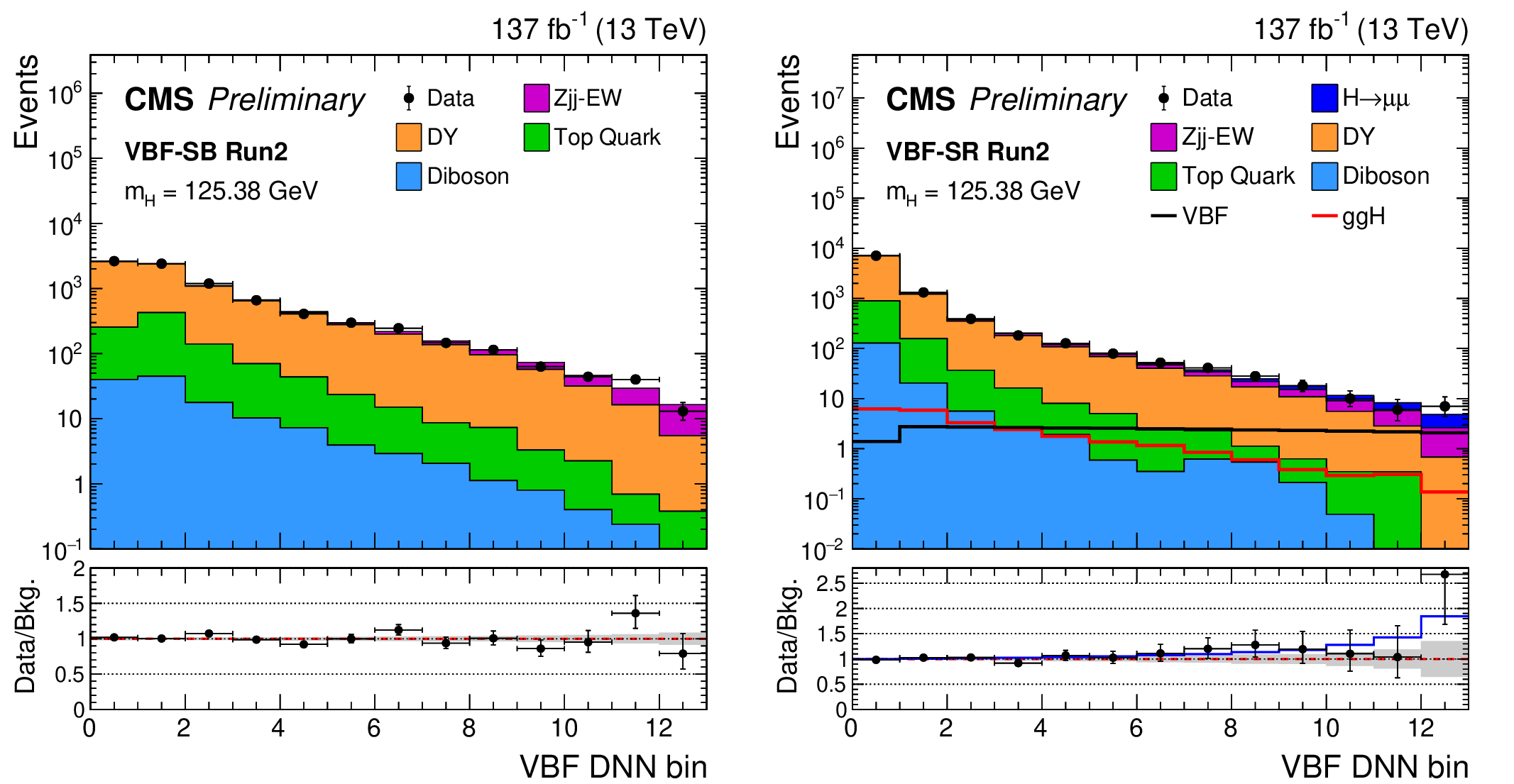
Figure 3:
The observed DNN output distribution in the VBF-SB (left) and VBF-SR (right) regions for the combination of 2016, 2017, and 2018 data, compared to the post-fit prediction from SM processes. The lower panel shows the ratio between data and the post-fit background prediction from the signal-plus-background fit. The best-fit ${{\mathrm{H} \to \mu \mu}}$ signal contribution is indicated by the blue line, and the grey band indicates the total background uncertainty. |
png pdf |
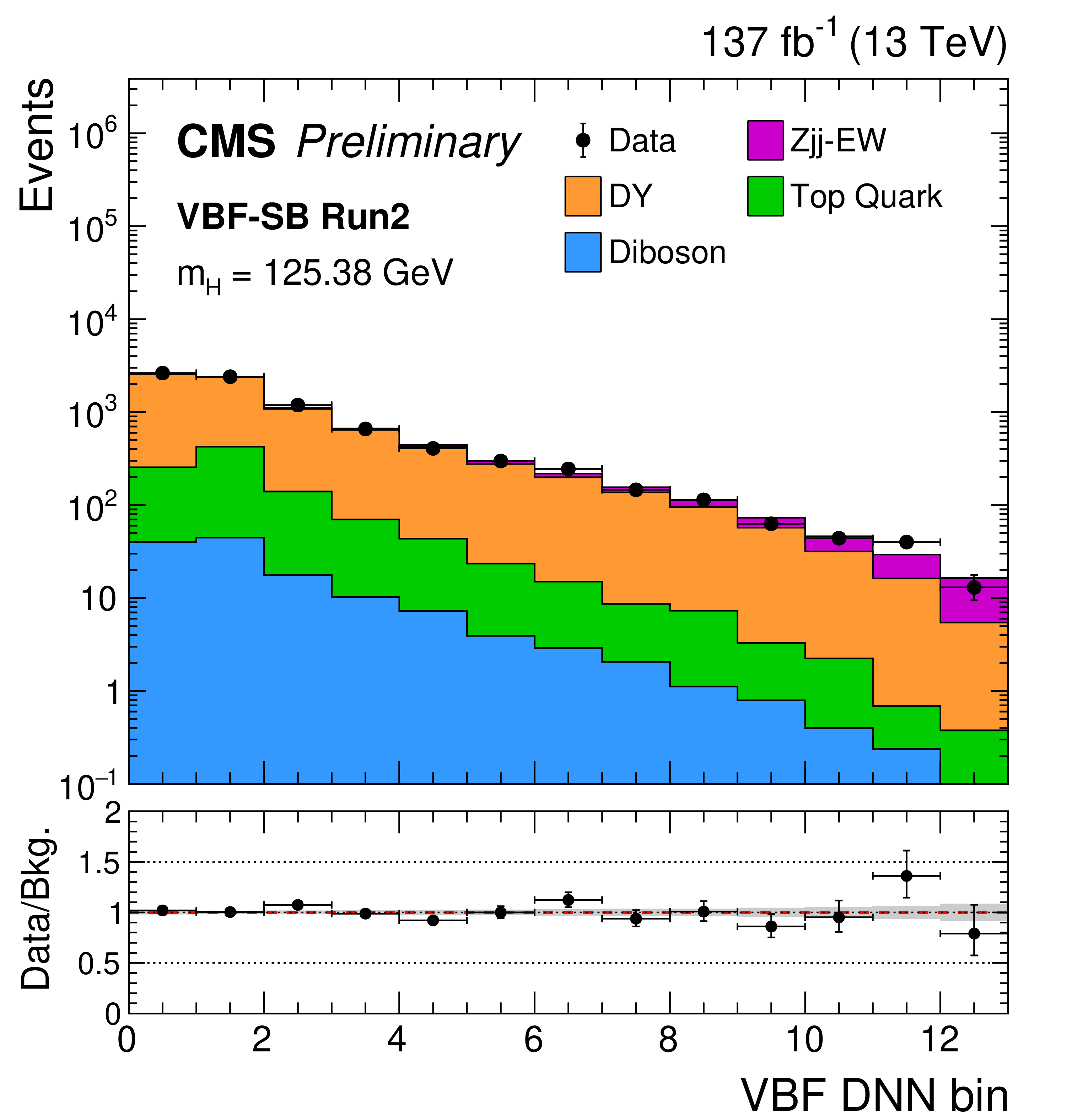
Figure 3-a:
The observed DNN output distribution in the VBF-SB region for the combination of 2016, 2017, and 2018 data, compared to the post-fit prediction from SM processes. The lower panel shows the ratio between data and the post-fit background prediction from the signal-plus-background fit. The best-fit ${{\mathrm{H} \to \mu \mu}}$ signal contribution is indicated by the blue line, and the grey band indicates the total background uncertainty. |

png pdf |
Figure 3-b:
The observed DNN output distribution in the VBF-SR region for the combination of 2016, 2017, and 2018 data, compared to the post-fit prediction from SM processes. The lower panel shows the ratio between data and the post-fit background prediction from the signal-plus-background fit. The best-fit ${{\mathrm{H} \to \mu \mu}}$ signal contribution is indicated by the blue line, and the grey band indicates the total background uncertainty. |
png pdf |
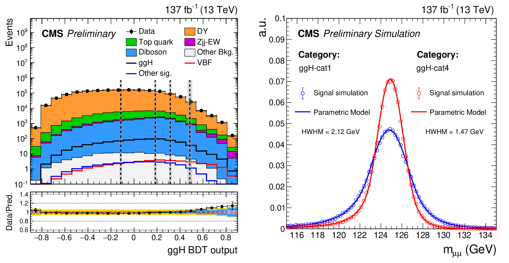
Figure 4:
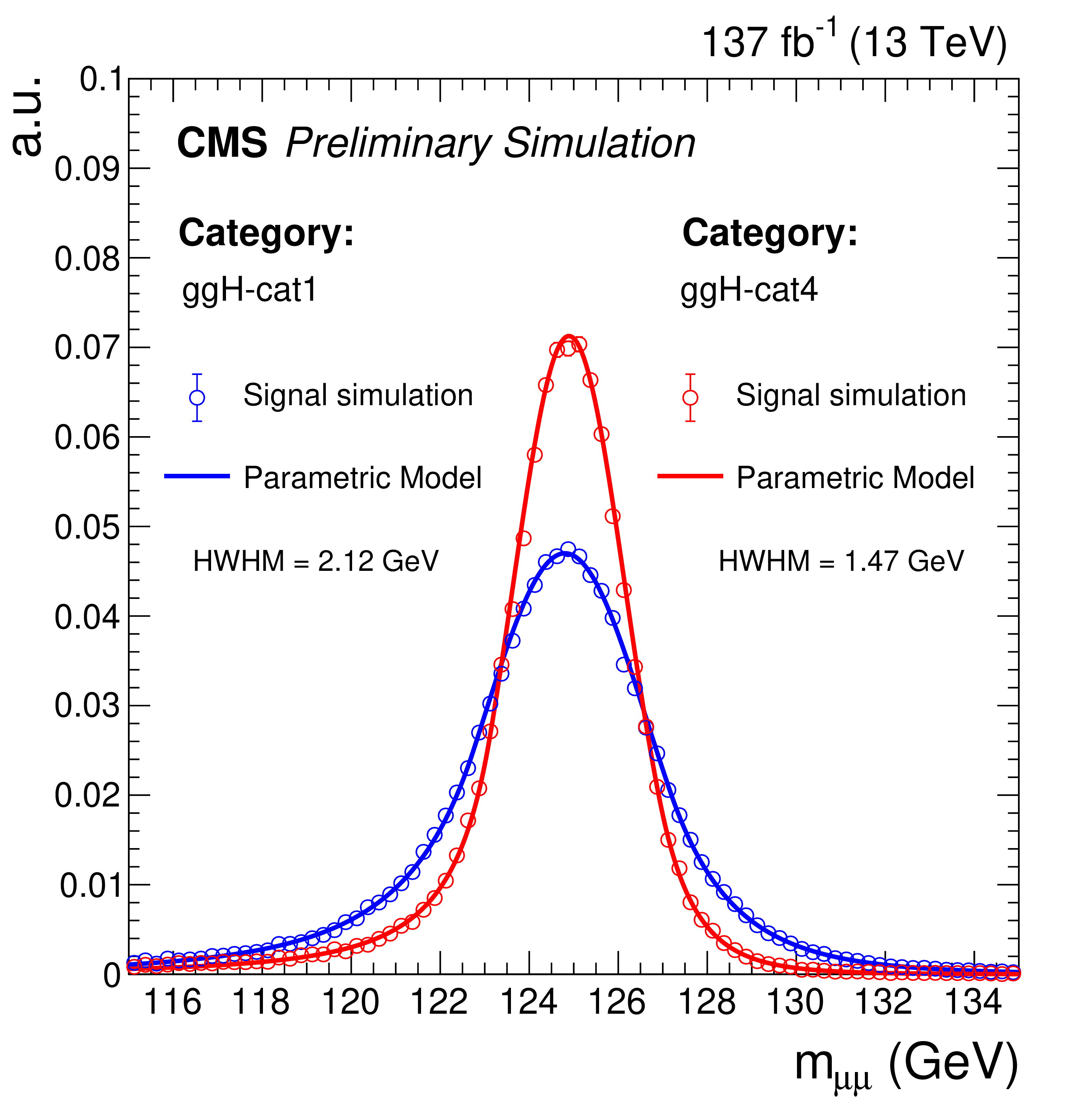
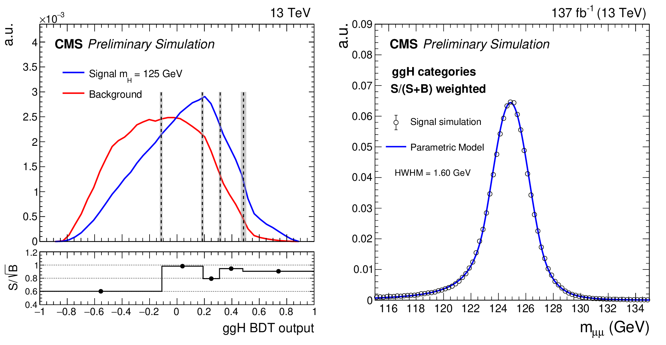
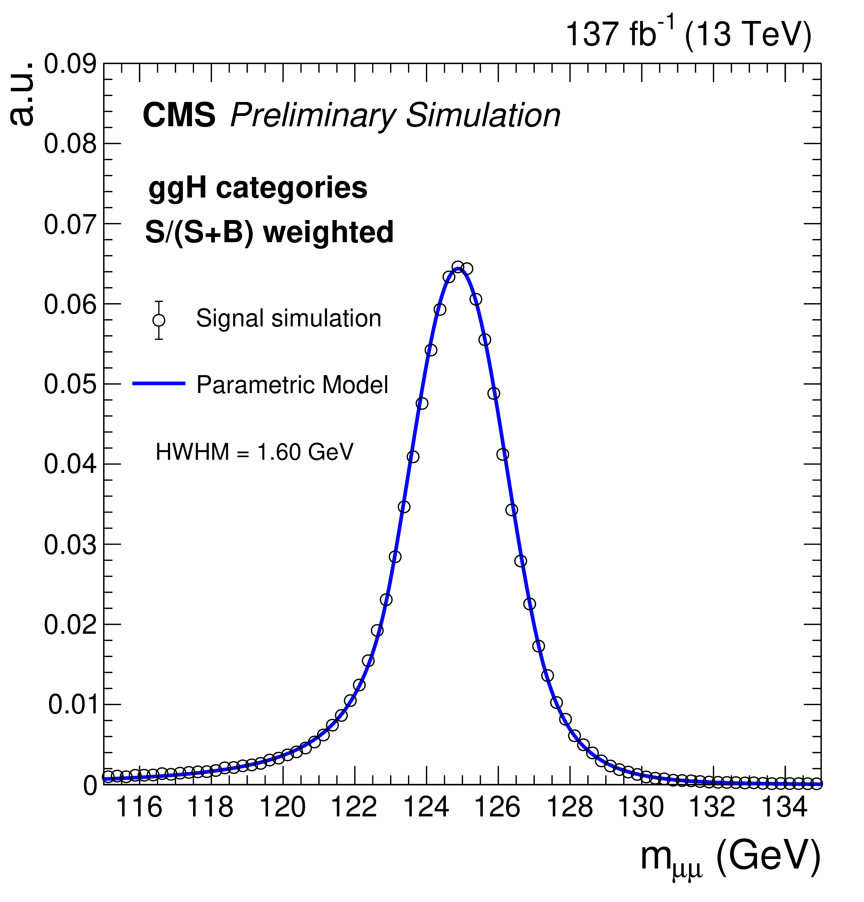
Left: the observed BDT output distribution compared to the prediction from the simulation of various SM background processes. Dimuon events passing the event selection requirements of the $\mathrm{g} \mathrm{g} \mathrm{H} $ category, with $m_{\mu \mu}$ between 110-150 GeV, are considered. The expected distributions for $\mathrm{g} \mathrm{g} \mathrm{H} $, VBF, and other signal processes are overlaid. The gray vertical boxes indicate the range of variation of the BDT boundaries for the optimized event categories defined in each data-taking period. In the lower panel, the ratio between data and the expected background is shown. The grey band indicates the uncertainty due to the limited size of the simulated samples. The azure band corresponds to the sum in quadrature between the statistical and experimental systematic uncertainties, while the orange band additionally includes the theoretical uncertainties affecting the background prediction. Right: the signal shape model for the simulated $ {{\mathrm{H} \to \mu \mu}} $ sample with ${m_{\mathrm{H}}} =$ 125 GeV in the best (red) and the worst (blue) resolution categories. |
png pdf |
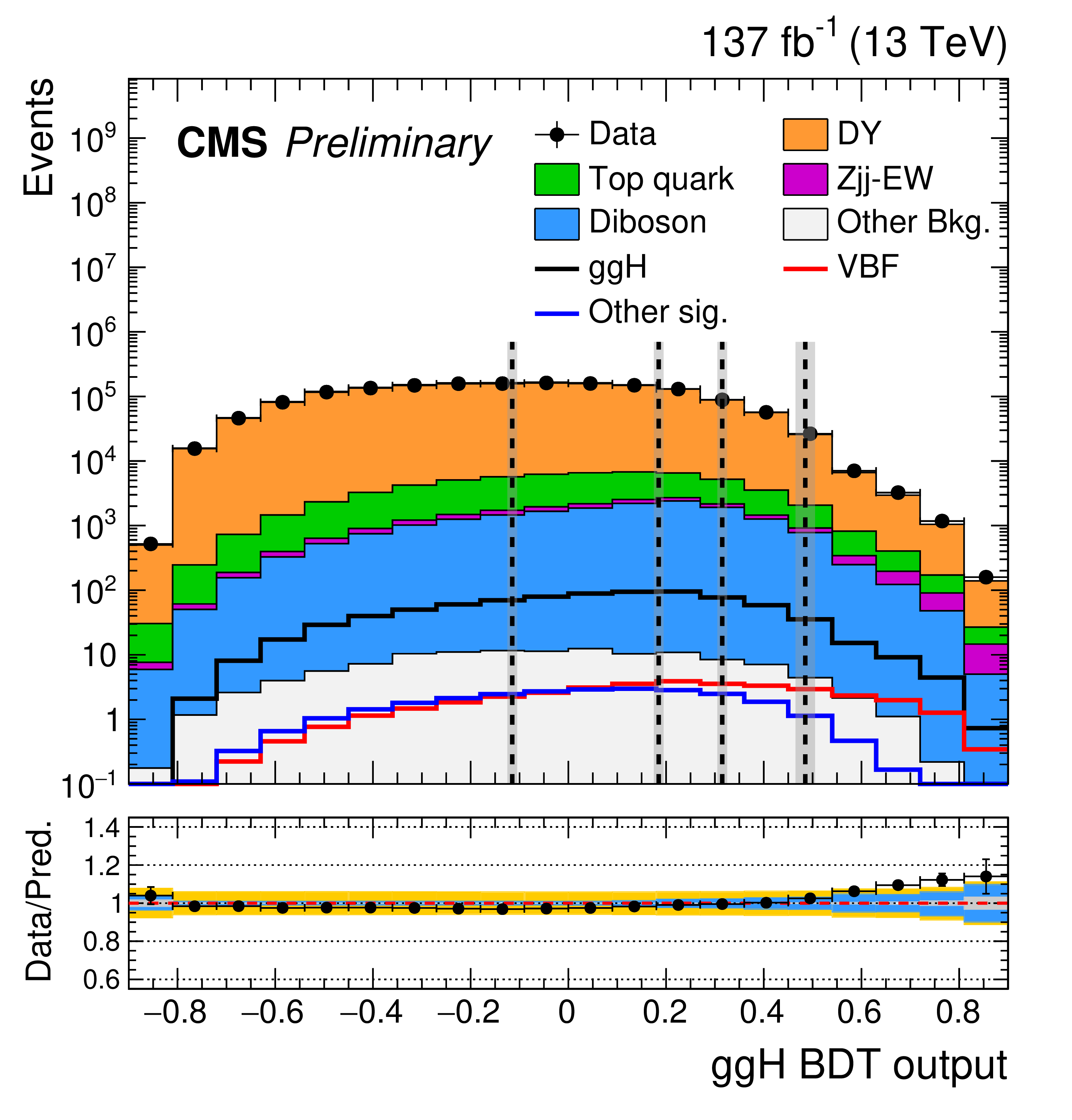
Figure 4-a:
The observed BDT output distribution compared to the prediction from the simulation of various SM background processes. Dimuon events passing the event selection requirements of the $\mathrm{g} \mathrm{g} \mathrm{H} $ category, with $m_{\mu \mu}$ between 110-150 GeV, are considered. The expected distributions for $\mathrm{g} \mathrm{g} \mathrm{H} $, VBF, and other signal processes are overlaid. The gray vertical boxes indicate the range of variation of the BDT boundaries for the optimized event categories defined in each data-taking period. In the lower panel, the ratio between data and the expected background is shown. The grey band indicates the uncertainty due to the limited size of the simulated samples. The azure band corresponds to the sum in quadrature between the statistical and experimental systematic uncertainties, while the orange band additionally includes the theoretical uncertainties affecting the background prediction. |
png pdf |
Figure 4-b:
The signal shape model for the simulated $ {{\mathrm{H} \to \mu \mu}} $ sample with ${m_{\mathrm{H}}} =$ 125 GeV in the best (red) and the worst (blue) resolution categories. |
png pdf |
Figure 5:
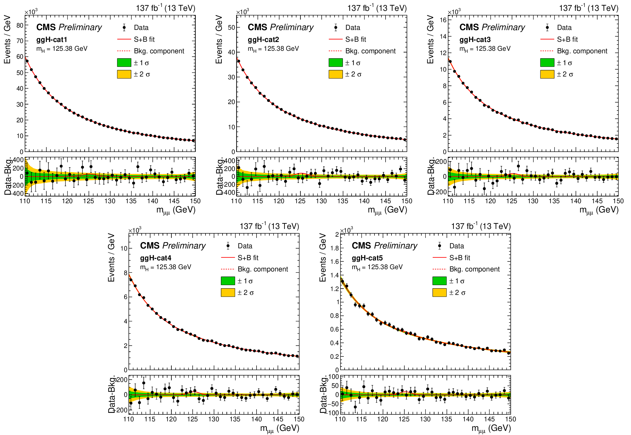
Comparison between the observed data and the total background extracted from a signal-plus-background fit performed across the $\mathrm{g} \mathrm{g} \mathrm{H} $ categories. First row, from left to right : ${\mathrm{g} \mathrm{g} \mathrm{H} \textrm {-cat1}}$, ${\mathrm{g} \mathrm{g} \mathrm{H} \textrm {-cat2}}$, and ${\mathrm{g} \mathrm{g} \mathrm{H} \textrm {-cat3}}$. Second row, from left to right : ${\mathrm{g} \mathrm{g} \mathrm{H} \textrm {-cat4}}$ and ${\mathrm{g} \mathrm{g} \mathrm{H} \textrm {-cat5}}$. The one (green) and two (yellow) standard deviation bands include the uncertainties in the background component of the fit. The lower panel shows the residuals after background subtraction and the red line indicates the signal with ${m_{\mathrm{H}}} =$ 125.38 GeV extracted from the fit. |

png pdf |
Figure 5-a:
Comparison between the observed data and the total background extracted from a signal-plus-background fit performed across the $\mathrm{g} \mathrm{g} \mathrm{H} $ categories: ${\mathrm{g} \mathrm{g} \mathrm{H} \textrm {-cat1}}$. The one (green) and two (yellow) standard deviation bands include the uncertainties in the background component of the fit. The lower panel shows the residuals after background subtraction and the red line indicates the signal with ${m_{\mathrm{H}}} =$ 125.38 GeV extracted from the fit. |
png pdf |
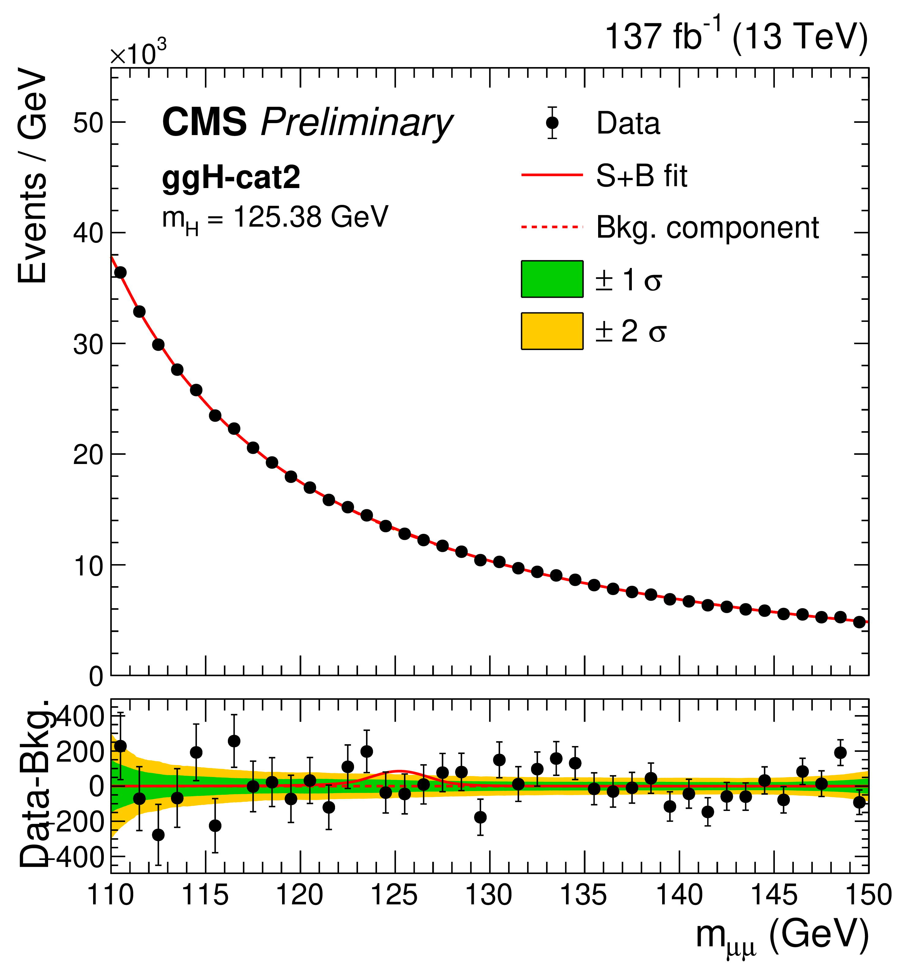
Figure 5-b:
Comparison between the observed data and the total background extracted from a signal-plus-background fit performed across the $\mathrm{g} \mathrm{g} \mathrm{H} $ categories: ${\mathrm{g} \mathrm{g} \mathrm{H} \textrm {-cat2}}$. The one (green) and two (yellow) standard deviation bands include the uncertainties in the background component of the fit. The lower panel shows the residuals after background subtraction and the red line indicates the signal with ${m_{\mathrm{H}}} =$ 125.38 GeV extracted from the fit. |

png pdf |
Figure 5-c:
Comparison between the observed data and the total background extracted from a signal-plus-background fit performed across the $\mathrm{g} \mathrm{g} \mathrm{H} $ categories: ${\mathrm{g} \mathrm{g} \mathrm{H} \textrm {-cat3}}$. The one (green) and two (yellow) standard deviation bands include the uncertainties in the background component of the fit. The lower panel shows the residuals after background subtraction and the red line indicates the signal with ${m_{\mathrm{H}}} =$ 125.38 GeV extracted from the fit. |
png pdf |
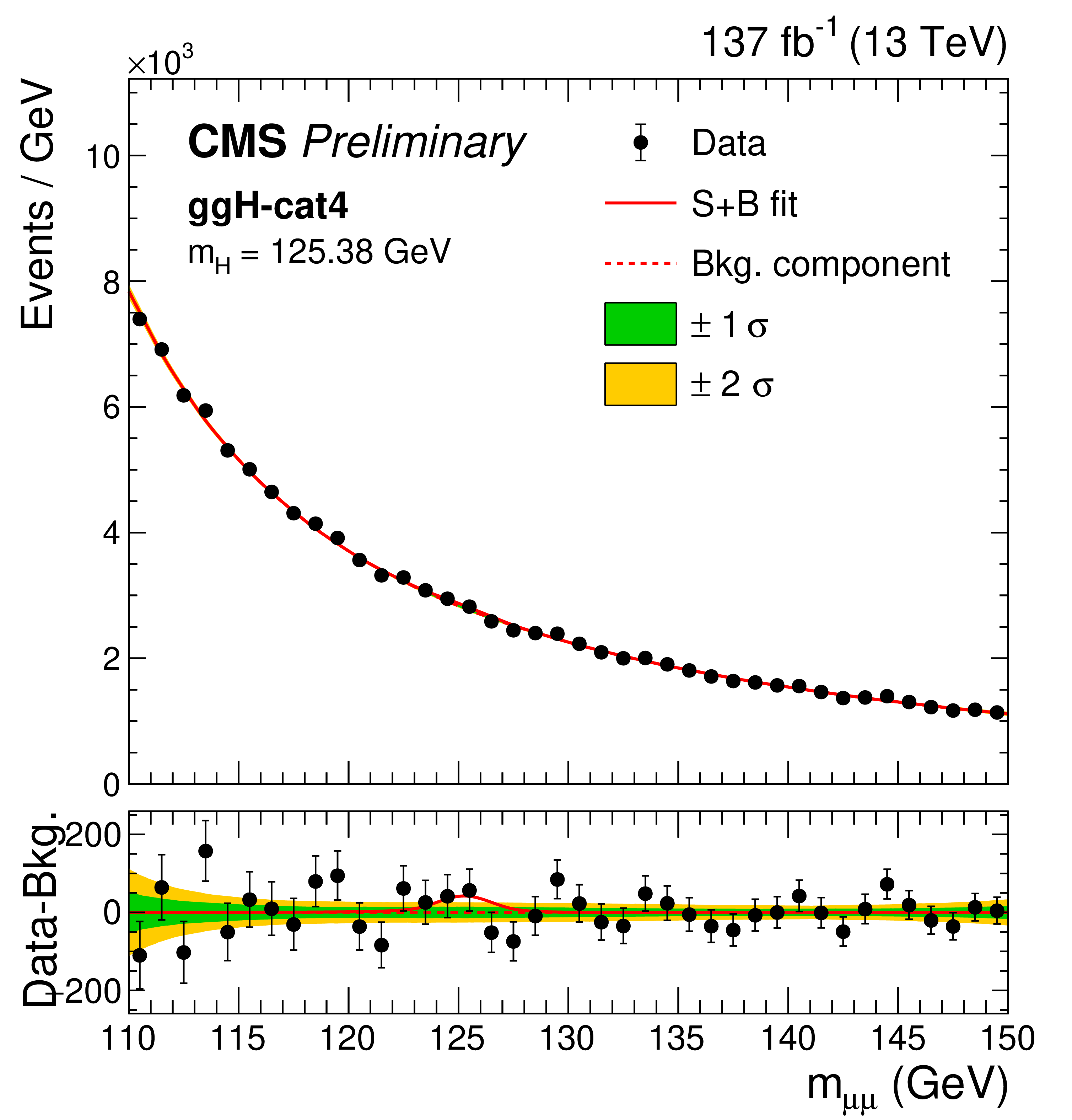
Figure 5-d:
Comparison between the observed data and the total background extracted from a signal-plus-background fit performed across the $\mathrm{g} \mathrm{g} \mathrm{H} $ categories: ${\mathrm{g} \mathrm{g} \mathrm{H} \textrm {-cat4}}$. The one (green) and two (yellow) standard deviation bands include the uncertainties in the background component of the fit. The lower panel shows the residuals after background subtraction and the red line indicates the signal with ${m_{\mathrm{H}}} =$ 125.38 GeV extracted from the fit. |

png pdf |
Figure 5-e:
Comparison between the observed data and the total background extracted from a signal-plus-background fit performed across the $\mathrm{g} \mathrm{g} \mathrm{H} $ categories: ${\mathrm{g} \mathrm{g} \mathrm{H} \textrm {-cat5}}$. The one (green) and two (yellow) standard deviation bands include the uncertainties in the background component of the fit. The lower panel shows the residuals after background subtraction and the red line indicates the signal with ${m_{\mathrm{H}}} =$ 125.38 GeV extracted from the fit. |
png pdf |
Figure 6:
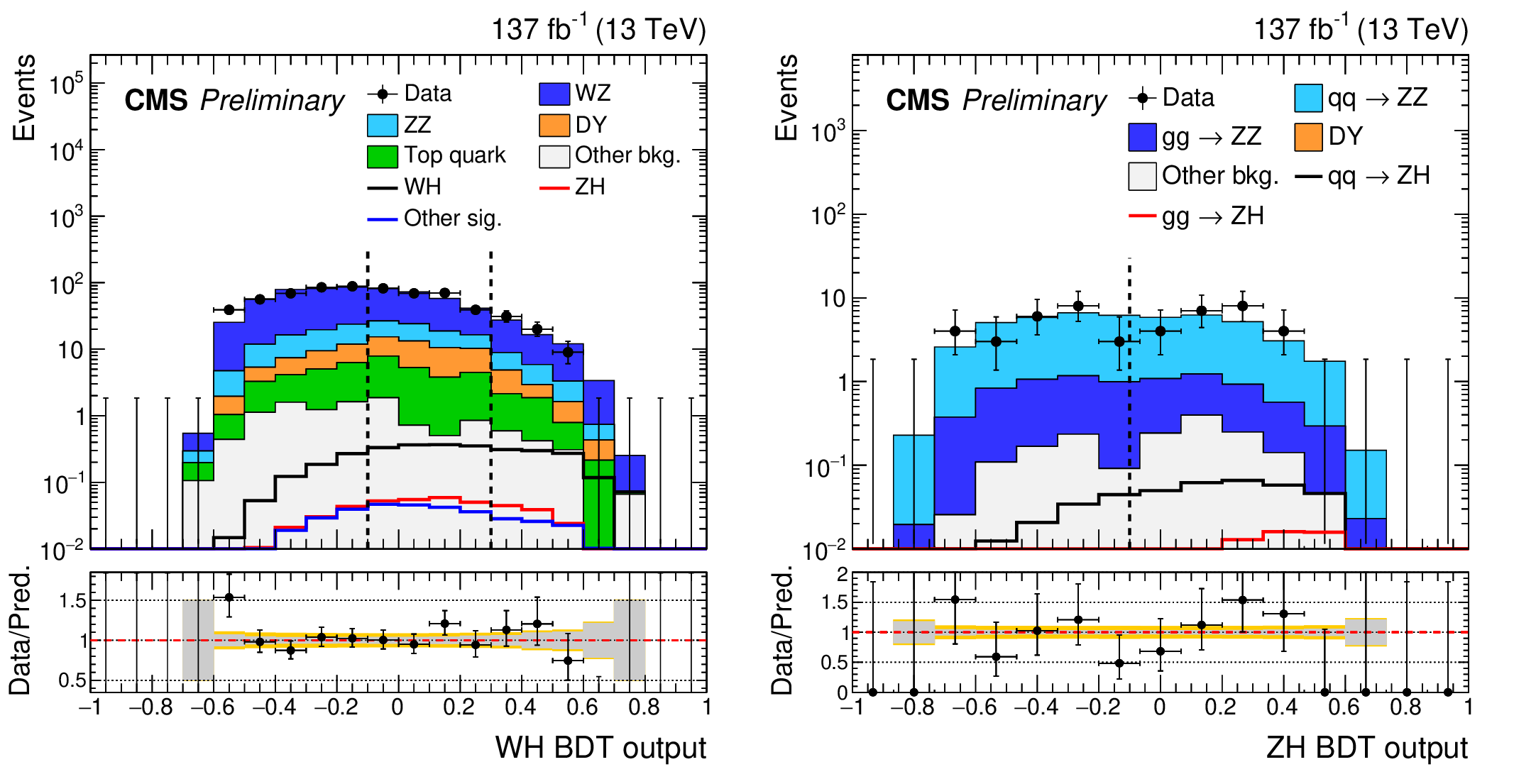
The observed BDT output distribution in the $\mathrm{W} \mathrm{H} $ (left) and $\mathrm{Z} \mathrm{H} $ (right) categories compared to the prediction from the simulation of various SM background processes. Signal distributions expected from different production modes of the 125 GeV Higgs boson are overlaid. The description of the ratio panel is the same as in Fig. 4. The dashed vertical lines indicate the boundaries of the optimized event categories. |
png pdf |
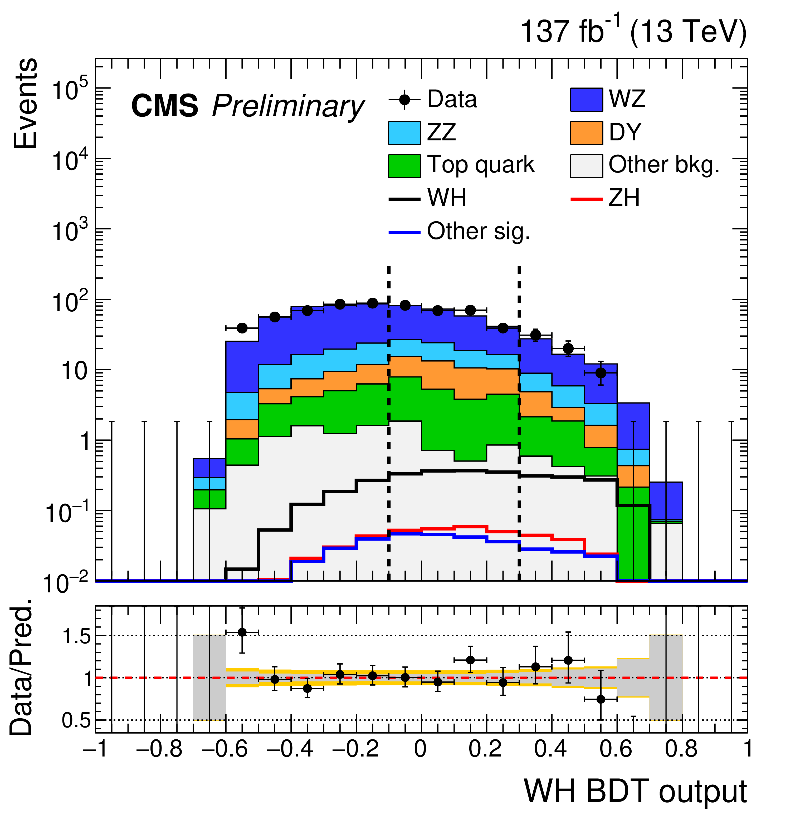
Figure 6-a:
The observed BDT output distribution in the $\mathrm{W} \mathrm{H} $ $\mathrm{Z} \mathrm{H} $ category compared to the prediction from the simulation of various SM background processes. Signal distributions expected from different production modes of the 125 GeV Higgs boson are overlaid. The description of the ratio panel is the same as in Fig. 4. The dashed vertical lines indicate the boundaries of the optimized event categories. |
png pdf |
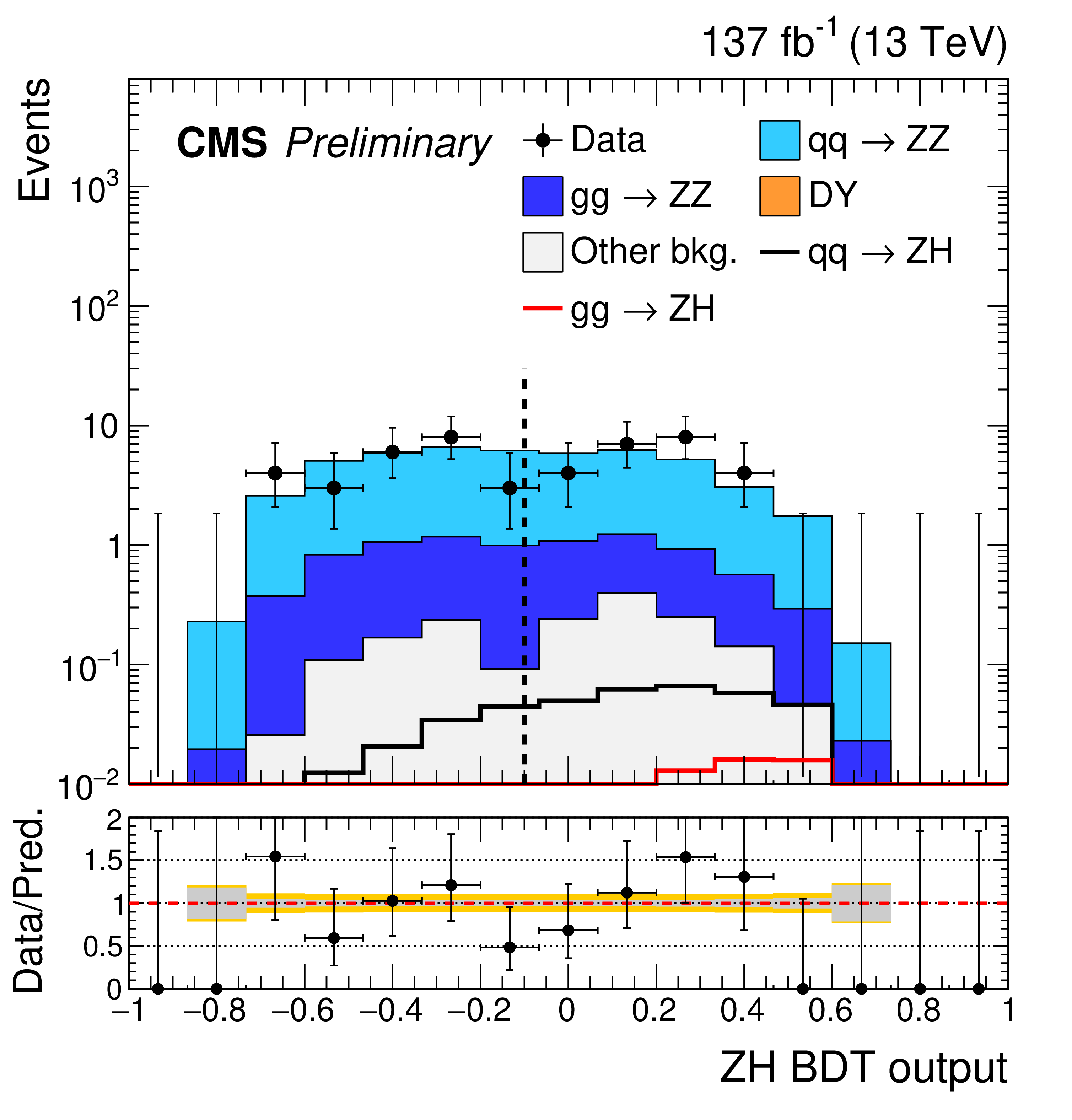
Figure 6-b:
The observed BDT output distribution in the $\mathrm{W} \mathrm{H} $ (left) and $\mathrm{Z} \mathrm{H} $ (right) categories compared to the prediction from the simulation of various SM background processes. Signal distributions expected from different production modes of the 125 GeV Higgs boson are overlaid. The description of the ratio panel is the same as in Fig. 4. The dashed vertical lines indicate the boundaries of the optimized event categories. |
png pdf |
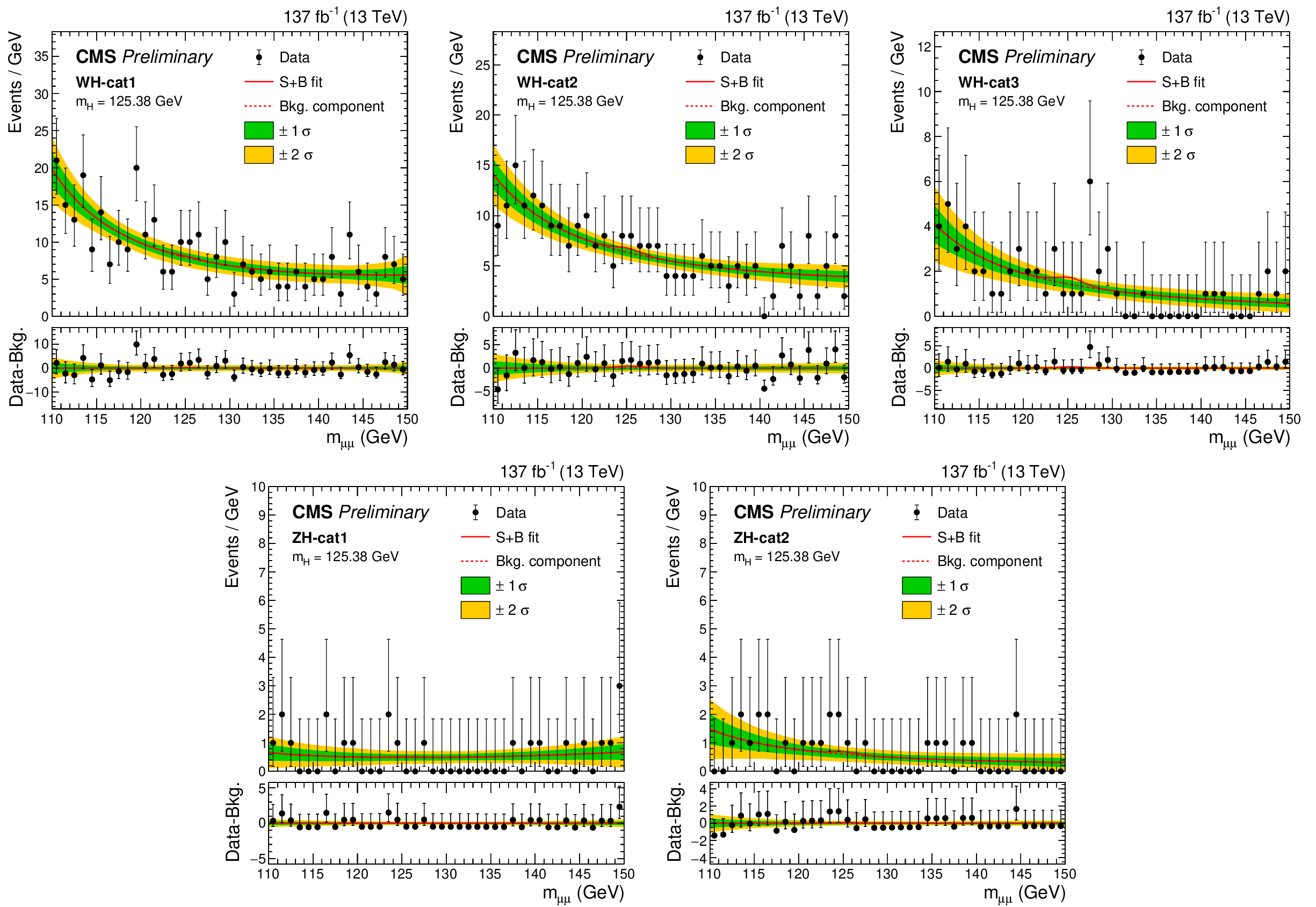
Figure 7:
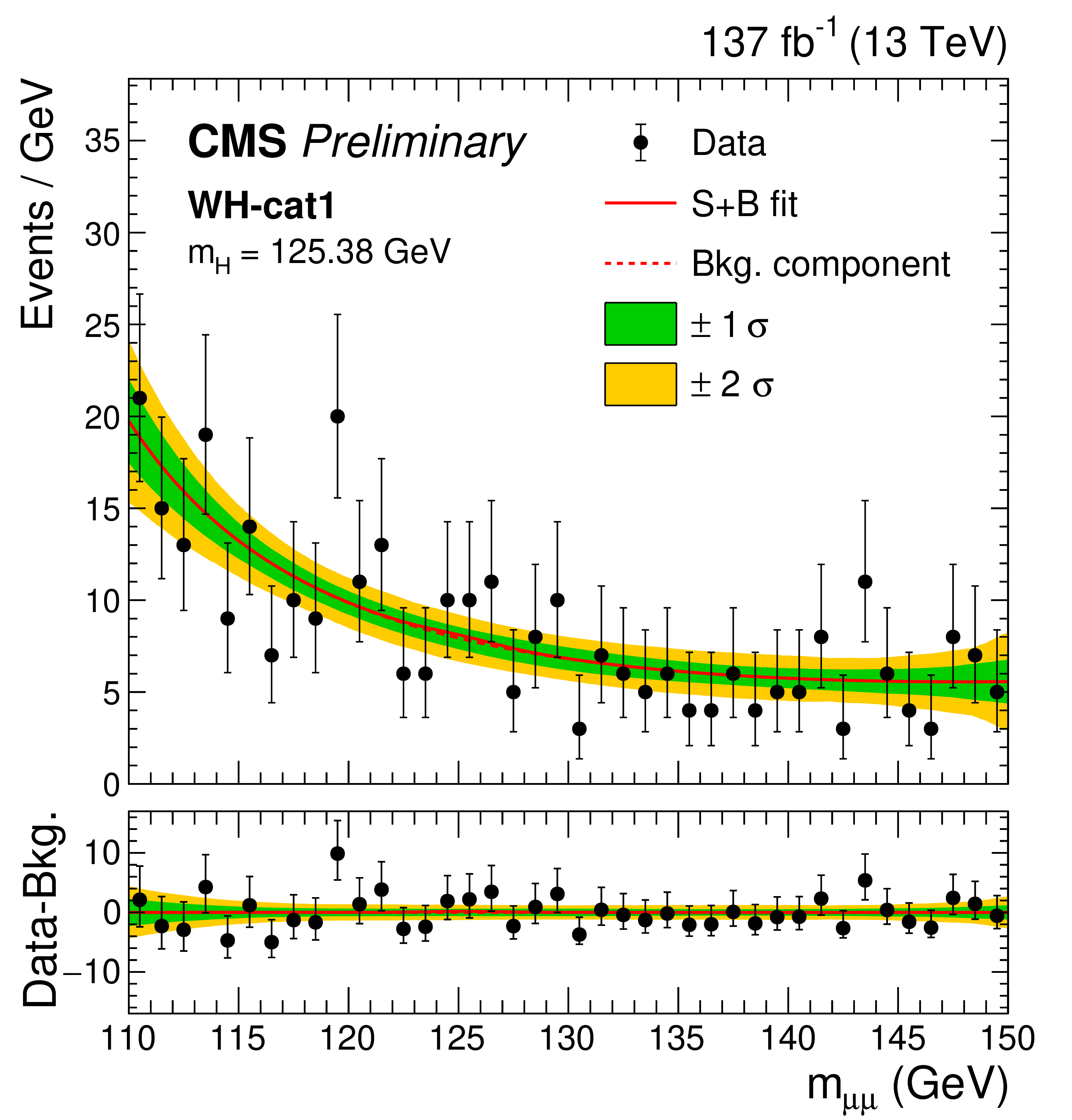
Comparison between the observed data and the total background extracted from a signal-plus-background fit performed across $\mathrm{W} \mathrm{H} $ (first row) and $\mathrm{Z} \mathrm{H} $ (second row) event categories. First row, from left to right : ${\mathrm{W} \mathrm{H} \textrm {-cat1}}$, ${\mathrm{W} \mathrm{H} \textrm {-cat2}}$, and ${\mathrm{W} \mathrm{H} \textrm {-cat3}}$. Second row, from left to right : ${\mathrm{Z} \mathrm{H} \textrm {-cat1}}$ and ${\mathrm{Z} \mathrm{H} \textrm {-cat2}}$. The one (green) and two (yellow) standard deviation bands include the uncertainties in the background component of the fit. The lower panel shows the residuals after the background subtraction, where the red line indicates the signal with ${m_{\mathrm{H}}} =$ 125.38 GeV extracted from the fit. |
png pdf |
Figure 7-a:
Comparison between the observed data and the total background extracted from a signal-plus-background fit performed in the ${\mathrm{W} \mathrm{H} \textrm {-cat1}}$ event category. The one (green) and two (yellow) standard deviation bands include the uncertainties in the background component of the fit. The lower panel shows the residuals after the background subtraction, where the red line indicates the signal with ${m_{\mathrm{H}}} =$ 125.38 GeV extracted from the fit. |
png pdf |
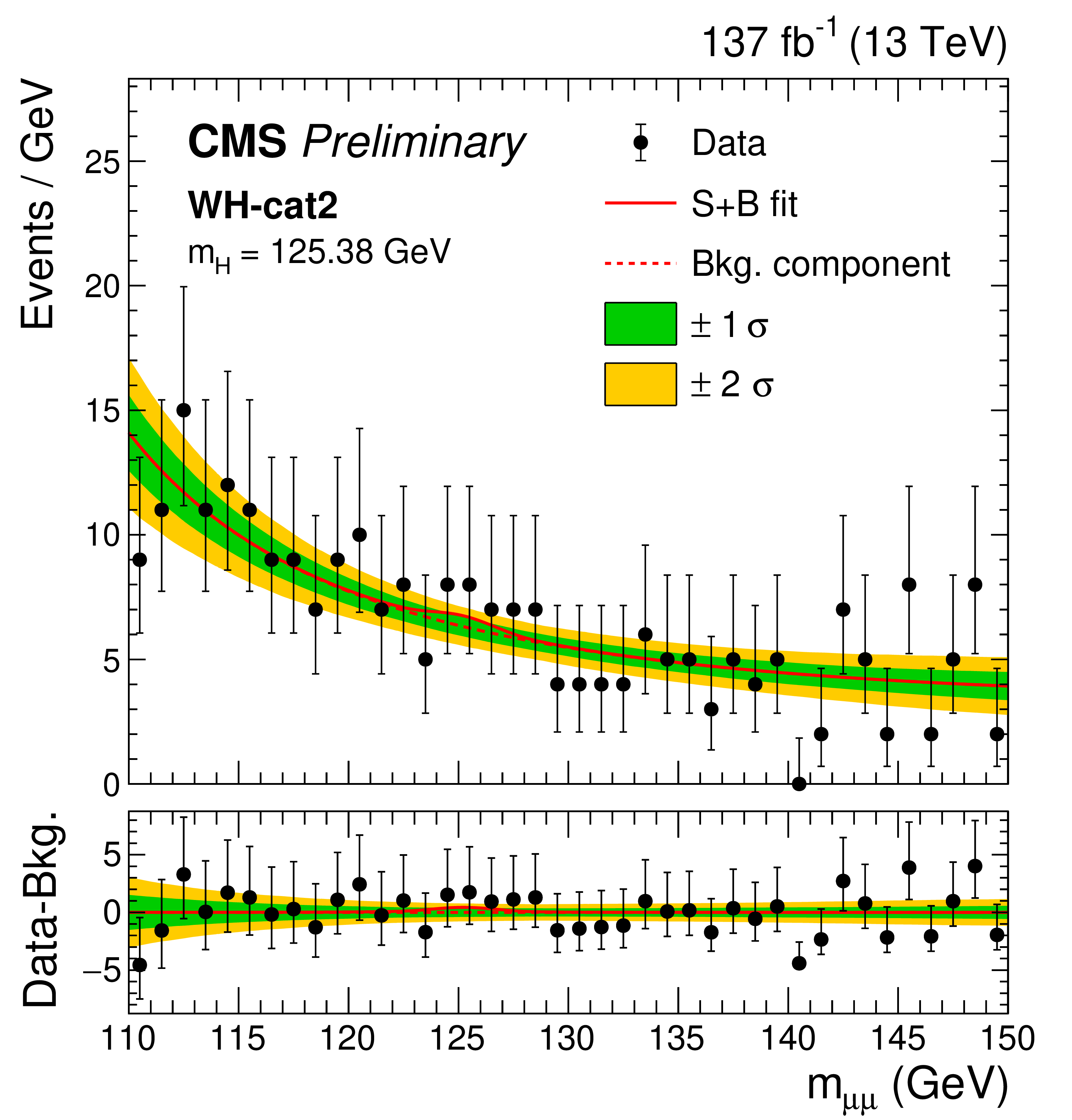
Figure 7-b:
Comparison between the observed data and the total background extracted from a signal-plus-background fit performed in the ${\mathrm{W} \mathrm{H} \textrm {-cat2}}$ event category. The one (green) and two (yellow) standard deviation bands include the uncertainties in the background component of the fit. The lower panel shows the residuals after the background subtraction, where the red line indicates the signal with ${m_{\mathrm{H}}} =$ 125.38 GeV extracted from the fit. |
png pdf |
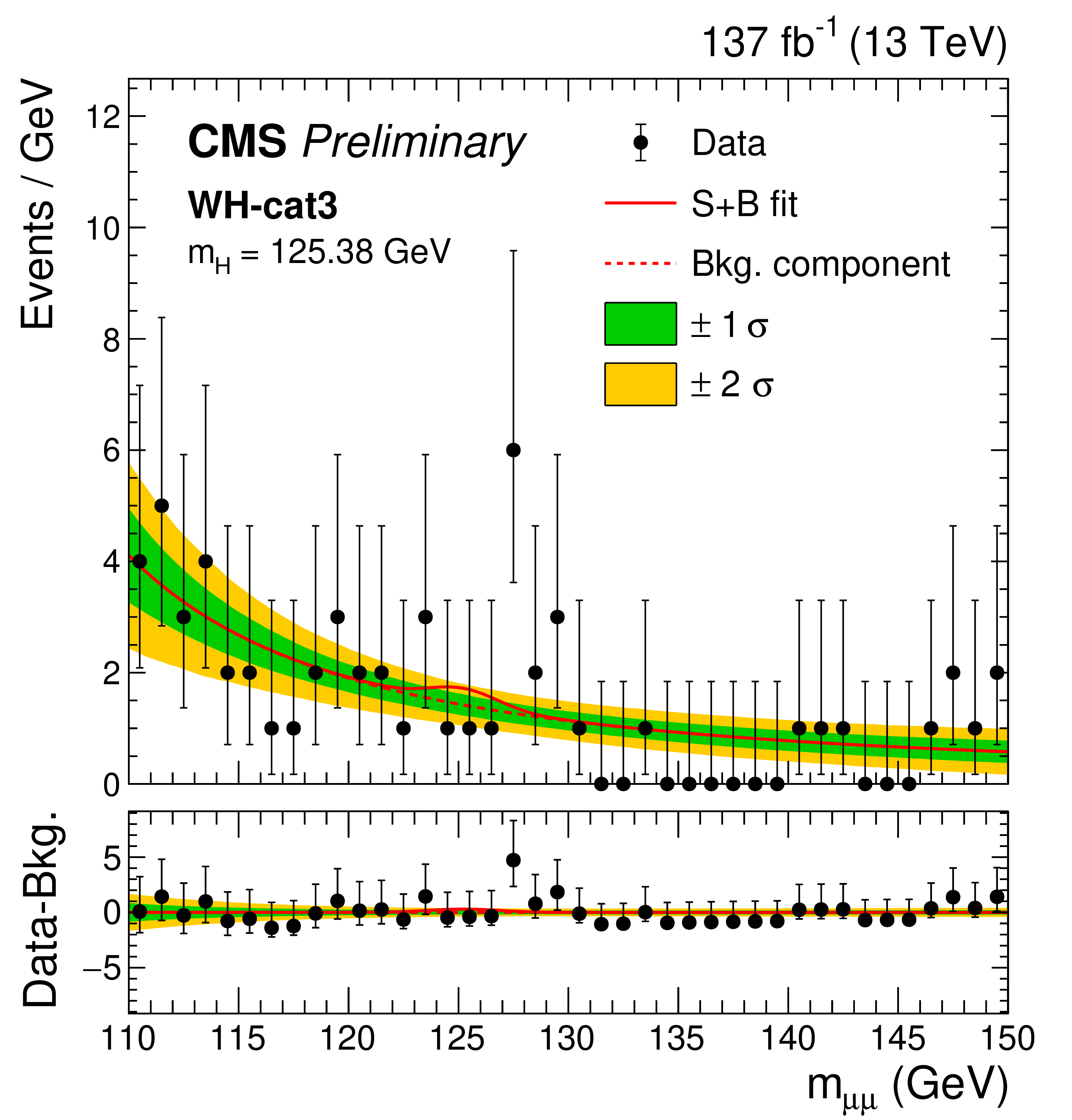
Figure 7-c:
Comparison between the observed data and the total background extracted from a signal-plus-background fit performed in the ${\mathrm{W} \mathrm{H} \textrm {-cat3}}$ event category. The one (green) and two (yellow) standard deviation bands include the uncertainties in the background component of the fit. The lower panel shows the residuals after the background subtraction, where the red line indicates the signal with ${m_{\mathrm{H}}} =$ 125.38 GeV extracted from the fit. |
png pdf |
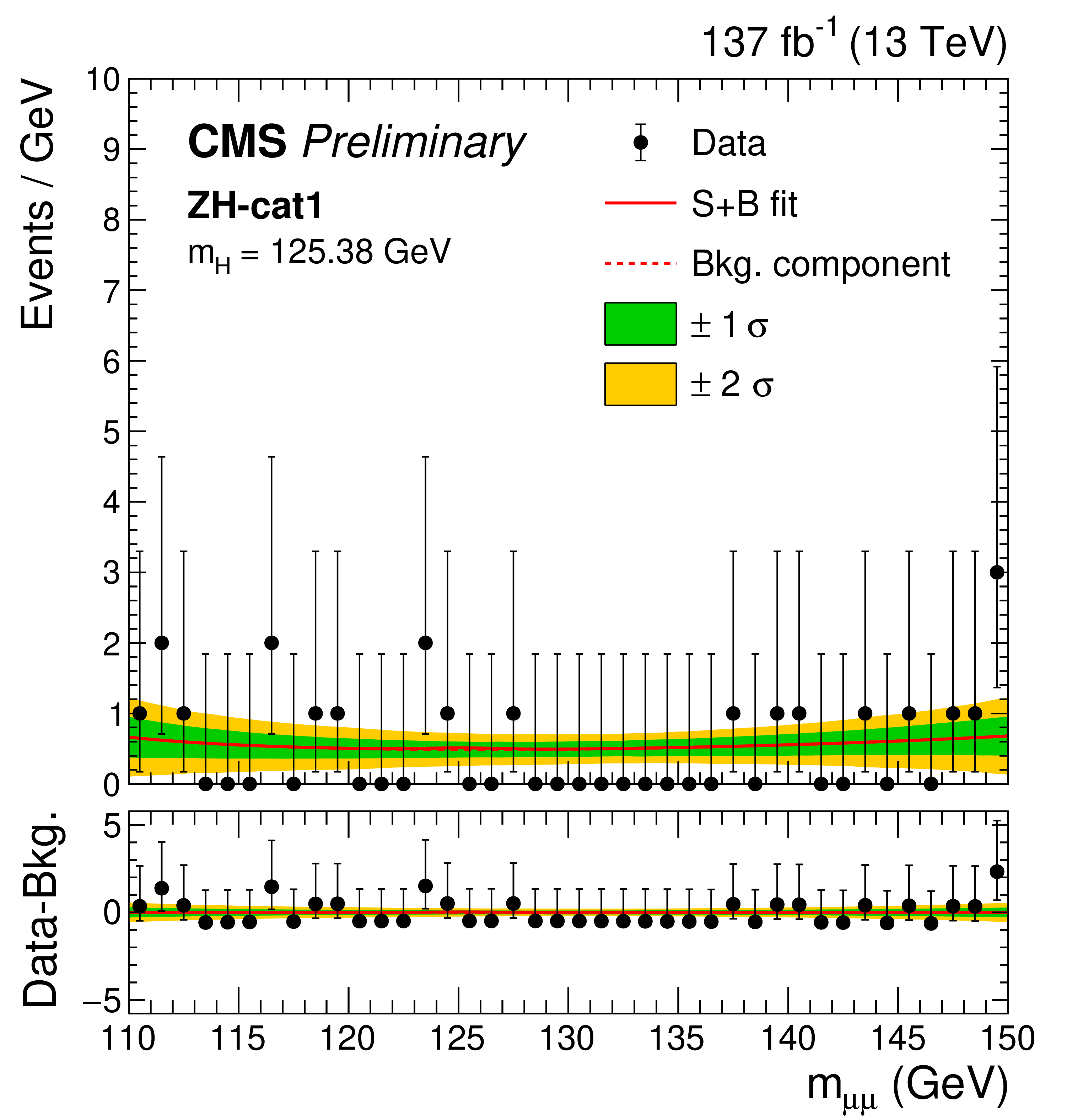
Figure 7-d:
Comparison between the observed data and the total background extracted from a signal-plus-background fit performed in the ${\mathrm{Z} \mathrm{H} \textrm {-cat1}}$ event category. The one (green) and two (yellow) standard deviation bands include the uncertainties in the background component of the fit. The lower panel shows the residuals after the background subtraction, where the red line indicates the signal with ${m_{\mathrm{H}}} =$ 125.38 GeV extracted from the fit. |

png pdf |
Figure 7-e:
Comparison between the observed data and the total background extracted from a signal-plus-background fit performed in the ${\mathrm{Z} \mathrm{H} \textrm {-cat2}}$ event category. The one (green) and two (yellow) standard deviation bands include the uncertainties in the background component of the fit. The lower panel shows the residuals after the background subtraction, where the red line indicates the signal with ${m_{\mathrm{H}}} =$ 125.38 GeV extracted from the fit. |
png pdf |
Figure 8:
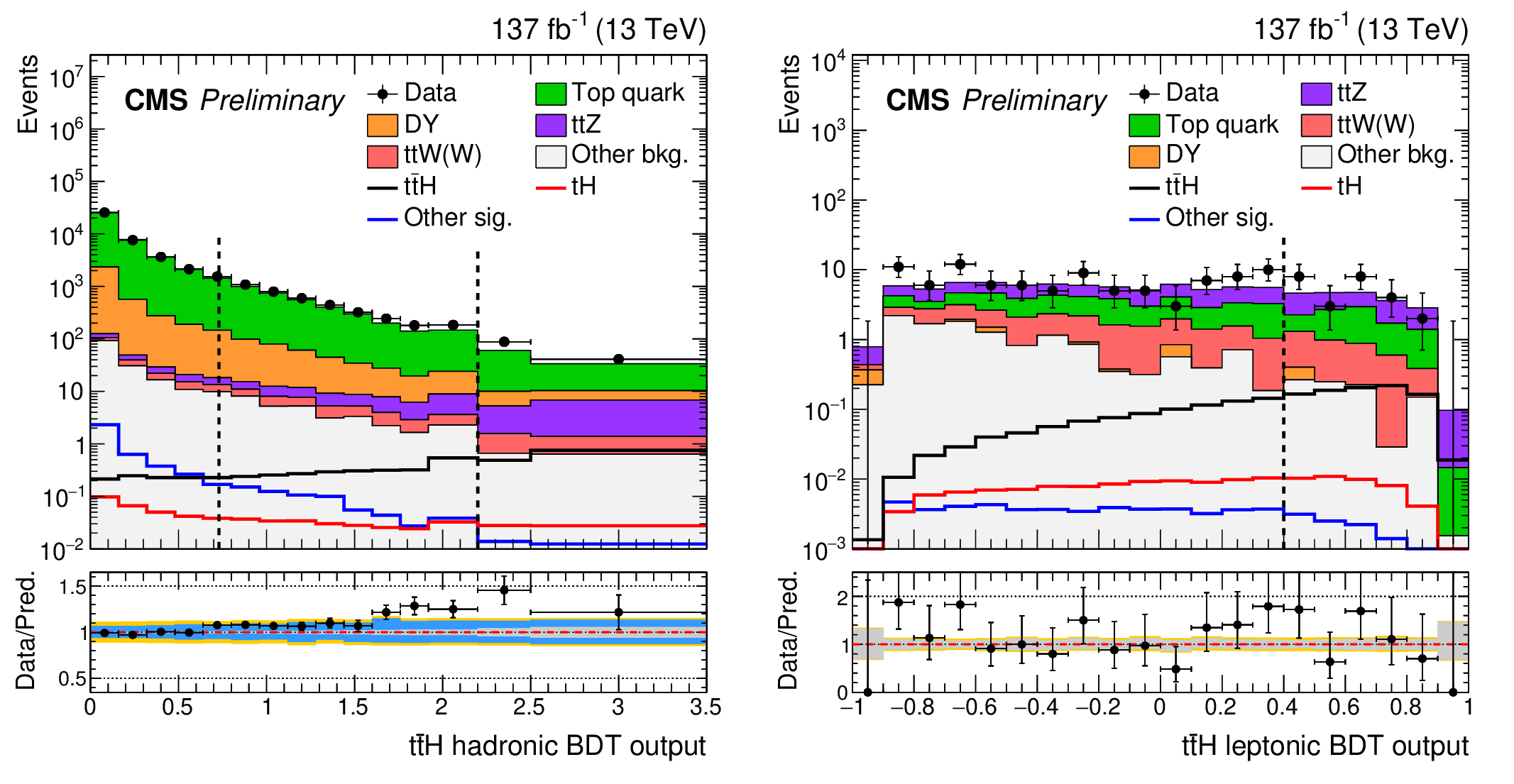
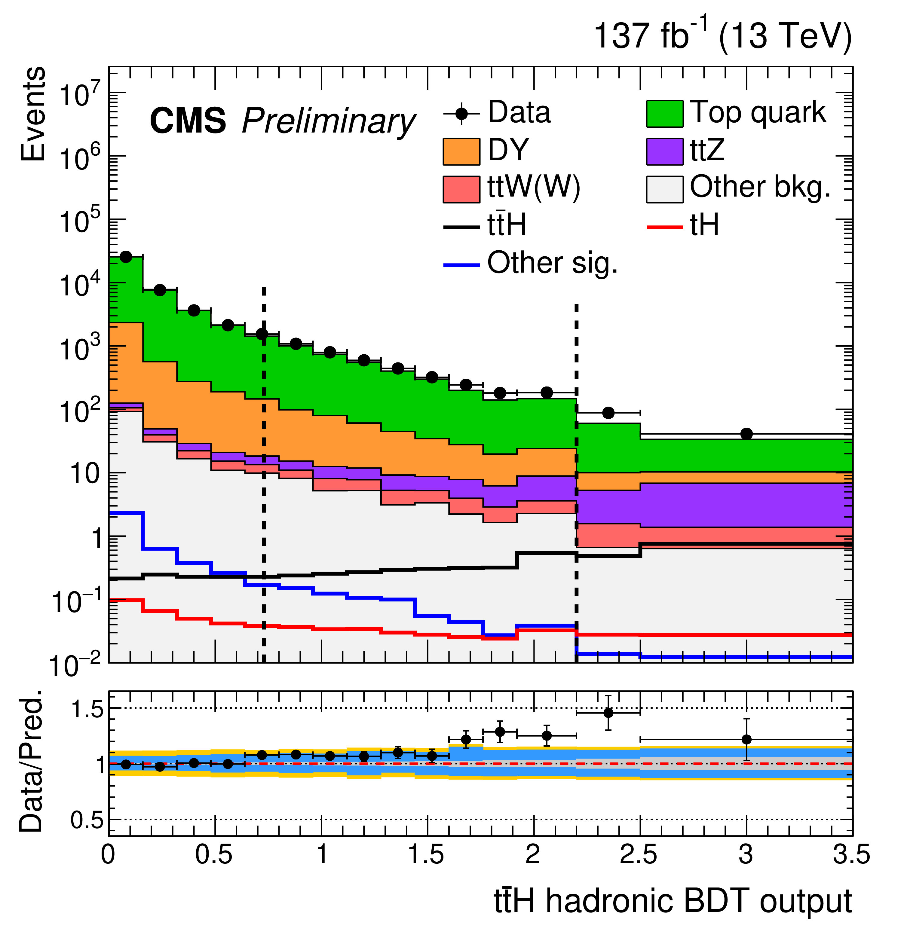
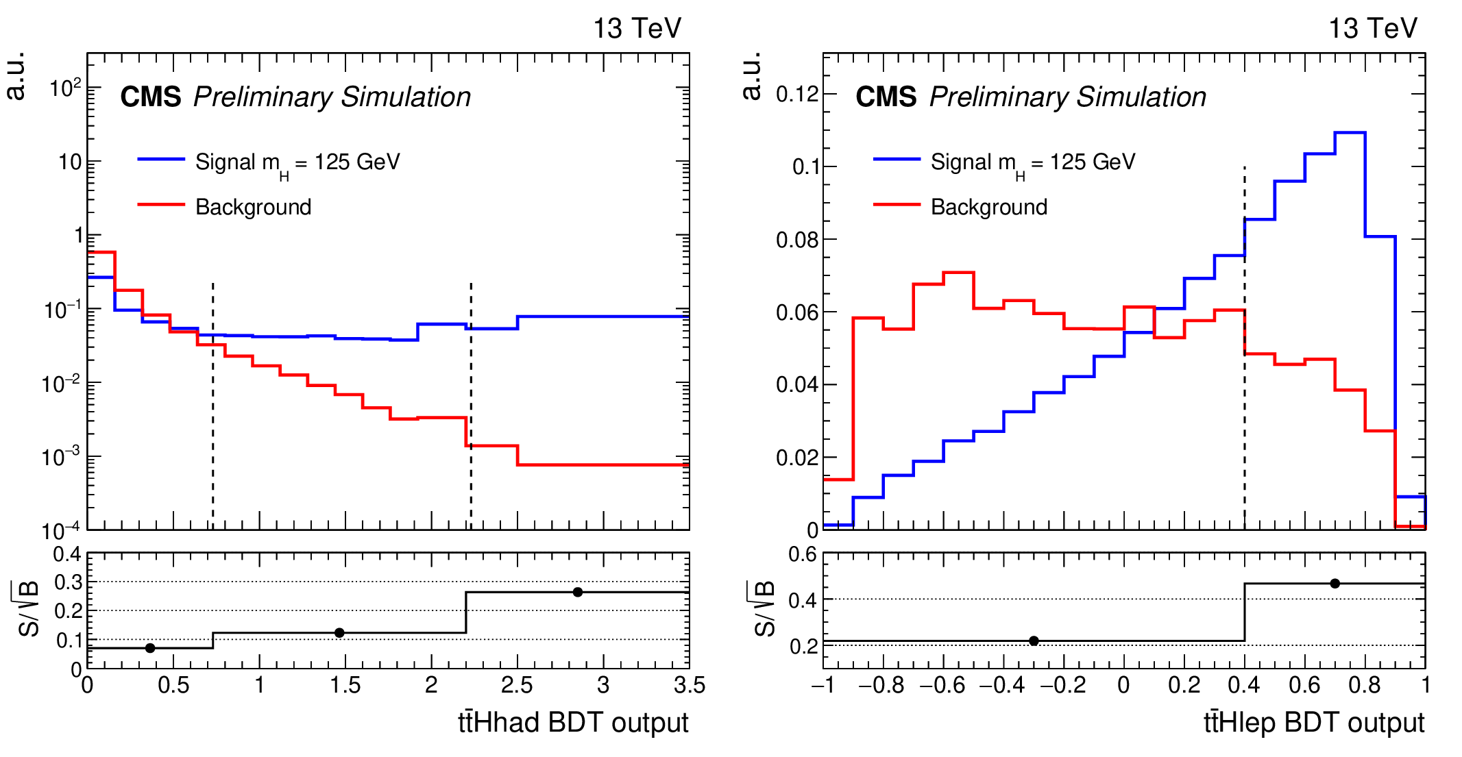
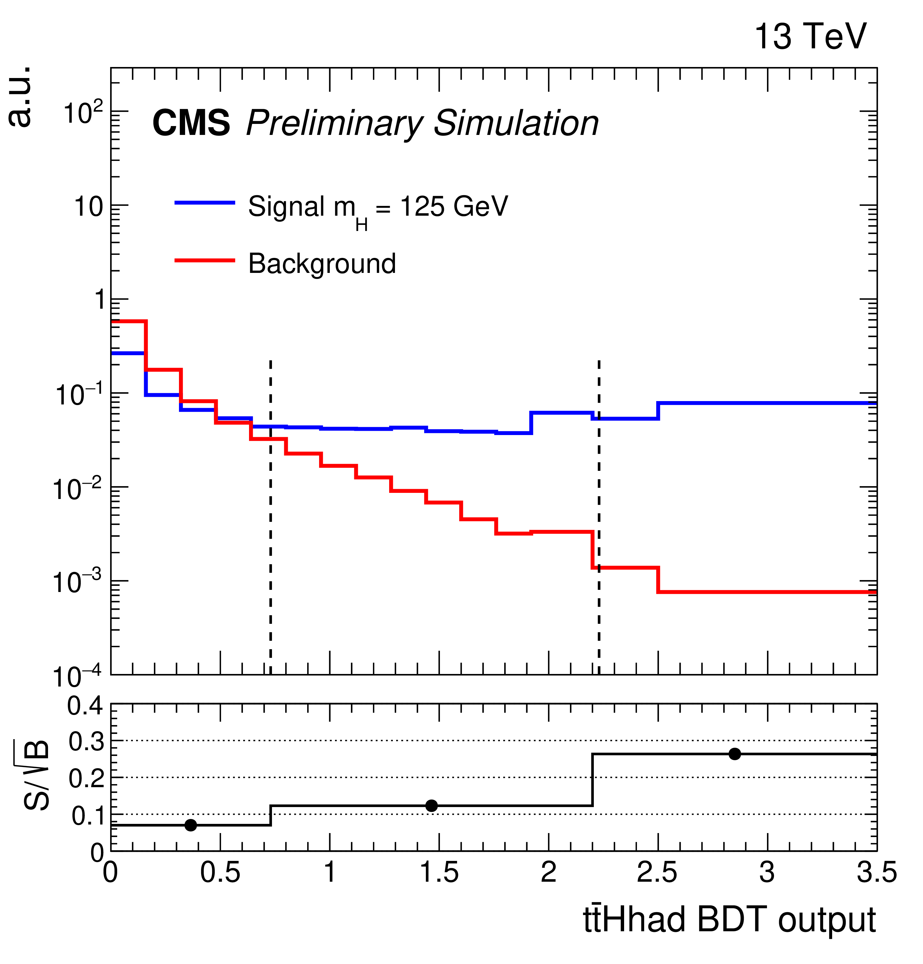
The observed BDT output distribution in the ${\mathrm{t} {}\mathrm{\bar{t}}} \mathrm{H} $ hadronic (left) and leptonic (right) categories compared to the prediction from the simulation of various SM background processes. Signal distributions expected from different production modes of the 125 GeV Higgs boson are overlaid. The dashed vertical lines indicate the boundaries of the optimized event categories. The description of the ratio panels is the same as in Fig. 4. |
png pdf |
Figure 8-a:
The observed BDT output distribution in the ${\mathrm{t} {}\mathrm{\bar{t}}} \mathrm{H} $ hadronic categories compared to the prediction from the simulation of various SM background processes. Signal distributions expected from different production modes of the 125 GeV Higgs boson are overlaid. The dashed vertical lines indicate the boundaries of the optimized event categories. The description of the ratio panel is the same as in Fig. 4. |

png pdf |
Figure 8-b:
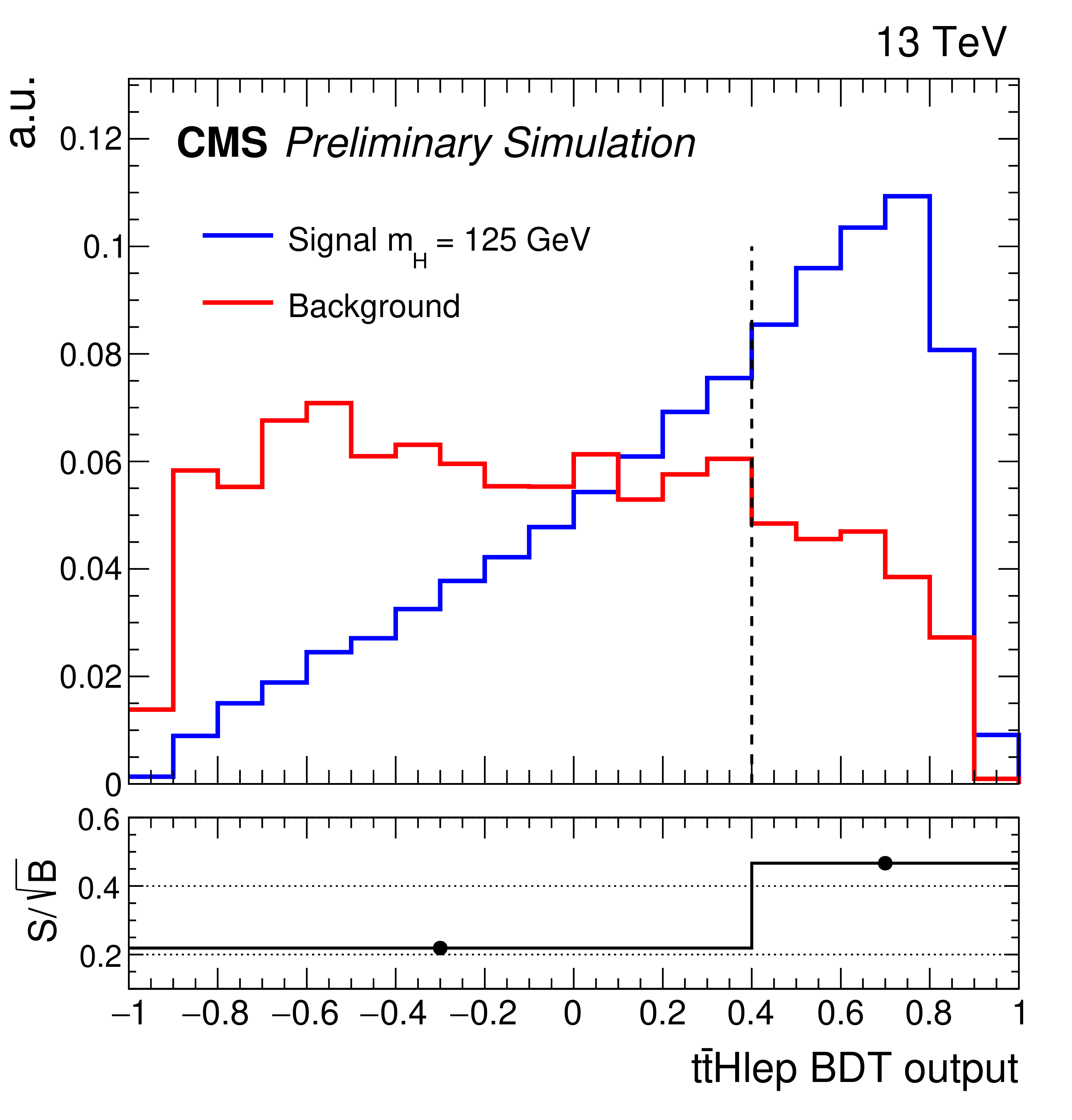
The observed BDT output distribution in the ${\mathrm{t} {}\mathrm{\bar{t}}} \mathrm{H} $ leptonic categories compared to the prediction from the simulation of various SM background processes. Signal distributions expected from different production modes of the 125 GeV Higgs boson are overlaid. The dashed vertical lines indicate the boundaries of the optimized event categories. The description of the ratio panel is the same as in Fig. 4. |

png pdf |
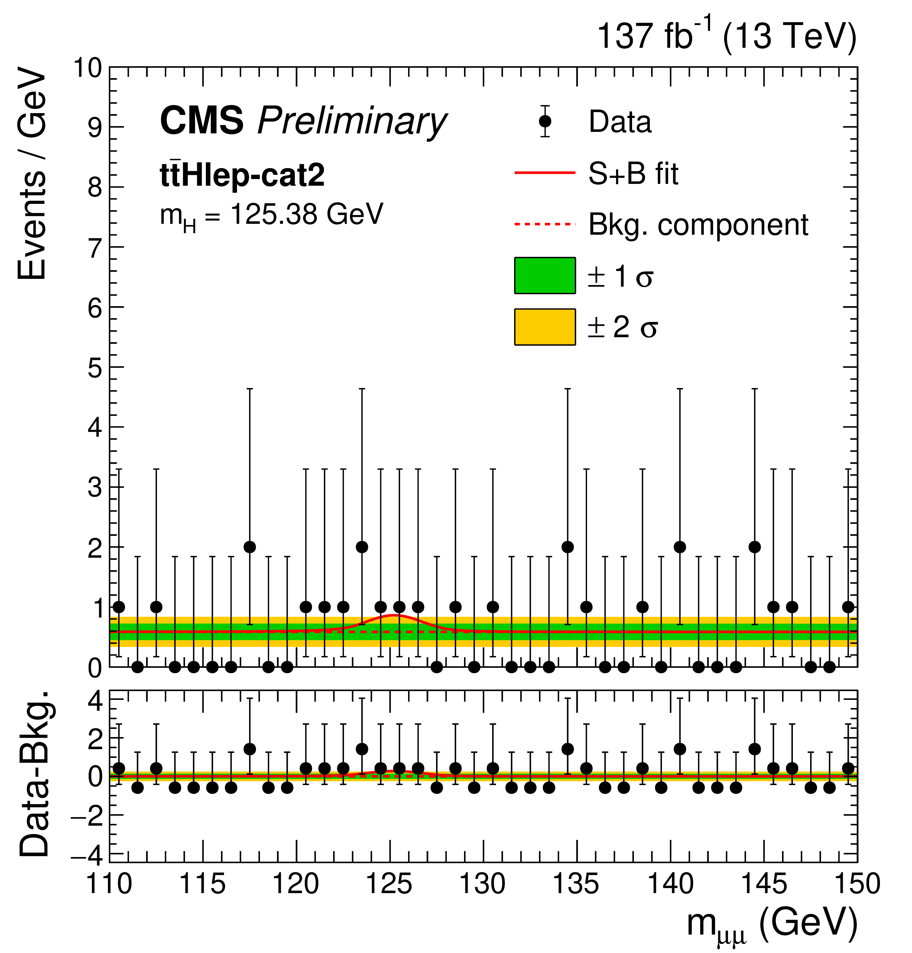
Figure 9:
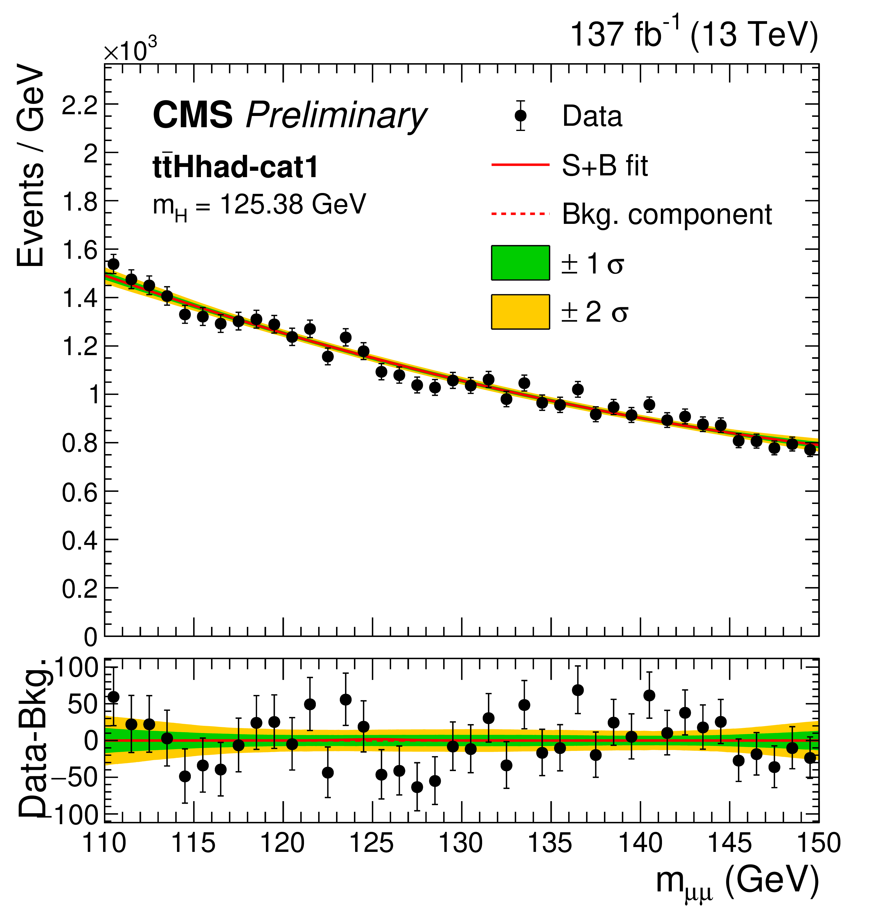
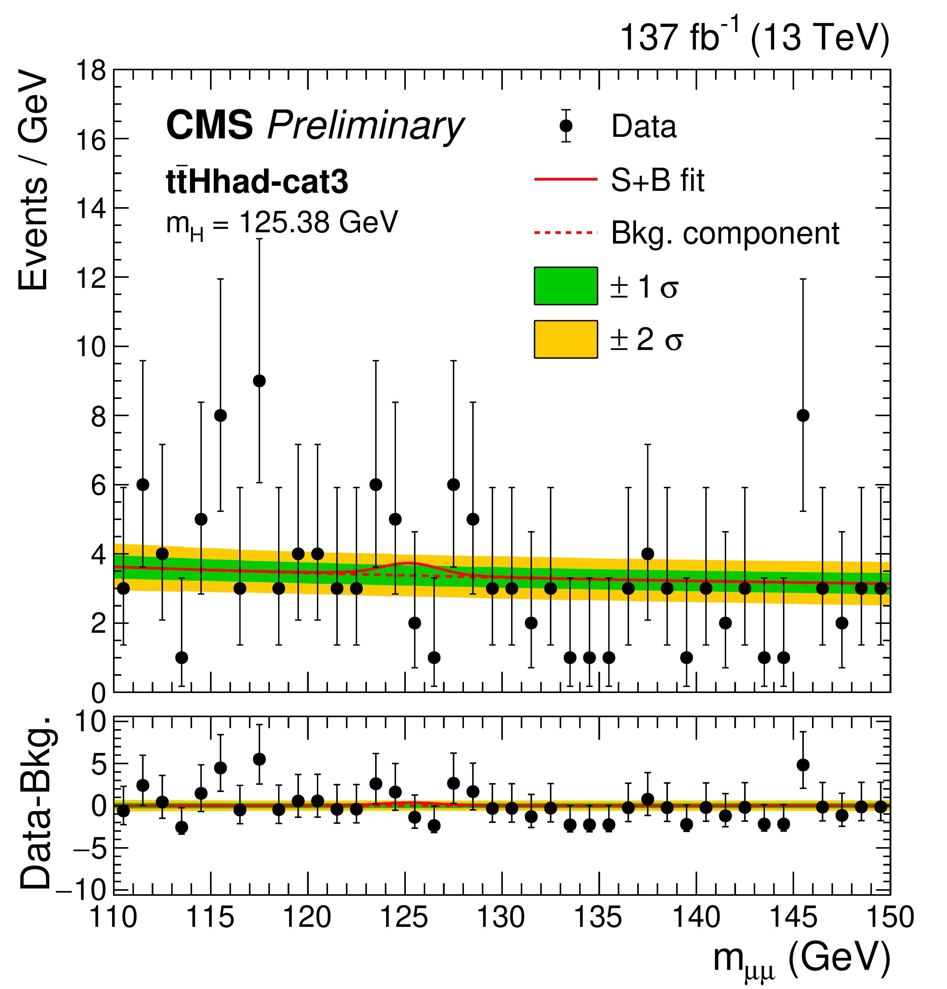
Comparison between the observed data and the total background extracted from a signal-plus-background fit performed across ${\mathrm{t} {}\mathrm{\bar{t}}} \mathrm{H} $ hadronic (first row) and leptonic (second row) event categories. First row, from left to right : ${{\mathrm{t} {}\mathrm{\bar{t}}} \mathrm{H} \textrm {had-cat1}}$, ${{\mathrm{t} {}\mathrm{\bar{t}}} \mathrm{H} \textrm {had-cat2}}$, and ${{\mathrm{t} {}\mathrm{\bar{t}}} \mathrm{H} \textrm {had-cat3}}$. Second row, from left to right : ${{\mathrm{t} {}\mathrm{\bar{t}}} \mathrm{H} \textrm {lep-cat1}}$ and ${{\mathrm{t} {}\mathrm{\bar{t}}} \mathrm{H} \textrm {lep-cat2}}$. The one (green) and two (yellow) standard deviation bands include the uncertainties in the background component of the fit. The lower panel shows the residuals after the background subtraction, where the red line indicates the signal with ${m_{\mathrm{H}}} =$ 125.38 GeV extracted from the fit. |
png pdf |
Figure 9-a:
Comparison between the observed data and the total background extracted from a signal-plus-background fit performed in the ${{\mathrm{t} {}\mathrm{\bar{t}}} \mathrm{H} \textrm {had-cat1}}$ event category. The one (green) and two (yellow) standard deviation bands include the uncertainties in the background component of the fit. The lower panel shows the residuals after the background subtraction, where the red line indicates the signal with ${m_{\mathrm{H}}} =$ 125.38 GeV extracted from the fit. |

png pdf |
Figure 9-b:
Comparison between the observed data and the total background extracted from a signal-plus-background fit performed in the ${{\mathrm{t} {}\mathrm{\bar{t}}} \mathrm{H} \textrm {had-cat2}}$ event category. The one (green) and two (yellow) standard deviation bands include the uncertainties in the background component of the fit. The lower panel shows the residuals after the background subtraction, where the red line indicates the signal with ${m_{\mathrm{H}}} =$ 125.38 GeV extracted from the fit. |
png pdf |
Figure 9-c:
Comparison between the observed data and the total background extracted from a signal-plus-background fit performed in the ${{\mathrm{t} {}\mathrm{\bar{t}}} \mathrm{H} \textrm {had-cat3}}$ event category. The one (green) and two (yellow) standard deviation bands include the uncertainties in the background component of the fit. The lower panel shows the residuals after the background subtraction, where the red line indicates the signal with ${m_{\mathrm{H}}} =$ 125.38 GeV extracted from the fit. |

png pdf |
Figure 9-d:
Comparison between the observed data and the total background extracted from a signal-plus-background fit performed in the ${{\mathrm{t} {}\mathrm{\bar{t}}} \mathrm{H} \textrm {lep-cat1}}$ event category. The one (green) and two (yellow) standard deviation bands include the uncertainties in the background component of the fit. The lower panel shows the residuals after the background subtraction, where the red line indicates the signal with ${m_{\mathrm{H}}} =$ 125.38 GeV extracted from the fit. |
png pdf |
Figure 9-e:
Comparison between the observed data and the total background extracted from a signal-plus-background fit performed in the ${{\mathrm{t} {}\mathrm{\bar{t}}} \mathrm{H} \textrm {lep-cat2}}$ event category. The one (green) and two (yellow) standard deviation bands include the uncertainties in the background component of the fit. The lower panel shows the residuals after the background subtraction, where the red line indicates the signal with ${m_{\mathrm{H}}} =$ 125.38 GeV extracted from the fit. |

png pdf |
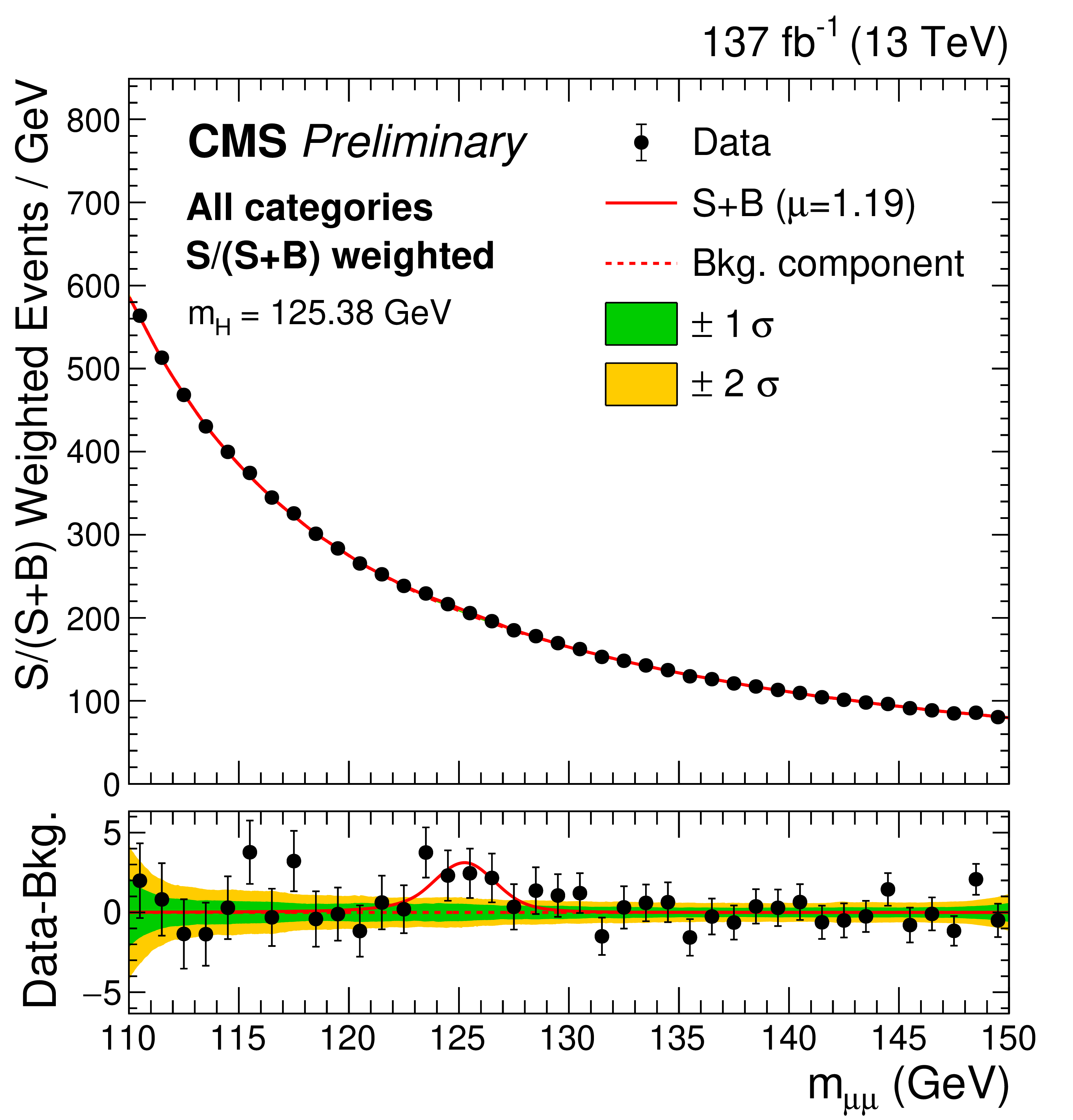
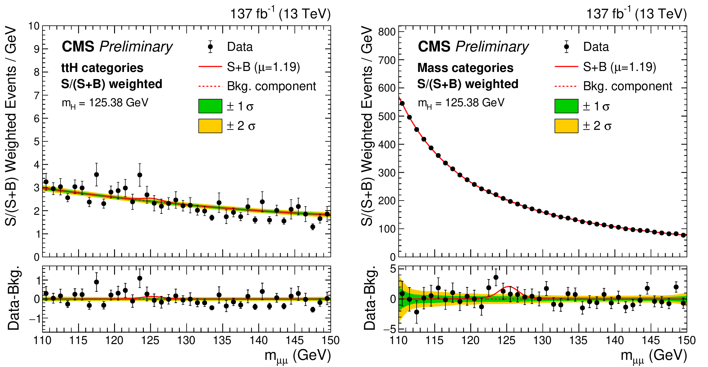
Figure 10:
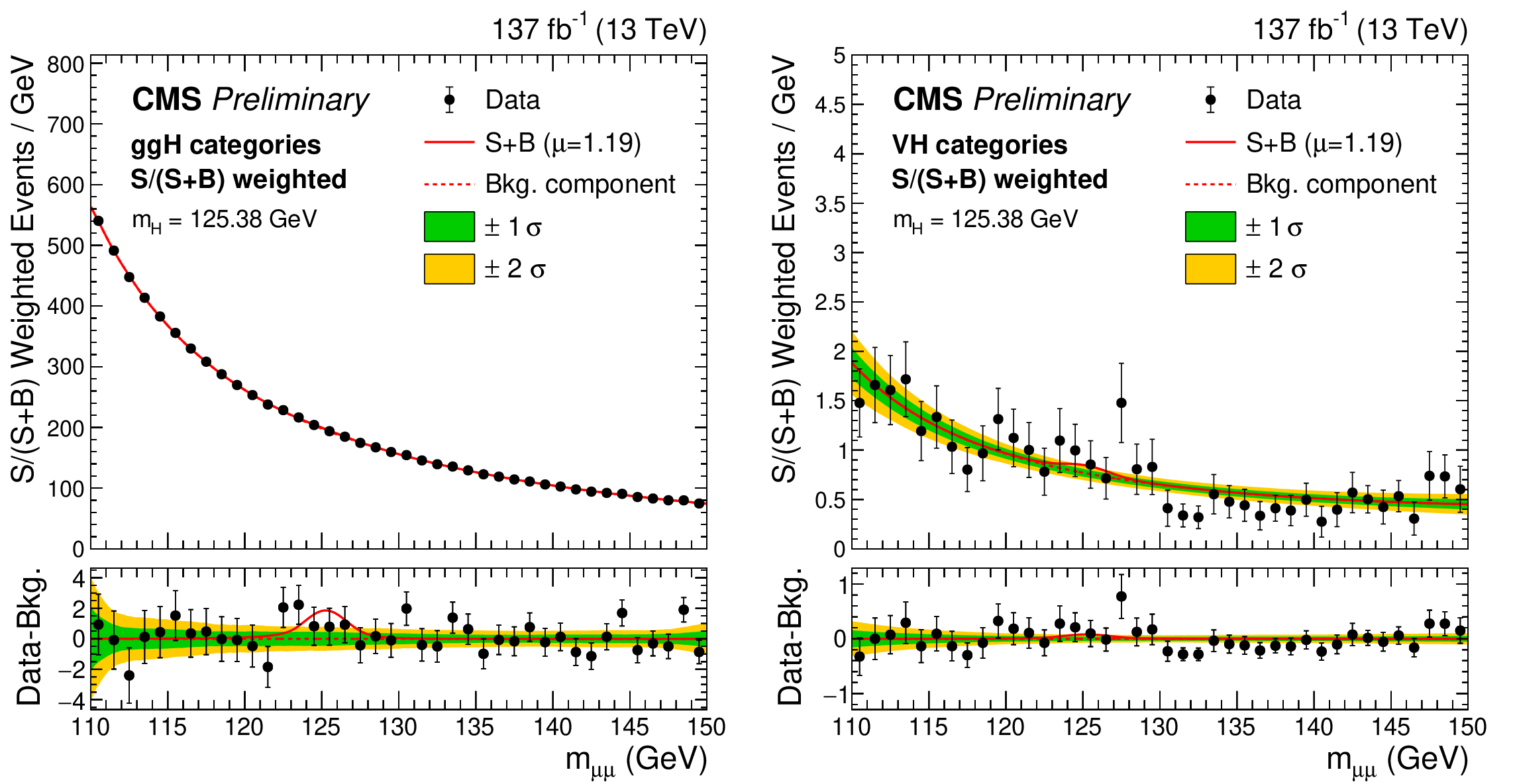
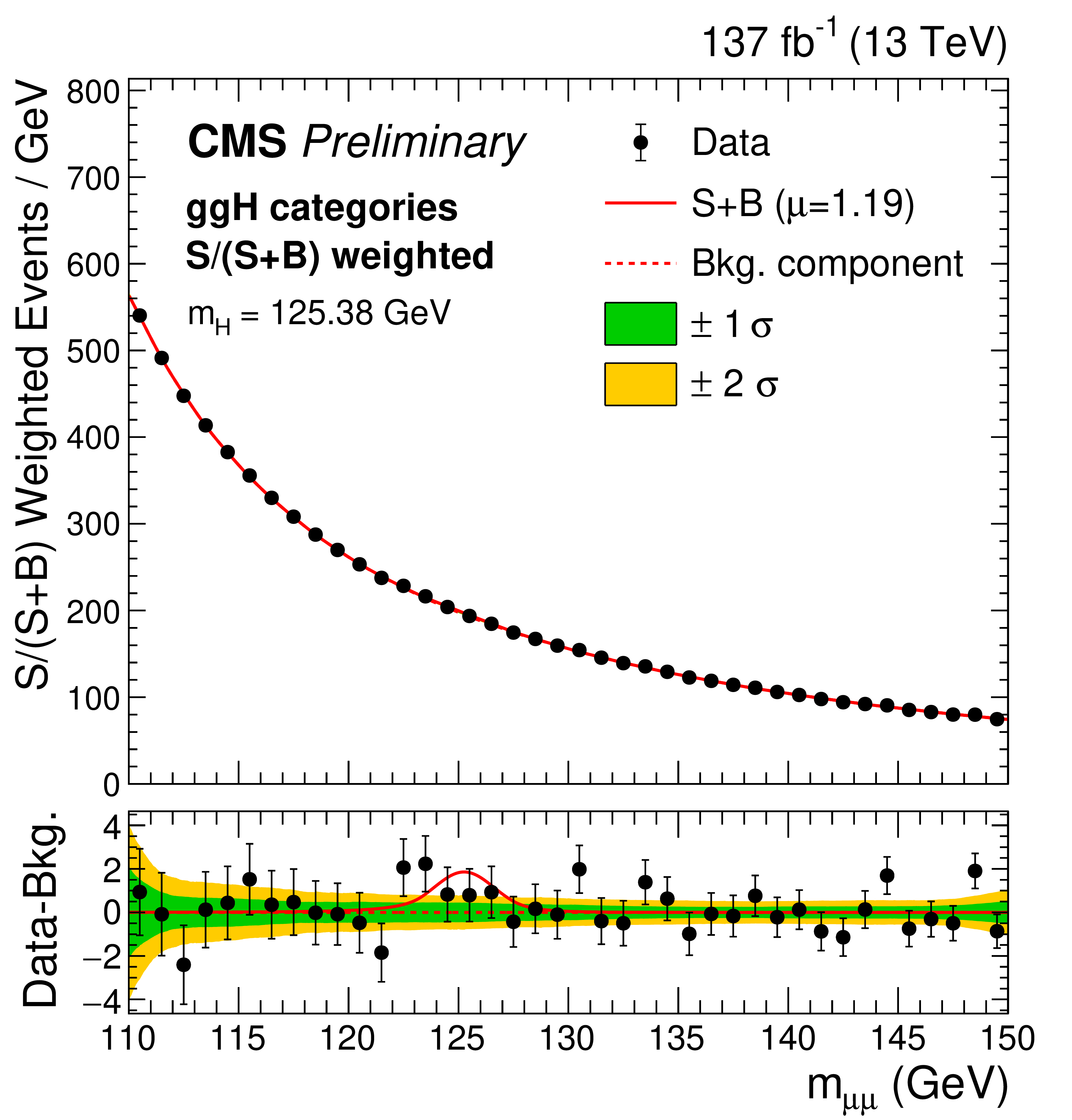
Left: the $m_{\mu \mu}$ distribution for the weighted combination of VBF-SB and VBF-SR events. Each event is weighted proportionally to the ${\text {S}/(\text {S}+\text {B}})$ ratio, calculated as a function of the mass-decorrelated DNN output. The lower panel shows the residuals after subtracting the background prediction from the signal-plus-background fit. The best-fit ${{\mathrm{H} \to \mu \mu}}$ signal contribution is indicated by the blue line, and the grey band indicates the total background uncertainty from the background-only fit. Right: the $m_{\mu \mu}$ distribution for the weighted combination of all event categories. The upper panel is dominated by the $\mathrm{g} \mathrm{g} \mathrm{H} $ categories with many data events but relatively small ${\text {S}/(\text {S}+\text {B}})$. The lower panel shows the residuals after background subtraction, with the best-fit SM ${{\mathrm{H} \to \mu \mu}}$ signal contribution with ${m_{\mathrm{H}}} = $ 125.38 GeV indicated by the red line. |
png pdf |
Figure 10-a:
The $m_{\mu \mu}$ distribution for the weighted combination of VBF-SB and VBF-SR events. Each event is weighted proportionally to the ${\text {S}/(\text {S}+\text {B}})$ ratio, calculated as a function of the mass-decorrelated DNN output. The lower panel shows the residuals after subtracting the background prediction from the signal-plus-background fit. The best-fit ${{\mathrm{H} \to \mu \mu}}$ signal contribution is indicated by the blue line, and the grey band indicates the total background uncertainty from the background-only fit. |
png pdf |
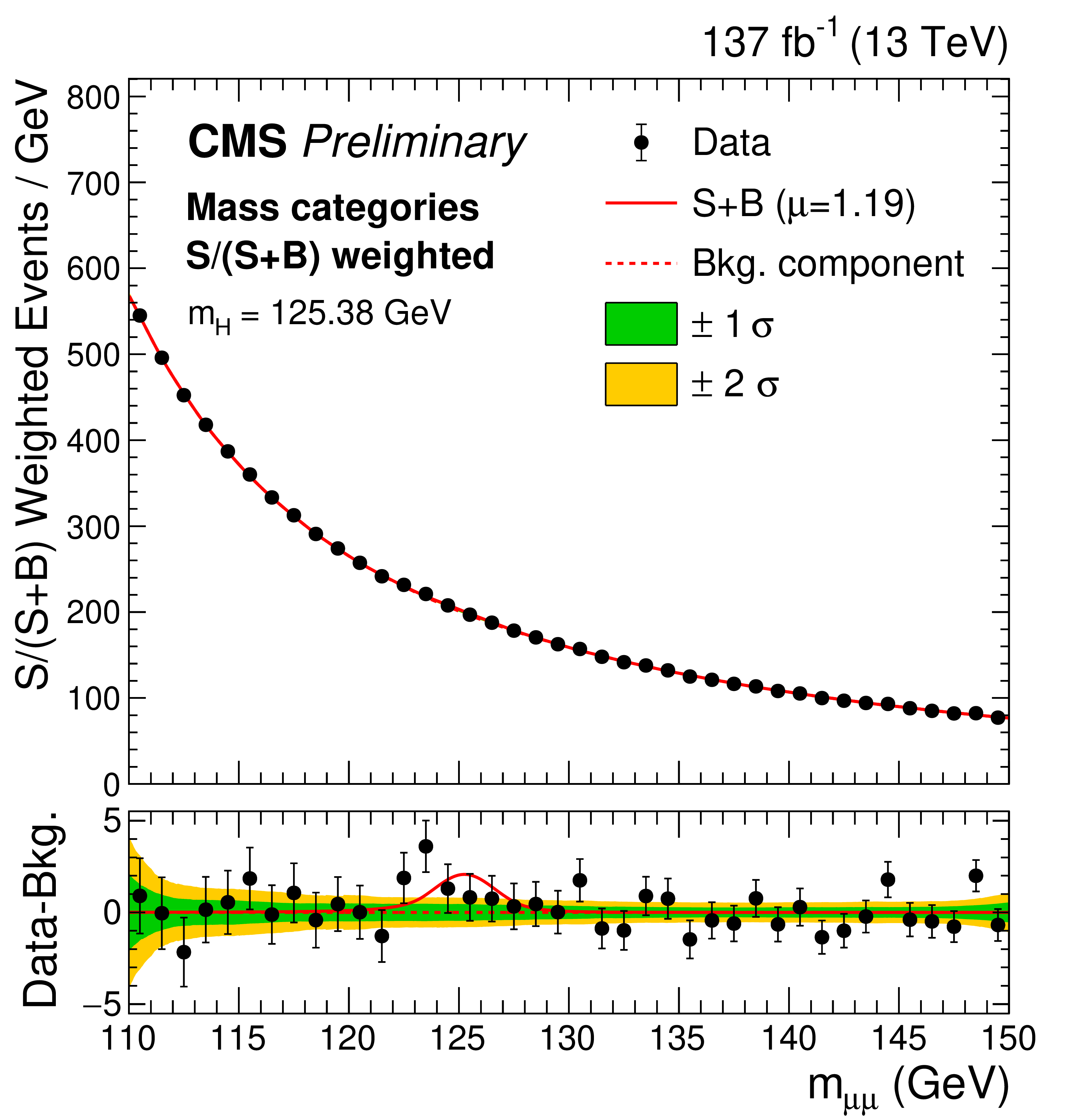
Figure 10-b:
The $m_{\mu \mu}$ distribution for the weighted combination of all event categories. The upper panel is dominated by the $\mathrm{g} \mathrm{g} \mathrm{H} $ categories with many data events but relatively small ${\text {S}/(\text {S}+\text {B}})$. The lower panel shows the residuals after background subtraction, with the best-fit SM ${{\mathrm{H} \to \mu \mu}}$ signal contribution with ${m_{\mathrm{H}}} = $ 125.38 GeV indicated by the red line. |
png pdf |
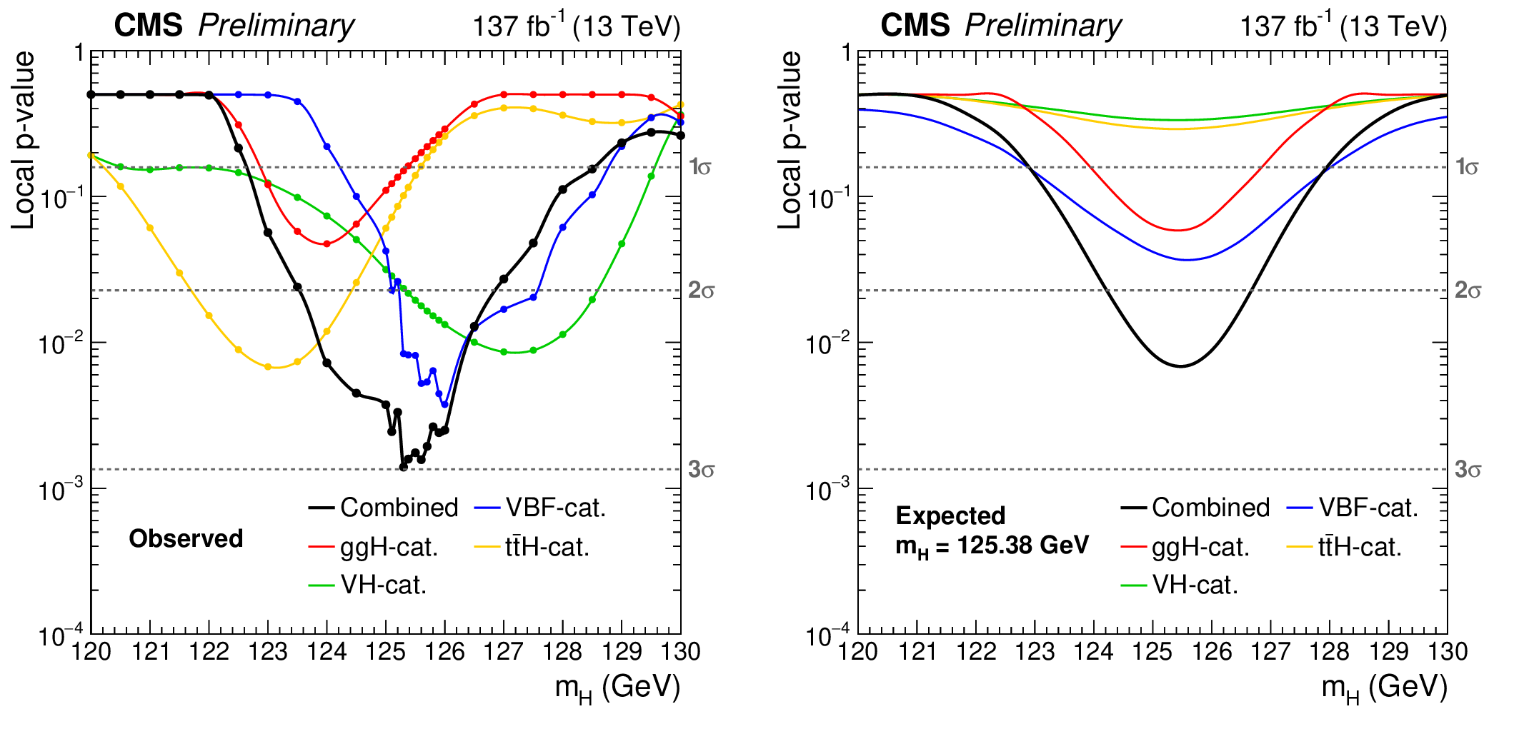
Figure 11:
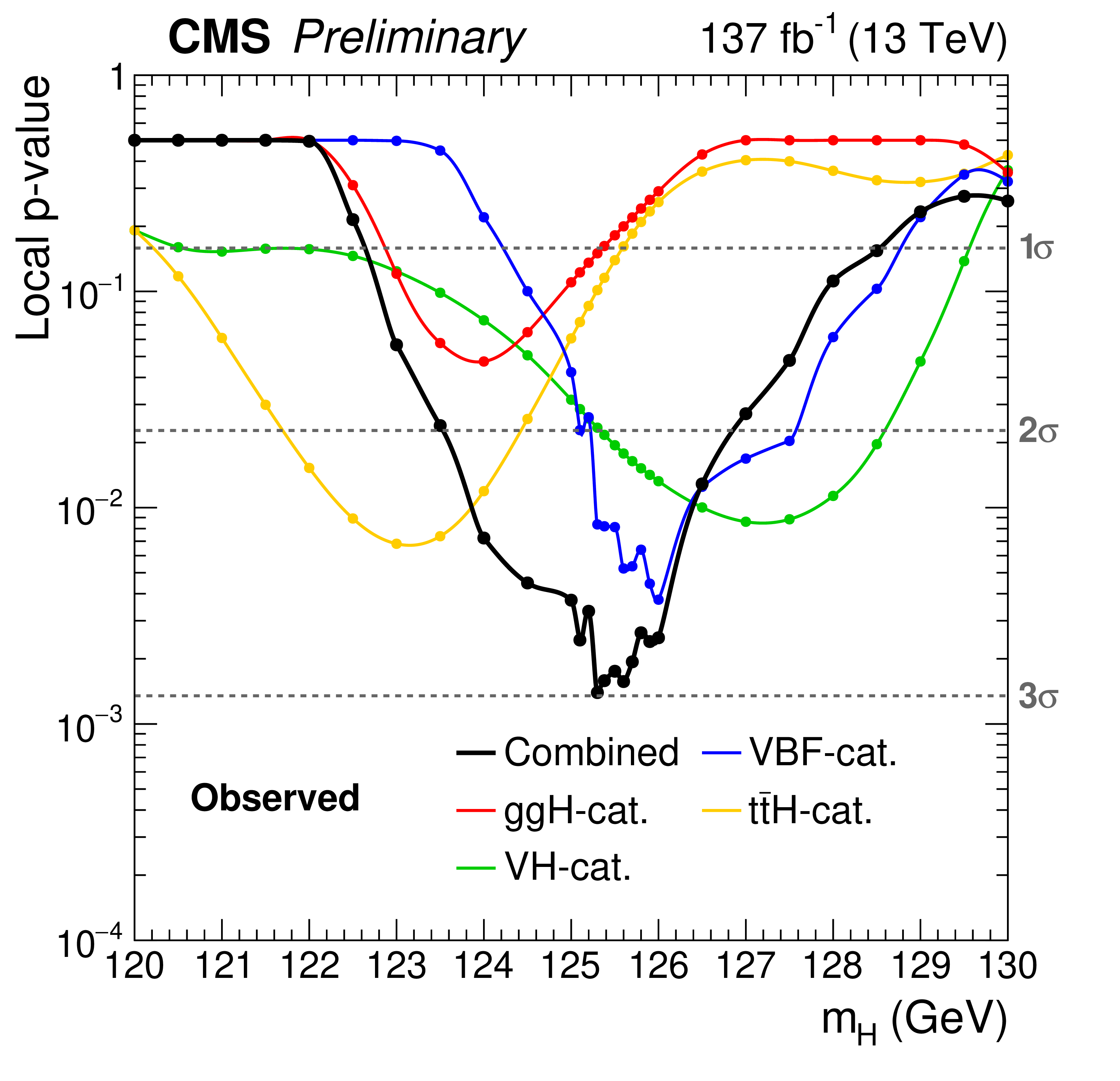
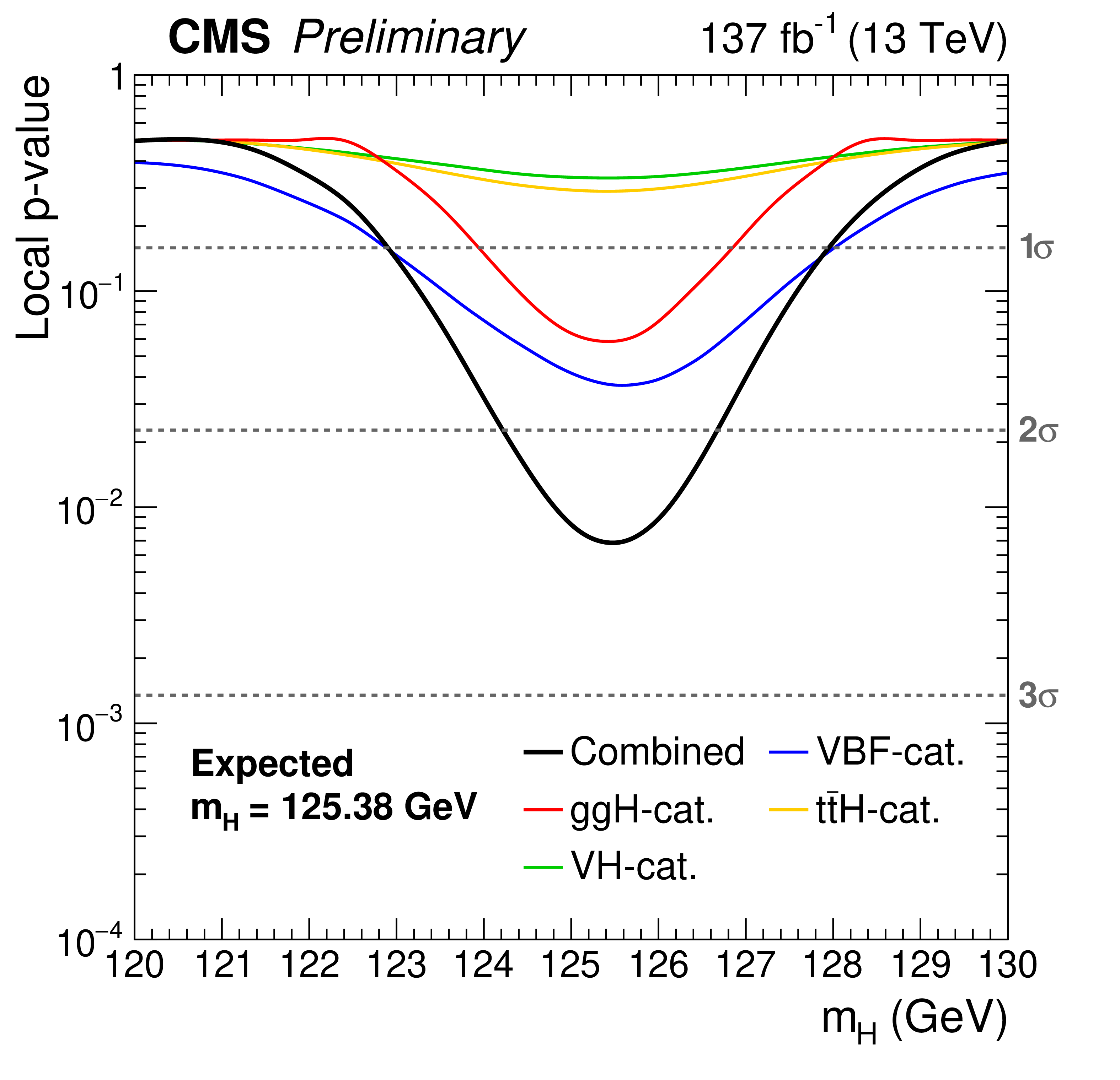
Left: observed local p-values as a function of $ {m_{\mathrm{H}}} $, extracted from the combined fit as well as from each individual production category, are shown. Right: the expected p-values are calculated using the background expectation obtained from the signal-plus-background fit and injecting a signal with ${m_{\mathrm{H}}} =$ 125.38 GeV and $ \mu =$ 1. |
png pdf |
Figure 11-a:
Observed local p-values as a function of $ {m_{\mathrm{H}}} $, extracted from the combined fit as well as from each individual production category, are shown. |
png pdf |
Figure 11-b:
Expected p-values are calculated using the background expectation obtained from the signal-plus-background fit and injecting a signal with ${m_{\mathrm{H}}} =$ 125.38 GeV and $ \mu =$ 1. |
png pdf |
Figure 12:
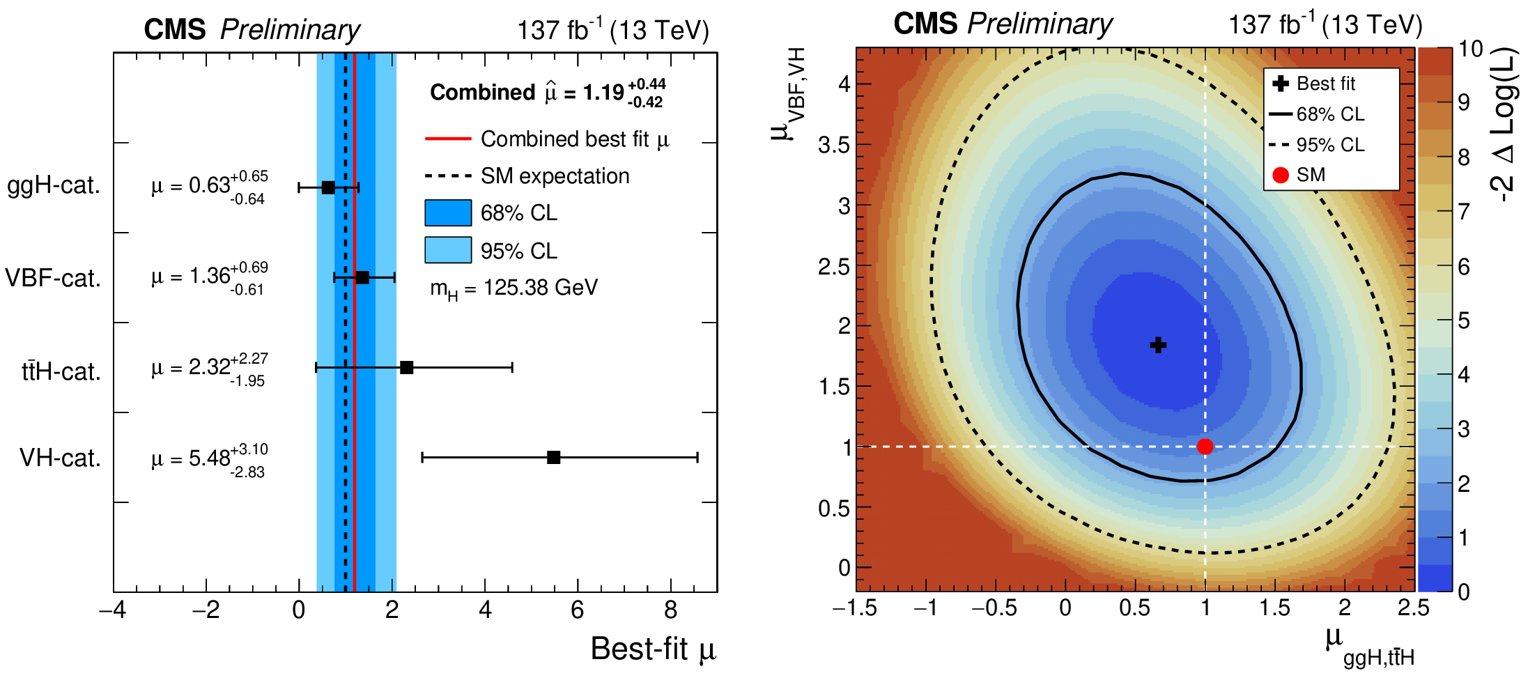
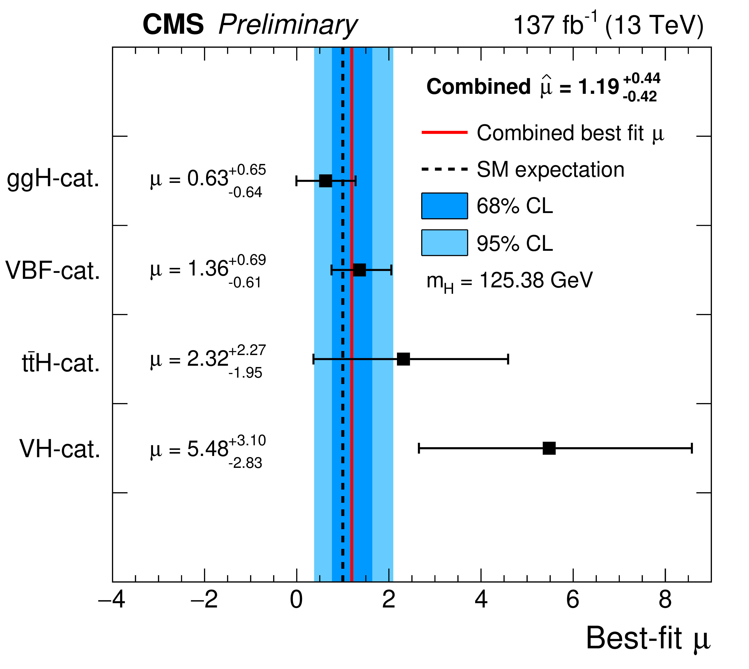
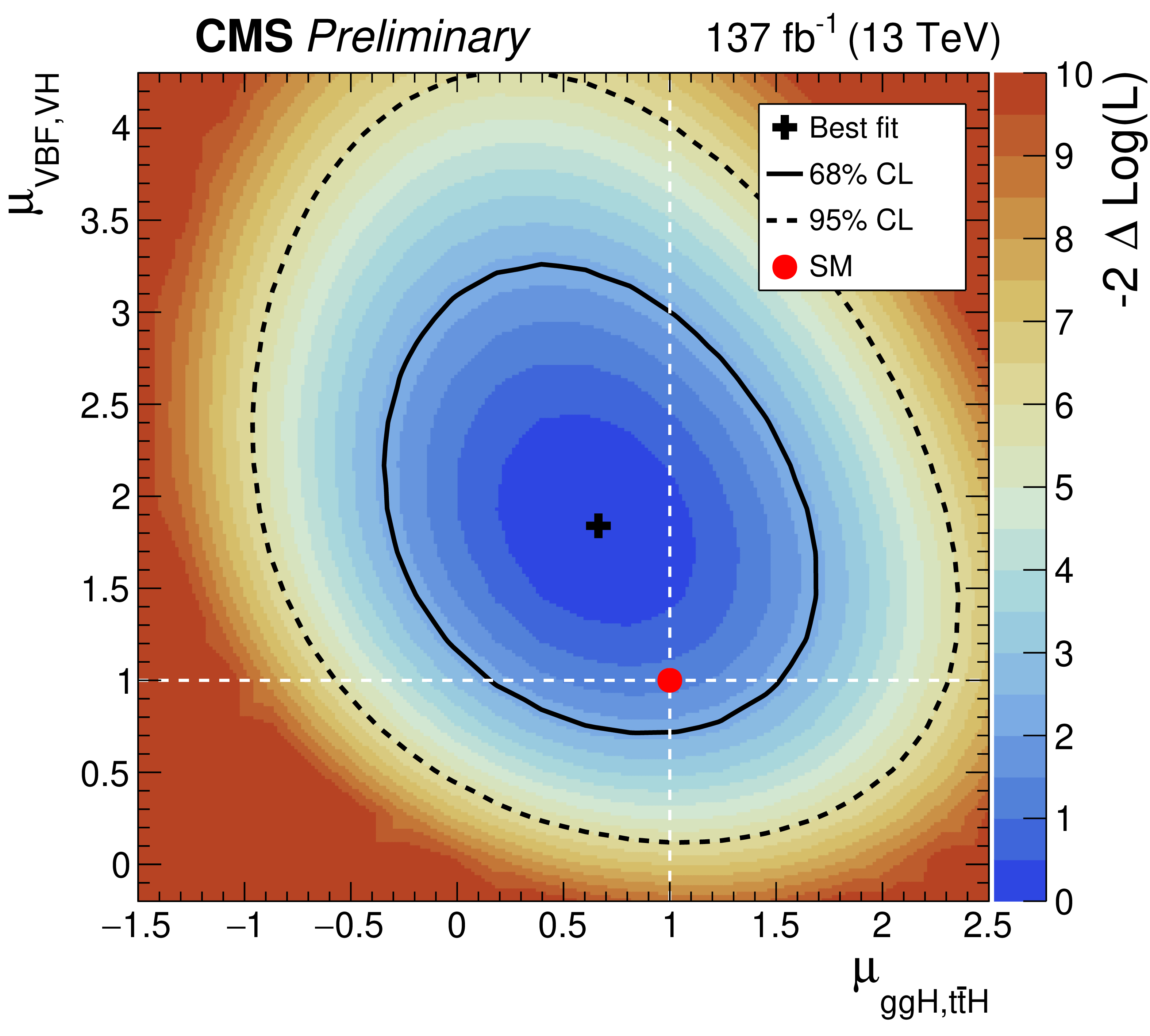
Left: signal strength modifiers measured for ${m_{\mathrm{H}}} =$ 125.38 GeV in each production category (black points) are compared to the result of the combined fit (solid red line) and the SM expectation (dashed grey line). Right: scan of the profiled likelihood ratio as a function of $\mu _{\mathrm{g} \mathrm{g} \mathrm{H},{\mathrm{t} {}\mathrm{\bar{t}}} \mathrm{H}}$ and $\mu _{\mathrm {VBF},\mathrm {V}\mathrm{H}}$ with the corresponding 1$\sigma $ and 2$\sigma $ uncertainty contours. The black cross indicates the best-fit values $(\hat{\mu}_{\mathrm{g} \mathrm{g} \mathrm{H},{\mathrm{t} {}\mathrm{\bar{t}}} \mathrm{H}},\hat{\mu}_{\mathrm {VBF},\mathrm {V}\mathrm{H}})=(0.66,1.84)$, while the red circle represents the SM expectation. |
png pdf |
Figure 12-a:
Signal strength modifiers measured for ${m_{\mathrm{H}}} =$ 125.38 GeV in each production category (black points) are compared to the result of the combined fit (solid red line) and the SM expectation (dashed grey line). |
png pdf |
Figure 12-b:
Scan of the profiled likelihood ratio as a function of $\mu _{\mathrm{g} \mathrm{g} \mathrm{H},{\mathrm{t} {}\mathrm{\bar{t}}} \mathrm{H}}$ and $\mu _{\mathrm {VBF},\mathrm {V}\mathrm{H}}$ with the corresponding 1$\sigma $ and 2$\sigma $ uncertainty contours. The black cross indicates the best-fit values $(\hat{\mu}_{\mathrm{g} \mathrm{g} \mathrm{H},{\mathrm{t} {}\mathrm{\bar{t}}} \mathrm{H}},\hat{\mu}_{\mathrm {VBF},\mathrm {V}\mathrm{H}})=(0.66,1.84)$, while the red circle represents the SM expectation. |
png pdf |
Figure 13:
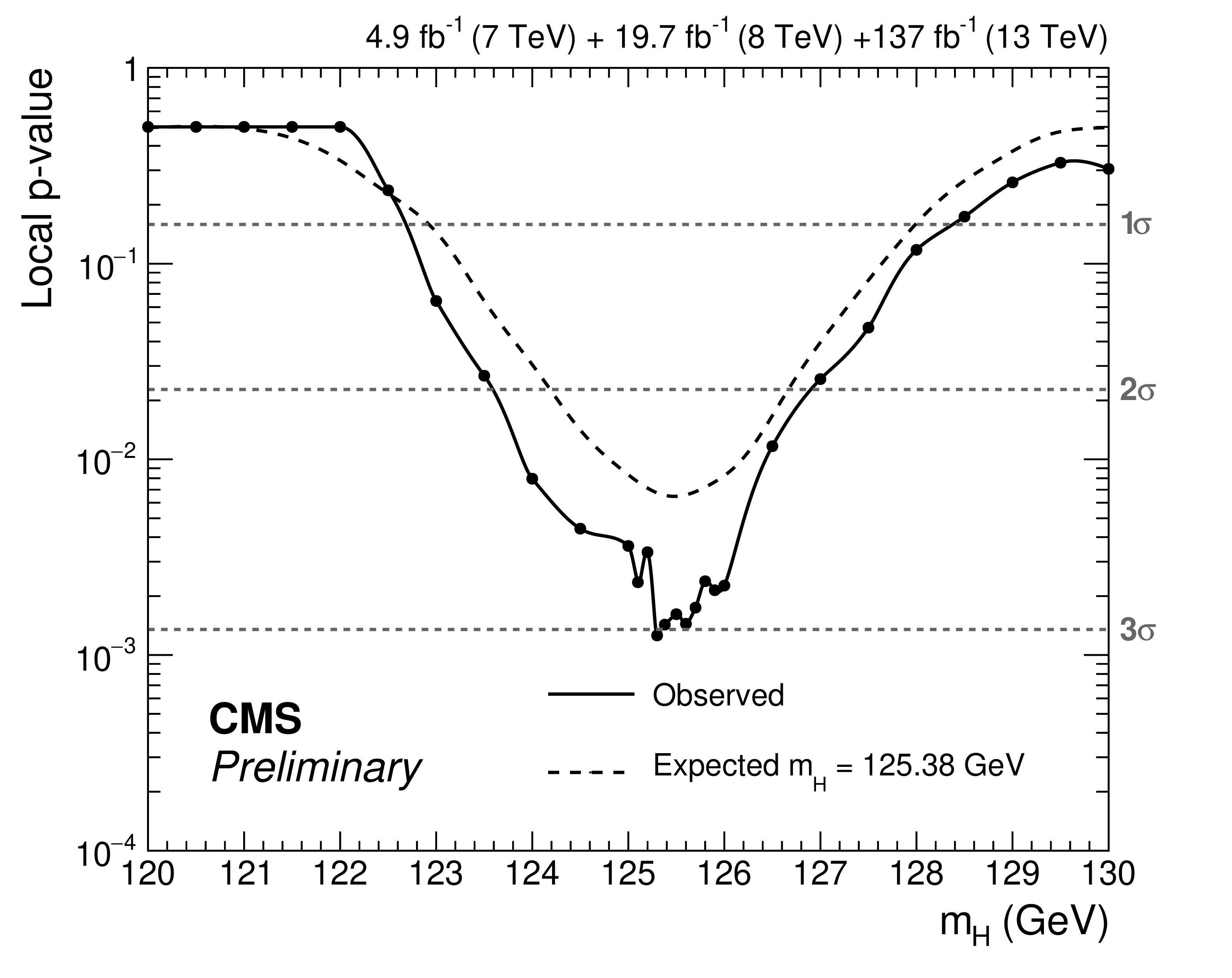
Observed (solid black) and expected (dashed black) local p-values as a function of $ {m_{\mathrm{H}}} $, extracted from the combined fit performed on data recorded at ${\sqrt {s}}=$ 7, 8, 13 TeV, are shown. The expected p-values are calculated using the background expectation obtained from the signal-plus-background fit and injecting a signal with ${m_{\mathrm{H}}} =$ 125.38 GeV and $ \mu =$ 1. |
png pdf |
Figure 14:
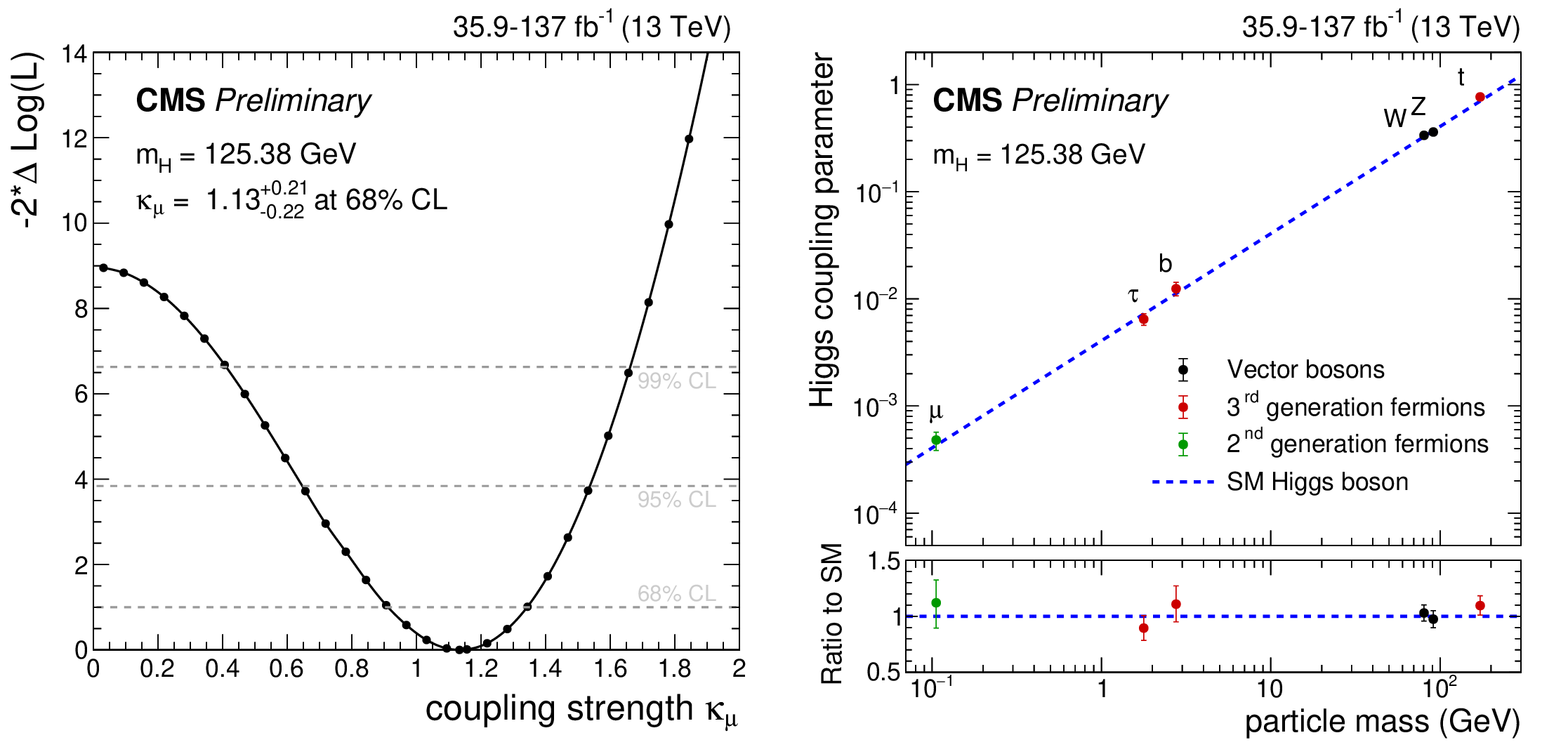
Left: observed profile likelihood ratio as a function of $\kappa _{\mu}$ for ${m_{\mathrm{H}}} = $ 125.38 GeV, obtained from a combined fit with Ref. [10] in the $\kappa $-framework model. The best-fit value for $\kappa _{\mu}$ is 1.13 and the corresponding observed 68% CL interval is 0.91 $ < \kappa _{\mu} < $ 1.34. Right: the best-fit estimates for the reduced coupling modifiers extracted for fermions and weak bosons from the resolved $\kappa $-framework model compared to their corresponding prediction from the SM. The error bars represent 68% CL intervals for the measured parameters. The lower panel shows the ratios of the measured coupling modifiers values to their SM predictions. |

png pdf |
Figure 14-a:
Observed profile likelihood ratio as a function of $\kappa _{\mu}$ for ${m_{\mathrm{H}}} = $ 125.38 GeV, obtained from a combined fit with Ref. [10] in the $\kappa $-framework model. The best-fit value for $\kappa _{\mu}$ is 1.13 and the corresponding observed 68% CL interval is 0.91 $ < \kappa _{\mu} < $ 1.34. |

png pdf |
Figure 14-b:
The best-fit estimates for the reduced coupling modifiers extracted for fermions and weak bosons from the resolved $\kappa $-framework model compared to their corresponding prediction from the SM. The error bars represent 68% CL intervals for the measured parameters. The lower panel shows the ratios of the measured coupling modifiers values to their SM predictions. |
| Tables | |
png pdf |
Table 1:
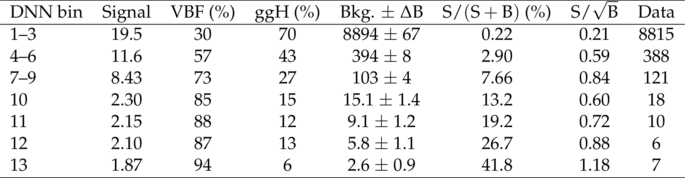
Event yields in each bin or in group of bins defined along the DNN output in the VBF-SR for various processes. The background yields and the corresponding uncertainties are obtained after performing a combined signal-plus-background fit across analysis regions and data-taking periods. The observed event yields and the expected signal contribution at $ {m_{\mathrm{H}}} = $ 125.38 GeV, produced via VBF and $\mathrm{g} \mathrm{g} \mathrm{H} $ modes and assuming SM cross sections and ${{\mathcal {B}(\mathrm{H} \to \mu \mu)}}$, are also reported. |

png pdf |
Table 2:
The product of acceptance and selection efficiency for the different signal production processes, the total expected number of signal events with ${m_{\mathrm{H}}} =$ 125.38 GeV, the hwhm of the signal peak, the estimated number of background events and the observation in data within ${\pm}$hwhm, and the ${\text {S}/(\text {S}+\text {B})}$ and the ${\text {S}/\sqrt {\text {B}}}$ ratios within ${\pm}$hwhm, for each of the optimized $\mathrm{g} \mathrm{g} \mathrm{H} $ event categories. |
png pdf |
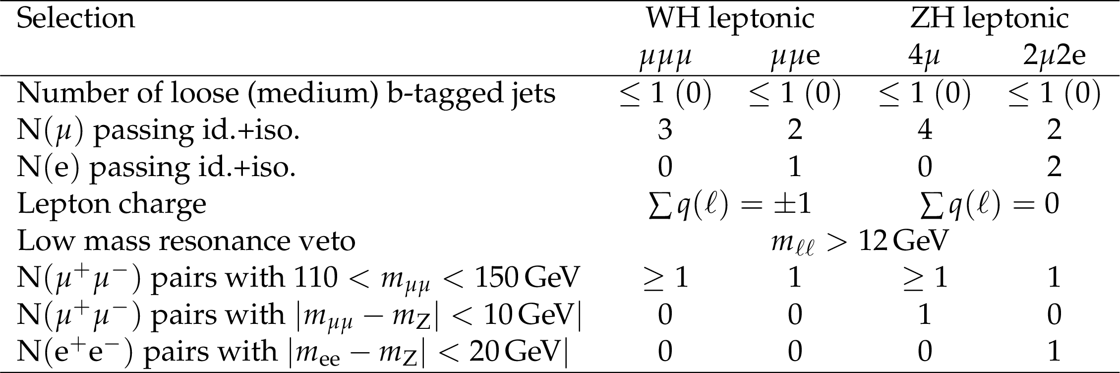
Table 3:
Summary of the kinematic selection used to define the $\mathrm{W} \mathrm{H} $ and $\mathrm{Z} \mathrm{H} $ production categories. |
png pdf |
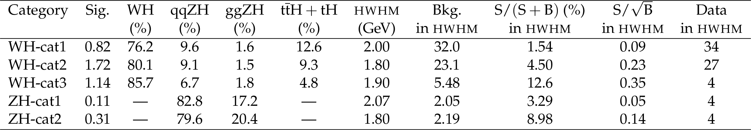
Table 4:
The product of acceptance and selection efficiency for the different signal production processes, the total expected number of signal events with ${m_{\mathrm{H}}} =$ 125.38 GeV, the hwhm of the signal peak, the estimated number of background events and the observed number of events within $\pm$hwhm, and the ${\text {S}/(\text {S}+\text {B})}$ and the ${\text {S}/\sqrt {\text {B}}}$ ratios computed within the hwhm of the signal peak for each of the optimized event categories defined along the $\mathrm{W} \mathrm{H} $ and $\mathrm{Z} \mathrm{H} $ BDT outputs. |
png pdf |
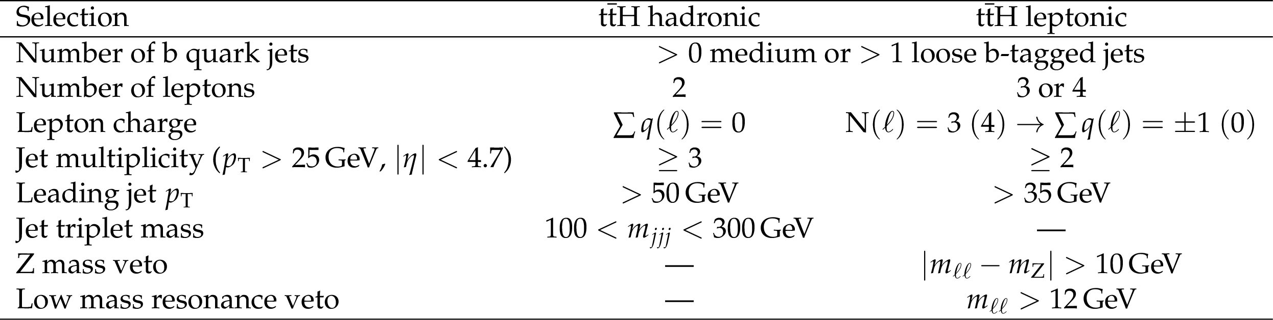
Table 5:
Summary of the kinematic selections used to define the ${\mathrm{t} {}\mathrm{\bar{t}}} \mathrm{H} $ hadronic and leptonic production categories. |

png pdf |
Table 6:
The product of acceptance and selection efficiency for the different signal production processes, the total expected number of signal events with ${m_{\mathrm{H}}} =$ 125.38 GeV, the hwhm of the signal peak, the estimated number of background events and the observed number of events within $\pm$hwhm, and the ${\text {S}/(\text {S}+\text {B})}$ and $\text {S}/\sqrt {\text {B}}$ ratios computed within the hwhm of the signal peak, for each of the optimized event categories defined along the ${\mathrm{t} {}\mathrm{\bar{t}}} \mathrm{H} $ hadronic and leptonic BDT outputs. |

png pdf |
Table 7:
Major sources of uncertainty in the measurement of the signal strength $\mu $ and their impact. The total post-fit uncertainty on $\mu $ is separated into four components: statistical, size of the simulated samples, experimental, and theoretical. |
png pdf |
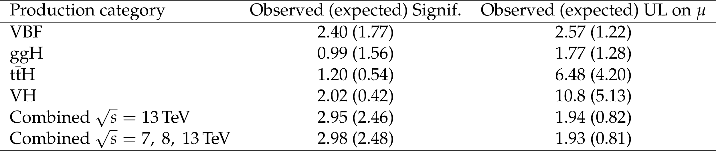
Table 8:
Observed and expected significances for the incompatibility with the background-only hypothesis for ${m_{\mathrm{H}}} = $ 125.38 GeV and the corresponding 95% CL upper limits on $\mu $ (in absence of ${{\mathrm{H} \to \mu \mu}}$ decays) for each production category as well as for the 13 TeV and the 7+8+13 TeV combined fits. |
| Summary |
| A measurement of the Higgs boson decay to a pair of muons is presented. This result combines searches in four exclusive categories targeting the production of the Higgs boson via gluon fusion, via vector boson fusion, in association with a weak vector boson, and in association with a pair of top quarks. The measurement is performed using $\sqrt{s}=$ 13 TeV proton-proton (pp) collision data, corresponding to an integrated luminosity of 137 fb$^{-1}$, recorded by the CMS experiment at the CERN LHC. An excess of events is observed in data with a significance of 3.0 standard deviations, where the expectation for the standard model (SM) Higgs boson with $ m_{\mathrm{H}} = $ 125.38 GeV is 2.5. The measured signal strength, relative to the SM expectation, is 1.19$^{+0.41}_{-0.39}$ (stat) $^{+0.17}_{-0.16}$ (syst). The combination of this result with that from data recorded at centre-of-mass energies of 7 and 8 TeV improves both expected and observed sensitivity by 1%. This result constitutes the first evidence for the Higgs boson decay to fermions of the second generation. |
| Additional Figures | |
png pdf |
Additional Figure 1:
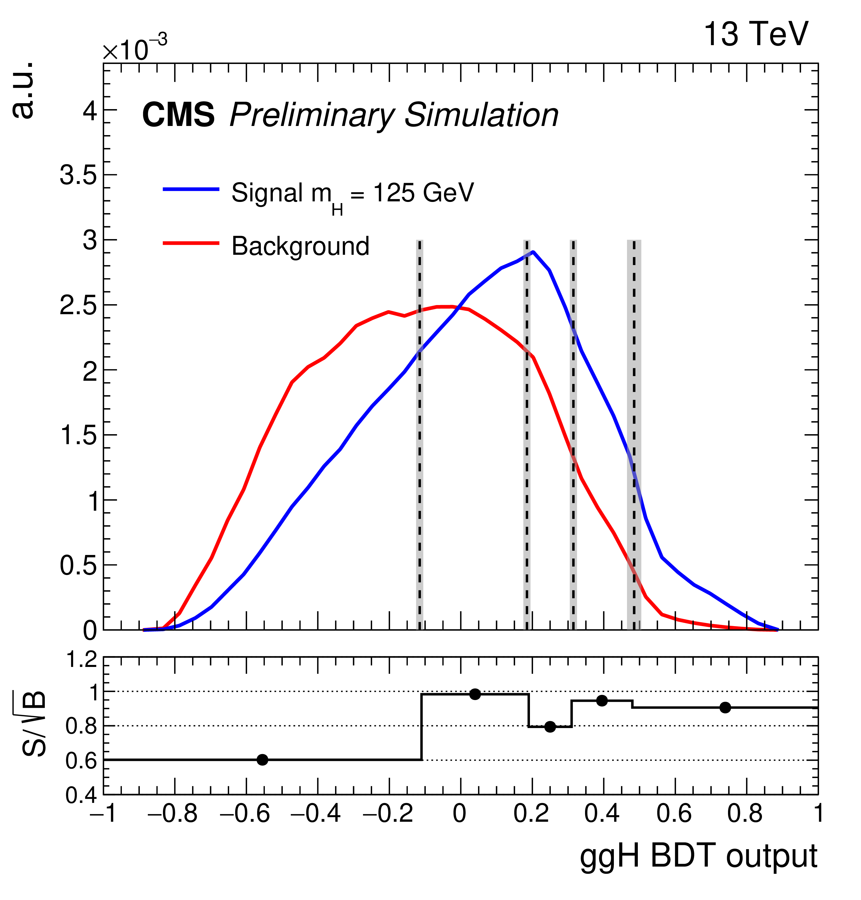
Left: the shapes of the BDT discriminant in signal (blue) and background (red) events are obtained by summing the expectations from the various signal and background processes, respectively. The grey vertical boxes indicate the range of variation of the BDT boundaries for the optimized event categories defined in each data-taking period. In the lower panel, the ${\mathrm {S}/\sqrt {\mathrm {B}}}$ per category, calculated by integrating signal and background expected events inside the hwhm range around the signal peak, is reported. Right: the signal shape model for the simulated $ {{{\mathrm {H}} \to \mu \mu}} $ sample with $ m_{\mathrm {H}} = $ 125 GeV for the weighted sum of all $ {\mathrm {g}} {\mathrm {g}} {\mathrm {H}} $ event categories. Events are weighted per category according to the expected ${\text {S}/(\text {S}+\text {B})}$, computed within the hwhm range of the signal peak. |
png pdf |
Additional Figure 1-a:
The shapes of the BDT discriminant in signal (blue) and background (red) events are obtained by summing the expectations from the various signal and background processes, respectively. The grey vertical boxes indicate the range of variation of the BDT boundaries for the optimized event categories defined in each data-taking period. In the lower panel, the ${\mathrm {S}/\sqrt {\mathrm {B}}}$ per category, calculated by integrating signal and background expected events inside the hwhm range around the signal peak, is reported. |
png pdf |
Additional Figure 1-b:
The signal shape model for the simulated $ {{{\mathrm {H}} \to \mu \mu}} $ sample with $ m_{\mathrm {H}} = $ 125 GeV for the weighted sum of all $ {\mathrm {g}} {\mathrm {g}} {\mathrm {H}} $ event categories. Events are weighted per category according to the expected ${\text {S}/(\text {S}+\text {B})}$, computed within the hwhm range of the signal peak. |
png pdf |
Additional Figure 2:
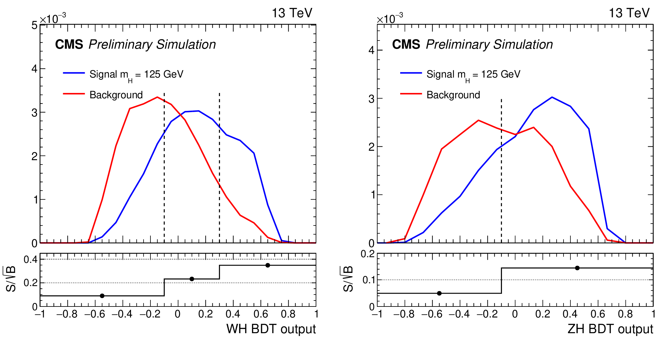
Distribution of the $ {\mathrm {W}} {\mathrm {H}} $ (left) and $ {\mathrm {Z}} {\mathrm {H}} $ (right) BDT outputs in signal (blue) and background (red) simulated events. The dashed vertical lines indicate the boundaries of the optimized event categories. In the lower panel, the ${\mathrm {S}/\sqrt {\mathrm {B}}}$ per category, obtained by integrating signal and background expected events in the $\pm$hwhm range around the signal peak, is reported. |

png pdf |
Additional Figure 2-a:
Distribution of the $ {\mathrm {W}} {\mathrm {H}} $ $ {\mathrm {Z}} {\mathrm {H}} $ BDT output in signal (blue) and background (red) simulated events. The dashed vertical lines indicate the boundaries of the optimized event categories. In the lower panel, the ${\mathrm {S}/\sqrt {\mathrm {B}}}$ per category, obtained by integrating signal and background expected events in the $\pm$hwhm range around the signal peak, is reported. |

png pdf |
Additional Figure 2-b:
Distribution of the $ {\mathrm {W}} {\mathrm {H}} $ $ {\mathrm {Z}} {\mathrm {H}} $ BDT output in signal (blue) and background (red) simulated events. The dashed vertical lines indicate the boundaries of the optimized event categories. In the lower panel, the ${\mathrm {S}/\sqrt {\mathrm {B}}}$ per category, obtained by integrating signal and background expected events in the $\pm$hwhm range around the signal peak, is reported. |
png pdf |
Additional Figure 3:
Distribution of the $ {{\mathrm {t}\overline {\mathrm {t}}}} {\mathrm {H}} $ hadronic (left) and $ {{\mathrm {t}\overline {\mathrm {t}}}} {\mathrm {H}} $ leptonic (right) BDT outputs in signal (blue) and background (red) simulated events. The dashed vertical lines indicate the boundaries of the optimized event categories. In the lower panel, the ${\text {S}/\sqrt {\smash [b]{\text {B}}}}$ obtained by integrating signal and background expected events inside the hwhm range of the signal peak, is reported. |
png pdf |
Additional Figure 3-a:
Distribution of the $ {{\mathrm {t}\overline {\mathrm {t}}}} {\mathrm {H}} $ hadronic BDT output in signal (blue) and background (red) simulated events. The dashed vertical lines indicate the boundaries of the optimized event categories. In the lower panel, the ${\text {S}/\sqrt {\smash [b]{\text {B}}}}$ obtained by integrating signal and background expected events inside the hwhm range of the signal peak, is reported. |
png pdf |
Additional Figure 3-b:
Distribution of the $ {{\mathrm {t}\overline {\mathrm {t}}}} {\mathrm {H}} $ leptonic BDT output in signal (blue) and background (red) simulated events. The dashed vertical lines indicate the boundaries of the optimized event categories. In the lower panel, the ${\text {S}/\sqrt {\smash [b]{\text {B}}}}$ obtained by integrating signal and background expected events inside the hwhm range of the signal peak, is reported. |
png pdf |
Additional Figure 4:
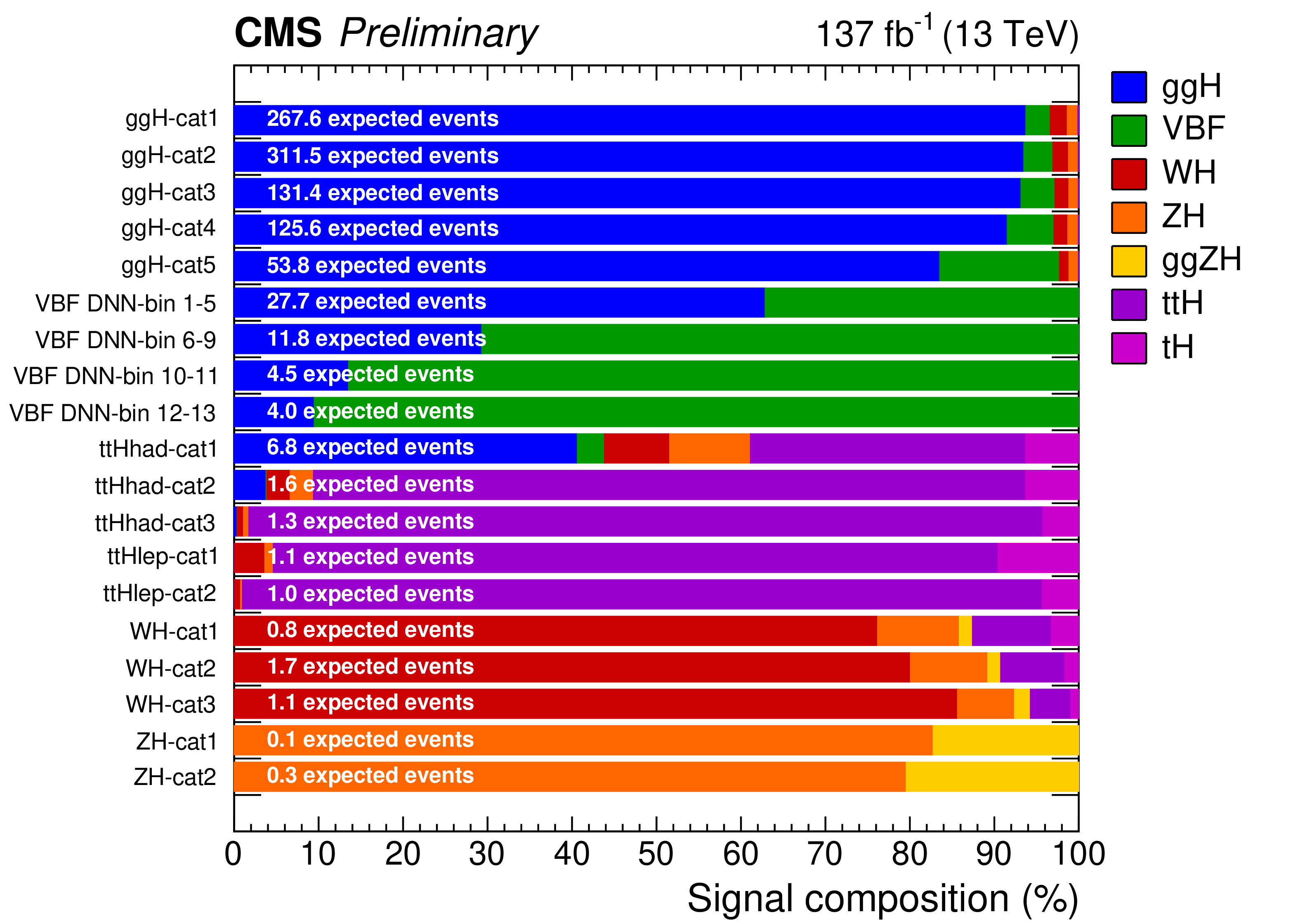
Expected fraction of signal events per production mode in the different event categories for $m_{{\mathrm {H}}} = $ 125.38 GeV. The VBF category is split into four independent entries grouping the content of the bins defined along the DNN output in the VBF-SR. The $\mathrm {t} {\mathrm {H}} $ contribution is defined as the sum of $\mathrm {t} {\mathrm {H}} {\mathrm {q}}$ and $\mathrm {t} {\mathrm {H}} {\mathrm {W}}$ processes. |
png pdf |
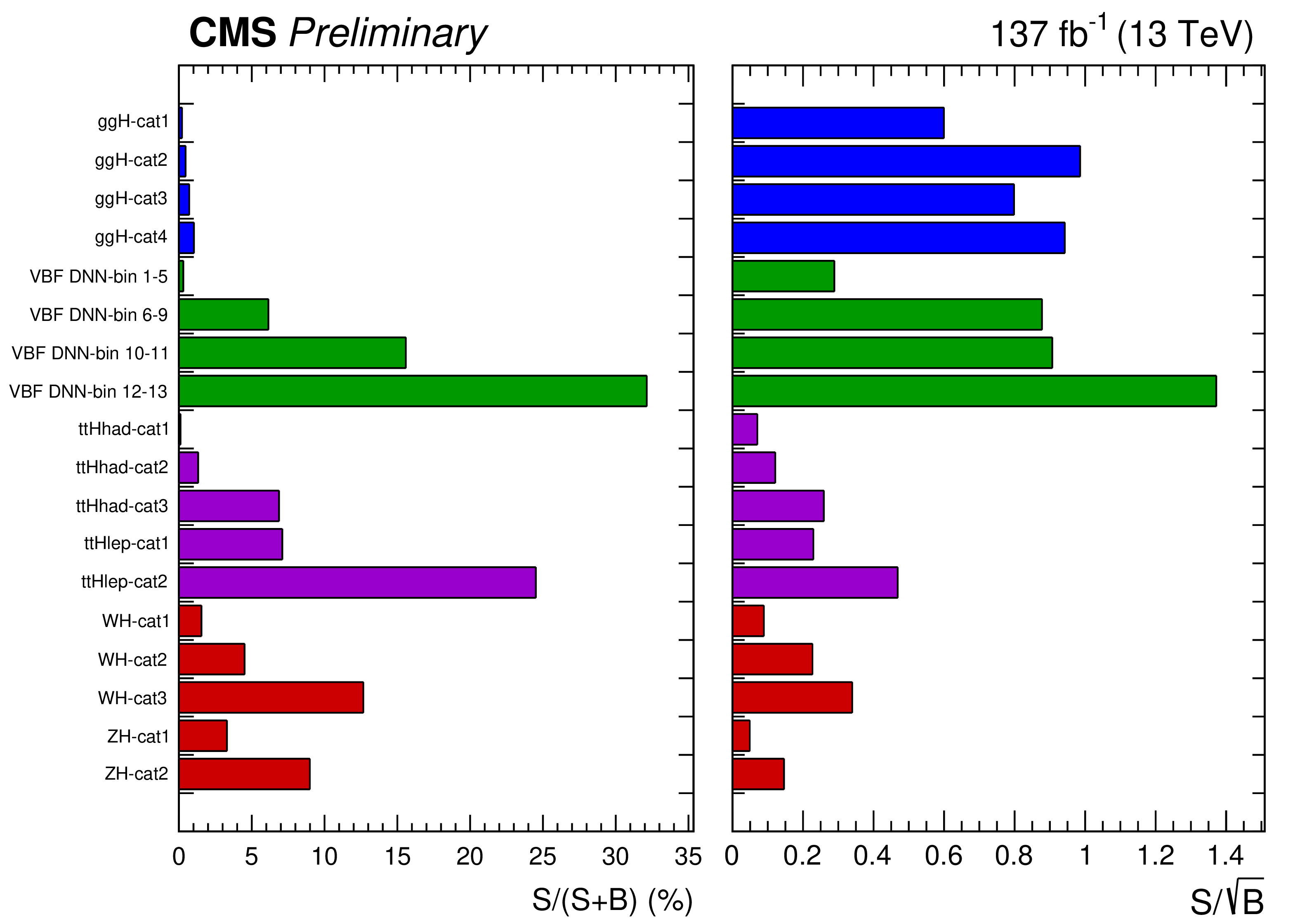
Additional Figure 5:
Expected $\text {S}/(\text {S}+\text {B})$ and $\text {S}/\sqrt {\text {B}}$ ratios in each event category, where S and B indicate the number of expected signal with $m_{{\mathrm {H}}} = $ 125.38 GeV and estimated background events, respectively. In the $ {\mathrm {g}} {\mathrm {g}} {\mathrm {H}} $, $\mathrm {V} {\mathrm {H}} $, and $ {{\mathrm {t}\overline {\mathrm {t}}}} {\mathrm {H}} $ categories, signal and background yields are obtained by integrating the corresponding expectations inside the hwhm range around the signal peak. In contrast, in the VBF category events are split into four subcategories, grouping the expected signal and the predicted background yields in each bin defined along the DNN output in the VBF-SR. |
png pdf |
Additional Figure 6:
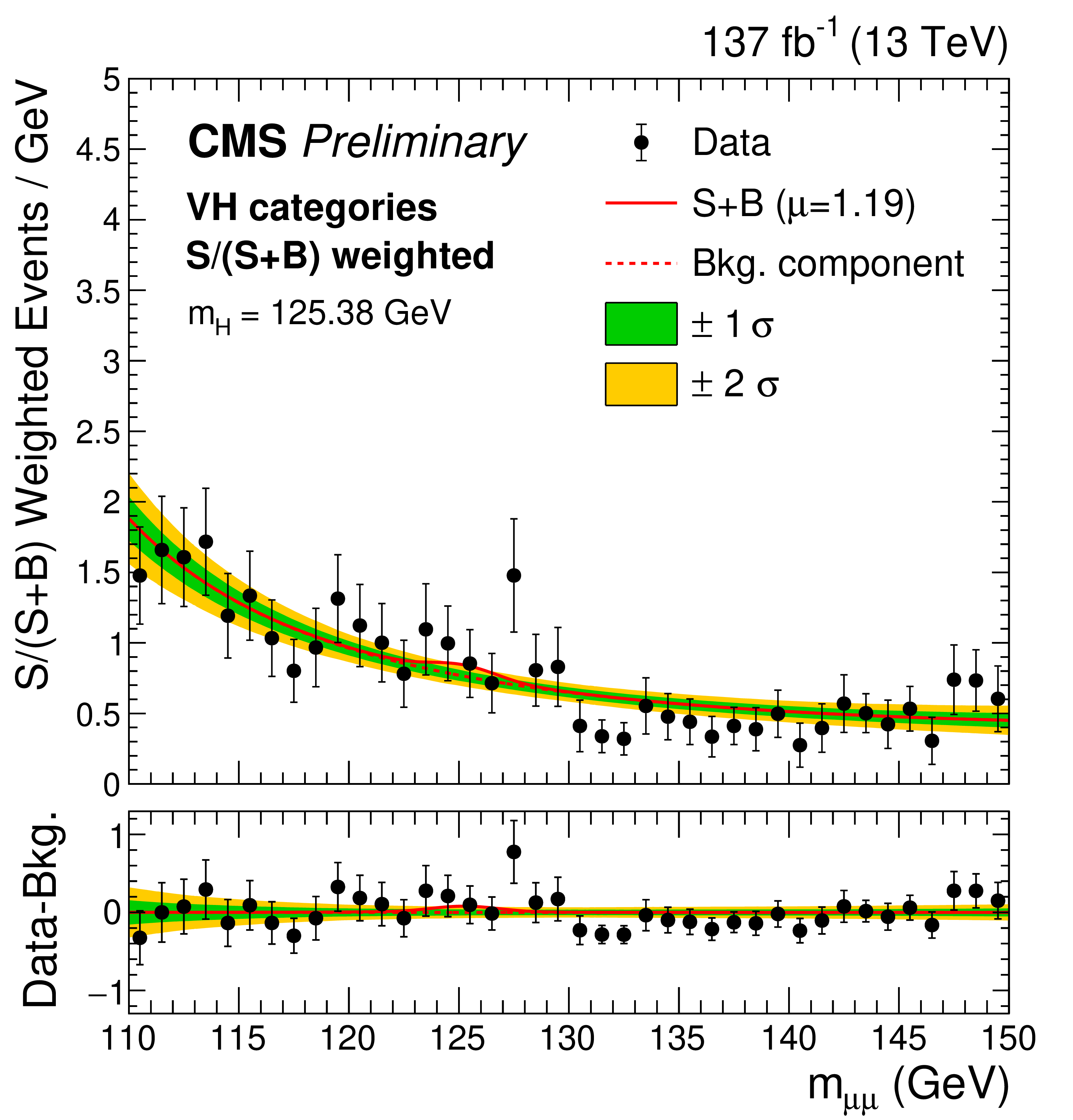
Left: the $m_{\mu \mu}$ distribution for the weighted combination of $ {\mathrm {g}} {\mathrm {g}} {\mathrm {H}} $ event categories. Categories are weighted proportionally to the ${\text {S}/(\text {S}+\text {B}})$ ratio, where S and B are the number of expected signal and background events with mass within $\pm$hwhm of the expected signal peak with $m_{\mathrm {H}} = $ 125.38 GeV. Right: the $m_{\mu \mu}$ distribution for a similar weighted combination of $\mathrm {V} {\mathrm {H}} $ event categories. The lower panels show the residuals after background subtraction, with the best-fit SM ${{{\mathrm {H}} \to \mu \mu}}$ signal contribution with $m_{\mathrm {H}} = $ 125.38 GeV indicated by the red line. |
png pdf |
Additional Figure 6-a:
The $m_{\mu \mu}$ distribution for the weighted combination of $ {\mathrm {g}} {\mathrm {g}} {\mathrm {H}} $ event categories. Categories are weighted proportionally to the ${\text {S}/(\text {S}+\text {B}})$ ratio, where S and B are the number of expected signal and background events with mass within $\pm$hwhm of the expected signal peak with $m_{\mathrm {H}} = $ 125.38 GeV. |
png pdf |
Additional Figure 6-b:
The $m_{\mu \mu}$ distribution for a similar weighted combination of $\mathrm {V} {\mathrm {H}} $ event categories. The lower panels show the residuals after background subtraction, with the best-fit SM ${{{\mathrm {H}} \to \mu \mu}}$ signal contribution with $m_{\mathrm {H}} = $ 125.38 GeV indicated by the red line. |
png pdf |
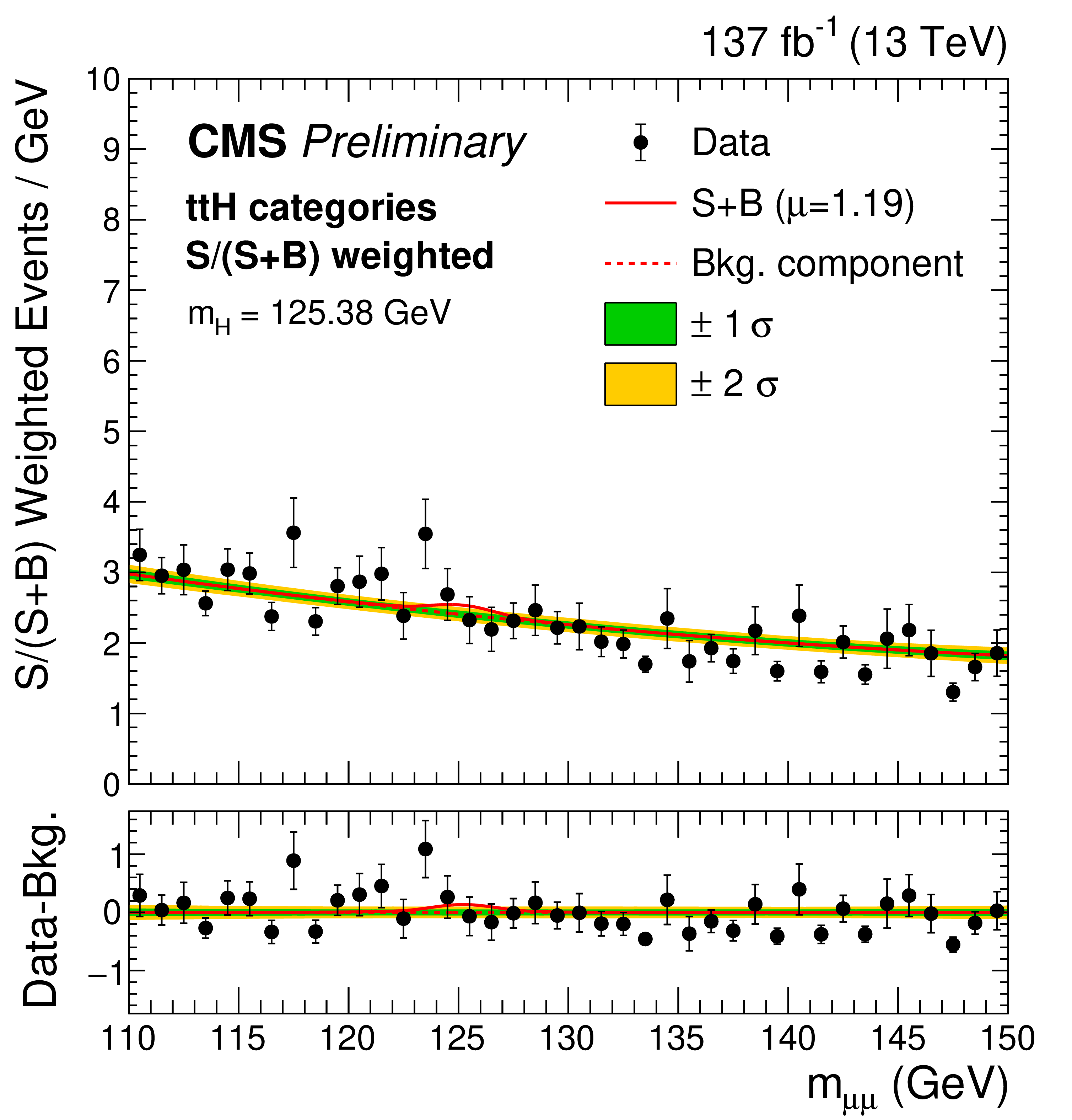
Additional Figure 7:
Left: the $m_{\mu \mu}$ distribution for the weighted combination of $ {{\mathrm {t}\overline {\mathrm {t}}}} {\mathrm {H}} $ event categories. Categories are weighted proportionally to the ${\text {S}/(\text {S}+\text {B}})$ ratio, where S and B are the number of expected signal and background events with mass within $\pm$hwhm of the expected signal peak with $m_{\mathrm {H}} = $ 125.38 GeV. Right: the $m_{\mu \mu}$ distribution for a similar weighted combination of $ {\mathrm {g}} {\mathrm {g}} {\mathrm {H}} $, $\mathrm {V} {\mathrm {H}} $, and $ {{\mathrm {t}\overline {\mathrm {t}}}} {\mathrm {H}} $ event categories. The lower panels show the residuals after background subtraction, with the best-fit SM ${{{\mathrm {H}} \to \mu \mu}}$ signal contribution with $m_{\mathrm {H}} = $ 125.38 GeV indicated by the red line. |
png pdf |
Additional Figure 7-a:
The $m_{\mu \mu}$ distribution for the weighted combination of $ {{\mathrm {t}\overline {\mathrm {t}}}} {\mathrm {H}} $ event categories. Categories are weighted proportionally to the ${\text {S}/(\text {S}+\text {B}})$ ratio, where S and B are the number of expected signal and background events with mass within $\pm$hwhm of the expected signal peak with $m_{\mathrm {H}} = $ 125.38 GeV. |
png pdf |
Additional Figure 7-b:
The $m_{\mu \mu}$ distribution for a similar weighted combination of $ {\mathrm {g}} {\mathrm {g}} {\mathrm {H}} $, $\mathrm {V} {\mathrm {H}} $, and $ {{\mathrm {t}\overline {\mathrm {t}}}} {\mathrm {H}} $ event categories. The lower panels show the residuals after background subtraction, with the best-fit SM ${{{\mathrm {H}} \to \mu \mu}}$ signal contribution with $m_{\mathrm {H}} = $ 125.38 GeV indicated by the red line. |

png pdf |
Additional Figure 8:
Profile likelihood ratios as a function of $\mu $ for $m_{\mathrm {H}} = $ 125.38 GeV, where the solid curves represent the observation in data and the dashed line represents the expected result from the combined signal-plus-background fit. The observed likelihood scans are reported for the full combination (black), as well as for the individual $ {\mathrm {g}} {\mathrm {g}} {\mathrm {H}} $, VBF, $\mathrm {V} {\mathrm {H}} $,and $ {{\mathrm {t}\overline {\mathrm {t}}}} {\mathrm {H}} $ categories. |

png pdf |
Additional Figure 9:
Observed local p-values as a function of $ {m_{{\mathrm {H}}}} $ are shows as extracted from the combined fit performed on data recorded at ${\sqrt {s}=7, 8, \text {and 13} TeV}$ (black solid line), as well as from each individual production category of the 13 TeV analysis (blue, red, orange, and green solid lines) and for the 7+8 TeV result (magenta solid line). |

png pdf |
Additional Figure 10:
The best-fit estimates for the reduced coupling modifiers extracted for fermions and weak bosons from the resolved $\kappa $-framework model compared to their corresponding prediction from the SM. The green points represent the coupling modifiers for the interactions between the Higgs and vector bosons, while the red, magenta, and blue points refer to the couplings with muons, taus, and quarks of the third generation, respectively. The associated error bars represent 68% CL intervals for the measured parameters. The lower panel shows the ratios of the measured coupling modifiers values to their SM predictions. |
png pdf |
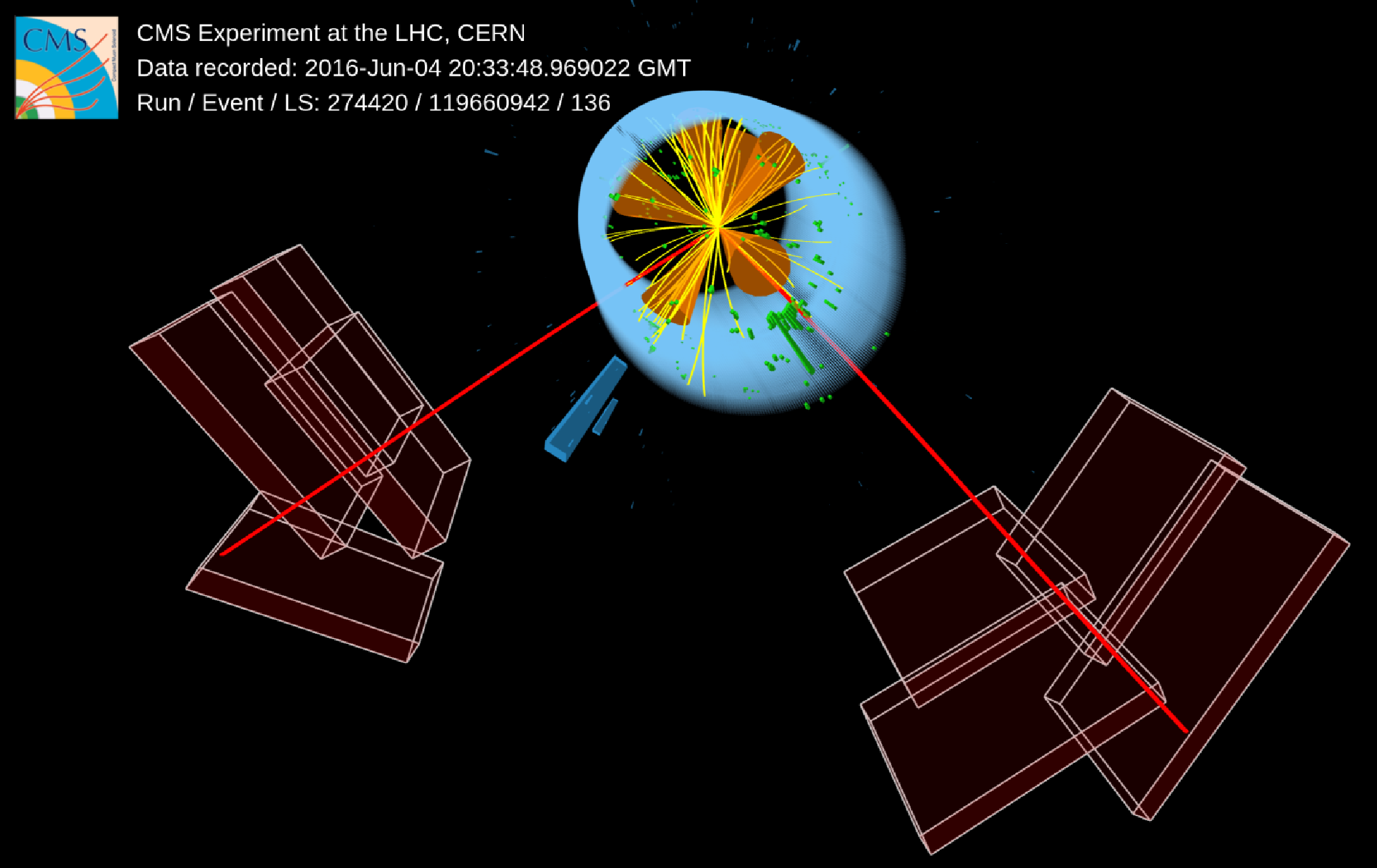
Additional Figure 11:
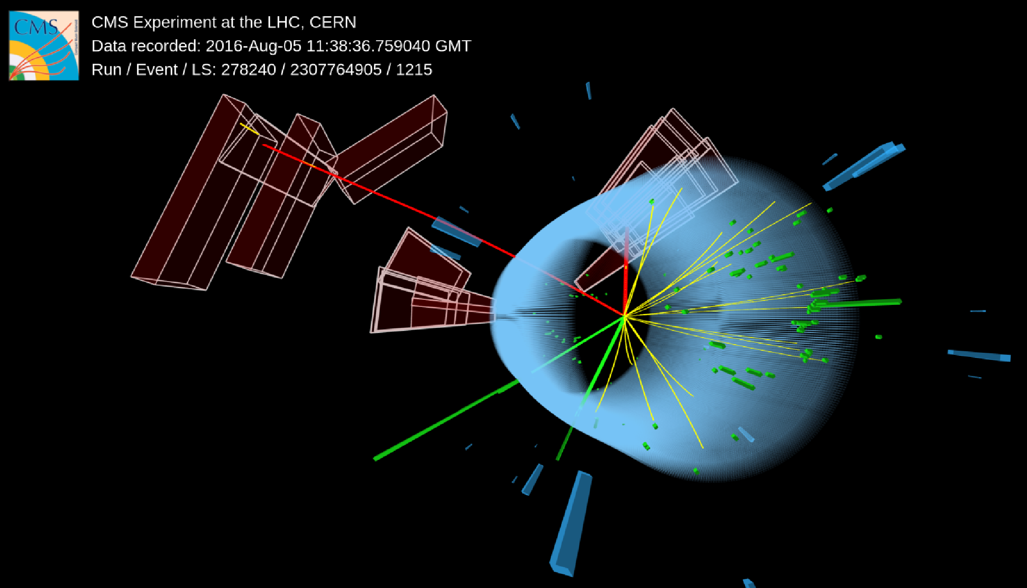
Event in which a candidate Higgs boson produced via vector boson fusion (VBF) decays into a pair of muons, indicated by the solid red lines, with an invariant mass of 125.01 GeV and per-event mass uncertainty of 1.83 GeV. The two forward VBF-jet candidates are depicted by the orange cones whose invariant mass (${m_{\mathrm {jj}}}$) is 2.19 TeV. No additional leptons (electrons or muons) with ${{p_{\mathrm {T}}} } > $ 20 GeV are present in the event. |
png pdf |
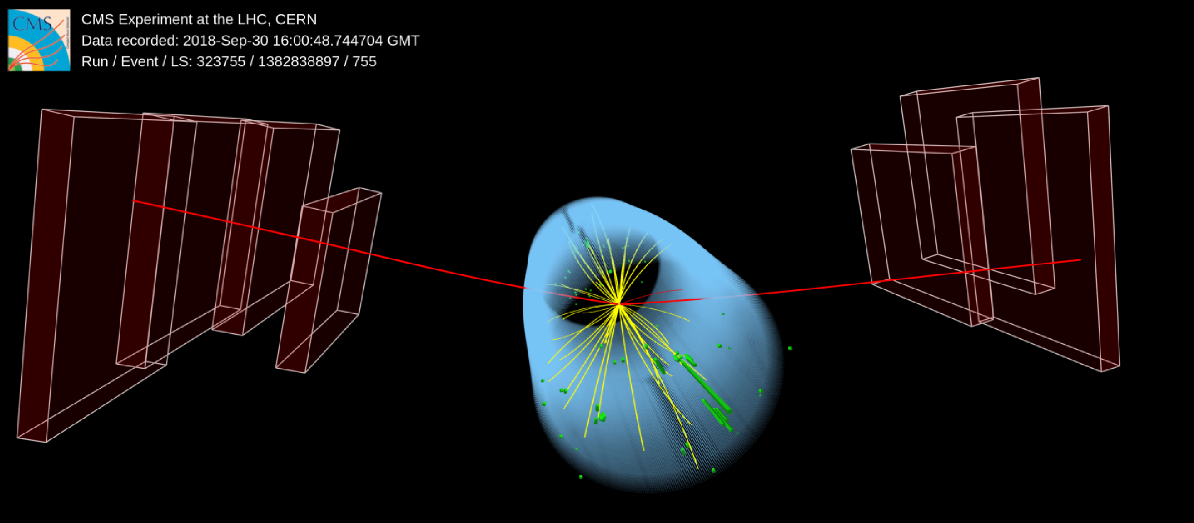
Additional Figure 12:
Event in which a candidate Higgs boson produced via gluon fusion (ggH) decays into a pair of muons, indicated by the solid red lines, with an invariant mass of 125.46 GeV and per-event mass uncertainty of 1.13 GeV. The two muons are emitted back-to-back with respect to the interaction point. No additional jets with ${{p_{\mathrm {T}}} } > $ 25 GeV or leptons (electrons or muons) with ${{p_{\mathrm {T}}} } > $ 20 GeV are present in the event. |
png pdf |
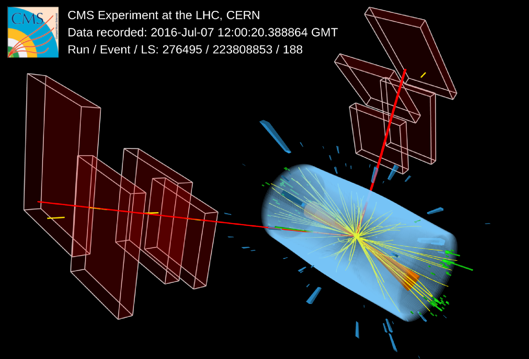
Additional Figure 13:
Event in which a candidate Higgs boson produced in association with a $ {{\mathrm {t}\overline {\mathrm {t}}}} $ pair (ttH) decays into a pair of muons, indicated by the solid red lines, while both top quarks decay hadronically. The $m_{\mu \mu}$ of the Higgs candidate is 125.40 GeV and the corresponding per-event mass uncertainty is 1.24 GeV. Jets produced by the hadronic decays of the two top quarks are depicted by the orange cones. No additional leptons (electrons or muons) with ${{p_{\mathrm {T}}} } > $ 20 GeV are present in the event. |
png pdf |
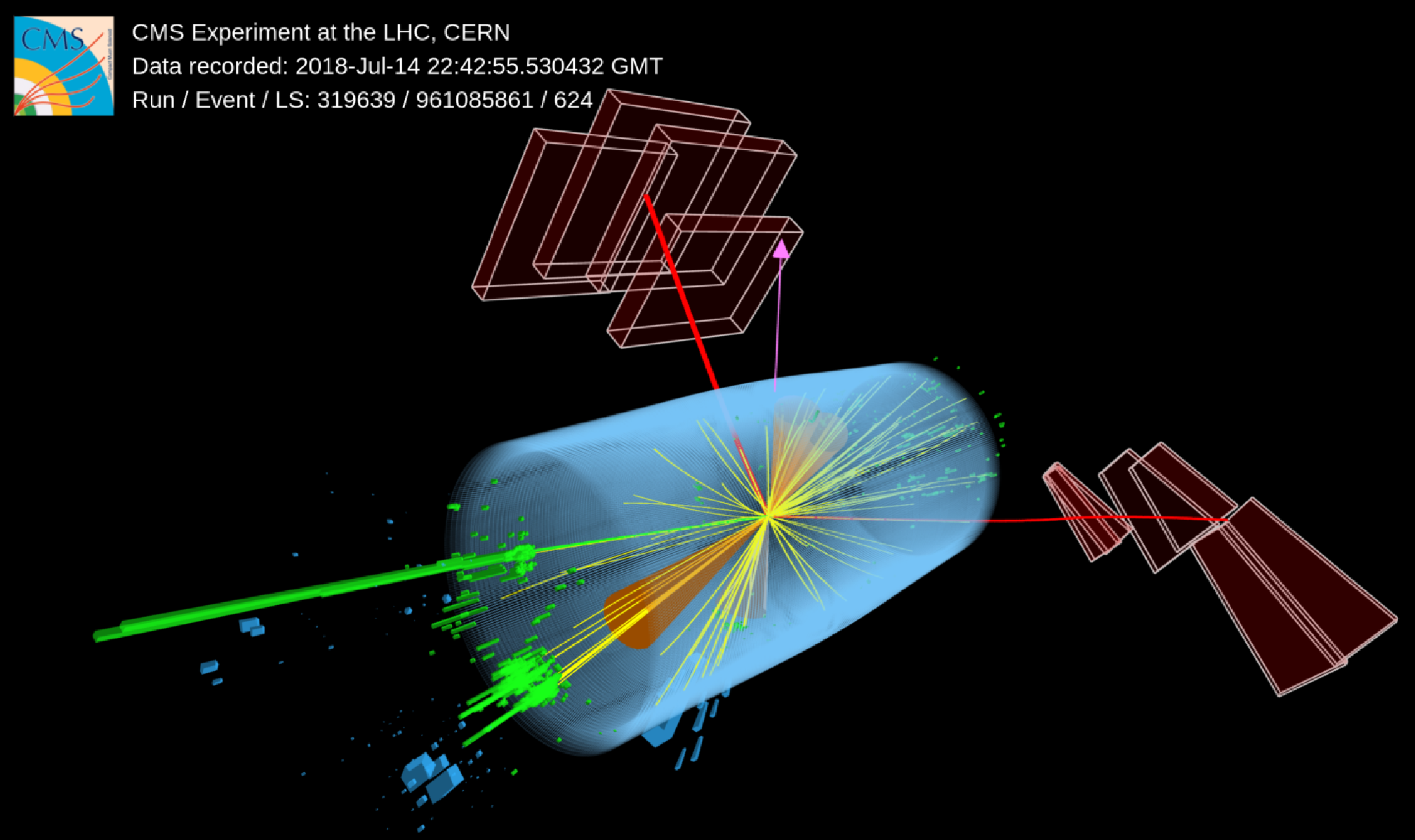
Additional Figure 14:
Event in which a candidate Higgs boson produced in association with a $ {{\mathrm {t}\overline {\mathrm {t}}}} $ pair (ttH) decays into a pair of muons, indicated by the solid red lines, with an invariant mass of 125.30 GeV and per-event mass uncertainty of 1.22 GeV. One of the two top quarks produces in its decay an electron, indicated by the solid green line, and a neutrino that yields missing transverse energy depicted by the pink arrow. The other top quark candidate decays into jets indicated by the the orange cones. No additional leptons (electrons or muons) with ${{p_{\mathrm {T}}} } > $ 20 GeV are present in the event. |
png pdf |
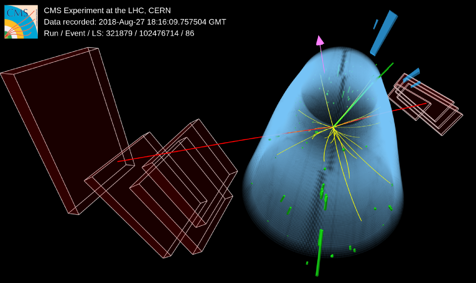
Additional Figure 15:
Event in which a candidate Higgs boson produced in association with a W boson (WH) decays into a pair of muons, indicated by the solid red lines, with an invariant mass of 123.18 GeV and per-event mass uncertainty of 1.03 GeV. The W boson candidate decays leptonically into an electron and a neutrino. The two muons are emitted back-to-back with respect to the interaction point. The electron is indicated by a solid green line, while the missing transverse energy produced by the presence of the neutrino is depicted by the pink arrow. No additional leptons (electrons or muons) with ${{p_{\mathrm {T}}} } > $ 20 GeV or jets with ${{p_{\mathrm {T}}} } > $ 25 GeV are present in the event. |
png pdf |
Additional Figure 16:
Event in which a candidate Higgs boson produced in association with a Z boson (ZH) decays into a pair of muons, indicated by the solid red lines, with an invariant mass of 125.69 GeV and per-event mass uncertainty of 1.55 GeV. The Z boson candidate instead decays leptonically into pair of electrons indicated by the solid green lines. No additional leptons (electrons or muons) with ${{p_{\mathrm {T}}} } > $ 20 GeV or jets with ${{p_{\mathrm {T}}} } > $ 25 GeV are present in the event. |
| References | ||||
| 1 | ATLAS Collaboration | Observation of a new particle in the search for the Standard Model Higgs boson with the ATLAS detector at the LHC | PLB 716 (2012) 1 | 1207.7214 |
| 2 | CMS Collaboration | Observation of a new boson at a mass of 125 GeV with the CMS experiment at the LHC | PLB 716 (2012) 30 | CMS-HIG-12-028 1207.7235 |
| 3 | CMS Collaboration | Observation of a new boson with mass near 125 GeV in pp collisions at $ \sqrt{s} = $ 7 and 8 TeV | JHEP 06 (2013) 081 | CMS-HIG-12-036 1303.4571 |
| 4 | CMS Collaboration | Observation of the Higgs boson decay to a pair of $ \tau $ leptons with the CMS detector | PLB 779 (2018) 283 | CMS-HIG-16-043 1708.00373 |
| 5 | CMS Collaboration | Observation of $ \mathrm{t\bar{t}}\mathrm{H} $ production | PRL 120 (2018) 231801 | CMS-HIG-17-035 1804.02610 |
| 6 | CMS Collaboration | Observation of Higgs boson decay to bottom quarks | PRL 121 (2018) 121801 | CMS-HIG-18-016 1808.08242 |
| 7 | CMS Collaboration | Measurements of Higgs boson properties in the diphoton decay channel in proton-proton collisions at $ \sqrt{s} =$ 13 TeV | JHEP 11 (2018) 185 | CMS-HIG-16-040 1804.02716 |
| 8 | CMS Collaboration | Measurements of properties of the Higgs boson decaying to a W boson pair in pp collisions at $ \sqrt{s}= $ 13 TeV | PLB 791 (2019) 96 | CMS-HIG-16-042 1806.05246 |
| 9 | CMS Collaboration | Measurements of properties of the Higgs boson decaying into the four-lepton final state in pp collisions at $ \sqrt{s}= $ 13 TeV | JHEP 11 (2017) 047 | CMS-HIG-16-041 1706.09936 |
| 10 | CMS Collaboration | Combined measurements of Higgs boson couplings in proton-proton collisions at $ \sqrt{s} =$ 13 TeV | EPJC 79 (2019) 421 | CMS-HIG-17-031 1809.10733 |
| 11 | ATLAS Collaboration | Cross-section measurements of the Higgs boson decaying into a pair of $ \tau $-leptons in proton-proton collisions at $ \sqrt{s}= $ 13 TeV with the ATLAS detector | Phys. Rev D. 99 (2019) 072001 | 1811.08856 |
| 12 | ATLAS Collaboration | Observation of $ \mathrm{H} \rightarrow \mathrm{b\bar{b}} $ decays and $ \mathrm{V}\mathrm{H} $ production with the ATLAS detector | PLB 786 (2018) 59 | 1808.08238 |
| 13 | ATLAS Collaboration | Observation of Higgs boson production in association with a top quark pair at the LHC with the ATLAS detector | PLB 784 (2018) 173 | 1806.00425 |
| 14 | ATLAS Collaboration | Measurements of gluon-gluon fusion and vector-boson fusion Higgs boson production cross-sections in the $ {\mathrm{H} \to \mathrm{W}\mathrm{W}^{*} \to \mathrm{e}\nu\mu\nu} $ decay channel in pp collisions at $ \sqrt{s}= $ 13 TeV with the ATLAS detector | PLB 789 (2019) 508 | 1808.09054 |
| 15 | ATLAS Collaboration | Measurement of the Higgs boson coupling properties in the $ \mathrm{H}\rightarrow \mathrm{Z}\mathrm{Z}^{*} \rightarrow 4\ell $ decay channel at $ \sqrt{s}= $ 13 TeV with the ATLAS detector | JHEP 03 (2018) 095 | 1712.02304 |
| 16 | ATLAS Collaboration | Measurements of Higgs boson properties in the diphoton decay channel with 36$ fb$^{-1} of pp collision data at $ \sqrt{s} =$ 13 TeV with the ATLAS detector | PRD 98 (2018) 052005 | 1802.04146 |
| 17 | ATLAS Collaboration | Combined measurements of Higgs boson production and decay using up to 80$ fb$^{-1} of proton-proton collision data at $ \sqrt{s}= $ 13 TeV collected with the ATLAS experiment | PRD 101 (2020) 012002 | 1909.02845 |
| 18 | F. Englert and R. Brout | Broken symmetry and the mass of gauge vector mesons | PRL 13 (1964) 321 | |
| 19 | P. W. Higgs | Broken symmetries and the masses of gauge bosons | PRL 13 (1964) 508 | |
| 20 | P. W. Higgs | Spontaneous symmetry breakdown without massless bosons | PR145 (1966) 1156 | |
| 21 | LHC Higgs Cross Section Working Group | Handbook of LHC Higgs Cross Sections: 4. Deciphering the Nature of the Higgs Sector | CERN (2016) | 1610.07922 |
| 22 | CMS Collaboration | Search for the Higgs boson decaying to two muons in proton-proton collisions at $ \sqrt{s} =$ 13 TeV | PRL 122 (2019) 021801 | CMS-HIG-17-019 1807.06325 |
| 23 | ATLAS Collaboration | A search for the dimuon decay of the Standard Model Higgs boson with the ATLAS detector | Submitted to PLB (7, 2020) | 2007.07830 |
| 24 | CMS Collaboration | A measurement of the Higgs boson mass in the diphoton decay channel | PLB 805 (2020) 135425 | CMS-HIG-19-004 2002.06398 |
| 25 | CMS Collaboration | The CMS trigger system | JINST 12 (2017) P01020 | CMS-TRG-12-001 1609.02366 |
| 26 | CMS Collaboration | The CMS experiment at the CERN LHC | JINST 3 (2008) S08004 | CMS-00-001 |
| 27 | CMS Collaboration | Particle-flow reconstruction and global event description with the CMS detector | JINST 12 (2017) P10003 | CMS-PRF-14-001 1706.04965 |
| 28 | M. Cacciari, G. P. Salam, and G. Soyez | The anti-$ {k_{\mathrm{T}}} $ jet clustering algorithm | JHEP 04 (2008) 063 | 0802.1189 |
| 29 | M. Cacciari, G. P. Salam, and G. Soyez | FastJet user manual | EPJC 72 (2012) 1896 | 1111.6097 |
| 30 | CMS Collaboration | Jet energy scale and resolution in the CMS experiment in pp collisions at 8 TeV | JINST 12 (2017) P02014 | CMS-JME-13-004 1607.03663 |
| 31 | CMS Collaboration | Performance of missing transverse momentum reconstruction in proton-proton collisions at $ \sqrt{s} =$ 13 TeV using the CMS detector | JINST 14 (2019) P07004 | CMS-JME-17-001 1903.06078 |
| 32 | CMS Collaboration | Identification of heavy-flavour jets with the CMS detector in pp collisions at 13 TeV | JINST 13 (2018) P05011 | CMS-BTV-16-002 1712.07158 |
| 33 | CMS Collaboration | Performance of the CMS muon detector and muon reconstruction with proton-proton collisions at $ \sqrt{s}= $ 13 TeV | JINST 13 (2018) P06015 | CMS-MUO-16-001 1804.04528 |
| 34 | CMS Collaboration | Performance of electron reconstruction and selection with the CMS detector in proton-proton collisions at $ \sqrt{s} =$ 8 TeV | JINST 10 (2015) P06005 | CMS-EGM-13-001 1502.02701 |
| 35 | GEANT4 Collaboration | GEANT4--a simulation toolkit | NIMA 506 (2003) 250 | |
| 36 | J. Alwall et al. | The automated computation of tree-level and next-to-leading order differential cross sections, and their matching to parton shower simulations | JHEP 07 (2014) 079 | 1405.0301 |
| 37 | P. Nason | A new method for combining NLO QCD with shower Monte Carlo algorithms | JHEP 11 (2004) 040 | hep-ph/0409146 |
| 38 | S. Frixione, P. Nason, and C. Oleari | Matching NLO QCD computations with Parton Shower simulations: the POWHEG method | JHEP 11 (2007) 070 | 0709.2092 |
| 39 | S. Alioli, P. Nason, C. Oleari, and E. Re | A general framework for implementing NLO calculations in shower monte carlo programs: the POWHEG BOX | JHEP 06 (2010) 043 | 1002.2581 |
| 40 | E. Bagnaschi, G. Degrassi, P. Slavich, and A. Vicini | Higgs production via gluon fusion in the POWHEG approach in the SM and in the MSSM | JHEP 02 (2012) 088 | 1111.2854 |
| 41 | P. Nason and C. Oleari | NLO Higgs boson production via vector-boson fusion matched with shower in POWHEG | JHEP 02 (2010) 037 | 0911.5299 |
| 42 | G. Luisoni, P. Nason, C. Oleari, and F. Tramontano | $ \mathrm{H}\mathrm{W}^{\pm}/\mathrm{H}\mathrm{Z}$ + 0 and 1 jet at NLO with the POWHEG BOX interfaced to GoSam and their merging within MiNLO | JHEP 10 (2013) 083 | 1306.2542 |
| 43 | C. Anastasiou et al. | High precision determination of the gluon fusion Higgs boson cross-section at the LHC | JHEP 05 (2016) 058 | 1602.00695 |
| 44 | M. Cacciari et al. | Fully Differential Vector-Boson-Fusion Higgs Production at Next-to-Next-to-Leading Order | PRL 115 (2015) 082002 | 1506.02660 |
| 45 | O. Brein, A. Djouadi, and R. Harlander | NNLO QCD corrections to the Higgs-strahlung processes at hadron colliders | PLB 579 (2004) 149 | hep-ph/0307206 |
| 46 | S. Dawson et al. | Associated Higgs production with top quarks at the large hadron collider: NLO QCD corrections | PRD 68 (2003) 034022 | hep-ph/0305087 |
| 47 | S. Frixione et al. | Weak corrections to Higgs hadroproduction in association with a top-quark pair | JHEP 09 (2014) 065 | 1407.0823 |
| 48 | A. Djouadi, J. Kalinowski, and M. Spira | HDECAY: A Program for Higgs boson decays in the standard model and its supersymmetric extension | CPC 108 (1998) 56 | hep-ph/9704448 |
| 49 | M. Spira | QCD effects in Higgs physics | Fortsch. Phys. 46 (1998) 203 | hep-ph/9705337 |
| 50 | K. Hamilton, P. Nason, E. Re, and G. Zanderighi | NNLOPS simulation of Higgs boson production | JHEP 10 (2013) 222 | 1309.0017 |
| 51 | K. Hamilton, P. Nason, and G. Zanderighi | Finite quark-mass effects in the NNLOPS POWHEG+MiNLO Higgs generator | JHEP 05 (2015) 140 | 1501.04637 |
| 52 | Y. Li and F. Petriello | Combining QCD and electroweak corrections to dilepton production in FEWZ | Phys. Rev D. 86 (2012) 094034 | 1208.5967 |
| 53 | M. Grazzini, S. Kallweit, D. Rathlev, and M. Wiesemann | $ \mathrm{W}^\pm \mathrm{Z} $ production at the LHC: fiducial cross sections and distributions in NNLO QCD | JHEP 05 (2017) 139 | 1703.09065 |
| 54 | M. Grazzini, S. Kallweit, and D. Rathlev | $ \mathrm{Z}\mathrm{Z} $ production at the LHC: fiducial cross sections and distributions in NNLO QCD | PLB 750 (2015) 407 | 1507.06257 |
| 55 | T. Gehrmann et al. | $ \mathrm{W}^+\mathrm{W}^- $ production at hadron colliders in Next to Next to Leading Order QCD | PRL 113 (2014) 212001 | 1408.5243 |
| 56 | J. M. Campbell, R. K. Ellis, and C. Williams | Vector boson pair production at the LHC | JHEP 07 (2011) 018 | 1105.0020 |
| 57 | M. Czakon and A. Mitov | Top++: A program for the calculation of the top-pair cross-section at hadron colliders | CPC 185 (2014) 2930 | 1112.5675 |
| 58 | P. Kant et al. | HATHOR for single top-quark production: Updated predictions and uncertainty estimates for single top-quark production in hadronic collisions | CPC 191 (2015) 74 | 1406.4403 |
| 59 | NNPDF Collaboration | Parton distributions for the LHC Run II | JHEP 04 (2015) 040 | 1410.8849 |
| 60 | NNPDF Collaboration | Parton distributions from high-precision collider data | EPJC 77 (2017) 663 | 1706.00428 |
| 61 | T. Sjostrand, S. Mrenna, and P. Z. Skands | A Brief Introduction to PYTHIA 8.1 | CPC 178 (2008) 852 | 0710.3820 |
| 62 | CMS Collaboration | Event generator tunes obtained from underlying event and multiparton scattering measurements | EPJC 76 (2016) 155 | CMS-GEN-14-001 1512.00815 |
| 63 | CMS Collaboration | Extraction and validation of a new set of CMS PYTHIA~8 tunes from underlying-event measurements | EPJC 80 (2020) 4 | CMS-GEN-17-001 1903.12179 |
| 64 | J. Alwall et al. | Comparative study of various algorithms for the merging of parton showers and matrix elements in hadronic collisions | EPJC 53 (2008) 473 | 0706.2569 |
| 65 | R. Frederix and S. Frixione | Merging meets matching in MC@NLO | JHEP 12 (2012) 061 | 1209.6215 |
| 66 | J. Bellm et al. | Herwig 7.0/Herwig++ 3.0 release note | EPJC 76 (2016) 196 | 1512.01178 |
| 67 | CMS Collaboration | Electroweak production of two jets in association with a $ \mathrm{Z} $ boson in proton-proton collisions at $ \sqrt{s} =$ 13 TeV | EPJC 78 (2018) 589 | CMS-SMP-16-018 1712.09814 |
| 68 | CMS Collaboration | Extraction and validation of a set of HERWIG 7 tunes from CMS underlying-event measurements | CMS-PAS-GEN-19-001 | CMS-PAS-GEN-19-001 |
| 69 | B. Cabouat and T. Sjostrand | Some Dipole Shower Studies | EPJC 78 (2018) 226 | 1710.00391 |
| 70 | B. Jager et al. | Parton-shower effects in Higgs production via Vector-Boson Fusion | 2003.12435 | |
| 71 | A. Bodek et al. | Extracting muon momentum scale corrections for hadron collider experiments | EPJC 72 (2012) 2194 | 1208.3710 |
| 72 | F. Chollet et al. | Keras | 2015 Software available from keras.io. \url https://keras.io | |
| 73 | M. Abadi et al. | TensorFlow: Large-scale machine learning on heterogeneous systems | 2015 Software available from tensorflow.org. \url https://www.tensorflow.org/ | |
| 74 | J. C. Collins and D. E. Soper | Angular distribution of dileptons in high-energy hadron collisions | PRD 16 (1977) 2219 | |
| 75 | F. Schissler and D. Zeppenfeld | Parton shower effects on $ \mathrm{W} $ and $ \mathrm{Z} $ production via vector boson fusion at NLO QCD | JHEP 04 (2013) 057 | 1302.2884 |
| 76 | CMS Collaboration | Performance of quark/gluon discrimination in 8 TeV pp data | CMS-PAS-JME-13-002 | CMS-PAS-JME-13-002 |
| 77 | CMS Collaboration | Jet algorithms performance in 13 TeV data | CMS-PAS-JME-16-003 | CMS-PAS-JME-16-003 |
| 78 | N. Srivastava et al. | Dropout: A simple way to prevent neural networks from overfitting | ||
| 79 | G. Cowan | Discovery sensitivity for a counting experiment with background uncertainty | 2012 \url https://www.pp.rhul.ac.uk/ cowan/stat/notes/medsigNote.pdf | |
| 80 | CMS Collaboration | Search for a standard model-like Higgs boson in the $ \mu^{+}\mu^{-} $ and $ \mathrm{e}^{+}\mathrm{e}^{-} $ decay channels at the LHC | PLB 744 (2015) 184 | CMS-HIG-13-007 1410.6679 |
| 81 | R. Barlow and C. Beeston | Fitting using finite monte carlo samples | Computer Physics Communications 77 (1993) 219 | |
| 82 | A. Hoecker et al. | TMVA - Toolkit for multivariate data analysis | physics/0703039 | |
| 83 | CMS Collaboration | Measurements of differential $ \mathrm{Z} $ boson production cross sections in proton-proton collisions at $ \sqrt{s}= $ 13 TeV | JHEP 12 (2019) 061 | CMS-SMP-17-010 1909.04133 |
| 84 | Particle Data Group Collaboration | Review of Particle Physics | PRD 98 (2018) 030001 | |
| 85 | D. Bourilkov | Photon-induced Background for dilepton searches and measurements in pp collisions at 13 TeV | 1606.00523 | |
| 86 | D. Bourilkov | Exploring the LHC landscape with dileptons | 1609.08994 | |
| 87 | P. D. Dauncey, M. Kenzie, N. Wardle, and G. J. Davies | Handling uncertainties in background shapes | JINST 10 (2015) P04015 | 1408.6865 |
| 88 | R. A. Fisher | On the interpretation of $ \chi^{2} $ from contingency tables, and the calculation of p | volume 85, p. 87 [Wiley, Royal Statistical Society] | |
| 89 | CMS Collaboration | Observation of single top quark production in association with a $ \mathrm{Z} $ boson in proton-proton collisions at $ \sqrt{s}= $ 13 TeV | PRL 122 (2019) 132003 | CMS-TOP-18-008 1812.05900 |
| 90 | CMS Collaboration | Evidence for associated production of a Higgs boson with a top quark pair in final states with electrons, muons, and hadronically decaying $ \tau $ leptons at $ \sqrt{s} =$ 13 TeV | JHEP 08 (2018) 066 | CMS-HIG-17-018 1803.05485 |
| 91 | G. Cowan, K. Cranmer, E. Gross, and O. Vitells | Asymptotic formulae for likelihood-based tests of new physics | EPJC 71 (2011) 1554 | 1007.1727 |
| 92 | The ATLAS and CMS Collaborations, and the LHC Higgs Combination Group | Procedure for the LHC Higgs boson search combination in Summer 2011 | CMS-NOTE-2011-005 | |
| 93 | T. Junk | Confidence level computation for combining searches with small statistics | NIMA 434 (1999) 435 | hep-ex/9902006 |
| 94 | A. L. Read | Presentation of search results: the CLs technique | JPG 28 (2002) 2693 | |
| 95 | CMS Collaboration | Combined Higgs boson production and decay measurements with up to 137 fb$^{-1}$ of proton-proton collision data at $ \sqrt{s} = $ 13 TeV | CMS-PAS-HIG-19-005 | CMS-PAS-HIG-19-005 |
|
|
Compact Muon Solenoid LHC, CERN |
|

|

|

|

|

|