

Compact Muon Solenoid
LHC, CERN
| CMS-PAS-HIG-19-002 | ||
| Measurements of differential Higgs boson production cross sections in the leptonic WW decay mode at $\sqrt{s} = $ 13 TeV | ||
| CMS Collaboration | ||
| September 2019 | ||
| Abstract: Measurements of differential production cross sections of the Higgs boson in pp collisions at $\sqrt{s} = $ 13 TeV are performed using events where the Higgs boson decays into a pair of W bosons which subsequently decay into an electron, a muon, and a pair of neutrinos. The analysis is based on data collected by the CMS detector at the LHC in 2016, 2017, and 2018, and corresponds to an integrated luminosity of 137 fb$^{-1}$. Production cross sections with respect to the transverse momentum of the Higgs boson and the number of hadronic jets are considered. Higgs boson signal spectra are extracted and simultaneously unfolded to correct for selection efficiency and resolution effects by means of maximum likelihood fits to the observed event distributions. | ||
|
Links:
CDS record (PDF) ;
CADI line (restricted) ;
These preliminary results are superseded in this paper, JHEP 03 (2021) 003. The superseded preliminary plots can be found here. |
||
| Figures | |
png pdf |
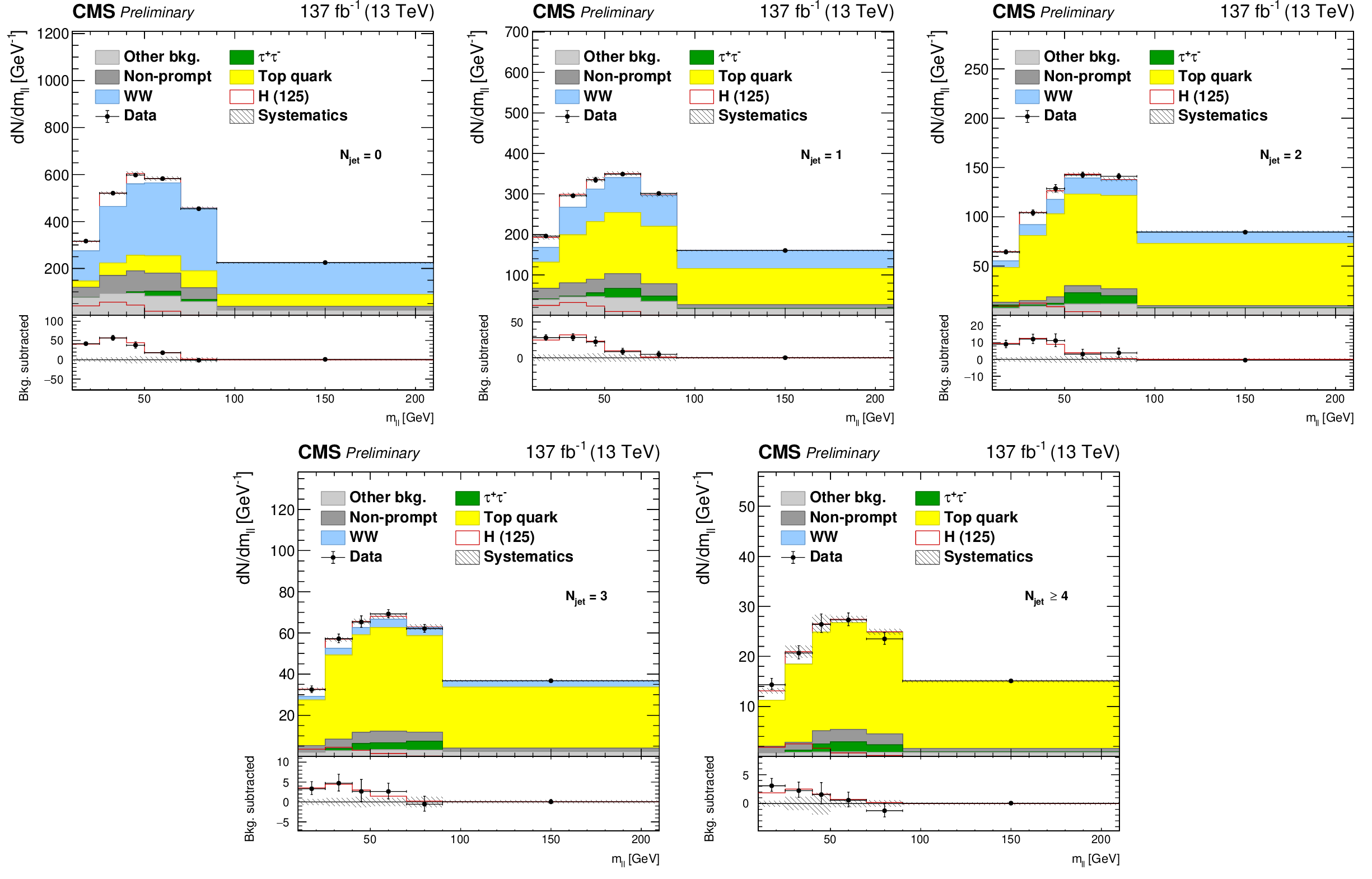
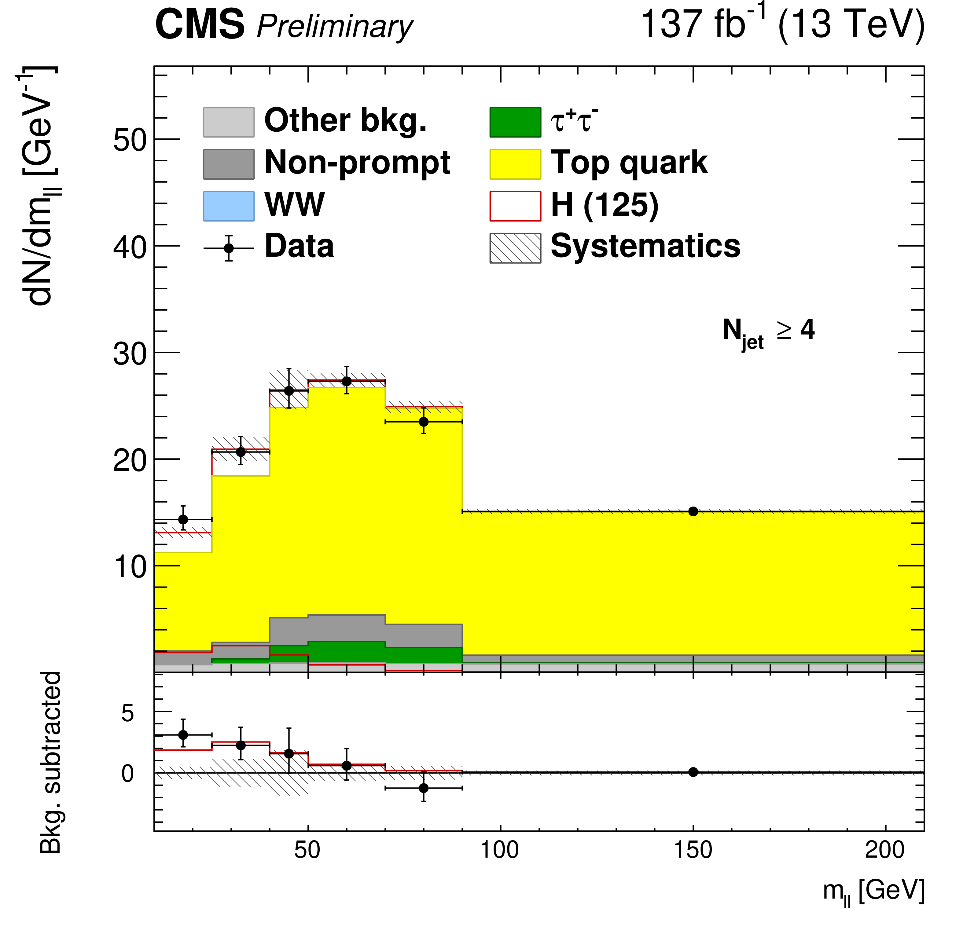
Figure 1:
Postfit ${m^{\ell \ell}}$ distributions for $ {N_{\text {jet}}} =$ 0 (top left), $ {N_{\text {jet}}} =$ 1 (top center), $ {N_{\text {jet}}} =$ 2 (top right), $ {N_{\text {jet}}} =$ 3 (bottom left), and $ {N_{\text {jet}}} \geq $ 4 (bottom right). The contribution of the background (stacked histograms) and signal (stacked and superimposed red histograms) processes is also shown. The systematic uncertainties affecting signal and background contributions are also shown as a dashed gray band. |
png pdf |
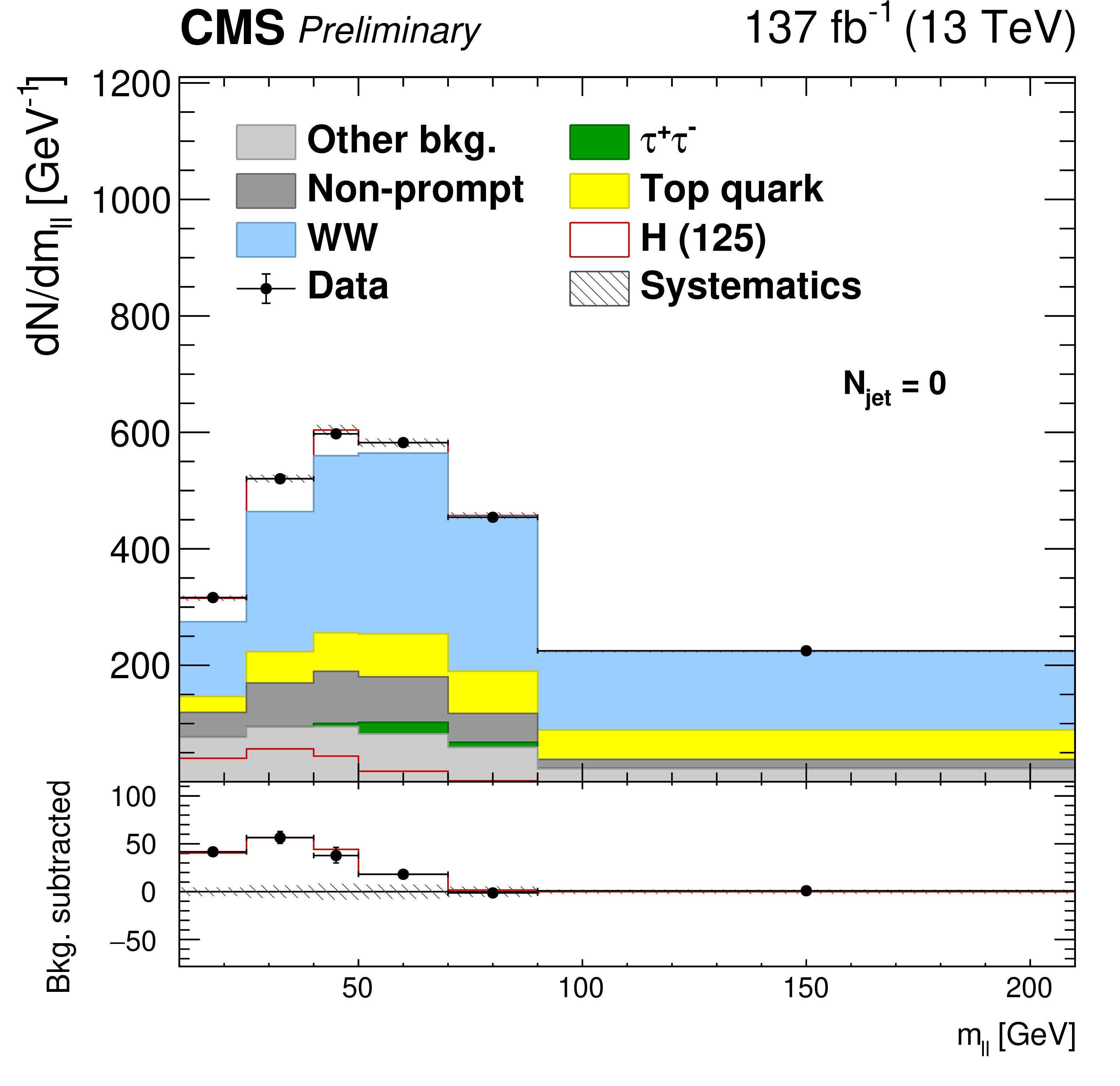
Figure 1-a:
Postfit ${m^{\ell \ell}}$ distributions for $ {N_{\text {jet}}} =$ 0 (top left), $ {N_{\text {jet}}} =$ 1 (top center), $ {N_{\text {jet}}} =$ 2 (top right), $ {N_{\text {jet}}} =$ 3 (bottom left), and $ {N_{\text {jet}}} \geq $ 4 (bottom right). The contribution of the background (stacked histograms) and signal (stacked and superimposed red histograms) processes is also shown. The systematic uncertainties affecting signal and background contributions are also shown as a dashed gray band. |
png pdf |
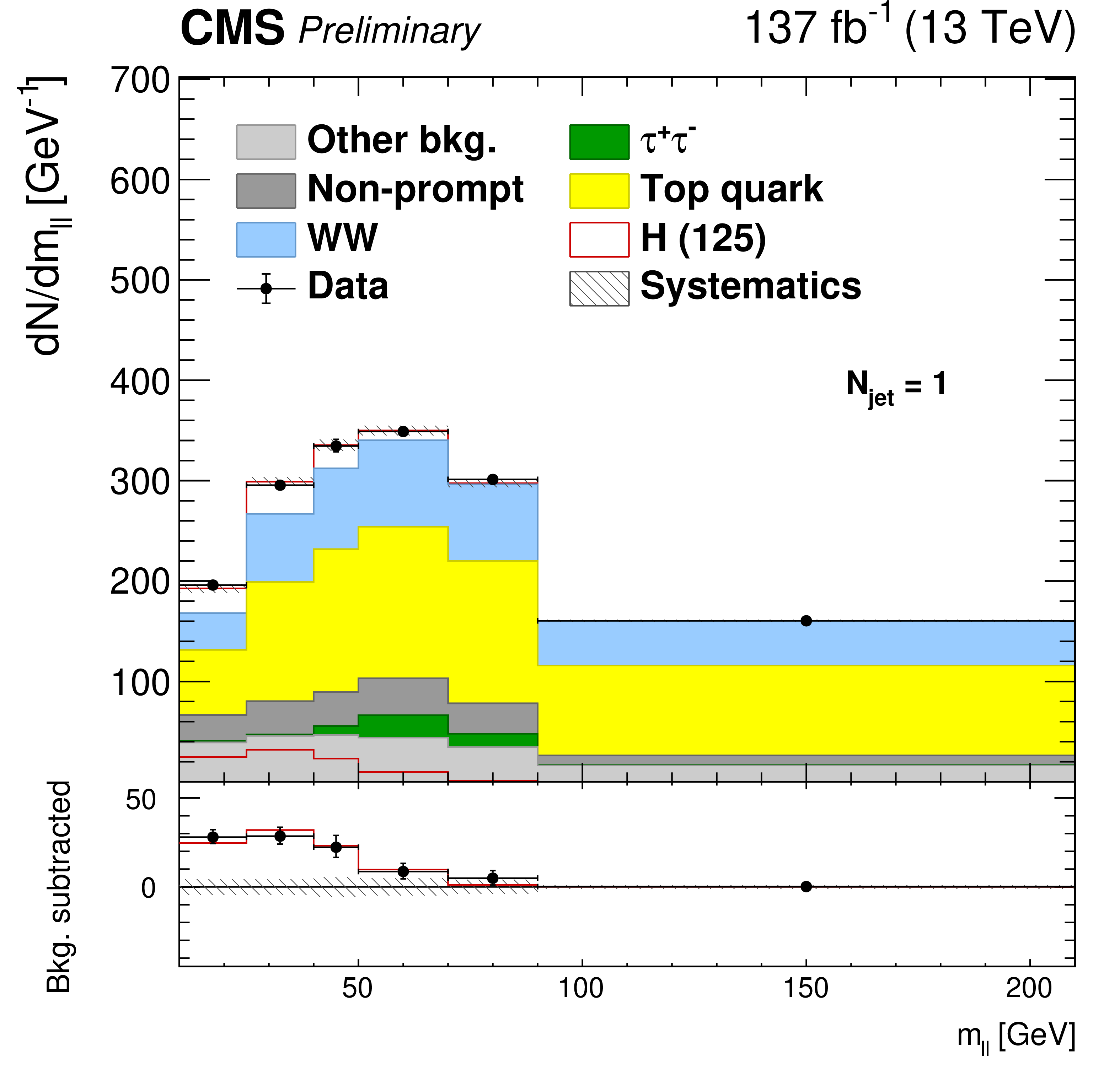
Figure 1-b:
Postfit ${m^{\ell \ell}}$ distributions for $ {N_{\text {jet}}} =$ 0 (top left), $ {N_{\text {jet}}} =$ 1 (top center), $ {N_{\text {jet}}} =$ 2 (top right), $ {N_{\text {jet}}} =$ 3 (bottom left), and $ {N_{\text {jet}}} \geq $ 4 (bottom right). The contribution of the background (stacked histograms) and signal (stacked and superimposed red histograms) processes is also shown. The systematic uncertainties affecting signal and background contributions are also shown as a dashed gray band. |

png pdf |
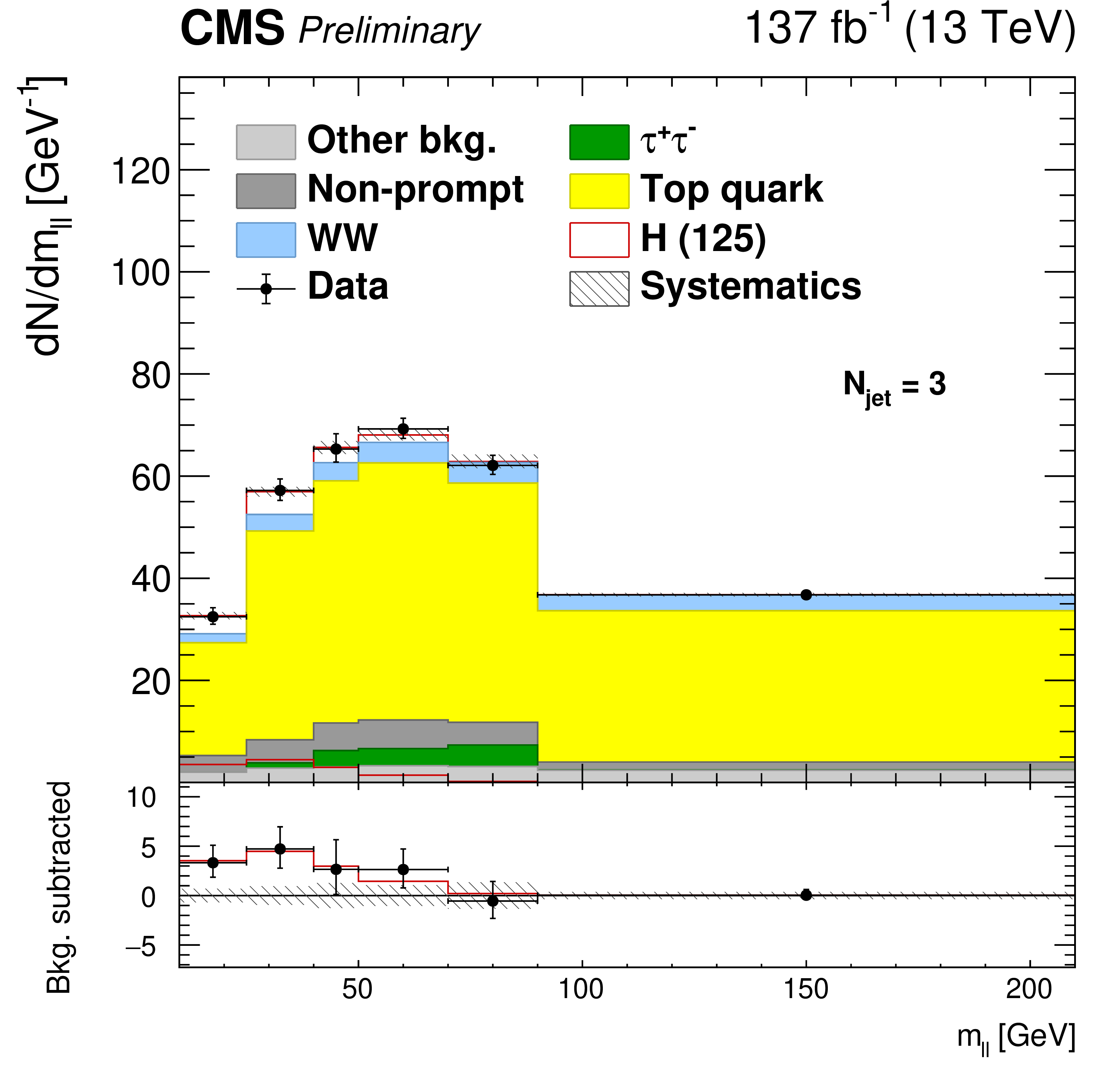
Figure 1-c:
Postfit ${m^{\ell \ell}}$ distributions for $ {N_{\text {jet}}} =$ 0 (top left), $ {N_{\text {jet}}} =$ 1 (top center), $ {N_{\text {jet}}} =$ 2 (top right), $ {N_{\text {jet}}} =$ 3 (bottom left), and $ {N_{\text {jet}}} \geq $ 4 (bottom right). The contribution of the background (stacked histograms) and signal (stacked and superimposed red histograms) processes is also shown. The systematic uncertainties affecting signal and background contributions are also shown as a dashed gray band. |
png pdf |
Figure 1-d:
Postfit ${m^{\ell \ell}}$ distributions for $ {N_{\text {jet}}} =$ 0 (top left), $ {N_{\text {jet}}} =$ 1 (top center), $ {N_{\text {jet}}} =$ 2 (top right), $ {N_{\text {jet}}} =$ 3 (bottom left), and $ {N_{\text {jet}}} \geq $ 4 (bottom right). The contribution of the background (stacked histograms) and signal (stacked and superimposed red histograms) processes is also shown. The systematic uncertainties affecting signal and background contributions are also shown as a dashed gray band. |
png pdf |
Figure 1-e:
Postfit ${m^{\ell \ell}}$ distributions for $ {N_{\text {jet}}} =$ 0 (top left), $ {N_{\text {jet}}} =$ 1 (top center), $ {N_{\text {jet}}} =$ 2 (top right), $ {N_{\text {jet}}} =$ 3 (bottom left), and $ {N_{\text {jet}}} \geq $ 4 (bottom right). The contribution of the background (stacked histograms) and signal (stacked and superimposed red histograms) processes is also shown. The systematic uncertainties affecting signal and background contributions are also shown as a dashed gray band. |
png pdf |
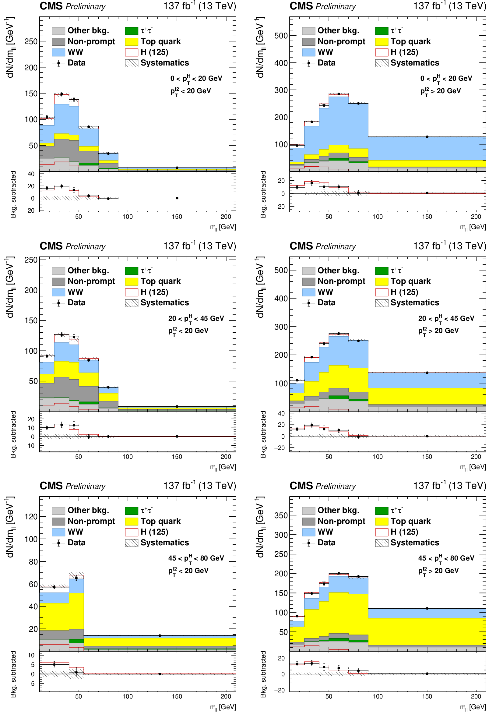
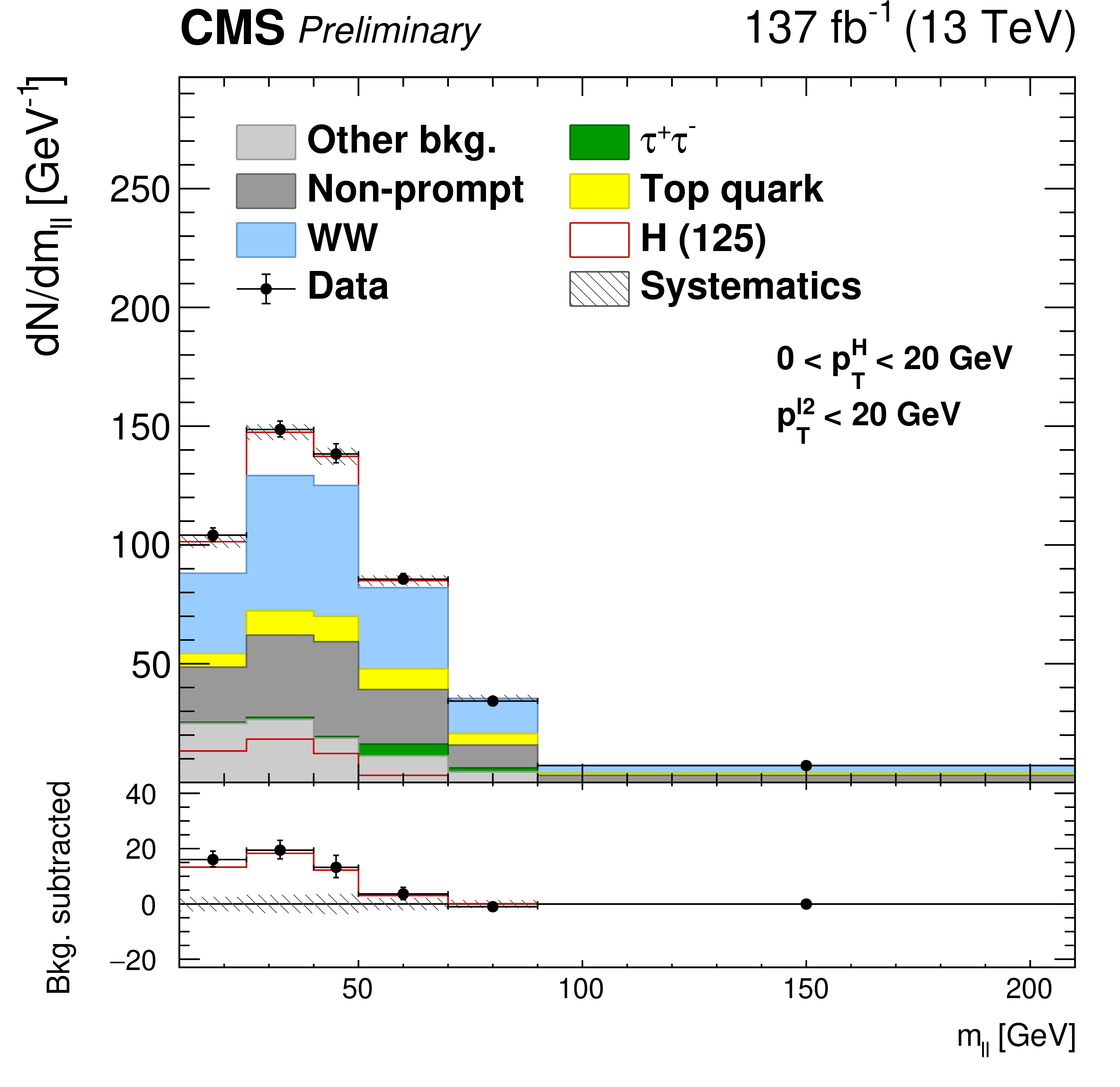
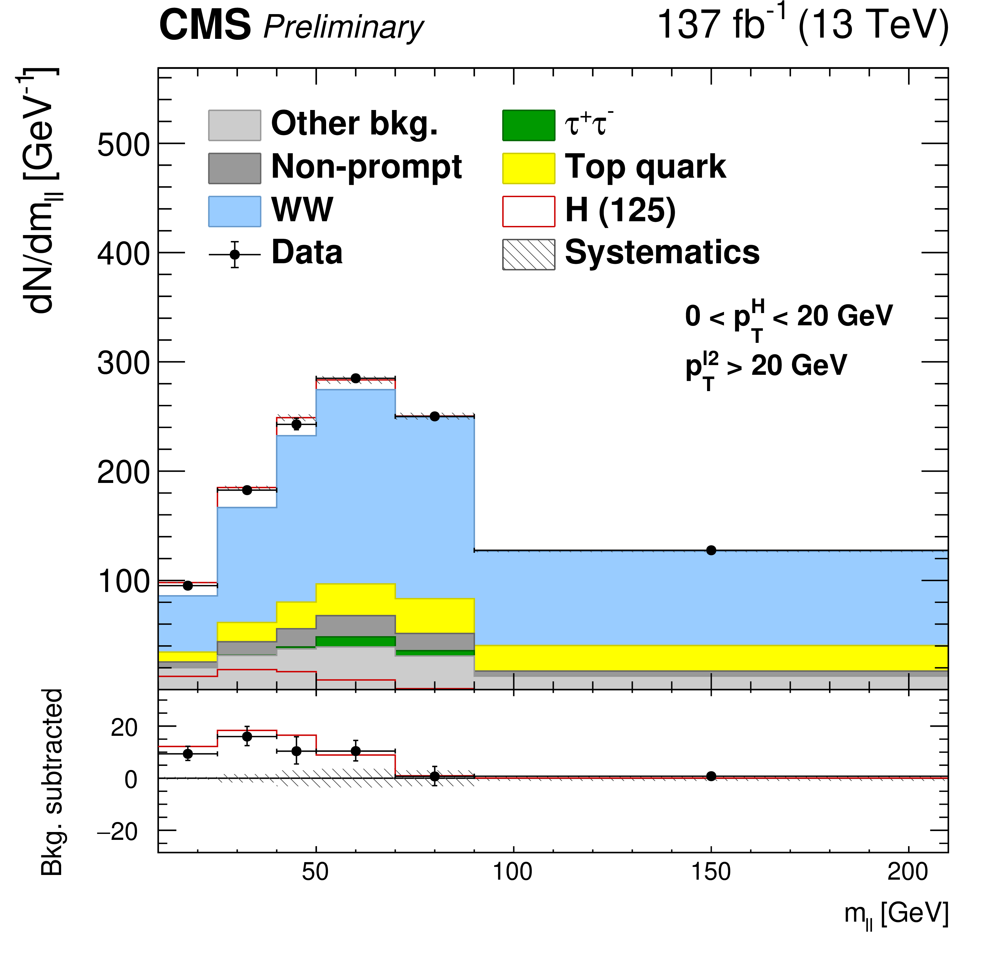
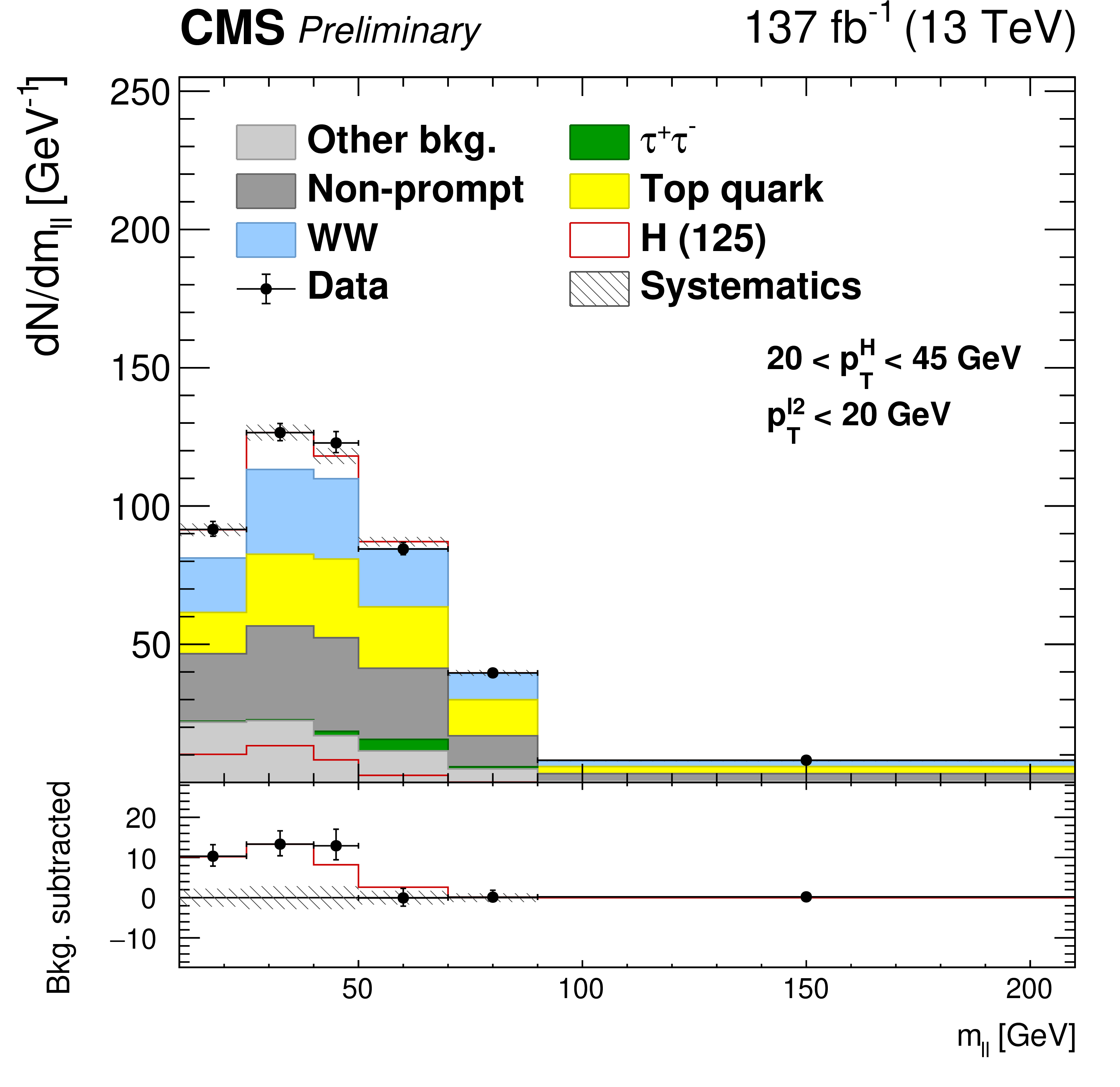
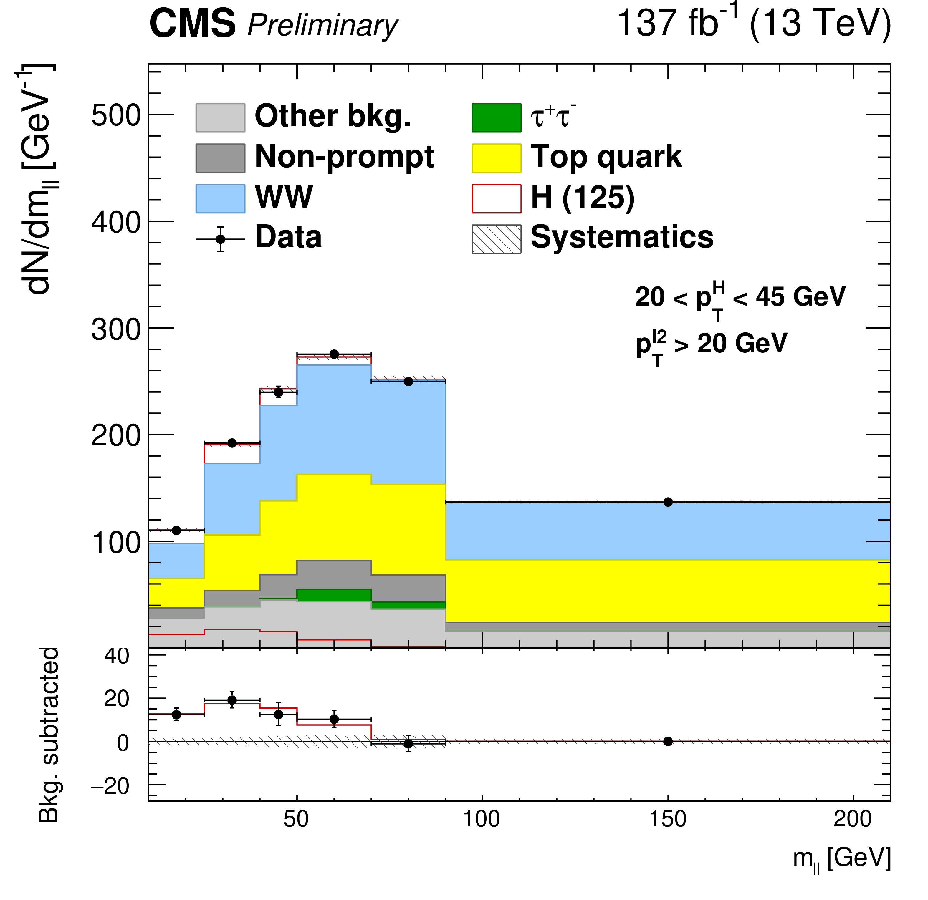
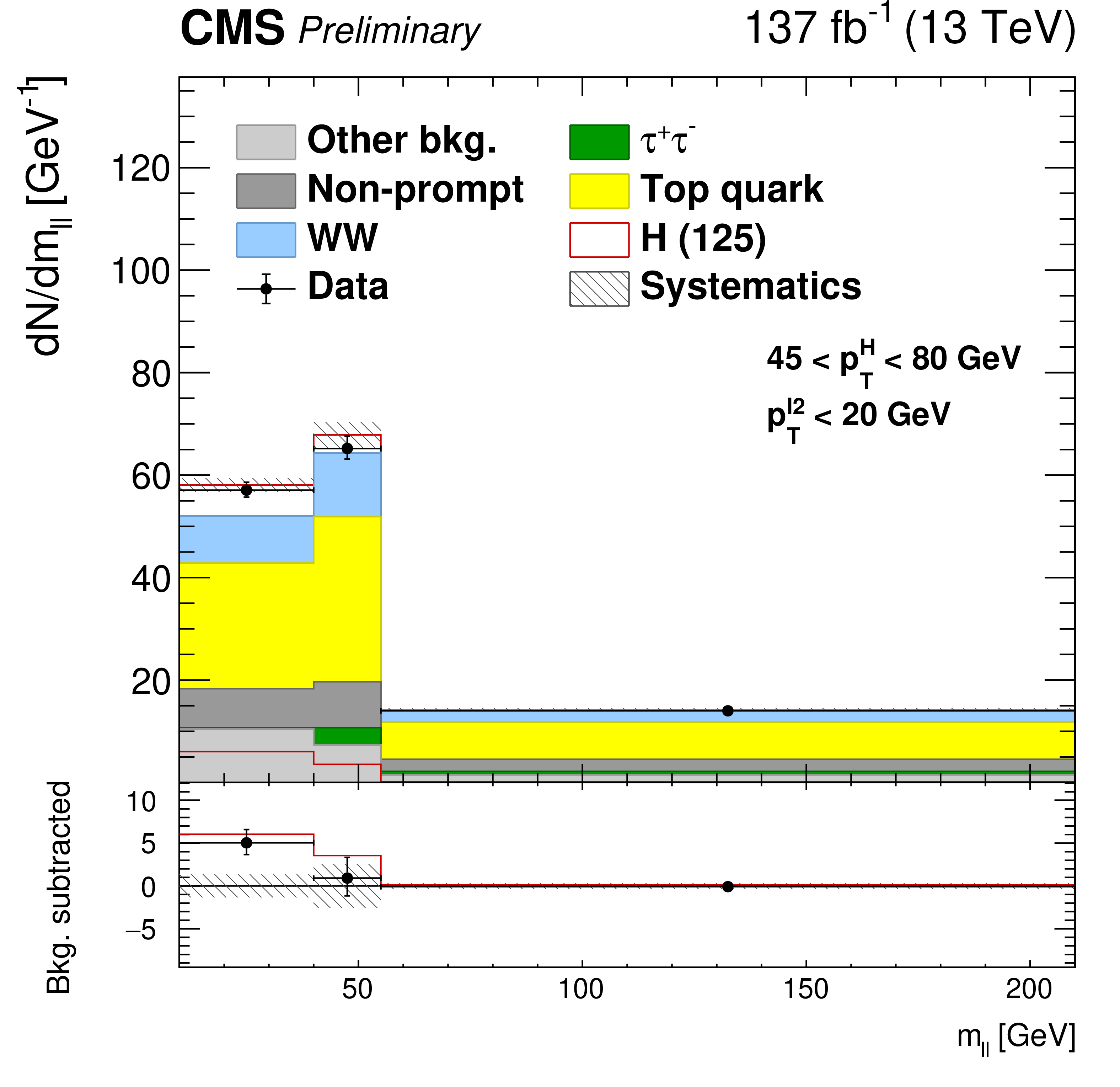
Figure 2:
Postfit ${m^{\ell \ell}}$ distributions for 0 $ < {{p_{\mathrm {T}}} ^{\mathrm{H}}} < $ 20 GeV (top row), 20 $ < {{p_{\mathrm {T}}} ^{\mathrm{H}}} < $ 45 GeV (middle row), and 45 $ < {{p_{\mathrm {T}}} ^{\mathrm{H}}} < $ 80 GeV (bottom row). Distributions are also split according to the ${{p_{\mathrm {T}}} ^{\ell _{2}}}$ categorization, i.e. $ {{p_{\mathrm {T}}} ^{\ell _{2}}} < $ 20 GeV (left column) and $ {{p_{\mathrm {T}}} ^{\ell _{2}}} >$ 20 GeV (right column). The contribution of the background (stacked histograms) and signal (stacked and superimposed red histograms) processes is also shown. The systematic uncertainties affecting signal and background contributions are also shown as a dashed gray band. |
png pdf |
Figure 2-a:
Postfit ${m^{\ell \ell}}$ distributions for 0 $ < {{p_{\mathrm {T}}} ^{\mathrm{H}}} < $ 20 GeV (top row), 20 $ < {{p_{\mathrm {T}}} ^{\mathrm{H}}} < $ 45 GeV (middle row), and 45 $ < {{p_{\mathrm {T}}} ^{\mathrm{H}}} < $ 80 GeV (bottom row). Distributions are also split according to the ${{p_{\mathrm {T}}} ^{\ell _{2}}}$ categorization, i.e. $ {{p_{\mathrm {T}}} ^{\ell _{2}}} < $ 20 GeV (left column) and $ {{p_{\mathrm {T}}} ^{\ell _{2}}} >$ 20 GeV (right column). The contribution of the background (stacked histograms) and signal (stacked and superimposed red histograms) processes is also shown. The systematic uncertainties affecting signal and background contributions are also shown as a dashed gray band. |
png pdf |
Figure 2-b:
Postfit ${m^{\ell \ell}}$ distributions for 0 $ < {{p_{\mathrm {T}}} ^{\mathrm{H}}} < $ 20 GeV (top row), 20 $ < {{p_{\mathrm {T}}} ^{\mathrm{H}}} < $ 45 GeV (middle row), and 45 $ < {{p_{\mathrm {T}}} ^{\mathrm{H}}} < $ 80 GeV (bottom row). Distributions are also split according to the ${{p_{\mathrm {T}}} ^{\ell _{2}}}$ categorization, i.e. $ {{p_{\mathrm {T}}} ^{\ell _{2}}} < $ 20 GeV (left column) and $ {{p_{\mathrm {T}}} ^{\ell _{2}}} >$ 20 GeV (right column). The contribution of the background (stacked histograms) and signal (stacked and superimposed red histograms) processes is also shown. The systematic uncertainties affecting signal and background contributions are also shown as a dashed gray band. |
png pdf |
Figure 2-c:
Postfit ${m^{\ell \ell}}$ distributions for 0 $ < {{p_{\mathrm {T}}} ^{\mathrm{H}}} < $ 20 GeV (top row), 20 $ < {{p_{\mathrm {T}}} ^{\mathrm{H}}} < $ 45 GeV (middle row), and 45 $ < {{p_{\mathrm {T}}} ^{\mathrm{H}}} < $ 80 GeV (bottom row). Distributions are also split according to the ${{p_{\mathrm {T}}} ^{\ell _{2}}}$ categorization, i.e. $ {{p_{\mathrm {T}}} ^{\ell _{2}}} < $ 20 GeV (left column) and $ {{p_{\mathrm {T}}} ^{\ell _{2}}} >$ 20 GeV (right column). The contribution of the background (stacked histograms) and signal (stacked and superimposed red histograms) processes is also shown. The systematic uncertainties affecting signal and background contributions are also shown as a dashed gray band. |
png pdf |
Figure 2-d:
Postfit ${m^{\ell \ell}}$ distributions for 0 $ < {{p_{\mathrm {T}}} ^{\mathrm{H}}} < $ 20 GeV (top row), 20 $ < {{p_{\mathrm {T}}} ^{\mathrm{H}}} < $ 45 GeV (middle row), and 45 $ < {{p_{\mathrm {T}}} ^{\mathrm{H}}} < $ 80 GeV (bottom row). Distributions are also split according to the ${{p_{\mathrm {T}}} ^{\ell _{2}}}$ categorization, i.e. $ {{p_{\mathrm {T}}} ^{\ell _{2}}} < $ 20 GeV (left column) and $ {{p_{\mathrm {T}}} ^{\ell _{2}}} >$ 20 GeV (right column). The contribution of the background (stacked histograms) and signal (stacked and superimposed red histograms) processes is also shown. The systematic uncertainties affecting signal and background contributions are also shown as a dashed gray band. |
png pdf |
Figure 2-e:
Postfit ${m^{\ell \ell}}$ distributions for 0 $ < {{p_{\mathrm {T}}} ^{\mathrm{H}}} < $ 20 GeV (top row), 20 $ < {{p_{\mathrm {T}}} ^{\mathrm{H}}} < $ 45 GeV (middle row), and 45 $ < {{p_{\mathrm {T}}} ^{\mathrm{H}}} < $ 80 GeV (bottom row). Distributions are also split according to the ${{p_{\mathrm {T}}} ^{\ell _{2}}}$ categorization, i.e. $ {{p_{\mathrm {T}}} ^{\ell _{2}}} < $ 20 GeV (left column) and $ {{p_{\mathrm {T}}} ^{\ell _{2}}} >$ 20 GeV (right column). The contribution of the background (stacked histograms) and signal (stacked and superimposed red histograms) processes is also shown. The systematic uncertainties affecting signal and background contributions are also shown as a dashed gray band. |

png pdf |
Figure 2-f:
Postfit ${m^{\ell \ell}}$ distributions for 0 $ < {{p_{\mathrm {T}}} ^{\mathrm{H}}} < $ 20 GeV (top row), 20 $ < {{p_{\mathrm {T}}} ^{\mathrm{H}}} < $ 45 GeV (middle row), and 45 $ < {{p_{\mathrm {T}}} ^{\mathrm{H}}} < $ 80 GeV (bottom row). Distributions are also split according to the ${{p_{\mathrm {T}}} ^{\ell _{2}}}$ categorization, i.e. $ {{p_{\mathrm {T}}} ^{\ell _{2}}} < $ 20 GeV (left column) and $ {{p_{\mathrm {T}}} ^{\ell _{2}}} >$ 20 GeV (right column). The contribution of the background (stacked histograms) and signal (stacked and superimposed red histograms) processes is also shown. The systematic uncertainties affecting signal and background contributions are also shown as a dashed gray band. |
png pdf |
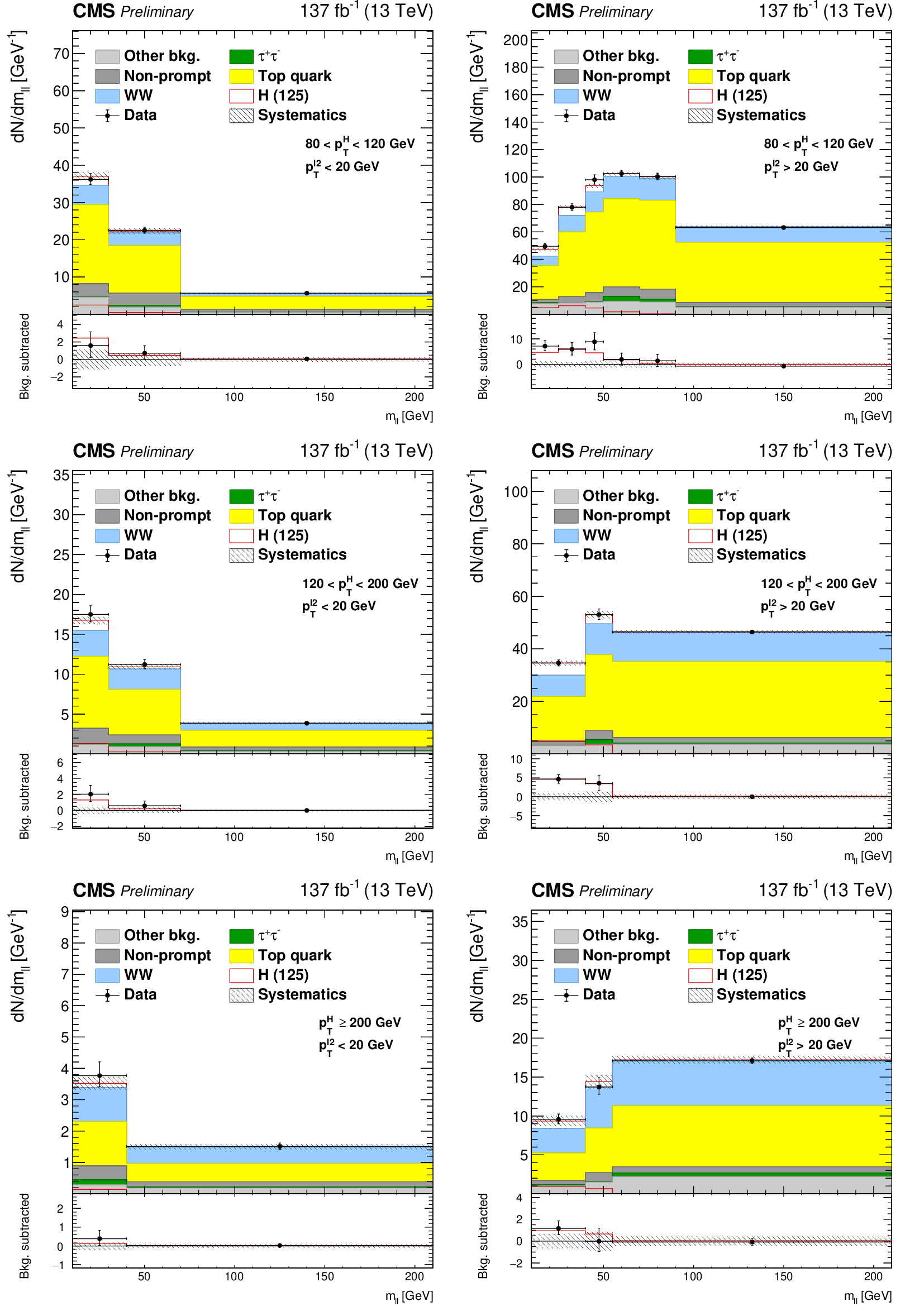
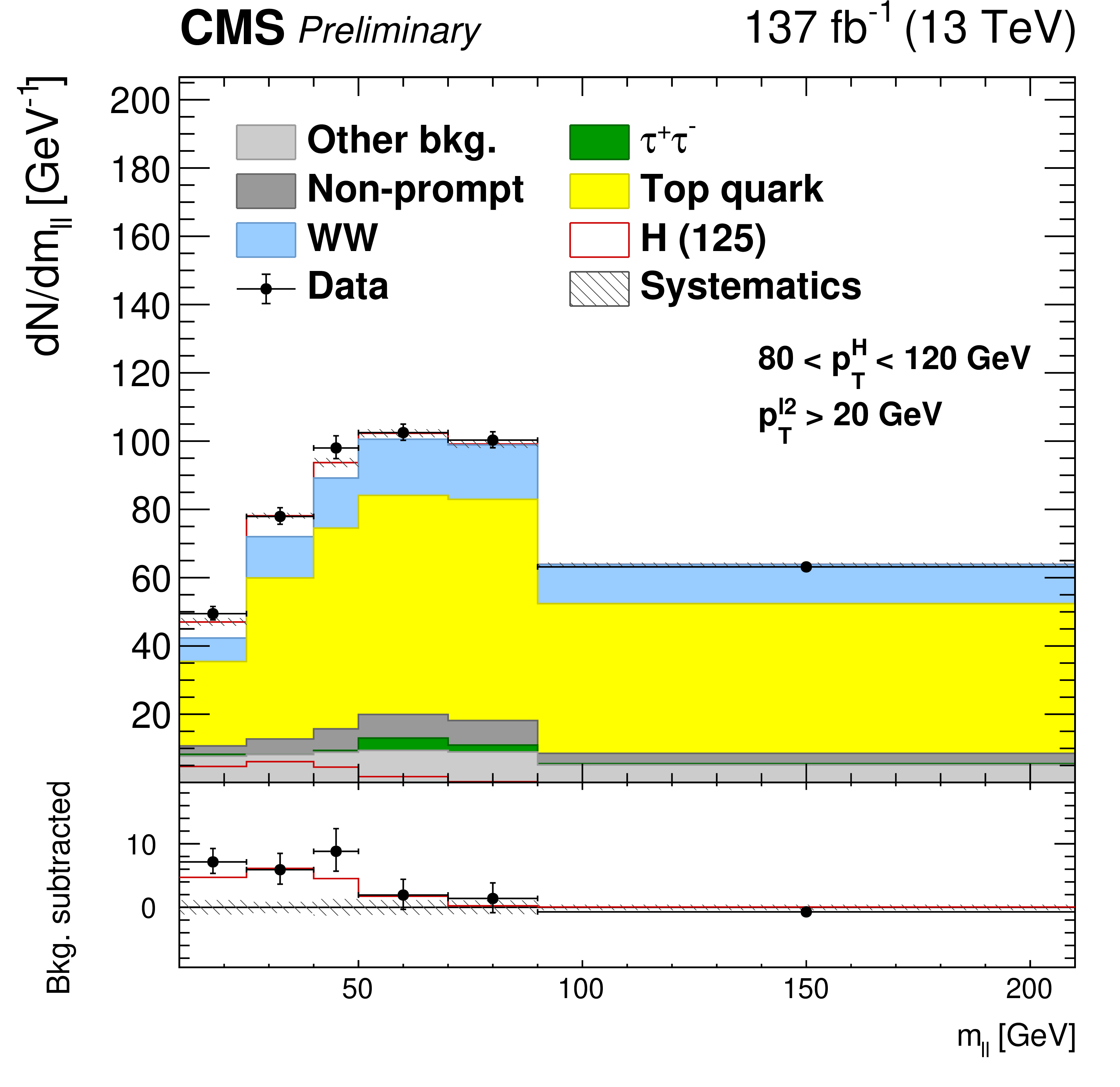
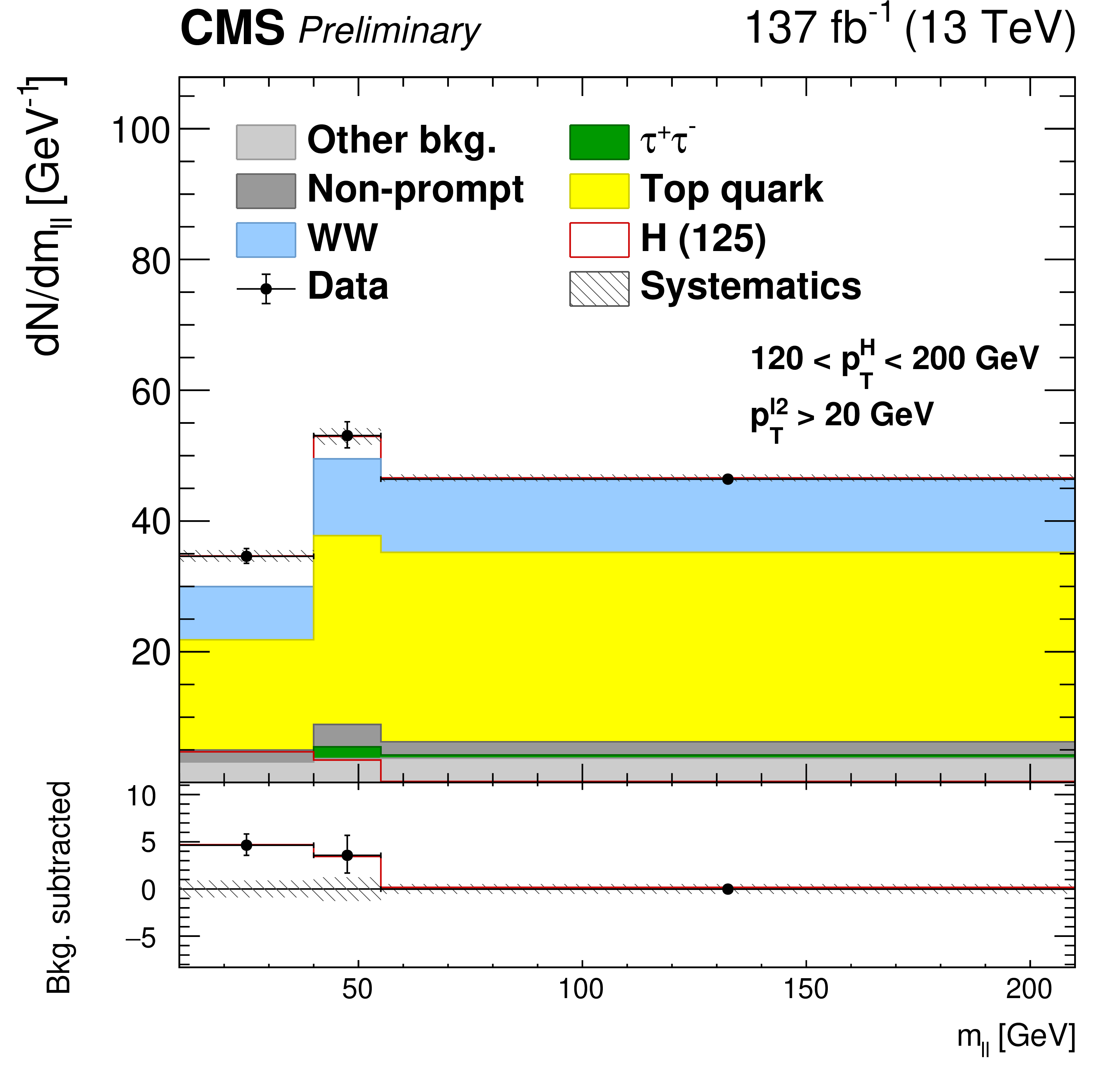
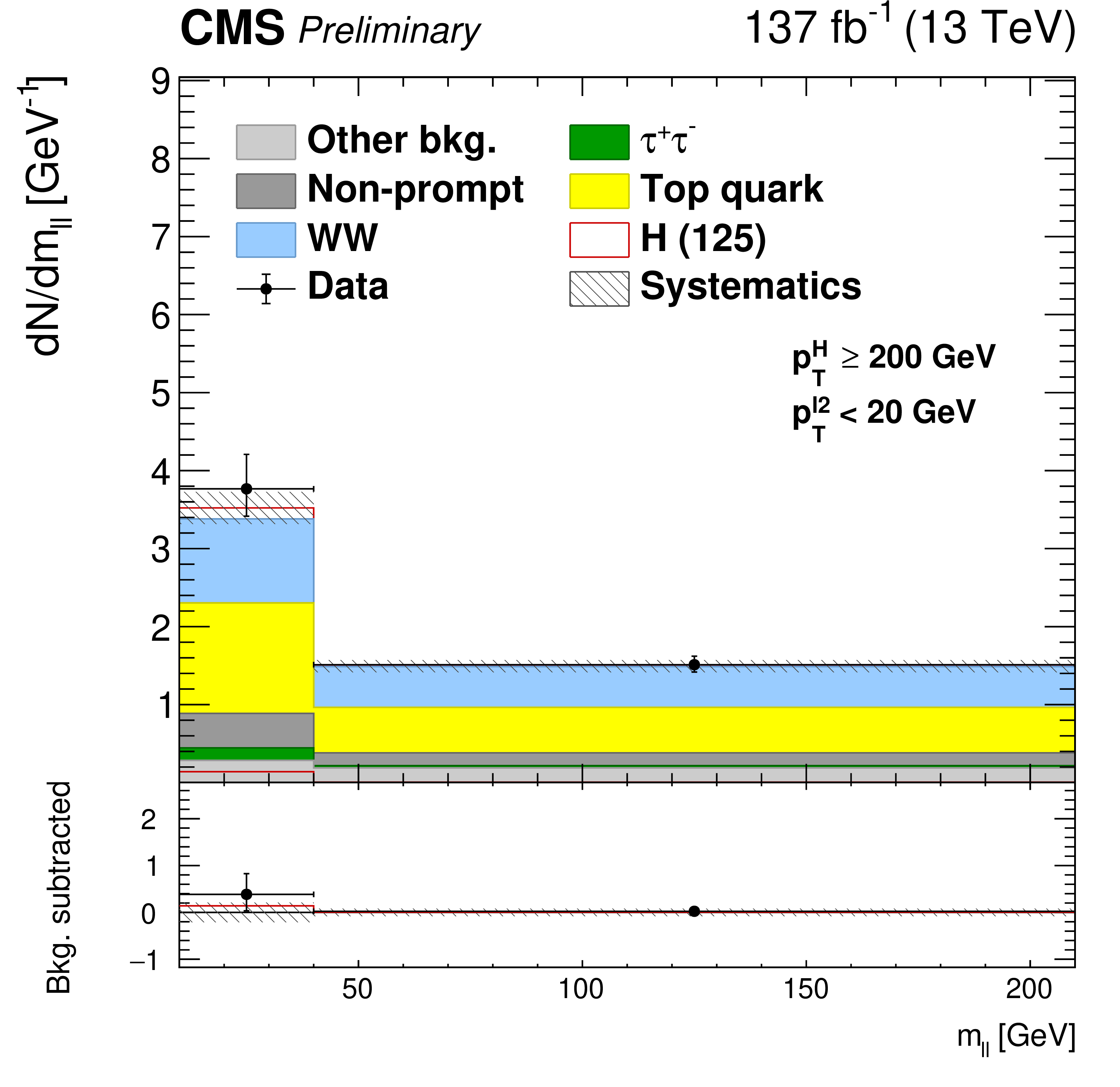
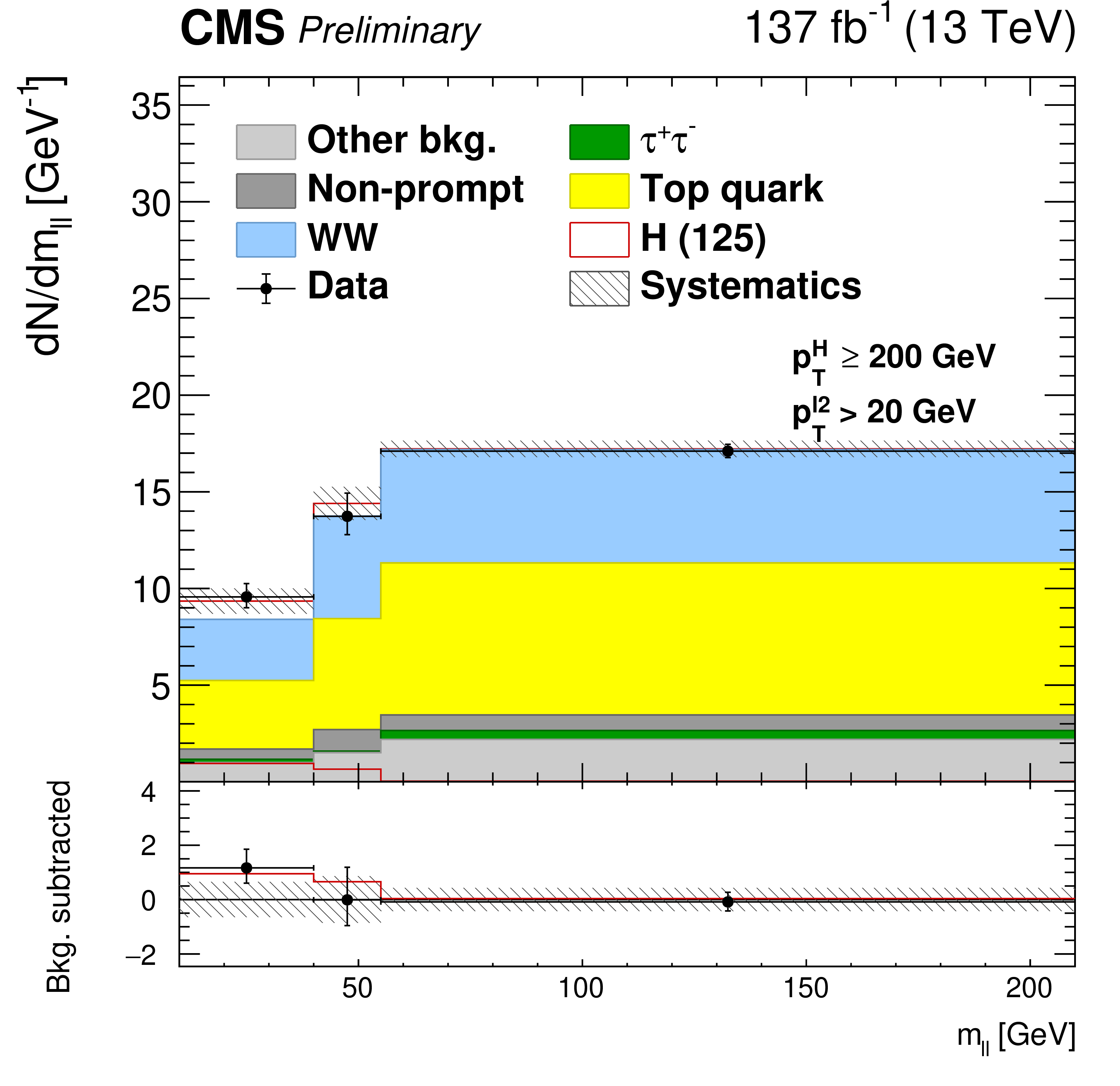
Figure 3:
Postfit ${m^{\ell \ell}}$ distributions for 80 $ < {{p_{\mathrm {T}}} ^{\mathrm{H}}} < $ 120 GeV (top row), 120 $ < {{p_{\mathrm {T}}} ^{\mathrm{H}}} < $ 200 GeV (middle row), and $ {{p_{\mathrm {T}}} ^{\mathrm{H}}} \geq $ 200 GeV (bottom row). Distributions are also split according to the ${{p_{\mathrm {T}}} ^{\ell _{2}}}$ categorization, i.e. $ {{p_{\mathrm {T}}} ^{\ell _{2}}} < $ 20 GeV (left column) and $ {{p_{\mathrm {T}}} ^{\ell _{2}}} > $ 20 GeV (right column). The contribution of the background (stacked histograms) and signal (stacked and superimposed red histograms) processes is also shown. The systematic uncertainties affecting signal and background contributions are also shown as a dashed gray band. |

png pdf |
Figure 3-a:
Postfit ${m^{\ell \ell}}$ distributions for 80 $ < {{p_{\mathrm {T}}} ^{\mathrm{H}}} < $ 120 GeV (top row), 120 $ < {{p_{\mathrm {T}}} ^{\mathrm{H}}} < $ 200 GeV (middle row), and $ {{p_{\mathrm {T}}} ^{\mathrm{H}}} \geq $ 200 GeV (bottom row). Distributions are also split according to the ${{p_{\mathrm {T}}} ^{\ell _{2}}}$ categorization, i.e. $ {{p_{\mathrm {T}}} ^{\ell _{2}}} < $ 20 GeV (left column) and $ {{p_{\mathrm {T}}} ^{\ell _{2}}} > $ 20 GeV (right column). The contribution of the background (stacked histograms) and signal (stacked and superimposed red histograms) processes is also shown. The systematic uncertainties affecting signal and background contributions are also shown as a dashed gray band. |
png pdf |
Figure 3-b:
Postfit ${m^{\ell \ell}}$ distributions for 80 $ < {{p_{\mathrm {T}}} ^{\mathrm{H}}} < $ 120 GeV (top row), 120 $ < {{p_{\mathrm {T}}} ^{\mathrm{H}}} < $ 200 GeV (middle row), and $ {{p_{\mathrm {T}}} ^{\mathrm{H}}} \geq $ 200 GeV (bottom row). Distributions are also split according to the ${{p_{\mathrm {T}}} ^{\ell _{2}}}$ categorization, i.e. $ {{p_{\mathrm {T}}} ^{\ell _{2}}} < $ 20 GeV (left column) and $ {{p_{\mathrm {T}}} ^{\ell _{2}}} > $ 20 GeV (right column). The contribution of the background (stacked histograms) and signal (stacked and superimposed red histograms) processes is also shown. The systematic uncertainties affecting signal and background contributions are also shown as a dashed gray band. |

png pdf |
Figure 3-c:
Postfit ${m^{\ell \ell}}$ distributions for 80 $ < {{p_{\mathrm {T}}} ^{\mathrm{H}}} < $ 120 GeV (top row), 120 $ < {{p_{\mathrm {T}}} ^{\mathrm{H}}} < $ 200 GeV (middle row), and $ {{p_{\mathrm {T}}} ^{\mathrm{H}}} \geq $ 200 GeV (bottom row). Distributions are also split according to the ${{p_{\mathrm {T}}} ^{\ell _{2}}}$ categorization, i.e. $ {{p_{\mathrm {T}}} ^{\ell _{2}}} < $ 20 GeV (left column) and $ {{p_{\mathrm {T}}} ^{\ell _{2}}} > $ 20 GeV (right column). The contribution of the background (stacked histograms) and signal (stacked and superimposed red histograms) processes is also shown. The systematic uncertainties affecting signal and background contributions are also shown as a dashed gray band. |
png pdf |
Figure 3-d:
Postfit ${m^{\ell \ell}}$ distributions for 80 $ < {{p_{\mathrm {T}}} ^{\mathrm{H}}} < $ 120 GeV (top row), 120 $ < {{p_{\mathrm {T}}} ^{\mathrm{H}}} < $ 200 GeV (middle row), and $ {{p_{\mathrm {T}}} ^{\mathrm{H}}} \geq $ 200 GeV (bottom row). Distributions are also split according to the ${{p_{\mathrm {T}}} ^{\ell _{2}}}$ categorization, i.e. $ {{p_{\mathrm {T}}} ^{\ell _{2}}} < $ 20 GeV (left column) and $ {{p_{\mathrm {T}}} ^{\ell _{2}}} > $ 20 GeV (right column). The contribution of the background (stacked histograms) and signal (stacked and superimposed red histograms) processes is also shown. The systematic uncertainties affecting signal and background contributions are also shown as a dashed gray band. |
png pdf |
Figure 3-e:
Postfit ${m^{\ell \ell}}$ distributions for 80 $ < {{p_{\mathrm {T}}} ^{\mathrm{H}}} < $ 120 GeV (top row), 120 $ < {{p_{\mathrm {T}}} ^{\mathrm{H}}} < $ 200 GeV (middle row), and $ {{p_{\mathrm {T}}} ^{\mathrm{H}}} \geq $ 200 GeV (bottom row). Distributions are also split according to the ${{p_{\mathrm {T}}} ^{\ell _{2}}}$ categorization, i.e. $ {{p_{\mathrm {T}}} ^{\ell _{2}}} < $ 20 GeV (left column) and $ {{p_{\mathrm {T}}} ^{\ell _{2}}} > $ 20 GeV (right column). The contribution of the background (stacked histograms) and signal (stacked and superimposed red histograms) processes is also shown. The systematic uncertainties affecting signal and background contributions are also shown as a dashed gray band. |
png pdf |
Figure 3-f:
Postfit ${m^{\ell \ell}}$ distributions for 80 $ < {{p_{\mathrm {T}}} ^{\mathrm{H}}} < $ 120 GeV (top row), 120 $ < {{p_{\mathrm {T}}} ^{\mathrm{H}}} < $ 200 GeV (middle row), and $ {{p_{\mathrm {T}}} ^{\mathrm{H}}} \geq $ 200 GeV (bottom row). Distributions are also split according to the ${{p_{\mathrm {T}}} ^{\ell _{2}}}$ categorization, i.e. $ {{p_{\mathrm {T}}} ^{\ell _{2}}} < $ 20 GeV (left column) and $ {{p_{\mathrm {T}}} ^{\ell _{2}}} > $ 20 GeV (right column). The contribution of the background (stacked histograms) and signal (stacked and superimposed red histograms) processes is also shown. The systematic uncertainties affecting signal and background contributions are also shown as a dashed gray band. |

png pdf |
Figure 4:
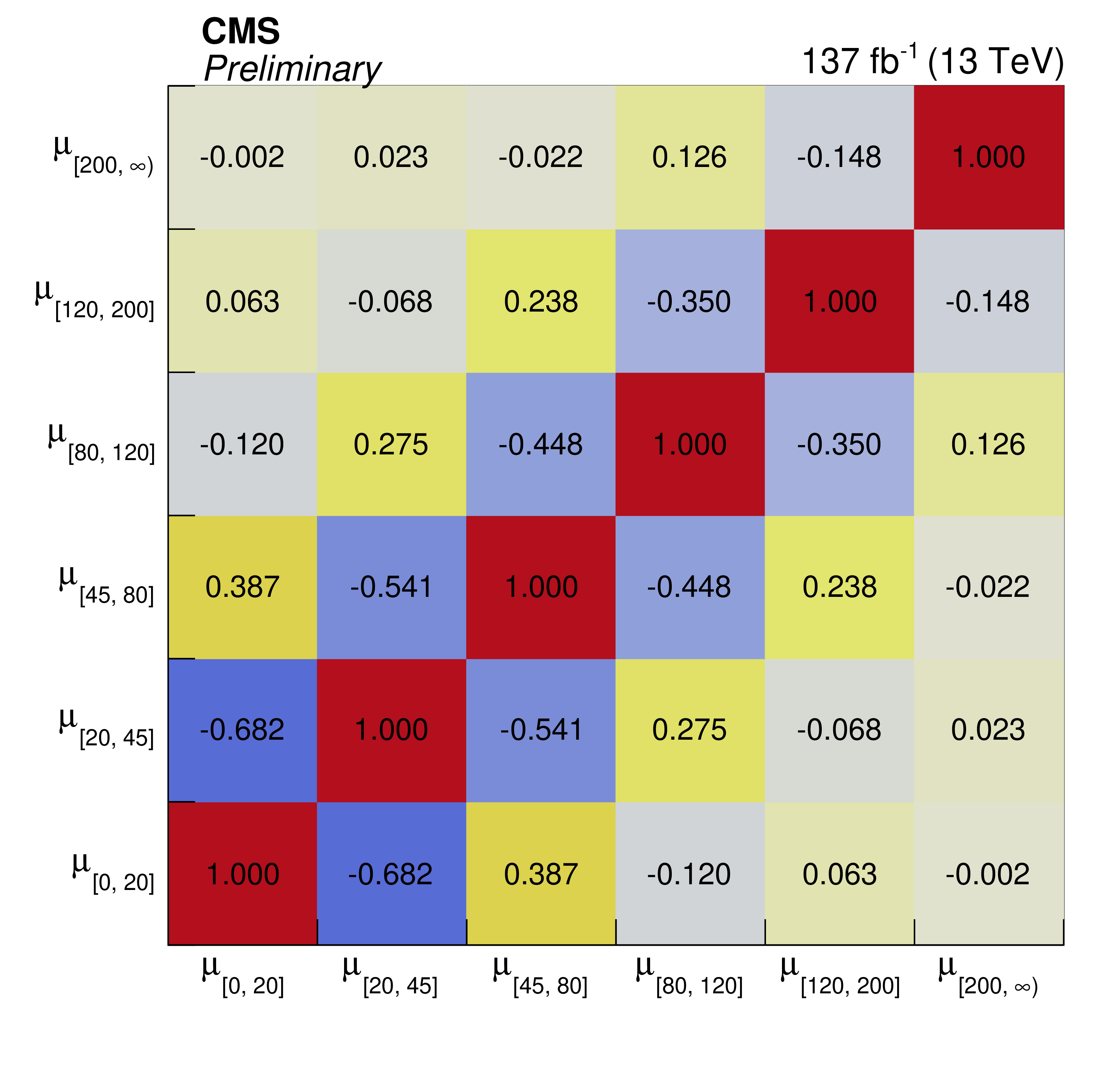
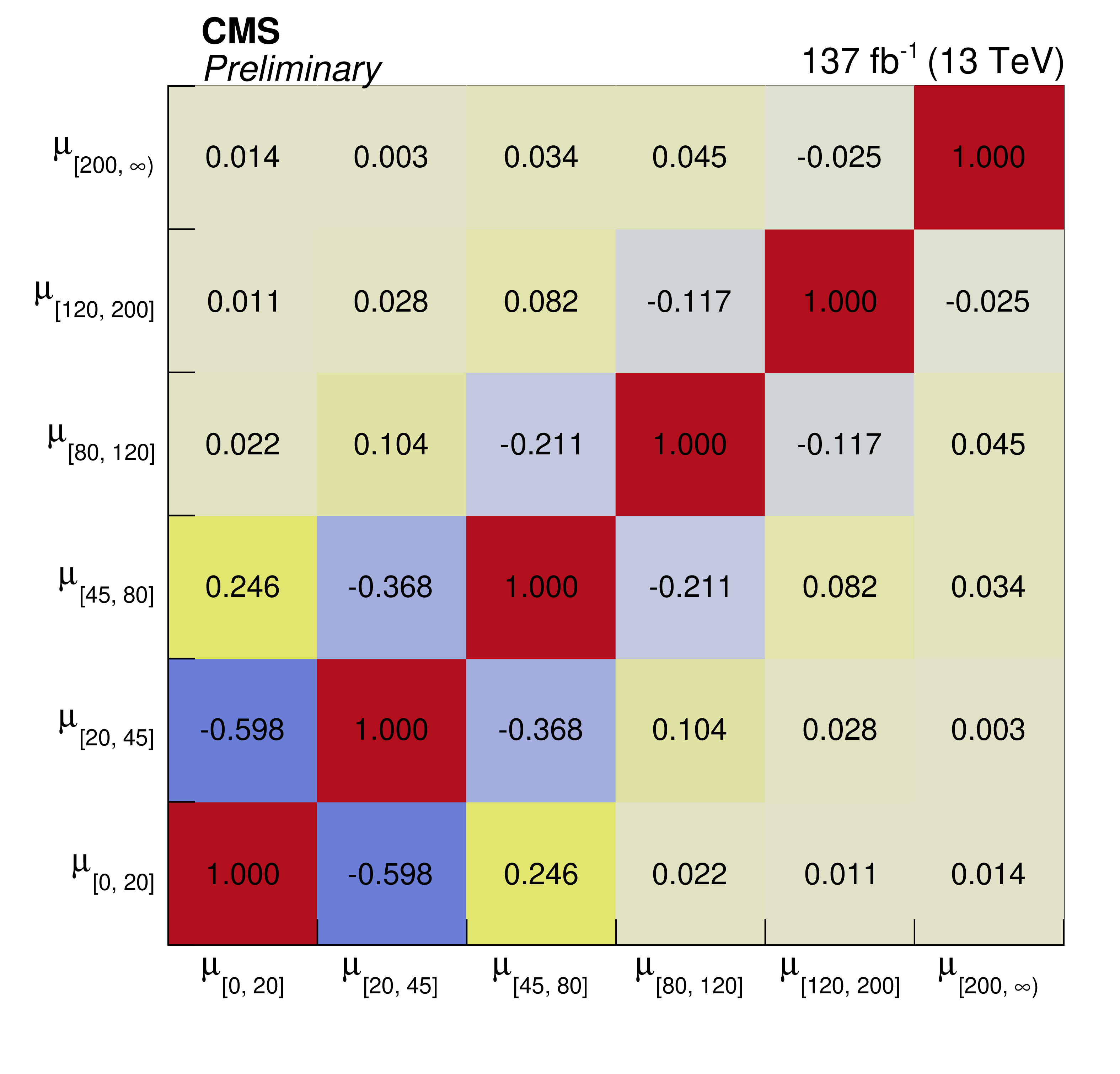
Correlation between signal strength modifiers in fiducial ${{p_{\mathrm {T}}} ^{\mathrm{H}}}$ bins obtained from unregularized (left) and regularized (right) fit to the combined data sets. Regularization strength is $\delta =$ 2.5. |
png pdf |
Figure 4-a:
Correlation between signal strength modifiers in fiducial ${{p_{\mathrm {T}}} ^{\mathrm{H}}}$ bins obtained from unregularized (left) and regularized (right) fit to the combined data sets. Regularization strength is $\delta =$ 2.5. |
png pdf |
Figure 4-b:
Correlation between signal strength modifiers in fiducial ${{p_{\mathrm {T}}} ^{\mathrm{H}}}$ bins obtained from unregularized (left) and regularized (right) fit to the combined data sets. Regularization strength is $\delta =$ 2.5. |
png pdf |
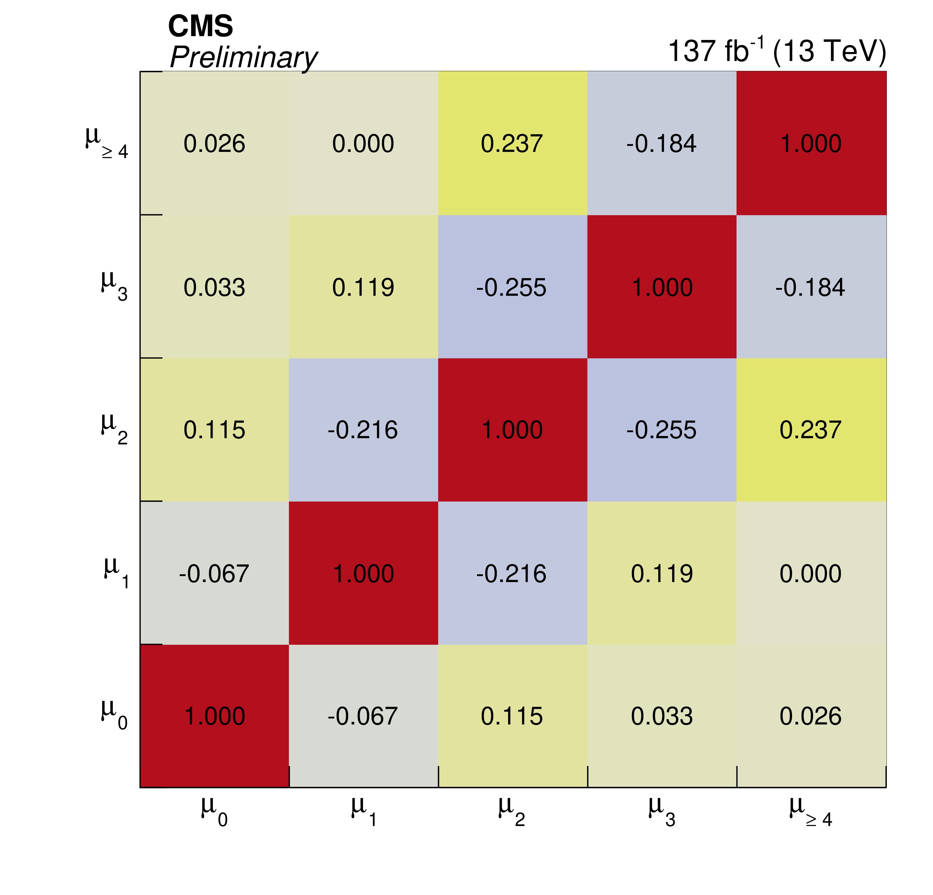
Figure 5:
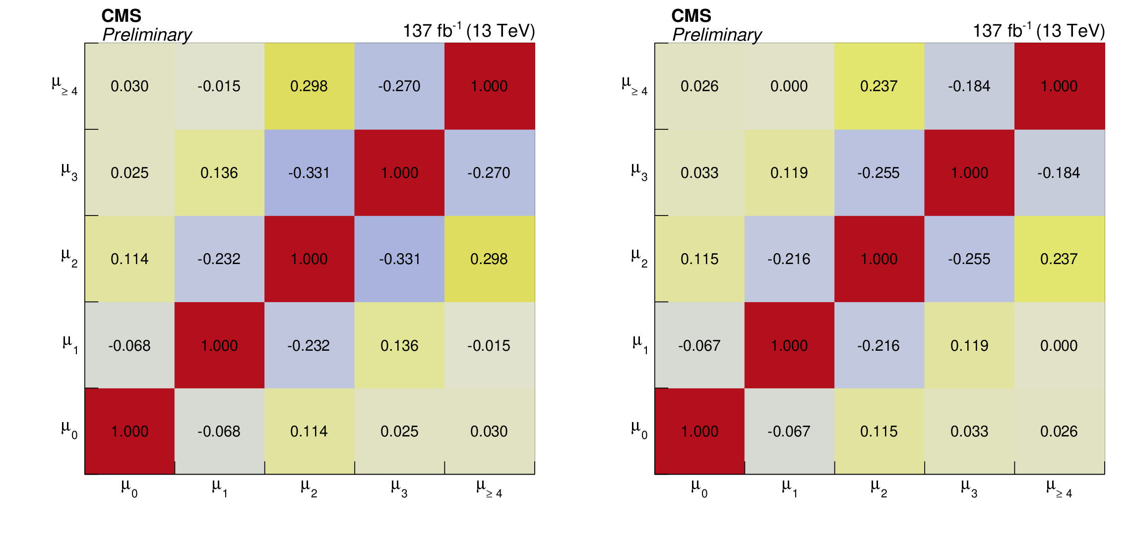
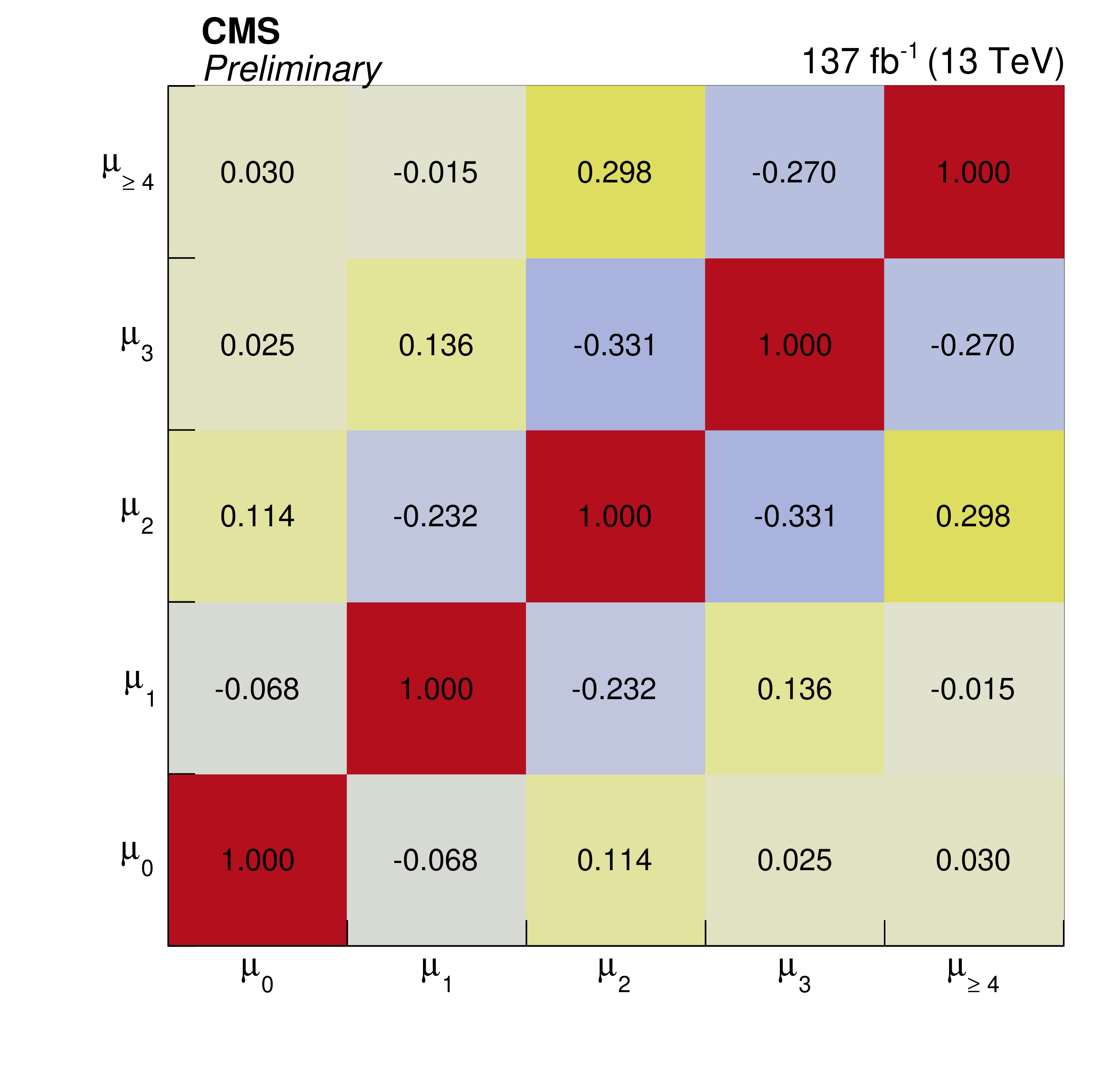
Correlation between signal strength modifiers in fiducial ${N_{\text {jet}}}$ bins obtained from unregularized (left) and regularized (right) fit to the combined data sets. Regularization strength is $\delta =$ 9.52. |
png pdf |
Figure 5-a:
Correlation between signal strength modifiers in fiducial ${N_{\text {jet}}}$ bins obtained from unregularized (left) and regularized (right) fit to the combined data sets. Regularization strength is $\delta =$ 9.52. |
png pdf |
Figure 5-b:
Correlation between signal strength modifiers in fiducial ${N_{\text {jet}}}$ bins obtained from unregularized (left) and regularized (right) fit to the combined data sets. Regularization strength is $\delta =$ 9.52. |
png pdf |
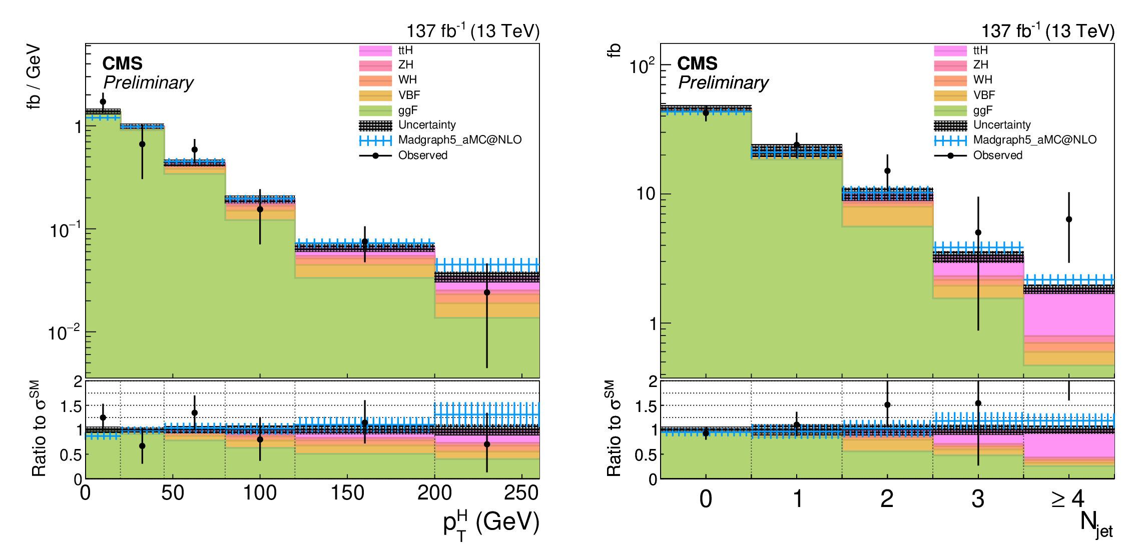
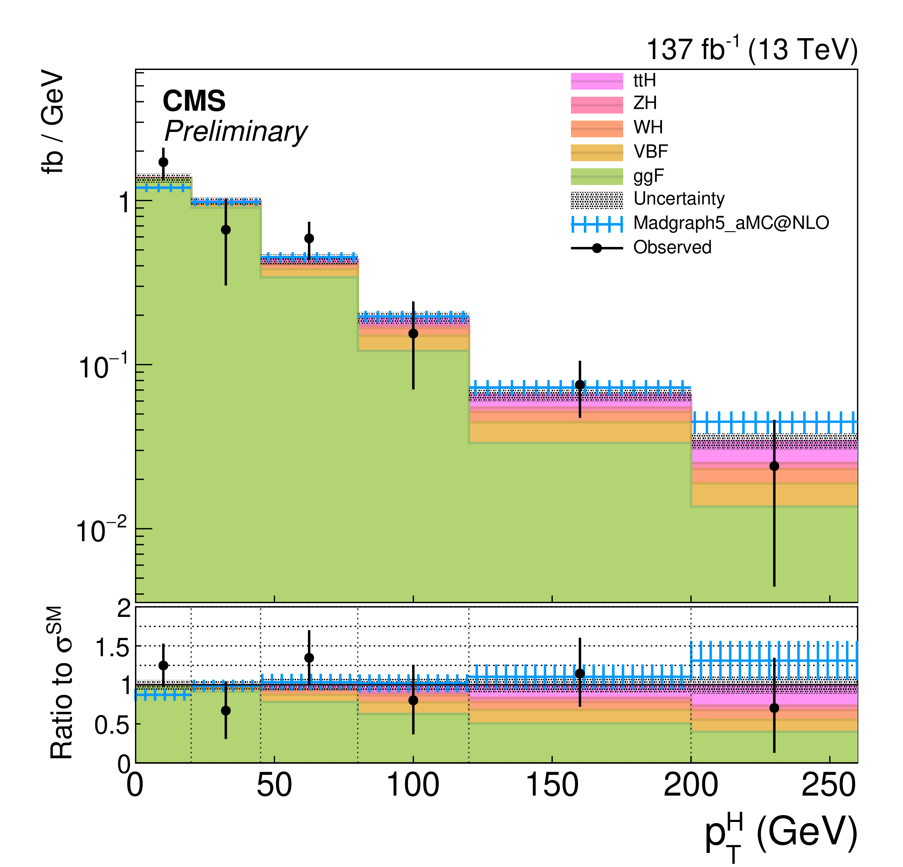
Figure 6:
Observed differential fiducial cross sections in bins of ${{p_{\mathrm {T}}} ^{\mathrm{H}}}$ (left) and ${N_{\text {jet}}}$ (right), overlaid with the predictions from nominal and alternative signal models. The uncertainty bands on the theoretical predictions correspond to quadratic sums of renormalization and factorization scale uncertainties, PDF uncertainties, and simulation statistical uncertainties. The filled histogram in the ratio plot shows the relative contributions of the Higgs boson production modes in each bin. |
png pdf |
Figure 6-a:
Observed differential fiducial cross sections in bins of ${{p_{\mathrm {T}}} ^{\mathrm{H}}}$ (left) and ${N_{\text {jet}}}$ (right), overlaid with the predictions from nominal and alternative signal models. The uncertainty bands on the theoretical predictions correspond to quadratic sums of renormalization and factorization scale uncertainties, PDF uncertainties, and simulation statistical uncertainties. The filled histogram in the ratio plot shows the relative contributions of the Higgs boson production modes in each bin. |

png pdf |
Figure 6-b:
Observed differential fiducial cross sections in bins of ${{p_{\mathrm {T}}} ^{\mathrm{H}}}$ (left) and ${N_{\text {jet}}}$ (right), overlaid with the predictions from nominal and alternative signal models. The uncertainty bands on the theoretical predictions correspond to quadratic sums of renormalization and factorization scale uncertainties, PDF uncertainties, and simulation statistical uncertainties. The filled histogram in the ratio plot shows the relative contributions of the Higgs boson production modes in each bin. |
| Tables | |
png pdf |
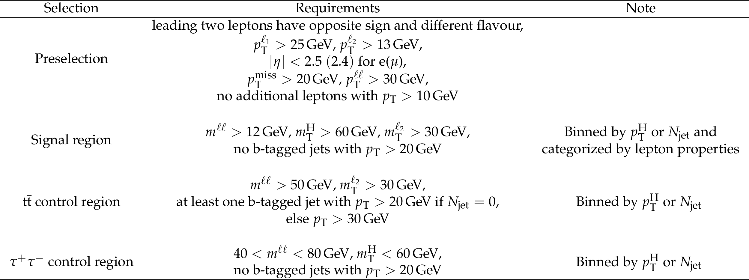
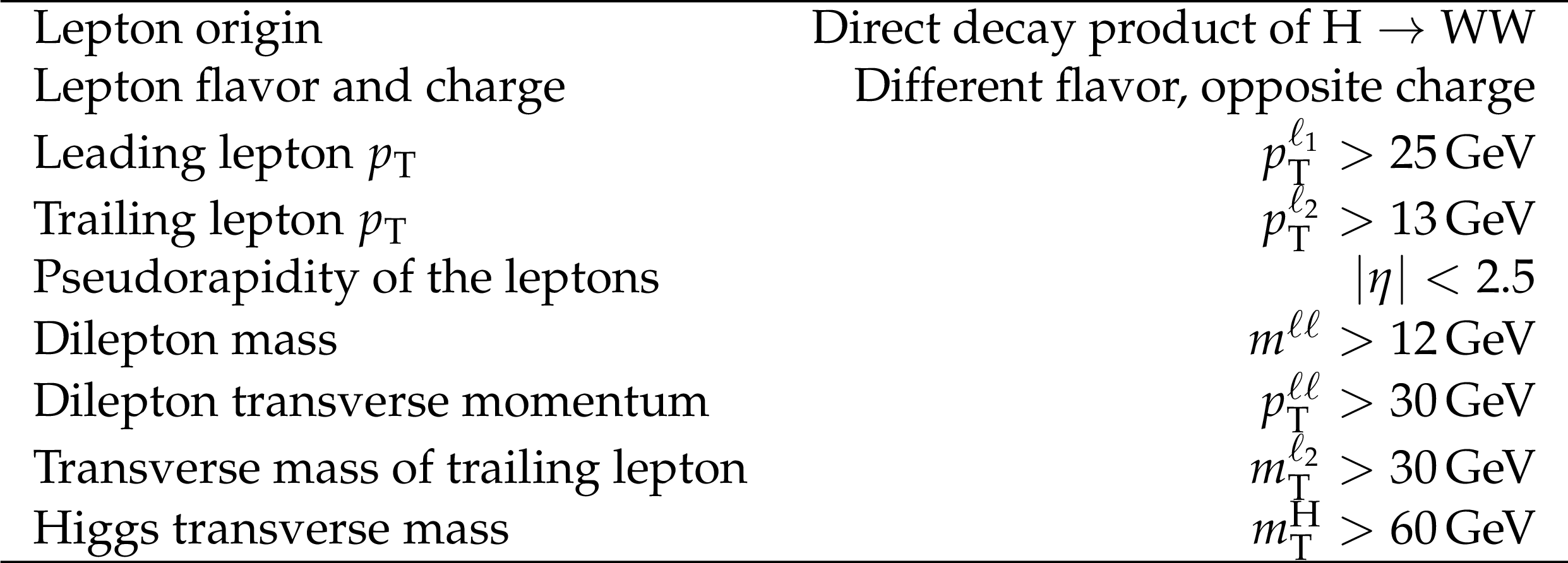
Table 1:
Selection criteria for the signal candidate events and the control samples. Preselection is the common criteria for all three selections. Observable ${{p_{\mathrm {T}}} ^{\ell _{1}}}$ is the magnitude of the transverse momentum of the leading lepton. See text for the definitions of the other observables in the table. |
png pdf |
Table 2:
Fiducial region definition. |
png pdf |
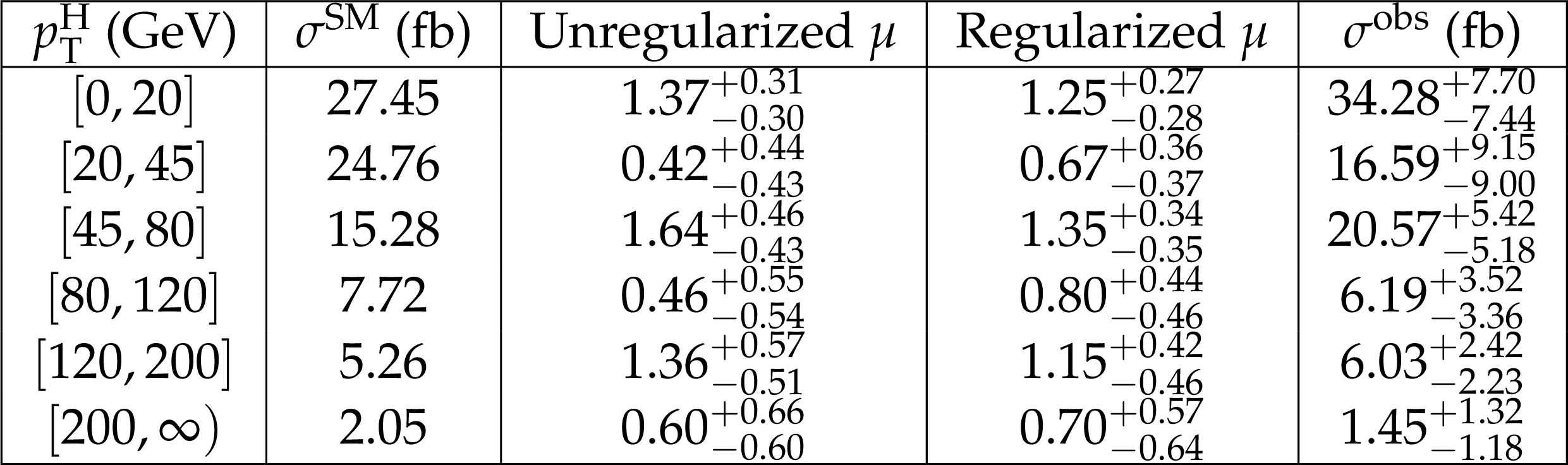
Table 3:
Observed signal strength modifiers and resulting differential cross sections in fiducial ${{p_{\mathrm {T}}} ^{\mathrm{H}}}$ bins. The cross section values are the products of ${\sigma ^{\text {SM}}}$ and the regularized $\mu $. |
png pdf |
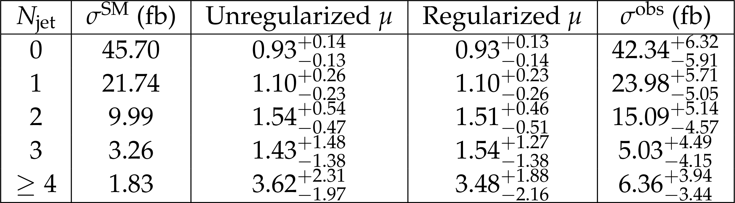
Table 4:
Observed signal strength modifiers and resulting differential cross sections in fiducial ${N_{\text {jet}}}$ bins. The cross section values are the products of ${\sigma ^{\text {SM}}}$ and the regularized $\mu $. |
| Summary |
| Differential and integrated fiducial cross sections for the Higgs boson production have been measured using the ${\mathrm{H}\to\mathrm{W}{}\mathrm{W}\to\mathrm{e}\nu\mu\nu}$ decay. The measurements have been performed with pp collision data sets recorded by the CMS detector at a center-of-mass energy of 13 TeV in 2016, 2017, and 2018, corresponding to a total integrated luminosity of 137 fb$^{-1}$. Differential cross sections with respect to the Higgs boson transverse momentum and the number of jets produced in association are considered, in a fiducial phase space defined to match the experimental kinematic acceptance. The cross sections are extracted through a simultaneous template fit to kinematic distributions of the signal candidate events finely categorized to maximize the sensitivity to Higgs boson production. The measurements are compared to SM theoretical calculations using POWHEG and MadGraph5+MCatNLO generators. The integrated fiducial cross section is measured to be 85.0$^{+9.9}_{-9.3}$ fb, consistent with the SM expectation. |
| References | ||||
| 1 | ATLAS Collaboration | Observation of a new particle in the search for the Standard Model Higgs boson with the ATLAS detector at the LHC | PLB 716 (2012) 1 | 1207.7214 |
| 2 | CMS Collaboration | Observation of a new boson at a mass of 125 GeV with the CMS experiment at the LHC | PLB 716 (2012) 30 | CMS-HIG-12-028 1207.7235 |
| 3 | CMS Collaboration | Observation of a New Boson with Mass Near 125 GeV in $ pp $ Collisions at $ \sqrt{s} = $ 7 and 8 TeV | JHEP 06 (2013) 081 | CMS-HIG-12-036 1303.4571 |
| 4 | F. Bishara, U. Haisch, P. F. Monni, and E. Re | Constraining Light-Quark Yukawa Couplings from Higgs Distributions | PRL 118 (2017) 121801 | 1606.09253 |
| 5 | ATLAS Collaboration | Measurements of Higgs boson properties in the diphoton decay channel using 80 fb$ ^{-1} $ of $ pp $ collision data at $ \sqrt {s} = $ 13 TeV with the ATLAS detector | ATLAS Conf ATLAS-CONF-2018-028 | |
| 6 | CMS Collaboration | Measurement and interpretation of differential cross sections for Higgs boson production at $ \sqrt{s}= $ 13 TeV | PLB 792 (2019) 369 | CMS-HIG-17-028 1812.06504 |
| 7 | ATLAS Collaboration | Measurement of fiducial differential cross sections of gluon-fusion production of Higgs bosons decaying to WW$ ^{*}\rightarrow\mathrm{e}\nu\mu\nu $ with the ATLAS detector at $ \sqrt{s}= $ 8 TeV | JHEP 08 (2016) 104 | 1604.02997 |
| 8 | CMS Collaboration | Measurement of the transverse momentum spectrum of the Higgs boson produced in pp collisions at $ \sqrt{s}= $ 8 TeV using $ H \to WW $ decays | JHEP 03 (2017) 032 | CMS-HIG-15-010 1606.01522 |
| 9 | ATLAS Collaboration | Measurements of gluon-gluon fusion and vector-boson fusion Higgs boson production cross-sections in the $ H \to WW^{\ast} \to e\nu\mu\nu $ decay channel in $ pp $ collisions at $ \sqrt{s}= $ 13 TeV with the ATLAS detector | PLB 789 (2019) 508 | 1808.09054 |
| 10 | CMS Collaboration | Measurements of properties of the Higgs boson decaying to a W boson pair in pp collisions at $ \sqrt{s}= $ 13 TeV | PLB 791 (2019) 96 | CMS-HIG-16-042 1806.05246 |
| 11 | CMS Collaboration | Measurement of Higgs boson production and properties in the WW decay channel with leptonic final states | JHEP 01 (2014) 096 | CMS-HIG-13-023 1312.1129 |
| 12 | CMS Collaboration | Performance of electron reconstruction and selection with the CMS detector in proton-proton collisions at $ \sqrt{s} = $ 8 TeV | JINST 10 (2015) P06005 | CMS-EGM-13-001 1502.02701 |
| 13 | CMS Collaboration | Performance of the CMS muon detector and muon reconstruction with proton-proton collisions at $ \sqrt{s}= $ 13 TeV | JINST 13 (2018) P06015 | CMS-MUO-16-001 1804.04528 |
| 14 | CMS Collaboration | Particle-flow reconstruction and global event description with the cms detector | JINST 12 (2017) P10003 | CMS-PRF-14-001 1706.04965 |
| 15 | M. Cacciari and G. P. Salam | Dispelling the $ N^{3} $ myth for the $ k_t $ jet-finder | PLB 641 (2006) 57 | hep-ph/0512210 |
| 16 | M. Cacciari, G. P. Salam, and G. Soyez | The anti-$ {k_{\mathrm{T}}} $ jet clustering algorithm | JHEP 04 (2008) 063 | 0802.1189 |
| 17 | M. Cacciari, G. P. Salam, and G. Soyez | FastJet user manual | EPJC 72 (2012) 1896 | 1111.6097 |
| 18 | CMS Collaboration | Jet energy scale and resolution in the CMS experiment in pp collisions at 8 TeV | JINST 12 (2017) P02014 | CMS-JME-13-004 1607.03663 |
| 19 | CMS Collaboration | Pileup mitigation at CMS in 13 TeV data | CMS-PAS-JME-18-001 | CMS-PAS-JME-18-001 |
| 20 | CMS Collaboration | The CMS trigger system | JINST 12 (2017) P01020 | CMS-TRG-12-001 1609.02366 |
| 21 | CMS Collaboration | The CMS experiment at the CERN LHC | JINST 3 (2008) S08004 | CMS-00-001 |
| 22 | CMS Collaboration | CMS luminosity measurements for the 2016 data-taking period | CMS-PAS-LUM-17-001 | CMS-PAS-LUM-17-001 |
| 23 | CMS Collaboration | CMS luminosity measurement for the 2017 data-taking period at $ \sqrt{s} = $ 13 TeV | CMS-PAS-LUM-17-004 | CMS-PAS-LUM-17-004 |
| 24 | CMS Collaboration | CMS luminosity measurement for the 2018 data-taking period at $ \sqrt{s} = $ 13 TeV | CMS-PAS-LUM-18-002 | CMS-PAS-LUM-18-002 |
| 25 | T. Sjostrand et al. | An Introduction to PYTHIA 8.2 | CPC 191 (2015) 159 | 1410.3012 |
| 26 | NNPDF Collaboration | Parton distributions with QED corrections | NPB 877 (2013) 290 | 1308.0598 |
| 27 | NNPDF Collaboration | Unbiased global determination of parton distributions and their uncertainties at NNLO and at LO | NPB 855 (2012) 153 | 1107.2652 |
| 28 | CMS Collaboration | Event generator tunes obtained from underlying event and multiparton scattering measurements | EPJC 76 (2016) 155 | CMS-GEN-14-001 1512.00815 |
| 29 | NNPDF Collaboration | Parton distributions from high-precision collider data | EPJC 77 (2017) 663 | 1706.00428 |
| 30 | CMS Collaboration | Extraction and validation of a new set of CMS PYTHIA8 tunes from underlying-event measurements | Submitted to EPJC | CMS-GEN-17-001 1903.12179 |
| 31 | P. Nason | A New method for combining NLO QCD with shower Monte Carlo algorithms | JHEP 11 (2004) 040 | hep-ph/0409146 |
| 32 | S. Frixione, P. Nason, and C. Oleari | Matching NLO QCD computations with Parton Shower simulations: the POWHEG method | JHEP 11 (2007) 070 | 0709.2092 |
| 33 | S. Alioli, P. Nason, C. Oleari, and E. Re | A general framework for implementing NLO calculations in shower Monte Carlo programs: the POWHEG BOX | JHEP 06 (2010) 043 | 1002.2581 |
| 34 | K. Hamilton, P. Nason, and G. Zanderighi | Finite quark-mass effects in the NNLOPS POWHEG+MiNLO Higgs generator | JHEP 05 (2015) 140 | 1501.04637 |
| 35 | S. Bolognesi et al. | On the spin and parity of a single-produced resonance at the LHC | PRD 86 (2012) 095031 | 1208.4018 |
| 36 | J. Alwall et al. | The automated computation of tree-level and next-to-leading order differential cross sections, and their matching to parton shower simulations | JHEP 07 (2014) 079 | 1405.0301 |
| 37 | J. M. Campbell and R. K. Ellis | An Update on vector boson pair production at hadron colliders | PRD 60 (1999) 113006 | hep-ph/9905386 |
| 38 | J. M. Campbell, R. K. Ellis, and C. Williams | Vector boson pair production at the LHC | JHEP 07 (2011) 018 | 1105.0020 |
| 39 | J. M. Campbell, R. K. Ellis, and W. T. Giele | A Multi-Threaded Version of MCFM | EPJC 75 (2015) 246 | 1503.06182 |
| 40 | GEANT4 Collaboration | GEANT4--a simulation toolkit | NIMA 506 (2003) 250 | |
| 41 | P. Meade, H. Ramani, and M. Zeng | Transverse momentum resummation effects in $ W^+W^- $ measurements | PRD 90 (2014) 114006 | 1407.4481 |
| 42 | P. Jaiswal and T. Okui | Explanation of the $ WW $ excess at the LHC by jet-veto resummation | PRD 90 (2014) 073009 | 1407.4537 |
| 43 | S. Schmitt | TUnfold: an algorithm for correcting migration effects in high energy physics | JINST 7 (2012) T10003 | 1205.6201 |
| 44 | LHC Higgs Cross Section Working Group Collaboration | Handbook of LHC Higgs Cross Sections: 4. Deciphering the Nature of the Higgs Sector | 1610.07922 | |
| 45 | G. Passarino | Higgs CAT | EPJC 74 (2014) 2866 | 1312.2397 |
| 46 | S. Forte et al. | Gluon-gluon fusion | LHCHXSWG-DRAFT-INT-2016-011, Jun | |
| 47 | M. Bahr et al. | Herwig++ Physics and Manual | EPJC 58 (2008) 639 | 0803.0883 |
| 48 | J. Bellm et al. | Herwig 7.0/Herwig++ 3.0 release note | EPJC 76 (2016) 196 | 1512.01178 |
|
|
Compact Muon Solenoid LHC, CERN |
|

|

|

|

|

|