

Compact Muon Solenoid
LHC, CERN
| CMS-PAS-EXO-21-018 | ||
| Search for dilepton resonances from decays of (pseudo)scalar bosons produced in association with a massive vector boson or top quark anti-top quark pair at $\sqrt{s}= $ 13 TeV | ||
| CMS Collaboration | ||
| July 2022 | ||
| Abstract: A search for beyond the standard model scalar and pseudoscalar bosons that decay into pairs of electrons, muons, or tau leptons is presented. The search probes such new bosons that are produced in association with a W or Z boson, or a top quark anti-top quark pair, in events with with three or four leptons, including hadronic decays of tau leptons. The proton-proton collision dataset used in the analysis is collected by the CMS experiment at the LHC in 2016-2018 at a center-of-mass energy of 13 TeV, and corresponds to an integrated luminosity of 138 fb$^{-1}$. The observations are consistent with the expectations from standard model processes. Upper limits at 95% confidence level are placed on the product of cross section and branching fraction of such new particles with scalar, pseudoscalar, or Higgs-like couplings. Considering a single production, coupling, and decay scenario at a time, the observations exclude product of cross section and branching fraction values above 50-0.5 fb, 30-0.5 fb and 200-1 fb for new scalar, pseudoscalar, and Higgs-like bosons, respectively, that have a mass in the range 15-350 GeV and exclusively decay into dielectron or dimuon pairs. Similarly, assuming such new bosons exclusively decay into pairs of tau leptons, the product of cross section and branching fraction values above 35-0.004 pb, 80-0.004 pb, and 250-0.008 pb are excluded for scalar, pseudoscalar, and Higgs-like couplings, respectively. These are the most restrictive direct limits in these production and decay modes on an extension of the standard model with scalar or pseudoscalar particles. | ||
|
Links:
CDS record (PDF) ;
CADI line (restricted) ;
These preliminary results are superseded in this paper, Submitted to PRD. The superseded preliminary plots can be found here. |
||
| Figures | |

png pdf |
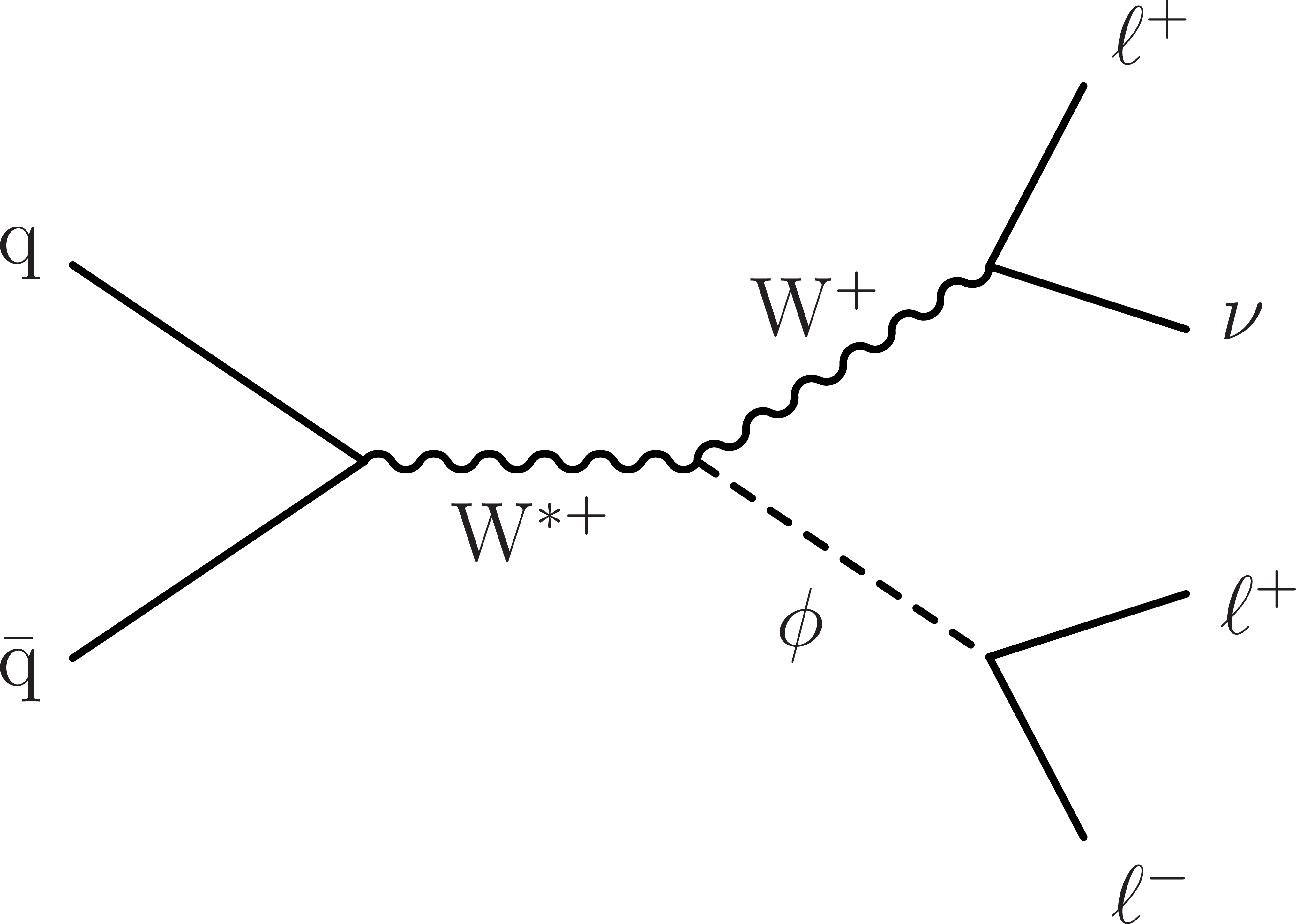
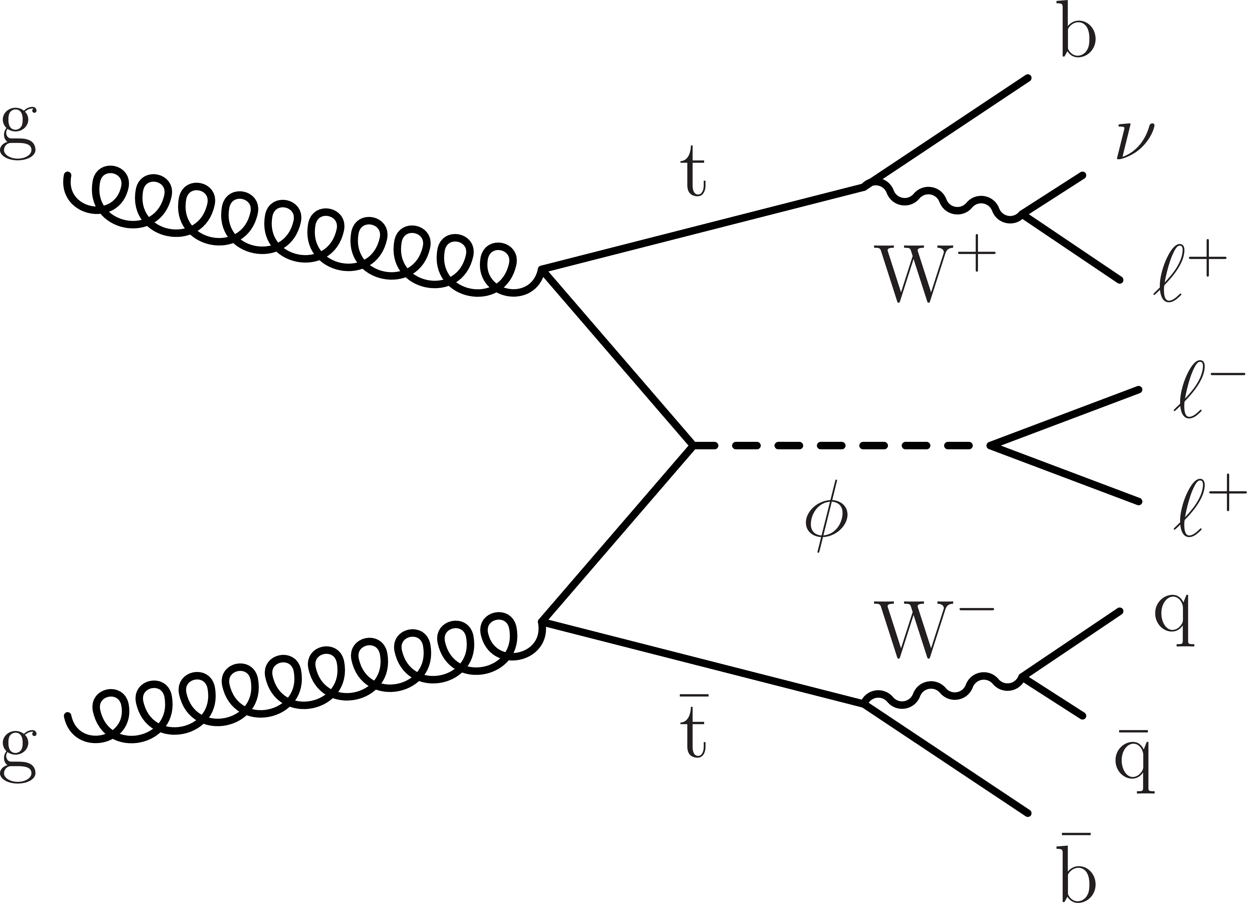
Figure 1:
Example production and decay diagrams for W$\phi$, Z$\phi$, and $ {{\mathrm{t} {}\mathrm{\bar{t}}} \phi}$ signal models, producing multilepton final states. |
png pdf |
Figure 1-a:
Example production and decay diagrams for W$\phi$, Z$\phi$, and $ {{\mathrm{t} {}\mathrm{\bar{t}}} \phi}$ signal models, producing multilepton final states. |

png pdf |
Figure 1-b:
Example production and decay diagrams for W$\phi$, Z$\phi$, and $ {{\mathrm{t} {}\mathrm{\bar{t}}} \phi}$ signal models, producing multilepton final states. |
png pdf |
Figure 1-c:
Example production and decay diagrams for W$\phi$, Z$\phi$, and $ {{\mathrm{t} {}\mathrm{\bar{t}}} \phi}$ signal models, producing multilepton final states. |
png pdf |
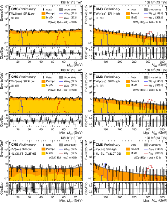
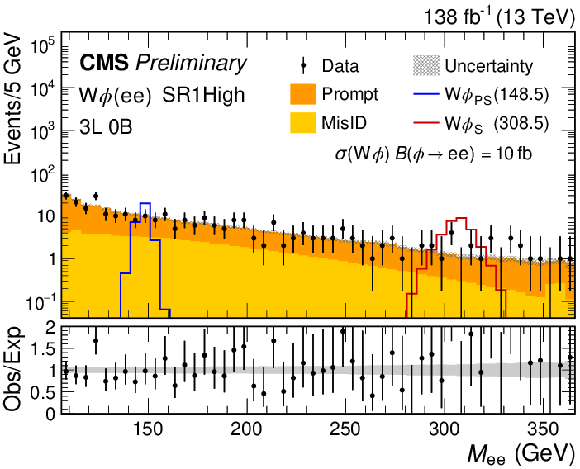
Figure 2:
Dilepton mass spectra for the $ {{\mathrm{W}}\phi}(\mathrm{e} \mathrm{e})$ SR1 (upper) and SR2 (center) and $ {{\mathrm{Z}}\phi}(\mathrm{e} \mathrm{e})$ SR (lower) event selections for the combined 2016-2018 data set. The lower panel shows the ratio of observed events to the total expected SM background prediction, and the gray band represents the sum of statistical and systematic uncertainties in the background prediction. The expected background distributions and the uncertainties are shown after fitting the data under the background-only hypothesis. For illustration, two example signal hypotheses for the production and decay of a scalar and a pseudoscalar $\phi $ boson are shown, and their masses are indicated in the legend. |

png pdf |
Figure 2-a:
Dilepton mass spectra for the $ {{\mathrm{W}}\phi}(\mathrm{e} \mathrm{e})$ SR1 (upper) and SR2 (center) and $ {{\mathrm{Z}}\phi}(\mathrm{e} \mathrm{e})$ SR (lower) event selections for the combined 2016-2018 data set. The lower panel shows the ratio of observed events to the total expected SM background prediction, and the gray band represents the sum of statistical and systematic uncertainties in the background prediction. The expected background distributions and the uncertainties are shown after fitting the data under the background-only hypothesis. For illustration, two example signal hypotheses for the production and decay of a scalar and a pseudoscalar $\phi $ boson are shown, and their masses are indicated in the legend. |
png pdf |
Figure 2-b:
Dilepton mass spectra for the $ {{\mathrm{W}}\phi}(\mathrm{e} \mathrm{e})$ SR1 (upper) and SR2 (center) and $ {{\mathrm{Z}}\phi}(\mathrm{e} \mathrm{e})$ SR (lower) event selections for the combined 2016-2018 data set. The lower panel shows the ratio of observed events to the total expected SM background prediction, and the gray band represents the sum of statistical and systematic uncertainties in the background prediction. The expected background distributions and the uncertainties are shown after fitting the data under the background-only hypothesis. For illustration, two example signal hypotheses for the production and decay of a scalar and a pseudoscalar $\phi $ boson are shown, and their masses are indicated in the legend. |
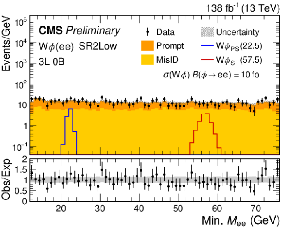
png pdf |
Figure 2-c:
Dilepton mass spectra for the $ {{\mathrm{W}}\phi}(\mathrm{e} \mathrm{e})$ SR1 (upper) and SR2 (center) and $ {{\mathrm{Z}}\phi}(\mathrm{e} \mathrm{e})$ SR (lower) event selections for the combined 2016-2018 data set. The lower panel shows the ratio of observed events to the total expected SM background prediction, and the gray band represents the sum of statistical and systematic uncertainties in the background prediction. The expected background distributions and the uncertainties are shown after fitting the data under the background-only hypothesis. For illustration, two example signal hypotheses for the production and decay of a scalar and a pseudoscalar $\phi $ boson are shown, and their masses are indicated in the legend. |
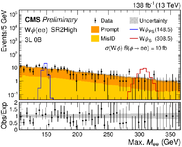
png pdf |
Figure 2-d:
Dilepton mass spectra for the $ {{\mathrm{W}}\phi}(\mathrm{e} \mathrm{e})$ SR1 (upper) and SR2 (center) and $ {{\mathrm{Z}}\phi}(\mathrm{e} \mathrm{e})$ SR (lower) event selections for the combined 2016-2018 data set. The lower panel shows the ratio of observed events to the total expected SM background prediction, and the gray band represents the sum of statistical and systematic uncertainties in the background prediction. The expected background distributions and the uncertainties are shown after fitting the data under the background-only hypothesis. For illustration, two example signal hypotheses for the production and decay of a scalar and a pseudoscalar $\phi $ boson are shown, and their masses are indicated in the legend. |
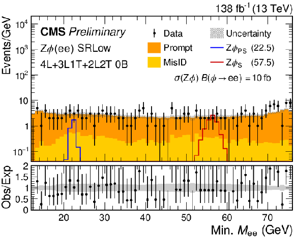
png pdf |
Figure 2-e:
Dilepton mass spectra for the $ {{\mathrm{W}}\phi}(\mathrm{e} \mathrm{e})$ SR1 (upper) and SR2 (center) and $ {{\mathrm{Z}}\phi}(\mathrm{e} \mathrm{e})$ SR (lower) event selections for the combined 2016-2018 data set. The lower panel shows the ratio of observed events to the total expected SM background prediction, and the gray band represents the sum of statistical and systematic uncertainties in the background prediction. The expected background distributions and the uncertainties are shown after fitting the data under the background-only hypothesis. For illustration, two example signal hypotheses for the production and decay of a scalar and a pseudoscalar $\phi $ boson are shown, and their masses are indicated in the legend. |
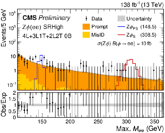
png pdf |
Figure 2-f:
Dilepton mass spectra for the $ {{\mathrm{W}}\phi}(\mathrm{e} \mathrm{e})$ SR1 (upper) and SR2 (center) and $ {{\mathrm{Z}}\phi}(\mathrm{e} \mathrm{e})$ SR (lower) event selections for the combined 2016-2018 data set. The lower panel shows the ratio of observed events to the total expected SM background prediction, and the gray band represents the sum of statistical and systematic uncertainties in the background prediction. The expected background distributions and the uncertainties are shown after fitting the data under the background-only hypothesis. For illustration, two example signal hypotheses for the production and decay of a scalar and a pseudoscalar $\phi $ boson are shown, and their masses are indicated in the legend. |
png pdf |
Figure 3:
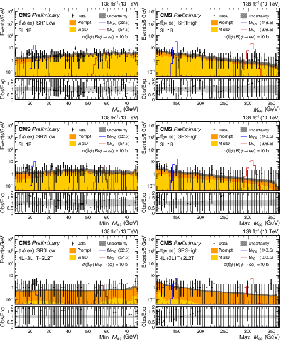
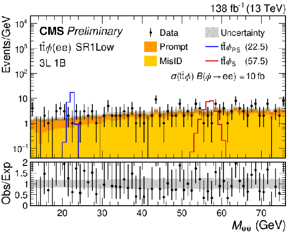
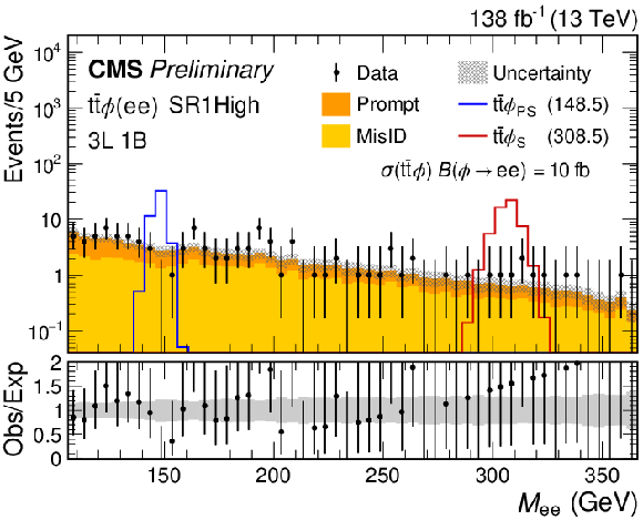
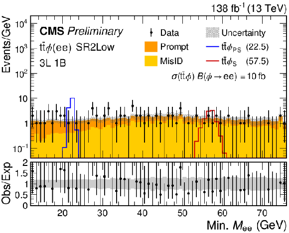
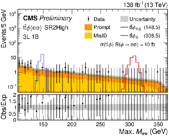
Dilepton mass spectra for the $ {{\mathrm{t} {}\mathrm{\bar{t}}} \phi}(\mathrm{e} \mathrm{e})$ SR1 (upper) and SR2 (center) and SR3 (lower) event selections for the combined 2016-2018 data set. The lower panel shows the ratio of observed events to the total expected SM background prediction, and the gray band represents the sum of statistical and systematic uncertainties in the background prediction. The expected background distributions and the uncertainties are shown after fitting the data under the background-only hypothesis. For illustration, two example signal hypotheses for the production and decay of a scalar and a pseudoscalar $\phi $ boson are shown, and their masses are indicated in the legend. |
png pdf |
Figure 3-a:
Dilepton mass spectra for the $ {{\mathrm{t} {}\mathrm{\bar{t}}} \phi}(\mathrm{e} \mathrm{e})$ SR1 (upper) and SR2 (center) and SR3 (lower) event selections for the combined 2016-2018 data set. The lower panel shows the ratio of observed events to the total expected SM background prediction, and the gray band represents the sum of statistical and systematic uncertainties in the background prediction. The expected background distributions and the uncertainties are shown after fitting the data under the background-only hypothesis. For illustration, two example signal hypotheses for the production and decay of a scalar and a pseudoscalar $\phi $ boson are shown, and their masses are indicated in the legend. |
png pdf |
Figure 3-b:
Dilepton mass spectra for the $ {{\mathrm{t} {}\mathrm{\bar{t}}} \phi}(\mathrm{e} \mathrm{e})$ SR1 (upper) and SR2 (center) and SR3 (lower) event selections for the combined 2016-2018 data set. The lower panel shows the ratio of observed events to the total expected SM background prediction, and the gray band represents the sum of statistical and systematic uncertainties in the background prediction. The expected background distributions and the uncertainties are shown after fitting the data under the background-only hypothesis. For illustration, two example signal hypotheses for the production and decay of a scalar and a pseudoscalar $\phi $ boson are shown, and their masses are indicated in the legend. |
png pdf |
Figure 3-c:
Dilepton mass spectra for the $ {{\mathrm{t} {}\mathrm{\bar{t}}} \phi}(\mathrm{e} \mathrm{e})$ SR1 (upper) and SR2 (center) and SR3 (lower) event selections for the combined 2016-2018 data set. The lower panel shows the ratio of observed events to the total expected SM background prediction, and the gray band represents the sum of statistical and systematic uncertainties in the background prediction. The expected background distributions and the uncertainties are shown after fitting the data under the background-only hypothesis. For illustration, two example signal hypotheses for the production and decay of a scalar and a pseudoscalar $\phi $ boson are shown, and their masses are indicated in the legend. |
png pdf |
Figure 3-d:
Dilepton mass spectra for the $ {{\mathrm{t} {}\mathrm{\bar{t}}} \phi}(\mathrm{e} \mathrm{e})$ SR1 (upper) and SR2 (center) and SR3 (lower) event selections for the combined 2016-2018 data set. The lower panel shows the ratio of observed events to the total expected SM background prediction, and the gray band represents the sum of statistical and systematic uncertainties in the background prediction. The expected background distributions and the uncertainties are shown after fitting the data under the background-only hypothesis. For illustration, two example signal hypotheses for the production and decay of a scalar and a pseudoscalar $\phi $ boson are shown, and their masses are indicated in the legend. |
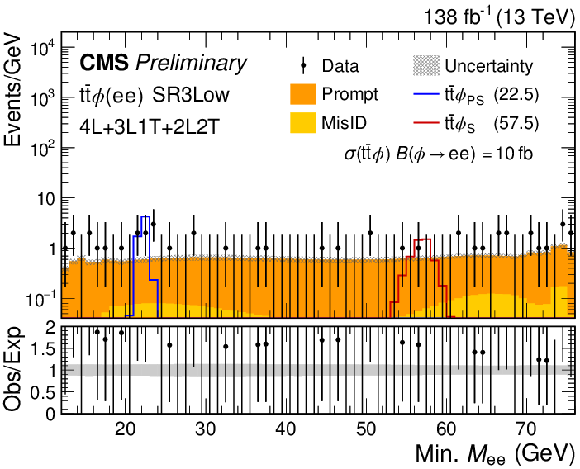
png pdf |
Figure 3-e:
Dilepton mass spectra for the $ {{\mathrm{t} {}\mathrm{\bar{t}}} \phi}(\mathrm{e} \mathrm{e})$ SR1 (upper) and SR2 (center) and SR3 (lower) event selections for the combined 2016-2018 data set. The lower panel shows the ratio of observed events to the total expected SM background prediction, and the gray band represents the sum of statistical and systematic uncertainties in the background prediction. The expected background distributions and the uncertainties are shown after fitting the data under the background-only hypothesis. For illustration, two example signal hypotheses for the production and decay of a scalar and a pseudoscalar $\phi $ boson are shown, and their masses are indicated in the legend. |
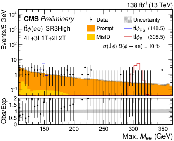
png pdf |
Figure 3-f:
Dilepton mass spectra for the $ {{\mathrm{t} {}\mathrm{\bar{t}}} \phi}(\mathrm{e} \mathrm{e})$ SR1 (upper) and SR2 (center) and SR3 (lower) event selections for the combined 2016-2018 data set. The lower panel shows the ratio of observed events to the total expected SM background prediction, and the gray band represents the sum of statistical and systematic uncertainties in the background prediction. The expected background distributions and the uncertainties are shown after fitting the data under the background-only hypothesis. For illustration, two example signal hypotheses for the production and decay of a scalar and a pseudoscalar $\phi $ boson are shown, and their masses are indicated in the legend. |
png pdf |
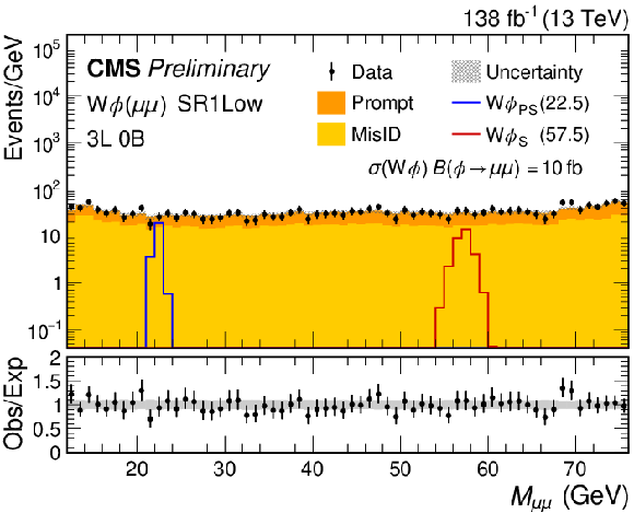
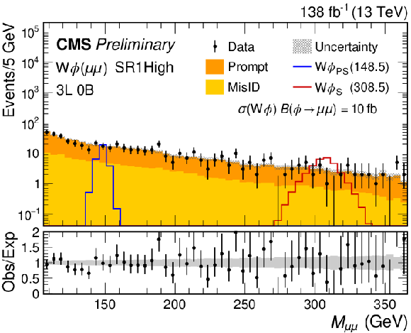
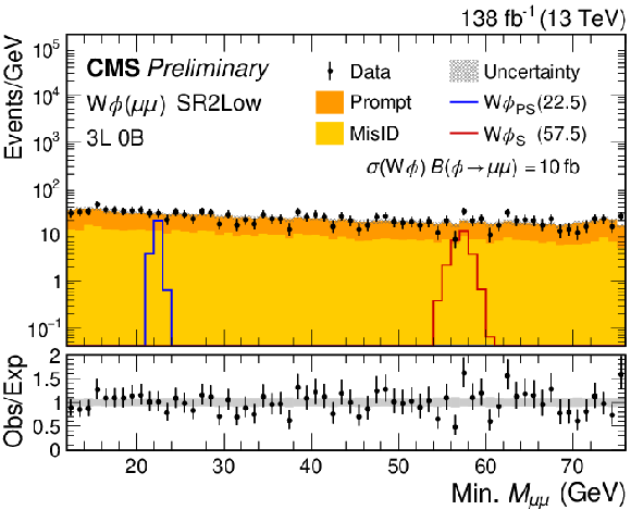
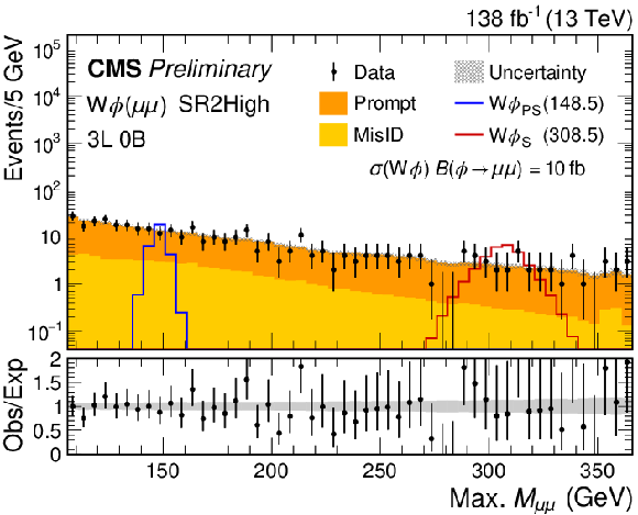
Figure 4:
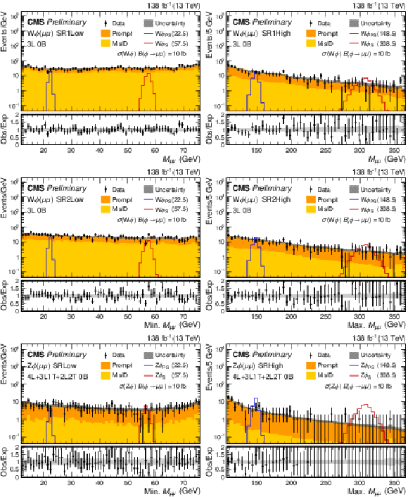
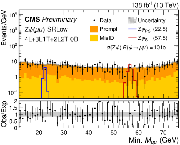
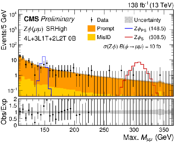
Dilepton mass spectra for the $ {{\mathrm{W}}\phi}(\mu \mu)$ SR1 (upper) and SR2 (center) and $ {{\mathrm{Z}}\phi}(\mu \mu)$ SR (lower) event selections for the combined 2016-2018 data set. The lower panel shows the ratio of observed events to the total expected SM background prediction, and the gray band represents the sum of statistical and systematic uncertainties in the background prediction. The expected background distributions and the uncertainties are shown after fitting the data under the background-only hypothesis. For illustration, two example signal hypotheses for the production and decay of a scalar and a pseudoscalar $\phi $ boson are shown, and their masses are indicated in the legend. |
png pdf |
Figure 4-a:
Dilepton mass spectra for the $ {{\mathrm{W}}\phi}(\mu \mu)$ SR1 (upper) and SR2 (center) and $ {{\mathrm{Z}}\phi}(\mu \mu)$ SR (lower) event selections for the combined 2016-2018 data set. The lower panel shows the ratio of observed events to the total expected SM background prediction, and the gray band represents the sum of statistical and systematic uncertainties in the background prediction. The expected background distributions and the uncertainties are shown after fitting the data under the background-only hypothesis. For illustration, two example signal hypotheses for the production and decay of a scalar and a pseudoscalar $\phi $ boson are shown, and their masses are indicated in the legend. |
png pdf |
Figure 4-b:
Dilepton mass spectra for the $ {{\mathrm{W}}\phi}(\mu \mu)$ SR1 (upper) and SR2 (center) and $ {{\mathrm{Z}}\phi}(\mu \mu)$ SR (lower) event selections for the combined 2016-2018 data set. The lower panel shows the ratio of observed events to the total expected SM background prediction, and the gray band represents the sum of statistical and systematic uncertainties in the background prediction. The expected background distributions and the uncertainties are shown after fitting the data under the background-only hypothesis. For illustration, two example signal hypotheses for the production and decay of a scalar and a pseudoscalar $\phi $ boson are shown, and their masses are indicated in the legend. |
png pdf |
Figure 4-c:
Dilepton mass spectra for the $ {{\mathrm{W}}\phi}(\mu \mu)$ SR1 (upper) and SR2 (center) and $ {{\mathrm{Z}}\phi}(\mu \mu)$ SR (lower) event selections for the combined 2016-2018 data set. The lower panel shows the ratio of observed events to the total expected SM background prediction, and the gray band represents the sum of statistical and systematic uncertainties in the background prediction. The expected background distributions and the uncertainties are shown after fitting the data under the background-only hypothesis. For illustration, two example signal hypotheses for the production and decay of a scalar and a pseudoscalar $\phi $ boson are shown, and their masses are indicated in the legend. |
png pdf |
Figure 4-d:
Dilepton mass spectra for the $ {{\mathrm{W}}\phi}(\mu \mu)$ SR1 (upper) and SR2 (center) and $ {{\mathrm{Z}}\phi}(\mu \mu)$ SR (lower) event selections for the combined 2016-2018 data set. The lower panel shows the ratio of observed events to the total expected SM background prediction, and the gray band represents the sum of statistical and systematic uncertainties in the background prediction. The expected background distributions and the uncertainties are shown after fitting the data under the background-only hypothesis. For illustration, two example signal hypotheses for the production and decay of a scalar and a pseudoscalar $\phi $ boson are shown, and their masses are indicated in the legend. |
png pdf |
Figure 4-e:
Dilepton mass spectra for the $ {{\mathrm{W}}\phi}(\mu \mu)$ SR1 (upper) and SR2 (center) and $ {{\mathrm{Z}}\phi}(\mu \mu)$ SR (lower) event selections for the combined 2016-2018 data set. The lower panel shows the ratio of observed events to the total expected SM background prediction, and the gray band represents the sum of statistical and systematic uncertainties in the background prediction. The expected background distributions and the uncertainties are shown after fitting the data under the background-only hypothesis. For illustration, two example signal hypotheses for the production and decay of a scalar and a pseudoscalar $\phi $ boson are shown, and their masses are indicated in the legend. |
png pdf |
Figure 4-f:
Dilepton mass spectra for the $ {{\mathrm{W}}\phi}(\mu \mu)$ SR1 (upper) and SR2 (center) and $ {{\mathrm{Z}}\phi}(\mu \mu)$ SR (lower) event selections for the combined 2016-2018 data set. The lower panel shows the ratio of observed events to the total expected SM background prediction, and the gray band represents the sum of statistical and systematic uncertainties in the background prediction. The expected background distributions and the uncertainties are shown after fitting the data under the background-only hypothesis. For illustration, two example signal hypotheses for the production and decay of a scalar and a pseudoscalar $\phi $ boson are shown, and their masses are indicated in the legend. |
png pdf |
Figure 5:
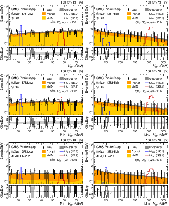
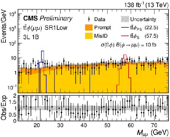
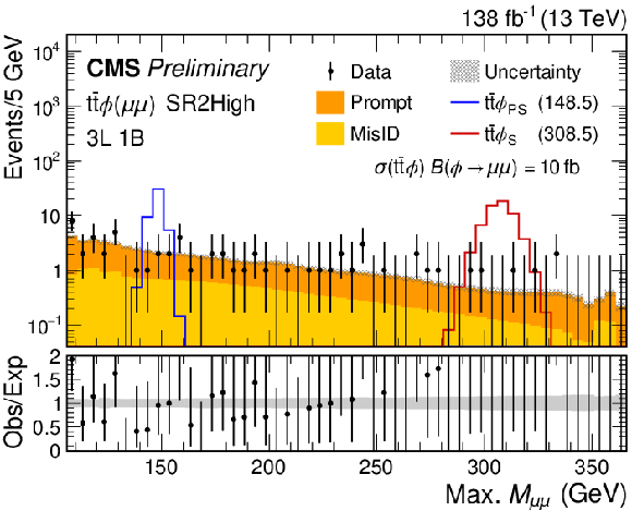
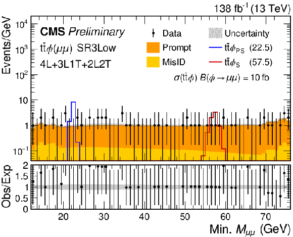
Dilepton mass spectra for the $ {{\mathrm{t} {}\mathrm{\bar{t}}} \phi}(\mu \mu)$ SR1 (upper) and SR2 (center) and SR3 (lower) event selections for the combined 2016-2018 data set. The lower panel shows the ratio of observed events to the total expected SM background prediction, and the gray band represents the sum of statistical and systematic uncertainties in the background prediction. The expected background distributions and the uncertainties are shown after fitting the data under the background-only hypothesis. For illustration, two example signal hypotheses for the production and decay of a scalar and a pseudoscalar $\phi $ boson are shown, and their masses are indicated in the legend. |
png pdf |
Figure 5-a:
Dilepton mass spectra for the $ {{\mathrm{t} {}\mathrm{\bar{t}}} \phi}(\mu \mu)$ SR1 (upper) and SR2 (center) and SR3 (lower) event selections for the combined 2016-2018 data set. The lower panel shows the ratio of observed events to the total expected SM background prediction, and the gray band represents the sum of statistical and systematic uncertainties in the background prediction. The expected background distributions and the uncertainties are shown after fitting the data under the background-only hypothesis. For illustration, two example signal hypotheses for the production and decay of a scalar and a pseudoscalar $\phi $ boson are shown, and their masses are indicated in the legend. |

png pdf |
Figure 5-b:
Dilepton mass spectra for the $ {{\mathrm{t} {}\mathrm{\bar{t}}} \phi}(\mu \mu)$ SR1 (upper) and SR2 (center) and SR3 (lower) event selections for the combined 2016-2018 data set. The lower panel shows the ratio of observed events to the total expected SM background prediction, and the gray band represents the sum of statistical and systematic uncertainties in the background prediction. The expected background distributions and the uncertainties are shown after fitting the data under the background-only hypothesis. For illustration, two example signal hypotheses for the production and decay of a scalar and a pseudoscalar $\phi $ boson are shown, and their masses are indicated in the legend. |

png pdf |
Figure 5-c:
Dilepton mass spectra for the $ {{\mathrm{t} {}\mathrm{\bar{t}}} \phi}(\mu \mu)$ SR1 (upper) and SR2 (center) and SR3 (lower) event selections for the combined 2016-2018 data set. The lower panel shows the ratio of observed events to the total expected SM background prediction, and the gray band represents the sum of statistical and systematic uncertainties in the background prediction. The expected background distributions and the uncertainties are shown after fitting the data under the background-only hypothesis. For illustration, two example signal hypotheses for the production and decay of a scalar and a pseudoscalar $\phi $ boson are shown, and their masses are indicated in the legend. |
png pdf |
Figure 5-d:
Dilepton mass spectra for the $ {{\mathrm{t} {}\mathrm{\bar{t}}} \phi}(\mu \mu)$ SR1 (upper) and SR2 (center) and SR3 (lower) event selections for the combined 2016-2018 data set. The lower panel shows the ratio of observed events to the total expected SM background prediction, and the gray band represents the sum of statistical and systematic uncertainties in the background prediction. The expected background distributions and the uncertainties are shown after fitting the data under the background-only hypothesis. For illustration, two example signal hypotheses for the production and decay of a scalar and a pseudoscalar $\phi $ boson are shown, and their masses are indicated in the legend. |
png pdf |
Figure 5-e:
Dilepton mass spectra for the $ {{\mathrm{t} {}\mathrm{\bar{t}}} \phi}(\mu \mu)$ SR1 (upper) and SR2 (center) and SR3 (lower) event selections for the combined 2016-2018 data set. The lower panel shows the ratio of observed events to the total expected SM background prediction, and the gray band represents the sum of statistical and systematic uncertainties in the background prediction. The expected background distributions and the uncertainties are shown after fitting the data under the background-only hypothesis. For illustration, two example signal hypotheses for the production and decay of a scalar and a pseudoscalar $\phi $ boson are shown, and their masses are indicated in the legend. |

png pdf |
Figure 5-f:
Dilepton mass spectra for the $ {{\mathrm{t} {}\mathrm{\bar{t}}} \phi}(\mu \mu)$ SR1 (upper) and SR2 (center) and SR3 (lower) event selections for the combined 2016-2018 data set. The lower panel shows the ratio of observed events to the total expected SM background prediction, and the gray band represents the sum of statistical and systematic uncertainties in the background prediction. The expected background distributions and the uncertainties are shown after fitting the data under the background-only hypothesis. For illustration, two example signal hypotheses for the production and decay of a scalar and a pseudoscalar $\phi $ boson are shown, and their masses are indicated in the legend. |
png pdf |
Figure 6:
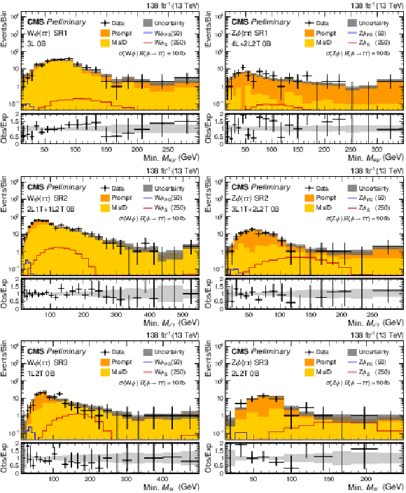
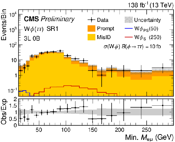
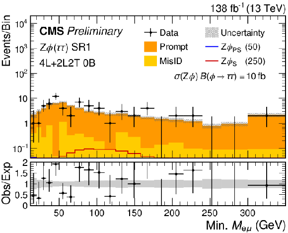
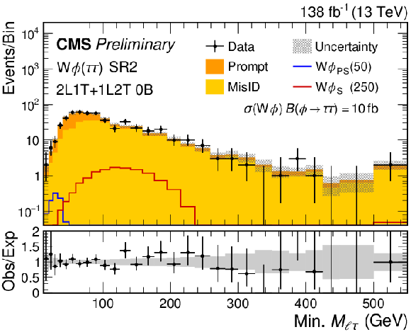
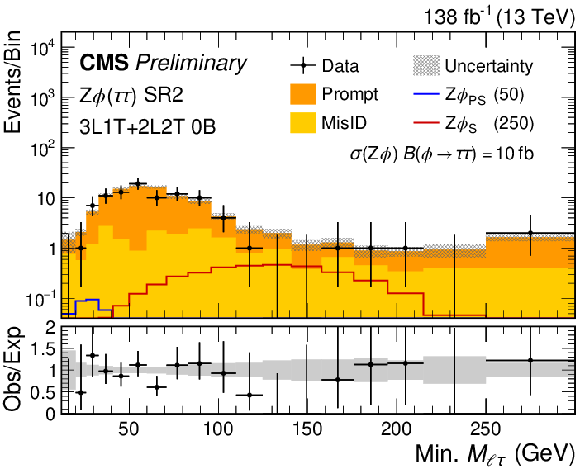
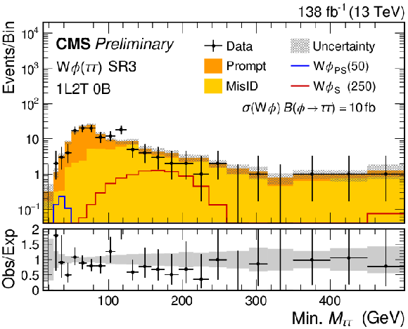
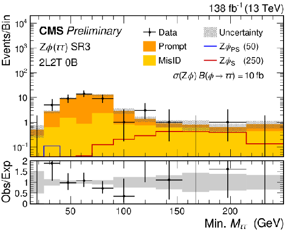
Dilepton mass spectra for the $ {{\mathrm{W}}\phi}(\tau \tau)$ SR (left) and $ {{\mathrm{Z}}\phi}(\tau \tau)$ SR (right) event selections for the combined 2016-2018 data set. The lower panel shows the ratio of observed events to the total expected SM background prediction, and the gray band represents the sum of statistical and systematic uncertainties in the background prediction. The expected background distributions and the uncertainties are shown after fitting the data under the background-only hypothesis. For illustration, two example signal hypotheses for the production and decay of a scalar and a pseudoscalar $\phi $ boson are shown, and their masses are indicated in the legend. |
png pdf |
Figure 6-a:
Dilepton mass spectra for the $ {{\mathrm{W}}\phi}(\tau \tau)$ SR (left) and $ {{\mathrm{Z}}\phi}(\tau \tau)$ SR (right) event selections for the combined 2016-2018 data set. The lower panel shows the ratio of observed events to the total expected SM background prediction, and the gray band represents the sum of statistical and systematic uncertainties in the background prediction. The expected background distributions and the uncertainties are shown after fitting the data under the background-only hypothesis. For illustration, two example signal hypotheses for the production and decay of a scalar and a pseudoscalar $\phi $ boson are shown, and their masses are indicated in the legend. |
png pdf |
Figure 6-b:
Dilepton mass spectra for the $ {{\mathrm{W}}\phi}(\tau \tau)$ SR (left) and $ {{\mathrm{Z}}\phi}(\tau \tau)$ SR (right) event selections for the combined 2016-2018 data set. The lower panel shows the ratio of observed events to the total expected SM background prediction, and the gray band represents the sum of statistical and systematic uncertainties in the background prediction. The expected background distributions and the uncertainties are shown after fitting the data under the background-only hypothesis. For illustration, two example signal hypotheses for the production and decay of a scalar and a pseudoscalar $\phi $ boson are shown, and their masses are indicated in the legend. |
png pdf |
Figure 6-c:
Dilepton mass spectra for the $ {{\mathrm{W}}\phi}(\tau \tau)$ SR (left) and $ {{\mathrm{Z}}\phi}(\tau \tau)$ SR (right) event selections for the combined 2016-2018 data set. The lower panel shows the ratio of observed events to the total expected SM background prediction, and the gray band represents the sum of statistical and systematic uncertainties in the background prediction. The expected background distributions and the uncertainties are shown after fitting the data under the background-only hypothesis. For illustration, two example signal hypotheses for the production and decay of a scalar and a pseudoscalar $\phi $ boson are shown, and their masses are indicated in the legend. |
png pdf |
Figure 6-d:
Dilepton mass spectra for the $ {{\mathrm{W}}\phi}(\tau \tau)$ SR (left) and $ {{\mathrm{Z}}\phi}(\tau \tau)$ SR (right) event selections for the combined 2016-2018 data set. The lower panel shows the ratio of observed events to the total expected SM background prediction, and the gray band represents the sum of statistical and systematic uncertainties in the background prediction. The expected background distributions and the uncertainties are shown after fitting the data under the background-only hypothesis. For illustration, two example signal hypotheses for the production and decay of a scalar and a pseudoscalar $\phi $ boson are shown, and their masses are indicated in the legend. |
png pdf |
Figure 6-e:
Dilepton mass spectra for the $ {{\mathrm{W}}\phi}(\tau \tau)$ SR (left) and $ {{\mathrm{Z}}\phi}(\tau \tau)$ SR (right) event selections for the combined 2016-2018 data set. The lower panel shows the ratio of observed events to the total expected SM background prediction, and the gray band represents the sum of statistical and systematic uncertainties in the background prediction. The expected background distributions and the uncertainties are shown after fitting the data under the background-only hypothesis. For illustration, two example signal hypotheses for the production and decay of a scalar and a pseudoscalar $\phi $ boson are shown, and their masses are indicated in the legend. |
png pdf |
Figure 6-f:
Dilepton mass spectra for the $ {{\mathrm{W}}\phi}(\tau \tau)$ SR (left) and $ {{\mathrm{Z}}\phi}(\tau \tau)$ SR (right) event selections for the combined 2016-2018 data set. The lower panel shows the ratio of observed events to the total expected SM background prediction, and the gray band represents the sum of statistical and systematic uncertainties in the background prediction. The expected background distributions and the uncertainties are shown after fitting the data under the background-only hypothesis. For illustration, two example signal hypotheses for the production and decay of a scalar and a pseudoscalar $\phi $ boson are shown, and their masses are indicated in the legend. |
png pdf |
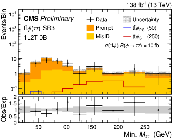
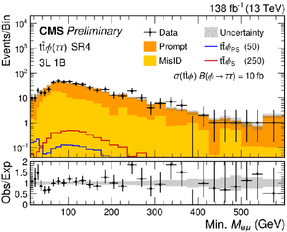
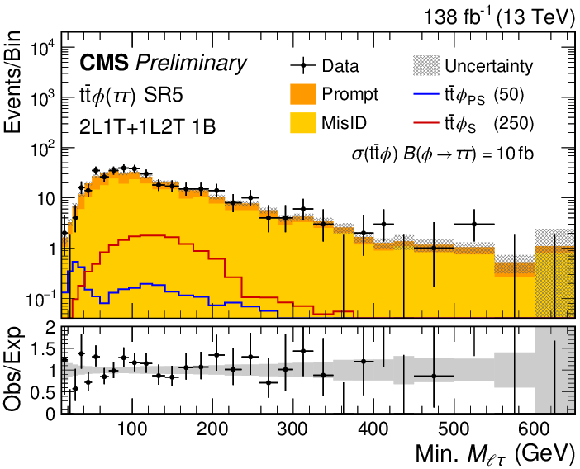
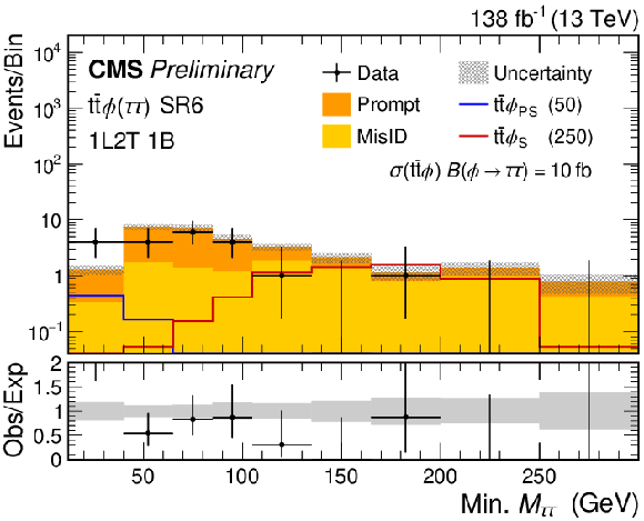
Figure 7:
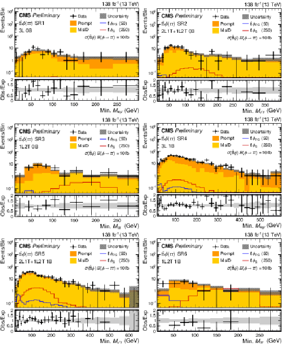
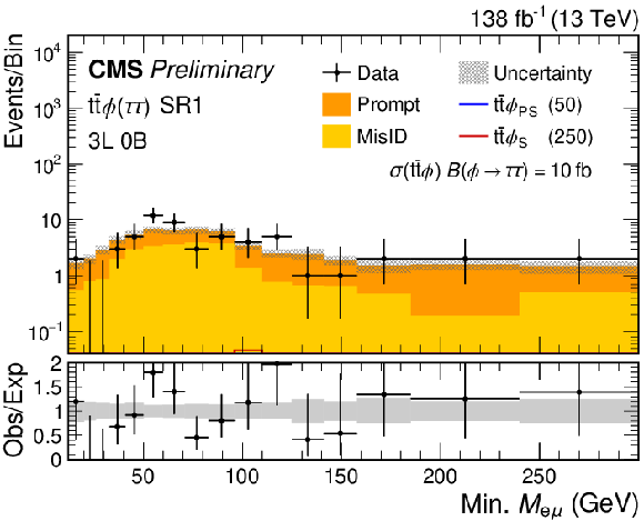
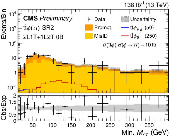
Dilepton mass spectra for the $ {{\mathrm{t} {}\mathrm{\bar{t}}} \phi}(\tau \tau)$ SR1-6 event selections for the combined 2016-2018 data set. The lower panel shows the ratio of observed events to the total expected SM background prediction, and the gray band represents the sum of statistical and systematic uncertainties in the background prediction. The expected background distributions and the uncertainties are shown after fitting the data under the background-only hypothesis. For illustration, two example signal hypotheses for the production and decay of a scalar and a pseudoscalar $\phi $ boson are shown, and their masses are indicated in the legend. |
png pdf |
Figure 7-a:
Dilepton mass spectra for the $ {{\mathrm{t} {}\mathrm{\bar{t}}} \phi}(\tau \tau)$ SR1-6 event selections for the combined 2016-2018 data set. The lower panel shows the ratio of observed events to the total expected SM background prediction, and the gray band represents the sum of statistical and systematic uncertainties in the background prediction. The expected background distributions and the uncertainties are shown after fitting the data under the background-only hypothesis. For illustration, two example signal hypotheses for the production and decay of a scalar and a pseudoscalar $\phi $ boson are shown, and their masses are indicated in the legend. |
png pdf |
Figure 7-b:
Dilepton mass spectra for the $ {{\mathrm{t} {}\mathrm{\bar{t}}} \phi}(\tau \tau)$ SR1-6 event selections for the combined 2016-2018 data set. The lower panel shows the ratio of observed events to the total expected SM background prediction, and the gray band represents the sum of statistical and systematic uncertainties in the background prediction. The expected background distributions and the uncertainties are shown after fitting the data under the background-only hypothesis. For illustration, two example signal hypotheses for the production and decay of a scalar and a pseudoscalar $\phi $ boson are shown, and their masses are indicated in the legend. |
png pdf |
Figure 7-c:
Dilepton mass spectra for the $ {{\mathrm{t} {}\mathrm{\bar{t}}} \phi}(\tau \tau)$ SR1-6 event selections for the combined 2016-2018 data set. The lower panel shows the ratio of observed events to the total expected SM background prediction, and the gray band represents the sum of statistical and systematic uncertainties in the background prediction. The expected background distributions and the uncertainties are shown after fitting the data under the background-only hypothesis. For illustration, two example signal hypotheses for the production and decay of a scalar and a pseudoscalar $\phi $ boson are shown, and their masses are indicated in the legend. |
png pdf |
Figure 7-d:
Dilepton mass spectra for the $ {{\mathrm{t} {}\mathrm{\bar{t}}} \phi}(\tau \tau)$ SR1-6 event selections for the combined 2016-2018 data set. The lower panel shows the ratio of observed events to the total expected SM background prediction, and the gray band represents the sum of statistical and systematic uncertainties in the background prediction. The expected background distributions and the uncertainties are shown after fitting the data under the background-only hypothesis. For illustration, two example signal hypotheses for the production and decay of a scalar and a pseudoscalar $\phi $ boson are shown, and their masses are indicated in the legend. |
png pdf |
Figure 7-e:
Dilepton mass spectra for the $ {{\mathrm{t} {}\mathrm{\bar{t}}} \phi}(\tau \tau)$ SR1-6 event selections for the combined 2016-2018 data set. The lower panel shows the ratio of observed events to the total expected SM background prediction, and the gray band represents the sum of statistical and systematic uncertainties in the background prediction. The expected background distributions and the uncertainties are shown after fitting the data under the background-only hypothesis. For illustration, two example signal hypotheses for the production and decay of a scalar and a pseudoscalar $\phi $ boson are shown, and their masses are indicated in the legend. |
png pdf |
Figure 7-f:
Dilepton mass spectra for the $ {{\mathrm{t} {}\mathrm{\bar{t}}} \phi}(\tau \tau)$ SR1-6 event selections for the combined 2016-2018 data set. The lower panel shows the ratio of observed events to the total expected SM background prediction, and the gray band represents the sum of statistical and systematic uncertainties in the background prediction. The expected background distributions and the uncertainties are shown after fitting the data under the background-only hypothesis. For illustration, two example signal hypotheses for the production and decay of a scalar and a pseudoscalar $\phi $ boson are shown, and their masses are indicated in the legend. |
png pdf |
Figure 8:
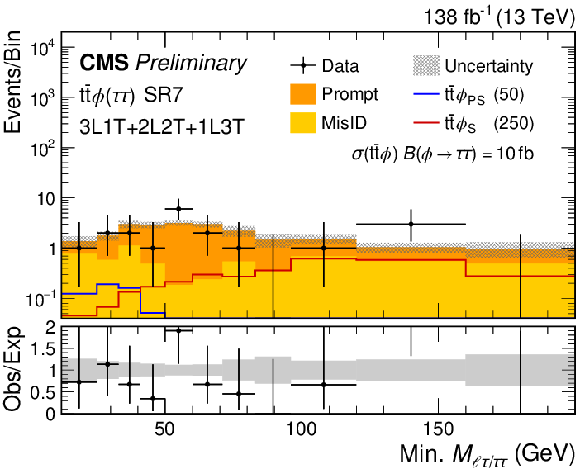
Dilepton mass spectra for the $ {{\mathrm{t} {}\mathrm{\bar{t}}} \phi}(\tau \tau)$ SR7 event selection for the combined 2016-2018 data set. The lower panel shows the ratio of observed events to the total expected SM background prediction, and the gray band represents the sum of statistical and systematic uncertainties in the background prediction. The expected background distributions and the uncertainties are shown after fitting the data under the background-only hypothesis. For illustration, two example signal hypotheses for the production and decay of a scalar and a pseudoscalar $\phi $ boson are shown, and their masses are indicated in the legend. |

png pdf |
Figure 9:
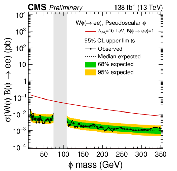
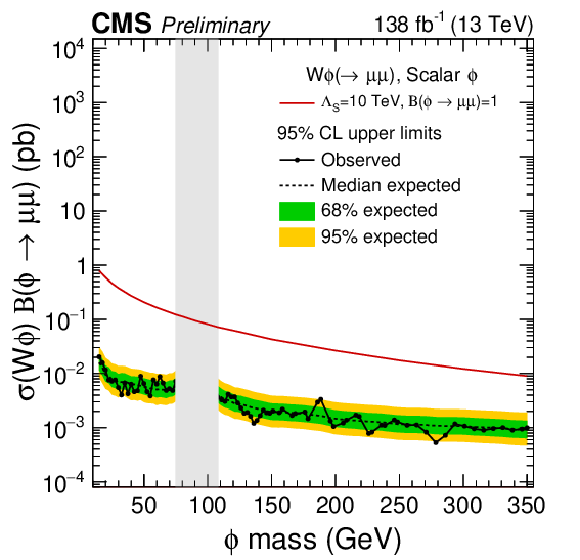
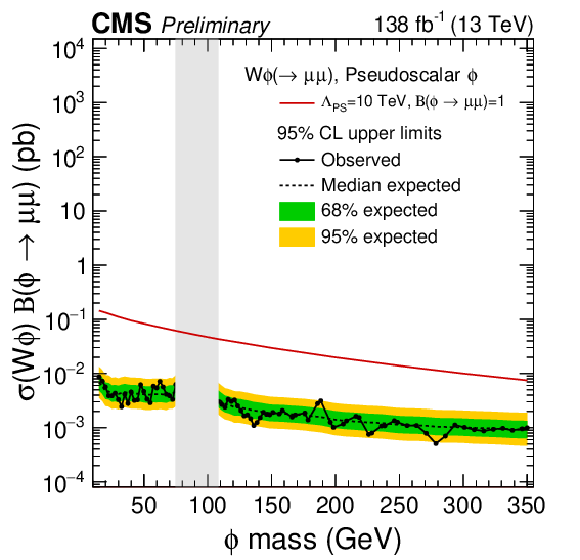
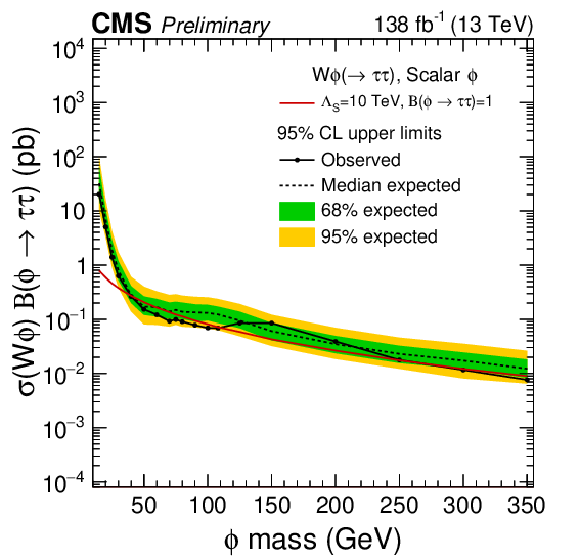
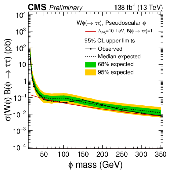
The 95% confidence level upper limits on the product of the signal production cross section and branching fraction of the W$\phi$ signal model in the dielectron (upper), dimuon (center) and ditau (lower) decay scenarios. The results for the scalar coupling are shown on the left and pseudoscalar on the right. The vertical gray band indicates the mass region not considered in the analysis. The red line is the theoretical prediction for the product of the production cross section and branching fraction of the W$\phi$ model. |

png pdf |
Figure 9-a:
The 95% confidence level upper limits on the product of the signal production cross section and branching fraction of the W$\phi$ signal model in the dielectron (upper), dimuon (center) and ditau (lower) decay scenarios. The results for the scalar coupling are shown on the left and pseudoscalar on the right. The vertical gray band indicates the mass region not considered in the analysis. The red line is the theoretical prediction for the product of the production cross section and branching fraction of the W$\phi$ model. |
png pdf |
Figure 9-b:
The 95% confidence level upper limits on the product of the signal production cross section and branching fraction of the W$\phi$ signal model in the dielectron (upper), dimuon (center) and ditau (lower) decay scenarios. The results for the scalar coupling are shown on the left and pseudoscalar on the right. The vertical gray band indicates the mass region not considered in the analysis. The red line is the theoretical prediction for the product of the production cross section and branching fraction of the W$\phi$ model. |
png pdf |
Figure 9-c:
The 95% confidence level upper limits on the product of the signal production cross section and branching fraction of the W$\phi$ signal model in the dielectron (upper), dimuon (center) and ditau (lower) decay scenarios. The results for the scalar coupling are shown on the left and pseudoscalar on the right. The vertical gray band indicates the mass region not considered in the analysis. The red line is the theoretical prediction for the product of the production cross section and branching fraction of the W$\phi$ model. |
png pdf |
Figure 9-d:
The 95% confidence level upper limits on the product of the signal production cross section and branching fraction of the W$\phi$ signal model in the dielectron (upper), dimuon (center) and ditau (lower) decay scenarios. The results for the scalar coupling are shown on the left and pseudoscalar on the right. The vertical gray band indicates the mass region not considered in the analysis. The red line is the theoretical prediction for the product of the production cross section and branching fraction of the W$\phi$ model. |
png pdf |
Figure 9-e:
The 95% confidence level upper limits on the product of the signal production cross section and branching fraction of the W$\phi$ signal model in the dielectron (upper), dimuon (center) and ditau (lower) decay scenarios. The results for the scalar coupling are shown on the left and pseudoscalar on the right. The vertical gray band indicates the mass region not considered in the analysis. The red line is the theoretical prediction for the product of the production cross section and branching fraction of the W$\phi$ model. |
png pdf |
Figure 9-f:
The 95% confidence level upper limits on the product of the signal production cross section and branching fraction of the W$\phi$ signal model in the dielectron (upper), dimuon (center) and ditau (lower) decay scenarios. The results for the scalar coupling are shown on the left and pseudoscalar on the right. The vertical gray band indicates the mass region not considered in the analysis. The red line is the theoretical prediction for the product of the production cross section and branching fraction of the W$\phi$ model. |
png pdf |
Figure 10:
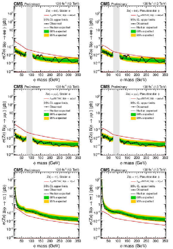
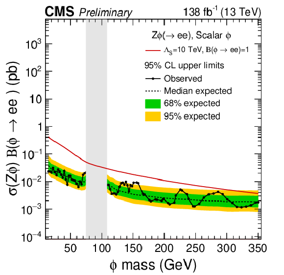
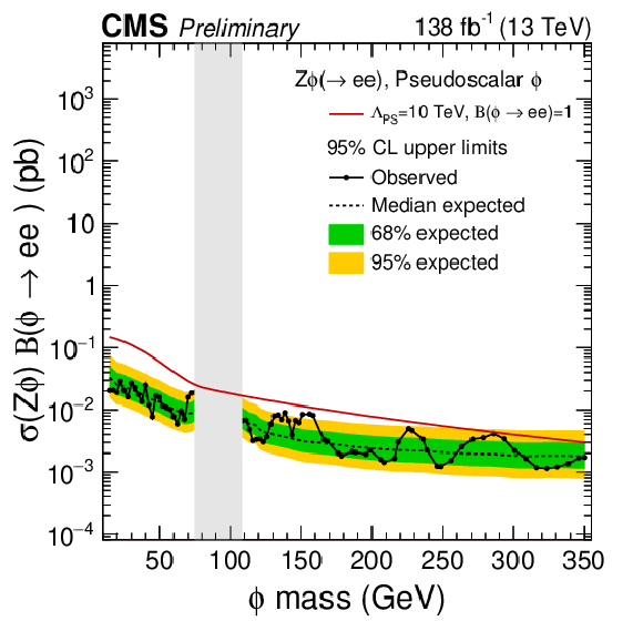
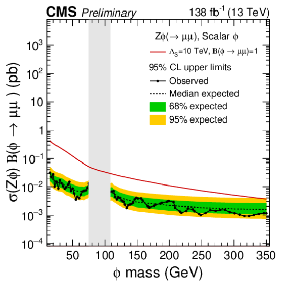
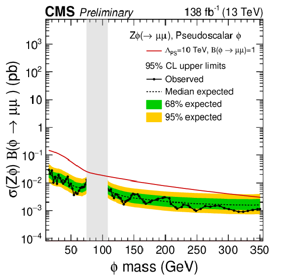
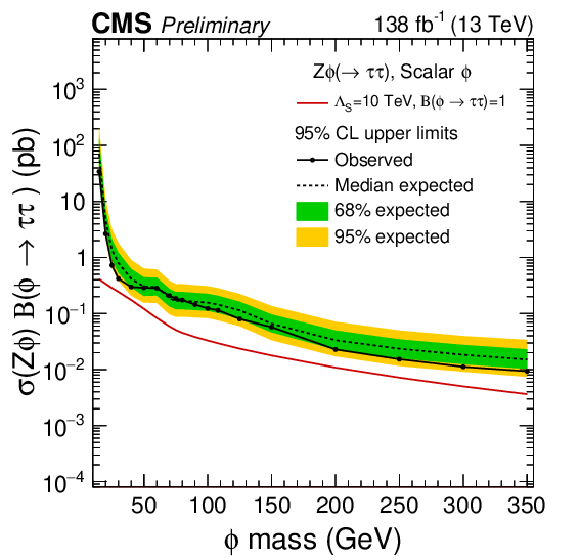
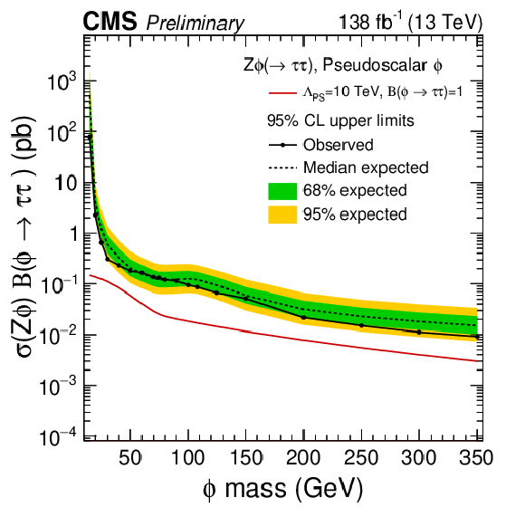
The 95% confidence level upper limits on the product of the signal production cross section and branching fraction of the Z$\phi$ signal model in the dielectron (upper), dimuon (center) and ditau (lower) decay scenarios. The results for the scalar coupling are shown on the left and pseudoscalar on the right. The vertical gray band indicates the mass region not considered in the analysis. The red line is the theoretical prediction for the product of the production cross section and branching fraction of the Z$\phi$ model. |
png pdf |
Figure 10-a:
The 95% confidence level upper limits on the product of the signal production cross section and branching fraction of the Z$\phi$ signal model in the dielectron (upper), dimuon (center) and ditau (lower) decay scenarios. The results for the scalar coupling are shown on the left and pseudoscalar on the right. The vertical gray band indicates the mass region not considered in the analysis. The red line is the theoretical prediction for the product of the production cross section and branching fraction of the Z$\phi$ model. |
png pdf |
Figure 10-b:
The 95% confidence level upper limits on the product of the signal production cross section and branching fraction of the Z$\phi$ signal model in the dielectron (upper), dimuon (center) and ditau (lower) decay scenarios. The results for the scalar coupling are shown on the left and pseudoscalar on the right. The vertical gray band indicates the mass region not considered in the analysis. The red line is the theoretical prediction for the product of the production cross section and branching fraction of the Z$\phi$ model. |
png pdf |
Figure 10-c:
The 95% confidence level upper limits on the product of the signal production cross section and branching fraction of the Z$\phi$ signal model in the dielectron (upper), dimuon (center) and ditau (lower) decay scenarios. The results for the scalar coupling are shown on the left and pseudoscalar on the right. The vertical gray band indicates the mass region not considered in the analysis. The red line is the theoretical prediction for the product of the production cross section and branching fraction of the Z$\phi$ model. |
png pdf |
Figure 10-d:
The 95% confidence level upper limits on the product of the signal production cross section and branching fraction of the Z$\phi$ signal model in the dielectron (upper), dimuon (center) and ditau (lower) decay scenarios. The results for the scalar coupling are shown on the left and pseudoscalar on the right. The vertical gray band indicates the mass region not considered in the analysis. The red line is the theoretical prediction for the product of the production cross section and branching fraction of the Z$\phi$ model. |
png pdf |
Figure 10-e:
The 95% confidence level upper limits on the product of the signal production cross section and branching fraction of the Z$\phi$ signal model in the dielectron (upper), dimuon (center) and ditau (lower) decay scenarios. The results for the scalar coupling are shown on the left and pseudoscalar on the right. The vertical gray band indicates the mass region not considered in the analysis. The red line is the theoretical prediction for the product of the production cross section and branching fraction of the Z$\phi$ model. |
png pdf |
Figure 10-f:
The 95% confidence level upper limits on the product of the signal production cross section and branching fraction of the Z$\phi$ signal model in the dielectron (upper), dimuon (center) and ditau (lower) decay scenarios. The results for the scalar coupling are shown on the left and pseudoscalar on the right. The vertical gray band indicates the mass region not considered in the analysis. The red line is the theoretical prediction for the product of the production cross section and branching fraction of the Z$\phi$ model. |
png pdf |
Figure 11:
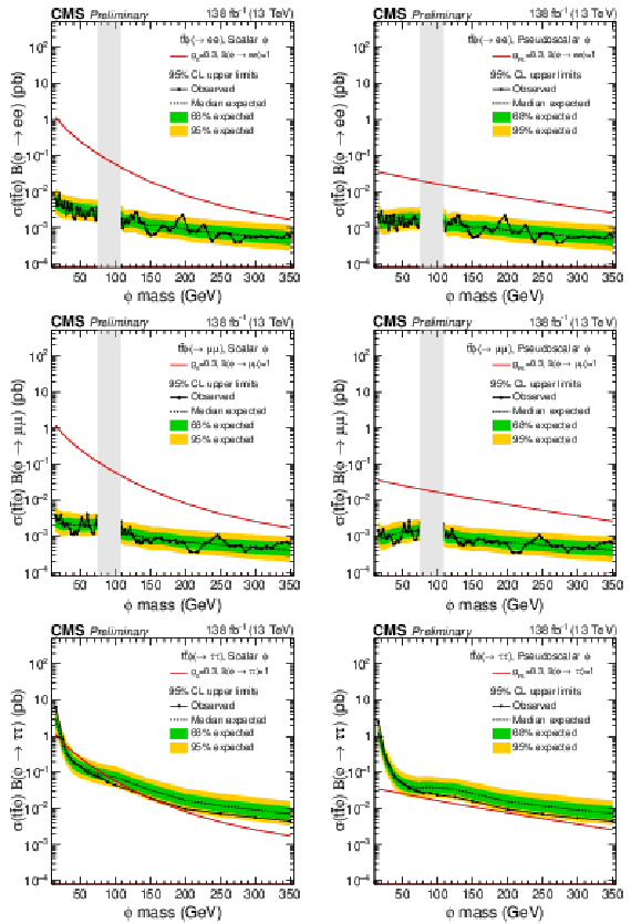
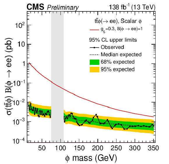
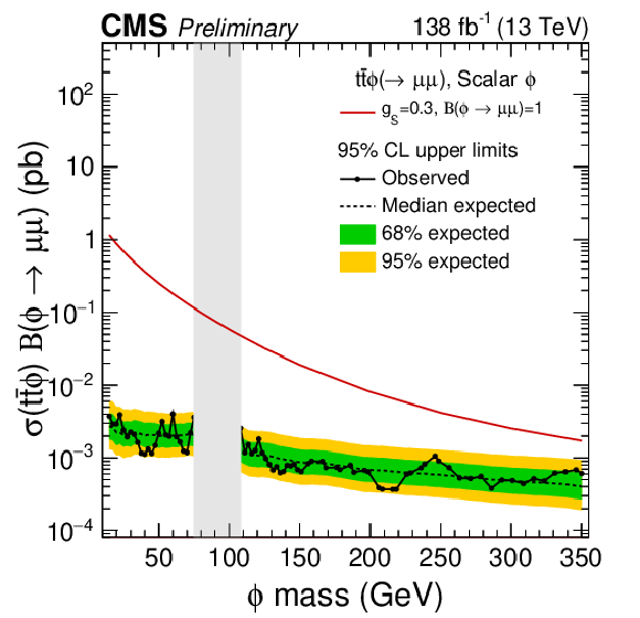
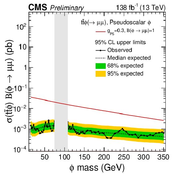
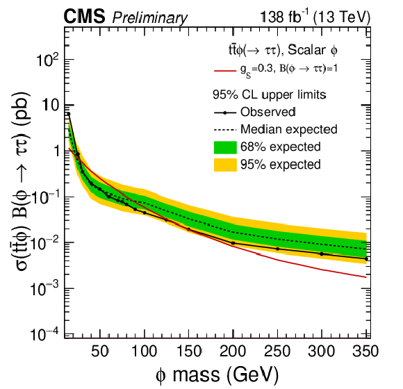
The 95% confidence level upper limits on the product of the signal production cross section and branching fraction of the $ {{\mathrm{t} {}\mathrm{\bar{t}}} \phi}$ signal model in the dielectron (upper), dimuon (center) and ditau (lower) decay scenarios. The results for the scalar coupling are shown on the left and pseudoscalar on the right. The vertical gray band indicates the mass region not considered in the analysis. The red line is the theoretical prediction for the product of the production cross section and branching fraction of the $ {{\mathrm{t} {}\mathrm{\bar{t}}} \phi}$ model. |
png pdf |
Figure 11-a:
The 95% confidence level upper limits on the product of the signal production cross section and branching fraction of the $ {{\mathrm{t} {}\mathrm{\bar{t}}} \phi}$ signal model in the dielectron (upper), dimuon (center) and ditau (lower) decay scenarios. The results for the scalar coupling are shown on the left and pseudoscalar on the right. The vertical gray band indicates the mass region not considered in the analysis. The red line is the theoretical prediction for the product of the production cross section and branching fraction of the $ {{\mathrm{t} {}\mathrm{\bar{t}}} \phi}$ model. |

png pdf |
Figure 11-b:
The 95% confidence level upper limits on the product of the signal production cross section and branching fraction of the $ {{\mathrm{t} {}\mathrm{\bar{t}}} \phi}$ signal model in the dielectron (upper), dimuon (center) and ditau (lower) decay scenarios. The results for the scalar coupling are shown on the left and pseudoscalar on the right. The vertical gray band indicates the mass region not considered in the analysis. The red line is the theoretical prediction for the product of the production cross section and branching fraction of the $ {{\mathrm{t} {}\mathrm{\bar{t}}} \phi}$ model. |
png pdf |
Figure 11-c:
The 95% confidence level upper limits on the product of the signal production cross section and branching fraction of the $ {{\mathrm{t} {}\mathrm{\bar{t}}} \phi}$ signal model in the dielectron (upper), dimuon (center) and ditau (lower) decay scenarios. The results for the scalar coupling are shown on the left and pseudoscalar on the right. The vertical gray band indicates the mass region not considered in the analysis. The red line is the theoretical prediction for the product of the production cross section and branching fraction of the $ {{\mathrm{t} {}\mathrm{\bar{t}}} \phi}$ model. |
png pdf |
Figure 11-d:
The 95% confidence level upper limits on the product of the signal production cross section and branching fraction of the $ {{\mathrm{t} {}\mathrm{\bar{t}}} \phi}$ signal model in the dielectron (upper), dimuon (center) and ditau (lower) decay scenarios. The results for the scalar coupling are shown on the left and pseudoscalar on the right. The vertical gray band indicates the mass region not considered in the analysis. The red line is the theoretical prediction for the product of the production cross section and branching fraction of the $ {{\mathrm{t} {}\mathrm{\bar{t}}} \phi}$ model. |
png pdf |
Figure 11-e:
The 95% confidence level upper limits on the product of the signal production cross section and branching fraction of the $ {{\mathrm{t} {}\mathrm{\bar{t}}} \phi}$ signal model in the dielectron (upper), dimuon (center) and ditau (lower) decay scenarios. The results for the scalar coupling are shown on the left and pseudoscalar on the right. The vertical gray band indicates the mass region not considered in the analysis. The red line is the theoretical prediction for the product of the production cross section and branching fraction of the $ {{\mathrm{t} {}\mathrm{\bar{t}}} \phi}$ model. |

png pdf |
Figure 11-f:
The 95% confidence level upper limits on the product of the signal production cross section and branching fraction of the $ {{\mathrm{t} {}\mathrm{\bar{t}}} \phi}$ signal model in the dielectron (upper), dimuon (center) and ditau (lower) decay scenarios. The results for the scalar coupling are shown on the left and pseudoscalar on the right. The vertical gray band indicates the mass region not considered in the analysis. The red line is the theoretical prediction for the product of the production cross section and branching fraction of the $ {{\mathrm{t} {}\mathrm{\bar{t}}} \phi}$ model. |
png pdf |
Figure 12:
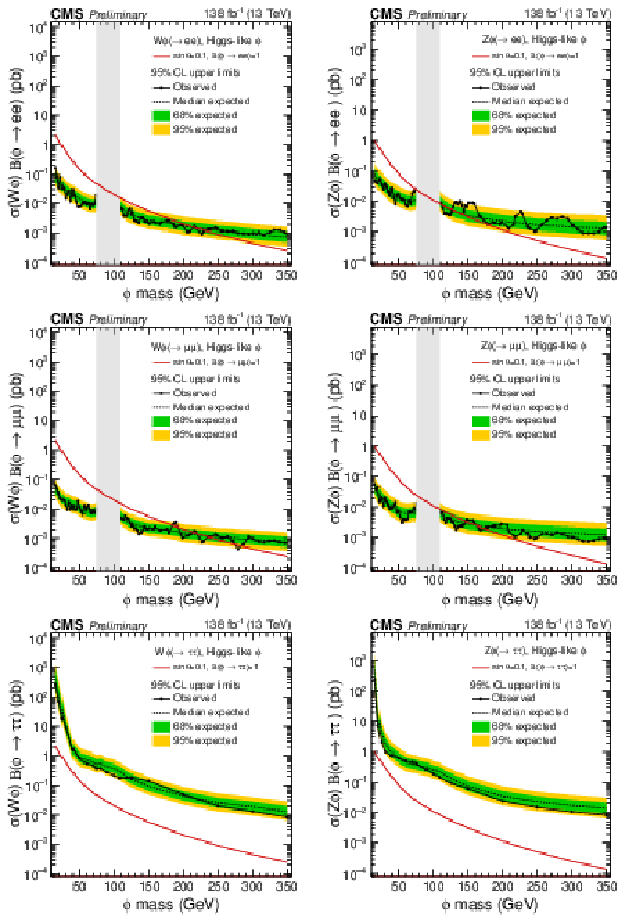
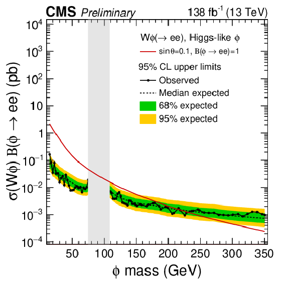
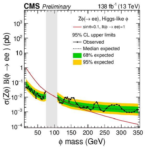
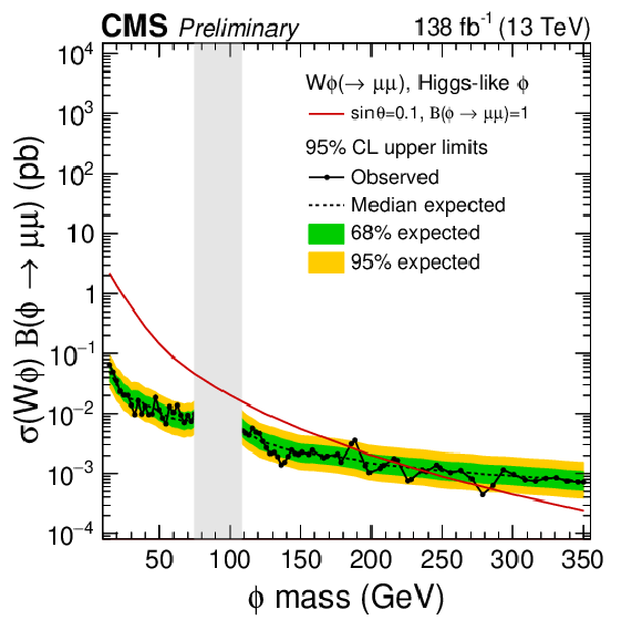
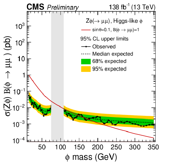
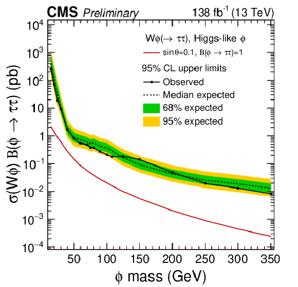
The 95% confidence level upper limits on the product of the signal production cross section and branching fraction of the W$\phi$ signal model on the left and the Z$\phi$ signal model on the right with Higgs-like couplings in the dielectron (upper), dimuon (center) and ditau (lower) decay scenarios. The vertical gray band indicates the mass region not considered in the analysis. The red line is the theoretical prediction for the product of the production cross section and branching fraction of the W$\phi$ and Z$\phi$ signal models. |
png pdf |
Figure 12-a:
The 95% confidence level upper limits on the product of the signal production cross section and branching fraction of the W$\phi$ signal model on the left and the Z$\phi$ signal model on the right with Higgs-like couplings in the dielectron (upper), dimuon (center) and ditau (lower) decay scenarios. The vertical gray band indicates the mass region not considered in the analysis. The red line is the theoretical prediction for the product of the production cross section and branching fraction of the W$\phi$ and Z$\phi$ signal models. |
png pdf |
Figure 12-b:
The 95% confidence level upper limits on the product of the signal production cross section and branching fraction of the W$\phi$ signal model on the left and the Z$\phi$ signal model on the right with Higgs-like couplings in the dielectron (upper), dimuon (center) and ditau (lower) decay scenarios. The vertical gray band indicates the mass region not considered in the analysis. The red line is the theoretical prediction for the product of the production cross section and branching fraction of the W$\phi$ and Z$\phi$ signal models. |
png pdf |
Figure 12-c:
The 95% confidence level upper limits on the product of the signal production cross section and branching fraction of the W$\phi$ signal model on the left and the Z$\phi$ signal model on the right with Higgs-like couplings in the dielectron (upper), dimuon (center) and ditau (lower) decay scenarios. The vertical gray band indicates the mass region not considered in the analysis. The red line is the theoretical prediction for the product of the production cross section and branching fraction of the W$\phi$ and Z$\phi$ signal models. |
png pdf |
Figure 12-d:
The 95% confidence level upper limits on the product of the signal production cross section and branching fraction of the W$\phi$ signal model on the left and the Z$\phi$ signal model on the right with Higgs-like couplings in the dielectron (upper), dimuon (center) and ditau (lower) decay scenarios. The vertical gray band indicates the mass region not considered in the analysis. The red line is the theoretical prediction for the product of the production cross section and branching fraction of the W$\phi$ and Z$\phi$ signal models. |
png pdf |
Figure 12-e:
The 95% confidence level upper limits on the product of the signal production cross section and branching fraction of the W$\phi$ signal model on the left and the Z$\phi$ signal model on the right with Higgs-like couplings in the dielectron (upper), dimuon (center) and ditau (lower) decay scenarios. The vertical gray band indicates the mass region not considered in the analysis. The red line is the theoretical prediction for the product of the production cross section and branching fraction of the W$\phi$ and Z$\phi$ signal models. |

png pdf |
Figure 12-f:
The 95% confidence level upper limits on the product of the signal production cross section and branching fraction of the W$\phi$ signal model on the left and the Z$\phi$ signal model on the right with Higgs-like couplings in the dielectron (upper), dimuon (center) and ditau (lower) decay scenarios. The vertical gray band indicates the mass region not considered in the analysis. The red line is the theoretical prediction for the product of the production cross section and branching fraction of the W$\phi$ and Z$\phi$ signal models. |
| Tables | |

png pdf |
Table 1:
A summary of control regions for the irreducible SM processes ZZ, Z$\gamma$, WZ, and $ {{{\mathrm{t} {}\mathrm{\bar{t}}}}{\mathrm{Z}}}$, and for the misidentified lepton backgrounds (MisID e/$\mu $ and MisID $\tau$). The ${{p_{\mathrm {T}}} ^\text {miss}}$, ${M_{\rm T}}$, the minimum 3L lepton ${p_{\mathrm {T}}} $ (${p_{\mathrm {T}}} ^{\mathrm {3}}$), $ {M_{\ell}}$, and $ {S_{\rm T}}$ are in units of GeV. The 3L OnZ CR is further split into 3L MisID e$\mu$ CR, 3L WZ CR, and 3L $ {{{\mathrm{t} {}\mathrm{\bar{t}}}}{\mathrm{Z}}}$ CR. |

png pdf |
Table 2:
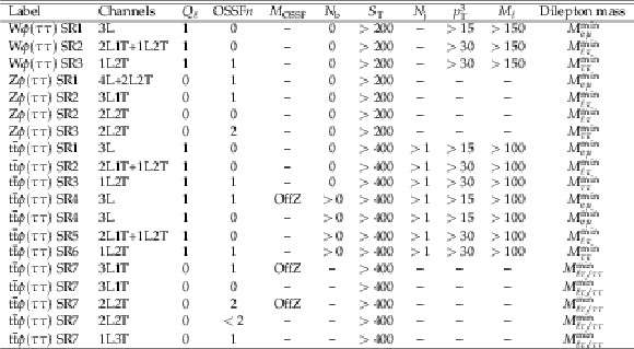
Low and high mass signal region selections for $ {{\mathrm{X}}\phi}\to \mathrm{e} \mathrm{e} /\mu \mu $ signal models. Events satisfying the control region requirements are vetoed throughout, and only those with a reconstructed $\phi $ candidate are retained using the specified dilepton mass variable. $ {S_{\rm T}}$, $ {p_{\mathrm {T}}} ^3$, and $ {M_{\ell}}$ requirements are specified in units of $ GeV $. The two entries in the labels, channels, and dilepton mass variables are provided for the $X\phi \to \mathrm{e} \mathrm{e} $ and $X\phi \to \mu \mu $ signal scenarios as appropriate. |
png pdf |
Table 3:
Signal selections for $ {{\mathrm{X}}\phi}\to \tau \tau $ signal models. Events satisfying the control region requirements are vetoed throughout, and only those with a reconstructed $\phi $ candidate are retained using the specified dilepton mass variable. $ {S_{\rm T}}$, $ {p_{\mathrm {T}}} ^3$, and $ {M_{\ell}}$ requirements are specified in units of $ GeV $. |
png pdf |
Table 4:
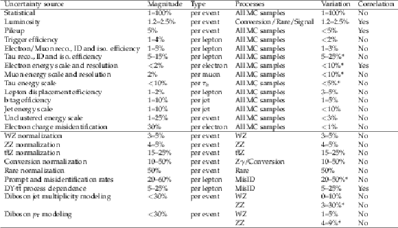
Sources, magnitudes, effective variations, and correlation properties of systematic uncertainties in the signal regions. Uncertainty sources marked as "Yes'' under the Correlation column have their nuisance parameters correlated across the 3 years of data collection. Uncertainty sources marked with an "*'' in the Variation column are not flat. |
| Summary |
| A search has been performed for physics beyond the standard model using 138 fb$^{-1}$ of pp collision data collected with the CMS detector at $\sqrt{s} = $ 13 TeV. A resonant dilepton signature has been sought after in multilepton events, but no statistically significant excess compatible with the considered signal scenarios is observed over the SM background expectation in the probed mass spectra. The results constrain the allowed parameter space of the targeted signal models of new spin-0 particles with scalar, pseudoscalar, or Higgs-like couplings. Constraints are calculated at 95% confidence level on the product of production cross section and branching fraction of such bosons with masses in the range of 15 to 350 GeV produced in association with a W or a Z boson, or a $\mathrm{t\bar{t}}$ pair and exclusively decaying into dielectron, dimuon, and ditau pairs. The observations exclude product of cross section and branching fraction values above 50-0.5 fb, 30-0.5 fb and 200-1 fb for new scalar, pseudoscalar, and Higgs-like bosons, respectively, for exclusive decays of $\phi$ bosons into dielectron or dimuon pairs. Similarly, assuming such new bosons exclusively decay into pairs of tau leptons, the product of cross section and branching fraction values above 35-0.004 pb, 80-0.004 pb, and 250-0.008 pb are excluded for scalar, pseudoscalar, and Higgs-like couplings, respectively, in the probed mass range. These are the most restrictive direct limits in these production and decay modes on an extension of the standard model with scalar or pseudoscalar particle. For the ${\mathrm{t\bar{t}}\phi}\to\tau\tau$ as well as the W$\phi$ and Z$\phi$ signal models, these also constitute the first direct constraints on an extension of the standard model with such scalar or pseudoscalar states in this mass range. |
| References | ||||
| 1 | G. Cacciapaglia, G. Ferretti, T. Flacke, and H. Serodio | Light scalars in composite Higgs models | Front. Phys. 7 (2019) 22 | 1902.06890 |
| 2 | U. Ellwanger, C. Hugonie, and A. M. Teixeira | The next-to-minimal supersymmetric standard model | PR 496 (2010) 1 | 0910.1785 |
| 3 | M. Maniatis | The next-to-minimal supersymmetric extension of the standard model reviewed | Int. J. Mod. Phys. A 25 (2010) 3505 | 0906.0777 |
| 4 | M. R. Buckley, D. Feld, and D. Goncalves | Scalar simplified models for dark matter | PRD 91 (2015) 015017 | 1410.6497 |
| 5 | M. Casolino et al. | Probing a light CP-odd scalar in di-top-associated production at the LHC | EPJC 75 (2015) 498 | 1507.07004 |
| 6 | W.-F. Chang, T. Modak, and J. N. Ng | Signal for a light singlet scalar at the LHC | PRD 97 (2018) 055020 | 1711.05722 |
| 7 | CMS Collaboration | Search for physics beyond the standard model in multilepton final states in proton-proton collisions at $ \sqrt{s} = $ 13 TeV | JHEP 03 (2020) 051 | CMS-EXO-19-002 1911.04968 |
| 8 | CMS Collaboration | The CMS experiment at the CERN LHC | JINST 3 (2008) S08004 | CMS-00-001 |
| 9 | CMS Collaboration | The CMS trigger system | JINST 12 (2017) P01020 | CMS-TRG-12-001 1609.02366 |
| 10 | J. Alwall et al. | The automated computation of tree-level and next-to-leading order differential cross sections, and their matching to parton shower simulations | JHEP 07 (2014) 079 | 1405.0301 |
| 11 | P. Nason | A new method for combining NLO QCD with shower Monte Carlo algorithms | JHEP 11 (2004) 040 | hep-ph/0409146 |
| 12 | S. Frixione, P. Nason, and C. Oleari | Matching NLO QCD computations with parton shower simulations: the POWHEG method | JHEP 11 (2007) 070 | 0709.2092 |
| 13 | S. Alioli, P. Nason, C. Oleari, and E. Re | A general framework for implementing NLO calculations in shower Monte Carlo programs: the POWHEG BOX | JHEP 06 (2010) 043 | 1002.2581 |
| 14 | J. M. Campbell and R. K. Ellis | MCFM for the Tevatron and the LHC | NPPS 205--206 (2010) 10 | 1007.3492 |
| 15 | Y. Gao et al. | Spin determination of single-produced resonances at hadron colliders | PRD 81 (2010) 075022 | 1001.3396 |
| 16 | S. Bolognesi et al. | On the spin and parity of a single-produced resonance at the LHC | PRD 86 (2012) 095031 | 1208.4018 |
| 17 | I. Anderson et al. | Constraining anomalous HVV interactions at proton and lepton colliders | PRD 89 (2014) 035007 | 1309.4819 |
| 18 | A. V. Gritsan, R. Rontsch, M. Schulze, and M. Xiao | Constraining anomalous Higgs boson couplings to the heavy flavor fermions using matrix element techniques | PRD 94 (2016) 055023 | 1606.03107 |
| 19 | T. Sjostrand et al. | An introduction to PYTHIA 8.2 | CPC 191 (2015) 159 | 1410.3012 |
| 20 | NNPDF Collaboration | Parton distributions for the LHC Run II | JHEP 04 (2015) 040 | 1410.8849 |
| 21 | NNPDF Collaboration | Parton distributions from high-precision collider data | EPJC 77 (2017) 663 | 1706.00428 |
| 22 | CMS Collaboration | Event generator tunes obtained from underlying event and multiparton scattering measurements | EPJC 76 (2016) 155 | CMS-GEN-14-001 1512.00815 |
| 23 | CMS Collaboration | Extraction and validation of a new set of CMS PYTHIA8 tunes from underlying-event measurements | EPJC 80 (2020) 4 | CMS-GEN-17-001 1903.12179 |
| 24 | S. Hoeche et al. | Matching parton showers and matrix elements | 2006 | hep-ph/0602031 |
| 25 | R. Frederix and S. Frixione | Merging meets matching in MC@NLO | JHEP 12 (2012) 061 | 1209.6215 |
| 26 | GEANT4 Collaboration | GEANT4--a simulation toolkit | NIMA 506 (2003) 250 | |
| 27 | CMS Collaboration | Technical proposal for the Phase-II upgrade of the Compact Muon Solenoid | CMS-PAS-TDR-15-002 | CMS-PAS-TDR-15-002 |
| 28 | CMS Collaboration | Particle-flow reconstruction and global event description with the CMS detector | JINST 12 (2017) P10003 | CMS-PRF-14-001 1706.04965 |
| 29 | CMS Collaboration | Electron and photon reconstruction and identification with the CMS experiment at the CERN LHC | JINST 16 (2021) P05014 | CMS-EGM-17-001 2012.06888 |
| 30 | CMS Collaboration | Performance of the CMS muon detector and muon reconstruction with proton-proton collisions at $ \sqrt{s}= $ 13 TeV | JINST 13 (2018) P06015 | CMS-MUO-16-001 1804.04528 |
| 31 | CMS Collaboration | Performance of reconstruction and identification of $ \tau $ leptons decaying to hadrons and $ \nu_\tau $ in pp collisions at $ \sqrt{s}= $ 13 TeV | JINST 13 (2018) P10005 | CMS-TAU-16-003 1809.02816 |
| 32 | M. Cacciari, G. P. Salam, and G. Soyez | The anti-$ {k_{\mathrm{T}}} $ jet clustering algorithm | JHEP 04 (2008) 063 | 0802.1189 |
| 33 | M. Cacciari, G. P. Salam, and G. Soyez | Fastjet user manual | EPJC 72 (2012) 1896 | 1111.6097 |
| 34 | M. Cacciari, G. P. Salam, and G. Soyez | The catchment area of jets | JHEP 04 (2008) 005 | 0802.1188 |
| 35 | M. Cacciari and G. P. Salam | Pileup subtraction using jet areas | PLB 659 (2008) 119 | 0707.1378 |
| 36 | CMS Collaboration | Jet energy scale and resolution in the CMS experiment in pp collisions at 8 TeV | JINST 12 (2017) P02014 | CMS-JME-13-004 1607.03663 |
| 37 | CMS Collaboration | Jet algorithms performance in 13 TeV data | CMS-PAS-JME-16-003 | CMS-PAS-JME-16-003 |
| 38 | CMS Collaboration | Identification of heavy-flavour jets with the CMS detector in pp collisions at 13 TeV | JINST 13 (2018) P05011 | CMS-BTV-16-002 1712.07158 |
| 39 | CMS Collaboration | Performance of missing transverse momentum reconstruction in proton-proton collisions at $ \sqrt{s} = $ 13 TeV using the CMS detector | JINST 14 (2019) P07004 | CMS-JME-17-001 1903.06078 |
| 40 | D. Bertolini, P. Harris, M. Low, and N. Tran | Pileup per particle identification | JHEP 10 (2014) 059 | 1407.6013 |
| 41 | CMS Collaboration | Identification of hadronic tau lepton decays using a deep neural network | 2022. Submitted to JINST | CMS-TAU-20-001 2201.08458 |
| 42 | Particle Data Group Collaboration | Review of Particle Physics, 2020-2021. RPP | PTEP 2020 (2020) 083C01. 2093 p | |
| 43 | CMS Collaboration | Measurement of the inclusive W and Z production cross sections in pp collisions at $ \sqrt{s}= $ 7 TeV | JHEP 10 (2011) 132 | CMS-EWK-10-005 1107.4789 |
| 44 | K. S. Cranmer | Kernel estimation in high-energy physics | CPC 136 (2001) 198--207 | hep-ex/0011057 |
| 45 | M. Cacciari et al. | The $\mathrm{ t\bar{t} }$ cross-section at 1.8 and 1.96 TeV: A study of the systematics due to parton densities and scale dependence | JHEP 04 (2004) 068 | hep-ph/0303085 |
| 46 | CMS Collaboration | Precision luminosity measurement in proton-proton collisions at $ \sqrt{s} = $ 13 TeV in 2015 and 2016 at CMS | EPJC 81 (2021) 800 | CMS-LUM-17-003 2104.01927 |
| 47 | CMS Collaboration | CMS luminosity measurement for the 2017 data-taking period at $ \sqrt{s} = $ 13 TeV | CMS-PAS-LUM-17-004 | CMS-PAS-LUM-17-004 |
| 48 | CMS Collaboration | CMS luminosity measurement for the 2018 data-taking period at $ \sqrt{s} = $ 13 TeV | CMS-PAS-LUM-18-002 | CMS-PAS-LUM-18-002 |
| 49 | E. Gross and O. Vitells | Trial factors for the look elsewhere effect in high energy physics | EPJC 70 (2010) 525 | 1005.1891 |
| 50 | T. Junk | Confidence level computation for combining searches with small statistics | NIMA 434 (1999) 435 | hep-ex/9902006 |
| 51 | A. L. Read | Presentation of search results: The CL$ _{s} $ technique | JPG 28 (2002) 2693 | |
| 52 | G. Cowan, K. Cranmer, E. Gross, and O. Vitells | Asymptotic formulae for likelihood-based tests of new physics | EPJC 71 (2011) 1554 | 1007.1727 |
| 53 | ATLAS and CMS Collaborations, and LHC Higgs Combination Group | Procedure for the LHC Higgs boson search combination in summer 2011 | CMS-NOTE-2011-005 | |

|
Compact Muon Solenoid LHC, CERN |

|

|

|

|

|

|