CMS-PAS-EXO-21-006

CMS-PAS-EXO-21-006
Search for long-lived particles decaying to a pair of muons in proton-proton collisions at $\sqrt{s}=$ 13 TeV
CMS Collaboration
January 2022

Abstract: An inclusive search for long-lived exotic particles decaying to a pair of muons is presented. The search uses a data set collected by the CMS experiment at the LHC in proton-proton collisions at $\sqrt{s}=$ 13 TeV in 2016 and 2018 and corresponding to an integrated luminosity of 97.6 fb $^{-1}$ . The experimental signature is a pair of oppositely charged muons originating from a common secondary vertex spatially separated from the proton interaction point by distances ranging from several hundred $\mu$ m to several meters. The results are interpreted in the frameworks of the Hidden Abelian Higgs model, in which the Higgs boson decays to a pair of long-lived dark photons, and of a simplified model, in which long-lived particles are produced in decays of an exotic heavy neutral scalar boson.
Links: CDS record (PDF) ; CADI line (restricted) ; These preliminary results are superseded in this paper, JHEP 05 (2023) 228. The superseded preliminary plots can be found here.

Figures	Summary	Additional Figures & Tables	References	CMS Publications

Figures
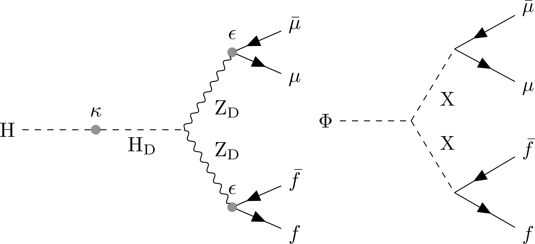
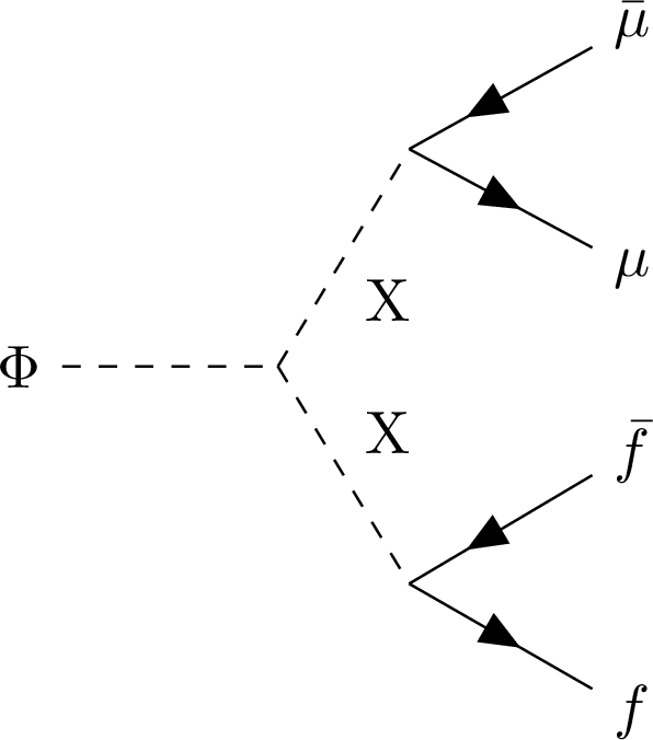
png pdf	Figure 1: Feynman diagrams of (left) the HAHM model, showing the production of Z $_D$ via the Higgs portal with the subsequent Z $_D$ decays via the vector portal, and (right) the heavy scalar model. The symbols $f$ and $\bar{f}$ represent, respectively, fermions and antifermions lighter than half the LLP mass.
png pdf	Figure 1-a: Feynman diagrams of (left) the HAHM model, showing the production of Z $_D$ via the Higgs portal with the subsequent Z $_D$ decays via the vector portal, and (right) the heavy scalar model. The symbols $f$ and $\bar{f}$ represent, respectively, fermions and antifermions lighter than half the LLP mass.
png pdf	Figure 1-b: Feynman diagrams of (left) the HAHM model, showing the production of Z $_D$ via the Higgs portal with the subsequent Z $_D$ decays via the vector portal, and (right) the heavy scalar model. The symbols $f$ and $\bar{f}$ represent, respectively, fermions and antifermions lighter than half the LLP mass.
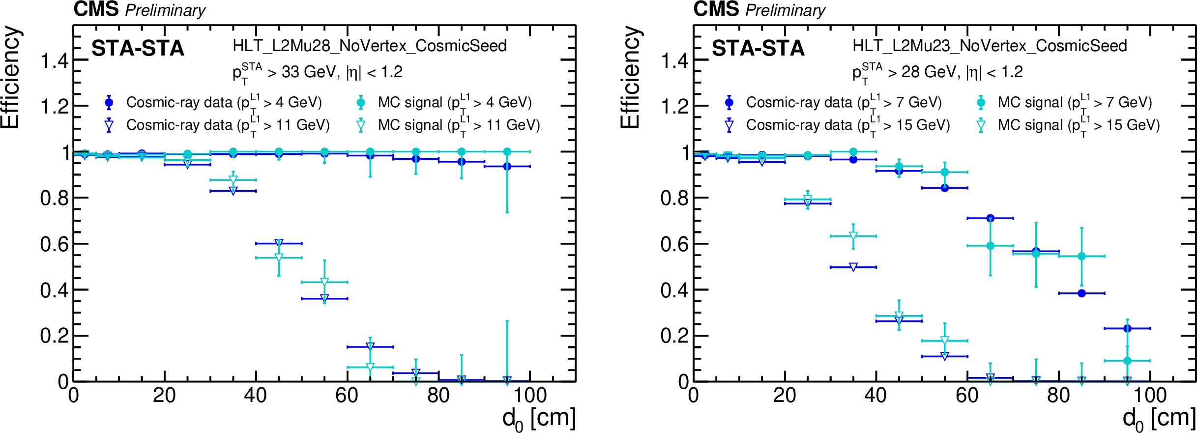
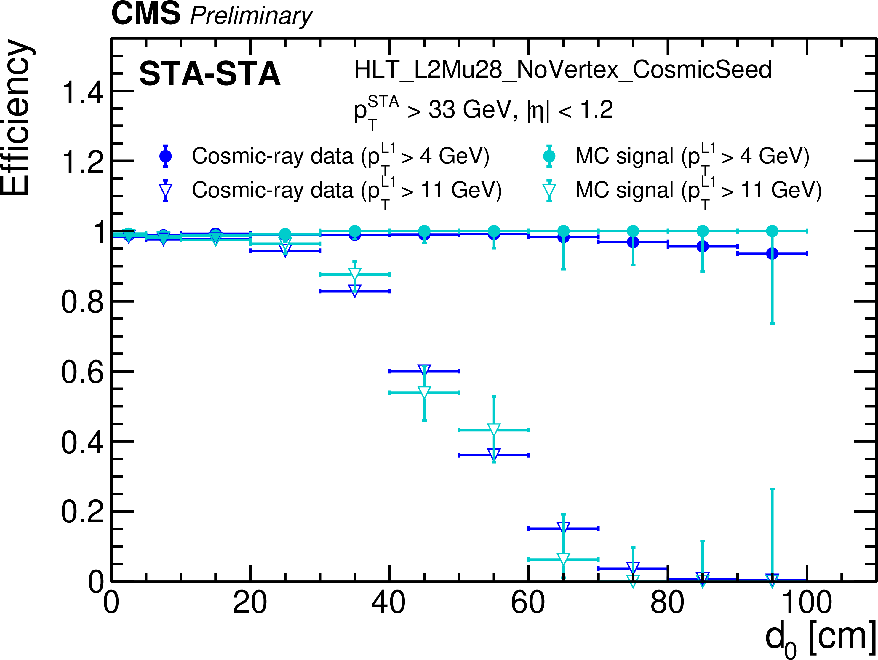
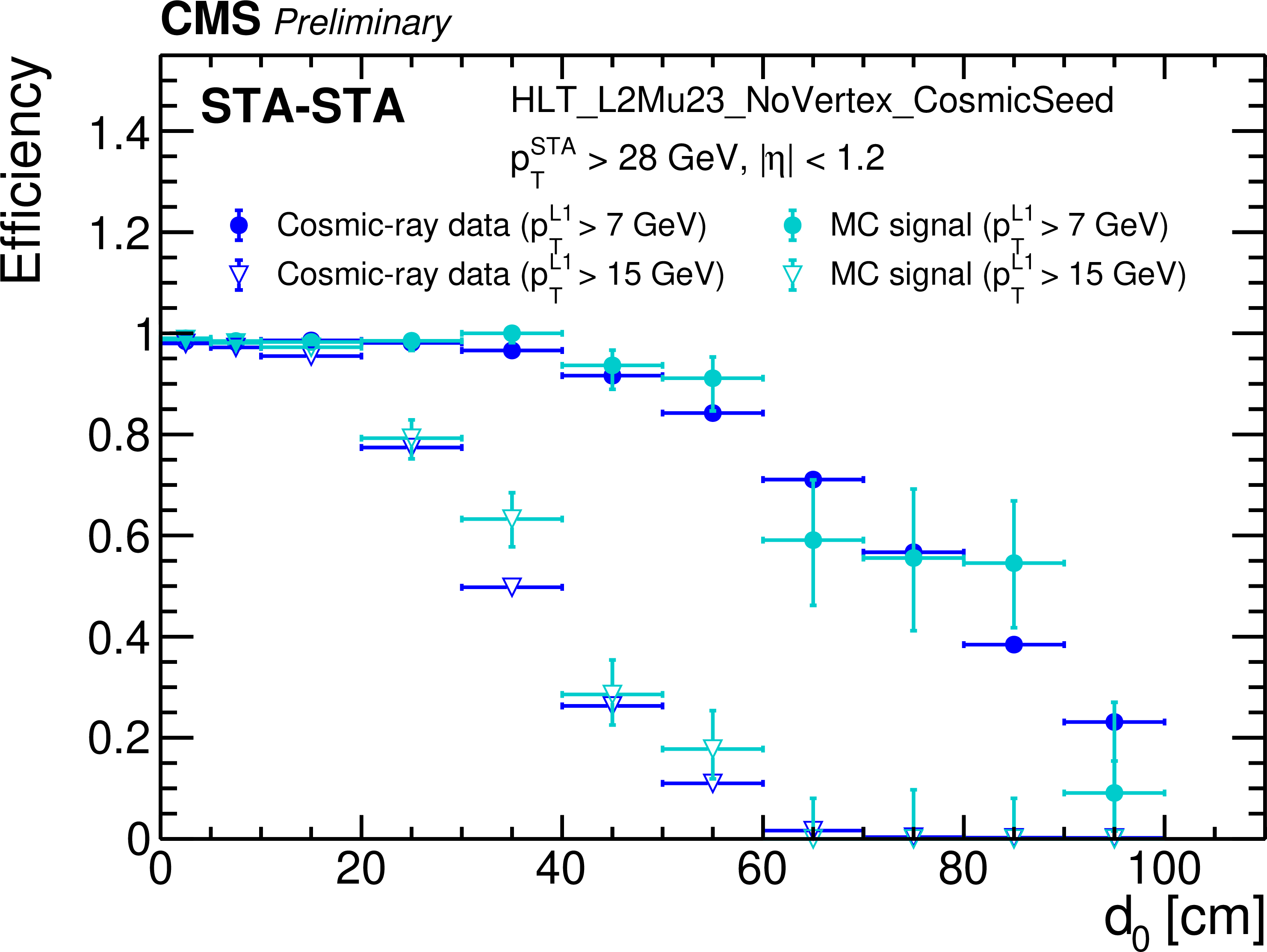
png pdf	Figure 2: Level-1 muon trigger efficiency in cosmic ray muon data (blue) and signal simulation (green) as a function of ${d_{{\mathrm {0}}}}$ , for the Level-1 trigger $p_{\mathrm{T}}$ thresholds used in the (left) 2016 and (right) 2018 analysis triggers. The denominator in the efficiency calculations is the number of STA muons with ${\| \eta \|} <$ 1.2 and $p_{\mathrm{T}} >$ 33 GeV (left) and 28 GeV (right).
png pdf root	Figure 2-a: Level-1 muon trigger efficiency in cosmic ray muon data (blue) and signal simulation (green) as a function of ${d_{{\mathrm {0}}}}$ , for the Level-1 trigger $p_{\mathrm{T}}$ thresholds used in the (left) 2016 and (right) 2018 analysis triggers. The denominator in the efficiency calculations is the number of STA muons with ${\| \eta \|} <$ 1.2 and $p_{\mathrm{T}} >$ 33 GeV (left) and 28 GeV (right).
png pdf root	Figure 2-b: Level-1 muon trigger efficiency in cosmic ray muon data (blue) and signal simulation (green) as a function of ${d_{{\mathrm {0}}}}$ , for the Level-1 trigger $p_{\mathrm{T}}$ thresholds used in the (left) 2016 and (right) 2018 analysis triggers. The denominator in the efficiency calculations is the number of STA muons with ${\| \eta \|} <$ 1.2 and $p_{\mathrm{T}} >$ 33 GeV (left) and 28 GeV (right).
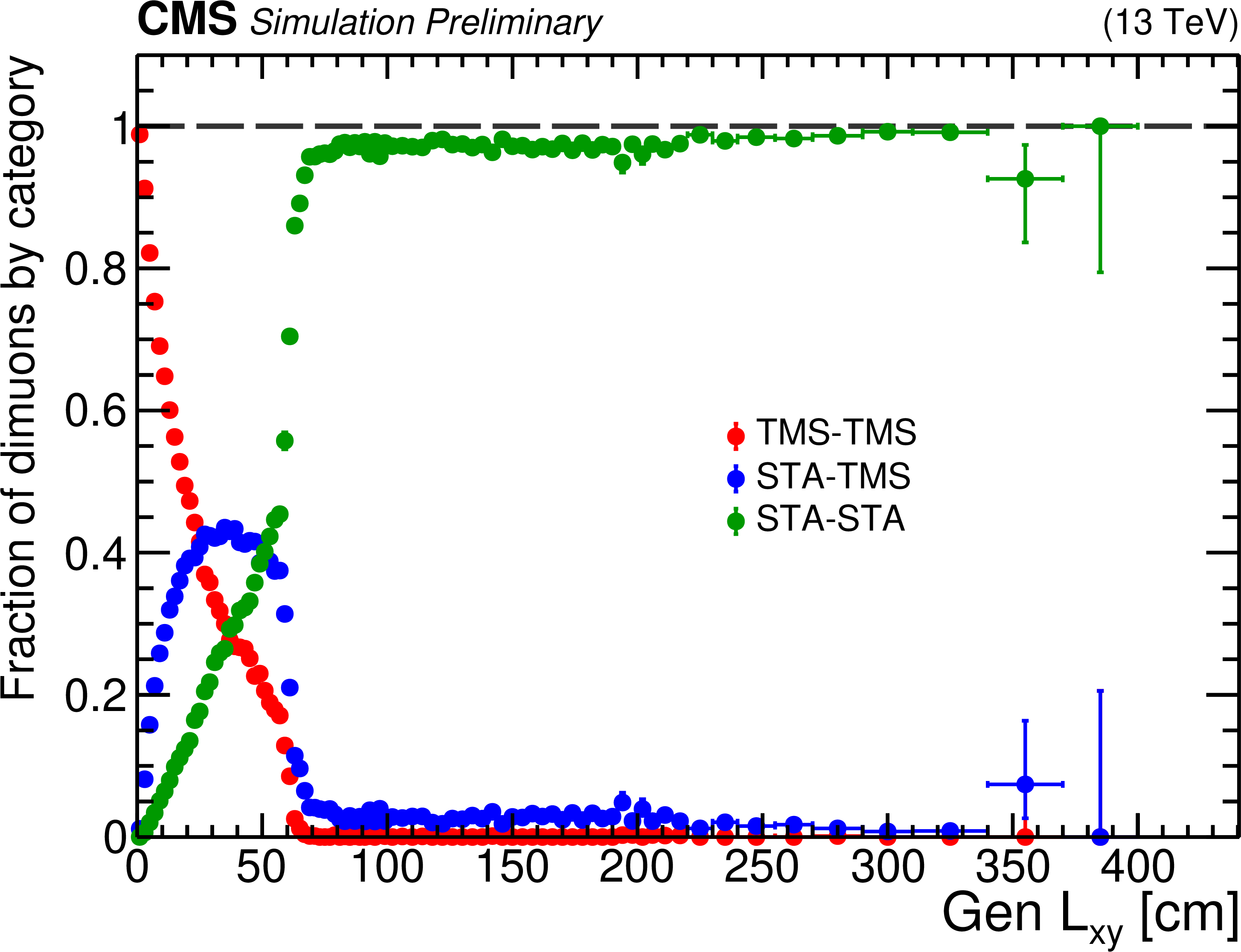
png pdf root	Figure 3: Fractions of signal events with zero (green), one (blue), and two (red) STA muons matched to TMS muons by the STA-to-TMS muon association procedure, as a function of true ${L_{{\mathrm {xy}}}}$ , in all simulated $\Phi\to 2{\mathrm{X}} \to 2\mu$ signal samples combined. The fractions are computed relative to the number of signal events passing the trigger and containing two STA muons with more than 12 muon hits and $p_{\mathrm{T}} >$ 10 GeV matched to generated muons from ${\mathrm{X}} \to \mu \mu$ decays.
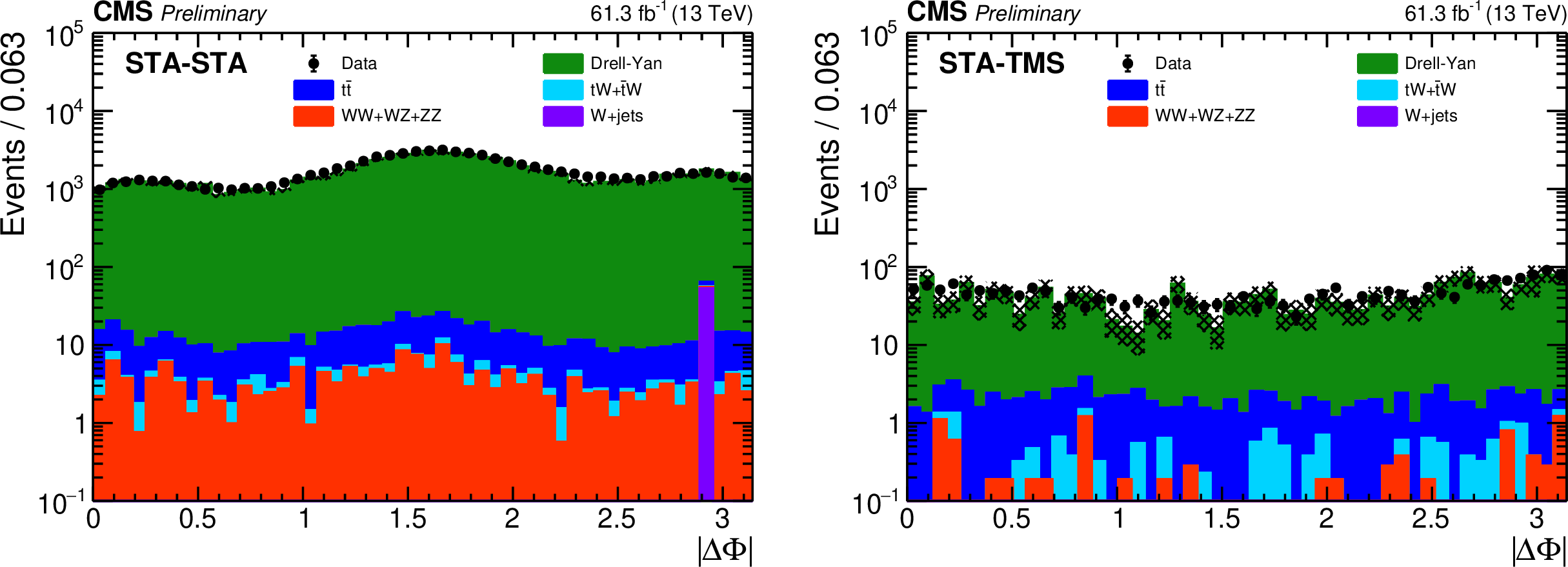
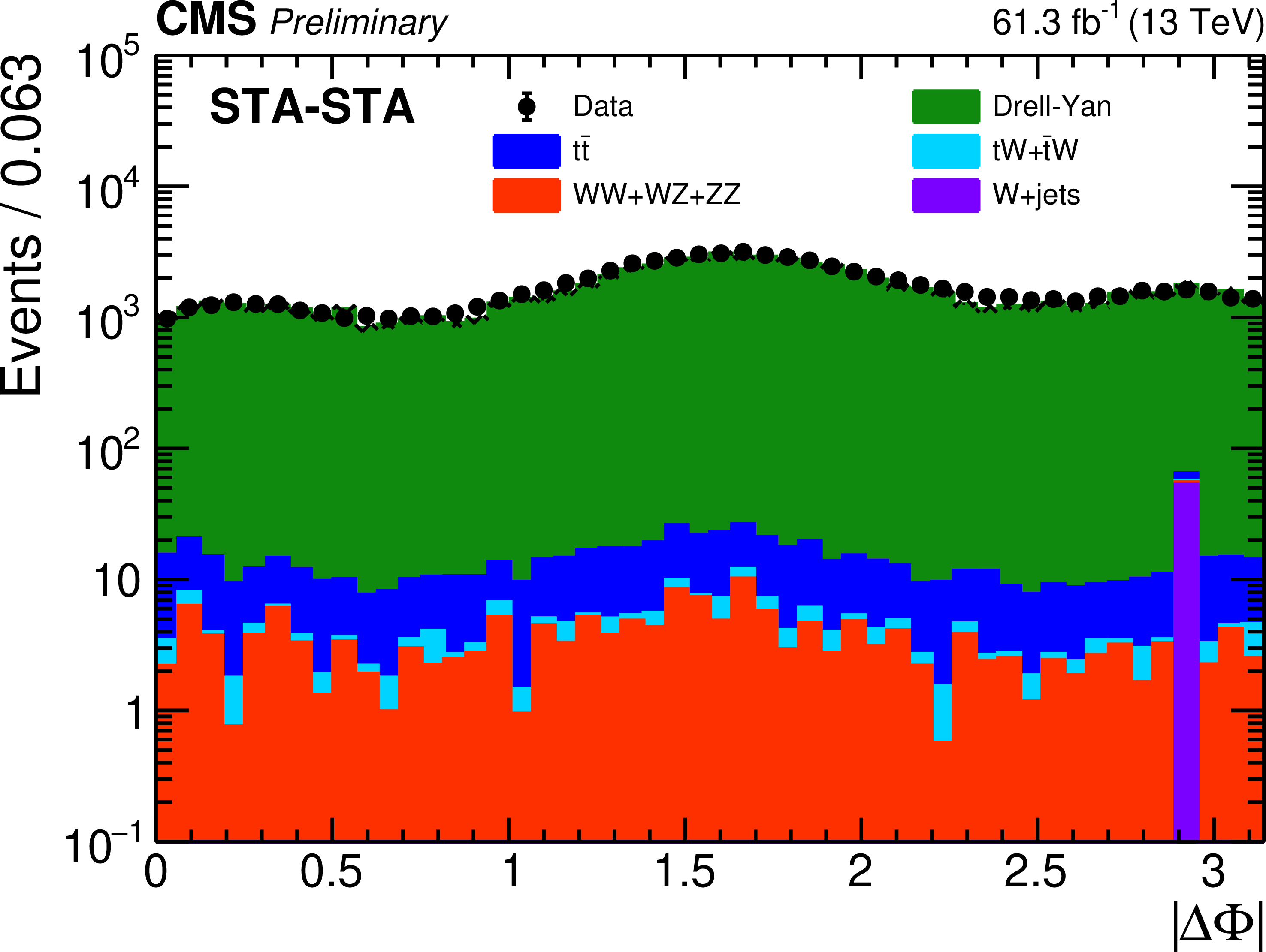
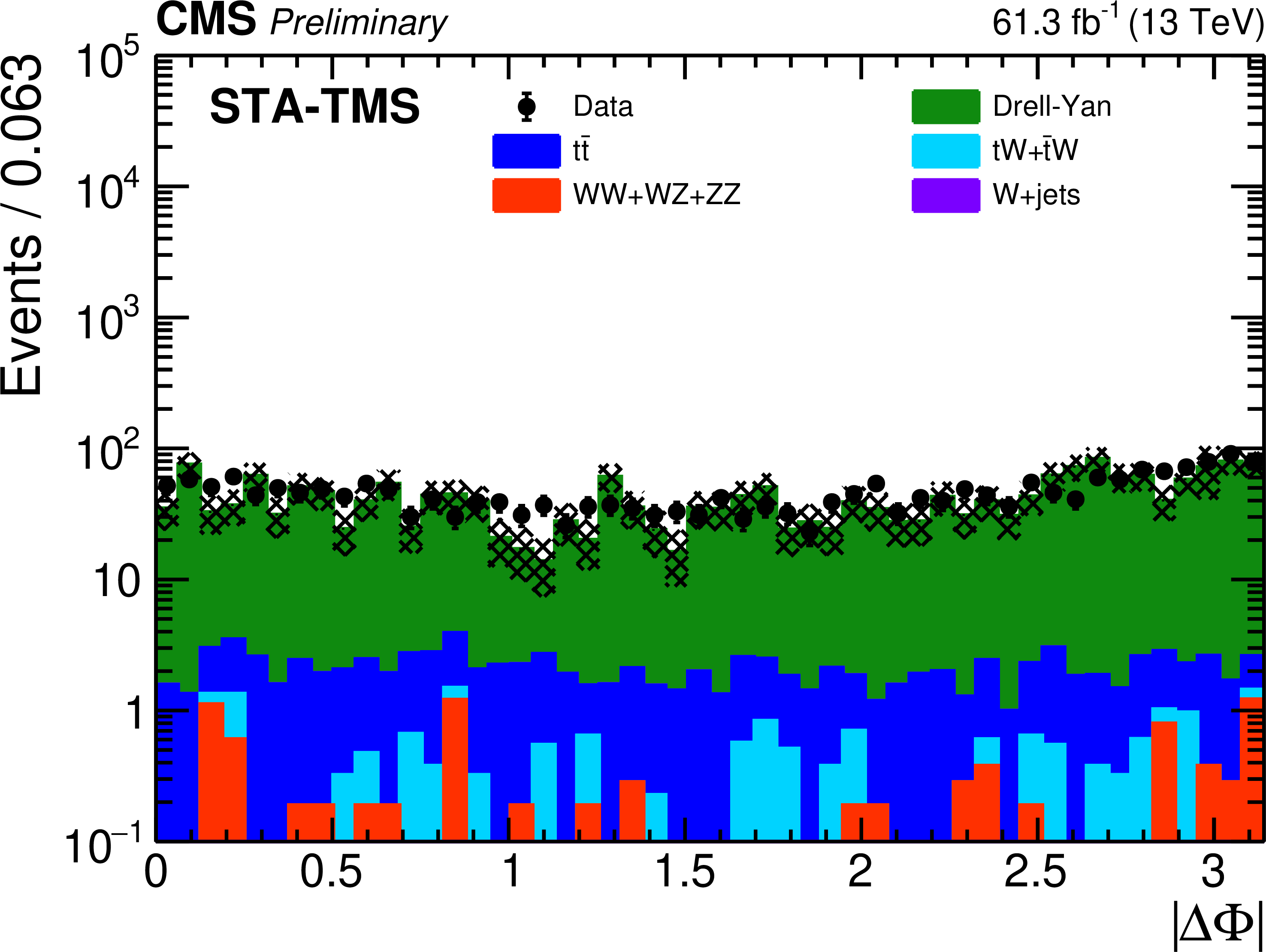
png pdf	Figure 4: Distributions of ${{\| \Delta \Phi \|}}$ for (left) STA-STA and (right) STA-TMS dimuons in 2018 data (black dots) and simulated background processes (stacked histograms), for events in the control regions with the STA to TMS association of the STA muons reversed as described in the text. All nominal selection requirements, including dimuon $L_{\mathrm {xy}} / \sigma _{L_{\mathrm {xy}}}$ and TMS muon $d_{\mathrm {0}} / \sigma _{d_{\mathrm {0}}}$ , are applied to the STA-STA and STA-TMS dimuons. The simulated processes are scaled to correspond to the luminosity of the data.
png pdf root	Figure 4-a: Distributions of ${{\| \Delta \Phi \|}}$ for (left) STA-STA and (right) STA-TMS dimuons in 2018 data (black dots) and simulated background processes (stacked histograms), for events in the control regions with the STA to TMS association of the STA muons reversed as described in the text. All nominal selection requirements, including dimuon $L_{\mathrm {xy}} / \sigma _{L_{\mathrm {xy}}}$ and TMS muon $d_{\mathrm {0}} / \sigma _{d_{\mathrm {0}}}$ , are applied to the STA-STA and STA-TMS dimuons. The simulated processes are scaled to correspond to the luminosity of the data.
png pdf root	Figure 4-b: Distributions of ${{\| \Delta \Phi \|}}$ for (left) STA-STA and (right) STA-TMS dimuons in 2018 data (black dots) and simulated background processes (stacked histograms), for events in the control regions with the STA to TMS association of the STA muons reversed as described in the text. All nominal selection requirements, including dimuon $L_{\mathrm {xy}} / \sigma _{L_{\mathrm {xy}}}$ and TMS muon $d_{\mathrm {0}} / \sigma _{d_{\mathrm {0}}}$ , are applied to the STA-STA and STA-TMS dimuons. The simulated processes are scaled to correspond to the luminosity of the data.
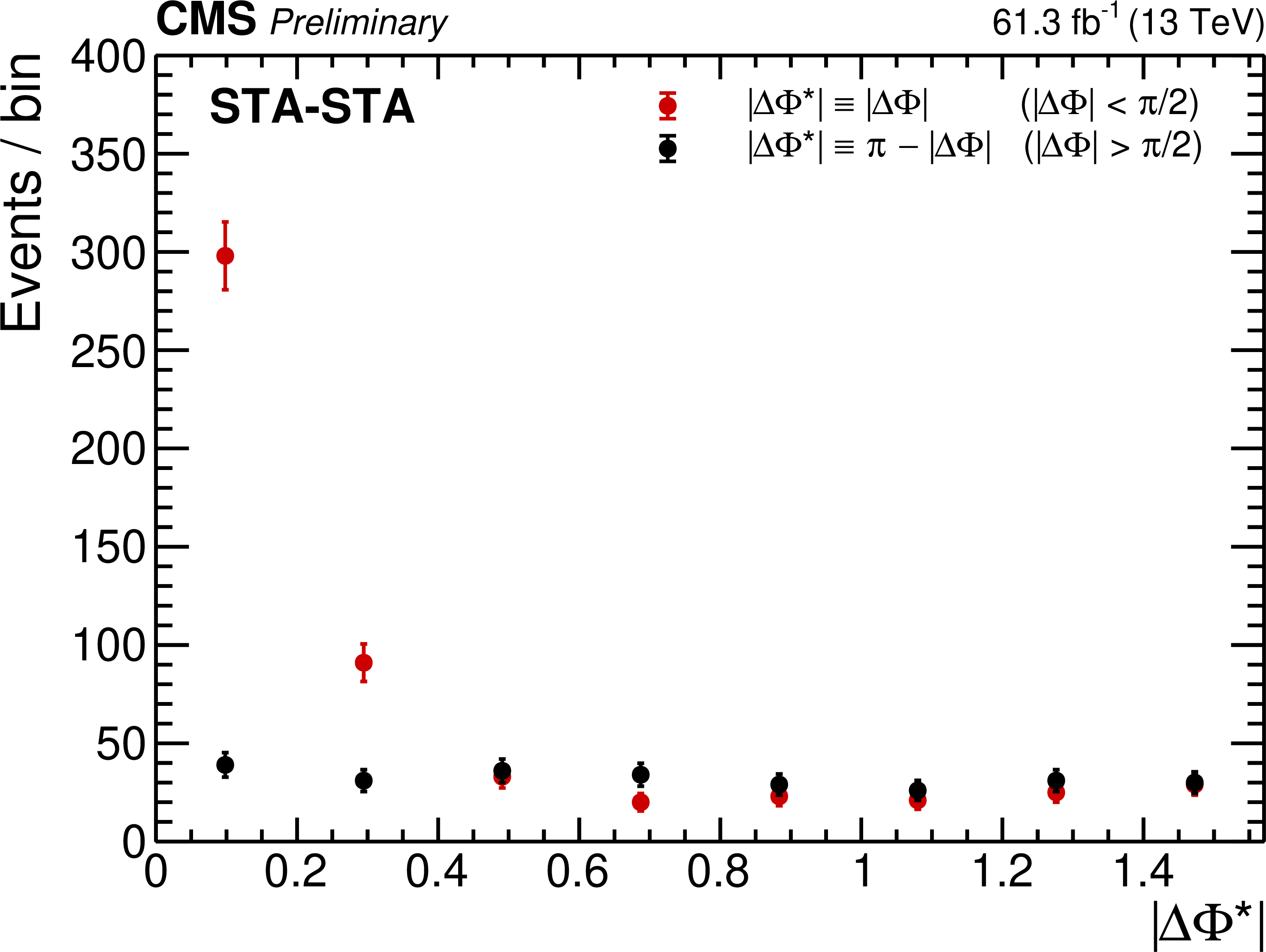
png pdf	Figure 5: Distributions of (left) $\| \Delta \Phi ^{*} \|$ (defined in the legend) of STA-STA dimuons and (right) ${m_{\mu \mu}}$ of TMS-TMS dimuons associated with STA-STA dimuons. Both distributions show STA-STA dimuons in 2018 data in the control region enriched in QCD events, as described in the text. In the left plot, exactly one STA muon is associated with a TMS muon, while in the right plot, both are. All nominal selection requirements, including ${m_{\mu \mu}} >$ 10 GeV and $L_{\mathrm {xy}} / \sigma _{L_{\mathrm {xy}}} >$ 6, are applied to the STA-STA dimuons.
png pdf root	Figure 5-a: Distributions of (left) $\| \Delta \Phi ^{*} \|$ (defined in the legend) of STA-STA dimuons and (right) ${m_{\mu \mu}}$ of TMS-TMS dimuons associated with STA-STA dimuons. Both distributions show STA-STA dimuons in 2018 data in the control region enriched in QCD events, as described in the text. In the left plot, exactly one STA muon is associated with a TMS muon, while in the right plot, both are. All nominal selection requirements, including ${m_{\mu \mu}} >$ 10 GeV and $L_{\mathrm {xy}} / \sigma _{L_{\mathrm {xy}}} >$ 6, are applied to the STA-STA dimuons.
png pdf root	Figure 5-b: Distributions of (left) $\| \Delta \Phi ^{*} \|$ (defined in the legend) of STA-STA dimuons and (right) ${m_{\mu \mu}}$ of TMS-TMS dimuons associated with STA-STA dimuons. Both distributions show STA-STA dimuons in 2018 data in the control region enriched in QCD events, as described in the text. In the left plot, exactly one STA muon is associated with a TMS muon, while in the right plot, both are. All nominal selection requirements, including ${m_{\mu \mu}} >$ 10 GeV and $L_{\mathrm {xy}} / \sigma _{L_{\mathrm {xy}}} >$ 6, are applied to the STA-STA dimuons.
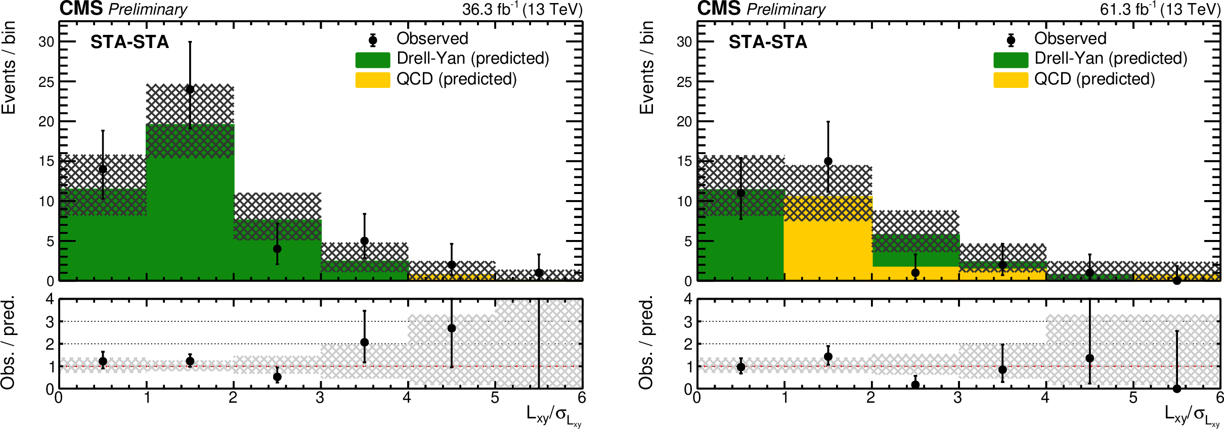
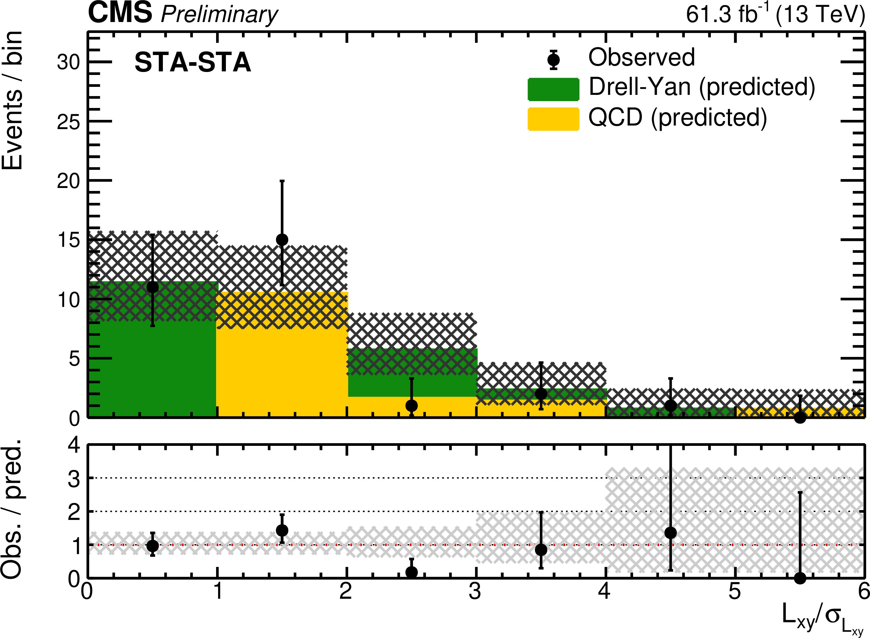
png pdf	Figure 6: Distributions of $L_{\mathrm {xy}} / \sigma _{L_{\mathrm {xy}}}$ of STA-STA dimuons in the $L_{\mathrm {xy}} / \sigma _{L_{\mathrm {xy}}} <$ 6 VR, in (left) 2016 and (right) 2018 data, compared to the background predictions. The observed distributions (black circles) are overlayed on stacked histograms containing the expected numbers of DY (green) and QCD (yellow) background events. The lower panels show the ratio of the observed to predicted numbers of events. Shaded area shows the statistical uncertainty in the background prediction.
png pdf root	Figure 6-a: Distributions of $L_{\mathrm {xy}} / \sigma _{L_{\mathrm {xy}}}$ of STA-STA dimuons in the $L_{\mathrm {xy}} / \sigma _{L_{\mathrm {xy}}} <$ 6 VR, in (left) 2016 and (right) 2018 data, compared to the background predictions. The observed distributions (black circles) are overlayed on stacked histograms containing the expected numbers of DY (green) and QCD (yellow) background events. The lower panels show the ratio of the observed to predicted numbers of events. Shaded area shows the statistical uncertainty in the background prediction.
png pdf root	Figure 6-b: Distributions of $L_{\mathrm {xy}} / \sigma _{L_{\mathrm {xy}}}$ of STA-STA dimuons in the $L_{\mathrm {xy}} / \sigma _{L_{\mathrm {xy}}} <$ 6 VR, in (left) 2016 and (right) 2018 data, compared to the background predictions. The observed distributions (black circles) are overlayed on stacked histograms containing the expected numbers of DY (green) and QCD (yellow) background events. The lower panels show the ratio of the observed to predicted numbers of events. Shaded area shows the statistical uncertainty in the background prediction.
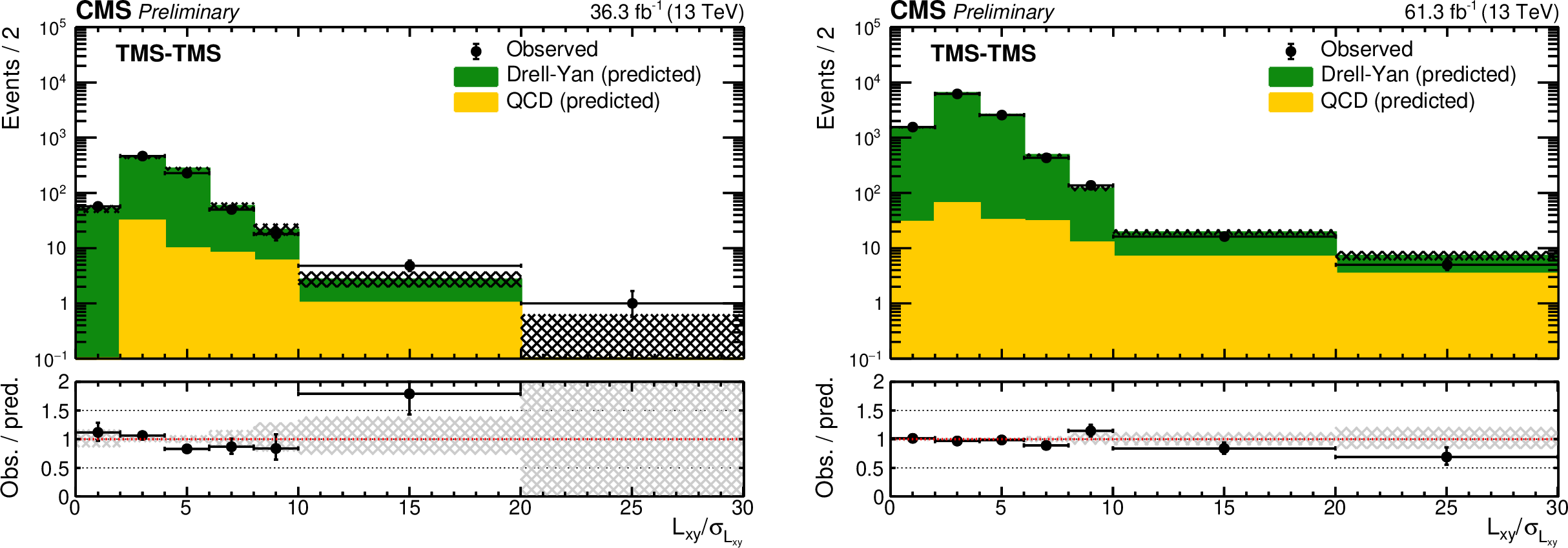
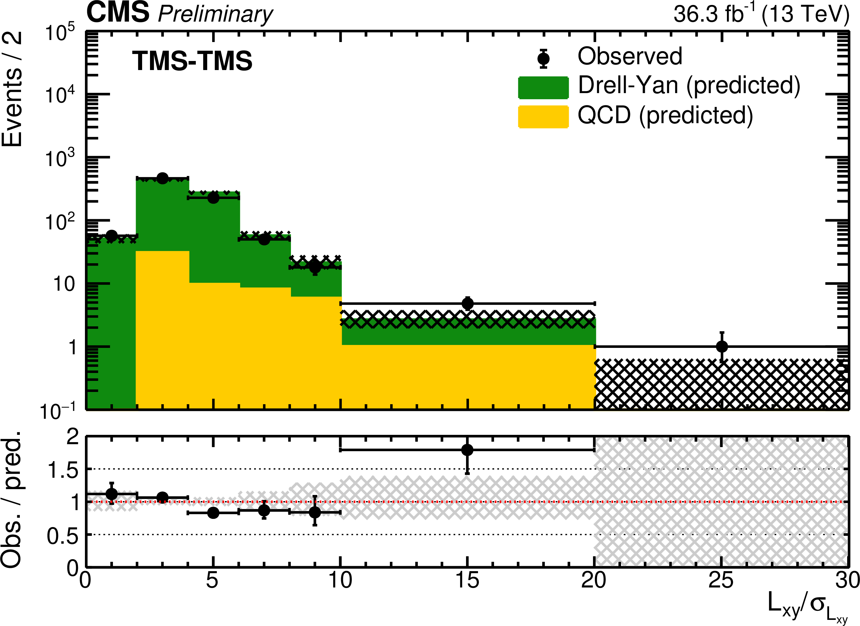
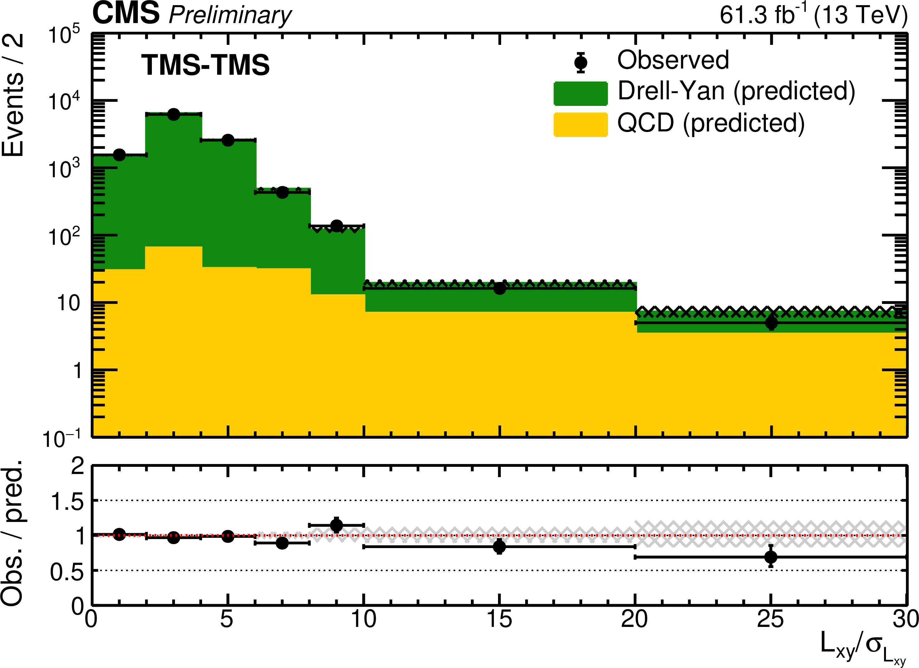
png pdf	Figure 7: Distributions of $L_{\mathrm {xy}} / \sigma _{L_{\mathrm {xy}}}$ of TMS-TMS dimuons in the 2 $< \min{(d_{\mathrm {0}} / \sigma _{d_{\mathrm {0}}})} <$ 6 VR, in (left) 2016 and (right) 2018 data, compared to the background predictions. The observed distributions (black circles) are overlayed on stacked histograms containing the expected numbers of DY (green) and QCD (yellow) background events. The last bin includes events in the overflow. The lower panels show the ratio of the observed to predicted numbers of events. Shaded area shows the statistical uncertainty in the background prediction.
png pdf root	Figure 7-a: Distributions of $L_{\mathrm {xy}} / \sigma _{L_{\mathrm {xy}}}$ of TMS-TMS dimuons in the 2 $< \min{(d_{\mathrm {0}} / \sigma _{d_{\mathrm {0}}})} <$ 6 VR, in (left) 2016 and (right) 2018 data, compared to the background predictions. The observed distributions (black circles) are overlayed on stacked histograms containing the expected numbers of DY (green) and QCD (yellow) background events. The last bin includes events in the overflow. The lower panels show the ratio of the observed to predicted numbers of events. Shaded area shows the statistical uncertainty in the background prediction.
png pdf root	Figure 7-b: Distributions of $L_{\mathrm {xy}} / \sigma _{L_{\mathrm {xy}}}$ of TMS-TMS dimuons in the 2 $< \min{(d_{\mathrm {0}} / \sigma _{d_{\mathrm {0}}})} <$ 6 VR, in (left) 2016 and (right) 2018 data, compared to the background predictions. The observed distributions (black circles) are overlayed on stacked histograms containing the expected numbers of DY (green) and QCD (yellow) background events. The last bin includes events in the overflow. The lower panels show the ratio of the observed to predicted numbers of events. Shaded area shows the statistical uncertainty in the background prediction.
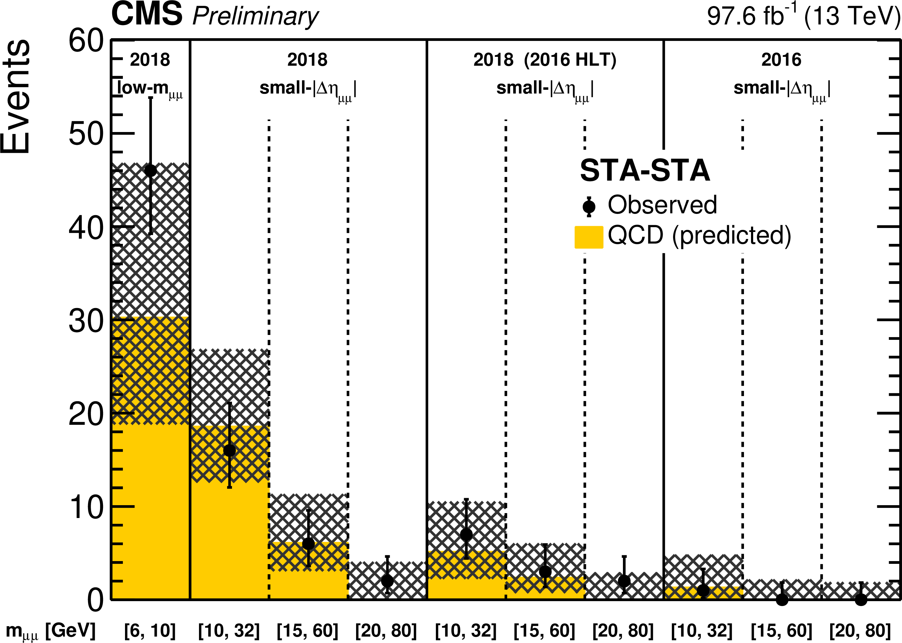
png pdf root	Figure 8: Comparison of observed (black circles) and predicted (histograms) yields of STA-STA dimuons in the validation regions enriched in QCD background events. The first bin shows the yields in the low-mass VR in 2018 data. The other three groups of bins, separated by solid lines, show the yields in the small- ${{\| \Delta \eta _{\mu \mu} \|}}$ VR, in (from left to right) the entire 2018 data set, a subset of 2018 data enriched in events collected in 2016, and the 2016 data set. Each of these three VRs is further subdivided into three ${m_{\mu \mu}}$ intervals, 10-32, 15-60, and 20-80 GeV. The expected number of background events is computed according to Eqs. (3) and (4), separately in each ${m_{\mu \mu}}$ bin. Shaded area shows the statistical uncertainty in the background prediction.
png pdf	Figure 9: Distributions in the $\pi /4 < {{\| \Delta \Phi \|}} < \pi /2$ VR in 2018 data: (left) the smaller of the two $d_{\mathrm {0}} / \sigma _{d_{\mathrm {0}}}$ values in the TMS-TMS dimuon; (right) $d_{\mathrm {0}} / \sigma _{d_{\mathrm {0}}}$ of the TMS muon in the STA-TMS dimuon. The observed distributions (black circles) are compared to the results of the background prediction method applied to events with $\pi /2 < {{\| \Delta \Phi \|}} < 3\pi /4$ . The stacked histograms show the expected numbers of DY (green) and QCD (yellow) background events. The last bin includes events in the overflow. The lower panels show the ratios of the observed to predicted numbers of events. Shaded area shows the statistical uncertainty in the background prediction.
png pdf root	Figure 9-a: Distributions in the $\pi /4 < {{\| \Delta \Phi \|}} < \pi /2$ VR in 2018 data: (left) the smaller of the two $d_{\mathrm {0}} / \sigma _{d_{\mathrm {0}}}$ values in the TMS-TMS dimuon; (right) $d_{\mathrm {0}} / \sigma _{d_{\mathrm {0}}}$ of the TMS muon in the STA-TMS dimuon. The observed distributions (black circles) are compared to the results of the background prediction method applied to events with $\pi /2 < {{\| \Delta \Phi \|}} < 3\pi /4$ . The stacked histograms show the expected numbers of DY (green) and QCD (yellow) background events. The last bin includes events in the overflow. The lower panels show the ratios of the observed to predicted numbers of events. Shaded area shows the statistical uncertainty in the background prediction.
png pdf root	Figure 9-b: Distributions in the $\pi /4 < {{\| \Delta \Phi \|}} < \pi /2$ VR in 2018 data: (left) the smaller of the two $d_{\mathrm {0}} / \sigma _{d_{\mathrm {0}}}$ values in the TMS-TMS dimuon; (right) $d_{\mathrm {0}} / \sigma _{d_{\mathrm {0}}}$ of the TMS muon in the STA-TMS dimuon. The observed distributions (black circles) are compared to the results of the background prediction method applied to events with $\pi /2 < {{\| \Delta \Phi \|}} < 3\pi /4$ . The stacked histograms show the expected numbers of DY (green) and QCD (yellow) background events. The last bin includes events in the overflow. The lower panels show the ratios of the observed to predicted numbers of events. Shaded area shows the statistical uncertainty in the background prediction.
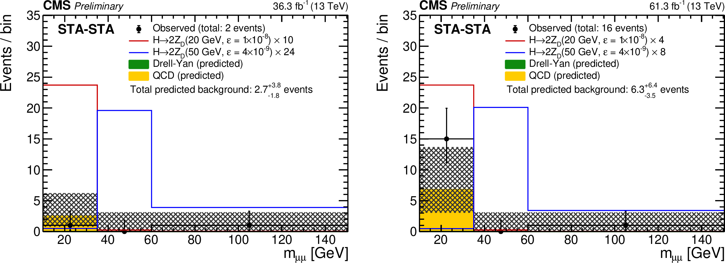
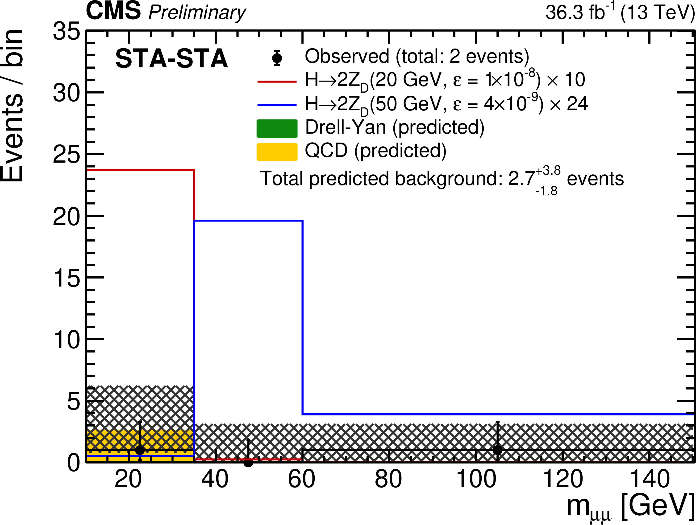
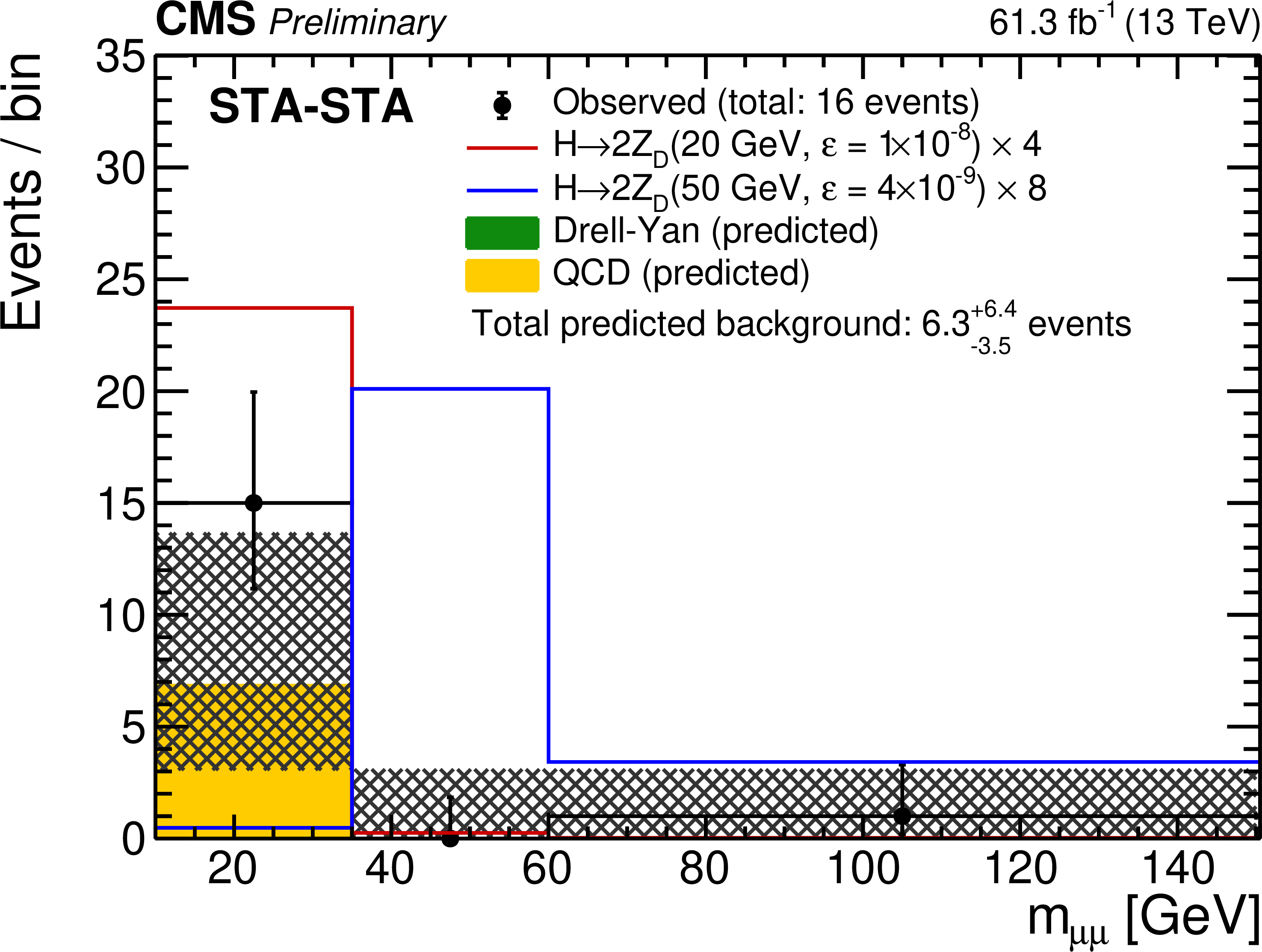
png pdf	Figure 10: Comparison between the number of events observed in (left) 2016 and (right) 2018 data in the STA-STA dimuon category with the expected number of background events, in representative ${m_{\mu \mu}}$ intervals. The black circles show the number of observed events; the green and yellow components of the stacked histograms represent the estimated numbers of DY and QCD events, respectively. The last bin includes events in the overflow. The uncertainties in the total expected background (shaded area) are statistical only. Signal contributions expected from simulated $\mathrm{H} \to \mathrm{Z_D}\mathrm{Z_D}$ with $m(\mathrm{Z_D})$ of 20 and 50 GeV are shown in red and blue, respectively. Their yields are set to the corresponding median expected exclusion limits at 95% CL and scaled up to improve their visibility. The legends include the total number of observed events as well as the ${m_{\mu \mu}}$ -integrated number of expected background events, which is obtained by applying the background evaluation method to the events in all mass intervals combined.
png pdf root	Figure 10-a: Comparison between the number of events observed in (left) 2016 and (right) 2018 data in the STA-STA dimuon category with the expected number of background events, in representative ${m_{\mu \mu}}$ intervals. The black circles show the number of observed events; the green and yellow components of the stacked histograms represent the estimated numbers of DY and QCD events, respectively. The last bin includes events in the overflow. The uncertainties in the total expected background (shaded area) are statistical only. Signal contributions expected from simulated $\mathrm{H} \to \mathrm{Z_D}\mathrm{Z_D}$ with $m(\mathrm{Z_D})$ of 20 and 50 GeV are shown in red and blue, respectively. Their yields are set to the corresponding median expected exclusion limits at 95% CL and scaled up to improve their visibility. The legends include the total number of observed events as well as the ${m_{\mu \mu}}$ -integrated number of expected background events, which is obtained by applying the background evaluation method to the events in all mass intervals combined.
png pdf root	Figure 10-b: Comparison between the number of events observed in (left) 2016 and (right) 2018 data in the STA-STA dimuon category with the expected number of background events, in representative ${m_{\mu \mu}}$ intervals. The black circles show the number of observed events; the green and yellow components of the stacked histograms represent the estimated numbers of DY and QCD events, respectively. The last bin includes events in the overflow. The uncertainties in the total expected background (shaded area) are statistical only. Signal contributions expected from simulated $\mathrm{H} \to \mathrm{Z_D}\mathrm{Z_D}$ with $m(\mathrm{Z_D})$ of 20 and 50 GeV are shown in red and blue, respectively. Their yields are set to the corresponding median expected exclusion limits at 95% CL and scaled up to improve their visibility. The legends include the total number of observed events as well as the ${m_{\mu \mu}}$ -integrated number of expected background events, which is obtained by applying the background evaluation method to the events in all mass intervals combined.
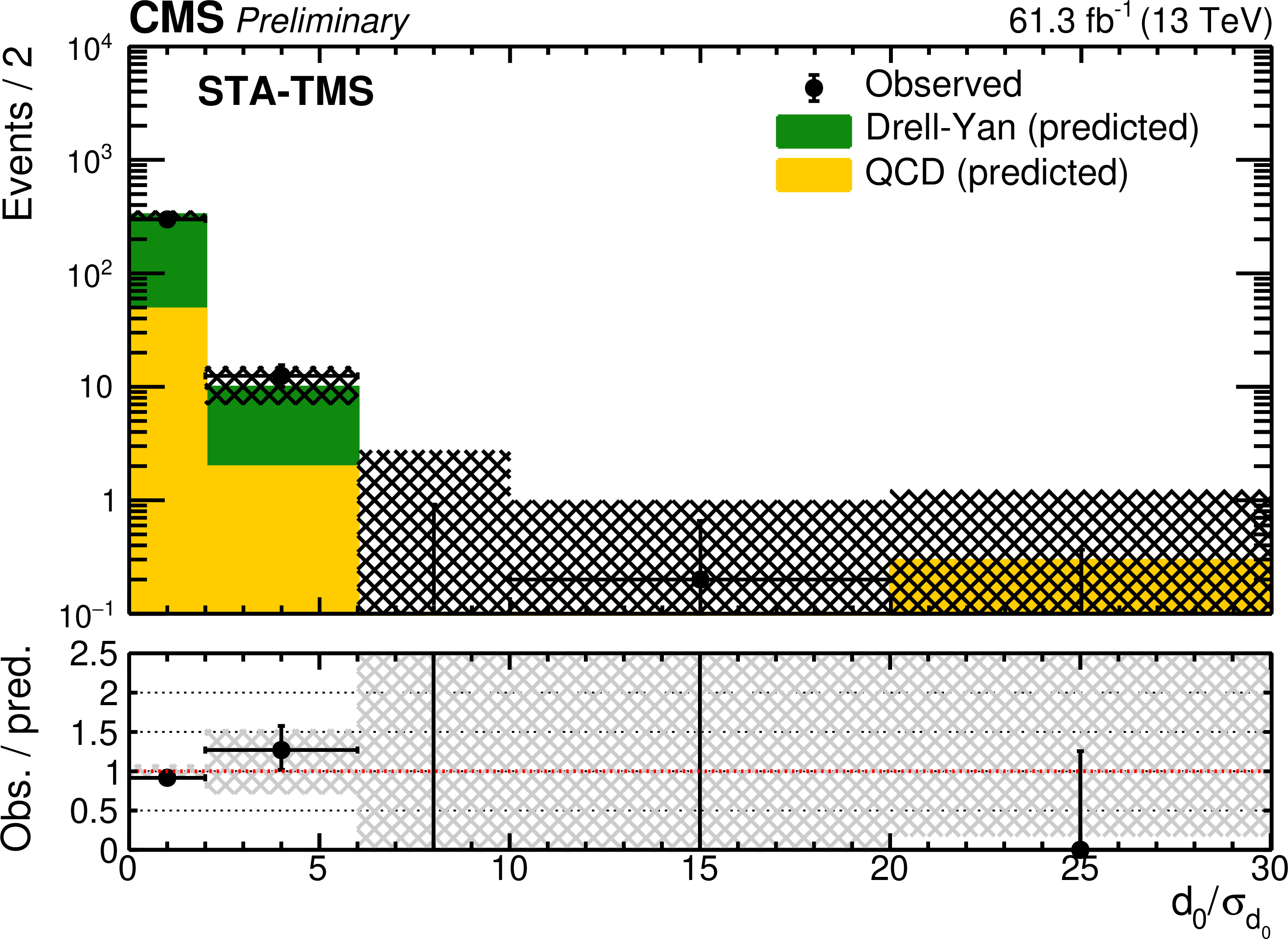
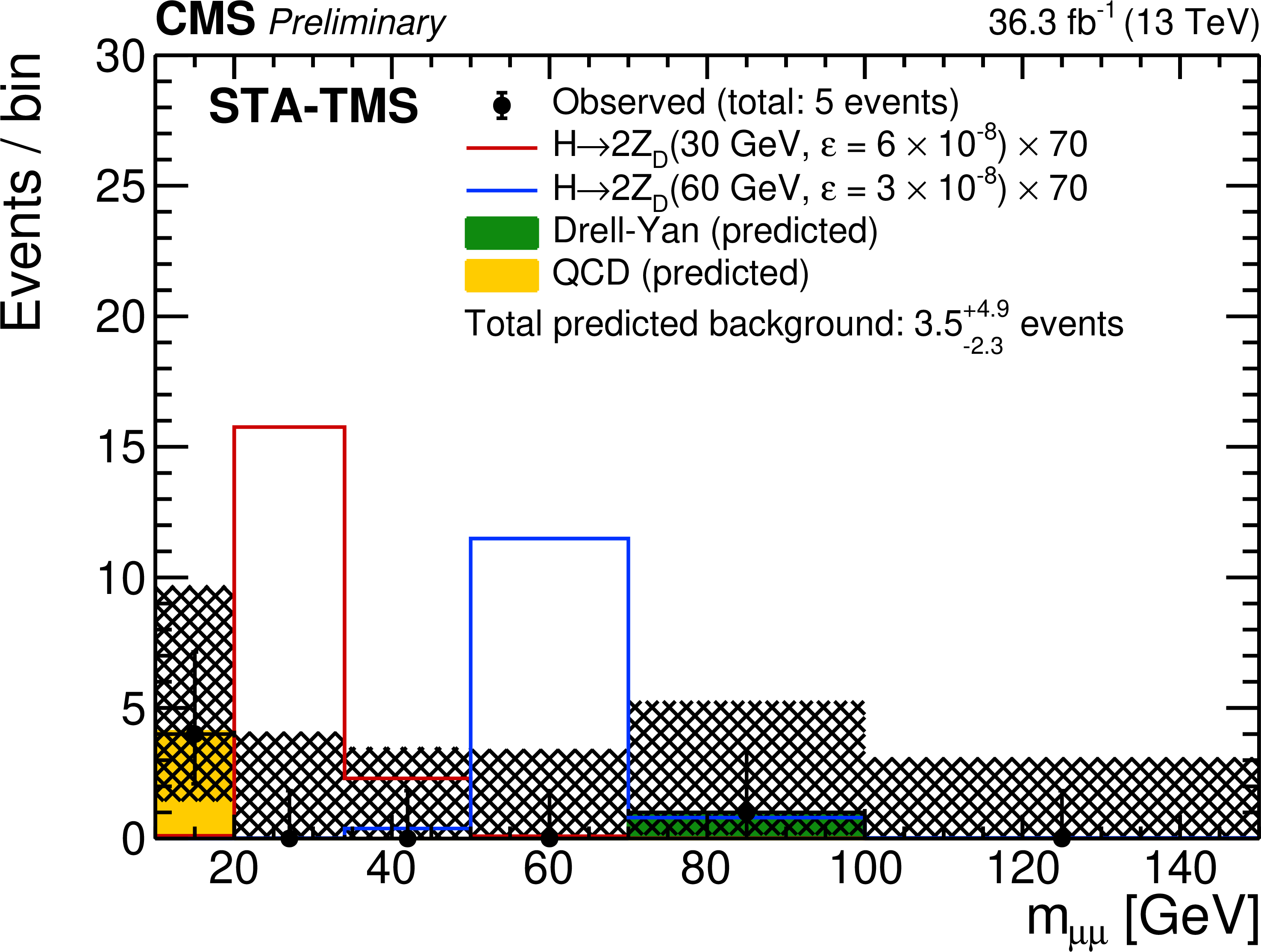
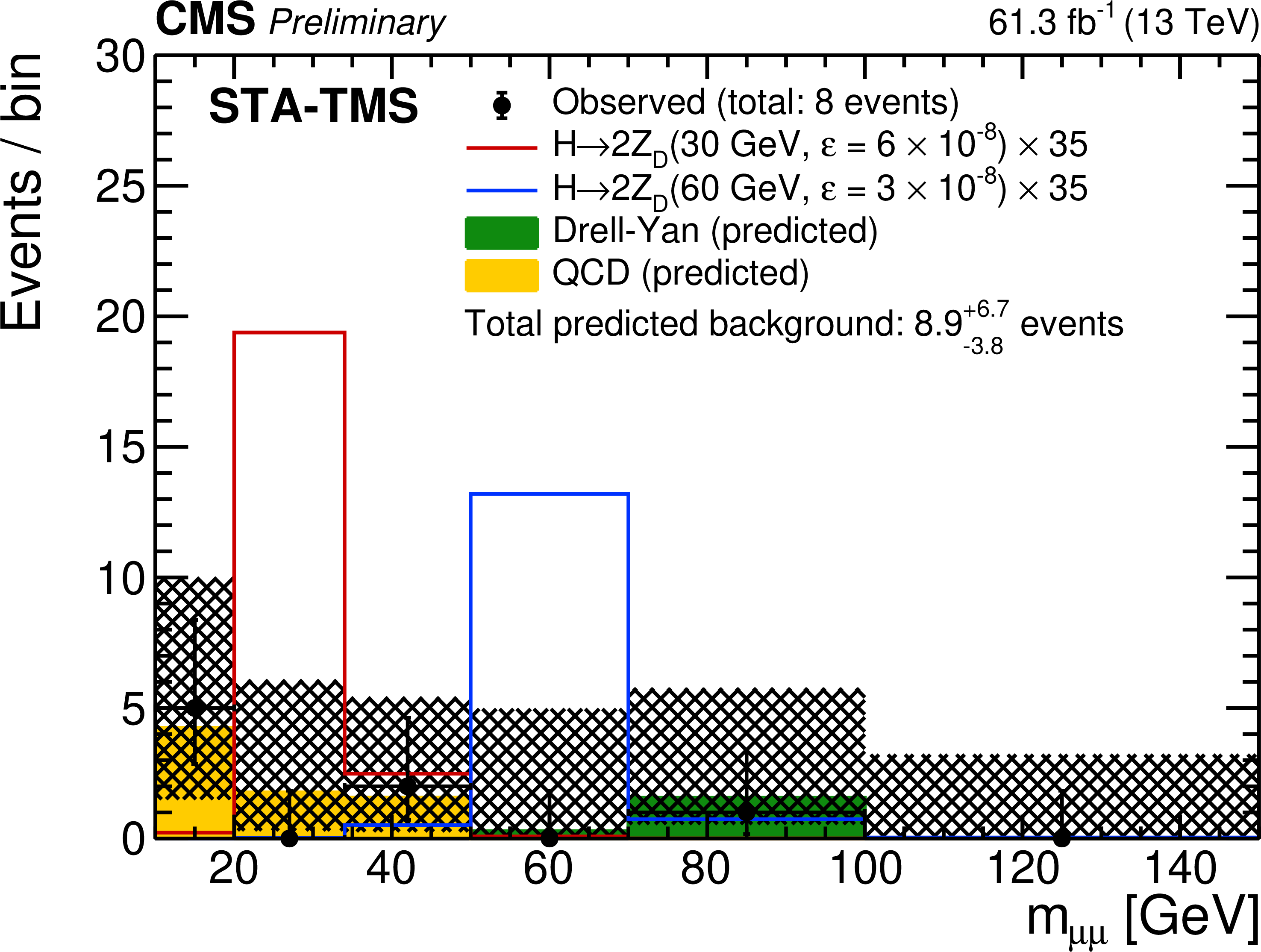
png pdf	Figure 11: Comparison between the number of events observed in (left) 2016 and (right) 2018 data in the STA-TMS dimuon category with the expected number of background events, in representative ${m_{\mu \mu}}$ intervals. The black circles show the number of observed events; the green and yellow components of the stacked histograms represent the estimated numbers of DY and QCD events, respectively. The last bin includes events in the overflow. The uncertainties in the total expected background (shaded area) are statistical only. Signal contributions expected from simulated $\mathrm{H} \to \mathrm{Z_D}\mathrm{Z_D}$ with $m(\mathrm{Z_D})$ of 30 and 60 GeV are shown in red and blue, respectively. Their yields are set to the corresponding median expected exclusion limits at 95% CL and scaled up to improve their visibility. The legends include the total number of observed events as well as the ${m_{\mu \mu}}$ -integrated number of expected background events, which is obtained by applying the background evaluation method to the events in all mass intervals combined.
png pdf root	Figure 11-a: Comparison between the number of events observed in (left) 2016 and (right) 2018 data in the STA-TMS dimuon category with the expected number of background events, in representative ${m_{\mu \mu}}$ intervals. The black circles show the number of observed events; the green and yellow components of the stacked histograms represent the estimated numbers of DY and QCD events, respectively. The last bin includes events in the overflow. The uncertainties in the total expected background (shaded area) are statistical only. Signal contributions expected from simulated $\mathrm{H} \to \mathrm{Z_D}\mathrm{Z_D}$ with $m(\mathrm{Z_D})$ of 30 and 60 GeV are shown in red and blue, respectively. Their yields are set to the corresponding median expected exclusion limits at 95% CL and scaled up to improve their visibility. The legends include the total number of observed events as well as the ${m_{\mu \mu}}$ -integrated number of expected background events, which is obtained by applying the background evaluation method to the events in all mass intervals combined.
png pdf root	Figure 11-b: Comparison between the number of events observed in (left) 2016 and (right) 2018 data in the STA-TMS dimuon category with the expected number of background events, in representative ${m_{\mu \mu}}$ intervals. The black circles show the number of observed events; the green and yellow components of the stacked histograms represent the estimated numbers of DY and QCD events, respectively. The last bin includes events in the overflow. The uncertainties in the total expected background (shaded area) are statistical only. Signal contributions expected from simulated $\mathrm{H} \to \mathrm{Z_D}\mathrm{Z_D}$ with $m(\mathrm{Z_D})$ of 30 and 60 GeV are shown in red and blue, respectively. Their yields are set to the corresponding median expected exclusion limits at 95% CL and scaled up to improve their visibility. The legends include the total number of observed events as well as the ${m_{\mu \mu}}$ -integrated number of expected background events, which is obtained by applying the background evaluation method to the events in all mass intervals combined.
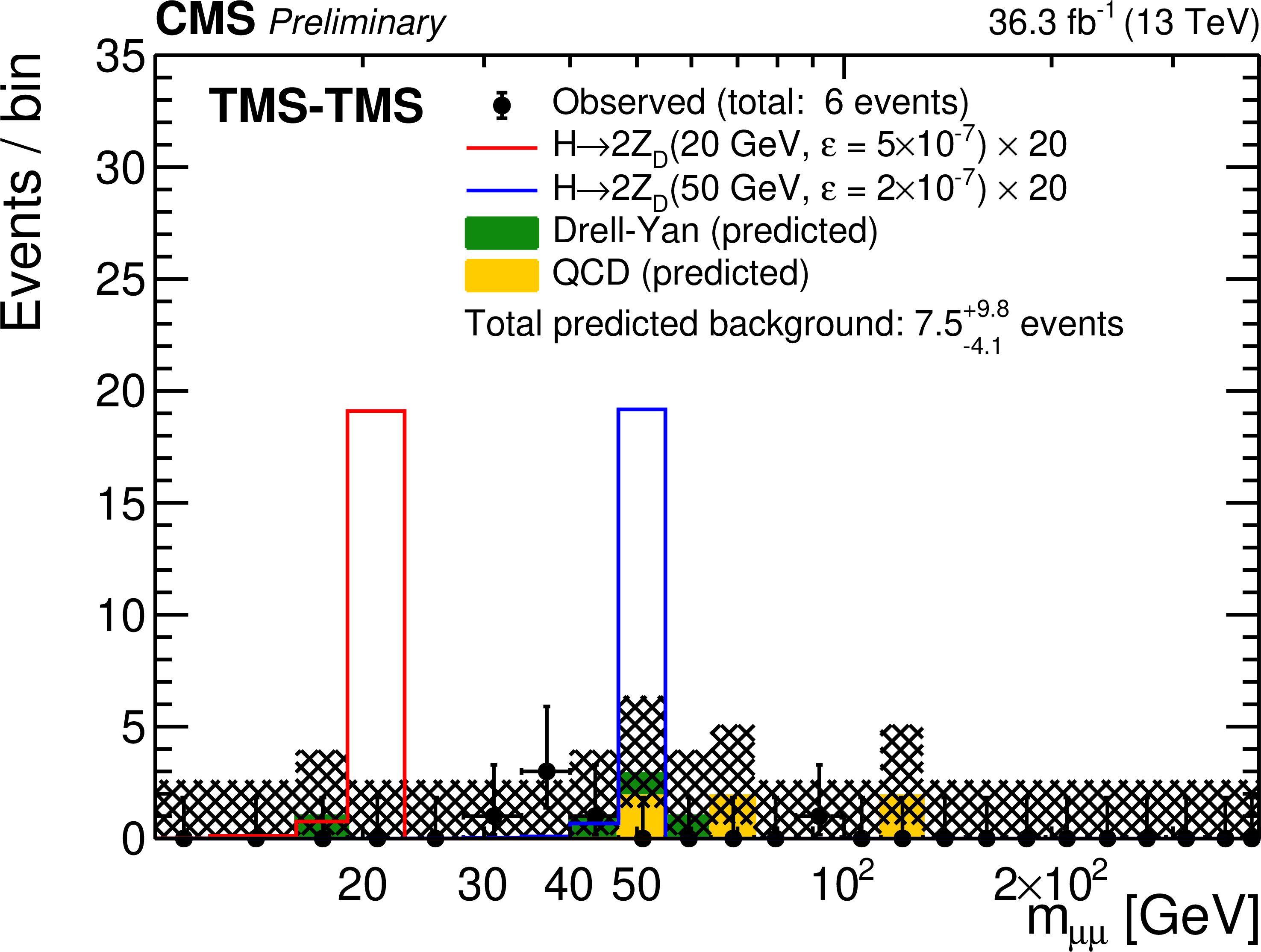
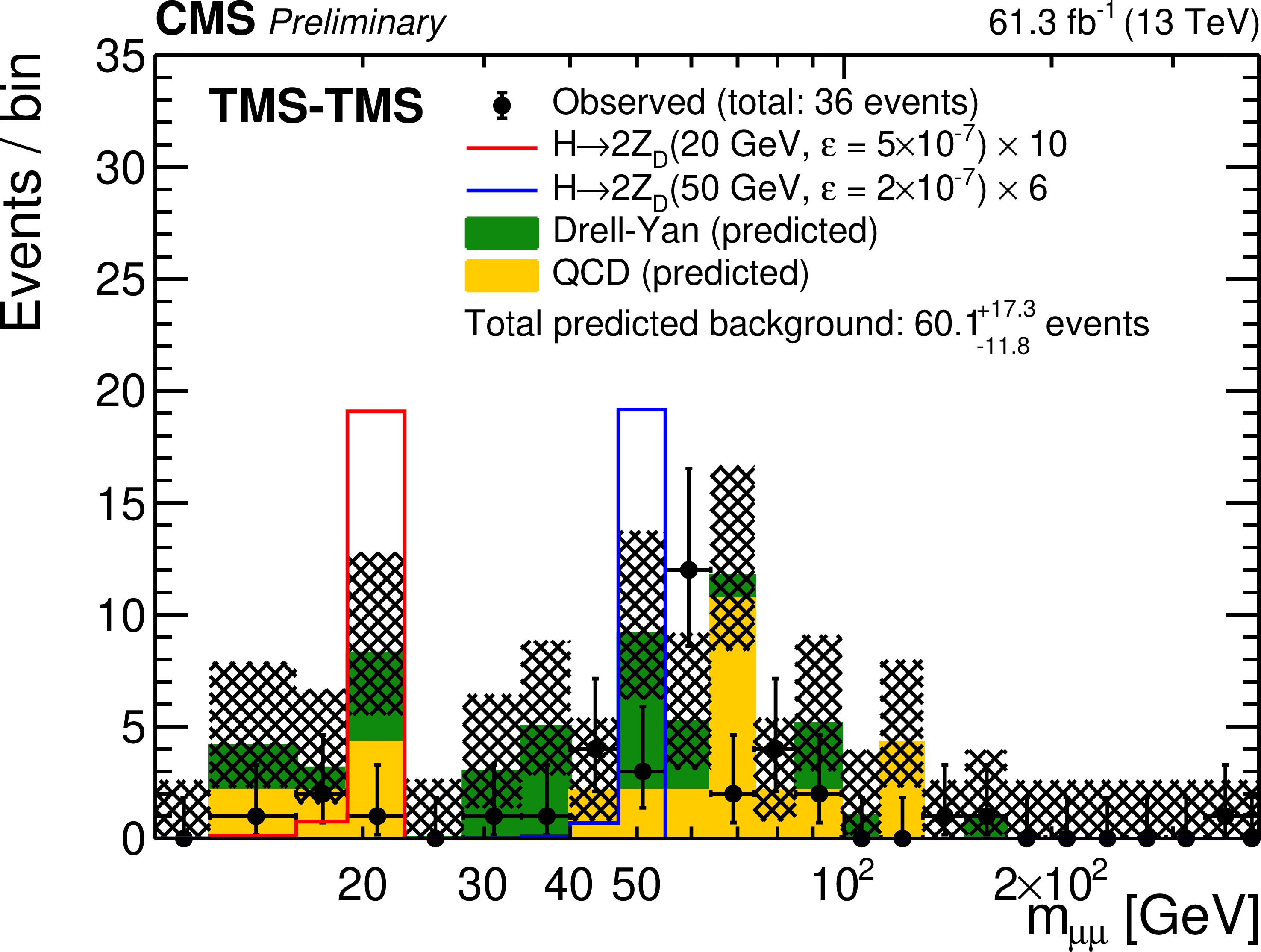
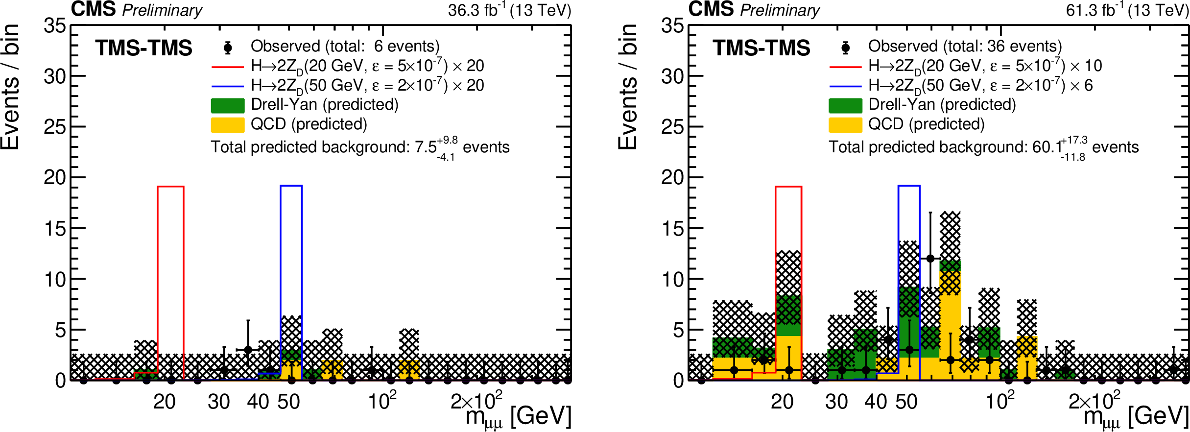
png pdf	Figure 12: Comparison between the number of events observed in (left) 2016 and (right) 2018 data in the TMS-TMS dimuon category with the expected number of background events, in representative ${m_{\mu \mu}}$ intervals. The black circles show the number of observed events; the green and yellow components of the stacked histograms represent the estimated numbers of DY and QCD events, respectively. The last bin includes events in the overflow. The uncertainties in the total expected background (shaded area) are statistical only. Signal contributions expected from simulated $\mathrm{H} \to \mathrm{Z_D}\mathrm{Z_D}$ with $m(\mathrm{Z_D})$ of 20 and 50 GeV are shown in red and blue, respectively. Their yields are set to the corresponding median expected exclusion limits at 95% CL and scaled up to improve their visibility. The legends include the total number of observed events as well as the ${m_{\mu \mu}}$ -integrated number of expected background events, which is obtained by applying the background evaluation method to the events in all mass intervals combined.
png pdf root	Figure 12-a: Comparison between the number of events observed in (left) 2016 and (right) 2018 data in the TMS-TMS dimuon category with the expected number of background events, in representative ${m_{\mu \mu}}$ intervals. The black circles show the number of observed events; the green and yellow components of the stacked histograms represent the estimated numbers of DY and QCD events, respectively. The last bin includes events in the overflow. The uncertainties in the total expected background (shaded area) are statistical only. Signal contributions expected from simulated $\mathrm{H} \to \mathrm{Z_D}\mathrm{Z_D}$ with $m(\mathrm{Z_D})$ of 20 and 50 GeV are shown in red and blue, respectively. Their yields are set to the corresponding median expected exclusion limits at 95% CL and scaled up to improve their visibility. The legends include the total number of observed events as well as the ${m_{\mu \mu}}$ -integrated number of expected background events, which is obtained by applying the background evaluation method to the events in all mass intervals combined.
png pdf root	Figure 12-b: Comparison between the number of events observed in (left) 2016 and (right) 2018 data in the TMS-TMS dimuon category with the expected number of background events, in representative ${m_{\mu \mu}}$ intervals. The black circles show the number of observed events; the green and yellow components of the stacked histograms represent the estimated numbers of DY and QCD events, respectively. The last bin includes events in the overflow. The uncertainties in the total expected background (shaded area) are statistical only. Signal contributions expected from simulated $\mathrm{H} \to \mathrm{Z_D}\mathrm{Z_D}$ with $m(\mathrm{Z_D})$ of 20 and 50 GeV are shown in red and blue, respectively. Their yields are set to the corresponding median expected exclusion limits at 95% CL and scaled up to improve their visibility. The legends include the total number of observed events as well as the ${m_{\mu \mu}}$ -integrated number of expected background events, which is obtained by applying the background evaluation method to the events in all mass intervals combined.
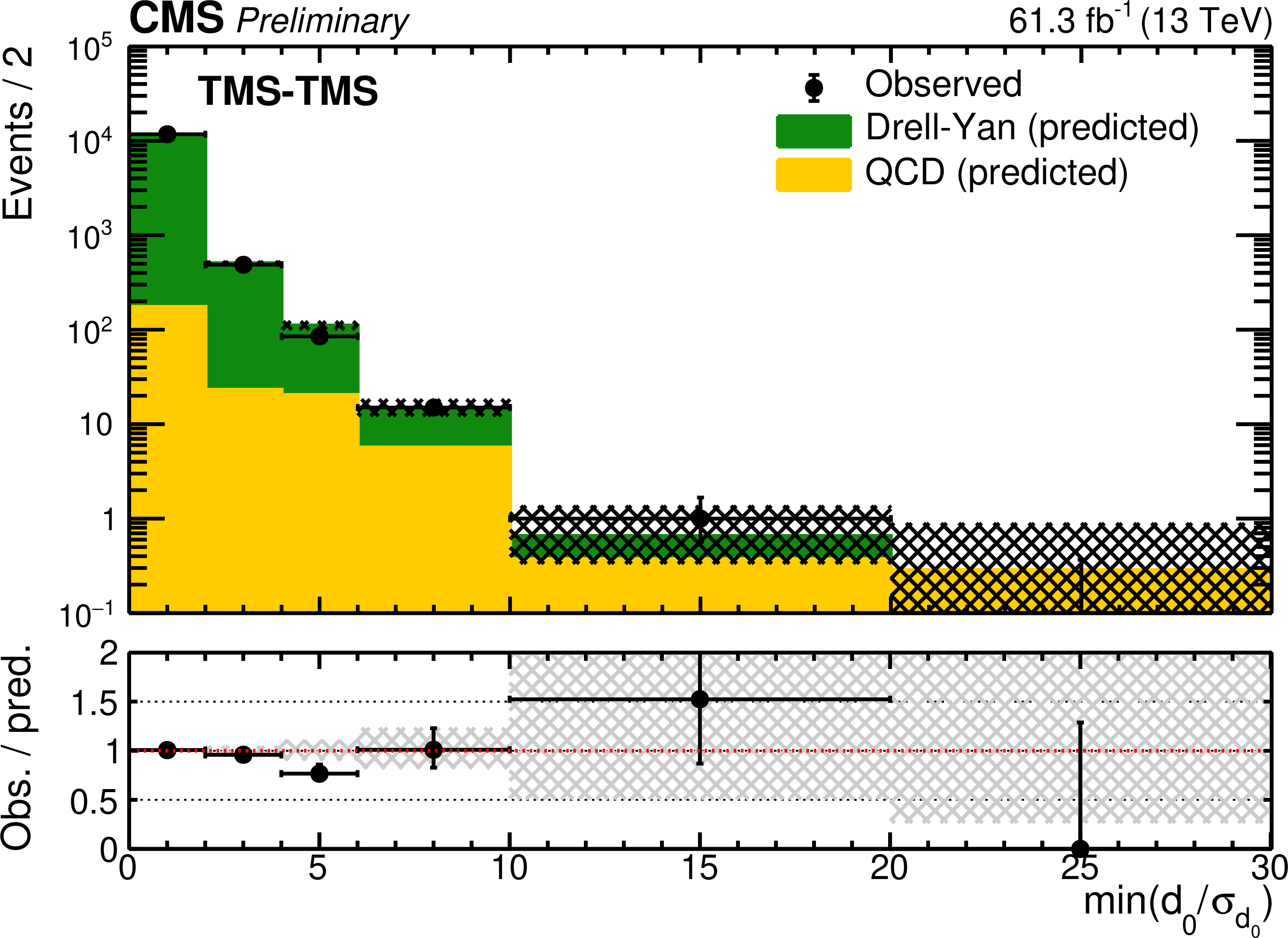
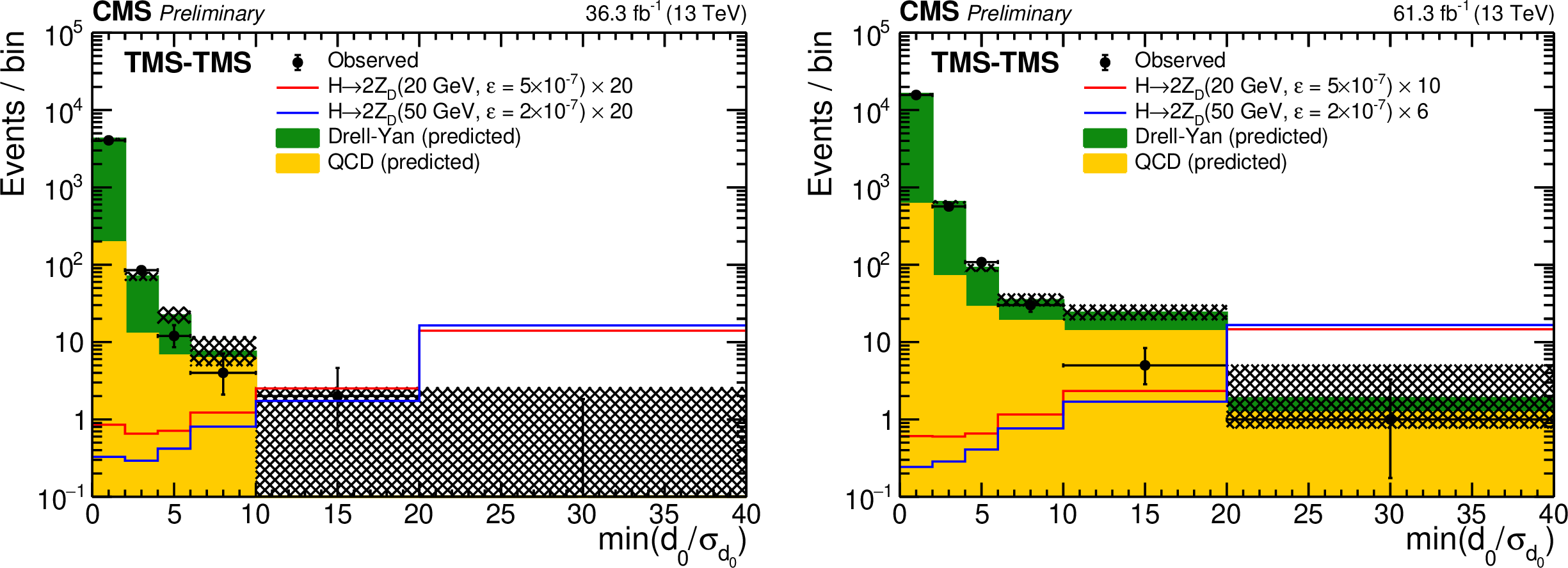
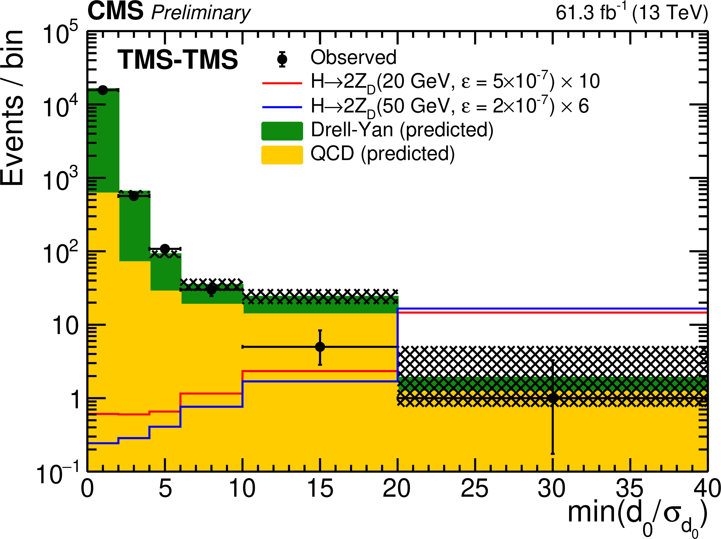
png pdf	Figure 13: Comparison between the number of events observed in (left) 2016 and (right) 2018 data in the TMS-TMS dimuon category with the expected number of background events, as a function of the smaller of the two $d_{\mathrm {0}} / \sigma _{d_{\mathrm {0}}}$ values in the TMS-TMS dimuon. The black circles show the number of observed events; the green and yellow components of the stacked histograms represent the estimated numbers of DY and QCD events, respectively. The last bin includes events in the overflow. The uncertainties in the total expected background (shaded area) are statistical only. Signal contributions expected from simulated $\mathrm{H} \to \mathrm{Z_D}\mathrm{Z_D}$ with $m(\mathrm{Z_D})$ of 20 and 50 GeV are shown in red and blue, respectively. Their yields are set to the corresponding median expected exclusion limits at 95% CL and scaled up to improve their visibility.
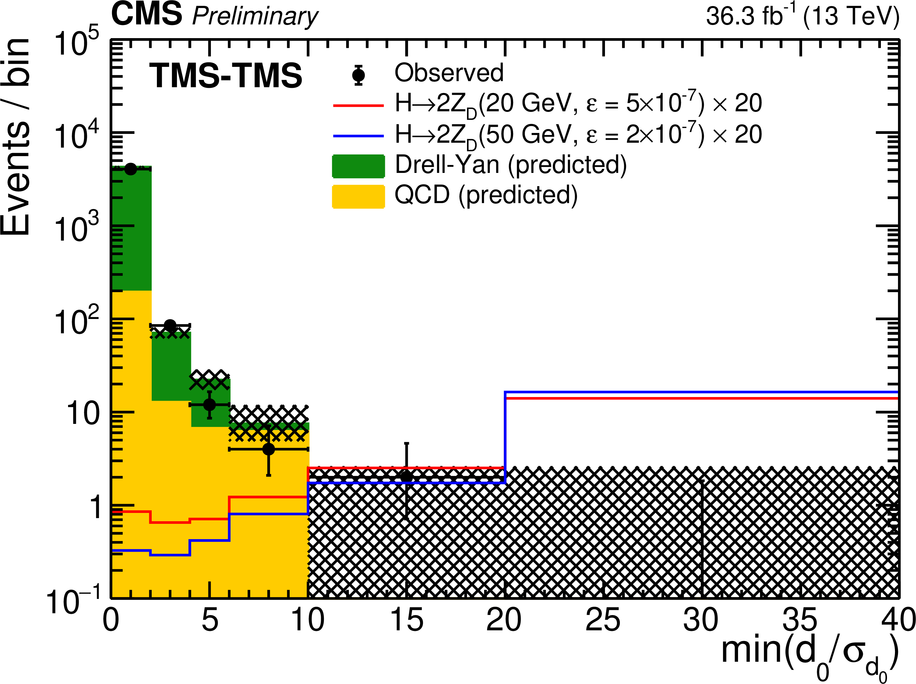
png pdf root	Figure 13-a: Comparison between the number of events observed in (left) 2016 and (right) 2018 data in the TMS-TMS dimuon category with the expected number of background events, as a function of the smaller of the two $d_{\mathrm {0}} / \sigma _{d_{\mathrm {0}}}$ values in the TMS-TMS dimuon. The black circles show the number of observed events; the green and yellow components of the stacked histograms represent the estimated numbers of DY and QCD events, respectively. The last bin includes events in the overflow. The uncertainties in the total expected background (shaded area) are statistical only. Signal contributions expected from simulated $\mathrm{H} \to \mathrm{Z_D}\mathrm{Z_D}$ with $m(\mathrm{Z_D})$ of 20 and 50 GeV are shown in red and blue, respectively. Their yields are set to the corresponding median expected exclusion limits at 95% CL and scaled up to improve their visibility.
png pdf root	Figure 13-b: Comparison between the number of events observed in (left) 2016 and (right) 2018 data in the TMS-TMS dimuon category with the expected number of background events, as a function of the smaller of the two $d_{\mathrm {0}} / \sigma _{d_{\mathrm {0}}}$ values in the TMS-TMS dimuon. The black circles show the number of observed events; the green and yellow components of the stacked histograms represent the estimated numbers of DY and QCD events, respectively. The last bin includes events in the overflow. The uncertainties in the total expected background (shaded area) are statistical only. Signal contributions expected from simulated $\mathrm{H} \to \mathrm{Z_D}\mathrm{Z_D}$ with $m(\mathrm{Z_D})$ of 20 and 50 GeV are shown in red and blue, respectively. Their yields are set to the corresponding median expected exclusion limits at 95% CL and scaled up to improve their visibility.
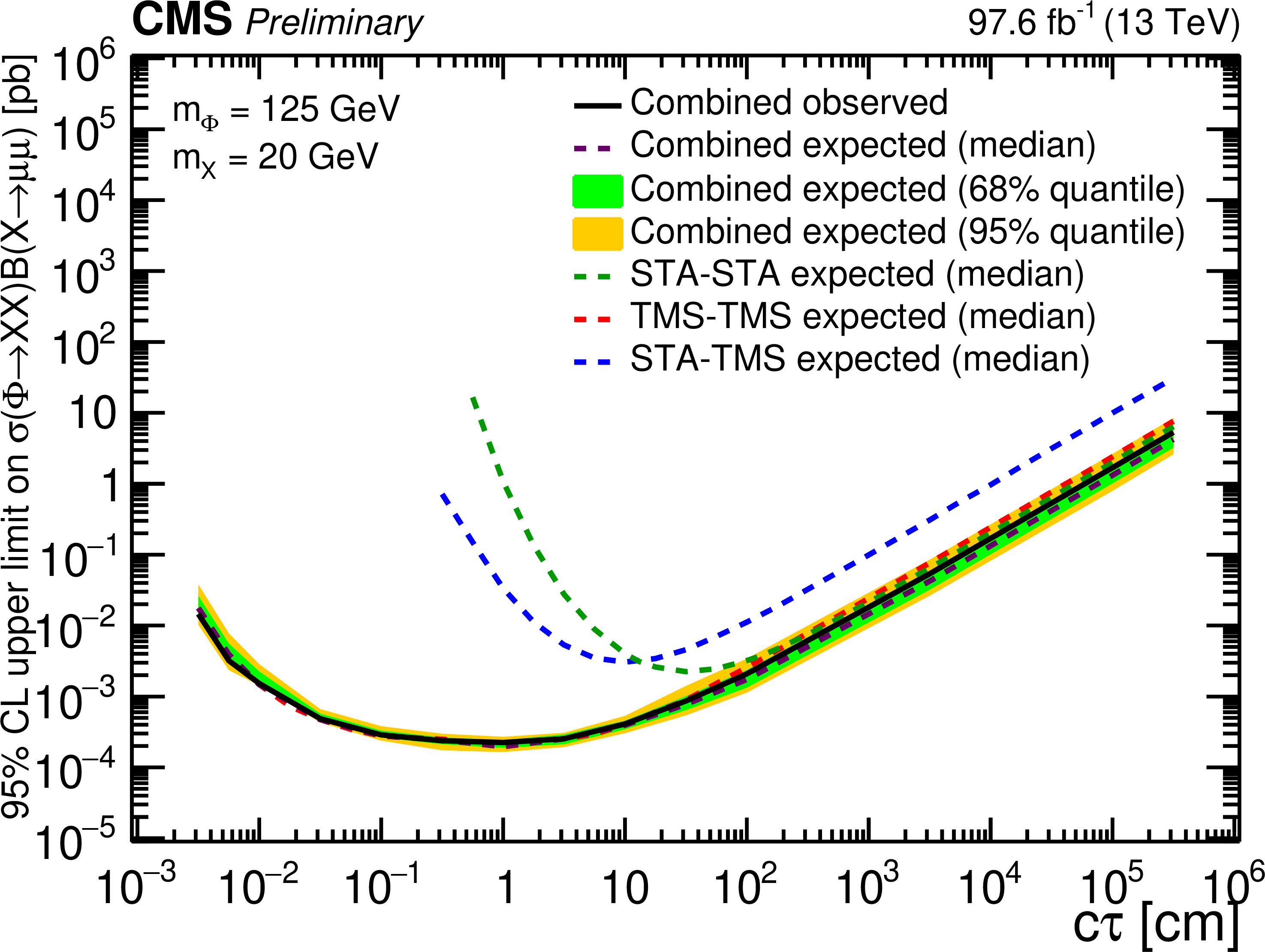
png pdf	Figure 14: The 95% CL upper limits on $\sigma(\Phi\to {\mathrm{X}} {\mathrm{X}}){\mathcal {B}({\mathrm{X}}} \to \mu \mu)$ as a function of ${c\tau} (\mathrm{X})$ in the heavy scalar model, for ${m(\Phi)} =$ 125 GeV and (left) ${m(\mathrm{X})} =$ 20 GeV and (right) ${m(\mathrm{X})} =$ 50 GeV. The median expected limits obtained from the STA-STA, STA-TMS, and TMS-TMS dimuon categories are shown as dashed green, blue, and red curves, respectively; the combined median expected limits are shown as dashed black curves; the combined observed limits are shown as solid black curves. The green and the yellow bands correspond, respectively, to the 68% and 95% central quantiles for the combined expected limits.
png pdf root	Figure 14-a: The 95% CL upper limits on $\sigma(\Phi\to {\mathrm{X}} {\mathrm{X}}){\mathcal {B}({\mathrm{X}}} \to \mu \mu)$ as a function of ${c\tau} (\mathrm{X})$ in the heavy scalar model, for ${m(\Phi)} =$ 125 GeV and (left) ${m(\mathrm{X})} =$ 20 GeV and (right) ${m(\mathrm{X})} =$ 50 GeV. The median expected limits obtained from the STA-STA, STA-TMS, and TMS-TMS dimuon categories are shown as dashed green, blue, and red curves, respectively; the combined median expected limits are shown as dashed black curves; the combined observed limits are shown as solid black curves. The green and the yellow bands correspond, respectively, to the 68% and 95% central quantiles for the combined expected limits.
png pdf root	Figure 14-b: The 95% CL upper limits on $\sigma(\Phi\to {\mathrm{X}} {\mathrm{X}}){\mathcal {B}({\mathrm{X}}} \to \mu \mu)$ as a function of ${c\tau} (\mathrm{X})$ in the heavy scalar model, for ${m(\Phi)} =$ 125 GeV and (left) ${m(\mathrm{X})} =$ 20 GeV and (right) ${m(\mathrm{X})} =$ 50 GeV. The median expected limits obtained from the STA-STA, STA-TMS, and TMS-TMS dimuon categories are shown as dashed green, blue, and red curves, respectively; the combined median expected limits are shown as dashed black curves; the combined observed limits are shown as solid black curves. The green and the yellow bands correspond, respectively, to the 68% and 95% central quantiles for the combined expected limits.
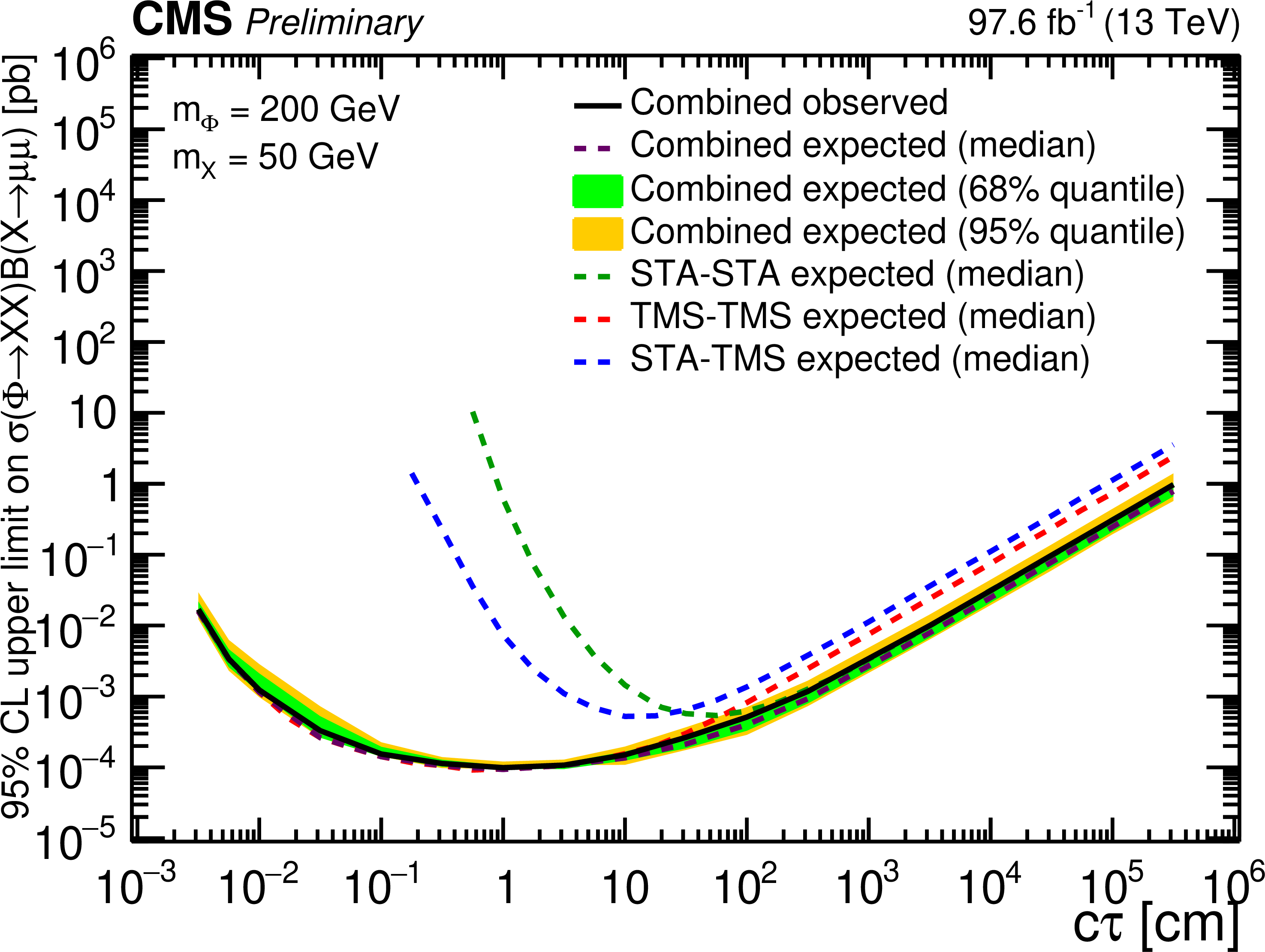
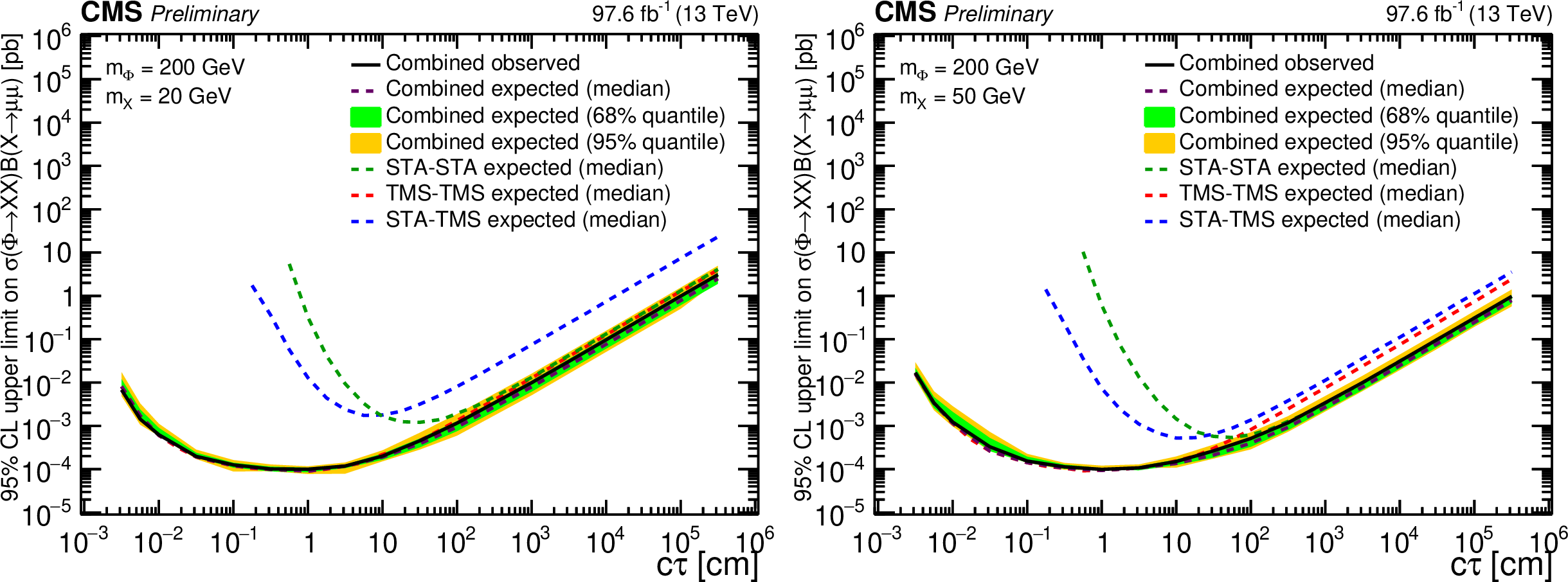
png pdf	Figure 15: The 95% CL upper limits on $\sigma(\Phi\to {\mathrm{X}} {\mathrm{X}}){\mathcal {B}({\mathrm{X}}} \to \mu \mu)$ as a function of ${c\tau} (\mathrm{X})$ in the heavy scalar model, for ${m(\Phi)} =$ 200 GeV and (left) ${m(\mathrm{X})} =$ 20 GeV and (right) ${m(\mathrm{X})} =$ 50 GeV. The median expected limits obtained from the STA-STA, STA-TMS, and TMS-TMS dimuon categories are shown as dashed green, blue, and red curves, respectively; the combined median expected limits are shown as dashed black curves; the combined observed limits are shown as solid black curves. The green and the yellow bands correspond, respectively, to the 68% and 95% central quantiles for the combined expected limits.
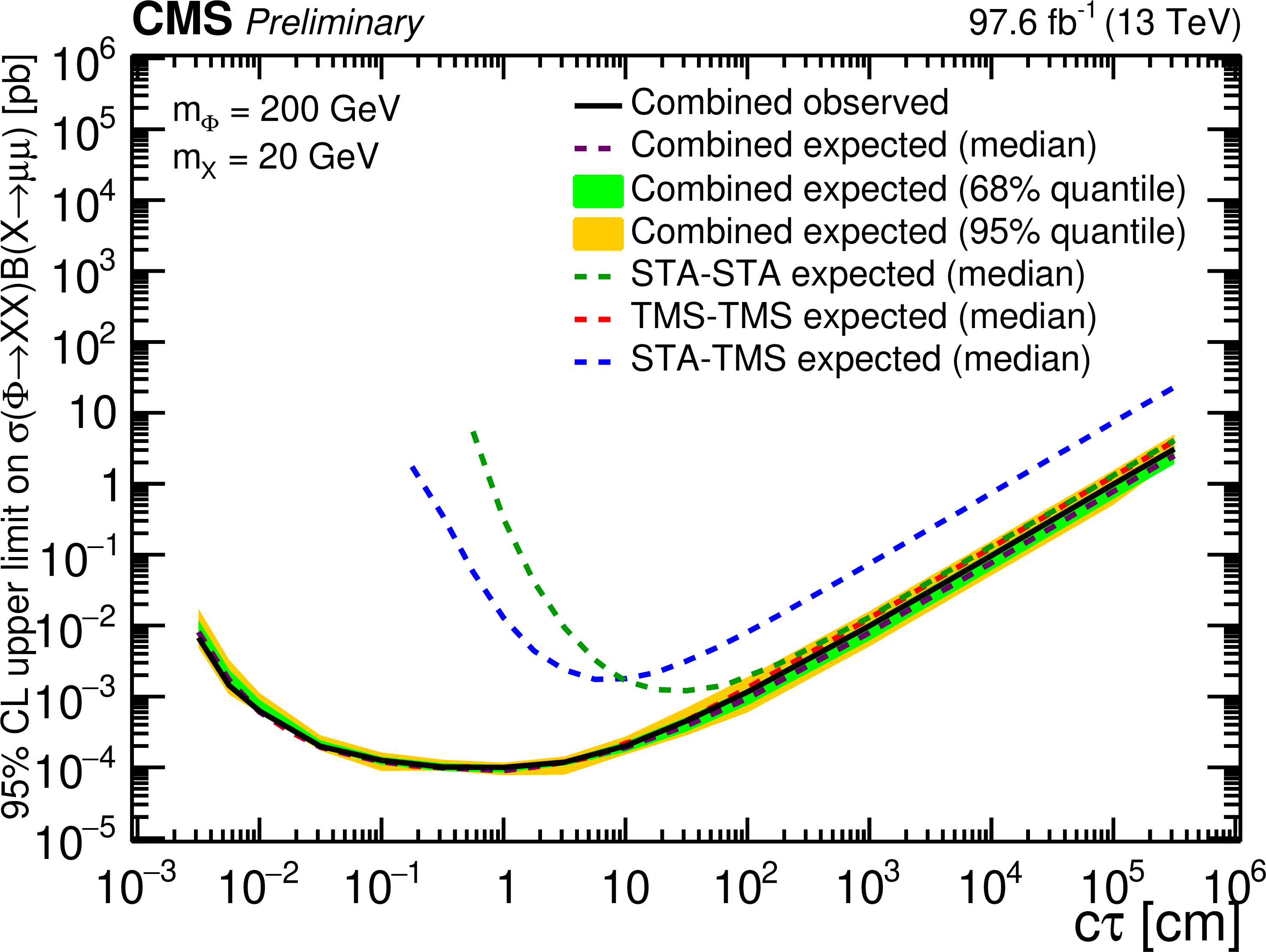
png pdf root	Figure 15-a: The 95% CL upper limits on $\sigma(\Phi\to {\mathrm{X}} {\mathrm{X}}){\mathcal {B}({\mathrm{X}}} \to \mu \mu)$ as a function of ${c\tau} (\mathrm{X})$ in the heavy scalar model, for ${m(\Phi)} =$ 200 GeV and (left) ${m(\mathrm{X})} =$ 20 GeV and (right) ${m(\mathrm{X})} =$ 50 GeV. The median expected limits obtained from the STA-STA, STA-TMS, and TMS-TMS dimuon categories are shown as dashed green, blue, and red curves, respectively; the combined median expected limits are shown as dashed black curves; the combined observed limits are shown as solid black curves. The green and the yellow bands correspond, respectively, to the 68% and 95% central quantiles for the combined expected limits.
png pdf root	Figure 15-b: The 95% CL upper limits on $\sigma(\Phi\to {\mathrm{X}} {\mathrm{X}}){\mathcal {B}({\mathrm{X}}} \to \mu \mu)$ as a function of ${c\tau} (\mathrm{X})$ in the heavy scalar model, for ${m(\Phi)} =$ 200 GeV and (left) ${m(\mathrm{X})} =$ 20 GeV and (right) ${m(\mathrm{X})} =$ 50 GeV. The median expected limits obtained from the STA-STA, STA-TMS, and TMS-TMS dimuon categories are shown as dashed green, blue, and red curves, respectively; the combined median expected limits are shown as dashed black curves; the combined observed limits are shown as solid black curves. The green and the yellow bands correspond, respectively, to the 68% and 95% central quantiles for the combined expected limits.
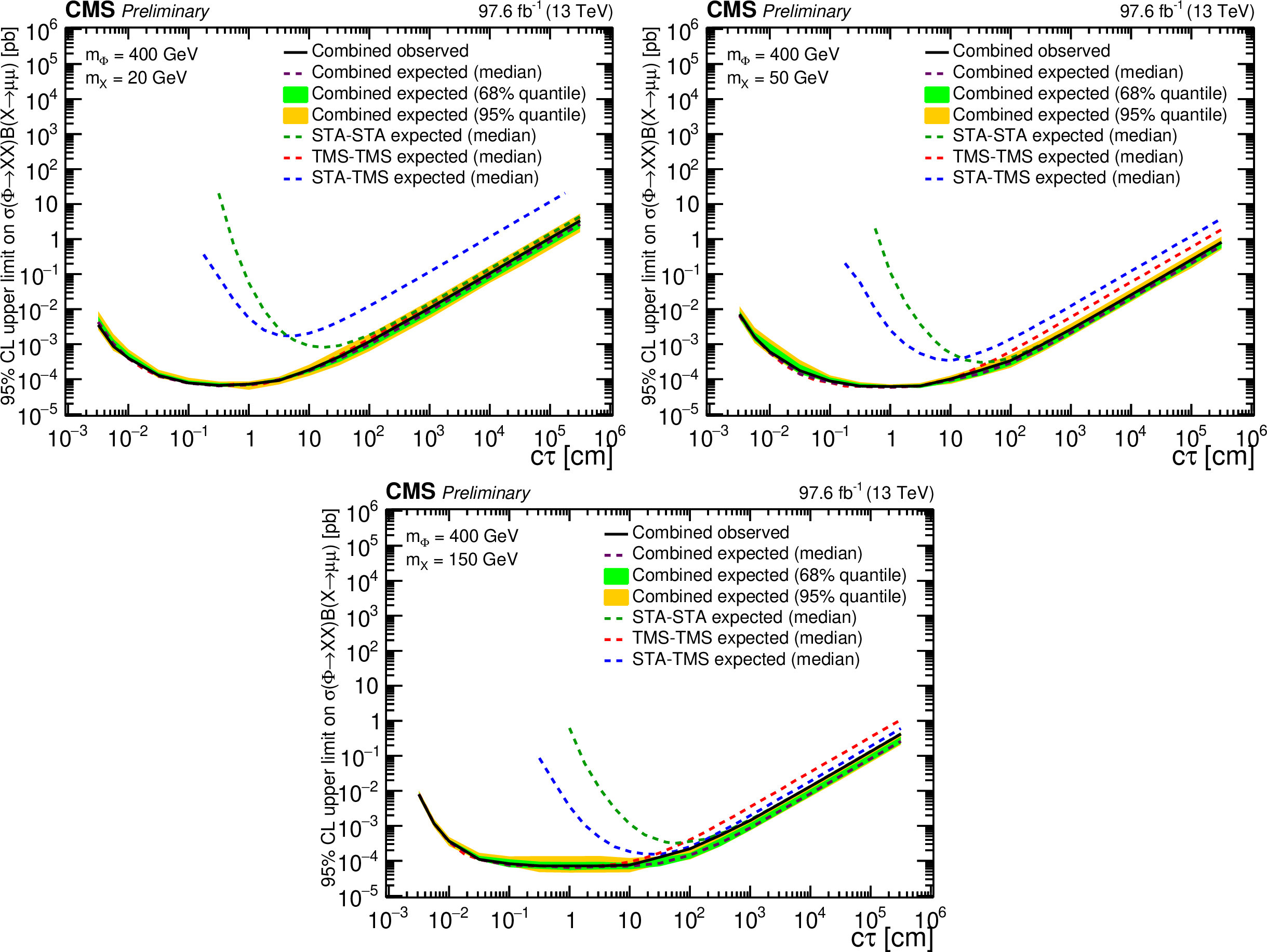
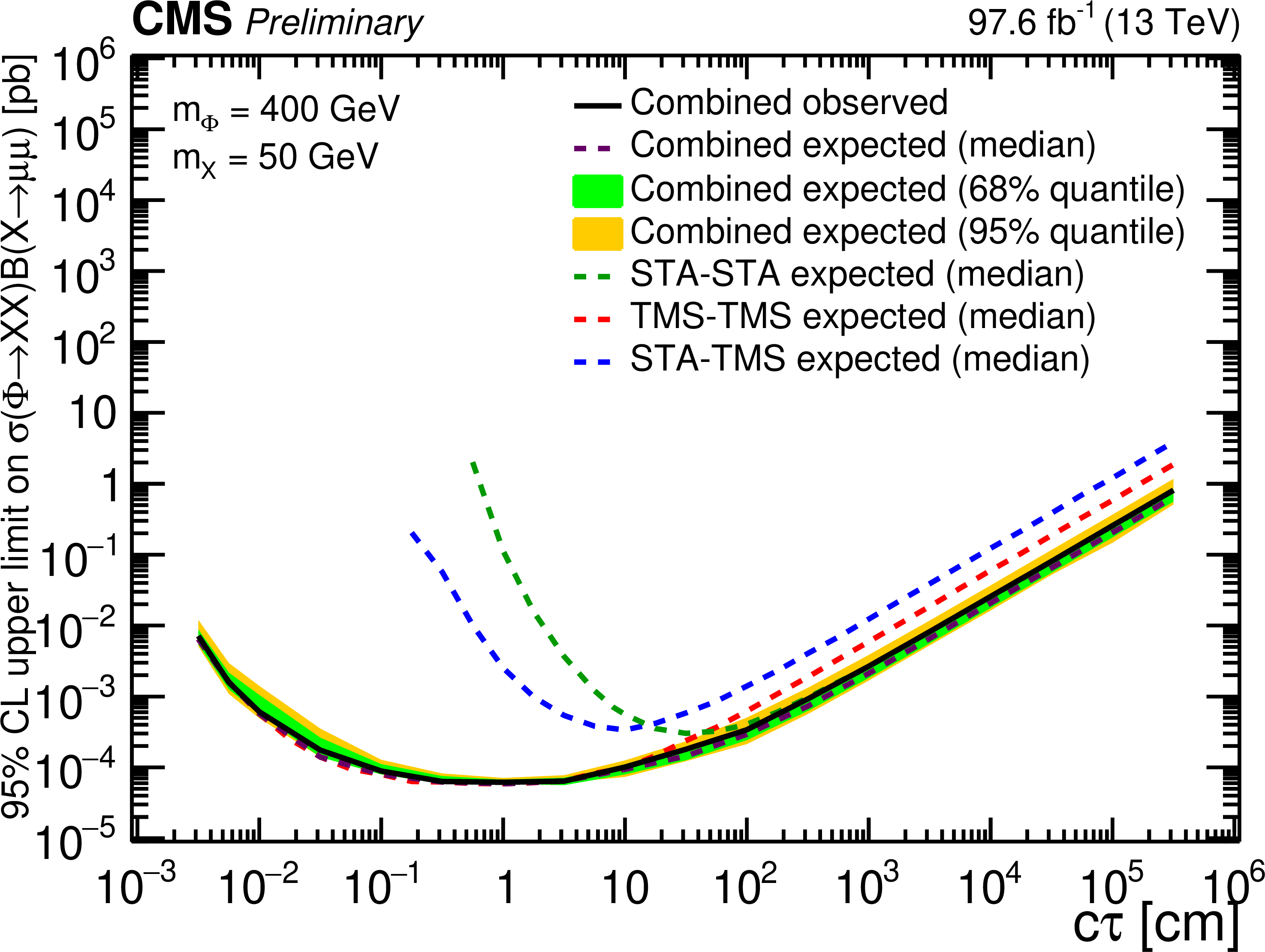
png pdf	Figure 16: The 95% CL upper limits on $\sigma(\Phi\to {\mathrm{X}} {\mathrm{X}}){\mathcal {B}({\mathrm{X}}} \to \mu \mu)$ as a function of ${c\tau} (\mathrm{X})$ in the heavy scalar model, for ${m(\Phi)} =$ 400 GeV and (upper left) ${m(\mathrm{X})} =$ 20 GeV, (upper right) ${m(\mathrm{X})} =$ 50 GeV, and (lower) ${m(\mathrm{X})} =$ 150 GeV. The median expected limits obtained from the STA-STA, STA-TMS, and TMS-TMS dimuon categories are shown as dashed green, blue, and red curves, respectively; the combined median expected limits are shown as dashed black curves; the combined observed limits are shown as solid black curves. The green and the yellow bands correspond, respectively, to the 68% and 95% quantiles for the combined expected limits.
png pdf root	Figure 16-a: The 95% CL upper limits on $\sigma(\Phi\to {\mathrm{X}} {\mathrm{X}}){\mathcal {B}({\mathrm{X}}} \to \mu \mu)$ as a function of ${c\tau} (\mathrm{X})$ in the heavy scalar model, for ${m(\Phi)} =$ 400 GeV and (upper left) ${m(\mathrm{X})} =$ 20 GeV, (upper right) ${m(\mathrm{X})} =$ 50 GeV, and (lower) ${m(\mathrm{X})} =$ 150 GeV. The median expected limits obtained from the STA-STA, STA-TMS, and TMS-TMS dimuon categories are shown as dashed green, blue, and red curves, respectively; the combined median expected limits are shown as dashed black curves; the combined observed limits are shown as solid black curves. The green and the yellow bands correspond, respectively, to the 68% and 95% quantiles for the combined expected limits.
png pdf root	Figure 16-b: The 95% CL upper limits on $\sigma(\Phi\to {\mathrm{X}} {\mathrm{X}}){\mathcal {B}({\mathrm{X}}} \to \mu \mu)$ as a function of ${c\tau} (\mathrm{X})$ in the heavy scalar model, for ${m(\Phi)} =$ 400 GeV and (upper left) ${m(\mathrm{X})} =$ 20 GeV, (upper right) ${m(\mathrm{X})} =$ 50 GeV, and (lower) ${m(\mathrm{X})} =$ 150 GeV. The median expected limits obtained from the STA-STA, STA-TMS, and TMS-TMS dimuon categories are shown as dashed green, blue, and red curves, respectively; the combined median expected limits are shown as dashed black curves; the combined observed limits are shown as solid black curves. The green and the yellow bands correspond, respectively, to the 68% and 95% quantiles for the combined expected limits.
png pdf root	Figure 16-c: The 95% CL upper limits on $\sigma(\Phi\to {\mathrm{X}} {\mathrm{X}}){\mathcal {B}({\mathrm{X}}} \to \mu \mu)$ as a function of ${c\tau} (\mathrm{X})$ in the heavy scalar model, for ${m(\Phi)} =$ 400 GeV and (upper left) ${m(\mathrm{X})} =$ 20 GeV, (upper right) ${m(\mathrm{X})} =$ 50 GeV, and (lower) ${m(\mathrm{X})} =$ 150 GeV. The median expected limits obtained from the STA-STA, STA-TMS, and TMS-TMS dimuon categories are shown as dashed green, blue, and red curves, respectively; the combined median expected limits are shown as dashed black curves; the combined observed limits are shown as solid black curves. The green and the yellow bands correspond, respectively, to the 68% and 95% quantiles for the combined expected limits.
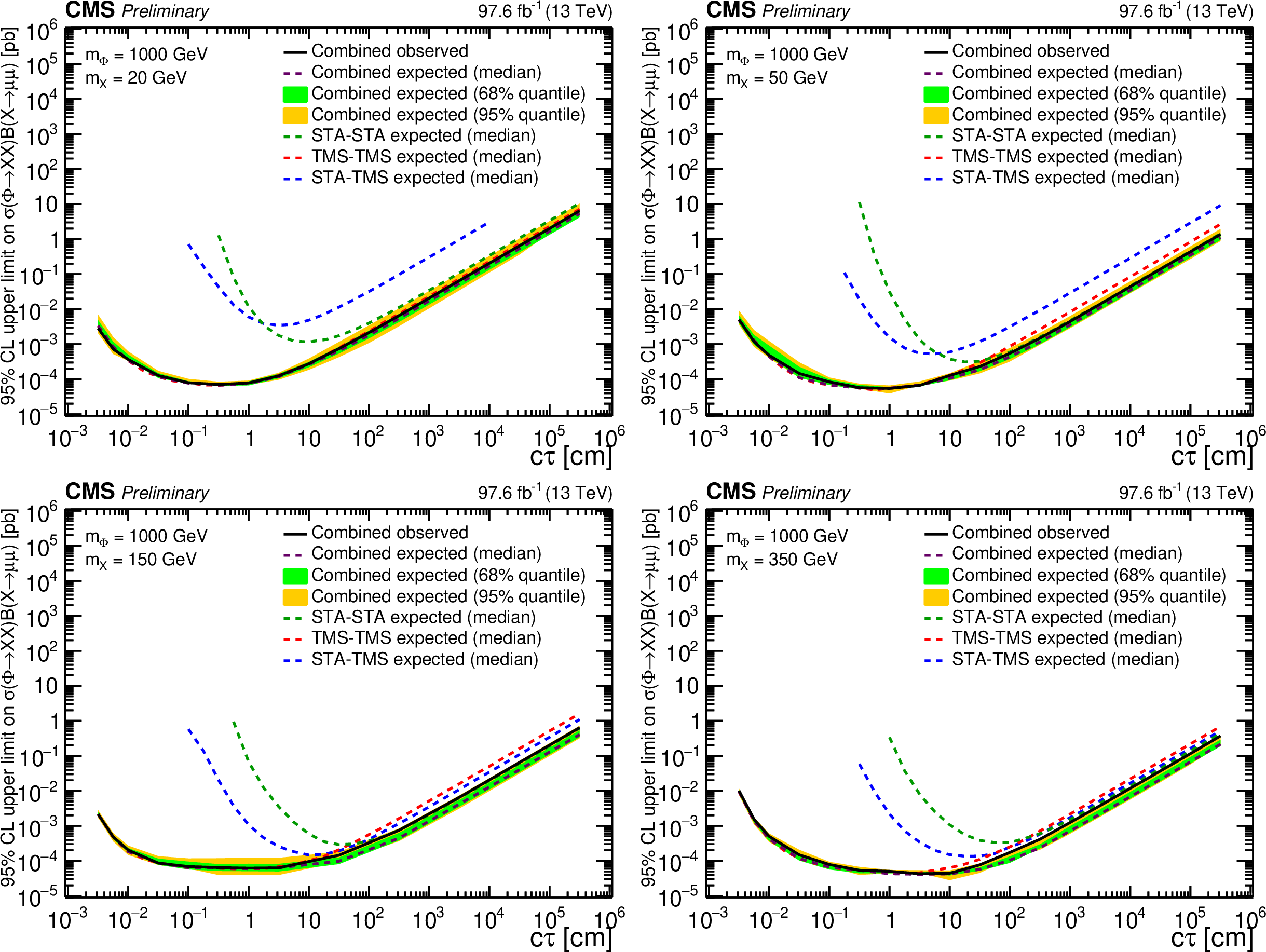
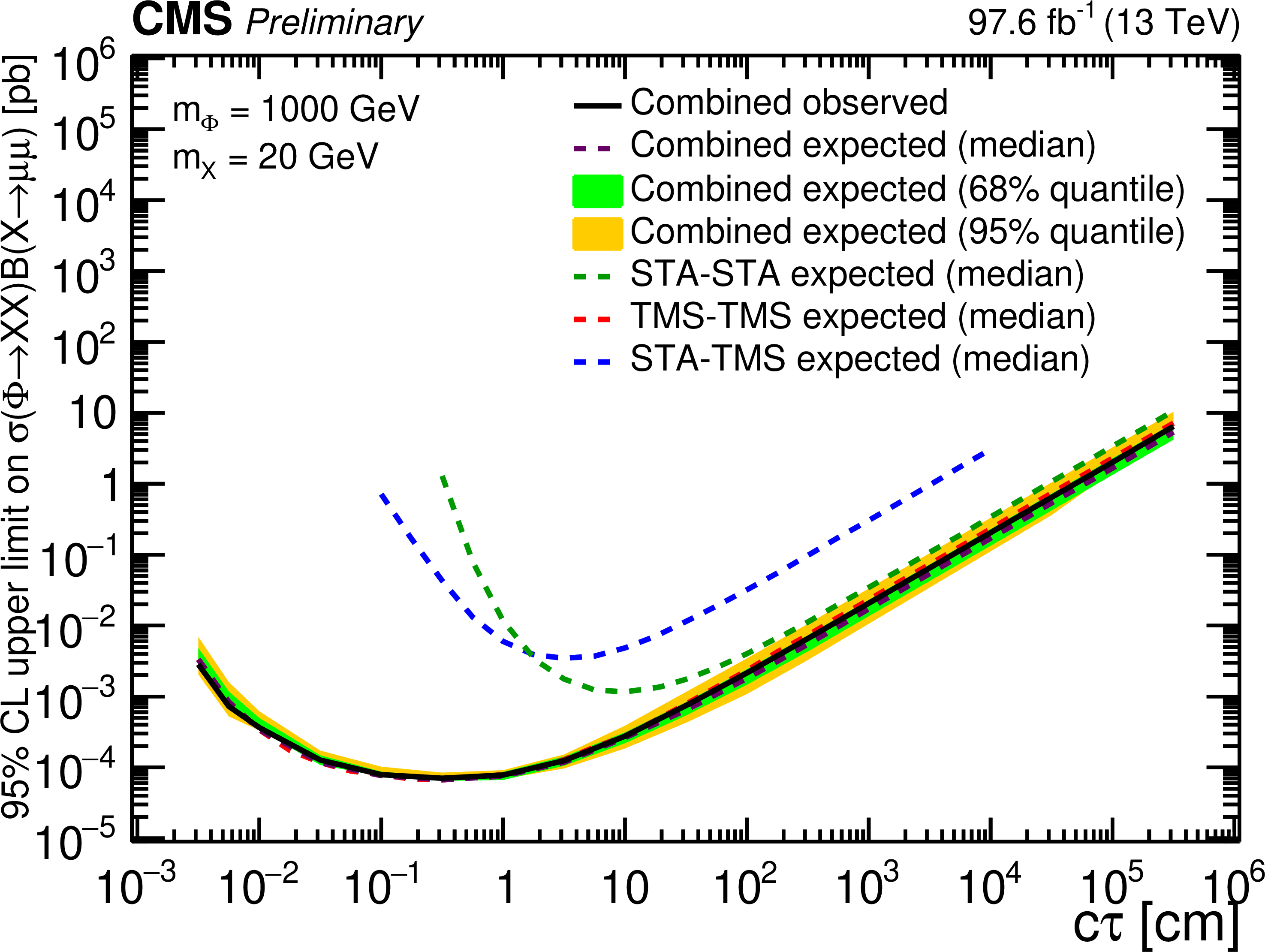
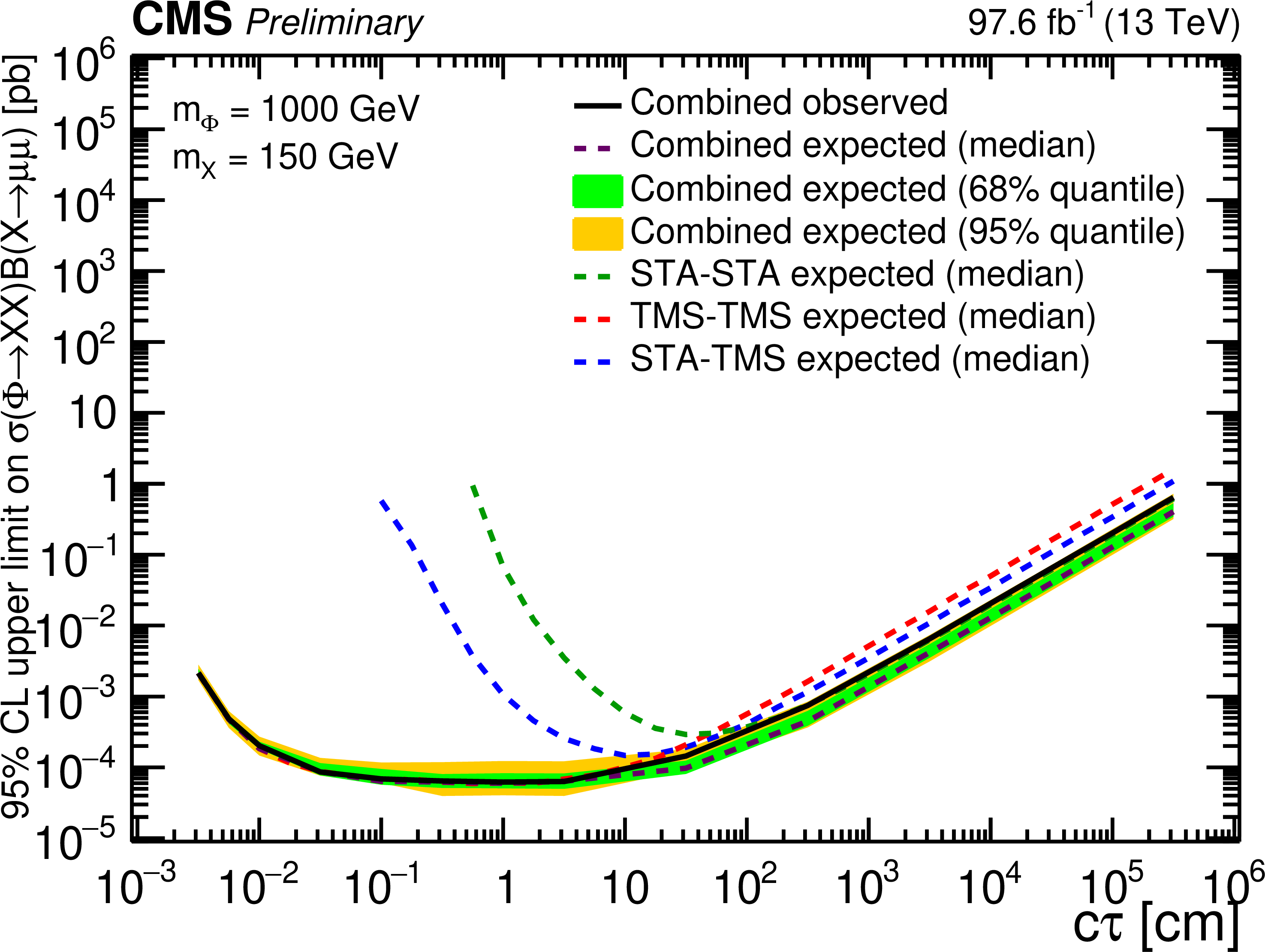
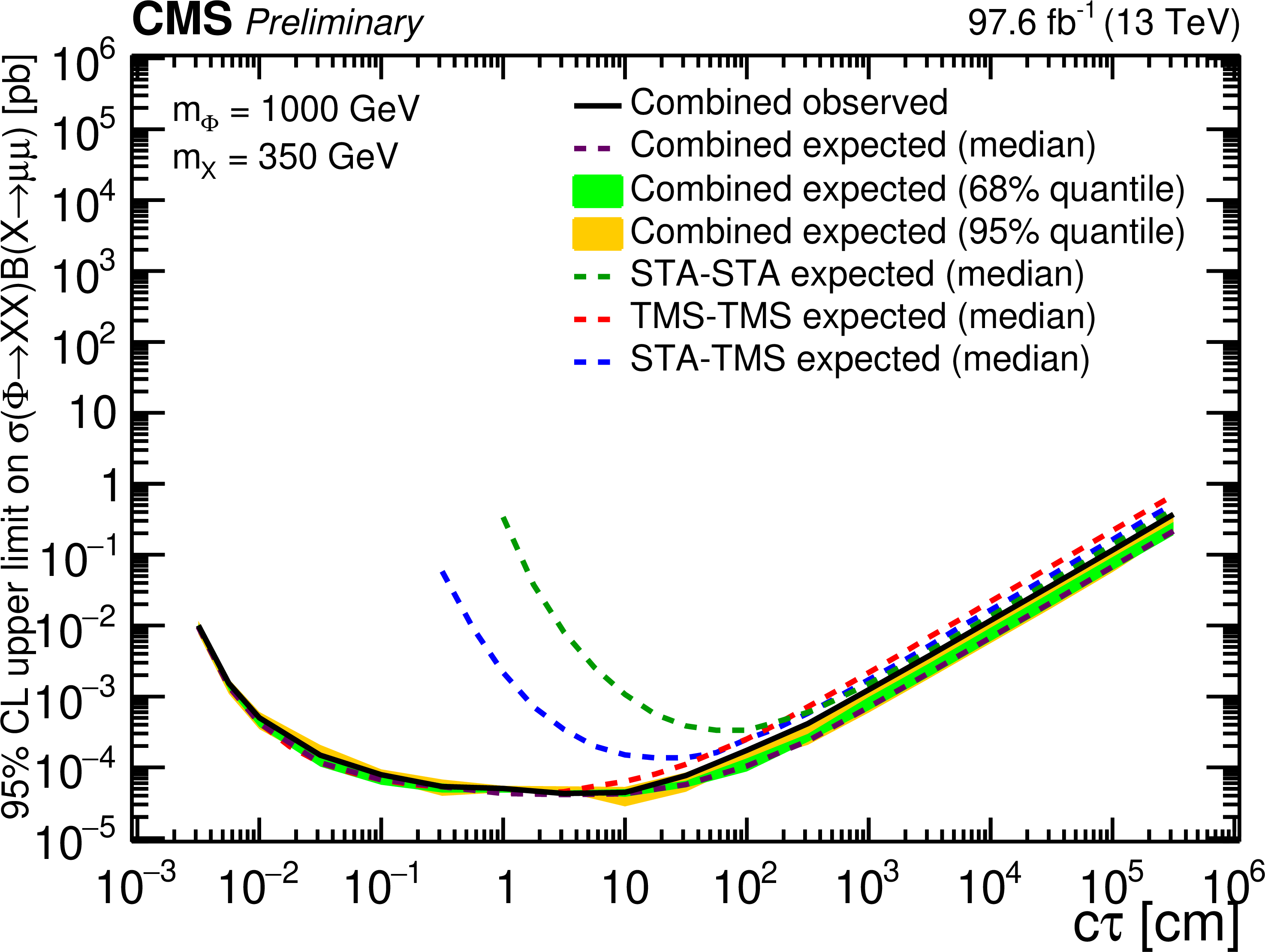
png pdf	Figure 17: The 95% CL upper limits on $\sigma(\Phi\to {\mathrm{X}} {\mathrm{X}}){\mathcal {B}({\mathrm{X}}} \to \mu \mu)$ as a function of ${c\tau} (\mathrm{X})$ in the heavy scalar model, for ${m(\Phi)} =$ 1 TeV and (upper left) ${m(\mathrm{X})} =$ 20 GeV, (upper right) ${m(\mathrm{X})} =$ 50 GeV, (lower left) ${m(\mathrm{X})} =$ 150 GeV, and (lower right) ${m(\mathrm{X})} =$ 350 GeV. The median expected limits obtained from the STA-STA, STA-TMS, and TMS-TMS dimuon categories are shown as dashed green, blue, and red curves, respectively; the combined median expected limits are shown as dashed black curves; the combined observed limits are shown as solid black curves. The green and the yellow bands correspond, respectively, to the 68% and 95% quantiles for the combined expected limits.
png pdf root	Figure 17-a: The 95% CL upper limits on $\sigma(\Phi\to {\mathrm{X}} {\mathrm{X}}){\mathcal {B}({\mathrm{X}}} \to \mu \mu)$ as a function of ${c\tau} (\mathrm{X})$ in the heavy scalar model, for ${m(\Phi)} =$ 1 TeV and (upper left) ${m(\mathrm{X})} =$ 20 GeV, (upper right) ${m(\mathrm{X})} =$ 50 GeV, (lower left) ${m(\mathrm{X})} =$ 150 GeV, and (lower right) ${m(\mathrm{X})} =$ 350 GeV. The median expected limits obtained from the STA-STA, STA-TMS, and TMS-TMS dimuon categories are shown as dashed green, blue, and red curves, respectively; the combined median expected limits are shown as dashed black curves; the combined observed limits are shown as solid black curves. The green and the yellow bands correspond, respectively, to the 68% and 95% quantiles for the combined expected limits.
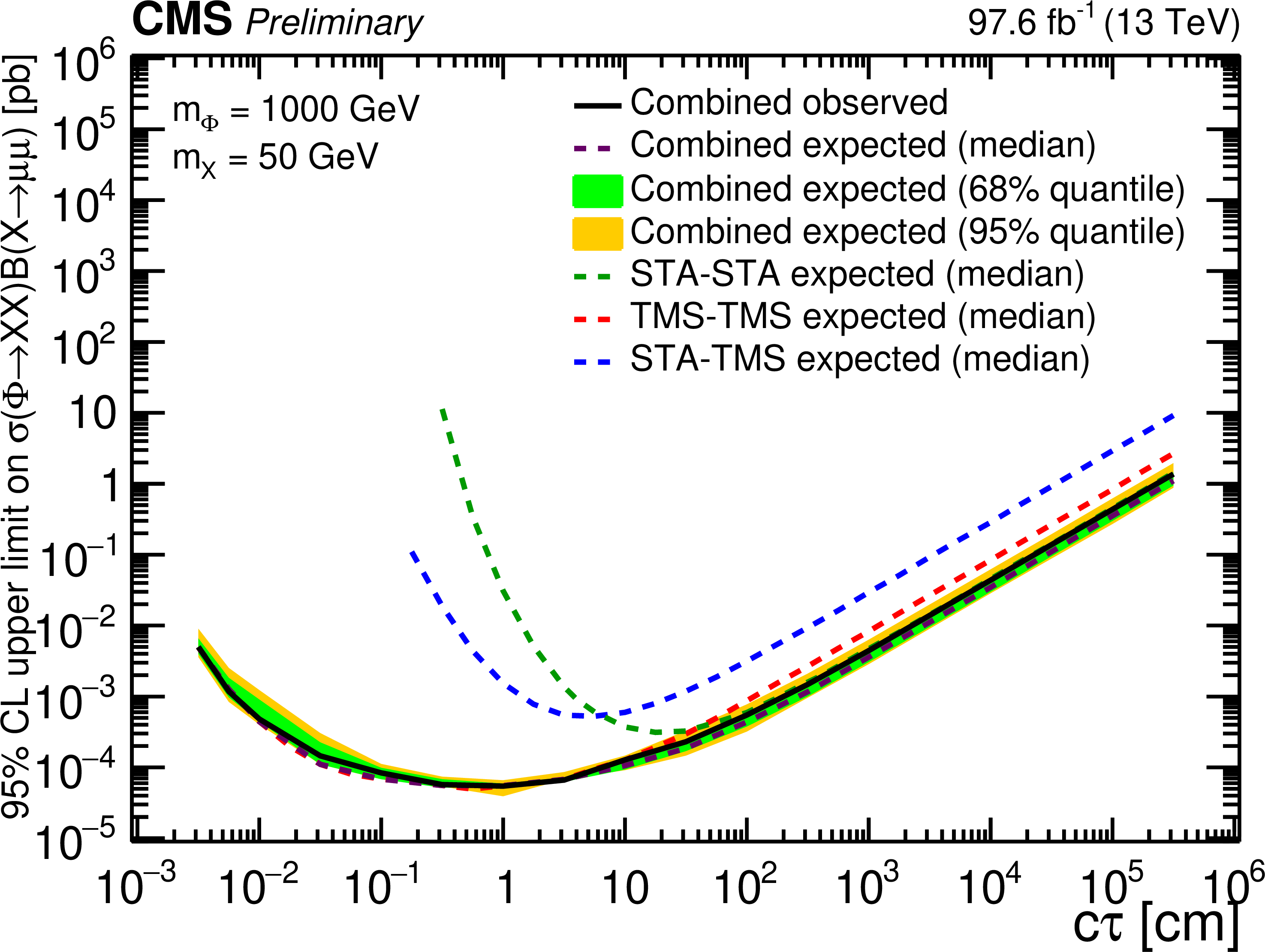
png pdf root	Figure 17-b: The 95% CL upper limits on $\sigma(\Phi\to {\mathrm{X}} {\mathrm{X}}){\mathcal {B}({\mathrm{X}}} \to \mu \mu)$ as a function of ${c\tau} (\mathrm{X})$ in the heavy scalar model, for ${m(\Phi)} =$ 1 TeV and (upper left) ${m(\mathrm{X})} =$ 20 GeV, (upper right) ${m(\mathrm{X})} =$ 50 GeV, (lower left) ${m(\mathrm{X})} =$ 150 GeV, and (lower right) ${m(\mathrm{X})} =$ 350 GeV. The median expected limits obtained from the STA-STA, STA-TMS, and TMS-TMS dimuon categories are shown as dashed green, blue, and red curves, respectively; the combined median expected limits are shown as dashed black curves; the combined observed limits are shown as solid black curves. The green and the yellow bands correspond, respectively, to the 68% and 95% quantiles for the combined expected limits.
png pdf root	Figure 17-c: The 95% CL upper limits on $\sigma(\Phi\to {\mathrm{X}} {\mathrm{X}}){\mathcal {B}({\mathrm{X}}} \to \mu \mu)$ as a function of ${c\tau} (\mathrm{X})$ in the heavy scalar model, for ${m(\Phi)} =$ 1 TeV and (upper left) ${m(\mathrm{X})} =$ 20 GeV, (upper right) ${m(\mathrm{X})} =$ 50 GeV, (lower left) ${m(\mathrm{X})} =$ 150 GeV, and (lower right) ${m(\mathrm{X})} =$ 350 GeV. The median expected limits obtained from the STA-STA, STA-TMS, and TMS-TMS dimuon categories are shown as dashed green, blue, and red curves, respectively; the combined median expected limits are shown as dashed black curves; the combined observed limits are shown as solid black curves. The green and the yellow bands correspond, respectively, to the 68% and 95% quantiles for the combined expected limits.
png pdf root	Figure 17-d: The 95% CL upper limits on $\sigma(\Phi\to {\mathrm{X}} {\mathrm{X}}){\mathcal {B}({\mathrm{X}}} \to \mu \mu)$ as a function of ${c\tau} (\mathrm{X})$ in the heavy scalar model, for ${m(\Phi)} =$ 1 TeV and (upper left) ${m(\mathrm{X})} =$ 20 GeV, (upper right) ${m(\mathrm{X})} =$ 50 GeV, (lower left) ${m(\mathrm{X})} =$ 150 GeV, and (lower right) ${m(\mathrm{X})} =$ 350 GeV. The median expected limits obtained from the STA-STA, STA-TMS, and TMS-TMS dimuon categories are shown as dashed green, blue, and red curves, respectively; the combined median expected limits are shown as dashed black curves; the combined observed limits are shown as solid black curves. The green and the yellow bands correspond, respectively, to the 68% and 95% quantiles for the combined expected limits.
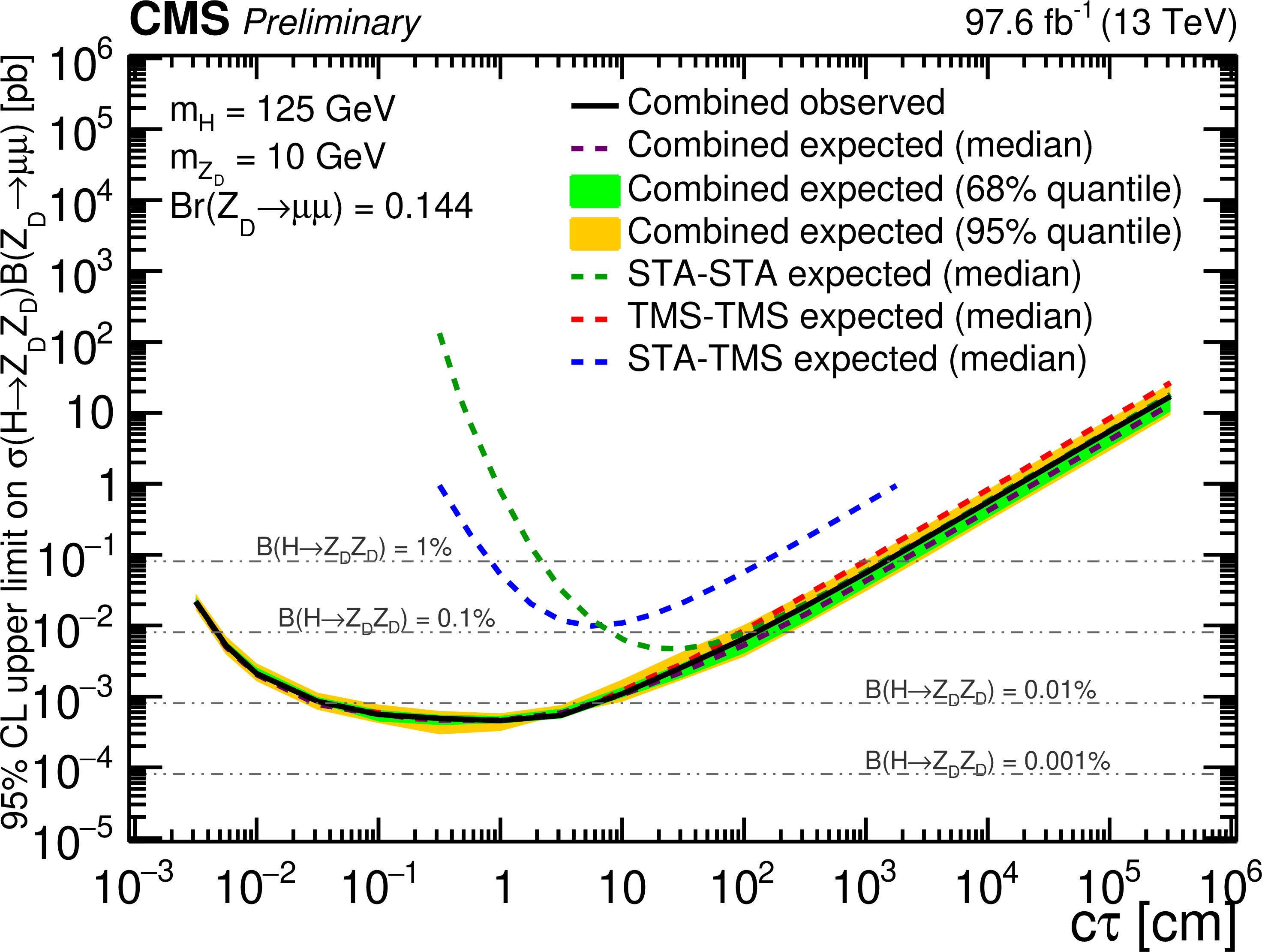
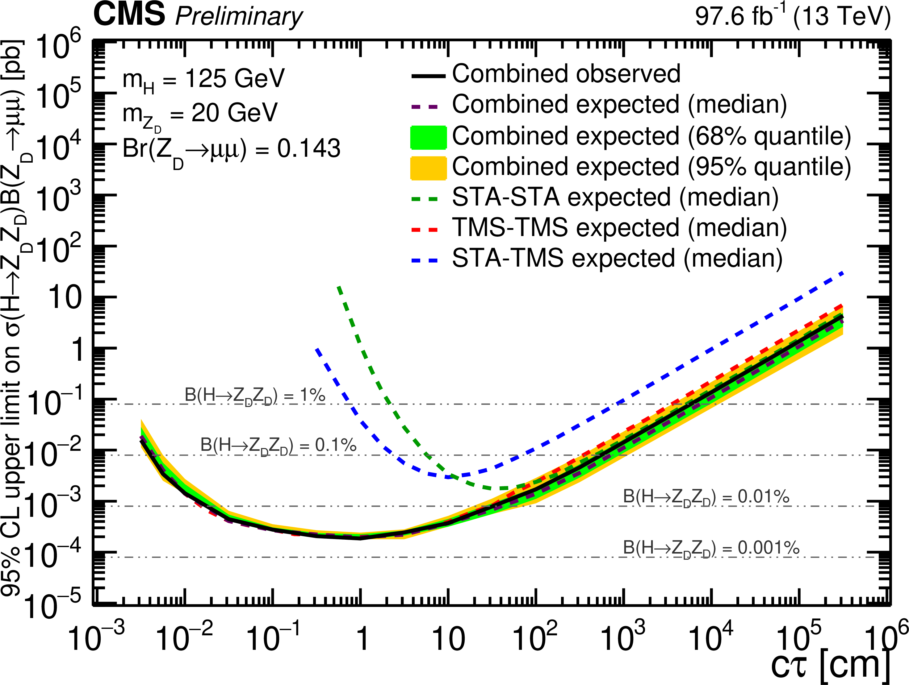
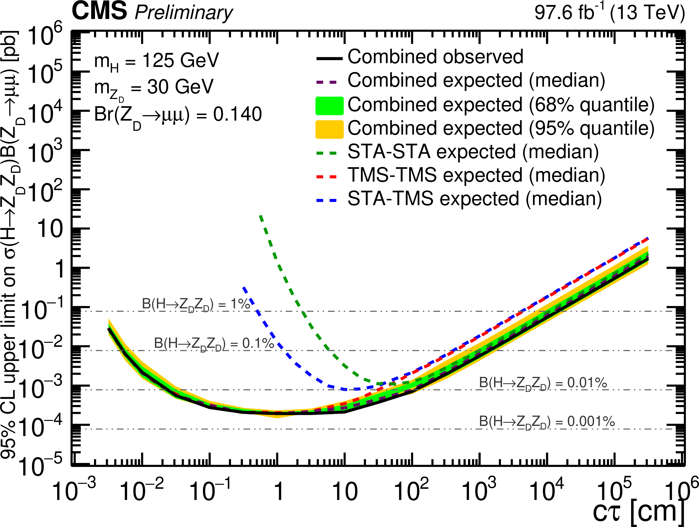
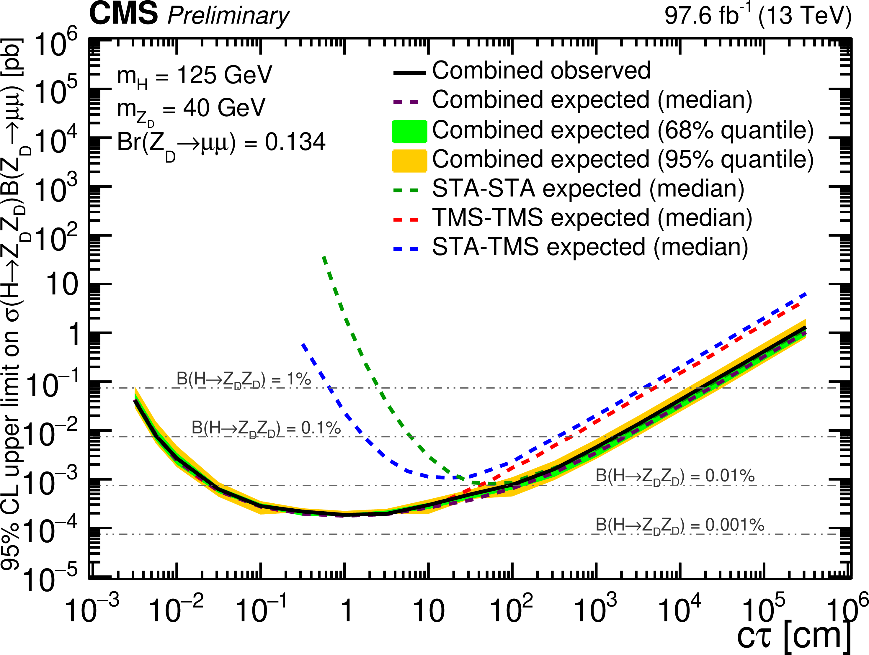
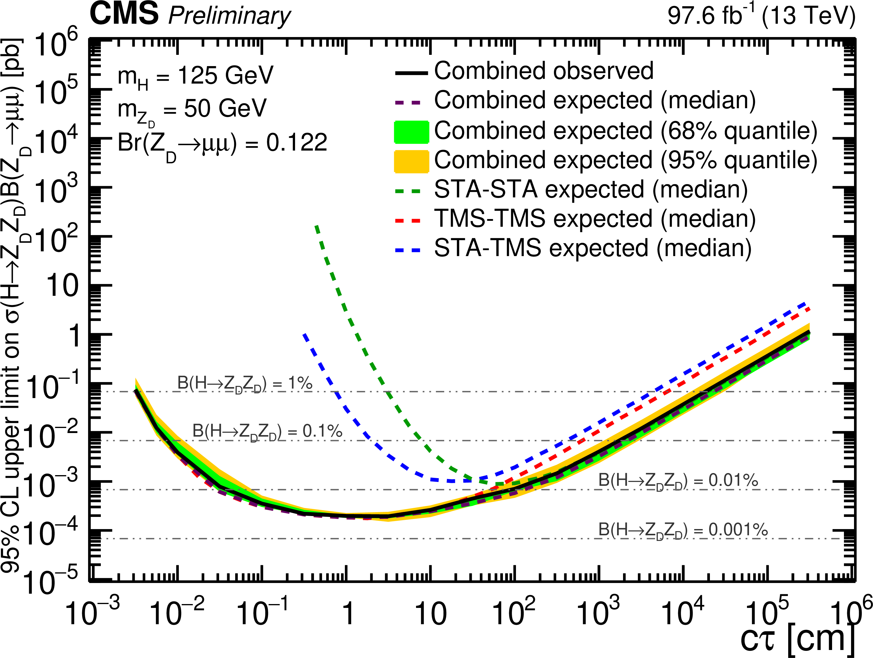
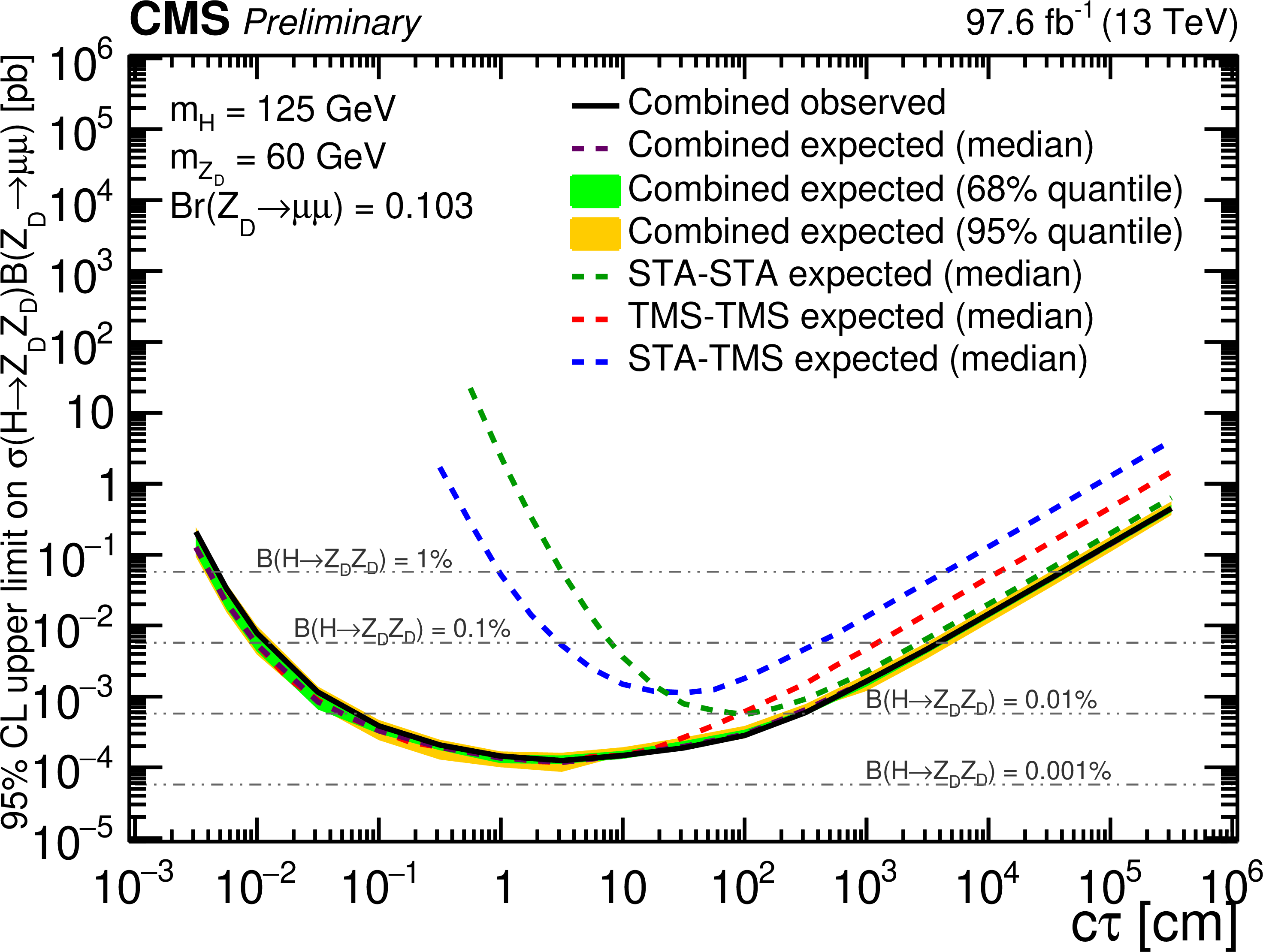
png pdf	Figure 18: The 95% CL upper limits on $\sigma (\mathrm{H} \to \mathrm{Z_D}\mathrm{Z_D}) \mathcal {B}(\mathrm{Z_D}\to \mu \mu)$ as a function of ${c\tau} (\mathrm{Z_D})$ in the HAHM model, for $m(\mathrm{Z_D})$ ranging from 10 GeV (upper left) to 60 GeV (lower right). The median expected limits obtained from the STA-STA, STA-TMS, and TMS-TMS dimuon categories are shown as dashed green, blue, and red curves, respectively; the combined median expected limits are shown as dashed black curves; the combined observed limits are shown as solid black curves. The green and the yellow bands correspond, respectively, to the 68% and 95% central quantiles for the combined expected limits. The horizontal lines in gray correspond to the theoretical predictions for values of $\mathcal {B}(\mathrm{H} \to \mathrm{Z_D}\mathrm{Z_D})$ indicated next to the lines.
png pdf root	Figure 18-a: The 95% CL upper limits on $\sigma (\mathrm{H} \to \mathrm{Z_D}\mathrm{Z_D}) \mathcal {B}(\mathrm{Z_D}\to \mu \mu)$ as a function of ${c\tau} (\mathrm{Z_D})$ in the HAHM model, for $m(\mathrm{Z_D})$ ranging from 10 GeV (upper left) to 60 GeV (lower right). The median expected limits obtained from the STA-STA, STA-TMS, and TMS-TMS dimuon categories are shown as dashed green, blue, and red curves, respectively; the combined median expected limits are shown as dashed black curves; the combined observed limits are shown as solid black curves. The green and the yellow bands correspond, respectively, to the 68% and 95% central quantiles for the combined expected limits. The horizontal lines in gray correspond to the theoretical predictions for values of $\mathcal {B}(\mathrm{H} \to \mathrm{Z_D}\mathrm{Z_D})$ indicated next to the lines.
png pdf root	Figure 18-b: The 95% CL upper limits on $\sigma (\mathrm{H} \to \mathrm{Z_D}\mathrm{Z_D}) \mathcal {B}(\mathrm{Z_D}\to \mu \mu)$ as a function of ${c\tau} (\mathrm{Z_D})$ in the HAHM model, for $m(\mathrm{Z_D})$ ranging from 10 GeV (upper left) to 60 GeV (lower right). The median expected limits obtained from the STA-STA, STA-TMS, and TMS-TMS dimuon categories are shown as dashed green, blue, and red curves, respectively; the combined median expected limits are shown as dashed black curves; the combined observed limits are shown as solid black curves. The green and the yellow bands correspond, respectively, to the 68% and 95% central quantiles for the combined expected limits. The horizontal lines in gray correspond to the theoretical predictions for values of $\mathcal {B}(\mathrm{H} \to \mathrm{Z_D}\mathrm{Z_D})$ indicated next to the lines.
png pdf root	Figure 18-c: The 95% CL upper limits on $\sigma (\mathrm{H} \to \mathrm{Z_D}\mathrm{Z_D}) \mathcal {B}(\mathrm{Z_D}\to \mu \mu)$ as a function of ${c\tau} (\mathrm{Z_D})$ in the HAHM model, for $m(\mathrm{Z_D})$ ranging from 10 GeV (upper left) to 60 GeV (lower right). The median expected limits obtained from the STA-STA, STA-TMS, and TMS-TMS dimuon categories are shown as dashed green, blue, and red curves, respectively; the combined median expected limits are shown as dashed black curves; the combined observed limits are shown as solid black curves. The green and the yellow bands correspond, respectively, to the 68% and 95% central quantiles for the combined expected limits. The horizontal lines in gray correspond to the theoretical predictions for values of $\mathcal {B}(\mathrm{H} \to \mathrm{Z_D}\mathrm{Z_D})$ indicated next to the lines.
png pdf root	Figure 18-d: The 95% CL upper limits on $\sigma (\mathrm{H} \to \mathrm{Z_D}\mathrm{Z_D}) \mathcal {B}(\mathrm{Z_D}\to \mu \mu)$ as a function of ${c\tau} (\mathrm{Z_D})$ in the HAHM model, for $m(\mathrm{Z_D})$ ranging from 10 GeV (upper left) to 60 GeV (lower right). The median expected limits obtained from the STA-STA, STA-TMS, and TMS-TMS dimuon categories are shown as dashed green, blue, and red curves, respectively; the combined median expected limits are shown as dashed black curves; the combined observed limits are shown as solid black curves. The green and the yellow bands correspond, respectively, to the 68% and 95% central quantiles for the combined expected limits. The horizontal lines in gray correspond to the theoretical predictions for values of $\mathcal {B}(\mathrm{H} \to \mathrm{Z_D}\mathrm{Z_D})$ indicated next to the lines.
png pdf root	Figure 18-e: The 95% CL upper limits on $\sigma (\mathrm{H} \to \mathrm{Z_D}\mathrm{Z_D}) \mathcal {B}(\mathrm{Z_D}\to \mu \mu)$ as a function of ${c\tau} (\mathrm{Z_D})$ in the HAHM model, for $m(\mathrm{Z_D})$ ranging from 10 GeV (upper left) to 60 GeV (lower right). The median expected limits obtained from the STA-STA, STA-TMS, and TMS-TMS dimuon categories are shown as dashed green, blue, and red curves, respectively; the combined median expected limits are shown as dashed black curves; the combined observed limits are shown as solid black curves. The green and the yellow bands correspond, respectively, to the 68% and 95% central quantiles for the combined expected limits. The horizontal lines in gray correspond to the theoretical predictions for values of $\mathcal {B}(\mathrm{H} \to \mathrm{Z_D}\mathrm{Z_D})$ indicated next to the lines.
png pdf root	Figure 18-f: The 95% CL upper limits on $\sigma (\mathrm{H} \to \mathrm{Z_D}\mathrm{Z_D}) \mathcal {B}(\mathrm{Z_D}\to \mu \mu)$ as a function of ${c\tau} (\mathrm{Z_D})$ in the HAHM model, for $m(\mathrm{Z_D})$ ranging from 10 GeV (upper left) to 60 GeV (lower right). The median expected limits obtained from the STA-STA, STA-TMS, and TMS-TMS dimuon categories are shown as dashed green, blue, and red curves, respectively; the combined median expected limits are shown as dashed black curves; the combined observed limits are shown as solid black curves. The green and the yellow bands correspond, respectively, to the 68% and 95% central quantiles for the combined expected limits. The horizontal lines in gray correspond to the theoretical predictions for values of $\mathcal {B}(\mathrm{H} \to \mathrm{Z_D}\mathrm{Z_D})$ indicated next to the lines.
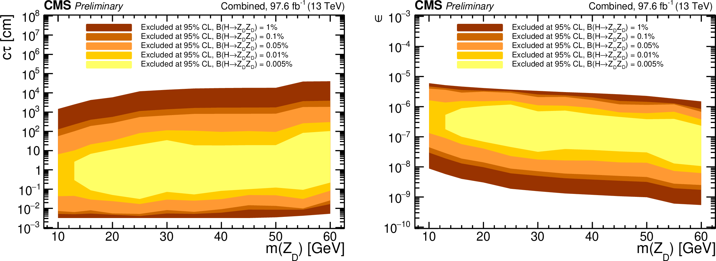
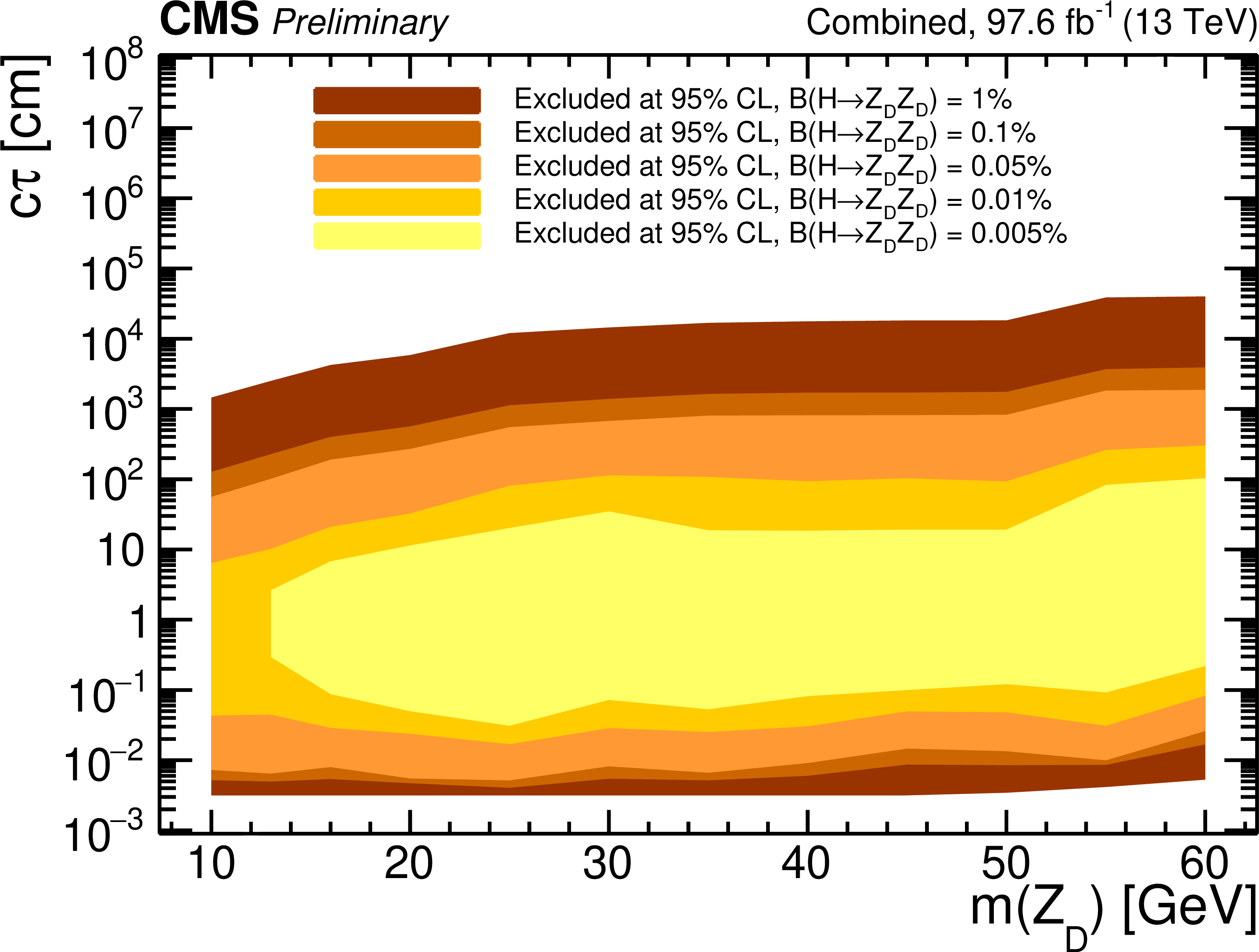
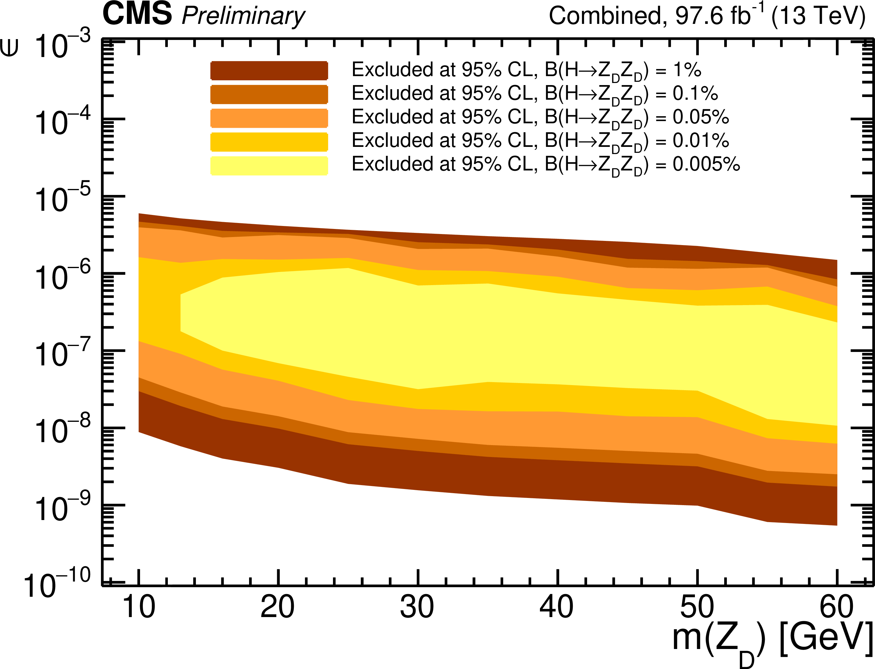
png pdf	Figure 19: Observed 95% CL exclusion contours in the HAHM model, in the (left) ( $m(\mathrm{Z_D})$ , ${c\tau} (\mathrm{Z_D})$ ) and (right) ( $m(\mathrm{Z_D})$ , $\epsilon$ ) planes. The contours correspond to several representative values of $\mathcal {B}(\mathrm{H} \to \mathrm{Z_D}\mathrm{Z_D})$ ranging from 0.005% to 1%.
png pdf root	Figure 19-a: Observed 95% CL exclusion contours in the HAHM model, in the (left) ( $m(\mathrm{Z_D})$ , ${c\tau} (\mathrm{Z_D})$ ) and (right) ( $m(\mathrm{Z_D})$ , $\epsilon$ ) planes. The contours correspond to several representative values of $\mathcal {B}(\mathrm{H} \to \mathrm{Z_D}\mathrm{Z_D})$ ranging from 0.005% to 1%.
png pdf root	Figure 19-b: Observed 95% CL exclusion contours in the HAHM model, in the (left) ( $m(\mathrm{Z_D})$ , ${c\tau} (\mathrm{Z_D})$ ) and (right) ( $m(\mathrm{Z_D})$ , $\epsilon$ ) planes. The contours correspond to several representative values of $\mathcal {B}(\mathrm{H} \to \mathrm{Z_D}\mathrm{Z_D})$ ranging from 0.005% to 1%.

Summary

A data set collected by the CMS experiment in proton-proton collisions at

$\sqrt{s} =$ 13 TeV in 2016 and 2018 and corresponding to an integrated luminosity of 97.6 fb

$^{-1}$ has been used to conduct an inclusive search for long-lived exotic neutral particles (LLPs) decaying to a pair of muons. The search is largely model-independent and is sensitive to a broad range of LLP lifetimes and masses. No excess of events above the standard model prediction is observed. The results are interpreted as upper limits on the parameters of the Hidden Abelian Higgs model, in which the Higgs boson decays to a pair of long-lived dark photons Z

$_D$ , and of a simplified model, in which LLPs are produced in decays of an exotic heavy neutral scalar boson. The branching fraction of the Higgs boson to dark photons of 1% is excluded at 95% confidence level in the Z

$_D$ range between 20 and 60 GeV and for

${c\tau}$ (Z

$_D$ ) from a few tens of

$\mu$ m to approximately 100 m. The results of this search significantly extend the excluded range of model parameters. They provide the best limits to date for the Hidden Abelian Higgs model with Z

$_D$ masses larger than 20 GeV and all

${c\tau}$ (Z

$_D$ ) values except those between about 0.5 and 200 mm, where our search is complemented by the CMS search using data collected with high-rate triggers [35]. At exotic scalar boson masses larger than the Higgs boson mass, our results represent the best current constraints for all considered LLP masses and lifetimes.

Additional Figures
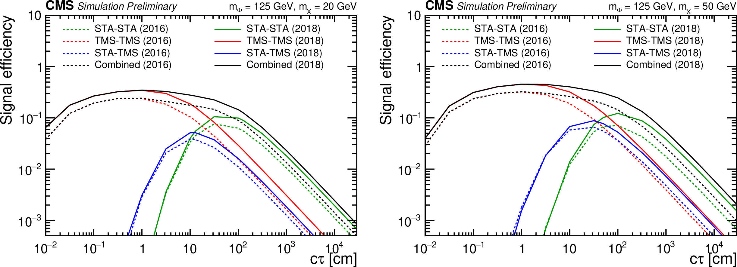
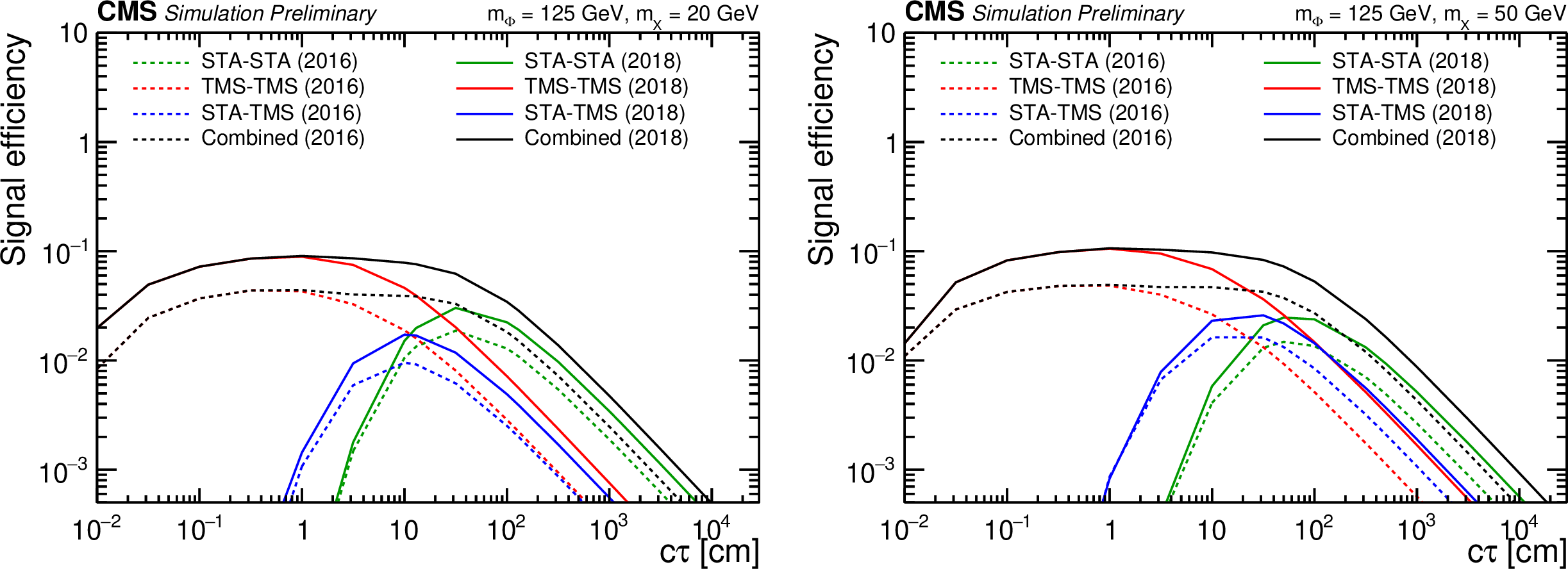
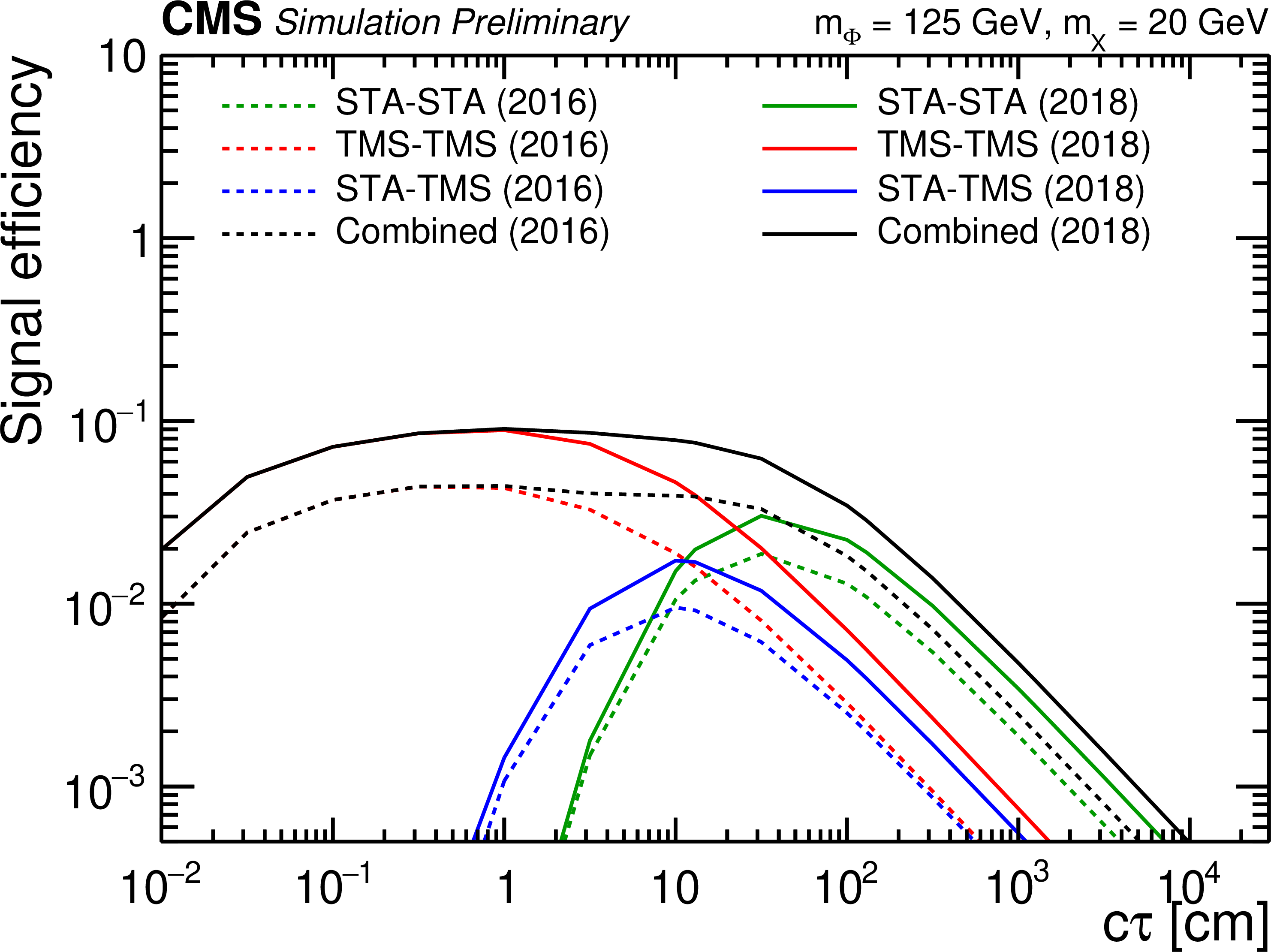
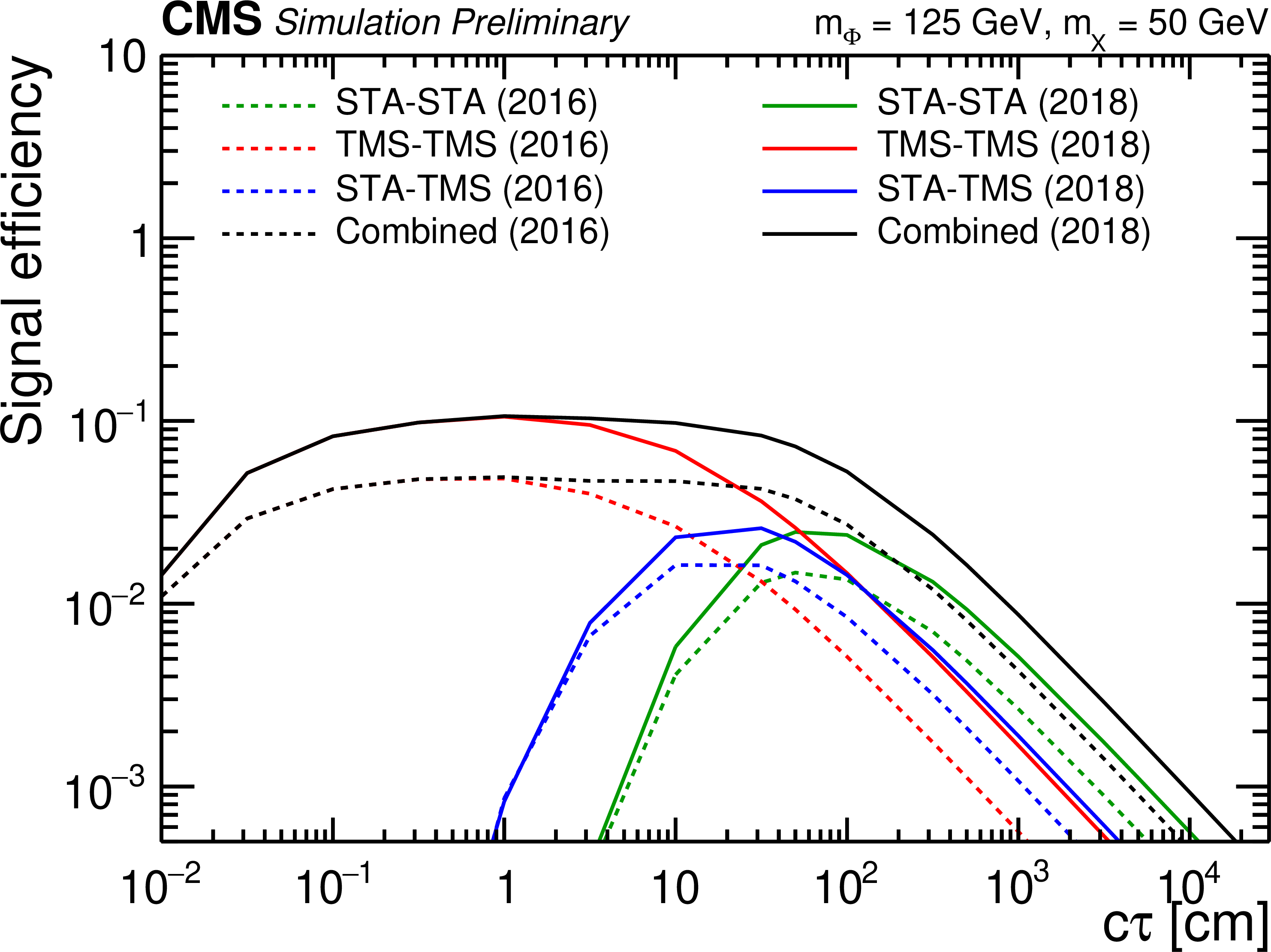
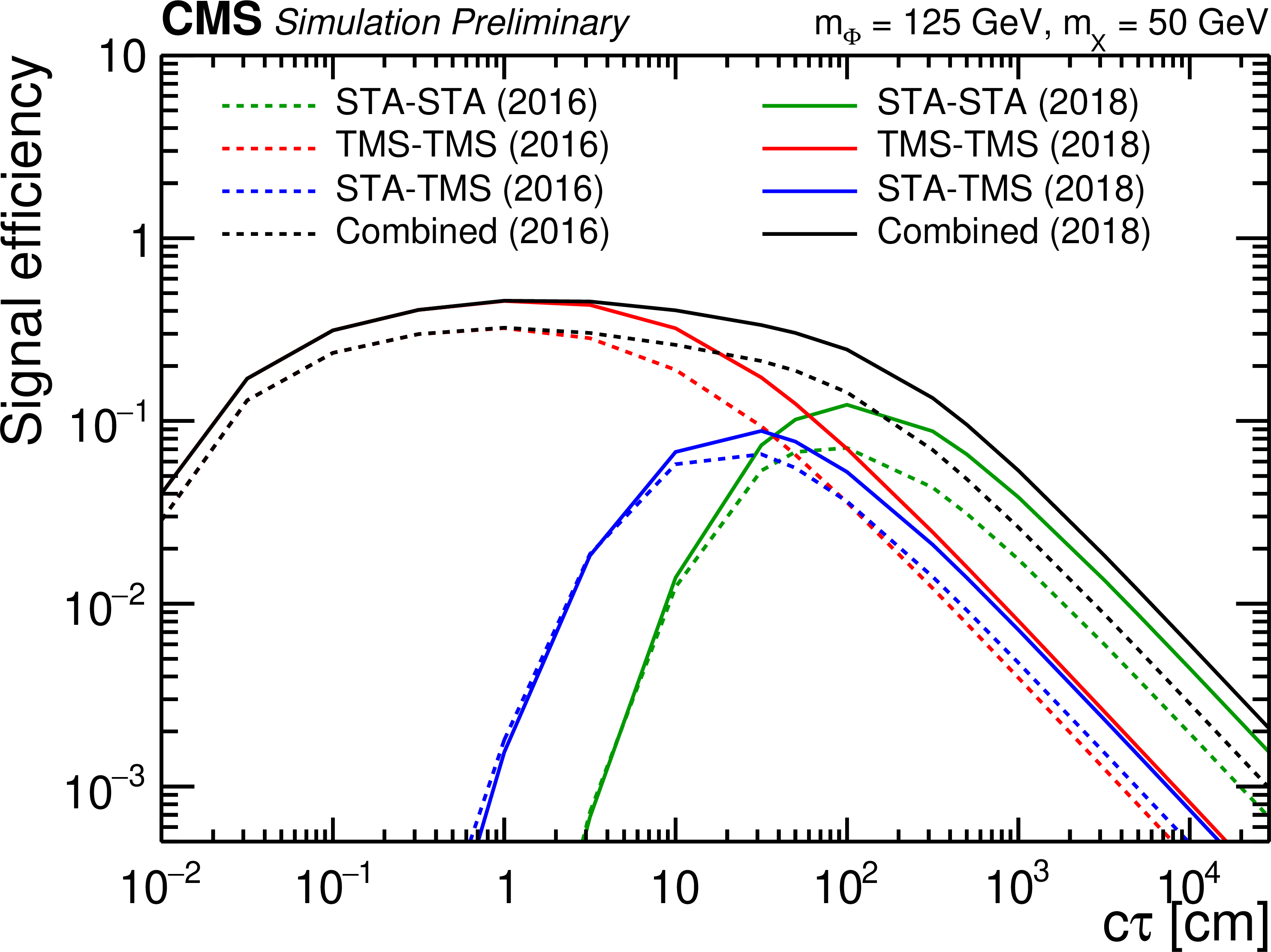
png pdf	Additional Figure 1: Overall signal efficiencies as a function of $c\tau$ for the $\Phi \to 2\text {X}\to 2\mu$ signal process with $m_\Phi =$ 125 GeV (left: $m_\text {X}=$ 20 GeV, right: $m_\text {X}=$ 50 GeV). Each figure shows efficiencies in the three dimuon categories, STA-STA (green), TMS-TMS (red), and STA-TMS (blue), as well as the combined efficiency (black) calculated as the sum of the efficiencies of the individual categories. The signal efficiencies for the 2016 and 2018 datasets are shown as dashed and solid lines, respectively.
png pdf root	Additional Figure 1-a: Overall signal efficiencies as a function of $c\tau$ for the $\Phi \to 2\text {X}\to 2\mu$ signal process with $m_\Phi =$ 125 GeV (left: $m_\text {X}=$ 20 GeV, right: $m_\text {X}=$ 50 GeV). Each figure shows efficiencies in the three dimuon categories, STA-STA (green), TMS-TMS (red), and STA-TMS (blue), as well as the combined efficiency (black) calculated as the sum of the efficiencies of the individual categories. The signal efficiencies for the 2016 and 2018 datasets are shown as dashed and solid lines, respectively.
png pdf root	Additional Figure 1-b: Overall signal efficiencies as a function of $c\tau$ for the $\Phi \to 2\text {X}\to 2\mu$ signal process with $m_\Phi =$ 125 GeV (left: $m_\text {X}=$ 20 GeV, right: $m_\text {X}=$ 50 GeV). Each figure shows efficiencies in the three dimuon categories, STA-STA (green), TMS-TMS (red), and STA-TMS (blue), as well as the combined efficiency (black) calculated as the sum of the efficiencies of the individual categories. The signal efficiencies for the 2016 and 2018 datasets are shown as dashed and solid lines, respectively.
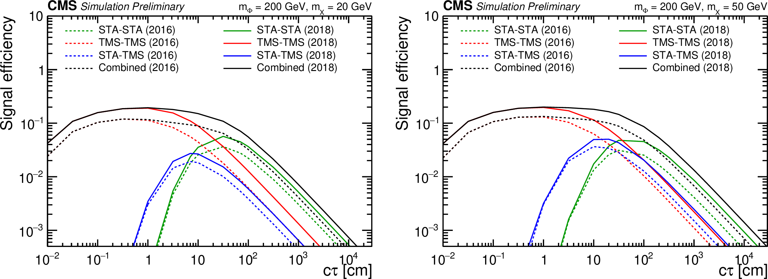
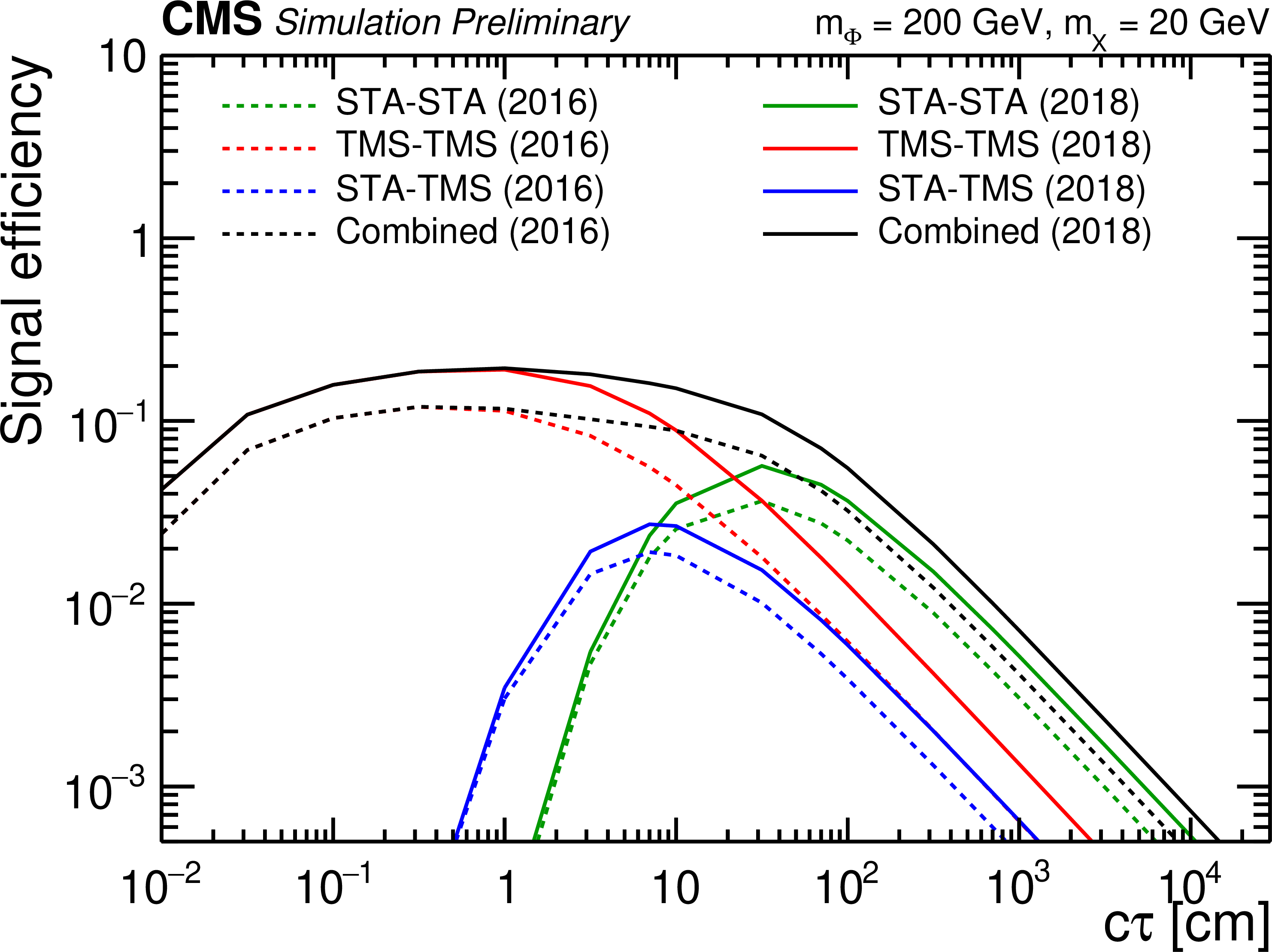
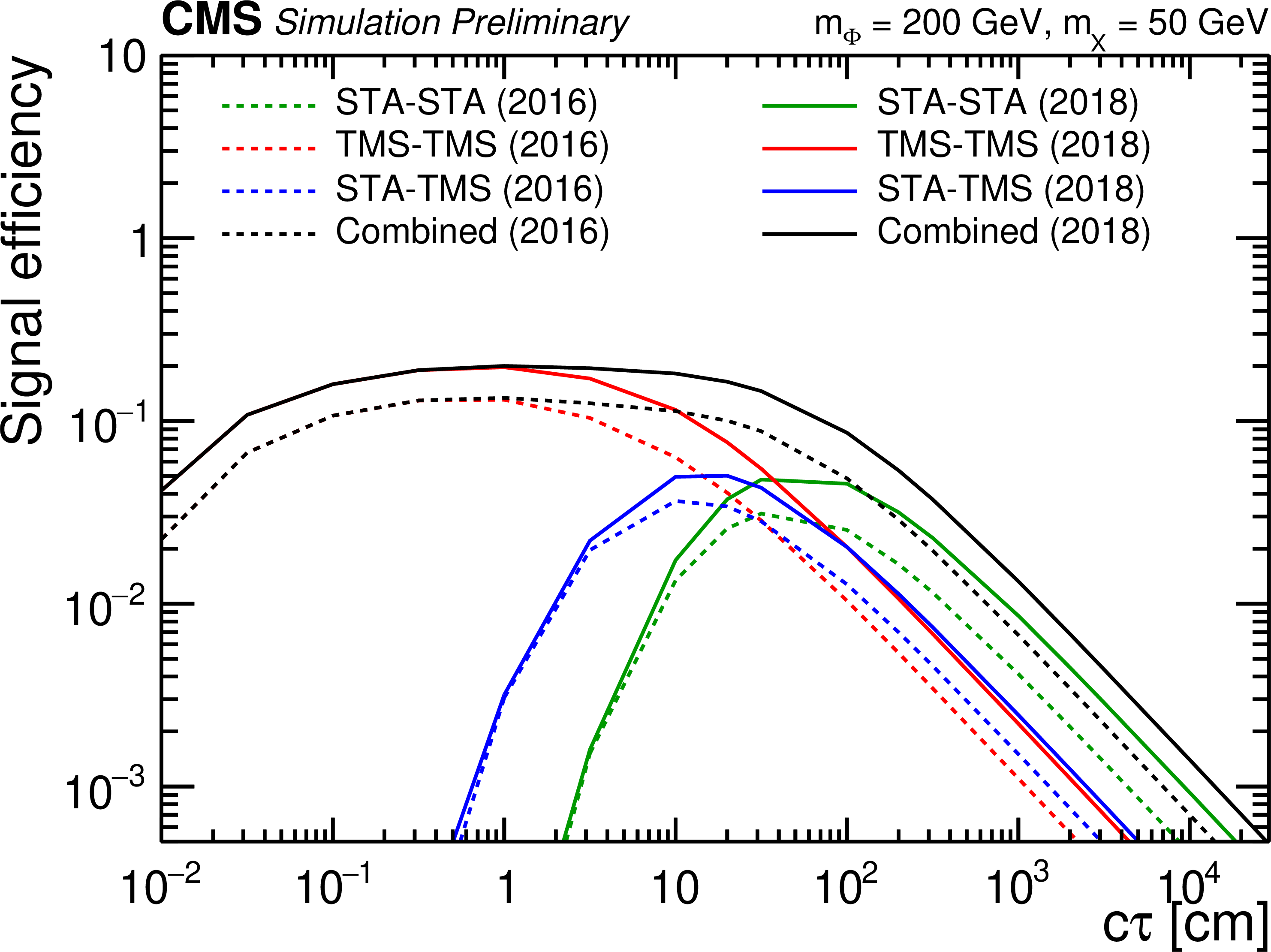
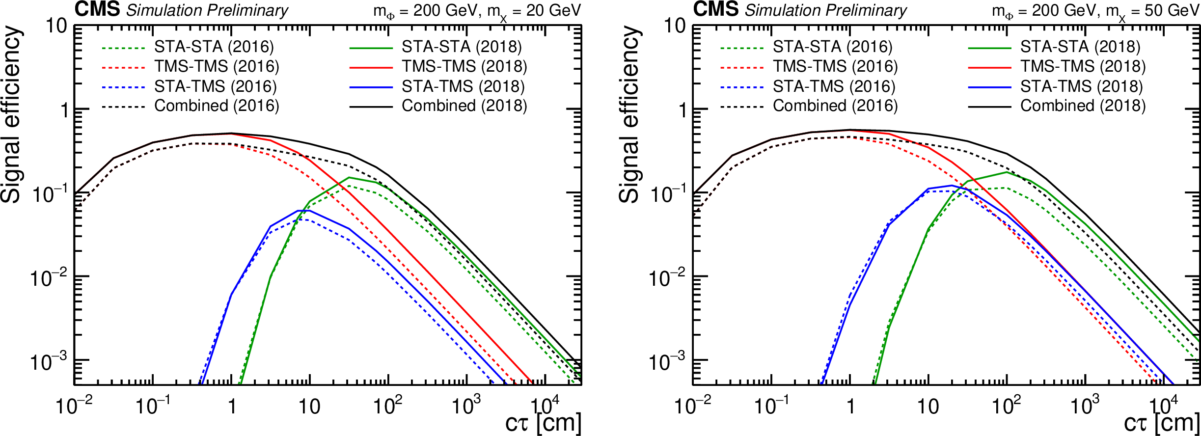
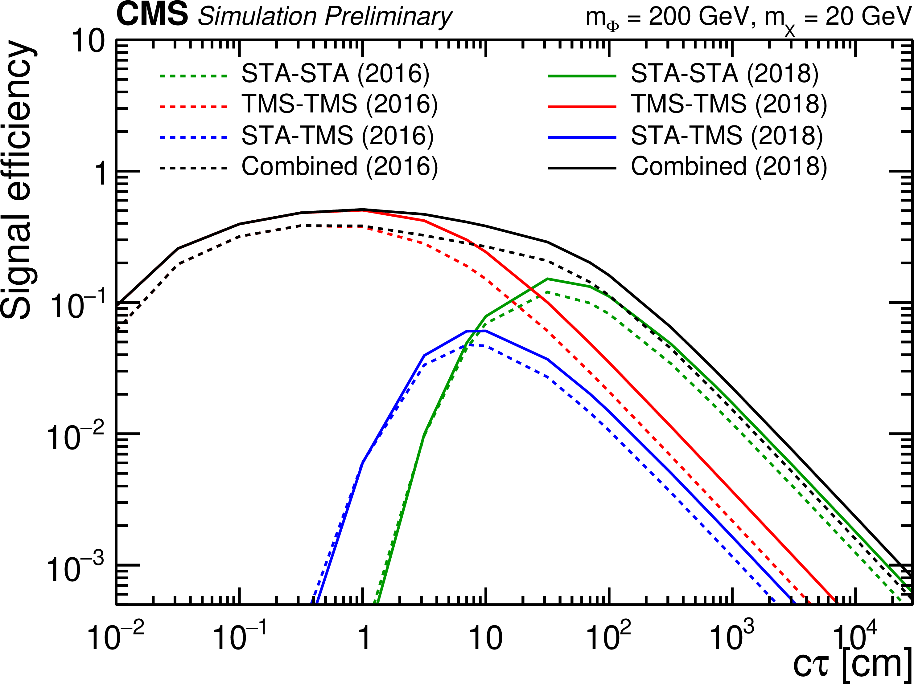
png pdf	Additional Figure 2: Overall signal efficiencies as a function of $c\tau$ for the $\Phi \to 2\text {X}\to 2\mu$ signal process with $m_\Phi =$ 200 GeV (left: $m_\text {X}=$ 20 GeV, right: $m_\text {X}=$ 50 GeV). Each figure shows efficiencies in the three dimuon categories, STA-STA (green), TMS-TMS (red), and STA-TMS (blue), as well as the combined efficiency (black) calculated as the sum of the efficiencies of the individual categories. The signal efficiencies for the 2016 and 2018 datasets are shown as dashed and solid lines, respectively.
png pdf root	Additional Figure 2-a: Overall signal efficiencies as a function of $c\tau$ for the $\Phi \to 2\text {X}\to 2\mu$ signal process with $m_\Phi =$ 200 GeV (left: $m_\text {X}=$ 20 GeV, right: $m_\text {X}=$ 50 GeV). Each figure shows efficiencies in the three dimuon categories, STA-STA (green), TMS-TMS (red), and STA-TMS (blue), as well as the combined efficiency (black) calculated as the sum of the efficiencies of the individual categories. The signal efficiencies for the 2016 and 2018 datasets are shown as dashed and solid lines, respectively.
png pdf root	Additional Figure 2-b: Overall signal efficiencies as a function of $c\tau$ for the $\Phi \to 2\text {X}\to 2\mu$ signal process with $m_\Phi =$ 200 GeV (left: $m_\text {X}=$ 20 GeV, right: $m_\text {X}=$ 50 GeV). Each figure shows efficiencies in the three dimuon categories, STA-STA (green), TMS-TMS (red), and STA-TMS (blue), as well as the combined efficiency (black) calculated as the sum of the efficiencies of the individual categories. The signal efficiencies for the 2016 and 2018 datasets are shown as dashed and solid lines, respectively.
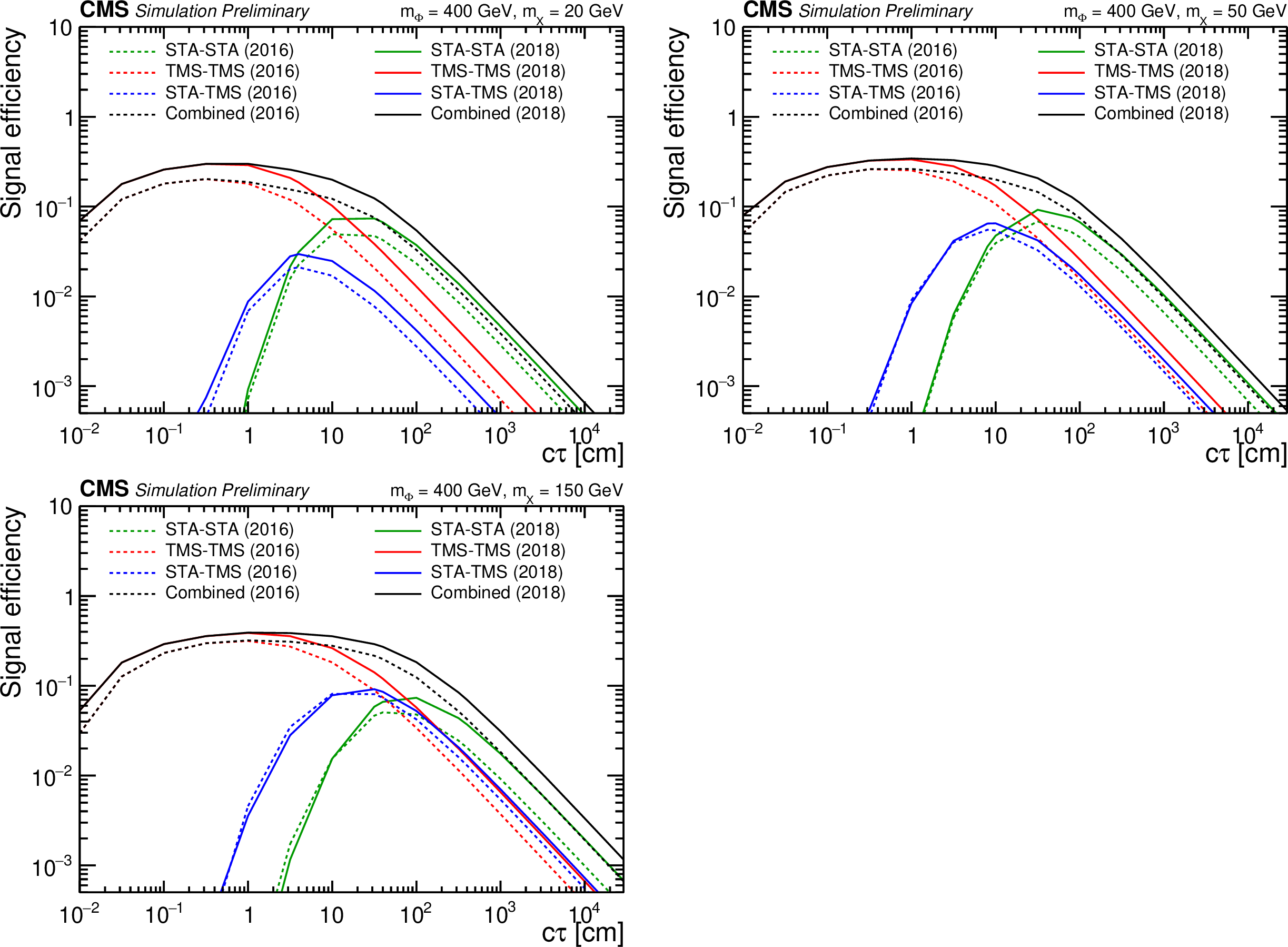
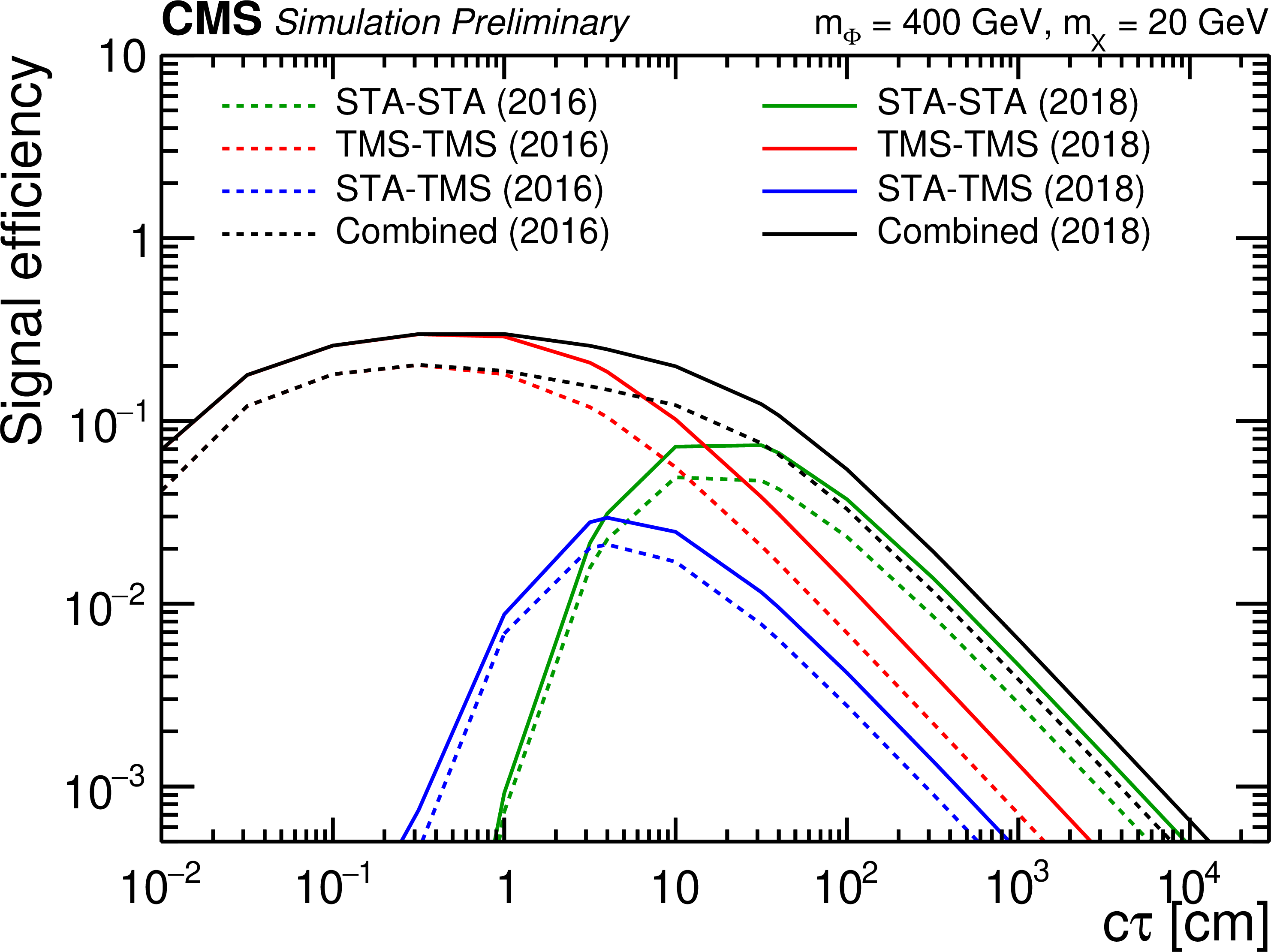
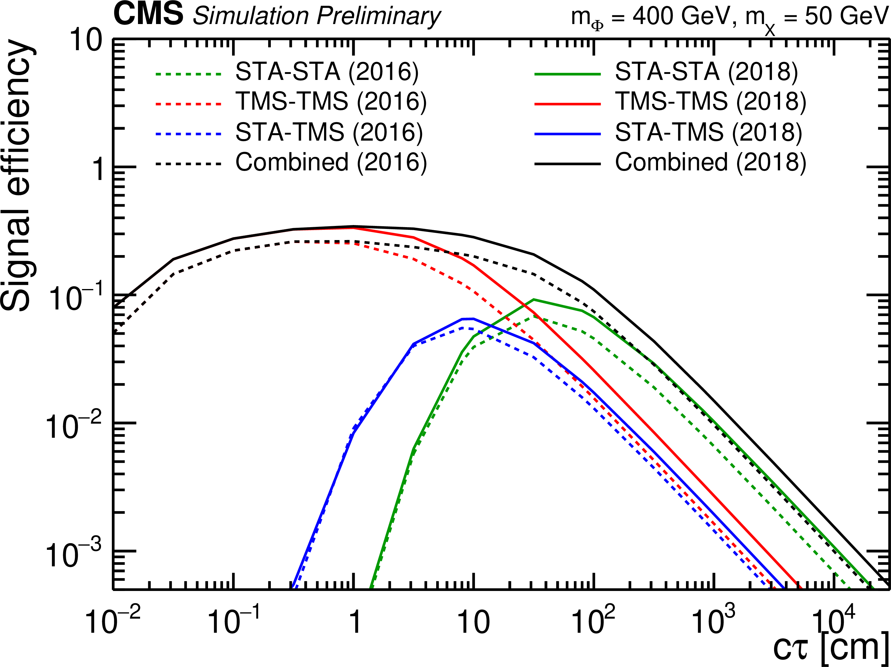
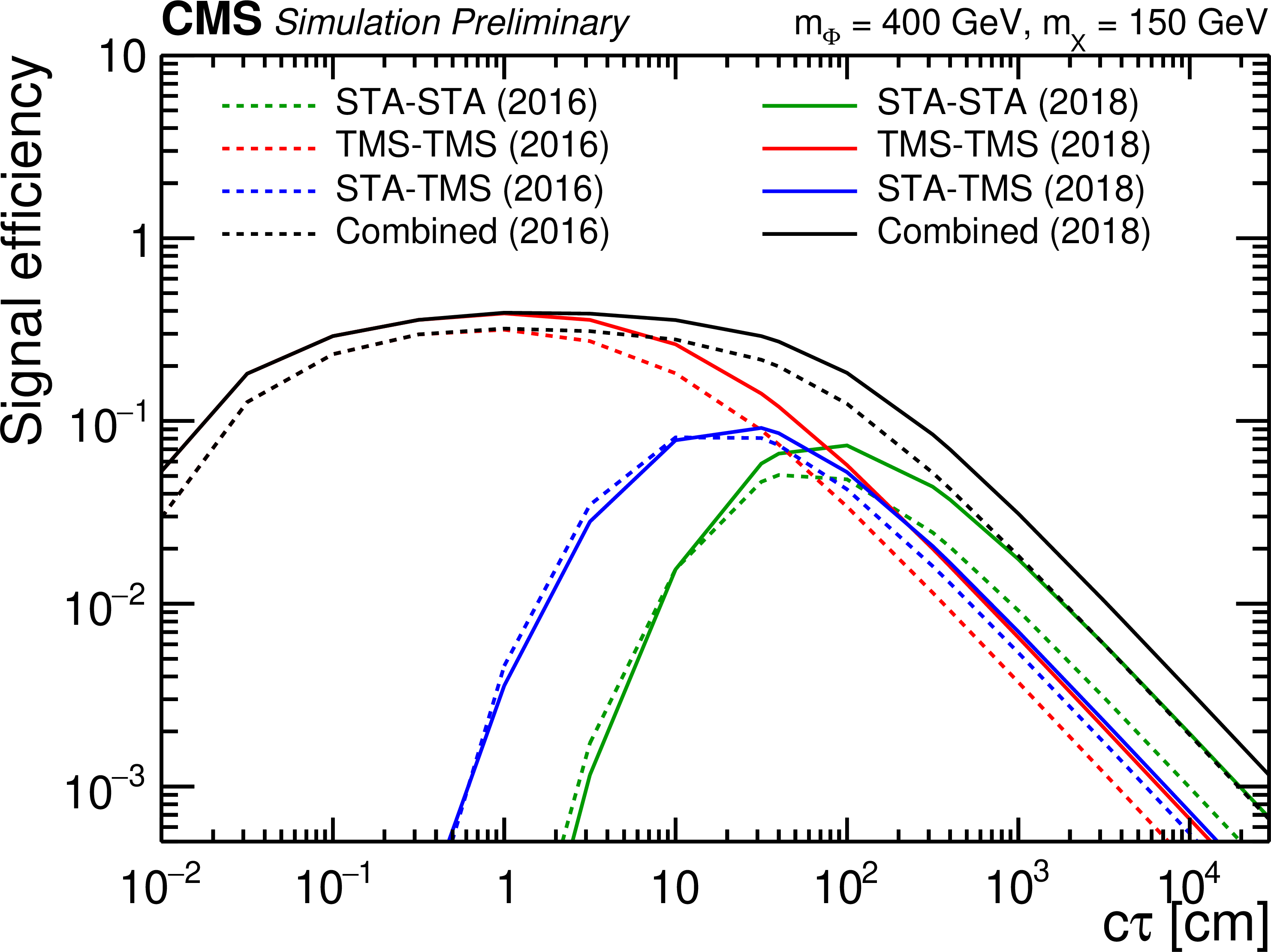
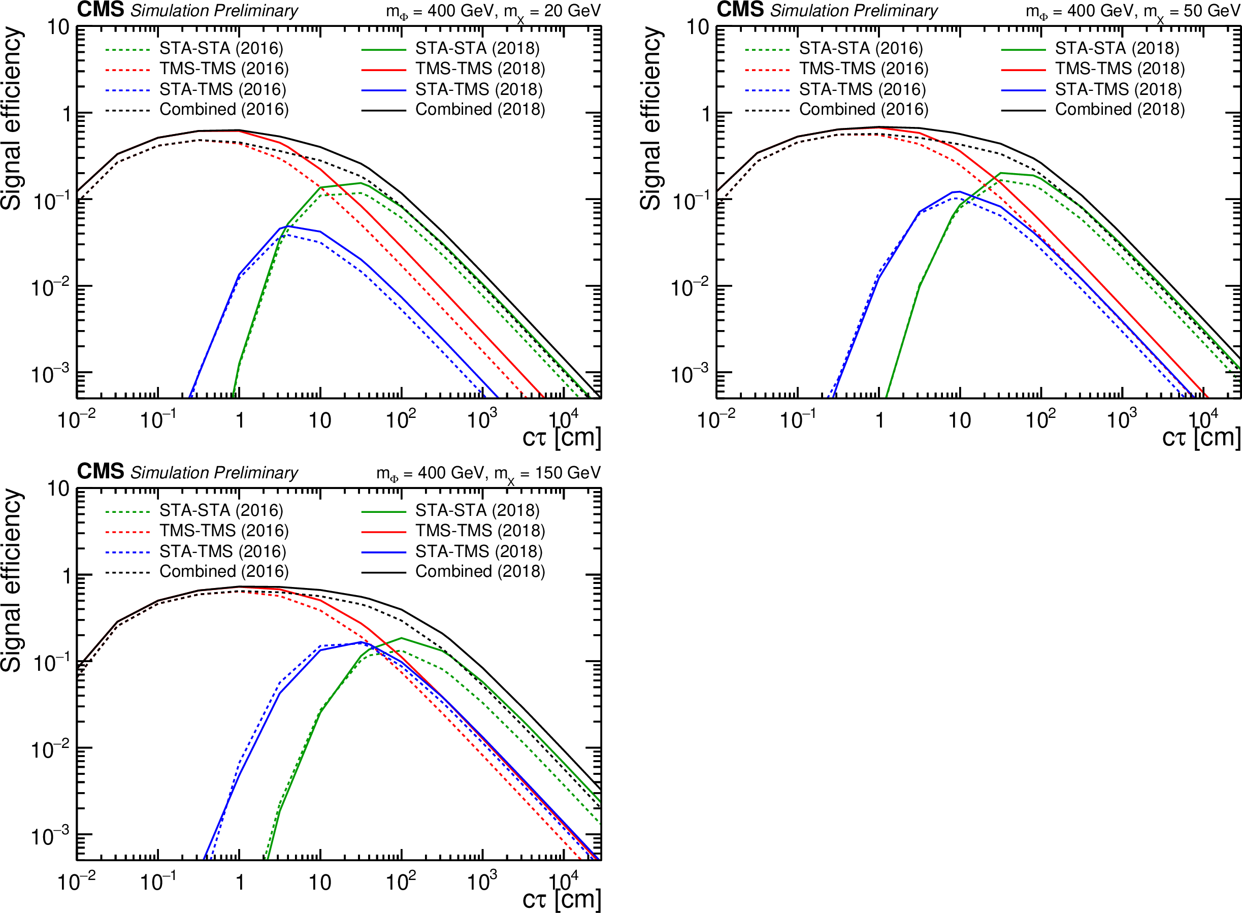
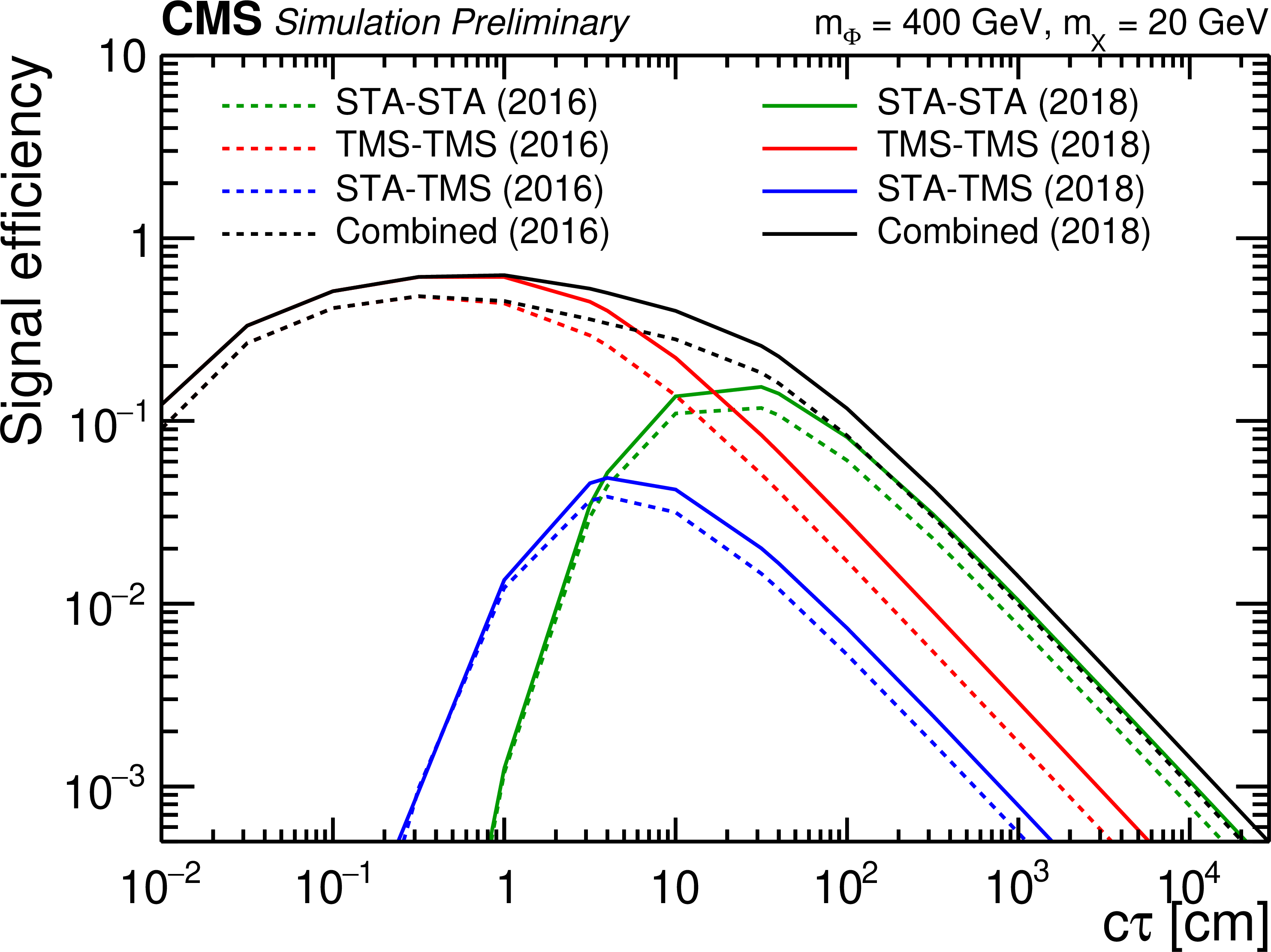
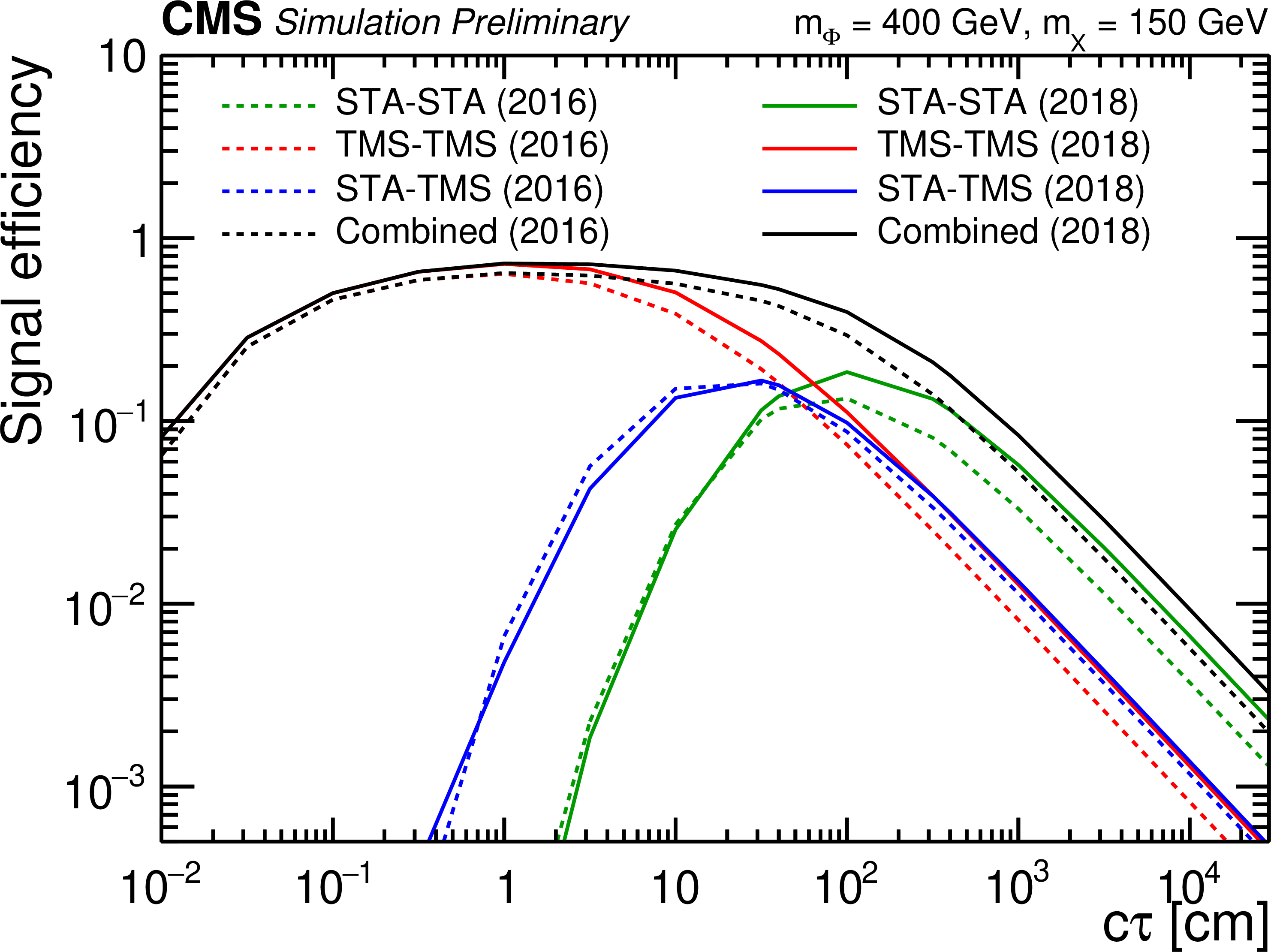
png pdf	Additional Figure 3: Overall signal efficiencies as a function of $c\tau$ for the $\Phi \to 2\text {X}\to 2\mu$ signal process with $m_\Phi =$ 400 GeV (top left: $m_\text {X}=$ 20 GeV, top right: $m_\text {X}=$ 50 GeV, bottom: $m_\text {X}=$ 150 GeV). Each figure shows efficiencies in the three dimuon categories, STA-STA (green), TMS-TMS (red), and STA-TMS (blue), as well as the combined efficiency (black) calculated as the sum of the efficiencies of the individual categories. The signal efficiencies for the 2016 and 2018 datasets are shown as dashed and solid lines, respectively.
png pdf root	Additional Figure 3-a: Overall signal efficiencies as a function of $c\tau$ for the $\Phi \to 2\text {X}\to 2\mu$ signal process with $m_\Phi =$ 400 GeV (top left: $m_\text {X}=$ 20 GeV, top right: $m_\text {X}=$ 50 GeV, bottom: $m_\text {X}=$ 150 GeV). Each figure shows efficiencies in the three dimuon categories, STA-STA (green), TMS-TMS (red), and STA-TMS (blue), as well as the combined efficiency (black) calculated as the sum of the efficiencies of the individual categories. The signal efficiencies for the 2016 and 2018 datasets are shown as dashed and solid lines, respectively.
png pdf root	Additional Figure 3-b: Overall signal efficiencies as a function of $c\tau$ for the $\Phi \to 2\text {X}\to 2\mu$ signal process with $m_\Phi =$ 400 GeV (top left: $m_\text {X}=$ 20 GeV, top right: $m_\text {X}=$ 50 GeV, bottom: $m_\text {X}=$ 150 GeV). Each figure shows efficiencies in the three dimuon categories, STA-STA (green), TMS-TMS (red), and STA-TMS (blue), as well as the combined efficiency (black) calculated as the sum of the efficiencies of the individual categories. The signal efficiencies for the 2016 and 2018 datasets are shown as dashed and solid lines, respectively.
png pdf root	Additional Figure 3-c: Overall signal efficiencies as a function of $c\tau$ for the $\Phi \to 2\text {X}\to 2\mu$ signal process with $m_\Phi =$ 400 GeV (top left: $m_\text {X}=$ 20 GeV, top right: $m_\text {X}=$ 50 GeV, bottom: $m_\text {X}=$ 150 GeV). Each figure shows efficiencies in the three dimuon categories, STA-STA (green), TMS-TMS (red), and STA-TMS (blue), as well as the combined efficiency (black) calculated as the sum of the efficiencies of the individual categories. The signal efficiencies for the 2016 and 2018 datasets are shown as dashed and solid lines, respectively.
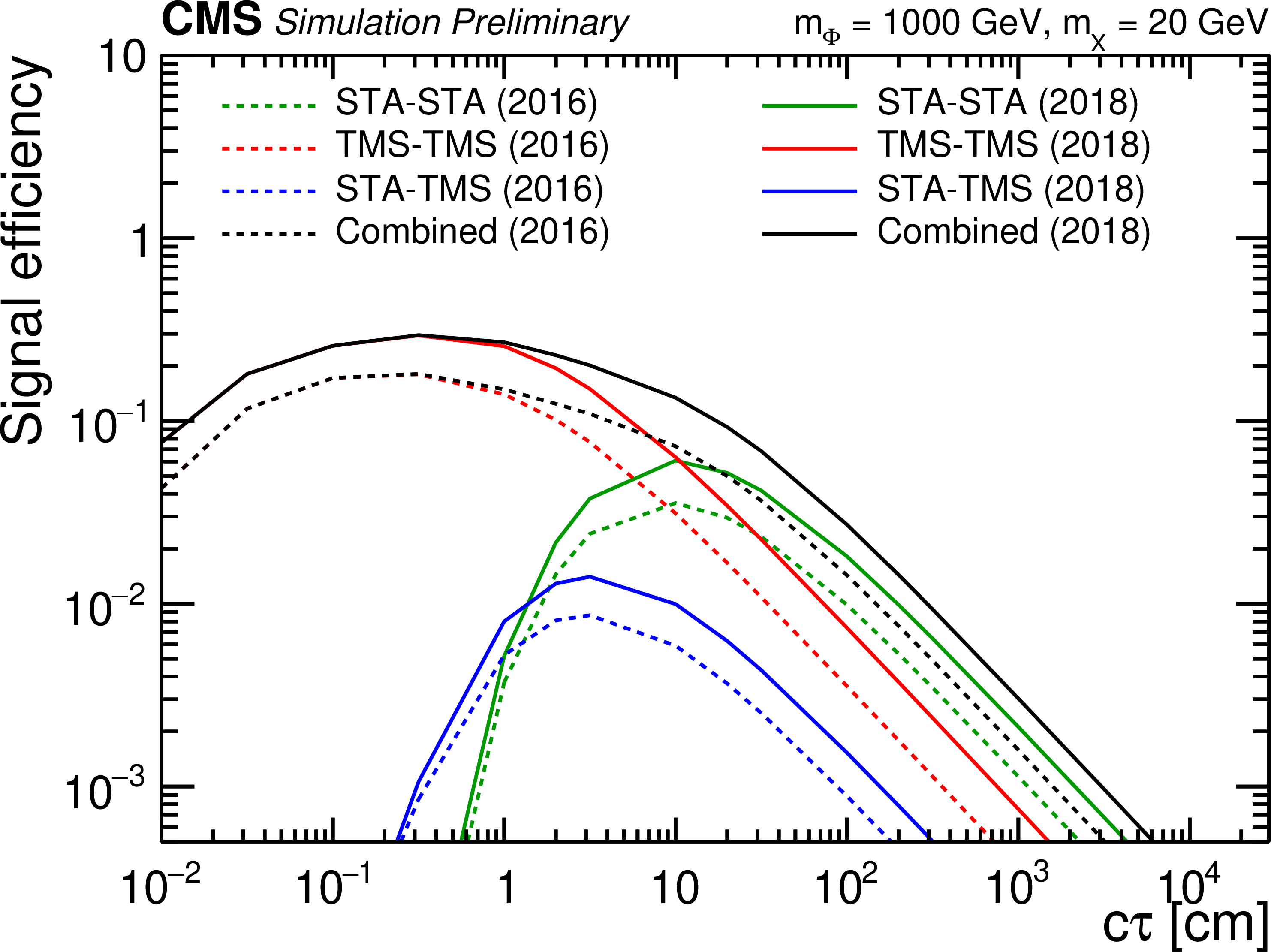
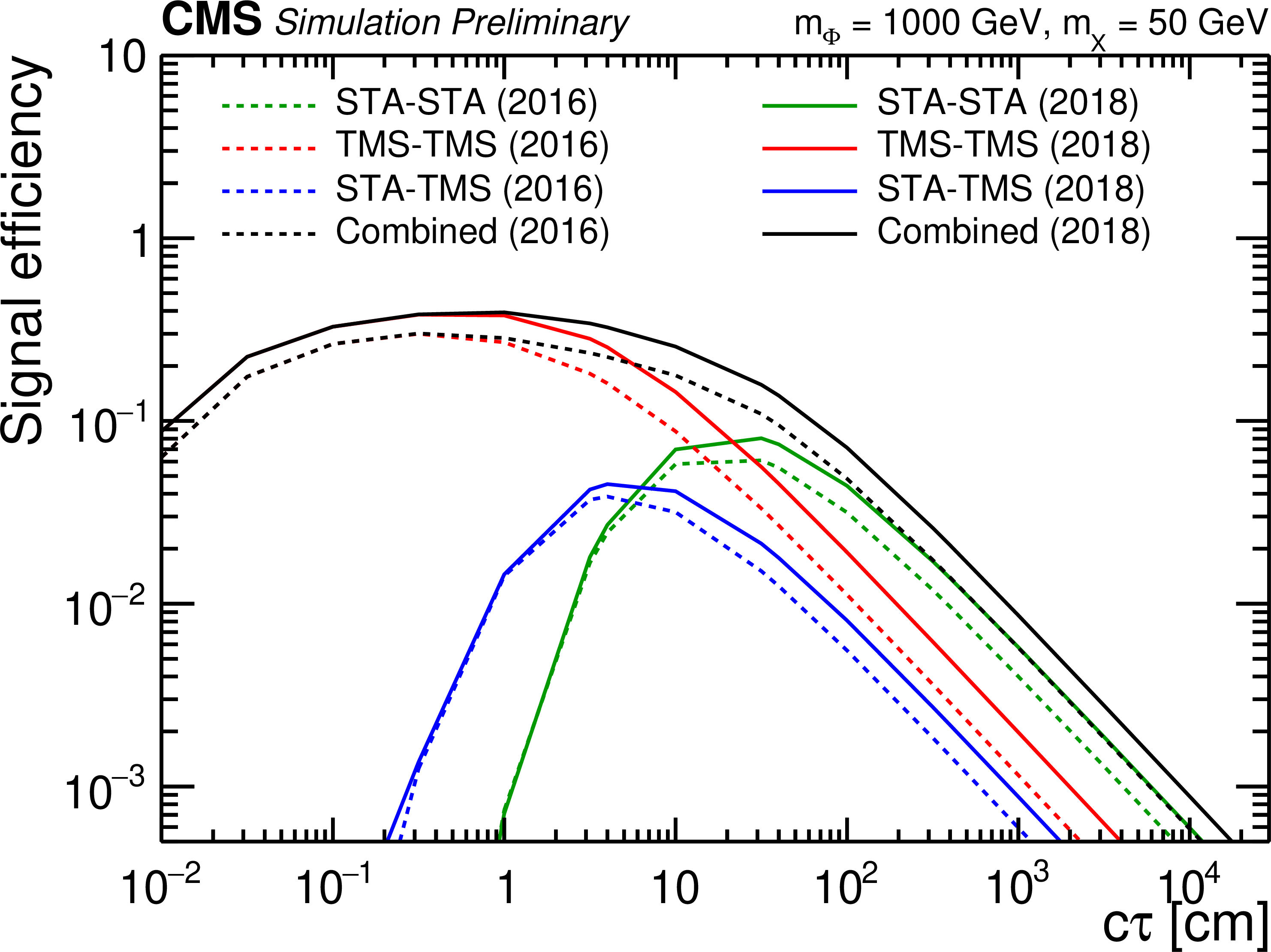
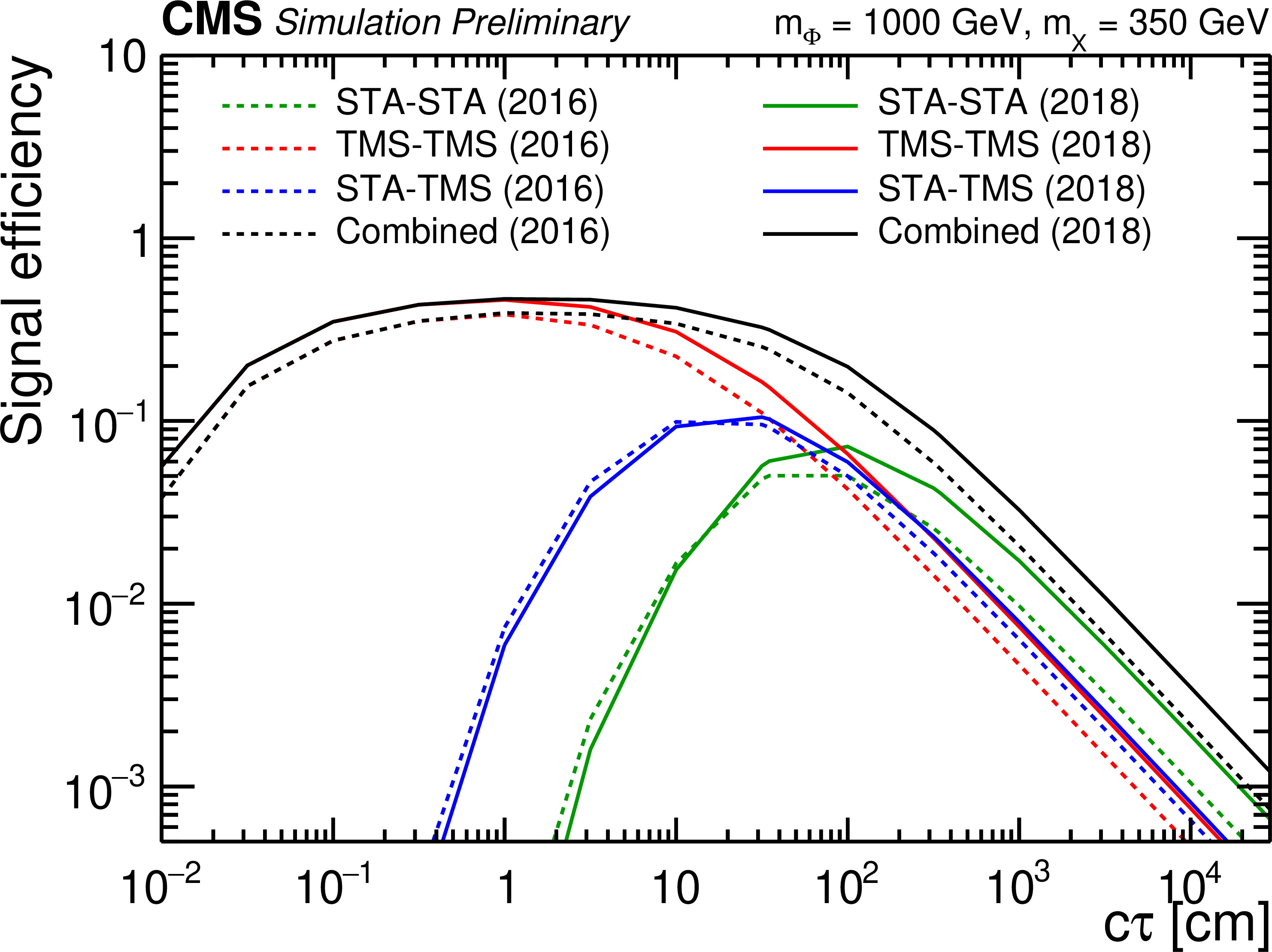
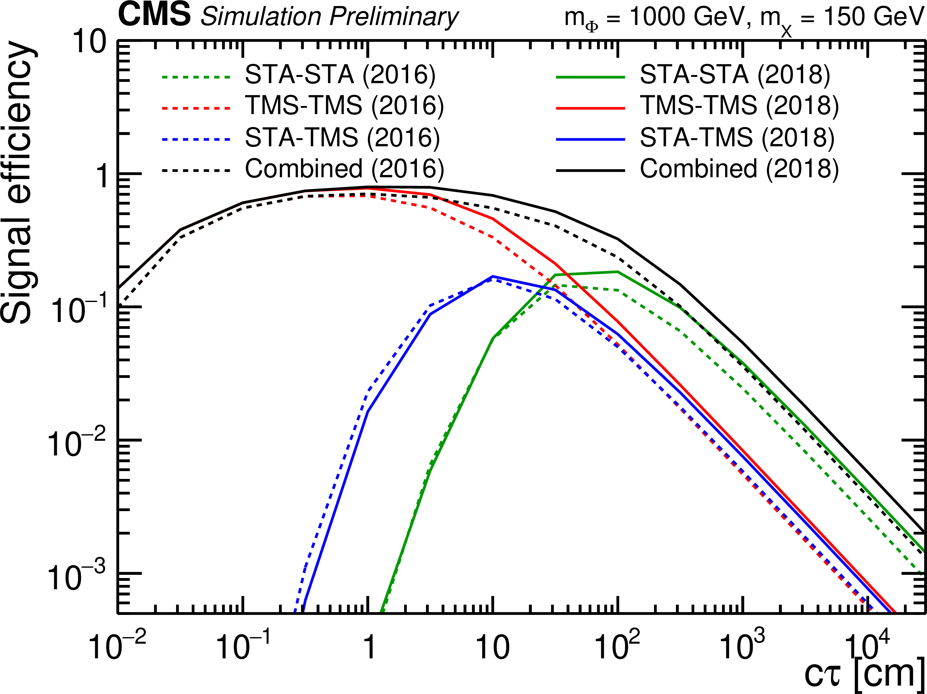
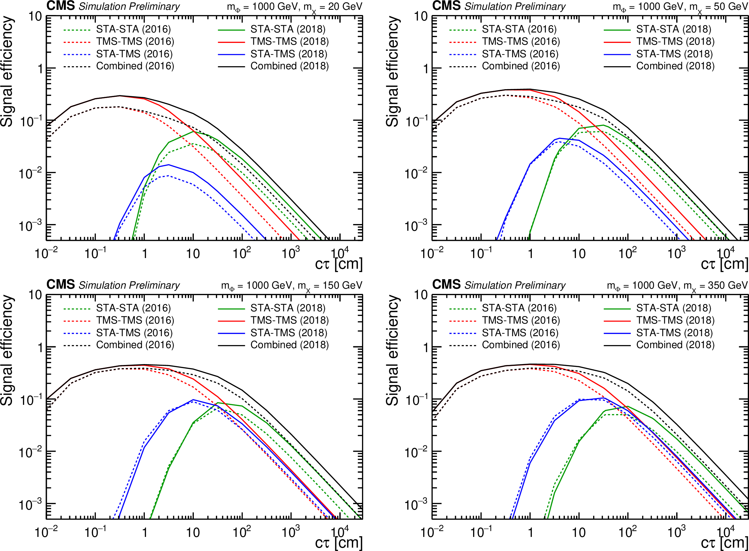
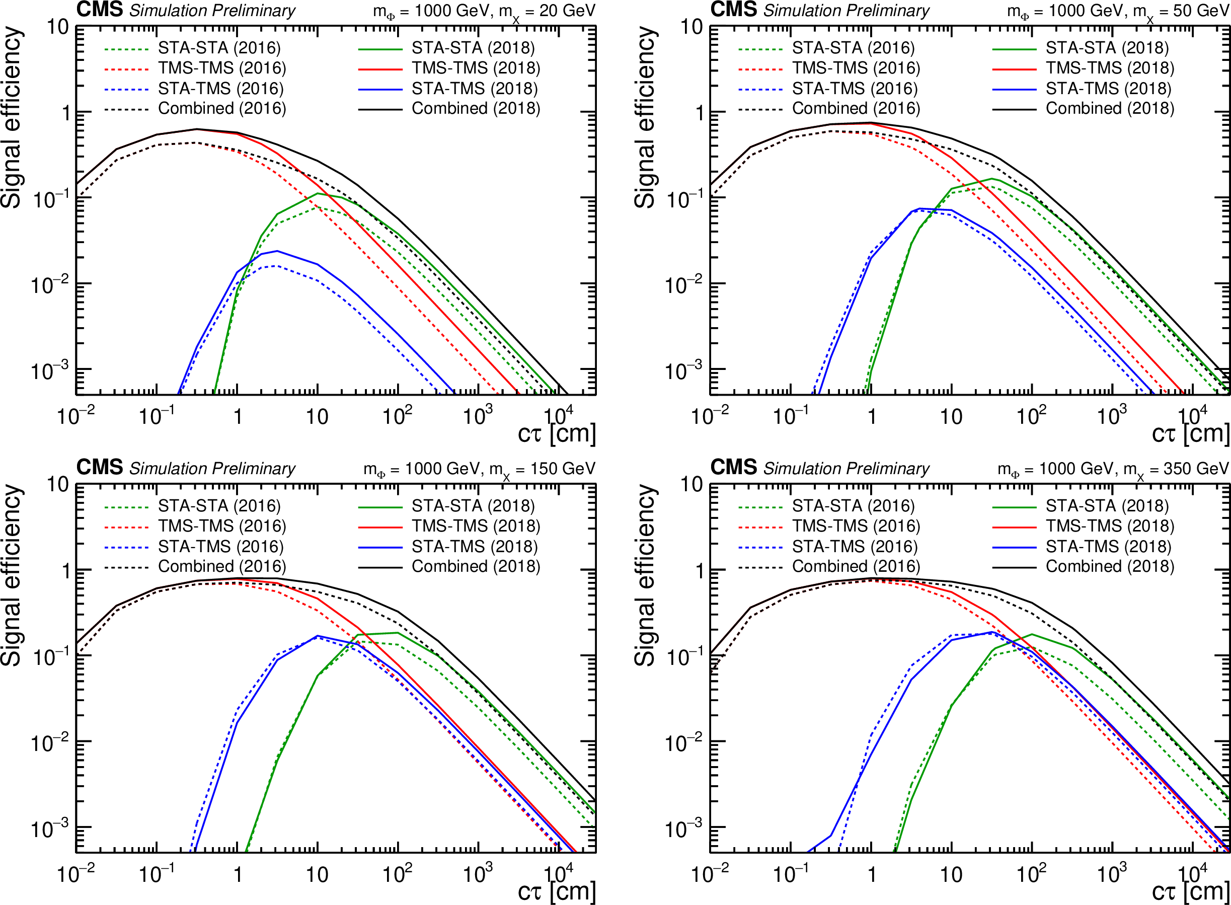
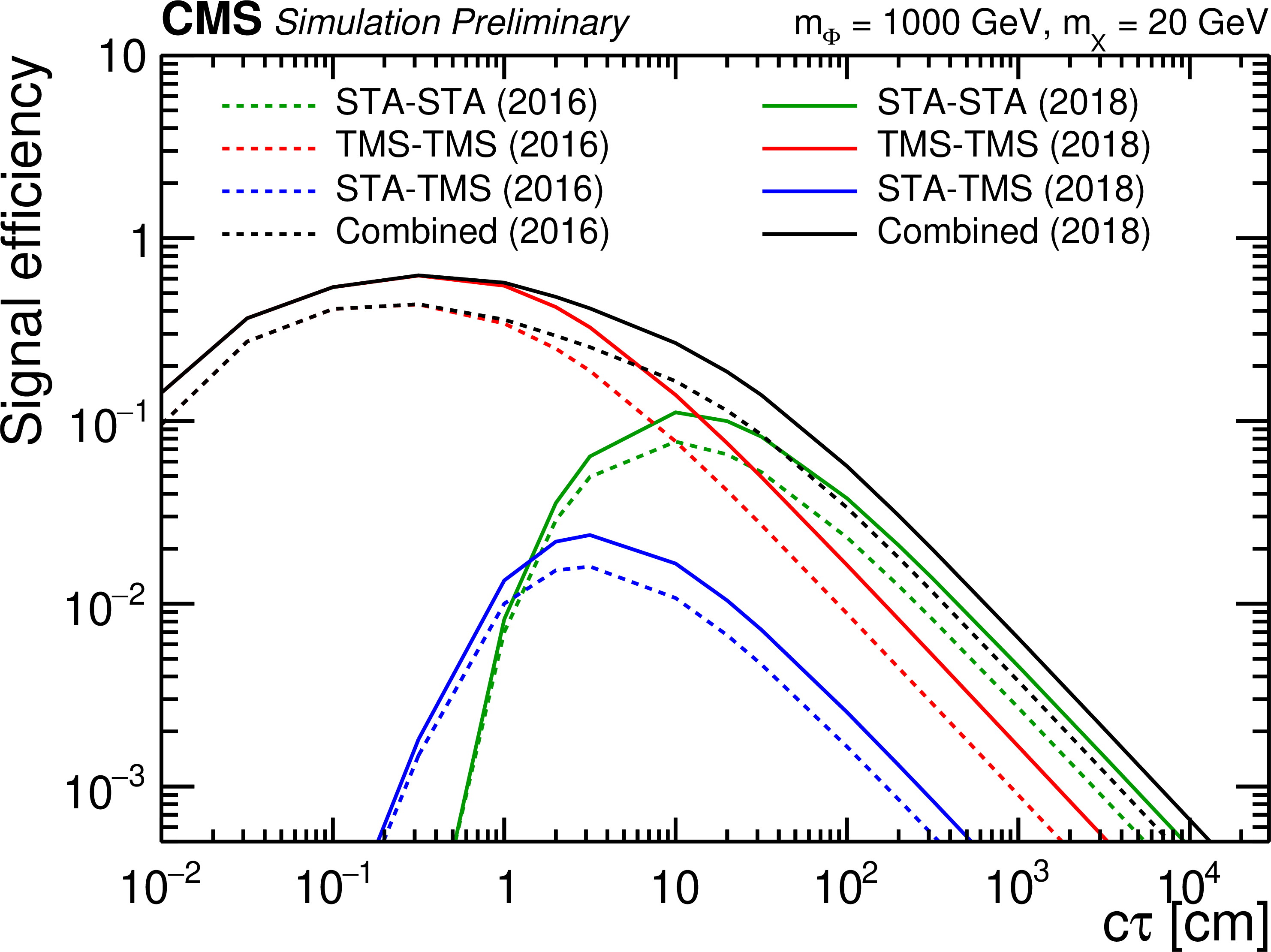
png pdf	Additional Figure 4: Overall signal efficiencies as a function of $c\tau$ for the $\Phi \to 2\text {X}\to 2\mu$ signal process with $m_\Phi =$ 1 TeV (top left: $m_\text {X}=$ 20 GeV, top right: $m_\text {X}=$ 50 GeV, bottom left: $m_\text {X}=$ 150 GeV, bottom right: $m_\text {X}=$ 350 GeV). Each figure shows efficiencies in the three dimuon categories, STA-STA (green), TMS-TMS (red), and STA-TMS (blue), as well as the combined efficiency (black) calculated as the sum of the efficiencies of the individual categories. The signal efficiencies for the 2016 and 2018 datasets are shown as dashed and solid lines, respectively.
png pdf root	Additional Figure 4-a: Overall signal efficiencies as a function of $c\tau$ for the $\Phi \to 2\text {X}\to 2\mu$ signal process with $m_\Phi =$ 1 TeV (top left: $m_\text {X}=$ 20 GeV, top right: $m_\text {X}=$ 50 GeV, bottom left: $m_\text {X}=$ 150 GeV, bottom right: $m_\text {X}=$ 350 GeV). Each figure shows efficiencies in the three dimuon categories, STA-STA (green), TMS-TMS (red), and STA-TMS (blue), as well as the combined efficiency (black) calculated as the sum of the efficiencies of the individual categories. The signal efficiencies for the 2016 and 2018 datasets are shown as dashed and solid lines, respectively.
png pdf root	Additional Figure 4-b: Overall signal efficiencies as a function of $c\tau$ for the $\Phi \to 2\text {X}\to 2\mu$ signal process with $m_\Phi =$ 1 TeV (top left: $m_\text {X}=$ 20 GeV, top right: $m_\text {X}=$ 50 GeV, bottom left: $m_\text {X}=$ 150 GeV, bottom right: $m_\text {X}=$ 350 GeV). Each figure shows efficiencies in the three dimuon categories, STA-STA (green), TMS-TMS (red), and STA-TMS (blue), as well as the combined efficiency (black) calculated as the sum of the efficiencies of the individual categories. The signal efficiencies for the 2016 and 2018 datasets are shown as dashed and solid lines, respectively.
png pdf root	Additional Figure 4-c: Overall signal efficiencies as a function of $c\tau$ for the $\Phi \to 2\text {X}\to 2\mu$ signal process with $m_\Phi =$ 1 TeV (top left: $m_\text {X}=$ 20 GeV, top right: $m_\text {X}=$ 50 GeV, bottom left: $m_\text {X}=$ 150 GeV, bottom right: $m_\text {X}=$ 350 GeV). Each figure shows efficiencies in the three dimuon categories, STA-STA (green), TMS-TMS (red), and STA-TMS (blue), as well as the combined efficiency (black) calculated as the sum of the efficiencies of the individual categories. The signal efficiencies for the 2016 and 2018 datasets are shown as dashed and solid lines, respectively.
png pdf root	Additional Figure 4-d: Overall signal efficiencies as a function of $c\tau$ for the $\Phi \to 2\text {X}\to 2\mu$ signal process with $m_\Phi =$ 1 TeV (top left: $m_\text {X}=$ 20 GeV, top right: $m_\text {X}=$ 50 GeV, bottom left: $m_\text {X}=$ 150 GeV, bottom right: $m_\text {X}=$ 350 GeV). Each figure shows efficiencies in the three dimuon categories, STA-STA (green), TMS-TMS (red), and STA-TMS (blue), as well as the combined efficiency (black) calculated as the sum of the efficiencies of the individual categories. The signal efficiencies for the 2016 and 2018 datasets are shown as dashed and solid lines, respectively.
png pdf	Additional Figure 5: Overall signal efficiencies as a function of $c\tau$ for the $\Phi \to 2\text {X}\to 4\mu$ signal process with $m_\Phi =$ 125 GeV (left: $m_\text {X}=$ 20 GeV, right: $m_\text {X}=$ 50 GeV). Each figure shows efficiencies in the three dimuon categories, STA-STA (green), TMS-TMS (red), and STA-TMS (blue), as well as the combined efficiency (black) calculated as the sum of the efficiencies of the individual categories. The signal efficiencies for the 2016 and 2018 datasets are shown as dashed and solid lines, respectively.
png pdf root	Additional Figure 5-a: Overall signal efficiencies as a function of $c\tau$ for the $\Phi \to 2\text {X}\to 4\mu$ signal process with $m_\Phi =$ 125 GeV (left: $m_\text {X}=$ 20 GeV, right: $m_\text {X}=$ 50 GeV). Each figure shows efficiencies in the three dimuon categories, STA-STA (green), TMS-TMS (red), and STA-TMS (blue), as well as the combined efficiency (black) calculated as the sum of the efficiencies of the individual categories. The signal efficiencies for the 2016 and 2018 datasets are shown as dashed and solid lines, respectively.
png pdf root	Additional Figure 5-b: Overall signal efficiencies as a function of $c\tau$ for the $\Phi \to 2\text {X}\to 4\mu$ signal process with $m_\Phi =$ 125 GeV (left: $m_\text {X}=$ 20 GeV, right: $m_\text {X}=$ 50 GeV). Each figure shows efficiencies in the three dimuon categories, STA-STA (green), TMS-TMS (red), and STA-TMS (blue), as well as the combined efficiency (black) calculated as the sum of the efficiencies of the individual categories. The signal efficiencies for the 2016 and 2018 datasets are shown as dashed and solid lines, respectively.
png pdf	Additional Figure 6: Overall signal efficiencies as a function of $c\tau$ for the $\Phi \to 2\text {X}\to 4\mu$ signal process with $m_\Phi =$ 200 GeV (left: $m_\text {X}=$ 20 GeV, right: $m_\text {X}=$ 50 GeV). Each figure shows efficiencies in the three dimuon categories, STA-STA (green), TMS-TMS (red), and STA-TMS (blue), as well as the combined efficiency (black) calculated as the sum of the efficiencies of the individual categories. The signal efficiencies for the 2016 and 2018 datasets are shown as dashed and solid lines, respectively.
png pdf root	Additional Figure 6-a: Overall signal efficiencies as a function of $c\tau$ for the $\Phi \to 2\text {X}\to 4\mu$ signal process with $m_\Phi =$ 200 GeV (left: $m_\text {X}=$ 20 GeV, right: $m_\text {X}=$ 50 GeV). Each figure shows efficiencies in the three dimuon categories, STA-STA (green), TMS-TMS (red), and STA-TMS (blue), as well as the combined efficiency (black) calculated as the sum of the efficiencies of the individual categories. The signal efficiencies for the 2016 and 2018 datasets are shown as dashed and solid lines, respectively.
png pdf root	Additional Figure 6-b: Overall signal efficiencies as a function of $c\tau$ for the $\Phi \to 2\text {X}\to 4\mu$ signal process with $m_\Phi =$ 200 GeV (left: $m_\text {X}=$ 20 GeV, right: $m_\text {X}=$ 50 GeV). Each figure shows efficiencies in the three dimuon categories, STA-STA (green), TMS-TMS (red), and STA-TMS (blue), as well as the combined efficiency (black) calculated as the sum of the efficiencies of the individual categories. The signal efficiencies for the 2016 and 2018 datasets are shown as dashed and solid lines, respectively.
png pdf	Additional Figure 7: Overall signal efficiencies as a function of $c\tau$ for the $\Phi \to 2\text {X}\to 4\mu$ signal process with $m_\Phi =$ 400 GeV (top left: $m_\text {X}=$ 20 GeV, top right: $m_\text {X}=$ 50 GeV, bottom: $m_\text {X}=$ 150 GeV). Each figure shows efficiencies in the three dimuon categories, STA-STA (green), TMS-TMS (red), and STA-TMS (blue), as well as the combined efficiency (black) calculated as the sum of the efficiencies of the individual categories. The signal efficiencies for the 2016 and 2018 datasets are shown as dashed and solid lines, respectively.
png pdf root	Additional Figure 7-a: Overall signal efficiencies as a function of $c\tau$ for the $\Phi \to 2\text {X}\to 4\mu$ signal process with $m_\Phi =$ 400 GeV (top left: $m_\text {X}=$ 20 GeV, top right: $m_\text {X}=$ 50 GeV, bottom: $m_\text {X}=$ 150 GeV). Each figure shows efficiencies in the three dimuon categories, STA-STA (green), TMS-TMS (red), and STA-TMS (blue), as well as the combined efficiency (black) calculated as the sum of the efficiencies of the individual categories. The signal efficiencies for the 2016 and 2018 datasets are shown as dashed and solid lines, respectively.
png pdf root	Additional Figure 7-b: Overall signal efficiencies as a function of $c\tau$ for the $\Phi \to 2\text {X}\to 4\mu$ signal process with $m_\Phi =$ 400 GeV (top left: $m_\text {X}=$ 20 GeV, top right: $m_\text {X}=$ 50 GeV, bottom: $m_\text {X}=$ 150 GeV). Each figure shows efficiencies in the three dimuon categories, STA-STA (green), TMS-TMS (red), and STA-TMS (blue), as well as the combined efficiency (black) calculated as the sum of the efficiencies of the individual categories. The signal efficiencies for the 2016 and 2018 datasets are shown as dashed and solid lines, respectively.
png pdf root	Additional Figure 7-c: Overall signal efficiencies as a function of $c\tau$ for the $\Phi \to 2\text {X}\to 4\mu$ signal process with $m_\Phi =$ 400 GeV (top left: $m_\text {X}=$ 20 GeV, top right: $m_\text {X}=$ 50 GeV, bottom: $m_\text {X}=$ 150 GeV). Each figure shows efficiencies in the three dimuon categories, STA-STA (green), TMS-TMS (red), and STA-TMS (blue), as well as the combined efficiency (black) calculated as the sum of the efficiencies of the individual categories. The signal efficiencies for the 2016 and 2018 datasets are shown as dashed and solid lines, respectively.
png pdf	Additional Figure 8: Overall signal efficiencies as a function of $c\tau$ for the $\Phi \to 2\text {X}\to 4\mu$ signal process with $m_\Phi =$ 1 TeV (top left: $m_\text {X}=$ 20 GeV, top right: $m_\text {X}=$ 50 GeV, bottom left: $m_\text {X}=$ 150 GeV, bottom right: $m_\text {X}=$ 350 GeV). Each figure shows efficiencies in the three dimuon categories, STA-STA (green), TMS-TMS (red), and STA-TMS (blue), as well as the combined efficiency (black) calculated as the sum of the efficiencies of the individual categories. The signal efficiencies for the 2016 and 2018 datasets are shown as dashed and solid lines, respectively.
png pdf root	Additional Figure 8-a: Overall signal efficiencies as a function of $c\tau$ for the $\Phi \to 2\text {X}\to 4\mu$ signal process with $m_\Phi =$ 1 TeV (top left: $m_\text {X}=$ 20 GeV, top right: $m_\text {X}=$ 50 GeV, bottom left: $m_\text {X}=$ 150 GeV, bottom right: $m_\text {X}=$ 350 GeV). Each figure shows efficiencies in the three dimuon categories, STA-STA (green), TMS-TMS (red), and STA-TMS (blue), as well as the combined efficiency (black) calculated as the sum of the efficiencies of the individual categories. The signal efficiencies for the 2016 and 2018 datasets are shown as dashed and solid lines, respectively.
png pdf root	Additional Figure 8-b: Overall signal efficiencies as a function of $c\tau$ for the $\Phi \to 2\text {X}\to 4\mu$ signal process with $m_\Phi =$ 1 TeV (top left: $m_\text {X}=$ 20 GeV, top right: $m_\text {X}=$ 50 GeV, bottom left: $m_\text {X}=$ 150 GeV, bottom right: $m_\text {X}=$ 350 GeV). Each figure shows efficiencies in the three dimuon categories, STA-STA (green), TMS-TMS (red), and STA-TMS (blue), as well as the combined efficiency (black) calculated as the sum of the efficiencies of the individual categories. The signal efficiencies for the 2016 and 2018 datasets are shown as dashed and solid lines, respectively.
png pdf root	Additional Figure 8-c: Overall signal efficiencies as a function of $c\tau$ for the $\Phi \to 2\text {X}\to 4\mu$ signal process with $m_\Phi =$ 1 TeV (top left: $m_\text {X}=$ 20 GeV, top right: $m_\text {X}=$ 50 GeV, bottom left: $m_\text {X}=$ 150 GeV, bottom right: $m_\text {X}=$ 350 GeV). Each figure shows efficiencies in the three dimuon categories, STA-STA (green), TMS-TMS (red), and STA-TMS (blue), as well as the combined efficiency (black) calculated as the sum of the efficiencies of the individual categories. The signal efficiencies for the 2016 and 2018 datasets are shown as dashed and solid lines, respectively.
png pdf root	Additional Figure 8-d: Overall signal efficiencies as a function of $c\tau$ for the $\Phi \to 2\text {X}\to 4\mu$ signal process with $m_\Phi =$ 1 TeV (top left: $m_\text {X}=$ 20 GeV, top right: $m_\text {X}=$ 50 GeV, bottom left: $m_\text {X}=$ 150 GeV, bottom right: $m_\text {X}=$ 350 GeV). Each figure shows efficiencies in the three dimuon categories, STA-STA (green), TMS-TMS (red), and STA-TMS (blue), as well as the combined efficiency (black) calculated as the sum of the efficiencies of the individual categories. The signal efficiencies for the 2016 and 2018 datasets are shown as dashed and solid lines, respectively.
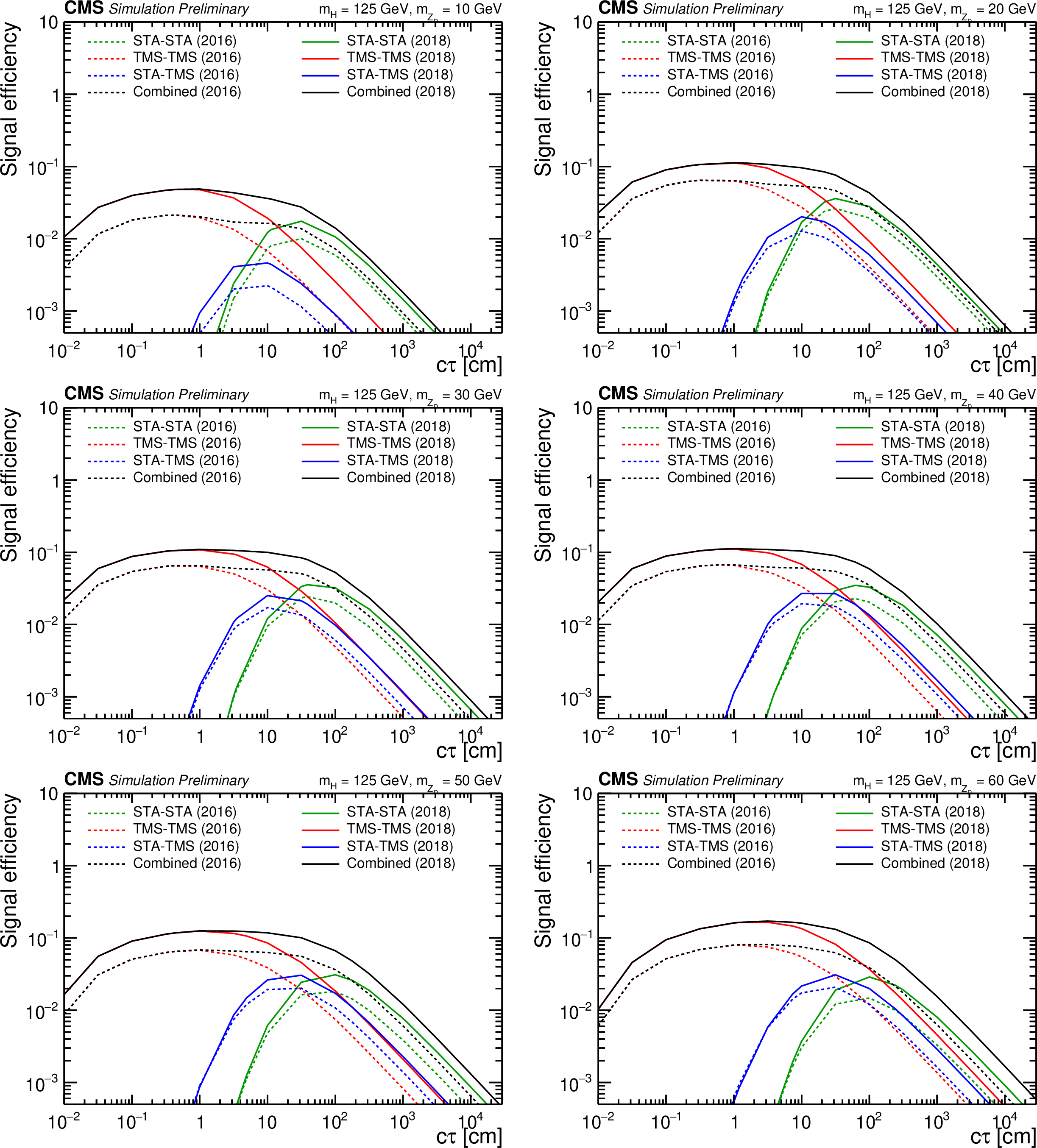
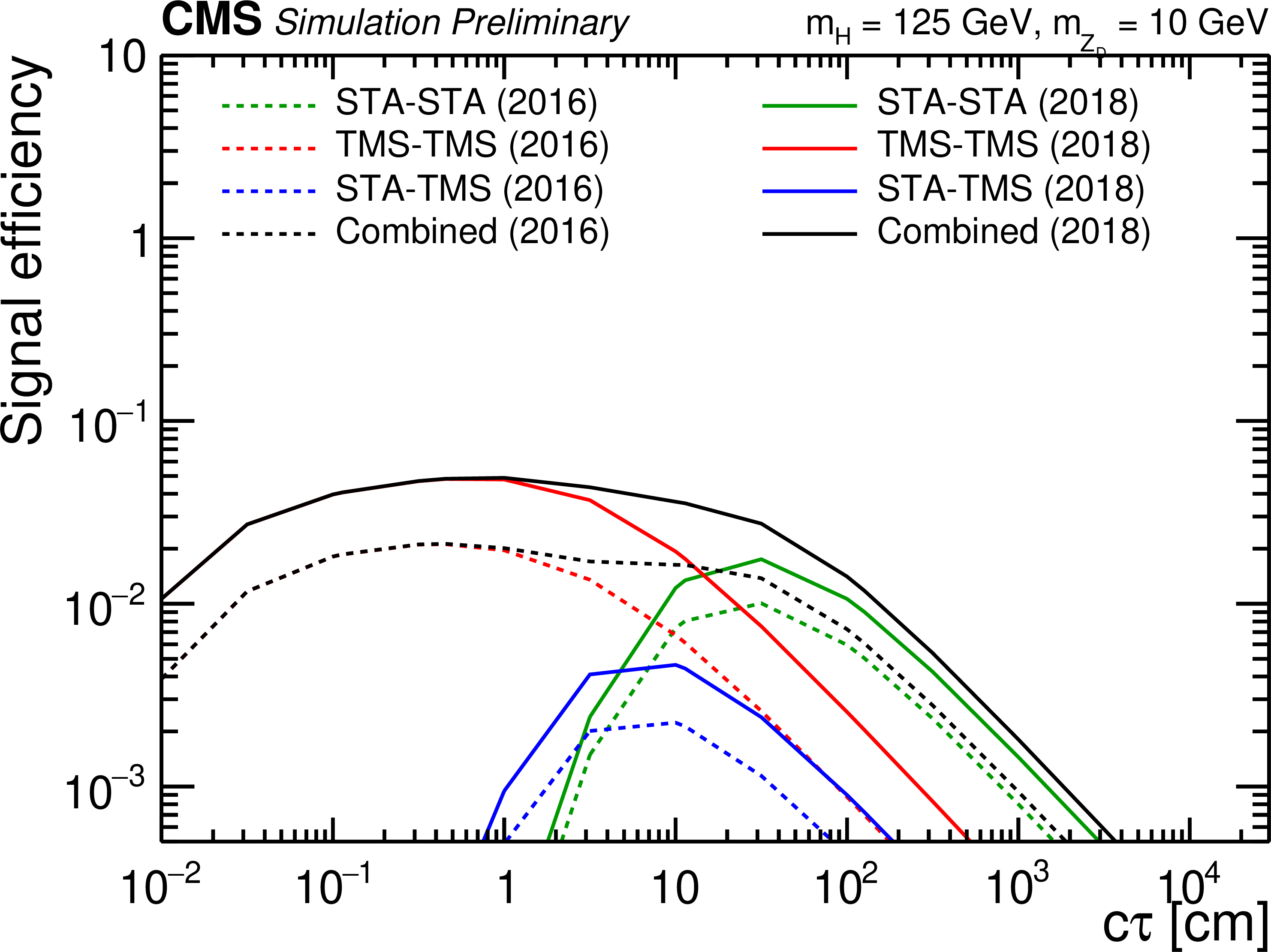
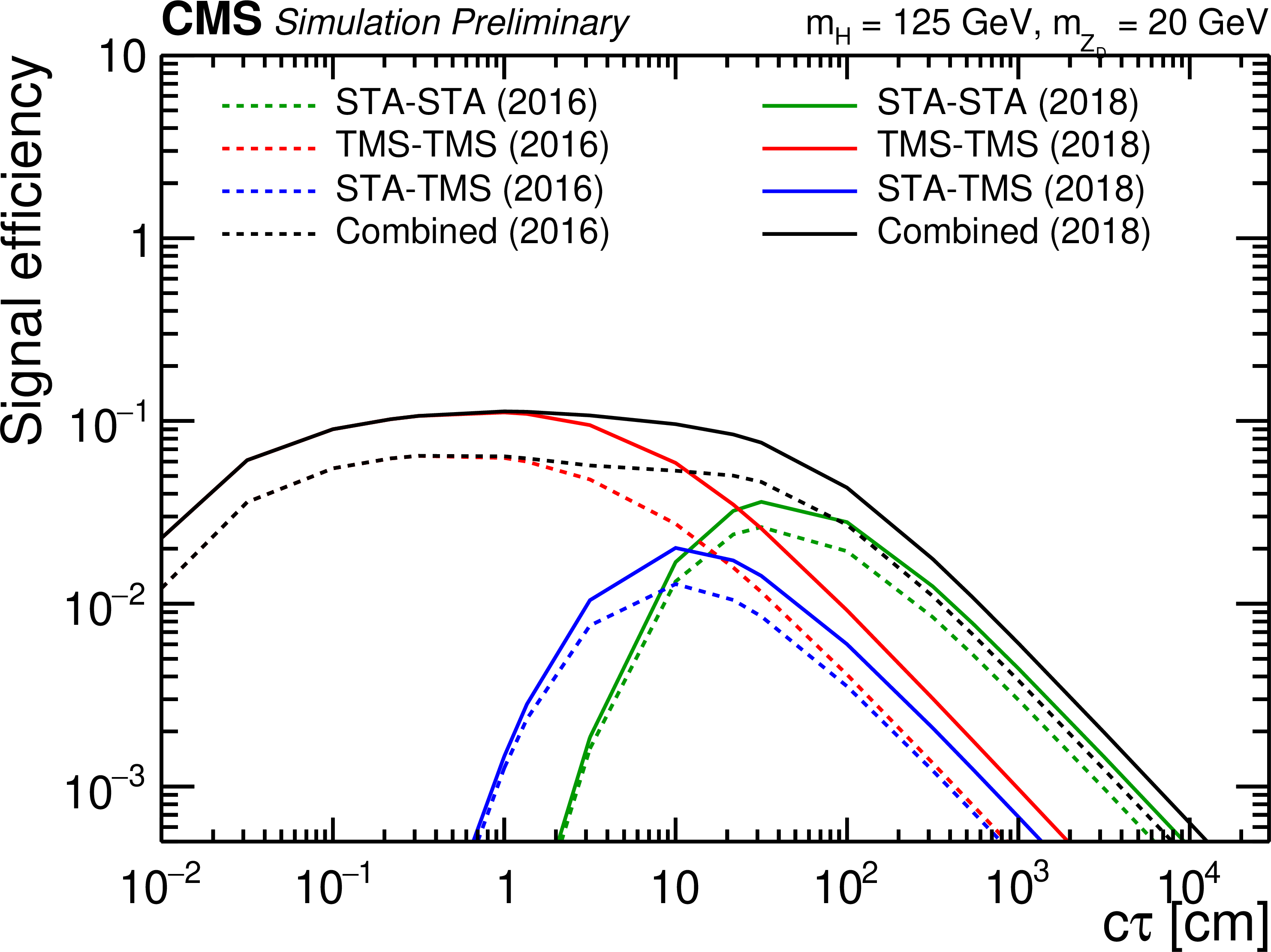
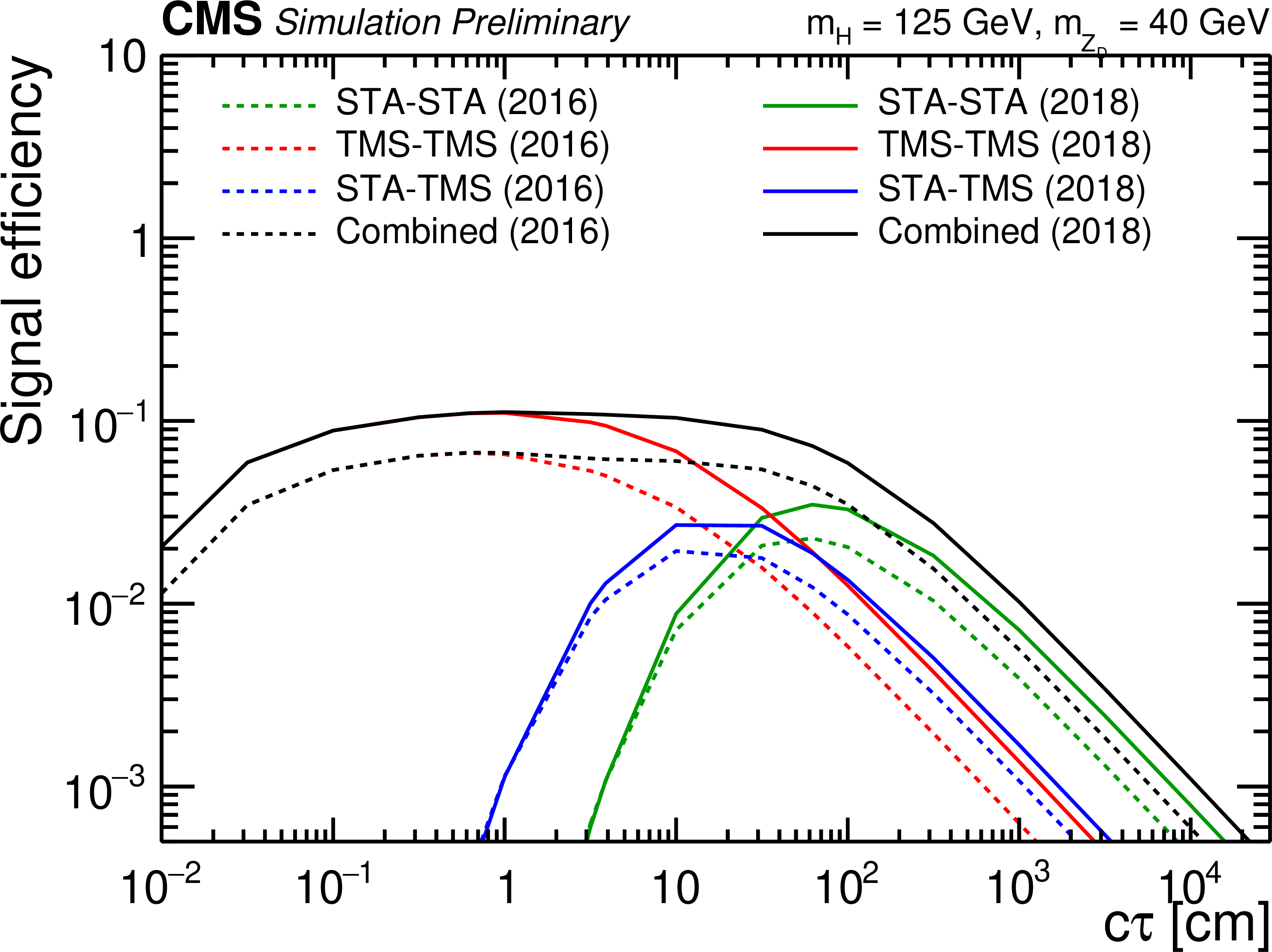
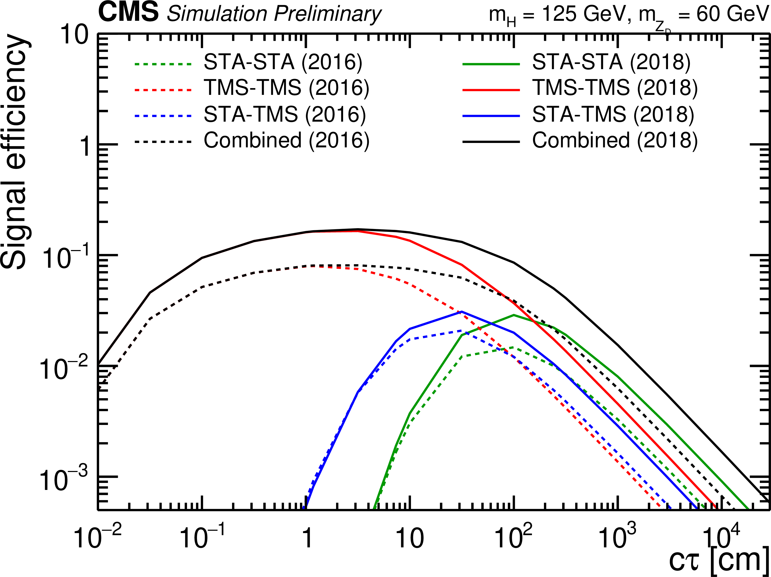
png pdf	Additional Figure 9: Overall signal efficiencies as a function of $c\tau$ for the $\text {H}\to 2\mathrm{Z_D}\to 2\mu \, 2\text {X}$ signal process with $m(\text {H})=$ 125 GeV (top left to bottom right: $m_{\mathrm{Z_D}}=$ 10, 20, 30, 40, 50, 60 GeV). Each figure shows efficiencies in the three dimuon categories, STA-STA (green), TMS-TMS (red), and STA-TMS (blue), as well the combined efficiency (black) calculated as the sum of the efficiencies of the individual categories. The signal efficiencies for the 2016 and 2018 datasets are shown as dashed and solid lines, respectively.
png pdf root	Additional Figure 9-a: Overall signal efficiencies as a function of $c\tau$ for the $\text {H}\to 2\mathrm{Z_D}\to 2\mu \, 2\text {X}$ signal process with $m(\text {H})=$ 125 GeV (top left to bottom right: $m_{\mathrm{Z_D}}=$ 10, 20, 30, 40, 50, 60 GeV). Each figure shows efficiencies in the three dimuon categories, STA-STA (green), TMS-TMS (red), and STA-TMS (blue), as well the combined efficiency (black) calculated as the sum of the efficiencies of the individual categories. The signal efficiencies for the 2016 and 2018 datasets are shown as dashed and solid lines, respectively.
png pdf root	Additional Figure 9-b: Overall signal efficiencies as a function of $c\tau$ for the $\text {H}\to 2\mathrm{Z_D}\to 2\mu \, 2\text {X}$ signal process with $m(\text {H})=$ 125 GeV (top left to bottom right: $m_{\mathrm{Z_D}}=$ 10, 20, 30, 40, 50, 60 GeV). Each figure shows efficiencies in the three dimuon categories, STA-STA (green), TMS-TMS (red), and STA-TMS (blue), as well the combined efficiency (black) calculated as the sum of the efficiencies of the individual categories. The signal efficiencies for the 2016 and 2018 datasets are shown as dashed and solid lines, respectively.
png pdf root	Additional Figure 9-c: Overall signal efficiencies as a function of $c\tau$ for the $\text {H}\to 2\mathrm{Z_D}\to 2\mu \, 2\text {X}$ signal process with $m(\text {H})=$ 125 GeV (top left to bottom right: $m_{\mathrm{Z_D}}=$ 10, 20, 30, 40, 50, 60 GeV). Each figure shows efficiencies in the three dimuon categories, STA-STA (green), TMS-TMS (red), and STA-TMS (blue), as well the combined efficiency (black) calculated as the sum of the efficiencies of the individual categories. The signal efficiencies for the 2016 and 2018 datasets are shown as dashed and solid lines, respectively.
png pdf root	Additional Figure 9-d: Overall signal efficiencies as a function of $c\tau$ for the $\text {H}\to 2\mathrm{Z_D}\to 2\mu \, 2\text {X}$ signal process with $m(\text {H})=$ 125 GeV (top left to bottom right: $m_{\mathrm{Z_D}}=$ 10, 20, 30, 40, 50, 60 GeV). Each figure shows efficiencies in the three dimuon categories, STA-STA (green), TMS-TMS (red), and STA-TMS (blue), as well the combined efficiency (black) calculated as the sum of the efficiencies of the individual categories. The signal efficiencies for the 2016 and 2018 datasets are shown as dashed and solid lines, respectively.
png pdf root	Additional Figure 9-e: Overall signal efficiencies as a function of $c\tau$ for the $\text {H}\to 2\mathrm{Z_D}\to 2\mu \, 2\text {X}$ signal process with $m(\text {H})=$ 125 GeV (top left to bottom right: $m_{\mathrm{Z_D}}=$ 10, 20, 30, 40, 50, 60 GeV). Each figure shows efficiencies in the three dimuon categories, STA-STA (green), TMS-TMS (red), and STA-TMS (blue), as well the combined efficiency (black) calculated as the sum of the efficiencies of the individual categories. The signal efficiencies for the 2016 and 2018 datasets are shown as dashed and solid lines, respectively.
png pdf root	Additional Figure 9-f: Overall signal efficiencies as a function of $c\tau$ for the $\text {H}\to 2\mathrm{Z_D}\to 2\mu \, 2\text {X}$ signal process with $m(\text {H})=$ 125 GeV (top left to bottom right: $m_{\mathrm{Z_D}}=$ 10, 20, 30, 40, 50, 60 GeV). Each figure shows efficiencies in the three dimuon categories, STA-STA (green), TMS-TMS (red), and STA-TMS (blue), as well the combined efficiency (black) calculated as the sum of the efficiencies of the individual categories. The signal efficiencies for the 2016 and 2018 datasets are shown as dashed and solid lines, respectively.
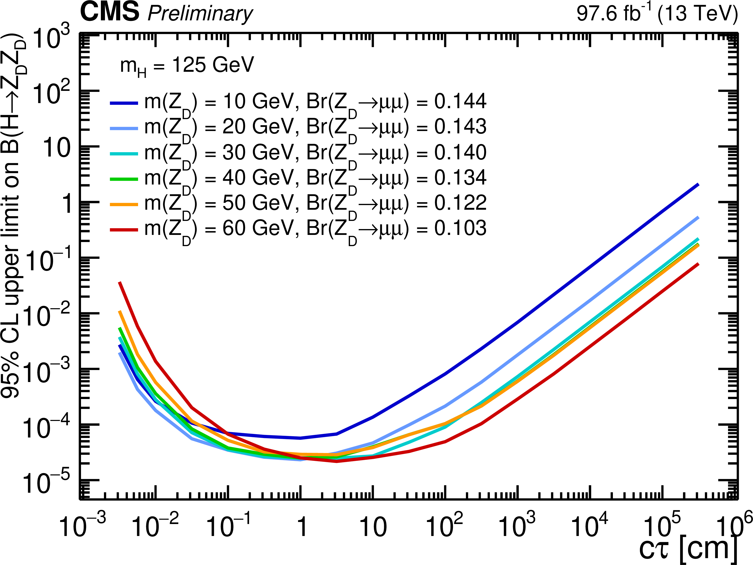
png pdf root	Additional Figure 10: The 95% CL combined observed upper limits on $\mathcal {B} (\text {H} \to \mathrm{Z_D} \mathrm{Z_D})$ as a function of $c\tau _{\mathrm{Z_D}}$ in the HAHM model, for $m_{\mathrm{Z_D}}$ ranging from 10 GeV to 60 GeV.
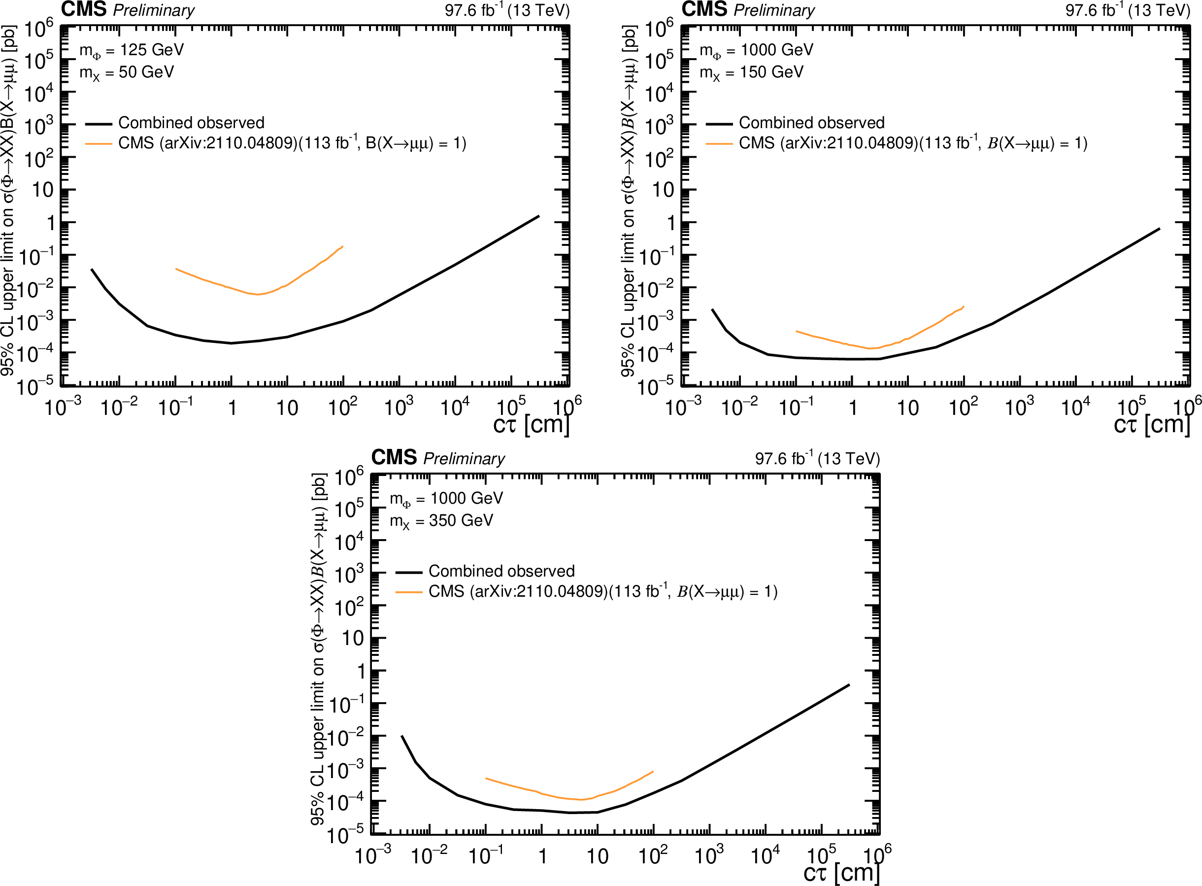
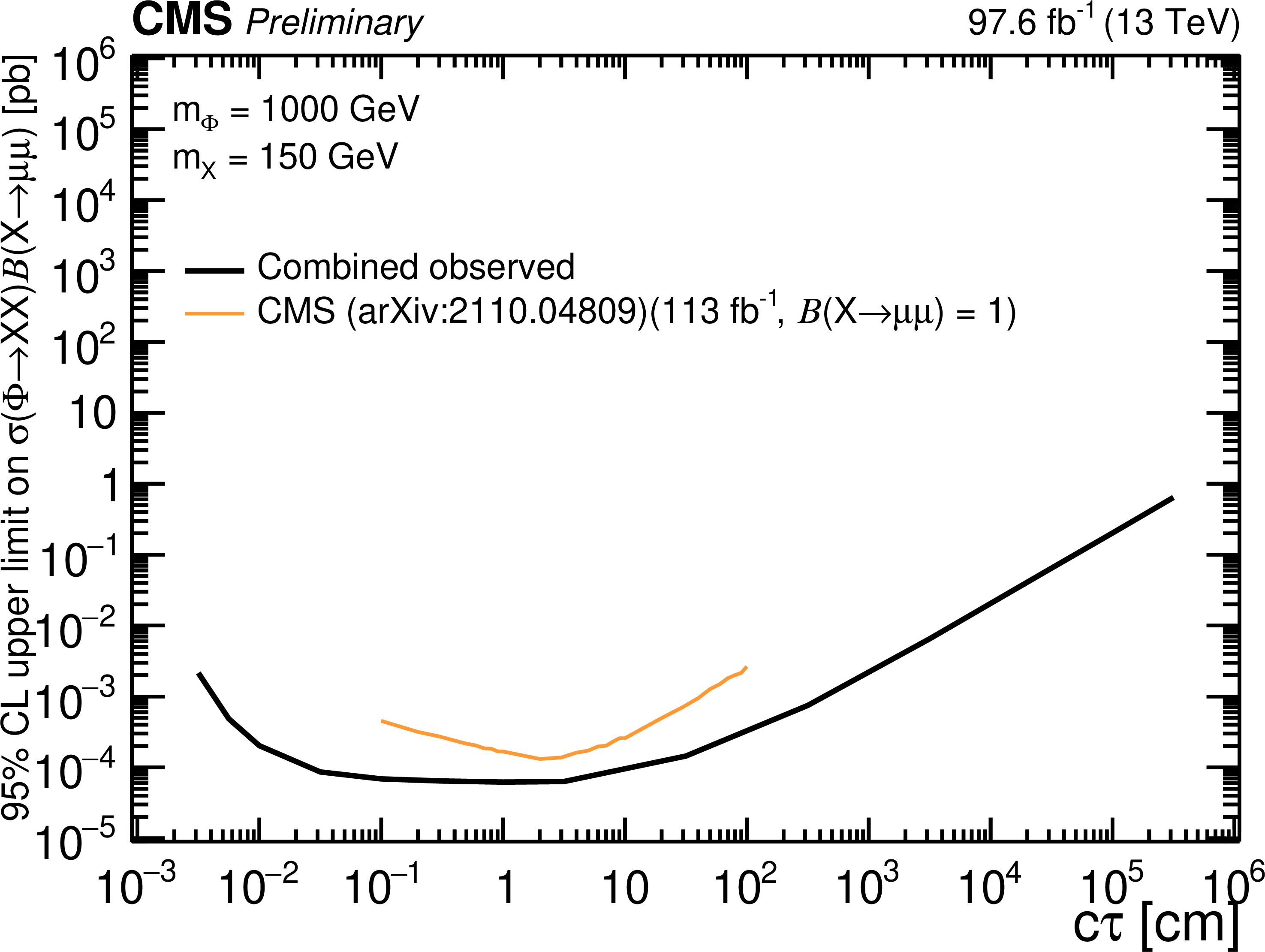
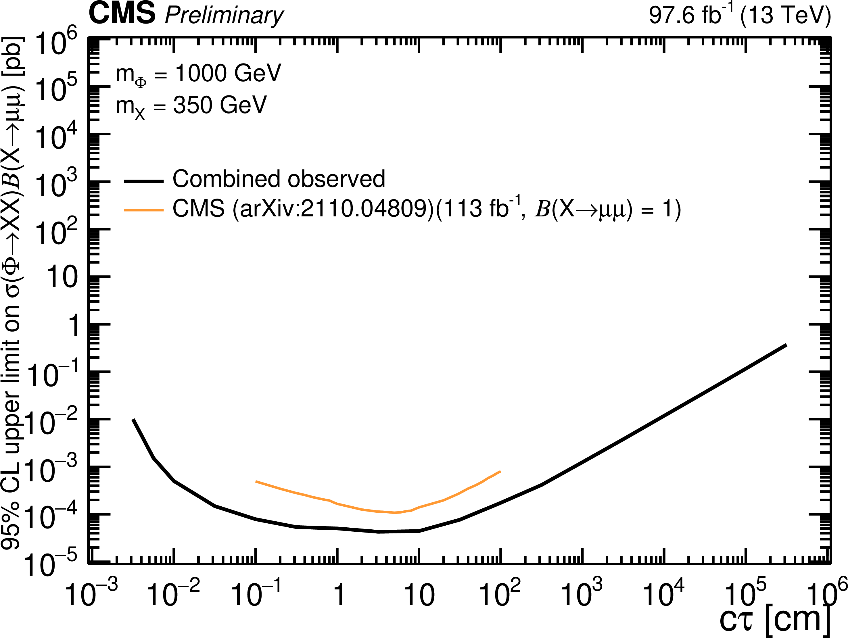
png pdf	Additional Figure 11: The 95% CL upper limits on $\sigma (\Phi \to \text {X} \text {X})\mathcal {B}(\text {X}\to \mu \mu)$ as a function of $c\tau _\text {X}$ in the heavy scalar model, for $m_\Phi =$ 125 GeV and $m_\text {X}=$ 50 GeV (top left), $m_\Phi =$ 1000 GeV and $m_\text {X}=$ 150 GeV (top right), and $m_\Phi =$ 1000 GeV and $m_\text {X}=$ 350 GeV (bottom). To facilitate a comparison to existing upper limits for the probed signal hypotheses, the combined observed limits (black) are compared to recent CMS results (orange).
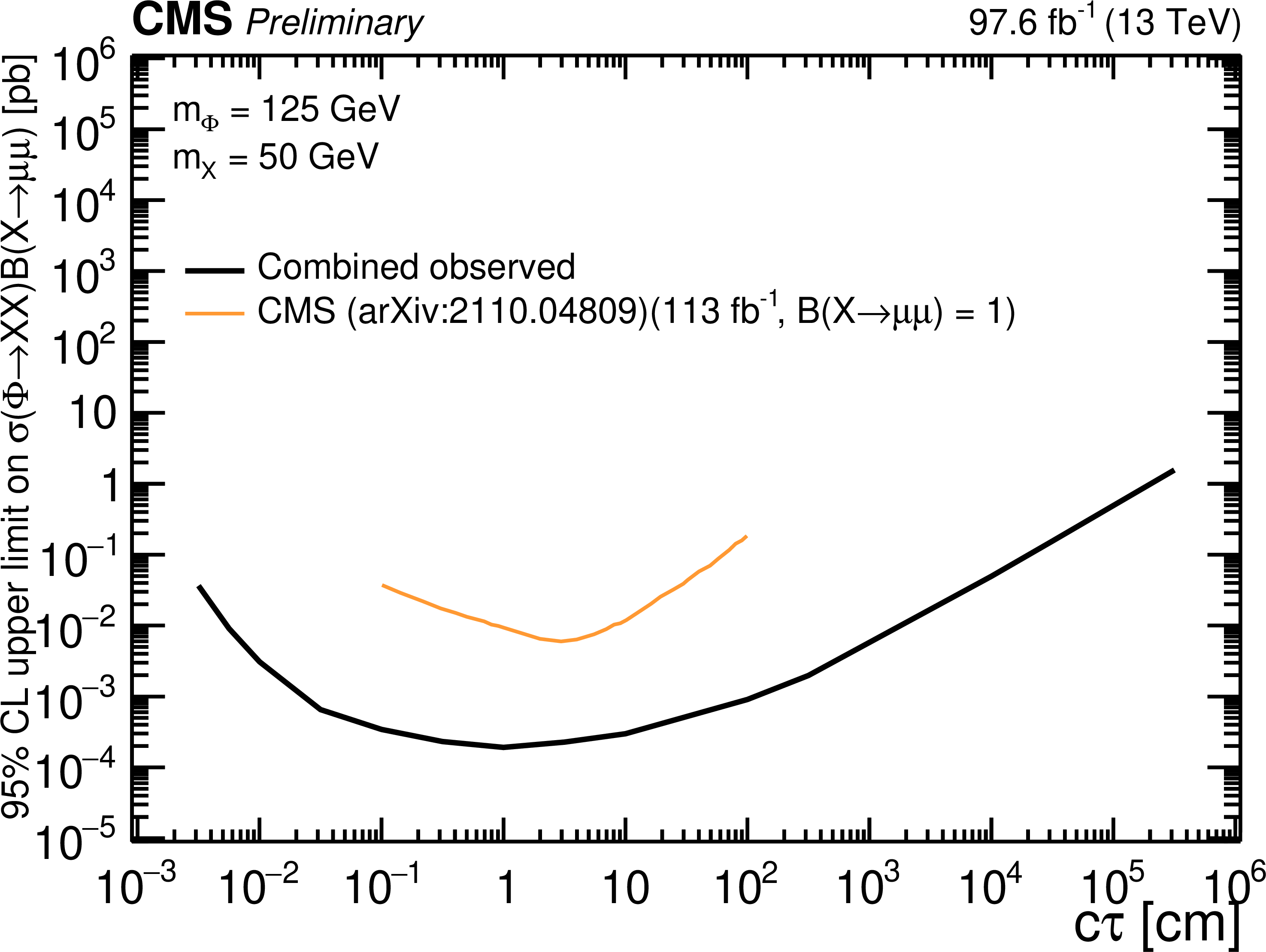
png pdf	Additional Figure 11-a: The 95% CL upper limits on $\sigma (\Phi \to \text {X} \text {X})\mathcal {B}(\text {X}\to \mu \mu)$ as a function of $c\tau _\text {X}$ in the heavy scalar model, for $m_\Phi =$ 125 GeV and $m_\text {X}=$ 50 GeV (top left), $m_\Phi =$ 1000 GeV and $m_\text {X}=$ 150 GeV (top right), and $m_\Phi =$ 1000 GeV and $m_\text {X}=$ 350 GeV (bottom). To facilitate a comparison to existing upper limits for the probed signal hypotheses, the combined observed limits (black) are compared to recent CMS results (orange).
png pdf	Additional Figure 11-b: The 95% CL upper limits on $\sigma (\Phi \to \text {X} \text {X})\mathcal {B}(\text {X}\to \mu \mu)$ as a function of $c\tau _\text {X}$ in the heavy scalar model, for $m_\Phi =$ 125 GeV and $m_\text {X}=$ 50 GeV (top left), $m_\Phi =$ 1000 GeV and $m_\text {X}=$ 150 GeV (top right), and $m_\Phi =$ 1000 GeV and $m_\text {X}=$ 350 GeV (bottom). To facilitate a comparison to existing upper limits for the probed signal hypotheses, the combined observed limits (black) are compared to recent CMS results (orange).
png pdf	Additional Figure 11-c: The 95% CL upper limits on $\sigma (\Phi \to \text {X} \text {X})\mathcal {B}(\text {X}\to \mu \mu)$ as a function of $c\tau _\text {X}$ in the heavy scalar model, for $m_\Phi =$ 125 GeV and $m_\text {X}=$ 50 GeV (top left), $m_\Phi =$ 1000 GeV and $m_\text {X}=$ 150 GeV (top right), and $m_\Phi =$ 1000 GeV and $m_\text {X}=$ 350 GeV (bottom). To facilitate a comparison to existing upper limits for the probed signal hypotheses, the combined observed limits (black) are compared to recent CMS results (orange).
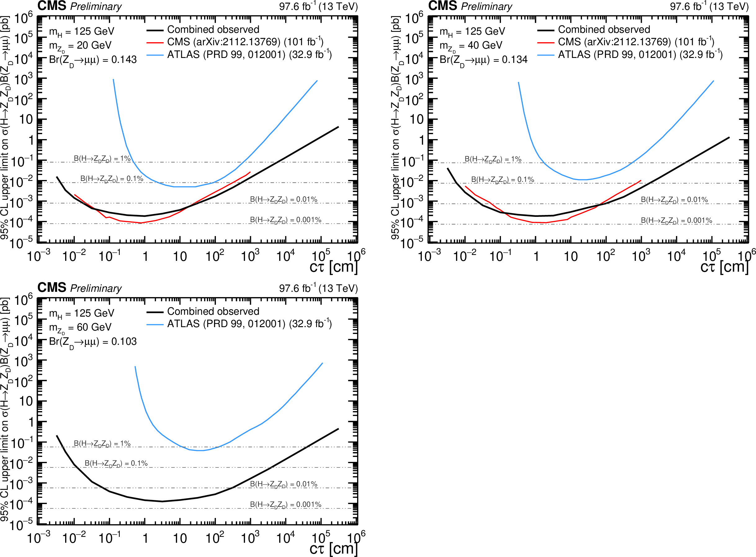
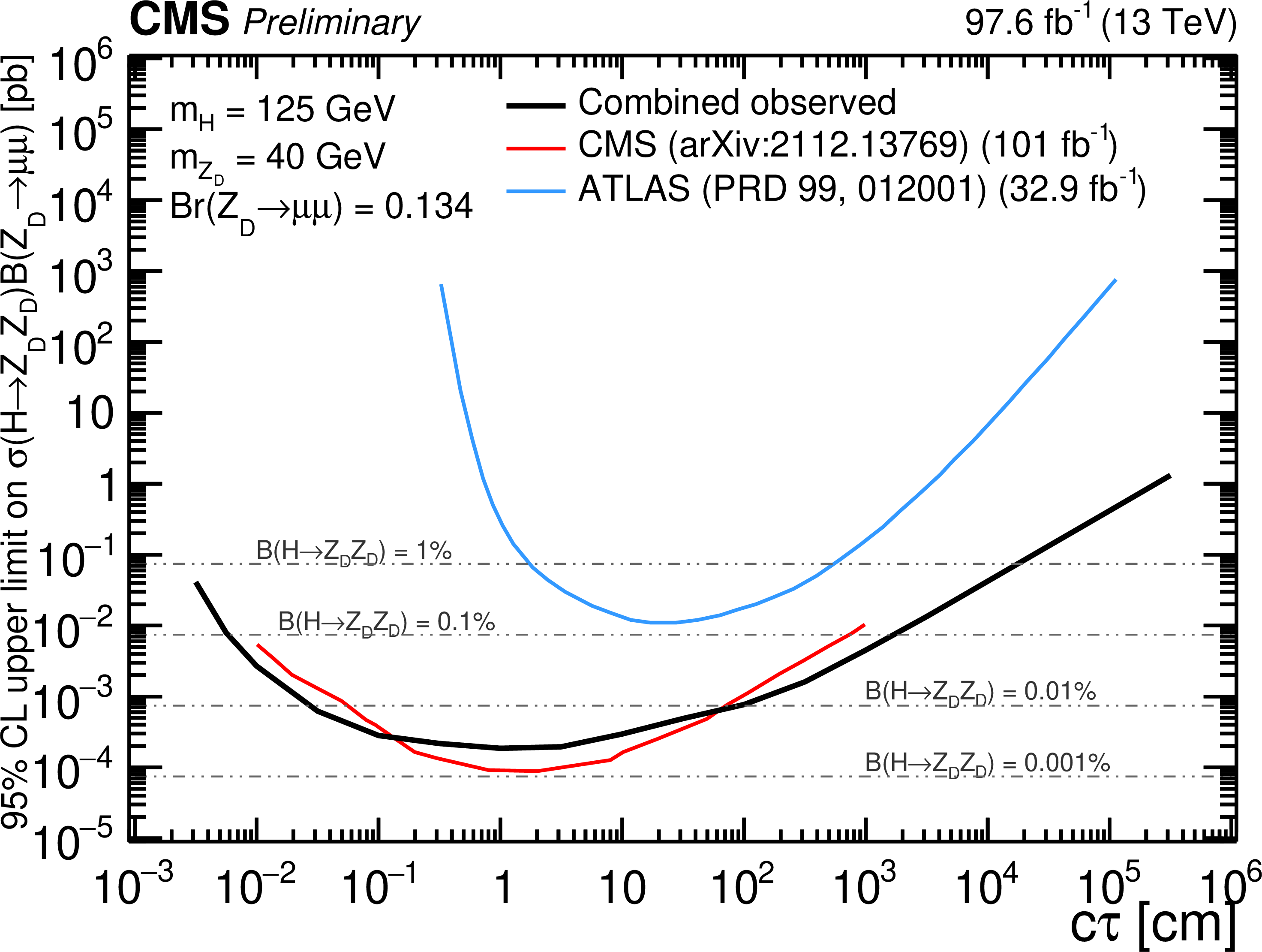
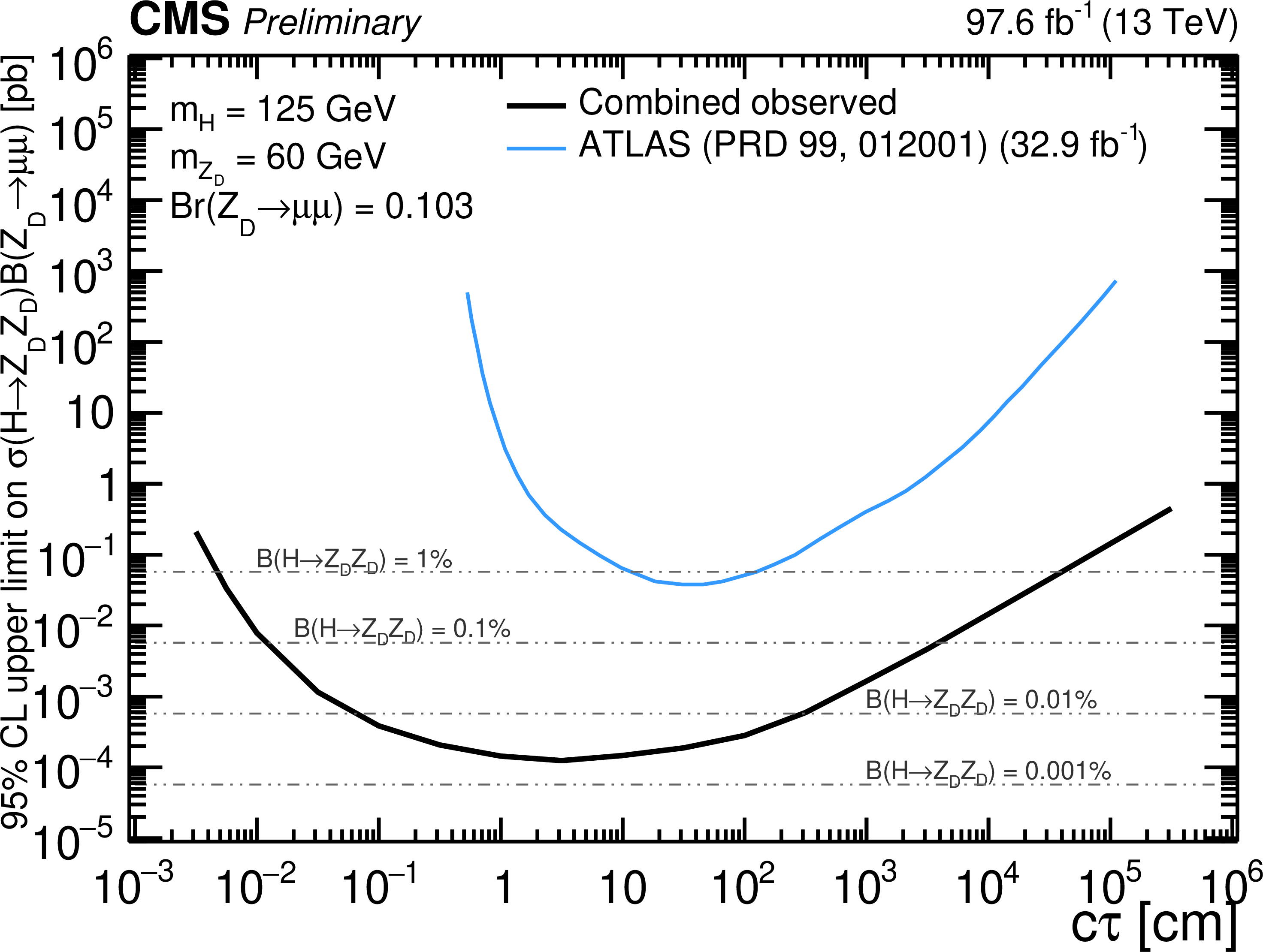
png pdf	Additional Figure 12: The 95% CL upper limits on $\sigma (\text {H} \to \mathrm{Z_D} \mathrm{Z_D})\mathcal {B}(\mathrm{Z_D}\to \mu \mu)$ as a function of $c\tau _{\mathrm{Z_D}}$ in the heavy scalar model, for $m_\text {H}=$ 125 GeV and $m_{\mathrm{Z_D}}=$ 20 GeV (top left), $m_{\mathrm{Z_D}}=$ 40 GeV (top right), and $m_{\mathrm{Z_D}}=$ 60 GeV (bottom). To facilitate a comparison to existing upper limits for the probed signal hypotheses, the combined observed limits (black) are compared to recent CMS (red) and ATLAS (blue) results.
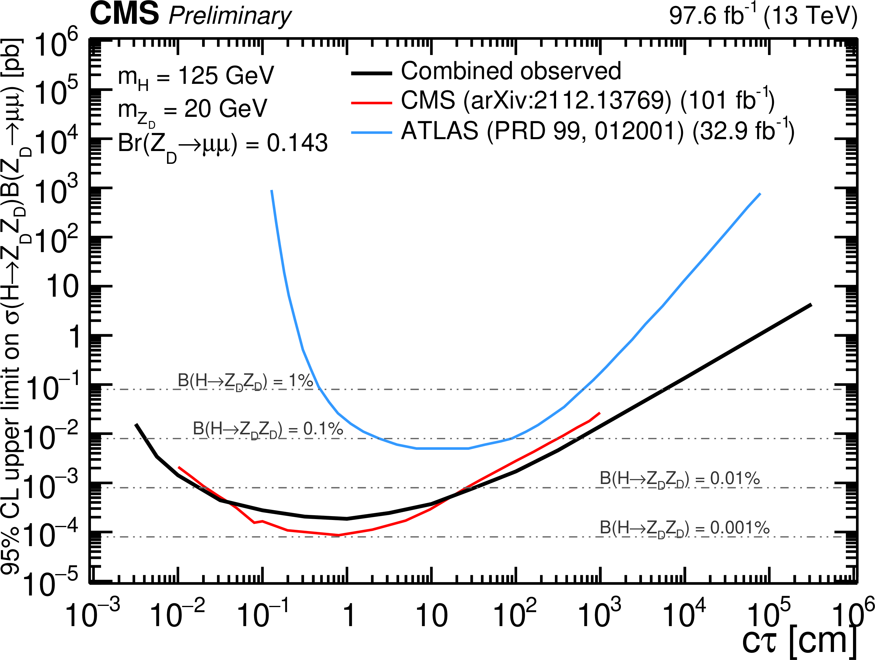
png pdf	Additional Figure 12-a: The 95% CL upper limits on $\sigma (\text {H} \to \mathrm{Z_D} \mathrm{Z_D})\mathcal {B}(\mathrm{Z_D}\to \mu \mu)$ as a function of $c\tau _{\mathrm{Z_D}}$ in the heavy scalar model, for $m_\text {H}=$ 125 GeV and $m_{\mathrm{Z_D}}=$ 20 GeV (top left), $m_{\mathrm{Z_D}}=$ 40 GeV (top right), and $m_{\mathrm{Z_D}}=$ 60 GeV (bottom). To facilitate a comparison to existing upper limits for the probed signal hypotheses, the combined observed limits (black) are compared to recent CMS (red) and ATLAS (blue) results.
png pdf	Additional Figure 12-b: The 95% CL upper limits on $\sigma (\text {H} \to \mathrm{Z_D} \mathrm{Z_D})\mathcal {B}(\mathrm{Z_D}\to \mu \mu)$ as a function of $c\tau _{\mathrm{Z_D}}$ in the heavy scalar model, for $m_\text {H}=$ 125 GeV and $m_{\mathrm{Z_D}}=$ 20 GeV (top left), $m_{\mathrm{Z_D}}=$ 40 GeV (top right), and $m_{\mathrm{Z_D}}=$ 60 GeV (bottom). To facilitate a comparison to existing upper limits for the probed signal hypotheses, the combined observed limits (black) are compared to recent CMS (red) and ATLAS (blue) results.
png pdf	Additional Figure 12-c: The 95% CL upper limits on $\sigma (\text {H} \to \mathrm{Z_D} \mathrm{Z_D})\mathcal {B}(\mathrm{Z_D}\to \mu \mu)$ as a function of $c\tau _{\mathrm{Z_D}}$ in the heavy scalar model, for $m_\text {H}=$ 125 GeV and $m_{\mathrm{Z_D}}=$ 20 GeV (top left), $m_{\mathrm{Z_D}}=$ 40 GeV (top right), and $m_{\mathrm{Z_D}}=$ 60 GeV (bottom). To facilitate a comparison to existing upper limits for the probed signal hypotheses, the combined observed limits (black) are compared to recent CMS (red) and ATLAS (blue) results.

Additional Tables
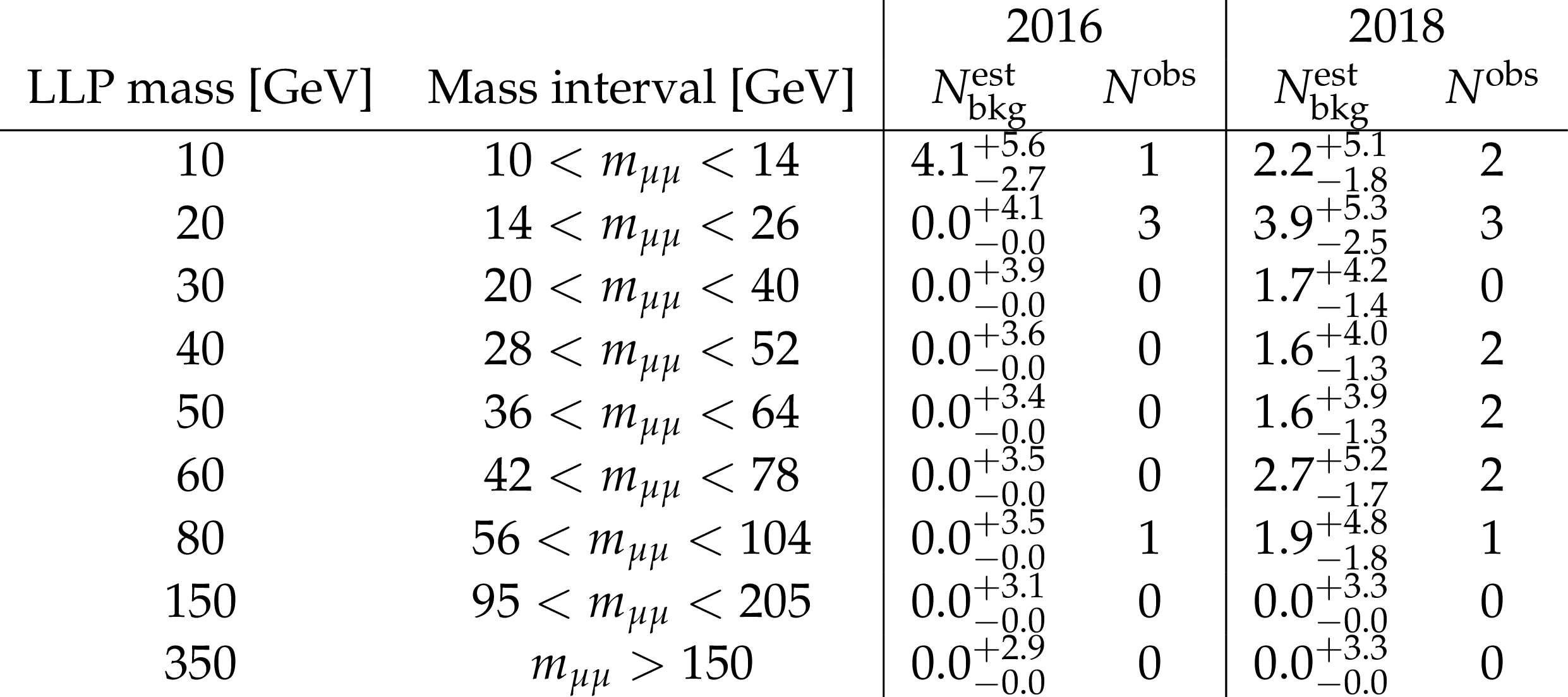
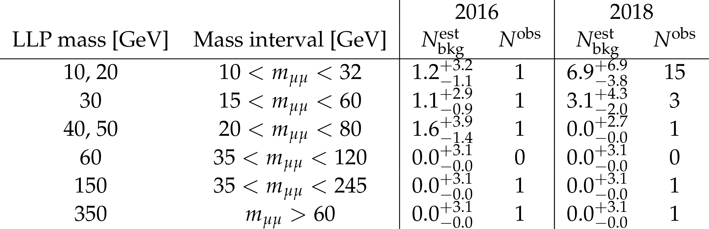
png pdf	Additional Table 1: Background estimation and observed number of events in the STA-STA dimuon category in 2016 and 2018 data. For each probed LLP mass, the chosen mass interval is shown. The mass interval is followed by the estimated and observed counts for the given year. The quoted uncertainties are statistical only.
png pdf	Additional Table 2: Background estimations and observed numbers of events in the TMS-TMS dimuon category in 2016 data. The mass interval is followed by the estimated and observed counts within each $\text {min}(d_0/\sigma _{d_0})$ bin in this mass interval. The quoted uncertainties are statistical only.
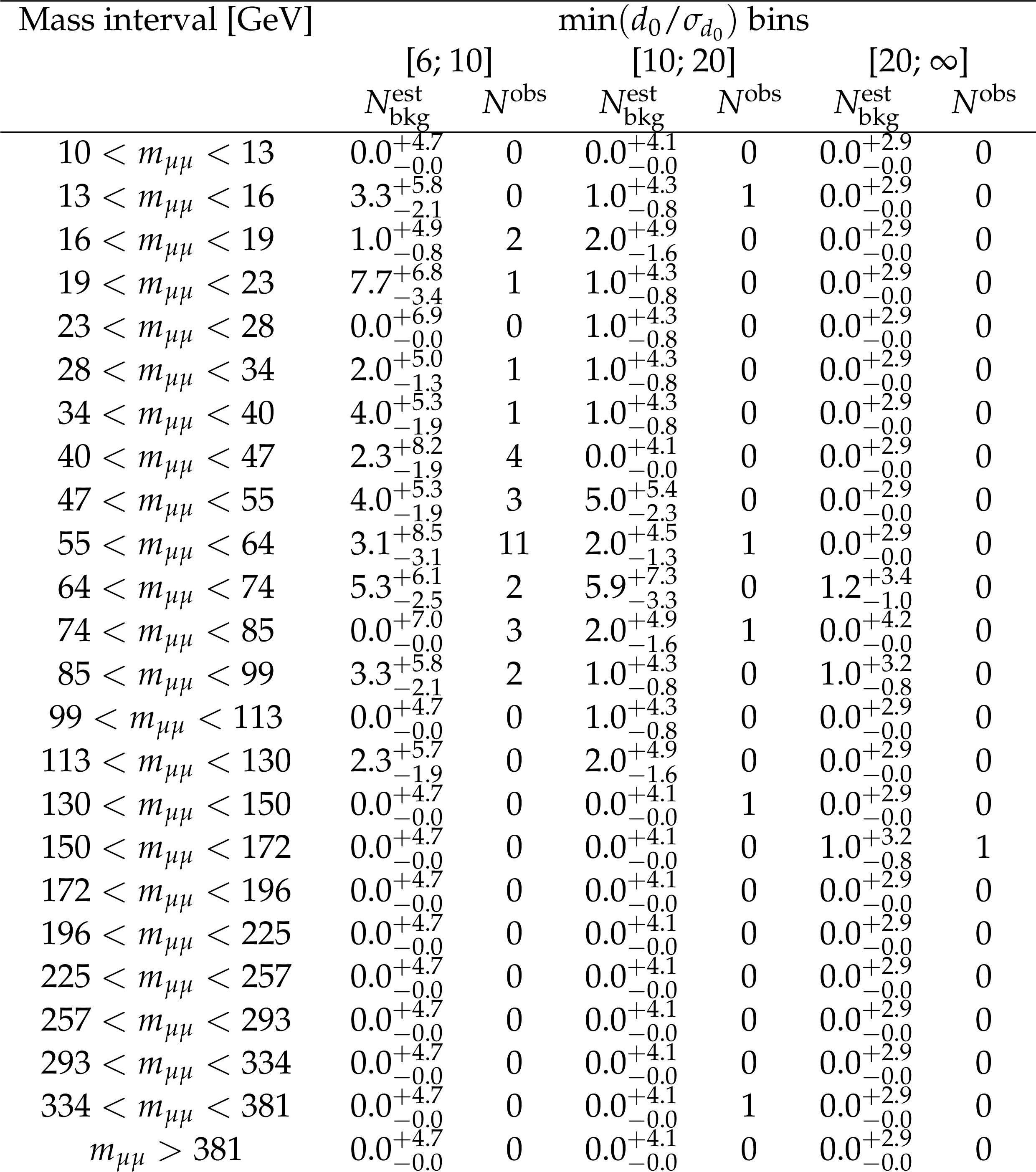
png pdf	Additional Table 3: Background estimations and observed numbers of events in the TMS-TMS dimuon category in 2018 data. The mass interval is followed by the estimated and observed counts within each $\text {min}(d_0/\sigma _{d_0})$ bin in this mass interval. The quoted uncertainties are statistical only.
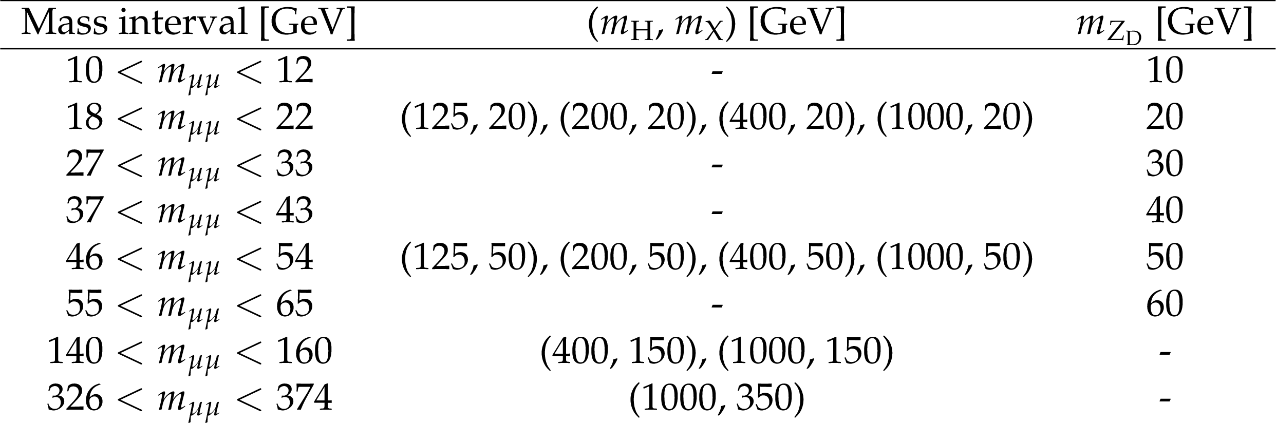
png pdf	Additional Table 4: Correspondence between the mass intervals in the TMS-TMS category and the parameters of the simulated signal samples.
png pdf	Additional Table 5: Background estimation and observed number of events in the STA-TMS dimuon category in 2016 and 2018 data. For each probed LLP mass, the chosen mass interval is shown. The mass interval is followed by the estimated and observed counts for the given year. The quoted uncertainties are statistical only.
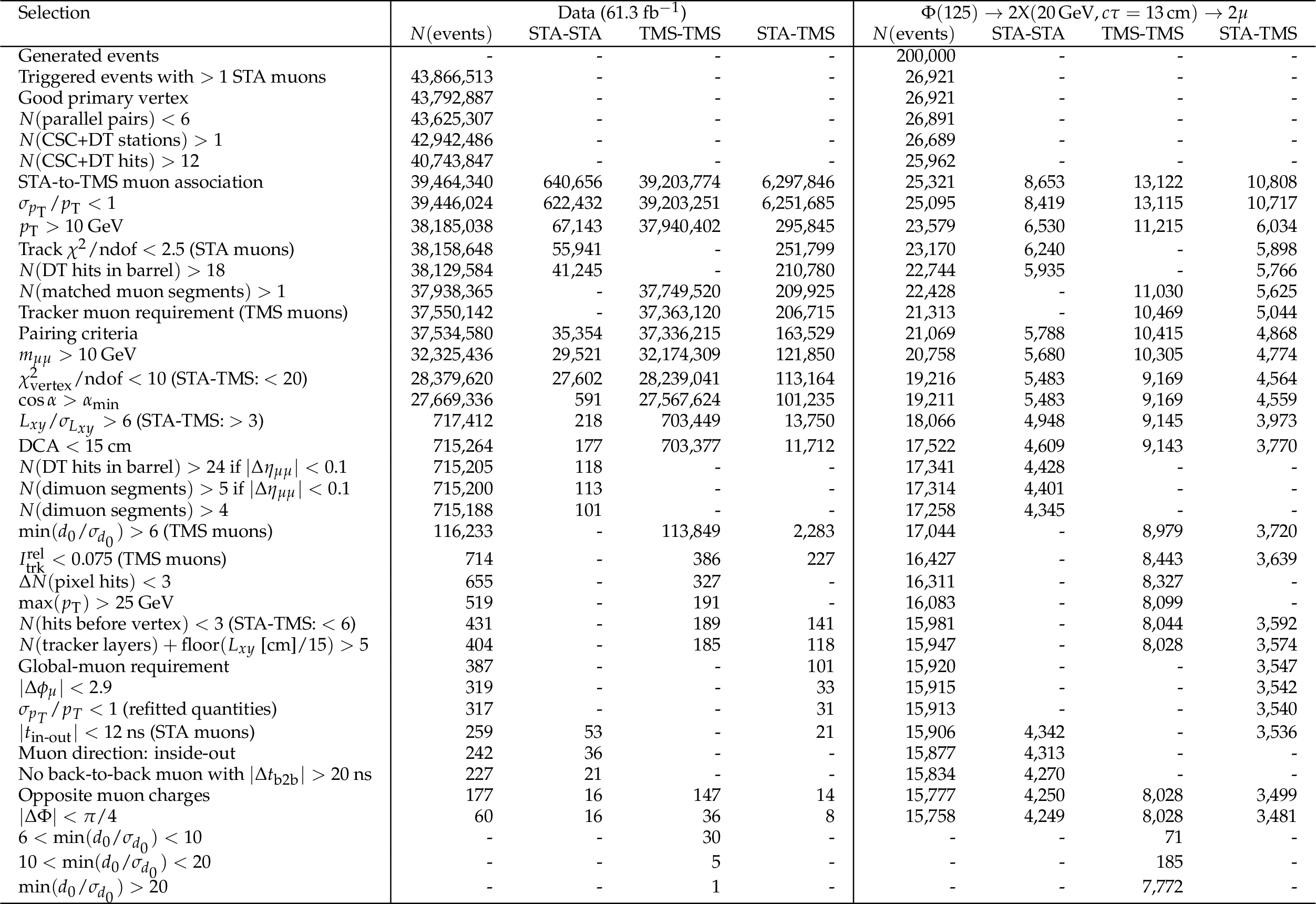
png pdf	Additional Table 6: Number of events passing consecutive sets of selection criteria for 2018 collision data and the signal process $\Phi (125)\to 2\text {X}(20\, \text {GeV}, c\tau = 13\, \text {cm})\to 2\mu$ . Each row introduces a new criterion that is applied in addition to the selection of the previous row. In addition to the total number of events, $N(\text {events})$ , the event yields of the individual dimuon vertex categories, STA-STA, TMS-TMS, and STA-TMS, are shown in separate columns for each data set. In these columns, events containing selected dimuons of different categories are independently counted for each category.

References
1	R. Barbier et al.	R-parity violating supersymmetry	PR 420 (2005) 1	hep-ph/0406039
2	J. L. Hewett, B. Lillie, M. Masip, and T. G. Rizzo	Signatures of long-lived gluinos in split supersymmetry	JHEP 09 (2004) 070	hep-ph/0408248
3	T. Han, Z. Si, K. M. Zurek, and M. J. Strassler	Phenomenology of hidden valleys at hadron colliders	JHEP 07 (2008) 008	0712.2041
4	D. Curtin, R. Essig, S. Gori, and J. Shelton	Illuminating dark photons with high-energy colliders	JHEP 02 (2015) 157	1412.0018
5	M. J. Strassler and K. M. Zurek	Discovering the Higgs through highly-displaced vertices	PLB 661 (2008) 263	hep-ph/0605193
6	CMS Collaboration	Search for long-lived particles that decay into final states containing two electrons or two muons in proton-proton collisions at $\sqrt{s} =$ 8 TeV	PRD 91 (2015) 052012	CMS-EXO-12-037 1411.6977
7	CMS Collaboration	Search for long-lived particles that decay into final states containing two muons, reconstructed using only the CMS muon chambers		CMS-PAS-EXO-14-012
8	ATLAS Collaboration	Search for long-lived particles in final states with displaced dimuon vertices in ${\mathrm{p}}{\mathrm{p}}$ collisions at $\sqrt{s}=$ 13 TeV with the ATLAS detector	PRD 99 (2019) 012001	1808.03057
9	CMS Collaboration	Performance of the CMS muon detector and muon reconstruction with proton-proton collisions at $\sqrt{s} =$ 13 TeV	JINST 13 (2018) P06015	CMS-MUO-16-001 1804.04528
10	CMS Collaboration	The CMS experiment at the CERN LHC	JINST 3 (2008) S08004	CMS-00-001
11	CMS Collaboration	Performance of the CMS Level-1 trigger in proton-proton collisions at $\sqrt{s} =$ 13 TeV	JINST 15 (2020) P10017	CMS-TRG-17-001 2006.10165
12	CMS Collaboration	The CMS trigger system	JINST 12 (2017) P01020	CMS-TRG-12-001 1609.02366
13	CMS Collaboration	Precision luminosity measurement in proton-proton collisions at $\sqrt{s} =$ 13 TeV in 2015 and 2016 at CMS	Submitted to EPJC	CMS-LUM-17-003 2104.01927
14	CMS Collaboration	CMS luminosity measurements for the 2018 data-taking period at $\sqrt{s} =$ 13 TeV		CMS-PAS-LUM-18-002
15	J. D. Wells	How to find a hidden world at the Large Hadron Collider	in Perspectives on LHC Physics, G. Kane and A. Pierce, eds., World Scientific	0803.1243
16	J. Alwall et al.	The automated computation of tree-level and next-to-leading order differential cross sections, and their matching to parton shower simulations	JHEP 07 (2014) 079	1405.0301
17	T. Sjostrand et al.	An Introduction to PYTHIA 8.2	CPC 191 (2015) 159	1410.3012
18	M. Cepeda et al.	Report from Working Group 2: Higgs Physics at the HL-LHC and HE-LHC	CERN Yellow Reports CERN-2019-007	1902.00134
19	J. Butterworth et al.	PDF4LHC recommendations for LHC Run II	JPG 43 (2016) 023001	1510.03865
20	CMS Collaboration	Event generator tunes obtained from underlying event and multiparton scattering measurements	EPJC 76 (2016) 155	CMS-GEN-14-001 1512.00815
21	NNPDF Collaboration	Parton distributions from high-precision collider data	EPJC 77 (2017) 663	1706.00428
22	CMS Collaboration	Extraction and validation of a new set of CMS PYTHIA8 tunes from underlying-event measurements		CMS-GEN-17-001 1903.12179
23	GEANT4 Collaboration	GEANT4: A Simulation toolkit	NIMA 506 (2003) 250
24	CMS Collaboration	Performance of CMS muon reconstruction in ${\mathrm{p}}{\mathrm{p}}$ collision events at $\sqrt{s}=$ 7 TeV	JINST 7 (2012) P10002	CMS-MUO-10-004 1206.4071
25	R. Fruhwirth	Application of Kalman filtering to track and vertex fitting	NIMA 262 (1987) 444
26	T. Speer et al.	Vertex Fitting in the CMS Tracker	CMS-NOTE-2006-032
27	R. D. Cousins, J. T. Linnemann, and J. Tucker	Evaluation of three methods for calculating statistical significance when incorporating a systematic uncertainty into a test of the background-only hypothesis for a Poisson process	NIMA 595 (2008) 480	physics/0702156
28	CMS Collaboration	Search for new particles decaying to a jet and an emerging jet	JHEP 02 (2019) 179	CMS-EXO-18-001 1810.10069
29	A. L. Read	Presentation of search results: The CL $_{\text{s}}$ technique	JPG 28 (2002) 2693
30	T. Junk	Confidence level computation for combining searches with small statistics	NIMA 434 (1999) 435	hep-ex/9902006
31	CMS Collaboration	Documentation for the Higgs Combine Tool	\url http://cms-analysis.github.io/HiggsAnalysis-CombinedLimit
32	The ATLAS Collaboration, The CMS Collaboration, The LHC Higgs Combination Group	Procedure for the LHC Higgs boson search combination in Summer 2011	CMS-NOTE-2011-005
33	CMS Collaboration	Search for invisible decays of a Higgs boson produced through vector boson fusion in proton--proton collisions at $\sqrt{s} =$ 13 TeV	PLB 793 (2019) 520	CMS-HIG-17-023 1809.05937
34	CMS Collaboration	Combined measurements of Higgs boson couplings in proton-proton collisions at $\sqrt{s} =$ 13 TeV	EPJC 79 (2019) 421	CMS-HIG-17-031 1809.10733
35	CMS Collaboration	Search for long-lived particles decaying into muon pairs in proton-proton collisions at $\sqrt{s} =$ 13 TeV	Submitted to JHEP	CMS-EXO-20-014 2112.13769