

Compact Muon Solenoid
LHC, CERN
| CMS-PAS-EXO-20-010 | ||
| Search for inelastic dark matter in events with two displaced muons and missing transverse momentum in proton-proton collisions at $ \sqrt{s} = $ 13 TeV | ||
| CMS Collaboration | ||
| 3 March 2023 | ||
| Abstract: A search is presented for dark matter in events with a pair of displaced muons and missing transverse momentum. The analysis is performed using 138 fb$ ^{-1} $ of proton-proton collision data at 13 TeV center-of-mass energy produced by the LHC and collected with the CMS detector from 2016 to 2018. No significant excess is observed over the predicted background. Upper limits are set on the product of the inelastically coupled dark matter production cross section and the decay branching fraction. This is the first search for inelastic dark matter performed at a hadron collider. | ||
|
Links:
CDS record (PDF) ;
Physics Briefing ;
CADI line (restricted) ;
These preliminary results are superseded in this paper, PRL 132 (2024) 041802. The superseded preliminary plots can be found here. |
||
| Figures & Tables | Summary | Additional Figures & Tables | References | CMS Publications |
|---|
| Figures | |
png pdf |
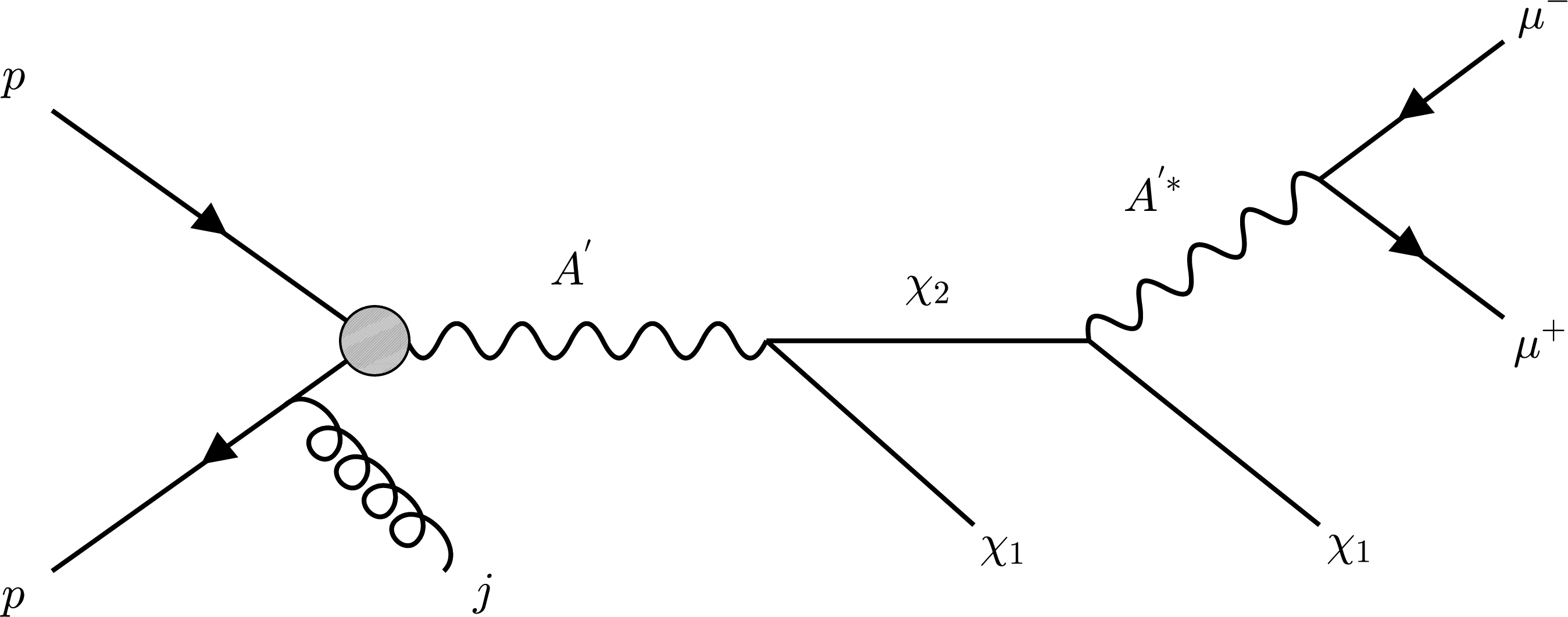
Figure 1:
Feynman diagram of inelastic dark matter production and decay in proton-proton collisions. The heavy dark matter state $ \chi_2 $ can be long-lived. |
png pdf |
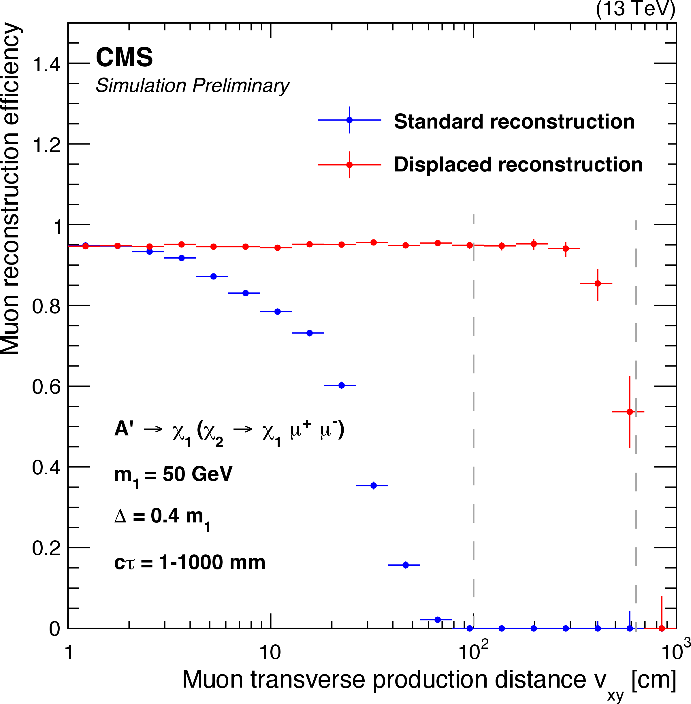
Figure 2:
Reconstruction efficiency of standard (blue) and displaced (red) reconstruction algorithms as a function of transverse vertex displacement $ v_{xy} $ in the central region of the detector ($ |\eta| < $ 1.2), for a representative signal sample. The two dashed gray lines denote the end of the fiducial tracker and muon chamber regions, respectively. |

png pdf |
Figure 3:
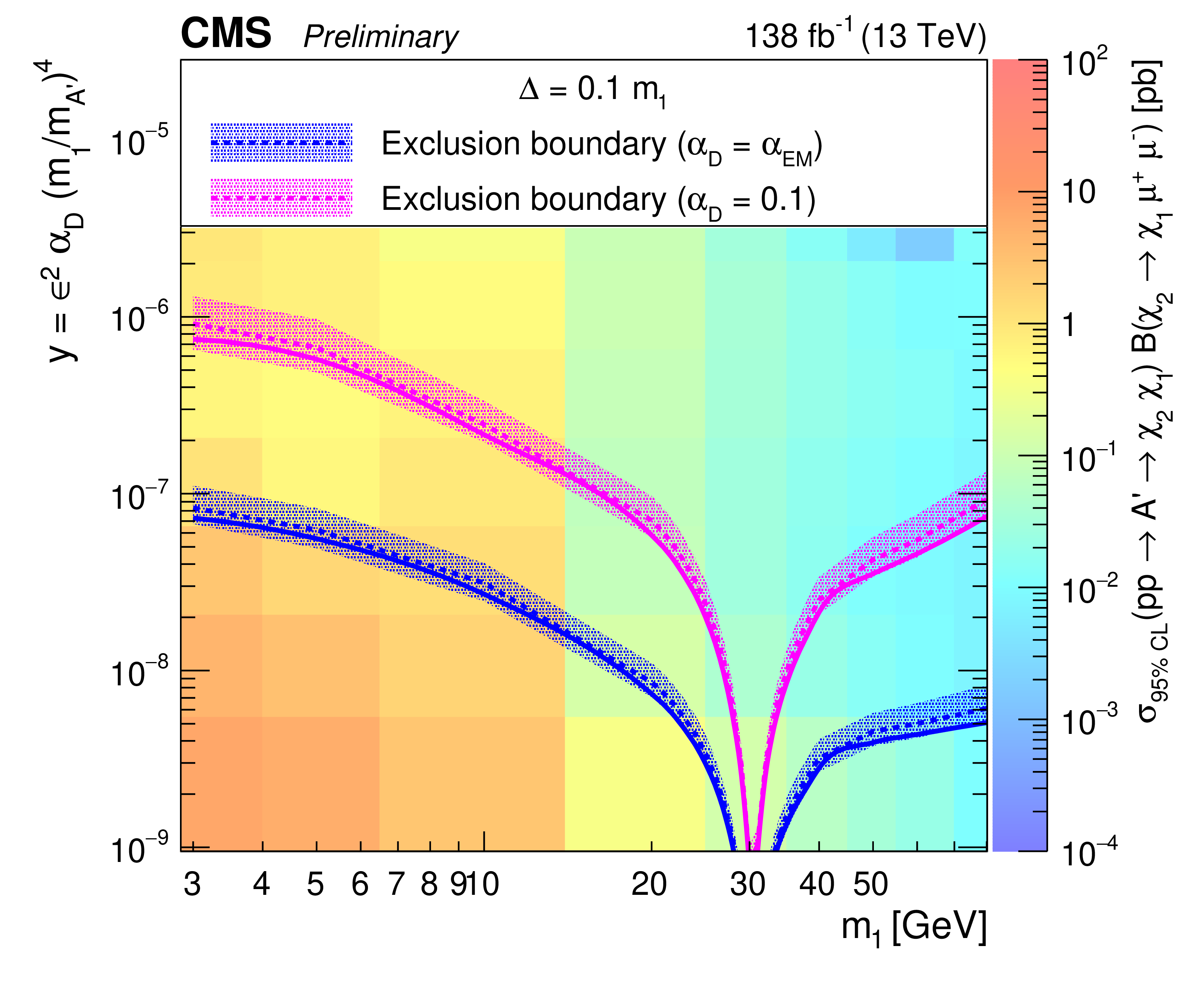
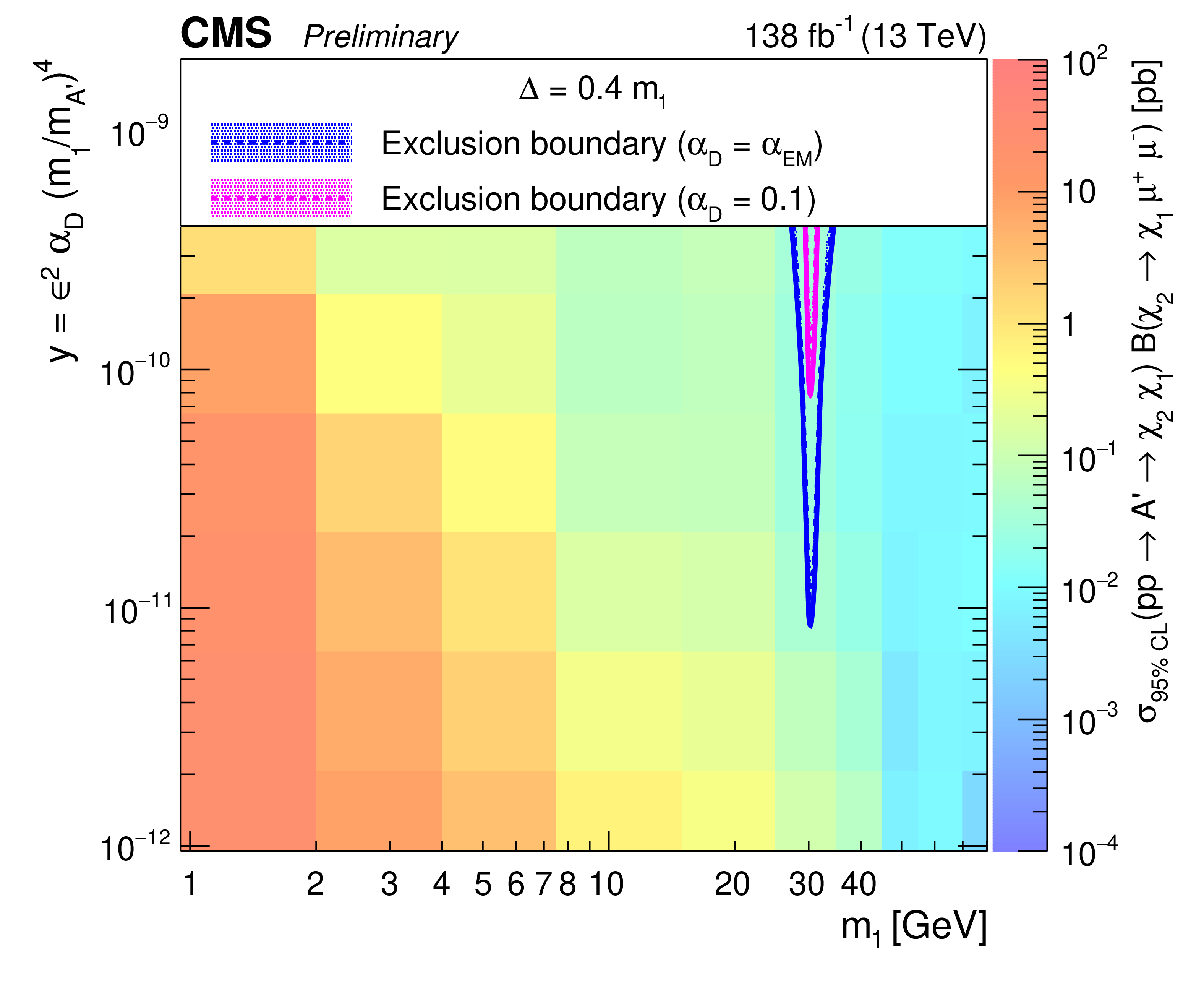
Two-dimensional exclusion surfaces for $ \Delta = 0.1 \, m_1 $ (left) and $ \Delta = 0.4 \, m_1 $ (right), as a function of $ m_1 $ and $ y $ (see text). Filled histograms denote observed limits on the product of the dark matter production cross section and decay branching fraction, while dashed lines denote excluded regions at 95% CL, with one-sigma bands. Regions above the lines are excluded, depending on the $ \alpha_D $ hypothesis: $ \alpha_D = \alpha_{EM} $ (blue) or $ \alpha_D = $ 0.1 (magenta). |
png pdf |
Figure 3-a:
Two-dimensional exclusion surfaces for $ \Delta = 0.1 \, m_1 $, as a function of $ m_1 $ and $ y $ (see text). Filled histograms denote observed limits on the product of the dark matter production cross section and decay branching fraction, while dashed lines denote excluded regions at 95% CL, with one-sigma bands. Regions above the lines are excluded, depending on the $ \alpha_D $ hypothesis: $ \alpha_D = \alpha_{EM} $ (blue) or $ \alpha_D = $ 0.1 (magenta). |
png pdf |
Figure 3-b:
Two-dimensional exclusion surfaces for $ \Delta = 0.4 \, m_1 $, as a function of $ m_1 $ and $ y $ (see text). Filled histograms denote observed limits on the product of the dark matter production cross section and decay branching fraction, while dashed lines denote excluded regions at 95% CL, with one-sigma bands. Regions above the lines are excluded, depending on the $ \alpha_D $ hypothesis: $ \alpha_D = \alpha_{EM} $ (blue) or $ \alpha_D = $ 0.1 (magenta). |
| Tables | |
png pdf |
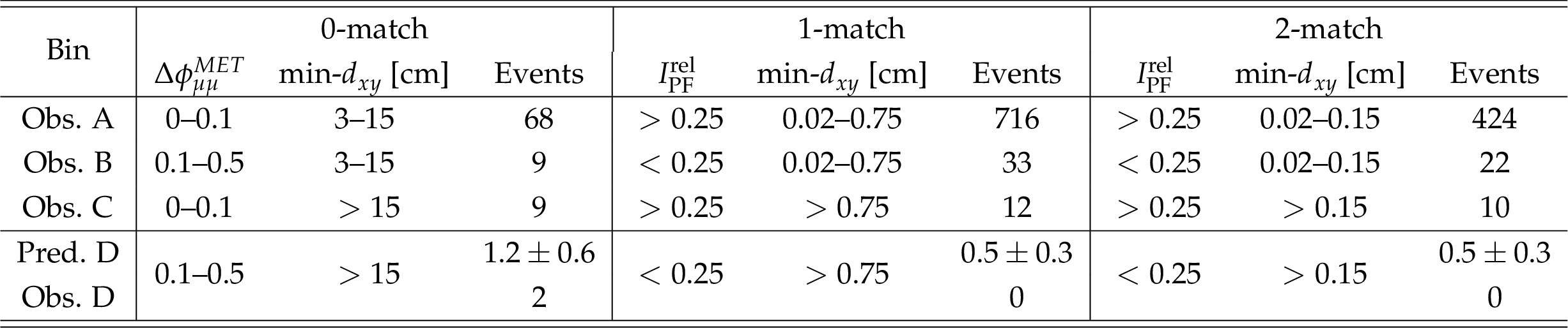
Table 1:
Definition of ABCD bins and yields in data, per match category. The total signal systematic uncertainty averaged over all years is approximately 20%, 30%, and 40% for the 0-, 1-, and 2-match categories respectively (see supplemental material for a breakdown). The predicted yield in bin D is based on the assumption of zero signal. |
| Summary |
| In summary, a search was presented for inelastically-coupled dark matter with a unique final-state signature including a soft, displaced muon pair collimated with $ {\vec p}_{\mathrm{T}}^{\,\text{miss}} $. Proton-proton collisions at 13 TeV center-of-mass energy produced at the LHC and collected by CMS from 2016 to 2018 were analyzed, totaling 138 fb$ ^{-1} $ of data. The striking nature of the signal provides various handles that were exploited to enhance the sensitivity to the benchmark model. A data-driven background estimation strategy based on a modified ABCD method was used to predict the background. No significant excess is observed over SM expectations. Upper limits are set on the product of the dark matter production cross section and decay branching fraction into muons as a function of dark matter mass $ m_1 $ and $ y \equiv \epsilon^2 \, \alpha_D \, (m_1/m_{A'})^4 $. This is the first search for inelastic dark matter at a hadron collider. |
| Additional Figures | |
png pdf |
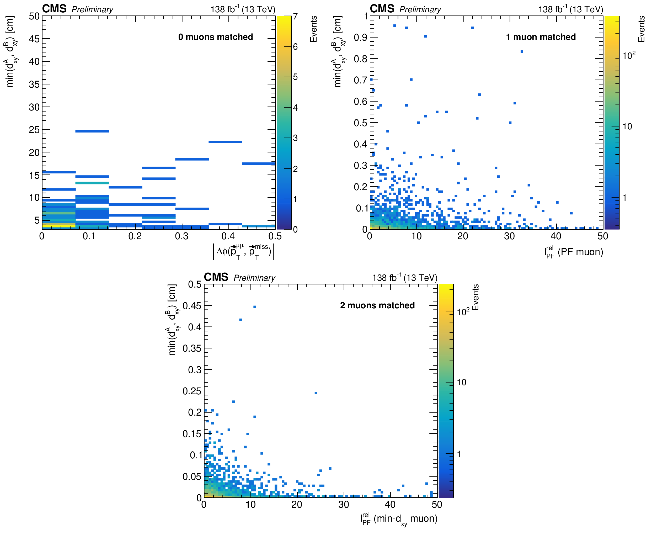
Additional Figure 1:
(Upper left) Observed distribution in data of $\Delta\phi_{\mu\mu}^{\text{MET}}$ vs. min-$d_{xy}$ in the 0-match category. (Upper right) Observed distribution in data of vs. vs. min-$d_{xy}$ in the 1-match category. (Lower center) Observed distribution in data of $I^{\text{rel}}_{\text{PF}}$ vs. min-$d_{xy}$ in the 2-match category. |
png pdf |
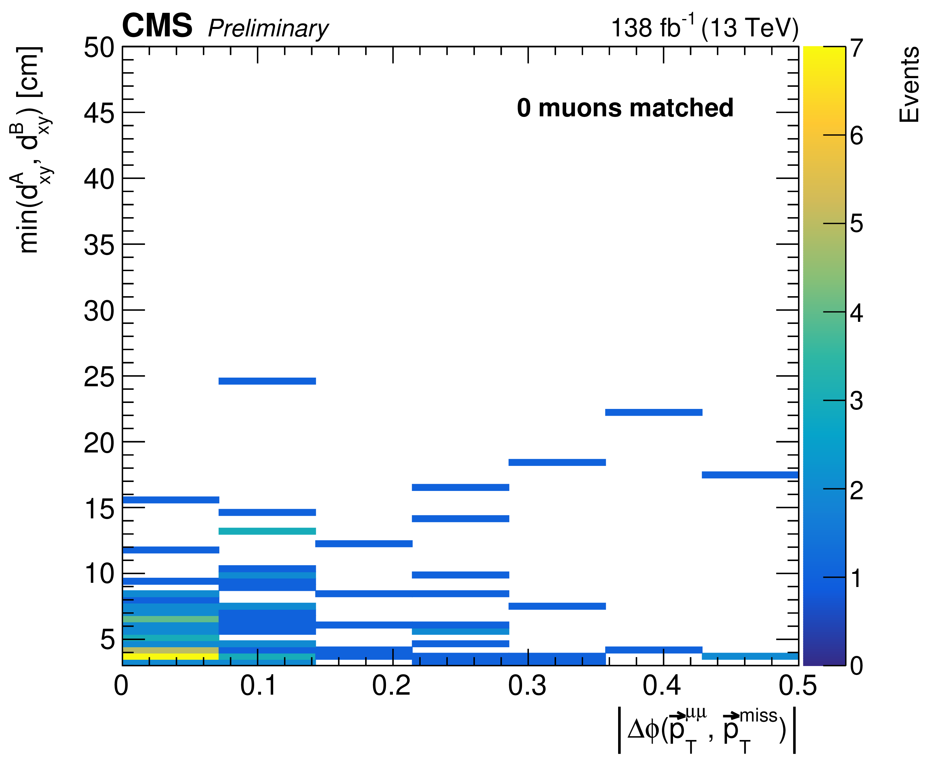
Additional Figure 1-a:
Observed distribution in data of $\Delta\phi_{\mu\mu}^{\text{MET}}$ vs. min-$d_{xy}$ in the 0-match category. |
png pdf |
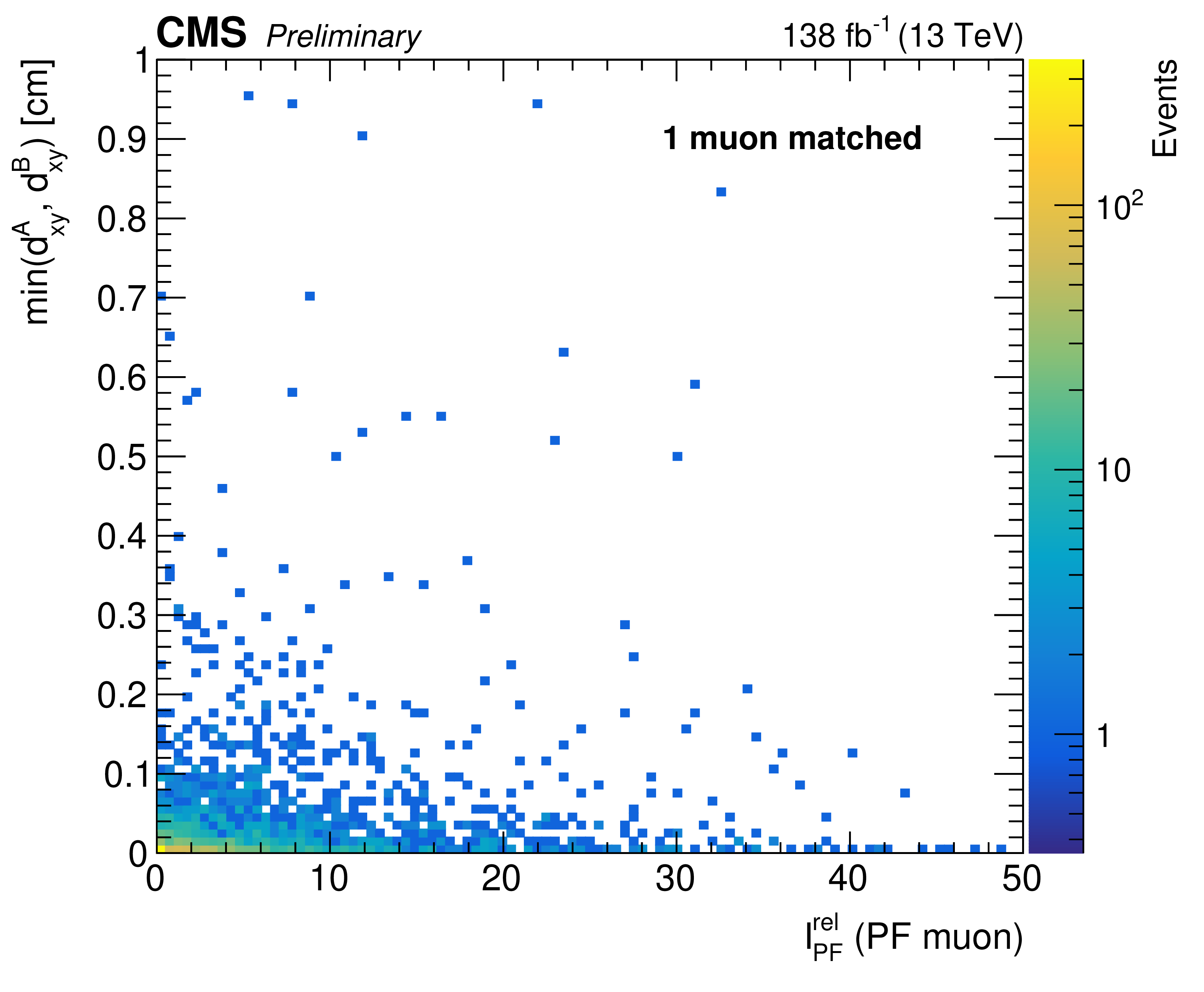
Additional Figure 1-b:
Observed distribution in data of vs. vs. min-$d_{xy}$ in the 1-match category. (Lower center) Observed distribution in data of $I^{\text{rel}}_{\text{PF}}$ vs. min-$d_{xy}$ in the 2-match category. |
png pdf |
Additional Figure 1-c:
(Upper left) Observed distribution in data of $\Delta\phi_{\mu\mu}^{\text{MET}}$ vs. min-$d_{xy}$ in the 0-match category. (Upper right) Observed distribution in data of vs. vs. min-$d_{xy}$ in the 1-match category. (Lower center) Observed distribution in data of $I^{\text{rel}}_{\text{PF}}$ vs. min-$d_{xy}$ in the 2-match category. |
png pdf |
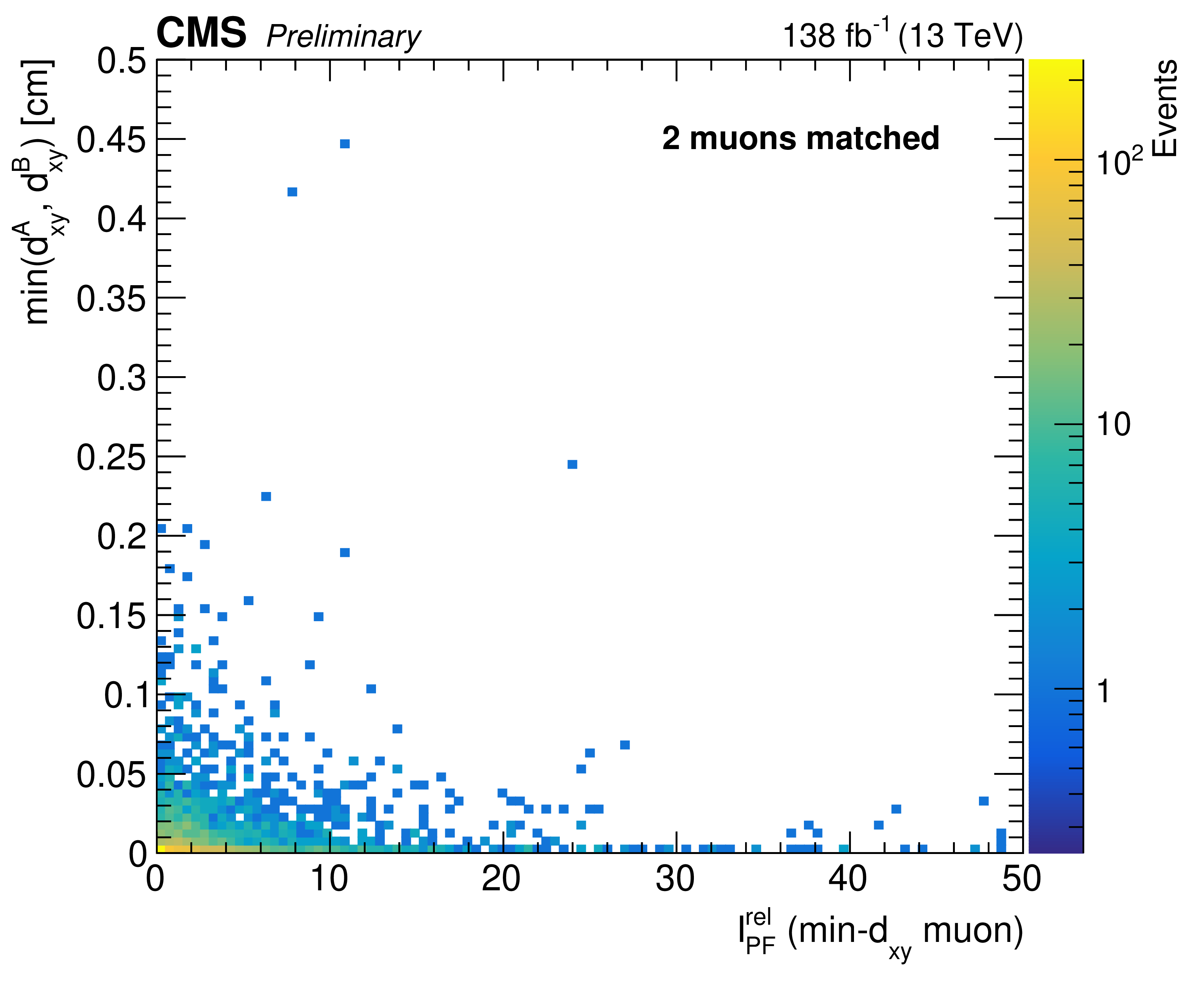
Additional Figure 2:
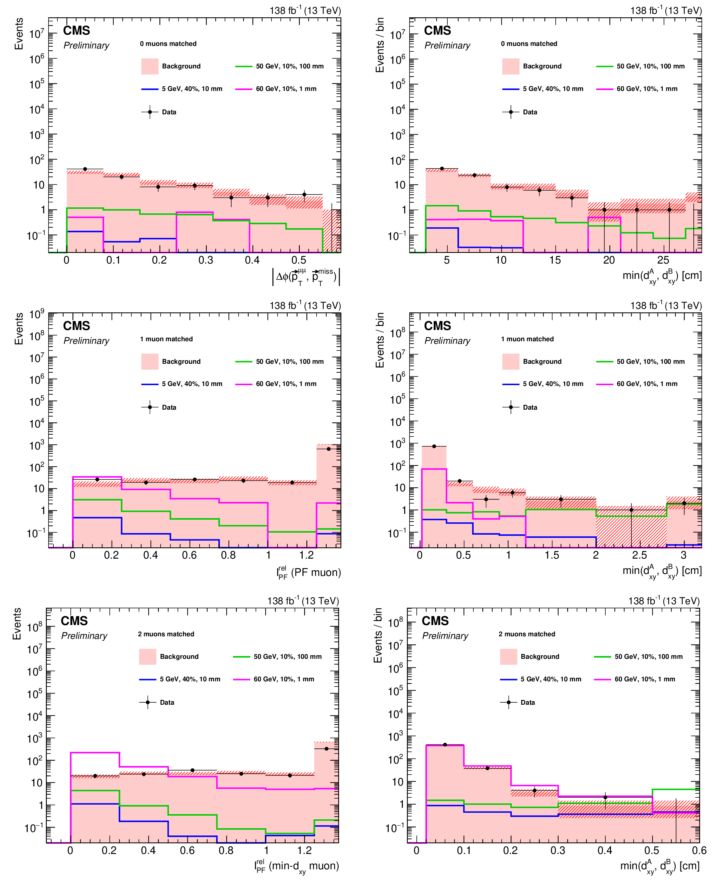
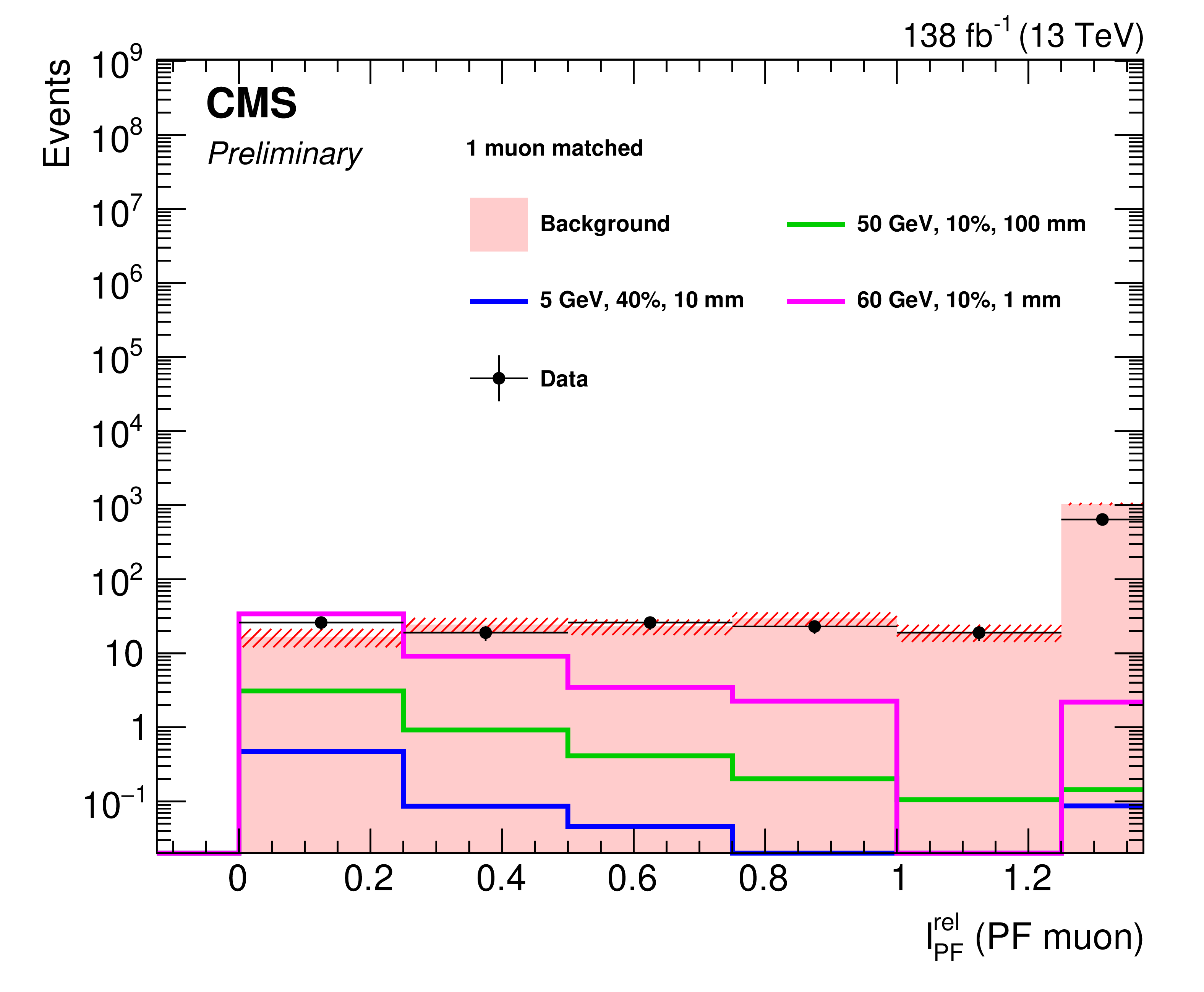
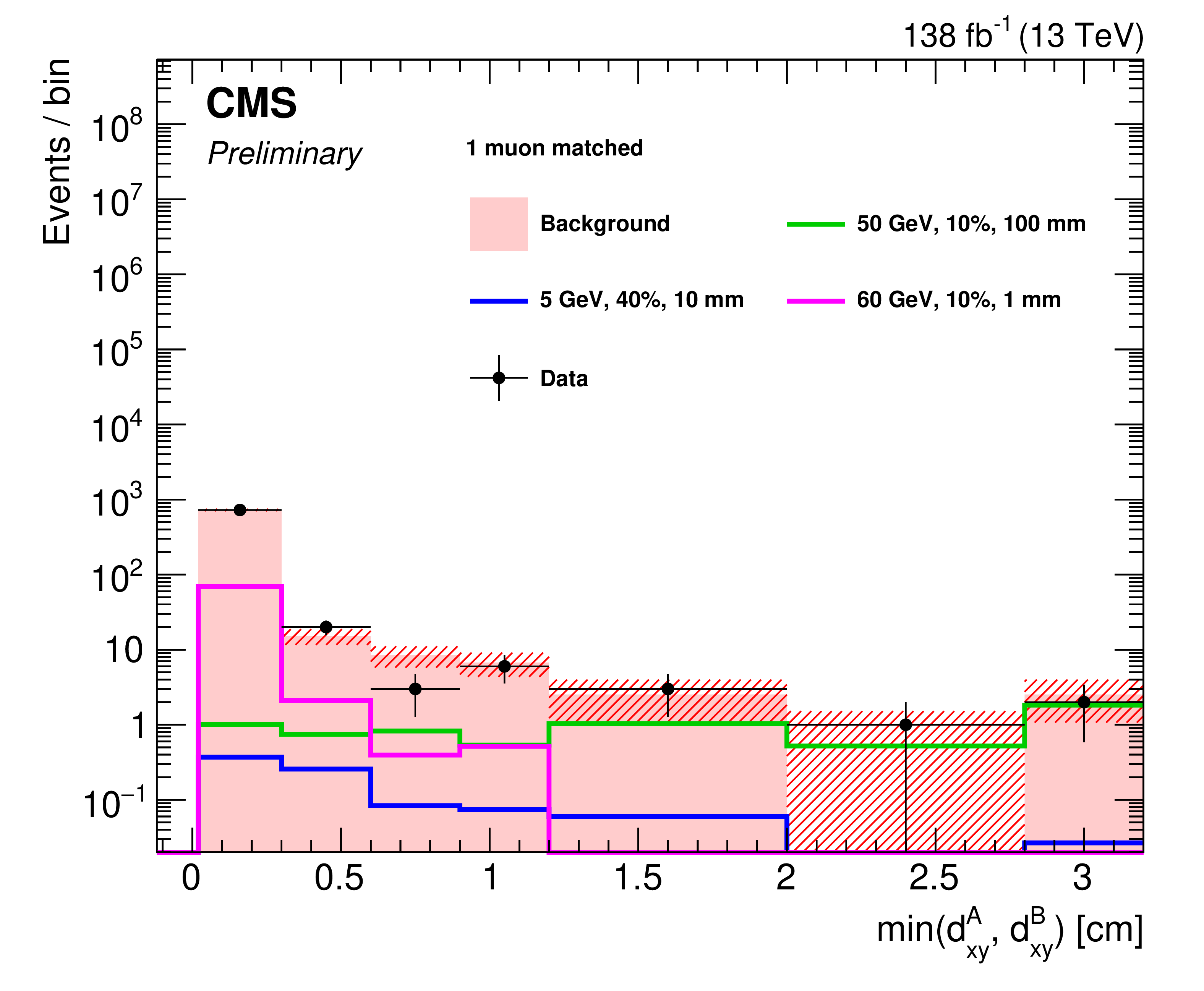
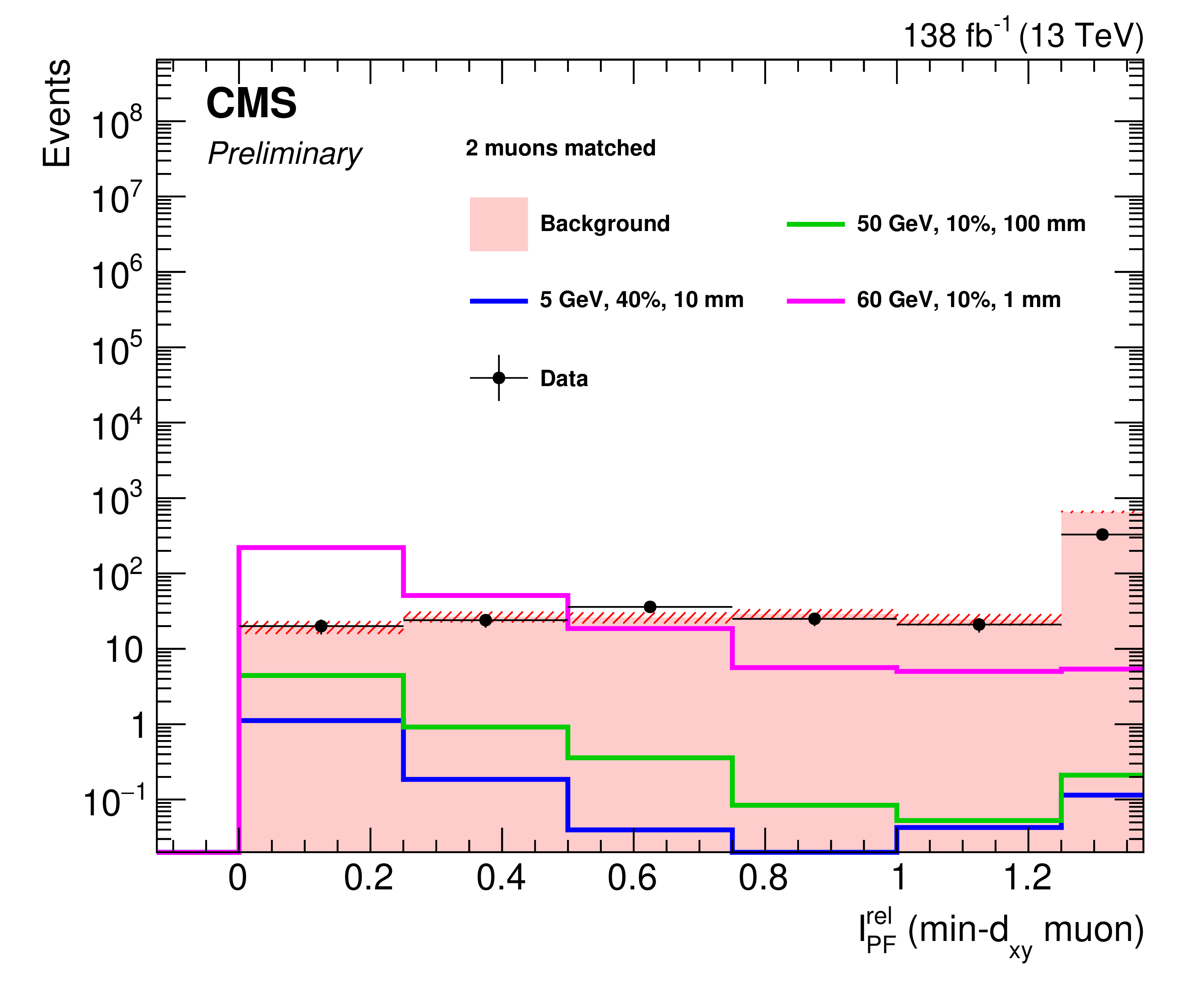
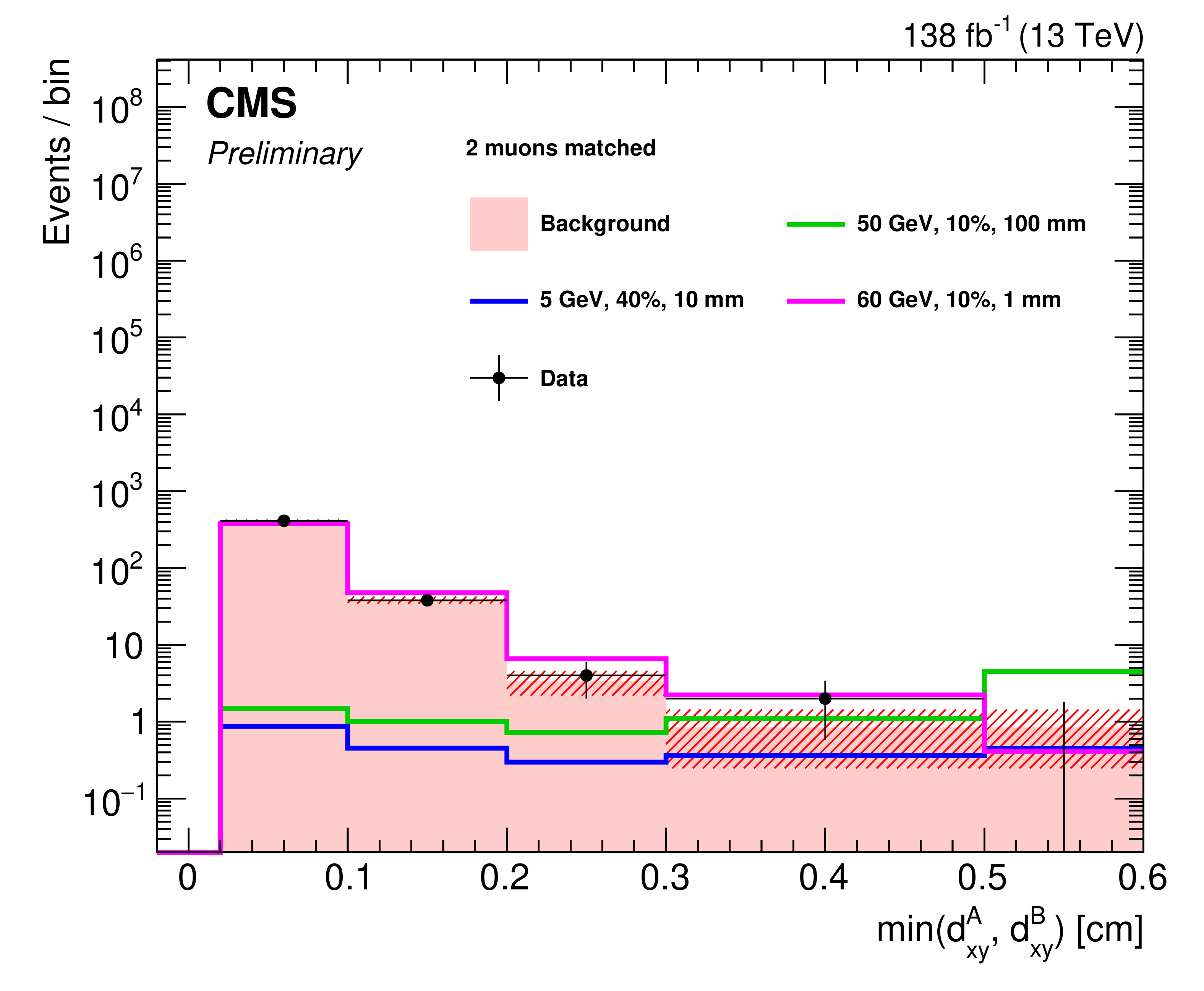
Observed distributions in data (black points) of min-$d_{xy}$ (right panels), $\Delta\phi_{\mu\mu}^{\text{MET}}$ (upper left panel), and $I^{\text{rel}}_{\text{PF}}$ (middle and lower left panels), overlaid with the background prediction extracted from data in an orthogonal control region (filled red histogram). Benchmark signal hypotheses are also shown. |
png pdf |
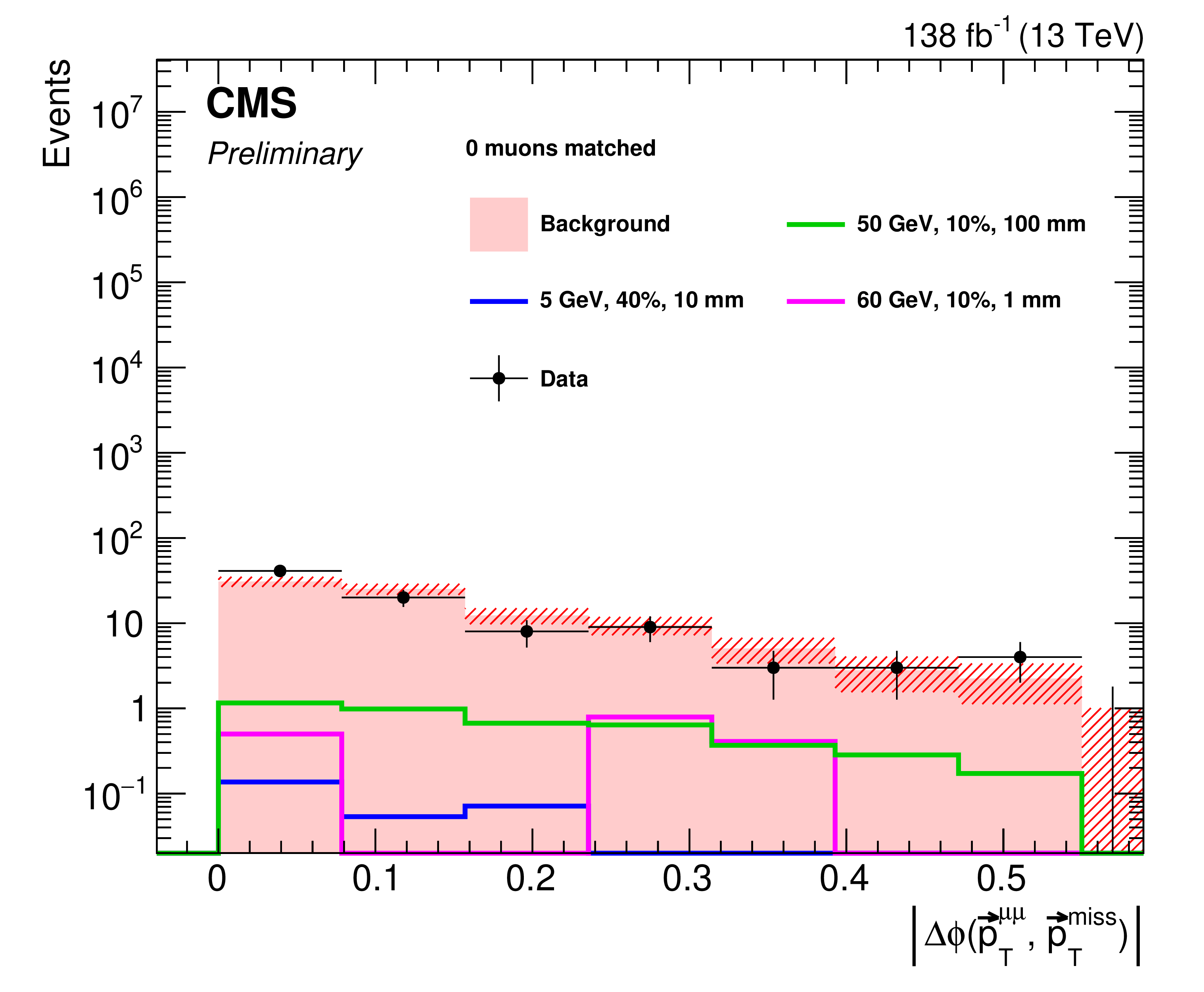
Additional Figure 2-a:
Observed distribution in data (black points) of $\Delta\phi_{\mu\mu}^{\text{MET}}$ (0 muon matched), overlaid with the background prediction extracted from data in an orthogonal control region (filled red histogram). Benchmark signal hypotheses are also shown. |
png pdf |
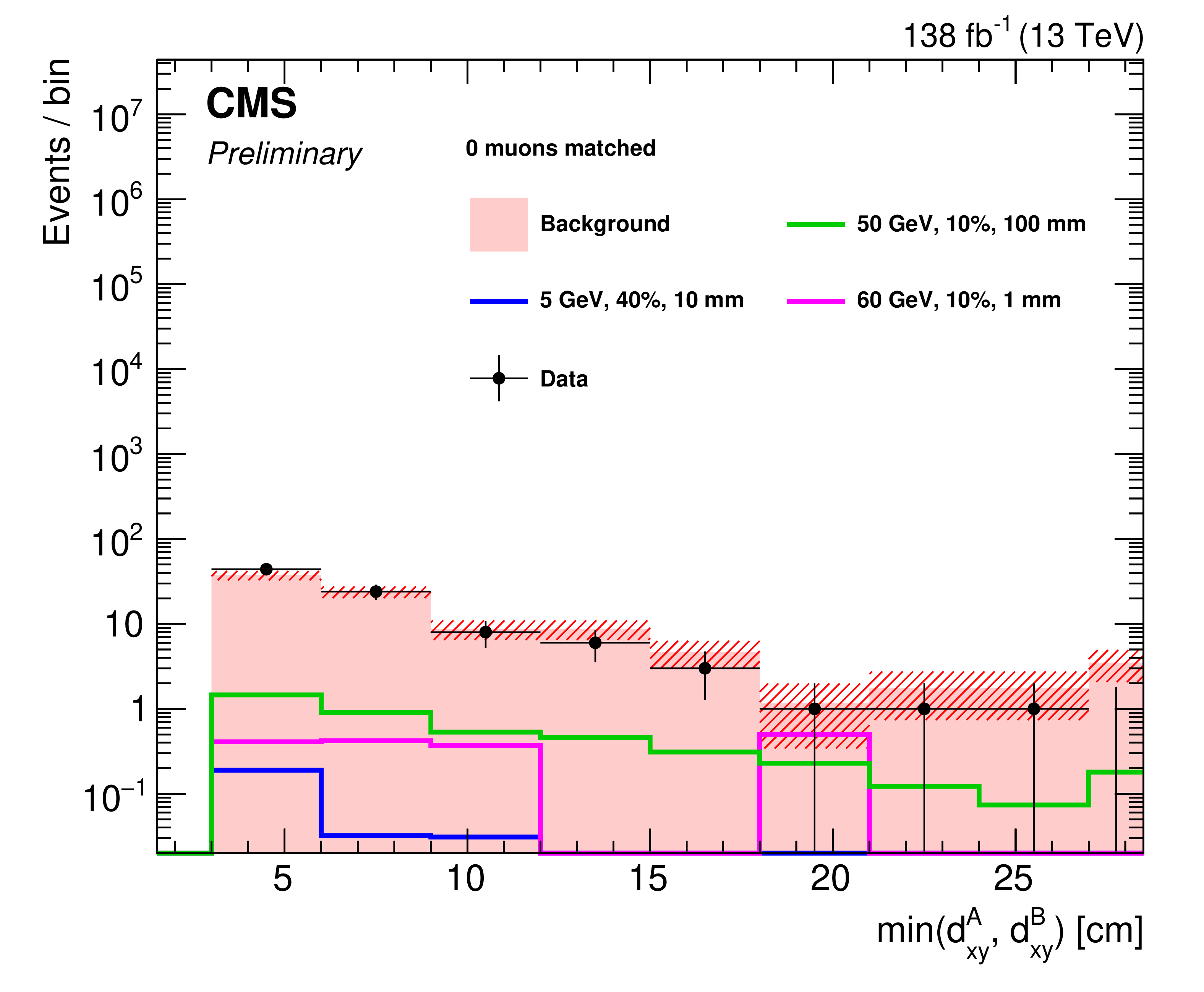
Additional Figure 2-b:
Observed distribution in data (black points) of min-$d_{xy}$ (0 muon matched), overlaid with the background prediction extracted from data in an orthogonal control region (filled red histogram). Benchmark signal hypotheses are also shown. |
png pdf |
Additional Figure 2-c:
Observed distribution in data (black points) of $I^{\text{rel}}_{\text{PF}}$ (1 muon matched), overlaid with the background prediction extracted from data in an orthogonal control region (filled red histogram). Benchmark signal hypotheses are also shown. |
png pdf |
Additional Figure 2-d:
Observed distribution in data (black points) of min-$d_{xy}$ (1 muon matched), overlaid with the background prediction extracted from data in an orthogonal control region (filled red histogram). Benchmark signal hypotheses are also shown. |
png pdf |
Additional Figure 2-e:
Observed distribution in data (black points) of $I^{\text{rel}}_{\text{PF}}$ (2 muon matched), overlaid with the background prediction extracted from data in an orthogonal control region (filled red histogram). Benchmark signal hypotheses are also shown. |
png pdf |
Additional Figure 2-f:
Observed distribution in data (black points) of min-$d_{xy}$ (2 muon2 matched), overlaid with the background prediction extracted from data in an orthogonal control region (filled red histogram). Benchmark signal hypotheses are also shown. |
png pdf |
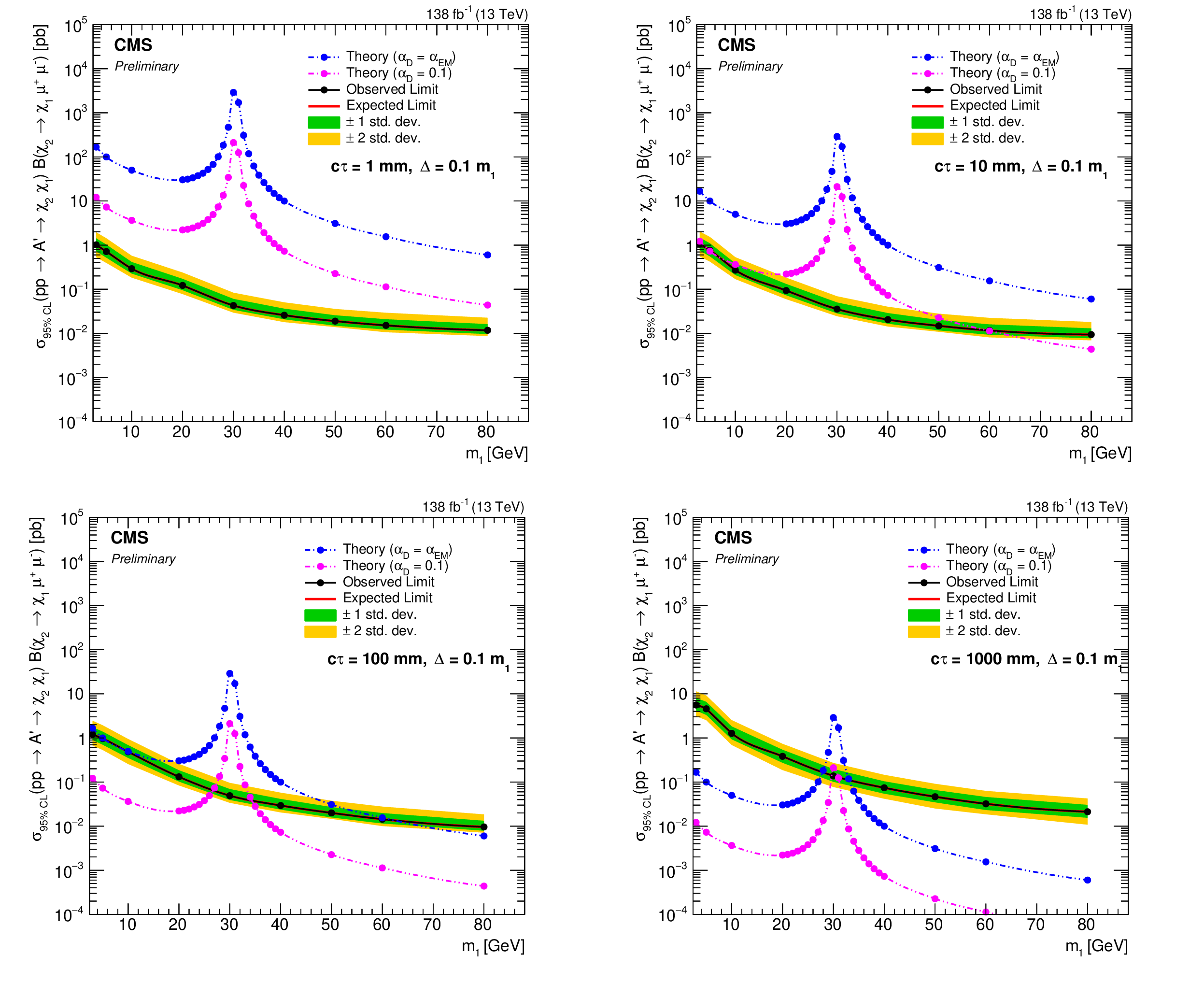
Additional Figure 3:
The observed and expected upper limits at 95% CL on the product of $ A' $ production cross section and $ \chi_2 \to \chi_1 \mu^+\mu^- $ branching fraction for an inelastic dark matter model with mass splitting $ \Delta = 0.1 \, m_1 $, shown as a function of $ m_1 $. The one (two) standard deviation variation in the expected limit is shown in the inner green (outer yellow) band. The blue and magenta dashed lines represent the theoretically predicted cross sections, assuming $ \alpha_D = \alpha_{EM} $ and $ \alpha_D = $ 0.1, respectively. Clockwise from the upper left: $ c\tau = $ 1 mm; $ c\tau = $ 10 mm; $ c\tau = $ 1000 mm; $ c\tau = $ 100 mm. |
png pdf |
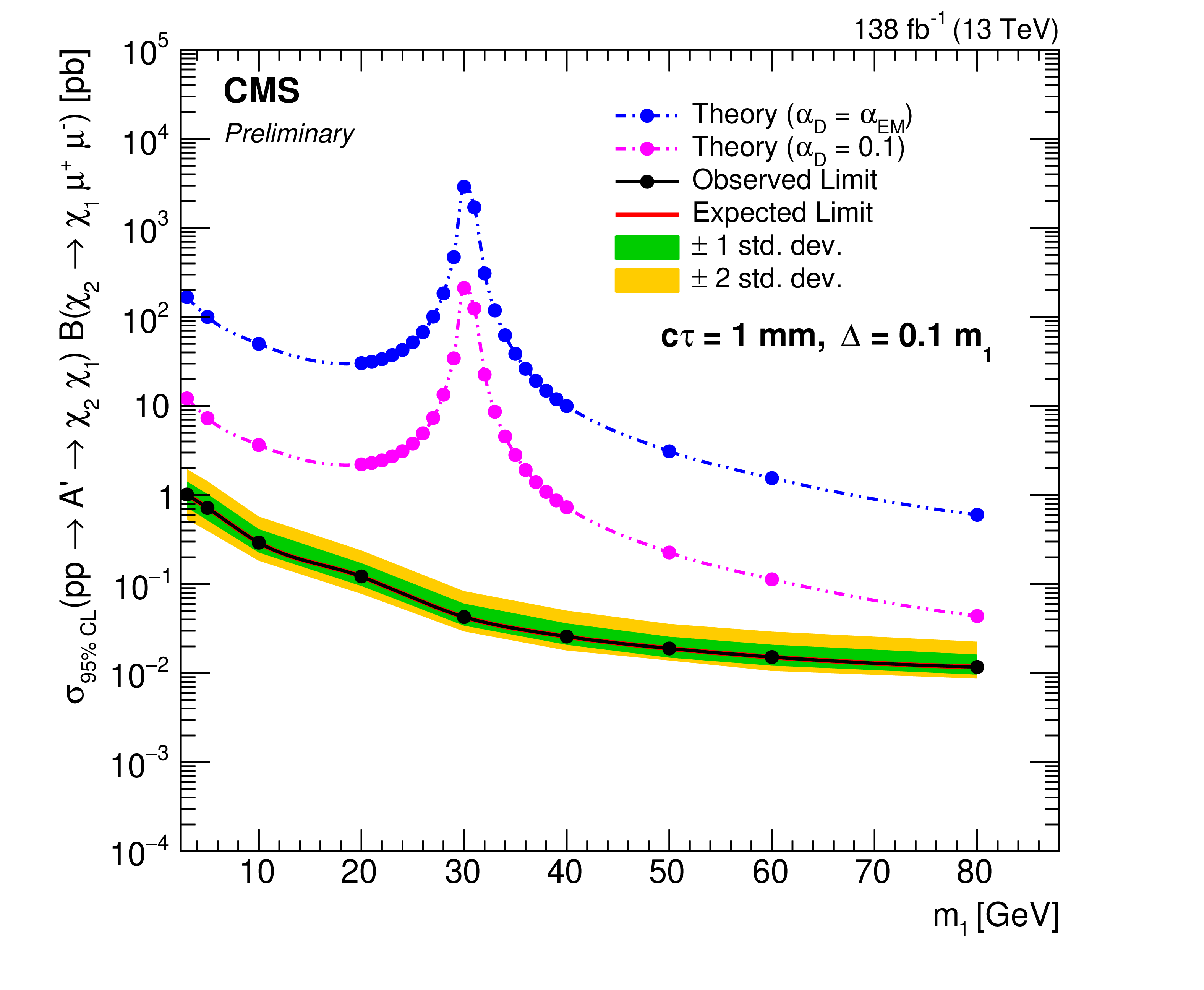
Additional Figure 3-a:
The observed and expected upper limits at 95% CL on the product of $ A' $ production cross section and $ \chi_2 \to \chi_1 \mu^+\mu^- $ branching fraction for an inelastic dark matter model with mass splitting $ \Delta = 0.1 \, m_1 $, shown as a function of $ m_1 $. The one (two) standard deviation variation in the expected limit is shown in the inner green (outer yellow) band. The blue and magenta dashed lines represent the theoretically predicted cross sections, assuming $ \alpha_D = \alpha_{EM} $ and $ \alpha_D = $ 0.1, respectively. $ c\tau = $ 1 mm. |
png pdf |
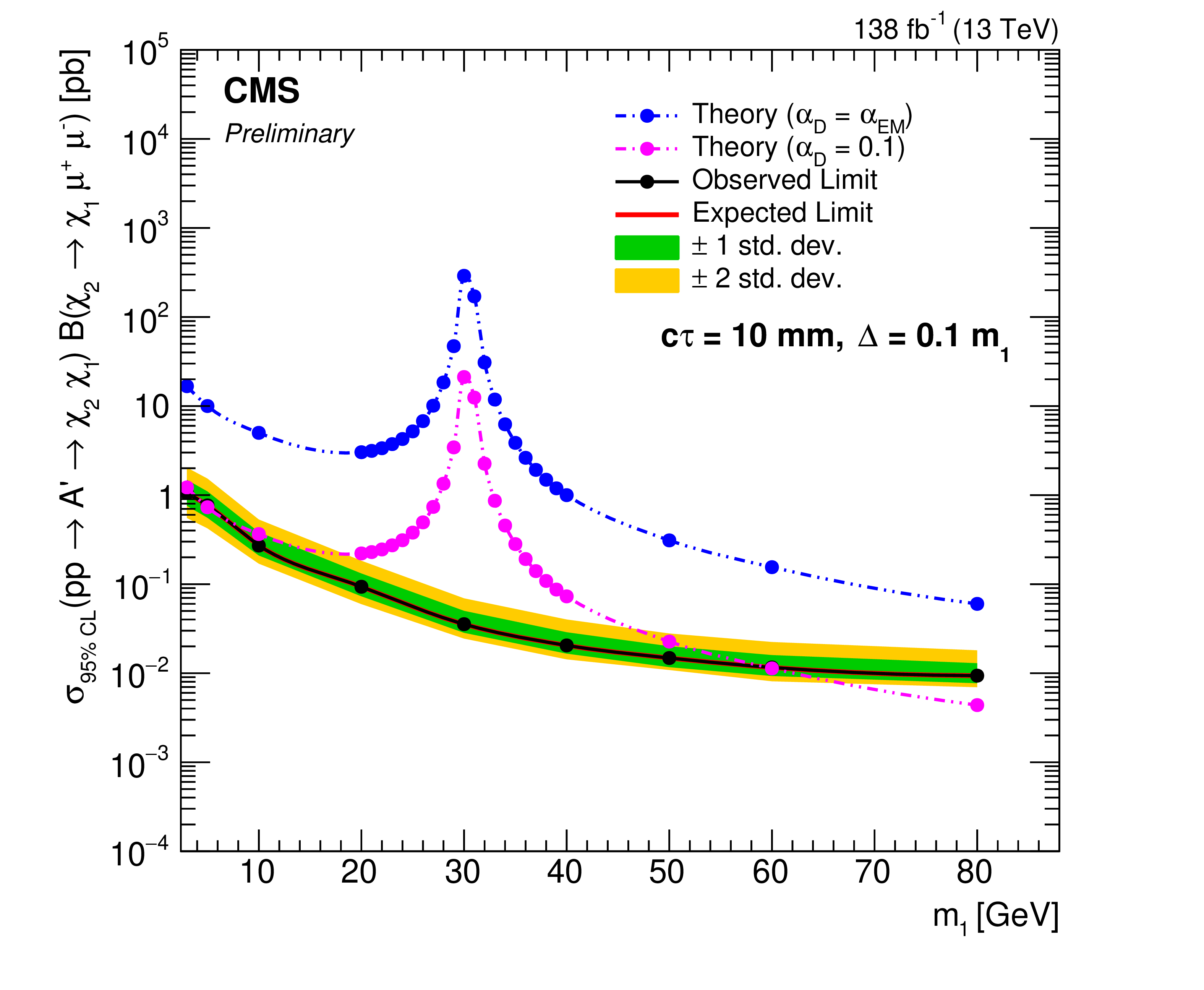
Additional Figure 3-b:
The observed and expected upper limits at 95% CL on the product of $ A' $ production cross section and $ \chi_2 \to \chi_1 \mu^+\mu^- $ branching fraction for an inelastic dark matter model with mass splitting $ \Delta = 0.1 \, m_1 $, shown as a function of $ m_1 $. The one (two) standard deviation variation in the expected limit is shown in the inner green (outer yellow) band. The blue and magenta dashed lines represent the theoretically predicted cross sections, assuming $ \alpha_D = \alpha_{EM} $ and $ \alpha_D = $ 0.1, respectively. $ c\tau = $ 10 mm. |
png pdf |
Additional Figure 3-c:
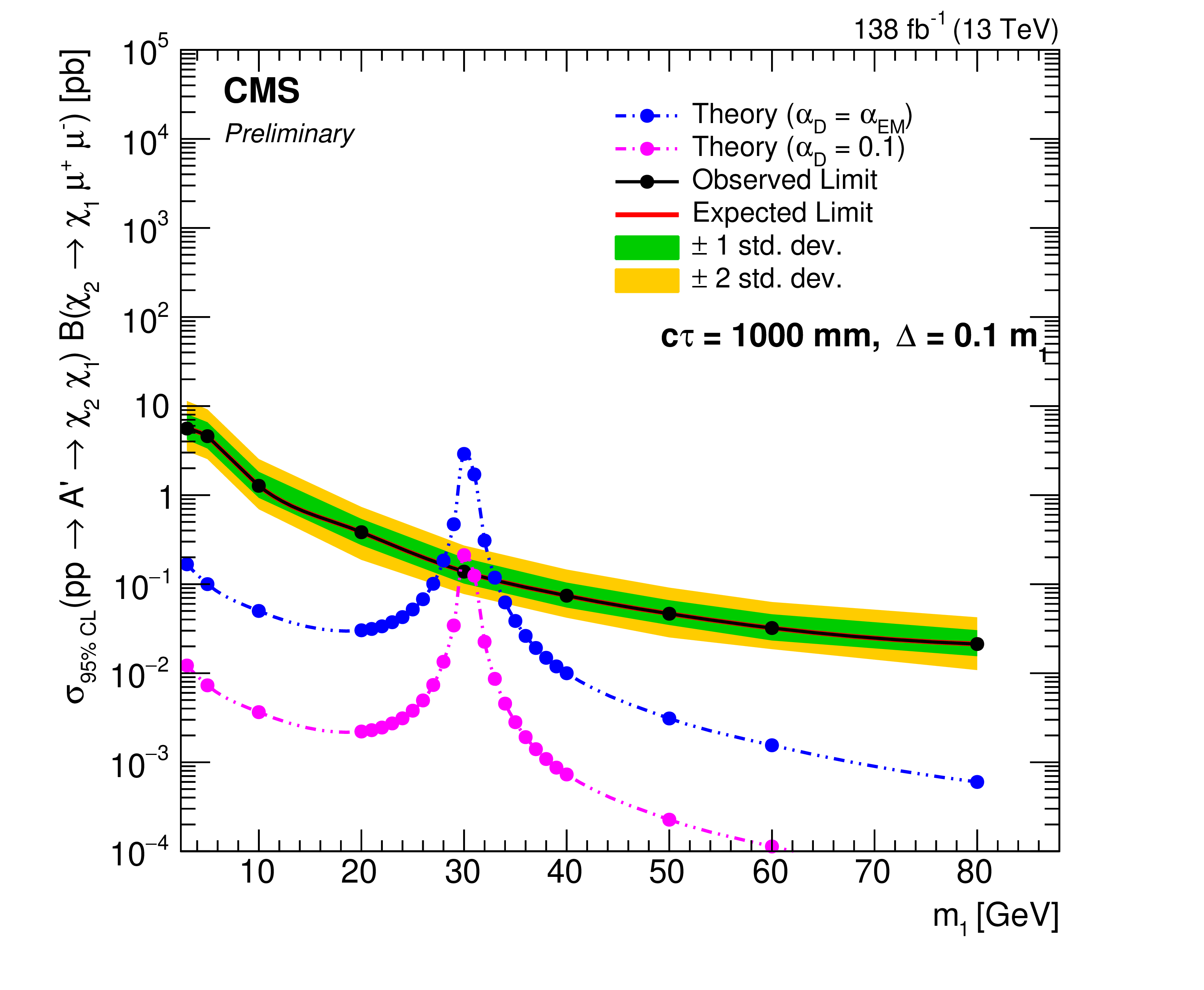
The observed and expected upper limits at 95% CL on the product of $ A' $ production cross section and $ \chi_2 \to \chi_1 \mu^+\mu^- $ branching fraction for an inelastic dark matter model with mass splitting $ \Delta = 0.1 \, m_1 $, shown as a function of $ m_1 $. The one (two) standard deviation variation in the expected limit is shown in the inner green (outer yellow) band. The blue and magenta dashed lines represent the theoretically predicted cross sections, assuming $ \alpha_D = \alpha_{EM} $ and $ \alpha_D = $ 0.1, respectively. $ c\tau = $ 1000 mm. |
png pdf |
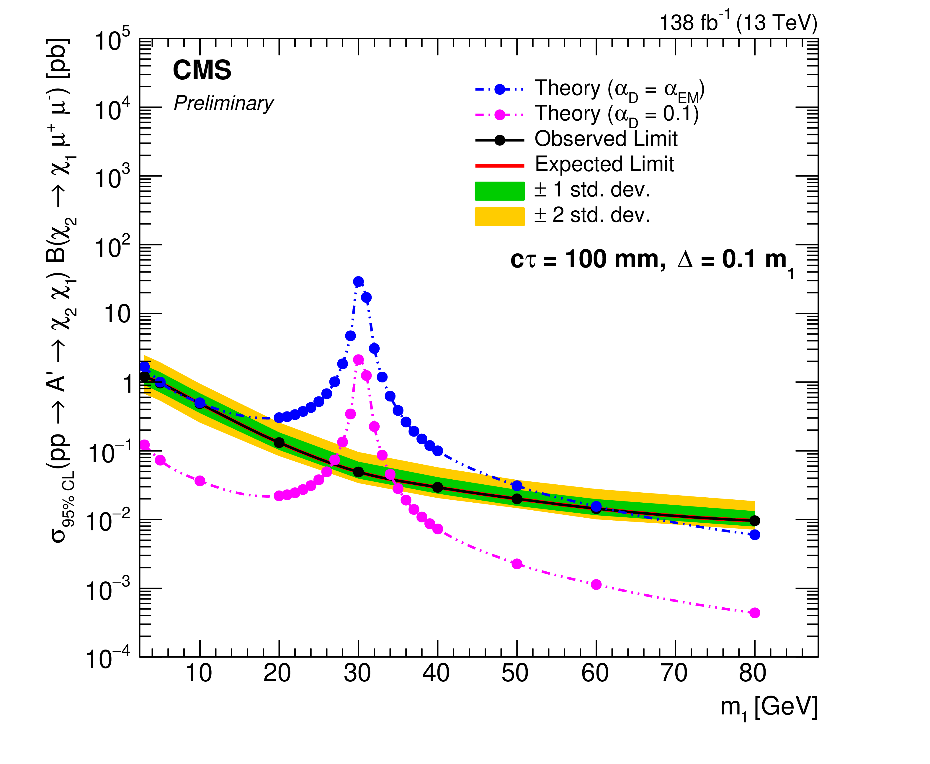
Additional Figure 3-d:
The observed and expected upper limits at 95% CL on the product of $ A' $ production cross section and $ \chi_2 \to \chi_1 \mu^+\mu^- $ branching fraction for an inelastic dark matter model with mass splitting $ \Delta = 0.1 \, m_1 $, shown as a function of $ m_1 $. The one (two) standard deviation variation in the expected limit is shown in the inner green (outer yellow) band. The blue and magenta dashed lines represent the theoretically predicted cross sections, assuming $ \alpha_D = \alpha_{EM} $ and $ \alpha_D = $ 0.1, respectively. $ c\tau = $ 100 mm. |
png pdf |
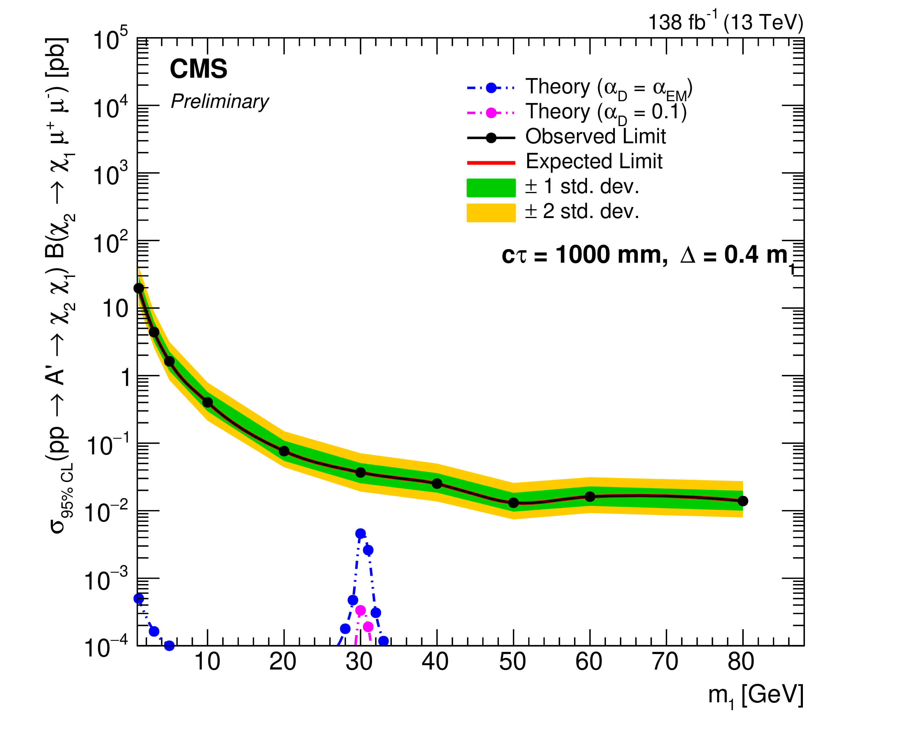
Additional Figure 4:
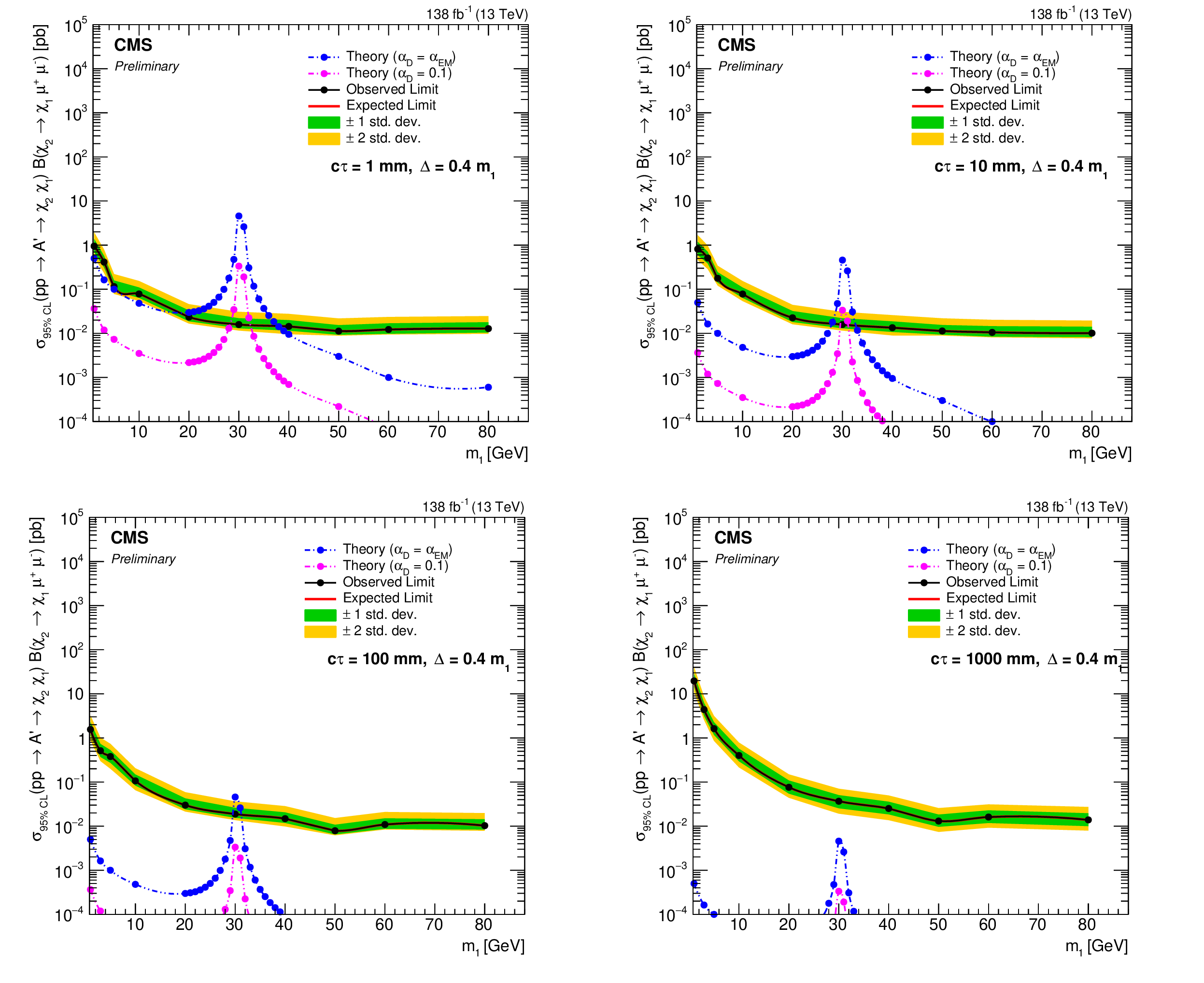
The observed and expected upper limits at 95% CL on the product of $ A' $ production cross section and $ \chi_2 \to \chi_1 \mu^+\mu^- $ branching fraction for an inelastic dark matter model with mass splitting $ \Delta = 0.4 \, m_1 $, shown as a function of $ m_1 $. The one (two) standard deviation variation in the expected limit is shown in the inner green (outer yellow) band. The blue and magenta dashed lines represent the theoretically predicted cross sections, assuming $ \alpha_D = \alpha_{EM} $ and $ \alpha_D = $ 0.1, respectively. Clockwise from the upper left: $ c\tau = $ 1 mm; $ c\tau = $ 10 mm; $ c\tau = $ 1000 mm; $ c\tau = $ 100 mm. |

png pdf |
Additional Figure 4-a:
The observed and expected upper limits at 95% CL on the product of $ A' $ production cross section and $ \chi_2 \to \chi_1 \mu^+\mu^- $ branching fraction for an inelastic dark matter model with mass splitting $ \Delta = 0.4 \, m_1 $, shown as a function of $ m_1 $. The one (two) standard deviation variation in the expected limit is shown in the inner green (outer yellow) band. The blue and magenta dashed lines represent the theoretically predicted cross sections, assuming $ \alpha_D = \alpha_{EM} $ and $ \alpha_D = $ 0.1, respectively. $ c\tau = $ 1 mm. |
png pdf |
Additional Figure 4-b:
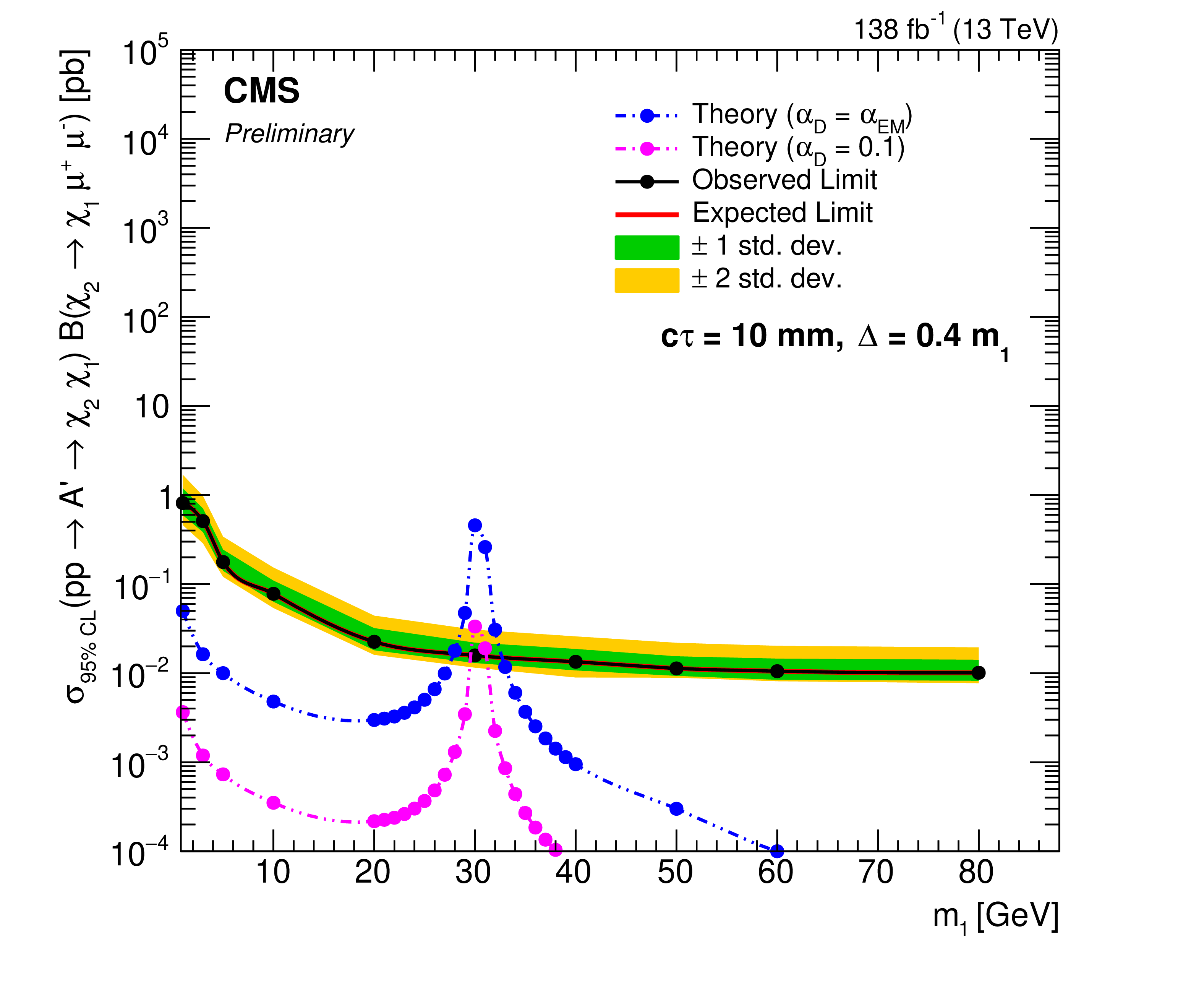
The observed and expected upper limits at 95% CL on the product of $ A' $ production cross section and $ \chi_2 \to \chi_1 \mu^+\mu^- $ branching fraction for an inelastic dark matter model with mass splitting $ \Delta = 0.4 \, m_1 $, shown as a function of $ m_1 $. The one (two) standard deviation variation in the expected limit is shown in the inner green (outer yellow) band. The blue and magenta dashed lines represent the theoretically predicted cross sections, assuming $ \alpha_D = \alpha_{EM} $ and $ \alpha_D = $ 0.1, respectively. $ c\tau = $ 10 mm. |
png pdf |
Additional Figure 4-c:
The observed and expected upper limits at 95% CL on the product of $ A' $ production cross section and $ \chi_2 \to \chi_1 \mu^+\mu^- $ branching fraction for an inelastic dark matter model with mass splitting $ \Delta = 0.4 \, m_1 $, shown as a function of $ m_1 $. The one (two) standard deviation variation in the expected limit is shown in the inner green (outer yellow) band. The blue and magenta dashed lines represent the theoretically predicted cross sections, assuming $ \alpha_D = \alpha_{EM} $ and $ \alpha_D = $ 0.1, respectively. $ c\tau = $ 10000 mm. |
png pdf |
Additional Figure 4-d:
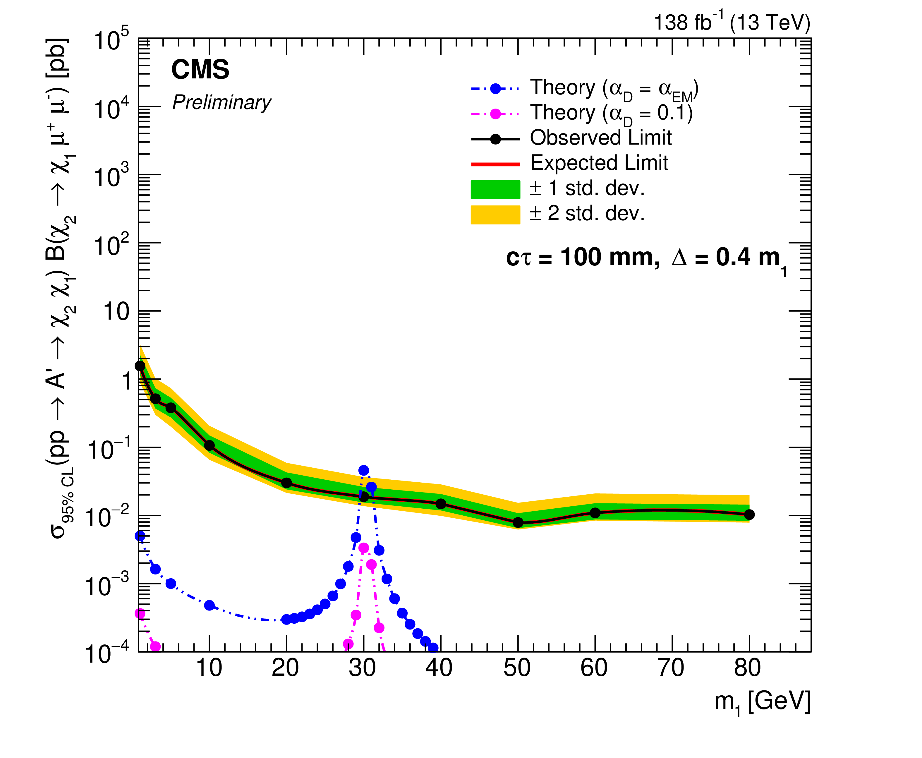
The observed and expected upper limits at 95% CL on the product of $ A' $ production cross section and $ \chi_2 \to \chi_1 \mu^+\mu^- $ branching fraction for an inelastic dark matter model with mass splitting $ \Delta = 0.4 \, m_1 $, shown as a function of $ m_1 $. The one (two) standard deviation variation in the expected limit is shown in the inner green (outer yellow) band. The blue and magenta dashed lines represent the theoretically predicted cross sections, assuming $ \alpha_D = \alpha_{EM} $ and $ \alpha_D = $ 0.1, respectively. $ c\tau = $ 100 mm. |

png pdf |
Additional Figure 5:
The observed and expected upper limits at 95% CL on the product of $ A' $ production cross section and $ \chi_2 \to \chi_1 \mu^+\mu^- $ branching fraction for an inelastic dark matter model with varying $ m_1 $ and $ \Delta $, shown as a function of $ c\tau $. The one (two) standard deviation variation in the expected limit is shown in the inner green (outer yellow) band. The blue and magenta dashed lines represent the theoretically predicted cross sections, assuming $ \alpha_D = \alpha_{EM} $ and $ \alpha_D = $ 0.1, respectively. Clockwise from the upper left: $ m_1 = $ 3 GeV, $ \Delta = 0.1 \, m_1 $; $ m_1 = $ 20 GeV, $ \Delta = 0.1 \, m_1 $; $ m_1 = $ 60 GeV, $ \Delta = 0.4 \, m_1 $; $ m_1 = $ 60 GeV, $ \Delta = 0.1 \, m_1 $. |
png pdf |
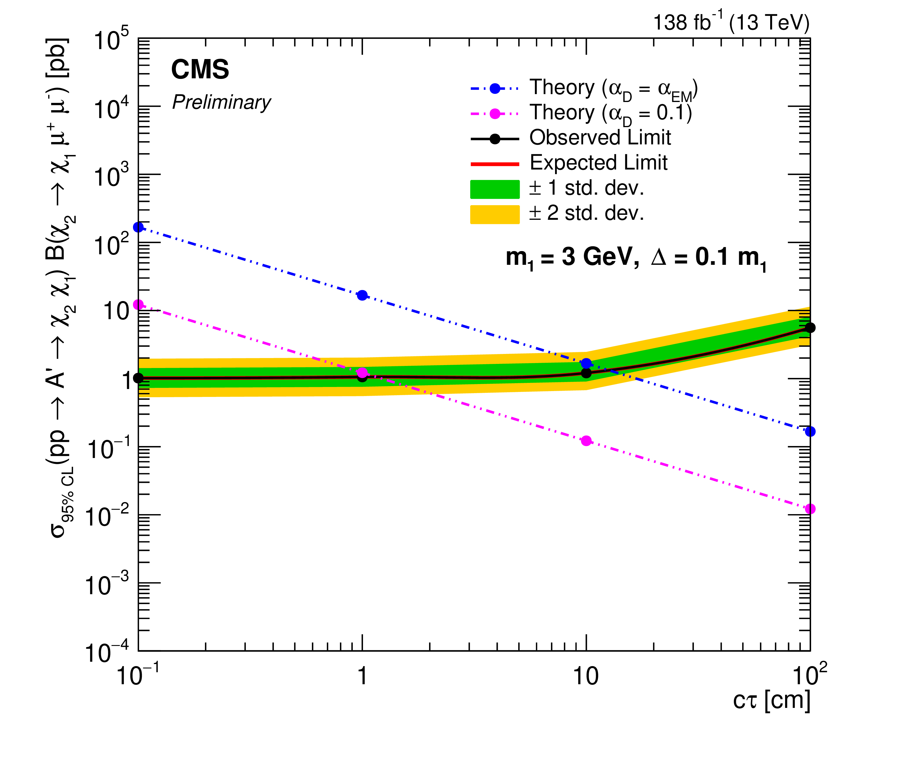
Additional Figure 5-a:
The observed and expected upper limits at 95% CL on the product of $ A' $ production cross section and $ \chi_2 \to \chi_1 \mu^+\mu^- $ branching fraction for an inelastic dark matter model with varying $ m_1 $ and $ \Delta $, shown as a function of $ c\tau $. The one (two) standard deviation variation in the expected limit is shown in the inner green (outer yellow) band. The blue and magenta dashed lines represent the theoretically predicted cross sections, assuming $ \alpha_D = \alpha_{EM} $ and $ \alpha_D = $ 0.1, respectively. $ m_1 = $ 3 GeV, $ \Delta = 0.1 \, m_1 $. |

png pdf |
Additional Figure 5-b:
The observed and expected upper limits at 95% CL on the product of $ A' $ production cross section and $ \chi_2 \to \chi_1 \mu^+\mu^- $ branching fraction for an inelastic dark matter model with varying $ m_1 $ and $ \Delta $, shown as a function of $ c\tau $. The one (two) standard deviation variation in the expected limit is shown in the inner green (outer yellow) band. The blue and magenta dashed lines represent the theoretically predicted cross sections, assuming $ \alpha_D = \alpha_{EM} $ and $ \alpha_D = $ 0.1, respectively. $ m_1 = $ 20 GeV, $ \Delta = 0.1 \, m_1 $. |

png pdf |
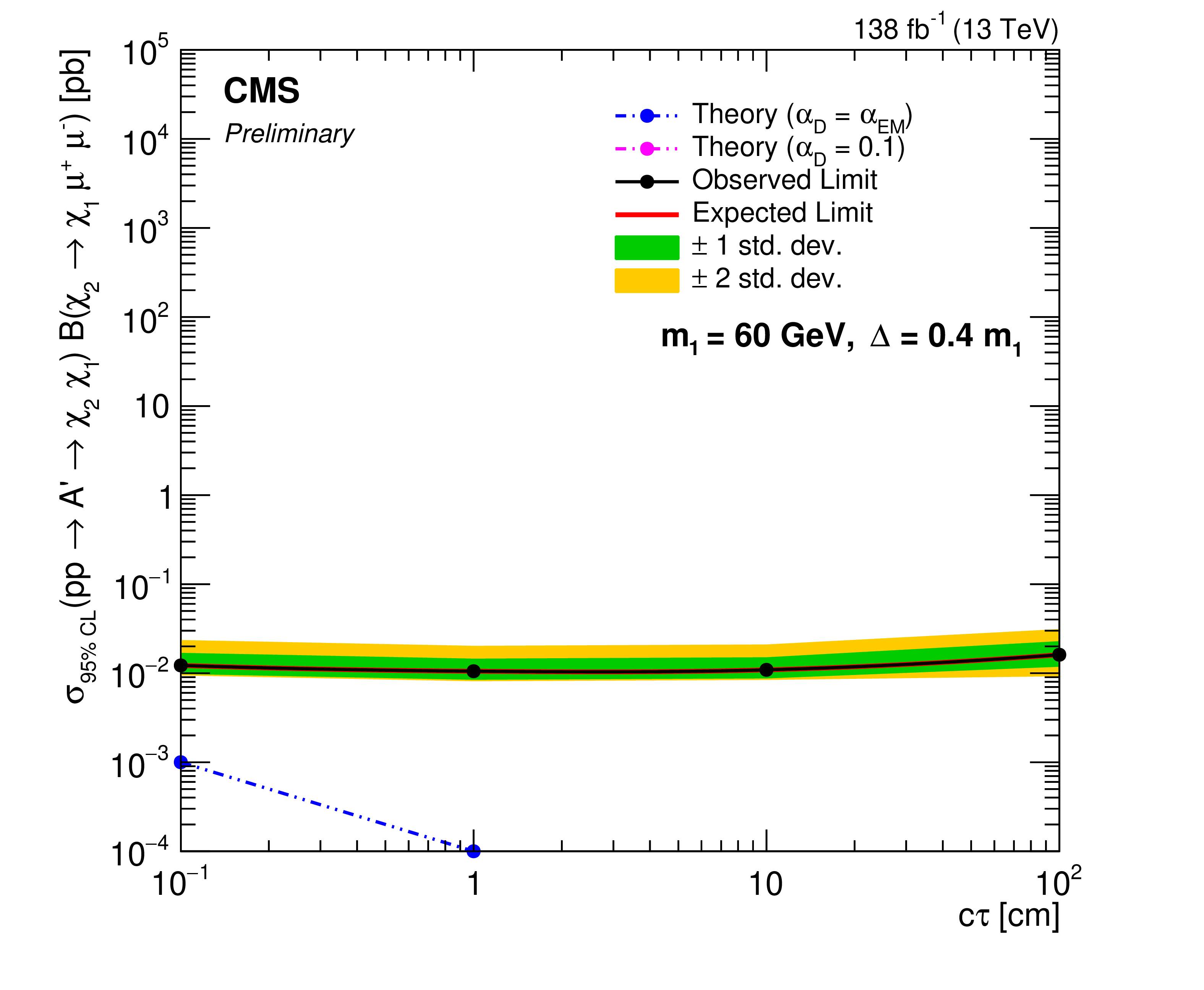
Additional Figure 5-c:
The observed and expected upper limits at 95% CL on the product of $ A' $ production cross section and $ \chi_2 \to \chi_1 \mu^+\mu^- $ branching fraction for an inelastic dark matter model with varying $ m_1 $ and $ \Delta $, shown as a function of $ c\tau $. The one (two) standard deviation variation in the expected limit is shown in the inner green (outer yellow) band. The blue and magenta dashed lines represent the theoretically predicted cross sections, assuming $ \alpha_D = \alpha_{EM} $ and $ \alpha_D = $ 0.1, respectively. $ m_1 = $ 60 GeV, $ \Delta = 0.4 \, m_1 $. |
png pdf |
Additional Figure 5-d:
The observed and expected upper limits at 95% CL on the product of $ A' $ production cross section and $ \chi_2 \to \chi_1 \mu^+\mu^- $ branching fraction for an inelastic dark matter model with varying $ m_1 $ and $ \Delta $, shown as a function of $ c\tau $. The one (two) standard deviation variation in the expected limit is shown in the inner green (outer yellow) band. The blue and magenta dashed lines represent the theoretically predicted cross sections, assuming $ \alpha_D = \alpha_{EM} $ and $ \alpha_D = $ 0.1, respectively. $ m_1 = $ 60 GeV, $ \Delta = 0.1 \, m_1 $. |
png pdf |
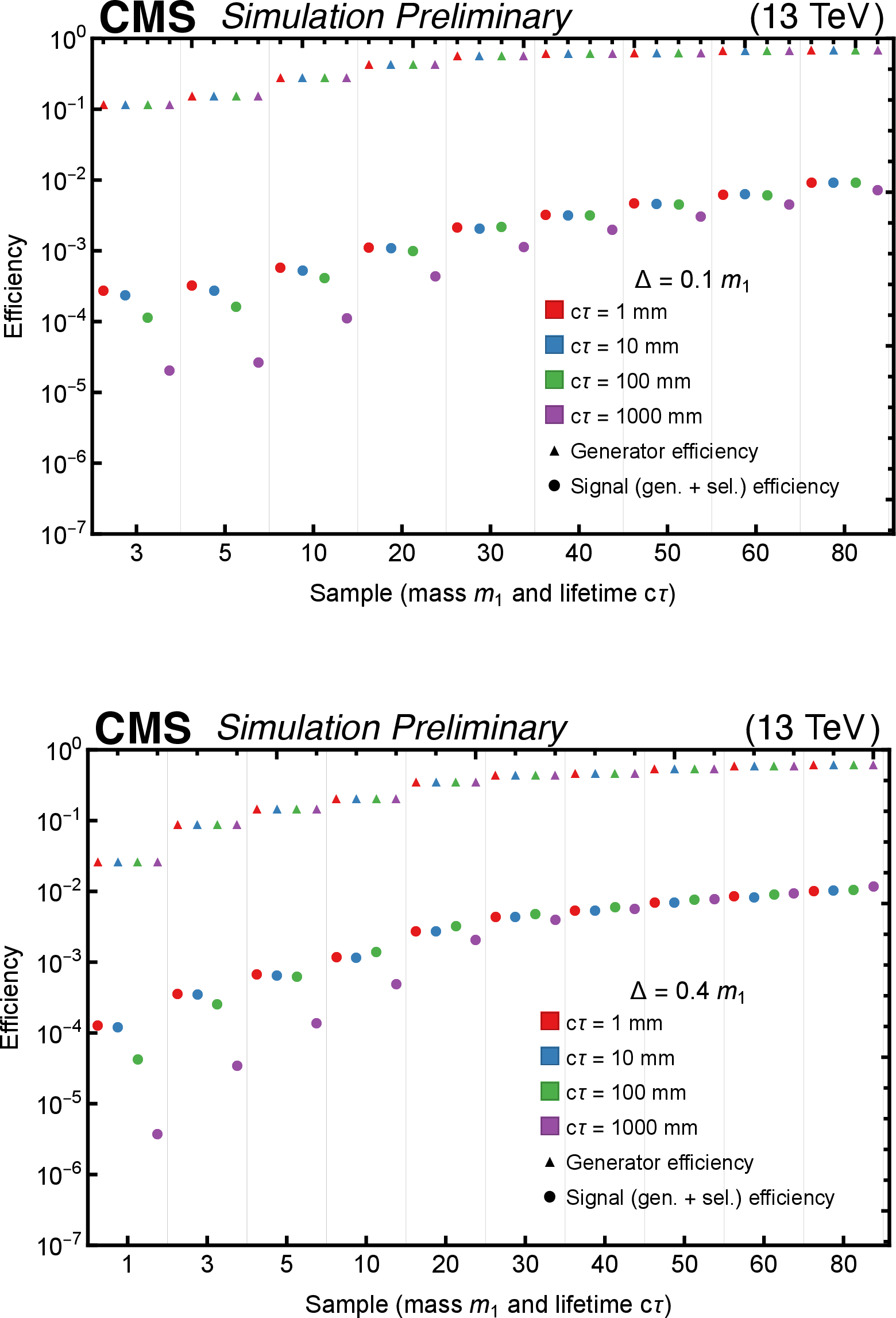
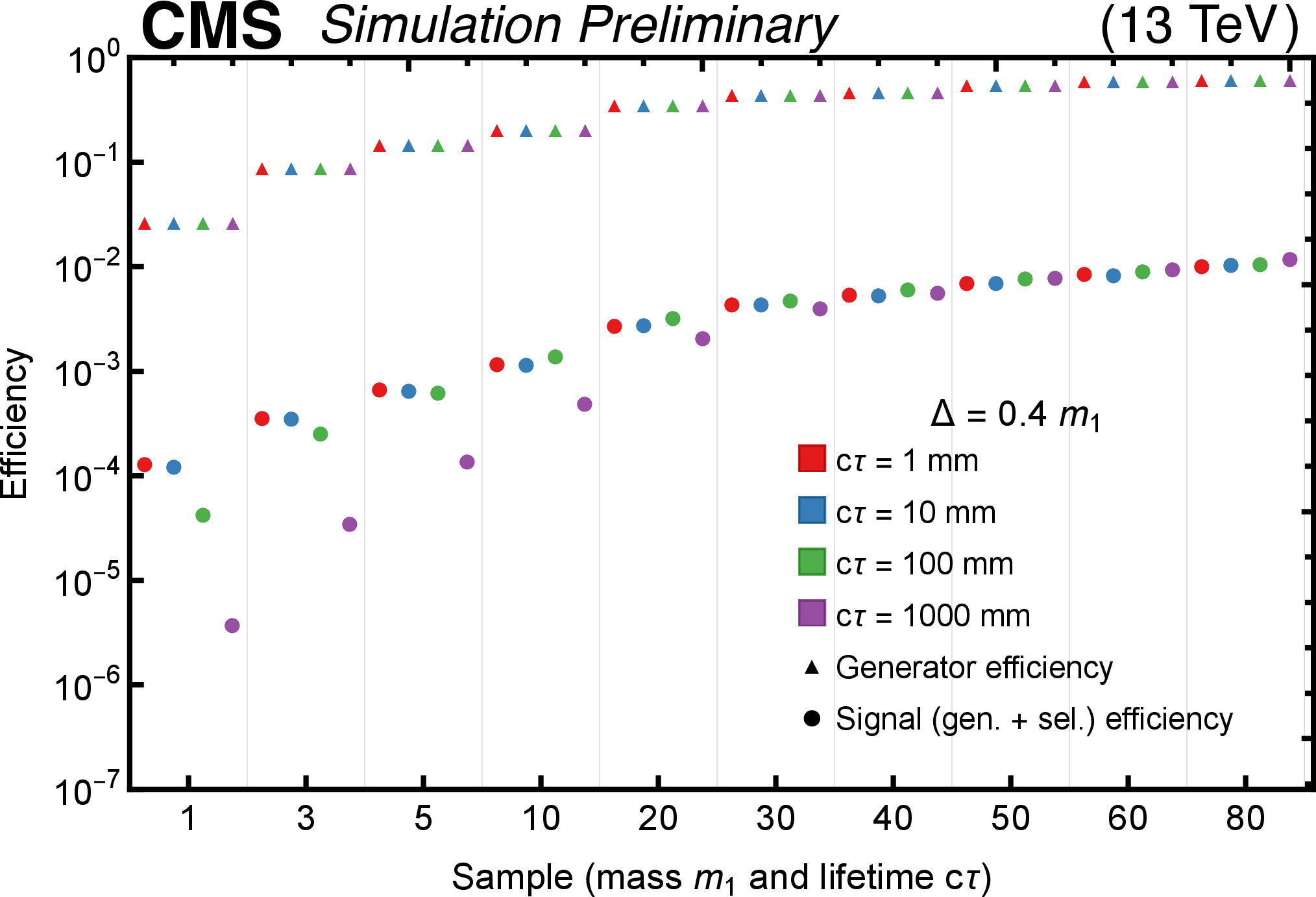
Additional Figure 6:
Signal efficiency of the simulated samples in the analysis, before splitting into muon match categories. Triangles denote the efficiency of filters imposed at generator level, while circles denote the total (generator filter plus selection) signal efficiency. The generator filters comprise the requirements: leading jet $ p_{\mathrm{T}} > $ 80 GeV and $ p_{\mathrm{T}}^\text{miss} > $ 80 GeV. |

png pdf |
Additional Figure 6-a:
Signal efficiency of the simulated samples in the analysis, before splitting into muon match categories. Triangles denote the efficiency of filters imposed at generator level, while circles denote the total (generator filter plus selection) signal efficiency. The generator filters comprise the requirements: leading jet $ p_{\mathrm{T}} > $ 80 GeV and $ p_{\mathrm{T}}^\text{miss} > $ 80 GeV. |
png pdf |
Additional Figure 6-b:
Signal efficiency of the simulated samples in the analysis, before splitting into muon match categories. Triangles denote the efficiency of filters imposed at generator level, while circles denote the total (generator filter plus selection) signal efficiency. The generator filters comprise the requirements: leading jet $ p_{\mathrm{T}} > $ 80 GeV and $ p_{\mathrm{T}}^\text{miss} > $ 80 GeV. |
png pdf |
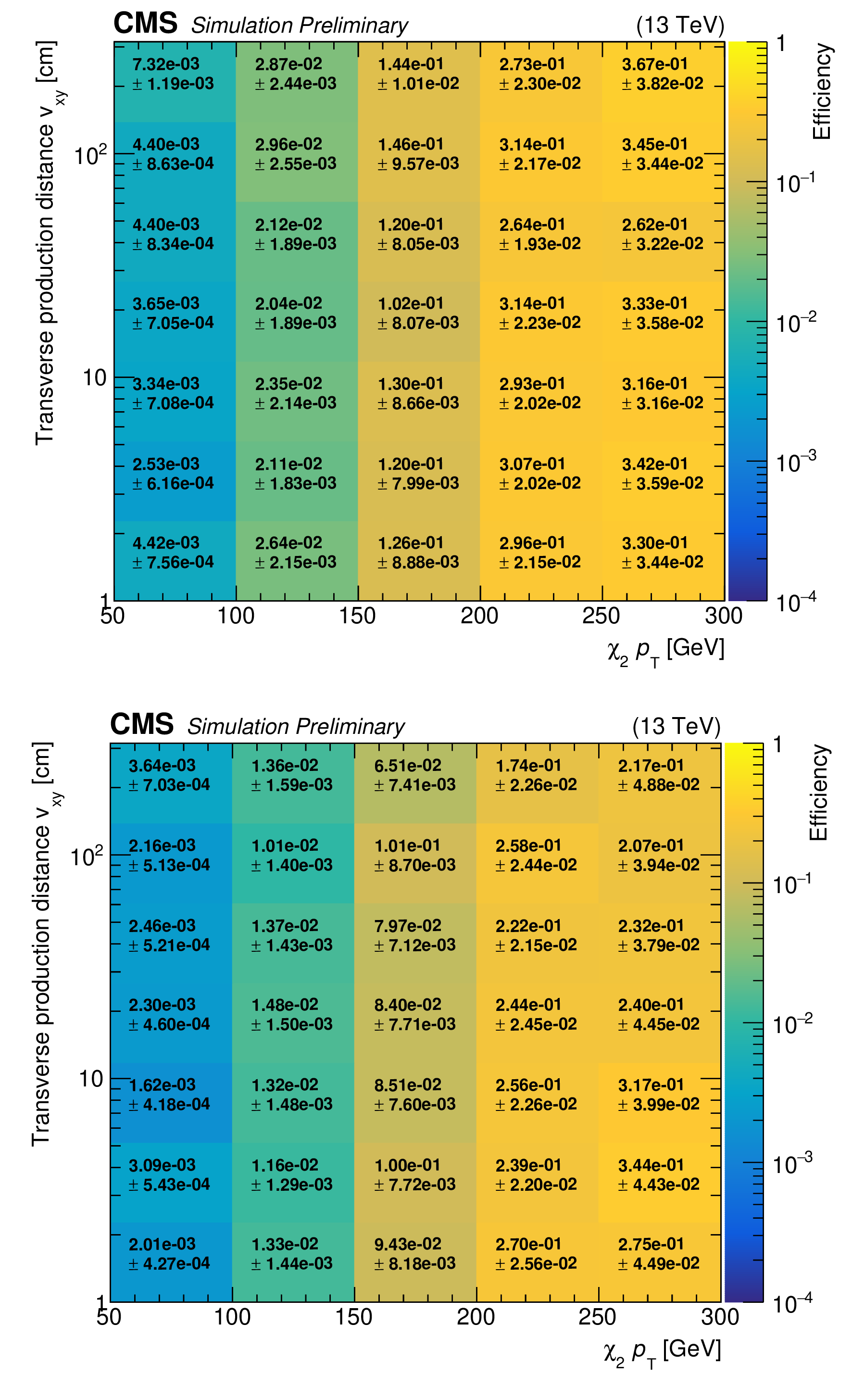
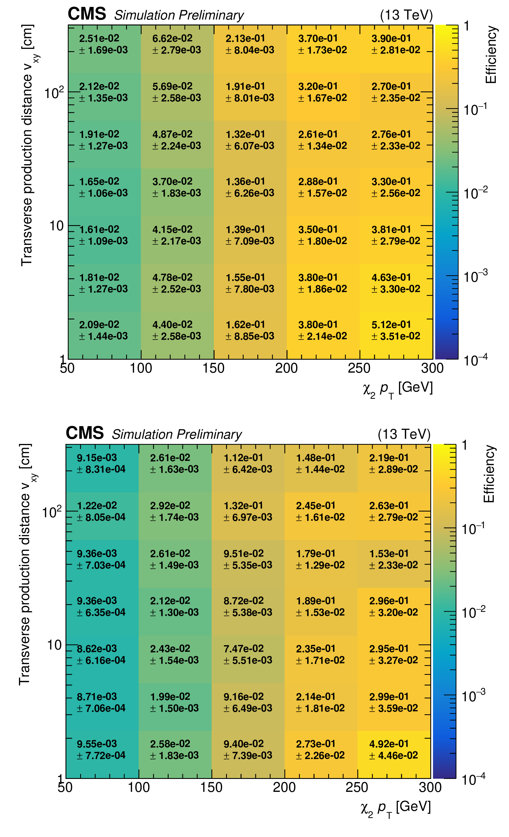
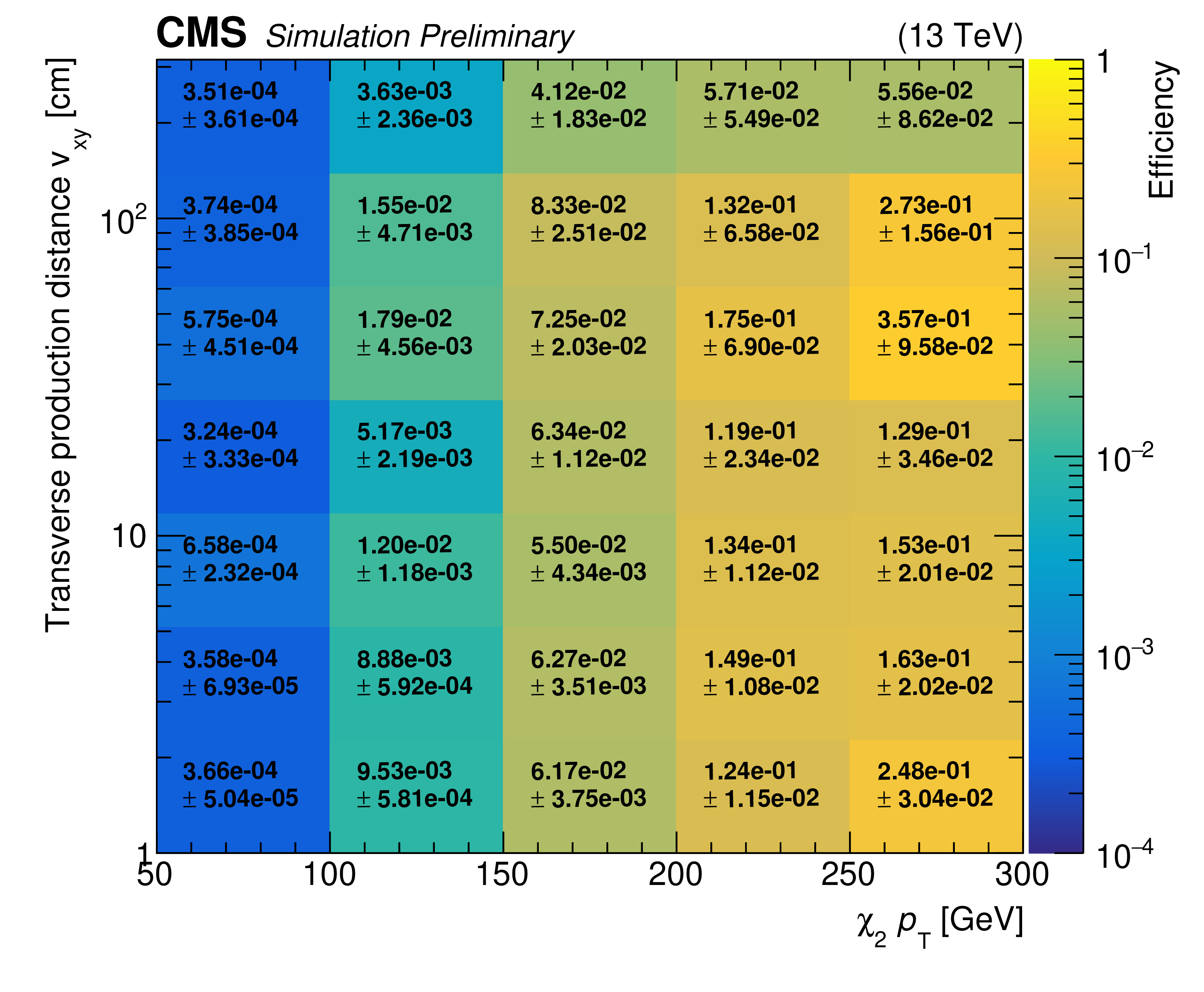
Additional Figure 7:
Signal efficiency versus generated $ \chi_2 p_{\mathrm{T}} $ and decay transverse position $ v_{xy} $ for an inelastic dark matter model with $ m_1 = $ 50 GeV and $ \Delta = 0.1 \, m_1 $, before splitting into muon match categories. Upper: $ \chi_2 |\eta| < $ 1.2. Lower: $ \chi_2 |\eta| > $ 1.2. The efficiency is calculated after application of generator filters. |
png pdf |
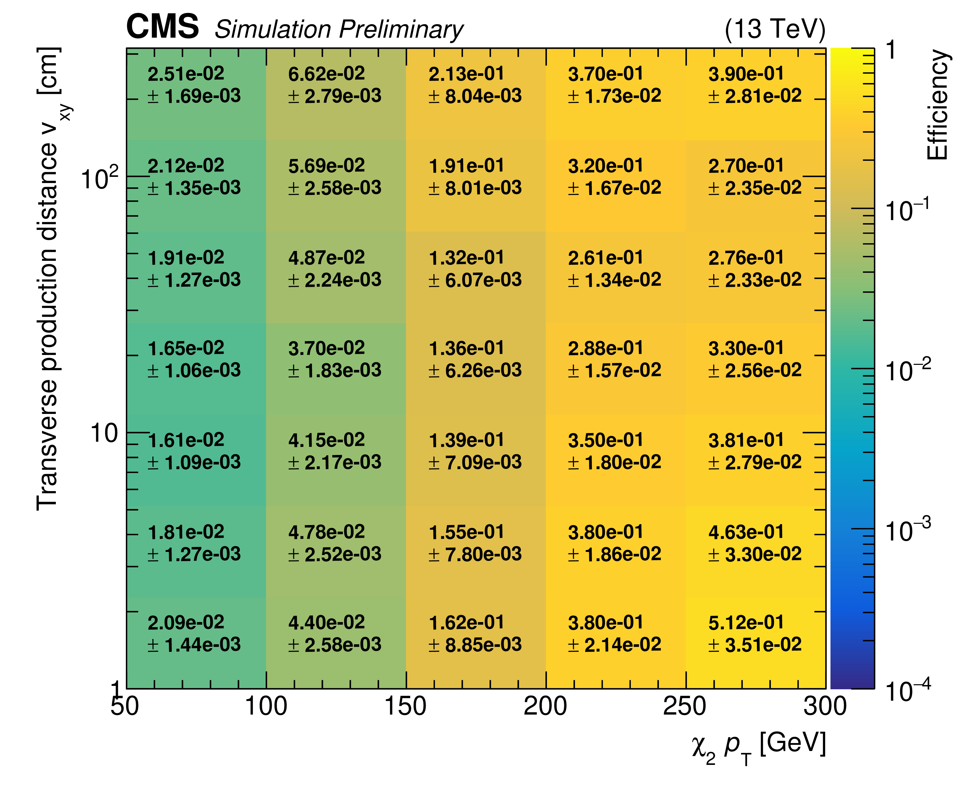
Additional Figure 7-a:
Signal efficiency versus generated $ \chi_2 p_{\mathrm{T}} $ and decay transverse position $ v_{xy} $ for an inelastic dark matter model with $ m_1 = $ 50 GeV and $ \Delta = 0.1 \, m_1 $, before splitting into muon match categories. $ \chi_2 |\eta| < $ 1.2. The efficiency is calculated after application of generator filters. |
png pdf |
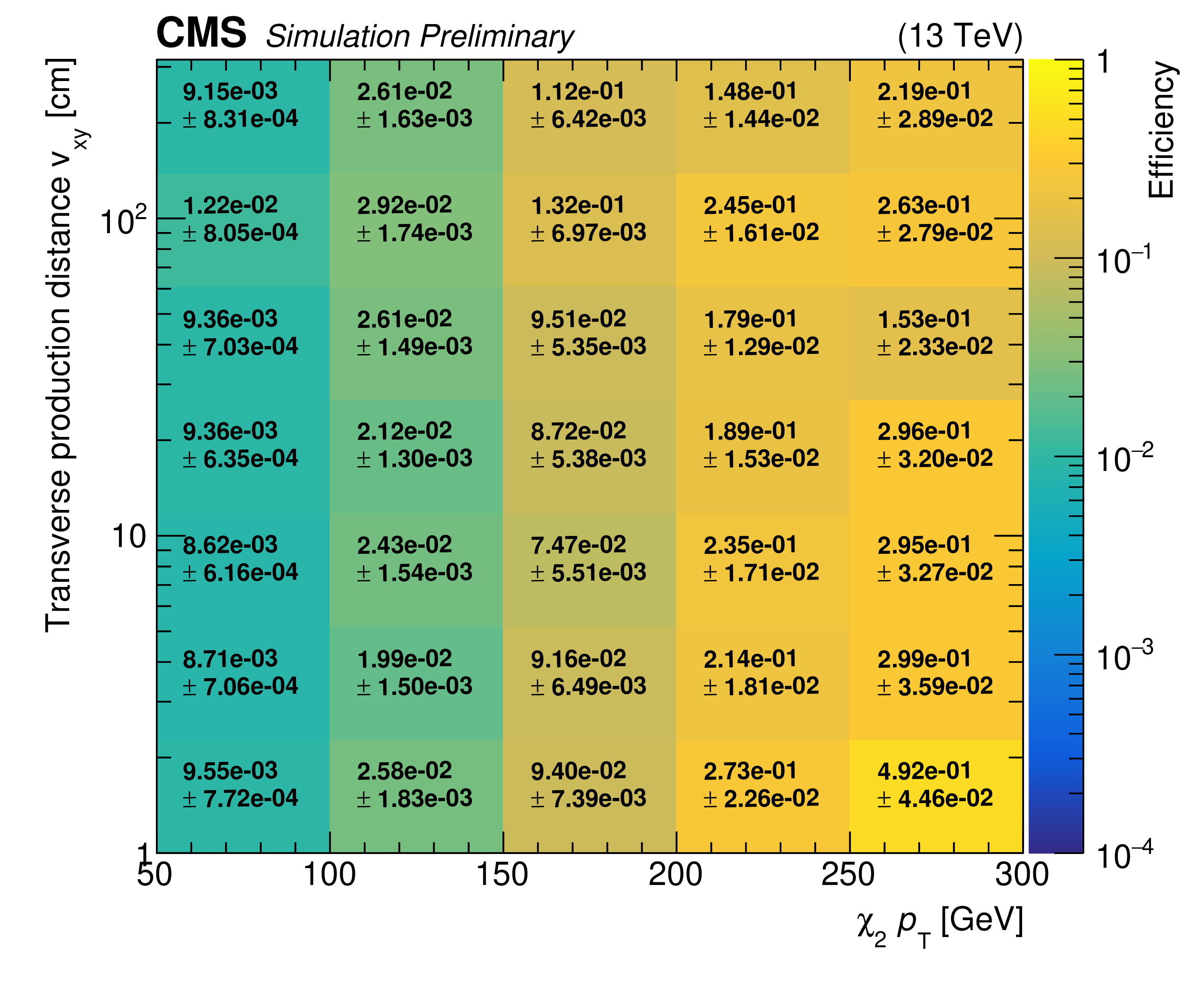
Additional Figure 7-b:
Signal efficiency versus generated $ \chi_2 p_{\mathrm{T}} $ and decay transverse position $ v_{xy} $ for an inelastic dark matter model with $ m_1 = $ 50 GeV and $ \Delta = 0.1 \, m_1 $, before splitting into muon match categories. $ \chi_2 |\eta| > $ 1.2. The efficiency is calculated after application of generator filters. |
png pdf |
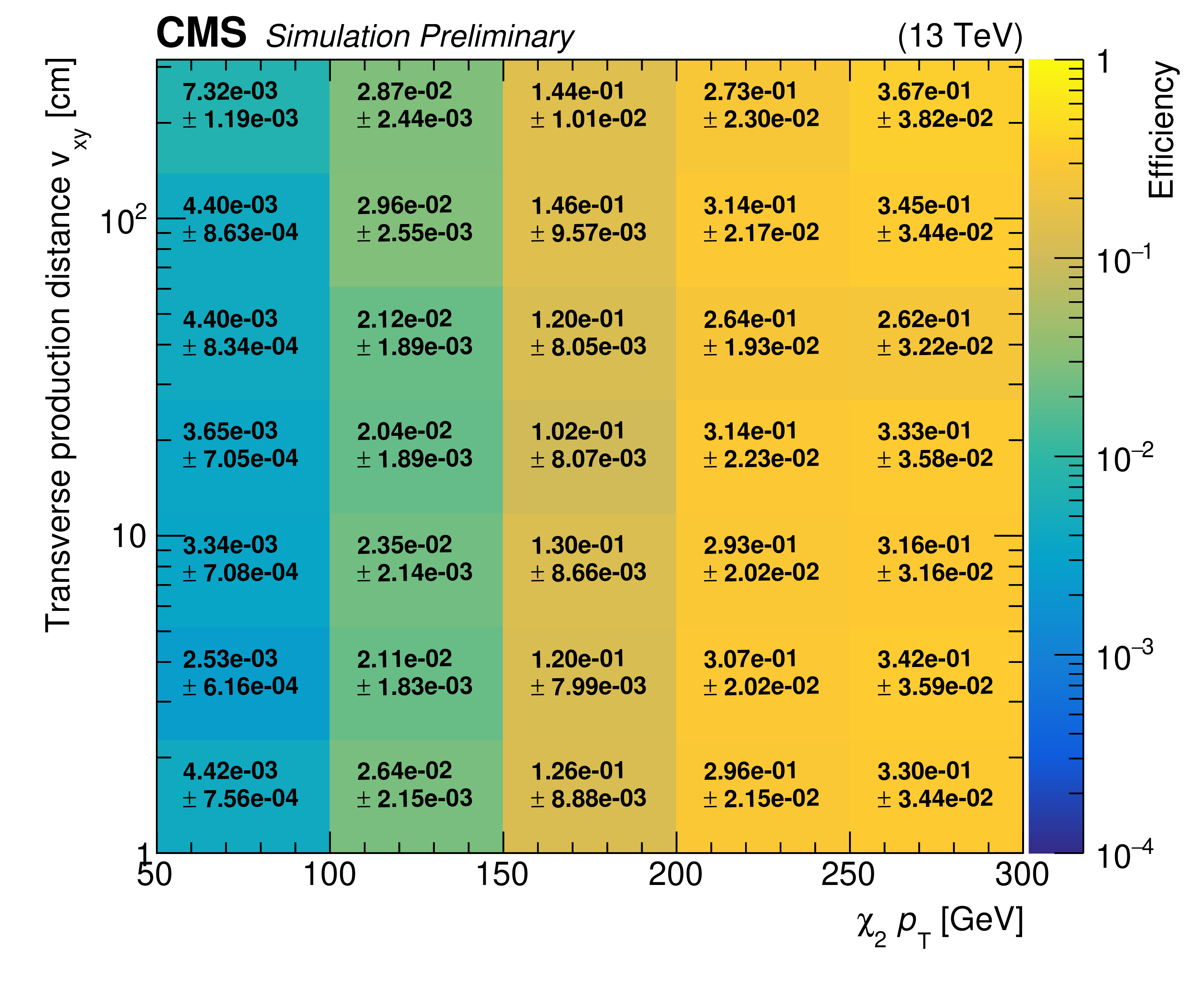
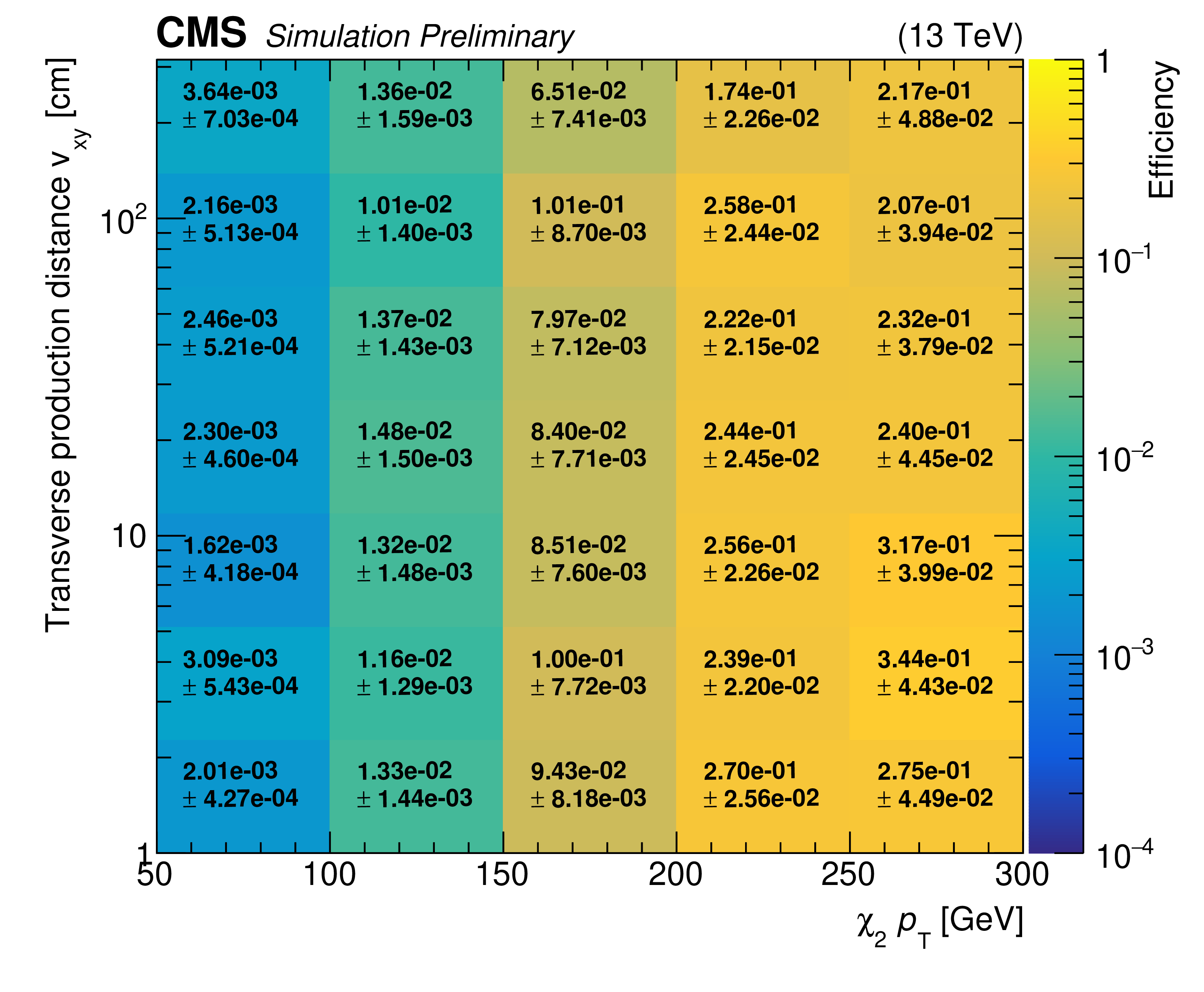
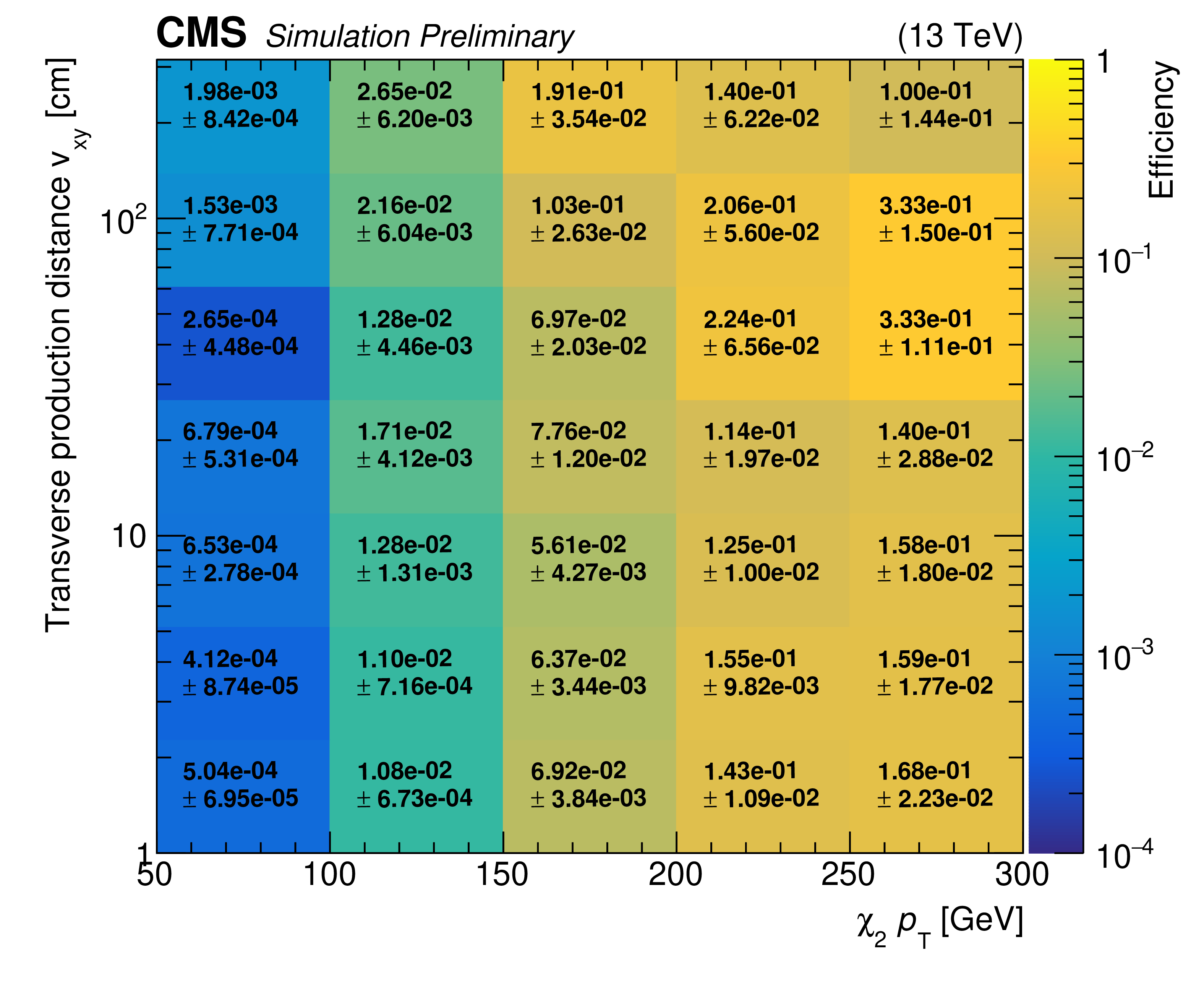
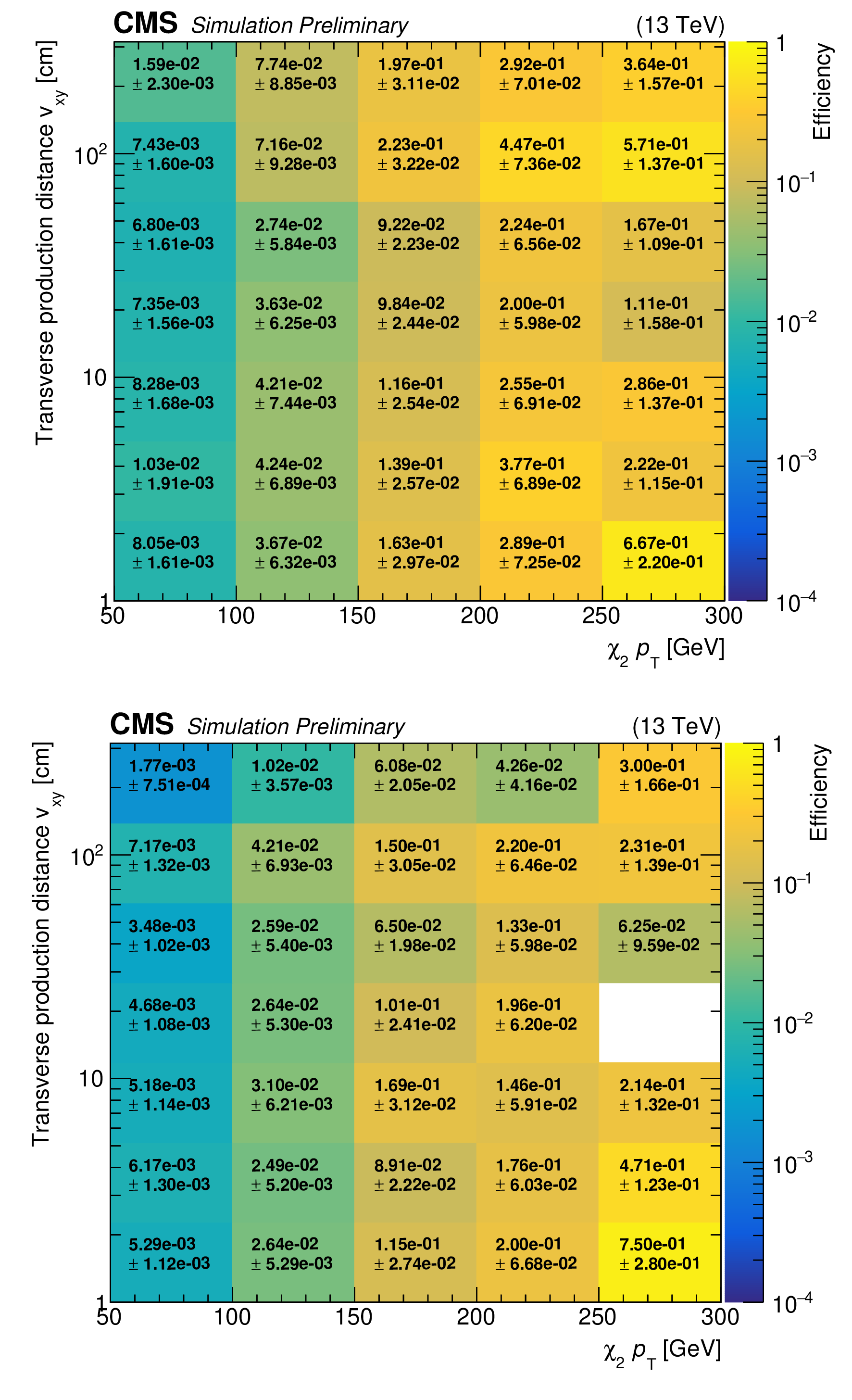
Additional Figure 8:
Signal efficiency versus generated $ \chi_2 p_{\mathrm{T}} $ and decay transverse position $ v_{xy} $ for an inelastic dark matter model with $ m_1 = $ 50 GeV and $ \Delta = 0.4 \, m_1 $, before splitting into muon match categories. Upper: $ \chi_2 |\eta| < $ 1.2. Lower: $ \chi_2 |\eta| > $ 1.2. The efficiency is calculated after application of generator filters. |
png pdf |
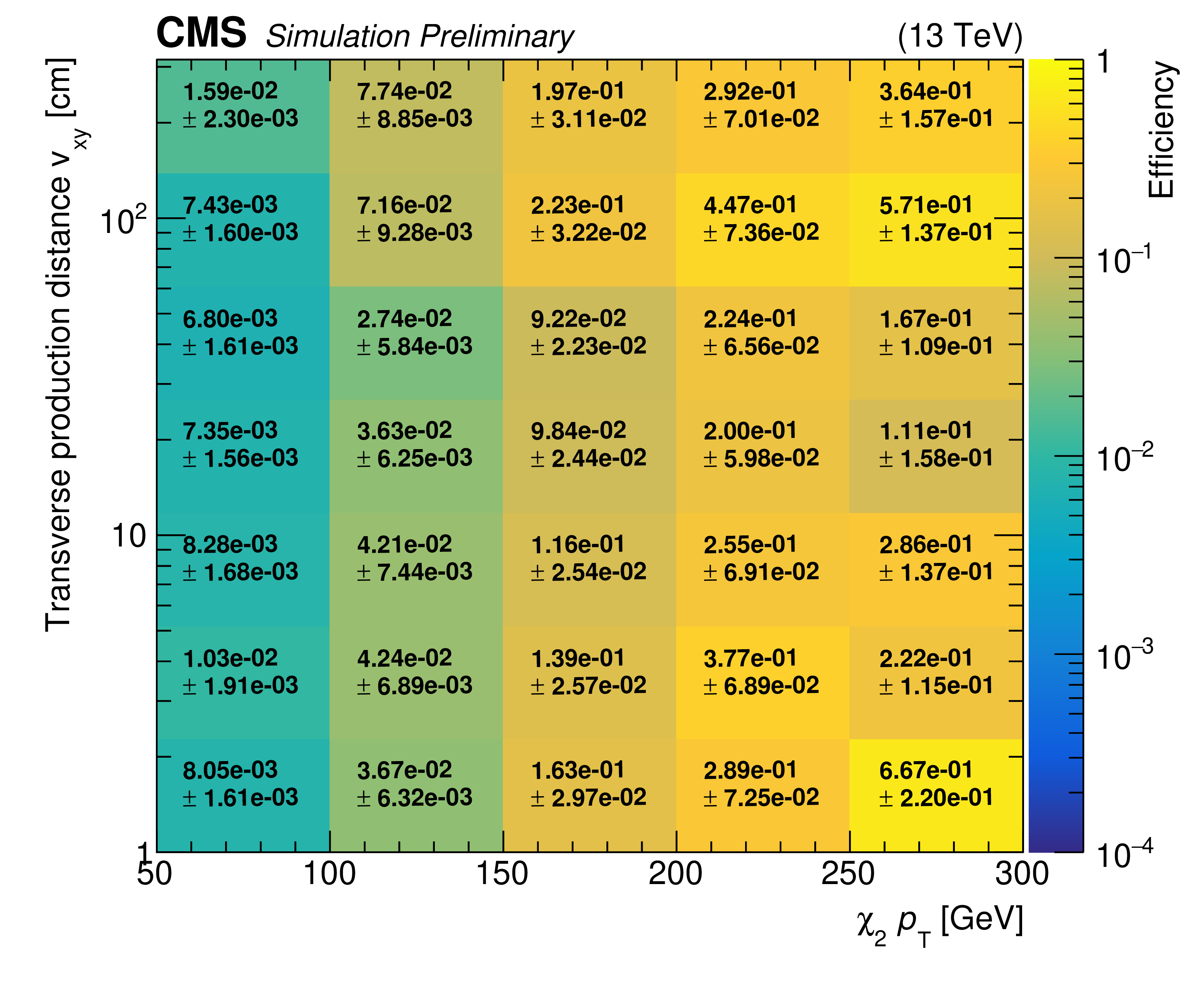
Additional Figure 8-a:
Signal efficiency versus generated $ \chi_2 p_{\mathrm{T}} $ and decay transverse position $ v_{xy} $ for an inelastic dark matter model with $ m_1 = $ 50 GeV and $ \Delta = 0.4 \, m_1 $, before splitting into muon match categories. Upper: $ \chi_2 |\eta| < $ 1.2. Lower: $ \chi_2 |\eta| > $ 1.2. The efficiency is calculated after application of generator filters. |
png pdf |
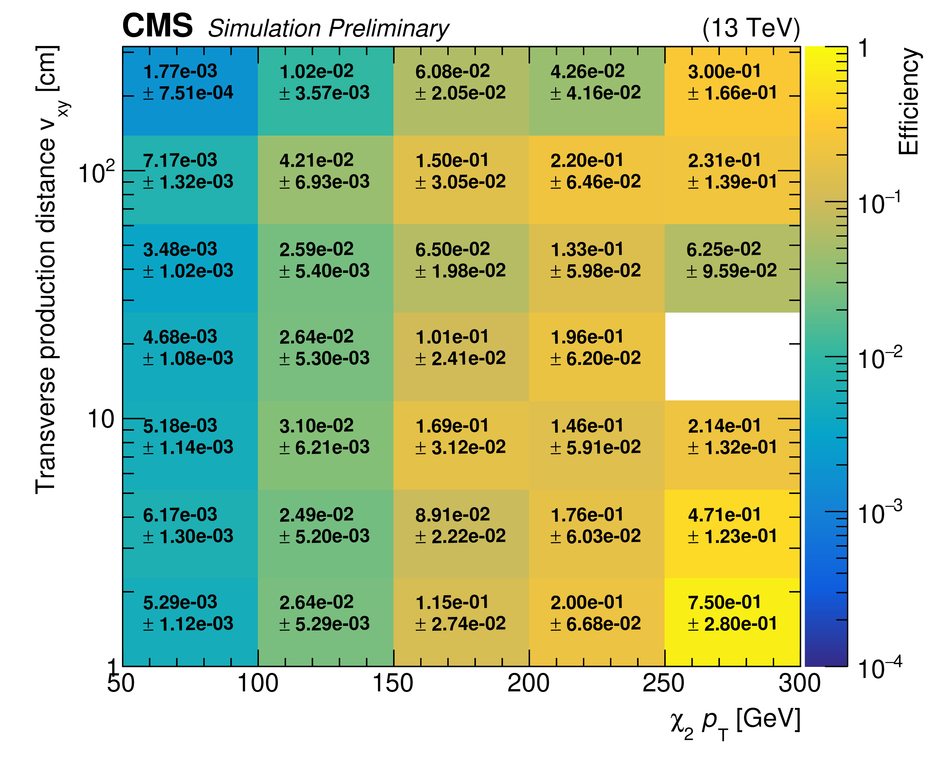
Additional Figure 8-b:
Signal efficiency versus generated $ \chi_2 p_{\mathrm{T}} $ and decay transverse position $ v_{xy} $ for an inelastic dark matter model with $ m_1 = $ 50 GeV and $ \Delta = 0.4 \, m_1 $, before splitting into muon match categories. Upper: $ \chi_2 |\eta| < $ 1.2. Lower: $ \chi_2 |\eta| > $ 1.2. The efficiency is calculated after application of generator filters. |

png pdf |
Additional Figure 9:
Signal efficiency versus generated $ \chi_2 p_{\mathrm{T}} $ and decay transverse position $ v_{xy} $ for an inelastic dark matter model with $ m_1 = $ 5 GeV and $ \Delta = 0.1 \, m_1 $, before splitting into muon match categories. Upper: $ \chi_2 |\eta| < $ 1.2. Lower: $ \chi_2 |\eta| > $ 1.2. The efficiency is calculated after application of generator filters. |
png pdf |
Additional Figure 9-a:
Signal efficiency versus generated $ \chi_2 p_{\mathrm{T}} $ and decay transverse position $ v_{xy} $ for an inelastic dark matter model with $ m_1 = $ 5 GeV and $ \Delta = 0.1 \, m_1 $, before splitting into muon match categories. Upper: $ \chi_2 |\eta| < $ 1.2. Lower: $ \chi_2 |\eta| > $ 1.2. The efficiency is calculated after application of generator filters. |
png pdf |
Additional Figure 9-b:
Signal efficiency versus generated $ \chi_2 p_{\mathrm{T}} $ and decay transverse position $ v_{xy} $ for an inelastic dark matter model with $ m_1 = $ 5 GeV and $ \Delta = 0.1 \, m_1 $, before splitting into muon match categories. Upper: $ \chi_2 |\eta| < $ 1.2. Lower: $ \chi_2 |\eta| > $ 1.2. The efficiency is calculated after application of generator filters. |
png pdf |
Additional Figure 10:
Signal efficiency versus generated $ \chi_2 p_{\mathrm{T}} $ and decay transverse position $ v_{xy} $ for an inelastic dark matter model with $ m_1 = $ 5 GeV and $ \Delta = 0.4 \, m_1 $, before splitting into muon match categories. Upper: $ \chi_2 |\eta| < $ 1.2. Lower: $ \chi_2 |\eta| > $ 1.2. The efficiency is calculated after application of generator filters. |
png pdf |
Additional Figure 10-a:
Signal efficiency versus generated $ \chi_2 p_{\mathrm{T}} $ and decay transverse position $ v_{xy} $ for an inelastic dark matter model with $ m_1 = $ 5 GeV and $ \Delta = 0.4 \, m_1 $, before splitting into muon match categories. Upper: $ \chi_2 |\eta| < $ 1.2. Lower: $ \chi_2 |\eta| > $ 1.2. The efficiency is calculated after application of generator filters. |
png pdf |
Additional Figure 10-b:
Signal efficiency versus generated $ \chi_2 p_{\mathrm{T}} $ and decay transverse position $ v_{xy} $ for an inelastic dark matter model with $ m_1 = $ 5 GeV and $ \Delta = 0.4 \, m_1 $, before splitting into muon match categories. Upper: $ \chi_2 |\eta| < $ 1.2. Lower: $ \chi_2 |\eta| > $ 1.2. The efficiency is calculated after application of generator filters. |

png pdf |
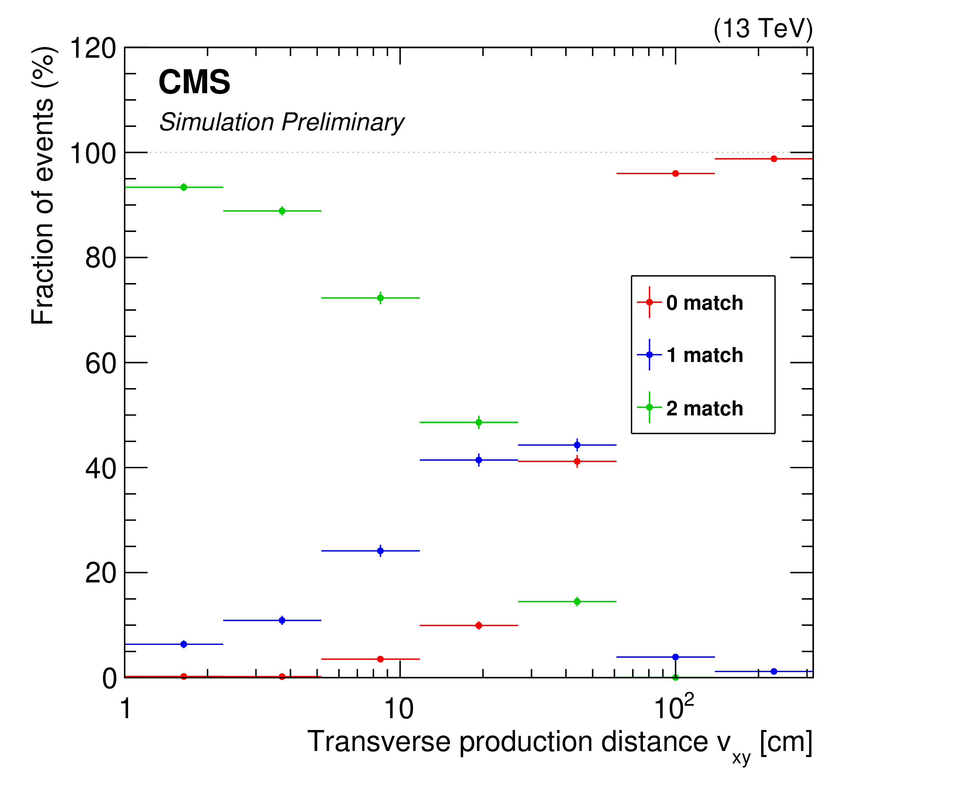
Additional Figure 11:
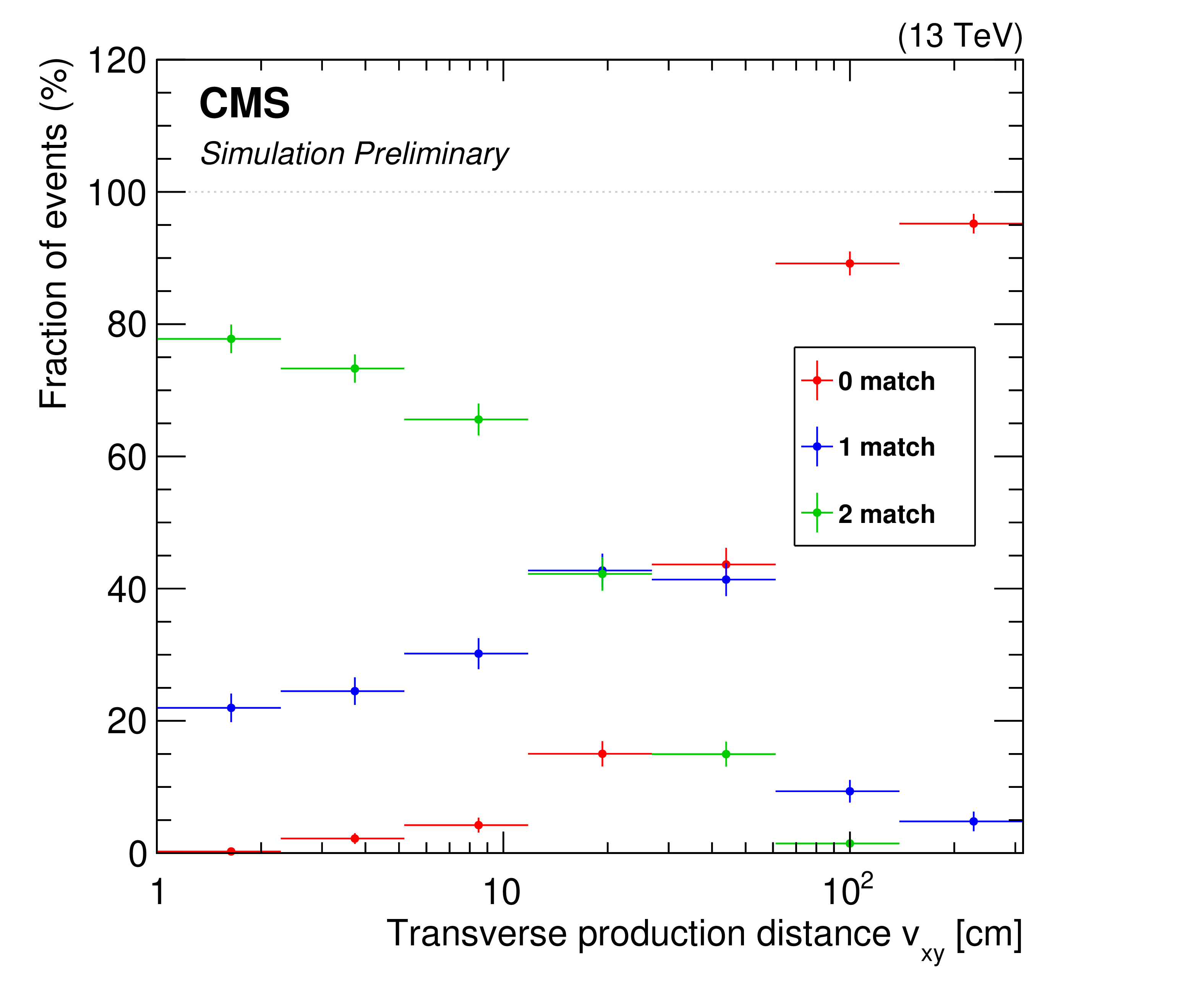
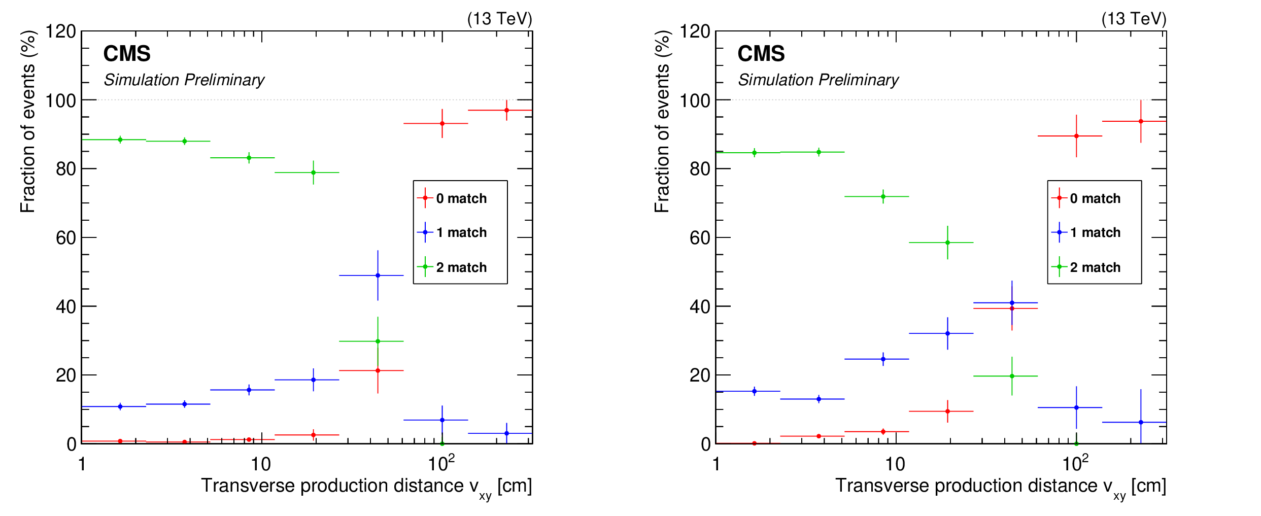
Fraction of events in each muon match category versus generated $ \chi_2 $ decay transverse position $ v_{xy} $ for an inelastic dark matter model with $ m_1 = $ 50 GeV and $ \Delta = 0.4 \, m_1 $. Left: $ \chi_2 |\eta| < $ 1.2. Right: $ \chi_2 |\eta| > $ 1.2. Other observables such as $ \Delta R(\mu\mu) $ have a subdominant impact on the matching distribution and are therefore not reported here. |
png pdf |
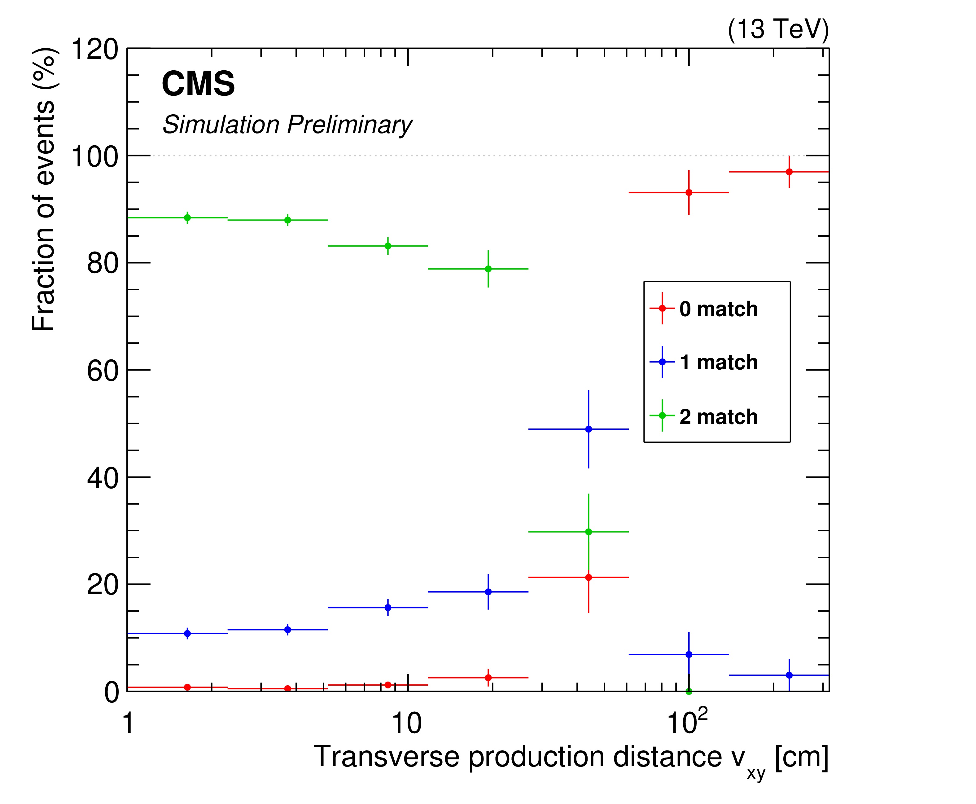
Additional Figure 11-a:
Fraction of events in each muon match category versus generated $ \chi_2 $ decay transverse position $ v_{xy} $ for an inelastic dark matter model with $ m_1 = $ 50 GeV and $ \Delta = 0.4 \, m_1 $. Left: $ \chi_2 |\eta| < $ 1.2. Right: $ \chi_2 |\eta| > $ 1.2. Other observables such as $ \Delta R(\mu\mu) $ have a subdominant impact on the matching distribution and are therefore not reported here. |
png pdf |
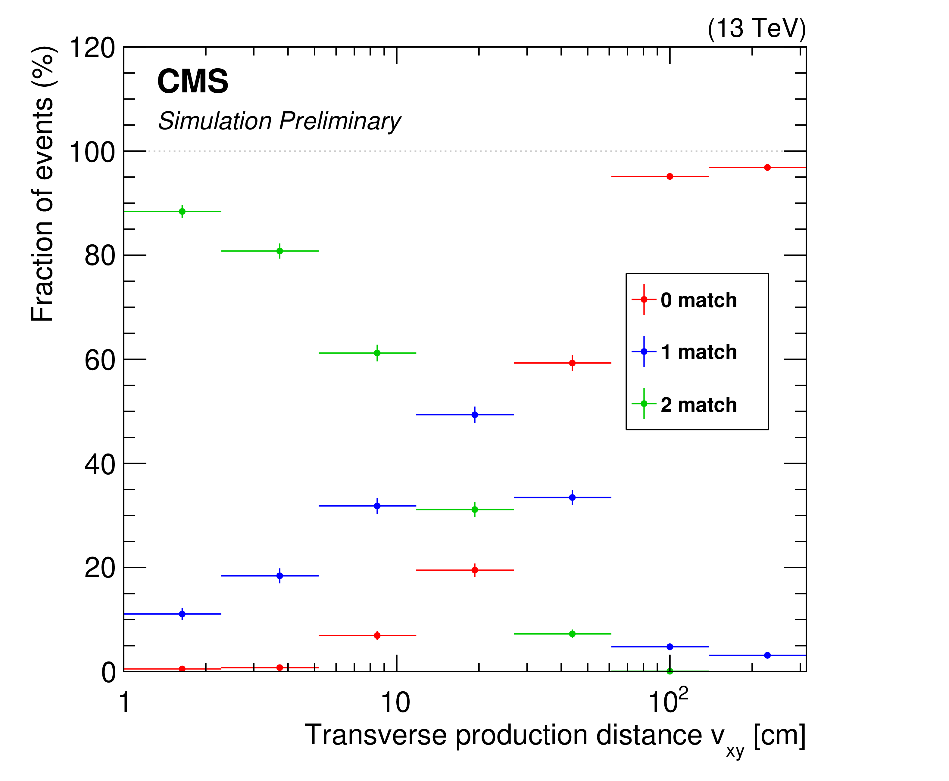
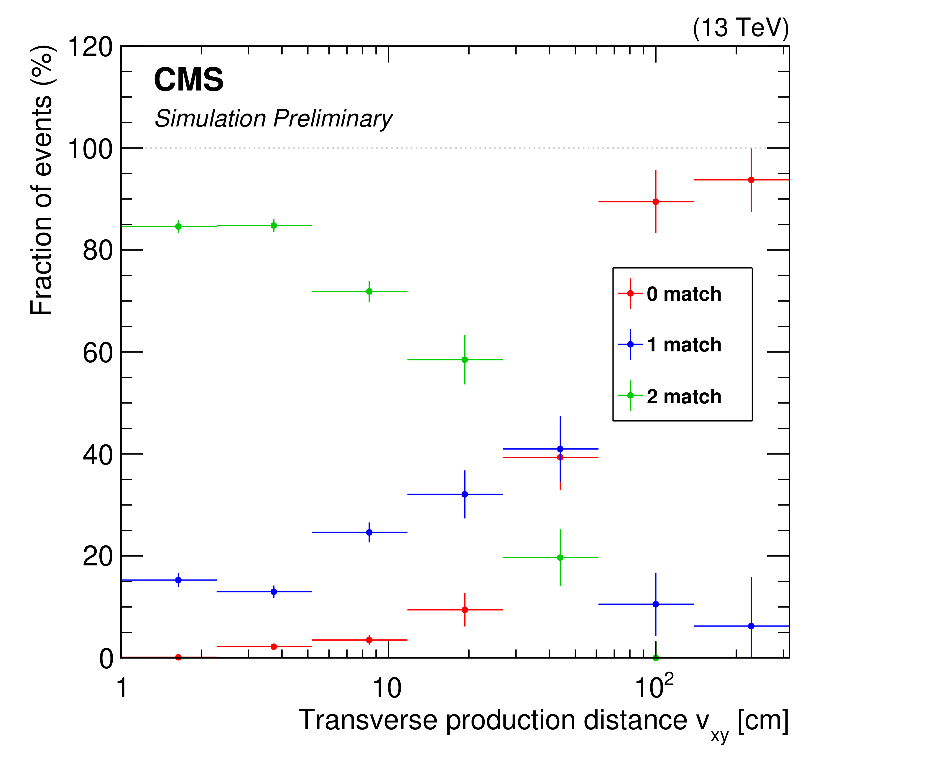
Additional Figure 11-b:
Fraction of events in each muon match category versus generated $ \chi_2 $ decay transverse position $ v_{xy} $ for an inelastic dark matter model with $ m_1 = $ 50 GeV and $ \Delta = 0.4 \, m_1 $. Left: $ \chi_2 |\eta| < $ 1.2. Right: $ \chi_2 |\eta| > $ 1.2. Other observables such as $ \Delta R(\mu\mu) $ have a subdominant impact on the matching distribution and are therefore not reported here. |
png pdf |
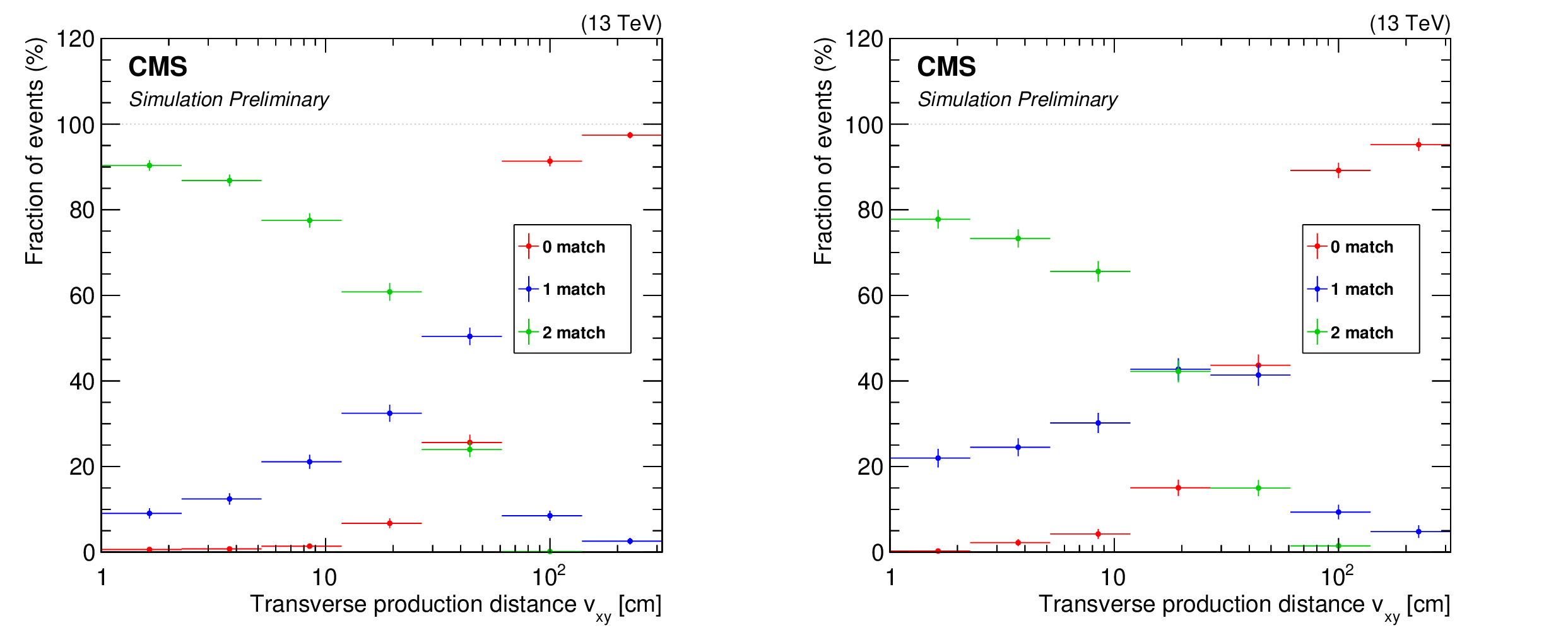
Additional Figure 12:
Fraction of events in each muon match category versus generated $ \chi_2 $ decay transverse position $ v_{xy} $ for an inelastic dark matter model with $ m_1 = $ 50 GeV and $ \Delta = 0.1 \, m_1 $. Left: $ \chi_2 |\eta| < $ 1.2. Right: $ \chi_2 |\eta| > $ 1.2. Other observables such as $ \Delta R(\mu\mu) $ have a subdominant impact on the matching distribution and are therefore not reported here. |
png pdf |
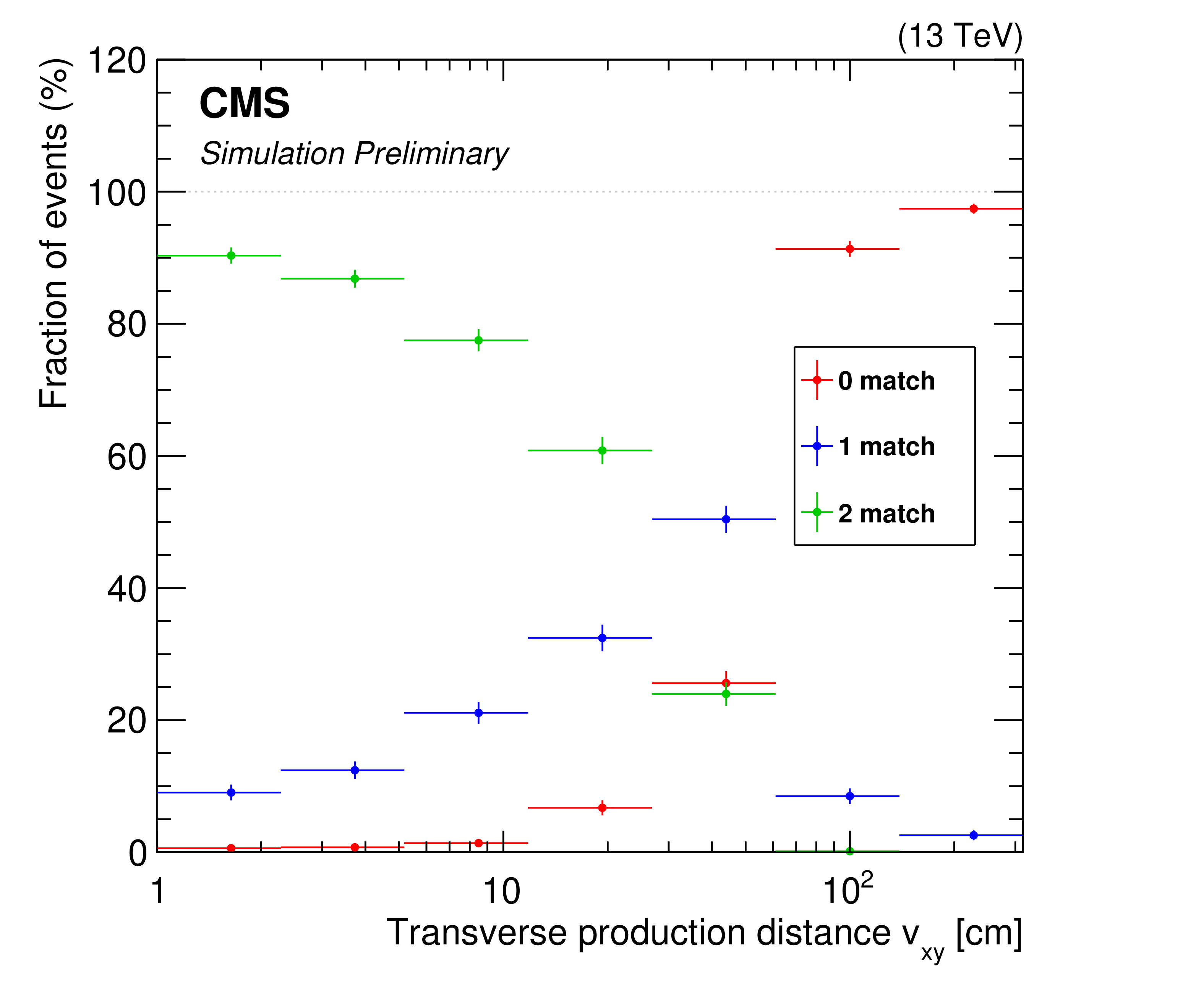
Additional Figure 12-a:
Fraction of events in each muon match category versus generated $ \chi_2 $ decay transverse position $ v_{xy} $ for an inelastic dark matter model with $ m_1 = $ 50 GeV and $ \Delta = 0.1 \, m_1 $. Left: $ \chi_2 |\eta| < $ 1.2. Right: $ \chi_2 |\eta| > $ 1.2. Other observables such as $ \Delta R(\mu\mu) $ have a subdominant impact on the matching distribution and are therefore not reported here. |
png pdf |
Additional Figure 12-b:
Fraction of events in each muon match category versus generated $ \chi_2 $ decay transverse position $ v_{xy} $ for an inelastic dark matter model with $ m_1 = $ 50 GeV and $ \Delta = 0.1 \, m_1 $. Left: $ \chi_2 |\eta| < $ 1.2. Right: $ \chi_2 |\eta| > $ 1.2. Other observables such as $ \Delta R(\mu\mu) $ have a subdominant impact on the matching distribution and are therefore not reported here. |
png pdf |
Additional Figure 13:
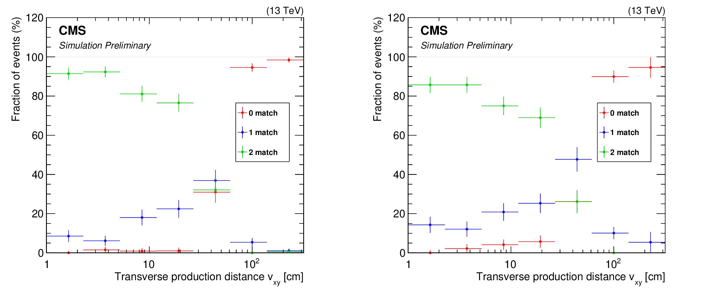
Fraction of events in each muon match category versus generated $ \chi_2 $ decay transverse position $ v_{xy} $ for an inelastic dark matter model with $ m_1 = $ 5 GeV and $ \Delta = 0.4 \, m_1 $. Left: $ \chi_2 |\eta| < $ 1.2. Right: $ \chi_2 |\eta| > $ 1.2. Other observables such as $ \Delta R(\mu\mu) $ have a subdominant impact on the matching distribution and are therefore not reported here. |
png pdf |
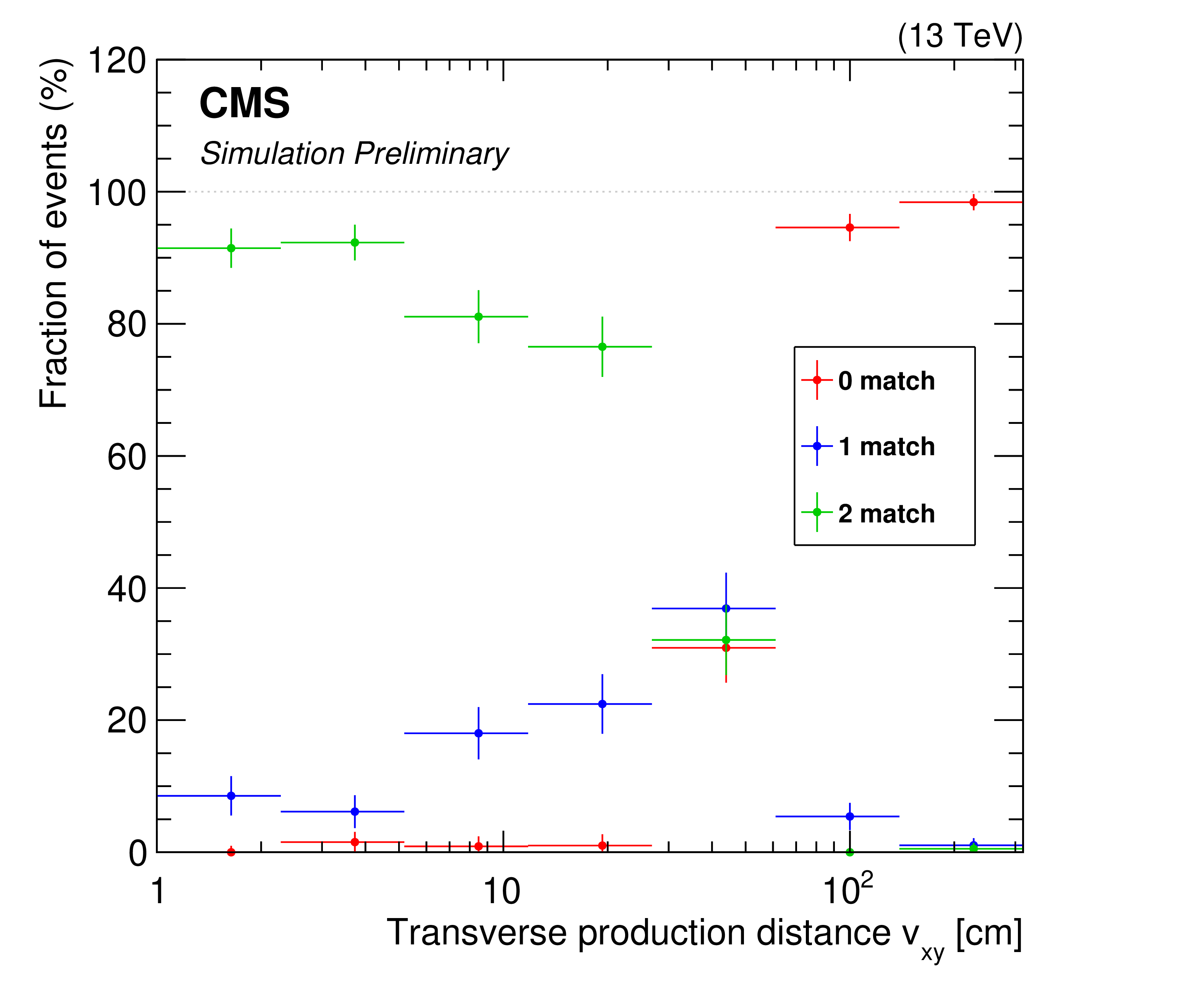
Additional Figure 13-a:
Fraction of events in each muon match category versus generated $ \chi_2 $ decay transverse position $ v_{xy} $ for an inelastic dark matter model with $ m_1 = $ 5 GeV and $ \Delta = 0.4 \, m_1 $. Left: $ \chi_2 |\eta| < $ 1.2. Right: $ \chi_2 |\eta| > $ 1.2. Other observables such as $ \Delta R(\mu\mu) $ have a subdominant impact on the matching distribution and are therefore not reported here. |
png pdf |
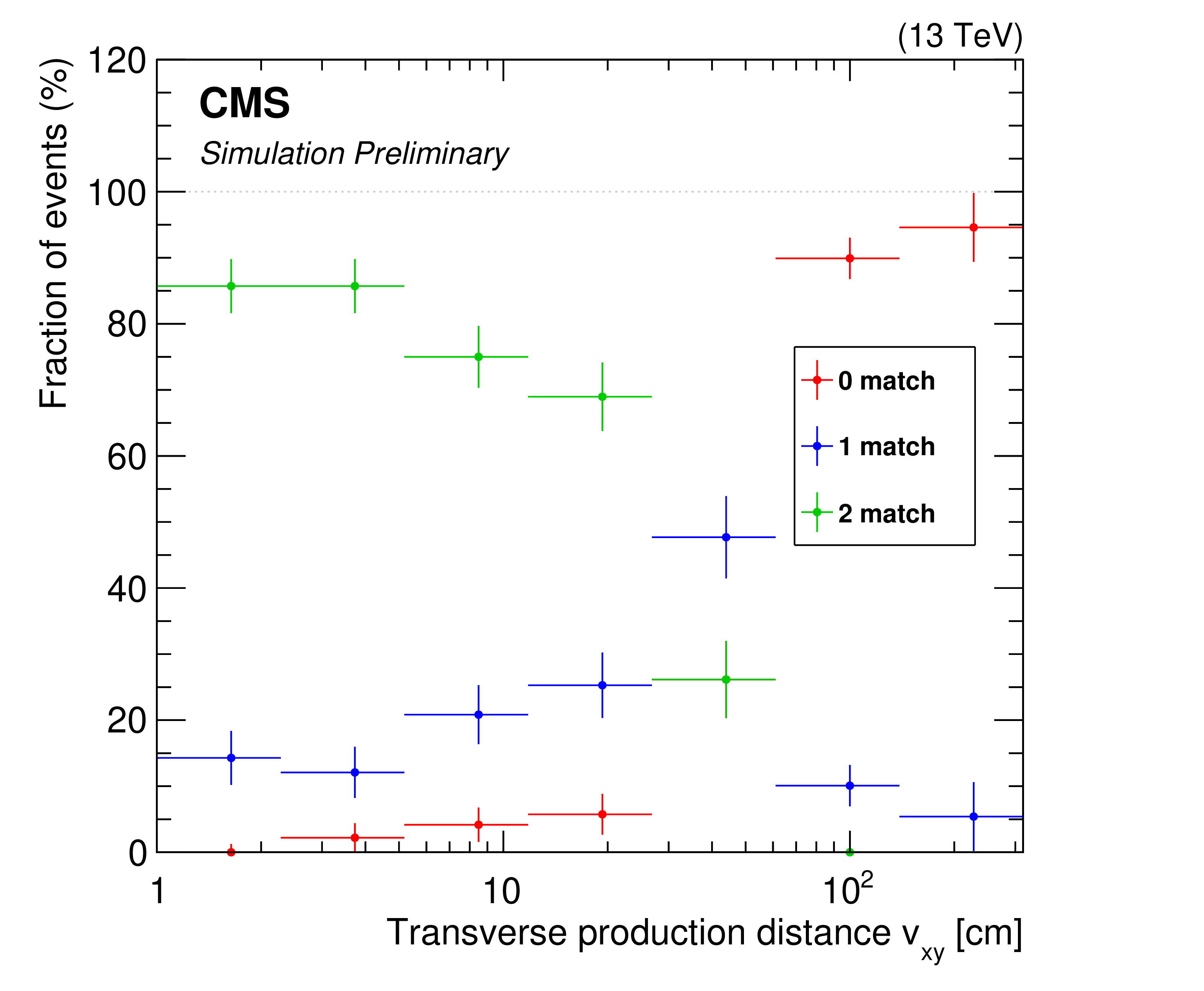
Additional Figure 13-b:
Fraction of events in each muon match category versus generated $ \chi_2 $ decay transverse position $ v_{xy} $ for an inelastic dark matter model with $ m_1 = $ 5 GeV and $ \Delta = 0.4 \, m_1 $. Left: $ \chi_2 |\eta| < $ 1.2. Right: $ \chi_2 |\eta| > $ 1.2. Other observables such as $ \Delta R(\mu\mu) $ have a subdominant impact on the matching distribution and are therefore not reported here. |
png pdf |
Additional Figure 14:
Fraction of events in each muon match category versus generated $ \chi_2 $ decay transverse position $ v_{xy} $ for an inelastic dark matter model with $ m_1 = $ 5 GeV and $ \Delta = 0.1 \, m_1 $. Left: $ \chi_2 |\eta| < $ 1.2. Right: $ \chi_2 |\eta| > $ 1.2. Other observables such as $ \Delta R(\mu\mu) $ have a subdominant impact on the matching distribution and are therefore not reported here. |
png pdf |
Additional Figure 14-a:
Fraction of events in each muon match category versus generated $ \chi_2 $ decay transverse position $ v_{xy} $ for an inelastic dark matter model with $ m_1 = $ 5 GeV and $ \Delta = 0.1 \, m_1 $. Left: $ \chi_2 |\eta| < $ 1.2. Right: $ \chi_2 |\eta| > $ 1.2. Other observables such as $ \Delta R(\mu\mu) $ have a subdominant impact on the matching distribution and are therefore not reported here. |
png pdf |
Additional Figure 14-b:
Fraction of events in each muon match category versus generated $ \chi_2 $ decay transverse position $ v_{xy} $ for an inelastic dark matter model with $ m_1 = $ 5 GeV and $ \Delta = 0.1 \, m_1 $. Left: $ \chi_2 |\eta| < $ 1.2. Right: $ \chi_2 |\eta| > $ 1.2. Other observables such as $ \Delta R(\mu\mu) $ have a subdominant impact on the matching distribution and are therefore not reported here. |
png pdf |
Additional Figure 15:
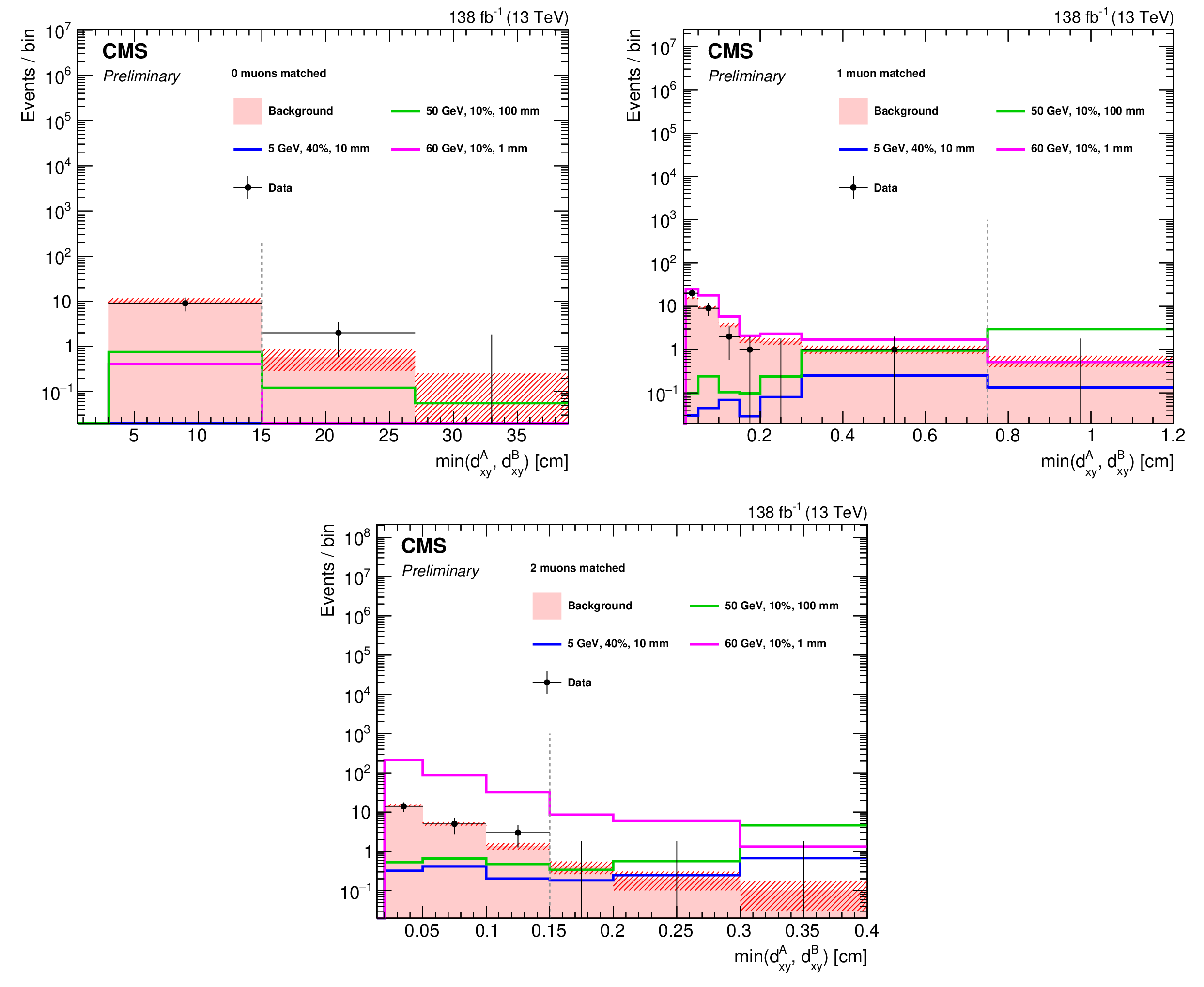
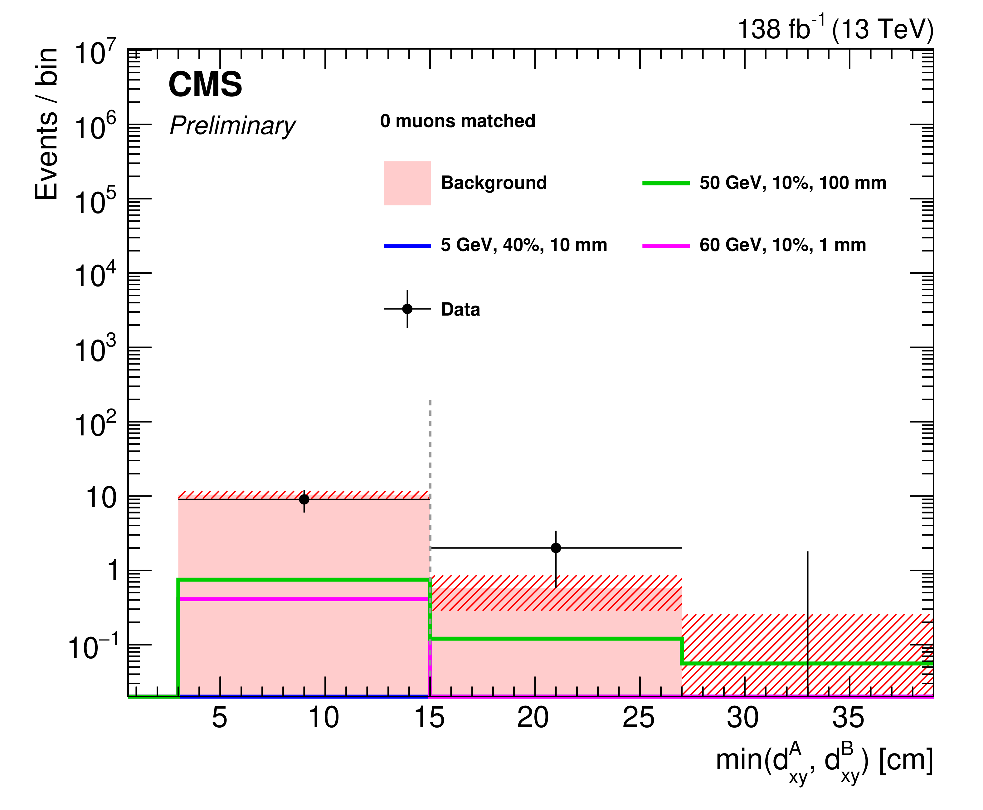
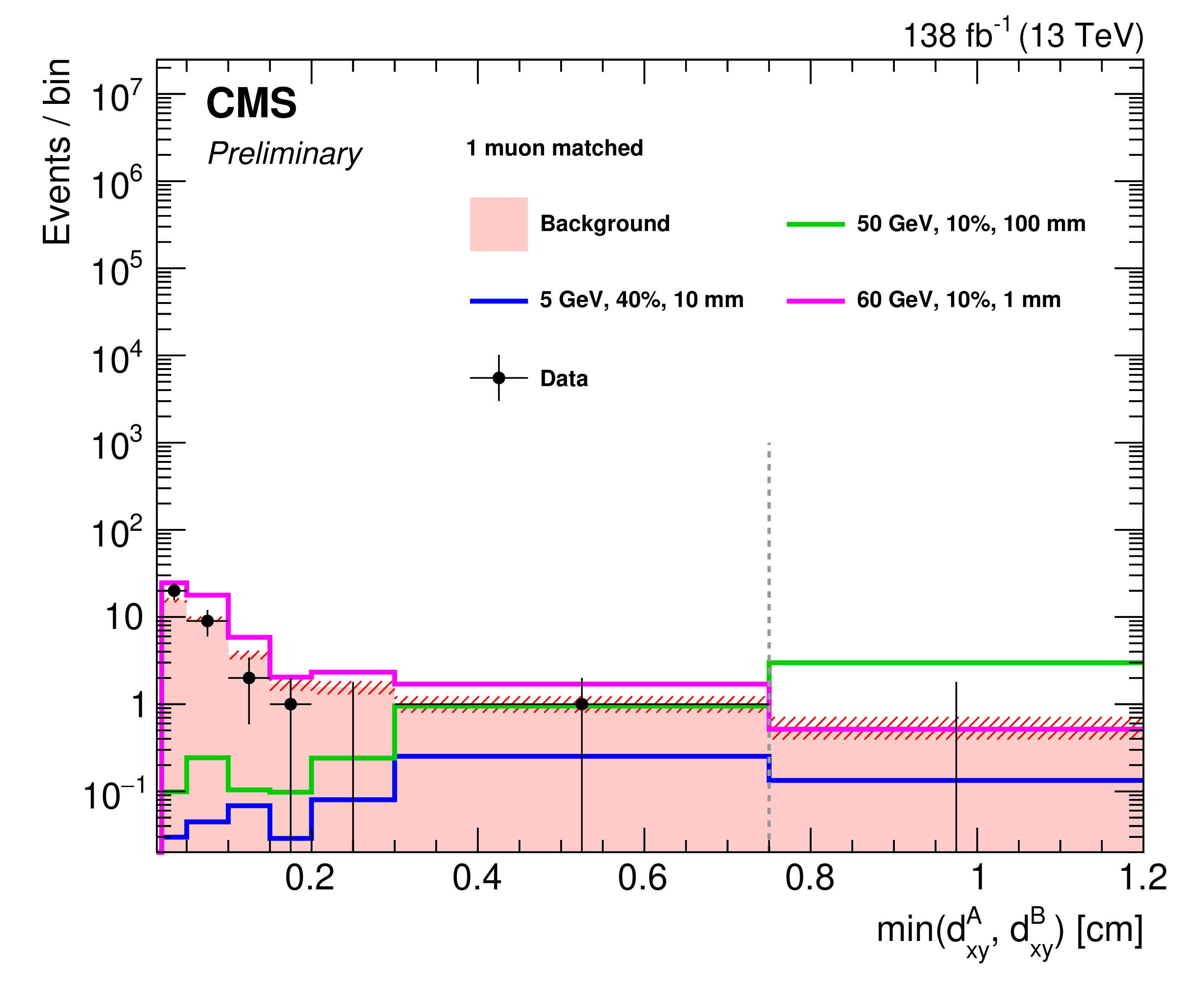
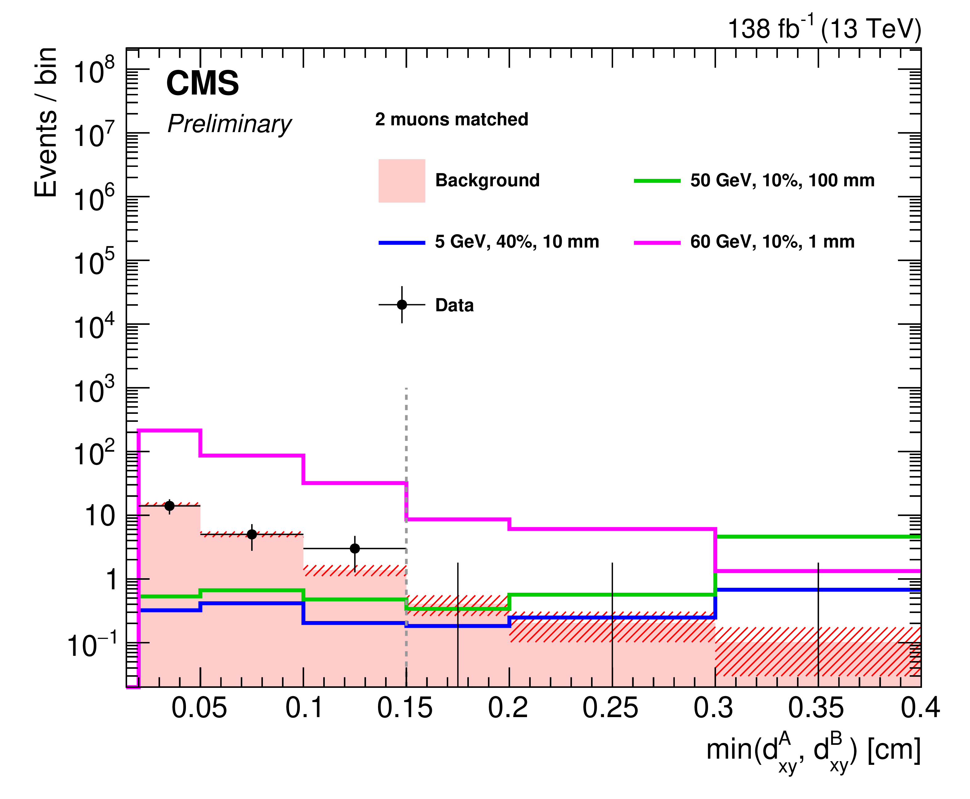
Measured distributions of min-$d_{xy}$ in the 0-match category (upper left), 1-match category (upper right), and 2-match category (lower) in the signal-enriched region of the ABCD plane. Events must pass $I^{\text{rel}}_{\text{PF}}$ requirements in the 1- and 2-match categories and the $\Delta\phi_{\mu\mu}^{\text{MET}}$ requirement in the 0-match category. The shapes of the background prediction (filled red histograms) are extracted from the remaining region of the ABCD plane and normalized to the signal-enriched yields. Benchmark signal hypotheses are also shown. Vertical dashed gray lines define the most signal-sensitive ABCD bins. The last bin contains the overflow events. |
png pdf |
Additional Figure 15-a:
Measured distribution of min-$d_{xy}$ in the 0-match category in the signal-enriched region of the ABCD plane. Events must pass $\Delta\phi_{\mu\mu}^{\text{MET}}$ requirement. The shapes of the background prediction (filled red histograms) are extracted from the remaining region of the ABCD plane and normalized to the signal-enriched yields. Benchmark signal hypotheses are also shown. Vertical dashed gray lines define the most signal-sensitive ABCD bins. The last bin contains the overflow events. |
png pdf |
Additional Figure 15-b:
Measured distribution of min-$d_{xy}$ in the 1-match category in the signal-enriched region of the ABCD plane. Events must pass $I^{\text{rel}}_{\text{PF}}$ requirements. The shapes of the background prediction (filled red histograms) are extracted from the remaining region of the ABCD plane and normalized to the signal-enriched yields. Benchmark signal hypotheses are also shown. Vertical dashed gray lines define the most signal-sensitive ABCD bins. The last bin contains the overflow events. |
png pdf |
Additional Figure 15-c:
Measured distribution of min-$d_{xy}$ in the 2-match category in the signal-enriched region of the ABCD plane. Events must pass $I^{\text{rel}}_{\text{PF}}$ requirements. The shapes of the background prediction (filled red histograms) are extracted from the remaining region of the ABCD plane and normalized to the signal-enriched yields. Benchmark signal hypotheses are also shown. Vertical dashed gray lines define the most signal-sensitive ABCD bins. The last bin contains the overflow events. |
| Additional Tables | |
png pdf |
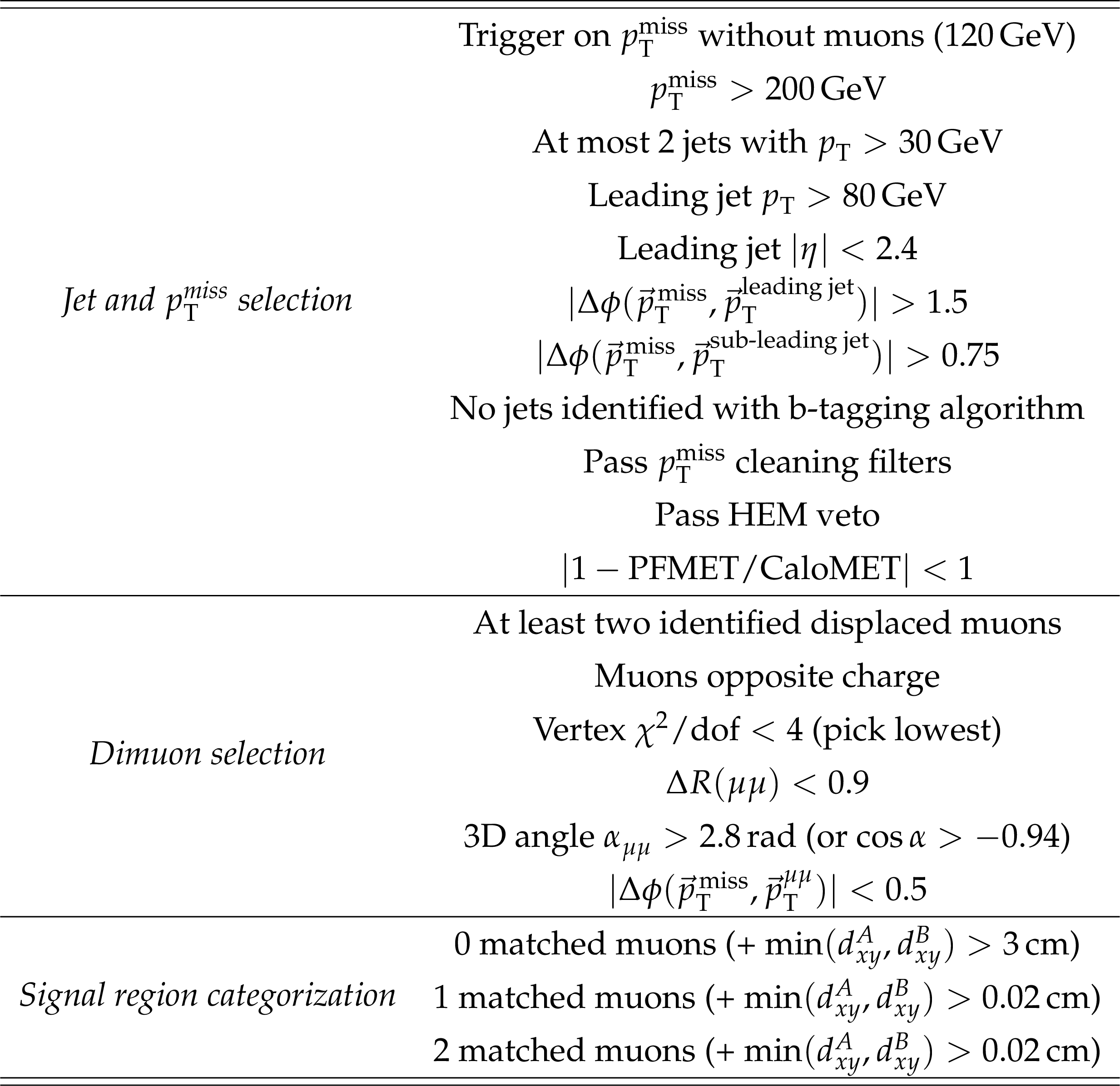
Additional Table 1:
Summary of the selection used to define the signal region. |

png pdf |
Additional Table 2:
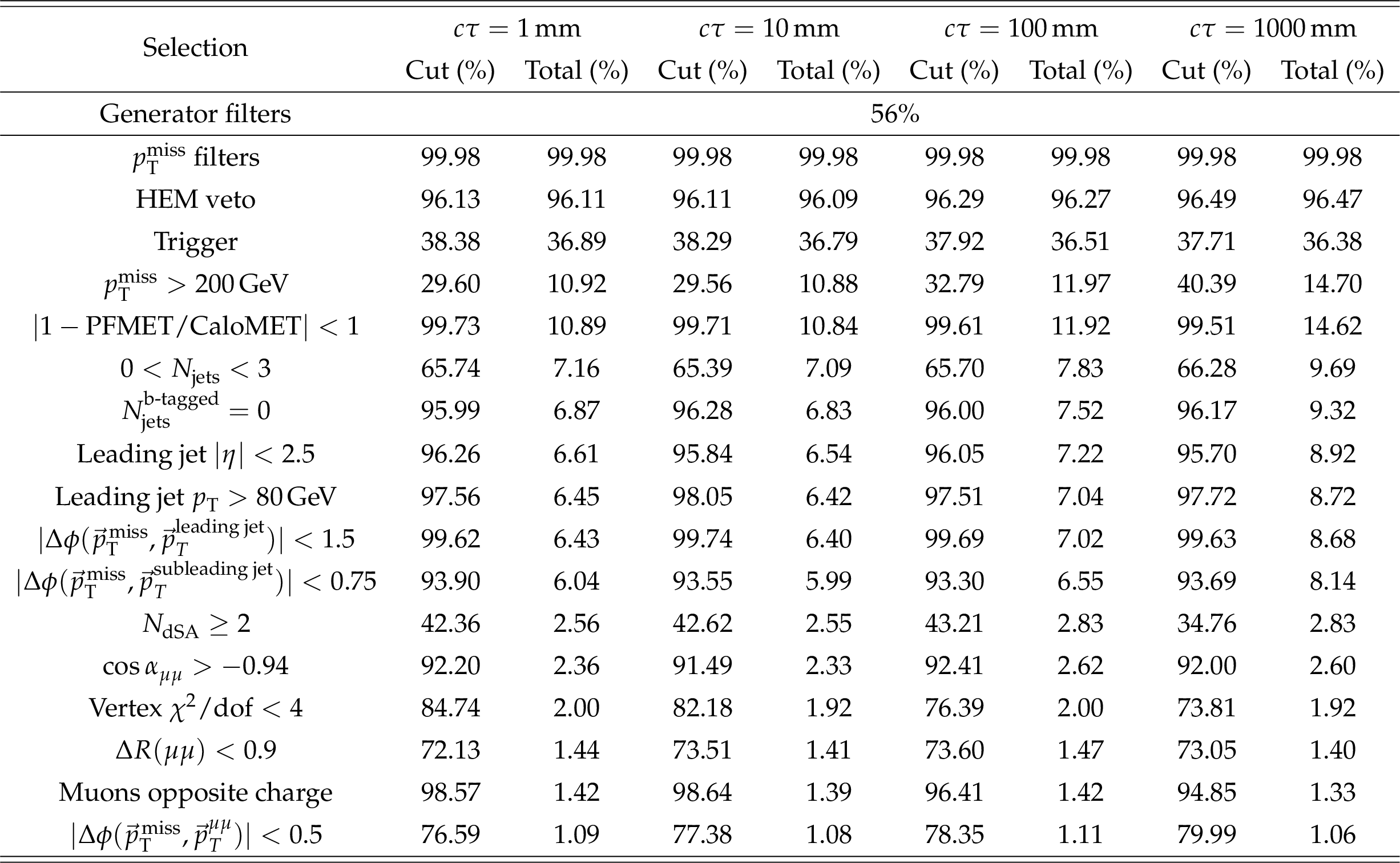
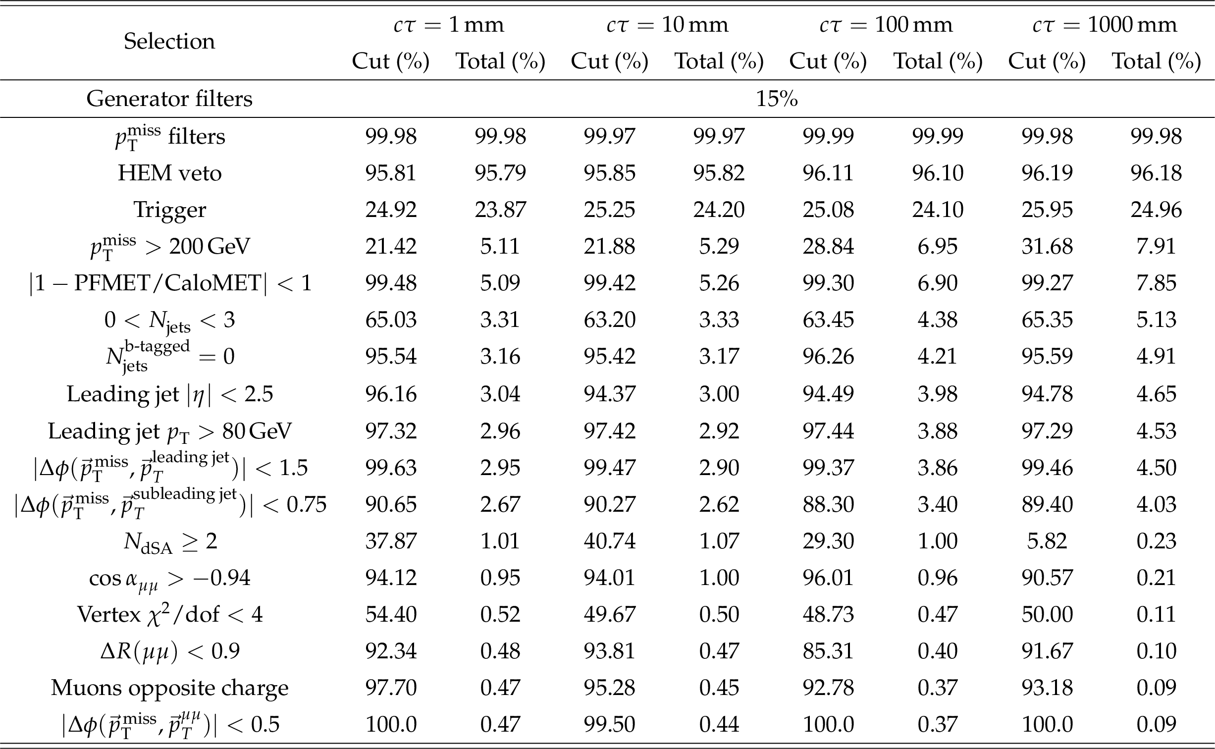
Selection efficiencies for iDM with $ m_1 = $ 5 GeV and $ \Delta = 0.1 \, m_1 $. |
png pdf |
Additional Table 3:
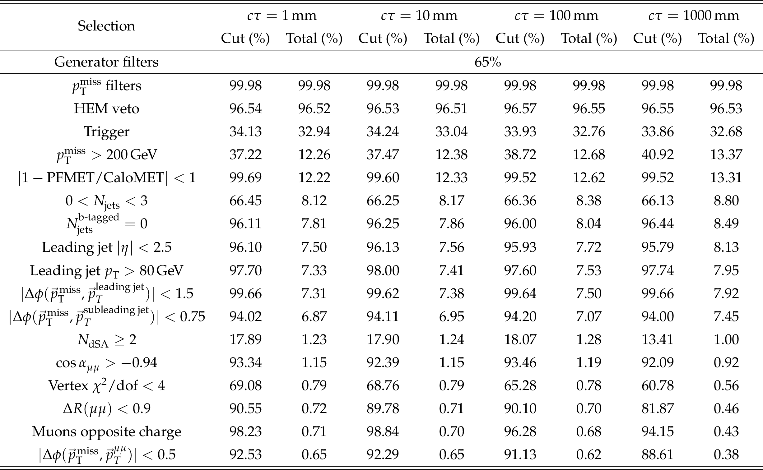
Selection efficiencies for iDM with $ m_1 = $ 50 GeV and $ \Delta = 0.4 \, m_1 $. |
png pdf |
Additional Table 4:
Selection efficiencies for iDM with $ m_1 = $ 5 GeV and $ \Delta = 0.4 \, m_1 $. |
png pdf |
Additional Table 5:
Selection efficiencies for iDM with $ m_1 = $ 50 GeV and $ \Delta = 0.1 \, m_1 $. |
png pdf |
Additional Table 6:
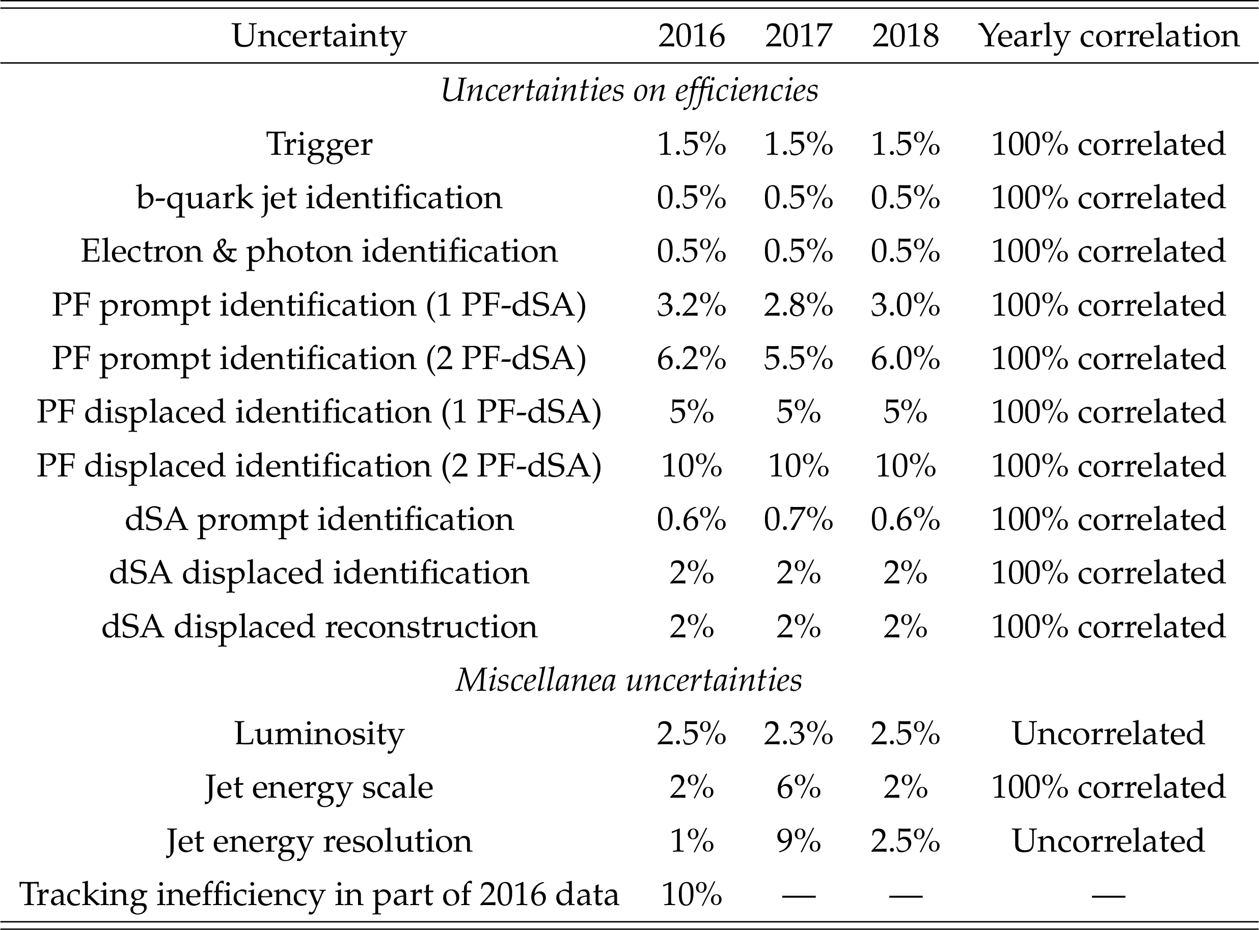
Summary of the systematic uncertainties in the analysis. All uncertainties are applied to signal yields independently of the bin in the ABCD plane. |
| References | ||||
| 1 | D. Clowe, A. Gonzalez, and M. Markevitch | Weak-lensing mass reconstruction of the interacting cluster 1e 0657-558: Direct evidence for the existence of dark matter | ApJ 604 (2004) 596 | astro-ph/0312273 |
| 2 | Planck Collaboration | Planck 2015 results. XIII. Cosmological parameters | A\&A 594 A13, 2016 | 1502.01589 |
| 3 | E. Komatsu et al. | Five-Year Wilkinson Microwave Anisotropy Probe Observations: Cosmological Interpretation | ApJS 180 (2009) 330 | 0803.0547 |
| 4 | XENON Collaboration | Search for inelastic scattering of WIMP dark matter in XENON1T | PRD 103 (2021) 063028 | 2011.10431 |
| 5 | Fermi-LAT Collaboration | Searching for dark matter annihilation from milky way dwarf spheroidal galaxies with six years of Fermi Large Area Telescope data | PRL 115 (2015) 231301 | 1503.02641 |
| 6 | SuperCDMS Collaboration | Search for low-mass weakly interacting massive particles with SuperCDMS | PRL 112 (2014) 241302 | 1402.7137 |
| 7 | LUX Collaboration | Results from a search for dark matter in the complete lux exposure | PRL 118 (2017) 021303 | 1608.07648 |
| 8 | ATLAS Collaboration | Search for new phenomena in events with an energetic jet and missing transverse momentum in $ pp $ collisions at $ \sqrt{s}=$ 13 TeV with the ATLAS detector | PRD 103 (2021) 112006 | 2102.10874 |
| 9 | CMS Collaboration | Search for new particles in events with energetic jets and large missing transverse momentum in proton-proton collisions at $ \sqrt{s} = $ 13 TeV | JHEP 11 (2021) 153 | CMS-EXO-20-004 2107.13021 |
| 10 | J. Alimena et al. | Searching for long-lived particles beyond the Standard Model at the Large Hadron Collider | JPG 47 (2020) 090501 | 1903.04497 |
| 11 | ATLAS Collaboration | Search for light long-lived neutral particles produced in $ pp $ collisions at $ \sqrt{s} = $ 13 TeV and decaying into collimated leptons or light hadrons with the ATLAS detector | EPJC 80 (2020) 450 | 1909.01246 |
| 12 | E. Izaguirre, G. Krnjaic, and B. Shuve | Discovering inelastic thermal-relic dark matter at colliders | PRD 93 (2016) 063523 | 1508.03050 |
| 13 | A. Berlin and F. Kling | Inelastic dark matter at the LHC lifetime frontier: ATLAS, CMS, LHCb, CODEX-b, FASER, and MATHUSLA | PRD 99 (2019) 015021 | 1810.01879 |
| 14 | B. Holdom | Two U(1)'s and Epsilon Charge Shifts | PLB 166 (1986) 196 | |
| 15 | CMS Collaboration | Search for dark matter produced with an energetic jet or a hadronically decaying W or Z boson at $ \sqrt{s}= $ 13 TeV | JHEP 07 (2017) 14 | CMS-EXO-16-037 1703.01651 |
| 16 | ATLAS Collaboration | Constraints on mediator-based dark matter and scalar dark energy models using $ \sqrt{s} = $ 13 TeV pp collision data collected by the ATLAS detector | JHEP 05 (2019) 142 | 1903.01400 |
| 17 | CMS Collaboration | The CMS experiment at the CERN LHC | JINST 3 (2008) S08004 | |
| 18 | CMS Collaboration | Particle-flow reconstruction and global event description with the CMS detector | JINST 12 (2017) P10003 | CMS-PRF-14-001 1706.04965 |
| 19 | J. Alwall et al. | The automated computation of tree-level and next-to-leading order differential cross sections, and their matching to parton shower simulations | JHEP 07 (2014) 079 | 1405.0301 |
| 20 | J. Alwall et al. | Comparative study of various algorithms for the merging of parton showers and matrix elements in hadronic collisions | EPJC 53 (2007) 473 | 0706.2569 |
| 21 | T. Sjöstrand et al. | An introduction to PYTHIA 8.2 | Comput. Phys. Commun. 191 (2015) 159 | 1410.3012 |
| 22 | CMS Collaboration | Event generator tunes obtained from underlying event and multiparton scattering measurements | EPJC 76 (2016) 155 | CMS-GEN-14-001 1512.00815 |
| 23 | CMS Collaboration | Extraction and validation of a new set of CMS PYTHIA8 tunes from underlying-event measurements | EPJC 80 (2020) 4 | CMS-GEN-17-001 1903.12179 |
| 24 | R. D. Ball et al. | Parton distributions for the LHC run II | JHEP 04 (2015) 40 | 1410.8849 |
| 25 | R. D. Ball et al. | Parton distributions from high-precision collider data | EPJC 77 (2017) 663 | 1706.00428 |
| 26 | GEANT4 Collaboration | GEANT 4--a simulation toolkit | NIM A 506 (2003) 250 | |
| 27 | CMS Collaboration | Identification of heavy-flavour jets with the CMS detector in pp collisions at 13 TeV | JINST 13 (2017) P05011 | CMS-BTV-16-002 1712.07158 |
| 28 | CMS Collaboration | B-tagging performance of the CMS Legacy dataset 2018. | CMS Detector Performance Note CMS-DP-2021-004, 2021 CDS |
|
| 29 | CMS Collaboration | Performance of missing transverse momentum reconstruction in proton-proton collisions at s = 13 TeV using the CMS detector | JINST 14 (2019) P07004 | CMS-JME-17-001 1903.06078 |
| 30 | CMS Collaboration | The CMS muon system in Run2: Preparation, status and first results | Technical Report CMS CR-2015/237, INFN Bologna, 2015 link |
1510.05424 |
| 31 | CMS Collaboration | Search for decays of stopped exotic long-lived particles produced in proton-proton collisions at $ \sqrt{s}= $ 13 TeV | JHEP 05 (2018) 127 | CMS-EXO-16-004 1801.00359 |
| 32 | CMS Collaboration | Performance of the CMS muon detector and muon reconstruction with proton-proton collisions at $ \sqrt{s} = $ 13 TeV | JINST 13 (2018) P06015 | CMS-MUO-16-001 1804.04528 |
| 33 | R. Frühwirth | Application of Kalman filtering to track and vertex fitting | NIM A 262 (1987) 444 | |
| 34 | CMS Collaboration | Search for long-lived particles using delayed photons in proton-proton collisions at $ \sqrt{s} = $ 13 TeV | PRD 100 (2019) 112003 | CMS-EXO-19-005 1909.06166 |
| 35 | CMS Collaboration | CMS luminosity measurements for the 2016 data taking period | CMS Physics Analysis Summary, 2017 CMS-PAS-LUM-17-001 |
CMS-PAS-LUM-17-001 |
| 36 | CMS Collaboration | CMS luminosity measurement for the 2017 data-taking period at $ \sqrt{s} = $ 13 TeV | CMS Physics Analysis Summary, 2018 CMS-PAS-LUM-17-004 |
CMS-PAS-LUM-17-004 |
| 37 | CMS Collaboration | CMS luminosity measurement for the 2018 data-taking period at $ \sqrt{s} = $ 13 TeV | CMS Physics Analysis Summary, 2019 CMS-PAS-LUM-18-002 |
CMS-PAS-LUM-18-002 |
| 38 | A. L. Read | Presentation of search results: the CL$ _{\text{s}} $ technique | JPG 28 (2002) 2693 | |
| 39 | T. Junk | Confidence level computation for combining searches with small statistics | NIM A 434 (1999) 435 | hep-ex/9902006 |
|
|
Compact Muon Solenoid LHC, CERN |
|

|

|

|

|

|