

Compact Muon Solenoid
LHC, CERN
| CMS-PAS-EXO-19-002 | ||
| Search for new physics in multilepton final states in pp collisions at $\sqrt{s}= $ 13 TeV | ||
| CMS Collaboration | ||
| March 2019 | ||
| Abstract: A search for new physics in events with three or more electrons or muons is presented. The data sample corresponds to 137 fb$^{-1}$ of integrated luminosity in pp collisions at $\sqrt{s}= $ 13 TeV collected by the CMS experiment at the CERN LHC in 2016, 2017, and 2018. The targeted signal models are pair production of type-III seesaw heavy fermions and associated production of a light scalar or pseudoscalar boson with a pair of top quarks, in final states with at least three leptons. The heavy fermions may produce non-resonant excesses in the tails of the transverse mass as well as the sum of leptonic transverse momenta and missing transverse energy, whereas light scalars or pseudoscalars may create resonant dilepton mass spectra in multilepton events with or without b quark jets. The observations are found to be consistent with expectations from standard model processes. The results exclude heavy fermions of the type-III seesaw model with masses below 880 GeV for the lepton flavor democratic scenario. Assuming a Yukawa coupling of unity strength to top quarks, the branching ratio of new scalar (pseudoscalar) bosons to dielectrons and dimuons above 0.003 (0.03) and 0.04 (0.03) are excluded for masses in the range of 15-75 GeV and 108-340 GeV, respectively. | ||
|
Links:
CDS record (PDF) ;
CADI line (restricted) ;
These preliminary results are superseded in this paper, JHEP 03 (2020) 051. The superseded preliminary plots can be found here. |
||
| Figures | |
png pdf |
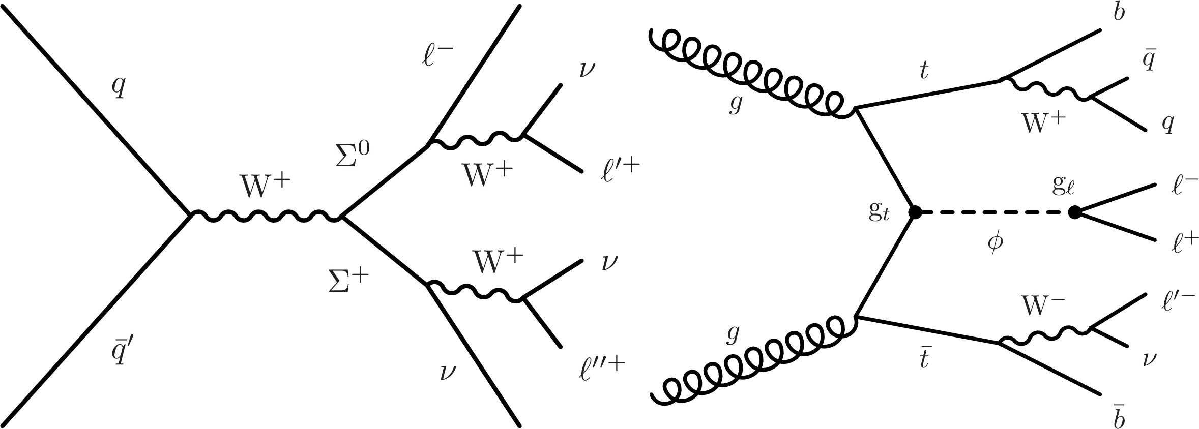
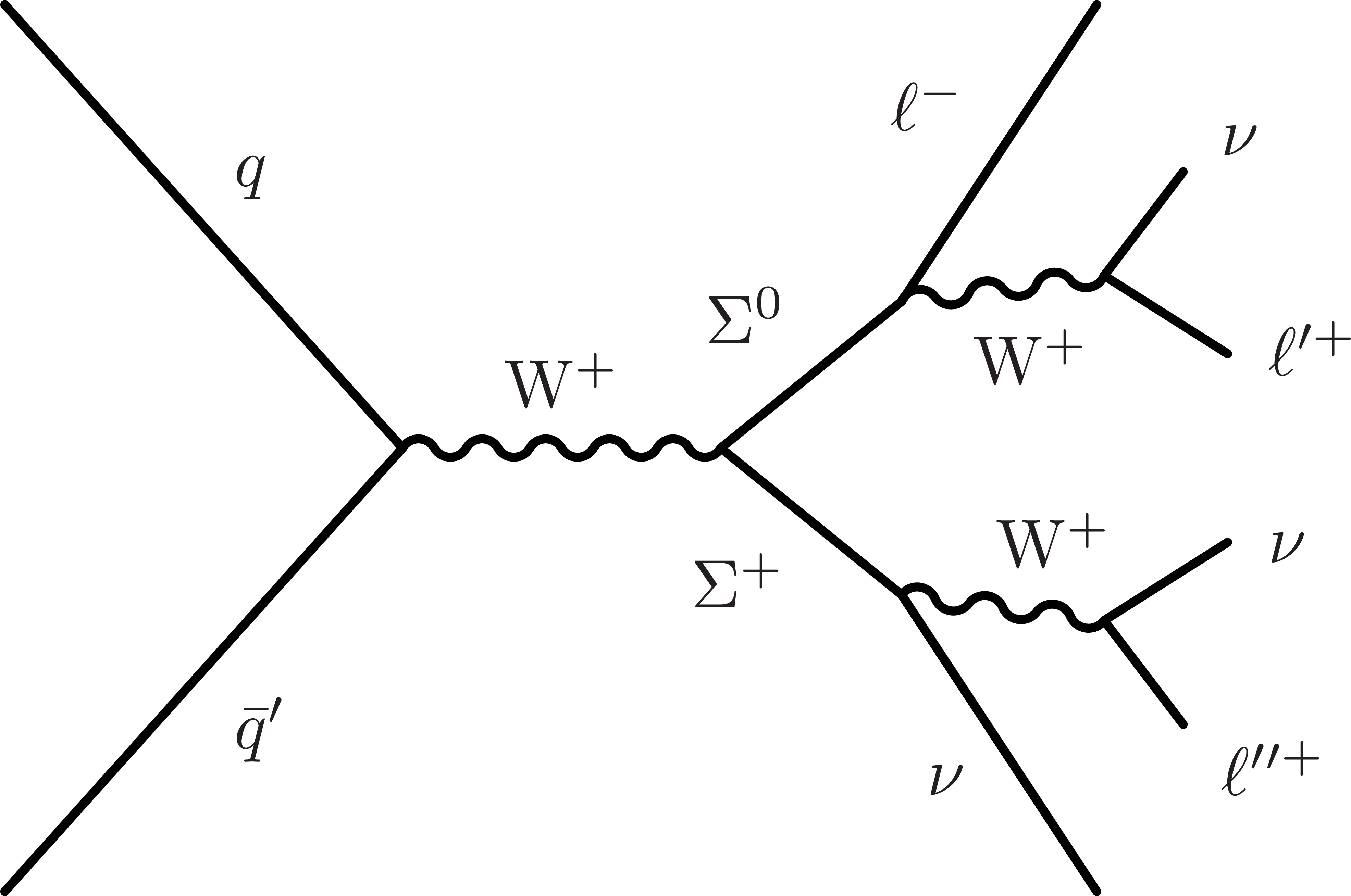
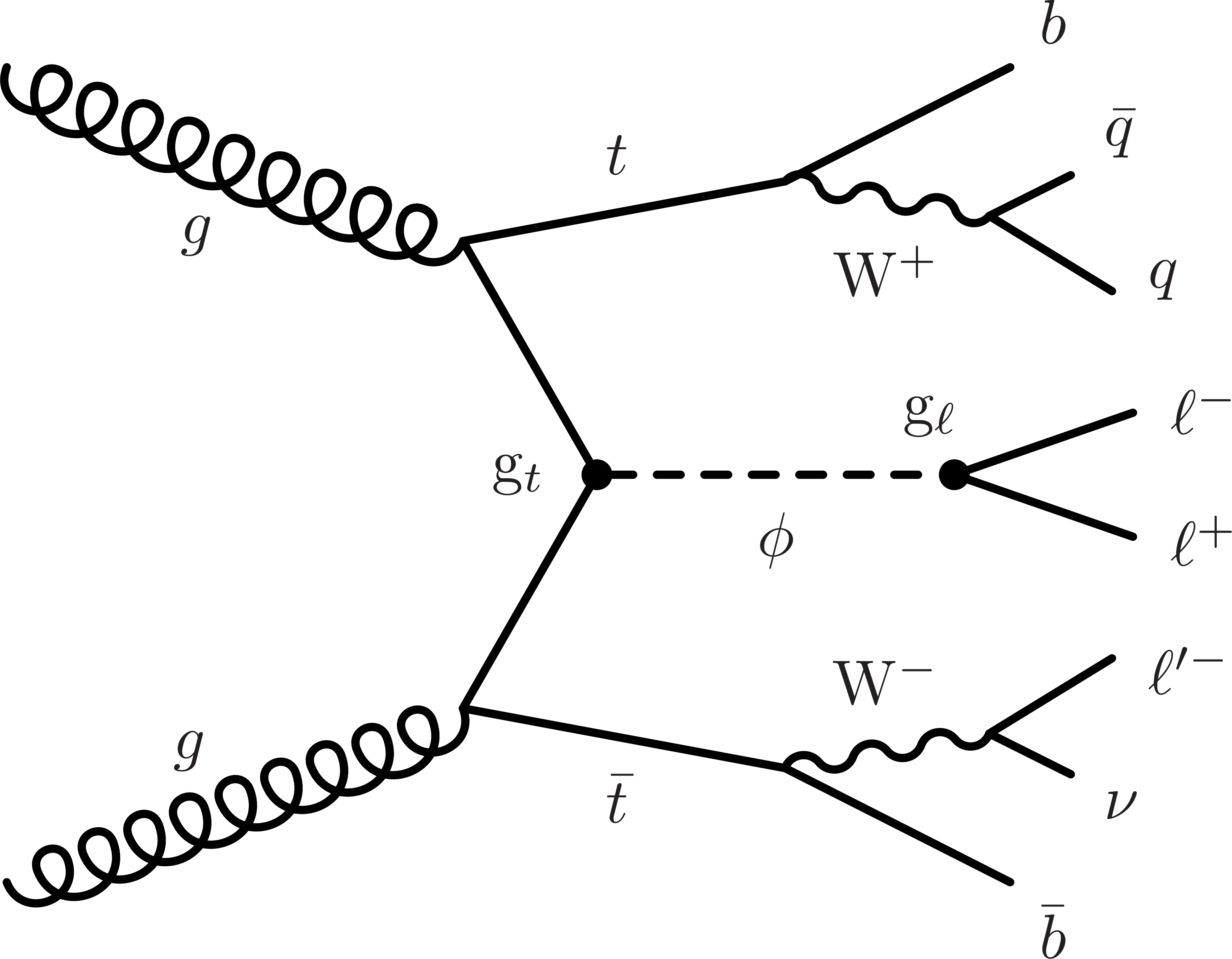
Figure 1:
Leading order Feynman diagrams for the type-III seesaw (left) and $ \mathrm{t\bar{t}}\phi$ (right) signal models, depicting example production and decay modes in pp collisions. |
png pdf |
Figure 1-a:
Leading order Feynman diagrams for the type-III seesaw (left) and $ \mathrm{t\bar{t}}\phi$ (right) signal models, depicting example production and decay modes in pp collisions. |
png pdf |
Figure 1-b:
Leading order Feynman diagrams for the type-III seesaw (left) and $ \mathrm{t\bar{t}}\phi$ (right) signal models, depicting example production and decay modes in pp collisions. |

png pdf |
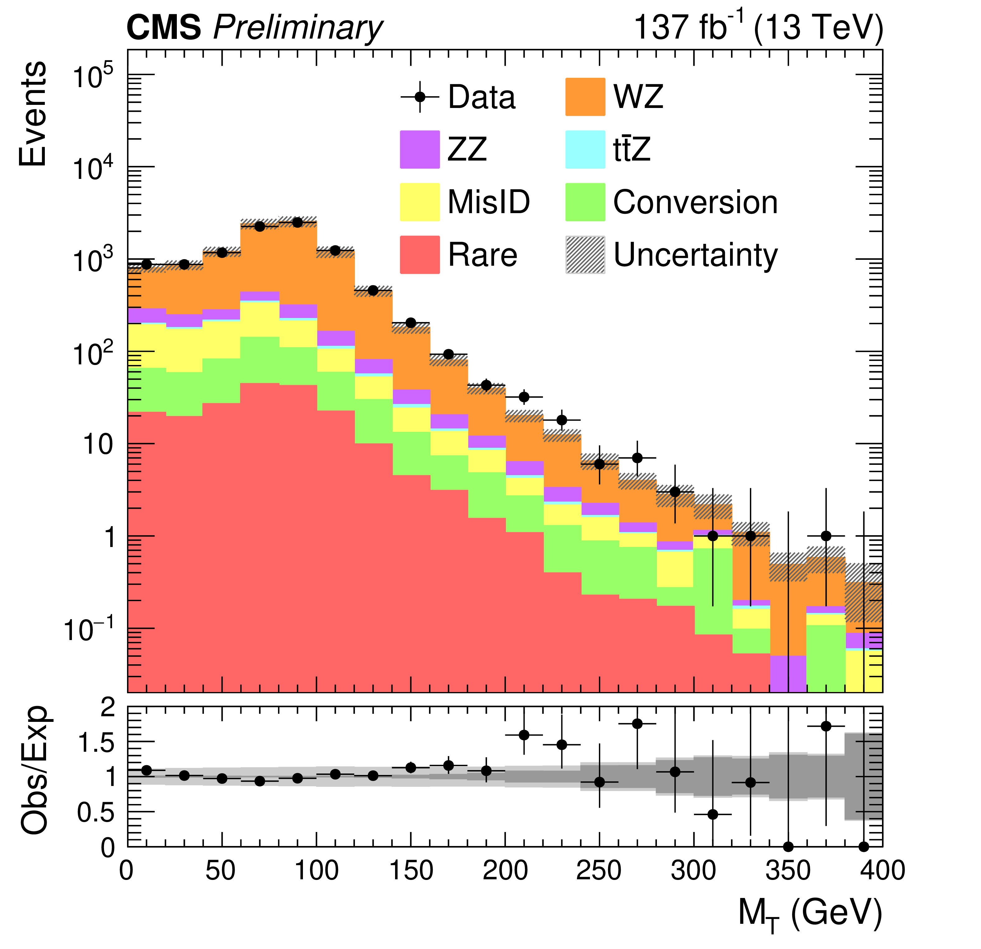
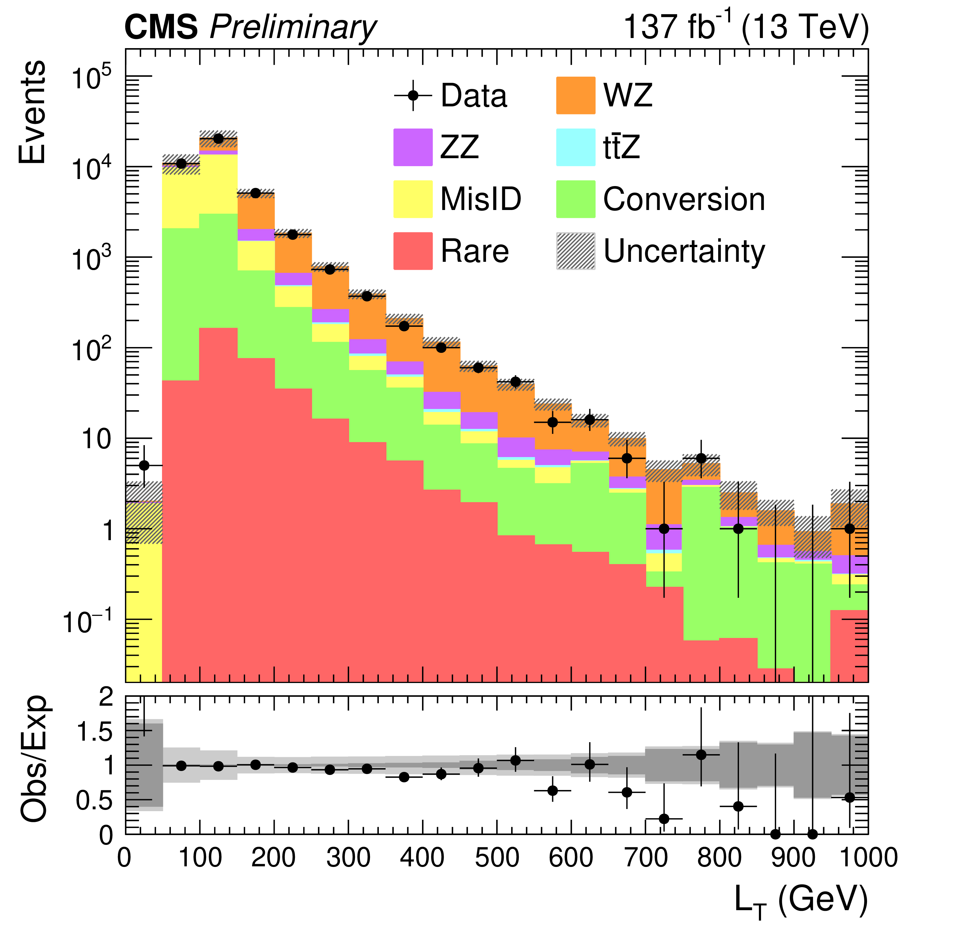
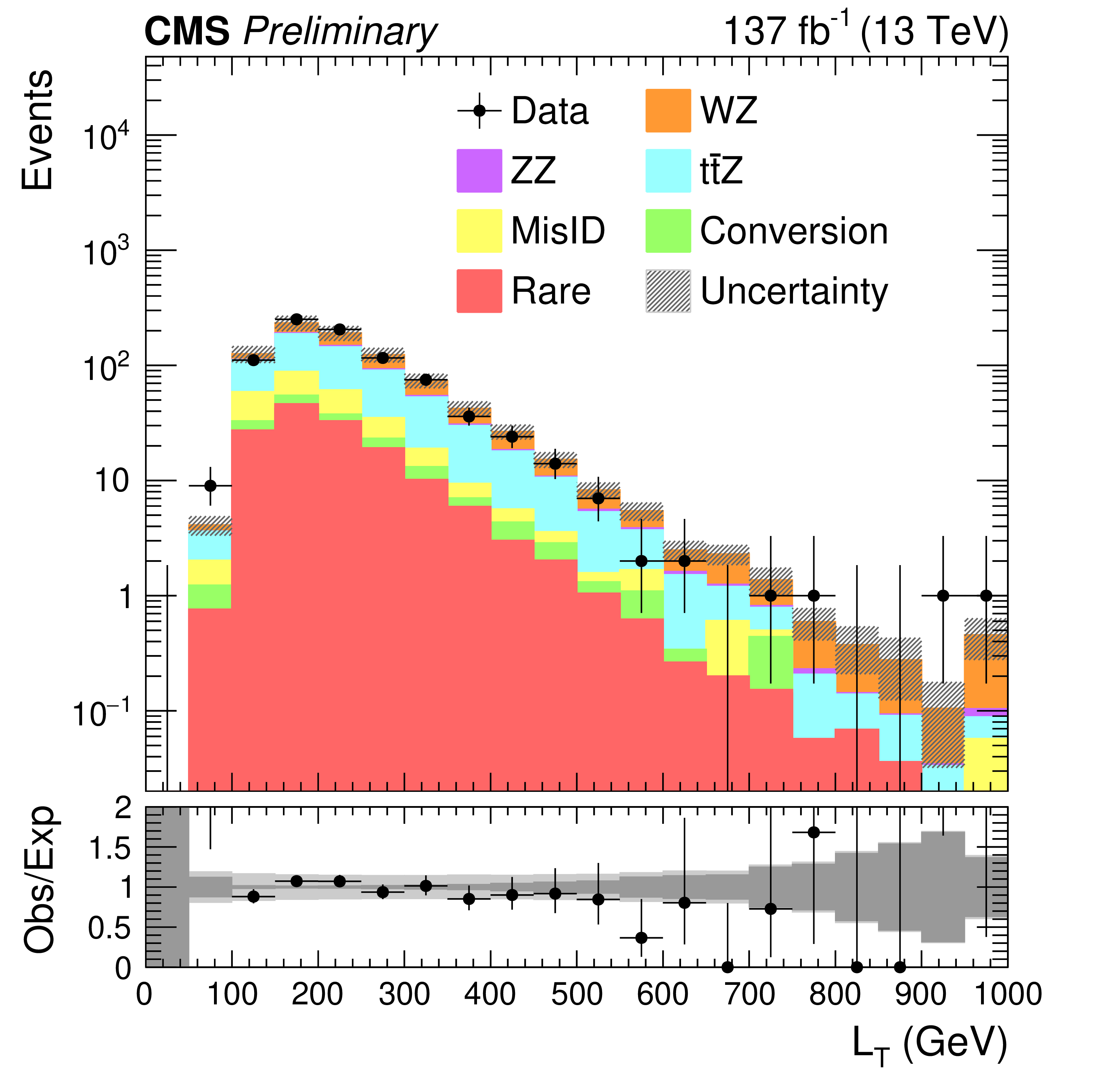
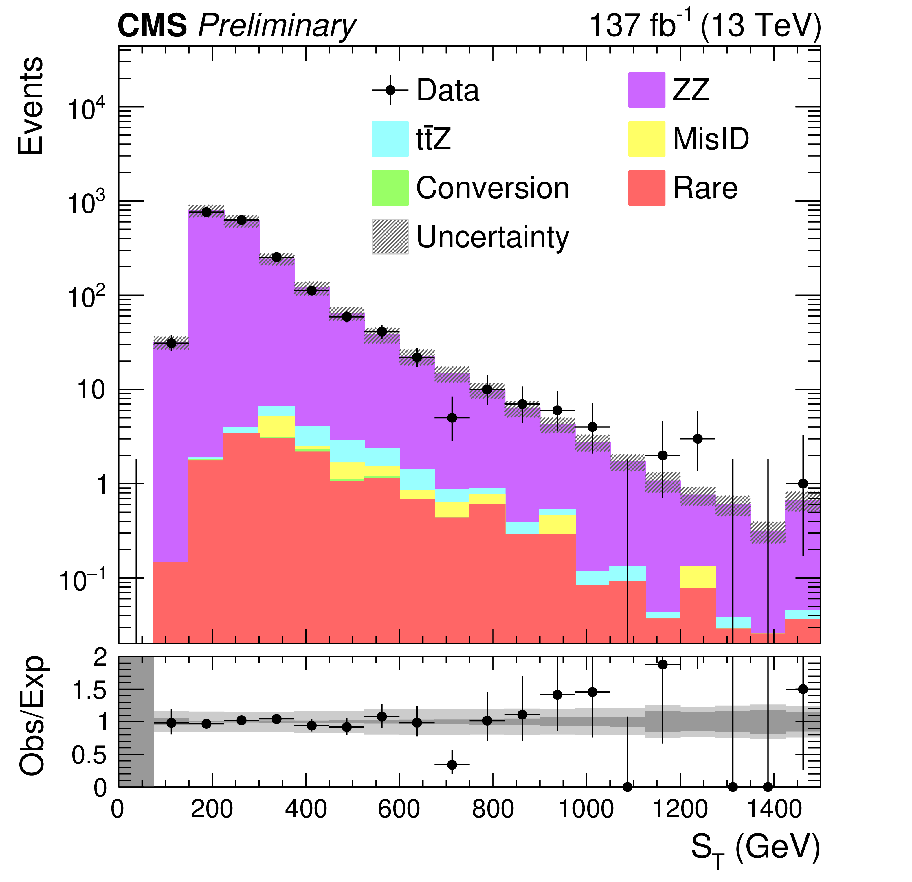
Figure 2:
The $ {M_{\rm T}}$ distribution in the WZ enriched control selection (upper left), the $ {L_{\rm T}}$ distribution in the misidentifed lepton enriched control selection (upper right), the $ {L_{\rm T}}$ distribution in the $ \mathrm{t\bar{t}Z}$ enriched control selection (lower left), and the $ {S_{\rm T}}$ distribution in the ZZ enriched control selection (lower right). The lower panels show the ratio of observed to expected events. The hatched gray band in the upper panels and the light gray bands in the lower panels represent the total (systematic and statistical) uncertainty in each bin, whereas the dark gray bands in the lower panels represent the statistical uncertainty only. The last bins contain the overflow events in each distribution. |
png pdf |
Figure 2-a:
The $ {M_{\rm T}}$ distribution in the WZ enriched control selection (upper left), the $ {L_{\rm T}}$ distribution in the misidentifed lepton enriched control selection (upper right), the $ {L_{\rm T}}$ distribution in the $ \mathrm{t\bar{t}Z}$ enriched control selection (lower left), and the $ {S_{\rm T}}$ distribution in the ZZ enriched control selection (lower right). The lower panels show the ratio of observed to expected events. The hatched gray band in the upper panels and the light gray bands in the lower panels represent the total (systematic and statistical) uncertainty in each bin, whereas the dark gray bands in the lower panels represent the statistical uncertainty only. The last bins contain the overflow events in each distribution. |
png pdf |
Figure 2-b:
The $ {M_{\rm T}}$ distribution in the WZ enriched control selection (upper left), the $ {L_{\rm T}}$ distribution in the misidentifed lepton enriched control selection (upper right), the $ {L_{\rm T}}$ distribution in the $ \mathrm{t\bar{t}Z}$ enriched control selection (lower left), and the $ {S_{\rm T}}$ distribution in the ZZ enriched control selection (lower right). The lower panels show the ratio of observed to expected events. The hatched gray band in the upper panels and the light gray bands in the lower panels represent the total (systematic and statistical) uncertainty in each bin, whereas the dark gray bands in the lower panels represent the statistical uncertainty only. The last bins contain the overflow events in each distribution. |
png pdf |
Figure 2-c:
The $ {M_{\rm T}}$ distribution in the WZ enriched control selection (upper left), the $ {L_{\rm T}}$ distribution in the misidentifed lepton enriched control selection (upper right), the $ {L_{\rm T}}$ distribution in the $ \mathrm{t\bar{t}Z}$ enriched control selection (lower left), and the $ {S_{\rm T}}$ distribution in the ZZ enriched control selection (lower right). The lower panels show the ratio of observed to expected events. The hatched gray band in the upper panels and the light gray bands in the lower panels represent the total (systematic and statistical) uncertainty in each bin, whereas the dark gray bands in the lower panels represent the statistical uncertainty only. The last bins contain the overflow events in each distribution. |
png pdf |
Figure 2-d:
The $ {M_{\rm T}}$ distribution in the WZ enriched control selection (upper left), the $ {L_{\rm T}}$ distribution in the misidentifed lepton enriched control selection (upper right), the $ {L_{\rm T}}$ distribution in the $ \mathrm{t\bar{t}Z}$ enriched control selection (lower left), and the $ {S_{\rm T}}$ distribution in the ZZ enriched control selection (lower right). The lower panels show the ratio of observed to expected events. The hatched gray band in the upper panels and the light gray bands in the lower panels represent the total (systematic and statistical) uncertainty in each bin, whereas the dark gray bands in the lower panels represent the statistical uncertainty only. The last bins contain the overflow events in each distribution. |
png pdf |
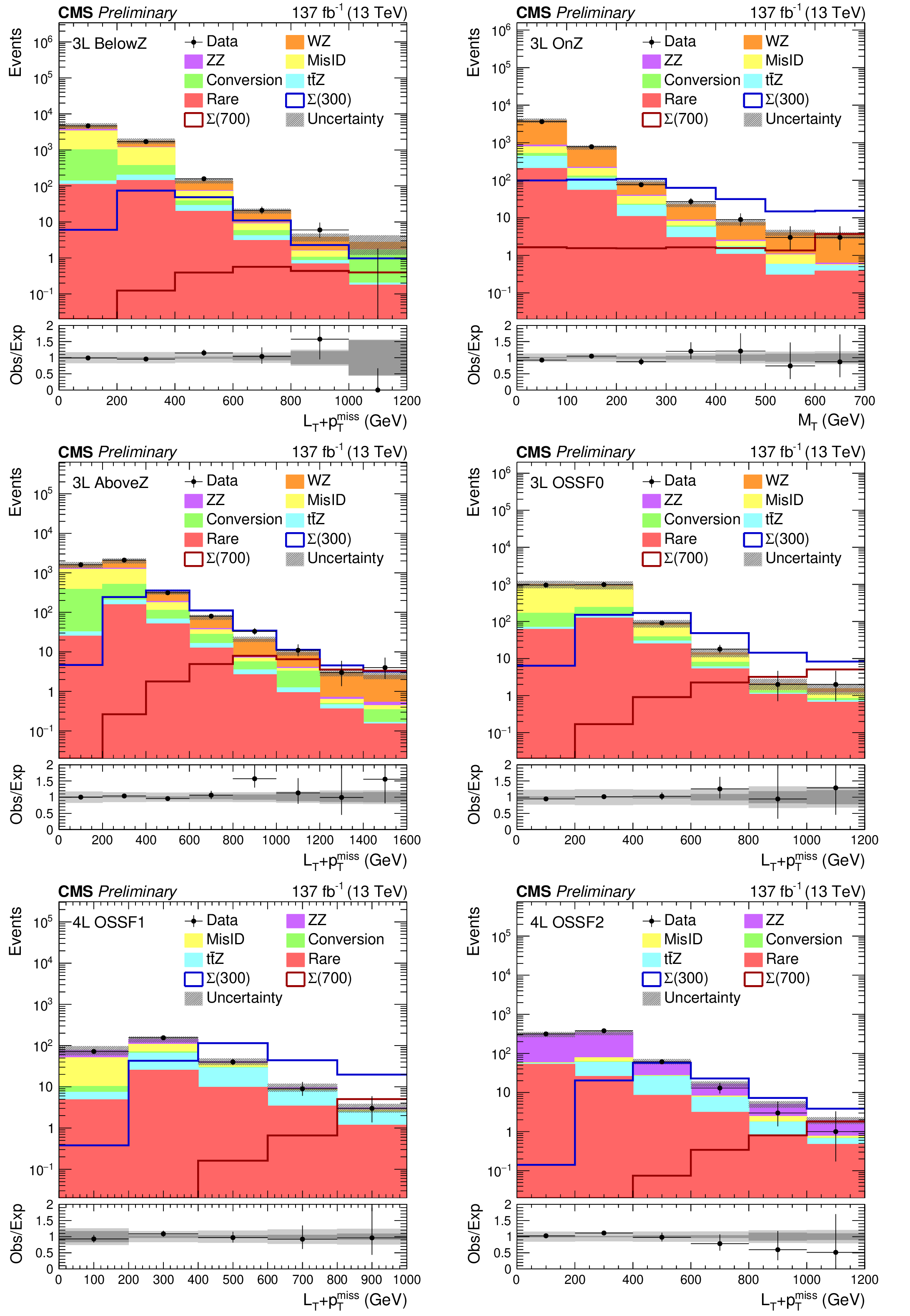
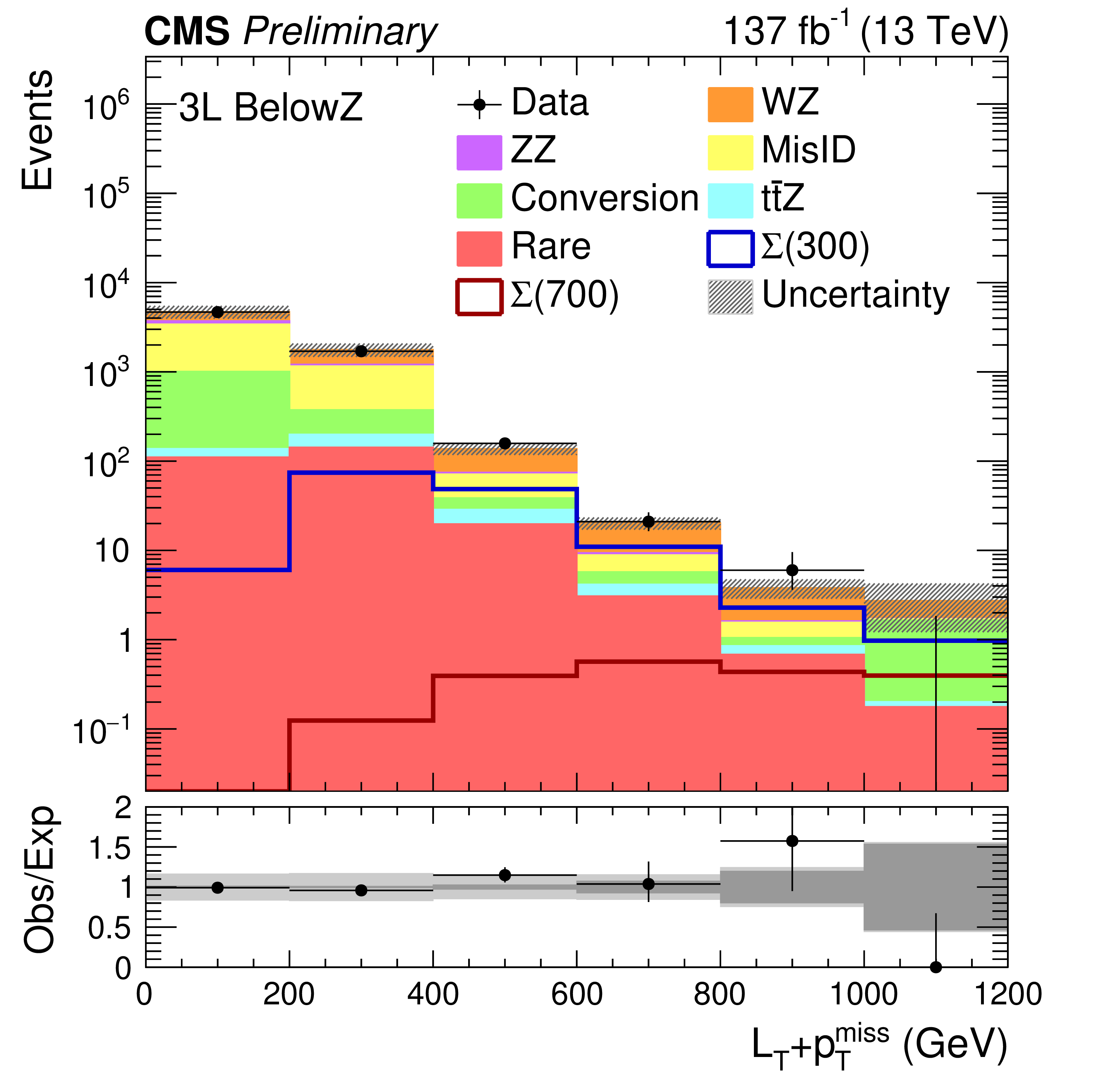
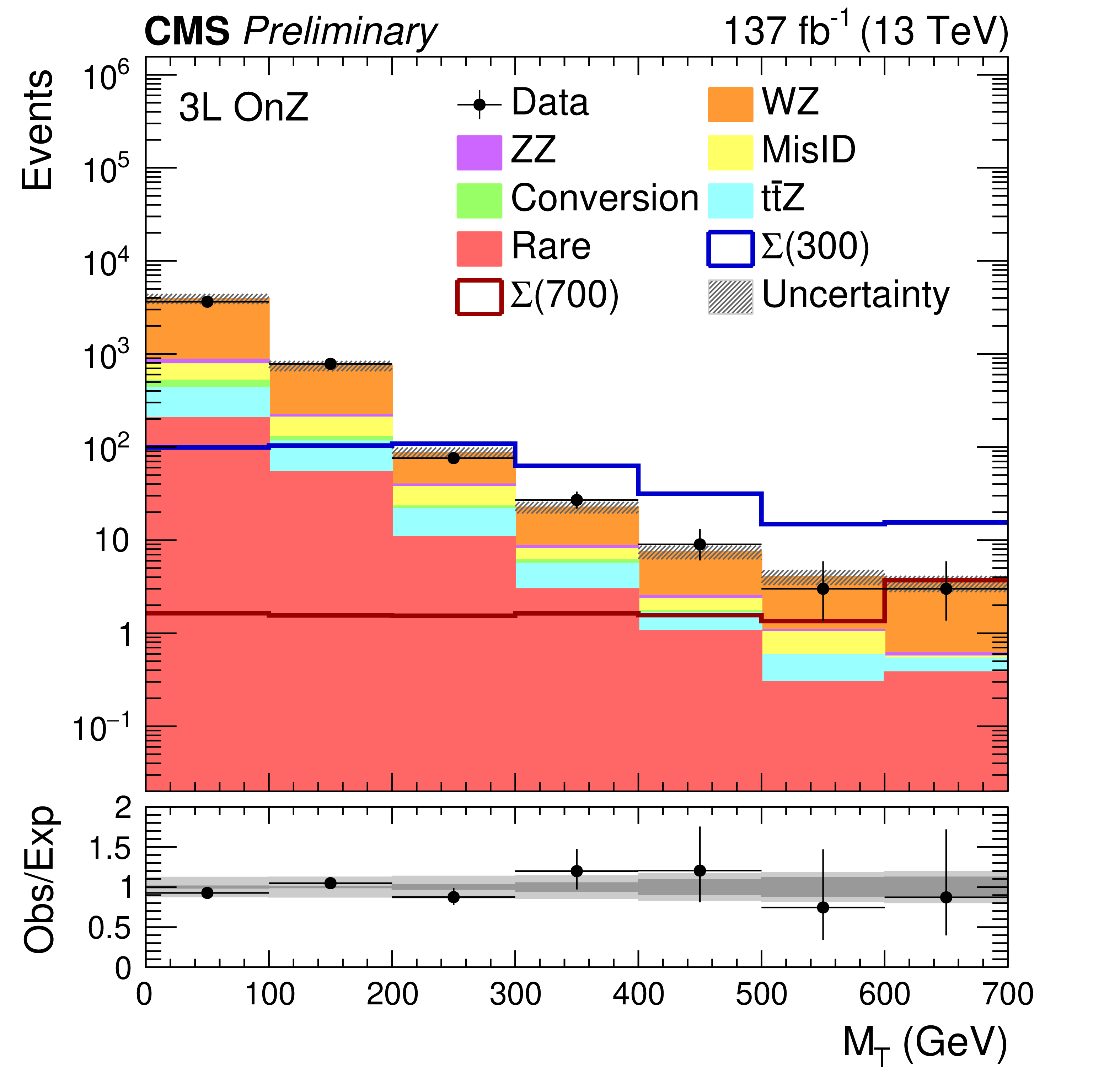
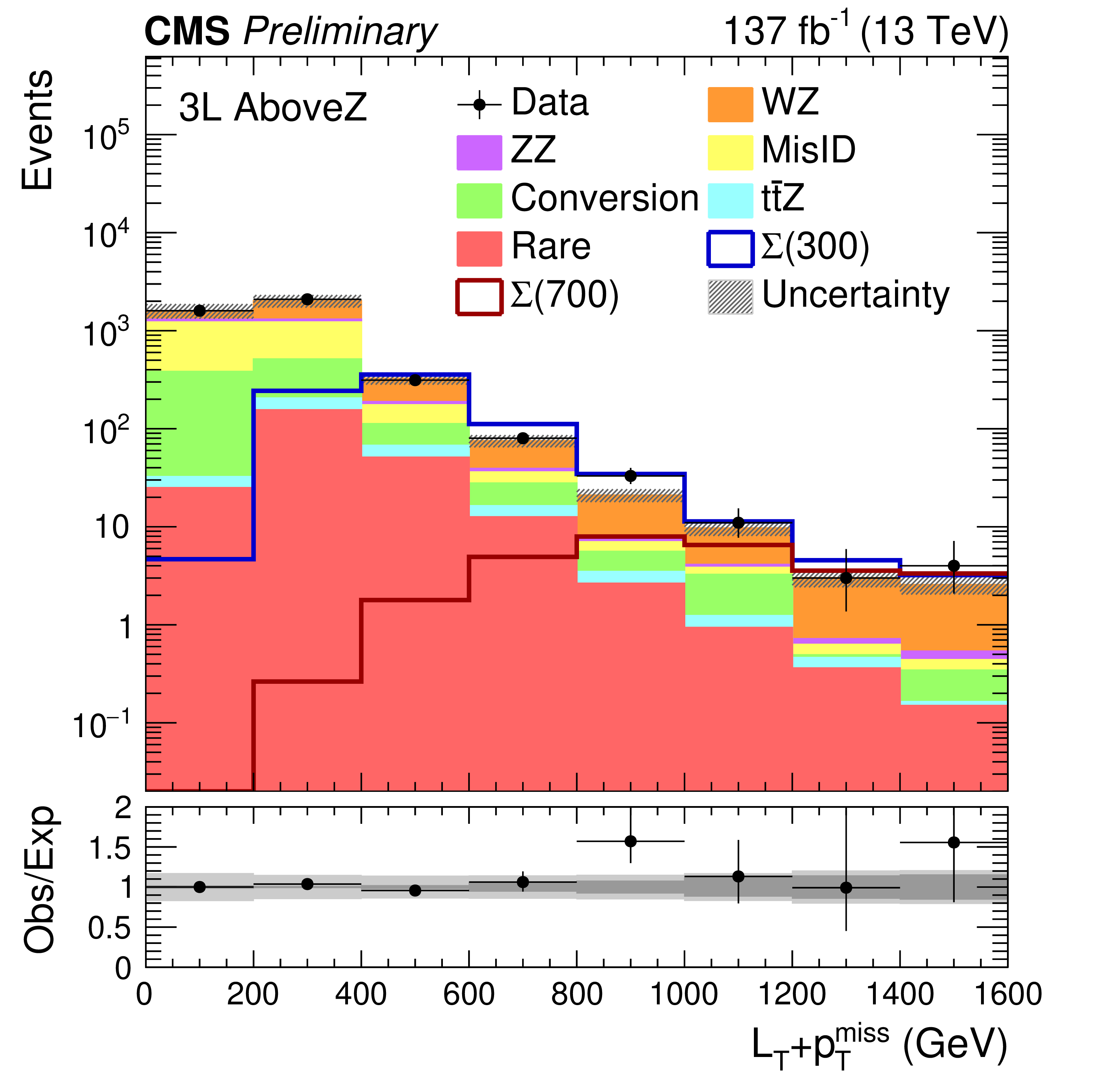
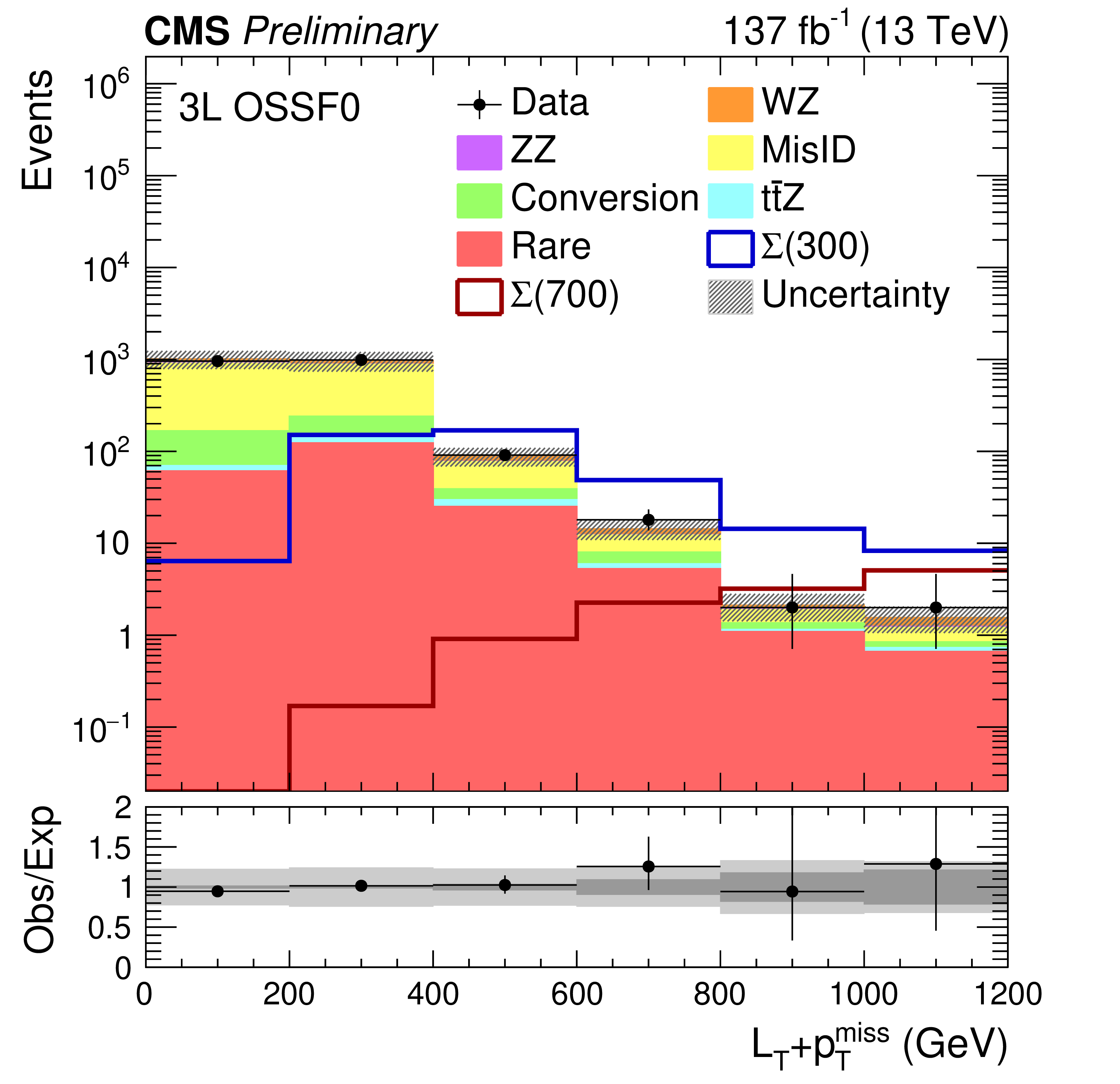
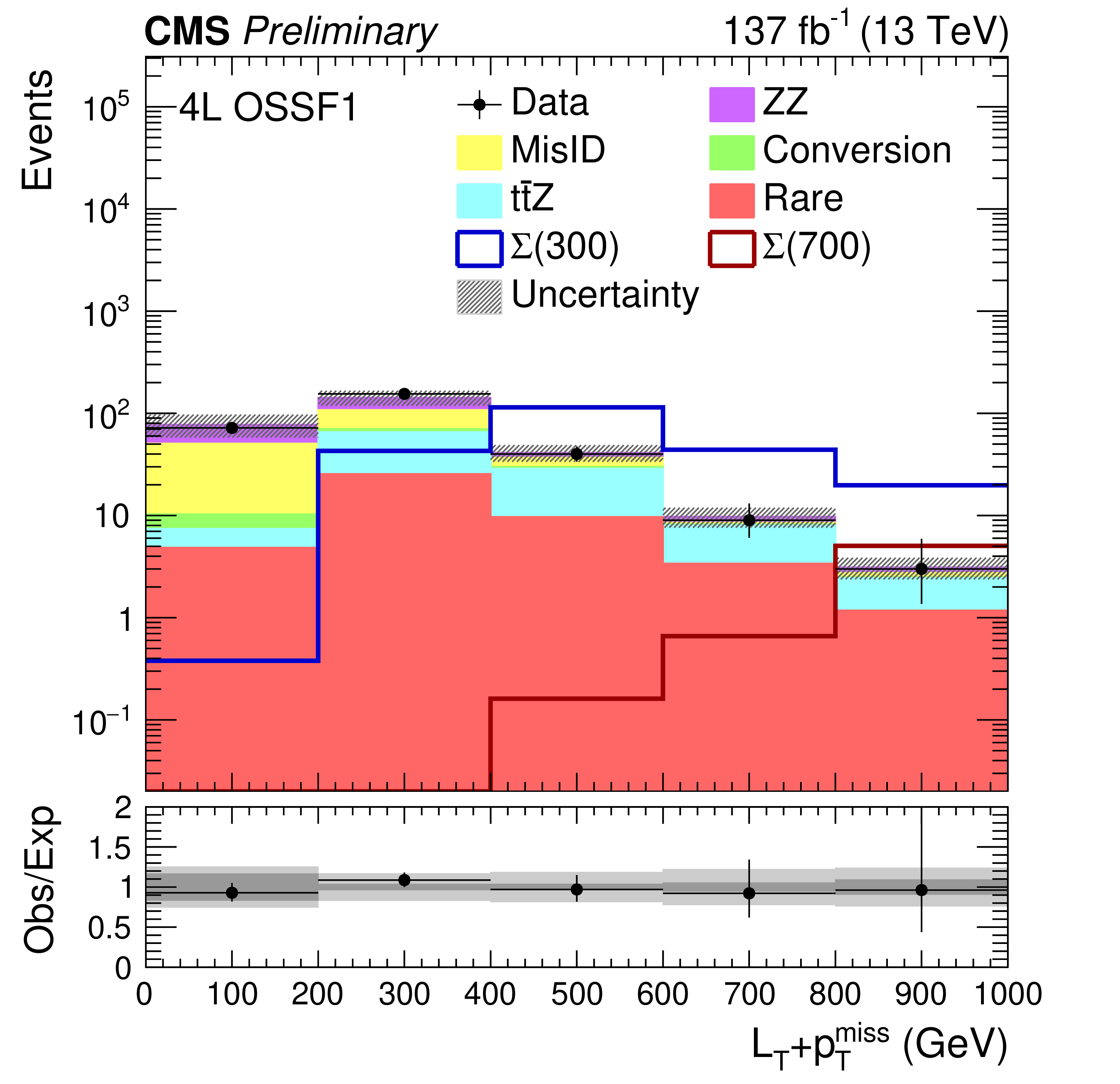
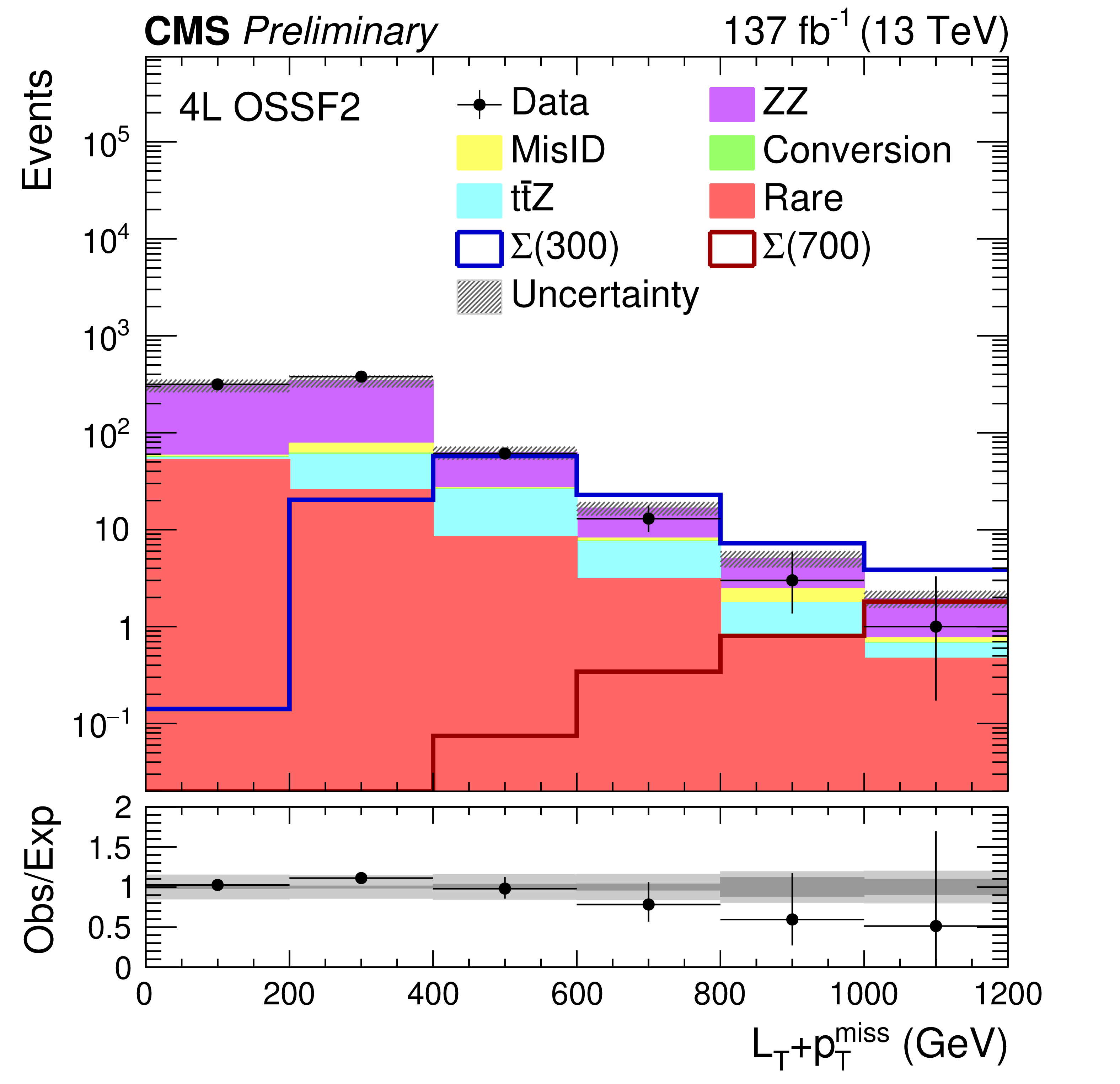
Figure 3:
Type-III seesaw signal regions in 3L below-Z (upper left), on-Z (upper right), above-Z (center left), OSSF0 (center right), and in 4L OSSF1 (lower left) and OSSF2 (lower right) events. The total SM background is shown as a stacked histogram of all contributing processes. The predictions for type-III seesaw models with $\Sigma $ masses of 300 GeV and 700 GeV are also shown. The lower panels show the ratio of observed to expected events. The hatched gray band in the upper panels and the light gray bands in the lower panels represent the total (systematic and statistical) uncertainty in each bin, whereas the dark gray bands in the lower panels represent the statistical uncertainty only. The last bins contain the overflow events in each distribution. |
png pdf |
Figure 3-a:
Type-III seesaw signal regions in 3L below-Z (upper left), on-Z (upper right), above-Z (center left), OSSF0 (center right), and in 4L OSSF1 (lower left) and OSSF2 (lower right) events. The total SM background is shown as a stacked histogram of all contributing processes. The predictions for type-III seesaw models with $\Sigma $ masses of 300 GeV and 700 GeV are also shown. The lower panels show the ratio of observed to expected events. The hatched gray band in the upper panels and the light gray bands in the lower panels represent the total (systematic and statistical) uncertainty in each bin, whereas the dark gray bands in the lower panels represent the statistical uncertainty only. The last bins contain the overflow events in each distribution. |
png pdf |
Figure 3-b:
Type-III seesaw signal regions in 3L below-Z (upper left), on-Z (upper right), above-Z (center left), OSSF0 (center right), and in 4L OSSF1 (lower left) and OSSF2 (lower right) events. The total SM background is shown as a stacked histogram of all contributing processes. The predictions for type-III seesaw models with $\Sigma $ masses of 300 GeV and 700 GeV are also shown. The lower panels show the ratio of observed to expected events. The hatched gray band in the upper panels and the light gray bands in the lower panels represent the total (systematic and statistical) uncertainty in each bin, whereas the dark gray bands in the lower panels represent the statistical uncertainty only. The last bins contain the overflow events in each distribution. |
png pdf |
Figure 3-c:
Type-III seesaw signal regions in 3L below-Z (upper left), on-Z (upper right), above-Z (center left), OSSF0 (center right), and in 4L OSSF1 (lower left) and OSSF2 (lower right) events. The total SM background is shown as a stacked histogram of all contributing processes. The predictions for type-III seesaw models with $\Sigma $ masses of 300 GeV and 700 GeV are also shown. The lower panels show the ratio of observed to expected events. The hatched gray band in the upper panels and the light gray bands in the lower panels represent the total (systematic and statistical) uncertainty in each bin, whereas the dark gray bands in the lower panels represent the statistical uncertainty only. The last bins contain the overflow events in each distribution. |
png pdf |
Figure 3-d:
Type-III seesaw signal regions in 3L below-Z (upper left), on-Z (upper right), above-Z (center left), OSSF0 (center right), and in 4L OSSF1 (lower left) and OSSF2 (lower right) events. The total SM background is shown as a stacked histogram of all contributing processes. The predictions for type-III seesaw models with $\Sigma $ masses of 300 GeV and 700 GeV are also shown. The lower panels show the ratio of observed to expected events. The hatched gray band in the upper panels and the light gray bands in the lower panels represent the total (systematic and statistical) uncertainty in each bin, whereas the dark gray bands in the lower panels represent the statistical uncertainty only. The last bins contain the overflow events in each distribution. |
png pdf |
Figure 3-e:
Type-III seesaw signal regions in 3L below-Z (upper left), on-Z (upper right), above-Z (center left), OSSF0 (center right), and in 4L OSSF1 (lower left) and OSSF2 (lower right) events. The total SM background is shown as a stacked histogram of all contributing processes. The predictions for type-III seesaw models with $\Sigma $ masses of 300 GeV and 700 GeV are also shown. The lower panels show the ratio of observed to expected events. The hatched gray band in the upper panels and the light gray bands in the lower panels represent the total (systematic and statistical) uncertainty in each bin, whereas the dark gray bands in the lower panels represent the statistical uncertainty only. The last bins contain the overflow events in each distribution. |
png pdf |
Figure 3-f:
Type-III seesaw signal regions in 3L below-Z (upper left), on-Z (upper right), above-Z (center left), OSSF0 (center right), and in 4L OSSF1 (lower left) and OSSF2 (lower right) events. The total SM background is shown as a stacked histogram of all contributing processes. The predictions for type-III seesaw models with $\Sigma $ masses of 300 GeV and 700 GeV are also shown. The lower panels show the ratio of observed to expected events. The hatched gray band in the upper panels and the light gray bands in the lower panels represent the total (systematic and statistical) uncertainty in each bin, whereas the dark gray bands in the lower panels represent the statistical uncertainty only. The last bins contain the overflow events in each distribution. |
png pdf |
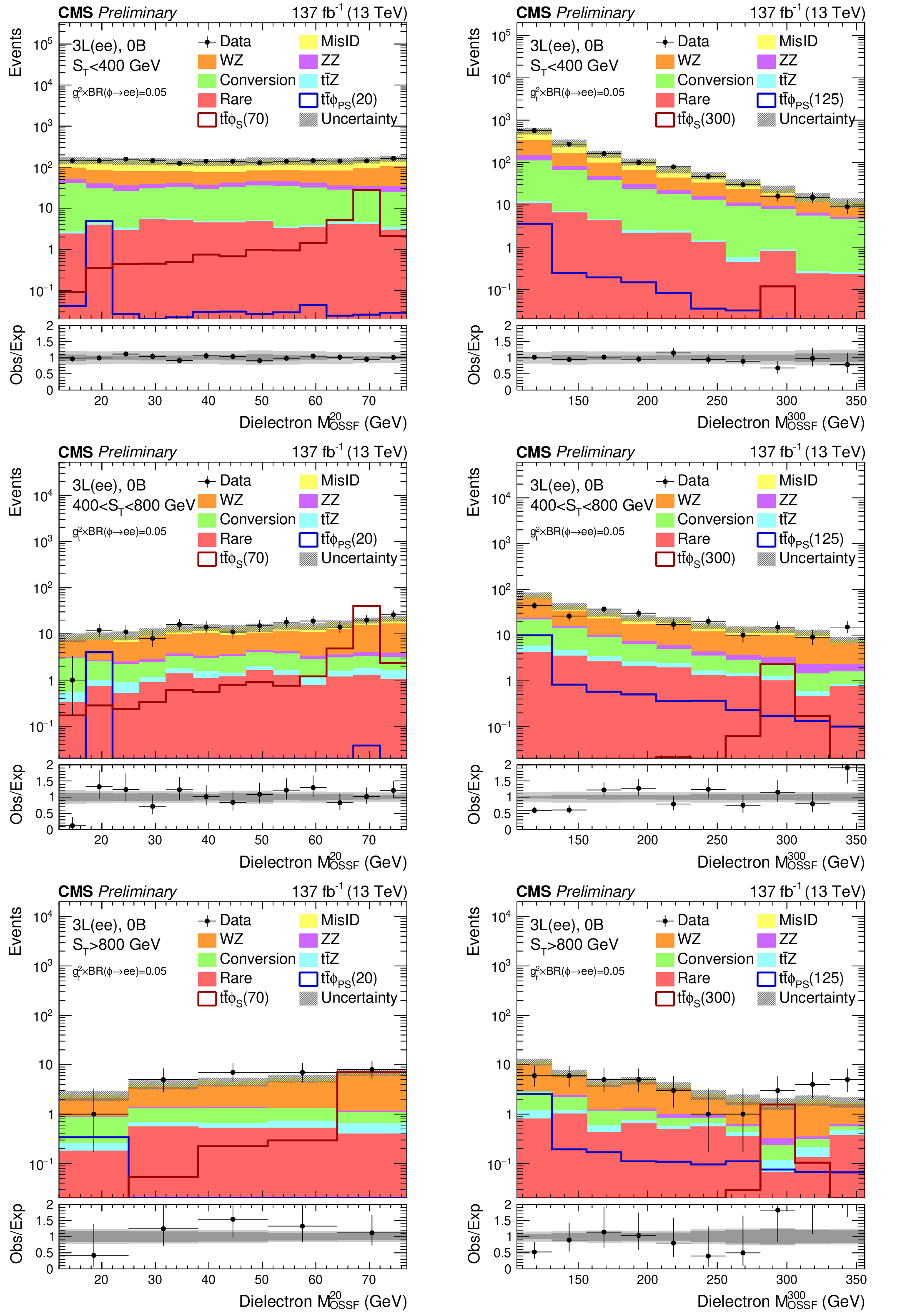
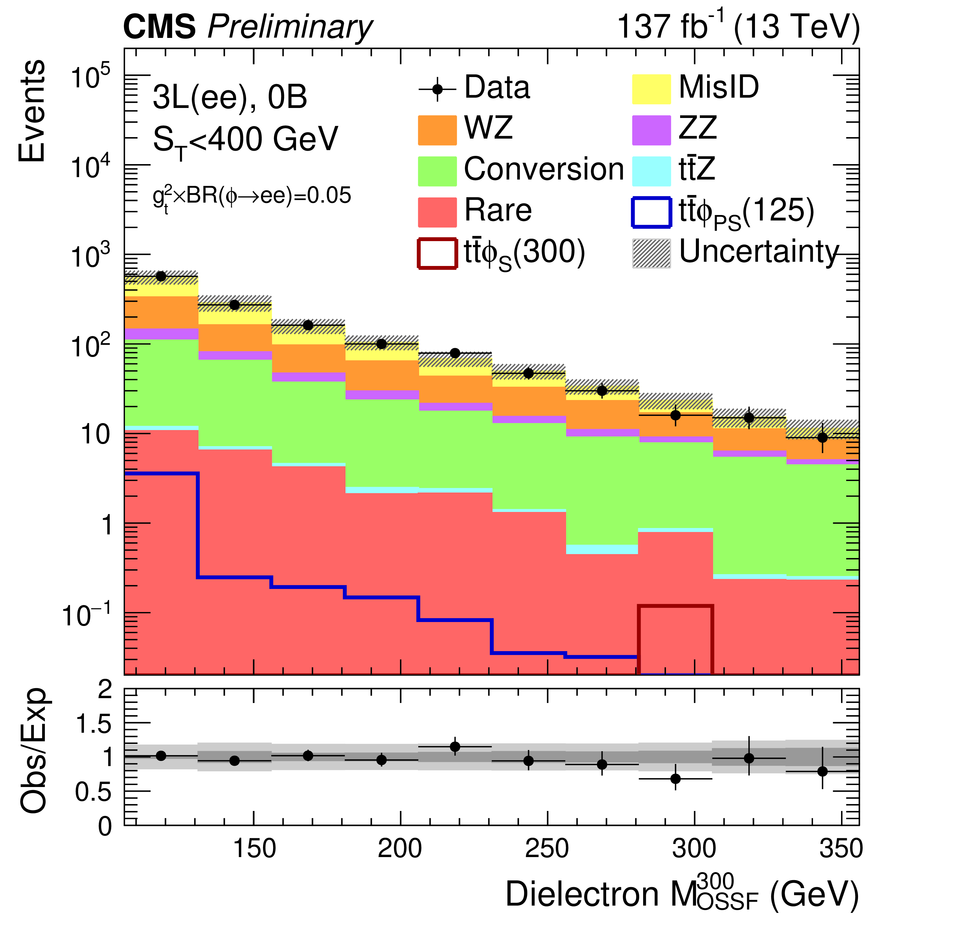
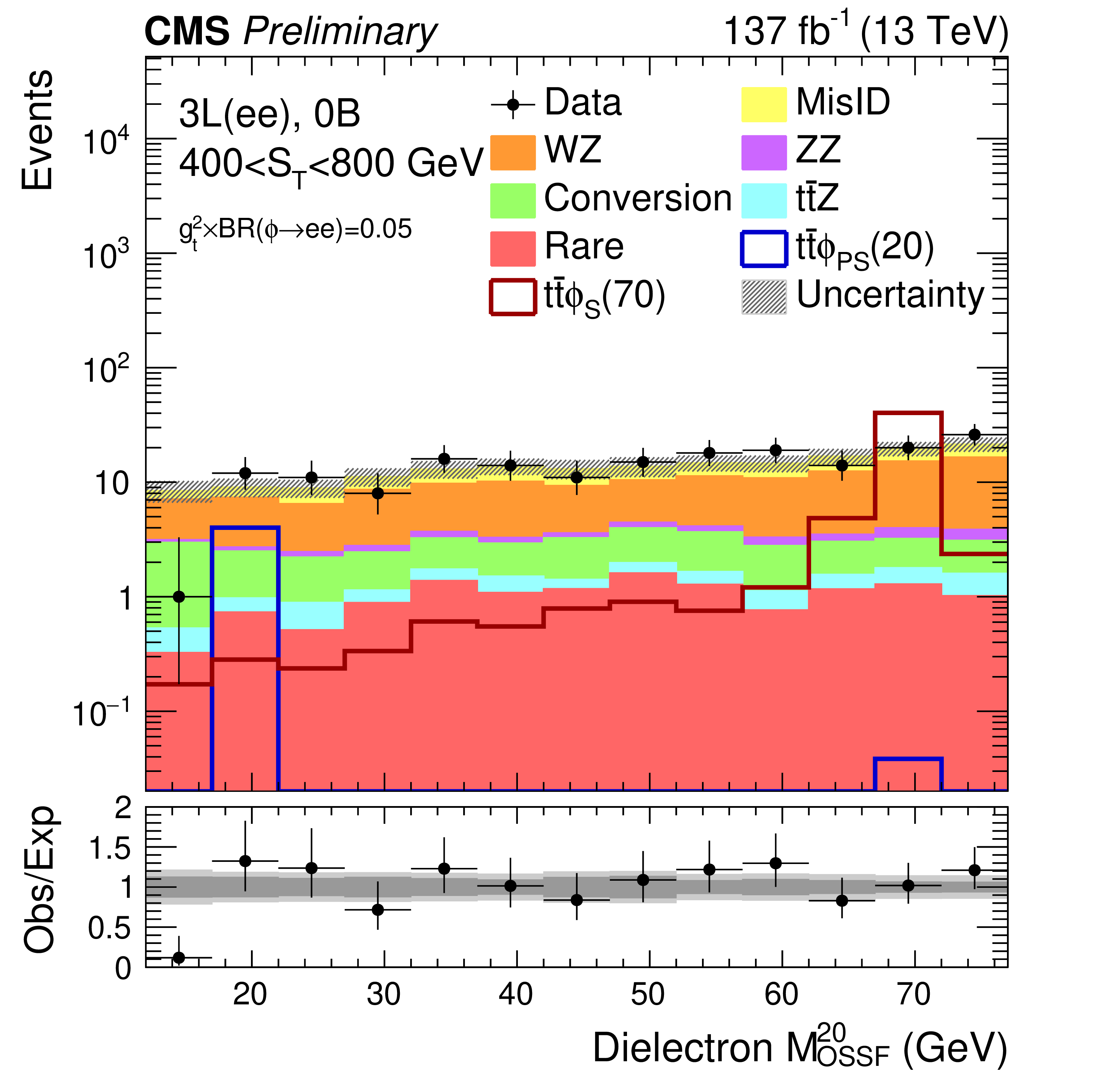
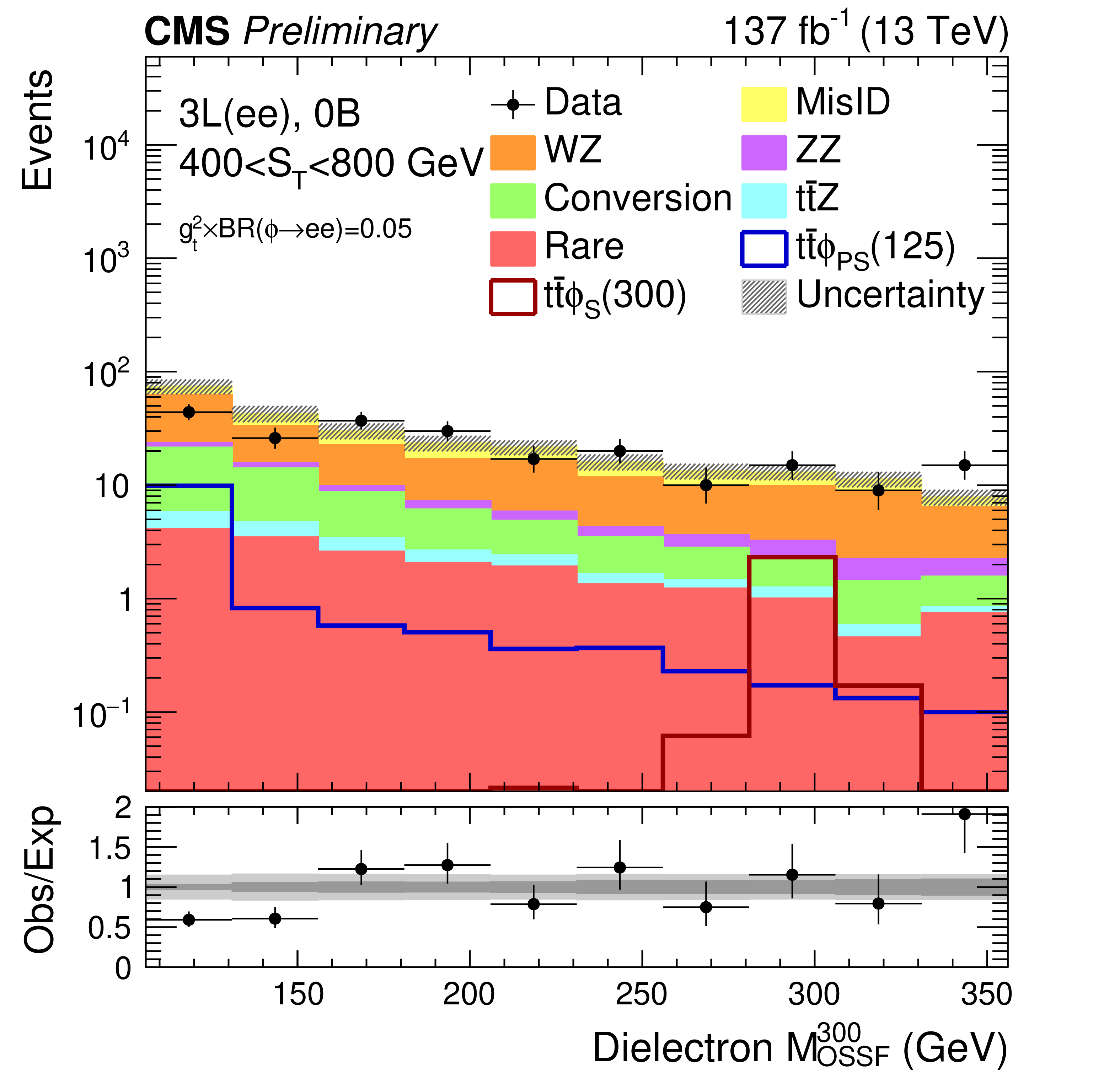
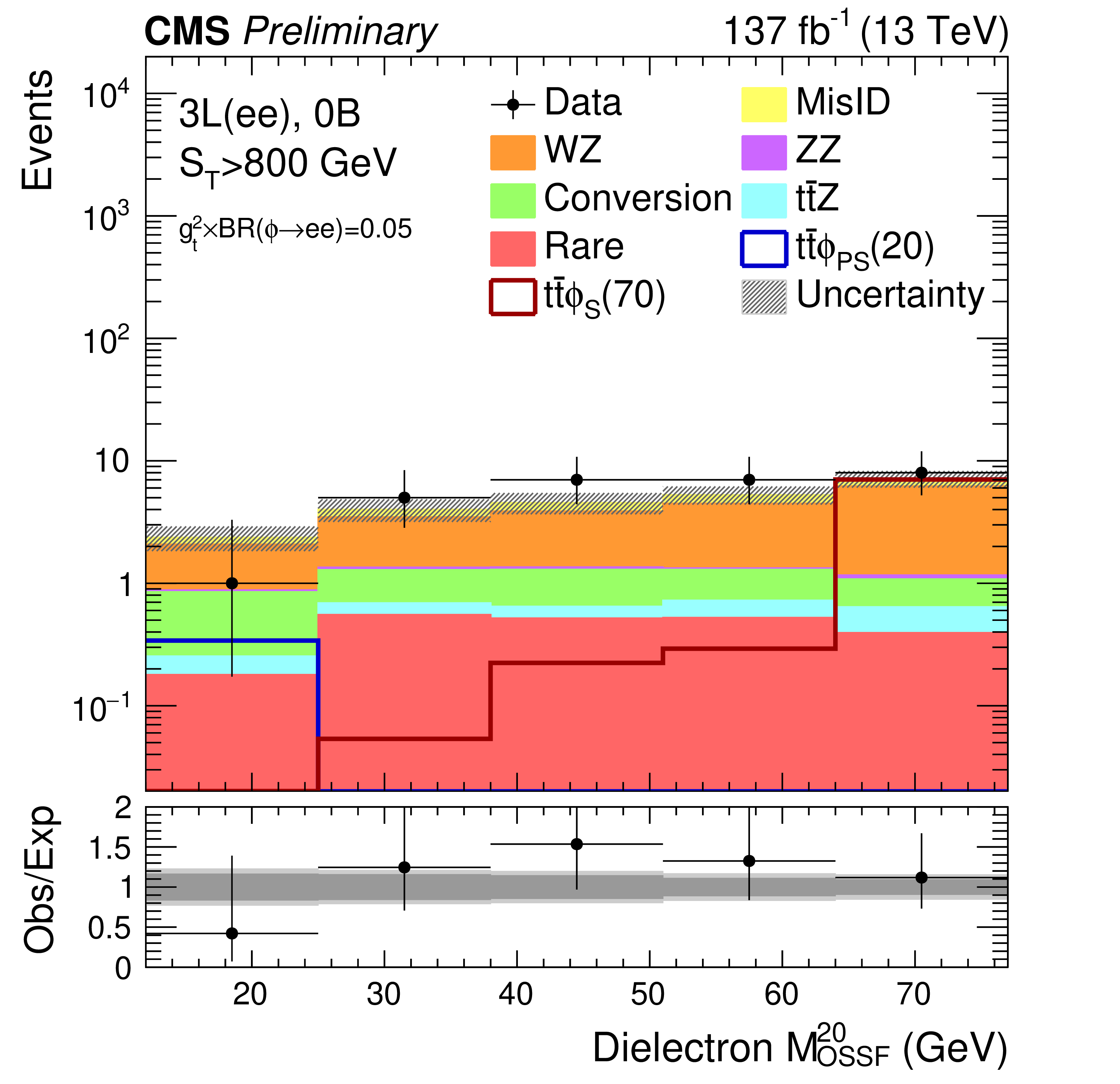
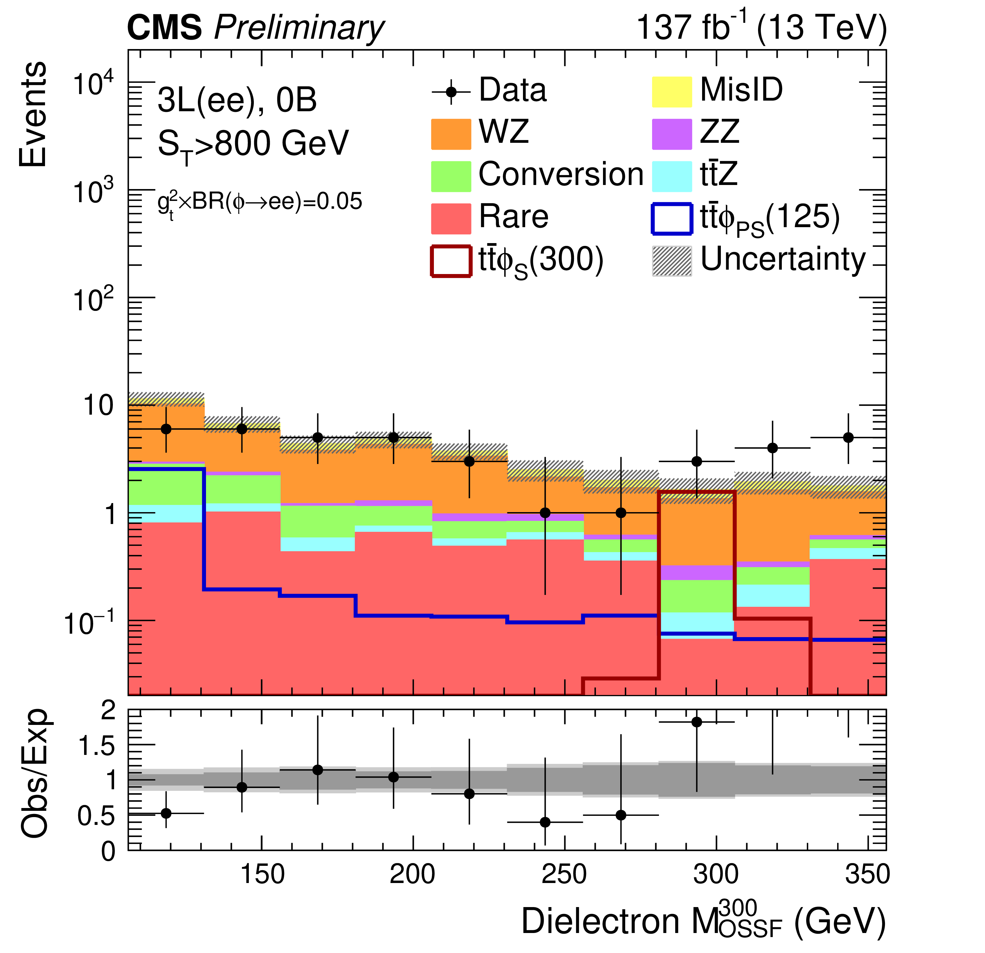
Figure 4:
Dielectron $ {M_{\rm OSSF}}^{20}$ (left column) and $ {M_{\rm OSSF}}^{300}$ (right column) distributions in 3L(ee) 0B $ \mathrm{t\bar{t}}\phi$ signal regions. Upper, center, and lower plots are with 0 $ < {S_{\rm T}} < $ 400 GeV, 400 $ < {S_{\rm T}} < $ 800 GeV, and $ {S_{\rm T}} > $ 800 GeV, respectively. The total SM background is shown as a stacked histogram of all contributing processes. The predictions for $ \mathrm{t\bar{t}}\phi(\rightarrow {\rm ee})$ models with a pseudoscalar (scalar) $\phi $ of 20 and 125 (70 and 300) GeV mass are also shown. The lower panels show the ratio of observed to expected events. The hatched gray band in the upper panels and the light gray bands in the lower panels represent the total (systematic and statistical) uncertainty in each bin, whereas the dark gray bands in the lower panels represent the statistical uncertainty only. The last bins do not contain the overflow events as these are outside the probed mass range. |

png pdf |
Figure 4-a:
Dielectron $ {M_{\rm OSSF}}^{20}$ (left column) and $ {M_{\rm OSSF}}^{300}$ (right column) distributions in 3L(ee) 0B $ \mathrm{t\bar{t}}\phi$ signal regions. Upper, center, and lower plots are with 0 $ < {S_{\rm T}} < $ 400 GeV, 400 $ < {S_{\rm T}} < $ 800 GeV, and $ {S_{\rm T}} > $ 800 GeV, respectively. The total SM background is shown as a stacked histogram of all contributing processes. The predictions for $ \mathrm{t\bar{t}}\phi(\rightarrow {\rm ee})$ models with a pseudoscalar (scalar) $\phi $ of 20 and 125 (70 and 300) GeV mass are also shown. The lower panels show the ratio of observed to expected events. The hatched gray band in the upper panels and the light gray bands in the lower panels represent the total (systematic and statistical) uncertainty in each bin, whereas the dark gray bands in the lower panels represent the statistical uncertainty only. The last bins do not contain the overflow events as these are outside the probed mass range. |
png pdf |
Figure 4-b:
Dielectron $ {M_{\rm OSSF}}^{20}$ (left column) and $ {M_{\rm OSSF}}^{300}$ (right column) distributions in 3L(ee) 0B $ \mathrm{t\bar{t}}\phi$ signal regions. Upper, center, and lower plots are with 0 $ < {S_{\rm T}} < $ 400 GeV, 400 $ < {S_{\rm T}} < $ 800 GeV, and $ {S_{\rm T}} > $ 800 GeV, respectively. The total SM background is shown as a stacked histogram of all contributing processes. The predictions for $ \mathrm{t\bar{t}}\phi(\rightarrow {\rm ee})$ models with a pseudoscalar (scalar) $\phi $ of 20 and 125 (70 and 300) GeV mass are also shown. The lower panels show the ratio of observed to expected events. The hatched gray band in the upper panels and the light gray bands in the lower panels represent the total (systematic and statistical) uncertainty in each bin, whereas the dark gray bands in the lower panels represent the statistical uncertainty only. The last bins do not contain the overflow events as these are outside the probed mass range. |
png pdf |
Figure 4-c:
Dielectron $ {M_{\rm OSSF}}^{20}$ (left column) and $ {M_{\rm OSSF}}^{300}$ (right column) distributions in 3L(ee) 0B $ \mathrm{t\bar{t}}\phi$ signal regions. Upper, center, and lower plots are with 0 $ < {S_{\rm T}} < $ 400 GeV, 400 $ < {S_{\rm T}} < $ 800 GeV, and $ {S_{\rm T}} > $ 800 GeV, respectively. The total SM background is shown as a stacked histogram of all contributing processes. The predictions for $ \mathrm{t\bar{t}}\phi(\rightarrow {\rm ee})$ models with a pseudoscalar (scalar) $\phi $ of 20 and 125 (70 and 300) GeV mass are also shown. The lower panels show the ratio of observed to expected events. The hatched gray band in the upper panels and the light gray bands in the lower panels represent the total (systematic and statistical) uncertainty in each bin, whereas the dark gray bands in the lower panels represent the statistical uncertainty only. The last bins do not contain the overflow events as these are outside the probed mass range. |
png pdf |
Figure 4-d:
Dielectron $ {M_{\rm OSSF}}^{20}$ (left column) and $ {M_{\rm OSSF}}^{300}$ (right column) distributions in 3L(ee) 0B $ \mathrm{t\bar{t}}\phi$ signal regions. Upper, center, and lower plots are with 0 $ < {S_{\rm T}} < $ 400 GeV, 400 $ < {S_{\rm T}} < $ 800 GeV, and $ {S_{\rm T}} > $ 800 GeV, respectively. The total SM background is shown as a stacked histogram of all contributing processes. The predictions for $ \mathrm{t\bar{t}}\phi(\rightarrow {\rm ee})$ models with a pseudoscalar (scalar) $\phi $ of 20 and 125 (70 and 300) GeV mass are also shown. The lower panels show the ratio of observed to expected events. The hatched gray band in the upper panels and the light gray bands in the lower panels represent the total (systematic and statistical) uncertainty in each bin, whereas the dark gray bands in the lower panels represent the statistical uncertainty only. The last bins do not contain the overflow events as these are outside the probed mass range. |
png pdf |
Figure 4-e:
Dielectron $ {M_{\rm OSSF}}^{20}$ (left column) and $ {M_{\rm OSSF}}^{300}$ (right column) distributions in 3L(ee) 0B $ \mathrm{t\bar{t}}\phi$ signal regions. Upper, center, and lower plots are with 0 $ < {S_{\rm T}} < $ 400 GeV, 400 $ < {S_{\rm T}} < $ 800 GeV, and $ {S_{\rm T}} > $ 800 GeV, respectively. The total SM background is shown as a stacked histogram of all contributing processes. The predictions for $ \mathrm{t\bar{t}}\phi(\rightarrow {\rm ee})$ models with a pseudoscalar (scalar) $\phi $ of 20 and 125 (70 and 300) GeV mass are also shown. The lower panels show the ratio of observed to expected events. The hatched gray band in the upper panels and the light gray bands in the lower panels represent the total (systematic and statistical) uncertainty in each bin, whereas the dark gray bands in the lower panels represent the statistical uncertainty only. The last bins do not contain the overflow events as these are outside the probed mass range. |
png pdf |
Figure 4-f:
Dielectron $ {M_{\rm OSSF}}^{20}$ (left column) and $ {M_{\rm OSSF}}^{300}$ (right column) distributions in 3L(ee) 0B $ \mathrm{t\bar{t}}\phi$ signal regions. Upper, center, and lower plots are with 0 $ < {S_{\rm T}} < $ 400 GeV, 400 $ < {S_{\rm T}} < $ 800 GeV, and $ {S_{\rm T}} > $ 800 GeV, respectively. The total SM background is shown as a stacked histogram of all contributing processes. The predictions for $ \mathrm{t\bar{t}}\phi(\rightarrow {\rm ee})$ models with a pseudoscalar (scalar) $\phi $ of 20 and 125 (70 and 300) GeV mass are also shown. The lower panels show the ratio of observed to expected events. The hatched gray band in the upper panels and the light gray bands in the lower panels represent the total (systematic and statistical) uncertainty in each bin, whereas the dark gray bands in the lower panels represent the statistical uncertainty only. The last bins do not contain the overflow events as these are outside the probed mass range. |
png pdf |
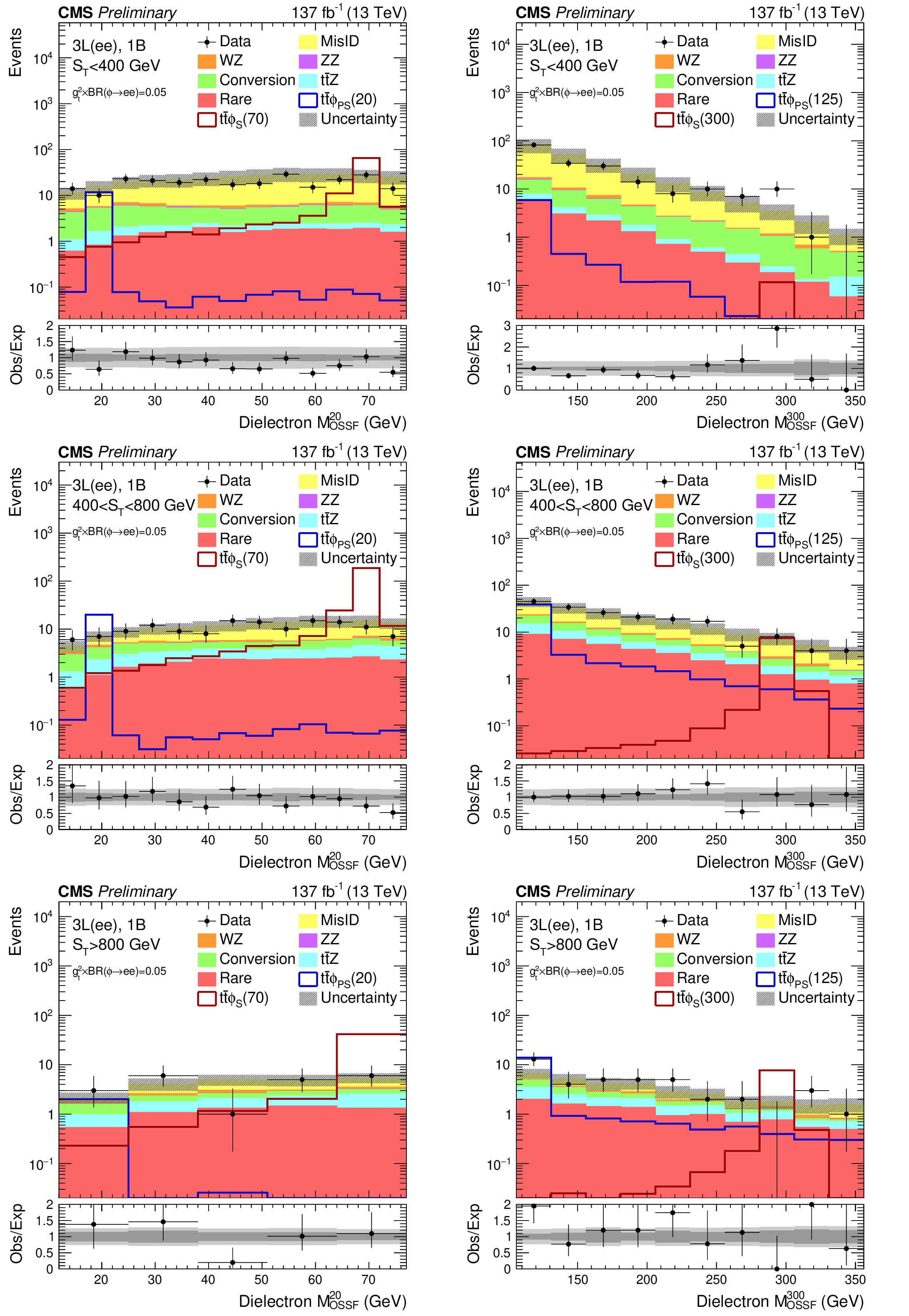
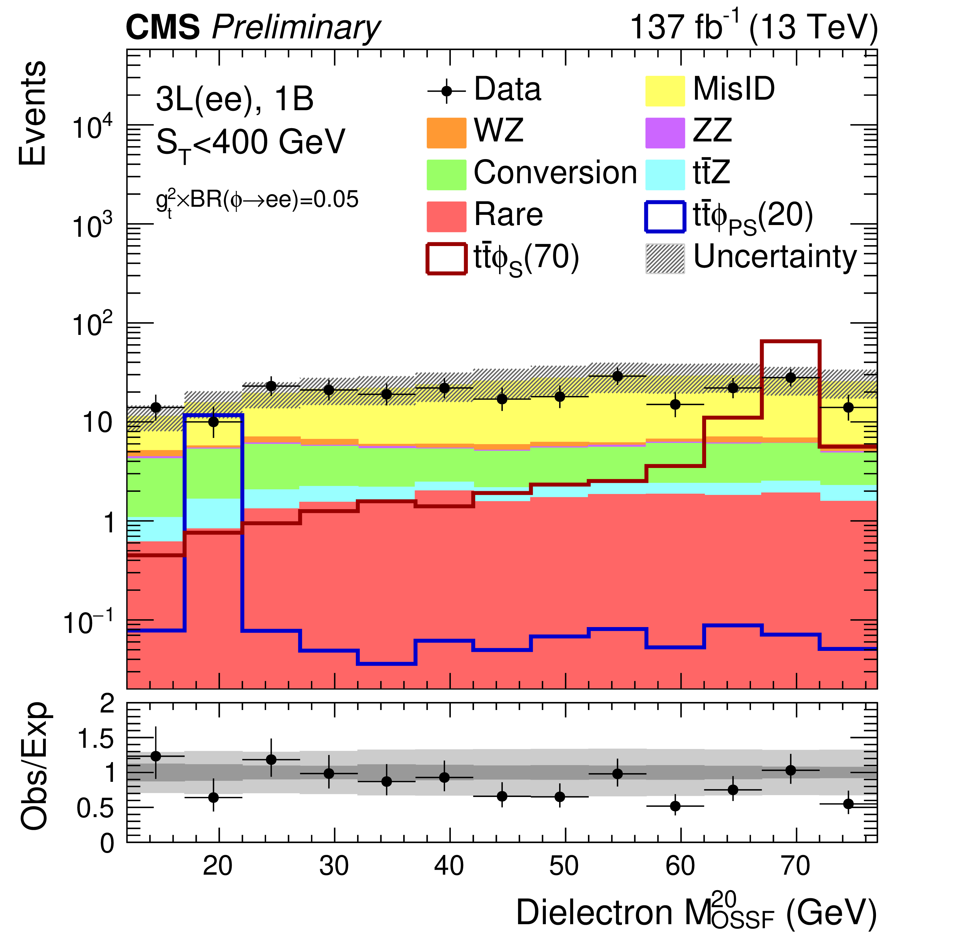
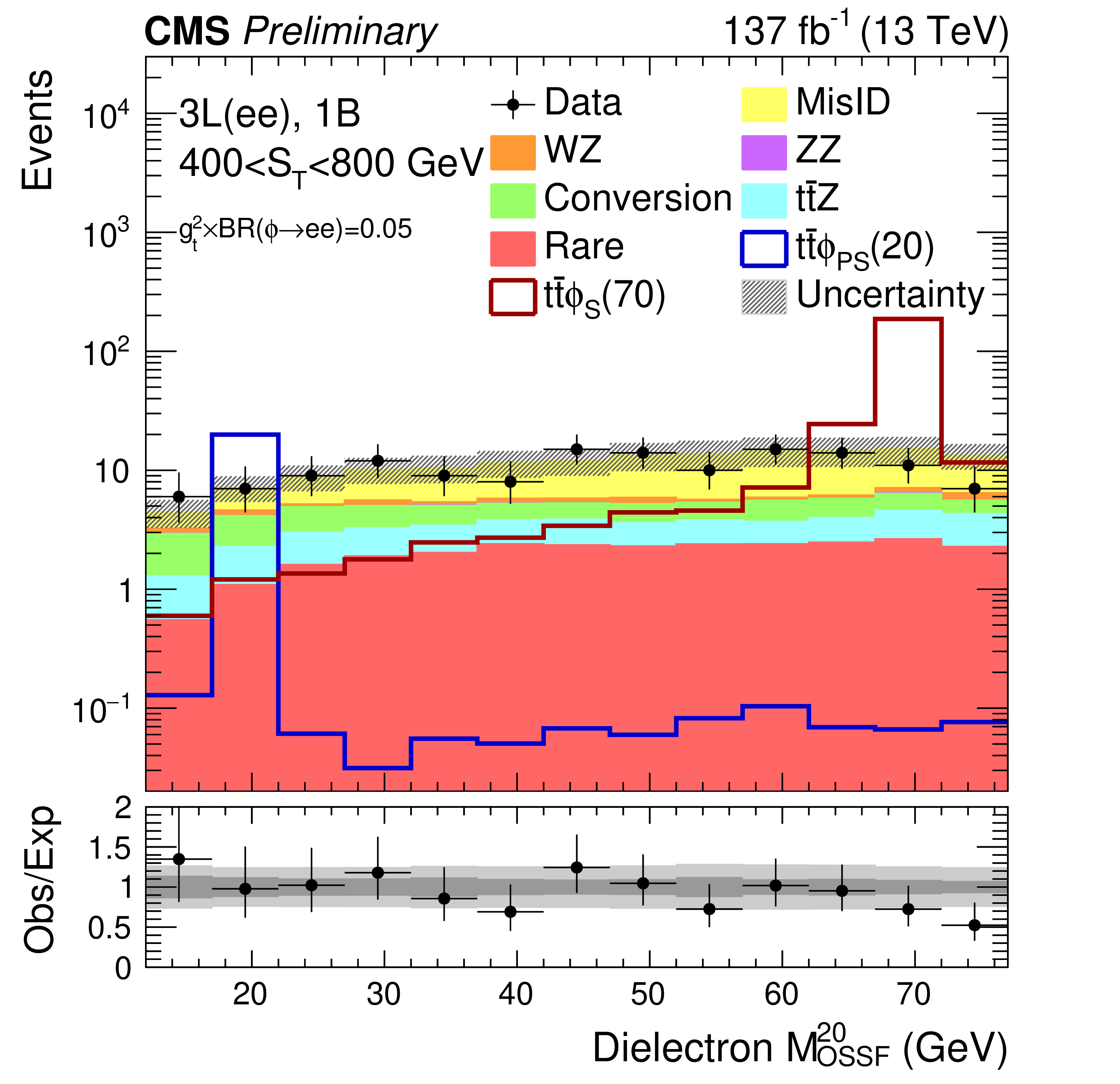
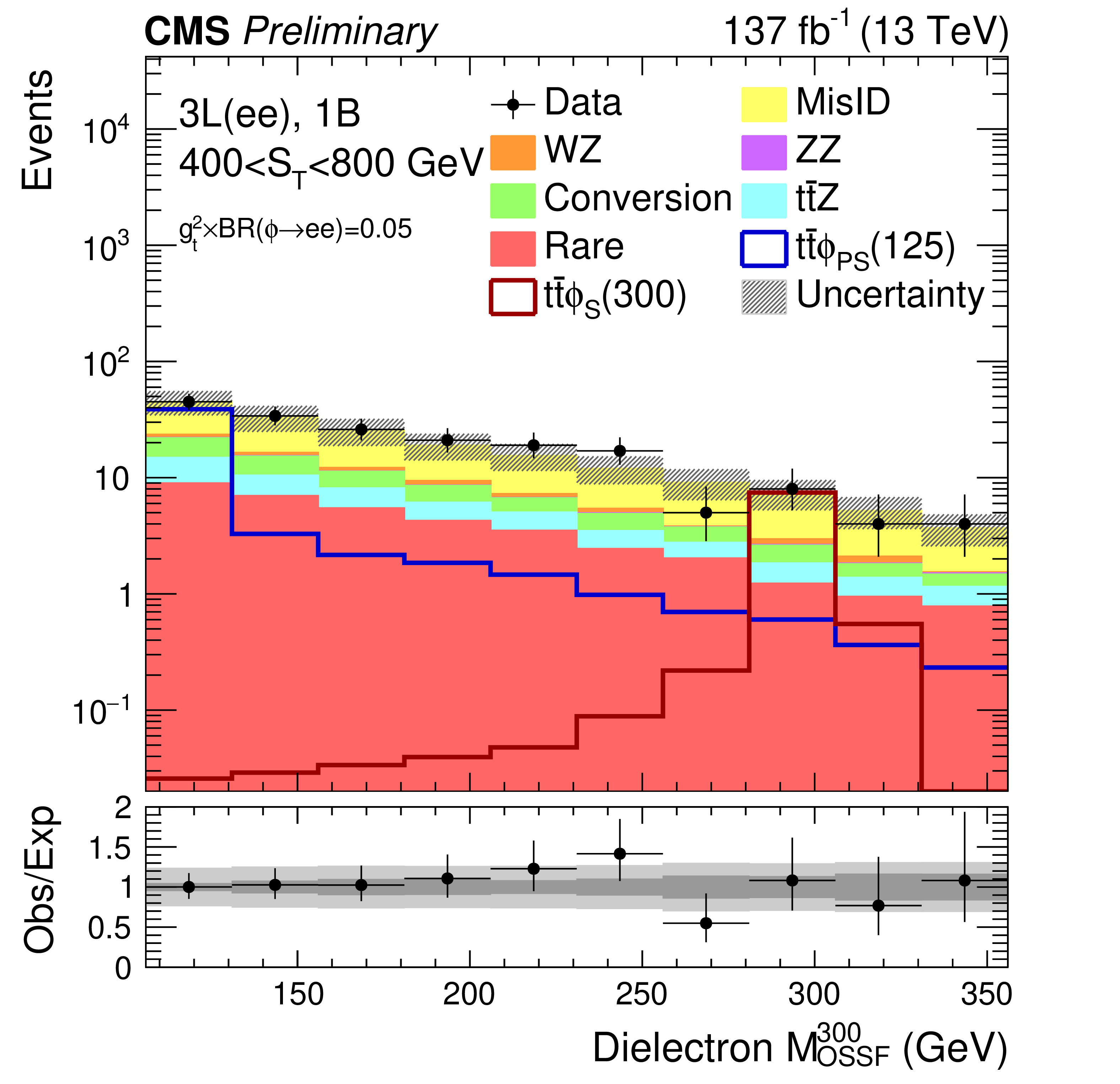
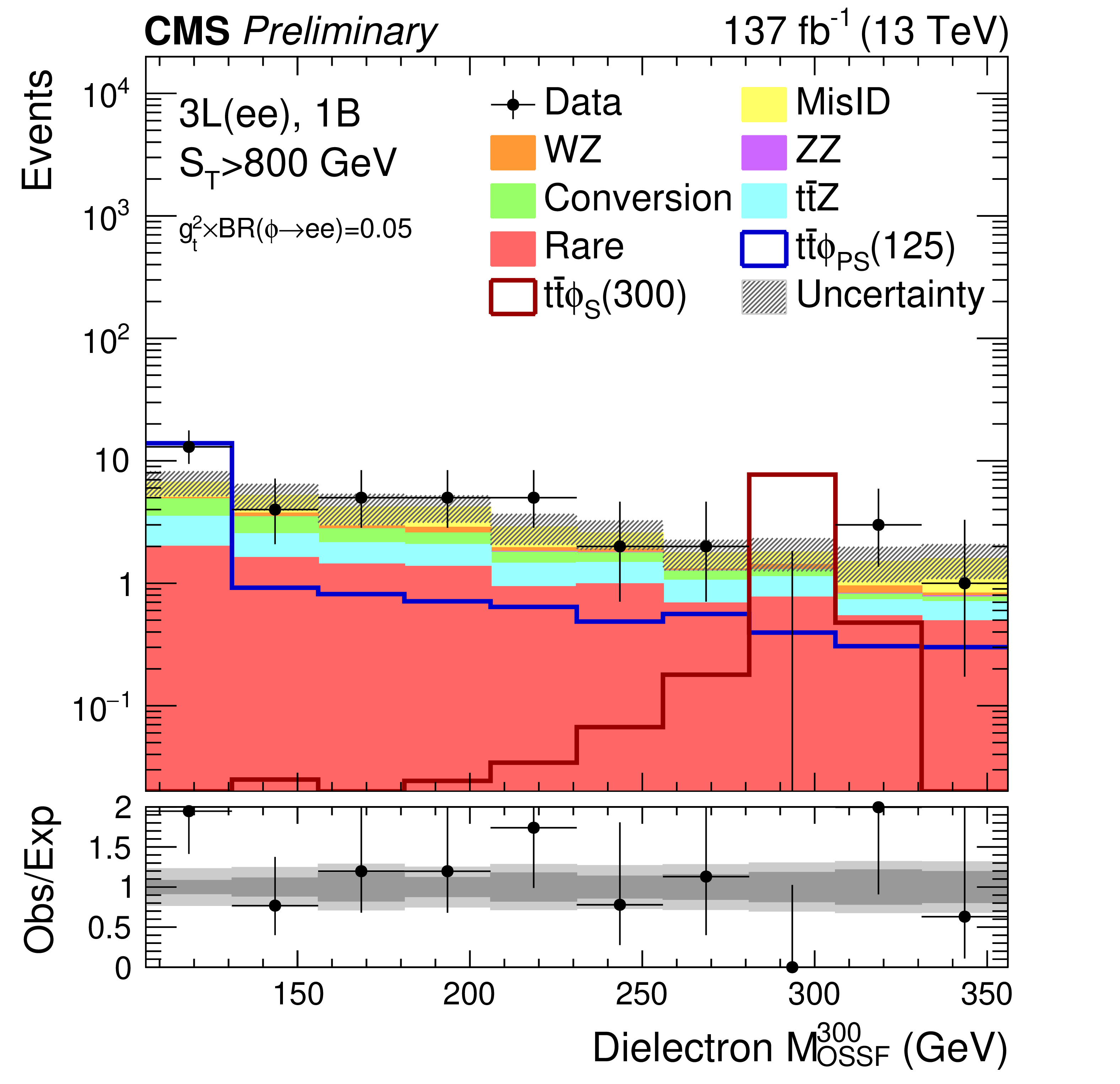
Figure 5:
Dielectron $ {M_{\rm OSSF}}^{20}$ (left column) and $ {M_{\rm OSSF}}^{300}$ (right column) distributions in 3L(ee) 1B $ \mathrm{t\bar{t}}\phi$ signal regions. Upper, center, and lower plots are with 0 $ < {S_{\rm T}} < $ 400 GeV, 400 $ < {S_{\rm T}} < $ 800 GeV, and $ {S_{\rm T}} > $ 800 GeV, respectively. The total SM background is shown as a stacked histogram of all contributing processes. The predictions for $ \mathrm{t\bar{t}}\phi(\rightarrow {\rm ee})$ models with a pseudoscalar (scalar) $\phi $ of 20 and 125 (70 and 300) GeV mass are also shown. The lower panels show the ratio of observed to expected events. The hatched gray band in the upper panels and the light gray bands in the lower panels represent the total (systematic and statistical) uncertainty in each bin, whereas the dark gray bands in the lower panels represent the statistical uncertainty only. The last bins do not contain the overflow events as these are outside the probed mass range. |
png pdf |
Figure 5-a:
Dielectron $ {M_{\rm OSSF}}^{20}$ (left column) and $ {M_{\rm OSSF}}^{300}$ (right column) distributions in 3L(ee) 1B $ \mathrm{t\bar{t}}\phi$ signal regions. Upper, center, and lower plots are with 0 $ < {S_{\rm T}} < $ 400 GeV, 400 $ < {S_{\rm T}} < $ 800 GeV, and $ {S_{\rm T}} > $ 800 GeV, respectively. The total SM background is shown as a stacked histogram of all contributing processes. The predictions for $ \mathrm{t\bar{t}}\phi(\rightarrow {\rm ee})$ models with a pseudoscalar (scalar) $\phi $ of 20 and 125 (70 and 300) GeV mass are also shown. The lower panels show the ratio of observed to expected events. The hatched gray band in the upper panels and the light gray bands in the lower panels represent the total (systematic and statistical) uncertainty in each bin, whereas the dark gray bands in the lower panels represent the statistical uncertainty only. The last bins do not contain the overflow events as these are outside the probed mass range. |

png pdf |
Figure 5-b:
Dielectron $ {M_{\rm OSSF}}^{20}$ (left column) and $ {M_{\rm OSSF}}^{300}$ (right column) distributions in 3L(ee) 1B $ \mathrm{t\bar{t}}\phi$ signal regions. Upper, center, and lower plots are with 0 $ < {S_{\rm T}} < $ 400 GeV, 400 $ < {S_{\rm T}} < $ 800 GeV, and $ {S_{\rm T}} > $ 800 GeV, respectively. The total SM background is shown as a stacked histogram of all contributing processes. The predictions for $ \mathrm{t\bar{t}}\phi(\rightarrow {\rm ee})$ models with a pseudoscalar (scalar) $\phi $ of 20 and 125 (70 and 300) GeV mass are also shown. The lower panels show the ratio of observed to expected events. The hatched gray band in the upper panels and the light gray bands in the lower panels represent the total (systematic and statistical) uncertainty in each bin, whereas the dark gray bands in the lower panels represent the statistical uncertainty only. The last bins do not contain the overflow events as these are outside the probed mass range. |
png pdf |
Figure 5-c:
Dielectron $ {M_{\rm OSSF}}^{20}$ (left column) and $ {M_{\rm OSSF}}^{300}$ (right column) distributions in 3L(ee) 1B $ \mathrm{t\bar{t}}\phi$ signal regions. Upper, center, and lower plots are with 0 $ < {S_{\rm T}} < $ 400 GeV, 400 $ < {S_{\rm T}} < $ 800 GeV, and $ {S_{\rm T}} > $ 800 GeV, respectively. The total SM background is shown as a stacked histogram of all contributing processes. The predictions for $ \mathrm{t\bar{t}}\phi(\rightarrow {\rm ee})$ models with a pseudoscalar (scalar) $\phi $ of 20 and 125 (70 and 300) GeV mass are also shown. The lower panels show the ratio of observed to expected events. The hatched gray band in the upper panels and the light gray bands in the lower panels represent the total (systematic and statistical) uncertainty in each bin, whereas the dark gray bands in the lower panels represent the statistical uncertainty only. The last bins do not contain the overflow events as these are outside the probed mass range. |
png pdf |
Figure 5-d:
Dielectron $ {M_{\rm OSSF}}^{20}$ (left column) and $ {M_{\rm OSSF}}^{300}$ (right column) distributions in 3L(ee) 1B $ \mathrm{t\bar{t}}\phi$ signal regions. Upper, center, and lower plots are with 0 $ < {S_{\rm T}} < $ 400 GeV, 400 $ < {S_{\rm T}} < $ 800 GeV, and $ {S_{\rm T}} > $ 800 GeV, respectively. The total SM background is shown as a stacked histogram of all contributing processes. The predictions for $ \mathrm{t\bar{t}}\phi(\rightarrow {\rm ee})$ models with a pseudoscalar (scalar) $\phi $ of 20 and 125 (70 and 300) GeV mass are also shown. The lower panels show the ratio of observed to expected events. The hatched gray band in the upper panels and the light gray bands in the lower panels represent the total (systematic and statistical) uncertainty in each bin, whereas the dark gray bands in the lower panels represent the statistical uncertainty only. The last bins do not contain the overflow events as these are outside the probed mass range. |

png pdf |
Figure 5-e:
Dielectron $ {M_{\rm OSSF}}^{20}$ (left column) and $ {M_{\rm OSSF}}^{300}$ (right column) distributions in 3L(ee) 1B $ \mathrm{t\bar{t}}\phi$ signal regions. Upper, center, and lower plots are with 0 $ < {S_{\rm T}} < $ 400 GeV, 400 $ < {S_{\rm T}} < $ 800 GeV, and $ {S_{\rm T}} > $ 800 GeV, respectively. The total SM background is shown as a stacked histogram of all contributing processes. The predictions for $ \mathrm{t\bar{t}}\phi(\rightarrow {\rm ee})$ models with a pseudoscalar (scalar) $\phi $ of 20 and 125 (70 and 300) GeV mass are also shown. The lower panels show the ratio of observed to expected events. The hatched gray band in the upper panels and the light gray bands in the lower panels represent the total (systematic and statistical) uncertainty in each bin, whereas the dark gray bands in the lower panels represent the statistical uncertainty only. The last bins do not contain the overflow events as these are outside the probed mass range. |
png pdf |
Figure 5-f:
Dielectron $ {M_{\rm OSSF}}^{20}$ (left column) and $ {M_{\rm OSSF}}^{300}$ (right column) distributions in 3L(ee) 1B $ \mathrm{t\bar{t}}\phi$ signal regions. Upper, center, and lower plots are with 0 $ < {S_{\rm T}} < $ 400 GeV, 400 $ < {S_{\rm T}} < $ 800 GeV, and $ {S_{\rm T}} > $ 800 GeV, respectively. The total SM background is shown as a stacked histogram of all contributing processes. The predictions for $ \mathrm{t\bar{t}}\phi(\rightarrow {\rm ee})$ models with a pseudoscalar (scalar) $\phi $ of 20 and 125 (70 and 300) GeV mass are also shown. The lower panels show the ratio of observed to expected events. The hatched gray band in the upper panels and the light gray bands in the lower panels represent the total (systematic and statistical) uncertainty in each bin, whereas the dark gray bands in the lower panels represent the statistical uncertainty only. The last bins do not contain the overflow events as these are outside the probed mass range. |
png pdf |
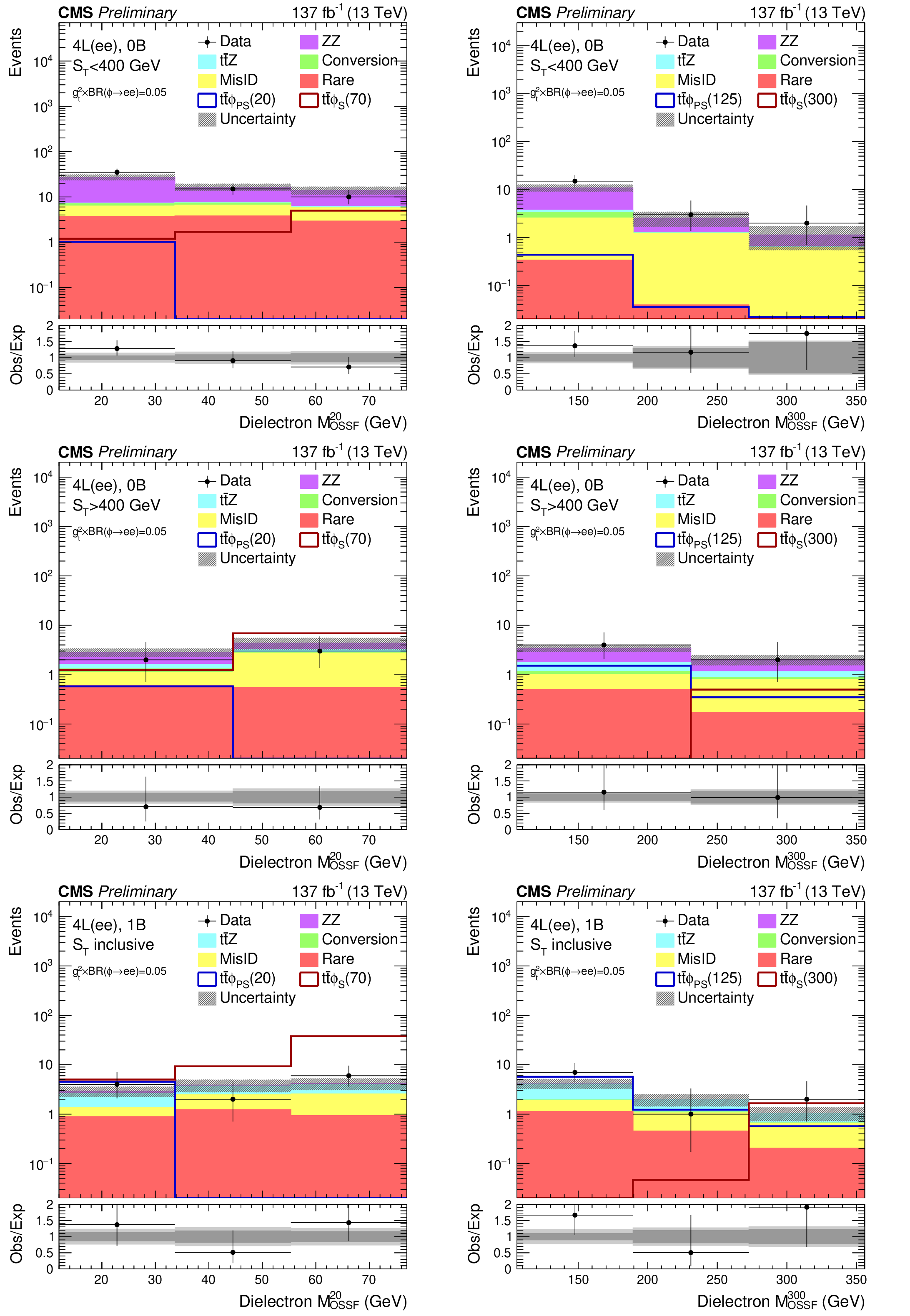
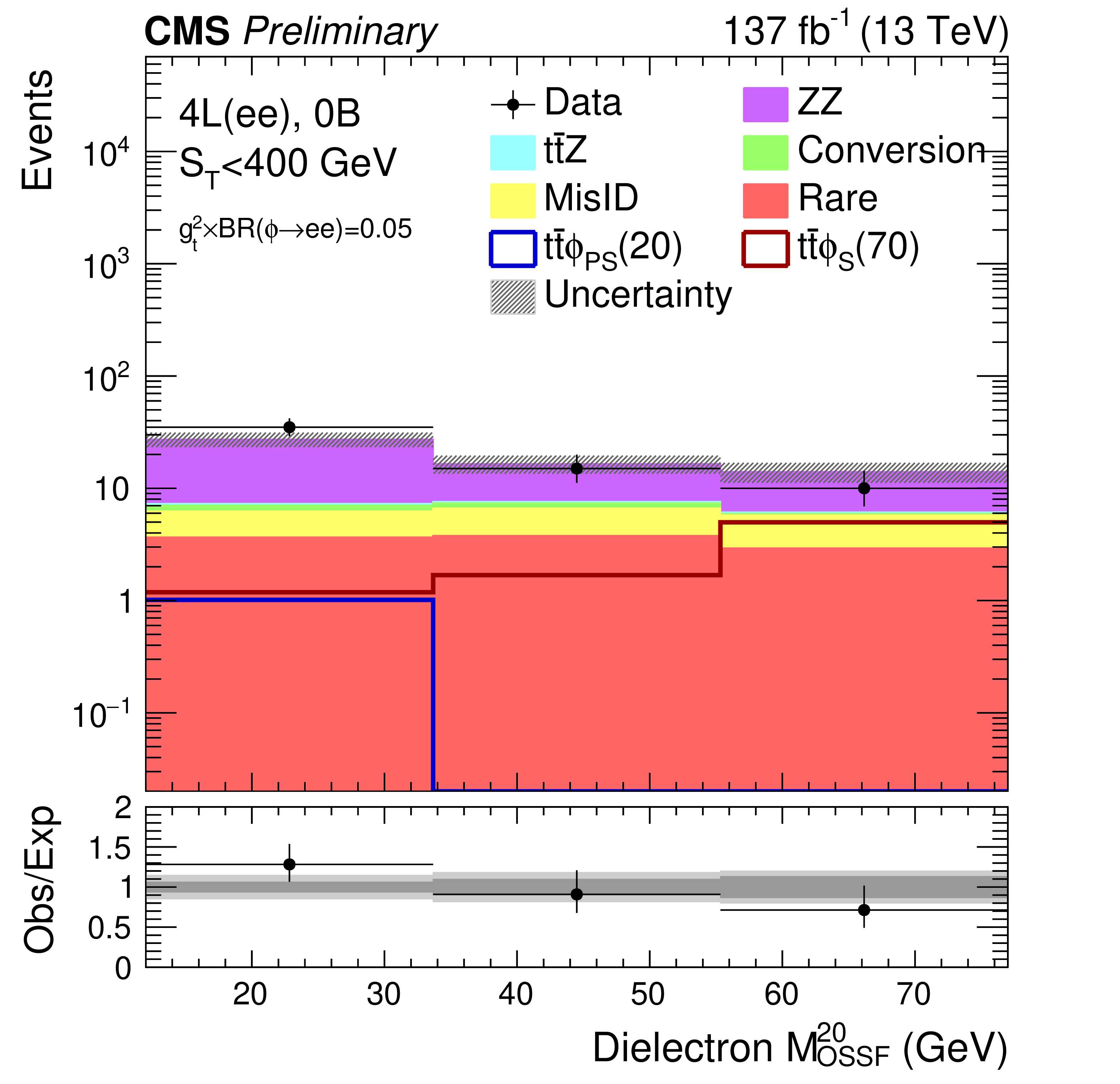
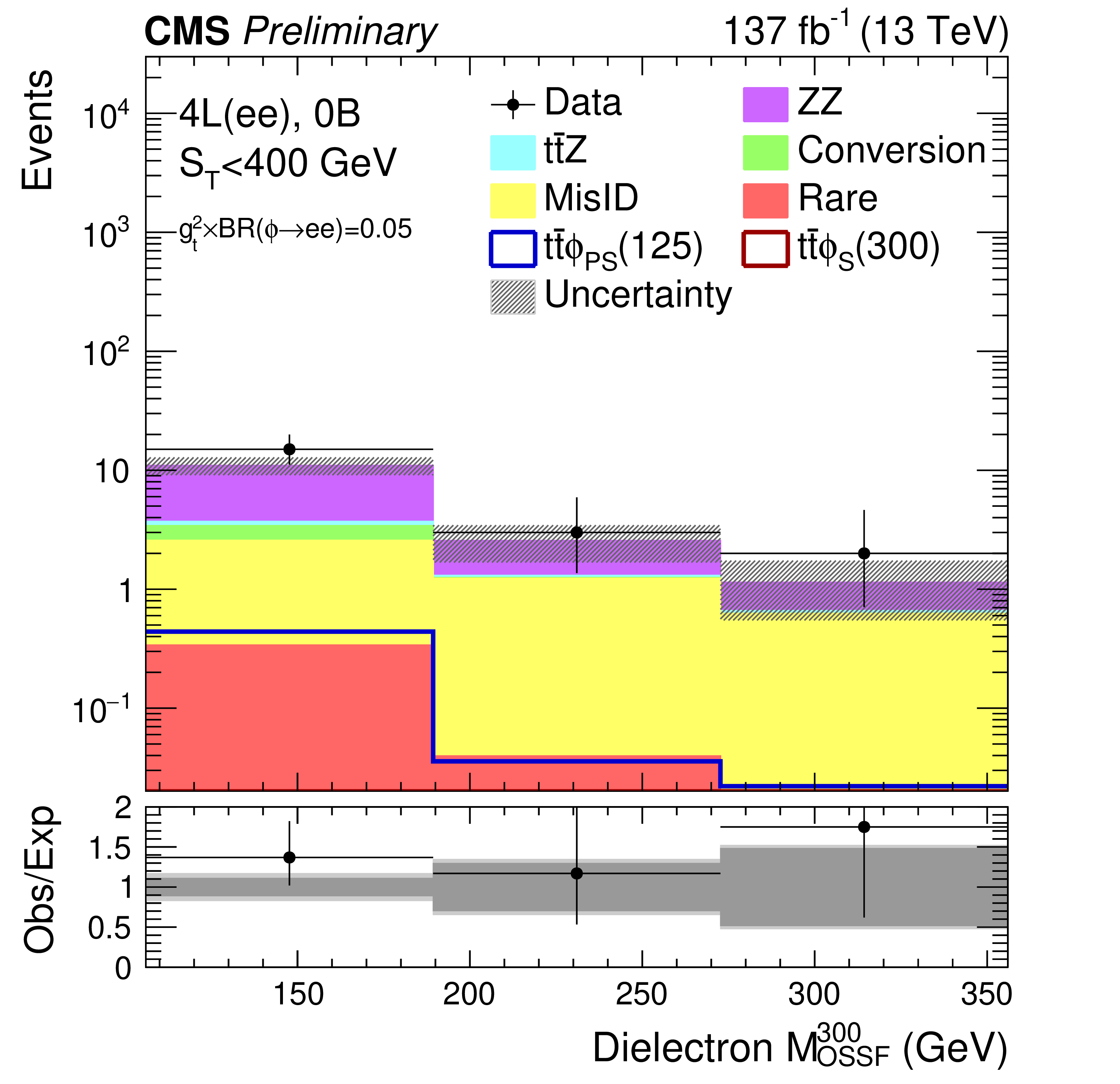
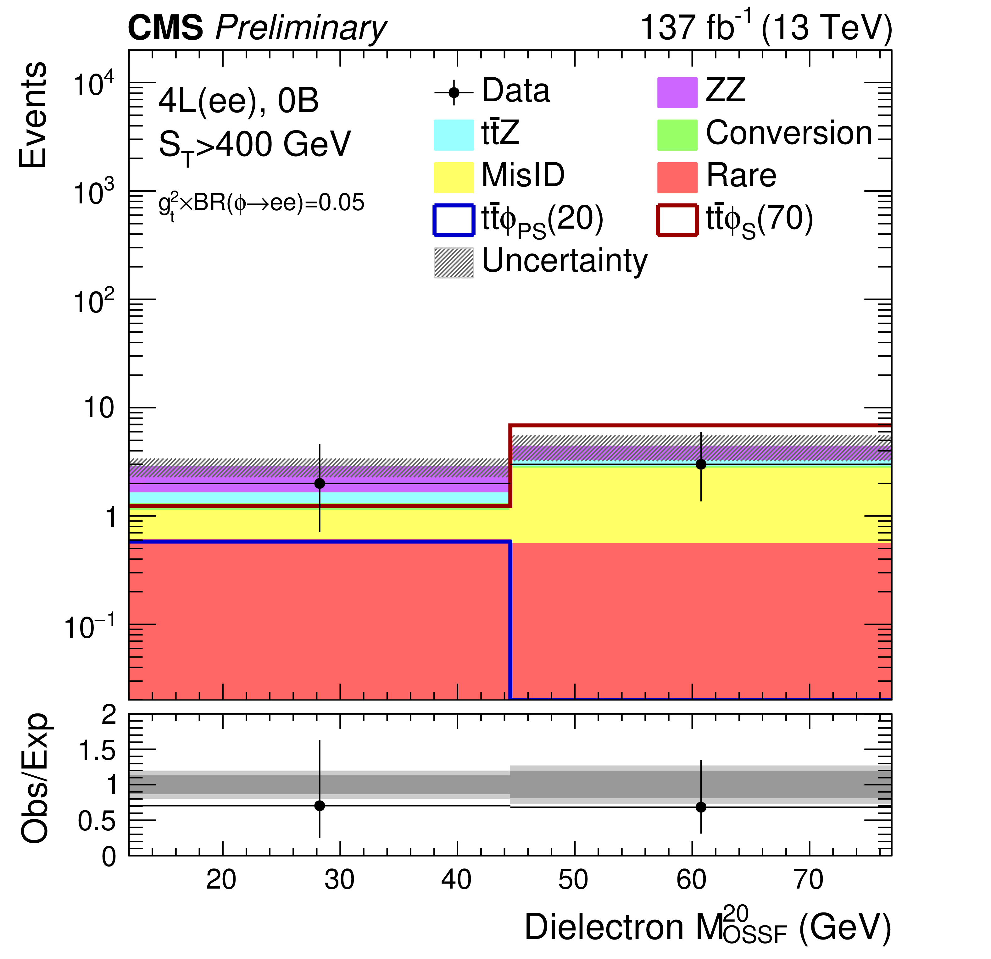
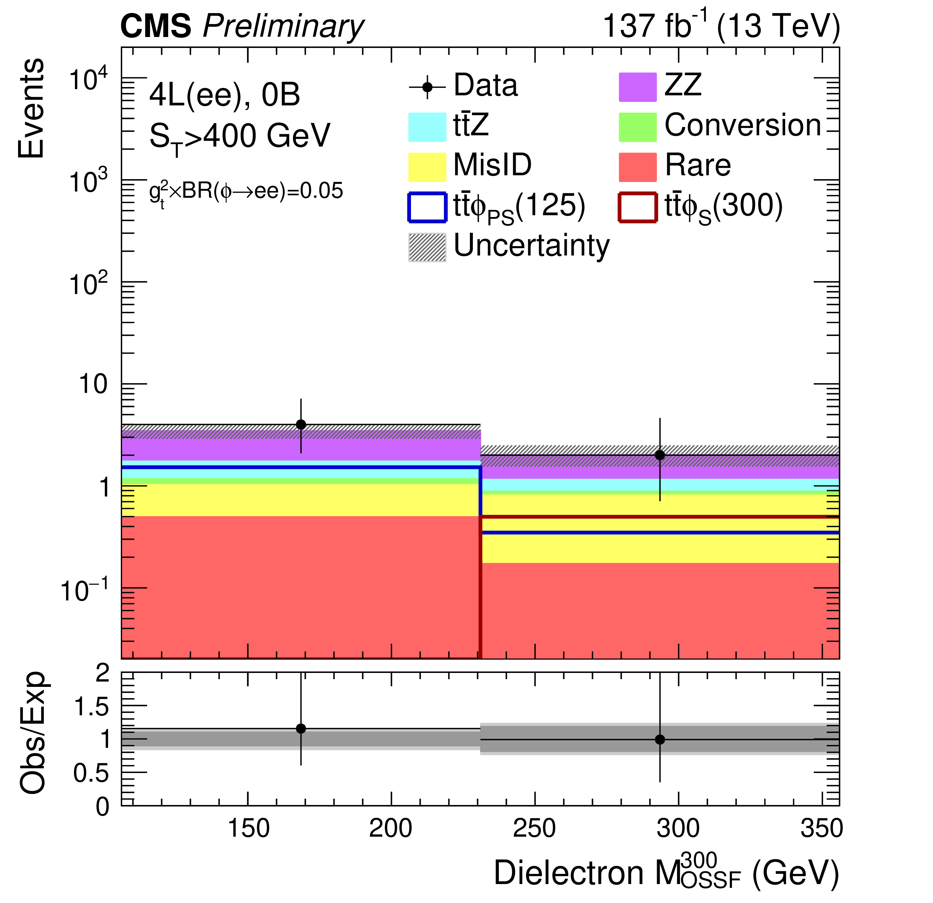
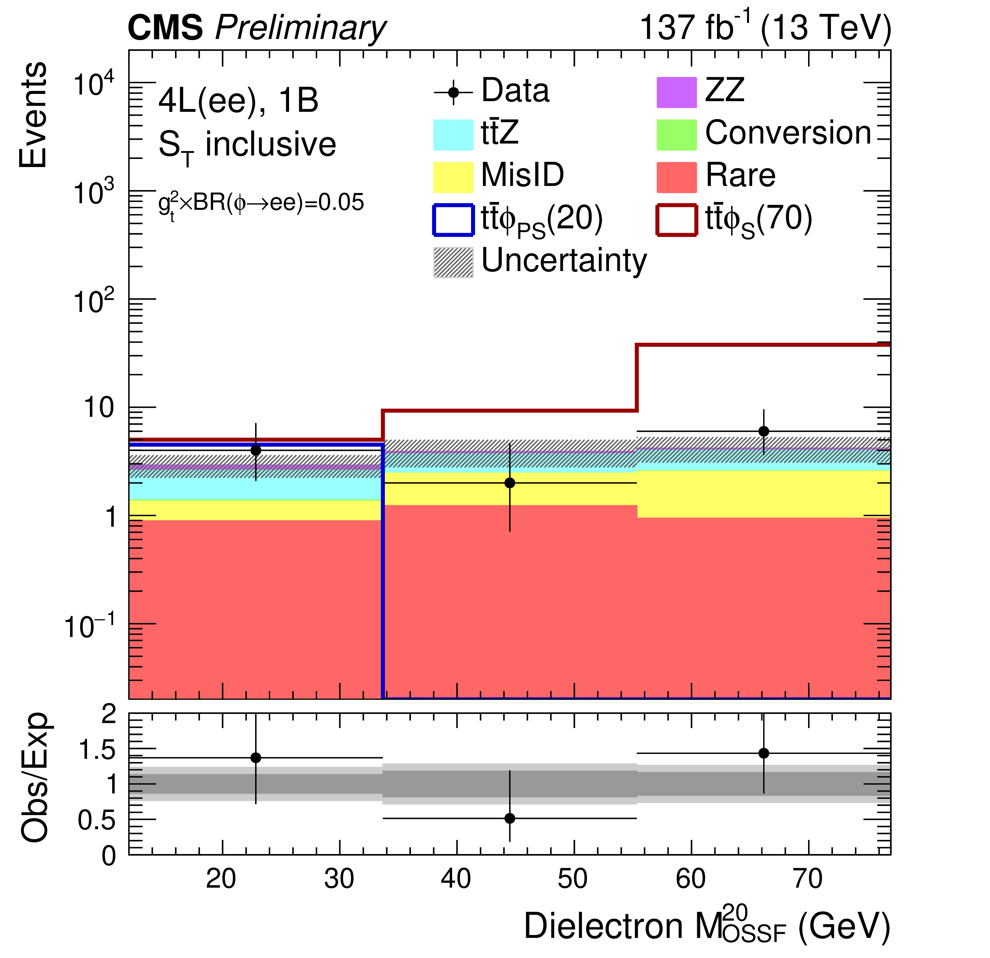
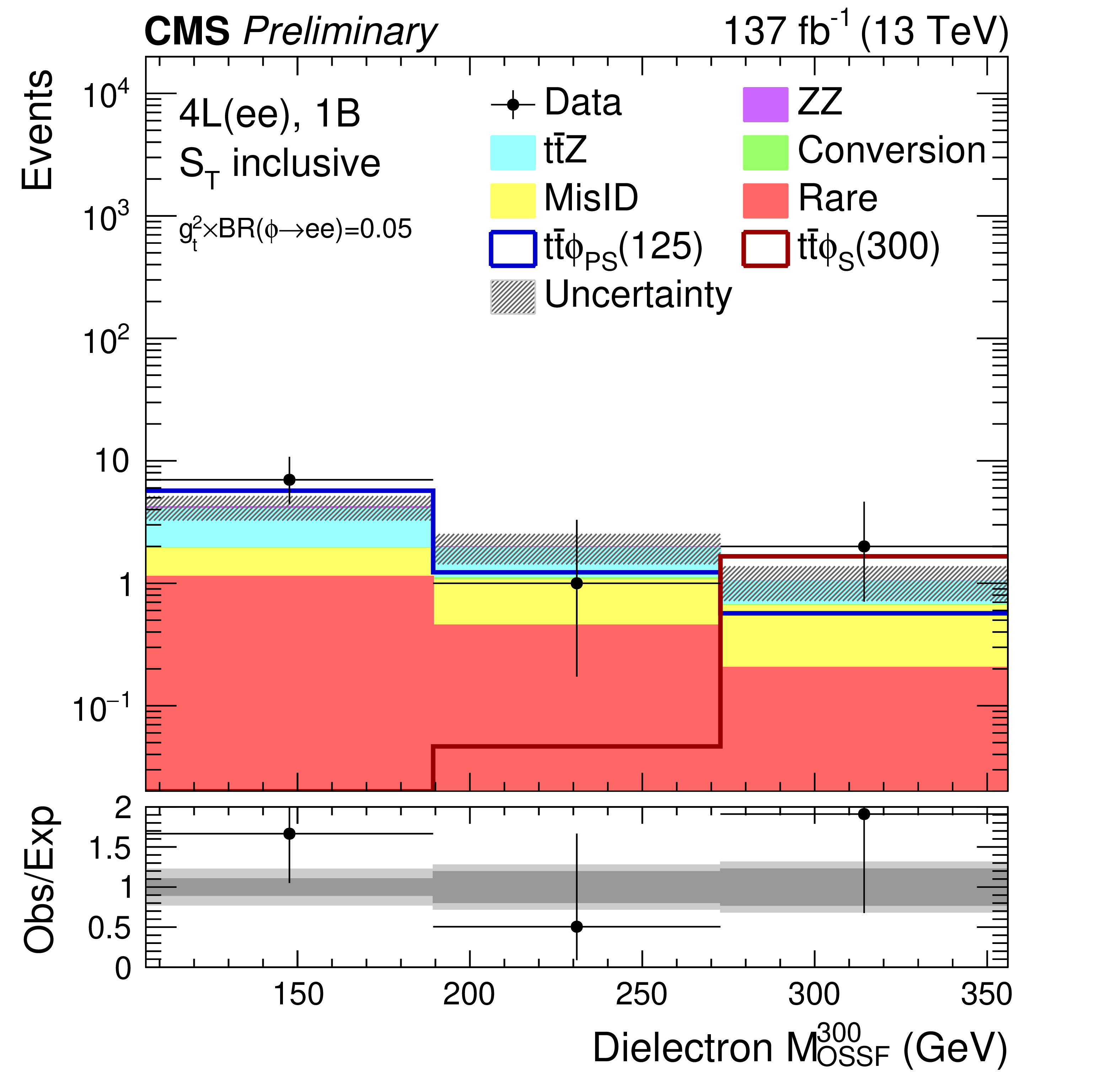
Figure 6:
Dielectron $ {M_{\rm OSSF}}^{20}$ (left column) and $ {M_{\rm OSSF}}^{300}$ (right column) distributions in 4L(ee) $ \mathrm{t\bar{t}}\phi$ signal regions. Upper, center, and lower plots are with 0B 0 $ < {S_{\rm T}} < $ 400 GeV, 0B $ {S_{\rm T}} < $ 400 GeV, and 1B $ {S_{\rm T}}$-inclusive, respectively. The total SM background is shown as a stacked histogram of all contributing processes. The predictions for $ \mathrm{t\bar{t}}\phi(\rightarrow {\rm ee})$ models with a pseudoscalar (scalar) $\phi $ of 20 and 125 (70 and 300) GeV mass are also shown. The lower panels show the ratio of observed to expected events. The hatched gray band in the upper panels and the light gray bands in the lower panels represent the total (systematic and statistical) uncertainty in each bin, whereas the dark gray bands in the lower panels represent the statistical uncertainty only. The last bins do not contain the overflow events as these are outside the probed mass range. |
png pdf |
Figure 6-a:
Dielectron $ {M_{\rm OSSF}}^{20}$ (left column) and $ {M_{\rm OSSF}}^{300}$ (right column) distributions in 4L(ee) $ \mathrm{t\bar{t}}\phi$ signal regions. Upper, center, and lower plots are with 0B 0 $ < {S_{\rm T}} < $ 400 GeV, 0B $ {S_{\rm T}} < $ 400 GeV, and 1B $ {S_{\rm T}}$-inclusive, respectively. The total SM background is shown as a stacked histogram of all contributing processes. The predictions for $ \mathrm{t\bar{t}}\phi(\rightarrow {\rm ee})$ models with a pseudoscalar (scalar) $\phi $ of 20 and 125 (70 and 300) GeV mass are also shown. The lower panels show the ratio of observed to expected events. The hatched gray band in the upper panels and the light gray bands in the lower panels represent the total (systematic and statistical) uncertainty in each bin, whereas the dark gray bands in the lower panels represent the statistical uncertainty only. The last bins do not contain the overflow events as these are outside the probed mass range. |
png pdf |
Figure 6-b:
Dielectron $ {M_{\rm OSSF}}^{20}$ (left column) and $ {M_{\rm OSSF}}^{300}$ (right column) distributions in 4L(ee) $ \mathrm{t\bar{t}}\phi$ signal regions. Upper, center, and lower plots are with 0B 0 $ < {S_{\rm T}} < $ 400 GeV, 0B $ {S_{\rm T}} < $ 400 GeV, and 1B $ {S_{\rm T}}$-inclusive, respectively. The total SM background is shown as a stacked histogram of all contributing processes. The predictions for $ \mathrm{t\bar{t}}\phi(\rightarrow {\rm ee})$ models with a pseudoscalar (scalar) $\phi $ of 20 and 125 (70 and 300) GeV mass are also shown. The lower panels show the ratio of observed to expected events. The hatched gray band in the upper panels and the light gray bands in the lower panels represent the total (systematic and statistical) uncertainty in each bin, whereas the dark gray bands in the lower panels represent the statistical uncertainty only. The last bins do not contain the overflow events as these are outside the probed mass range. |
png pdf |
Figure 6-c:
Dielectron $ {M_{\rm OSSF}}^{20}$ (left column) and $ {M_{\rm OSSF}}^{300}$ (right column) distributions in 4L(ee) $ \mathrm{t\bar{t}}\phi$ signal regions. Upper, center, and lower plots are with 0B 0 $ < {S_{\rm T}} < $ 400 GeV, 0B $ {S_{\rm T}} < $ 400 GeV, and 1B $ {S_{\rm T}}$-inclusive, respectively. The total SM background is shown as a stacked histogram of all contributing processes. The predictions for $ \mathrm{t\bar{t}}\phi(\rightarrow {\rm ee})$ models with a pseudoscalar (scalar) $\phi $ of 20 and 125 (70 and 300) GeV mass are also shown. The lower panels show the ratio of observed to expected events. The hatched gray band in the upper panels and the light gray bands in the lower panels represent the total (systematic and statistical) uncertainty in each bin, whereas the dark gray bands in the lower panels represent the statistical uncertainty only. The last bins do not contain the overflow events as these are outside the probed mass range. |
png pdf |
Figure 6-d:
Dielectron $ {M_{\rm OSSF}}^{20}$ (left column) and $ {M_{\rm OSSF}}^{300}$ (right column) distributions in 4L(ee) $ \mathrm{t\bar{t}}\phi$ signal regions. Upper, center, and lower plots are with 0B 0 $ < {S_{\rm T}} < $ 400 GeV, 0B $ {S_{\rm T}} < $ 400 GeV, and 1B $ {S_{\rm T}}$-inclusive, respectively. The total SM background is shown as a stacked histogram of all contributing processes. The predictions for $ \mathrm{t\bar{t}}\phi(\rightarrow {\rm ee})$ models with a pseudoscalar (scalar) $\phi $ of 20 and 125 (70 and 300) GeV mass are also shown. The lower panels show the ratio of observed to expected events. The hatched gray band in the upper panels and the light gray bands in the lower panels represent the total (systematic and statistical) uncertainty in each bin, whereas the dark gray bands in the lower panels represent the statistical uncertainty only. The last bins do not contain the overflow events as these are outside the probed mass range. |
png pdf |
Figure 6-e:
Dielectron $ {M_{\rm OSSF}}^{20}$ (left column) and $ {M_{\rm OSSF}}^{300}$ (right column) distributions in 4L(ee) $ \mathrm{t\bar{t}}\phi$ signal regions. Upper, center, and lower plots are with 0B 0 $ < {S_{\rm T}} < $ 400 GeV, 0B $ {S_{\rm T}} < $ 400 GeV, and 1B $ {S_{\rm T}}$-inclusive, respectively. The total SM background is shown as a stacked histogram of all contributing processes. The predictions for $ \mathrm{t\bar{t}}\phi(\rightarrow {\rm ee})$ models with a pseudoscalar (scalar) $\phi $ of 20 and 125 (70 and 300) GeV mass are also shown. The lower panels show the ratio of observed to expected events. The hatched gray band in the upper panels and the light gray bands in the lower panels represent the total (systematic and statistical) uncertainty in each bin, whereas the dark gray bands in the lower panels represent the statistical uncertainty only. The last bins do not contain the overflow events as these are outside the probed mass range. |
png pdf |
Figure 6-f:
Dielectron $ {M_{\rm OSSF}}^{20}$ (left column) and $ {M_{\rm OSSF}}^{300}$ (right column) distributions in 4L(ee) $ \mathrm{t\bar{t}}\phi$ signal regions. Upper, center, and lower plots are with 0B 0 $ < {S_{\rm T}} < $ 400 GeV, 0B $ {S_{\rm T}} < $ 400 GeV, and 1B $ {S_{\rm T}}$-inclusive, respectively. The total SM background is shown as a stacked histogram of all contributing processes. The predictions for $ \mathrm{t\bar{t}}\phi(\rightarrow {\rm ee})$ models with a pseudoscalar (scalar) $\phi $ of 20 and 125 (70 and 300) GeV mass are also shown. The lower panels show the ratio of observed to expected events. The hatched gray band in the upper panels and the light gray bands in the lower panels represent the total (systematic and statistical) uncertainty in each bin, whereas the dark gray bands in the lower panels represent the statistical uncertainty only. The last bins do not contain the overflow events as these are outside the probed mass range. |
png pdf |
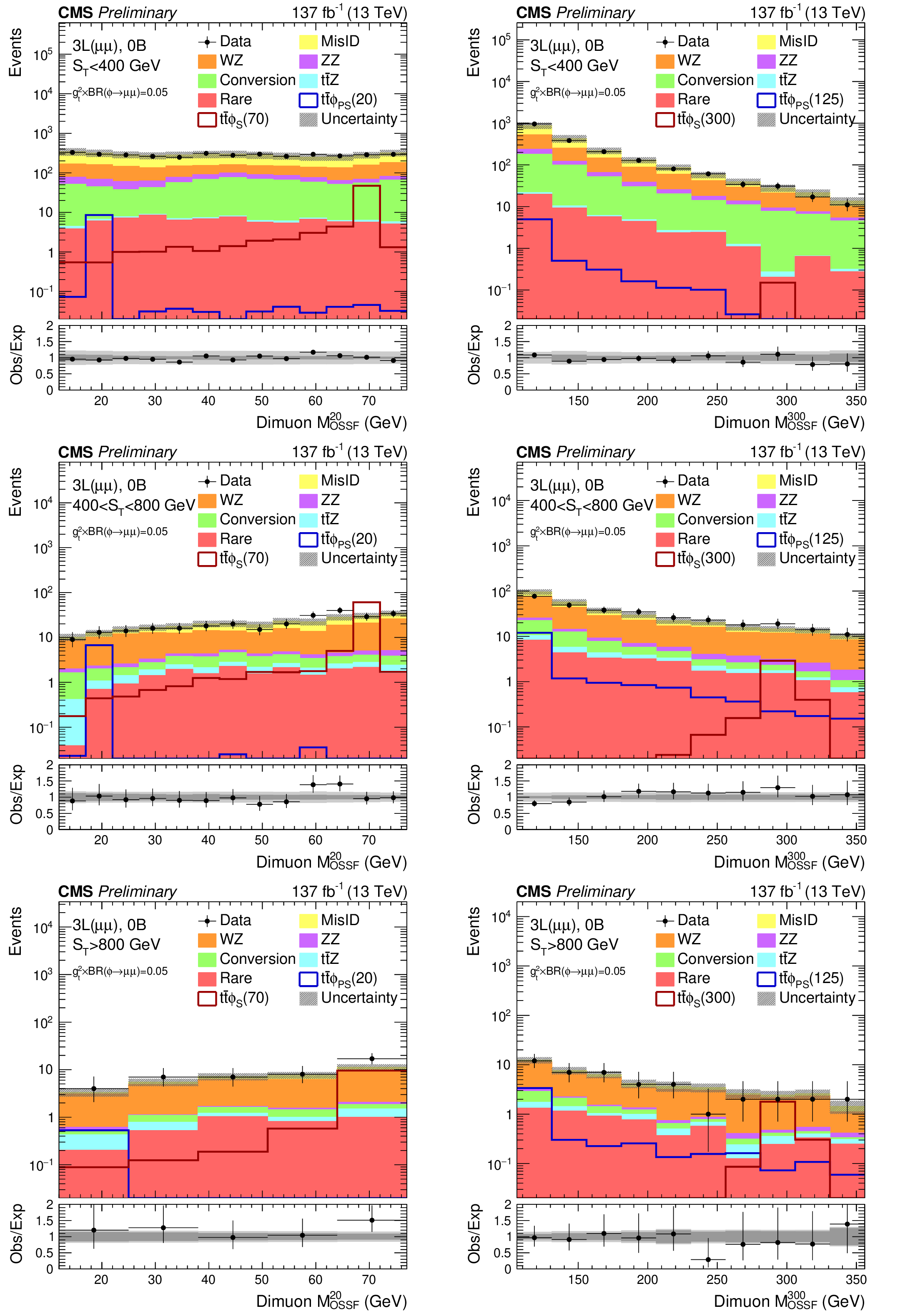
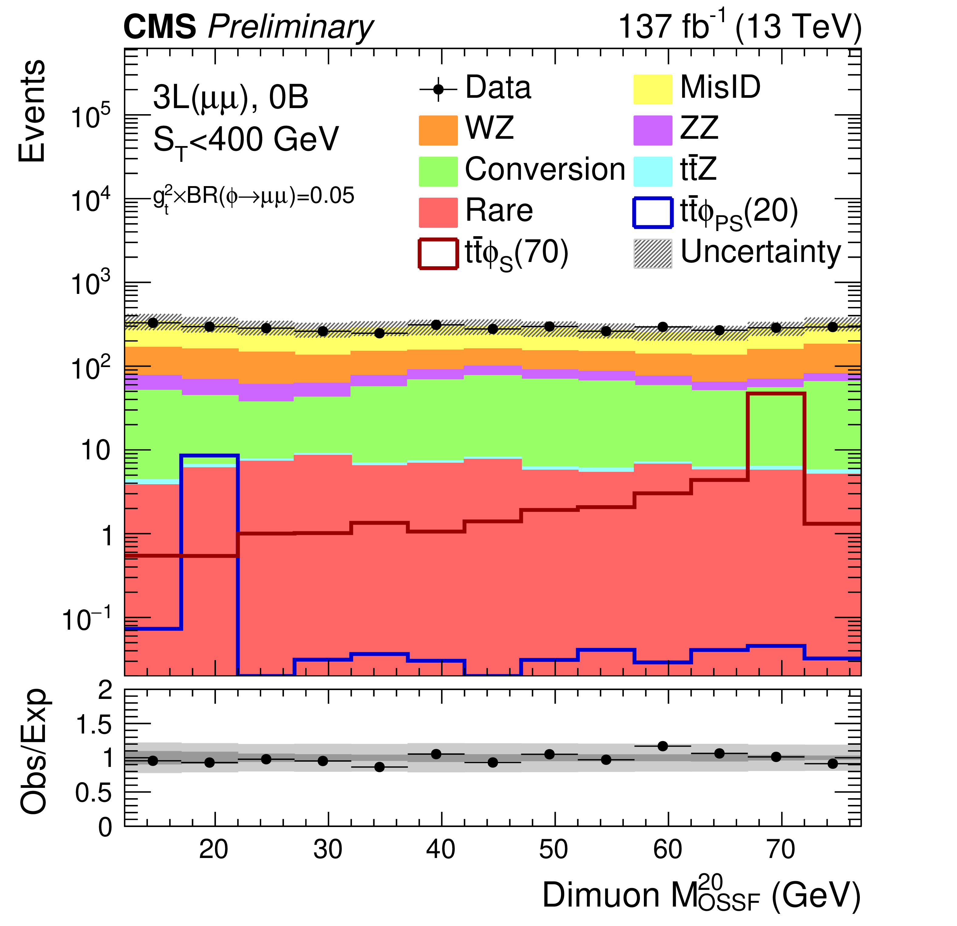
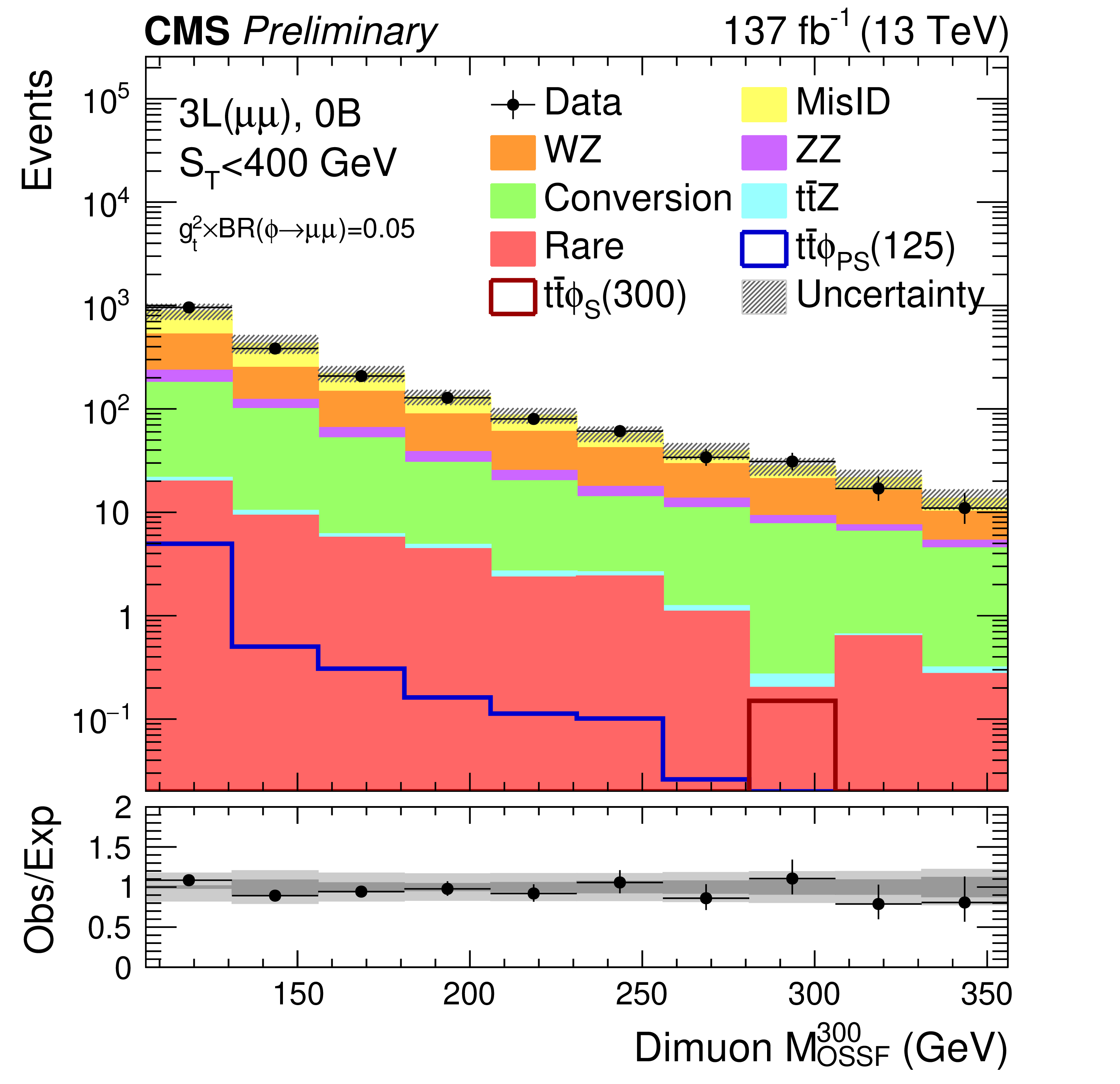
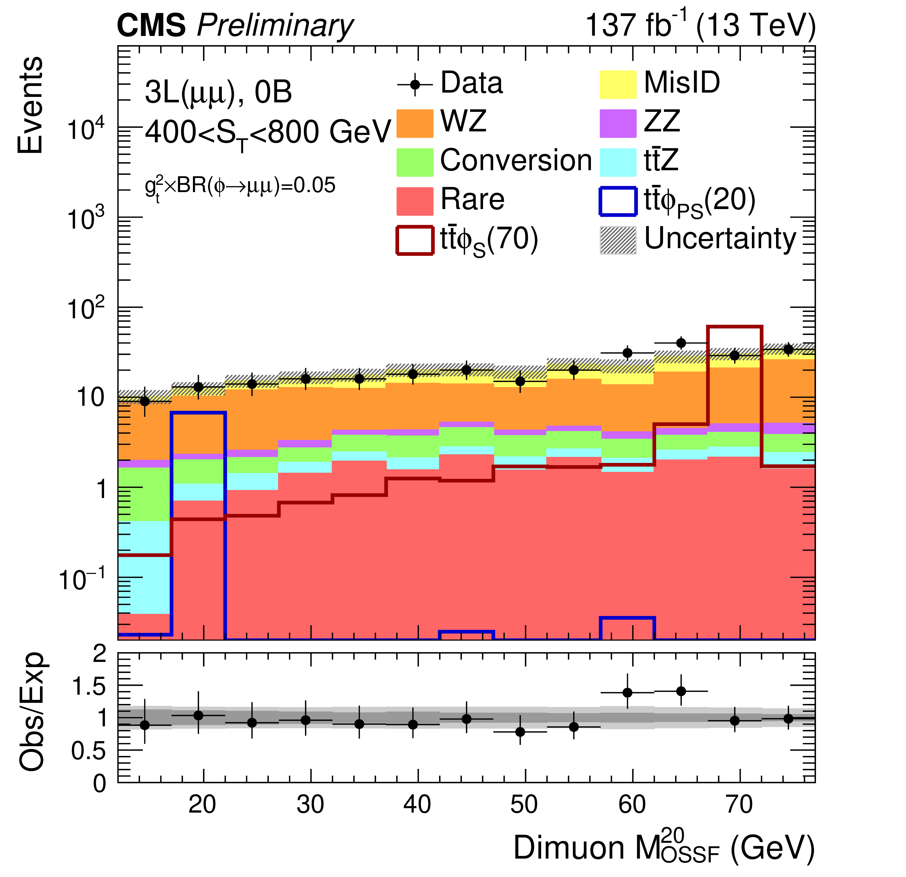
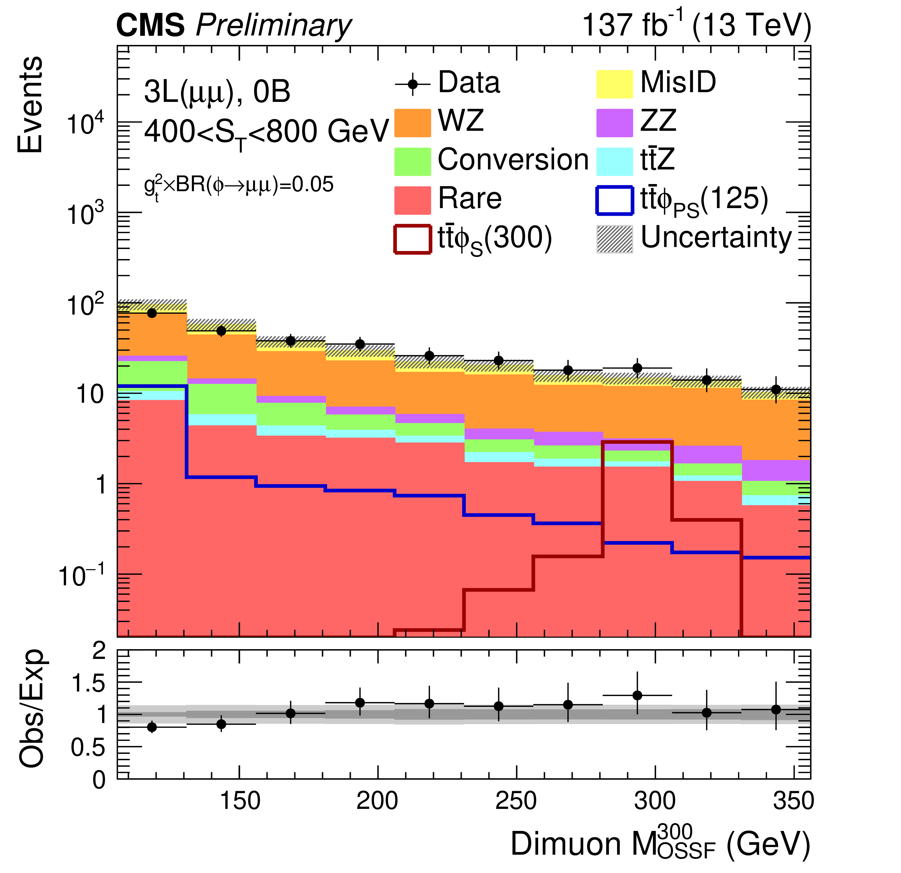
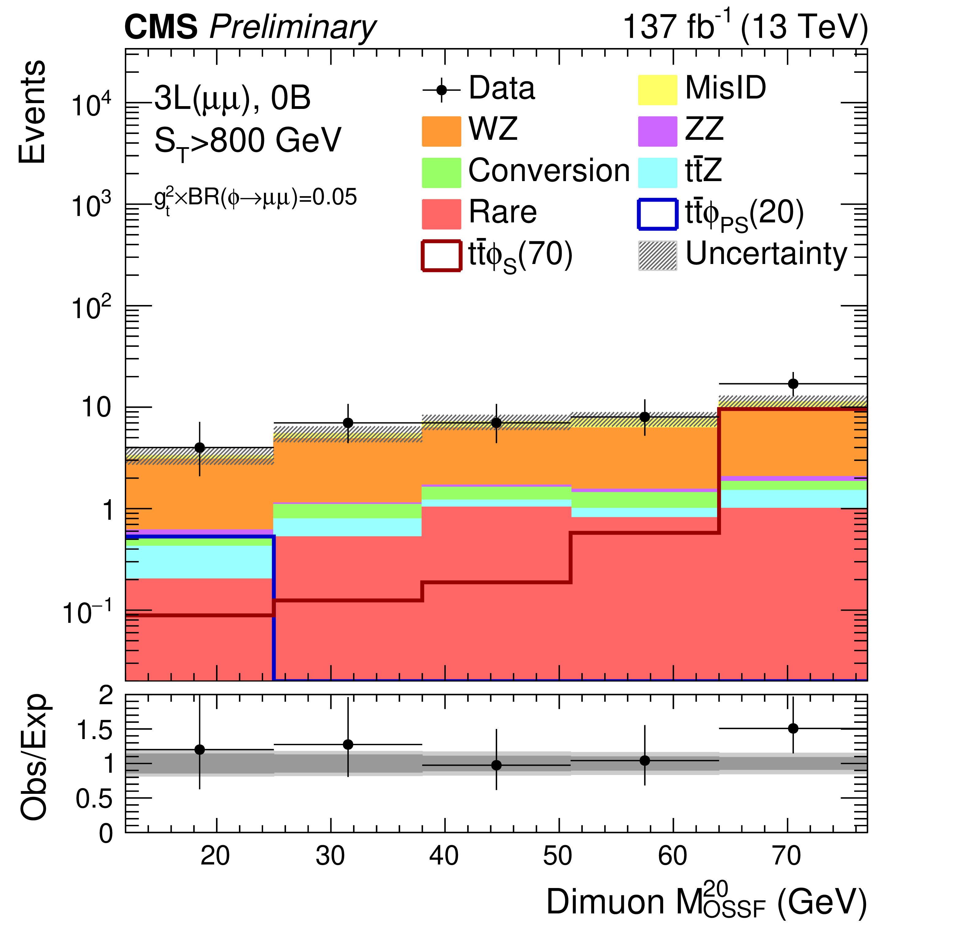
Figure 7:
Dimuon $ {M_{\rm OSSF}}^{20}$ (left column) and $ {M_{\rm OSSF}}^{300}$ (right column) distributions in 3L$(\mu \mu )$ 0B $ \mathrm{t\bar{t}}\phi$ signal regions. Upper, center, and lower plots are with 0 $ < {S_{\rm T}} < $ 400 GeV, 400 $ < {S_{\rm T}} < $ 800 GeV, and $ {S_{\rm T}} > $ 800 GeV, respectively. The total SM background is shown as a stacked histogram of all contributing processes. The predictions for $ \mathrm{t\bar{t}}\phi(\rightarrow \mu \mu )$ models with a pseudoscalar (scalar) $\phi $ of 20 and 125 (70 and 300) GeV mass are also shown. The lower panels show the ratio of observed to expected events. The hatched gray band in the upper panels and the light gray bands in the lower panels represent the total (systematic and statistical) uncertainty in each bin, whereas the dark gray bands in the lower panels represent the statistical uncertainty only. The last bins do not contain the overflow events as these are outside the probed mass range. |
png pdf |
Figure 7-a:
Dimuon $ {M_{\rm OSSF}}^{20}$ (left column) and $ {M_{\rm OSSF}}^{300}$ (right column) distributions in 3L$(\mu \mu )$ 0B $ \mathrm{t\bar{t}}\phi$ signal regions. Upper, center, and lower plots are with 0 $ < {S_{\rm T}} < $ 400 GeV, 400 $ < {S_{\rm T}} < $ 800 GeV, and $ {S_{\rm T}} > $ 800 GeV, respectively. The total SM background is shown as a stacked histogram of all contributing processes. The predictions for $ \mathrm{t\bar{t}}\phi(\rightarrow \mu \mu )$ models with a pseudoscalar (scalar) $\phi $ of 20 and 125 (70 and 300) GeV mass are also shown. The lower panels show the ratio of observed to expected events. The hatched gray band in the upper panels and the light gray bands in the lower panels represent the total (systematic and statistical) uncertainty in each bin, whereas the dark gray bands in the lower panels represent the statistical uncertainty only. The last bins do not contain the overflow events as these are outside the probed mass range. |
png pdf |
Figure 7-b:
Dimuon $ {M_{\rm OSSF}}^{20}$ (left column) and $ {M_{\rm OSSF}}^{300}$ (right column) distributions in 3L$(\mu \mu )$ 0B $ \mathrm{t\bar{t}}\phi$ signal regions. Upper, center, and lower plots are with 0 $ < {S_{\rm T}} < $ 400 GeV, 400 $ < {S_{\rm T}} < $ 800 GeV, and $ {S_{\rm T}} > $ 800 GeV, respectively. The total SM background is shown as a stacked histogram of all contributing processes. The predictions for $ \mathrm{t\bar{t}}\phi(\rightarrow \mu \mu )$ models with a pseudoscalar (scalar) $\phi $ of 20 and 125 (70 and 300) GeV mass are also shown. The lower panels show the ratio of observed to expected events. The hatched gray band in the upper panels and the light gray bands in the lower panels represent the total (systematic and statistical) uncertainty in each bin, whereas the dark gray bands in the lower panels represent the statistical uncertainty only. The last bins do not contain the overflow events as these are outside the probed mass range. |
png pdf |
Figure 7-c:
Dimuon $ {M_{\rm OSSF}}^{20}$ (left column) and $ {M_{\rm OSSF}}^{300}$ (right column) distributions in 3L$(\mu \mu )$ 0B $ \mathrm{t\bar{t}}\phi$ signal regions. Upper, center, and lower plots are with 0 $ < {S_{\rm T}} < $ 400 GeV, 400 $ < {S_{\rm T}} < $ 800 GeV, and $ {S_{\rm T}} > $ 800 GeV, respectively. The total SM background is shown as a stacked histogram of all contributing processes. The predictions for $ \mathrm{t\bar{t}}\phi(\rightarrow \mu \mu )$ models with a pseudoscalar (scalar) $\phi $ of 20 and 125 (70 and 300) GeV mass are also shown. The lower panels show the ratio of observed to expected events. The hatched gray band in the upper panels and the light gray bands in the lower panels represent the total (systematic and statistical) uncertainty in each bin, whereas the dark gray bands in the lower panels represent the statistical uncertainty only. The last bins do not contain the overflow events as these are outside the probed mass range. |
png pdf |
Figure 7-d:
Dimuon $ {M_{\rm OSSF}}^{20}$ (left column) and $ {M_{\rm OSSF}}^{300}$ (right column) distributions in 3L$(\mu \mu )$ 0B $ \mathrm{t\bar{t}}\phi$ signal regions. Upper, center, and lower plots are with 0 $ < {S_{\rm T}} < $ 400 GeV, 400 $ < {S_{\rm T}} < $ 800 GeV, and $ {S_{\rm T}} > $ 800 GeV, respectively. The total SM background is shown as a stacked histogram of all contributing processes. The predictions for $ \mathrm{t\bar{t}}\phi(\rightarrow \mu \mu )$ models with a pseudoscalar (scalar) $\phi $ of 20 and 125 (70 and 300) GeV mass are also shown. The lower panels show the ratio of observed to expected events. The hatched gray band in the upper panels and the light gray bands in the lower panels represent the total (systematic and statistical) uncertainty in each bin, whereas the dark gray bands in the lower panels represent the statistical uncertainty only. The last bins do not contain the overflow events as these are outside the probed mass range. |
png pdf |
Figure 7-e:
Dimuon $ {M_{\rm OSSF}}^{20}$ (left column) and $ {M_{\rm OSSF}}^{300}$ (right column) distributions in 3L$(\mu \mu )$ 0B $ \mathrm{t\bar{t}}\phi$ signal regions. Upper, center, and lower plots are with 0 $ < {S_{\rm T}} < $ 400 GeV, 400 $ < {S_{\rm T}} < $ 800 GeV, and $ {S_{\rm T}} > $ 800 GeV, respectively. The total SM background is shown as a stacked histogram of all contributing processes. The predictions for $ \mathrm{t\bar{t}}\phi(\rightarrow \mu \mu )$ models with a pseudoscalar (scalar) $\phi $ of 20 and 125 (70 and 300) GeV mass are also shown. The lower panels show the ratio of observed to expected events. The hatched gray band in the upper panels and the light gray bands in the lower panels represent the total (systematic and statistical) uncertainty in each bin, whereas the dark gray bands in the lower panels represent the statistical uncertainty only. The last bins do not contain the overflow events as these are outside the probed mass range. |

png pdf |
Figure 7-f:
Dimuon $ {M_{\rm OSSF}}^{20}$ (left column) and $ {M_{\rm OSSF}}^{300}$ (right column) distributions in 3L$(\mu \mu )$ 0B $ \mathrm{t\bar{t}}\phi$ signal regions. Upper, center, and lower plots are with 0 $ < {S_{\rm T}} < $ 400 GeV, 400 $ < {S_{\rm T}} < $ 800 GeV, and $ {S_{\rm T}} > $ 800 GeV, respectively. The total SM background is shown as a stacked histogram of all contributing processes. The predictions for $ \mathrm{t\bar{t}}\phi(\rightarrow \mu \mu )$ models with a pseudoscalar (scalar) $\phi $ of 20 and 125 (70 and 300) GeV mass are also shown. The lower panels show the ratio of observed to expected events. The hatched gray band in the upper panels and the light gray bands in the lower panels represent the total (systematic and statistical) uncertainty in each bin, whereas the dark gray bands in the lower panels represent the statistical uncertainty only. The last bins do not contain the overflow events as these are outside the probed mass range. |
png pdf |
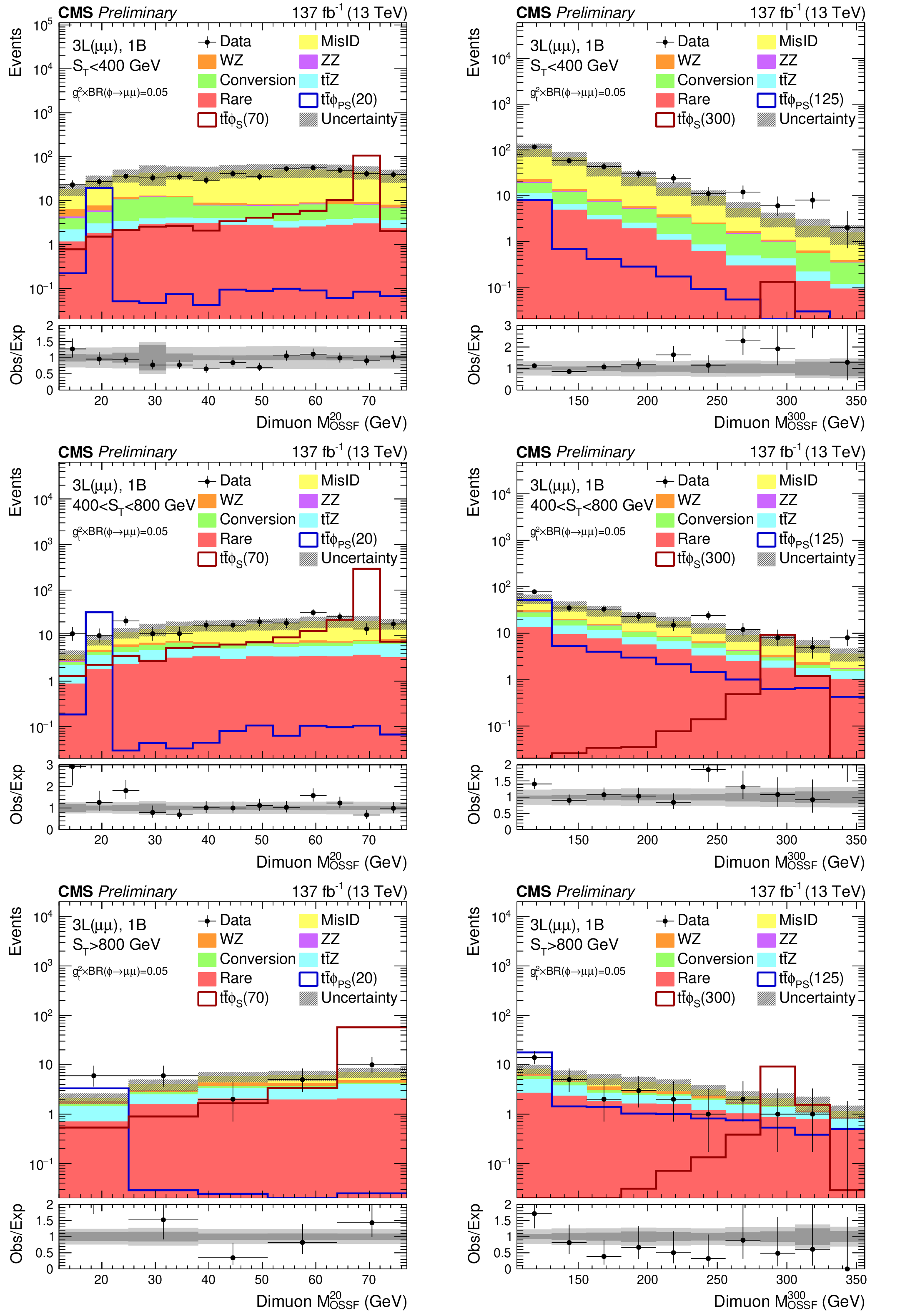
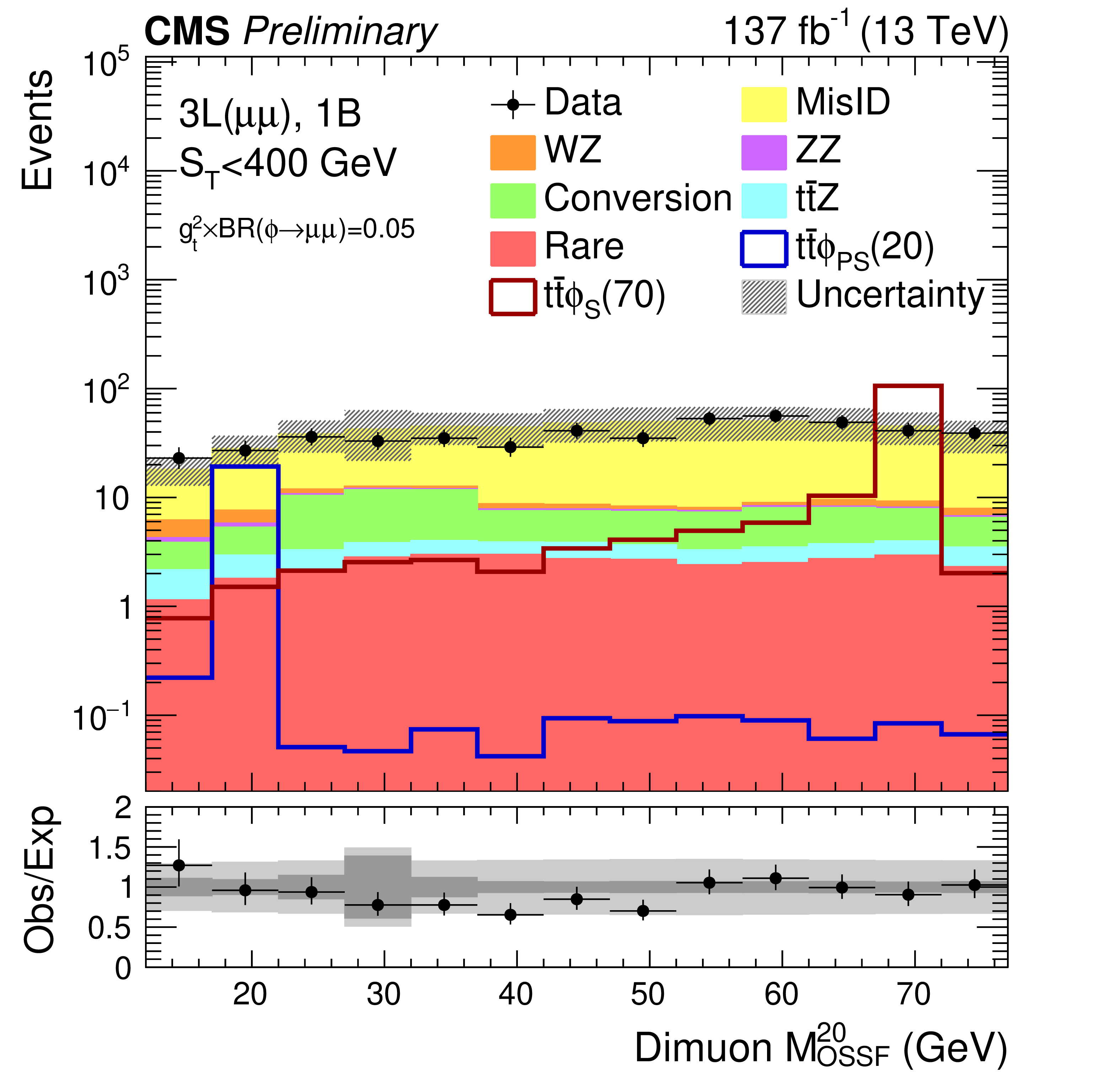
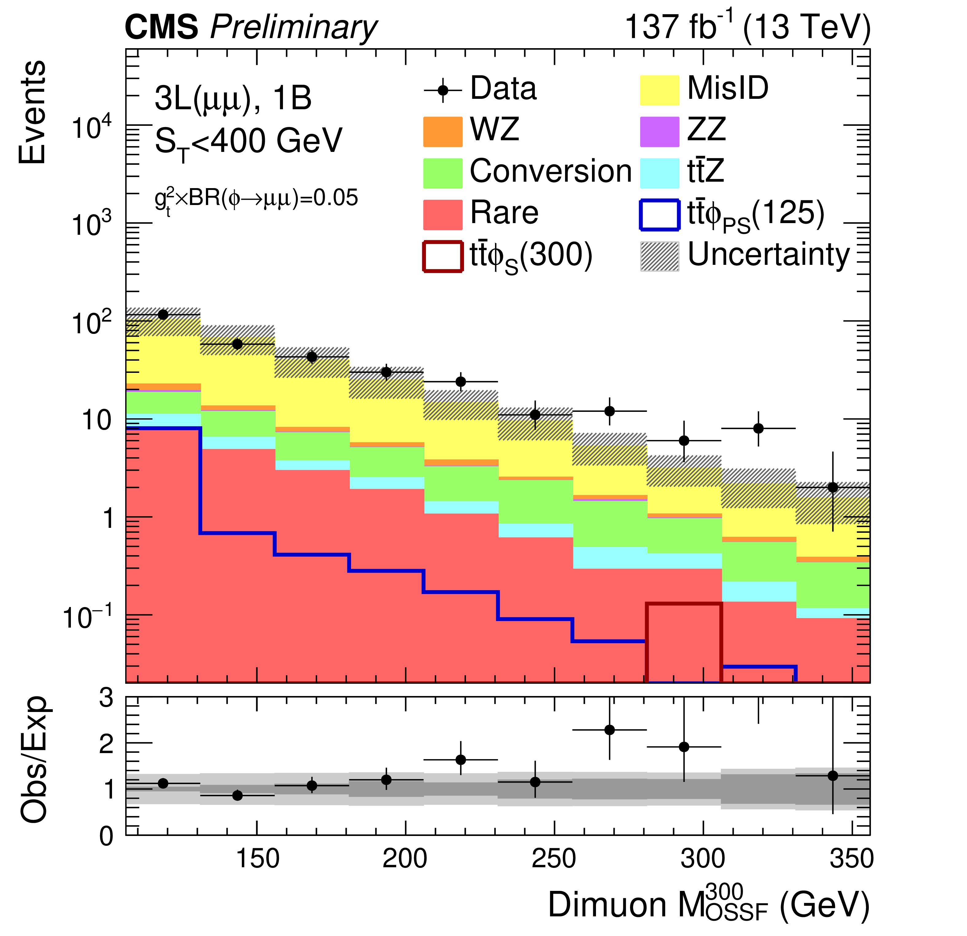
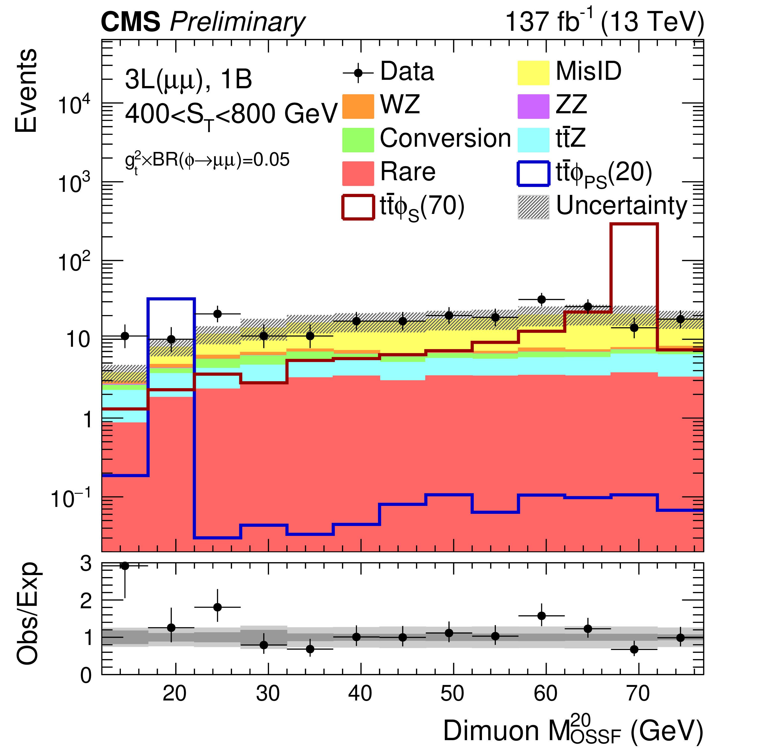
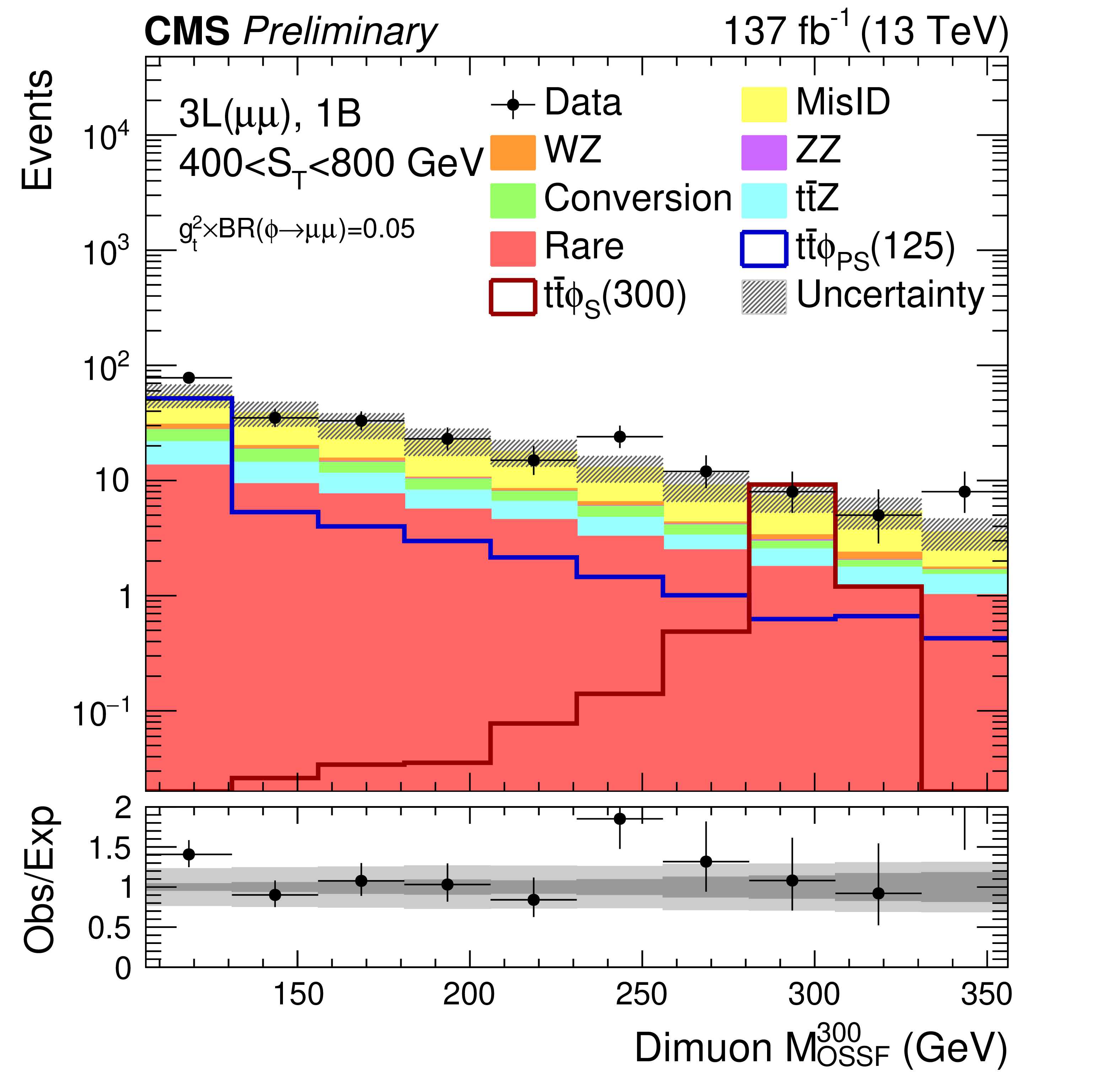
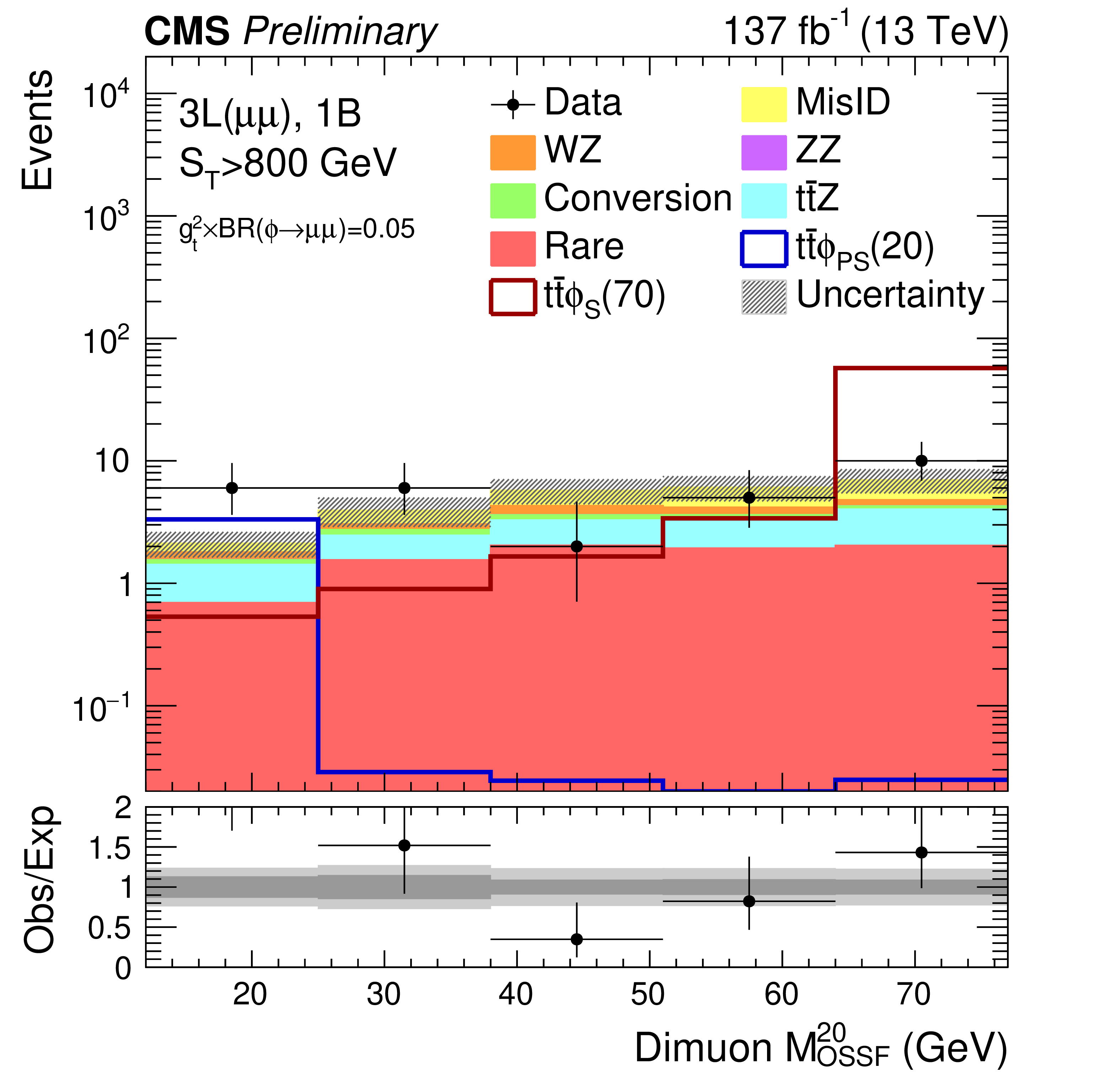
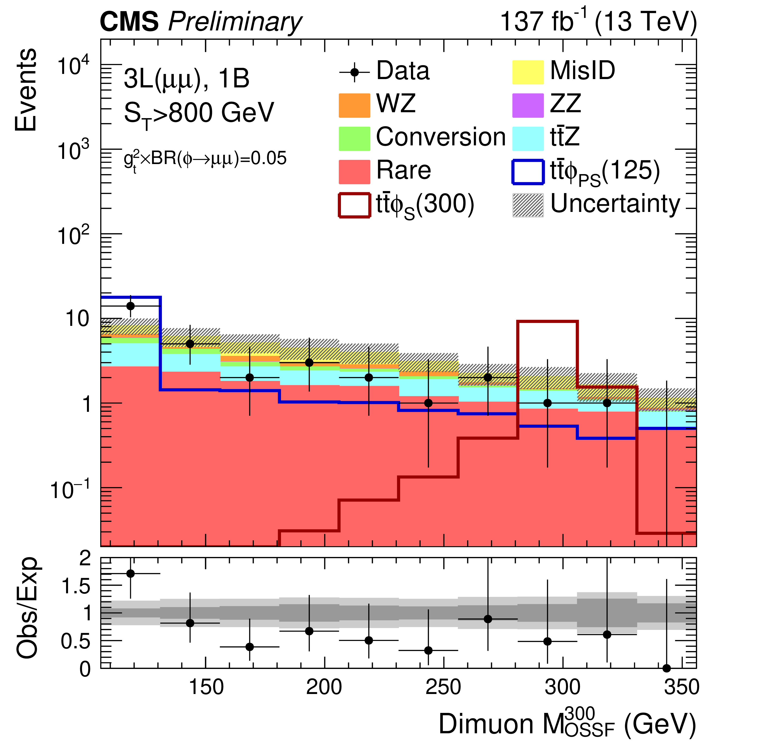
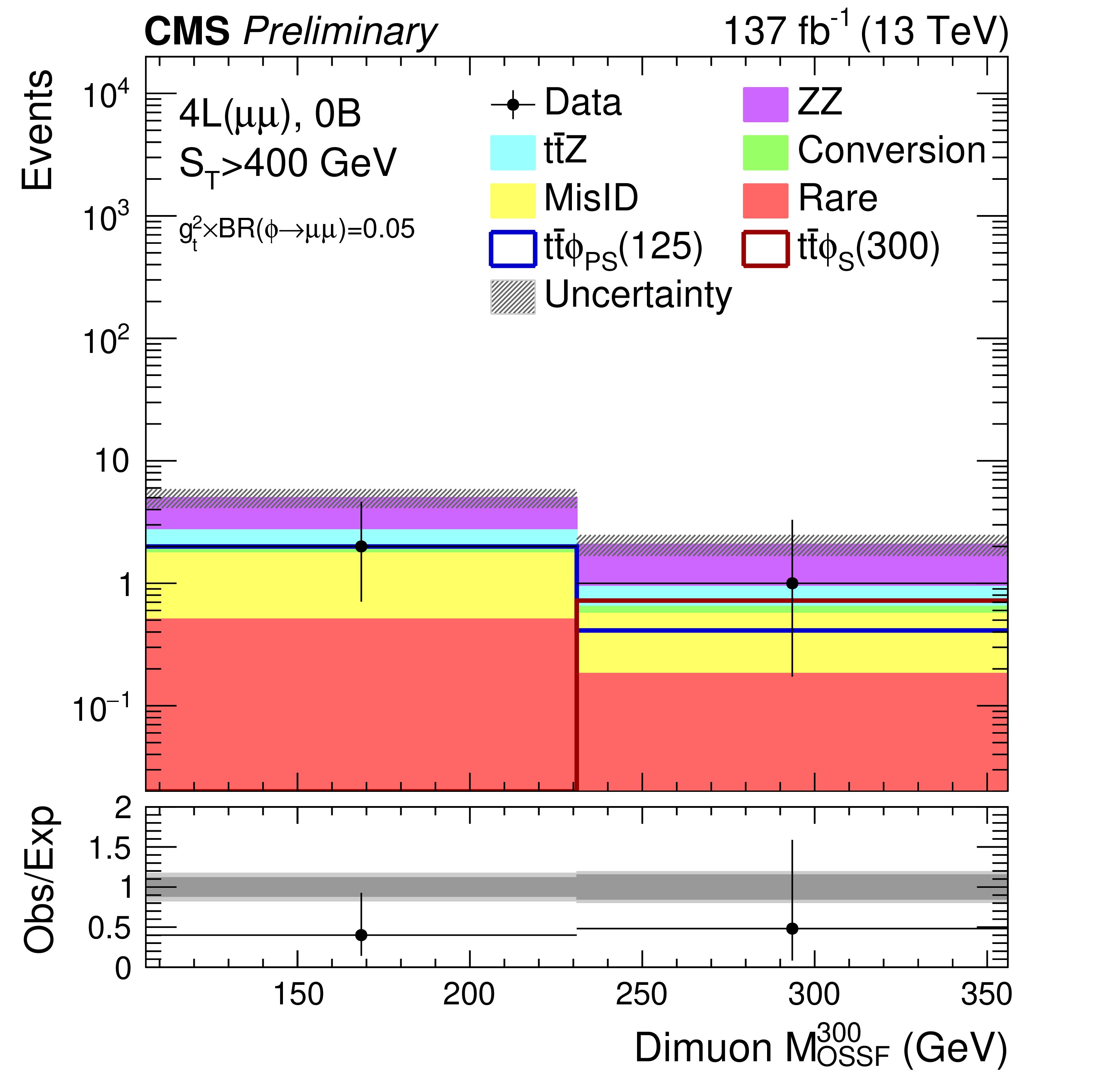
Figure 8:
Dimuon $ {M_{\rm OSSF}}^{20}$ (left column) and $ {M_{\rm OSSF}}^{300}$ (right column) distributions in 3L$(\mu \mu )$ 1B $ \mathrm{t\bar{t}}\phi$ signal regions. Upper, center, and lower plots are with 0 $ < {S_{\rm T}} < $ 400 GeV, 400 $ < {S_{\rm T}} < $ 800 GeV, and $ {S_{\rm T}} > $ 800 GeV, respectively. The total SM background is shown as a stacked histogram of all contributing processes. The predictions for $ \mathrm{t\bar{t}}\phi(\rightarrow \mu \mu )$ models with a pseudoscalar (scalar) $\phi $ of 20 and 125 (70 and 300) GeV mass are also shown. The lower panels show the ratio of observed to expected events. The hatched gray band in the upper panels and the light gray bands in the lower panels represent the total (systematic and statistical) uncertainty in each bin, whereas the dark gray bands in the lower panels represent the statistical uncertainty only. The last bins do not contain the overflow events as these are outside the probed mass range. |
png pdf |
Figure 8-a:
Dimuon $ {M_{\rm OSSF}}^{20}$ (left column) and $ {M_{\rm OSSF}}^{300}$ (right column) distributions in 3L$(\mu \mu )$ 1B $ \mathrm{t\bar{t}}\phi$ signal regions. Upper, center, and lower plots are with 0 $ < {S_{\rm T}} < $ 400 GeV, 400 $ < {S_{\rm T}} < $ 800 GeV, and $ {S_{\rm T}} > $ 800 GeV, respectively. The total SM background is shown as a stacked histogram of all contributing processes. The predictions for $ \mathrm{t\bar{t}}\phi(\rightarrow \mu \mu )$ models with a pseudoscalar (scalar) $\phi $ of 20 and 125 (70 and 300) GeV mass are also shown. The lower panels show the ratio of observed to expected events. The hatched gray band in the upper panels and the light gray bands in the lower panels represent the total (systematic and statistical) uncertainty in each bin, whereas the dark gray bands in the lower panels represent the statistical uncertainty only. The last bins do not contain the overflow events as these are outside the probed mass range. |
png pdf |
Figure 8-b:
Dimuon $ {M_{\rm OSSF}}^{20}$ (left column) and $ {M_{\rm OSSF}}^{300}$ (right column) distributions in 3L$(\mu \mu )$ 1B $ \mathrm{t\bar{t}}\phi$ signal regions. Upper, center, and lower plots are with 0 $ < {S_{\rm T}} < $ 400 GeV, 400 $ < {S_{\rm T}} < $ 800 GeV, and $ {S_{\rm T}} > $ 800 GeV, respectively. The total SM background is shown as a stacked histogram of all contributing processes. The predictions for $ \mathrm{t\bar{t}}\phi(\rightarrow \mu \mu )$ models with a pseudoscalar (scalar) $\phi $ of 20 and 125 (70 and 300) GeV mass are also shown. The lower panels show the ratio of observed to expected events. The hatched gray band in the upper panels and the light gray bands in the lower panels represent the total (systematic and statistical) uncertainty in each bin, whereas the dark gray bands in the lower panels represent the statistical uncertainty only. The last bins do not contain the overflow events as these are outside the probed mass range. |
png pdf |
Figure 8-c:
Dimuon $ {M_{\rm OSSF}}^{20}$ (left column) and $ {M_{\rm OSSF}}^{300}$ (right column) distributions in 3L$(\mu \mu )$ 1B $ \mathrm{t\bar{t}}\phi$ signal regions. Upper, center, and lower plots are with 0 $ < {S_{\rm T}} < $ 400 GeV, 400 $ < {S_{\rm T}} < $ 800 GeV, and $ {S_{\rm T}} > $ 800 GeV, respectively. The total SM background is shown as a stacked histogram of all contributing processes. The predictions for $ \mathrm{t\bar{t}}\phi(\rightarrow \mu \mu )$ models with a pseudoscalar (scalar) $\phi $ of 20 and 125 (70 and 300) GeV mass are also shown. The lower panels show the ratio of observed to expected events. The hatched gray band in the upper panels and the light gray bands in the lower panels represent the total (systematic and statistical) uncertainty in each bin, whereas the dark gray bands in the lower panels represent the statistical uncertainty only. The last bins do not contain the overflow events as these are outside the probed mass range. |
png pdf |
Figure 8-d:
Dimuon $ {M_{\rm OSSF}}^{20}$ (left column) and $ {M_{\rm OSSF}}^{300}$ (right column) distributions in 3L$(\mu \mu )$ 1B $ \mathrm{t\bar{t}}\phi$ signal regions. Upper, center, and lower plots are with 0 $ < {S_{\rm T}} < $ 400 GeV, 400 $ < {S_{\rm T}} < $ 800 GeV, and $ {S_{\rm T}} > $ 800 GeV, respectively. The total SM background is shown as a stacked histogram of all contributing processes. The predictions for $ \mathrm{t\bar{t}}\phi(\rightarrow \mu \mu )$ models with a pseudoscalar (scalar) $\phi $ of 20 and 125 (70 and 300) GeV mass are also shown. The lower panels show the ratio of observed to expected events. The hatched gray band in the upper panels and the light gray bands in the lower panels represent the total (systematic and statistical) uncertainty in each bin, whereas the dark gray bands in the lower panels represent the statistical uncertainty only. The last bins do not contain the overflow events as these are outside the probed mass range. |
png pdf |
Figure 8-e:
Dimuon $ {M_{\rm OSSF}}^{20}$ (left column) and $ {M_{\rm OSSF}}^{300}$ (right column) distributions in 3L$(\mu \mu )$ 1B $ \mathrm{t\bar{t}}\phi$ signal regions. Upper, center, and lower plots are with 0 $ < {S_{\rm T}} < $ 400 GeV, 400 $ < {S_{\rm T}} < $ 800 GeV, and $ {S_{\rm T}} > $ 800 GeV, respectively. The total SM background is shown as a stacked histogram of all contributing processes. The predictions for $ \mathrm{t\bar{t}}\phi(\rightarrow \mu \mu )$ models with a pseudoscalar (scalar) $\phi $ of 20 and 125 (70 and 300) GeV mass are also shown. The lower panels show the ratio of observed to expected events. The hatched gray band in the upper panels and the light gray bands in the lower panels represent the total (systematic and statistical) uncertainty in each bin, whereas the dark gray bands in the lower panels represent the statistical uncertainty only. The last bins do not contain the overflow events as these are outside the probed mass range. |
png pdf |
Figure 8-f:
Dimuon $ {M_{\rm OSSF}}^{20}$ (left column) and $ {M_{\rm OSSF}}^{300}$ (right column) distributions in 3L$(\mu \mu )$ 1B $ \mathrm{t\bar{t}}\phi$ signal regions. Upper, center, and lower plots are with 0 $ < {S_{\rm T}} < $ 400 GeV, 400 $ < {S_{\rm T}} < $ 800 GeV, and $ {S_{\rm T}} > $ 800 GeV, respectively. The total SM background is shown as a stacked histogram of all contributing processes. The predictions for $ \mathrm{t\bar{t}}\phi(\rightarrow \mu \mu )$ models with a pseudoscalar (scalar) $\phi $ of 20 and 125 (70 and 300) GeV mass are also shown. The lower panels show the ratio of observed to expected events. The hatched gray band in the upper panels and the light gray bands in the lower panels represent the total (systematic and statistical) uncertainty in each bin, whereas the dark gray bands in the lower panels represent the statistical uncertainty only. The last bins do not contain the overflow events as these are outside the probed mass range. |

png pdf |
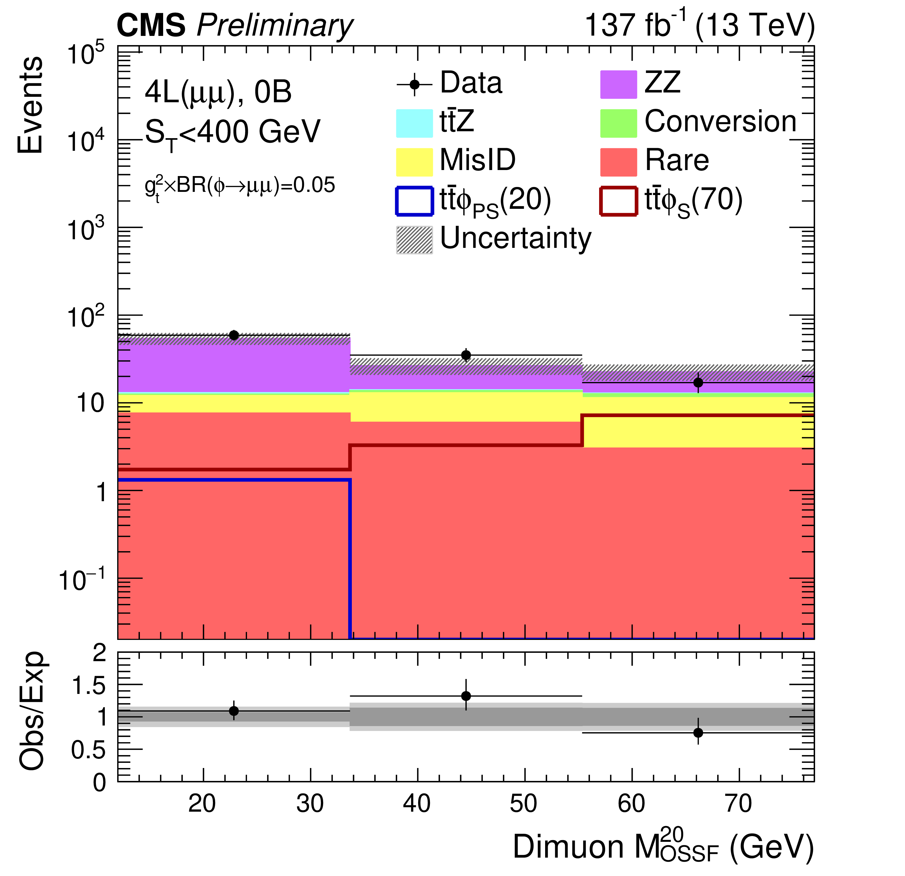
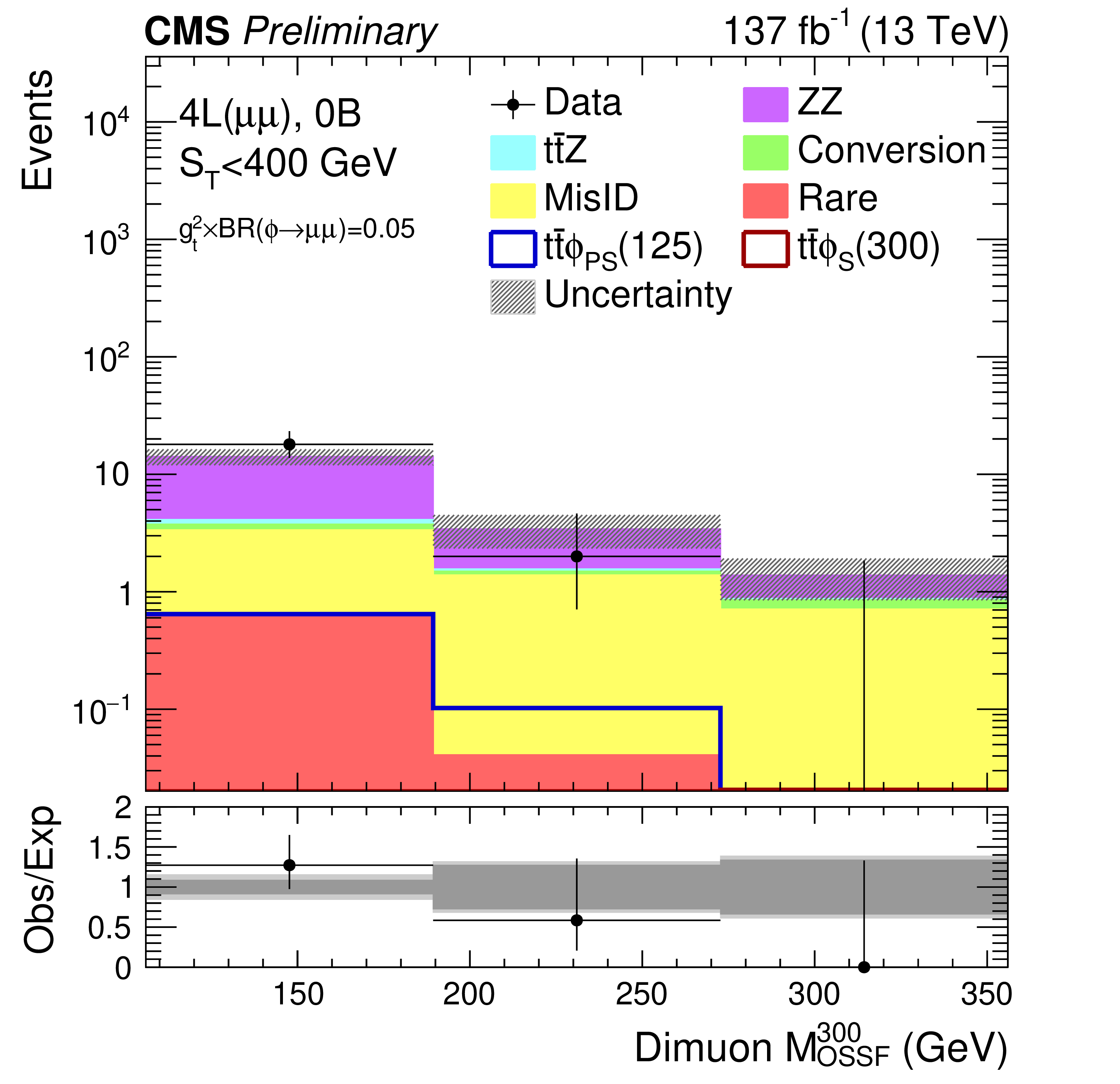
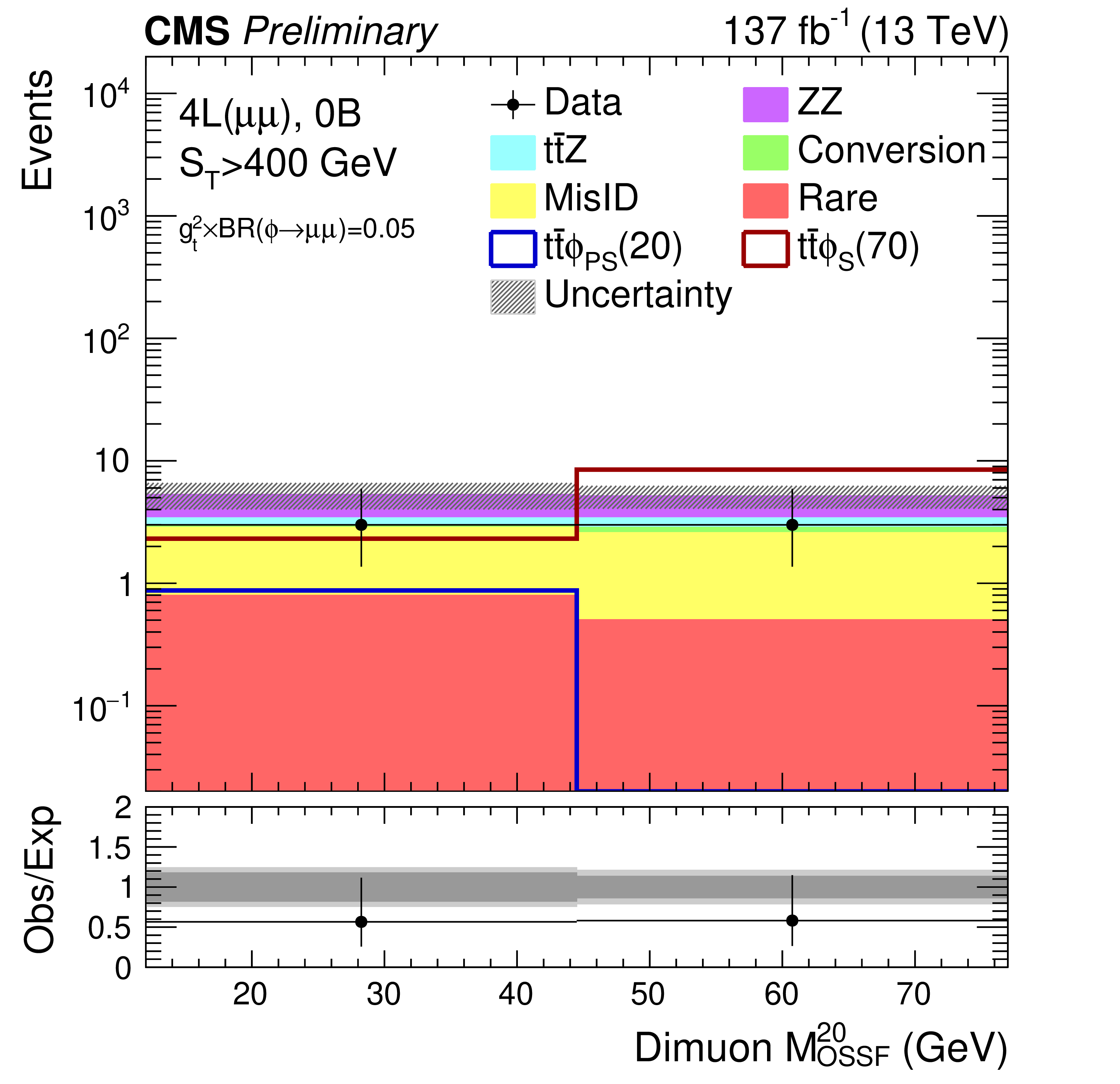
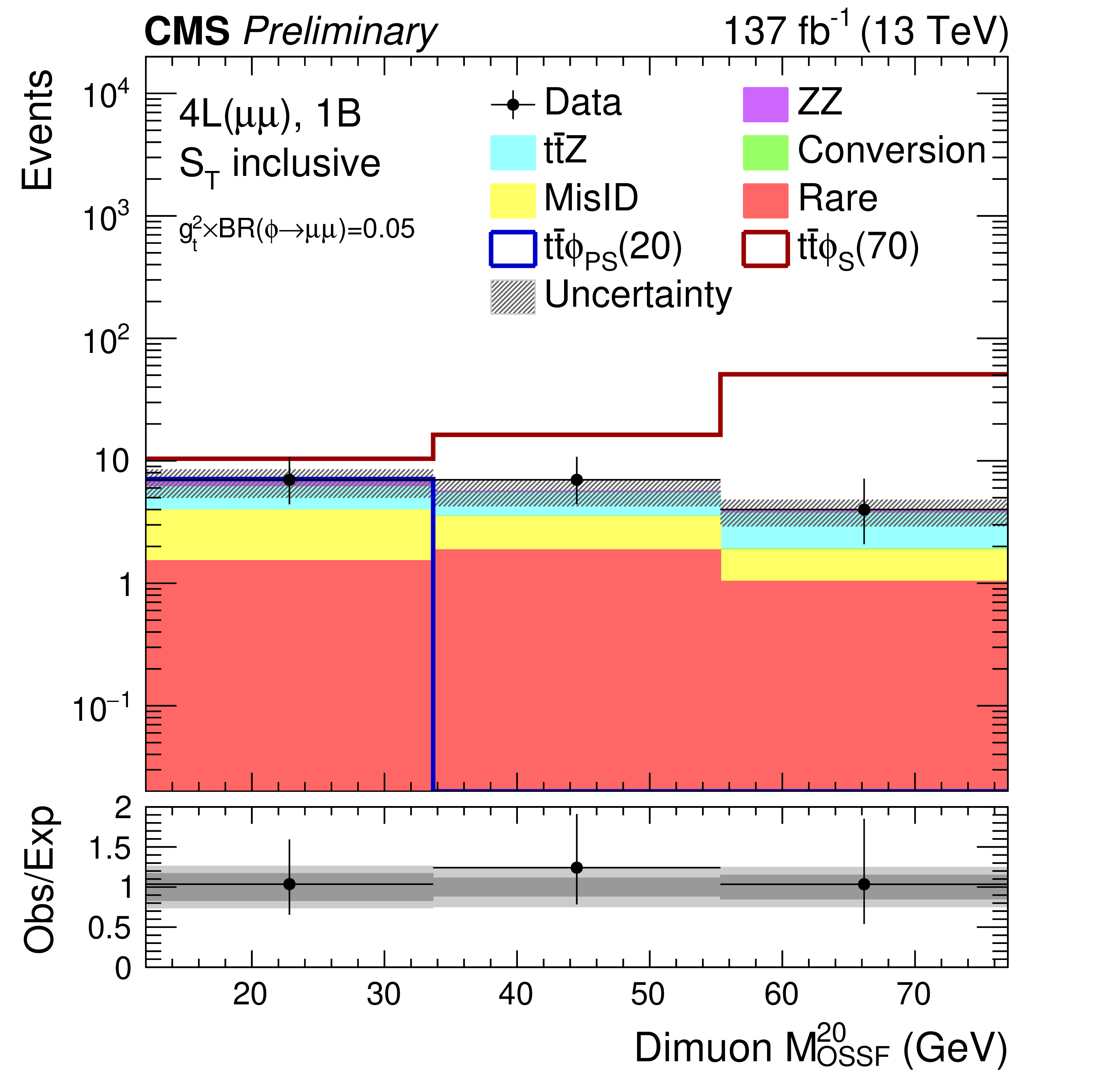
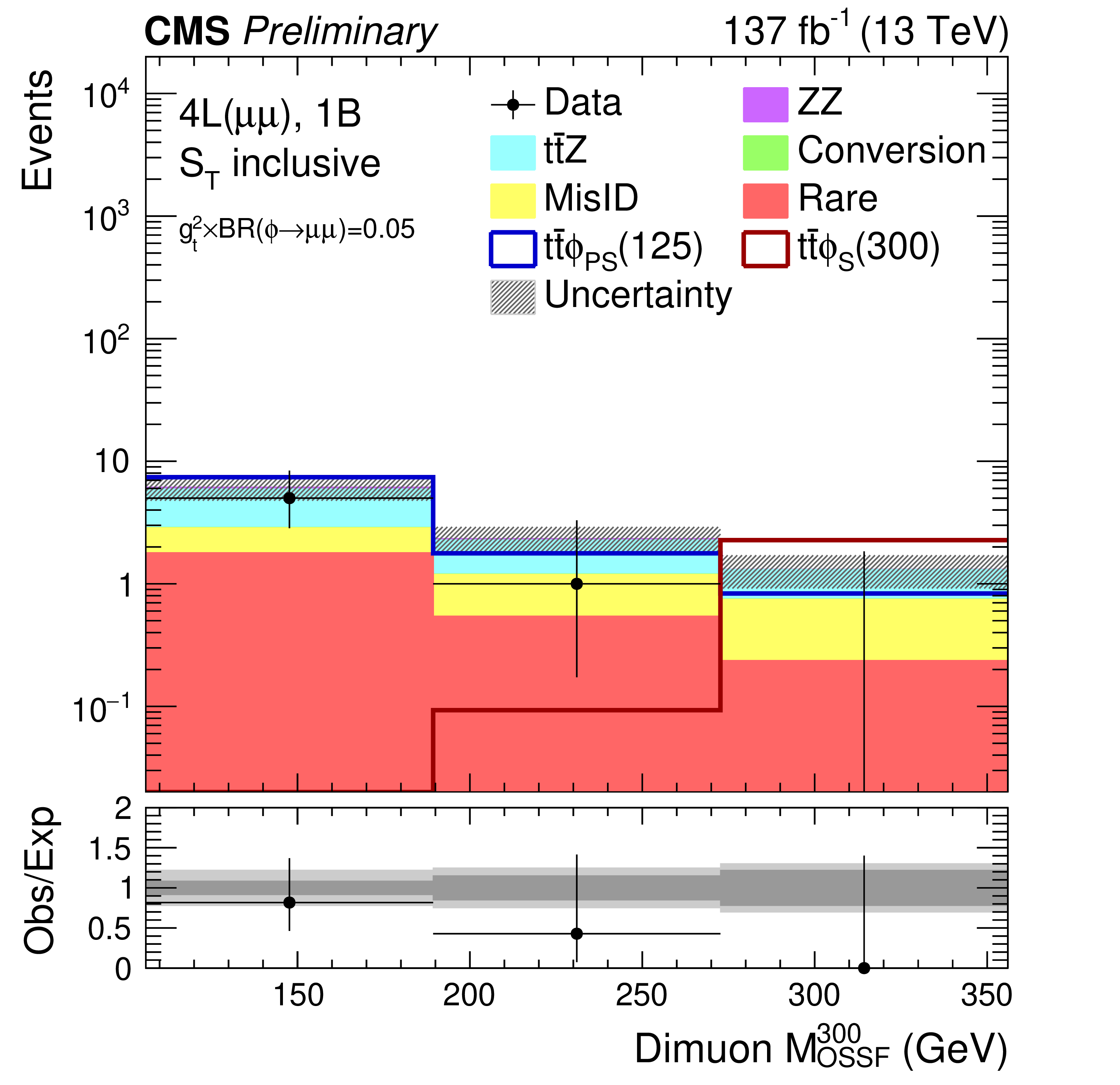
Figure 9:
Dimuon $ {M_{\rm OSSF}}^{20}$ (left column) and $ {M_{\rm OSSF}}^{300}$ (right column) distributions in 4L$(\mu \mu )$ $ \mathrm{t\bar{t}}\phi$ signal regions. Upper, center, and lower plots are with 0B 0 $ < {S_{\rm T}} < $ 400 GeV, 0B $ {S_{\rm T}} < $ 400 GeV, and 1B $ {S_{\rm T}}$-inclusive, respectively. The total SM background is shown as a stacked histogram of all contributing processes. The predictions for $ \mathrm{t\bar{t}}\phi(\rightarrow \mu \mu )$ models with a pseudoscalar (scalar) $\phi $ of 20 and 125 (70 and 300) GeV mass are also shown. The lower panels show the ratio of observed to expected events. The hatched gray band in the upper panels and the light gray bands in the lower panels represent the total (systematic and statistical) uncertainty in each bin, whereas the dark gray bands in the lower panels represent the statistical uncertainty only. The last bins do not contain the overflow events as these are outside the probed mass range. |
png pdf |
Figure 9-a:
Dimuon $ {M_{\rm OSSF}}^{20}$ (left column) and $ {M_{\rm OSSF}}^{300}$ (right column) distributions in 4L$(\mu \mu )$ $ \mathrm{t\bar{t}}\phi$ signal regions. Upper, center, and lower plots are with 0B 0 $ < {S_{\rm T}} < $ 400 GeV, 0B $ {S_{\rm T}} < $ 400 GeV, and 1B $ {S_{\rm T}}$-inclusive, respectively. The total SM background is shown as a stacked histogram of all contributing processes. The predictions for $ \mathrm{t\bar{t}}\phi(\rightarrow \mu \mu )$ models with a pseudoscalar (scalar) $\phi $ of 20 and 125 (70 and 300) GeV mass are also shown. The lower panels show the ratio of observed to expected events. The hatched gray band in the upper panels and the light gray bands in the lower panels represent the total (systematic and statistical) uncertainty in each bin, whereas the dark gray bands in the lower panels represent the statistical uncertainty only. The last bins do not contain the overflow events as these are outside the probed mass range. |
png pdf |
Figure 9-b:
Dimuon $ {M_{\rm OSSF}}^{20}$ (left column) and $ {M_{\rm OSSF}}^{300}$ (right column) distributions in 4L$(\mu \mu )$ $ \mathrm{t\bar{t}}\phi$ signal regions. Upper, center, and lower plots are with 0B 0 $ < {S_{\rm T}} < $ 400 GeV, 0B $ {S_{\rm T}} < $ 400 GeV, and 1B $ {S_{\rm T}}$-inclusive, respectively. The total SM background is shown as a stacked histogram of all contributing processes. The predictions for $ \mathrm{t\bar{t}}\phi(\rightarrow \mu \mu )$ models with a pseudoscalar (scalar) $\phi $ of 20 and 125 (70 and 300) GeV mass are also shown. The lower panels show the ratio of observed to expected events. The hatched gray band in the upper panels and the light gray bands in the lower panels represent the total (systematic and statistical) uncertainty in each bin, whereas the dark gray bands in the lower panels represent the statistical uncertainty only. The last bins do not contain the overflow events as these are outside the probed mass range. |
png pdf |
Figure 9-c:
Dimuon $ {M_{\rm OSSF}}^{20}$ (left column) and $ {M_{\rm OSSF}}^{300}$ (right column) distributions in 4L$(\mu \mu )$ $ \mathrm{t\bar{t}}\phi$ signal regions. Upper, center, and lower plots are with 0B 0 $ < {S_{\rm T}} < $ 400 GeV, 0B $ {S_{\rm T}} < $ 400 GeV, and 1B $ {S_{\rm T}}$-inclusive, respectively. The total SM background is shown as a stacked histogram of all contributing processes. The predictions for $ \mathrm{t\bar{t}}\phi(\rightarrow \mu \mu )$ models with a pseudoscalar (scalar) $\phi $ of 20 and 125 (70 and 300) GeV mass are also shown. The lower panels show the ratio of observed to expected events. The hatched gray band in the upper panels and the light gray bands in the lower panels represent the total (systematic and statistical) uncertainty in each bin, whereas the dark gray bands in the lower panels represent the statistical uncertainty only. The last bins do not contain the overflow events as these are outside the probed mass range. |
png pdf |
Figure 9-d:
Dimuon $ {M_{\rm OSSF}}^{20}$ (left column) and $ {M_{\rm OSSF}}^{300}$ (right column) distributions in 4L$(\mu \mu )$ $ \mathrm{t\bar{t}}\phi$ signal regions. Upper, center, and lower plots are with 0B 0 $ < {S_{\rm T}} < $ 400 GeV, 0B $ {S_{\rm T}} < $ 400 GeV, and 1B $ {S_{\rm T}}$-inclusive, respectively. The total SM background is shown as a stacked histogram of all contributing processes. The predictions for $ \mathrm{t\bar{t}}\phi(\rightarrow \mu \mu )$ models with a pseudoscalar (scalar) $\phi $ of 20 and 125 (70 and 300) GeV mass are also shown. The lower panels show the ratio of observed to expected events. The hatched gray band in the upper panels and the light gray bands in the lower panels represent the total (systematic and statistical) uncertainty in each bin, whereas the dark gray bands in the lower panels represent the statistical uncertainty only. The last bins do not contain the overflow events as these are outside the probed mass range. |
png pdf |
Figure 9-e:
Dimuon $ {M_{\rm OSSF}}^{20}$ (left column) and $ {M_{\rm OSSF}}^{300}$ (right column) distributions in 4L$(\mu \mu )$ $ \mathrm{t\bar{t}}\phi$ signal regions. Upper, center, and lower plots are with 0B 0 $ < {S_{\rm T}} < $ 400 GeV, 0B $ {S_{\rm T}} < $ 400 GeV, and 1B $ {S_{\rm T}}$-inclusive, respectively. The total SM background is shown as a stacked histogram of all contributing processes. The predictions for $ \mathrm{t\bar{t}}\phi(\rightarrow \mu \mu )$ models with a pseudoscalar (scalar) $\phi $ of 20 and 125 (70 and 300) GeV mass are also shown. The lower panels show the ratio of observed to expected events. The hatched gray band in the upper panels and the light gray bands in the lower panels represent the total (systematic and statistical) uncertainty in each bin, whereas the dark gray bands in the lower panels represent the statistical uncertainty only. The last bins do not contain the overflow events as these are outside the probed mass range. |
png pdf |
Figure 9-f:
Dimuon $ {M_{\rm OSSF}}^{20}$ (left column) and $ {M_{\rm OSSF}}^{300}$ (right column) distributions in 4L$(\mu \mu )$ $ \mathrm{t\bar{t}}\phi$ signal regions. Upper, center, and lower plots are with 0B 0 $ < {S_{\rm T}} < $ 400 GeV, 0B $ {S_{\rm T}} < $ 400 GeV, and 1B $ {S_{\rm T}}$-inclusive, respectively. The total SM background is shown as a stacked histogram of all contributing processes. The predictions for $ \mathrm{t\bar{t}}\phi(\rightarrow \mu \mu )$ models with a pseudoscalar (scalar) $\phi $ of 20 and 125 (70 and 300) GeV mass are also shown. The lower panels show the ratio of observed to expected events. The hatched gray band in the upper panels and the light gray bands in the lower panels represent the total (systematic and statistical) uncertainty in each bin, whereas the dark gray bands in the lower panels represent the statistical uncertainty only. The last bins do not contain the overflow events as these are outside the probed mass range. |
png pdf |
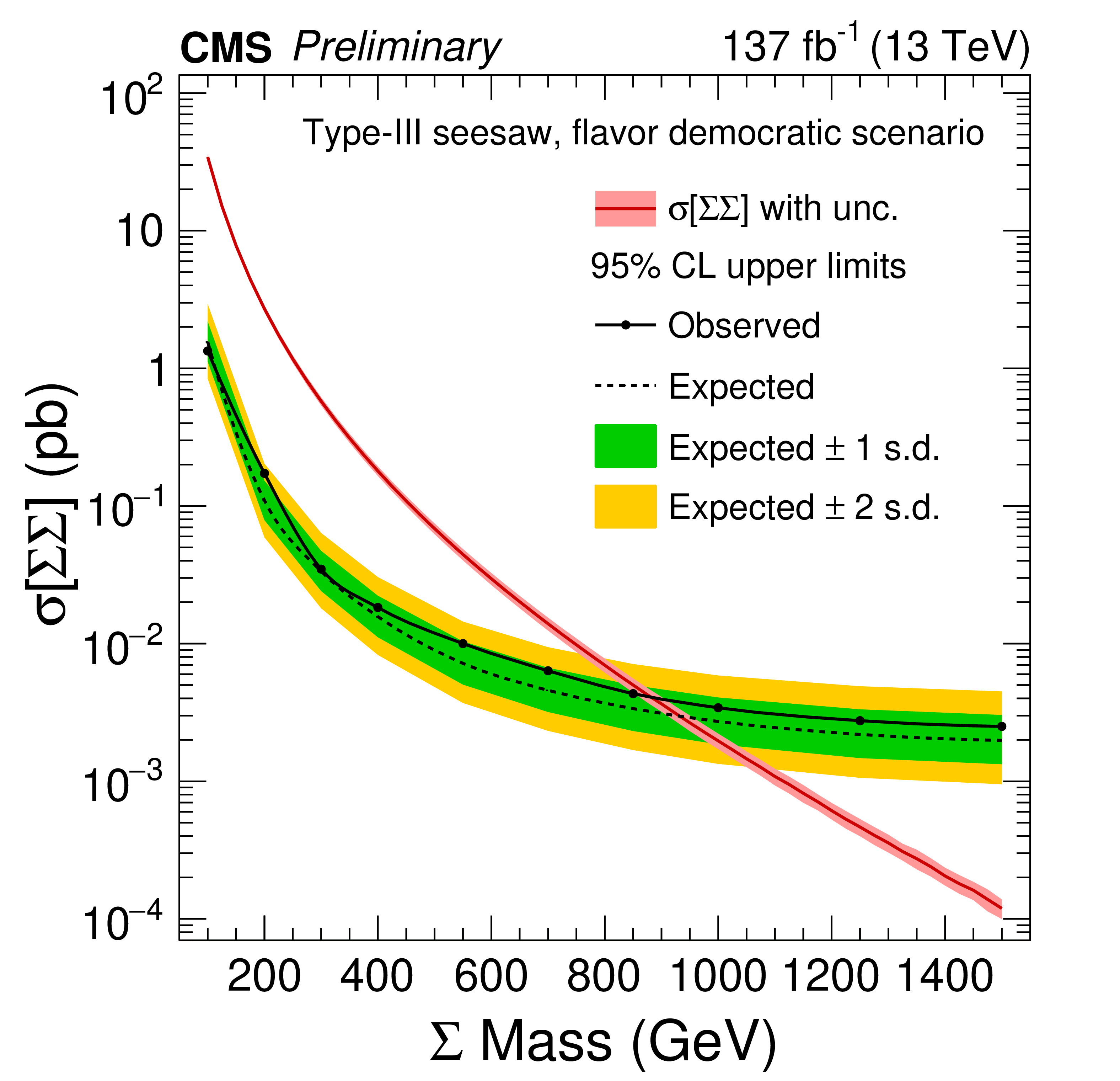
Figure 10:
The 95% confidence level upper limits on the total production cross section of heavy fermion pairs. Also shown is the theoretical prediction for the cross section of the $\Sigma $ pair production via the type III seesaw mechanism, with its uncertainty. Type-III seesaw heavy fermions are excluded for masses below 880 GeV (expected 930 GeV) in the flavor democratic scenario. |
png pdf |
Figure 11:
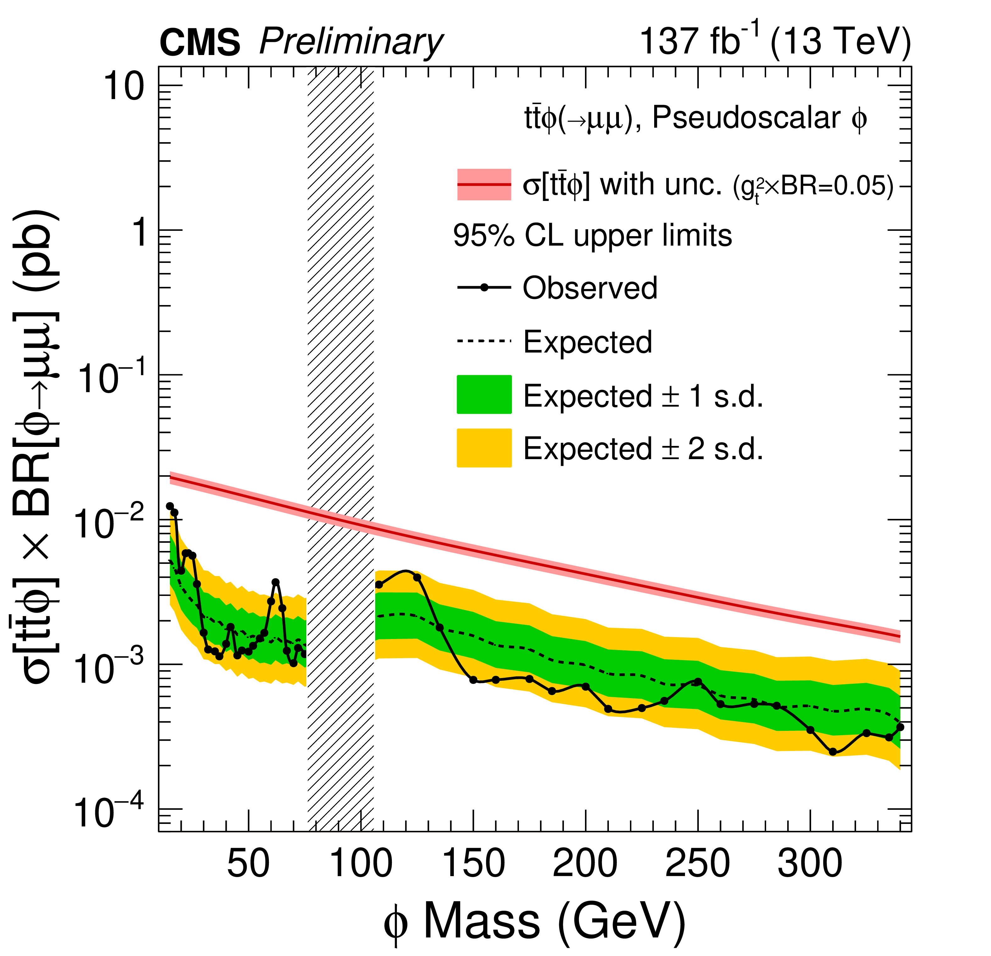
The 95% confidence level upper limits on the production cross section times branching ratio for a scalar $\phi $ boson in dielectron (upper left) and dimuon (lower left) channels, and for a pseudoscalar $\phi $ boson in dielectron (upper right) and dimuon (lower right) channels, where $\phi $ is produced in association with a top quark pair. Also shown are the theoretical predictions for the production cross section times branching ratio of the $ \mathrm{t\bar{t}}\phi$ model, with their uncertainties, and assuming g$_{t}^2\times {\rm BR}(\phi \rightarrow \ell \ell)=$ 0.05. All $ \mathrm{t\bar{t}}\phi$ signal scenarios are excluded for production cross sections above 20 fb for $\phi $ masses in the range of 15-75 GeV, and above 5 fb for $\phi $ masses in the range of 108-340 GeV. |
png pdf |
Figure 11-a:
The 95% confidence level upper limits on the production cross section times branching ratio for a scalar $\phi $ boson in dielectron (upper left) and dimuon (lower left) channels, and for a pseudoscalar $\phi $ boson in dielectron (upper right) and dimuon (lower right) channels, where $\phi $ is produced in association with a top quark pair. Also shown are the theoretical predictions for the production cross section times branching ratio of the $ \mathrm{t\bar{t}}\phi$ model, with their uncertainties, and assuming g$_{t}^2\times {\rm BR}(\phi \rightarrow \ell \ell)=$ 0.05. All $ \mathrm{t\bar{t}}\phi$ signal scenarios are excluded for production cross sections above 20 fb for $\phi $ masses in the range of 15-75 GeV, and above 5 fb for $\phi $ masses in the range of 108-340 GeV. |
png pdf |
Figure 11-b:
The 95% confidence level upper limits on the production cross section times branching ratio for a scalar $\phi $ boson in dielectron (upper left) and dimuon (lower left) channels, and for a pseudoscalar $\phi $ boson in dielectron (upper right) and dimuon (lower right) channels, where $\phi $ is produced in association with a top quark pair. Also shown are the theoretical predictions for the production cross section times branching ratio of the $ \mathrm{t\bar{t}}\phi$ model, with their uncertainties, and assuming g$_{t}^2\times {\rm BR}(\phi \rightarrow \ell \ell)=$ 0.05. All $ \mathrm{t\bar{t}}\phi$ signal scenarios are excluded for production cross sections above 20 fb for $\phi $ masses in the range of 15-75 GeV, and above 5 fb for $\phi $ masses in the range of 108-340 GeV. |
png pdf |
Figure 11-c:
The 95% confidence level upper limits on the production cross section times branching ratio for a scalar $\phi $ boson in dielectron (upper left) and dimuon (lower left) channels, and for a pseudoscalar $\phi $ boson in dielectron (upper right) and dimuon (lower right) channels, where $\phi $ is produced in association with a top quark pair. Also shown are the theoretical predictions for the production cross section times branching ratio of the $ \mathrm{t\bar{t}}\phi$ model, with their uncertainties, and assuming g$_{t}^2\times {\rm BR}(\phi \rightarrow \ell \ell)=$ 0.05. All $ \mathrm{t\bar{t}}\phi$ signal scenarios are excluded for production cross sections above 20 fb for $\phi $ masses in the range of 15-75 GeV, and above 5 fb for $\phi $ masses in the range of 108-340 GeV. |
png pdf |
Figure 11-d:
The 95% confidence level upper limits on the production cross section times branching ratio for a scalar $\phi $ boson in dielectron (upper left) and dimuon (lower left) channels, and for a pseudoscalar $\phi $ boson in dielectron (upper right) and dimuon (lower right) channels, where $\phi $ is produced in association with a top quark pair. Also shown are the theoretical predictions for the production cross section times branching ratio of the $ \mathrm{t\bar{t}}\phi$ model, with their uncertainties, and assuming g$_{t}^2\times {\rm BR}(\phi \rightarrow \ell \ell)=$ 0.05. All $ \mathrm{t\bar{t}}\phi$ signal scenarios are excluded for production cross sections above 20 fb for $\phi $ masses in the range of 15-75 GeV, and above 5 fb for $\phi $ masses in the range of 108-340 GeV. |
png pdf |
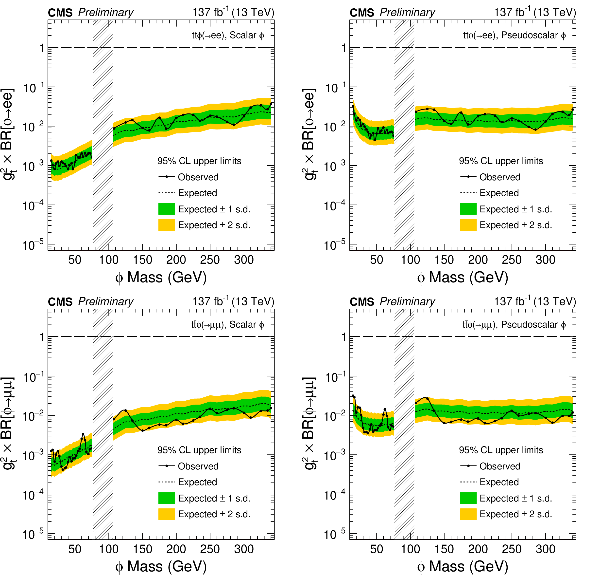
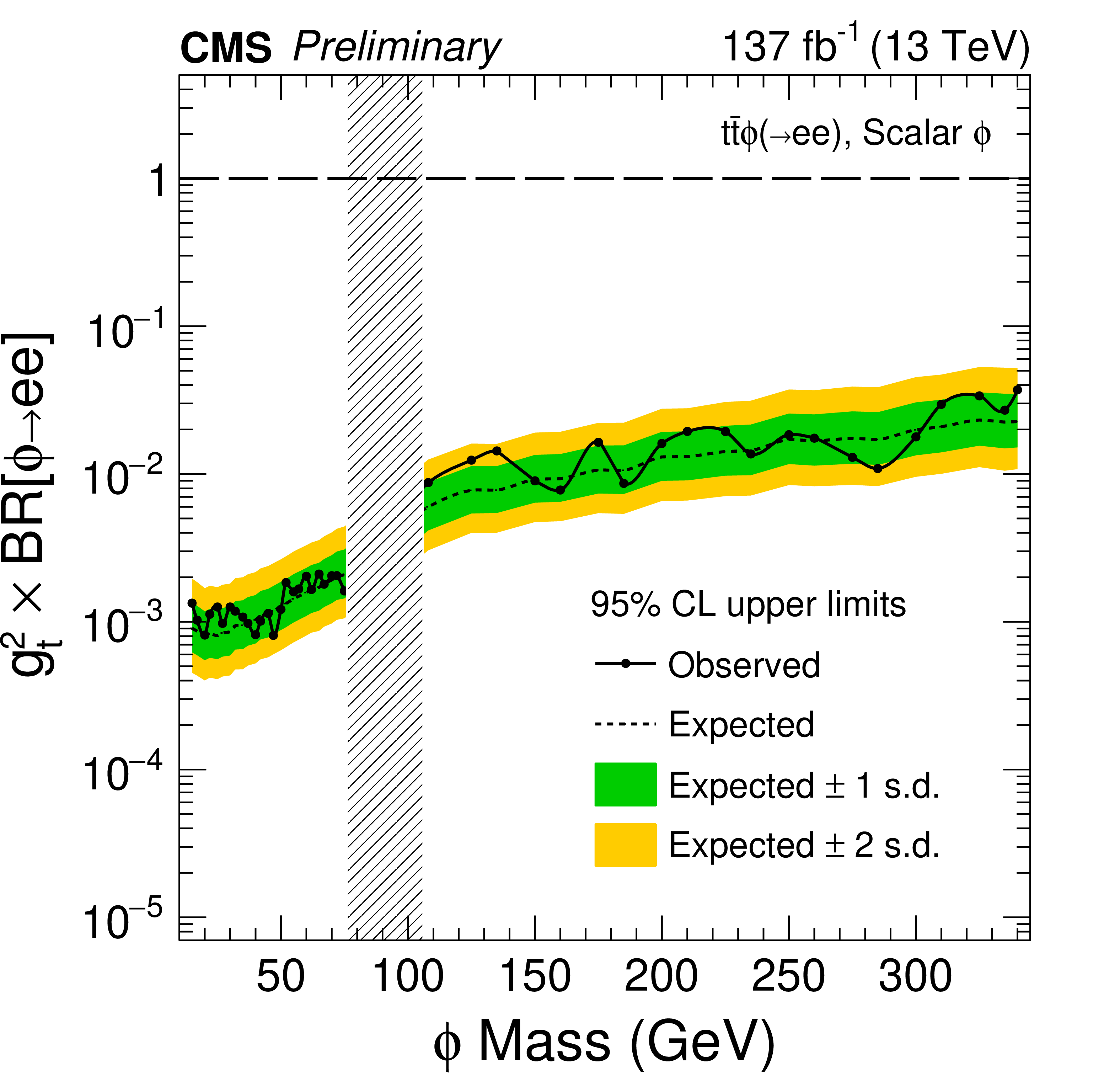
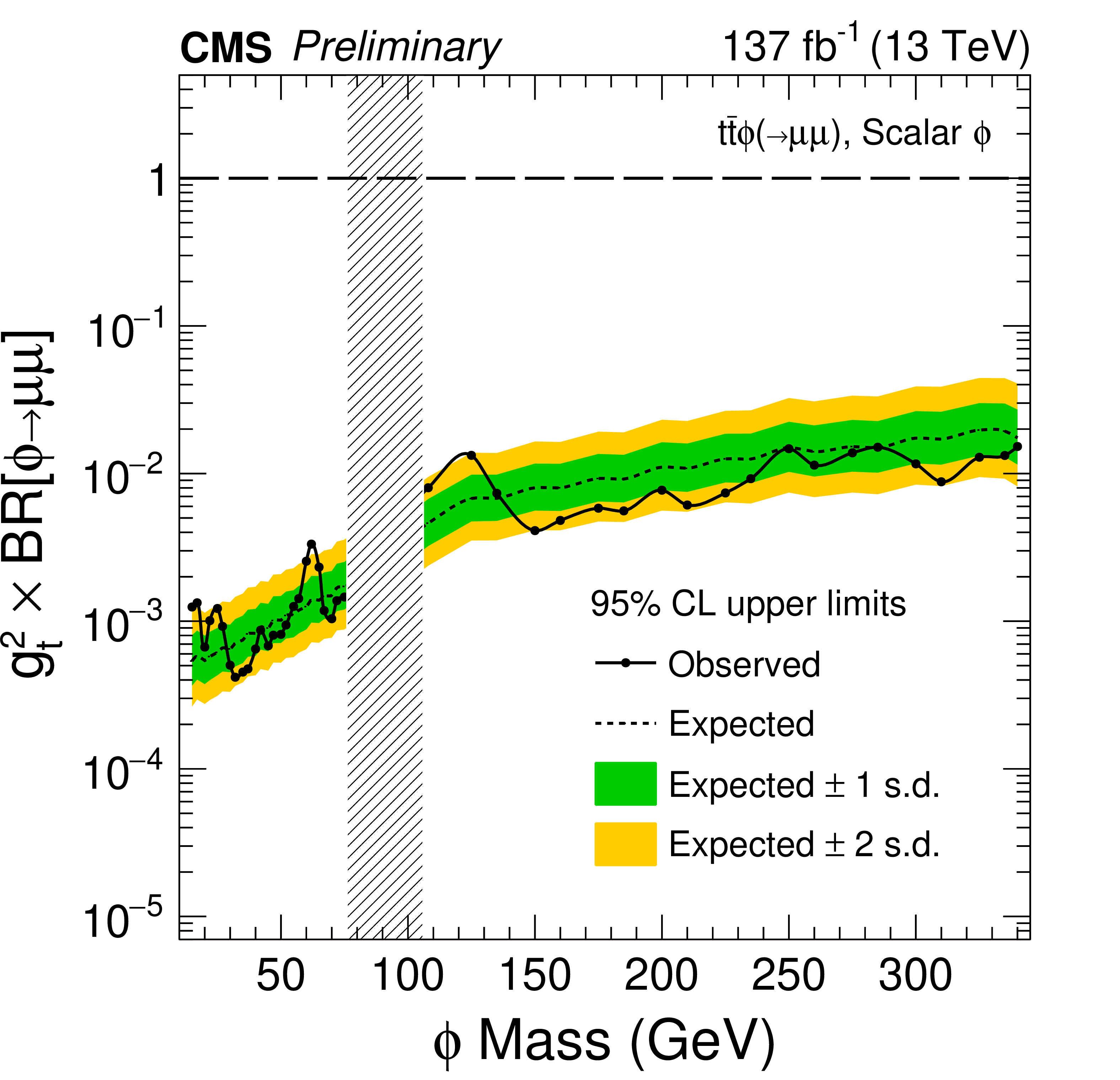
Figure 12:
The 95% confidence level upper limits on the square of the Yukawa coupling to top quarks times branching ratio for a scalar $\phi $ boson in dielectron (upper left) and dimuon (lower left) channels, and for a pseudoscalar $\phi $ boson in dielectron (upper right) and dimuon (lower right) channels, where $\phi $ is produced in association with a top quark pair. Assuming a Yukawa coupling of unity strength to top quarks, the branching ratio of new scalar (pseudoscalar) bosons to dielectrons and dimuons above 0.003 (0.03) are excluded for masses in the range of 15-75 GeV, and above 0.04 (0.03) for masses in the range of 108-340 GeV. |
png pdf |
Figure 12-a:
The 95% confidence level upper limits on the square of the Yukawa coupling to top quarks times branching ratio for a scalar $\phi $ boson in dielectron (upper left) and dimuon (lower left) channels, and for a pseudoscalar $\phi $ boson in dielectron (upper right) and dimuon (lower right) channels, where $\phi $ is produced in association with a top quark pair. Assuming a Yukawa coupling of unity strength to top quarks, the branching ratio of new scalar (pseudoscalar) bosons to dielectrons and dimuons above 0.003 (0.03) are excluded for masses in the range of 15-75 GeV, and above 0.04 (0.03) for masses in the range of 108-340 GeV. |

png pdf |
Figure 12-b:
The 95% confidence level upper limits on the square of the Yukawa coupling to top quarks times branching ratio for a scalar $\phi $ boson in dielectron (upper left) and dimuon (lower left) channels, and for a pseudoscalar $\phi $ boson in dielectron (upper right) and dimuon (lower right) channels, where $\phi $ is produced in association with a top quark pair. Assuming a Yukawa coupling of unity strength to top quarks, the branching ratio of new scalar (pseudoscalar) bosons to dielectrons and dimuons above 0.003 (0.03) are excluded for masses in the range of 15-75 GeV, and above 0.04 (0.03) for masses in the range of 108-340 GeV. |
png pdf |
Figure 12-c:
The 95% confidence level upper limits on the square of the Yukawa coupling to top quarks times branching ratio for a scalar $\phi $ boson in dielectron (upper left) and dimuon (lower left) channels, and for a pseudoscalar $\phi $ boson in dielectron (upper right) and dimuon (lower right) channels, where $\phi $ is produced in association with a top quark pair. Assuming a Yukawa coupling of unity strength to top quarks, the branching ratio of new scalar (pseudoscalar) bosons to dielectrons and dimuons above 0.003 (0.03) are excluded for masses in the range of 15-75 GeV, and above 0.04 (0.03) for masses in the range of 108-340 GeV. |
png pdf |
Figure 12-d:
The 95% confidence level upper limits on the square of the Yukawa coupling to top quarks times branching ratio for a scalar $\phi $ boson in dielectron (upper left) and dimuon (lower left) channels, and for a pseudoscalar $\phi $ boson in dielectron (upper right) and dimuon (lower right) channels, where $\phi $ is produced in association with a top quark pair. Assuming a Yukawa coupling of unity strength to top quarks, the branching ratio of new scalar (pseudoscalar) bosons to dielectrons and dimuons above 0.003 (0.03) are excluded for masses in the range of 15-75 GeV, and above 0.04 (0.03) for masses in the range of 108-340 GeV. |
| Tables | |
png pdf |
Table 1:
Multilepton signal region definitions for the signal models. All events containing a same-flavor lepton pair with mass below 12 GeV, and 3L events containing an OSSF lepton pair with mass below 76 GeV when the trilepton mass is within a Z boson mass window (91 $\pm$ 15 GeV) are vetoed. |
png pdf |
Table 2:
Sources of systematic uncertainties, affected background and signal processes, relative variation on the affected processes, and correlation model across years in signal regions. |
png pdf |
Table 3:
Acceptance times efficiency values in 3 and 4 lepton channels for the signal models at various mass hypotheses. |
| Summary |
| In summary, we performed a search for new physics in multilepton events in 137 fb$^{-1}$ of pp collision data collected by the CMS detector. The observations are found to be consistent with the expectations from standard model processes, with no statistically significant signal-like excess in any of the probed channels. The results are used to constrain the allowed parameter space of the targeted signal models. At 95% confidence level, we exclude heavy fermions of the type-III seesaw model with masses below 880 GeV in the lepton flavor democratic scenario. Similarly, assuming a Yukawa coupling of unity strength to top quarks, the branching ratio of new scalar (pseudoscalar) bosons to dielectrons and dimuons above 0.003 (0.03) are excluded for masses in the range of 15-75 GeV, and above 0.04 (0.03) for masses in the range of 108-340 GeV. |
| References | ||||
| 1 | P. Minkowski | $ \mu \to \mathrm{e}\gamma $ at a Rate of One Out of $ 10^{9} $ Muon Decays? | PL67B (1977) 421--428 | |
| 2 | R. N. Mohapatra and G. Senjanovic | Neutrino Mass and Spontaneous Parity Nonconservation | PRL 44 (1980) 912 | |
| 3 | M. Magg and C. Wetterich | Neutrino Mass Problem and Gauge Hierarchy | PL94B (1980) 61--64 | |
| 4 | R. N. Mohapatra and G. Senjanovic | Neutrino Masses and Mixings in Gauge Models with Spontaneous Parity Violation | PRD23 (1981) 165 | |
| 5 | J. Schechter and J. W. F. Valle | Neutrino Masses in SU(2) x U(1) Theories | PRD22 (1980) 2227 | |
| 6 | J. Schechter and J. W. F. Valle | Neutrino Decay and Spontaneous Violation of Lepton Number | PRD25 (1982) 774 | |
| 7 | R. Foot, H. Lew, X. G. He, and G. C. Joshi | Seesaw Neutrino Masses Induced by a Triplet of Leptons | Z. Phys. C44 (1989) 441 | |
| 8 | R. N. Mohapatra | Mechanism for Understanding Small Neutrino Mass in Superstring Theories | PRL 56 (1986) 561--563 | |
| 9 | R. N. Mohapatra and J. W. F. Valle | Neutrino Mass and Baryon Number Nonconservation in Superstring Models | PRD34 (1986) 1642 | |
| 10 | C. Biggio and F. Bonnet | Implementation of the Type III Seesaw Model in FeynRules/MadGraph and Prospects for Discovery with Early LHC Data | EPJC72 (2012) 1899 | 1107.3463 |
| 11 | A. Abada et al. | $ \mu \to \mathrm{e}\gamma $ and $ \tau\to\ell\gamma $ decays in the fermion triplet seesaw model | PRD78 (2008) 033007 | 0803.0481 |
| 12 | A. Abada et al. | Low energy effects of neutrino masses | JHEP 12 (2007) 061 | 0707.4058 |
| 13 | F. del Aguila, J. de Blas, and M. Perez-Victoria | Effects of new leptons in Electroweak Precision Data | PRD78 (2008) 013010 | 0803.4008 |
| 14 | G. Cacciapaglia, G. Ferretti, T. Flacke, and H. Serodio | Light scalars in composite Higgs models | Front. Phys. 7 (2019) 22 | 1902.06890 |
| 15 | U. Ellwanger, C. Hugonie, and A. M. Teixeira | The Next-to-Minimal Supersymmetric Standard Model | PR 496 (2010) 1--77 | 0910.1785 |
| 16 | M. Maniatis | The Next-to-Minimal Supersymmetric extension of the Standard Model reviewed | Int. J. Mod. Phys. A25 (2010) 3505--3602 | 0906.0777 |
| 17 | M. R. Buckley, D. Feld, and D. Goncalves | Scalar Simplified Models for Dark Matter | PRD91 (2015) 015017 | 1410.6497 |
| 18 | M. Casolino et al. | Probing a light CP-odd scalar in di-top-associated production at the LHC | EPJC75 (2015) 498 | 1507.07004 |
| 19 | W.-F. Chang, T. Modak, and J. N. Ng | Signal for a light singlet scalar at the LHC | PRD97 (2018), no. 5, 055020 | 1711.05722 |
| 20 | CMS Collaboration | Search for heavy lepton partners of neutrinos in proton-proton collisions in the context of the type III seesaw mechanism | PLB718 (2012) 348--368 | CMS-EXO-11-073 1210.1797 |
| 21 | CMS Collaboration | Search for heavy lepton partners of neutrinos in pp collisions at 8 TeV in the context of type III seesaw mechanism | CMS-PAS-EXO-14-001 | CMS-PAS-EXO-14-001 |
| 22 | ATLAS Collaboration | Search for type-III Seesaw heavy leptons in pp collisions at $ \sqrt{s}= $ 8 TeV with the ATLAS Detector | PRD92 (2015), no. 3, 032001 | 1506.01839 |
| 23 | ATLAS Collaboration | Search for type-III seesaw heavy leptons in proton-proton collisions at $ \sqrt{s}= $ 13 TeV with the ATLAS detector | ATLAS Conference Note ATLAS-CONF-2018-020 | |
| 24 | CMS Collaboration | Search for Evidence of the Type-III Seesaw Mechanism in Multilepton Final States in Proton-Proton Collisions at $ \sqrt{s}=13\text{}\text{}\mathrm{TeV} $ | PRL 119 (2017), no. 22, 221802 | CMS-EXO-17-006 1708.07962 |
| 25 | CMS Collaboration | The CMS experiment at the CERN LHC | JINST 3 (2008) S08004 | CMS-00-001 |
| 26 | CMS Collaboration | The CMS trigger system | JINST 12 (2017), no. 01, P01020 | CMS-TRG-12-001 1609.02366 |
| 27 | P. Nason | A New method for combining NLO QCD with shower Monte Carlo algorithms | JHEP 11 (2004) 040 | hep-ph/0409146 |
| 28 | S. Frixione, P. Nason, and C. Oleari | Matching NLO QCD computations with Parton Shower simulations: the POWHEG method | JHEP 11 (2007) 070 | 0709.2092 |
| 29 | S. Alioli, P. Nason, C. Oleari, and E. Re | A general framework for implementing NLO calculations in shower Monte Carlo programs: the POWHEG BOX | JHEP 06 (2010) 043 | 1002.2581 |
| 30 | J. M. Campbell and R. K. Ellis | MCFM for the Tevatron and the LHC | NPPS 205-206 (2010) 10--15 | 1007.3492 |
| 31 | J. Alwall et al. | The automated computation of tree-level and next-to-leading order differential cross sections, and their matching to parton shower simulations | JHEP 07 (2014) 079 | 1405.0301 |
| 32 | Y. Gao et al. | Spin determination of single-produced resonances at hadron colliders | PRD81 (2010) 075022 | 1001.3396 |
| 33 | S. Bolognesi et al. | On the spin and parity of a single-produced resonance at the LHC | PRD86 (2012) 095031 | 1208.4018 |
| 34 | I. Anderson et al. | Constraining anomalous HVV interactions at proton and lepton colliders | PRD89 (2014), no. 3, 035007 | 1309.4819 |
| 35 | A. V. Gritsan, R. Rontsch, M. Schulze, and M. Xiao | Constraining anomalous Higgs boson couplings to the heavy flavor fermions using matrix element techniques | PRD94 (2016), no. 5, 055023 | 1606.03107 |
| 36 | B. Fuks, M. Klasen, D. R. Lamprea, and M. Rothering | Gaugino production in proton-proton collisions at a center-of-mass energy of 8 TeV | JHEP 10 (2012) 081 | 1207.2159 |
| 37 | B. Fuks, M. Klasen, D. R. Lamprea, and M. Rothering | Precision predictions for electroweak superpartner production at hadron colliders with Resummino | EPJC73 (2013) 2480 | 1304.0790 |
| 38 | D. de Florian et al. | Handbook of LHC Higgs cross sections: 4. deciphering the nature of the Higgs sector | CERN-2017-002-M | 1610.07922 |
| 39 | NNPDF Collaboration | Parton distributions for the LHC Run II | JHEP 04 (2015) 040 | 1410.8849 |
| 40 | NNPDF Collaboration | Parton distributions from high-precision collider data | EPJC77 (2017), no. 10, 663 | 1706.00428 |
| 41 | T. Sjostrand et al. | An Introduction to PYTHIA 8.2 | CPC 191 (2015) 159--177 | 1410.3012 |
| 42 | CMS Collaboration | Event generator tunes obtained from underlying event and multiparton scattering measurements | EPJC76 (2016), no. 3, 155 | CMS-GEN-14-001 1512.00815 |
| 43 | CMS Collaboration | Extraction and validation of a new set of CMS PYTHIA8 tunes from underlying-event measurements | CMS-PAS-GEN-17-001 | CMS-PAS-GEN-17-001 |
| 44 | R. Frederix and S. Frixione | Merging meets matching in MC@NLO | JHEP 12 (2012) 061 | 1209.6215 |
| 45 | GEANT4 Collaboration | GEANT4: A Simulation toolkit | NIMA506 (2003) 250--303 | |
| 46 | CMS Collaboration | Performance of Electron Reconstruction and Selection with the CMS Detector in Proton-Proton Collisions at $ \sqrt{s}= $ 8 TeV | JINST 10 (2015), no. 06, P06005 | CMS-EGM-13-001 1502.02701 |
| 47 | CMS Collaboration | Particle-flow reconstruction and global event description with the CMS detector | JINST 12 (2017), no. 10, P10003 | CMS-PRF-14-001 1706.04965 |
| 48 | M. Cacciari, G. P. Salam, and G. Soyez | The anti-$ k_t $ jet clustering algorithm | JHEP 04 (2008) 063 | 0802.1189 |
| 49 | M. Cacciari, G. P. Salam, and G. Soyez | FastJet User Manual | EPJC72 (2012) 1896 | 1111.6097 |
| 50 | CMS Collaboration | Identification of heavy-flavour jets with the CMS detector in pp collisions at 13 TeV | JINST 13 (2018), no. 05, P05011 | CMS-BTV-16-002 1712.07158 |
| 51 | CMS Collaboration | Performance of missing transverse momentum in pp collisions at $ \sqrt{s}= $ 13 TeV using the CMS detector | CMS-PAS-JME-17-001 | CMS-PAS-JME-17-001 |
| 52 | CMS Collaboration | Search for Third-Generation Scalar Leptoquarks in the t$ \tau $ Channel in Proton-Proton Collisions at $ \sqrt{s} = $ 8 TeV | JHEP 07 (2015) 042 | CMS-EXO-14-008 1503.09049 |
| 53 | M. Cacciari et al. | The t anti-t cross-section at 1.8-TeV and 1.96-TeV: A Study of the systematics due to parton densities and scale dependence | JHEP 04 (2004) 068 | hep-ph/0303085 |
| 54 | J. Butterworth et al. | PDF4LHC recommendations for LHC Run II | JPG43 (2016) 023001 | 1510.03865 |
| 55 | CMS Collaboration | CMS Luminosity Measurements for the 2016 Data Taking Period | CMS-PAS-LUM-17-001 | CMS-PAS-LUM-17-001 |
| 56 | CMS Collaboration | CMS luminosity measurement for the 2017 data-taking period at $ \sqrt{s} = $ 13 TeV | CMS-PAS-LUM-17-004 | CMS-PAS-LUM-17-004 |
| 57 | E. Gross and O. Vitells | Trial factors for the look elsewhere effect in high energy physics | EPJC70 (2010) 525--530 | 1005.1891 |
| 58 | T. Junk | Confidence level computation for combining searches with small statistics | NIMA434 (1999) 435--443 | hep-ex/9902006 |
| 59 | A. L. Read | Presentation of search results: The CL(s) technique | JPG28 (2002) 2693--2704 | |
| 60 | ATLAS and CMS Collaborations | Procedure for the LHC Higgs boson search combination in Summer 2011 | CMS-NOTE-2011-005 | |
|
|
Compact Muon Solenoid LHC, CERN |
|

|

|

|

|

|