CMS-PAS-B2G-21-004

CMS-PAS-B2G-21-004
Search for pair-produced vector-like leptons in $\geq $ 3b $+$ N $\tau$ final states
CMS Collaboration
March 2022

Abstract: A search for vector-like leptons (VLLs) is presented in the context of the 4321 model, a UV-complete model with the potential to explain existing B-physics measurements that are in tension with standard model predictions. The analyzed data correspond to an integrated luminosity of 97 fb$^{-1}$, and were recorded by the CMS detector at the LHC in proton-proton collisions at $\sqrt{s}=$ 13 TeV at the LHC. Final states with $\geq$3 b jets and two third-generation leptons ($\tau\tau$, $\tau\nu_{\tau}$, or $\nu_{\tau}\nu_{\tau}$) are targeted. Expected upper limits are derived on the VLL production cross section in the VLL mass range 500-1050 GeV, assuming only electroweak production. At the low end of this mass range, the expected limits are below the expected production cross section, whereas at the high end of the mass range the expected upper limits on the production cross section are several times higher than the expected cross section for electroweak production. A mild excess, consistent with a possible signal, is observed in the data, such that the observed upper limits are approximately double the expected limits. The maximum likelihood fit prefers the presence of signal at the level of 2.8$ \sigma$, for a representative VLL mass point of 600 GeV.
Links: CDS record (PDF) ; CADI line (restricted) ; These preliminary results are superseded in this paper, Submitted to PLB. The superseded preliminary plots can be found here.

Figures & Tables	Summary	References	CMS Publications

Figures
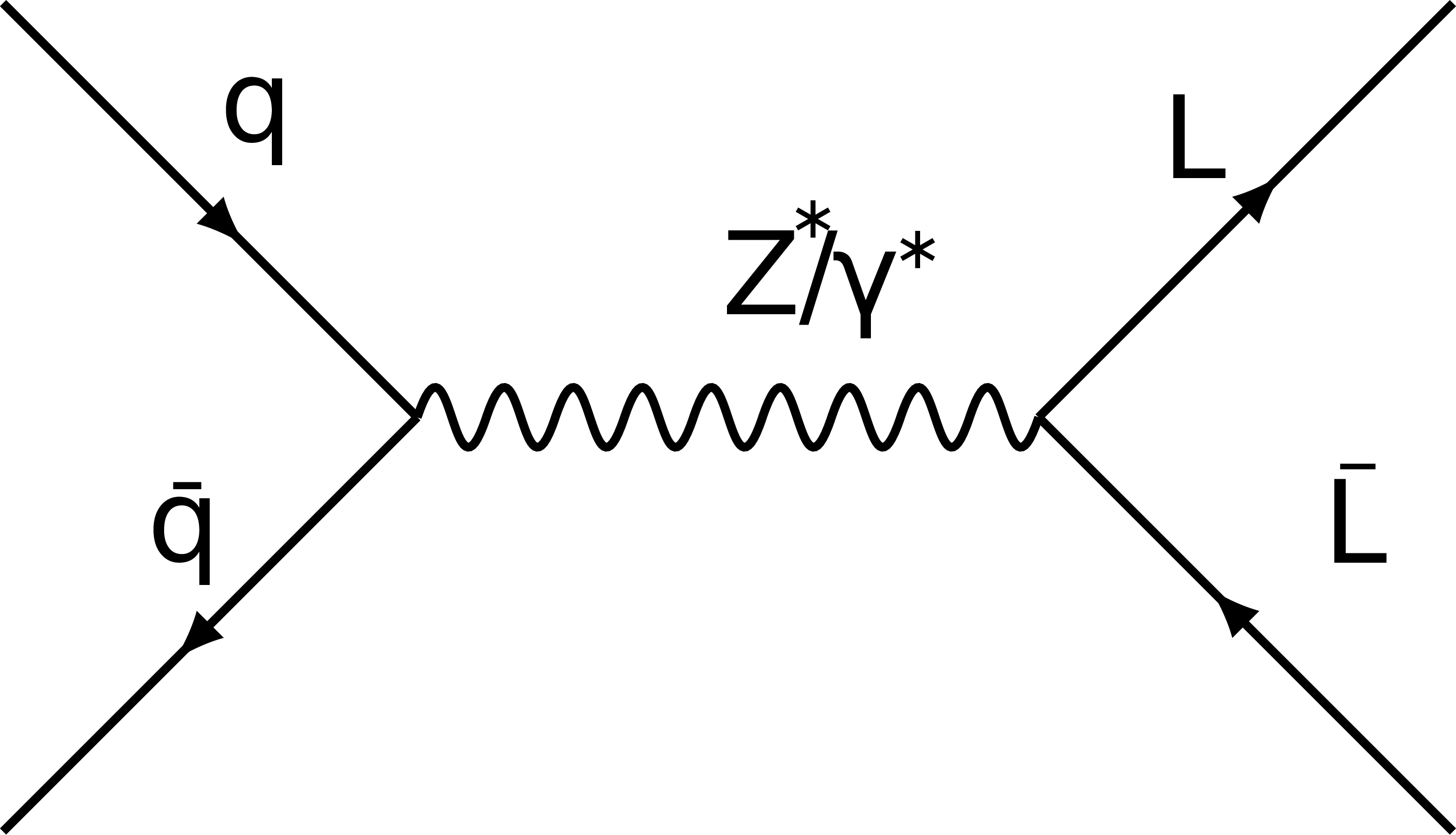
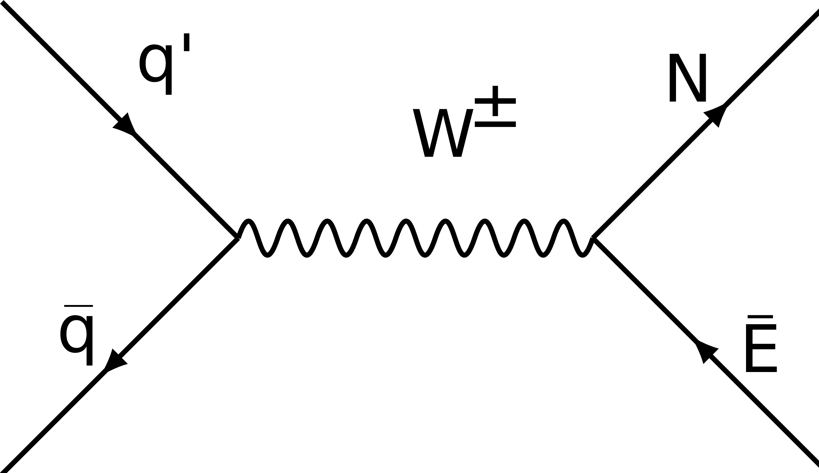
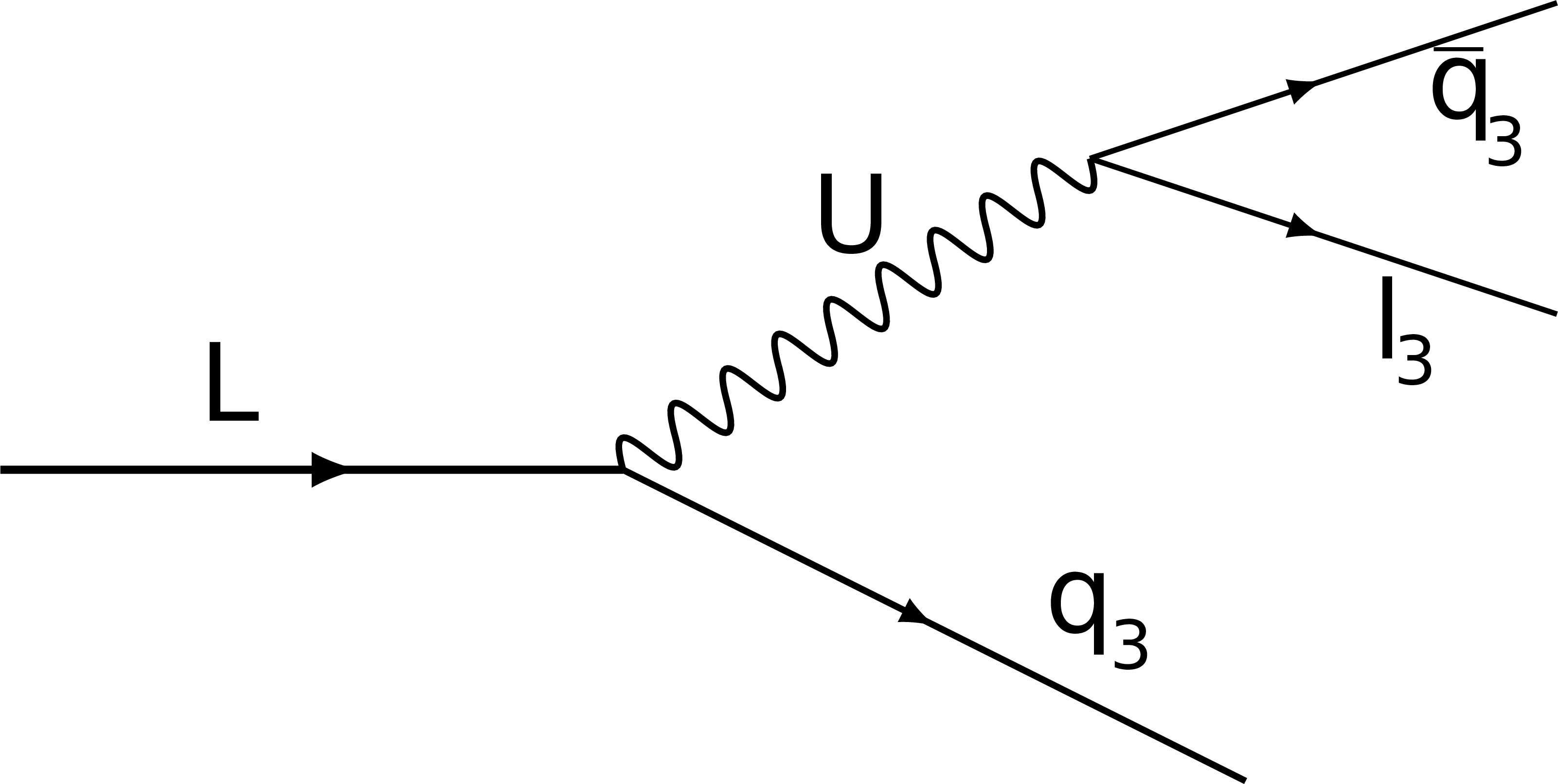
png pdf	Figure 1: Left and centre: example Feynman diagrams showing production of VLL pairs through s-channel bosons, as expected at the LHC. In these diagrams, L represents either the neutral VLL, N, or the charged VLL, E. Right: vector-like lepton decays proceed through their interactions with the vector leptoquark, U. These decays are primarily to third-generation leptons and quarks.
png pdf	Figure 1-a: Left and centre: example Feynman diagrams showing production of VLL pairs through s-channel bosons, as expected at the LHC. In these diagrams, L represents either the neutral VLL, N, or the charged VLL, E. Right: vector-like lepton decays proceed through their interactions with the vector leptoquark, U. These decays are primarily to third-generation leptons and quarks.
png pdf	Figure 1-b: Left and centre: example Feynman diagrams showing production of VLL pairs through s-channel bosons, as expected at the LHC. In these diagrams, L represents either the neutral VLL, N, or the charged VLL, E. Right: vector-like lepton decays proceed through their interactions with the vector leptoquark, U. These decays are primarily to third-generation leptons and quarks.
png pdf	Figure 1-c: Left and centre: example Feynman diagrams showing production of VLL pairs through s-channel bosons, as expected at the LHC. In these diagrams, L represents either the neutral VLL, N, or the charged VLL, E. Right: vector-like lepton decays proceed through their interactions with the vector leptoquark, U. These decays are primarily to third-generation leptons and quarks.
png pdf	Figure 2: Diagram of the event categorization and the various signal and control regions used in the analysis. The regions within the solid box are all used in the maximum likelihood fit. The regions in the dashed box are used to determine some parameters used in data-driven background estimations. The selections are mutually exclusive between all regions, so that each event only enters a single region. For brevity, not all selection criteria are shown; the detailed selection criteria are described in the text.
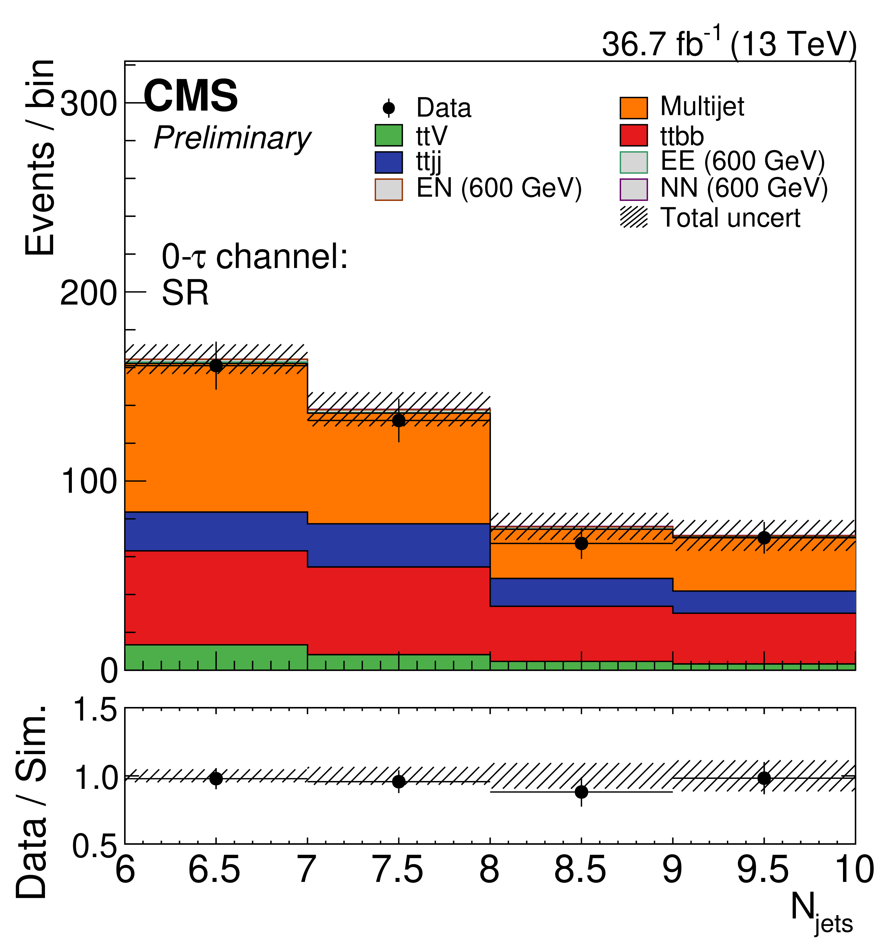
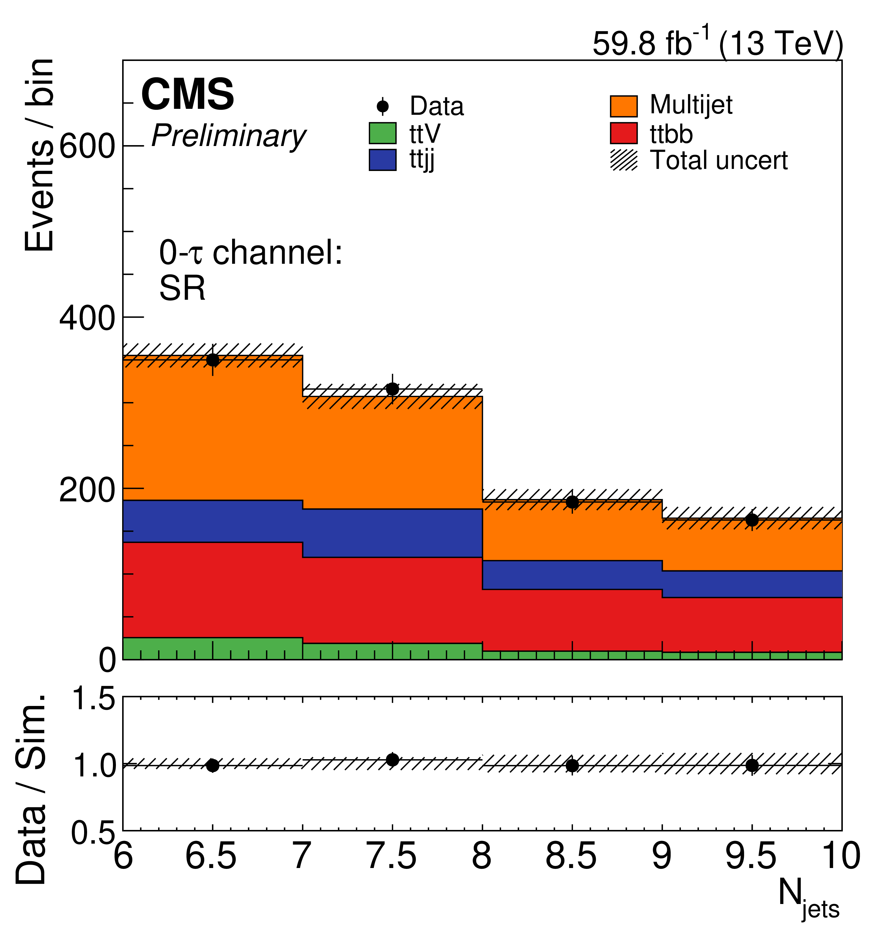
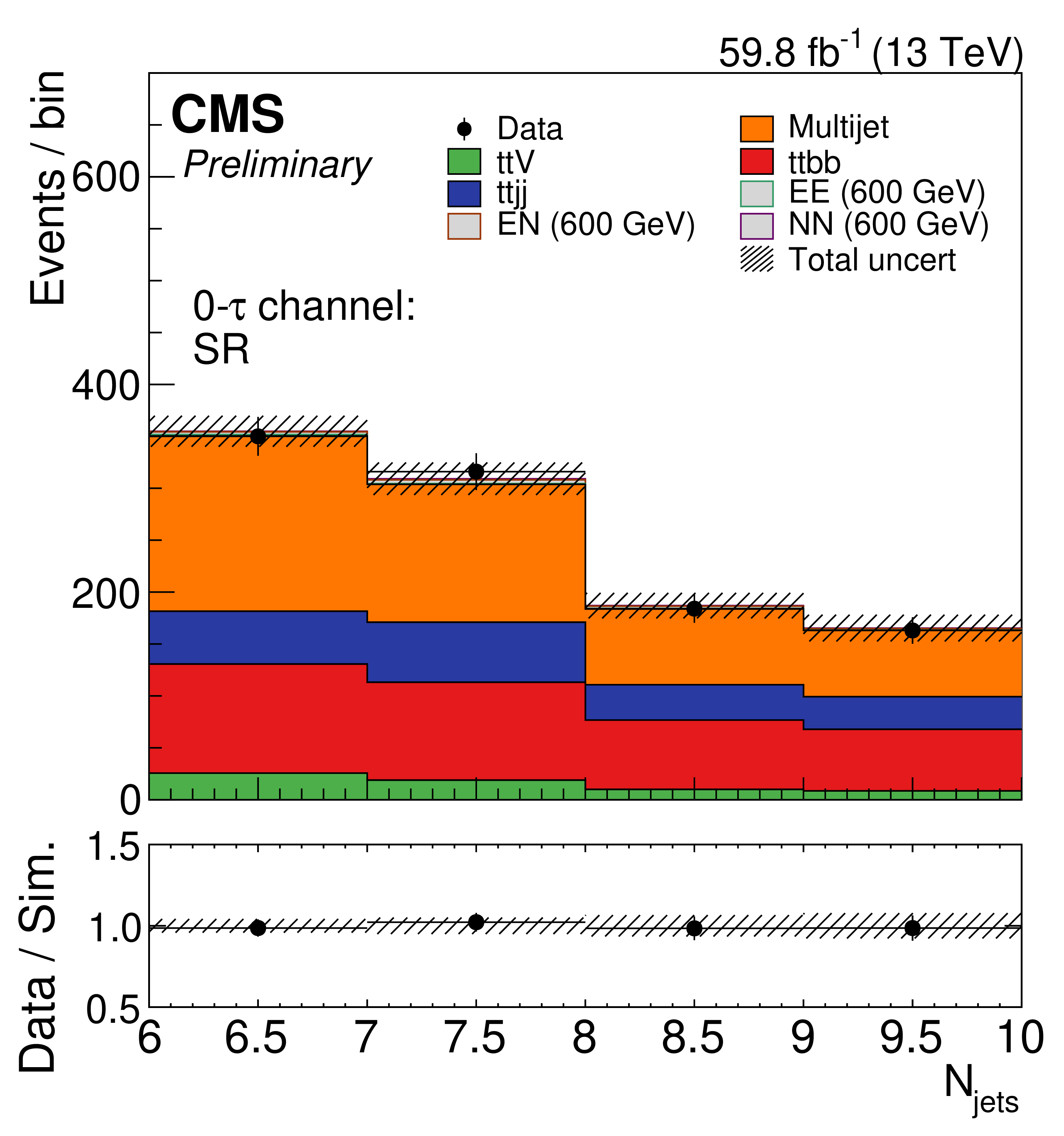
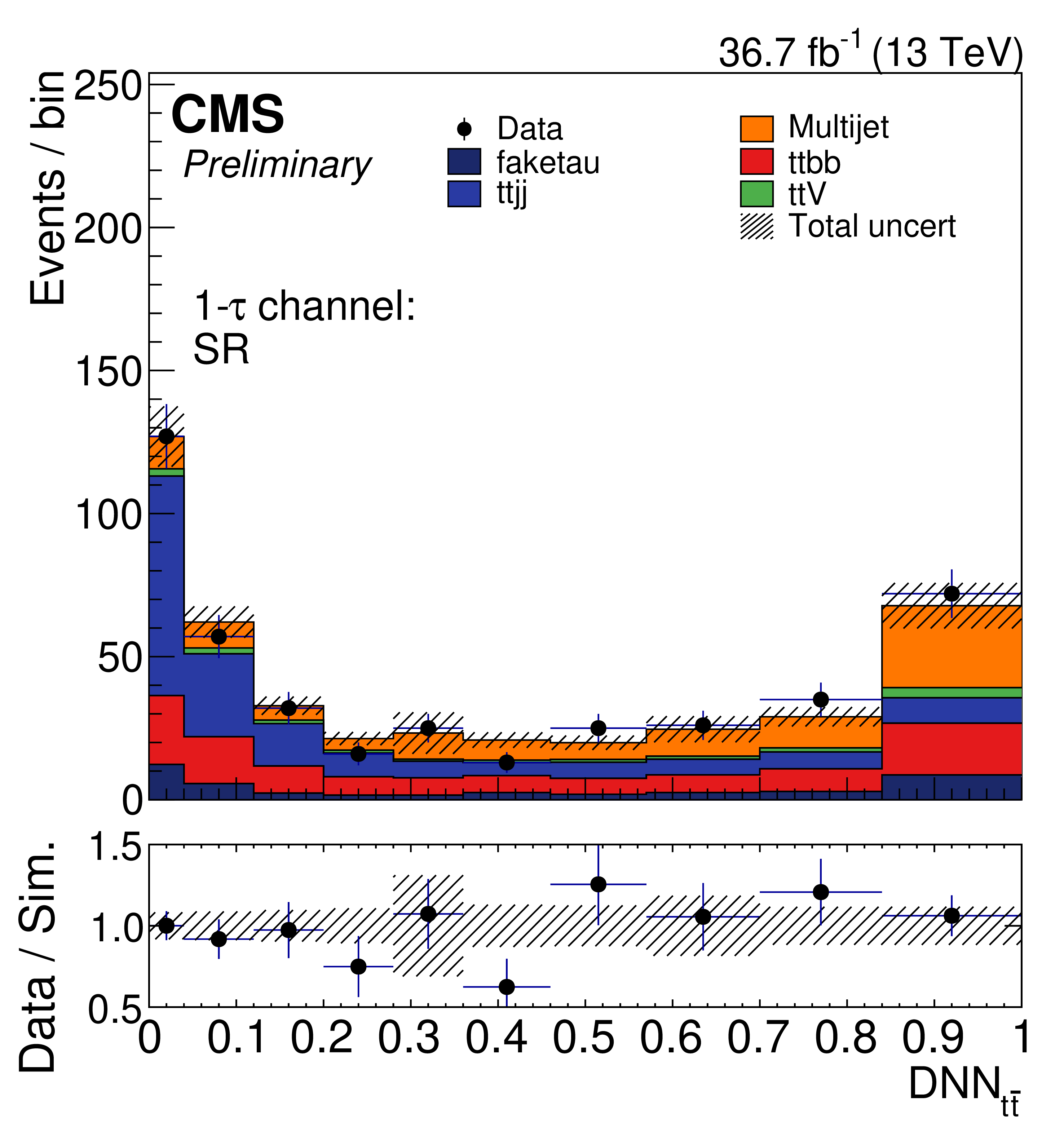
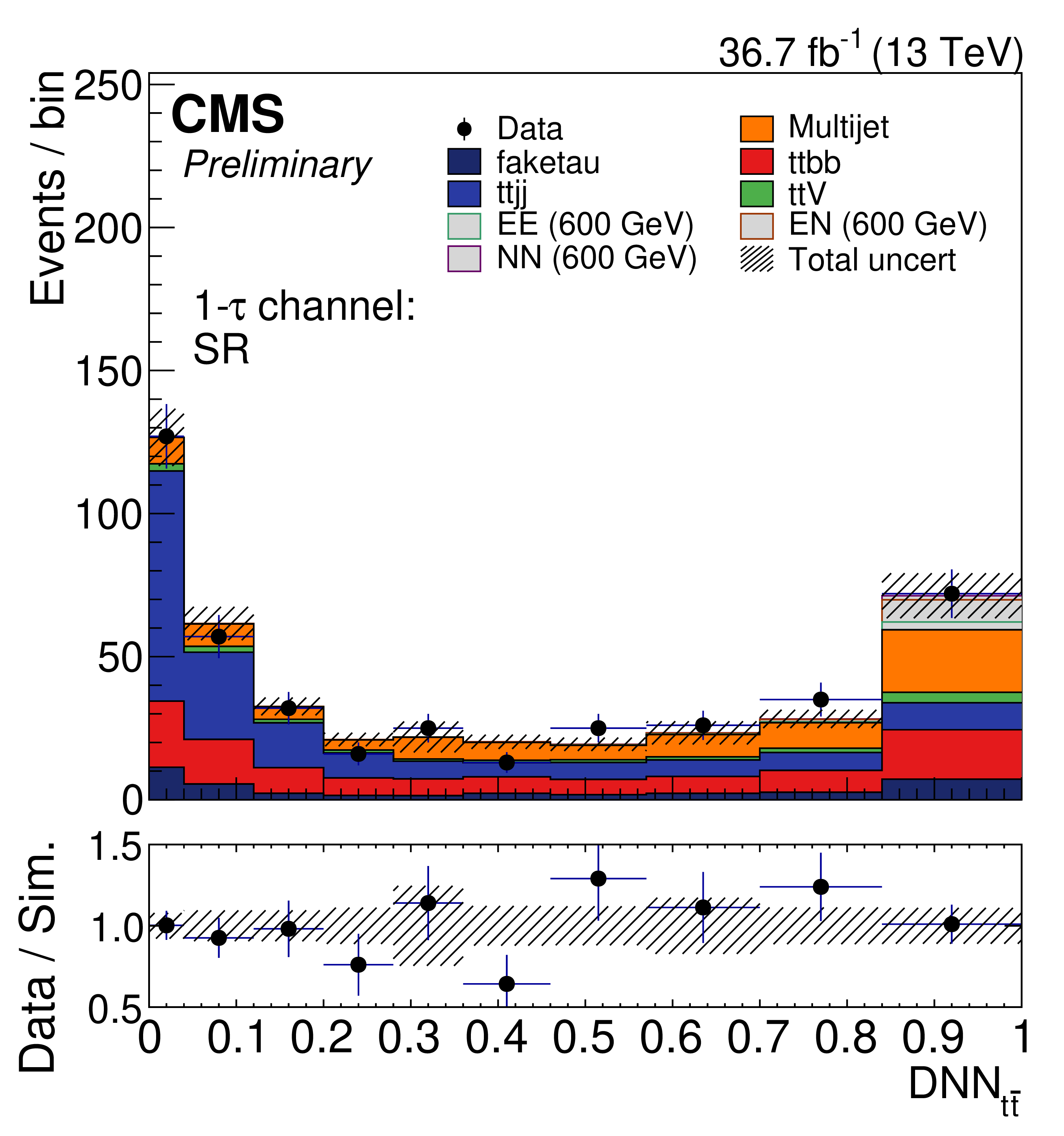
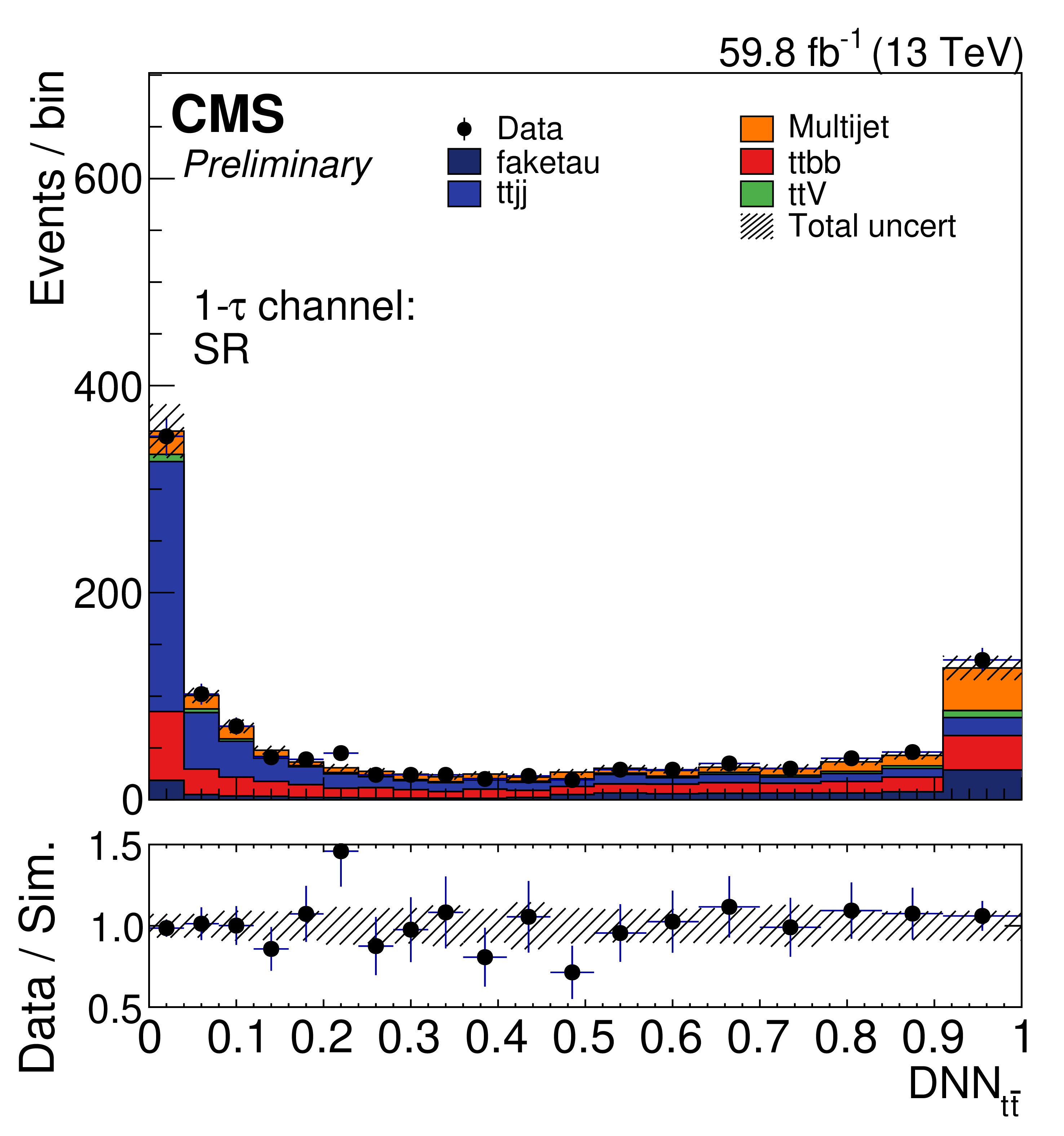
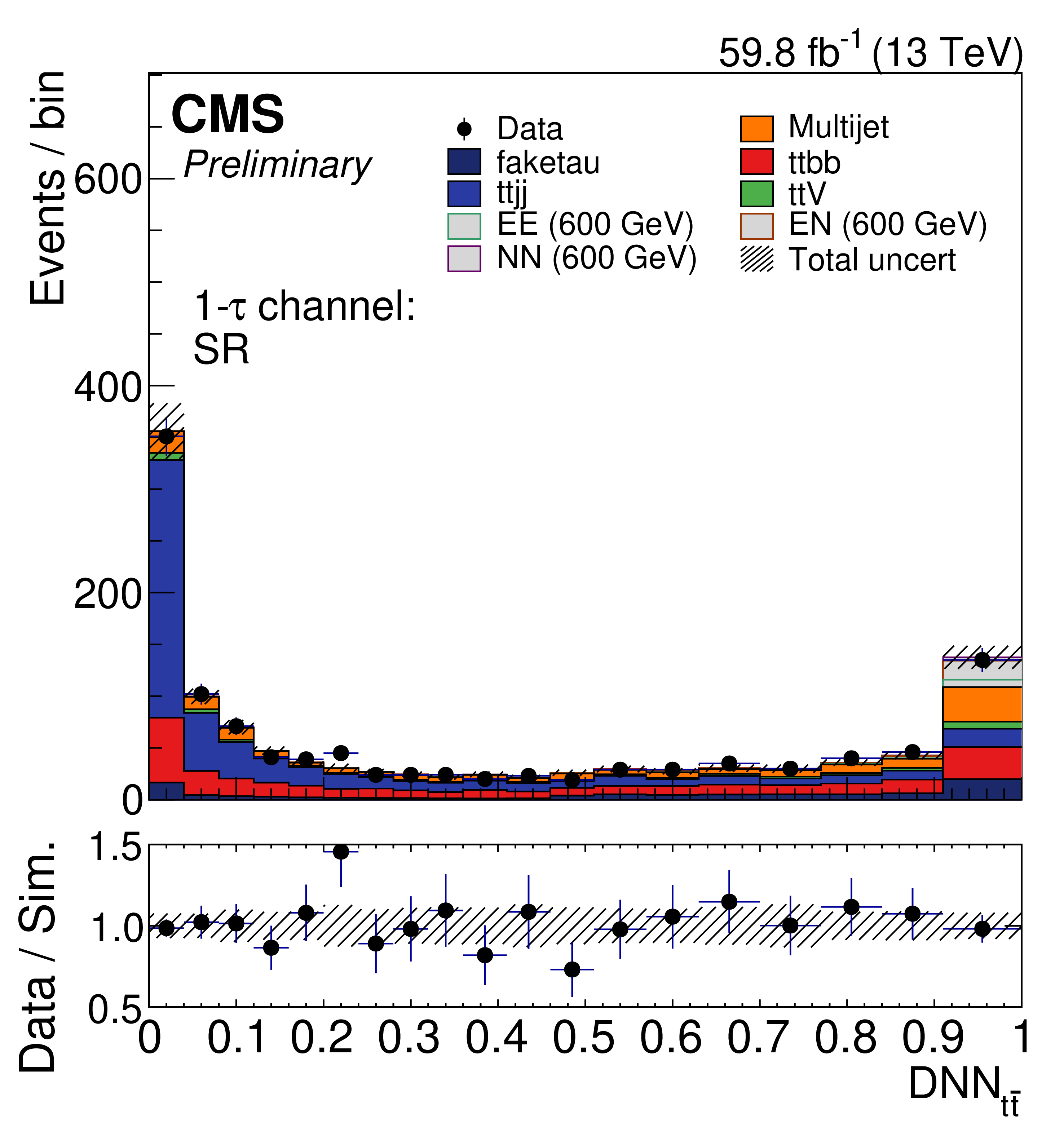
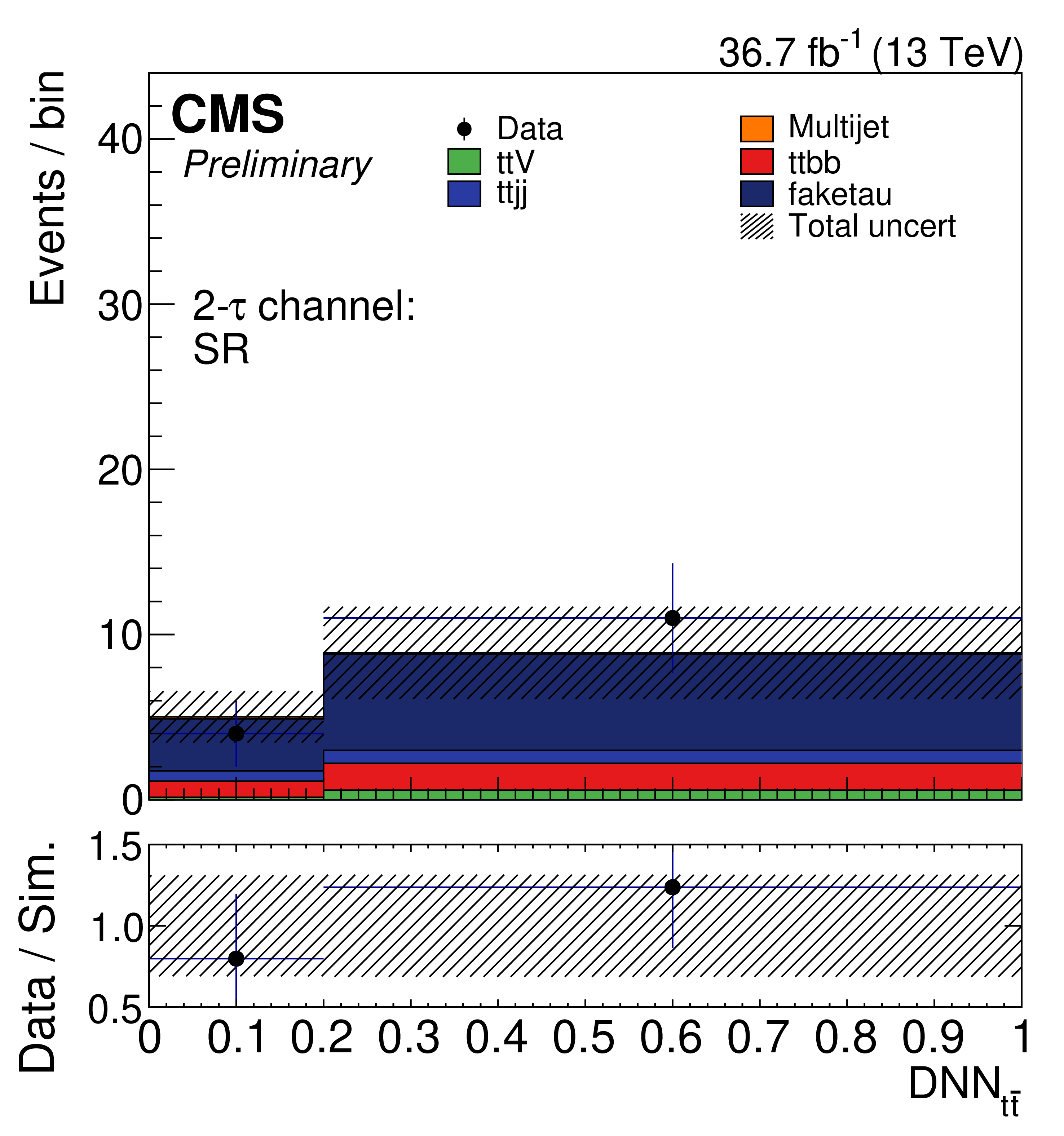
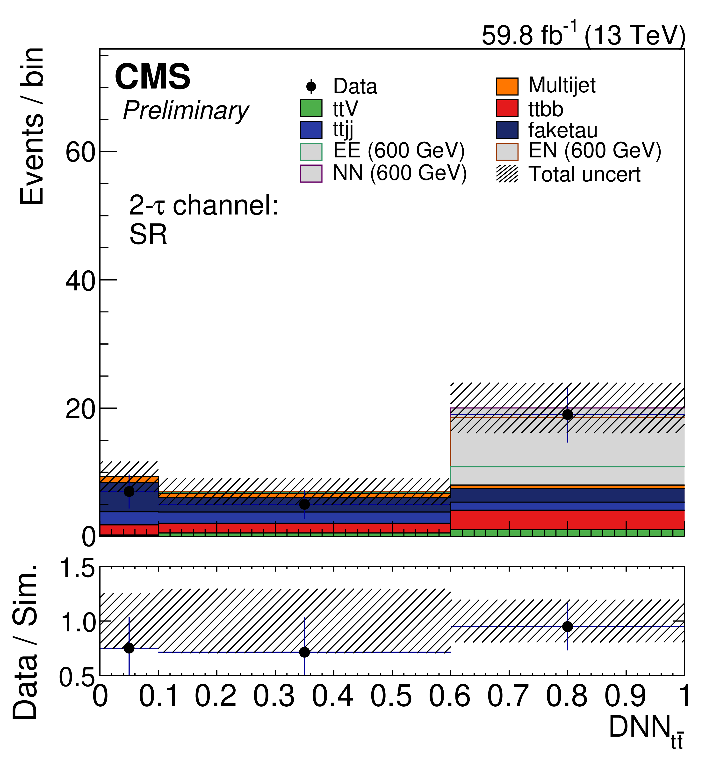
png pdf	Figure 3: Postfit plots for 2017 (two leftmost columns) and 2018 (two rightmost columns) showing the distributions of the main observables in the signal region for the different ${{\tau _\mathrm {h}}}$ multiplicity channels (from top to bottom: 0-${{\tau _\mathrm {h}}}$, 1-${{\tau _\mathrm {h}}}$, 2-${{\tau _\mathrm {h}}}$). The first and third column show the background-only fits and the second and fourth columns show the fit including the signal model.
png pdf	Figure 3-a: Postfit plots for 2017 (two leftmost columns) and 2018 (two rightmost columns) showing the distributions of the main observables in the signal region for the different ${{\tau _\mathrm {h}}}$ multiplicity channels (from top to bottom: 0-${{\tau _\mathrm {h}}}$, 1-${{\tau _\mathrm {h}}}$, 2-${{\tau _\mathrm {h}}}$). The first and third column show the background-only fits and the second and fourth columns show the fit including the signal model.
png pdf	Figure 3-b: Postfit plots for 2017 (two leftmost columns) and 2018 (two rightmost columns) showing the distributions of the main observables in the signal region for the different ${{\tau _\mathrm {h}}}$ multiplicity channels (from top to bottom: 0-${{\tau _\mathrm {h}}}$, 1-${{\tau _\mathrm {h}}}$, 2-${{\tau _\mathrm {h}}}$). The first and third column show the background-only fits and the second and fourth columns show the fit including the signal model.
png pdf	Figure 3-c: Postfit plots for 2017 (two leftmost columns) and 2018 (two rightmost columns) showing the distributions of the main observables in the signal region for the different ${{\tau _\mathrm {h}}}$ multiplicity channels (from top to bottom: 0-${{\tau _\mathrm {h}}}$, 1-${{\tau _\mathrm {h}}}$, 2-${{\tau _\mathrm {h}}}$). The first and third column show the background-only fits and the second and fourth columns show the fit including the signal model.
png pdf	Figure 3-d: Postfit plots for 2017 (two leftmost columns) and 2018 (two rightmost columns) showing the distributions of the main observables in the signal region for the different ${{\tau _\mathrm {h}}}$ multiplicity channels (from top to bottom: 0-${{\tau _\mathrm {h}}}$, 1-${{\tau _\mathrm {h}}}$, 2-${{\tau _\mathrm {h}}}$). The first and third column show the background-only fits and the second and fourth columns show the fit including the signal model.
png pdf	Figure 3-e: Postfit plots for 2017 (two leftmost columns) and 2018 (two rightmost columns) showing the distributions of the main observables in the signal region for the different ${{\tau _\mathrm {h}}}$ multiplicity channels (from top to bottom: 0-${{\tau _\mathrm {h}}}$, 1-${{\tau _\mathrm {h}}}$, 2-${{\tau _\mathrm {h}}}$). The first and third column show the background-only fits and the second and fourth columns show the fit including the signal model.
png pdf	Figure 3-f: Postfit plots for 2017 (two leftmost columns) and 2018 (two rightmost columns) showing the distributions of the main observables in the signal region for the different ${{\tau _\mathrm {h}}}$ multiplicity channels (from top to bottom: 0-${{\tau _\mathrm {h}}}$, 1-${{\tau _\mathrm {h}}}$, 2-${{\tau _\mathrm {h}}}$). The first and third column show the background-only fits and the second and fourth columns show the fit including the signal model.
png pdf	Figure 3-g: Postfit plots for 2017 (two leftmost columns) and 2018 (two rightmost columns) showing the distributions of the main observables in the signal region for the different ${{\tau _\mathrm {h}}}$ multiplicity channels (from top to bottom: 0-${{\tau _\mathrm {h}}}$, 1-${{\tau _\mathrm {h}}}$, 2-${{\tau _\mathrm {h}}}$). The first and third column show the background-only fits and the second and fourth columns show the fit including the signal model.
png pdf	Figure 3-h: Postfit plots for 2017 (two leftmost columns) and 2018 (two rightmost columns) showing the distributions of the main observables in the signal region for the different ${{\tau _\mathrm {h}}}$ multiplicity channels (from top to bottom: 0-${{\tau _\mathrm {h}}}$, 1-${{\tau _\mathrm {h}}}$, 2-${{\tau _\mathrm {h}}}$). The first and third column show the background-only fits and the second and fourth columns show the fit including the signal model.
png pdf	Figure 3-i: Postfit plots for 2017 (two leftmost columns) and 2018 (two rightmost columns) showing the distributions of the main observables in the signal region for the different ${{\tau _\mathrm {h}}}$ multiplicity channels (from top to bottom: 0-${{\tau _\mathrm {h}}}$, 1-${{\tau _\mathrm {h}}}$, 2-${{\tau _\mathrm {h}}}$). The first and third column show the background-only fits and the second and fourth columns show the fit including the signal model.
png pdf	Figure 3-j: Postfit plots for 2017 (two leftmost columns) and 2018 (two rightmost columns) showing the distributions of the main observables in the signal region for the different ${{\tau _\mathrm {h}}}$ multiplicity channels (from top to bottom: 0-${{\tau _\mathrm {h}}}$, 1-${{\tau _\mathrm {h}}}$, 2-${{\tau _\mathrm {h}}}$). The first and third column show the background-only fits and the second and fourth columns show the fit including the signal model.
png pdf	Figure 3-k: Postfit plots for 2017 (two leftmost columns) and 2018 (two rightmost columns) showing the distributions of the main observables in the signal region for the different ${{\tau _\mathrm {h}}}$ multiplicity channels (from top to bottom: 0-${{\tau _\mathrm {h}}}$, 1-${{\tau _\mathrm {h}}}$, 2-${{\tau _\mathrm {h}}}$). The first and third column show the background-only fits and the second and fourth columns show the fit including the signal model.
png pdf	Figure 3-l: Postfit plots for 2017 (two leftmost columns) and 2018 (two rightmost columns) showing the distributions of the main observables in the signal region for the different ${{\tau _\mathrm {h}}}$ multiplicity channels (from top to bottom: 0-${{\tau _\mathrm {h}}}$, 1-${{\tau _\mathrm {h}}}$, 2-${{\tau _\mathrm {h}}}$). The first and third column show the background-only fits and the second and fourth columns show the fit including the signal model.
png pdf	Figure 4: Expected and observed 95% confidence level upper limits on the electroweak vector-like lepton cross section times branching fraction, combining the 2017 and 2018 data and all ${\tau _\mathrm {h}}$ multiplicity channels combined.

Tables
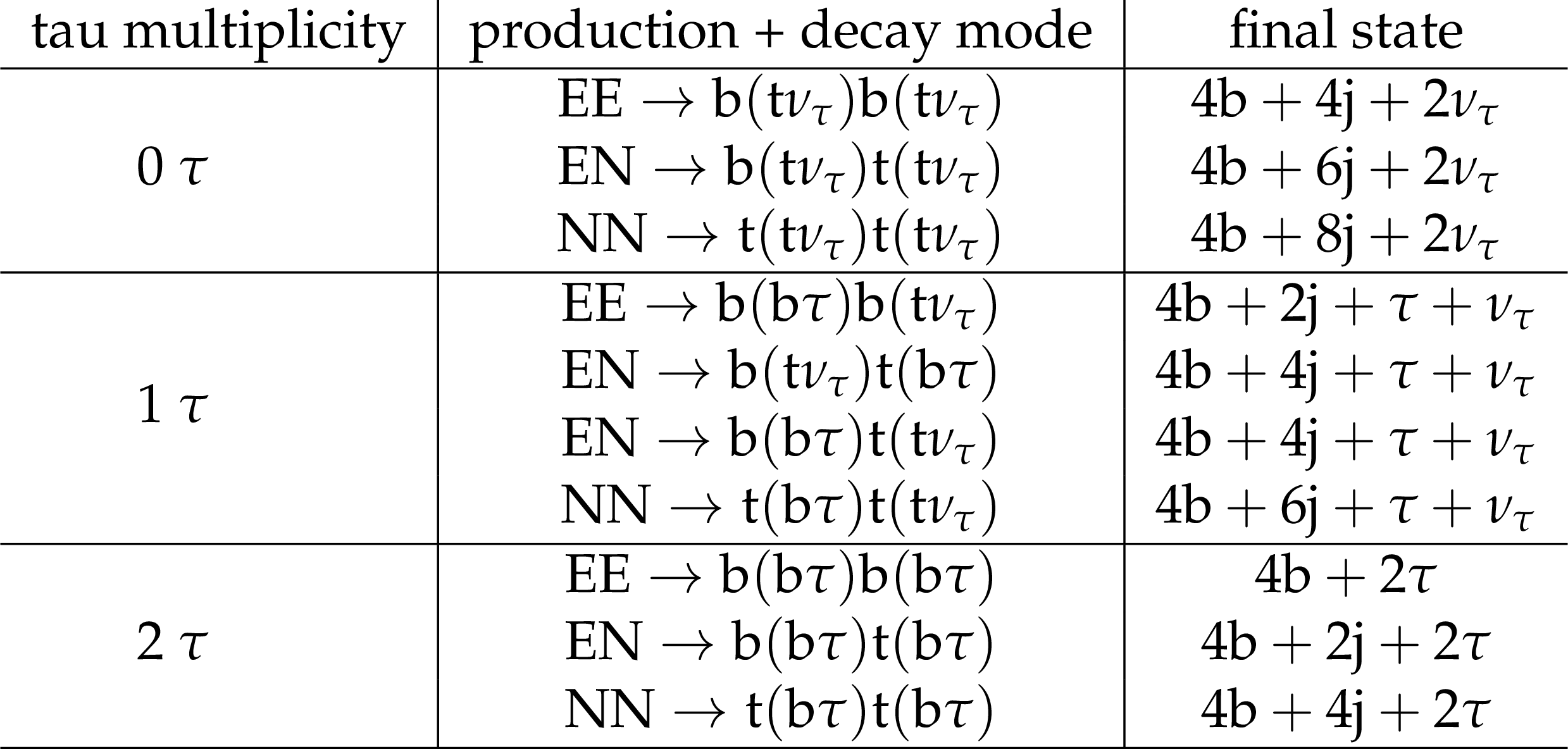
png pdf	Table 1: Illustrative contributions from different VLL production and decay modes to the 0-, 1-, and 2-$\tau$ signal regions. The decay products in parentheses represent the objects coming from the intermediate vector leptoquark, U, in the decay. For brevity, no distinction is made between particles and antiparticles, the multiplicities of each decay mode are not shown, and the impacts of object misidentification are not considered in the table. E and N represent the charged and neutral VLLs; t, b, $\tau$, and $\nu_\tau$ represent top quarks, bottom quarks, tau leptons and tau neutrinos; and j represents any quark other than t or b.
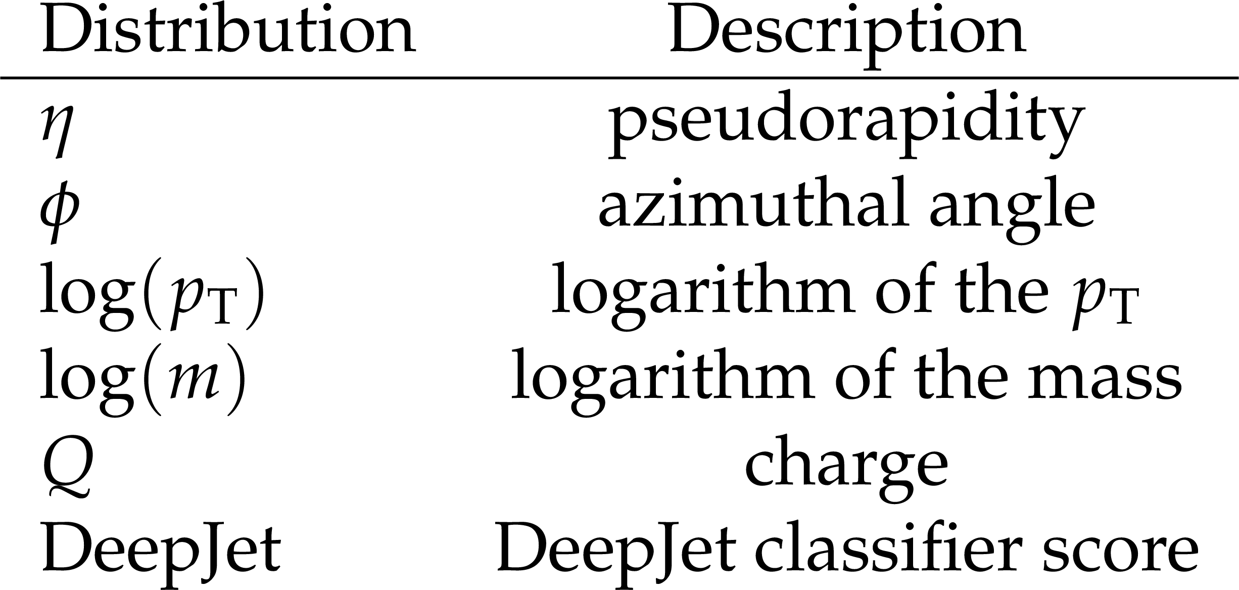
png pdf	Table 2: List of input features used during training of the ABCNet model for VLL classification.

Summary

The first search for vector-like leptons in the context of the 4321 model has been presented, using proton-proton collision data collected with the CMS detector at $\sqrt{s} = $ 13 TeV, corresponding to an integrated luminosity of 96.5 fb$^{-1}$. The probed model consists of an extension of the standard model with an $\textrm{SU}(4) \times \textrm{SU}(3)' \times \textrm{SU}(2)_L \times \textrm{U}(1)'$ gauge sector that can provide a combined explanation to multiple anomalies observed in B hadron decays, which point to lepton flavour nonuniversality. In the model, a leptoquark is predicted as the primary source of lepton flavour violation while the UV-completion predicts additional vector-like fermion families. In particular, vector-like leptons are investigated by their coupling to standard model fermions through leptoquark interactions, resulting in third generation fermion signatures. Final states containing at least three b-tagged jets and varying $\tau$ lepton multiplicities are considered. To improve the search sensitivity, machine learning methods based on graph neural networks were used to learn the kinematic relationship between particles in a large jet multiplicity environment.

Vector-like lepton masses up to 640 GeV were expected to be excluded at the 95% confidence level. Mild excesses in the data, compared with the expectation, are observed in the signal-sensitive bins of the 1-${{\tau_\mathrm{h}}}$ and 2-${{\tau_\mathrm{h}}}$ regions for both 2017 and 2018 data. As a result, no VLL masses are excluded at the 95% confidence level and limits are set between 10 and 30 fb, depending on the VLL mass hypothesis. The observed excess is consistent with the presence of VLLs in the context of the 4321 model, and the excess of events over the background-only hypothesis corresponds to a significance of 2.8$\sigma$.

References
1	L. Di Luzio et al.	Maximal flavour violation: a Cabibbo mechanism for leptoquarks	JHEP 2018 (2018) 081	1808.00942
2	L. Di Luzio, A. Greljo, and M. Nardecchia	Gauge leptoquark as the origin of B-physics anomalies	PRD 96 (2017) 115011	1708.08450
3	LHCb Collaboration	Measurement of the ratio of branching fractions $ \mathcal{B}(\bar{B}^0 \to d^{+}\tau^{-}\bar{\nu}_{\tau})/\mathcal{B}(\bar{B}^0 \to d^{+}\mu^{-}\bar{\nu}_{\mu}) $	PRL 115 (2015) 111803	1506.08614
4	LHCb Collaboration	Measurement of the ratio of the $ b^0 \to d^{-} \tau^+ \nu_{\tau} $ and $ b^0 \to d^{-} \mu^+ \nu_{\mu} $ branching fractions using three-prong $ \tau $-lepton decays	PRL 120 (2018) 171802	1708.08856
5	LHCb Collaboration	Test of lepton universality in beauty-quark decays	2021	2103.11769
6	F. Abe, D. Amidei, G. Apollinari, and M. Atac	Measurement of the ratio B(W$ \rightarrow \tau \nu$)/B(W $\rightarrow e \nu$) in $ p\bar{p} $ collisions at $ \sqrt{s} = $ 1.8 TeV	PRL 68 (1992) 3398
7	D0 Collaboration	A measurement of the $ w \to \tau \nu $ production cross section in $ p\bar{p} $ collisions at $ \sqrt{s} = $ 1.8 TeV	PRL 84 (2000) 5710	hep-ex/9912065
8	ATLAS Collaboration	Test of the universality of $ \tau $ and $ \mu $ lepton couplings in $ w $-boson decays with the ATLAS detector	NP 17 (2021), no. 7, 813	2007.14040
9	LHCb Collaboration	Measurement of forward $ w\to e\nu $ production in $ pp $ collisions at $ \sqrt{s}= $ 8 TeV	JHEP 10 (2016) 030	1608.01484
10	C. Cornella et al.	Reading the footprints of the B-meson flavor anomalies	JHEP 2021 (2021), no. 8	2103.16558
11	T. Hastie, R. Tibshirani, and J. Friedman		Springer-Verlag, second edition, 2013 , ISBN 978-0-387-84858-7
12	V. Mikuni and F. Canelli	ABCNet: An attention-based method for particle tagging	EPJPlus 135 (2020) 463	2001.05311
13	G. Kasieczka, B. Nachman, M. D. Schwartz, and D. Shih	Automating the ABCD method with machine learning	PRD 103 (2021), no. 3, 035021	2007.14400
14	CMS Collaboration	The CMS experiment at the CERN LHC	JINST 3 (2008) S08004	CMS-00-001
15	CMS Collaboration	Performance of the CMS Level-1 trigger in proton-proton collisions at $ \sqrt{s} = $ 13 TeV	JINST 15 (2020) P10017	CMS-TRG-17-001 2006.10165
16	CMS Collaboration	The CMS trigger system	JINST 12 (2017) P01020	CMS-TRG-12-001 1609.02366
17	M. Cacciari, G. P. Salam, and G. Soyez	The anti-$ k_t $ jet clustering algorithm	JHEP 04 (2008) 063	0802.1189
18	M. Cacciari, G. P. Salam, and G. Soyez	FastJet user manual	EPJC 72 (2012) 1896	1111.6097
19	CMS Collaboration	Particle-flow reconstruction and global event description with the CMS detector	JINST 12 (2017) P10003	CMS-PRF-14-001 1706.04965
20	CMS Collaboration	Jet energy scale and resolution in the cms experiment in pp collisions at 8 TeV	JINST 12 (2017) P02014	CMS-JME-13-004 1607.03663
21	CMS Collaboration	Identification of heavy-flavour jets with the CMS detector in pp collisions at 13 TeV	JINST 13 (2018) P05011	CMS-BTV-16-002 1712.07158
22	E. Bols et al.	Jet flavour classification using DeepJet	JINST 15 (2020) P12012	2008.10519
23	CMS Collaboration	Performance of the DeepJet b tagging algorithm using 41.9/fb of data from proton-proton collisions at 13 TeV with Phase 1 CMS detector	CDS
24	CMS Collaboration	Performance of reconstruction and identification of $ \tau $ leptons decaying to hadrons and $ \nu_\tau $ in pp collisions at $ \sqrt{s}= $ 13 TeV	JINST 13 (2018) P10005	CMS-TAU-16-003 1809.02816
25	CMS Collaboration	Identification of hadronic tau lepton decays using a deep neural network	2022. Submitted to JINST	CMS-TAU-20-001 2201.08458
26	CMS Collaboration	Performance of missing transverse momentum reconstruction in proton-proton collisions at $ \sqrt{s} = $ 13 TeV using the CMS detector	JINST 14 (2019) P07004	CMS-JME-17-001 1903.06078
27	CMS Collaboration	Performance of the CMS muon detector and muon reconstruction with proton-proton collisions at $ \sqrt{s} = $ 13 TeV	JINST 13 (2018) P06015	CMS-MUO-16-001 1804.04528
28	CMS Collaboration	CMS technical design report for the pixel detector upgrade	CDS
29	CMS Collaboration	Performance of b tagging algorithms in proton-proton collisions at 13 TeV with Phase 1 CMS detector	CDS
30	J. Alwall et al.	The automated computation of tree-level and next-to-leading order differential cross sections, and their matching to parton shower simulations	JHEP 07 (2014) 079	1405.0301
31	A. Alloul et al.	FeynRules 2.0 -- a complete toolbox for tree-level phenomenology	Computer Physics Communications 185 (2014) 2250	1310.1921
32	T. Sjostrand, S. Mrenna, and P. Skands	A brief introduction to PYTHIA 8.1	Comp. Phys. Comm. 178 (2008) 852	0710.3820
33	CMS Collaboration	Extraction and validation of a new set of CMS PYTHIA8 tunes from underlying-event measurements	EPJC 80 (2020) 4	CMS-GEN-17-001 1903.12179
34	R. D. Ball et al.	Parton distributions from high-precision collider data	EPJC 77 (2017)	1706.00428
35	P. Nason	A new method for combining NLO QCD with shower Monte Carlo algorithms	JHEP 11 (2004) 040	hep-ph/0409146
36	S. Frixione, P. Nason, and C. Oleari	Matching NLO QCD computations with parton shower simulations: the POWHEG method	JHEP 11 (2007) 070	0709.2092
37	S. Alioli, P. Nason, C. Oleari, and E. Re	A general framework for implementing NLO calculations in shower Monte Carlo programs: the POWHEG BOX	JHEP 06 (2010) 043	1002.2581
38	M. Beneke, P. Falgari, S. Klein, and C. Schwinn	Hadronic top-quark pair production with NNLL threshold resummation	NPB 855 (2012) 695	1109.1536v1
39	M. Cacciari et al.	Top-pair production at hadron colliders with next-to-next-to-leading logarithmic soft-gluon resummation	PLB 710 (2012) 612	1111.5869
40	P. Barnreuther, M. Czakon, and A. Mitov	Percent-level-precision physics at the Tevatron: Next-to-next-to-leading order QCD corrections to $ q\bar{q} \to t\bar{t}+x $	PRL 109 (2012)	1204.5201
41	M. Czakon and A. Mitov	NNLO corrections to top-pair production at hadron colliders: the all-fermionic scattering channels	JHEP 2012 (2012)	1207.0236
42	M. Czakon and A. Mitov	NNLO corrections to top pair production at hadron colliders: the quark-gluon reaction	JHEP 2013 (2013)	1210.6832
43	M. Czakon, P. Fiedler, and A. Mitov	Total top-quark pair-production cross section at hadron colliders through O($ \alpha_s^4 $)	PRL 110 (2013)	1303.6254
44	M. Czakon and A. Mitov	Top++: a program for the calculation of the top-pair cross-section at hadron colliders	CPC 185 (2014) 2930	1112.5675
45	CMS Collaboration	Measurement of the $ \mathrm{t\bar{t}}\mathrm{b\bar{b}} $ production cross section in the all-jet final state in pp collisions at $ \sqrt{s} = $ 13 TeV	PLB 803 (2020) 135285	CMS-TOP-18-011 1909.05306
46	CMS Collaboration	Measurement of the cross section for $ \mathrm{t\bar{t}} $ production with additional jets and b jets in pp collisions at $ \sqrt{s} = $ 13 TeV	JHEP 2007 (2020) 125	CMS-TOP-18-002 2003.06467
47	CMS Collaboration	Measurements of $ \mathrm{t \bar{t}} $ cross sections in association with b jets and inclusive jets and their ratio using dilepton final states in pp collisions at $ \sqrt{s} = $ 13 TeV	PLB 776 (2018) 355	CMS-TOP-16-010 1705.10141
48	ATLAS Collaboration	Measurements of inclusive and differential fiducial cross-sections of $ \mathrm{t\bar{t}} $ production with additional heavy-flavour jets in proton-proton collisions at $ \sqrt{s} = $ 13 TeV with the ATLAS detector	JHEP 2019 (2019)	1811.12113
49	R. J. Barlow and C. Beeston	Fitting using finite Monte Carlo samples	CPC 77 (1993) 219
50	J. Butterworth et al.	PDF4LHC recommendations for LHC Run II	JPG 43 (2016) 023001	1510.03865
51	A. L. Read	Presentation of search results: The CL$ _{\text{s}} $ technique	JPG 28 (2002) 2693
52	T. Junk	Confidence level computation for combining searches with small statistics	NIMA 434 (1999) 435	hep-ex/9902006
53	G. Cowan, K. Cranmer, E. Gross, and O. Vitells	Asymptotic formulae for likelihood-based tests of new physics	EPJC 71 (2011) 1554	1007.1727
54	S. S. Wilks	The large-sample distribution of the likelihood ratio for testing composite hypotheses	The Annals of Mathematical Statistics 9 (1938), no. 1, 60