

Compact Muon Solenoid
LHC, CERN
| CMS-PAS-B2G-19-006 | ||
| Search for a spin-1 heavy resonance that decays to a Z boson and Higgs boson in the semileptonic final states with LHC Run-2 data | ||
| CMS Collaboration | ||
| July 2020 | ||
| Abstract: This note describes the search for a heavy spin-1 resonance decaying into a Z boson and the 125-GeV Higgs boson, where the Z boson is identified through its leptonic decays (electrons, muons or neutrinos) and the Higgs boson is identified through its decay to quarks. The search is performed in the boosted regime for resonances with masses larger than 800 GeV. Model-independent upper limits are derived as a function of the resonance mass and natural width, and interpreted within the theoretical framework of the Heavy Vector Triplet model. | ||
|
Links:
CDS record (PDF) ;
CADI line (restricted) ;
These preliminary results are superseded in this paper, Accepted by EPJC. The superseded preliminary plots can be found here. |
||
| Figures | |
png pdf |
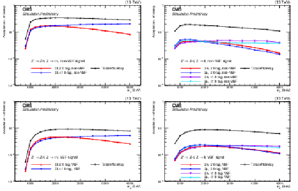
Figure 1:
Signal acceptance $\times $ efficiency in 0$\ell $ (left) and 2$\ell $ (right) categories for the signal produced through $\mathrm{q\bar{q}}$ annihilation (top) and vector boson fusion (bottom). |
png pdf |
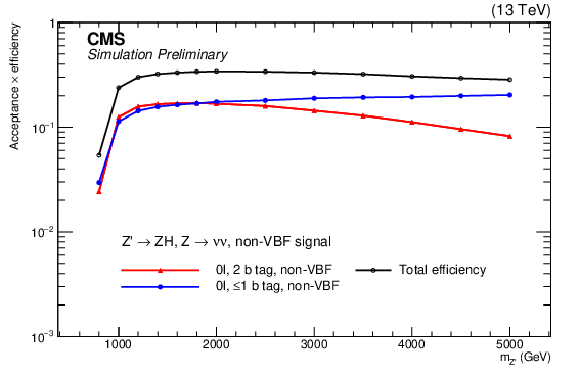
Figure 1-a:
Signal acceptance $\times $ efficiency in 0$\ell $ (left) and 2$\ell $ (right) categories for the signal produced through $\mathrm{q\bar{q}}$ annihilation (top) and vector boson fusion (bottom). |
png pdf |
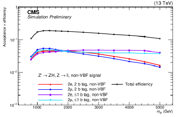
Figure 1-b:
Signal acceptance $\times $ efficiency in 0$\ell $ (left) and 2$\ell $ (right) categories for the signal produced through $\mathrm{q\bar{q}}$ annihilation (top) and vector boson fusion (bottom). |
png pdf |
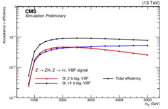
Figure 1-c:
Signal acceptance $\times $ efficiency in 0$\ell $ (left) and 2$\ell $ (right) categories for the signal produced through $\mathrm{q\bar{q}}$ annihilation (top) and vector boson fusion (bottom). |

png pdf |
Figure 1-d:
Signal acceptance $\times $ efficiency in 0$\ell $ (left) and 2$\ell $ (right) categories for the signal produced through $\mathrm{q\bar{q}}$ annihilation (top) and vector boson fusion (bottom). |

png pdf |
Figure 2:
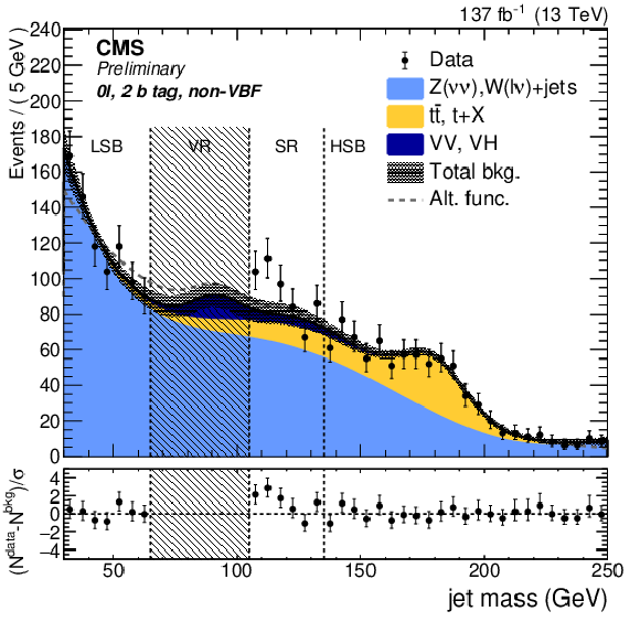
Fit to data as a function of ${m_{{j_{\mathrm{H}}}}}$ in the 2 b-tag (left), $\leq $1 b-tag (right), 0 lepton (top), 2 electron (middle), and 2 muon (bottom) categories. The shaded band around the total background represents the uncertainty from the fit to data in the jet mass sidebands. The observed data are indicated by black markers. The bottom panel shows for each bin $(N^{data}-N^{bkg})/\sigma $, where $\sigma $ is the statistical uncertainty in data. |
png pdf |
Figure 2-a:
Fit to data as a function of ${m_{{j_{\mathrm{H}}}}}$ in the 2 b-tag (left), $\leq $1 b-tag (right), 0 lepton (top), 2 electron (middle), and 2 muon (bottom) categories. The shaded band around the total background represents the uncertainty from the fit to data in the jet mass sidebands. The observed data are indicated by black markers. The bottom panel shows for each bin $(N^{data}-N^{bkg})/\sigma $, where $\sigma $ is the statistical uncertainty in data. |

png pdf |
Figure 2-b:
Fit to data as a function of ${m_{{j_{\mathrm{H}}}}}$ in the 2 b-tag (left), $\leq $1 b-tag (right), 0 lepton (top), 2 electron (middle), and 2 muon (bottom) categories. The shaded band around the total background represents the uncertainty from the fit to data in the jet mass sidebands. The observed data are indicated by black markers. The bottom panel shows for each bin $(N^{data}-N^{bkg})/\sigma $, where $\sigma $ is the statistical uncertainty in data. |

png pdf |
Figure 2-c:
Fit to data as a function of ${m_{{j_{\mathrm{H}}}}}$ in the 2 b-tag (left), $\leq $1 b-tag (right), 0 lepton (top), 2 electron (middle), and 2 muon (bottom) categories. The shaded band around the total background represents the uncertainty from the fit to data in the jet mass sidebands. The observed data are indicated by black markers. The bottom panel shows for each bin $(N^{data}-N^{bkg})/\sigma $, where $\sigma $ is the statistical uncertainty in data. |

png pdf |
Figure 2-d:
Fit to data as a function of ${m_{{j_{\mathrm{H}}}}}$ in the 2 b-tag (left), $\leq $1 b-tag (right), 0 lepton (top), 2 electron (middle), and 2 muon (bottom) categories. The shaded band around the total background represents the uncertainty from the fit to data in the jet mass sidebands. The observed data are indicated by black markers. The bottom panel shows for each bin $(N^{data}-N^{bkg})/\sigma $, where $\sigma $ is the statistical uncertainty in data. |

png pdf |
Figure 2-e:
Fit to data as a function of ${m_{{j_{\mathrm{H}}}}}$ in the 2 b-tag (left), $\leq $1 b-tag (right), 0 lepton (top), 2 electron (middle), and 2 muon (bottom) categories. The shaded band around the total background represents the uncertainty from the fit to data in the jet mass sidebands. The observed data are indicated by black markers. The bottom panel shows for each bin $(N^{data}-N^{bkg})/\sigma $, where $\sigma $ is the statistical uncertainty in data. |

png pdf |
Figure 2-f:
Fit to data as a function of ${m_{{j_{\mathrm{H}}}}}$ in the 2 b-tag (left), $\leq $1 b-tag (right), 0 lepton (top), 2 electron (middle), and 2 muon (bottom) categories. The shaded band around the total background represents the uncertainty from the fit to data in the jet mass sidebands. The observed data are indicated by black markers. The bottom panel shows for each bin $(N^{data}-N^{bkg})/\sigma $, where $\sigma $ is the statistical uncertainty in data. |

png pdf |
Figure 3:
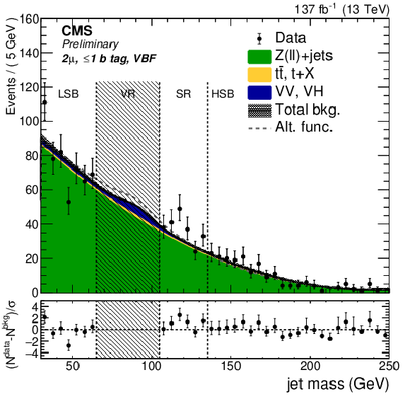
Fit to data as a function of ${m_{{j_{\mathrm{H}}}}}$ in the VBF 2 b-tag (left), $\leq $1 b-tag (right), 0 lepton (top), 2 electron (middle), and 2 muon (bottom) categories. The shaded band around the total background represents the uncertainty from the fit to data in the jet mass sidebands. The observed data are indicated by black markers. The bottom panel shows for each bin $(N^{data}-N^{bkg})/\sigma $, where $\sigma $ is the statistical uncertainty in data. |

png pdf |
Figure 3-a:
Fit to data as a function of ${m_{{j_{\mathrm{H}}}}}$ in the VBF 2 b-tag (left), $\leq $1 b-tag (right), 0 lepton (top), 2 electron (middle), and 2 muon (bottom) categories. The shaded band around the total background represents the uncertainty from the fit to data in the jet mass sidebands. The observed data are indicated by black markers. The bottom panel shows for each bin $(N^{data}-N^{bkg})/\sigma $, where $\sigma $ is the statistical uncertainty in data. |
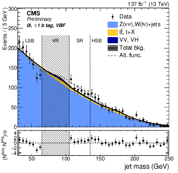
png pdf |
Figure 3-b:
Fit to data as a function of ${m_{{j_{\mathrm{H}}}}}$ in the VBF 2 b-tag (left), $\leq $1 b-tag (right), 0 lepton (top), 2 electron (middle), and 2 muon (bottom) categories. The shaded band around the total background represents the uncertainty from the fit to data in the jet mass sidebands. The observed data are indicated by black markers. The bottom panel shows for each bin $(N^{data}-N^{bkg})/\sigma $, where $\sigma $ is the statistical uncertainty in data. |
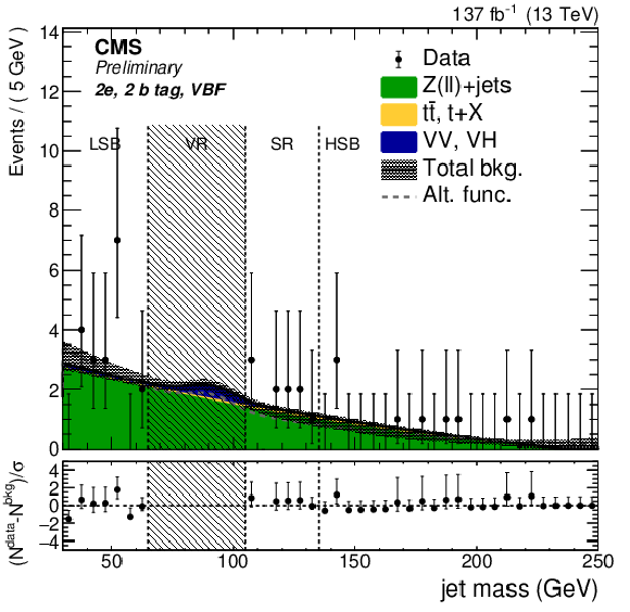
png pdf |
Figure 3-c:
Fit to data as a function of ${m_{{j_{\mathrm{H}}}}}$ in the VBF 2 b-tag (left), $\leq $1 b-tag (right), 0 lepton (top), 2 electron (middle), and 2 muon (bottom) categories. The shaded band around the total background represents the uncertainty from the fit to data in the jet mass sidebands. The observed data are indicated by black markers. The bottom panel shows for each bin $(N^{data}-N^{bkg})/\sigma $, where $\sigma $ is the statistical uncertainty in data. |
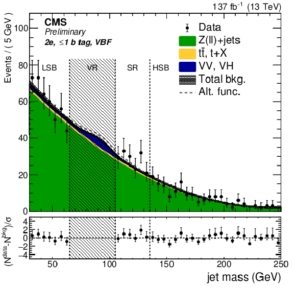
png pdf |
Figure 3-d:
Fit to data as a function of ${m_{{j_{\mathrm{H}}}}}$ in the VBF 2 b-tag (left), $\leq $1 b-tag (right), 0 lepton (top), 2 electron (middle), and 2 muon (bottom) categories. The shaded band around the total background represents the uncertainty from the fit to data in the jet mass sidebands. The observed data are indicated by black markers. The bottom panel shows for each bin $(N^{data}-N^{bkg})/\sigma $, where $\sigma $ is the statistical uncertainty in data. |

png pdf |
Figure 3-e:
Fit to data as a function of ${m_{{j_{\mathrm{H}}}}}$ in the VBF 2 b-tag (left), $\leq $1 b-tag (right), 0 lepton (top), 2 electron (middle), and 2 muon (bottom) categories. The shaded band around the total background represents the uncertainty from the fit to data in the jet mass sidebands. The observed data are indicated by black markers. The bottom panel shows for each bin $(N^{data}-N^{bkg})/\sigma $, where $\sigma $ is the statistical uncertainty in data. |
png pdf |
Figure 3-f:
Fit to data as a function of ${m_{{j_{\mathrm{H}}}}}$ in the VBF 2 b-tag (left), $\leq $1 b-tag (right), 0 lepton (top), 2 electron (middle), and 2 muon (bottom) categories. The shaded band around the total background represents the uncertainty from the fit to data in the jet mass sidebands. The observed data are indicated by black markers. The bottom panel shows for each bin $(N^{data}-N^{bkg})/\sigma $, where $\sigma $ is the statistical uncertainty in data. |
png pdf |
Figure 4:
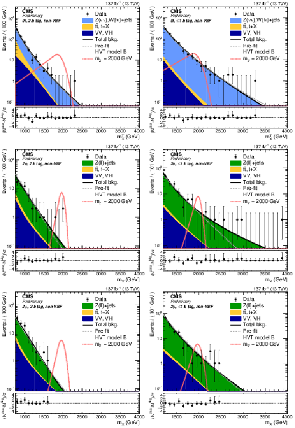
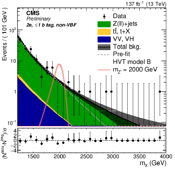
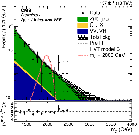
Distribution of ${m_{\mathrm{X}}}$ or ${m_{\mathrm{X}}^{\text {T}}}$ in the 2 b tag (left), $\leq $1 b tag (right), 0 lepton (top), 2 electron (middle), and 2 muon (bottom) categories. The shaded bands represent the uncertainty from the background estimation. The observed data are represented by black markers. The bottom panel shows for each bin $(N^{data}-N^{bkg})/\sigma $, where $\sigma $ is the statistical uncertainty in data. |

png pdf |
Figure 4-a:
Distribution of ${m_{\mathrm{X}}}$ or ${m_{\mathrm{X}}^{\text {T}}}$ in the 2 b tag (left), $\leq $1 b tag (right), 0 lepton (top), 2 electron (middle), and 2 muon (bottom) categories. The shaded bands represent the uncertainty from the background estimation. The observed data are represented by black markers. The bottom panel shows for each bin $(N^{data}-N^{bkg})/\sigma $, where $\sigma $ is the statistical uncertainty in data. |

png pdf |
Figure 4-b:
Distribution of ${m_{\mathrm{X}}}$ or ${m_{\mathrm{X}}^{\text {T}}}$ in the 2 b tag (left), $\leq $1 b tag (right), 0 lepton (top), 2 electron (middle), and 2 muon (bottom) categories. The shaded bands represent the uncertainty from the background estimation. The observed data are represented by black markers. The bottom panel shows for each bin $(N^{data}-N^{bkg})/\sigma $, where $\sigma $ is the statistical uncertainty in data. |

png pdf |
Figure 4-c:
Distribution of ${m_{\mathrm{X}}}$ or ${m_{\mathrm{X}}^{\text {T}}}$ in the 2 b tag (left), $\leq $1 b tag (right), 0 lepton (top), 2 electron (middle), and 2 muon (bottom) categories. The shaded bands represent the uncertainty from the background estimation. The observed data are represented by black markers. The bottom panel shows for each bin $(N^{data}-N^{bkg})/\sigma $, where $\sigma $ is the statistical uncertainty in data. |
png pdf |
Figure 4-d:
Distribution of ${m_{\mathrm{X}}}$ or ${m_{\mathrm{X}}^{\text {T}}}$ in the 2 b tag (left), $\leq $1 b tag (right), 0 lepton (top), 2 electron (middle), and 2 muon (bottom) categories. The shaded bands represent the uncertainty from the background estimation. The observed data are represented by black markers. The bottom panel shows for each bin $(N^{data}-N^{bkg})/\sigma $, where $\sigma $ is the statistical uncertainty in data. |

png pdf |
Figure 4-e:
Distribution of ${m_{\mathrm{X}}}$ or ${m_{\mathrm{X}}^{\text {T}}}$ in the 2 b tag (left), $\leq $1 b tag (right), 0 lepton (top), 2 electron (middle), and 2 muon (bottom) categories. The shaded bands represent the uncertainty from the background estimation. The observed data are represented by black markers. The bottom panel shows for each bin $(N^{data}-N^{bkg})/\sigma $, where $\sigma $ is the statistical uncertainty in data. |
png pdf |
Figure 4-f:
Distribution of ${m_{\mathrm{X}}}$ or ${m_{\mathrm{X}}^{\text {T}}}$ in the 2 b tag (left), $\leq $1 b tag (right), 0 lepton (top), 2 electron (middle), and 2 muon (bottom) categories. The shaded bands represent the uncertainty from the background estimation. The observed data are represented by black markers. The bottom panel shows for each bin $(N^{data}-N^{bkg})/\sigma $, where $\sigma $ is the statistical uncertainty in data. |
png pdf |
Figure 5:
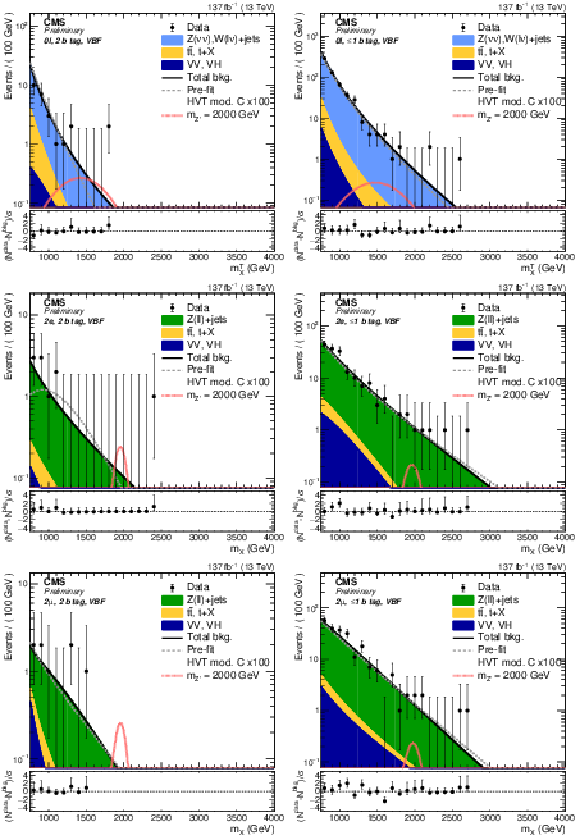
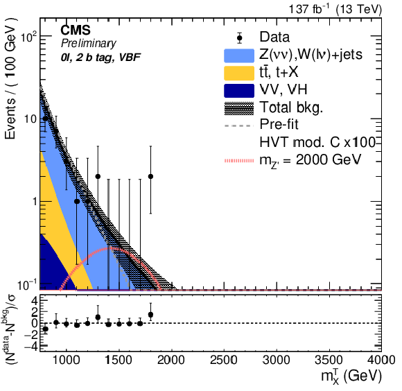
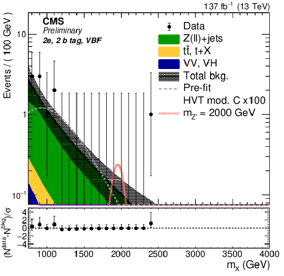
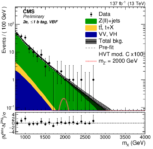
Distribution of ${m_{\mathrm{X}}}$ or ${m_{\mathrm{X}}^{\text {T}}}$ in the VBF 2 b tag (left), $\leq $1 b tag (right), 0 lepton (top), 2 electron (middle), and 2 muon (bottom) categories. The shaded bands represent the uncertainty from the background estimation. The observed data are represented by black markers. The bottom panel shows for each bin $(N^{data}-N^{bkg})/\sigma $, where $\sigma $ is the statistical uncertainty in data. |
png pdf |
Figure 5-a:
Distribution of ${m_{\mathrm{X}}}$ or ${m_{\mathrm{X}}^{\text {T}}}$ in the VBF 2 b tag (left), $\leq $1 b tag (right), 0 lepton (top), 2 electron (middle), and 2 muon (bottom) categories. The shaded bands represent the uncertainty from the background estimation. The observed data are represented by black markers. The bottom panel shows for each bin $(N^{data}-N^{bkg})/\sigma $, where $\sigma $ is the statistical uncertainty in data. |

png pdf |
Figure 5-b:
Distribution of ${m_{\mathrm{X}}}$ or ${m_{\mathrm{X}}^{\text {T}}}$ in the VBF 2 b tag (left), $\leq $1 b tag (right), 0 lepton (top), 2 electron (middle), and 2 muon (bottom) categories. The shaded bands represent the uncertainty from the background estimation. The observed data are represented by black markers. The bottom panel shows for each bin $(N^{data}-N^{bkg})/\sigma $, where $\sigma $ is the statistical uncertainty in data. |
png pdf |
Figure 5-c:
Distribution of ${m_{\mathrm{X}}}$ or ${m_{\mathrm{X}}^{\text {T}}}$ in the VBF 2 b tag (left), $\leq $1 b tag (right), 0 lepton (top), 2 electron (middle), and 2 muon (bottom) categories. The shaded bands represent the uncertainty from the background estimation. The observed data are represented by black markers. The bottom panel shows for each bin $(N^{data}-N^{bkg})/\sigma $, where $\sigma $ is the statistical uncertainty in data. |
png pdf |
Figure 5-d:
Distribution of ${m_{\mathrm{X}}}$ or ${m_{\mathrm{X}}^{\text {T}}}$ in the VBF 2 b tag (left), $\leq $1 b tag (right), 0 lepton (top), 2 electron (middle), and 2 muon (bottom) categories. The shaded bands represent the uncertainty from the background estimation. The observed data are represented by black markers. The bottom panel shows for each bin $(N^{data}-N^{bkg})/\sigma $, where $\sigma $ is the statistical uncertainty in data. |

png pdf |
Figure 5-e:
Distribution of ${m_{\mathrm{X}}}$ or ${m_{\mathrm{X}}^{\text {T}}}$ in the VBF 2 b tag (left), $\leq $1 b tag (right), 0 lepton (top), 2 electron (middle), and 2 muon (bottom) categories. The shaded bands represent the uncertainty from the background estimation. The observed data are represented by black markers. The bottom panel shows for each bin $(N^{data}-N^{bkg})/\sigma $, where $\sigma $ is the statistical uncertainty in data. |
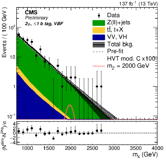
png pdf |
Figure 5-f:
Distribution of ${m_{\mathrm{X}}}$ or ${m_{\mathrm{X}}^{\text {T}}}$ in the VBF 2 b tag (left), $\leq $1 b tag (right), 0 lepton (top), 2 electron (middle), and 2 muon (bottom) categories. The shaded bands represent the uncertainty from the background estimation. The observed data are represented by black markers. The bottom panel shows for each bin $(N^{data}-N^{bkg})/\sigma $, where $\sigma $ is the statistical uncertainty in data. |

png pdf |
Figure 6:
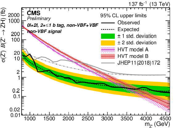
Observed and expected (with $ \pm $1(2)$\sigma$ band) 95% C.L. upper limit on $\sigma \times {\mathcal {B}}({\mathrm{Z'} \to \mathrm{Z} \mathrm{H}})$ categories combined with the non-VBF signal (left) and VBF signal (right), including all statistical and systematics uncertainties. |
png pdf |
Figure 6-a:
Observed and expected (with $ \pm $1(2)$\sigma$ band) 95% C.L. upper limit on $\sigma \times {\mathcal {B}}({\mathrm{Z'} \to \mathrm{Z} \mathrm{H}})$ categories combined with the non-VBF signal (left) and VBF signal (right), including all statistical and systematics uncertainties. |

png pdf |
Figure 6-b:
Observed and expected (with $ \pm $1(2)$\sigma$ band) 95% C.L. upper limit on $\sigma \times {\mathcal {B}}({\mathrm{Z'} \to \mathrm{Z} \mathrm{H}})$ categories combined with the non-VBF signal (left) and VBF signal (right), including all statistical and systematics uncertainties. |

png pdf |
Figure 7:
Observed exclusion limit in the space of the HVT model parameters [$ {g_\text {V}} {c_\text {H}} $,$g^2 {c_\text {F}} / {g_\text {V}} $], described in the text, for three different mass hypotheses of 1.5, 2.0 and 3.0 TeV for the non-VBF signal. The benchmark scenarios corresponding to HVT models A and B are represented by a purple cross and a red point. The region of parameters space where the natural resonance width ($\Gamma _{Z'}$) is larger than the typical experimental resolution of 4%, for which the narrow-width approximation is not valid, is shaded in grey. |
| Tables | |
png pdf |
Table 1:
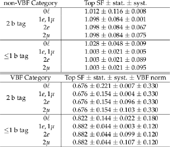
Scale factors (SF) derived for the normalization of the ${\mathrm{t} {}\mathrm{\bar{t}}}$ and single top quark backgrounds for different event categories. Uncertainties due to the limited size of the event samples (stat) and systematic effects (syst) are reported as well. |

png pdf |
Table 2:
The three background components and their relative uncertainties are reported. The V+jets background uncertainty originates from the variation of the parameters within the fit uncertainties (fit) and the difference between the nominal and alternative function choice for the fit to ${m_{{j_{\mathrm{H}}}}}$ (alt). The ${\mathrm{t} {}\mathrm{\bar{t}}}$ and single top quark uncertainties arise from the ${m_{{j_{\mathrm{H}}}}}$ modeling, the statistical component of the top quark scale factor uncertainties, and the extrapolation uncertainty from the control region to the signal range. The ${{{\mathrm {V}}} {{\mathrm {V}}}}$ normalization uncertainties come from the ${m_{{j_{\mathrm{H}}}}}$ modeling, and the uncertainties affecting the normalization. The sum of the backgrounds is affected by the propagation of these uncertainties. |
png pdf |
Table 3:
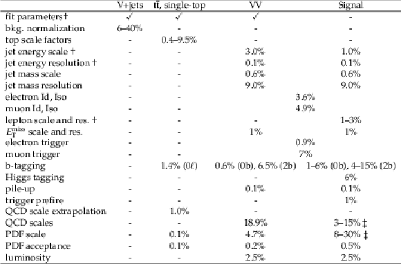
Summary of systematic uncertainties for the background and signal samples. The entries labelled with $\dagger $ are also propagated to the shapes of the distributions. Uncertainties marked with $\ddagger $ impact the signal cross section. Uncertainties in the same line are treated as correlated. All uncertainties except luminosity are correlated between years. |
| Summary |
| A search for a heavy resonance with mass between 800 and 5000 GeV, decaying into a Z boson and a Higgs boson, has been described. The data sample was collected by the CMS experiment from 2016-2018 at $\sqrt{s} = $ 13 TeV and corresponds to integrated luminosity of 137.2 fb$^{-1}$. The final states explored include the leptonic decay modes of the Z boson, in events with zero and two charged electrons or muons. Higgs bosons are reconstructed from their decays to hadrons. For models with a narrow spin-1 resonance, a Z' with mass below 3.5 and 3.7 TeV are excluded at 95% confidence level in models where the heavy vector bosons couple predominantly to fermions and bosons, respectively. If the heavy resonances couple exclusively to SM bosons, a Z' cross section smaller than 0.3-23 fb is excluded, depending on the Z' mass. These are the most stringent limits placed on the HVT Z' model to date and the first search including the full Run 2 LHC data. |
| References | ||||
| 1 | ATLAS Collaboration | Observation of a new particle in the search for the Standard Model Higgs boson with the ATLAS detector at the LHC | PLB 716 (2012) 1 | 1207.7214 |
| 2 | CMS Collaboration | Observation of a new boson at a mass of 125 GeV with the CMS experiment at the LHC | PLB 716 (2012) 30 | CMS-HIG-12-028 1207.7235 |
| 3 | CMS Collaboration | Observation of a new boson with mass near 125 GeV in pp collisions at $ \sqrt{s} = $ 7 and 8 TeV | JHEP 06 (2013) 081 | CMS-HIG-12-036 1303.4571 |
| 4 | CMS Collaboration | Precise determination of the mass of the Higgs boson and tests of compatibility of its couplings with the standard model predictions using proton collisions at 7 and 8 TeV | EPJC 75 (2015) 212 | CMS-HIG-14-009 1412.8662 |
| 5 | ATLAS Collaboration | Measurement of the Higgs boson mass from the $ H\rightarrow{}\gamma{}\gamma{} $ and $ H\rightarrow{}Z{Z}^{*}\rightarrow{}4\ell{} $ channels in $ pp $ collisions at center-of-mass energies of 7 and 8~TeV with the ATLAS detector | PRD 90 (2014) 052004 | 1406.3827 |
| 6 | ATLAS Collaboration | Evidence for the spin-0 nature of the Higgs boson using ATLAS data | PLB 726 (2013) 120 | 1307.1432 |
| 7 | CMS and ATLAS Collaborations | Combined Measurement of the Higgs Boson Mass in $ pp $ Collisions at $ \sqrt{s}= $ 7 and 8 TeV with the ATLAS and CMS Experiments | PRL 114 (2015) 191803 | 1503.07589 |
| 8 | T. Han, H. E. Logan, B. McElrath, and L.-T. Wang | Phenomenology of the little Higgs model | PRD 67 (2003) 095004 | hep-ph/0301040 |
| 9 | M. Schmaltz and D. Tucker-Smith | Little higgs theories | Annual Review of Nuclear and Particle Science 55 (2005) 229 | |
| 10 | M. Perelstein | Little higgs models and their phenomenology | Progress in Particle and Nuclear Physics 58 (2007) 247 | hep-ph/0512128 |
| 11 | R. Contino, D. Pappadopulo, D. Marzocca, and R. Rattazzi | On the effect of resonances in composite higgs phenomenology | Journal of High Energy Physics 2011 (2011) 1 | 1109.1570 |
| 12 | D. Marzocca, M. Serone, and J. Shu | General composite higgs models | Journal of High Energy Physics 2012 (2012) 1 | 1205.0770 |
| 13 | B. Bellazzini, C. Csaki, and J. Serra | Composite Higgses | EPJC 74 (2014) 2766 | 1401.2457 |
| 14 | CMS Collaboration | Search for heavy resonances decaying into a vector boson and a higgs boson in final states with charged leptons, neutrinos, and b quarks at $ \sqrt{s} = $ 13 TeV | JHEP 11 (2018) 172 | CMS-B2G-17-004 1807.02826 |
| 15 | ATLAS Collaboration | Search for heavy resonances decaying into a W or Z boson and a Higgs boson in final states with leptons and $ b $-jets in 36 fb$ ^{-1} $ of $ \sqrt{s} = $ 13 TeV pp collisions with the ATLAS detector | JHEP 03 (2018) 174 | 1712.06518 |
| 16 | CMS Collaboration | Combination of CMS searches for heavy resonances decaying to pairs of bosons or leptons | PLB 798 (2019) 134952 | CMS-B2G-18-006 1906.00057 |
| 17 | ATLAS Collaboration | Combination of searches for heavy resonances decaying into bosonic and leptonic final states using 36 fb$ ^{-1} $ of proton-proton collision data at $ \sqrt{s} = $ 13 TeV with the ATLAS detector | PRD 98 (2018) 052008 | 1808.02380 |
| 18 | T. Dorigo | Hadron collider searches for diboson resonances | Progress in Particle and Nuclear Physics 100 (2018) 211 | 1802.00354 |
| 19 | D. Pappadopulo, A. Thamm, R. Torre, and A. Wulzer | Heavy vector triplets: bridging theory and data | Journal of High Energy Physics 2014 (2014) 1 | 1402.4431 |
| 20 | V. D. Barger, W.-Y. Keung, and E. Ma | A Gauge Model With Light W and Z Bosons | PRD 22 (1980) 727 | |
| 21 | CMS Collaboration | The CMS experiment at the CERN LHC | JINST 3 (2008) S08004 | CMS-00-001 |
| 22 | J. Alwall et al. | The automated computation of tree-level and next-to-leading order differential cross sections, and their matching to parton shower simulations | JHEP 07 (2014) 079 | 1405.0301 |
| 23 | J. Alwall et al. | Comparative study of various algorithms for the merging of parton showers and matrix elements in hadronic collisions | EPJC 53 (2008) 473 | 0706.2569 |
| 24 | J. M. Lindert et al. | Precise predictions for v+jets dark matter backgrounds | EPJC 77 (2017) 829 | 1705.04664 |
| 25 | P. Nason | A new method for combining NLO QCD with shower Monte Carlo algorithms | JHEP 11 (2004) 040 | hep-ph/0409146 |
| 26 | S. Frixione, P. Nason, and C. Oleari | Matching NLO QCD computations with Parton Shower simulations: the POWHEG method | JHEP 11 (2007) 070 | 0709.2092 |
| 27 | S. Alioli, P. Nason, C. Oleari, and E. Re | A general framework for implementing NLO calculations in shower Monte Carlo programs: the POWHEG BOX | JHEP 06 (2010) 043 | 1002.2581 |
| 28 | M. Czakon and A. Mitov | Top++: A program for the calculation of the top-pair cross-section at hadron colliders | CPC 185 (2014) 2930 | 1112.5675 |
| 29 | T. Sjostrand, S. Mrenna, and P. Skands | A brief introduction to PYTHIA 8.1 | CPC 178 (2008) 852 | 0710.3820 |
| 30 | T. Sjostrand, S. Mrenna, and P. Skands | PYTHIA 6.4 physics and manual | JHEP 05 (2006) 026 | hep-ph/0603175 |
| 31 | P. Skands, S. Carrazza, and J. Rojo | Tuning PYTHIA 8.1: the Monash 2013 Tune | EPJC 74 (2014) 3024 | 1404.5630 |
| 32 | CMS Collaboration | Event generator tunes obtained from underlying event and multiparton scattering measurements | EPJC 76 (2016) 155 | CMS-GEN-14-001 1512.00815 |
| 33 | CMS Collaboration | Extraction and validation of a new set of cms pythia8 tunes from underlying-event measurements | EPJC 80 (2020) 4 | CMS-GEN-17-001 1903.12179 |
| 34 | CMS Collaboration | Investigations of the impact of the parton shower tuning in Pythia 8 in the modelling of $ \mathrm{t\overline{t}} $ at $ \sqrt{s}= $ 8 and 13 TeV | CMS-PAS-TOP-16-021 | CMS-PAS-TOP-16-021 |
| 35 | S. Agostinelli et al. | Geant4--a simulation toolkit | Nuclear Instruments and Methods in Physics Research Section A: Accelerators, Spectrometers, Detectors and Associated Equipment 506 (2003) 250 | |
| 36 | CMS Collaboration | Particle-flow event reconstruction in CMS and performance for jets, taus, and $ E_{\mathrm{T}}^{\text{miss}} $ | CDS | |
| 37 | CMS Collaboration | Commissioning of the particle-flow event reconstruction with the first LHC collisions recorded in the CMS detector | CDS | |
| 38 | M. Cacciari, G. P. Salam, and G. Soyez | The anti-$ k_t $ jet clustering algorithm | JHEP 04 (2008) 063 | 0802.1189 |
| 39 | M. Cacciari, G. P. Salam, and G. Soyez | FastJet user manual | EPJC 72 (2012) 1896 | 1111.6097 |
| 40 | M. Cacciari, G. P. Salam, and G. Soyez | The catchment area of jets | JHEP 04 (2008) 005 | 0802.1188 |
| 41 | CMS Collaboration | Pileup Removal Algorithms | CMS-PAS-JME-14-001 | CMS-PAS-JME-14-001 |
| 42 | D. Bertolini, P. Harris, M. Low, and N. Tran | Pileup per particle identification | Journal of High Energy Physics 2014 (2014) 59 | 1407.6013 |
| 43 | CMS Collaboration | Jet energy scale and resolution in the CMS experiment in pp collisions at 8 TeV | JINST 12 (2017) P02014 | CMS-JME-13-004 1607.03663 |
| 44 | CMS Collaboration | Performance of missing transverse momentum in pp collisions at $ \sqrt{s} = $ 13 TeV using the CMS detector | CMS-PAS-JME-17-001 | CMS-PAS-JME-17-001 |
| 45 | M. Dasgupta, A. Fregoso, S. Marzani, and G. P. Salam | Towards an understanding of jet substructure | JHEP 09 (2013) 029 | 1307.0007 |
| 46 | J. M. Butterworth, A. R. Davison, M. Rubin, and G. P. Salam | Jet substructure as a new Higgs search channel at the LHC | PRL 100 (2008) 242001 | 0802.2470 |
| 47 | A. J. Larkoski, S. Marzani, G. Soyez, and J. Thaler | Soft Drop | JHEP 05 (2014) 146 | 1402.2657 |
| 48 | CMS Collaboration | Identification techniques for highly boosted W bosons that decay into hadrons | JHEP 12 (2014) 017 | CMS-JME-13-006 1410.4227 |
| 49 | D. Guest et al. | Jet flavor classification in high-energy physics with deep neural networks | PRD 94 (2016) 112002 | 1607.08633 |
| 50 | CMS Collaboration | Performance of electron reconstruction and selection with the cms detector in proton-proton collisions at $ \sqrt{s} = $ 8 TeV | JINST 10 (2015) P06005 | CMS-EGM-13-001 1502.02701 |
| 51 | CMS Collaboration | Performance of reconstruction and identification of $ \tau $ leptons decaying to hadrons and $ \nu\tau $ in pp collisions at $ \sqrt{s} = $ 13 TeV | JINST 13 (2018) P10005 | CMS-TAU-16-003 1809.02816 |
| 52 | CMS Collaboration | Search for a heavy resonance decaying into a Z boson and a vector boson in the $ \nu\overline\nu\mathrm{q}\overline{\mathrm{q}} $ final state | Journal of High Energy Physics 2018 (2018) | CMS-B2G-17-005 1803.03838 |
| 53 | CMS Collaboration | Search for a heavy resonance decaying into a Z boson and a Z or W boson in 2$\ell $2q final states at $ \sqrt{s}= $ 13 TeV | Journal of High Energy Physics 2018 (2018) | CMS-B2G-17-013 1803.10093 |
| 54 | CMS Collaboration | CMS Luminosity Measurement for the 2016 Data Taking Period | CMS-PAS-LUM-15-001 | CMS-PAS-LUM-15-001 |
| 55 | CMS Collaboration | CMS luminosity measurement for the 2017 data-taking period at $ \sqrt{s}= $ 13 TeV | CMS-PAS-LUM-17-004 | CMS-PAS-LUM-17-004 |
| 56 | CMS Collaboration | CMS luminosity measurement for the 2018 data-taking period at $ \sqrt{s}= $ 13 TeV | CMS-PAS-LUM-18-002 | CMS-PAS-LUM-18-002 |

|
Compact Muon Solenoid LHC, CERN |

|

|

|

|

|

|