

Compact Muon Solenoid
LHC, CERN
| CMS-SMP-19-005 ; CERN-EP-2025-242 | ||
| Measurements of electroweak production of a photon in association with two jets in proton-proton collisions at $ \sqrt{s}= $ 13 TeV | ||
| CMS Collaboration | ||
| 29 November 2025 | ||
| Accepted for publication in J. High Energy Phys. | ||
| Abstract: The first observation of electroweak production of a photon in association with two forward jets in proton-proton collisions is presented. The measurement uses data recorded by the CMS experiment at the LHC during 2016-2018 at a center-of-mass energy of 13 TeV, corresponding to an integrated luminosity of 138 fb$ ^{-1} $. The analysis is performed in a region enriched in photon production via vector boson fusion, with a requirement on the transverse momentum of the photon to exceed 200 GeV. The cross section is measured to be 202$ ^{+36}_{-32} $ fb, at a significance with respect to the null hypothesis that exceeds five standard deviations. This is in agreement with the standard model prediction of 177$ ^{+13}_{-12} $ fb. Differential cross sections are measured as a function of various observables. Limits are set on dimension-6 effective field theory operators that contribute to the WW$ \gamma $ interaction. The observed 95% confidence intervals for the corresponding Warsaw basis Wilson coefficients $ c_{\mathrm{W}} $ and $ c_{\mathrm{H}\mathrm{W}\mathrm{B}} $ are [$-$0.11, 0.16] and [$-$1.6, 1.5], respectively. | ||
| Links: e-print arXiv:2512.00502 [hep-ex] (PDF) ; CDS record ; inSPIRE record ; HepData record ; CADI line (restricted) ; | ||
| Figures | |
png pdf |
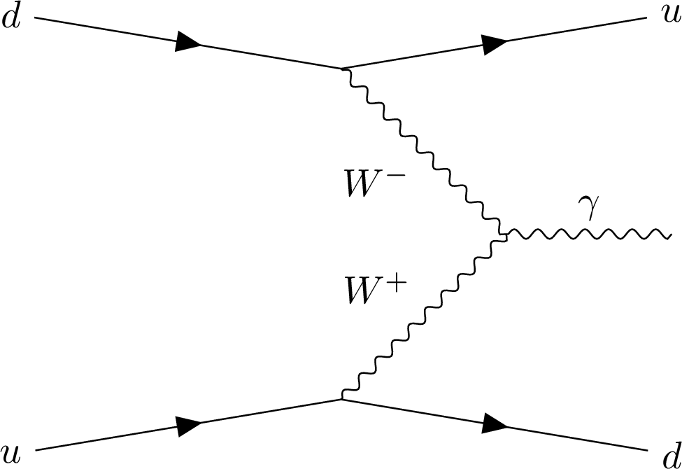
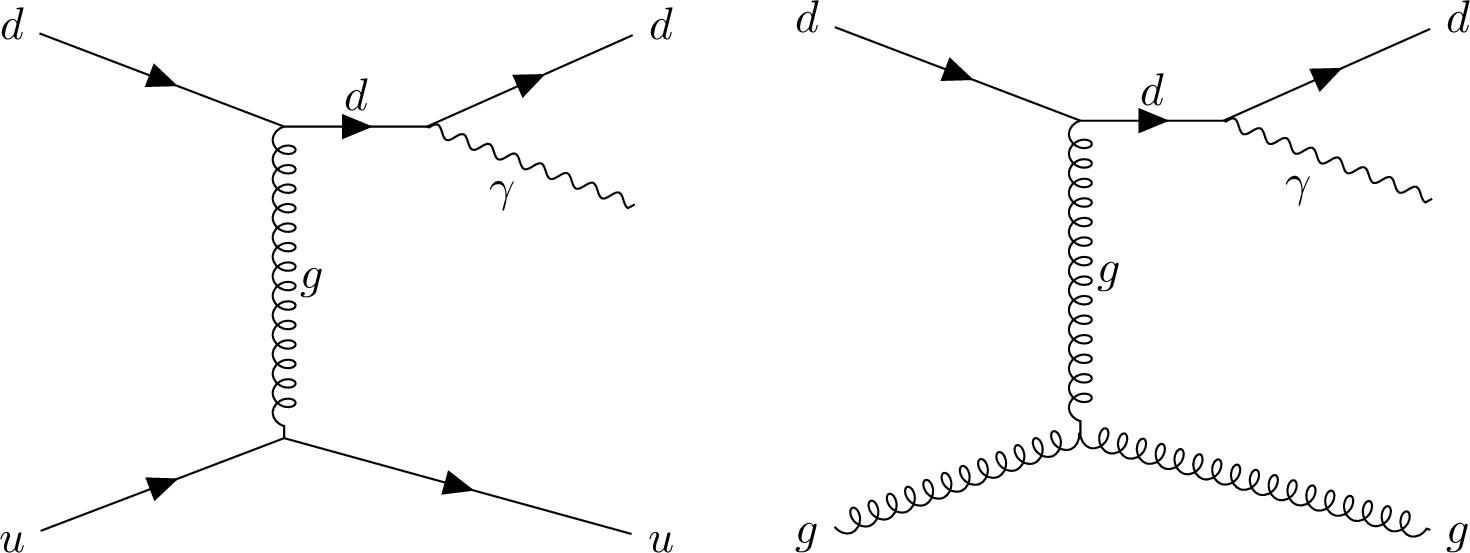
Figure 1:
Representative Feynman diagram for EW $ \gamma $\text{jj} production with a photon produced via vector boson fusion. |
png pdf |
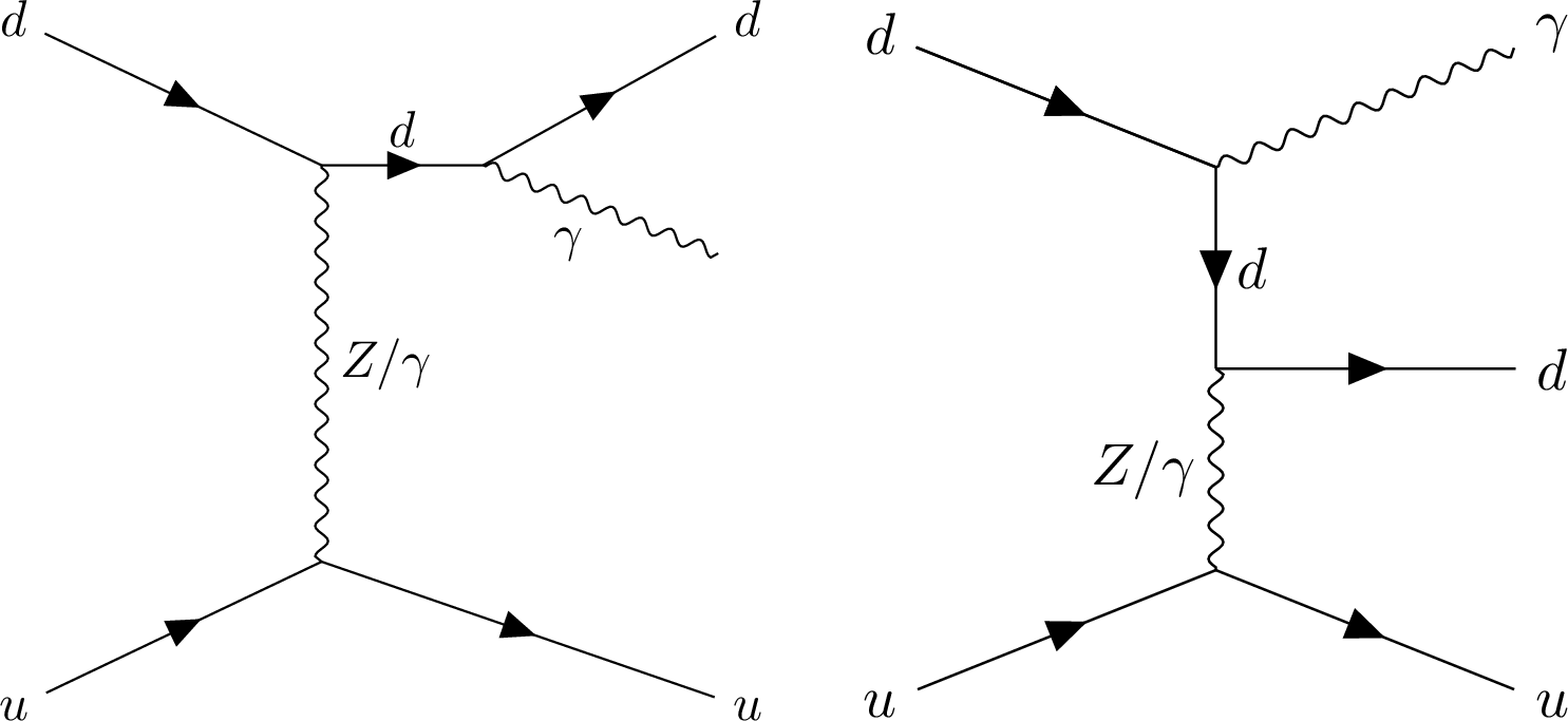
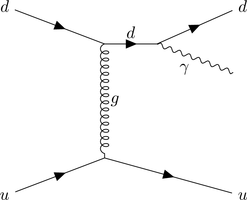
Figure 2:
Representative Feynman diagrams for photons produced in FSR (left) and ISR (right). |
png pdf |
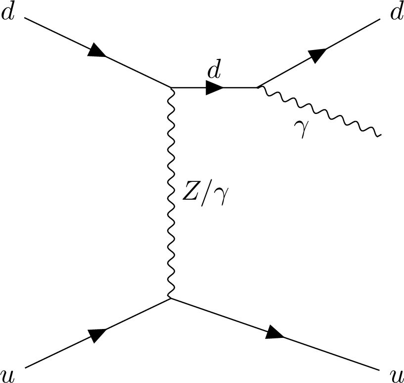
Figure 2-a:
Representative Feynman diagrams for photons produced in FSR (left) and ISR (right). |
png pdf |
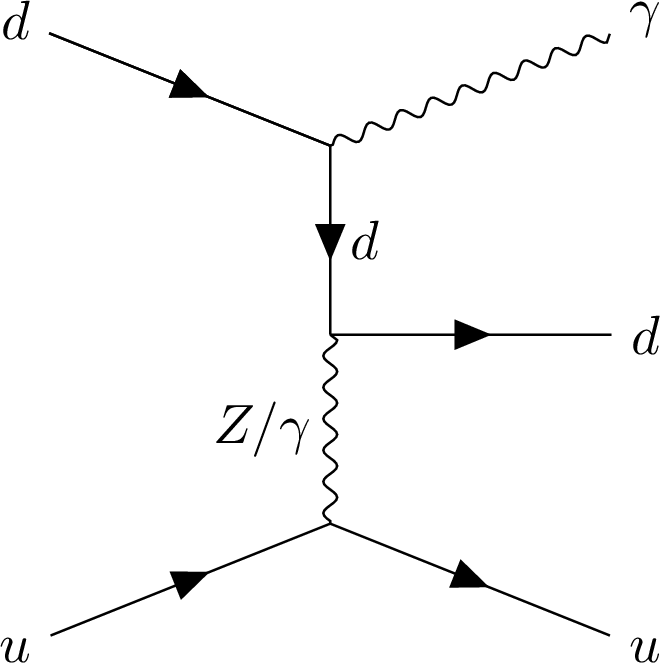
Figure 2-b:
Representative Feynman diagrams for photons produced in FSR (left) and ISR (right). |
png pdf |
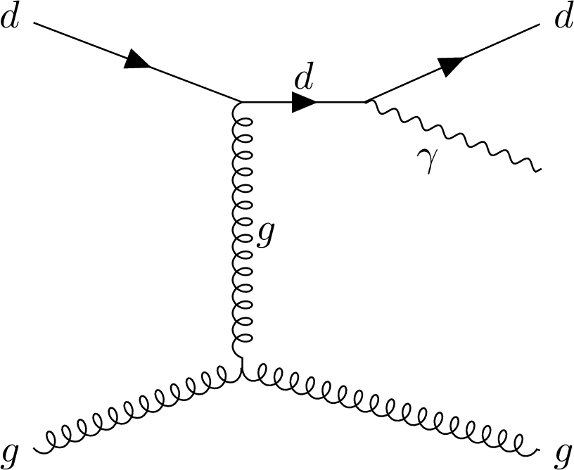
Figure 3:
Representative Feynman diagrams for QCD-induced production of a photon and two jets. |
png pdf |
Figure 3-a:
Representative Feynman diagrams for QCD-induced production of a photon and two jets. |
png pdf |
Figure 3-b:
Representative Feynman diagrams for QCD-induced production of a photon and two jets. |
png pdf |
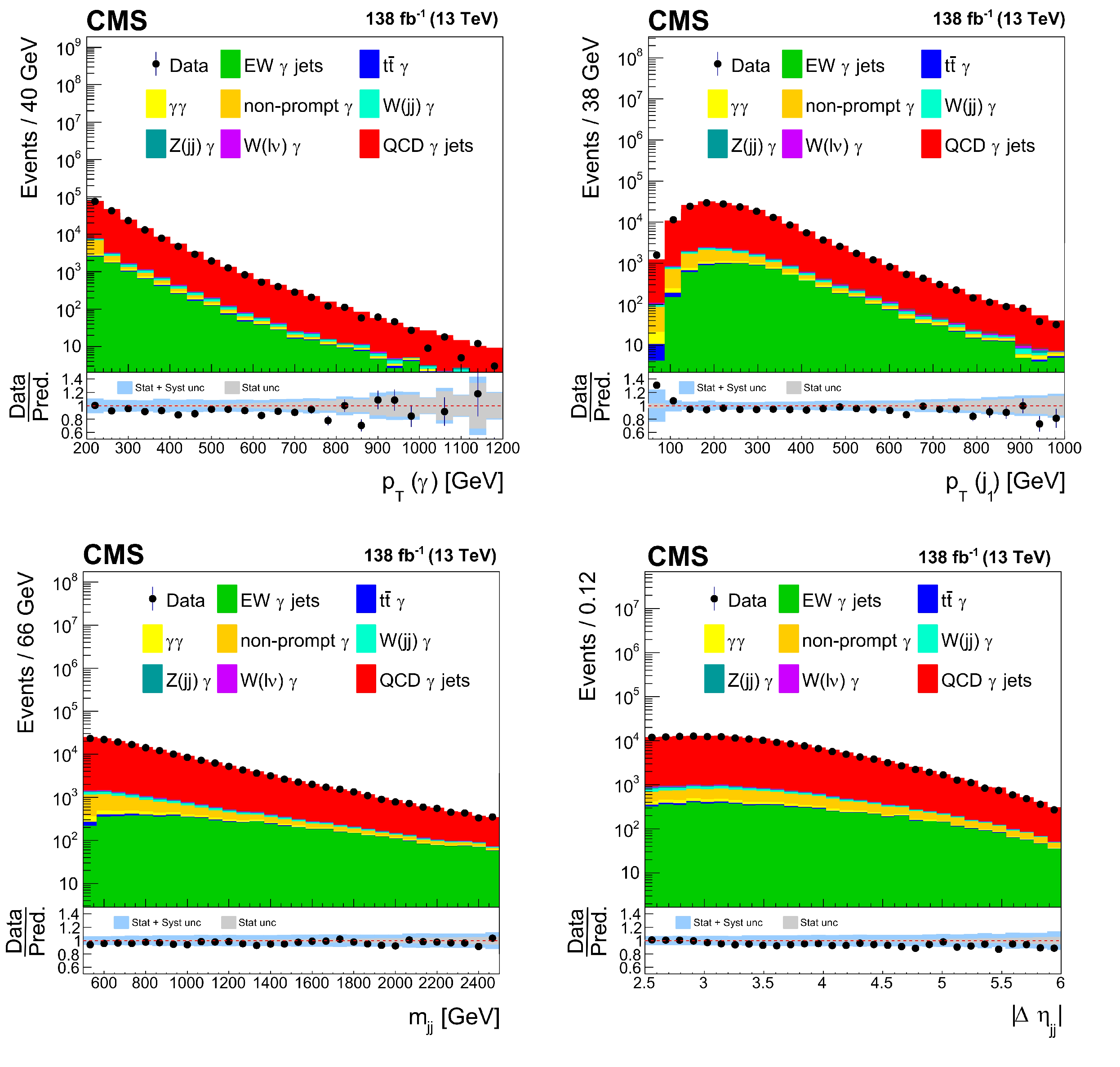
Figure 4:
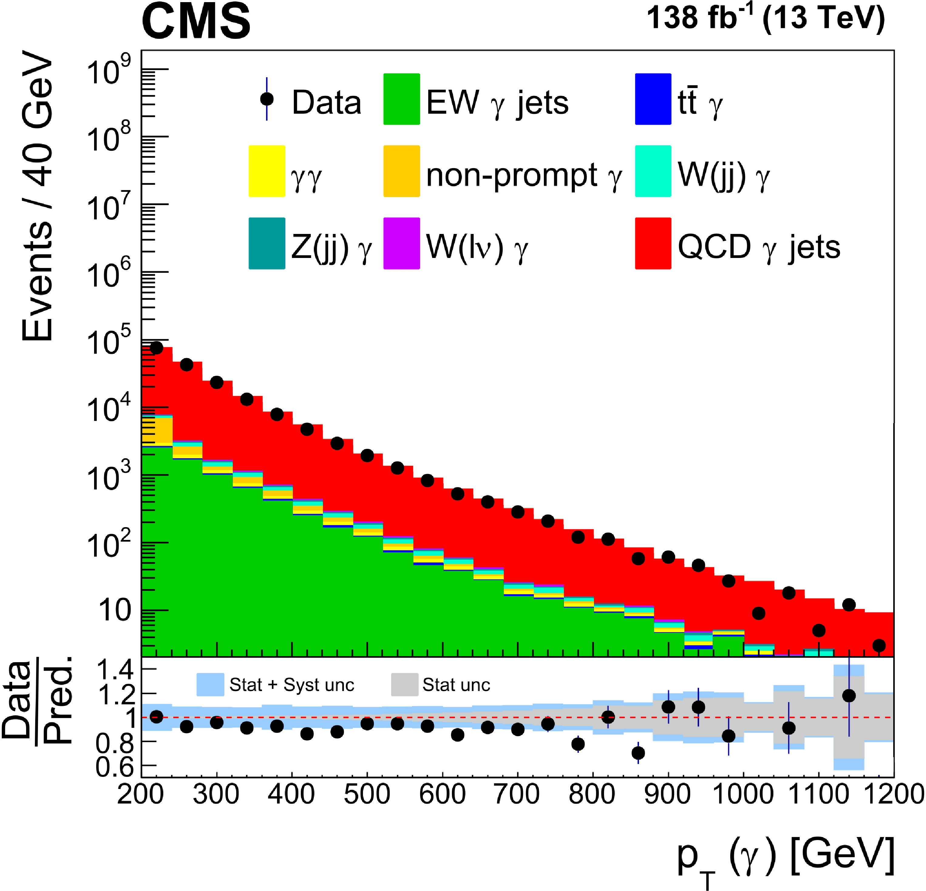
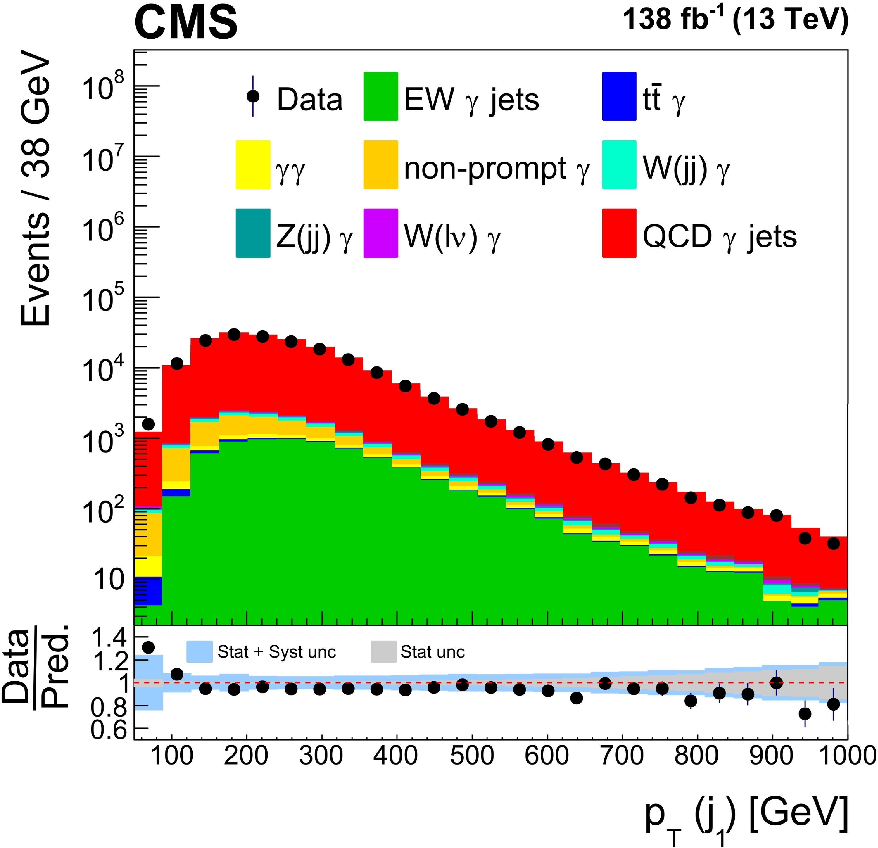
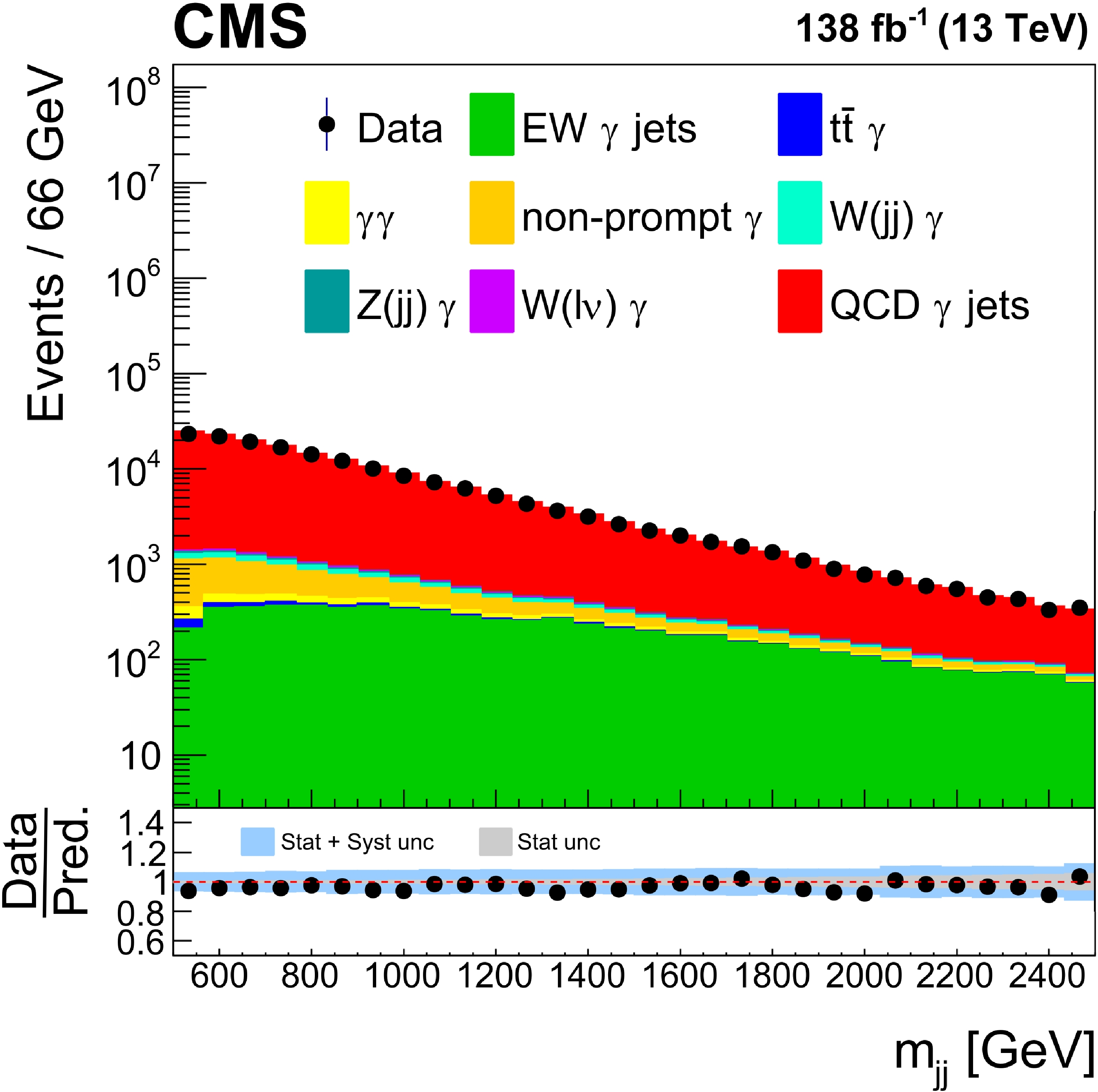
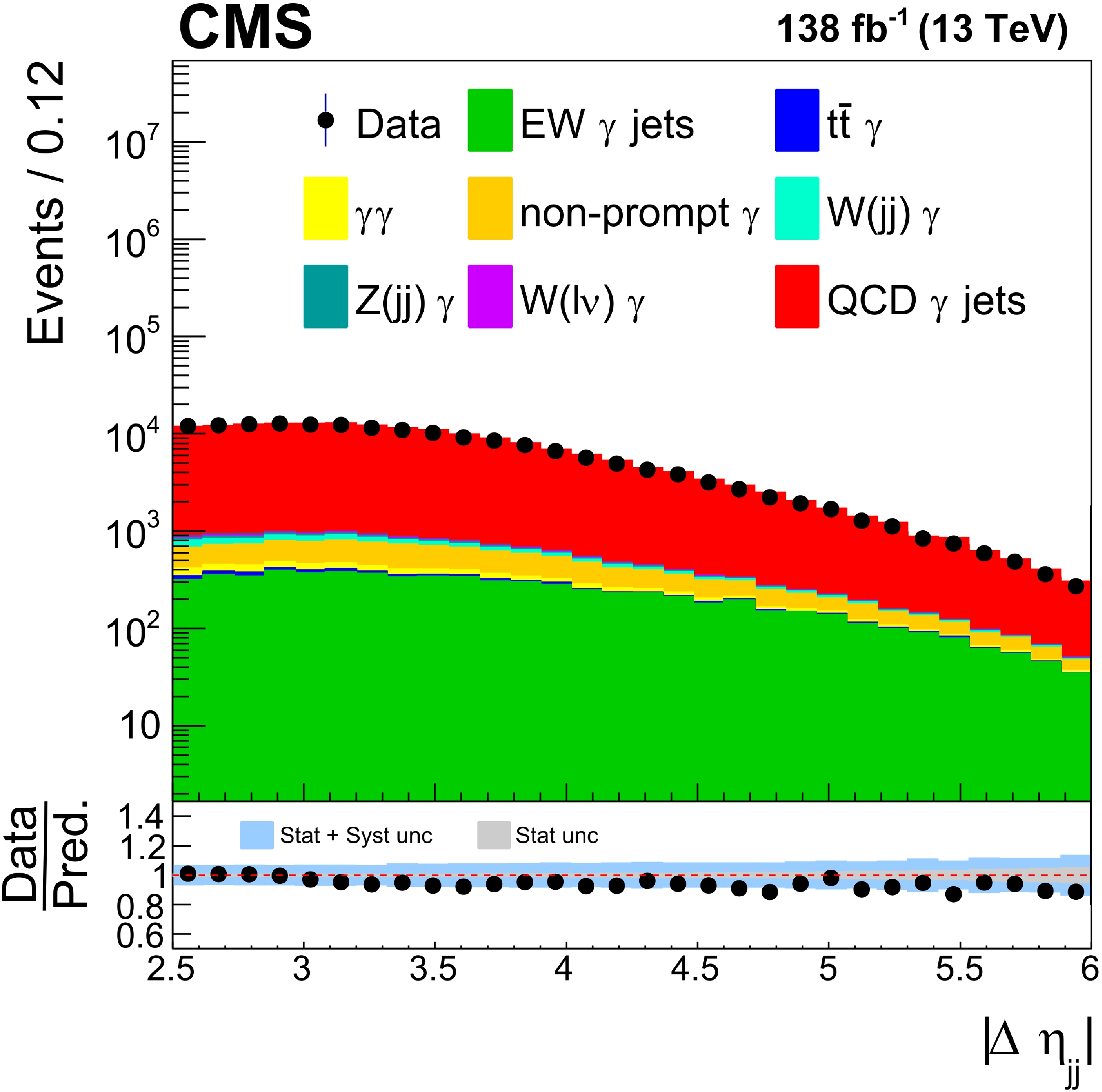
Distribution of (upper left) photon $ p_{\mathrm{T}} $, (upper right) leading jet $ p_{\mathrm{T}} $, (lower left) $ m_\mathrm{jj} $, and (lower right) $ |\Delta\eta_{\text{jj}}| $ in data and simulated processes, except the contribution of nonprompt photons that is estimated from data as discussed in Section 5. Simulted samples are normalized to their theoretical cross sections. The black points with error bars represent the data and their statistical uncertainties. The last bin includes the overflow events. The lower panels shows the ratio of the data to the expectation with the inner (outer) band representing the statistical (total) uncertainty in the combined signal and background expectations. |
png pdf |
Figure 4-a:
Distribution of (upper left) photon $ p_{\mathrm{T}} $, (upper right) leading jet $ p_{\mathrm{T}} $, (lower left) $ m_\mathrm{jj} $, and (lower right) $ |\Delta\eta_{\text{jj}}| $ in data and simulated processes, except the contribution of nonprompt photons that is estimated from data as discussed in Section 5. Simulted samples are normalized to their theoretical cross sections. The black points with error bars represent the data and their statistical uncertainties. The last bin includes the overflow events. The lower panels shows the ratio of the data to the expectation with the inner (outer) band representing the statistical (total) uncertainty in the combined signal and background expectations. |
png pdf |
Figure 4-b:
Distribution of (upper left) photon $ p_{\mathrm{T}} $, (upper right) leading jet $ p_{\mathrm{T}} $, (lower left) $ m_\mathrm{jj} $, and (lower right) $ |\Delta\eta_{\text{jj}}| $ in data and simulated processes, except the contribution of nonprompt photons that is estimated from data as discussed in Section 5. Simulted samples are normalized to their theoretical cross sections. The black points with error bars represent the data and their statistical uncertainties. The last bin includes the overflow events. The lower panels shows the ratio of the data to the expectation with the inner (outer) band representing the statistical (total) uncertainty in the combined signal and background expectations. |
png pdf |
Figure 4-c:
Distribution of (upper left) photon $ p_{\mathrm{T}} $, (upper right) leading jet $ p_{\mathrm{T}} $, (lower left) $ m_\mathrm{jj} $, and (lower right) $ |\Delta\eta_{\text{jj}}| $ in data and simulated processes, except the contribution of nonprompt photons that is estimated from data as discussed in Section 5. Simulted samples are normalized to their theoretical cross sections. The black points with error bars represent the data and their statistical uncertainties. The last bin includes the overflow events. The lower panels shows the ratio of the data to the expectation with the inner (outer) band representing the statistical (total) uncertainty in the combined signal and background expectations. |
png pdf |
Figure 4-d:
Distribution of (upper left) photon $ p_{\mathrm{T}} $, (upper right) leading jet $ p_{\mathrm{T}} $, (lower left) $ m_\mathrm{jj} $, and (lower right) $ |\Delta\eta_{\text{jj}}| $ in data and simulated processes, except the contribution of nonprompt photons that is estimated from data as discussed in Section 5. Simulted samples are normalized to their theoretical cross sections. The black points with error bars represent the data and their statistical uncertainties. The last bin includes the overflow events. The lower panels shows the ratio of the data to the expectation with the inner (outer) band representing the statistical (total) uncertainty in the combined signal and background expectations. |
png pdf |
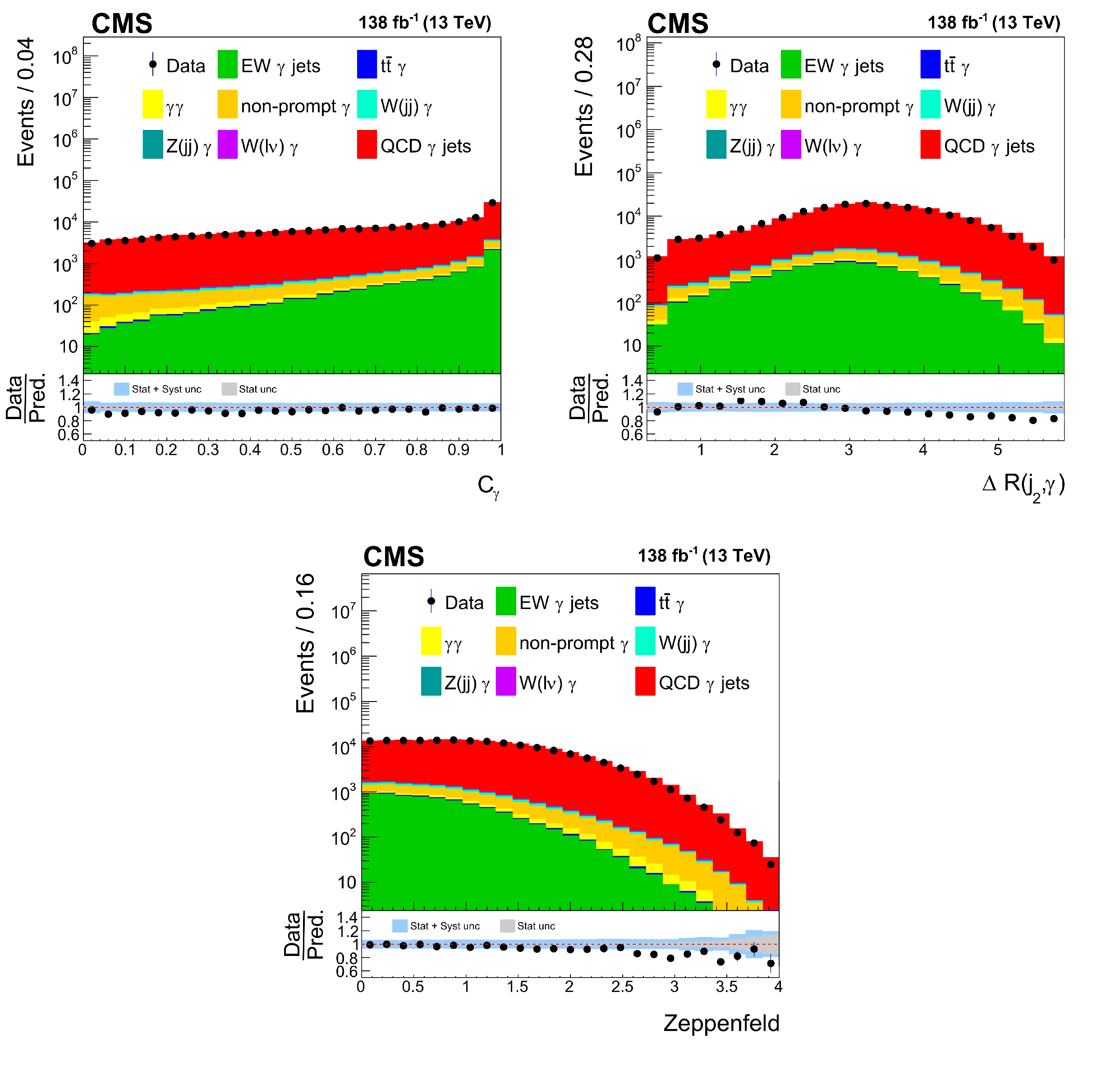
Figure 5:
Distribution of (upper left) $ C_{\gamma} $, (upper right) $ \Delta R(j_2,\gamma) $, and (lower) the Zeppenfeld variable in data and simulated processes, except the contribution of nonprompt photons that is estimated from data as discussed in Section 5. Simulted samples are normalized to their theoretical cross sections. The black points with error bars represent the data and their statistical uncertainties. The last bin includes the overflow events. The lower panels shows the ratio of the data to the expectation with the inner (outer) band representing the statistical (total) uncertainty in the combined signal and background expectations. |
png pdf |
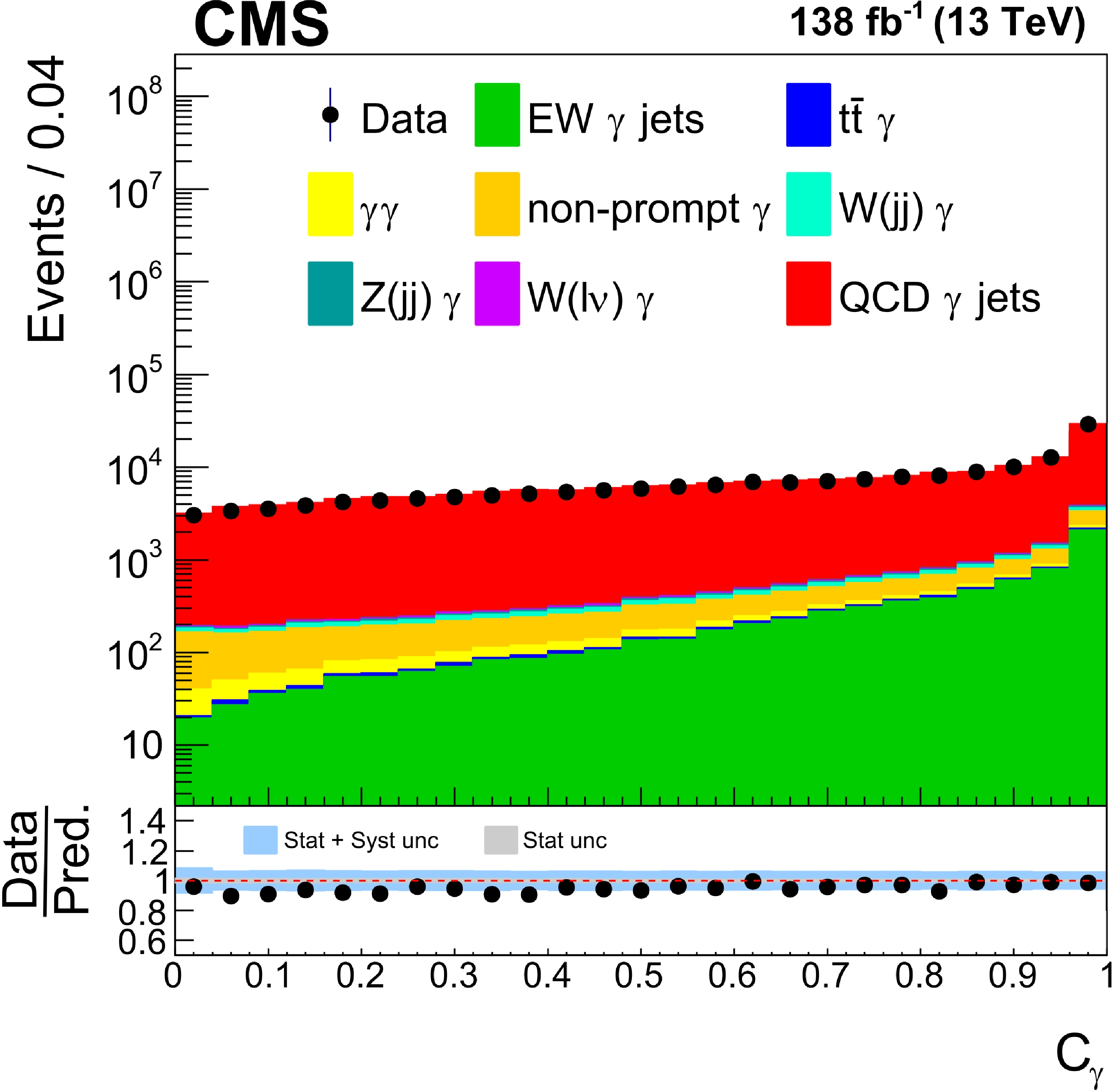
Figure 5-a:
Distribution of (upper left) $ C_{\gamma} $, (upper right) $ \Delta R(j_2,\gamma) $, and (lower) the Zeppenfeld variable in data and simulated processes, except the contribution of nonprompt photons that is estimated from data as discussed in Section 5. Simulted samples are normalized to their theoretical cross sections. The black points with error bars represent the data and their statistical uncertainties. The last bin includes the overflow events. The lower panels shows the ratio of the data to the expectation with the inner (outer) band representing the statistical (total) uncertainty in the combined signal and background expectations. |
png pdf |
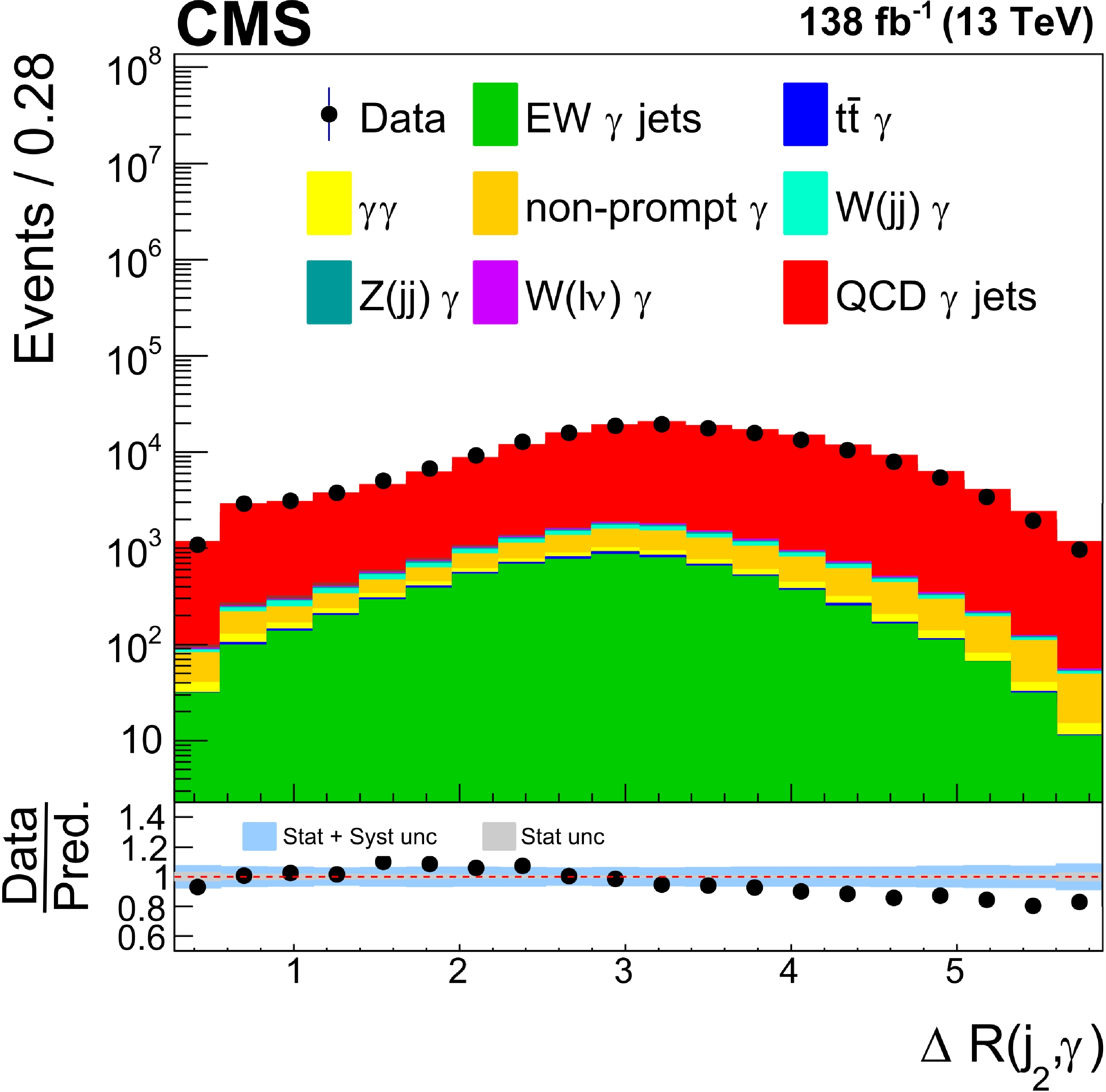
Figure 5-b:
Distribution of (upper left) $ C_{\gamma} $, (upper right) $ \Delta R(j_2,\gamma) $, and (lower) the Zeppenfeld variable in data and simulated processes, except the contribution of nonprompt photons that is estimated from data as discussed in Section 5. Simulted samples are normalized to their theoretical cross sections. The black points with error bars represent the data and their statistical uncertainties. The last bin includes the overflow events. The lower panels shows the ratio of the data to the expectation with the inner (outer) band representing the statistical (total) uncertainty in the combined signal and background expectations. |
png pdf |
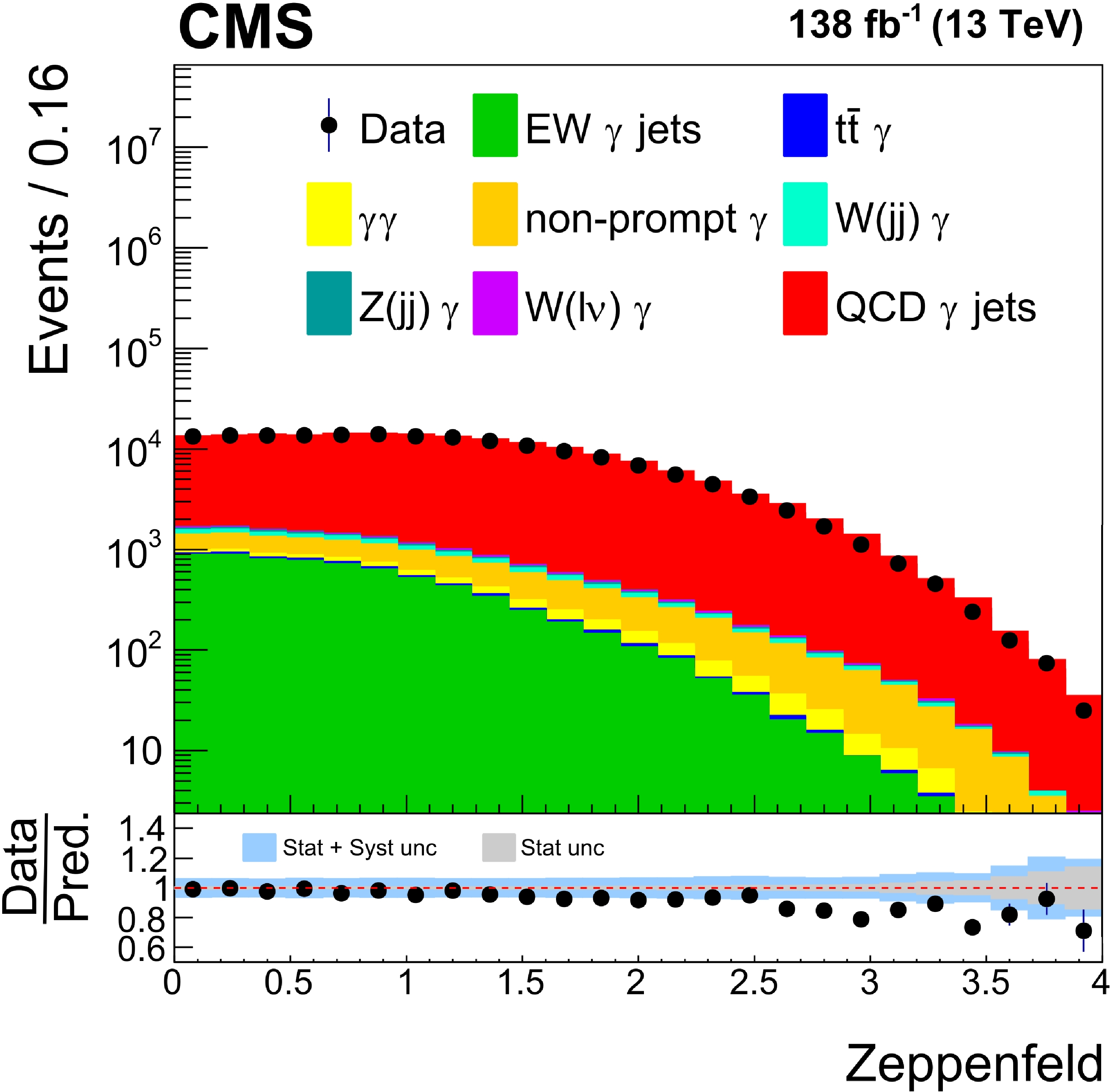
Figure 5-c:
Distribution of (upper left) $ C_{\gamma} $, (upper right) $ \Delta R(j_2,\gamma) $, and (lower) the Zeppenfeld variable in data and simulated processes, except the contribution of nonprompt photons that is estimated from data as discussed in Section 5. Simulted samples are normalized to their theoretical cross sections. The black points with error bars represent the data and their statistical uncertainties. The last bin includes the overflow events. The lower panels shows the ratio of the data to the expectation with the inner (outer) band representing the statistical (total) uncertainty in the combined signal and background expectations. |
png pdf |
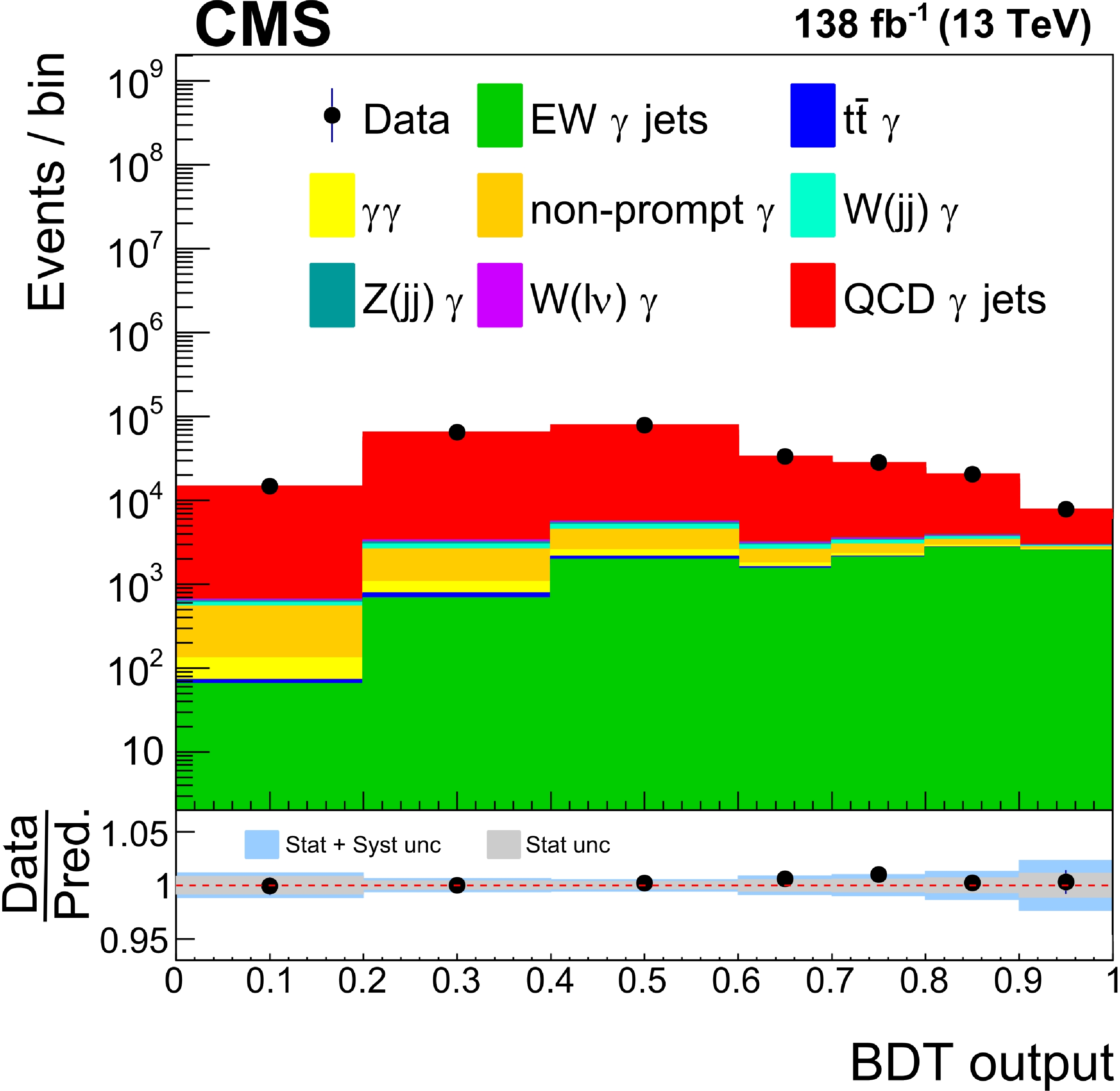
Figure 6:
The postfit BDT output distribution. The data are compared to the sum of the signal and the background contributions. The black points with error bars represent the data and their statistical uncertainties. The lower panel shows the ratio of the data to prediction where the inner (outer) band represents the statistical (total) uncertainty in the combined signal and background contributions after the fit. |
png pdf |
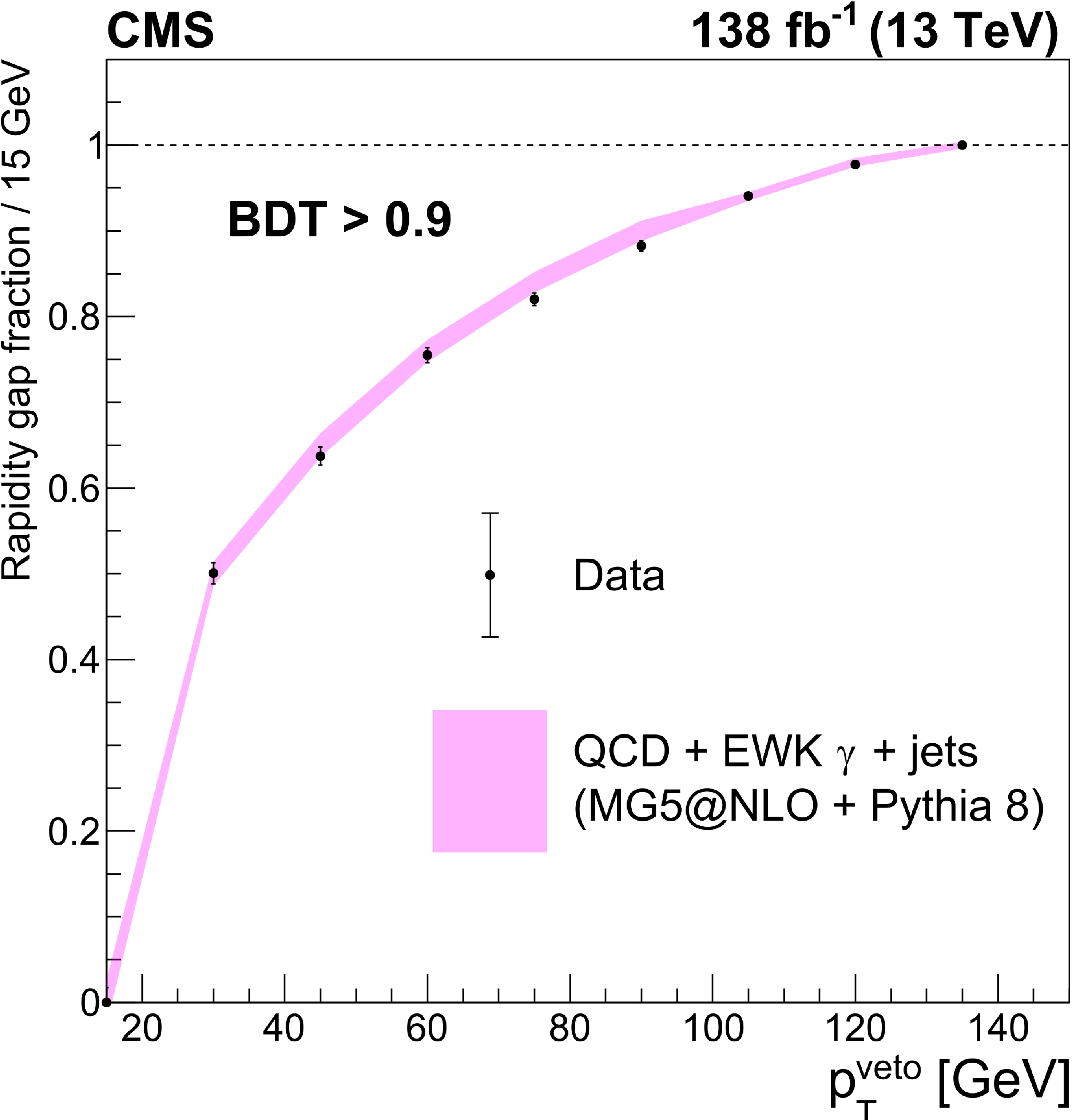
Figure 7:
The rapidity gap fraction as a function of $ p_{\mathrm{T}}^{\text{veto}} $ in data and simulated samples for EW $ \gamma $\text{jj} and QCD \PGgjj. The black points with error bars represent the data and their statistical uncertainties. The theory prediction, calculated using MG5+PYTHIA, together with the MC statistical uncertainties are shown by the colored band. |
png pdf |
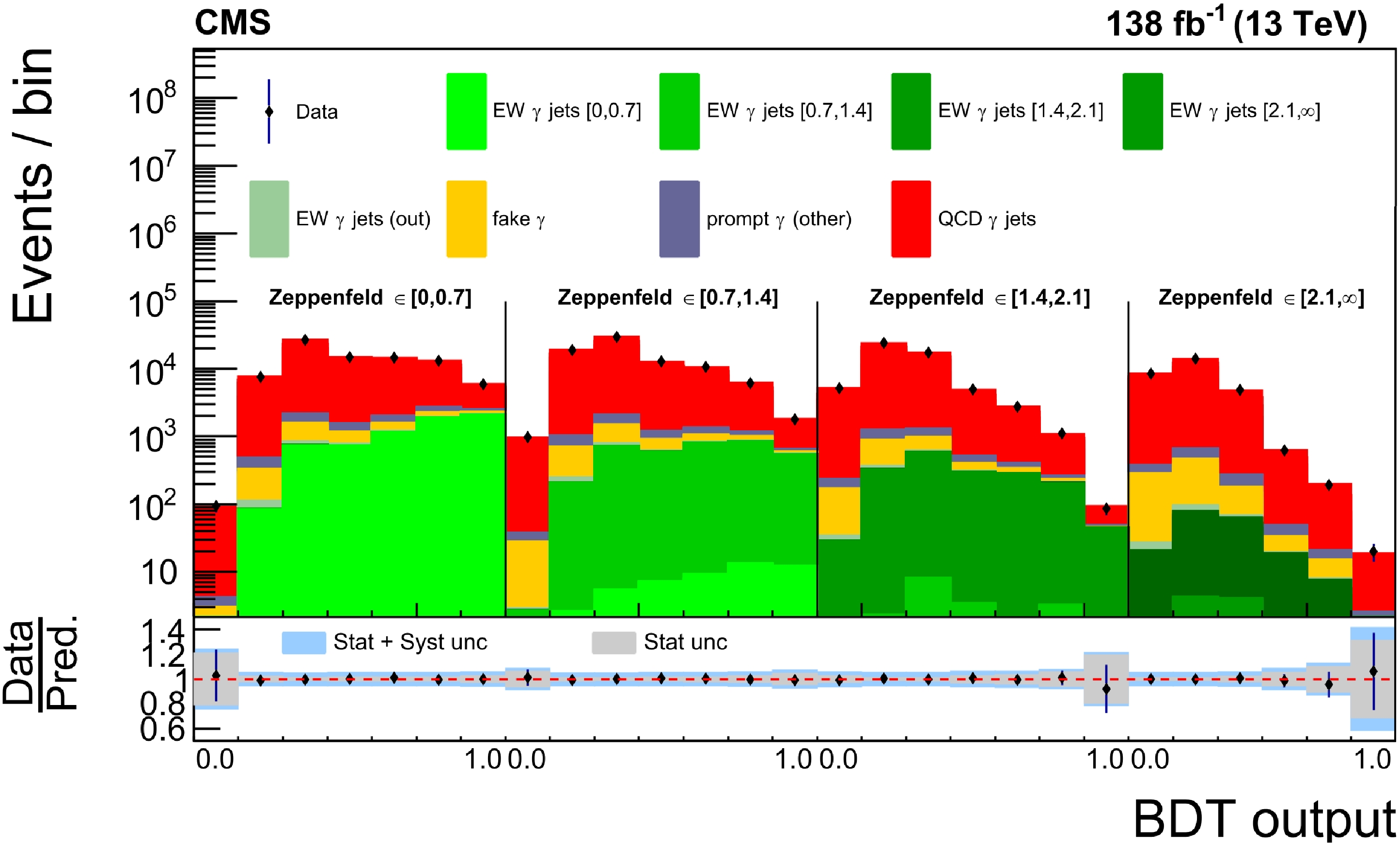
Figure 8:
The unrolled BDT distribution in bins of the Zeppenfeld observable after the fit to the data. Signal events from different Zeppenfeld ranges at the generator level are represented by different colors, whereas different Zeppenfeld ranges at the detector level are displayed as an overlaid distribution. The different shades of green correspond to increasing ranges of the Zeppenfeld observable at the generator level ([0,0.7],[0.7,1.4],[1.4,2.1],[2.1,$ \infty $]). The label ``out'' refers to signal events outside the defined phase space. The black points with error bars represent the data and their statistical uncertainties. The lower panel shows the ratio of the data to the prediction. The inner and outer bands represent, respectively, the statistical and total uncertainties on all simulated samples after the fit. |
png pdf |
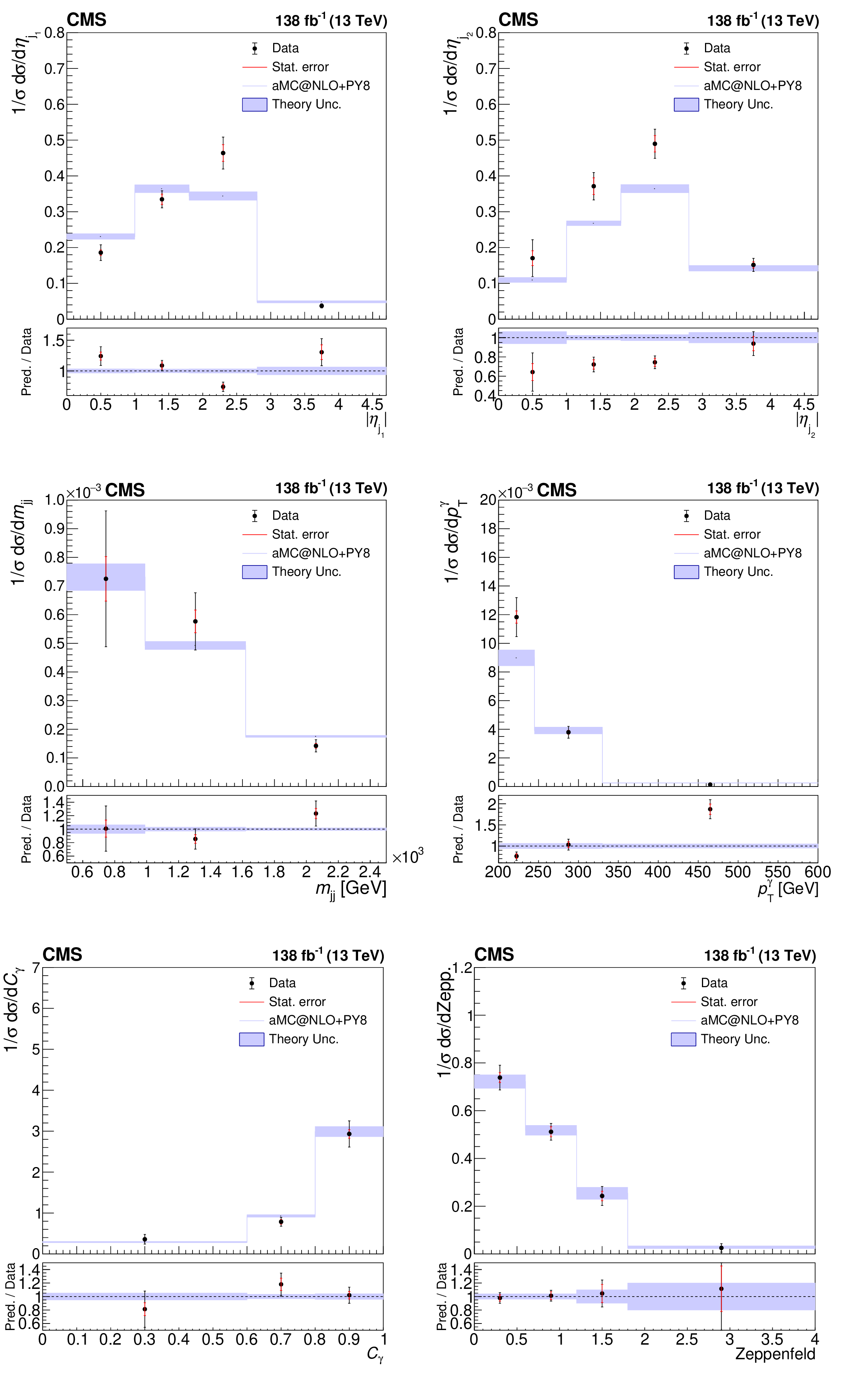
Figure 9:
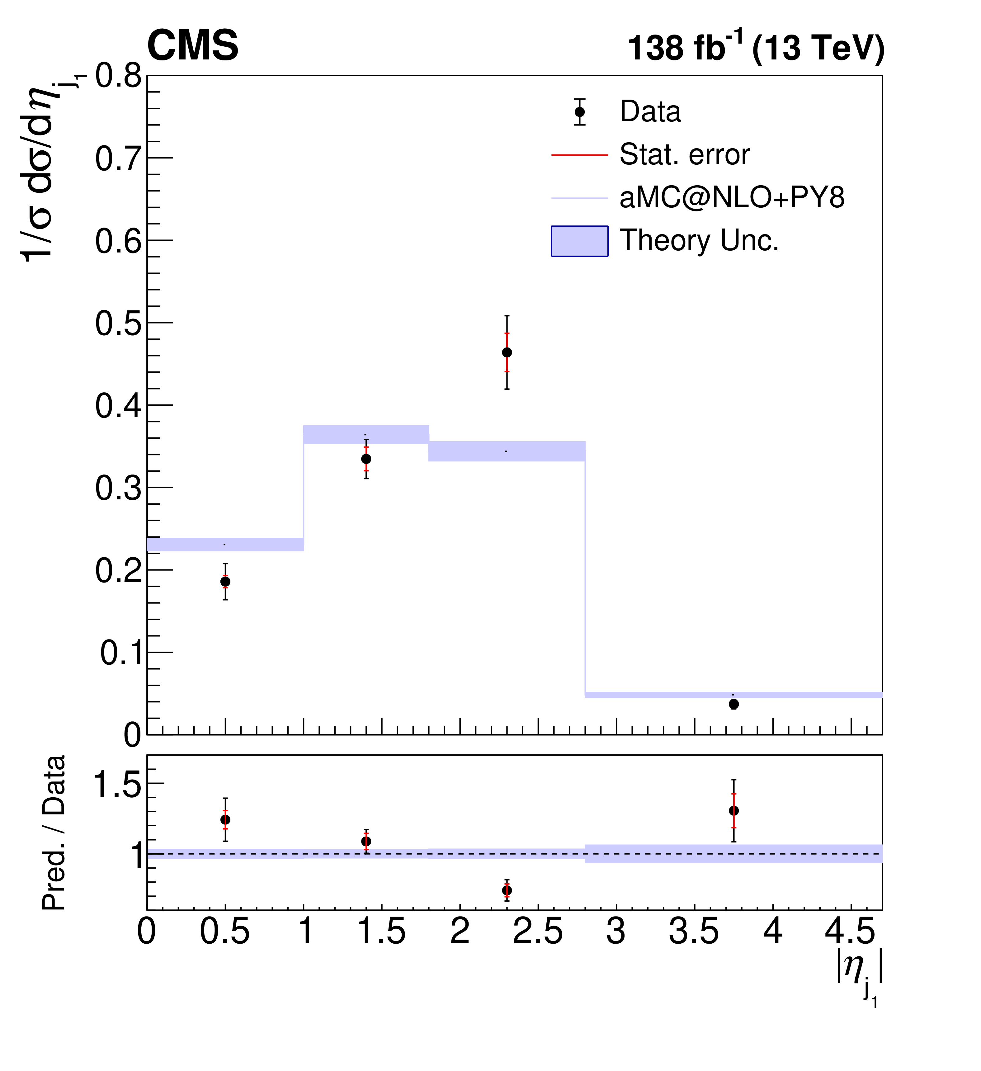
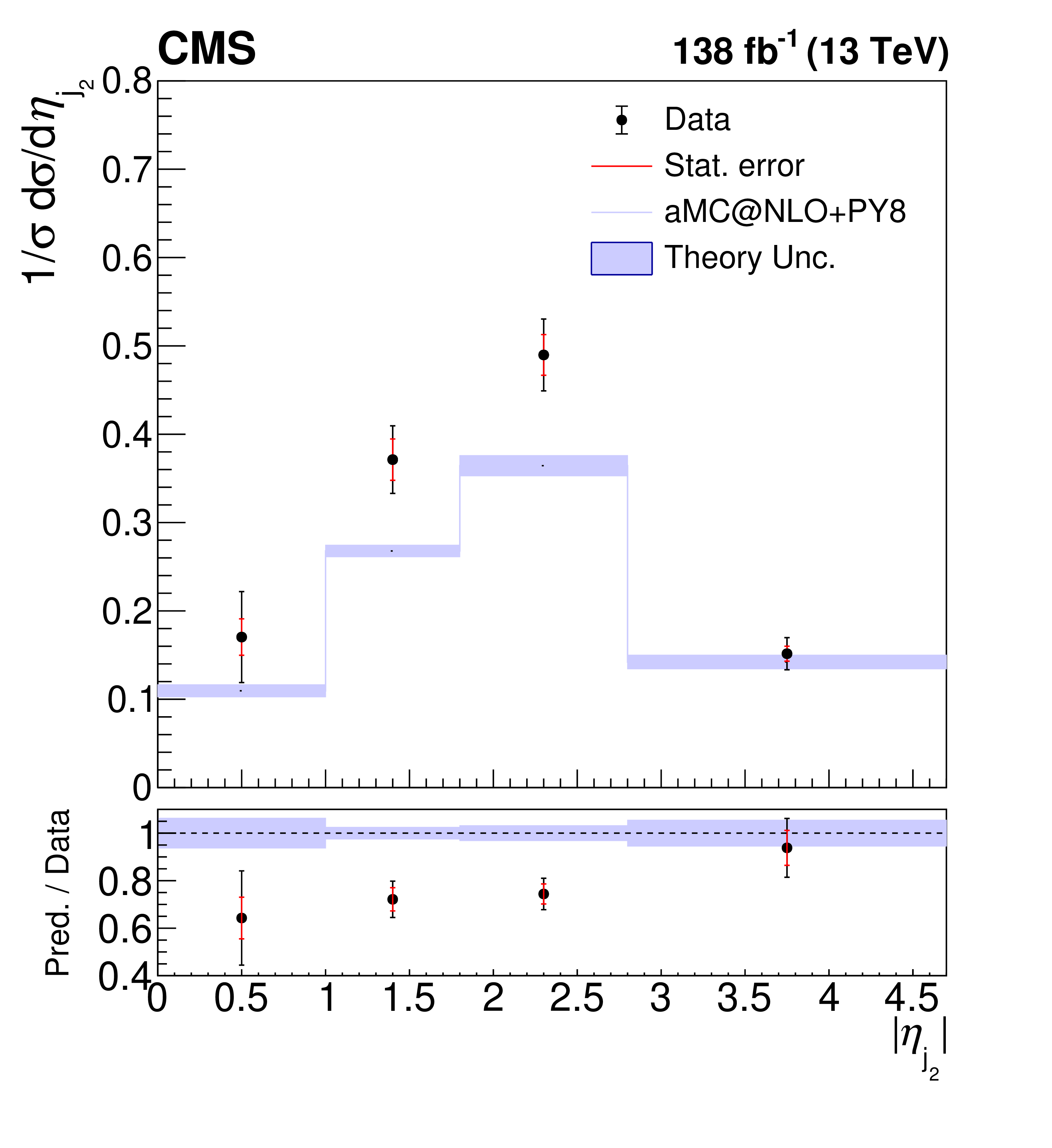
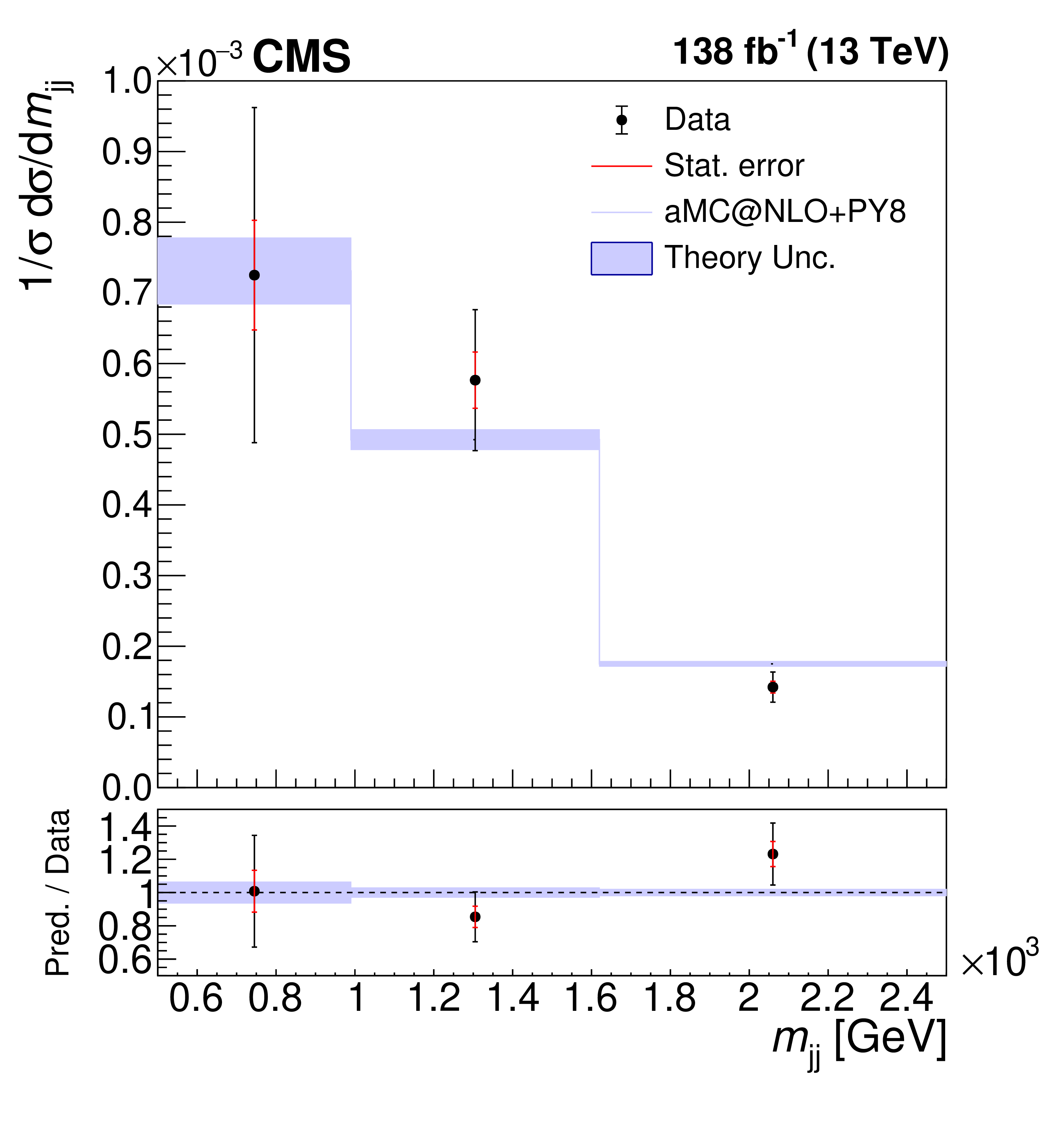
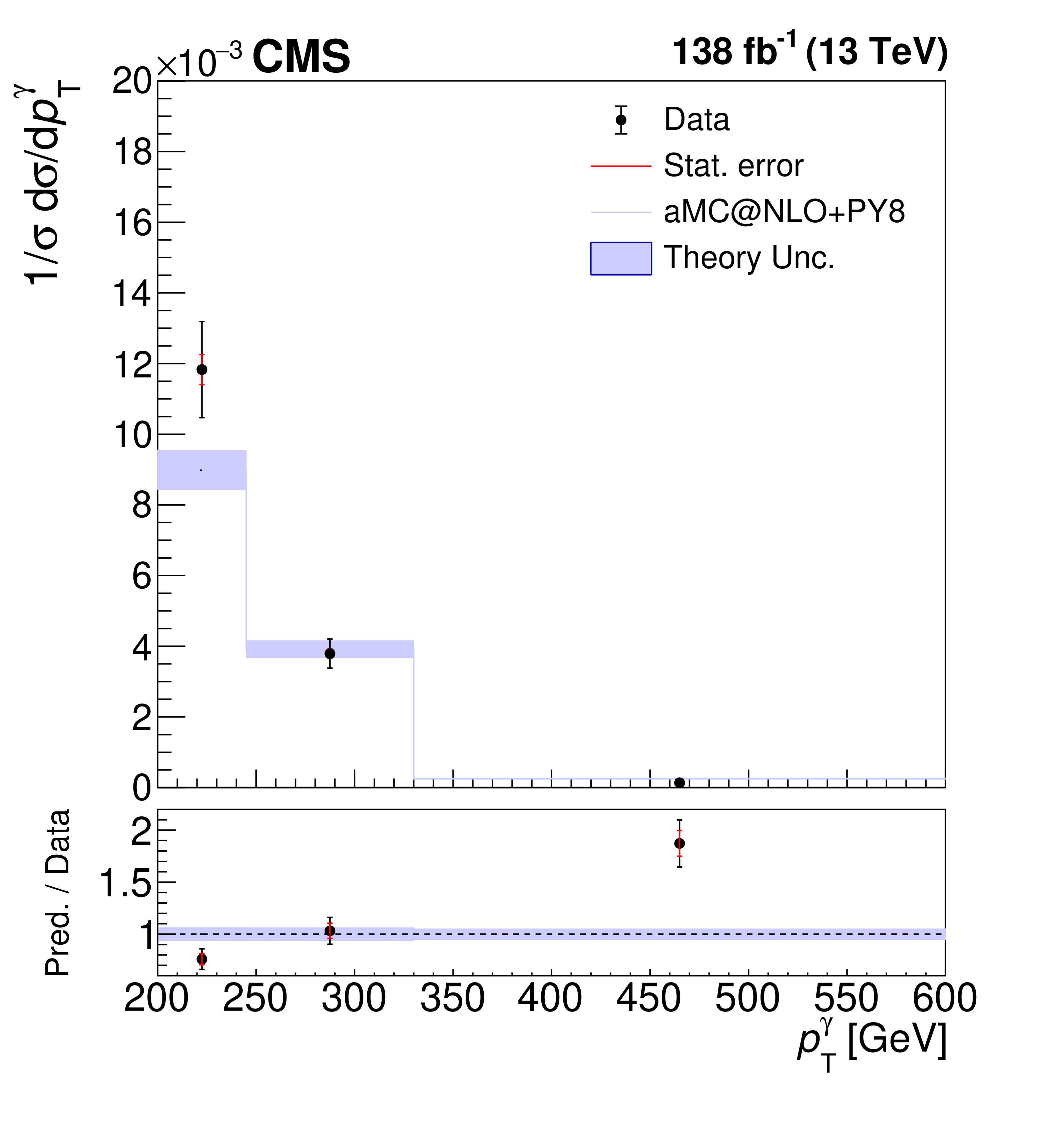
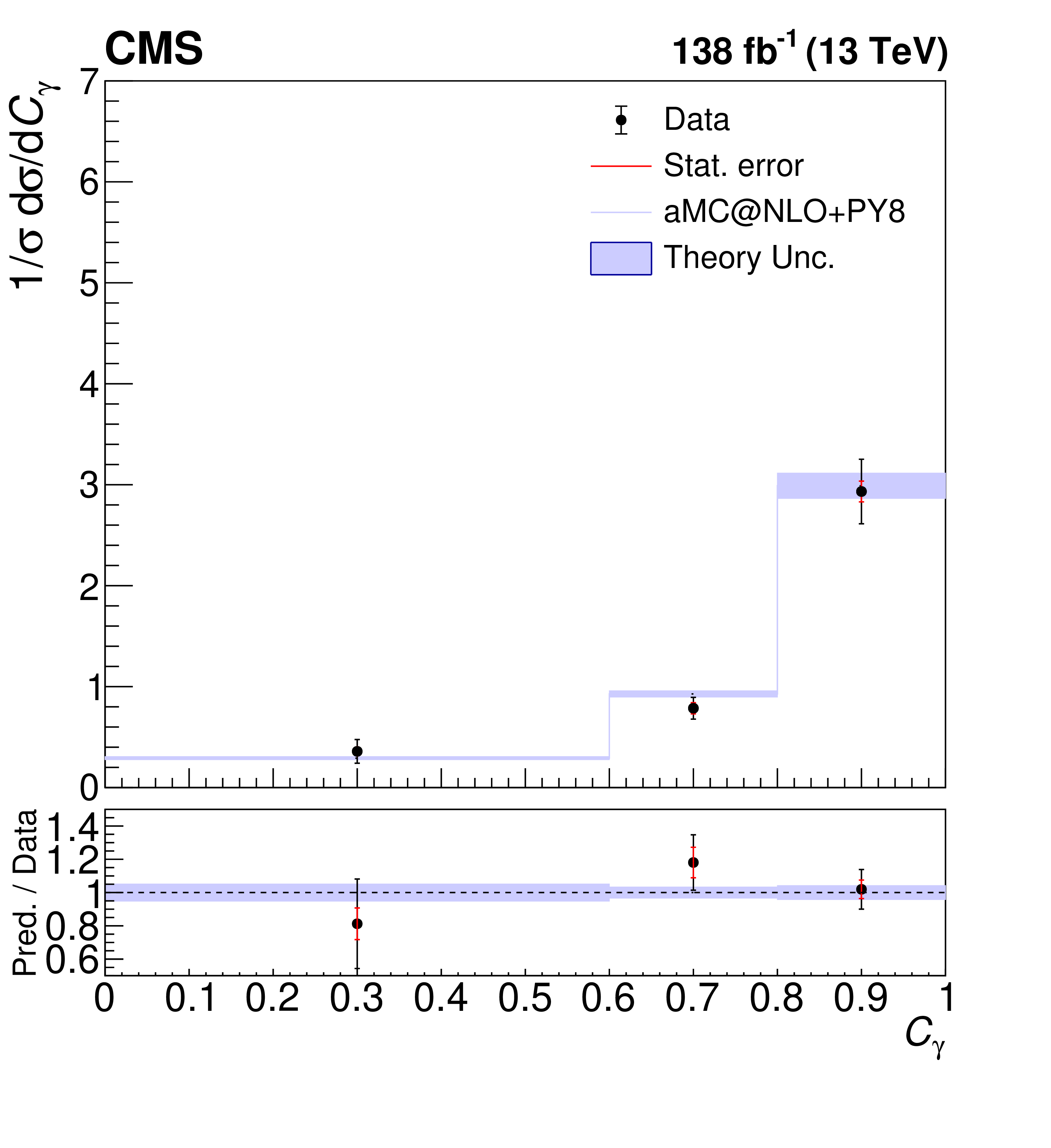
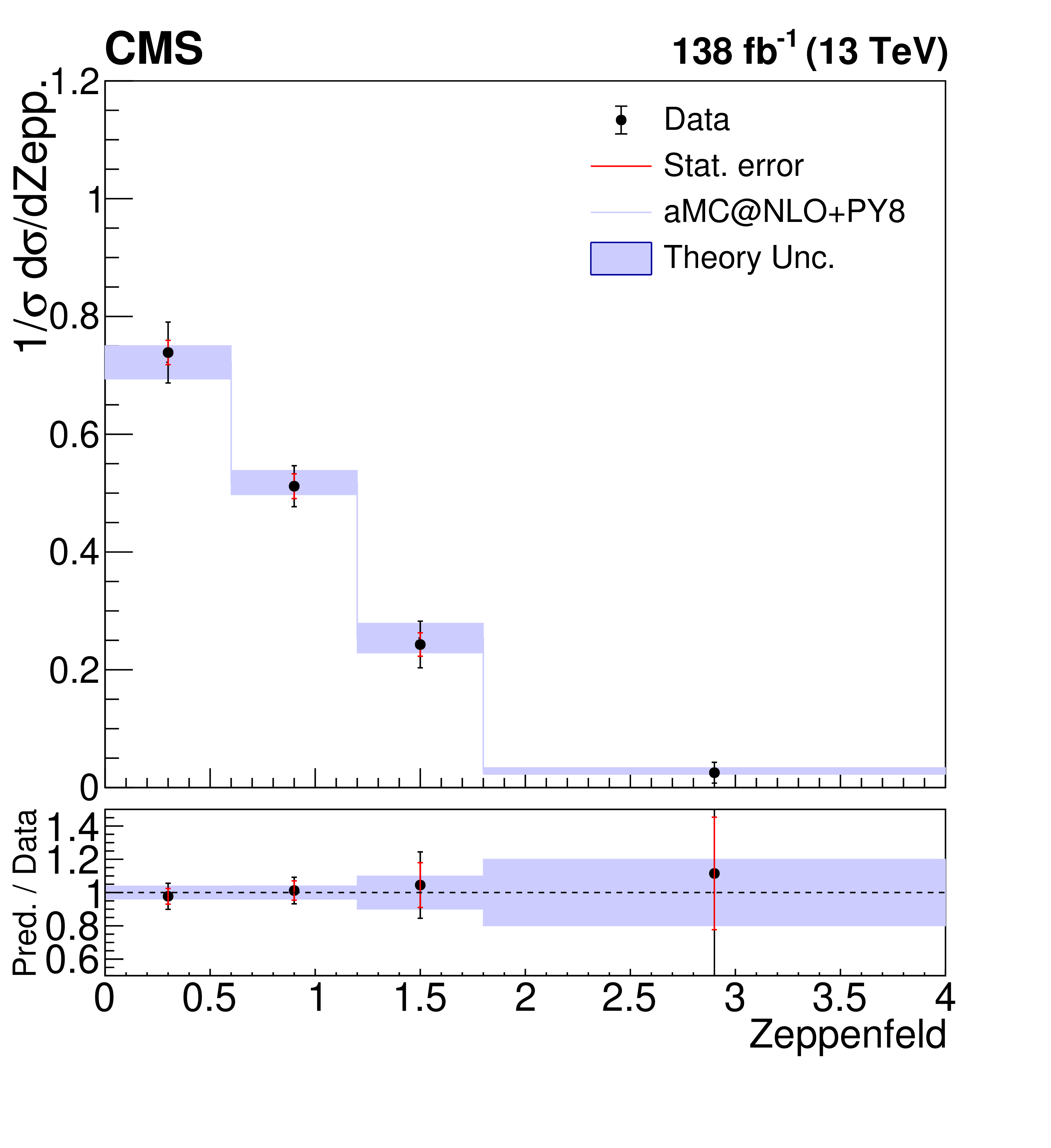
Normalized differential cross sections, compared with the SM predictions, as functions of (upper left) $ \eta_{\text{j}_1} $, (upper right) $ \eta_{\text{j}_2} $, (middle left) $ m_\mathrm{jj} $, (middle right) $ p_{\mathrm{T}}^\gamma $, (lower left) $ C_{\gamma} $, and (lower right) the Zeppenfeld variable. The red bars on the data points represent the statistical errors, whereas the black bars show the total uncertainties. |
png pdf |
Figure 9-a:
Normalized differential cross sections, compared with the SM predictions, as functions of (upper left) $ \eta_{\text{j}_1} $, (upper right) $ \eta_{\text{j}_2} $, (middle left) $ m_\mathrm{jj} $, (middle right) $ p_{\mathrm{T}}^\gamma $, (lower left) $ C_{\gamma} $, and (lower right) the Zeppenfeld variable. The red bars on the data points represent the statistical errors, whereas the black bars show the total uncertainties. |
png pdf |
Figure 9-b:
Normalized differential cross sections, compared with the SM predictions, as functions of (upper left) $ \eta_{\text{j}_1} $, (upper right) $ \eta_{\text{j}_2} $, (middle left) $ m_\mathrm{jj} $, (middle right) $ p_{\mathrm{T}}^\gamma $, (lower left) $ C_{\gamma} $, and (lower right) the Zeppenfeld variable. The red bars on the data points represent the statistical errors, whereas the black bars show the total uncertainties. |
png pdf |
Figure 9-c:
Normalized differential cross sections, compared with the SM predictions, as functions of (upper left) $ \eta_{\text{j}_1} $, (upper right) $ \eta_{\text{j}_2} $, (middle left) $ m_\mathrm{jj} $, (middle right) $ p_{\mathrm{T}}^\gamma $, (lower left) $ C_{\gamma} $, and (lower right) the Zeppenfeld variable. The red bars on the data points represent the statistical errors, whereas the black bars show the total uncertainties. |
png pdf |
Figure 9-d:
Normalized differential cross sections, compared with the SM predictions, as functions of (upper left) $ \eta_{\text{j}_1} $, (upper right) $ \eta_{\text{j}_2} $, (middle left) $ m_\mathrm{jj} $, (middle right) $ p_{\mathrm{T}}^\gamma $, (lower left) $ C_{\gamma} $, and (lower right) the Zeppenfeld variable. The red bars on the data points represent the statistical errors, whereas the black bars show the total uncertainties. |
png pdf |
Figure 9-e:
Normalized differential cross sections, compared with the SM predictions, as functions of (upper left) $ \eta_{\text{j}_1} $, (upper right) $ \eta_{\text{j}_2} $, (middle left) $ m_\mathrm{jj} $, (middle right) $ p_{\mathrm{T}}^\gamma $, (lower left) $ C_{\gamma} $, and (lower right) the Zeppenfeld variable. The red bars on the data points represent the statistical errors, whereas the black bars show the total uncertainties. |
png pdf |
Figure 9-f:
Normalized differential cross sections, compared with the SM predictions, as functions of (upper left) $ \eta_{\text{j}_1} $, (upper right) $ \eta_{\text{j}_2} $, (middle left) $ m_\mathrm{jj} $, (middle right) $ p_{\mathrm{T}}^\gamma $, (lower left) $ C_{\gamma} $, and (lower right) the Zeppenfeld variable. The red bars on the data points represent the statistical errors, whereas the black bars show the total uncertainties. |
png pdf |
Figure 10:
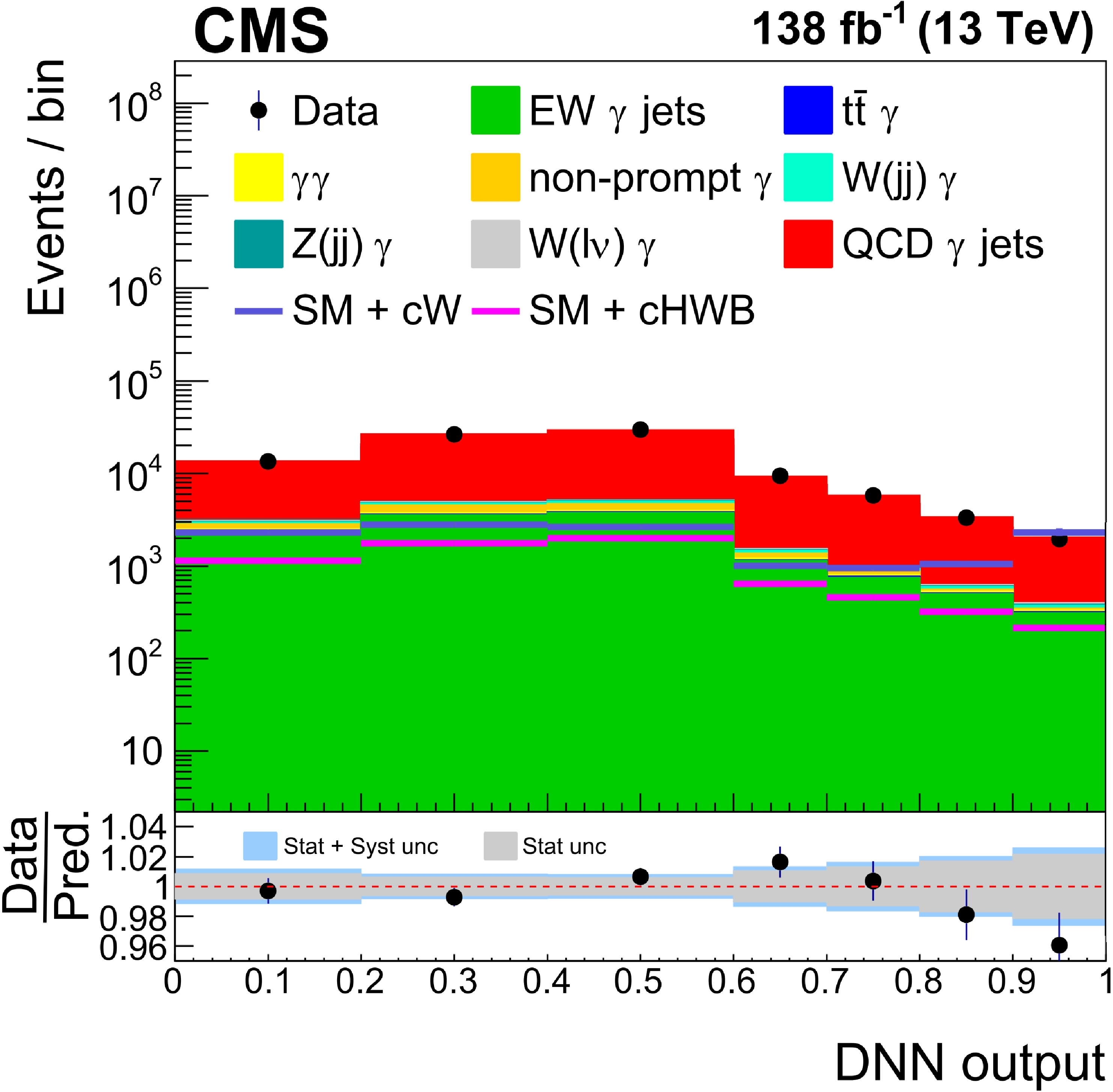
The distribution of the DNN output trained for $ c_{\mathrm{W}} $ and $ c_{\mathrm{H}\mathrm{W}\mathrm{B}} $ coefficients in data and simulation. The simulation is corrected using the results of the inclusive $ \sigma_{\text{EW} {\gamma}\text{jj} } $ measurement. The black points with error bars represent the data and their statistical uncertainties. The purple and indigo lines show the distributions for the EW $ \gamma $\text{jj} process when $ c_{\mathrm{H}\mathrm{W}\mathrm{B}} $ and $ c_{\mathrm{W}} $, respectively, are set to one. The lower panel shows the ratio of the data to the prediction. The inner and outer bands represent, respectively, the statistical and total uncertainties on all simulated samples as evaluated in the inclusive $ \sigma_{\text{EW} {\gamma}\text{jj} } $ measurement. |
png pdf |
Figure 11:
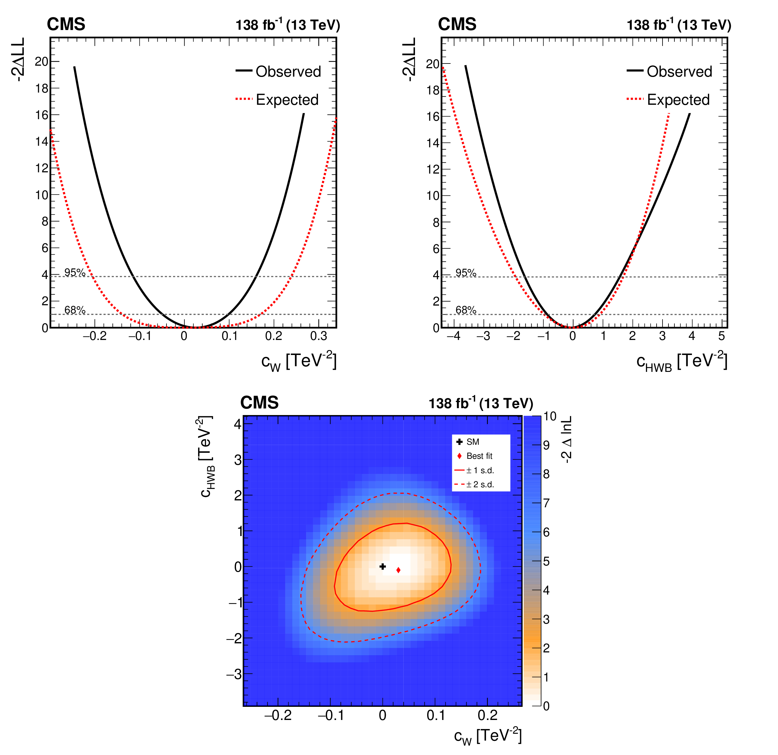
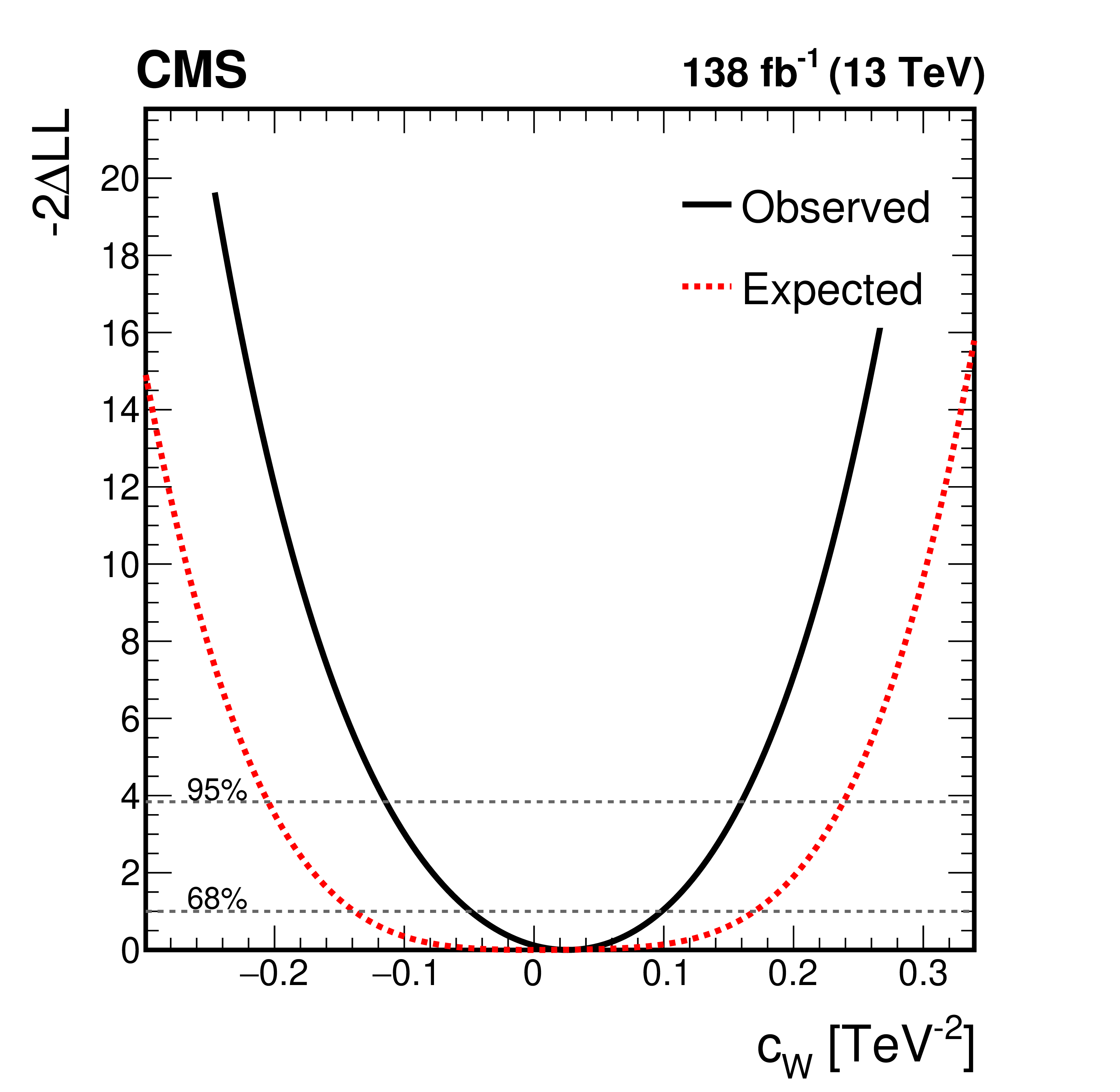
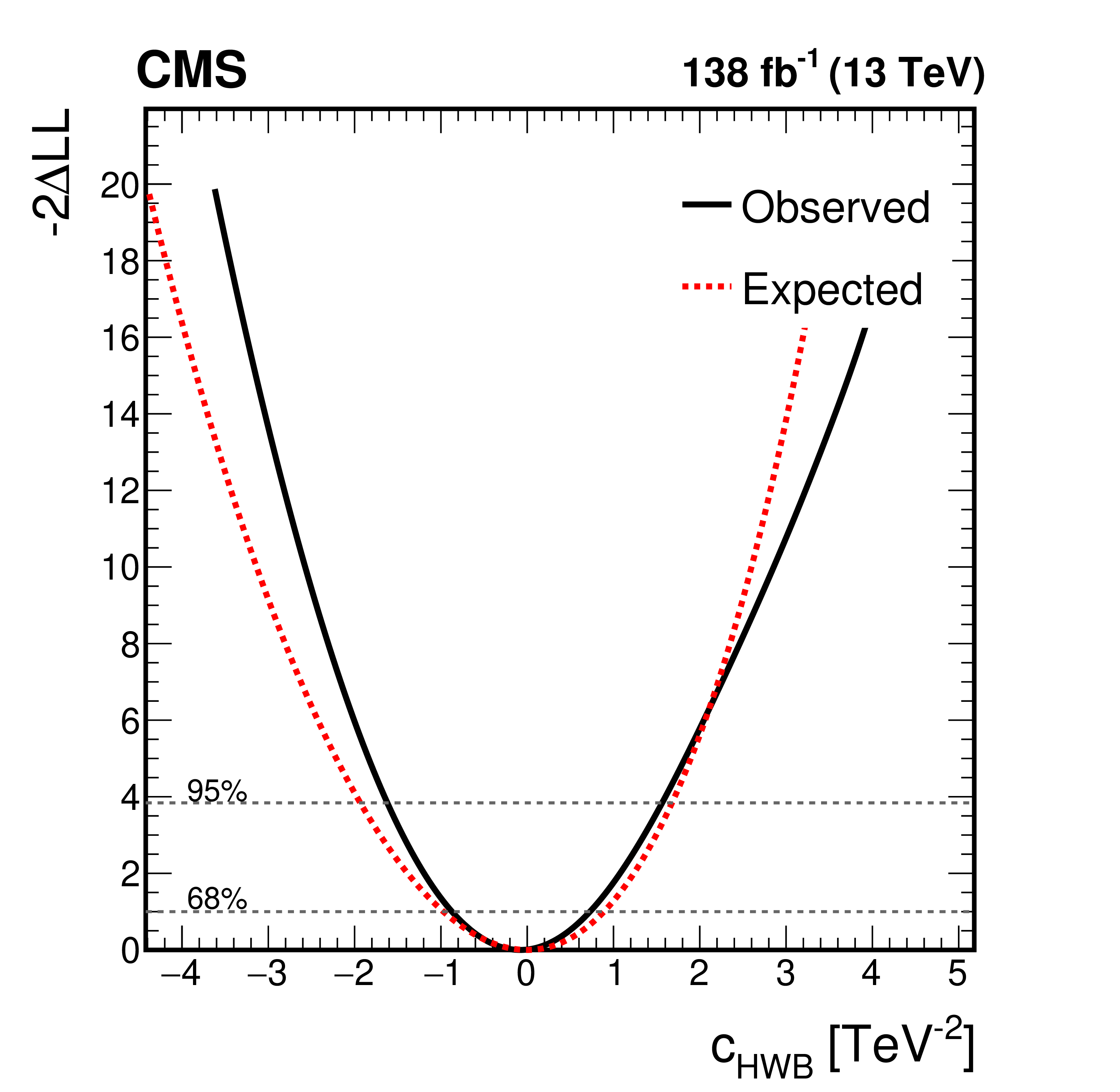
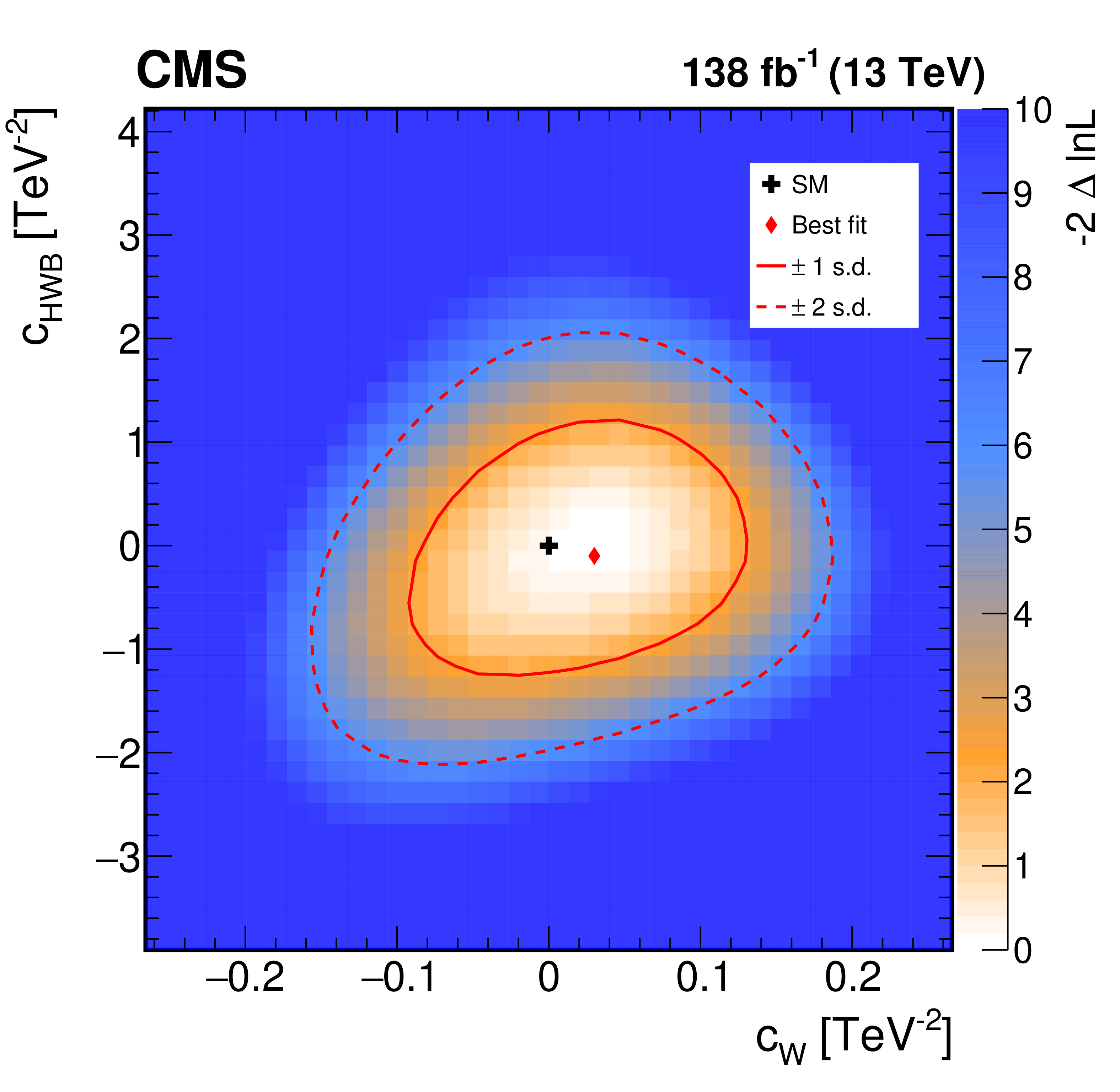
Negative of twice in the difference in the log-likelihood as a function of $ c_{\mathrm{W}} $ and $ c_{\mathrm{H}\mathrm{W}\mathrm{B}} $ based on 138 fb$ ^{-1} $ of CMS data at 13 TeV. Upper left: the one-dimensional likelihood scan for $ c_{\mathrm{W}} $, showing the observed (black solid line) and expected (red dashed line) standard values, with 68% and 95% confidence intervals indicated by horizontal dashed lines. Upper right: the one-dimensional likelihood scan for $ c_{\mathrm{H}\mathrm{W}\mathrm{B}} $, similarly presenting observed and expected limits. Lower: the two-dimensional likelihood contour for $ c_{\mathrm{W}} $ and $ c_{\mathrm{H}\mathrm{W}\mathrm{B}} $, indicating the standard model (black cross), the best fit values (red dot), and contours corresponding to one (red solid line) and two (red dashed line) standard deviations. |
png pdf |
Figure 11-a:
Negative of twice in the difference in the log-likelihood as a function of $ c_{\mathrm{W}} $ and $ c_{\mathrm{H}\mathrm{W}\mathrm{B}} $ based on 138 fb$ ^{-1} $ of CMS data at 13 TeV. Upper left: the one-dimensional likelihood scan for $ c_{\mathrm{W}} $, showing the observed (black solid line) and expected (red dashed line) standard values, with 68% and 95% confidence intervals indicated by horizontal dashed lines. Upper right: the one-dimensional likelihood scan for $ c_{\mathrm{H}\mathrm{W}\mathrm{B}} $, similarly presenting observed and expected limits. Lower: the two-dimensional likelihood contour for $ c_{\mathrm{W}} $ and $ c_{\mathrm{H}\mathrm{W}\mathrm{B}} $, indicating the standard model (black cross), the best fit values (red dot), and contours corresponding to one (red solid line) and two (red dashed line) standard deviations. |
png pdf |
Figure 11-b:
Negative of twice in the difference in the log-likelihood as a function of $ c_{\mathrm{W}} $ and $ c_{\mathrm{H}\mathrm{W}\mathrm{B}} $ based on 138 fb$ ^{-1} $ of CMS data at 13 TeV. Upper left: the one-dimensional likelihood scan for $ c_{\mathrm{W}} $, showing the observed (black solid line) and expected (red dashed line) standard values, with 68% and 95% confidence intervals indicated by horizontal dashed lines. Upper right: the one-dimensional likelihood scan for $ c_{\mathrm{H}\mathrm{W}\mathrm{B}} $, similarly presenting observed and expected limits. Lower: the two-dimensional likelihood contour for $ c_{\mathrm{W}} $ and $ c_{\mathrm{H}\mathrm{W}\mathrm{B}} $, indicating the standard model (black cross), the best fit values (red dot), and contours corresponding to one (red solid line) and two (red dashed line) standard deviations. |
png pdf |
Figure 11-c:
Negative of twice in the difference in the log-likelihood as a function of $ c_{\mathrm{W}} $ and $ c_{\mathrm{H}\mathrm{W}\mathrm{B}} $ based on 138 fb$ ^{-1} $ of CMS data at 13 TeV. Upper left: the one-dimensional likelihood scan for $ c_{\mathrm{W}} $, showing the observed (black solid line) and expected (red dashed line) standard values, with 68% and 95% confidence intervals indicated by horizontal dashed lines. Upper right: the one-dimensional likelihood scan for $ c_{\mathrm{H}\mathrm{W}\mathrm{B}} $, similarly presenting observed and expected limits. Lower: the two-dimensional likelihood contour for $ c_{\mathrm{W}} $ and $ c_{\mathrm{H}\mathrm{W}\mathrm{B}} $, indicating the standard model (black cross), the best fit values (red dot), and contours corresponding to one (red solid line) and two (red dashed line) standard deviations. |
| Tables | |
png pdf |
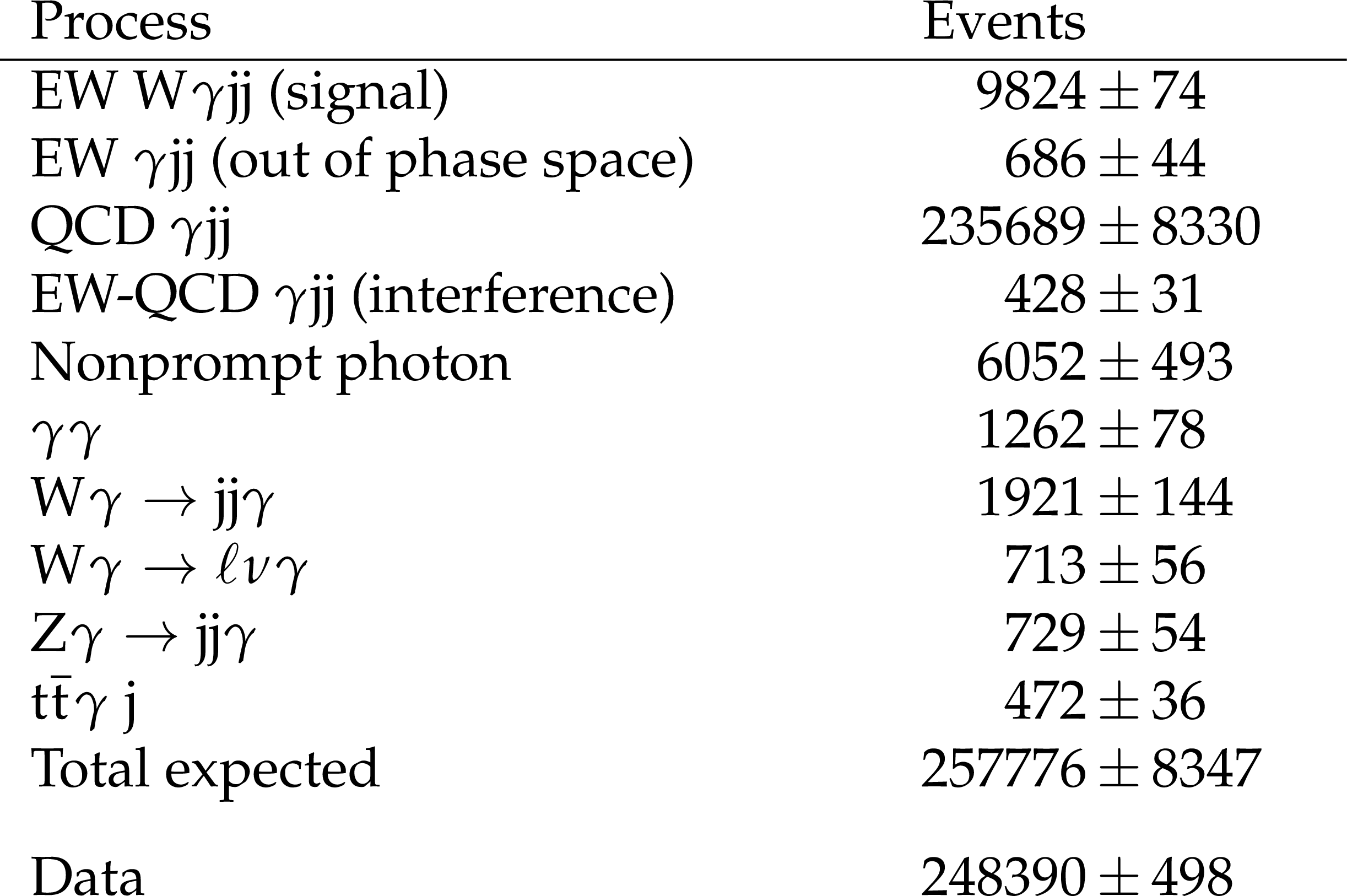
Table 1:
Expected event yields and their uncertainties for signal and backgrounds, including also the estimation of the nonprompt photon contribution. The number of observed data events are also included for comparison. |
png pdf |
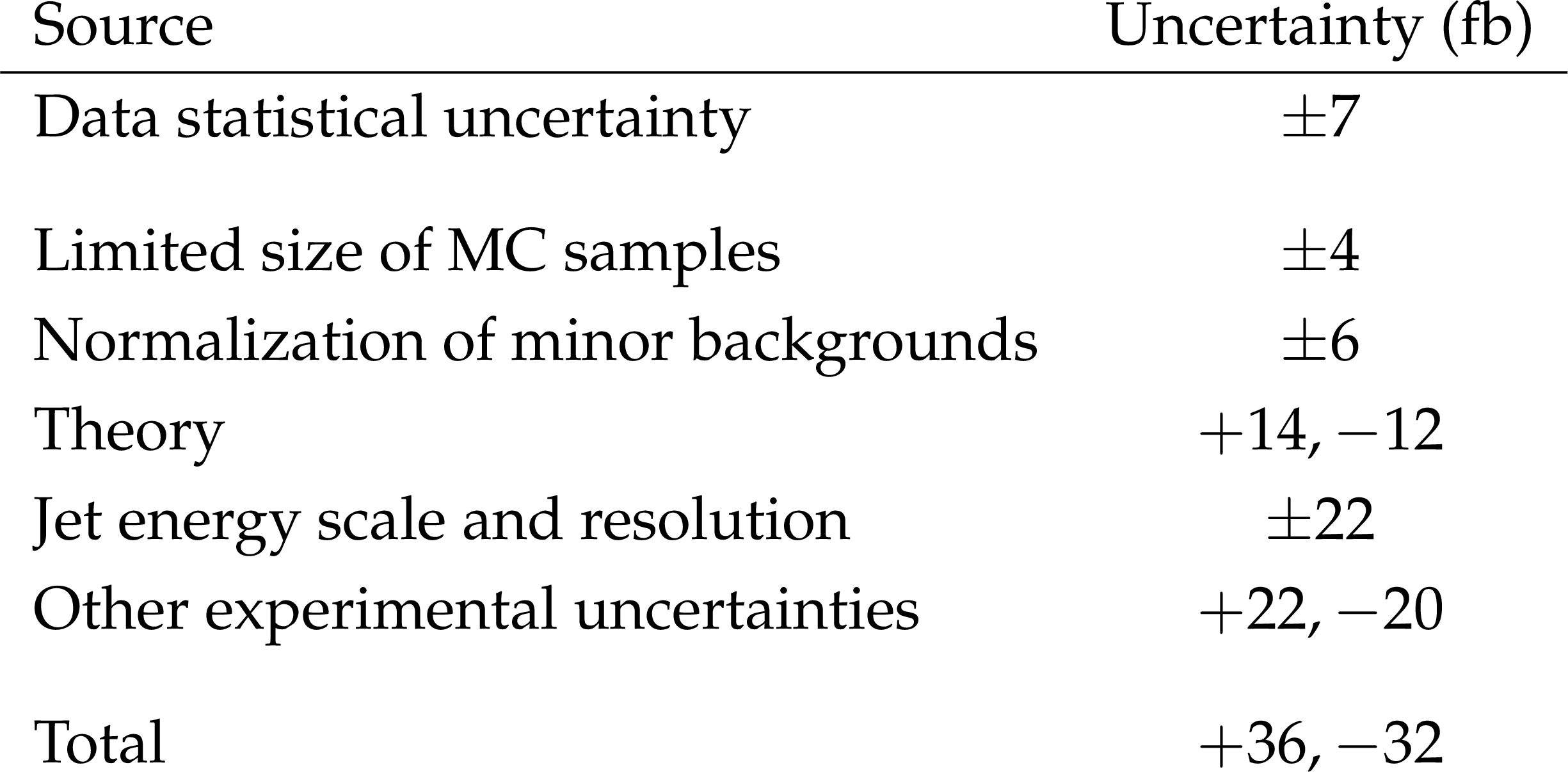
Table 2:
Summary of uncertainties affecting the measurement as extracted from the fit to data. The total uncertainty is obtained by adding individual contributions in quadrature. |
| Summary |
| The first observation has been presented of the electroweak production of a photon in association with two jets (EW $ \gamma \text{jj} $) using proton-proton collisions at $ \sqrt{s}= $ 13 TeV recorded with the CMS detector in 2016-2018 and corresponding to an integrated luminosity of 138 fb$ ^{-1} $. Events are selected by requiring a photon with transverse momentum $ p_{\mathrm{T}}^{\gamma} > $ 200 GeV and two jets separated by at least $ |\Delta \eta| > $ 2.5 with an invariant mass $ m_\mathrm{jj} > $ 500 GeV. The measured inclusive EW $ \gamma \text{jj}$ cross section is $ \sigma_{\text{EW} {\gamma}\text{jj} }= $ 202 $ \pm $ 7 (stat) $ ^{+35}_{-32} $ (syst) fb in agreement with the predicted standard model cross section of 177$ ^{+13}_{-12} $ fb. Normalized differential cross sections are also measured as functions of several observables and compared with standard model predictions at next to leading order in perturbative quantum chromodynamics. Within the uncertainties, predictions agree with measurements in all observables except the pseudorapidity of the tagging jets. In particular, measured normalized cross sections differ from prediction by about two standard deviations in the pseudorapidity distribution of the softer tagging jet. The gap fraction is measured in a signal-enriched region and is found to be in agreement with the prediction, supporting the accuracy of the modeling of hadronic activities in VBF-like processes. A deep neural network is trained to probe new WW$ \gamma $ interactions in the context of an effective field theory, described by dimension-6 operators. The observed 95% confidence intervals for the Warsaw basis Wilson coefficients $ c_{\mathrm{W}} $ and $ c_{\mathrm{H}\mathrm{W}\mathrm{B}} $ are [$-$0.11,0.16] and [$-$1.6,1.5], respectively. |
| References | ||||
| 1 | M. Rauch | Vector-boson fusion and vector-boson scattering | 1610.08420 | |
| 2 | J. D. Bjorken | Rapidity gaps and jets as a new-physics signature in very-high-energy hadron-hadron collisions | PRD 47 (1993) 101 | |
| 3 | C. Baldenegro et al. | Jets separated by a large pseudorapidity gap at the Tevatron and at the LHC | JHEP 08 (2022) 250 | 2206.04965 |
| 4 | CMS Collaboration | Measurement of the hadronic activity in events with a Z and two jets and extraction of the cross section for the electroweak production of a Z with two jets in $ pp $ collisions at $ \sqrt{s} = $ 7 TeV | JHEP 10 (2013) 062 | CMS-FSQ-12-019 1305.7389 |
| 5 | ATLAS Collaboration | Measurement of the electroweak production of dijets in association with a Z-boson and distributions sensitive to vector boson fusion in proton-proton collisions at $ \sqrt{s} = $ 8 TeV using the ATLAS detector | JHEP 04 (2014) 031 | 1401.7610 |
| 6 | CMS Collaboration | Measurement of electroweak production of two jets in association with a Z boson in proton-proton collisions at $ \sqrt{s} = $ 8 TeV | EPJC 75 (2015) 66 | CMS-FSQ-12-035 1410.3153 |
| 7 | CMS Collaboration | Electroweak production of two jets in association with a Z boson in proton-proton collisions at $ \sqrt{s}= $ 13 TeV | EPJC 78 (2018) 589 | CMS-SMP-16-018 1712.09814 |
| 8 | ATLAS Collaboration | Measurement of the cross-section for electroweak production of dijets in association with a Z boson in pp collisions at $ \sqrt {s} = $ 13 TeV with the ATLAS detector | PLB 775 (2017) 206 | 1709.10264 |
| 9 | CMS Collaboration | Measurement of electroweak production of a W boson and two forward jets in proton-proton collisions at $ \sqrt{s}= $ 8 TeV | JHEP 11 (2016) 147 | CMS-SMP-13-012 1607.06975 |
| 10 | ATLAS Collaboration | Measurements of electroweak Wjj production and constraints on anomalous gauge couplings with the ATLAS detector | EPJC 77 (2017) 474 | 1703.04362 |
| 11 | CMS Collaboration | Measurement of electroweak production of a W boson in association with two jets in proton-proton collisions at $ \sqrt{s} = $ 13 TeV | EPJC 80 (2020) 43 | CMS-SMP-17-011 1903.04040 |
| 12 | ATLAS Collaboration | Measurement of isolated-photon plus two-jet production in $ pp $ collisions at $ \sqrt s= $ 13 TeV with the ATLAS detector | JHEP 03 (2020) 179 | 1912.09866 |
| 13 | ATLAS Collaboration | Observation and measurement of Higgs boson decays to $ {WW}^{*} $ with the ATLAS detector | PRD 92 (2014) 012006 | 1412.2641 |
| 14 | D. L. Rainwater, R. Szalapski, and D. Zeppenfeld | Probing color--singlet exchange in Z + 2--jet events at the CERN LHC | PRD 54 (1996) 6680 | hep-ph/9605444 |
| 15 | B. Grzadkowski, M. Iskrzynski, M. Misiak, and J. Rosiek | Dimension-six terms in the standard model Lagrangian | JHEP 10 (2010) 085 | 1008.4884 |
| 16 | J. Ellis | SMEFT constraints on new physics beyond the standard model | in Proceedings of the BSM-2021 Conference: Beyond Standard Model: From Theory to Experiment. 2021 link |
2105.14942 |
| 17 | CMS Collaboration | HEPData record for this analysis | link | |
| 18 | CMS Collaboration | The CMS experiment at the CERN LHC | JINST 3 (2008) S08004 | |
| 19 | CMS Collaboration | Development of the CMS detector for the CERN LHC Run 3 | JINST 19 (2024) P05064 | |
| 20 | CMS Collaboration | The CMS trigger system | JINST 12 (2017) P01020 | CMS-TRG-12-001 1609.02366 |
| 21 | CMS Collaboration | Performance of the CMS high-level trigger during LHC run 2 | JINST 19 (2024) P11021 | CMS-TRG-19-001 2410.17038 |
| 22 | J. Alwall et al. | The automated computation of tree-level and next-to-leading order differential cross sections, and their matching to parton shower simulations | JHEP 07 (2014) 079 | |
| 23 | S. Frixione | Isolated photons in perturbative QCD | PLB 429 (1998) 369 | hep-ph/9801442 |
| 24 | E. Bothmann et al. | Event generation with Sherpa 2.2 | SciPost Phys. 7 (2019) 034 | |
| 25 | T. Sjostrand et al. | An introduction to PYTHIA 8.2 | Comput. Phys. Commun. 191 (2015) 159 | 1410.3012 |
| 26 | CMS Collaboration | Event generator tunes obtained from underlying event and multiparton scattering measurements | EPJC 76 (2016) 155 | CMS-GEN-14-001 1512.00815 |
| 27 | B. Jäger et al. | Parton-shower effects in Higgs production via vector-boson fusion | EPJC 80 (2020) 756 | 2003.12435 |
| 28 | NNPDF Collaboration | Parton distributions from high-precision collider data | EPJC 77 (2017) 663 | 1706.00428 |
| 29 | GEANT4 Collaboration | GEANT 4--A simulation toolkit | NIM A 506 (2003) 250 | |
| 30 | CMS Collaboration | Particle-flow reconstruction and global event description with the CMS detector | JINST 12 (2017) P10003 | CMS-PRF-14-001 1706.04965 |
| 31 | CMS Collaboration | Technical proposal for the Phase-II upgrade of the Compact Muon Solenoid | CMS Technical Proposal CERN-LHCC-2015-010, CMS-TDR-15-02, 2015 CDS |
|
| 32 | CMS Collaboration | Electron and photon reconstruction and identification with the CMS experiment at the CERN LHC | JINST 16 (2021) P05014 | CMS-EGM-17-001 2012.06888 |
| 33 | CMS Collaboration | Performance of the CMS muon detector and muon reconstruction with proton-proton collisions at $ \sqrt{s}= $ 13 TeV | JINST 13 (2018) P06015 | CMS-MUO-16-001 1804.04528 |
| 34 | J. Rembser on behalf of the CMS Collaboration | CMS electron and photon performance at 13 TeV | J. Phys. Conf. Ser. 1162 (2019) 012008 | |
| 35 | M. Cacciari, G. P. Salam, and G. Soyez | The anti-$ k_{\mathrm{T}} $ jet clustering algorithm | JHEP 04 (2008) 063 | 0802.1189 |
| 36 | M. Cacciari, G. P. Salam, and G. Soyez | FastJet user manual | EPJC 72 (2012) 1896 | 1111.6097 |
| 37 | CMS Collaboration | Jet energy scale and resolution in the CMS experiment in pp collisions at 8 TeV | JINST 12 (2017) P02014 | CMS-JME-13-004 1607.03663 |
| 38 | CMS Collaboration | Jet algorithms performance in 13 TeV data | Technical Report, CERN, Geneva, 2017 CMS-PAS-JME-16-003 |
CMS-PAS-JME-16-003 |
| 39 | ATLAS Collaboration | Measurement of the inclusive isolated prompt photon cross section in pp collisions at $ \sqrt{s} = $ 8 TeV with the ATLAS detector | JHEP 08 (2016) 5 | 1605.03495 |
| 40 | T. Chen and C. Guestrin | XGBoost: a scalable tree boosting system | in Proceedings of the 22nd ACM SIGKDD International Conference on Knowledge Discovery and Data Mining, 2016 link |
|
| 41 | CMS Collaboration | The CMS statistical analysis and combination tool: COMBINE | Comput. Softw. Big Sci. 8 (2024) 19 | CMS-CAT-23-001 2404.06614 |
| 42 | J. Butterworth et al. | PDF4LHC recommendations for LHC Run II | JPG 43 (2016) 023001 | 1510.03865 |
| 43 | CMS Collaboration | Performance of the CMS electromagnetic calorimeter in pp collisions at \ensuremath\sqrts = 13 TeV | JINST 19 (2024) P09004 | CMS-EGM-18-002 2403.15518 |
| 44 | CMS Collaboration | Precision luminosity measurement in proton-proton collisions at $ \sqrt{s} = $ 13 TeV in 2015 and 2016 at CMS | EPJC 81 (2021) 800 | CMS-LUM-17-003 2104.01927 |
| 45 | CMS Collaboration | CMS luminosity measurement for the 2017 data-taking period at $ \sqrt{s} = $ 13 TeV | Technical Report, CERN, Geneva, 2018 CMS-PAS-LUM-17-004 |
CMS-PAS-LUM-17-004 |
| 46 | CMS Collaboration | CMS luminosity measurement for the 2018 data-taking period at $ \sqrt{s} = $ 13 TeV | Technical Report, CERN, Geneva, 2019 CMS-PAS-LUM-18-002 |
CMS-PAS-LUM-18-002 |
| 47 | CMS Collaboration | Measurement of the inelastic proton-proton cross section at $ \sqrt{s}= $ 13 TeV | JHEP 07 (2018) 161 | CMS-FSQ-15-005 1802.02613 |
| 48 | R. J. Barlow and C. Beeston | Fitting using finite Monte Carlo samples | Comput. Phys. Commun. 77 (1993) 219 | |
| 49 | I. Brivio and M. Trott | The standard model as an effective field theory | Phys. Rept. 793 (2019) 1 | 1706.08945 |
| 50 | I. Brivio | SMEFTsim 3.0 -- a practical guide | JHEP 04 (2021) 073 | 2012.11343 |
| 51 | F. Chollet et al. | Keras | link | |
| 52 | M. Abadi et al. | TensorFlow: large-scale machine learning on heterogeneous systems | Software available from, 2015 link |
|
| 53 | ATLAS Collaboration | Differential cross-section measurements for the electroweak production of dijets in association with a Z boson in proton--proton collisions at ATLAS | Eur, Phys, 2021 J. C 81 (2021) 163 |
2006.15458 |
| 54 | CMS Collaboration | Search for anomalous triple gauge couplings in WW and WZ production in lepton + jet events in proton-proton collisions at $ \sqrt{s} = $ 13 TeV | JHEP 12 (2019) 062 | CMS-SMP-18-008 1907.08354 |
|
|
Compact Muon Solenoid LHC, CERN |
|

|

|

|

|

|