

Compact Muon Solenoid
LHC, CERN
| CMS-JME-24-001 ; CERN-EP-2025-193 | ||
| Improving missing transverse momentum estimation with a deep neural network | ||
| CMS Collaboration | ||
| 15 September 2025 | ||
| Accepted for publication in Phys. Rev. D | ||
| Abstract: At hadron colliders, the net transverse momentum of particles that do not interact with the detector (missing transverse momentum, $ {\vec p}_{\mathrm{T}}^{\, \text{miss}} $) is a crucial observable in many analyses. In the standard model, $ {\vec p}_{\mathrm{T}}^{\, \text{miss}} $ originates from neutrinos. Many beyond-the-standard-model particles, such as dark matter candidates, are also expected to leave the experimental apparatus undetected. This paper presents a novel $ {\vec p}_{\mathrm{T}}^{\, \text{miss}} $ estimator, DEEPMET, which is based on deep neural networks that were developed by the CMS Collaboration at the LHC. The DEEPMET algorithm produces a weight for each reconstructed particle based on its properties. The estimator is based on the negative vector sum of the weighted transverse momenta of all reconstructed particles in an event. Compared with other estimators currently employed by CMS, DEEPMET improves the $ {\vec p}_{\mathrm{T}}^{\, \text{miss}} $ resolution by 10-30%, shows improvement for a wide range of final states, is easier to train, and is more resilient against the effects of additional proton-proton interactions accompanying the collision of interest. | ||
| Links: e-print arXiv:2509.12012 [hep-ex] (PDF) ; CDS record ; inSPIRE record ; HepData record ; Physics Briefing ; CADI line (restricted) ; | ||
| Figures | |
png pdf |
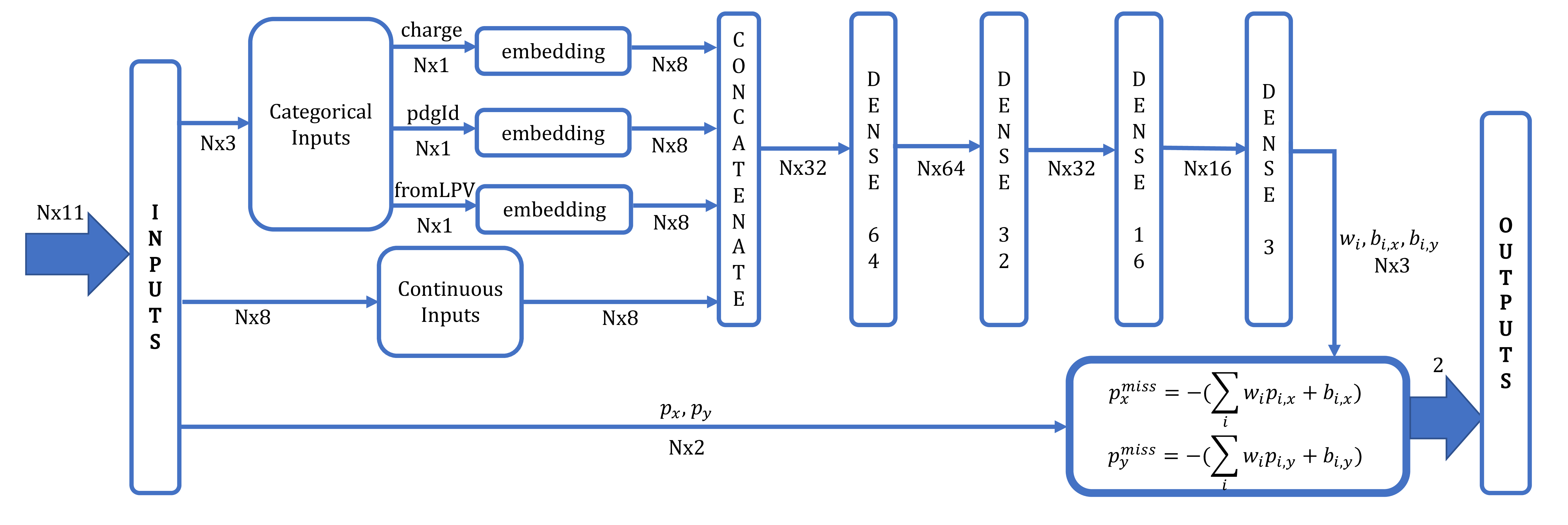
Figure 1:
The DEEPMET DNN architecture. For each event, all PF candidates in the event are considered as input. $ N\times n $ represents the number of PF candidates in the event multiplied by the dimensionality of the per-particle feature space, where $ n $ can be 1, 2, 3, 8, 16, 32, and 64 in the architecture. |
png pdf |
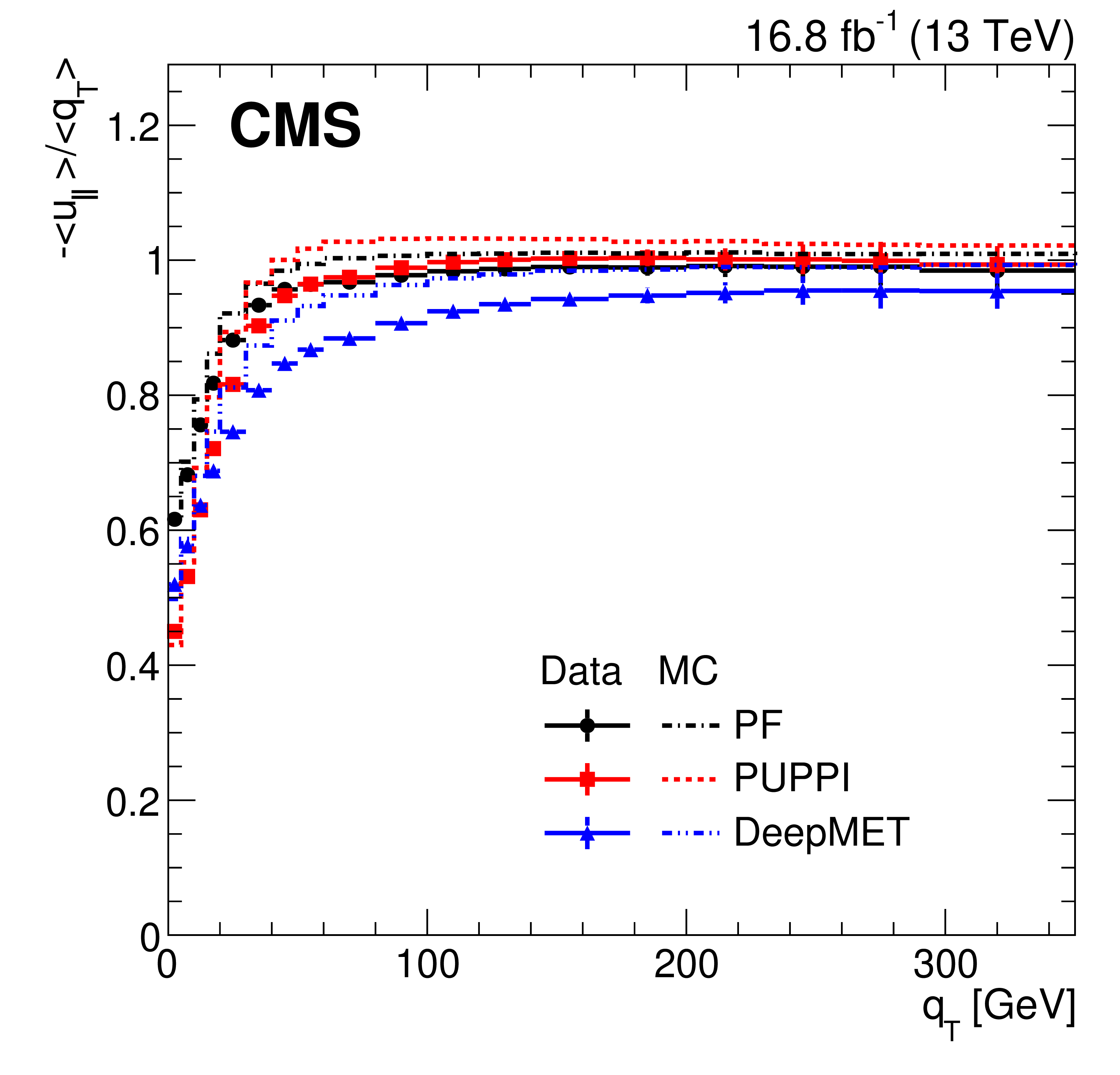
Figure 2:
Recoil responses of different $ {\vec p}_{\mathrm{T}}^{\, \text{miss}} $ estimators in data (markers) and MC simulations (dashed) after the $ \mathrm{Z}\to\mu\mu $ selections. |
png pdf |
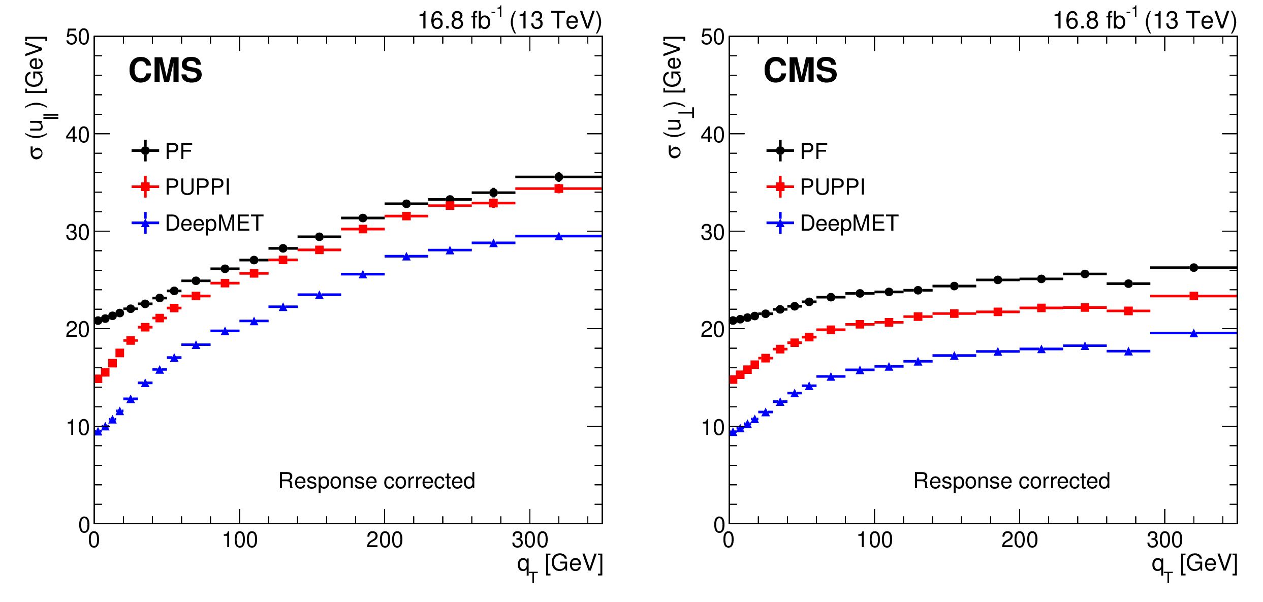
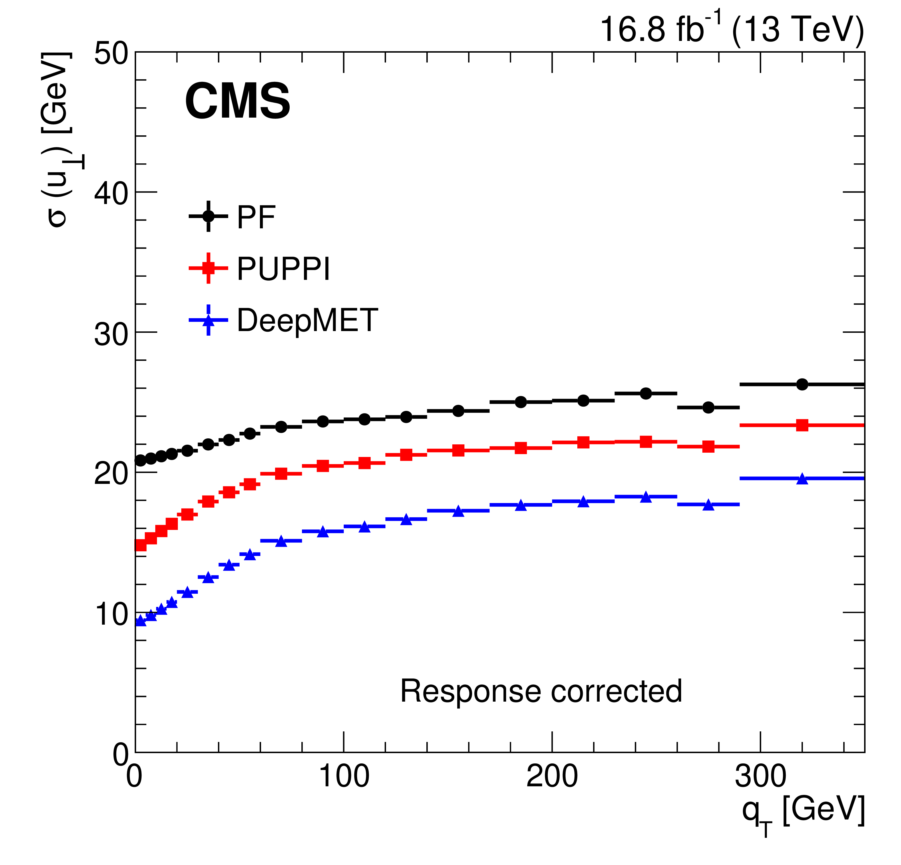
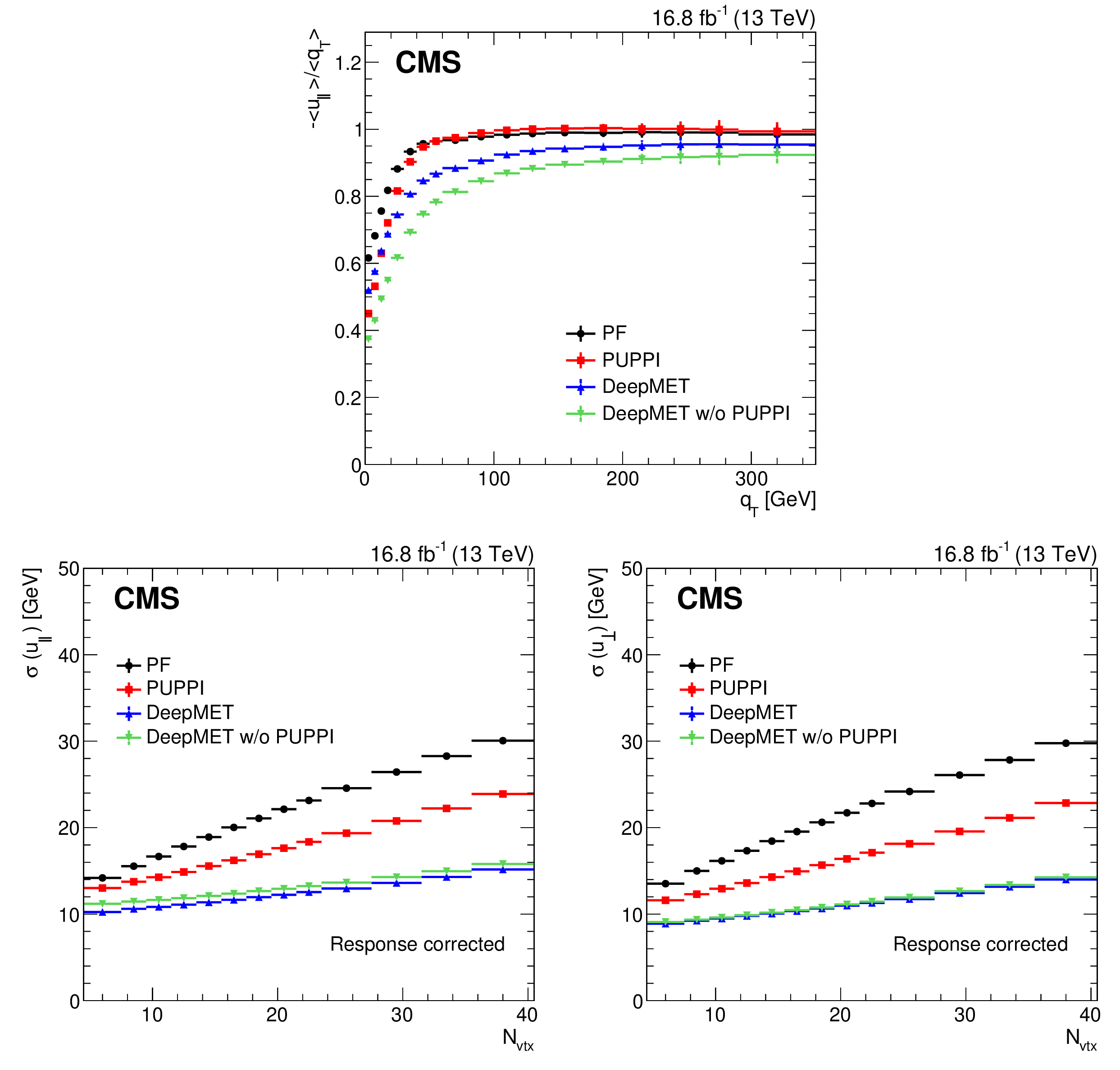
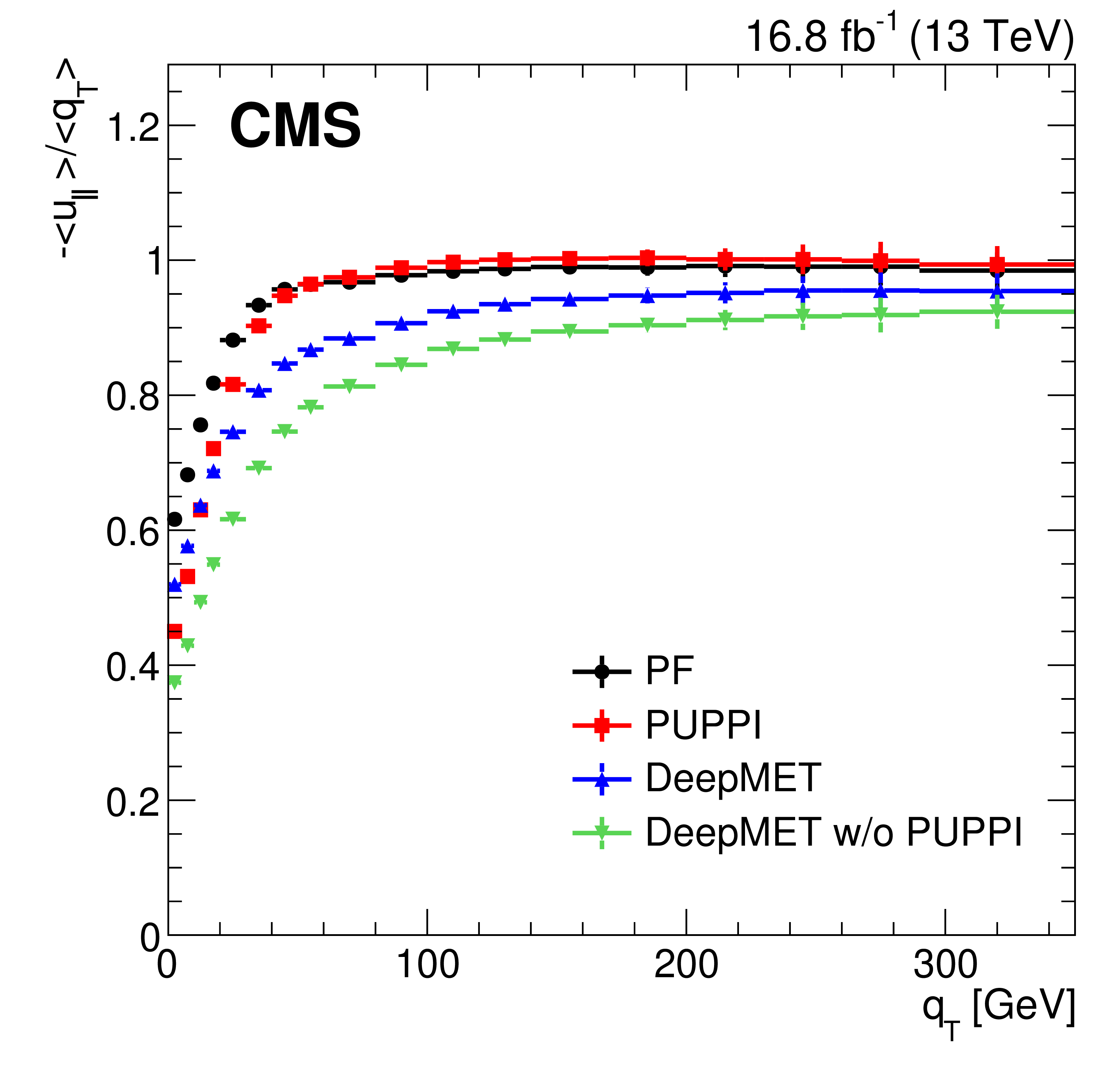
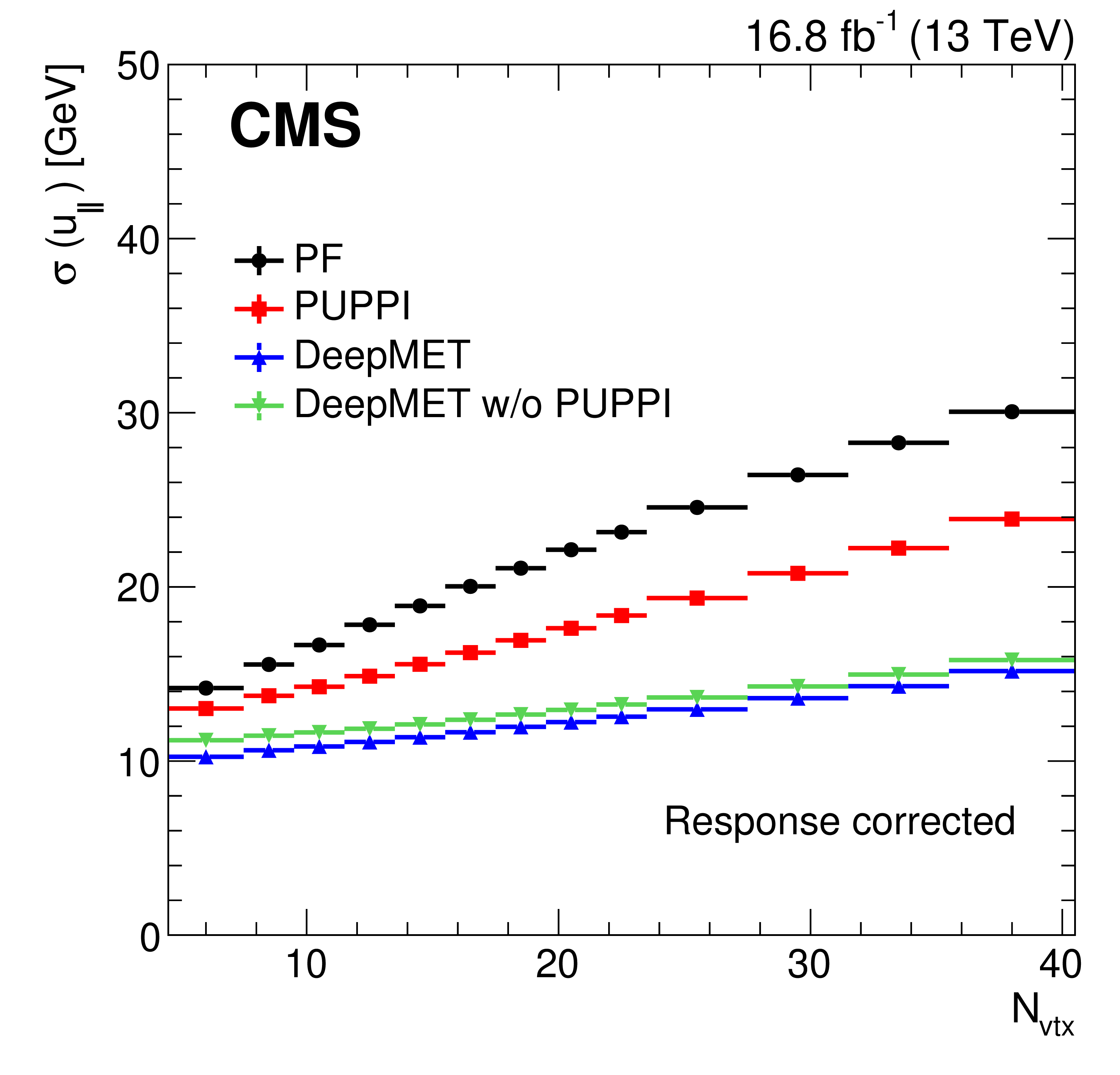
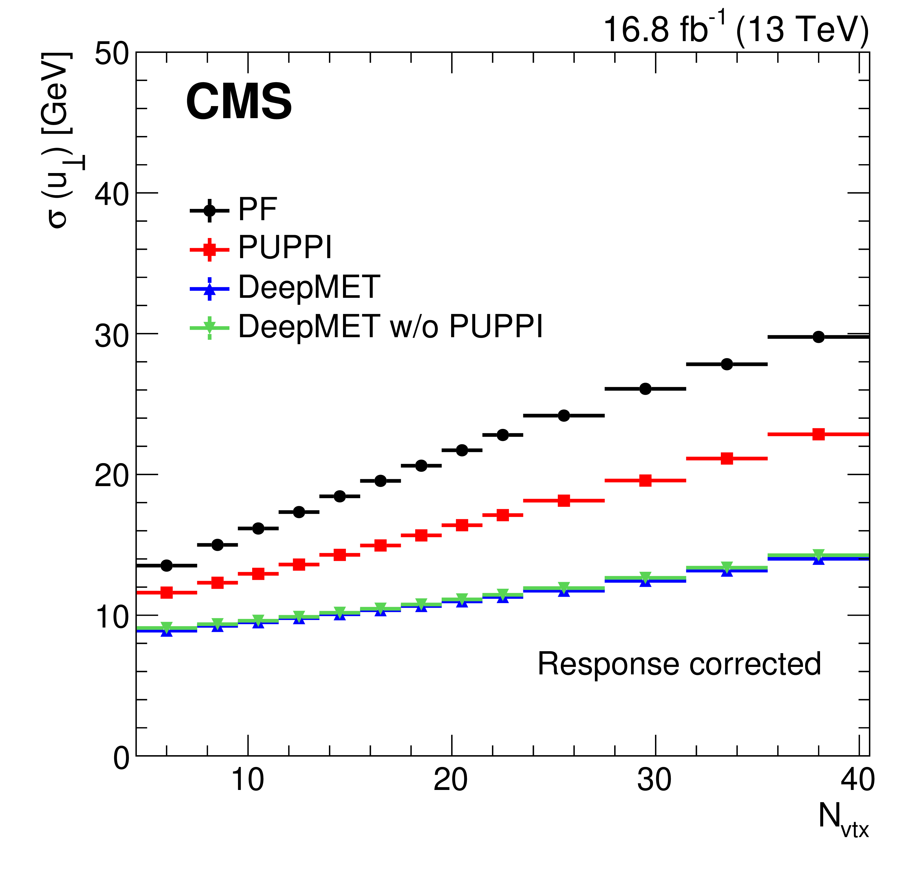
Figure 3:
Response-corrected resolutions of $ u_{\parallel} $ (left) and $ u_{\perp} $ (right) vs. $ q_{\mathrm{T}} $ of different $ {\vec p}_{\mathrm{T}}^{\, \text{miss}} $ estimators in data after the $ \mathrm{Z}\to\mu\mu $ selections. |
png pdf |
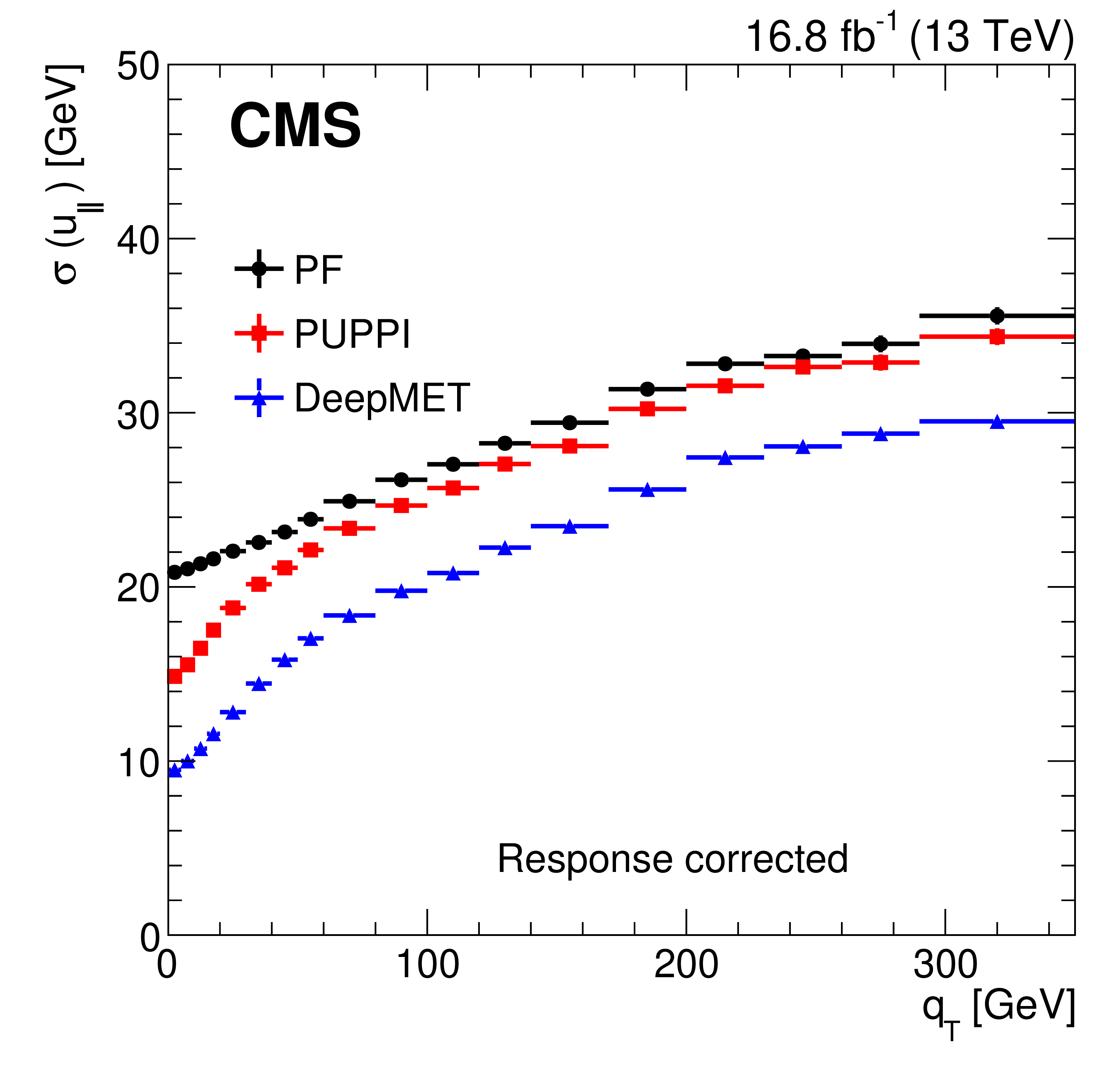
Figure 3-a:
Response-corrected resolutions of $ u_{\parallel} $ (left) and $ u_{\perp} $ (right) vs. $ q_{\mathrm{T}} $ of different $ {\vec p}_{\mathrm{T}}^{\, \text{miss}} $ estimators in data after the $ \mathrm{Z}\to\mu\mu $ selections. |
png pdf |
Figure 3-b:
Response-corrected resolutions of $ u_{\parallel} $ (left) and $ u_{\perp} $ (right) vs. $ q_{\mathrm{T}} $ of different $ {\vec p}_{\mathrm{T}}^{\, \text{miss}} $ estimators in data after the $ \mathrm{Z}\to\mu\mu $ selections. |
png pdf |
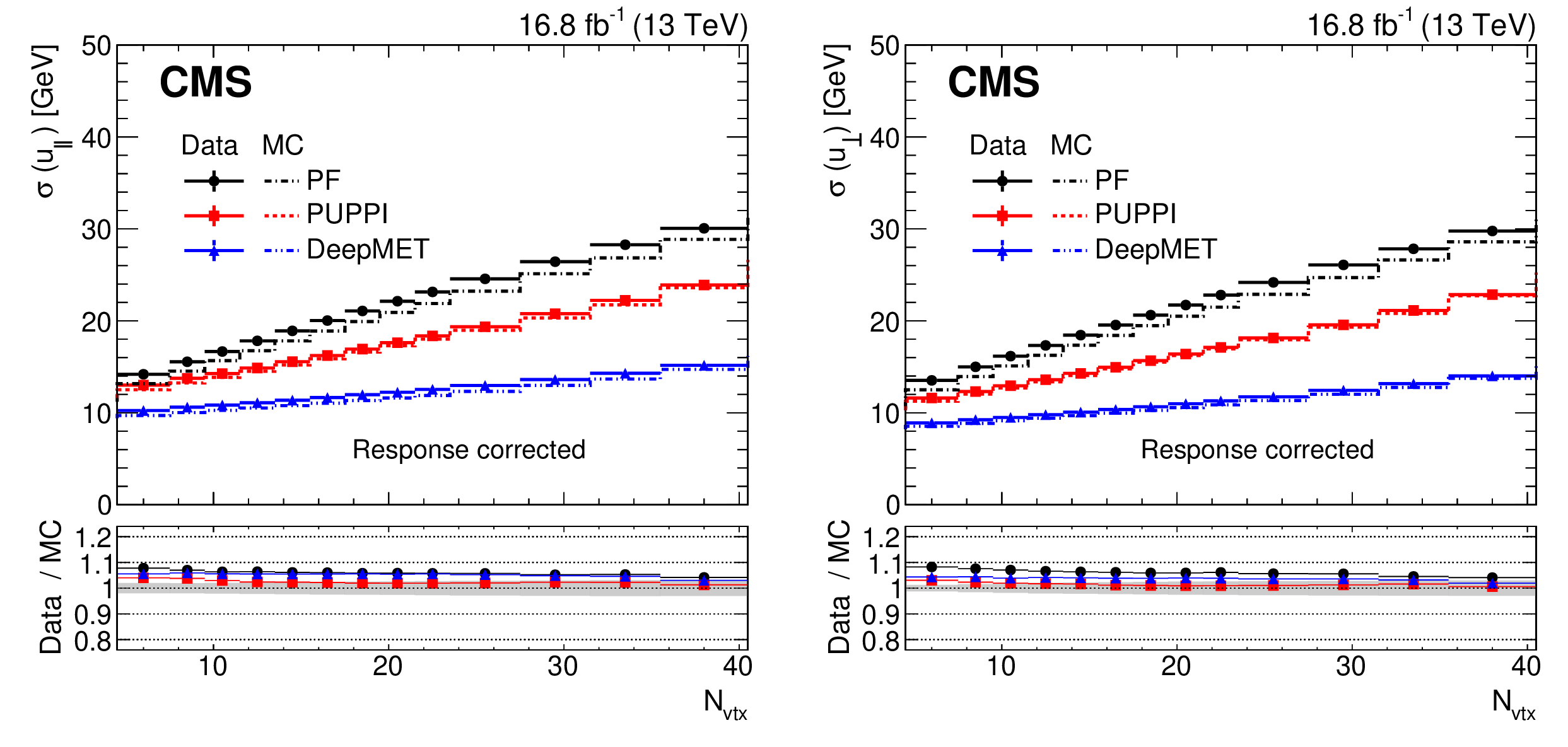
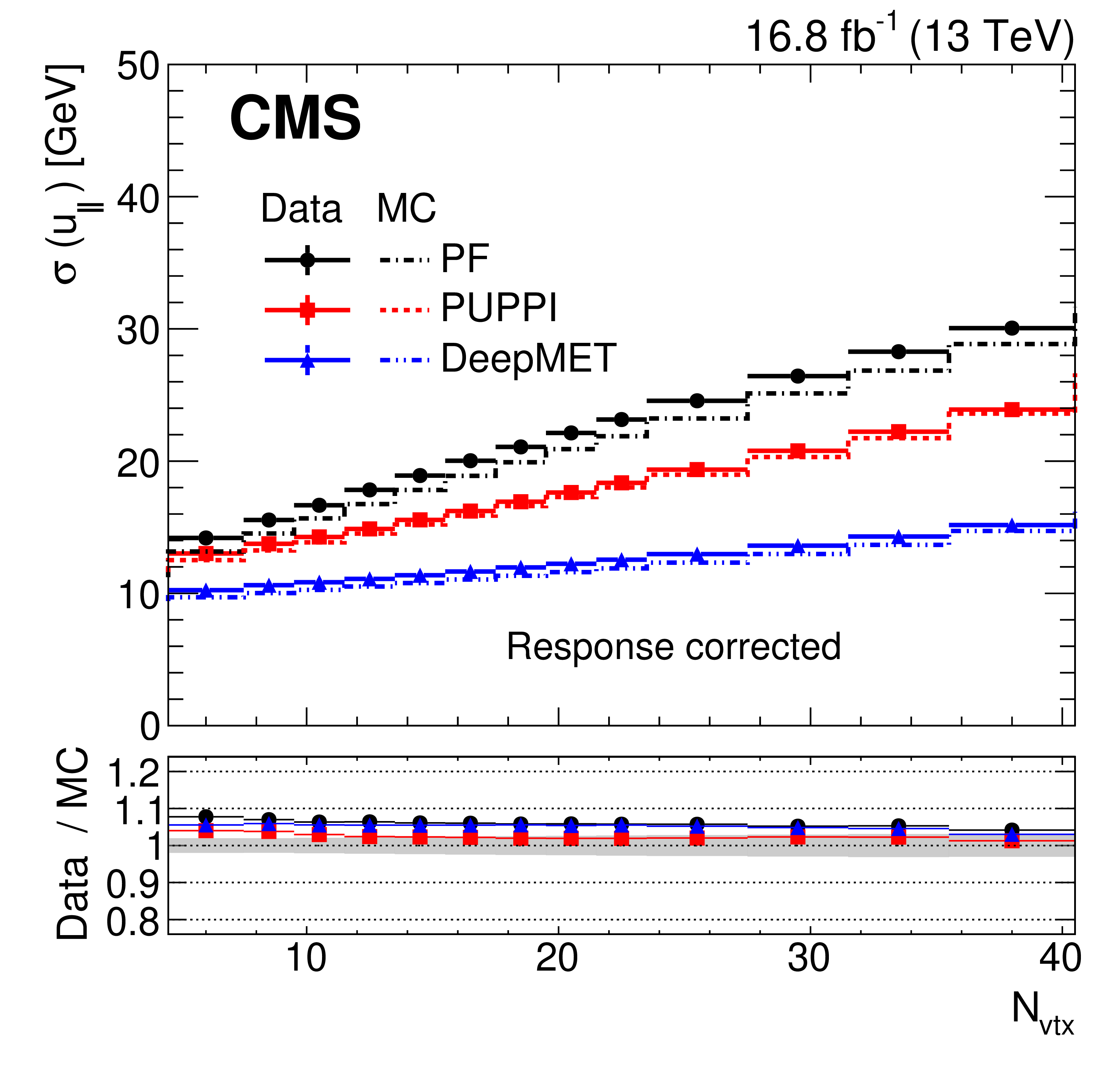
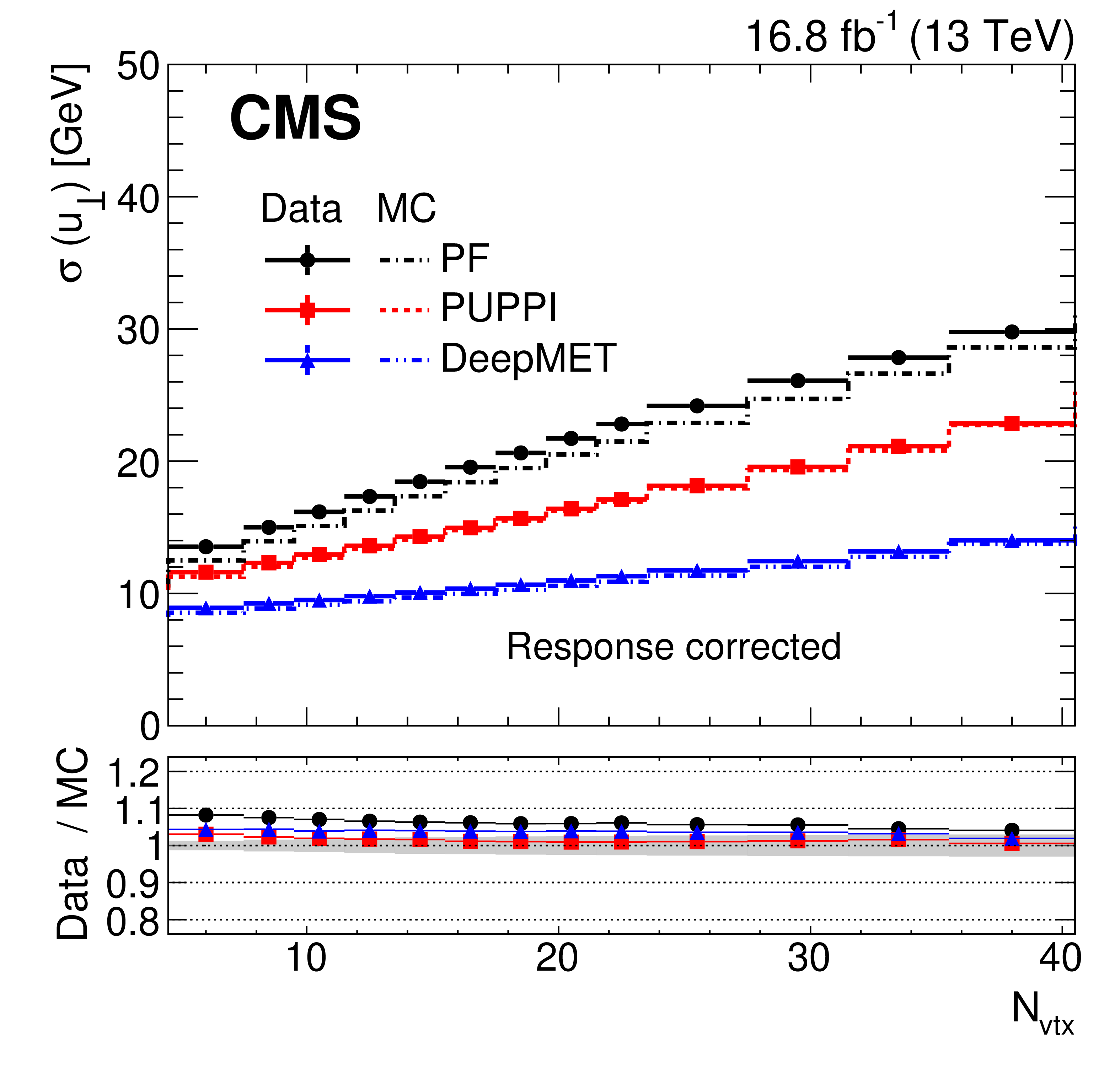
Figure 4:
Response-corrected resolutions of $ u_{\parallel} $ (left) and $ u_{\perp} $ (right) vs. $ $ number of reconstructed PVs of different $ {\vec p}_{\mathrm{T}}^{\, \text{miss}} $ estimators in data (solid) and MC simulations (dashed) after the $ \mathrm{Z}\to\mu\mu $ selections. The systematic uncertainties for PUPPI $ {\vec p}_{\mathrm{T}}^{\, \text{miss}} $ due to the JES, the JER, and $ E_U $ are added in quadrature and displayed with the gray band. |
png pdf |
Figure 4-a:
Response-corrected resolutions of $ u_{\parallel} $ (left) and $ u_{\perp} $ (right) vs. $ $ number of reconstructed PVs of different $ {\vec p}_{\mathrm{T}}^{\, \text{miss}} $ estimators in data (solid) and MC simulations (dashed) after the $ \mathrm{Z}\to\mu\mu $ selections. The systematic uncertainties for PUPPI $ {\vec p}_{\mathrm{T}}^{\, \text{miss}} $ due to the JES, the JER, and $ E_U $ are added in quadrature and displayed with the gray band. |
png pdf |
Figure 4-b:
Response-corrected resolutions of $ u_{\parallel} $ (left) and $ u_{\perp} $ (right) vs. $ $ number of reconstructed PVs of different $ {\vec p}_{\mathrm{T}}^{\, \text{miss}} $ estimators in data (solid) and MC simulations (dashed) after the $ \mathrm{Z}\to\mu\mu $ selections. The systematic uncertainties for PUPPI $ {\vec p}_{\mathrm{T}}^{\, \text{miss}} $ due to the JES, the JER, and $ E_U $ are added in quadrature and displayed with the gray band. |
png pdf |
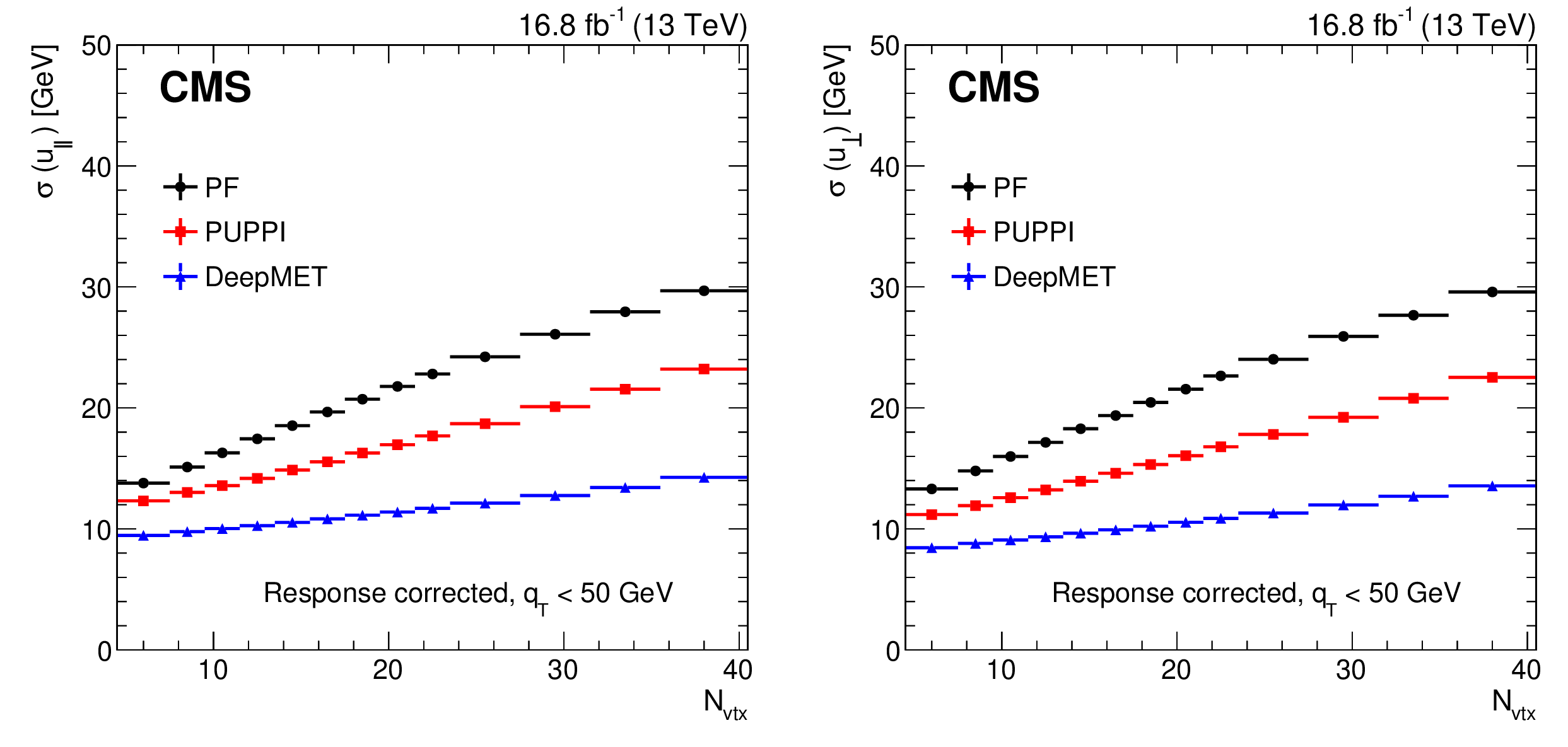
Figure 5:
Response-corrected resolutions of $ u_{\parallel} $ (left) and $ u_{\perp} $ (right) vs. $ $ number of reconstructed PVs of different $ {\vec p}_{\mathrm{T}}^{\, \text{miss}} $ estimators in data after the $ \mathrm{Z}\to\mu\mu $ selections in the region with $ q_{\mathrm{T}} $ smaller than 50 GeV. |
png pdf |
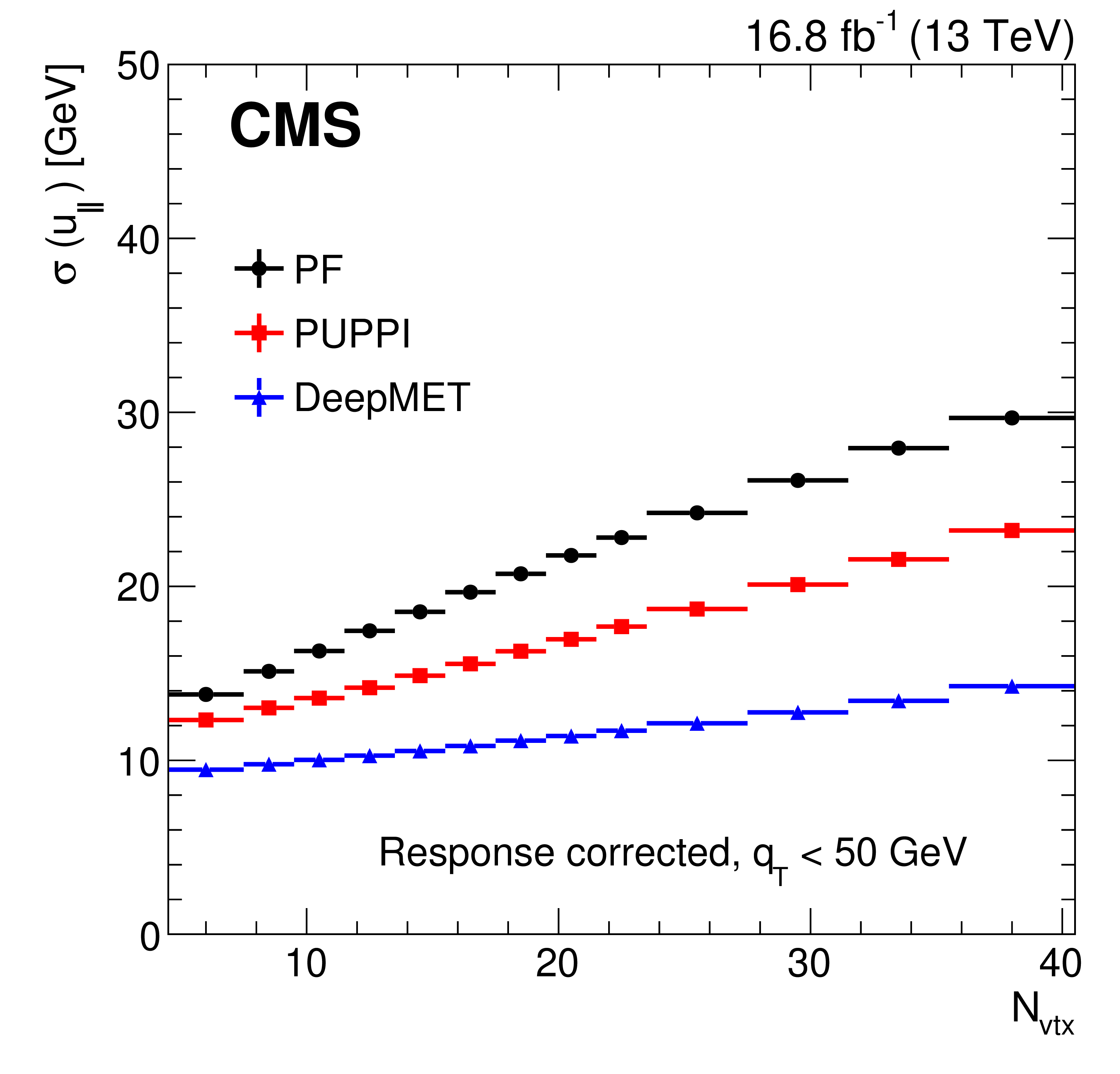
Figure 5-a:
Response-corrected resolutions of $ u_{\parallel} $ (left) and $ u_{\perp} $ (right) vs. $ $ number of reconstructed PVs of different $ {\vec p}_{\mathrm{T}}^{\, \text{miss}} $ estimators in data after the $ \mathrm{Z}\to\mu\mu $ selections in the region with $ q_{\mathrm{T}} $ smaller than 50 GeV. |
png pdf |
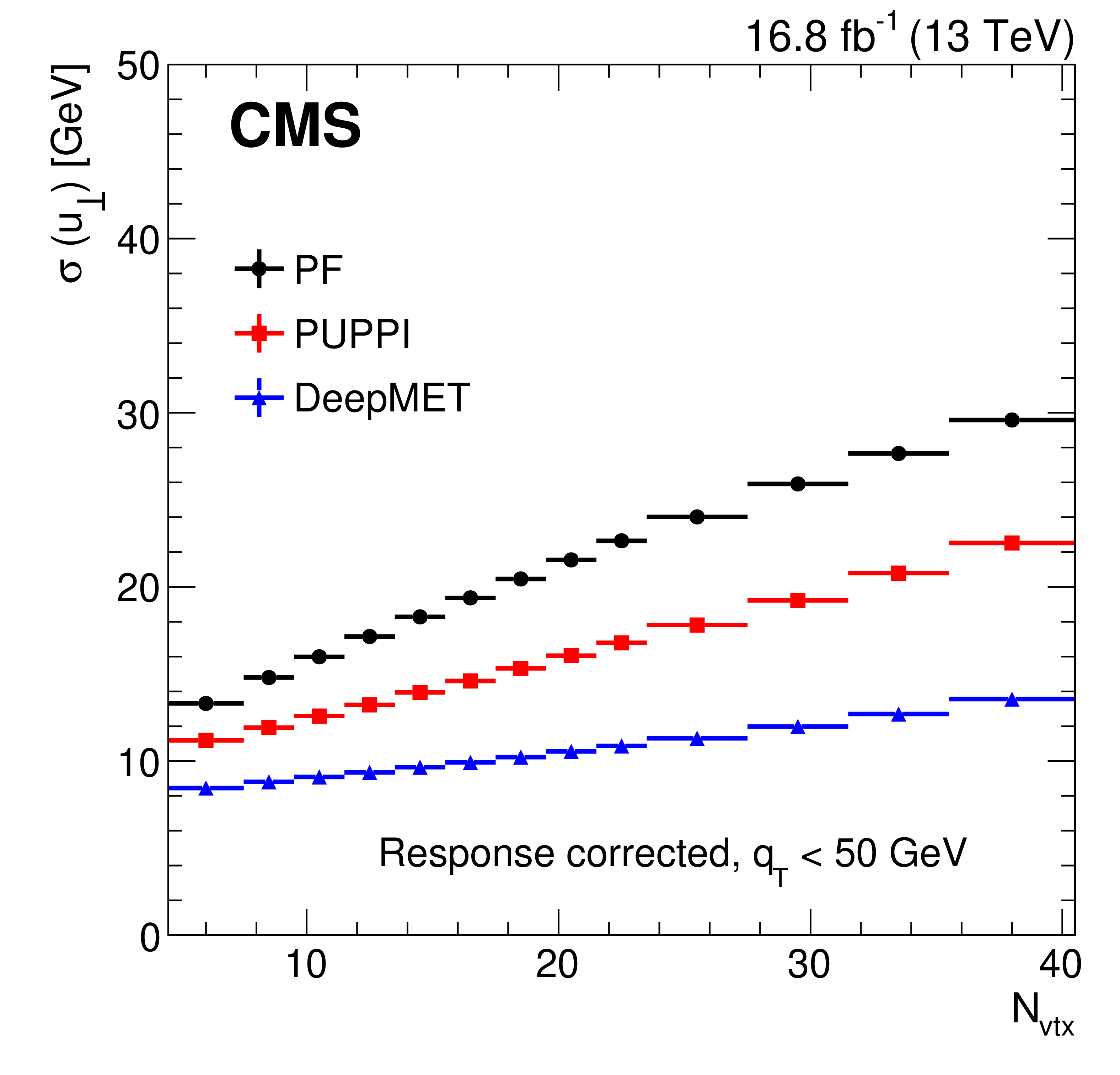
Figure 5-b:
Response-corrected resolutions of $ u_{\parallel} $ (left) and $ u_{\perp} $ (right) vs. $ $ number of reconstructed PVs of different $ {\vec p}_{\mathrm{T}}^{\, \text{miss}} $ estimators in data after the $ \mathrm{Z}\to\mu\mu $ selections in the region with $ q_{\mathrm{T}} $ smaller than 50 GeV. |
png pdf |
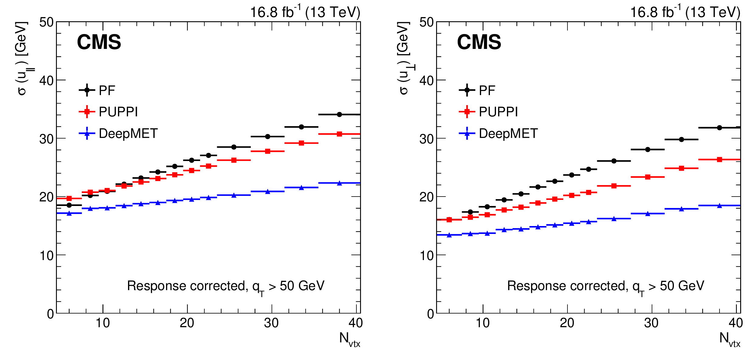
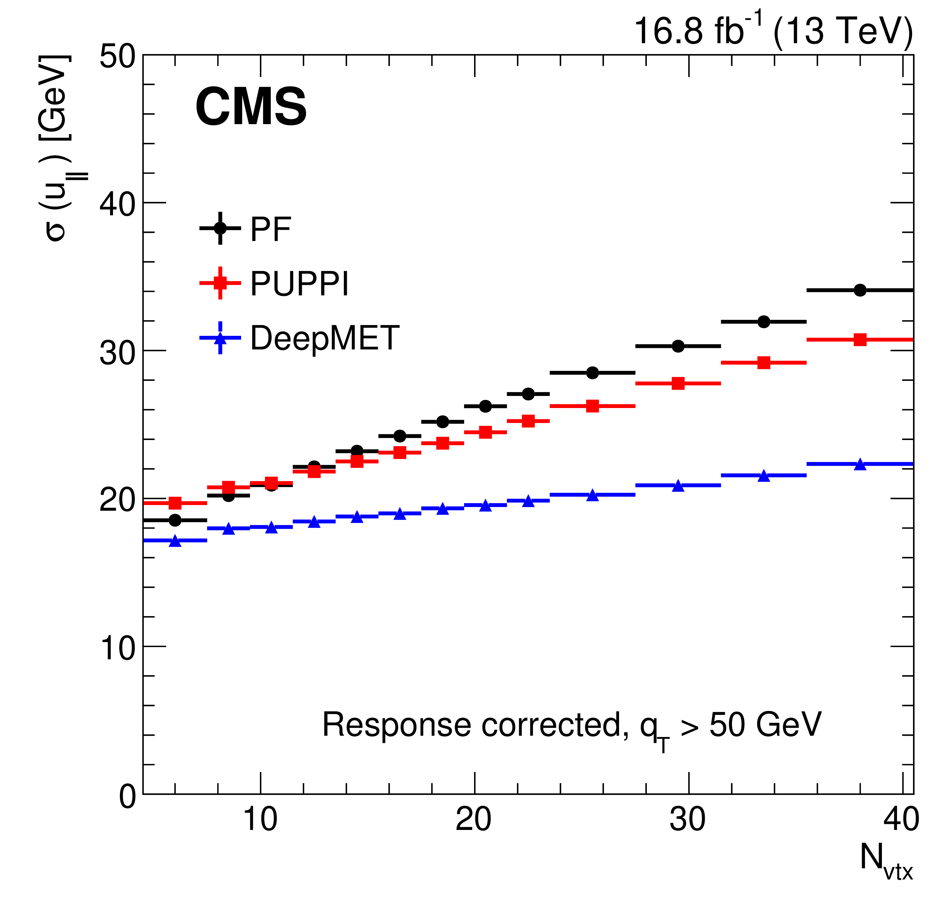
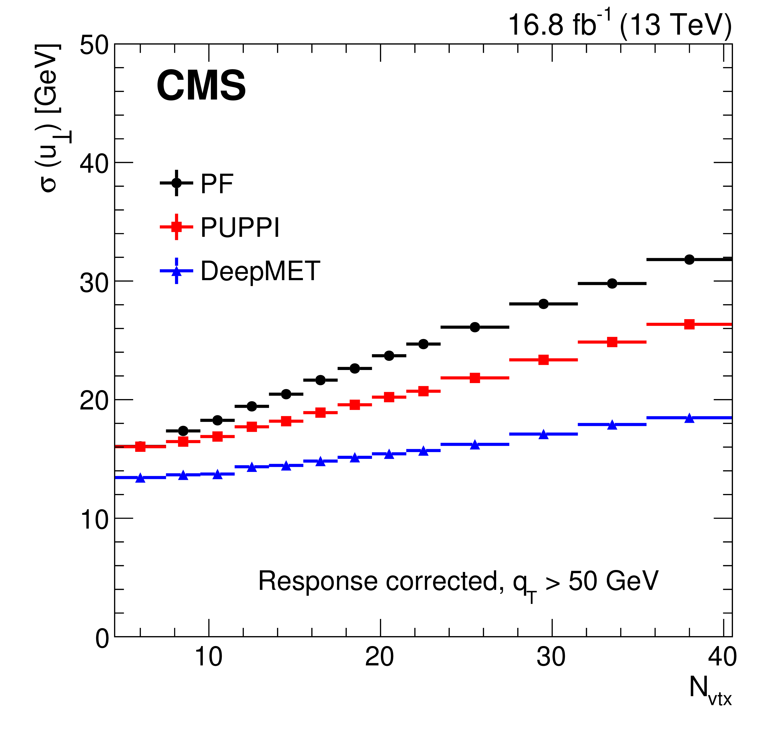
Figure 6:
Response-corrected resolutions of $ u_{\parallel} $ (left) and $ u_{\perp} $ (right) vs. $ $ number of reconstructed PVs of different $ {\vec p}_{\mathrm{T}}^{\, \text{miss}} $ estimators in data after the $ \mathrm{Z}\to\mu\mu $ selections in the region with $ q_{\mathrm{T}} $ larger than 50 GeV. |
png pdf |
Figure 6-a:
Response-corrected resolutions of $ u_{\parallel} $ (left) and $ u_{\perp} $ (right) vs. $ $ number of reconstructed PVs of different $ {\vec p}_{\mathrm{T}}^{\, \text{miss}} $ estimators in data after the $ \mathrm{Z}\to\mu\mu $ selections in the region with $ q_{\mathrm{T}} $ larger than 50 GeV. |
png pdf |
Figure 6-b:
Response-corrected resolutions of $ u_{\parallel} $ (left) and $ u_{\perp} $ (right) vs. $ $ number of reconstructed PVs of different $ {\vec p}_{\mathrm{T}}^{\, \text{miss}} $ estimators in data after the $ \mathrm{Z}\to\mu\mu $ selections in the region with $ q_{\mathrm{T}} $ larger than 50 GeV. |
png pdf |
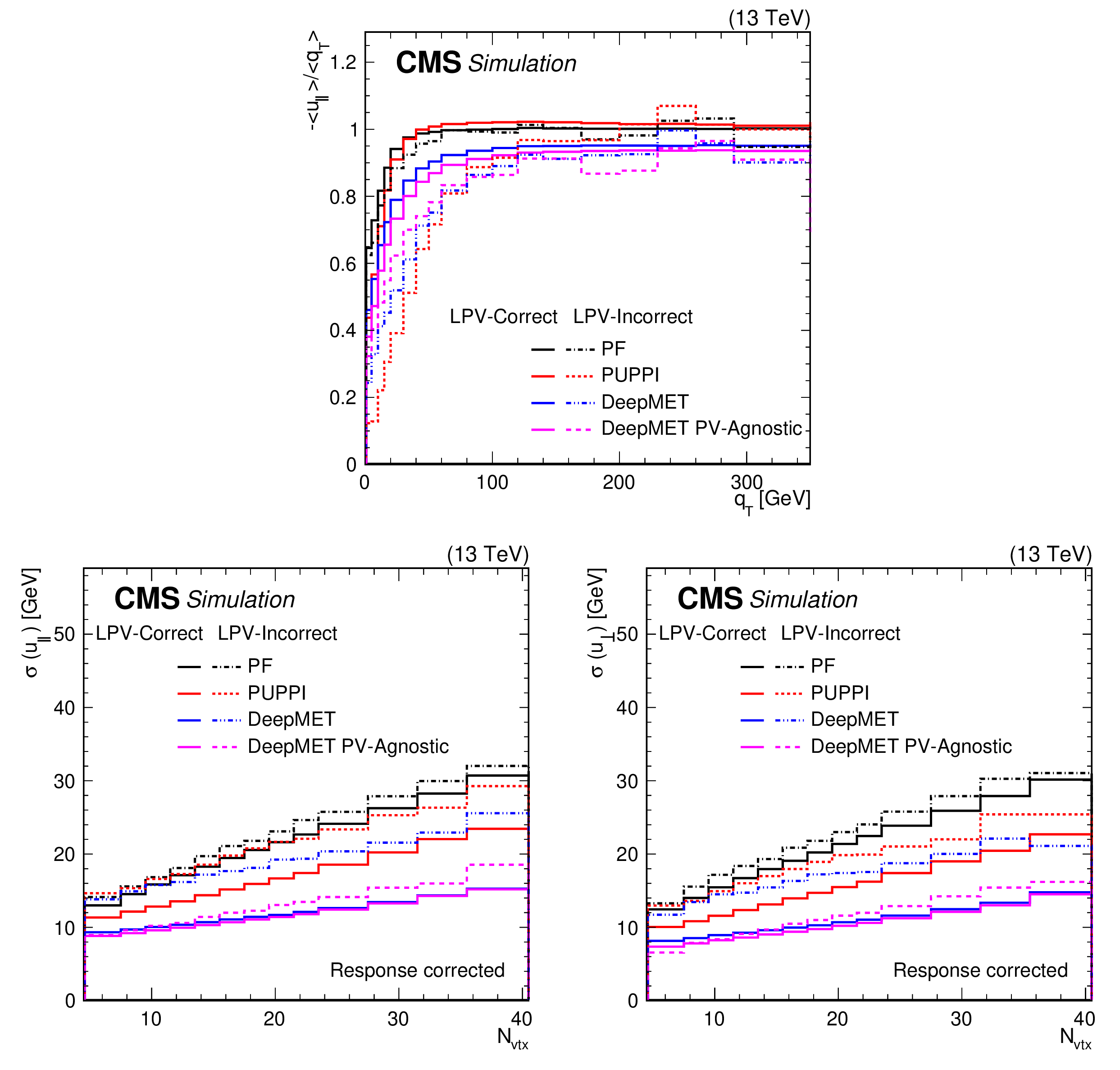
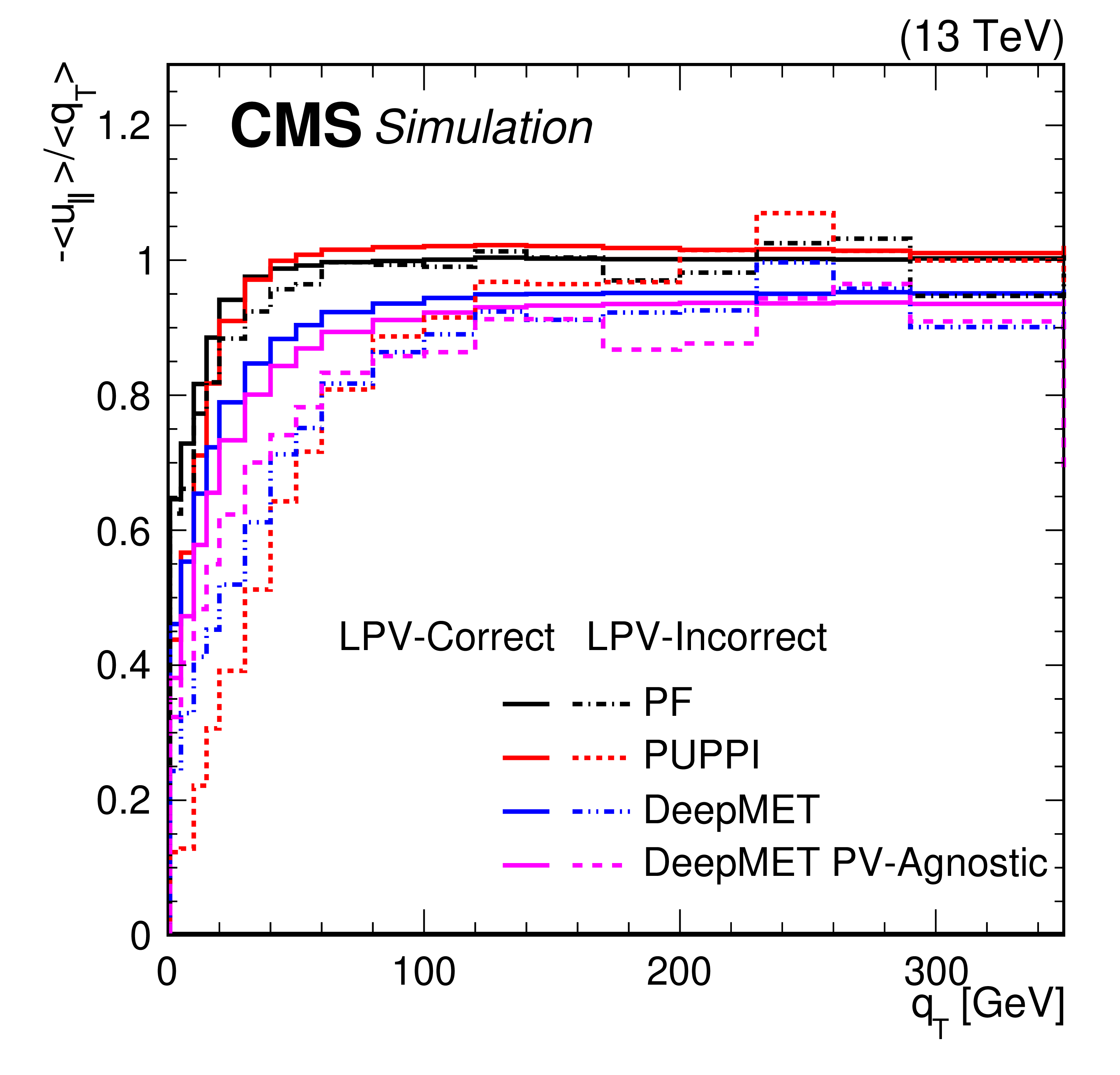
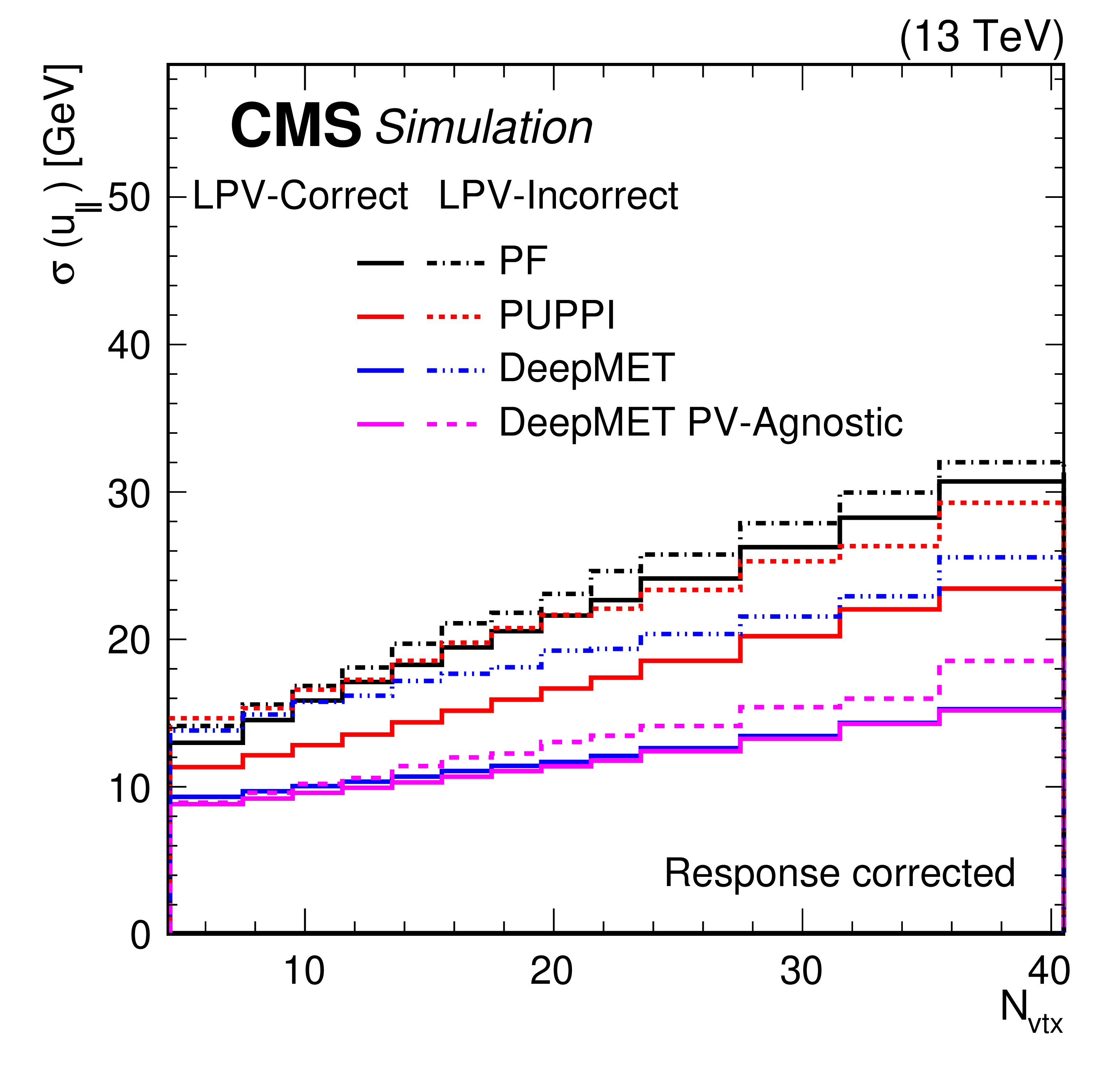
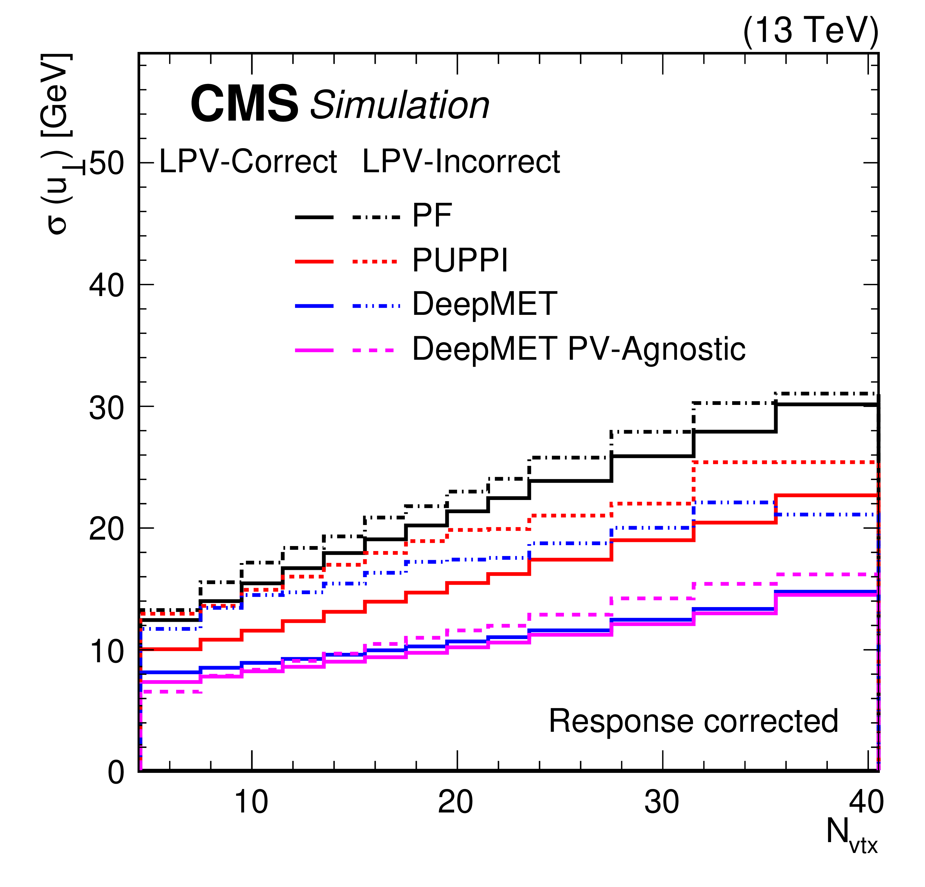
Figure 7:
Response (upper), response-corrected resolutions of $ u_{\parallel} $ (lower left) and $ u_{\perp} $ (lower right) of different $ {\vec p}_{\mathrm{T}}^{\, \text{miss}} $ estimators in W+jets MC simulations. Solid (dashed) lines are from events where the LPV is (in)correctly identified. |
png pdf |
Figure 7-a:
Response (upper), response-corrected resolutions of $ u_{\parallel} $ (lower left) and $ u_{\perp} $ (lower right) of different $ {\vec p}_{\mathrm{T}}^{\, \text{miss}} $ estimators in W+jets MC simulations. Solid (dashed) lines are from events where the LPV is (in)correctly identified. |
png pdf |
Figure 7-b:
Response (upper), response-corrected resolutions of $ u_{\parallel} $ (lower left) and $ u_{\perp} $ (lower right) of different $ {\vec p}_{\mathrm{T}}^{\, \text{miss}} $ estimators in W+jets MC simulations. Solid (dashed) lines are from events where the LPV is (in)correctly identified. |
png pdf |
Figure 7-c:
Response (upper), response-corrected resolutions of $ u_{\parallel} $ (lower left) and $ u_{\perp} $ (lower right) of different $ {\vec p}_{\mathrm{T}}^{\, \text{miss}} $ estimators in W+jets MC simulations. Solid (dashed) lines are from events where the LPV is (in)correctly identified. |
png pdf |
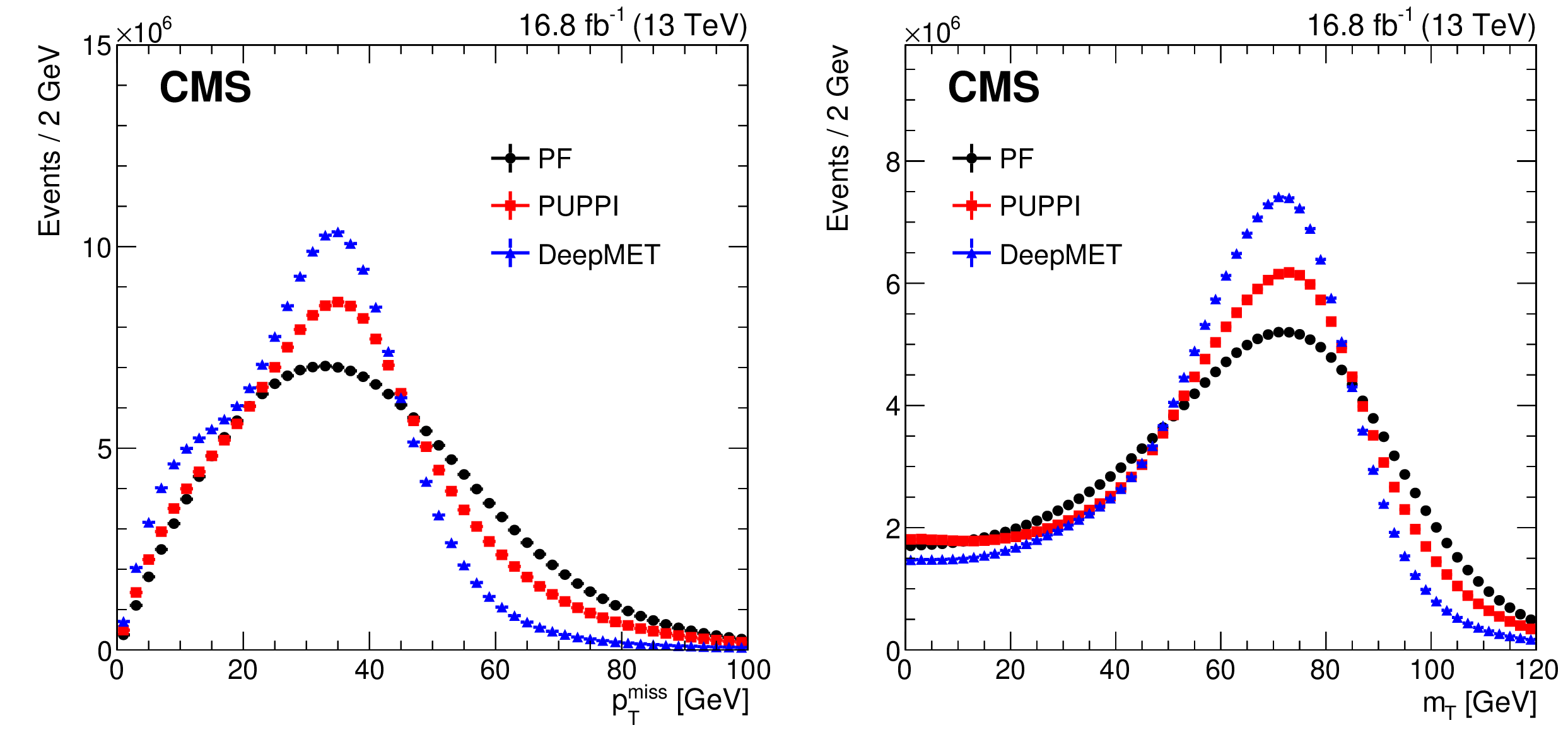
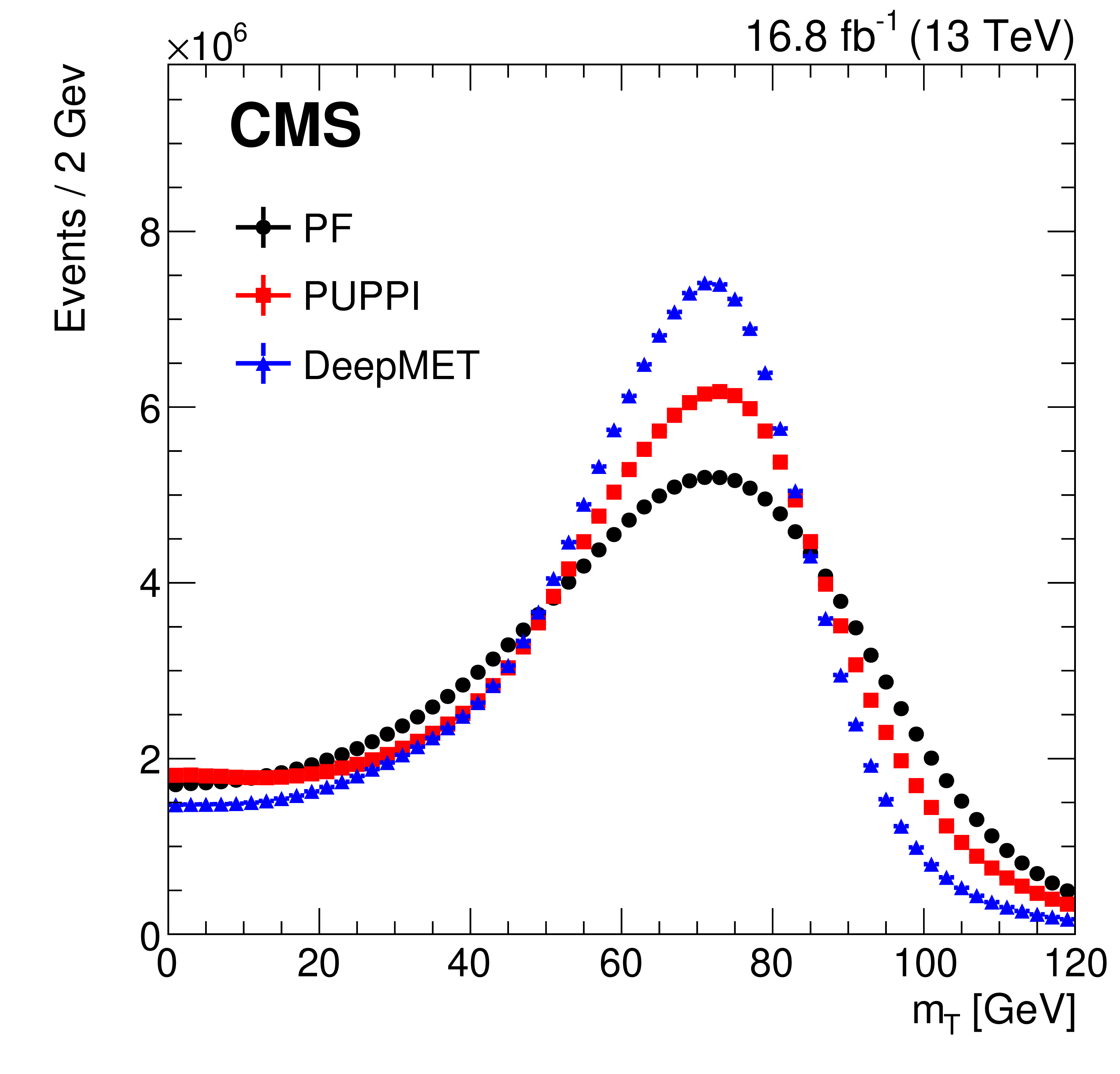
Figure 8:
Distributions of $ p_{\mathrm{T}}^\text{miss} $ (left) and $ m_\mathrm{T} $ (right) of different $ {\vec p}_{\mathrm{T}}^{\, \text{miss}} $ estimators in data after $ \mathrm{W}\to\mu\nu $ selections. |
png pdf |
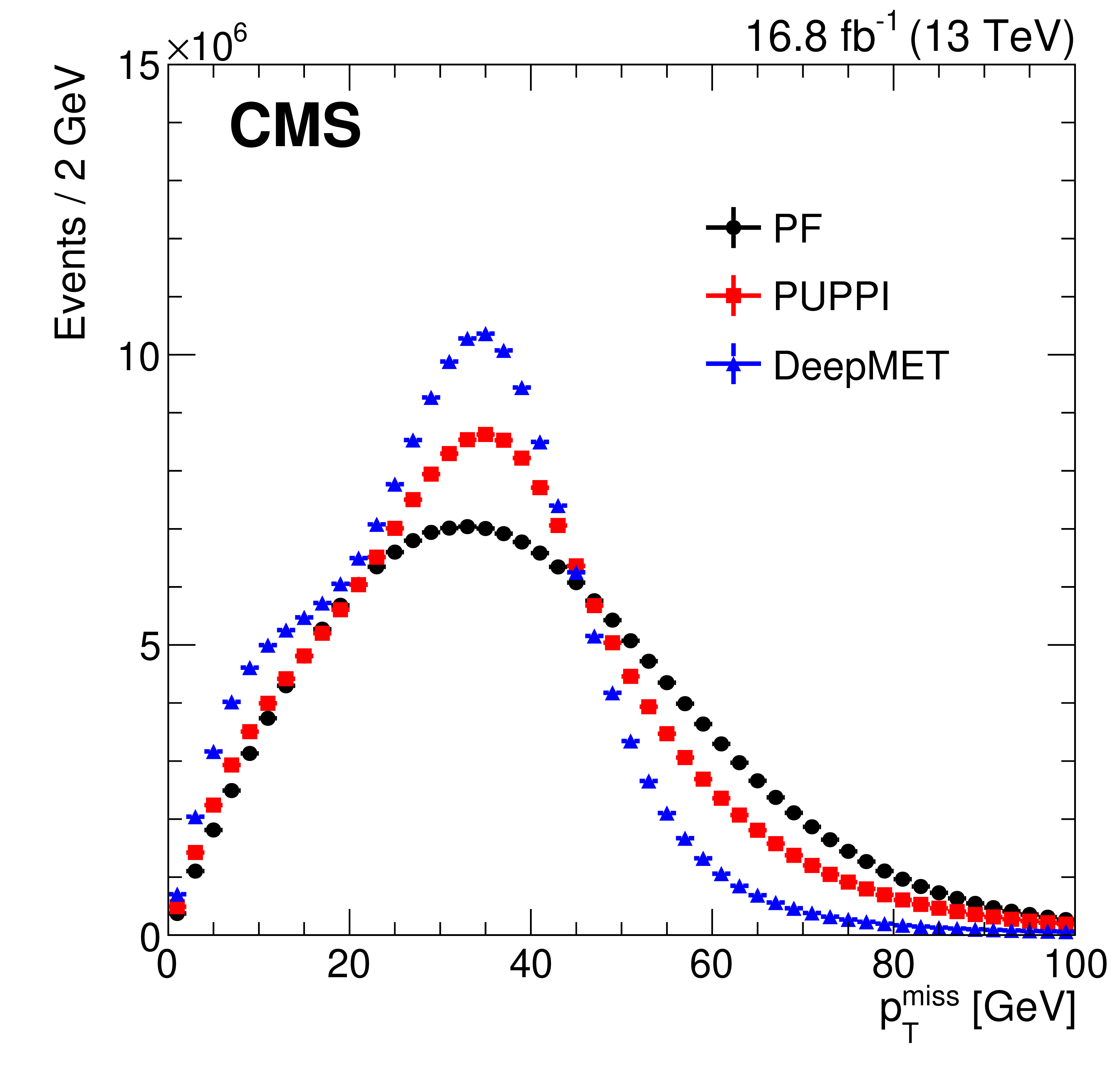
Figure 8-a:
Distributions of $ p_{\mathrm{T}}^\text{miss} $ (left) and $ m_\mathrm{T} $ (right) of different $ {\vec p}_{\mathrm{T}}^{\, \text{miss}} $ estimators in data after $ \mathrm{W}\to\mu\nu $ selections. |
png pdf |
Figure 8-b:
Distributions of $ p_{\mathrm{T}}^\text{miss} $ (left) and $ m_\mathrm{T} $ (right) of different $ {\vec p}_{\mathrm{T}}^{\, \text{miss}} $ estimators in data after $ \mathrm{W}\to\mu\nu $ selections. |
png pdf |
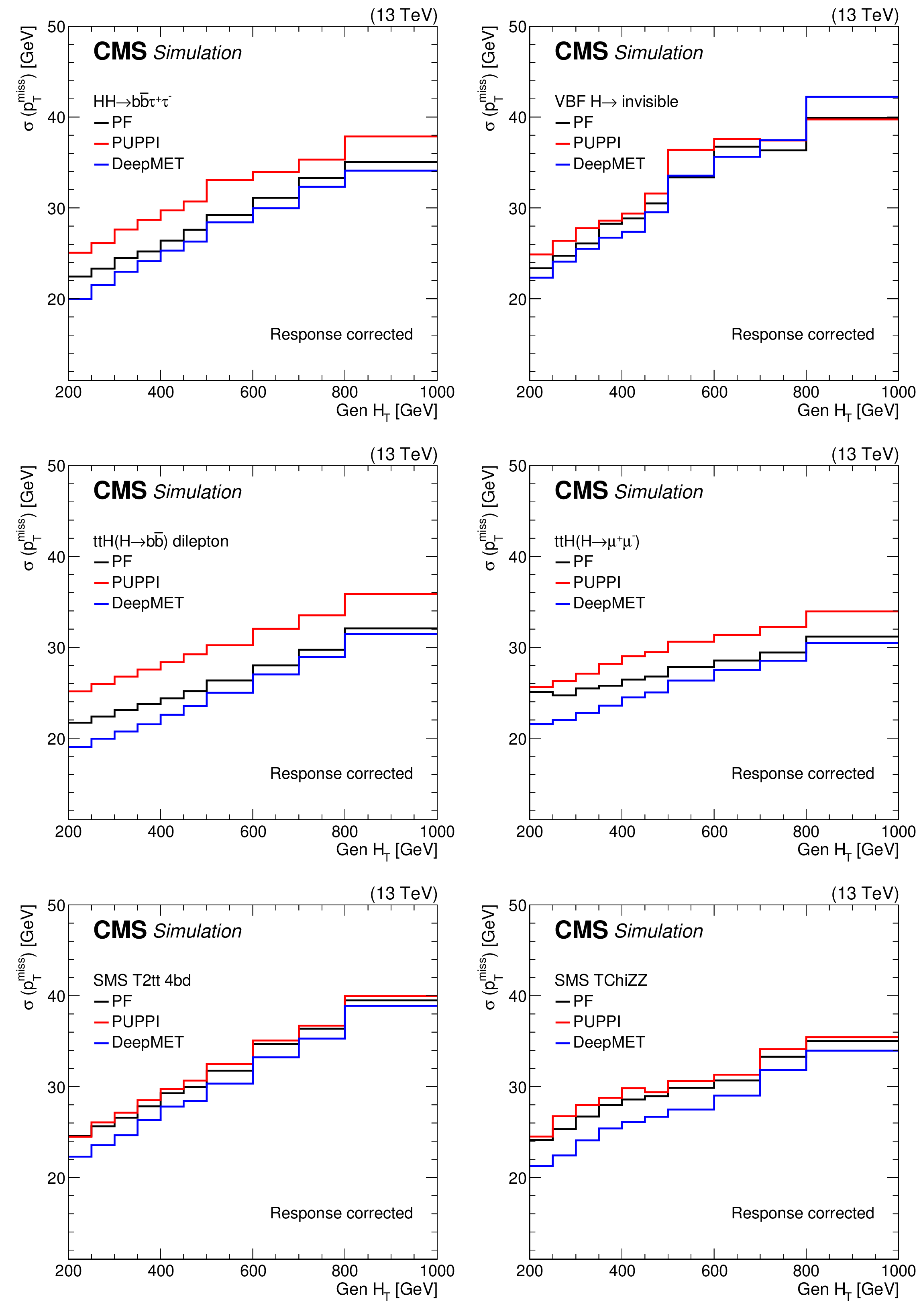
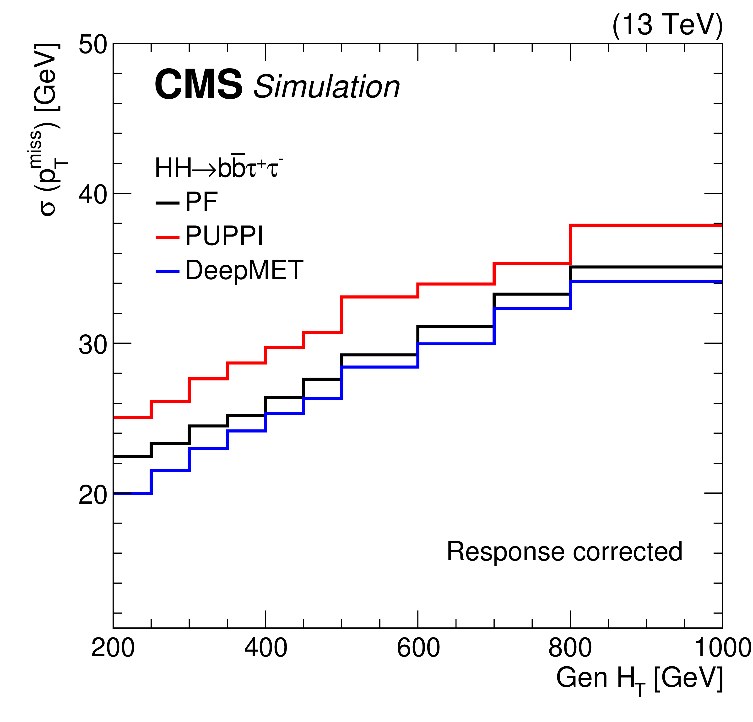
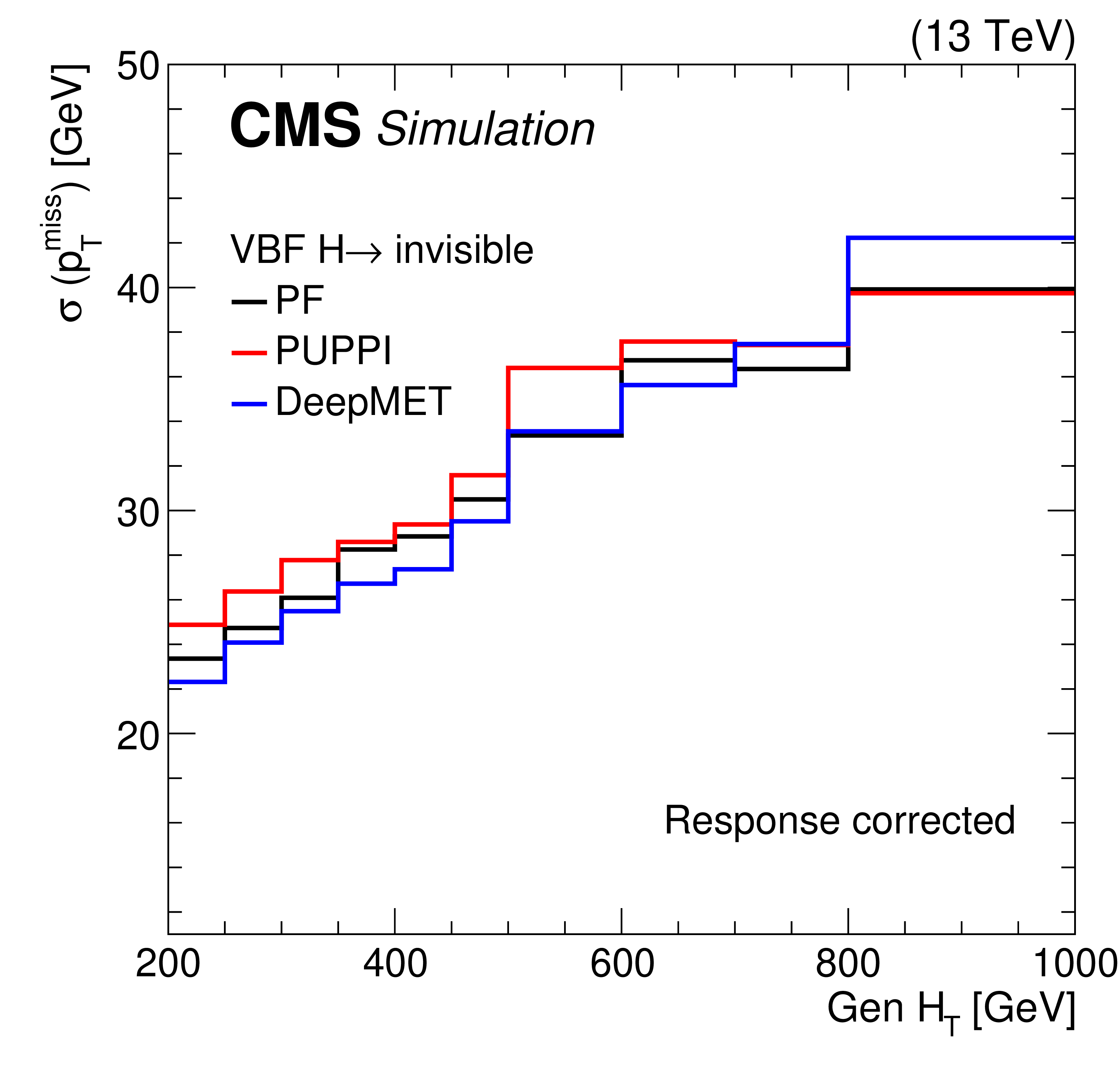
Figure 9:
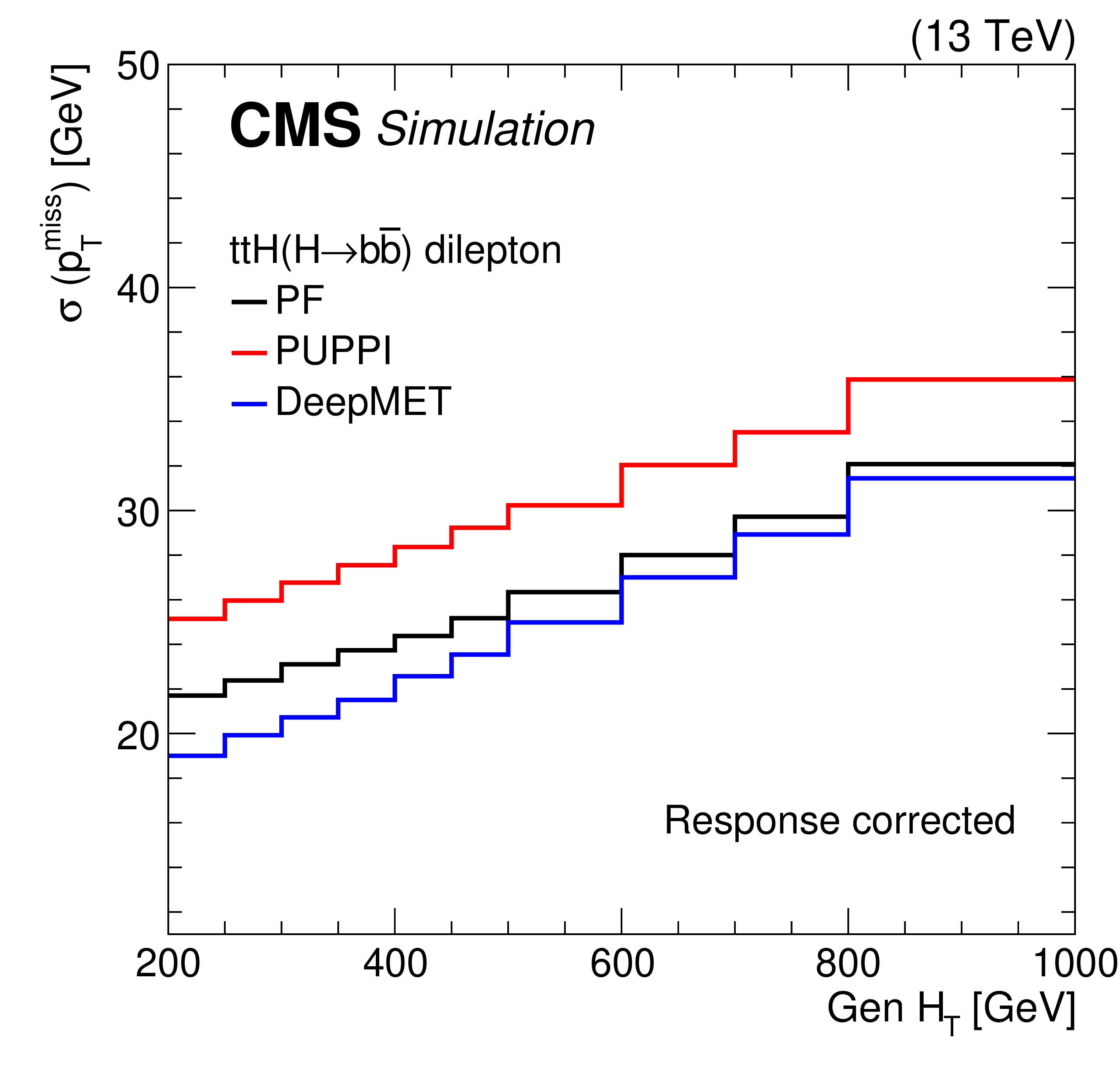
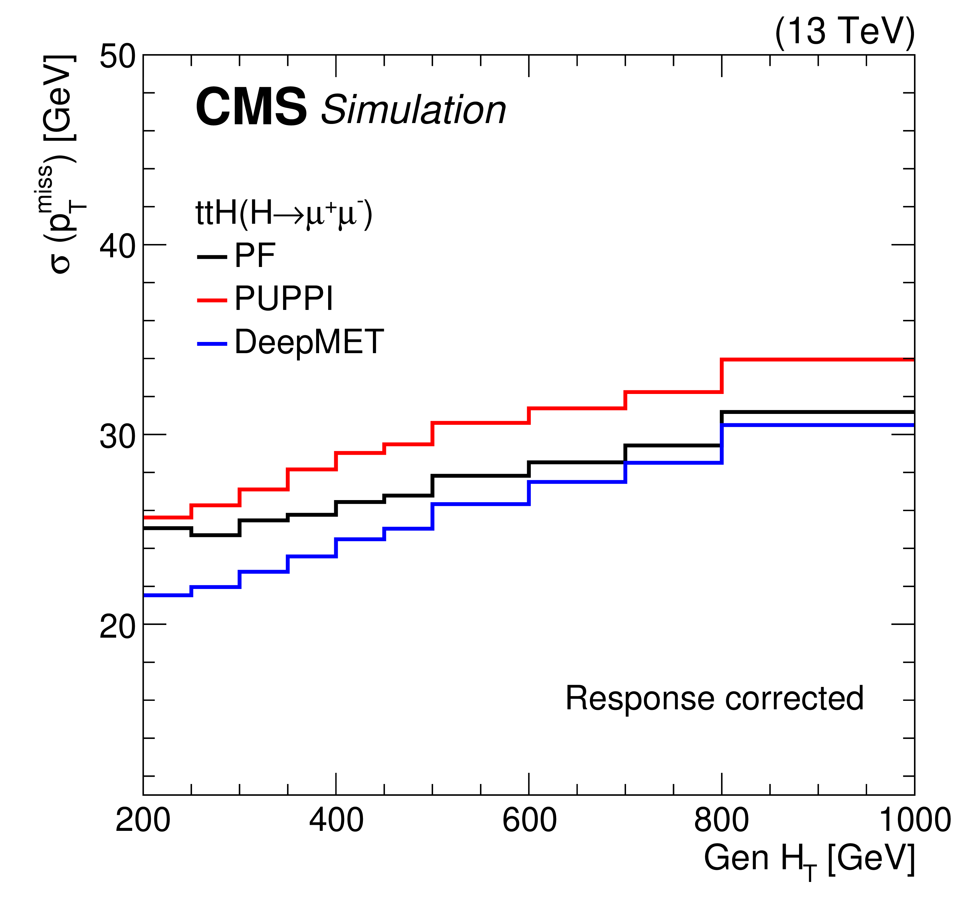
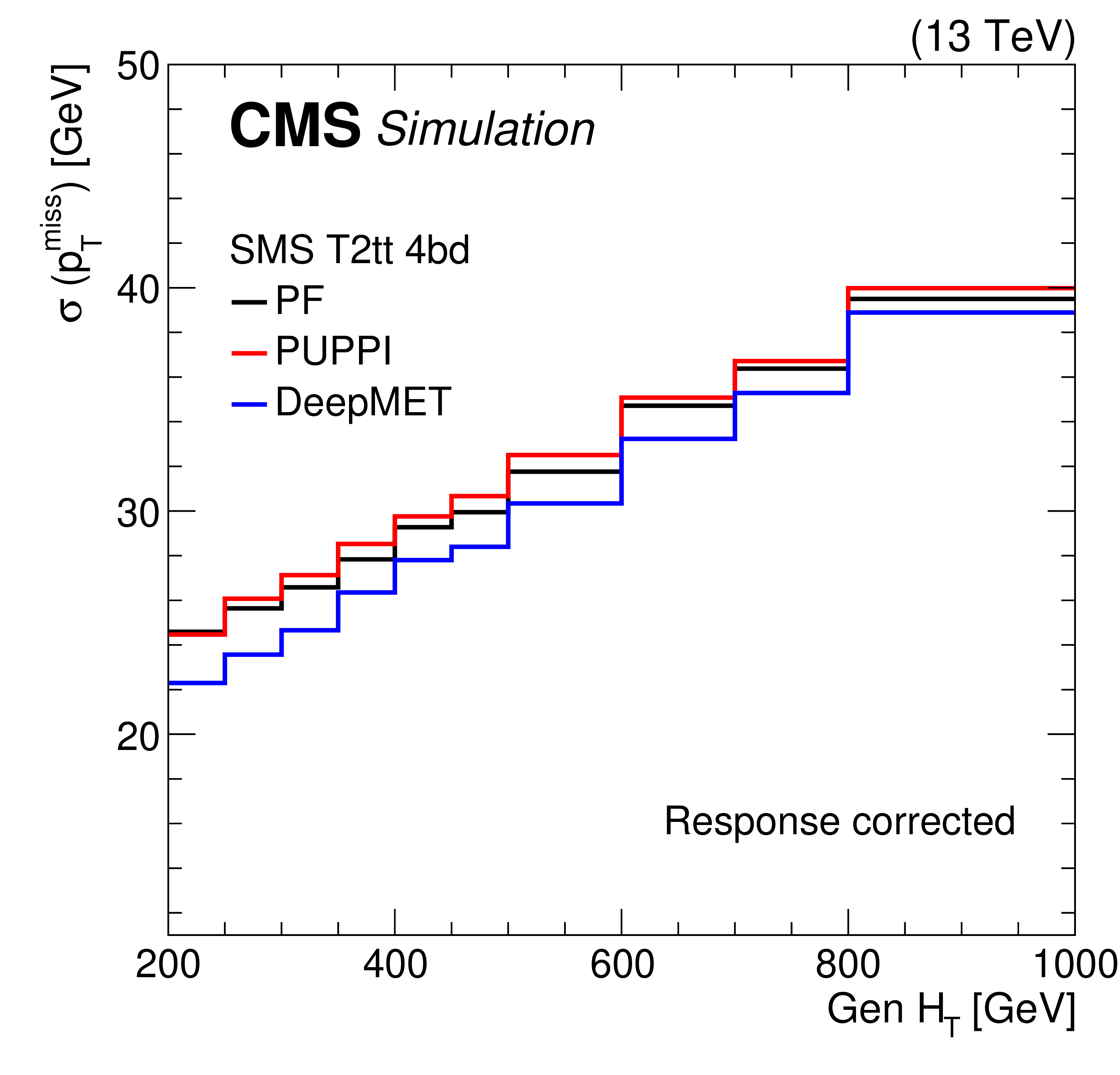
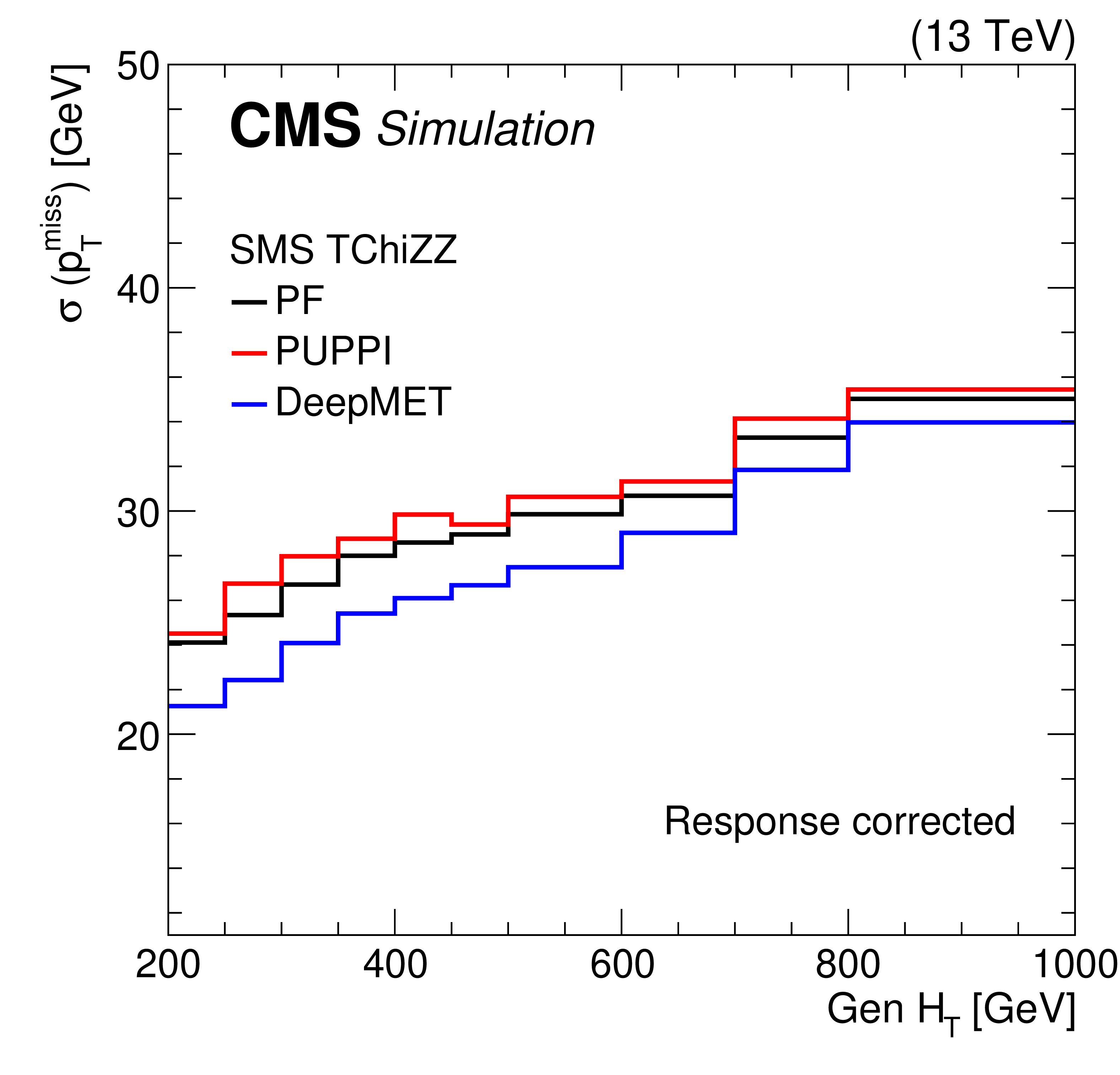
Comparison of $ p_{\mathrm{T}}^\text{miss} $ resolution for various physics processes in simulated events. The considered processes are HH production via gluon fusion with $ \mathrm{H}\mathrm{H}\to\mathrm{b}\mathrm{b}\tau\tau $ (upper left), H production via vector boson fusion with $ \mathrm{H}\to\text{invisible} $ (upper right), $ \mathrm{t}\mathrm{t}\mathrm{H} $ production with either $ \mathrm{H}\to\mathrm{b}\mathrm{b} $ (middle left) or $ \mathrm{H}\to\mu\mu $ (middle right), the SMS T2b-4bd process (lower left), and the SMS TChiZZ process (lower right). |
png pdf |
Figure 9-a:
Comparison of $ p_{\mathrm{T}}^\text{miss} $ resolution for various physics processes in simulated events. The considered processes are HH production via gluon fusion with $ \mathrm{H}\mathrm{H}\to\mathrm{b}\mathrm{b}\tau\tau $ (upper left), H production via vector boson fusion with $ \mathrm{H}\to\text{invisible} $ (upper right), $ \mathrm{t}\mathrm{t}\mathrm{H} $ production with either $ \mathrm{H}\to\mathrm{b}\mathrm{b} $ (middle left) or $ \mathrm{H}\to\mu\mu $ (middle right), the SMS T2b-4bd process (lower left), and the SMS TChiZZ process (lower right). |
png pdf |
Figure 9-b:
Comparison of $ p_{\mathrm{T}}^\text{miss} $ resolution for various physics processes in simulated events. The considered processes are HH production via gluon fusion with $ \mathrm{H}\mathrm{H}\to\mathrm{b}\mathrm{b}\tau\tau $ (upper left), H production via vector boson fusion with $ \mathrm{H}\to\text{invisible} $ (upper right), $ \mathrm{t}\mathrm{t}\mathrm{H} $ production with either $ \mathrm{H}\to\mathrm{b}\mathrm{b} $ (middle left) or $ \mathrm{H}\to\mu\mu $ (middle right), the SMS T2b-4bd process (lower left), and the SMS TChiZZ process (lower right). |
png pdf |
Figure 9-c:
Comparison of $ p_{\mathrm{T}}^\text{miss} $ resolution for various physics processes in simulated events. The considered processes are HH production via gluon fusion with $ \mathrm{H}\mathrm{H}\to\mathrm{b}\mathrm{b}\tau\tau $ (upper left), H production via vector boson fusion with $ \mathrm{H}\to\text{invisible} $ (upper right), $ \mathrm{t}\mathrm{t}\mathrm{H} $ production with either $ \mathrm{H}\to\mathrm{b}\mathrm{b} $ (middle left) or $ \mathrm{H}\to\mu\mu $ (middle right), the SMS T2b-4bd process (lower left), and the SMS TChiZZ process (lower right). |
png pdf |
Figure 9-d:
Comparison of $ p_{\mathrm{T}}^\text{miss} $ resolution for various physics processes in simulated events. The considered processes are HH production via gluon fusion with $ \mathrm{H}\mathrm{H}\to\mathrm{b}\mathrm{b}\tau\tau $ (upper left), H production via vector boson fusion with $ \mathrm{H}\to\text{invisible} $ (upper right), $ \mathrm{t}\mathrm{t}\mathrm{H} $ production with either $ \mathrm{H}\to\mathrm{b}\mathrm{b} $ (middle left) or $ \mathrm{H}\to\mu\mu $ (middle right), the SMS T2b-4bd process (lower left), and the SMS TChiZZ process (lower right). |
png pdf |
Figure 9-e:
Comparison of $ p_{\mathrm{T}}^\text{miss} $ resolution for various physics processes in simulated events. The considered processes are HH production via gluon fusion with $ \mathrm{H}\mathrm{H}\to\mathrm{b}\mathrm{b}\tau\tau $ (upper left), H production via vector boson fusion with $ \mathrm{H}\to\text{invisible} $ (upper right), $ \mathrm{t}\mathrm{t}\mathrm{H} $ production with either $ \mathrm{H}\to\mathrm{b}\mathrm{b} $ (middle left) or $ \mathrm{H}\to\mu\mu $ (middle right), the SMS T2b-4bd process (lower left), and the SMS TChiZZ process (lower right). |
png pdf |
Figure 9-f:
Comparison of $ p_{\mathrm{T}}^\text{miss} $ resolution for various physics processes in simulated events. The considered processes are HH production via gluon fusion with $ \mathrm{H}\mathrm{H}\to\mathrm{b}\mathrm{b}\tau\tau $ (upper left), H production via vector boson fusion with $ \mathrm{H}\to\text{invisible} $ (upper right), $ \mathrm{t}\mathrm{t}\mathrm{H} $ production with either $ \mathrm{H}\to\mathrm{b}\mathrm{b} $ (middle left) or $ \mathrm{H}\to\mu\mu $ (middle right), the SMS T2b-4bd process (lower left), and the SMS TChiZZ process (lower right). |
png pdf |
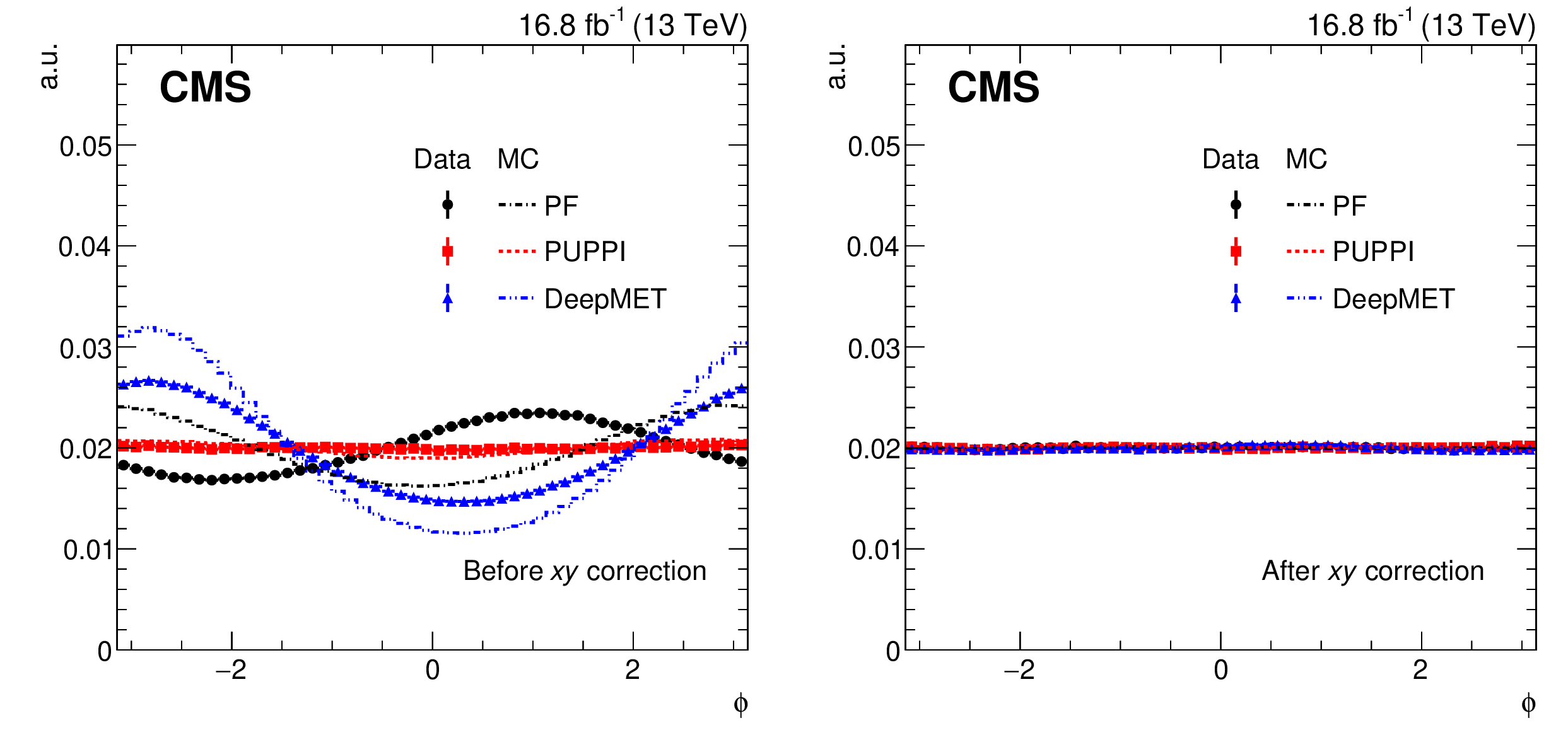
Figure 10:
The $ \phi $ distribution of different $ {\vec p}_{\mathrm{T}}^{\, \text{miss}} $ estimators before (left) and after (right) the $ xy $ corrections, in data (markers) and MC simulations (dashed) after the $ \mathrm{Z}\to\mu\mu $ selections. |
png pdf |
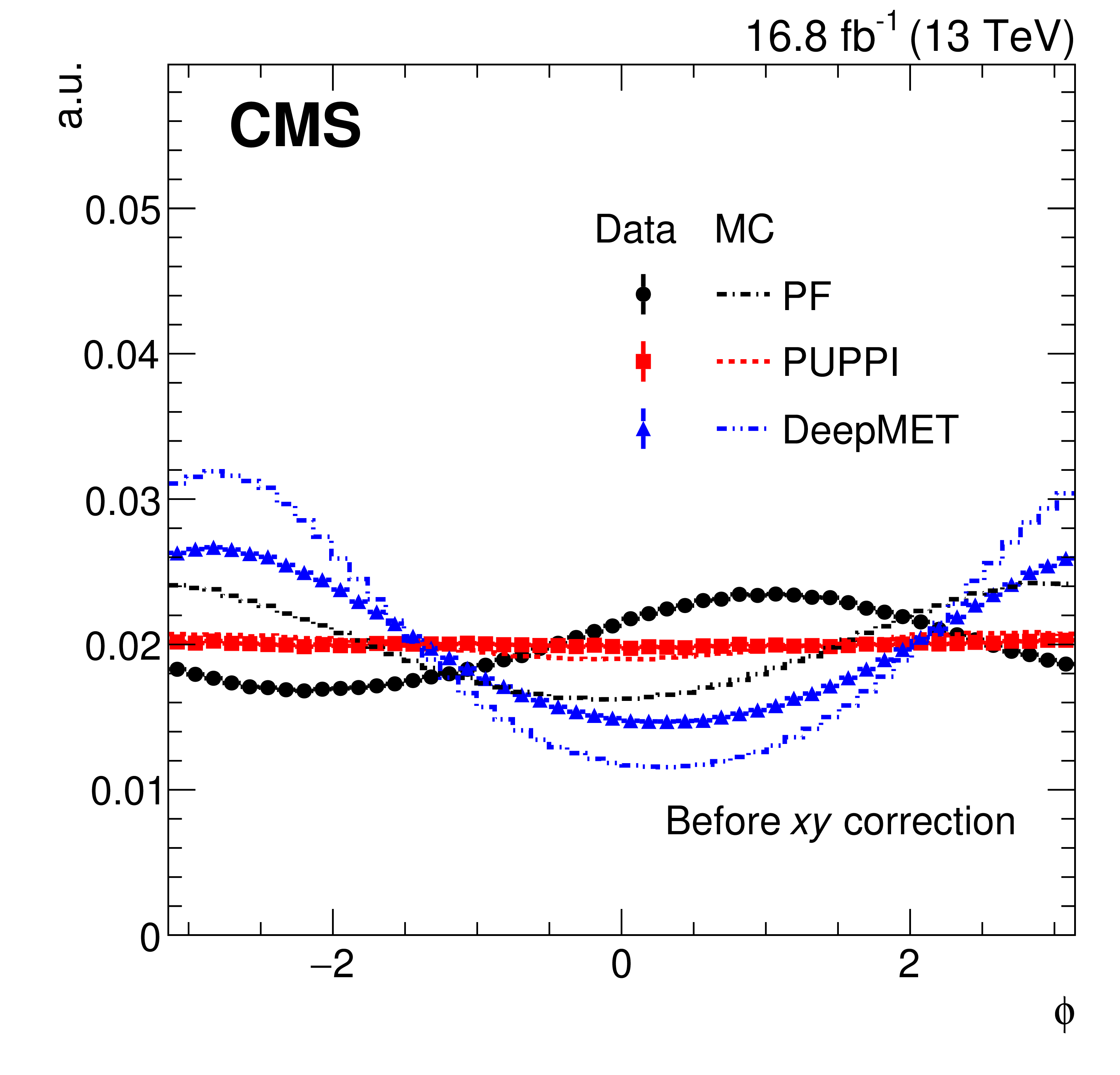
Figure 10-a:
The $ \phi $ distribution of different $ {\vec p}_{\mathrm{T}}^{\, \text{miss}} $ estimators before (left) and after (right) the $ xy $ corrections, in data (markers) and MC simulations (dashed) after the $ \mathrm{Z}\to\mu\mu $ selections. |
png pdf |
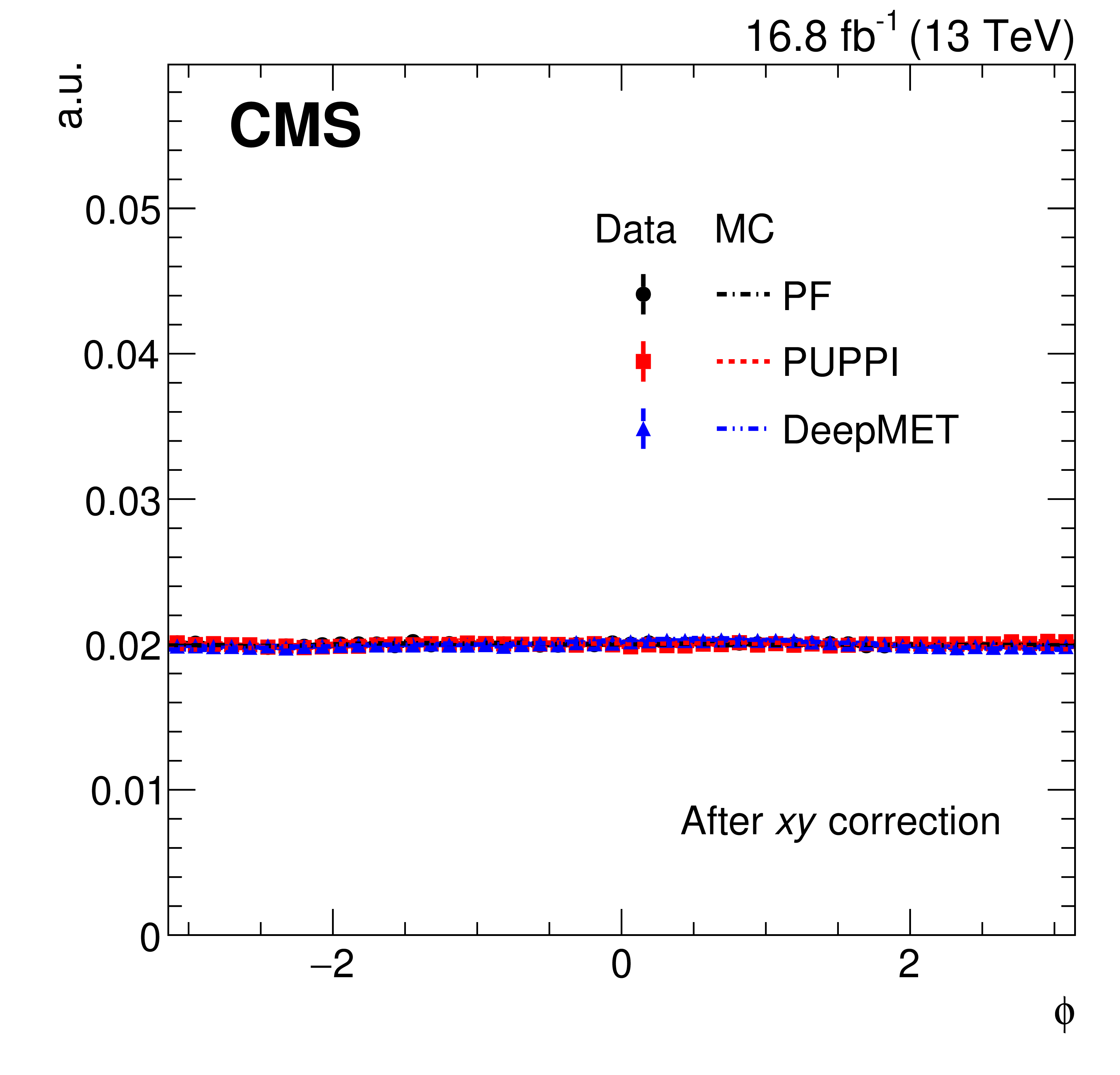
Figure 10-b:
The $ \phi $ distribution of different $ {\vec p}_{\mathrm{T}}^{\, \text{miss}} $ estimators before (left) and after (right) the $ xy $ corrections, in data (markers) and MC simulations (dashed) after the $ \mathrm{Z}\to\mu\mu $ selections. |
png pdf |
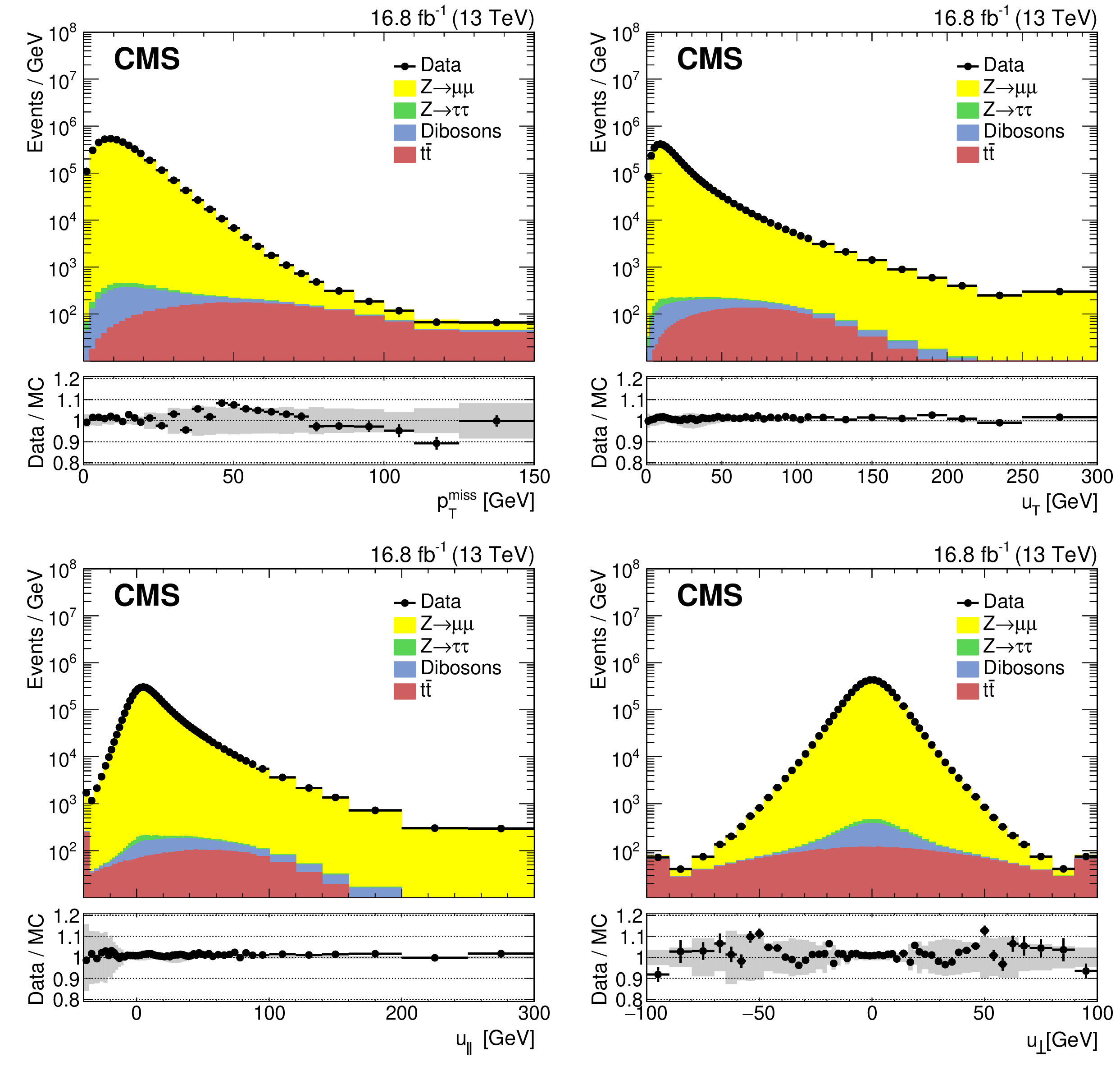
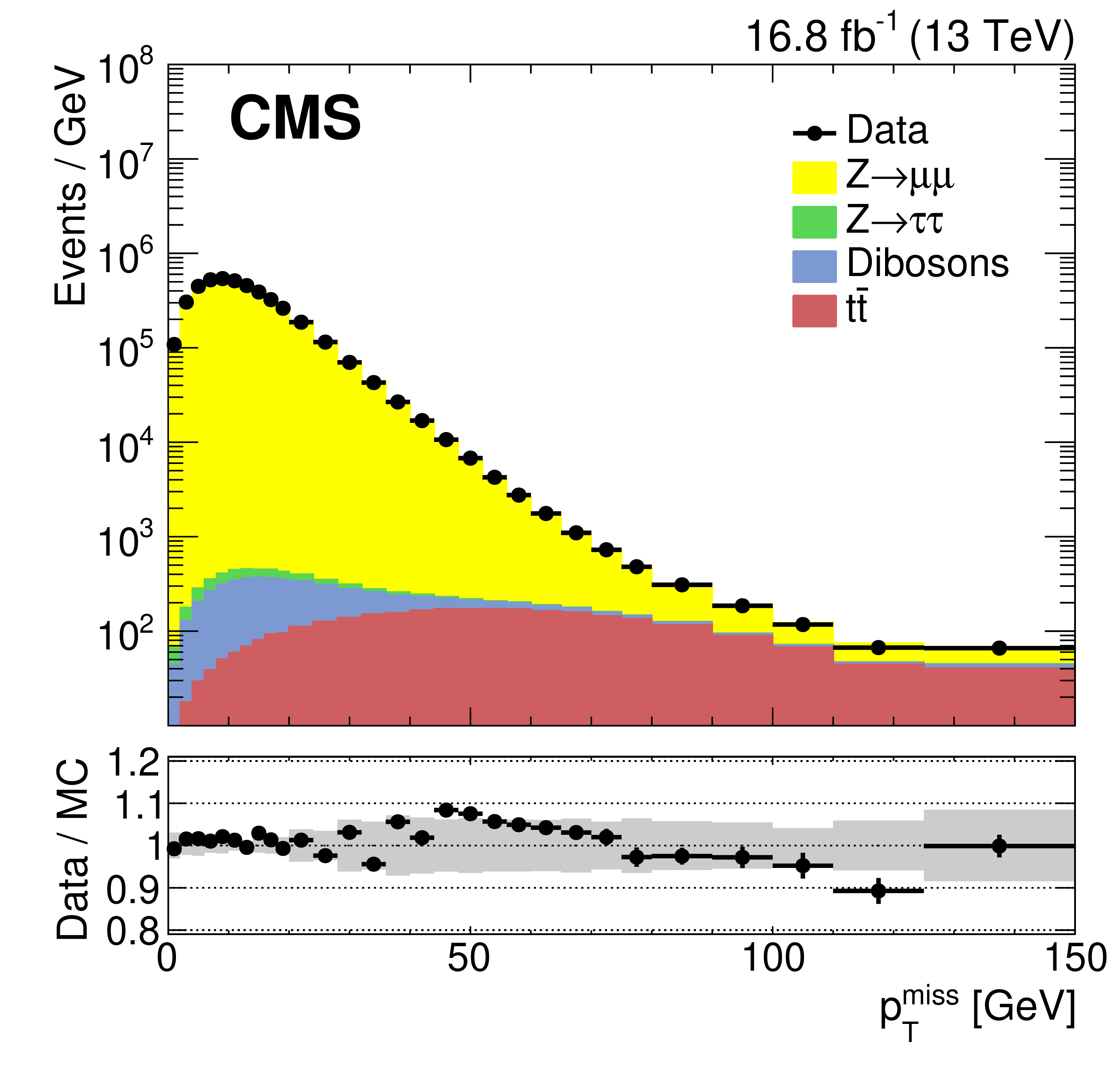
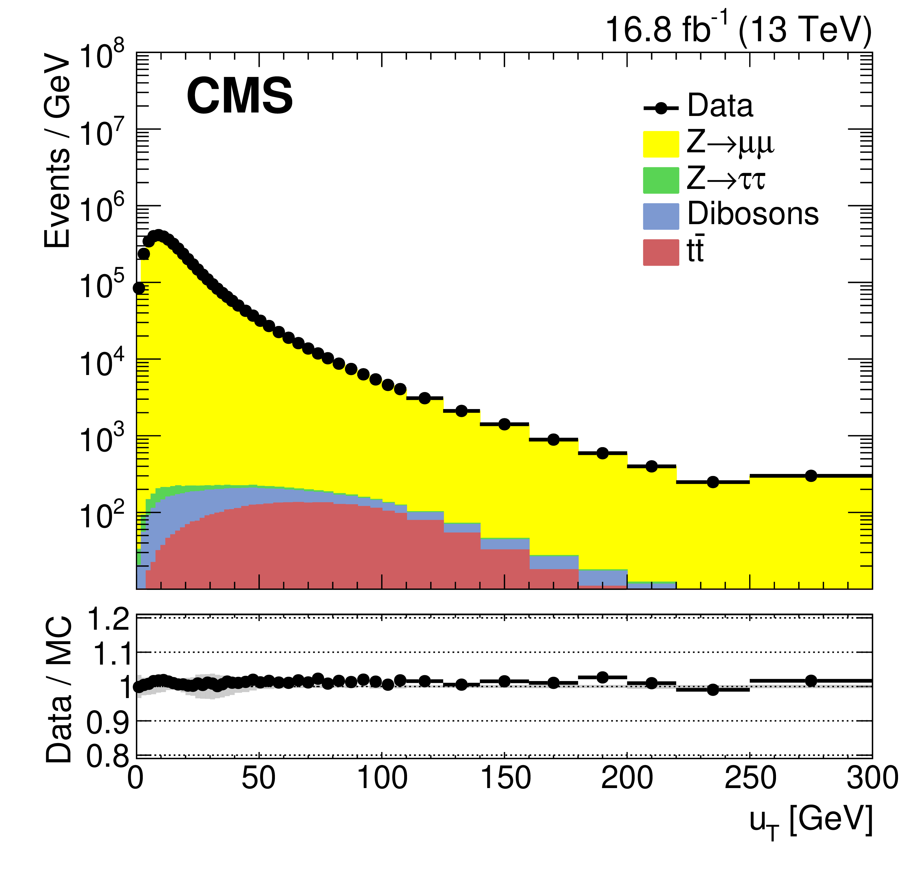
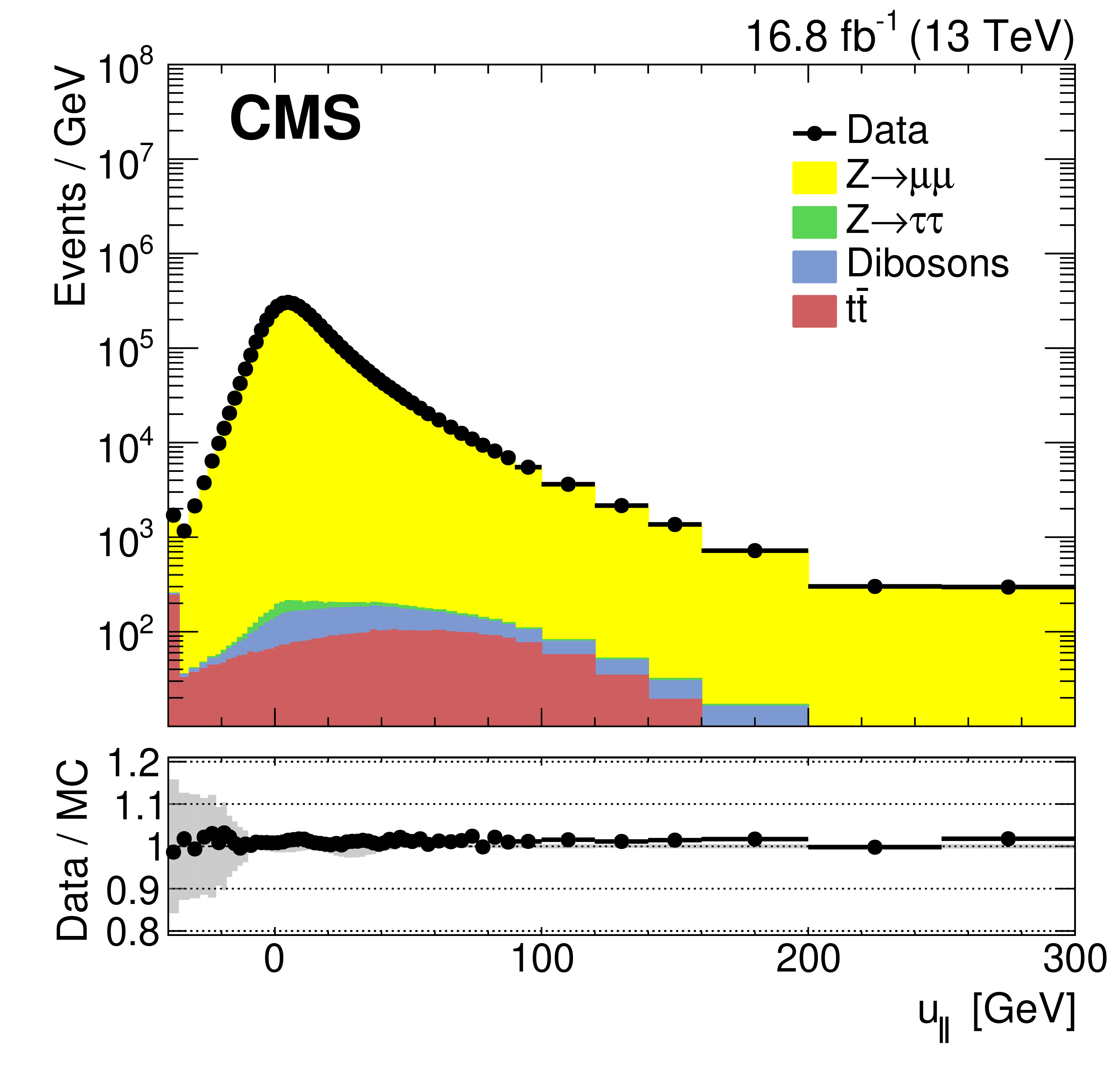
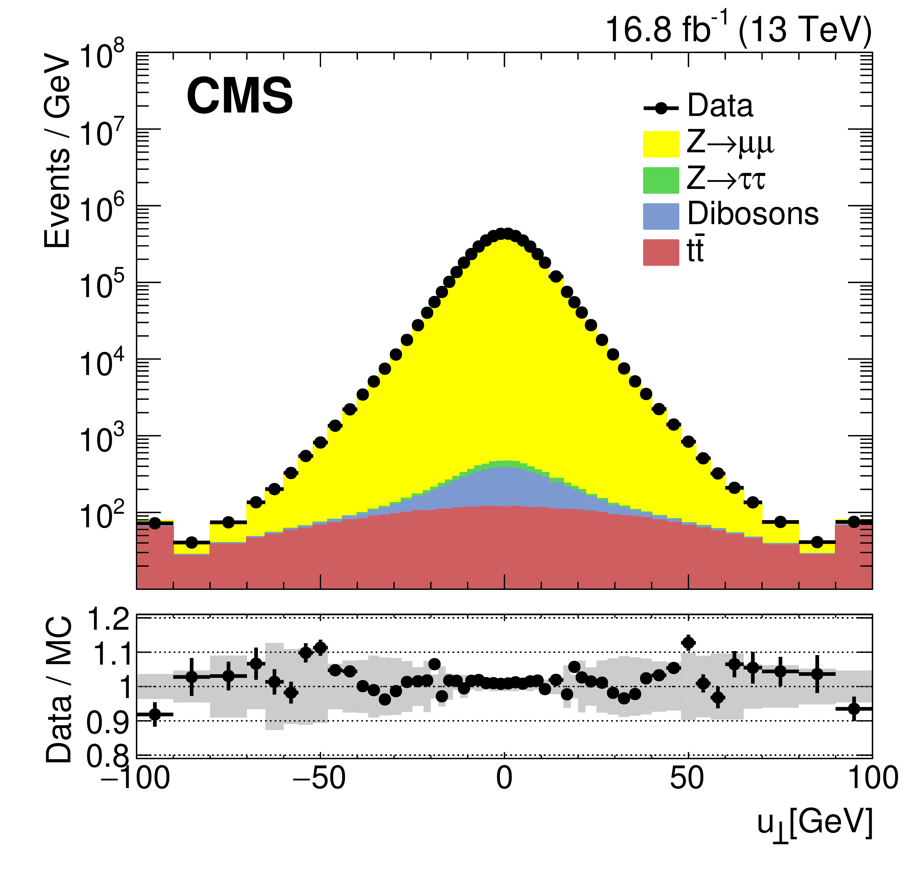
Figure 11:
Data-to-simulation comparisons of DEEPMET $ p_{\mathrm{T}}^\text{miss} $ (upper left), recoil $ p_{\mathrm{T}} $ (upper right), $ u_{\parallel} $ (lower left), and $ u_{\perp} $ (lower right) after the quantile correction. The underflow (overflow) contents are included in the first (last) bin. The gray band represents the systematic uncertainties discussed in Section 8.4. |
png pdf |
Figure 11-a:
Data-to-simulation comparisons of DEEPMET $ p_{\mathrm{T}}^\text{miss} $ (upper left), recoil $ p_{\mathrm{T}} $ (upper right), $ u_{\parallel} $ (lower left), and $ u_{\perp} $ (lower right) after the quantile correction. The underflow (overflow) contents are included in the first (last) bin. The gray band represents the systematic uncertainties discussed in Section 8.4. |
png pdf |
Figure 11-b:
Data-to-simulation comparisons of DEEPMET $ p_{\mathrm{T}}^\text{miss} $ (upper left), recoil $ p_{\mathrm{T}} $ (upper right), $ u_{\parallel} $ (lower left), and $ u_{\perp} $ (lower right) after the quantile correction. The underflow (overflow) contents are included in the first (last) bin. The gray band represents the systematic uncertainties discussed in Section 8.4. |
png pdf |
Figure 11-c:
Data-to-simulation comparisons of DEEPMET $ p_{\mathrm{T}}^\text{miss} $ (upper left), recoil $ p_{\mathrm{T}} $ (upper right), $ u_{\parallel} $ (lower left), and $ u_{\perp} $ (lower right) after the quantile correction. The underflow (overflow) contents are included in the first (last) bin. The gray band represents the systematic uncertainties discussed in Section 8.4. |
png pdf |
Figure 11-d:
Data-to-simulation comparisons of DEEPMET $ p_{\mathrm{T}}^\text{miss} $ (upper left), recoil $ p_{\mathrm{T}} $ (upper right), $ u_{\parallel} $ (lower left), and $ u_{\perp} $ (lower right) after the quantile correction. The underflow (overflow) contents are included in the first (last) bin. The gray band represents the systematic uncertainties discussed in Section 8.4. |
png pdf |
Figure 12:
Response (upper) and response-corrected resolutions of $ u_{\parallel} $ (lower left) and $ u_{\perp} $ (lower right) of different $ {\vec p}_{\mathrm{T}}^{\, \text{miss}} $ estimators in data after the $ \mathrm{Z}\to\mu\mu $ selections. |
png pdf |
Figure 12-a:
Response (upper) and response-corrected resolutions of $ u_{\parallel} $ (lower left) and $ u_{\perp} $ (lower right) of different $ {\vec p}_{\mathrm{T}}^{\, \text{miss}} $ estimators in data after the $ \mathrm{Z}\to\mu\mu $ selections. |
png pdf |
Figure 12-b:
Response (upper) and response-corrected resolutions of $ u_{\parallel} $ (lower left) and $ u_{\perp} $ (lower right) of different $ {\vec p}_{\mathrm{T}}^{\, \text{miss}} $ estimators in data after the $ \mathrm{Z}\to\mu\mu $ selections. |
png pdf |
Figure 12-c:
Response (upper) and response-corrected resolutions of $ u_{\parallel} $ (lower left) and $ u_{\perp} $ (lower right) of different $ {\vec p}_{\mathrm{T}}^{\, \text{miss}} $ estimators in data after the $ \mathrm{Z}\to\mu\mu $ selections. |
| Tables | |
png pdf |
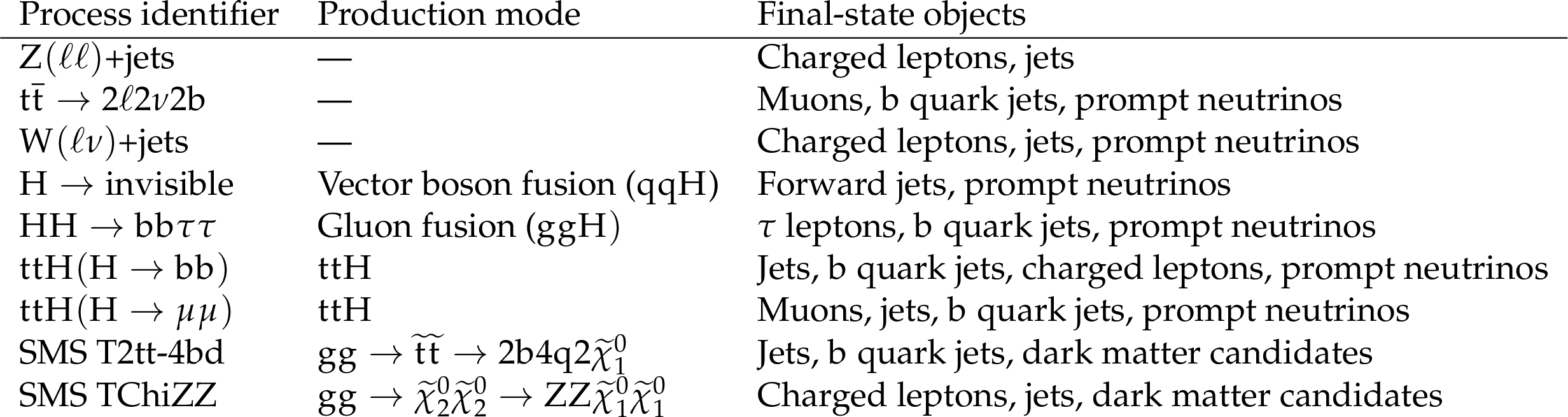
Table 1:
Overview of the simulated event samples used for performance studies. |
png pdf |
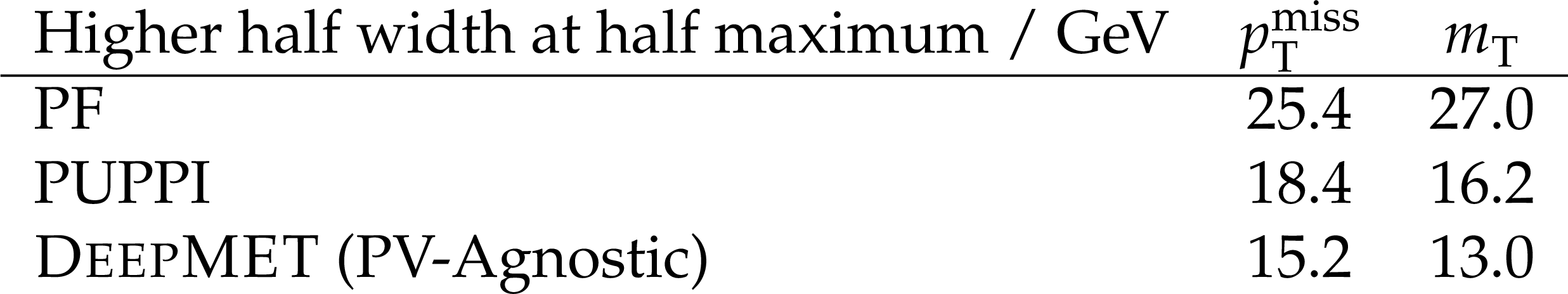
Table 2:
Higher half width at half maximum in $ p_{\mathrm{T}}^\text{miss} $ and $ m_\mathrm{T} $ in data after the $ \mathrm{W}\to\mu\nu $ selections. |
| Summary |
| This paper presents a new $ {\vec p}_{\mathrm{T}}^{\, \text{miss}} $ estimator, DEEPMET, which is based on a deep neural network. The DEEPMET algorithm utilizes each individual particle reconstructed by the CMS particle-flow algorithm as input and assigns a weight $ w_i $ and two bias terms, $ b_{i,x} $ and $ b_{i,y} $, to each candidate. The estimated $ {\vec p}_{\mathrm{T}}^{\, \text{miss}} $ is the negative vector sum of the weighted transverse momenta of all candidates, plus their bias contributions. With 4541 trainable parameters, the training and deployment of DEEPMET is computationally efficient. DEEPMET is trained using Z+jets and $ \mathrm{t} \overline{\mathrm{t}} $ samples, but achieves 10-30% better resolution compared with the current PF and PUPPI $ {\vec p}_{\mathrm{T}}^{\, \text{miss}} $ estimators across multiple physics processes, such as Z+jets, W+jets, Higgs boson production, and processes with dark matter candidates. Another important feature of the DEEPMET algorithm is its high resilience to pileup, improving the physics reach in LHC Run 2 and Run 3, and future High-Luminosity LHC conditions. Specifically for the measurement of the W boson mass, a PV-Agnostic version of DEEPMET is designed to be more robust in $ \mathrm{W} \to \mu\nu $ events where the LPV is not always identified correctly. Events containing $ \mathrm{Z} \to \mu\mu $ decays are used to calibrate $ {\vec p}_{\mathrm{T}}^{\, \text{miss}} $, including corrections for asymmetries in detector response, as well as for $ {\vec p}_{\mathrm{T}}^{\, \text{miss}} $ scale and resolution. Good agreement between data and simulation is found. The DEEPMET estimator demonstrates the potential to improve the precision of SM measurements and to achieve higher sensitivity in beyond the standard model physics searches. |
| References | ||||
| 1 | CMS Collaboration | The CMS experiment at the CERN LHC | JINST 3 (2008) S08004 | |
| 2 | ATLAS Collaboration | The ATLAS experiment at the CERN Large Hadron Collider | JINST 3 (2008) S08003 | |
| 3 | CMS Collaboration | Pileup mitigation at CMS in 13 TeV data | JINST 15 (2020) P09018 | CMS-JME-18-001 2003.00503 |
| 4 | D. Bertolini, P. Harris, M. Low, and N. Tran | Pileup per particle identification | JHEP 10 (2014) 059 | 1407.6013 |
| 5 | CMS Collaboration | Pileup-per-particle identification: optimisation for Run 2 Legacy and beyond | CMS Detector Performance Summary CMS-DP-2021-001, 2021 CDS |
|
| 6 | CMS Collaboration | Performance of the CMS missing transverse momentum reconstruction in pp data at $ \sqrt{s} = $ 8 TeV | JINST 10 (2015) P02006 | CMS-JME-13-003 1411.0511 |
| 7 | CMS Collaboration | Evidence for the 125 GeV Higgs boson decaying to a pair of $ \tau $ leptons | JHEP 05 (2014) 104 | CMS-HIG-13-004 1401.5041 |
| 8 | CMS Collaboration | HEPData record for this analysis | link | |
| 9 | CMS Collaboration | Performance of the CMS Level-1 trigger in proton-proton collisions at $ \sqrt{s} = $ 13 TeV | JINST 15 (2020) P10017 | CMS-TRG-17-001 2006.10165 |
| 10 | CMS Collaboration | The CMS trigger system | JINST 12 (2017) P01020 | CMS-TRG-12-001 1609.02366 |
| 11 | CMS Collaboration | Performance of the CMS high-level trigger during LHC Run 2 | JINST 19 (2024) P11021 | CMS-TRG-19-001 2410.17038 |
| 12 | CMS Collaboration | Description and performance of track and primary-vertex reconstruction with the CMS tracker | JINST 9 (2014) P10009 | CMS-TRK-11-001 1405.6569 |
| 13 | CMS Collaboration | Technical proposal for the Phase-II upgrade of the Compact Muon Solenoid | CMS Technical Proposal CERN-LHCC-2015-010, CMS-TDR-15-02, 2015 CDS |
|
| 14 | CMS Collaboration | Particle-flow reconstruction and global event description with the CMS detector | JINST 12 (2017) P10003 | CMS-PRF-14-001 1706.04965 |
| 15 | CMS Collaboration | Performance of the CMS muon detector and muon reconstruction with proton-proton collisions at $ \sqrt{s}= $ 13 TeV | JINST 13 (2018) P06015 | CMS-MUO-16-001 1804.04528 |
| 16 | M. Cacciari, G. P. Salam, and G. Soyez | The anti-$ k_{\mathrm{T}} $ jet clustering algorithm | JHEP 04 (2008) 063 | 0802.1189 |
| 17 | M. Cacciari, G. P. Salam, and G. Soyez | FastJet user manual | EPJC 72 (2012) 1896 | 1111.6097 |
| 18 | CMS Collaboration | Jet energy scale and resolution in the CMS experiment in pp collisions at 8 TeV | JINST 12 (2017) P02014 | CMS-JME-13-004 1607.03663 |
| 19 | CMS Collaboration | Performance of missing transverse momentum reconstruction in proton-proton collisions at $ \sqrt{s} = $ 13 TeV using the CMS detector | JINST 14 (2019) P07004 | CMS-JME-17-001 1903.06078 |
| 20 | CMS Collaboration | Precision luminosity measurement in proton-proton collisions at $ \sqrt{s} = $ 13 TeV in 2015 and 2016 at CMS | EPJC 81 (2021) 800 | CMS-LUM-17-003 2104.01927 |
| 21 | J. Alwall et al. | The automated computation of tree-level and next-to-leading order differential cross sections, and their matching to parton shower simulations | JHEP 07 (2014) 079 | 1405.0301 |
| 22 | P. Nason | A new method for combining NLO QCD with shower Monte Carlo algorithms | JHEP 11 (2004) 040 | hep-ph/0409146 |
| 23 | S. Frixione, P. Nason, and C. Oleari | Matching NLO QCD computations with parton shower simulations: the POWHEG method | JHEP 11 (2007) 070 | 0709.2092 |
| 24 | S. Alioli, P. Nason, C. Oleari, and E. Re | NLO vector-boson production matched with shower in POWHEG | JHEP 07 (2008) 060 | 0805.4802 |
| 25 | S. Alioli, P. Nason, C. Oleari, and E. Re | A general framework for implementing NLO calculations in shower Monte Carlo programs: the POWHEG BOX | JHEP 06 (2010) 043 | 1002.2581 |
| 26 | T. Sjöstrand et al. | An introduction to PYTHIA 8.2 | Comput. Phys. Commun. 191 (2015) 159 | 1410.3012 |
| 27 | P. Skands, S. Carrazza, and J. Rojo | Tuning PYTHIA 8.1: the Monash 2013 tune | EPJC 74 (2014) 3024 | 1404.5630 |
| 28 | CMS Collaboration | Extraction and validation of a new set of CMS PYTHIA 8 tunes from underlying-event measurements | EPJC 80 (2020) 4 | CMS-GEN-17-001 1903.12179 |
| 29 | NNPDF Collaboration | Parton distributions from high-precision collider data | EPJC 77 (2017) 663 | 1706.00428 |
| 30 | J. Alwall, P. Schuster, and N. Toro | Simplified models for a first characterization of new physics at the LHC | PRD 79 (2009) 075020 | 0810.3921 |
| 31 | LHC New Physics Working Group | Simplified models for LHC new physics searches | JPG 39 (2012) 105005 | 1105.2838 |
| 32 | CMS Collaboration | Search for supersymmetry in proton-proton collisions at 13 TeV in final states with jets and missing transverse momentum | JHEP 10 (2019) 244 | CMS-SUS-19-006 1908.04722 |
| 33 | CMS Collaboration | Search for electroweak production of charginos and neutralinos at $ \sqrt{s}= $ 13 TeV in final states containing hadronic decays of WW, WZ, or WH and missing transverse momentum | PLB 842 (2023) 137460 | CMS-SUS-21-002 2205.09597 |
| 34 | GEANT4 Collaboration | GEANT 4---a simulation toolkit | NIM A 506 (2003) 250 | |
| 35 | S. Ioffe and C. Szegedy | Batch normalization: accelerating deep network training by reducing internal covariate shift | 1502.03167 | |
| 36 | F. Chollet et al. | Keras | link | |
| 37 | M. Abadi et al. | TensorFlow: A system for large-scale machine learning | 1605.08695 | |
| 38 | I. Loshchilov and F. Hutter | Decoupled weight decay regularization | 1711.05101 | |
| 39 | CMS Collaboration | Measurement of the transverse momentum spectra of weak vector bosons produced in proton-proton collisions at $ \sqrt{s}= $ 8 TeV | JHEP 02 (2017) 096 | CMS-SMP-14-012 1606.05864 |
| 40 | CMS Collaboration | High-precision measurement of the W boson mass with the CMS experiment at the LHC | Submitted to Nature, 2024 | CMS-SMP-23-002 2412.13872 |
| 41 | CMS Collaboration | CMS physics: Technical design report volume 1: Detector performance and software | CMS Technical Design Report CERN-LHCC-2006-001, CMS-TDR-8-1, 2006 CDS |
|
| 42 | CMS Collaboration | CMSSW on Github | http://cms-sw.github.io/ | |
| 43 | CMS Collaboration | Portable acceleration of CMS computing workflows with coprocessors as a service | Comput. Softw. Big Sci. 8 (2024) 17 | CMS-MLG-23-001 2402.15366 |
|
|
Compact Muon Solenoid LHC, CERN |
|

|

|

|

|

|