CMS-HIG-25-002

CMS-HIG-25-002 ; ATL-PHYS-PUB-2025-018
Highlights of the HL-LHC physics projections by ATLAS and CMS
ATLAS and CMS Collaborations
31 March 2025
Submitted to EPPSU
Abstract: The High-Luminosity LHC (HL-LHC) physics programme will be crucial for deepening our understanding of fundamental physics, enabling in particular precision studies of the Higgs sector and enhancing sensitivity to rare processes and potential new physics. With unprecedented integrated luminosity, it will offer a unique opportunity to probe the standard model (SM) with extreme accuracy and explore connections to open questions in particle physics, astroparticle physics, and cosmology. The physics reach of the upgraded ATLAS and CMS detectors at the end of their programme will not only be significant in its own right but will also serve as a critical foundation for decision-making on future colliders, shaping the 2026 update of the European Strategy for Particle Physics.
Links: e-print arXiv:2504.00672 [hep-ex] (PDF) ; CDS record ; inSPIRE record ; CADI line (restricted) ;

Figures & Tables	References	CMS Publications

Highlights of the HL-LHC physics projections by ATLAS and CMS: File submitted to the European Strategy Update.
CMS Collaboration author list.

Figures
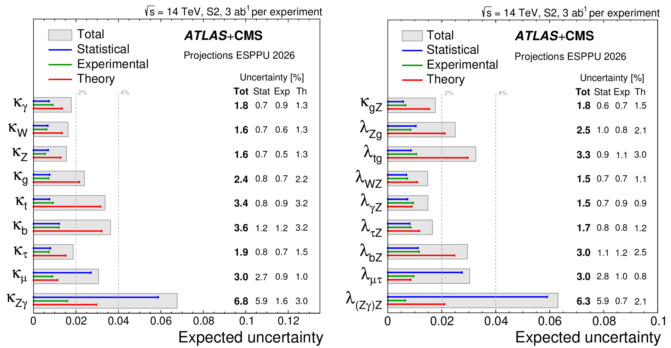
png pdf	Figure 1: The projected uncertainty in the combined coupling signal strength modifiers (left) and their ratios (right) with 3 ab $^{-1}$ of $pp$ collisions under the S2 systematic uncertainty scenario, assuming that the Higgs boson decays only to final states predicted by the SM.
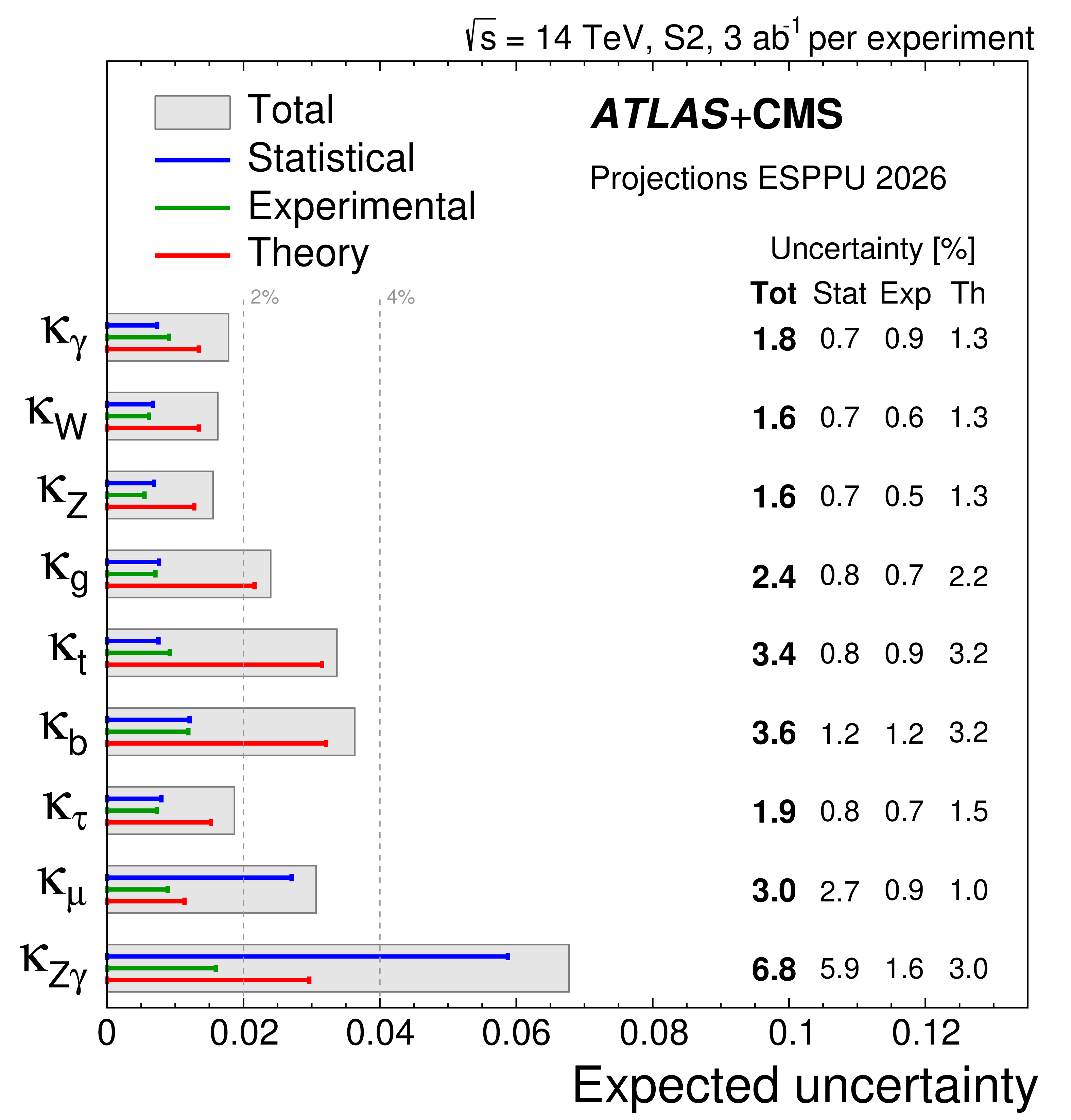
png pdf	Figure 1-a: The projected uncertainty in the combined coupling signal strength modifiers (left) and their ratios (right) with 3 ab $^{-1}$ of $pp$ collisions under the S2 systematic uncertainty scenario, assuming that the Higgs boson decays only to final states predicted by the SM.
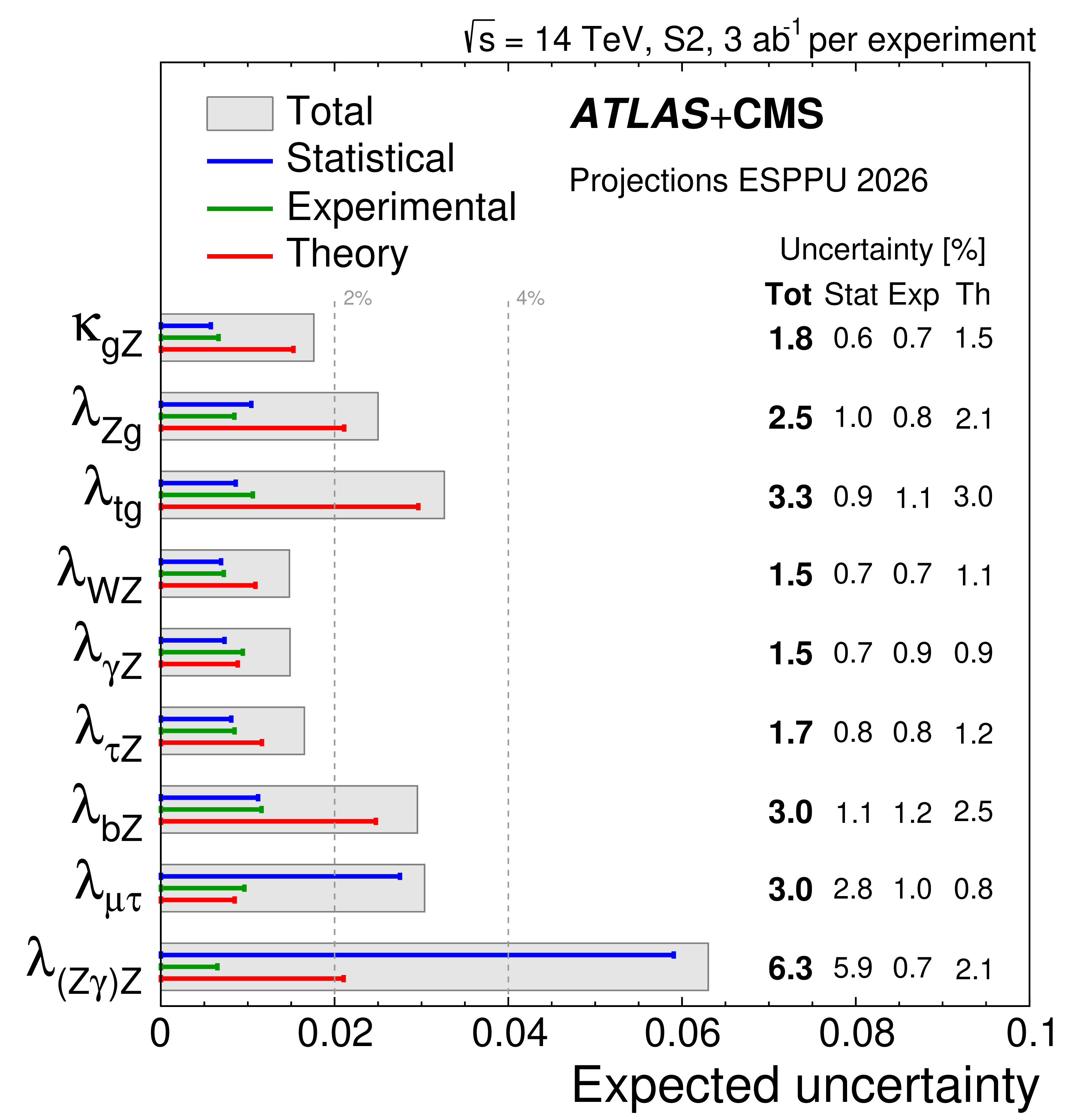
png pdf	Figure 1-b: The projected uncertainty in the combined coupling signal strength modifiers (left) and their ratios (right) with 3 ab $^{-1}$ of $pp$ collisions under the S2 systematic uncertainty scenario, assuming that the Higgs boson decays only to final states predicted by the SM.
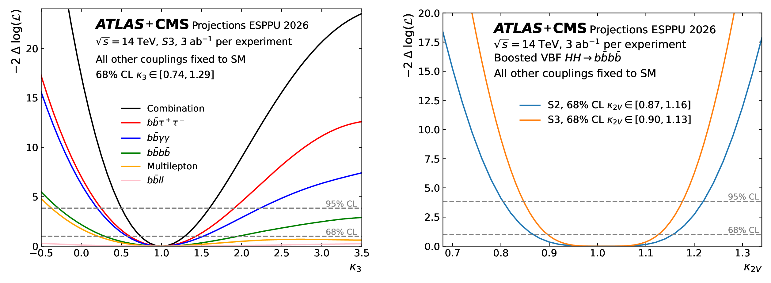
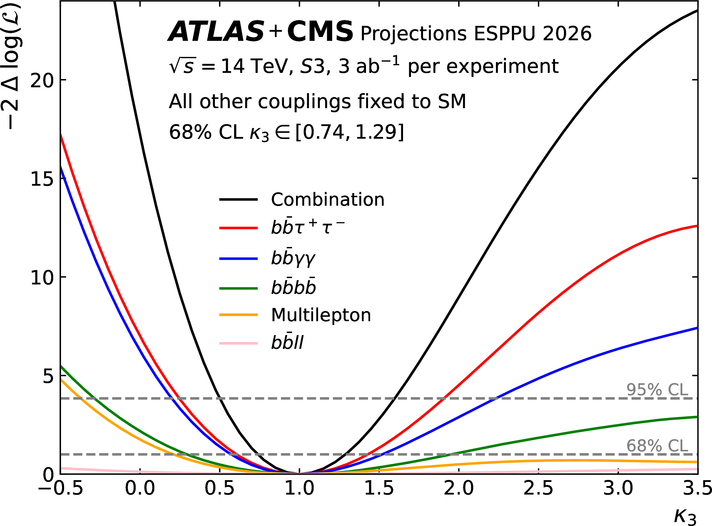
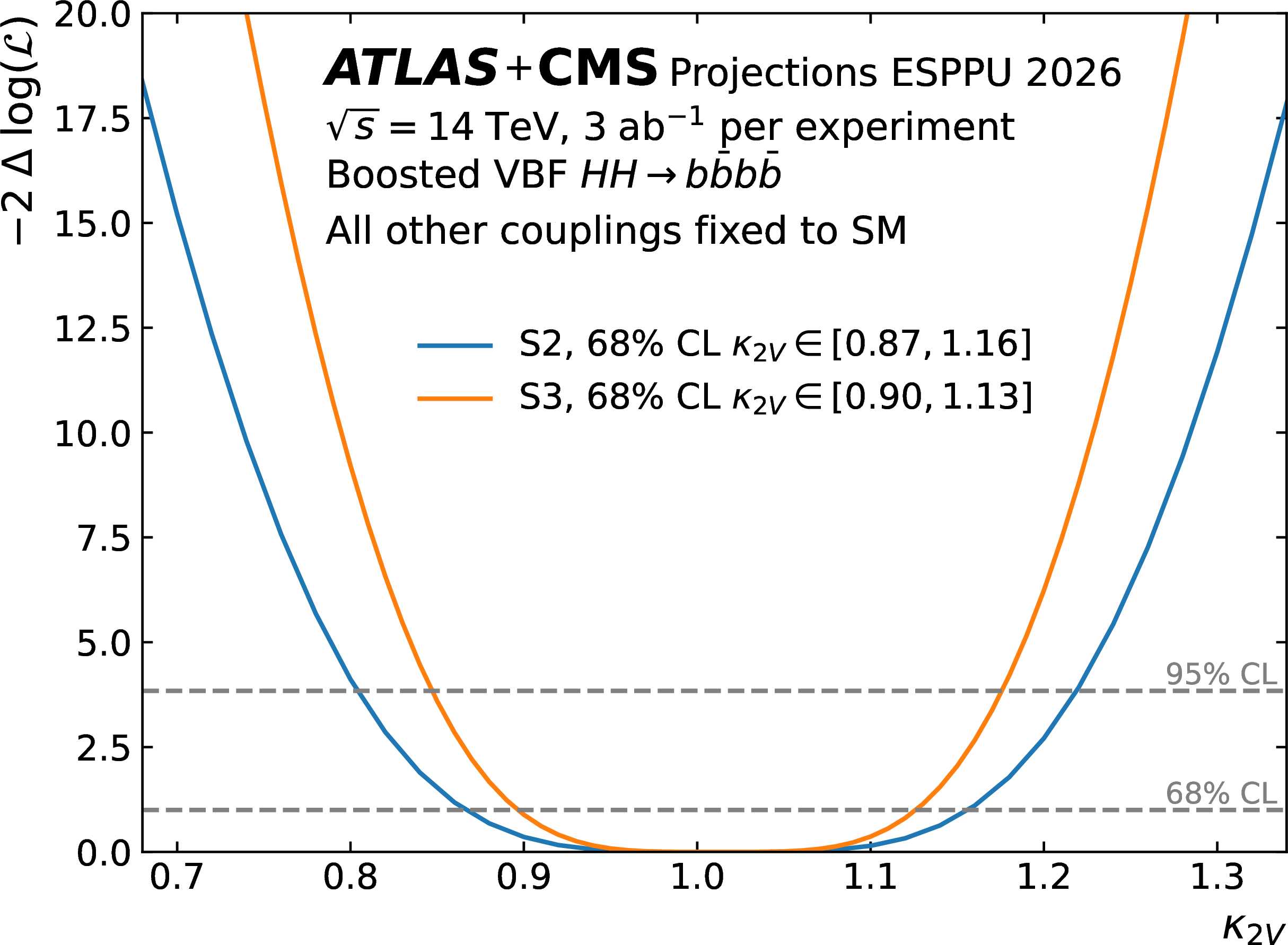
png pdf	Figure 2: Left: Expected ATLAS+CMS $\kappa_{3}$ likelihood scans for single decay channels and the combination for 3 ab $^{-1}$ for the S3 scenario, obtained fixing $\kappa_{3}^\mathrm{true}=$ 1. Right: The ATLAS+CMS projections for $\kappa_{2V}$ in the S2 and S3 scenarios, fixing $\kappa_{2V}^\mathrm{true}=$ 1.
png pdf	Figure 2-a: Left: Expected ATLAS+CMS $\kappa_{3}$ likelihood scans for single decay channels and the combination for 3 ab $^{-1}$ for the S3 scenario, obtained fixing $\kappa_{3}^\mathrm{true}=$ 1. Right: The ATLAS+CMS projections for $\kappa_{2V}$ in the S2 and S3 scenarios, fixing $\kappa_{2V}^\mathrm{true}=$ 1.
png pdf	Figure 2-b: Left: Expected ATLAS+CMS $\kappa_{3}$ likelihood scans for single decay channels and the combination for 3 ab $^{-1}$ for the S3 scenario, obtained fixing $\kappa_{3}^\mathrm{true}=$ 1. Right: The ATLAS+CMS projections for $\kappa_{2V}$ in the S2 and S3 scenarios, fixing $\kappa_{2V}^\mathrm{true}=$ 1.
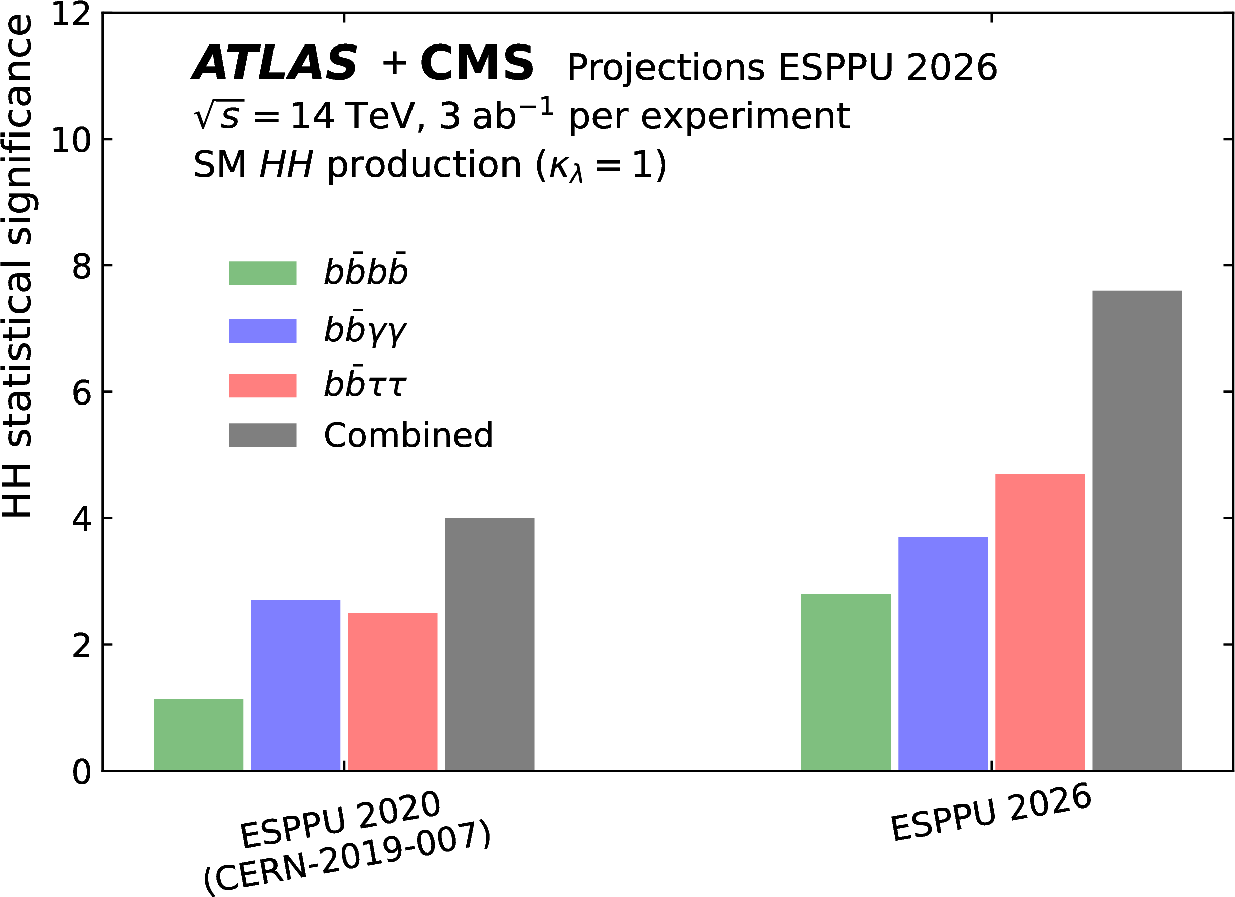
png pdf	Figure 3: Comparison of the ESPPU 2020 and ESPPU 2026 projected 3 ab $^{-1}$ HH sensitivities from various final states, and their combinations.
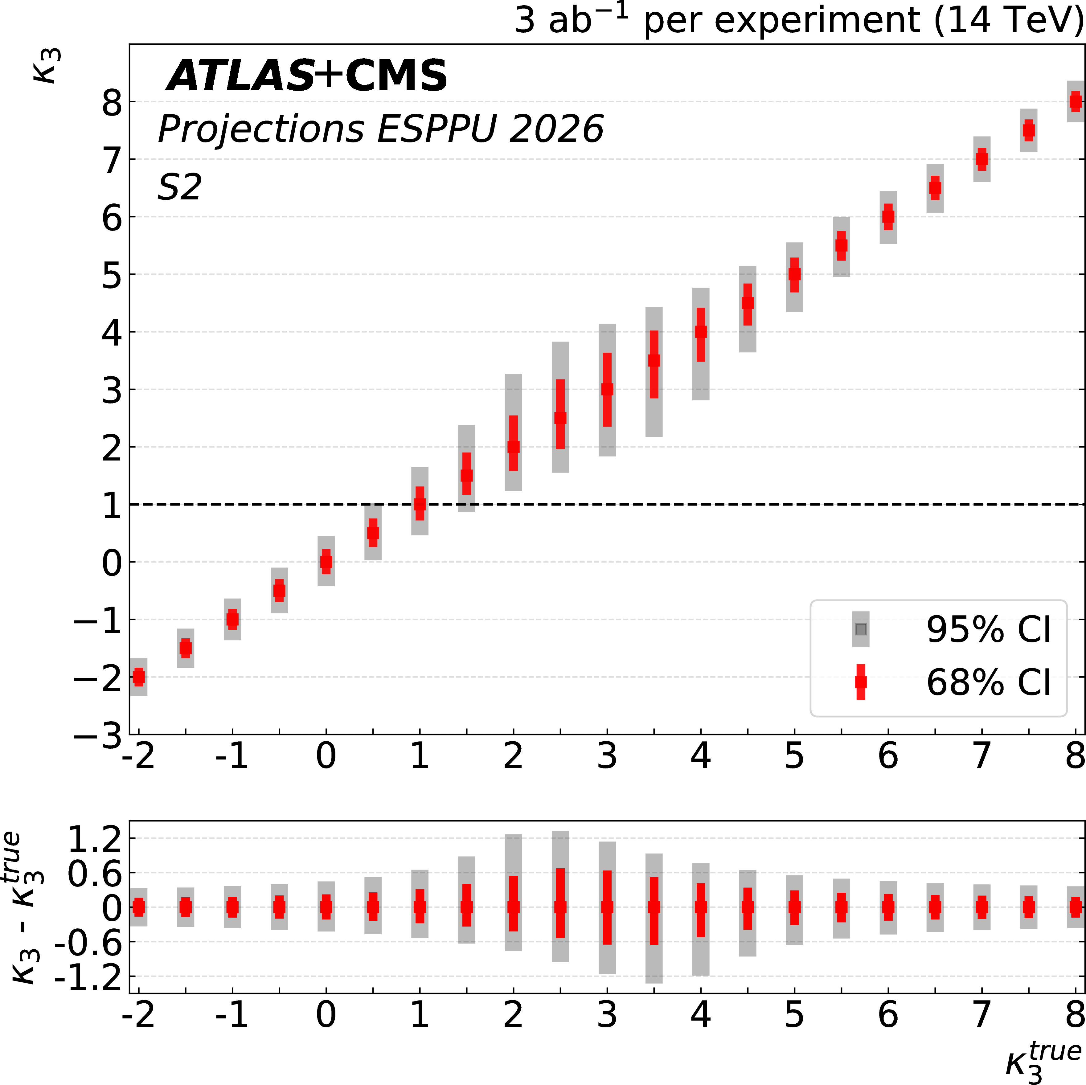
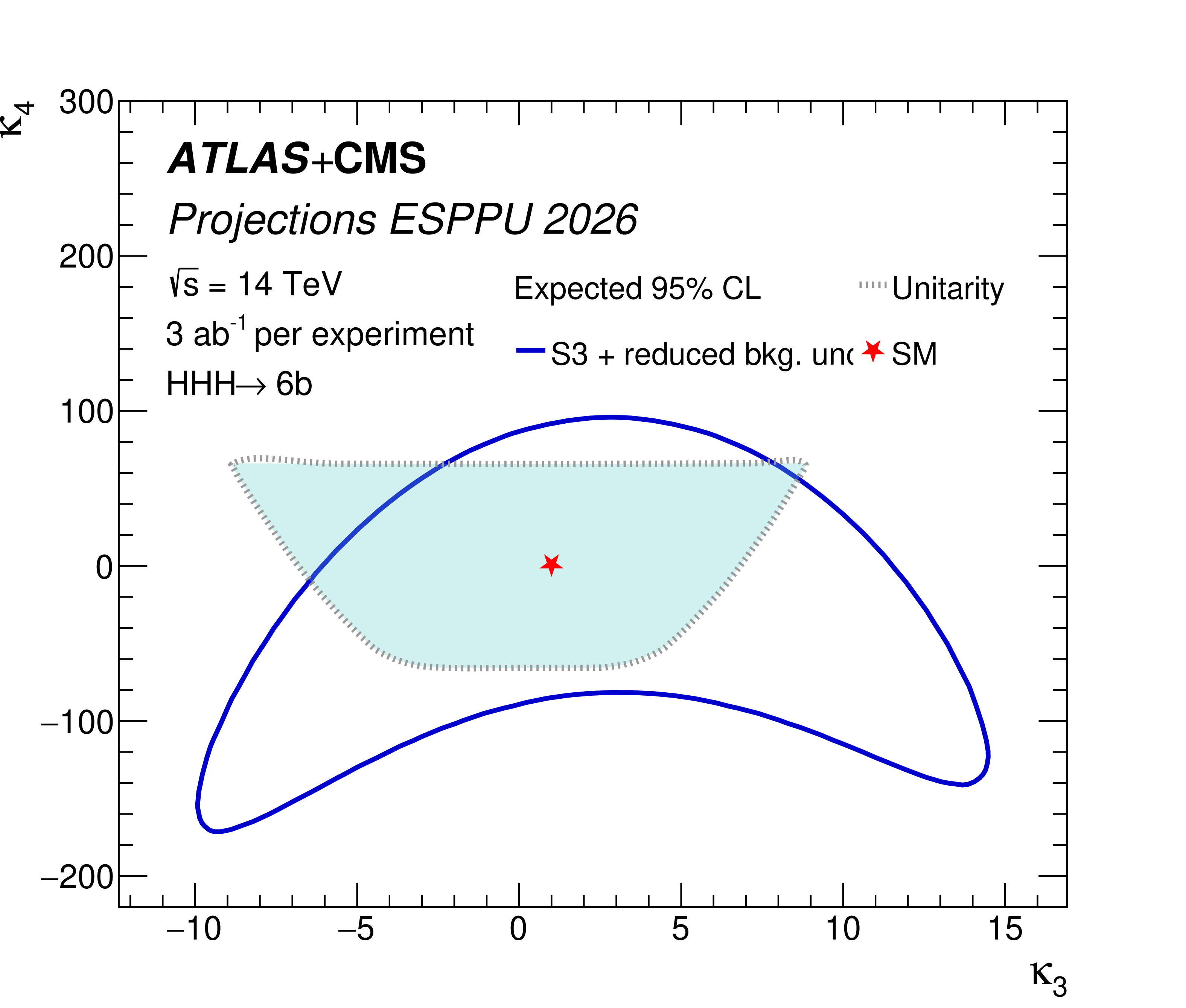
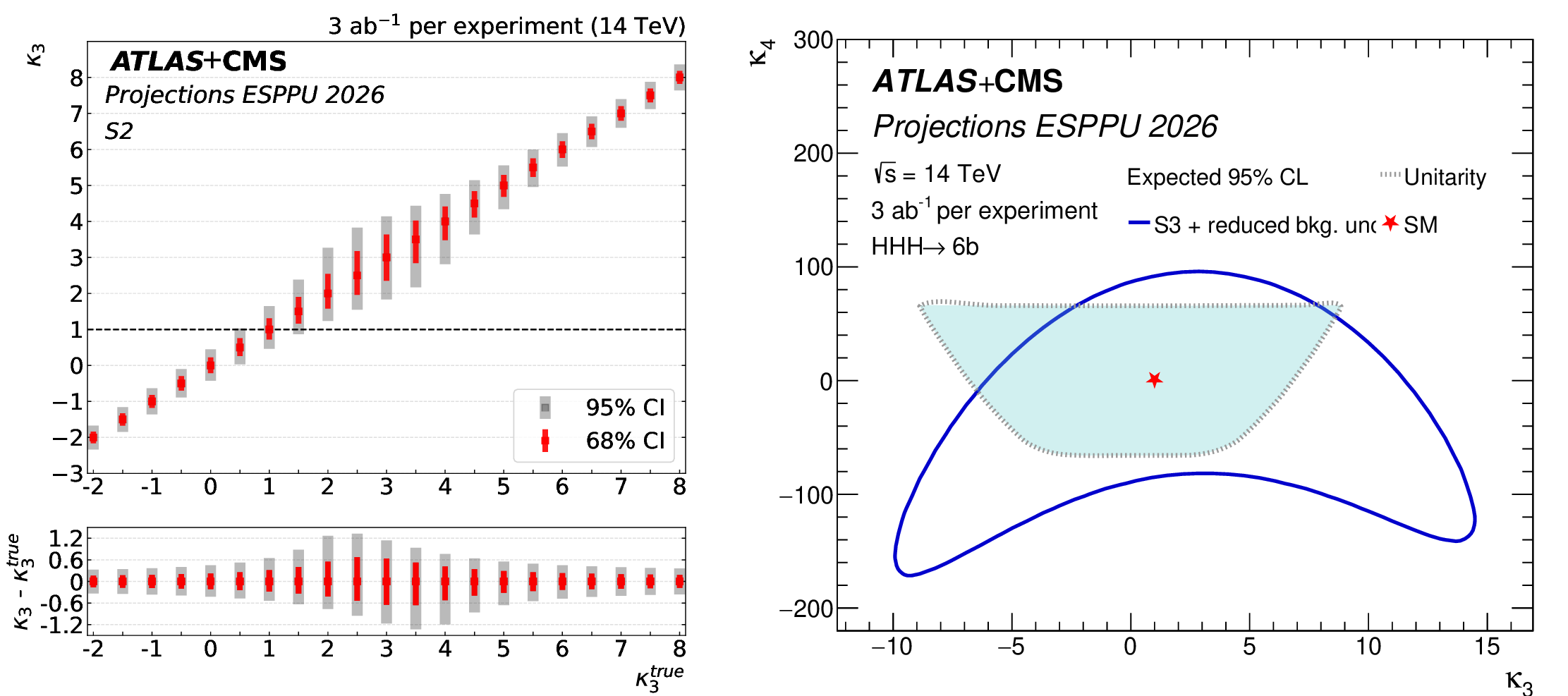
png pdf	Figure 4: Left: The ATLAS+CMS projection on the precision of the determination of $\kappa_{3}$ as a function of $\kappa_{3}^\mathrm{true}$ . The 68% and 95% confidence intervals are shown in the upper plot, while the lower plot shows the $\kappa_{3}$ deviation from the simulated $\kappa_{3}^\mathrm{true}$ value and its 68% and 95% confidence intervals. Right: 95% CL constraints from the $\mathrm{HHH}$ search projection on $\kappa_3$ and $\kappa_4$ . Results are shown for 3 ab $^{-1}$ per experiment at $\sqrt{s}=$ 14 TeV in scenario S3 with data-driven background uncertainties. Unitarity limits, as calculated in Ref. [57], are overlaid in the region bounded by the grey dashed line.
png pdf	Figure 4-a: Left: The ATLAS+CMS projection on the precision of the determination of $\kappa_{3}$ as a function of $\kappa_{3}^\mathrm{true}$ . The 68% and 95% confidence intervals are shown in the upper plot, while the lower plot shows the $\kappa_{3}$ deviation from the simulated $\kappa_{3}^\mathrm{true}$ value and its 68% and 95% confidence intervals. Right: 95% CL constraints from the $\mathrm{HHH}$ search projection on $\kappa_3$ and $\kappa_4$ . Results are shown for 3 ab $^{-1}$ per experiment at $\sqrt{s}=$ 14 TeV in scenario S3 with data-driven background uncertainties. Unitarity limits, as calculated in Ref. [57], are overlaid in the region bounded by the grey dashed line.
png pdf	Figure 4-b: Left: The ATLAS+CMS projection on the precision of the determination of $\kappa_{3}$ as a function of $\kappa_{3}^\mathrm{true}$ . The 68% and 95% confidence intervals are shown in the upper plot, while the lower plot shows the $\kappa_{3}$ deviation from the simulated $\kappa_{3}^\mathrm{true}$ value and its 68% and 95% confidence intervals. Right: 95% CL constraints from the $\mathrm{HHH}$ search projection on $\kappa_3$ and $\kappa_4$ . Results are shown for 3 ab $^{-1}$ per experiment at $\sqrt{s}=$ 14 TeV in scenario S3 with data-driven background uncertainties. Unitarity limits, as calculated in Ref. [57], are overlaid in the region bounded by the grey dashed line.
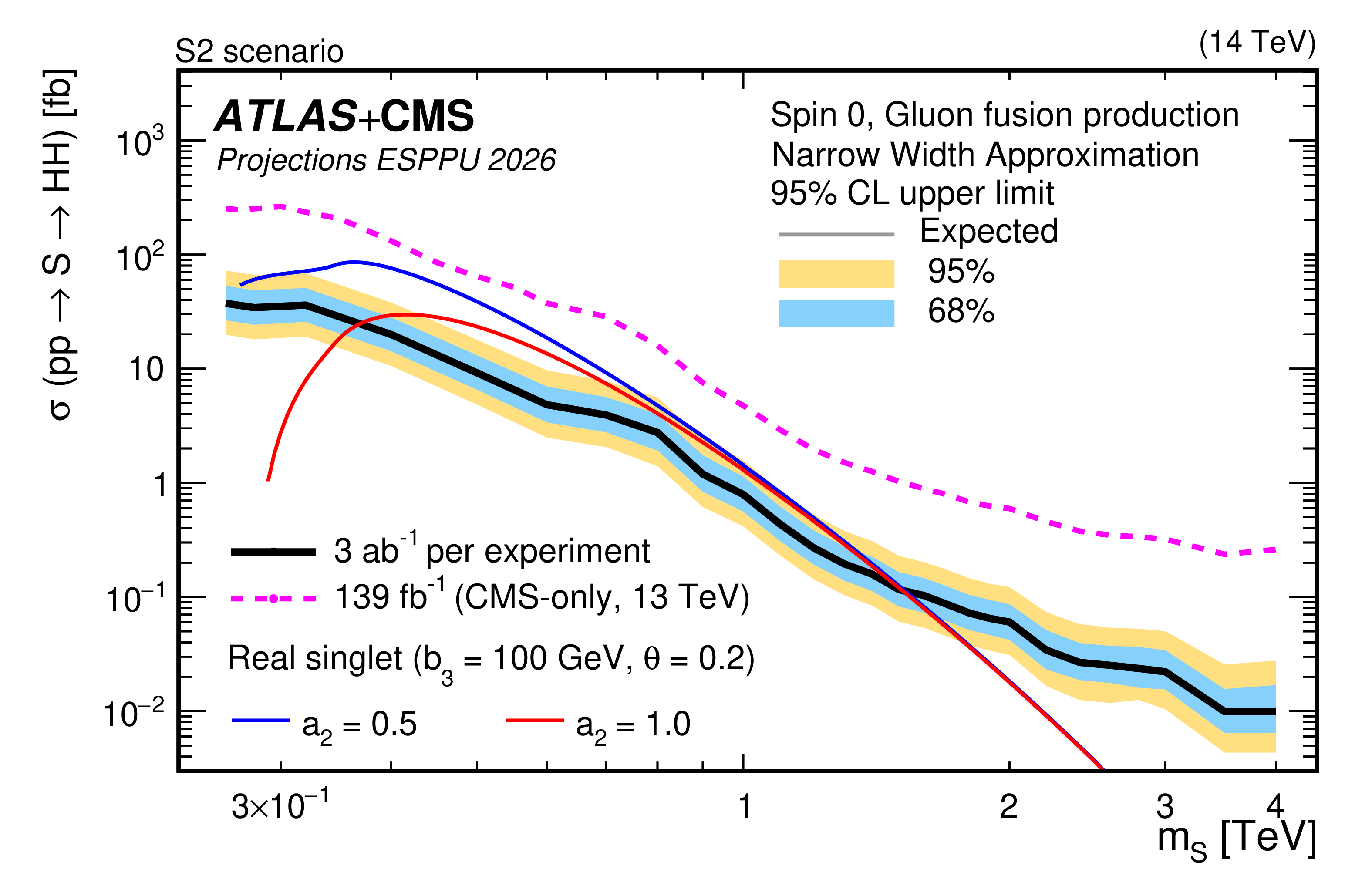
png pdf	Figure 5: Expected 95% CL upper limits on the $\mathrm{ \sigma(pp \to S \to HH }$ cross section as a function of the scalar mass $m_{\mathrm{S}}$ , produced via gluon fusion using the narrow width approximation. The projection is derived assuming 3 ab $^{-1}$ per experiment for the S2 scenario at 14 TeV. For comparison, production cross section curves for the model described in Section 7 are shown, for two values of the scalar portal coupling $a_2$ .
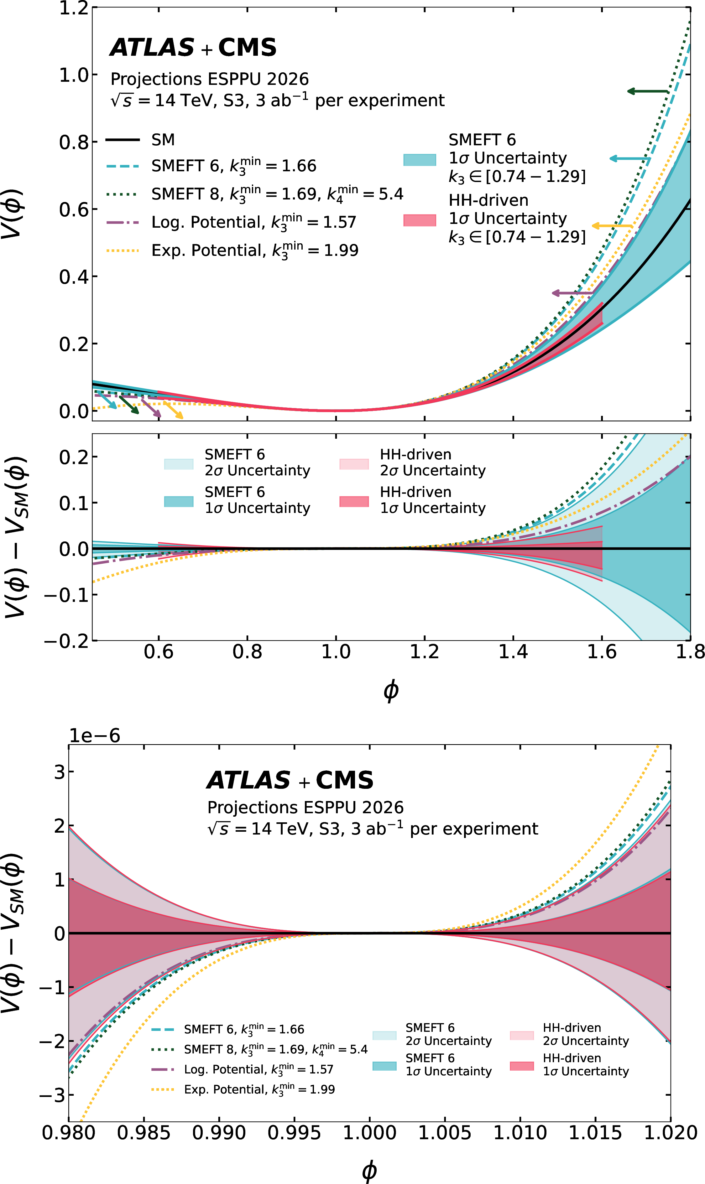
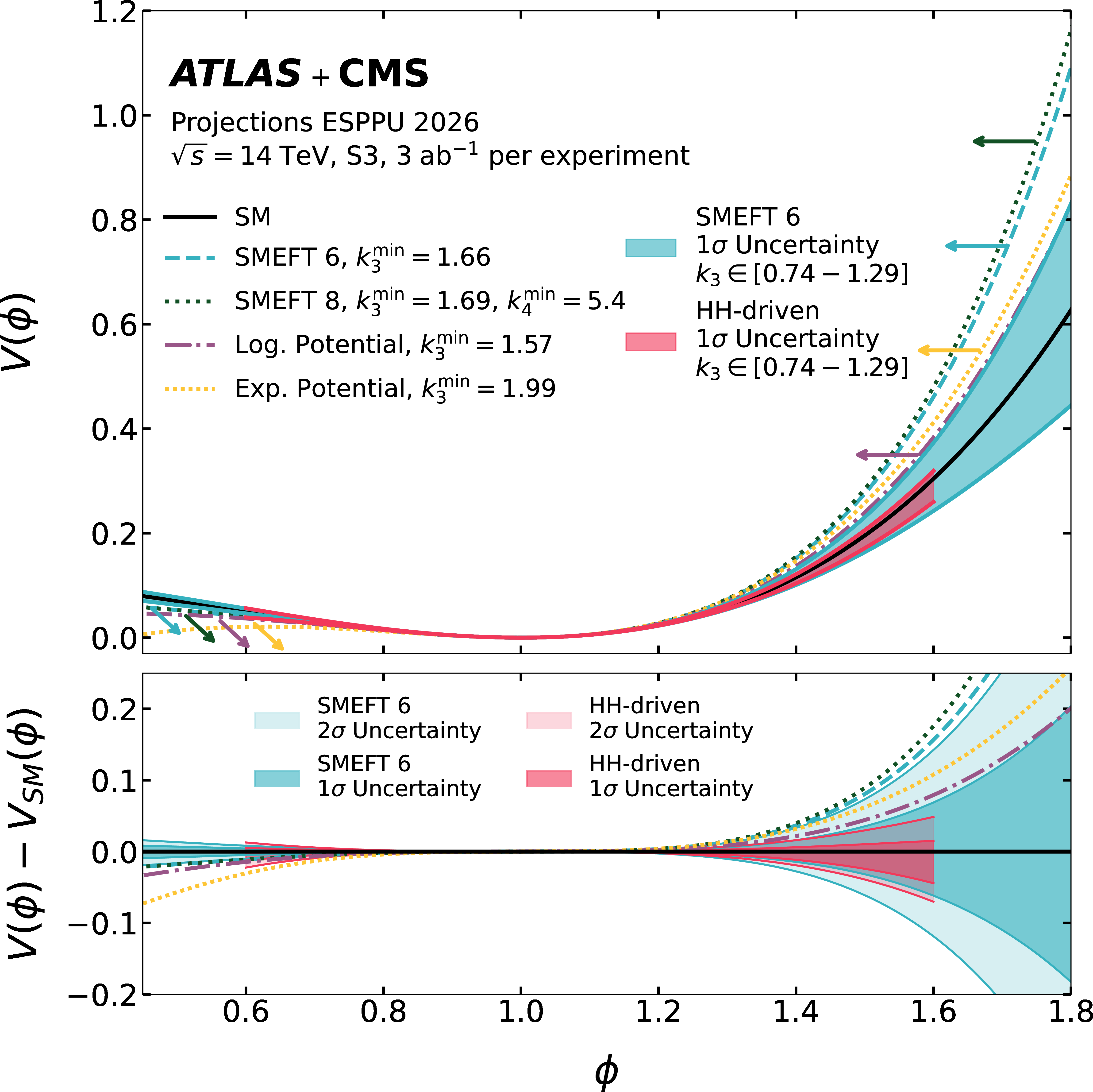
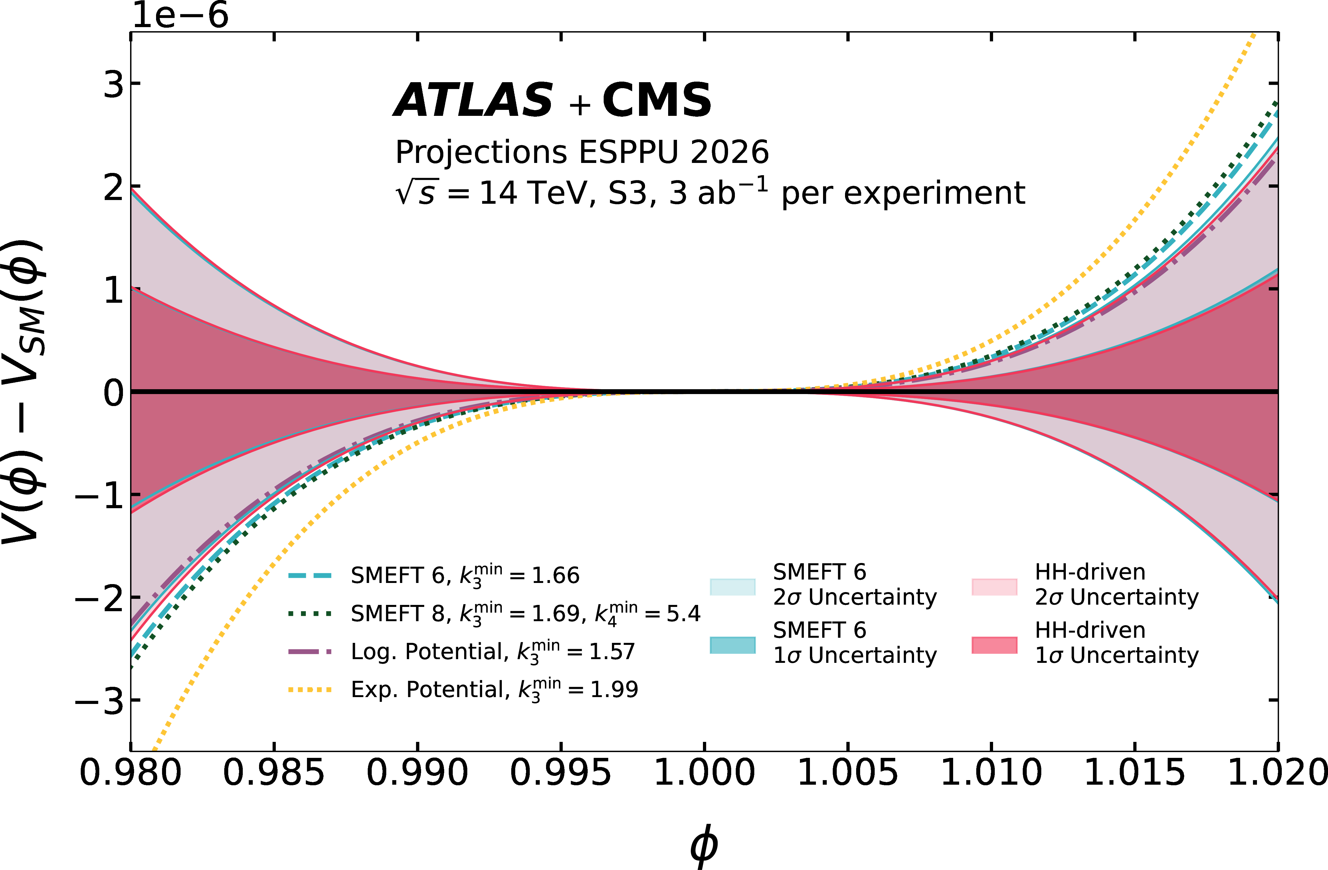
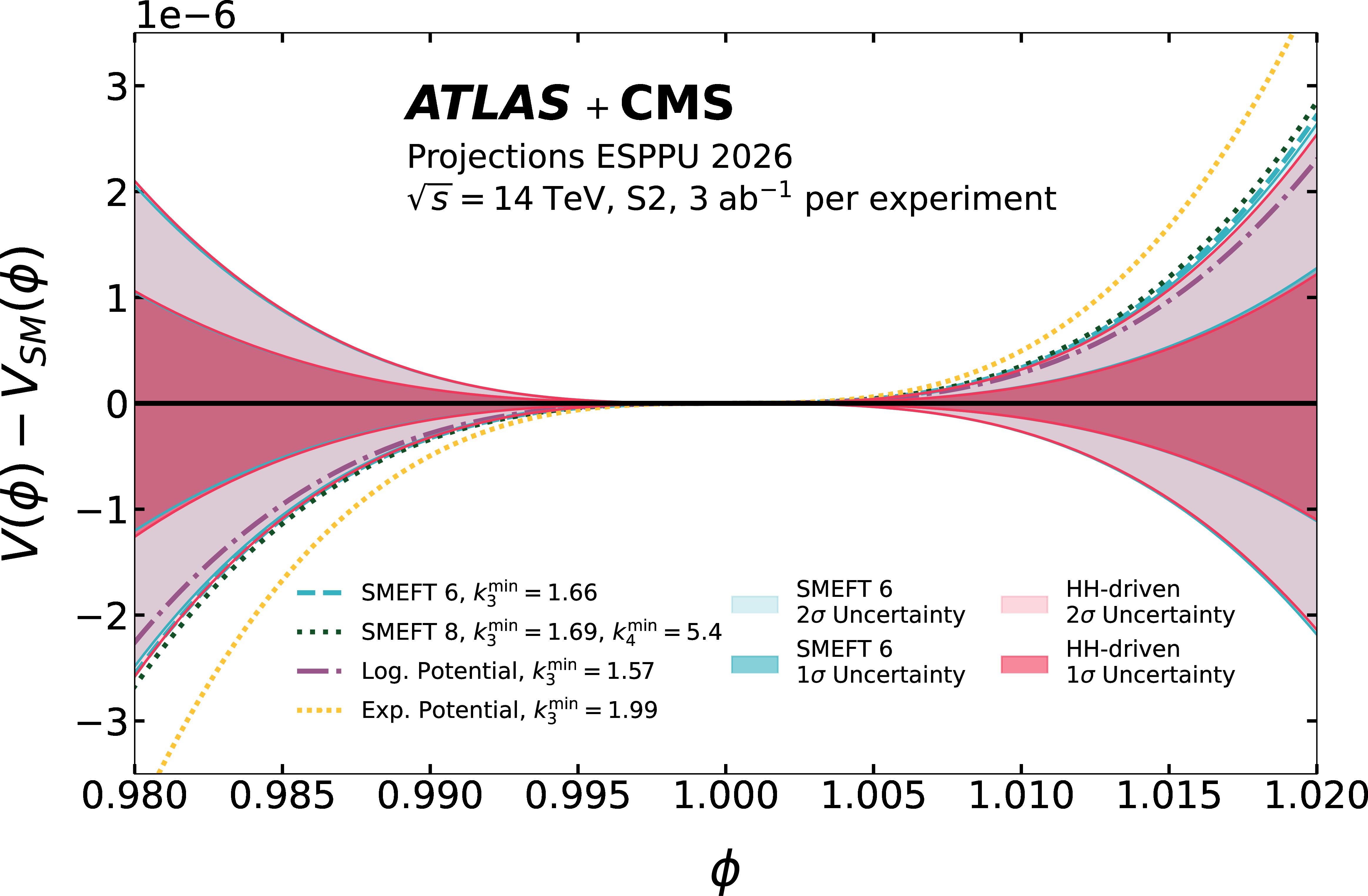
png pdf	Figure 6: (Top) BEH potentials in various models which predict a first-order phase transition [70]. The models are compared with the SM BEH potential. Two approaches (SMEFT 6 and HH-driven) are used to show the expected uncertainties on the Higgs self-coupling achieved by combining ATLAS and CMS at 3 ab $^{-1}$ in the S3 scenario. The dashed lines show the boundary of the regions for which the alternative models predict a strong first-order phase transition. The arrows indicate the region where the strong first-order phase transition happens. Further details can be found in the text. The bottom panel shows the difference between the potential $V(\phi)$ and its SM expectation $V_{SM}(\phi)$ . Here, the 68% and 95% CL uncertainty bands on the shape of $V(\phi)$ are shown, for the HH-driven and SMEFT 6 potentials (see text). (Bottom) A zoom into the $V(\phi)-V_{SM}(\phi)$ difference around the minimum of $V(\phi)$ , corresponding to the validity range of the HH-driven band.
png pdf	Figure 6-a: (Top) BEH potentials in various models which predict a first-order phase transition [70]. The models are compared with the SM BEH potential. Two approaches (SMEFT 6 and HH-driven) are used to show the expected uncertainties on the Higgs self-coupling achieved by combining ATLAS and CMS at 3 ab $^{-1}$ in the S3 scenario. The dashed lines show the boundary of the regions for which the alternative models predict a strong first-order phase transition. The arrows indicate the region where the strong first-order phase transition happens. Further details can be found in the text. The bottom panel shows the difference between the potential $V(\phi)$ and its SM expectation $V_{SM}(\phi)$ . Here, the 68% and 95% CL uncertainty bands on the shape of $V(\phi)$ are shown, for the HH-driven and SMEFT 6 potentials (see text). (Bottom) A zoom into the $V(\phi)-V_{SM}(\phi)$ difference around the minimum of $V(\phi)$ , corresponding to the validity range of the HH-driven band.
png pdf	Figure 6-b: (Top) BEH potentials in various models which predict a first-order phase transition [70]. The models are compared with the SM BEH potential. Two approaches (SMEFT 6 and HH-driven) are used to show the expected uncertainties on the Higgs self-coupling achieved by combining ATLAS and CMS at 3 ab $^{-1}$ in the S3 scenario. The dashed lines show the boundary of the regions for which the alternative models predict a strong first-order phase transition. The arrows indicate the region where the strong first-order phase transition happens. Further details can be found in the text. The bottom panel shows the difference between the potential $V(\phi)$ and its SM expectation $V_{SM}(\phi)$ . Here, the 68% and 95% CL uncertainty bands on the shape of $V(\phi)$ are shown, for the HH-driven and SMEFT 6 potentials (see text). (Bottom) A zoom into the $V(\phi)-V_{SM}(\phi)$ difference around the minimum of $V(\phi)$ , corresponding to the validity range of the HH-driven band.
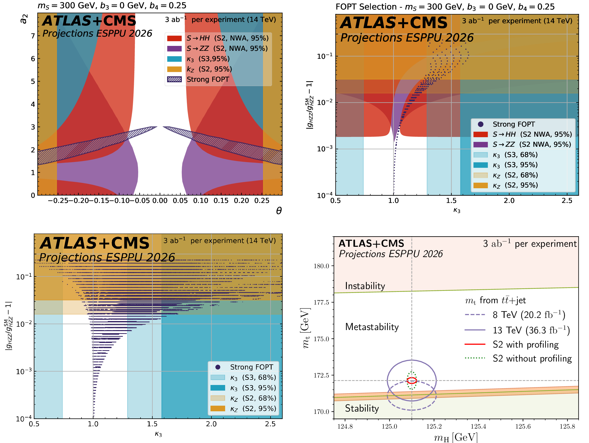
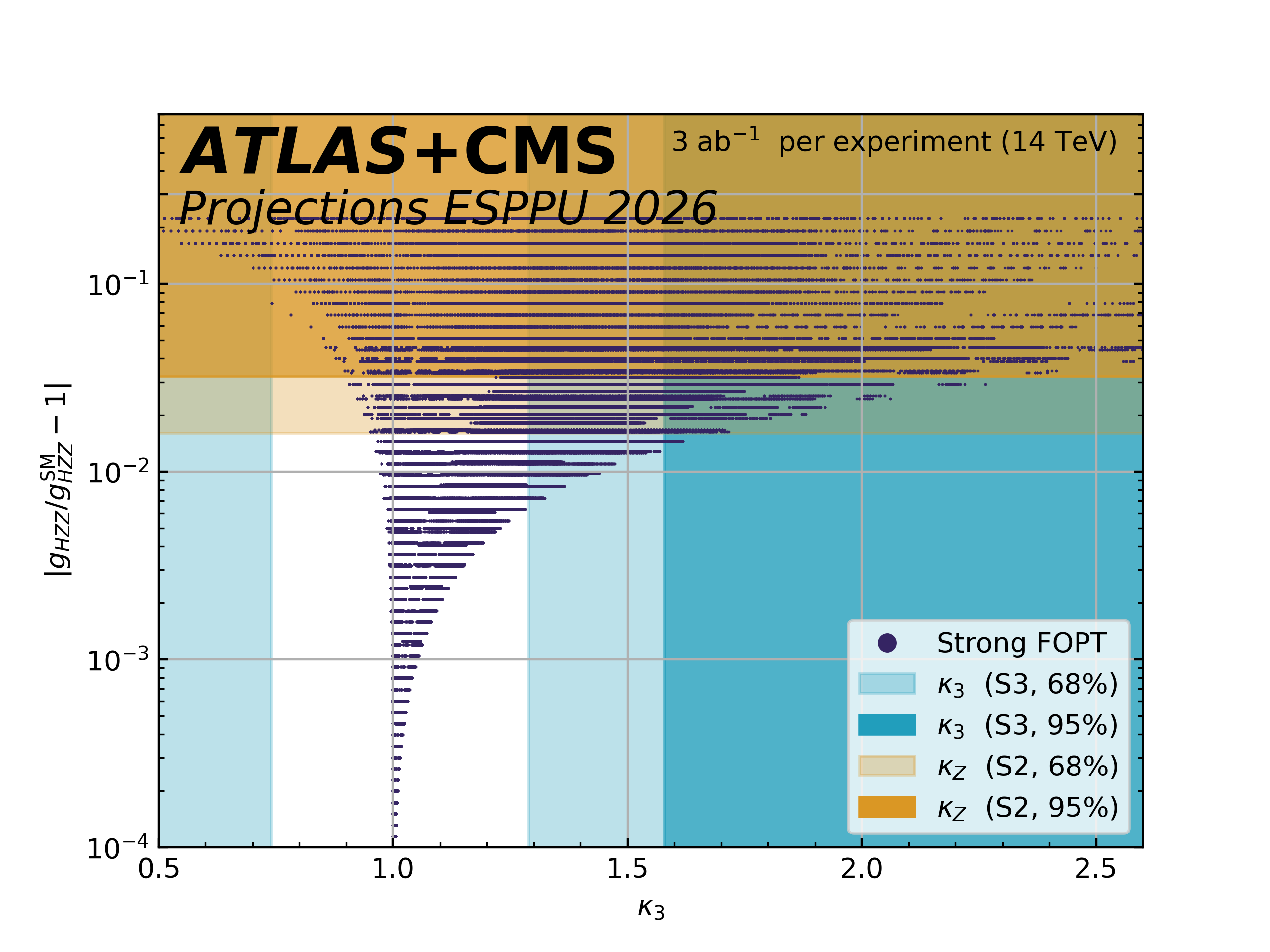
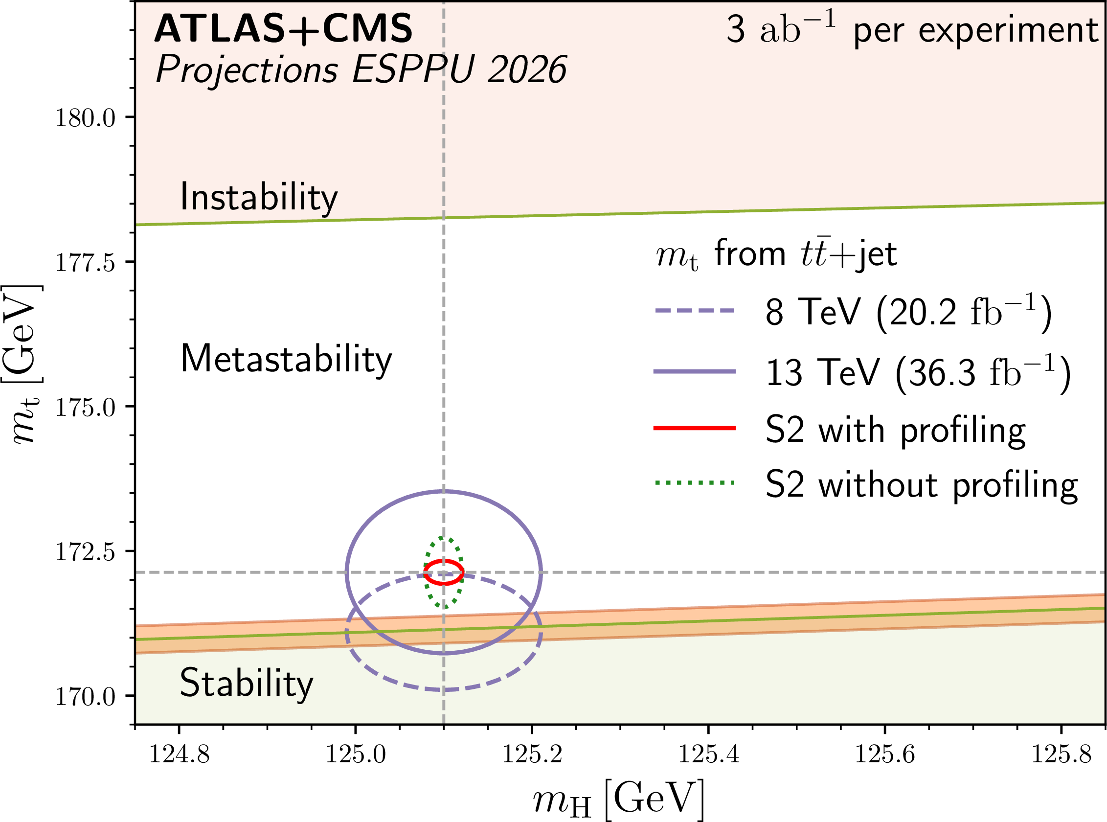
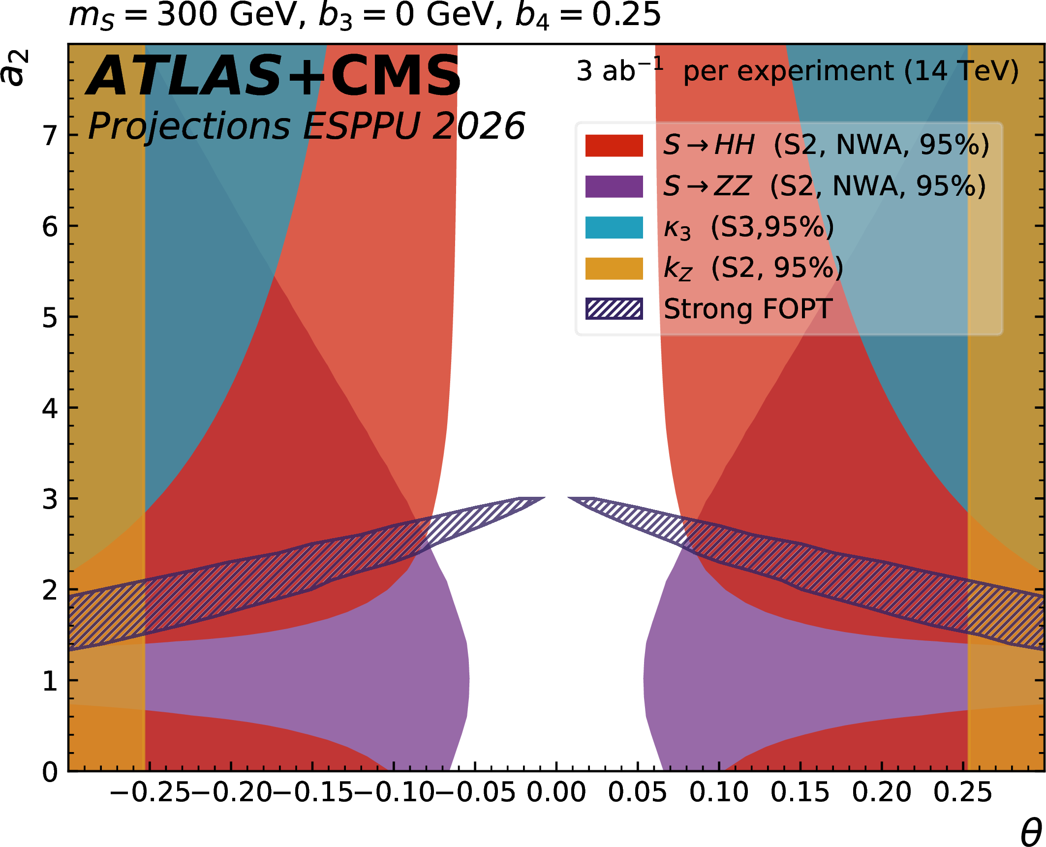
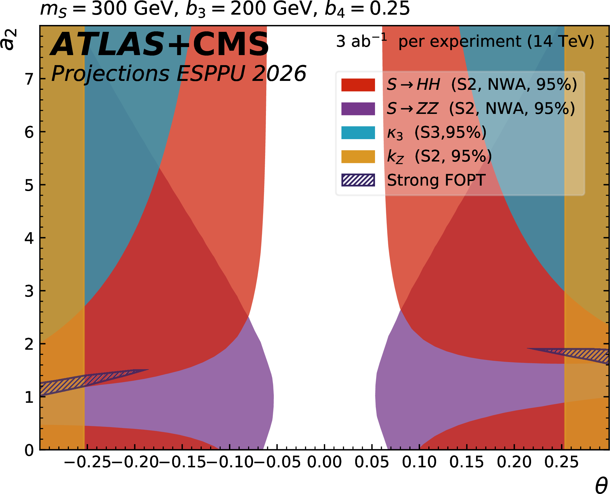
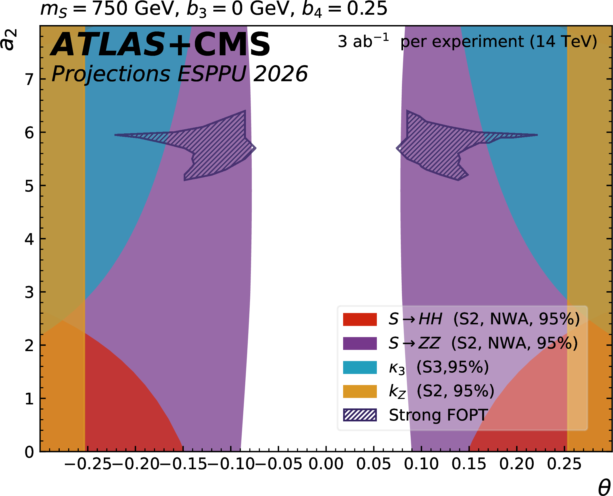
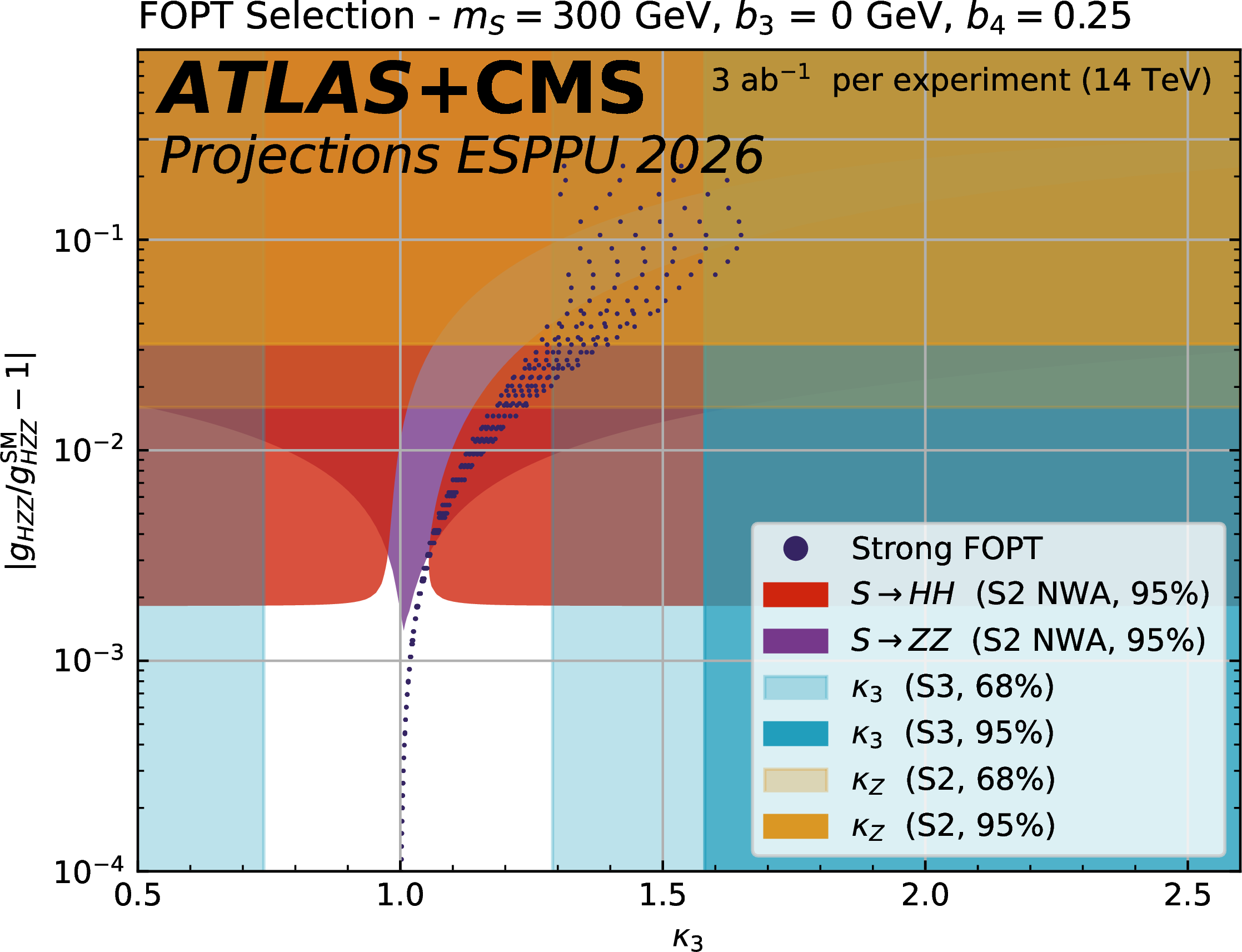
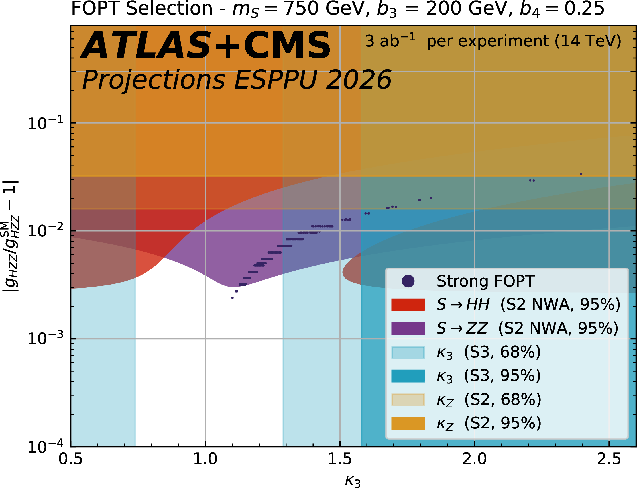
png pdf	Figure 7: Top left: Bounds on the heavy scalar model, in the plane of the scalar portal coupling, $a_2$ , versus the scalar singlet mixing angle $\theta$ [73]. The dark blue hatched contours show the regions of the $a_2$ versus $\theta$ parameter space in the scalar singlet model where a strong first-order phase transition is possible for $m_{\mathrm{S}}=$ 300 GeV, $b_3=$ 0 GeV and $b_4=$ 0.25. The other contours show the 95% CL exclusion in this plane from the resonant searches into $S\rightarrow \mathrm{HH} /\mathrm{ZZ}$ signatures, from the $H$ coupling to $Z$ and from $\kappa_3$ constraints. Top right: The same contours are shown in the plane of the deviation of the Higgs boson coupling to the $Z$ with respect to the SM one, versus $\kappa_{3}$ . The dark blue points show the area where a strong first-order phase transition in the early universe is possible within the scalar singlet model discussed in the text for $m_{\mathrm{S}}=$ 300 GeV, $b_3=$ 0, and $b_4=$ 0.25. Bottom left: Exclusion bounds in the plane of the Higgs boson to $\mathrm{ZZ}$ coupling with respect to the SM one versus $\kappa_{3}$ ; 68% and 95% exclusion bounds are displayed. The dark blue points populate the area where a strong first-order phase transition in the early universe is possible within the scalar singlet model discussed in the text for all choices of $m_{\mathrm{S}}$ , $b_3$ , and $b_4$ . Bottom right: Projections for the HL-LHC measurements of the Higgs boson and top quark mass. The top quark mass measurement in ${\mathrm{t}\overline{\mathrm{t}}} \text{+jet}$ is shown from ATLAS at 8 TeV [75] and CMS at 13 TeV [76]. The ATLAS+CMS projection is shown with profiling of the systematic uncertainties in the extraction of the top quark mass, based on the S2 scenario. Figure adapted from Ref. [77] with unchanged value and uncertainty in the strong coupling $\alpha_\mathrm{S}$ . The band between the stable and metastable region represents the uncertainty in $\alpha_\mathrm{S}$ .
png pdf	Figure 7-a: Top left: Bounds on the heavy scalar model, in the plane of the scalar portal coupling, $a_2$ , versus the scalar singlet mixing angle $\theta$ [73]. The dark blue hatched contours show the regions of the $a_2$ versus $\theta$ parameter space in the scalar singlet model where a strong first-order phase transition is possible for $m_{\mathrm{S}}=$ 300 GeV, $b_3=$ 0 GeV and $b_4=$ 0.25. The other contours show the 95% CL exclusion in this plane from the resonant searches into $S\rightarrow \mathrm{HH} /\mathrm{ZZ}$ signatures, from the $H$ coupling to $Z$ and from $\kappa_3$ constraints. Top right: The same contours are shown in the plane of the deviation of the Higgs boson coupling to the $Z$ with respect to the SM one, versus $\kappa_{3}$ . The dark blue points show the area where a strong first-order phase transition in the early universe is possible within the scalar singlet model discussed in the text for $m_{\mathrm{S}}=$ 300 GeV, $b_3=$ 0, and $b_4=$ 0.25. Bottom left: Exclusion bounds in the plane of the Higgs boson to $\mathrm{ZZ}$ coupling with respect to the SM one versus $\kappa_{3}$ ; 68% and 95% exclusion bounds are displayed. The dark blue points populate the area where a strong first-order phase transition in the early universe is possible within the scalar singlet model discussed in the text for all choices of $m_{\mathrm{S}}$ , $b_3$ , and $b_4$ . Bottom right: Projections for the HL-LHC measurements of the Higgs boson and top quark mass. The top quark mass measurement in ${\mathrm{t}\overline{\mathrm{t}}} \text{+jet}$ is shown from ATLAS at 8 TeV [75] and CMS at 13 TeV [76]. The ATLAS+CMS projection is shown with profiling of the systematic uncertainties in the extraction of the top quark mass, based on the S2 scenario. Figure adapted from Ref. [77] with unchanged value and uncertainty in the strong coupling $\alpha_\mathrm{S}$ . The band between the stable and metastable region represents the uncertainty in $\alpha_\mathrm{S}$ .
png pdf	Figure 7-b: Top left: Bounds on the heavy scalar model, in the plane of the scalar portal coupling, $a_2$ , versus the scalar singlet mixing angle $\theta$ [73]. The dark blue hatched contours show the regions of the $a_2$ versus $\theta$ parameter space in the scalar singlet model where a strong first-order phase transition is possible for $m_{\mathrm{S}}=$ 300 GeV, $b_3=$ 0 GeV and $b_4=$ 0.25. The other contours show the 95% CL exclusion in this plane from the resonant searches into $S\rightarrow \mathrm{HH} /\mathrm{ZZ}$ signatures, from the $H$ coupling to $Z$ and from $\kappa_3$ constraints. Top right: The same contours are shown in the plane of the deviation of the Higgs boson coupling to the $Z$ with respect to the SM one, versus $\kappa_{3}$ . The dark blue points show the area where a strong first-order phase transition in the early universe is possible within the scalar singlet model discussed in the text for $m_{\mathrm{S}}=$ 300 GeV, $b_3=$ 0, and $b_4=$ 0.25. Bottom left: Exclusion bounds in the plane of the Higgs boson to $\mathrm{ZZ}$ coupling with respect to the SM one versus $\kappa_{3}$ ; 68% and 95% exclusion bounds are displayed. The dark blue points populate the area where a strong first-order phase transition in the early universe is possible within the scalar singlet model discussed in the text for all choices of $m_{\mathrm{S}}$ , $b_3$ , and $b_4$ . Bottom right: Projections for the HL-LHC measurements of the Higgs boson and top quark mass. The top quark mass measurement in ${\mathrm{t}\overline{\mathrm{t}}} \text{+jet}$ is shown from ATLAS at 8 TeV [75] and CMS at 13 TeV [76]. The ATLAS+CMS projection is shown with profiling of the systematic uncertainties in the extraction of the top quark mass, based on the S2 scenario. Figure adapted from Ref. [77] with unchanged value and uncertainty in the strong coupling $\alpha_\mathrm{S}$ . The band between the stable and metastable region represents the uncertainty in $\alpha_\mathrm{S}$ .
png	Figure 7-c: Top left: Bounds on the heavy scalar model, in the plane of the scalar portal coupling, $a_2$ , versus the scalar singlet mixing angle $\theta$ [73]. The dark blue hatched contours show the regions of the $a_2$ versus $\theta$ parameter space in the scalar singlet model where a strong first-order phase transition is possible for $m_{\mathrm{S}}=$ 300 GeV, $b_3=$ 0 GeV and $b_4=$ 0.25. The other contours show the 95% CL exclusion in this plane from the resonant searches into $S\rightarrow \mathrm{HH} /\mathrm{ZZ}$ signatures, from the $H$ coupling to $Z$ and from $\kappa_3$ constraints. Top right: The same contours are shown in the plane of the deviation of the Higgs boson coupling to the $Z$ with respect to the SM one, versus $\kappa_{3}$ . The dark blue points show the area where a strong first-order phase transition in the early universe is possible within the scalar singlet model discussed in the text for $m_{\mathrm{S}}=$ 300 GeV, $b_3=$ 0, and $b_4=$ 0.25. Bottom left: Exclusion bounds in the plane of the Higgs boson to $\mathrm{ZZ}$ coupling with respect to the SM one versus $\kappa_{3}$ ; 68% and 95% exclusion bounds are displayed. The dark blue points populate the area where a strong first-order phase transition in the early universe is possible within the scalar singlet model discussed in the text for all choices of $m_{\mathrm{S}}$ , $b_3$ , and $b_4$ . Bottom right: Projections for the HL-LHC measurements of the Higgs boson and top quark mass. The top quark mass measurement in ${\mathrm{t}\overline{\mathrm{t}}} \text{+jet}$ is shown from ATLAS at 8 TeV [75] and CMS at 13 TeV [76]. The ATLAS+CMS projection is shown with profiling of the systematic uncertainties in the extraction of the top quark mass, based on the S2 scenario. Figure adapted from Ref. [77] with unchanged value and uncertainty in the strong coupling $\alpha_\mathrm{S}$ . The band between the stable and metastable region represents the uncertainty in $\alpha_\mathrm{S}$ .
png pdf	Figure 7-d: Top left: Bounds on the heavy scalar model, in the plane of the scalar portal coupling, $a_2$ , versus the scalar singlet mixing angle $\theta$ [73]. The dark blue hatched contours show the regions of the $a_2$ versus $\theta$ parameter space in the scalar singlet model where a strong first-order phase transition is possible for $m_{\mathrm{S}}=$ 300 GeV, $b_3=$ 0 GeV and $b_4=$ 0.25. The other contours show the 95% CL exclusion in this plane from the resonant searches into $S\rightarrow \mathrm{HH} /\mathrm{ZZ}$ signatures, from the $H$ coupling to $Z$ and from $\kappa_3$ constraints. Top right: The same contours are shown in the plane of the deviation of the Higgs boson coupling to the $Z$ with respect to the SM one, versus $\kappa_{3}$ . The dark blue points show the area where a strong first-order phase transition in the early universe is possible within the scalar singlet model discussed in the text for $m_{\mathrm{S}}=$ 300 GeV, $b_3=$ 0, and $b_4=$ 0.25. Bottom left: Exclusion bounds in the plane of the Higgs boson to $\mathrm{ZZ}$ coupling with respect to the SM one versus $\kappa_{3}$ ; 68% and 95% exclusion bounds are displayed. The dark blue points populate the area where a strong first-order phase transition in the early universe is possible within the scalar singlet model discussed in the text for all choices of $m_{\mathrm{S}}$ , $b_3$ , and $b_4$ . Bottom right: Projections for the HL-LHC measurements of the Higgs boson and top quark mass. The top quark mass measurement in ${\mathrm{t}\overline{\mathrm{t}}} \text{+jet}$ is shown from ATLAS at 8 TeV [75] and CMS at 13 TeV [76]. The ATLAS+CMS projection is shown with profiling of the systematic uncertainties in the extraction of the top quark mass, based on the S2 scenario. Figure adapted from Ref. [77] with unchanged value and uncertainty in the strong coupling $\alpha_\mathrm{S}$ . The band between the stable and metastable region represents the uncertainty in $\alpha_\mathrm{S}$ .
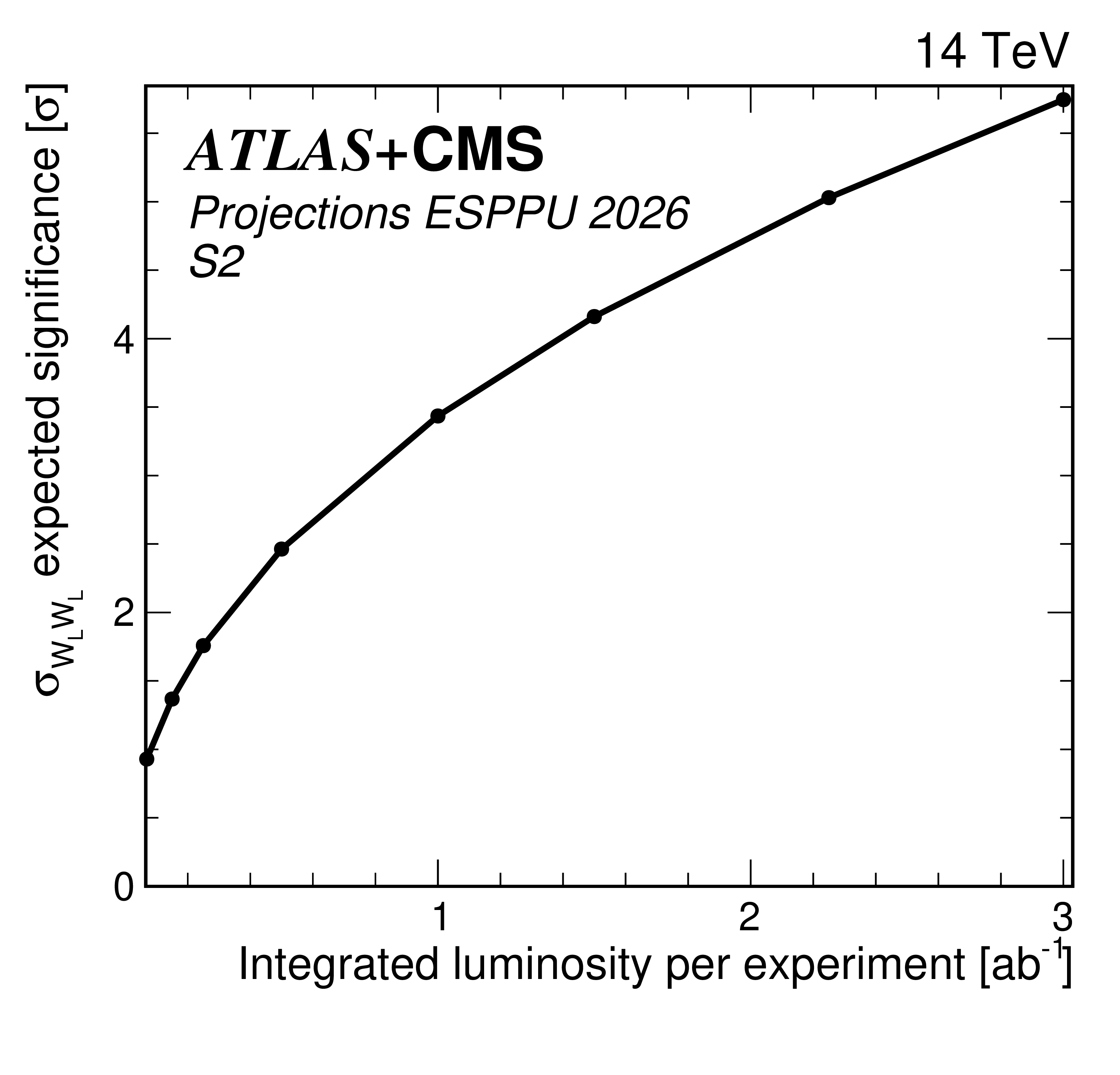
png pdf	Figure 8: Expected significance of the longitudinally polarized $WW$ scattering as a function of the luminosity in the S2 scenario.
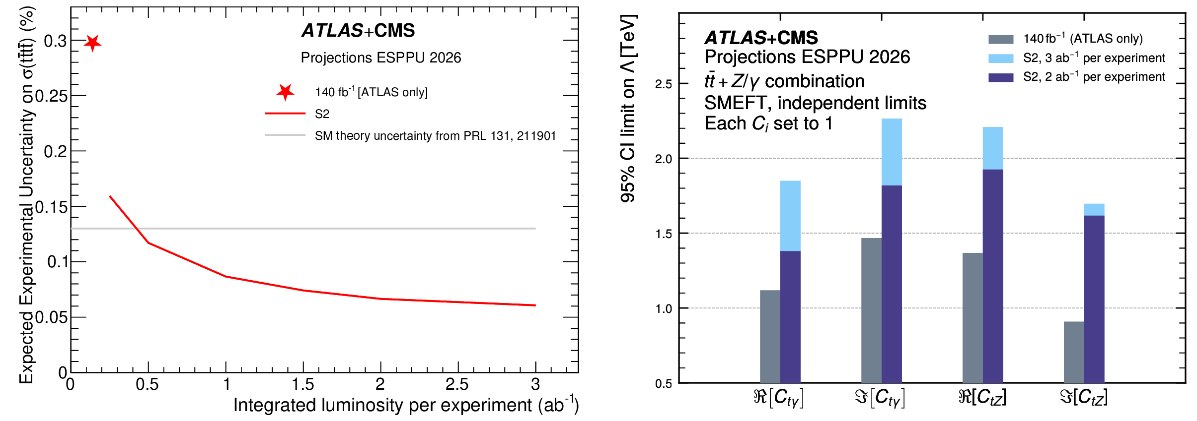
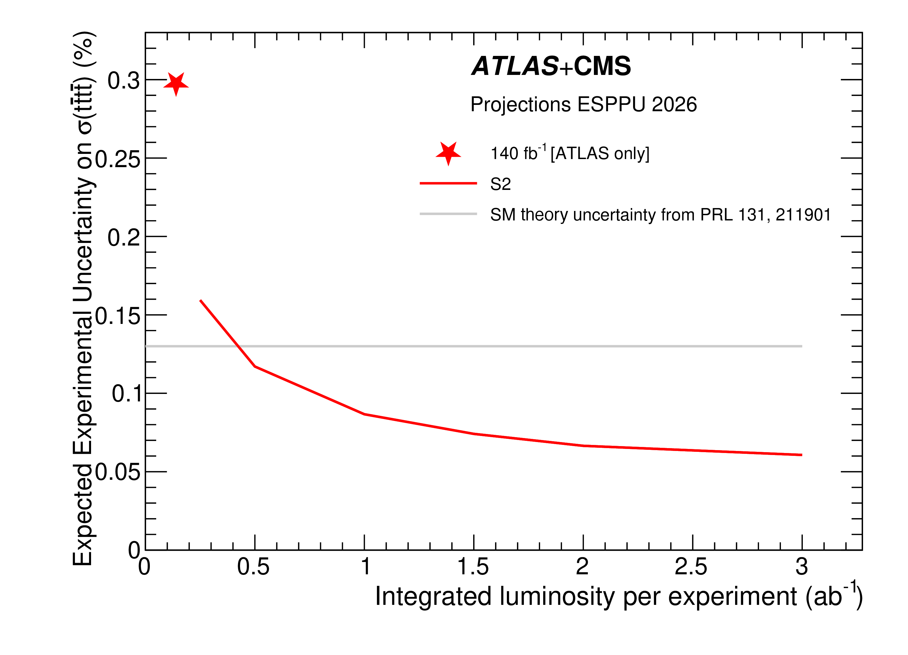
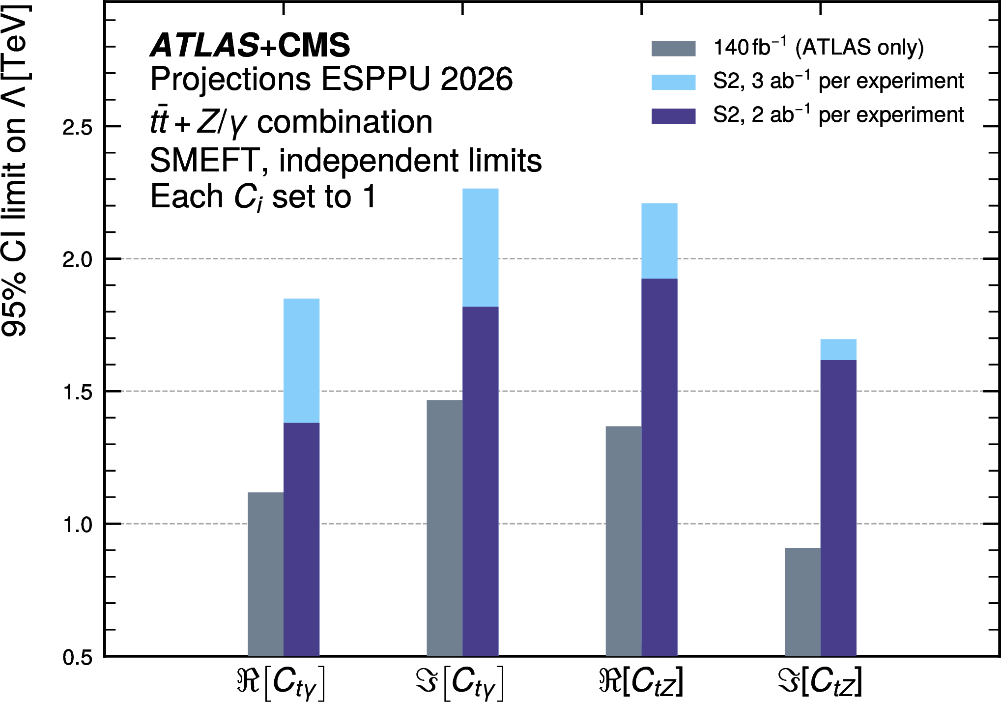
png pdf	Figure 9: Left: Expected experimental uncertainty in the $\mathrm{t\bar{t}t\bar{t}}$ cross section measurement. Right: Projected 95% confidence intervals on the new physics energy scale $\Lambda$ from the combined constraints of $\mathrm{t \bar t Z }$ and $\mathrm{t \bar t \gamma}$ cross section measurements on EFT operators related to the electroweak dipole moments of the top quark, derived for EFT operator couplings $C_i=$ 1.
png pdf	Figure 9-a: Left: Expected experimental uncertainty in the $\mathrm{t\bar{t}t\bar{t}}$ cross section measurement. Right: Projected 95% confidence intervals on the new physics energy scale $\Lambda$ from the combined constraints of $\mathrm{t \bar t Z }$ and $\mathrm{t \bar t \gamma}$ cross section measurements on EFT operators related to the electroweak dipole moments of the top quark, derived for EFT operator couplings $C_i=$ 1.
png pdf	Figure 9-b: Left: Expected experimental uncertainty in the $\mathrm{t\bar{t}t\bar{t}}$ cross section measurement. Right: Projected 95% confidence intervals on the new physics energy scale $\Lambda$ from the combined constraints of $\mathrm{t \bar t Z }$ and $\mathrm{t \bar t \gamma}$ cross section measurements on EFT operators related to the electroweak dipole moments of the top quark, derived for EFT operator couplings $C_i=$ 1.
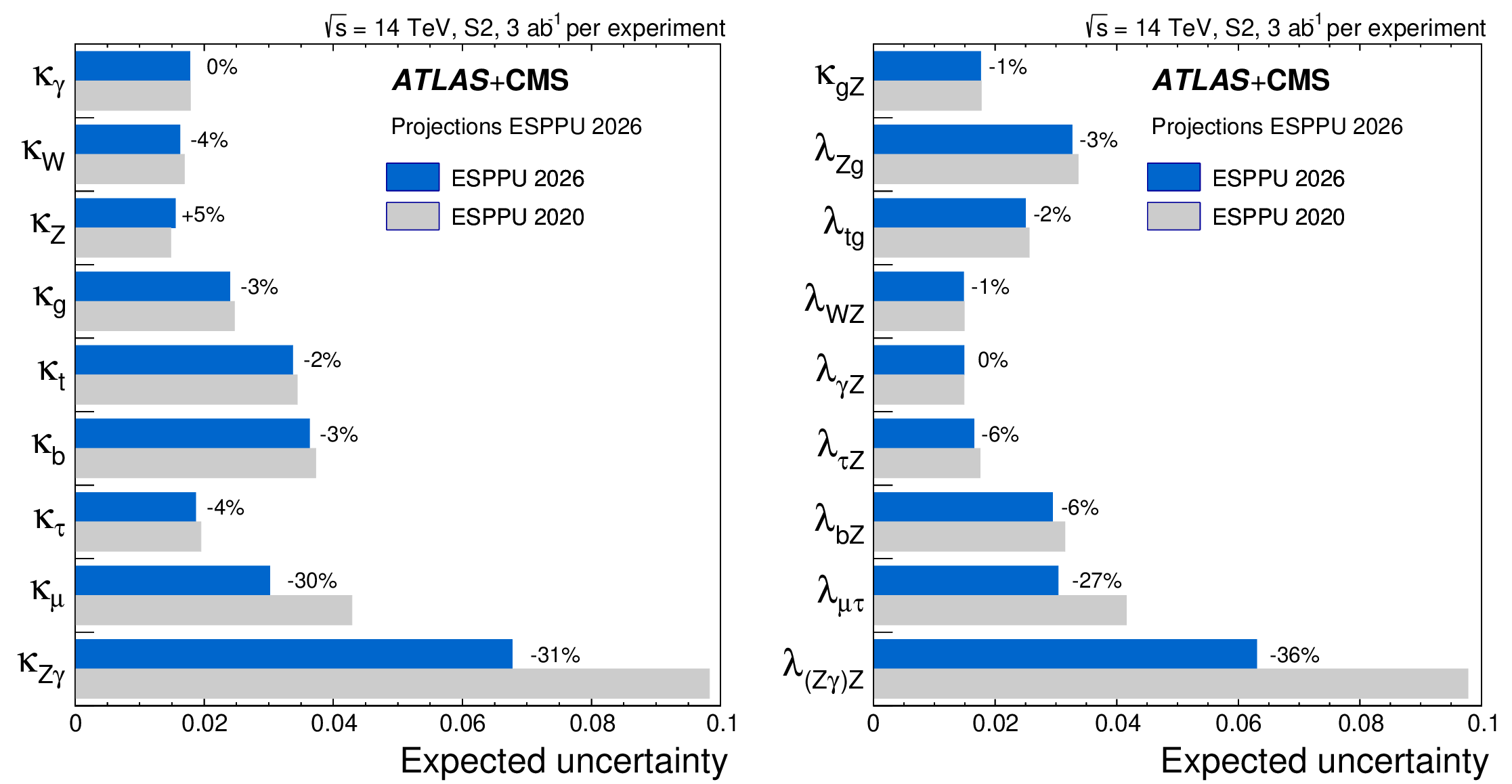
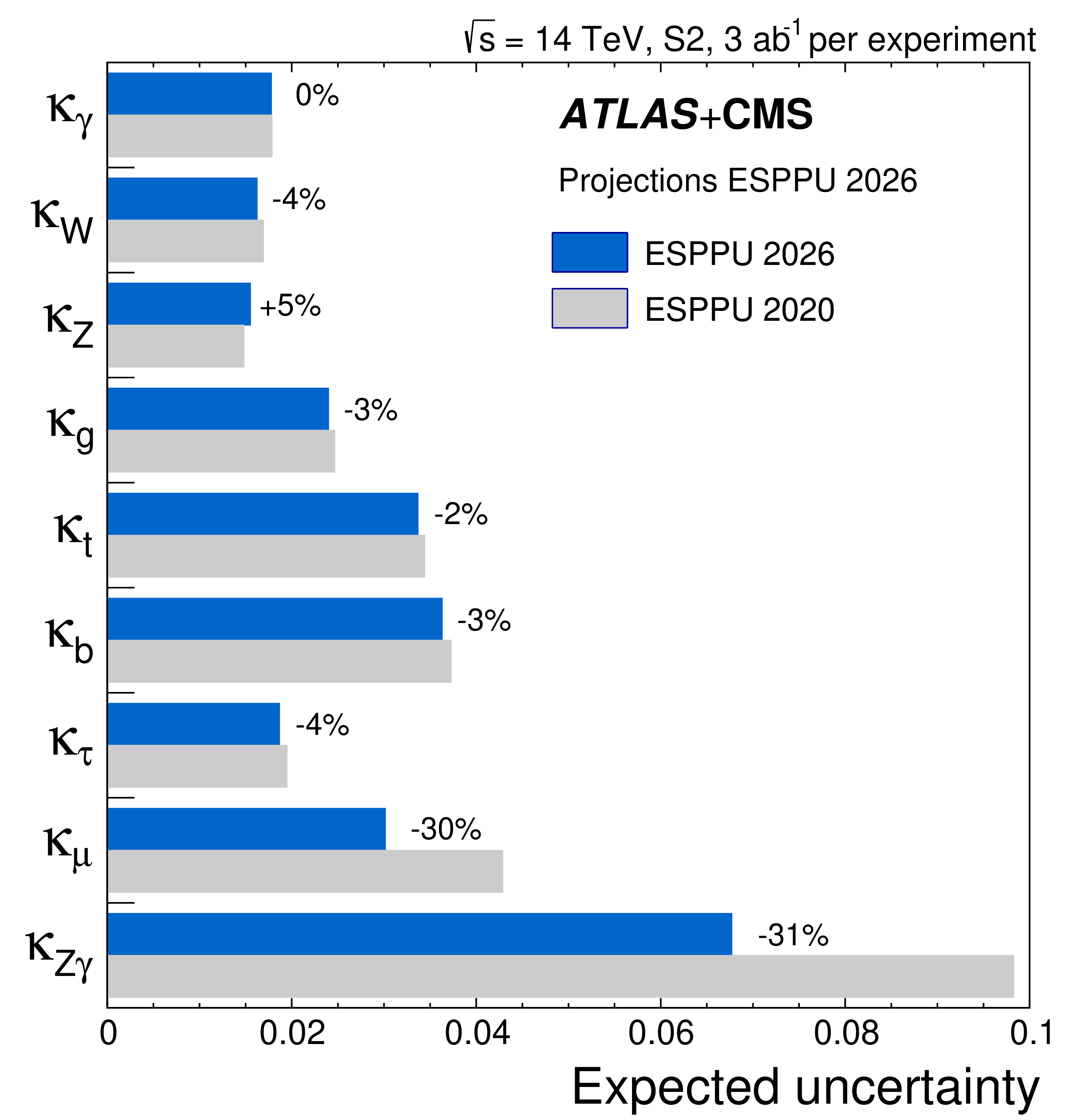
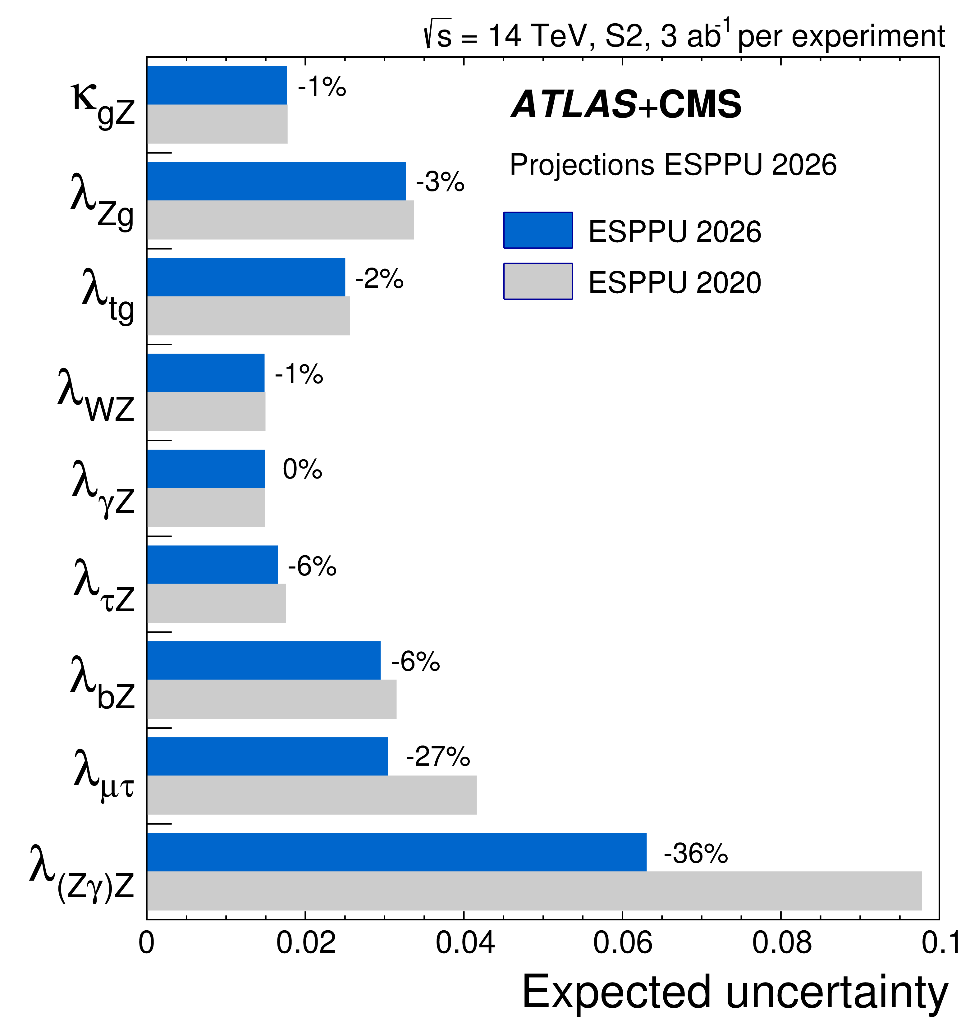
png pdf	Figure 10: ESPPU 2026 projections of coupling modifier uncertainties (left) and their ratios (right), compared to the previous HL-LHC projections [2]. The shown percentages represent the relative difference between the two projections. The precision of $\kappa_{\mathrm{Z}}$ is slightly lower due to the refined treatment of the $\mathrm{ZH}$ theory uncertainty.
png pdf	Figure 10-a: ESPPU 2026 projections of coupling modifier uncertainties (left) and their ratios (right), compared to the previous HL-LHC projections [2]. The shown percentages represent the relative difference between the two projections. The precision of $\kappa_{\mathrm{Z}}$ is slightly lower due to the refined treatment of the $\mathrm{ZH}$ theory uncertainty.
png pdf	Figure 10-b: ESPPU 2026 projections of coupling modifier uncertainties (left) and their ratios (right), compared to the previous HL-LHC projections [2]. The shown percentages represent the relative difference between the two projections. The precision of $\kappa_{\mathrm{Z}}$ is slightly lower due to the refined treatment of the $\mathrm{ZH}$ theory uncertainty.
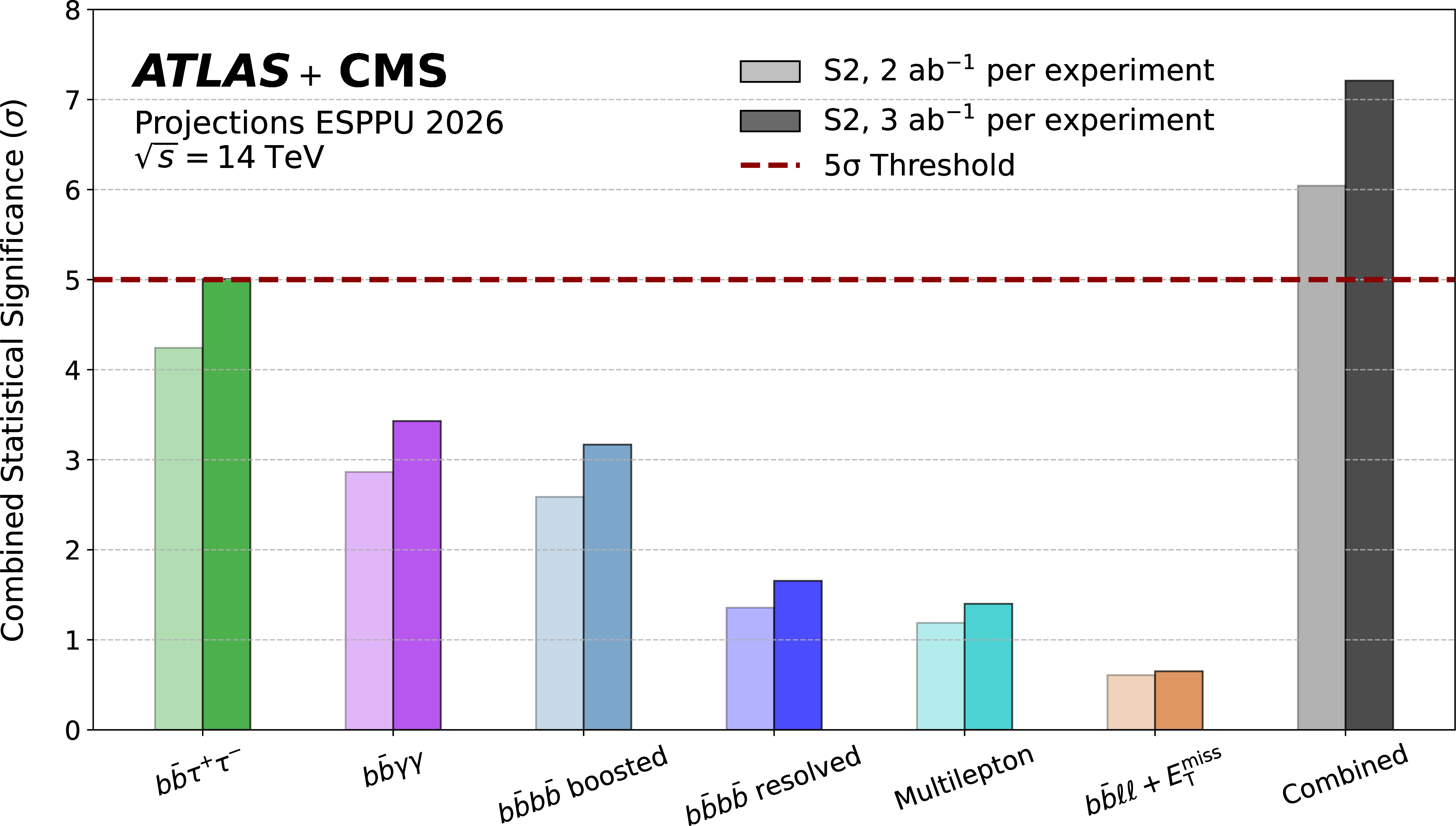
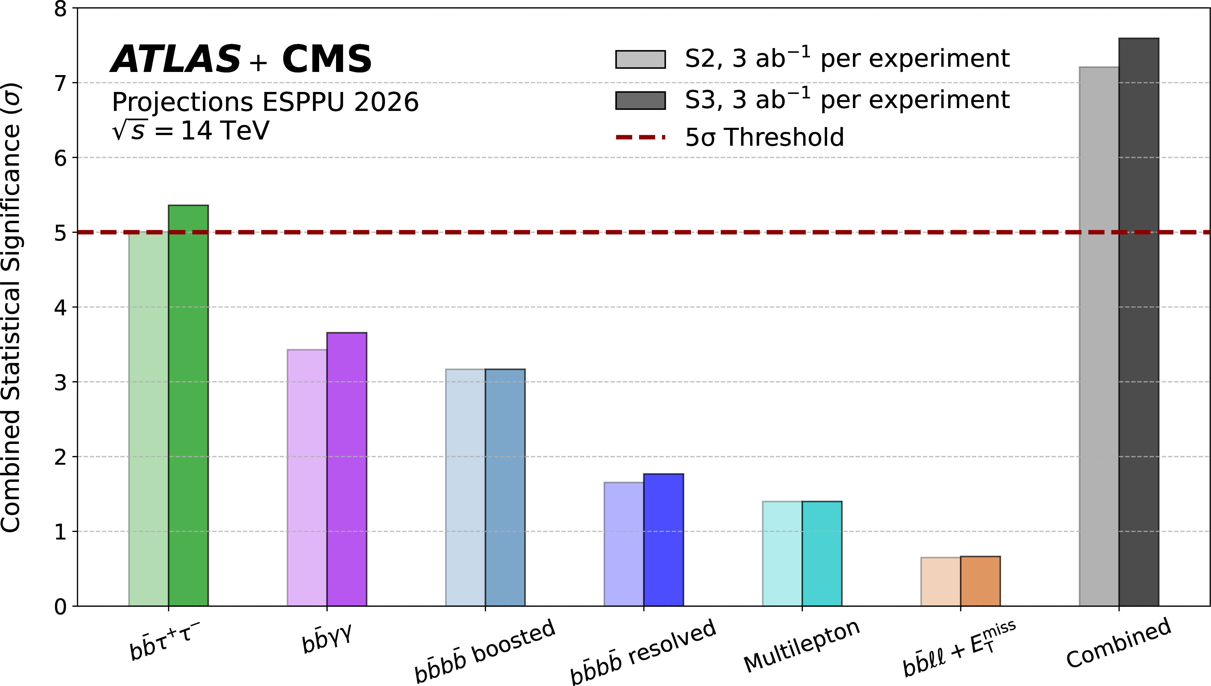
png pdf	Figure 11: $\mathrm{HH}$ significances per final state channel, combined between ATLAS and CMS, in a comparison between integrated luminosities for the S2 systematics scenario (left) and in a comparison between systematics scenarios at 3 ab $^{-1}$ (right).
png pdf	Figure 11-a: $\mathrm{HH}$ significances per final state channel, combined between ATLAS and CMS, in a comparison between integrated luminosities for the S2 systematics scenario (left) and in a comparison between systematics scenarios at 3 ab $^{-1}$ (right).
png pdf	Figure 11-b: $\mathrm{HH}$ significances per final state channel, combined between ATLAS and CMS, in a comparison between integrated luminosities for the S2 systematics scenario (left) and in a comparison between systematics scenarios at 3 ab $^{-1}$ (right).
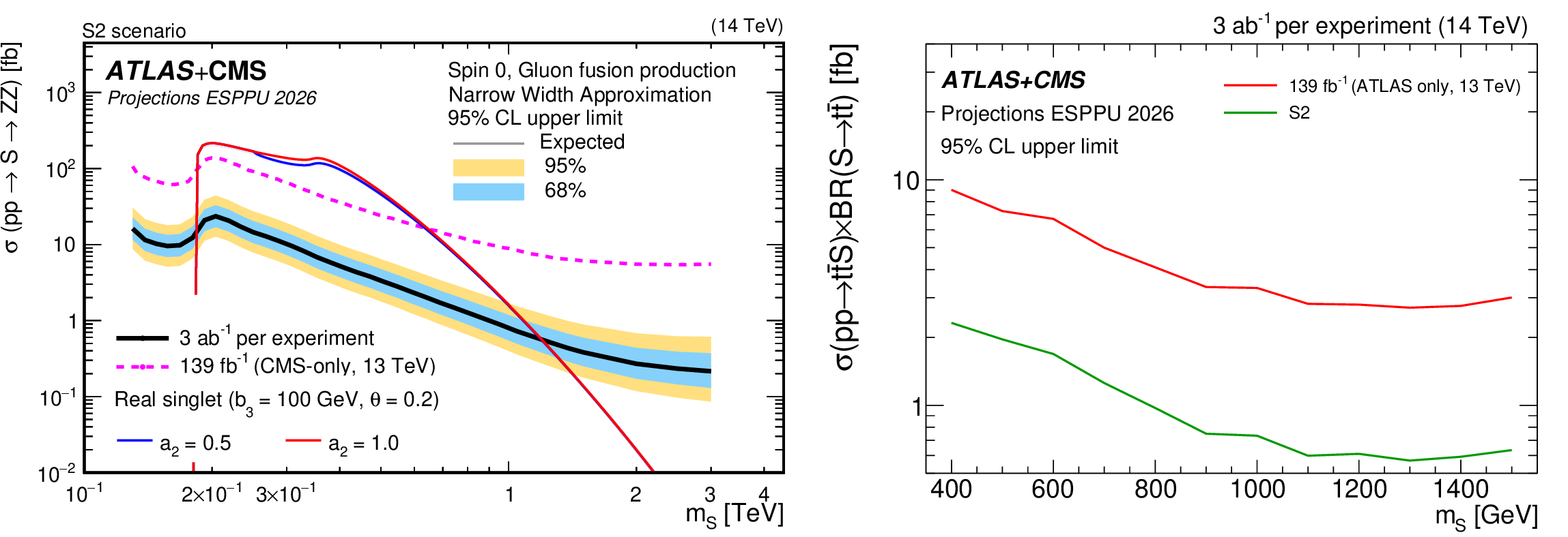
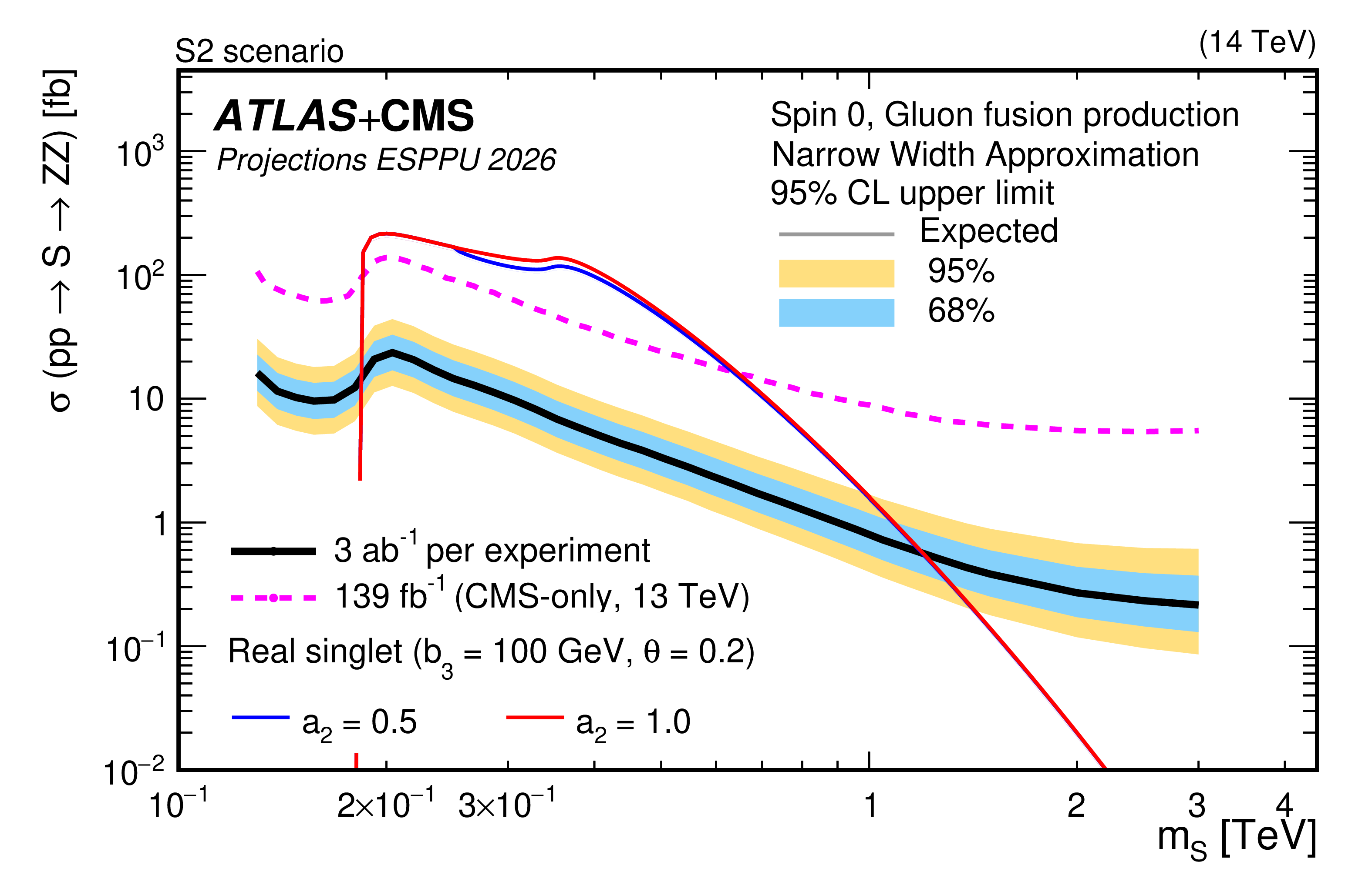
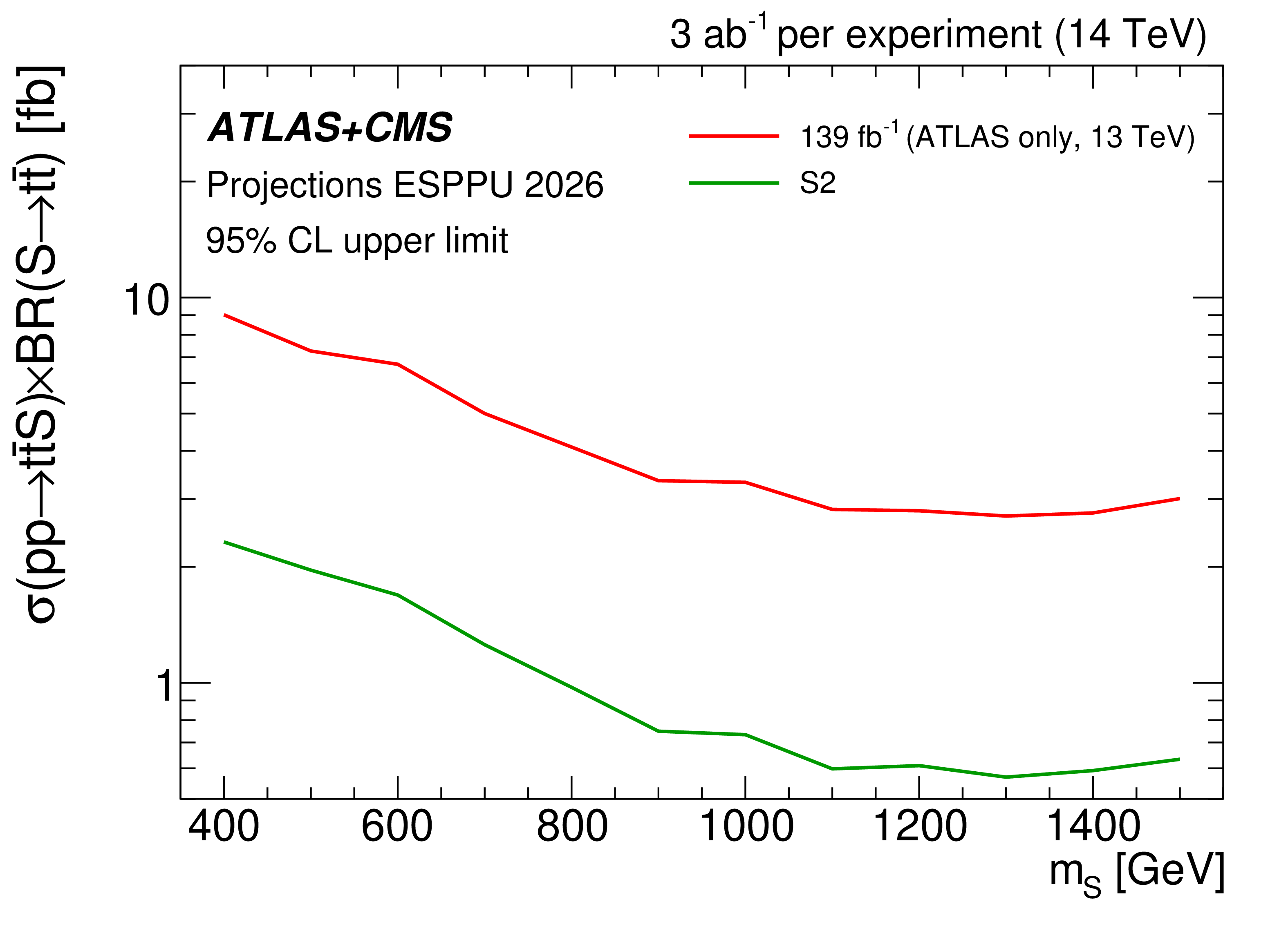
png pdf	Figure 12: Expected 95% CL upper limits on the $\mathrm{ \sigma(pp \to S \to ZZ)}$ (left) and $\mathrm{ \sigma(pp \to S t \bar t \to t \bar t t \bar t) }$ (right) cross sections as a function of the scalar mass $m_{\mathrm{S}}$ , produced via gluon fusion using the narrow width approximation. The projection is derived assuming 3 ab $^{-1}$ per experiment for the S2 scenario at 14 TeV.
png pdf	Figure 12-a: Expected 95% CL upper limits on the $\mathrm{ \sigma(pp \to S \to ZZ)}$ (left) and $\mathrm{ \sigma(pp \to S t \bar t \to t \bar t t \bar t) }$ (right) cross sections as a function of the scalar mass $m_{\mathrm{S}}$ , produced via gluon fusion using the narrow width approximation. The projection is derived assuming 3 ab $^{-1}$ per experiment for the S2 scenario at 14 TeV.
png pdf	Figure 12-b: Expected 95% CL upper limits on the $\mathrm{ \sigma(pp \to S \to ZZ)}$ (left) and $\mathrm{ \sigma(pp \to S t \bar t \to t \bar t t \bar t) }$ (right) cross sections as a function of the scalar mass $m_{\mathrm{S}}$ , produced via gluon fusion using the narrow width approximation. The projection is derived assuming 3 ab $^{-1}$ per experiment for the S2 scenario at 14 TeV.
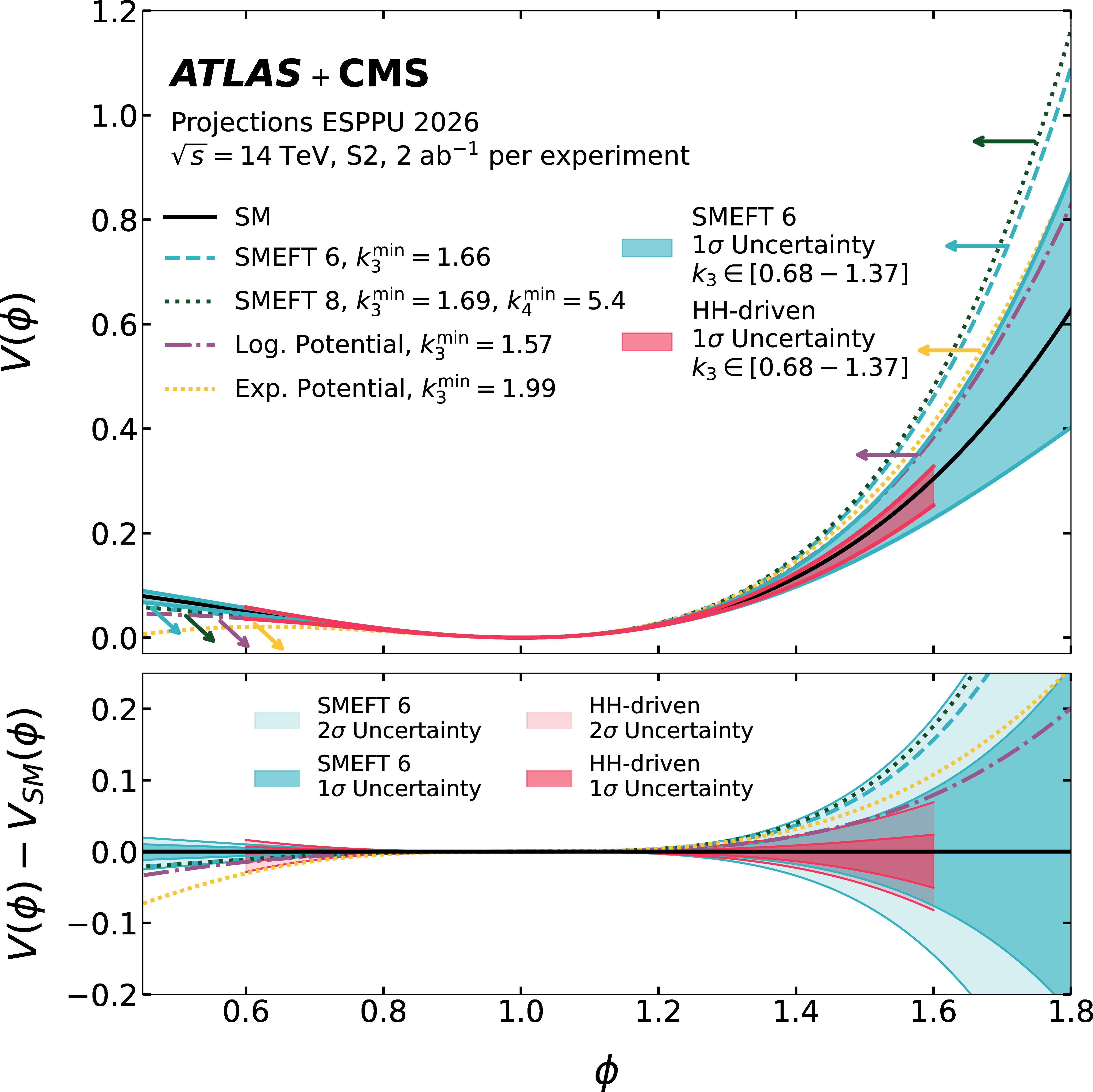
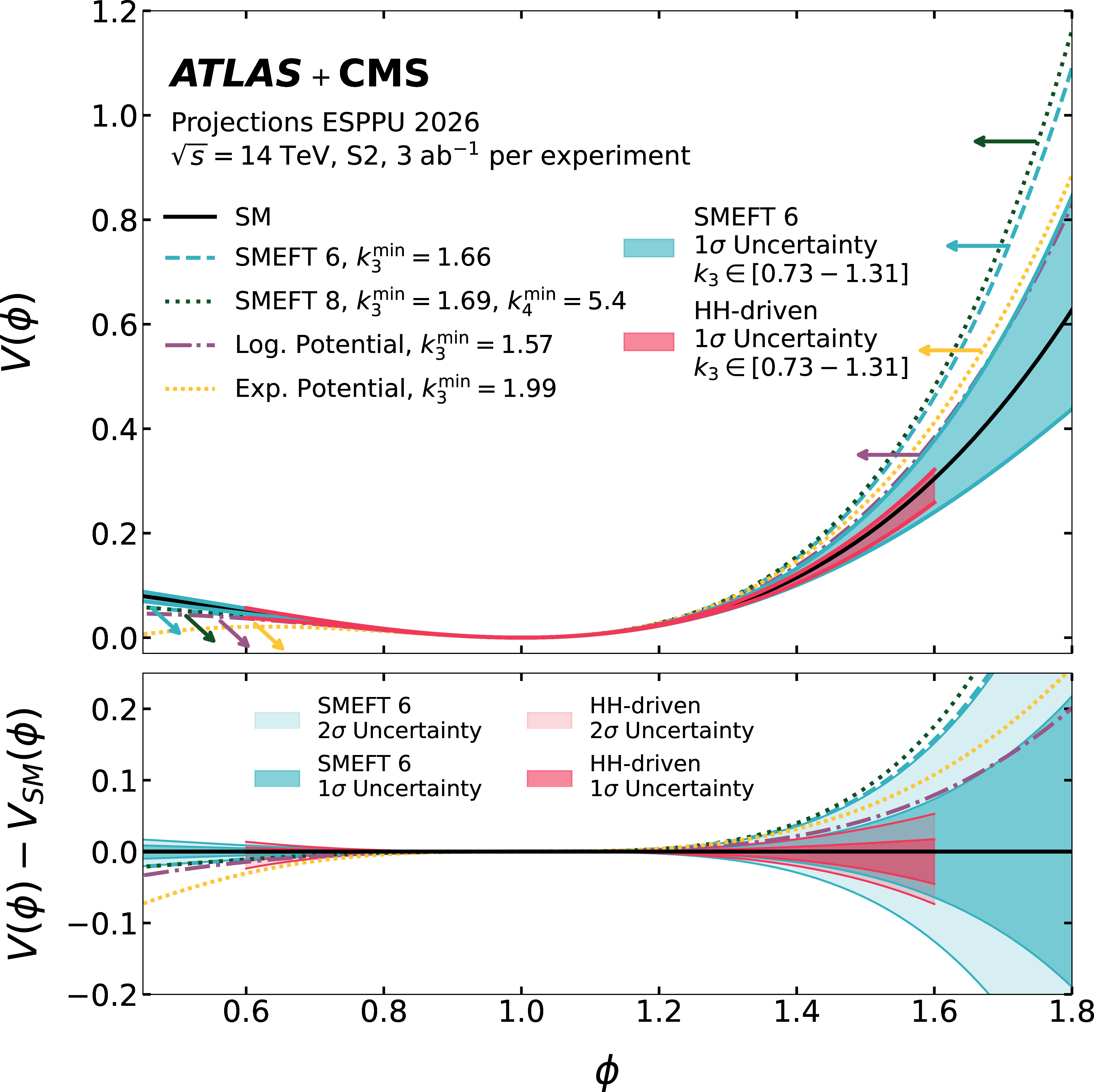
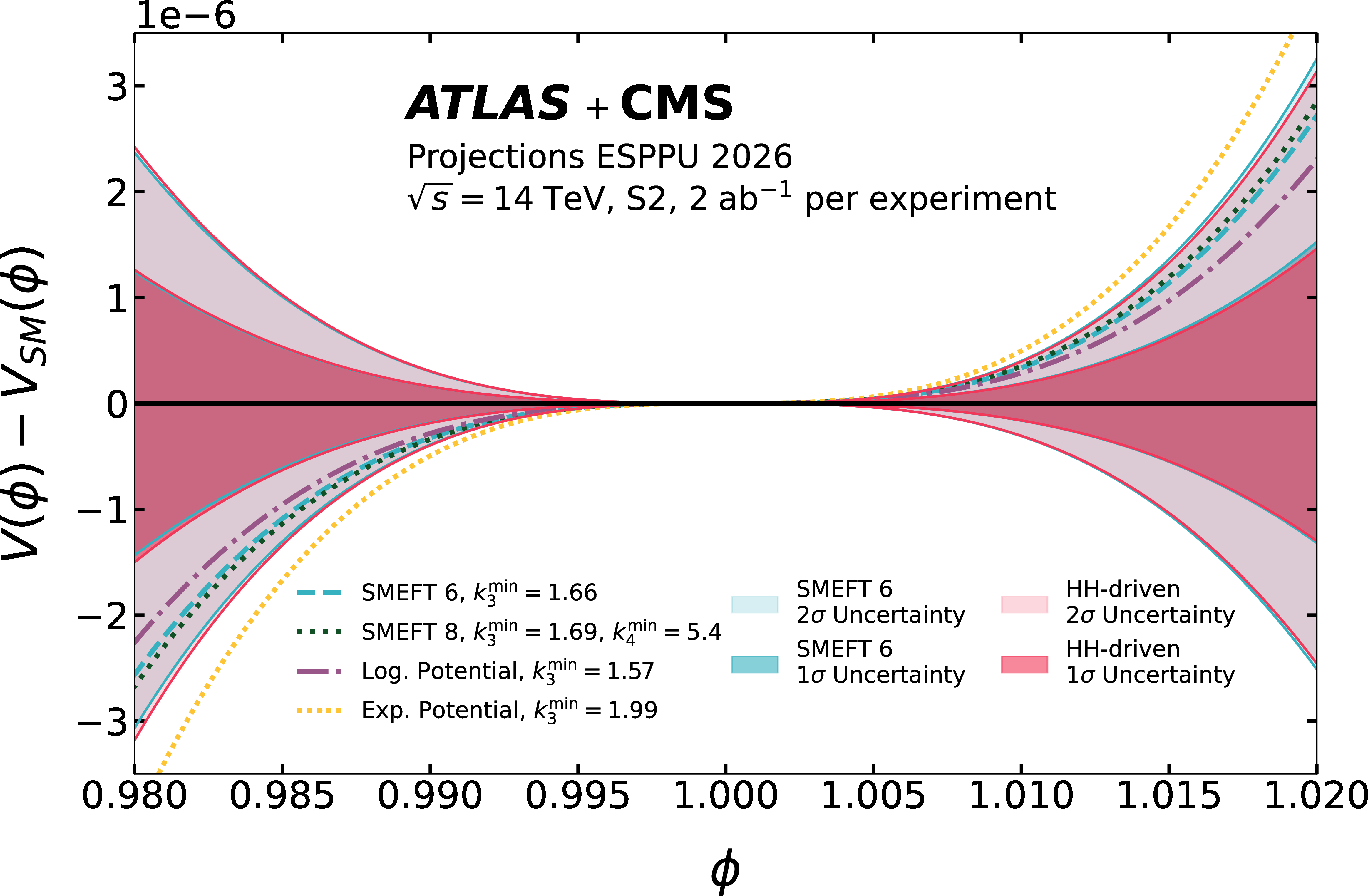
png pdf	Figure 13: BEH potentials in various models which predict first-order phase transition [73]. The models are compared with the SM BEH potential. Two approaches (SMEFT 6 and HH-driven) are used to show the expected uncertainties on the Higgs self-coupling achieved by combining ATLAS and CMS at 2 ab $^{-1}$ (top-left) and at 3 ab $^{-1}$ (top-right) in the S2 scenario, in a wide range of the BEH field value. The bottom panels show the difference between the potential $V(\phi)$ and its SM expectation $V_{SM}(\phi)$ . Here, the 68% and 95% CL uncertainty bands on the shape of $V(\phi)$ are shown, for the HH-driven and SMEFT 6 potentials (see text). The bottom plots show the zoom into the $V(\phi)-V_{SM}(\phi)$ difference around the minimum of $V(\phi)$ , corresponding to the validity range of the HH-driven band.
png pdf	Figure 13-a: BEH potentials in various models which predict first-order phase transition [73]. The models are compared with the SM BEH potential. Two approaches (SMEFT 6 and HH-driven) are used to show the expected uncertainties on the Higgs self-coupling achieved by combining ATLAS and CMS at 2 ab $^{-1}$ (top-left) and at 3 ab $^{-1}$ (top-right) in the S2 scenario, in a wide range of the BEH field value. The bottom panels show the difference between the potential $V(\phi)$ and its SM expectation $V_{SM}(\phi)$ . Here, the 68% and 95% CL uncertainty bands on the shape of $V(\phi)$ are shown, for the HH-driven and SMEFT 6 potentials (see text). The bottom plots show the zoom into the $V(\phi)-V_{SM}(\phi)$ difference around the minimum of $V(\phi)$ , corresponding to the validity range of the HH-driven band.
png pdf	Figure 13-b: BEH potentials in various models which predict first-order phase transition [73]. The models are compared with the SM BEH potential. Two approaches (SMEFT 6 and HH-driven) are used to show the expected uncertainties on the Higgs self-coupling achieved by combining ATLAS and CMS at 2 ab $^{-1}$ (top-left) and at 3 ab $^{-1}$ (top-right) in the S2 scenario, in a wide range of the BEH field value. The bottom panels show the difference between the potential $V(\phi)$ and its SM expectation $V_{SM}(\phi)$ . Here, the 68% and 95% CL uncertainty bands on the shape of $V(\phi)$ are shown, for the HH-driven and SMEFT 6 potentials (see text). The bottom plots show the zoom into the $V(\phi)-V_{SM}(\phi)$ difference around the minimum of $V(\phi)$ , corresponding to the validity range of the HH-driven band.
png pdf	Figure 13-c: BEH potentials in various models which predict first-order phase transition [73]. The models are compared with the SM BEH potential. Two approaches (SMEFT 6 and HH-driven) are used to show the expected uncertainties on the Higgs self-coupling achieved by combining ATLAS and CMS at 2 ab $^{-1}$ (top-left) and at 3 ab $^{-1}$ (top-right) in the S2 scenario, in a wide range of the BEH field value. The bottom panels show the difference between the potential $V(\phi)$ and its SM expectation $V_{SM}(\phi)$ . Here, the 68% and 95% CL uncertainty bands on the shape of $V(\phi)$ are shown, for the HH-driven and SMEFT 6 potentials (see text). The bottom plots show the zoom into the $V(\phi)-V_{SM}(\phi)$ difference around the minimum of $V(\phi)$ , corresponding to the validity range of the HH-driven band.
png pdf	Figure 13-d: BEH potentials in various models which predict first-order phase transition [73]. The models are compared with the SM BEH potential. Two approaches (SMEFT 6 and HH-driven) are used to show the expected uncertainties on the Higgs self-coupling achieved by combining ATLAS and CMS at 2 ab $^{-1}$ (top-left) and at 3 ab $^{-1}$ (top-right) in the S2 scenario, in a wide range of the BEH field value. The bottom panels show the difference between the potential $V(\phi)$ and its SM expectation $V_{SM}(\phi)$ . Here, the 68% and 95% CL uncertainty bands on the shape of $V(\phi)$ are shown, for the HH-driven and SMEFT 6 potentials (see text). The bottom plots show the zoom into the $V(\phi)-V_{SM}(\phi)$ difference around the minimum of $V(\phi)$ , corresponding to the validity range of the HH-driven band.
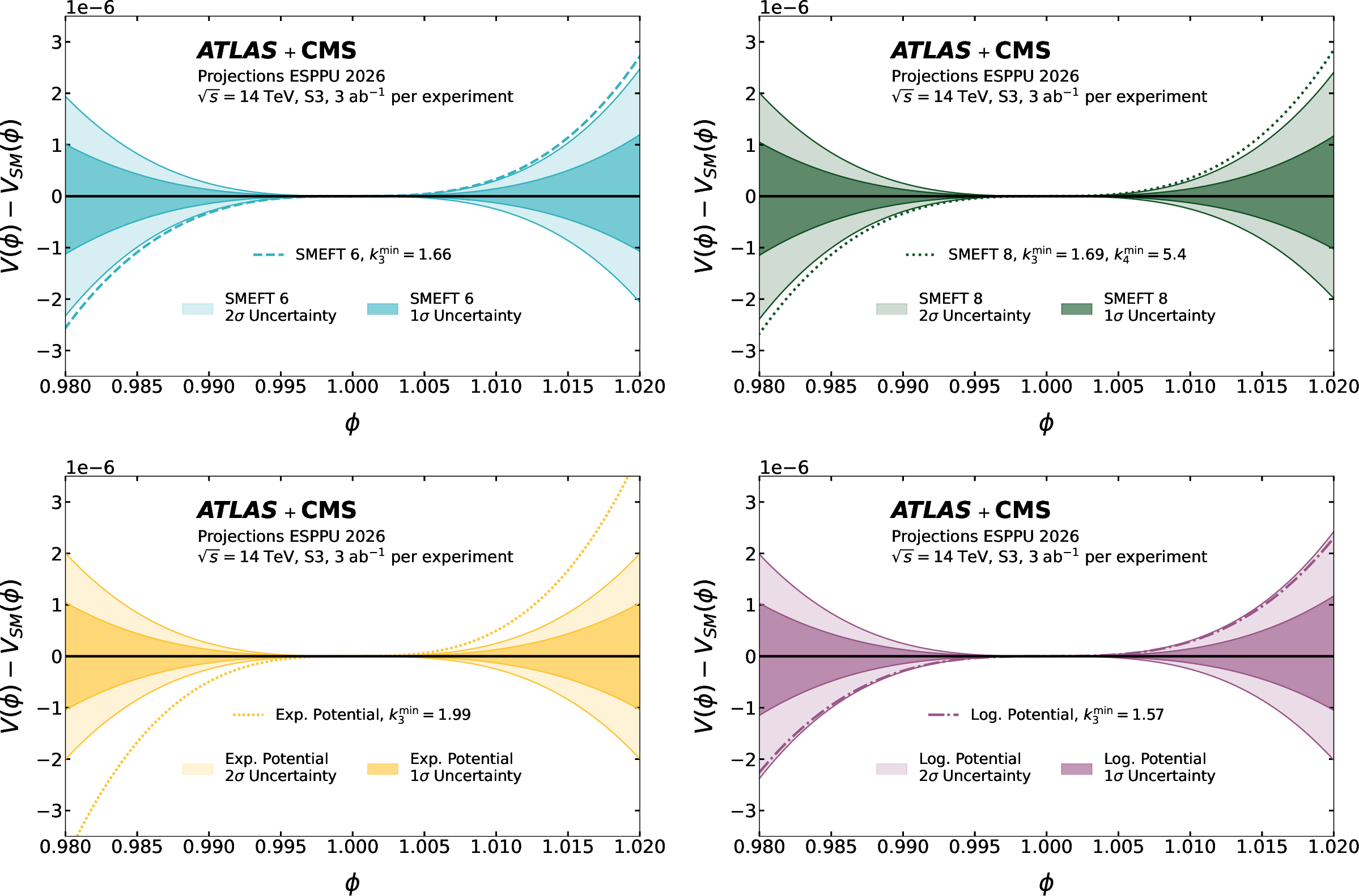
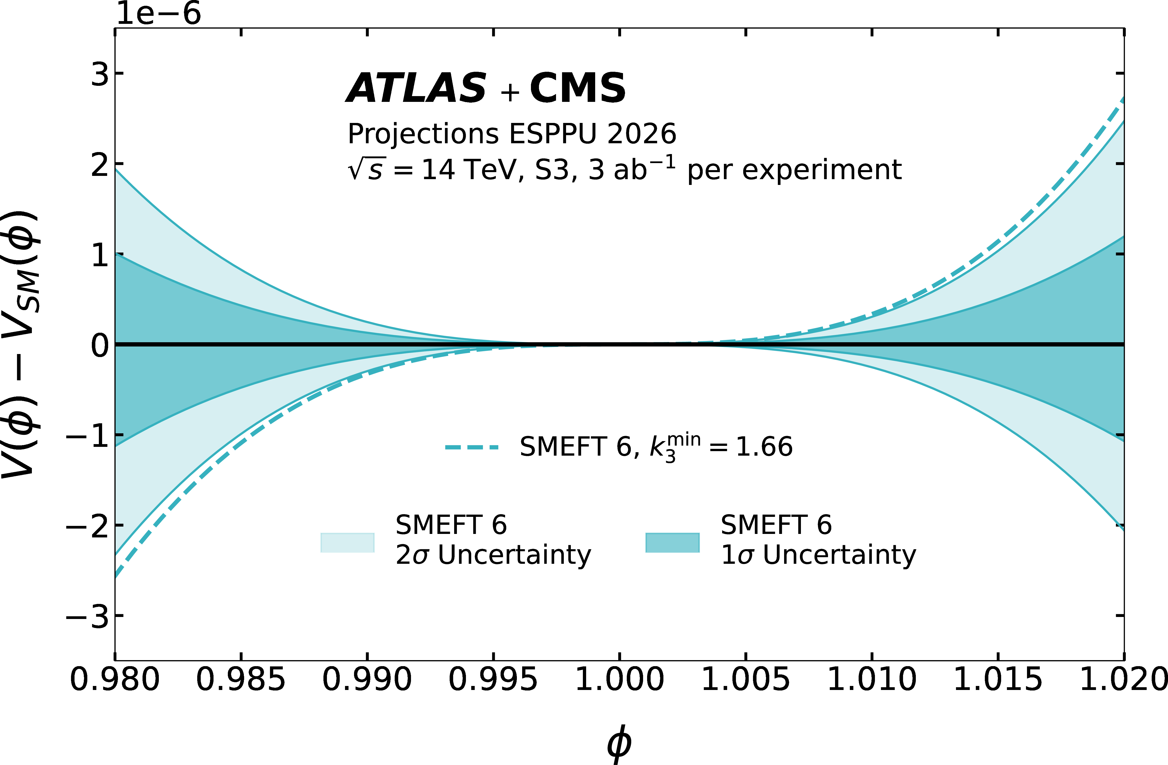
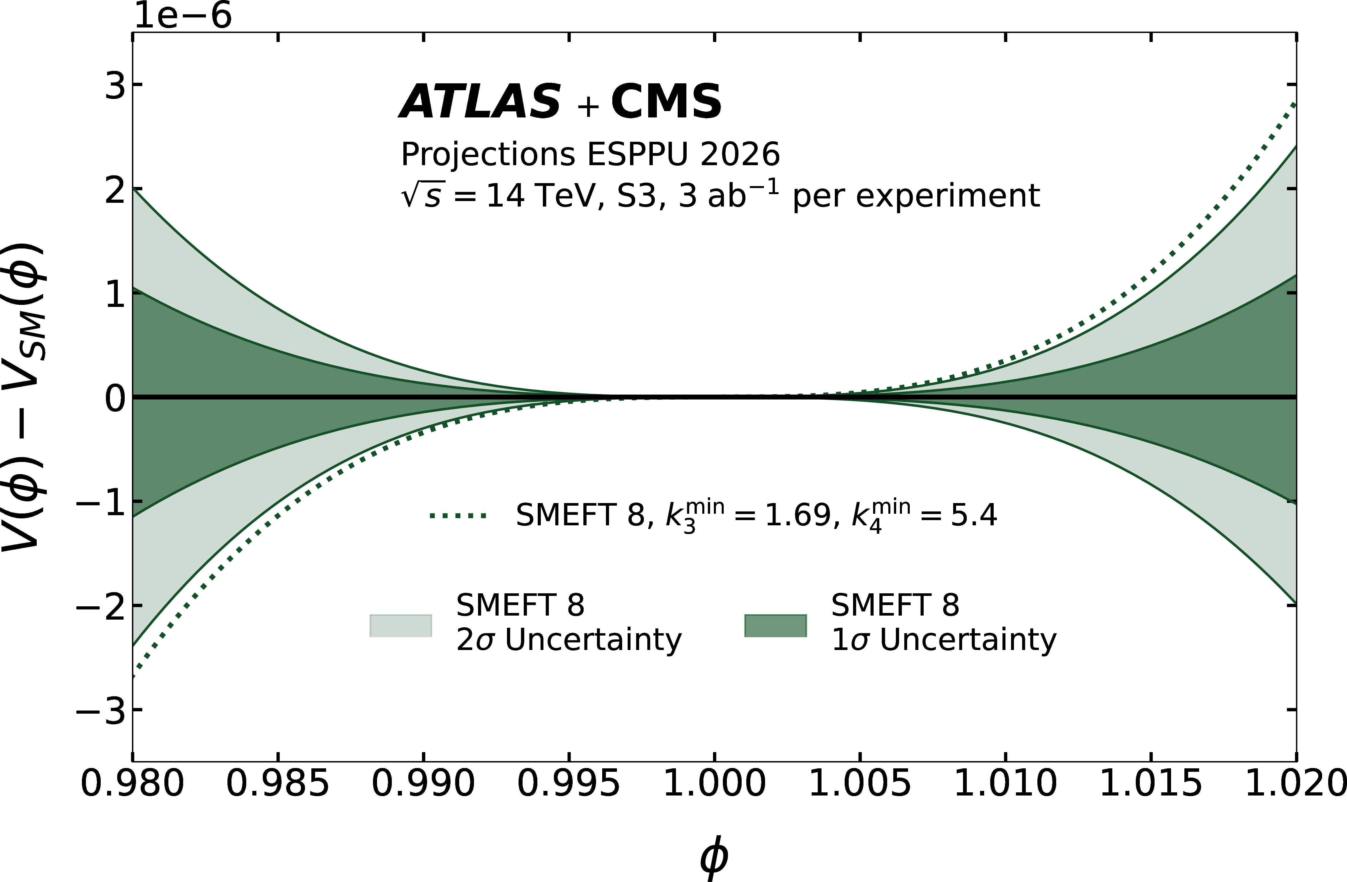
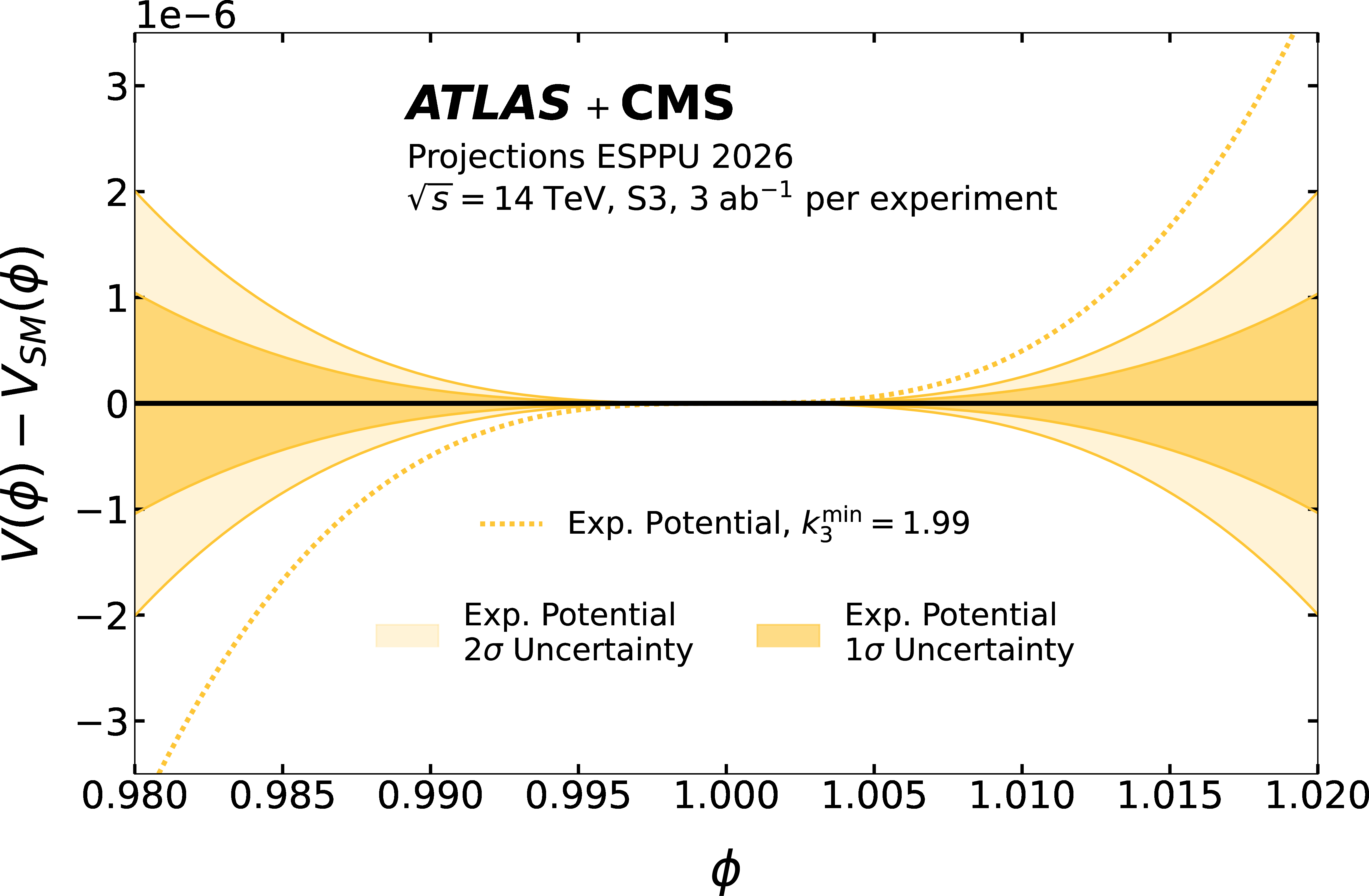
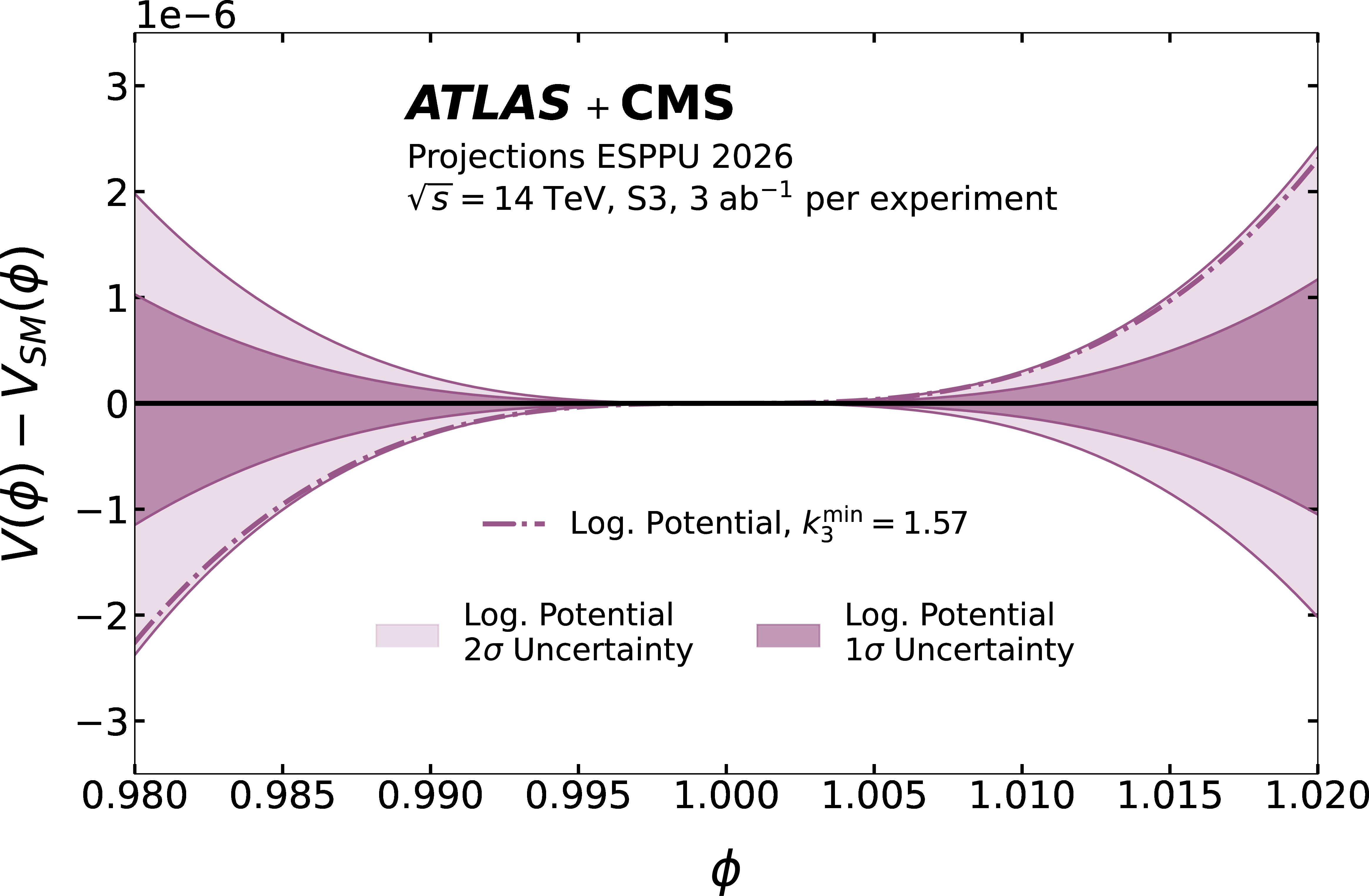
png pdf	Figure 14: The difference between the BEH potential $V(\phi)$ and its SM expectation $V_{SM}(\phi)$ in four scenarios: SMEFT 6 (top left), SMEFT 8 (top right), exponential (bottom left), and logarithmic (bottom right) potentials. The 68% and 95% uncertainty bands from the ATLAS+CMS combination is compared to the boundary of the regions for which each model predicts a strong first-order phase transition. The $\phi$ range corresponds to the validity range of the HH-driven band. The projection is derived in S3 scenario assuming 3 ab $^{-1}$ per experiment.
png pdf	Figure 14-a: The difference between the BEH potential $V(\phi)$ and its SM expectation $V_{SM}(\phi)$ in four scenarios: SMEFT 6 (top left), SMEFT 8 (top right), exponential (bottom left), and logarithmic (bottom right) potentials. The 68% and 95% uncertainty bands from the ATLAS+CMS combination is compared to the boundary of the regions for which each model predicts a strong first-order phase transition. The $\phi$ range corresponds to the validity range of the HH-driven band. The projection is derived in S3 scenario assuming 3 ab $^{-1}$ per experiment.
png pdf	Figure 14-b: The difference between the BEH potential $V(\phi)$ and its SM expectation $V_{SM}(\phi)$ in four scenarios: SMEFT 6 (top left), SMEFT 8 (top right), exponential (bottom left), and logarithmic (bottom right) potentials. The 68% and 95% uncertainty bands from the ATLAS+CMS combination is compared to the boundary of the regions for which each model predicts a strong first-order phase transition. The $\phi$ range corresponds to the validity range of the HH-driven band. The projection is derived in S3 scenario assuming 3 ab $^{-1}$ per experiment.
png pdf	Figure 14-c: The difference between the BEH potential $V(\phi)$ and its SM expectation $V_{SM}(\phi)$ in four scenarios: SMEFT 6 (top left), SMEFT 8 (top right), exponential (bottom left), and logarithmic (bottom right) potentials. The 68% and 95% uncertainty bands from the ATLAS+CMS combination is compared to the boundary of the regions for which each model predicts a strong first-order phase transition. The $\phi$ range corresponds to the validity range of the HH-driven band. The projection is derived in S3 scenario assuming 3 ab $^{-1}$ per experiment.
png pdf	Figure 14-d: The difference between the BEH potential $V(\phi)$ and its SM expectation $V_{SM}(\phi)$ in four scenarios: SMEFT 6 (top left), SMEFT 8 (top right), exponential (bottom left), and logarithmic (bottom right) potentials. The 68% and 95% uncertainty bands from the ATLAS+CMS combination is compared to the boundary of the regions for which each model predicts a strong first-order phase transition. The $\phi$ range corresponds to the validity range of the HH-driven band. The projection is derived in S3 scenario assuming 3 ab $^{-1}$ per experiment.
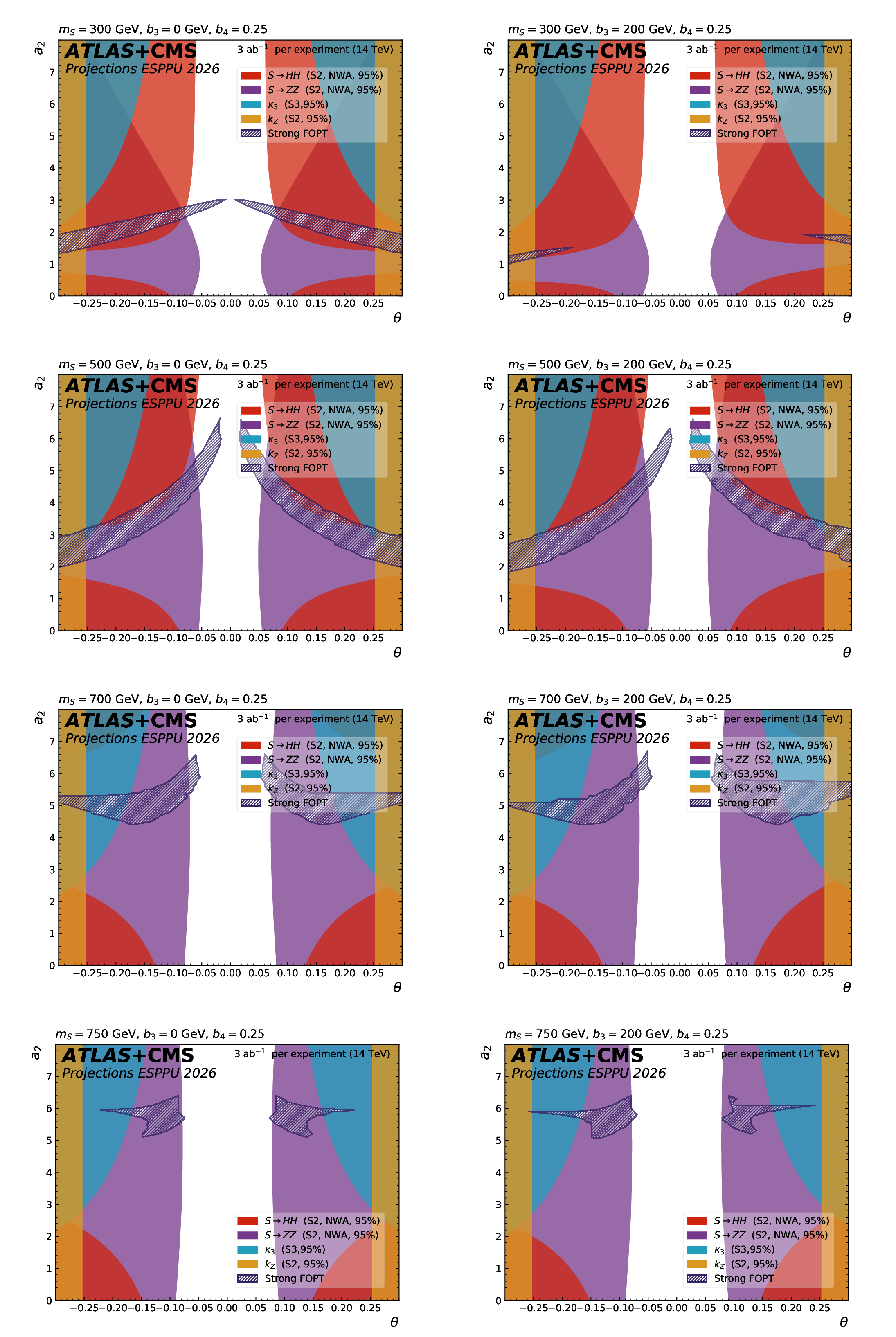
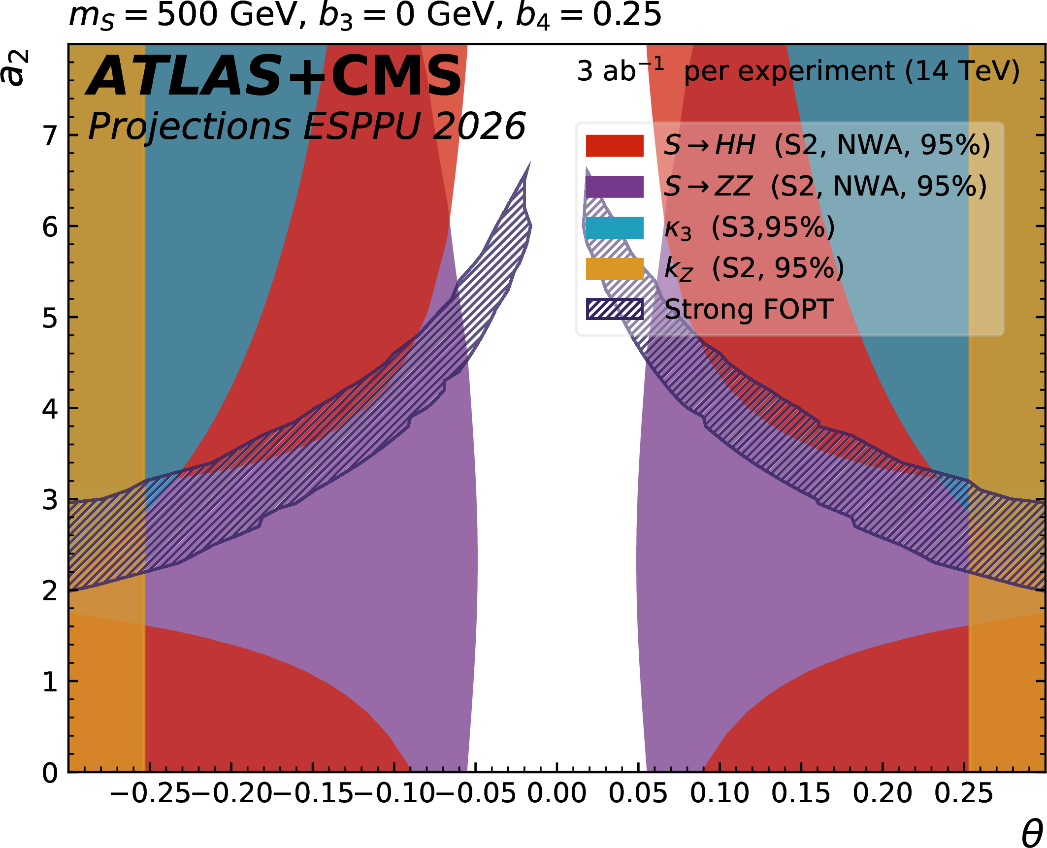
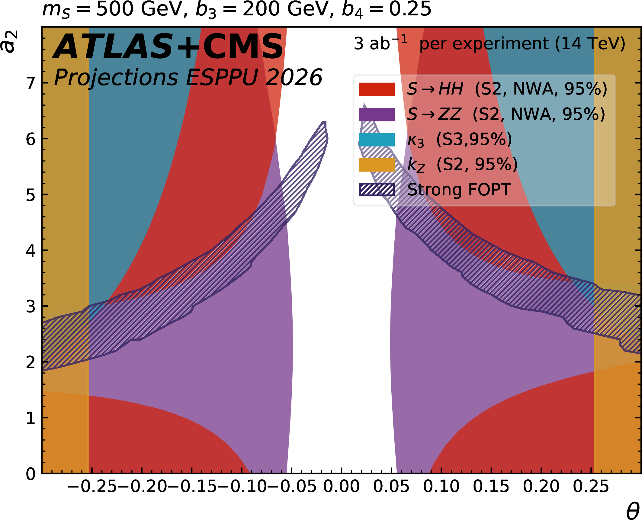
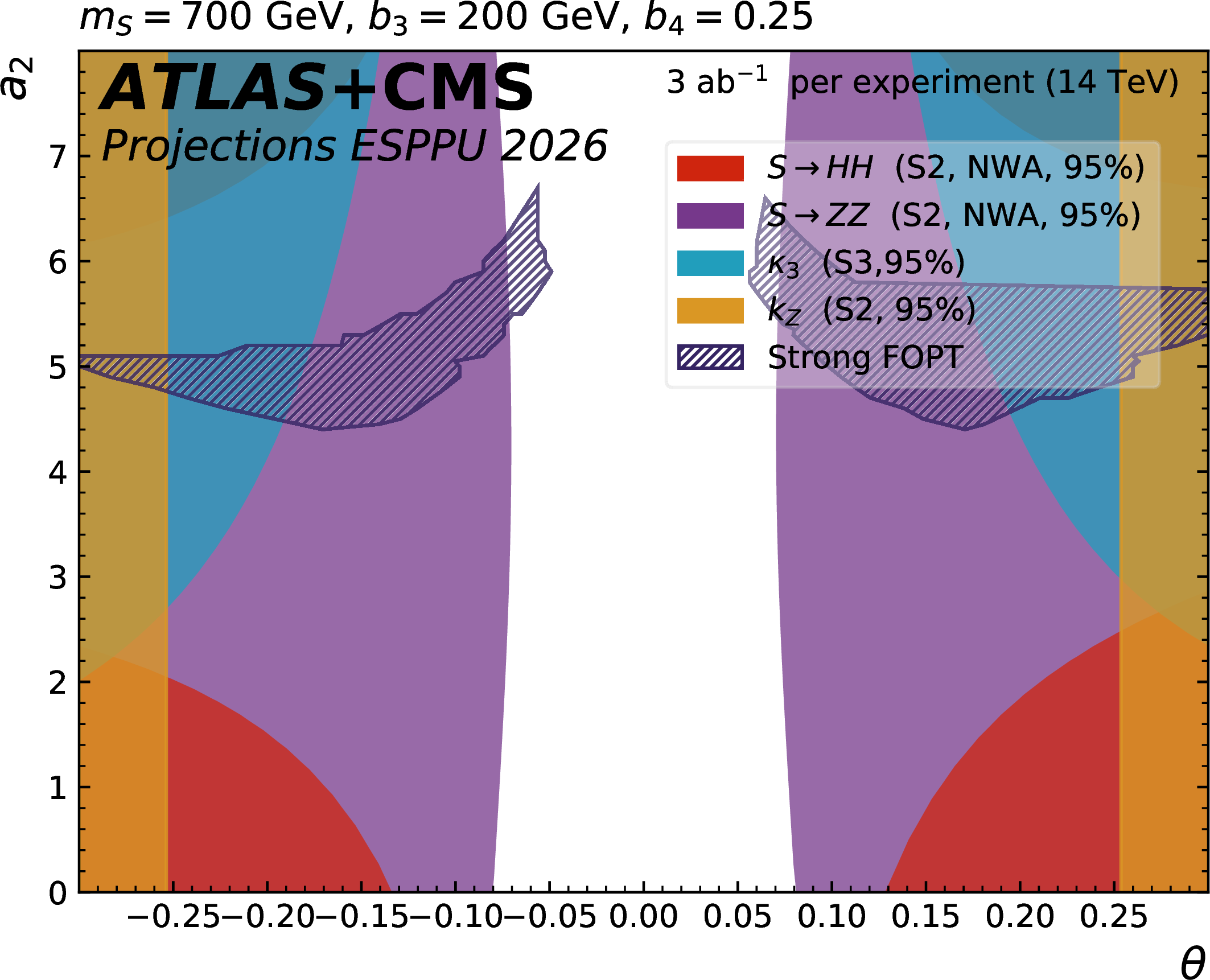
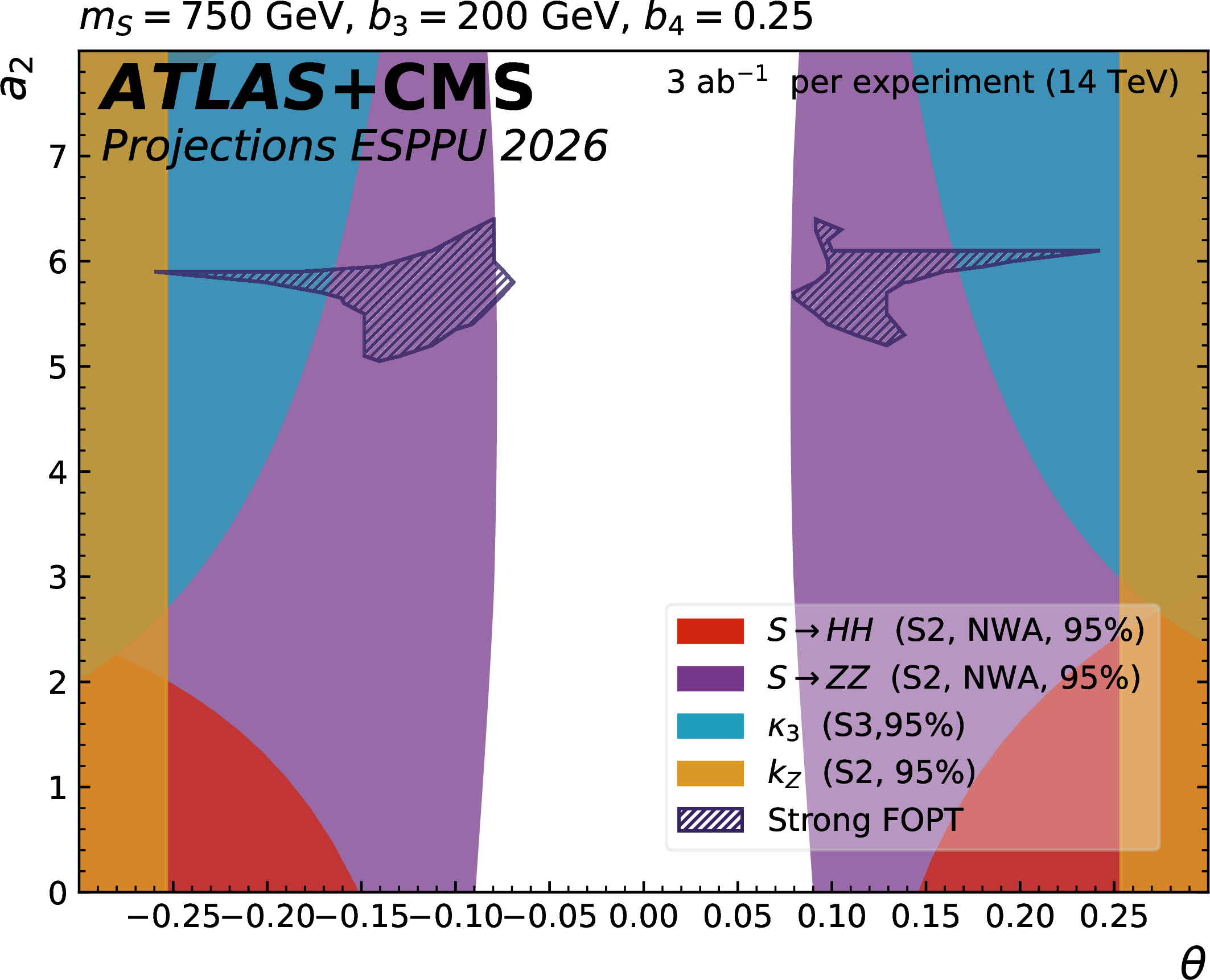
png pdf	Figure 15: The dark blue hatched contours show the regions of the $a_2$ versus $\theta$ parameter space in the scalar singlet model where a strong first-order phase transition is possible. The other contours show the 95% CL exclusion in this plane from the searches for resonant $\mathrm{ S \to HH(ZZ) }$ decays, from the H coupling to Z and from $\kappa_{3}$ constraints. The different plots correspond to representative parameter choices in the model.
png pdf	Figure 15-a: The dark blue hatched contours show the regions of the $a_2$ versus $\theta$ parameter space in the scalar singlet model where a strong first-order phase transition is possible. The other contours show the 95% CL exclusion in this plane from the searches for resonant $\mathrm{ S \to HH(ZZ) }$ decays, from the H coupling to Z and from $\kappa_{3}$ constraints. The different plots correspond to representative parameter choices in the model.
png pdf	Figure 15-b: The dark blue hatched contours show the regions of the $a_2$ versus $\theta$ parameter space in the scalar singlet model where a strong first-order phase transition is possible. The other contours show the 95% CL exclusion in this plane from the searches for resonant $\mathrm{ S \to HH(ZZ) }$ decays, from the H coupling to Z and from $\kappa_{3}$ constraints. The different plots correspond to representative parameter choices in the model.
png pdf	Figure 15-c: The dark blue hatched contours show the regions of the $a_2$ versus $\theta$ parameter space in the scalar singlet model where a strong first-order phase transition is possible. The other contours show the 95% CL exclusion in this plane from the searches for resonant $\mathrm{ S \to HH(ZZ) }$ decays, from the H coupling to Z and from $\kappa_{3}$ constraints. The different plots correspond to representative parameter choices in the model.
png pdf	Figure 15-d: The dark blue hatched contours show the regions of the $a_2$ versus $\theta$ parameter space in the scalar singlet model where a strong first-order phase transition is possible. The other contours show the 95% CL exclusion in this plane from the searches for resonant $\mathrm{ S \to HH(ZZ) }$ decays, from the H coupling to Z and from $\kappa_{3}$ constraints. The different plots correspond to representative parameter choices in the model.
png pdf	Figure 15-e: The dark blue hatched contours show the regions of the $a_2$ versus $\theta$ parameter space in the scalar singlet model where a strong first-order phase transition is possible. The other contours show the 95% CL exclusion in this plane from the searches for resonant $\mathrm{ S \to HH(ZZ) }$ decays, from the H coupling to Z and from $\kappa_{3}$ constraints. The different plots correspond to representative parameter choices in the model.
png pdf	Figure 15-f: The dark blue hatched contours show the regions of the $a_2$ versus $\theta$ parameter space in the scalar singlet model where a strong first-order phase transition is possible. The other contours show the 95% CL exclusion in this plane from the searches for resonant $\mathrm{ S \to HH(ZZ) }$ decays, from the H coupling to Z and from $\kappa_{3}$ constraints. The different plots correspond to representative parameter choices in the model.
png pdf	Figure 15-g: The dark blue hatched contours show the regions of the $a_2$ versus $\theta$ parameter space in the scalar singlet model where a strong first-order phase transition is possible. The other contours show the 95% CL exclusion in this plane from the searches for resonant $\mathrm{ S \to HH(ZZ) }$ decays, from the H coupling to Z and from $\kappa_{3}$ constraints. The different plots correspond to representative parameter choices in the model.
png pdf	Figure 15-h: The dark blue hatched contours show the regions of the $a_2$ versus $\theta$ parameter space in the scalar singlet model where a strong first-order phase transition is possible. The other contours show the 95% CL exclusion in this plane from the searches for resonant $\mathrm{ S \to HH(ZZ) }$ decays, from the H coupling to Z and from $\kappa_{3}$ constraints. The different plots correspond to representative parameter choices in the model.
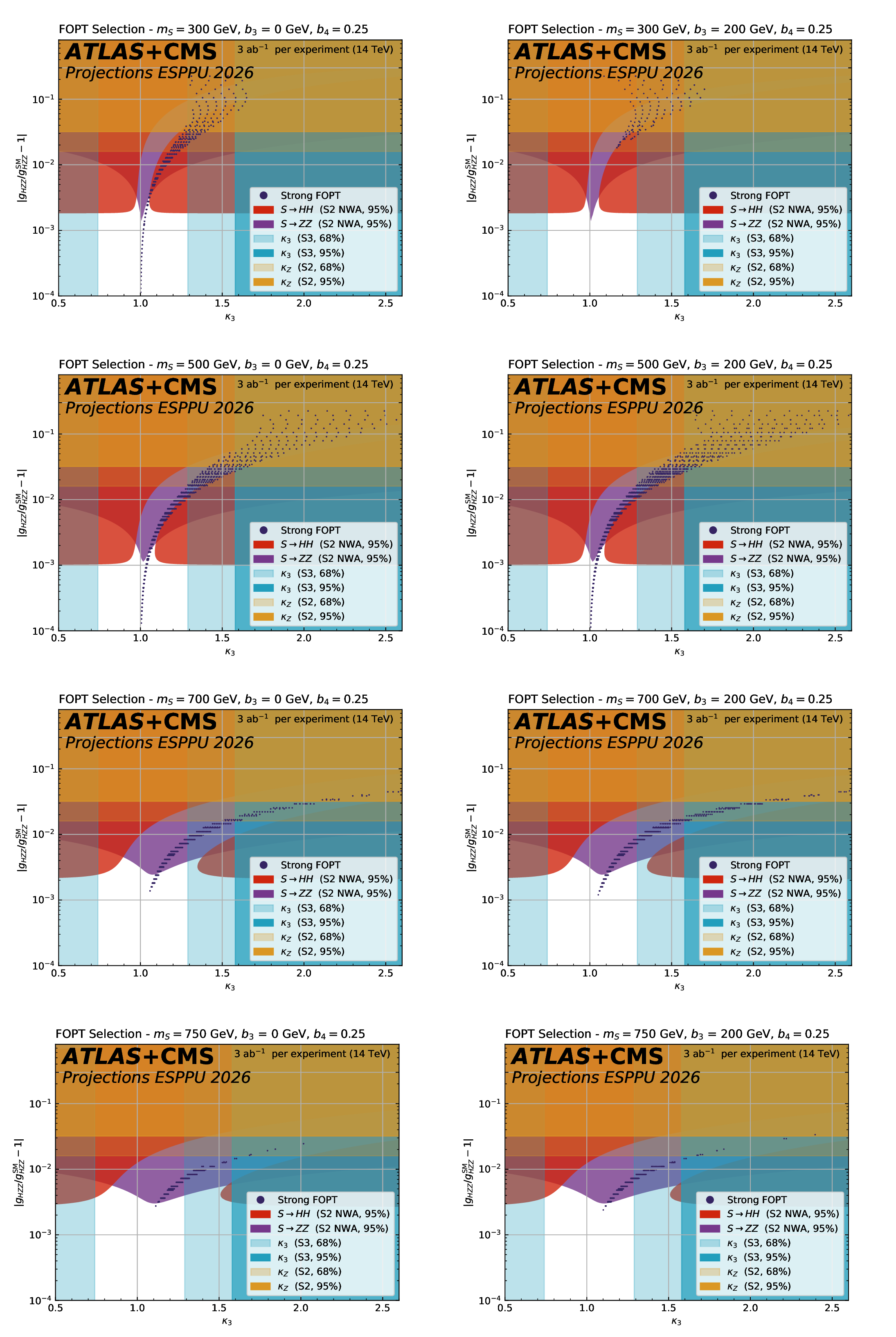
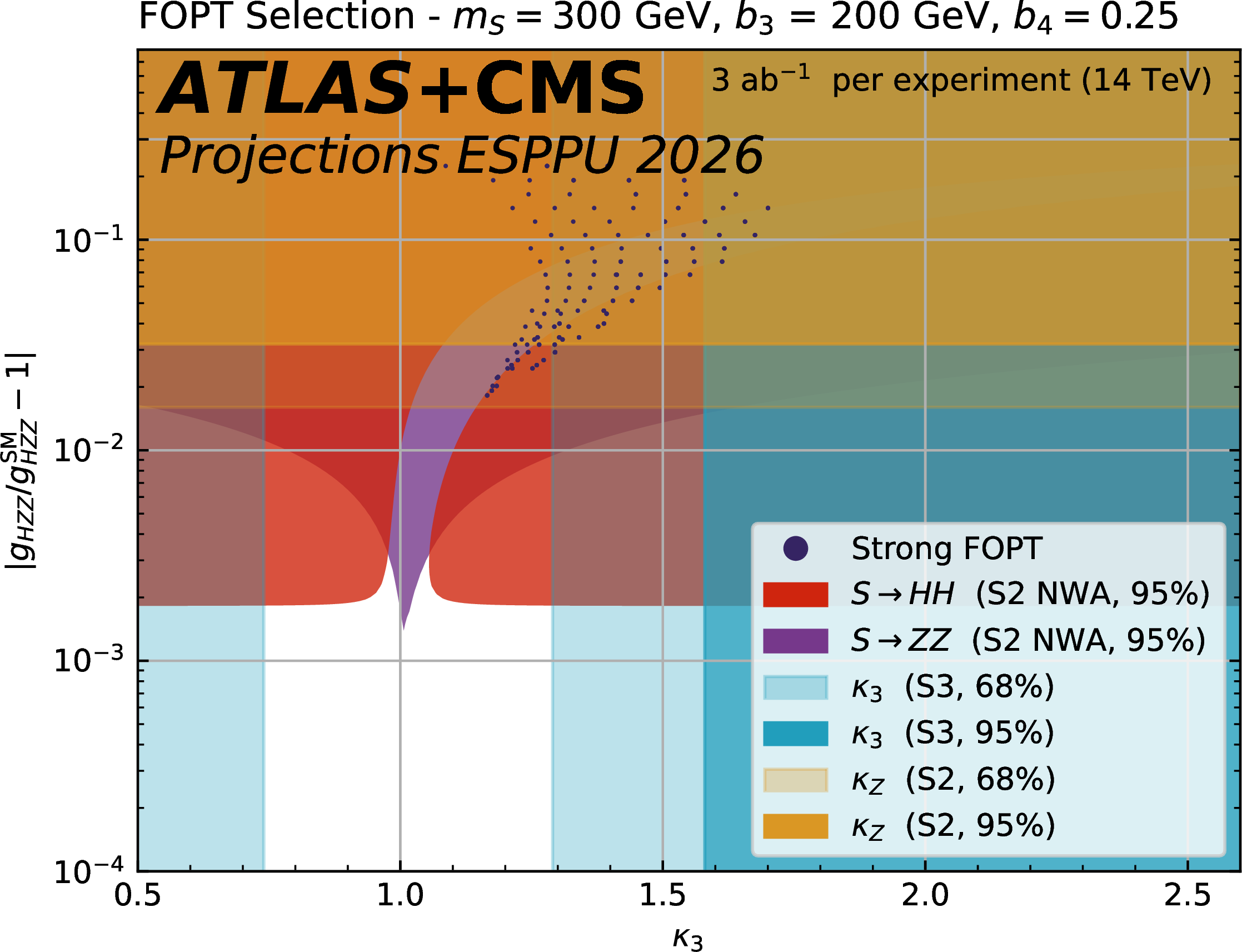
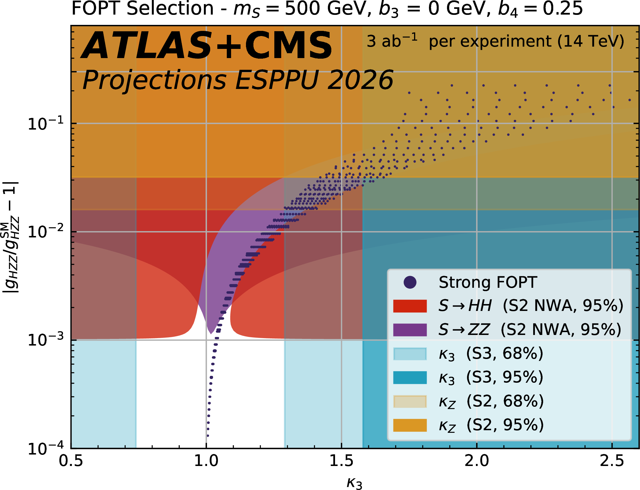
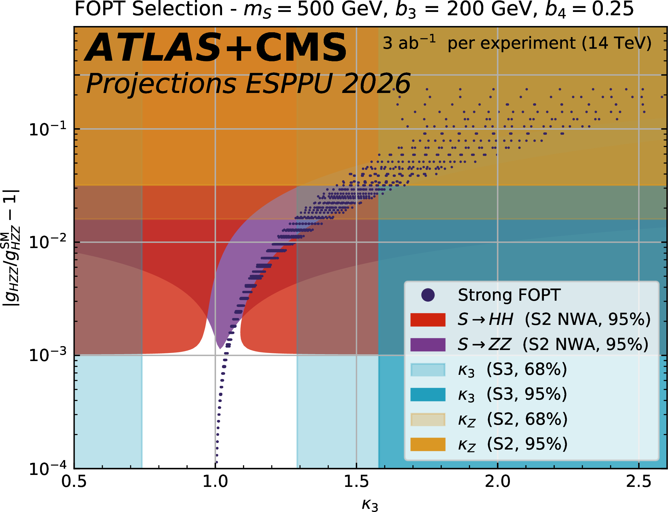
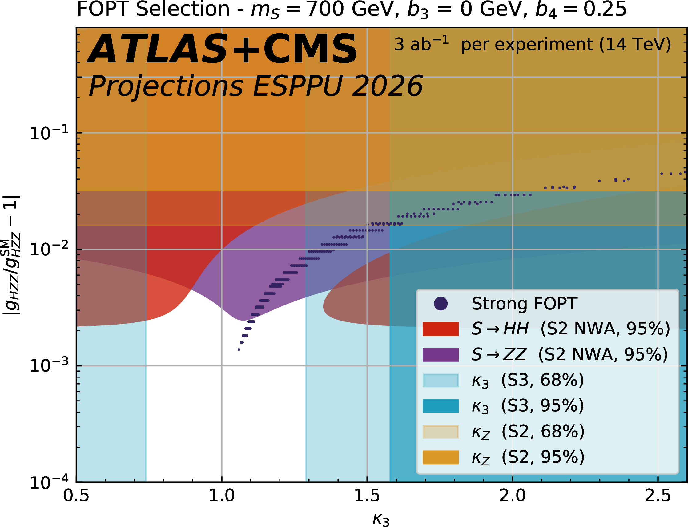
png pdf	Figure 16: The dark blue hatched contours show the parameter space in the scalar singlet model where a strong first-order phase transition is possible in the plane of the Higgs coupling to the Z versus $\kappa_{3}$ . 95% CL exclusion contours from the searches for resonant $\mathrm{ S \to HH(ZZ) }$ decays and from $\kappa_{3}$ and $k_{\mathrm{Z}}$ are overlaid. The plots show the exclusion in different $M_{\mathrm{S}}$ versus $b_3$ slices of the parameter space when $b_4=$ 0.25
png pdf	Figure 16-a: The dark blue hatched contours show the parameter space in the scalar singlet model where a strong first-order phase transition is possible in the plane of the Higgs coupling to the Z versus $\kappa_{3}$ . 95% CL exclusion contours from the searches for resonant $\mathrm{ S \to HH(ZZ) }$ decays and from $\kappa_{3}$ and $k_{\mathrm{Z}}$ are overlaid. The plots show the exclusion in different $M_{\mathrm{S}}$ versus $b_3$ slices of the parameter space when $b_4=$ 0.25
png pdf	Figure 16-b: The dark blue hatched contours show the parameter space in the scalar singlet model where a strong first-order phase transition is possible in the plane of the Higgs coupling to the Z versus $\kappa_{3}$ . 95% CL exclusion contours from the searches for resonant $\mathrm{ S \to HH(ZZ) }$ decays and from $\kappa_{3}$ and $k_{\mathrm{Z}}$ are overlaid. The plots show the exclusion in different $M_{\mathrm{S}}$ versus $b_3$ slices of the parameter space when $b_4=$ 0.25
png pdf	Figure 16-c: The dark blue hatched contours show the parameter space in the scalar singlet model where a strong first-order phase transition is possible in the plane of the Higgs coupling to the Z versus $\kappa_{3}$ . 95% CL exclusion contours from the searches for resonant $\mathrm{ S \to HH(ZZ) }$ decays and from $\kappa_{3}$ and $k_{\mathrm{Z}}$ are overlaid. The plots show the exclusion in different $M_{\mathrm{S}}$ versus $b_3$ slices of the parameter space when $b_4=$ 0.25
png pdf	Figure 16-d: The dark blue hatched contours show the parameter space in the scalar singlet model where a strong first-order phase transition is possible in the plane of the Higgs coupling to the Z versus $\kappa_{3}$ . 95% CL exclusion contours from the searches for resonant $\mathrm{ S \to HH(ZZ) }$ decays and from $\kappa_{3}$ and $k_{\mathrm{Z}}$ are overlaid. The plots show the exclusion in different $M_{\mathrm{S}}$ versus $b_3$ slices of the parameter space when $b_4=$ 0.25
png pdf	Figure 16-e: The dark blue hatched contours show the parameter space in the scalar singlet model where a strong first-order phase transition is possible in the plane of the Higgs coupling to the Z versus $\kappa_{3}$ . 95% CL exclusion contours from the searches for resonant $\mathrm{ S \to HH(ZZ) }$ decays and from $\kappa_{3}$ and $k_{\mathrm{Z}}$ are overlaid. The plots show the exclusion in different $M_{\mathrm{S}}$ versus $b_3$ slices of the parameter space when $b_4=$ 0.25
png pdf	Figure 16-f: The dark blue hatched contours show the parameter space in the scalar singlet model where a strong first-order phase transition is possible in the plane of the Higgs coupling to the Z versus $\kappa_{3}$ . 95% CL exclusion contours from the searches for resonant $\mathrm{ S \to HH(ZZ) }$ decays and from $\kappa_{3}$ and $k_{\mathrm{Z}}$ are overlaid. The plots show the exclusion in different $M_{\mathrm{S}}$ versus $b_3$ slices of the parameter space when $b_4=$ 0.25
png pdf	Figure 16-g: The dark blue hatched contours show the parameter space in the scalar singlet model where a strong first-order phase transition is possible in the plane of the Higgs coupling to the Z versus $\kappa_{3}$ . 95% CL exclusion contours from the searches for resonant $\mathrm{ S \to HH(ZZ) }$ decays and from $\kappa_{3}$ and $k_{\mathrm{Z}}$ are overlaid. The plots show the exclusion in different $M_{\mathrm{S}}$ versus $b_3$ slices of the parameter space when $b_4=$ 0.25
png pdf	Figure 16-h: The dark blue hatched contours show the parameter space in the scalar singlet model where a strong first-order phase transition is possible in the plane of the Higgs coupling to the Z versus $\kappa_{3}$ . 95% CL exclusion contours from the searches for resonant $\mathrm{ S \to HH(ZZ) }$ decays and from $\kappa_{3}$ and $k_{\mathrm{Z}}$ are overlaid. The plots show the exclusion in different $M_{\mathrm{S}}$ versus $b_3$ slices of the parameter space when $b_4=$ 0.25
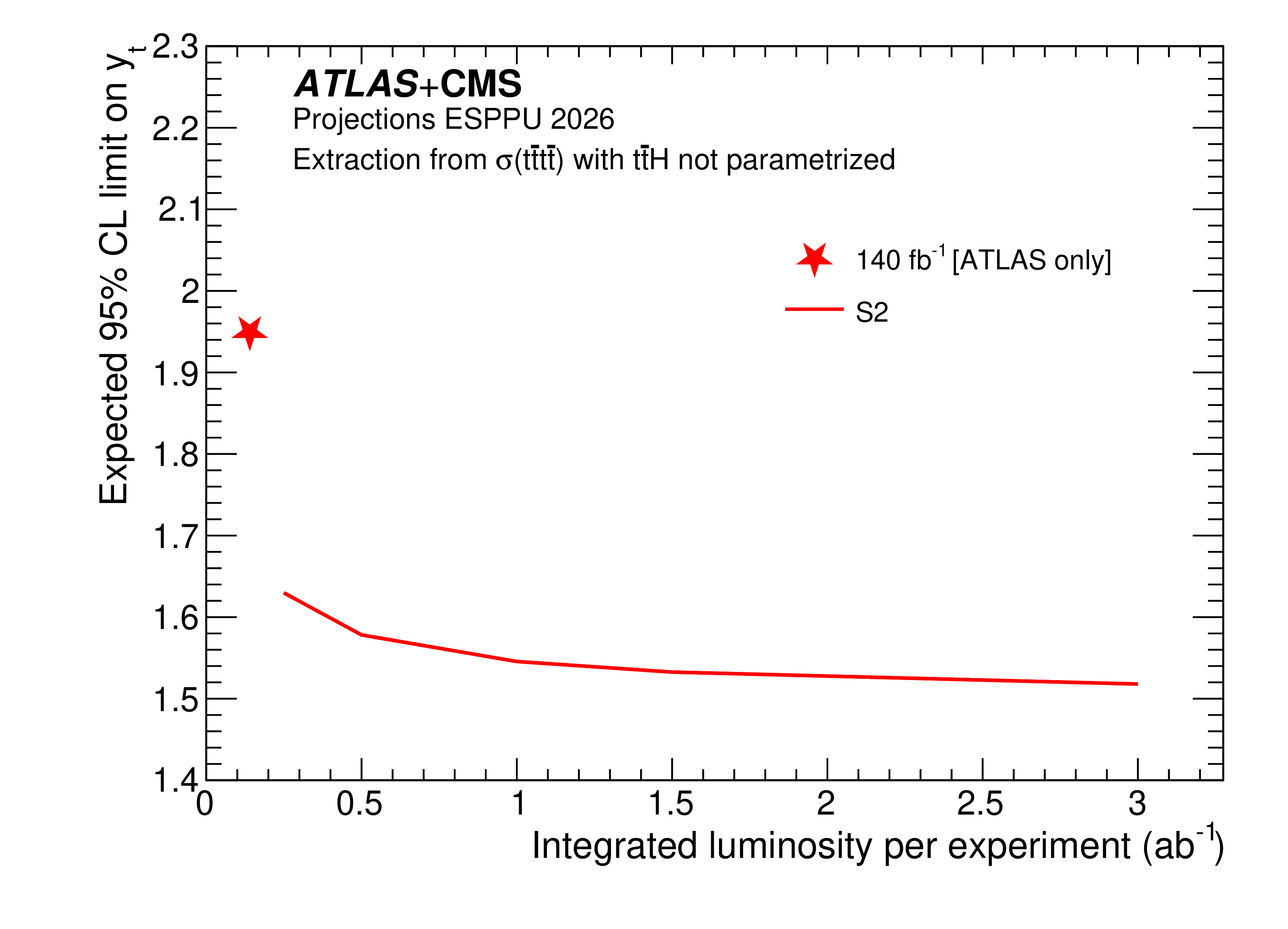
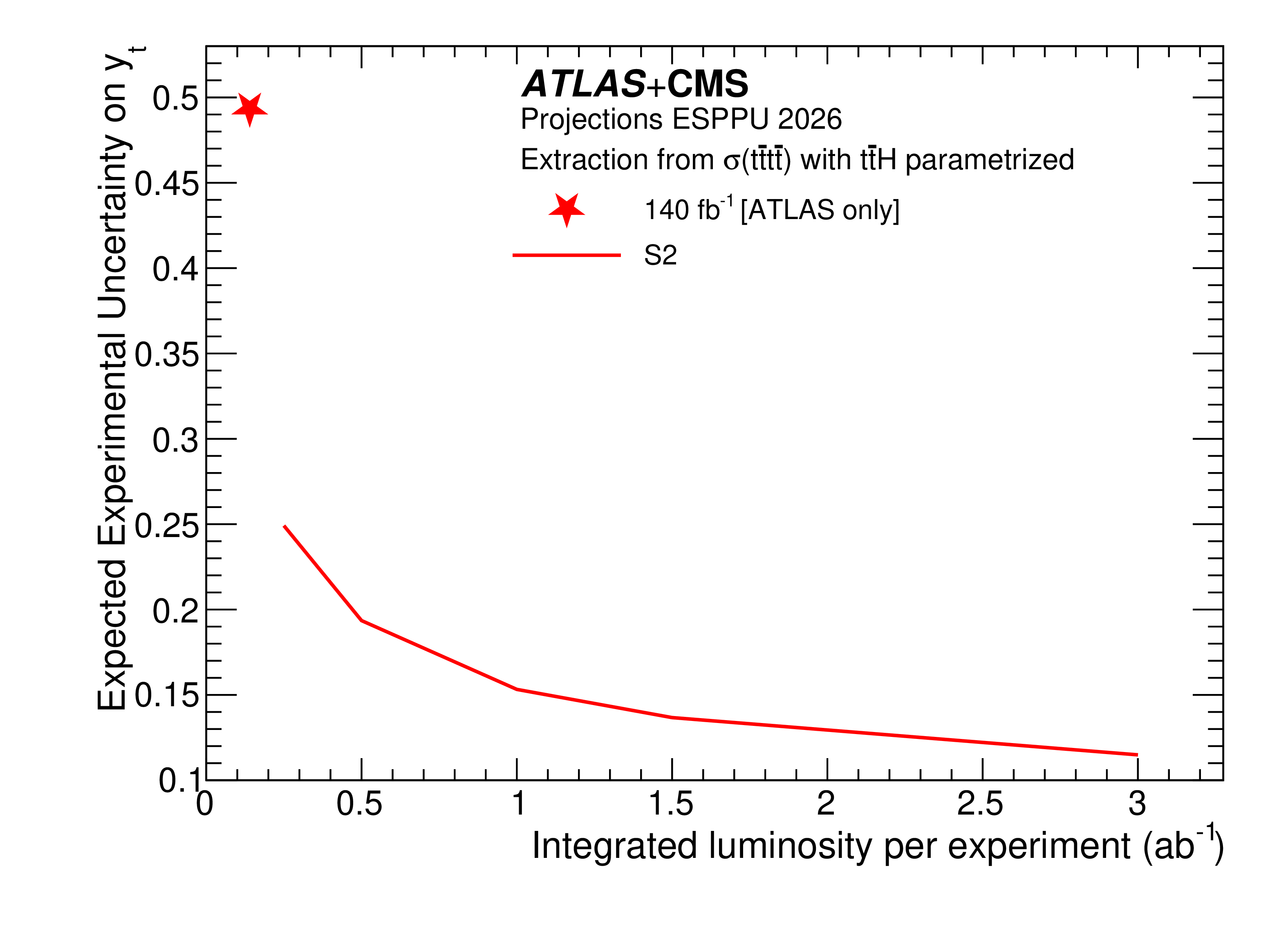
png pdf	Figure 17: Left: Expected uncertainty on $y_t$ as a function of the integrated luminosity, in the S2 scenario, obtained when the $\mathrm{ t\bar{t}H }$ contribution is freely floating. Right: Expected experimental uncertainty on $y_{t}$ as a function of the integrated luminosity, in the S2 scenario, obtained when the $\mathrm{ t\bar{t}H }$ events are parametrized as a function of $\kappa_{\mathrm{t}}$ .
png pdf	Figure 17-a: Left: Expected uncertainty on $y_t$ as a function of the integrated luminosity, in the S2 scenario, obtained when the $\mathrm{ t\bar{t}H }$ contribution is freely floating. Right: Expected experimental uncertainty on $y_{t}$ as a function of the integrated luminosity, in the S2 scenario, obtained when the $\mathrm{ t\bar{t}H }$ events are parametrized as a function of $\kappa_{\mathrm{t}}$ .
png pdf	Figure 17-b: Left: Expected uncertainty on $y_t$ as a function of the integrated luminosity, in the S2 scenario, obtained when the $\mathrm{ t\bar{t}H }$ contribution is freely floating. Right: Expected experimental uncertainty on $y_{t}$ as a function of the integrated luminosity, in the S2 scenario, obtained when the $\mathrm{ t\bar{t}H }$ events are parametrized as a function of $\kappa_{\mathrm{t}}$ .
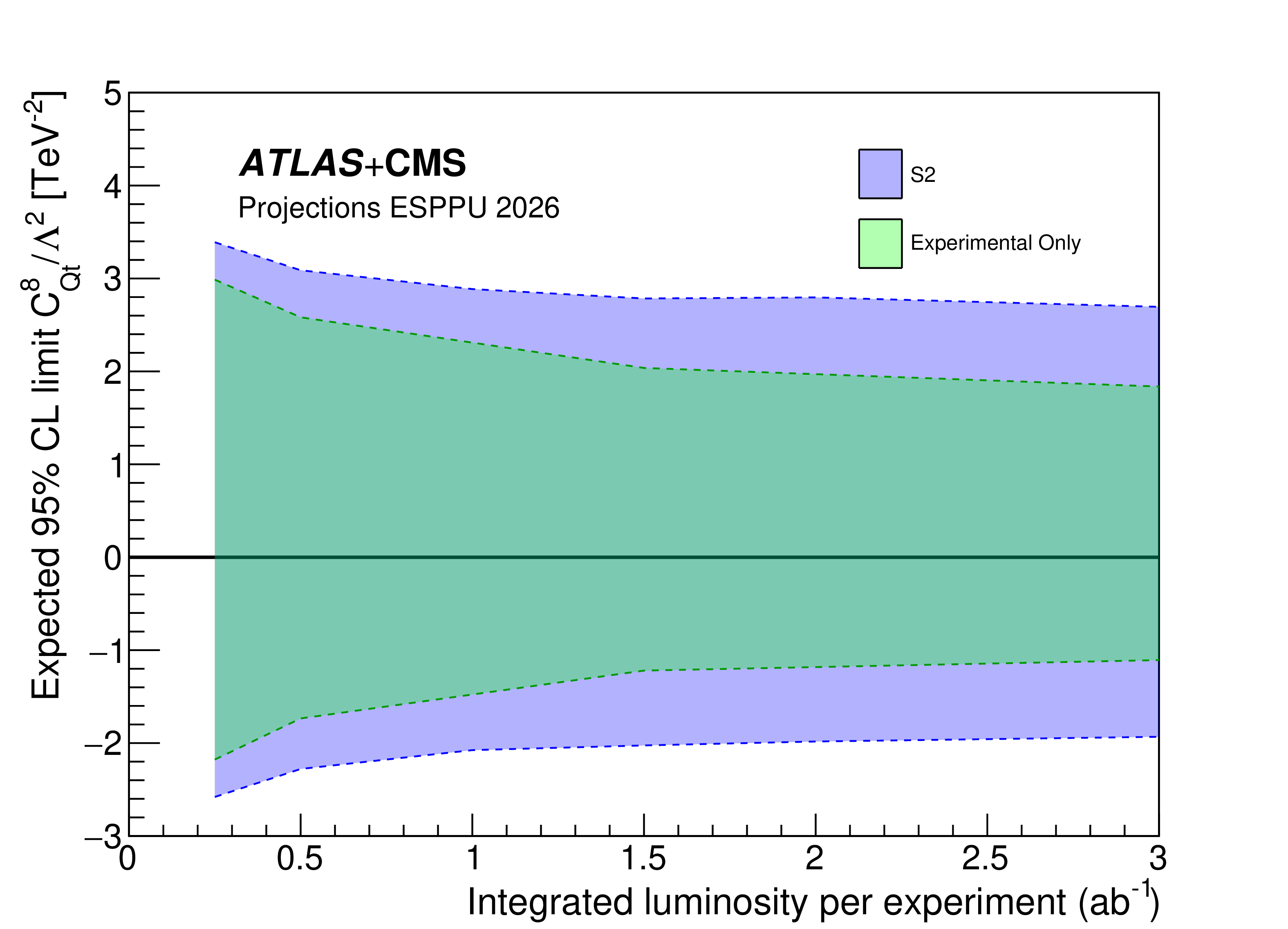
png pdf	Figure 18: Evolution of the expected 95% CL bound on $C_i/\Lambda^2$ as a function of integrated luminosity for the SMEFT operator $\mathcal{O}^{8}_{Qt}$ obtained from the ATLAS+CMS combination of the inclusive $\mathrm{ t\bar{t}t\bar{t} }$ production cross section measurements in the S2 scenario. The impact of the experimental and total uncertainties are shown separately.

Tables
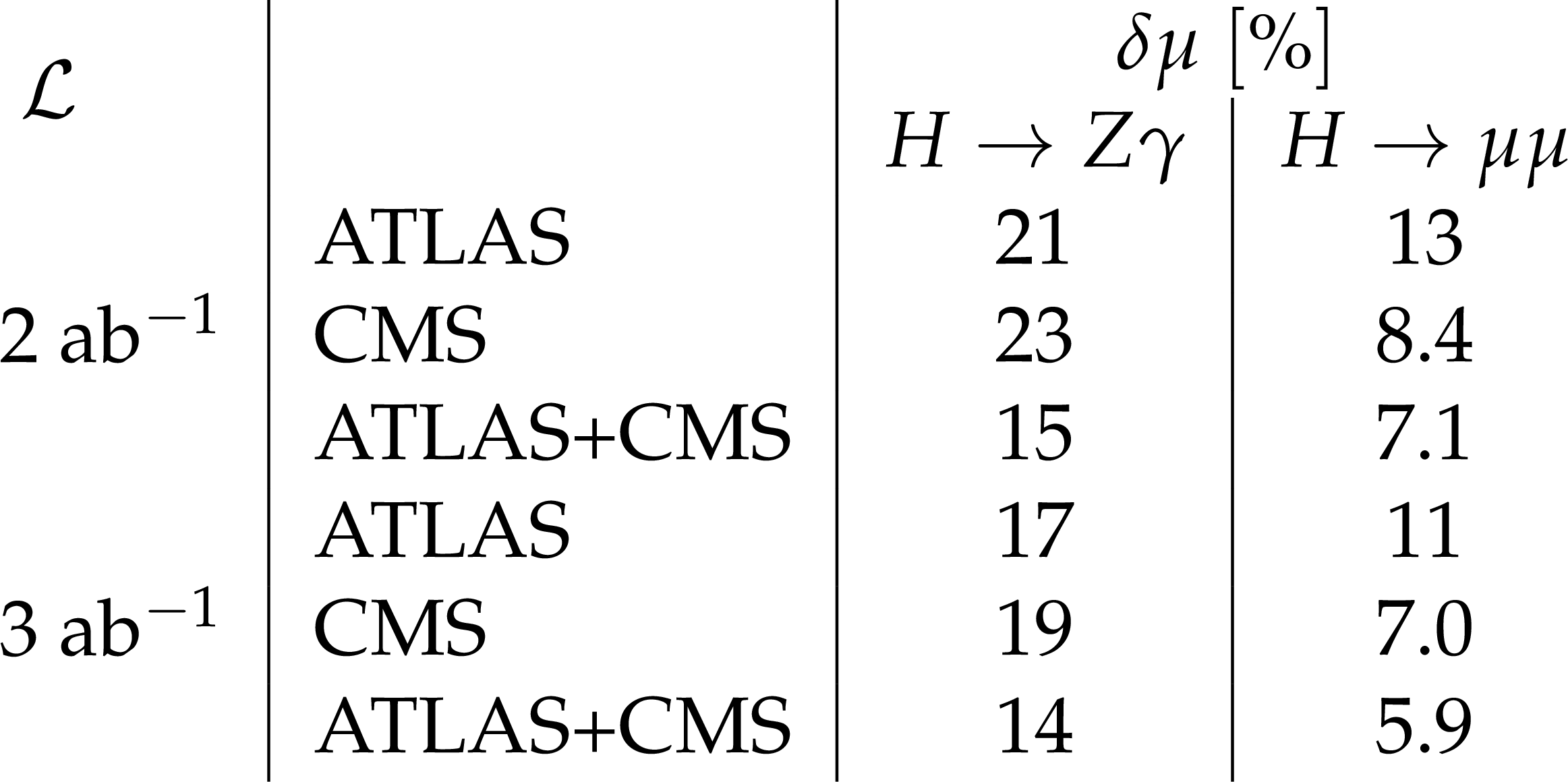
png pdf	Table 1: Projected uncertainties in percentage on the $H\rightarrow Z\gamma$ and $H\rightarrow \mu\mu$ signal strengths ( $\mu$ ) for the ATLAS [10] and CMS experiments [19], as well as their combination, for different integrated luminosities per experiment and uncertainty scenario S2. The $H\rightarrow \mu\mu$ analyses are combined assuming no experimental correlation between the two experiments, while the theoretical uncertainty is fully correlated.
png pdf	Table 2: Combined ATLAS and CMS expected statistical significance for $\mathrm{HH}$ production and the corresponding 68% confidence interval on $\kappa_{3}$ at 3 ab $^{-1}$ , derived assuming $\kappa_{3}^\mathrm{true}=$ 1. The last row reports the projected ATLAS+CMS percentage uncertainty on $\kappa_{3}$ in the various scenarios. The measurement labelled by the $\dagger$ symbol have been used in the ATLAS+CMS combination. When the $\dagger$ symbol is present on only one of the two experiments, this measurement has been extrapolated to 6 ab $^{-1}$ assuming the same sensitivity on that channel for the two experiments.
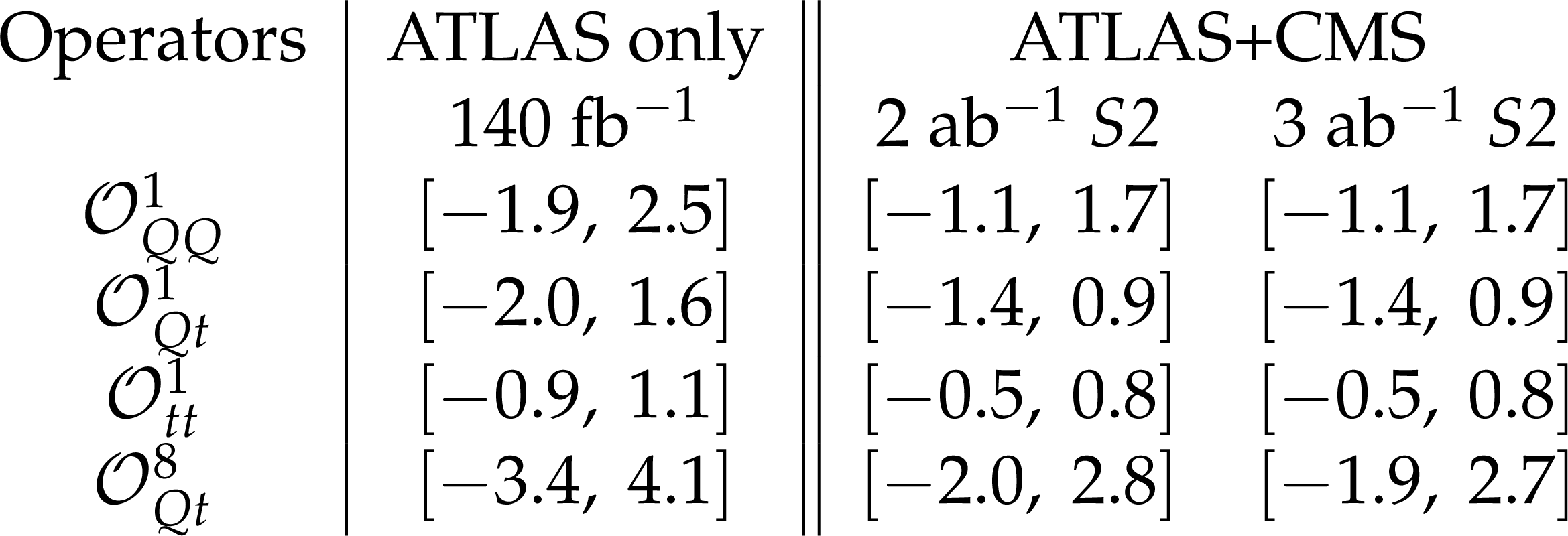
png pdf	Table 3: Expected 95% CL intervals on EFT coupling parameters, derived setting the new physics scale $\Lambda =$ 1 TeV and assuming a single non-zero EFT parameter at a time, in the context of deviations induced in the $\mathrm{ t\bar{t}t\bar{t} }$ process.

References
1	A. Dainese et al.	Report on the Physics at the HL-LHC,and Perspectives for the HE-LHC	Volume 7 of CERN Yellow Reports: Monographs, CERN, 2019 link
2	ATLAS and CMS Collaborations	Report on the Physics at the HL-LHC and Perspectives for the HE-LHC	Volume 7 of CERN Yellow Reports: Monographs, CERN, 2019 link
3	M. Cepeda	Report from Working Group 2: Higgs Physics at the HL-LHC and HE-LHC	Volume 7 of CERN Yellow Reports: Monographs, CERN, 2019 link
4	ATLAS, CMS Collaboration	Snowmass White Paper Contribution: Physics with the Phase-2 ATLAS and CMS Detectors	ATL-PHYS-PUB-2022-018, 2022 CMS-PAS-FTR-22-001
5	G. Hiller, T. Höhne, D. F. Litim, and T. Steudtner	Vacuum stability in the Standard Model and beyond	PRD 110 (2024) 115017	2401.08811
6	D. Curtin, P. Meade, and C.-T. Yu	Testing Electroweak Baryogenesis with Future Colliders	JHEP 11 (2014) 127	1409.0005
7	G. Kurup and M. Perelstein	Dynamics of Electroweak Phase Transition In Singlet-Scalar Extension of the Standard Model	PRD 96 (2017) 015036	1704.03381
8	ATLAS Collaboration	Expected performance of the ATLAS detector at the High-Luminosity LHC	ATLAS PUB Note ATL-PHYS-PUB-2019-005, 2019
9	CMS Collaboration	Expected performance of the physics objects with the upgraded CMS detector at the HL-LHC	CMS Note CMS-NOTE-2018-006, 2018 CDS
10	ATLAS Collaboration	Updated projections for Higgs boson measurements using $H\to\gamma\gamma$ , $Z\gamma$ and $\mu\mu$ decays and for the combined measurement of Higgs boson couplings with the ATLAS detector at the HL-LHC	ATLAS PUB note, 2025
11	ATLAS Collaboration	Expected sensitivity of the ATLAS experiment to $H \to b\bar{b}$ and $H \to c\bar{c}$ decays in the $VH$ production mode at the High Luminosity LHC	ATLAS PUB Note ATL-PHYS-PUB-2025-012, 2025
12	ATLAS Collaboration	Projected sensitivity of measurements of Higgs boson pair production with the ATLAS experiment at the HL-LHC	ATLAS PUB Note ATL-PHYS-PUB-2025-006, 2025
13	ATLAS Collaboration	Updated projection of the sensitivity of searches for Higgs boson pair production in the $b\bar{b}\tau^{+}\tau^{-}$ final state from LHC Run 2 to the High Luminosity LHC with the ATLAS detector	ATLAS PUB Note ATL-PHYS-PUB-2024-016, 2024
14	ATLAS Collaboration	Projected sensitivity of searches for Higgs boson pair production in final states with light leptons, taus, and photons with the ATLAS detector at the HL-LHC	ATLAS PUB Note ATL-PHYS-PUB-2025-004, 2025
15	ATLAS Collaboration	HL-LHC prospects for the measurement of triple-Higgs production in the 6b final state at the ATLAS experiment	ATLAS PUB Note ATL-PHYS-PUB-2025-003, 2025
16	ATLAS Collaboration	Projected sensitivity to top-quark couplings in $t\bar{t}\gamma$ and $t\bar{t}z$ production at the hl-lhc with the atlas experiment	ATLAS PUB Note ATL-PHYS-PUB-2025-015, 2025
17	ATLAS Collaboration	Projected sensitivities for cross-section measurements and new physics searches in four-top-quark production at the hl-lhc	ATLAS PUB Note ATL-PHYS-PUB-2025-017, 2025
18	ATLAS Collaboration	Projected uncertainty in the determination of the top quark pole mass at the hl-lhc with atlas	ATLAS PUB Note ATL-PHYS-PUB-2025-019, 2025
19	CMS Collaboration	HL-LHC projections for single Higgs boson measurements at the CMS experiment	CMS Note CMS-NOTE-2025-007, 2025 CDS
20	CMS Collaboration	Projection of CMS experimental reach on HH production at HL-LHC	CMS Note CMS-NOTE-2025-006, 2025 CDS
21	CMS Collaboration	HL-LHC projections for searches for new resonances	CMS Note CMS-NOTE-2025-003, 2025 CDS
22	CMS Collaboration	Projections for top quark mass measurements at the HL-LHC	CMS Note CMS-NOTE-2025-002, 2025 CDS
23	ATLAS Collaboration	The atlas upgrade for the hl-lhc	ATLAS PUB Note ATL-UPGRADE-PUB-2025-001, 2025
24	ATLAS Collaboration	Atlas software and computing for the future	ATLAS PUB note, ATL-SOFT-PUB-2025-002, 2025
25	C. O. Software and Computing	CMS Offline Software and Computing input to the European Strategy for Particle Physics - 2026 update	CMS Note CMS-NOTE-2025-005, 2025
26	ATLAS Collaboration	Projections for measurements of Higgs boson cross sections, branching ratios, coupling parameters and mass with the ATLAS detector at the HL-LHC	ATLAS PUB Note ATL-PHYS-PUB-2018-054, 2018
27	CMS Collaboration	Sensitivity projections for Higgs boson properties measurements at the HL-LHC	Physics Analysis Summary, 2018 CMS-PAS-FTR-18-011	CMS-PAS-FTR-18-011
28	J. R. Andersen et al.	Les Houches 2015: Physics at TeV Colliders Standard Model Working Group Report	in 9th Les Houches Workshop on Physics at TeV Colliders, 2016	1605.04692
29	N. Berger et al.	Simplified template cross sections - stage 1.1	Report LHCHXSWG-2019-003, 2019	1906.02754
30	LHC Higgs Cross Section Working Group Collaboration	Handbook of LHC Higgs Cross Sections: 4. Deciphering the Nature of the Higgs Sector	link	1610.07922
31	ATLAS Collaboration	Measurement of the properties of Higgs boson production at $\sqrt{s} =$ 13 TeV in the $H\to\gamma\gamma$ channel using 139 fb $^{-1}$ of $pp$ collision data with the ATLAS experiment	JHEP 07 (2023) 088	2207.00348
32	CMS Collaboration	Measurements of Higgs boson production cross sections and couplings in the diphoton decay channel at $\sqrt{\mathrm{s}} =$ 13 TeV	JHEP 07 (2021) 027	CMS-HIG-19-015 2103.06956
33	CMS Collaboration	Measurement of the production cross section of a Higgs boson with large transverse momentum in its decays to a pair of \ensuremath\tau leptons in proton-proton collisions at s=13TeV	PLB 857 (2024) 138964	CMS-HIG-21-017 2403.20201
34	CMS Collaboration	Inclusive search for highly boosted Higgs bosons decaying to bottom quark-antiquark pairs in proton-proton collisions at $\sqrt{s} =$ 13 TeV	JHEP 12 (2020) 085	CMS-HIG-19-003 2006.13251
35	ATLAS Collaboration	Constraints on Higgs boson production with large transverse momentum using $H \to b \bar{b}$ decays in the ATLAS detector	PRD 105 (2022) 092003	2111.08340
36	K. Becker et al.	Recommended predictions for the boosted-Higgs cross section	Report LHCHXSWG-2019-002, 2019
37	CMS Collaboration	A unified approach for jet tagging in Run 3 at $\sqrt{s} =$ 13.6 TeV in CMS	Detector Performance Summary CMS-DP-2024-066, 2024 CDS
38	ATLAS Collaboration	Neural Network Jet Flavour Tagging with the Upgraded ATLAS Inner Tracker Detector at the High-Luminosity LHC	ATLAS PUB Note ATL-PHYS-PUB-2022-047, 2022
39	ATLAS Collaboration	Graph Neural Network Jet Flavour Tagging with the ATLAS Detector	ATLAS PUB Note ATL-PHYS-PUB-2022-027, 2022
40	ATLAS, CMS Collaboration	Evidence for the Higgs Boson Decay to a Z Boson and a Photon at the LHC	PRL 132 (2024) 021803	2309.03501
41	ATLAS Collaboration	A search for the $Z\gamma$ decay mode of the Higgs boson in $pp$ collisions at $\sqrt{s} =$ 13 TeV with the ATLAS detector	PLB 809 (2020) 135754	2005.05382
42	CMS Collaboration	Search for Higgs boson decays to a Z boson and a photon in proton-proton collisions at $\sqrt{s} =$ 13 TeV	JHEP 05 (2023) 233	CMS-HIG-19-014 2204.12945
43	I. Low, J. Lykken, and G. Shaughnessy	Singlet scalars as higgs boson imposters at the large hadron collider	(August, ), 2011 PRD 84 (2011)
44	A. Azatov, R. Contino, A. Di Iura, and J. Galloway	New Prospects for Higgs Compositeness in $h \to Z\gamma$	PRD 88 (2013) 075019	1308.2676
45	ATLAS Collaboration	A search for the dimuon decay of the Standard Model Higgs boson with the ATLAS detector	PLB 812 (2021) 135980	2007.07830
46	CMS Collaboration	Evidence for Higgs boson decay to a pair of muons	JHEP 01 (2021) 148	CMS-HIG-19-006 2009.04363
47	CMS Collaboration	Prospects for the precise measurement of the Higgs boson properties in the $\textrm{H}\rightarrow\mu\mu$ decay channel at the HL-LHC	CMS Physics Analysis Summary, 2022 CMS-PAS-FTR-21-006	CMS-PAS-FTR-21-006
48	ATLAS Collaboration	Technical Design Report for the ATLAS Inner Tracker Pixel Detector	Technical Design Report CERN-LHCC-2017-021, ATLAS-TDR-030, 2017 link
49	CMS Collaboration	The Phase-2 Upgrade of the CMS Tracker	Technical Design Report CERN-LHCC-2017-009, CMS-TDR-014, 2017 link
50	ATLAS Collaboration	Projection of $H\to\tau\tau$ cross-section measurement results to the HL-LHC	ATLAS PUB Note ATL-PHYS-PUB-2022-003, 2022
51	A. Valassi	Combining correlated measurements of several different physical quantities	NIM A 500 (2003) 391
52	CMS Collaboration	Performance of the CNN-based tau identification algorithm with Domain Adaptation using Adversarial Machine Learning for Run 3	Detector Performance Summary CMS-DP-2024-063, 2024 CDS
53	CMS Collaboration	Enriching the Physics Program of the CMS Experiment via Data Scouting and Data Parking	Accepted by Phys. Rept., 2024	CMS-EXO-23-007 2403.16134
54	ATLAS Collaboration	Updated projection of the sensitivity of searches for Higgs boson pair production in the $b\bar{b}\gamma\gamma$ final state from LHC Run 2 to the High Luminosity LHC with the ATLAS detector	ATLAS PUB Note ATL-PHYS-PUB-2025-001, 2025
55	ATLAS Collaboration	Search for pair production of boosted Higgs bosons via vector-boson fusion in the $b\bar b b\bar b$ final state using pp collisions at $\sqrt{s}=$ 13 TeV with the ATLAS detector	PLB 858 (2024) 139007	2404.17193
56	ATLAS Collaboration	HL-LHC prospects for the search of boosted Higgs boson pair production via vector-boson fusion in the $b\bar{b}b\bar{b}$ final state at the ATLAS experiment	ATLAS PUB Note ATL-PHYS-PUB-2025-005, 2025
57	P. Stylianou and G. Weiglein	Constraints on the trilinear and quartic Higgs couplings from triple Higgs production at the LHC and beyond	EPJC 84 (2024) 366	2312.04646
58	ATLAS Collaboration	A search for triple Higgs boson production in the 6 $b$ final state using $pp$ collisions at $\sqrt{s}=$ 13 TeV with the ATLAS detector	PRD 111 (2025) 032006	2411.02040
59	CMS Collaboration	Searches for Higgs Boson Production through Decays of Heavy Resonances	Accepted by Phys. Rept., 2024	2403.16926
60	CMS Collaboration	Search for heavy scalar resonances decaying to a pair of Z bosons in the 4-lepton final state at 13 TeV	CMS Physics Analysis Summary, 2024 CMS-PAS-HIG-24-002	CMS-PAS-HIG-24-002
61	CMS Collaboration	Search for a new heavy scalar boson decaying into a Higgs boson and a new scalar particle in the four b-quarks final state using proton-proton collisions at $sqrt{s}=$ 13 TeV	CMS Physics Analysis Summary, 2024 CMS-PAS-HIG-20-012	CMS-PAS-HIG-20-012
62	CMS Collaboration	Search for the nonresonant and resonant production of a Higgs boson in association with an additional scalar boson in the $\gamma\gamma\tau\tau$ final state	CMS Physics Analysis Summary, 2024 CMS-PAS-HIG-22-012	CMS-PAS-HIG-22-012
63	ATLAS Collaboration	Search for $t\bar{t}H/A \rightarrow t\bar{t}t\bar{t}$ production in proton--proton collisions at $\sqrt{s}=$ 13 TeV\ with the ATLAS detector		2408.17164
64	ATLAS Collaboration	Search for $t\bartH/A \to t\bart t\bart$ production in the multilepton final state in proton--proton collisions at $\sqrts = 13\,\textTeV$ with the ATLAS detector	JHEP 07 (2023) 203	2211.01136
65	C. Degrande et al.	Automated one-loop computations in the standard model effective field theory	PRD 103 (2021) 096024	2008.11743
66	I. Brivio, Y. Jiang, and M. Trott	The SMEFTsim package, theory and tools	JHEP 12 (2017) 070	1709.06492
67	P. Huang, A. Long, and L.-T. Wang	Probing the Electroweak Phase Transition with Higgs Factories and Gravitational Waves	PRD 94 (2016) 075008	1608.06619
68	M. Ramsey-Musolf, T. Tenkanen, and V. Tran	Refining Gravitational Wave and Collider Physics Dialogue via Singlet Scalar Extension		2409.17554
69	Y. Aoki et al.	The Order of the quantum chromodynamics transition predicted by the standard model of particle physics	Nature 443 (2006) 675	hep-lat/0611014
70	A. Kotwal, M. J. Ramsey-Musolf, J. M. No, and P. Winslow	Singlet-catalyzed electroweak phase transitions in the 100 TeV frontier	PRD 94 (2016) 035022	1605.06123
71	L. Niemi, M. Ramsey-Musolf, and G. Xia	Nonperturbative study of the electroweak phase transition in the real scalar singlet extended standard model	PRD 110 (2024) 115016	2405.01191
72	W. Zhang et al.	Probing electroweak phase transition in the singlet Standard Model via bb\ensuremath\gamma\ensuremath\gamma and 4l channels	JHEP 12 (2023) 018	2303.03612
73	Bosse, M. et al.	Constraining the real scalar single extension of the standard model	Technical report, to appear, 2025
74	P. Huang, A. Long, and L.-T. Wang	Probing the Electroweak Phase Transition with Higgs Factories and Gravitational Waves	PRD 94 (2016) 075008	1608.06619
75	ATLAS Collaboration	Measurement of the top-quark mass in $t\bar{t}+$ 1-jet events collected with the ATLAS detector in $pp$ collisions at $\sqrt{s}=$ 8 TeV	JHEP 11 (2019) 150	1905.02302
76	CMS Collaboration	Measurement of the top quark pole mass using $\textrm{t}\overline{\textrm{t}}$ +jet events in the dilepton final state in proton-proton collisions at $\sqrt{s} =$ 13 TeV	JHEP 07 (2023) 077	CMS-TOP-21-008 2207.02270
77	A. V. Bednyakov, B. A. Kniehl, A. F. Pikelner, and O. L. Veretin	Stability of the Electroweak Vacuum: Gauge Independence and Advanced Precision	PRL 115 (2015) 201802	1507.08833
78	A. Andreassen, W. Frost, and M. Schwartz	Scale Invariant Instantons and the Complete Lifetime of the Standard Model	PRD 97 (2018) 056006	1707.08124
79	CMS Collaboration	Review of top quark mass measurements in CMS	Phys. Rept. 1115 (2025) 116	CMS-TOP-23-003 2403.01313
80	ATLAS Collaboration	Climbing to the top of the atlas 13 tev data	Submitted to Phys. Rept, 2024	2404.10674
81	ATLAS Collaboration	Measurement of the top quark mass with the atlas detector using $t\bar{t}$ events with a high transverse momentum top quark	Submitted to Phys. Lett. B, 2025	2502.18216
82	CMS Collaboration	Measurement of the differential $\mathrm{t} \overline{\mathrm{t}}$ production cross section as a function of the jet mass and extraction of the top quark mass in hadronic decays of boosted top quarks	EPJC 83 (2023) 560	CMS-TOP-21-012 2211.01456
83	S. Badger, M. Becchetti, N. Giraudo, and S. Zoia	Two-loop integrals for $t\overline{t}$ +jet production at hadron colliders in the leading colour approximation	JHEP 07 (2024) 073	2404.12325
84	ATLAS Collaboration	Projected uncertainty for a high- $p_{\mathrm{T}}$ top quark mass measurement with the ATLAS detector at the HL-LHC	ATLAS PUB Note ATL-PHYS-PUB-2025-009, 2025
85	CMS Collaboration	Projection of the Higgs boson mass and on-shell width measurements in $H \rightarrow ZZ \rightarrow 4\ell$ decay channel at the HL-LHC	CMS Physics Analysis Summary, 2022 CMS-PAS-FTR-21-007	CMS-PAS-FTR-21-007
86	CMS Collaboration	Prospects for the measurement of vector boson scattering production in leptonic \linebreak $W^\pm W^\pm$ and $W Z$ diboson events at $\sqrt{s}=$ 14 TeV at the High-Luminosity LHC	CMS Physics Analysis Summary, 2021 CMS-PAS-FTR-21-001	CMS-PAS-FTR-21-001
87	ATLAS Collaboration	Observation of four-top-quark production in the multilepton final state with the ATLAS detector	no.~6, 496, , . [Erratum: Eur.Phys.J.C 84, 156 ()], 2023 EPJC 83 (2023)	2303.15061
88	CMS Collaboration	Observation of four top quark production in proton-proton collisions at $\sqrt{s}=$ 13TeV	PLB 847 (2023) 138290	CMS-TOP-22-013 2305.13439
89	M. van Beekveld, A. Kulesza, and L. M. Valero	Threshold Resummation for the Production of Four Top Quarks at the LHC	PRL 131 (2023) 21	2212.03259
90	C. Zhang	Constraining $qqtt$ operators from four-top production: a case for enhanced EFT sensitivity	Chin. Phys. C 42 (2018) 023104	1708.05928
91	ATLAS Collaboration	Measurements of inclusive and differential cross-sections of $t\overline{t}\gamma$ production in $pp$ collisions at $\sqrt{s} =$ 13 TeV with the ATLAS detector	JHEP 10 (2024) 191	2403.09452
92	M. Reichert et al.	Probing baryogenesis through the Higgs boson self-coupling	no.~7, 075008, 2018 PRD 97 (2018)	1711.00019