

Compact Muon Solenoid
LHC, CERN
| CMS-PAS-TOP-24-006 | ||
| Search for three-top-quark production in the single lepton, same-sign dilepton, and multilepton final states in proton-proton collisions at $ \sqrt{s}= $ 13 TeV | ||
| CMS Collaboration | ||
| 2026-03-31 | ||
| Abstract: A search for the standard model production of three top quarks is presented. The data analyzed were collected with the CMS detector at the CERN LHC in proton-proton collisions at a center-of-mass energy of 13 TeV and correspond to an integrated luminosity of 138 fb$ ^{-1} $. Selected events are required to contain jets and either one lepton (electron or muon), two same-sign charged leptons, or at least three leptons. The results are derived from the combination of these three lepton categories. Novel multivariate techniques are employed to take full advantage of kinematic differences between the studied signal and the major background. This analysis provides the first LHC result specifically targeting three-top-quark production. No significant deviations with respect to the standard model predictions are observed, and an upper limit of 25 $ \mathrm{fb} $ is set on the signal cross section at 95% confidence level. | ||
| Links: CDS record (PDF) ; CADI line (restricted) ; | ||
| Figures | |
png pdf |
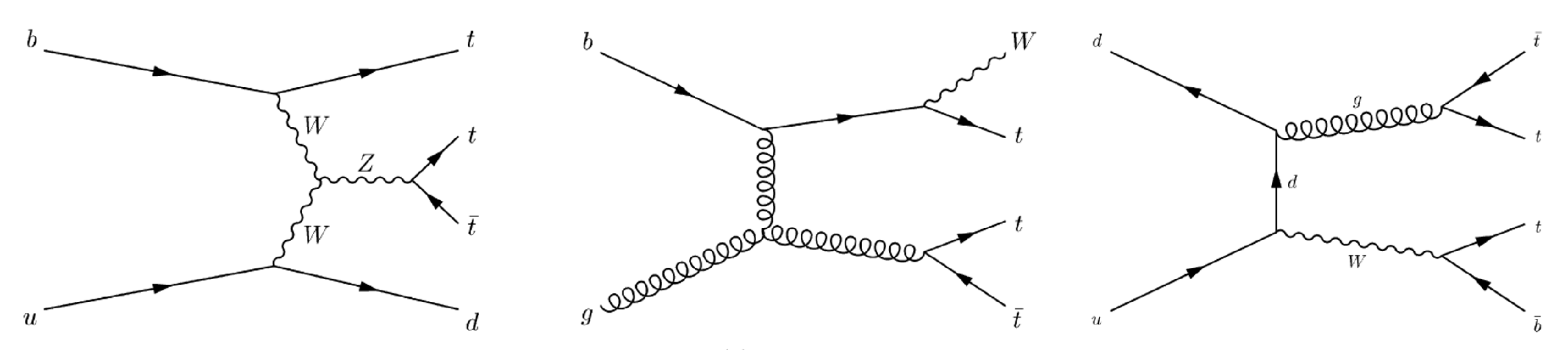
Figure 1:
Principal Feynman diagrams at LO for SM three-top-quark production in the $ t $ channel (left), in association with a W boson (center), and via the $ s $ channel (right). |
png pdf |
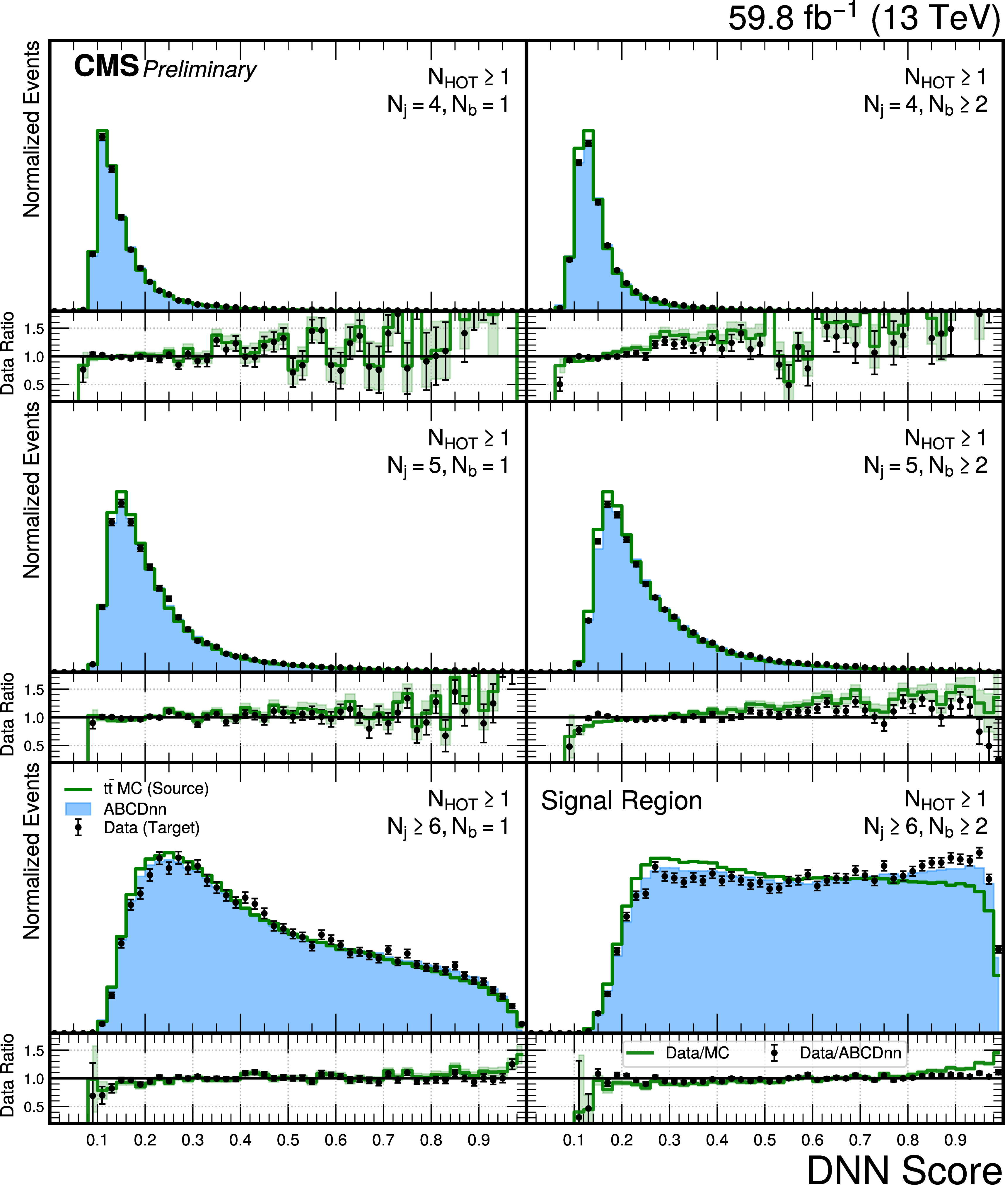
Figure 2:
Distributions of the DNN score for uncorrected simulated $ \mathrm{t} \overline{\mathrm{t}} $ events (green), the observed data (black markers), and the ABCDnn-corrected prediction (blue) for events with $ N_{\text{HOT}}\geq $ 1 from the 2018 data set. Distributions in the upper, middle, and lower rows are shown for events with four, five, and at least six jets, respectively, whereas the left and right columns differ in the number of b-tagged jets (one and at least two, respectively). The lower panels show the ratio and statistical error of data to $ \mathrm{t} \overline{\mathrm{t}} $ simulation before and after the ABCDnn model is applied. |
png pdf |
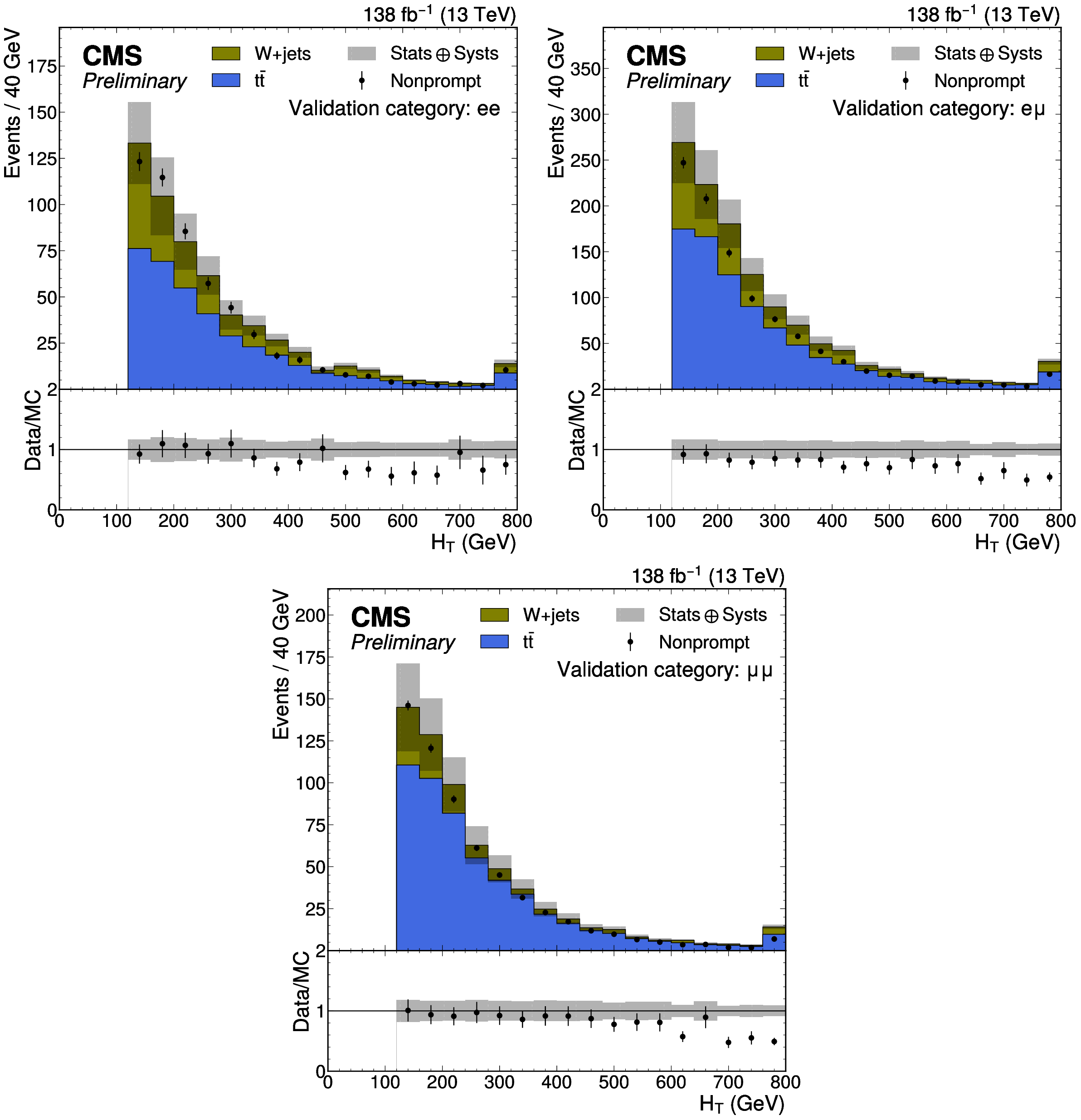
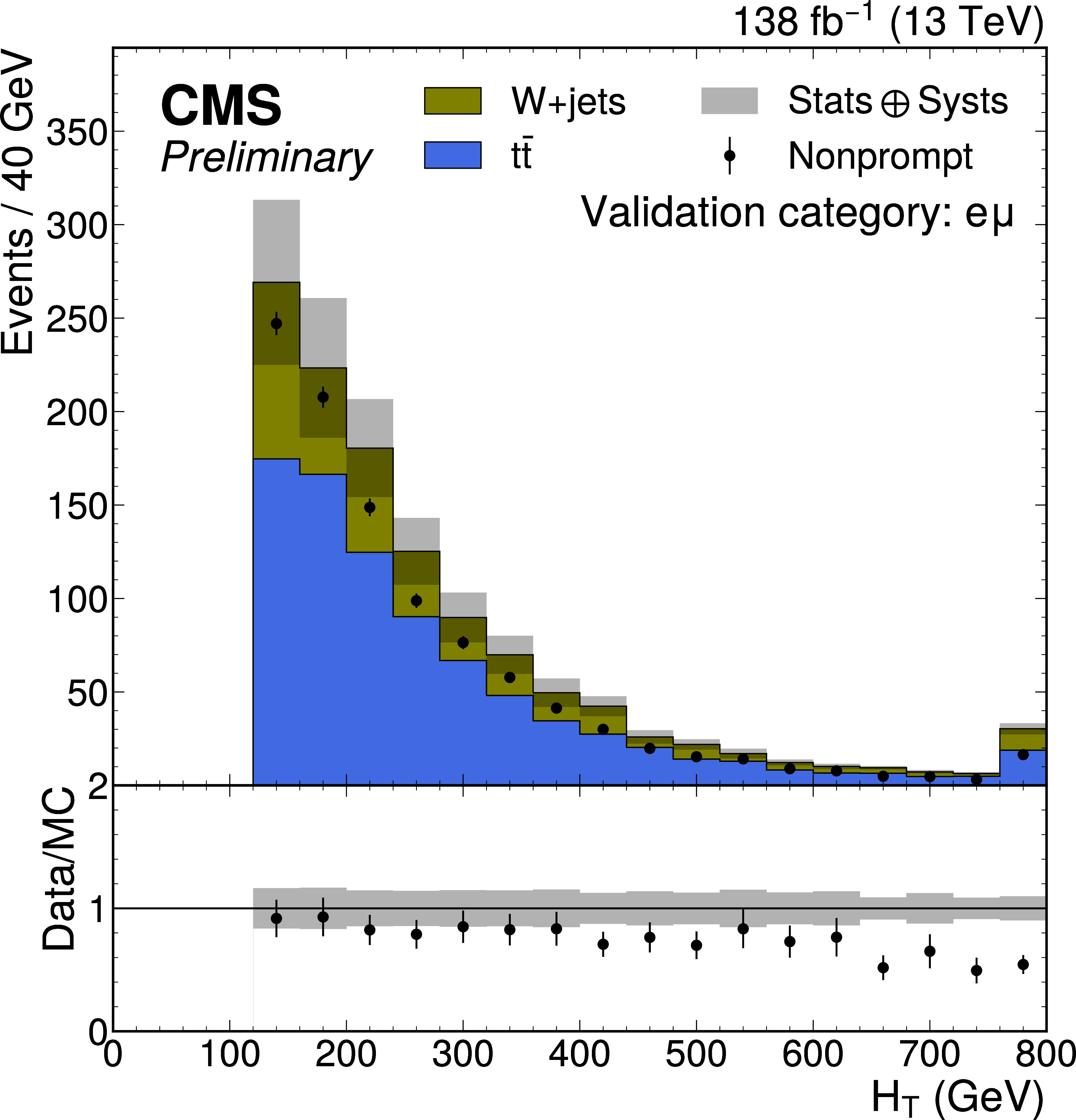
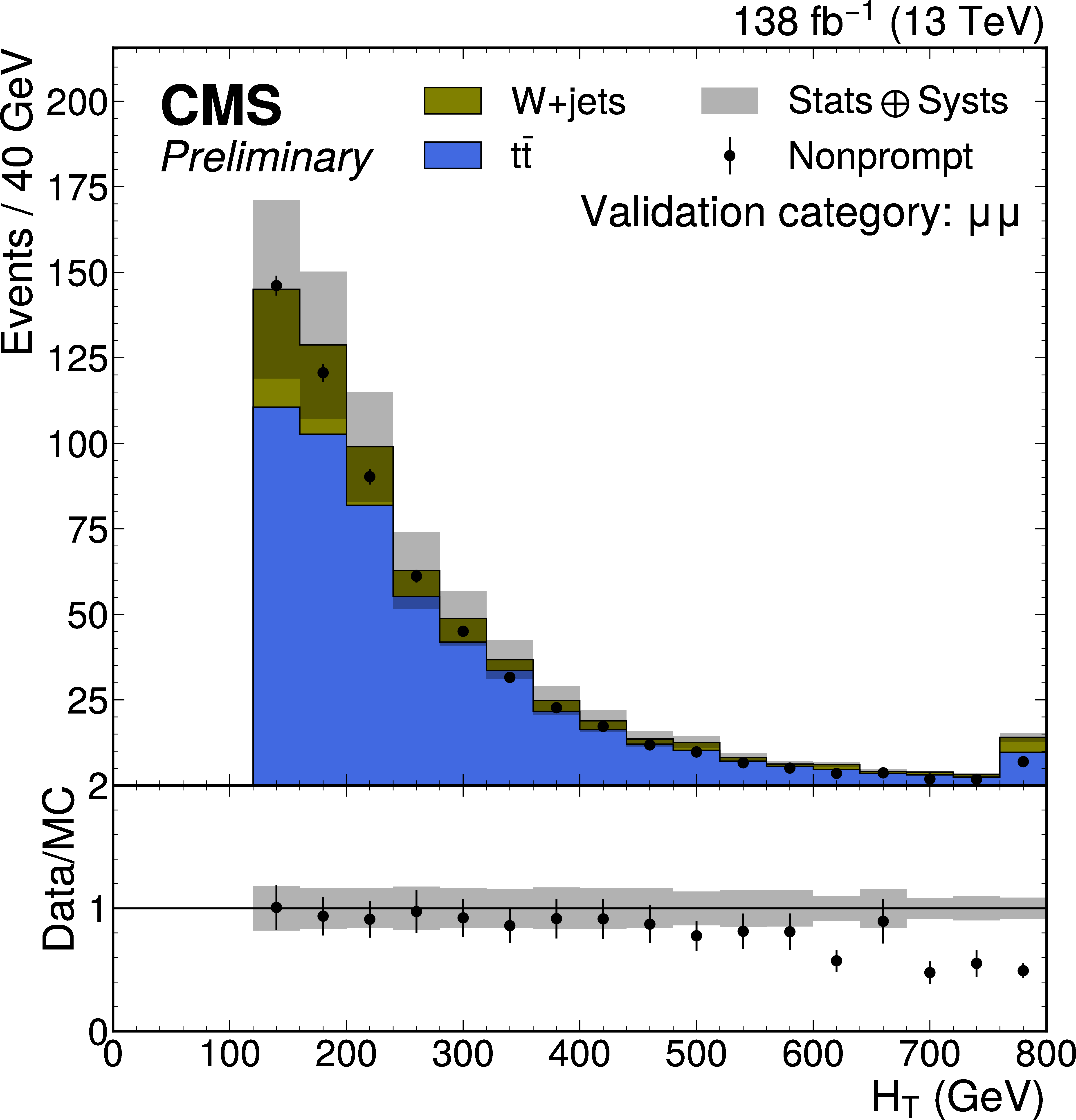
Figure 3:
Transverse energy $ H_{\mathrm{T}} $ distributions validating the estimation of the nonprompt-lepton background. The distributions are separated by lepton flavor: $ \mathrm{e}\mathrm{e} $ (upper left), $ \mathrm{e}\mu $ (upper right), and $ \mu\mu $ (lower). |
png pdf |
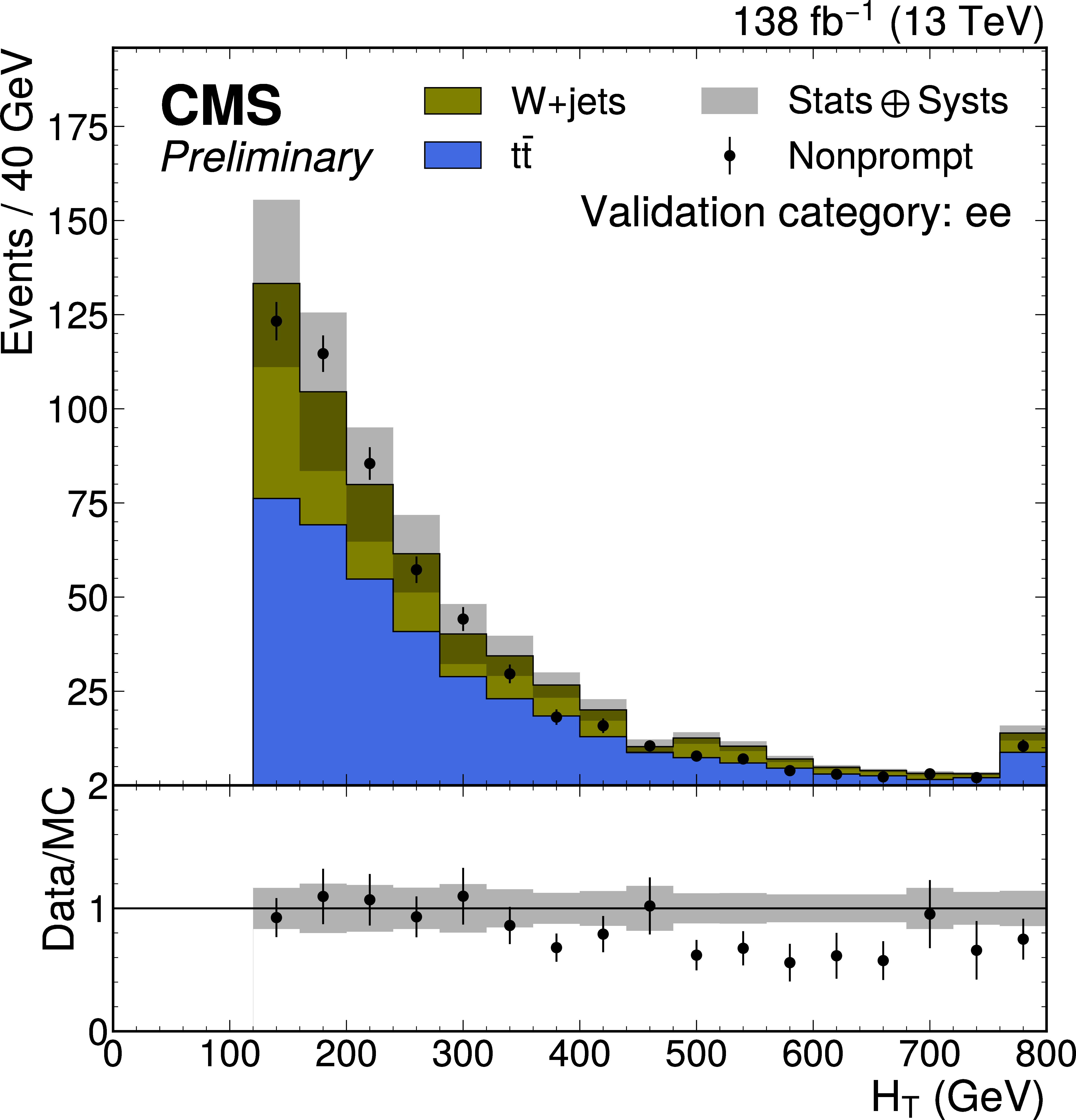
Figure 3-a:
Transverse energy $ H_{\mathrm{T}} $ distributions validating the estimation of the nonprompt-lepton background. The distributions are separated by lepton flavor: $ \mathrm{e}\mathrm{e} $ (upper left), $ \mathrm{e}\mu $ (upper right), and $ \mu\mu $ (lower). |
png pdf |
Figure 3-b:
Transverse energy $ H_{\mathrm{T}} $ distributions validating the estimation of the nonprompt-lepton background. The distributions are separated by lepton flavor: $ \mathrm{e}\mathrm{e} $ (upper left), $ \mathrm{e}\mu $ (upper right), and $ \mu\mu $ (lower). |
png pdf |
Figure 3-c:
Transverse energy $ H_{\mathrm{T}} $ distributions validating the estimation of the nonprompt-lepton background. The distributions are separated by lepton flavor: $ \mathrm{e}\mathrm{e} $ (upper left), $ \mathrm{e}\mu $ (upper right), and $ \mu\mu $ (lower). |
png pdf |
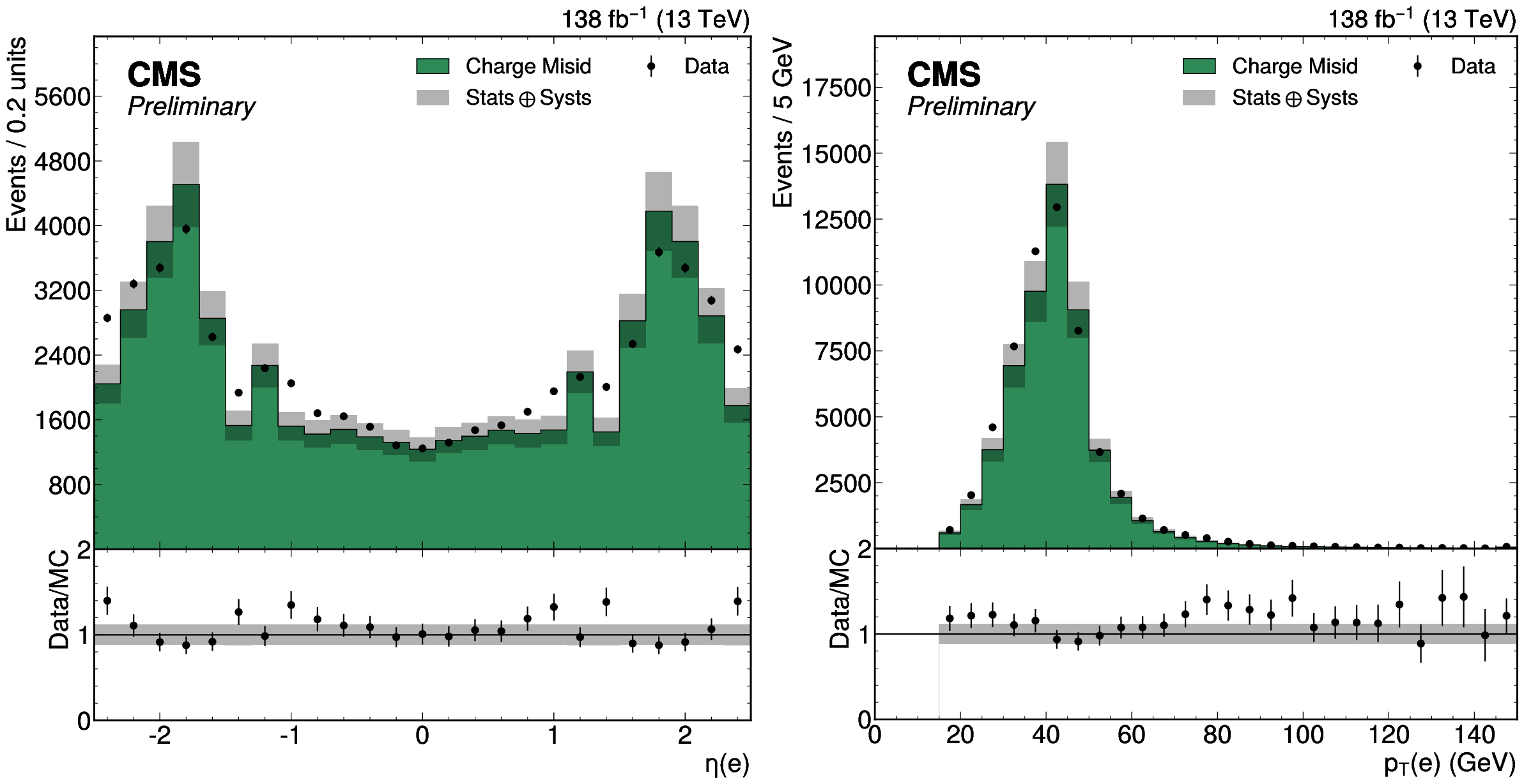
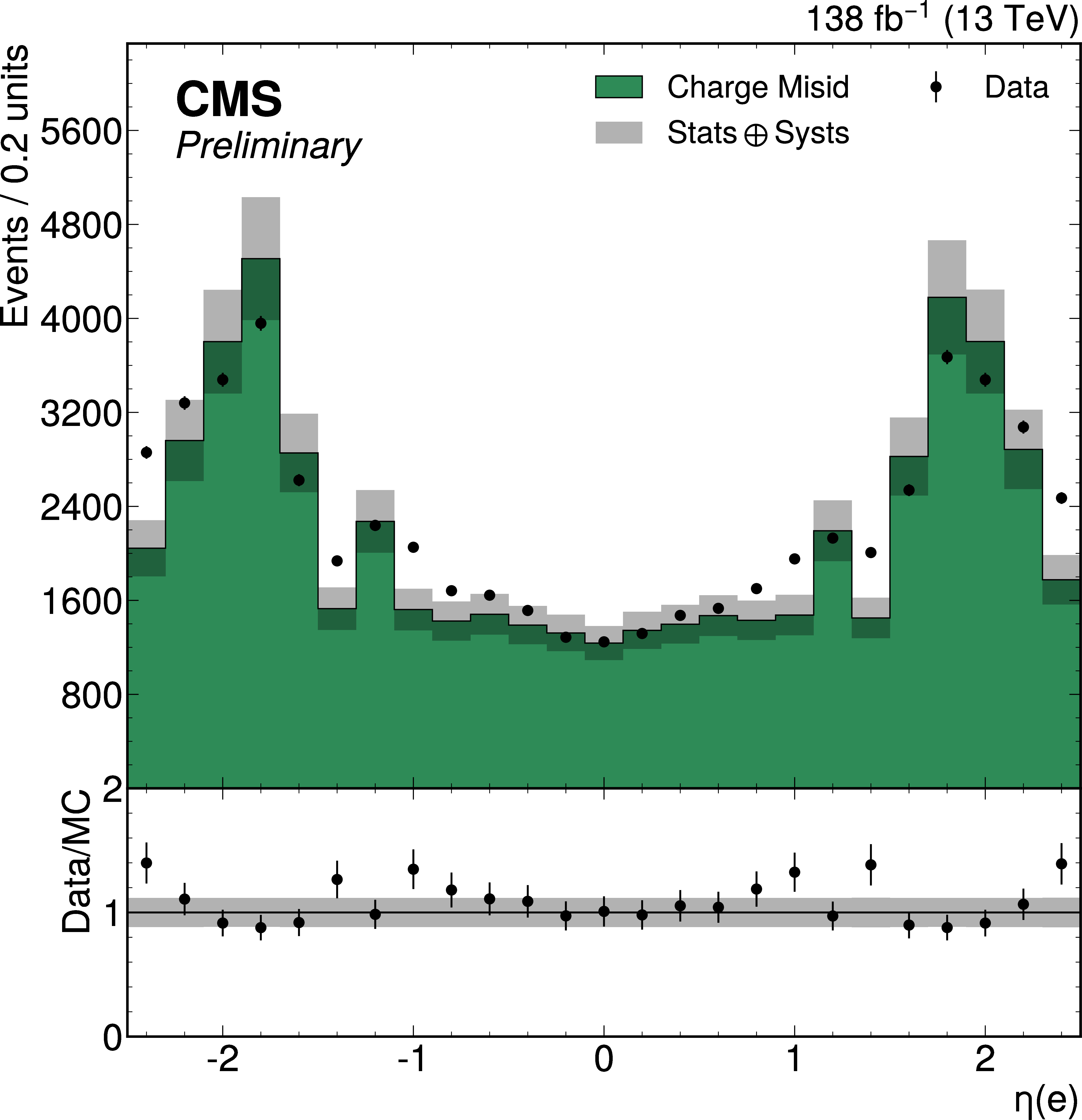
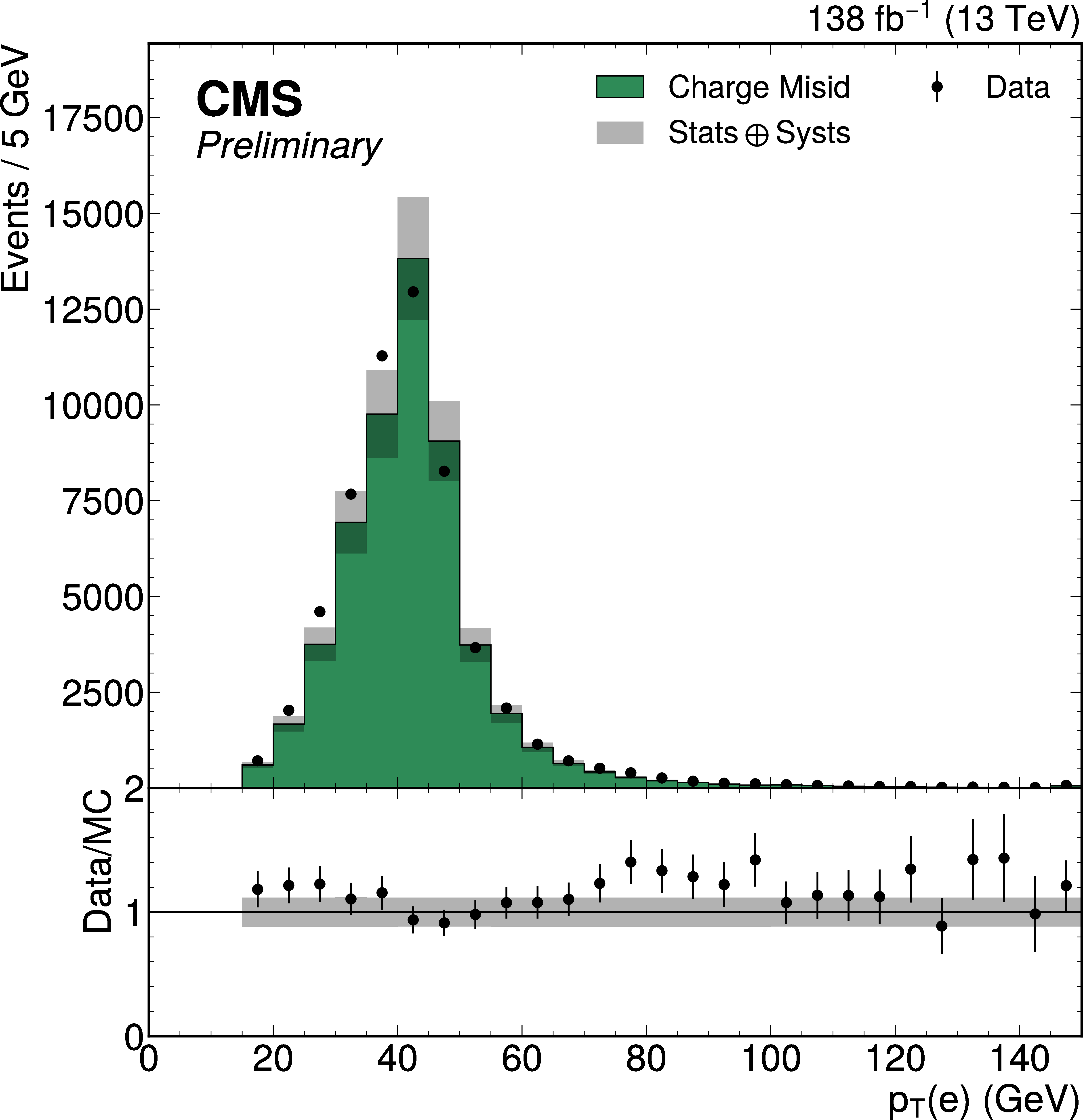
Figure 4:
Distributions of the lepton $ \eta $ (left) and $ p_{\mathrm{T}} $ (right) showing the closure of the electron charge misidentification rate. |
png pdf |
Figure 4-a:
Distributions of the lepton $ \eta $ (left) and $ p_{\mathrm{T}} $ (right) showing the closure of the electron charge misidentification rate. |
png pdf |
Figure 4-b:
Distributions of the lepton $ \eta $ (left) and $ p_{\mathrm{T}} $ (right) showing the closure of the electron charge misidentification rate. |
png pdf |
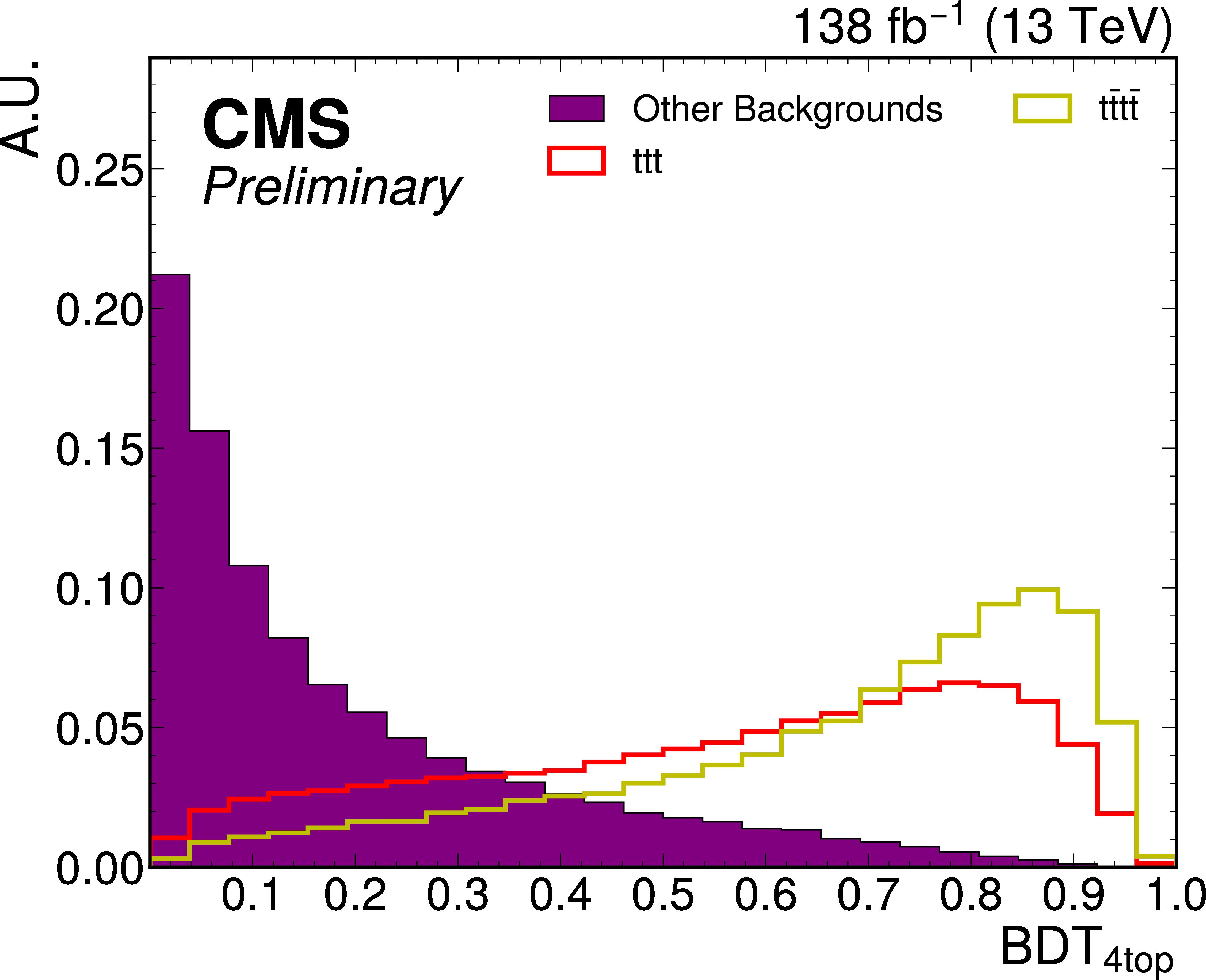
Figure 5:
Distributions of the four-top-quark BDT score after training with normalized distributions for $ \mathrm{t}\mathrm{t}\mathrm{t} $, $ {\mathrm{t}\overline{\mathrm{t}}} {\mathrm{t}\overline{\mathrm{t}}} $, and the other standard model backgrounds. |
png pdf |
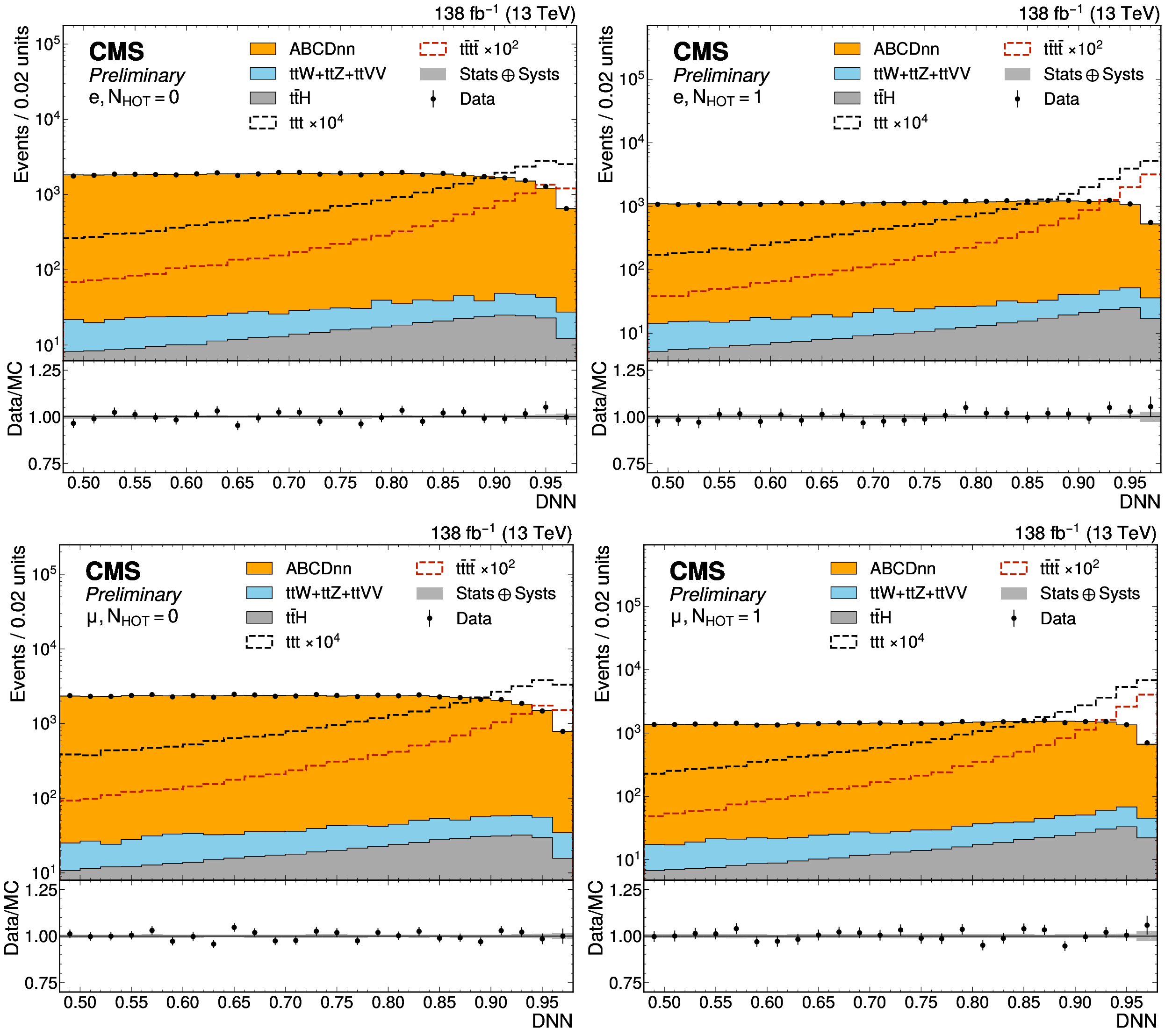
Figure 6:
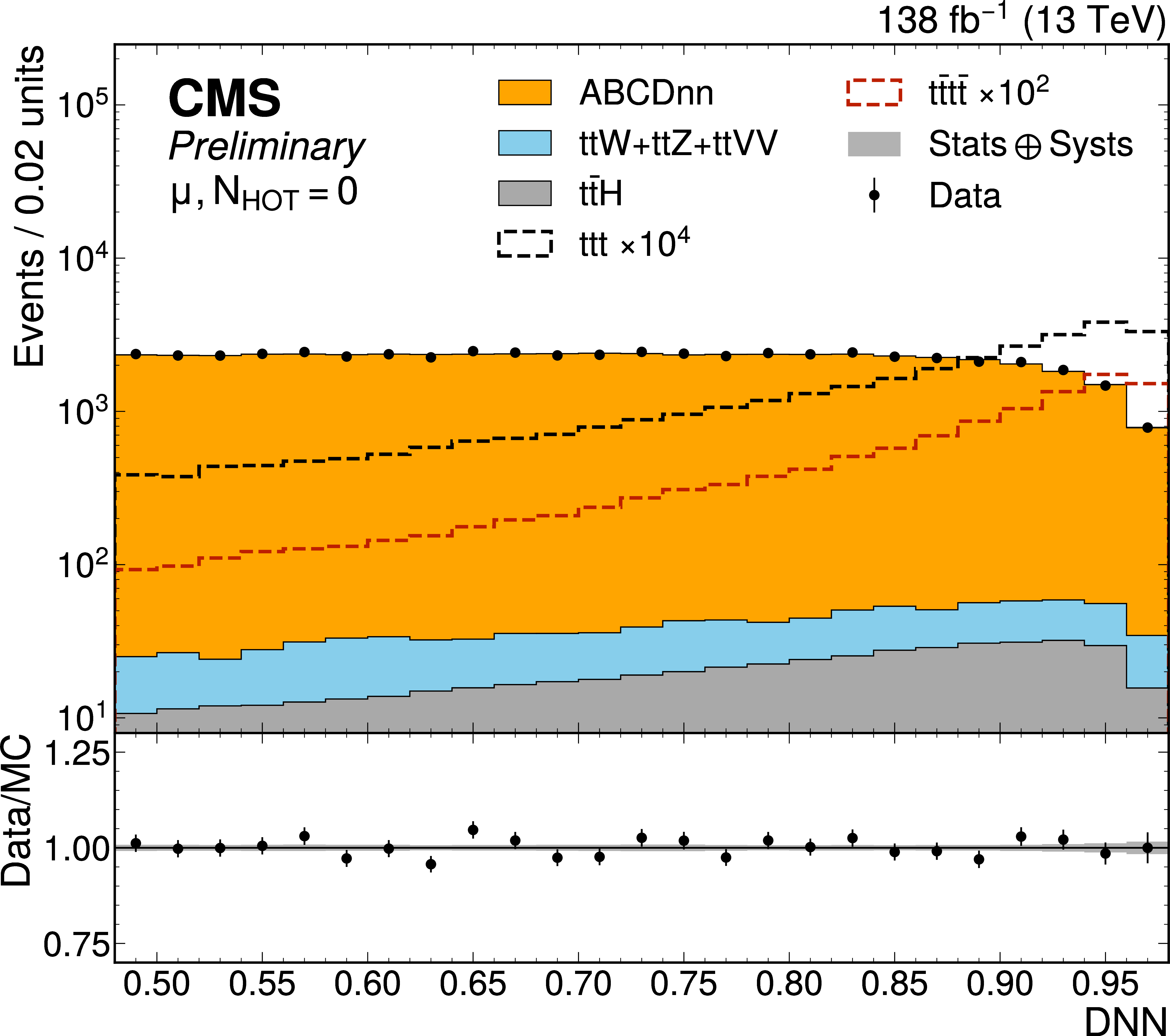
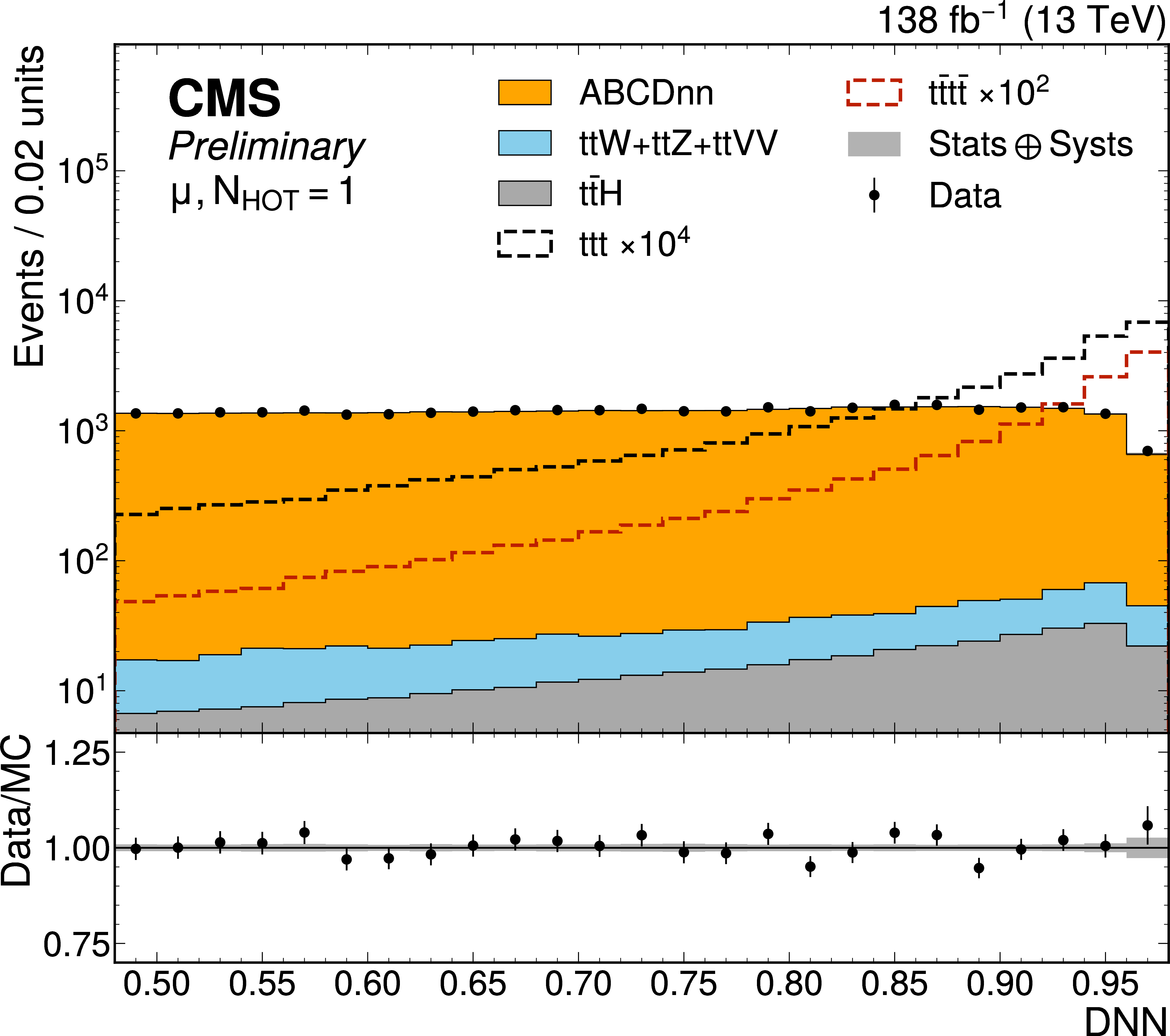
Distribution of the DNN score in the SL channel in the signal regions with $ N_{\text{HOT}}= $ 0 (left column) or $ N_{\text{HOT}}\geq $ 1 (right column) in the electron channel (upper row) and muon channel (lower row) after a signal-plus-background fit across all channels. The solid histograms for the simulated SM backgrounds are stacked, while the four-top-quark process and the three-top-quark signal distributions are overlaid. The grey shaded area in the upper and lower panels represents the total uncertainty in the sum of the SM backgrounds and signal. The data are represented by black markers with the vertical bar indicating the associated statistical uncertainty. The last bin contains overflow events. The lower panels show the ratio of data and the postfit SM background. |
png pdf |
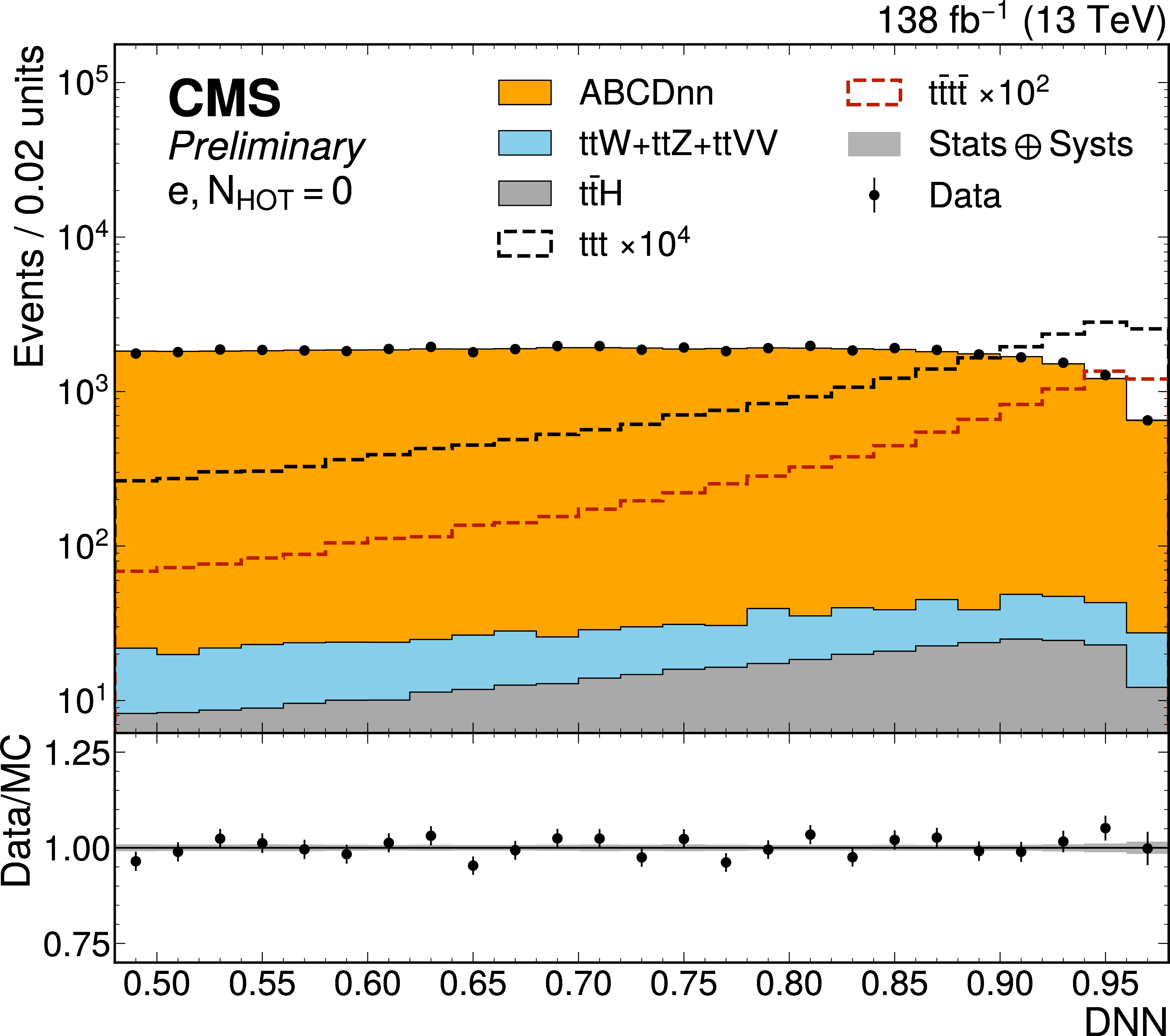
Figure 6-a:
Distribution of the DNN score in the SL channel in the signal regions with $ N_{\text{HOT}}= $ 0 (left column) or $ N_{\text{HOT}}\geq $ 1 (right column) in the electron channel (upper row) and muon channel (lower row) after a signal-plus-background fit across all channels. The solid histograms for the simulated SM backgrounds are stacked, while the four-top-quark process and the three-top-quark signal distributions are overlaid. The grey shaded area in the upper and lower panels represents the total uncertainty in the sum of the SM backgrounds and signal. The data are represented by black markers with the vertical bar indicating the associated statistical uncertainty. The last bin contains overflow events. The lower panels show the ratio of data and the postfit SM background. |

png pdf |
Figure 6-b:
Distribution of the DNN score in the SL channel in the signal regions with $ N_{\text{HOT}}= $ 0 (left column) or $ N_{\text{HOT}}\geq $ 1 (right column) in the electron channel (upper row) and muon channel (lower row) after a signal-plus-background fit across all channels. The solid histograms for the simulated SM backgrounds are stacked, while the four-top-quark process and the three-top-quark signal distributions are overlaid. The grey shaded area in the upper and lower panels represents the total uncertainty in the sum of the SM backgrounds and signal. The data are represented by black markers with the vertical bar indicating the associated statistical uncertainty. The last bin contains overflow events. The lower panels show the ratio of data and the postfit SM background. |
png pdf |
Figure 6-c:
Distribution of the DNN score in the SL channel in the signal regions with $ N_{\text{HOT}}= $ 0 (left column) or $ N_{\text{HOT}}\geq $ 1 (right column) in the electron channel (upper row) and muon channel (lower row) after a signal-plus-background fit across all channels. The solid histograms for the simulated SM backgrounds are stacked, while the four-top-quark process and the three-top-quark signal distributions are overlaid. The grey shaded area in the upper and lower panels represents the total uncertainty in the sum of the SM backgrounds and signal. The data are represented by black markers with the vertical bar indicating the associated statistical uncertainty. The last bin contains overflow events. The lower panels show the ratio of data and the postfit SM background. |
png pdf |
Figure 6-d:
Distribution of the DNN score in the SL channel in the signal regions with $ N_{\text{HOT}}= $ 0 (left column) or $ N_{\text{HOT}}\geq $ 1 (right column) in the electron channel (upper row) and muon channel (lower row) after a signal-plus-background fit across all channels. The solid histograms for the simulated SM backgrounds are stacked, while the four-top-quark process and the three-top-quark signal distributions are overlaid. The grey shaded area in the upper and lower panels represents the total uncertainty in the sum of the SM backgrounds and signal. The data are represented by black markers with the vertical bar indicating the associated statistical uncertainty. The last bin contains overflow events. The lower panels show the ratio of data and the postfit SM background. |
png pdf |
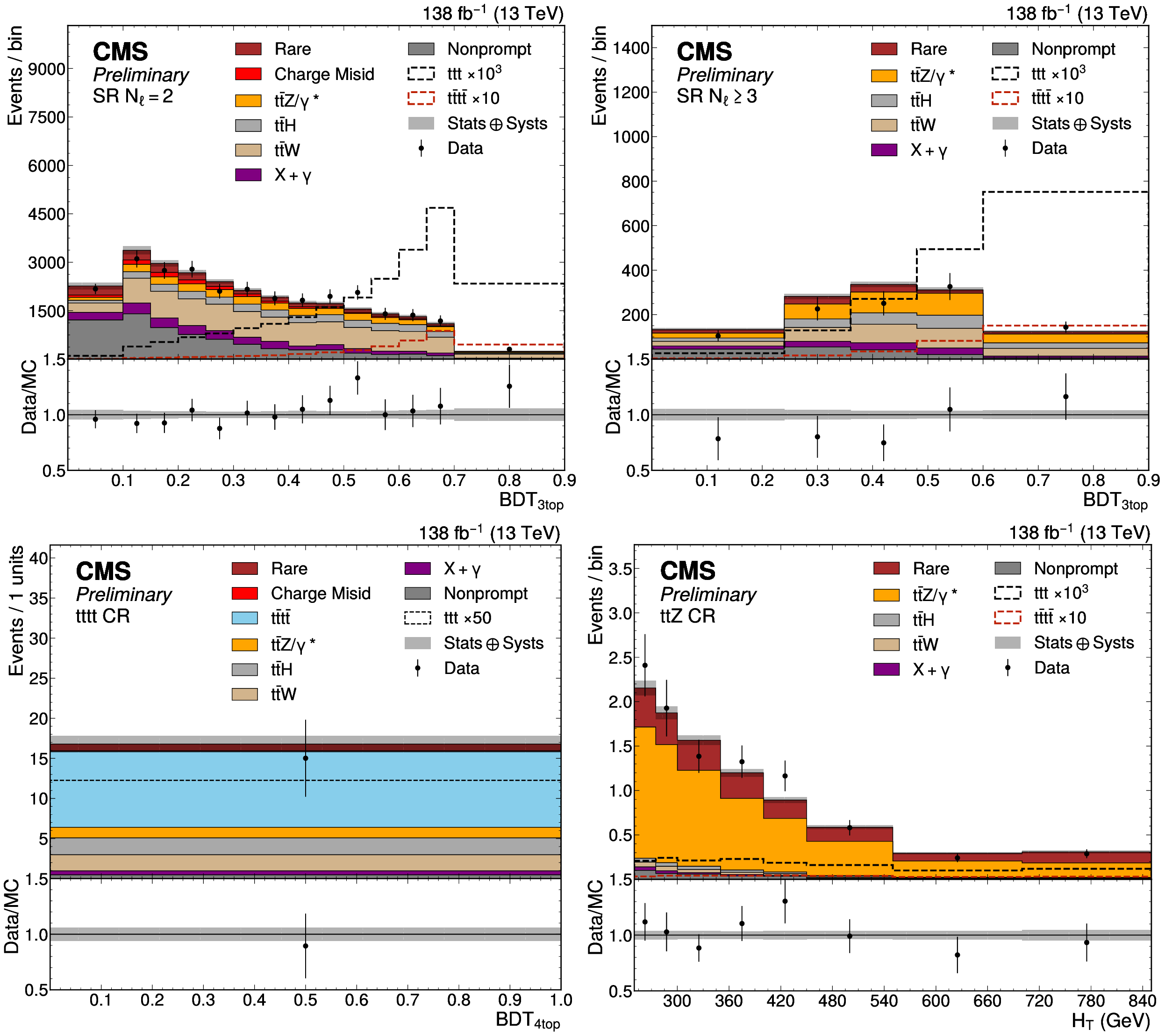
Figure 7:
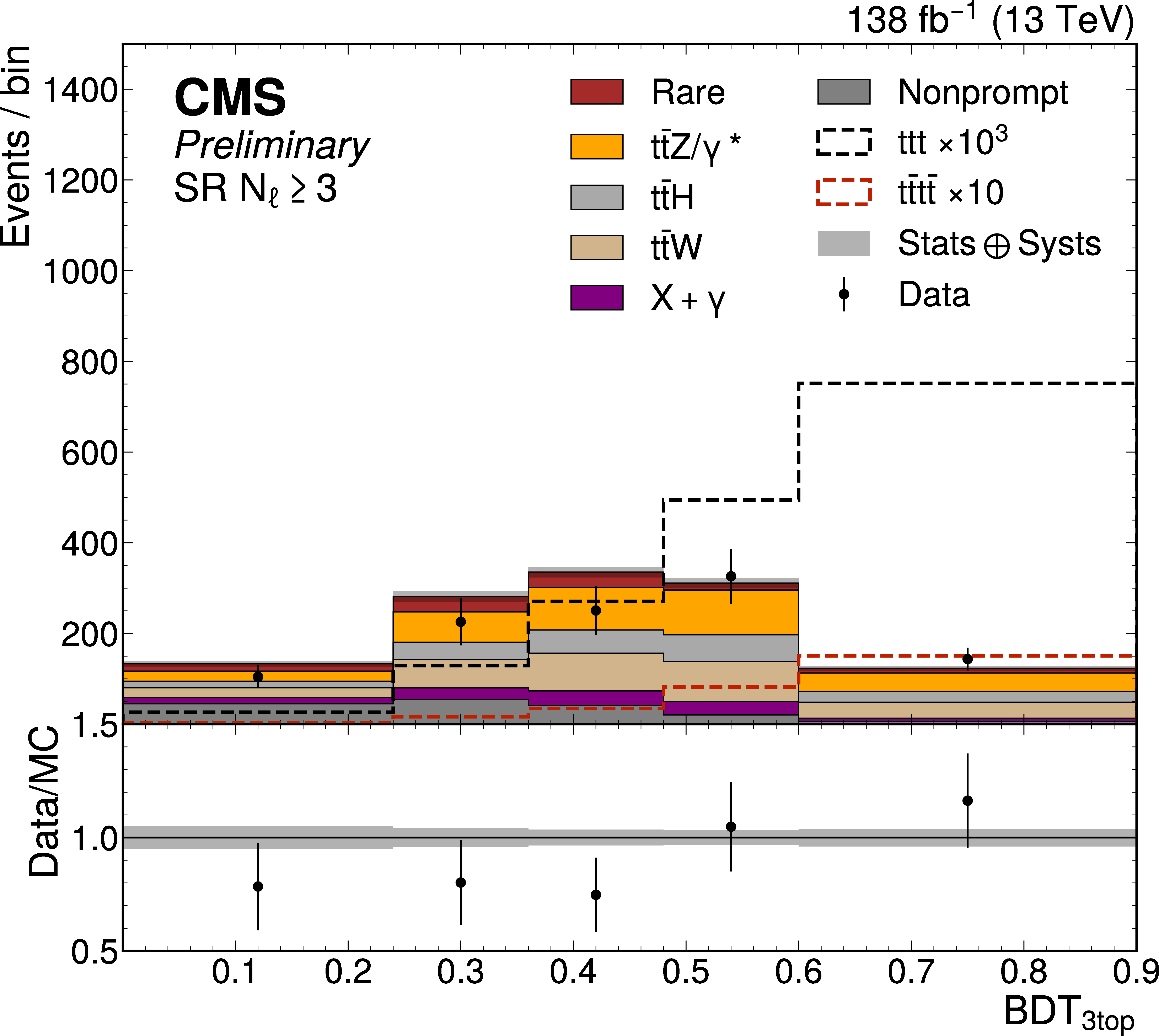
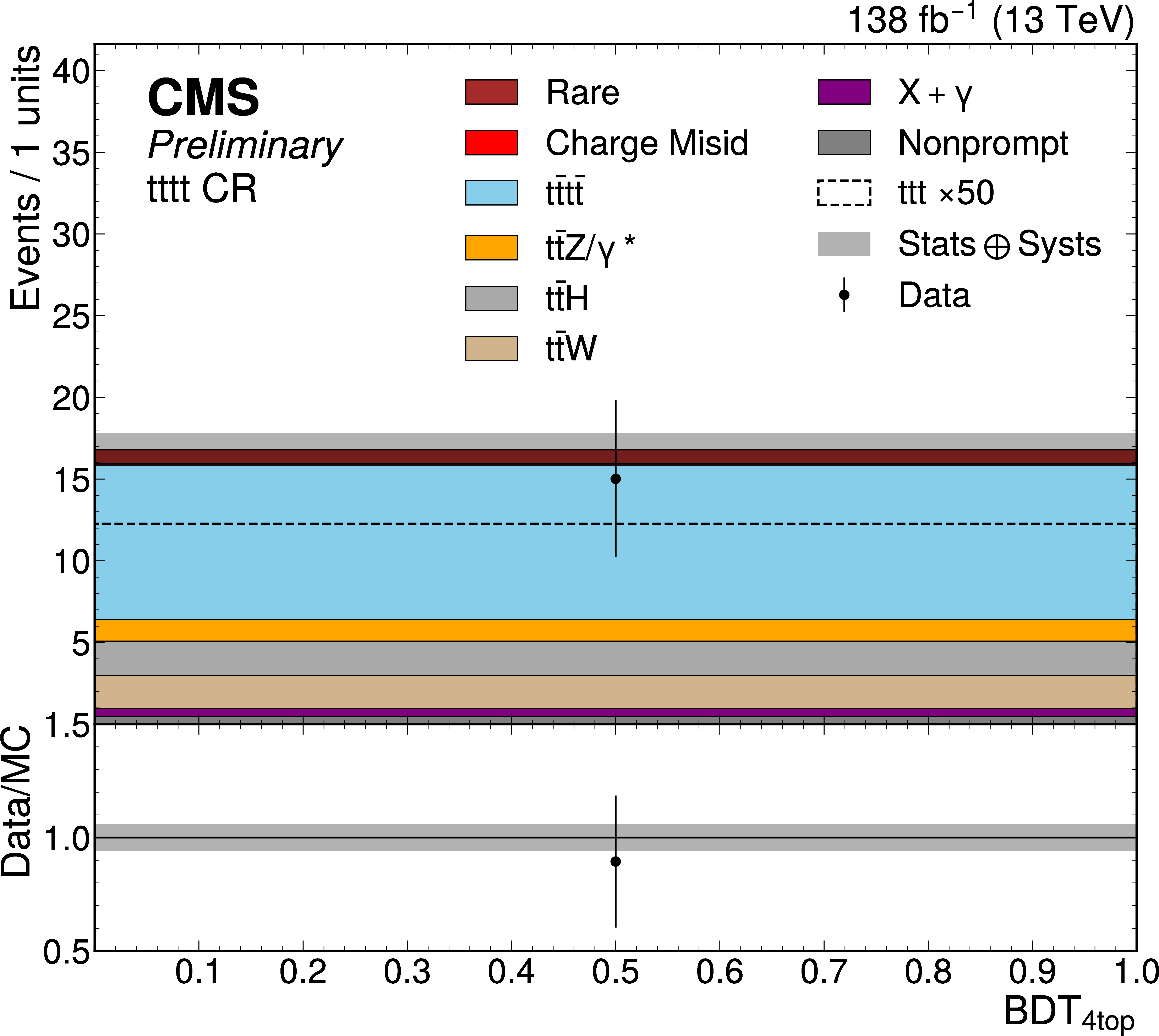
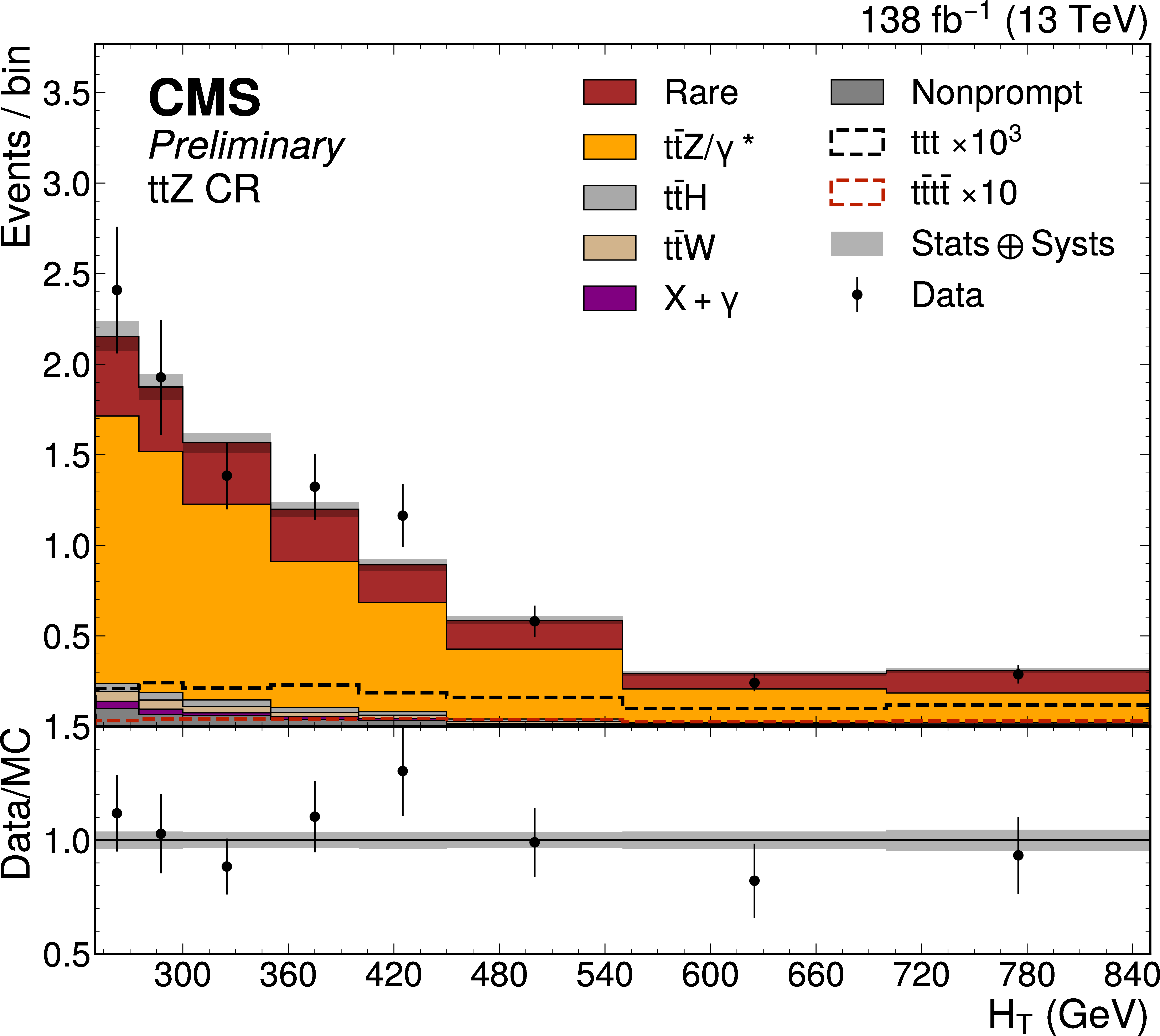
The SSDL and ML discriminant distributions in the SSDL region (upper left), ML region (upper right), four-top-quark control region (lower left), and $ tt\mathrm{Z} $ control region (lower right), after a signal-plus-background fit across all channels. The solid histograms for the simulated SM backgrounds are stacked, while the four-top-quark process and the three-top-quark signal distributions are overlaid. The grey shaded area in the upper and lower panels represents the total uncertainty in the sum of the SM backgrounds and signal. The data are represented by black markers with the vertical bar indicating the associated statistical uncertainty. The last bin contains overflow events. The lower panels show the ratio of data and the postfit SM background. |
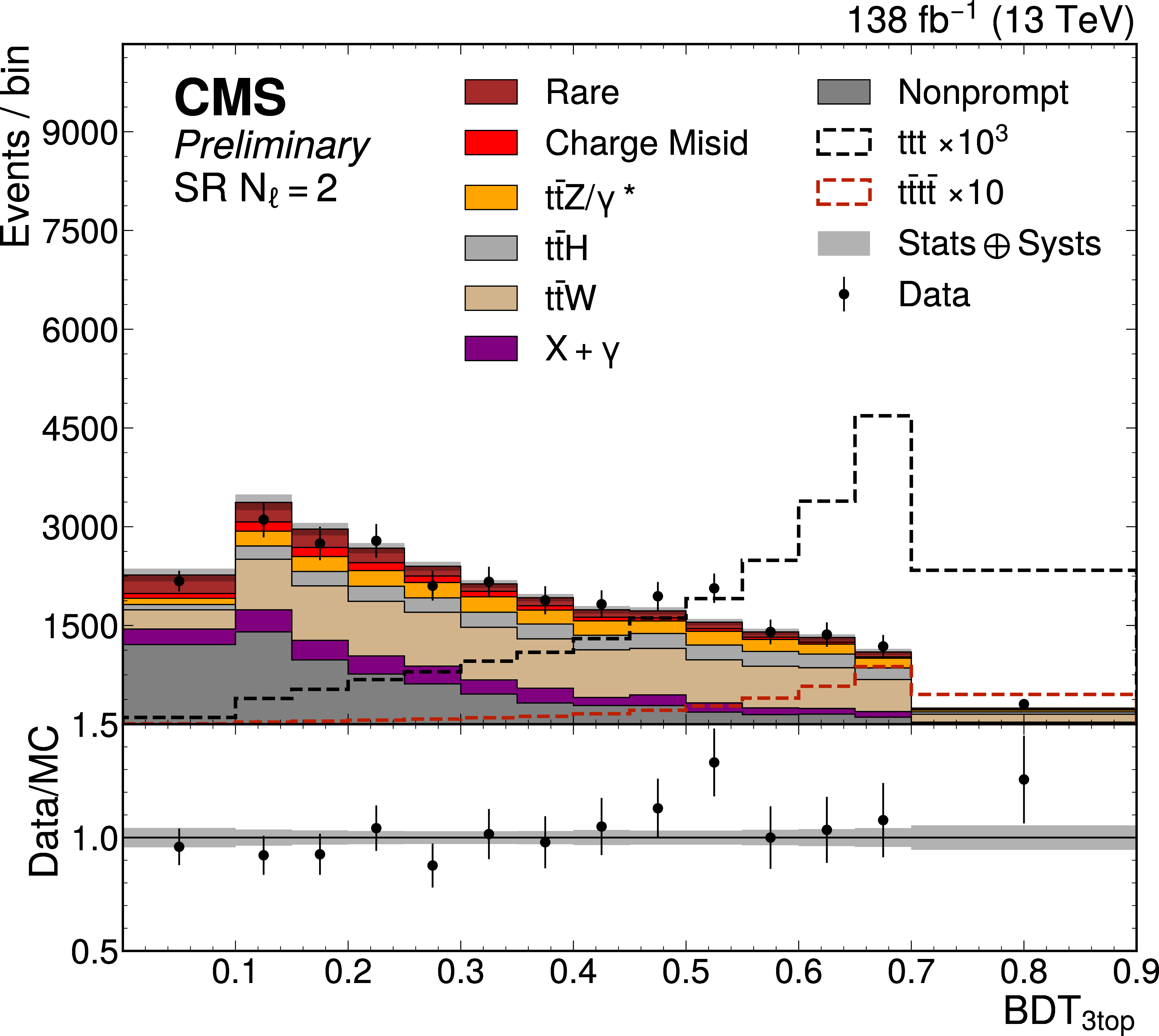
png pdf |
Figure 7-a:
The SSDL and ML discriminant distributions in the SSDL region (upper left), ML region (upper right), four-top-quark control region (lower left), and $ tt\mathrm{Z} $ control region (lower right), after a signal-plus-background fit across all channels. The solid histograms for the simulated SM backgrounds are stacked, while the four-top-quark process and the three-top-quark signal distributions are overlaid. The grey shaded area in the upper and lower panels represents the total uncertainty in the sum of the SM backgrounds and signal. The data are represented by black markers with the vertical bar indicating the associated statistical uncertainty. The last bin contains overflow events. The lower panels show the ratio of data and the postfit SM background. |
png pdf |
Figure 7-b:
The SSDL and ML discriminant distributions in the SSDL region (upper left), ML region (upper right), four-top-quark control region (lower left), and $ tt\mathrm{Z} $ control region (lower right), after a signal-plus-background fit across all channels. The solid histograms for the simulated SM backgrounds are stacked, while the four-top-quark process and the three-top-quark signal distributions are overlaid. The grey shaded area in the upper and lower panels represents the total uncertainty in the sum of the SM backgrounds and signal. The data are represented by black markers with the vertical bar indicating the associated statistical uncertainty. The last bin contains overflow events. The lower panels show the ratio of data and the postfit SM background. |
png pdf |
Figure 7-c:
The SSDL and ML discriminant distributions in the SSDL region (upper left), ML region (upper right), four-top-quark control region (lower left), and $ tt\mathrm{Z} $ control region (lower right), after a signal-plus-background fit across all channels. The solid histograms for the simulated SM backgrounds are stacked, while the four-top-quark process and the three-top-quark signal distributions are overlaid. The grey shaded area in the upper and lower panels represents the total uncertainty in the sum of the SM backgrounds and signal. The data are represented by black markers with the vertical bar indicating the associated statistical uncertainty. The last bin contains overflow events. The lower panels show the ratio of data and the postfit SM background. |
png pdf |
Figure 7-d:
The SSDL and ML discriminant distributions in the SSDL region (upper left), ML region (upper right), four-top-quark control region (lower left), and $ tt\mathrm{Z} $ control region (lower right), after a signal-plus-background fit across all channels. The solid histograms for the simulated SM backgrounds are stacked, while the four-top-quark process and the three-top-quark signal distributions are overlaid. The grey shaded area in the upper and lower panels represents the total uncertainty in the sum of the SM backgrounds and signal. The data are represented by black markers with the vertical bar indicating the associated statistical uncertainty. The last bin contains overflow events. The lower panels show the ratio of data and the postfit SM background. |
png pdf |
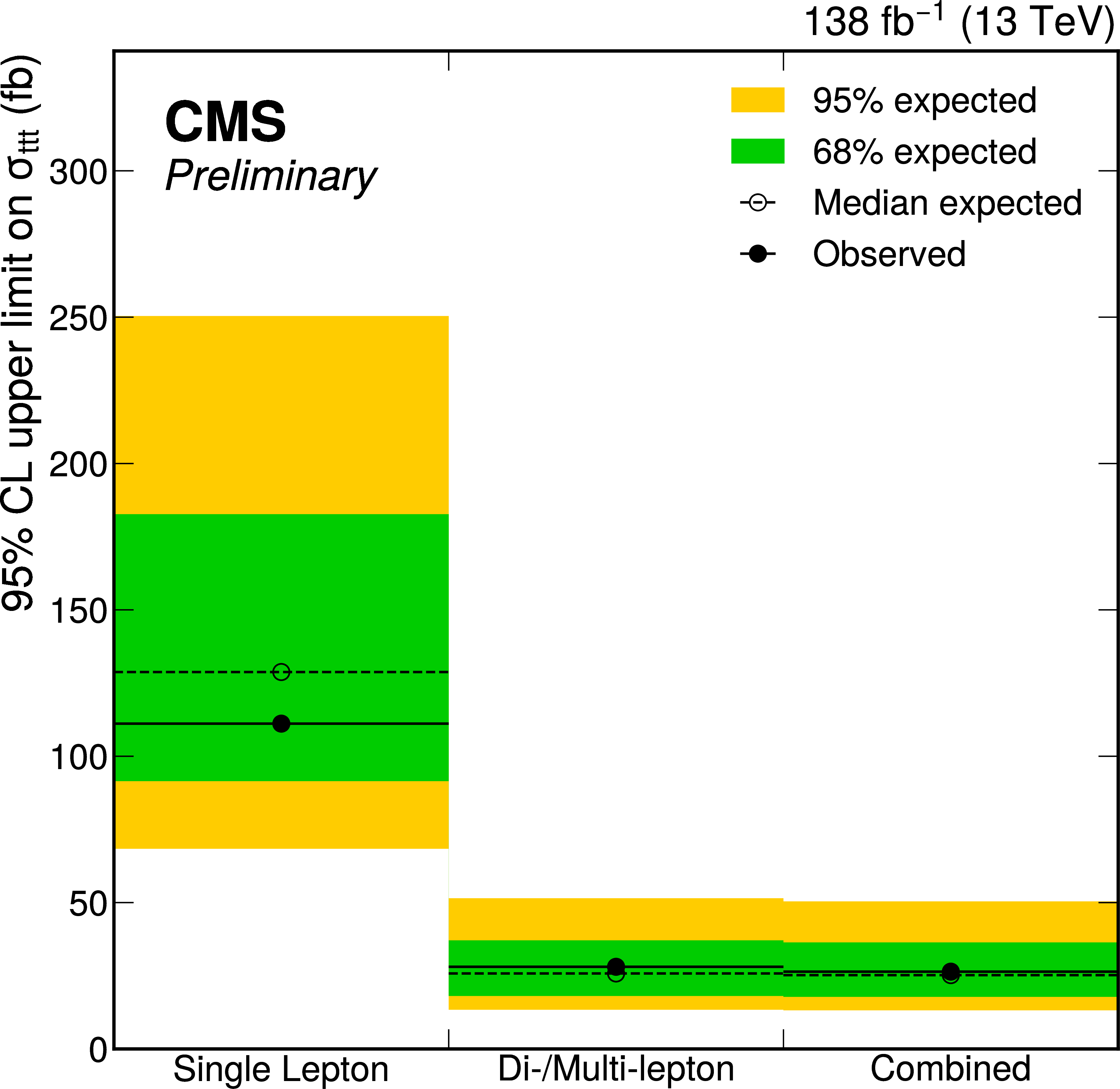
Figure 8:
Upper limits at 95% CL for $ \sigma_{\mathrm{t}\mathrm{t}\mathrm{t}} $ for each channel and their combination. The observed (expected) limits are shown as a solid (dashed) black line and the inner (green) band and the outer (yellow) band indicate the regions containing 68% and 95%, respectively, of the distribution of limits expected under the background-only hypothesis. |
| Tables | |
png pdf |
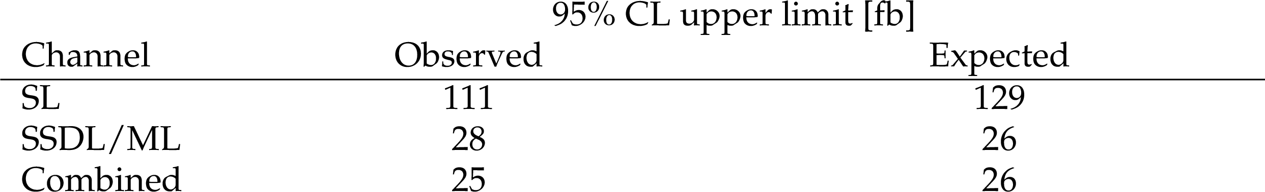
Table 1:
Observed and expected upper limits at 95% CL on $ \sigma_{\mathrm{t}\mathrm{t}\mathrm{t}} $ for each channel and their combination. |
| Summary |
| A search for standard model three-top-quark ($ \mathrm{t}\mathrm{t}\mathrm{t} $) production in proton-proton collisions at a center-of-mass energy of 13 TeV has been presented. The analysis was performed using data corresponding to an integrated luminosity of 138 fb$ ^{-1} $ recorded by the CMS experiment between 2016 and 2018. This note presents the first dedicated analysis of $ \mathrm{t}\mathrm{t}\mathrm{t} $ production at the LHC. The final states were categorized by the number and charge of prompt electrons and muons, which can be produced from leptonic W boson decays. The single lepton, same-sign dilepton, and multilepton final states were considered. Several new strategies were introduced to mitigate the impact of the dominant or poorly modeled backgrounds, including machine-learning-driven background estimation methods utilizing data in background-enriched control regions. Optimized multivariate methods were also employed to discriminate between the dominant backgrounds and the three-top-quark signal. An observed upper limit of 25$ \text{fb}$ is set on the $ \mathrm{t}\mathrm{t}\mathrm{t} $ cross section at 95% confidence level. |
| References | ||||
| 1 | ATLAS Collaboration | Observation of four-top-quark production in the multilepton final state with the ATLAS detector | [Erratum: Eur.Phys.J.C 84, 156] EPJC 83 (2023) 496 |
2303.15061 |
| 2 | CMS Collaboration | Observation of four top quark production in proton-proton collisions at $ \sqrt{s}= $ 13 TeV | PLB 847 (2023) 138290 | CMS-TOP-22-013 2305.13439 |
| 3 | S. L. Glashow, J. Iliopoulos, and L. Maiani | Weak interactions with lepton-hadron symmetry | PRD 2 (1970) 1285 | |
| 4 | L. Maiani | The GIM Mechanism: origin, predictions and recent uses | in the 48th Rencontres de Moriond on Electroweak Interactions and Unified Theories, 2013 | 1303.6154 |
| 5 | V. Barger, W.-Y. Keung, and B. Yencho | Triple-top signal of new physics at the LHC | PLB 687 (2010) 70 | 1001.0221 |
| 6 | Q.-H. Cao, S.-L. Chen, Y. Liu, and X.-P. Wang | What can we learn from triple top-quark production? | PRD 100 (2019) 055035 | 1901.04643 |
| 7 | H. Khanpour | Probing top quark FCNC couplings in the triple-top signal at the high energy LHC and future circular collider | NPB 958 (2020) 115141 | 1909.03998 |
| 8 | CMS Collaboration | The CMS experiment at the CERN LHC | JINST 3 (2008) S08004 | |
| 9 | CMS Collaboration | Development of the CMS detector for the CERN LHC Run 3 | JINST 19 (2024) P05064 | |
| 10 | CMS Collaboration | Performance of the CMS level-1 trigger in proton-proton collisions at $ \sqrt{s} = $ 13 TeV | JINST 15 (2020) P10017 | CMS-TRG-17-001 2006.10165 |
| 11 | CMS Collaboration | The CMS trigger system | JINST 12 (2017) P01020 | CMS-TRG-12-001 1609.02366 |
| 12 | CMS Collaboration | Performance of the CMS high-level trigger during LHC Run 2 | JINST 19 (2024) P11021 | CMS-TRG-19-001 2410.17038 |
| 13 | CMS Collaboration | Electron and photon reconstruction and identification with the CMS experiment at the CERN LHC | JINST 16 (2021) P05014 | CMS-EGM-17-001 2012.06888 |
| 14 | CMS Collaboration | Performance of the CMS muon detector and muon reconstruction with proton-proton collisions at $ \sqrt{s}= $ 13 TeV | JINST 13 (2018) P06015 | CMS-MUO-16-001 1804.04528 |
| 15 | CMS Collaboration | Description and performance of track and primary-vertex reconstruction with the CMS tracker | JINST 9 (2014) P10009 | CMS-TRK-11-001 1405.6569 |
| 16 | CMS Collaboration | Particle-flow reconstruction and global event description with the CMS detector | JINST 12 (2017) P10003 | CMS-PRF-14-001 1706.04965 |
| 17 | CMS Collaboration | Performance of reconstruction and identification of $ \tau $ leptons decaying to hadrons and $ \nu_\tau $ in pp collisions at $ \sqrt{s}= $ 13 TeV | JINST 13 (2018) P10005 | CMS-TAU-16-003 1809.02816 |
| 18 | CMS Collaboration | Jet energy scale and resolution in the CMS experiment in pp collisions at 8 TeV | JINST 12 (2017) P02014 | CMS-JME-13-004 1607.03663 |
| 19 | CMS Collaboration | Performance of missing transverse momentum reconstruction in proton-proton collisions at $ \sqrt{s} = $ 13 TeV using the CMS detector | JINST 14 (2019) P07004 | CMS-JME-17-001 1903.06078 |
| 20 | P. Artoisenet, R. Frederix, O. Mattelaer, and R. Rietkerk | Automatic spin-entangled decays of heavy resonances in Monte Carlo simulations | JHEP 03 (2013) 015 | 1212.3460 |
| 21 | J. Alwall et al. | The automated computation of tree-level and next-to-leading order differential cross sections, and their matching to parton shower simulations | JHEP 07 (2014) 079 | 1405.0301 |
| 22 | M. van Beekveld, A. Kulesza, and L. M. Valero | Threshold Resummation for the Production of Four Top Quarks at the LHC | PRL 131 (2023) 211901 | 2212.03259 |
| 23 | P. Nason | A new method for combining NLO QCD with shower Monte Carlo algorithms | JHEP 11 (2004) 040 | hep-ph/0409146 |
| 24 | S. Frixione, P. Nason, and C. Oleari | Matching NLO QCD computations with parton shower simulations: the POWHEG method | JHEP 11 (2007) 070 | 0709.2092 |
| 25 | S. Alioli, P. Nason, C. Oleari, and E. Re | A general framework for implementing NLO calculations in shower Monte Carlo programs: the POWHEG BOX | JHEP 06 (2010) 043 | 1002.2581 |
| 26 | M. L. Mangano, M. Moretti, F. Piccinini, and M. Treccani | Matching matrix elements and shower evolution for top-quark production in hadronic collisions | JHEP 01 (2007) 013 | hep-ph/0611129 |
| 27 | R. Frederix and S. Frixione | Merging meets matching in MC@NLO | JHEP 12 (2012) 061 | 1209.6215 |
| 28 | NNPDF Collaboration | Parton distributions from high-precision collider data | EPJC 77 (2017) 663 | 1706.00428 |
| 29 | T. Sjöstrand et al. | An introduction to PYTHIA 8.2 | Comput. Phys. Commun. 191 (2015) 159 | 1410.3012 |
| 30 | CMS Collaboration | Extraction and validation of a new set of CMS PYTHIA8 tunes from underlying-event measurements | EPJC 80 (2020) 4 | CMS-GEN-17-001 1903.12179 |
| 31 | GEANT4 Collaboration | GEANT 4---a simulation toolkit | NIM A 506 (2003) 250 | |
| 32 | M. Cacciari, G. P. Salam, and G. Soyez | The anti-$ k_{\mathrm{T}} $ jet clustering algorithm | JHEP 04 (2008) 063 | 0802.1189 |
| 33 | M. Cacciari, G. P. Salam, and G. Soyez | FastJet user manual | EPJC 72 (2012) 1896 | 1111.6097 |
| 34 | K. Rehermann and B. Tweedie | Efficient Identification of Boosted Semileptonic Top Quarks at the LHC | JHEP 03 (2011) 059 | 1007.2221 |
| 35 | CMS Collaboration | ECAL 2016 refined calibration and Run2 summary plots | CMS Detector Performance Summary CMS-DP-2020-021, 2020 CDS |
|
| 36 | CMS Collaboration | Performance of electron reconstruction and selection with the CMS detector in proton-proton collisions at $ \sqrt{s} = $ 8 TeV | JINST 10 (2015) P06005 | CMS-EGM-13-001 1502.02701 |
| 37 | CMS Collaboration | Muon identification using multivariate techniques in the CMS experiment in proton-proton collisions at $ \sqrt{s}= $ 13 TeV | JINST 19 (2024) P02031 | CMS-MUO-22-001 2310.03844 |
| 38 | CMS Collaboration | Pileup mitigation at CMS in 13 TeV data | JINST 15 (2020) P09018 | CMS-JME-18-001 2003.00503 |
| 39 | E. Bols et al. | Jet flavour classification using DeepJet | JINST 15 (2020) P12012 | 2008.10519 |
| 40 | G. C. Fox and S. Wolfram | Observables for the analysis of event shapes in $ {e}^{+}{e}^{-} $ annihilation and other processes | PRL 41 (1978) 1581 | |
| 41 | S. Choi, J. Lim, and H. Oh | Data-driven estimation of background distribution through neural autoregressive flows | link | |
| 42 | S. Choi and H. Oh | Improved extrapolation methods of data-driven background estimation in high-energy physics | link | |
| 43 | CMS Collaboration | Precision luminosity measurement in proton-proton collisions at $ \sqrt{s} = $ 13 TeV in 2015 and 2016 at CMS | EPJC 81 (2021) 800 | CMS-LUM-17-003 2104.01927 |
| 44 | CMS Collaboration | CMS luminosity measurement for the 2017 data-taking period at $ \sqrt{s} = $ 13 TeV | CMS Physics Analysis Summary, 2018 link |
CMS-PAS-LUM-17-004 |
| 45 | CMS Collaboration | CMS luminosity measurement for the 2018 data-taking period at $ \sqrt{s} = $ 13 TeV | CMS Physics Analysis Summary, 2019 link |
CMS-PAS-LUM-18-002 |
| 46 | CMS Collaboration | Performance of the CMS muon trigger system in proton-proton collisions at $ \sqrt{s} = $ 13 TeV | JINST 16 (2021) P07001 | CMS-MUO-19-001 2102.04790 |
| 47 | CMS Collaboration | Identification of heavy-flavour jets with the CMS detector in pp collisions at 13 TeV | JINST 13 (2018) P05011 | CMS-BTV-16-002 1712.07158 |
| 48 | NNPDF Collaboration | Parton distributions for the LHC Run II | JHEP 04 (2015) 040 | 1410.8849 |
| 49 | J. Butterworth et al. | PDF4LHC recommendations for LHC Run II | JPG 43 (2016) 023001 | 1510.03865 |
| 50 | R. Barlow and C. Beeston | Fitting using finite monte carlo samples | Computer Physics Communications 77 (1993) 219 | |
| 51 | CMS Collaboration | The CMS Statistical Analysis and Combination Tool: Combine | Comput. Softw. Big Sci. 8 (2024) 19 | CMS-CAT-23-001 2404.06614 |
| 52 | W. Verkerke and D. Kirkby | The RooFit toolkit for data modeling | in the International Conference on Computing in High Energy and Nuclear Physics (CHEP ): La Jolla CA, United States, March 24--28 Proc. 1 (2003) 3 |
physics/0306116 |
| 53 | L. Moneta et al. | The RooStats project | in the International Workshop on Advanced Computing and Analysis Techniques in Physics Research (ACAT) PoS (ACAT) 057 |
1009.1003 |
| 54 | C. Patrignani | Review of particle physics | Chinese Physics C 40 (2016) 100001 | |
| 55 | ATLAS Collaboration, CMS Collaboration, LHC Higgs Combination Group | Procedure for the LHC Higgs boson search combination in Summer 2011 | Technical Report CMS-NOTE-2011-005, ATL-PHYS-PUB-2011-11, CERN, 2011 | |
| 56 | T. Junk | Confidence level computation for combining searches with small statistics | NIM A 434 (1999) 435 | hep-ex/9902006 |
| 57 | A. L. Read | Presentation of search results: the CLs technique | Journal of Physics G. Nuclear and Particle Physics 28 (2002) 2693 | |
| 58 | G. Cowan, K. Cranmer, E. Gross, and O. Vitells | Asymptotic formulae for likelihood-based tests of new physics | [Erratum: Eur.Phys.J.C 73, 2501] EPJC 71 (2011) 1554 |
1007.1727 |
|
|
Compact Muon Solenoid LHC, CERN |
|

|

|

|

|

|