Compact Muon Solenoid
LHC, CERN

Visit us: CMS Public Website, CMS Physics ; Contact us: CMS Publications Committee

CMS-PAS-HIG-25-004

Constraints on the Higgs boson total decay width using signal-background interference in the diphoton final state with proton-proton collisions at $ \sqrt{s}= $ 13 TeV

CMS Collaboration

2025-08-27

Abstract: The standard model Higgs boson with a mass of 125 GeV is predicted to have a decay width $ \Gamma_{\mathrm{H}} $ of 4.1 MeV. Direct $ \Gamma_{\mathrm{H}} $ measurements using on-shell Higgs boson production are limited by the experimental resolution which is of the order of 1 GeV in the diphoton and four-lepton final states. This note presents, for the first time at the LHC, a constraint on $ \Gamma_{\mathrm{H}} $ from the diphoton invariant mass distribution in the on-shell Higgs boson decay, using the interference between the amplitudes of the $ gg \rightarrow H \rightarrow \gamma \gamma $ process and one of the continuum QCD $ gg\to \gamma\gamma $ process. This study was carried out using the proton-proton collision data at a center-of-mass energy of 13 TeV, collected by the CMS experiment during LHC Run 2 and corresponding to an integrated luminosity of 138 fb$ ^{\mathrm{-1}} $. The observed (expected) limit on the Higgs boson width is $ \Gamma_{\mathrm{H}} < $ 92 (138) MeV at the 95% confidence level.

Links: CDS record (PDF) ; CADI line (restricted) ;

Figures
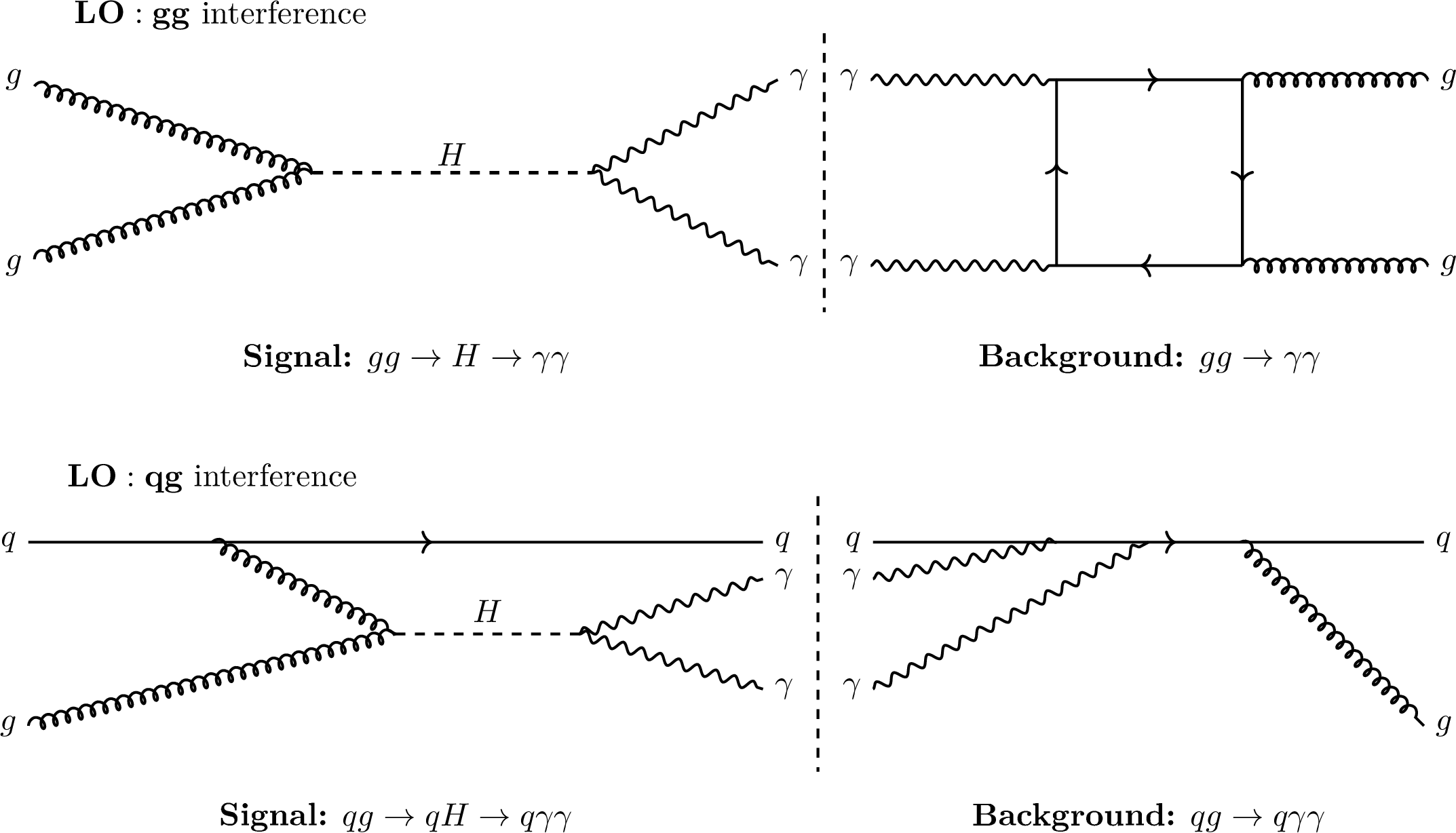
png pdf	Figure 1: Representative Feynman diagrams for lowest-order interference between the Higgs boson resonance and the continuum diphoton production. The dashed vertical lines separate the resonant amplitudes (left) from the continuum ones (right). In order to make clear the correspondence between interfering particle states, the horizontal diagrams are inverted horizontally.
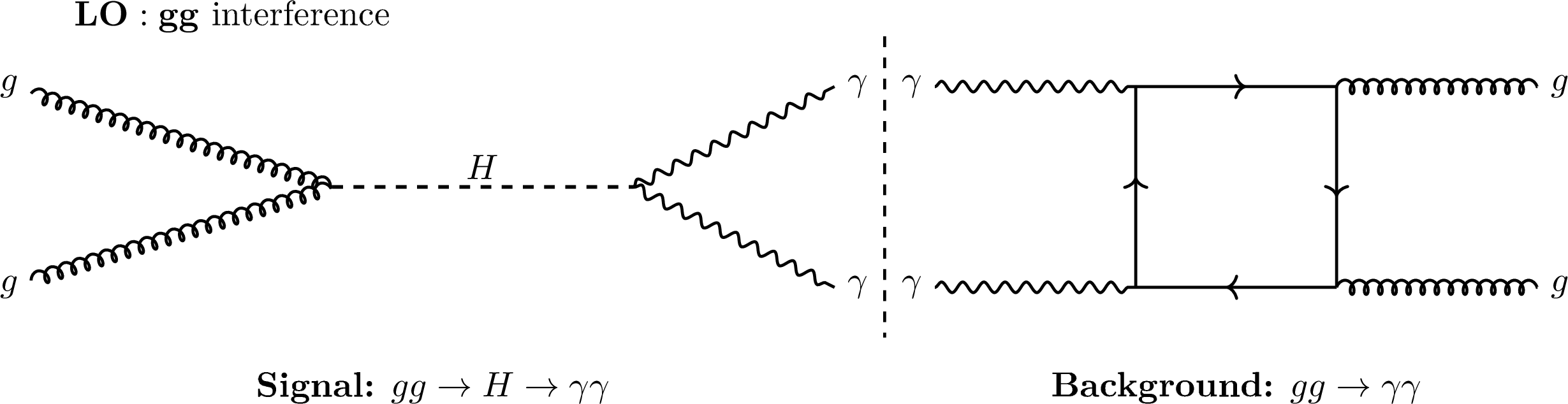
png pdf	Figure 1-a: Representative Feynman diagrams for lowest-order interference between the Higgs boson resonance and the continuum diphoton production. The dashed vertical lines separate the resonant amplitudes (left) from the continuum ones (right). In order to make clear the correspondence between interfering particle states, the horizontal diagrams are inverted horizontally.
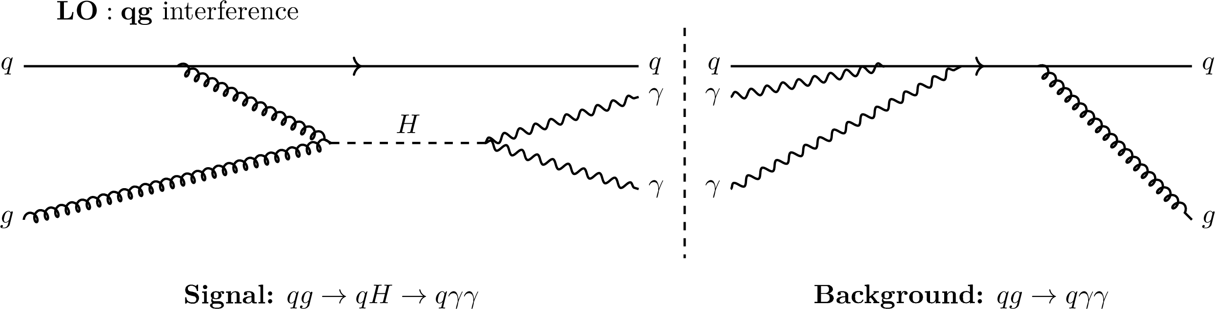
png pdf	Figure 1-b: Representative Feynman diagrams for lowest-order interference between the Higgs boson resonance and the continuum diphoton production. The dashed vertical lines separate the resonant amplitudes (left) from the continuum ones (right). In order to make clear the correspondence between interfering particle states, the horizontal diagrams are inverted horizontally.
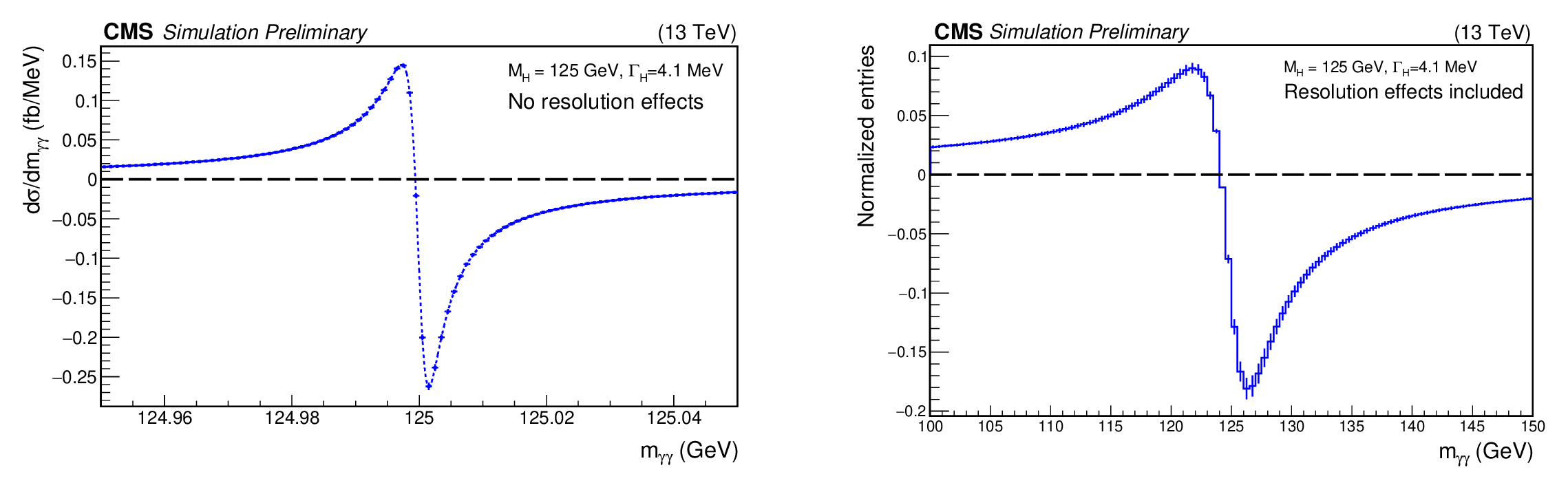
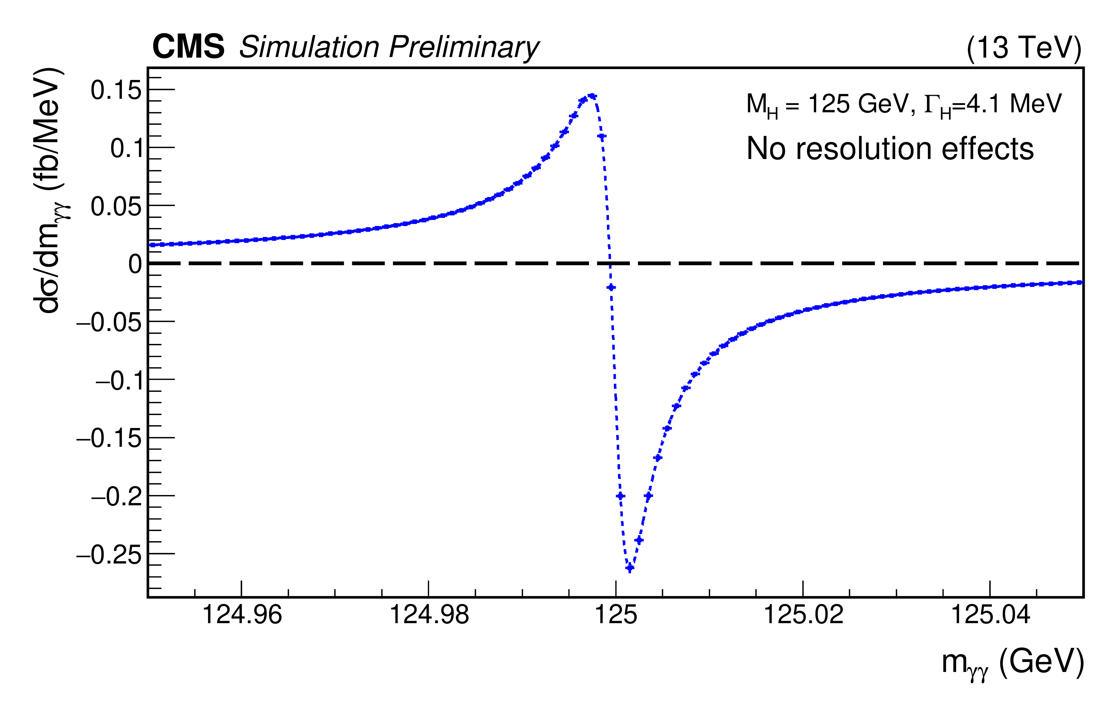
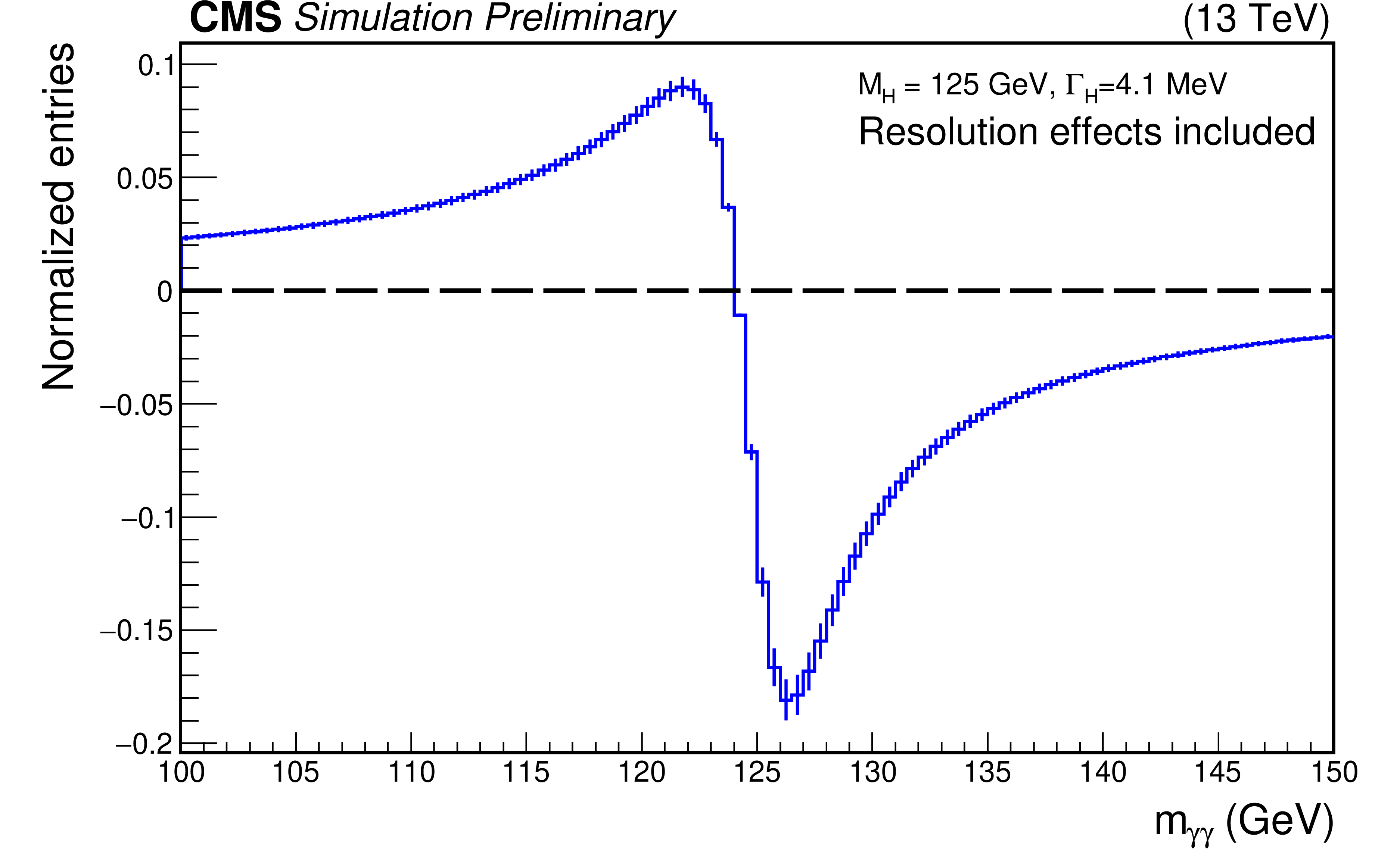
png pdf	Figure 2: Distribution of $ m_{\gamma\gamma} $ for the interference contribution in Eq. 1, without experimental resolution effects (left), and including experimental resolution (right). The experimental resolution is implemented through CMS Run 2 full simulation, for samples with $ M_{\mathrm{H}} = $ 125 GeV and $ \Gamma_\mathrm{H} = \Gamma_{\mathrm{H}}^{SM} $.
png pdf	Figure 2-a: Distribution of $ m_{\gamma\gamma} $ for the interference contribution in Eq. 1, without experimental resolution effects (left), and including experimental resolution (right). The experimental resolution is implemented through CMS Run 2 full simulation, for samples with $ M_{\mathrm{H}} = $ 125 GeV and $ \Gamma_\mathrm{H} = \Gamma_{\mathrm{H}}^{SM} $.
png pdf	Figure 2-b: Distribution of $ m_{\gamma\gamma} $ for the interference contribution in Eq. 1, without experimental resolution effects (left), and including experimental resolution (right). The experimental resolution is implemented through CMS Run 2 full simulation, for samples with $ M_{\mathrm{H}} = $ 125 GeV and $ \Gamma_\mathrm{H} = \Gamma_{\mathrm{H}}^{SM} $.
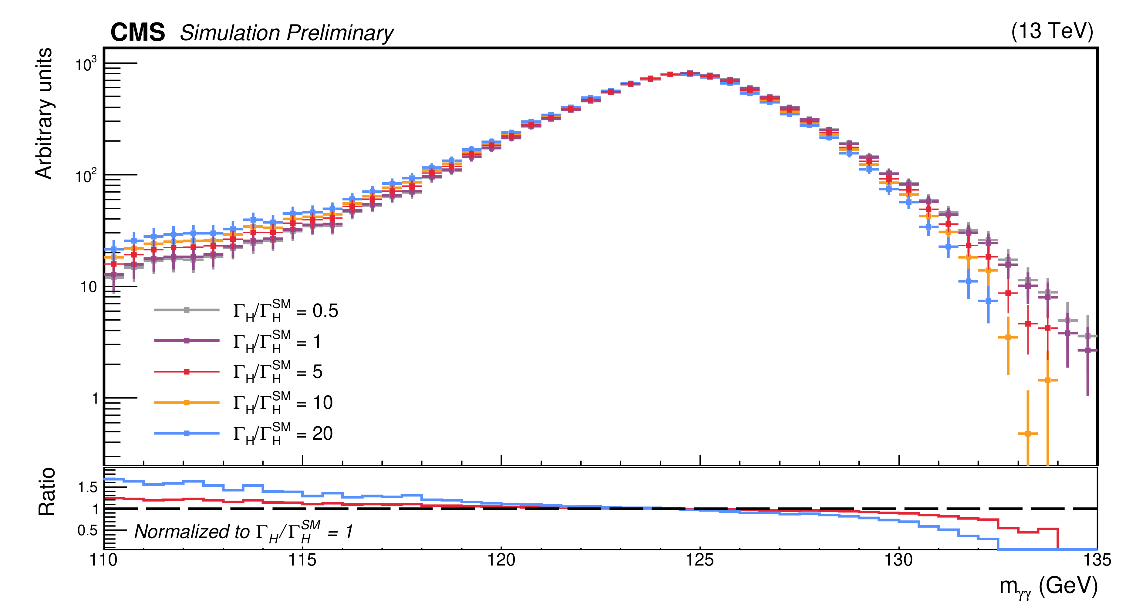
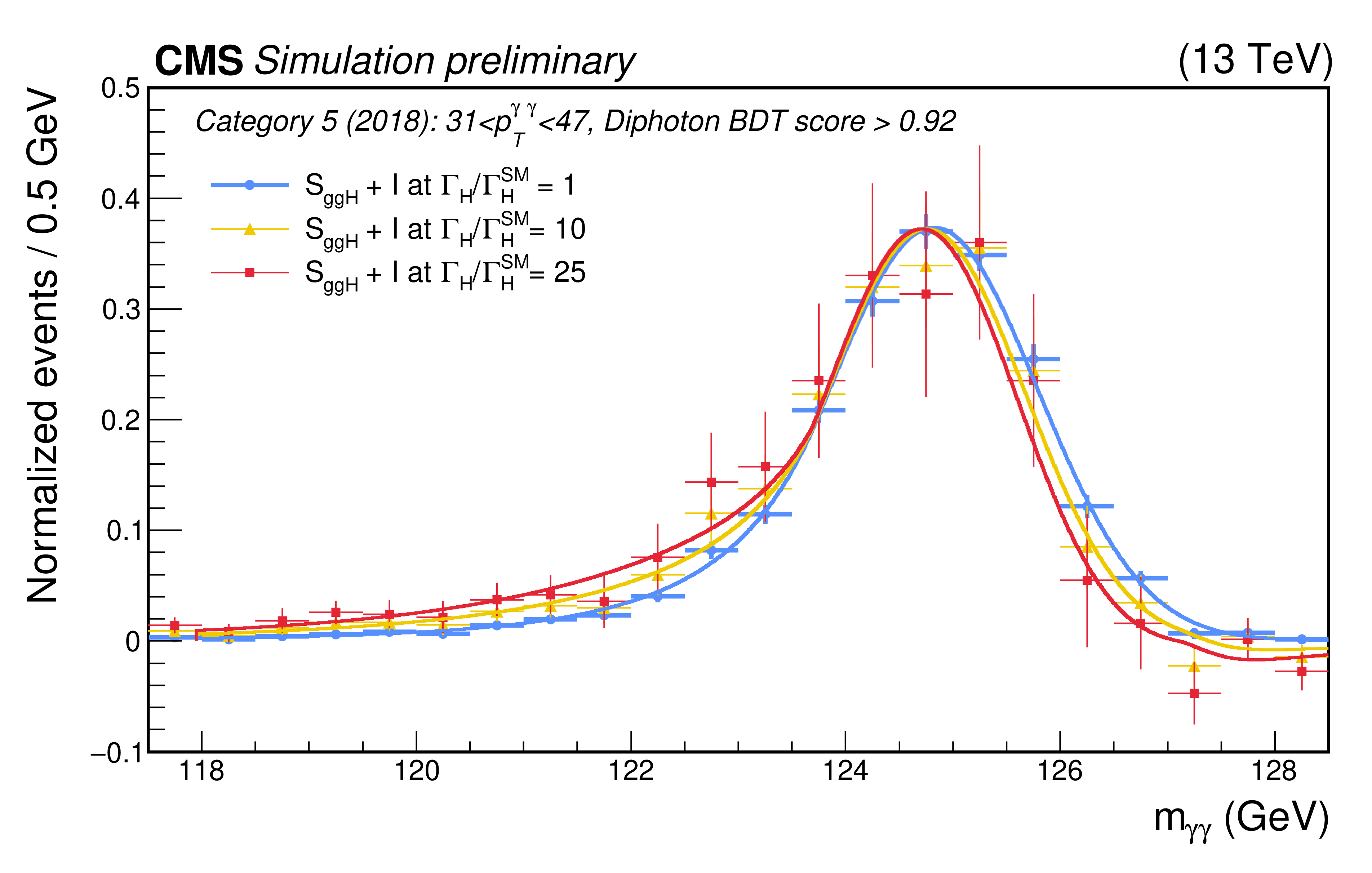
png pdf	Figure 3: Sum between ggH signal and interference mass spectra for different $ \Gamma_\mathrm{H} $ values and $ M_{\mathrm{H}} = $ 125 GeV, considering resolution effects using full CMS detector simulation.
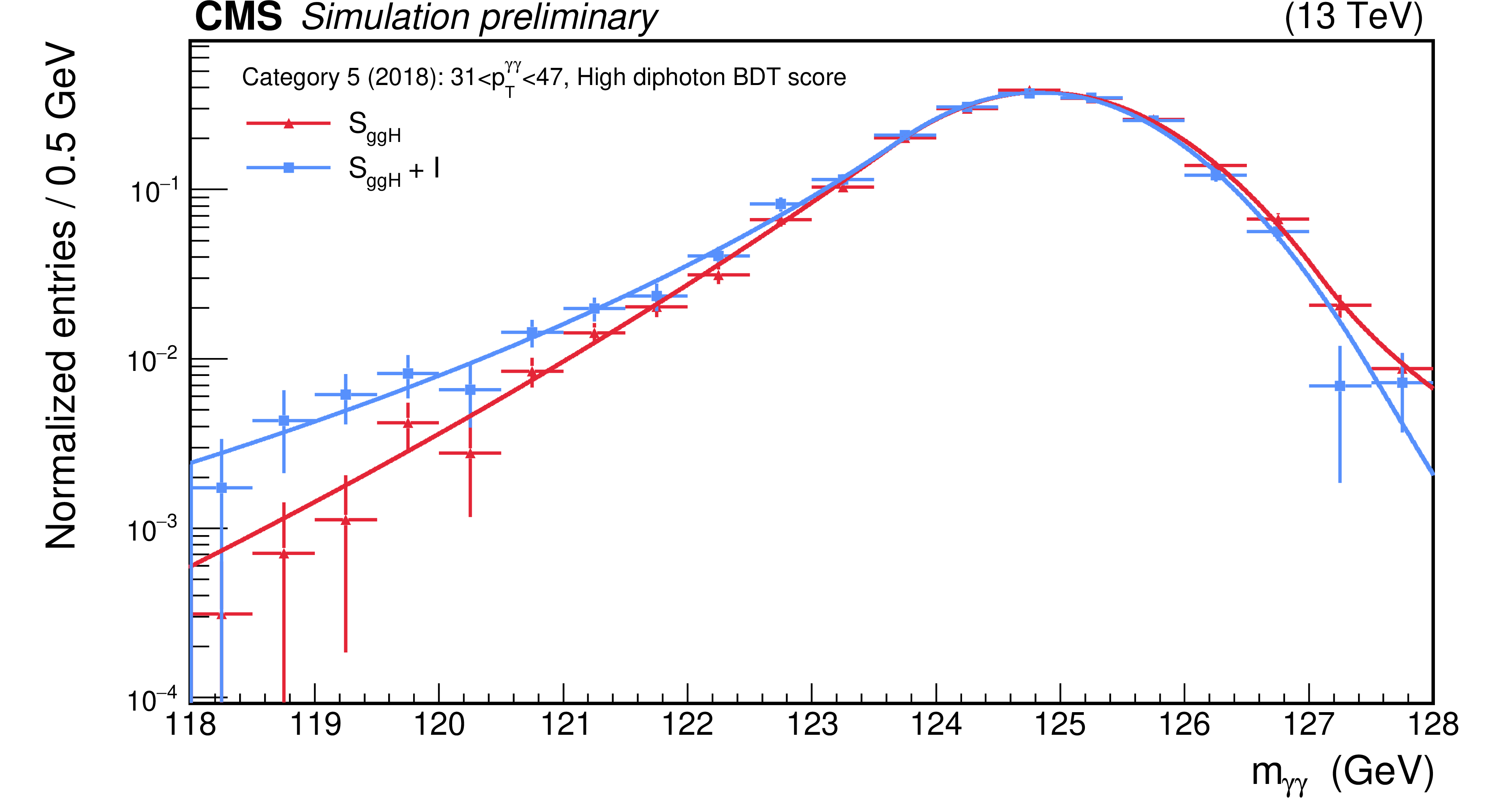
png pdf	Figure 4: Diphoton invariant mass spectrum for simulated $ S_{ggH} $ and $ S_{ggH} + I $ samples at $ M_{\mathrm{H}} = $ 125 GeV and $ \Gamma_{\mathrm{H}} = \Gamma_{\mathrm{H}}^{SM} $ in an example category (data points), together with the fitted signal models (lines).
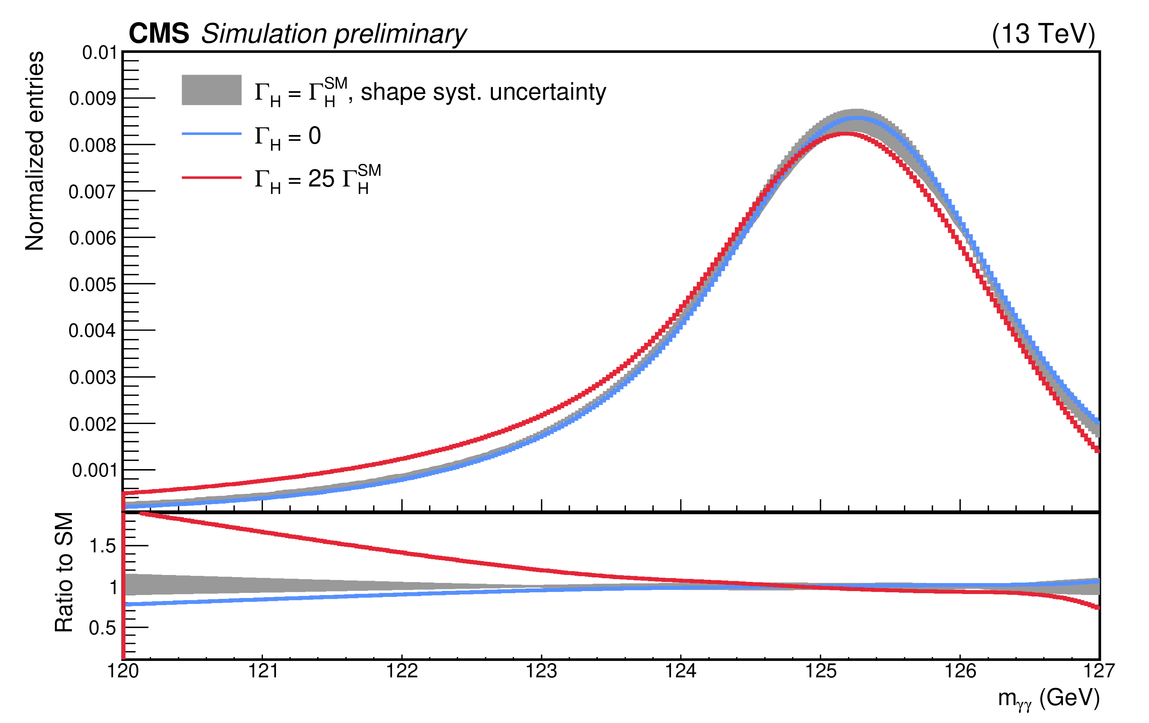
png pdf	Figure 5: Signal model probablity density functions for the nominal signal model, together with the $ \Gamma_{\mathrm{H}}/\Gamma_{\mathrm{H}}^{SM}=$ 0, 25 cases, and with the envelope at 68% CL of all experimental systematics affecting the signal shape (grey shade). The signal model in figure is the weighted sum of all signal models for process and category. Each category has a weight corresponding to S/(S+B), where S and B are, respectively, the expected signal and background yields around the Higgs boson peak. The value $ \Gamma_{\mathrm{H}}/\Gamma_{\mathrm{H}}^{SM}= $ 25 was chosen because it is close to the expected limit.
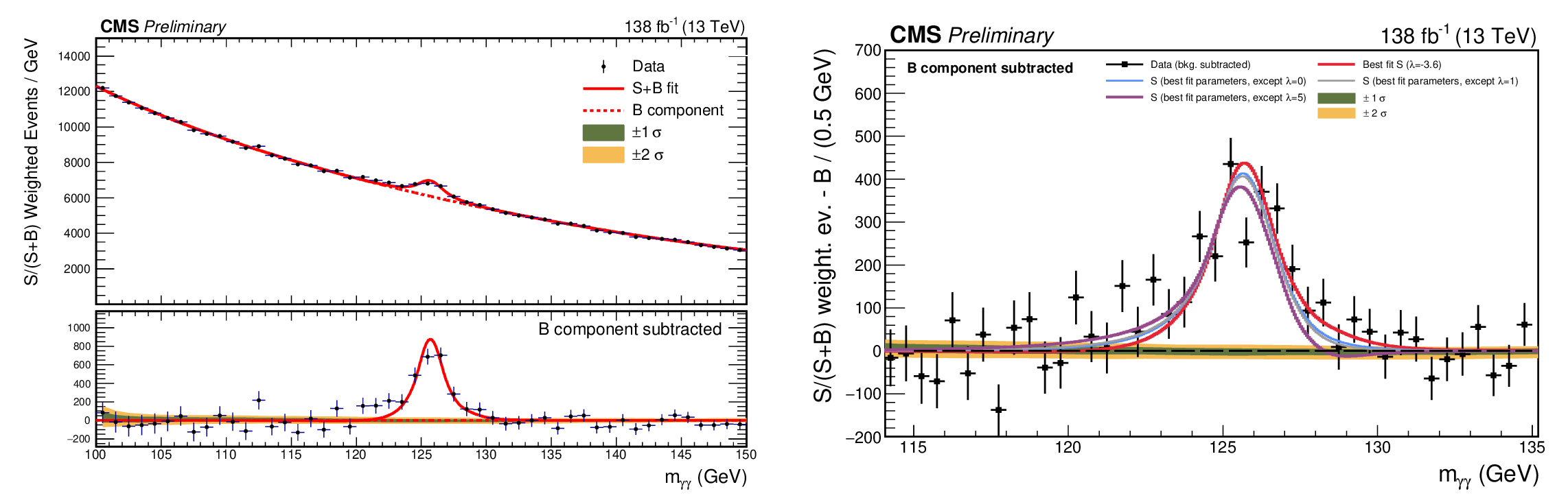
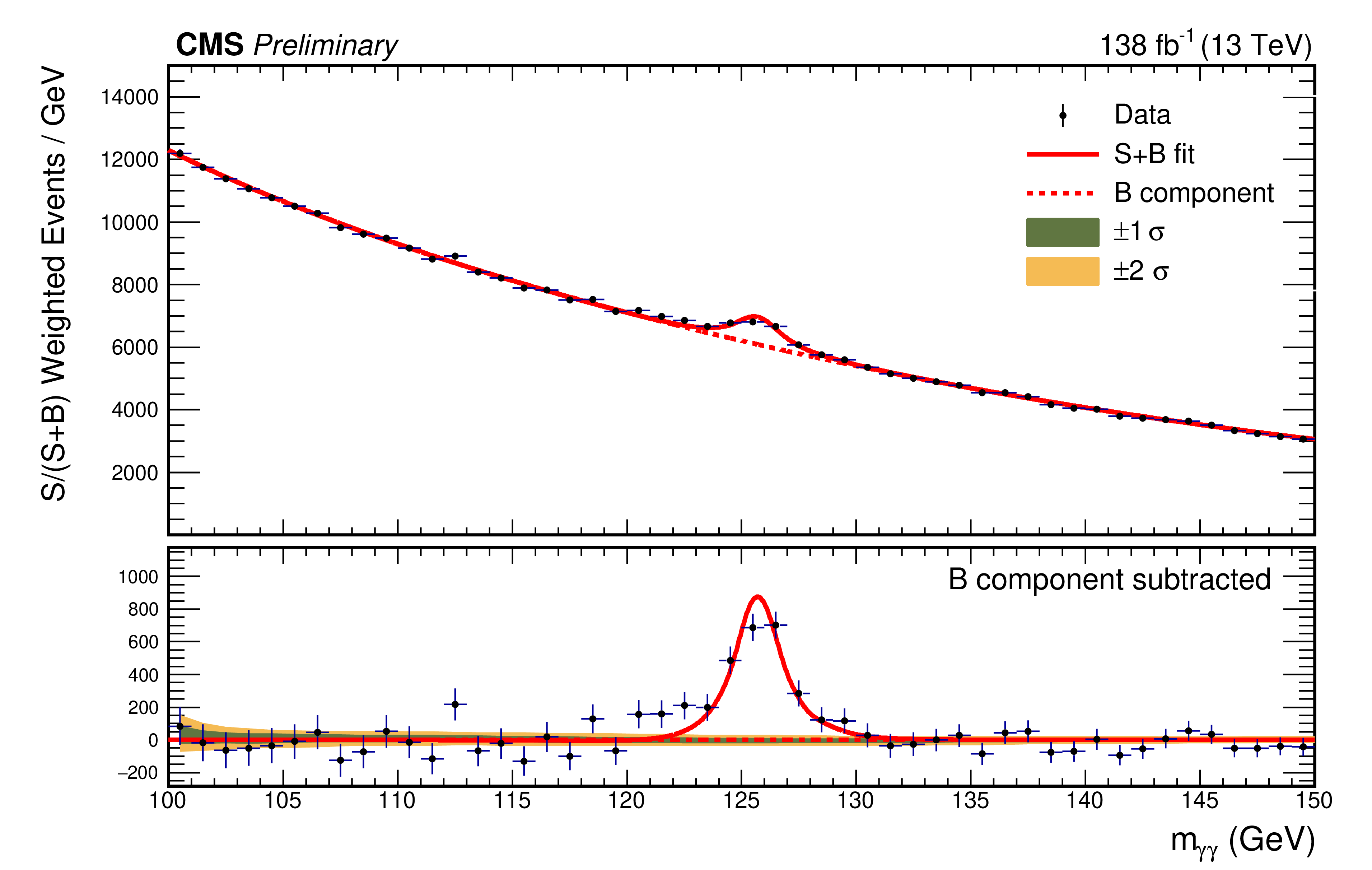
png pdf	Figure 6: The best fit signal-plus-background model is shown overlaid on the S/(S+B)-weighted distribution of the data points (black) from the fit in the left panel. The right panel shows an enlarged view aroung the Higgs boson peak, together with signal-plus-background predictions with all parameters at their best fit values, except $ \lambda $, evaluated at $ \lambda=$ 0, 1, 5. S and B represent the fitted number of Higgs boson candidates and background events in the mass peak region. The green and yellow bands correspond to the one and two standard deviation uncertainties in the background component of the fit. The solid red line indicates the total best fit signal-plus-background prediction, while the dashed red line represents the background-only contribution. The lower panel displays the residuals obtained by subtracting the background component from the data. The fit is performed in 100-180 GeV range.
png pdf	Figure 6-a: The best fit signal-plus-background model is shown overlaid on the S/(S+B)-weighted distribution of the data points (black) from the fit in the left panel. The right panel shows an enlarged view aroung the Higgs boson peak, together with signal-plus-background predictions with all parameters at their best fit values, except $ \lambda $, evaluated at $ \lambda=$ 0, 1, 5. S and B represent the fitted number of Higgs boson candidates and background events in the mass peak region. The green and yellow bands correspond to the one and two standard deviation uncertainties in the background component of the fit. The solid red line indicates the total best fit signal-plus-background prediction, while the dashed red line represents the background-only contribution. The lower panel displays the residuals obtained by subtracting the background component from the data. The fit is performed in 100-180 GeV range.
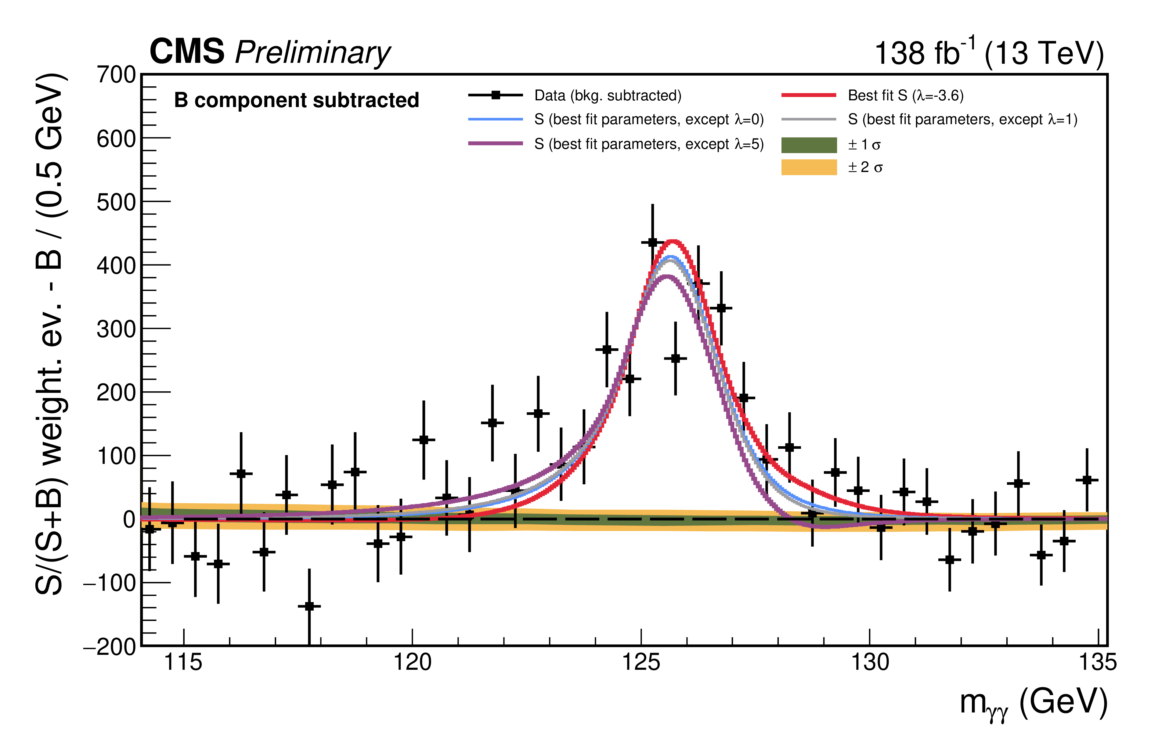
png pdf	Figure 6-b: The best fit signal-plus-background model is shown overlaid on the S/(S+B)-weighted distribution of the data points (black) from the fit in the left panel. The right panel shows an enlarged view aroung the Higgs boson peak, together with signal-plus-background predictions with all parameters at their best fit values, except $ \lambda $, evaluated at $ \lambda=$ 0, 1, 5. S and B represent the fitted number of Higgs boson candidates and background events in the mass peak region. The green and yellow bands correspond to the one and two standard deviation uncertainties in the background component of the fit. The solid red line indicates the total best fit signal-plus-background prediction, while the dashed red line represents the background-only contribution. The lower panel displays the residuals obtained by subtracting the background component from the data. The fit is performed in 100-180 GeV range.
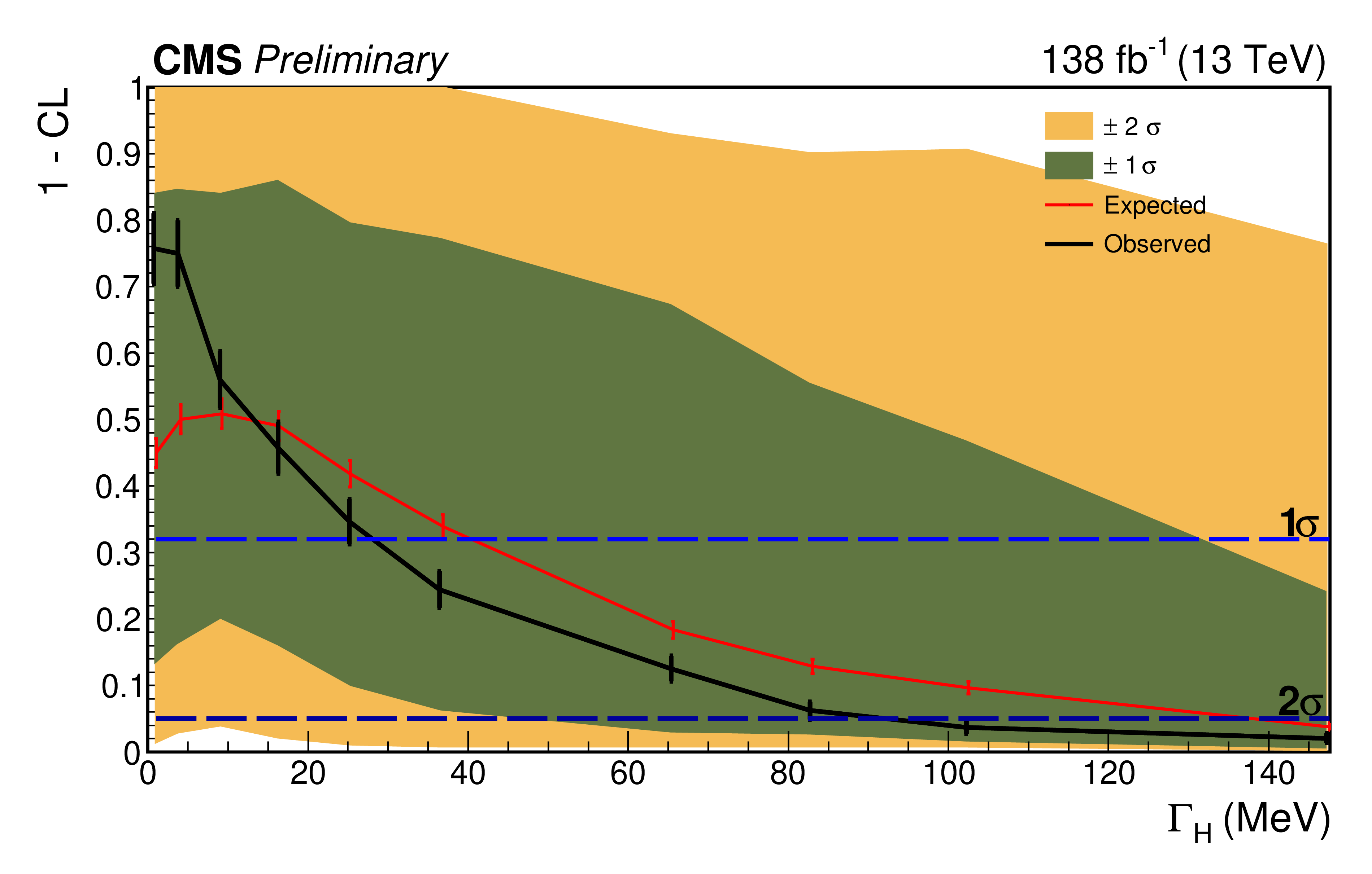
png pdf	Figure 7: Scan obtained with the Feldman-Cousins approach (with 1000 toys for each point), in terms of 1-CL vs. $ \Gamma_\mathrm{H}/\Gamma_\mathrm{H}^{SM} $, in the median expected scenario (red line), observed (black line), together with 1$ \sigma $ and 2$ \sigma $ bands.

Tables
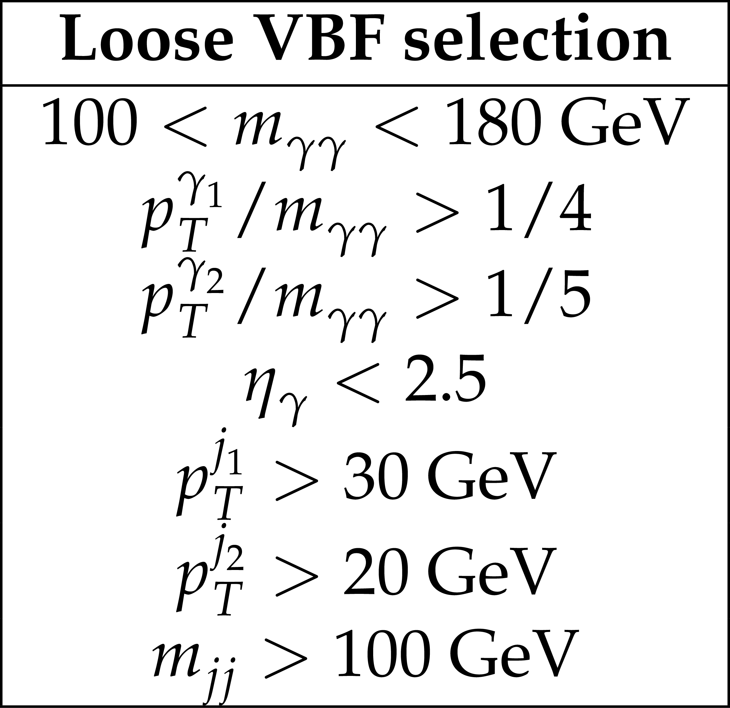
png pdf	Table 1: Criteria for the loose VBF selection. The leading (sub-leading) photons are indicated as $ \gamma_1, \gamma_2 $, while the leading (sub-leading) jets are indicated as $ j_1, j_2 $.
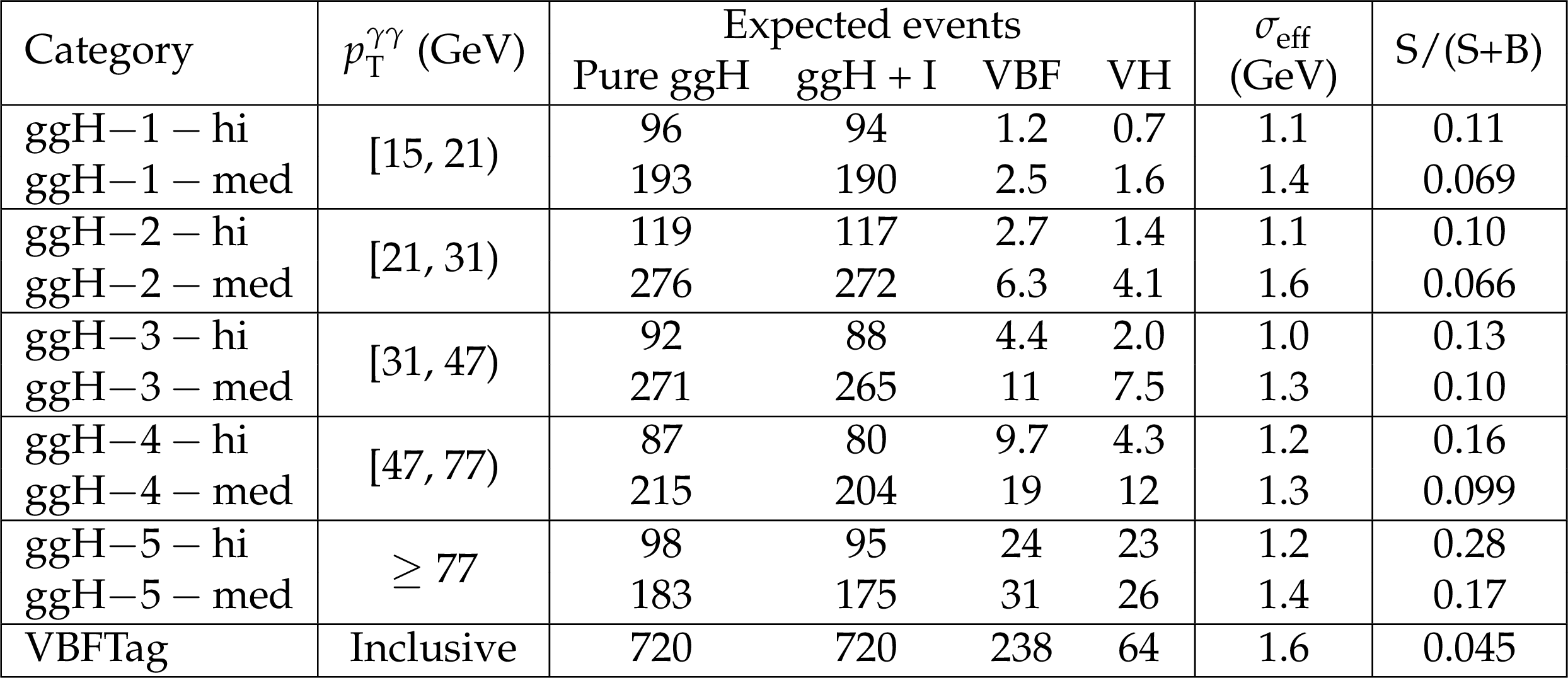
png pdf	Table 2: Boundaries in $ p_{T}^{\gamma\gamma} $, expected event yields for all years, mass resolution, and expected signal fraction for each category averaged over the different years. The category label (hi, med) defines the type of diphoton BDT region selected, i.e., respectively, high and medium. The mass resolution $ \sigma_{\text{eff}} $ is defined as the width of the region, centered on the peak, that contains 68% of the signal distribution, while the expected signal fraction S/(S+B) is the ratio between signal and total events in the same region defined for the mass resolution. Note that the total events are not the sum of the events from the four processes, because ggH and (ggH+I) are combined depending on the values of $ \mu $ and $ \Gamma_\mathrm{H} $. Following Eq. 8, in the case of $ \mu=$ 1, $\Gamma_\mathrm{H} = $ 0, only the pure ggH process would be observed, together with VBF and VH, while in the case of $ \mu=$ 1, $\Gamma_{\mathrm{H}} = \Gamma_{\mathrm{H}}^{SM} $, only (ggH+I), VBF and VH would be observed.

Summary

In this note, a new constraint on the Higgs boson decay width $ \Gamma_\mathrm{H} $ in the diphoton channel is reported. For the first time at LHC, the measurement exploits the distortions in the mass spectrum induced by the interference between gluon-gluon fusion Higgs boson production ($ gg \to H \to \gamma \gamma $) signal and continuum $ gg \to \gamma \gamma $ background. The measurement is performed using proton-proton (pp) $ \sqrt{s} = $ 13 TeV collision data collected by the CMS detector during the LHC Run 2. The observed (expected) result is: $ \Gamma_\mathrm{H} < $ 92 (138) MeV at 95% CL, which largely improves previous limits using measurements of on-shell Higgs boson final states, despite it remains worse than the constrains from off-shell and on-shell comparison.

Additional Figures
png pdf	Additional Figure 1: Diphoton invariant mass spectrum for simulated $ S_{ggH} + I $ (gluon-gluon fusion plus interference) samples at $ M_H = $ 125 GeV and $ \Gamma_H = \Gamma_H^{SM} $ in an example category (light blue data points), together with the fitted signal model (light blue line). The extrapolation of both MC samples and signal models to $ \Gamma_H = 10 \Gamma_{H}^{SM} $ and $ \Gamma_H = 25 \Gamma_{H}^{SM} $ is shown, respectively, in yellow and red.
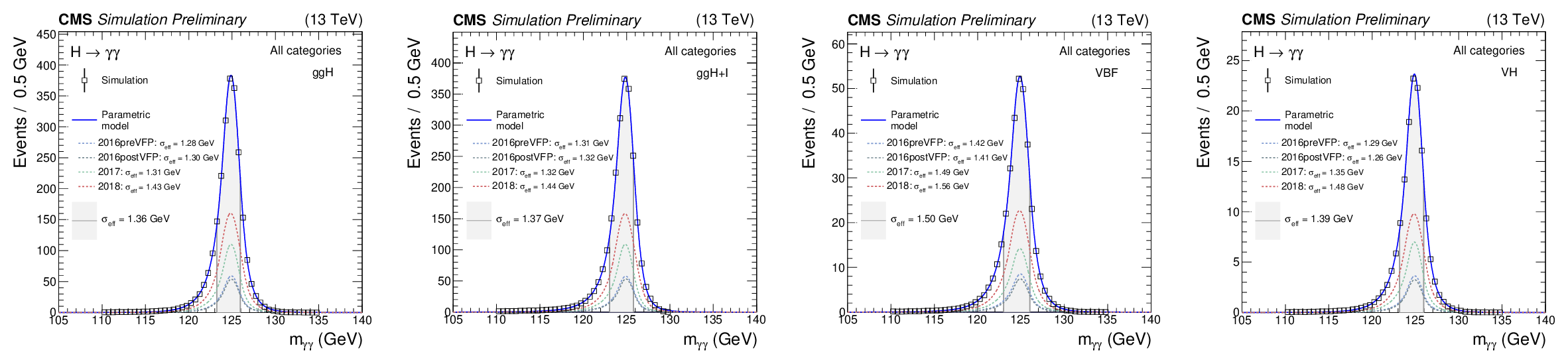
png pdf	Additional Figure 2: Diphoton invariant mass spectrum inclusive in all categories of simulated samples and parametric signal models for the four different processes: $ S_{ggH} $ (GG2H), $ S_{ggH} +I $ (GG2HPLUSINT), VBF and VH. The dashed lines represent the contribution from the single data-taking eras. The 2016 data is split in two separate eras, 2016preVFP and 2016postVFP. Theeras are treated separately due to the substantial change in detector conditions between them. In the 2016preVFP era, the strip tracker had a lower signal-to-noise ratio and fewer hits on tracks due to saturation effects in the readout chip under high-luminosity conditions. This was mitigated in the 2016postVFP era by changing the feedback preamplifier bias voltage (VFP).
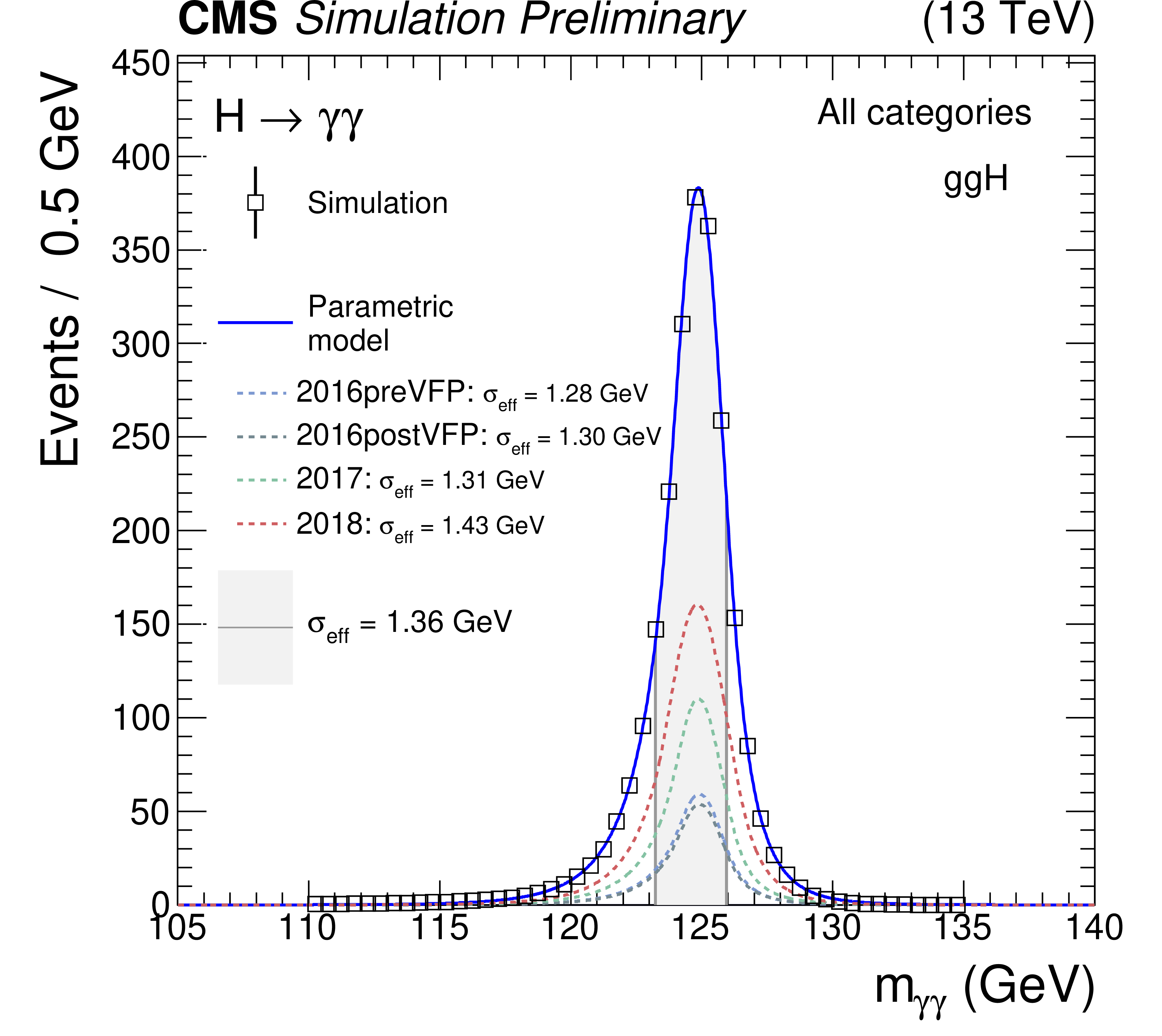
png pdf	Additional Figure 2-a: Diphoton invariant mass spectrum inclusive in all categories of simulated samples and parametric signal models for the four different processes: $ S_{ggH} $ (GG2H), $ S_{ggH} +I $ (GG2HPLUSINT), VBF and VH. The dashed lines represent the contribution from the single data-taking eras. The 2016 data is split in two separate eras, 2016preVFP and 2016postVFP. Theeras are treated separately due to the substantial change in detector conditions between them. In the 2016preVFP era, the strip tracker had a lower signal-to-noise ratio and fewer hits on tracks due to saturation effects in the readout chip under high-luminosity conditions. This was mitigated in the 2016postVFP era by changing the feedback preamplifier bias voltage (VFP).
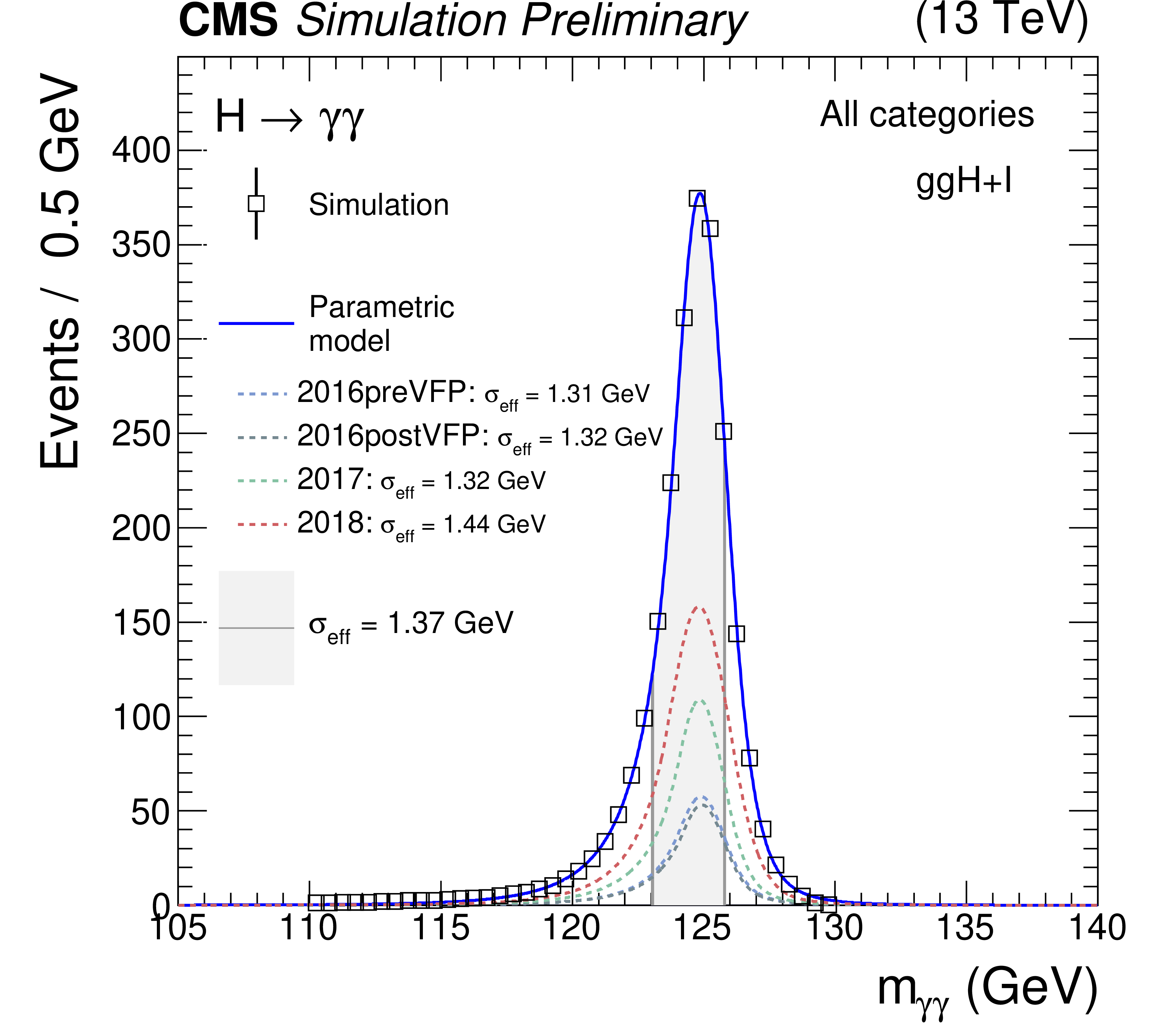
png pdf	Additional Figure 2-b: Diphoton invariant mass spectrum inclusive in all categories of simulated samples and parametric signal models for the four different processes: $ S_{ggH} $ (GG2H), $ S_{ggH} +I $ (GG2HPLUSINT), VBF and VH. The dashed lines represent the contribution from the single data-taking eras. The 2016 data is split in two separate eras, 2016preVFP and 2016postVFP. Theeras are treated separately due to the substantial change in detector conditions between them. In the 2016preVFP era, the strip tracker had a lower signal-to-noise ratio and fewer hits on tracks due to saturation effects in the readout chip under high-luminosity conditions. This was mitigated in the 2016postVFP era by changing the feedback preamplifier bias voltage (VFP).
png pdf	Additional Figure 2-c: Diphoton invariant mass spectrum inclusive in all categories of simulated samples and parametric signal models for the four different processes: $ S_{ggH} $ (GG2H), $ S_{ggH} +I $ (GG2HPLUSINT), VBF and VH. The dashed lines represent the contribution from the single data-taking eras. The 2016 data is split in two separate eras, 2016preVFP and 2016postVFP. Theeras are treated separately due to the substantial change in detector conditions between them. In the 2016preVFP era, the strip tracker had a lower signal-to-noise ratio and fewer hits on tracks due to saturation effects in the readout chip under high-luminosity conditions. This was mitigated in the 2016postVFP era by changing the feedback preamplifier bias voltage (VFP).
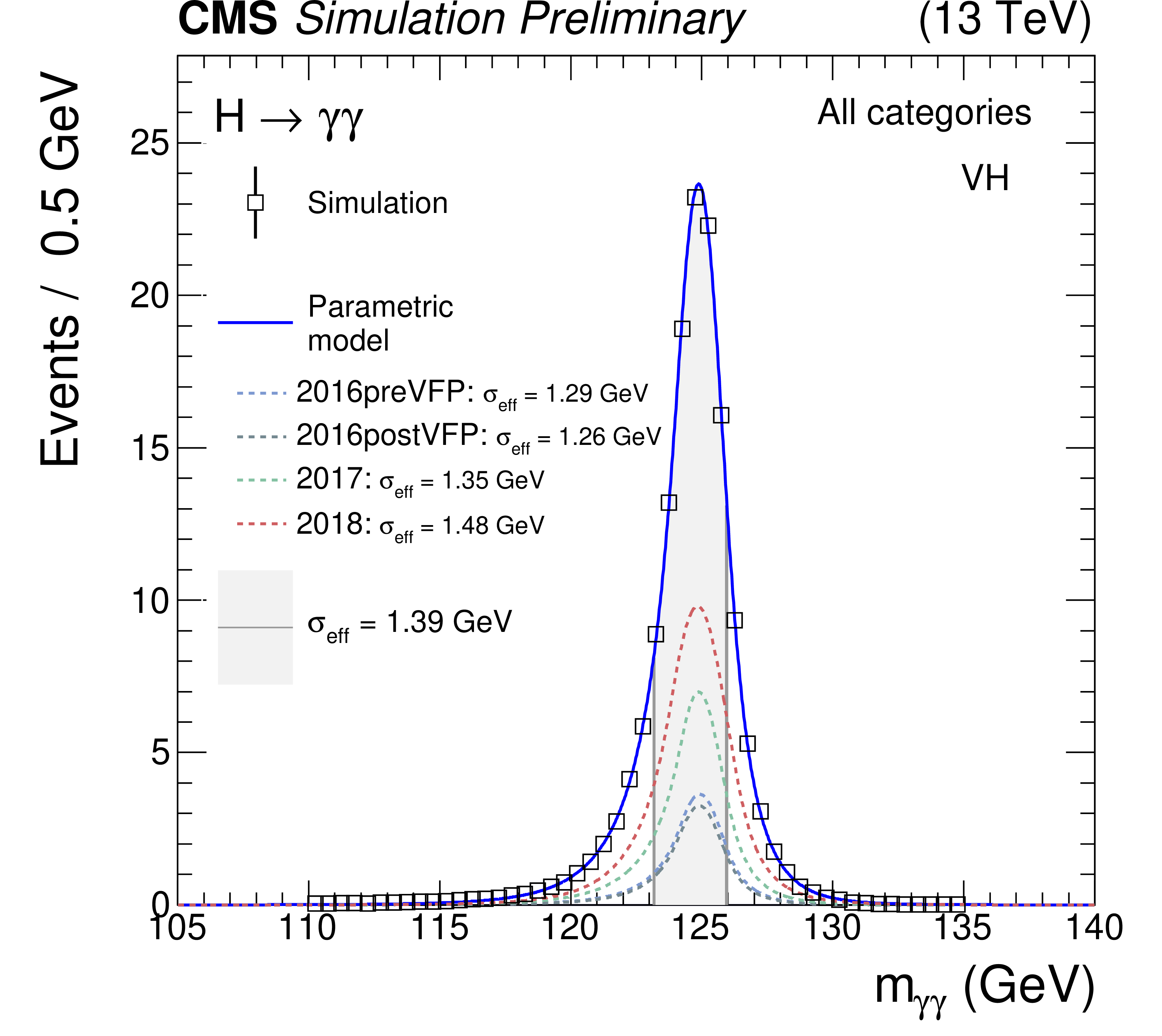
png pdf	Additional Figure 2-d: Diphoton invariant mass spectrum inclusive in all categories of simulated samples and parametric signal models for the four different processes: $ S_{ggH} $ (GG2H), $ S_{ggH} +I $ (GG2HPLUSINT), VBF and VH. The dashed lines represent the contribution from the single data-taking eras. The 2016 data is split in two separate eras, 2016preVFP and 2016postVFP. Theeras are treated separately due to the substantial change in detector conditions between them. In the 2016preVFP era, the strip tracker had a lower signal-to-noise ratio and fewer hits on tracks due to saturation effects in the readout chip under high-luminosity conditions. This was mitigated in the 2016postVFP era by changing the feedback preamplifier bias voltage (VFP).

References
1	CMS Collaboration	Observation of a new boson at a mass of 125 GeV with the CMS experiment at the LHC	Physics Letters B 716 (2012) 30	CMS-HIG-12-028 1207.7235
2	A. Djouadi, J. Kalinowski, and M. Spira	Hdecay: a program for higgs boson decays in the standard model and its supersymmetric extension	Computer Physics Communications 108 (1998) 56
3	CMS Collaboration	Measurement of the Higgs boson mass and width using the four leptons final state	technical report, CERN, Geneva, 2023 CDS
4	ATLAS Collaboration	Measurement of off-shell Higgs boson production in the $ H^*\rightarrow ZZ\rightarrow 4\ell $ decay channel using a neural simulation-based inference technique in 13 TeV pp collisions with the ATLAS detector	Reports on Progress in Physics 88 (2025) 057803	2412.01548
5	F. Caola and K. Melnikov	Constraining the Higgs boson width with $ ZZ $ production at the LHC	PRD 88 (2013) 054024	1307.4935
6	ATLAS Collaboration	Constraining off-shell Higgs boson production and the Higgs boson total width using $ WW\to \ell\nu\ell\nu $ final states with the ATLAS detector		2504.07710
7	ATLAS Collaboration	Constraint on the total width of the Higgs boson from Higgs boson and four-top-quark measurements in pp collisions at $ \sqrt{s} = $ 13 Tev with the ATLAS detector	Physics Letters B 861 (2025) 139277	2407.10631
8	L. J. Dixon and Y. Li	Bounding the Higgs boson width through interferometry	Physical Review Letters 111 (2013)	1305.3854
9	CMS Collaboration	Combined measurements and interpretations of Higgs boson production and decay at sqrt(s)=13 TeV	technical report, CERN, Geneva, 2025 CDS
10	CMS Collaboration	The CMS experiment at the CERN LHC	JINST 3 (2008) S08004
11	CMS Collaboration	Development of the CMS detector for the CERN LHC Run 3	JINST 19 (2024) P05064	CMS-PRF-21-001 2309.05466
12	CMS Collaboration	Performance of the CMS Level-1 trigger in proton-proton collisions at $ \sqrt{s}= $ 13 TeV	JINST 15 (2020) P10017	CMS-TRG-17-001 2006.10165
13	CMS Collaboration	The CMS trigger system	JINST 12 (2017) P01020	CMS-TRG-12-001 1609.02366
14	CMS Collaboration	Performance of the CMS high-level trigger during LHC run 2	JINST 19 (2024) P11021	CMS-TRG-19-001 2410.17038
15	CMS Collaboration	Electron and photon reconstruction and identification with the CMS experiment at the CERN LHC	JINST 16 (2021) P05014	CMS-EGM-17-001 2012.06888
16	CMS Collaboration	Performance of the CMS muon detector and muon reconstruction with proton-proton collisions at $ \sqrt{s}= $ 13 TeV	JINST 13 (2018) P06015	CMS-MUO-16-001 1804.04528
17	CMS Collaboration	Performance of Photon Reconstruction and Identification with the CMS Detector in Proton-Proton Collisions at sqrt(s) = 8 TeV	JINST 10 (2015) P08010	CMS-EGM-14-001 1502.02702
18	CMS Collaboration	Precision luminosity measurement in proton-proton collisions at $ \sqrt{s}= $ 13 TeV in 2015 and 2016 at CMS	EPJC 81 (2021) 800	CMS-LUM-17-003 2104.01927
19	CMS Collaboration	CMS luminosity measurement for the 2017 data-taking period at $ \sqrt{s}= $ 13 TeV	CMS Physics Analysis Summary, 2018 link	CMS-PAS-LUM-17-004
20	CMS Collaboration	CMS luminosity measurement for the 2018 data-taking period at $ \sqrt{s}= $ 13 TeV	CMS Physics Analysis Summary, 2019 link	CMS-PAS-LUM-18-002
21	CMS Collaboration	Measurements of Higgs boson production cross sections and couplings in the diphoton decay channel at $ \sqrt{s} = $ 13 Tev	Journal of High Energy Physics 2021 (2021) 27	CMS-HIG-19-015 2103.06956
22	J. Alwall et al.	The automated computation of tree-level and next-to-leading order differential cross sections, and their matching to parton shower simulations	Journal of High Energy Physics 2014 (2014)	1405.0301
23	T. Sjostrand, S. Mrenna, and P. Skands	A brief introduction to pythia 8.1	Computer Physics Communications 178 (2008) 852	0710.3820
24	CMS Collaboration	Extraction and validation of a new set of CMS PYTHIA8 tunes from underlying-event measurements	The European Physical Journal C 80 (2020)	CMS-GEN-17-001 1903.12179
25	R. D. Ball et al.	Parton distributions from high-precision collider data: NNPDF Collaboration	The European Physical Journal C 77 (2017)	1706.00428
26	GEANT4 Collaboration	Geant4 - a simulation toolkit	Nuclear Instruments and Methods in Physics Research Section A: Accelerators, Spectrometers, 2003 Detectors and Associated Equipment 506 (2003) 250
27	CMS Collaboration	Particle-Flow Event Reconstruction in CMS and Performance for Jets, Taus, and MET	Technical Report, CERN, 2009 CMS-PAS-PFT-09-001
28	M. Cacciari, G. P. Salam, and G. Soyez	The anti-$ k_{\mathrm{T}} $ jet clustering algorithm	JHEP 04 (2008) 063	0802.1189
29	M. Cacciari, G. P. Salam, and G. Soyez	FastJet user manual	EPJC 72 (2012) 1896	1111.6097
30	CMS Collaboration	Jet energy scale and resolution in the CMS experiment in pp collisions at 8 TeV	JINST 12 (2017) P02014	CMS-JME-13-004 1607.03663
31	CMS Collaboration	Photon Identification using Boosted Decision Trees in CMS	Technical Report, CERN, 2010 CMS-PAS-EGM-10-006
32	CMS Collaboration	Measurement of the Higgs boson inclusive and differential fiducial production cross sections in the diphoton decay channel with pp collisions at $ \sqrt{s} = $ 13 TeV	JHEP 07 (2023) 091	CMS-HIG-19-016 2208.12279
33	CERN	CERN Yellow Reports: Monographs, Vol 2 (2017): Handbook of LHC Higgs cross sections: 4. Deciphering the nature of the Higgs sector	link
34	R. Barlow	Extended maximum likelihood	Nuclear Instruments and Methods in Physics Research Section A: Accelerators, Spectrometers, 1990 Detectors and Associated Equipment 297 (1990) 496
35	M. Oreglia et al.	Study of the reaction $ {\psi}^{'}\rightarrow\gamma\gamma{J}/{\psi} $	PRD 25 (1982) 2259
36	CMS Collaboration	A measurement of the Higgs boson mass in the diphoton decay channel	Physics Letters B 805 (2020) 135425	CMS-HIG-19-004 2002.06398
37	R. A. Fisher	On the interpretation of $ \chi^2 $ from contingency tables, and the calculation of p	Journal of the Royal Statistical Society 85 (1922) 87
38	P. Dauncey, M. Kenzie, N. Wardle, and G. Davies	Handling uncertainties in background shapes: the discrete profiling method	Journal of Instrumentation 10 (2015) P04015	1408.6865
39	F. L. Gewers et al.	Principal Component Analysis: A natural approach to data exploration	ACM Comput. Surv. 54 (2021)
40	CMS Collaboration	The CMS Statistical Analysis and Combination Tool: Combine	Computing and Software for Big Science 8 (2024) 19

Compact Muon Solenoid LHC, CERN

© Copyright CERN 2024 for the benefit of the CMS Collaboration