CMS-PAS-HIG-24-001

CMS-PAS-HIG-24-001
Search for HHWW couplings in the VBS production of $ \mathrm{W^{\pm}W^{\pm}H} $, with $ \mathrm{H\rightarrow b\bar{b}} $ decays
CMS Collaboration
27 July 2024

Abstract: A search is performed for anomalous HHWW couplings based on the process $ \mathrm{pp\rightarrow W^{\pm}W^{\pm}H+jj} $, using proton-proton collision data collected by the CMS experiment at a center-of-mass energy of $ \sqrt{s}= $ 13 TeV in the LHC Run 2, corresponding to a total integrated luminosity of 138 fb$ ^{-1} $. The search is performed in final states that contain a forward-backward jet pair, two W bosons that decay to same-sign leptons, and a Higgs boson that decays into two bottom quarks. Boosted decision trees are trained to separate the signal from the background. The HHWW coupling modifier $ \kappa_{WW} $ is constrained at 95% confidence level to be in the interval $[-3.3, 5.3]$, consistent with the expected interval of $[-2.4, 4.4]$.
Links: CDS record (PDF) ; CADI line (restricted) ;

Figures & Tables	Summary	References	CMS Publications

Figures
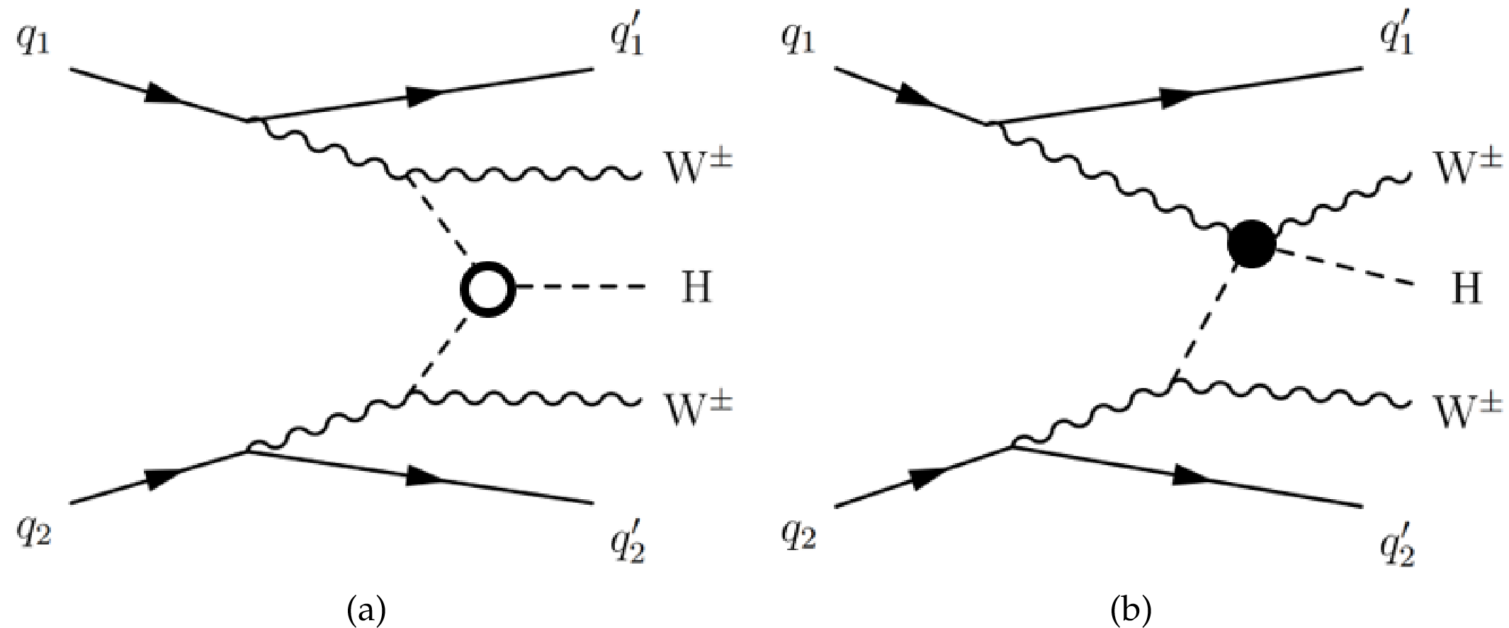
png pdf	Figure 1: Tree-level Feynman diagrams of vector boson scattering multi-boson productions with Higgs boson in the final state, with (a) related to the Higgs self-coupling ($ {\kappa_\lambda} $), and (b) related to the Higgs gauge quartic coupling ($ {\kappa_{VV}} $).
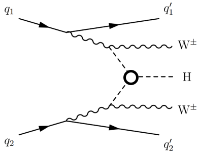
png	Figure 1-a: Tree-level Feynman diagrams of vector boson scattering multi-boson productions with Higgs boson in the final state, with (a) related to the Higgs self-coupling ($ {\kappa_\lambda} $), and (b) related to the Higgs gauge quartic coupling ($ {\kappa_{VV}} $).
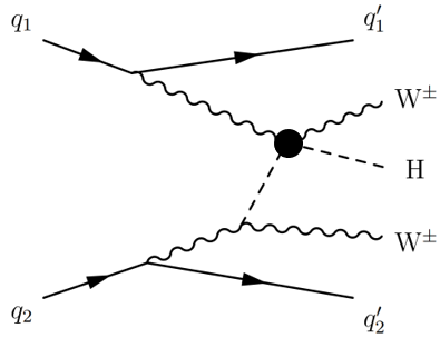
png	Figure 1-b: Tree-level Feynman diagrams of vector boson scattering multi-boson productions with Higgs boson in the final state, with (a) related to the Higgs self-coupling ($ {\kappa_\lambda} $), and (b) related to the Higgs gauge quartic coupling ($ {\kappa_{VV}} $).
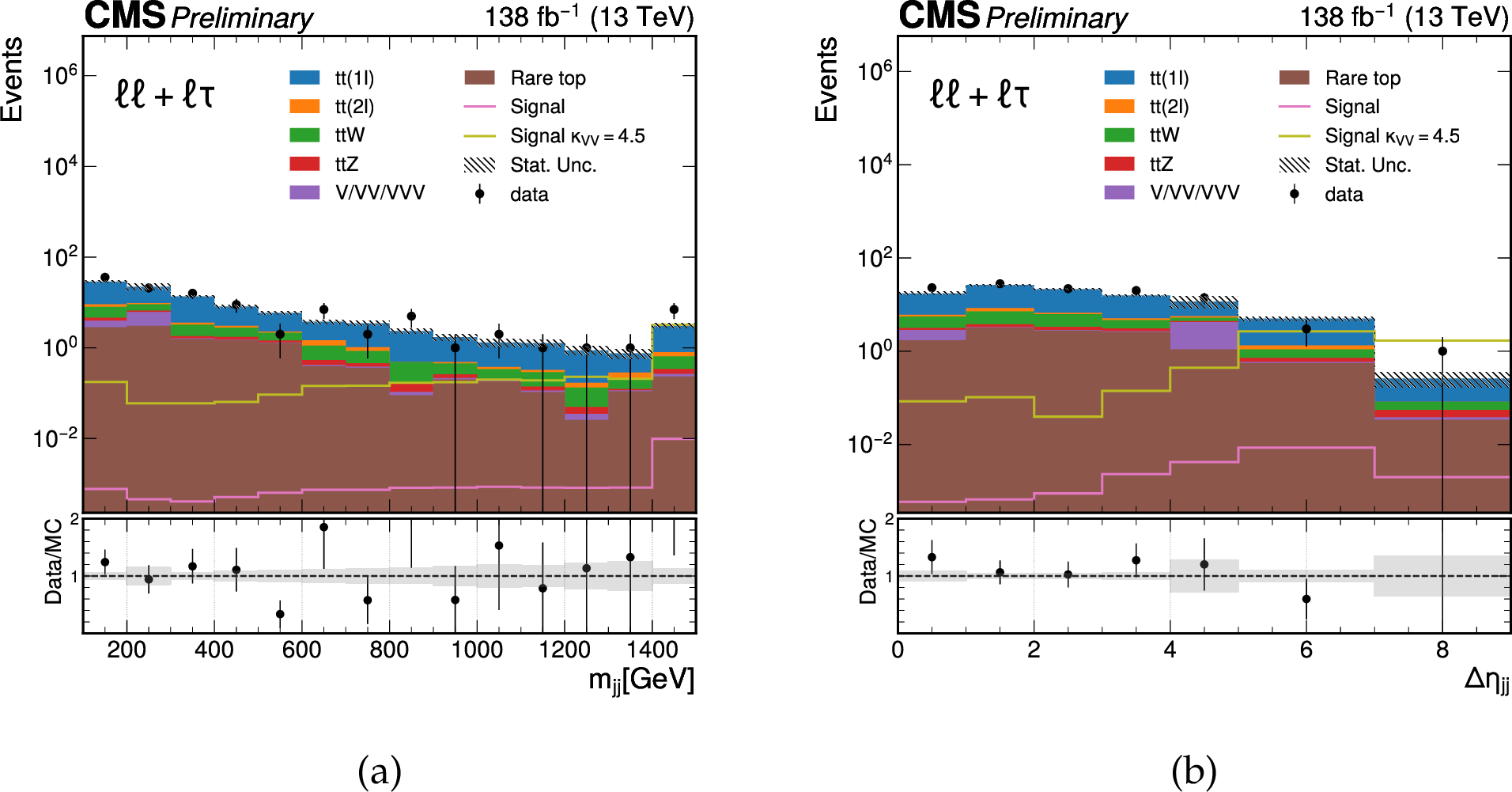
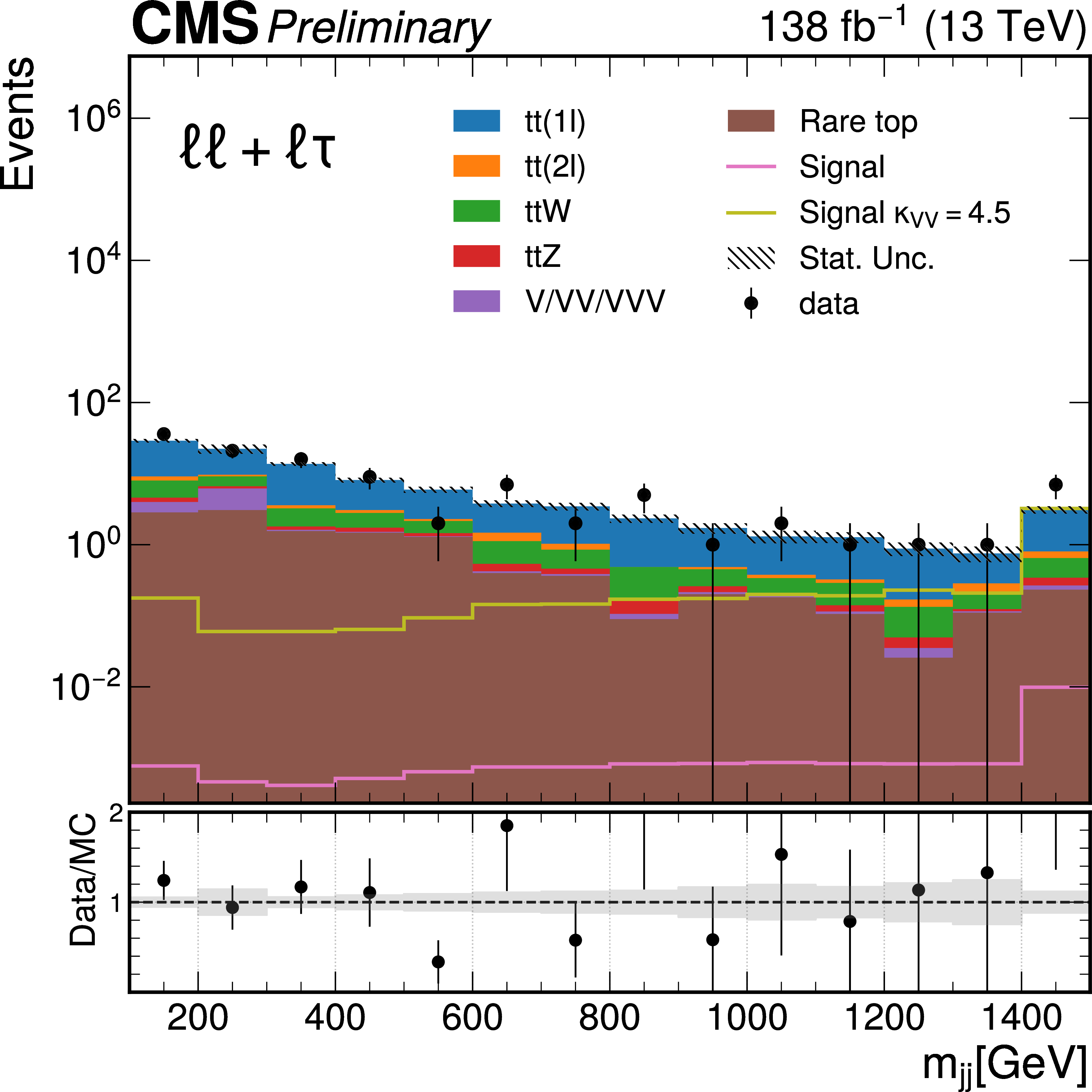
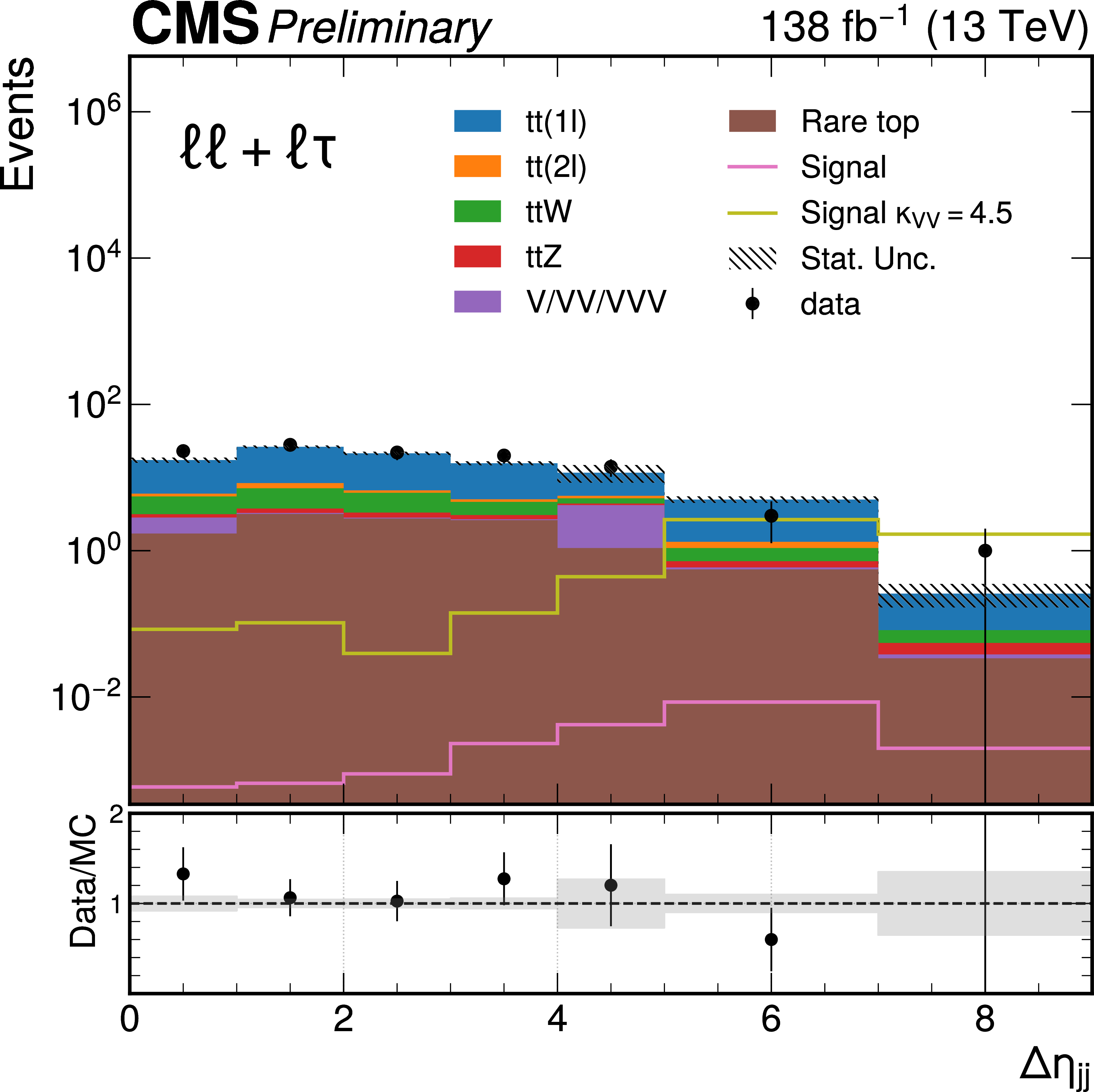
png pdf	Figure 2: Data-MC comparison of $ m_{jj} $ and $ \Delta\eta_{jj} $ distributions in the pre-selection regions. Two signal hypotheses, with one for $ {\kappa_{VV}} = $ 1 which represents the SM and the other for $ {\kappa_{VV}} = $ 4.5, are plotted. The uncertainty band in the ratio plots represents the pre-fit statistical uncertainty of the Monte Carlo, which corresponds to the uncertainty band in the distribution plots.
png pdf	Figure 2-a: Data-MC comparison of $ m_{jj} $ and $ \Delta\eta_{jj} $ distributions in the pre-selection regions. Two signal hypotheses, with one for $ {\kappa_{VV}} = $ 1 which represents the SM and the other for $ {\kappa_{VV}} = $ 4.5, are plotted. The uncertainty band in the ratio plots represents the pre-fit statistical uncertainty of the Monte Carlo, which corresponds to the uncertainty band in the distribution plots.
png pdf	Figure 2-b: Data-MC comparison of $ m_{jj} $ and $ \Delta\eta_{jj} $ distributions in the pre-selection regions. Two signal hypotheses, with one for $ {\kappa_{VV}} = $ 1 which represents the SM and the other for $ {\kappa_{VV}} = $ 4.5, are plotted. The uncertainty band in the ratio plots represents the pre-fit statistical uncertainty of the Monte Carlo, which corresponds to the uncertainty band in the distribution plots.
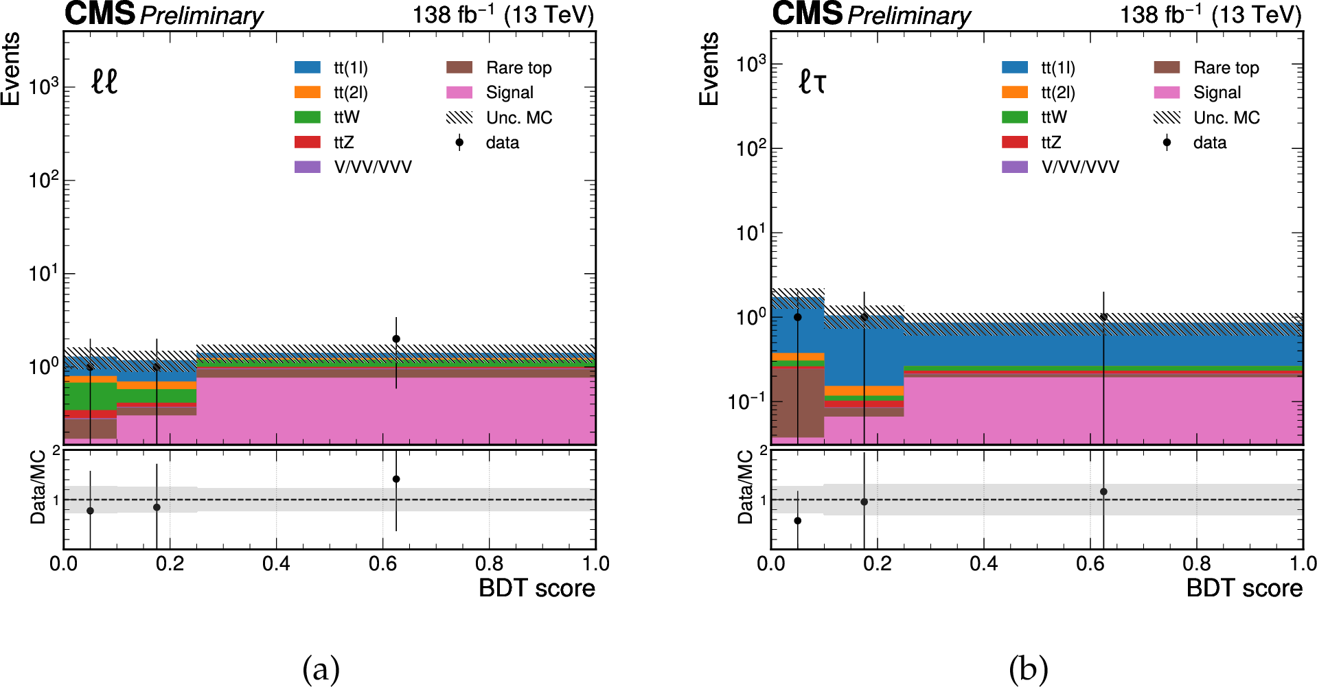
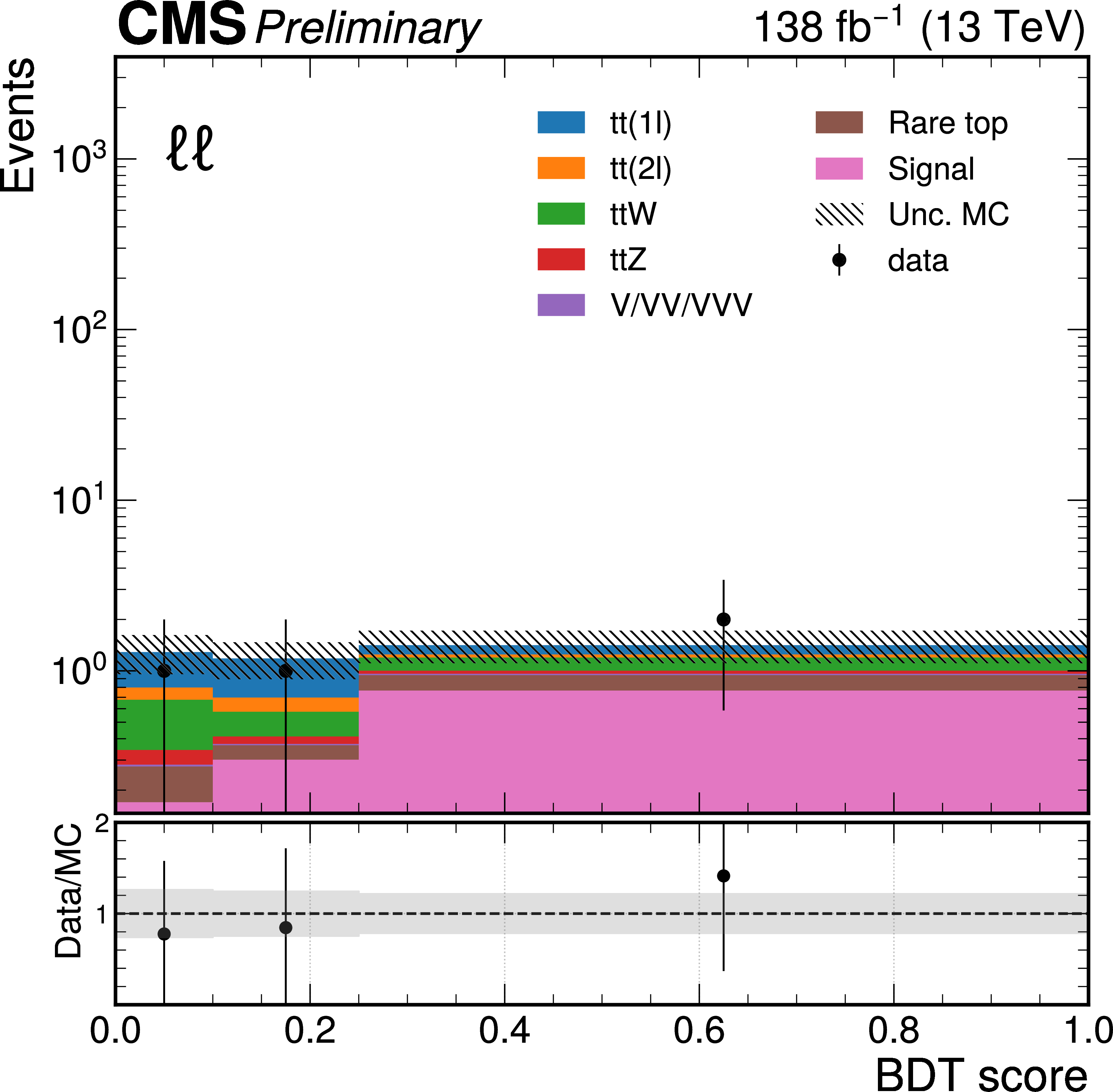
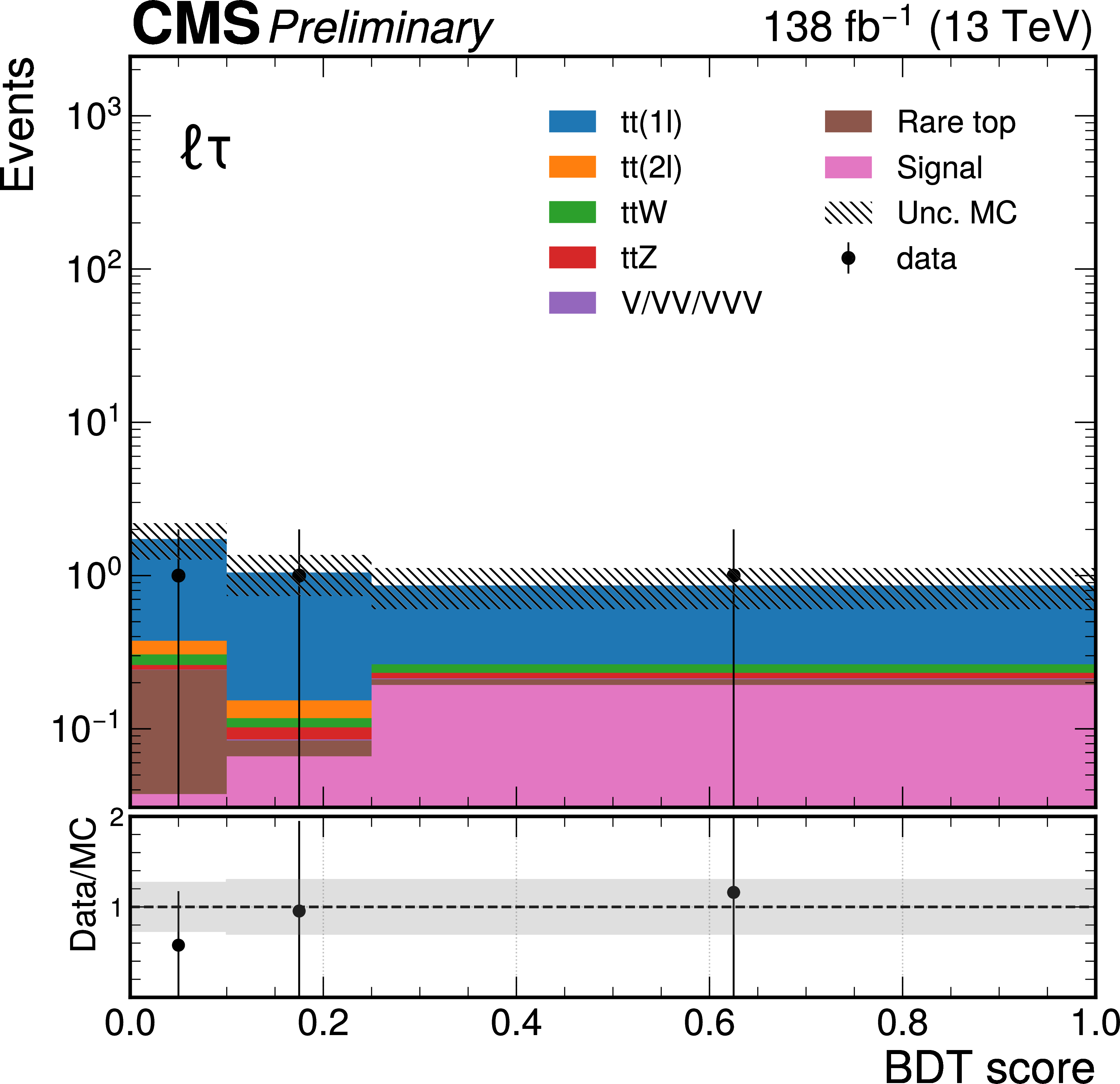
png pdf	Figure 3: Post-fit shapes for the SR, including (a) $ \ell\ell $ final state (b) $ \ell\tau $ final state. The uncertainty band in the ratio plots represents the post-fit uncertainty of the Monte Carlo, which corresponds to the uncertainty band in the distribution plots.
png pdf	Figure 3-a: Post-fit shapes for the SR, including (a) $ \ell\ell $ final state (b) $ \ell\tau $ final state. The uncertainty band in the ratio plots represents the post-fit uncertainty of the Monte Carlo, which corresponds to the uncertainty band in the distribution plots.
png pdf	Figure 3-b: Post-fit shapes for the SR, including (a) $ \ell\ell $ final state (b) $ \ell\tau $ final state. The uncertainty band in the ratio plots represents the post-fit uncertainty of the Monte Carlo, which corresponds to the uncertainty band in the distribution plots.
png pdf	Figure 4: Limits of $ \kappa_{VV} $ with CL=95%.

Tables
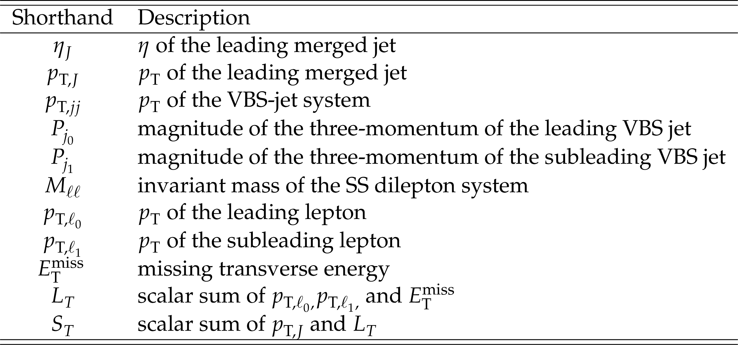
png pdf	Table 1: Input variables used for the event kinematics BDT.
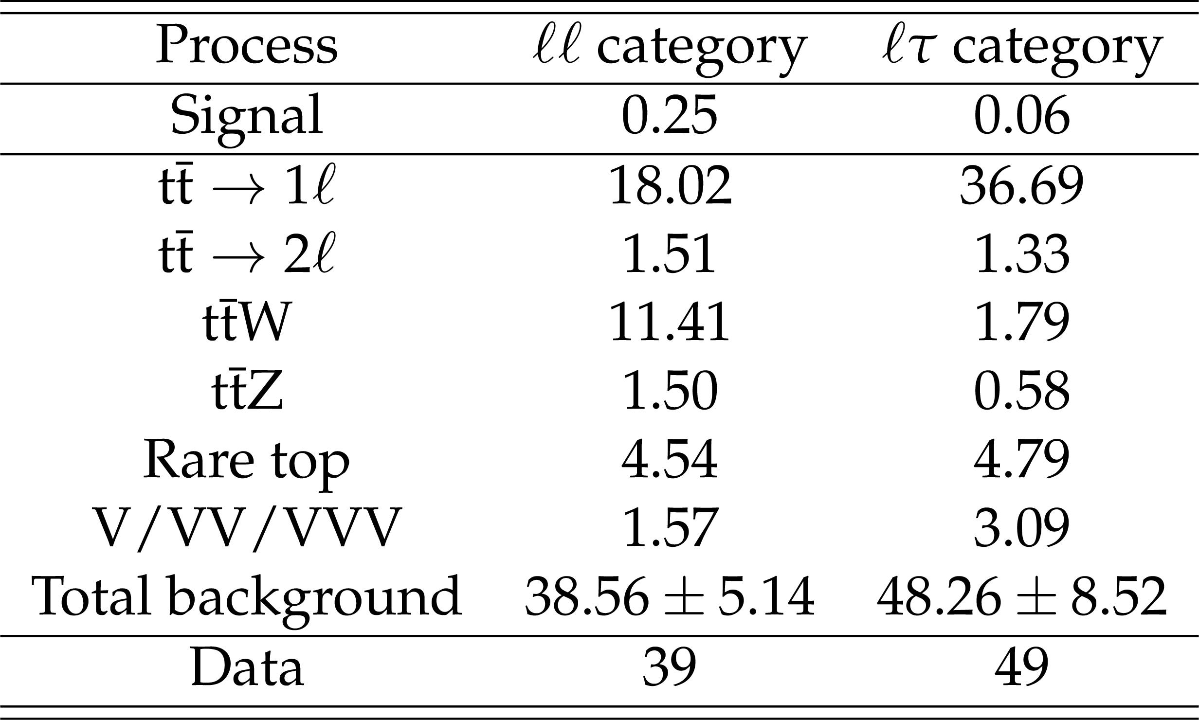
png pdf	Table 2: The post-fit yields of the CR, for $ \ell\ell $ and $ \ell\tau $ categories separately. The errors for total background include the statistical and systematic uncertainties.

Summary

Data recorded with the CMS experiment during LHC Run 2 amounting to 138 $ \mathrm{fb}^{-1} $ of pp collisions at $ \sqrt{s}= $ 13 TeV are used to search for anomalous couplings in the process $ \mathrm{pp} \rightarrow \mathrm{W}^{ \pm} \mathrm{W}^{ \pm} \mathrm{H}+\mathrm{jj} $, where the Higgs boson decays to two bottom quarks and the W bosons decay leptonically. The analysis focuses on the channel in which the two b-jets are merged. The observed(expected) 95% CL interval for $ \kappa_{WW} $ is $[-3.3, 5.3]$($[-2.4, 4.4]$). This marks the first analysis of the $ \mathrm{pp} \rightarrow \mathrm{W}^{ \pm} \mathrm{W}^{ \pm} \mathrm{H}+\mathrm{jj} $ process and opens the possibility of further analysis of the same process with different final states.

References
1	CMS Collaboration	Observation of a new boson at a mass of 125 GeV with the CMS experiment at the LHC	PLB 716 (2012) 30
2	C. Englert et al.	VBS $ W^{\pm}W^{\pm}H $ production at the HL-LHC and a 100 TeV pp-collider	International Journal of Modern Physics A 32 (2017) 1750106
3	CMS Collaboration	Precision luminosity measurement in proton-proton collisions at $ \sqrt{s}= $ 13 TeV in 2015 and 2016 at CMS	EPJC 81 (2021) 800	CMS-LUM-17-003 2104.01927
4	CMS Collaboration	CMS luminosity measurement for the 2017 data-taking period at $ \sqrt{s} = $ 13 TeV	CMS Physics Analysis Summary, 2018 link	CMS-PAS-LUM-17-004
5	CMS Collaboration	CMS luminosity measurement for the 2018 data-taking period at $ \sqrt{s} = $ 13 TeV	CMS Physics Analysis Summary, 2019 link	CMS-PAS-LUM-18-002
6	CMS Collaboration	The CMS experiment at the CERN LHC	JINST 3 (2008) S08004
7	CMS Collaboration	Performance of the CMS Level-1 trigger in proton-proton collisions at $ \sqrt{s} = $ 13 TeV	JINST 15 (2020) P10017	CMS-TRG-17-001 2006.10165
8	CMS Collaboration	The CMS trigger system	JINST 12 (2017) P01020
9	GEANT4 Collaboration	GEANT 4--a simulation toolkit	NIM A 506 (2003) 250
10	J. Alwall et al.	The automated computation of tree-level and next-to-leading order differential cross sections, and their matching to parton shower simulations	JHEP 07 (2014) 079	1405.0301
11	T. Sjöstrand et al.	An introduction to PYTHIA 8.2	Comput. Phys. Commun. 191 (2015) 159	1410.3012
12	NNPDF Collaboration	Parton distributions from high-precision collider data	EPJC 77 (2017) 663	1706.00428
13	P. Nason	A new method for combining NLO QCD with shower Monte Carlo algorithms	JHEP 11 (2004) 040	hep-ph/0409146
14	S. Frixione, P. Nason, and C. Oleari	Matching NLO QCD computations with parton shower simulations: the POWHEG method	JHEP 11 (2007) 070	0709.2092
15	S. Alioli, P. Nason, C. Oleari, and E. Re	A general framework for implementing NLO calculations in shower Monte Carlo programs: the POWHEG box	JHEP 06 (2010) 043	1002.2581
16	A. M. Sirunyan et al.	Particle-flow reconstruction and global event description with the CMS detector	JINST 12 (2017) P10003
17	CMS Collaboration	Electron and photon reconstruction and identification with the CMS experiment at the CERN LHC	JINST 16 (2021) P05014	CMS-EGM-17-001 2012.06888
18	CMS Collaboration	Performance of the CMS muon detector and muon reconstruction with proton-proton collisions at $ \sqrt{s}= $ 13 TeV	JINST 13 (2018) P06015	CMS-MUO-16-001 1804.04528
19	CMS Collaboration	Performance of reconstruction and identification of $ \tau $ leptons decaying to hadrons and $ \nu_\tau $ in pp collisions at $ \sqrt{s}= $ 13 TeV	JINST 13 (2018) P10005	CMS-TAU-16-003 1809.02816
20	CMS Collaboration	Identification of hadronic tau lepton decays using a deep neural network	JINST 17 (2022) P07023	CMS-TAU-20-001 2201.08458
21	M. Cacciari, G. P. Salam, and G. Soyez	FastJet user manual	EPJC 72 (2012) 1896	1111.6097
22	M. Cacciari, G. P. Salam, and G. Soyez	The anti-$ k_t $ jet clustering algorithm	JHEP 04 (2008) 063	0802.1189
23	E. Bols et al.	Jet flavour classification using DeepJet	JINST 15 (2020) P12012	2008.10519
24	CMS Collaboration	Performance summary of AK4 jet b tagging with data from proton-proton collisions at 13 TeV with the CMS detector	CMS Detector Performance Note CMS-DP-2023-005, 2023 CDS
25	A. J. Larkoski, S. Marzani, G. Soyez, and J. Thaler	Soft drop	JHEP 05 (2014) 146	1402.2657
26	H. Qu and L. Gouskos	Jet tagging via particle clouds	PRD 101 (2020) 056019
27	T. Chen and C. Guestrin	XGBoost: A scalable tree boosting system	in Proc. 22nd ACM SIGKDD Int. Conf. on Knowledge Discovery and Data Mining, KDD '16, New York, 2016 link
28	CMS Collaboration	The CMS statistical analysis and combination tool: Combine	Accepted by Comput. Softw. Big Sci, 2024	CMS-CAT-23-001 2404.06614
29	CMS Collaboration	Study of WH production through vector boson scattering and extraction of the relative sign of the W and Z couplings to the Higgs boson in proton-proton collisions at $ \sqrt{s} = $ 13 TeV	Submitted to Phys. Lett. B	CMS-HIG-23-007 2405.16566
30	D. de Florian et al.	Handbook of LHC Higgs Cross Sections: 4. Deciphering the Nature of the Higgs Sector	CYRM-2017-002 (CERN), 2017 link	1610.07922
31	R. J. Barlow and C. Beeston	Fitting using finite Monte Carlo samples	Comput. Phys. Commun. 77 (1993) 219