

Compact Muon Solenoid
LHC, CERN
| CMS-PAS-EXO-24-005 | ||
| Search for scalar leptoquarks produced via muon-quark scattering in pp collisions at $ \sqrt{s} = $ 13 TeV | ||
| CMS Collaboration | ||
| 2025-09-04 | ||
| Abstract: The first search for scalar leptoquarks at the TeV scale produced in muon-quark collisions is presented. It is based on a set of proton-proton (pp) collision data recorded with the CMS detector at the LHC at a center-of-mass energy of 13 TeV corresponding to an integrated luminosity of 138 fb$^{-1}$. Due to quantum fluctuations, protons also contain charged leptons, making it possible to study lepton-induced processes. When a muon from one proton beam interacts with a quark from the other beam, the process allows the study of resonant single leptoquark production and its subsequent decay. The final state includes events with one or two muons plus a jet which can come from the hadronization of either a light quark or a b quark. The main physical observable is the invariant mass of the muon-jet system whose distribution peaks at the leptoquark mass. Upper limits are set on the product of the leptoquark production cross section and branching fraction to the muon-quark final state. The results exclude wide regions in the parameter plane of the leptoquark mass and the leptoquark-muon-quark coupling. | ||
| Links: CDS record (PDF) ; CADI line (restricted) ; | ||
| Figures | |
png pdf |
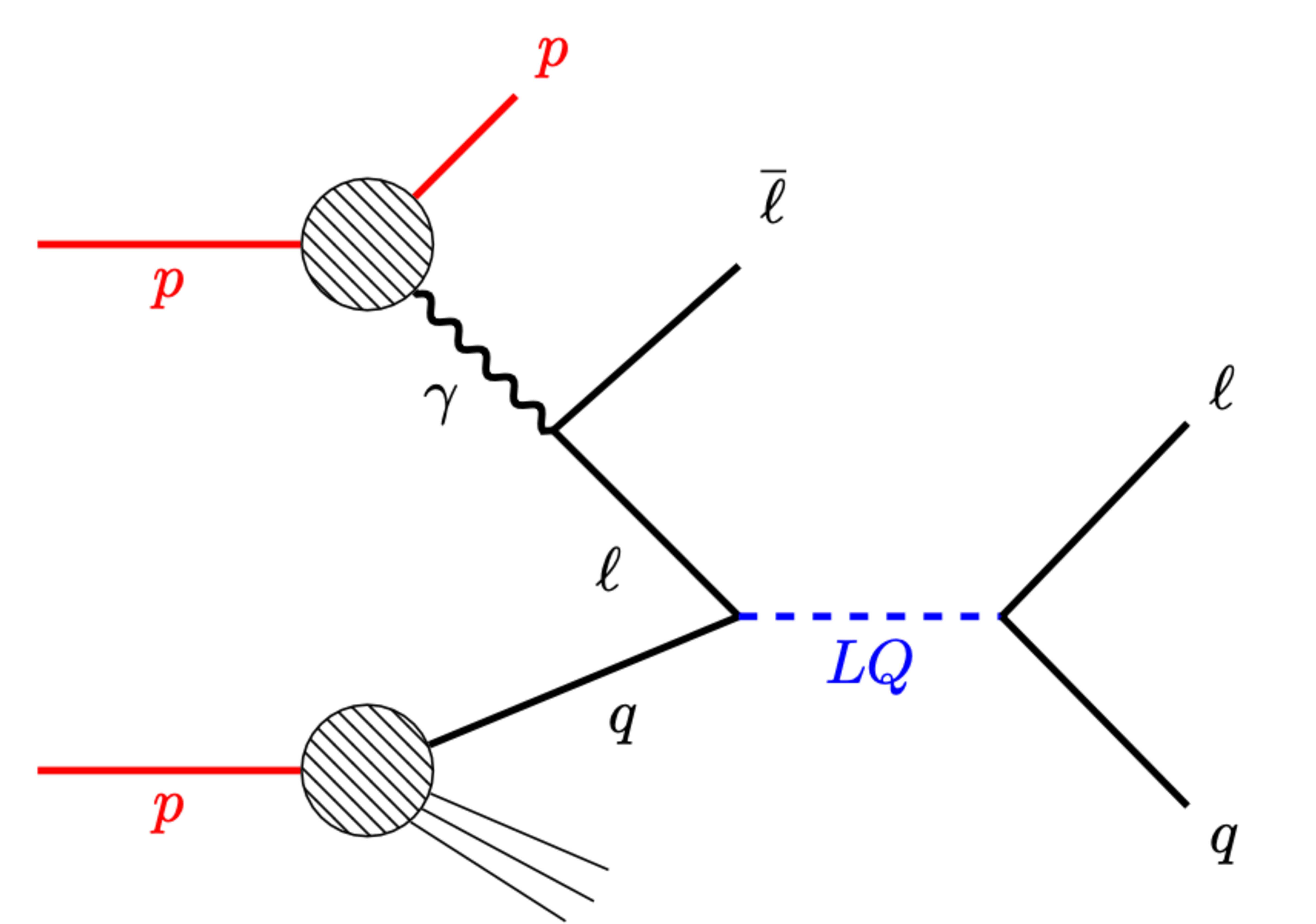
Figure 1:
Feynman diagram of the lepton-induced LQ production. |
png pdf |
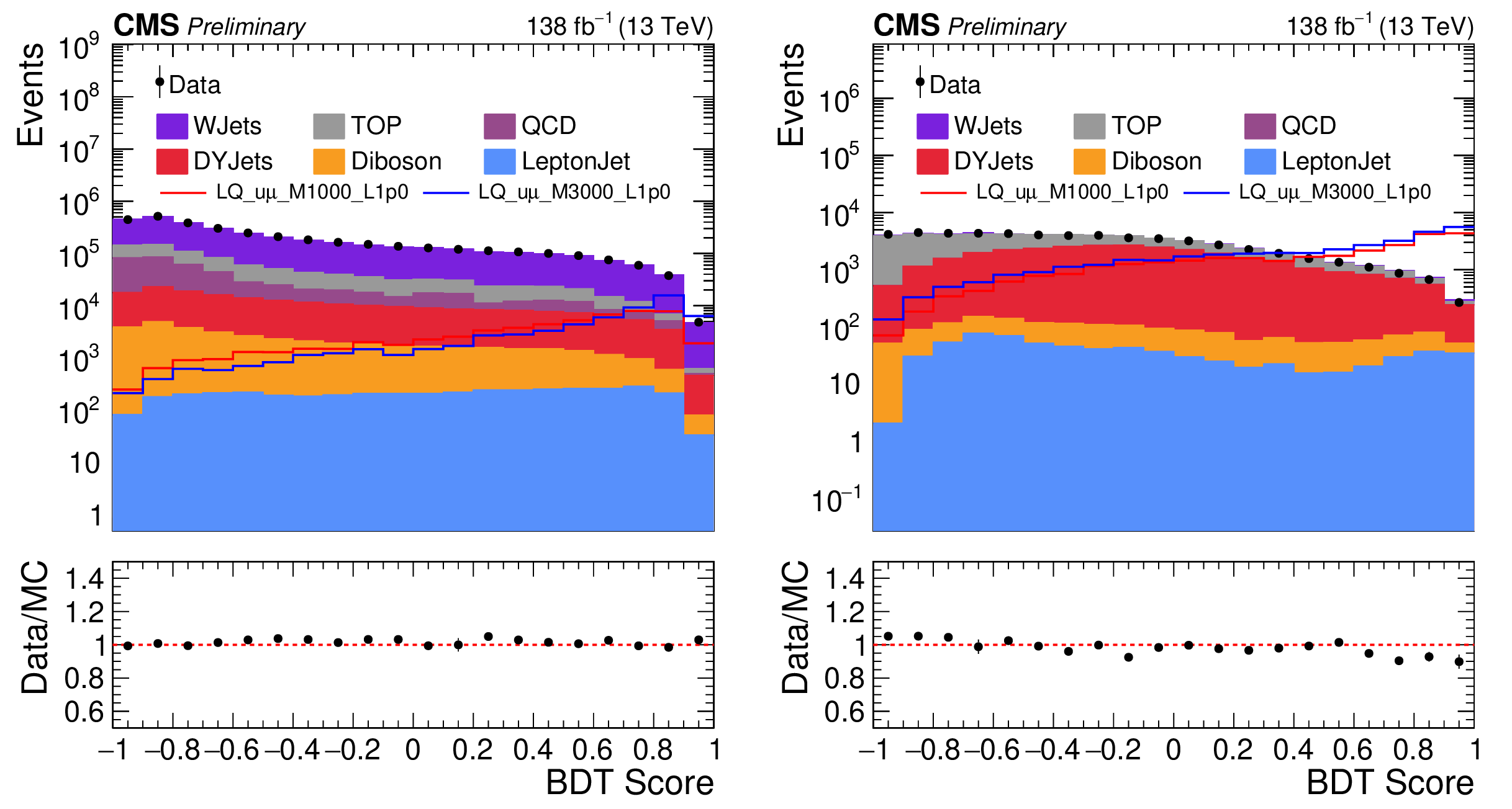
Figure 2:
Comparison of data and background BDT discriminant distributions at the preselection level for 1 (2) muon signal region on the left (right). The error bars are the data statistical uncertainties. The distributions of two simulated signal samples are also shown. They correspond to signal hypotheses with $M_{\text{LQ}} = $ 1 TeV, $\lambda_{\mathrm{u}\mu} = $ 1.0, and $M_{\text{LQ}} = $ 3 TeV, $\lambda_{\mathrm{u}\mu} = $ 1.0. The signal cross section is set to a value of 1 pb for visibility. This value exceeds the expected upper cross section limit of this search by approximately two to three orders of magnitude. |
png pdf |
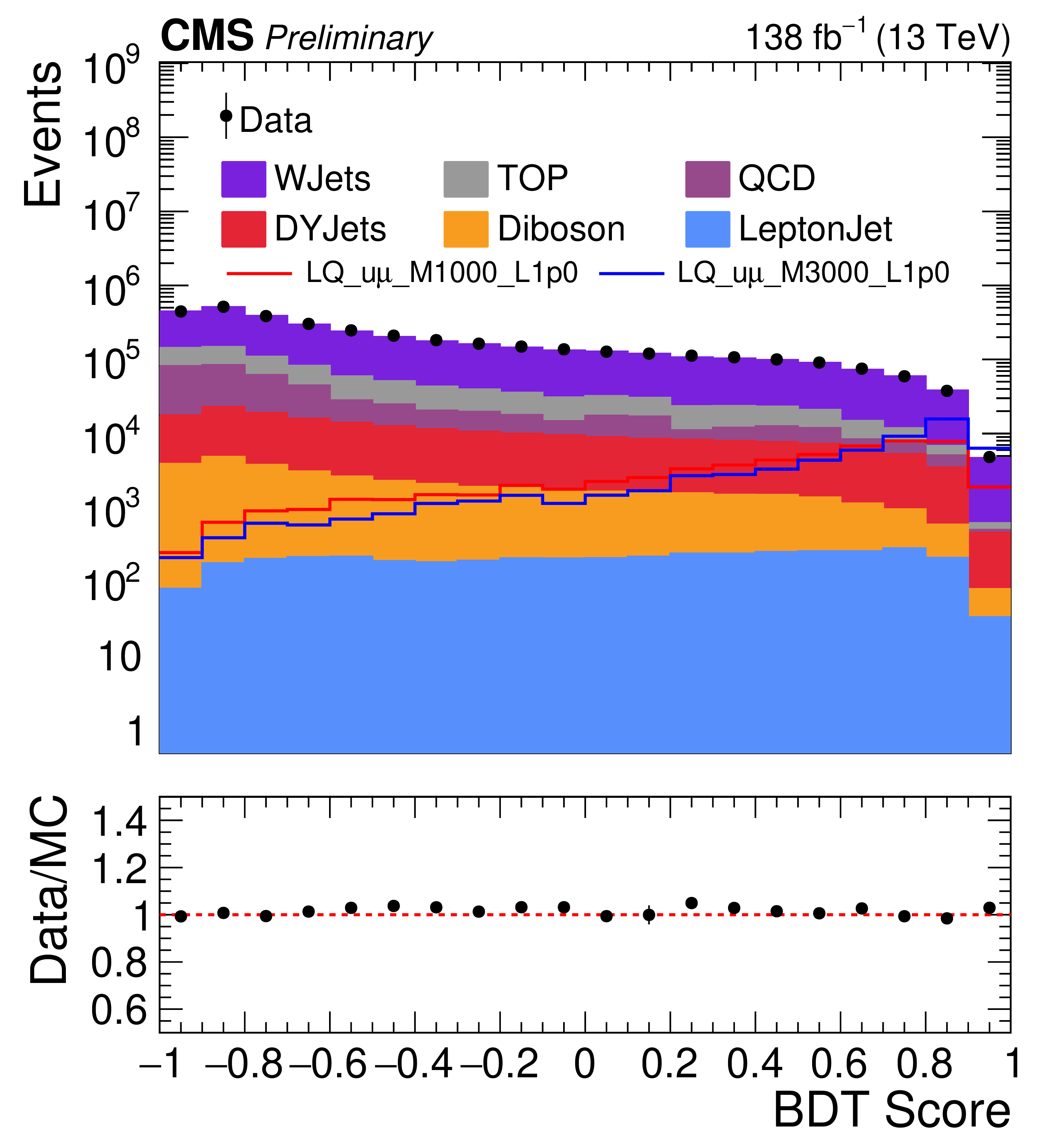
Figure 2-a:
Comparison of data and background BDT discriminant distributions at the preselection level for 1 (2) muon signal region on the left (right). The error bars are the data statistical uncertainties. The distributions of two simulated signal samples are also shown. They correspond to signal hypotheses with $M_{\text{LQ}} = $ 1 TeV, $\lambda_{\mathrm{u}\mu} = $ 1.0, and $M_{\text{LQ}} = $ 3 TeV, $\lambda_{\mathrm{u}\mu} = $ 1.0. The signal cross section is set to a value of 1 pb for visibility. This value exceeds the expected upper cross section limit of this search by approximately two to three orders of magnitude. |
png pdf |
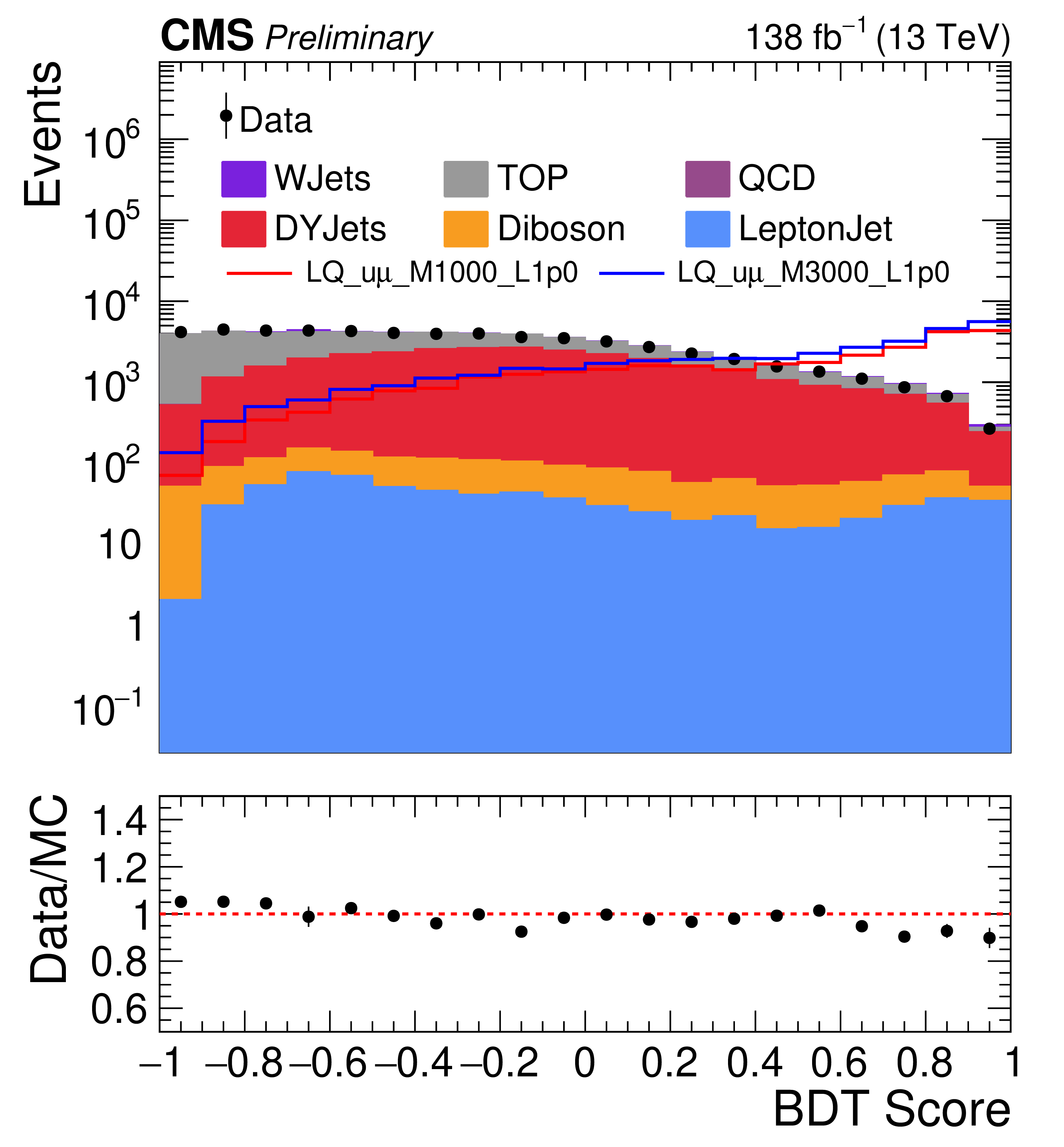
Figure 2-b:
Comparison of data and background BDT discriminant distributions at the preselection level for 1 (2) muon signal region on the left (right). The error bars are the data statistical uncertainties. The distributions of two simulated signal samples are also shown. They correspond to signal hypotheses with $M_{\text{LQ}} = $ 1 TeV, $\lambda_{\mathrm{u}\mu} = $ 1.0, and $M_{\text{LQ}} = $ 3 TeV, $\lambda_{\mathrm{u}\mu} = $ 1.0. The signal cross section is set to a value of 1 pb for visibility. This value exceeds the expected upper cross section limit of this search by approximately two to three orders of magnitude. |
png pdf |
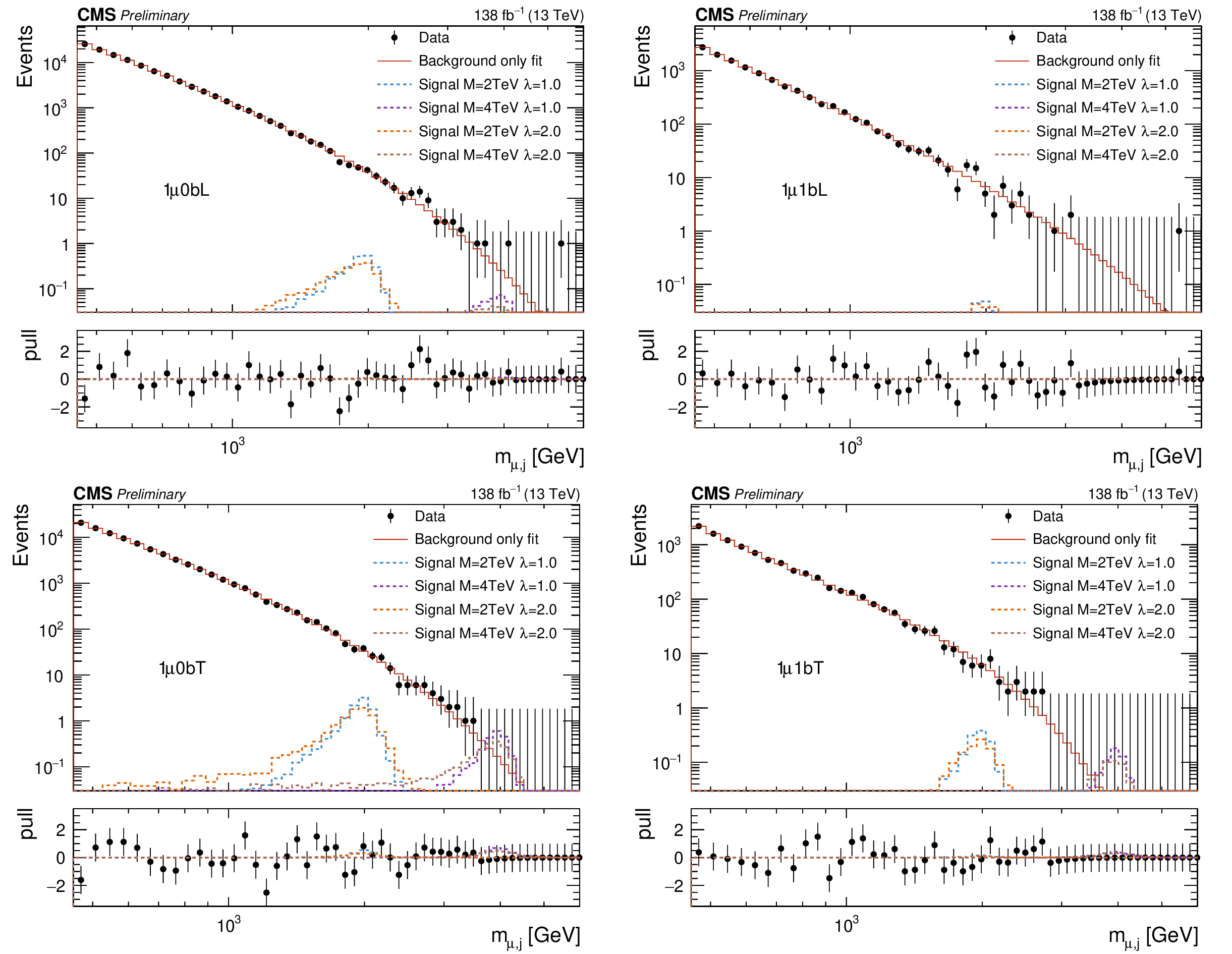
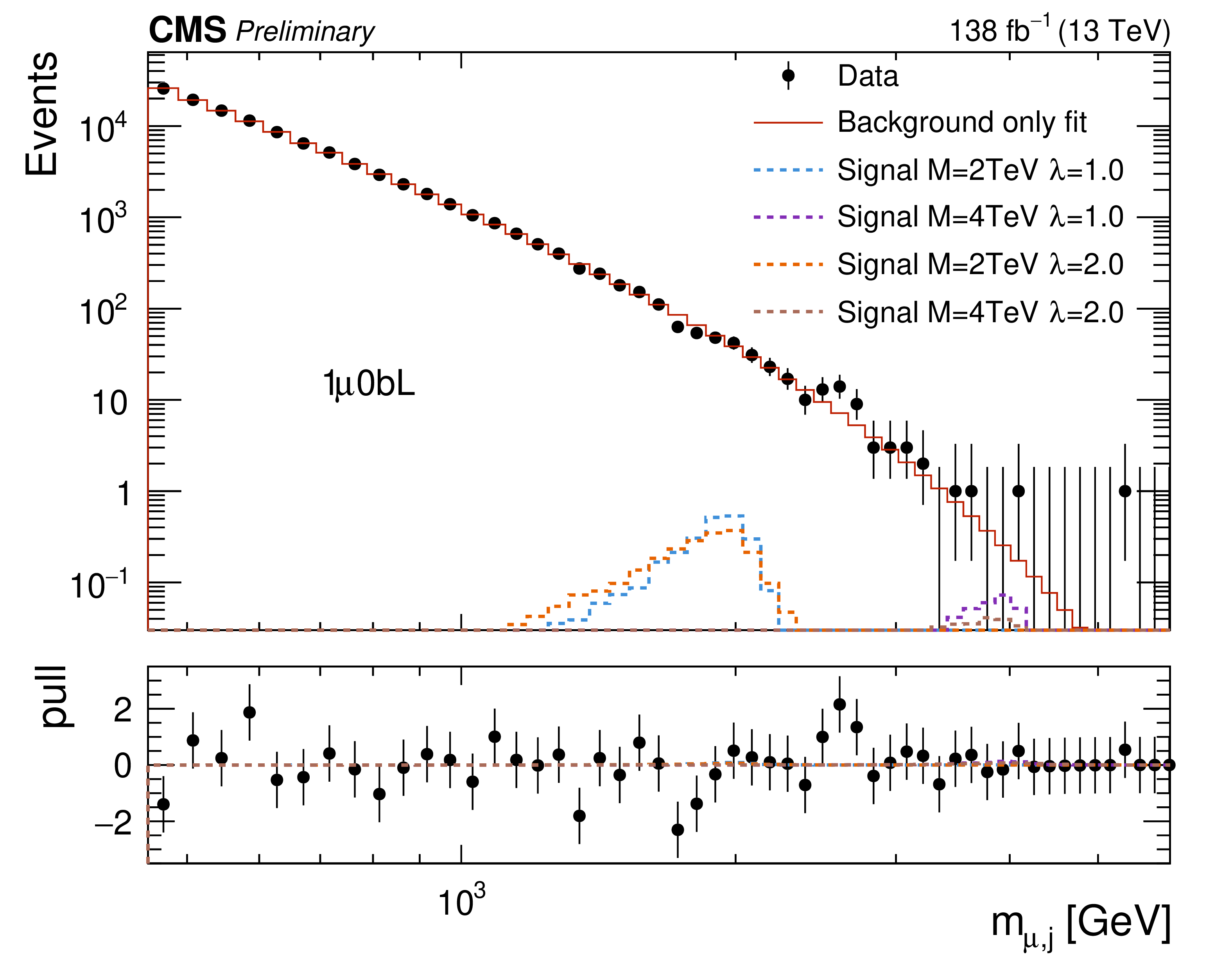
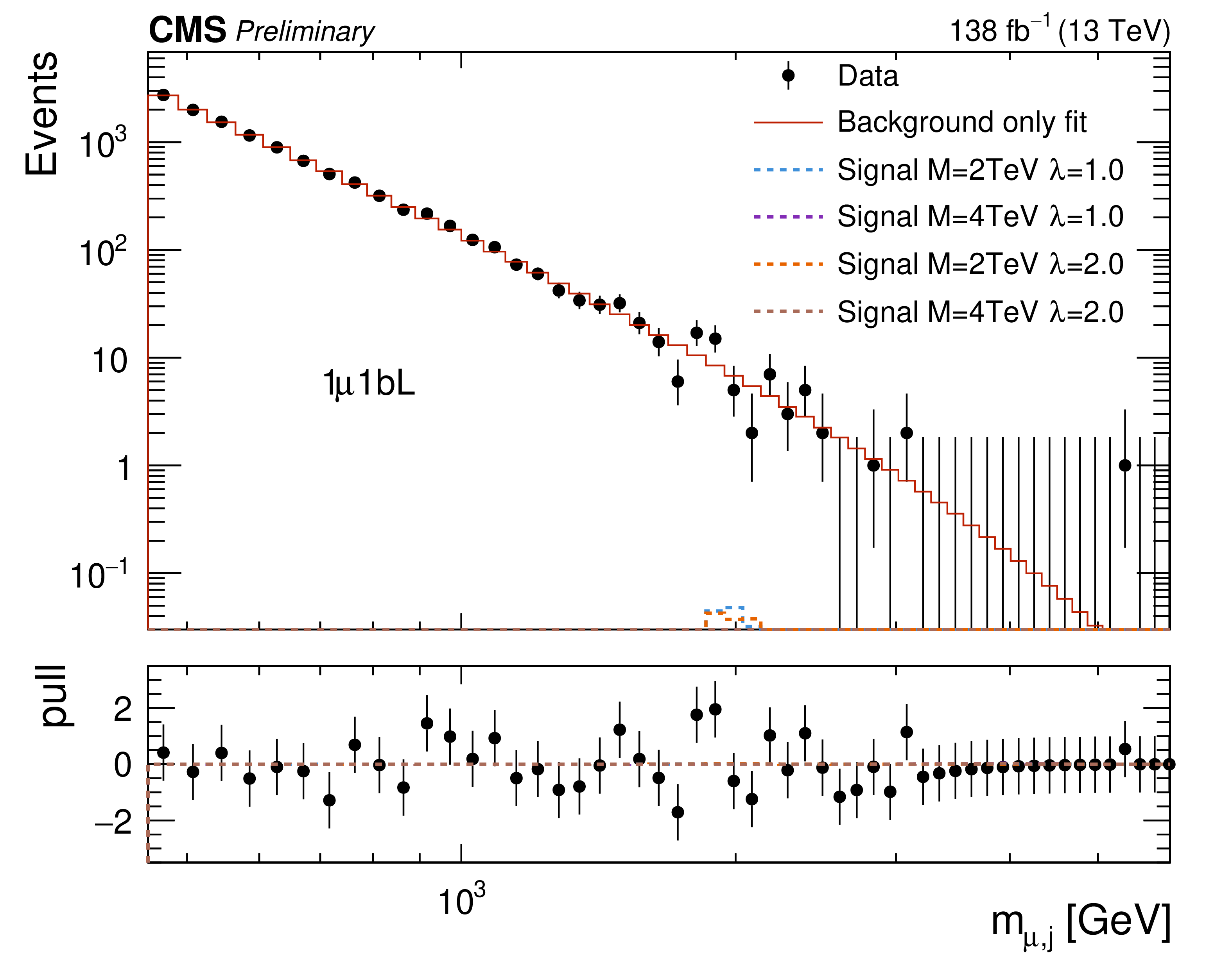
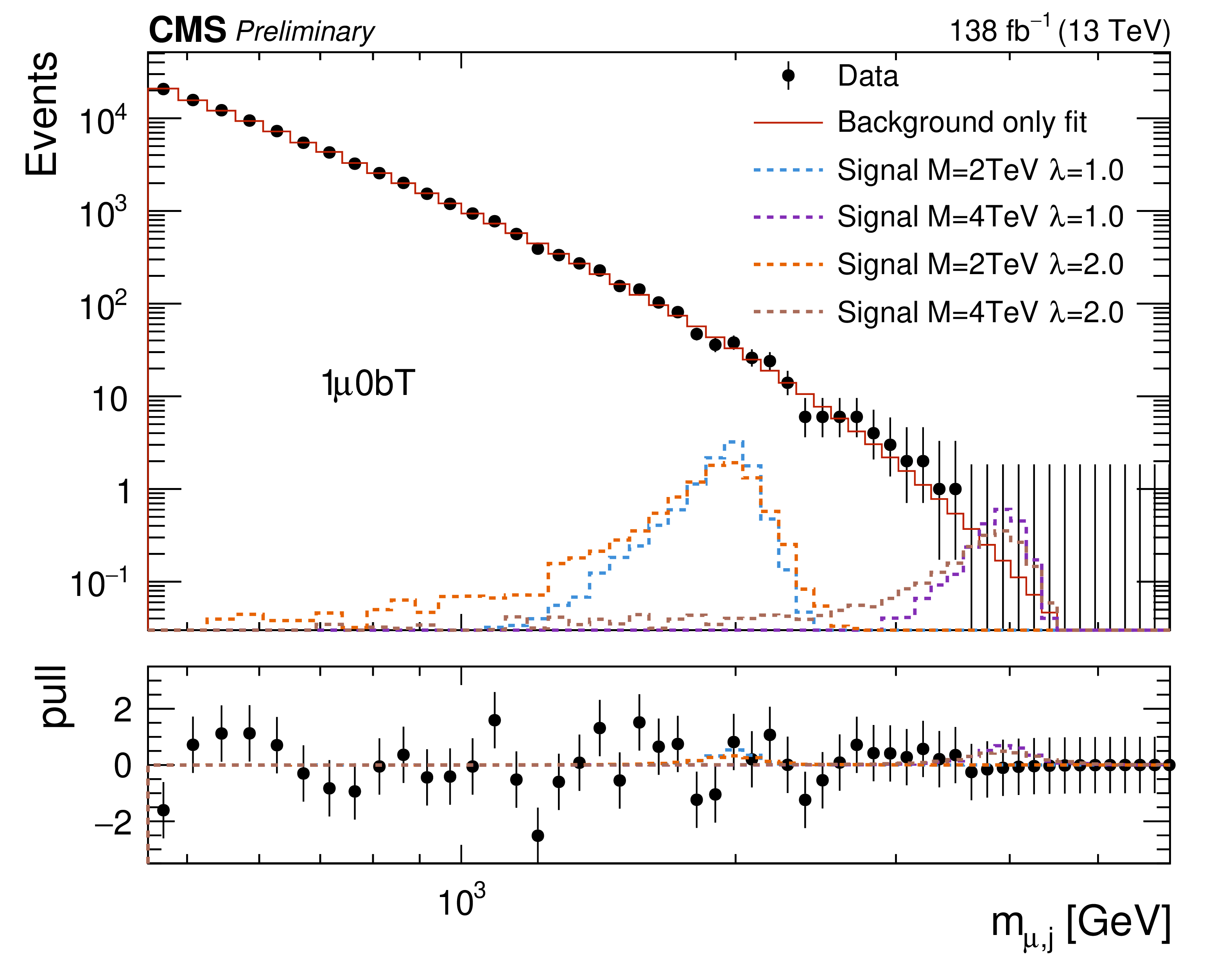
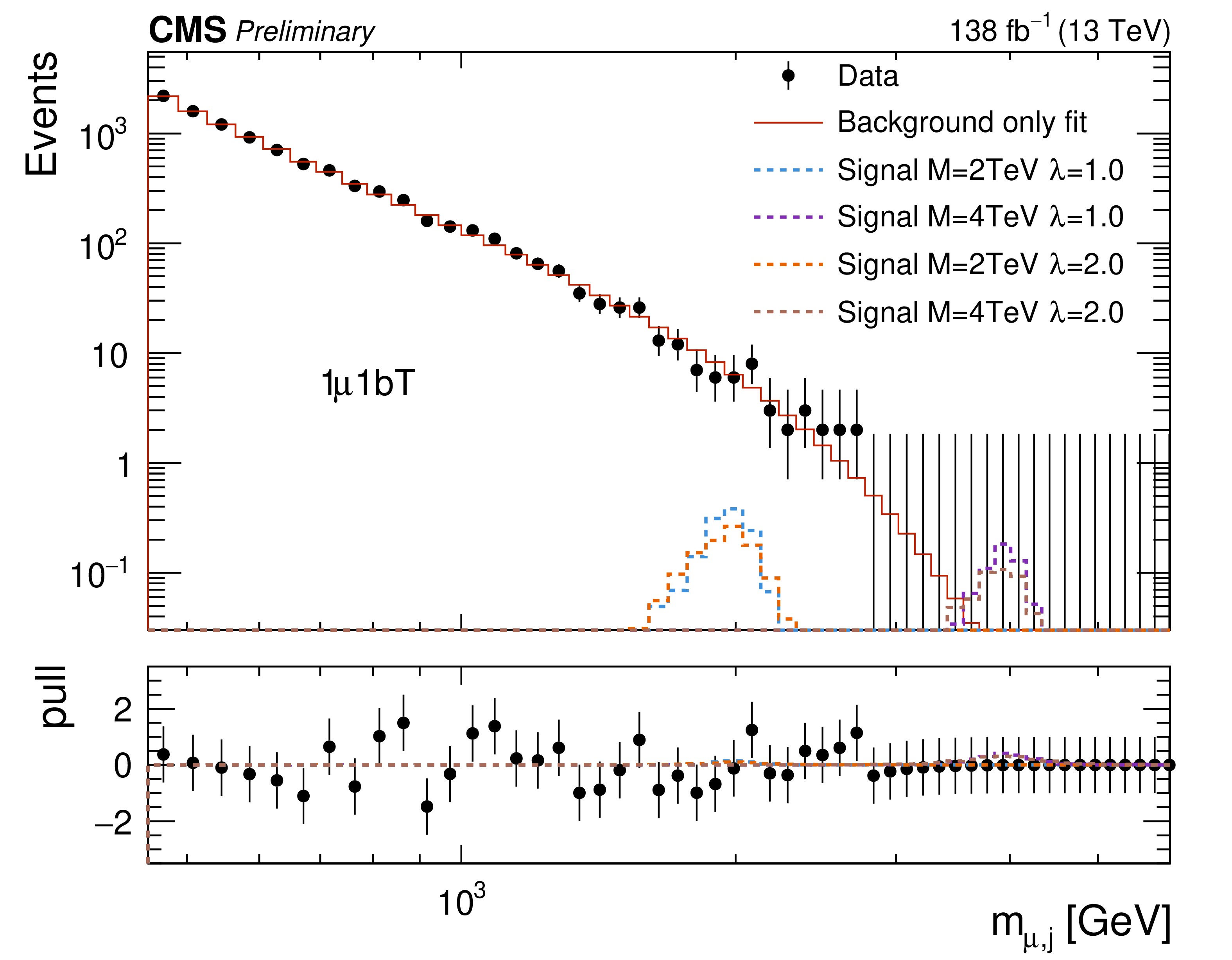
Figure 3:
Empirical background fits to the $M_{\mu,\text{j}} $ invariant mass distributions for all analysis categories within the one-muon signal region: one muon BDT loose + no-btag (upper left), one muon BDT loose + btag (upper right), one muon BDT tight + no-btag (lower left), one muon BDT tight + btag (lower right). The red line is the background estimation obtained using the empirical function. The blue (green) line represents a signal hypothesis with $M_{\text{LQ}} = $ 2 (4) TeV and $\lambda_{\mathrm{u}\mu} = $ 1, while the orange (blue) line represents a signal hypothesis with $M_{\text{LQ}} = $ 2 (4) TeV and $\lambda_{\mathrm{u}\mu} = $ 2. All signals are normalized to the expected upper-limit cross section. The horizontal axis shows the value of the $M_{\mu,\text{j}} $ spectra, while the vertical axis shows the number of events in each bin. The bottom panel shows the difference between the data and the background fit function divided by the statistical uncertainty. |
png pdf |
Figure 3-a:
Empirical background fits to the $M_{\mu,\text{j}} $ invariant mass distributions for all analysis categories within the one-muon signal region: one muon BDT loose + no-btag (upper left), one muon BDT loose + btag (upper right), one muon BDT tight + no-btag (lower left), one muon BDT tight + btag (lower right). The red line is the background estimation obtained using the empirical function. The blue (green) line represents a signal hypothesis with $M_{\text{LQ}} = $ 2 (4) TeV and $\lambda_{\mathrm{u}\mu} = $ 1, while the orange (blue) line represents a signal hypothesis with $M_{\text{LQ}} = $ 2 (4) TeV and $\lambda_{\mathrm{u}\mu} = $ 2. All signals are normalized to the expected upper-limit cross section. The horizontal axis shows the value of the $M_{\mu,\text{j}} $ spectra, while the vertical axis shows the number of events in each bin. The bottom panel shows the difference between the data and the background fit function divided by the statistical uncertainty. |
png pdf |
Figure 3-b:
Empirical background fits to the $M_{\mu,\text{j}} $ invariant mass distributions for all analysis categories within the one-muon signal region: one muon BDT loose + no-btag (upper left), one muon BDT loose + btag (upper right), one muon BDT tight + no-btag (lower left), one muon BDT tight + btag (lower right). The red line is the background estimation obtained using the empirical function. The blue (green) line represents a signal hypothesis with $M_{\text{LQ}} = $ 2 (4) TeV and $\lambda_{\mathrm{u}\mu} = $ 1, while the orange (blue) line represents a signal hypothesis with $M_{\text{LQ}} = $ 2 (4) TeV and $\lambda_{\mathrm{u}\mu} = $ 2. All signals are normalized to the expected upper-limit cross section. The horizontal axis shows the value of the $M_{\mu,\text{j}} $ spectra, while the vertical axis shows the number of events in each bin. The bottom panel shows the difference between the data and the background fit function divided by the statistical uncertainty. |
png pdf |
Figure 3-c:
Empirical background fits to the $M_{\mu,\text{j}} $ invariant mass distributions for all analysis categories within the one-muon signal region: one muon BDT loose + no-btag (upper left), one muon BDT loose + btag (upper right), one muon BDT tight + no-btag (lower left), one muon BDT tight + btag (lower right). The red line is the background estimation obtained using the empirical function. The blue (green) line represents a signal hypothesis with $M_{\text{LQ}} = $ 2 (4) TeV and $\lambda_{\mathrm{u}\mu} = $ 1, while the orange (blue) line represents a signal hypothesis with $M_{\text{LQ}} = $ 2 (4) TeV and $\lambda_{\mathrm{u}\mu} = $ 2. All signals are normalized to the expected upper-limit cross section. The horizontal axis shows the value of the $M_{\mu,\text{j}} $ spectra, while the vertical axis shows the number of events in each bin. The bottom panel shows the difference between the data and the background fit function divided by the statistical uncertainty. |
png pdf |
Figure 3-d:
Empirical background fits to the $M_{\mu,\text{j}} $ invariant mass distributions for all analysis categories within the one-muon signal region: one muon BDT loose + no-btag (upper left), one muon BDT loose + btag (upper right), one muon BDT tight + no-btag (lower left), one muon BDT tight + btag (lower right). The red line is the background estimation obtained using the empirical function. The blue (green) line represents a signal hypothesis with $M_{\text{LQ}} = $ 2 (4) TeV and $\lambda_{\mathrm{u}\mu} = $ 1, while the orange (blue) line represents a signal hypothesis with $M_{\text{LQ}} = $ 2 (4) TeV and $\lambda_{\mathrm{u}\mu} = $ 2. All signals are normalized to the expected upper-limit cross section. The horizontal axis shows the value of the $M_{\mu,\text{j}} $ spectra, while the vertical axis shows the number of events in each bin. The bottom panel shows the difference between the data and the background fit function divided by the statistical uncertainty. |
png pdf |
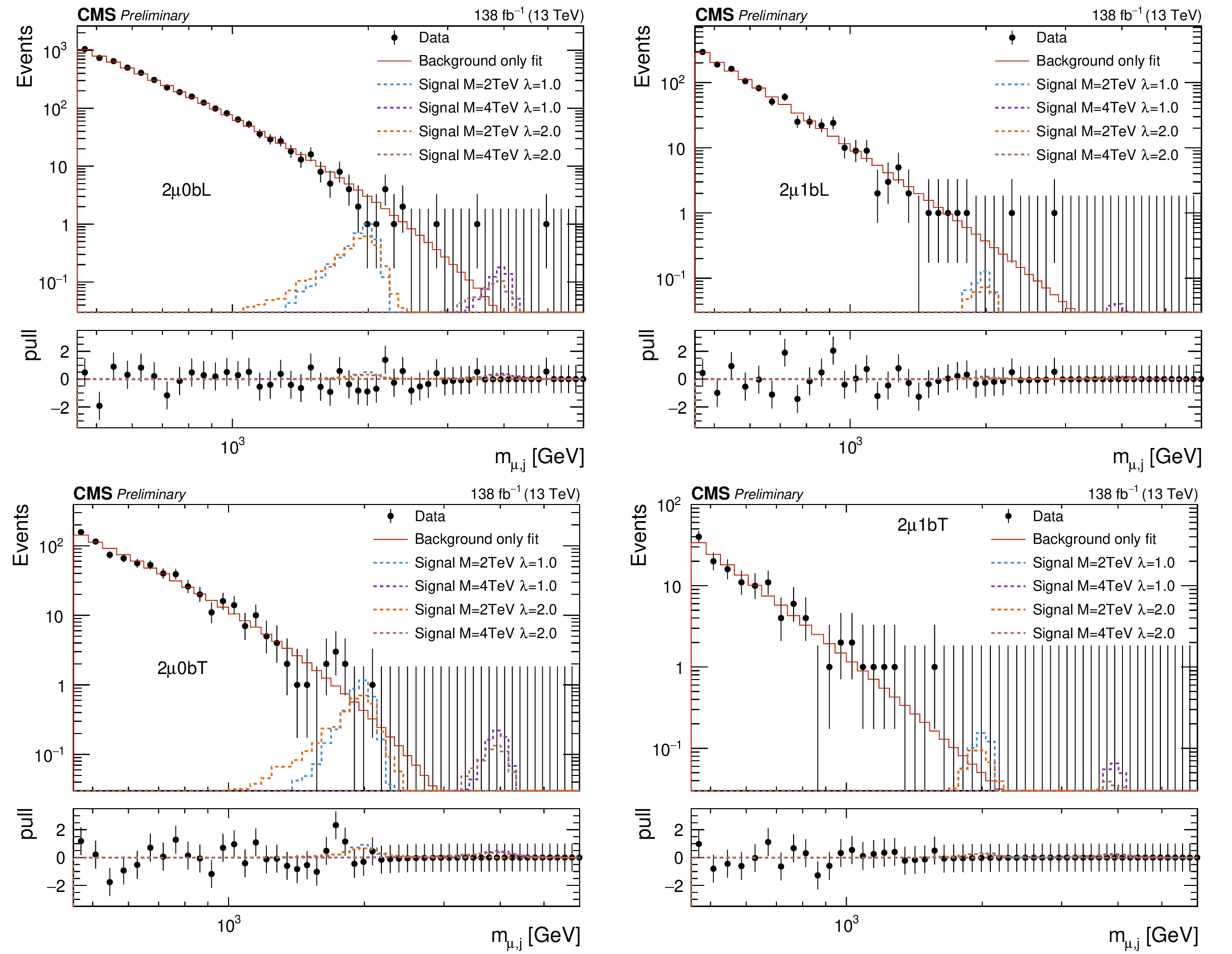
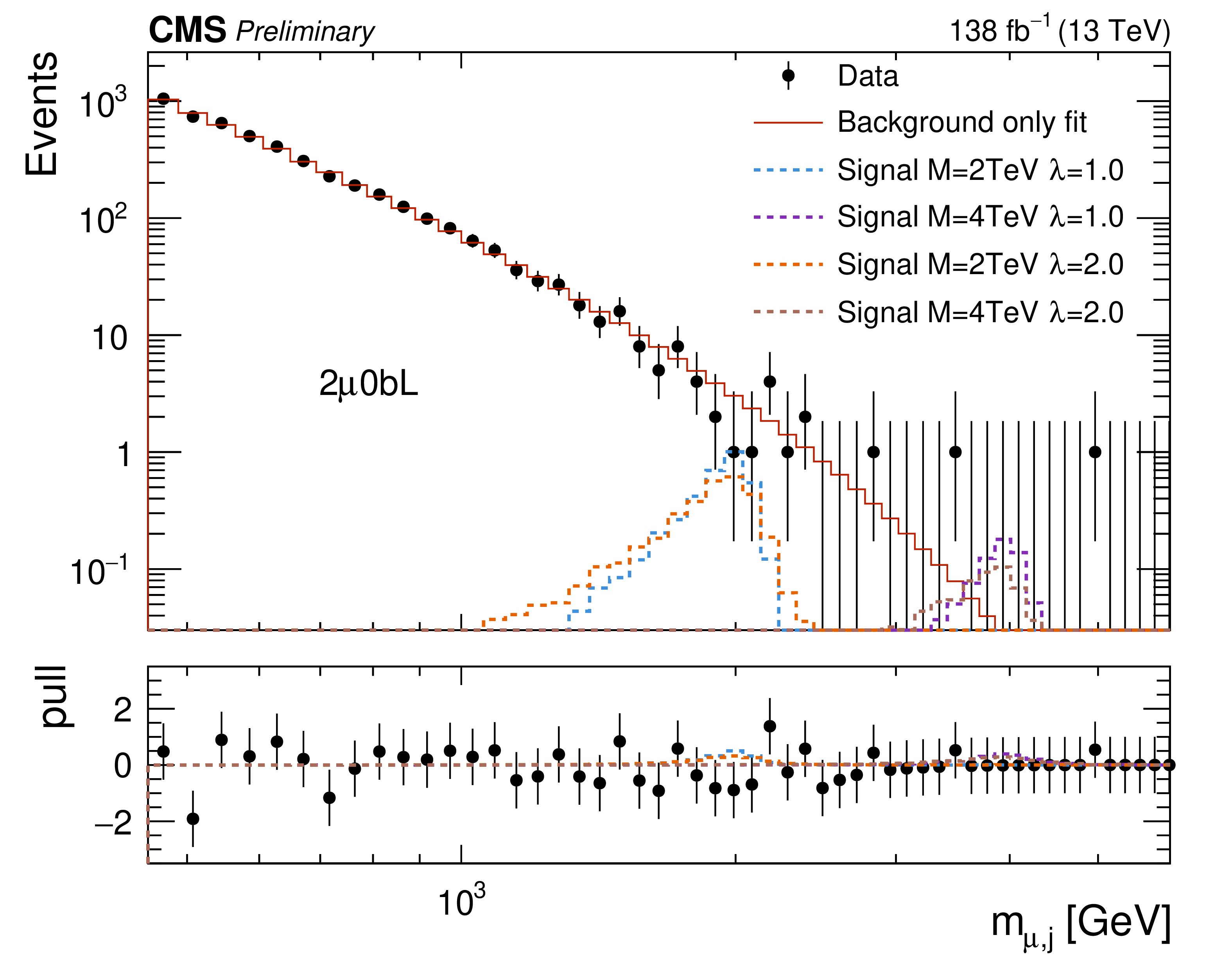
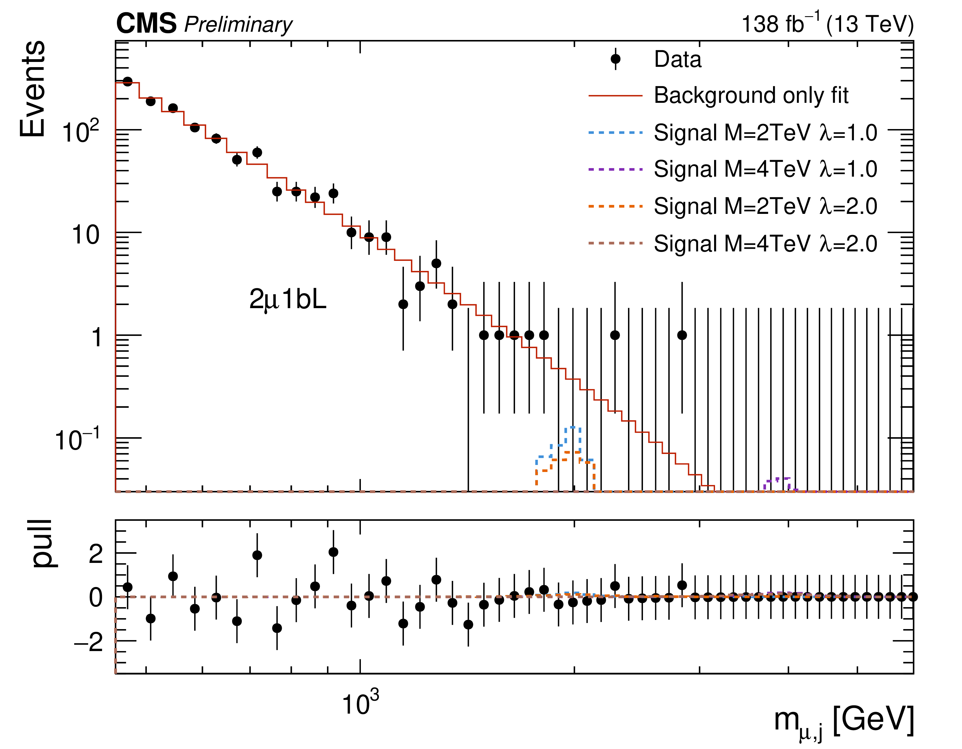
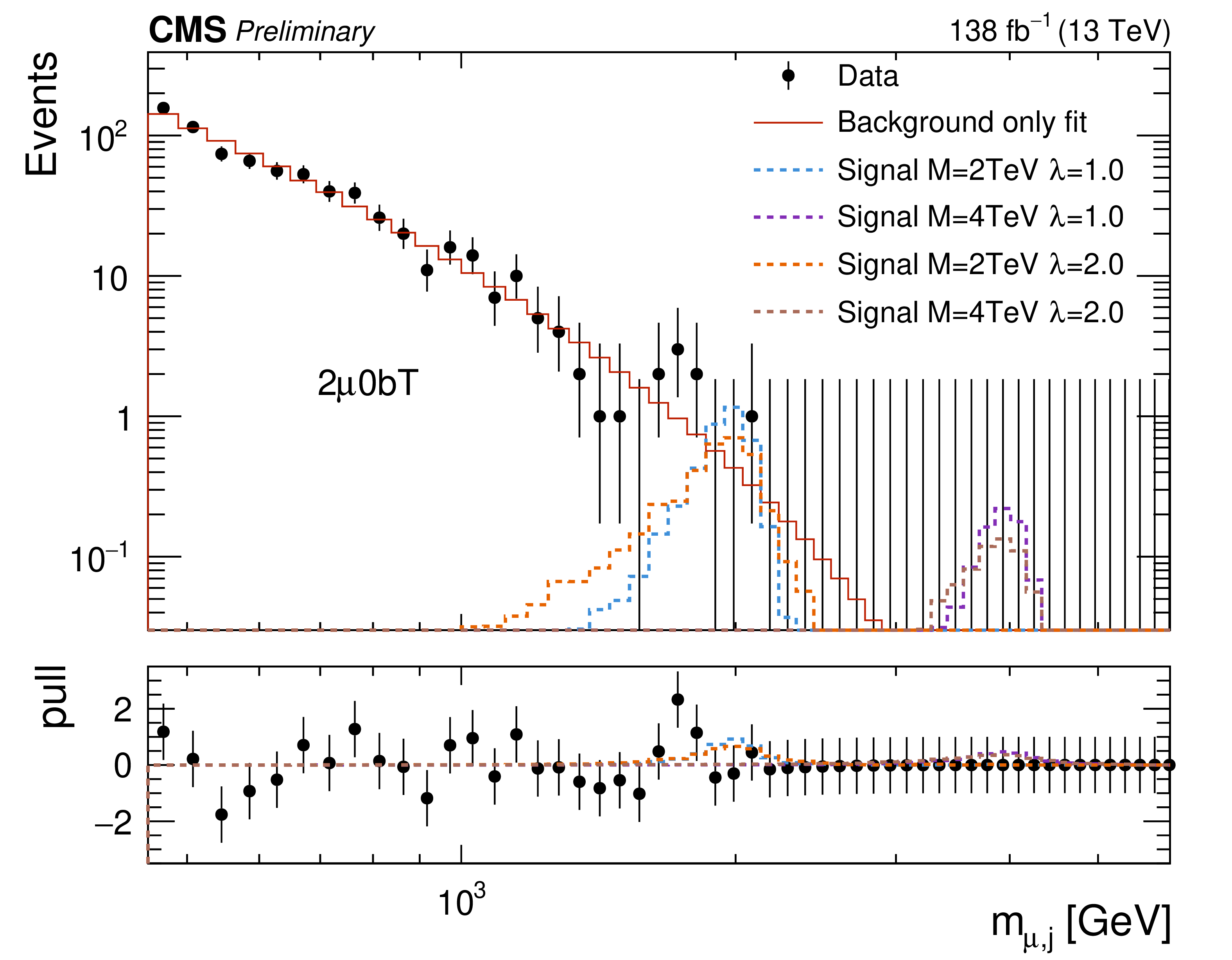
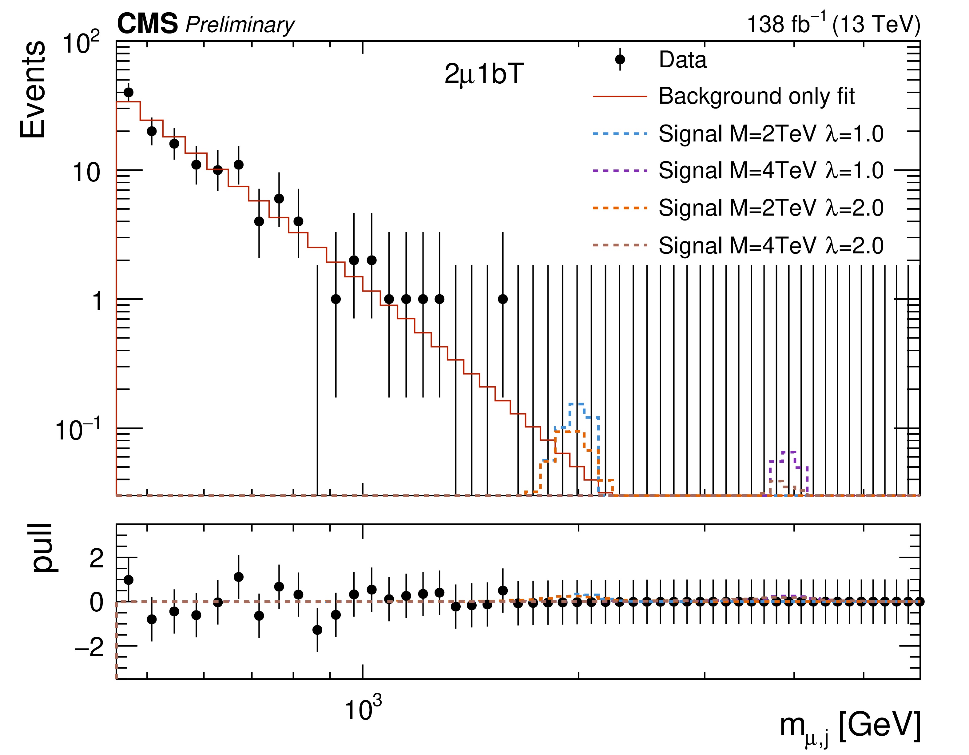
Figure 4:
Empirical background fits to the $M_{\mu,\text{j}} $ invariant mass distributions for all analysis categories within the two-muon signal region: two muons BDT loose + no-btag (upper left), two muon BDT loose + btag (upper right), two muons BDT tight + no-btag (lower left), two muons BDT tight + btag (lower right). The red line is the background estimation obtained using the empirical function. The blue (green) line represents a signal hypothesis with $M_{\text{LQ}} = $ 2 (4) TeV and $\lambda_{\mathrm{u}\mu} = $ 1, while the orange (blue) line represents a signal hypothesis with $M_{\text{LQ}} = $ 2 (4) TeV and $\lambda_{\mathrm{u}\mu} = $ 2. All signals are normalized to the expected upper-limit cross section. The horizontal axis shows the value of the $M_{\mu,\text{j}} $ spectra, while the vertical axis shows the number of events in each bin. The bottom panel shows the difference between the data and the background fit function divided by the statistical uncertainty. |
png pdf |
Figure 4-a:
Empirical background fits to the $M_{\mu,\text{j}} $ invariant mass distributions for all analysis categories within the two-muon signal region: two muons BDT loose + no-btag (upper left), two muon BDT loose + btag (upper right), two muons BDT tight + no-btag (lower left), two muons BDT tight + btag (lower right). The red line is the background estimation obtained using the empirical function. The blue (green) line represents a signal hypothesis with $M_{\text{LQ}} = $ 2 (4) TeV and $\lambda_{\mathrm{u}\mu} = $ 1, while the orange (blue) line represents a signal hypothesis with $M_{\text{LQ}} = $ 2 (4) TeV and $\lambda_{\mathrm{u}\mu} = $ 2. All signals are normalized to the expected upper-limit cross section. The horizontal axis shows the value of the $M_{\mu,\text{j}} $ spectra, while the vertical axis shows the number of events in each bin. The bottom panel shows the difference between the data and the background fit function divided by the statistical uncertainty. |
png pdf |
Figure 4-b:
Empirical background fits to the $M_{\mu,\text{j}} $ invariant mass distributions for all analysis categories within the two-muon signal region: two muons BDT loose + no-btag (upper left), two muon BDT loose + btag (upper right), two muons BDT tight + no-btag (lower left), two muons BDT tight + btag (lower right). The red line is the background estimation obtained using the empirical function. The blue (green) line represents a signal hypothesis with $M_{\text{LQ}} = $ 2 (4) TeV and $\lambda_{\mathrm{u}\mu} = $ 1, while the orange (blue) line represents a signal hypothesis with $M_{\text{LQ}} = $ 2 (4) TeV and $\lambda_{\mathrm{u}\mu} = $ 2. All signals are normalized to the expected upper-limit cross section. The horizontal axis shows the value of the $M_{\mu,\text{j}} $ spectra, while the vertical axis shows the number of events in each bin. The bottom panel shows the difference between the data and the background fit function divided by the statistical uncertainty. |
png pdf |
Figure 4-c:
Empirical background fits to the $M_{\mu,\text{j}} $ invariant mass distributions for all analysis categories within the two-muon signal region: two muons BDT loose + no-btag (upper left), two muon BDT loose + btag (upper right), two muons BDT tight + no-btag (lower left), two muons BDT tight + btag (lower right). The red line is the background estimation obtained using the empirical function. The blue (green) line represents a signal hypothesis with $M_{\text{LQ}} = $ 2 (4) TeV and $\lambda_{\mathrm{u}\mu} = $ 1, while the orange (blue) line represents a signal hypothesis with $M_{\text{LQ}} = $ 2 (4) TeV and $\lambda_{\mathrm{u}\mu} = $ 2. All signals are normalized to the expected upper-limit cross section. The horizontal axis shows the value of the $M_{\mu,\text{j}} $ spectra, while the vertical axis shows the number of events in each bin. The bottom panel shows the difference between the data and the background fit function divided by the statistical uncertainty. |
png pdf |
Figure 4-d:
Empirical background fits to the $M_{\mu,\text{j}} $ invariant mass distributions for all analysis categories within the two-muon signal region: two muons BDT loose + no-btag (upper left), two muon BDT loose + btag (upper right), two muons BDT tight + no-btag (lower left), two muons BDT tight + btag (lower right). The red line is the background estimation obtained using the empirical function. The blue (green) line represents a signal hypothesis with $M_{\text{LQ}} = $ 2 (4) TeV and $\lambda_{\mathrm{u}\mu} = $ 1, while the orange (blue) line represents a signal hypothesis with $M_{\text{LQ}} = $ 2 (4) TeV and $\lambda_{\mathrm{u}\mu} = $ 2. All signals are normalized to the expected upper-limit cross section. The horizontal axis shows the value of the $M_{\mu,\text{j}} $ spectra, while the vertical axis shows the number of events in each bin. The bottom panel shows the difference between the data and the background fit function divided by the statistical uncertainty. |
png pdf |
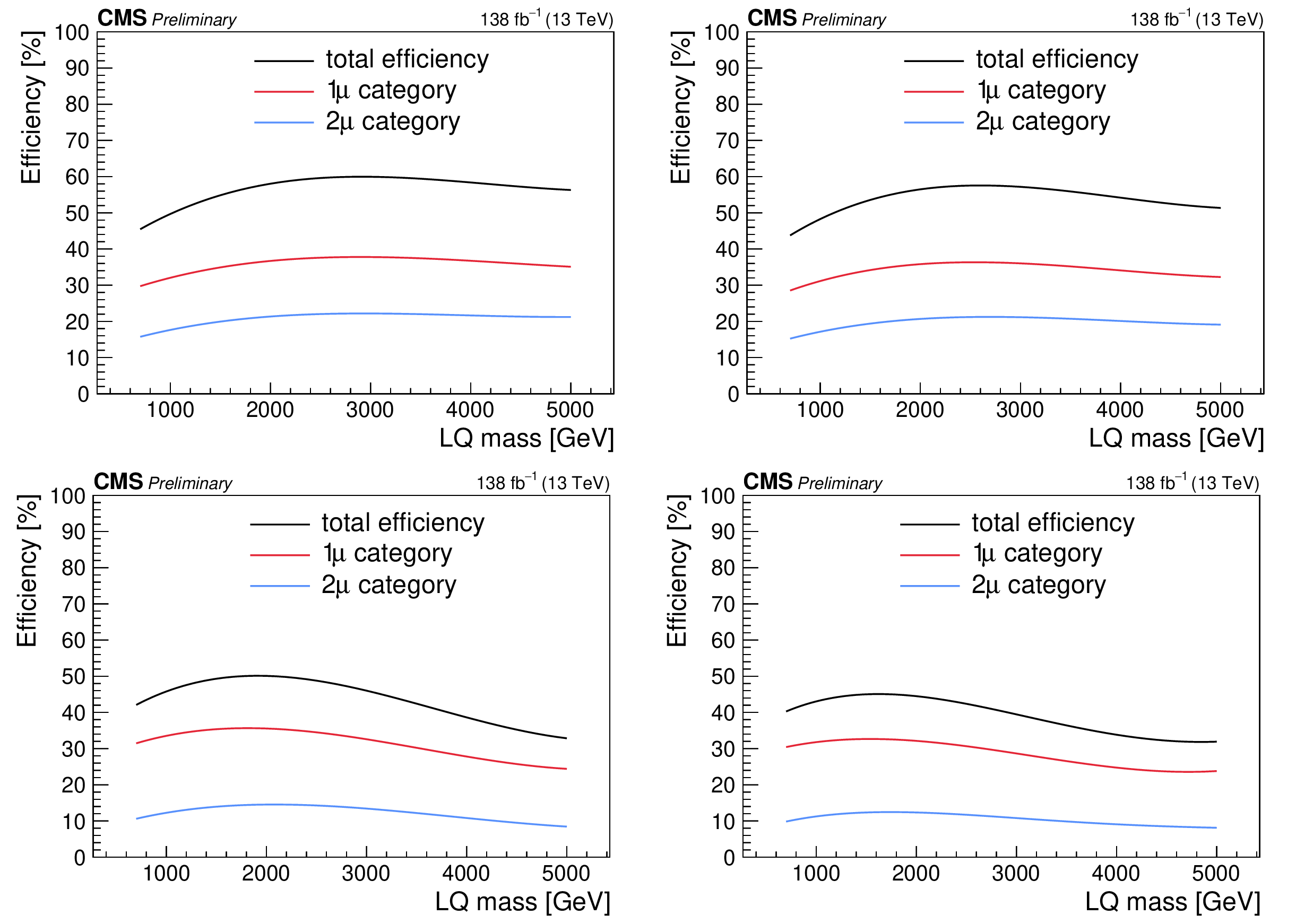
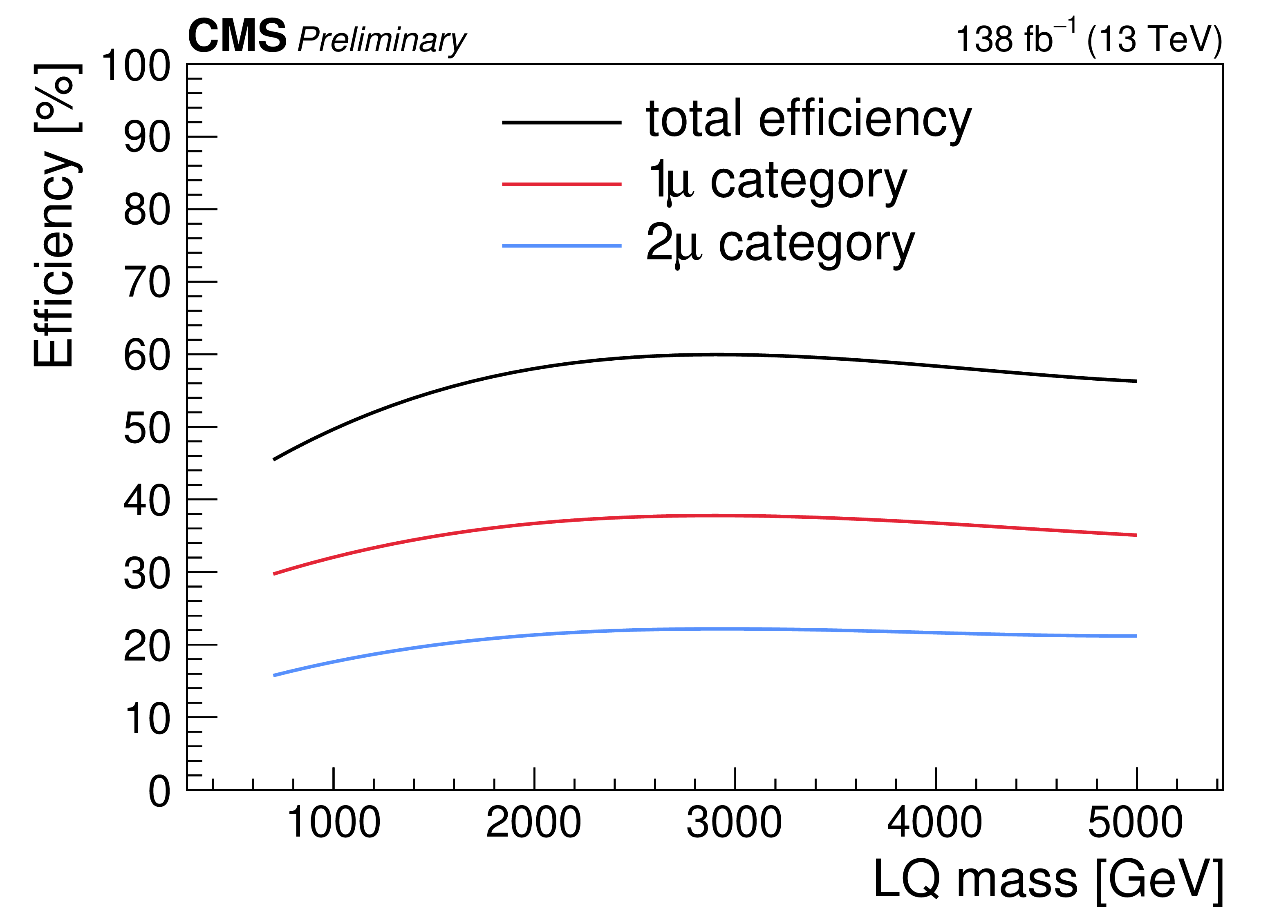
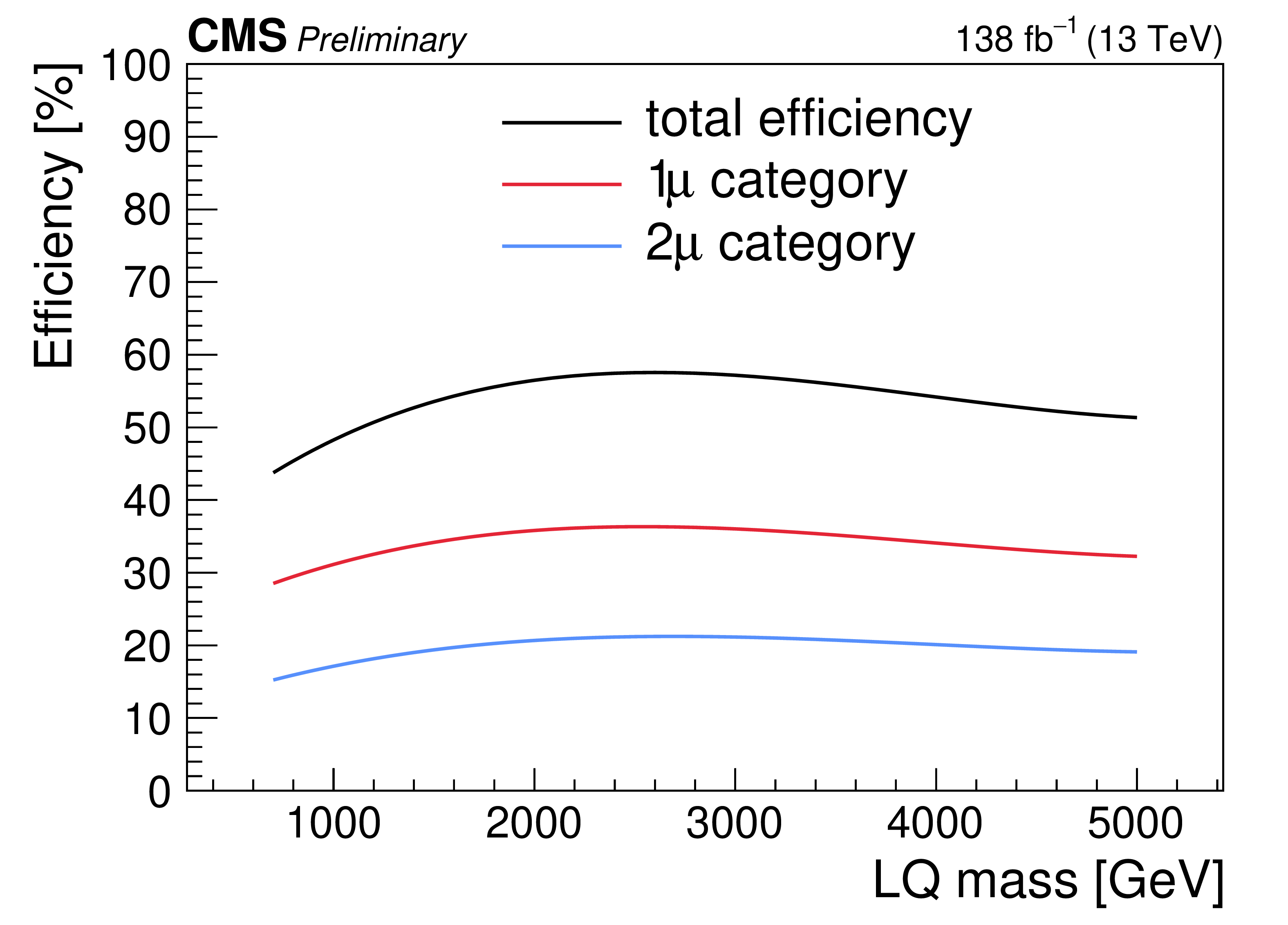
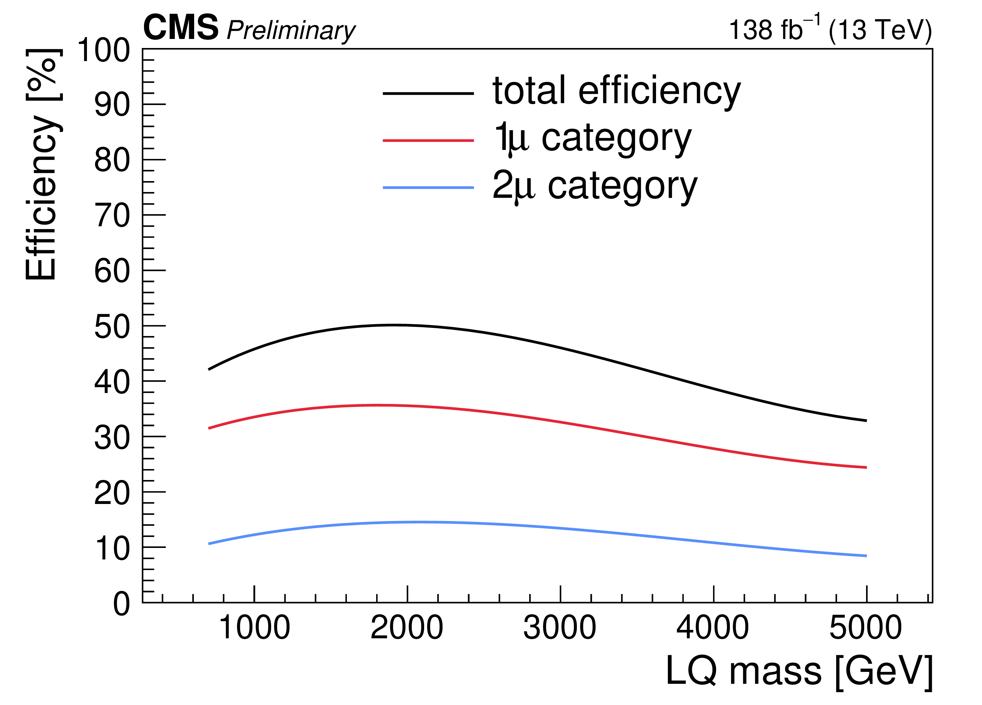
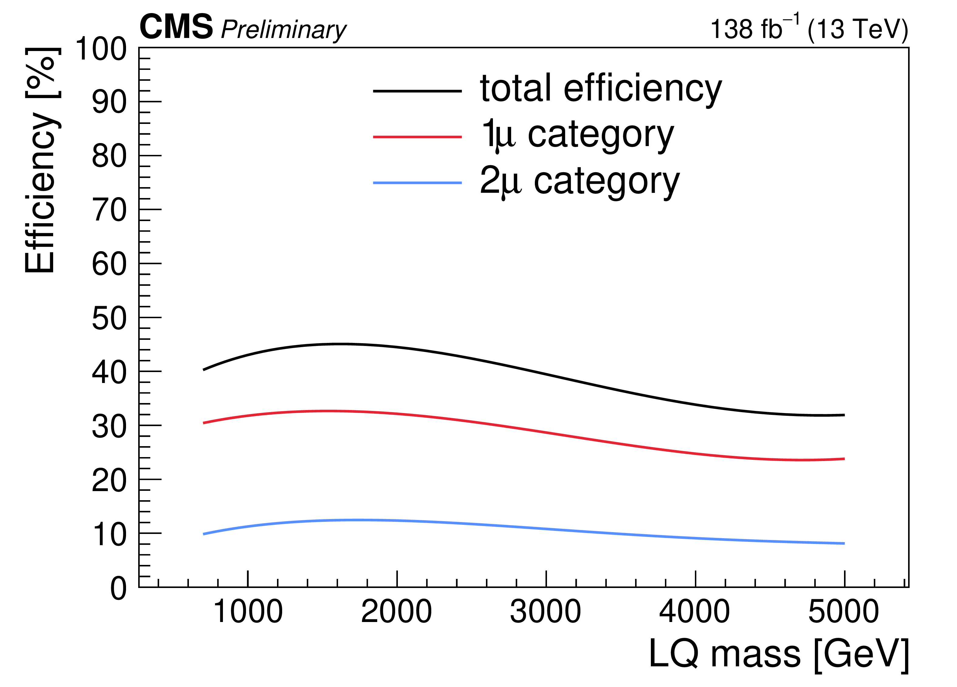
Figure 5:
Signal efficiency as a function of the LQ mass for $\lambda_{\mathrm{u}\mu} = $ 1.0 (2.0) on the upper left (upper right). Signal efficiency as a function of the LQ mass for $\lambda_{\mathrm{b}\mu} = $ 1.0 (2.0) on the lower left (lower right). The black points are the total efficiency, defined as the sum of the efficiency of the two signal regions. The red and blue points are the efficiency for the one- and two-muon signal regions, respectively. |
png pdf |
Figure 5-a:
Signal efficiency as a function of the LQ mass for $\lambda_{\mathrm{u}\mu} = $ 1.0 (2.0) on the upper left (upper right). Signal efficiency as a function of the LQ mass for $\lambda_{\mathrm{b}\mu} = $ 1.0 (2.0) on the lower left (lower right). The black points are the total efficiency, defined as the sum of the efficiency of the two signal regions. The red and blue points are the efficiency for the one- and two-muon signal regions, respectively. |
png pdf |
Figure 5-b:
Signal efficiency as a function of the LQ mass for $\lambda_{\mathrm{u}\mu} = $ 1.0 (2.0) on the upper left (upper right). Signal efficiency as a function of the LQ mass for $\lambda_{\mathrm{b}\mu} = $ 1.0 (2.0) on the lower left (lower right). The black points are the total efficiency, defined as the sum of the efficiency of the two signal regions. The red and blue points are the efficiency for the one- and two-muon signal regions, respectively. |
png pdf |
Figure 5-c:
Signal efficiency as a function of the LQ mass for $\lambda_{\mathrm{u}\mu} = $ 1.0 (2.0) on the upper left (upper right). Signal efficiency as a function of the LQ mass for $\lambda_{\mathrm{b}\mu} = $ 1.0 (2.0) on the lower left (lower right). The black points are the total efficiency, defined as the sum of the efficiency of the two signal regions. The red and blue points are the efficiency for the one- and two-muon signal regions, respectively. |
png pdf |
Figure 5-d:
Signal efficiency as a function of the LQ mass for $\lambda_{\mathrm{u}\mu} = $ 1.0 (2.0) on the upper left (upper right). Signal efficiency as a function of the LQ mass for $\lambda_{\mathrm{b}\mu} = $ 1.0 (2.0) on the lower left (lower right). The black points are the total efficiency, defined as the sum of the efficiency of the two signal regions. The red and blue points are the efficiency for the one- and two-muon signal regions, respectively. |
png pdf |
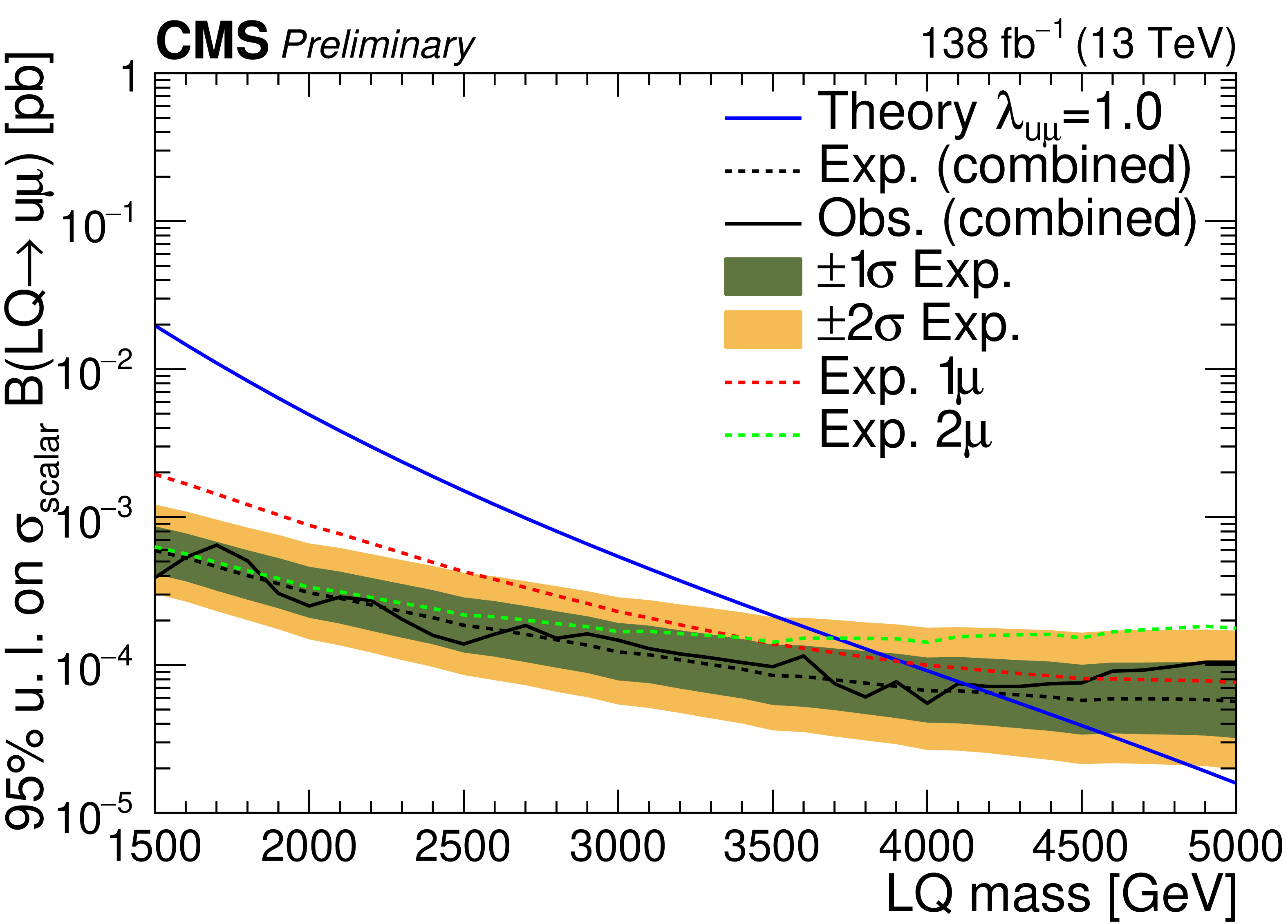
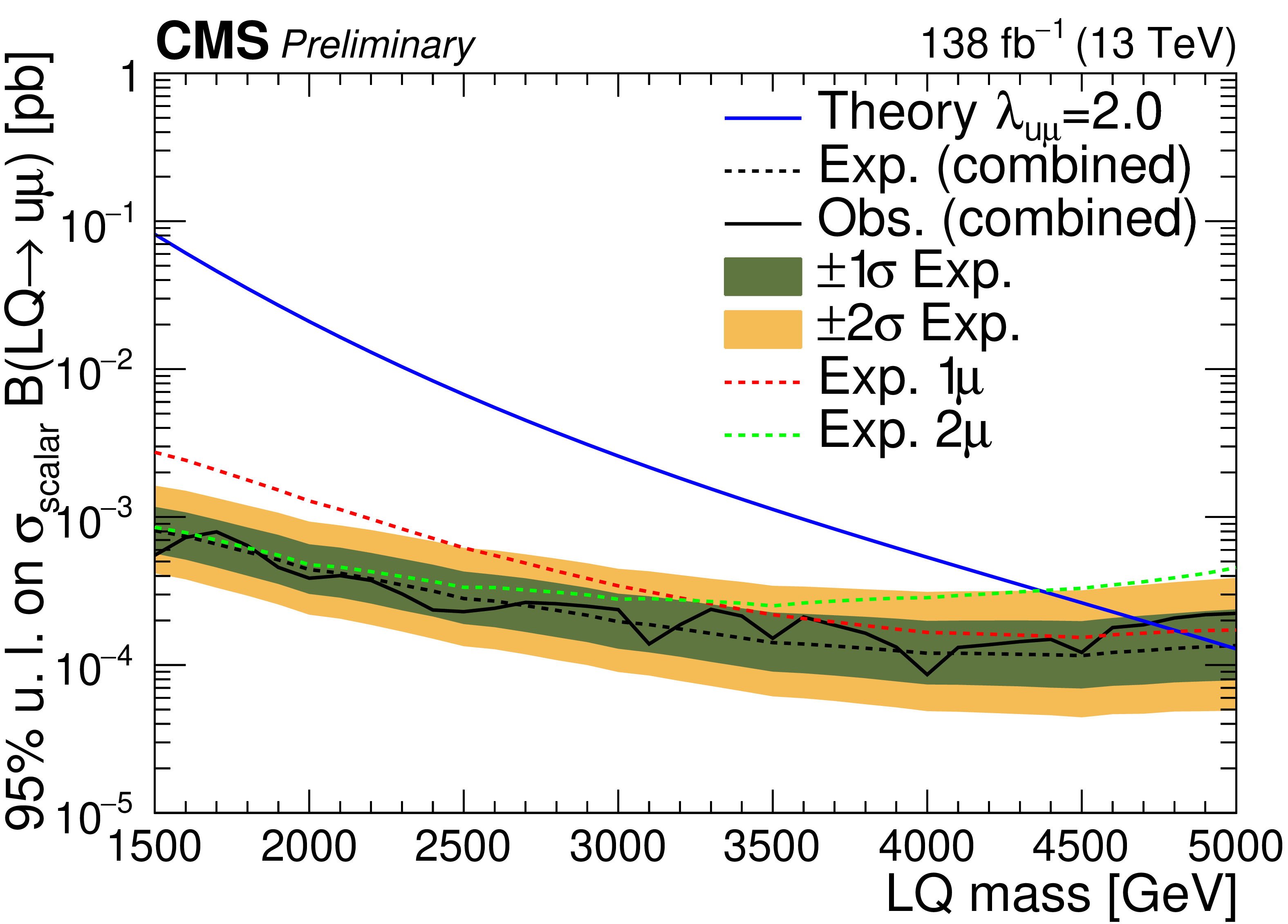
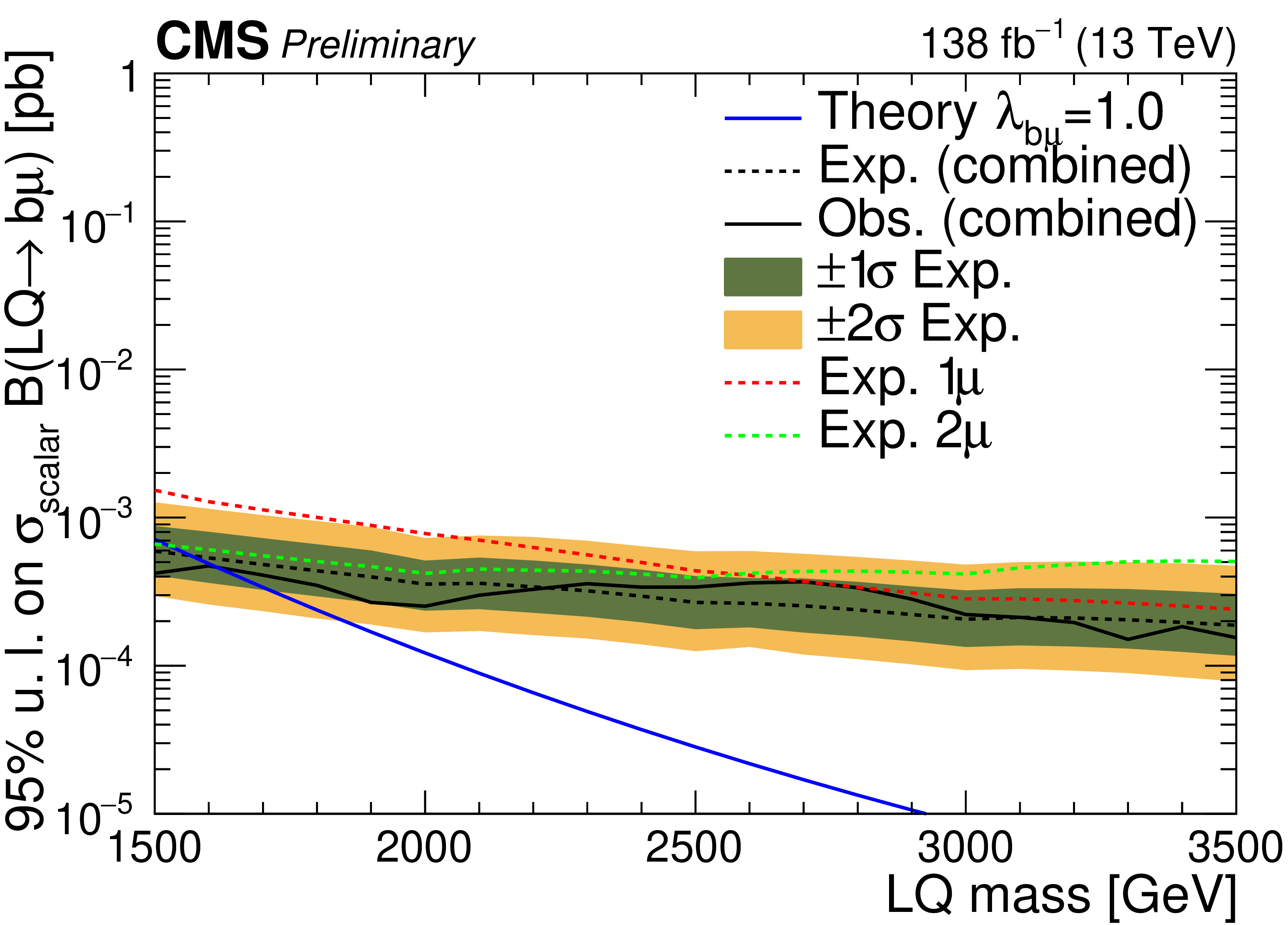
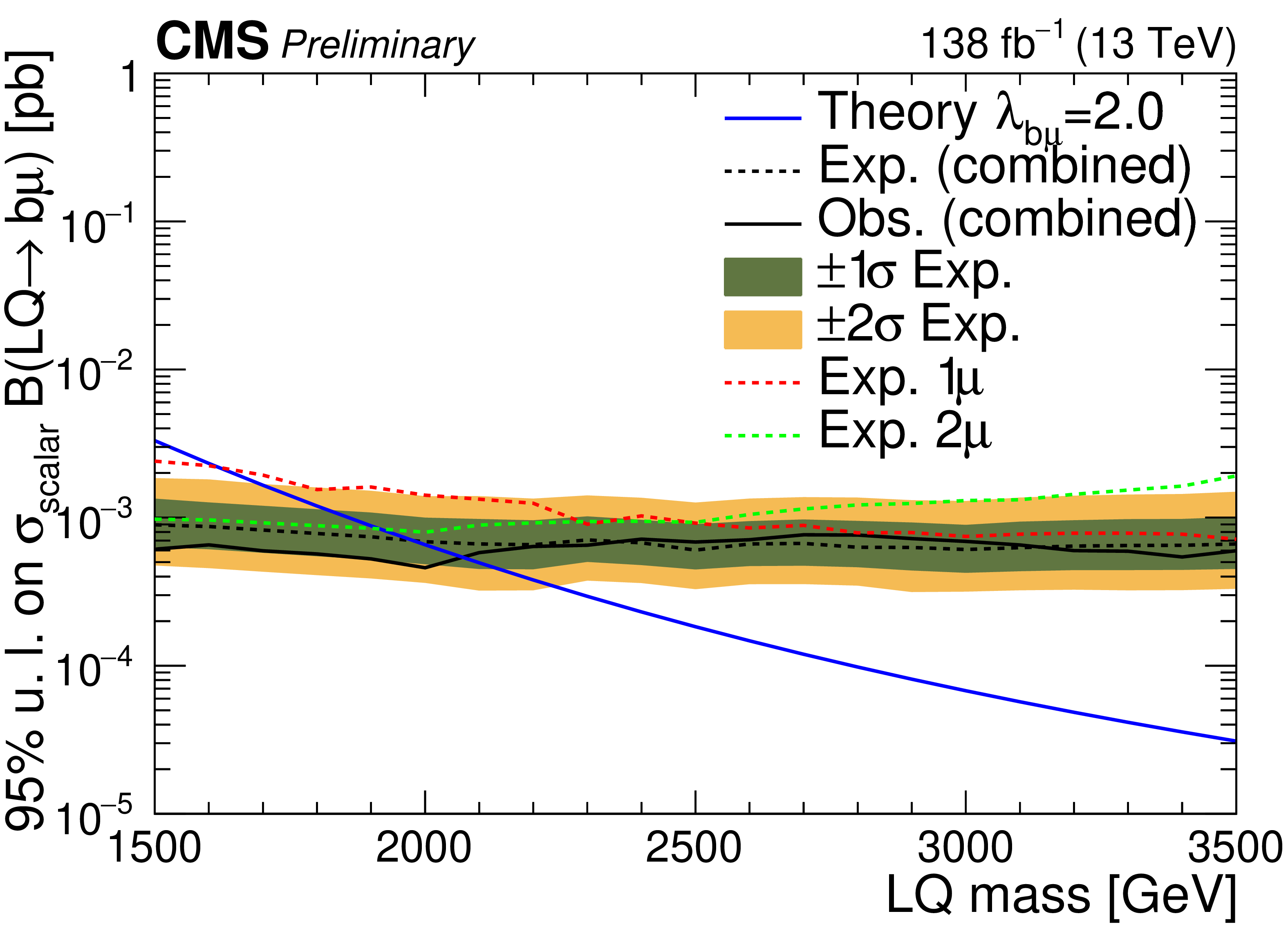
Figure 6:
Expected and observed 95$ % $ CL upper limits on $\sigma(\text{LQ}) \times \text{BR}$ as a function of $M_{\text{LQ}} $ are shown, respectively, with a dashed and solid black line, for fixed $\lambda_{\mathrm{u}\mu} =$ 1 ($\lambda_{\mathrm{u}\mu} = $ 2) on the upper left (upper right). Uncertainty bands ($\pm$1$\sigma$, $\pm$2$\sigma $) on expected limits are also shown. Expected limits for the 1 (2) muon category are also shown with a red (green) dashed line. The same results are shown in the lower plots for the heavy quark scenario. |
png pdf |
Figure 6-a:
Expected and observed 95$ % $ CL upper limits on $\sigma(\text{LQ}) \times \text{BR}$ as a function of $M_{\text{LQ}} $ are shown, respectively, with a dashed and solid black line, for fixed $\lambda_{\mathrm{u}\mu} =$ 1 ($\lambda_{\mathrm{u}\mu} = $ 2) on the upper left (upper right). Uncertainty bands ($\pm$1$\sigma$, $\pm$2$\sigma $) on expected limits are also shown. Expected limits for the 1 (2) muon category are also shown with a red (green) dashed line. The same results are shown in the lower plots for the heavy quark scenario. |
png pdf |
Figure 6-b:
Expected and observed 95$ % $ CL upper limits on $\sigma(\text{LQ}) \times \text{BR}$ as a function of $M_{\text{LQ}} $ are shown, respectively, with a dashed and solid black line, for fixed $\lambda_{\mathrm{u}\mu} =$ 1 ($\lambda_{\mathrm{u}\mu} = $ 2) on the upper left (upper right). Uncertainty bands ($\pm$1$\sigma$, $\pm$2$\sigma $) on expected limits are also shown. Expected limits for the 1 (2) muon category are also shown with a red (green) dashed line. The same results are shown in the lower plots for the heavy quark scenario. |
png pdf |
Figure 6-c:
Expected and observed 95$ % $ CL upper limits on $\sigma(\text{LQ}) \times \text{BR}$ as a function of $M_{\text{LQ}} $ are shown, respectively, with a dashed and solid black line, for fixed $\lambda_{\mathrm{u}\mu} =$ 1 ($\lambda_{\mathrm{u}\mu} = $ 2) on the upper left (upper right). Uncertainty bands ($\pm$1$\sigma$, $\pm$2$\sigma $) on expected limits are also shown. Expected limits for the 1 (2) muon category are also shown with a red (green) dashed line. The same results are shown in the lower plots for the heavy quark scenario. |
png pdf |
Figure 6-d:
Expected and observed 95$ % $ CL upper limits on $\sigma(\text{LQ}) \times \text{BR}$ as a function of $M_{\text{LQ}} $ are shown, respectively, with a dashed and solid black line, for fixed $\lambda_{\mathrm{u}\mu} =$ 1 ($\lambda_{\mathrm{u}\mu} = $ 2) on the upper left (upper right). Uncertainty bands ($\pm$1$\sigma$, $\pm$2$\sigma $) on expected limits are also shown. Expected limits for the 1 (2) muon category are also shown with a red (green) dashed line. The same results are shown in the lower plots for the heavy quark scenario. |
png pdf |
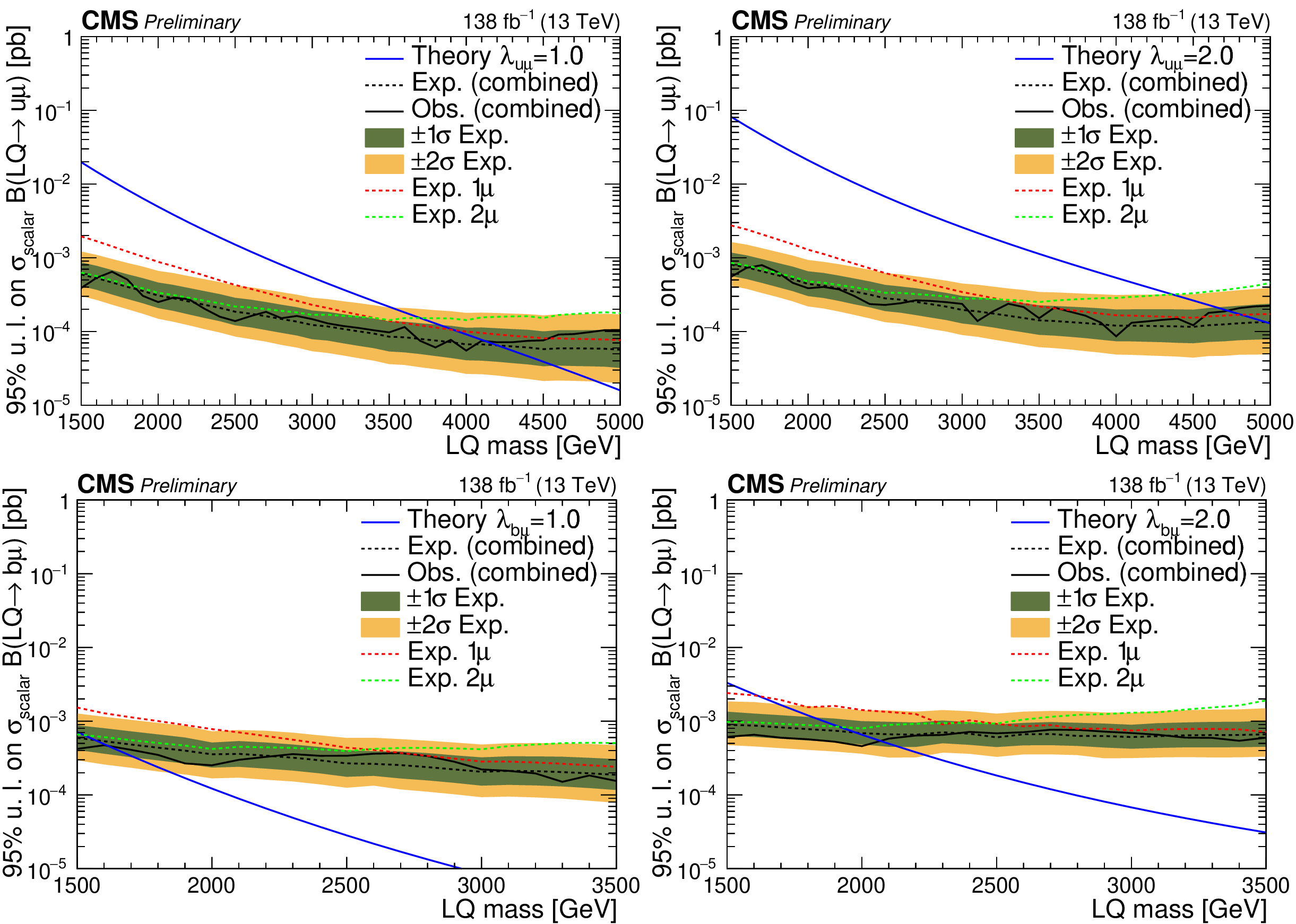
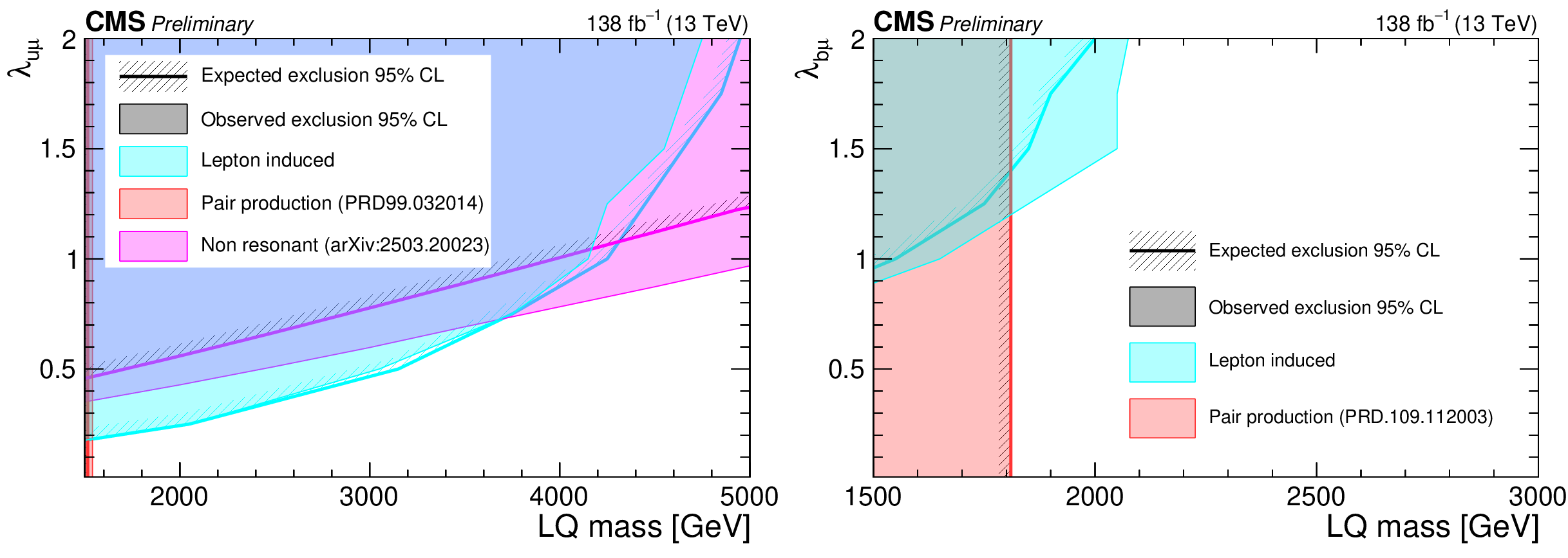
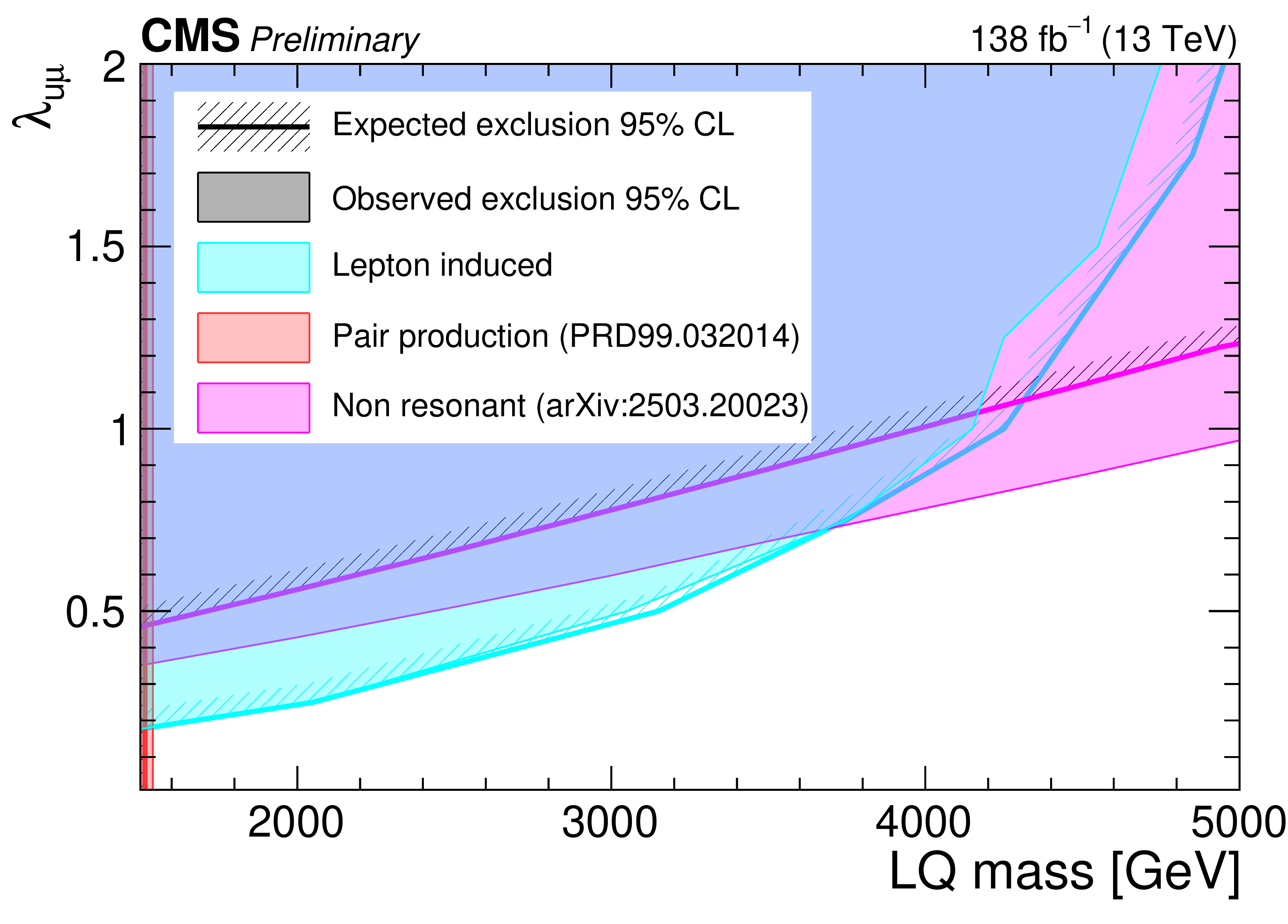
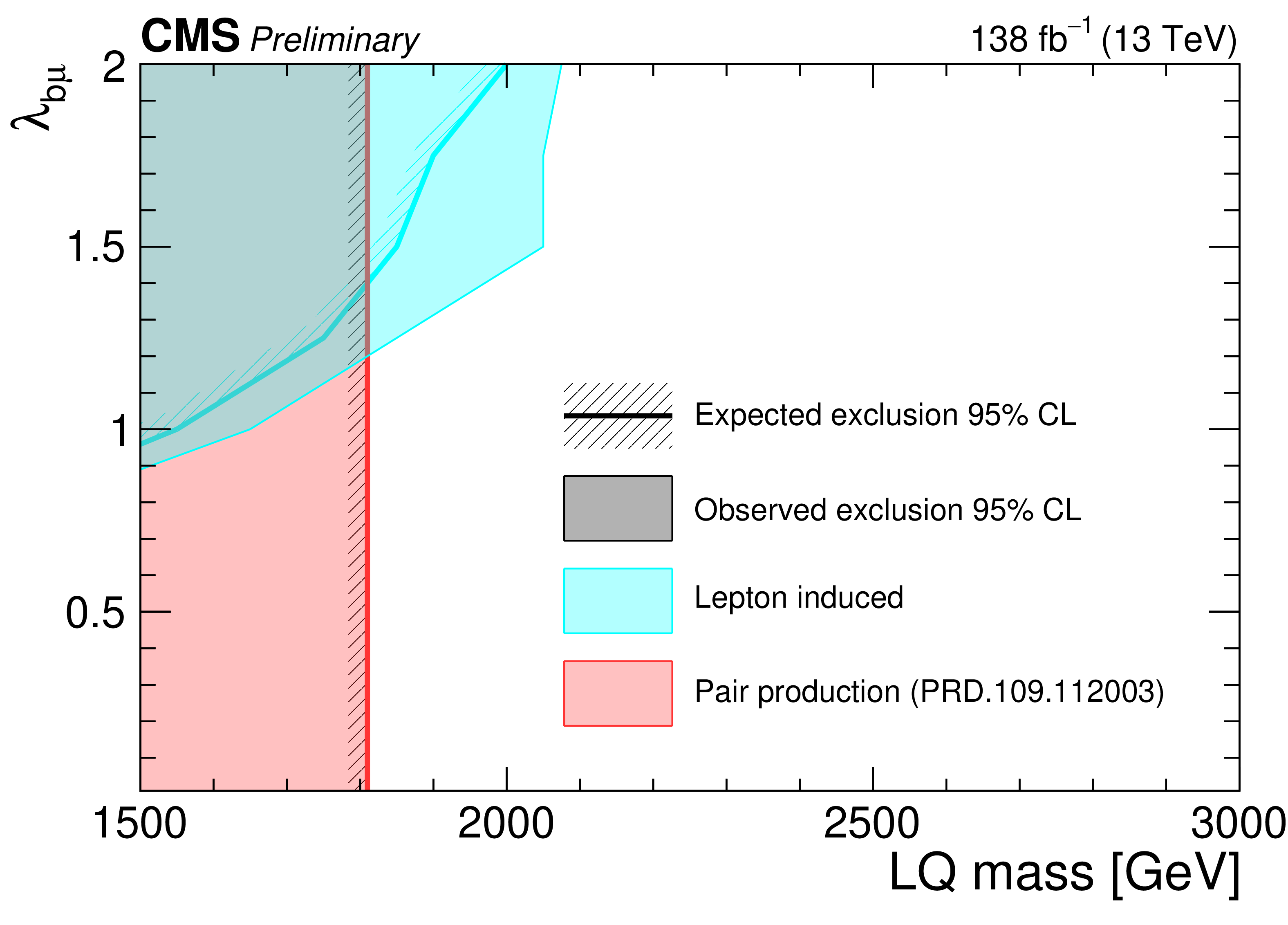
Figure 7:
Expected and observed 95% CL upper limits on $\sigma(\text{LQ}) $, as a function of $\lambda_{\mathrm{u}\mu} $ ($\lambda_{\mathrm{b}\mu} $) vs. $M_{\text{LQ}} $, for a LQ decaying into muons and light (heavy) quark on the left (right). For the light quark model the excluded regions are compared with those obtained from previous CMS searches [70,71]. This analysis improves the CMS sensitivity in the high mass (1.5 TeV $< M_{\text{LQ}} < $ 3.6 TeV) and high coupling (0.2 $< \lambda < $ 0.6) regions of the parameter space. For the heavy quark model, the excluded regions are compared with those obtained from previous CMS searches [69]. This analysis improves the CMS sensitivity in the high mass ($M_{\text{LQ}}>1.8 $) TeV and high coupling ($\lambda> $ 1) regions of the parameter space. |
png pdf |
Figure 7-a:
Expected and observed 95% CL upper limits on $\sigma(\text{LQ}) $, as a function of $\lambda_{\mathrm{u}\mu} $ ($\lambda_{\mathrm{b}\mu} $) vs. $M_{\text{LQ}} $, for a LQ decaying into muons and light (heavy) quark on the left (right). For the light quark model the excluded regions are compared with those obtained from previous CMS searches [70,71]. This analysis improves the CMS sensitivity in the high mass (1.5 TeV $< M_{\text{LQ}} < $ 3.6 TeV) and high coupling (0.2 $< \lambda < $ 0.6) regions of the parameter space. For the heavy quark model, the excluded regions are compared with those obtained from previous CMS searches [69]. This analysis improves the CMS sensitivity in the high mass ($M_{\text{LQ}}>1.8 $) TeV and high coupling ($\lambda> $ 1) regions of the parameter space. |
png pdf |
Figure 7-b:
Expected and observed 95% CL upper limits on $\sigma(\text{LQ}) $, as a function of $\lambda_{\mathrm{u}\mu} $ ($\lambda_{\mathrm{b}\mu} $) vs. $M_{\text{LQ}} $, for a LQ decaying into muons and light (heavy) quark on the left (right). For the light quark model the excluded regions are compared with those obtained from previous CMS searches [70,71]. This analysis improves the CMS sensitivity in the high mass (1.5 TeV $< M_{\text{LQ}} < $ 3.6 TeV) and high coupling (0.2 $< \lambda < $ 0.6) regions of the parameter space. For the heavy quark model, the excluded regions are compared with those obtained from previous CMS searches [69]. This analysis improves the CMS sensitivity in the high mass ($M_{\text{LQ}}>1.8 $) TeV and high coupling ($\lambda> $ 1) regions of the parameter space. |
| Tables | |
png pdf |
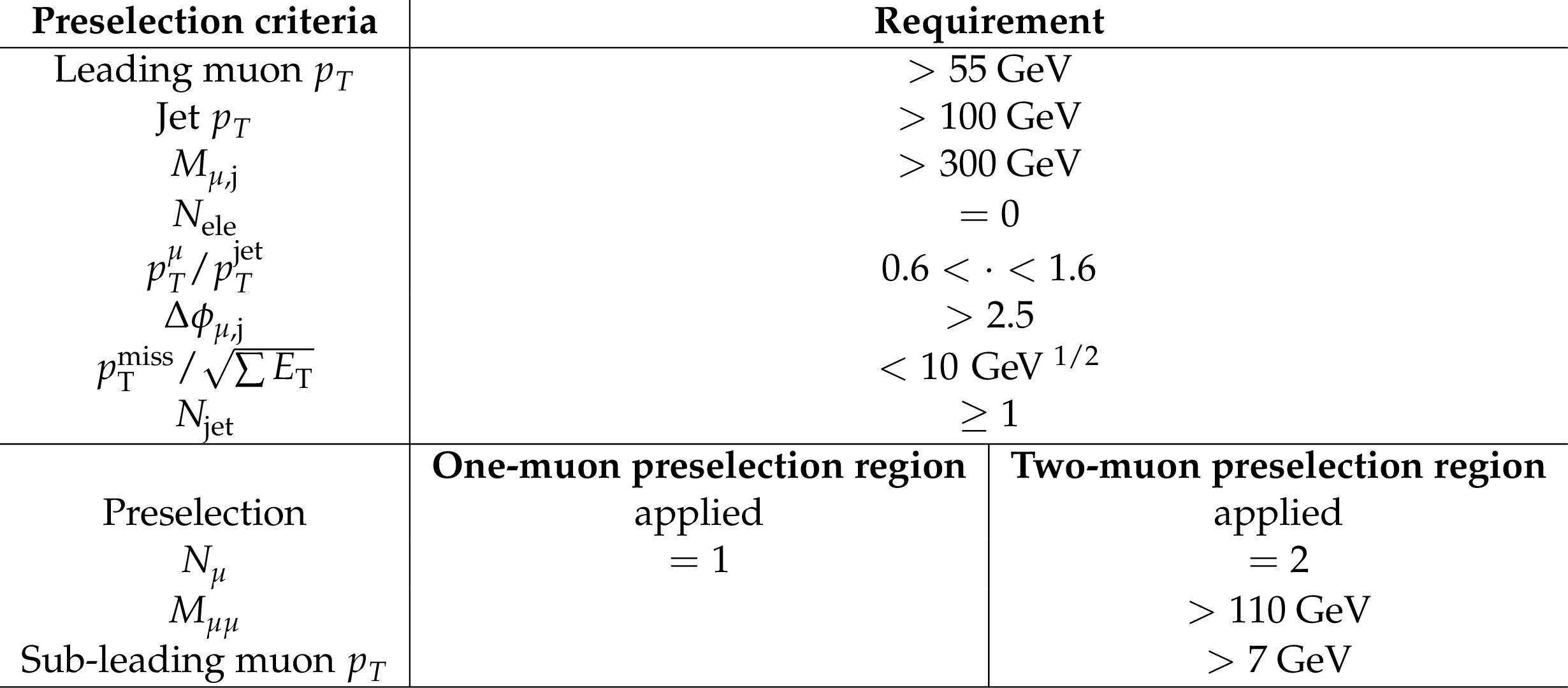
Table 1:
Preselection region for both channels. |
png pdf |
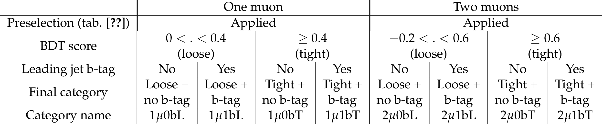
Table 2:
Final category selection for the signal regions. |
| Summary |
| This note presents a novel search for physics beyond the standard model using 138 fb$ ^{-1} $ of proton-proton collision data collected by the CMS experiment at the CERN LHC. The analysis extends the search for leptoquarks coupling to muons by exploiting a new production mechanism that leverages the charged lepton content of protons arising from quantum fluctuations. This mechanism enables the study of lepton-induced processes and resonant single leptoquark production and decay at the LHC. Upper limits on the product of the leptoquark production cross section and branching fraction to a muon-quark final state are derived, excluding leptoquarks with masses between 1.5 and 3.6 TeV and couplings between 0.2 and 0.6 for the light quark scenario, and masses above 1.8 TeV and couplings above 1 for the heavy quark scenario. These results significantly extend the mass and coupling range probed by previous searches in other production modes. |
| References | ||||
| 1 | J. C. Pati and A. Salam | Lepton number as the fourth color | PRD 10 (1974) 275 | |
| 2 | H. Georgi and S. L. Glashow | Unity of all elementary-particle forces | PRL 32 (1974) 438 | |
| 3 | H. Fritzsch and P. Minkowski | Unified interactions of leptons and hadrons | Annals of Physics 93 (1975) 193 | |
| 4 | J. C. Pati and A. Salam | Unified lepton-hadron symmetry and a gauge theory of the basic interactions | PRD 8 (1973) 1240 | |
| 5 | G. Senjanovic and A. Sokorac | Light Leptoquarks in SO(10) | Z. Phys. C 20 (1983) 255 | |
| 6 | P. H. Frampton and B.-H. Lee | Su(15) grand unification | PRL 64 (1990) 619 | |
| 7 | P. H. Frampton and T. W. Kephart | Higgs sector and proton decay in su(15) grand unification | PRD 42 (1990) 3892 | |
| 8 | H. Murayama and T. Yanagida | A viable SU(5) GUT with light leptoquark bosons | Mod. Phys. Lett. A 7 (1992) 147 | |
| 9 | B. Schrempp and F. Schrempp | Light leptoquarks | PLB 153 (1985) 101 | |
| 10 | S. Dimopoulos and L. Susskind | Mass generation by non-strong interactions | NPB 191 (1981) 370 | |
| 11 | S. Dimopoulos | Technicoloured signatures | NPB 168 (1980) 69 | |
| 12 | J. L. Hewett and T. G. Rizzo | Low-energy phenomenology of superstring-inspired e6 models | PR 183 (1989) 193 | |
| 13 | A. Neveu and J. H. Schwarz | Factorizable dual model of pions | NPB 31 (1971) 86 | |
| 14 | Y. A. Golfand and E. P. Likhtman | Extension of the Algebra of Poincare Group Generators and Violation of p Invariance | JETP Lett. 13 (1971) 323 | |
| 15 | P. Ramond | Dual Theory for Free Fermions | PRD 3 (1971) 2415 | |
| 16 | D. V. Volkov and V. P. Akulov | Possible universal neutrino interaction | volume 16, 1972 link |
|
| 17 | J. Wess and B. Zumino | Supergauge transformations in four dimensions | NPB 70 (1974) 39 | |
| 18 | P. Fayet | Supergauge invariant extension of the higgs mechanism and a model for the electron and its neutrino | NPB 90 (1975) 104 | |
| 19 | G. R. Farrar and P. Fayet | Phenomenology of the production, decay, and detection of new hadronic states associated with supersymmetry | PLB 76 (1978) 575 | |
| 20 | H. P. Nilles | Supersymmetry, supergravity and particle physics | PR 110 (1984) 1 | |
| 21 | R. Barbier et al. | R-parity-violating supersymmetry | PR 420 (2005) 1 | hep-ph/0406039 |
| 22 | CMS Collaboration | Search for scalar leptoquarks produced via $ \tau $-lepton--quark scattering in $ pp $ collisions at $ \sqrt{s}=13\text{ }\text{ }\mathrm{TeV} $ | PRL 132 (2024) 061801 | CMS-EXO-22-018 2308.06143 |
| 23 | L. Buonocore, P. Nason, F. Tramontano, and G. Zanderighi | Leptons in the proton | JHEP 2020 (2020) | 2005.06477 |
| 24 | A. Manohar, P. Nason, G. P. Salam, and G. Zanderighi | How bright is the proton? a precise determination of the photon parton distribution function | PRL 117 (2016) 242002 | 1607.04266 |
| 25 | A. V. Manohar, P. Nason, G. P. Salam, and G. Zanderighi | The photon content of the proton | JHEP 2017 (2017) | 1708.01256 |
| 26 | L. Buonocore et al. | Lepton-quark collisions at the large hadron collider | PRL 125 (2020) 231804 | 2005.06475 |
| 27 | A. Greljo and N. Selimovic | Lepton-quark fusion at hadron colliders, precisely | (03, ) 1, 2021 JHEP 202 (2021) 1 |
2012.02092 |
| 28 | L. Buonocore et al. | Resonant leptoquark at nlo with powheg | JHEP 2022 (2022) | 2209.02599 |
| 29 | CMS Collaboration | The CMS experiment at the CERN LHC | JINST 3 (2008) S08004 | |
| 30 | CMS Collaboration | Development of the CMS detector for the CERN LHC Run 3 | Accepted by JINST, 2023 | CMS-PRF-21-001 2309.05466 |
| 31 | CMS Collaboration | Performance of the CMS Level-1 trigger in proton-proton collisions at $ \sqrt{s} = $ 13 TeV | JINST 15 (2020) P10017 | CMS-TRG-17-001 2006.10165 |
| 32 | CMS Collaboration | The CMS trigger system | JINST 12 (2017) P01020 | CMS-TRG-12-001 1609.02366 |
| 33 | CMS Collaboration | Technical proposal for the Phase-II upgrade of the Compact Muon Solenoid | CMS Technical Proposal CERN-LHCC-2015-010, CMS-TDR-15-02, 2015 CDS |
|
| 34 | CMS Collaboration | Particle-flow reconstruction and global event description with the CMS detector | JINST 12 (2017) P10003 | CMS-PRF-14-001 1706.04965 |
| 35 | M. Cacciari, G. P. Salam, and G. Soyez | The anti-$ k_{\mathrm{T}} $ jet clustering algorithm | JHEP 04 (2008) 063 | 0802.1189 |
| 36 | M. Cacciari, G. P. Salam, and G. Soyez | FastJet user manual | EPJC 72 (2012) 1896 | 1111.6097 |
| 37 | CMS Collaboration | Pileup mitigation at CMS in 13 TeV data | JINST 15 (2020) P09018 | CMS-JME-18-001 2003.00503 |
| 38 | D. Bertolini, P. Harris, M. Low, and N. Tran | Pileup per particle identification | JHEP 10 (2014) 059 | 1407.6013 |
| 39 | CMS Collaboration | Jet energy scale and resolution in the CMS experiment in pp collisions at 8 TeV | JINST 12 (2017) P02014 | CMS-JME-13-004 1607.03663 |
| 40 | E. Bols et al. | Jet flavour classification using DeepJet | JINST 15 (2020) P12012 | 2008.10519 |
| 41 | CMS Collaboration | Performance of the DeepJet b tagging algorithm using 41.9/fb of data from proton-proton collisions at 13 TeV with Phase 1 CMS detector | CMS Detector Performance Note CMS-DP-2018-058, 2018 CDS |
|
| 42 | CMS Collaboration | Performance of the CMS muon detector and muon reconstruction with proton-proton collisions at $ \sqrt{s}= $ 13 TeV | JINST 13 (2018) P06015 | CMS-MUO-16-001 1804.04528 |
| 43 | CMS Collaboration | Performance of missing transverse momentum reconstruction in proton-proton collisions at $ \sqrt{s} = $ 13 TeV using the CMS detector | JINST 14 (2019) P07004 | CMS-JME-17-001 1903.06078 |
| 44 | CMS Collaboration | Precision luminosity measurement in proton-proton collisions at $ \sqrt{s} = $ 13 TeV in 2015 and 2016 at CMS | EPJC 81 (2021) 800 | CMS-LUM-17-003 2104.01927 |
| 45 | CMS Collaboration | CMS luminosity measurement for the 2017 data-taking period at $ \sqrt{s} = $ 13 TeV | CMS Physics Analysis Summary, 2018 link |
CMS-PAS-LUM-17-004 |
| 46 | CMS Collaboration | CMS luminosity measurement for the 2018 data-taking period at $ \sqrt{s} = $ 13 TeV | CMS Physics Analysis Summary, 2019 link |
CMS-PAS-LUM-18-002 |
| 47 | P. Nason | A new method for combining nlo qcd with shower monte carlo algorithms | JHEP 2004 (2004) 040 | hep-ph/0409146 |
| 48 | S. Alioli, P. Nason, C. Oleari, and E. Re | Nlo higgs boson production via gluon fusion matched with shower in powheg | Journal of High Energy Physics (apr, ) 002, 2009 link |
0812.0578 |
| 49 | S. Alioli, P. Nason, C. Oleari, and E. Re | A general framework for implementing nlo calculations in shower monte carlo programs: the powheg box | JHEP 2010 (2010) | 1002.2581 |
| 50 | S. Alioli et al. | Jet pair production in powheg | JHEP 2011 (2011) | 1012.3380 |
| 51 | S. Frixione, P. Nason, and C. Oleari | Matching nlo qcd computations with parton shower simulations: the powheg method | JHEP 2007 (2007) 070 | 0709.2092 |
| 52 | M. Bahr et al. | Herwig++ Physics and Manual | EPJC 58 (2008) 639 | 0803.0883 |
| 53 | J. Bellm et al. | Herwig++ 2.7 Release Note | 10, 2013 | 1310.6877 |
| 54 | J. Alwall et al. | The automated computation of tree-level and next-to-leading order differential cross sections, and their matching to parton shower simulations | JHEP 2014 (2014) | 1405.0301 |
| 55 | CMS Collaboration | Extraction and validation of a new set of cms pythia8 tunes from underlying-event measurements | EPJC 80 (2020) | CMS-GEN-17-001 1903.12179 |
| 56 | R. D. Ball et al. | Parton distributions from high-precision collider data: Nnpdf collaboration | EPJC 77 (2017) | 1706.00428 |
| 57 | R. D. Ball et al. | Unbiased global determination of parton distributions and their uncertainties at nnlo and at lo | NPB 855 (2012) 153 | 1107.2652 |
| 58 | R. D. Ball et al. | Parton distributions with qed corrections | NPB 877 (2013) 290 | 1308.0598 |
| 59 | GEANT4 Collaboration | Geant4 - a simulation toolkit | Nuclear Instruments and Methods in Physics Research Section A: Accelerators, Spectrometers, 2003 Detectors and Associated Equipment 506 (2003) 250 |
|
| 60 | A. Apresyan on behalf of the CMS Collaboration | Performance of MET reconstruction in CMS | in 16th International Conference on Calorimetry in High Energy Physics () 6-11 April, Giessen, Germany, volume 587, J.Phys.Conf.Ser., feb, 2014 CALOR 201 (2014) 01 |
|
| 61 | Y. Freund and R. E. Schapire | Experiments with a new boosting algorithm | in Proceedings of the Thirteenth International Conference on International Conference on Machine Learning, ICML'96, Morgan Kaufmann Publishers Inc., San Francisco, CA, USA, 1996 | |
| 62 | D. P. Solomatine and D. L. Shrestha | Adaboost.rt: a boosting algorithm for regression problems | in IEEE International Joint Conference on Neural Networks (IEEE Cat. No.04CH37541), number 2 in 2, 2004 link |
|
| 63 | H. Binder, O. Gefeller, M. Schmid, and A. Mayr | The evolution of boosting algorithms: From machine learning to statistical modelling | Methods of Information in Medicine 53 (2014) 419 | 1403.1452 |
| 64 | G. Punzi | Sensitivity of searches for new signals and its optimization | eConf MODT002, 2003 link |
physics/0308063 |
| 65 | CMS Collaboration | Search for high mass dijet resonances with a new background prediction method in proton-proton collisions at $ \sqrt{s} = $ 13 tev | JHEP 2020 (2020) | CMS-EXO-19-012 1911.03947 |
| 66 | CMS Collaboration | Search for narrow and broad dijet resonances in proton-proton collisions at $ \sqrt{s}= $ 13 tev and constraints on dark matter mediators and other new particles | JHEP 2018 (2018) | CMS-EXO-16-056 1806.00843 |
| 67 | CMS Collaboration | Search for Narrow Resonances using the Dijet Mass Spectrum in pp Collisions at sqrt s of 7 TeV | technical report, CERN, Geneva, 2012 CDS |
|
| 68 | A. L. Read | Linear interpolation of histograms | Nuclear Instruments and Methods in Physics Research Section A: Accelerators, Spectrometers, 1999 Detectors and Associated Equipment 425 (1999) 357 |
|
| 69 | CMS Collaboration | Search for pair production of scalar and vector leptoquarks decaying to muons and bottom quarks in proton-proton collisions at $ \sqrt{s}=13\text{ }\text{ }\mathrm{TeV} $ | PRD 109 (2024) 112003 | 2401.04795 |
| 70 | CMS Collaboration | Search for pair production of second-generation leptoquarks at $ \sqrt{s}= $13 tev | Physical Review D 99 (2019) | CMS-EXO-17-003 1808.05082 |
| 71 | C. Collaboration | Search for $ t $-channel scalar and vector leptoquark exchange in the high-mass dimuon and dielectron spectra in proton-proton collisions at $ \sqrt{s} = $ 13 tev | \url https://arxiv.org/abs/2503.3, 2025 link |
|
| 72 | T. Junk | Confidence level computation for combining searches with small statistics | Nuclear Instruments and Methods in Physics Research Section A: Accelerators, Spectrometers, 1999 Detectors and Associated Equipment 434 (1999) 435 |
hep-ex/9902006 |
| 73 | A. L. Read | Presentation of search results: the cls technique | Journal of Physics G:, 2002 Nuclear and Particle Physics 28 (2002) 2693 |
|
| 74 | ATLAS, CMS, LHC Higgs Combination Group Collaboration | Procedure for the LHC Higgs boson search combination in Summer 2011 | technical report, CERN, Geneva, 2011 | |
|
|
Compact Muon Solenoid LHC, CERN |
|

|

|

|

|

|