

Compact Muon Solenoid
LHC, CERN
| CMS-PAS-EXO-20-013 | ||
| Search for dark matter particles produced in association with a dark Higgs boson decaying into W$^{+}$W$^{-}$ in proton-proton collisions at $\sqrt{s}= $ 13 TeV with the CMS detector | ||
| CMS Collaboration | ||
| July 2021 | ||
| Abstract: A search for dark matter (DM) particles is performed using events with a pair of W bosons and large missing transverse momentum. The analysis is based on proton-proton collision data at a center-of-mass energy of 13 TeV collected by the CMS experiment at the LHC between 2016 and 2018 corresponding to an integrated luminosity of 137 fb$^{-1}$. No significant excess in the W$^{+}$W$^{-}$ dileptonic decay channel over the expected standard model background is observed. Limits are set on DM production in the context of the dark Higgs simplified model, with a dark Higgs mass above the W$^{+}$W$^{-}$ pair mass threshold. | ||
| Links: CDS record (PDF) ; Physics Briefing ; CADI line (restricted) ; | ||
| Figures | |
png pdf |
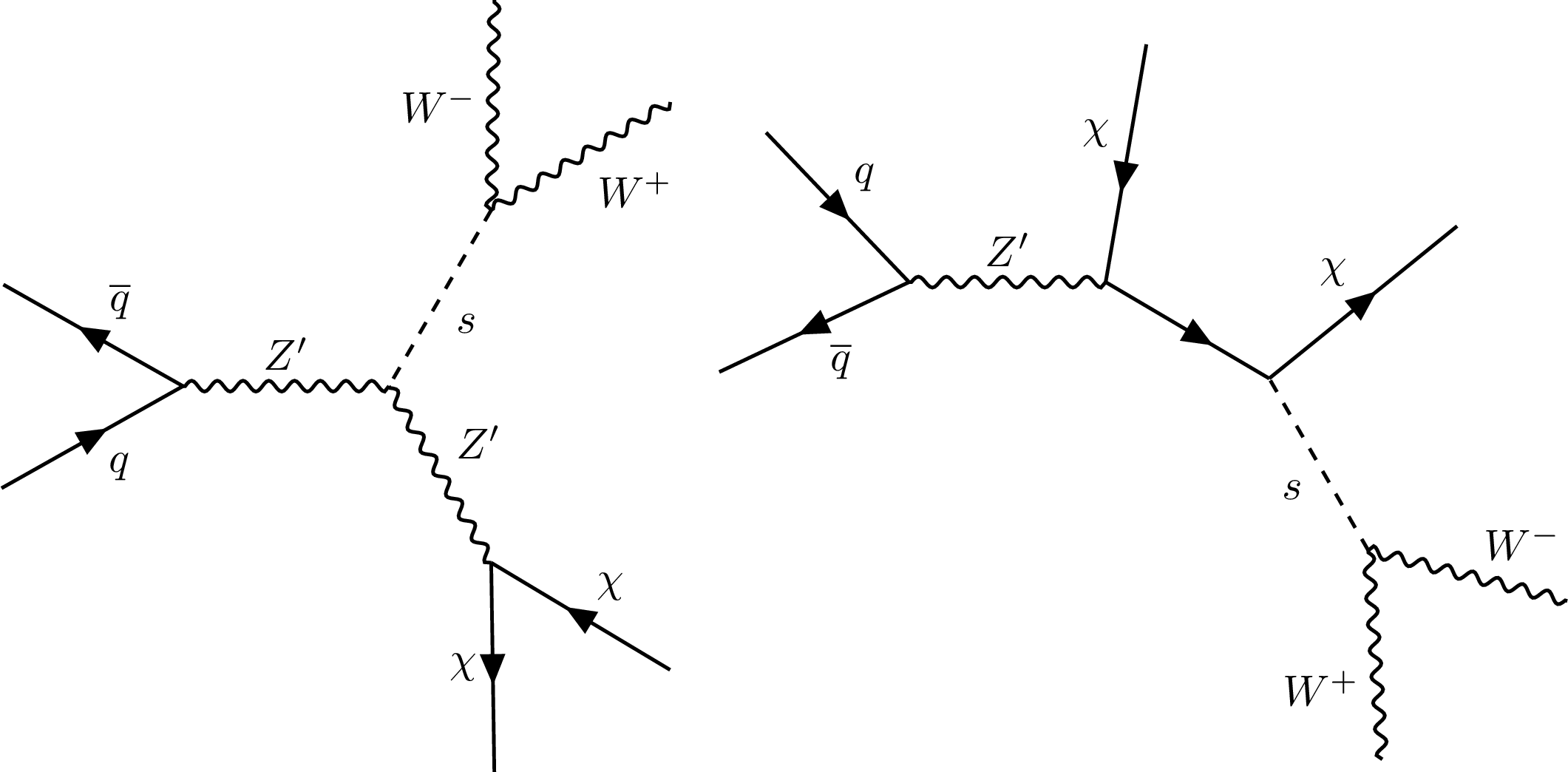
Figure 1:
Representative Born-level Feynman diagrams for the benchmark signal model considered in this note: $q \overline q \to \mathrm{Z'} \to s \chi \chi $, and $s \to \mathrm{W^{+}} \mathrm{W^{-}} $. |
png pdf |
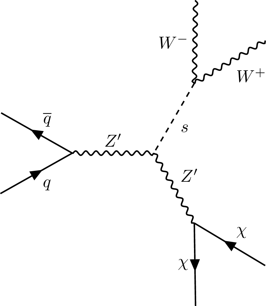
Figure 1-a:
Representative Born-level Feynman diagram for the $q \overline q \to \mathrm{Z'} \to s \chi \chi $ signal model. |
png pdf |
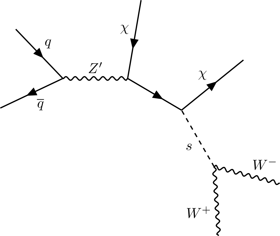
Figure 1-b:
Representative Born-level Feynman diagram for the $s \to \mathrm{W^{+}} \mathrm{W^{-}} $ signal model. |
png pdf |
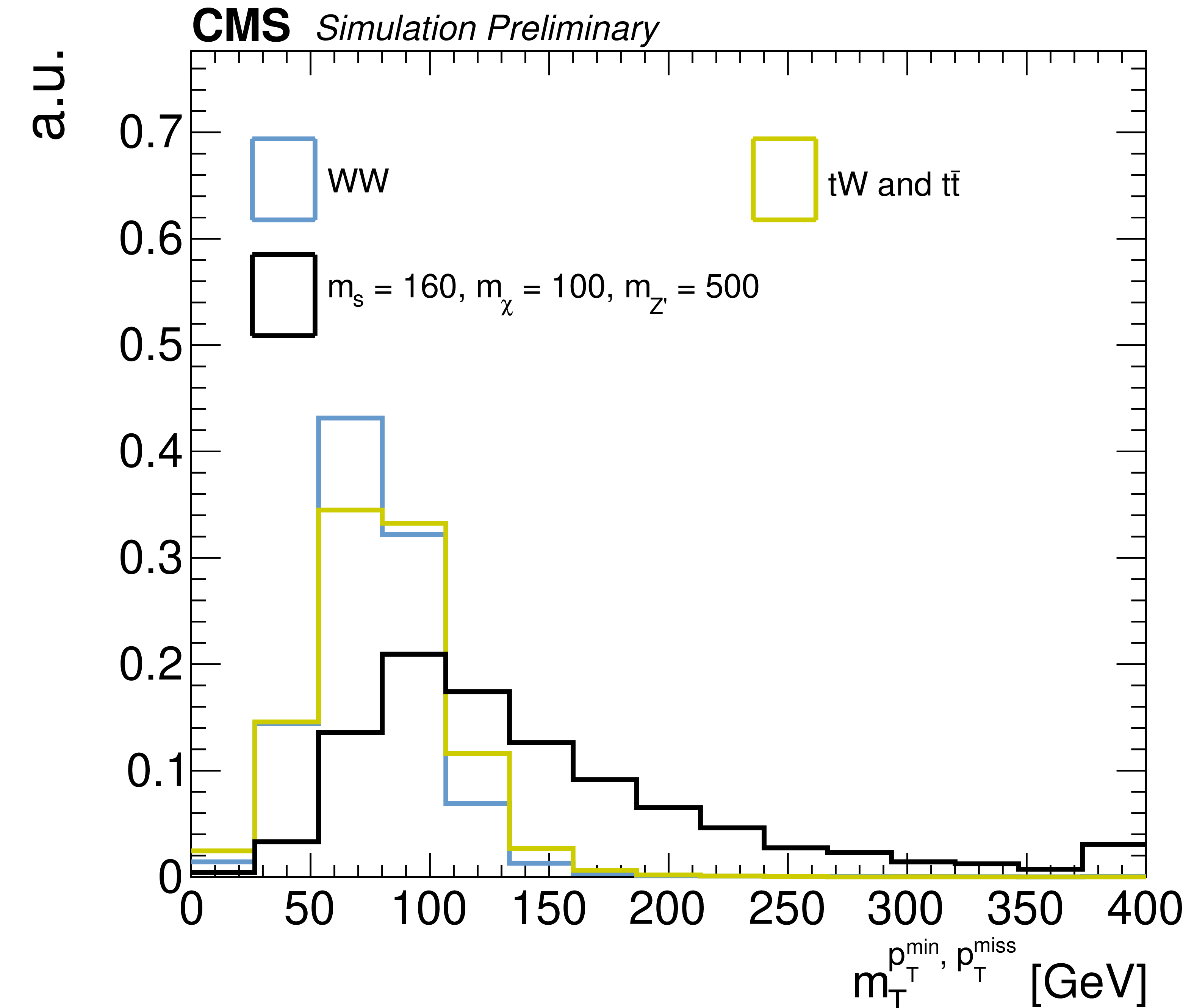
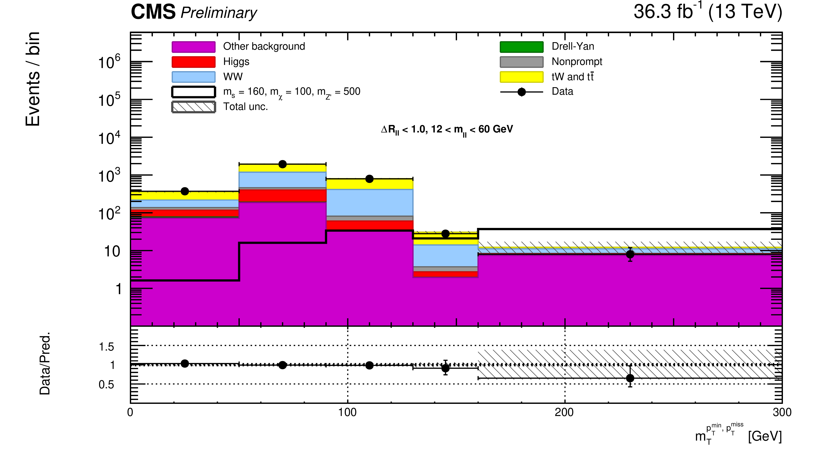
Figure 2:
Normalized $ {{m_{\mathrm {T}}} ^{\ell \text { min},\, {{p_{\mathrm {T}}} ^\text {miss}}}} $ distribution for a signal with $m_{s} = $ 160 GeV, $m_{\chi} = $ 100 GeV, $m_{\mathrm{Z'}} = $ 500 GeV, after the event preselection criteria are applied. Predictions of the two main backgrounds of the analysis, WW and $ {{\mathrm{t} {}\mathrm{\bar{t}}} {}+{}\mathrm{t} \mathrm{W}} $, are shown as blue and yellow solid lines respectively. The last bin includes the overflow. |

png pdf |
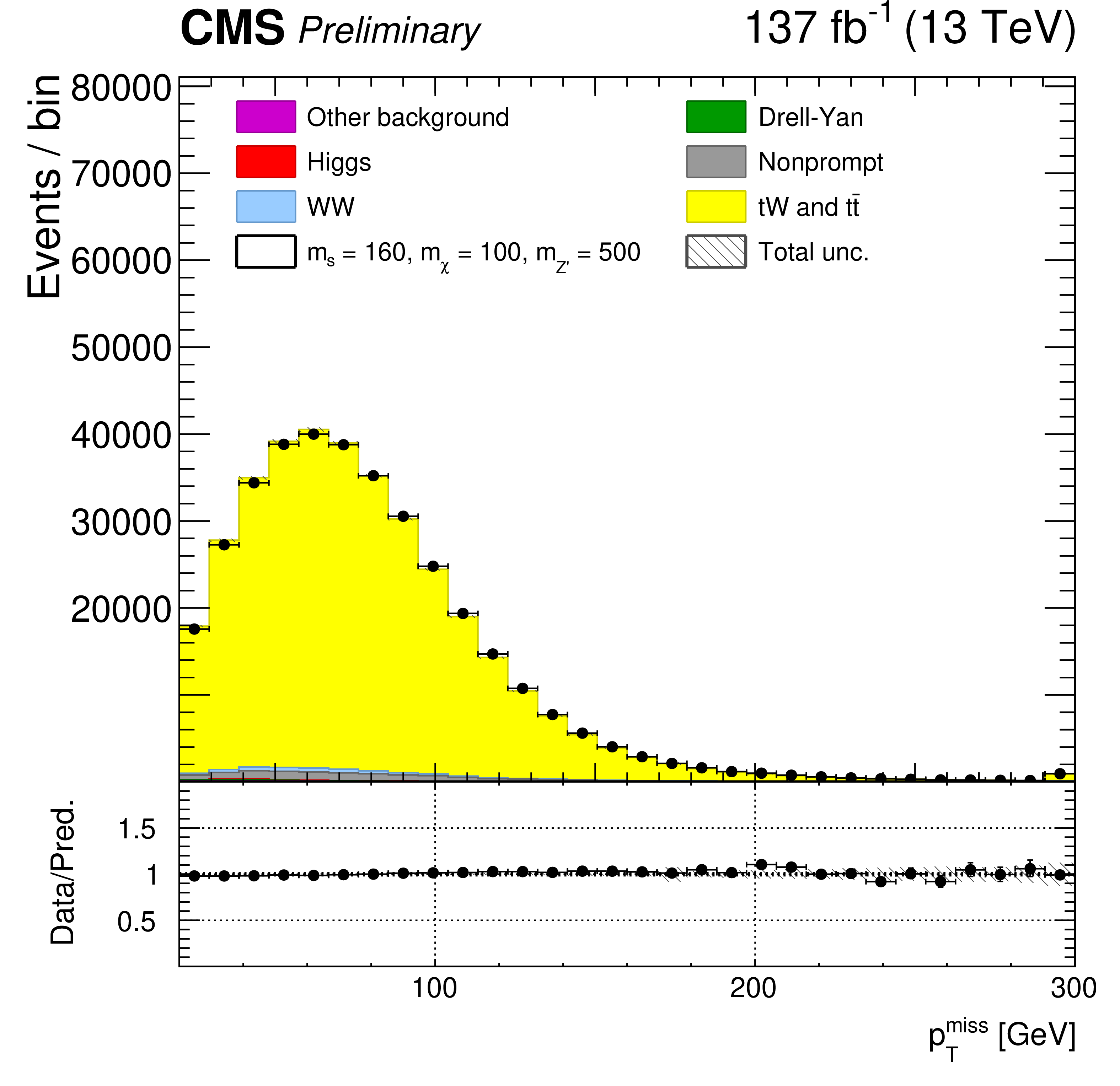
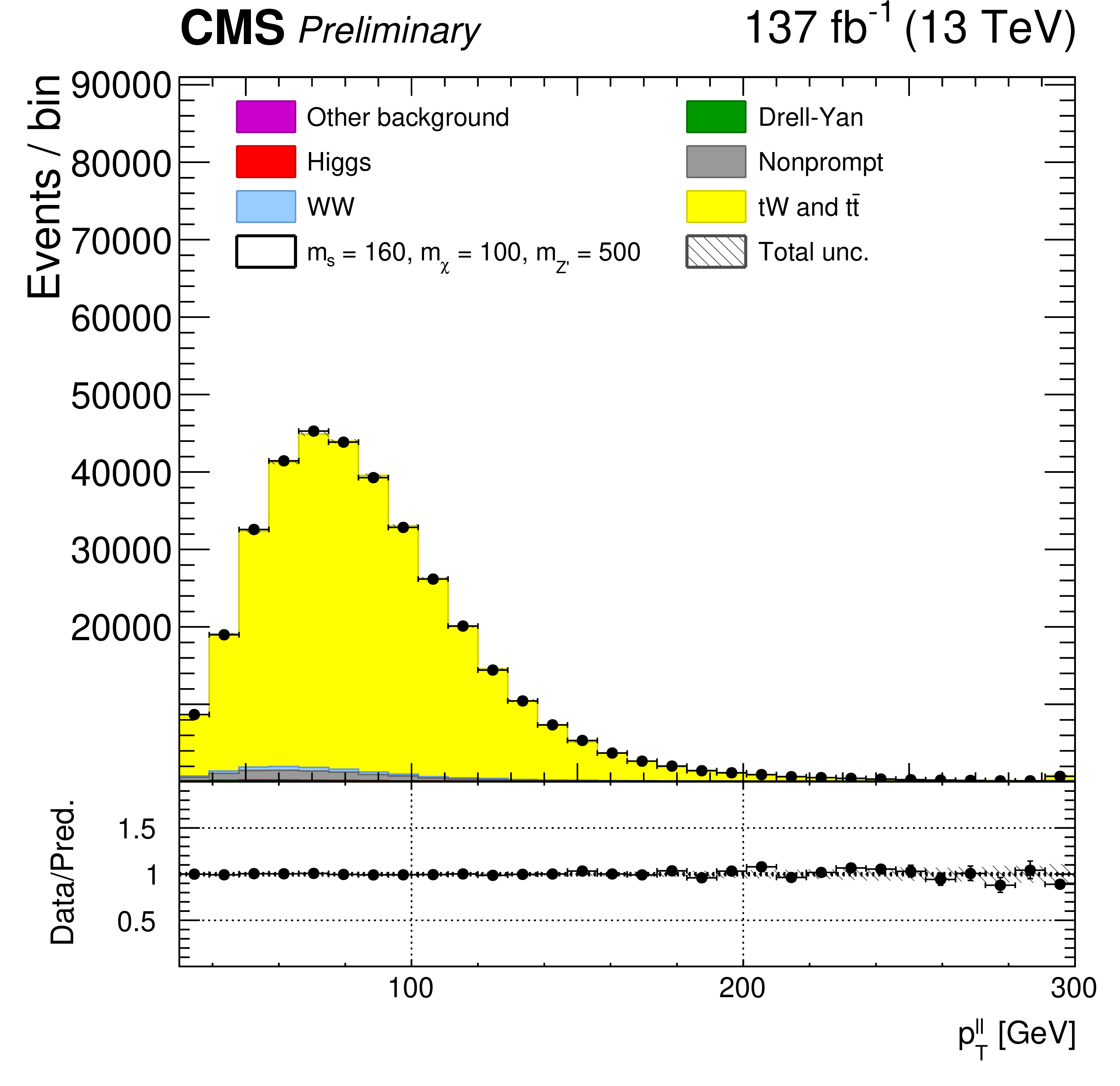
Figure 3:
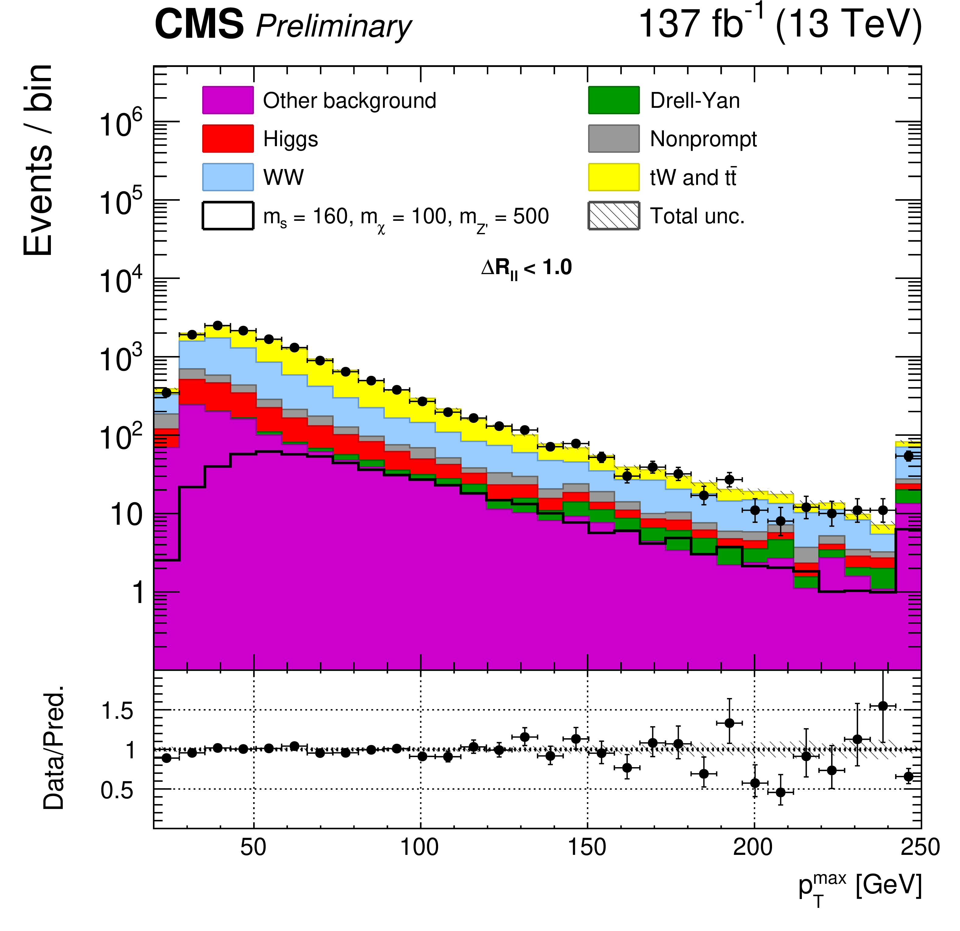
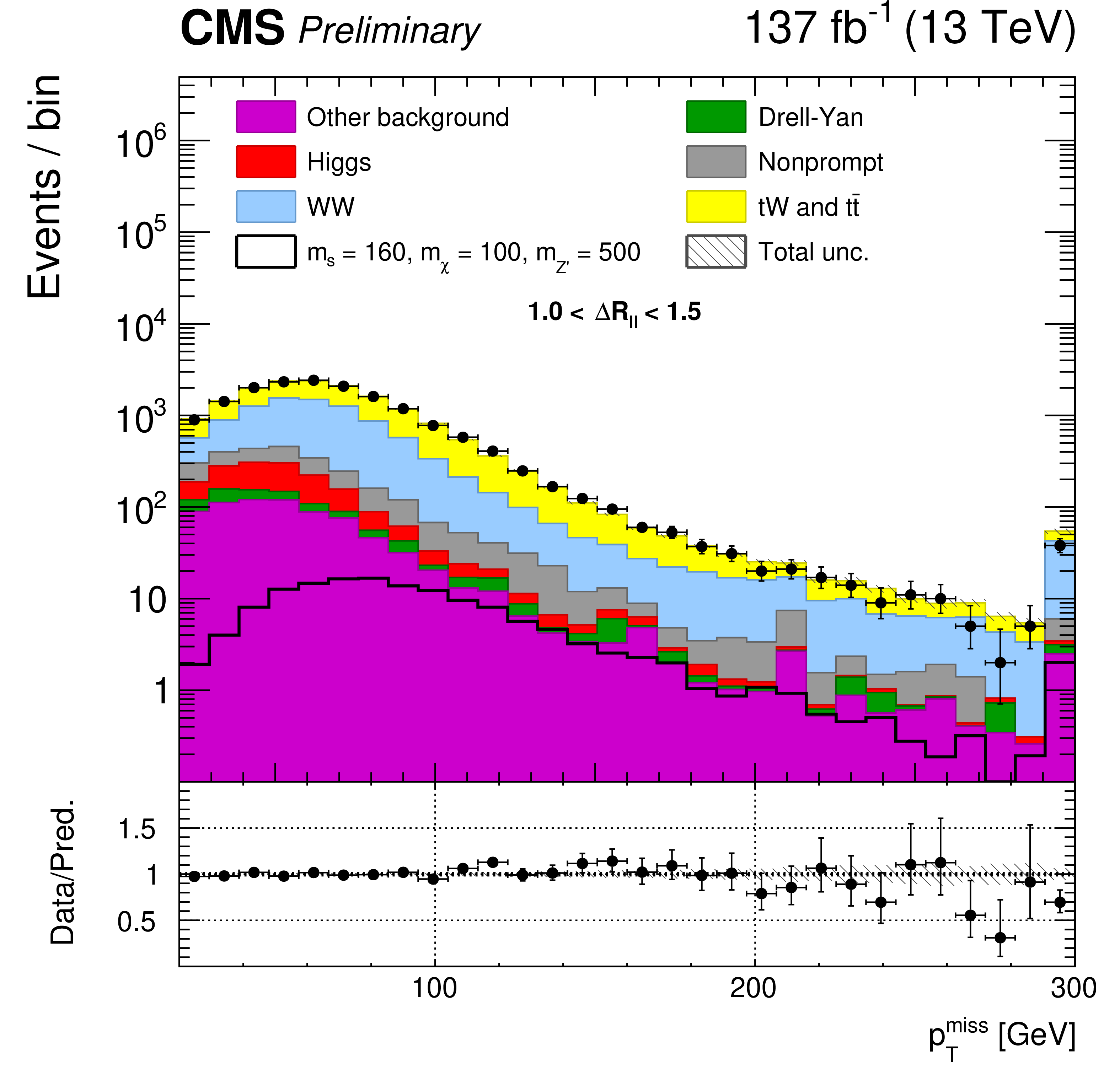
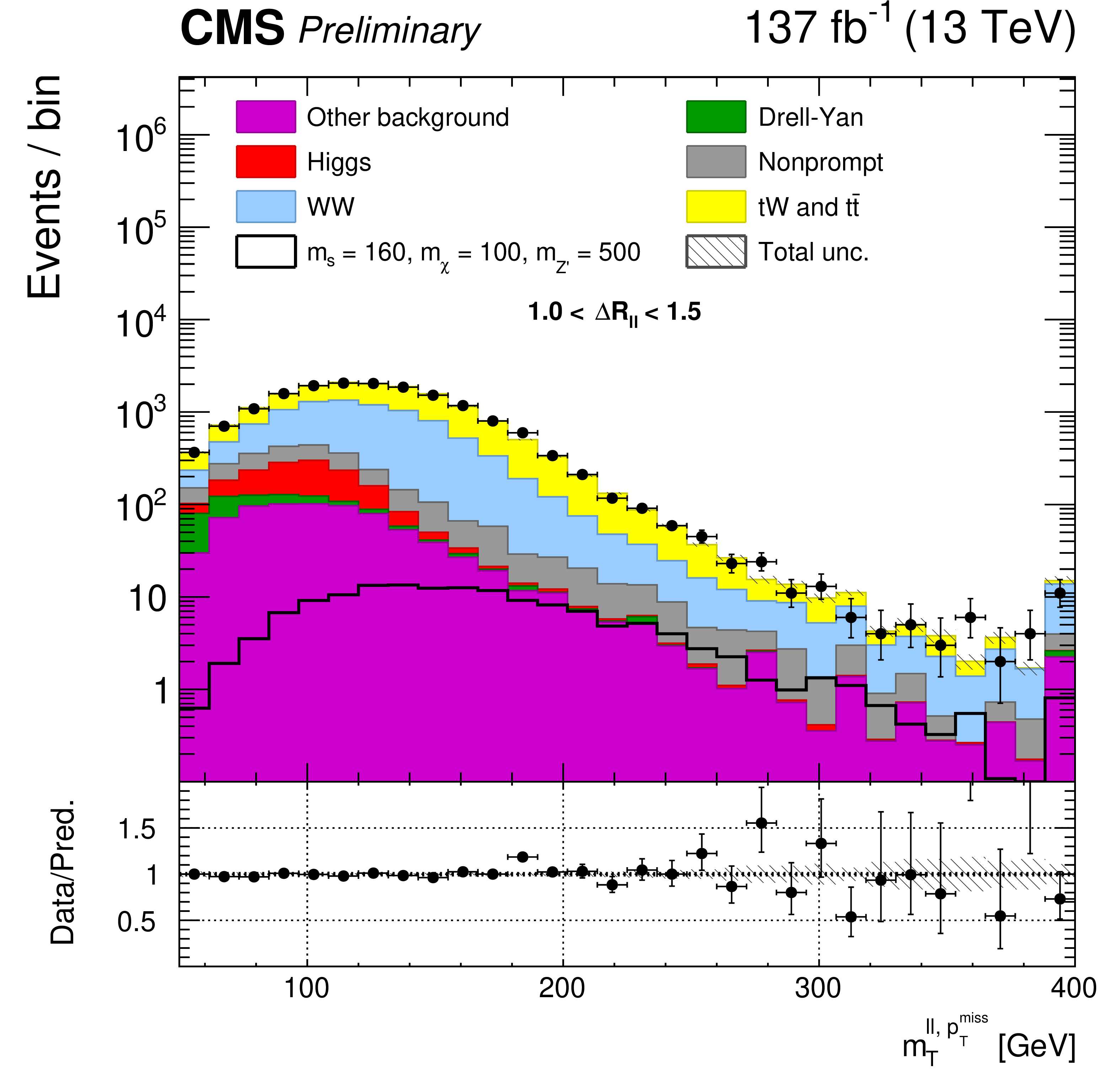
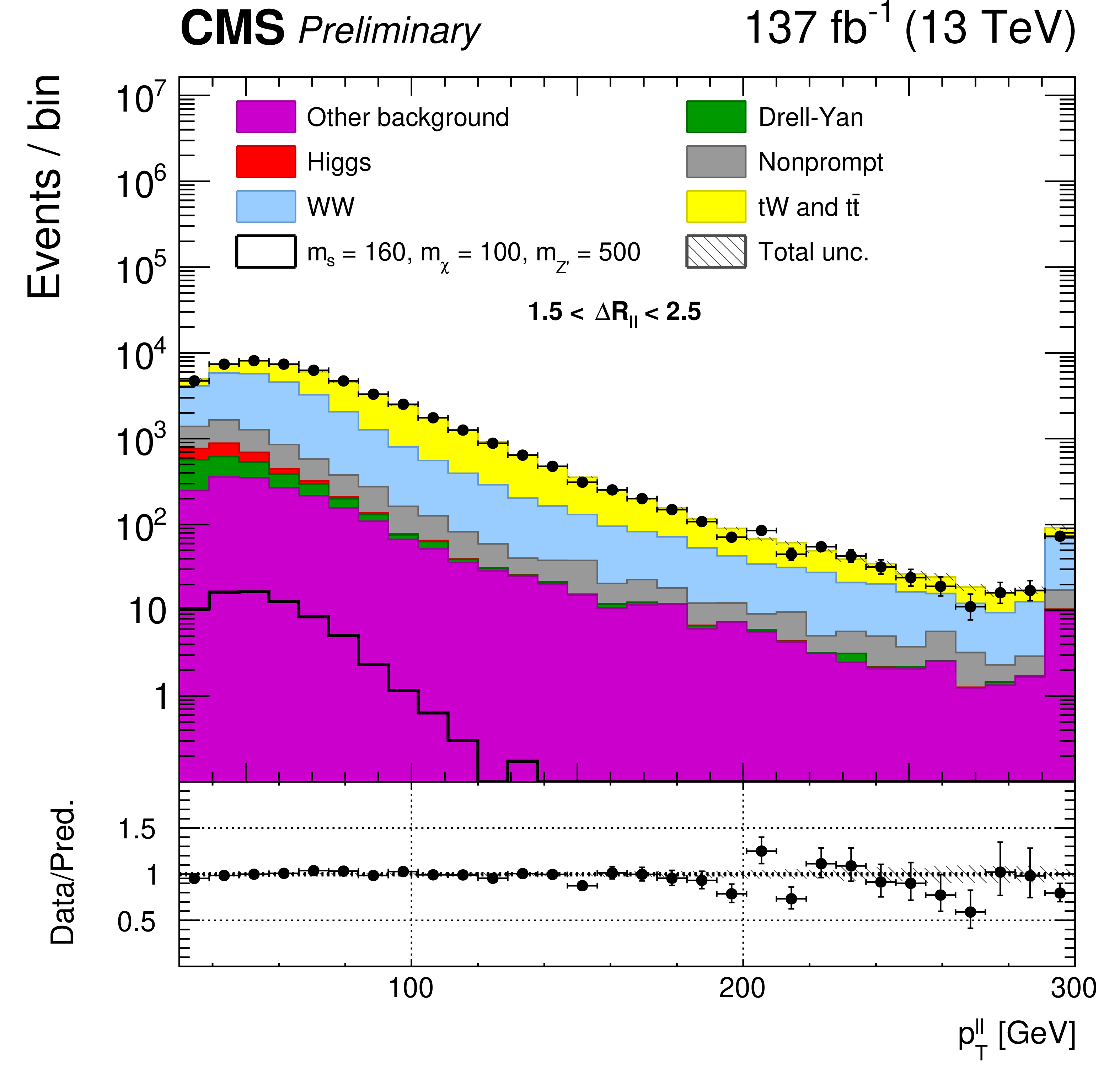
Kinematic distributions for selected events. The distributions show the leading (top left) and trailing (top right) lepton ${p_{\mathrm {T}}}$ ($ {{p_{\mathrm {T}}} ^{\ell \text { max}}} $ and $ {{p_{\mathrm {T}}} ^{\ell \text { min}}} $) for the full data set in SR1, the missing transverse momentum $ {{p_{\mathrm {T}}} ^\text {miss}} $ (middle left) and the transverse mass of the dilepton system plus $ {{p_{\mathrm {T}}} ^\text {miss}} $ (middle right), $ {{m_{\mathrm {T}}} ^{\ell\ell,\,\, {{p_{\mathrm {T}}} ^\text {miss}}}} $, for the full data set in SR2, and the dilepton invariant mass $ {m_{\ell \ell}} $ (bottom left) and the dilepton transverse momentum $ {{p_{\mathrm {T}}} ^{{\ell} {\ell}}}$ (bottom right) for the full data set in SR3. The predicted yields are shown with their best fit normalizations from the simultaneous fit. The error bars on the data points represent the statistical uncertainty of the data, and the hatched areas represent the combined systematic and statistical uncertainty of the predicted yield in each bin. The black line indicates the signal prediction of $m_{s} = $ 160 GeV, $m_{\chi} = $ 100 GeV, $m_{\mathrm{Z'}} = $ 500 GeV. The last bin includes the overflow. |
png pdf |
Figure 3-a:
Leading lepton ${p_{\mathrm {T}}}$ ($ {{p_{\mathrm {T}}} ^{\ell \text { max}}} $), for the full data set in SR1. The predicted yields are shown with their best fit normalizations from the simultaneous fit. The error bars on the data points represent the statistical uncertainty of the data, and the hatched areas represent the combined systematic and statistical uncertainty of the predicted yield in each bin. The black line indicates the signal prediction of $m_{s} = $ 160 GeV, $m_{\chi} = $ 100 GeV, $m_{\mathrm{Z'}} = $ 500 GeV. The last bin includes the overflow. |

png pdf |
Figure 3-b:
Trailing lepton ${p_{\mathrm {T}}}$ ($ {{p_{\mathrm {T}}} ^{\ell \text { min}}} $), for the full data set in SR1. The predicted yields are shown with their best fit normalizations from the simultaneous fit. The error bars on the data points represent the statistical uncertainty of the data, and the hatched areas represent the combined systematic and statistical uncertainty of the predicted yield in each bin. The black line indicates the signal prediction of $m_{s} = $ 160 GeV, $m_{\chi} = $ 100 GeV, $m_{\mathrm{Z'}} = $ 500 GeV. The last bin includes the overflow. |
png pdf |
Figure 3-c:
The missing transverse momentum $ {{p_{\mathrm {T}}} ^\text {miss}} $, for the full data set in SR2, The predicted yields are shown with their best fit normalizations from the simultaneous fit. The error bars on the data points represent the statistical uncertainty of the data, and the hatched areas represent the combined systematic and statistical uncertainty of the predicted yield in each bin. The black line indicates the signal prediction of $m_{s} = $ 160 GeV, $m_{\chi} = $ 100 GeV, $m_{\mathrm{Z'}} = $ 500 GeV. The last bin includes the overflow. |
png pdf |
Figure 3-d:
The transverse mass of the dilepton system plus $ {{p_{\mathrm {T}}} ^\text {miss}} $ $ {{m_{\mathrm {T}}} ^{\ell\ell,\,\, {{p_{\mathrm {T}}} ^\text {miss}}}} $, for the full data set in SR2, The predicted yields are shown with their best fit normalizations from the simultaneous fit. The error bars on the data points represent the statistical uncertainty of the data, and the hatched areas represent the combined systematic and statistical uncertainty of the predicted yield in each bin. The black line indicates the signal prediction of $m_{s} = $ 160 GeV, $m_{\chi} = $ 100 GeV, $m_{\mathrm{Z'}} = $ 500 GeV. The last bin includes the overflow. |

png pdf |
Figure 3-e:
The dilepton invariant mass $ {m_{\ell \ell}} $, for the full data set in SR3. The predicted yields are shown with their best fit normalizations from the simultaneous fit. The error bars on the data points represent the statistical uncertainty of the data, and the hatched areas represent the combined systematic and statistical uncertainty of the predicted yield in each bin. The black line indicates the signal prediction of $m_{s} = $ 160 GeV, $m_{\chi} = $ 100 GeV, $m_{\mathrm{Z'}} = $ 500 GeV. The last bin includes the overflow. |
png pdf |
Figure 3-f:
The dilepton transverse momentum $ {{p_{\mathrm {T}}} ^{{\ell} {\ell}}}$, for the full data set in SR3. The predicted yields are shown with their best fit normalizations from the simultaneous fit. The error bars on the data points represent the statistical uncertainty of the data, and the hatched areas represent the combined systematic and statistical uncertainty of the predicted yield in each bin. The black line indicates the signal prediction of $m_{s} = $ 160 GeV, $m_{\chi} = $ 100 GeV, $m_{\mathrm{Z'}} = $ 500 GeV. The last bin includes the overflow. |
png pdf |
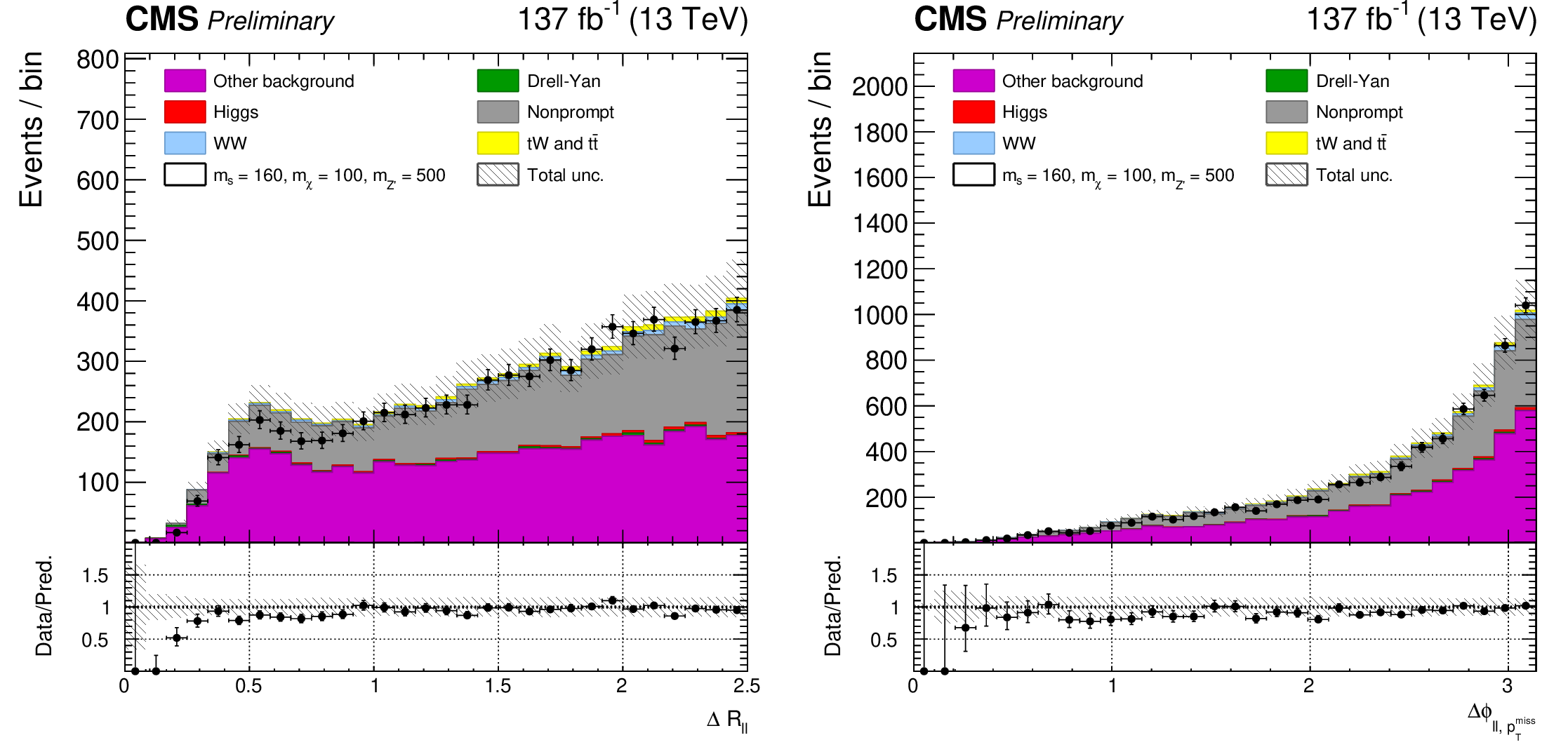
Figure 4:
Kinematic distributions from the non-prompt validation region. The distributions show the angular distance between the two leptons (left), $ {\Delta R_{{\ell} {\ell}}} $, and the $\Delta \phi $ between the dilepton system and the $ {{p_{\mathrm {T}}} ^\text {miss}} $ (right) for the full data set. The error bars on the data points represent the statistical uncertainty of the data, and the hatched areas represent the combined systematic and statistical uncertainty of the predicted yield in each bin. The predicted yields are shown with their best fit normalizations from the simultaneous fit. The last bin includes the overflow. |

png pdf |
Figure 4-a:
The angular distance between the two leptons, $ {\Delta R_{{\ell} {\ell}}} $, in the non-prompt validation region for the full data set. The error bars on the data points represent the statistical uncertainty of the data, and the hatched areas represent the combined systematic and statistical uncertainty of the predicted yield in each bin. The predicted yields are shown with their best fit normalizations from the simultaneous fit. The last bin includes the overflow. |
png pdf |
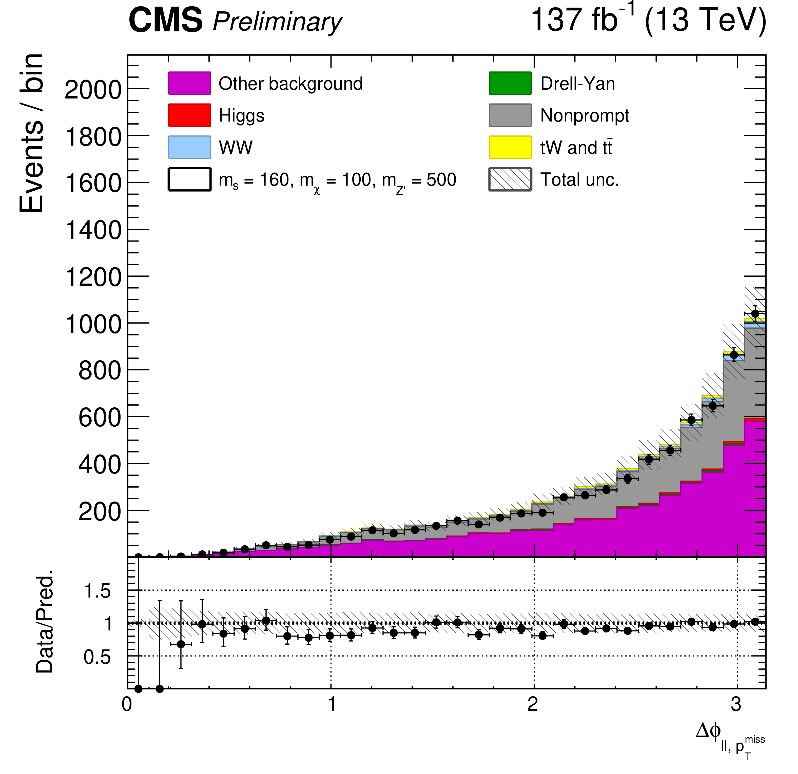
Figure 4-b:
The $\Delta \phi $ between the dilepton system and the $ {{p_{\mathrm {T}}} ^\text {miss}} $ in the non-prompt validation region for the full data set. The error bars on the data points represent the statistical uncertainty of the data, and the hatched areas represent the combined systematic and statistical uncertainty of the predicted yield in each bin. The predicted yields are shown with their best fit normalizations from the simultaneous fit. The last bin includes the overflow. |

png pdf |
Figure 5:
Kinematic distributions for events entering in the different control regions. The distributions show the leading (top left) and trailing (top right) lepton ${p_{\mathrm {T}}}$ ($ {{p_{\mathrm {T}}} ^{\ell \text { max}}} $ and $ {{p_{\mathrm {T}}} ^{\ell \text { min}}} $) for the full data set in the W$^{+}$W$^{-}$ control region, the angular distance between the two leptons, $ {\Delta R_{{\ell} {\ell}}} $ (middle left), and the dilepton invariant mass $ {m_{\ell \ell}} $ (middle right) for the full data set in the Drell-Yan control region, and the missing transverse momentum $ {{p_{\mathrm {T}}} ^\text {miss}} $ (bottom left) and the dilepton transverse momentum $ {{p_{\mathrm {T}}} ^{{\ell} {\ell}}}$ (bottom right) for the full data set in the $ {{\mathrm{t} {}\mathrm{\bar{t}}} {}+{}\mathrm{t} \mathrm{W}} $ control region. The predicted yields are shown with their best fit normalizations from the simultaneous fit. The error bars on the data points represent the statistical uncertainty of the data, and the hatched areas represent the combined systematic and statistical uncertainty of the predicted yield in each bin. The last bin includes the overflow. |
png pdf |
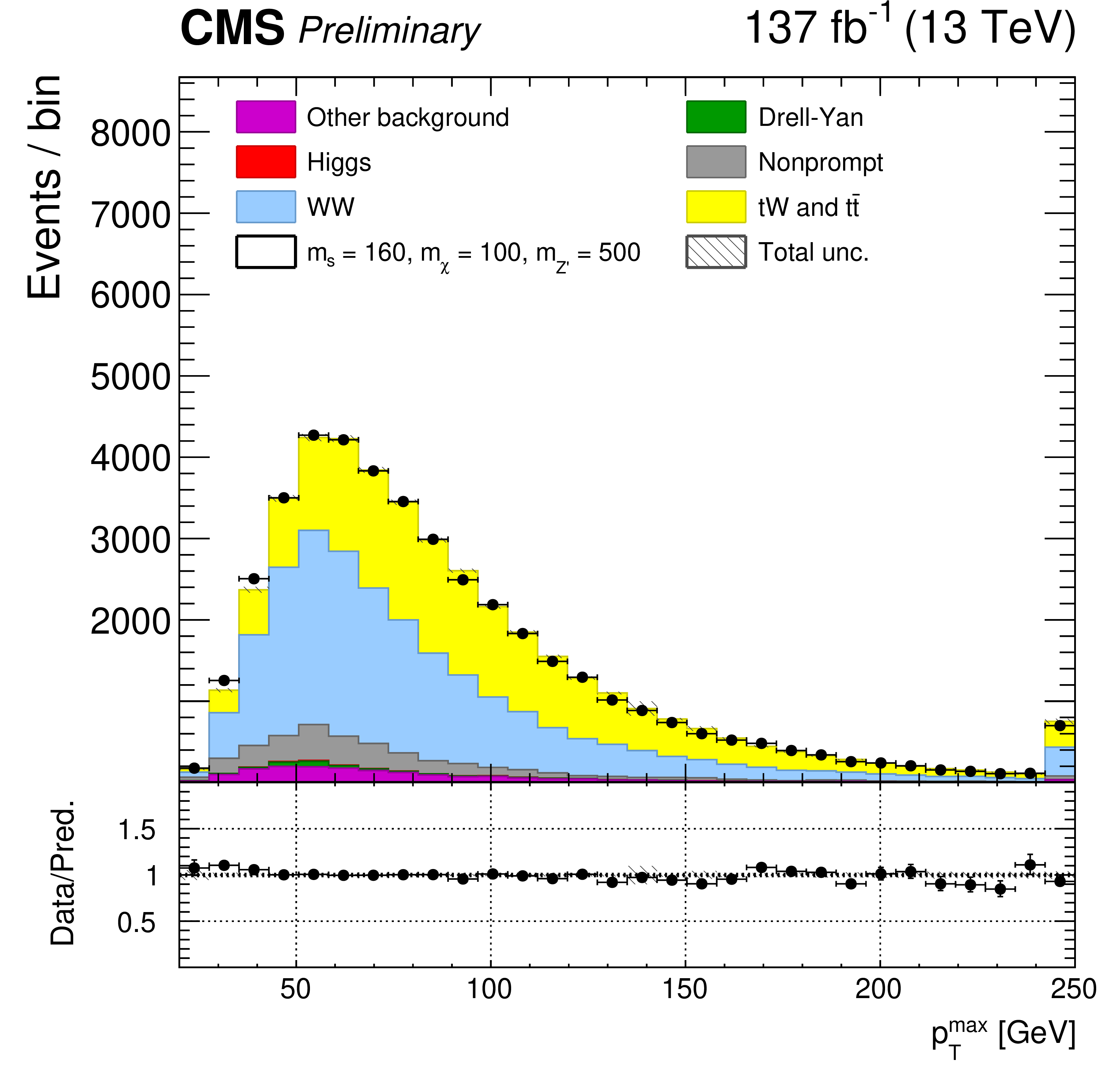
Figure 5-a:
The leading lepton ${p_{\mathrm {T}}}$ ($ {{p_{\mathrm {T}}} ^{\ell \text { max}}} $) for the full data set in the W$^{+}$W$^{-}$ control region. The predicted yields are shown with their best fit normalizations from the simultaneous fit. The error bars on the data points represent the statistical uncertainty of the data, and the hatched areas represent the combined systematic and statistical uncertainty of the predicted yield in each bin. The last bin includes the overflow. |

png pdf |
Figure 5-b:
The trailing lepton ${p_{\mathrm {T}}}$ ($ {{p_{\mathrm {T}}} ^{\ell \text { min}}} $) for the full data set in the W$^{+}$W$^{-}$ control region. The predicted yields are shown with their best fit normalizations from the simultaneous fit. The error bars on the data points represent the statistical uncertainty of the data, and the hatched areas represent the combined systematic and statistical uncertainty of the predicted yield in each bin. The last bin includes the overflow. |

png pdf |
Figure 5-c:
The angular distance between the two leptons, $ {\Delta R_{{\ell} {\ell}}} $, for the full data set in the Drell-Yan control region. The predicted yields are shown with their best fit normalizations from the simultaneous fit. The error bars on the data points represent the statistical uncertainty of the data, and the hatched areas represent the combined systematic and statistical uncertainty of the predicted yield in each bin. The last bin includes the overflow. |
png pdf |
Figure 5-d:
The dilepton invariant mass $ {m_{\ell \ell}} $, for the full data set in the Drell-Yan control region. The predicted yields are shown with their best fit normalizations from the simultaneous fit. The error bars on the data points represent the statistical uncertainty of the data, and the hatched areas represent the combined systematic and statistical uncertainty of the predicted yield in each bin. The last bin includes the overflow. |
png pdf |
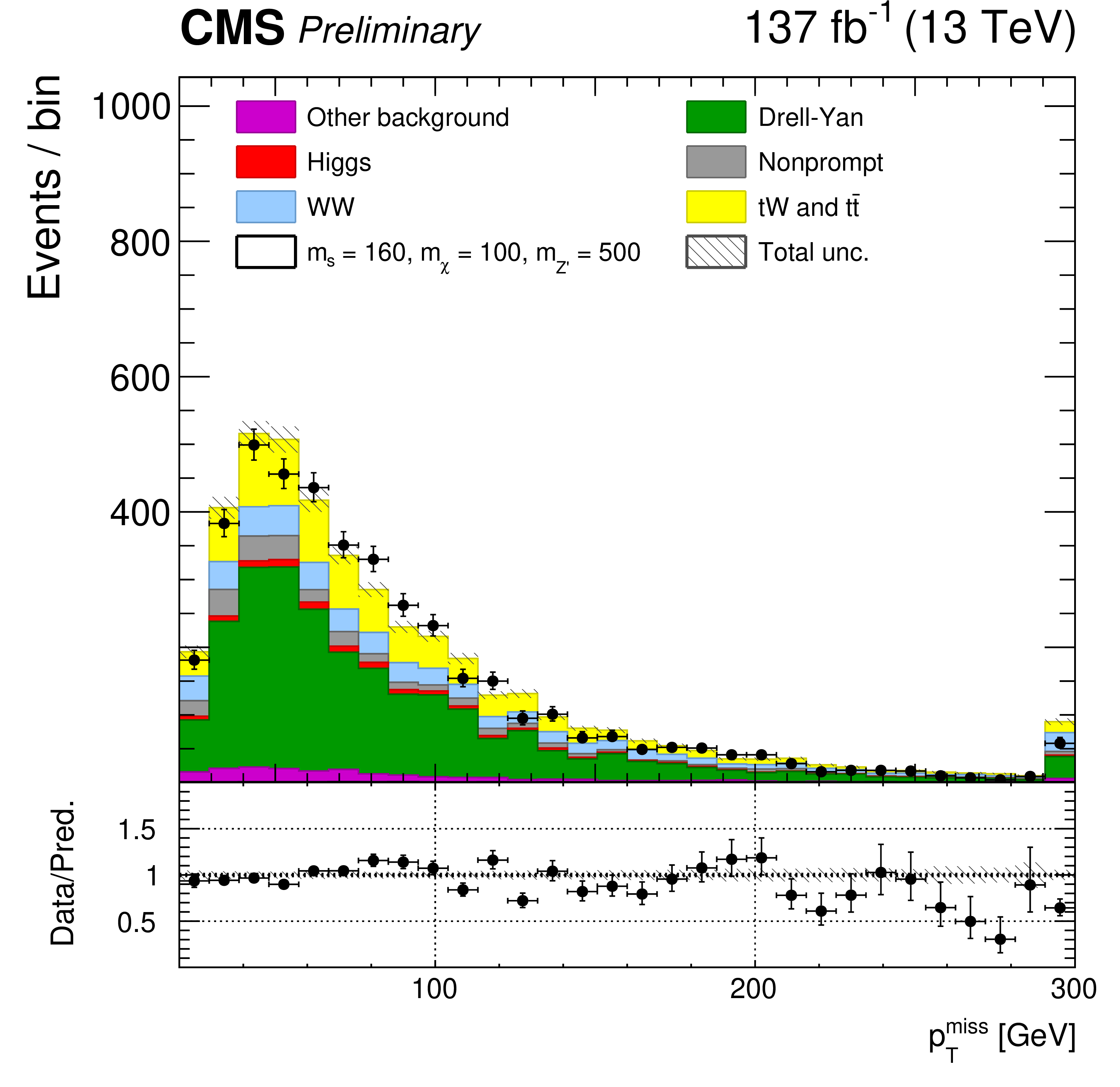
Figure 5-e:
The missing transverse momentum $ {{p_{\mathrm {T}}} ^\text {miss}} $, for the full data set in the $ {{\mathrm{t} {}\mathrm{\bar{t}}} {}+{}\mathrm{t} \mathrm{W}} $ control region. The predicted yields are shown with their best fit normalizations from the simultaneous fit. The error bars on the data points represent the statistical uncertainty of the data, and the hatched areas represent the combined systematic and statistical uncertainty of the predicted yield in each bin. The last bin includes the overflow. |
png pdf |
Figure 5-f:
The dilepton transverse momentum $ {{p_{\mathrm {T}}} ^{{\ell} {\ell}}}$, for the full data set in the $ {{\mathrm{t} {}\mathrm{\bar{t}}} {}+{}\mathrm{t} \mathrm{W}} $ control region. The predicted yields are shown with their best fit normalizations from the simultaneous fit. The error bars on the data points represent the statistical uncertainty of the data, and the hatched areas represent the combined systematic and statistical uncertainty of the predicted yield in each bin. The last bin includes the overflow. |

png pdf |
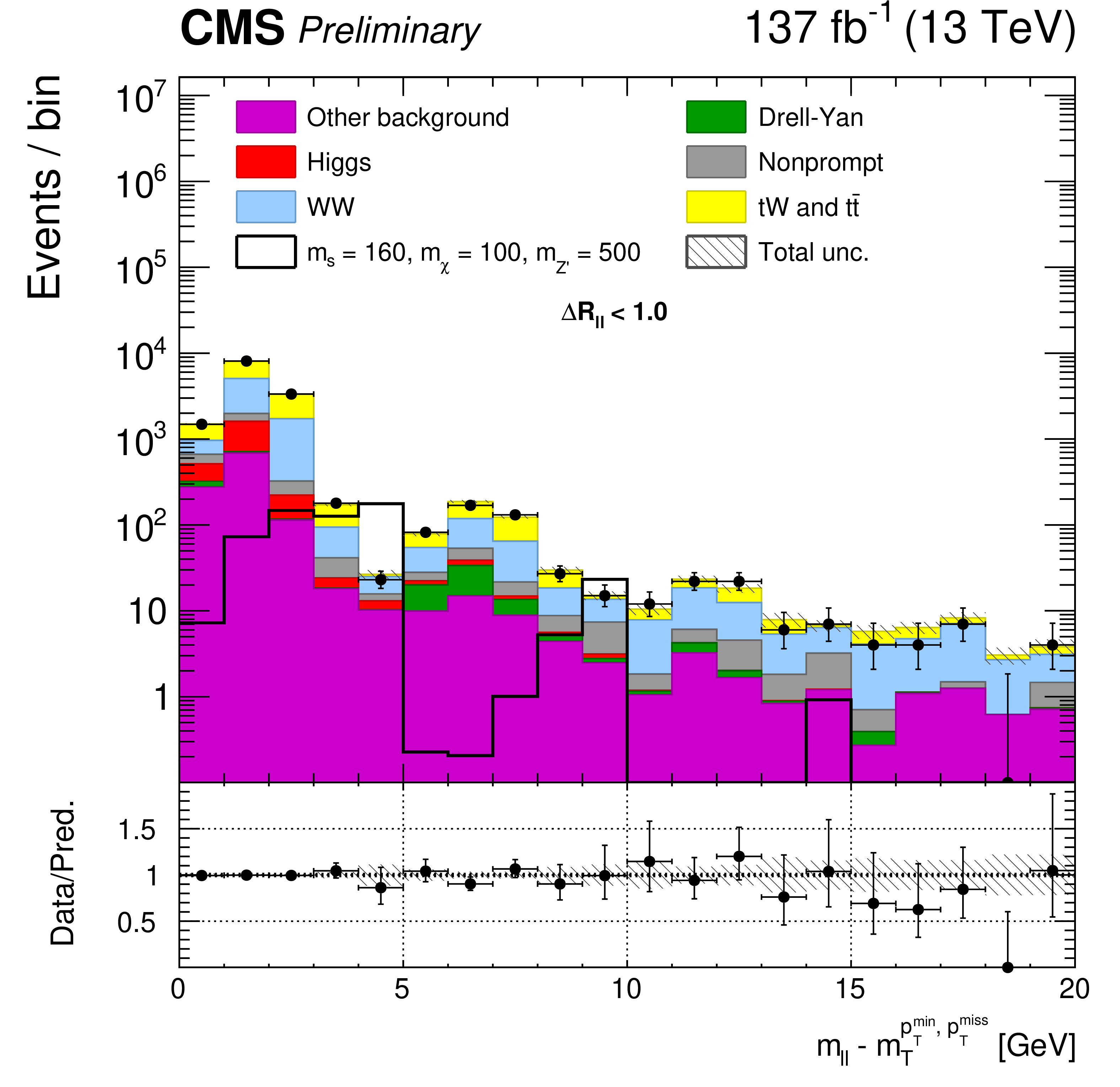
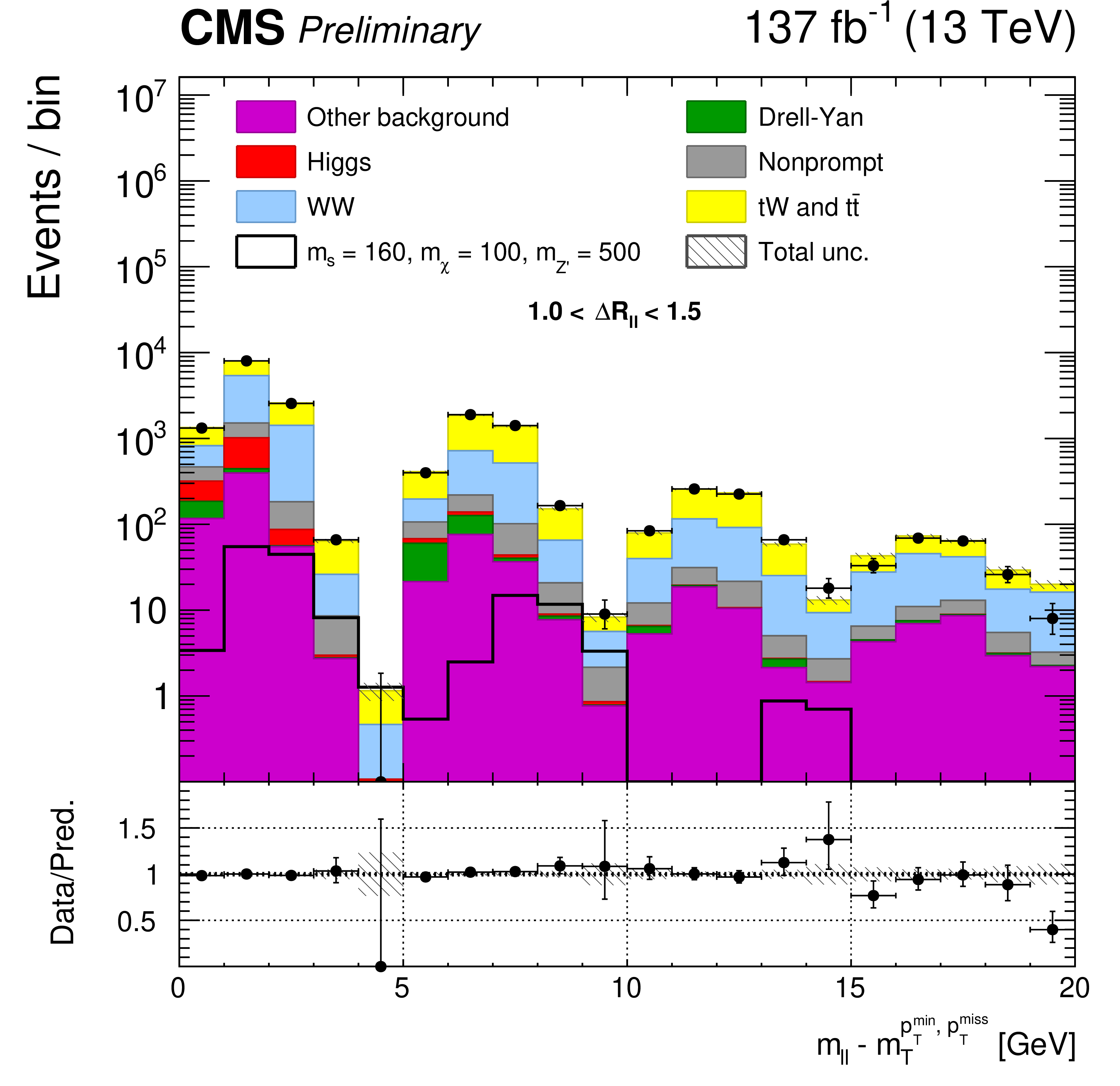
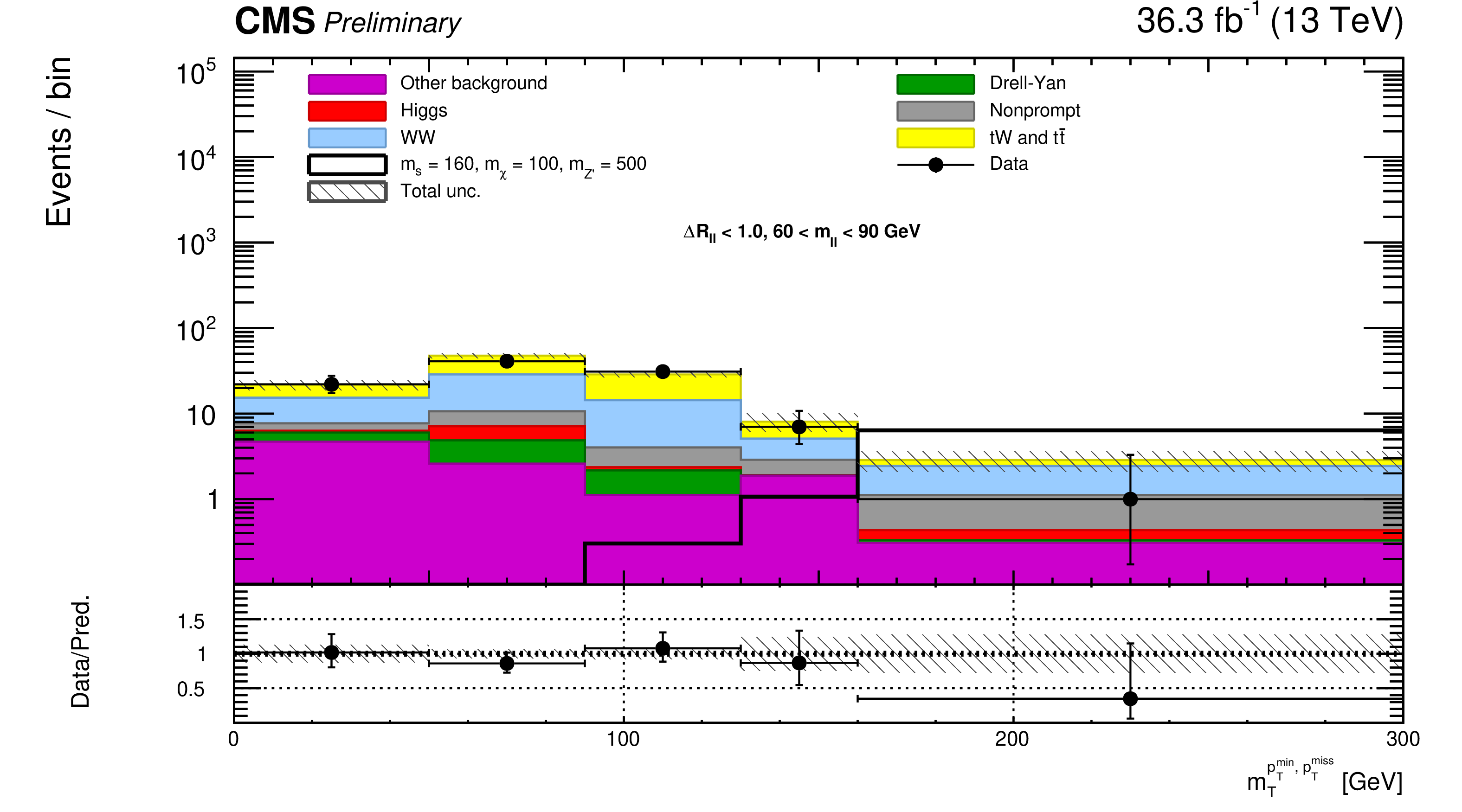
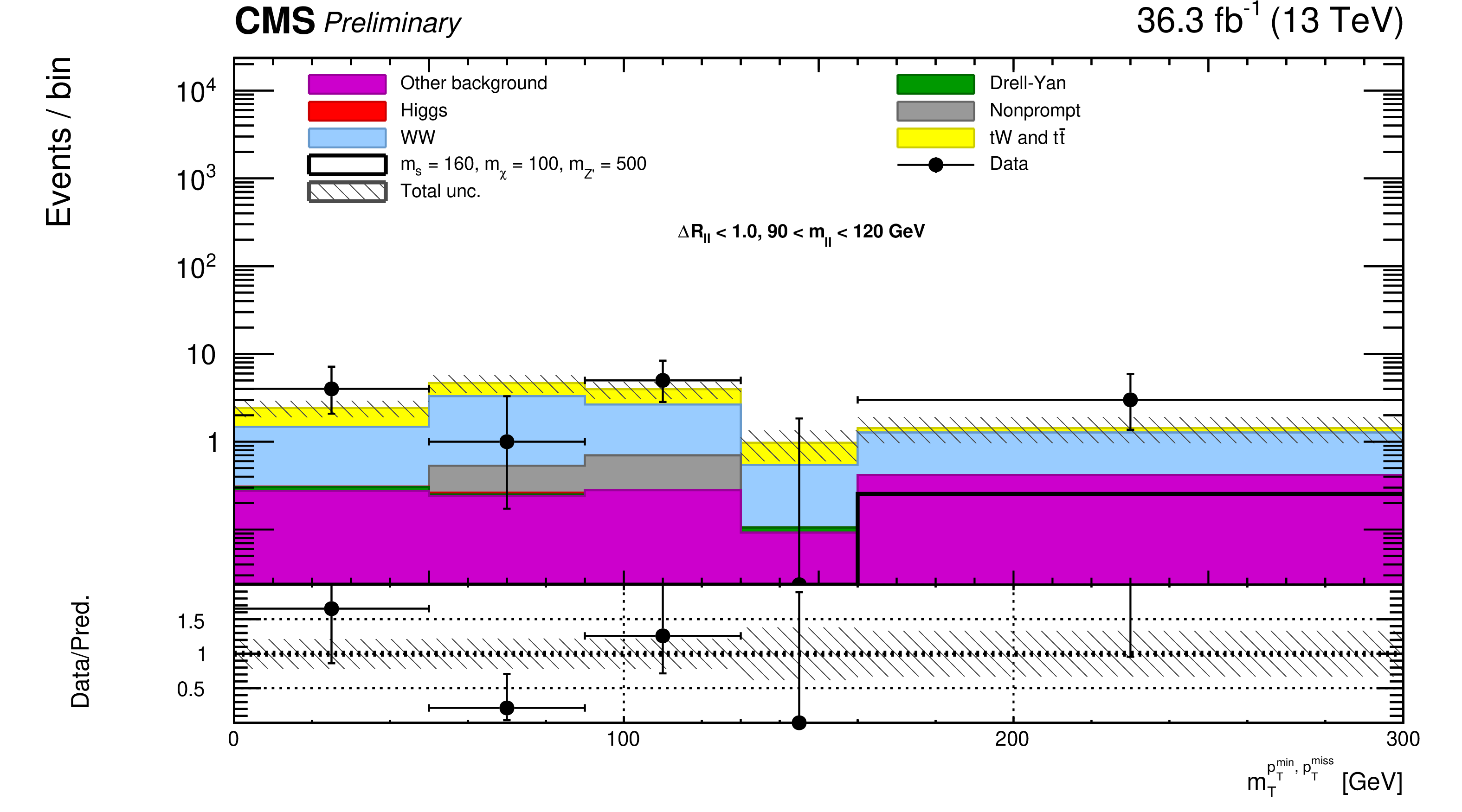
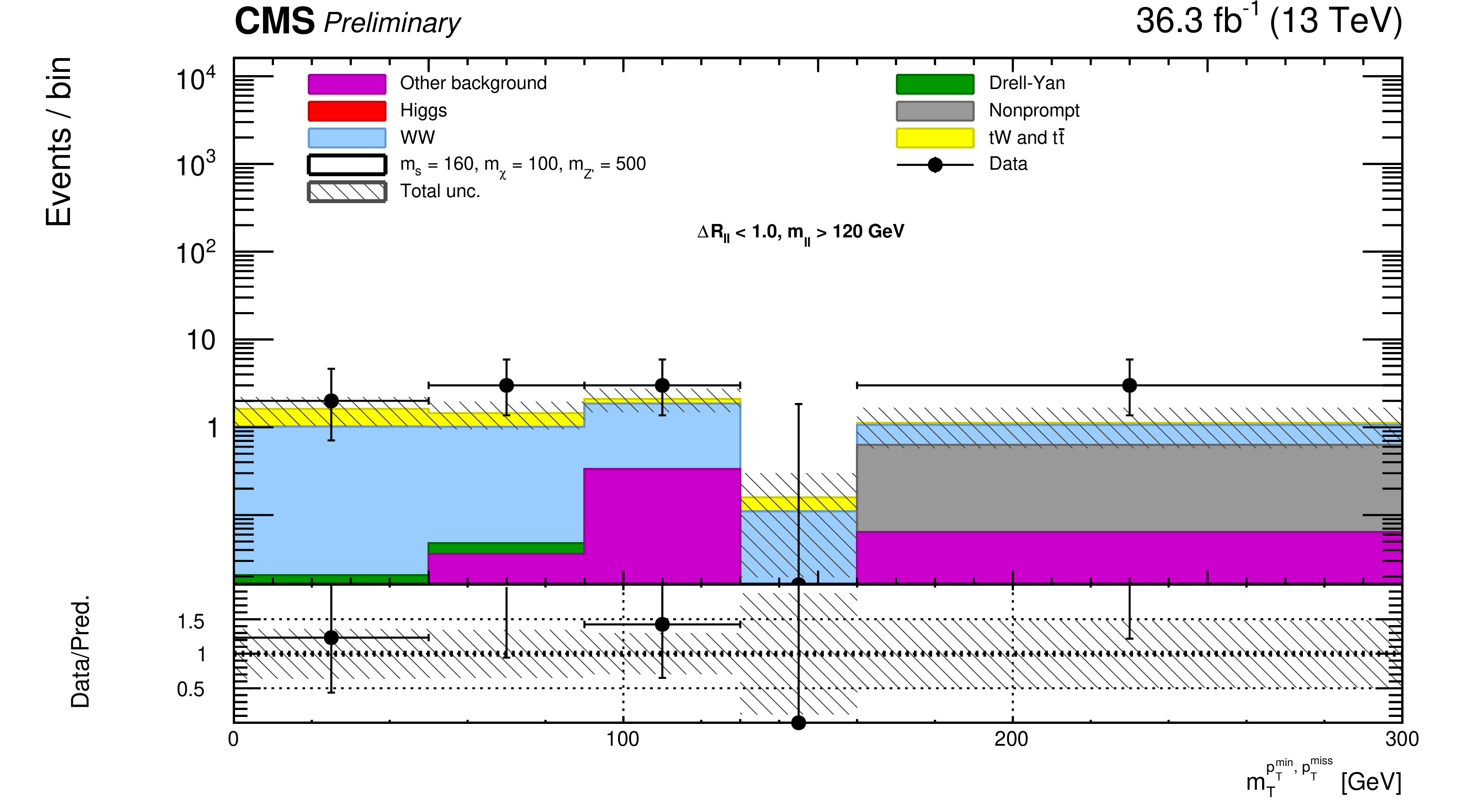
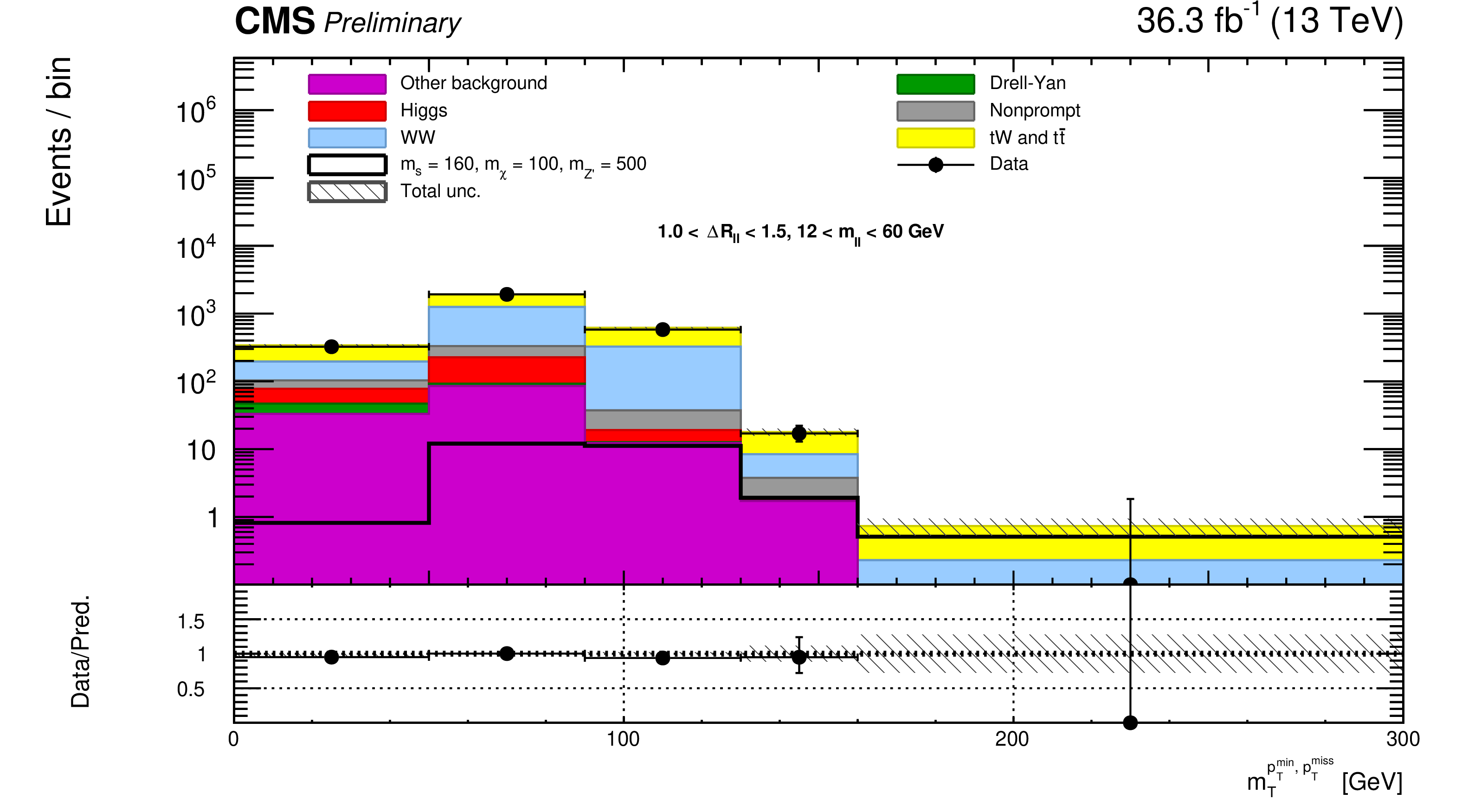
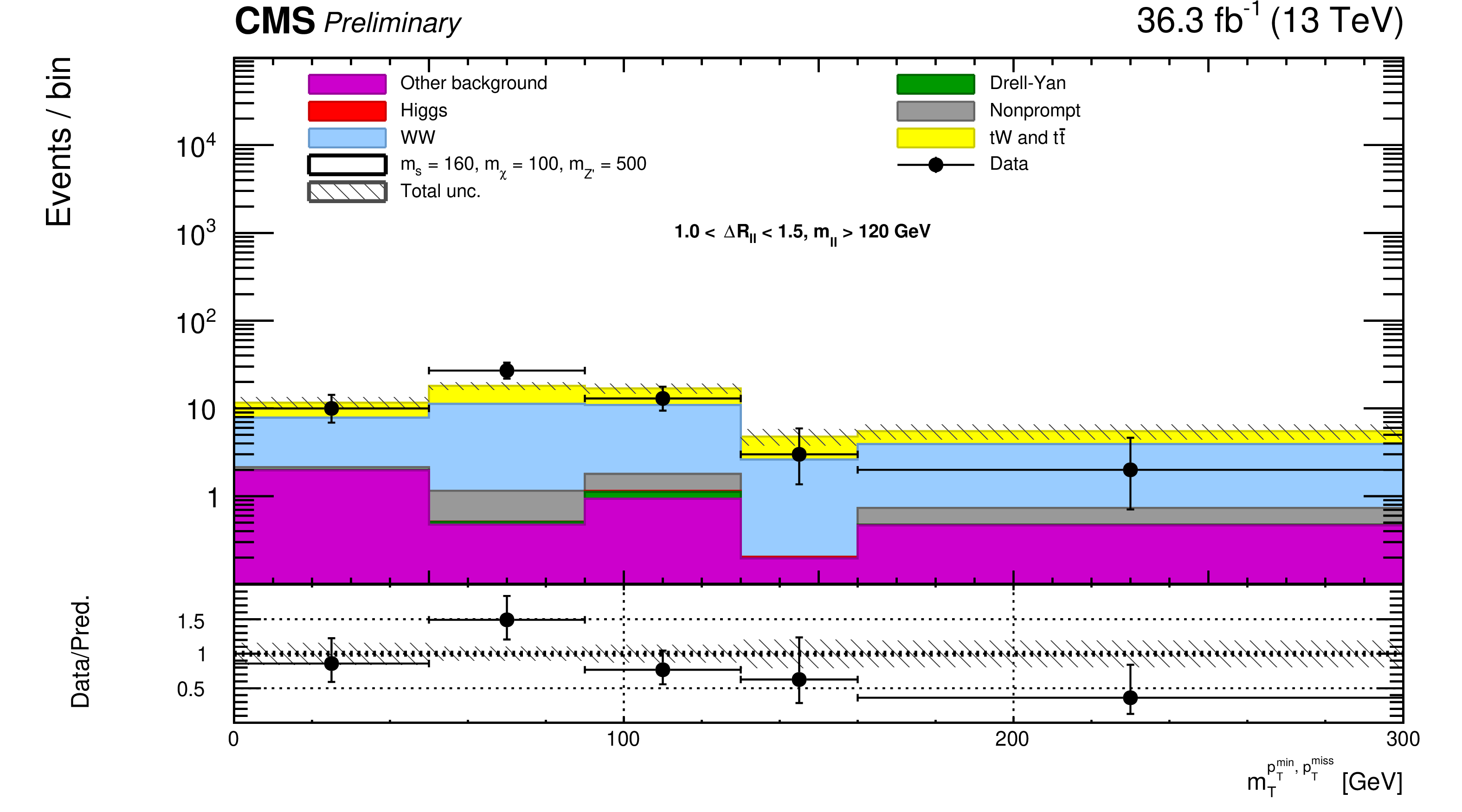
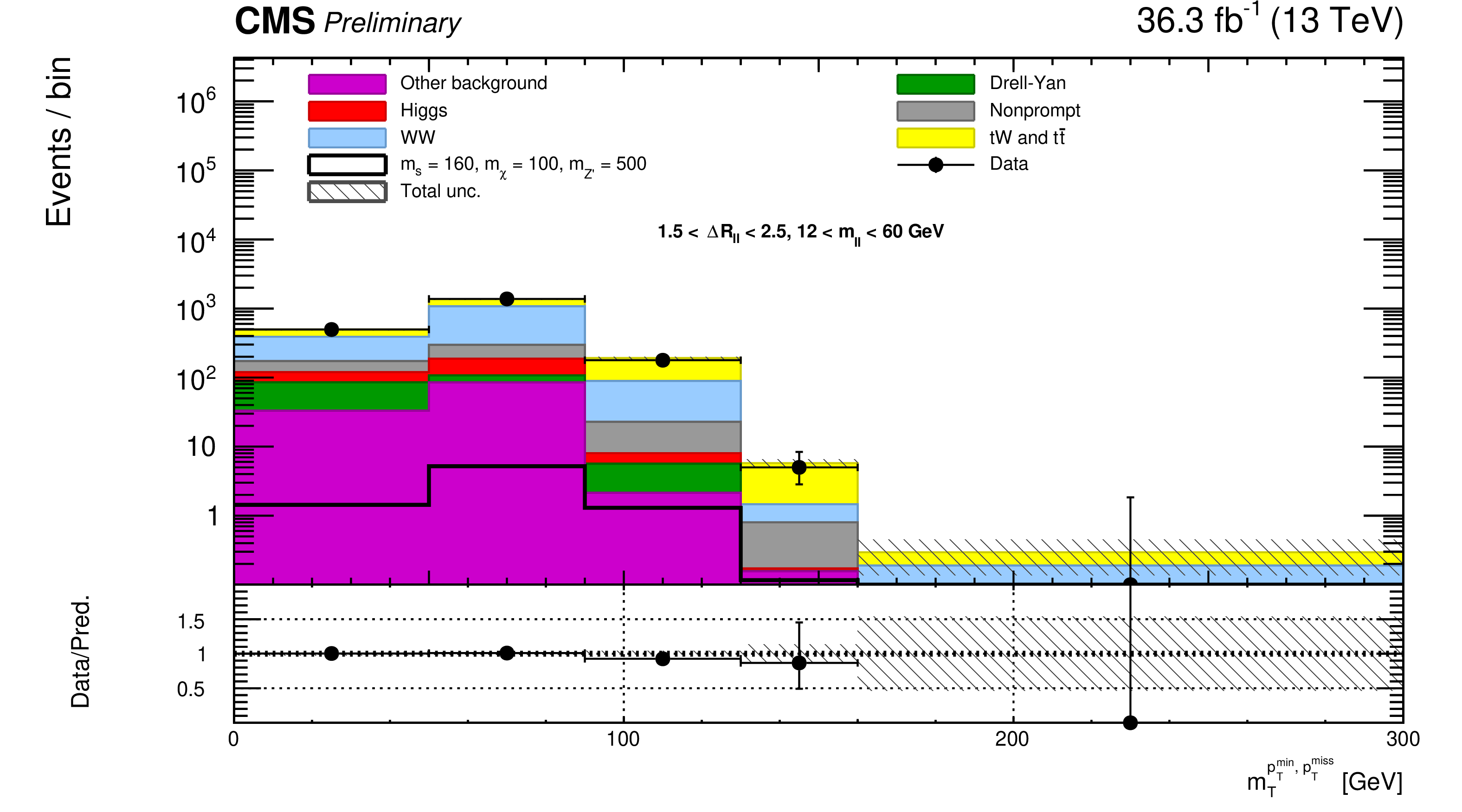
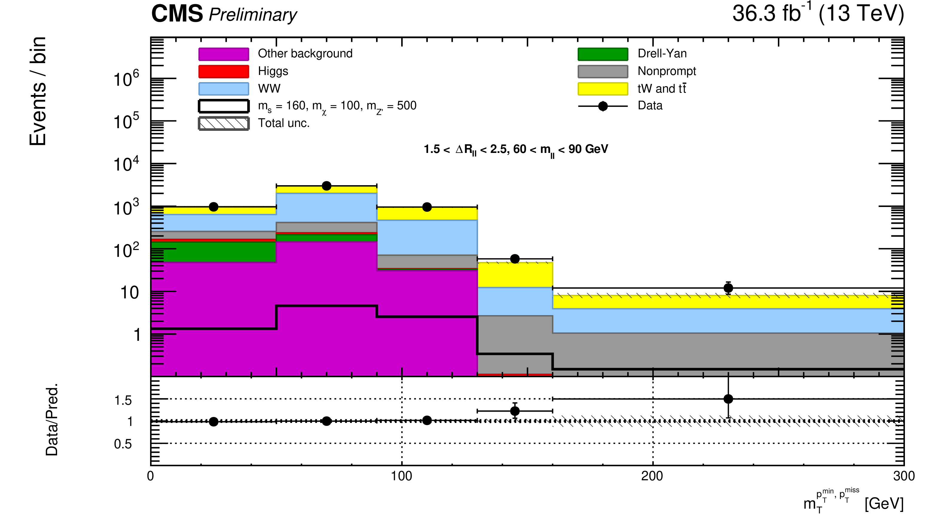
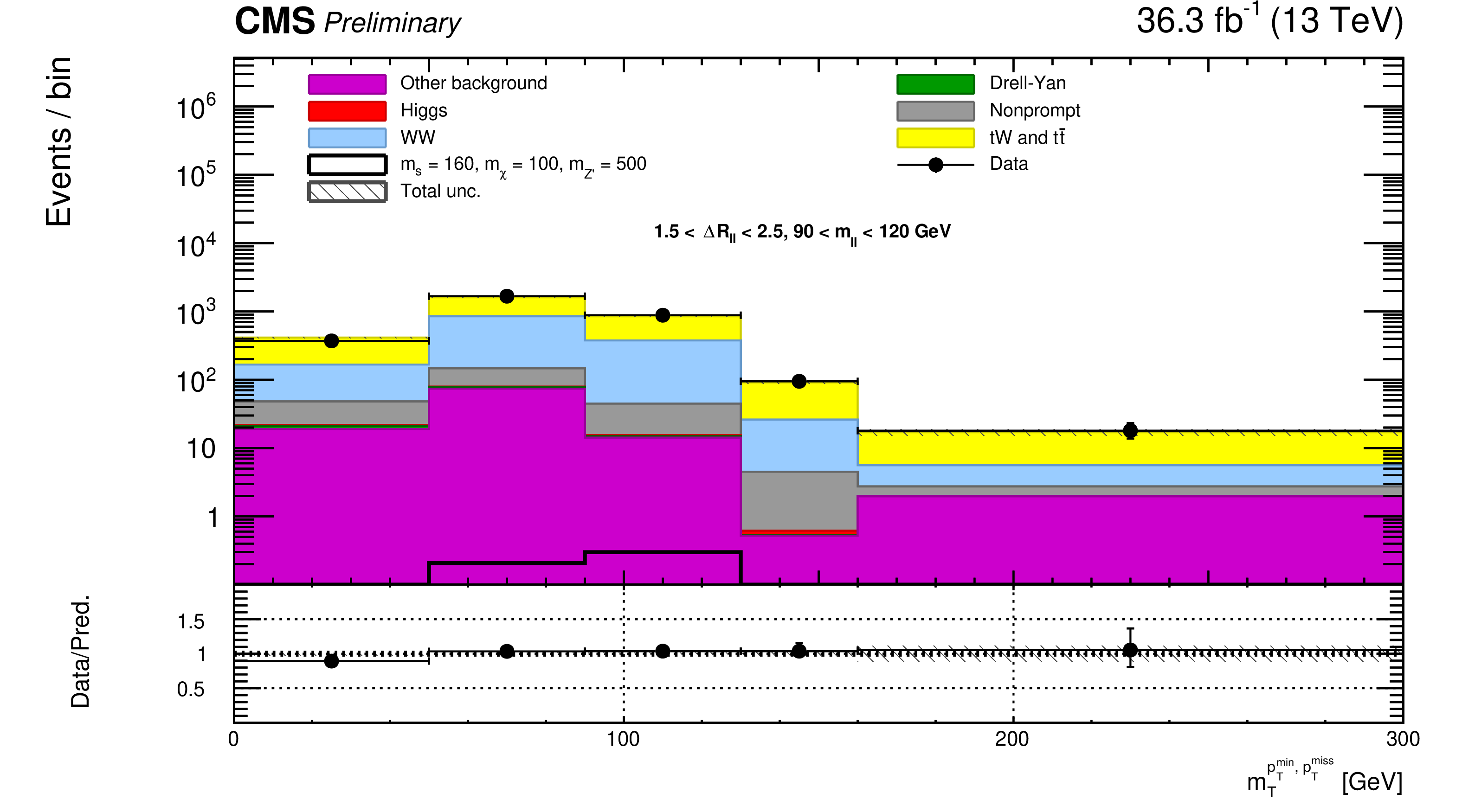
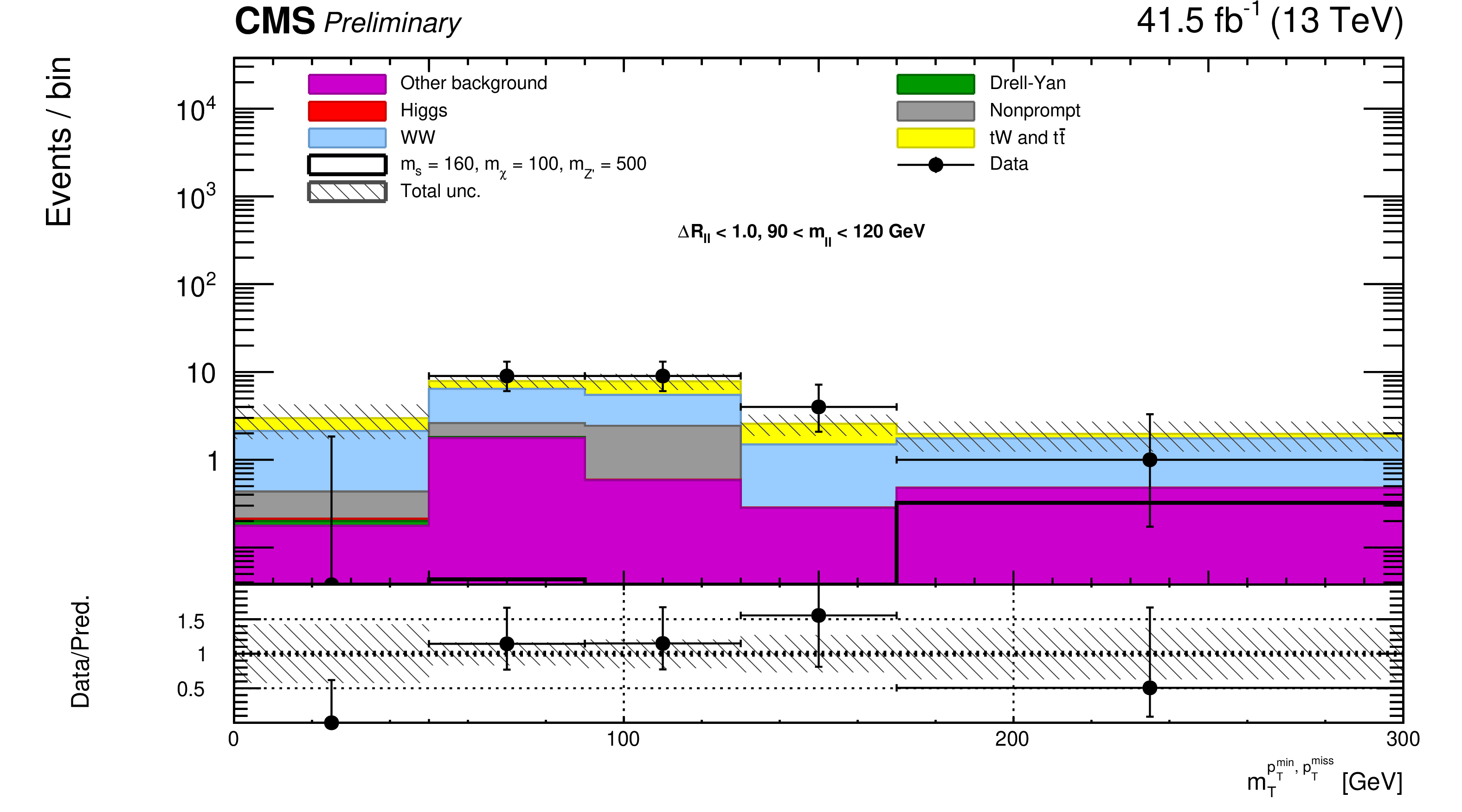
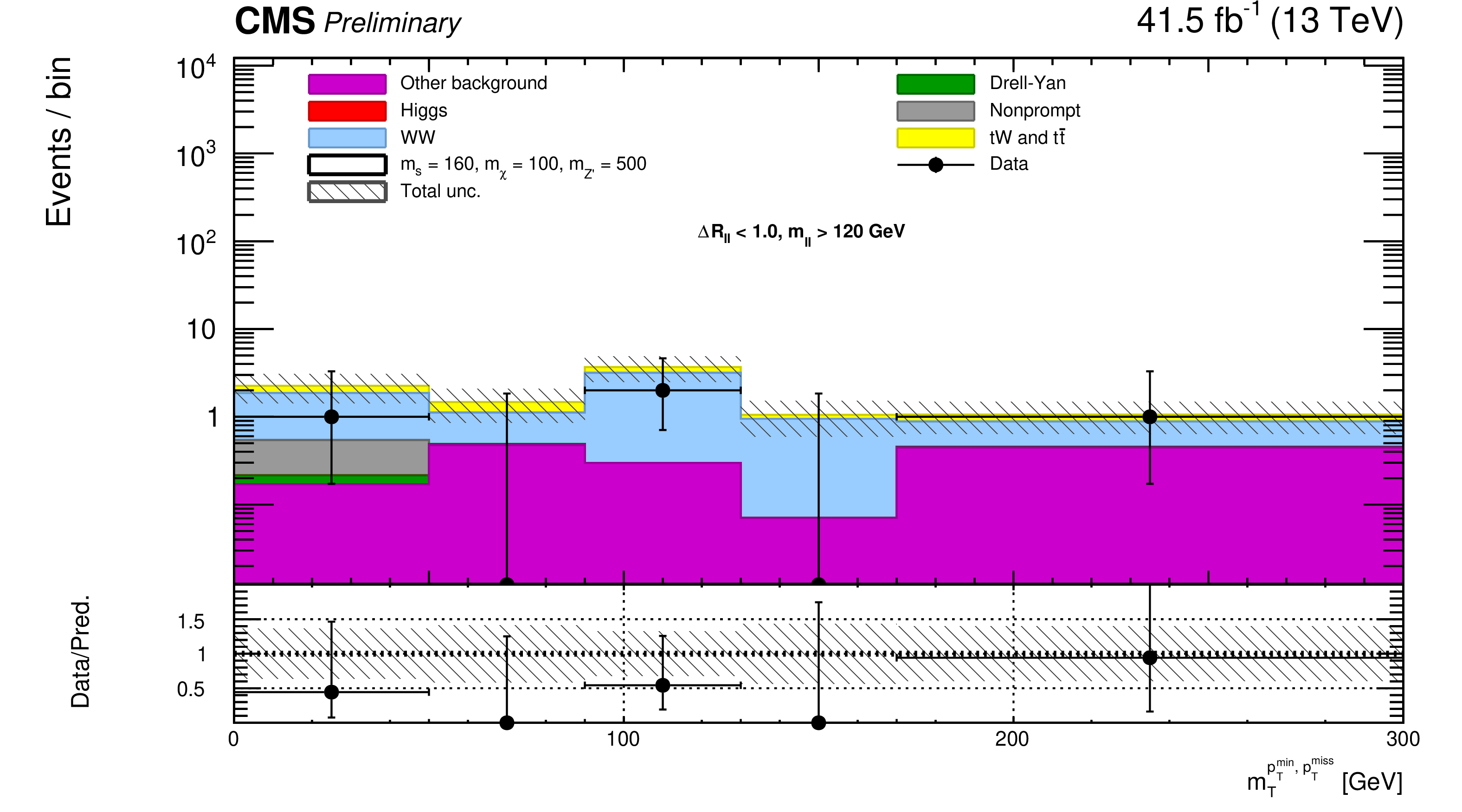
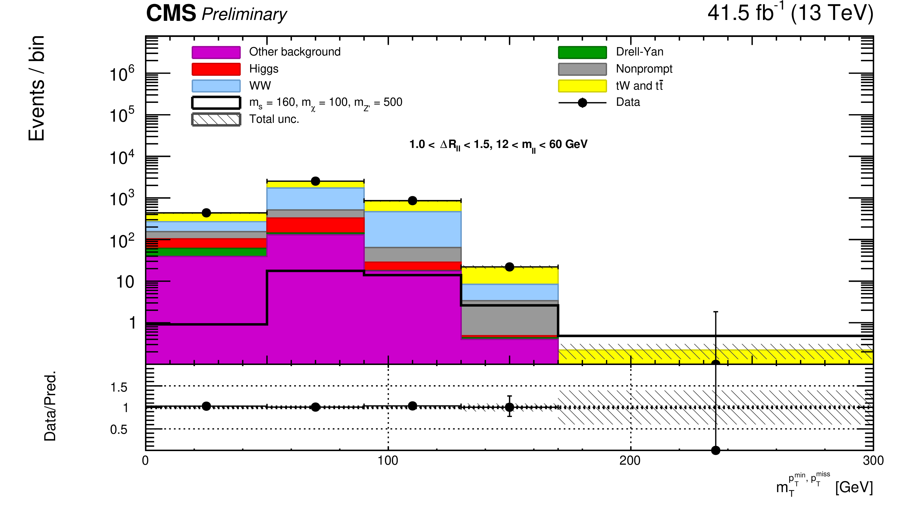
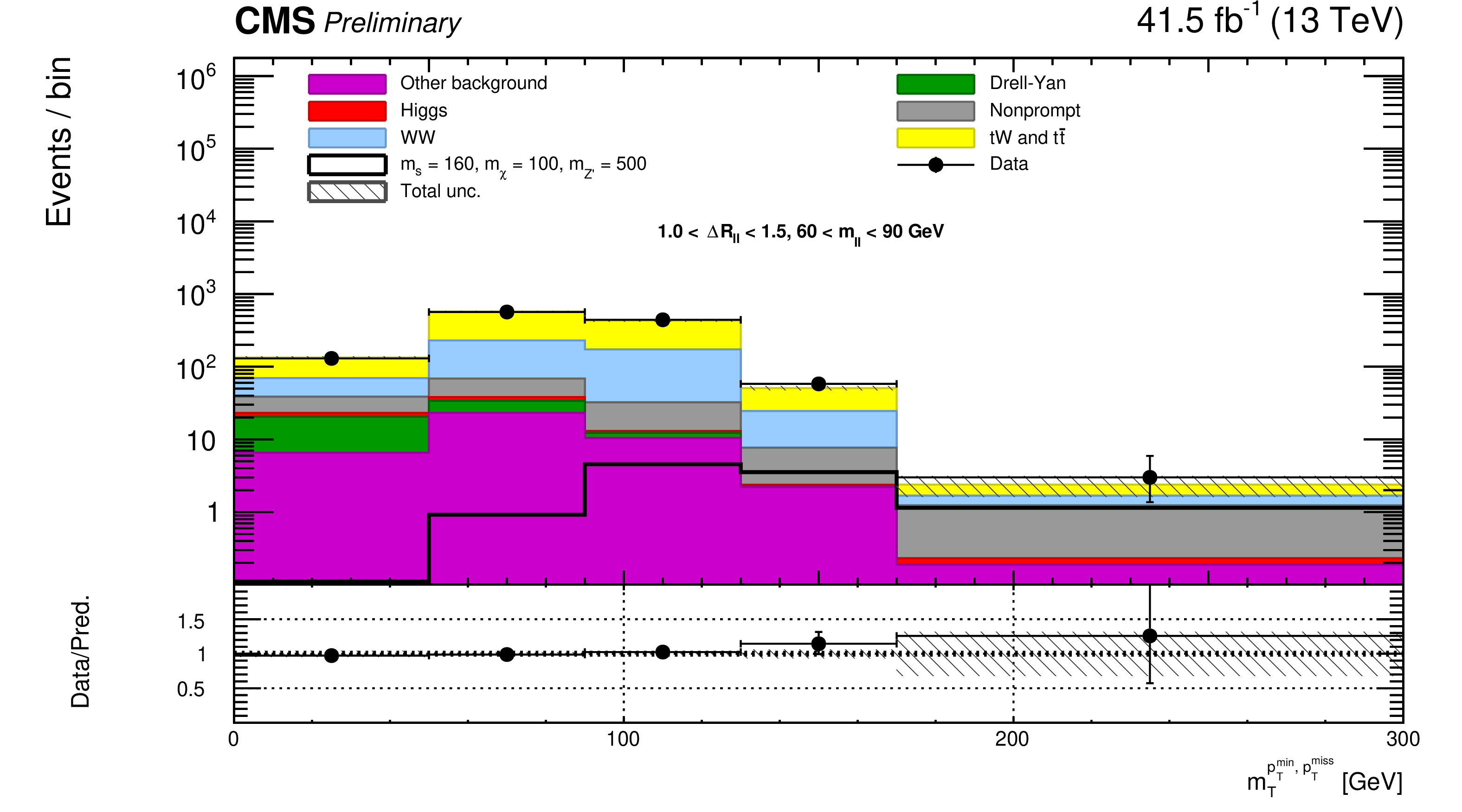
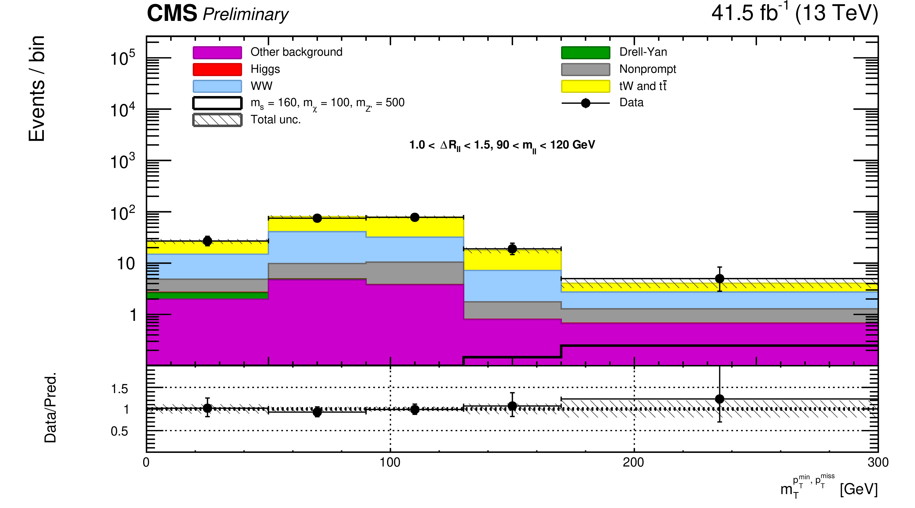
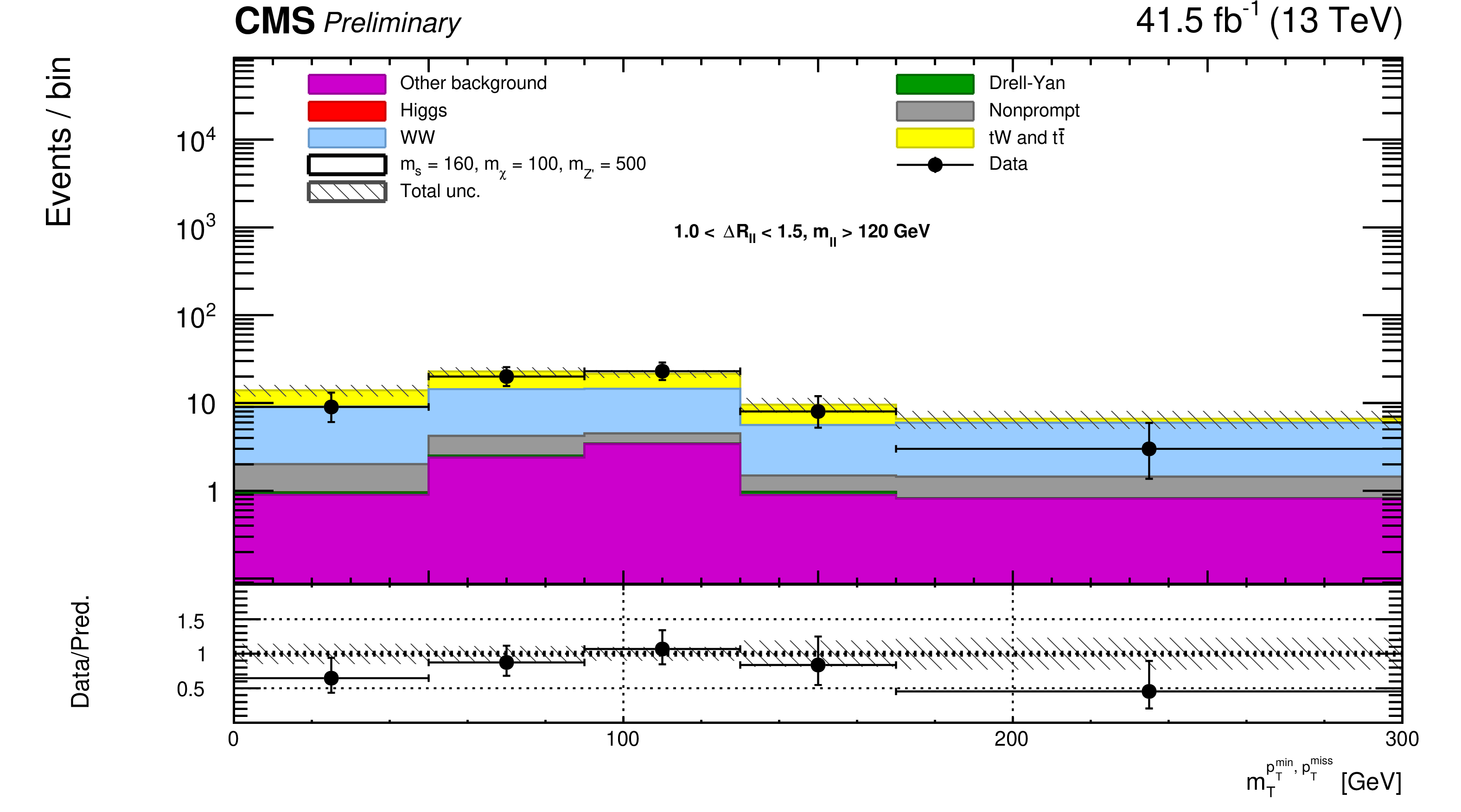
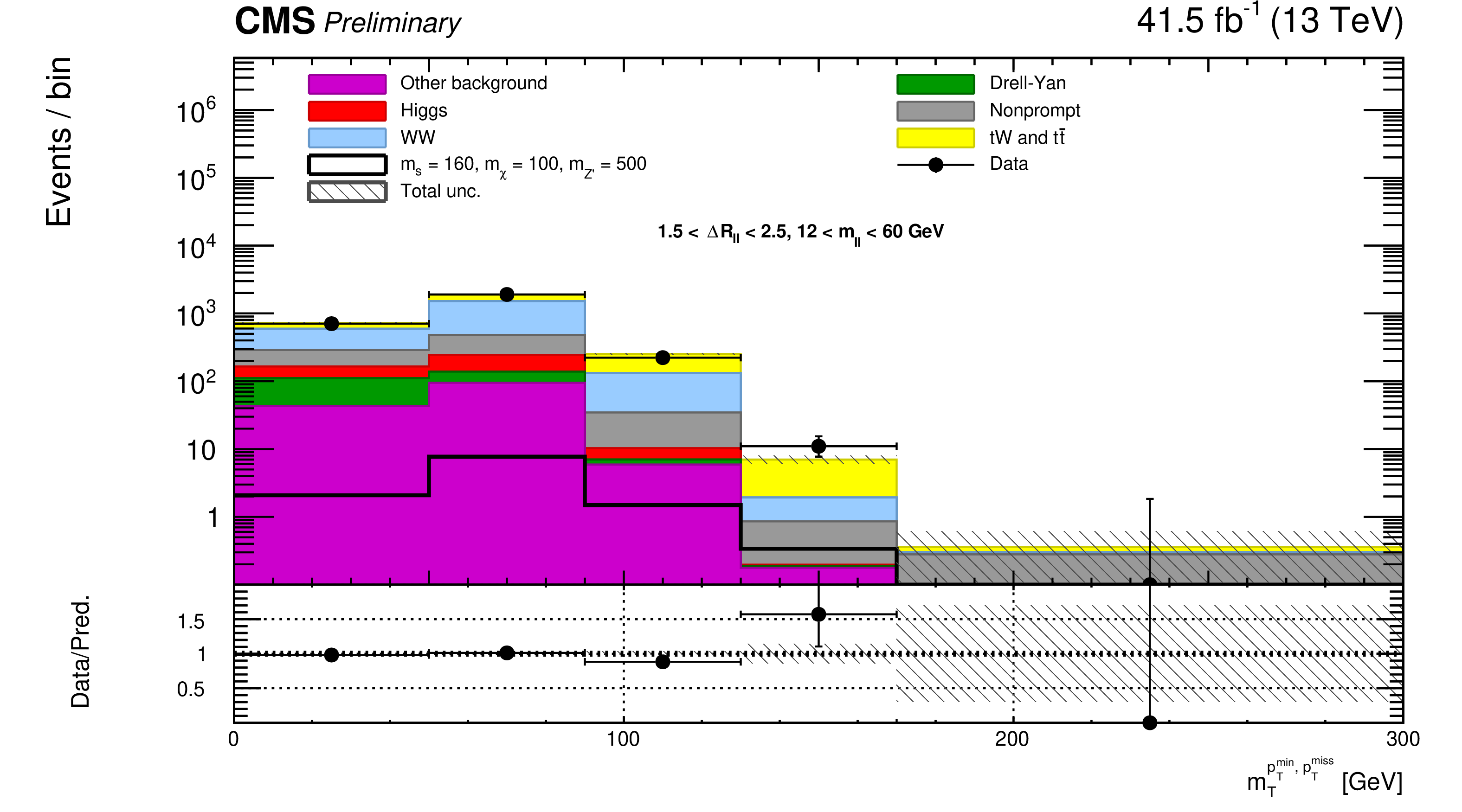
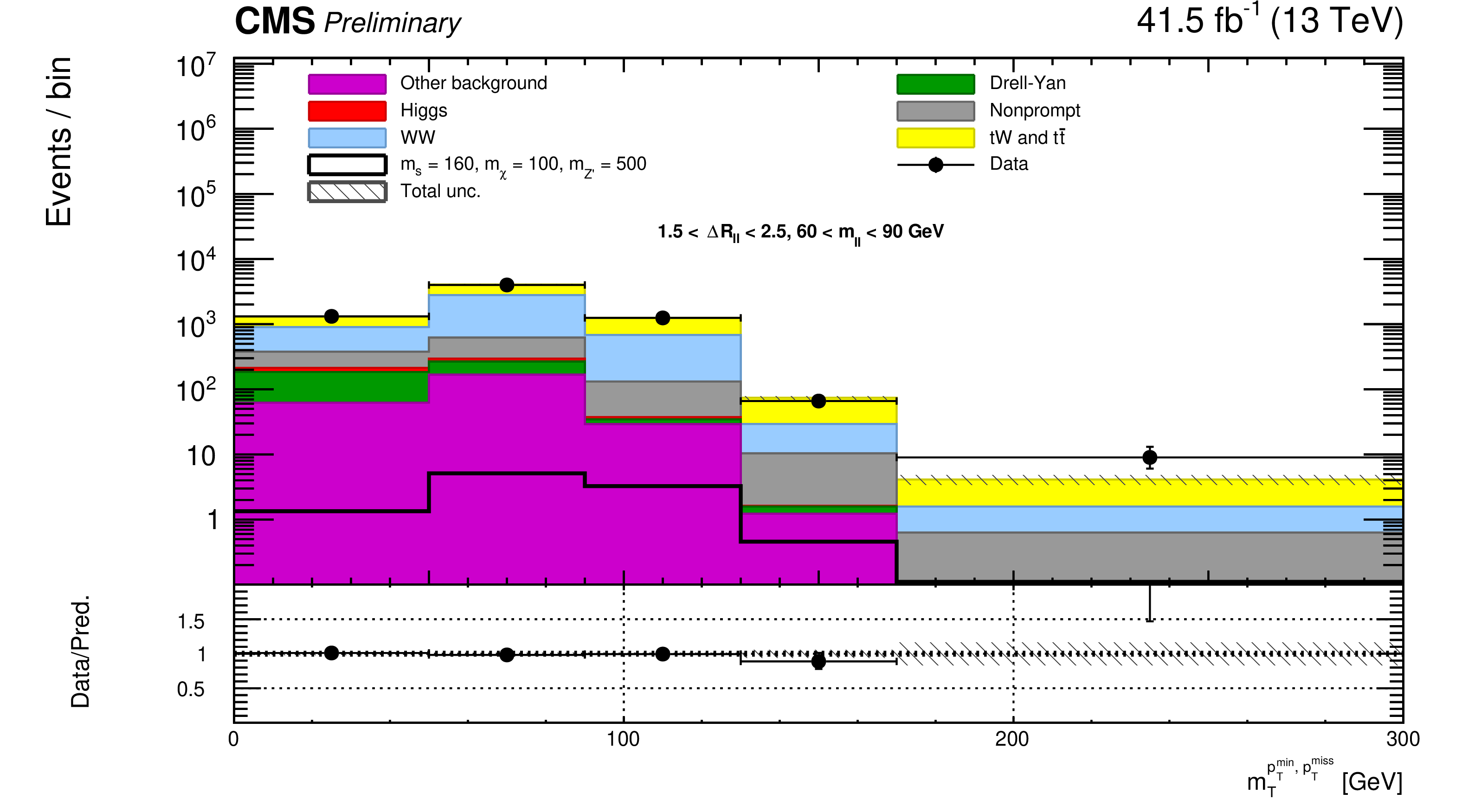
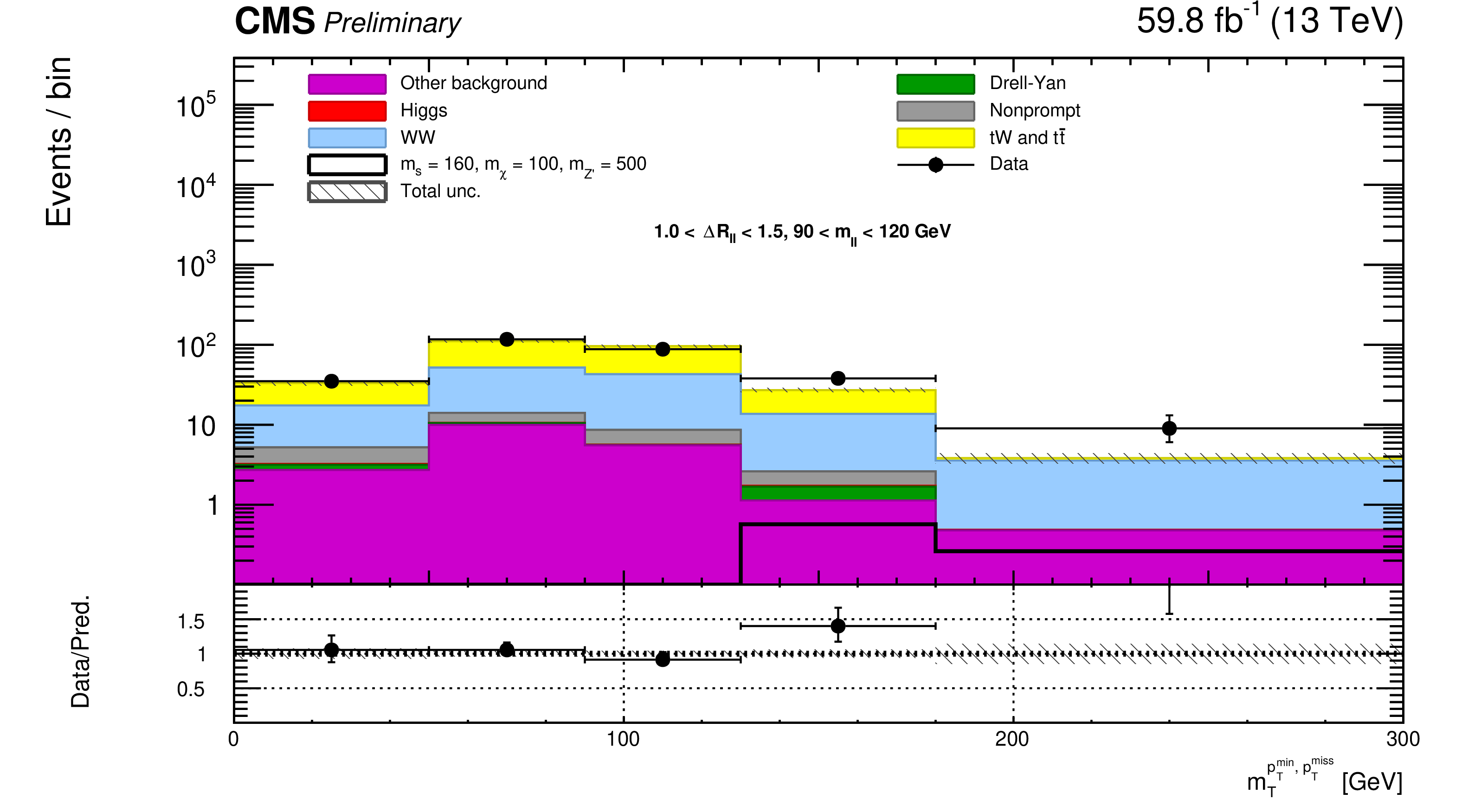
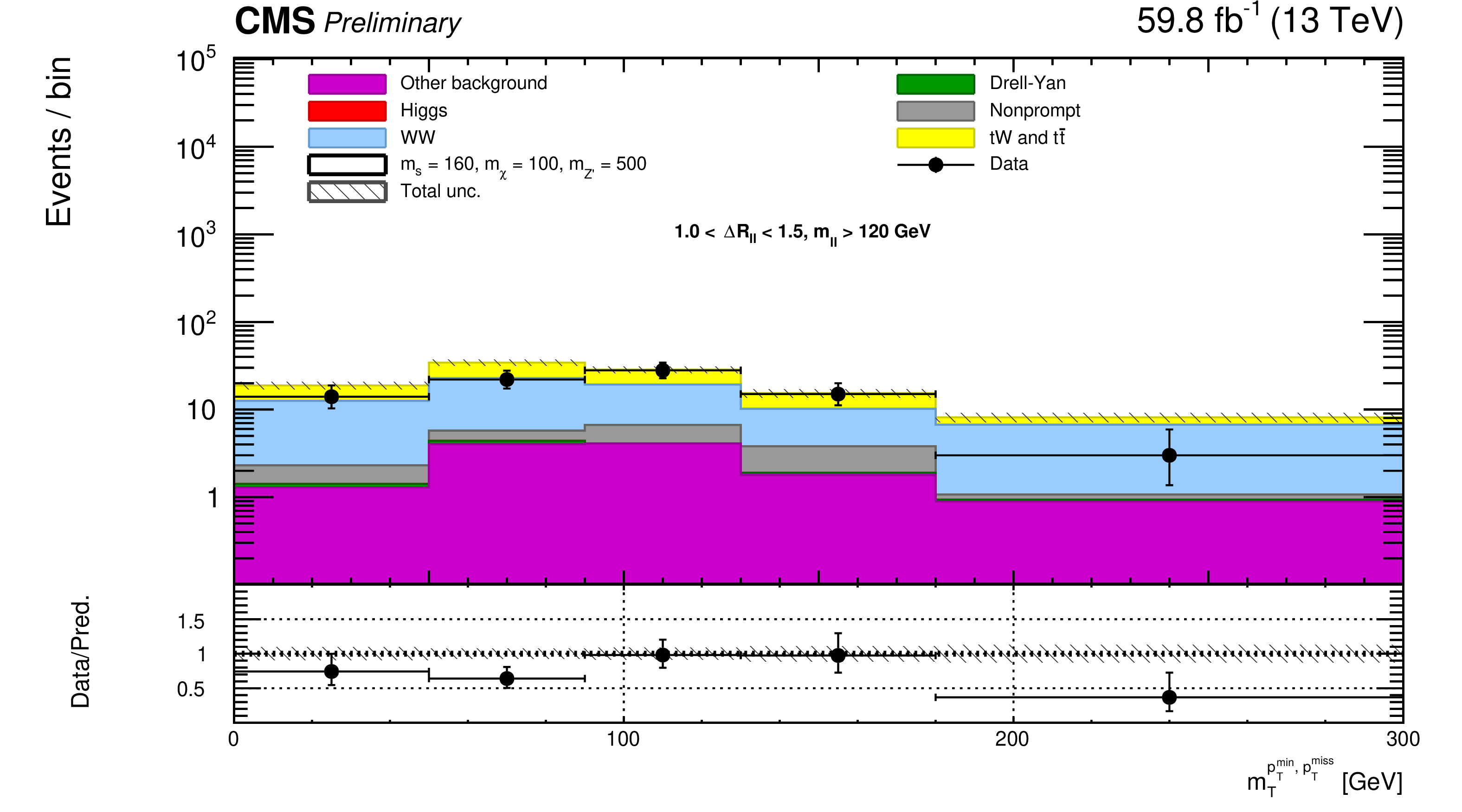
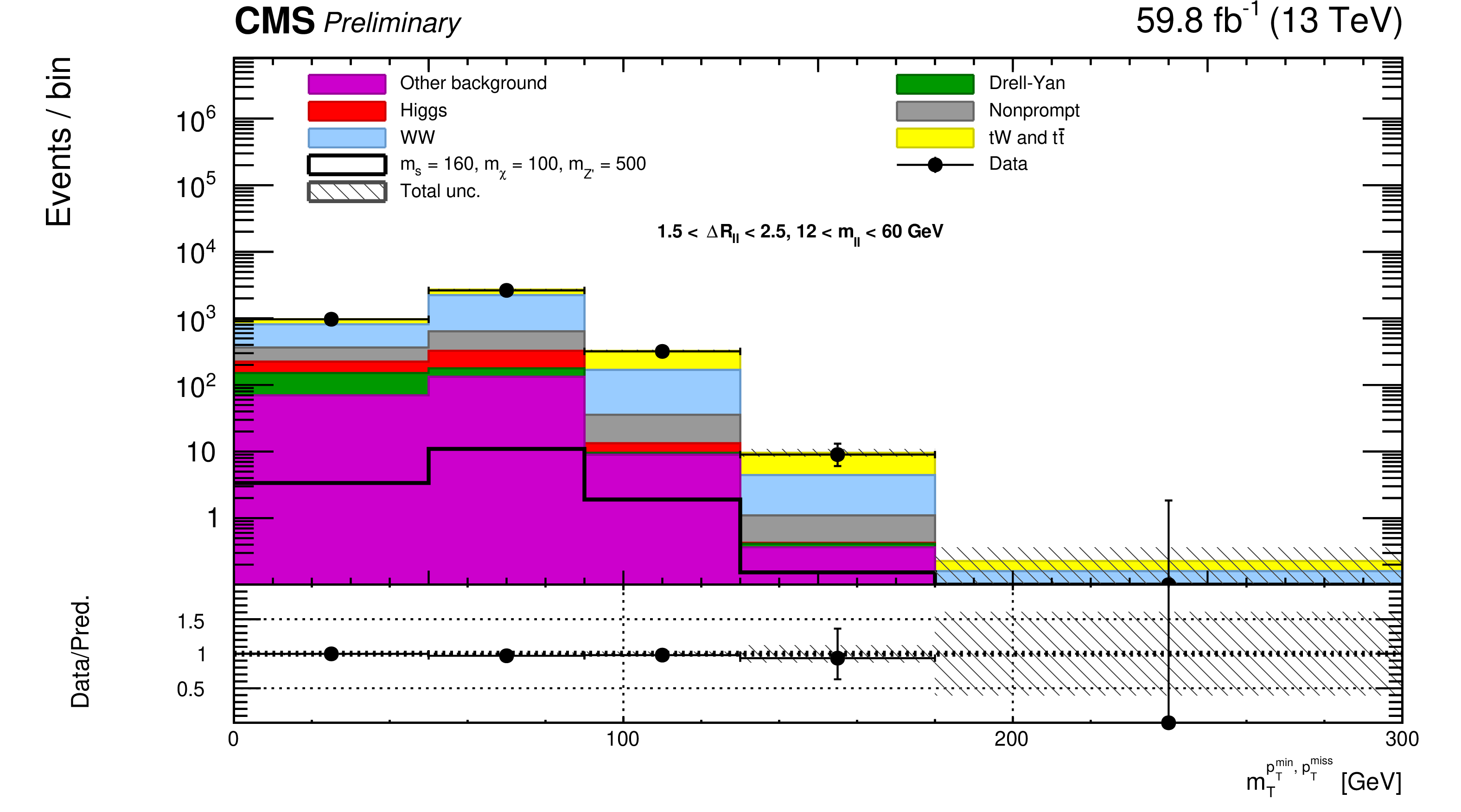
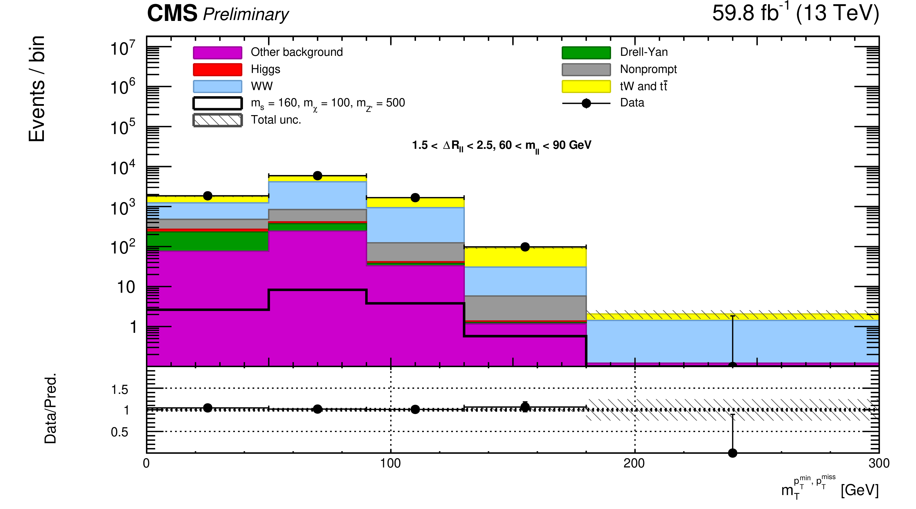
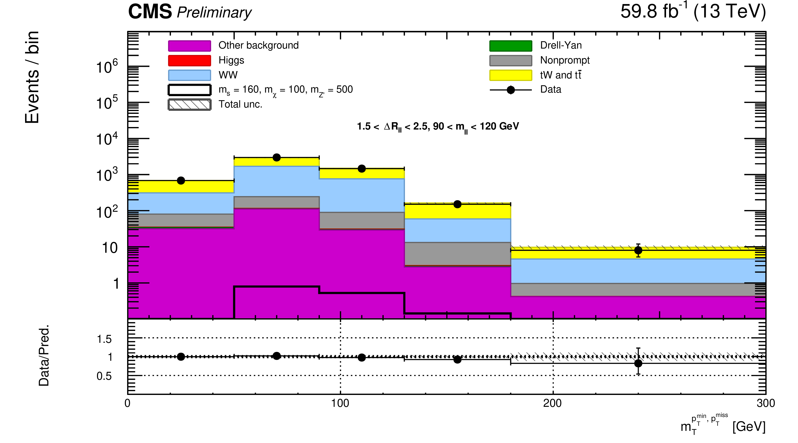
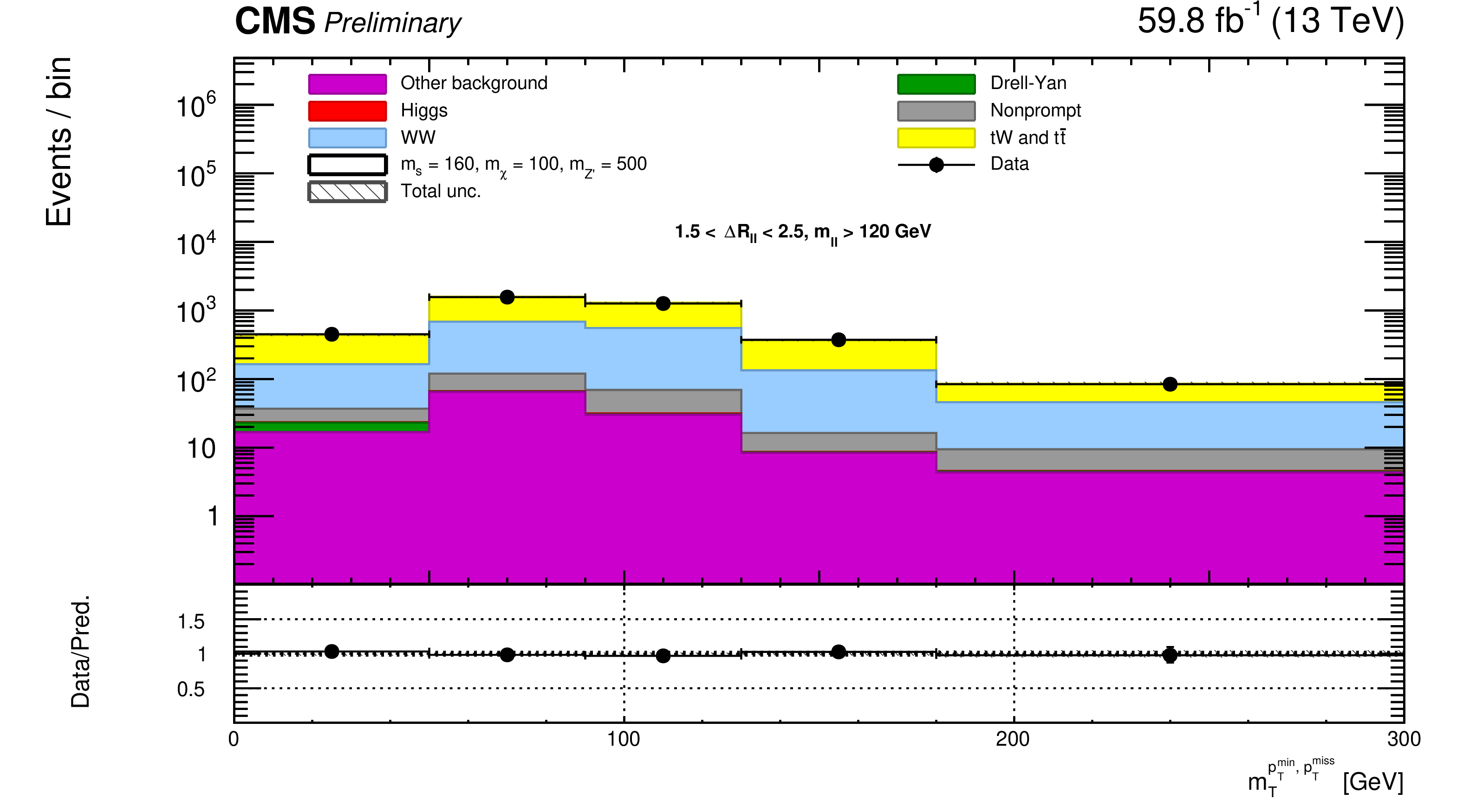
Figure 6:
Unrolled and equally spaced binned $ {m_{\ell \ell}} $-$ {{m_{\mathrm {T}}} ^{\ell \text { min},\, {{p_{\mathrm {T}}} ^\text {miss}}}} $ post-fit distributions for the full data set for in SR1 (top left), SR2 (top right), and SR3 (bottom). In each plot, every group of five bins (from left to right) corresponds to the $ {{m_{\mathrm {T}}} ^{\ell \text { min},\, {{p_{\mathrm {T}}} ^\text {miss}}}} $ distribution in a $ {m_{\ell \ell}} $ region, placed in ascending order. The black line indicates the signal prediction of $m_{s} = $ 160 GeV, $m_{\chi} = $ 100 GeV, $m_{\mathrm{Z'}} = $ 500 GeV. |
png pdf |
Figure 6-a:
Unrolled and equally spaced binned $ {m_{\ell \ell}} $-$ {{m_{\mathrm {T}}} ^{\ell \text { min},\, {{p_{\mathrm {T}}} ^\text {miss}}}} $ post-fit distributions for the full data set for in SR1. Every group of five bins (from left to right) corresponds to the $ {{m_{\mathrm {T}}} ^{\ell \text { min},\, {{p_{\mathrm {T}}} ^\text {miss}}}} $ distribution in a $ {m_{\ell \ell}} $ region, placed in ascending order. The black line indicates the signal prediction of $m_{s} = $ 160 GeV, $m_{\chi} = $ 100 GeV, $m_{\mathrm{Z'}} = $ 500 GeV. |
png pdf |
Figure 6-b:
Unrolled and equally spaced binned $ {m_{\ell \ell}} $-$ {{m_{\mathrm {T}}} ^{\ell \text { min},\, {{p_{\mathrm {T}}} ^\text {miss}}}} $ post-fit distributions for the full data set for in SR2. Every group of five bins (from left to right) corresponds to the $ {{m_{\mathrm {T}}} ^{\ell \text { min},\, {{p_{\mathrm {T}}} ^\text {miss}}}} $ distribution in a $ {m_{\ell \ell}} $ region, placed in ascending order. The black line indicates the signal prediction of $m_{s} = $ 160 GeV, $m_{\chi} = $ 100 GeV, $m_{\mathrm{Z'}} = $ 500 GeV. |

png pdf |
Figure 6-c:
Unrolled and equally spaced binned $ {m_{\ell \ell}} $-$ {{m_{\mathrm {T}}} ^{\ell \text { min},\, {{p_{\mathrm {T}}} ^\text {miss}}}} $ post-fit distributions for the full data set for in SR3. Every group of five bins (from left to right) corresponds to the $ {{m_{\mathrm {T}}} ^{\ell \text { min},\, {{p_{\mathrm {T}}} ^\text {miss}}}} $ distribution in a $ {m_{\ell \ell}} $ region, placed in ascending order. The black line indicates the signal prediction of $m_{s} = $ 160 GeV, $m_{\chi} = $ 100 GeV, $m_{\mathrm{Z'}} = $ 500 GeV. |

png pdf |
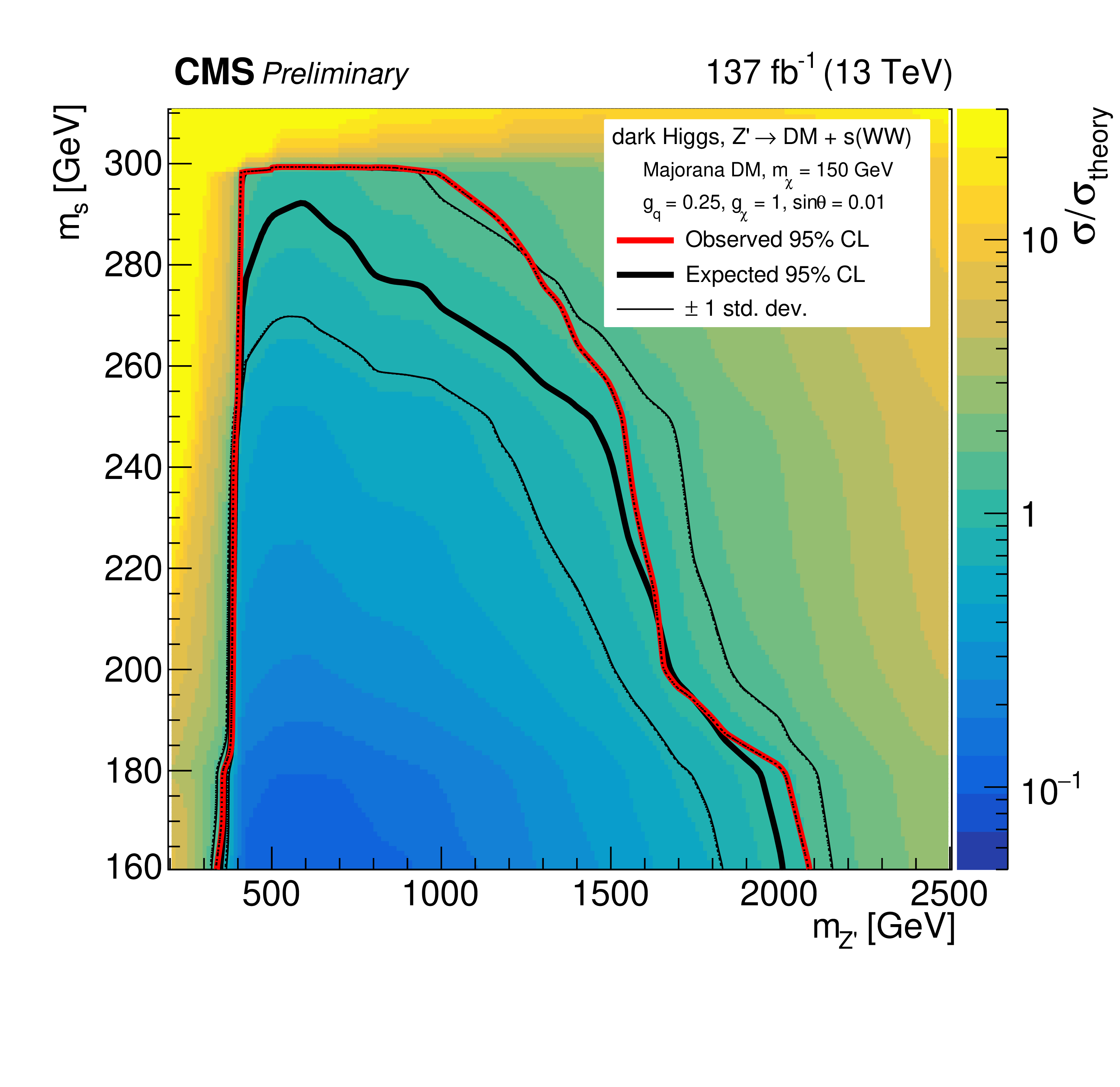
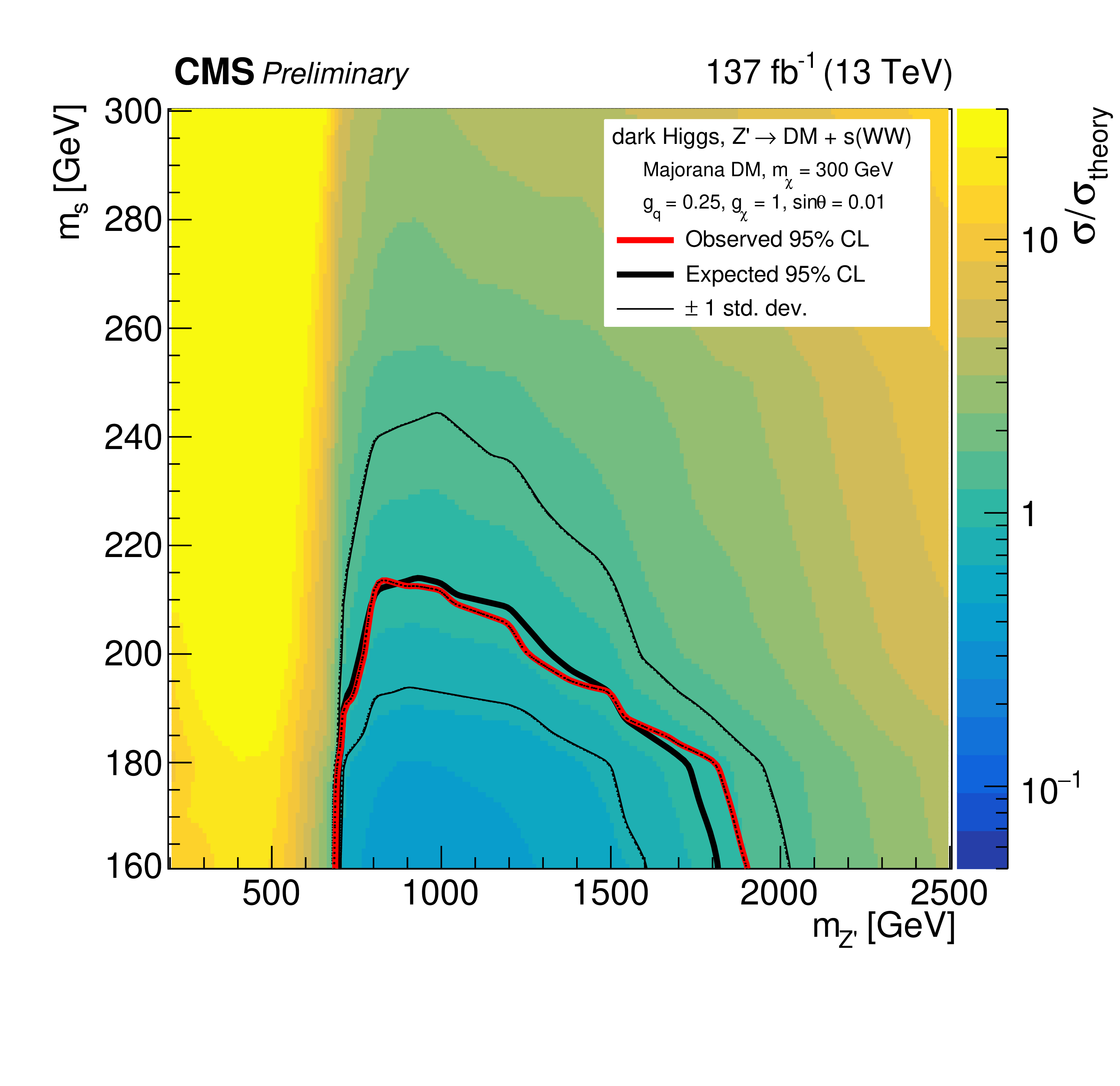
Figure 7:
Combined observed (expected) exclusion regions at 95% CL for the dark Higgs model in the ($m_{s}$, $m_{\mathrm{Z'}}$) plane, marked by the solid red (black) line. The expected $\pm $ 1$\sigma $ band is shown as the thinner black line. Upper left: $m_{\chi} = $ 100 GeV, upper right: $m_{\chi} = $ 150 GeV, bottom left: $m_{\chi} = $ 200 GeV, bottom right: $m_{\chi} = $ 300 GeV. |

png pdf |
Figure 7-a:
Combined observed (expected) exclusion regions at 95% CL for the dark Higgs model in the ($m_{s}$, $m_{\mathrm{Z'}}$) plane, marked by the solid red (black) line. for $m_{\chi} = $ 100 GeV. The expected $\pm $ 1$\sigma $ band is shown as the thinner black line. |
png pdf |
Figure 7-b:
Combined observed (expected) exclusion regions at 95% CL for the dark Higgs model in the ($m_{s}$, $m_{\mathrm{Z'}}$) plane, marked by the solid red (black) line. for $m_{\chi} = $ 150 GeV. The expected $\pm $ 1$\sigma $ band is shown as the thinner black line. |
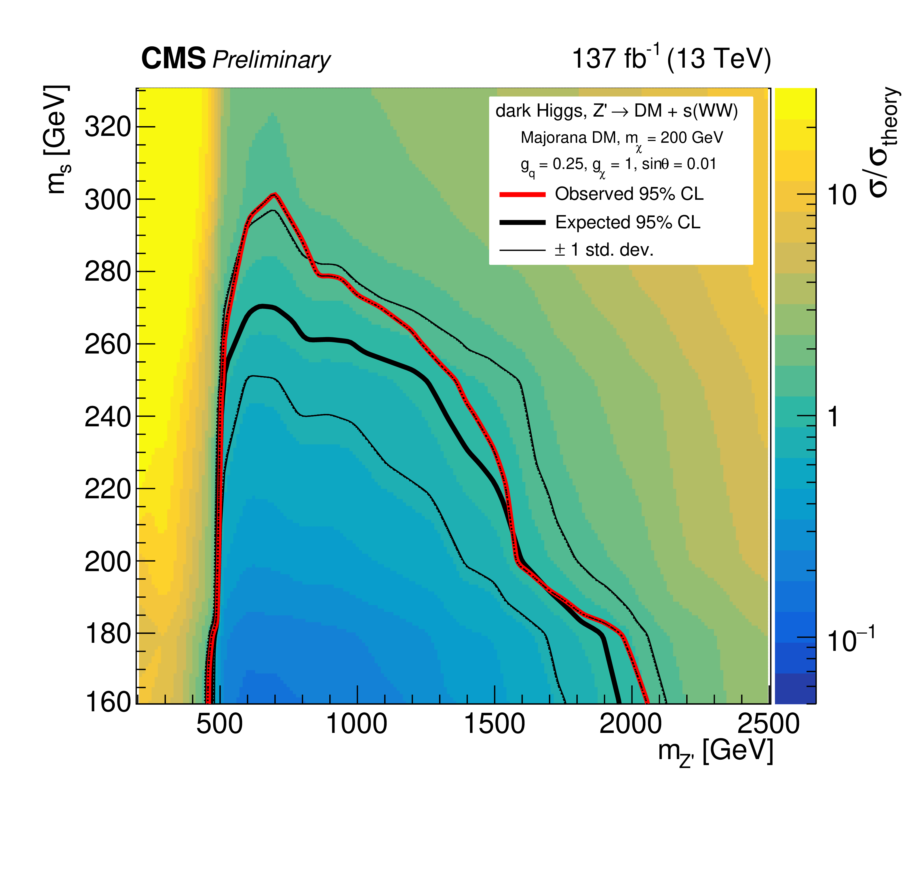
png pdf |
Figure 7-c:
Combined observed (expected) exclusion regions at 95% CL for the dark Higgs model in the ($m_{s}$, $m_{\mathrm{Z'}}$) plane, marked by the solid red (black) line. for $m_{\chi} = $ 200 GeV. The expected $\pm $ 1$\sigma $ band is shown as the thinner black line. |
png pdf |
Figure 7-d:
Combined observed (expected) exclusion regions at 95% CL for the dark Higgs model in the ($m_{s}$, $m_{\mathrm{Z'}}$) plane, marked by the solid red (black) line. for $m_{\chi} = $ 300 GeV. The expected $\pm $ 1$\sigma $ band is shown as the thinner black line. |

png pdf |
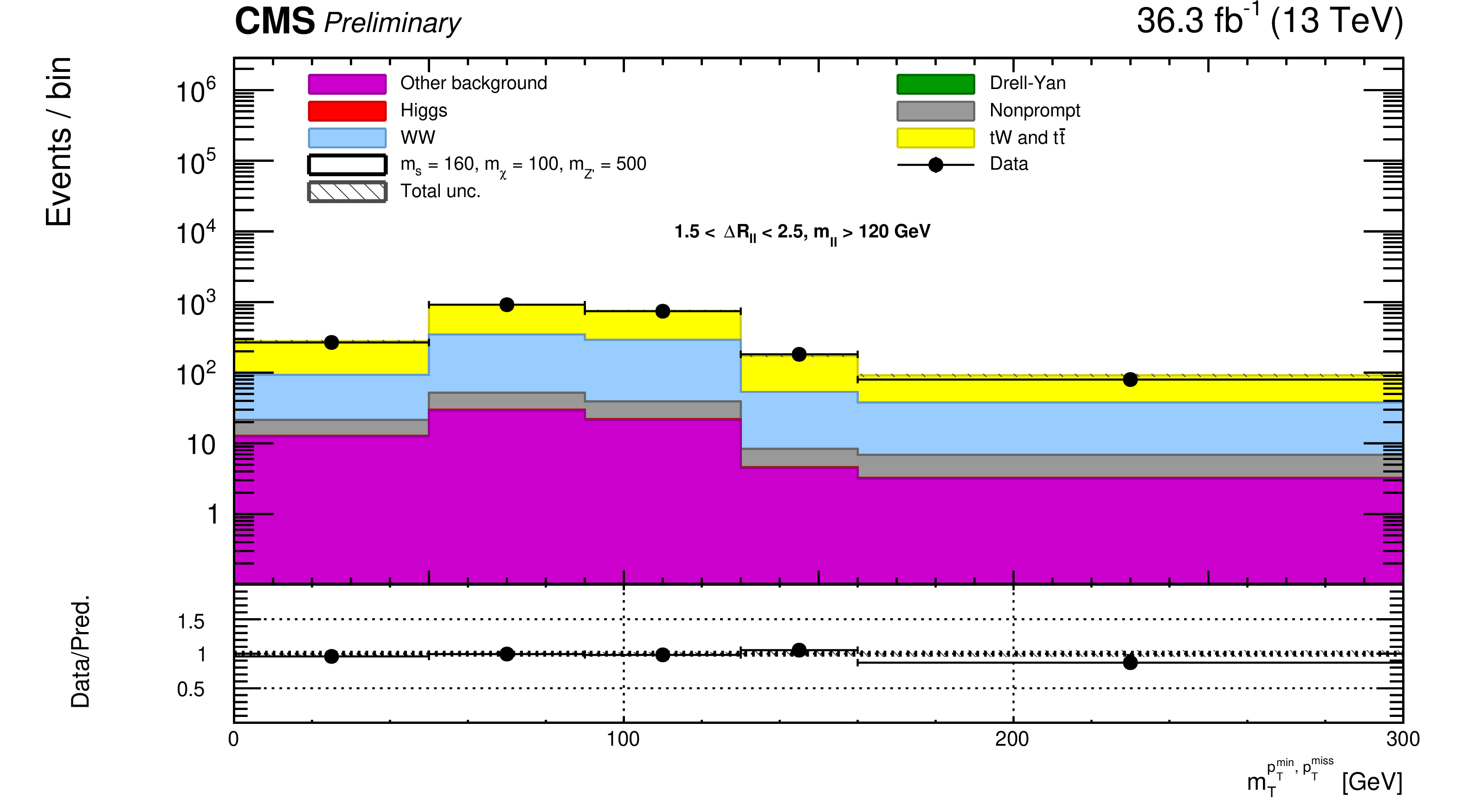
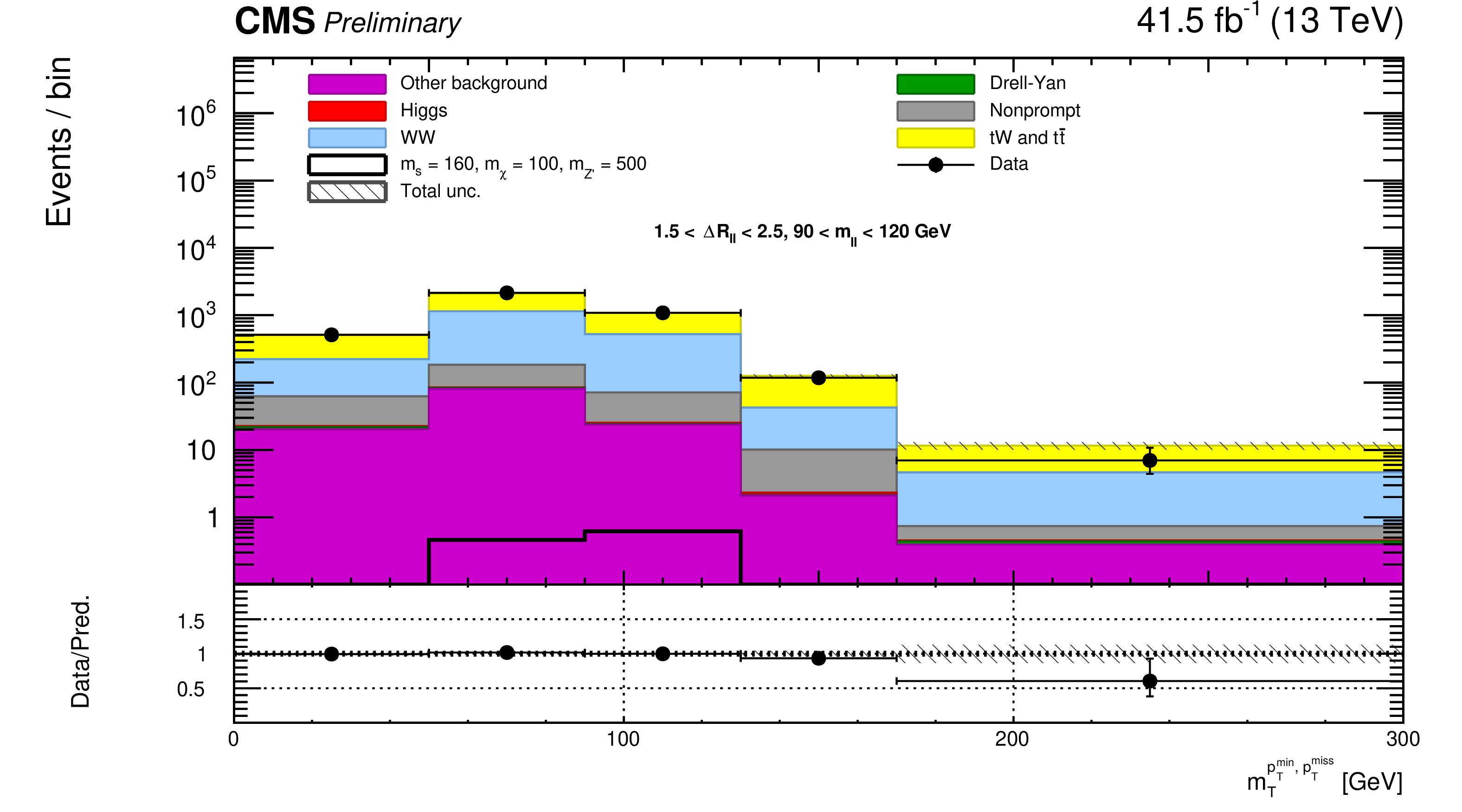
Figure 8:
$ {{m_{\mathrm {T}}} ^{\ell \text { min},\, {{p_{\mathrm {T}}} ^\text {miss}}}} $ distributions for the 2016 data set for the different signal regions. The black line indicates the signal prediction of $m_{s} = $ 160 GeV, $m_{\chi} = $ 100 GeV, $m_{\mathrm{Z'}} = $ 500 GeV. |
png pdf |
Figure 8-a:
$ {{m_{\mathrm {T}}} ^{\ell \text { min},\, {{p_{\mathrm {T}}} ^\text {miss}}}} $ distribution for the 2016 data set for one of the signal regions. The black line indicates the signal prediction of $m_{s} = $ 160 GeV, $m_{\chi} = $ 100 GeV, $m_{\mathrm{Z'}} = $ 500 GeV. |
png pdf |
Figure 8-b:
$ {{m_{\mathrm {T}}} ^{\ell \text { min},\, {{p_{\mathrm {T}}} ^\text {miss}}}} $ distribution for the 2016 data set for one of the signal regions. The black line indicates the signal prediction of $m_{s} = $ 160 GeV, $m_{\chi} = $ 100 GeV, $m_{\mathrm{Z'}} = $ 500 GeV. |
png pdf |
Figure 8-c:
$ {{m_{\mathrm {T}}} ^{\ell \text { min},\, {{p_{\mathrm {T}}} ^\text {miss}}}} $ distribution for the 2016 data set for one of the signal regions. The black line indicates the signal prediction of $m_{s} = $ 160 GeV, $m_{\chi} = $ 100 GeV, $m_{\mathrm{Z'}} = $ 500 GeV. |
png pdf |
Figure 8-d:
$ {{m_{\mathrm {T}}} ^{\ell \text { min},\, {{p_{\mathrm {T}}} ^\text {miss}}}} $ distribution for the 2016 data set for one of the signal regions. The black line indicates the signal prediction of $m_{s} = $ 160 GeV, $m_{\chi} = $ 100 GeV, $m_{\mathrm{Z'}} = $ 500 GeV. |
png pdf |
Figure 8-e:
$ {{m_{\mathrm {T}}} ^{\ell \text { min},\, {{p_{\mathrm {T}}} ^\text {miss}}}} $ distribution for the 2016 data set for one of the signal regions. The black line indicates the signal prediction of $m_{s} = $ 160 GeV, $m_{\chi} = $ 100 GeV, $m_{\mathrm{Z'}} = $ 500 GeV. |

png pdf |
Figure 8-f:
$ {{m_{\mathrm {T}}} ^{\ell \text { min},\, {{p_{\mathrm {T}}} ^\text {miss}}}} $ distribution for the 2016 data set for one of the signal regions. The black line indicates the signal prediction of $m_{s} = $ 160 GeV, $m_{\chi} = $ 100 GeV, $m_{\mathrm{Z'}} = $ 500 GeV. |

png pdf |
Figure 8-g:
$ {{m_{\mathrm {T}}} ^{\ell \text { min},\, {{p_{\mathrm {T}}} ^\text {miss}}}} $ distribution for the 2016 data set for one of the signal regions. The black line indicates the signal prediction of $m_{s} = $ 160 GeV, $m_{\chi} = $ 100 GeV, $m_{\mathrm{Z'}} = $ 500 GeV. |
png pdf |
Figure 8-h:
$ {{m_{\mathrm {T}}} ^{\ell \text { min},\, {{p_{\mathrm {T}}} ^\text {miss}}}} $ distribution for the 2016 data set for one of the signal regions. The black line indicates the signal prediction of $m_{s} = $ 160 GeV, $m_{\chi} = $ 100 GeV, $m_{\mathrm{Z'}} = $ 500 GeV. |
png pdf |
Figure 8-i:
$ {{m_{\mathrm {T}}} ^{\ell \text { min},\, {{p_{\mathrm {T}}} ^\text {miss}}}} $ distribution for the 2016 data set for one of the signal regions. The black line indicates the signal prediction of $m_{s} = $ 160 GeV, $m_{\chi} = $ 100 GeV, $m_{\mathrm{Z'}} = $ 500 GeV. |
png pdf |
Figure 8-j:
$ {{m_{\mathrm {T}}} ^{\ell \text { min},\, {{p_{\mathrm {T}}} ^\text {miss}}}} $ distribution for the 2016 data set for one of the signal regions. The black line indicates the signal prediction of $m_{s} = $ 160 GeV, $m_{\chi} = $ 100 GeV, $m_{\mathrm{Z'}} = $ 500 GeV. |
png pdf |
Figure 8-k:
$ {{m_{\mathrm {T}}} ^{\ell \text { min},\, {{p_{\mathrm {T}}} ^\text {miss}}}} $ distribution for the 2016 data set for one of the signal regions. The black line indicates the signal prediction of $m_{s} = $ 160 GeV, $m_{\chi} = $ 100 GeV, $m_{\mathrm{Z'}} = $ 500 GeV. |
png pdf |
Figure 8-l:
$ {{m_{\mathrm {T}}} ^{\ell \text { min},\, {{p_{\mathrm {T}}} ^\text {miss}}}} $ distribution for the 2016 data set for one of the signal regions. The black line indicates the signal prediction of $m_{s} = $ 160 GeV, $m_{\chi} = $ 100 GeV, $m_{\mathrm{Z'}} = $ 500 GeV. |
png pdf |
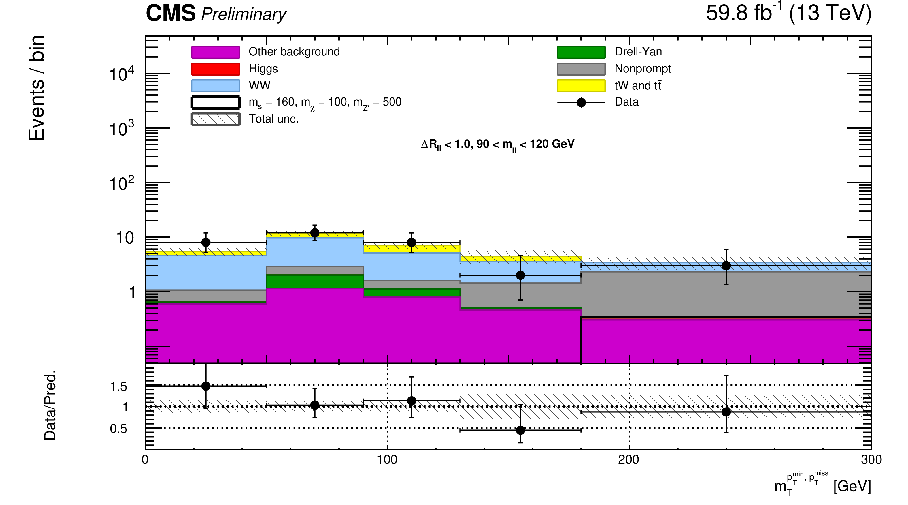
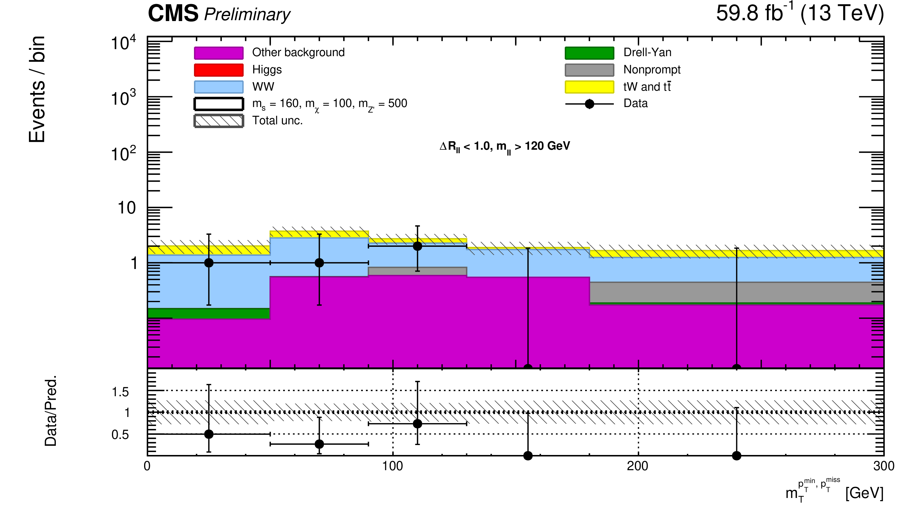
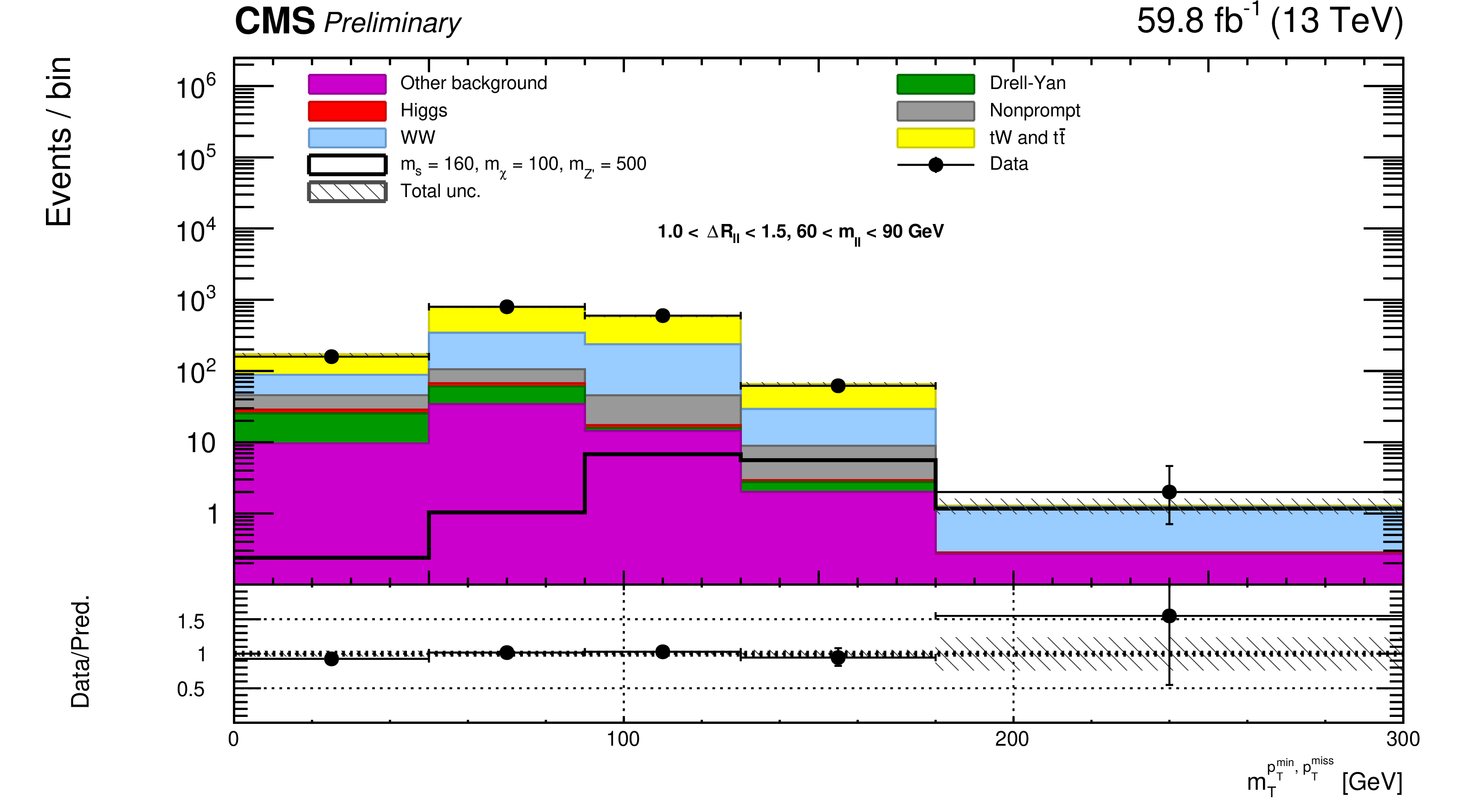
Figure 9:
$ {{m_{\mathrm {T}}} ^{\ell \text { min},\, {{p_{\mathrm {T}}} ^\text {miss}}}} $ distributions for the 2017 data set for the different signal regions. The black line indicates the signal prediction of $m_{s} = $ 160 GeV, $m_{\chi} = $ 100 GeV, $m_{\mathrm{Z'}} = $ 500 GeV. |
png pdf |
Figure 9-a:
$ {{m_{\mathrm {T}}} ^{\ell \text { min},\, {{p_{\mathrm {T}}} ^\text {miss}}}} $ distribution for the 2017 data set for one the signal regions. The black line indicates the signal prediction of $m_{s} = $ 160 GeV, $m_{\chi} = $ 100 GeV, $m_{\mathrm{Z'}} = $ 500 GeV. |
png pdf |
Figure 9-b:
$ {{m_{\mathrm {T}}} ^{\ell \text { min},\, {{p_{\mathrm {T}}} ^\text {miss}}}} $ distribution for the 2017 data set for one the signal regions. The black line indicates the signal prediction of $m_{s} = $ 160 GeV, $m_{\chi} = $ 100 GeV, $m_{\mathrm{Z'}} = $ 500 GeV. |
png pdf |
Figure 9-c:
$ {{m_{\mathrm {T}}} ^{\ell \text { min},\, {{p_{\mathrm {T}}} ^\text {miss}}}} $ distribution for the 2017 data set for one the signal regions. The black line indicates the signal prediction of $m_{s} = $ 160 GeV, $m_{\chi} = $ 100 GeV, $m_{\mathrm{Z'}} = $ 500 GeV. |
png pdf |
Figure 9-d:
$ {{m_{\mathrm {T}}} ^{\ell \text { min},\, {{p_{\mathrm {T}}} ^\text {miss}}}} $ distribution for the 2017 data set for one the signal regions. The black line indicates the signal prediction of $m_{s} = $ 160 GeV, $m_{\chi} = $ 100 GeV, $m_{\mathrm{Z'}} = $ 500 GeV. |
png pdf |
Figure 9-e:
$ {{m_{\mathrm {T}}} ^{\ell \text { min},\, {{p_{\mathrm {T}}} ^\text {miss}}}} $ distribution for the 2017 data set for one the signal regions. The black line indicates the signal prediction of $m_{s} = $ 160 GeV, $m_{\chi} = $ 100 GeV, $m_{\mathrm{Z'}} = $ 500 GeV. |
png pdf |
Figure 9-f:
$ {{m_{\mathrm {T}}} ^{\ell \text { min},\, {{p_{\mathrm {T}}} ^\text {miss}}}} $ distribution for the 2017 data set for one the signal regions. The black line indicates the signal prediction of $m_{s} = $ 160 GeV, $m_{\chi} = $ 100 GeV, $m_{\mathrm{Z'}} = $ 500 GeV. |
png pdf |
Figure 9-g:
$ {{m_{\mathrm {T}}} ^{\ell \text { min},\, {{p_{\mathrm {T}}} ^\text {miss}}}} $ distribution for the 2017 data set for one the signal regions. The black line indicates the signal prediction of $m_{s} = $ 160 GeV, $m_{\chi} = $ 100 GeV, $m_{\mathrm{Z'}} = $ 500 GeV. |
png pdf |
Figure 9-h:
$ {{m_{\mathrm {T}}} ^{\ell \text { min},\, {{p_{\mathrm {T}}} ^\text {miss}}}} $ distribution for the 2017 data set for one the signal regions. The black line indicates the signal prediction of $m_{s} = $ 160 GeV, $m_{\chi} = $ 100 GeV, $m_{\mathrm{Z'}} = $ 500 GeV. |
png pdf |
Figure 9-i:
$ {{m_{\mathrm {T}}} ^{\ell \text { min},\, {{p_{\mathrm {T}}} ^\text {miss}}}} $ distribution for the 2017 data set for one the signal regions. The black line indicates the signal prediction of $m_{s} = $ 160 GeV, $m_{\chi} = $ 100 GeV, $m_{\mathrm{Z'}} = $ 500 GeV. |
png pdf |
Figure 9-j:
$ {{m_{\mathrm {T}}} ^{\ell \text { min},\, {{p_{\mathrm {T}}} ^\text {miss}}}} $ distribution for the 2017 data set for one the signal regions. The black line indicates the signal prediction of $m_{s} = $ 160 GeV, $m_{\chi} = $ 100 GeV, $m_{\mathrm{Z'}} = $ 500 GeV. |
png pdf |
Figure 9-k:
$ {{m_{\mathrm {T}}} ^{\ell \text { min},\, {{p_{\mathrm {T}}} ^\text {miss}}}} $ distribution for the 2017 data set for one the signal regions. The black line indicates the signal prediction of $m_{s} = $ 160 GeV, $m_{\chi} = $ 100 GeV, $m_{\mathrm{Z'}} = $ 500 GeV. |

png pdf |
Figure 9-l:
$ {{m_{\mathrm {T}}} ^{\ell \text { min},\, {{p_{\mathrm {T}}} ^\text {miss}}}} $ distribution for the 2017 data set for one the signal regions. The black line indicates the signal prediction of $m_{s} = $ 160 GeV, $m_{\chi} = $ 100 GeV, $m_{\mathrm{Z'}} = $ 500 GeV. |

png pdf |
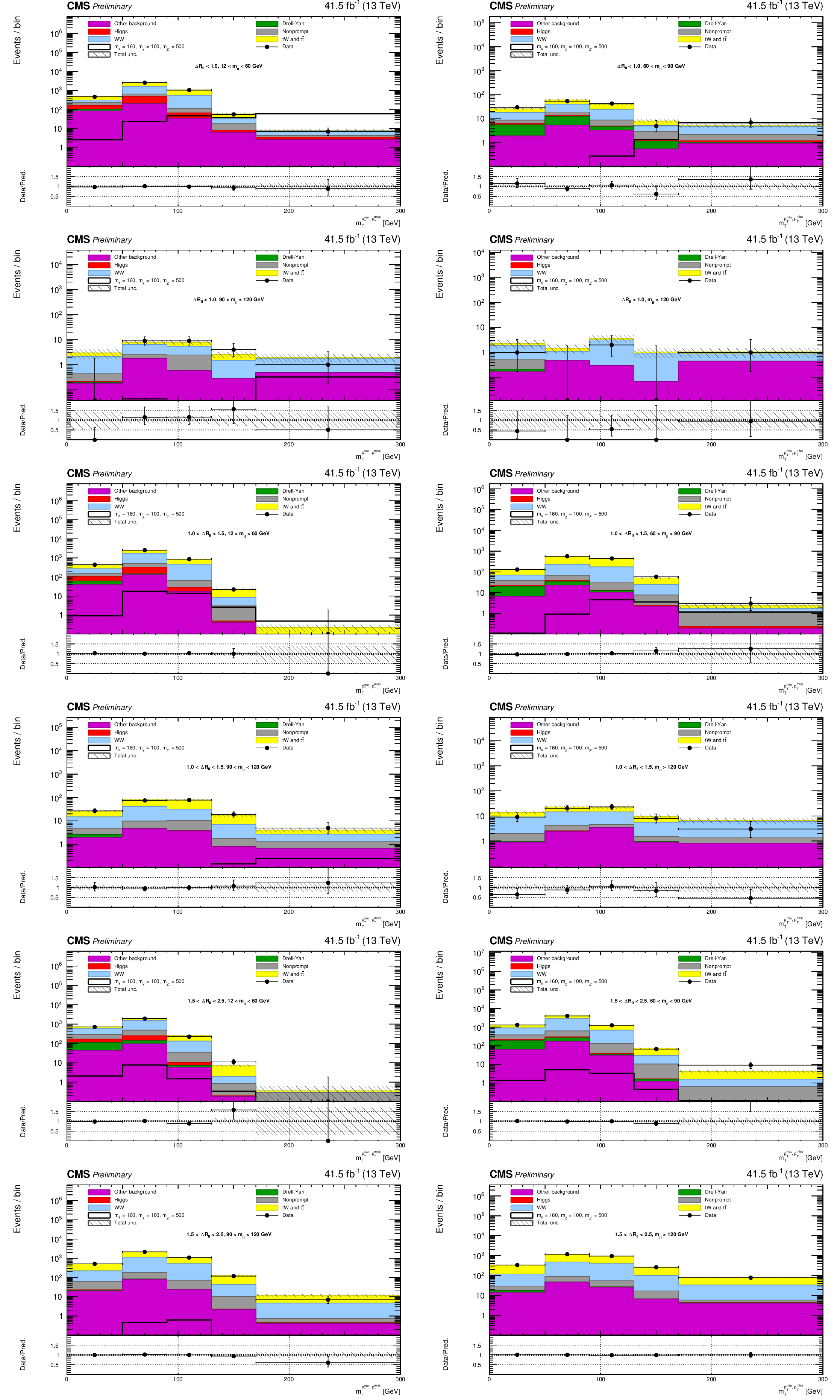
Figure 10:
$ {{m_{\mathrm {T}}} ^{\ell \text { min},\, {{p_{\mathrm {T}}} ^\text {miss}}}} $ distributions for the 2018 data set for the different signal regions. The black line indicates the signal prediction of $m_{s} = $ 160 GeV, $m_{\chi} = $ 100 GeV, $m_{\mathrm{Z'}} = $ 500 GeV. |

png pdf |
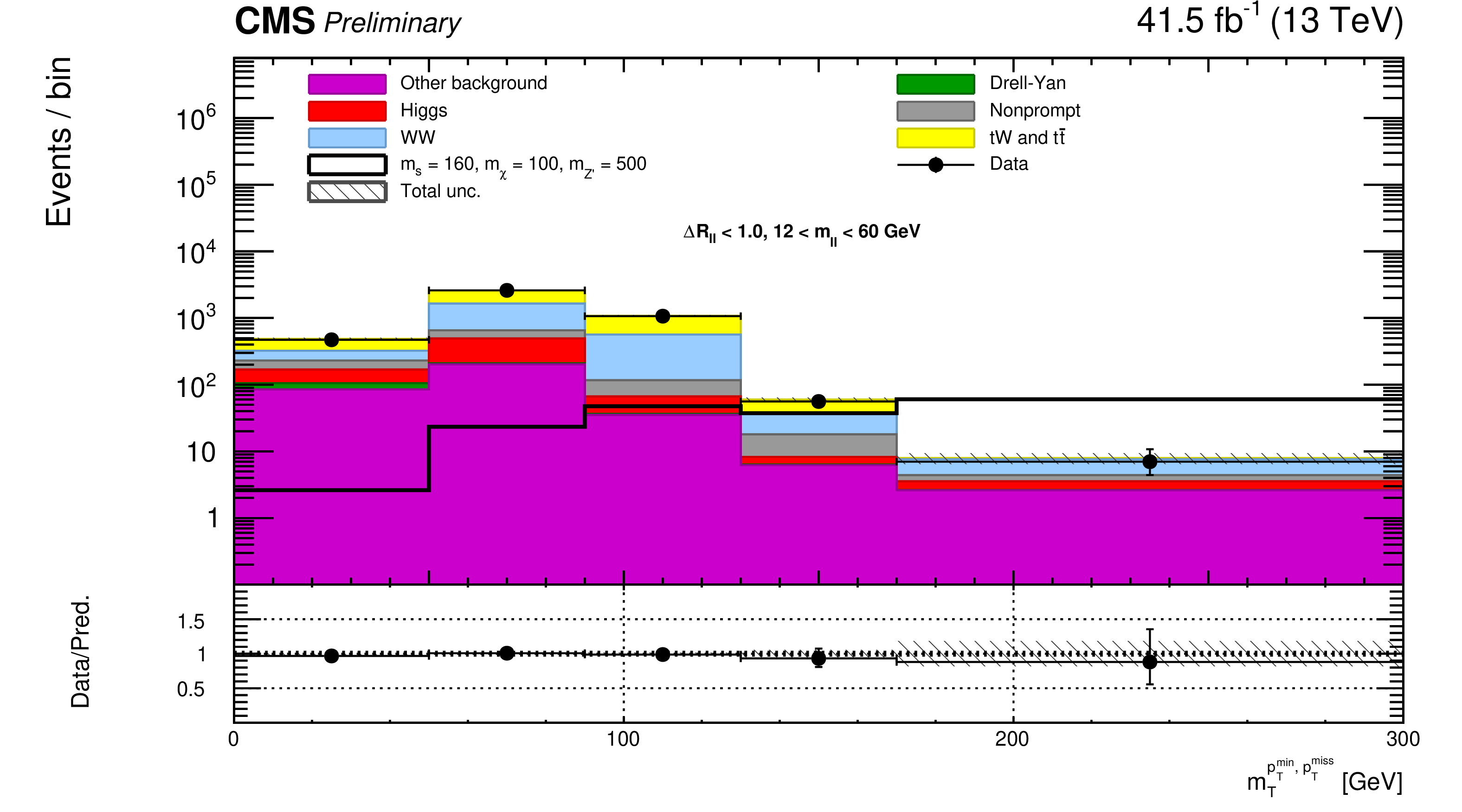
Figure 10-a:
$ {{m_{\mathrm {T}}} ^{\ell \text { min},\, {{p_{\mathrm {T}}} ^\text {miss}}}} $ distribution for the 2018 data set for one of the signal regions. The black line indicates the signal prediction of $m_{s} = $ 160 GeV, $m_{\chi} = $ 100 GeV, $m_{\mathrm{Z'}} = $ 500 GeV. |

png pdf |
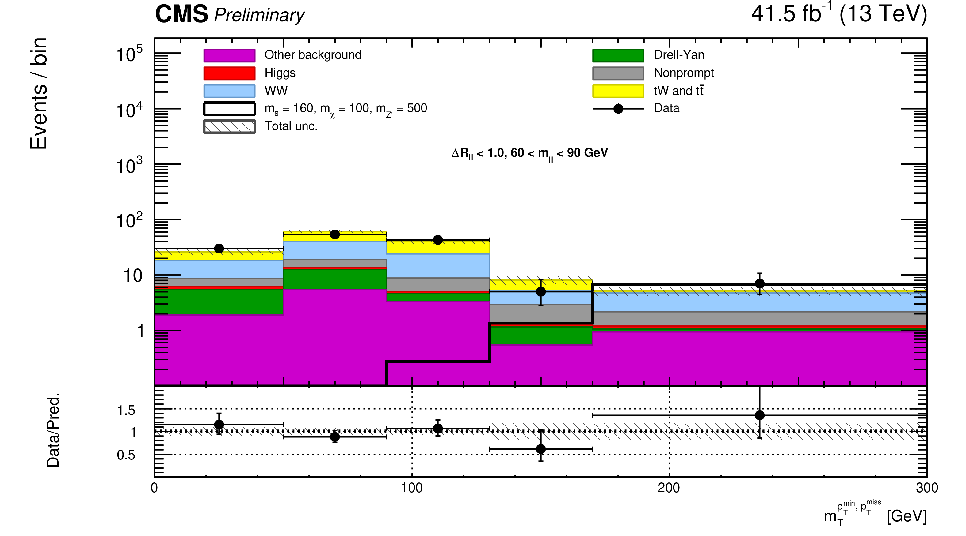
Figure 10-b:
$ {{m_{\mathrm {T}}} ^{\ell \text { min},\, {{p_{\mathrm {T}}} ^\text {miss}}}} $ distribution for the 2018 data set for one of the signal regions. The black line indicates the signal prediction of $m_{s} = $ 160 GeV, $m_{\chi} = $ 100 GeV, $m_{\mathrm{Z'}} = $ 500 GeV. |
png pdf |
Figure 10-c:
$ {{m_{\mathrm {T}}} ^{\ell \text { min},\, {{p_{\mathrm {T}}} ^\text {miss}}}} $ distribution for the 2018 data set for one of the signal regions. The black line indicates the signal prediction of $m_{s} = $ 160 GeV, $m_{\chi} = $ 100 GeV, $m_{\mathrm{Z'}} = $ 500 GeV. |
png pdf |
Figure 10-d:
$ {{m_{\mathrm {T}}} ^{\ell \text { min},\, {{p_{\mathrm {T}}} ^\text {miss}}}} $ distribution for the 2018 data set for one of the signal regions. The black line indicates the signal prediction of $m_{s} = $ 160 GeV, $m_{\chi} = $ 100 GeV, $m_{\mathrm{Z'}} = $ 500 GeV. |

png pdf |
Figure 10-e:
$ {{m_{\mathrm {T}}} ^{\ell \text { min},\, {{p_{\mathrm {T}}} ^\text {miss}}}} $ distribution for the 2018 data set for one of the signal regions. The black line indicates the signal prediction of $m_{s} = $ 160 GeV, $m_{\chi} = $ 100 GeV, $m_{\mathrm{Z'}} = $ 500 GeV. |
png pdf |
Figure 10-f:
$ {{m_{\mathrm {T}}} ^{\ell \text { min},\, {{p_{\mathrm {T}}} ^\text {miss}}}} $ distribution for the 2018 data set for one of the signal regions. The black line indicates the signal prediction of $m_{s} = $ 160 GeV, $m_{\chi} = $ 100 GeV, $m_{\mathrm{Z'}} = $ 500 GeV. |
png pdf |
Figure 10-g:
$ {{m_{\mathrm {T}}} ^{\ell \text { min},\, {{p_{\mathrm {T}}} ^\text {miss}}}} $ distribution for the 2018 data set for one of the signal regions. The black line indicates the signal prediction of $m_{s} = $ 160 GeV, $m_{\chi} = $ 100 GeV, $m_{\mathrm{Z'}} = $ 500 GeV. |
png pdf |
Figure 10-h:
$ {{m_{\mathrm {T}}} ^{\ell \text { min},\, {{p_{\mathrm {T}}} ^\text {miss}}}} $ distribution for the 2018 data set for one of the signal regions. The black line indicates the signal prediction of $m_{s} = $ 160 GeV, $m_{\chi} = $ 100 GeV, $m_{\mathrm{Z'}} = $ 500 GeV. |
png pdf |
Figure 10-i:
$ {{m_{\mathrm {T}}} ^{\ell \text { min},\, {{p_{\mathrm {T}}} ^\text {miss}}}} $ distribution for the 2018 data set for one of the signal regions. The black line indicates the signal prediction of $m_{s} = $ 160 GeV, $m_{\chi} = $ 100 GeV, $m_{\mathrm{Z'}} = $ 500 GeV. |
png pdf |
Figure 10-j:
$ {{m_{\mathrm {T}}} ^{\ell \text { min},\, {{p_{\mathrm {T}}} ^\text {miss}}}} $ distribution for the 2018 data set for one of the signal regions. The black line indicates the signal prediction of $m_{s} = $ 160 GeV, $m_{\chi} = $ 100 GeV, $m_{\mathrm{Z'}} = $ 500 GeV. |
png pdf |
Figure 10-k:
$ {{m_{\mathrm {T}}} ^{\ell \text { min},\, {{p_{\mathrm {T}}} ^\text {miss}}}} $ distribution for the 2018 data set for one of the signal regions. The black line indicates the signal prediction of $m_{s} = $ 160 GeV, $m_{\chi} = $ 100 GeV, $m_{\mathrm{Z'}} = $ 500 GeV. |
png pdf |
Figure 10-l:
$ {{m_{\mathrm {T}}} ^{\ell \text { min},\, {{p_{\mathrm {T}}} ^\text {miss}}}} $ distribution for the 2018 data set for one of the signal regions. The black line indicates the signal prediction of $m_{s} = $ 160 GeV, $m_{\chi} = $ 100 GeV, $m_{\mathrm{Z'}} = $ 500 GeV. |
| Tables | |
png pdf |
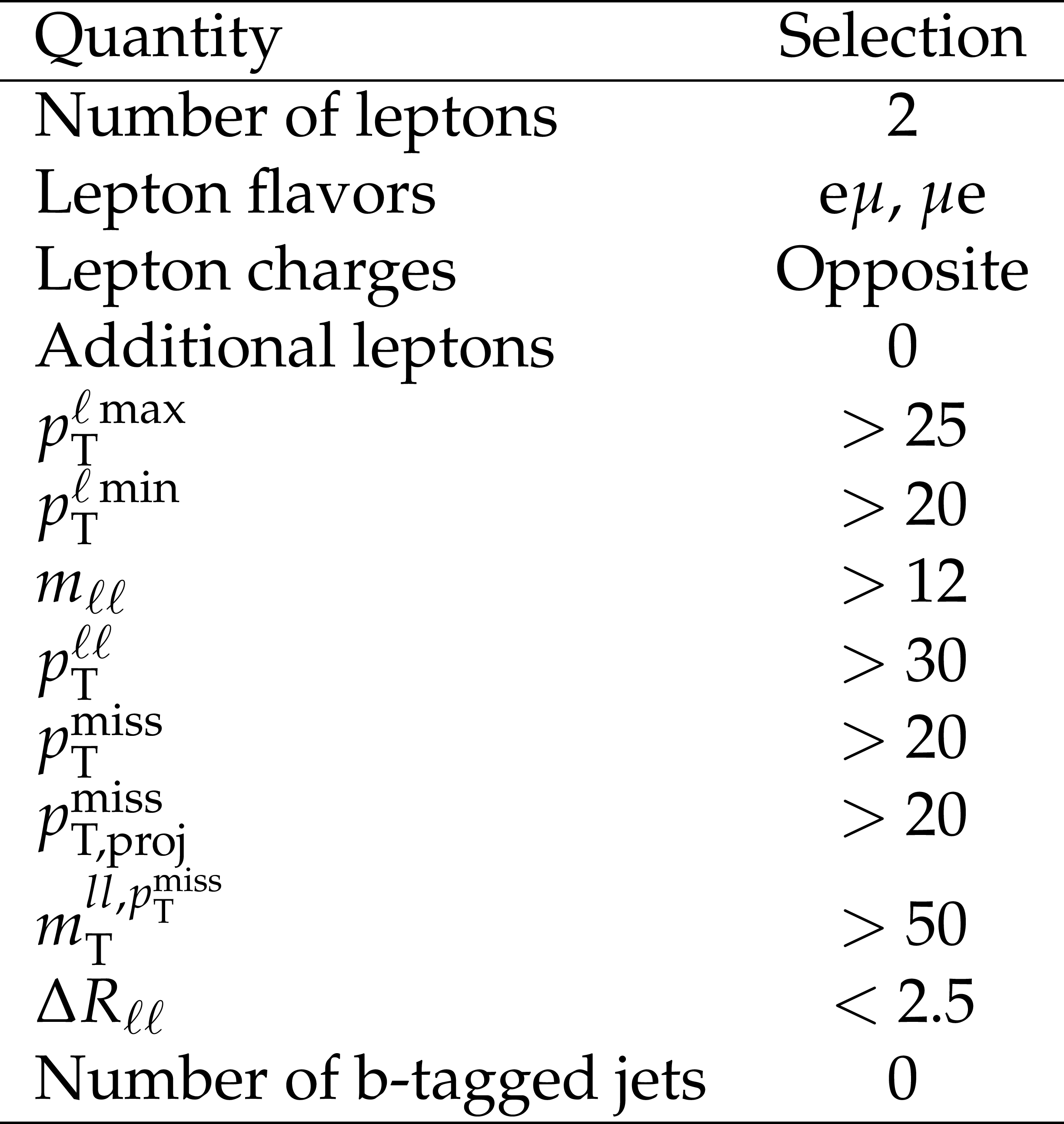
Table 1:
Summary of the event preselection criteria. Kinematic quantities are measured in GeV. |

png pdf |
Table 2:
Data and background post-fit yields for each data period and for each signal region. Signal prediction corresponds to pre-fit yields for a sample with $m_{s} = $ 160 GeV, $m_{\chi} = $ 100 GeV, $m_{\mathrm{Z'}} = $ 500 GeV. The total post-fit uncertainty is shown for the total background. |
| Summary |
| A search for dark matter particles produced in association with a dark Higgs boson has been presented. A sample of proton-proton collision data at a center-of-mass energy of 13 TeV is used, corresponding to an integrated luminosity of 137 fb$^{-1}$. The decay mode of the dark Higgs boson to a W$^{+}$W$^{-}$ pair has been explored; this is the first time the CMS Collaboration explores this model. Results from the dileptonic decay channel of the W$^{+}$W$^{-}$ pair are presented. No significant deviation from the Standard Model prediction is observed, so upper limits at 95% confidence level on the production cross section of dark matter are set on the dark Higgs model parameters. This analysis extends the search to a wider DM mass range, from 100 GeV to 300 GeV. The most stringent limit is set for a $m_{DM} = $ 150 GeV, excluding $m_{s}$ masses up to $\approx $300 GeV in a mass range $\approx $480 $< m_{\mathrm{Z'}} < $ 1200 GeV, and up to $m_{\mathrm{Z'}} \approx $ 2000 GeV for a $m_{s} = $ 160 GeV. |
| References | ||||
| 1 | R. J. Gaitskell | Direct detection of dark matter | Ann. Rev. Nucl. Part. Sci. 54 (2004) 315 | |
| 2 | V. Trimble | Existence and nature of dark matter in the universe | Ann. Rev. Astron. Astrophys. 25 (1987) 425 | |
| 3 | T. A. Porter, R. P. Johnson, and P. W. Graham | Dark Matter searches with astroparticle data | Ann. Rev. Astron. Astrophys. 49 (2011) 155 | 1104.2836 |
| 4 | G. Bertone, D. Hooper, and J. Silk | Particle dark matter: evidence, candidates and constraints | PR 405 (2005) 279 | hep-ph/0404175 |
| 5 | J. L. Feng | Dark Matter Candidates from Particle Physics and Methods of Detection | Ann. Rev. Astron. Astrophys. 48 (2010) 495 | 1003.0904 |
| 6 | R. J. Scherrer and M. S. Turner | On the relic, cosmic abundance of stable, weakly interacting massive particles | PRD 33 (1986) 1585 | |
| 7 | G. Steigman and M. S. Turner | Cosmological constraints on the properties of weakly interacting massive particles | NPB 253 (1985) 375 | |
| 8 | ATLAS Collaboration | Search for dark matter and other new phenomena in events with an energetic jet and large missing transverse momentum using the ATLAS detector | JHEP 01 (2018) 126 | 1711.03301 |
| 9 | CMS Collaboration | Search for new physics in final states with an energetic jet or a hadronically decaying $ \mathrm{W} $ or $ \mathrm{Z} $ boson and transverse momentum imbalance at $ \sqrt{s}=$ 13 TeV | PRD 97 (2018) 092005 | CMS-EXO-16-048 1712.02345 |
| 10 | ATLAS Collaboration | Search for dark matter produced in association with bottom or top quarks in $ \sqrt{s}= $ 13 TeV pp collisions with the ATLAS detector | EPJC 78 (2018) 18 | 1710.11412 |
| 11 | CMS Collaboration | Search for dark matter in events with energetic, hadronically decaying top quarks and missing transverse momentum at $ \sqrt{s}= $ 13 TeV | JHEP 06 (2018) 027 | CMS-EXO-16-051 1801.08427 |
| 12 | ATLAS Collaboration | Search for dark matter at $ \sqrt{s}= $ 13 TeV in final states containing an energetic photon and large missing transverse momentum with the ATLAS detector | EPJC 77 (2017) 393 | 1704.03848 |
| 13 | CMS Collaboration | Search for new physics in the monophoton final state in proton-proton collisions at $ \sqrt{s}= $ 13 TeV | JHEP 10 (2017) 073 | CMS-EXO-16-039 1706.03794 |
| 14 | ATLAS Collaboration | Search for an invisibly decaying Higgs boson or dark matter candidates produced in association with a $ Z $ boson in pp collisions at $ \sqrt{s} = $ 13 TeV with the ATLAS detector | PLB 776 (2018) 318 | 1708.09624 |
| 15 | CMS Collaboration | Search for new physics in events with a leptonically decaying Z boson and a large transverse momentum imbalance in proton-proton collisions at $ \sqrt{s} = $ 13 TeV | EPJC 78 (2018) 291 | CMS-EXO-16-052 1711.00431 |
| 16 | ATLAS Collaboration | Search for dark matter in events with a hadronically decaying vector boson and missing transverse momentum in pp collisions at $ \sqrt{s} = $ 13 TeV with the ATLAS detector | JHEP 10 (2018) 180 | 1807.11471 |
| 17 | CMS Collaboration | Search for dark matter particles produced in association with a Higgs boson in proton-proton collisions at $ \sqrt{s} = $ 13 TeV | JHEP 3 (2020) 25 | 1908.01713v2 |
| 18 | ATLAS Collaboration | Observation of a new particle in the search for the standard model Higgs boson with the ATLAS detector at the LHC | PLB 716 (2012) 1 | 1207.7214 |
| 19 | CMS Collaboration | Observation of a new boson at a mass of 125 GeV with the CMS experiment at the LHC | PLB 716 (2012) 30 | CMS-HIG-12-028 1207.7235 |
| 20 | CMS Collaboration | Observation of a new boson with mass near 125 GeV in pp collisions at $ \sqrt{s} = $ 7 and 8 TeV | JHEP 06 (2013) 081 | CMS-HIG-12-036 1303.4571 |
| 21 | ATLAS, CMS Collaboration | Measurements of the Higgs boson production and decay rates and constraints on its couplings from a combined ATLAS and CMS analysis of the LHC pp collision data at $ \sqrt{s}= $ 7 and 8 TeV | JHEP 8 (2016) 45 | 1606.02266v2 |
| 22 | M. Duerr et al. | How to save the wimp: global analysis of a dark matter model with two s-channel mediators | JHEP 9 (2016) 42 | 1606.07609v2 |
| 23 | M. Duerr et al. | Hunting the dark higgs | JHEP 4 (2017) 143 | 1701.08780v2 |
| 24 | ATLAS Collaboration | RECAST framework reinterpretation of an ATLAS Dark Matter Search constraining a model of a dark Higgs boson decaying to two $ b $-quarks | technical report, CERN | |
| 25 | ATLAS Collaboration | Search for dark matter produced in association with a dark higgs boson decaying into W$^{+}$W$^{-}$ or ZZ in fully hadronic final states from $ \sqrt{s}=$ 13 TeV pp collisions recorded with the ATLAS detector | PRL 126 (2021) 121802 | 2010.06548v2 |
| 26 | CMS Collaboration | The CMS trigger system | JINST 12 (2017) P01020 | CMS-TRG-12-001 1609.02366 |
| 27 | CMS Collaboration | The CMS Experiment at the CERN LHC | JINST 3 (2008) S08004 | CMS-00-001 |
| 28 | CMS Collaboration | CMS Luminosity Measurements for the 2016 Data Taking Period | CMS-PAS-LUM-17-001 | CMS-PAS-LUM-17-001 |
| 29 | CMS Collaboration | CMS luminosity measurement for the 2017 data-taking period at $ \sqrt{s} = $ 13 TeV | CMS-PAS-LUM-17-004 | CMS-PAS-LUM-17-004 |
| 30 | CMS Collaboration | CMS luminosity measurement for the 2018 data-taking period at $ \sqrt{s} = $ 13 TeV | CMS-PAS-LUM-18-002 | CMS-PAS-LUM-18-002 |
| 31 | T. Sjostrand et al. | An introduction to PYTHIA 8.2 | CPC 191 (2015) 159 | 1410.3012 |
| 32 | CMS Collaboration | Event generator tunes obtained from underlying event and multiparton scattering measurements | EPJC 76 (2016) 155 | CMS-GEN-14-001 1512.00815 |
| 33 | CMS Collaboration | Extraction and validation of a new set of CMS PYTHIA 8 tunes from underlying-event measurements | EPJC 80 (2020) 4 | CMS-GEN-17-001 1903.12179 |
| 34 | NNPDF Collaboration | Parton distributions with QED corrections | NPB 877 (2013) 290 | 1308.0598 |
| 35 | NNPDF Collaboration | Unbiased global determination of parton distributions and their uncertainties at NNLO and at LO | NPB 855 (2012) 153 | 1107.2652 |
| 36 | NNPDF Collaboration | Parton distributions from high-precision collider data | EPJC 77 (2017) 663 | 1706.00428 |
| 37 | J. Alwall et al. | The automated computation of tree-level and next-to-leading order differential cross sections, and their matching to parton shower simulations | JHEP 2014 (2014) 79 | |
| 38 | D. Abercrombie et al. | Dark Matter benchmark models for early LHC Run-2 Searches: Report of the ATLAS/CMS Dark Matter Forum | Phys. Dark Univ. 27 (2020) 100371 | 1507.00966v1 |
| 39 | T. Melia, P. Nason, R. Rontsch, and G. Zanderighi | W$ ^+ $W$ ^- $, WZ and ZZ production in the POWHEG BOX | JHEP 11 (2011) 078 | 1107.5051 |
| 40 | J. M. Campbell, R. K. Ellis, and C. Williams | Vector boson pair production at the LHC | JHEP 07 (2011) 018 | 1105.0020 |
| 41 | J. M. Campbell, R. K. Ellis, and W. T. Giele | A multi-threaded version of MCFM | EPJC 75 (2015) 246 | 1503.06182 |
| 42 | P. Meade, H. Ramani, and M. Zeng | Transverse momentum resummation effects in $ \mathrm{W}^+\mathrm{W}^- $ measurements | PRD 90 (2014) 114006 | 1407.4481 |
| 43 | P. Jaiswal and T. Okui | Explanation of the WW excess at the LHC by jet-veto resummation | PRD 90 (2014) 073009 | 1407.4537 |
| 44 | S. Gieseke, T. Kasprzik, and J. H. Kuhn | Vector-boson pair production and electroweak corrections in HERWIG++ | 2014 | |
| 45 | F. Caola, K. Melnikov, R. Rontsch, and L. Tancredi | QCD corrections to $ \mathrm{W}^+\mathrm{W}^- $ production through gluon fusion | PLB 754 (2016) 275 | 1511.08617 |
| 46 | P. Nason | A new method for combining NLO QCD with shower Monte Carlo algorithms | JHEP 11 (2004) 040 | hep-ph/0409146 |
| 47 | S. Frixione, P. Nason, and C. Oleari | Matching NLO QCD computations with parton shower simulations: the POWHEG method | JHEP 11 (2007) 070 | 0709.2092 |
| 48 | S. Alioli, P. Nason, C. Oleari, and E. Re | A general framework for implementing NLO calculations in shower Monte Carlo programs: the POWHEG BOX | JHEP 06 (2010) 043 | 1002.2581 |
| 49 | E. Bagnaschi, G. Degrassi, P. Slavich, and A. Vicini | Higgs production via gluon fusion in the POWHEG approach in the SM and in the MSSM | JHEP 02 (2012) 088 | 1111.2854 |
| 50 | P. Nason and C. Oleari | NLO Higgs boson production via vector-boson fusion matched with shower in POWHEG | JHEP 02 (2010) 037 | 0911.5299 |
| 51 | G. Luisoni, P. Nason, C. Oleari, and F. Tramontano | $ \mathrm{H}{}\mathrm{W}^{\pm}{}/{}\mathrm{H}{}\mathrm{Z} $ + 0 and 1 jet at NLO with the POWHEG BOX interfaced to GoSam and their merging within MiNLO | JHEP 10 (2013) 083 | 1306.2542 |
| 52 | H. B. Hartanto, B. Jager, L. Reina, and D. Wackeroth | Higgs boson production in association with top quarks in the POWHEG BOX | PRD 91 (2015) 094003 | 1501.04498 |
| 53 | S. Bolognesi et al. | On the spin and parity of a single-produced resonance at the LHC | PRD 86 (2012) 095031 | 1208.4018 |
| 54 | M. Czakon et al. | Top-pair production at the LHC through NNLO QCD and NLO EW | JHEP 10 (2017) 186 | 1705.04105 |
| 55 | K. Melnikov and F. Petriello | Electroweak gauge boson production at hadron colliders through $ O(\alpha_s^2) $ | PRD 74 (2006) 114017 | hep-ph/0609070 |
| 56 | CMS Collaboration | Measurement of the $ {\mathrm{t}\bar{\mathrm{t}}} $ production cross section in the e$\mu$ channel in proton-proton collisions at $ \sqrt{s} = $ 7 and 8 TeV | JHEP 08 (2016) 029 | CMS-TOP-13-004 1603.02303 |
| 57 | GEANT4 Collaboration | $ GEANT $4---a simulation toolkit | NIMA 506 (2003) 250 | |
| 58 | CMS Collaboration | Particle-flow reconstruction and global event description with the CMS detector | JINST 12 (2017) P10003 | CMS-PRF-14-001 1706.04965 |
| 59 | W. Waltenberger, R. Fruhwirth, and P. Vanlaer | Adaptive vertex fitting | JPG 34 (2007) N343 | |
| 60 | M. Cacciari, G. P. Salam, and G. Soyez | The anti-$ {k_{\mathrm{T}}} $ jet clustering algorithm | JHEP 04 (2008) 063 | 0802.1189 |
| 61 | M. Cacciari, G. P. Salam, and G. Soyez | FastJet user manual | EPJC 72 (2012) 1896 | 1111.6097 |
| 62 | CMS Collaboration | Performance of electron reconstruction and selection with the CMS detector in proton-proton collisions at $ \sqrt{s} = $ 8 TeV | JINST 10 (2015) P06005 | CMS-EGM-13-001 1502.02701 |
| 63 | CMS Collaboration | Performance of the CMS muon detector and muon reconstruction with proton-proton collisions at $ \sqrt{s} = $ 13 TeV | JINST 13 (2018) P06015 | CMS-MUO-16-001 1804.04528 |
| 64 | CMS Collaboration | Performance of the reconstruction and identification of high-momentum muons in proton-proton collisions at $ \sqrt{s} = $ 13 TeV | JINST 15 (2020) P02027 | CMS-MUO-17-001 1912.03516 |
| 65 | CMS Collaboration | Jet algorithms performance in 13 TeV data | CMS-PAS-JME-16-003 | CMS-PAS-JME-16-003 |
| 66 | CMS Collaboration | Jet energy scale and resolution in the CMS experiment in pp collisions at 8 TeV | Journal of Instrumentation 12 (2017) P02014 | |
| 67 | CMS Collaboration | Identification of heavy-flavour jets with the CMS detector in $ {\mathrm{p}}{\mathrm{p}} $ collisions at 13 TeV | JINST 13 (2018) P05011 | CMS-BTV-16-002 1712.07158 |
| 68 | CMS Collaboration | Performance of missing transverse momentum reconstruction in proton-proton collisions at $ \sqrt{s} = $ 13 TeV using the CMS detector | JINST 14 (2019) P07004 | CMS-JME-17-001 1903.06078 |
| 69 | D. Bertolini, P. Harris, M. Low, and N. Tran | Pileup per particle identification | JHEP 10 (2014) 059 | 1407.6013 |
| 70 | L. Moneta et al. | The RooStats Project | PoS ACAT2010 (2010) 057 | 1009.1003 |
| 71 | G. Cowan, K. Cranmer, E. Gross, and O. Vitells | Asymptotic formulae for likelihood-based tests of new physics | EPJC 71 (2011) 1--19 | 1007.1727 |
| 72 | CMS Collaboration | Measurements of properties of the Higgs boson decaying to a $ \mathrm{W} $ boson pair in $ {\mathrm{p}}{\mathrm{p}} $ collisions at $ \sqrt{s} = $ 13 TeV | PLB 791 (2019) 96 | CMS-HIG-16-042 1806.05246 |
| 73 | CMS Collaboration | Measurement of the inelastic proton-proton cross section at $ \sqrt{s} = $ 13 TeV | JHEP 07 (2018) 161 | CMS-FSQ-15-005 1802.02613 |
| 74 | F. Caola et al. | QCD corrections to vector boson pair production in gluon fusion including interference effects with off-shell Higgs at the LHC | JHEP 07 (2016) 087 | 1605.04610 |
|
|
Compact Muon Solenoid LHC, CERN |
|

|

|

|

|

|