CMS-PAS-MLG-23-005

CMS-PAS-MLG-23-005
Development of systematic-aware neural network trainings for binned-likelihood-analyses at the LHC
CMS Collaboration
25 July 2024

Abstract: We demonstrate a neural network training, capable of accounting for the effects of systematic variations of the utilized data model in the training process and describe its extension towards neural network multiclass classification. Trainings for binary and multiclass classification with seven output classes are performed, based on a comprehensive data model with 86 nontrivial shape-altering systematic variations, as used for a previous measurement. The neural network output functions are used to infer the signal strengths for inclusive Higgs boson production, as well as for Higgs boson production via gluon-fusion ( $r_{\mathrm{ggH}}$ ) and vector boson fusion ( $r_{\mathrm{qqH}}$ ). With respect to a conventional training, based on cross-entropy, we observe improvements of 12 and 16%, for the sensitivity in $r_{\mathrm{ggH}}$ and $r_{\mathrm{qqH}}$ , respectively.
Links: CDS record (PDF) ; CADI line (restricted) ; These preliminary results are superseded in this paper, Submitted to CSBS. The superseded preliminary plots can be found here.

Figures & Tables	Summary	References	CMS Publications

Figures
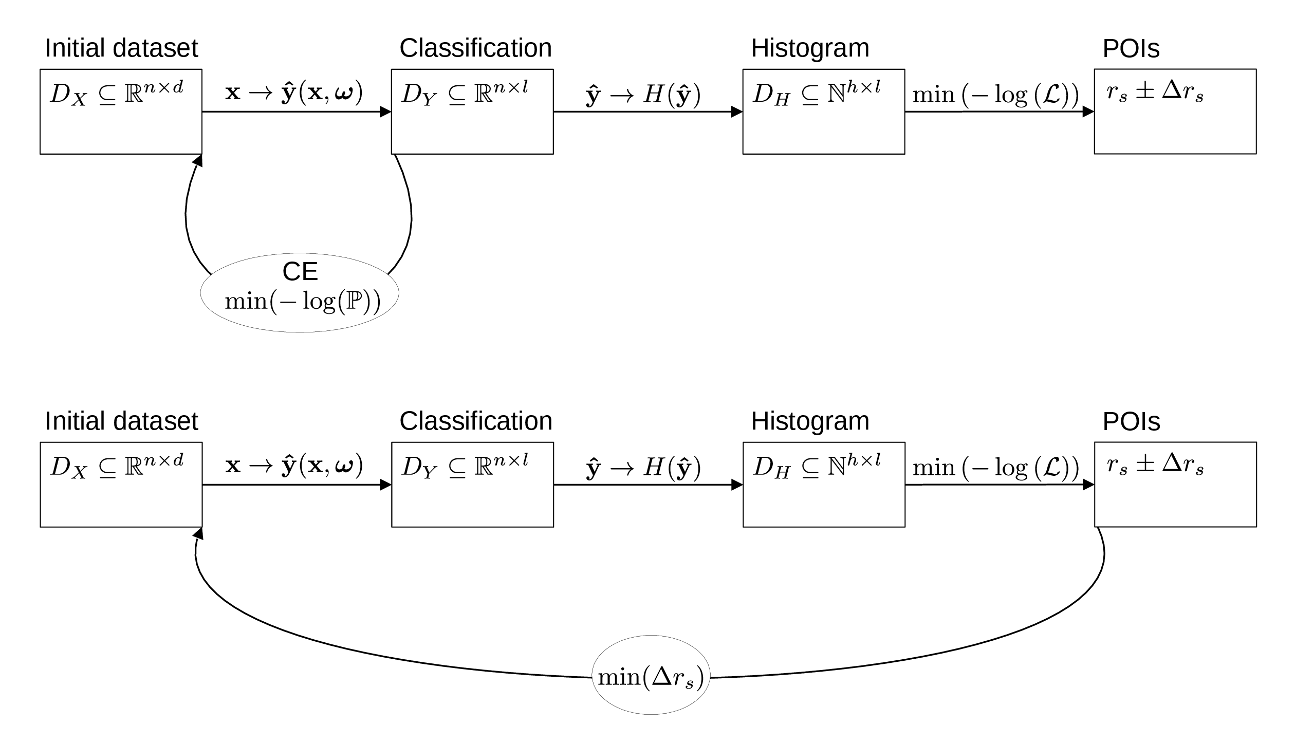
png pdf	Figure 1: Flow chart of a (upper part) $\mathrm{CENNT}$ and (lower part) $\mathrm{SANNT}$ . In the figure $D_{i}$ denotes the dataset, $n$ ( $d$ ) the number of events (observables) in the initial dataset $D_{X}$ ; $l$ the number of classes after event classification; and $h$ the number of histogram bins to enter the statistical inference of the POIs. The function symbol $\mathbb{P}$ represents the multinomial distribution, the symbol $\mathcal{L}$ has been defined in Eq. 1.
png pdf	Figure 1-a: Flow chart of a (upper part) $\mathrm{CENNT}$ and (lower part) $\mathrm{SANNT}$ . In the figure $D_{i}$ denotes the dataset, $n$ ( $d$ ) the number of events (observables) in the initial dataset $D_{X}$ ; $l$ the number of classes after event classification; and $h$ the number of histogram bins to enter the statistical inference of the POIs. The function symbol $\mathbb{P}$ represents the multinomial distribution, the symbol $\mathcal{L}$ has been defined in Eq. 1.
png pdf	Figure 1-b: Flow chart of a (upper part) $\mathrm{CENNT}$ and (lower part) $\mathrm{SANNT}$ . In the figure $D_{i}$ denotes the dataset, $n$ ( $d$ ) the number of events (observables) in the initial dataset $D_{X}$ ; $l$ the number of classes after event classification; and $h$ the number of histogram bins to enter the statistical inference of the POIs. The function symbol $\mathbb{P}$ represents the multinomial distribution, the symbol $\mathcal{L}$ has been defined in Eq. 1.
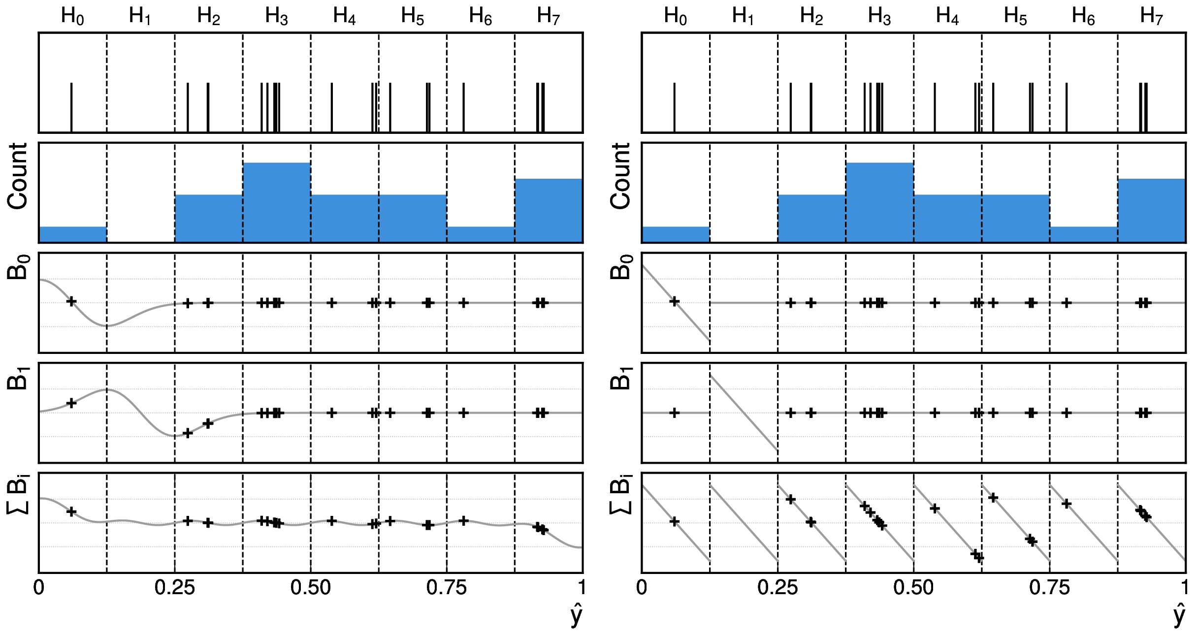
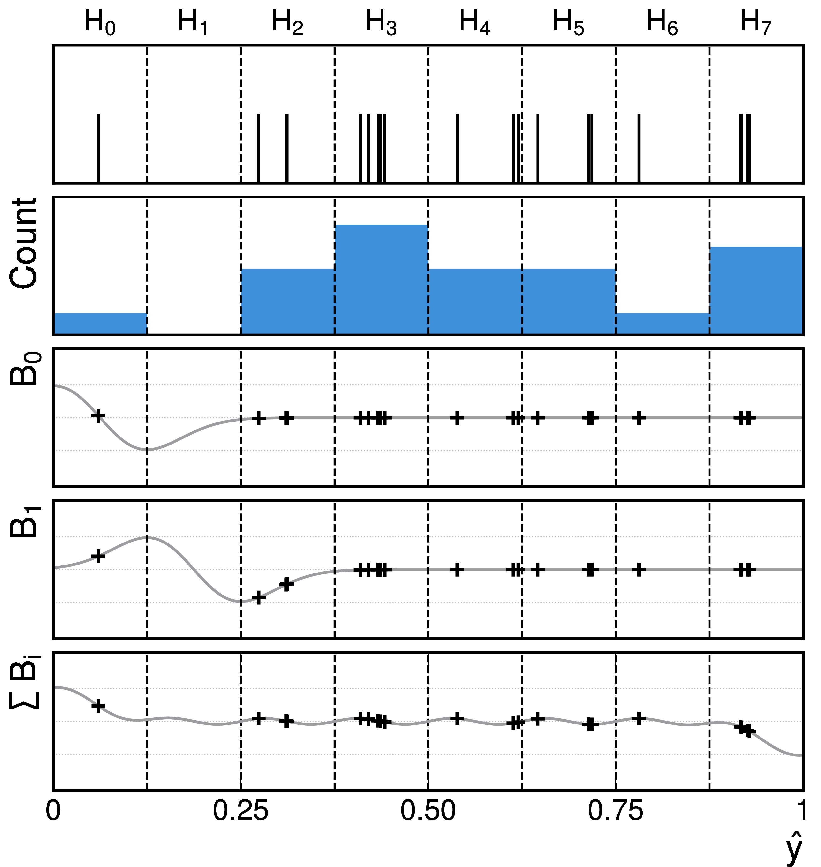
png pdf	Figure 2: Custom functions $\mathcal{B}_{i}$ for the backward pass of the backpropagation algorithm, as used (left) in Ref. [5] and (right) in this paper. In the first row of each sub-figure the same 20 random samples of a simple setup of pseudo-experiments, as described in Section 3.2 are shown. In the second row the resulting histogram $H$ , in the third and fourth rows the functions $B_{0}$ and $B_{1}$ for the individual bins $H_{0}$ and $H_{1}$ , and in the last row the collective effect of $\sum\mathcal{B}_{i}$ are shown.
png pdf	Figure 2-a: Custom functions $\mathcal{B}_{i}$ for the backward pass of the backpropagation algorithm, as used (left) in Ref. [5] and (right) in this paper. In the first row of each sub-figure the same 20 random samples of a simple setup of pseudo-experiments, as described in Section 3.2 are shown. In the second row the resulting histogram $H$ , in the third and fourth rows the functions $B_{0}$ and $B_{1}$ for the individual bins $H_{0}$ and $H_{1}$ , and in the last row the collective effect of $\sum\mathcal{B}_{i}$ are shown.
png pdf	Figure 2-b: Custom functions $\mathcal{B}_{i}$ for the backward pass of the backpropagation algorithm, as used (left) in Ref. [5] and (right) in this paper. In the first row of each sub-figure the same 20 random samples of a simple setup of pseudo-experiments, as described in Section 3.2 are shown. In the second row the resulting histogram $H$ , in the third and fourth rows the functions $B_{0}$ and $B_{1}$ for the individual bins $H_{0}$ and $H_{1}$ , and in the last row the collective effect of $\sum\mathcal{B}_{i}$ are shown.
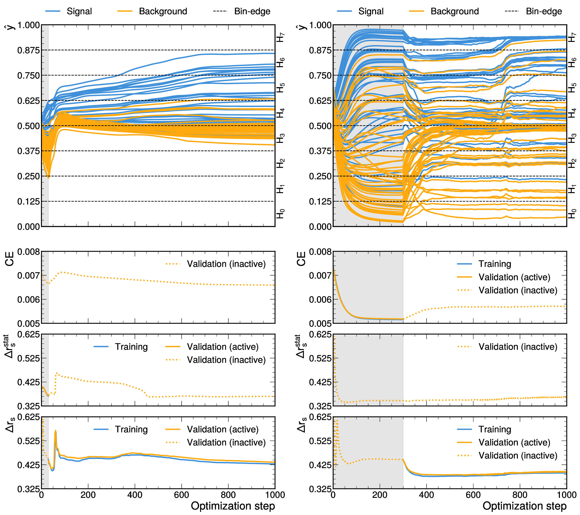
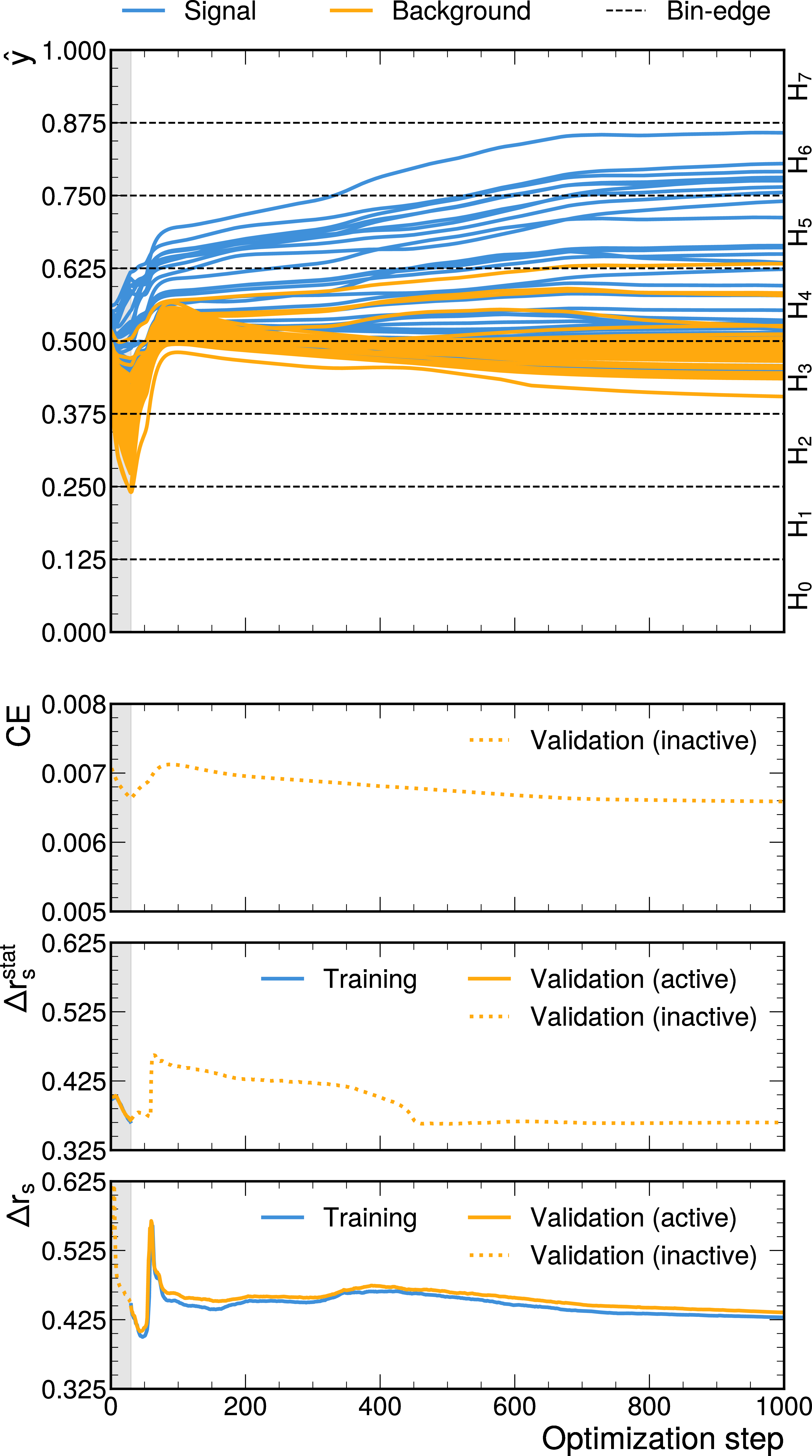
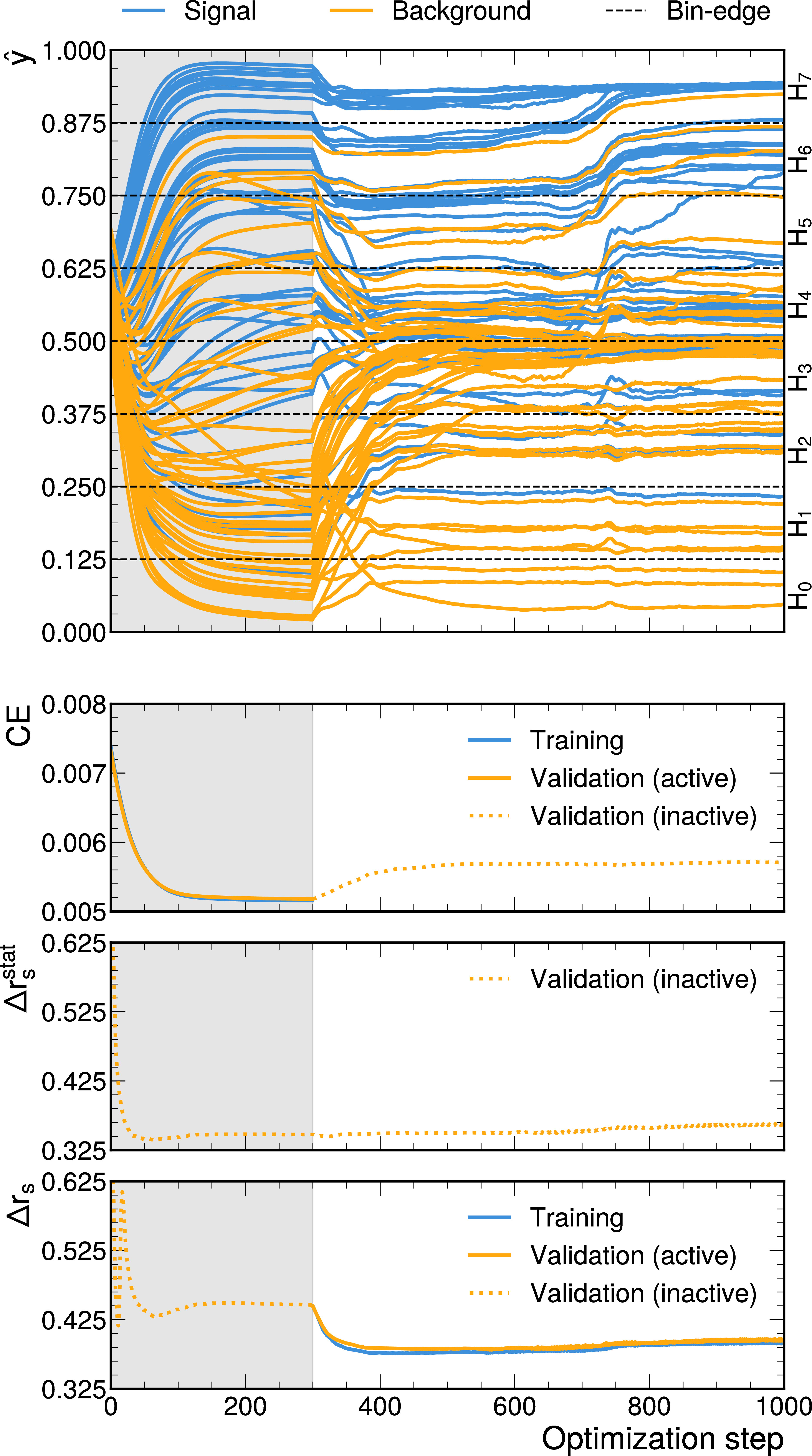
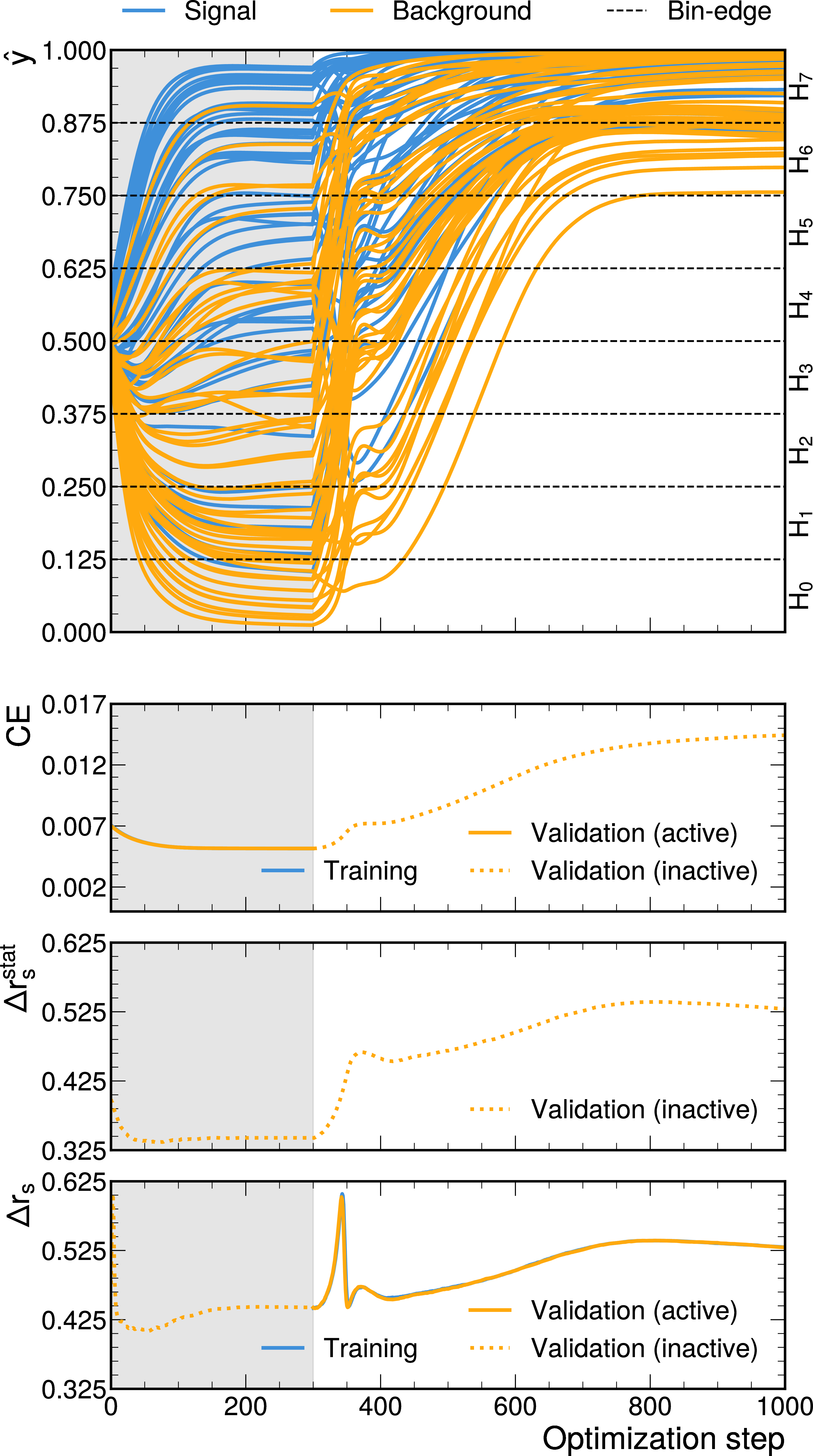
png pdf	Figure 3: Evolution of the loss functions CE, $\Delta r_{s}^{\mathrm{stat.}}$ and $\Delta r_{s}$ as used (left) in Ref. [5] and (right) for this paper. In the upper panels the evolution of $\hat{y}$ for randomly selected 50 (blue) signal and 50 (orange) background samples during training is shown. The gray shaded area indicates the pretraining. In the second and third panels from above the evolution of CE and $\Delta r_{s}^{\mathrm{stat.}}$ is shown. In the lowest panels the evolution of $L_{\mathrm{SANNT}}=\Delta r_{s}$ is shown. The evaluation on the training (validation) dataset is indicated in blue (orange). The evaluation of the correspondingly inactive loss function, during or after pretraining, evaluated on the validation dataset, is indicated by the dashed orange curves.
png pdf	Figure 3-a: Evolution of the loss functions CE, $\Delta r_{s}^{\mathrm{stat.}}$ and $\Delta r_{s}$ as used (left) in Ref. [5] and (right) for this paper. In the upper panels the evolution of $\hat{y}$ for randomly selected 50 (blue) signal and 50 (orange) background samples during training is shown. The gray shaded area indicates the pretraining. In the second and third panels from above the evolution of CE and $\Delta r_{s}^{\mathrm{stat.}}$ is shown. In the lowest panels the evolution of $L_{\mathrm{SANNT}}=\Delta r_{s}$ is shown. The evaluation on the training (validation) dataset is indicated in blue (orange). The evaluation of the correspondingly inactive loss function, during or after pretraining, evaluated on the validation dataset, is indicated by the dashed orange curves.
png pdf	Figure 3-b: Evolution of the loss functions CE, $\Delta r_{s}^{\mathrm{stat.}}$ and $\Delta r_{s}$ as used (left) in Ref. [5] and (right) for this paper. In the upper panels the evolution of $\hat{y}$ for randomly selected 50 (blue) signal and 50 (orange) background samples during training is shown. The gray shaded area indicates the pretraining. In the second and third panels from above the evolution of CE and $\Delta r_{s}^{\mathrm{stat.}}$ is shown. In the lowest panels the evolution of $L_{\mathrm{SANNT}}=\Delta r_{s}$ is shown. The evaluation on the training (validation) dataset is indicated in blue (orange). The evaluation of the correspondingly inactive loss function, during or after pretraining, evaluated on the validation dataset, is indicated by the dashed orange curves.
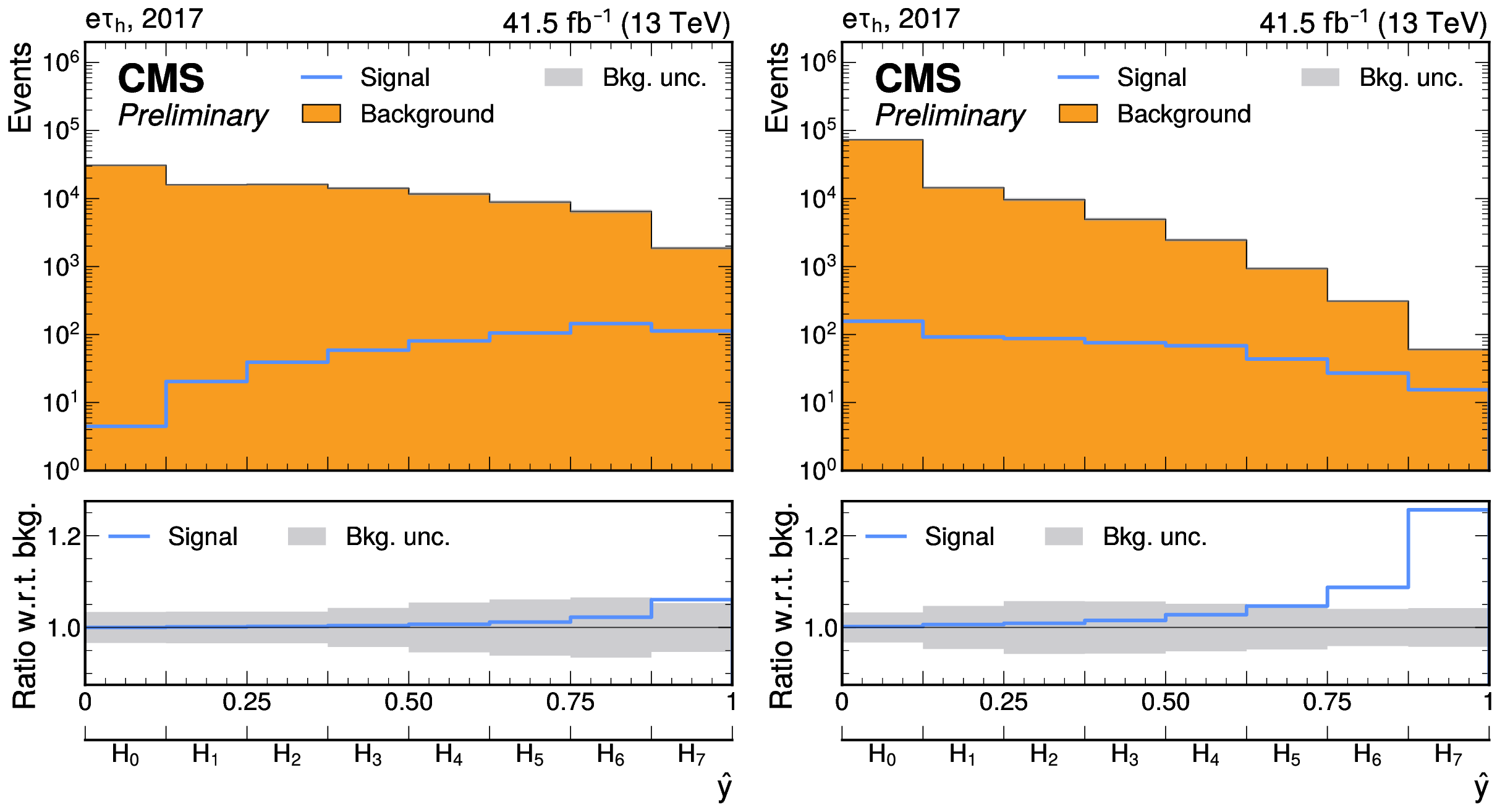
png pdf	Figure 4: Expected distributions of $\hat{y}(\,\cdot\,)$ for a binary classification task separating $S$ from $B$ , for the (left) $\mathrm{CENNT}$ and (right) $\mathrm{SANNT}$ , prior to any fit to $D_{H}^{\mathcal{A}}$ . The individual distributions for $S$ and $B$ are shown by the non-stacked open blue and filled orange histogram, respectively. In the lower panels of the figures the expected values of $S/B+1$ are shown. The gray bands correspond to the combined statistical and systematic uncertainty in $B$ .
png pdf	Figure 4-a: Expected distributions of $\hat{y}(\,\cdot\,)$ for a binary classification task separating $S$ from $B$ , for the (left) $\mathrm{CENNT}$ and (right) $\mathrm{SANNT}$ , prior to any fit to $D_{H}^{\mathcal{A}}$ . The individual distributions for $S$ and $B$ are shown by the non-stacked open blue and filled orange histogram, respectively. In the lower panels of the figures the expected values of $S/B+1$ are shown. The gray bands correspond to the combined statistical and systematic uncertainty in $B$ .
png pdf	Figure 4-b: Expected distributions of $\hat{y}(\,\cdot\,)$ for a binary classification task separating $S$ from $B$ , for the (left) $\mathrm{CENNT}$ and (right) $\mathrm{SANNT}$ , prior to any fit to $D_{H}^{\mathcal{A}}$ . The individual distributions for $S$ and $B$ are shown by the non-stacked open blue and filled orange histogram, respectively. In the lower panels of the figures the expected values of $S/B+1$ are shown. The gray bands correspond to the combined statistical and systematic uncertainty in $B$ .
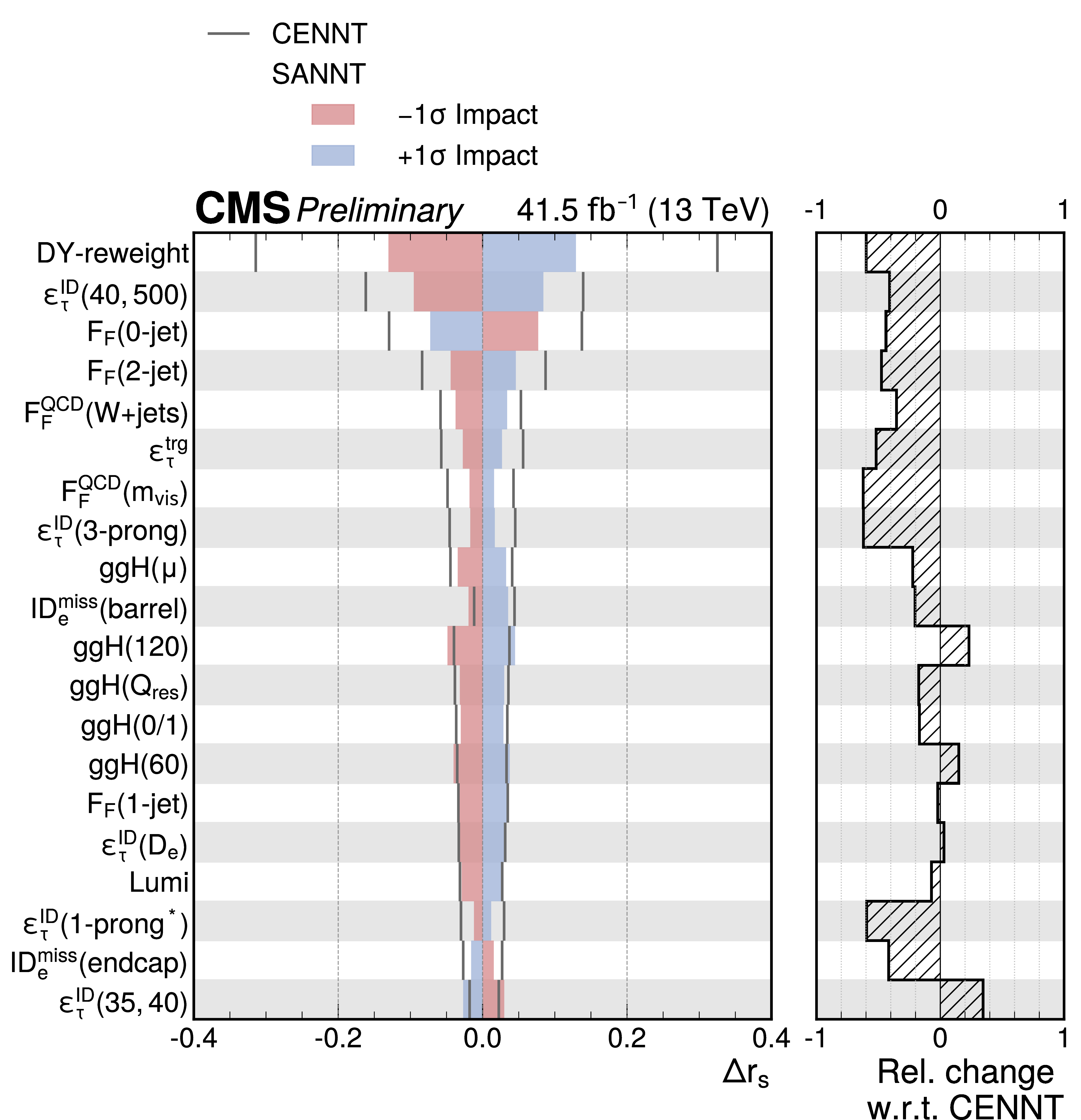
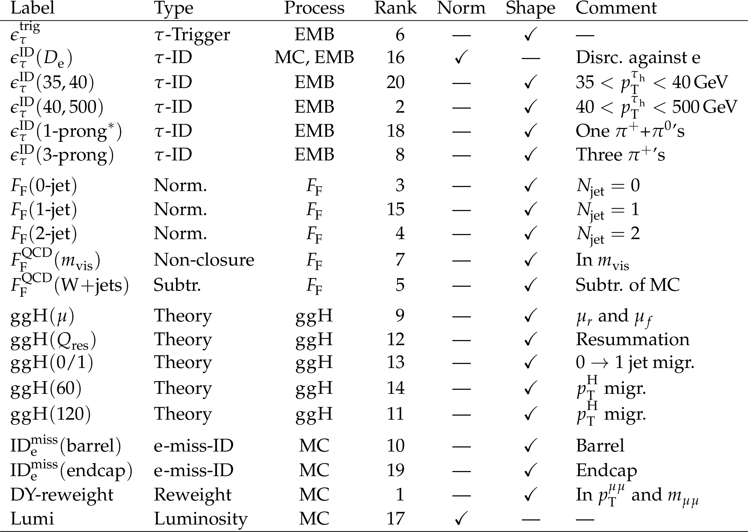
png pdf	Figure 5: The 20 nuisance parameters $\{\theta_{j}\}$ with the largest impacts on $r_{s}$ . The gray lines refer to the $\mathrm{CENNT}$ and the colored bars to the $\mathrm{SANNT}$ . The impacts can be read off from the $x$ -axis. Labels for each $\theta_{j}$ decreasing in magnitude when moving from top to bottom of the figure are shown on the $y$ -axis. The association of each $\theta_{j}$ label with the systematic variation it refers to, is summarized in Table 1. A more detailed discussion is given in the text.
png pdf	Figure 6: Negative log of the profile likelihood $-2\Delta\log\mathcal{L}$ as a function of $r_{s}$ , taking into account (red) all and (blue) only the statistical uncertainties in $\Delta r_{s}$ . The results as obtained from $\mathrm{CENNT}$ are indicated by the dashed lines, the median expected result of an ensemble of 100 repetitions of the $\mathrm{SANNT}$ varying random initializations are indicated by the continuous lines. The red and blue shaded bands surrounding the median expectations indicate 68% central intervals of these ensembles. In the lower panels the underlying distributions to these central intervals are shown.
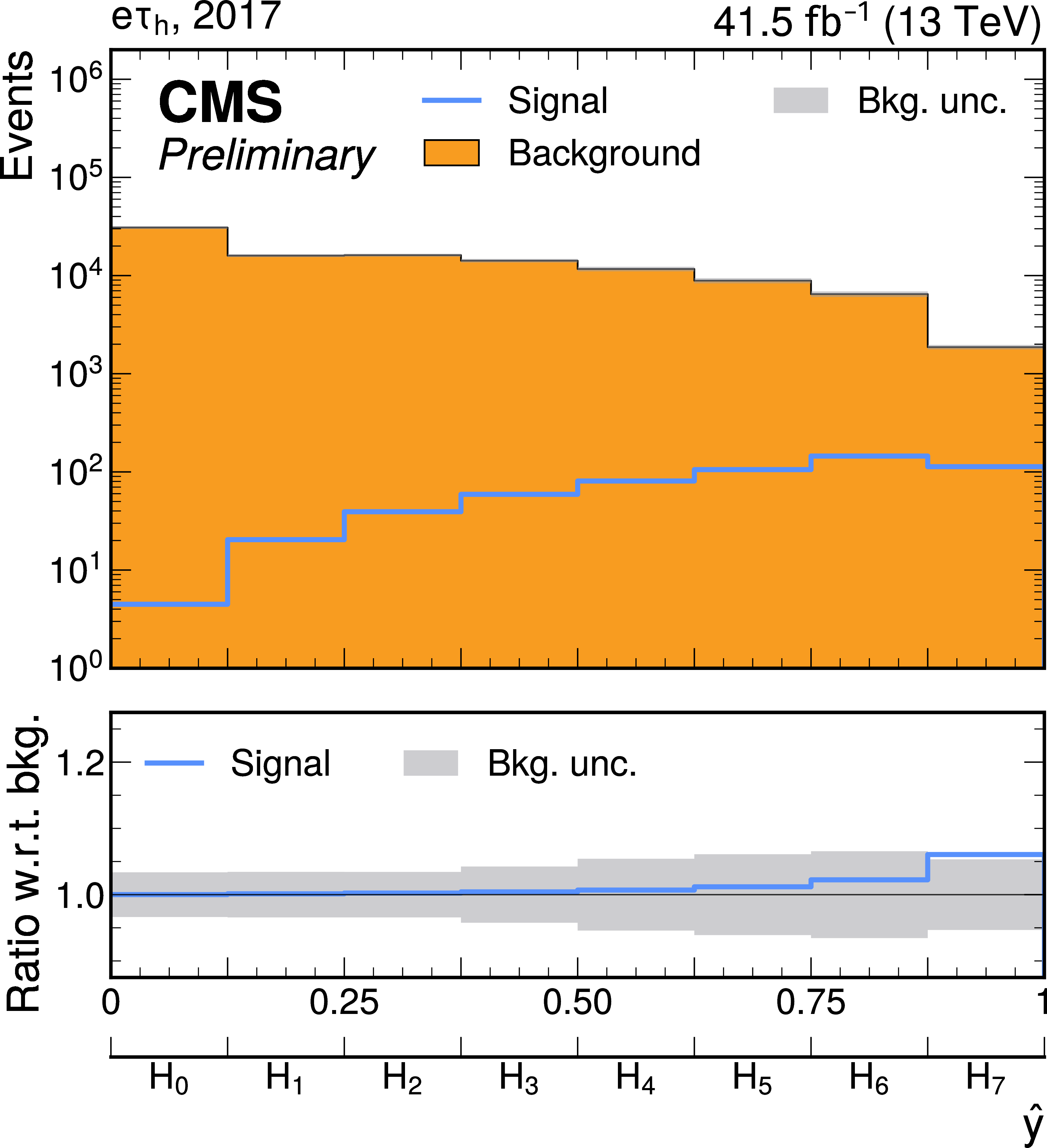
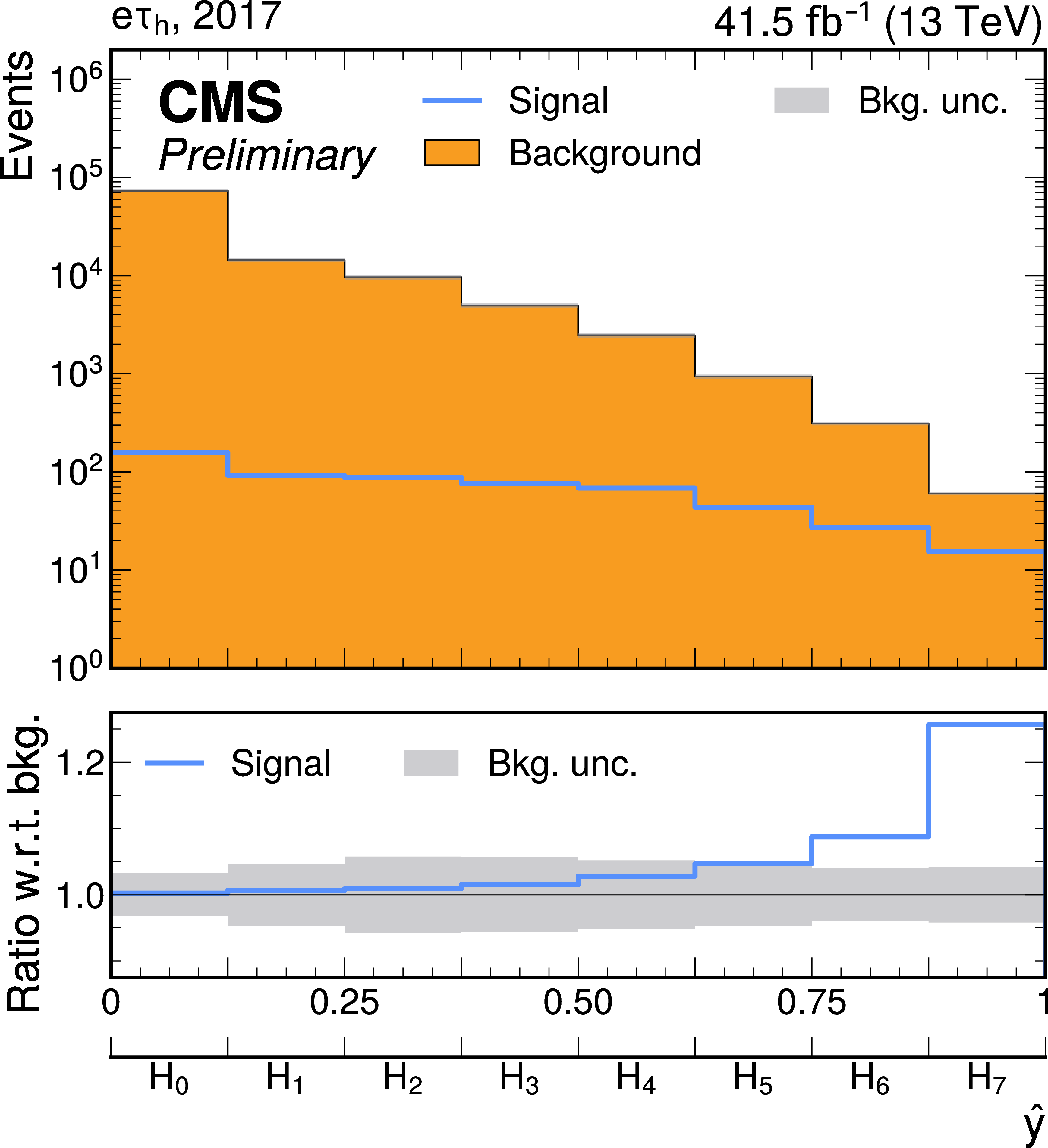
png pdf	Figure 7: Expected distributions of $\hat{y}_{l}(\,\cdot\,)$ for multiclass classification, based on seven event classes, as used for a differential STXS stage-0 cross section measurement of H production in Ref. [1], prior to any fit to $D_{H}^{\mathcal{A}}$ . In the upper (lower) part of the figure the results obtained after $\mathrm{CENNT}$ ( $\mathrm{SANNT}$ ) are shown. The background processes of $\Omega_{X}$ are indicated by stacked, differently colored, filled histograms. The expected $\mathrm{g}\mathrm{g}\mathrm{H}$ and $\mathrm{q}\mathrm{q}\mathrm{H}$ contributions are indicated by the non-stacked, cyan- and red-colored, open histograms. In the lower panels of the figure the expected values of $S/B+$ 1 are shown. The gray bands correspond to the combined statistical and systematic uncertainty in the background model.
png pdf	Figure 7-a: Expected distributions of $\hat{y}_{l}(\,\cdot\,)$ for multiclass classification, based on seven event classes, as used for a differential STXS stage-0 cross section measurement of H production in Ref. [1], prior to any fit to $D_{H}^{\mathcal{A}}$ . In the upper (lower) part of the figure the results obtained after $\mathrm{CENNT}$ ( $\mathrm{SANNT}$ ) are shown. The background processes of $\Omega_{X}$ are indicated by stacked, differently colored, filled histograms. The expected $\mathrm{g}\mathrm{g}\mathrm{H}$ and $\mathrm{q}\mathrm{q}\mathrm{H}$ contributions are indicated by the non-stacked, cyan- and red-colored, open histograms. In the lower panels of the figure the expected values of $S/B+$ 1 are shown. The gray bands correspond to the combined statistical and systematic uncertainty in the background model.
png pdf	Figure 7-b: Expected distributions of $\hat{y}_{l}(\,\cdot\,)$ for multiclass classification, based on seven event classes, as used for a differential STXS stage-0 cross section measurement of H production in Ref. [1], prior to any fit to $D_{H}^{\mathcal{A}}$ . In the upper (lower) part of the figure the results obtained after $\mathrm{CENNT}$ ( $\mathrm{SANNT}$ ) are shown. The background processes of $\Omega_{X}$ are indicated by stacked, differently colored, filled histograms. The expected $\mathrm{g}\mathrm{g}\mathrm{H}$ and $\mathrm{q}\mathrm{q}\mathrm{H}$ contributions are indicated by the non-stacked, cyan- and red-colored, open histograms. In the lower panels of the figure the expected values of $S/B+$ 1 are shown. The gray bands correspond to the combined statistical and systematic uncertainty in the background model.
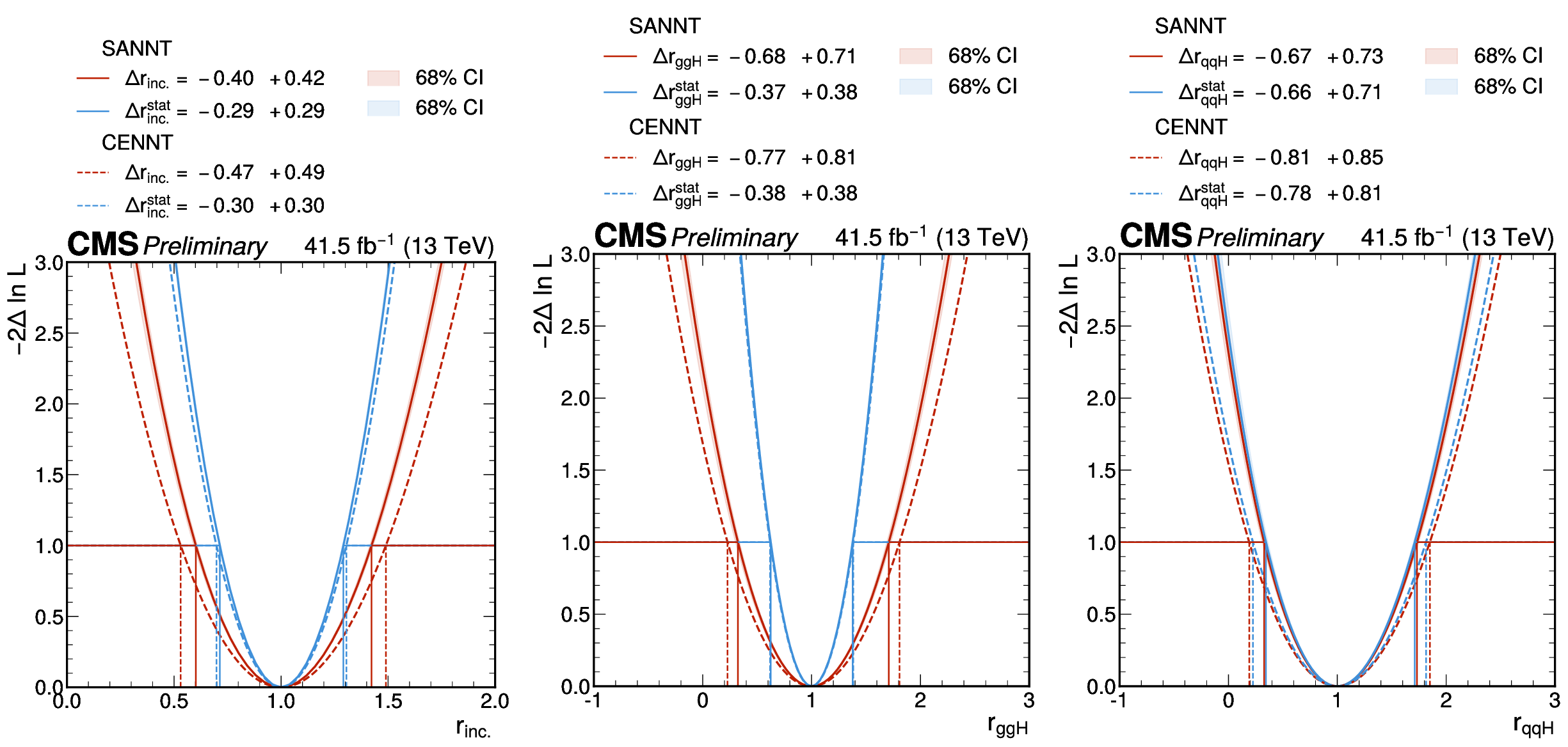
png pdf	Figure 8: Negative log of the profile likelihood $-2\Delta\log\mathcal{L}$ as a function of $r_{s}$ , for a differential STXS stage-0 cross section measurement of H production in the $\mathrm{H}\to\tau\tau$ decay channel, taking (red) all and (blue) only the statistical uncertainties in $\Delta r_{s}$ into account. In the left part of the figure $r_{\mathrm{inc.}}$ , for an inclusive measurement is shown, in the middle and right parts of the figure $r_{\mathrm{g}\mathrm{g}\mathrm{H}}$ and $r_{\mathrm{q}\mathrm{q}\mathrm{H}}$ for a combined differential STXS stage-0 measurement of these two contributions to the signal in two bins, are shown. The results as obtained from $\mathrm{CENNT}$ are indicated by the dashed lines, the median expected result of an ensemble of 100 repetitions of $\mathrm{SANNT}$ varying random initializations are indicated by the continuous lines. The red and blue shaded bands surrounding the median expectations indicate 68% central intervals of these ensembles.
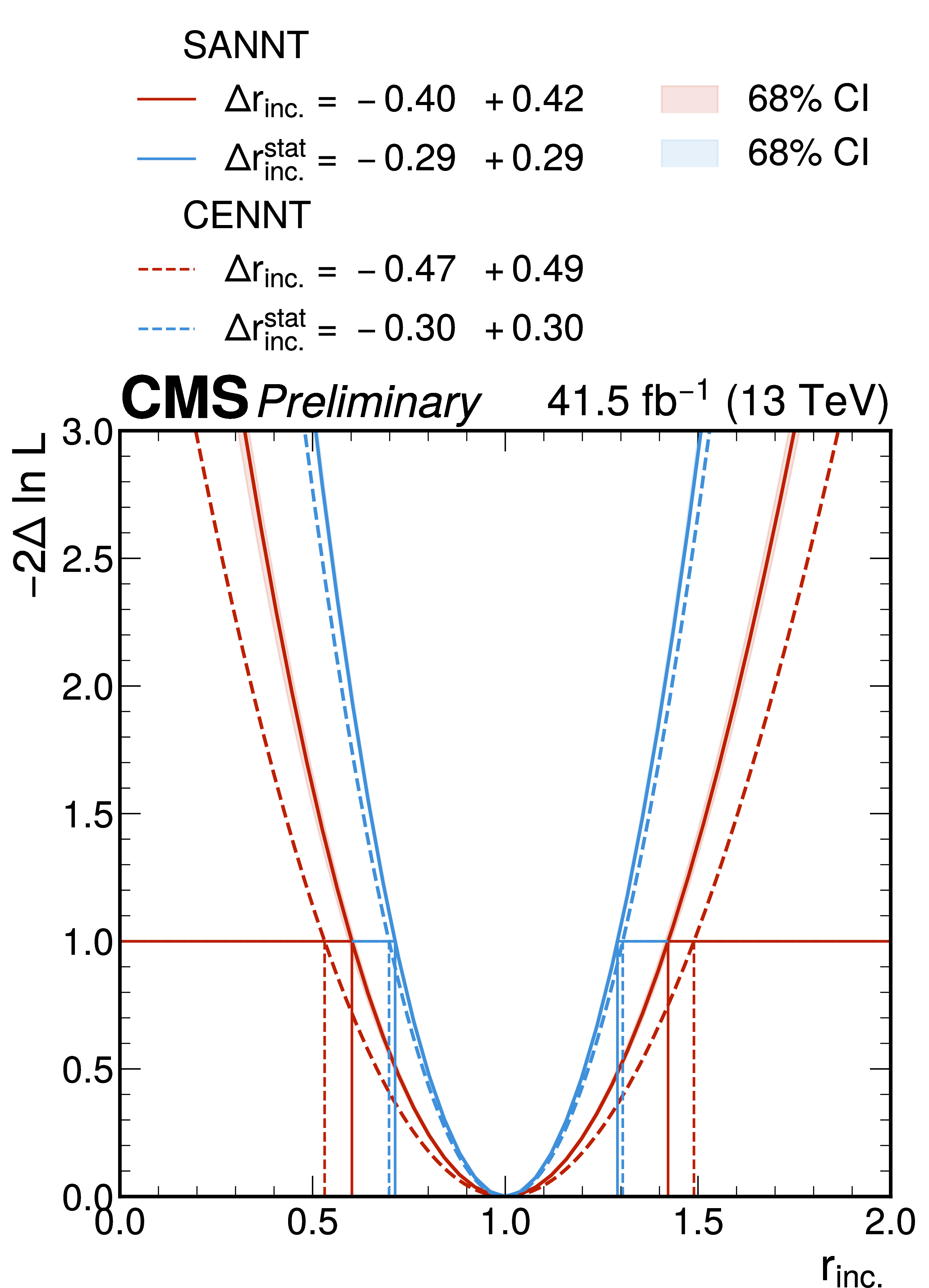
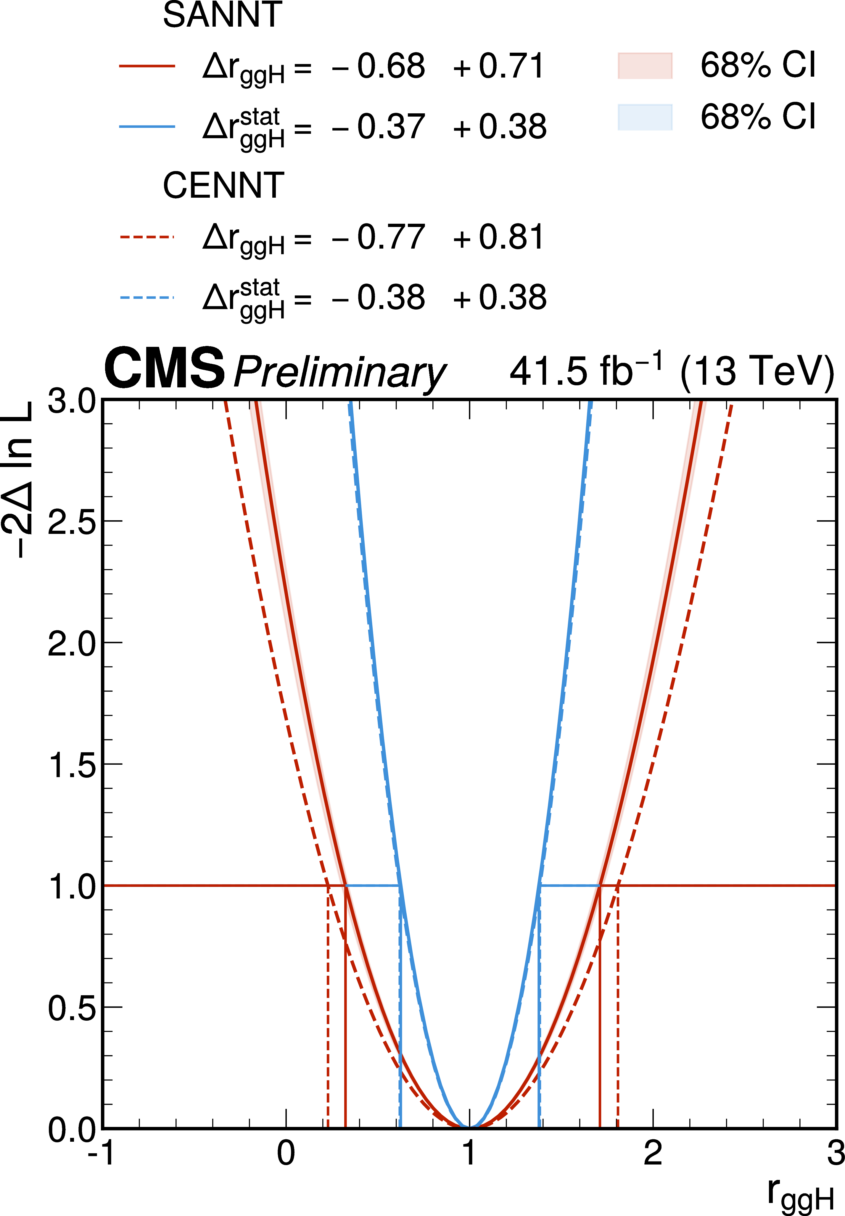
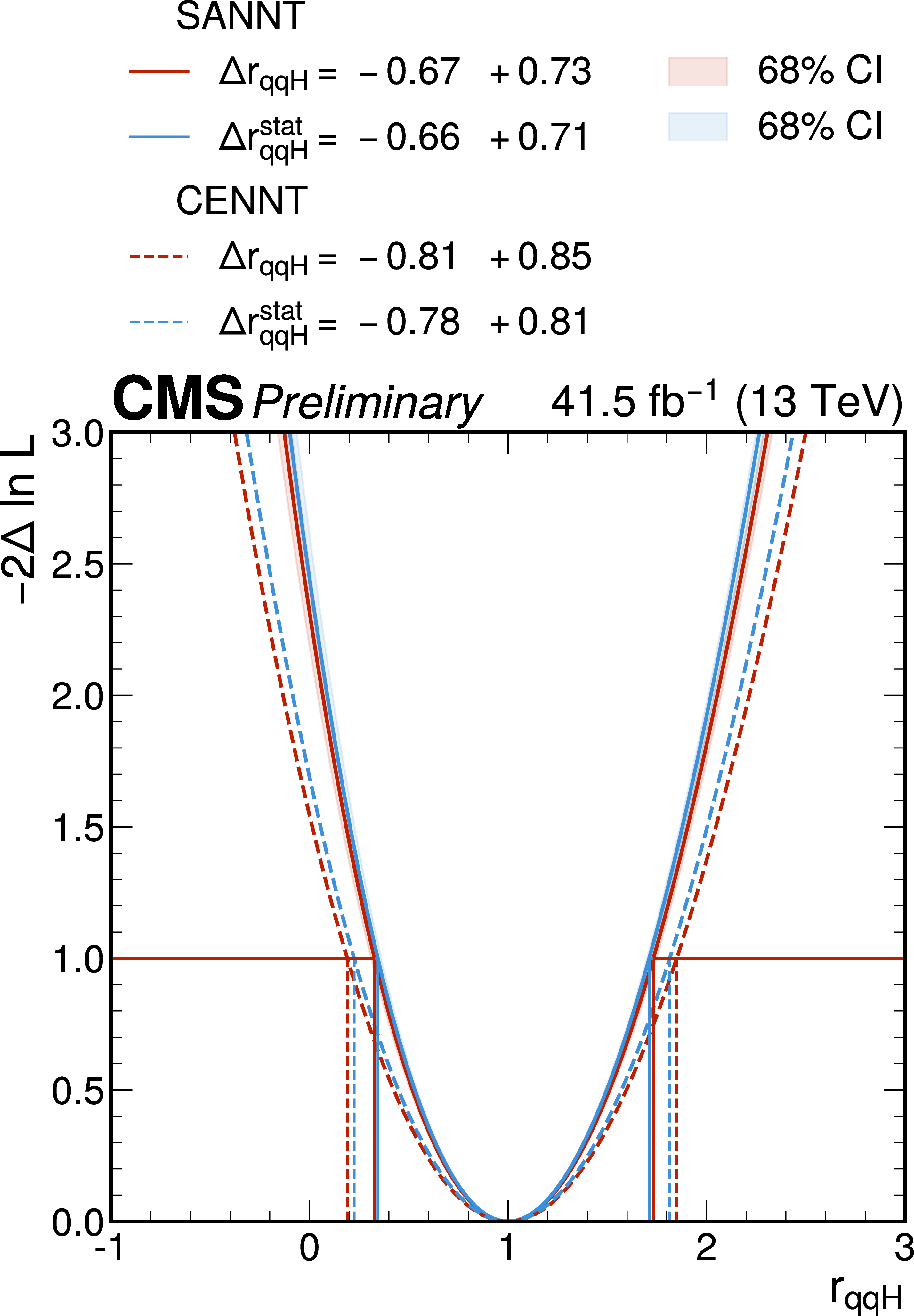
png pdf	Figure 8-a: Negative log of the profile likelihood $-2\Delta\log\mathcal{L}$ as a function of $r_{s}$ , for a differential STXS stage-0 cross section measurement of H production in the $\mathrm{H}\to\tau\tau$ decay channel, taking (red) all and (blue) only the statistical uncertainties in $\Delta r_{s}$ into account. In the left part of the figure $r_{\mathrm{inc.}}$ , for an inclusive measurement is shown, in the middle and right parts of the figure $r_{\mathrm{g}\mathrm{g}\mathrm{H}}$ and $r_{\mathrm{q}\mathrm{q}\mathrm{H}}$ for a combined differential STXS stage-0 measurement of these two contributions to the signal in two bins, are shown. The results as obtained from $\mathrm{CENNT}$ are indicated by the dashed lines, the median expected result of an ensemble of 100 repetitions of $\mathrm{SANNT}$ varying random initializations are indicated by the continuous lines. The red and blue shaded bands surrounding the median expectations indicate 68% central intervals of these ensembles.
png pdf	Figure 8-b: Negative log of the profile likelihood $-2\Delta\log\mathcal{L}$ as a function of $r_{s}$ , for a differential STXS stage-0 cross section measurement of H production in the $\mathrm{H}\to\tau\tau$ decay channel, taking (red) all and (blue) only the statistical uncertainties in $\Delta r_{s}$ into account. In the left part of the figure $r_{\mathrm{inc.}}$ , for an inclusive measurement is shown, in the middle and right parts of the figure $r_{\mathrm{g}\mathrm{g}\mathrm{H}}$ and $r_{\mathrm{q}\mathrm{q}\mathrm{H}}$ for a combined differential STXS stage-0 measurement of these two contributions to the signal in two bins, are shown. The results as obtained from $\mathrm{CENNT}$ are indicated by the dashed lines, the median expected result of an ensemble of 100 repetitions of $\mathrm{SANNT}$ varying random initializations are indicated by the continuous lines. The red and blue shaded bands surrounding the median expectations indicate 68% central intervals of these ensembles.
png pdf	Figure 8-c: Negative log of the profile likelihood $-2\Delta\log\mathcal{L}$ as a function of $r_{s}$ , for a differential STXS stage-0 cross section measurement of H production in the $\mathrm{H}\to\tau\tau$ decay channel, taking (red) all and (blue) only the statistical uncertainties in $\Delta r_{s}$ into account. In the left part of the figure $r_{\mathrm{inc.}}$ , for an inclusive measurement is shown, in the middle and right parts of the figure $r_{\mathrm{g}\mathrm{g}\mathrm{H}}$ and $r_{\mathrm{q}\mathrm{q}\mathrm{H}}$ for a combined differential STXS stage-0 measurement of these two contributions to the signal in two bins, are shown. The results as obtained from $\mathrm{CENNT}$ are indicated by the dashed lines, the median expected result of an ensemble of 100 repetitions of $\mathrm{SANNT}$ varying random initializations are indicated by the continuous lines. The red and blue shaded bands surrounding the median expectations indicate 68% central intervals of these ensembles.
png pdf	Figure 9: Evolution of the loss functions CE, $\Delta r_{s}^{\mathrm{stat.}}$ , and $\Delta r_{s}$ , as used for this paper. Instead of the custom functions $\mathcal{B}_{i}$ the identity operation (the so-called straight-through estimator) is used for SANNT. In the upper panel the evolution of $\hat{y}$ for randomly selected 50 (blue) signal and 50 (orange) background samples during training is shown. The gray shaded area indicates the pretraining. In the second panel from above the evolution of CE is shown. Though not actively used for the SANNT $\Delta r_{s}^{\mathrm{stat.}}$ is also shown, in the third panel from above. In the lower panel the evolution of $\Delta r_{s}$ is shown. The evaluation on the training (validation) dataset is indicated in blue (orange). The evolution of inactive loss functions, evaluated on the validation dataset, is indicated by the dashed orange curves.

Tables
png pdf	Table 1: Association of nuisance parameters $\{\theta_{j}\}$ with the systematic variations they refer to, for the 20 $\{\theta_{j}\}$ with the largest impacts on $r_{s}$ , as shown in Fig. 5. The label of each corresponding uncertainty is given in the first column, the type of uncertainty, process that it applies to, and rank in Fig. 5 are given in the second, third, and fourth column, respectively. More detailed discussion of is given in the text.
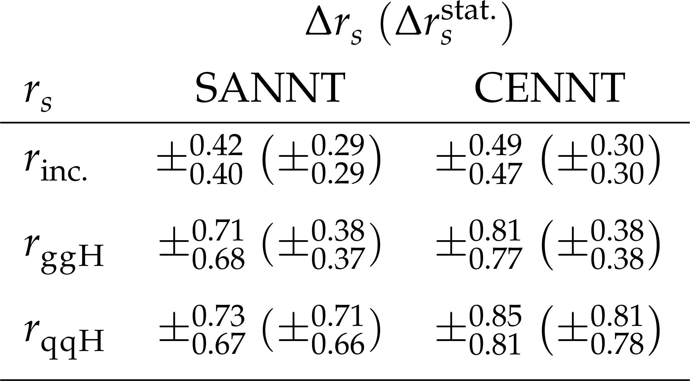
png pdf	Table 2: Expected combined statistical and systematic uncertainties $\Delta r_{s}$ and statistical uncertainties $\Delta r_{s}^{\mathrm{stat.}}$ , in the parameters $r_{\mathrm{inc.}}$ for an inclusive, and $r_{\mathrm{g}\mathrm{g}\mathrm{H}}$ and $r_{\mathrm{q}\mathrm{q}\mathrm{H}}$ for a differential STXS stage-0 cross section measurement of H production in the $\mathrm{H}\to\tau\tau$ decay channel, as obtained from fits to $D_{H}^{\mathcal{A}}$ . In the second (third) column the results after $\mathrm{SANNT}$ ( $\mathrm{CENNT}$ ) are shown.

Summary

We have demonstrated a neural network training, capable of accounting for the effects of systematic variations of the utilized data model in the training process and described its extension towards neural network multiclass classification. Trainings for binary and multiclass classification with seven output classes have been performed, based on a comprehensive data model with 86 nontrivial shape-altering systematic variations, as used for a previous measurement. The neural network output functions have been used to infer the signal strengths for inclusive Higgs boson production, as well as for Higgs boson production via gluon-fusion (

$r_{\mathrm{g}\mathrm{g}\mathrm{H}}$ ) and vector boson fusion (

$r_{\mathrm{q}\mathrm{q}\mathrm{H}}$ ). With respect to a conventional training, based on cross-entropy, we observe improvements of 12 and 16%, for the sensitivity in

$r_{\mathrm{g}\mathrm{g}\mathrm{H}}$ and

$r_{\mathrm{q}\mathrm{q}\mathrm{H}}$ , respectively. This is the first time that a neural network training, capable of accounting for the effects of systematic variations in the utilized data model in the training process, has been demonstrated on a data model of that complexity and the first time that such a training has been applied to multiclass classification.

References
1	CMS Collaboration	Measurements of Higgs boson production in the decay channel with a pair of $\tau$ leptons in proton-proton collisions at $\sqrt{s}=$ 13 TeV	EPJC 83 (2023) 562	CMS-HIG-19-010 2204.12957
2	M. Neal, Radford	Computing Likelihood Functions for High-Energy Physics Experiments when Distributions are Defined by Simulators with Nuisance Parameters	link
3	K. Cranmer, J. Pavez, and G. Louppe	Approximating Likelihood Ratios with Calibrated Discriminative Classifiers	link	1506.02169
4	P. De Castro and T. Dorigo	INFERNO: Inference-Aware Neural Optimisation	Comput. Phys. Commun. 244 (2019) 170	1806.04743
5	S. Wunsch, S. Jörger, R. Wolf, and G. Quast	Optimal Statistical Inference in the Presence of Systematic Uncertainties Using Neural Network Optimization Based on Binned Poisson Likelihoods with Nuisance Parameters	Comput. Softw. Big Sci. 5 (2021) 4	2003.07186
6	N. Simpson and L. Heinrich	neos: End-to-End-Optimised Summary Statistics for High Energy Physics	J. Phys. Conf. Ser. 2438 (2023) 012105	2203.05570
7	CMS Collaboration	Performance of the CMS Level-1 trigger in proton-proton collisions at $\sqrt{s} =$ 13 TeV	JINST 15 (2020) P10017	CMS-TRG-17-001 2006.10165
8	CMS Collaboration	The CMS trigger system	JINST 12 (2017) P01020	CMS-TRG-12-001 1609.02366
9	CMS Collaboration	The CMS experiment at the CERN LHC	JINST 3 (2008) S08004
10	CMS Collaboration	Particle-flow reconstruction and global event description with the CMS detector	JINST 12 (2017) P10003	CMS-PRF-14-001 1706.04965
11	CMS Collaboration	Technical proposal for the Phase-II upgrade of the Compact Muon Solenoid	CMS Technical Proposal CERN-LHCC-2015-010, CMS-TDR-15-02, 2015 CDS
12	CMS Collaboration	Performance of electron reconstruction and selection with the CMS detector in proton-proton collisions at $\sqrt{s} =$ 8 TeV	JINST 10 (2015) P06005	CMS-EGM-13-001 1502.02701
13	CMS Collaboration	Electron and photon reconstruction and identification with the CMS experiment at the CERN LHC	JINST 16 (2021) P05014	CMS-EGM-17-001 2012.06888
14	CMS Collaboration	Performance of CMS muon reconstruction in pp collision events at $\sqrt{s}=$ 7 TeV	JINST 7 (2012) P10002	CMS-MUO-10-004 1206.4071
15	CMS Collaboration	Performance of the CMS muon detector and muon reconstruction with proton-proton collisions at $\sqrt{s}=$ 13 TeV	JINST 13 (2018) P06015	CMS-MUO-16-001 1804.04528
16	M. Cacciari, G. P. Salam, and G. Soyez	The anti- $k_{\mathrm{T}}$ jet clustering algorithm	JHEP 04 (2008) 063	0802.1189
17	M. Cacciari, G. P. Salam, and G. Soyez	FastJet user manual	EPJC 72 (2012) 1896	1111.6097
18	CMS Collaboration	Identification of heavy-flavour jets with the CMS detector in pp collisions at 13 TeV	JINST 13 (2018) P05011	CMS-BTV-16-002 1712.07158
19	E. Bols et al.	Jet flavour classification using DeepJet	JINST 15 (2020) P12012	2008.10519
20	CMS Collaboration	Performance of reconstruction and identification of $\tau$ leptons decaying to hadrons and $\nu_\tau$ in pp collisions at $\sqrt{s}=$ 13 TeV	JINST 13 (2018) P10005	CMS-TAU-16-003 1809.02816
21	CMS Collaboration	Identification of hadronic tau lepton decays using a deep neural network	JINST 17 (2022) P07023	CMS-TAU-20-001 2201.08458
22	CMS Collaboration	Performance of the CMS missing transverse momentum reconstruction in pp data at $\sqrt{s}$ = 8 TeV	JINST 10 (2015) P02006	CMS-JME-13-003 1411.0511
23	D. Bertolini, P. Harris, M. Low, and N. Tran	Pileup per particle identification	JHEP 10 (2014) 059	1407.6013
24	CMS Collaboration	An embedding technique to determine $\tau\tau$ backgrounds in proton-proton collision data	JINST 14 (2019) P06032	CMS-TAU-18-001 1903.01216
25	CMS Collaboration	Measurement of the $\mathrm{Z}\gamma^{*}\to\tau\tau$ cross section in pp collisions at $\sqrt{s}=$ 13 TeV and validation of $\tau$ lepton analysis techniques	EPJC 78 (2018) 708	CMS-HIG-15-007 1801.03535
26	CMS Collaboration	Search for additional neutral MSSM Higgs bosons in the $\tau\tau$ final state in proton-proton collisions at $\sqrt{s}=$ 13 TeV	JHEP 09 (2018) 007	CMS-HIG-17-020 1803.06553
27	J. Alwall et al.	MadGraph 5: Going beyond	JHEP 06 (2011) 128	1106.0522
28	J. Alwall et al.	The automated computation of tree-level and next-to-leading order differential cross sections, and their matching to parton shower simulations	JHEP 07 (2014) 079	1405.0301
29	P. Nason	A new method for combining NLO QCD with shower Monte Carlo algorithms	JHEP 11 (2004) 040	hep-ph/0409146
30	S. Frixione, P. Nason, and C. Oleari	Matching NLO QCD computations with parton shower simulations: the POWHEG method	JHEP 11 (2007) 070	0709.2092
31	S. Alioli, P. Nason, C. Oleari, and E. Re	NLO Higgs boson production via gluon fusion matched with shower in POWHEG	JHEP 04 (2009) 002	0812.0578
32	S. Alioli, P. Nason, C. Oleari, and E. Re	A general framework for implementing NLO calculations in shower Monte Carlo programs: the POWHEG BOX	JHEP 06 (2010) 043	1002.2581
33	S. Alioli et al.	Jet pair production in POWHEG	JHEP 04 (2011) 081	1012.3380
34	E. Bagnaschi, G. Degrassi, P. Slavich, and A. Vicini	Higgs production via gluon fusion in the POWHEG approach in the SM and in the MSSM	JHEP 02 (2012) 088	1111.2854
35	T. Sjöstrand et al.	An introduction to PYTHIA 8.2	Comput. Phys. Commun. 191 (2015) 159	1410.3012
36	S. Agostinelli et al.	GEANT 4---a simulation toolkit	NIM A 506 (2003) 250
37	K. Fukushima	Cognitron: A self-organizing multilayered neural network	Biological Cybernetics 20 (1975) 121
38	V. Nair and G. E. Hinton	Rectified linear units improve restricted boltzmann machines	in Proceedings of the 27th International Conference on International Conference on Machine Learning, ICML'10, Madison, USA, 2010
39	L. Bianchini, J. Conway, E. K. Friis, and C. Veelken	Reconstruction of the Higgs mass in $H\to\tau\tau$ events by dynamical likelihood techniques	J. Phys. Conf. Ser. 513 (2014) 022035
40	A. V. Gritsan, R. Röntsch, M. Schulze, and M. Xiao	Constraining anomalous Higgs boson couplings to the heavy flavor fermions using matrix element techniques	PRD 94 (2016) 055023	1606.03107
41	LHC Higgs Cross Section Working Group	Handbook of LHC Higgs cross sections: 4. Deciphering the nature of the Higgs sector	CERN Report CERN-2017-002-M, 2016 link	1610.07922
42	N. Berger et al.	Simplified template cross sections - stage 1.1	LHC Higgs Cross Section Working Group Report LHCHXSWG-2019-003, DESY-19-070, 2019 link	1906.02754
43	G. Cowan, K. Cranmer, E. Gross, and O. Vitells	Asymptotic formulae for likelihood-based tests of new physics	EPJC 71 (2011) 1554	1007.1727
44	CMS Collaboration	The CMS statistical analysis and combination tool: Combine	Submitted to Comput. Softw. Big Sci, 2024	CMS-CAT-23-001 2404.06614
45	R. J. Barlow and C. Beeston	Fitting using finite Monte Carlo samples	Comput. Phys. Commun. 77 (1993) 219
46	C. R. Rao	Information and the accuracy attainable in the estimation of statistical parameters	in Breakthroughs in statistics, Springer, 1992
47	H. Cramér	Mathematical methods of statistics, volume 9	Princeton university press, 1999
48	R. A. Fisher	Theory of statistical estimation	Mathematical Proceedings of the Cambridge Philosophical Society 22 (1925) 700
49	S. Wunsch, R. Friese, R. Wolf, and G. Quast	Identifying the relevant dependencies of the neural network response on characteristics of the input space	Comput. Softw. Big Sci. 2 (2018) 5	1803.08782
50	J. Platt and A. Barr	Constrained differential optimization	in Neural Information Processing Systems, D. Anderson, ed., American Institute of Physics, 1987 link