

Compact Muon Solenoid
LHC, CERN
| CMS-PAS-HIG-22-006 | ||
| Search for Higgs boson pair production with one associated vector boson in proton-proton collisions at $ \sqrt{s}=$ 13 TeV | ||
| CMS Collaboration | ||
| 24 March 2023 | ||
| Abstract: A search is presented for Higgs boson pair production (HH) associated with a vector boson V (W or Z boson) with 138 fb$ ^{-1} $ of proton-proton (pp) collisions at a center-of-mass energy of 13 TeV with the CMS detector at the LHC at CERN. The processes in this search include $ \text{pp}\to\text{ZHH} $ and $ \text{pp}\to\text{WHH} $ production. All hadronic decays and leptonic decays of W and Z bosons involving electrons, muons, and neutrinos are utilized. The decay channel of the Higgs bosons is restricted to $ \text{b}\bar{\text{b}}\text{b}\bar{\text{b}} $. An observed (expected) upper limit at 95% confidence level (CL) is set at 294 (124) times the cross section from the standard model prediction of the $ \text{pp}\to\text{VHH} $ process. Constraints are also set on the modifier of the Higgs boson trilinear self-coupling $ \kappa_{\lambda} $, and on the coupling of two Higgs bosons with two vector bosons $ \kappa_{\text{VV}} $. The observed (expected) allowed intervals of these coupling modifiers from this search at 95 $ % \text{CL} $ are $ -$37.7 $< \kappa_{\lambda} < $ 37.2 ($ -$30.1 $< \kappa_{\lambda} < $ 28.9) and $ -$12.2 $< \kappa_{\text{VV}} < $ 13.5 ($ -$7.64 $< \kappa_{\text{VV}} < $ 8.90). In addition, a 95% CL upper limit is set at 43 (22) times the cross section of the $ \text{pp}\to\text{VHH} $ process when $ \kappa_{\lambda}= $ 5.5 and other couplings are set to standard model predictions. | ||
|
Links:
CDS record (PDF) ;
CADI line (restricted) ;
These preliminary results are superseded in this paper, Submitted to JHEP. The superseded preliminary plots can be found here. |
||
| Figures | |
png pdf |
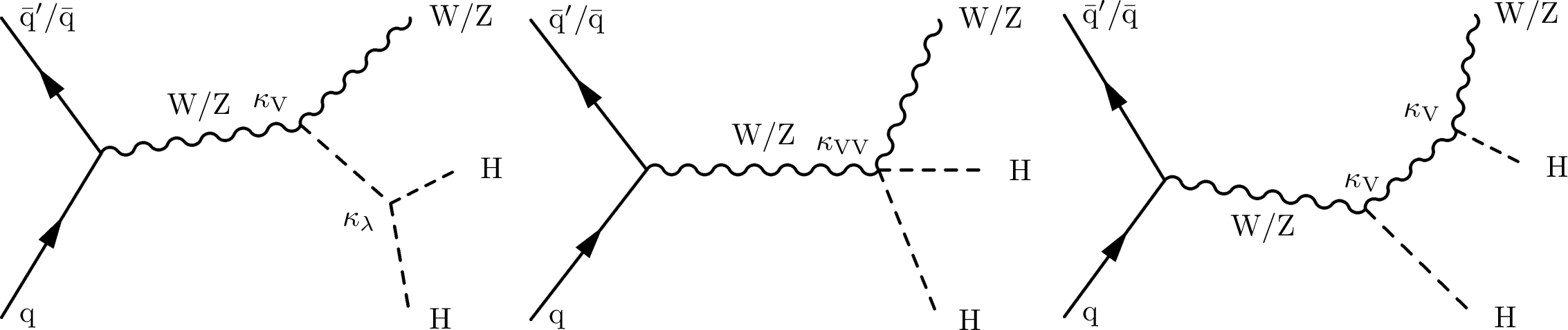
Figure 1:
The three LO quark-initiated diagrams above result in a final state with two Higgs bosons and a W or Z boson. The first diagram requires one $ \kappa_{\mathrm{V}} $-coupling vertex and one $ \kappa_{\lambda} $-coupling vertex. The second diagram requires only one $ \kappa_{\mathrm{V}\mathrm{V}} $-coupling vertex, and the final diagram requires two $ \kappa_{\mathrm{V}} $-coupling vertices. |
png pdf |
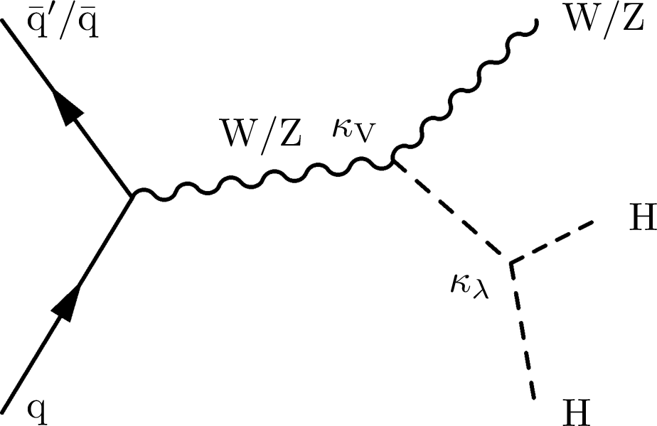
Figure 1-a:
The three LO quark-initiated diagrams above result in a final state with two Higgs bosons and a W or Z boson. The first diagram requires one $ \kappa_{\mathrm{V}} $-coupling vertex and one $ \kappa_{\lambda} $-coupling vertex. The second diagram requires only one $ \kappa_{\mathrm{V}\mathrm{V}} $-coupling vertex, and the final diagram requires two $ \kappa_{\mathrm{V}} $-coupling vertices. |
png pdf |
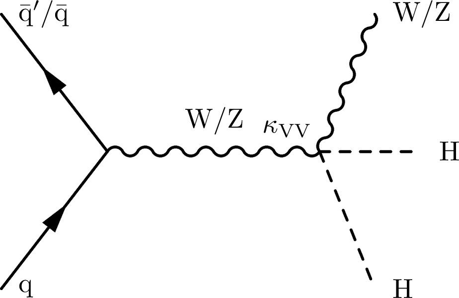
Figure 1-b:
The three LO quark-initiated diagrams above result in a final state with two Higgs bosons and a W or Z boson. The first diagram requires one $ \kappa_{\mathrm{V}} $-coupling vertex and one $ \kappa_{\lambda} $-coupling vertex. The second diagram requires only one $ \kappa_{\mathrm{V}\mathrm{V}} $-coupling vertex, and the final diagram requires two $ \kappa_{\mathrm{V}} $-coupling vertices. |

png pdf |
Figure 1-c:
The three LO quark-initiated diagrams above result in a final state with two Higgs bosons and a W or Z boson. The first diagram requires one $ \kappa_{\mathrm{V}} $-coupling vertex and one $ \kappa_{\lambda} $-coupling vertex. The second diagram requires only one $ \kappa_{\mathrm{V}\mathrm{V}} $-coupling vertex, and the final diagram requires two $ \kappa_{\mathrm{V}} $-coupling vertices. |
png pdf |
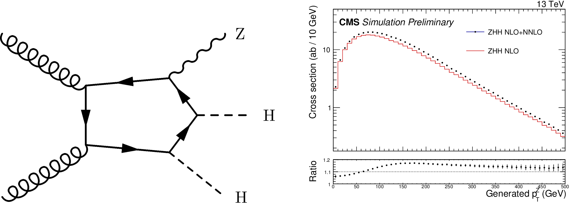
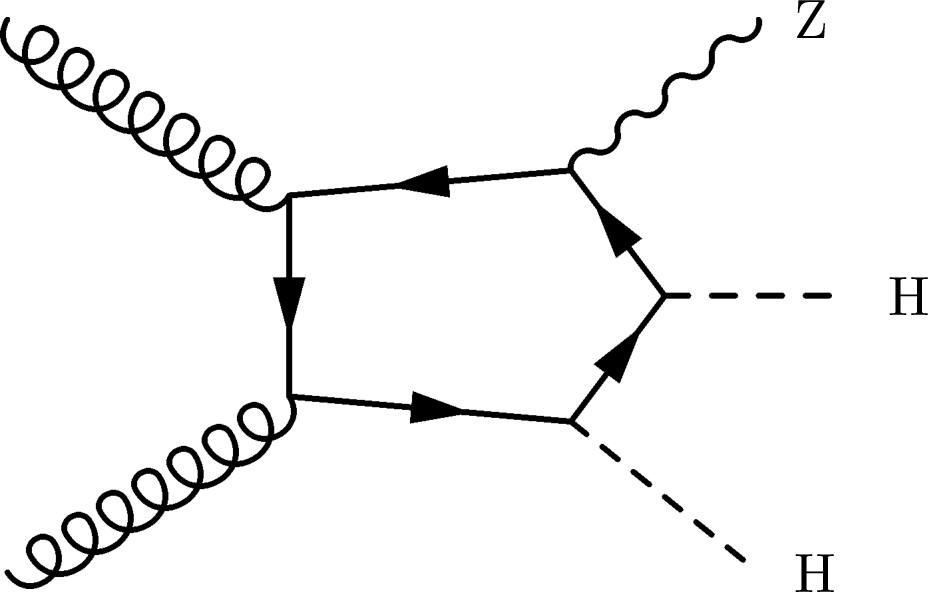
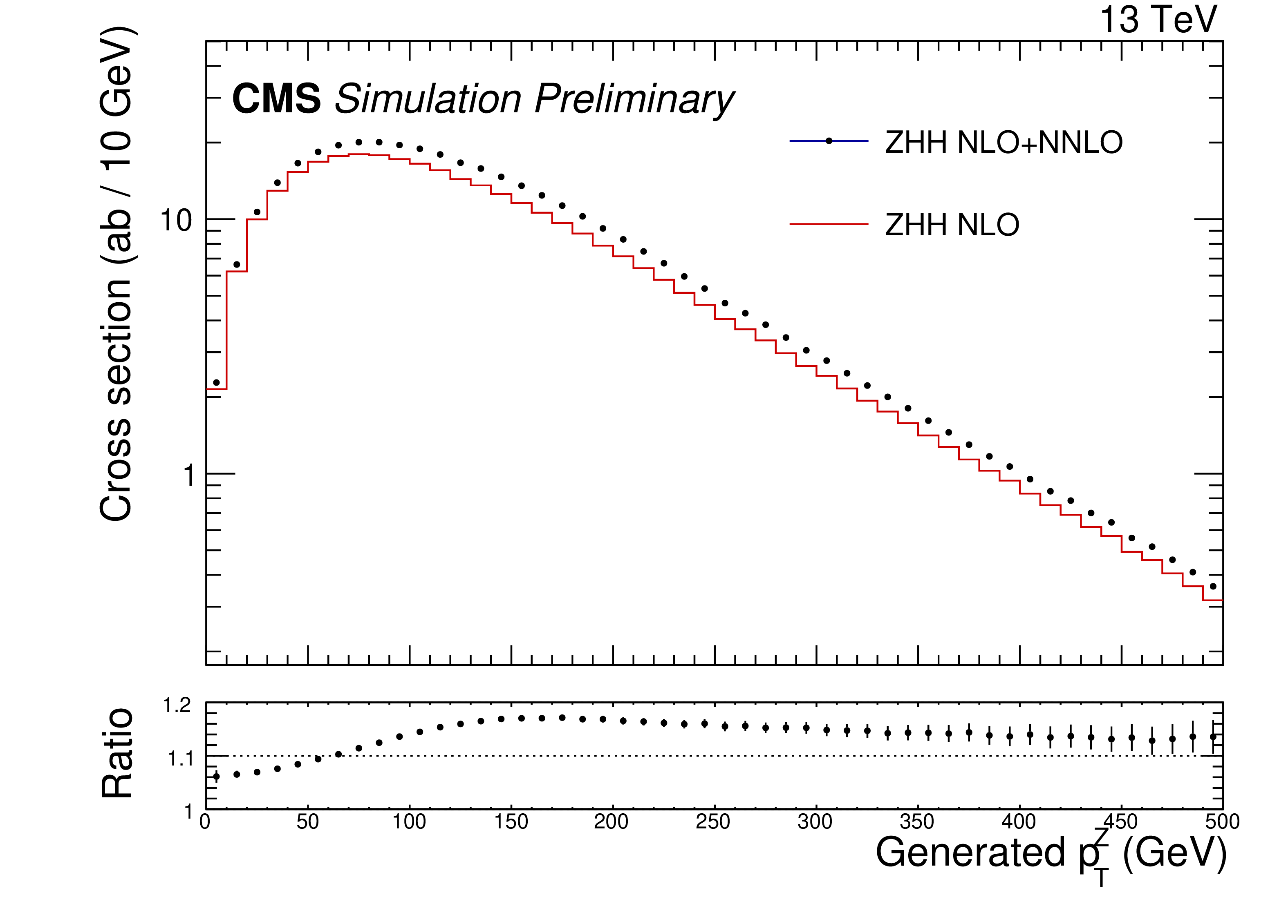
Figure 2:
left: representative diagram for ZHH production initiated by gluon fusion via a quark loop, which represents approximately 14% of the total cross section for this process. right: distribution of $ p_{\mathrm{T}}^{\mathrm{Z}} $ with and without the gluon-fusion process. |
png pdf |
Figure 2-a:
left: representative diagram for ZHH production initiated by gluon fusion via a quark loop, which represents approximately 14% of the total cross section for this process. right: distribution of $ p_{\mathrm{T}}^{\mathrm{Z}} $ with and without the gluon-fusion process. |
png pdf |
Figure 2-b:
left: representative diagram for ZHH production initiated by gluon fusion via a quark loop, which represents approximately 14% of the total cross section for this process. right: distribution of $ p_{\mathrm{T}}^{\mathrm{Z}} $ with and without the gluon-fusion process. |
png pdf |
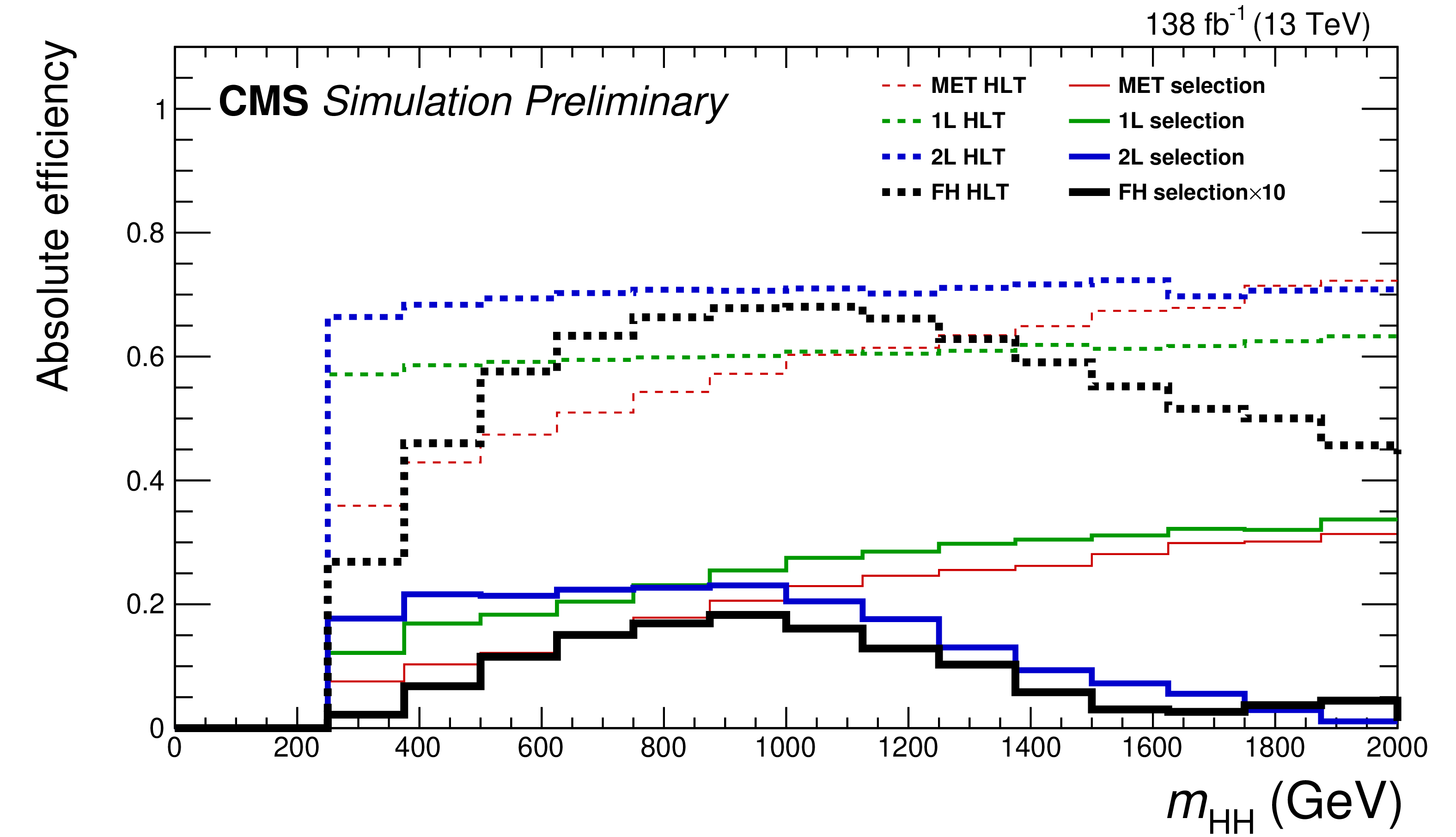
Figure 3:
Efficiencies of trigger selections (dashed lines) and full SR selections (solid lines) are shown for all four analysis channels. The selection efficiency of the $ \text{FH} $ channel is scaled up by 10 for visibility. The SR selections include trigger selections. Both sets of efficiencies are absolute efficiencies. |
png pdf |
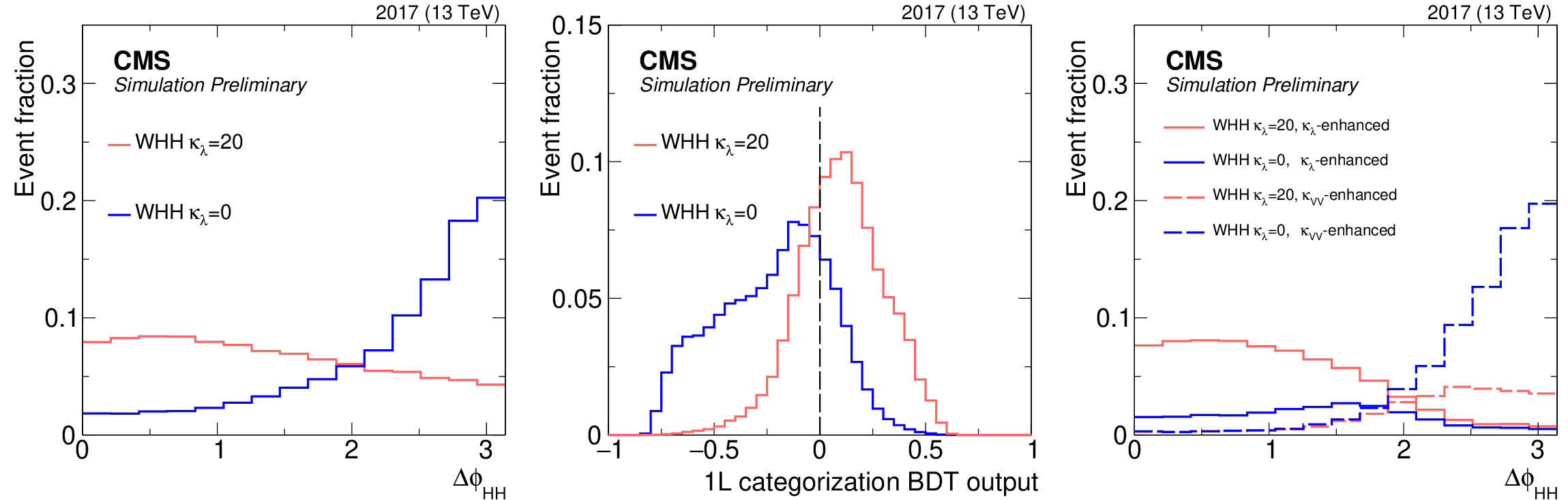
Figure 4:
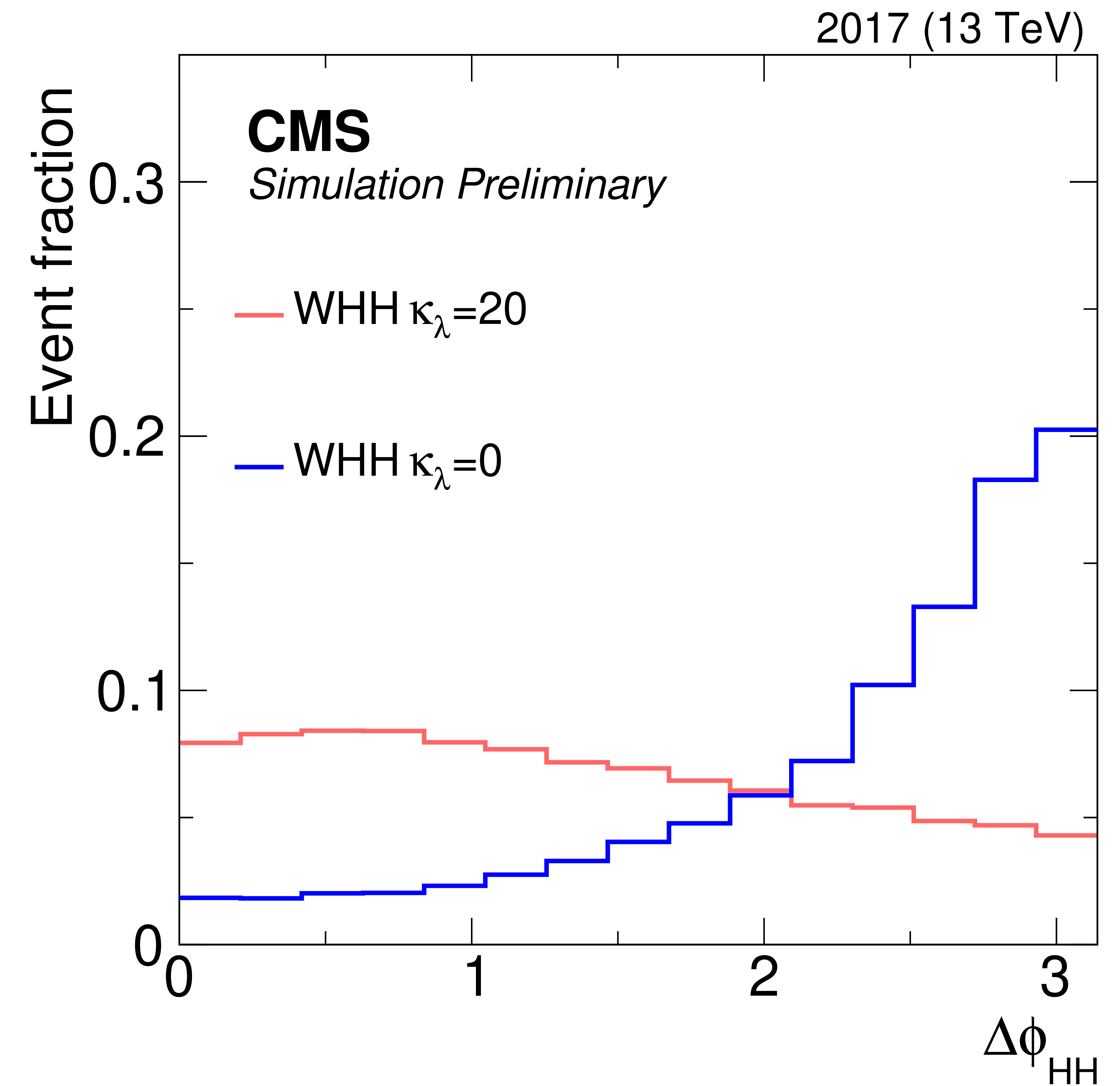
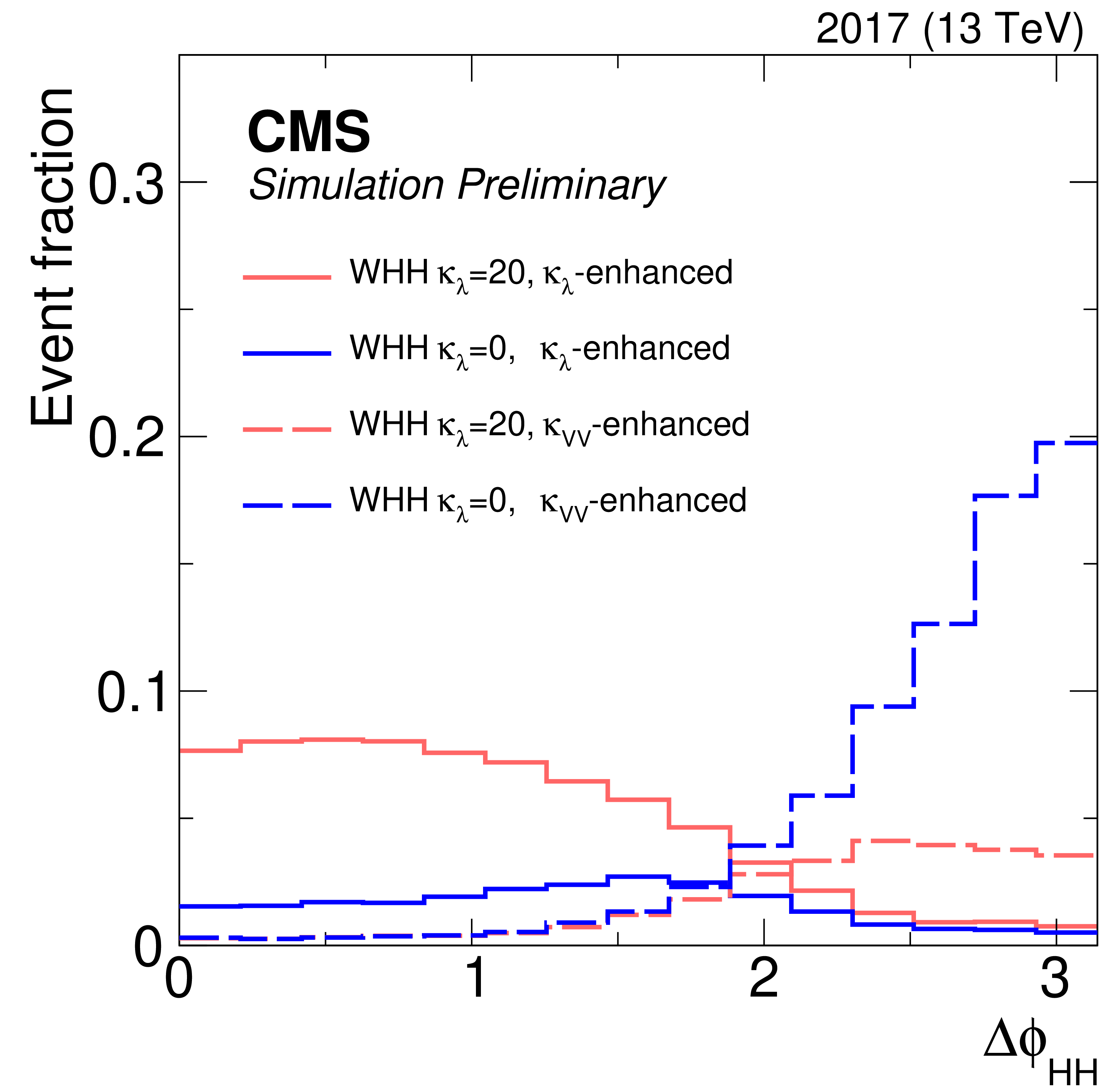
The kinematic distributions and primary phase spaces shift when coupling strengths are varied. Left: azimuthal angle between the two reconstructed Higgs boson candidates, $ \Delta\phi_{\mathrm{H}\mathrm{H}} $, in the 1L SR for two different coupling models, $ \kappa_{\lambda}= $ 20 and $ \kappa_{\lambda}= $ 0. Middle: the categorization BDT output for the same two models. The dashed vertical line shows where the categorization boundary was set. Right: the same two signal models on each side of categorization. All histograms are normalized to unity to highlight qualitative features. |
png pdf |
Figure 4-a:
The kinematic distributions and primary phase spaces shift when coupling strengths are varied. Left: azimuthal angle between the two reconstructed Higgs boson candidates, $ \Delta\phi_{\mathrm{H}\mathrm{H}} $, in the 1L SR for two different coupling models, $ \kappa_{\lambda}= $ 20 and $ \kappa_{\lambda}= $ 0. Middle: the categorization BDT output for the same two models. The dashed vertical line shows where the categorization boundary was set. Right: the same two signal models on each side of categorization. All histograms are normalized to unity to highlight qualitative features. |

png pdf |
Figure 4-b:
The kinematic distributions and primary phase spaces shift when coupling strengths are varied. Left: azimuthal angle between the two reconstructed Higgs boson candidates, $ \Delta\phi_{\mathrm{H}\mathrm{H}} $, in the 1L SR for two different coupling models, $ \kappa_{\lambda}= $ 20 and $ \kappa_{\lambda}= $ 0. Middle: the categorization BDT output for the same two models. The dashed vertical line shows where the categorization boundary was set. Right: the same two signal models on each side of categorization. All histograms are normalized to unity to highlight qualitative features. |
png pdf |
Figure 4-c:
The kinematic distributions and primary phase spaces shift when coupling strengths are varied. Left: azimuthal angle between the two reconstructed Higgs boson candidates, $ \Delta\phi_{\mathrm{H}\mathrm{H}} $, in the 1L SR for two different coupling models, $ \kappa_{\lambda}= $ 20 and $ \kappa_{\lambda}= $ 0. Middle: the categorization BDT output for the same two models. The dashed vertical line shows where the categorization boundary was set. Right: the same two signal models on each side of categorization. All histograms are normalized to unity to highlight qualitative features. |
png pdf |
Figure 5:
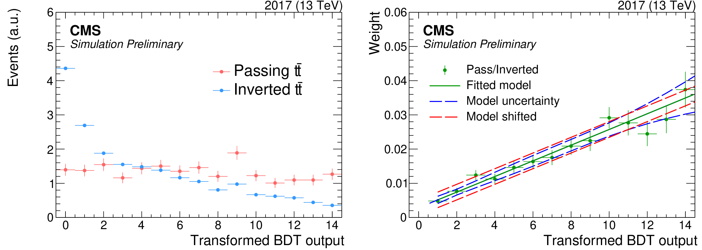
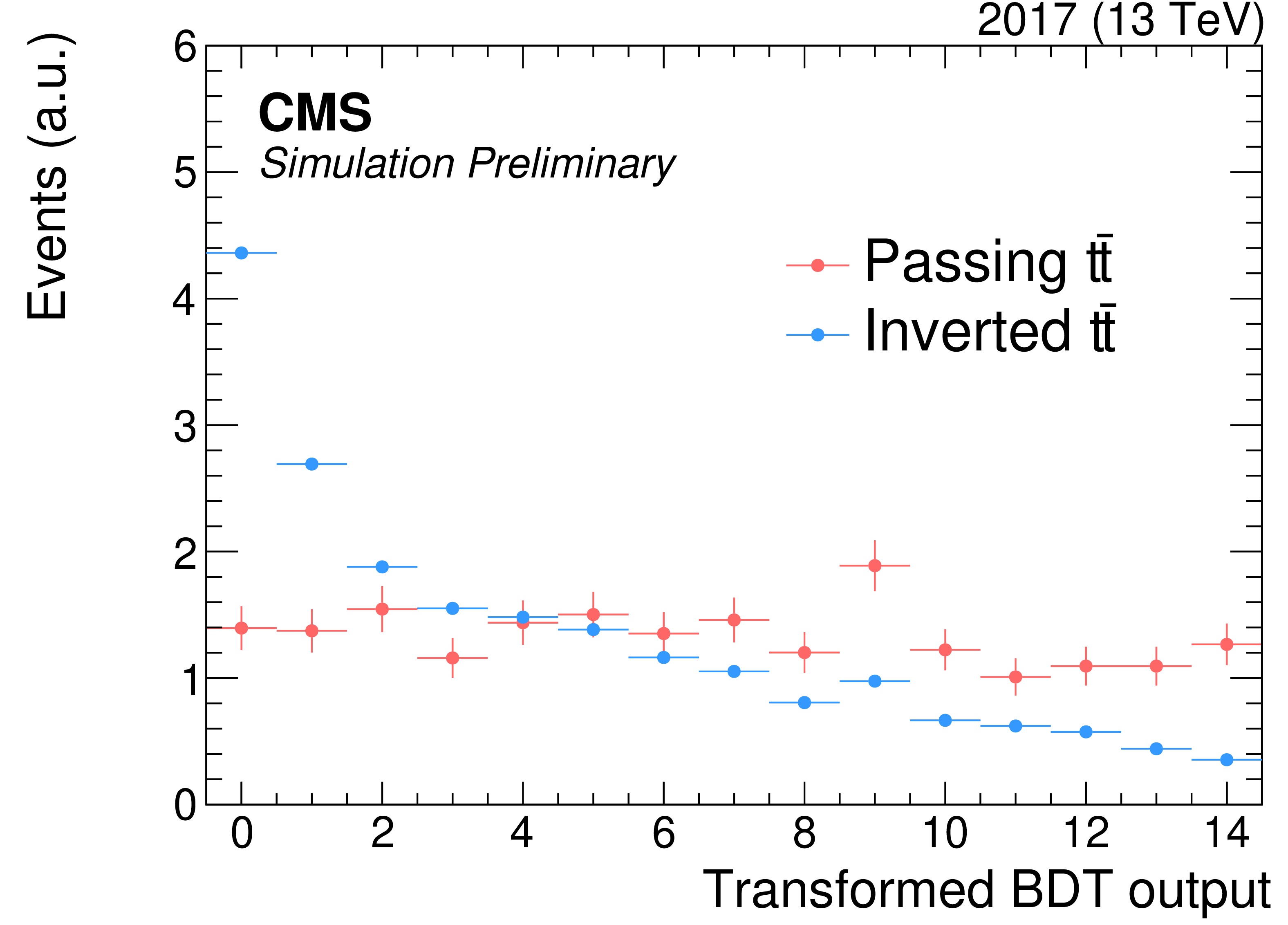
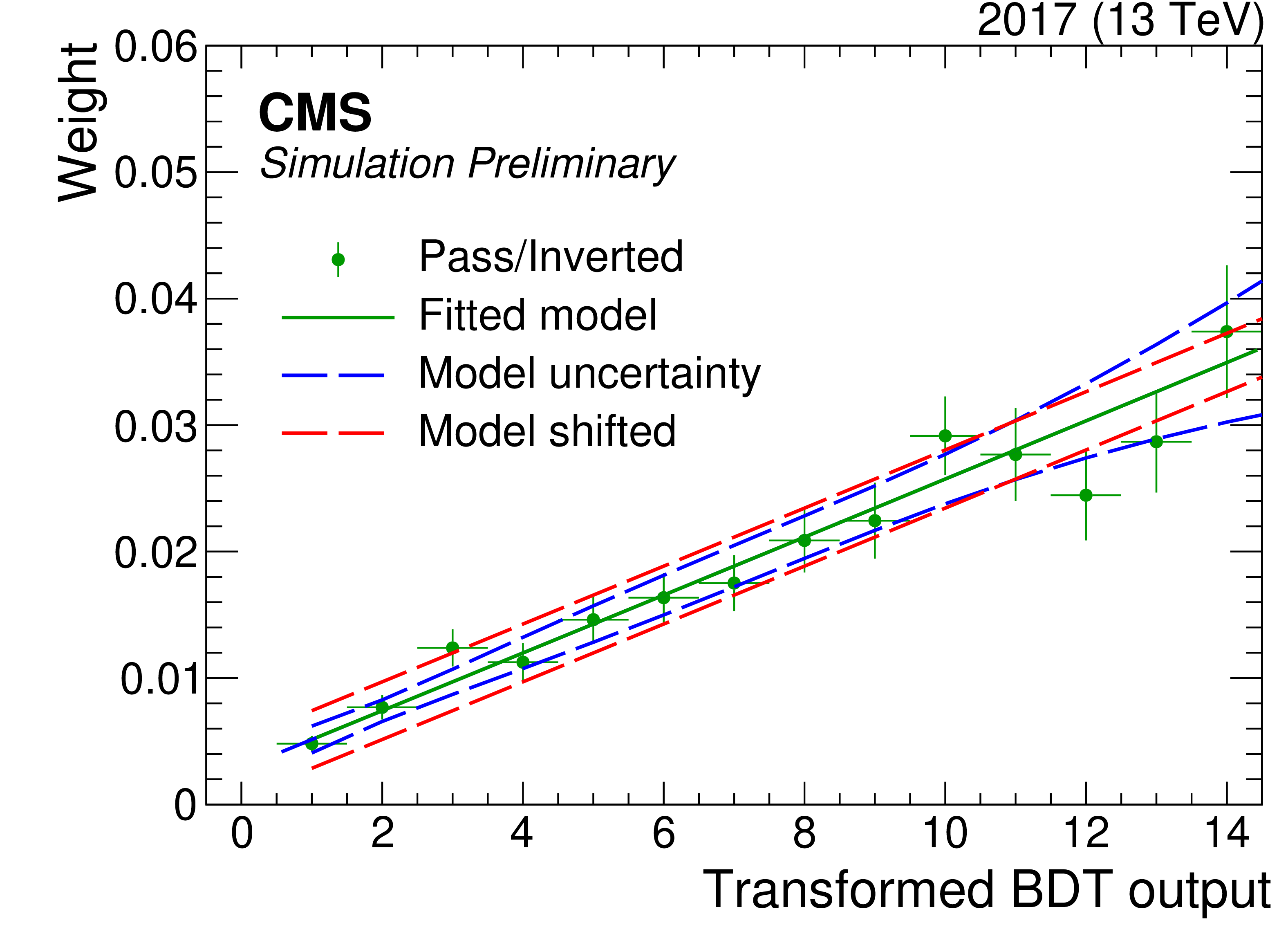
left: a reweighting BDT in the 1L LP region for the $ {\mathrm{t}\bar{\mathrm{t}}} \mathrm{b}\bar{\mathrm{b}} $ process that is transformed such that all bins have approximately the same amount of the limited precision passing $ {\mathrm{t}\bar{\mathrm{t}}} \mathrm{b}\bar{\mathrm{b}} $ sample shown in red. In blue is the same process where the b tagging cuts are inverted. right: the ratio is shown of passing $ {\mathrm{t}\bar{\mathrm{t}}} \mathrm{b}\bar{\mathrm{b}} $ to inverted $ {\mathrm{t}\bar{\mathrm{t}}} \mathrm{b}\bar{\mathrm{b}} $ (green points) as a function of the transformed reweighting BDT. The solid line is the second-order polynomial fit of the green points, which is used for the reweighting. In dashed blue and dashed red are the associated systematic uncertainties, which are obtained from the evaluation of the fit error on the weight and from shifting the BDT bin in evaluation of the model, respectively. |
png pdf |
Figure 5-a:
left: a reweighting BDT in the 1L LP region for the $ {\mathrm{t}\bar{\mathrm{t}}} \mathrm{b}\bar{\mathrm{b}} $ process that is transformed such that all bins have approximately the same amount of the limited precision passing $ {\mathrm{t}\bar{\mathrm{t}}} \mathrm{b}\bar{\mathrm{b}} $ sample shown in red. In blue is the same process where the b tagging cuts are inverted. right: the ratio is shown of passing $ {\mathrm{t}\bar{\mathrm{t}}} \mathrm{b}\bar{\mathrm{b}} $ to inverted $ {\mathrm{t}\bar{\mathrm{t}}} \mathrm{b}\bar{\mathrm{b}} $ (green points) as a function of the transformed reweighting BDT. The solid line is the second-order polynomial fit of the green points, which is used for the reweighting. In dashed blue and dashed red are the associated systematic uncertainties, which are obtained from the evaluation of the fit error on the weight and from shifting the BDT bin in evaluation of the model, respectively. |
png pdf |
Figure 5-b:
left: a reweighting BDT in the 1L LP region for the $ {\mathrm{t}\bar{\mathrm{t}}} \mathrm{b}\bar{\mathrm{b}} $ process that is transformed such that all bins have approximately the same amount of the limited precision passing $ {\mathrm{t}\bar{\mathrm{t}}} \mathrm{b}\bar{\mathrm{b}} $ sample shown in red. In blue is the same process where the b tagging cuts are inverted. right: the ratio is shown of passing $ {\mathrm{t}\bar{\mathrm{t}}} \mathrm{b}\bar{\mathrm{b}} $ to inverted $ {\mathrm{t}\bar{\mathrm{t}}} \mathrm{b}\bar{\mathrm{b}} $ (green points) as a function of the transformed reweighting BDT. The solid line is the second-order polynomial fit of the green points, which is used for the reweighting. In dashed blue and dashed red are the associated systematic uncertainties, which are obtained from the evaluation of the fit error on the weight and from shifting the BDT bin in evaluation of the model, respectively. |
png pdf |
Figure 6:
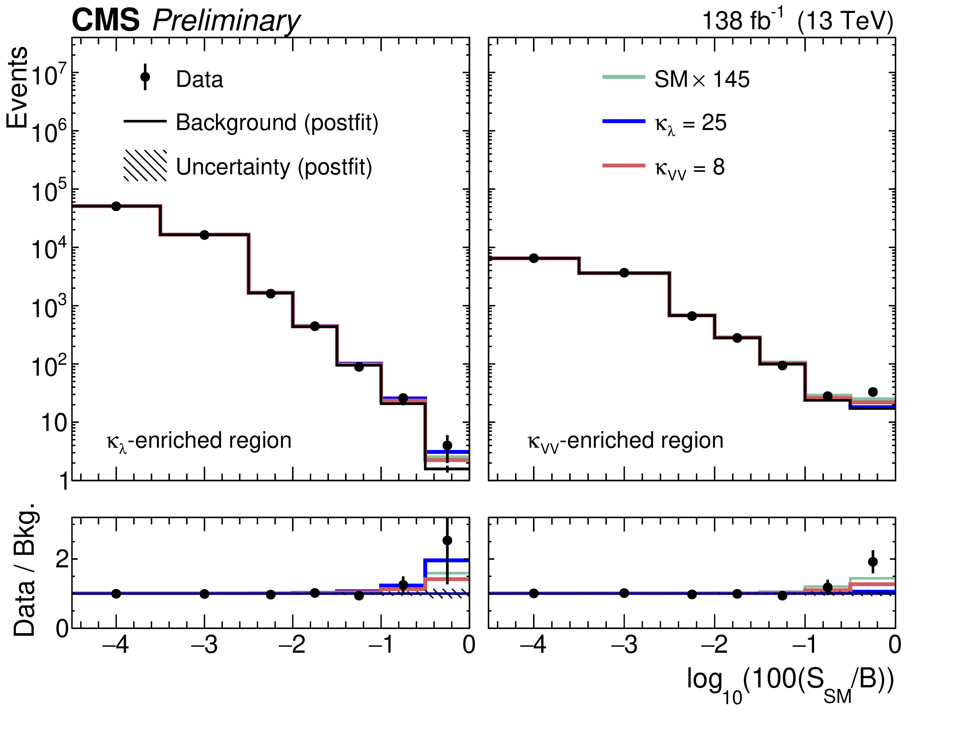
Machine learning distributions are transformed to $ \log_{10}\big( $ 100 (S}_\textSM/\text{B) $ \big) $ and summed for $ \kappa_{\lambda} $-enriched and $ \kappa_{\mathrm{V}\mathrm{V}} $-enriched SR samples separately. For the two enriched regions, data, simulated background, and three sensitive signal models are plotted. We observe that signal models with enhancement in a particular coupling appear enhanced also in the corresponding SR. |

png pdf |
Figure 7:
The results of two maximum likelihood fits are summarized above. The top entry, labeled ``Inclusive'', is the result of a single signal strength fit of all channels. The other four entries are from a fit of the same regions but with independent signal strengths in each channel. The thinner, blue bands are one standard deviation from the full likelihood scan in that parameter, while the thicker, red bands are one standard deviation bands of the systematic uncertainties only. |

png pdf |
Figure 8:
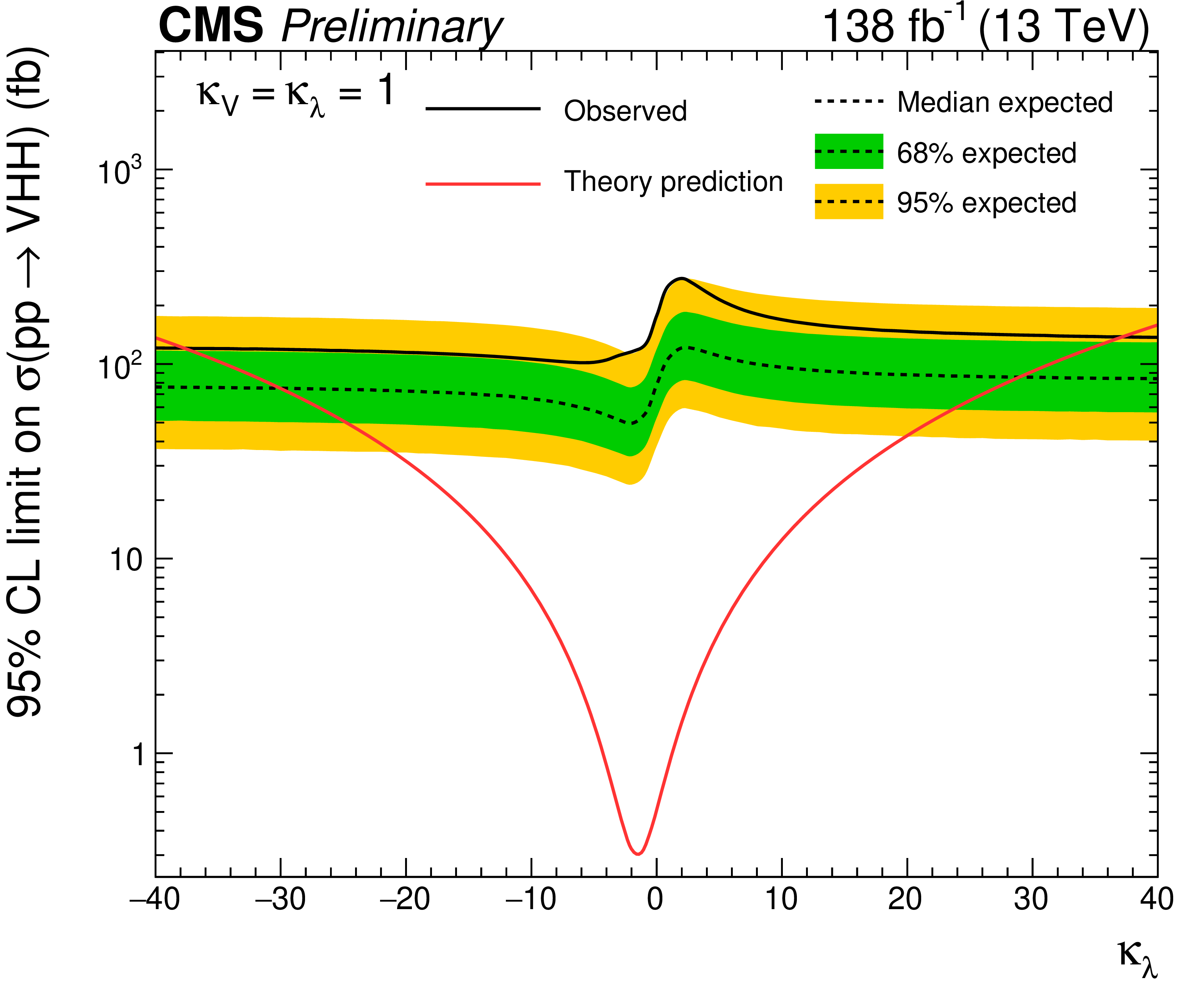
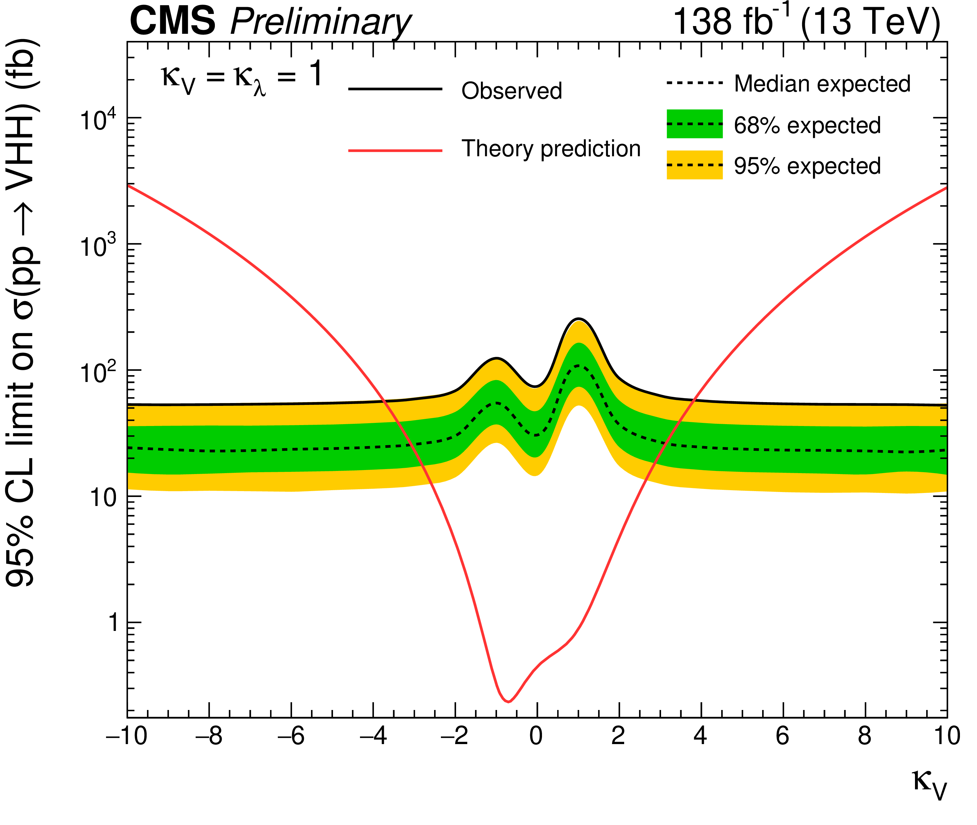
Upper 95% CL limits on signal cross section scanned over the $ \kappa $ parameter of interest while fixing the other two to their SM-predicted couplings. The independent axis is the scanned $ \kappa $ parameter, and the dependent axis is the 95% CL upper limit on signal cross section. The scans over $ \kappa_{\lambda} $, $ \kappa_{\mathrm{V}\mathrm{V}} $, and $ \kappa_{\mathrm{V}} $ are shown left, center, and right, respectively. |
png pdf |
Figure 8-a:
Upper 95% CL limits on signal cross section scanned over the $ \kappa $ parameter of interest while fixing the other two to their SM-predicted couplings. The independent axis is the scanned $ \kappa $ parameter, and the dependent axis is the 95% CL upper limit on signal cross section. The scans over $ \kappa_{\lambda} $, $ \kappa_{\mathrm{V}\mathrm{V}} $, and $ \kappa_{\mathrm{V}} $ are shown left, center, and right, respectively. |

png pdf |
Figure 8-b:
Upper 95% CL limits on signal cross section scanned over the $ \kappa $ parameter of interest while fixing the other two to their SM-predicted couplings. The independent axis is the scanned $ \kappa $ parameter, and the dependent axis is the 95% CL upper limit on signal cross section. The scans over $ \kappa_{\lambda} $, $ \kappa_{\mathrm{V}\mathrm{V}} $, and $ \kappa_{\mathrm{V}} $ are shown left, center, and right, respectively. |
png pdf |
Figure 8-c:
Upper 95% CL limits on signal cross section scanned over the $ \kappa $ parameter of interest while fixing the other two to their SM-predicted couplings. The independent axis is the scanned $ \kappa $ parameter, and the dependent axis is the 95% CL upper limit on signal cross section. The scans over $ \kappa_{\lambda} $, $ \kappa_{\mathrm{V}\mathrm{V}} $, and $ \kappa_{\mathrm{V}} $ are shown left, center, and right, respectively. |
png pdf |
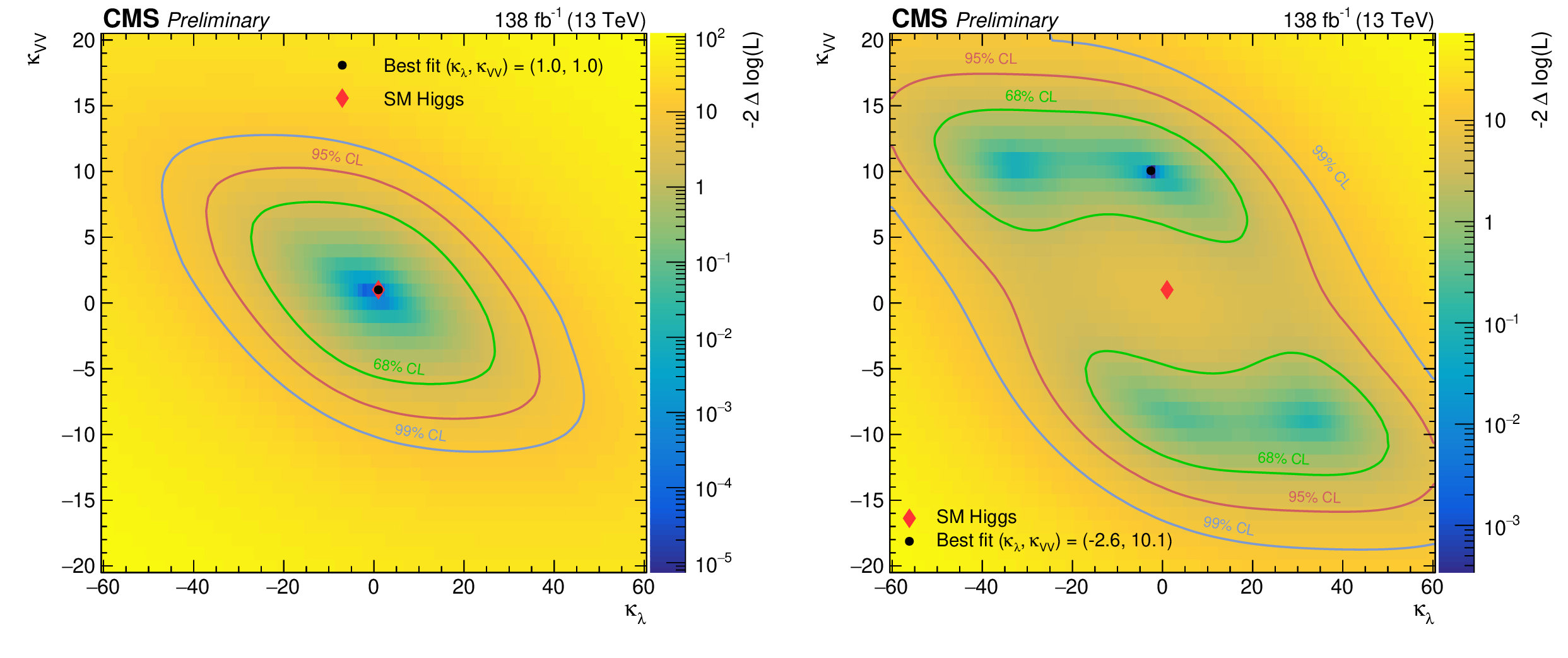
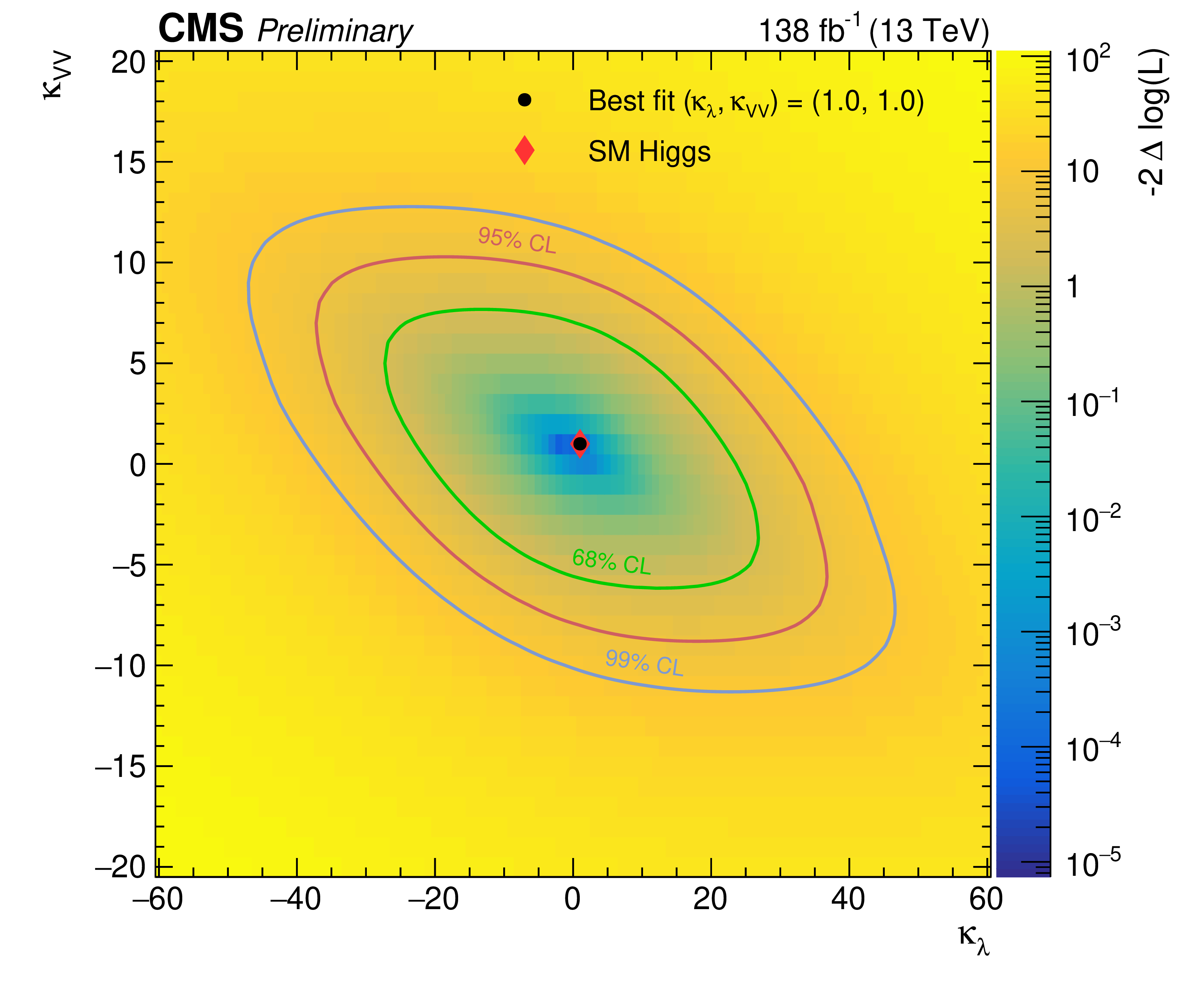
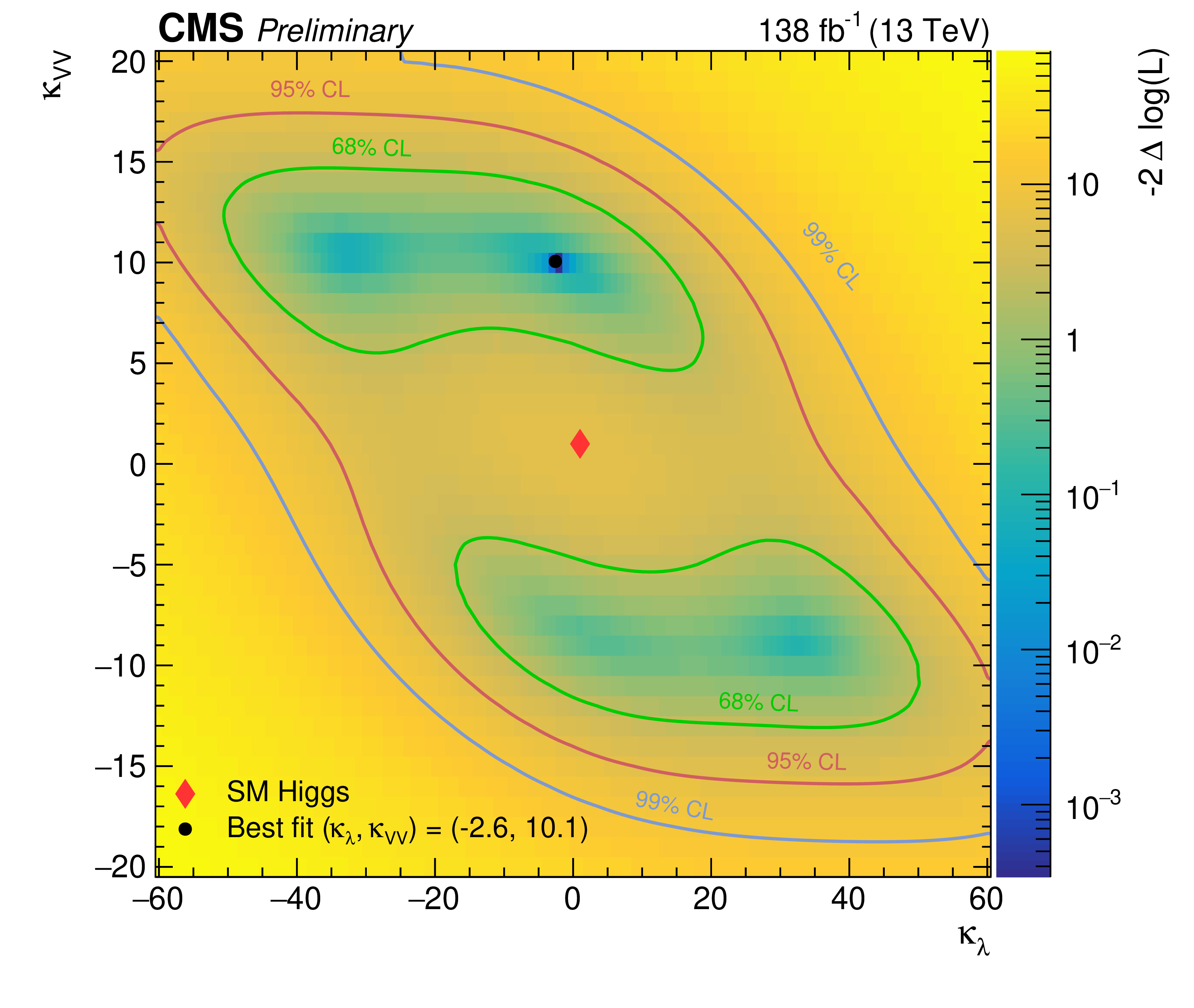
Figure 9:
Expected (left) and observed (right) likelihood scans in $ \kappa_{\lambda} $ versus $ \kappa_{\mathrm{V}\mathrm{V}} $ are shown, with other SM couplings fixed to the SM predicted strength. The excess is most prominent in the $ \kappa_{\mathrm{V}\mathrm{V}} $-enriched region, and so the most likely point of the scan at $ \kappa_{\mathrm{V}\mathrm{V}}= $ 10.1 and $ \kappa_{\lambda}=- $ 2.6 is pulled than two standard deviations from the SM mostly in the $ \kappa_{\mathrm{V}\mathrm{V}} $ dimension. |
png pdf |
Figure 9-a:
Expected (left) and observed (right) likelihood scans in $ \kappa_{\lambda} $ versus $ \kappa_{\mathrm{V}\mathrm{V}} $ are shown, with other SM couplings fixed to the SM predicted strength. The excess is most prominent in the $ \kappa_{\mathrm{V}\mathrm{V}} $-enriched region, and so the most likely point of the scan at $ \kappa_{\mathrm{V}\mathrm{V}}= $ 10.1 and $ \kappa_{\lambda}=- $ 2.6 is pulled than two standard deviations from the SM mostly in the $ \kappa_{\mathrm{V}\mathrm{V}} $ dimension. |
png pdf |
Figure 9-b:
Expected (left) and observed (right) likelihood scans in $ \kappa_{\lambda} $ versus $ \kappa_{\mathrm{V}\mathrm{V}} $ are shown, with other SM couplings fixed to the SM predicted strength. The excess is most prominent in the $ \kappa_{\mathrm{V}\mathrm{V}} $-enriched region, and so the most likely point of the scan at $ \kappa_{\mathrm{V}\mathrm{V}}= $ 10.1 and $ \kappa_{\lambda}=- $ 2.6 is pulled than two standard deviations from the SM mostly in the $ \kappa_{\mathrm{V}\mathrm{V}} $ dimension. |

png pdf |
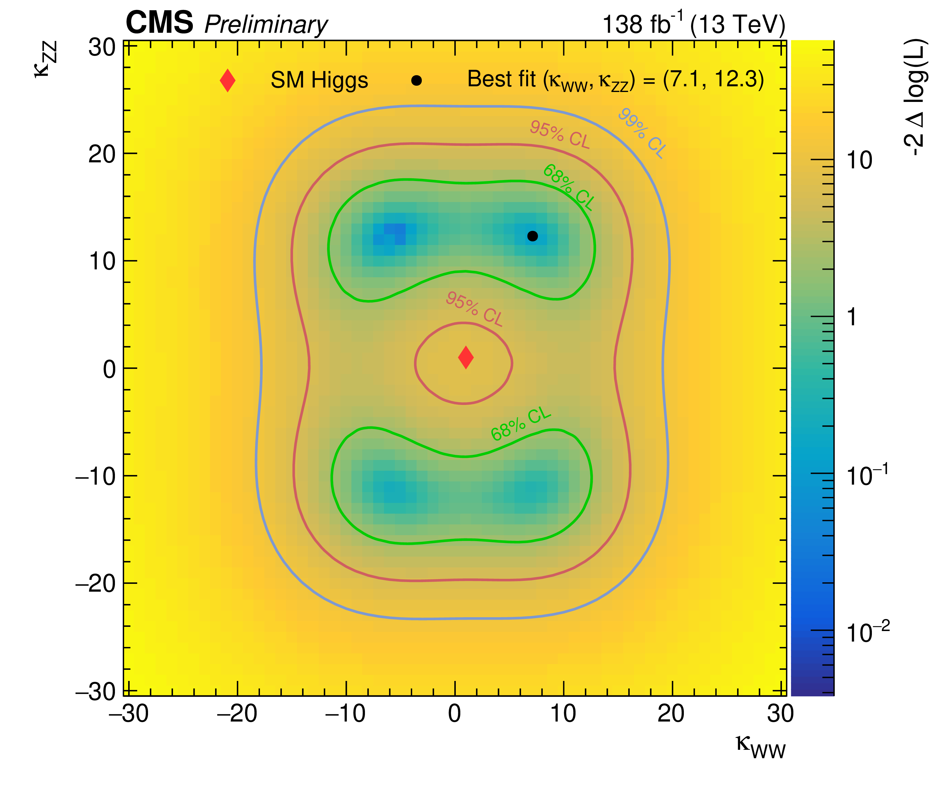
Figure 10:
Expected (left) and observed (right) likelihood scans of $ \kappa_{\mathrm{W}\mathrm{W}} $ versus $ \kappa_{\mathrm{Z}\mathrm{Z}} $ are shown, with other SM couplings fixed to the SM predicted strength. The excess is most prominent in the $ \text{MET} $ channel, and so the most likely point of the scan at $ \kappa_{\mathrm{W}\mathrm{W}}= $ 7.1 and $ \kappa_{\mathrm{Z}\mathrm{Z}}= $ 12.3 is pulled than two standard deviations from the SM mostly in the $ \kappa_{\mathrm{Z}\mathrm{Z}} $ dimension, to which the signal in the $ \text{MET} $ channel is solely sensitive. |

png pdf |
Figure 10-a:
Expected (left) and observed (right) likelihood scans of $ \kappa_{\mathrm{W}\mathrm{W}} $ versus $ \kappa_{\mathrm{Z}\mathrm{Z}} $ are shown, with other SM couplings fixed to the SM predicted strength. The excess is most prominent in the $ \text{MET} $ channel, and so the most likely point of the scan at $ \kappa_{\mathrm{W}\mathrm{W}}= $ 7.1 and $ \kappa_{\mathrm{Z}\mathrm{Z}}= $ 12.3 is pulled than two standard deviations from the SM mostly in the $ \kappa_{\mathrm{Z}\mathrm{Z}} $ dimension, to which the signal in the $ \text{MET} $ channel is solely sensitive. |
png pdf |
Figure 10-b:
Expected (left) and observed (right) likelihood scans of $ \kappa_{\mathrm{W}\mathrm{W}} $ versus $ \kappa_{\mathrm{Z}\mathrm{Z}} $ are shown, with other SM couplings fixed to the SM predicted strength. The excess is most prominent in the $ \text{MET} $ channel, and so the most likely point of the scan at $ \kappa_{\mathrm{W}\mathrm{W}}= $ 7.1 and $ \kappa_{\mathrm{Z}\mathrm{Z}}= $ 12.3 is pulled than two standard deviations from the SM mostly in the $ \kappa_{\mathrm{Z}\mathrm{Z}} $ dimension, to which the signal in the $ \text{MET} $ channel is solely sensitive. |
png pdf |
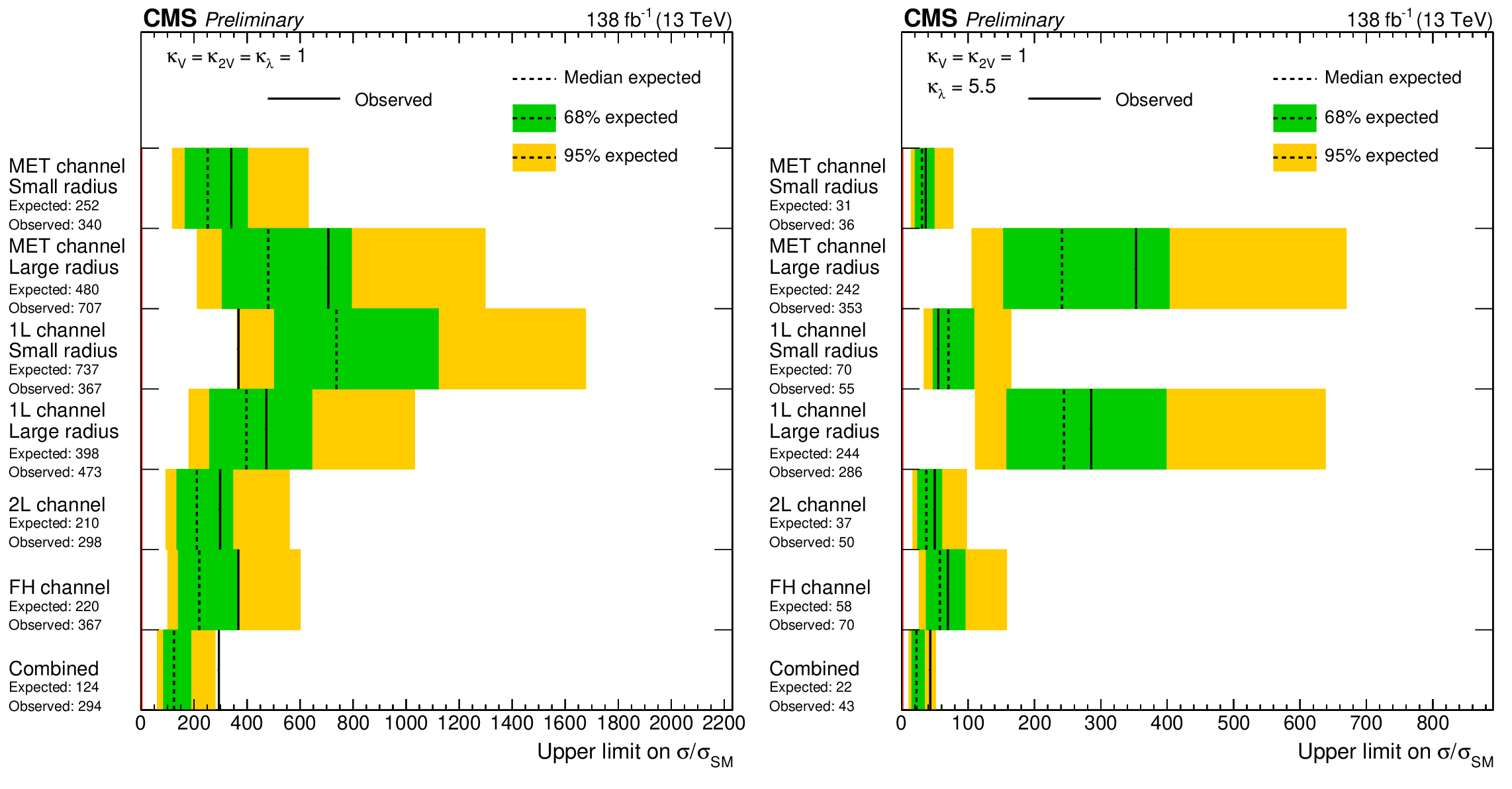
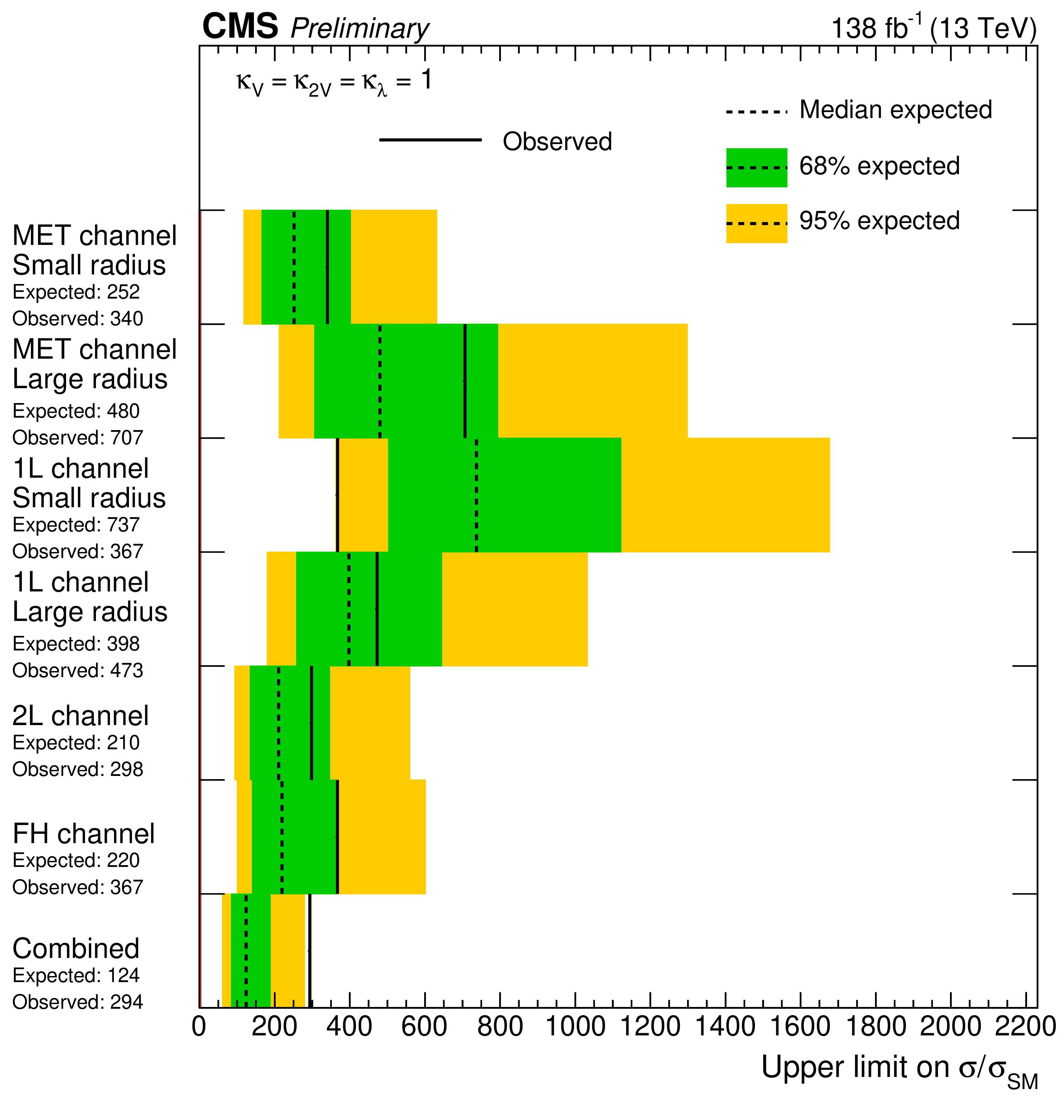
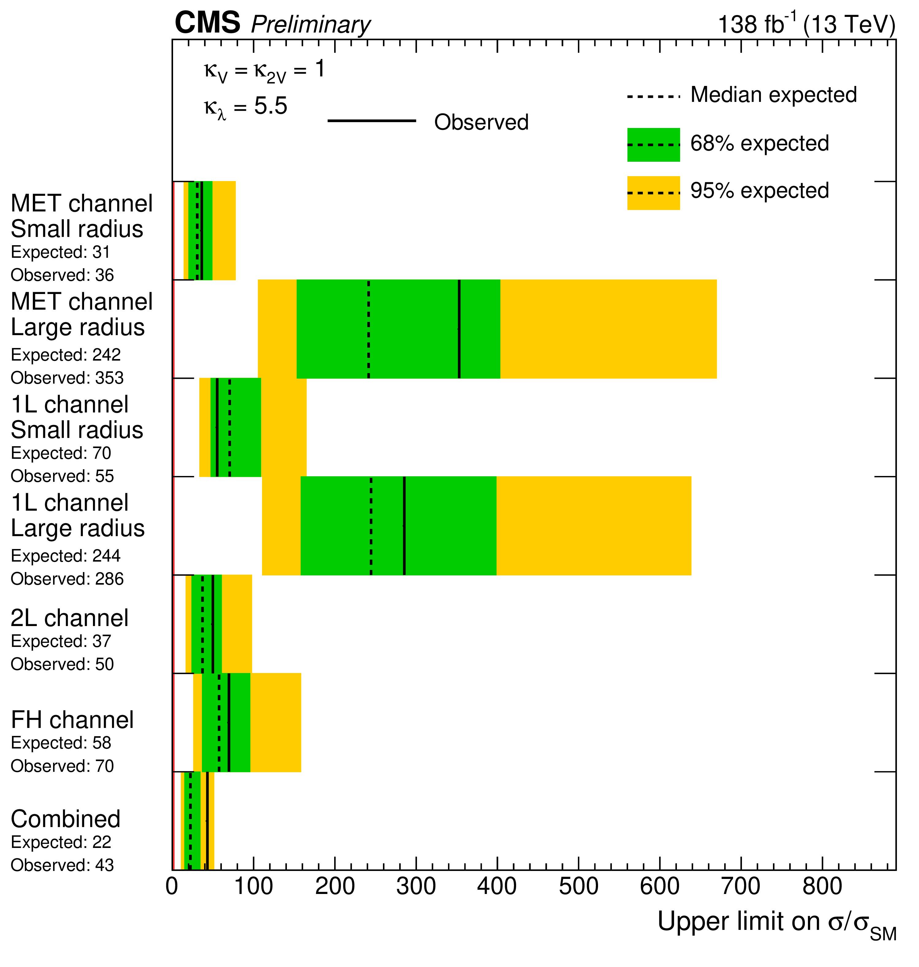
Figure 11:
The left plot shows the VHH cross section limits per channel and combined for SM-sized couplings, while results with $ \kappa_{\lambda}= $ 5.5 and $ \kappa_{\mathrm{V}\mathrm{V}}=\kappa_{\mathrm{V}}= $ 1.0 are shown on the right. The latter is a relatively sensitive region for VHH, where the primary HH production cross sections are near minimal because of destructive interference. |
png pdf |
Figure 11-a:
The left plot shows the VHH cross section limits per channel and combined for SM-sized couplings, while results with $ \kappa_{\lambda}= $ 5.5 and $ \kappa_{\mathrm{V}\mathrm{V}}=\kappa_{\mathrm{V}}= $ 1.0 are shown on the right. The latter is a relatively sensitive region for VHH, where the primary HH production cross sections are near minimal because of destructive interference. |
png pdf |
Figure 11-b:
The left plot shows the VHH cross section limits per channel and combined for SM-sized couplings, while results with $ \kappa_{\lambda}= $ 5.5 and $ \kappa_{\mathrm{V}\mathrm{V}}=\kappa_{\mathrm{V}}= $ 1.0 are shown on the right. The latter is a relatively sensitive region for VHH, where the primary HH production cross sections are near minimal because of destructive interference. |
| Tables | |
png pdf |
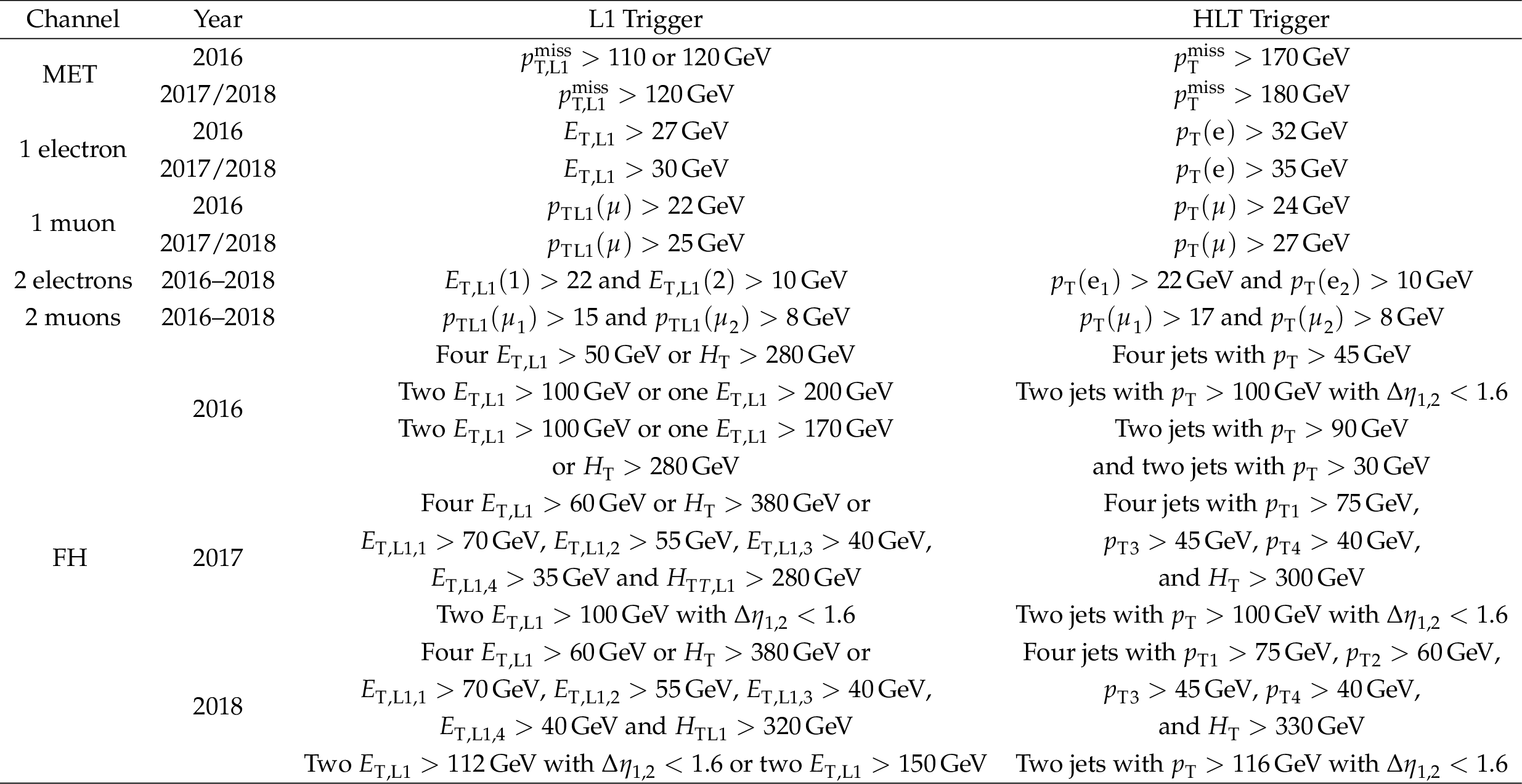
Table 1:
Kinematic thresholds for L1 and HLT triggers are listed below for each analysis channel with variations per year as needed. HLT reconstruction is very similiar to offline reconstruction. L1 reconstruction does not include any information from tracking. Transverse energy from ECAL plus HCAL systems is referred to as $ E_{\mathrm{T}}_{,\text{L1}} $. The scalar sum of $ E_{\mathrm{T}}_{,\text{L1}} $ from all energy deposits over a threshold of 30 GeV is $ H_{\text{T}} $. |
png pdf |
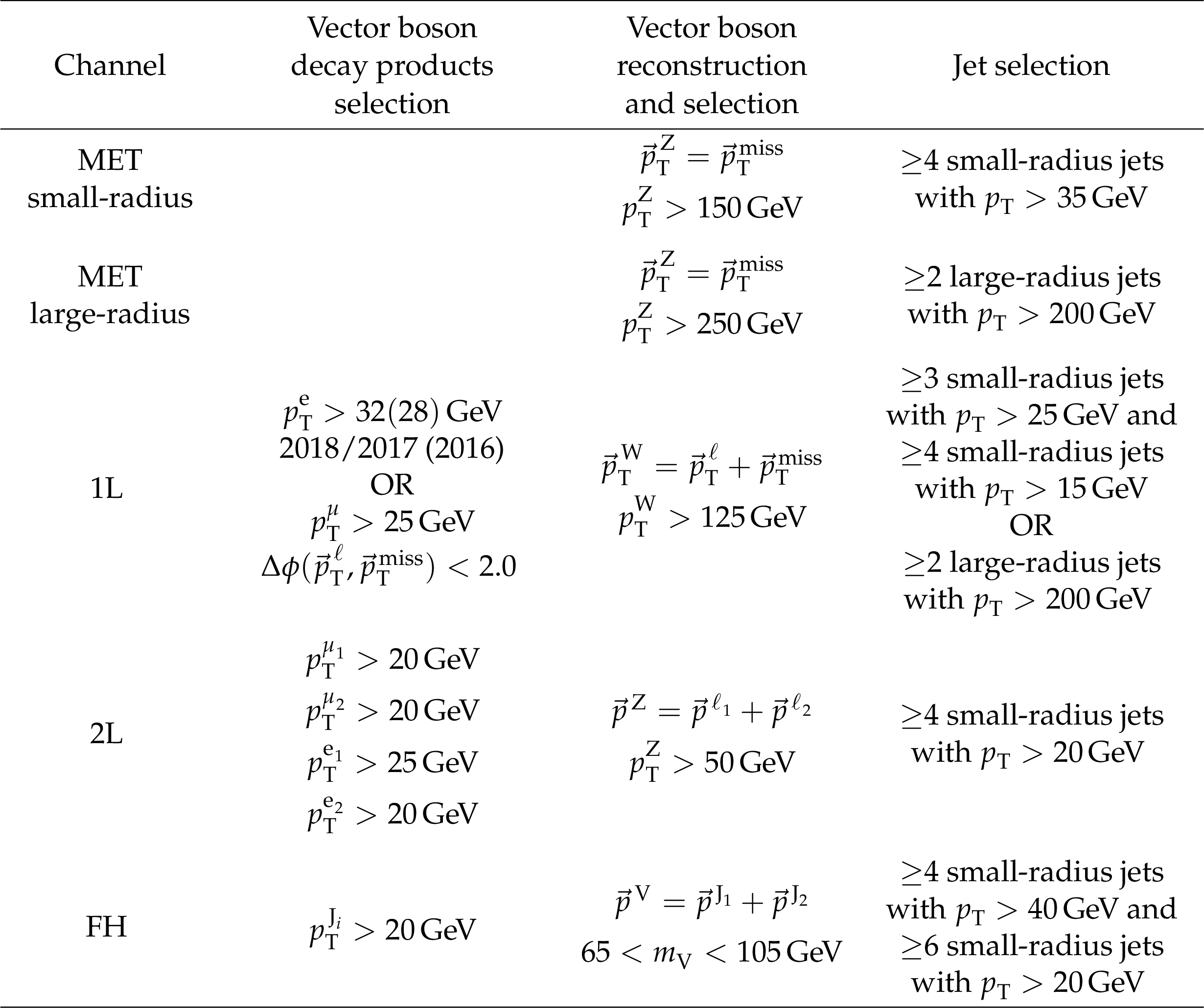
Table 2:
Thresholds on kinematic variables for all selected objects are listed for each channel. Objects are always required to be within the acceptance of the CMS subdetectors, which is $ |\eta| < $ 2.4 or 2.5 depending on the object and channel, as well as outside of barrel-endcap transition regions near $ |\eta|\sim $ 1.5. |
png pdf |
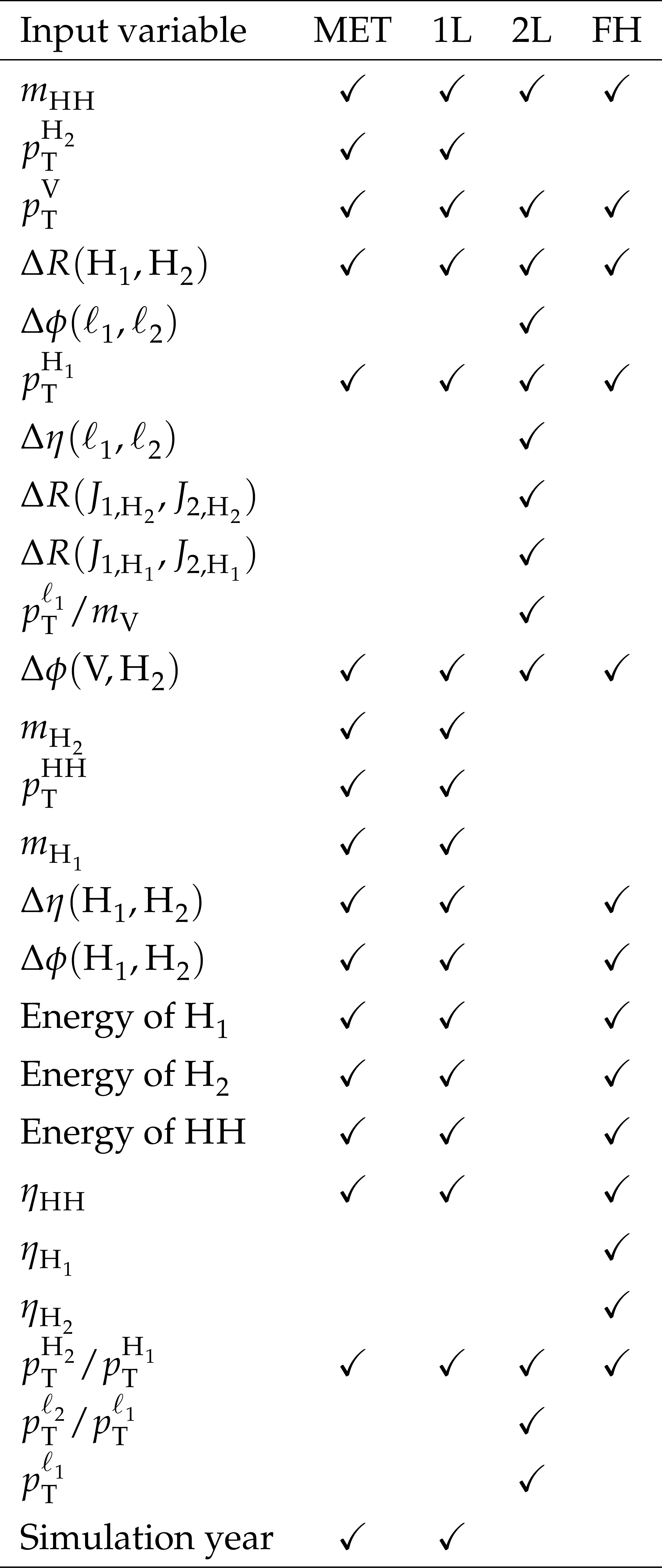
Table 3:
Kinematic variables used in the categorization BDTs for separation of the $ \kappa_{\lambda} $-enriched and $ \kappa_{\mathrm{V}\mathrm{V}} $-enriched regions. While there are some minor difference in importance of each variable per channel, the table is constructed such that variables at the top tend to be the most important, which is universally true for $ m_{\mathrm{H}\mathrm{H}} $, and the least important are at the bottom. |
png pdf |
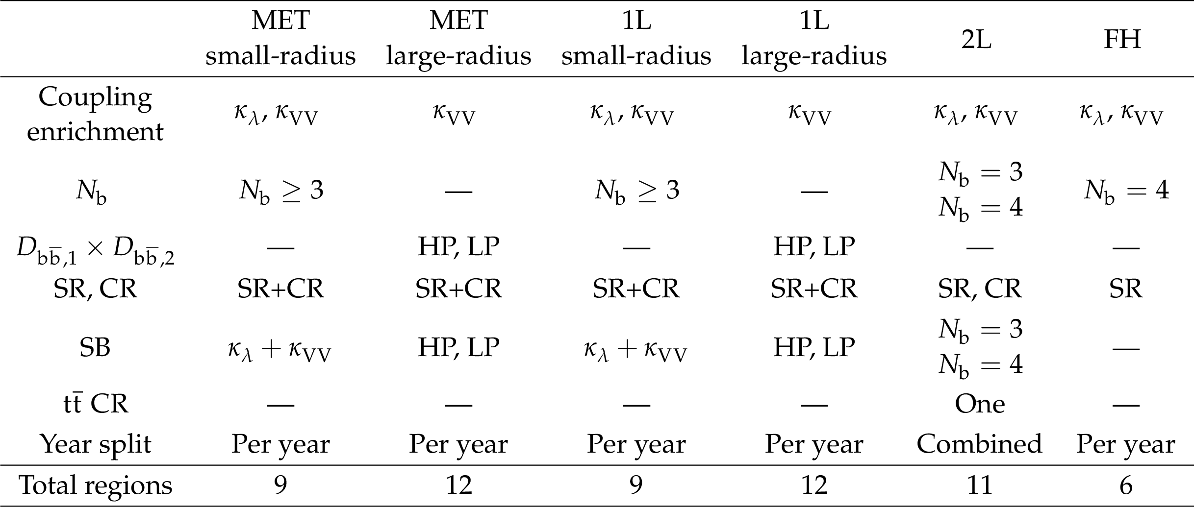
Table 4:
A summary of categorization in all channels. |
png pdf |
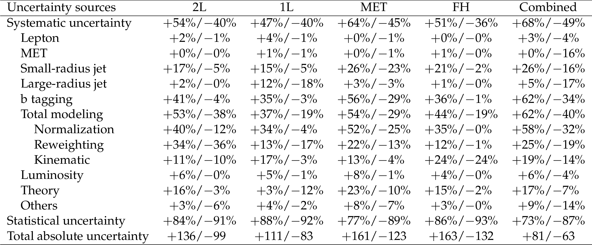
Table 5:
The contribution of each group of uncertainties is quantified relative to the total absolute uncertainty in signal strength, which is listed in the final line. To compute these relative contributes, the group of nuisance parameters are fixed to the best fit value while the likelihood is scanned again profiling all other nuisance parameters. The reduction in the up and down bands are shown in each line. The likelihood shape is asymmetric, and so up and down are quantified separately. |
png pdf |
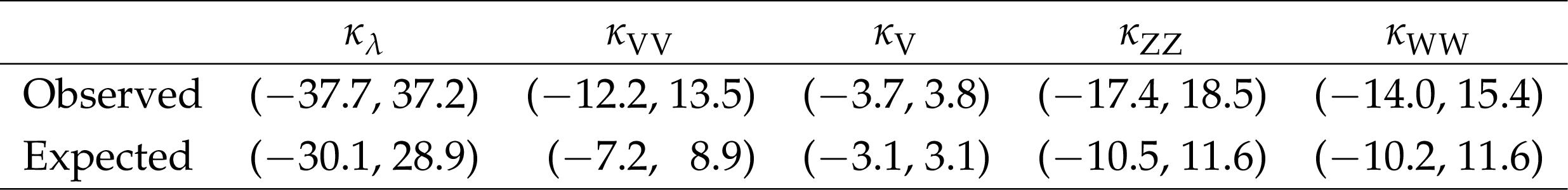
Table 6:
Observed and expected 95% CL upper limits on the coupling modifiers. |
| Summary |
| A search for Higgs boson pair production in association with a vector boson (VHH) using a data set comprising 138 fb$^{-1}$ of proton-proton collisions at $ \sqrt{s}= $ 13 TeV is presented. Final states including Higgs boson decay to bottom quarks are analyzed in events where the W or Z boson decay to electrons, muons, or hadrons. Coupling modifiers, defined relative to the SM coupling strength, are scanned and constrained for Higgs boson trilinear self-interaction coupling, $ \kappa_{\lambda} $, and two W or two Z with two Higgs bosons, $ \kappa_{\mathrm{V}\mathrm{V}} $. The observed (expected) 95% CL limits constrain $ \kappa_{\lambda} $ and $ \kappa_{\mathrm{V}\mathrm{V}} $ to be $ -$37.7 $< \kappa_{\lambda} < $ 37.2 ($ -$30.1 $< \kappa_{\lambda} < $ 28.9) and $ -$12.2 $< \kappa_{\lambda} < $ 13.5 ($ -$7.2 $< \kappa_{\lambda} < $ 8.9). In the range of 4 $ < \kappa_{\lambda} < $ 7 where matrix-element level interference is destructive for leading production mechanisms, VHH has constructive interference and the sensitivity of the VHH search is similar to $ \mathrm{b}\bar{\mathrm{b}}\tau\tau $ search on the equivalent data set. |
| References | ||||
| 1 | ATLAS Collaboration | Observation of a new particle in the search for the standard model Higgs boson with the ATLAS detector at the LHC | PLB 716 (2012) 1 | 1207.7214 |
| 2 | CMS Collaboration | Observation of a new boson at a mass of 125 GeV with the CMS experiment at the LHC | PLB 716 (2012) 30 | CMS-HIG-12-028 1207.7235 |
| 3 | J. Barrow and M. Turner | Baryosynthesis and the origin of galaxies | Nature 291 (1981) 469 | |
| 4 | CMS Collaboration | A portrait of the Higgs boson by the CMS experiment ten years after the discovery | Nature 607 (2022) 60 | CMS-HIG-22-001 2207.00043 |
| 5 | ATLAS Collaboration | A detailed map of Higgs boson interactions by the ATLAS experiment ten years after the discovery | Nature 607 (2022) 52 | 2207.00092 |
| 6 | LHC Higgs Cross Section Working Group Collaboration | Handbook of LHC Higgs cross sections: 4. deciphering the nature of the Higgs sector | link | 1610.07922 |
| 7 | CMS Collaboration | Search for nonresonant Higgs boson pair production in final states with two bottom quarks and two photons in proton-proton collisions at $ \sqrt{s} = $ 13 TeV | JHEP 03 (2021) 257 | CMS-HIG-19-018 2011.12373 |
| 8 | CMS Collaboration | Search for Higgs boson pair production in the four b quark final state in proton-proton collisions at $ \sqrt{s}= $ 13 TeV | PRL 129 (2022) 081802 | CMS-HIG-20-005 2202.09617 |
| 9 | CMS Collaboration | Search for nonresonant pair production of highly energetic Higgs bosons decaying to bottom quarks | Submitted to PRL | 2205.06667 |
| 10 | CMS Collaboration | Search for nonresonant Higgs boson pair production in final state with two bottom quarks and two tau leptons in proton-proton collisions at $ \sqrt{s} $ = 13 TeV | Submitted to PLB | CMS-HIG-20-010 2206.09401 |
| 11 | CMS Collaboration | Search for nonresonant Higgs boson pair production in the four leptons plus two b jets final state in proton-proton collisions at $ \sqrt{s} $ = 13 TeV | Submitted to JHEP | CMS-HIG-20-004 2206.10657 |
| 12 | CMS Collaboration | Search for Higgs boson pairs decaying to $ \mathrm{W}\mathrm{W}\mathrm{W}\mathrm{W} $, $ \mathrm{W}\mathrm{W}\tau\tau $, and $ \tau\tau\tau\tau $ in proton-proton collisions at $ \sqrt{s} $ = 13 TeV | Submitted to JHEP | CMS-HIG-21-002 2206.10268 |
| 13 | ATLAS Collaboration | Search for Higgs boson pair production in the two bottom quarks plus two photons final state in $ pp $ collisions at $ \sqrt{s}= $ 13 TeV with the ATLAS detector | PRD 106 (2022) 052001 | 2112.11876 |
| 14 | ATLAS Collaboration | Search for resonant and non-resonant Higgs boson pair production in the $ b\bar b\tau^+\tau^- $ decay channel using 13 TeV $ pp $ collision data from the ATLAS detector | Submitted to JHEP | 2209.10910 |
| 15 | ATLAS Collaboration | Search for nonresonant pair production of Higgs bosons in the $ b\bar{b}b\bar{b} $ final state in $ pp $ collisions at $ \sqrt{s}= $ 13 TeV with the ATLAS detector | Submitted to Phys. Rev. D, 2023 | 2301.03212 |
| 16 | ATLAS Collaboration | Constraining the Higgs boson self-coupling from single- and double-Higgs production with the ATLAS detector using pp collisions at $ \sqrt{s}= $ 13 TeV | Accepted by PLB | 2211.01216 |
| 17 | ATLAS Collaboration | Search for Higgs boson pair production in association with a vector boson in pp collisions at $ \sqrt{s}= $ 13 TeV with the ATLAS detector | Submitted to EPJC | 2210.05415 |
| 18 | CMS Collaboration | The CMS experiment at the CERN LHC | JINST 3 (2008) S08004 | |
| 19 | CMS Collaboration | Performance of the CMS Level-1 trigger in proton-proton collisions at $ \sqrt{s} = $ 13 TeV | JINST 15 (2020) P10017 | CMS-TRG-17-001 2006.10165 |
| 20 | CMS Collaboration | The CMS trigger system | JINST 12 (2017) P01020 | CMS-TRG-12-001 1609.02366 |
| 21 | J. Alwall et al. | The automated computation of tree-level and next-to-leading order differential cross sections, and their matching to parton shower simulations | JHEP 07 (2014) 079 | 1405.0301 |
| 22 | T. Sjöstrand et al. | An introduction to PYTHIA 8.2 | Comput. Phys. Commun. 191 (2015) 159 | 1410.3012 |
| 23 | CMS Collaboration | Extraction and validation of a new set of CMS PYTHIA8 tunes from underlying-event measurements | EPJC 80 (2020) 4 | CMS-GEN-17-001 1903.12179 |
| 24 | P. Nason | A new method for combining NLO QCD with shower Monte Carlo algorithms | JHEP 11 (2004) 040 | hep-ph/0409146 |
| 25 | S. Frixione, P. Nason, and C. Oleari | Matching NLO QCD computations with parton shower simulations: the POWHEG method | JHEP 11 (2007) 070 | 0709.2092 |
| 26 | S. Alioli, P. Nason, C. Oleari, and E. Re | A general framework for implementing NLO calculations in shower Monte Carlo programs: the POWHEG BOX | JHEP 06 (2010) 043 | 1002.2581 |
| 27 | T. Ježo and P. Nason | On the treatment of resonances in next-to-leading order calculations matched to a parton shower | JHEP 12 (2015) 065 | 1509.09071 |
| 28 | T. Ježo, J. M. Lindert, N. Moretti, and S. Pozzorini | New NLOPS predictions for $ \mathrm{t}\overline{\mathrm{t}}+\mathrm{b}\text{-jet} $ production at the LHC | EPJC 78 (2018) 502 | 1802.00426 |
| 29 | J. Alwall et al. | Comparative study of various algorithms for the merging of parton showers and matrix elements in hadronic collisions | EPJC 53 (2008) 473 | 0706.2569 |
| 30 | CMS Collaboration | Particle-flow reconstruction and global event description with the CMS detector | JINST 12 (2017) P10003 | CMS-PRF-14-001 1706.04965 |
| 31 | CMS Collaboration | Technical proposal for the Phase-II upgrade of the Compact Muon Solenoid | CMS Technical Proposal CERN-LHCC-2015-010, CMS-TDR-15-02 CDS |
|
| 32 | M. Cacciari, G. P. Salam, and G. Soyez | The anti-$ k_t $ jet clustering algorithm | JHEP 04 (2008) 063 | 0802.1189 |
| 33 | M. Cacciari, G. P. Salam, and G. Soyez | FastJet user manual | EPJC 72 (2012) 1896 | 1111.6097 |
| 34 | CMS Collaboration | Jet energy scale and resolution in the CMS experiment in pp collisions at 8 TeV | JINST 12 (2017) P02014 | CMS-JME-13-004 1607.03663 |
| 35 | CMS Collaboration | Pileup mitigation at CMS in 13 TeV data | JINST 15 (2020) P09018 | CMS-JME-18-001 2003.00503 |
| 36 | D. Bertolini, P. Harris, M. Low, and N. Tran | Pileup per particle identification | JHEP 10 (2014) 059 | 1407.6013 |
| 37 | E. Bols et al. | Jet flavour classification using DeepJet | JINST 15 (2020) P12012 | 2008.10519 |
| 38 | CMS Collaboration | Performance of the DeepJet b tagging algorithm using 41.9 fb$ ^{-1} $ of data from proton-proton collisions at 13 TeV with Phase 1 CMS detector | CMS Detector Performance Note CMS-DP-2018-058, 2018 CDS |
|
| 39 | CMS Collaboration | Identification of heavy-flavour jets with the CMS detector in pp collisions at 13 TeV | JINST 13 (2018) P05011 | CMS-BTV-16-002 1712.07158 |
| 40 | H. Qu and L. Gouskos | ParticleNet: Jet tagging via particle clouds | PRD 101 (2020) 056019 | 1902.08570 |
| 41 | CMS Collaboration | Performance of the CMS muon detector and muon reconstruction with proton-proton collisions at $ \sqrt{s}= $ 13 TeV | JINST 13 (2018) P06015 | CMS-MUO-16-001 1804.04528 |
| 42 | CMS Collaboration | Electron and photon reconstruction and identification with the CMS experiment at the CERN LHC | JINST 16 (2021) P05014 | CMS-EGM-17-001 2012.06888 |
| 43 | CMS Collaboration | ECAL 2016 refined calibration and Run 2 summary plots | CMS Detector Performance Summary CMS-DP-2020-021, 2020 CDS |
|
| 44 | K. He, X. Zhang, R. Ren, and J. Sun | Deep residual learning for image recognition | in 2016 IEEE Conference on Computer Vision and Pattern Recognition (CVPR): Las Vegas, 2016 Proc. 2016 (2016) IEEE |
1512.03385 |
| 45 | A. Vaswani et al. | Attention is all you need | in 31st Conf. on Neural Information Processing Systems (NIPS ): Long Beach, 2017 Proc. 3 (2017) 1 |
1706.03762 |
| 46 | NNPDF Collaboration | Parton distributions for the LHC Run II | JHEP 04 (2015) 040 | 1410.8849 |
| 47 | CMS Collaboration | Precision luminosity measurement in proton-proton collisions at $ \sqrt{s} = $ 13 TeV in 2015 and 2016 at CMS | EPJC 81 (2021) 800 | CMS-LUM-17-003 2104.01927 |
| 48 | CMS Collaboration | CMS luminosity measurement for the 2017 data-taking period at $ \sqrt{s} $ = 13 TeV | CMS Physics Analysis Summary, 2018 link |
CMS-PAS-LUM-17-004 |
| 49 | CMS Collaboration | CMS luminosity measurement for the 2018 data-taking period at $ \sqrt{s} $ = 13 TeV | CMS Physics Analysis Summary, 2019 link |
CMS-PAS-LUM-18-002 |
|
|
Compact Muon Solenoid LHC, CERN |
|

|

|

|

|

|