Compact Muon Solenoid
LHC, CERN

Visit us: CMS Public Website, CMS Physics ; Contact us: CMS Publications Committee

CMS-PAS-HIG-18-002

Measurements of Higgs boson properties from on-shell and off-shell production in the four-lepton final state

CMS Collaboration

September 2018

Abstract: Studies of on-shell and off-shell Higgs boson production in the four-lepton final state are presented, using data from the CMS experiment at the LHC that corresponds to an integrated luminosity of 80.2 fb$^{-1}$ at 13 TeV. Joint constraints are set on the width of the Higgs and parameters that express its anomalous couplings to two electroweak vector bosons using both on-shell and off-shell production of the Higgs boson. These results are combined with results from the data collected at center-of-mass energies of 7 and 8 TeV, corresponding to integrated luminosities of 5.1 and 19.7 fb$^{-1}$, respectively. Matrix element techniques, which combine kinematic information from the decay particles and the associated jets, are used to identify the production mechanism and to increase sensitivity to the Higgs boson signal and its anomalous couplings. The observations are consistent with expectations for a Standard Model Higgs boson. This document has been revised with respect to the version dated September 17, 2018.

Links: CDS record (PDF) ; CADI line (restricted) ; These preliminary results are superseded in this paper, PRD 99 (2019) 112003. The superseded preliminary plots can be found here.

Figures
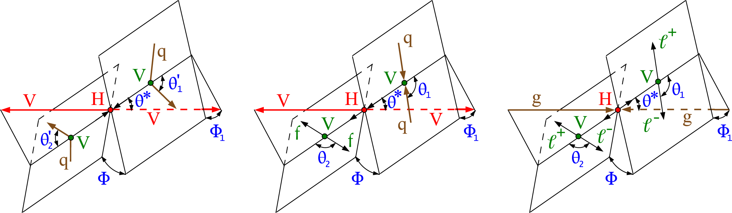
png pdf	Figure 1: Three topologies of the H boson production and decay: vector boson fusion ${{\mathrm {q}} {\mathrm {q}}} \to {\mathrm {V}} {\mathrm {V}} ({{\mathrm {q}} {\mathrm {q}}}) \to {\mathrm {H}} ({{\mathrm {q}} {\mathrm {q}}}) \to {\mathrm {V}} {\mathrm {V}} ({{\mathrm {q}} {\mathrm {q}}})$ (left); associated production ${{\mathrm {q}} {\mathrm {q}}} \to {\mathrm {V}} \to {\mathrm {V}} {\mathrm {H}} \to ({\mathrm {ff}}) {\mathrm {H}} \to ({\mathrm {ff}}) {\mathrm {V}} {\mathrm {V}}$ (middle); and gluon fusion ${\mathrm {g}} {\mathrm {g}} \to {\mathrm {H}} \to {\mathrm {V}} {\mathrm {V}} \to 4\ell$ (right) representing the topology without associated particles. The incoming particles are shown in brown, the intermediate vector bosons and their fermion daughters are shown in green, the H boson and its vector boson daughters are shown in red, and angles are shown in blue. In the first two cases the production and decay ${\mathrm {H}} \to {\mathrm {V}} {\mathrm {V}}$ is followed by the same four-lepton decay shown in the third case. The angles are defined in either the H or V boson rest frames [38,40].
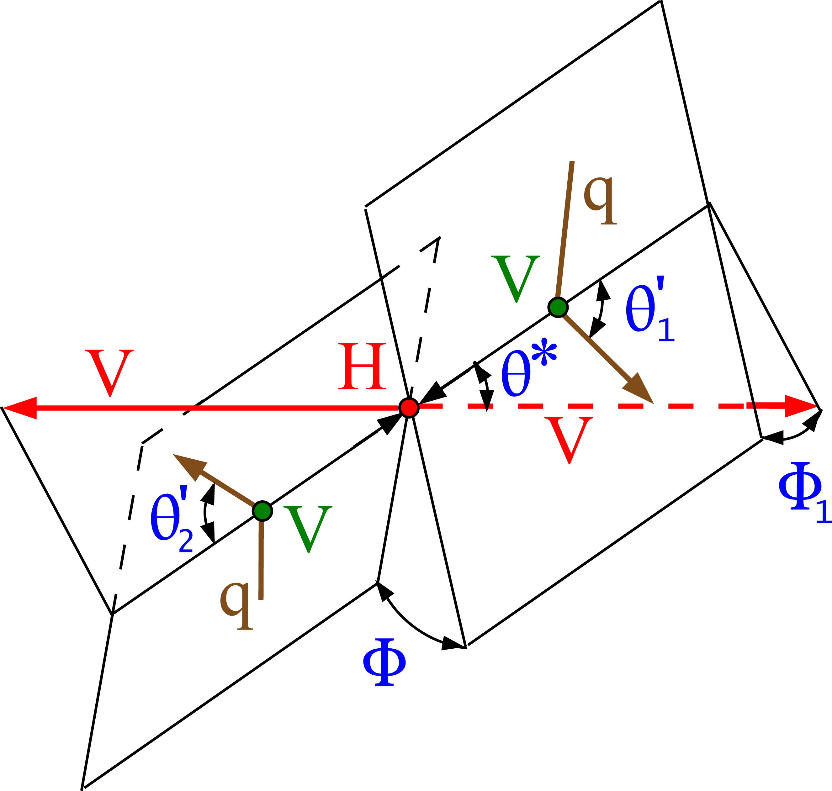
png pdf	Figure 1-a: Vector boson fusion ${{\mathrm {q}} {\mathrm {q}}} \to {\mathrm {V}} {\mathrm {V}} ({{\mathrm {q}} {\mathrm {q}}}) \to {\mathrm {H}} ({{\mathrm {q}} {\mathrm {q}}}) \to {\mathrm {V}} {\mathrm {V}} ({{\mathrm {q}} {\mathrm {q}}})$, representing one topology of H boson production and decay. The incoming particles are shown in brown, the intermediate vector bosons and their fermion daughters are shown in green, the H boson and its vector boson daughters are shown in red, and angles are shown in blue. The decay ${\mathrm {H}} \to {\mathrm {V}} {\mathrm {V}}$ is followed by the four-lepton decay. The angles are defined in either the H or V boson rest frames [38,40].
png pdf	Figure 1-b: Associated production ${{\mathrm {q}} {\mathrm {q}}} \to {\mathrm {V}} \to {\mathrm {V}} {\mathrm {H}} \to ({\mathrm {ff}}) {\mathrm {H}} \to ({\mathrm {ff}}) {\mathrm {V}} {\mathrm {V}}$, representing one topology of H boson production and decay. The incoming particles are shown in brown, the intermediate vector bosons and their fermion daughters are shown in green, the H boson and its vector boson daughters are shown in red, and angles are shown in blue. The decay ${\mathrm {H}} \to {\mathrm {V}} {\mathrm {V}}$ is followed by the four-lepton decay. The angles are defined in either the H or V boson rest frames [38,40].
png pdf	Figure 1-c: Gluon fusion ${\mathrm {g}} {\mathrm {g}} \to {\mathrm {H}} \to {\mathrm {V}} {\mathrm {V}} \to 4\ell$, representing one topology of the H boson production and decay, without associated particles. The incoming particles are shown in brown, the intermediate vector bosons and their fermion daughters are shown in green, the H boson and its vector boson daughters are shown in red, and angles are shown in blue. The production and decay ${\mathrm {H}} \to {\mathrm {V}} {\mathrm {V}}$ is followed by the four-lepton decay, as shown. The angles are defined in either the H or V boson rest frames [38,40].
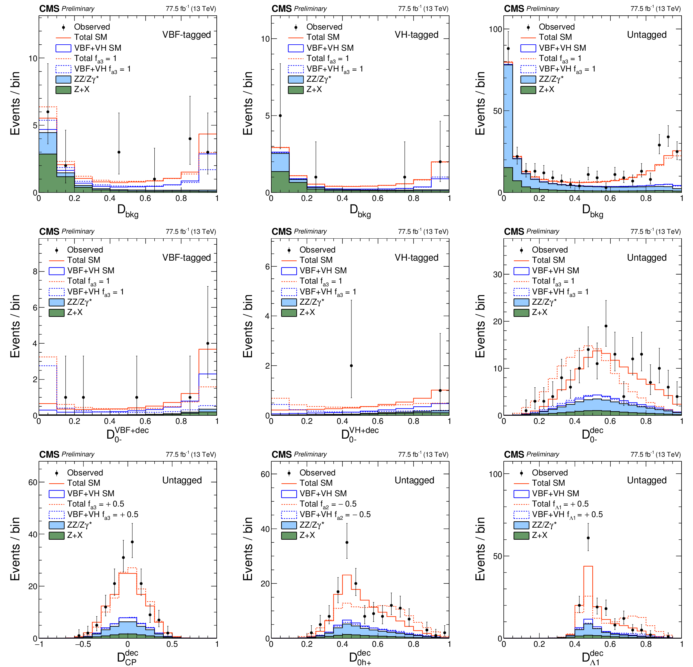
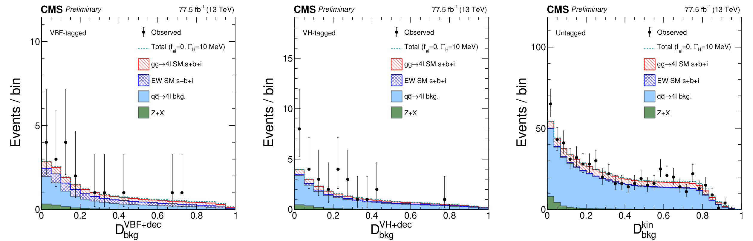
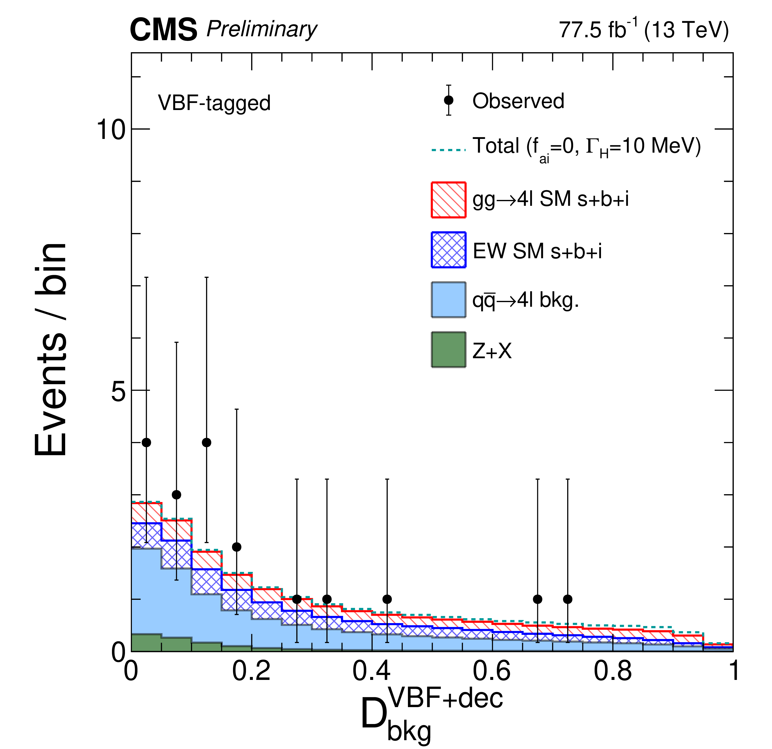
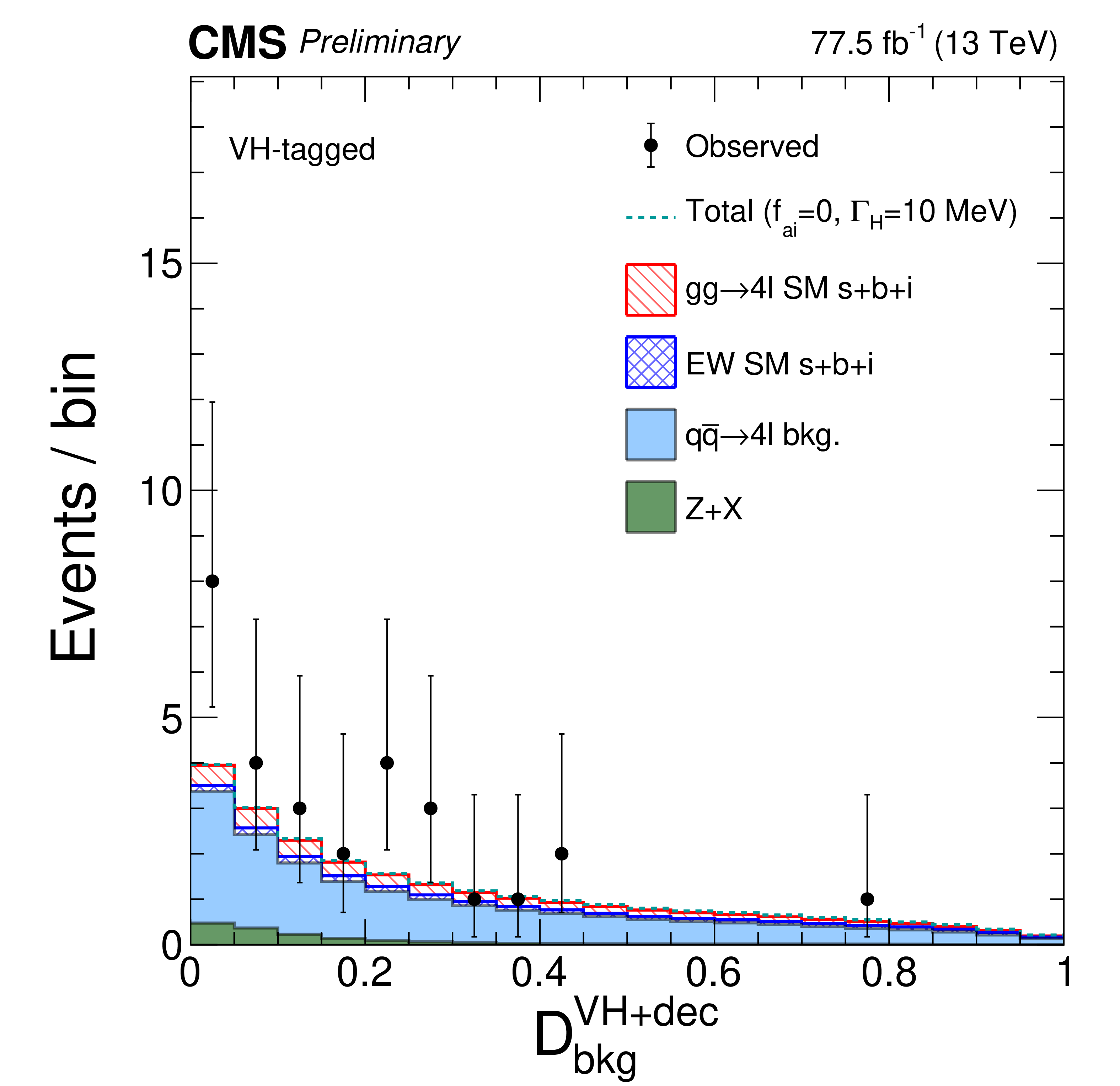
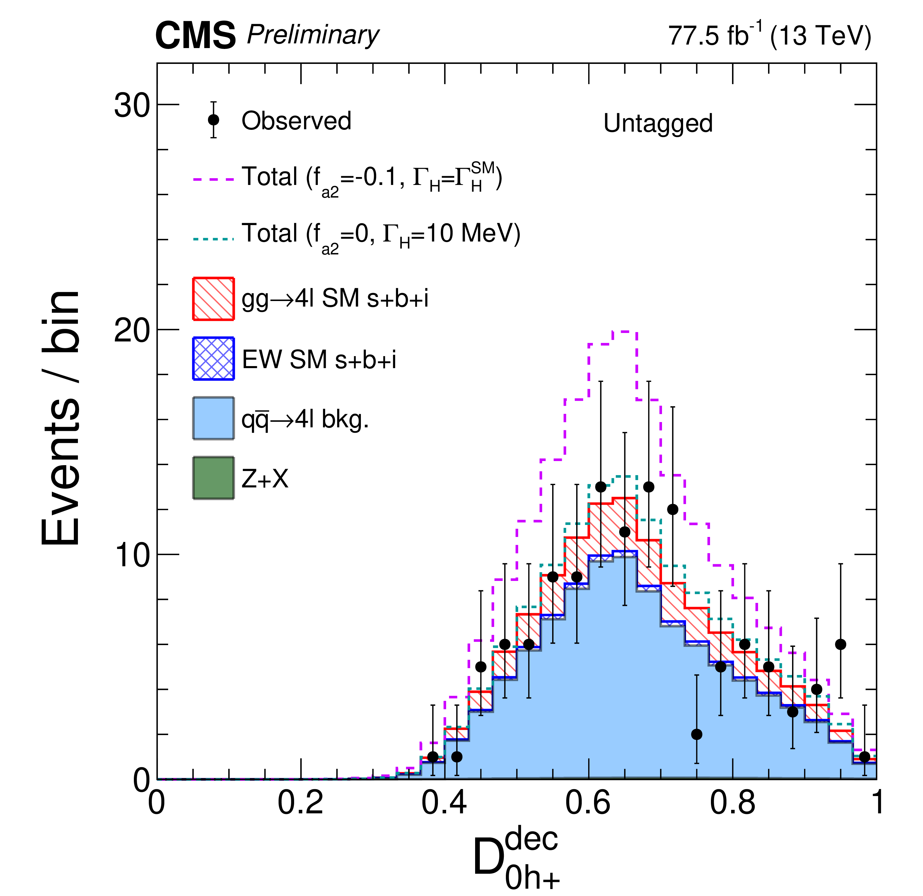
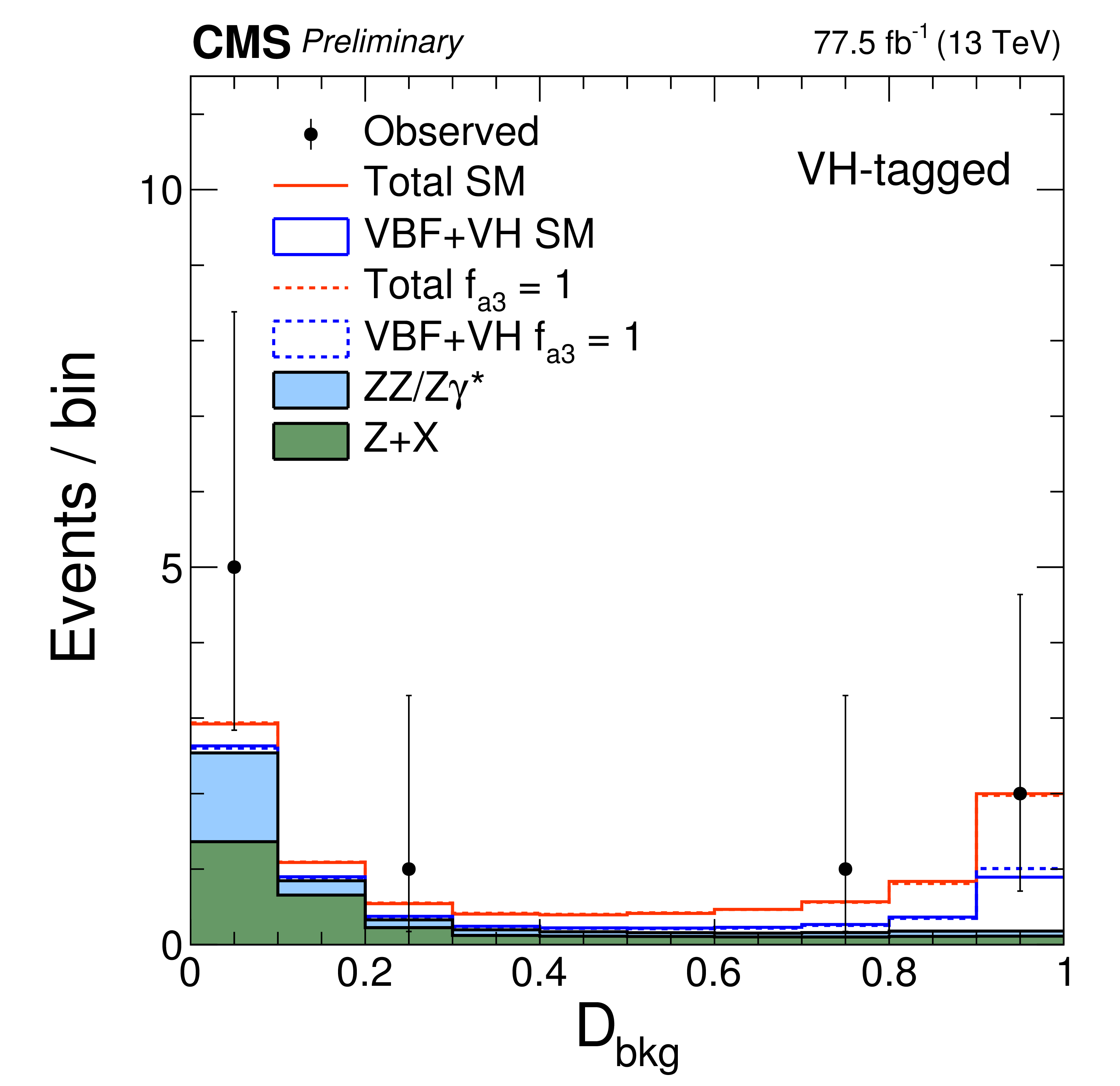
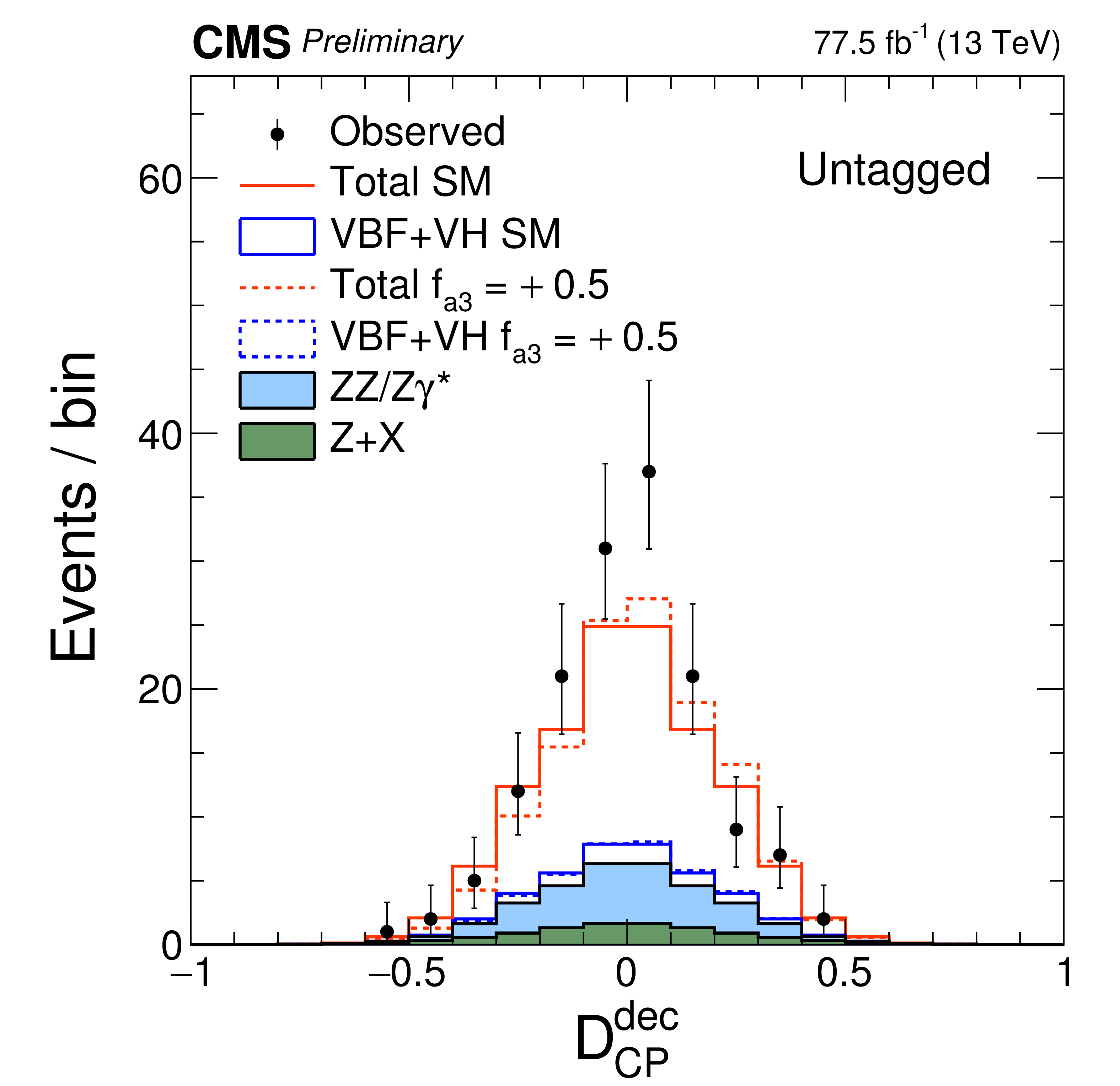
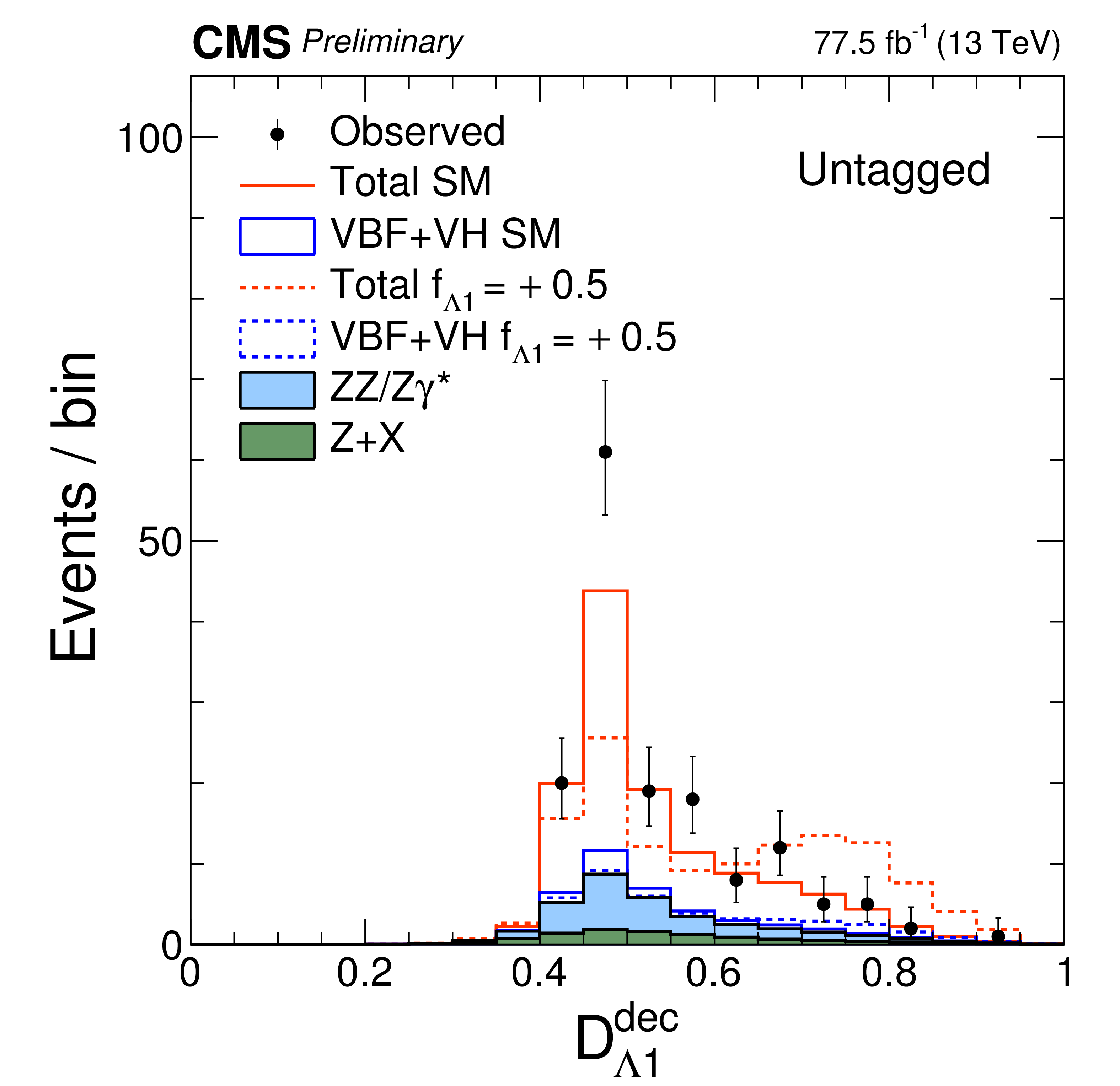
png pdf	Figure 2: The distributions of events in the on-shell region. The top row shows $\mathcal {D}_{\rm bkg}$ in the VBF-tagged (left), VH-tagged (middle), and untagged (right) categories of the ${a_{3}}$ analysis. The rest of the distributions are shown with the requirement $\mathcal {D}_{\rm bkg} >$ 0.5 in order to enhance signal over background contributions. The middle row shows $\mathcal {D}_{0-}$ in the corresponding three categories. The bottom row shows $\mathcal {D}_{CP}^{\rm dec}$ of the ${a_{3}}$, $\mathcal {D}_{0h+}^{\rm dec}$ of the ${a_{2}}$, and $\mathcal {D}_{\Lambda 1}^{\rm dec}$ of the ${\Lambda _{1}}$ analyses in the untagged categories.
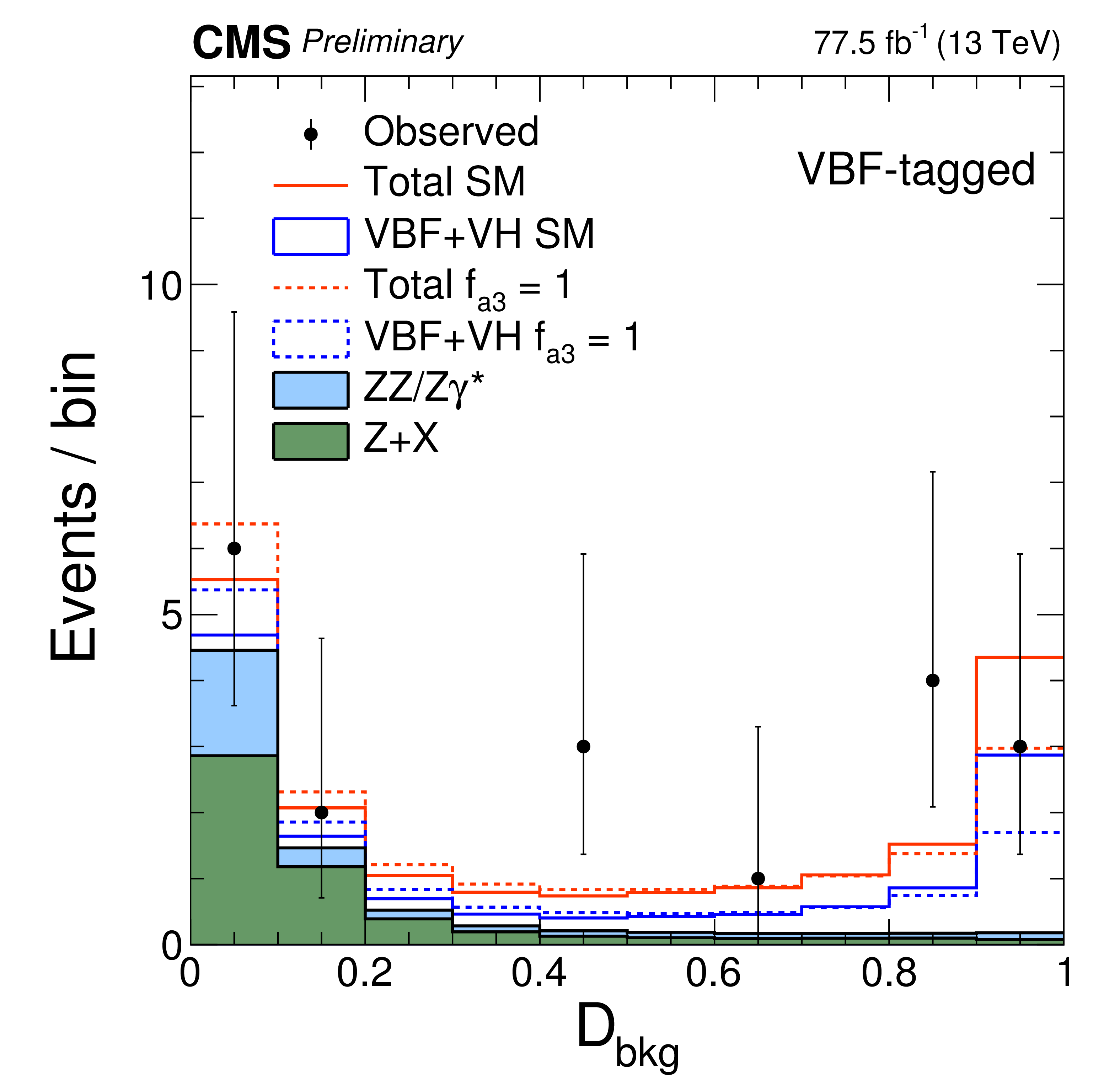
png pdf	Figure 2-a: Distribution of $\mathcal {D}_{\rm bkg}$ in the VBF-tagged category of the ${a_{3}}$ analysis for events events in the on-shell region.
png pdf	Figure 2-b: Distribution of $\mathcal {D}_{\rm bkg}$ in the VH-tagged category of the ${a_{3}}$ analysis for events events in the on-shell region.
png pdf	Figure 2-c: Distribution of $\mathcal {D}_{\rm bkg}$ in the untagged category of the ${a_{3}}$ analysis for events events in the on-shell region.
png pdf	Figure 2-d: Distribution of $\mathcal {D}_{0-}$ in the VBF-tagged category of the ${a_{3}}$ analysis for events events in the on-shell region. The distribution is shown with the requirement $\mathcal {D}_{\rm bkg} > 0.5$ in order to enhance signal over background contributions.
png pdf	Figure 2-e: Distribution of $\mathcal {D}_{0-}$ in the VH-tagged category of the ${a_{3}}$ analysis for events events in the on-shell region. The distribution is shown with the requirement $\mathcal {D}_{\rm bkg} > 0.5$ in order to enhance signal over background contributions.
png pdf	Figure 2-f: Distribution of $\mathcal {D}_{0-}$ in the untagged category of the ${a_{3}}$ analysis for events events in the on-shell region. The distribution is shown with the requirement $\mathcal {D}_{\rm bkg} > 0.5$ in order to enhance signal over background contributions.
png pdf	Figure 2-g: Distribution of $\mathcal {D}_{CP}^{\rm dec}$ of the ${a_{3}}$ analysis in the untagged category, for events events in the on-shell region. The distribution is shown with the requirement $\mathcal {D}_{\rm bkg} > 0.5$ in order to enhance signal over background contributions.
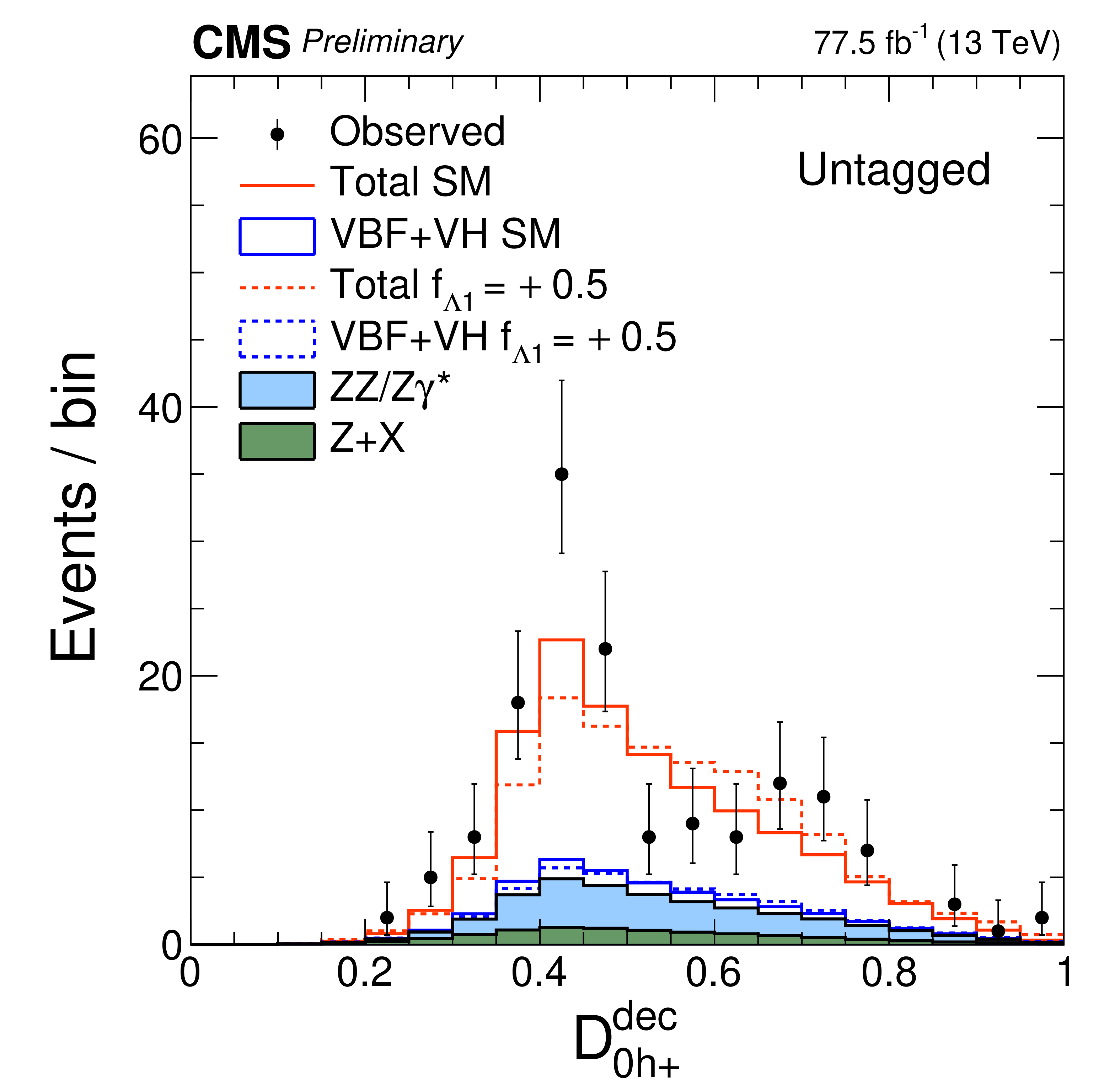
png pdf	Figure 2-h: Distribution of $\mathcal {D}_{0h+}^{\rm dec}$ of the ${a_{2}}$ analysis in the untagged category, for events events in the on-shell region. The distribution is shown with the requirement $\mathcal {D}_{\rm bkg} > 0.5$ in order to enhance signal over background contributions.
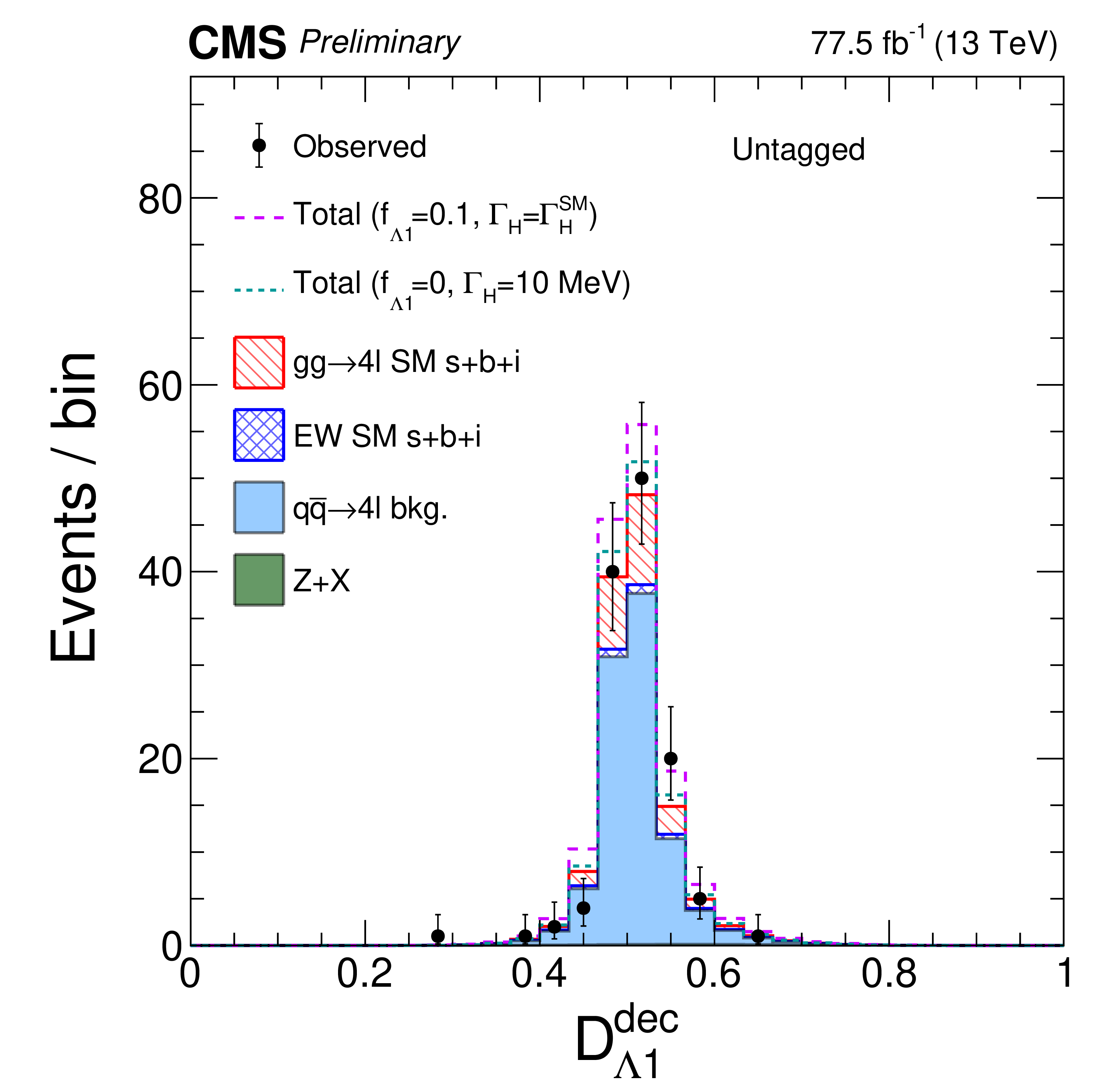
png pdf	Figure 2-i: Distribution of $\mathcal {D}_{\Lambda 1}^{\rm dec}$ of the ${\Lambda _{1}}$ analysis in the untagged category, for events events in the on-shell region. The distribution is shown with the requirement $\mathcal {D}_{\rm bkg} > 0.5$ in order to enhance signal over background contributions.
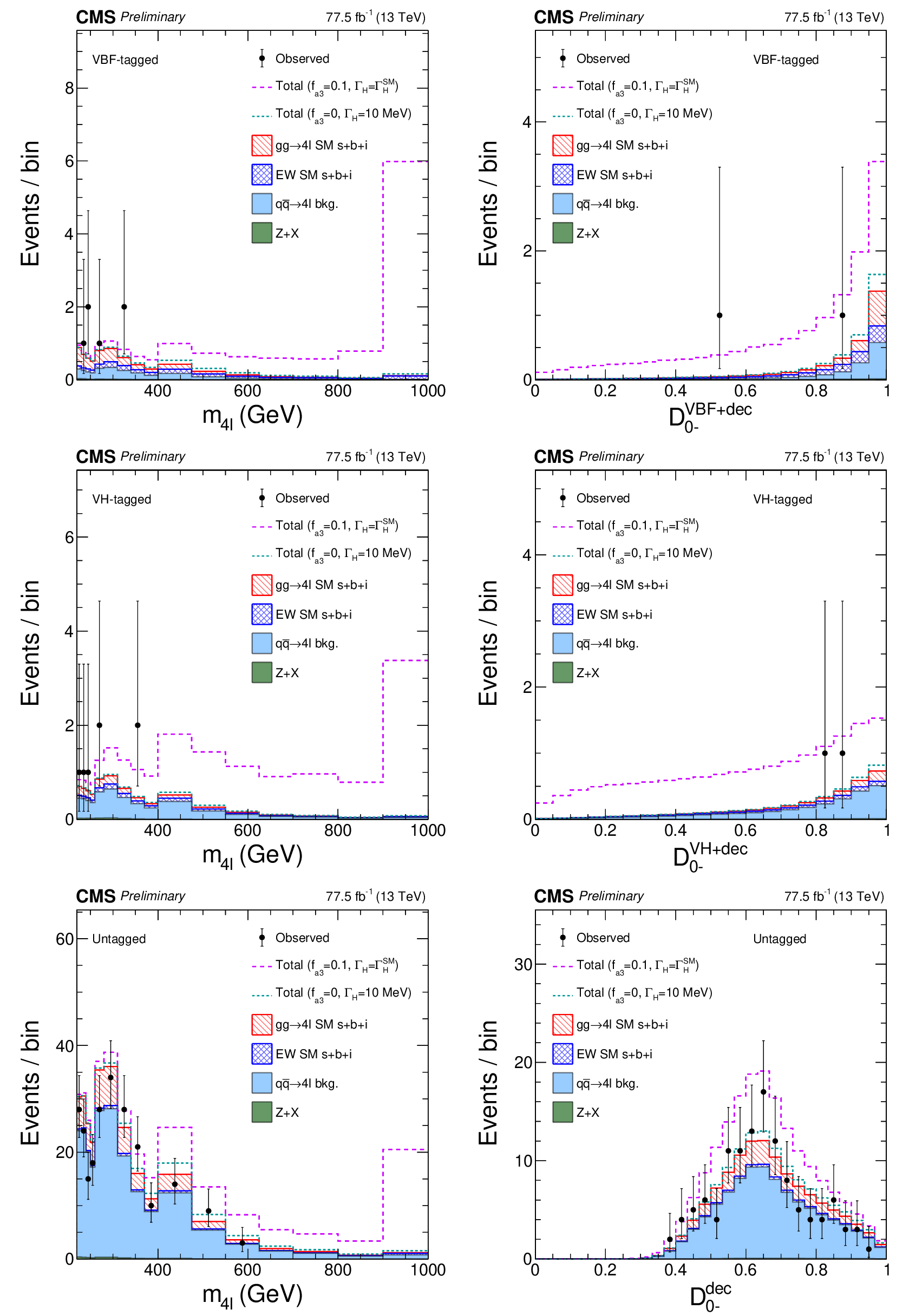
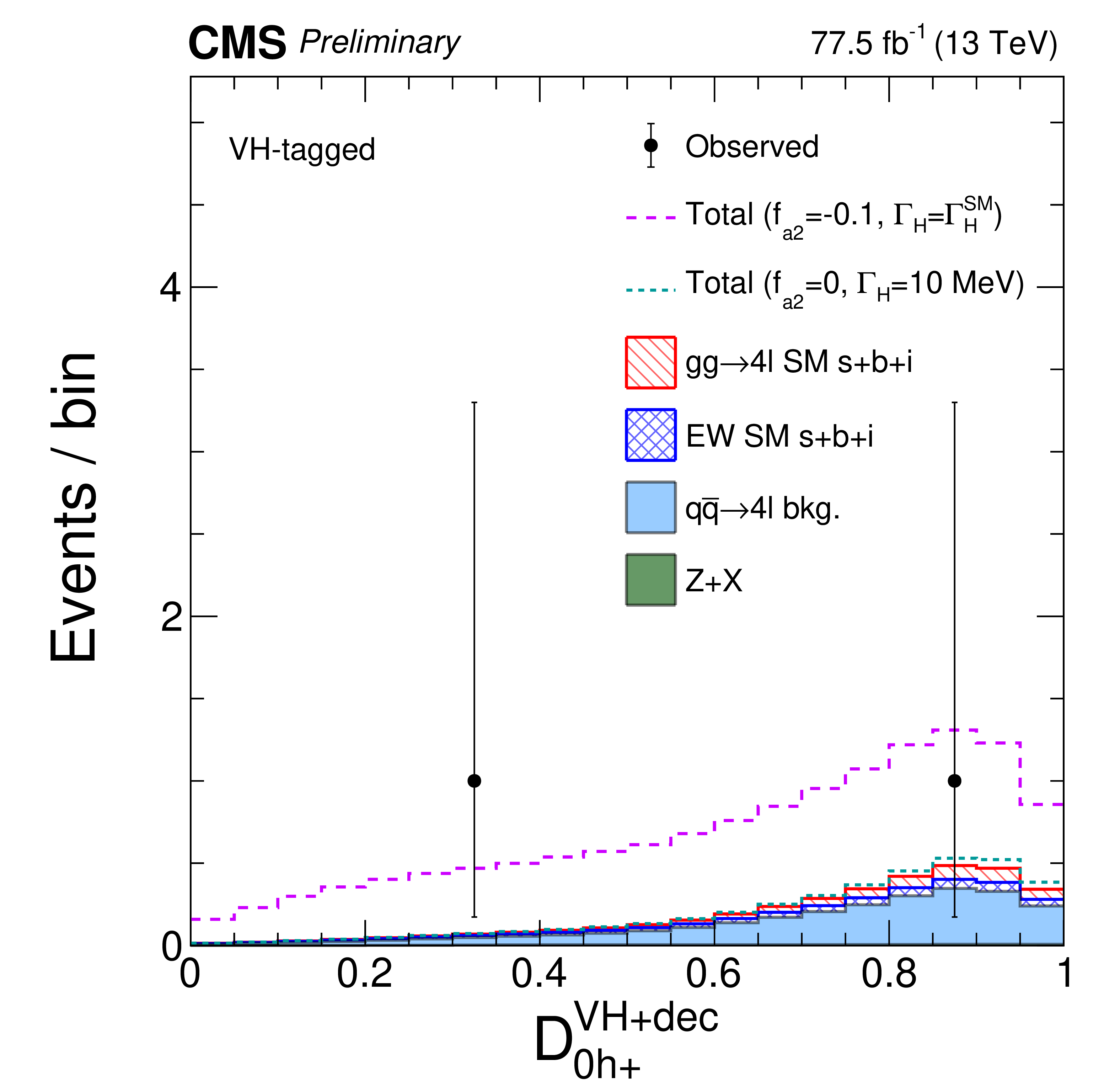
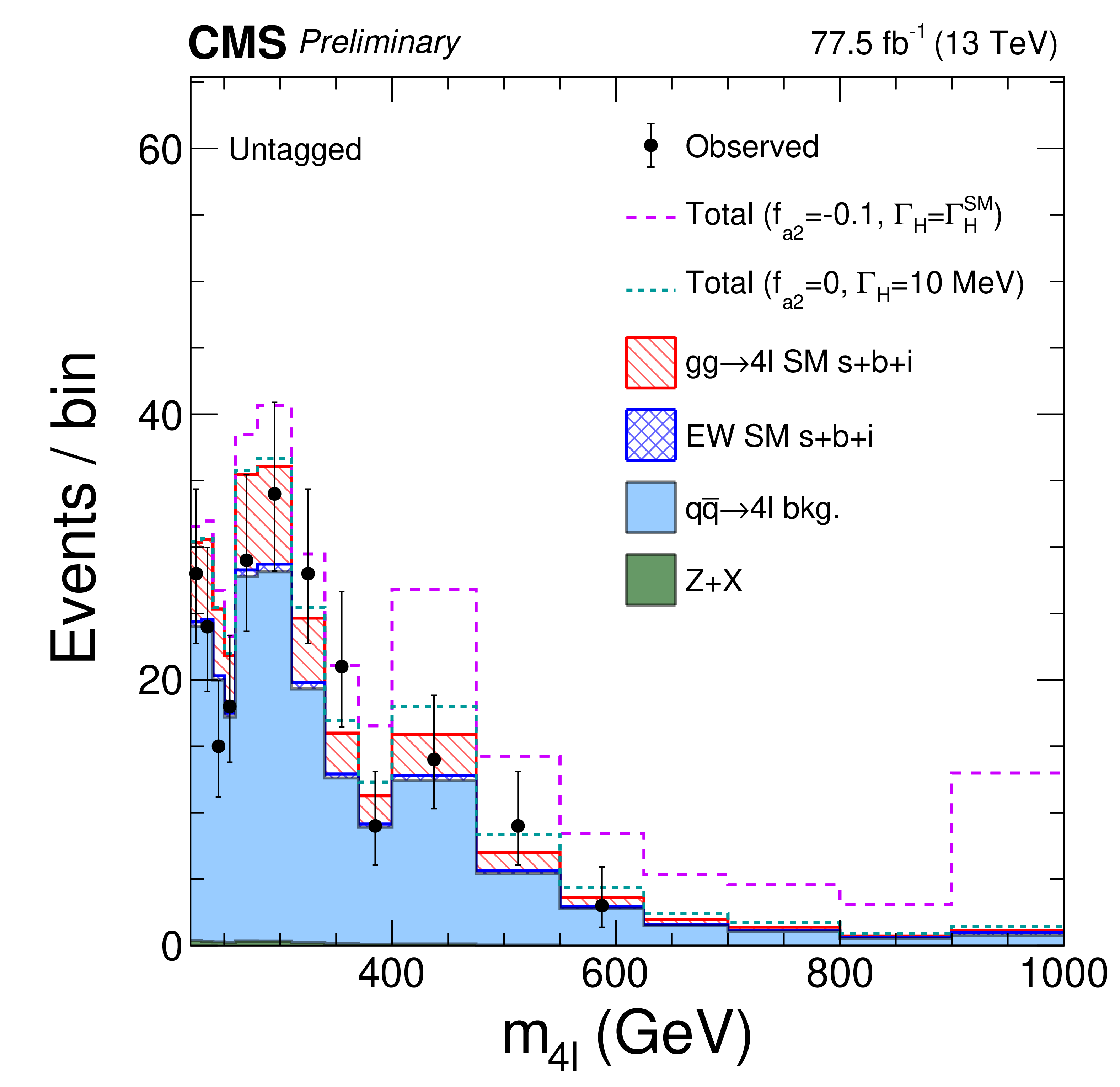
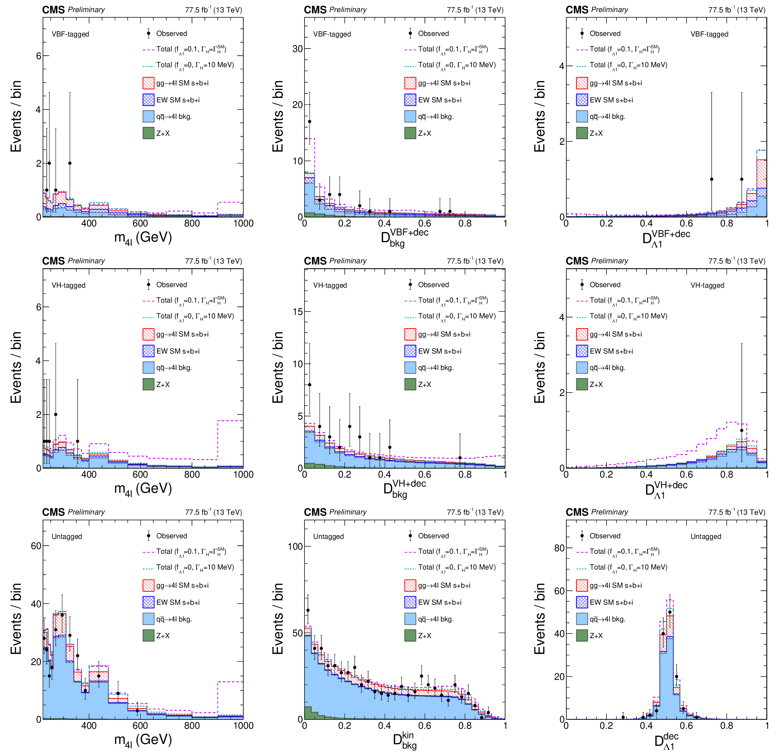
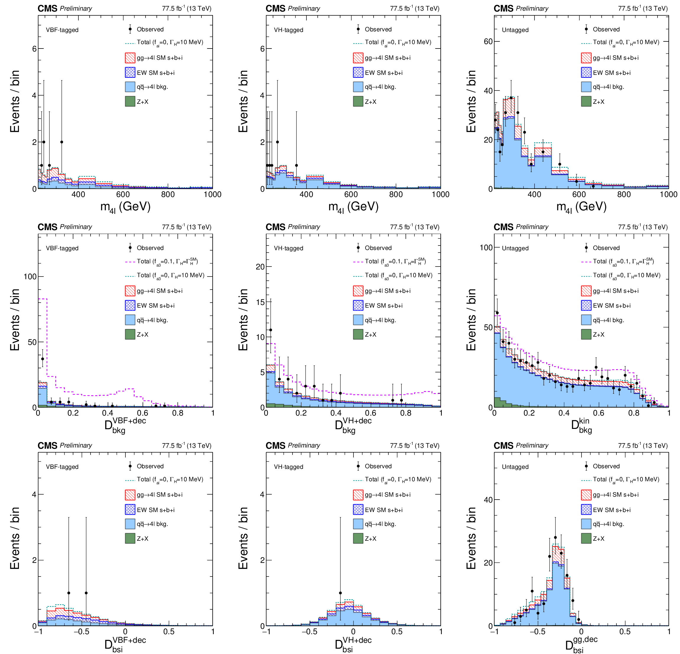
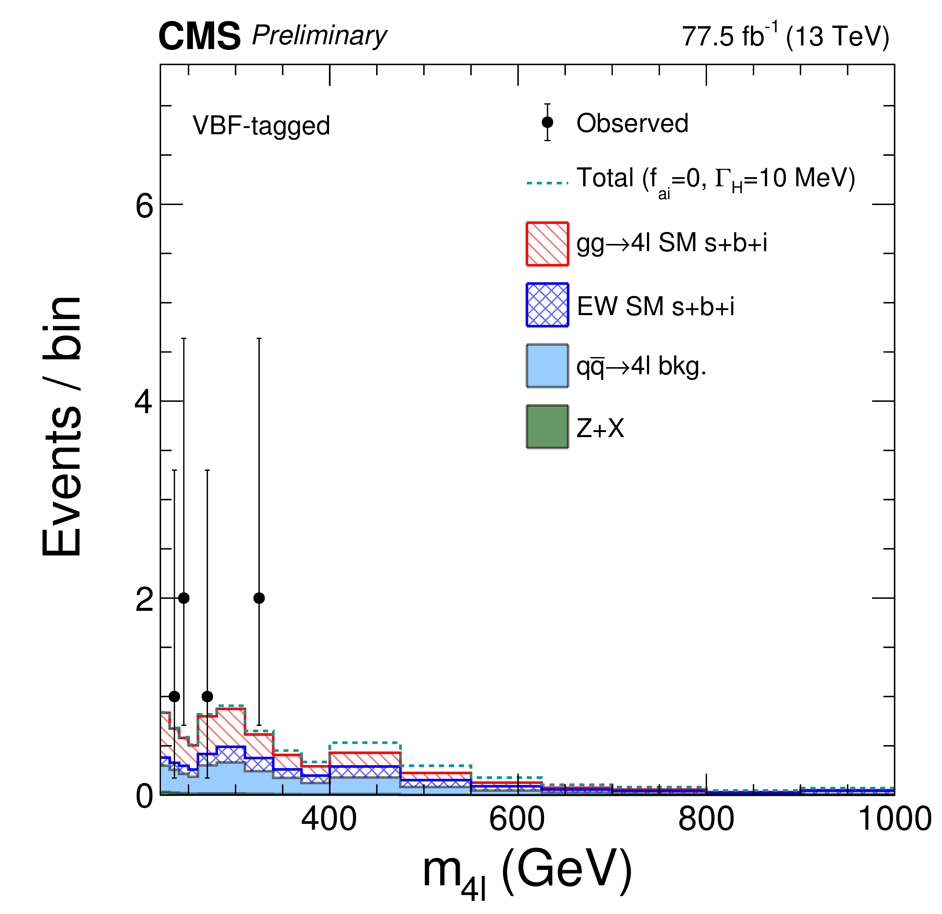
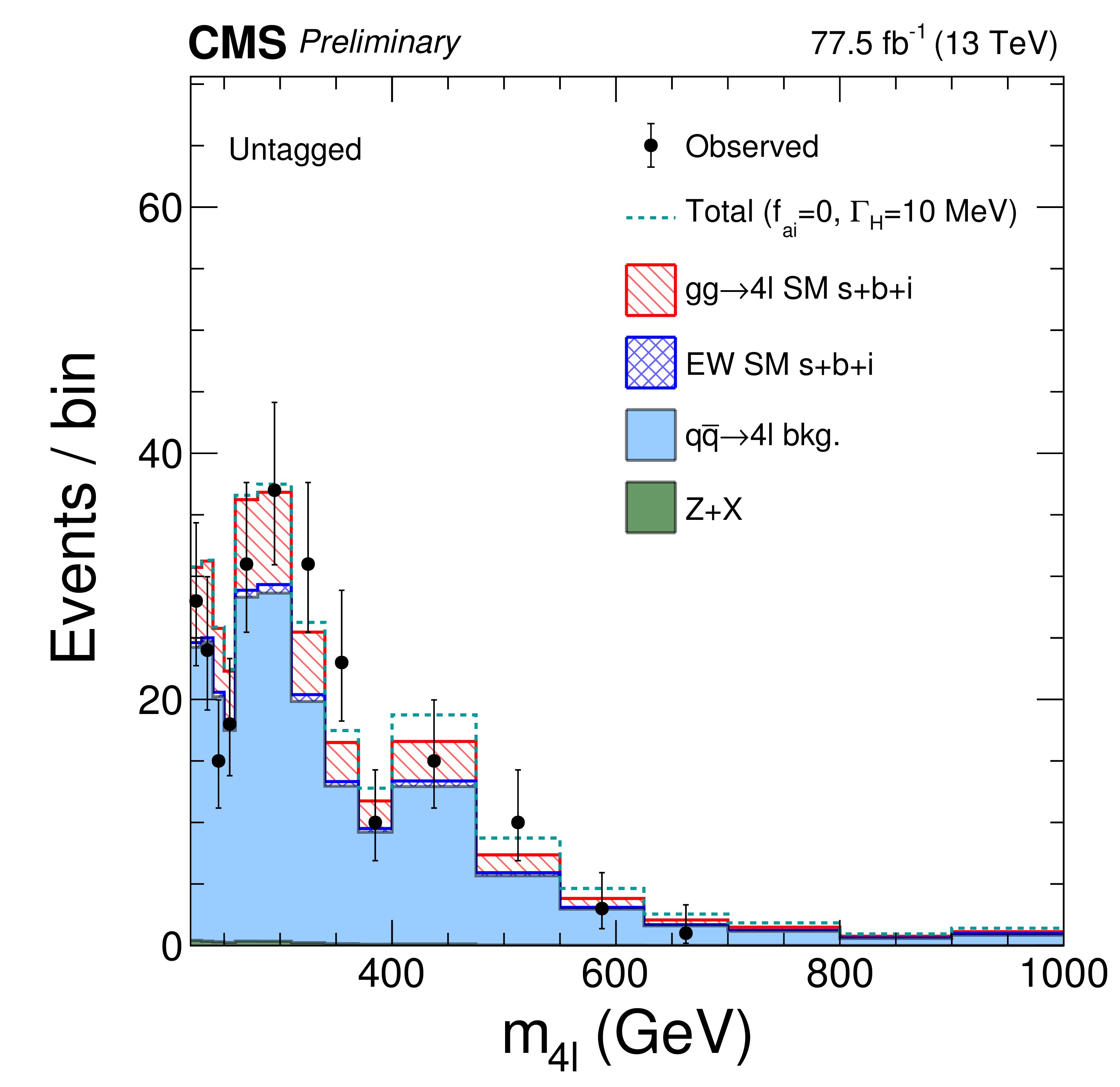
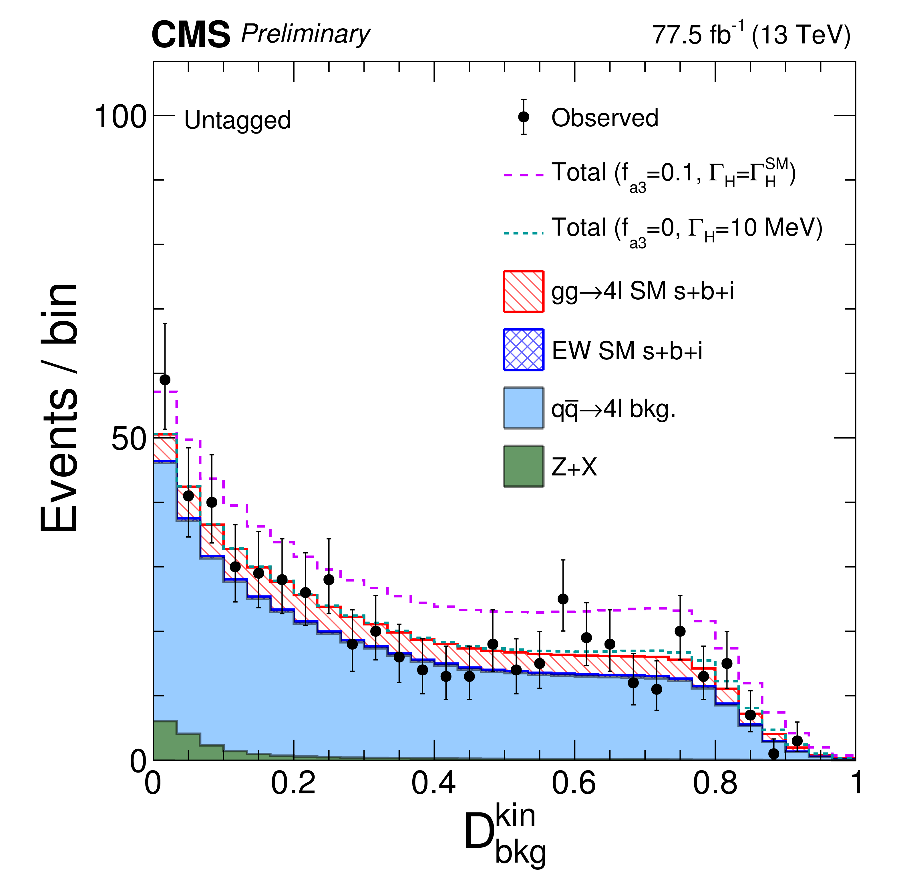
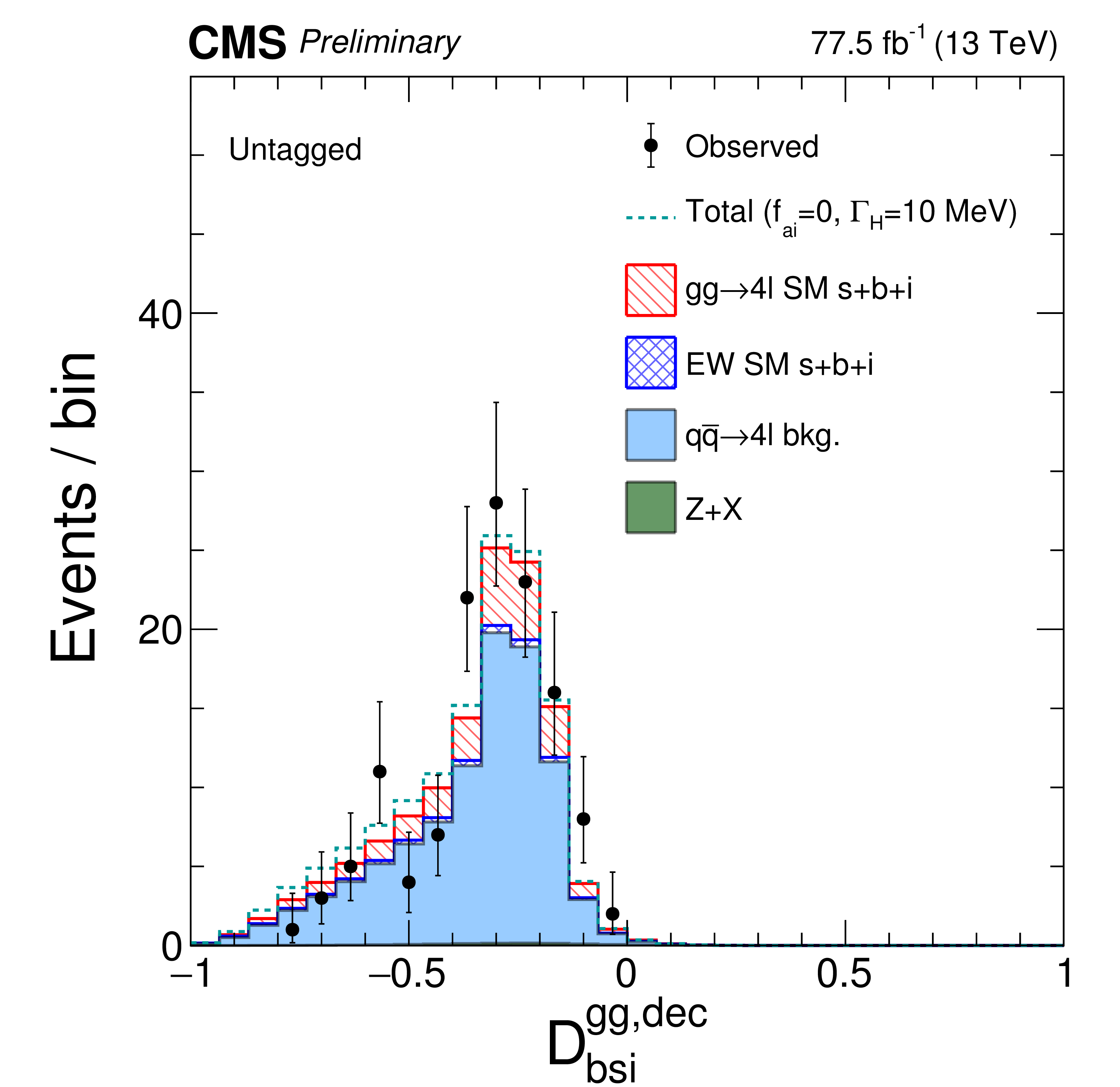
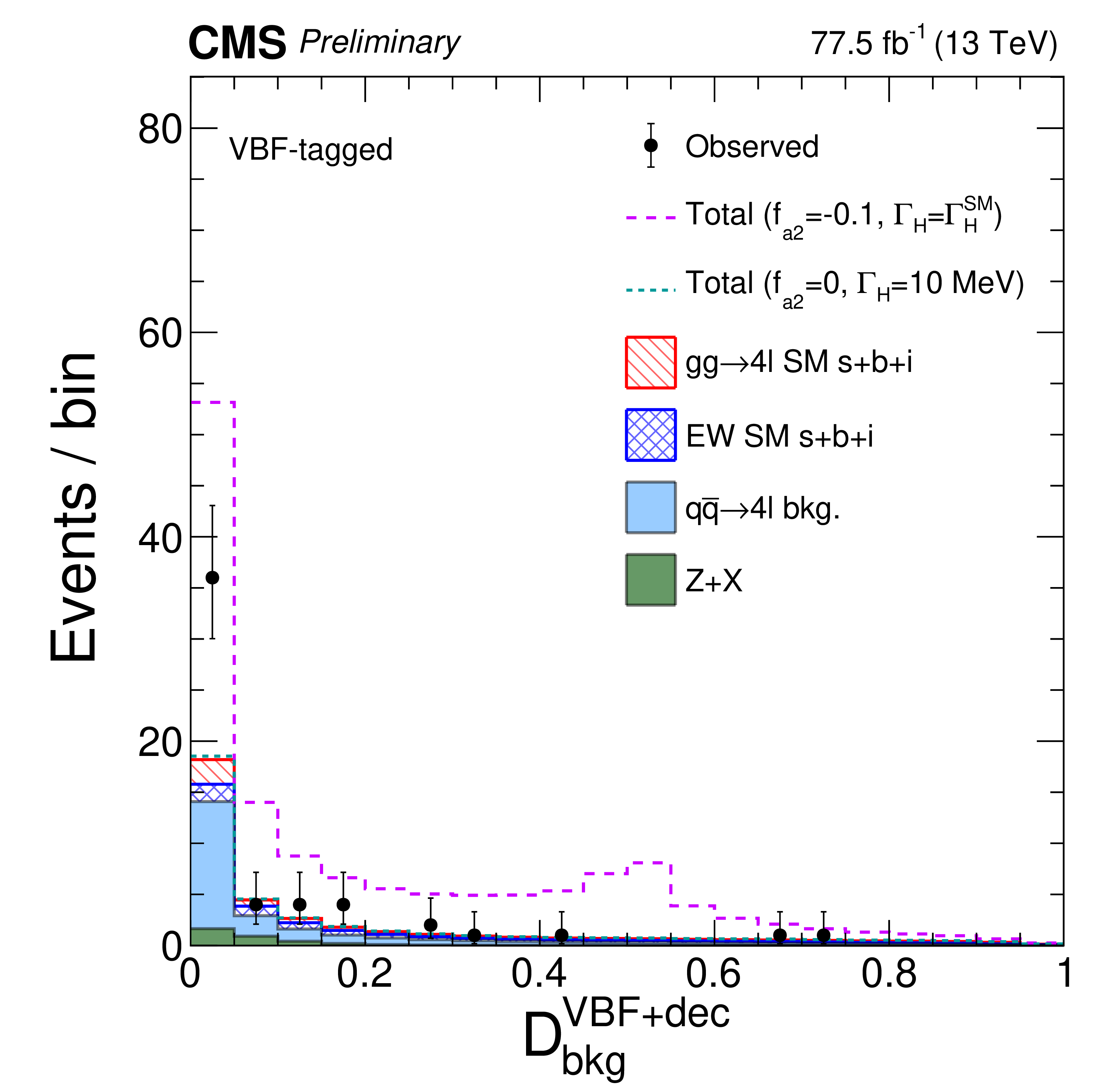
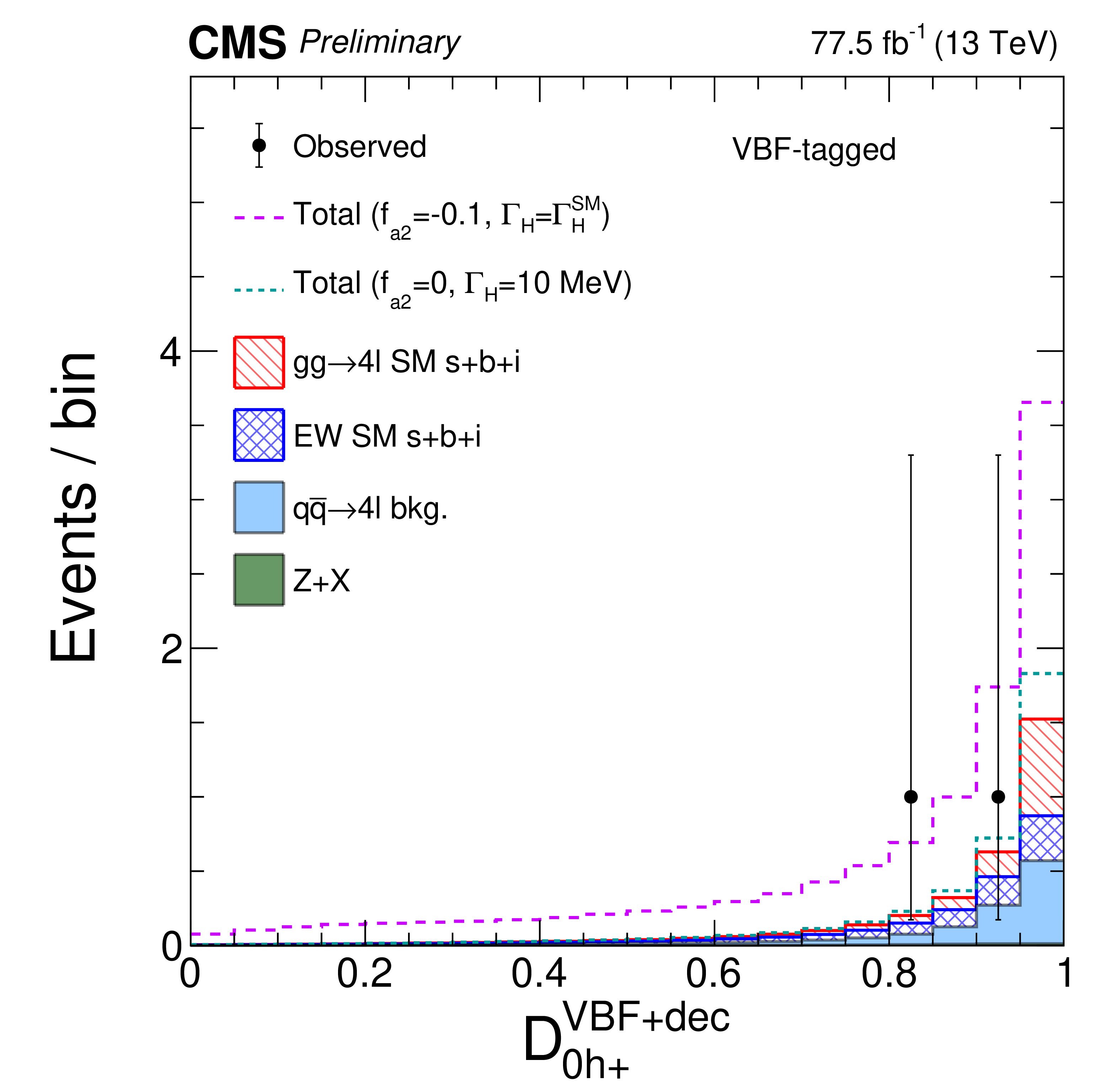
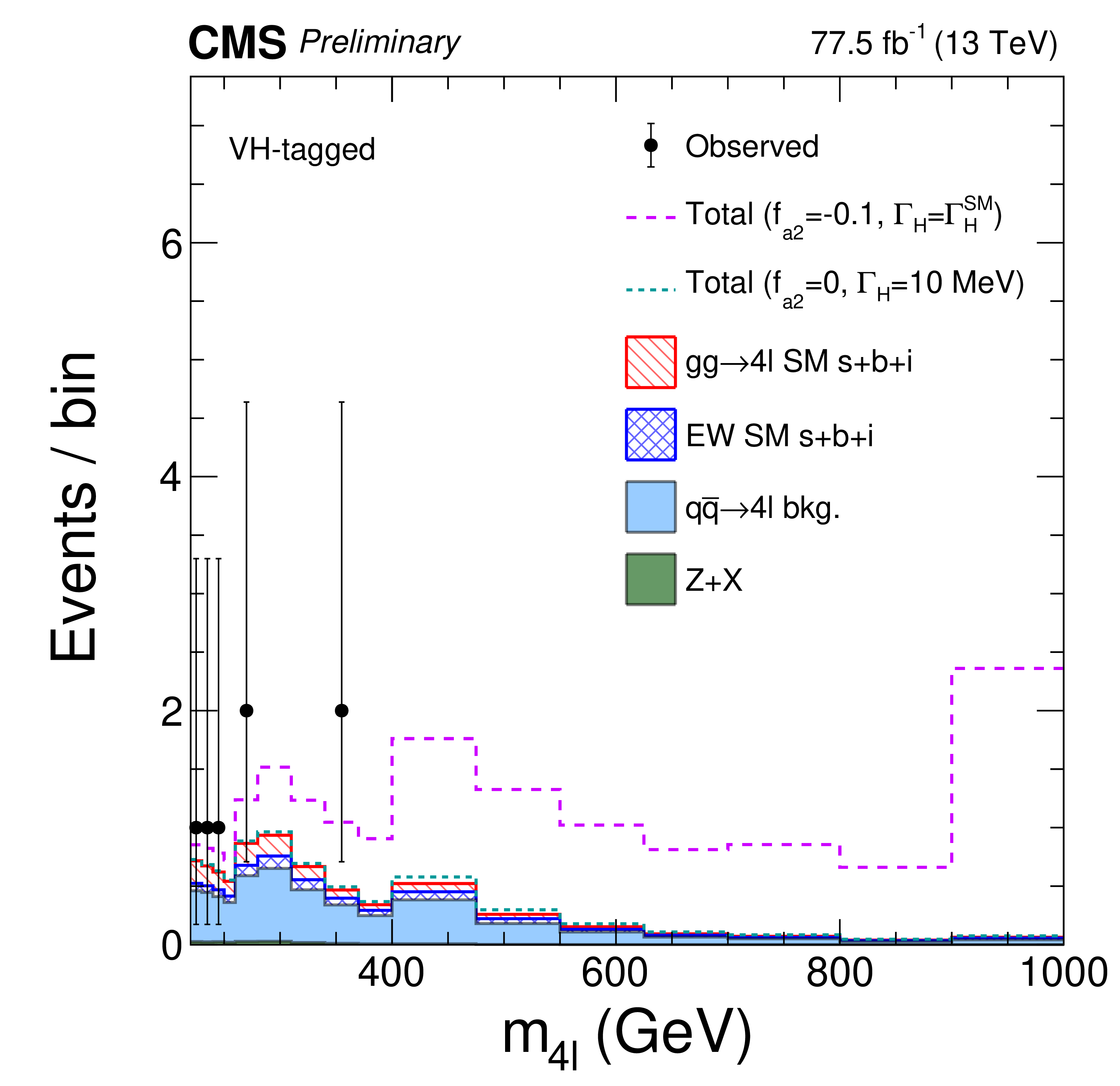
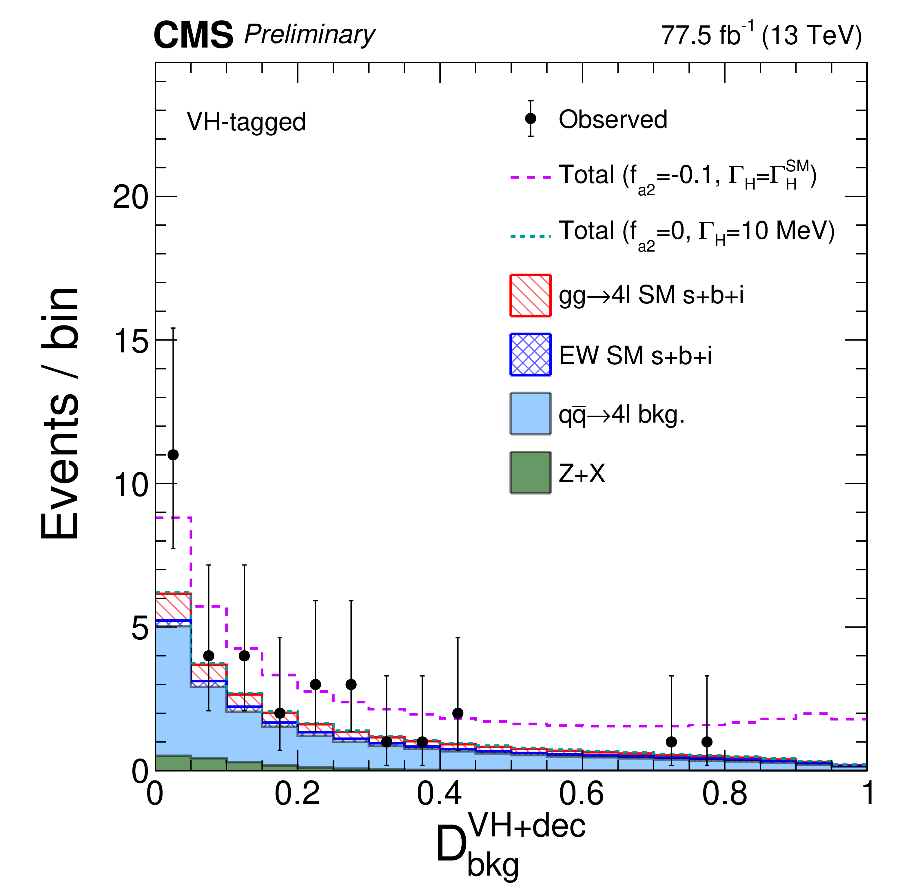
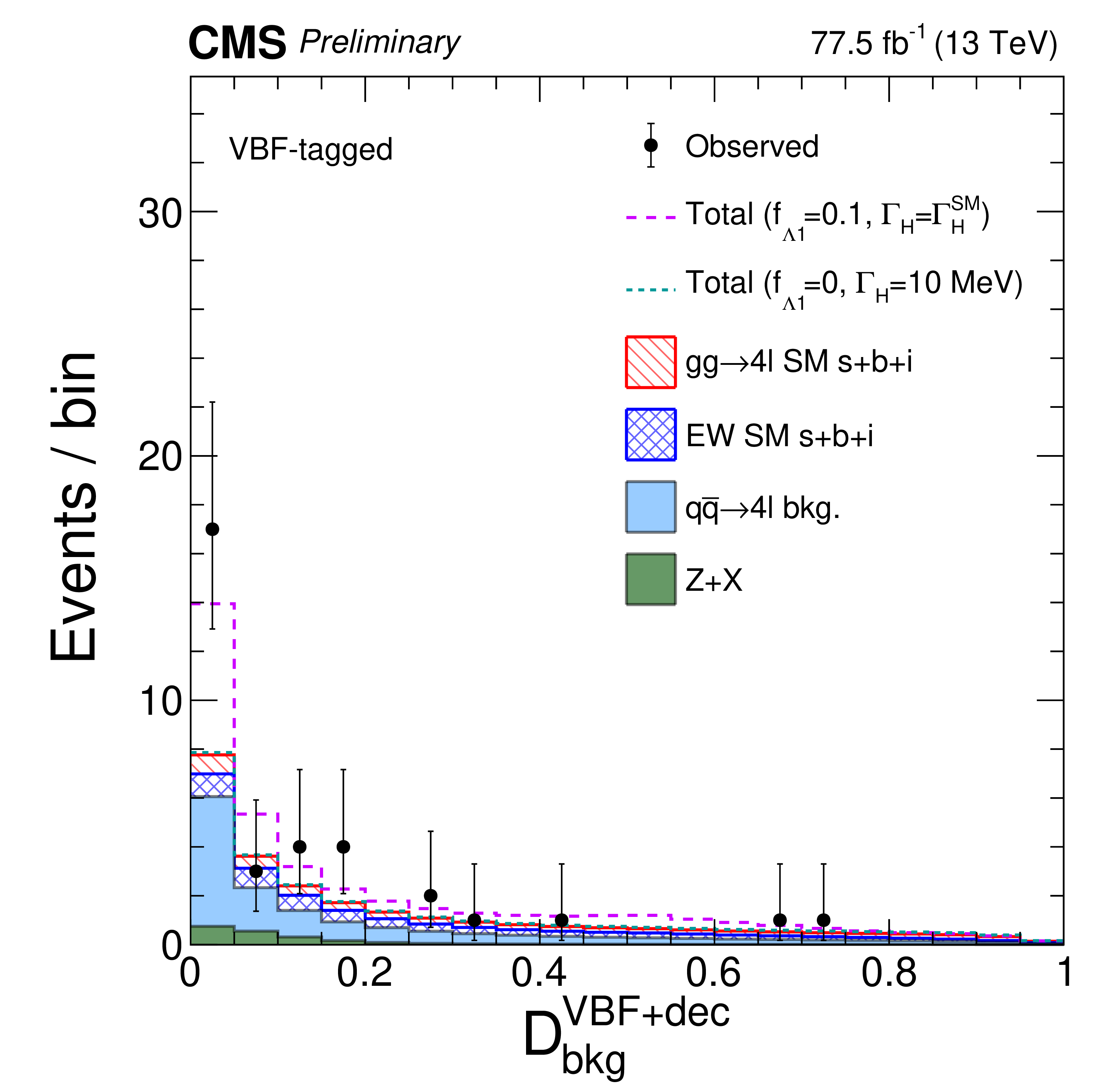
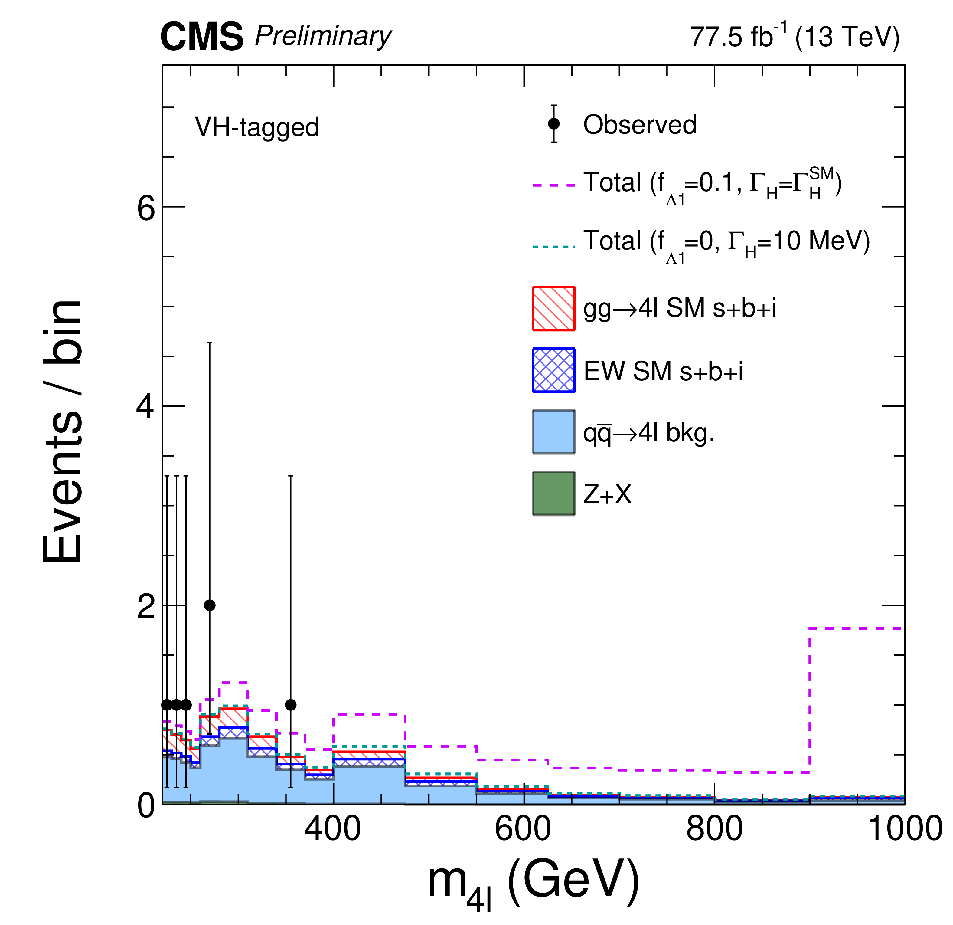
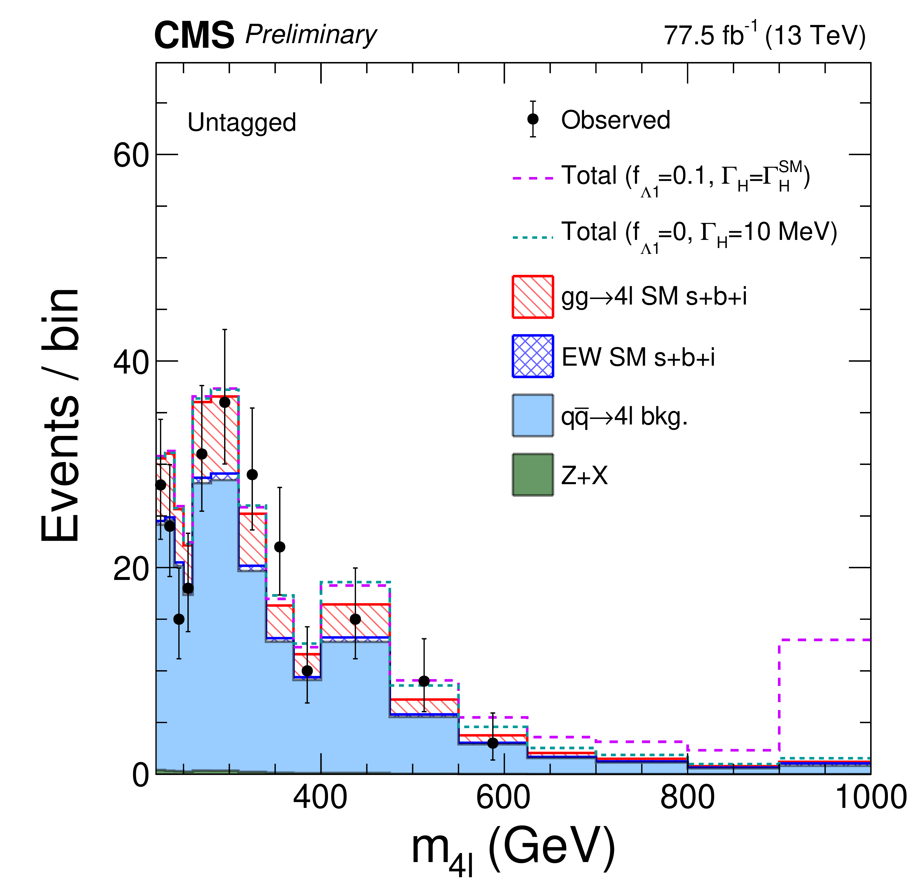
png pdf	Figure 3: The distributions of events in the off-shell region. The top row shows ${m_{4\ell}}$ in the VBF-tagged (left), VH-tagged (middle), and untagged (right) categories in the dedicated SM-like width analysis where a requirement on $\mathcal {D}^{{\rm VBF}+{\rm dec}}_{\rm bkg}$, $\mathcal {D}^{{\mathrm {V}} {\mathrm {H}} +{\rm dec}}_{\rm bkg}$, or $\mathcal {D}_{\rm bkg} >$ 0.6 is applied in order to enhance signal over background contributions. The middle row shows $\mathcal {D}^{{\rm VBF}+{\rm dec}}_{\rm bkg}$ (left), $\mathcal {D}^{{\mathrm {V}} {\mathrm {H}} +{\rm dec}}_{\rm bkg}$ (middle), $\mathcal {D}^{\rm kin}_{\rm bkg}$ (right) of the ${a_{3}}$ analysis in the corresponding three categories. The requirement ${m_{4\ell}} >$ 340 GeV is applied in order to enhance signal over background contributions. The bottom row shows $\mathcal {D}_{\rm bsi}$ in the corresponding three categories in the dedicated SM-like width analysis with both of the above requirements enhancing the signal contribution.
png pdf	Figure 3-a: The distribution of ${m_{4\ell}}$ for events in the off-shell region in the VBF-tagged category. The distribution is obtained in the dedicated SM-like width analysis where a requirement on $\mathcal {D}^{{\rm VBF}+{\rm dec}}_{\rm bkg} >$ 0.6 is applied in order to enhance signal over background contributions.
png pdf	Figure 3-b: The distribution of ${m_{4\ell}}$ for events in the off-shell region in the VH-tagged category. The distribution is obtained in the dedicated SM-like width analysis where a requirement on $\mathcal {D}^{{\mathrm {V}} {\mathrm {H}} +{\rm dec}}_{\rm bkg} >$ 0.6 is applied in order to enhance signal over background contributions.
png pdf	Figure 3-c: The distribution of ${m_{4\ell}}$ for events in the off-shell region in the untagged category. The distribution is obtained in the dedicated SM-like width analysis where a requirement on $\mathcal {D}_{\rm bkg} >$ 0.6 is applied in order to enhance signal over background contributions.
png pdf	Figure 3-d: The distribution of $\mathcal {D}^{{\rm VBF}+{\rm dec}}_{\rm bkg}$ of the ${a_{3}}$ analysis, for events in the off-shell region in the VBF-tagged category. The requirement ${m_{4\ell}} >$ 340 GeV is applied in order to enhance signal over background contributions.
png pdf	Figure 3-e: The distribution of $\mathcal {D}^{{\mathrm {V}} {\mathrm {H}} +{\rm dec}}_{\rm bkg}$ of the ${a_{3}}$ analysis, for events in the off-shell region in the VH-tagged category. The requirement ${m_{4\ell}} >$ 340 GeV is applied in order to enhance signal over background contributions.
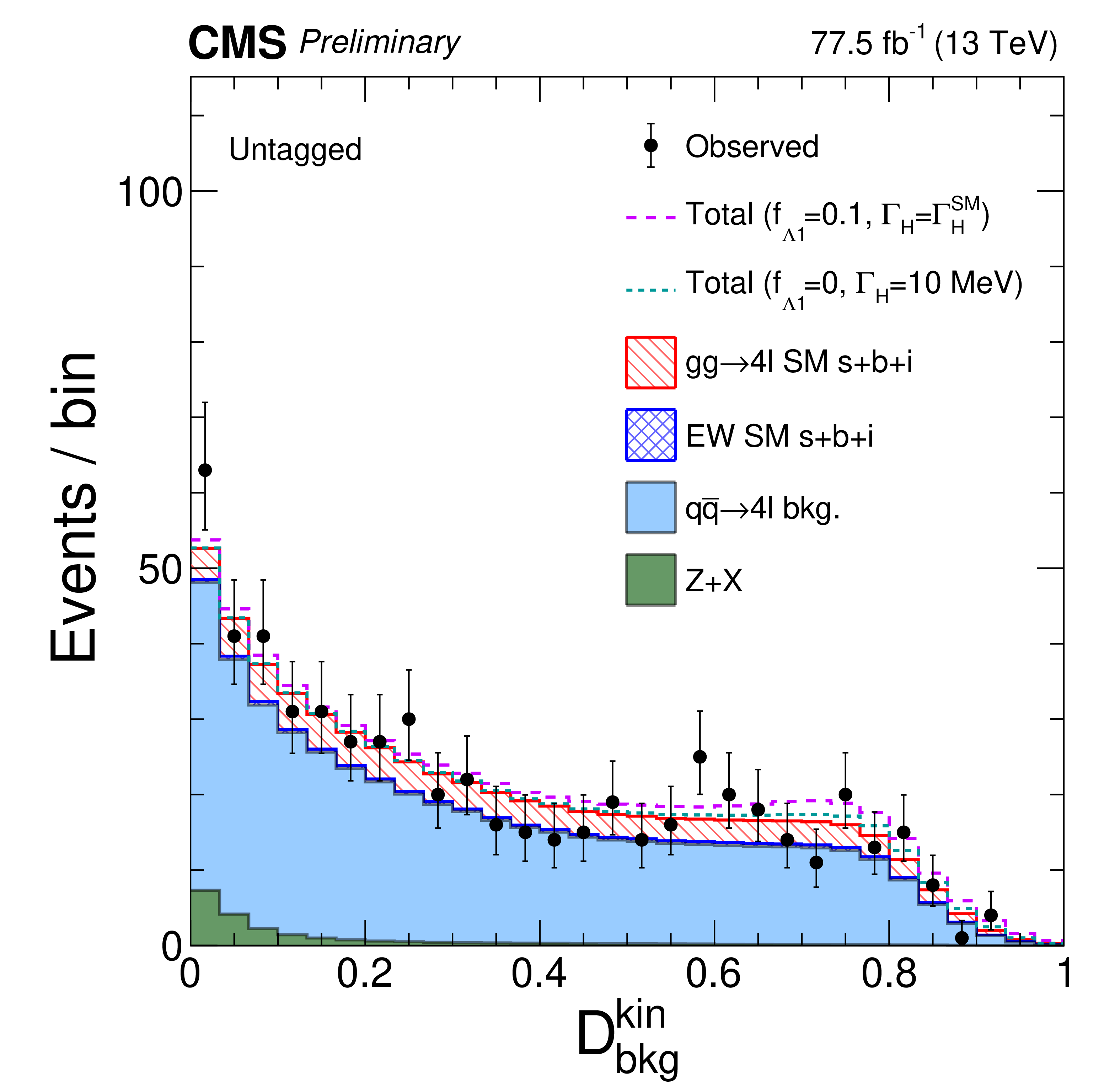
png pdf	Figure 3-f: The distribution of $\mathcal {D}^{\rm kin}_{\rm bkg}$ of the ${a_{3}}$ analysis, for events in the off-shell region in the untagged category. The requirement ${m_{4\ell}} >$ 340 GeV is applied in order to enhance signal over background contributions.
png pdf	Figure 3-g: The distribution of $\mathcal {D}_{\rm bsi}$ for events in the off-shell region in the VBF-tagged category. The distribution is obtained in the dedicated SM-like width analysis where a requirement on $\mathcal {D}^{{\rm VBF}+{\rm dec}}_{\rm bkg} >$ 0.6, and the requirement ${m_{4\ell}} >$ 340 GeV, are applied in order to enhance signal over background contributions.
png pdf	Figure 3-h: The distribution of $\mathcal {D}_{\rm bsi}$ for events in the off-shell region in the VH-tagged category. The distribution is obtained in the dedicated SM-like width analysis where a requirement on $\mathcal {D}^{{\mathrm {V}} {\mathrm {H}} +{\rm dec}}_{\rm bkg} >$ 0.6, and the requirement ${m_{4\ell}} >$ 340 GeV, are applied in order to enhance signal over background contributions.
png pdf	Figure 3-i: The distribution of $\mathcal {D}_{\rm bsi}$ for events in the off-shell region in the untagged category. The distribution is obtained in the dedicated SM-like width analysis where a requirement on $\mathcal {D}_{\rm bkg} >$ 0.6, and the requirement ${m_{4\ell}} >$ 340 GeV, are applied in order to enhance signal over background contributions.
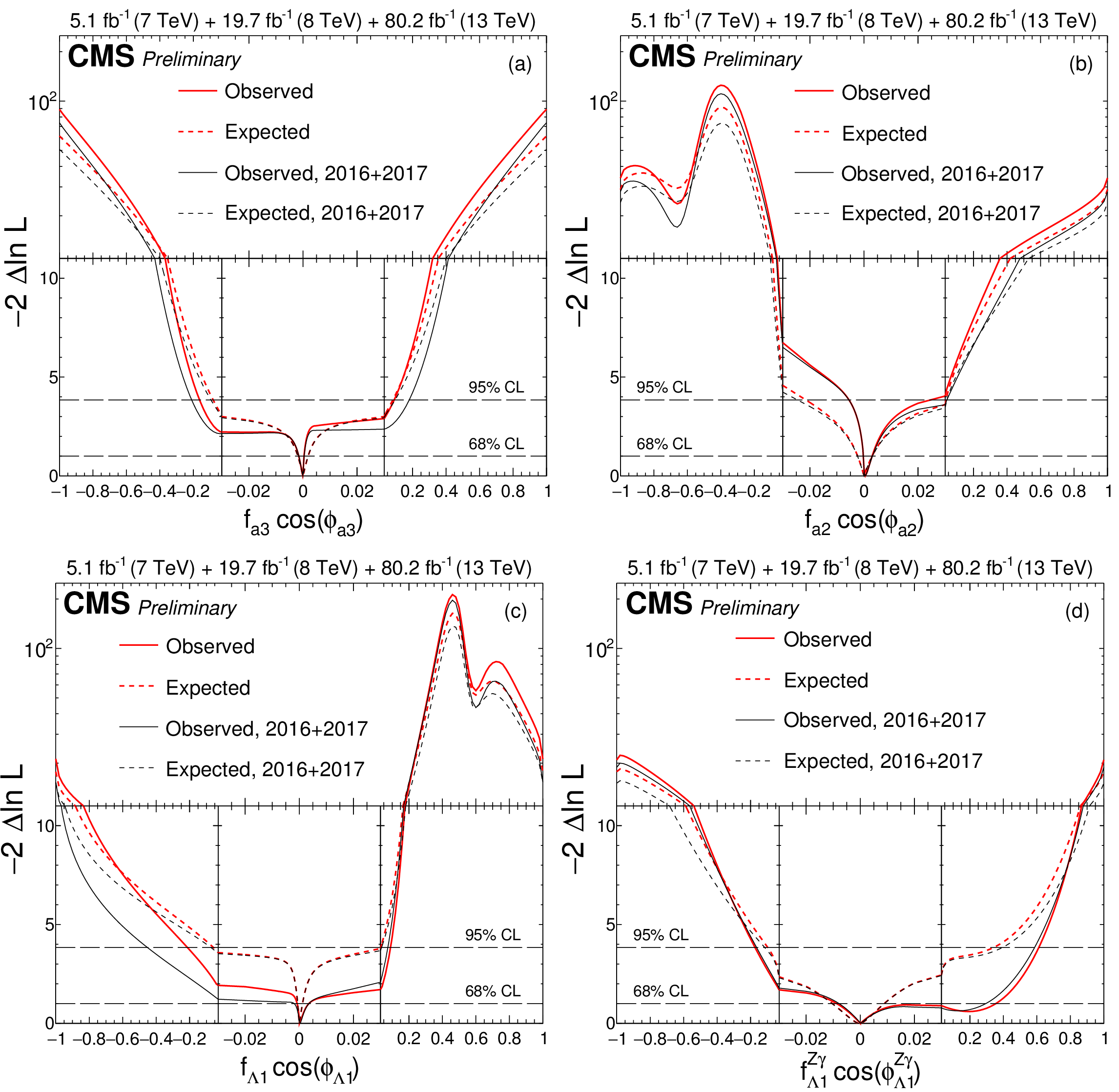
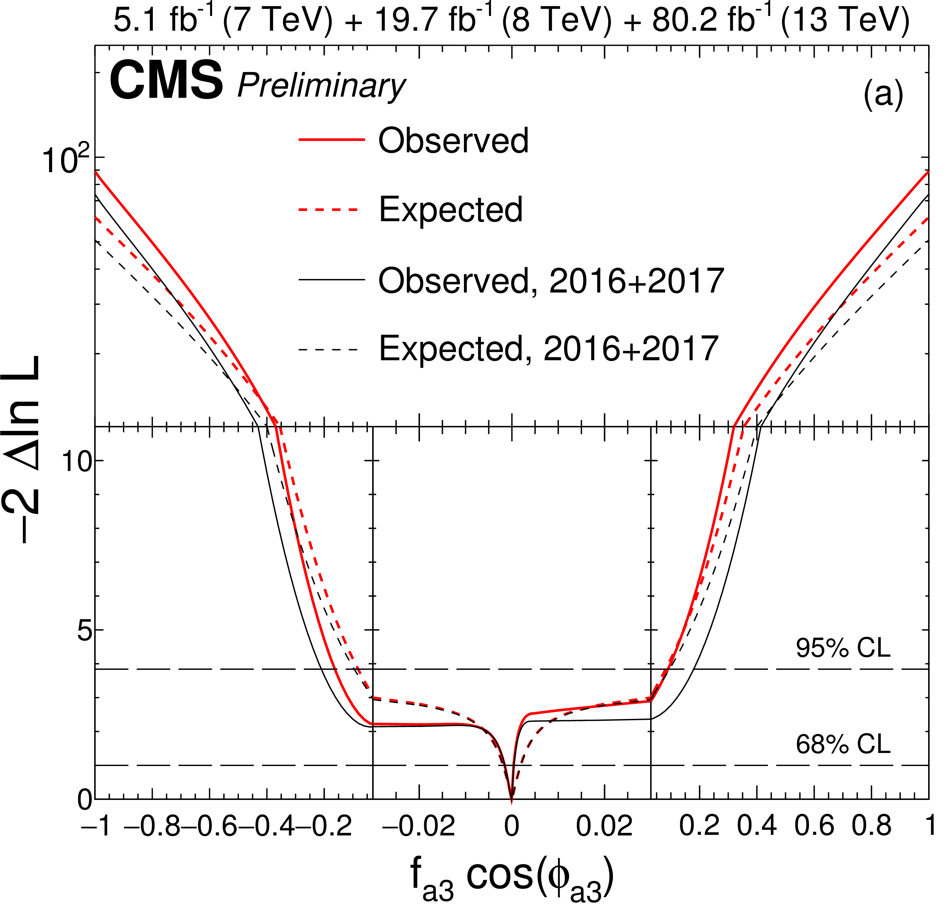
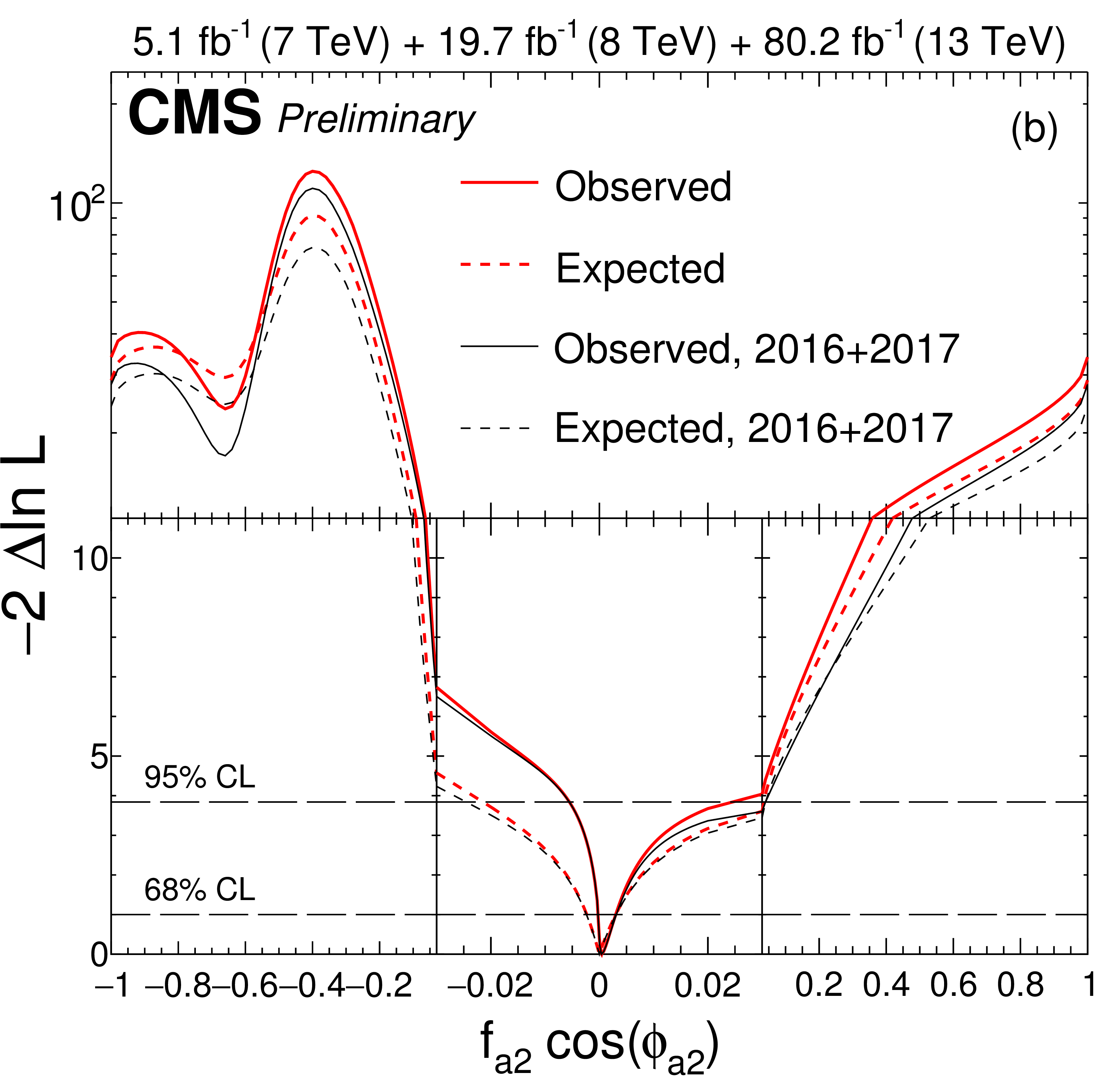
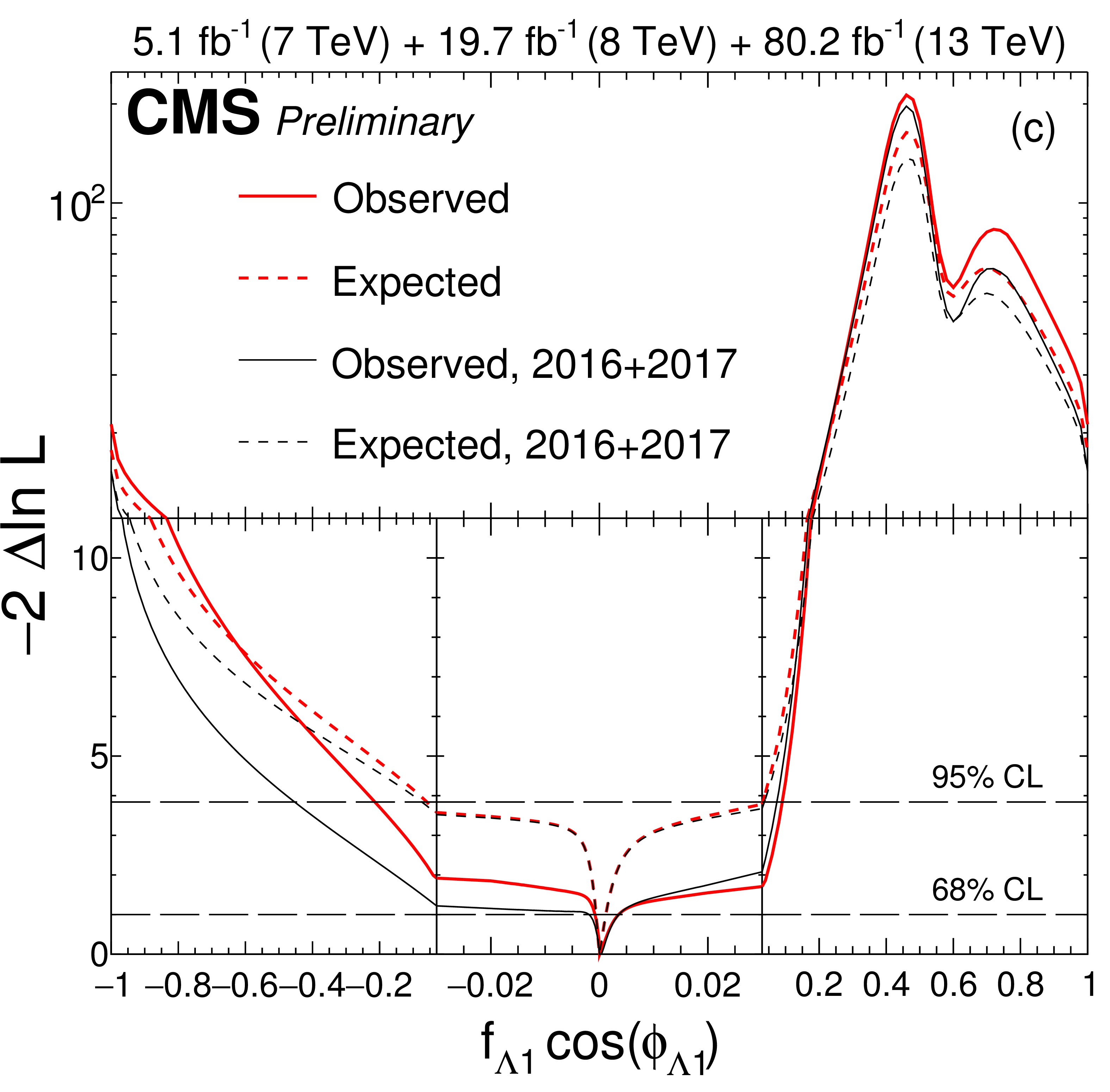
png pdf	Figure 4: Observed (solid) and expected (dashed) likelihood scans of ${{f_{a 3}} {\cos ({\phi _{a 3}} )}}$ (a), ${{f_{a 2}} {\cos ({\phi _{a 2}} )}}$ (b), ${{f_{\Lambda 1}} {\cos ({\phi _{\Lambda 1}} )}}$ (c), and ${{{f_{\Lambda 1}} ^{Z\gamma}} {\cos ({{\phi _{\Lambda 1}} ^{Z\gamma}} )}}$ (d) using on-shell events only. Results of analysis of the data from 2016 and 2017 only (black) and the combined Run 1 and Run 2 analysis (red) are shown. The dashed horizontal lines show the 68% and 95% CL regions.
png pdf	Figure 4-a: Observed (solid) and expected (dashed) likelihood scans of ${{f_{a 3}} {\cos ({\phi _{a 3}} )}}$, using on-shell events only. Results of analysis of the data from 2016 and 2017 only (black) and the combined Run 1 and Run 2 analysis (red) are shown. The dashed horizontal lines show the 68% and 95% CL regions.
png pdf	Figure 4-b: Observed (solid) and expected (dashed) likelihood scans of ${{f_{a 3}} {\cos ({\phi _{a 3}} )}}$, using on-shell events only. Results of analysis of the data from 2016 and 2017 only (black) and the combined Run 1 and Run 2 analysis (red) are shown. The dashed horizontal lines show the 68% and 95% CL regions.
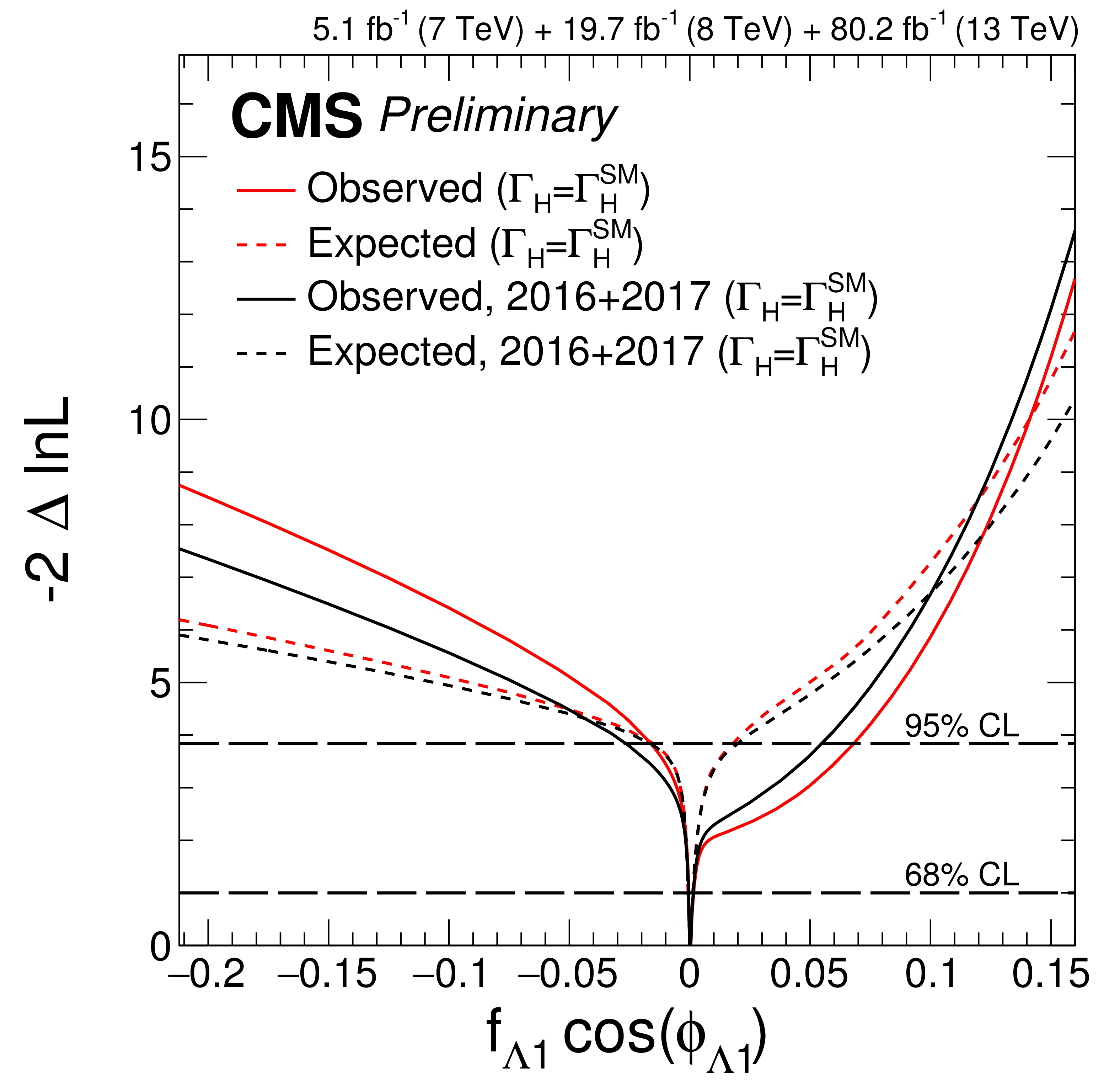
png pdf	Figure 4-c: Observed (solid) and expected (dashed) likelihood scans of ${{f_{\Lambda 1}} {\cos ({\phi _{\Lambda 1}} )}}$, using on-shell events only. Results of analysis of the data from 2016 and 2017 only (black) and the combined Run 1 and Run 2 analysis (red) are shown. The dashed horizontal lines show the 68% and 95% CL regions.
png pdf	Figure 4-d: Observed (solid) and expected (dashed) likelihood scans of ${{{f_{\Lambda 1}} ^{Z\gamma}} {\cos ({{\phi _{\Lambda 1}} ^{Z\gamma}} )}}$, using on-shell events only. Results of analysis of the data from 2016 and 2017 only (black) and the combined Run 1 and Run 2 analysis (red) are shown. The dashed horizontal lines show the 68% and 95% CL regions.
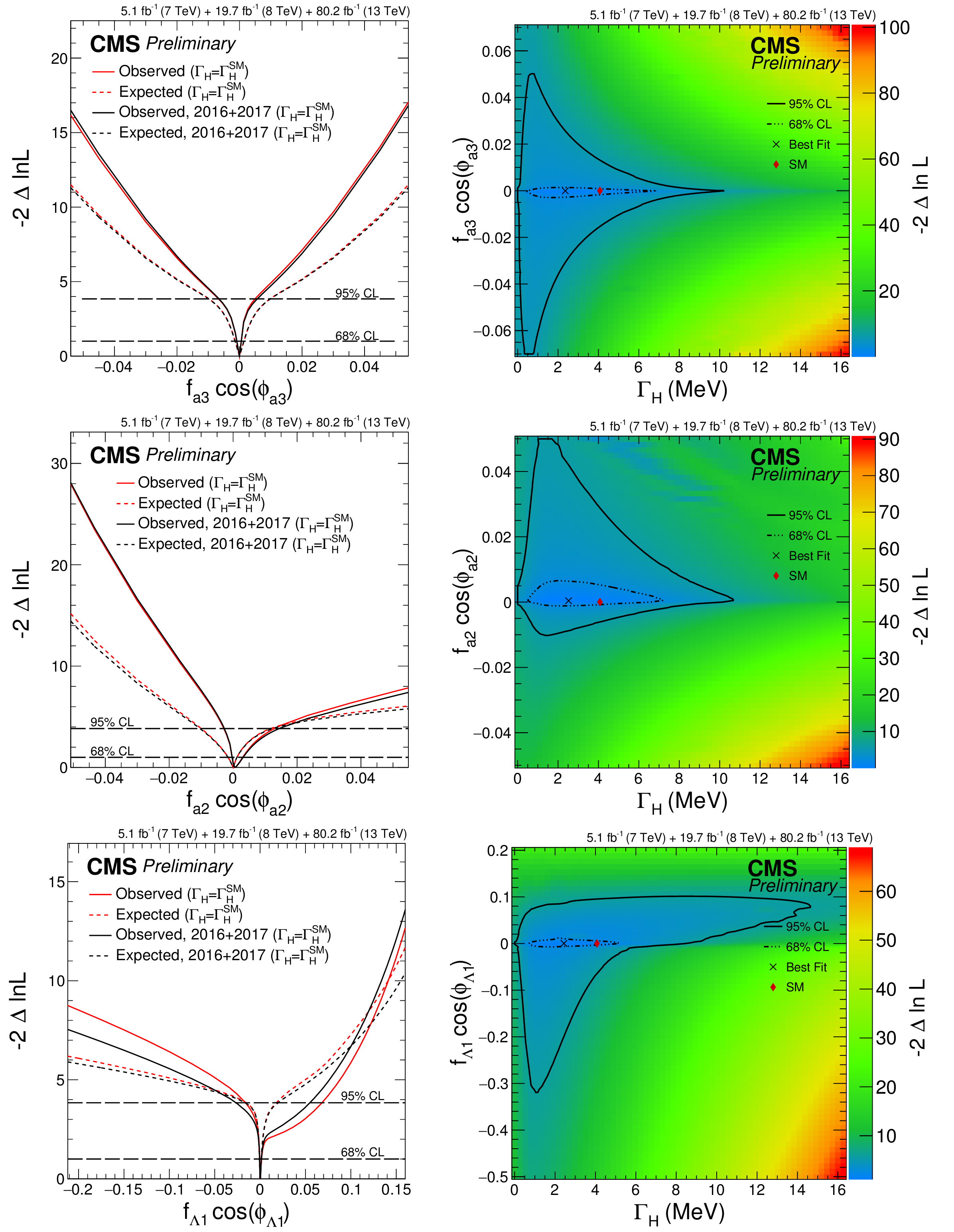
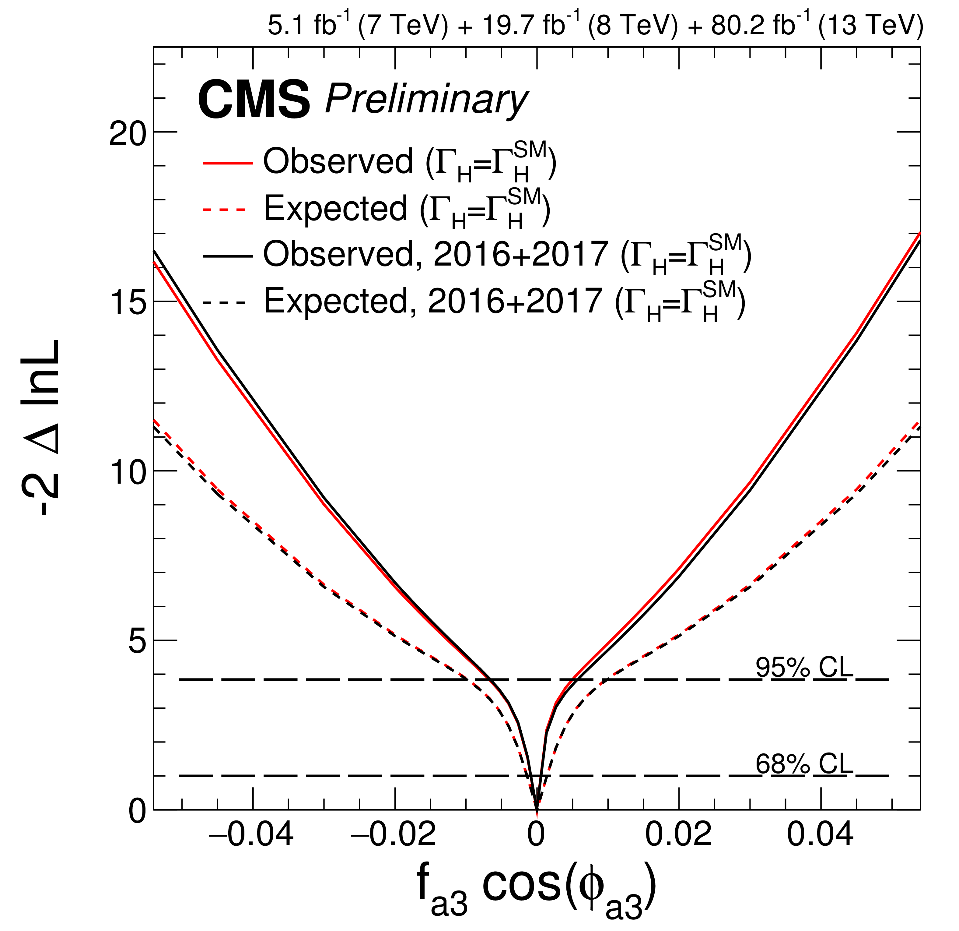
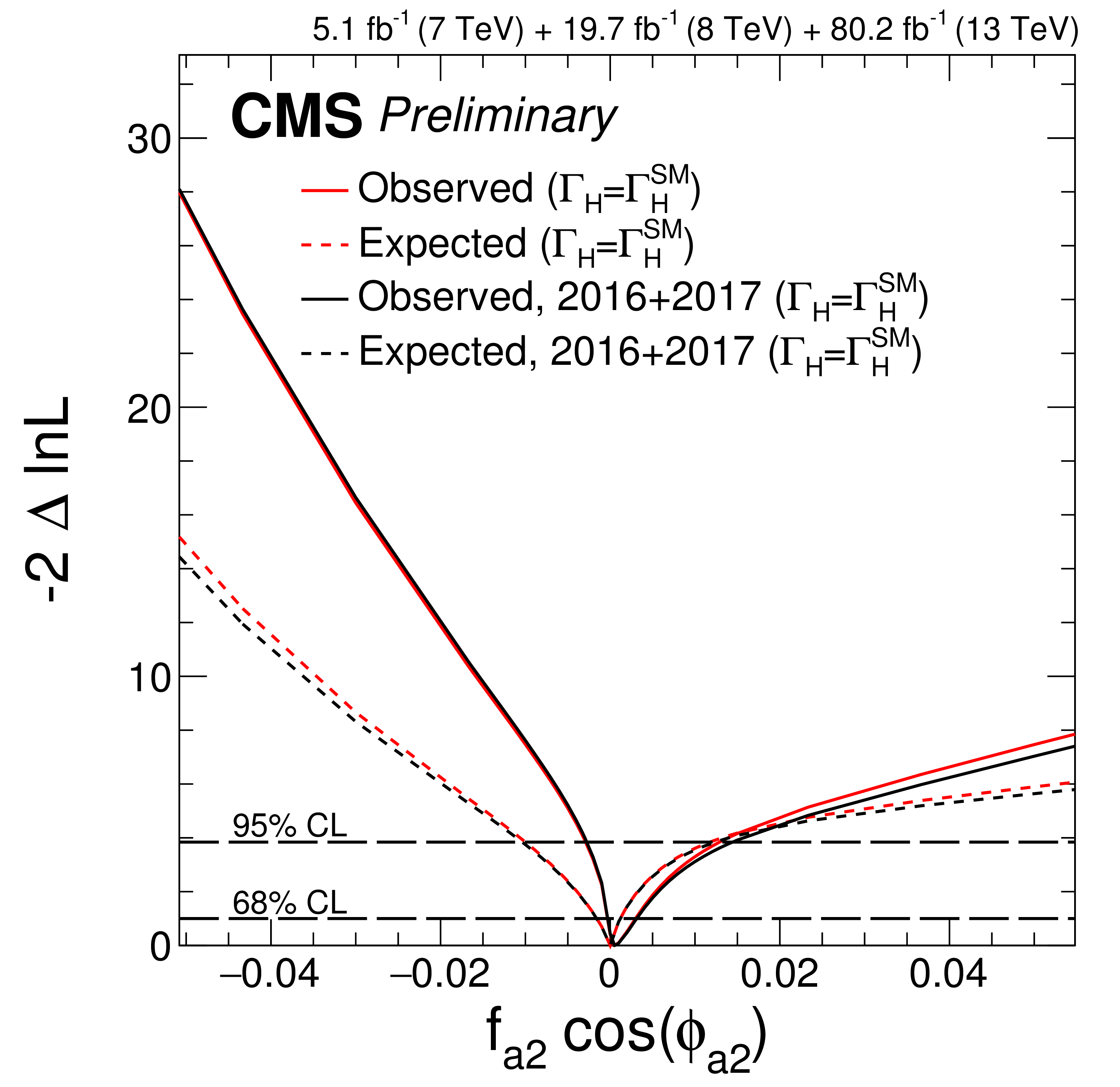
png pdf	Figure 5: Constraints on ${{f_{a 3}} {\cos ({\phi _{a 3}} )}}$ (top), ${{f_{a 2}} {\cos ({\phi _{a 2}} )}}$ (middle), and ${{f_{\Lambda 1}} {\cos ({\phi _{\Lambda 1}} )}}$ (bottom) under the assumption ${\Gamma _ {\mathrm {H}}} = {\Gamma _ {\mathrm {H}} ^{\mathrm {SM}}}$ (left) and with ${\Gamma _ {\mathrm {H}}}$ unconstrained (right). Left plots: Results of analysis of the data from 2016 and 2017 only (black) and the combined Run 2 and Run 1 analysis (red) are shown. The dashed horizontal lines show the 68% and 95% CL regions. Observed (solid) and expected (dashed) likelihood scans are shown. Right plots: Observed 2D likelihood scans are shown for the combined Run 2 and Run 1 analysis. The 68% and 95% CL regions are indicated with the dashed lines.
png pdf	Figure 5-a: Constraints on ${{f_{a 3}} {\cos ({\phi _{a 3}} )}}$, under the assumption ${\Gamma _ {\mathrm {H}}} = {\Gamma _ {\mathrm {H}} ^{\mathrm {SM}}}$. Results of analysis of the data from 2016 and 2017 only (black) and the combined Run 2 and Run 1 analysis (red) are shown. The dashed horizontal lines show the 68% and 95% CL regions. Observed (solid) and expected (dashed) likelihood scans are shown.
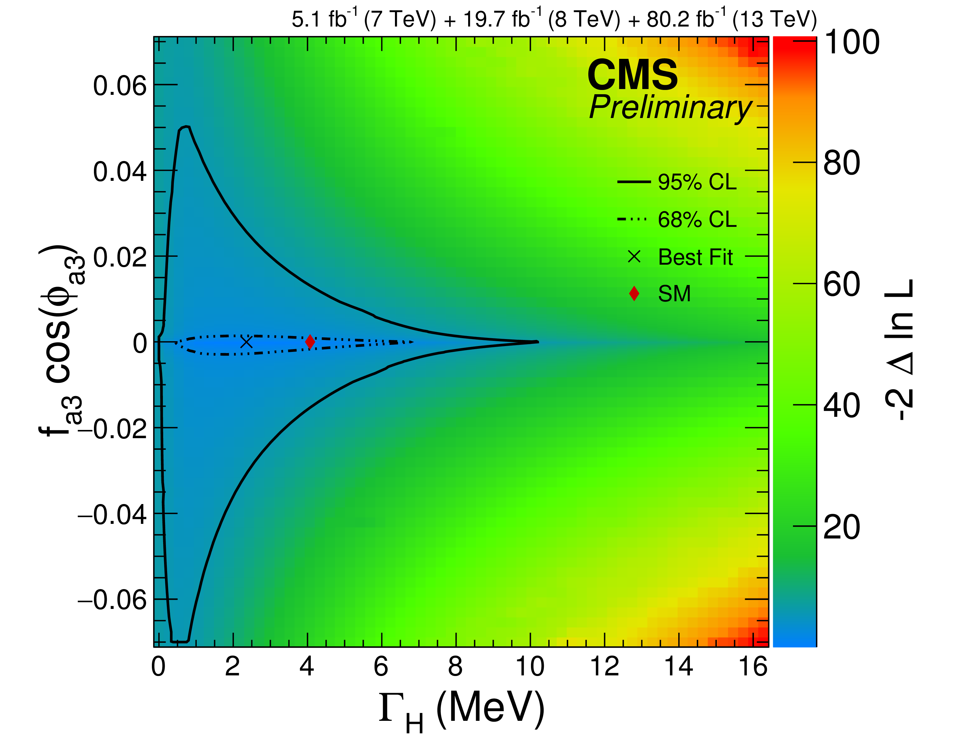
png pdf	Figure 5-b: Constraints on ${{f_{a 3}} {\cos ({\phi _{a 3}} )}}$, with ${\Gamma _ {\mathrm {H}}}$ unconstrained. Observed 2D likelihood scans are shown for the combined Run 2 and Run 1 analysis. The 68% and 95% CL regions are indicated with the dashed lines.
png pdf	Figure 5-c: Constraints on ${{f_{a 2}} {\cos ({\phi _{a 2}} )}}$, under the assumption ${\Gamma _ {\mathrm {H}}} = {\Gamma _ {\mathrm {H}} ^{\mathrm {SM}}}$. Results of analysis of the data from 2016 and 2017 only (black) and the combined Run 2 and Run 1 analysis (red) are shown. The dashed horizontal lines show the 68% and 95% CL regions. Observed (solid) and expected (dashed) likelihood scans are shown.
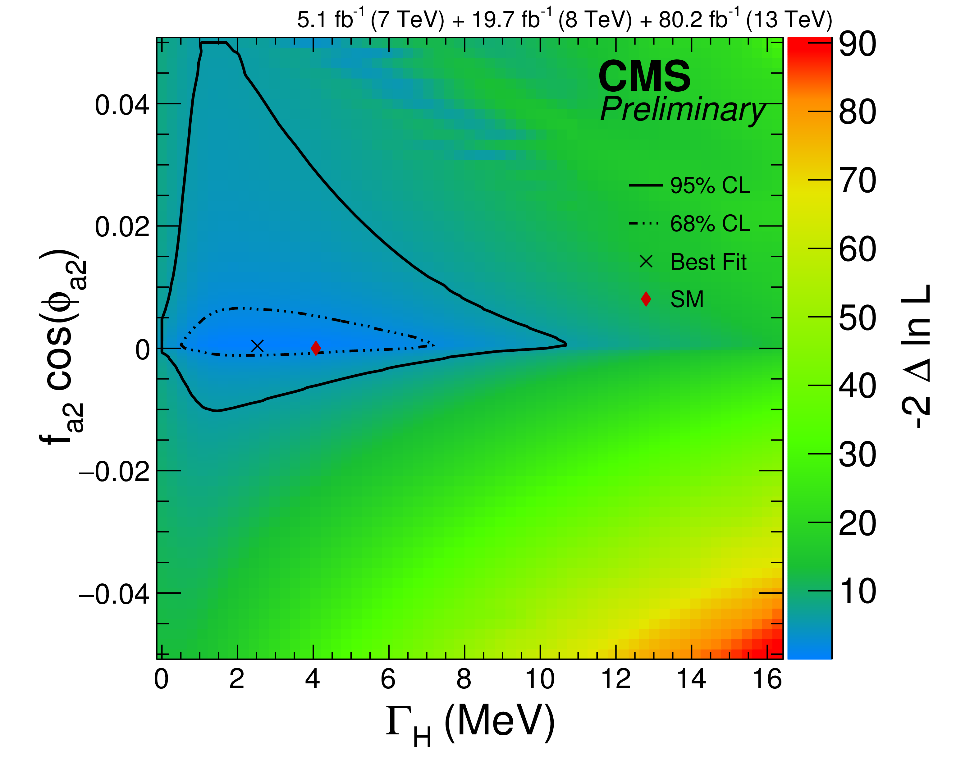
png pdf	Figure 5-d: Constraints on ${{f_{a 2}} {\cos ({\phi _{a 2}} )}}$, with ${\Gamma _ {\mathrm {H}}}$ unconstrained. Observed 2D likelihood scans are shown for the combined Run 2 and Run 1 analysis. The 68% and 95% CL regions are indicated with the dashed lines.
png pdf	Figure 5-e: Constraints on ${{f_{\Lambda 1}} {\cos ({\phi _{\Lambda 1}} )}}$, under the assumption ${\Gamma _ {\mathrm {H}}} = {\Gamma _ {\mathrm {H}} ^{\mathrm {SM}}}$. Results of analysis of the data from 2016 and 2017 only (black) and the combined Run 2 and Run 1 analysis (red) are shown. The dashed horizontal lines show the 68% and 95% CL regions. Observed (solid) and expected (dashed) likelihood scans are shown.
png pdf	Figure 5-f: Constraints on ${{f_{\Lambda 1}} {\cos ({\phi _{\Lambda 1}} )}}$, with ${\Gamma _ {\mathrm {H}}}$ unconstrained. Observed 2D likelihood scans are shown for the combined Run 2 and Run 1 analysis. The 68% and 95% CL regions are indicated with the dashed lines.
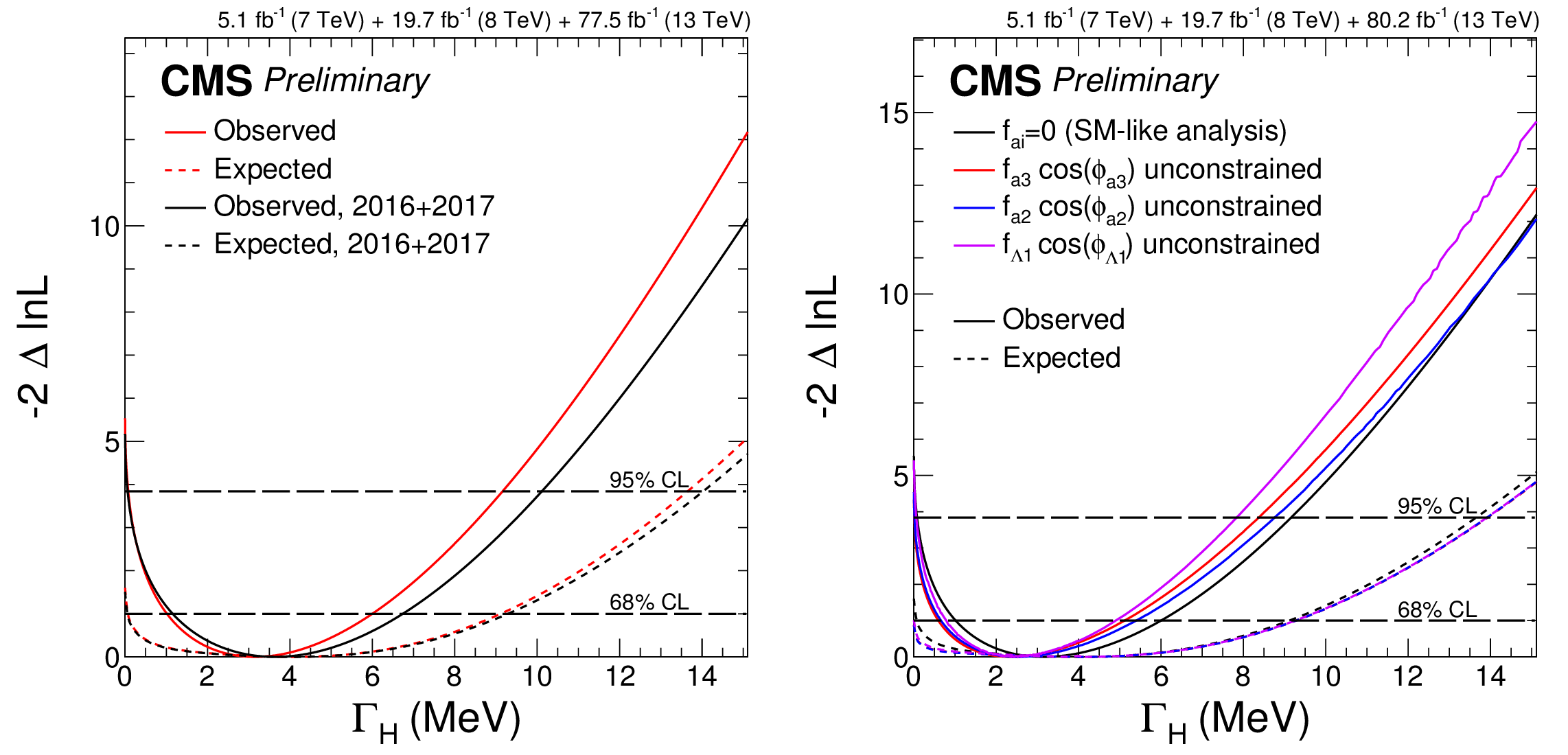
png pdf	Figure 6: Observed (solid) and expected (dashed) likelihood scans of ${\Gamma _ {\mathrm {H}}}$. Left plot: Results of analysis of the data from 2016 and 2017 only (black) and the combined Run 1 and Run 2 analysis (red) are shown for the SM-like couplings. Right plot: Results of analysis of the data from the combined Run 1 and Run 2 analyses for the SM-like couplings and with three anomalous coupling parameters of interest unconstrained: ${{f_{a 3}} {\cos ({\phi _{a 3}} )}}$ (red), ${{f_{a 2}} {\cos ({\phi _{a 2}} )}}$ (blue), and ${{f_{\Lambda 1}} {\cos ({\phi _{\Lambda 1}} )}}$ (violet). The dashed horizontal lines show the 68% and 95% CL regions.
png pdf	Figure 6-a: Observed (solid) and expected (dashed) likelihood scans of ${\Gamma _ {\mathrm {H}}}$. Results of analysis of the data from 2016 and 2017 only (black) and the combined Run 1 and Run 2 analysis (red) are shown for the SM-like couplings. The dashed horizontal lines show the 68% and 95% CL regions.
png pdf	Figure 6-b: Observed (solid) and expected (dashed) likelihood scans of ${\Gamma _ {\mathrm {H}}}$. Results of analysis of the data from the combined Run 1 and Run 2 analyses for the SM-like couplings and with three anomalous coupling parameters of interest unconstrained: ${{f_{a 3}} {\cos ({\phi _{a 3}} )}}$ (red), ${{f_{a 2}} {\cos ({\phi _{a 2}} )}}$ (blue), and ${{f_{\Lambda 1}} {\cos ({\phi _{\Lambda 1}} )}}$ (violet). The dashed horizontal lines show the 68% and 95% CL regions.

Tables
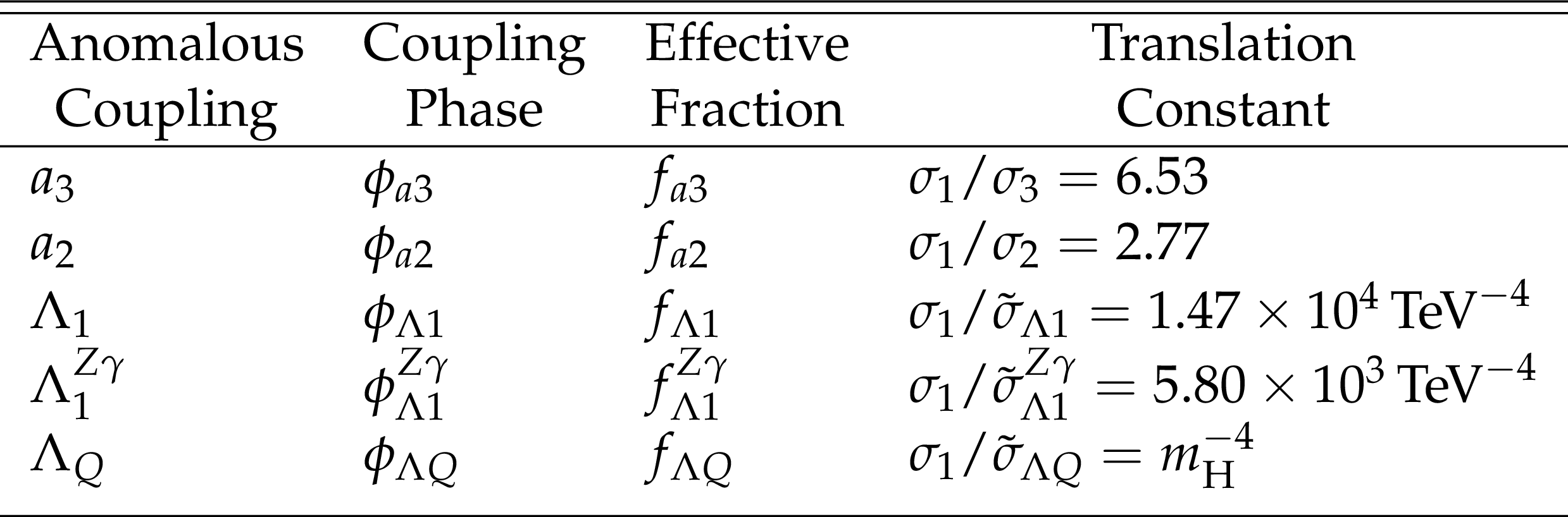
png pdf	Table 1: List of anomalous HVV couplings considered in the measurements assuming a spin-zero H boson. The definition of the effective fractions is discussed in the text and the translation constant is given in each case. The effective cross sections correspond to the processes ${\mathrm {H}} \to 2 {\mathrm {e}}2\mu$ and the Higgs boson mass $m_{{\mathrm {H}}} =$ 125 GeV using the JHUGen [38,39,40] calculation.
png pdf	Table 2: The numbers of events expected for the SM (or ${f_{a 3}} =$ 1 in parentheses) for different signal and background modes and the total observed numbers of events across the three ${a_{3}}$ analysis categories in the on-shell region.
png pdf	Table 3: The numbers of events expected for the SM (or ${f_{a 3}} =0$ in the ${a_{3}}$ analysis categorization in parentheses) for different signal and background modes and the total observed numbers of events across the three SM or ${a_{3}}$ analysis categories in the off-shell region. For the gluon fusion (gg) and electroweak processes (VV), the combined yield from signal (s), background (b), and interference (i) is shown.
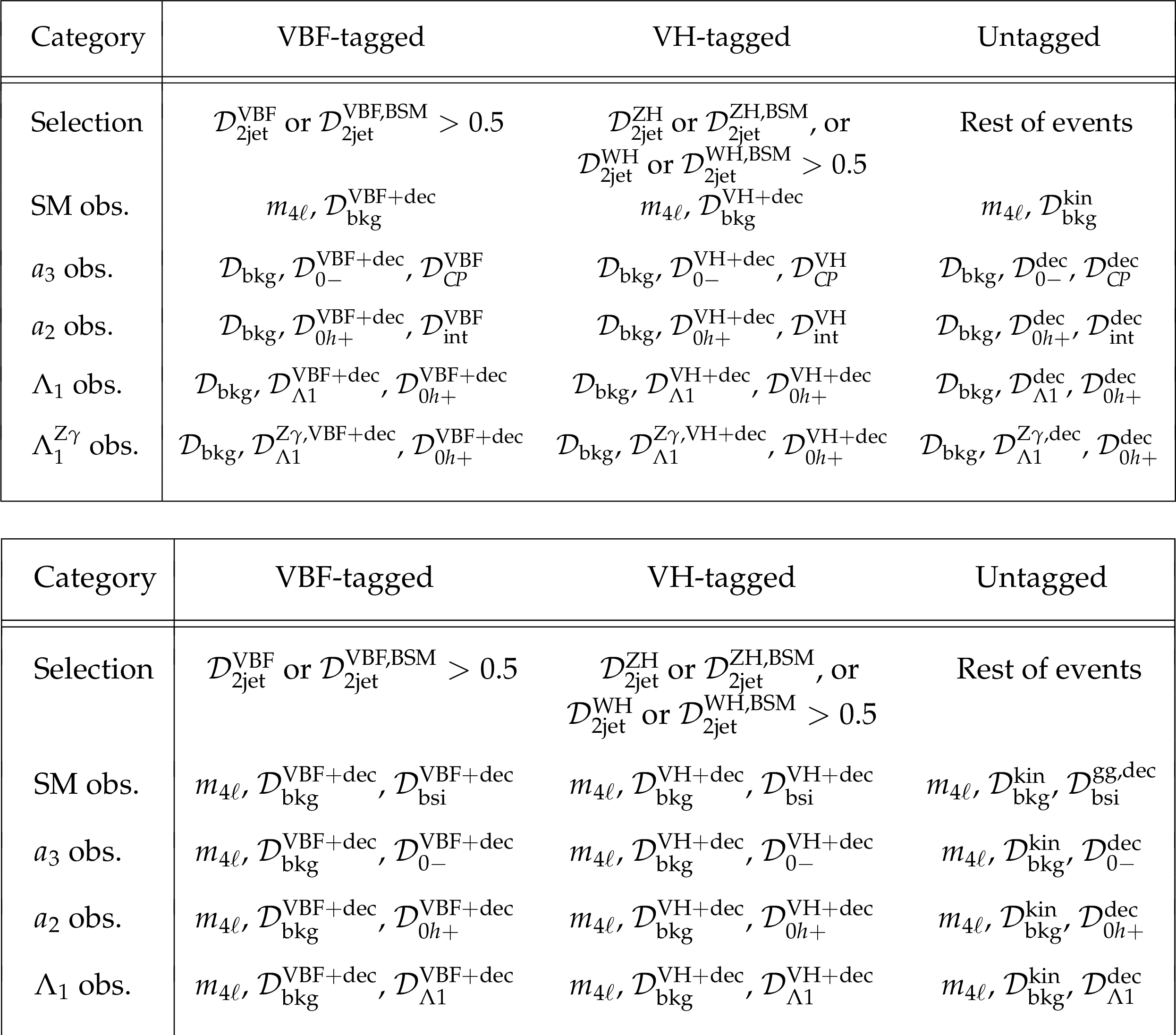
png pdf	Table 4: Summary of the three production categories in the on-shell ${m_{4\ell}}$ region. Three or two observables (abbreviated as obs.) are listed for each analysis and for each category. All discriminants are calculated with JHUGen signal matrix elements and mcfm background matrix elements. The discriminants $\mathcal {D}_{\rm bkg}$ in the tagged categories also include probabilities using associated jets and decay in addition to the ${m_{4\ell}}$ probability.
png pdf	Table 5: Summary of the three production categories in the off-shell ${m_{4\ell}}$ region, listed in a similar manner to Table 4. All discriminants are calculated with JHUGen or MCFM/JHUGen signal, and MCFM background matrix elements. The VH interference discriminant in the SM analysis hadronic VH-tagged category is defined as the simple average of the ones corresponding to ZH and WH processes separately.
png pdf	Table 6: Summary of allowed 68% CL (central values with uncertainties) and 95% CL (in square brackets) intervals on anomalous coupling parameters ${{f_{a i}} {\cos ({\phi _{a i}} )}}$ obtained from the on-shell data analysis of the Run 1 and Run 2 combined dataset.
png pdf	Table 7: Summary of allowed 68% CL (central values with uncertainties) and 95% CL (in square brackets) intervals on the anomalous coupling parameters ${{f_{a i}} {\cos ({\phi _{a i}} )}}$ obtained from the data analysis of the Run 2 (on-shell and off-shell) and Run 1 (on-shell only) combined dataset.
png pdf	Table 8: Summary of the total width ${\Gamma _ {\mathrm {H}}}$ measurement, showing allowed 68% CL (central values with uncertainties) and 95% CL (in square brackets). The limits are reported for the SM-like couplings using the Run 1 and Run 2 combination.

Summary

Studies of on-shell and off-shell Higgs boson production in the four-lepton final state are presented, using data from the CMS experiment at the LHC that corresponds to an integrated luminosity of 80.2 fb$^{-1}$ at 13 TeV. Joint constraints are set on the width and parameters that express its anomalous couplings to two electroweak vector bosons using both on-shell and off-shell production of the Higgs boson. These results are combined with results from the data collected at center-of-mass energies of 7 and 8 TeV, corresponding to integrated luminosities of 5.1 and 19.7 fb$^{-1}$, respectively. Matrix element techniques are utilized to combine kinematic information from the decay particles and the associated jets to identify the production mechanism and increase sensitivity to the anomalous couplings. The observations are found to be consistent with expectations for a Standard Model Higgs boson.

Additional Figures
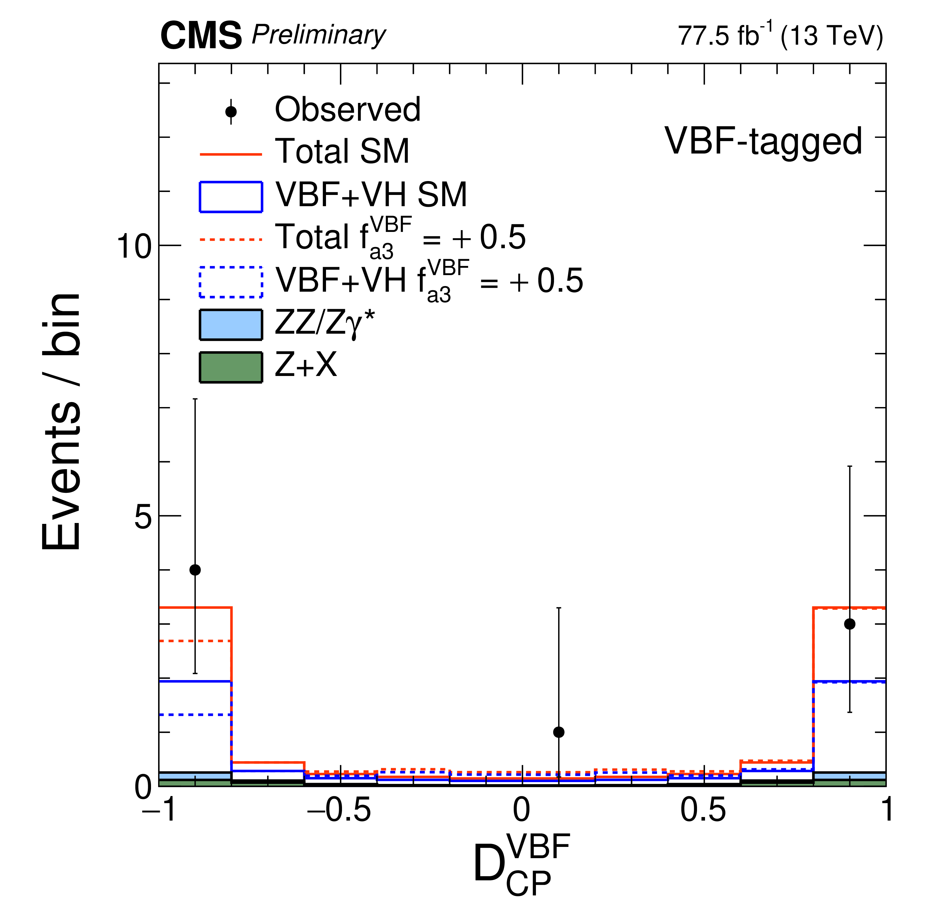
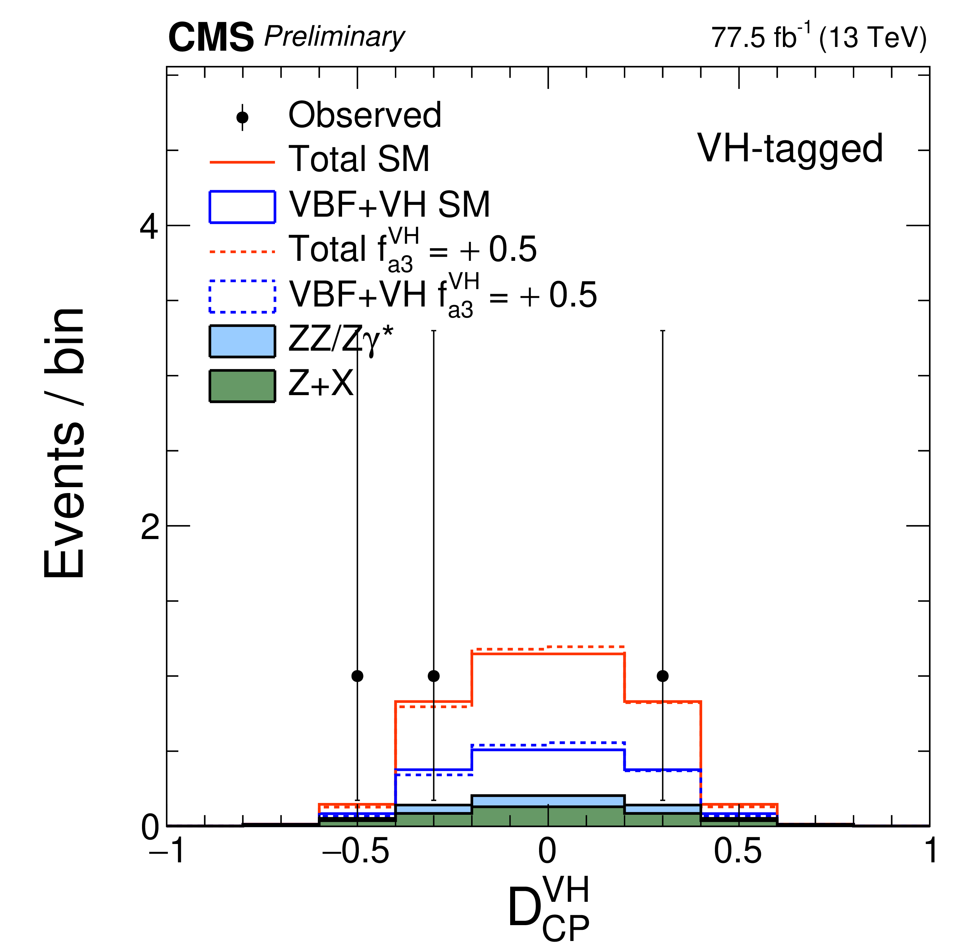
png pdf	Additional Figure 1: Distributions of $\mathcal {D}_{CP}$ in the on-shell $f_{a3}$ analysis. Two tagging categories are shown: VBF-tagged (a) and VH-tagged (b). The decay or production information used in the discriminants depends on the tagging category. $f_{a3}^\text {VBF}$ and $f_{a3}^{\mathrm {V} {\mathrm {H}}}$ are defined by analogy with $f_{a3}$, but using the cross sections for the VBF and VH processes, respectively. Points with error bars show data and histograms show expectations for background and SM or BSM signal as indicated in the legend.
png pdf	Additional Figure 1-a: Distribution of $\mathcal {D}_{CP}$ in the on-shell $f_{a3}$ analysis for the VBF-tagged tagging category. The decay or production information used in the discriminant depends on the tagging category. $f_{a3}^\text {VBF}$ is defined by analogy with $f_{a3}$, but using the cross section for the VBF process. Points with error bars show data and histograms show expectations for background and SM or BSM signal as indicated in the legend.
png pdf	Additional Figure 1-b: Distribution of $\mathcal {D}_{CP}$ in the on-shell $f_{a3}$ analysis for the VH-tagged tagging category. The decay or production information used in the discriminant depends on the tagging category. $f_{a3}^{\mathrm {V} {\mathrm {H}}}$ is defined by analogy with $f_{a3}$, but using the cross section for the VH process. Points with error bars show data and histograms show expectations for background and SM or BSM signal as indicated in the legend.
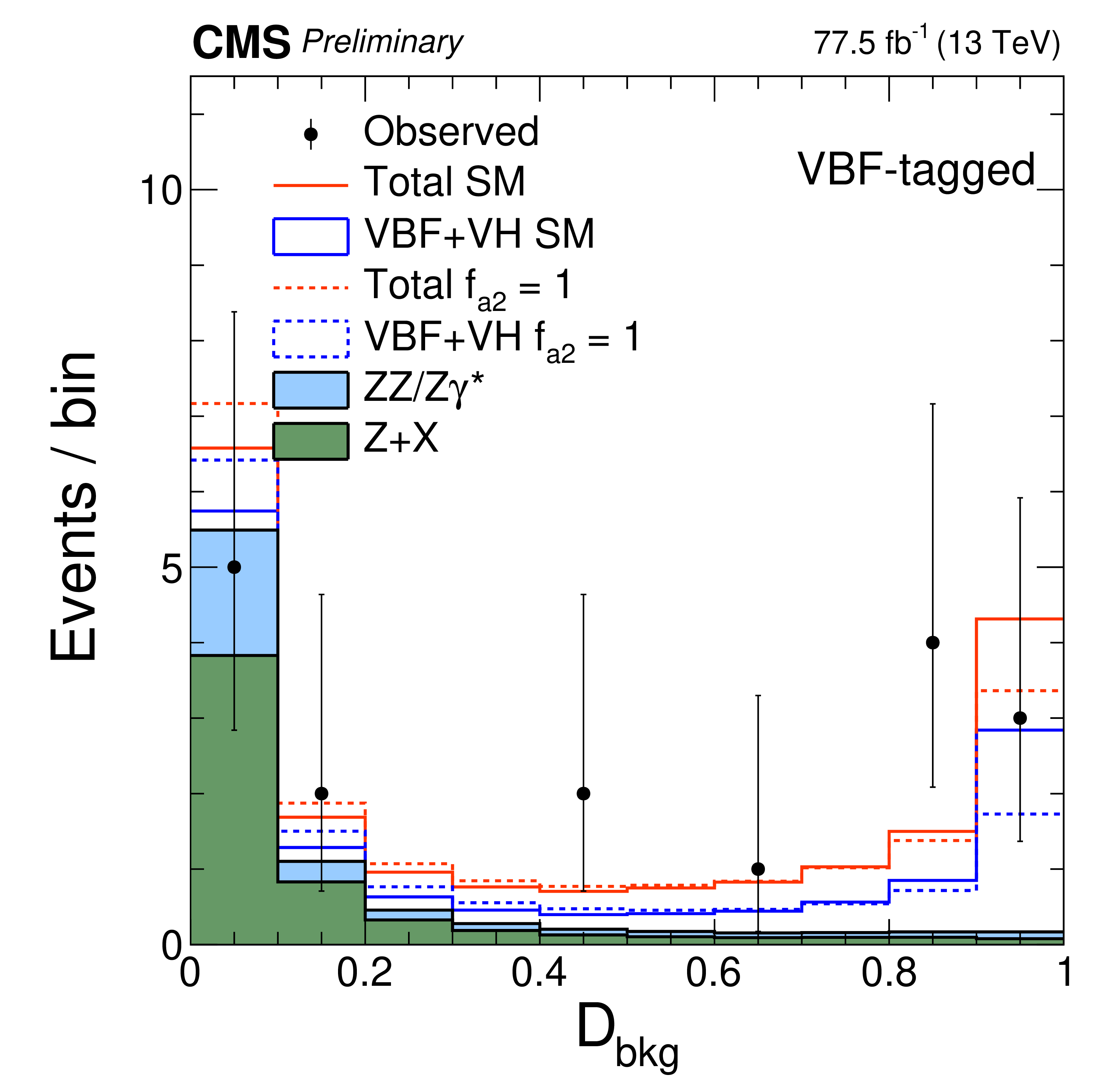
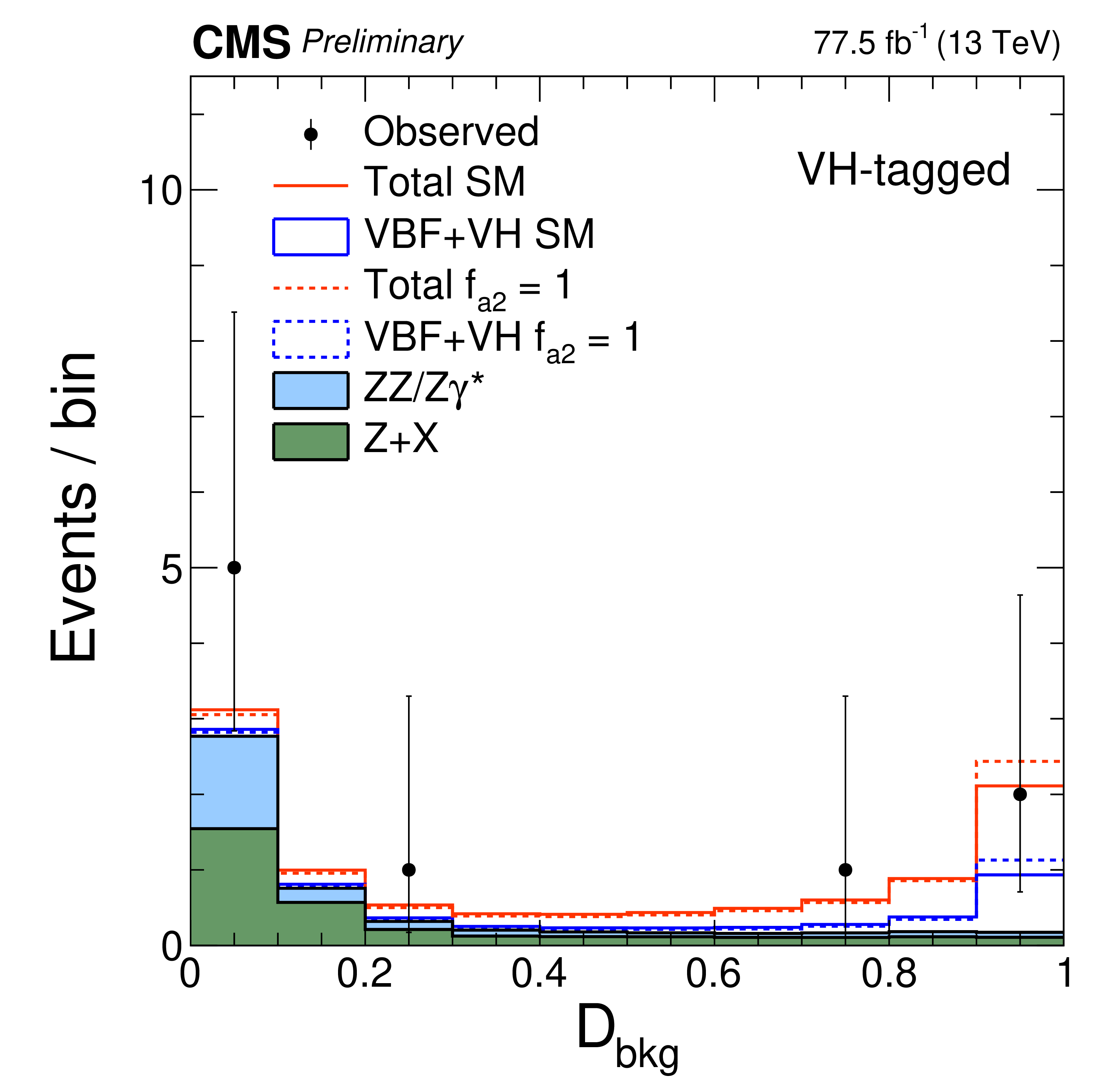
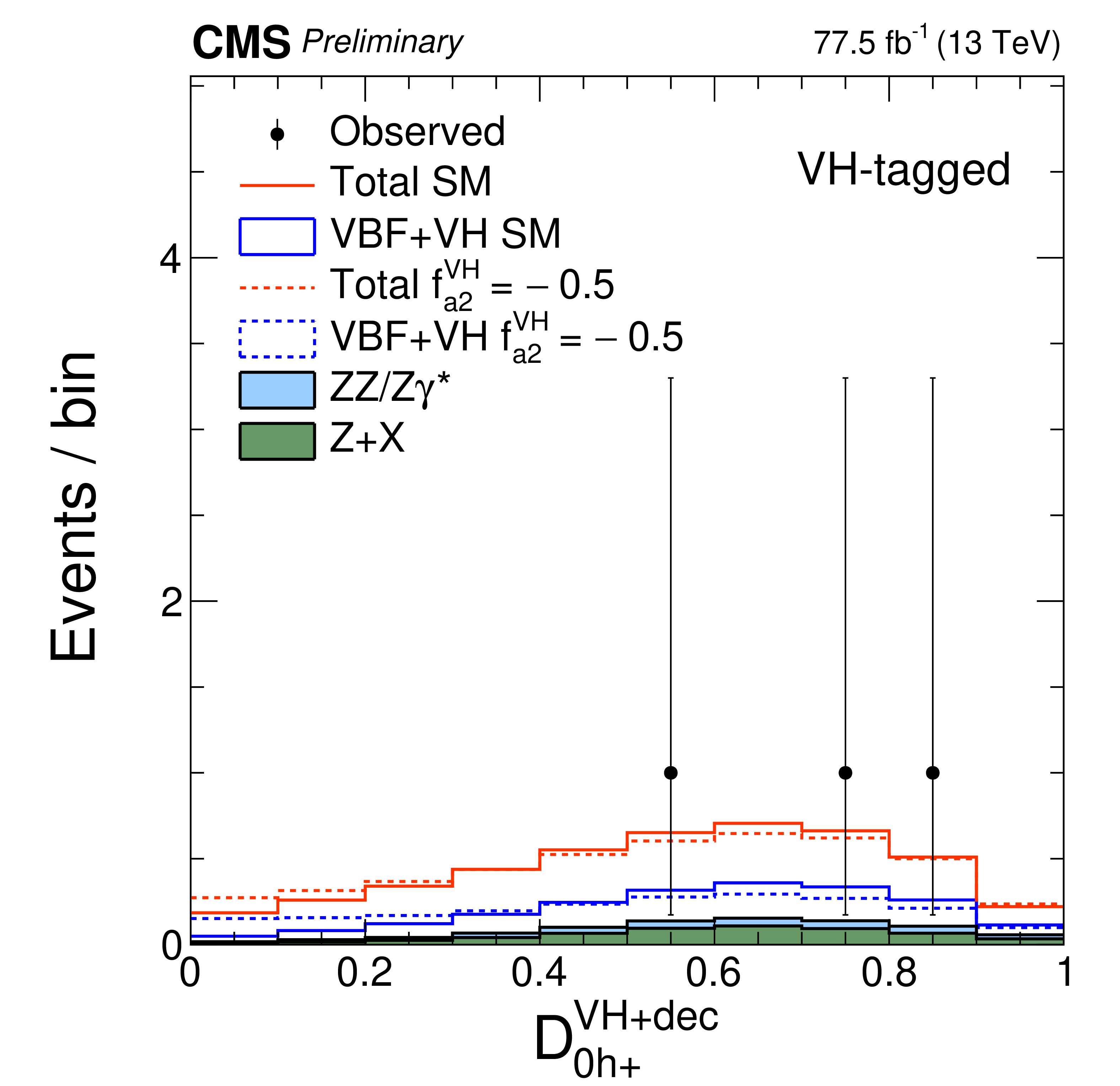
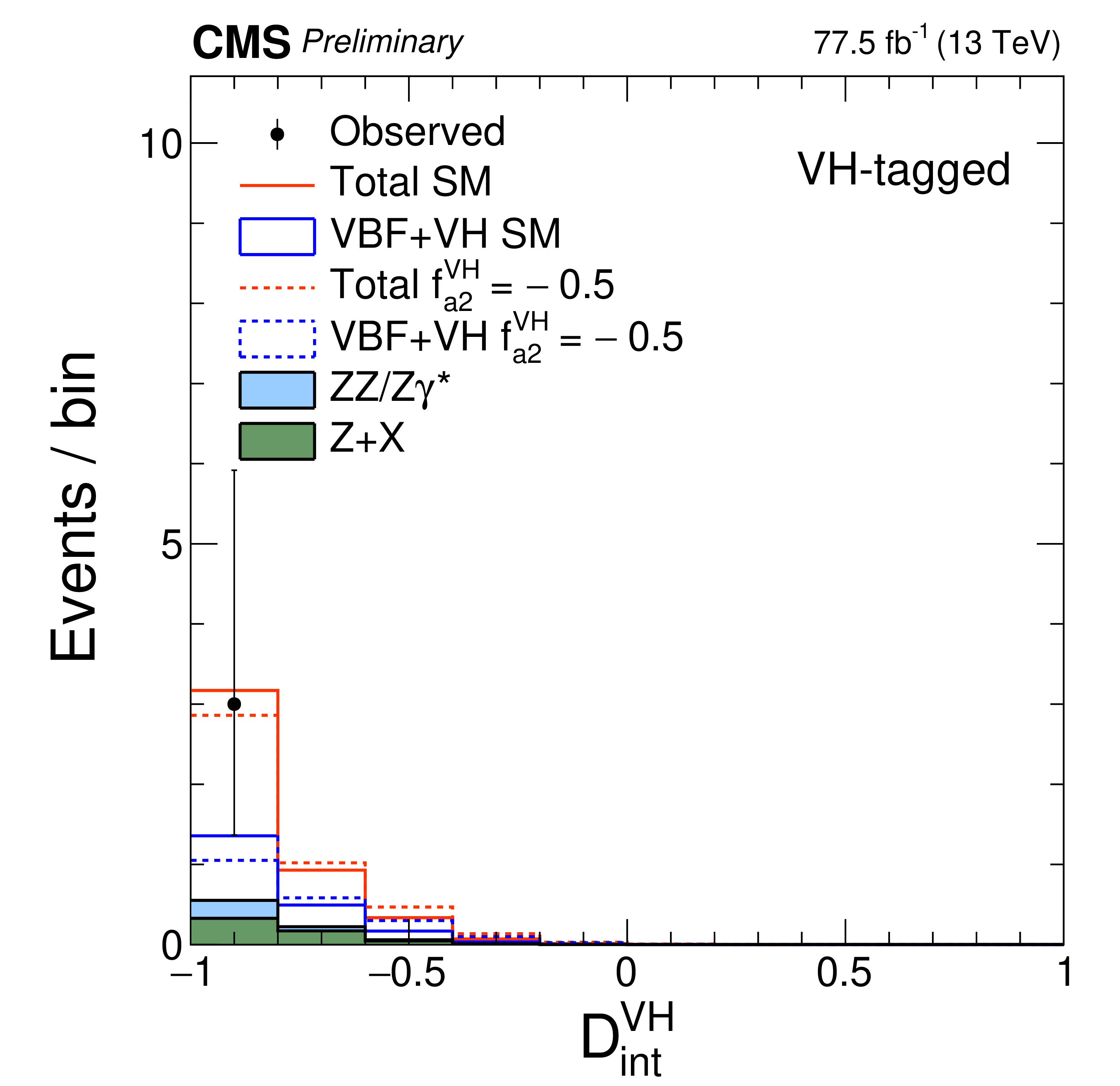
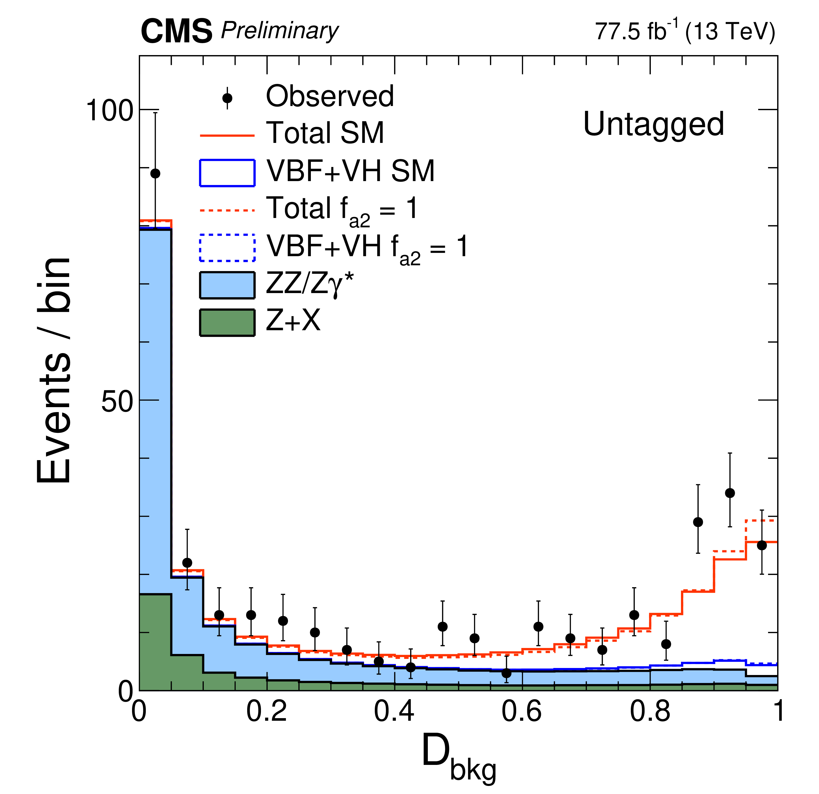
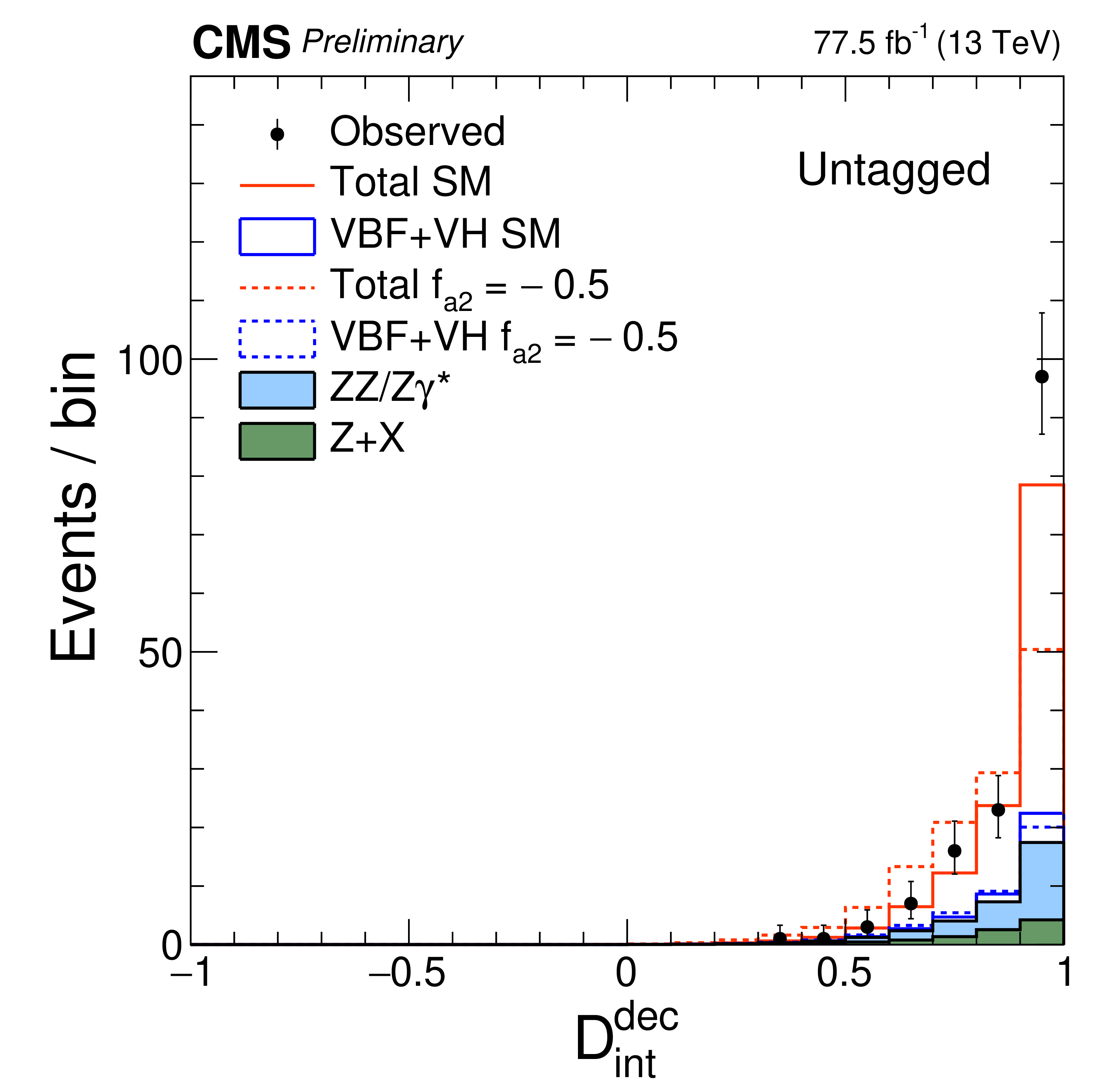
png pdf	Additional Figure 2: Distributions of kinematic discriminants in the on-shell $f_{a2}$ analysis: $\mathcal {D}_{\rm bkg}$ (a), (d), (g), $\mathcal {D}_{0h+}$ (b), (e), and $\mathcal {D}_\text {int}$ (c), (f), (h). Three tagging categories are shown: VBF-tagged (a)-(c), VH-tagged (d)-(f), and untagged (g), (h). The decay or production information used in the discriminants depends on the tagging category. $f_{a2}^\text {VBF}$ and $f_{a2}^{\mathrm {V} {\mathrm {H}}}$ are defined by analogy with $f_{a2}$, but using the cross sections for the VBF and VH processes, respectively. Points with error bars show data and histograms show expectations for background and SM or BSM signal as indicated in the legend.
png pdf	Additional Figure 2-a: Distributions of the $\mathcal {D}_{\rm bkg}$ kinematic discriminant in the on-shell $f_{a2}$ analysis, for the VBF-tagged category. The decay or production information used in the discriminant depends on the tagging category. Points with error bars show data and histograms show expectations for background and SM or BSM signal as indicated in the legend.
png pdf	Additional Figure 2-b: Distributions of the $\mathcal {D}_{0h+}$ kinematic discriminant in the on-shell $f_{a2}$ analysis, for the VBF-tagged category. The decay or production information used in the discriminant depends on the tagging category. $f_{a2}^\text {VBF}$ is defined by analogy with $f_{a2}$, but using the cross sections for the VBF process. Points with error bars show data and histograms show expectations for background and SM or BSM signal as indicated in the legend.
png pdf	Additional Figure 2-c: Distributions of the $\mathcal {D}_\text {int}$ kinematic discriminant in the on-shell $f_{a2}$ analysis, for the VBF-tagged category. The decay or production information used in the discriminant depends on the tagging category. $f_{a2}^\text {VBF}$ is defined by analogy with $f_{a2}$, but using the cross sections for the VBF process. Points with error bars show data and histograms show expectations for background and SM or BSM signal as indicated in the legend.
png pdf	Additional Figure 2-d: Distributions of the $\mathcal {D}_{\rm bkg}$ kinematic discriminant in the on-shell $f_{a2}$ analysis, for the VH-tagged category. The decay or production information used in the discriminant depends on the tagging category. Points with error bars show data and histograms show expectations for background and SM or BSM signal as indicated in the legend.
png pdf	Additional Figure 2-e: Distributions of the $\mathcal {D}_{0h+}$ kinematic discriminant in the on-shell $f_{a2}$ analysis, for the VH-tagged category. The decay or production information used in the discriminant depends on the tagging category. $f_{a2}^{\mathrm {V} {\mathrm {H}}}$ is defined by analogy with $f_{a2}$, but using the cross sections for the VH process. Points with error bars show data and histograms show expectations for background and SM or BSM signal as indicated in the legend.
png pdf	Additional Figure 2-f: Distributions of the $\mathcal {D}_\text {int}$ kinematic discriminant in the on-shell $f_{a2}$ analysis, for the VH-tagged category. The decay or production information used in the discriminant depends on the tagging category. $f_{a2}^{\mathrm {V} {\mathrm {H}}}$ is defined by analogy with $f_{a2}$, but using the cross sections for the VH process. Points with error bars show data and histograms show expectations for background and SM or BSM signal as indicated in the legend.
png pdf	Additional Figure 2-g: Distributions of the $\mathcal {D}_{\rm bkg}$ kinematic discriminant in the on-shell $f_{a2}$ analysis, for the untagged category. The decay or production information used in the discriminant depends on the tagging category. Points with error bars show data and histograms show expectations for background and SM or BSM signal as indicated in the legend.
png pdf	Additional Figure 2-h: Distributions of the $\mathcal {D}_\text {int}$ kinematic discriminant in the on-shell $f_{a2}$ analysis, for the untagged category. The decay or production information used in the discriminant depends on the tagging category. Points with error bars show data and histograms show expectations for background and SM or BSM signal as indicated in the legend.
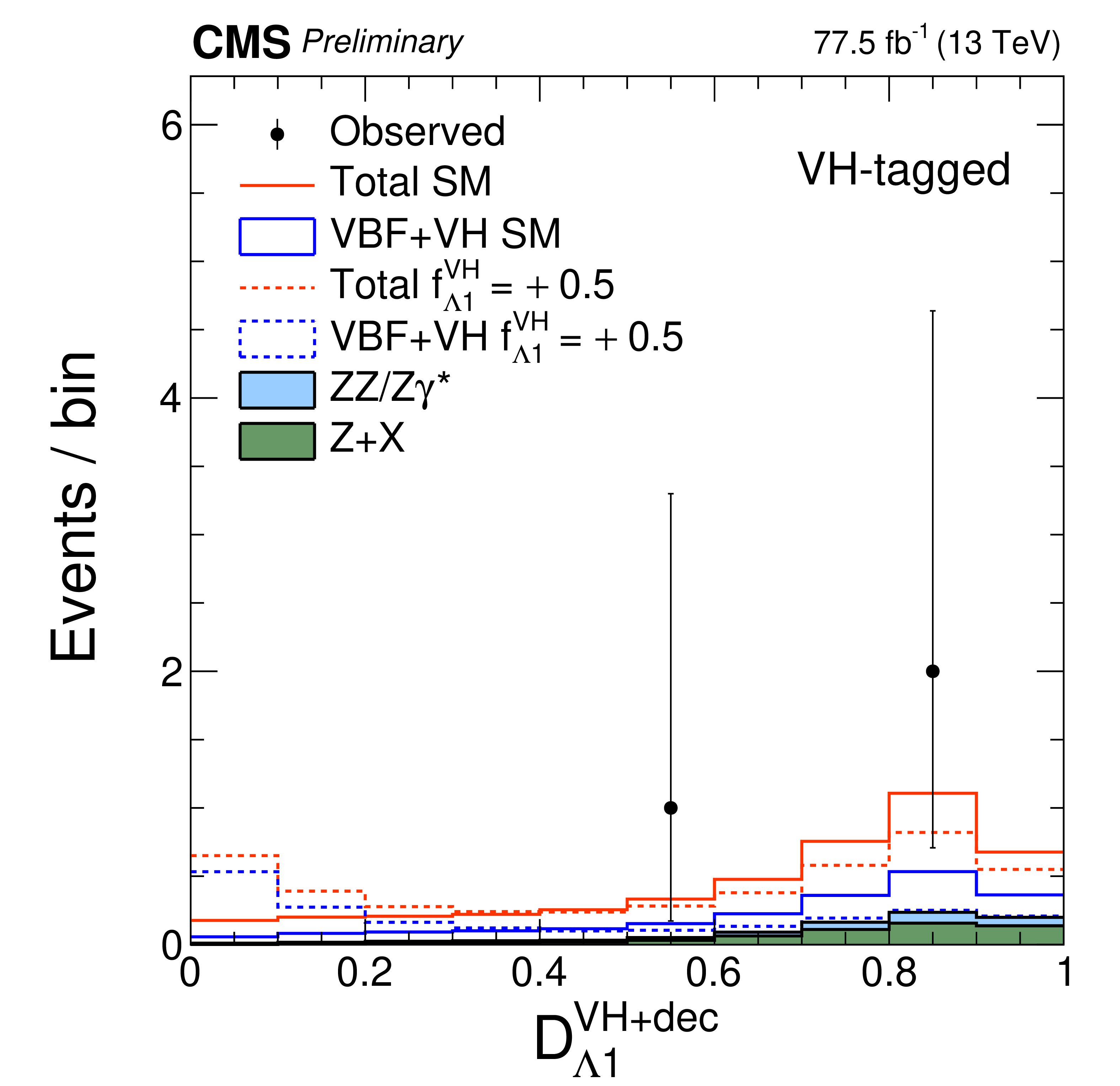
png pdf	Additional Figure 3: Distributions of kinematic discriminants in the on-shell $f_{\Lambda 1}$ analysis: $\mathcal {D}_{\rm bkg}$ (a), (d), (g), $\mathcal {D}_{\Lambda 1}$ (b), (e), and $\mathcal {D}_{0h+}$ (c), (f), (h). Three tagging categories are shown: VBF-tagged (a)-(c), VH-tagged (d)-(f), and untagged (g), (h). The decay or production information used in the discriminants depends on the tagging category. $f_{\Lambda 1}^\text {VBF}$ and $f_{\Lambda 1}^{\mathrm {V} {\mathrm {H}}}$ are defined by analogy with $f_{\Lambda 1}$, but using the cross sections for the VBF and VH processes, respectively. Points with error bars show data and histograms show expectations for background and SM or BSM signal as indicated in the legend.
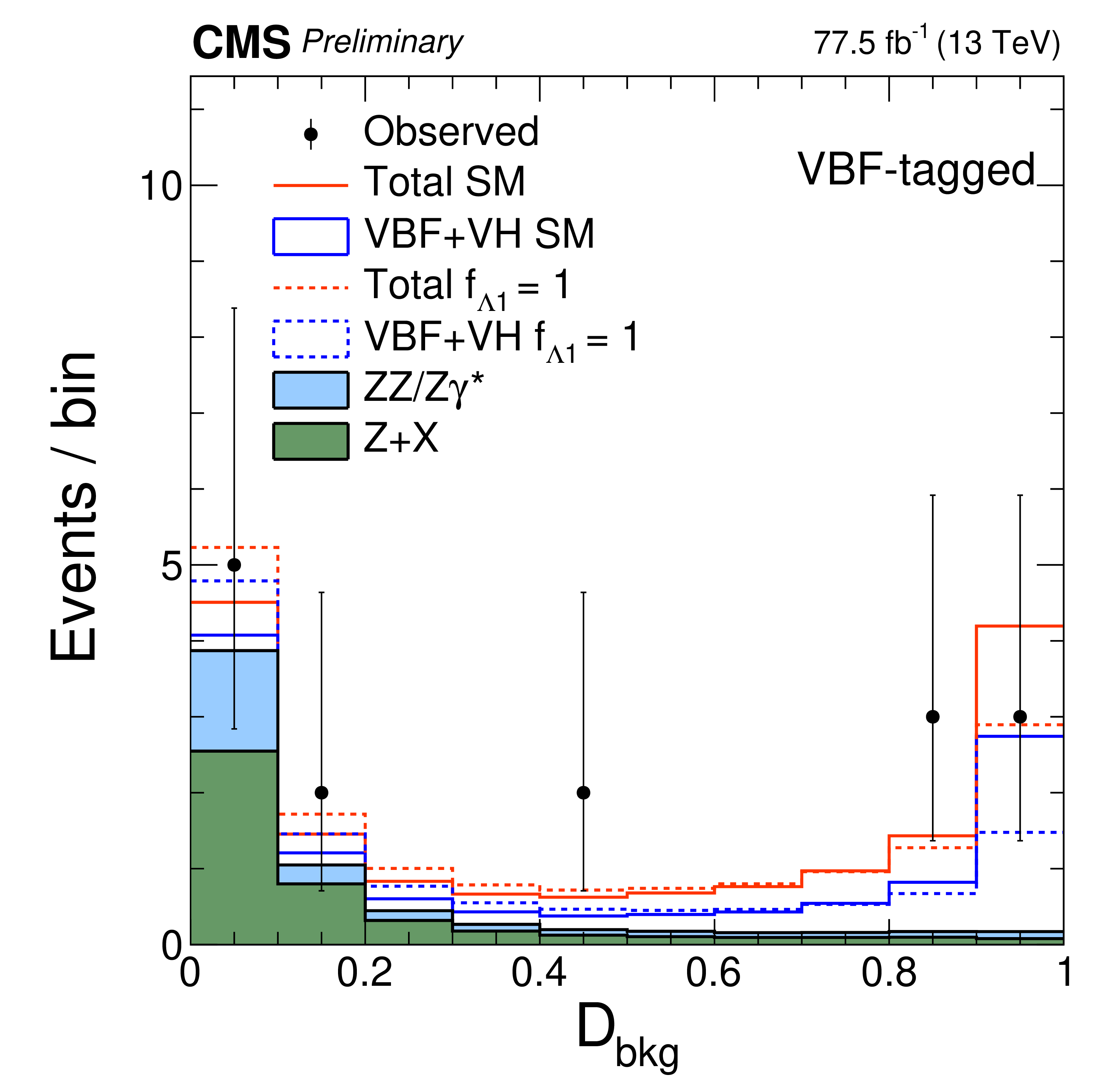
png pdf	Additional Figure 3-a: Distribution of the $\mathcal {D}_{\rm bkg}$ kinematic discriminant in the on-shell $f_{\Lambda 1}$ analysis for the VBF-tagged category. The decay or production information used in the discriminants depends on the tagging category. Points with error bars show data and histograms show expectations for background and SM or BSM signal as indicated in the legend.
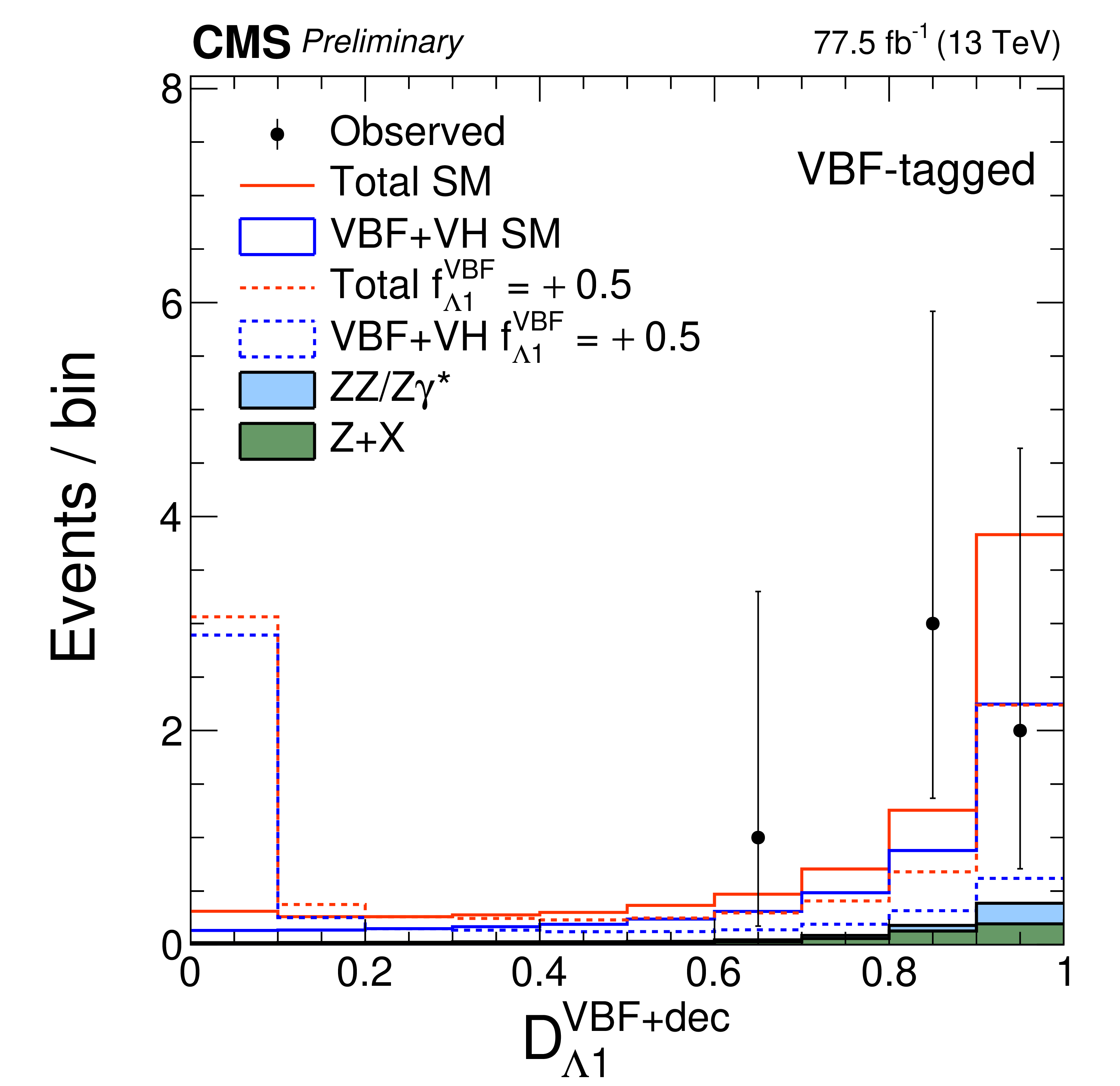
png pdf	Additional Figure 3-b: Distribution of the $\mathcal {D}_{\Lambda 1}$ kinematic discriminant in the on-shell $f_{\Lambda 1}$ analysis for the VBF-tagged category. The decay or production information used in the discriminants depends on the tagging category. $f_{\Lambda 1}^\text {VBF}$ is defined by analogy with $f_{\Lambda 1}$, but using the cross sections for the VBF process. Points with error bars show data and histograms show expectations for background and SM or BSM signal as indicated in the legend.
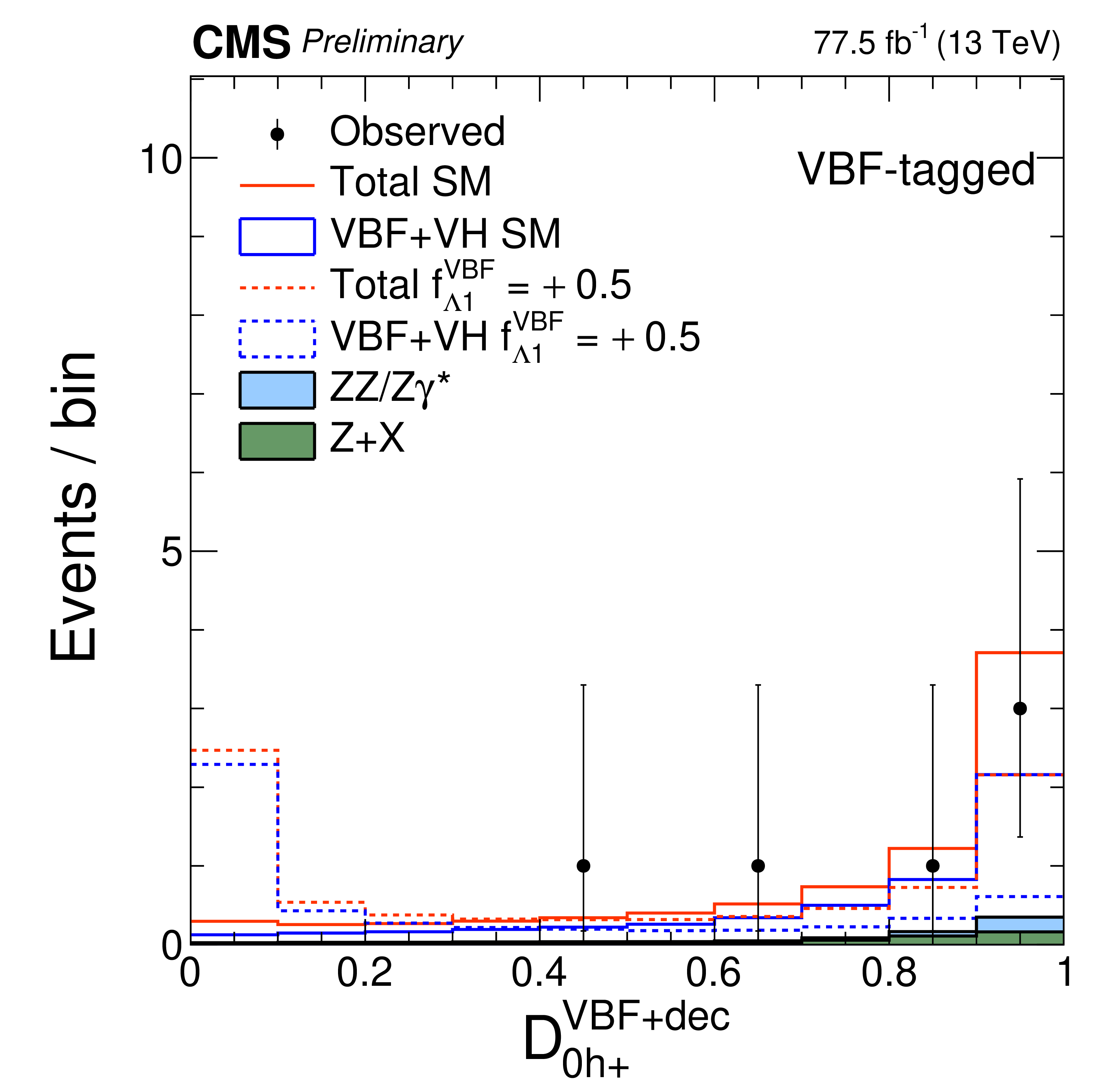
png pdf	Additional Figure 3-c: Distribution of the $\mathcal {D}_{0h+}$ kinematic discriminant in the on-shell $f_{\Lambda 1}$ analysis for the VBF-tagged category. The decay or production information used in the discriminants depends on the tagging category. $f_{\Lambda 1}^\text {VBF}$ is defined by analogy with $f_{\Lambda 1}$, but using the cross sections for the VBF process. Points with error bars show data and histograms show expectations for background and SM or BSM signal as indicated in the legend.
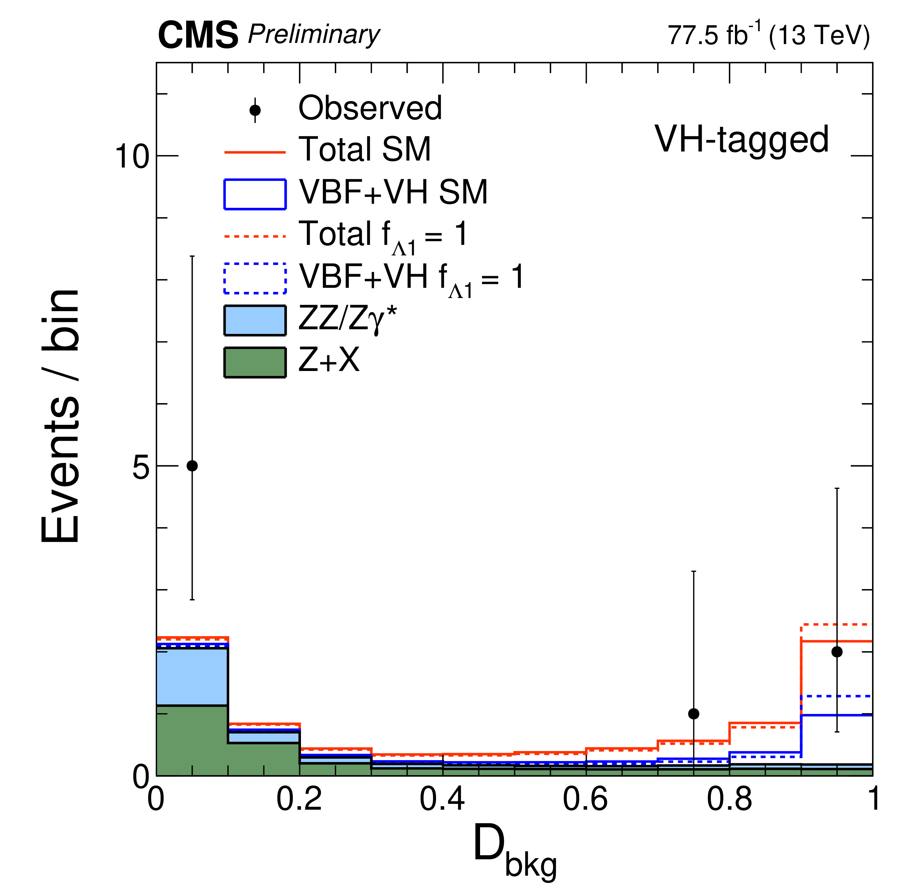
png pdf	Additional Figure 3-d: Distribution of the $\mathcal {D}_{\rm bkg}$ kinematic discriminant in the on-shell $f_{\Lambda 1}$ analysis for the VH-tagged category. The decay or production information used in the discriminants depends on the tagging category. Points with error bars show data and histograms show expectations for background and SM or BSM signal as indicated in the legend.
png pdf	Additional Figure 3-e: Distribution of the $\mathcal {D}_{\Lambda 1}$ kinematic discriminant in the on-shell $f_{\Lambda 1}$ analysis for the VH-tagged category. The decay or production information used in the discriminants depends on the tagging category. $f_{\Lambda 1}^{\mathrm {V} {\mathrm {H}}}$ is defined by analogy with $f_{\Lambda 1}$, but using the cross sections for the VH process. Points with error bars show data and histograms show expectations for background and SM or BSM signal as indicated in the legend.
png pdf	Additional Figure 3-f: Distribution of the $\mathcal {D}_{0h+}$ kinematic discriminant in the on-shell $f_{\Lambda 1}$ analysis for the VH-tagged category. The decay or production information used in the discriminants depends on the tagging category. $f_{\Lambda 1}^{\mathrm {V} {\mathrm {H}}}$ is defined by analogy with $f_{\Lambda 1}$, but using the cross sections for the VH process. Points with error bars show data and histograms show expectations for background and SM or BSM signal as indicated in the legend.
png pdf	Additional Figure 3-g: Distribution of the $\mathcal {D}_{\rm bkg}$ kinematic discriminant in the on-shell $f_{\Lambda 1}$ analysis for the untagged category. The decay or production information used in the discriminants depends on the tagging category. Points with error bars show data and histograms show expectations for background and SM or BSM signal as indicated in the legend.
png pdf	Additional Figure 3-h: Distribution of the $\mathcal {D}_{0h+}$ kinematic discriminant in the on-shell $f_{\Lambda 1}$ analysis for the untagged category. The decay or production information used in the discriminants depends on the tagging category. Points with error bars show data and histograms show expectations for background and SM or BSM signal as indicated in the legend.
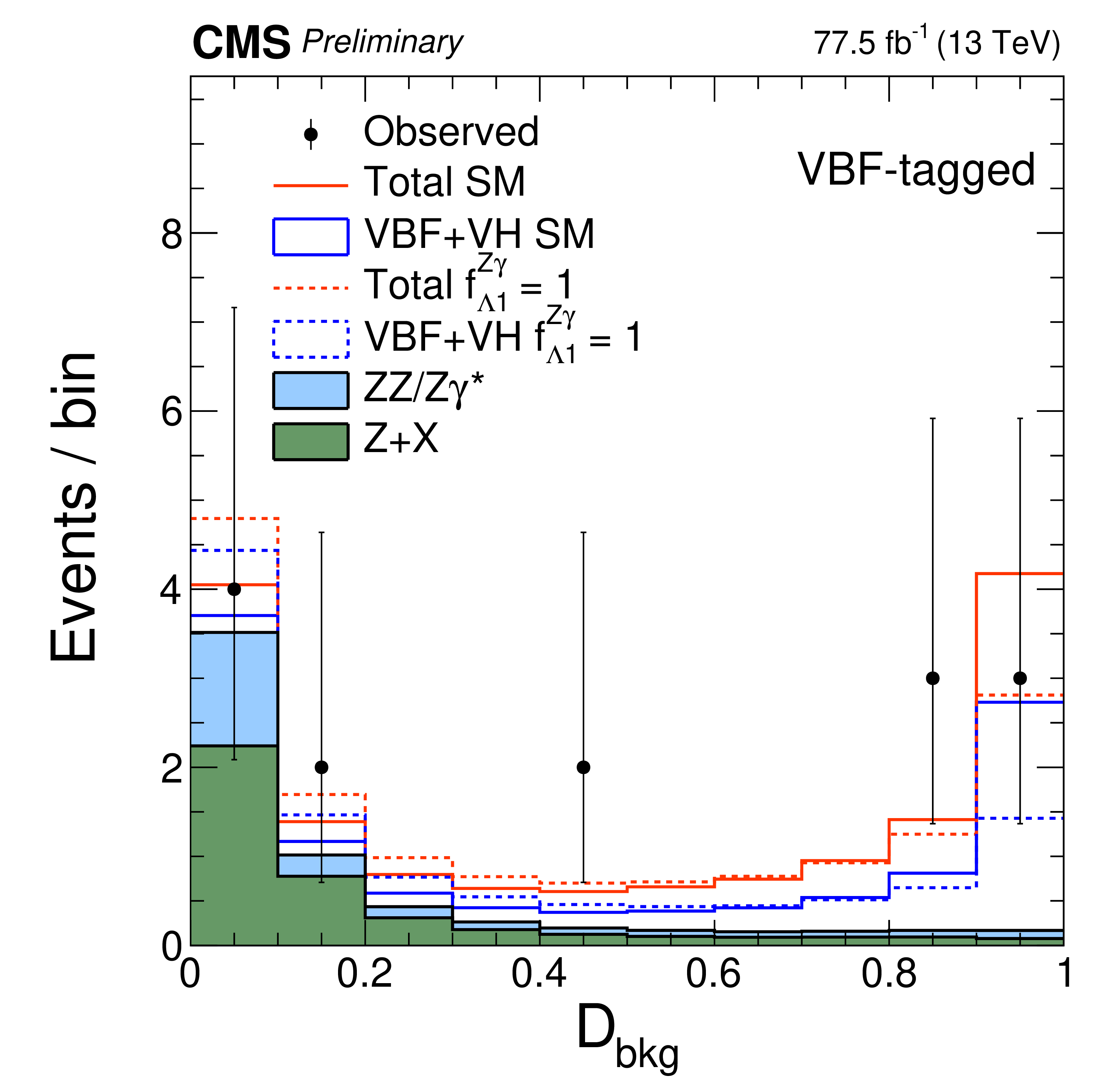
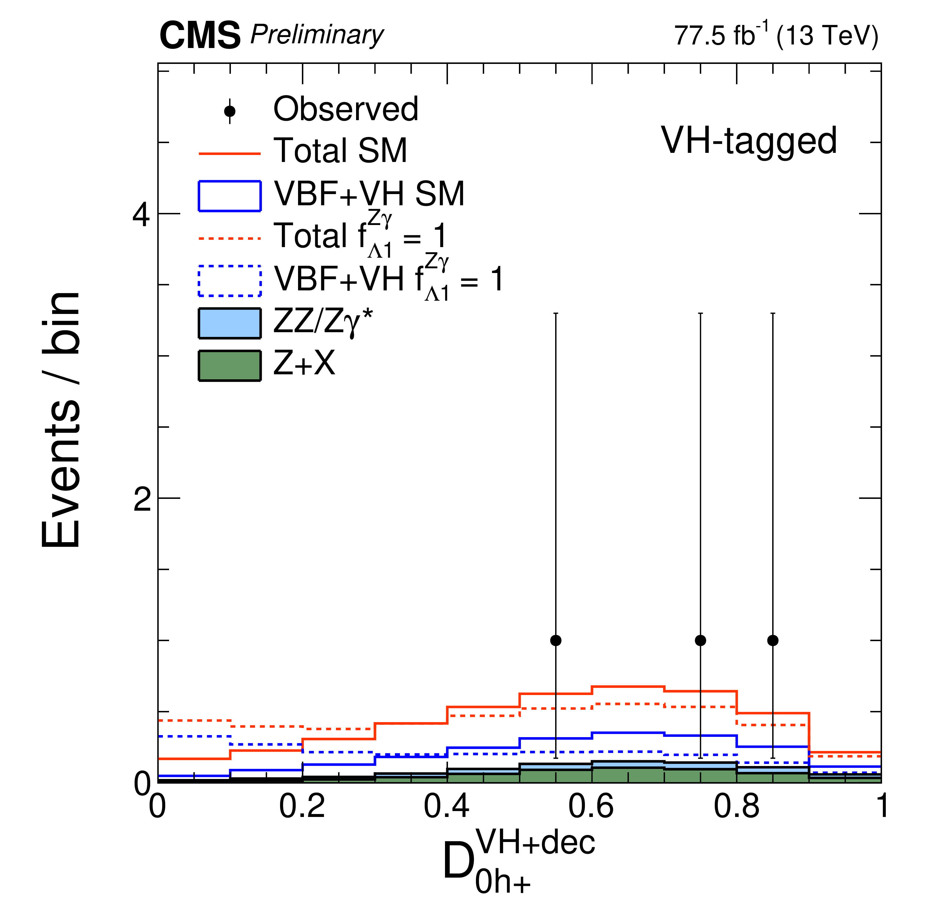
png pdf	Additional Figure 4: Distributions of kinematic discriminants in the on-shell $f_{\Lambda 1}^{{\mathrm {Z}} \gamma}$ analysis: $\mathcal {D}_{\rm bkg}$ (a), (d), (g), $\mathcal {D}_{\Lambda 1}^{{\mathrm {Z}} \gamma}$ (b), (e), and $\mathcal {D}_{0h+}$ (c), (f), (h). Three tagging categories are shown: VBF-tagged (a)-(c), VH-tagged (d)-(f), and untagged (g), (h). The decay or production information used in the discriminants depends on the tagging category. Points with error bars show data and histograms show expectations for background and SM or BSM signal as indicated in the legend.
png pdf	Additional Figure 4-a: Distribution of the $\mathcal {D}_{\rm bkg}$ kinematic discriminant in the on-shell $f_{\Lambda 1}^{{\mathrm {Z}} \gamma}$ analysis for the VBF-tagged category. The decay or production information used in the discriminant depends on the tagging category. Points with error bars show data and histograms show expectations for background and SM or BSM signal as indicated in the legend.
png pdf	Additional Figure 4-b: Distribution of the $\mathcal {D}_{\Lambda 1}^{{\mathrm {Z}} \gamma}$ kinematic discriminant in the on-shell $f_{\Lambda 1}^{{\mathrm {Z}} \gamma}$ analysis for the VBF-tagged category. The decay or production information used in the discriminant depends on the tagging category. Points with error bars show data and histograms show expectations for background and SM or BSM signal as indicated in the legend.
png pdf	Additional Figure 4-c: Distribution of the $\mathcal {D}_{0h+}$ kinematic discriminant in the on-shell $f_{\Lambda 1}^{{\mathrm {Z}} \gamma}$ analysis for the VBF-tagged category. The decay or production information used in the discriminant depends on the tagging category. Points with error bars show data and histograms show expectations for background and SM or BSM signal as indicated in the legend.
png pdf	Additional Figure 4-d: Distribution of the $\mathcal {D}_{\rm bkg}$ kinematic discriminant in the on-shell $f_{\Lambda 1}^{{\mathrm {Z}} \gamma}$ analysis for the VH-tagged category. The decay or production information used in the discriminant depends on the tagging category. Points with error bars show data and histograms show expectations for background and SM or BSM signal as indicated in the legend.
png pdf	Additional Figure 4-e: Distribution of the $\mathcal {D}_{\Lambda 1}^{{\mathrm {Z}} \gamma}$ kinematic discriminant in the on-shell $f_{\Lambda 1}^{{\mathrm {Z}} \gamma}$ analysis for the VH-tagged category. The decay or production information used in the discriminant depends on the tagging category. Points with error bars show data and histograms show expectations for background and SM or BSM signal as indicated in the legend.
png pdf	Additional Figure 4-f: Distribution of the $\mathcal {D}_{0h+}$ kinematic discriminant in the on-shell $f_{\Lambda 1}^{{\mathrm {Z}} \gamma}$ analysis for the VH-tagged category. The decay or production information used in the discriminant depends on the tagging category. Points with error bars show data and histograms show expectations for background and SM or BSM signal as indicated in the legend.
png pdf	Additional Figure 4-g: Distribution of the $\mathcal {D}_{\rm bkg}$ kinematic discriminant in the on-shell $f_{\Lambda 1}^{{\mathrm {Z}} \gamma}$ analysis for the untagged category. The decay or production information used in the discriminant depends on the tagging category. Points with error bars show data and histograms show expectations for background and SM or BSM signal as indicated in the legend.
png pdf	Additional Figure 4-h: Distribution of the $\mathcal {D}_{0h+}$ kinematic discriminant in the on-shell $f_{\Lambda 1}^{{\mathrm {Z}} \gamma}$ analysis for the untagged category. The decay or production information used in the discriminant depends on the tagging category. Points with error bars show data and histograms show expectations for background and SM or BSM signal as indicated in the legend.
png pdf	Additional Figure 5: Distributions of $\mathcal {D}_{\rm bkg}$ kinematic discriminants in the off-shell SM-like width analysis. Three tagging categories are shown: VBF-tagged (a), VH-tagged (b), and untagged (c). The decay or production information used in the discriminants depends on the tagging category. The requirement $m_{4\ell} >$ 340 GeV is applied in order to enhance signal over background contributions. Points with error bars show data and histograms show expectations for background and SM or BSM signal as indicated in the legend.
png pdf	Additional Figure 5-a: Distribution of $\mathcal {D}_{\rm bkg}$ kinematic discriminant in the off-shell SM-like width analysis for the VBF-tagged category. The decay or production information used in the discriminant depends on the tagging category. The requirement $m_{4\ell} >$ 340 GeV is applied in order to enhance signal over background contributions. Points with error bars show data and histograms show expectations for background and SM or BSM signal as indicated in the legend.
png pdf	Additional Figure 5-b: Distribution of $\mathcal {D}_{\rm bkg}$ kinematic discriminant in the off-shell SM-like width analysis for the VH-tagged category. The decay or production information used in the discriminant depends on the tagging category. The requirement $m_{4\ell} >$ 340 GeV is applied in order to enhance signal over background contributions. Points with error bars show data and histograms show expectations for background and SM or BSM signal as indicated in the legend.
png pdf	Additional Figure 5-c: Distribution of $\mathcal {D}_{\rm bkg}$ kinematic discriminant in the off-shell SM-like width analysis for the untagged category. The decay or production information used in the discriminant depends on the tagging category. The requirement $m_{4\ell} >$ 340 GeV is applied in order to enhance signal over background contributions. Points with error bars show data and histograms show expectations for background and SM or BSM signal as indicated in the legend.
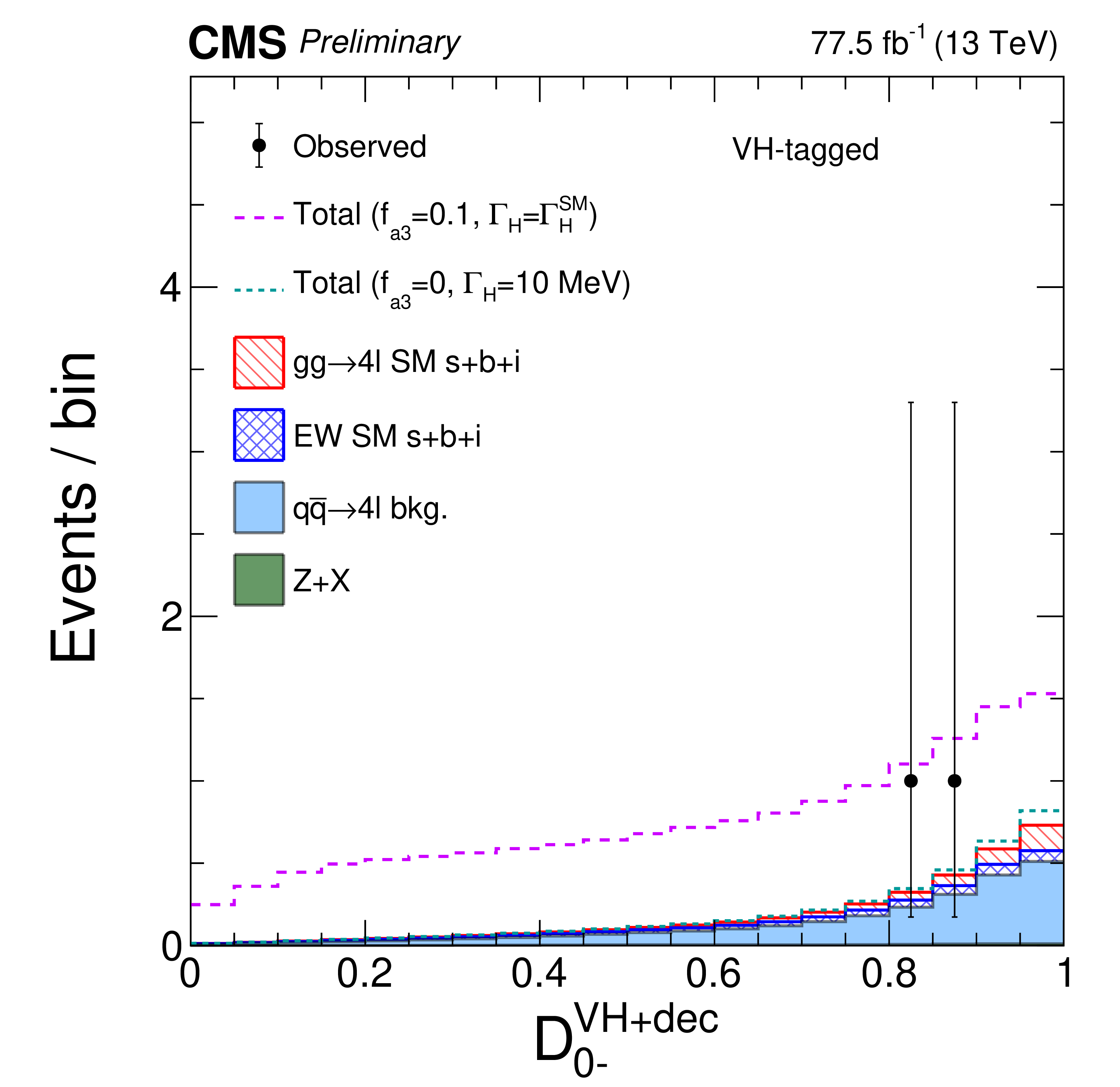
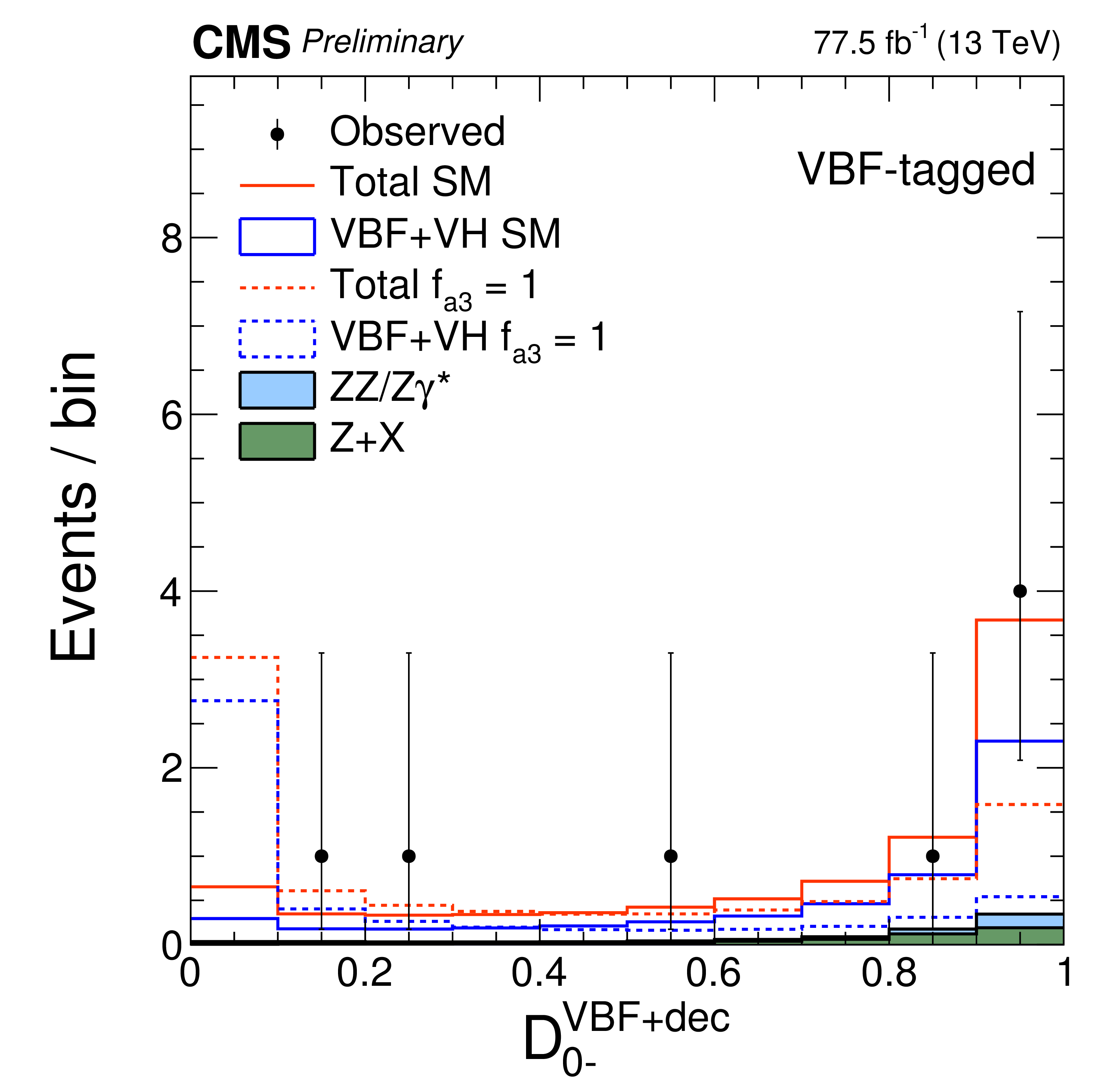
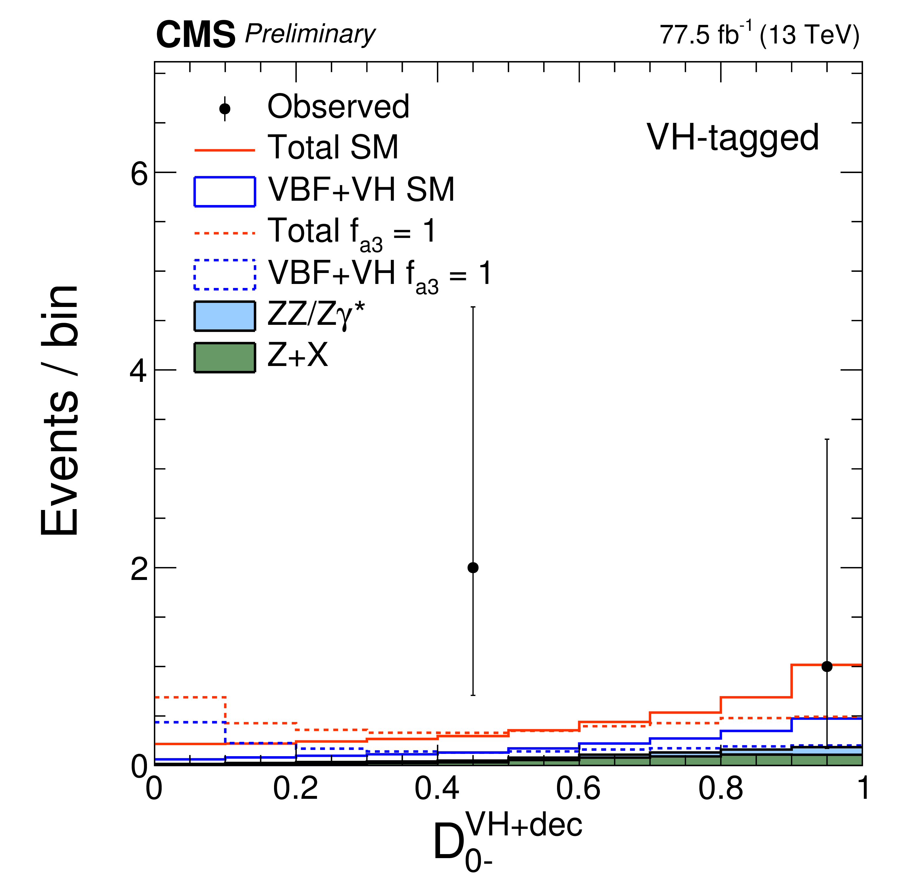
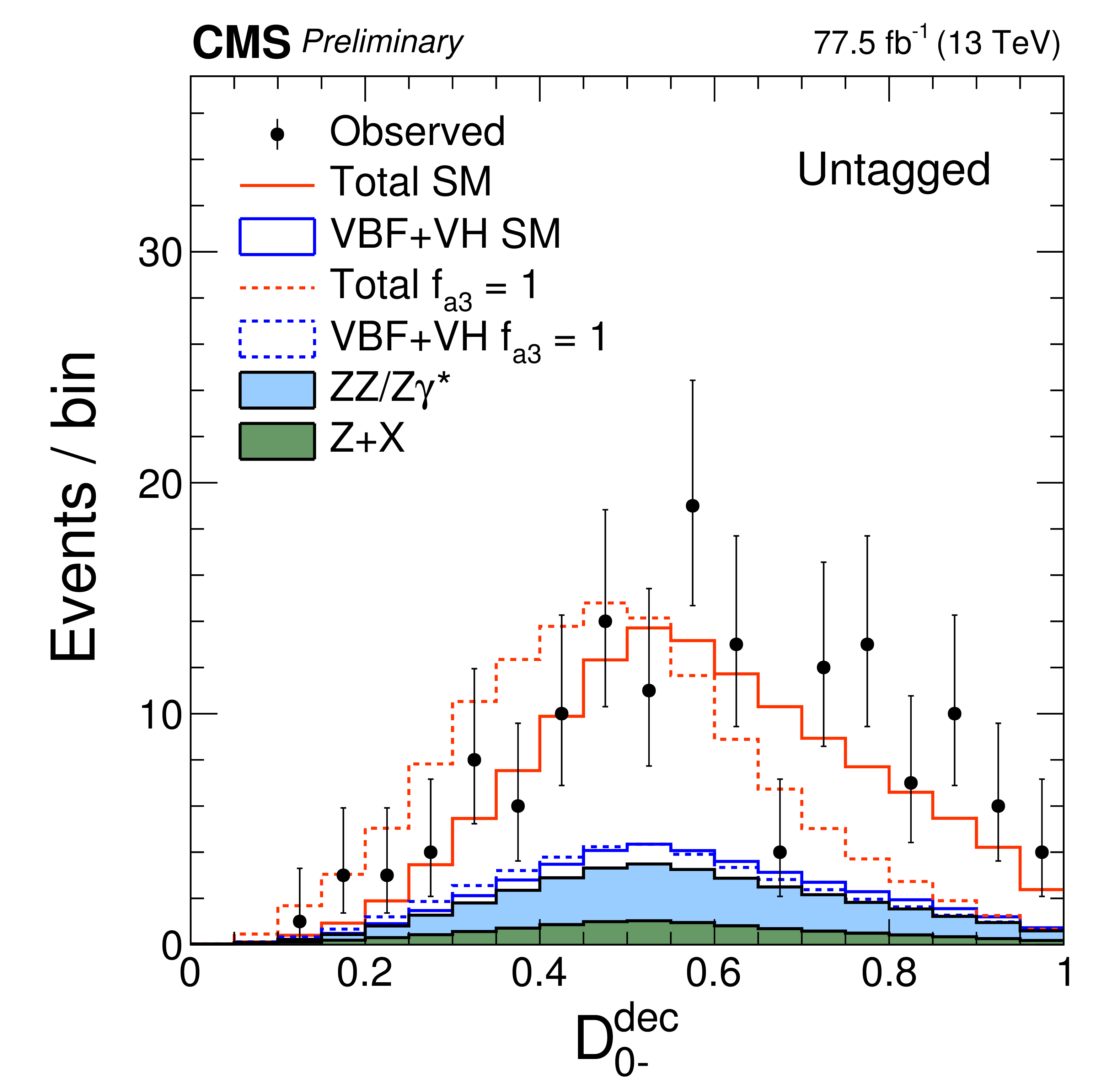
png pdf	Additional Figure 6: Distributions of kinematic discriminants in the off-shell $f_{a3}$ analysis: $m_{4\ell}$ (a), (c), (e), and $\mathcal {D}_{0-}$ (b), (d), (f). Three tagging categories are shown: VBF-tagged (a), (b), VH-tagged (c), (d), and untagged (e), (f). The decay or production information used in the discriminants depends on the tagging category. The requirement $m_{4\ell} >$ 340 GeV is applied in order to enhance signal over background contributions. Points with error bars show data and histograms show expectations for background and SM or BSM signal as indicated in the legend.
png pdf	Additional Figure 6-a: Distribution of the $m_{4\ell}$ kinematic discriminant in the off-shell $f_{a3}$ analysis for the VBF-tagged category. The decay or production information used in the discriminant depends on the tagging category. The requirement $m_{4\ell} >$ 340 GeV is applied in order to enhance signal over background contributions. Points with error bars show data and histograms show expectations for background and SM or BSM signal as indicated in the legend.
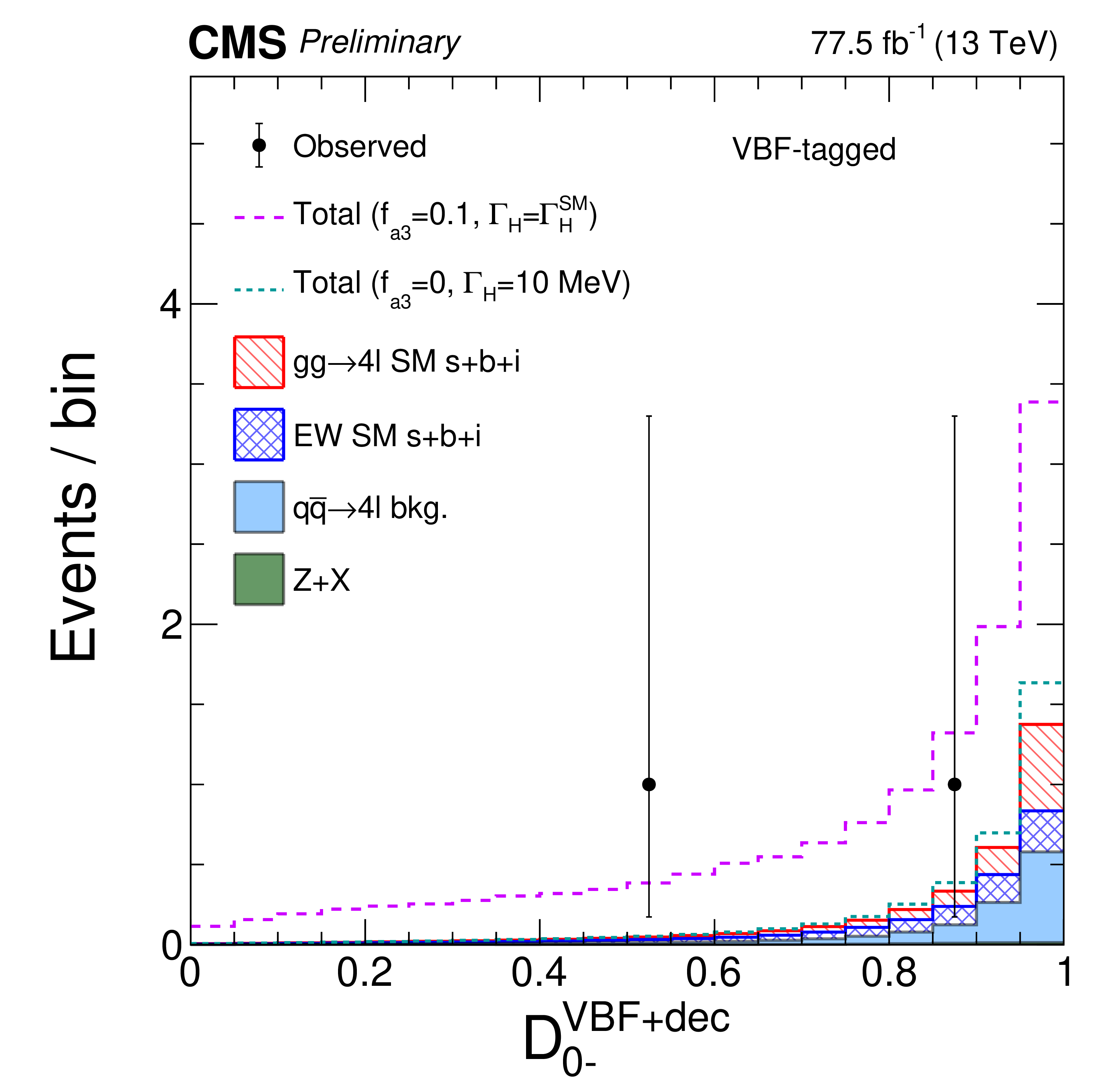
png pdf	Additional Figure 6-b: Distribution of the $\mathcal {D}_{0-}$ kinematic discriminant in the off-shell $f_{a3}$ analysis for the VBF-tagged category. The decay or production information used in the discriminant depends on the tagging category. The requirement $m_{4\ell} >$ 340 GeV is applied in order to enhance signal over background contributions. Points with error bars show data and histograms show expectations for background and SM or BSM signal as indicated in the legend.
png pdf	Additional Figure 6-c: Distribution of the $m_{4\ell}$ kinematic discriminant in the off-shell $f_{a3}$ analysis for the VH-tagged category. The decay or production information used in the discriminant depends on the tagging category. The requirement $m_{4\ell} >$ 340 GeV is applied in order to enhance signal over background contributions. Points with error bars show data and histograms show expectations for background and SM or BSM signal as indicated in the legend.
png pdf	Additional Figure 6-d: Distribution of the $\mathcal {D}_{0-}$ kinematic discriminant in the off-shell $f_{a3}$ analysis for the VH-tagged category. The decay or production information used in the discriminant depends on the tagging category. The requirement $m_{4\ell} >$ 340 GeV is applied in order to enhance signal over background contributions. Points with error bars show data and histograms show expectations for background and SM or BSM signal as indicated in the legend.
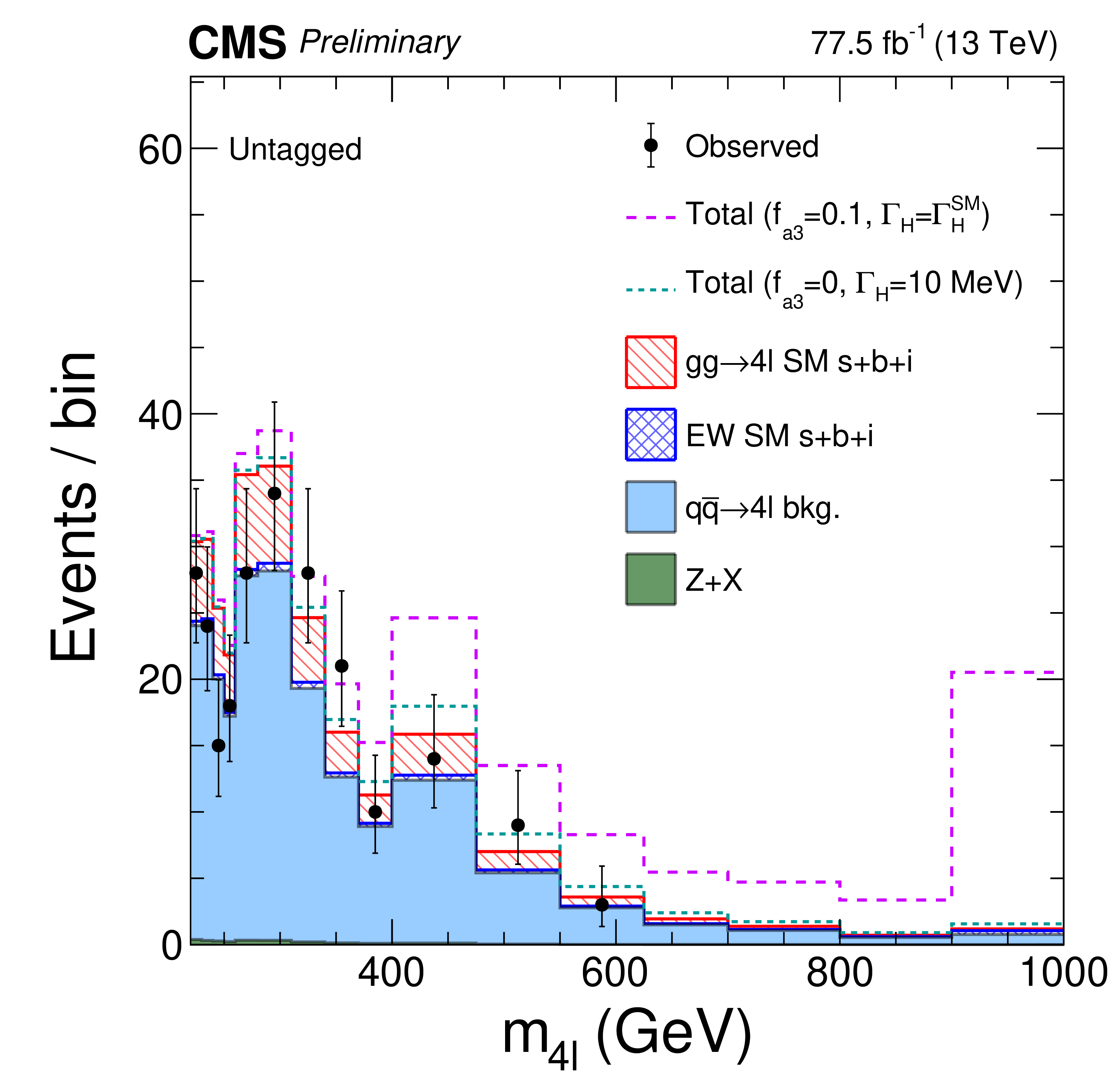
png pdf	Additional Figure 6-e: Distribution of the $m_{4\ell}$ kinematic discriminant in the off-shell $f_{a3}$ analysis for the untagged category. The decay or production information used in the discriminant depends on the tagging category. The requirement $m_{4\ell} >$ 340 GeV is applied in order to enhance signal over background contributions. Points with error bars show data and histograms show expectations for background and SM or BSM signal as indicated in the legend.
png pdf	Additional Figure 6-f: Distribution of the $\mathcal {D}_{0-}$ kinematic discriminant in the off-shell $f_{a3}$ analysis for the untagged category. The decay or production information used in the discriminant depends on the tagging category. The requirement $m_{4\ell} >$ 340 GeV is applied in order to enhance signal over background contributions. Points with error bars show data and histograms show expectations for background and SM or BSM signal as indicated in the legend.
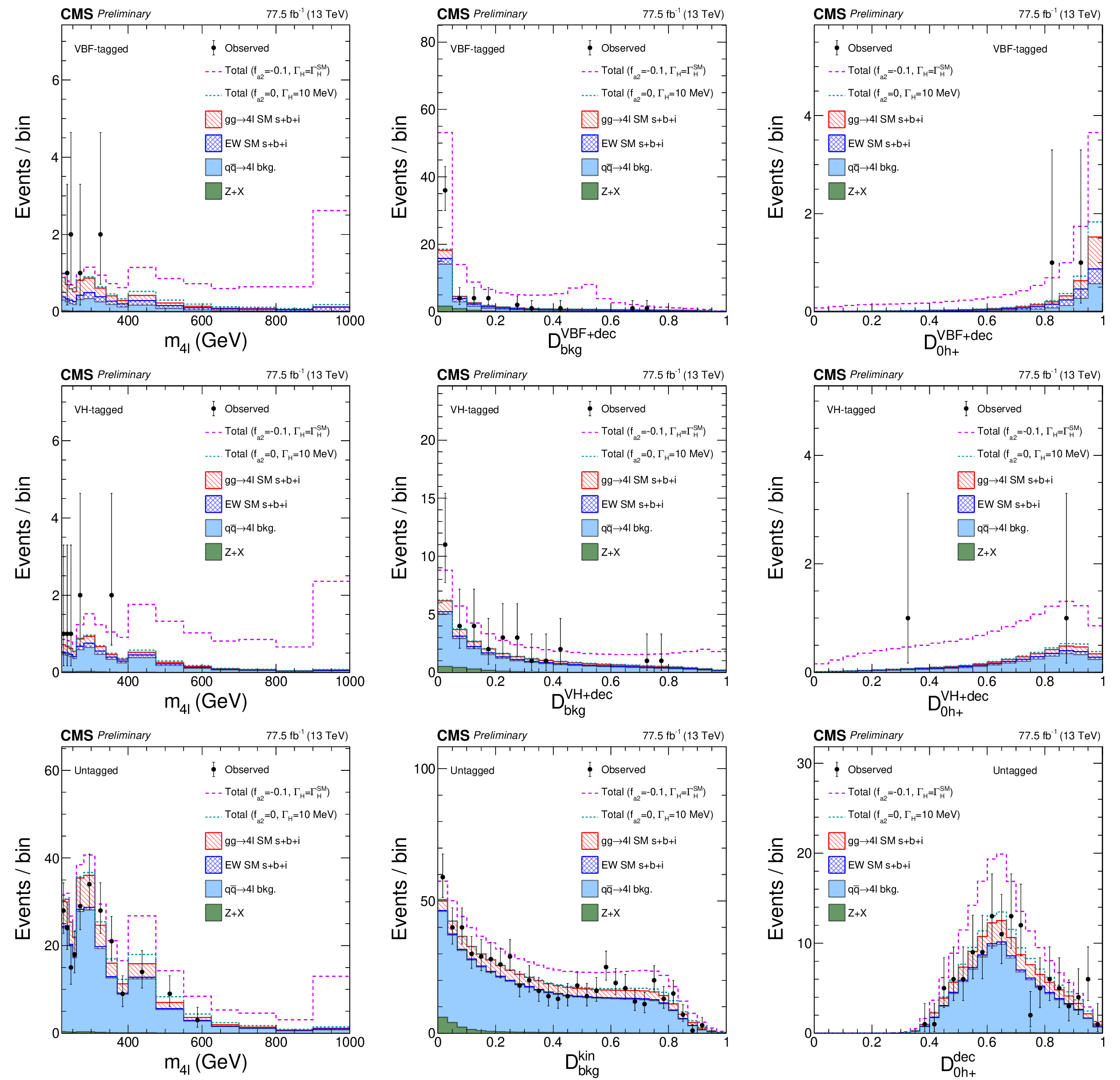
png pdf	Additional Figure 7: Distributions of kinematic discriminants in the off-shell $f_{a2}$ analysis: $m_{4\ell}$ (a), (d), (g), $\mathcal {D}_{\rm bkg}$ (b), (e), (h), and $\mathcal {D}_{0h+}$ (c), (f), (i). Three tagging categories are shown: VBF-tagged (a)-(c), VH-tagged (d)-(f), and untagged (g)-(h). The decay or production information used in the discriminants depends on the tagging category. The requirement $m_{4\ell} >$ 340 GeV is applied in order to enhance signal over background contributions. Points with error bars show data and histograms show expectations for background and SM or BSM signal as indicated in the legend.
png pdf	Additional Figure 7-a: Distribution of the $m_{4\ell}$ kinematic discriminant in the off-shell $f_{a2}$ analysis in the VBF-tagged category. The decay or production information used in the discriminant depends on the tagging category. The requirement $m_{4\ell} >$ 340 GeV is applied in order to enhance signal over background contributions. Points with error bars show data and histograms show expectations for background and SM or BSM signal as indicated in the legend.
png pdf	Additional Figure 7-b: Distribution of the $\mathcal {D}_{\rm bkg}$ kinematic discriminant in the off-shell $f_{a2}$ analysis in the VBF-tagged category. The decay or production information used in the discriminant depends on the tagging category. The requirement $m_{4\ell} >$ 340 GeV is applied in order to enhance signal over background contributions. Points with error bars show data and histograms show expectations for background and SM or BSM signal as indicated in the legend.
png pdf	Additional Figure 7-c: Distribution of the $\mathcal {D}_{0h+}$ kinematic discriminant in the off-shell $f_{a2}$ analysis in the VBF-tagged category. The decay or production information used in the discriminant depends on the tagging category. The requirement $m_{4\ell} >$ 340 GeV is applied in order to enhance signal over background contributions. Points with error bars show data and histograms show expectations for background and SM or BSM signal as indicated in the legend.
png pdf	Additional Figure 7-d: Distribution of the $m_{4\ell}$ kinematic discriminant in the off-shell $f_{a2}$ analysis in the VH-tagged category. The decay or production information used in the discriminant depends on the tagging category. The requirement $m_{4\ell} >$ 340 GeV is applied in order to enhance signal over background contributions. Points with error bars show data and histograms show expectations for background and SM or BSM signal as indicated in the legend.
png pdf	Additional Figure 7-e: Distribution of the $\mathcal {D}_{\rm bkg}$ kinematic discriminant in the off-shell $f_{a2}$ analysis in the VH-tagged category. The decay or production information used in the discriminant depends on the tagging category. The requirement $m_{4\ell} >$ 340 GeV is applied in order to enhance signal over background contributions. Points with error bars show data and histograms show expectations for background and SM or BSM signal as indicated in the legend.
png pdf	Additional Figure 7-f: Distribution of the $\mathcal {D}_{0h+}$ kinematic discriminant in the off-shell $f_{a2}$ analysis in the VH-tagged category. The decay or production information used in the discriminant depends on the tagging category. The requirement $m_{4\ell} >$ 340 GeV is applied in order to enhance signal over background contributions. Points with error bars show data and histograms show expectations for background and SM or BSM signal as indicated in the legend.
png pdf	Additional Figure 7-g: Distribution of the $m_{4\ell}$ kinematic discriminant in the off-shell $f_{a2}$ analysis in the untagged category. The decay or production information used in the discriminant depends on the tagging category. The requirement $m_{4\ell} >$ 340 GeV is applied in order to enhance signal over background contributions. Points with error bars show data and histograms show expectations for background and SM or BSM signal as indicated in the legend.
png pdf	Additional Figure 7-h: Distribution of the $\mathcal {D}_{\rm bkg}$ kinematic discriminant in the off-shell $f_{a2}$ analysis in the untagged category. The decay or production information used in the discriminant depends on the tagging category. The requirement $m_{4\ell} >$ 340 GeV is applied in order to enhance signal over background contributions. Points with error bars show data and histograms show expectations for background and SM or BSM signal as indicated in the legend.
png pdf	Additional Figure 7-i: Distribution of the $\mathcal {D}_{0h+}$ kinematic discriminant in the off-shell $f_{a2}$ analysis in the untagged category. The decay or production information used in the discriminant depends on the tagging category. The requirement $m_{4\ell} >$ 340 GeV is applied in order to enhance signal over background contributions. Points with error bars show data and histograms show expectations for background and SM or BSM signal as indicated in the legend.
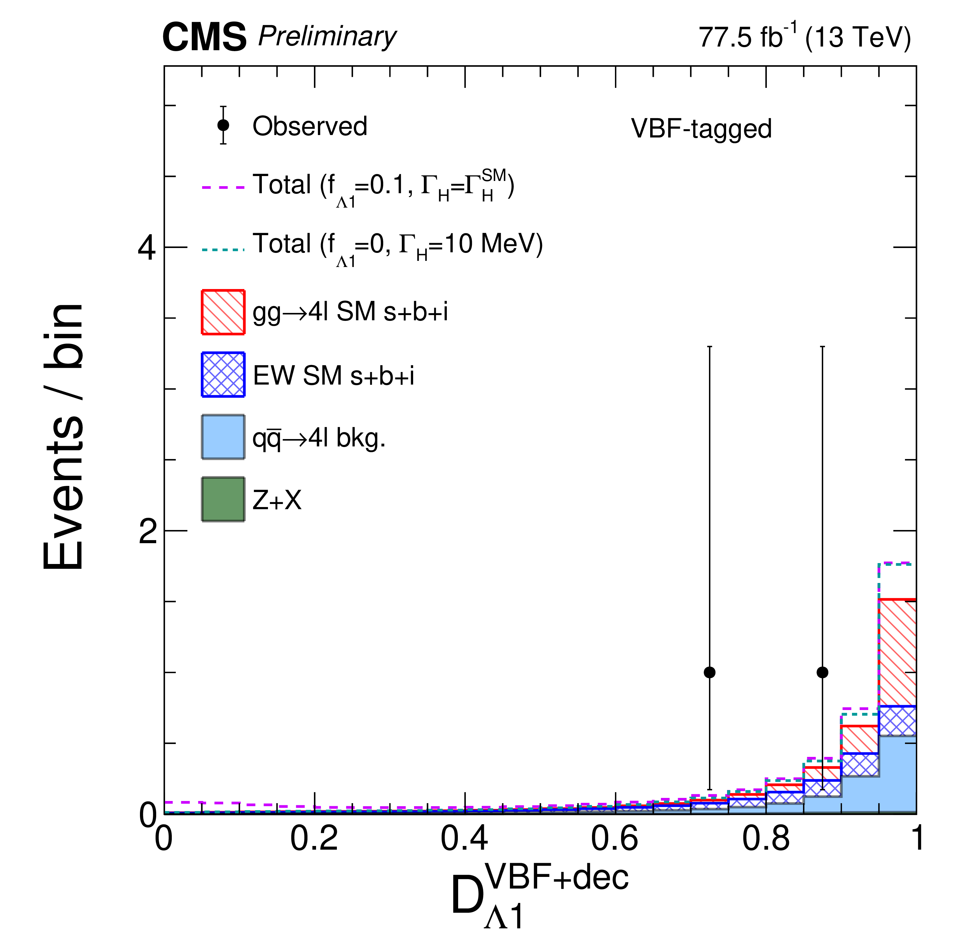
png pdf	Additional Figure 8: Distributions of kinematic discriminants in the off-shell $f_{\Lambda 1}$ analysis: $m_{4\ell}$ (a), (d), (g), $\mathcal {D}_{\rm bkg}$ (b), (e), (h), and $\mathcal {D}_{\Lambda 1}$ (c), (f), (i). Three tagging categories are shown: VBF-tagged (a)-(c), VH-tagged (d)-(f), and untagged (g)-(h). The decay or production information used in the discriminants depends on the tagging category. The requirement $m_{4\ell} >$ 340 GeV is applied in order to enhance signal over background contributions. Points with error bars show data and histograms show expectations for background and SM or BSM signal as indicated in the legend.
png pdf	Additional Figure 8-a: Distribution of the $m_{4\ell}$ kinematic discriminant in the off-shell $f_{\Lambda 1}$ analysis for the VBF-tagged category. The decay or production information used in the discriminant depends on the tagging category. The requirement $m_{4\ell} >$ 340 GeV is applied in order to enhance signal over background contributions. Points with error bars show data and histograms show expectations for background and SM or BSM signal as indicated in the legend.
png pdf	Additional Figure 8-b: Distribution of the $\mathcal {D}_{\rm bkg}$ kinematic discriminant in the off-shell $f_{\Lambda 1}$ analysis for the VBF-tagged category. The decay or production information used in the discriminant depends on the tagging category. The requirement $m_{4\ell} >$ 340 GeV is applied in order to enhance signal over background contributions. Points with error bars show data and histograms show expectations for background and SM or BSM signal as indicated in the legend.
png pdf	Additional Figure 8-c: Distribution of the $\mathcal {D}_{\Lambda 1}$ kinematic discriminant in the off-shell $f_{\Lambda 1}$ analysis for the VBF-tagged category. The decay or production information used in the discriminant depends on the tagging category. The requirement $m_{4\ell} >$ 340 GeV is applied in order to enhance signal over background contributions. Points with error bars show data and histograms show expectations for background and SM or BSM signal as indicated in the legend.
png pdf	Additional Figure 8-d: Distribution of the $m_{4\ell}$ kinematic discriminant in the off-shell $f_{\Lambda 1}$ analysis for the VH-tagged category. The decay or production information used in the discriminant depends on the tagging category. The requirement $m_{4\ell} >$ 340 GeV is applied in order to enhance signal over background contributions. Points with error bars show data and histograms show expectations for background and SM or BSM signal as indicated in the legend.
png pdf	Additional Figure 8-e: Distribution of the $\mathcal {D}_{\rm bkg}$ kinematic discriminant in the off-shell $f_{\Lambda 1}$ analysis for the VH-tagged category. The decay or production information used in the discriminant depends on the tagging category. The requirement $m_{4\ell} >$ 340 GeV is applied in order to enhance signal over background contributions. Points with error bars show data and histograms show expectations for background and SM or BSM signal as indicated in the legend.
png pdf	Additional Figure 8-f: Distribution of the $\mathcal {D}_{\Lambda 1}$ kinematic discriminant in the off-shell $f_{\Lambda 1}$ analysis for the VH-tagged category. The decay or production information used in the discriminant depends on the tagging category. The requirement $m_{4\ell} >$ 340 GeV is applied in order to enhance signal over background contributions. Points with error bars show data and histograms show expectations for background and SM or BSM signal as indicated in the legend.
png pdf	Additional Figure 8-g: Distribution of the $m_{4\ell}$ kinematic discriminant in the off-shell $f_{\Lambda 1}$ analysis for the untagged category. The decay or production information used in the discriminant depends on the tagging category. The requirement $m_{4\ell} >$ 340 GeV is applied in order to enhance signal over background contributions. Points with error bars show data and histograms show expectations for background and SM or BSM signal as indicated in the legend.
png pdf	Additional Figure 8-h: Distribution of the $\mathcal {D}_{\rm bkg}$ kinematic discriminant in the off-shell $f_{\Lambda 1}$ analysis for the untagged category. The decay or production information used in the discriminant depends on the tagging category. The requirement $m_{4\ell} >$ 340 GeV is applied in order to enhance signal over background contributions. Points with error bars show data and histograms show expectations for background and SM or BSM signal as indicated in the legend.
png pdf	Additional Figure 8-i: Distribution of the $\mathcal {D}_{\Lambda 1}$ kinematic discriminant in the off-shell $f_{\Lambda 1}$ analysis for the untagged category. The decay or production information used in the discriminant depends on the tagging category. The requirement $m_{4\ell} >$ 340 GeV is applied in order to enhance signal over background contributions. Points with error bars show data and histograms show expectations for background and SM or BSM signal as indicated in the legend.
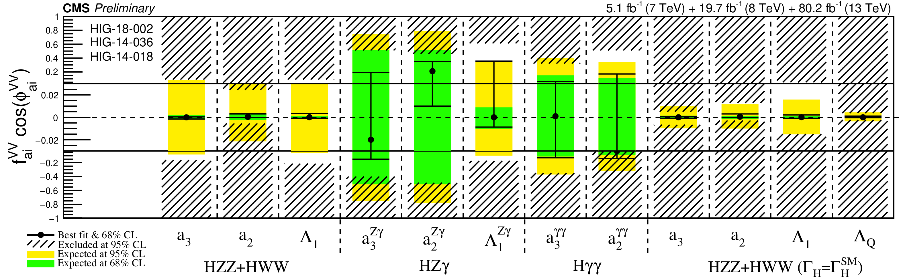
png pdf	Additional Figure 9: Summary of allowed confidence level intervals on anomalous coupling parameters in HVV interactions under the assumption that all the coupling ratios are real ($\phi _{ai}^{\mathrm {V} \mathrm {V}}=0$ or $\pi$). The ${\mathrm {H}} {\mathrm {Z}} {\mathrm {Z}} + {\mathrm {H}} {\mathrm {W}} {\mathrm {W}}$ coupling limits assume that $a_{i}^{{\mathrm {Z}} {\mathrm {Z}}}=a_{i}^{{\mathrm {W}} {\mathrm {W}}}$. The expected 68% and 95% CL regions are shown as green and yellow bands, and the observed regions are shown as points with errors and the excluded hatched regions. The limits on $f_{a2,3}^{{\mathrm {Z}} \gamma,\gamma \gamma}$ are from Ref. [25], and the limits on $f_{\Lambda Q}$ are from Ref. [13].

References
1	S. L. Glashow	Partial-symmetries of Weak Interactions	NP 22 (1961) 579
2	F. Englert and R. Brout	Broken Symmetry and the Mass of Gauge Vector Mesons	PRL 13 (1964) 321
3	P. W. Higgs	Broken symmetries, massless particles and gauge fields	PL12 (1964) 132
4	P. W. Higgs	Broken Symmetries and the Masses of Gauge Bosons	PRL 13 (1964) 508
5	G. S. Guralnik, C. R. Hagen, and T. W. B. Kibble	Global Conservation Laws and Massless Particles	PRL 13 (1964) 585
6	S. Weinberg	A Model of Leptons	PRL 19 (1967) 1264
7	A. Salam	Weak and electromagnetic interactions	in Elementary particle physics: relativistic groups and analyticity, N. Svartholm, ed., p. 367 Almqvist \& Wiksell, Stockholm, 1968 Proceedings of the eighth Nobel symposium
8	ATLAS Collaboration	Observation of a new particle in the search for the Standard Model Higgs boson with the ATLAS detector at the LHC	PLB 716 (2012) 1	1207.7214
9	CMS Collaboration	Observation of a new boson at a mass of 125 GeV with the CMS experiment at the LHC	PLB716 (2012) 30--61	CMS-HIG-12-028 1207.7235
10	CMS Collaboration	Observation of a new boson with mass near 125 GeV in pp collisions at $\sqrt{s} =$ 7 and 8 TeV	JHEP 06 (2013) 081	CMS-HIG-12-036 1303.4571
11	CMS Collaboration	Constraints on the Higgs boson width from off-shell production and decay to Z-boson pairs	PLB736 (2014) 64--85	CMS-HIG-14-002 1405.3455
12	ATLAS Collaboration	Constraints on the off-shell Higgs boson signal strength in the high-mass $ZZ$ and $WW$ final states with the ATLAS detector	EPJC75 (2015), no. 7, 335	1503.01060
13	CMS Collaboration	Limits on the Higgs boson lifetime and width from its decay to four charged leptons	PRD92 (2015), no. 7, 072010	CMS-HIG-14-036 1507.06656
14	CMS Collaboration	Search for Higgs boson off-shell production in proton-proton collisions at 7 and 8 TeV and derivation of constraints on its total decay width	JHEP 09 (2016) 051	CMS-HIG-14-032 1605.02329
15	ATLAS Collaboration	Constraints on off-shell Higgs boson production and the Higgs boson total width in $ZZ\to4\ell$ and $ZZ\to2\ell2\nu$ final states with the ATLAS detector		1808.01191
16	F. Caola and K. Melnikov	Constraining the Higgs boson width with ZZ production at the LHC	PRD88 (2013) 054024	1307.4935
17	N. Kauer and G. Passarino	Inadequacy of zero-width approximation for a light Higgs boson signal	JHEP 08 (2012) 116	1206.4803
18	J. M. Campbell, R. K. Ellis, and C. Williams	Bounding the Higgs width at the LHC using full analytic results for $\mathrm{g}\mathrm{g}\to \mathrm{e^-}\mathrm{e^+} \mu^- \mu^+$	JHEP 04 (2014) 060	1311.3589
19	CMS Collaboration	Precise determination of the mass of the Higgs boson and tests of compatibility of its couplings with the standard model predictions using proton collisions at 7 and 8 TeV	EPJC75 (2015), no. 5, 212	CMS-HIG-14-009 1412.8662
20	ATLAS Collaboration	Measurement of the Higgs boson mass from the $H\rightarrow \gamma\gamma$ and $H \rightarrow ZZ^{*} \rightarrow 4\ell$ channels with the ATLAS detector using 25 fb$^{-1}$ of $pp$ collision data	PRD 90 (2014) 052004	1406.3827
21	CMS Collaboration	Measurements of properties of the Higgs boson decaying into the four-lepton final state in pp collisions at $\sqrt{s}=$ 13 TeV	JHEP 11 (2017) 047	CMS-HIG-16-041 1706.09936
22	LHC Higgs Cross Section Working Group Collaboration	Handbook of LHC Higgs Cross Sections: 4. Deciphering the Nature of the Higgs Sector		1610.07922
23	CMS Collaboration	On the mass and spin-parity of the Higgs boson candidate via its decays to Z boson pairs	PRL 110 (2013) 081803	CMS-HIG-12-041 1212.6639
24	CMS Collaboration	Measurement of the properties of a Higgs boson in the four-lepton final state	PRD 89 (2014) 092007	CMS-HIG-13-002 1312.5353
25	CMS Collaboration	Constraints on the spin-parity and anomalous HVV couplings of the Higgs boson in proton collisions at 7 and 8 TeV	PRD92 (2015), no. 1, 012004	CMS-HIG-14-018 1411.3441
26	CMS Collaboration	Combined search for anomalous pseudoscalar HVV couplings in VH(H $\to b \bar b$) production and H $\to$ VV decay	PLB759 (2016) 672--696	CMS-HIG-14-035 1602.04305
27	CMS Collaboration	Constraints on anomalous Higgs boson couplings using production and decay information in the four-lepton final state	PLB775 (2017) 1--24	CMS-HIG-17-011 1707.00541
28	ATLAS Collaboration	Evidence for the spin-0 nature of the Higgs boson using ATLAS data	PLB 726 (2013) 120	1307.1432
29	ATLAS Collaboration	Study of the spin and parity of the Higgs boson in diboson decays with the ATLAS detector	EPJC75 (2015), no. 10, 476	1506.05669
30	ATLAS Collaboration	Test of CP Invariance in vector-boson fusion production of the Higgs boson using the Optimal Observable method in the ditau decay channel with the ATLAS detector	EPJC76 (2016), no. 12, 658	1602.04516
31	J. S. Gainer et al.	Beyond Geolocating: Constraining Higher Dimensional Operators in $H \to 4\ell$ with Off-Shell Production and More	PRD91 (2015), no. 3, 035011	1403.4951
32	C. Englert and M. Spannowsky	Limitations and opportunities of off-shell coupling measurements	PRD 90 (2014) 053003	1405.0285
33	M. Ghezzi, G. Passarino, and S. Uccirati	Bounding the Higgs Width Using Effective Field Theory	PoS LL2014 (2014) 072	1405.1925
34	CMS Collaboration Collaboration	Measurements of properties of the Higgs boson in the four-lepton final state at $\sqrt{s}=$ 13 TeV	CMS-PAS-HIG-18-001, CERN, Geneva
35	CMS Collaboration	Search for a new scalar resonance decaying to a pair of Z bosons in proton-proton collisions at $\sqrt{s}=$ 13 TeV	JHEP 06 (2018) 127	CMS-HIG-17-012 1804.01939
36	M. Gonzalez-Alonso, A. Greljo, G. Isidori, and D. Marzocca	Pseudo-observables in Higgs decays	EPJC75 (2015) 128	1412.6038
37	A. Greljo, G. Isidori, J. M. Lindert, and D. Marzocca	Pseudo-observables in electroweak Higgs production	EPJC76 (2016), no. 3, 158	1512.06135
38	Y. Gao et al.	Spin determination of single-produced resonances at hadron colliders	PRD 81 (2010) 075022	1001.3396
39	S. Bolognesi et al.	Spin and parity of a single-produced resonance at the LHC	PRD 86 (2012) 095031	1208.4018
40	I. Anderson et al.	Constraining anomalous HVV interactions at proton and lepton colliders	PRD 89 (2014) 035007	1309.4819
41	CMS Collaboration	The CMS experiment at the CERN LHC	JINST 3 (2008) S08004	CMS-00-001
42	CMS Collaboration	CMS Luminosity Measurements for the 2016 Data Taking Period	CMS-PAS-LUM-17-001	CMS-PAS-LUM-17-001
43	A. V. Gritsan, R. Roentsch, M. Schulze, and M. Xiao	Constraining anomalous Higgs boson couplings to the heavy flavor fermions using matrix element techniques	PRD94 (2016), no. 5, 055023	1606.03107
44	S. Frixione, P. Nason, and C. Oleari	Matching NLO QCD computations with Parton Shower simulations: the POWHEG method	JHEP 11 (2007) 070	0709.2092
45	E. Bagnaschi, G. Degrassi, P. Slavich, and A. Vicini	Higgs production via gluon fusion in the POWHEG approach in the SM and in the MSSM	JHEP 02 (2012) 088	1111.2854
46	P. Nason and C. Oleari	NLO Higgs boson production via vector-boson fusion matched with shower in POWHEG	JHEP 02 (2010) 037	0911.5299
47	G. Luisoni, P. Nason, C. Oleari, and F. Tramontano	$HW^{\pm}$/HZ + 0 and 1 jet at NLO with the POWHEG BOX interfaced to GoSam and their merging within MiNLO	JHEP 10 (2013) 083	1306.2542
48	H. B. Hartanto, B. Jager, L. Reina, and D. Wackeroth	Higgs boson production in association with top quarks in the POWHEG BOX	PRD91 (2015), no. 9, 094003	1501.04498
49	K. Hamilton, P. Nason, and G. Zanderighi	MINLO: Multi-Scale Improved NLO	JHEP 10 (2012) 155	1206.3572
50	J. M. Campbell and R. K. Ellis	MCFM for the Tevatron and the LHC	NPPS 205 (2010) 10	1007.3492
51	J. M. Campbell, R. K. Ellis, and C. Williams	Vector boson pair production at the LHC	JHEP 07 (2011) 018	1105.0020
52	J. M. Campbell and R. K. Ellis	Higgs Constraints from Vector Boson Fusion and Scattering	JHEP 04 (2015) 030	1502.02990
53	A. Ballestrero et al.	PHANTOM: a Monte Carlo event generator for six parton final states at high energy colliders	CPC 180 (2009) 401	0801.3359
54	S. Catani and M. Grazzini	An NNLO subtraction formalism in hadron collisions and its application to Higgs boson production at the LHC	PRL 98 (2007) 222002	hep-ph/0703012
55	M. Grazzini	NNLO predictions for the Higgs boson signal in the $H \to WW \to\ell\nu\ell\nu$ and $H \to ZZ \to 4\ell$ decay channels	JHEP 02 (2008) 043	0801.3232
56	M. Grazzini and H. Sargsyan	Heavy-quark mass effects in Higgs boson production at the LHC	JHEP 09 (2013) 129	1306.4581
57	F. Caola, K. Melnikov, R. Roentsch, and L. Tancredi	QCD corrections to ZZ production in gluon fusion at the LHC	PRD92 (2015), no. 9, 094028	1509.06734
58	K. Melnikov and M. Dowling	Production of two Z-bosons in gluon fusion in the heavy top quark approximation	PLB744 (2015) 43--47	1503.01274
59	M. Grazzini, S. Kallweit, and D. Rathlev	ZZ production at the LHC: fiducial cross sections and distributions in NNLO QCD	PLB750 (2015) 407--410	1507.06257
60	S. Gieseke, T. Kasprzik, and J. H. Kuehn	Vector-boson pair production and electroweak corrections in HERWIG++	EPJC 74 (2014) 2988	1401.3964
61	J. Baglio, L. D. Ninh, and M. M. Weber	Massive gauge boson pair production at the LHC: a next-to-leading order story	PRD 88 (2013) 113005	1307.4331
62	NNPDF Collaboration	Unbiased global determination of parton distributions and their uncertainties at NNLO and at LO	NPB855 (2012) 153--221	1107.2652
63	T. Sjostrand et al.	An introduction to pythia 8.2	Computer Physics Communications 191 (2015) 159
64	GEANT4 Collaboration	GEANT4---a simulation toolkit	NIMA 506 (2003) 250
65	M. Cacciari, G. P. Salam, and G. Soyez	The anti-$k_t$ jet clustering algorithm	JHEP 04 (2008) 063	0802.1189
66	M. Cacciari, G. P. Salam, and G. Soyez	FastJet user manual	EPJC 72 (2012) 1896	1111.6097

Compact Muon Solenoid LHC, CERN

© Copyright CERN 2018 for the benefit of the CMS Collaboration