

Compact Muon Solenoid
LHC, CERN
| CMS-PAS-EXO-20-009 | ||
| Search for long-lived heavy neutral leptons with displaced vertices in pp collisions at $\sqrt{s}=$ 13 TeV with the CMS detector | ||
| CMS Collaboration | ||
| July 2021 | ||
| Abstract: A search for heavy neutral leptons (HNLs), the hypothetical right-handed Dirac or Majorana neutrinos, is performed in final states with three charged leptons (electrons or muons) using proton-proton collision data collected by the CMS experiment at a center-of-mass energy of $\sqrt{s}=$ 13 TeV. The data correspond to an integrated luminosity of 137 fb$^{-1}$. The HNLs can be produced at the LHC through mixing with standard model (SM) neutrinos. For small values of the HNL mass ($ < $ 20 GeV) and of the HNL-SM neutrino mixing parameter squared (10$^{-7}$-10$^{-2}$), the decay length of these particles can be large enough to produce a resolved secondary vertex in the CMS silicon tracker. The study aims at identifying two leptons that form a displaced vertex with respect to the primary proton-proton collision vertex, while the third lepton is assumed to emerge from the primary vertex. No significant deviations from the SM expectations are observed, and constraints are obtained on the HNL mass and coupling strength parameters, extending the exclusion limits from previous searches in the mass range 1-18 GeV and mixing parameter values in the range of 10$^{-7}$-10$^{-5}$. | ||
|
Links:
CDS record (PDF) ;
CADI line (restricted) ;
These preliminary results are superseded in this paper, Submitted to JHEP. The superseded preliminary plots can be found here. |
||
| Figures | |
png pdf |
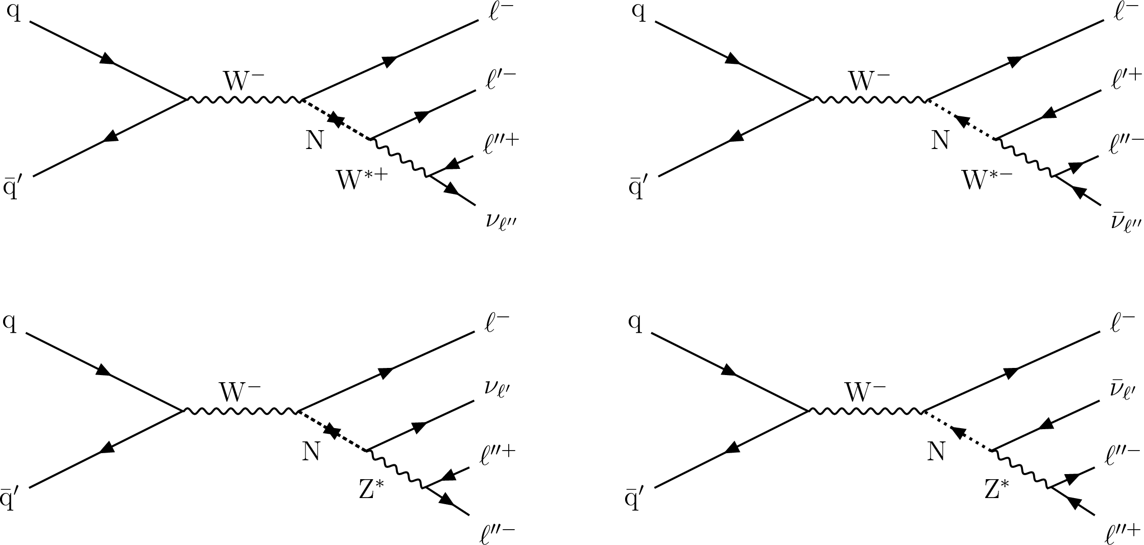
Figure 1:
Typical diagrams for the production of an HNL (N) through its mixing with a SM neutrino, leading to final states with three charged leptons and a neutrino. The HNL decay is mediated by either a W* (top row) or a Z* (bottom row) boson. In the diagrams on the left, N is assumed to be a Majorana neutrino, thus $\ell$ and $\ell'$ in the W*-mediated diagram (top) can have the same electric charge, with lepton-number violation (LNV). In the diagrams on the right the N decay conserves lepton number (LNC) and can be either a Majorana or a Dirac particle. Therefore $\ell$ and $\ell'$ in the W*-mediated diagram (top right) have always opposite charge. The present study only considers the former case, thus $\ell$ and $\ell'$ (or $\nu$-$\ell'$) always belong to the same lepton generation, and lepton flavor is conserved. In the case of the HNL decay mediated by a Z boson, $\ell$ and $\ell'$ are required to be of the same flavor. |
png pdf |
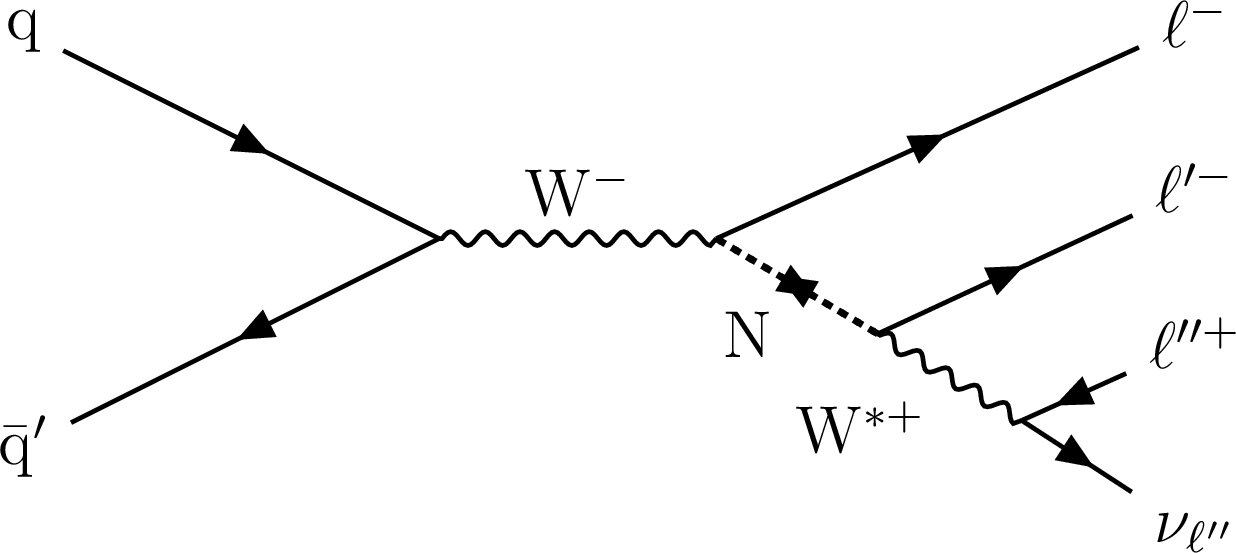
Figure 1-a:
Typical diagrams for the production of an HNL (N) through its mixing with a SM neutrino, leading to final states with three charged leptons and a neutrino. The HNL decay is mediated by either a W* (top row) or a Z* (bottom row) boson. In the diagrams on the left, N is assumed to be a Majorana neutrino, thus $\ell$ and $\ell'$ in the W*-mediated diagram (top) can have the same electric charge, with lepton-number violation (LNV). In the diagrams on the right the N decay conserves lepton number (LNC) and can be either a Majorana or a Dirac particle. Therefore $\ell$ and $\ell'$ in the W*-mediated diagram (top right) have always opposite charge. The present study only considers the former case, thus $\ell$ and $\ell'$ (or $\nu$-$\ell'$) always belong to the same lepton generation, and lepton flavor is conserved. In the case of the HNL decay mediated by a Z boson, $\ell$ and $\ell'$ are required to be of the same flavor. |

png pdf |
Figure 1-b:
Typical diagrams for the production of an HNL (N) through its mixing with a SM neutrino, leading to final states with three charged leptons and a neutrino. The HNL decay is mediated by either a W* (top row) or a Z* (bottom row) boson. In the diagrams on the left, N is assumed to be a Majorana neutrino, thus $\ell$ and $\ell'$ in the W*-mediated diagram (top) can have the same electric charge, with lepton-number violation (LNV). In the diagrams on the right the N decay conserves lepton number (LNC) and can be either a Majorana or a Dirac particle. Therefore $\ell$ and $\ell'$ in the W*-mediated diagram (top right) have always opposite charge. The present study only considers the former case, thus $\ell$ and $\ell'$ (or $\nu$-$\ell'$) always belong to the same lepton generation, and lepton flavor is conserved. In the case of the HNL decay mediated by a Z boson, $\ell$ and $\ell'$ are required to be of the same flavor. |
png pdf |
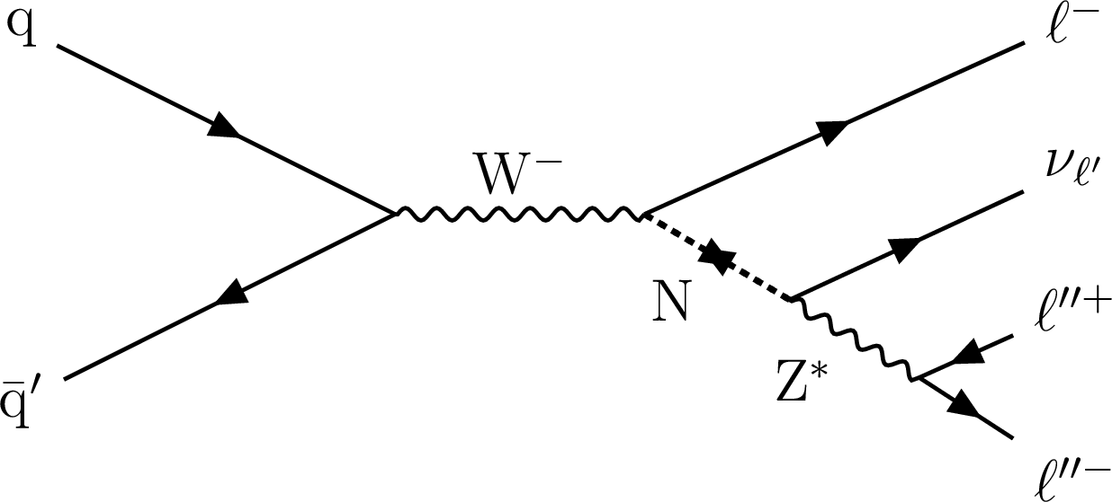
Figure 1-c:
Typical diagrams for the production of an HNL (N) through its mixing with a SM neutrino, leading to final states with three charged leptons and a neutrino. The HNL decay is mediated by either a W* (top row) or a Z* (bottom row) boson. In the diagrams on the left, N is assumed to be a Majorana neutrino, thus $\ell$ and $\ell'$ in the W*-mediated diagram (top) can have the same electric charge, with lepton-number violation (LNV). In the diagrams on the right the N decay conserves lepton number (LNC) and can be either a Majorana or a Dirac particle. Therefore $\ell$ and $\ell'$ in the W*-mediated diagram (top right) have always opposite charge. The present study only considers the former case, thus $\ell$ and $\ell'$ (or $\nu$-$\ell'$) always belong to the same lepton generation, and lepton flavor is conserved. In the case of the HNL decay mediated by a Z boson, $\ell$ and $\ell'$ are required to be of the same flavor. |

png pdf |
Figure 1-d:
Typical diagrams for the production of an HNL (N) through its mixing with a SM neutrino, leading to final states with three charged leptons and a neutrino. The HNL decay is mediated by either a W* (top row) or a Z* (bottom row) boson. In the diagrams on the left, N is assumed to be a Majorana neutrino, thus $\ell$ and $\ell'$ in the W*-mediated diagram (top) can have the same electric charge, with lepton-number violation (LNV). In the diagrams on the right the N decay conserves lepton number (LNC) and can be either a Majorana or a Dirac particle. Therefore $\ell$ and $\ell'$ in the W*-mediated diagram (top right) have always opposite charge. The present study only considers the former case, thus $\ell$ and $\ell'$ (or $\nu$-$\ell'$) always belong to the same lepton generation, and lepton flavor is conserved. In the case of the HNL decay mediated by a Z boson, $\ell$ and $\ell'$ are required to be of the same flavor. |
png pdf |
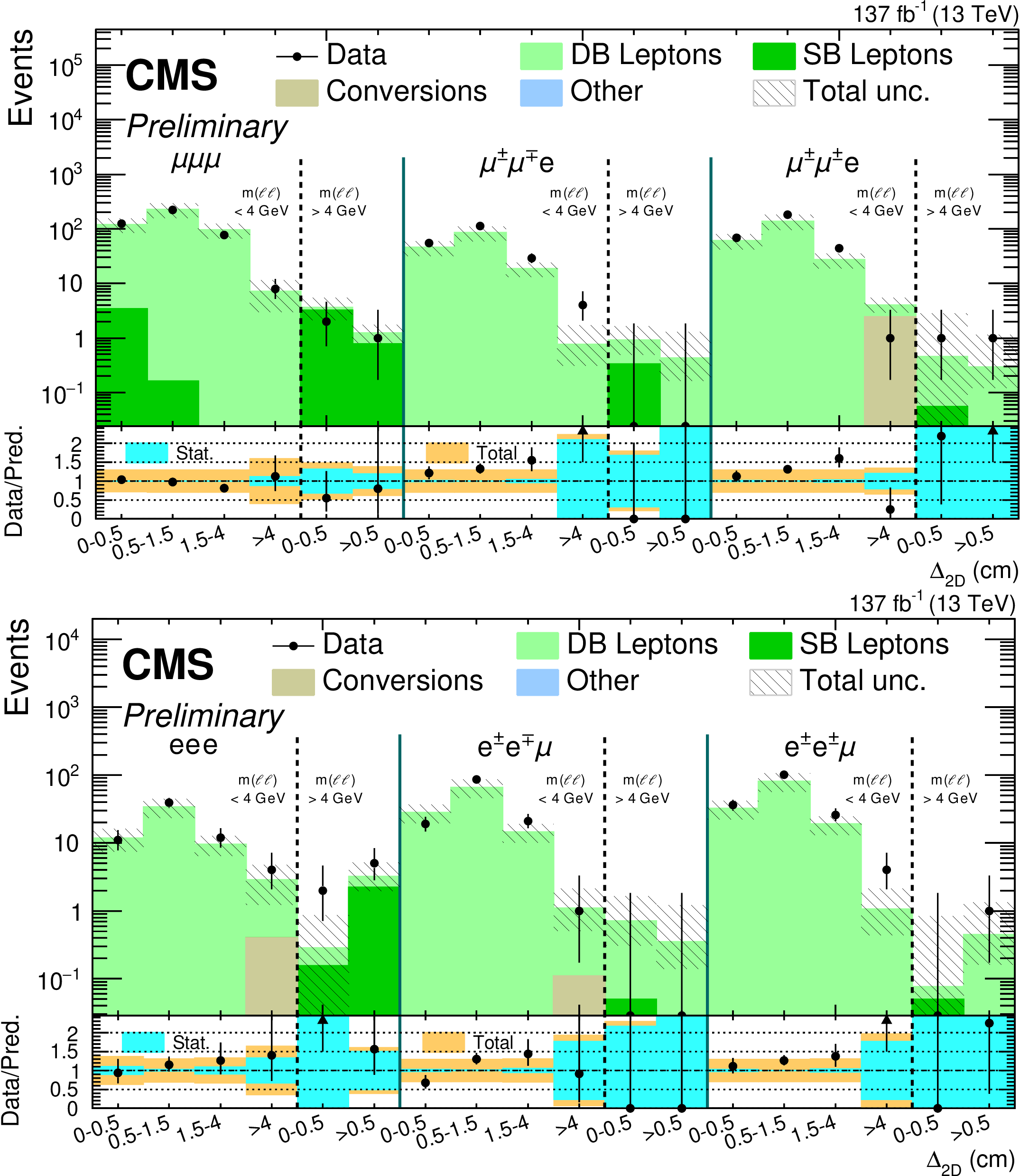
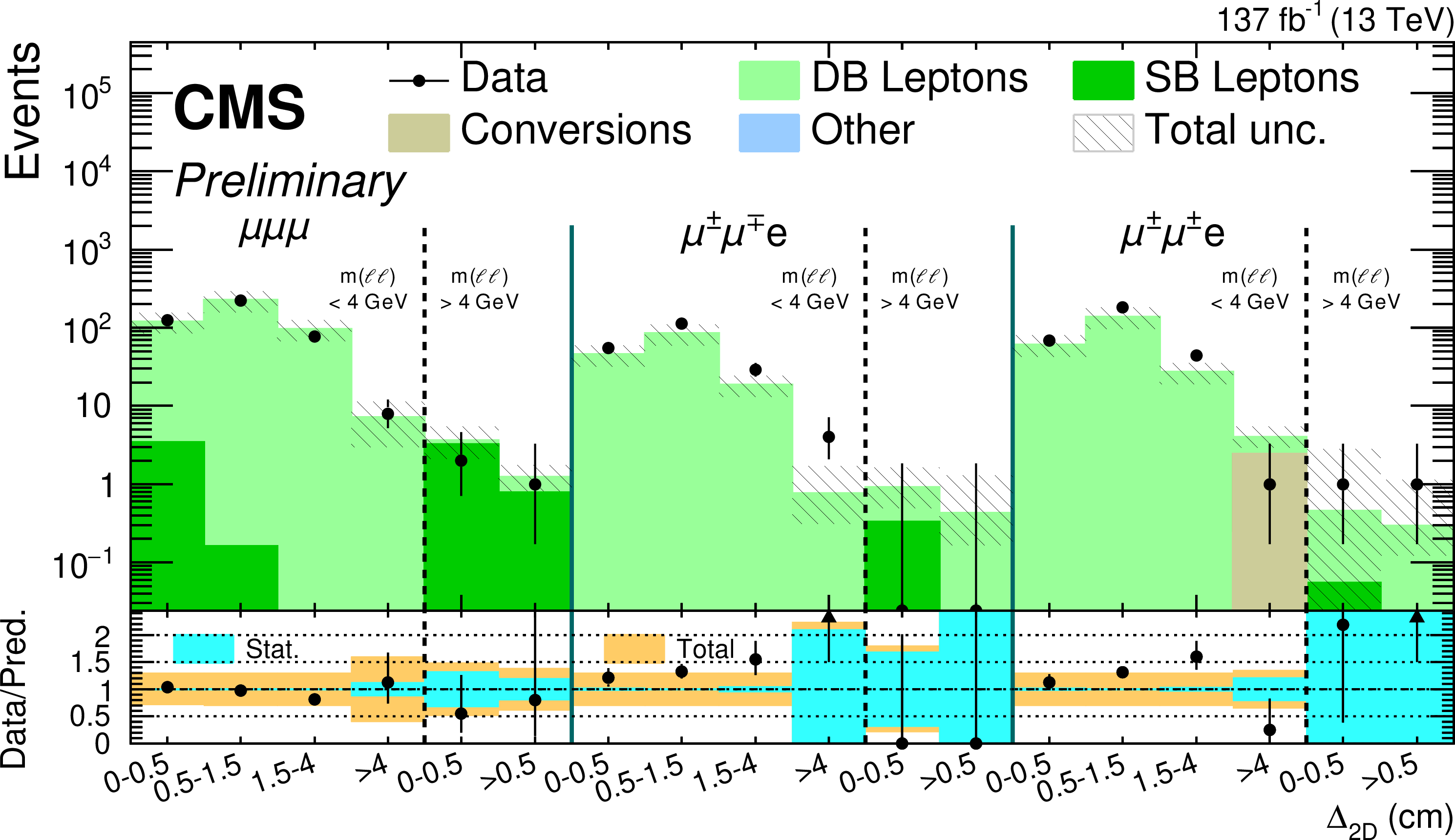
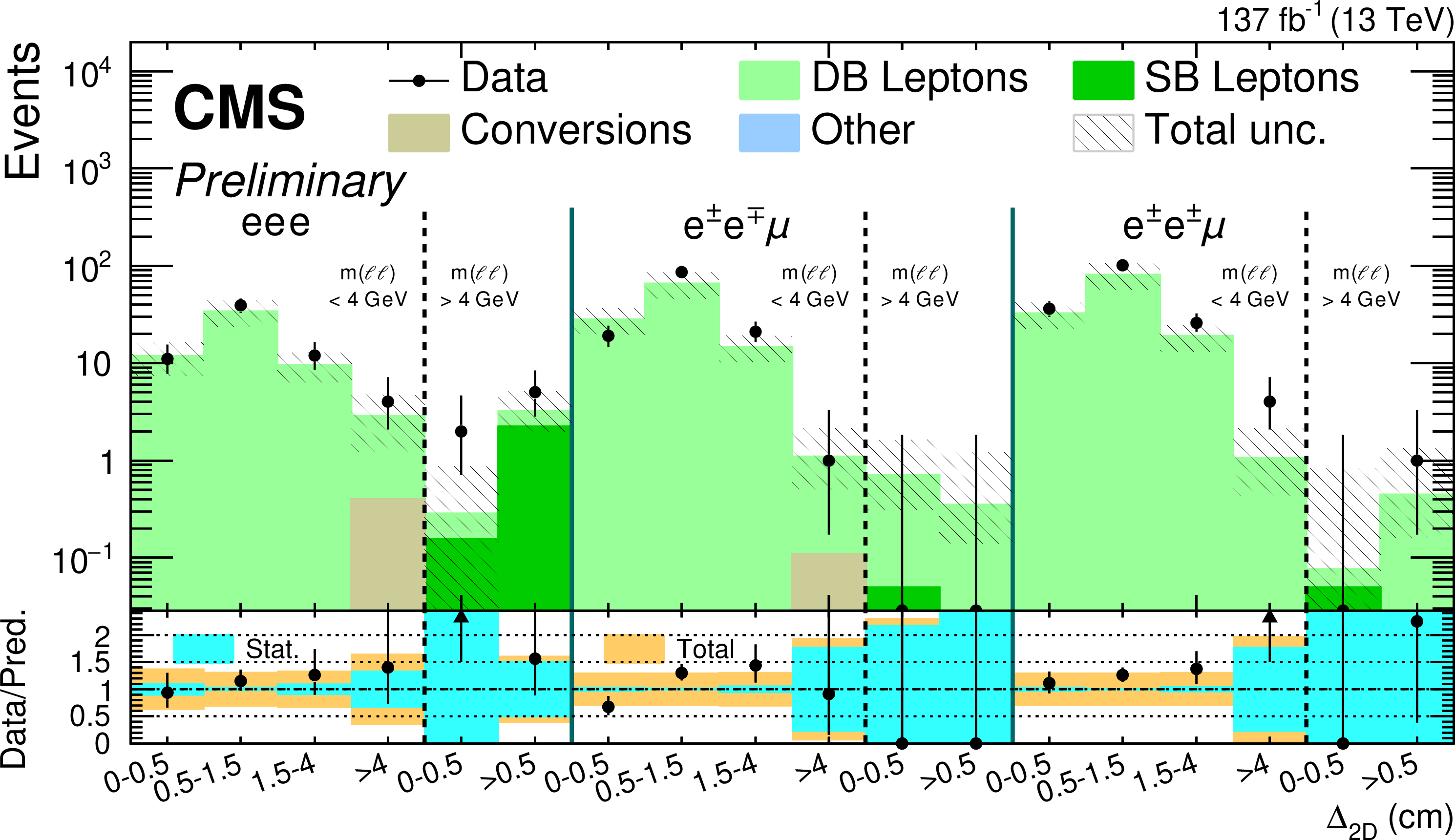
Figure 2:
Comparison between data and lepton background predictions in validation control region for final states with at least two muons (top) and at least two electrons (bottom). |
png pdf |
Figure 2-a:
Comparison between data and lepton background predictions in validation control region for final states with at least two muons (top) and at least two electrons (bottom). |
png pdf |
Figure 2-b:
Comparison between data and lepton background predictions in validation control region for final states with at least two muons (top) and at least two electrons (bottom). |
png pdf |
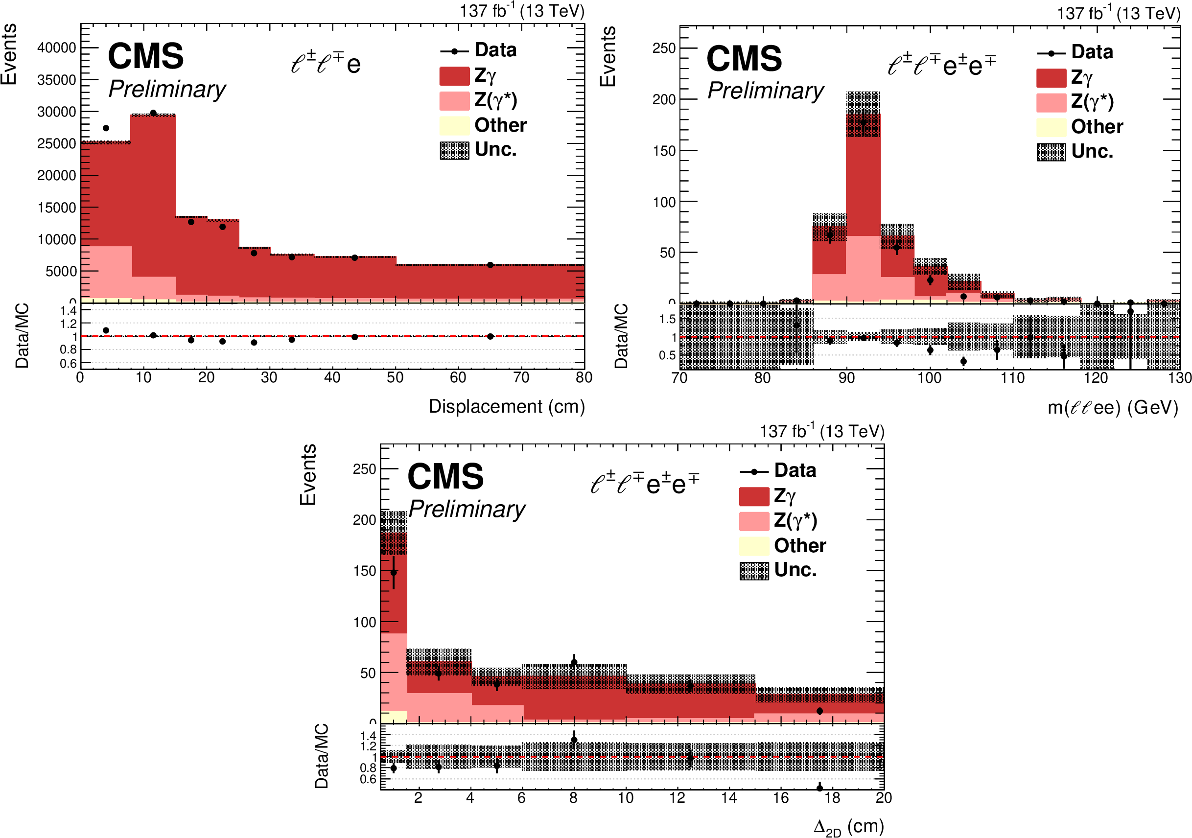
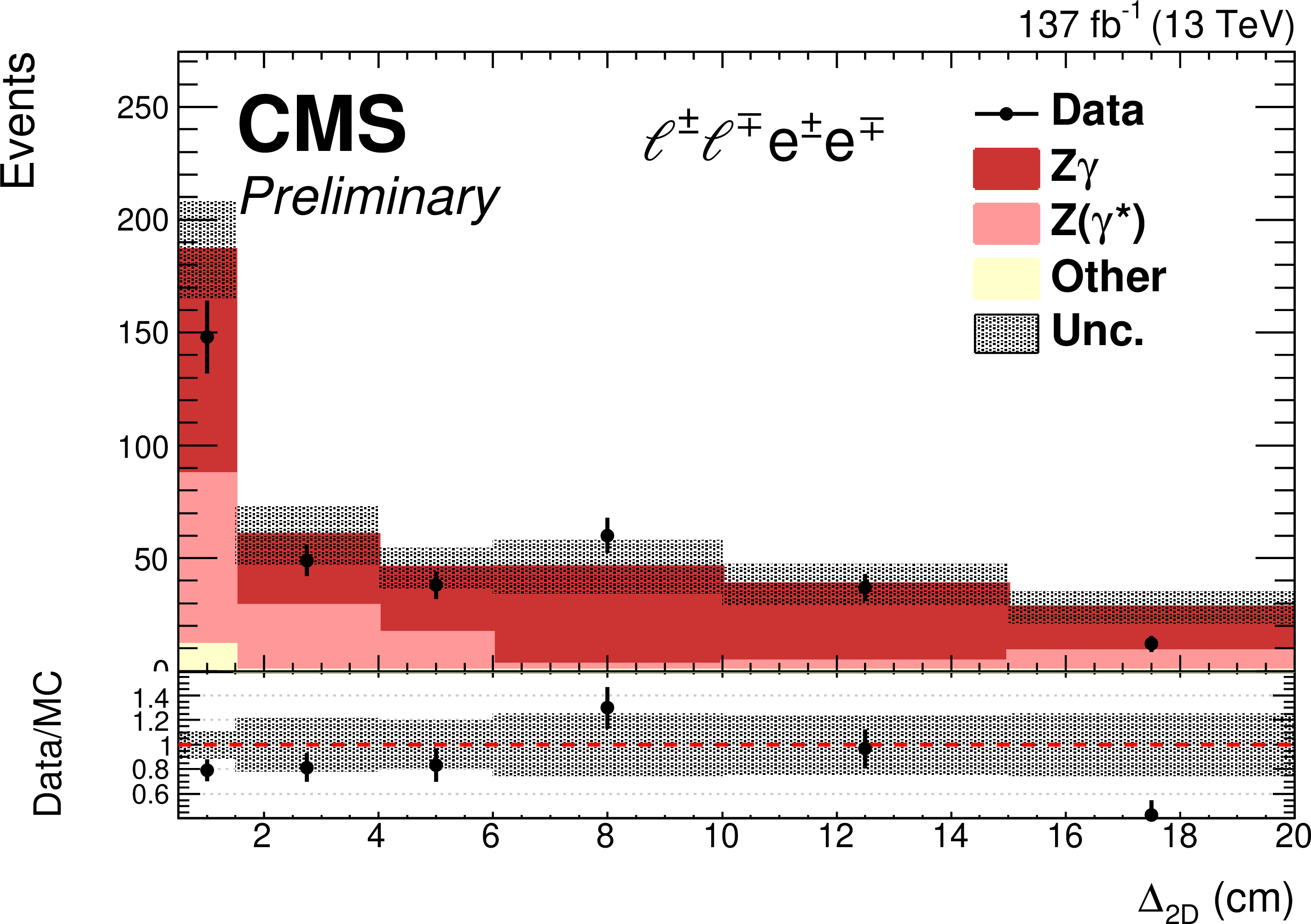
Figure 3:
Comparison between the observed number of events in data and simulation for converted photons. Events are selected in the final states with three (top left) or four (top right, bottom) leptons, with one (or two) of the leptons identified as nonprompt electron(s). The distributions are shown for the nonprompt electron displacement (top left) and reconstructed invariant mass of four leptons (top right). Additionally, the distance between the reconstructed primary and fitted secondary vertex is presented (bottom). The simulated events correspond to the processes with external conversions, Z$ \gamma ^{(*)}$ ; internally converted photons, Z ($\gamma ^{\ast}$); and other processes with the production of vector bosons and top quarks. |

png pdf |
Figure 3-a:
Comparison between the observed number of events in data and simulation for converted photons. Events are selected in the final states with three (top left) or four (top right, bottom) leptons, with one (or two) of the leptons identified as nonprompt electron(s). The distributions are shown for the nonprompt electron displacement (top left) and reconstructed invariant mass of four leptons (top right). Additionally, the distance between the reconstructed primary and fitted secondary vertex is presented (bottom). The simulated events correspond to the processes with external conversions, Z$ \gamma ^{(*)}$ ; internally converted photons, Z ($\gamma ^{\ast}$); and other processes with the production of vector bosons and top quarks. |

png pdf |
Figure 3-b:
Comparison between the observed number of events in data and simulation for converted photons. Events are selected in the final states with three (top left) or four (top right, bottom) leptons, with one (or two) of the leptons identified as nonprompt electron(s). The distributions are shown for the nonprompt electron displacement (top left) and reconstructed invariant mass of four leptons (top right). Additionally, the distance between the reconstructed primary and fitted secondary vertex is presented (bottom). The simulated events correspond to the processes with external conversions, Z$ \gamma ^{(*)}$ ; internally converted photons, Z ($\gamma ^{\ast}$); and other processes with the production of vector bosons and top quarks. |
png pdf |
Figure 3-c:
Comparison between the observed number of events in data and simulation for converted photons. Events are selected in the final states with three (top left) or four (top right, bottom) leptons, with one (or two) of the leptons identified as nonprompt electron(s). The distributions are shown for the nonprompt electron displacement (top left) and reconstructed invariant mass of four leptons (top right). Additionally, the distance between the reconstructed primary and fitted secondary vertex is presented (bottom). The simulated events correspond to the processes with external conversions, Z$ \gamma ^{(*)}$ ; internally converted photons, Z ($\gamma ^{\ast}$); and other processes with the production of vector bosons and top quarks. |

png pdf |
Figure 4:
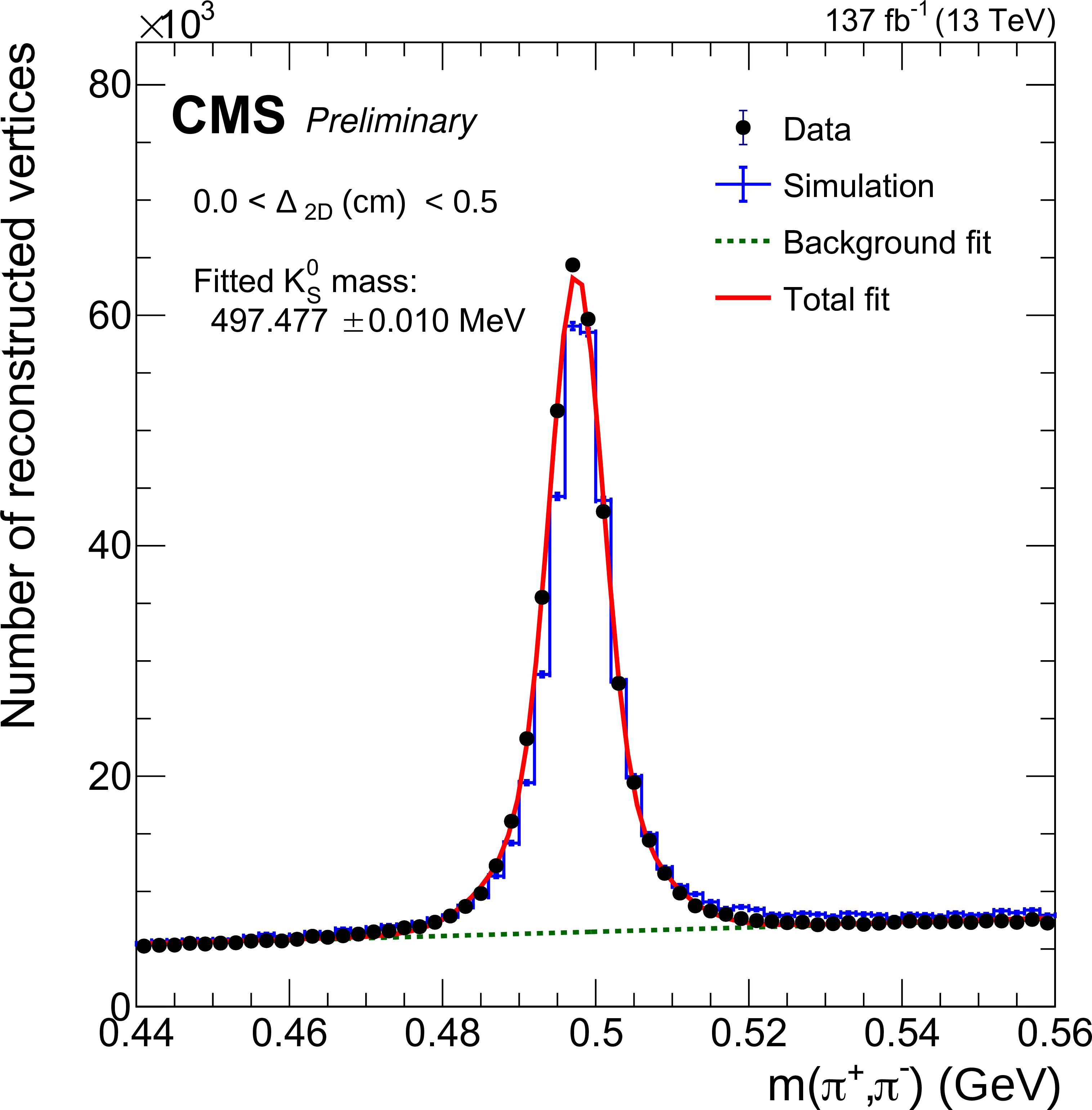
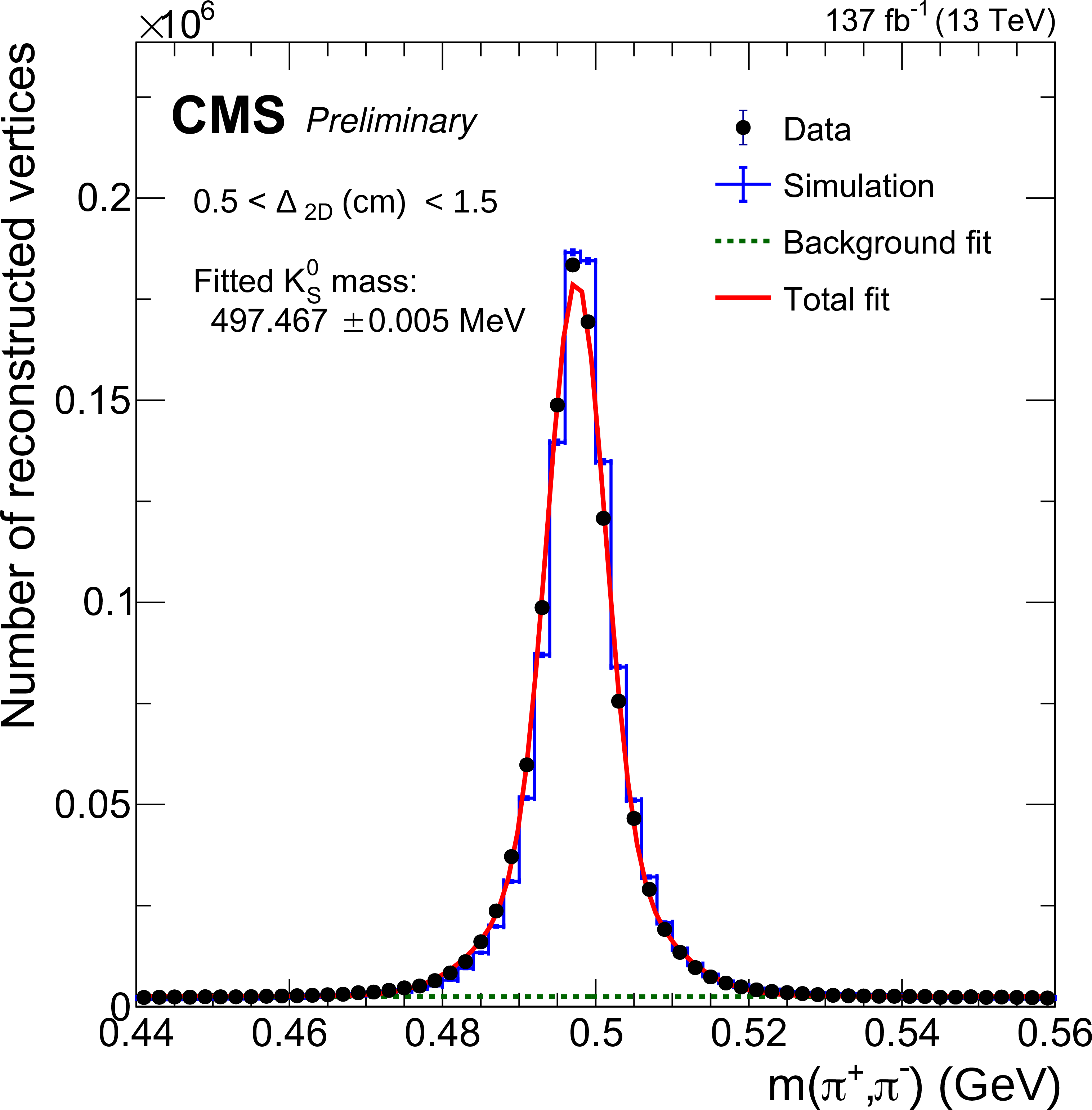
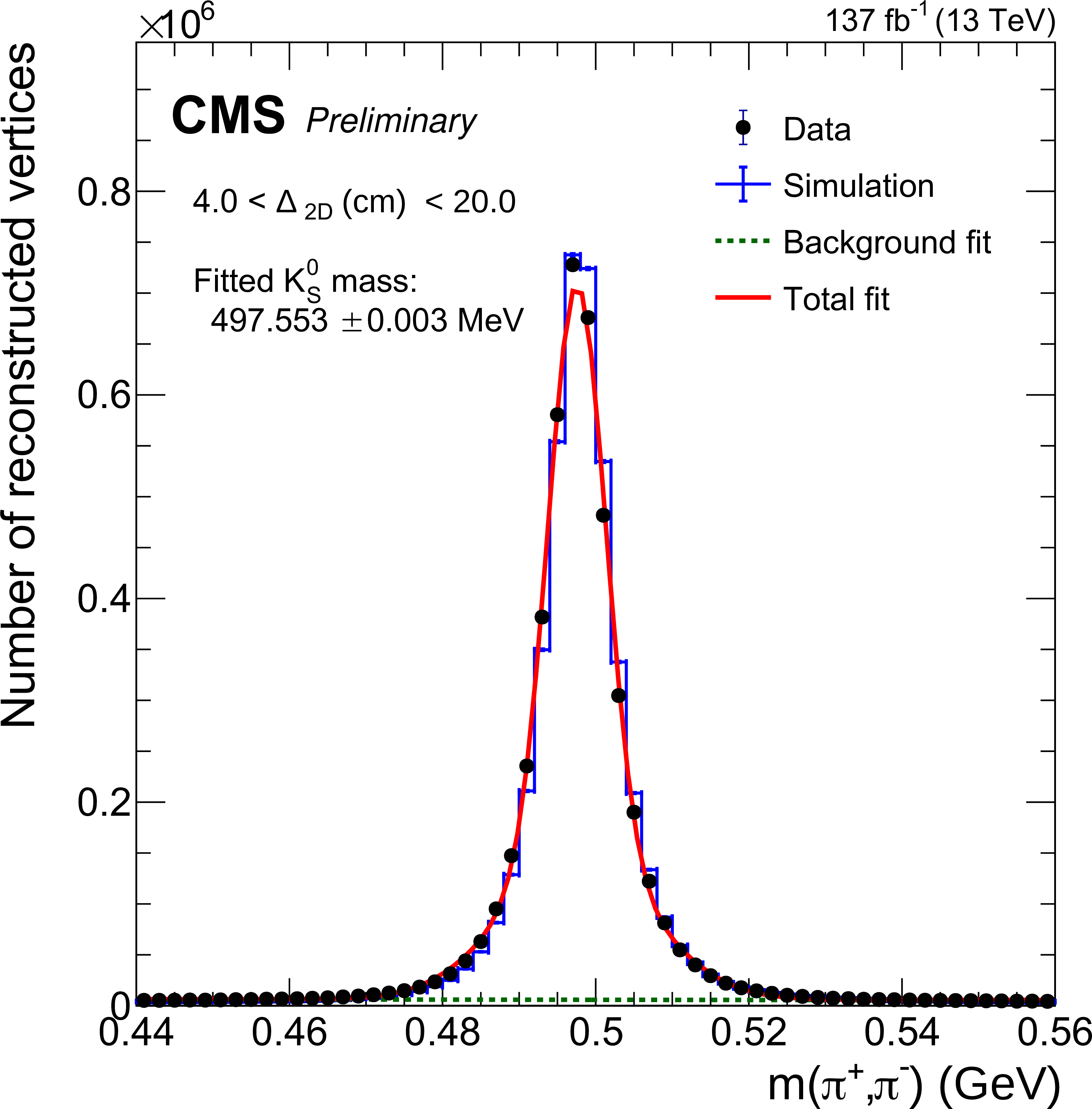
The invariant mass distribution of the ${\mathrm{K^0_S}}$ candidates reconstructed using the $\pi^{\pm} \pi^{\mp} $ tracks for various displacement regions. The fitted ${\mathrm{K^0_S}}$ mass in data in each region is also shown. The bottom plot shows the ${\mathrm{K^0_S}}$ yields after subtracting the background in data and in simulation, as well as their ratio, as a function of radial distance of the ${\mathrm{K^0_S}}$ vertex to the primary vertex. |
png pdf |
Figure 4-a:
The invariant mass distribution of the ${\mathrm{K^0_S}}$ candidates reconstructed using the $\pi^{\pm} \pi^{\mp} $ tracks for various displacement regions. The fitted ${\mathrm{K^0_S}}$ mass in data in each region is also shown. The bottom plot shows the ${\mathrm{K^0_S}}$ yields after subtracting the background in data and in simulation, as well as their ratio, as a function of radial distance of the ${\mathrm{K^0_S}}$ vertex to the primary vertex. |
png pdf |
Figure 4-b:
The invariant mass distribution of the ${\mathrm{K^0_S}}$ candidates reconstructed using the $\pi^{\pm} \pi^{\mp} $ tracks for various displacement regions. The fitted ${\mathrm{K^0_S}}$ mass in data in each region is also shown. The bottom plot shows the ${\mathrm{K^0_S}}$ yields after subtracting the background in data and in simulation, as well as their ratio, as a function of radial distance of the ${\mathrm{K^0_S}}$ vertex to the primary vertex. |

png pdf |
Figure 4-c:
The invariant mass distribution of the ${\mathrm{K^0_S}}$ candidates reconstructed using the $\pi^{\pm} \pi^{\mp} $ tracks for various displacement regions. The fitted ${\mathrm{K^0_S}}$ mass in data in each region is also shown. The bottom plot shows the ${\mathrm{K^0_S}}$ yields after subtracting the background in data and in simulation, as well as their ratio, as a function of radial distance of the ${\mathrm{K^0_S}}$ vertex to the primary vertex. |
png pdf |
Figure 4-d:
The invariant mass distribution of the ${\mathrm{K^0_S}}$ candidates reconstructed using the $\pi^{\pm} \pi^{\mp} $ tracks for various displacement regions. The fitted ${\mathrm{K^0_S}}$ mass in data in each region is also shown. The bottom plot shows the ${\mathrm{K^0_S}}$ yields after subtracting the background in data and in simulation, as well as their ratio, as a function of radial distance of the ${\mathrm{K^0_S}}$ vertex to the primary vertex. |

png pdf |
Figure 4-e:
The invariant mass distribution of the ${\mathrm{K^0_S}}$ candidates reconstructed using the $\pi^{\pm} \pi^{\mp} $ tracks for various displacement regions. The fitted ${\mathrm{K^0_S}}$ mass in data in each region is also shown. The bottom plot shows the ${\mathrm{K^0_S}}$ yields after subtracting the background in data and in simulation, as well as their ratio, as a function of radial distance of the ${\mathrm{K^0_S}}$ vertex to the primary vertex. |

png pdf |
Figure 5:
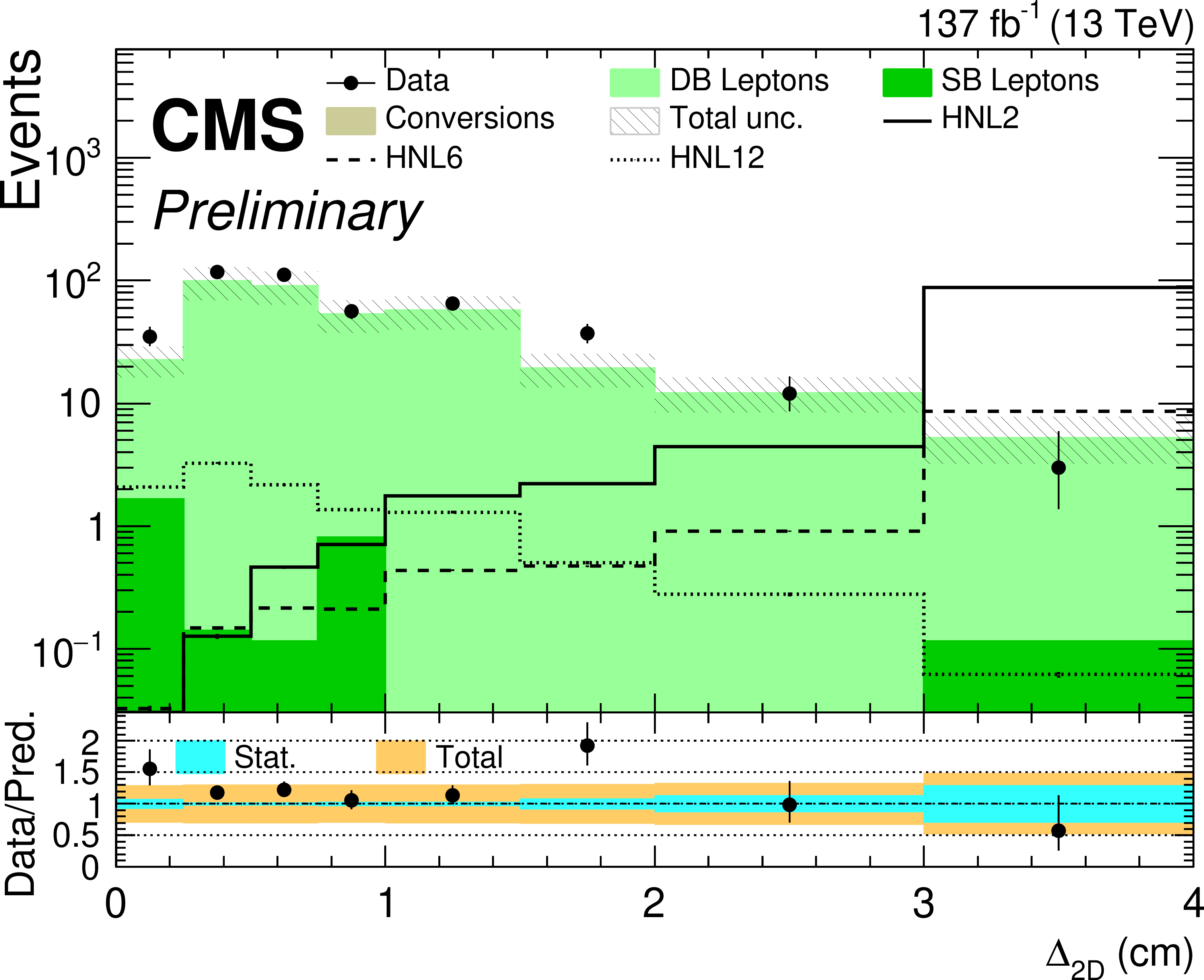
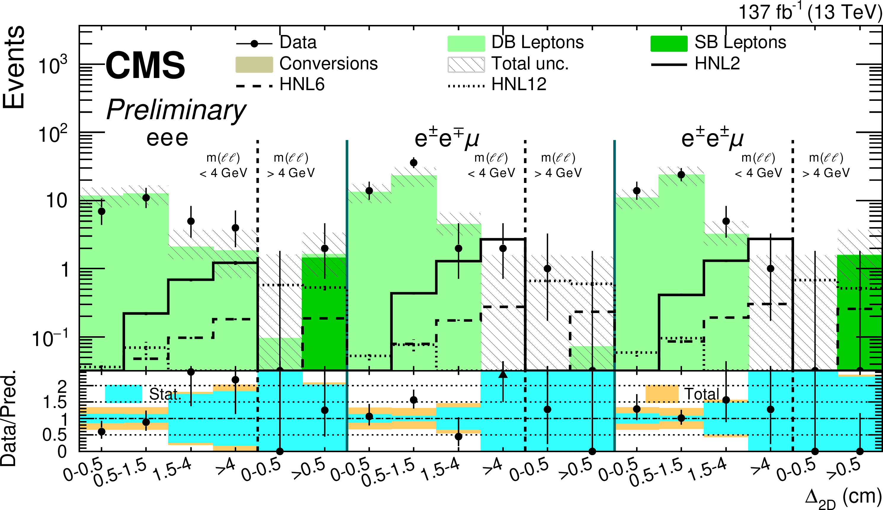
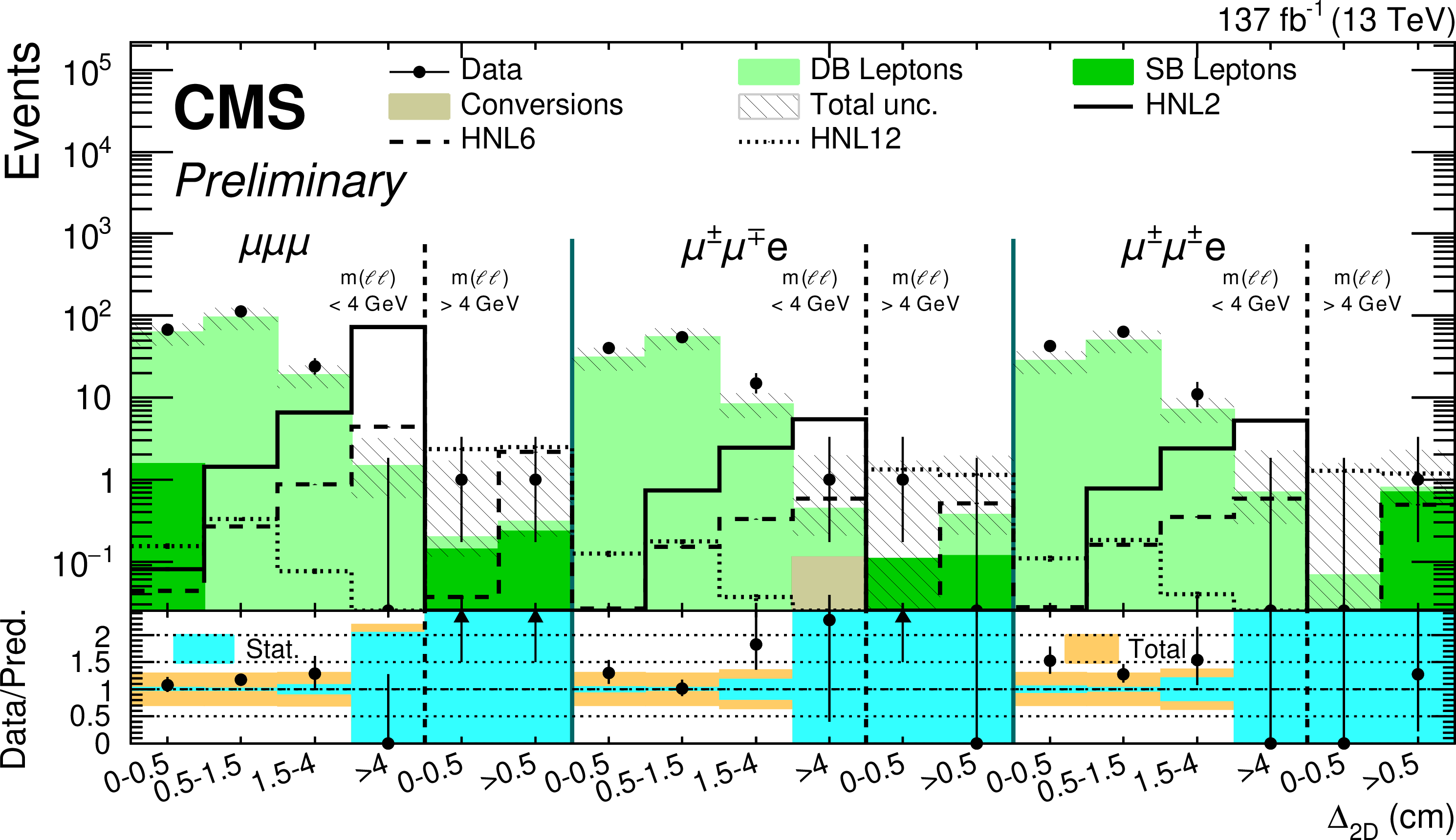
Comparison between the number of observed events in data and their background predictions (shaded histograms, stacked) for the ${\Delta _{\mathrm {2D}}}$ variable in ${\mathrm{e} \mathrm{e} \mathrm{X}}$ (left) and ${\mu \mu \mathrm{X}}$ (right) final states. Predictions for signal events are shown for several benchmark hypotheses for Majorana HNL: $ {m_{\mathrm{N}}} = $ 2 GeV and $ {{| {V_{{\mathrm{N}} \ell}} |}^2} = $ 0.8 $\times$ 10$^{-4}$ (HNL2), $ {m_{\mathrm{N}}} = $ 6 GeV and $ {{| {V_{{\mathrm{N}} \ell}} |}^2} = $ 1.3 $\times$ 10$^{-6}$ (HNL6), $ {m_{\mathrm{N}}} = $ 12 GeV and $ {{| {V_{{\mathrm{N}} \ell}} |}^2} = $ 1.0 $\times$ 10$^{-6}$ (HNL12). |

png pdf |
Figure 5-a:
Comparison between the number of observed events in data and their background predictions (shaded histograms, stacked) for the ${\Delta _{\mathrm {2D}}}$ variable in ${\mathrm{e} \mathrm{e} \mathrm{X}}$ (left) and ${\mu \mu \mathrm{X}}$ (right) final states. Predictions for signal events are shown for several benchmark hypotheses for Majorana HNL: $ {m_{\mathrm{N}}} = $ 2 GeV and $ {{| {V_{{\mathrm{N}} \ell}} |}^2} = $ 0.8 $\times$ 10$^{-4}$ (HNL2), $ {m_{\mathrm{N}}} = $ 6 GeV and $ {{| {V_{{\mathrm{N}} \ell}} |}^2} = $ 1.3 $\times$ 10$^{-6}$ (HNL6), $ {m_{\mathrm{N}}} = $ 12 GeV and $ {{| {V_{{\mathrm{N}} \ell}} |}^2} = $ 1.0 $\times$ 10$^{-6}$ (HNL12). |
png pdf |
Figure 5-b:
Comparison between the number of observed events in data and their background predictions (shaded histograms, stacked) for the ${\Delta _{\mathrm {2D}}}$ variable in ${\mathrm{e} \mathrm{e} \mathrm{X}}$ (left) and ${\mu \mu \mathrm{X}}$ (right) final states. Predictions for signal events are shown for several benchmark hypotheses for Majorana HNL: $ {m_{\mathrm{N}}} = $ 2 GeV and $ {{| {V_{{\mathrm{N}} \ell}} |}^2} = $ 0.8 $\times$ 10$^{-4}$ (HNL2), $ {m_{\mathrm{N}}} = $ 6 GeV and $ {{| {V_{{\mathrm{N}} \ell}} |}^2} = $ 1.3 $\times$ 10$^{-6}$ (HNL6), $ {m_{\mathrm{N}}} = $ 12 GeV and $ {{| {V_{{\mathrm{N}} \ell}} |}^2} = $ 1.0 $\times$ 10$^{-6}$ (HNL12). |

png pdf |
Figure 6:
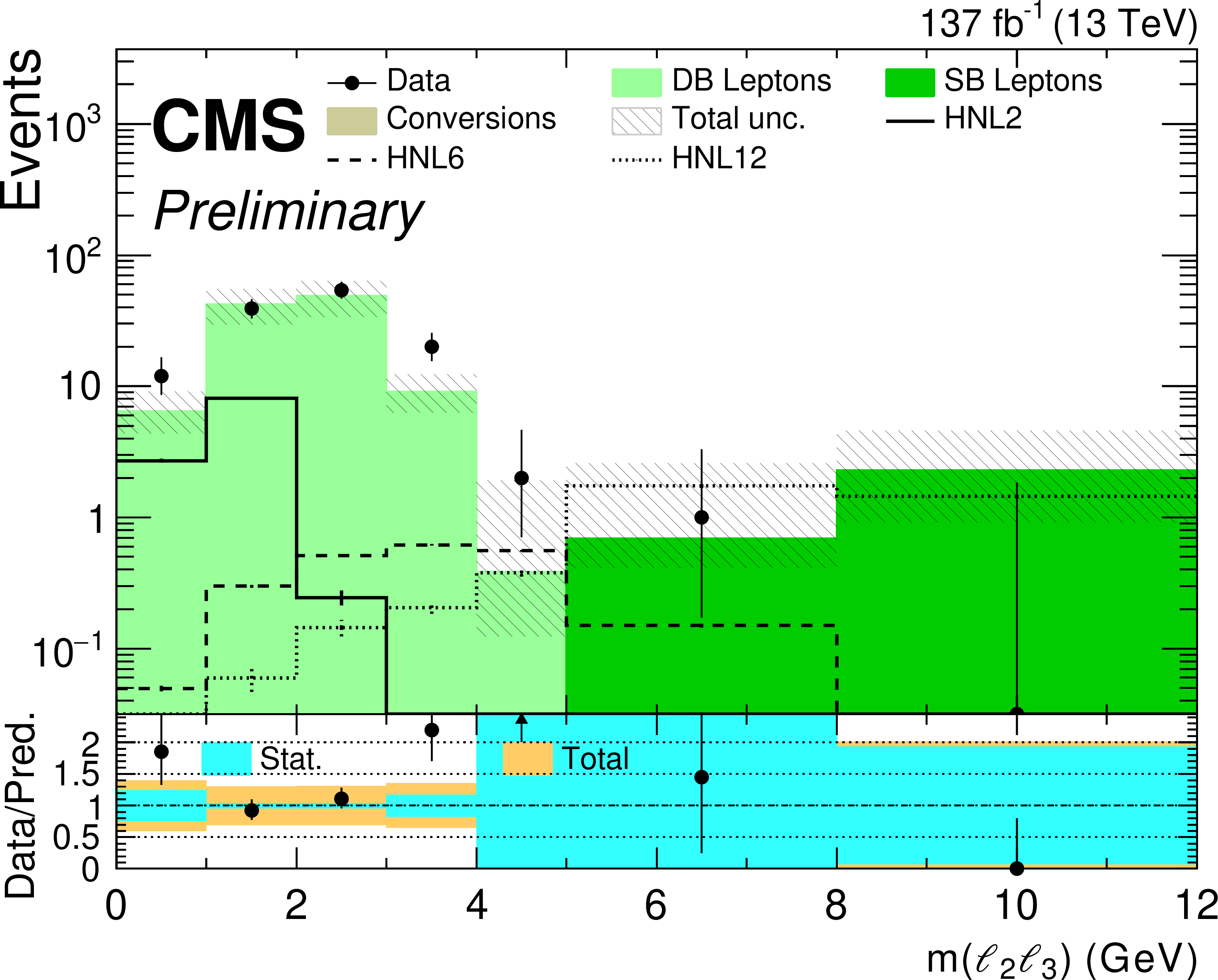
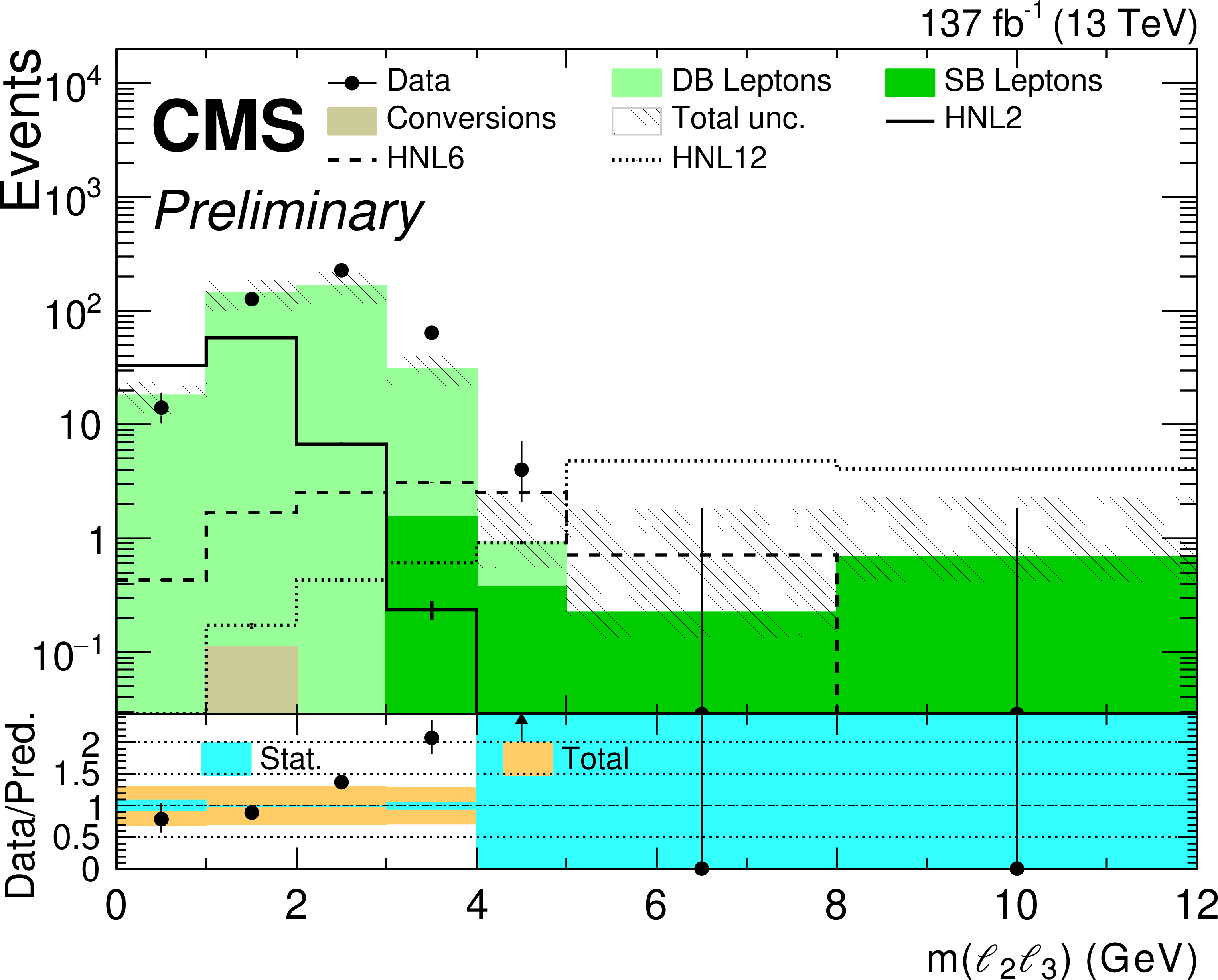
Comparison between the number of observed events in data and their background predictions (shaded histograms, stacked) for the ${m({\ell _2} {\ell _3})}$ variable in ${\mathrm{e} \mathrm{e} \mathrm{X}}$ (left) and ${\mu \mu \mathrm{X}}$ (right) final states. Predictions for signal events are shown for several benchmark hypotheses for Majorana HNL: $ {m_{\mathrm{N}}} = $ 2 GeV and $ {{| {V_{{\mathrm{N}} \ell}} |}^2} = $ 0.8 $\times$ 10$^{-4}$ (HNL2), $ {m_{\mathrm{N}}} = $ 6 GeV and $ {{| {V_{{\mathrm{N}} \ell}} |}^2} = $ 1.3 $\times$ 10$^{-6}$ (HNL6), $ {m_{\mathrm{N}}} = $ 12 GeV and $ {{| {V_{{\mathrm{N}} \ell}} |}^2} = $ 1.0 $\times$ 10$^{-6}$ (HNL12). |
png pdf |
Figure 6-a:
Comparison between the number of observed events in data and their background predictions (shaded histograms, stacked) for the ${m({\ell _2} {\ell _3})}$ variable in ${\mathrm{e} \mathrm{e} \mathrm{X}}$ (left) and ${\mu \mu \mathrm{X}}$ (right) final states. Predictions for signal events are shown for several benchmark hypotheses for Majorana HNL: $ {m_{\mathrm{N}}} = $ 2 GeV and $ {{| {V_{{\mathrm{N}} \ell}} |}^2} = $ 0.8 $\times$ 10$^{-4}$ (HNL2), $ {m_{\mathrm{N}}} = $ 6 GeV and $ {{| {V_{{\mathrm{N}} \ell}} |}^2} = $ 1.3 $\times$ 10$^{-6}$ (HNL6), $ {m_{\mathrm{N}}} = $ 12 GeV and $ {{| {V_{{\mathrm{N}} \ell}} |}^2} = $ 1.0 $\times$ 10$^{-6}$ (HNL12). |
png pdf |
Figure 6-b:
Comparison between the number of observed events in data and their background predictions (shaded histograms, stacked) for the ${m({\ell _2} {\ell _3})}$ variable in ${\mathrm{e} \mathrm{e} \mathrm{X}}$ (left) and ${\mu \mu \mathrm{X}}$ (right) final states. Predictions for signal events are shown for several benchmark hypotheses for Majorana HNL: $ {m_{\mathrm{N}}} = $ 2 GeV and $ {{| {V_{{\mathrm{N}} \ell}} |}^2} = $ 0.8 $\times$ 10$^{-4}$ (HNL2), $ {m_{\mathrm{N}}} = $ 6 GeV and $ {{| {V_{{\mathrm{N}} \ell}} |}^2} = $ 1.3 $\times$ 10$^{-6}$ (HNL6), $ {m_{\mathrm{N}}} = $ 12 GeV and $ {{| {V_{{\mathrm{N}} \ell}} |}^2} = $ 1.0 $\times$ 10$^{-6}$ (HNL12). |

png pdf |
Figure 7:
Predicted and observed yields in the different search regions for (top) ${\mathrm{e} \mathrm{e} \mathrm{X}}$ and (bottom) ${\mu \mu \mathrm{X}}$ final states, compared to one HNL signal scenario with nonzero ${{| {V_{{\mathrm{N}} \mathrm{e}}} |}^2}$ and ${{| {V_{{\mathrm{N}} \mu}} |}^2}$ parameter, respectively. The predictions for signal process are obtained assuming Majorana HNL. Predictions for signal events are shown for several benchmark hypotheses: $ {m_{\mathrm{N}}} = $ 2 GeV and $ {{| {V_{{\mathrm{N}} \ell}} |}^2} = $ 0.8 $\times$ 10$^{-4}$ (HNL2), $ {m_{\mathrm{N}}} = $ 6 GeV and $ {{| {V_{{\mathrm{N}} \ell}} |}^2} = $ 1.3 $\times$ 10$^{-6}$ (HNL6), $ {m_{\mathrm{N}}} = $ 12 GeV and $ {{| {V_{{\mathrm{N}} \ell}} |}^2} = $ 1.0 $\times$ 10$^{-6}$ (HNL12). The uncertainty band assigned to the background prediction includes statistical and systematic contributions. |
png pdf |
Figure 7-a:
Predicted and observed yields in the different search regions for (top) ${\mathrm{e} \mathrm{e} \mathrm{X}}$ and (bottom) ${\mu \mu \mathrm{X}}$ final states, compared to one HNL signal scenario with nonzero ${{| {V_{{\mathrm{N}} \mathrm{e}}} |}^2}$ and ${{| {V_{{\mathrm{N}} \mu}} |}^2}$ parameter, respectively. The predictions for signal process are obtained assuming Majorana HNL. Predictions for signal events are shown for several benchmark hypotheses: $ {m_{\mathrm{N}}} = $ 2 GeV and $ {{| {V_{{\mathrm{N}} \ell}} |}^2} = $ 0.8 $\times$ 10$^{-4}$ (HNL2), $ {m_{\mathrm{N}}} = $ 6 GeV and $ {{| {V_{{\mathrm{N}} \ell}} |}^2} = $ 1.3 $\times$ 10$^{-6}$ (HNL6), $ {m_{\mathrm{N}}} = $ 12 GeV and $ {{| {V_{{\mathrm{N}} \ell}} |}^2} = $ 1.0 $\times$ 10$^{-6}$ (HNL12). The uncertainty band assigned to the background prediction includes statistical and systematic contributions. |
png pdf |
Figure 7-b:
Predicted and observed yields in the different search regions for (top) ${\mathrm{e} \mathrm{e} \mathrm{X}}$ and (bottom) ${\mu \mu \mathrm{X}}$ final states, compared to one HNL signal scenario with nonzero ${{| {V_{{\mathrm{N}} \mathrm{e}}} |}^2}$ and ${{| {V_{{\mathrm{N}} \mu}} |}^2}$ parameter, respectively. The predictions for signal process are obtained assuming Majorana HNL. Predictions for signal events are shown for several benchmark hypotheses: $ {m_{\mathrm{N}}} = $ 2 GeV and $ {{| {V_{{\mathrm{N}} \ell}} |}^2} = $ 0.8 $\times$ 10$^{-4}$ (HNL2), $ {m_{\mathrm{N}}} = $ 6 GeV and $ {{| {V_{{\mathrm{N}} \ell}} |}^2} = $ 1.3 $\times$ 10$^{-6}$ (HNL6), $ {m_{\mathrm{N}}} = $ 12 GeV and $ {{| {V_{{\mathrm{N}} \ell}} |}^2} = $ 1.0 $\times$ 10$^{-6}$ (HNL12). The uncertainty band assigned to the background prediction includes statistical and systematic contributions. |

png pdf |
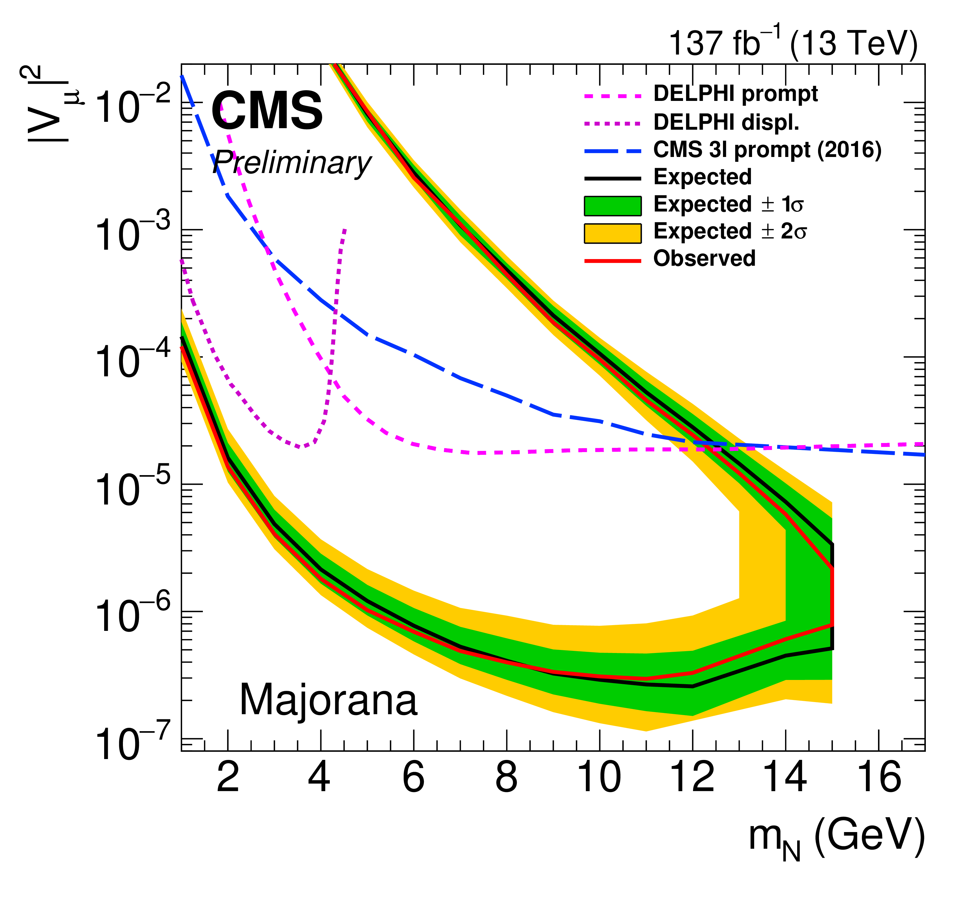
Figure 8:
Limits on ${{| {V_{{\mathrm{N}} \mathrm{e}}} |}^2}$ (left) and ${{| {V_{{\mathrm{N}} \mu}} |}^2}$ (right) as a function of ${m_{\mathrm{N}}}$ for a Majorana HNL. Results from the Delphi [62] and the CMS [22,23] Collaborations are shown for reference. |

png pdf |
Figure 8-a:
Limits on ${{| {V_{{\mathrm{N}} \mathrm{e}}} |}^2}$ (left) and ${{| {V_{{\mathrm{N}} \mu}} |}^2}$ (right) as a function of ${m_{\mathrm{N}}}$ for a Majorana HNL. Results from the Delphi [62] and the CMS [22,23] Collaborations are shown for reference. |
png pdf |
Figure 8-b:
Limits on ${{| {V_{{\mathrm{N}} \mathrm{e}}} |}^2}$ (left) and ${{| {V_{{\mathrm{N}} \mu}} |}^2}$ (right) as a function of ${m_{\mathrm{N}}}$ for a Majorana HNL. Results from the Delphi [62] and the CMS [22,23] Collaborations are shown for reference. |

png pdf |
Figure 9:
Limits on ${{| {V_{{\mathrm{N}} \mathrm{e}}} |}^2}$ (left) and ${{| {V_{{\mathrm{N}} \mu}} |}^2}$ (right) as a function of ${m_{\mathrm{N}}}$ for a Dirac HNL. Results from the Delphi [62] and the CMS [22,23] Collaborations are shown for reference. |

png pdf |
Figure 9-a:
Limits on ${{| {V_{{\mathrm{N}} \mathrm{e}}} |}^2}$ (left) and ${{| {V_{{\mathrm{N}} \mu}} |}^2}$ (right) as a function of ${m_{\mathrm{N}}}$ for a Dirac HNL. Results from the Delphi [62] and the CMS [22,23] Collaborations are shown for reference. |

png pdf |
Figure 9-b:
Limits on ${{| {V_{{\mathrm{N}} \mathrm{e}}} |}^2}$ (left) and ${{| {V_{{\mathrm{N}} \mu}} |}^2}$ (right) as a function of ${m_{\mathrm{N}}}$ for a Dirac HNL. Results from the Delphi [62] and the CMS [22,23] Collaborations are shown for reference. |
| Tables | |
png pdf |
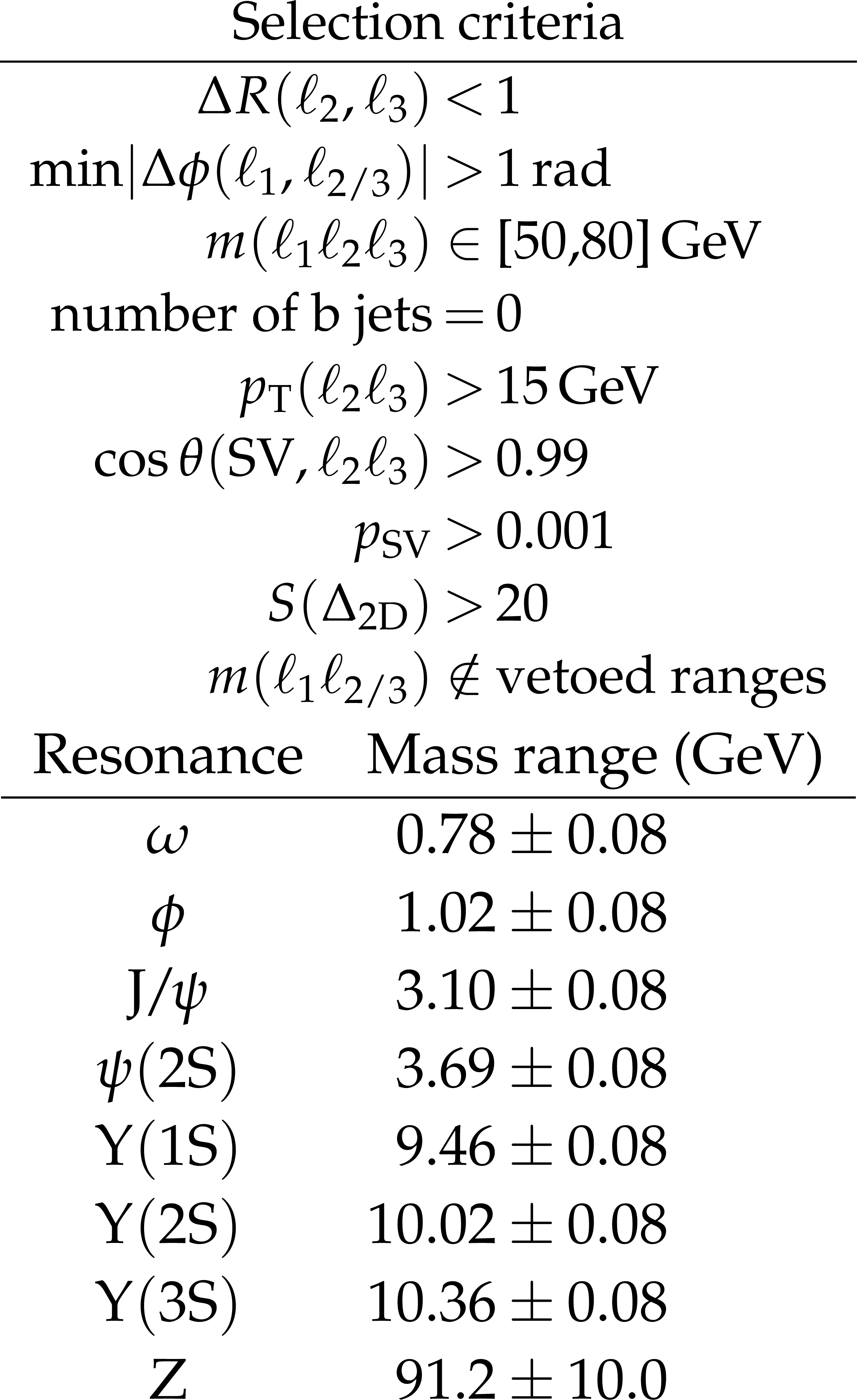
Table 1:
Baseline selection criteria (left) and dilepton invariant mass vetoes (right) applied in the analysis. |
png pdf |
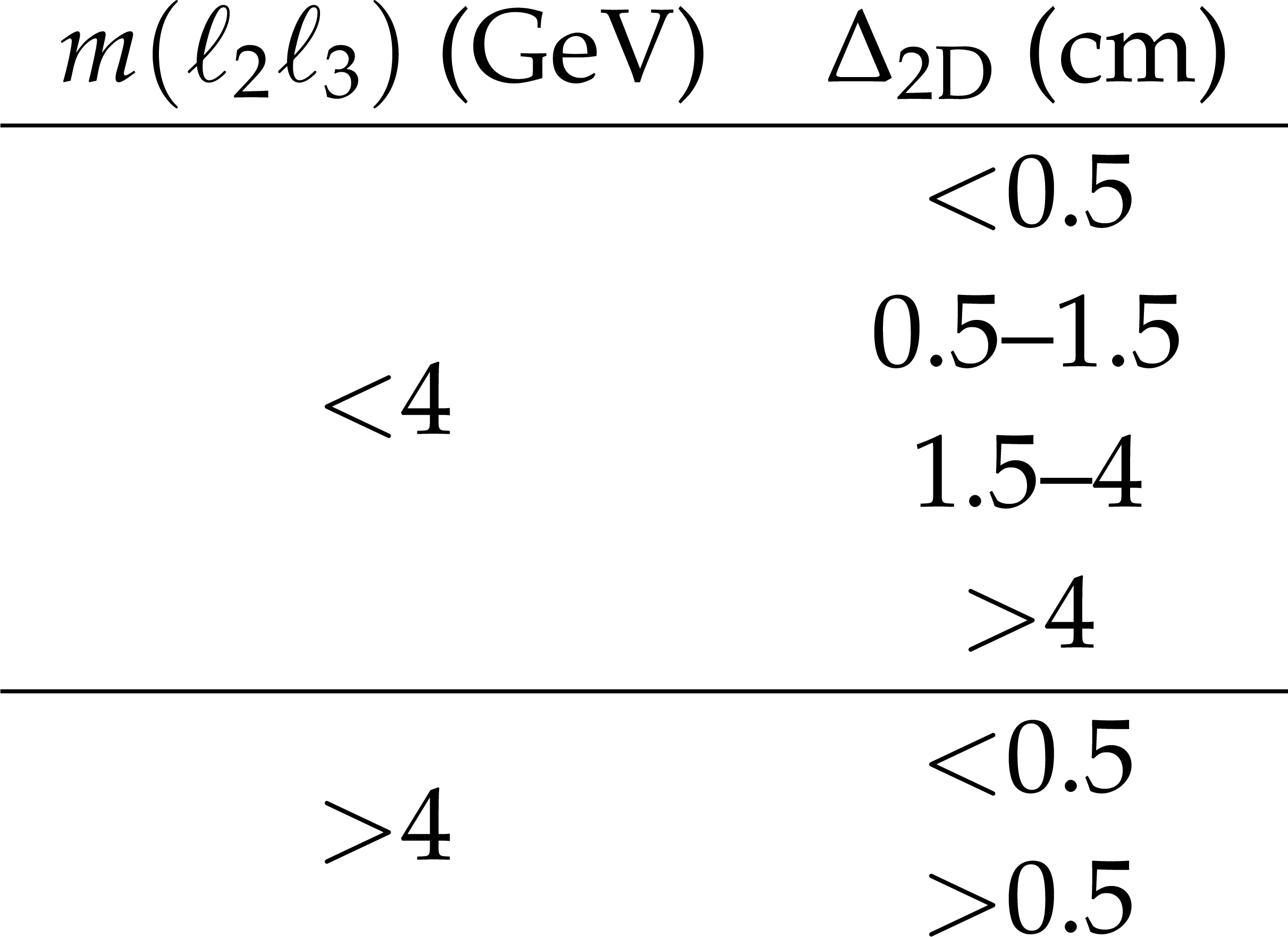
Table 2:
Definition of kinematic regions in terms of dilepton invariant mass ${m({\ell _2} {\ell _3})}$ and SV displacement ${\Delta _{\mathrm {2D}}}$. |
png pdf |
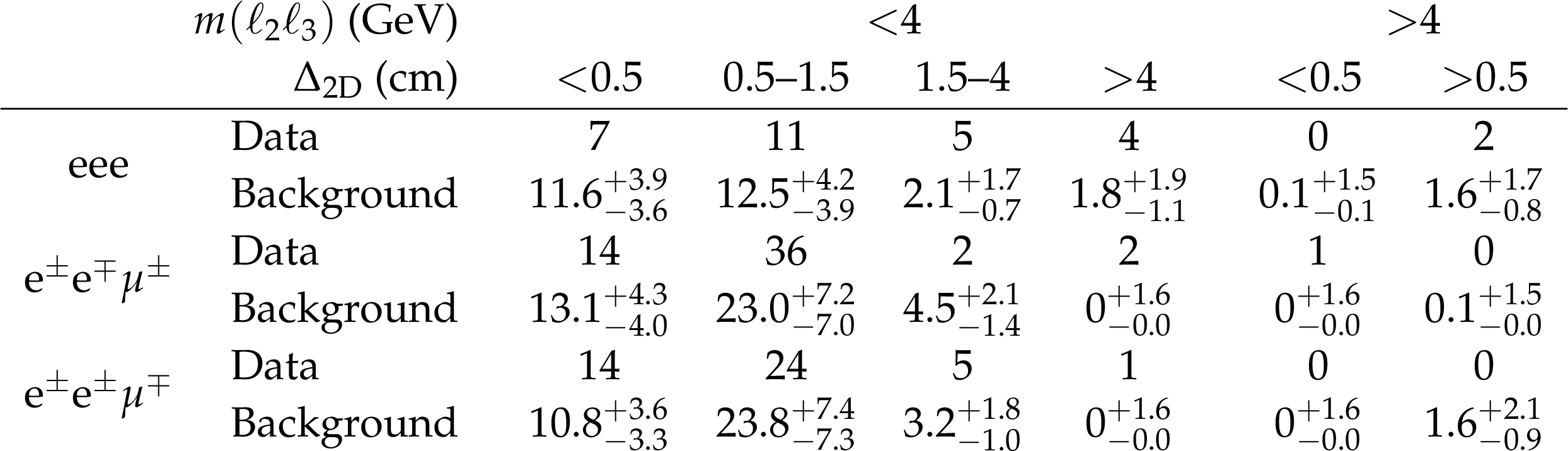
Table 3:
Number of predicted and observed events in the ${\mathrm{e} \mathrm{e} \mathrm{X}}$ final states. The quoted uncertainties include statistical and systematic uncertainties. |
png pdf |
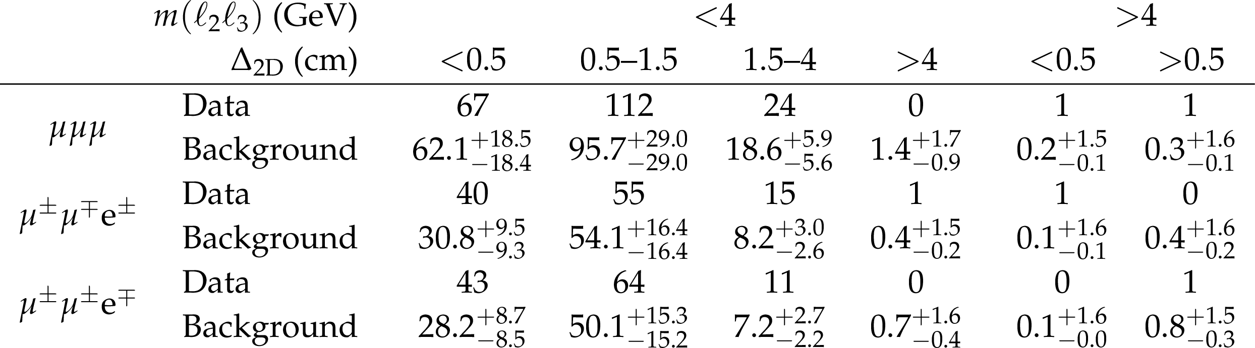
Table 4:
Number of predicted and observed events in the ${\mu \mu \mathrm{X}}$ final states. The quoted uncertainties include statistical and systematic uncertainties. |

png pdf |
Table 5:
Number of predicted signal events in the ${\mathrm{e} \mathrm{e} \mathrm{X}}$ final states. The results are presented for several benchmark signal hypotheses for Majorana HNL: $ {m_{\mathrm{N}}} = $ 2 GeV and $ {{| {V_{{\mathrm{N}} \mathrm{e}}} |}^2} = $ 0.8 $\times$ 10$^{-4}$ (HNL2), $ {m_{\mathrm{N}}} = $ 6 GeV and $ {{| {V_{{\mathrm{N}} \mathrm{e}}} |}^2} = $ 1.3 $\times$ 10$^{-6}$ (HNL6), $ {m_{\mathrm{N}}} = $ 12 GeV and $ {{| {V_{{\mathrm{N}} \mathrm{e}}} |}^2} = $ 1.0 $\times$ 10$^{-6}$ (HNL12). The quoted uncertainties include statistical and systematic uncertainties. |

png pdf |
Table 6:
Number of predicted signal events in the ${\mu \mu \mathrm{X}}$ final states. The results are presented for several benchmark signal hypotheses for Majorana HNL: $ {m_{\mathrm{N}}} = $ 2 GeV and $ {{| {V_{{\mathrm{N}} \mu}} |}^2} = $ 0.8 $\times$ 10$^{-4}$ (HNL2), $ {m_{\mathrm{N}}} = $ 6 GeV and $ {{| {V_{{\mathrm{N}} \mu}} |}^2} = $ 1.3 $\times$ 10$^{-6}$ (HNL6), $ {m_{\mathrm{N}}} = $ 12 GeV and $ {{| {V_{{\mathrm{N}} \mu}} |}^2} = $ 1.0 $\times$ 10$^{-6}$ (HNL12). The quoted uncertainties include statistical and systematic uncertainties. |
| Summary |
| A study on the search for heavy neutral leptons (HNLs) in final states with three leptons is performed using data from the CMS detector corresponding to an integrated luminosity of 137 fb$^{-1}$. The analysis uses dedicated methods to identify displaced leptons associated with HNL decays. Several novel methods were developed to apply data-driven estimates for the relevant background processes representing one of the important challenges in this type of search at the LHC. No significant deviation from the standard model predictions is observed in data, and 95% confidence level limits are set on HNL masses and coupling strengths of these particles to standard model neutrinos. These results represent the world best limits to date on this type of processes in the explored parameter space of the HNL production at the LHC. |
| References | ||||
| 1 | Super-Kamiokande Collaboration | Evidence for oscillation of atmospheric neutrinos | PRL 81 (1998) 1562 | hep-ex/9807003 |
| 2 | Super-Kamiokande Collaboration | Evidence for an oscillatory signature in atmospheric neutrino oscillation | PRL 93 (2004) 101801 | hep-ex/0404034 |
| 3 | Super-Kamiokande Collaboration | Measurement of atmospheric neutrino oscillation parameters by Super-Kamiokande I | PRD 71 (2005) 112005 | hep-ex/0501064 |
| 4 | K2K Collaboration | Evidence for muon neutrino oscillation in an accelerator-based experiment | PRL 94 (2005) 081802 | hep-ex/0411038 |
| 5 | MINOS Collaboration | Observation of muon neutrino disappearance with the MINOS detectors and the NuMI neutrino beam | PRL 97 (2006) 191801 | hep-ex/0607088 |
| 6 | T2K Collaboration | Indication of electron neutrino appearance from an accelerator-produced off-axis muon neutrino beam | PRL 107 (2011) 041801 | 1106.2822 |
| 7 | MINOS Collaboration | Improved search for muon-neutrino to electron-neutrino oscillations in MINOS | PRL 107 (2011) 181802 | 1108.0015 |
| 8 | Double Chooz Collaboration | Indication of reactor $ \PAGne $ disappearance in the Double Chooz experiment | PRL 108 (2012) 131801 | 1112.6353 |
| 9 | Daya Bay Collaboration | Observation of electron-antineutrino disappearance at Daya Bay | PRL 108 (2012) 171803 | 1203.1669 |
| 10 | RENO Collaboration | Observation of reactor electron antineutrinos disappearance in the RENO experiment | PRL 108 (2012) 191802 | 1204.0626 |
| 11 | Particle Data Group, P. Zyla et al. | Review of particle physics | Prog. Theor. Exp. Phys. 2020 (2020) 083C01 | |
| 12 | P. Hut and K. Olive | A cosmological upper limit on the mass of heavy neutrinos | PLB 87 (1979) 144 | |
| 13 | J. McCarthy | Search for double beta decay in Ca$ \textsuperscript48 $ | PR97 (1955) 1234 | |
| 14 | V. Lazarenko and S. Luk\'yanov | An attempt to detect double beta decay in Ca$ \textsuperscript48 $ | JETP 22 (1966) 521 | |
| 15 | M. Gell-Mann, P. Ramond, and R. Slansky | Complex spinors and unified theories | Conf. Proc. C 790927 (1979) 315 | 1306.4669 |
| 16 | M. Gronau, C. Leung, and J. Rosner | Extending limits on neutral heavy leptons | PRD 29 (1984) 2539 | |
| 17 | P. Minkowski | $ {\PGm\to\Pe\gamma} $ at a rate of one out of $ 10^9 $ muon decays? | PLB 67 (1977) 421 | |
| 18 | R. Mohapatra and G. Senjanovi\'c | Neutrino mass and spontaneous parity nonconservation | PRL 44 (1980) 912 | |
| 19 | M. Doi et al. | $ \CP $ violation in majorana neutrinos | PLB 102 (1981) 323 | |
| 20 | F. Deppisch, P. Bhupal Dev, and A. Pilaftsis | Neutrinos and collider physics | New J. Phys. 17 (2015) 075019 | 1502.06541 |
| 21 | ATLAS Collaboration | Search for heavy neutral leptons in decays of $ \mathrm{W} bosons $ produced in 13 $ TeV pp $ collisions using prompt and displaced signatures with the ATLAS detector | JHEP 10 (2019) 265 | 1905.09787 |
| 22 | CMS Collaboration | Search for heavy Majorana neutrinos in same-sign dilepton channels in proton-proton collisions at $ \sqrt{s}={13 TeV} $ | JHEP 01 (2019) 122 | CMS-EXO-17-028 1806.10905 |
| 23 | CMS Collaboration | Search for heavy neutral leptons in events with three charged leptons in proton-proton collisions at $ \sqrt{s}={13 TeV} $ | PRL 120 (2018) 221801 | CMS-EXO-17-012 1802.02965 |
| 24 | D. Alva, T. Han, and R. Ruiz | Heavy Majorana neutrinos from $ {\mathrm{W}\gamma} $ fusion at hadron colliders | JHEP 02 (2015) 072 | 1411.7305 |
| 25 | C. Degrande, O. Mattelaer, R. Ruiz, and J. Turner | Fully automated precision predictions for heavy neutrino production mechanisms at hadron colliders | PRD 94 (2016) 053002 | 1602.06957 |
| 26 | CMS Collaboration | Performance of the CMS Level-1 trigger in proton-proton collisions at $ \sqrt{s}={13 TeV} $ | JINST 15 (2020) P10017 | CMS-TRG-17-001 2006.10165 |
| 27 | CMS Collaboration | The CMS trigger system | JINST 12 (2017) P01020 | CMS-TRG-12-001 1609.02366 |
| 28 | CMS Collaboration | The CMS experiment at the CERN LHC | JINST 3 (2008) S08004 | CMS-00-001 |
| 29 | M. Cacciari, G. Salam, and G. Soyez | The anti-$ {k_{\mathrm{T}}} $ jet clustering algorithm | JHEP 04 (2008) 063 | 0802.1189 |
| 30 | M. Cacciari, G. Salam, and G. Soyez | FastJet user manual | EPJC 72 (2012) 1896 | 1111.6097 |
| 31 | CMS Collaboration | Particle-flow reconstruction and global event description with the CMS detector | JINST 12 (2017) P10003 | CMS-PRF-14-001 1706.04965 |
| 32 | CMS Collaboration | Electron and photon reconstruction and identification with the CMS experiment at the CERN LHC | JINST 16 (2021) P05014 | CMS-EGM-17-001 2012.06888 |
| 33 | CMS Collaboration | Performance of the CMS muon detector and muon reconstruction with proton-proton collisions at $ \sqrt{s}={13 TeV} $ | JINST 13 (2018) P06015 | CMS-MUO-16-001 1804.04528 |
| 34 | CMS Collaboration | Performance of missing transverse momentum reconstruction in proton-proton collisions at $ \sqrt{s}={13 TeV} $ using the CMS detector | JINST 14 (2019) P07004 | CMS-JME-17-001 1903.06078 |
| 35 | CMS Collaboration | Measurement of the inelastic proton-proton cross section at $ \sqrt{s}={13 TeV} $ | JHEP 07 (2018) 161 | CMS-FSQ-15-005 1802.02613 |
| 36 | GEANT4 Collaboration | GEANT4--a simulation toolkit | NIMA 506 (2003) 250 | |
| 37 | J. Alwall et al. | The automated computation of tree-level and next-to-leading order differential cross sections, and their matching to parton shower simulations | JHEP 07 (2014) 079 | 1405.0301 |
| 38 | A. Atre, T. Han, S. Pascoli, and B. Zhang | The search for heavy Majorana neutrinos | JHEP 05 (2009) 030 | 0901.3589 |
| 39 | R. Frederix and S. Frixione | Merging meets matching in MC@NLO | JHEP 12 (2012) 061 | 1209.6215 |
| 40 | J. Alwall et al. | Comparative study of various algorithms for the merging of parton showers and matrix elements in hadronic collisions | EPJC 53 (2008) 473 | 0706.2569 |
| 41 | P. Nason | A new method for combining NLO QCD with shower Monte Carlo algorithms | JHEP 11 (2004) 040 | hep-ph/0409146 |
| 42 | S. Frixione, P. Nason, and C. Oleari | Matching NLO QCD computations with parton shower simulations: the POWHEG method | JHEP 11 (2007) 070 | 0709.2092 |
| 43 | S. Alioli, P. Nason, C. Oleari, and E. Re | NLO single-top production matched with shower in POWHEG: $ s $- and $ t $-channel contributions | JHEP 09 (2009) 111 | 0907.4076 |
| 44 | S. Alioli, P. Nason, C. Oleari, and E. Re | A general framework for implementing NLO calculations in shower Monte Carlo programs: the POWHEG BOX | JHEP 06 (2010) 043 | 1002.2581 |
| 45 | E. Re | Single-top $ {\mathrm{W}\mathrm{t}} $-channel production matched with parton showers using the POWHEG method | EPJC 71 (2011) 1547 | 1009.2450 |
| 46 | T. Melia, P. Nason, R. Rontsch, and G. Zanderighi | $ {\mathrm{W^{+}}\mathrm{W^{-}}} $, $ {\mathrm{W}\mathrm{Z}} $ and $ {\mathrm{Z}\mathrm{Z}} $ production in the POWHEG BOX | JHEP 11 (2011) 078 | 1107.5051 |
| 47 | P. Nason and G. Zanderighi | $ {\mathrm{W^{+}}\mathrm{W^{-}}} $, $ {\mathrm{W}\mathrm{Z}} $ and $ {\mathrm{Z}\mathrm{Z}} $ production in the POWHEG-BOX-V2 | EPJC 74 (2014) 2702 | 1311.1365 |
| 48 | NNPDF Collaboration | Parton distributions for the LHC run II | JHEP 04 (2015) 040 | 1410.8849 |
| 49 | NNPDF Collaboration | Parton distributions from high-precision collider data | EPJC 77 (2017) 663 | 1706.00428 |
| 50 | T. Sjostrand et al. | An introduction to PYTHIA 8.2 | CPC 191 (2015) 159 | 1410.3012 |
| 51 | CMS Collaboration | Investigations of the impact of the parton shower tuning in $ PYTHIA8 $ in the modelling of $ \mathrm{t\bar{t}} $ at $ \sqrt{s}= $ 8 and 13 TeV | CMS-PAS-TOP-16-021 | CMS-PAS-TOP-16-021 |
| 52 | CMS Collaboration | Extraction and validation of a new set of CMS $ PYTHIA8 $ tunes from underlying-event measurements | EPJC 80 (2020) 4 | CMS-GEN-17-001 1903.12179 |
| 53 | M. Cacciari and G. Salam | Pileup subtraction using jet areas | PLB 659 (2008) 119 | 0707.1378 |
| 54 | CMS Collaboration | Jet energy scale and resolution in the CMS experiment in $ pp $ collisions at 8 TeV | JINST 12 (2017) P02014 | CMS-JME-13-004 1607.03663 |
| 55 | CMS Collaboration | Identification of heavy-flavour jets with the CMS detector in $ pp $ collisions at 13 TeV | JINST 13 (2018) P05011 | CMS-BTV-16-002 1712.07158 |
| 56 | R. Fruhwirth | Application of Kalman filtering to track and vertex fitting | NIMA 262 (1987) 444 | |
| 57 | CMS Collaboration | CMS luminosity measurement for the 2017 data-taking period at $ \sqrt{s}={13 TeV} $ | CMS-PAS-LUM-17-004 | CMS-PAS-LUM-17-004 |
| 58 | CMS Collaboration | CMS luminosity measurement for the 2018 data-taking period at $ \sqrt{s}={13 TeV} $ | CMS-PAS-LUM-18-002 | CMS-PAS-LUM-18-002 |
| 59 | CMS Collaboration | Precision luminosity measurement in proton-proton collisions at $ \sqrt{s}={13 TeV} $ in 2015 and 2016 at CMS | 2021. Submitted to EPJC | CMS-LUM-17-003 2104.01927 |
| 60 | The ATLAS Collaboration, The CMS Collaboration, The LHC Higgs Combination Group | Procedure for the LHC Higgs boson search combination in Summer 2011 | CMS-NOTE-2011-005 | |
| 61 | G. Cowan, K. Cranmer, E. Gross, and O. Vitells | Asymptotic formulae for likelihood-based tests of new physics | EPJC 71 (2011) 1554 | 1007.1727 |
| 62 | DELPHI Collaboration | Search for neutral heavy leptons produced in $ \mathrm{Z} $ decays | Z. Phys. C 74 (1997) 57, . [Erratum: \DOI10.1007/BF03546181] | |
|
|
Compact Muon Solenoid LHC, CERN |
|

|

|

|

|

|