

Compact Muon Solenoid
LHC, CERN
| CMS-PAS-SUS-24-004 | ||
| Phenomenological MSSM interpretation of CMS searches in pp collisions at 13 TeV | ||
| CMS Collaboration | ||
| 9 August 2024 | ||
| Abstract: A number of searches for new physics performed by the CMS experiment during years 2016-2018 of the CERN LHC data taking are interpreted in terms of a 19-parameter scan of the phenomenological minimal supersymmetric standard model (pMSSM). The data sets are of proton-proton collisions collected at $ \sqrt{s}= $ 13 TeV and correspond to an integrated luminosity of 138 fb$ ^{-1} $. The pMSSM is a generic realization of the MSSM with Lagrangian parameters defined at the supersymmetry (SUSY) scale (order 1 TeV), which captures most of the observable features of the general R-parity conserving weak scale MSSM and allows more general conclusions to be drawn about SUSY compared with simplified models. A global Bayesian analysis incorporates data from CMS as well as indirect probes, estimating the marginalized posterior probability densities of model parameters, masses, and observables based on the CMS results. The CMS data highly suppress the phase space with colored superpartner masses below 1 TeV, considerably constrain natural SUSY and the electroweak sector, and weakly constrain SUSY dark matter. | ||
| Links: CDS record (PDF) ; CADI line (restricted) ; | ||
| Figures | Summary | Additional Figures | References | CMS Publications |
|---|
| Figures | |
png pdf |
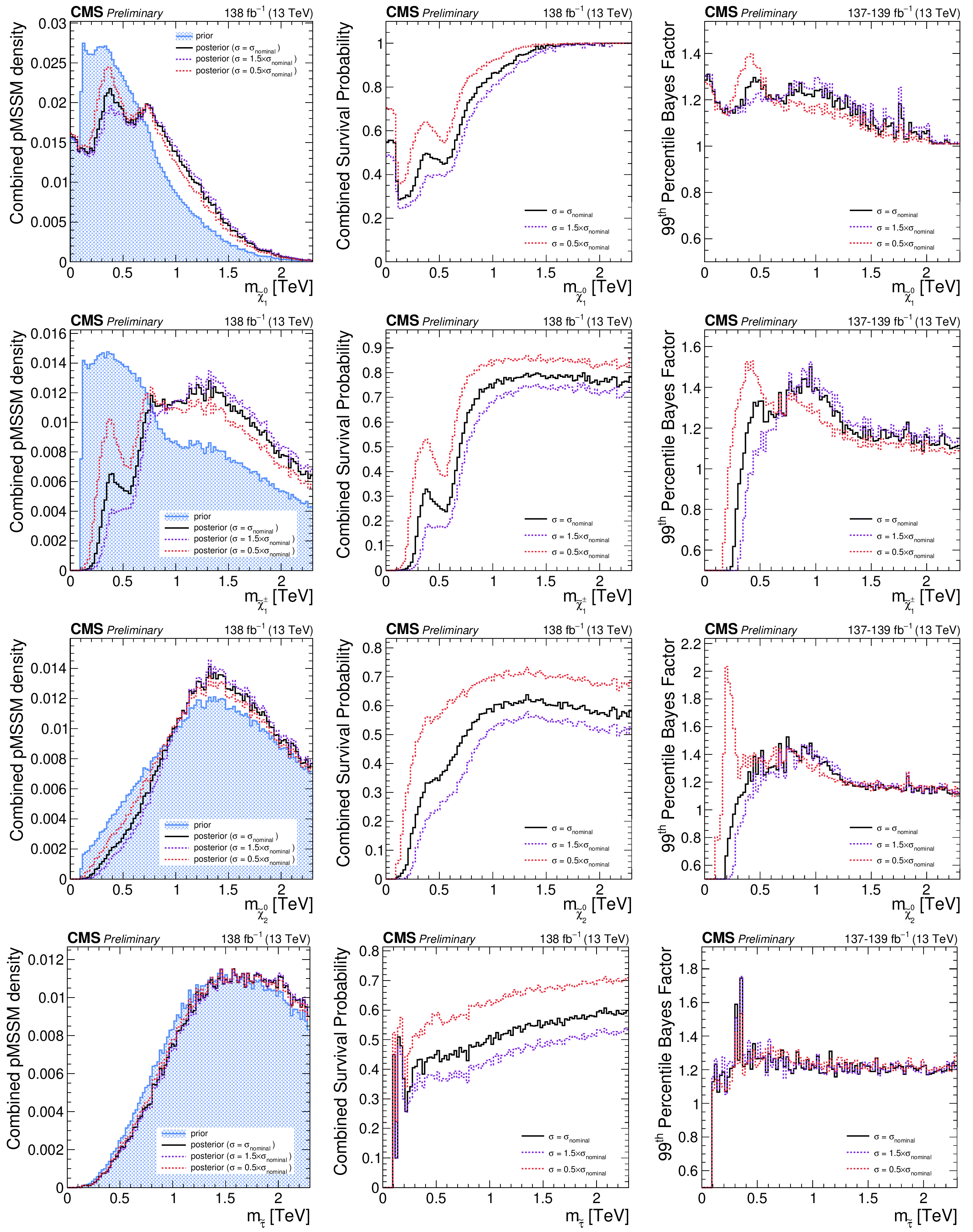
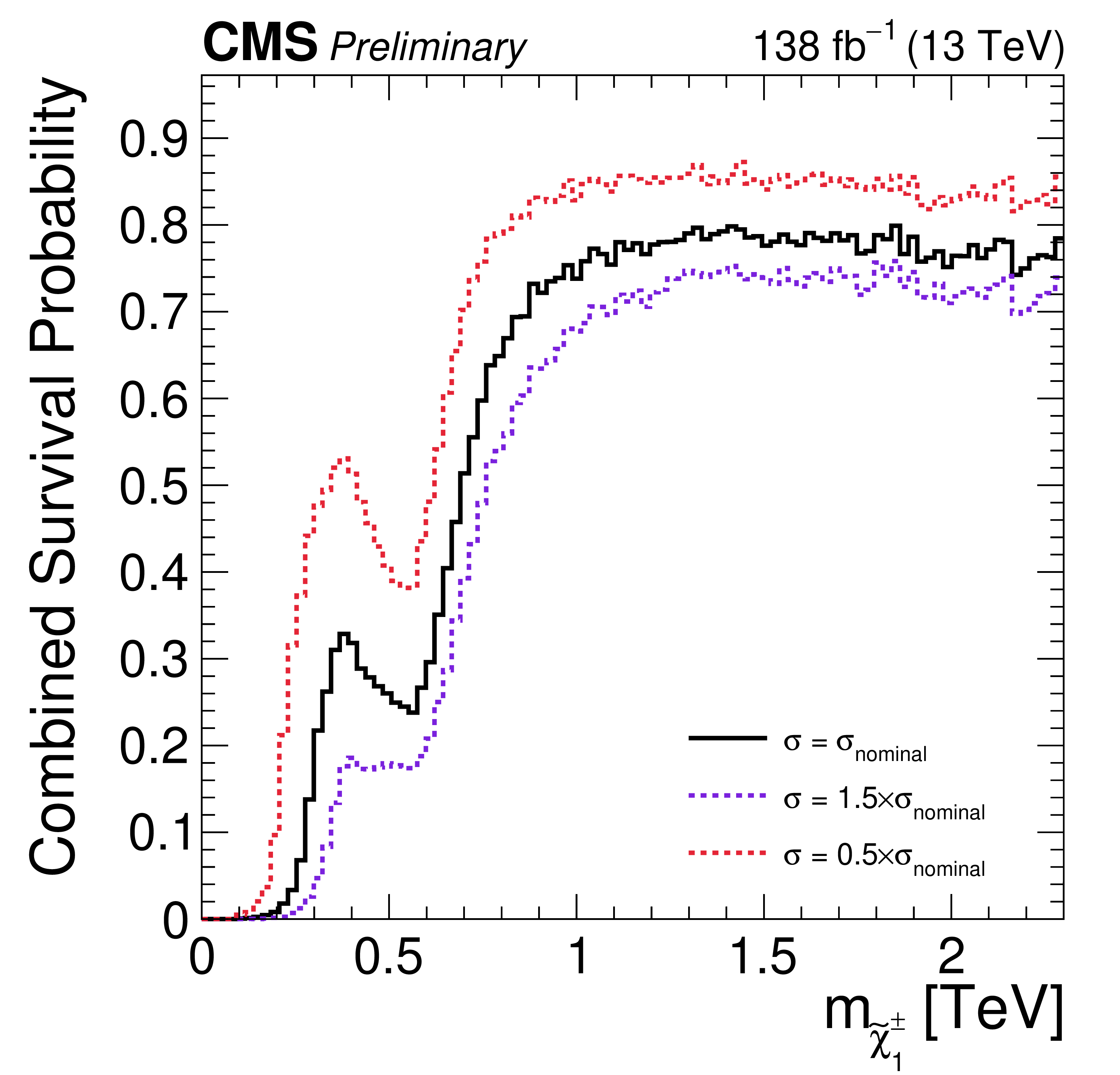
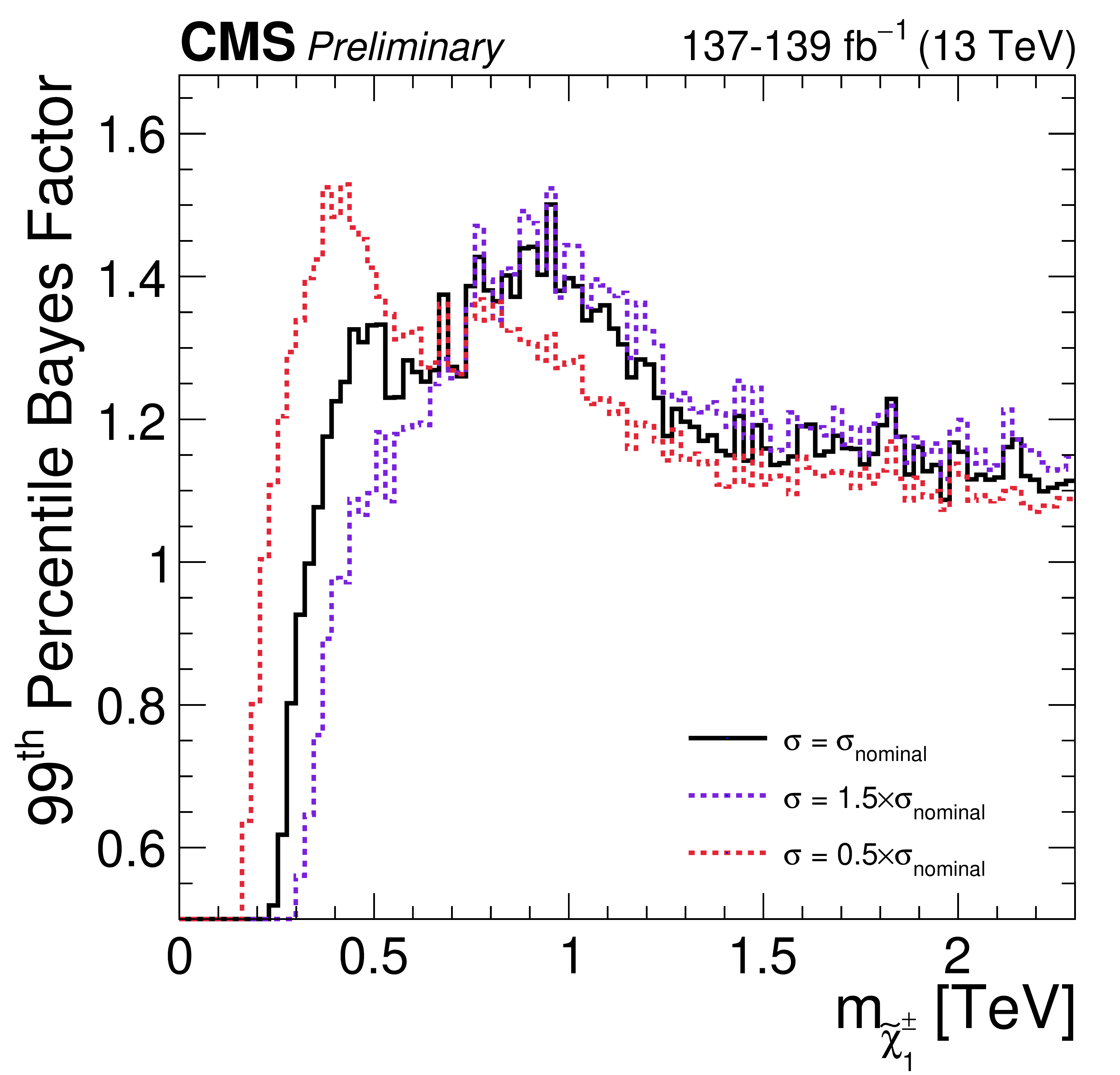
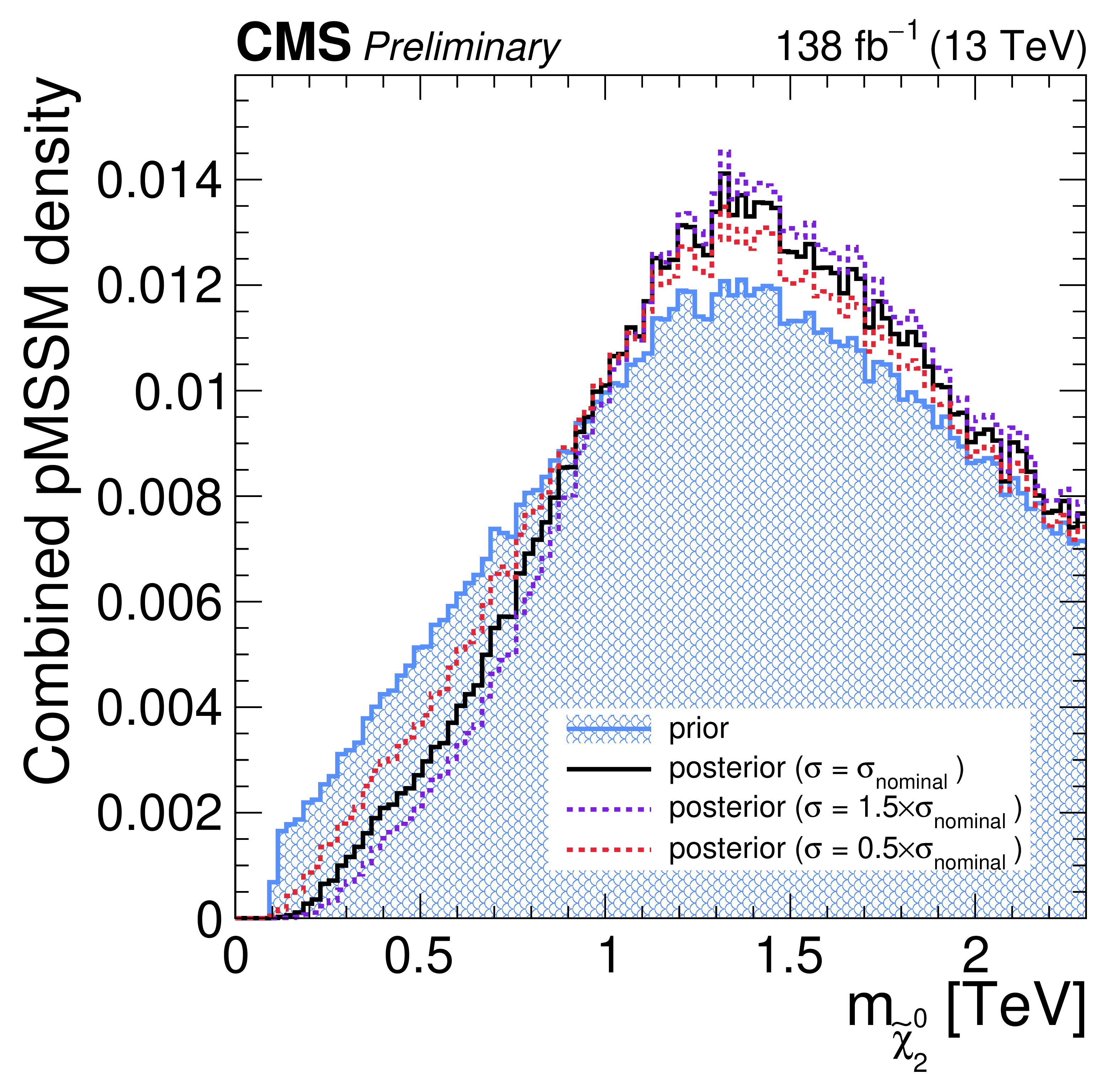
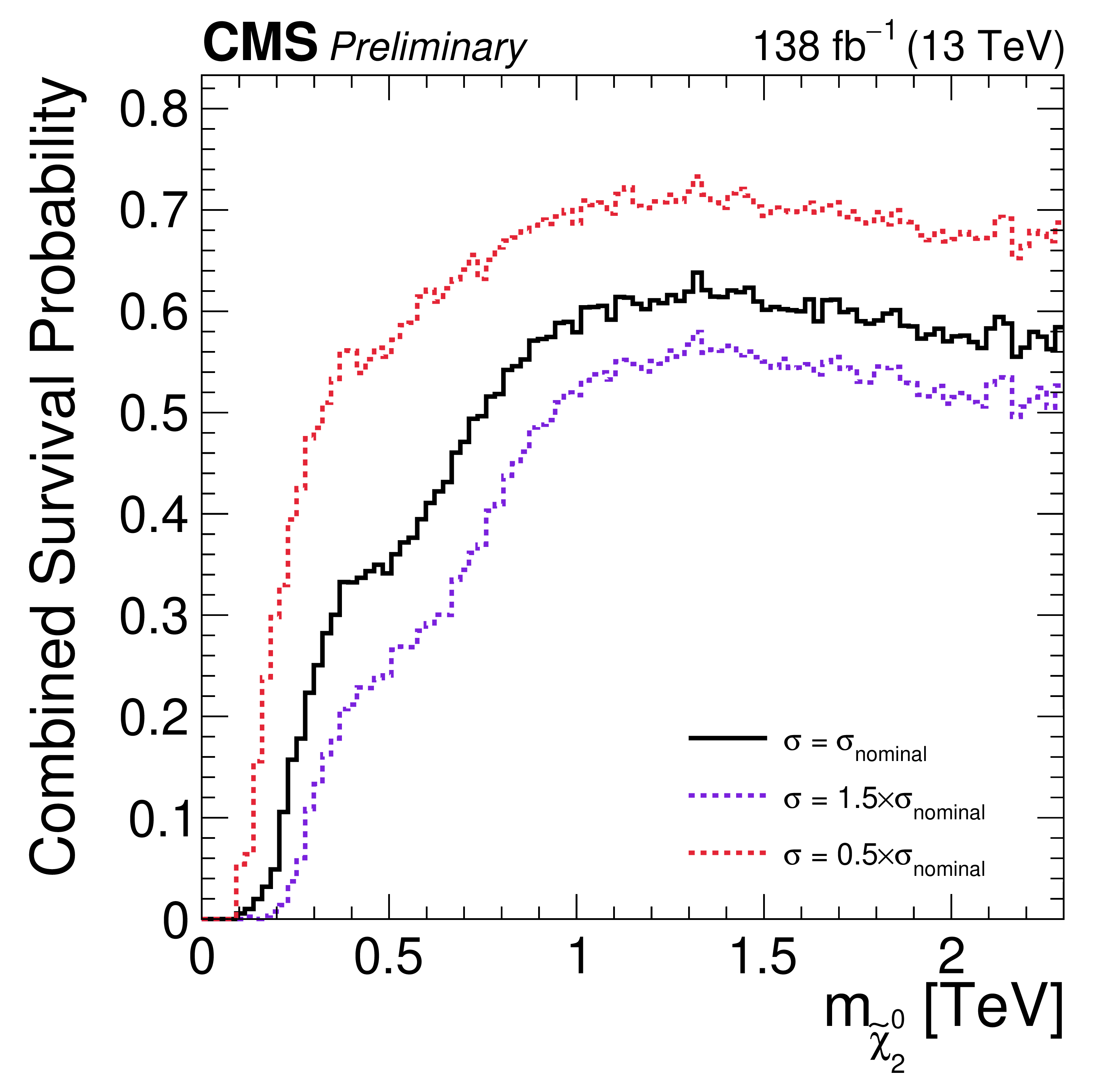
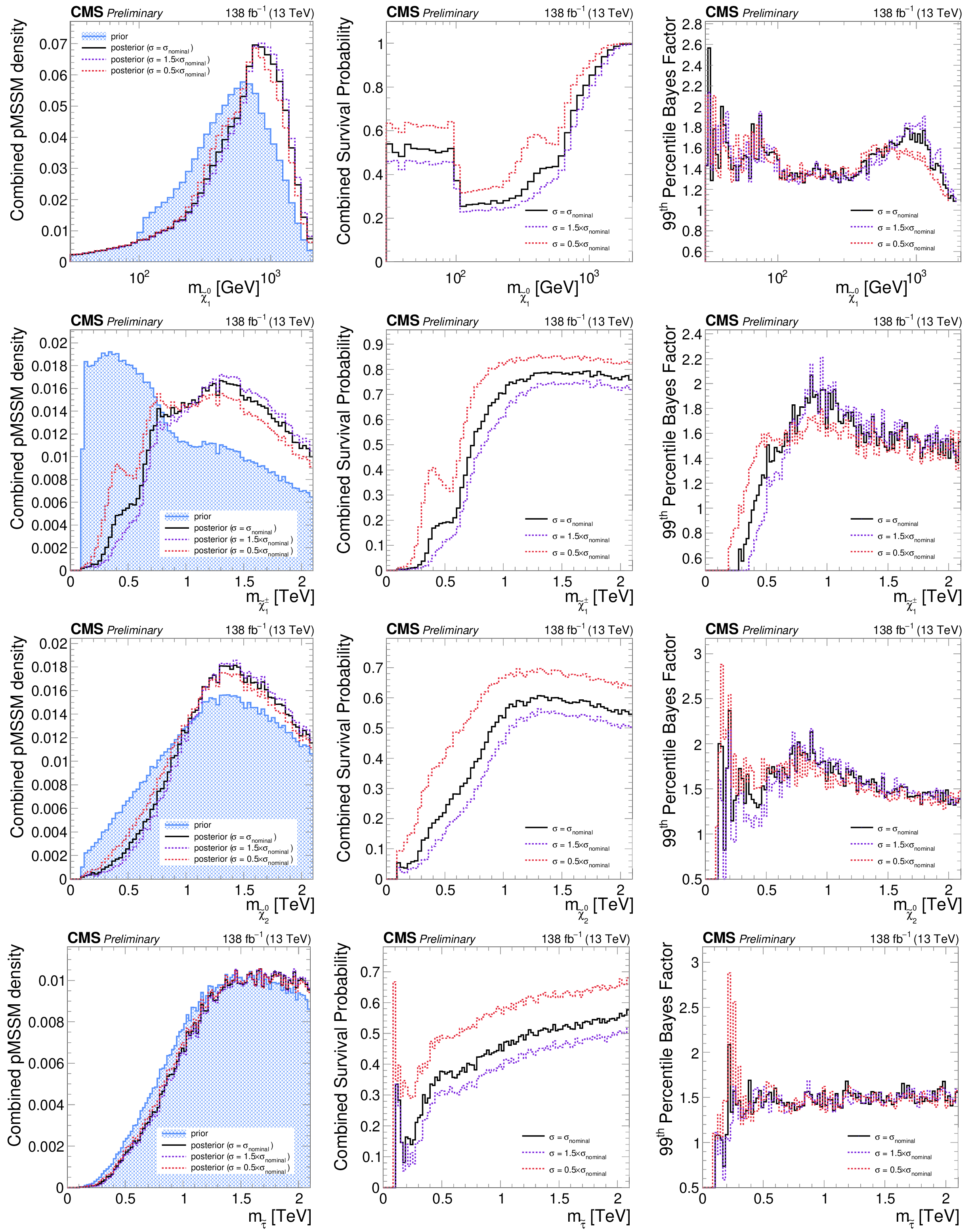
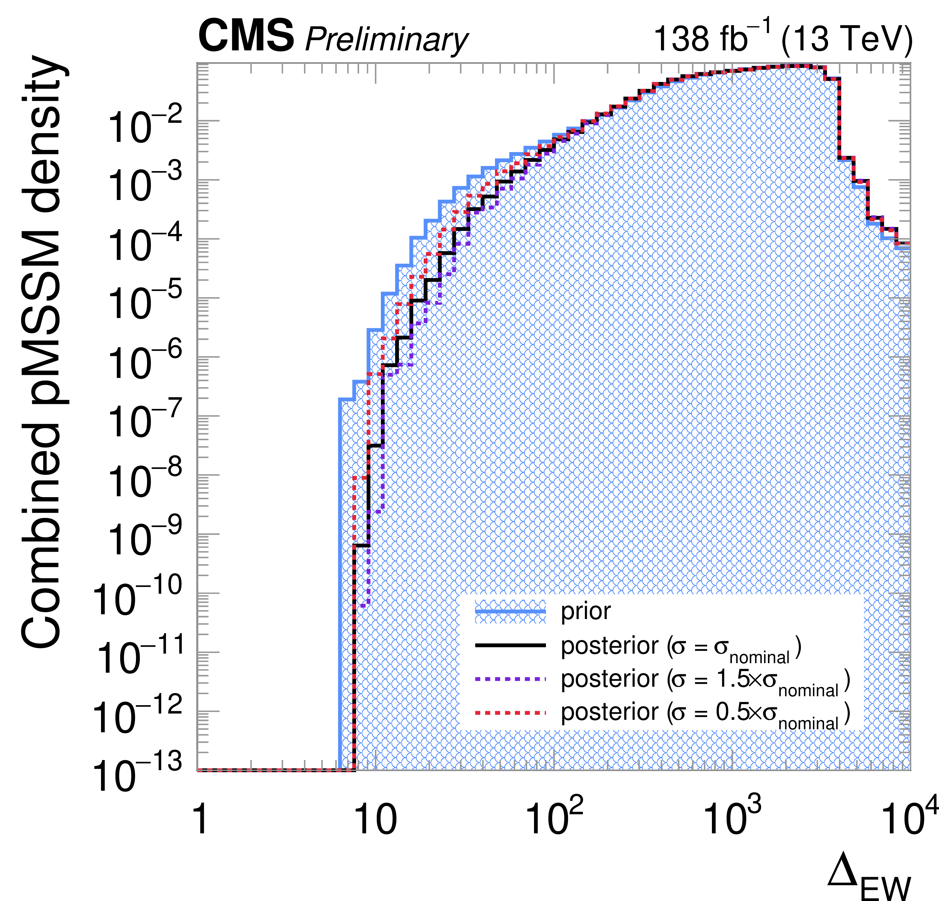
Figure 1:
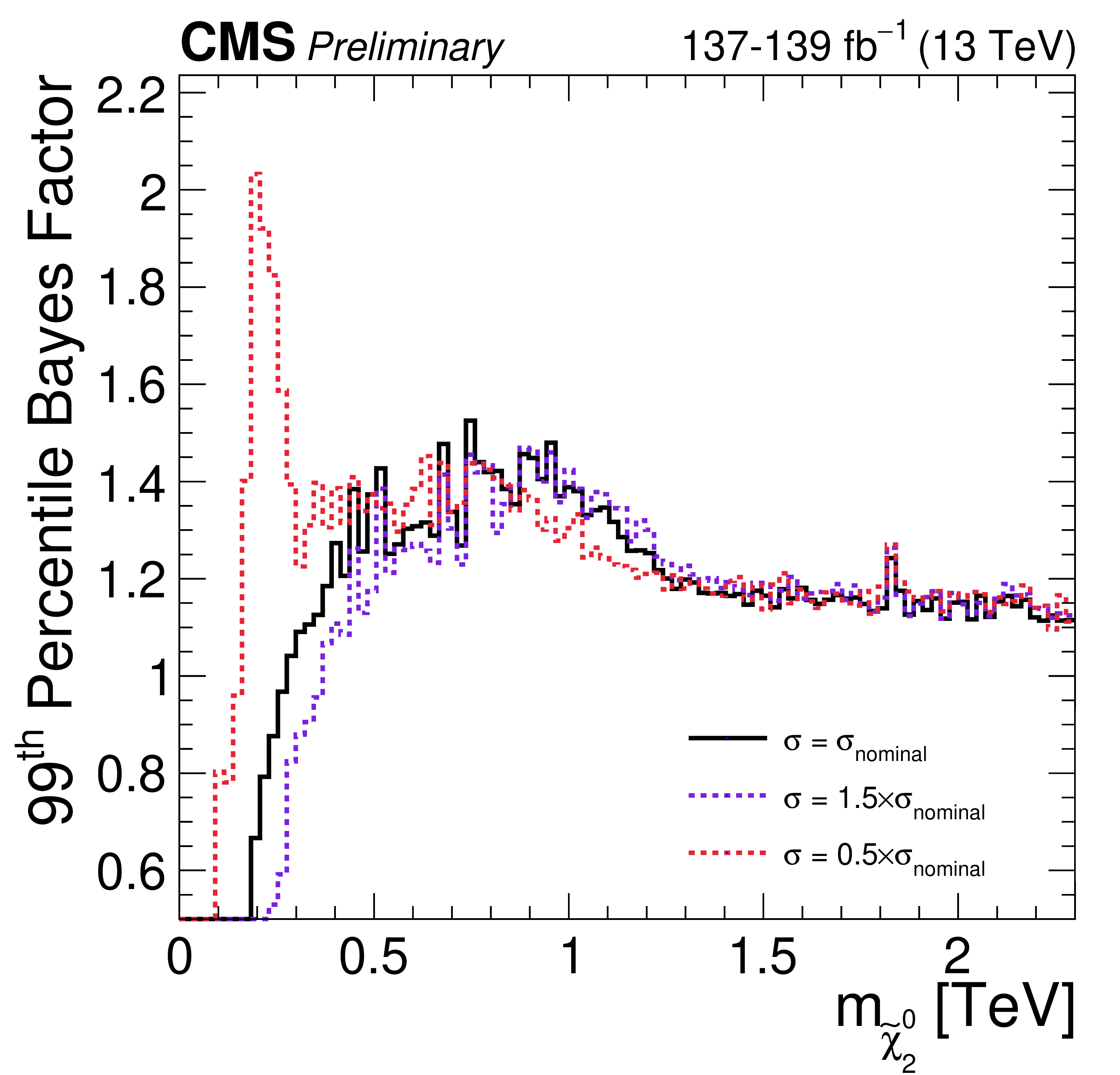
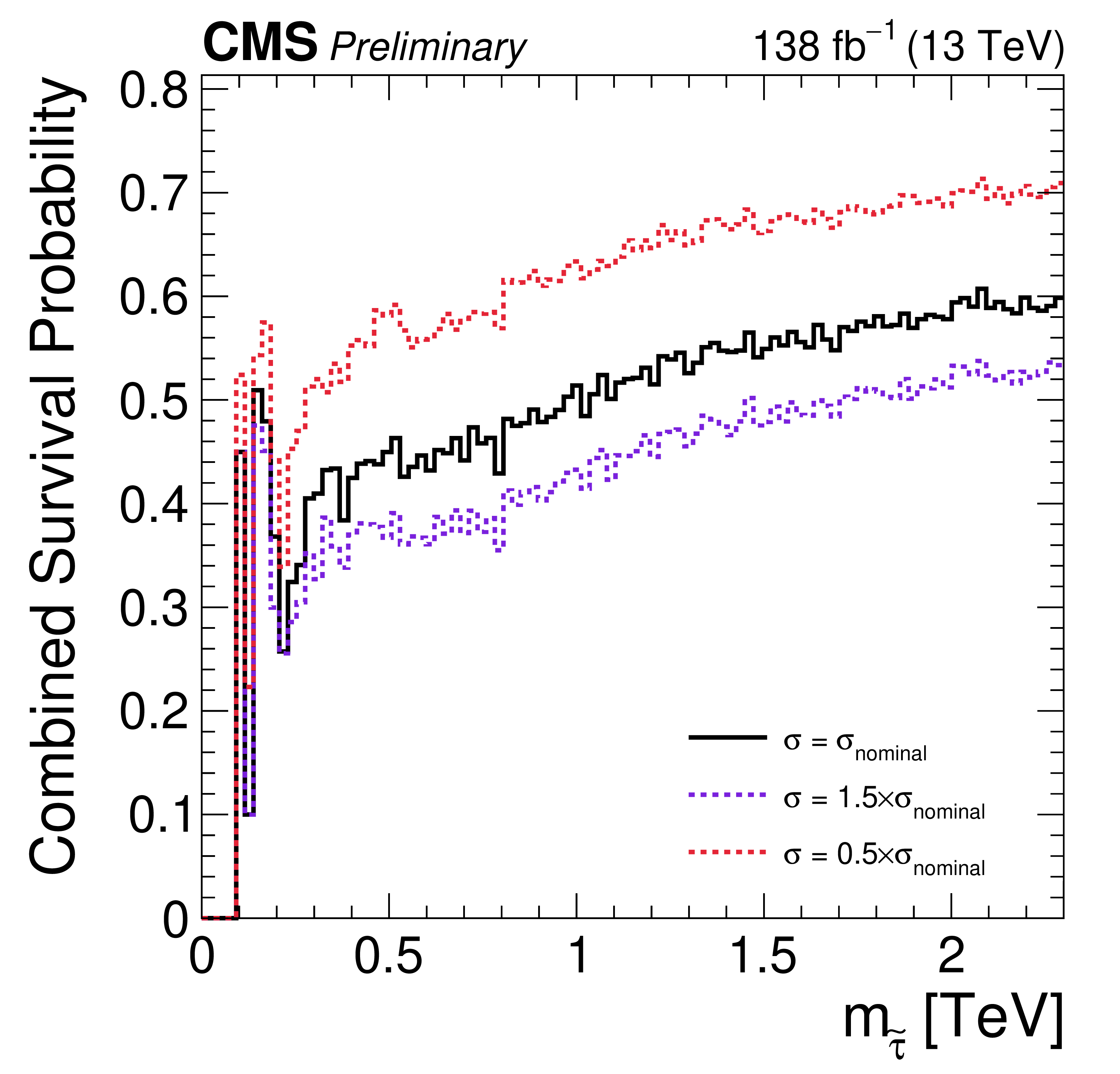
Marginalized prior and posterior density (left), survival probability (center), and upper quantiles of the BF (right) for the masses of the lowest-mass electroweakino states (top three) and the stau (lower). The posterior density is obtained assuming the nominal cross section (black) as well as the up (purple) and down (red) cross section variations. |
png pdf |
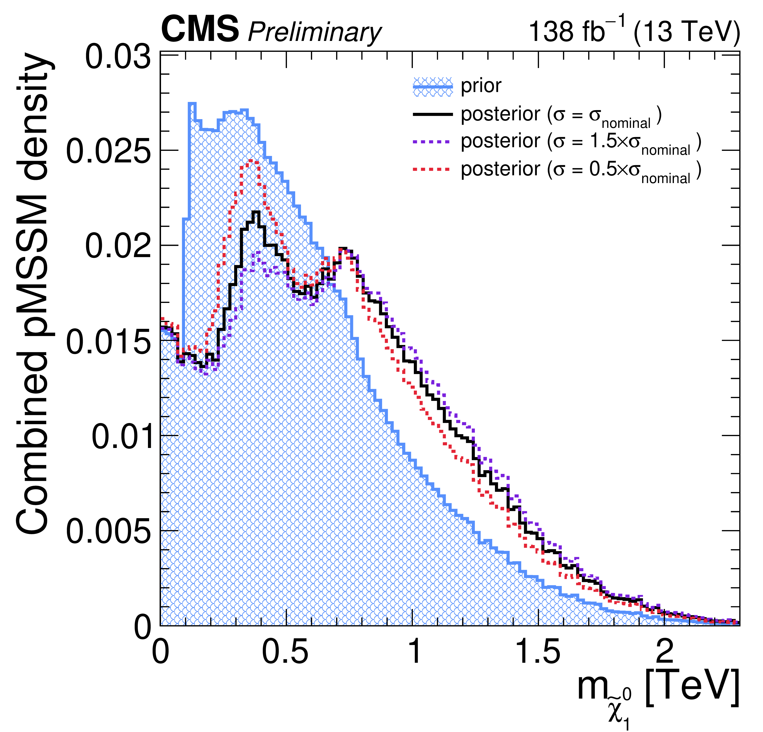
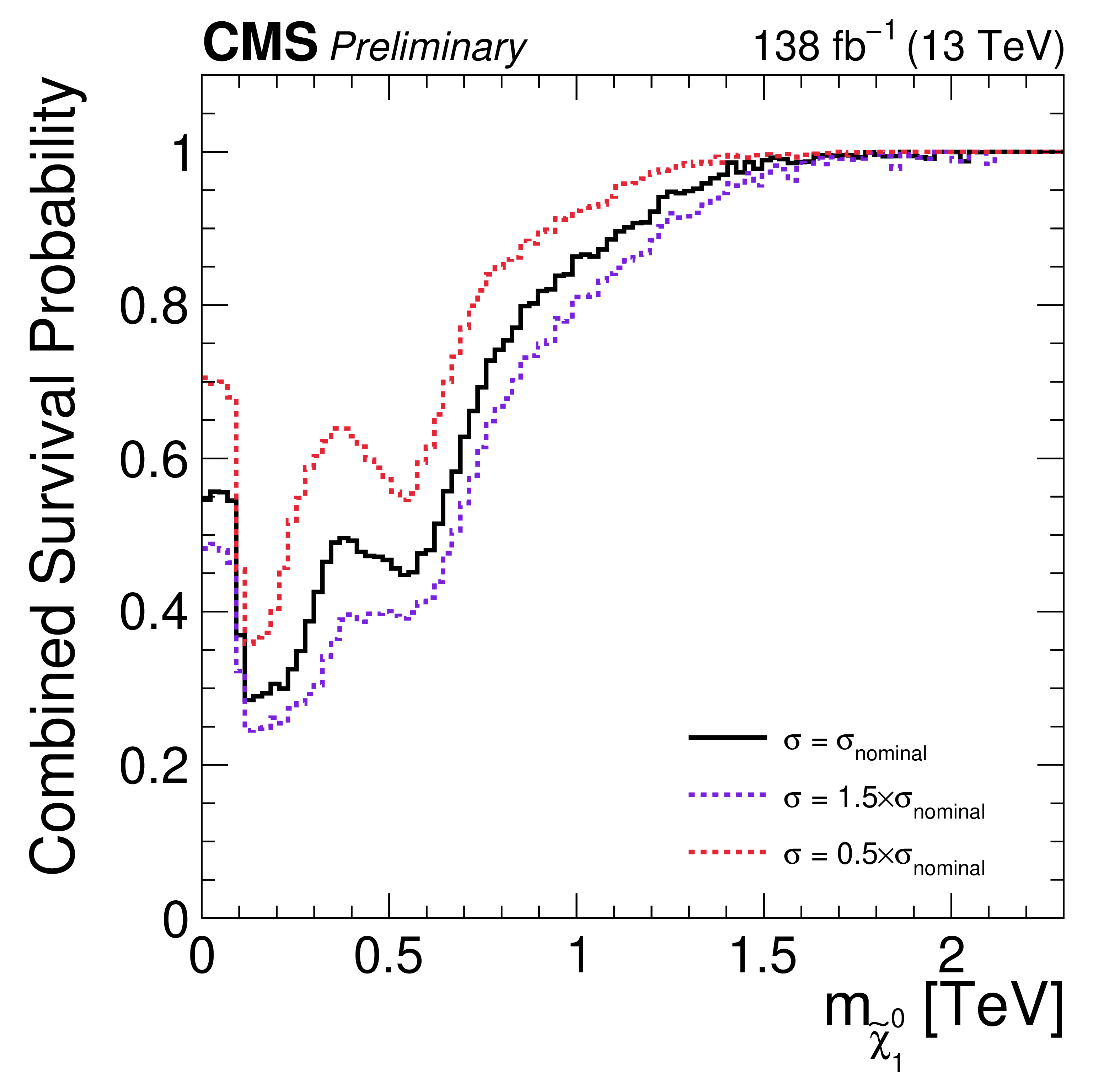
Figure 1-a:
Marginalized prior and posterior density (left), survival probability (center), and upper quantiles of the BF (right) for the masses of the lowest-mass electroweakino states (top three) and the stau (lower). The posterior density is obtained assuming the nominal cross section (black) as well as the up (purple) and down (red) cross section variations. |
png pdf |
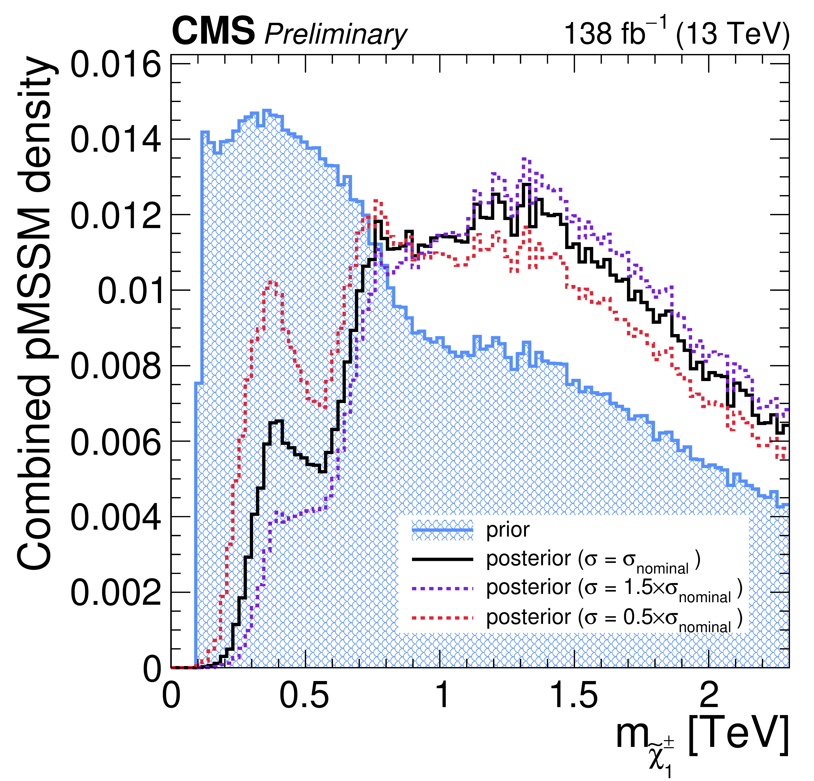
Figure 1-b:
Marginalized prior and posterior density (left), survival probability (center), and upper quantiles of the BF (right) for the masses of the lowest-mass electroweakino states (top three) and the stau (lower). The posterior density is obtained assuming the nominal cross section (black) as well as the up (purple) and down (red) cross section variations. |

png pdf |
Figure 1-c:
Marginalized prior and posterior density (left), survival probability (center), and upper quantiles of the BF (right) for the masses of the lowest-mass electroweakino states (top three) and the stau (lower). The posterior density is obtained assuming the nominal cross section (black) as well as the up (purple) and down (red) cross section variations. |
png pdf |
Figure 1-d:
Marginalized prior and posterior density (left), survival probability (center), and upper quantiles of the BF (right) for the masses of the lowest-mass electroweakino states (top three) and the stau (lower). The posterior density is obtained assuming the nominal cross section (black) as well as the up (purple) and down (red) cross section variations. |
png pdf |
Figure 1-e:
Marginalized prior and posterior density (left), survival probability (center), and upper quantiles of the BF (right) for the masses of the lowest-mass electroweakino states (top three) and the stau (lower). The posterior density is obtained assuming the nominal cross section (black) as well as the up (purple) and down (red) cross section variations. |
png pdf |
Figure 1-f:
Marginalized prior and posterior density (left), survival probability (center), and upper quantiles of the BF (right) for the masses of the lowest-mass electroweakino states (top three) and the stau (lower). The posterior density is obtained assuming the nominal cross section (black) as well as the up (purple) and down (red) cross section variations. |
png pdf |
Figure 1-g:
Marginalized prior and posterior density (left), survival probability (center), and upper quantiles of the BF (right) for the masses of the lowest-mass electroweakino states (top three) and the stau (lower). The posterior density is obtained assuming the nominal cross section (black) as well as the up (purple) and down (red) cross section variations. |
png pdf |
Figure 1-h:
Marginalized prior and posterior density (left), survival probability (center), and upper quantiles of the BF (right) for the masses of the lowest-mass electroweakino states (top three) and the stau (lower). The posterior density is obtained assuming the nominal cross section (black) as well as the up (purple) and down (red) cross section variations. |
png pdf |
Figure 1-i:
Marginalized prior and posterior density (left), survival probability (center), and upper quantiles of the BF (right) for the masses of the lowest-mass electroweakino states (top three) and the stau (lower). The posterior density is obtained assuming the nominal cross section (black) as well as the up (purple) and down (red) cross section variations. |

png pdf |
Figure 1-j:
Marginalized prior and posterior density (left), survival probability (center), and upper quantiles of the BF (right) for the masses of the lowest-mass electroweakino states (top three) and the stau (lower). The posterior density is obtained assuming the nominal cross section (black) as well as the up (purple) and down (red) cross section variations. |
png pdf |
Figure 1-k:
Marginalized prior and posterior density (left), survival probability (center), and upper quantiles of the BF (right) for the masses of the lowest-mass electroweakino states (top three) and the stau (lower). The posterior density is obtained assuming the nominal cross section (black) as well as the up (purple) and down (red) cross section variations. |

png pdf |
Figure 1-l:
Marginalized prior and posterior density (left), survival probability (center), and upper quantiles of the BF (right) for the masses of the lowest-mass electroweakino states (top three) and the stau (lower). The posterior density is obtained assuming the nominal cross section (black) as well as the up (purple) and down (red) cross section variations. |
png pdf |
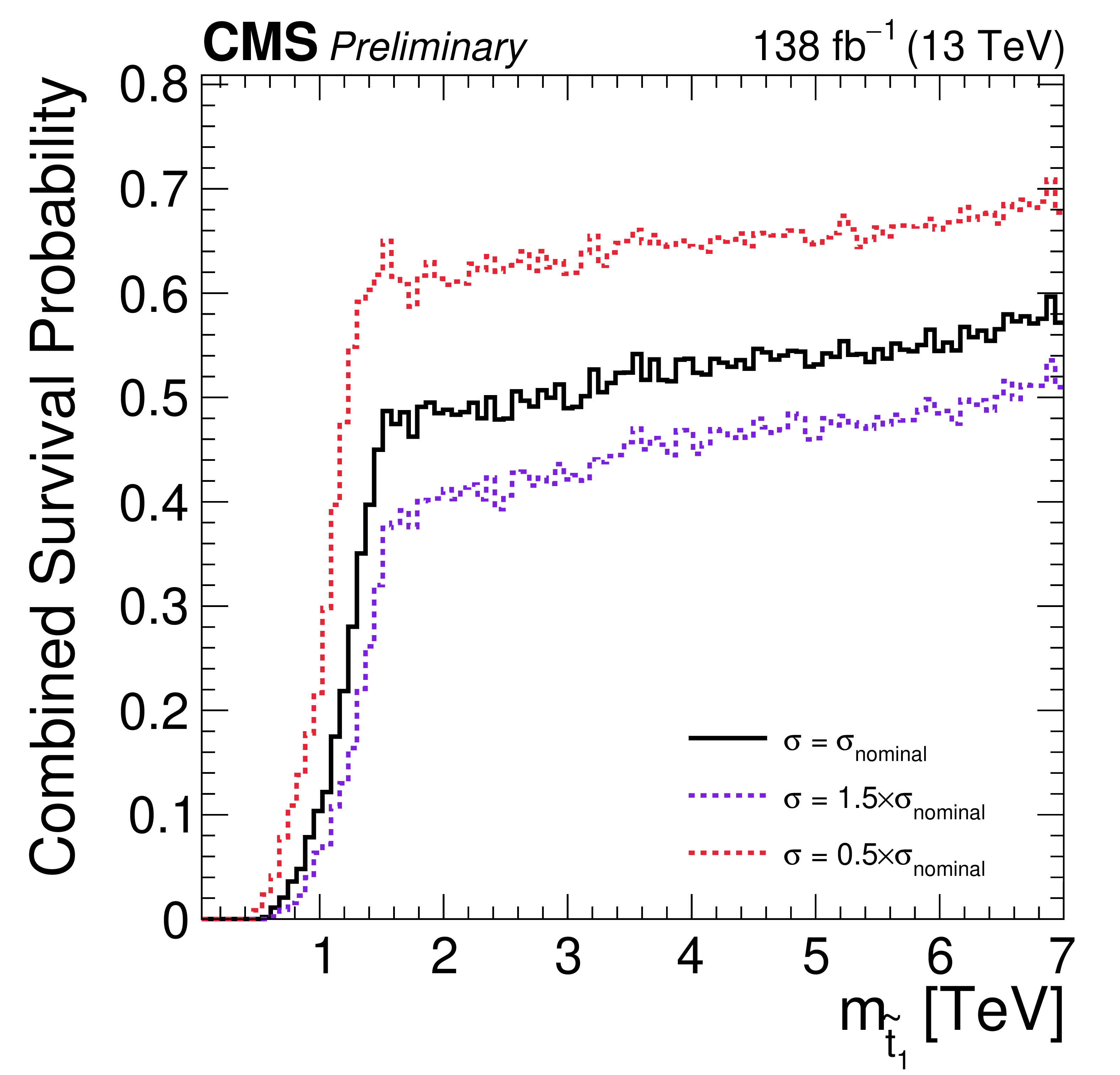
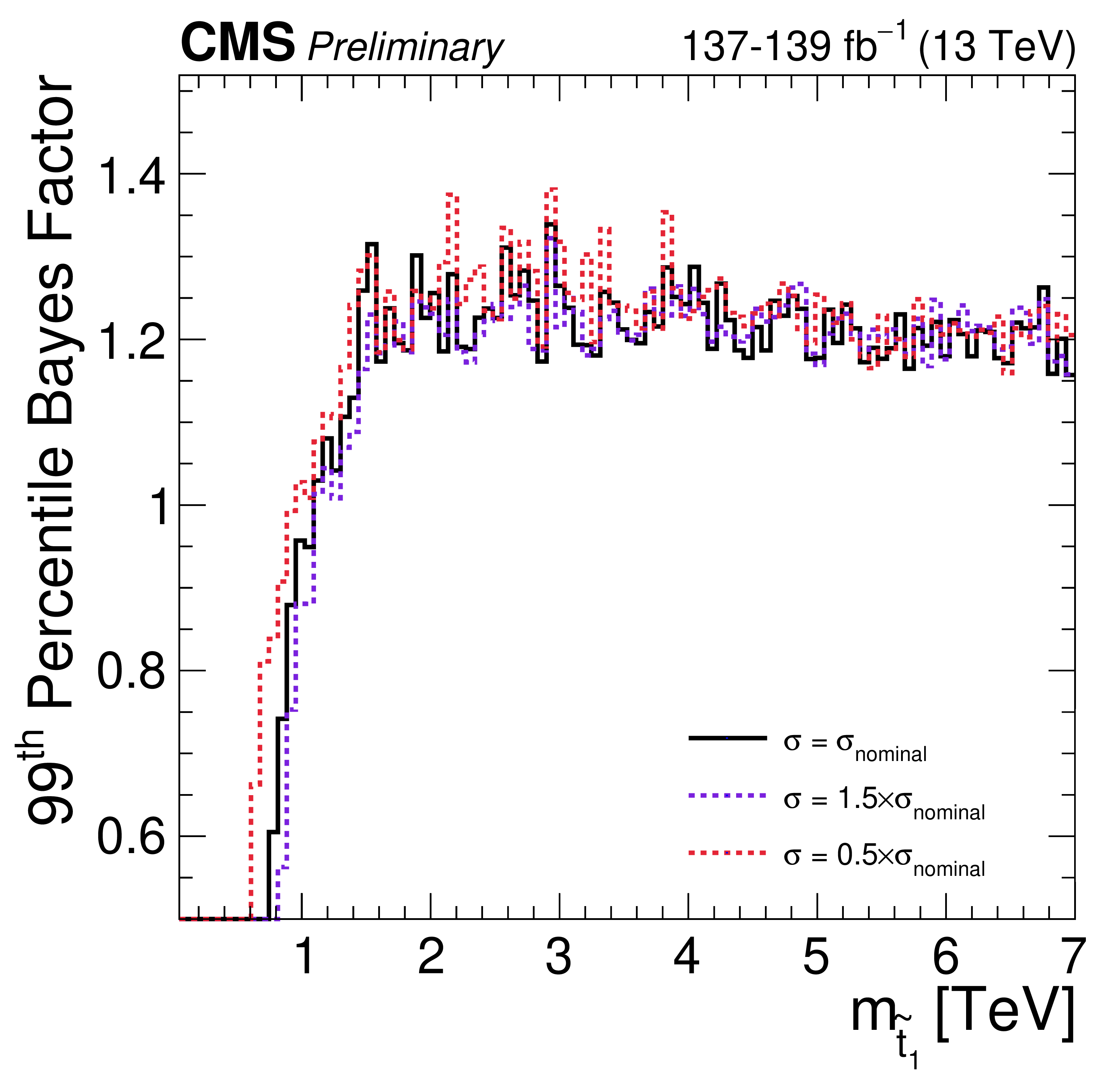
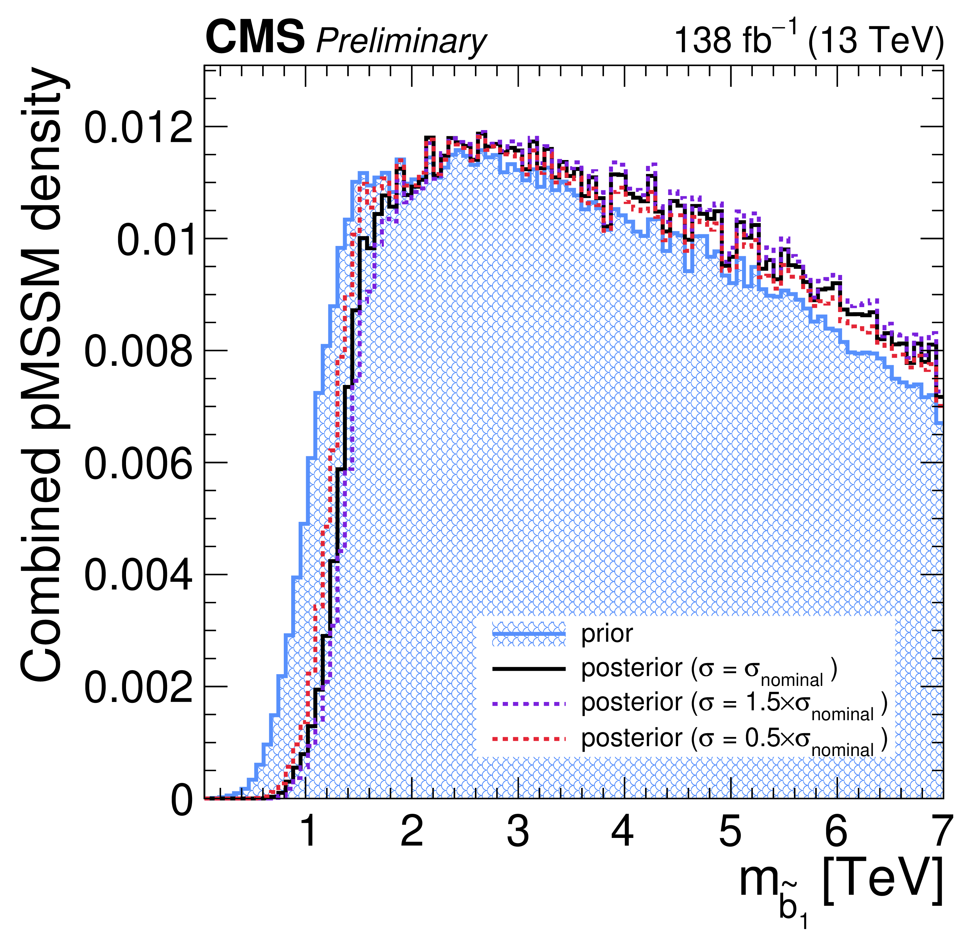
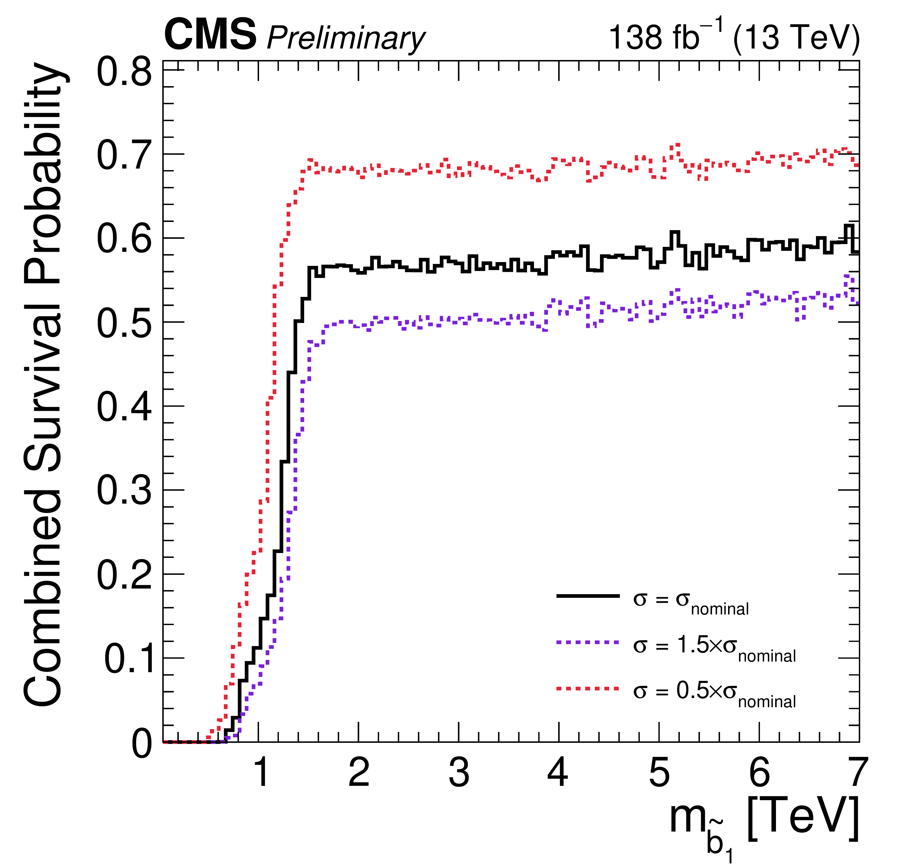
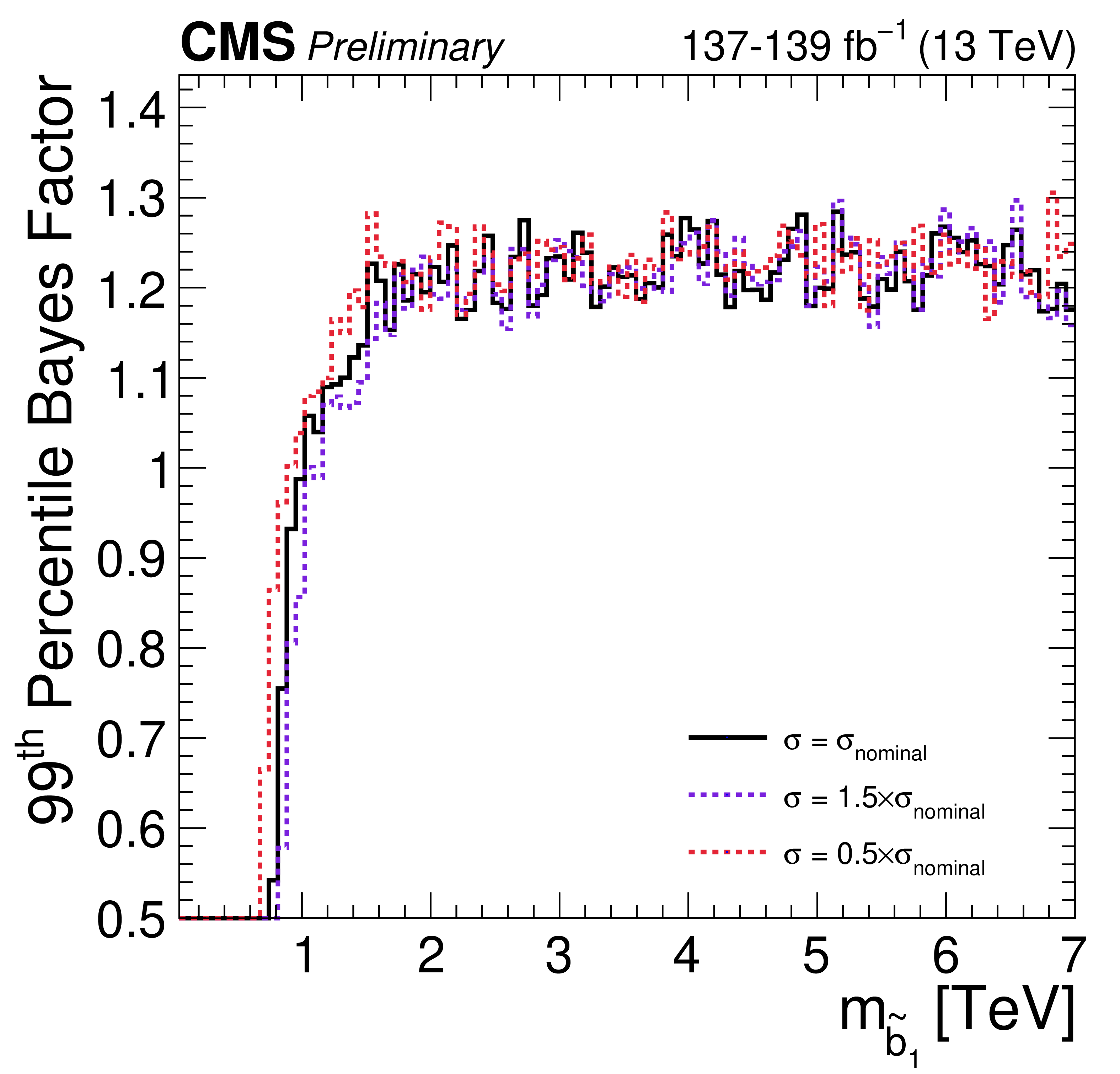
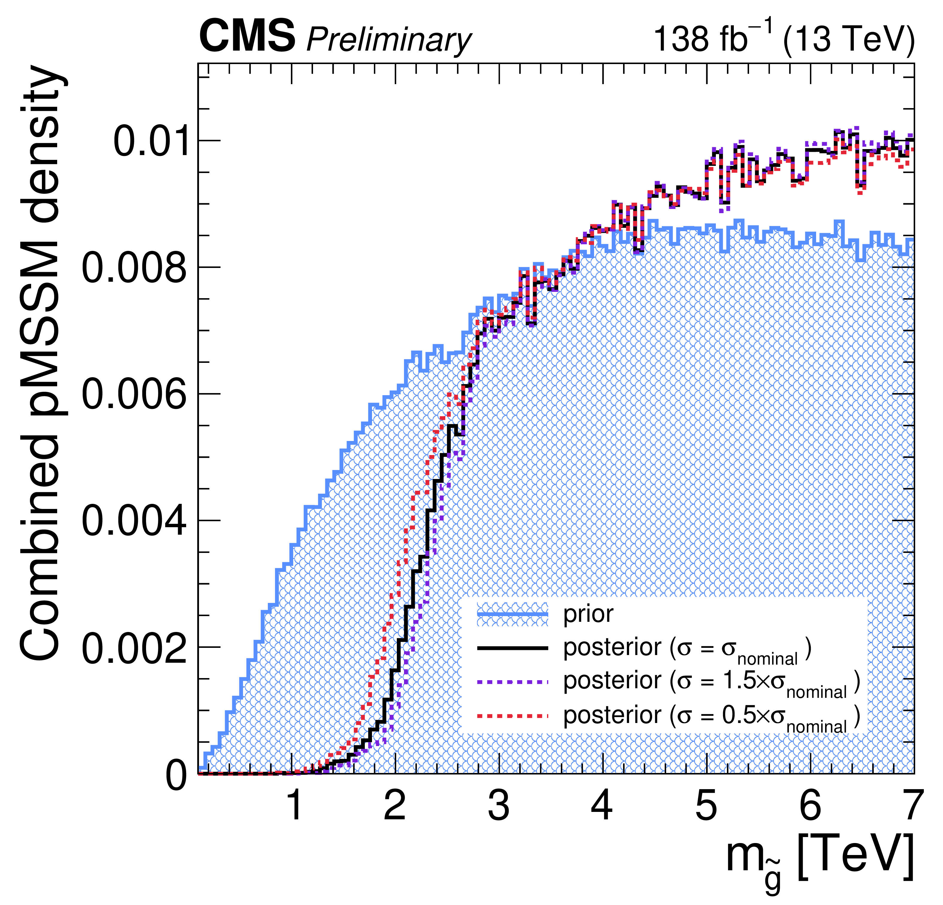
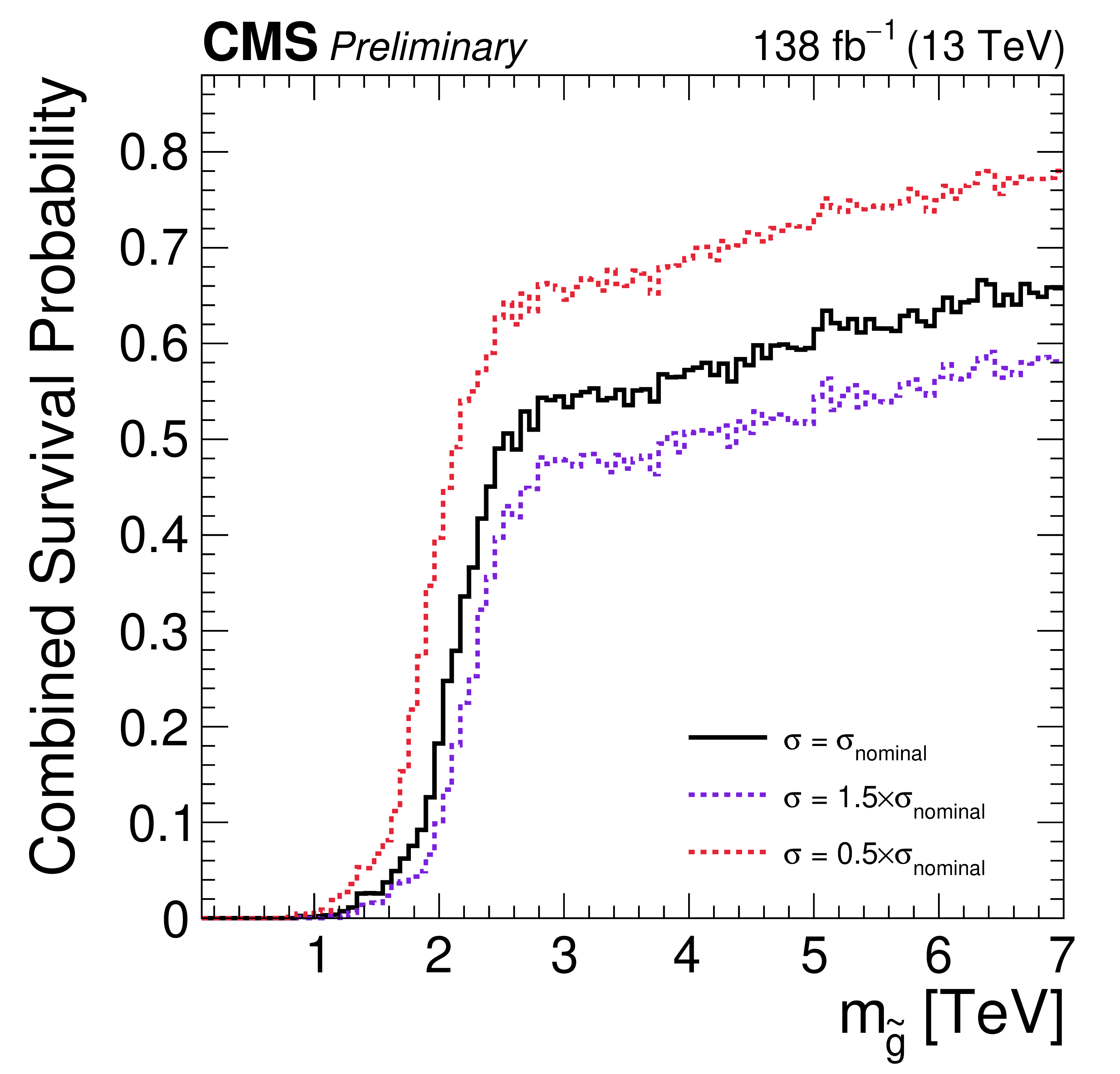
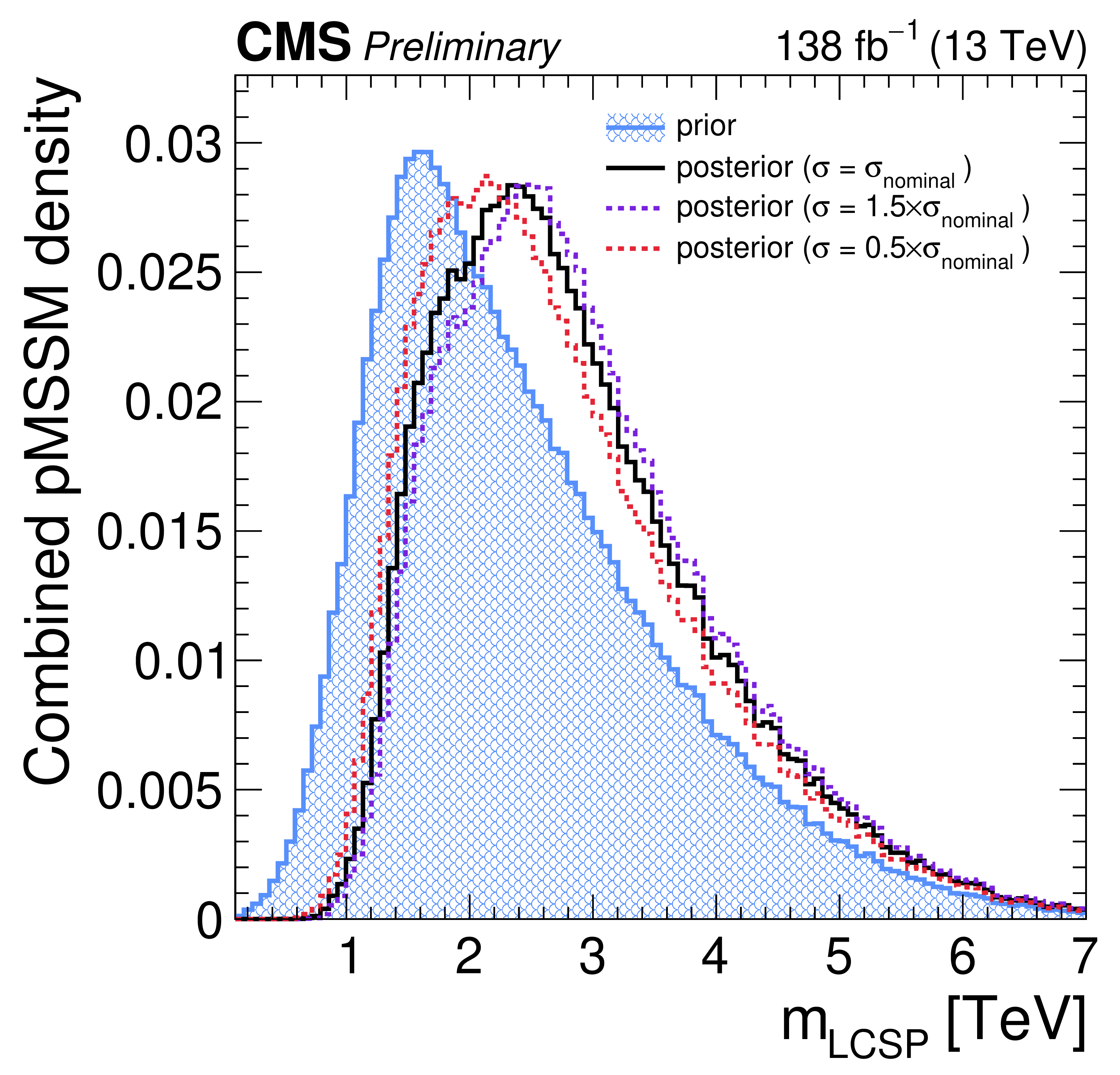
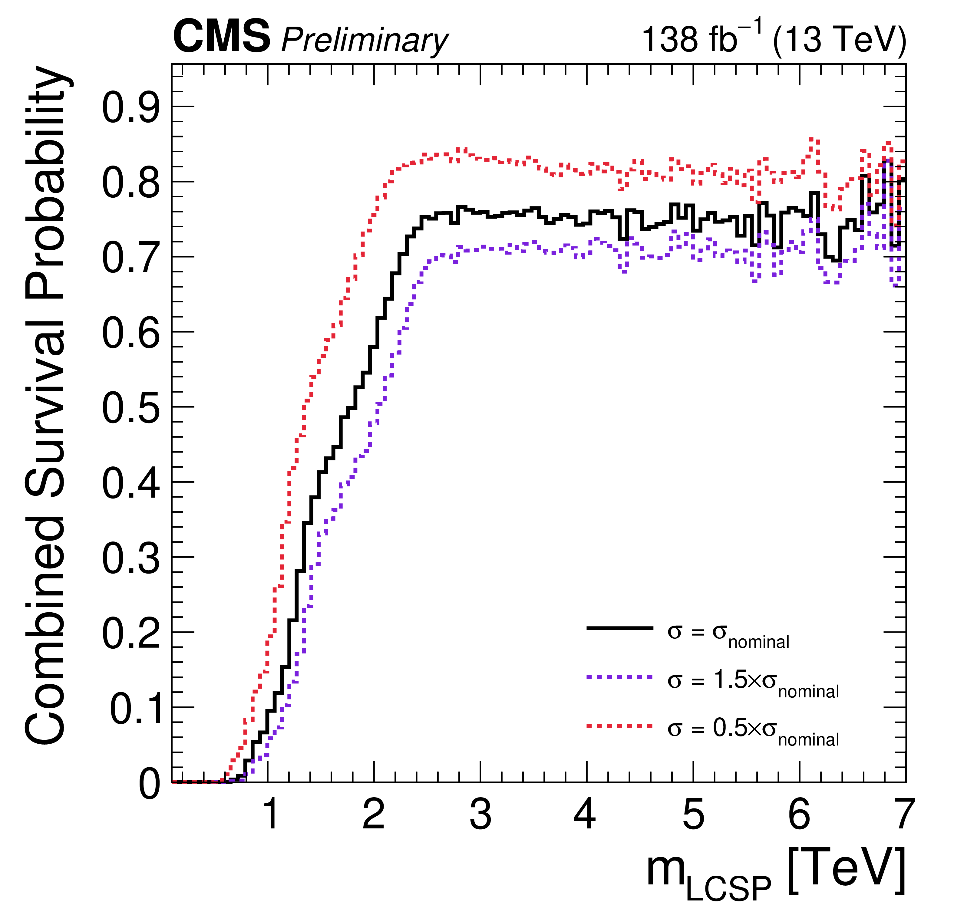
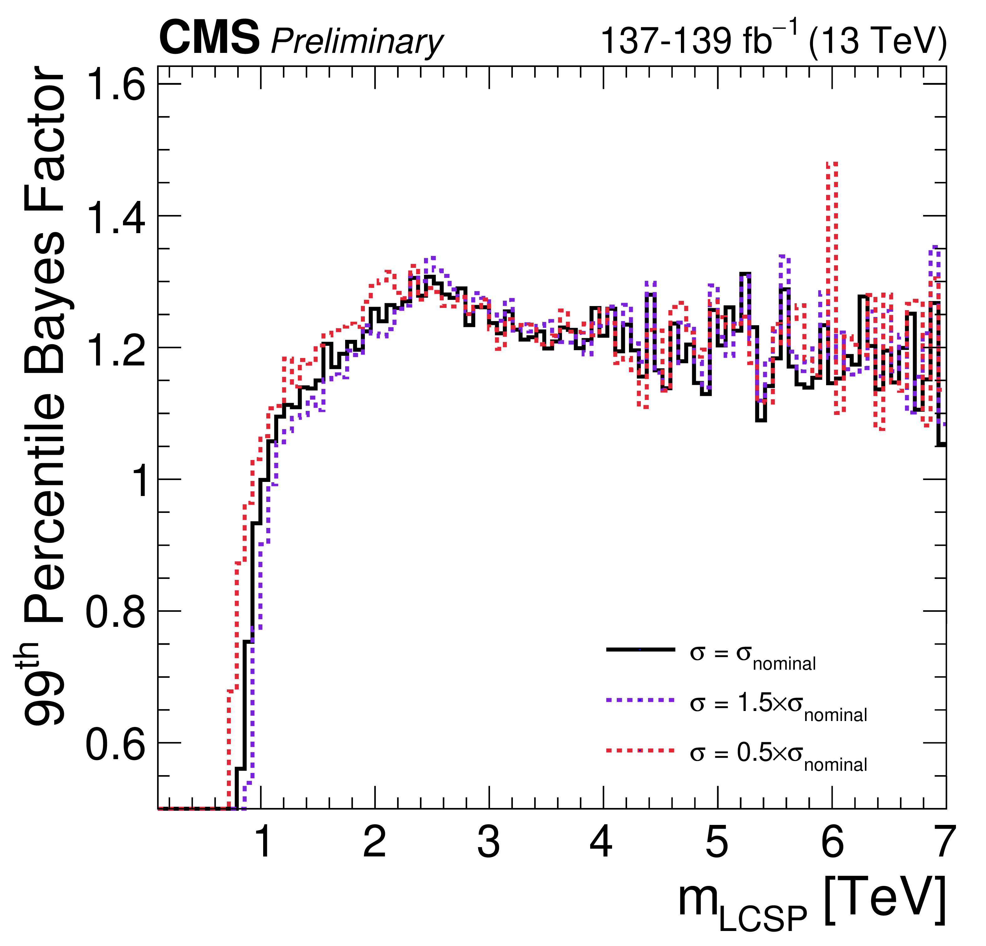
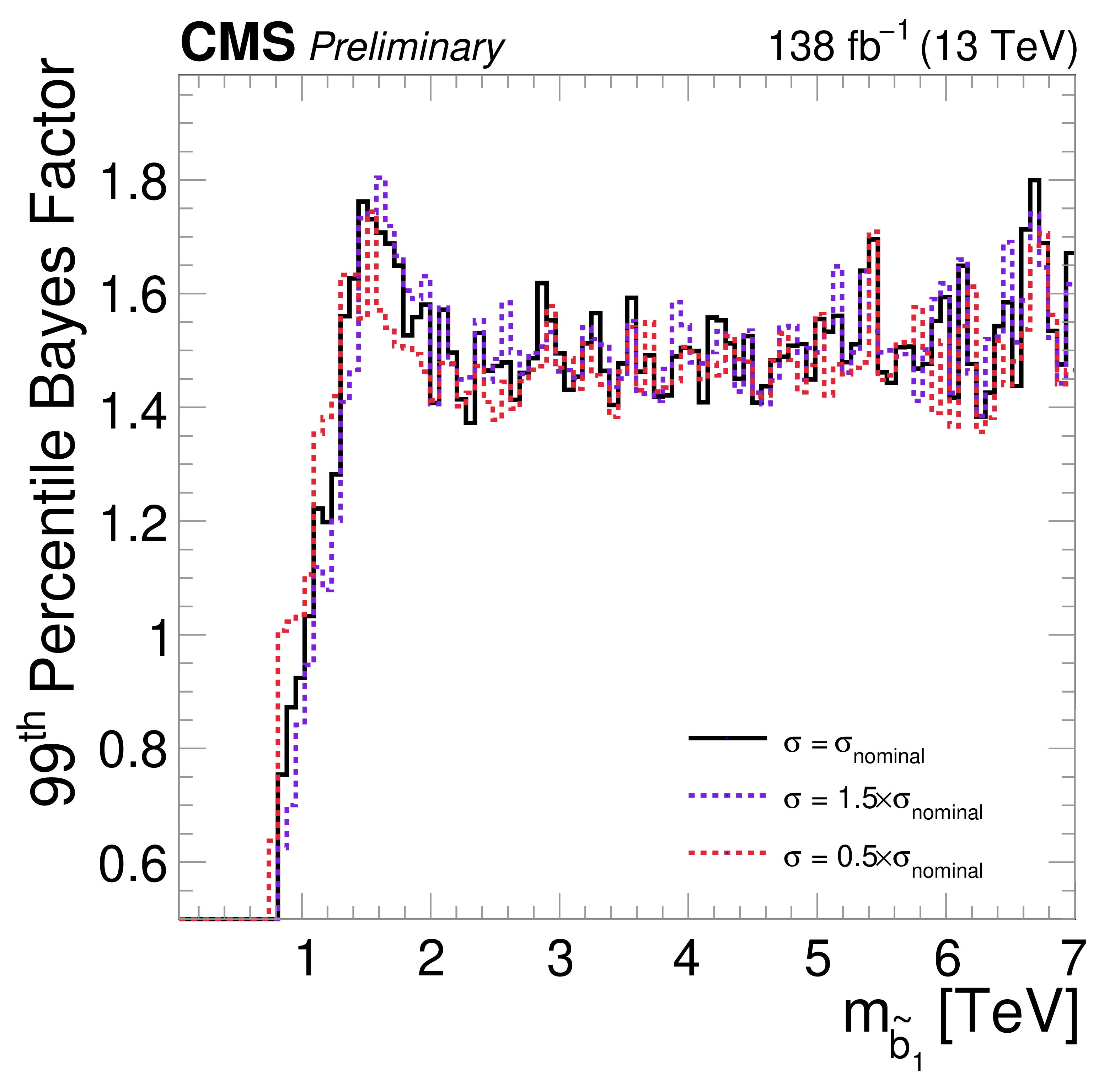
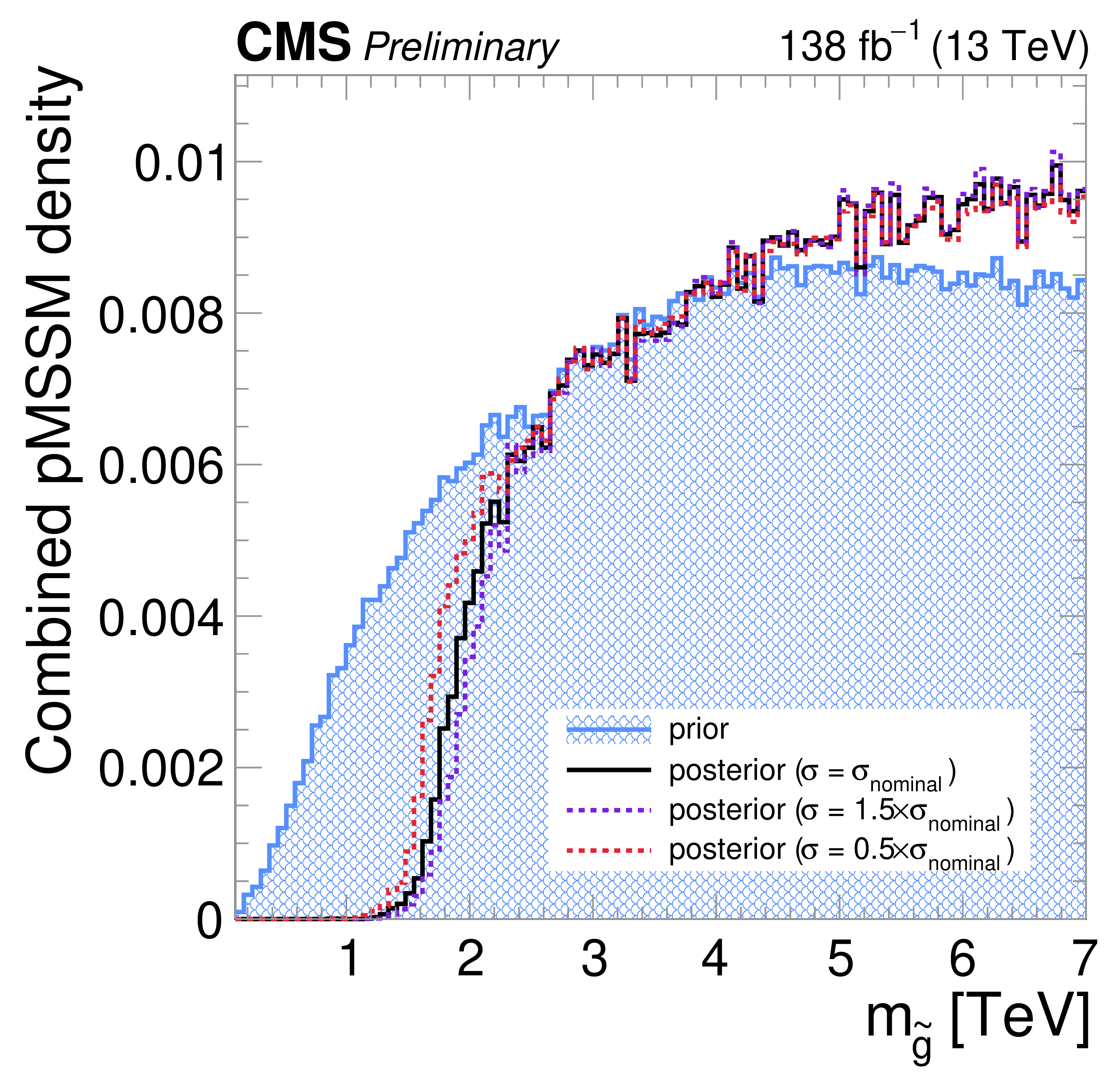
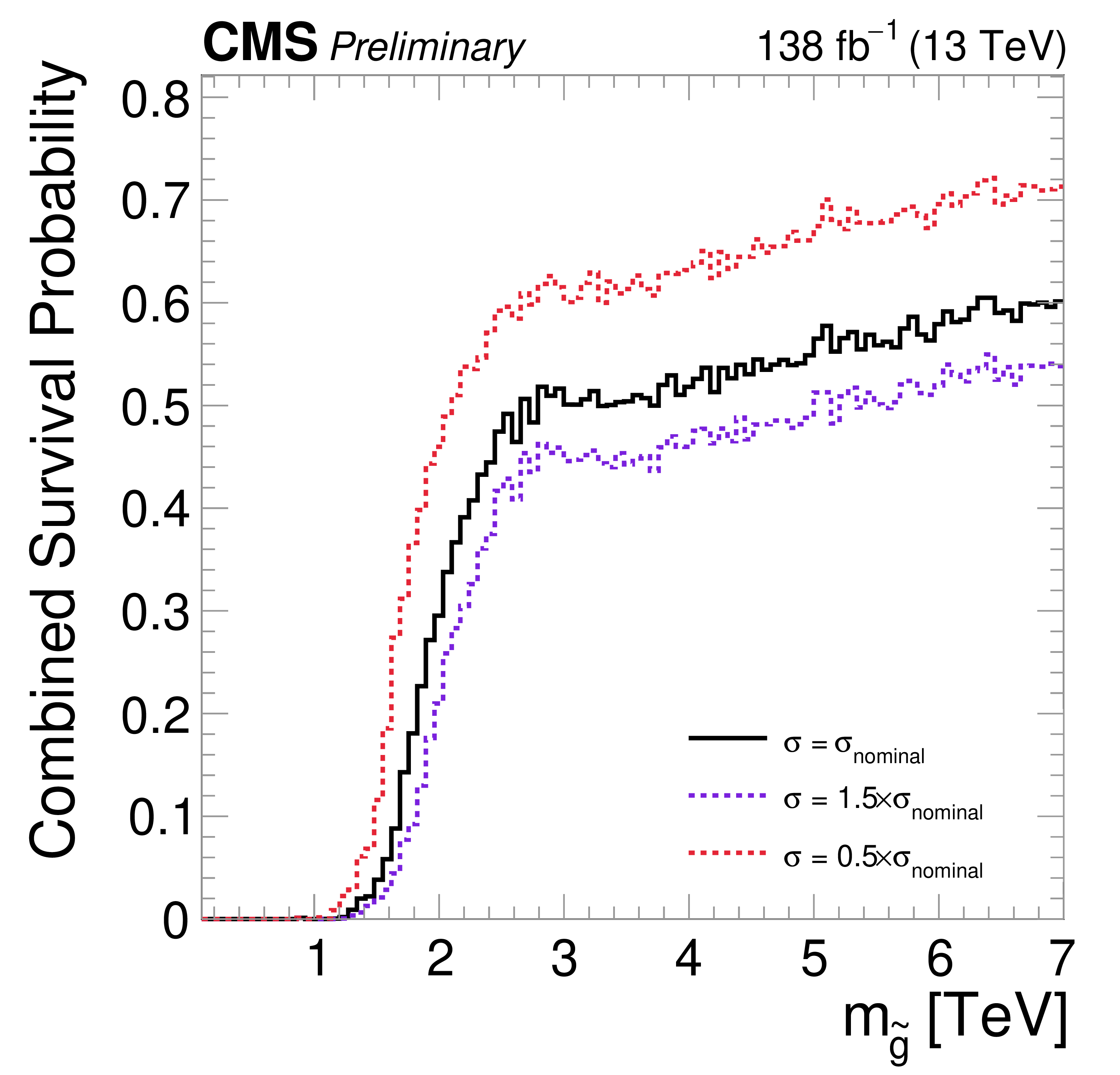
Figure 2:
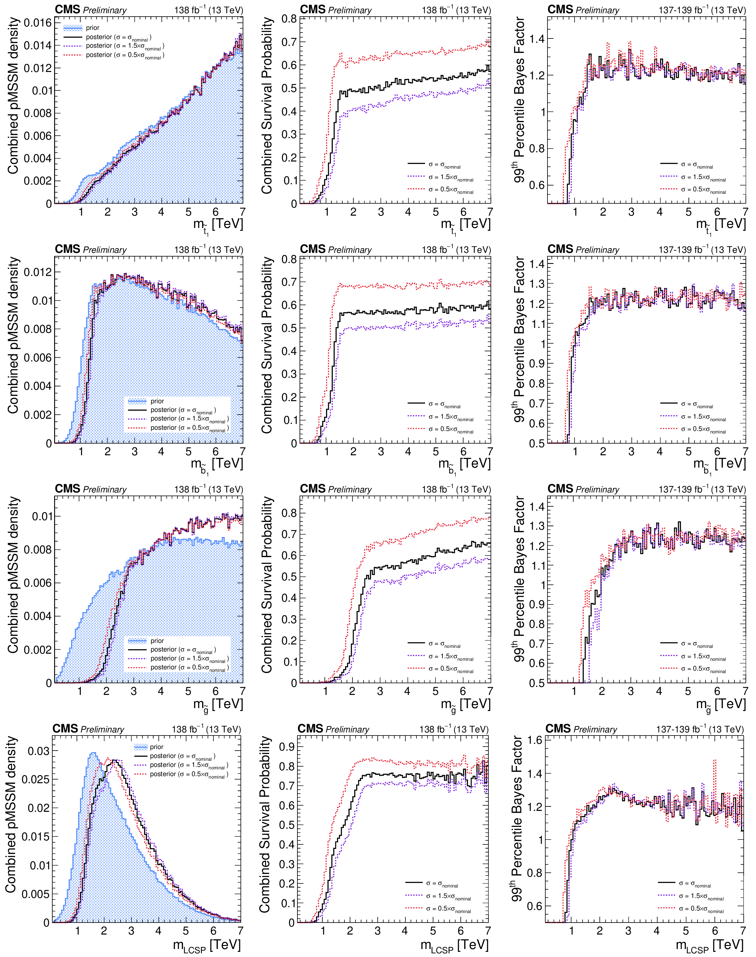
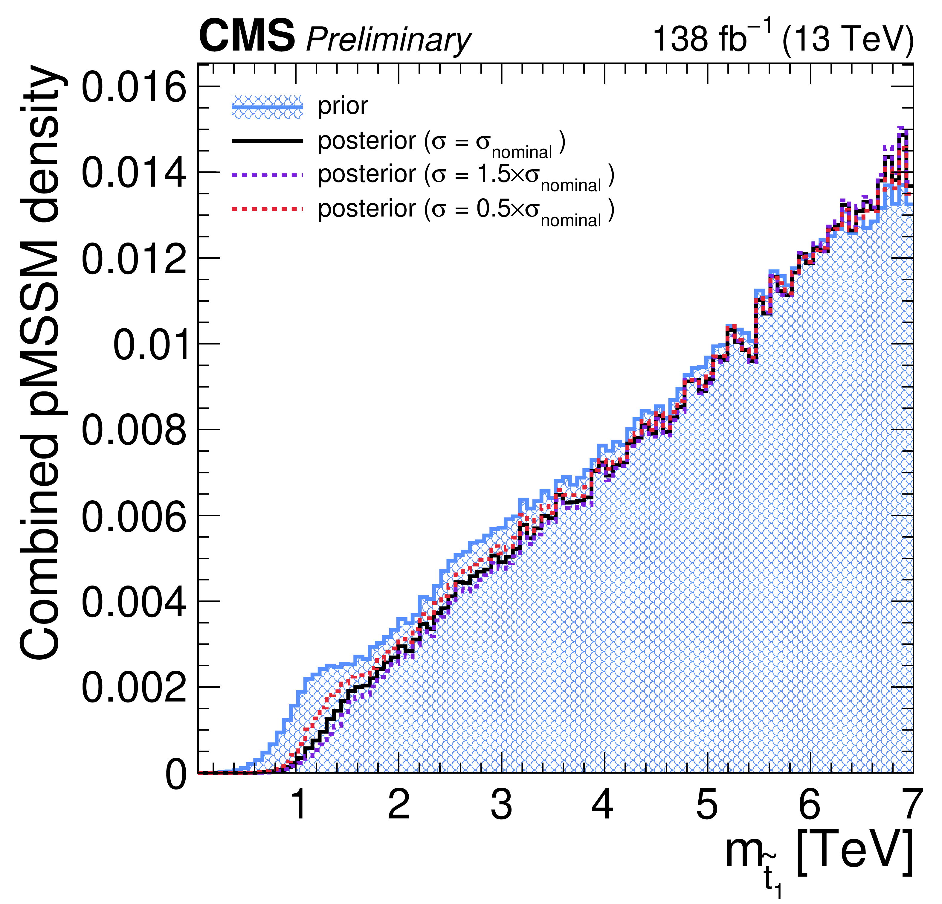
Marginalized prior and posterior density (left), survival probability (center), and upper quantiles of the BF (right) for the third generation squarks (top two), gluino (third row), and lightest colored superpartner (lower) masses. The posterior density is obtained assuming the nominal cross section (black) as well as the up (purple) and down (red) cross section variations. |
png pdf |
Figure 2-a:
Marginalized prior and posterior density (left), survival probability (center), and upper quantiles of the BF (right) for the third generation squarks (top two), gluino (third row), and lightest colored superpartner (lower) masses. The posterior density is obtained assuming the nominal cross section (black) as well as the up (purple) and down (red) cross section variations. |
png pdf |
Figure 2-b:
Marginalized prior and posterior density (left), survival probability (center), and upper quantiles of the BF (right) for the third generation squarks (top two), gluino (third row), and lightest colored superpartner (lower) masses. The posterior density is obtained assuming the nominal cross section (black) as well as the up (purple) and down (red) cross section variations. |
png pdf |
Figure 2-c:
Marginalized prior and posterior density (left), survival probability (center), and upper quantiles of the BF (right) for the third generation squarks (top two), gluino (third row), and lightest colored superpartner (lower) masses. The posterior density is obtained assuming the nominal cross section (black) as well as the up (purple) and down (red) cross section variations. |
png pdf |
Figure 2-d:
Marginalized prior and posterior density (left), survival probability (center), and upper quantiles of the BF (right) for the third generation squarks (top two), gluino (third row), and lightest colored superpartner (lower) masses. The posterior density is obtained assuming the nominal cross section (black) as well as the up (purple) and down (red) cross section variations. |
png pdf |
Figure 2-e:
Marginalized prior and posterior density (left), survival probability (center), and upper quantiles of the BF (right) for the third generation squarks (top two), gluino (third row), and lightest colored superpartner (lower) masses. The posterior density is obtained assuming the nominal cross section (black) as well as the up (purple) and down (red) cross section variations. |
png pdf |
Figure 2-f:
Marginalized prior and posterior density (left), survival probability (center), and upper quantiles of the BF (right) for the third generation squarks (top two), gluino (third row), and lightest colored superpartner (lower) masses. The posterior density is obtained assuming the nominal cross section (black) as well as the up (purple) and down (red) cross section variations. |
png pdf |
Figure 2-g:
Marginalized prior and posterior density (left), survival probability (center), and upper quantiles of the BF (right) for the third generation squarks (top two), gluino (third row), and lightest colored superpartner (lower) masses. The posterior density is obtained assuming the nominal cross section (black) as well as the up (purple) and down (red) cross section variations. |
png pdf |
Figure 2-h:
Marginalized prior and posterior density (left), survival probability (center), and upper quantiles of the BF (right) for the third generation squarks (top two), gluino (third row), and lightest colored superpartner (lower) masses. The posterior density is obtained assuming the nominal cross section (black) as well as the up (purple) and down (red) cross section variations. |

png pdf |
Figure 2-i:
Marginalized prior and posterior density (left), survival probability (center), and upper quantiles of the BF (right) for the third generation squarks (top two), gluino (third row), and lightest colored superpartner (lower) masses. The posterior density is obtained assuming the nominal cross section (black) as well as the up (purple) and down (red) cross section variations. |
png pdf |
Figure 2-j:
Marginalized prior and posterior density (left), survival probability (center), and upper quantiles of the BF (right) for the third generation squarks (top two), gluino (third row), and lightest colored superpartner (lower) masses. The posterior density is obtained assuming the nominal cross section (black) as well as the up (purple) and down (red) cross section variations. |
png pdf |
Figure 2-k:
Marginalized prior and posterior density (left), survival probability (center), and upper quantiles of the BF (right) for the third generation squarks (top two), gluino (third row), and lightest colored superpartner (lower) masses. The posterior density is obtained assuming the nominal cross section (black) as well as the up (purple) and down (red) cross section variations. |
png pdf |
Figure 2-l:
Marginalized prior and posterior density (left), survival probability (center), and upper quantiles of the BF (right) for the third generation squarks (top two), gluino (third row), and lightest colored superpartner (lower) masses. The posterior density is obtained assuming the nominal cross section (black) as well as the up (purple) and down (red) cross section variations. |
png pdf |
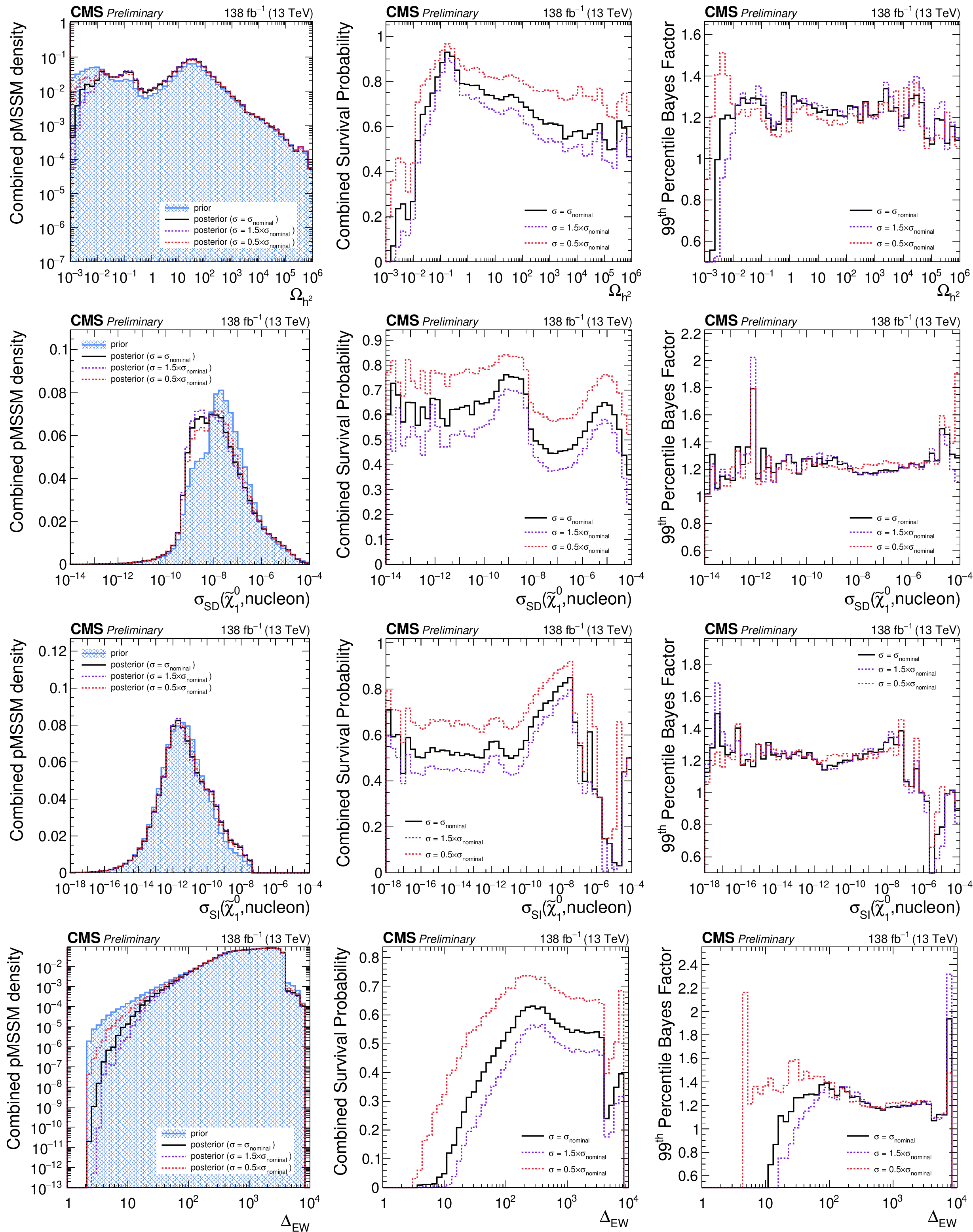
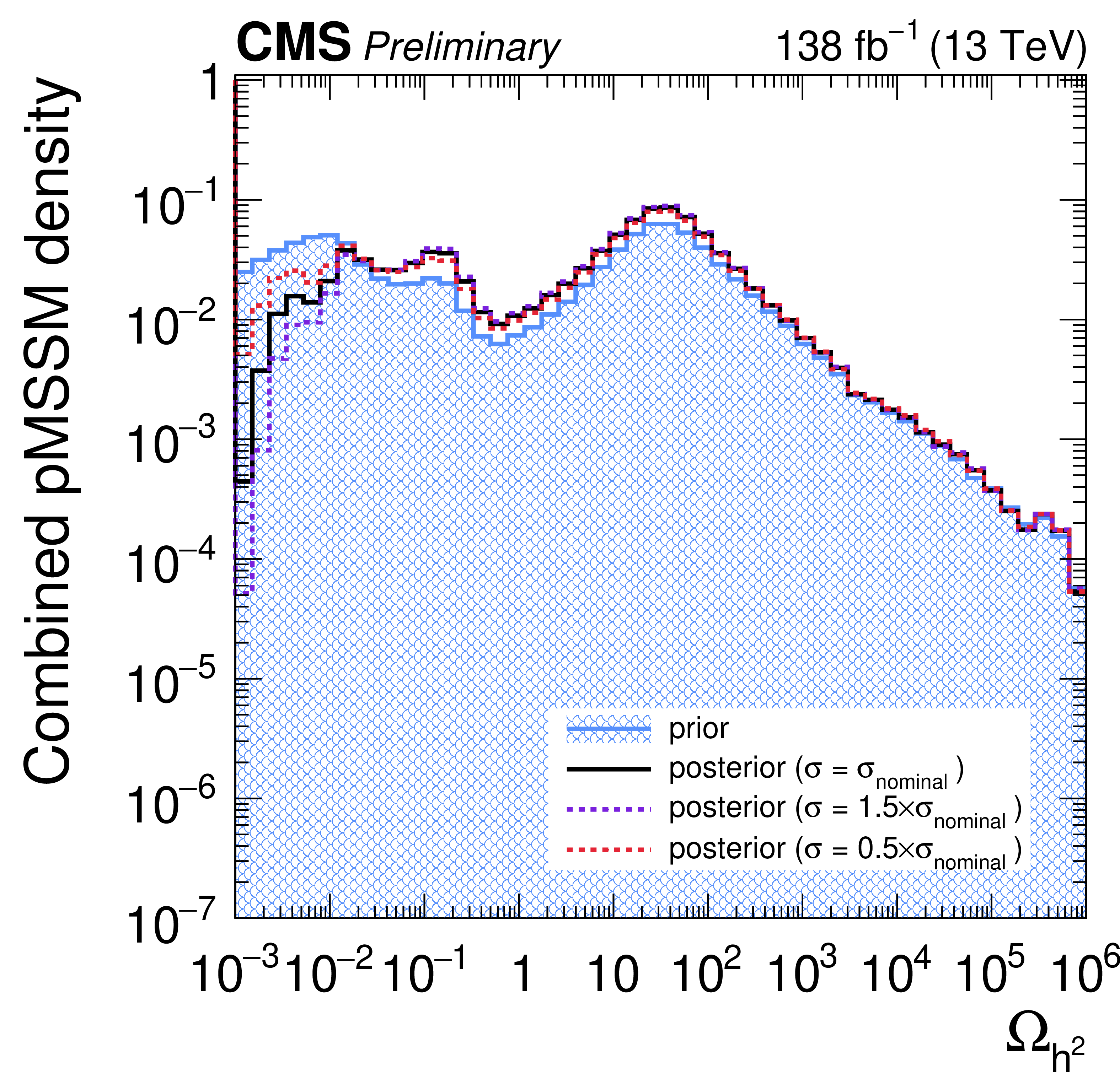
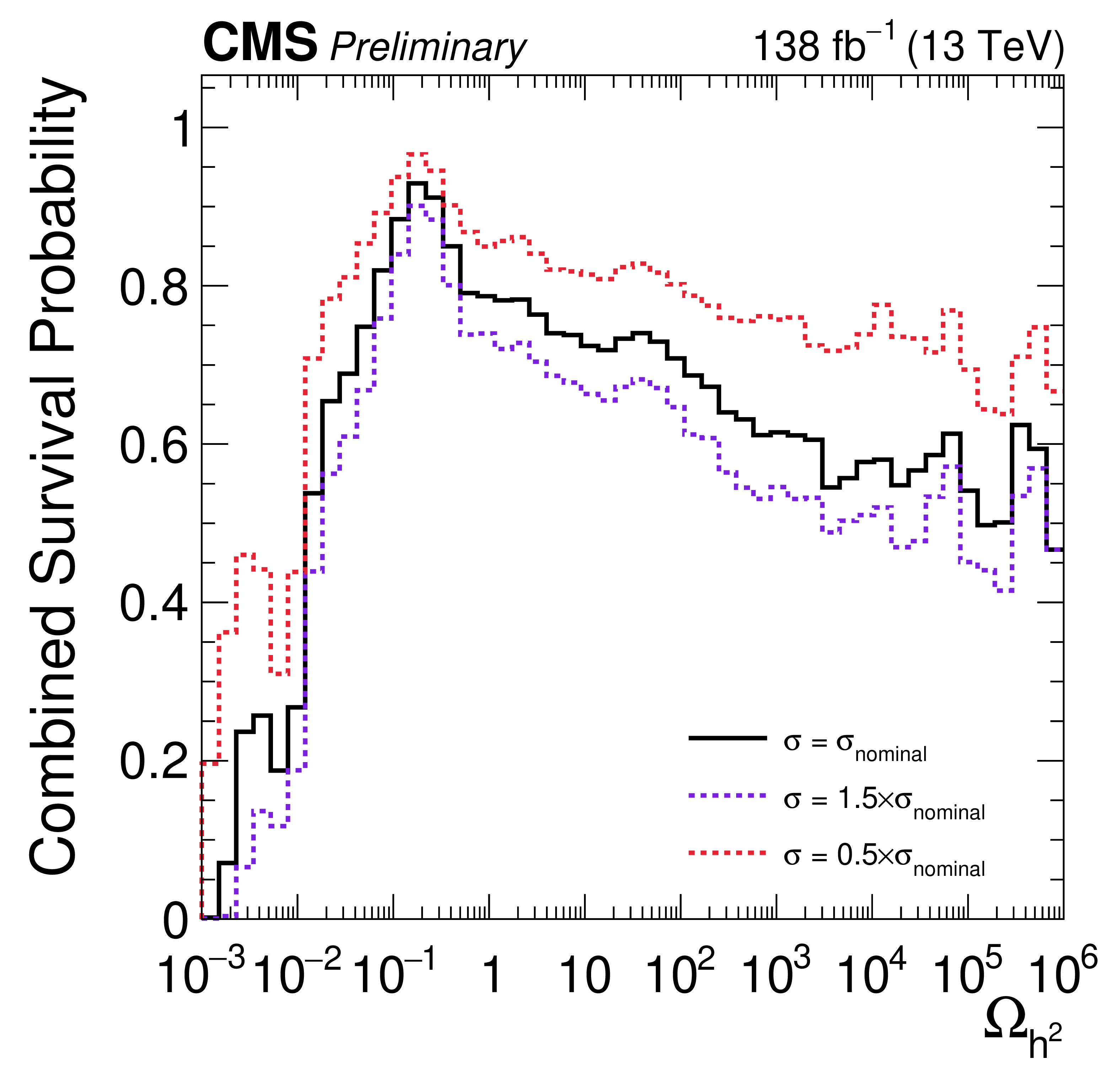
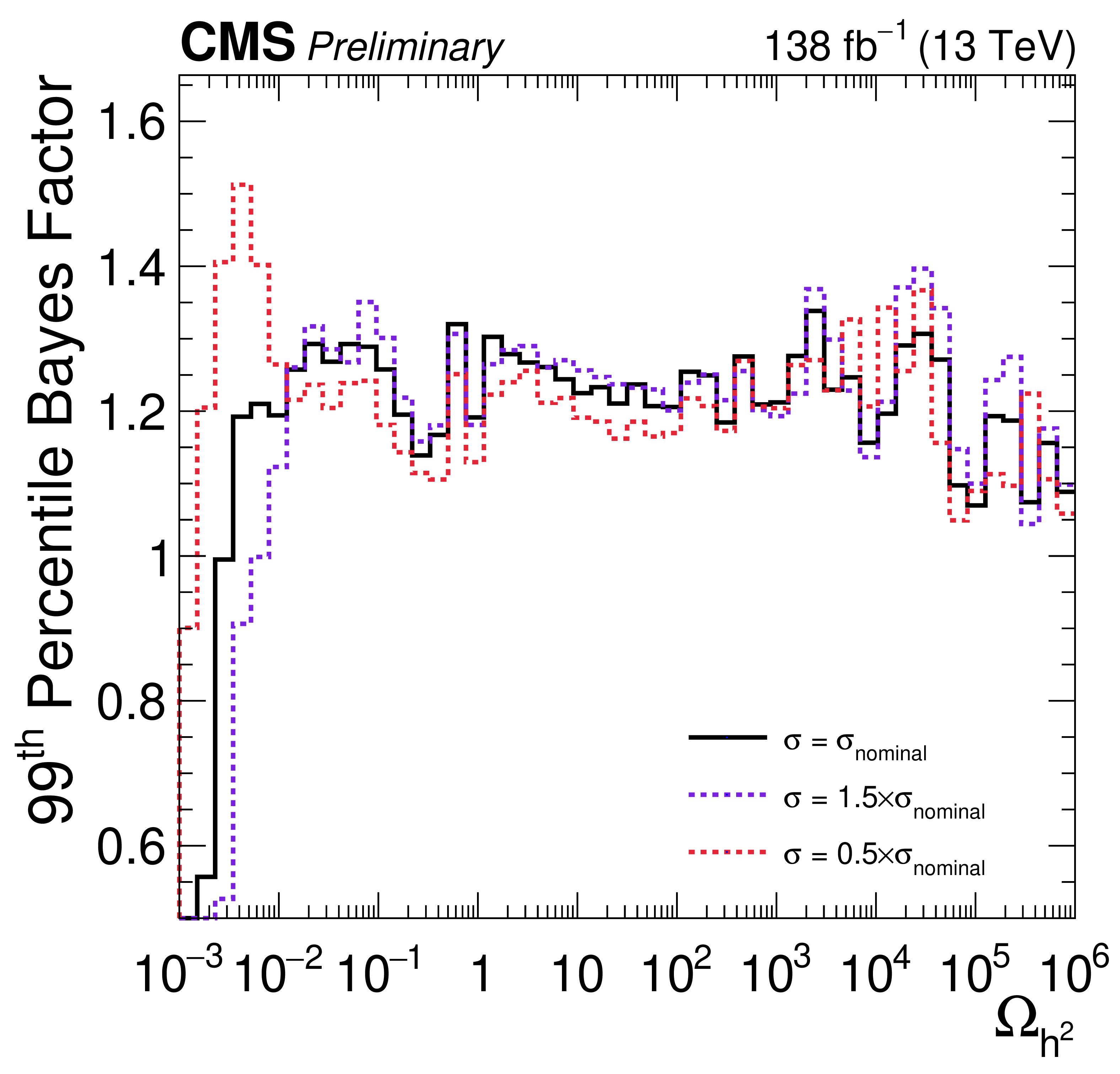
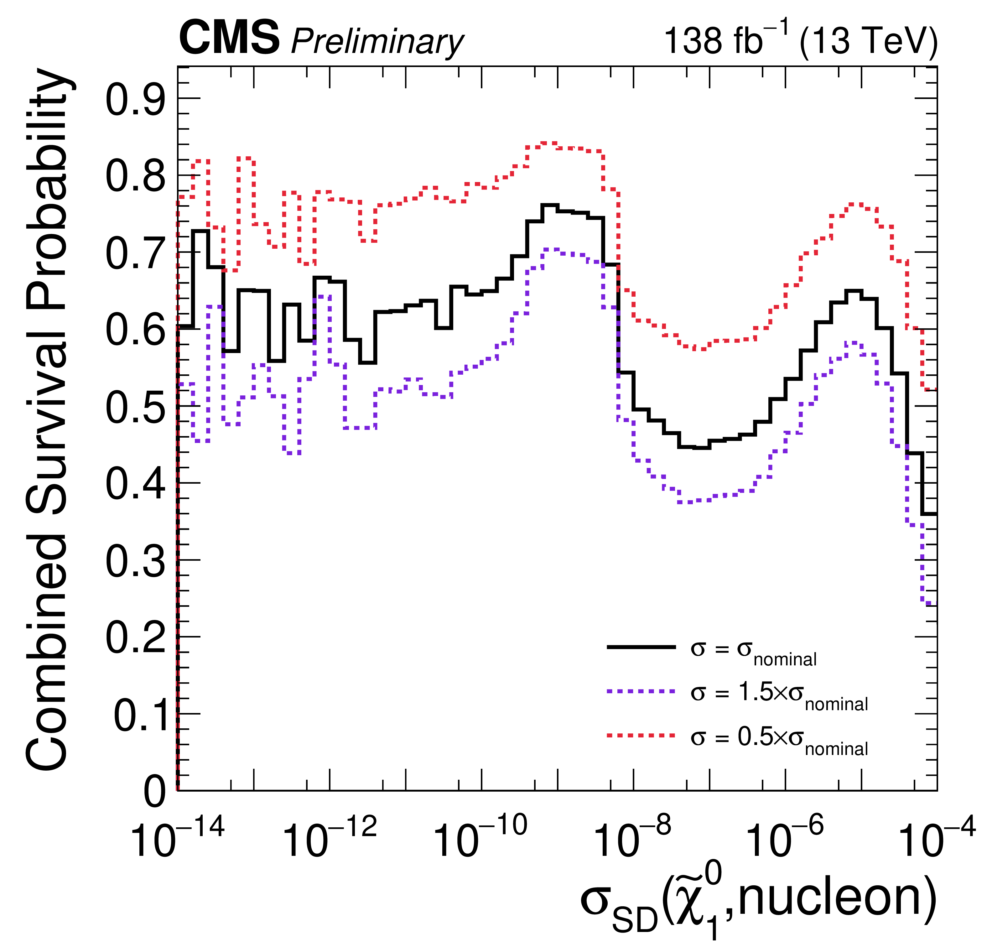
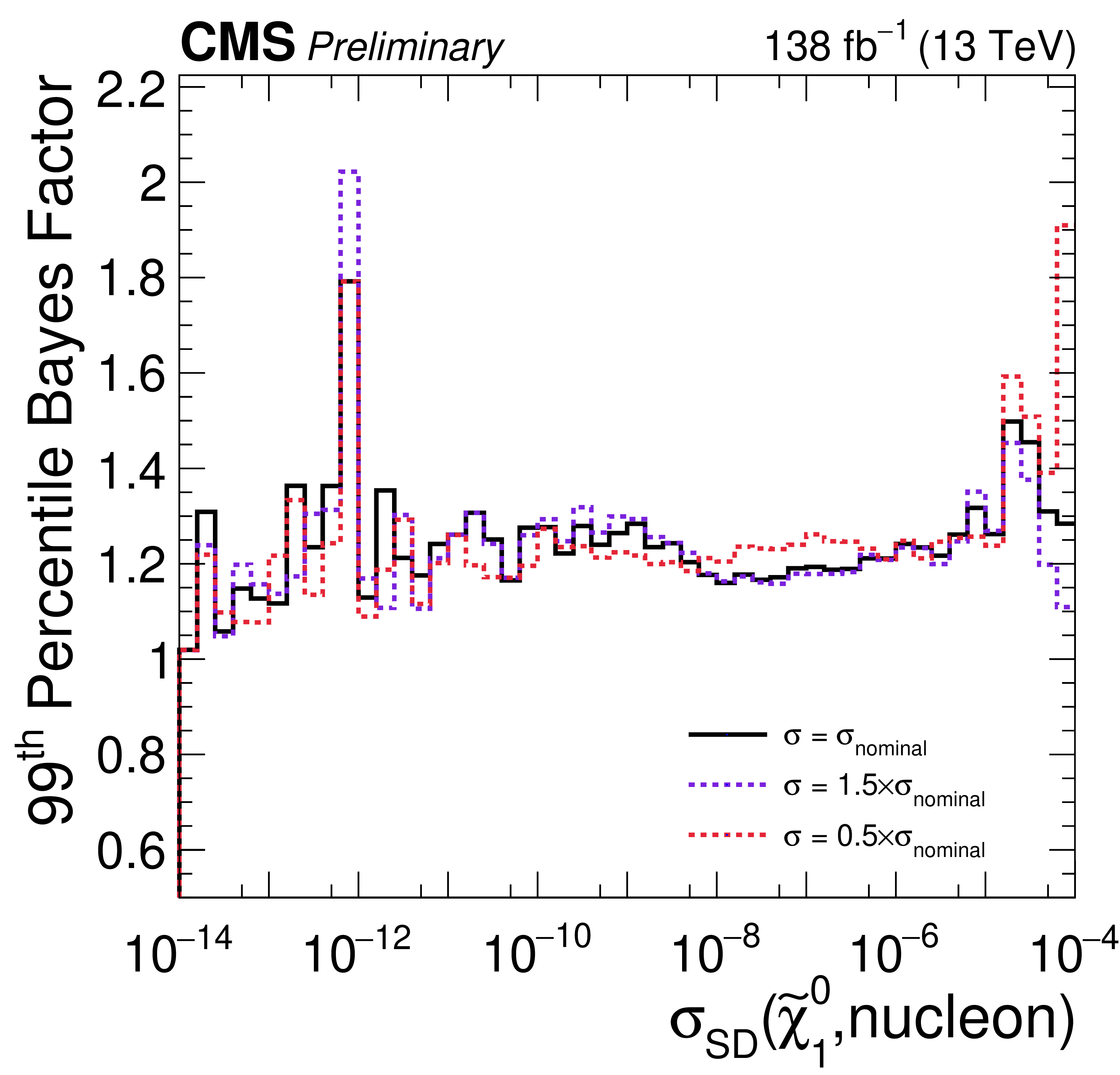
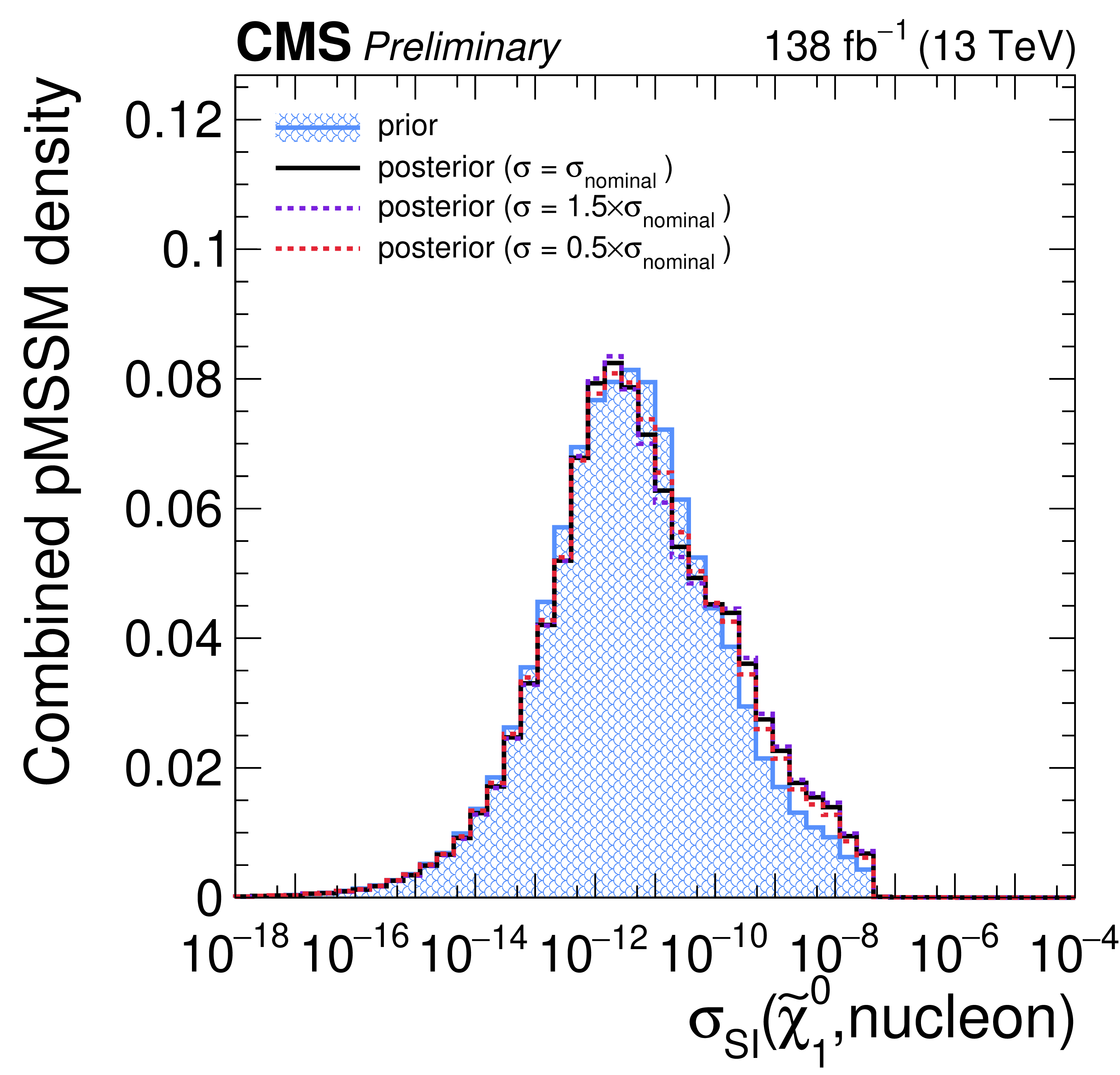
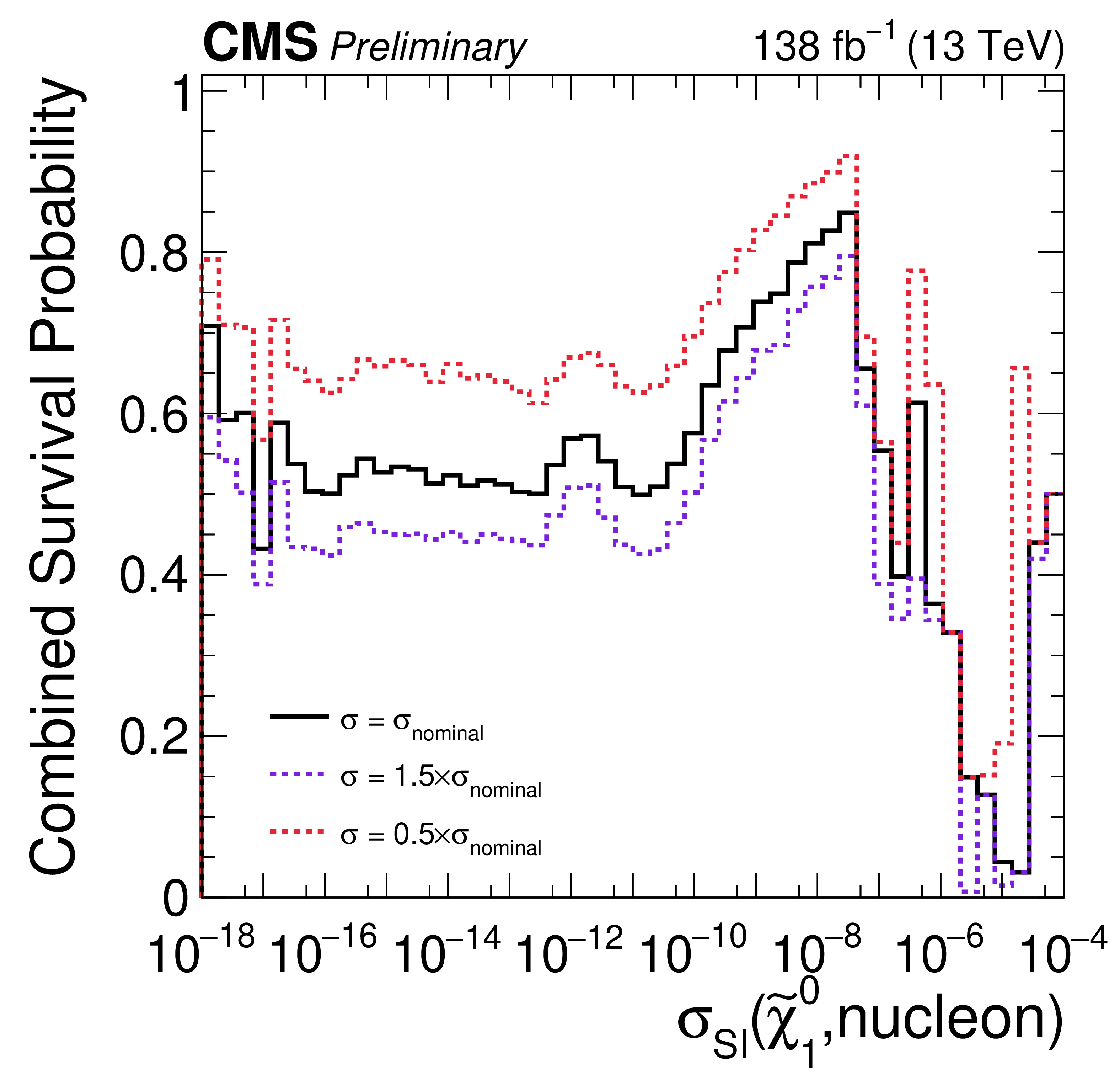
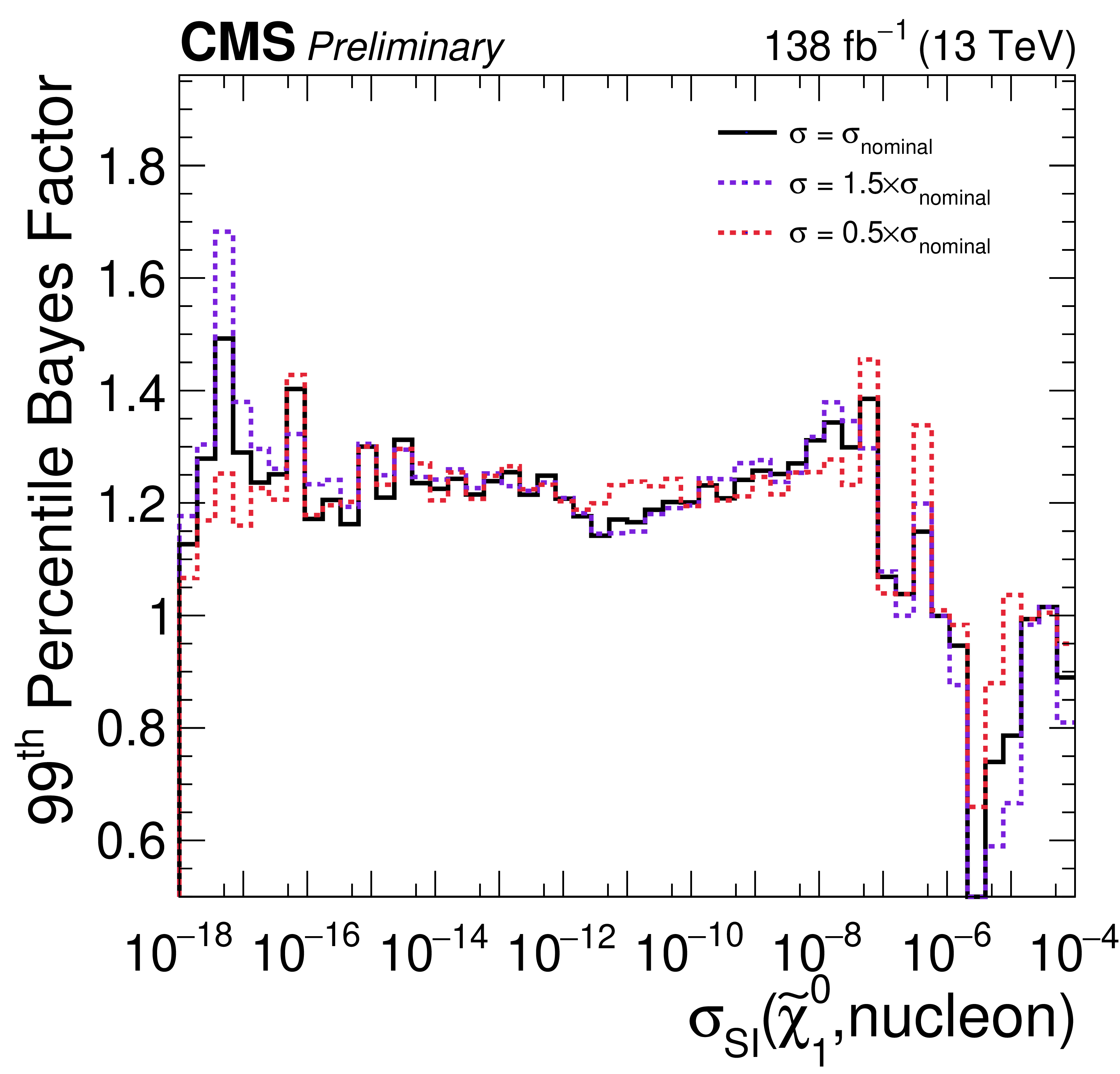
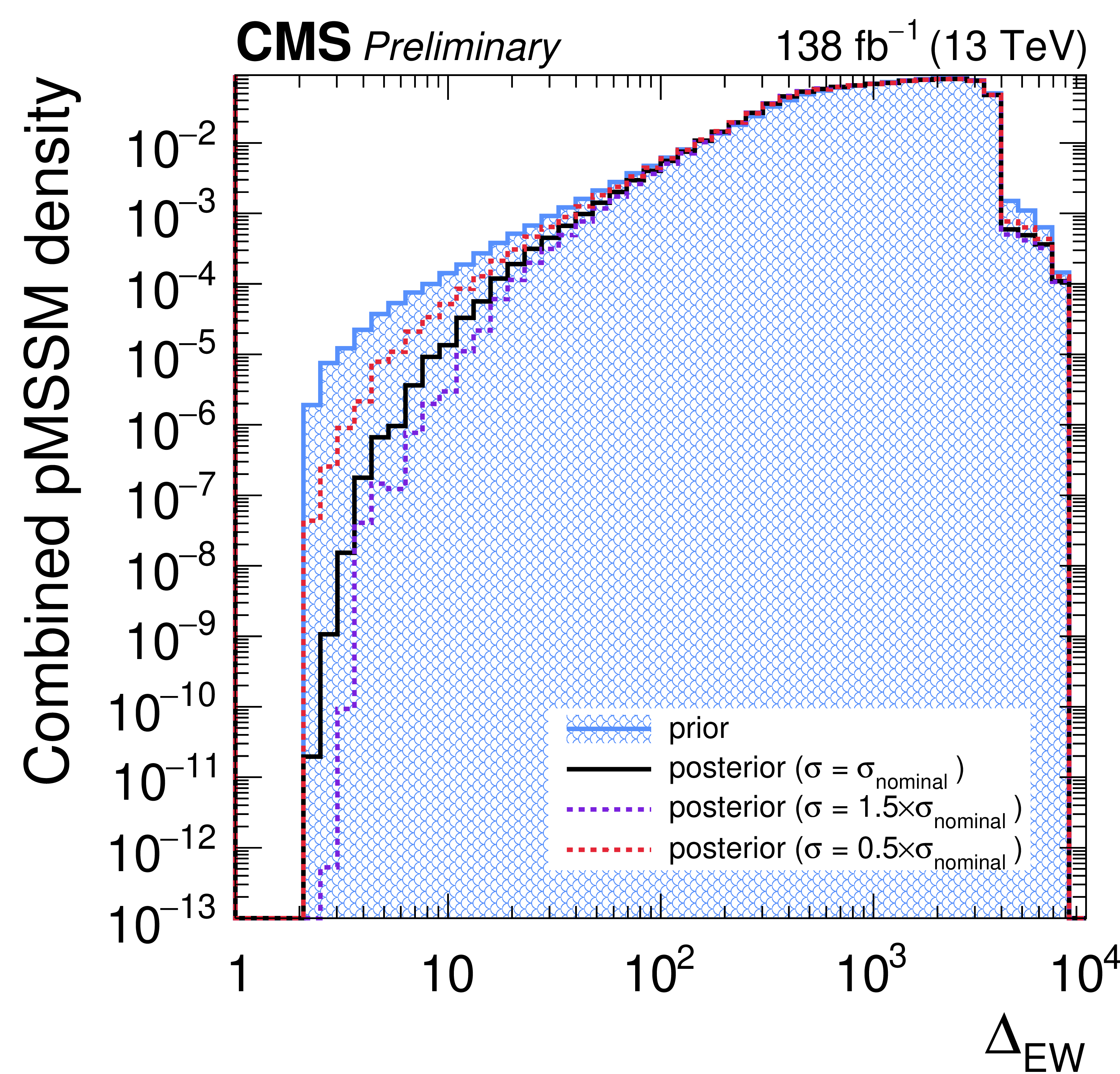
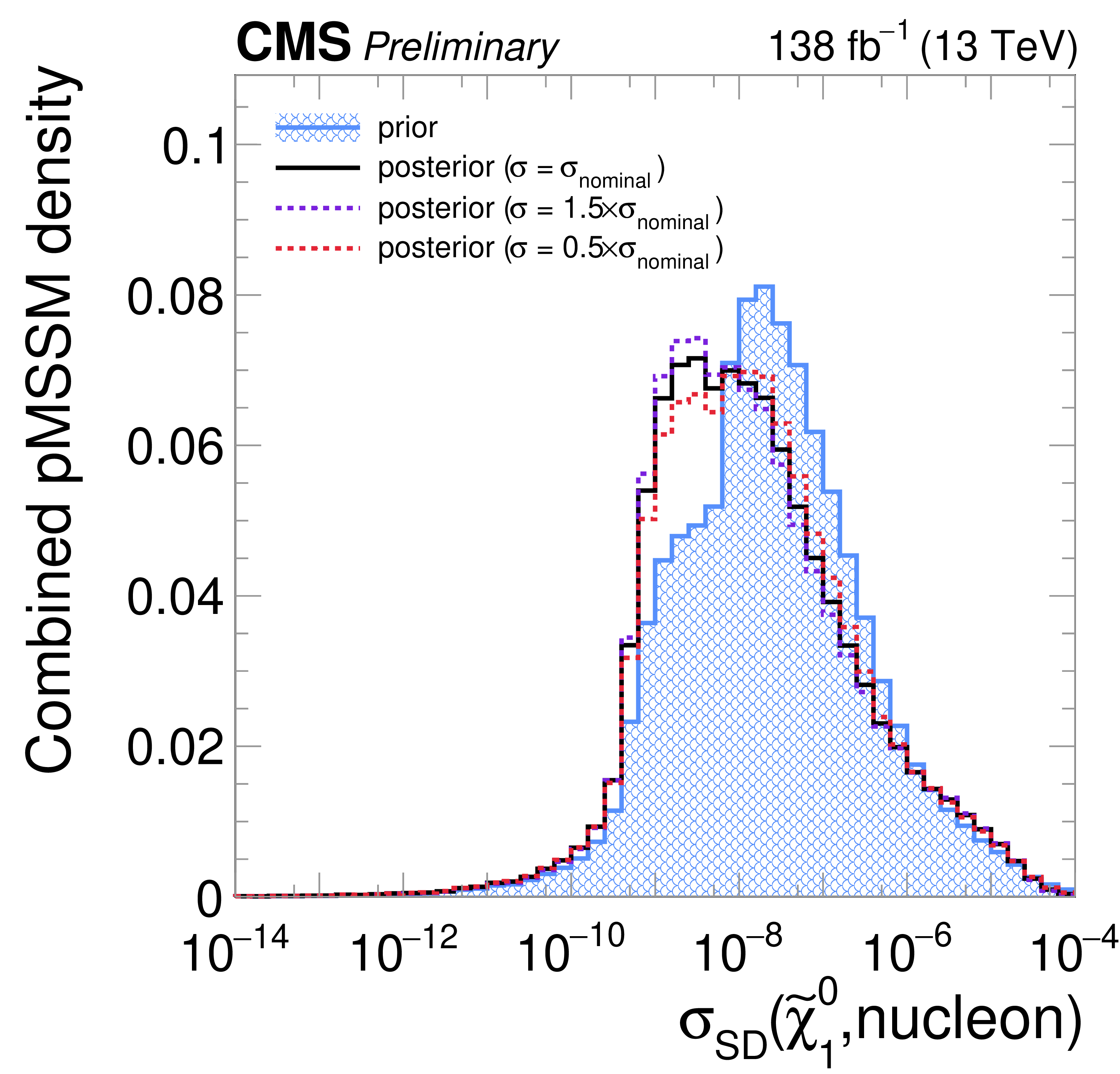
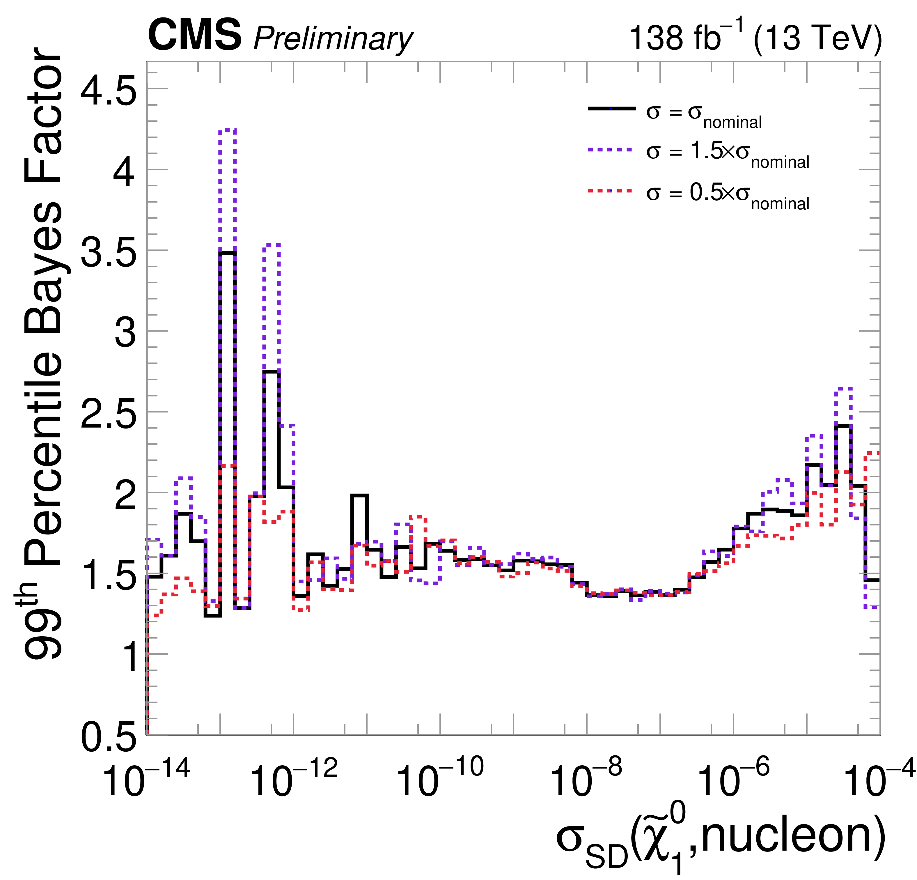
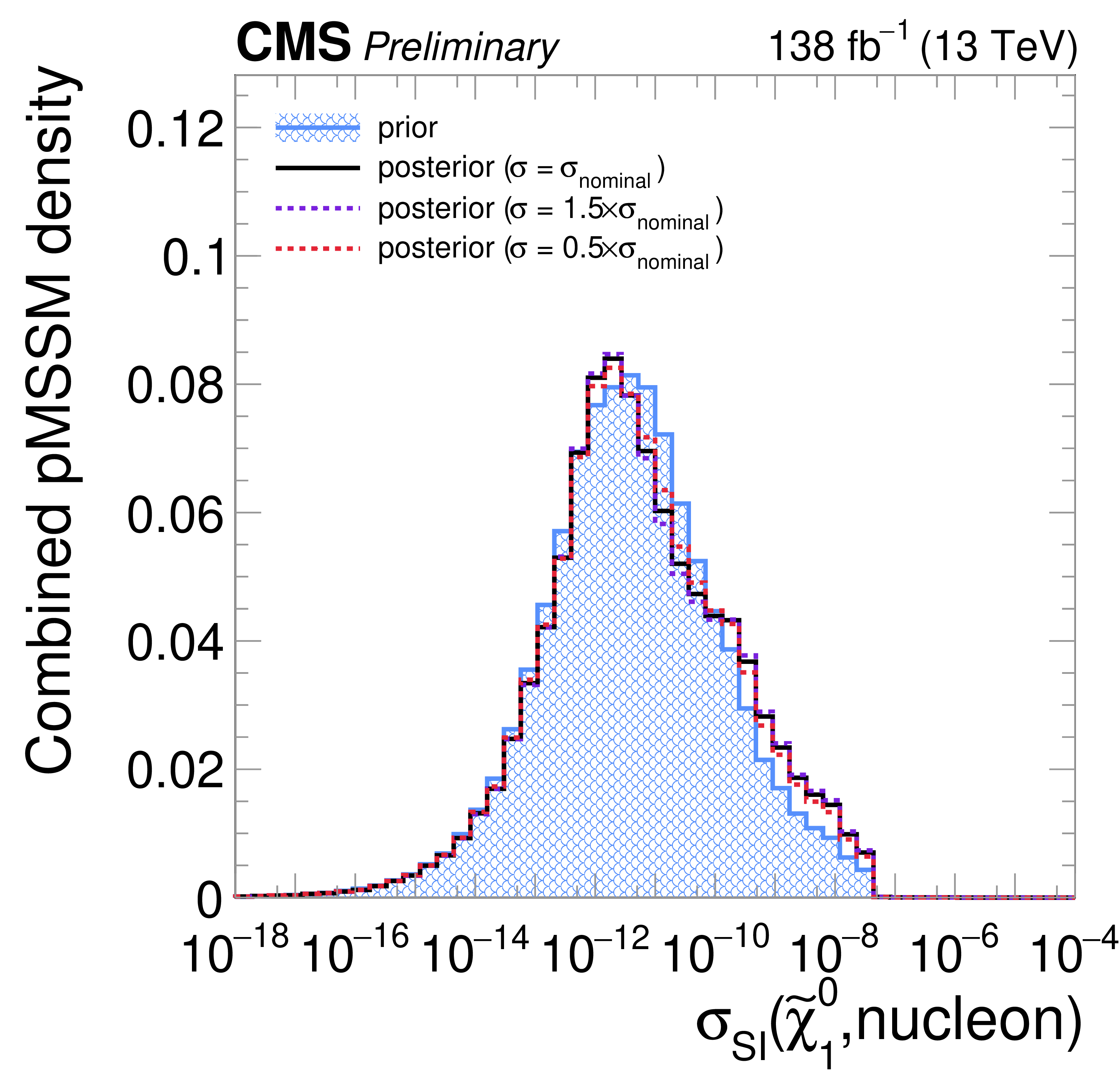
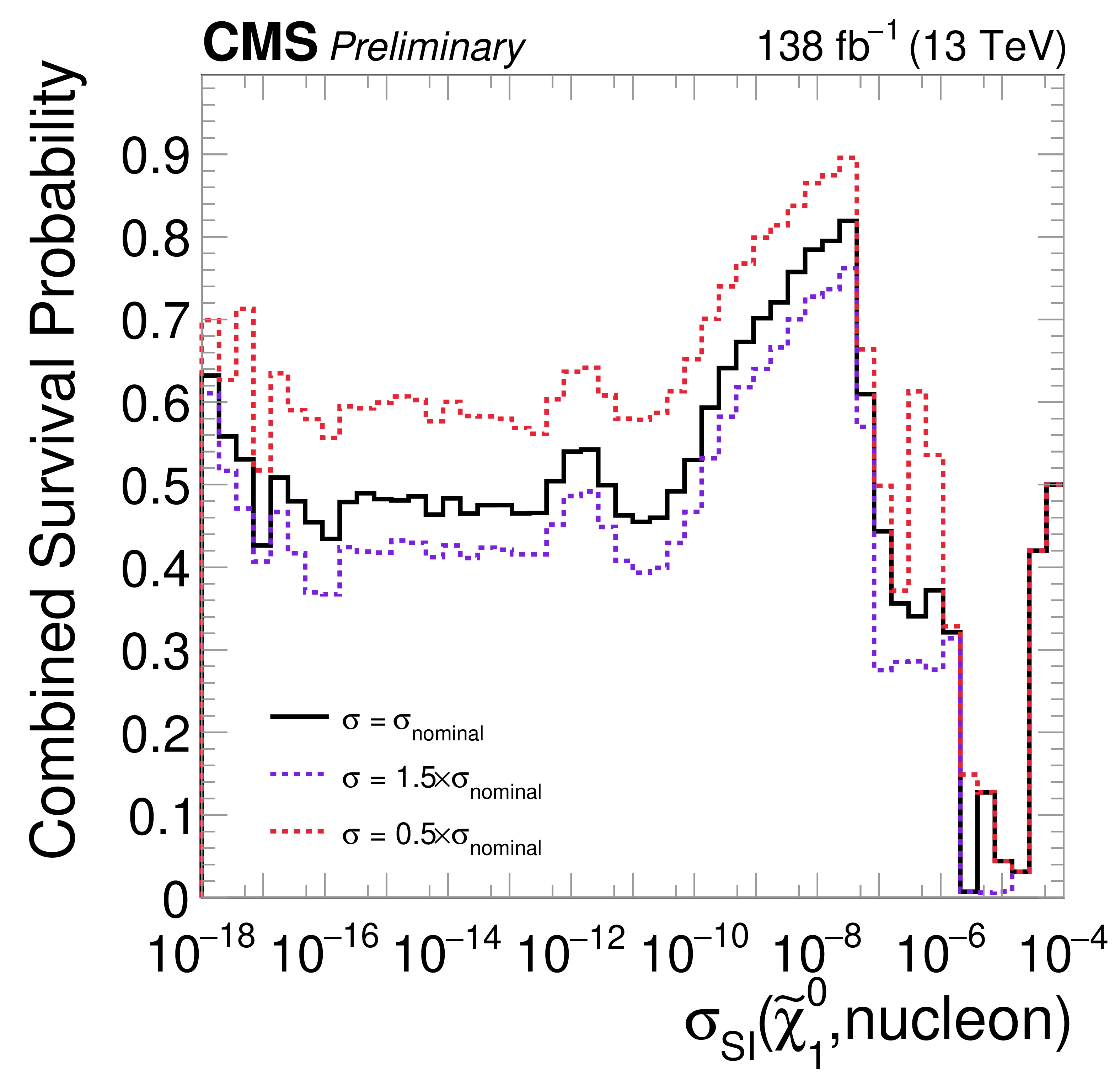
Figure 3:
Marginalized prior and posterior density (left), survival probability (center), and upper quantiles of the BF (right) for DM relic density (top), spin-dependent and spin-independent (middle), and fine-tuning criterion (lower). The posterior density is obtained assuming the nominal cross section (black) as well as the up (purple) and down (red) cross section variations. |
png pdf |
Figure 3-a:
Marginalized prior and posterior density (left), survival probability (center), and upper quantiles of the BF (right) for DM relic density (top), spin-dependent and spin-independent (middle), and fine-tuning criterion (lower). The posterior density is obtained assuming the nominal cross section (black) as well as the up (purple) and down (red) cross section variations. |
png pdf |
Figure 3-b:
Marginalized prior and posterior density (left), survival probability (center), and upper quantiles of the BF (right) for DM relic density (top), spin-dependent and spin-independent (middle), and fine-tuning criterion (lower). The posterior density is obtained assuming the nominal cross section (black) as well as the up (purple) and down (red) cross section variations. |
png pdf |
Figure 3-c:
Marginalized prior and posterior density (left), survival probability (center), and upper quantiles of the BF (right) for DM relic density (top), spin-dependent and spin-independent (middle), and fine-tuning criterion (lower). The posterior density is obtained assuming the nominal cross section (black) as well as the up (purple) and down (red) cross section variations. |

png pdf |
Figure 3-d:
Marginalized prior and posterior density (left), survival probability (center), and upper quantiles of the BF (right) for DM relic density (top), spin-dependent and spin-independent (middle), and fine-tuning criterion (lower). The posterior density is obtained assuming the nominal cross section (black) as well as the up (purple) and down (red) cross section variations. |
png pdf |
Figure 3-e:
Marginalized prior and posterior density (left), survival probability (center), and upper quantiles of the BF (right) for DM relic density (top), spin-dependent and spin-independent (middle), and fine-tuning criterion (lower). The posterior density is obtained assuming the nominal cross section (black) as well as the up (purple) and down (red) cross section variations. |
png pdf |
Figure 3-f:
Marginalized prior and posterior density (left), survival probability (center), and upper quantiles of the BF (right) for DM relic density (top), spin-dependent and spin-independent (middle), and fine-tuning criterion (lower). The posterior density is obtained assuming the nominal cross section (black) as well as the up (purple) and down (red) cross section variations. |
png pdf |
Figure 3-g:
Marginalized prior and posterior density (left), survival probability (center), and upper quantiles of the BF (right) for DM relic density (top), spin-dependent and spin-independent (middle), and fine-tuning criterion (lower). The posterior density is obtained assuming the nominal cross section (black) as well as the up (purple) and down (red) cross section variations. |
png pdf |
Figure 3-h:
Marginalized prior and posterior density (left), survival probability (center), and upper quantiles of the BF (right) for DM relic density (top), spin-dependent and spin-independent (middle), and fine-tuning criterion (lower). The posterior density is obtained assuming the nominal cross section (black) as well as the up (purple) and down (red) cross section variations. |
png pdf |
Figure 3-i:
Marginalized prior and posterior density (left), survival probability (center), and upper quantiles of the BF (right) for DM relic density (top), spin-dependent and spin-independent (middle), and fine-tuning criterion (lower). The posterior density is obtained assuming the nominal cross section (black) as well as the up (purple) and down (red) cross section variations. |
png pdf |
Figure 3-j:
Marginalized prior and posterior density (left), survival probability (center), and upper quantiles of the BF (right) for DM relic density (top), spin-dependent and spin-independent (middle), and fine-tuning criterion (lower). The posterior density is obtained assuming the nominal cross section (black) as well as the up (purple) and down (red) cross section variations. |

png pdf |
Figure 3-k:
Marginalized prior and posterior density (left), survival probability (center), and upper quantiles of the BF (right) for DM relic density (top), spin-dependent and spin-independent (middle), and fine-tuning criterion (lower). The posterior density is obtained assuming the nominal cross section (black) as well as the up (purple) and down (red) cross section variations. |
png pdf |
Figure 3-l:
Marginalized prior and posterior density (left), survival probability (center), and upper quantiles of the BF (right) for DM relic density (top), spin-dependent and spin-independent (middle), and fine-tuning criterion (lower). The posterior density is obtained assuming the nominal cross section (black) as well as the up (purple) and down (red) cross section variations. |
png pdf |
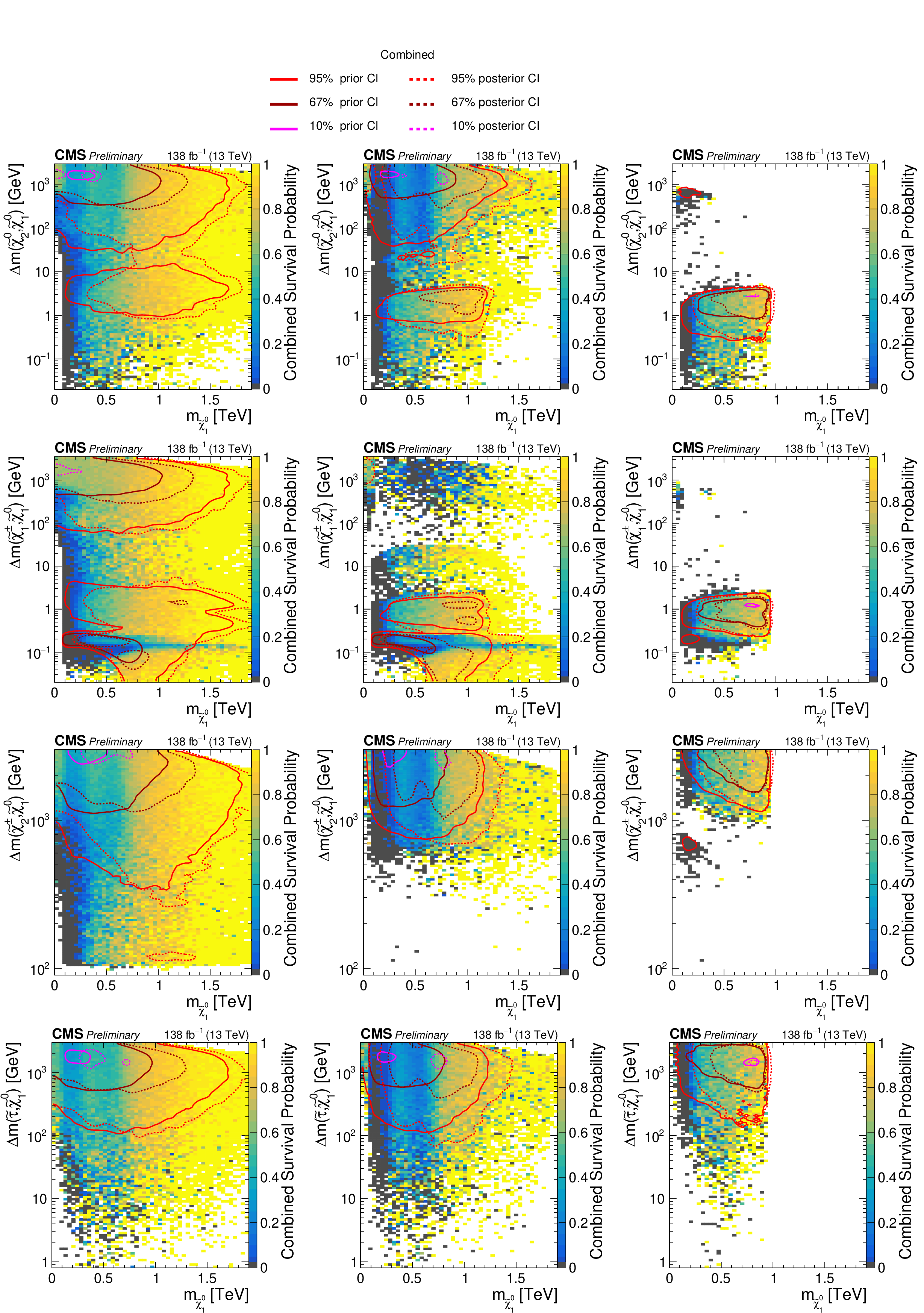
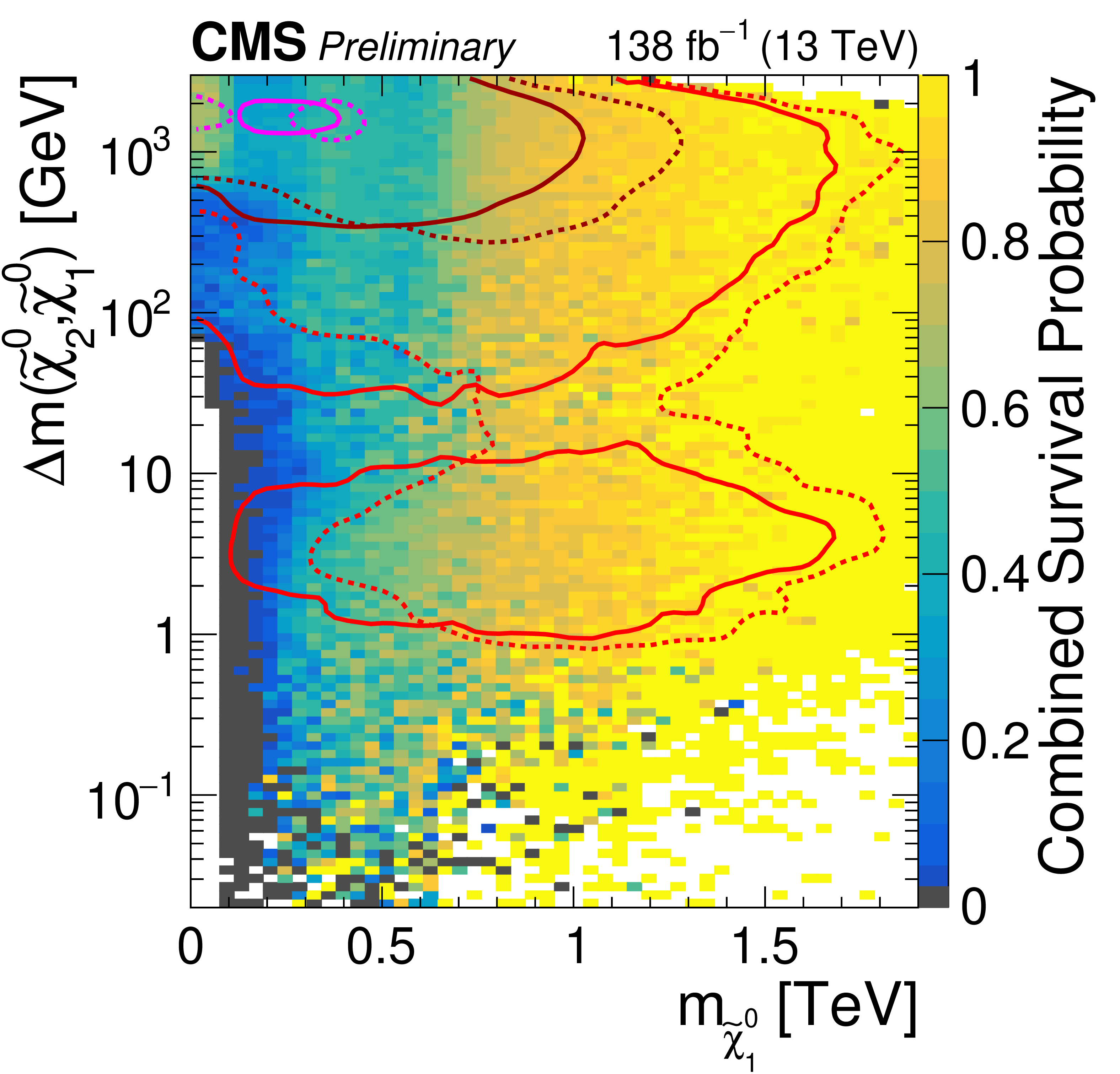
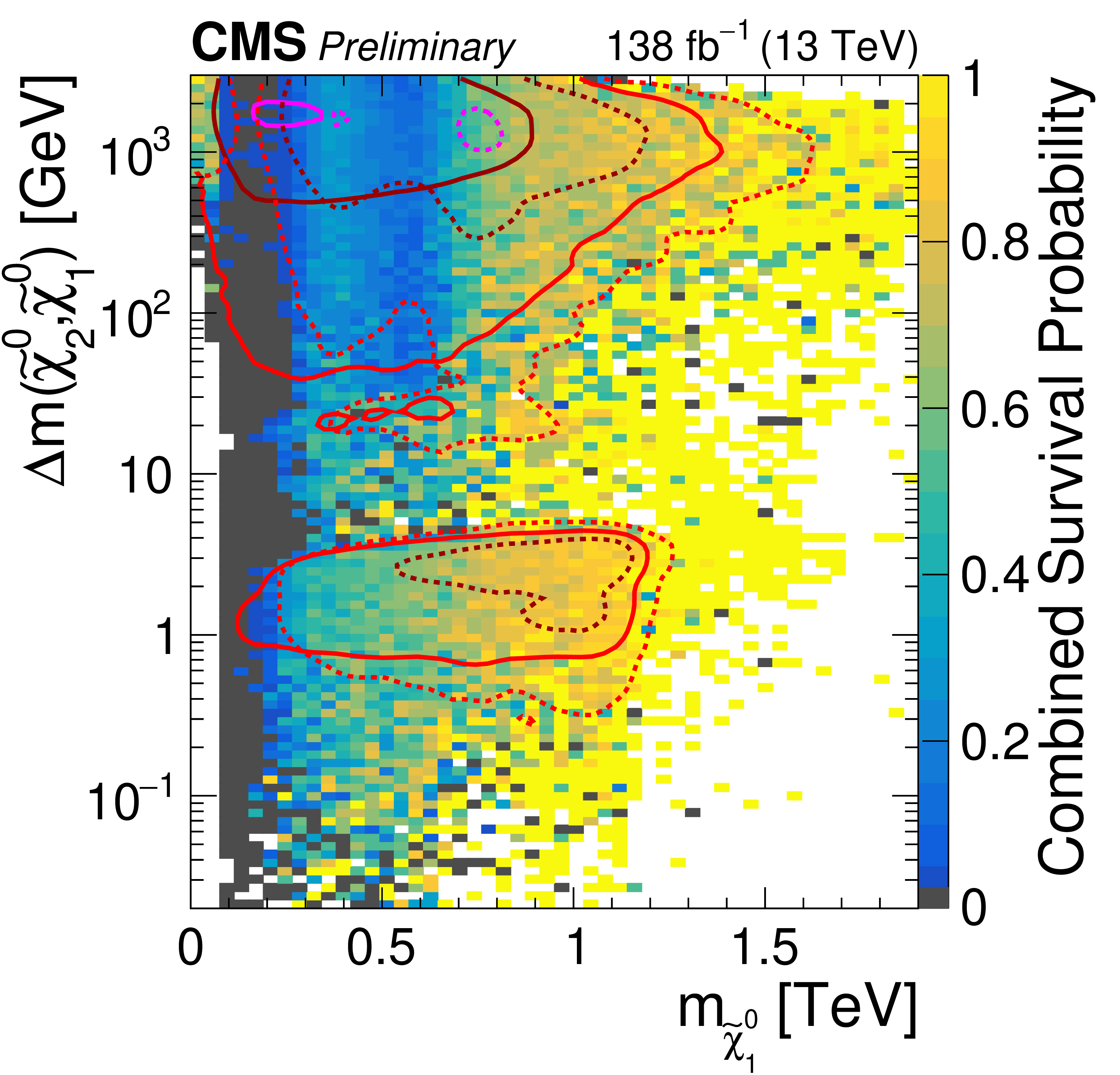
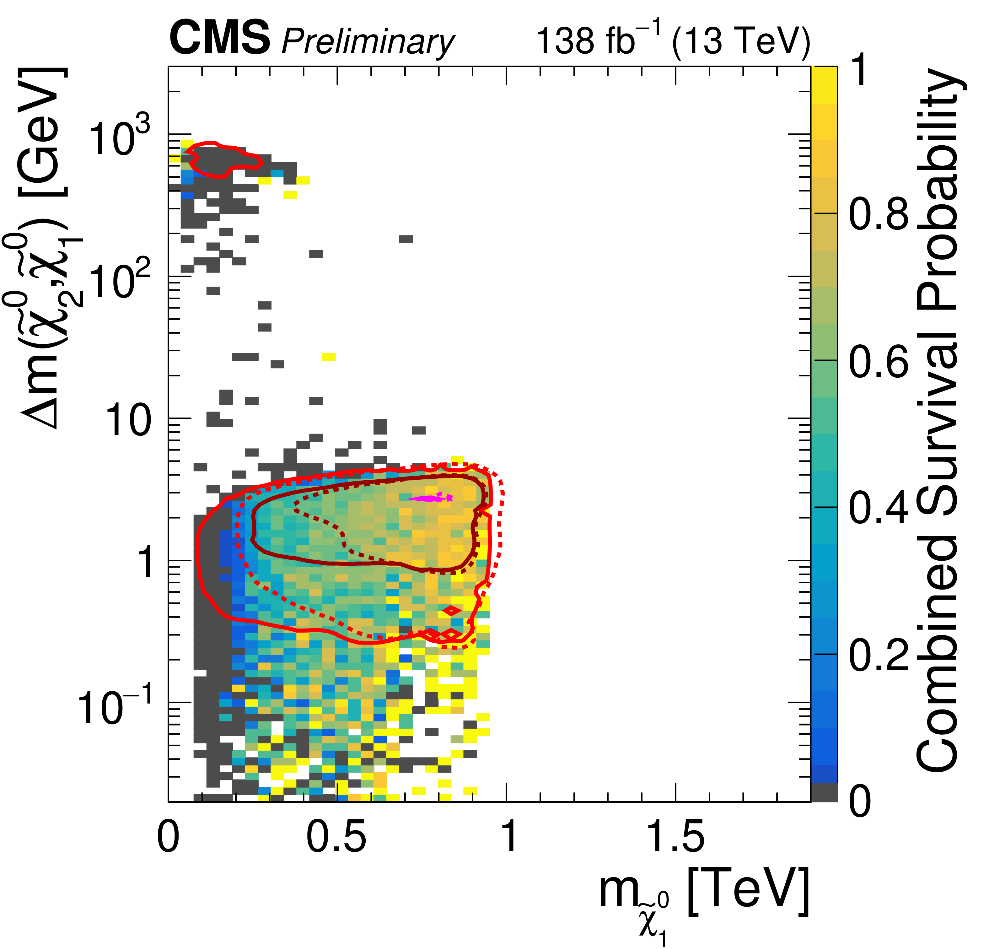
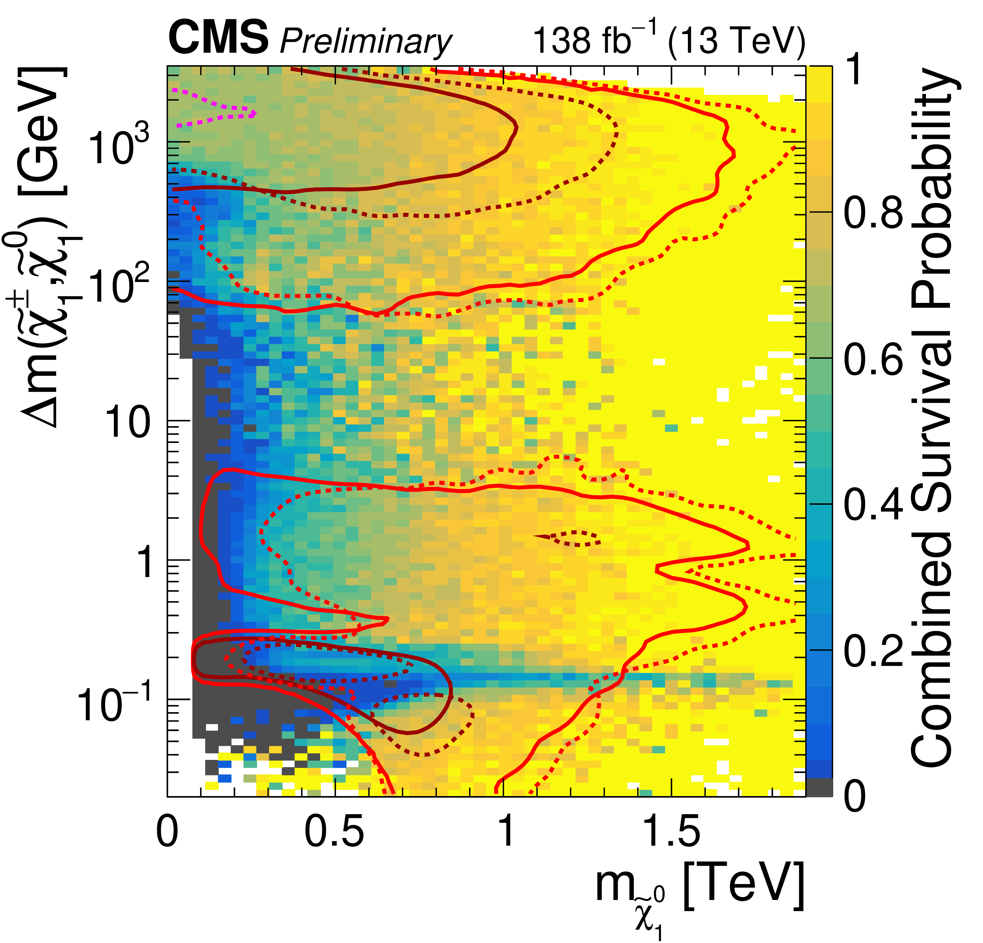
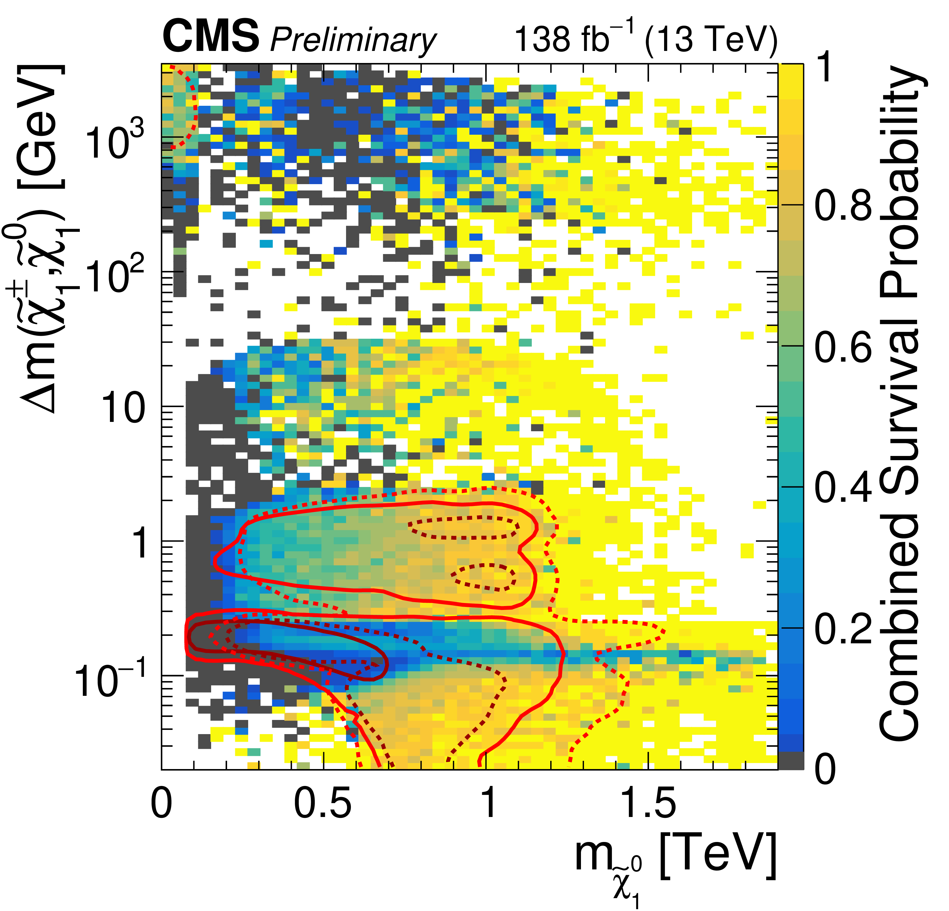
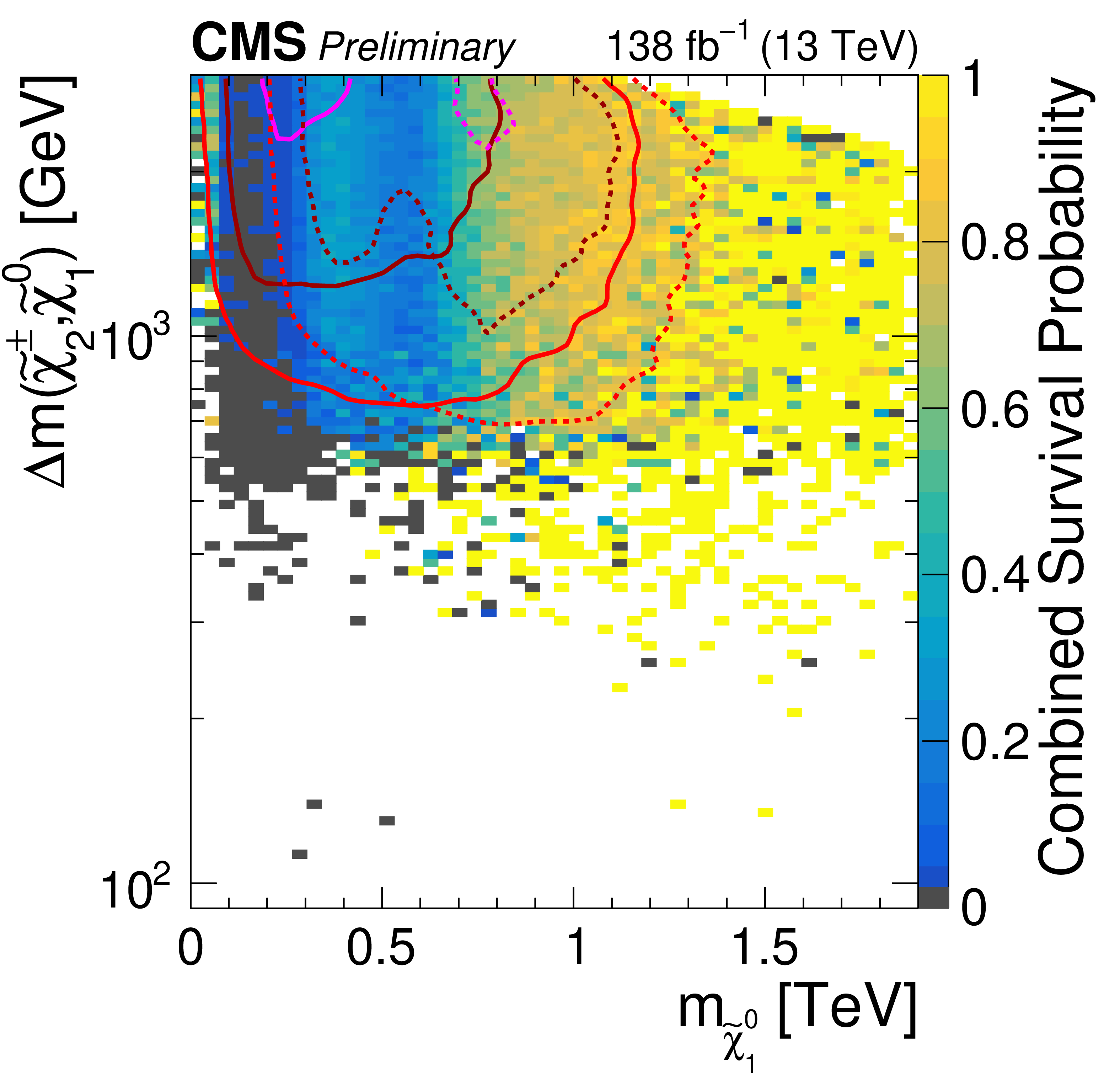
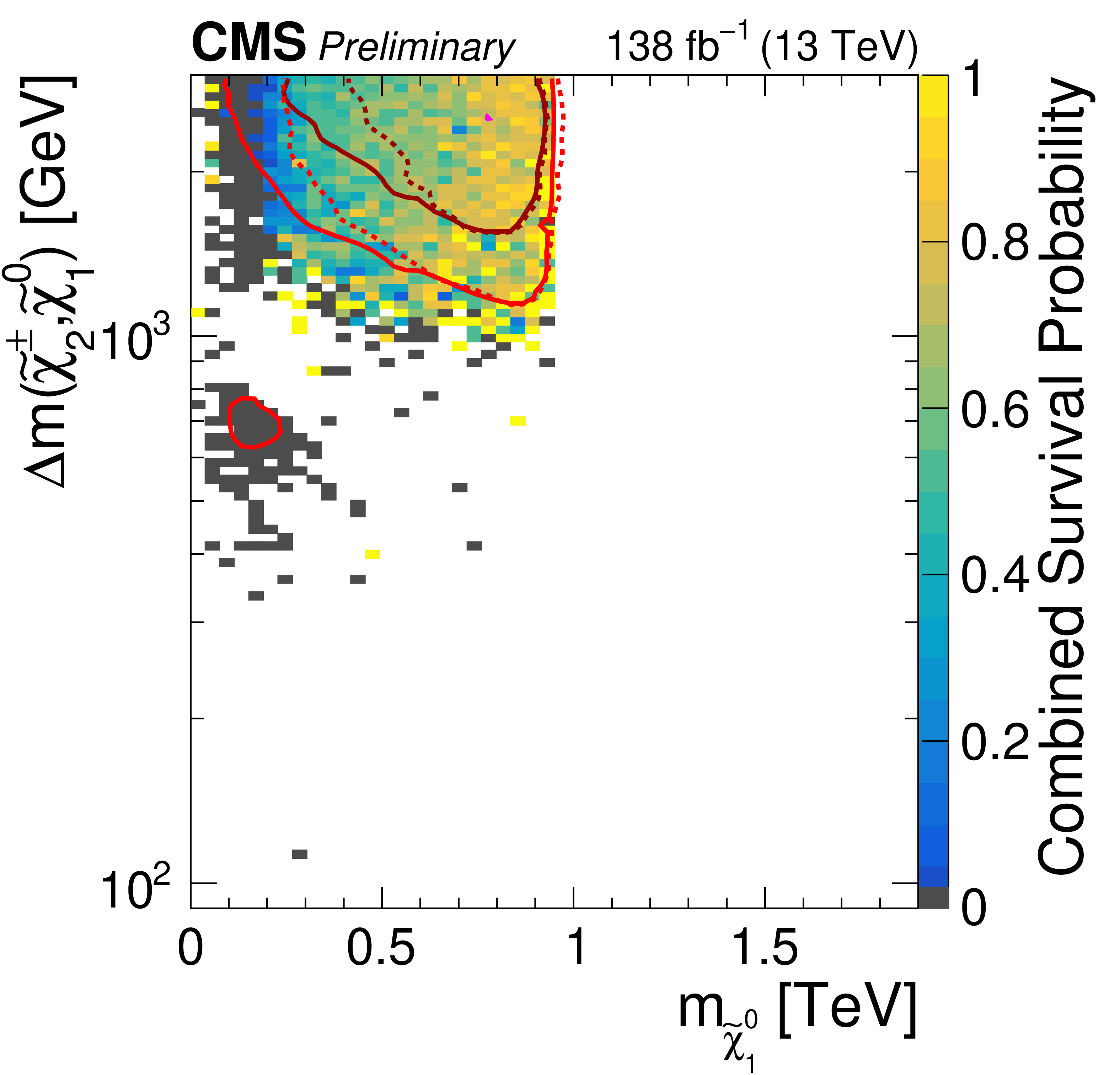
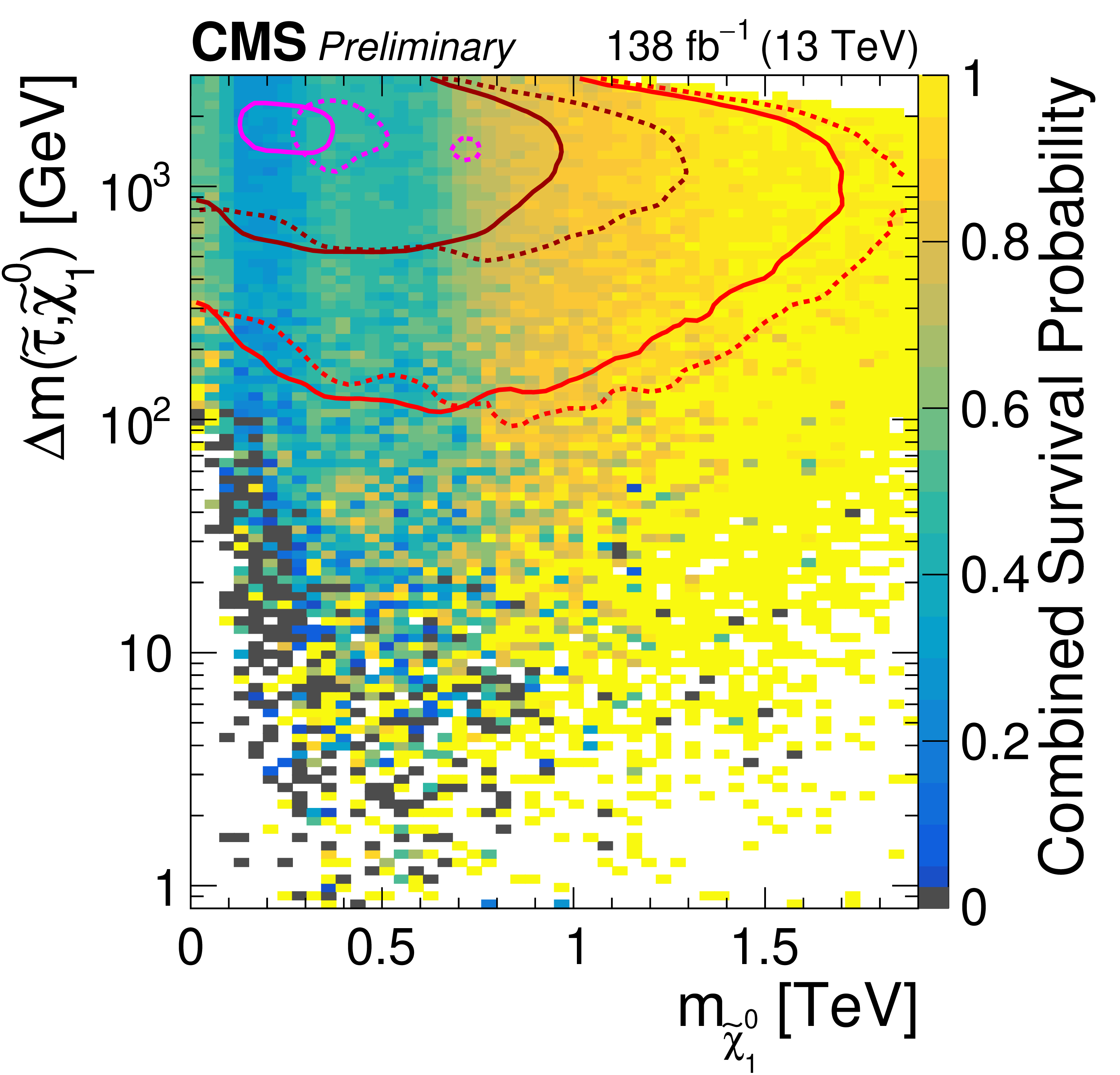
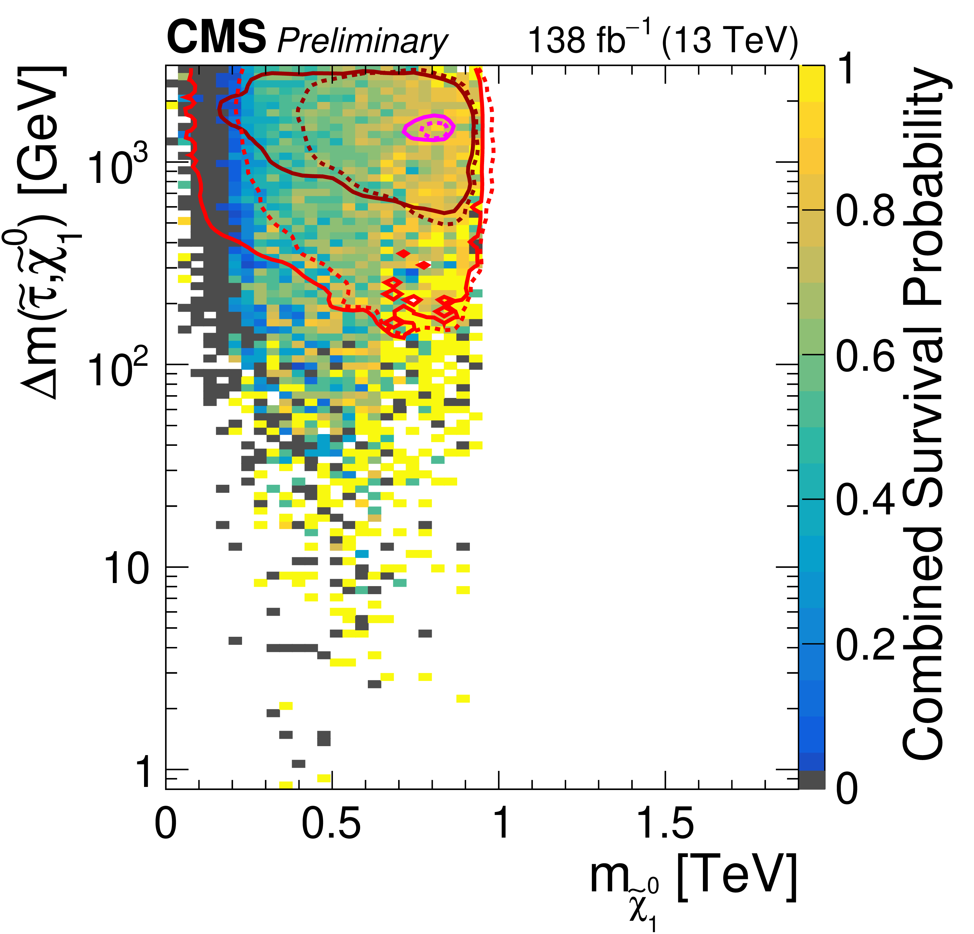
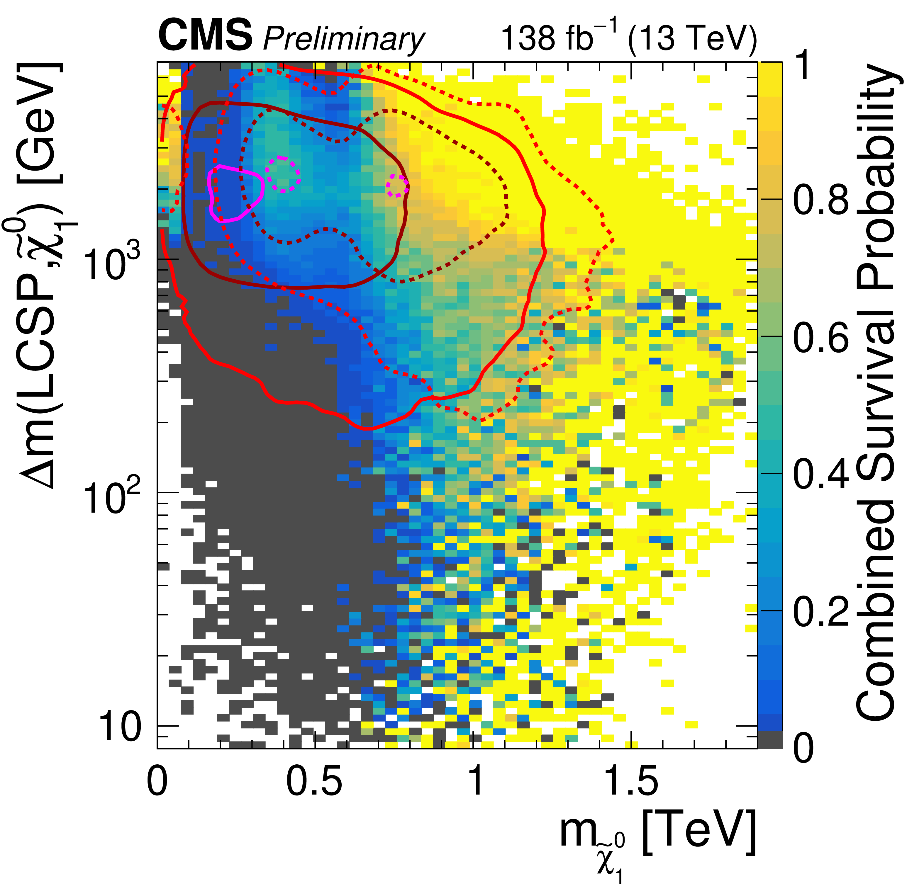
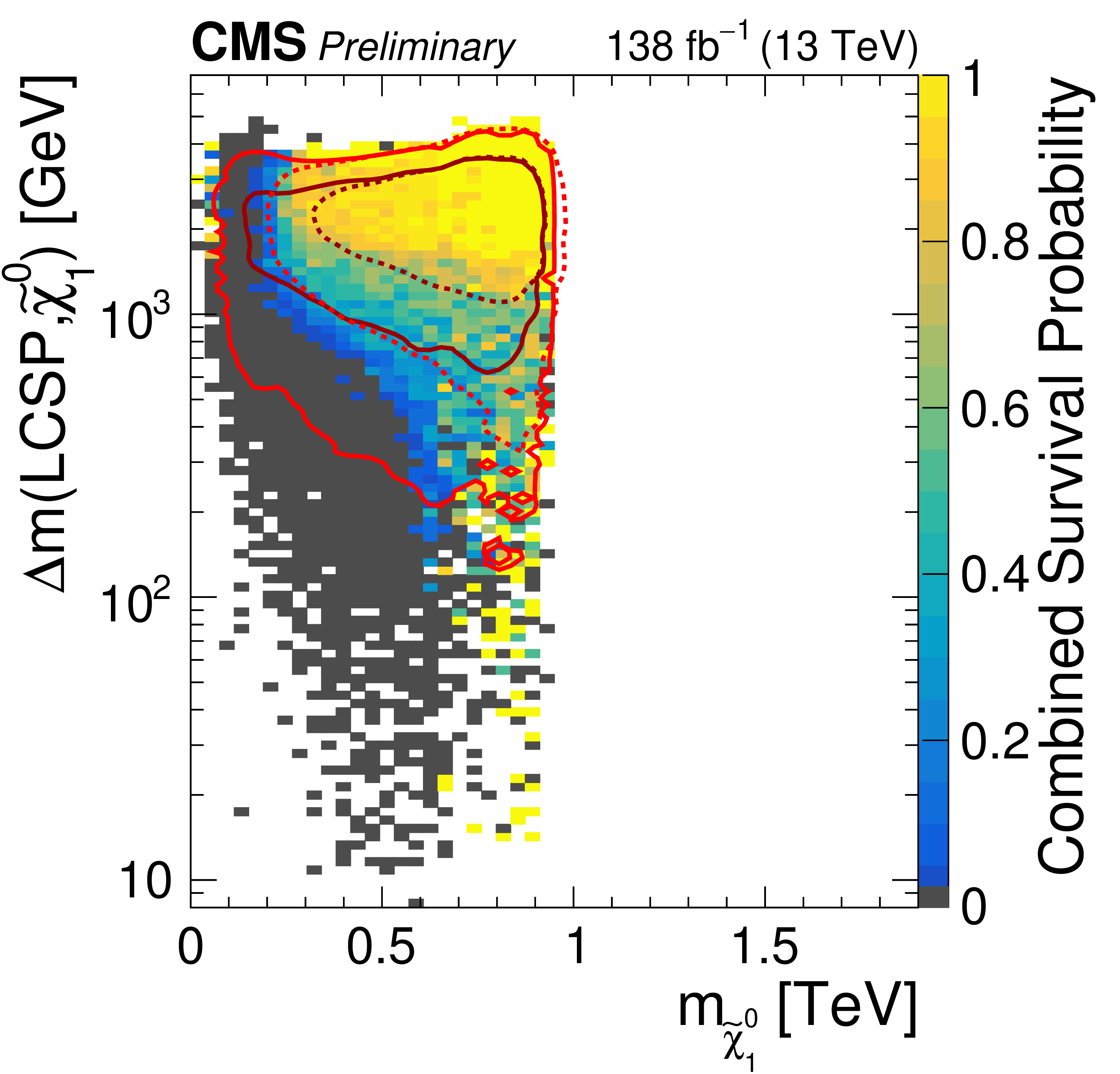
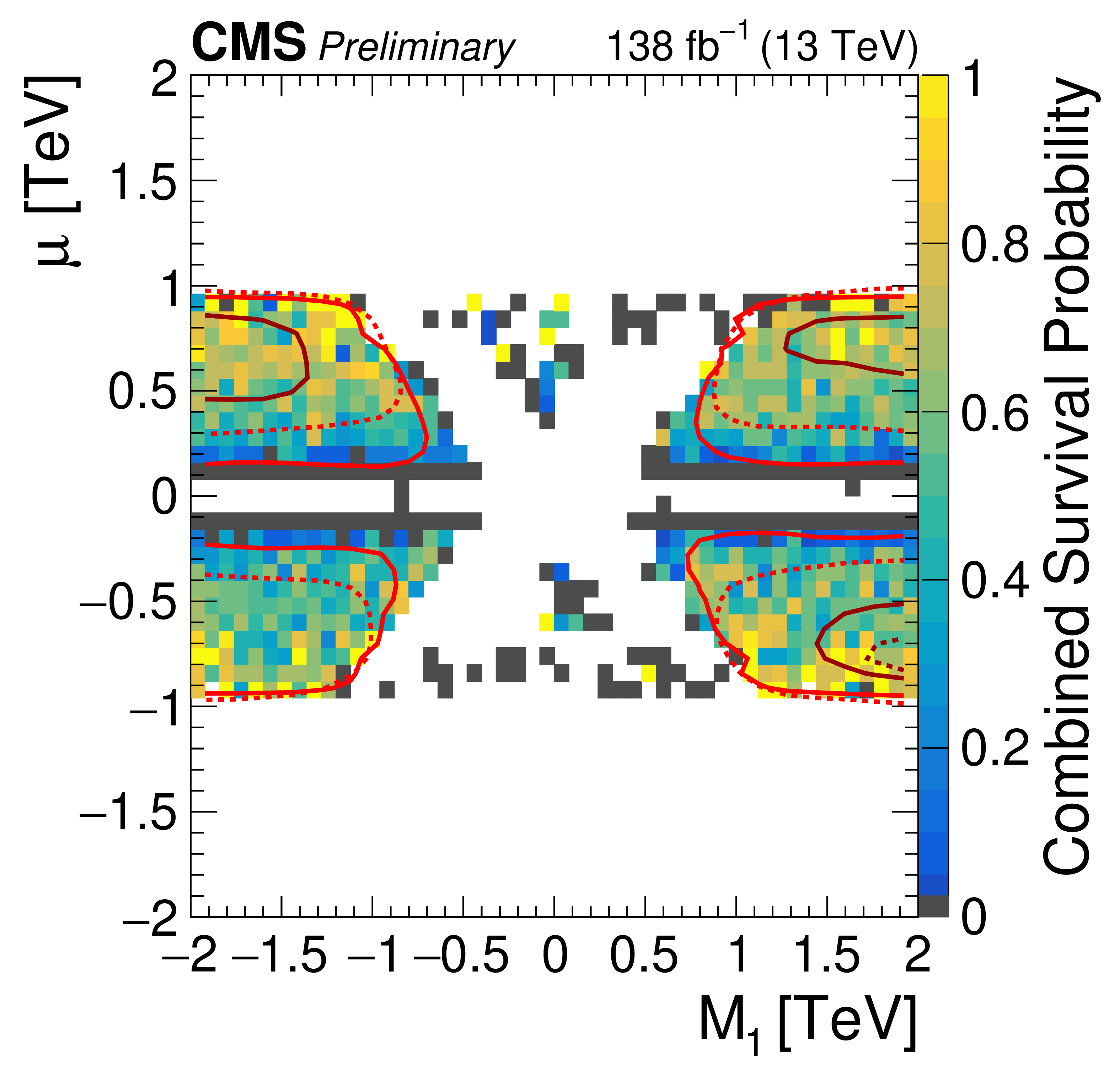
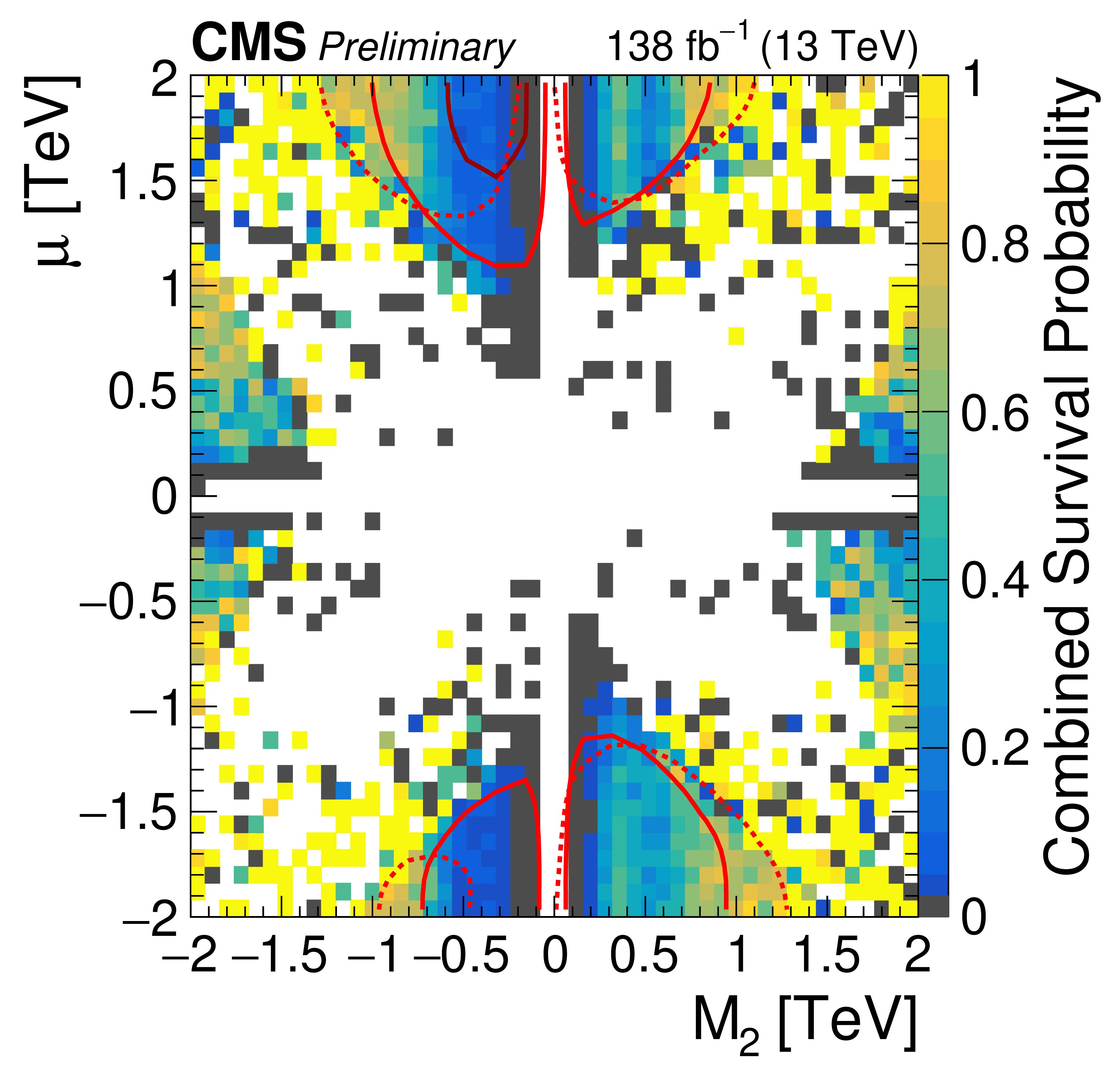
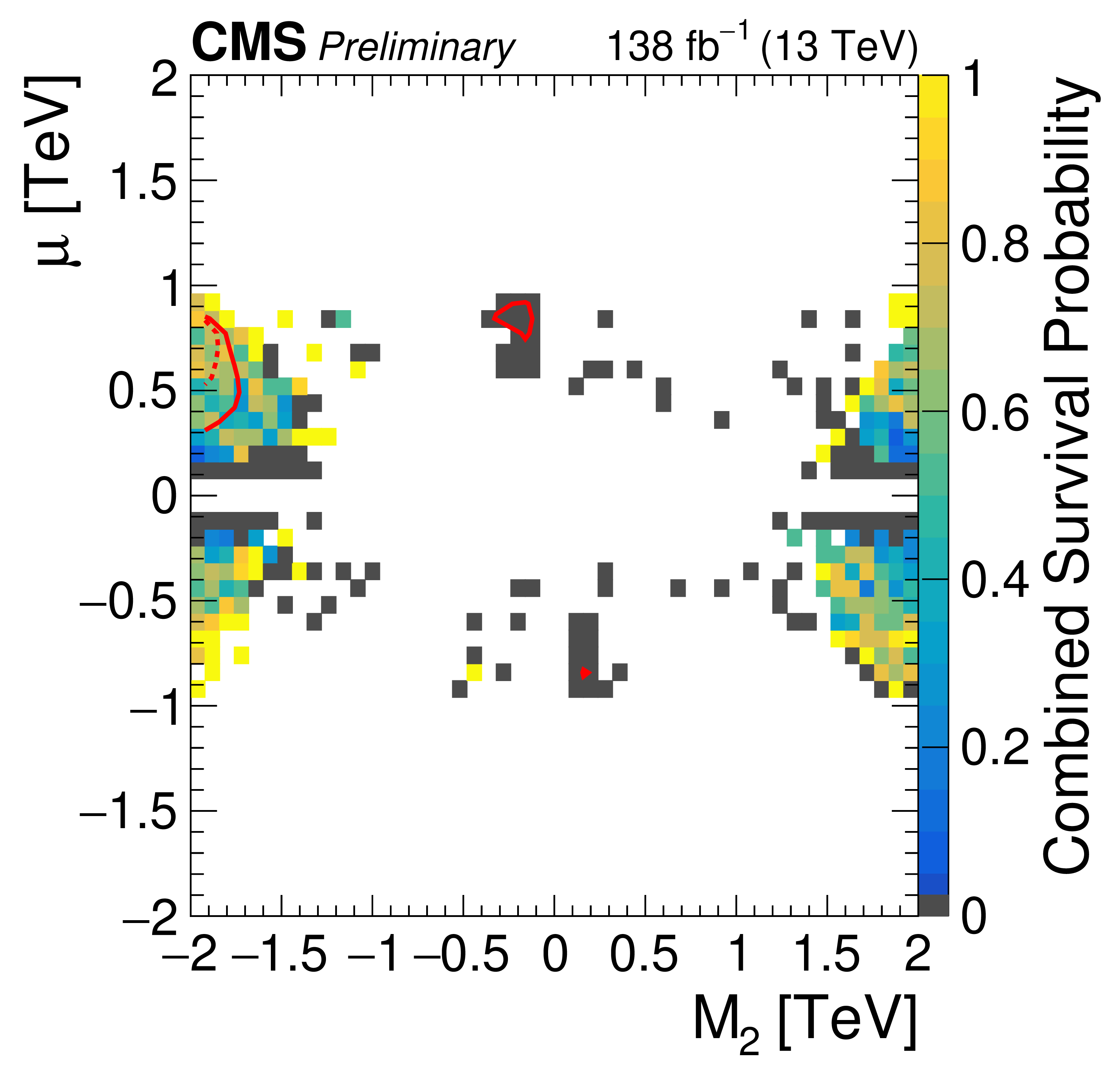
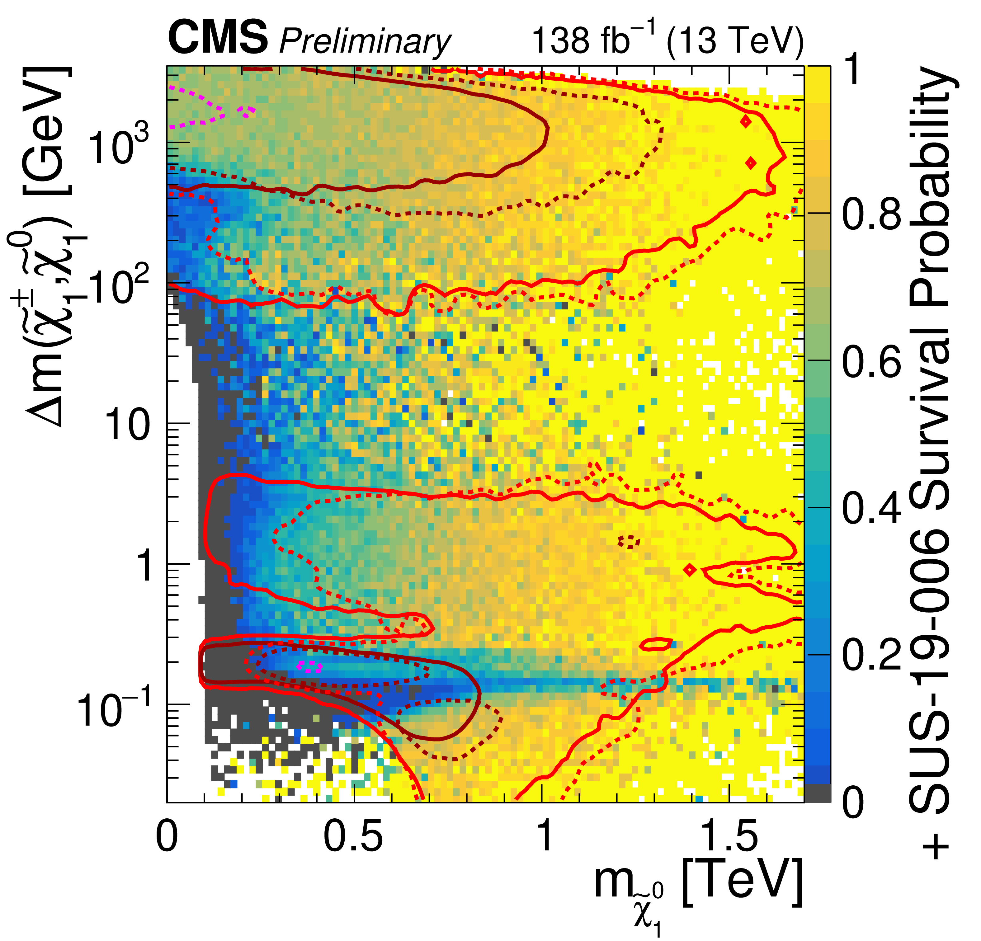
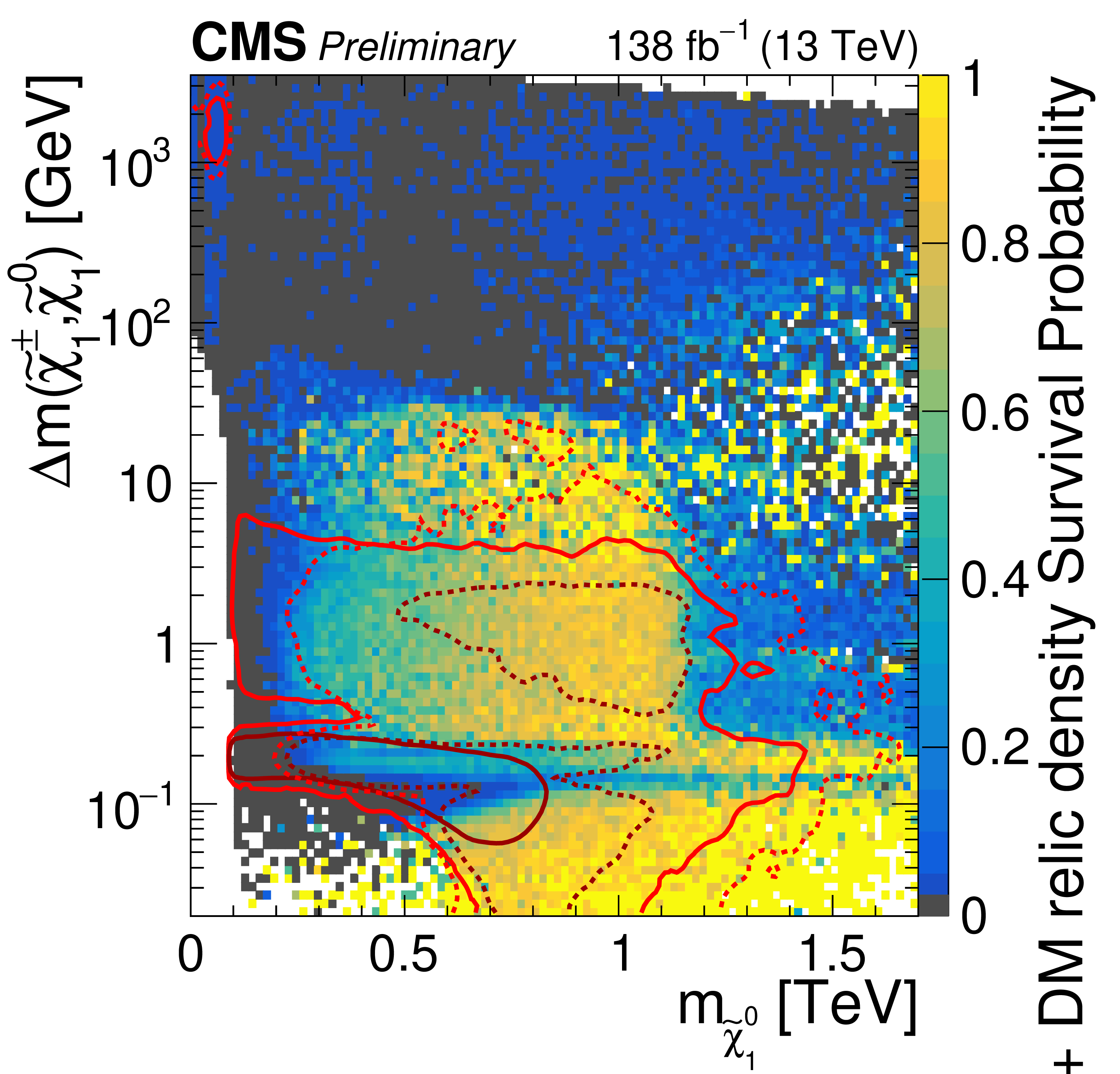
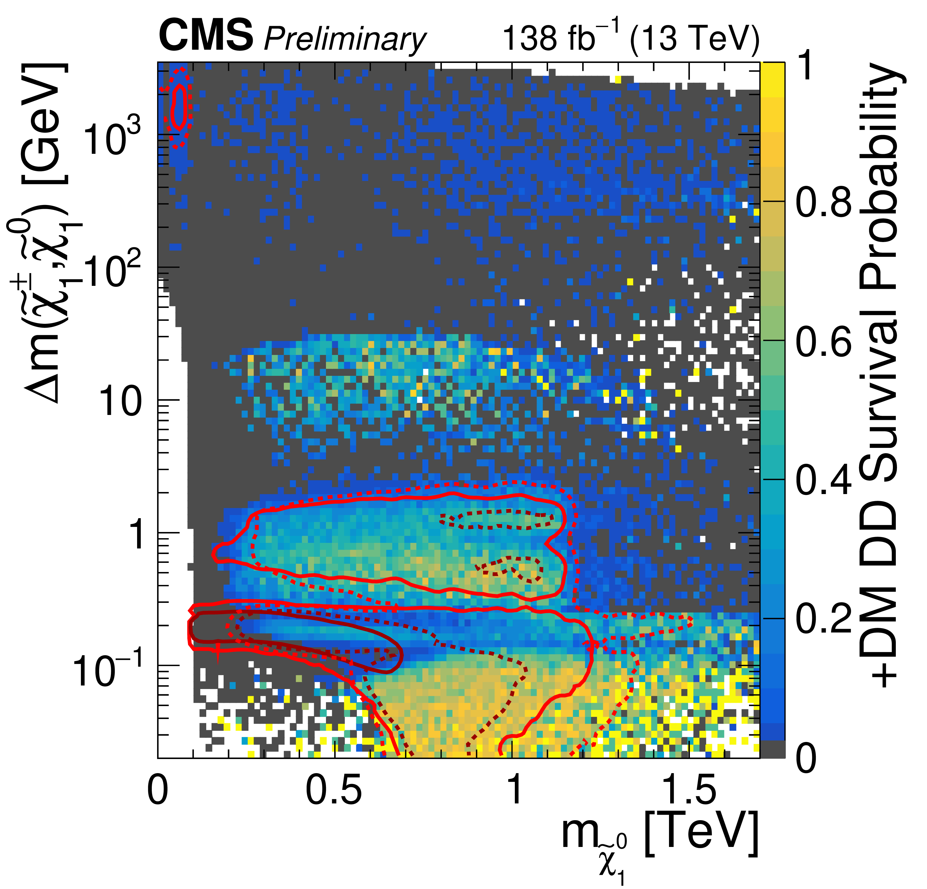
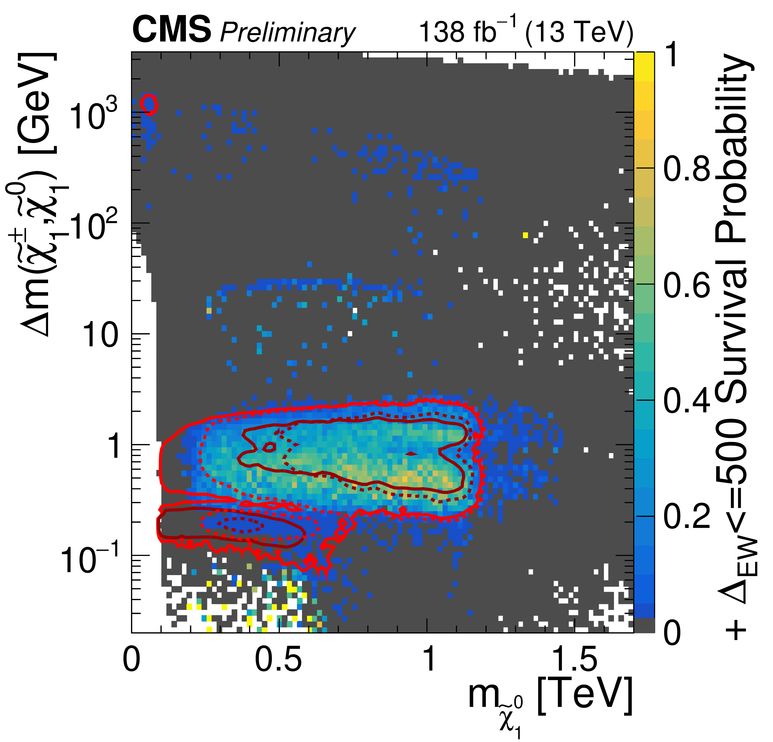
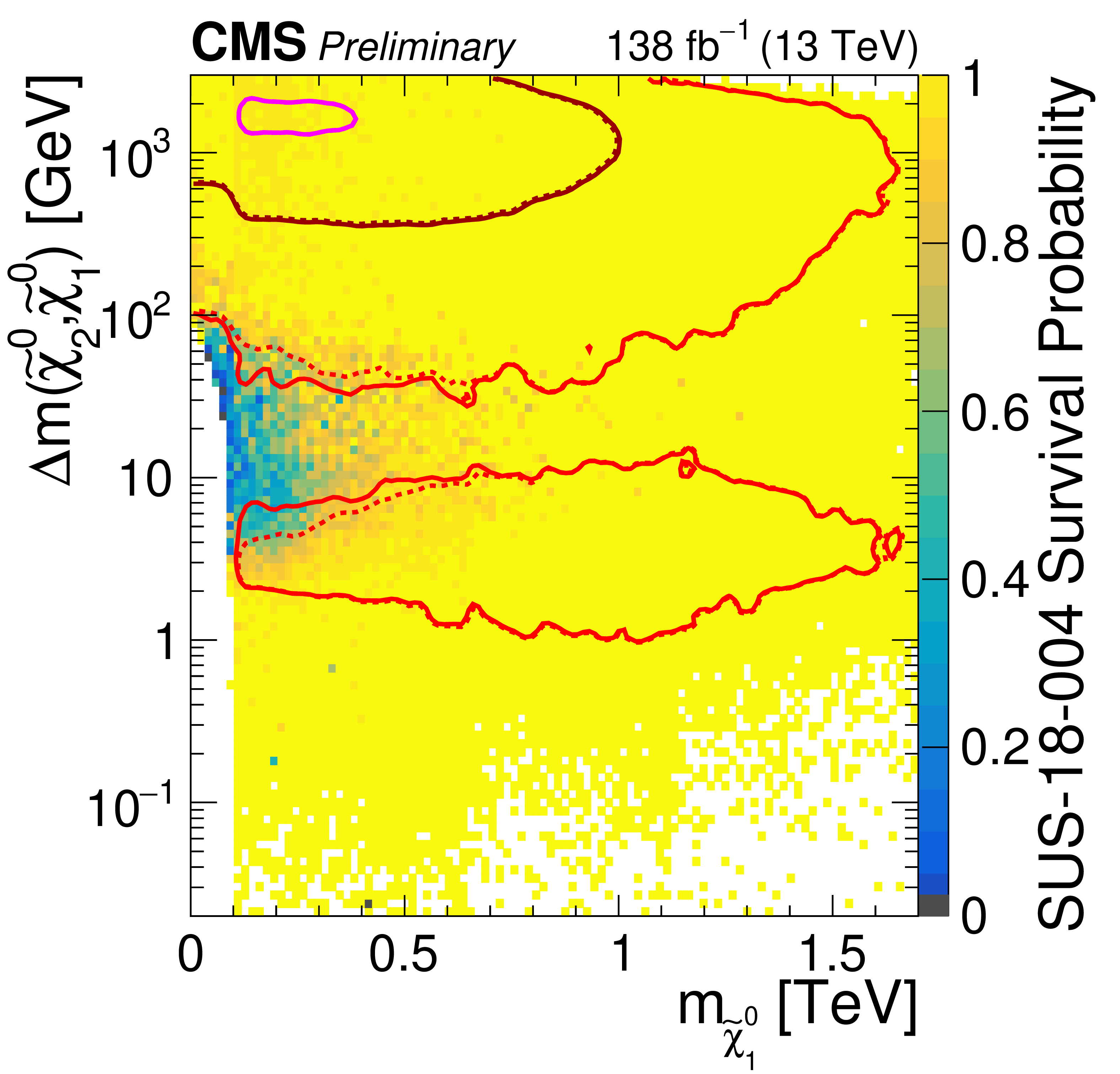
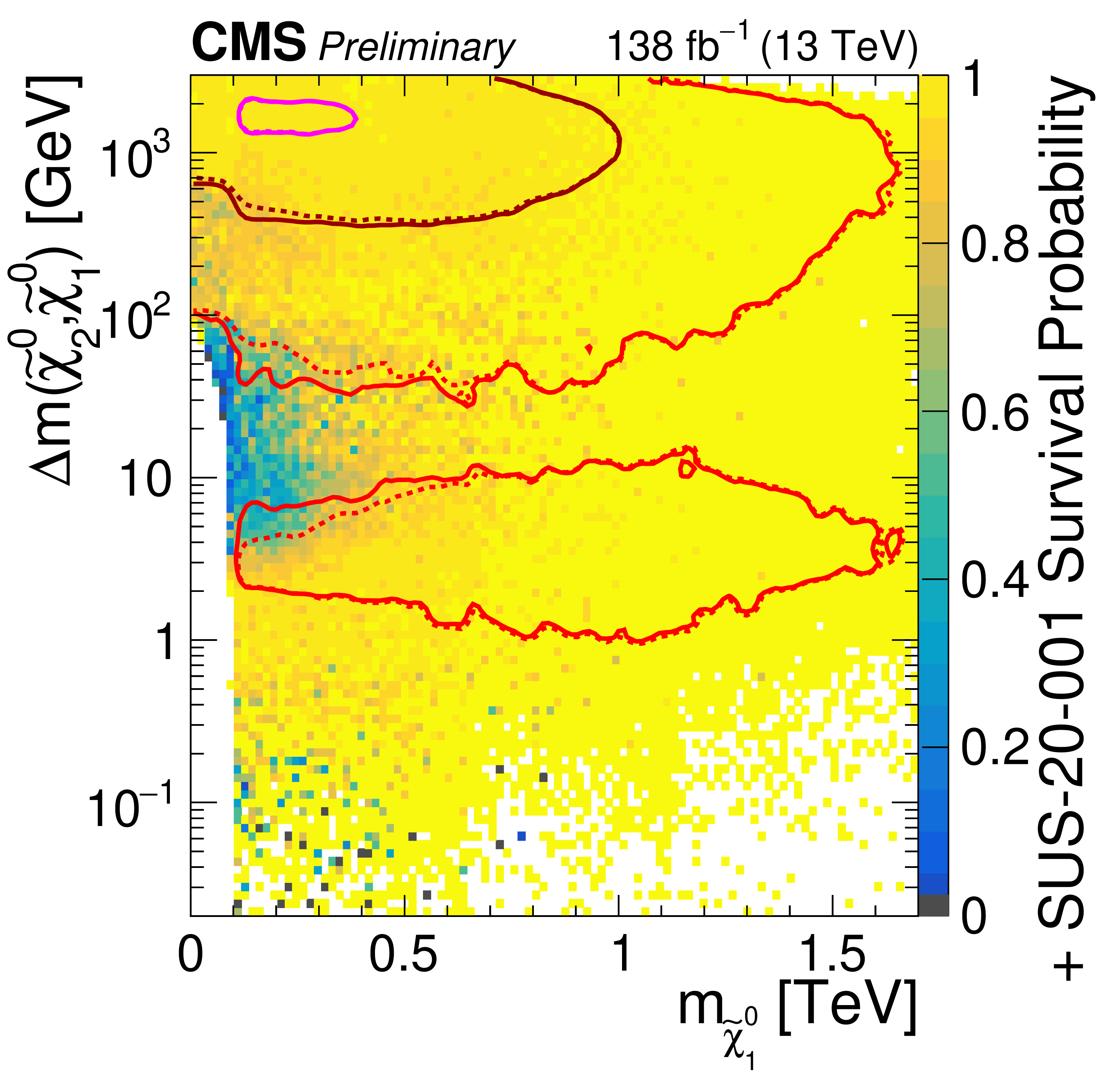
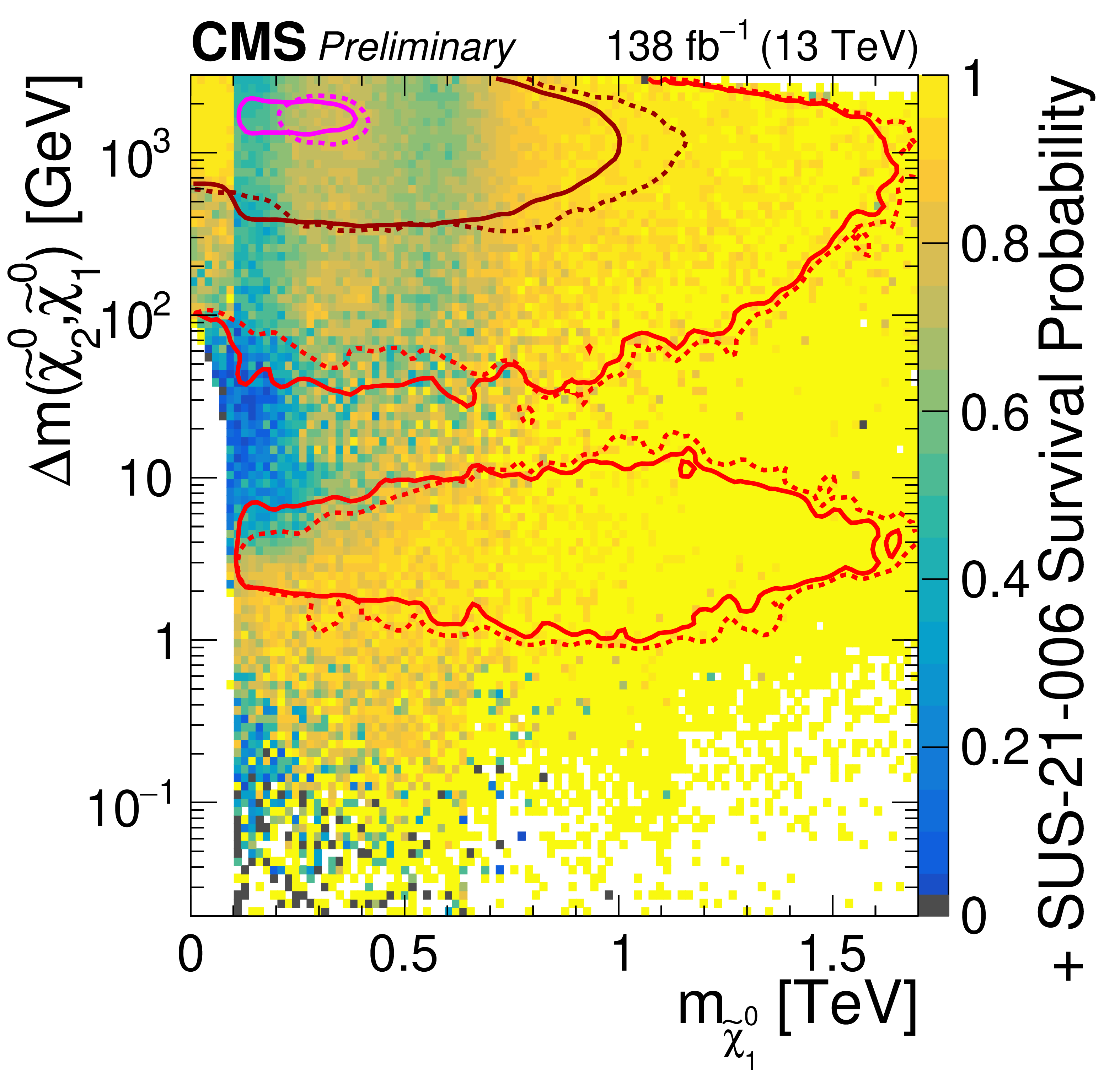
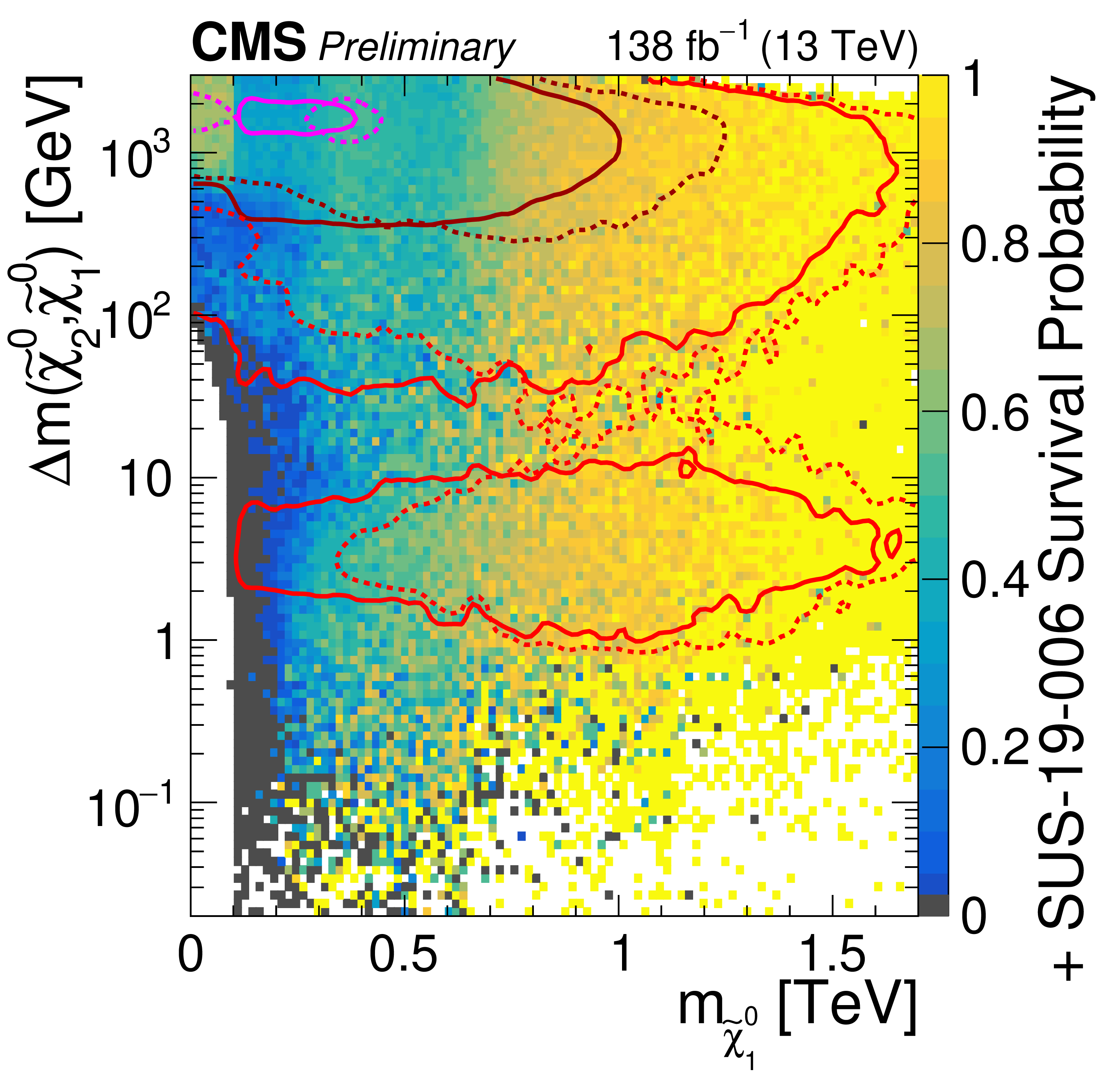
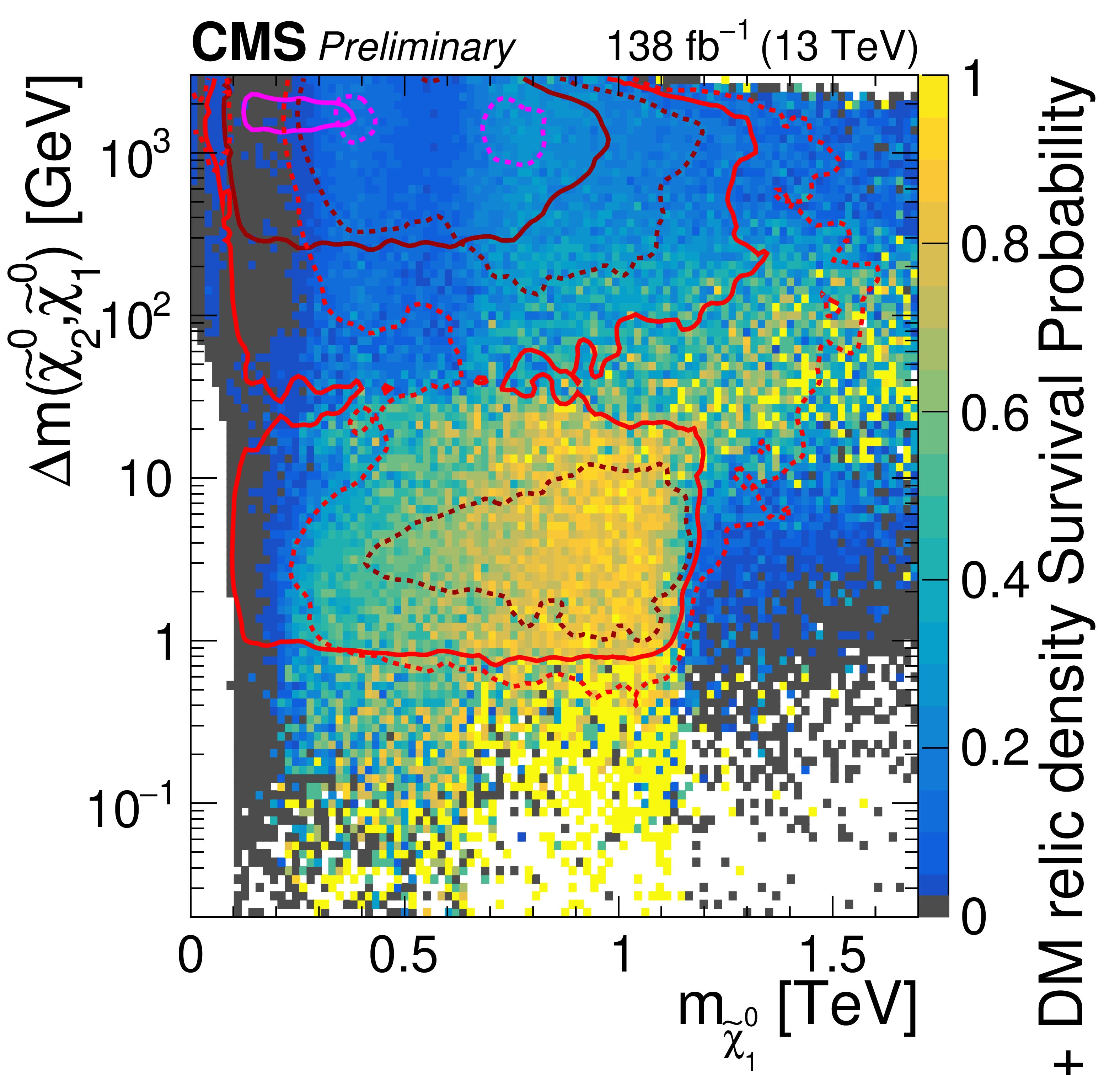
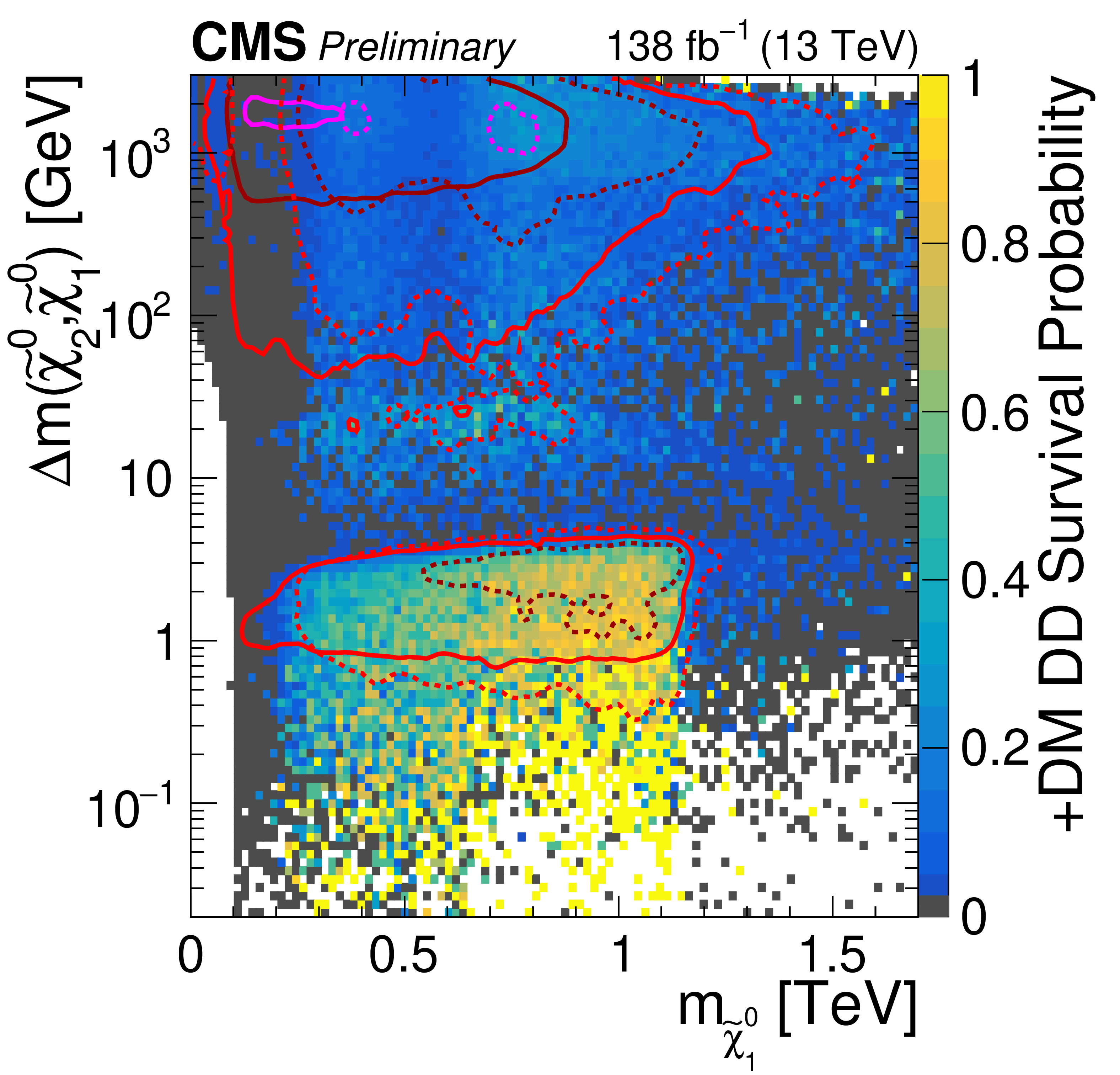
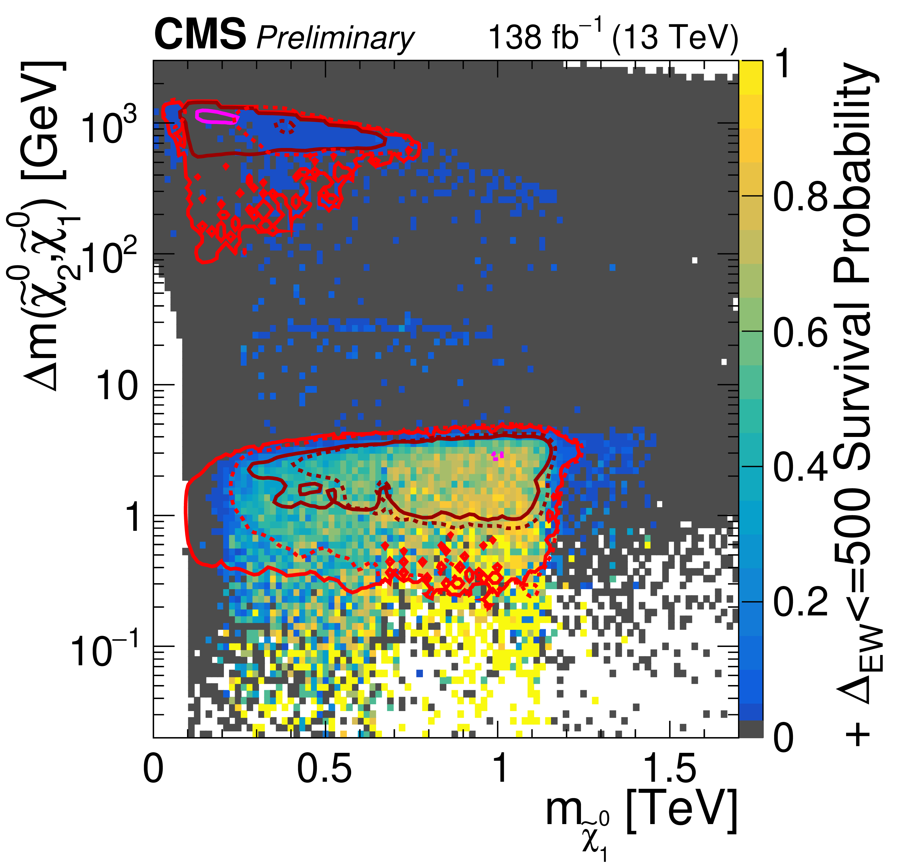
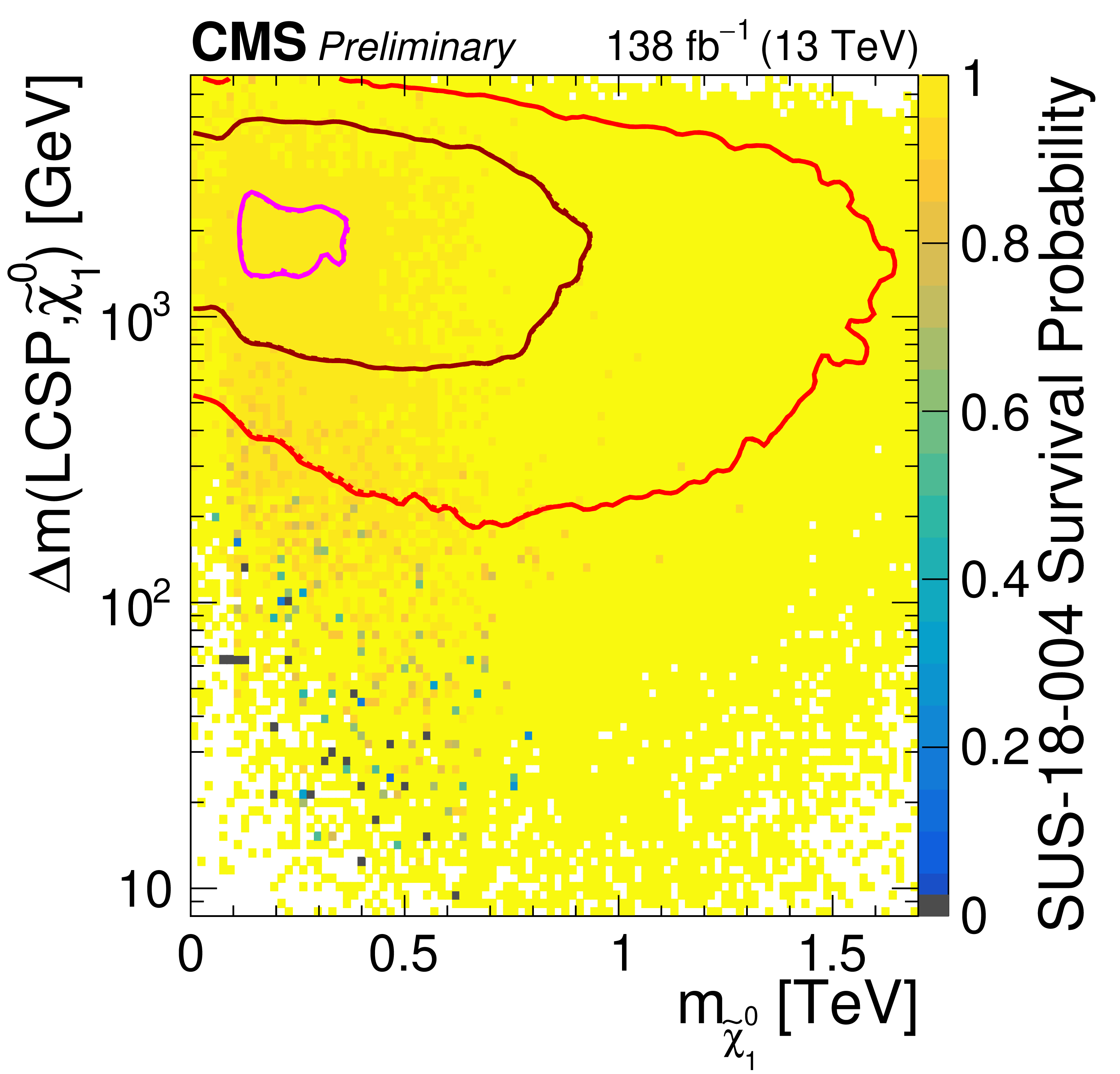
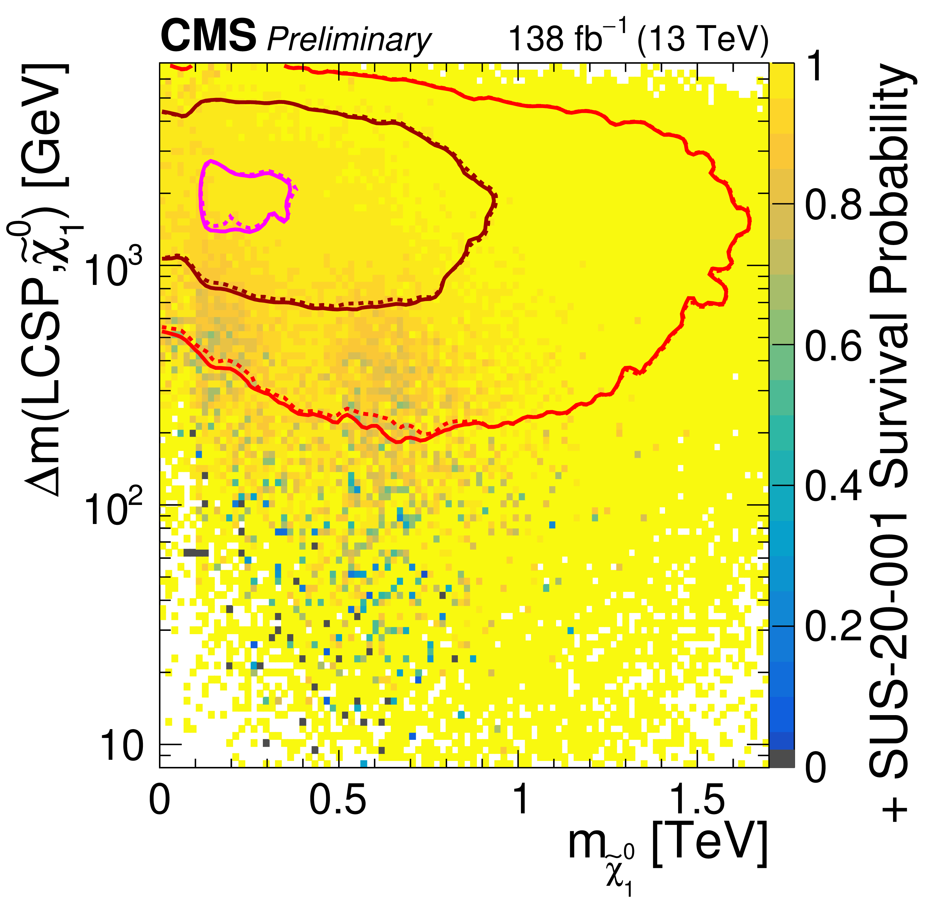
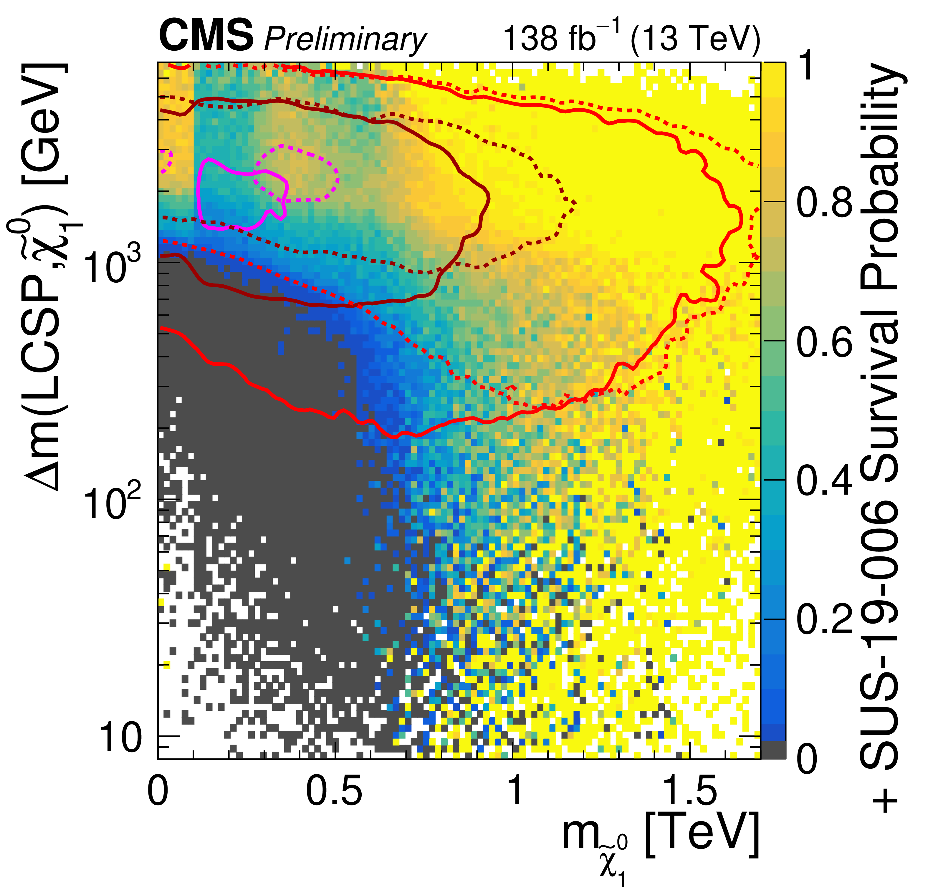
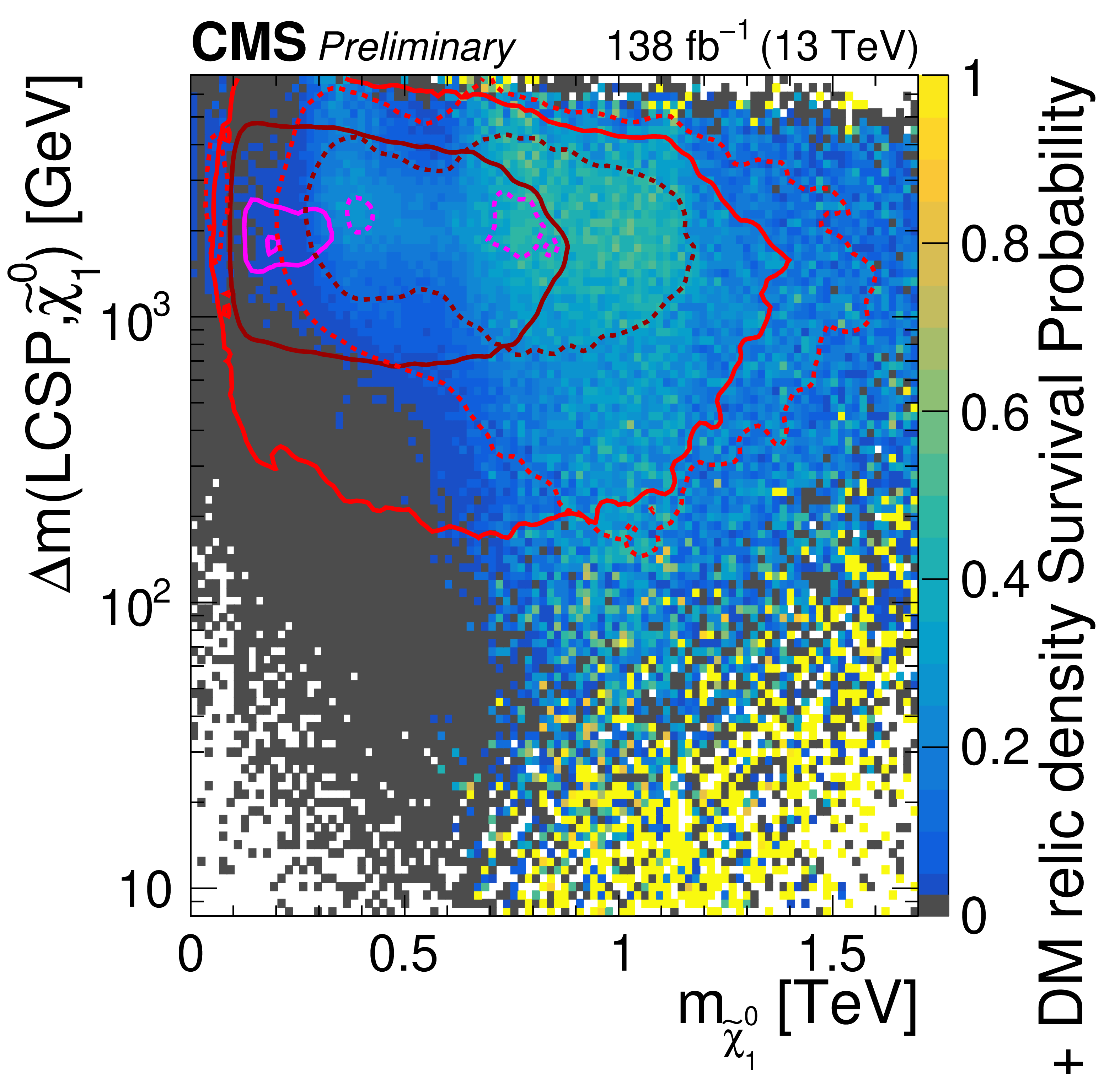
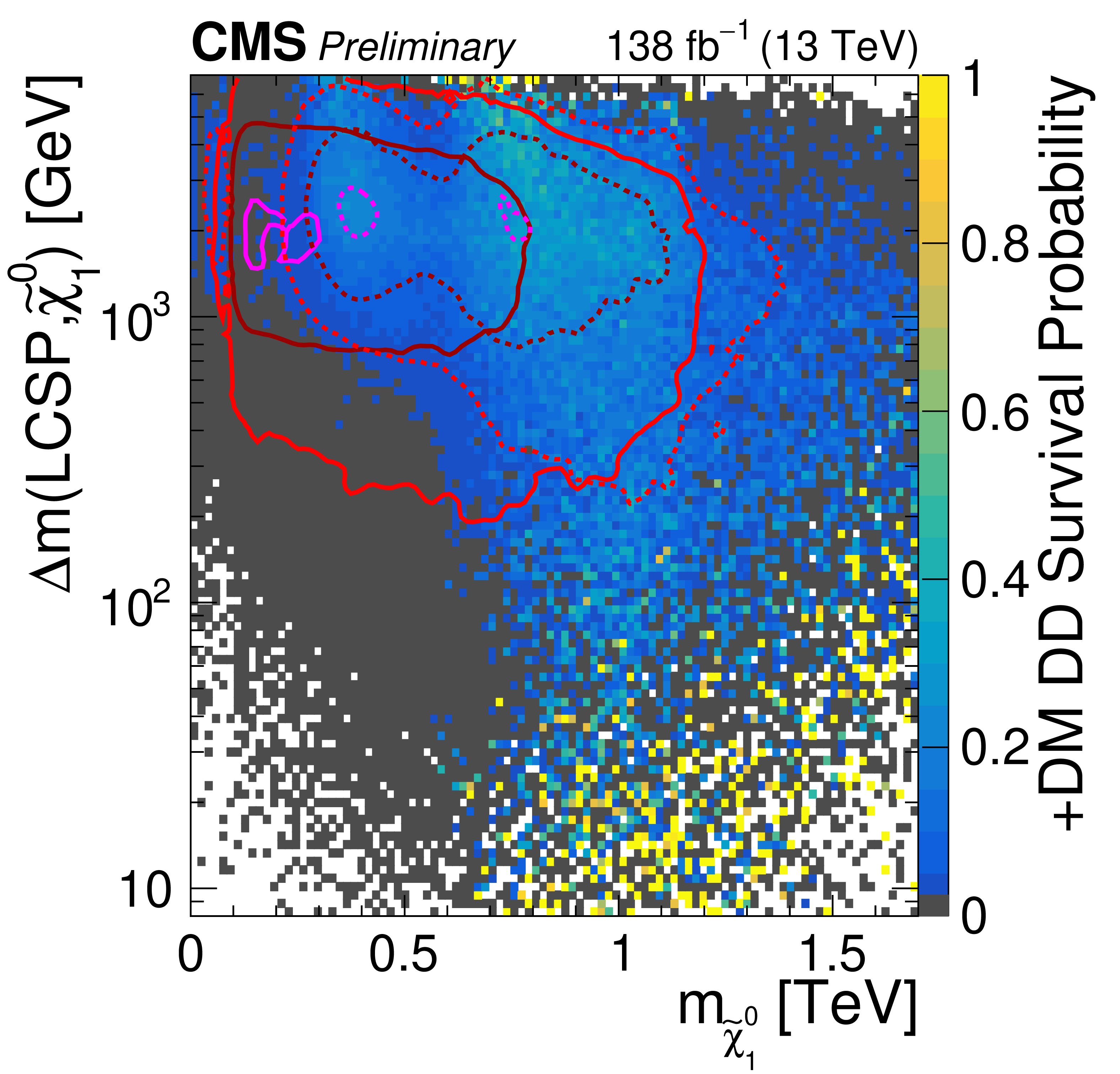
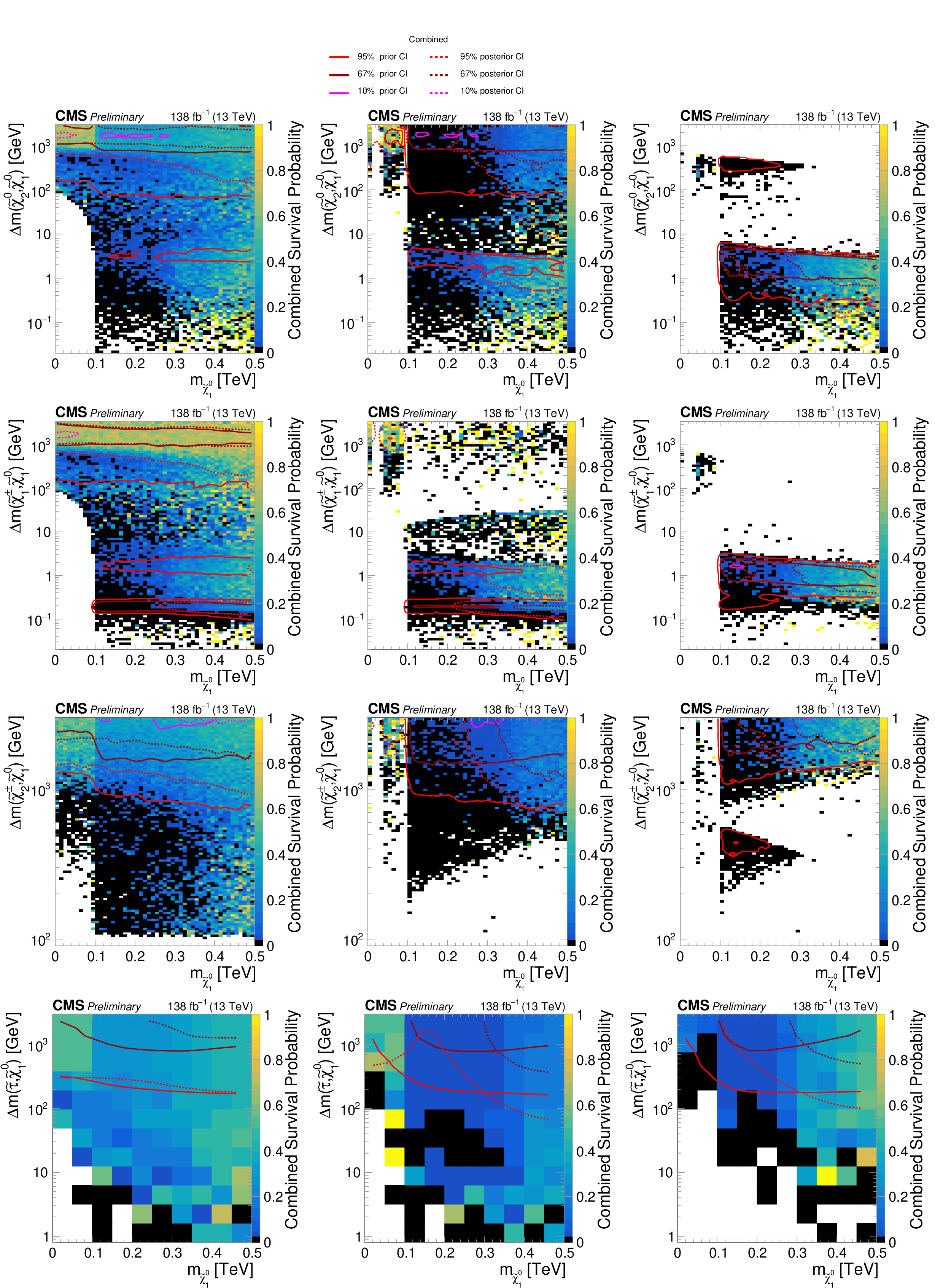
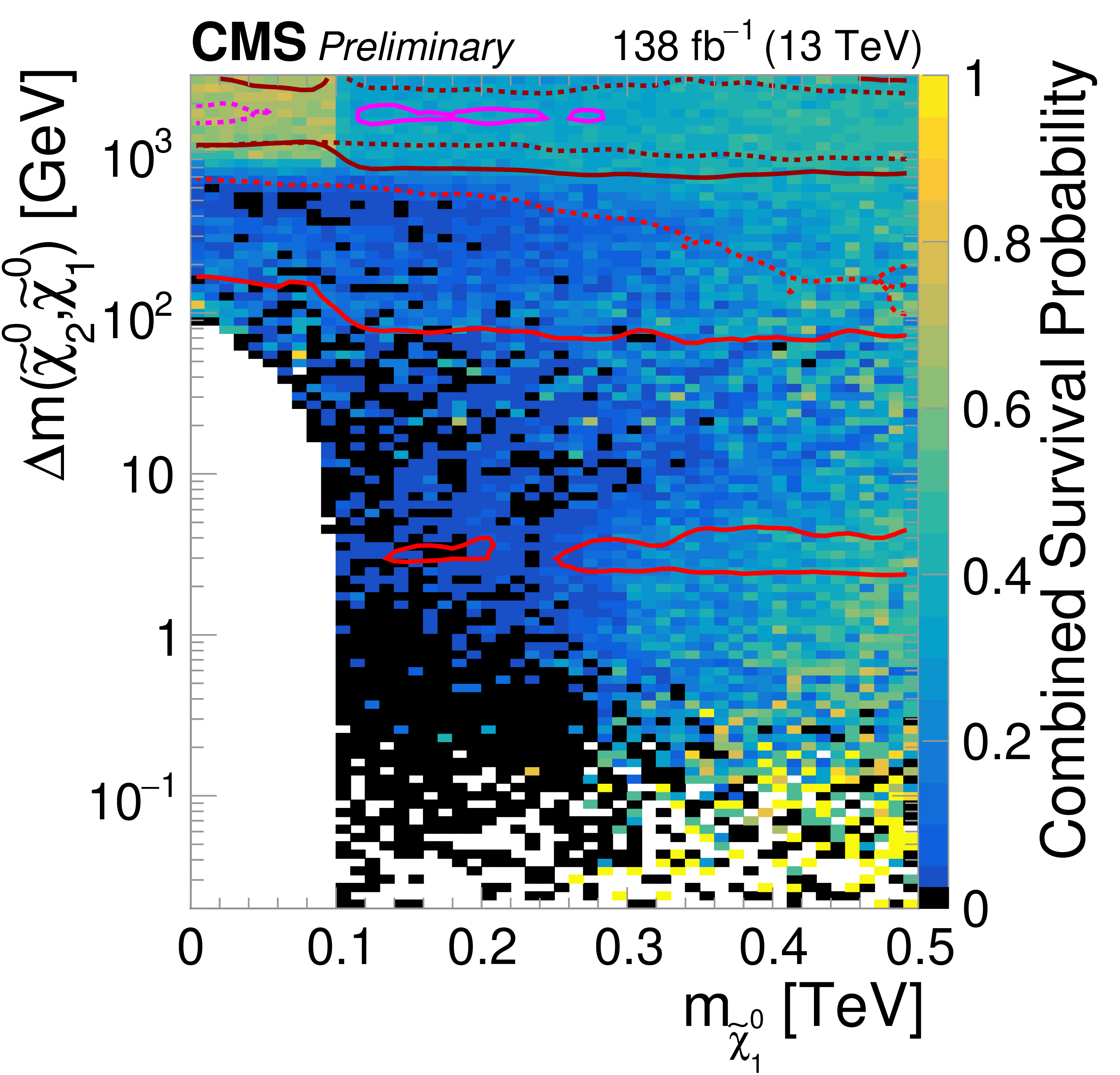
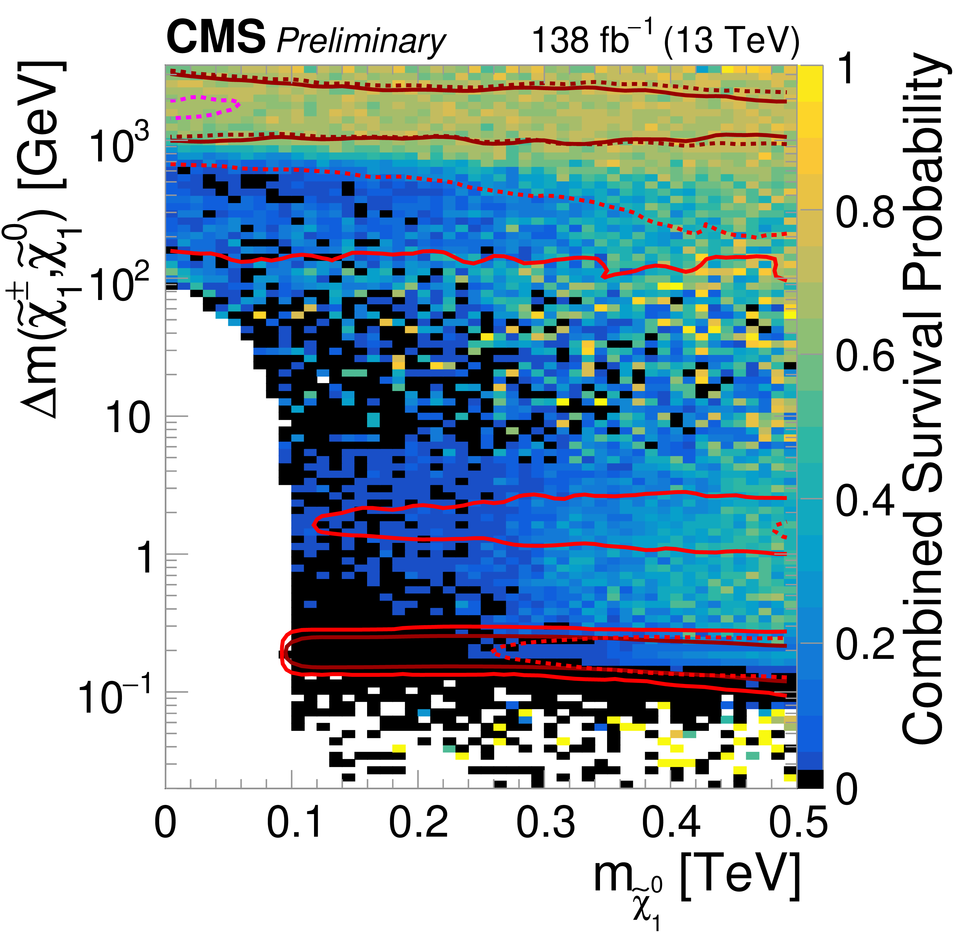
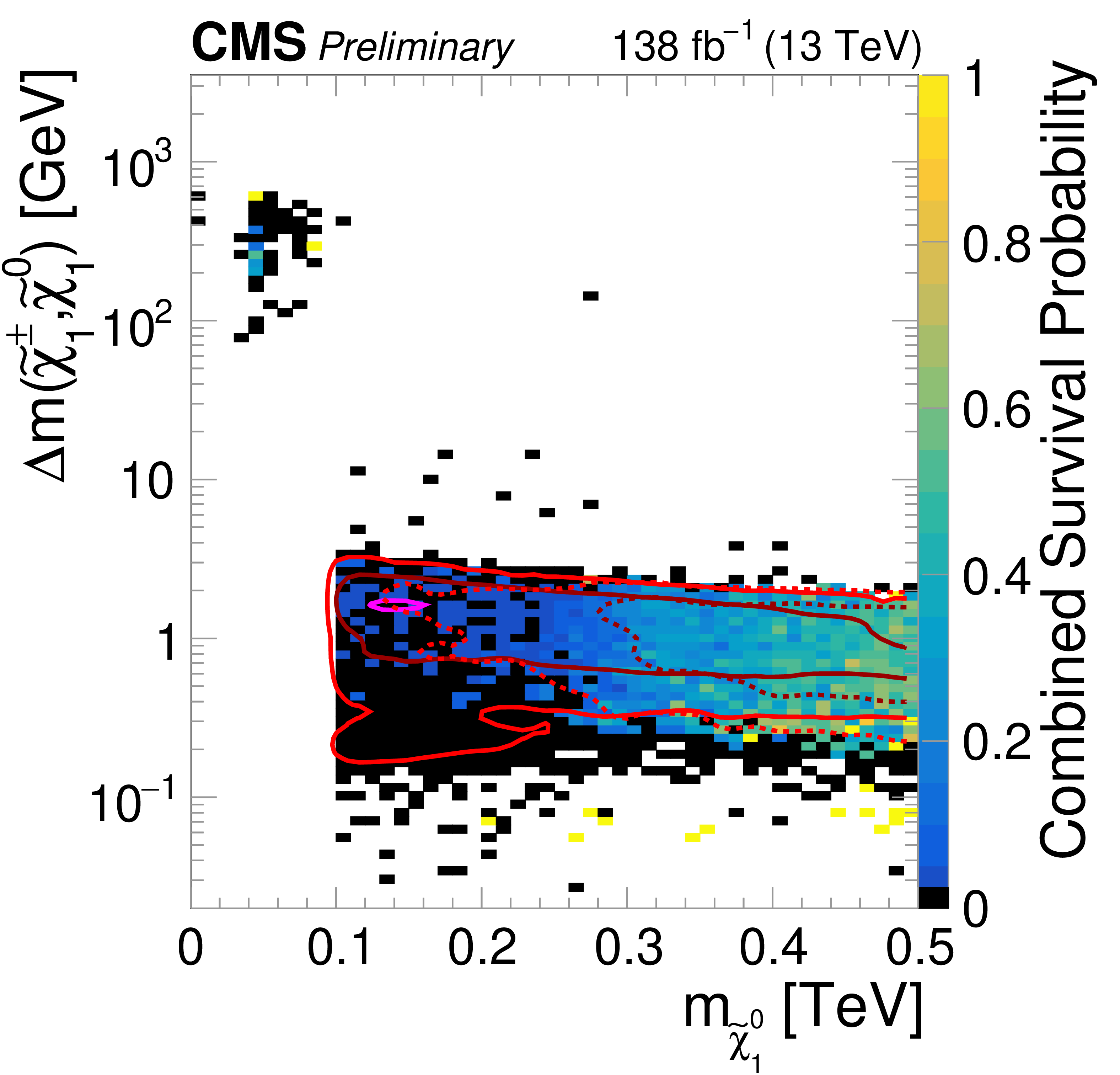
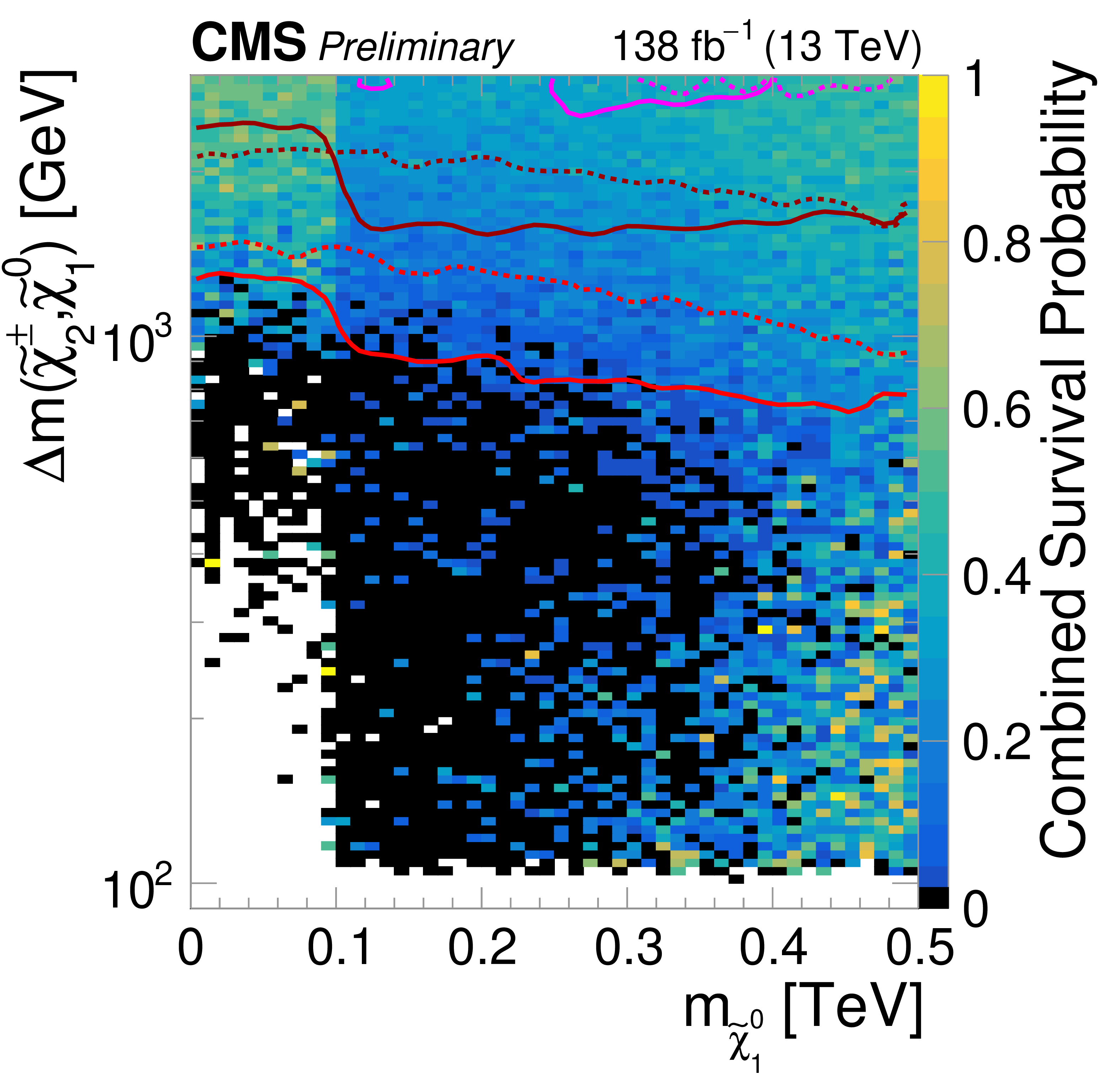
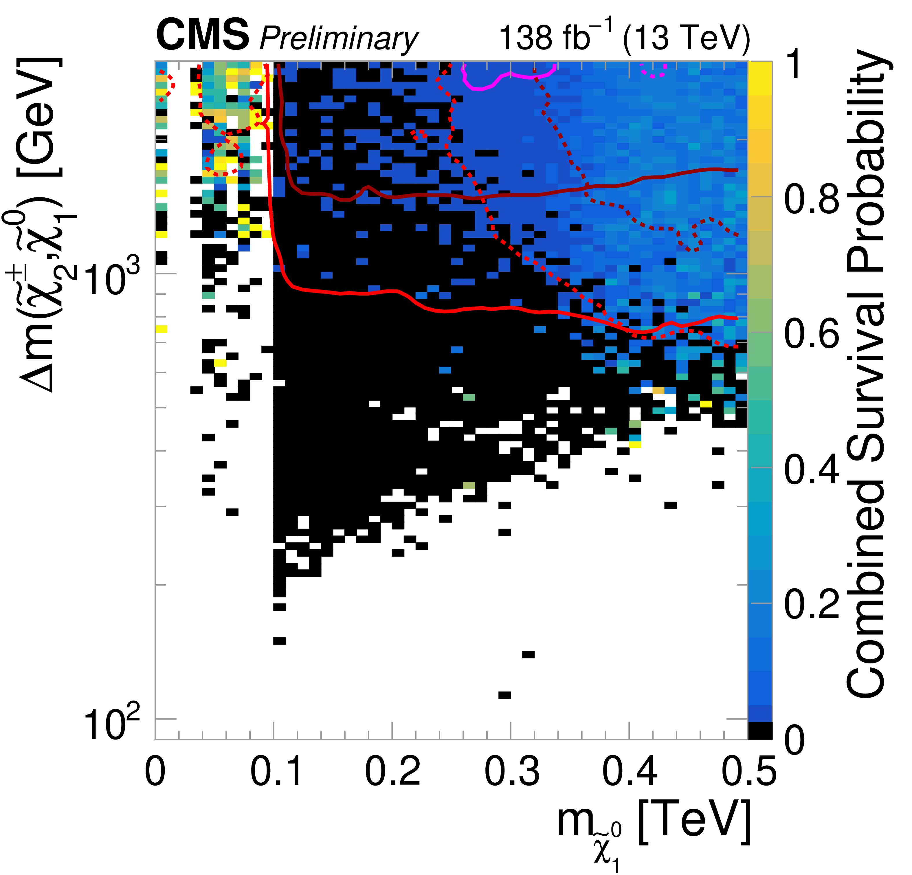
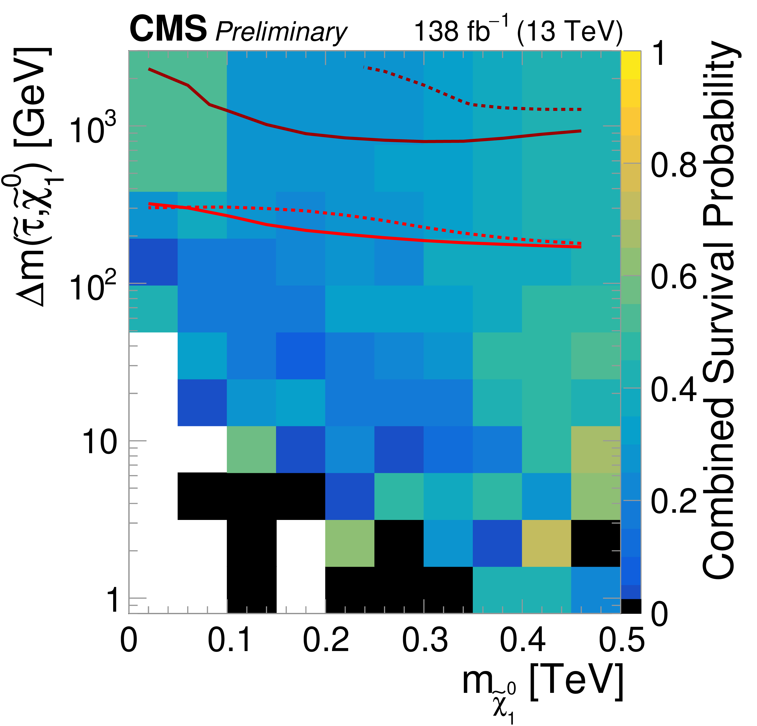
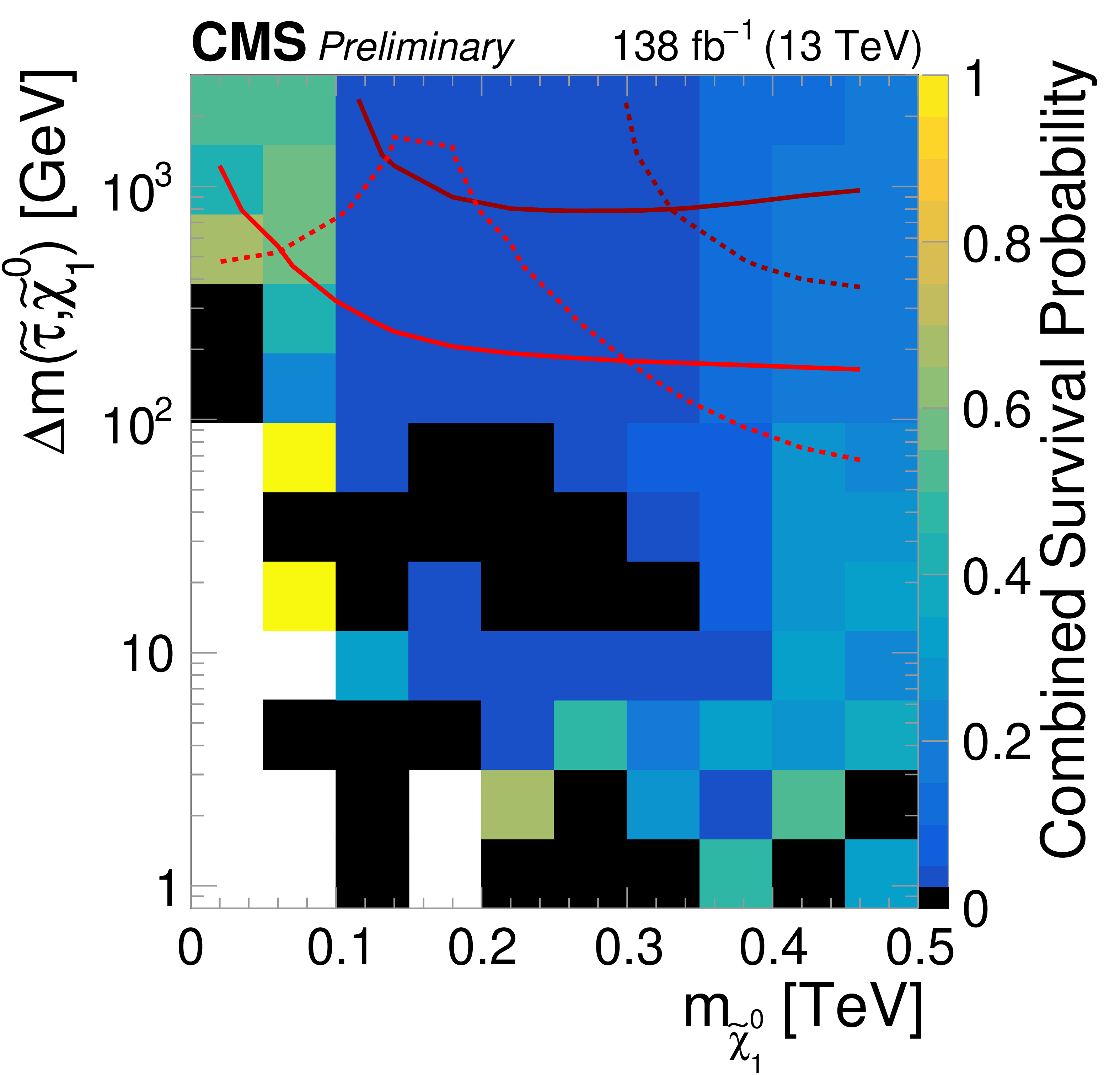
Figure 4:
Survival probability based on the full scan (left), based on the subset of the scan respecting DM constraints (center), and based on the natural DM subset (right), as a function of LSP mass and mass differences between the LSP and the lightest neutralino states or the stau mass. Black bins indicate where no pMSSM points survived the CMS analyses, and white indicate where no pMSSM points are present in the prior. Also shown are the prior (solid) and posterior (dashed) density contours corresponding to the respective constraints. |

png pdf |
Figure 4-a:
Survival probability based on the full scan (left), based on the subset of the scan respecting DM constraints (center), and based on the natural DM subset (right), as a function of LSP mass and mass differences between the LSP and the lightest neutralino states or the stau mass. Black bins indicate where no pMSSM points survived the CMS analyses, and white indicate where no pMSSM points are present in the prior. Also shown are the prior (solid) and posterior (dashed) density contours corresponding to the respective constraints. |
png pdf |
Figure 4-b:
Survival probability based on the full scan (left), based on the subset of the scan respecting DM constraints (center), and based on the natural DM subset (right), as a function of LSP mass and mass differences between the LSP and the lightest neutralino states or the stau mass. Black bins indicate where no pMSSM points survived the CMS analyses, and white indicate where no pMSSM points are present in the prior. Also shown are the prior (solid) and posterior (dashed) density contours corresponding to the respective constraints. |
png pdf |
Figure 4-c:
Survival probability based on the full scan (left), based on the subset of the scan respecting DM constraints (center), and based on the natural DM subset (right), as a function of LSP mass and mass differences between the LSP and the lightest neutralino states or the stau mass. Black bins indicate where no pMSSM points survived the CMS analyses, and white indicate where no pMSSM points are present in the prior. Also shown are the prior (solid) and posterior (dashed) density contours corresponding to the respective constraints. |
png pdf |
Figure 4-d:
Survival probability based on the full scan (left), based on the subset of the scan respecting DM constraints (center), and based on the natural DM subset (right), as a function of LSP mass and mass differences between the LSP and the lightest neutralino states or the stau mass. Black bins indicate where no pMSSM points survived the CMS analyses, and white indicate where no pMSSM points are present in the prior. Also shown are the prior (solid) and posterior (dashed) density contours corresponding to the respective constraints. |
png pdf |
Figure 4-e:
Survival probability based on the full scan (left), based on the subset of the scan respecting DM constraints (center), and based on the natural DM subset (right), as a function of LSP mass and mass differences between the LSP and the lightest neutralino states or the stau mass. Black bins indicate where no pMSSM points survived the CMS analyses, and white indicate where no pMSSM points are present in the prior. Also shown are the prior (solid) and posterior (dashed) density contours corresponding to the respective constraints. |
png pdf |
Figure 4-f:
Survival probability based on the full scan (left), based on the subset of the scan respecting DM constraints (center), and based on the natural DM subset (right), as a function of LSP mass and mass differences between the LSP and the lightest neutralino states or the stau mass. Black bins indicate where no pMSSM points survived the CMS analyses, and white indicate where no pMSSM points are present in the prior. Also shown are the prior (solid) and posterior (dashed) density contours corresponding to the respective constraints. |

png pdf |
Figure 4-g:
Survival probability based on the full scan (left), based on the subset of the scan respecting DM constraints (center), and based on the natural DM subset (right), as a function of LSP mass and mass differences between the LSP and the lightest neutralino states or the stau mass. Black bins indicate where no pMSSM points survived the CMS analyses, and white indicate where no pMSSM points are present in the prior. Also shown are the prior (solid) and posterior (dashed) density contours corresponding to the respective constraints. |

png pdf |
Figure 4-h:
Survival probability based on the full scan (left), based on the subset of the scan respecting DM constraints (center), and based on the natural DM subset (right), as a function of LSP mass and mass differences between the LSP and the lightest neutralino states or the stau mass. Black bins indicate where no pMSSM points survived the CMS analyses, and white indicate where no pMSSM points are present in the prior. Also shown are the prior (solid) and posterior (dashed) density contours corresponding to the respective constraints. |
png pdf |
Figure 4-i:
Survival probability based on the full scan (left), based on the subset of the scan respecting DM constraints (center), and based on the natural DM subset (right), as a function of LSP mass and mass differences between the LSP and the lightest neutralino states or the stau mass. Black bins indicate where no pMSSM points survived the CMS analyses, and white indicate where no pMSSM points are present in the prior. Also shown are the prior (solid) and posterior (dashed) density contours corresponding to the respective constraints. |
png pdf |
Figure 4-j:
Survival probability based on the full scan (left), based on the subset of the scan respecting DM constraints (center), and based on the natural DM subset (right), as a function of LSP mass and mass differences between the LSP and the lightest neutralino states or the stau mass. Black bins indicate where no pMSSM points survived the CMS analyses, and white indicate where no pMSSM points are present in the prior. Also shown are the prior (solid) and posterior (dashed) density contours corresponding to the respective constraints. |
png pdf |
Figure 4-k:
Survival probability based on the full scan (left), based on the subset of the scan respecting DM constraints (center), and based on the natural DM subset (right), as a function of LSP mass and mass differences between the LSP and the lightest neutralino states or the stau mass. Black bins indicate where no pMSSM points survived the CMS analyses, and white indicate where no pMSSM points are present in the prior. Also shown are the prior (solid) and posterior (dashed) density contours corresponding to the respective constraints. |

png pdf |
Figure 4-l:
Survival probability based on the full scan (left), based on the subset of the scan respecting DM constraints (center), and based on the natural DM subset (right), as a function of LSP mass and mass differences between the LSP and the lightest neutralino states or the stau mass. Black bins indicate where no pMSSM points survived the CMS analyses, and white indicate where no pMSSM points are present in the prior. Also shown are the prior (solid) and posterior (dashed) density contours corresponding to the respective constraints. |
png pdf |
Figure 4-m:
Survival probability based on the full scan (left), based on the subset of the scan respecting DM constraints (center), and based on the natural DM subset (right), as a function of LSP mass and mass differences between the LSP and the lightest neutralino states or the stau mass. Black bins indicate where no pMSSM points survived the CMS analyses, and white indicate where no pMSSM points are present in the prior. Also shown are the prior (solid) and posterior (dashed) density contours corresponding to the respective constraints. |

png pdf |
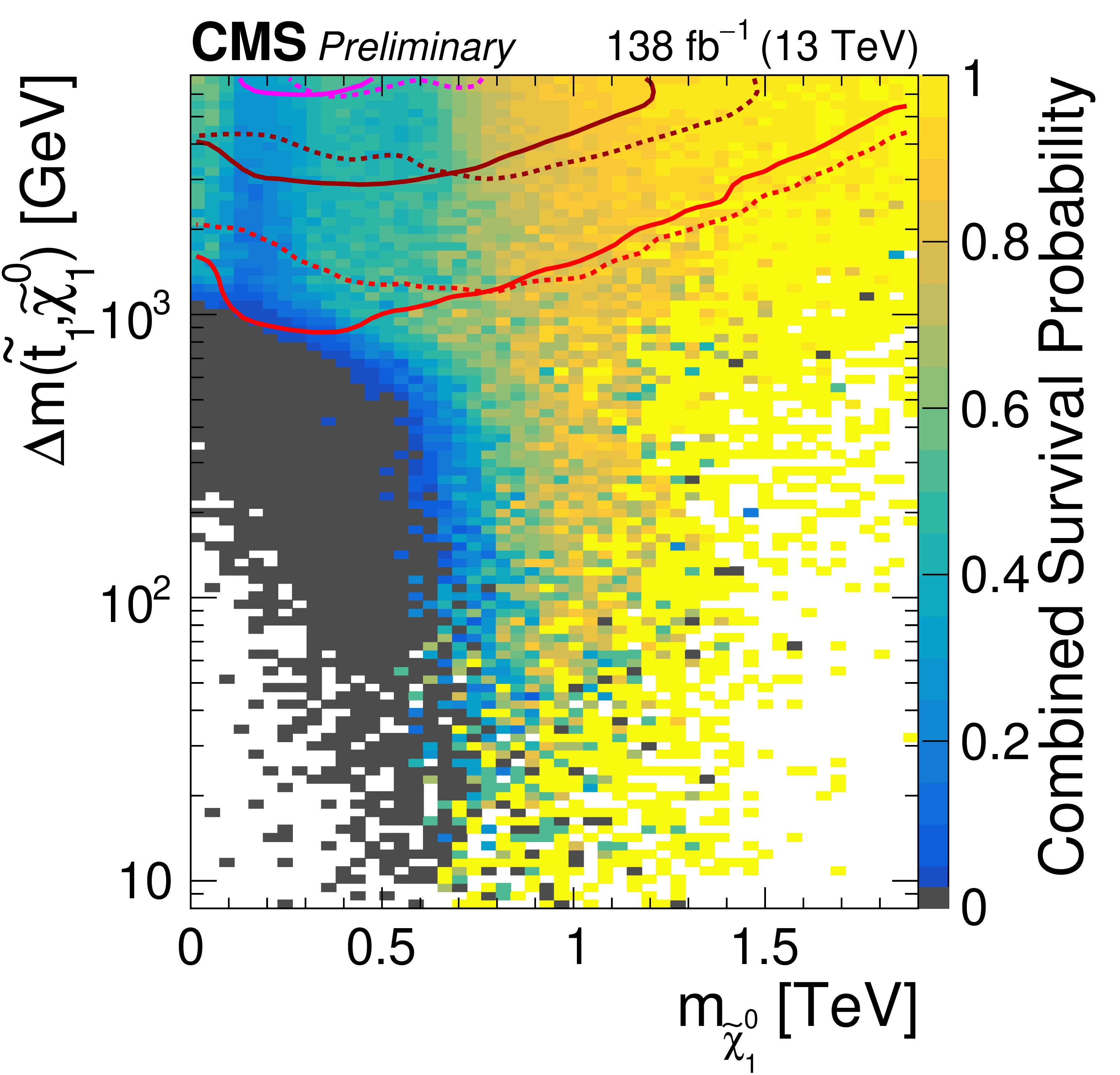
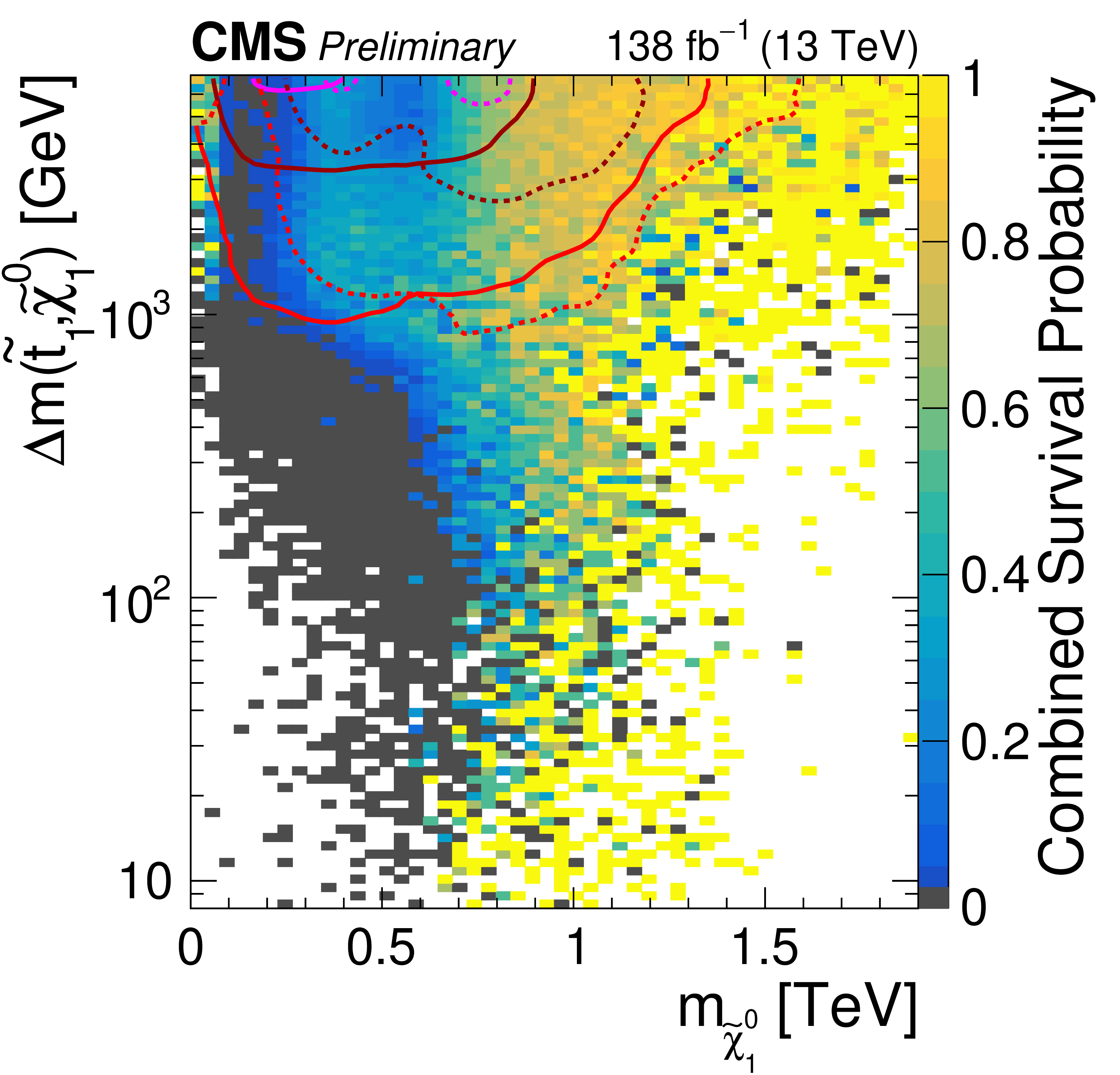
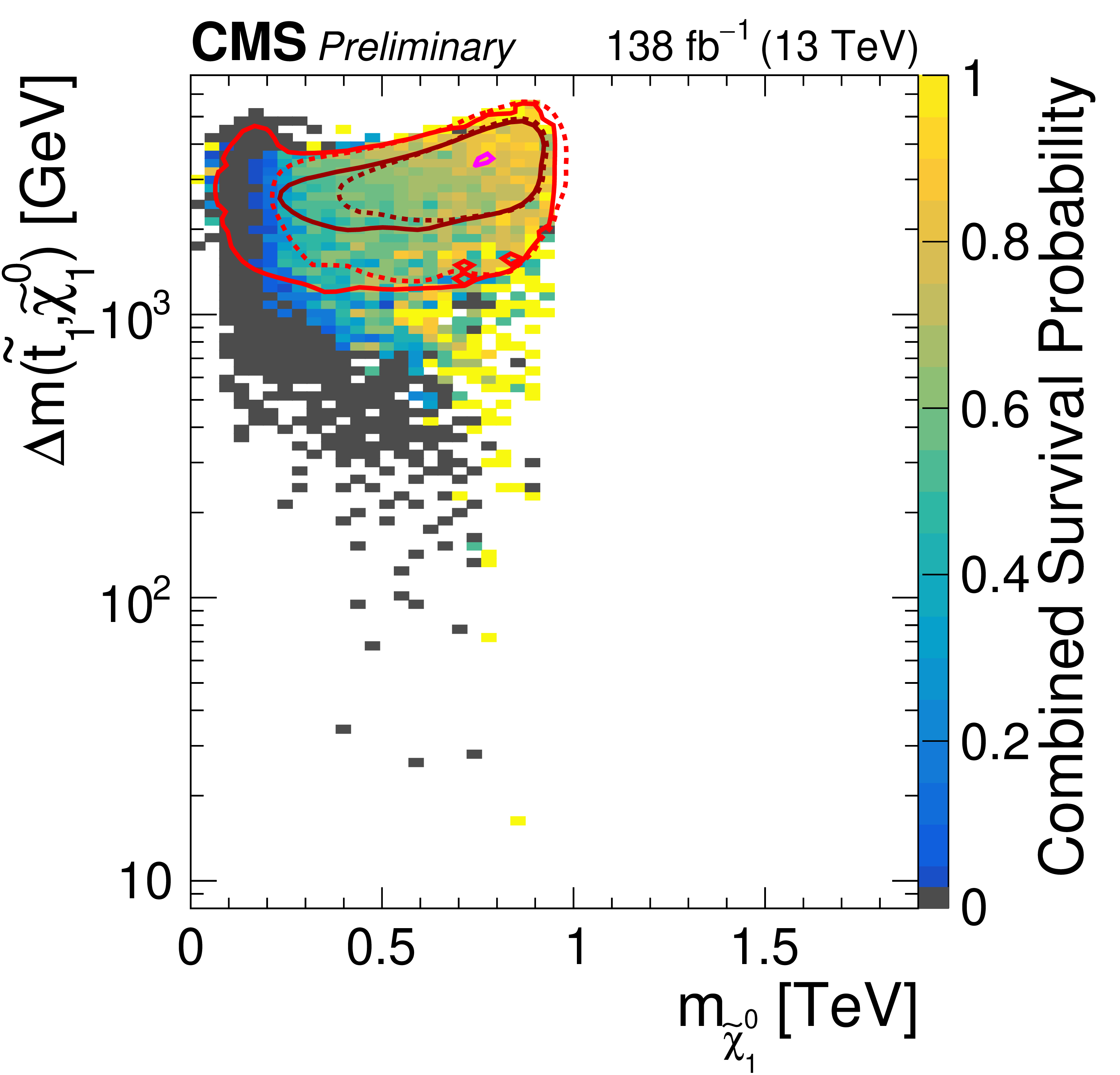
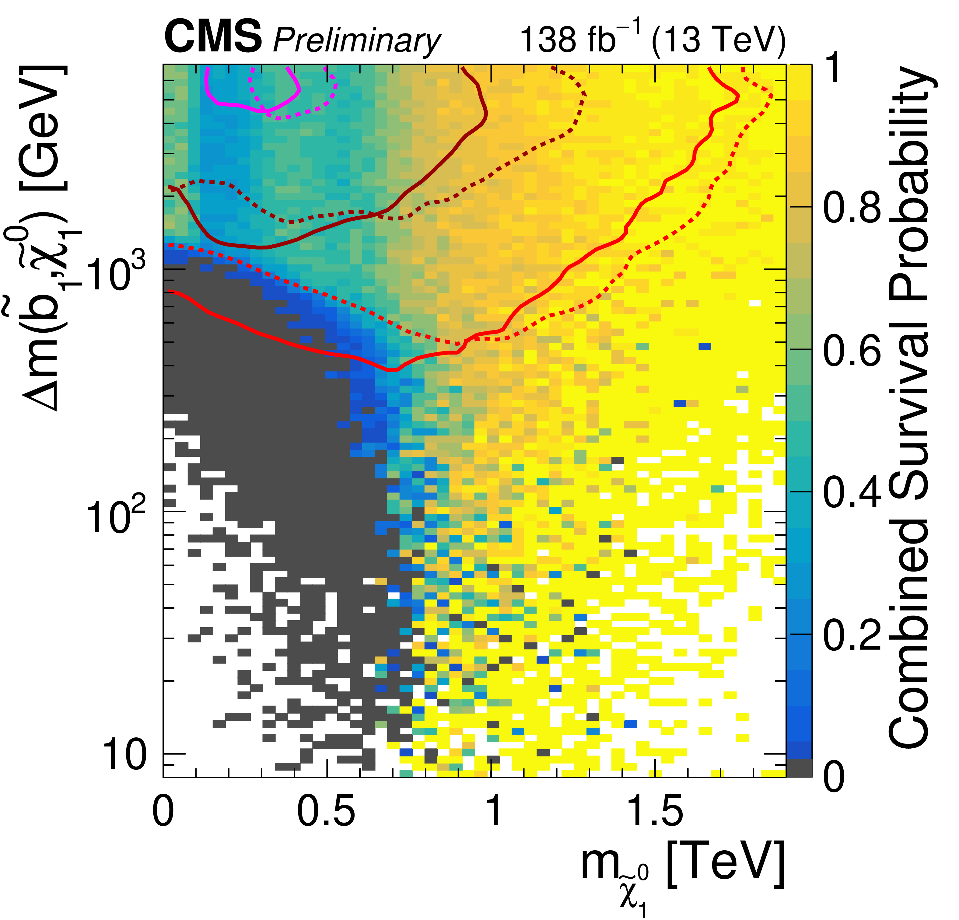
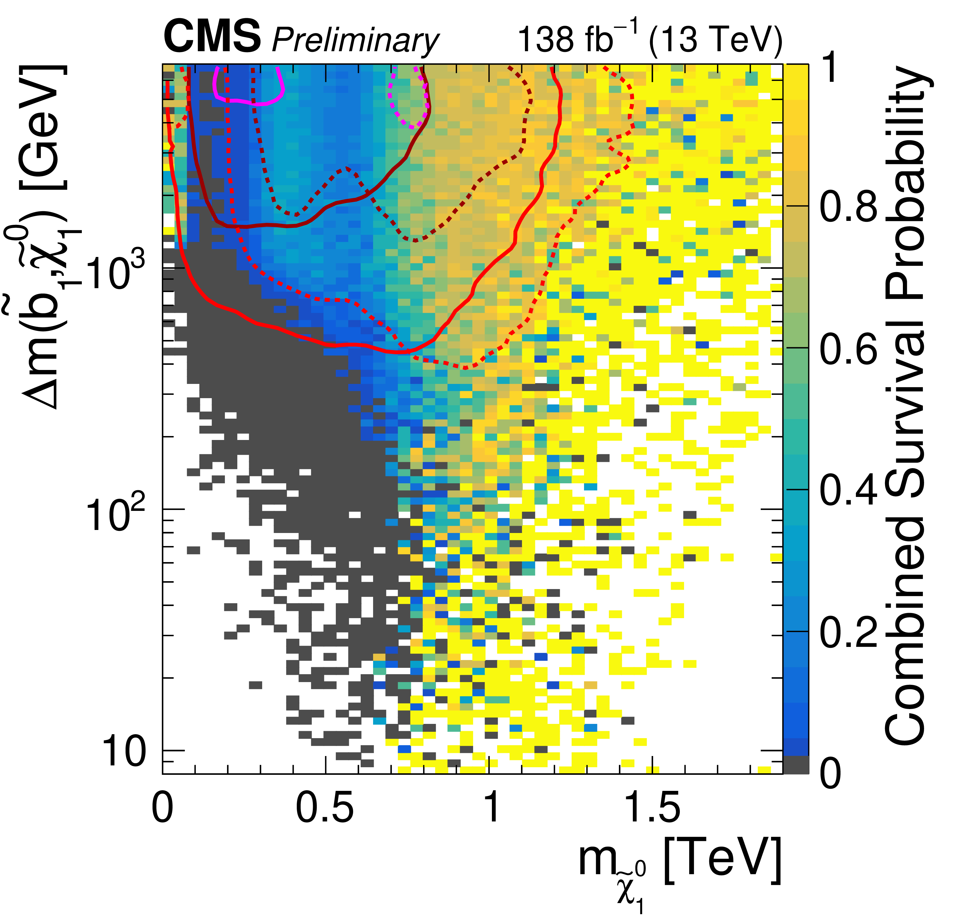
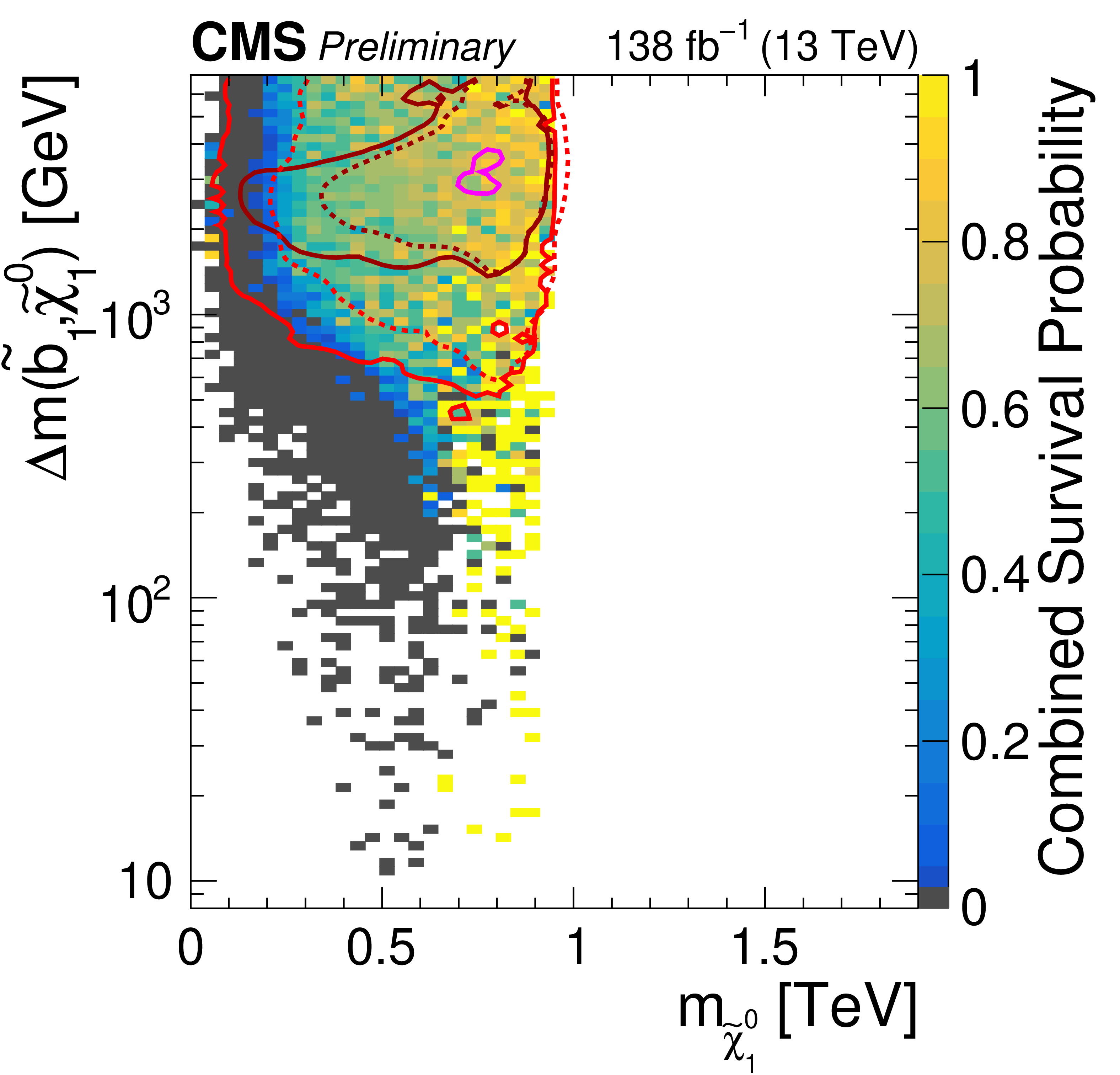
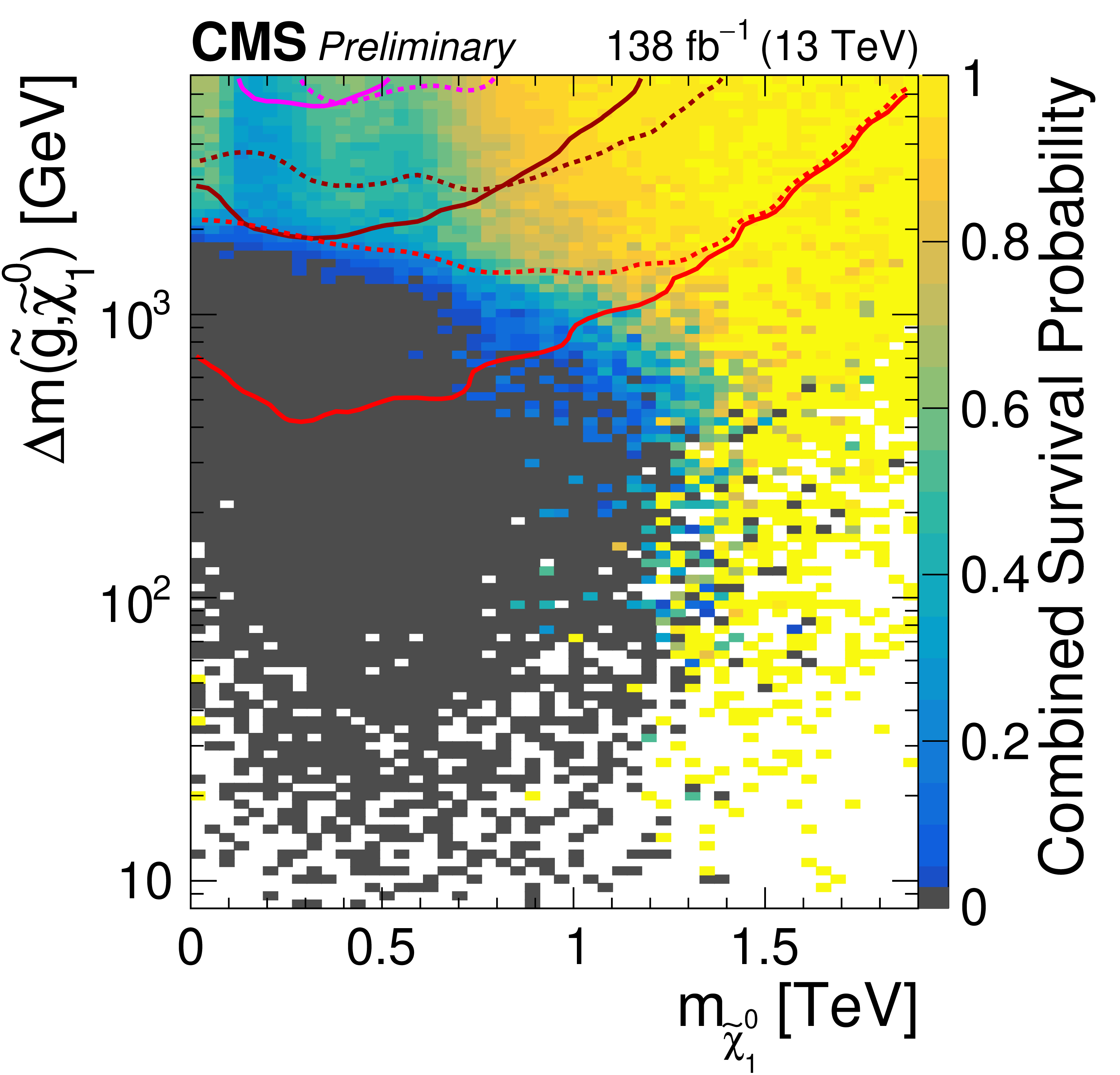
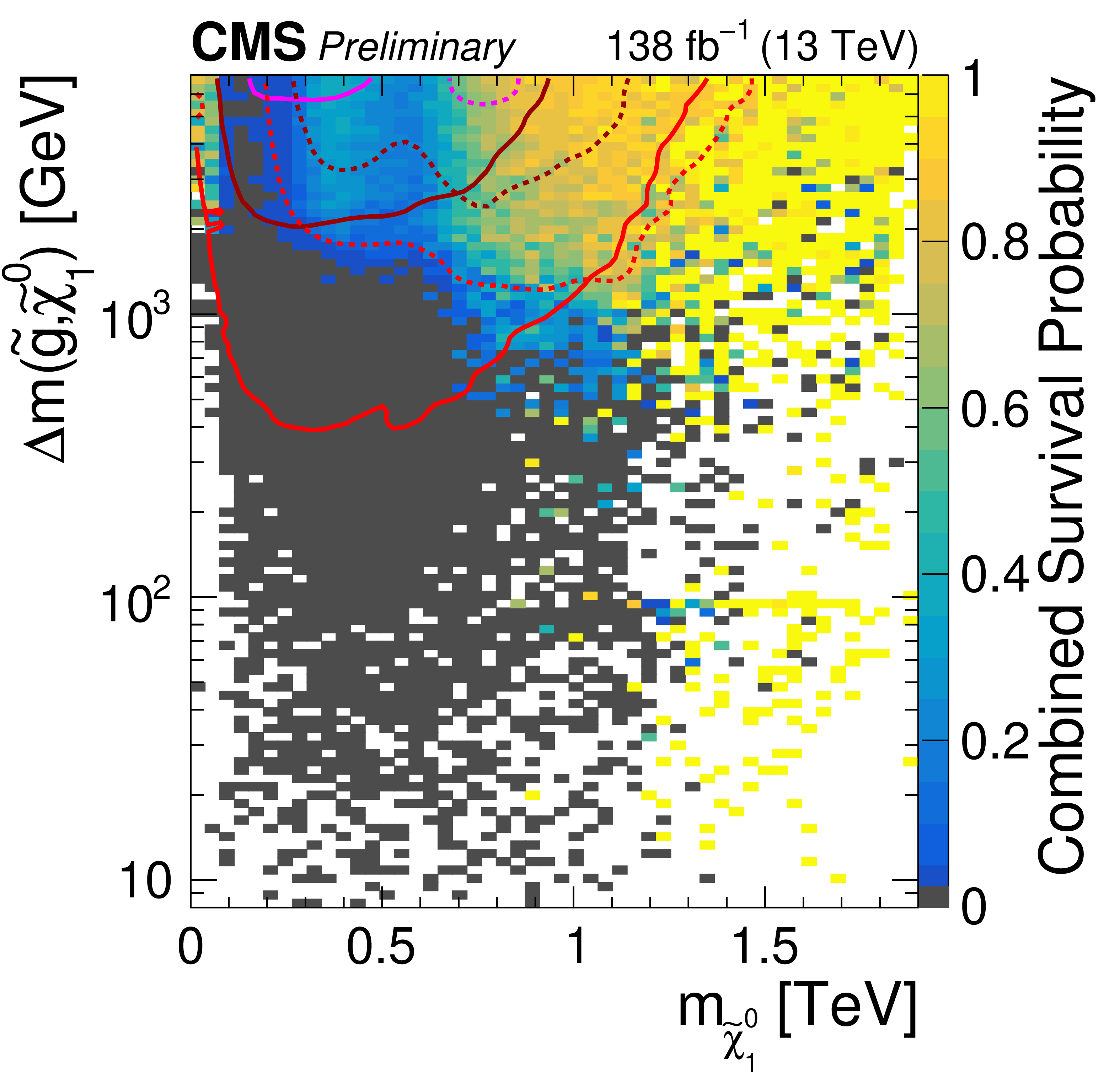
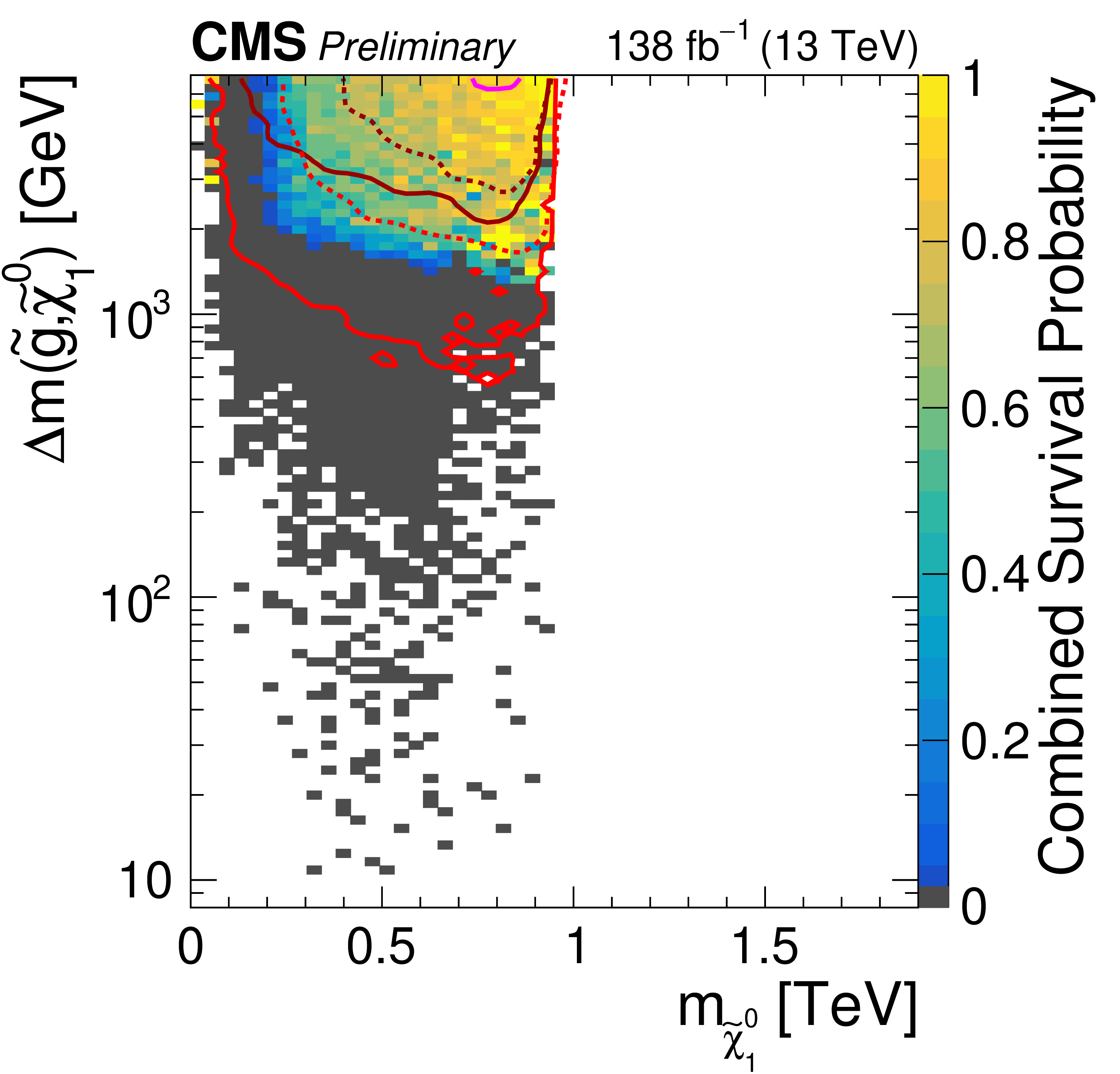
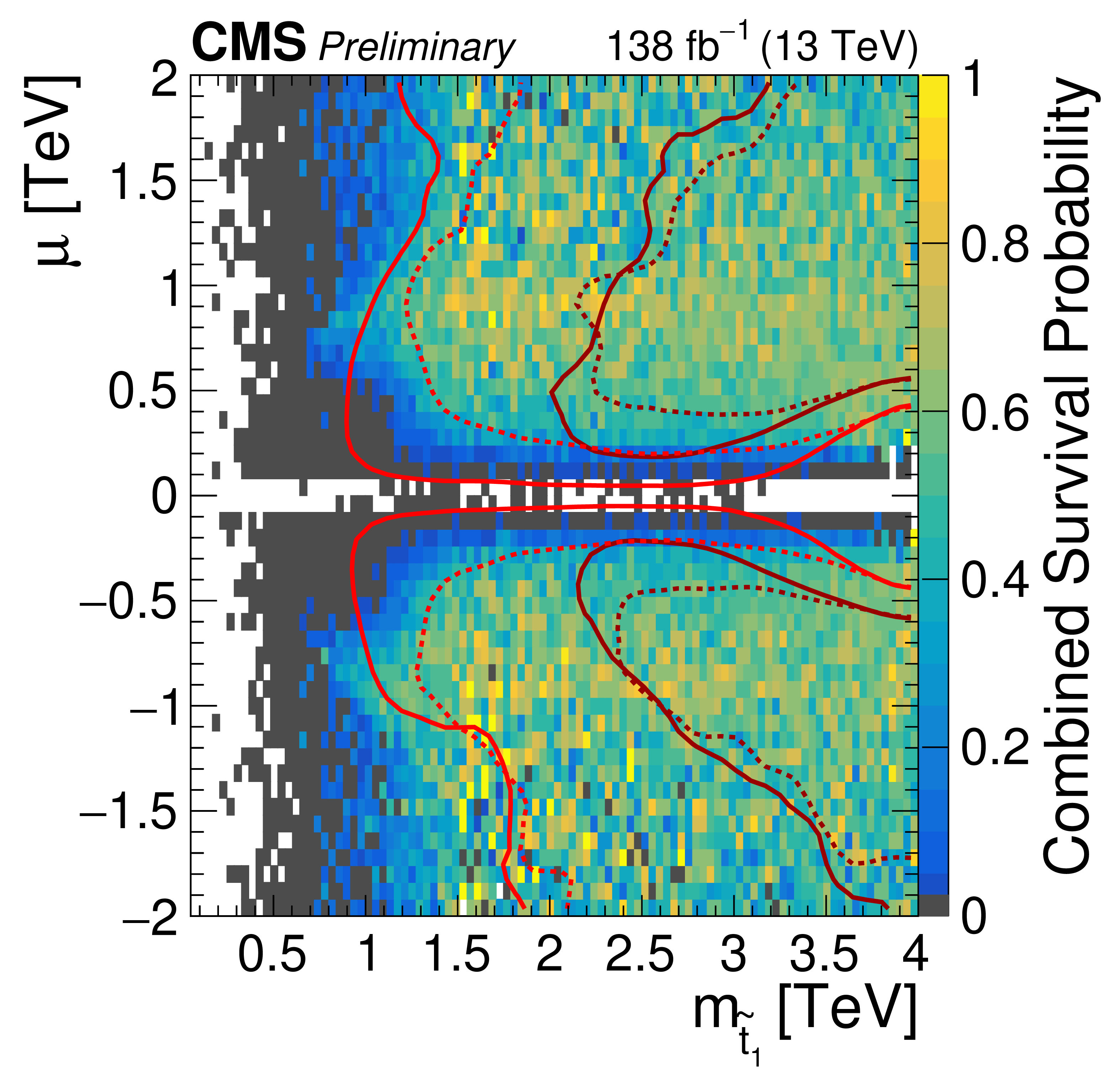
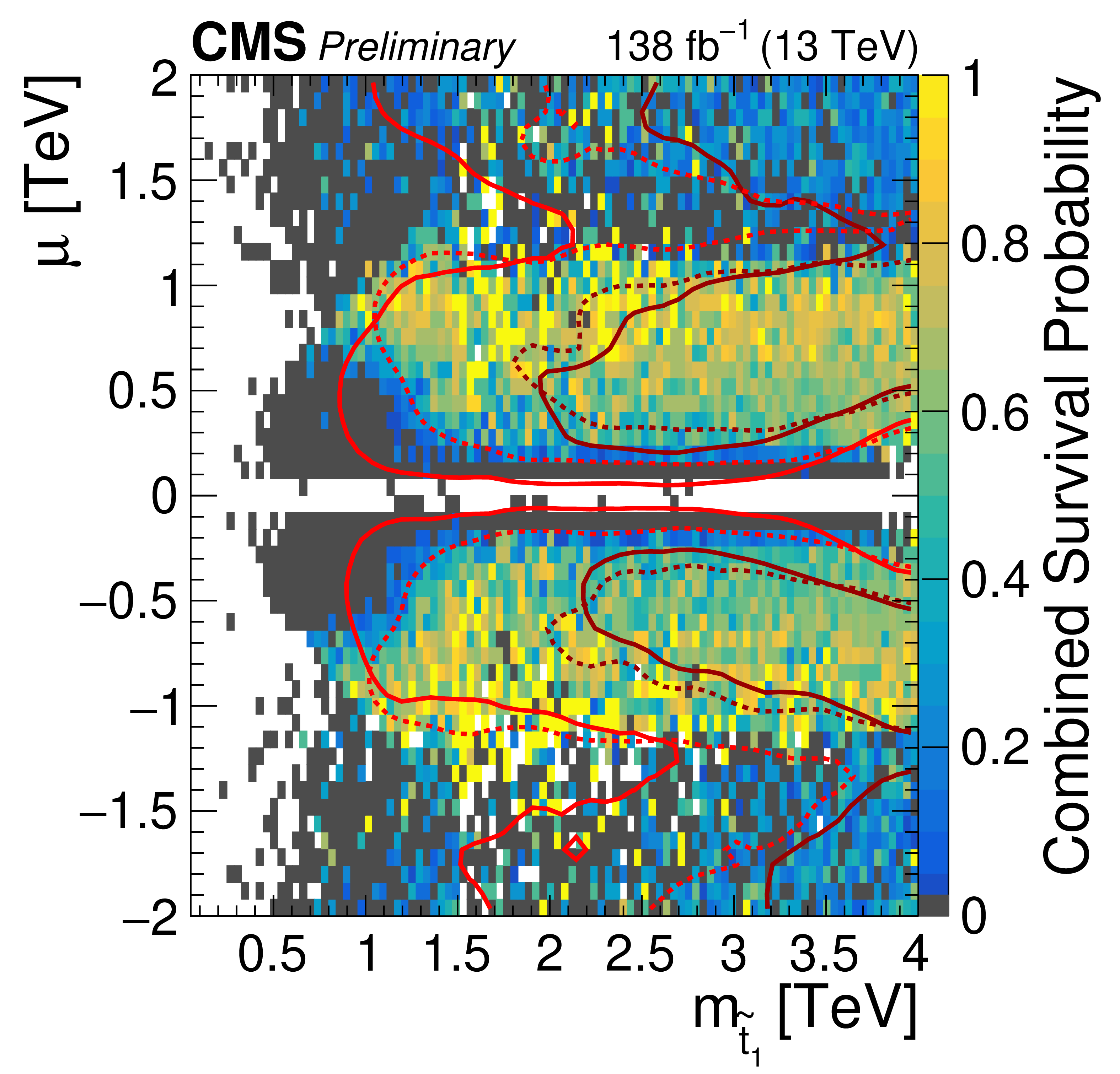
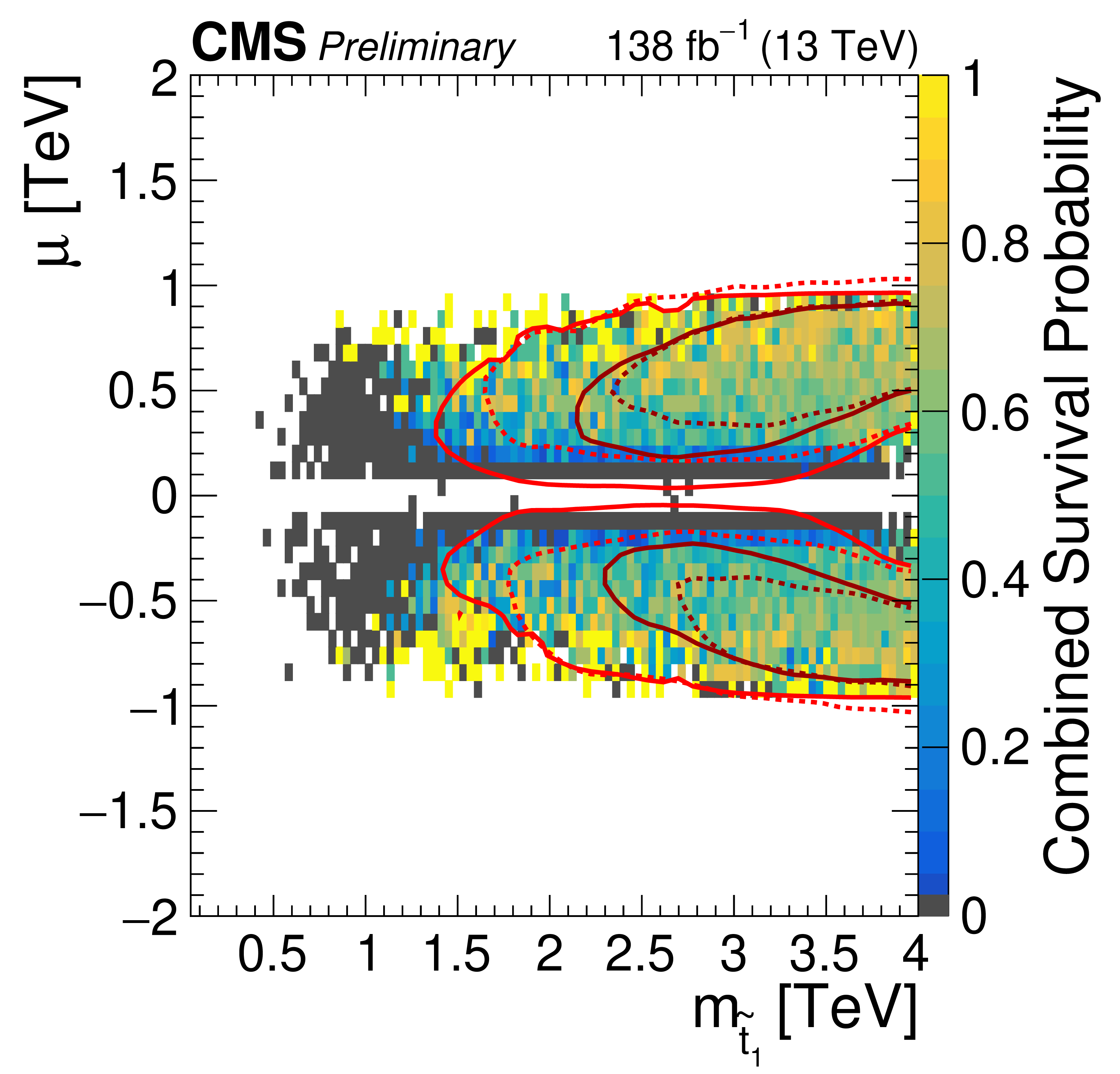
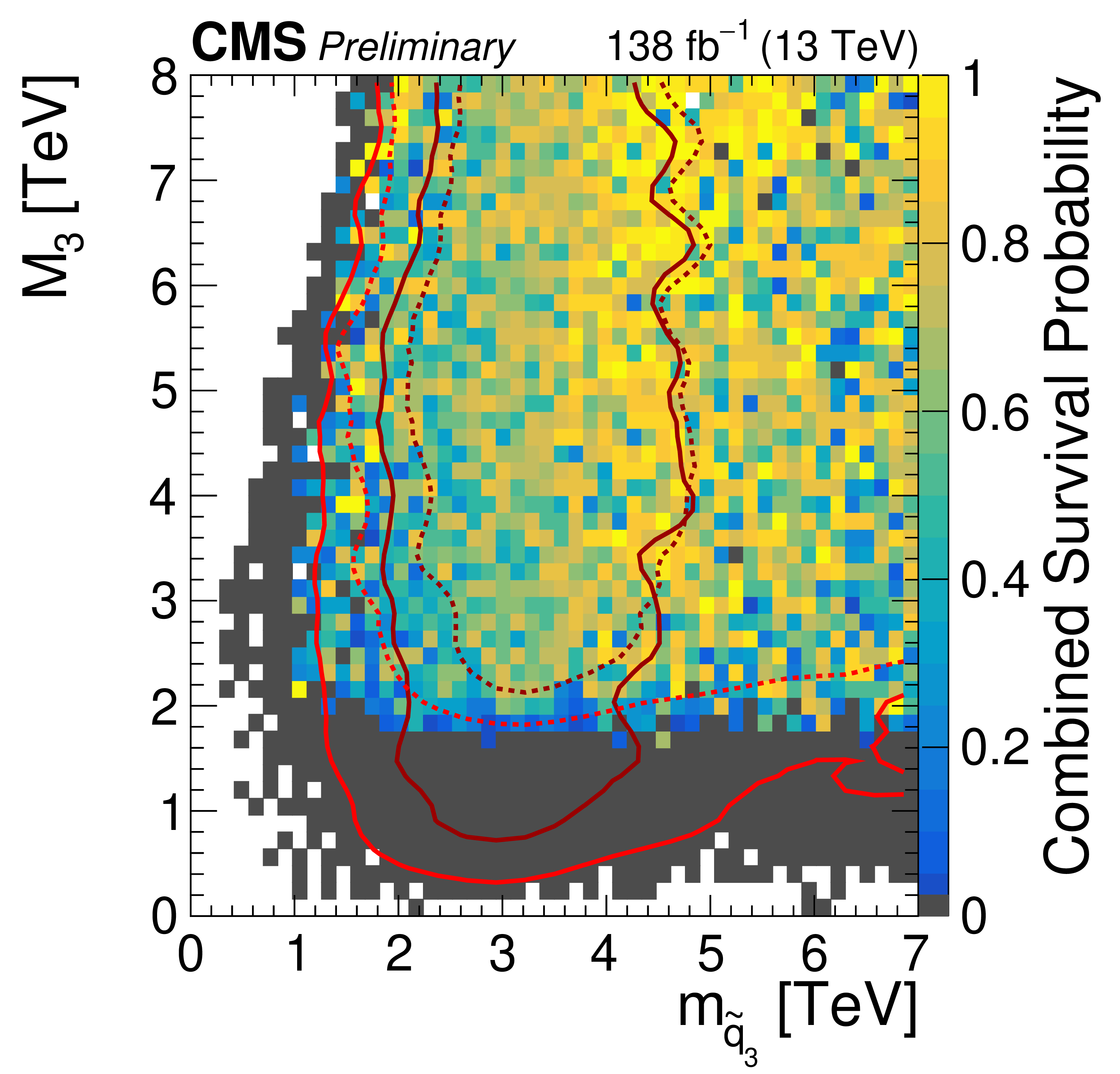
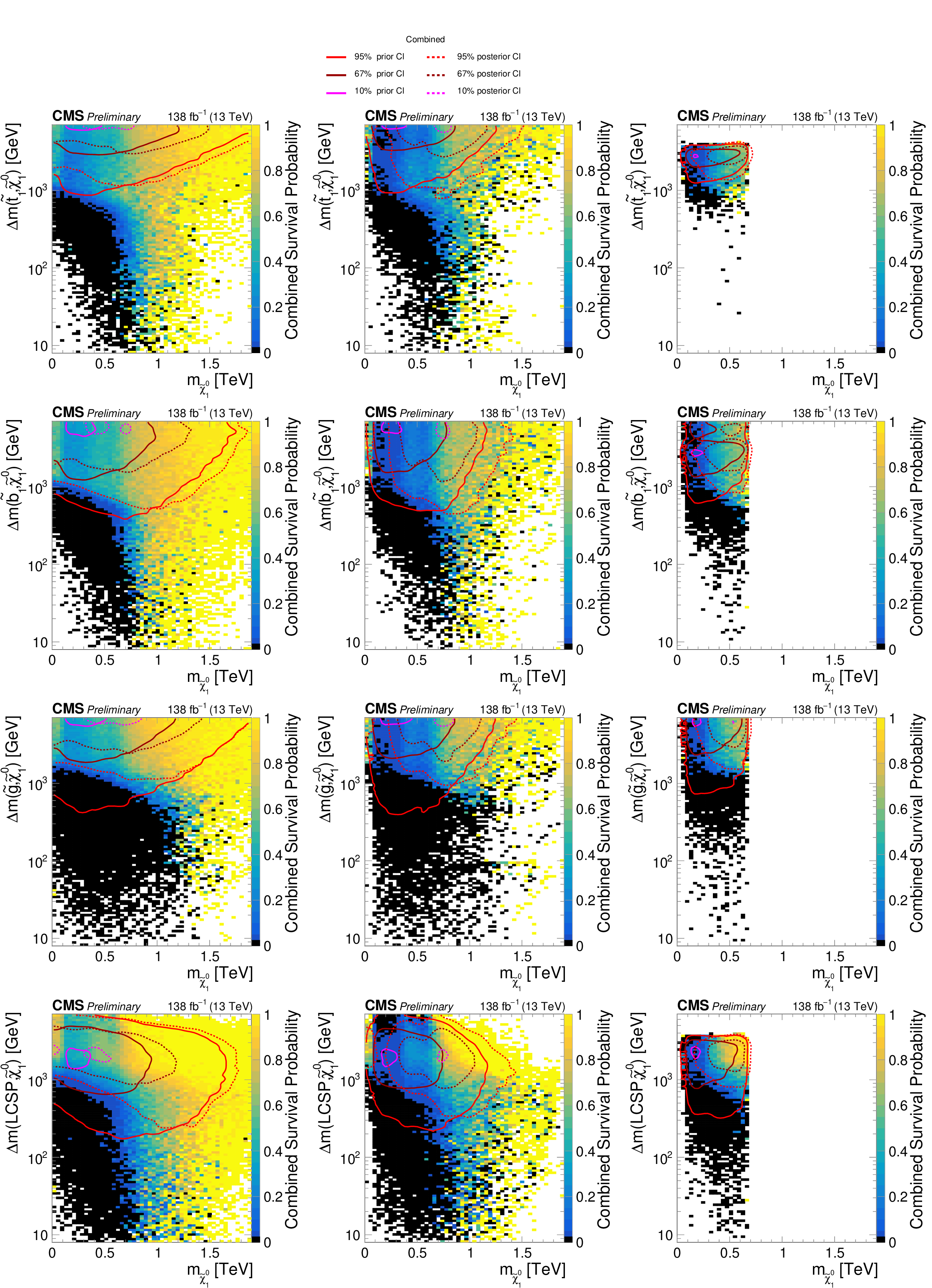
Figure 5:
Survival probability based on the full scan (left), based on the subset of the scan respecting DM constraints (center), and based on the natural DM subset (right), as a function of LSP mass and mass differences between the LSP and the lighter top and bottom squark, gluino, and LCSP masses. Black bins indicate where no pMSSM points survived the CMS analyses, and white indicate where no pMSSM points are present in the prior. Also shown are the prior (solid) and posterior (dashed) density contours corresponding to the respective constraints. |

png pdf |
Figure 5-a:
Survival probability based on the full scan (left), based on the subset of the scan respecting DM constraints (center), and based on the natural DM subset (right), as a function of LSP mass and mass differences between the LSP and the lighter top and bottom squark, gluino, and LCSP masses. Black bins indicate where no pMSSM points survived the CMS analyses, and white indicate where no pMSSM points are present in the prior. Also shown are the prior (solid) and posterior (dashed) density contours corresponding to the respective constraints. |
png pdf |
Figure 5-b:
Survival probability based on the full scan (left), based on the subset of the scan respecting DM constraints (center), and based on the natural DM subset (right), as a function of LSP mass and mass differences between the LSP and the lighter top and bottom squark, gluino, and LCSP masses. Black bins indicate where no pMSSM points survived the CMS analyses, and white indicate where no pMSSM points are present in the prior. Also shown are the prior (solid) and posterior (dashed) density contours corresponding to the respective constraints. |
png pdf |
Figure 5-c:
Survival probability based on the full scan (left), based on the subset of the scan respecting DM constraints (center), and based on the natural DM subset (right), as a function of LSP mass and mass differences between the LSP and the lighter top and bottom squark, gluino, and LCSP masses. Black bins indicate where no pMSSM points survived the CMS analyses, and white indicate where no pMSSM points are present in the prior. Also shown are the prior (solid) and posterior (dashed) density contours corresponding to the respective constraints. |
png pdf |
Figure 5-d:
Survival probability based on the full scan (left), based on the subset of the scan respecting DM constraints (center), and based on the natural DM subset (right), as a function of LSP mass and mass differences between the LSP and the lighter top and bottom squark, gluino, and LCSP masses. Black bins indicate where no pMSSM points survived the CMS analyses, and white indicate where no pMSSM points are present in the prior. Also shown are the prior (solid) and posterior (dashed) density contours corresponding to the respective constraints. |
png pdf |
Figure 5-e:
Survival probability based on the full scan (left), based on the subset of the scan respecting DM constraints (center), and based on the natural DM subset (right), as a function of LSP mass and mass differences between the LSP and the lighter top and bottom squark, gluino, and LCSP masses. Black bins indicate where no pMSSM points survived the CMS analyses, and white indicate where no pMSSM points are present in the prior. Also shown are the prior (solid) and posterior (dashed) density contours corresponding to the respective constraints. |
png pdf |
Figure 5-f:
Survival probability based on the full scan (left), based on the subset of the scan respecting DM constraints (center), and based on the natural DM subset (right), as a function of LSP mass and mass differences between the LSP and the lighter top and bottom squark, gluino, and LCSP masses. Black bins indicate where no pMSSM points survived the CMS analyses, and white indicate where no pMSSM points are present in the prior. Also shown are the prior (solid) and posterior (dashed) density contours corresponding to the respective constraints. |
png pdf |
Figure 5-g:
Survival probability based on the full scan (left), based on the subset of the scan respecting DM constraints (center), and based on the natural DM subset (right), as a function of LSP mass and mass differences between the LSP and the lighter top and bottom squark, gluino, and LCSP masses. Black bins indicate where no pMSSM points survived the CMS analyses, and white indicate where no pMSSM points are present in the prior. Also shown are the prior (solid) and posterior (dashed) density contours corresponding to the respective constraints. |
png pdf |
Figure 5-h:
Survival probability based on the full scan (left), based on the subset of the scan respecting DM constraints (center), and based on the natural DM subset (right), as a function of LSP mass and mass differences between the LSP and the lighter top and bottom squark, gluino, and LCSP masses. Black bins indicate where no pMSSM points survived the CMS analyses, and white indicate where no pMSSM points are present in the prior. Also shown are the prior (solid) and posterior (dashed) density contours corresponding to the respective constraints. |
png pdf |
Figure 5-i:
Survival probability based on the full scan (left), based on the subset of the scan respecting DM constraints (center), and based on the natural DM subset (right), as a function of LSP mass and mass differences between the LSP and the lighter top and bottom squark, gluino, and LCSP masses. Black bins indicate where no pMSSM points survived the CMS analyses, and white indicate where no pMSSM points are present in the prior. Also shown are the prior (solid) and posterior (dashed) density contours corresponding to the respective constraints. |
png pdf |
Figure 5-j:
Survival probability based on the full scan (left), based on the subset of the scan respecting DM constraints (center), and based on the natural DM subset (right), as a function of LSP mass and mass differences between the LSP and the lighter top and bottom squark, gluino, and LCSP masses. Black bins indicate where no pMSSM points survived the CMS analyses, and white indicate where no pMSSM points are present in the prior. Also shown are the prior (solid) and posterior (dashed) density contours corresponding to the respective constraints. |

png pdf |
Figure 5-k:
Survival probability based on the full scan (left), based on the subset of the scan respecting DM constraints (center), and based on the natural DM subset (right), as a function of LSP mass and mass differences between the LSP and the lighter top and bottom squark, gluino, and LCSP masses. Black bins indicate where no pMSSM points survived the CMS analyses, and white indicate where no pMSSM points are present in the prior. Also shown are the prior (solid) and posterior (dashed) density contours corresponding to the respective constraints. |
png pdf |
Figure 5-l:
Survival probability based on the full scan (left), based on the subset of the scan respecting DM constraints (center), and based on the natural DM subset (right), as a function of LSP mass and mass differences between the LSP and the lighter top and bottom squark, gluino, and LCSP masses. Black bins indicate where no pMSSM points survived the CMS analyses, and white indicate where no pMSSM points are present in the prior. Also shown are the prior (solid) and posterior (dashed) density contours corresponding to the respective constraints. |
png pdf |
Figure 5-m:
Survival probability based on the full scan (left), based on the subset of the scan respecting DM constraints (center), and based on the natural DM subset (right), as a function of LSP mass and mass differences between the LSP and the lighter top and bottom squark, gluino, and LCSP masses. Black bins indicate where no pMSSM points survived the CMS analyses, and white indicate where no pMSSM points are present in the prior. Also shown are the prior (solid) and posterior (dashed) density contours corresponding to the respective constraints. |
png pdf |
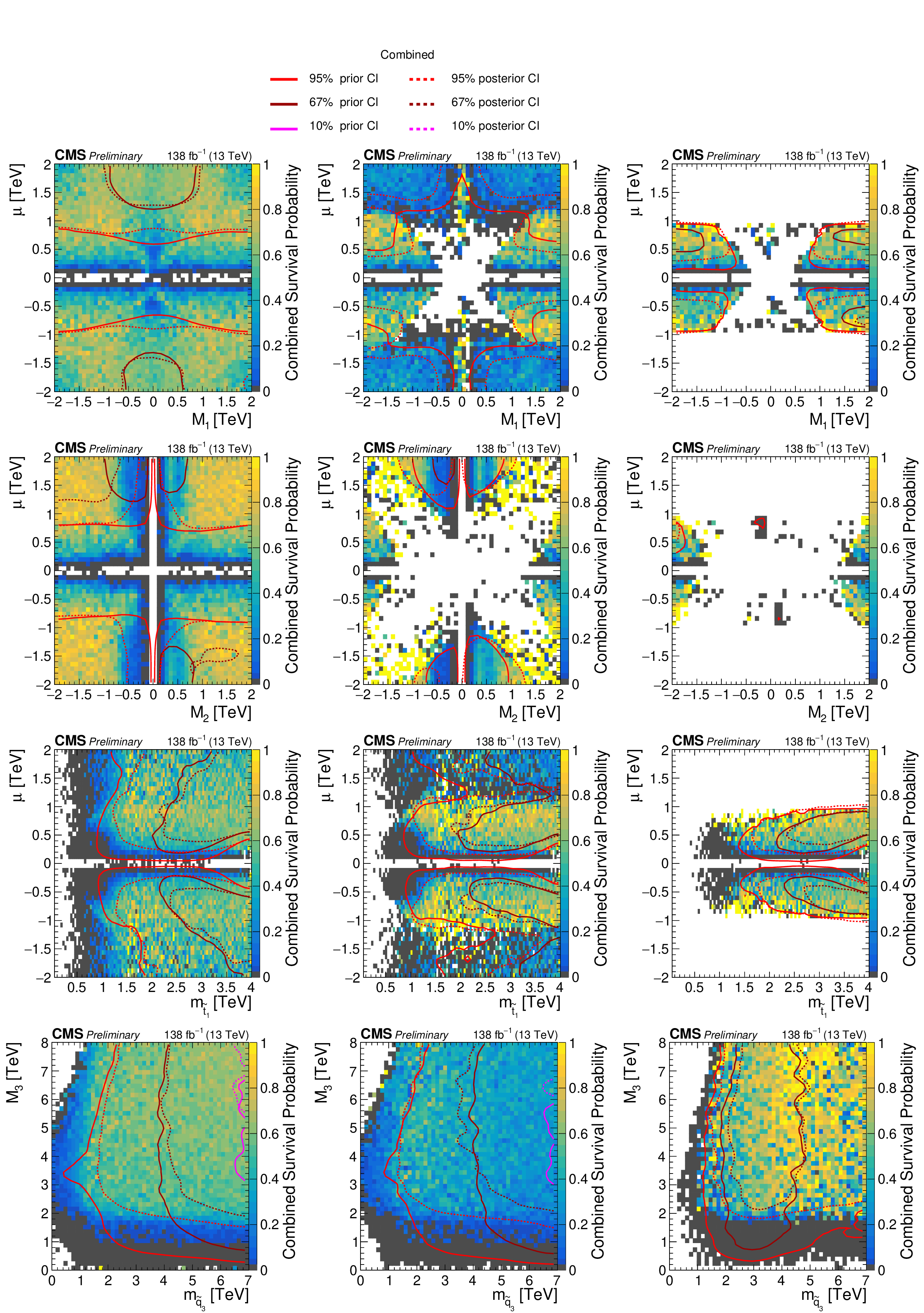
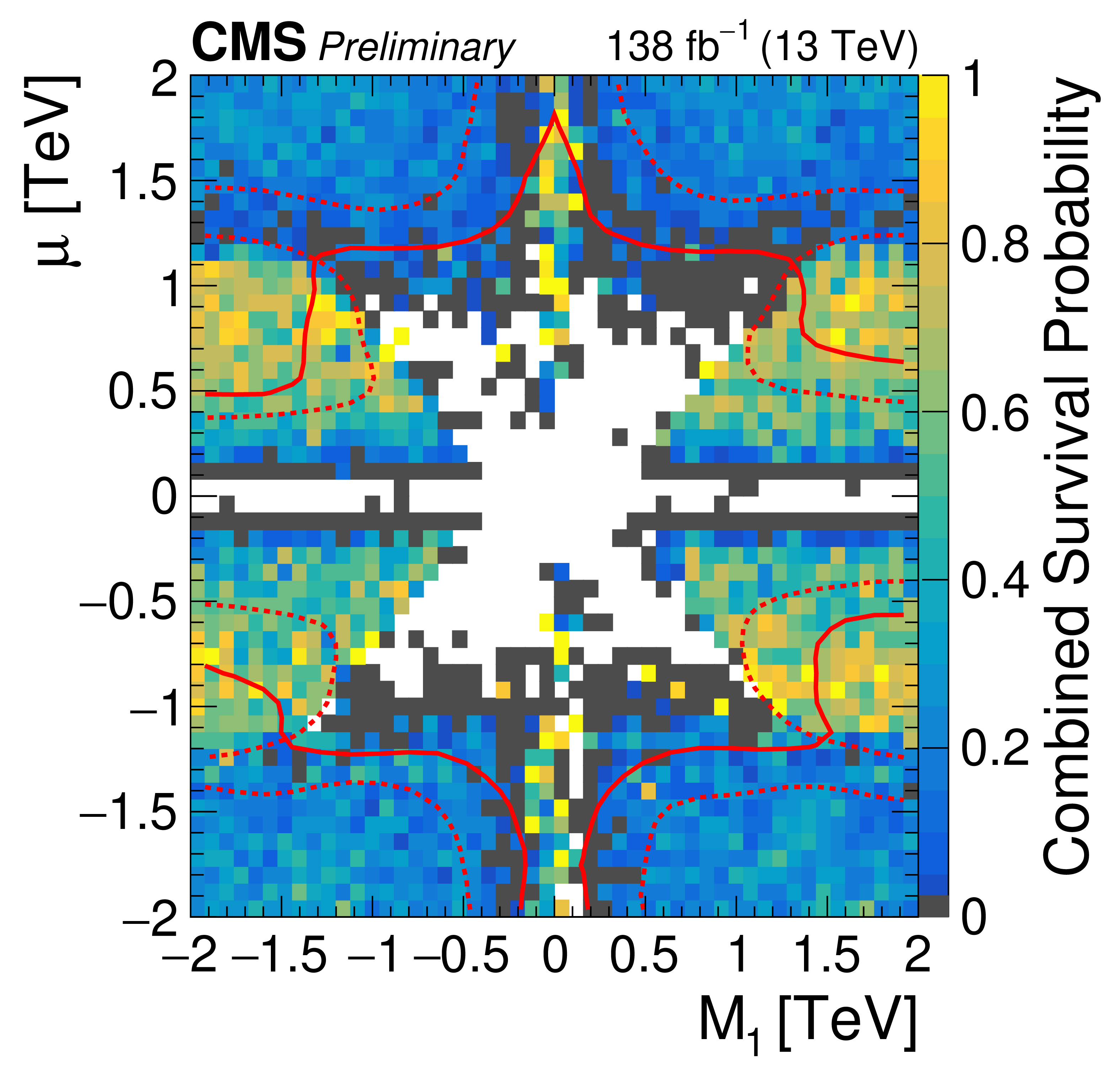
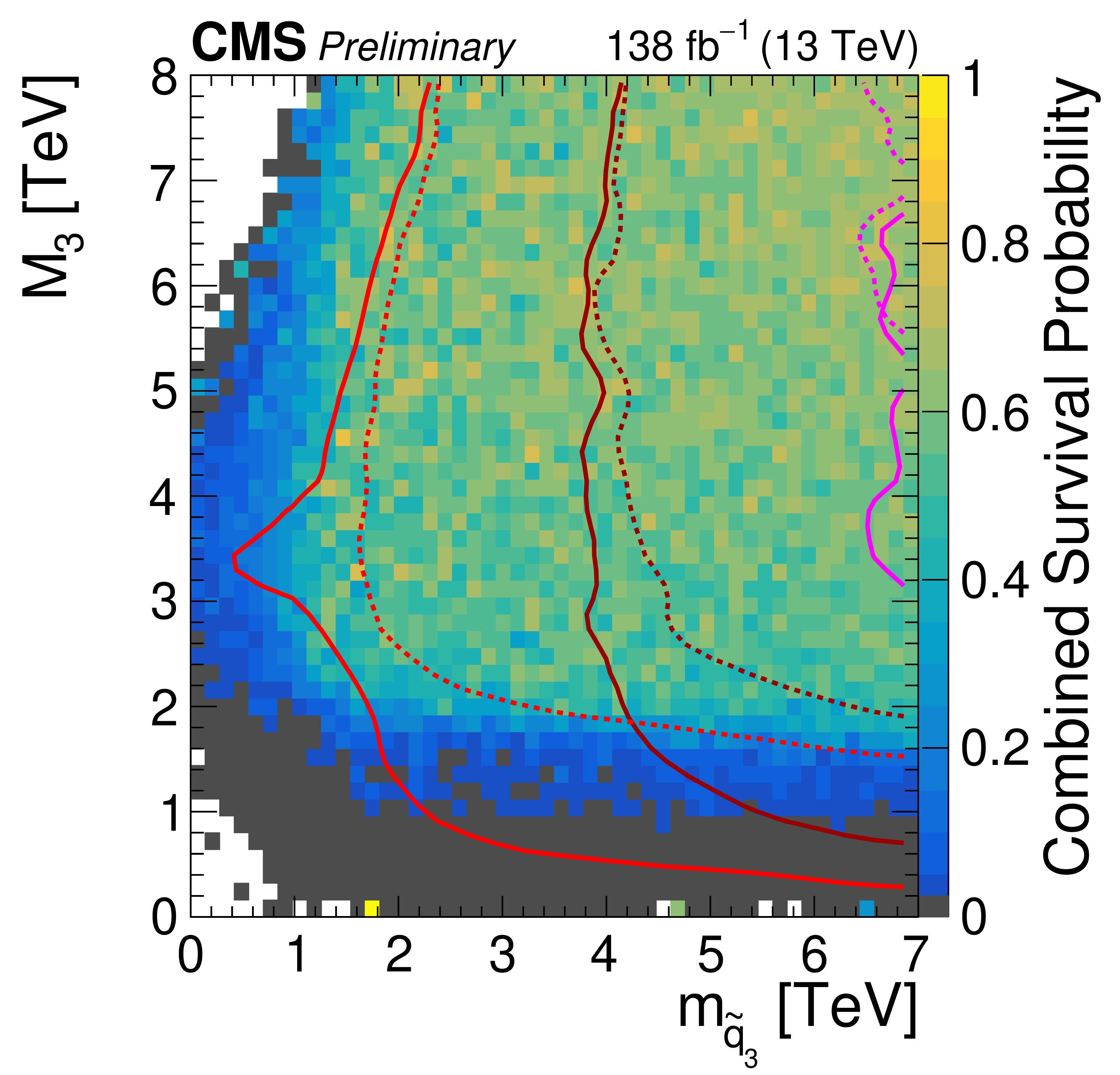
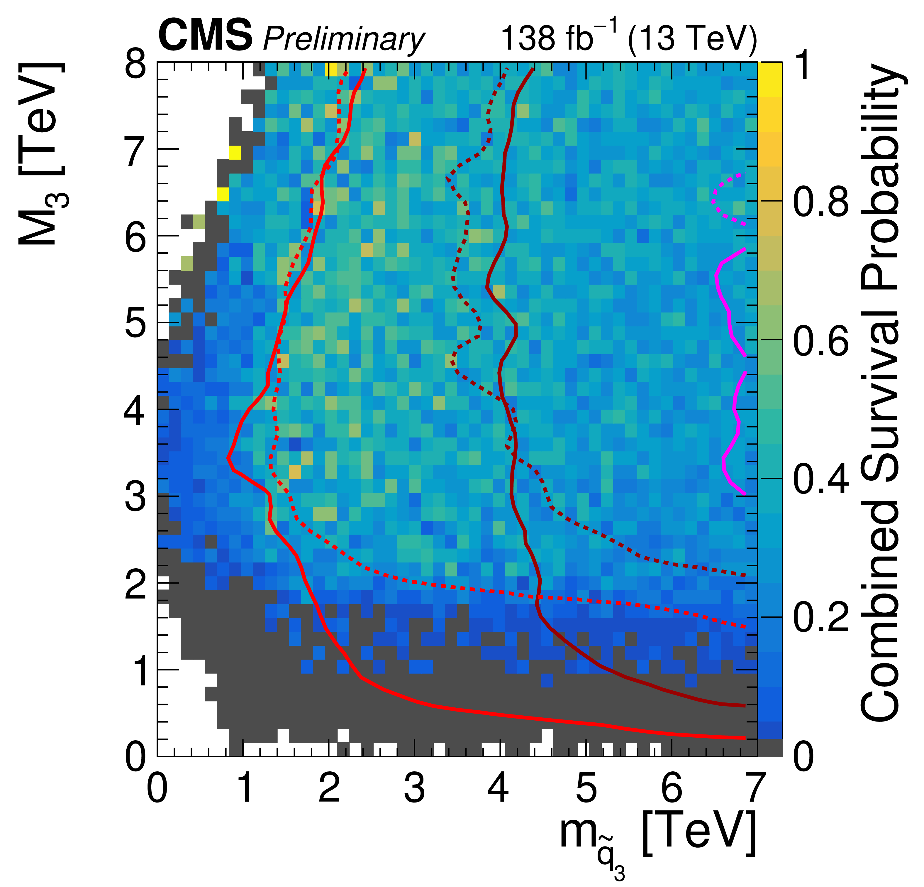
Figure 6:
Survival probability based on the full scan (left), based on the subset of the scan respecting DM constraints (center), and based on the natural DM subset (right), as a function of LSP mass and mass differences between the LSP and the lighter top and bottom squark, gluino, and LCSP masses. Black indicates bins where no pMSSM points survived the CMS analyses, and white indicates bins where no pMSSM points are present in the prior. Also shown are the prior (solid) and posterior (dashed) density contours corresponding to the respective constraints. |

png pdf |
Figure 6-a:
Survival probability based on the full scan (left), based on the subset of the scan respecting DM constraints (center), and based on the natural DM subset (right), as a function of LSP mass and mass differences between the LSP and the lighter top and bottom squark, gluino, and LCSP masses. Black indicates bins where no pMSSM points survived the CMS analyses, and white indicates bins where no pMSSM points are present in the prior. Also shown are the prior (solid) and posterior (dashed) density contours corresponding to the respective constraints. |

png pdf |
Figure 6-b:
Survival probability based on the full scan (left), based on the subset of the scan respecting DM constraints (center), and based on the natural DM subset (right), as a function of LSP mass and mass differences between the LSP and the lighter top and bottom squark, gluino, and LCSP masses. Black indicates bins where no pMSSM points survived the CMS analyses, and white indicates bins where no pMSSM points are present in the prior. Also shown are the prior (solid) and posterior (dashed) density contours corresponding to the respective constraints. |
png pdf |
Figure 6-c:
Survival probability based on the full scan (left), based on the subset of the scan respecting DM constraints (center), and based on the natural DM subset (right), as a function of LSP mass and mass differences between the LSP and the lighter top and bottom squark, gluino, and LCSP masses. Black indicates bins where no pMSSM points survived the CMS analyses, and white indicates bins where no pMSSM points are present in the prior. Also shown are the prior (solid) and posterior (dashed) density contours corresponding to the respective constraints. |
png pdf |
Figure 6-d:
Survival probability based on the full scan (left), based on the subset of the scan respecting DM constraints (center), and based on the natural DM subset (right), as a function of LSP mass and mass differences between the LSP and the lighter top and bottom squark, gluino, and LCSP masses. Black indicates bins where no pMSSM points survived the CMS analyses, and white indicates bins where no pMSSM points are present in the prior. Also shown are the prior (solid) and posterior (dashed) density contours corresponding to the respective constraints. |

png pdf |
Figure 6-e:
Survival probability based on the full scan (left), based on the subset of the scan respecting DM constraints (center), and based on the natural DM subset (right), as a function of LSP mass and mass differences between the LSP and the lighter top and bottom squark, gluino, and LCSP masses. Black indicates bins where no pMSSM points survived the CMS analyses, and white indicates bins where no pMSSM points are present in the prior. Also shown are the prior (solid) and posterior (dashed) density contours corresponding to the respective constraints. |
png pdf |
Figure 6-f:
Survival probability based on the full scan (left), based on the subset of the scan respecting DM constraints (center), and based on the natural DM subset (right), as a function of LSP mass and mass differences between the LSP and the lighter top and bottom squark, gluino, and LCSP masses. Black indicates bins where no pMSSM points survived the CMS analyses, and white indicates bins where no pMSSM points are present in the prior. Also shown are the prior (solid) and posterior (dashed) density contours corresponding to the respective constraints. |
png pdf |
Figure 6-g:
Survival probability based on the full scan (left), based on the subset of the scan respecting DM constraints (center), and based on the natural DM subset (right), as a function of LSP mass and mass differences between the LSP and the lighter top and bottom squark, gluino, and LCSP masses. Black indicates bins where no pMSSM points survived the CMS analyses, and white indicates bins where no pMSSM points are present in the prior. Also shown are the prior (solid) and posterior (dashed) density contours corresponding to the respective constraints. |
png pdf |
Figure 6-h:
Survival probability based on the full scan (left), based on the subset of the scan respecting DM constraints (center), and based on the natural DM subset (right), as a function of LSP mass and mass differences between the LSP and the lighter top and bottom squark, gluino, and LCSP masses. Black indicates bins where no pMSSM points survived the CMS analyses, and white indicates bins where no pMSSM points are present in the prior. Also shown are the prior (solid) and posterior (dashed) density contours corresponding to the respective constraints. |
png pdf |
Figure 6-i:
Survival probability based on the full scan (left), based on the subset of the scan respecting DM constraints (center), and based on the natural DM subset (right), as a function of LSP mass and mass differences between the LSP and the lighter top and bottom squark, gluino, and LCSP masses. Black indicates bins where no pMSSM points survived the CMS analyses, and white indicates bins where no pMSSM points are present in the prior. Also shown are the prior (solid) and posterior (dashed) density contours corresponding to the respective constraints. |
png pdf |
Figure 6-j:
Survival probability based on the full scan (left), based on the subset of the scan respecting DM constraints (center), and based on the natural DM subset (right), as a function of LSP mass and mass differences between the LSP and the lighter top and bottom squark, gluino, and LCSP masses. Black indicates bins where no pMSSM points survived the CMS analyses, and white indicates bins where no pMSSM points are present in the prior. Also shown are the prior (solid) and posterior (dashed) density contours corresponding to the respective constraints. |
png pdf |
Figure 6-k:
Survival probability based on the full scan (left), based on the subset of the scan respecting DM constraints (center), and based on the natural DM subset (right), as a function of LSP mass and mass differences between the LSP and the lighter top and bottom squark, gluino, and LCSP masses. Black indicates bins where no pMSSM points survived the CMS analyses, and white indicates bins where no pMSSM points are present in the prior. Also shown are the prior (solid) and posterior (dashed) density contours corresponding to the respective constraints. |
png pdf |
Figure 6-l:
Survival probability based on the full scan (left), based on the subset of the scan respecting DM constraints (center), and based on the natural DM subset (right), as a function of LSP mass and mass differences between the LSP and the lighter top and bottom squark, gluino, and LCSP masses. Black indicates bins where no pMSSM points survived the CMS analyses, and white indicates bins where no pMSSM points are present in the prior. Also shown are the prior (solid) and posterior (dashed) density contours corresponding to the respective constraints. |
png pdf |
Figure 6-m:
Survival probability based on the full scan (left), based on the subset of the scan respecting DM constraints (center), and based on the natural DM subset (right), as a function of LSP mass and mass differences between the LSP and the lighter top and bottom squark, gluino, and LCSP masses. Black indicates bins where no pMSSM points survived the CMS analyses, and white indicates bins where no pMSSM points are present in the prior. Also shown are the prior (solid) and posterior (dashed) density contours corresponding to the respective constraints. |
png pdf |
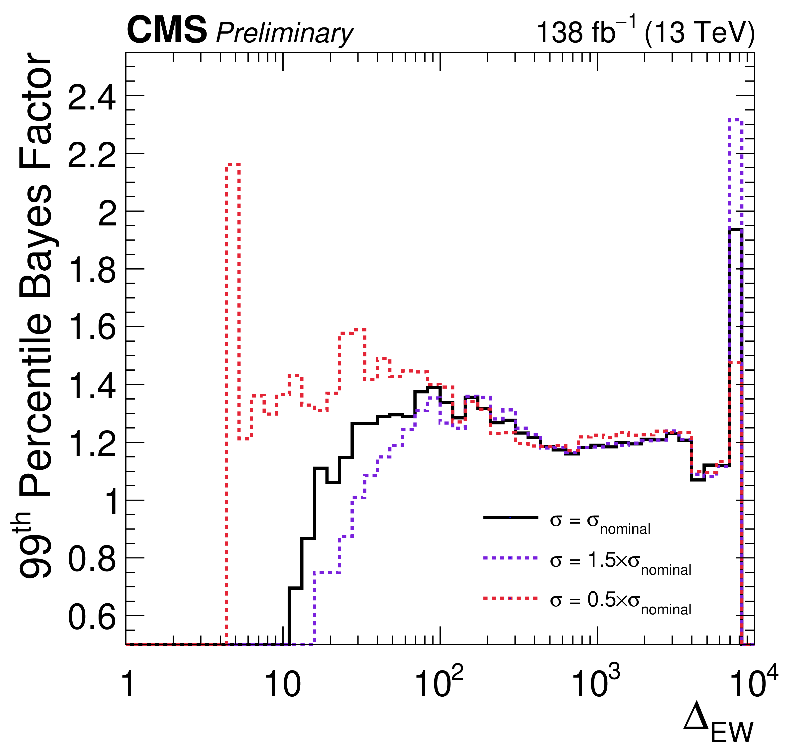
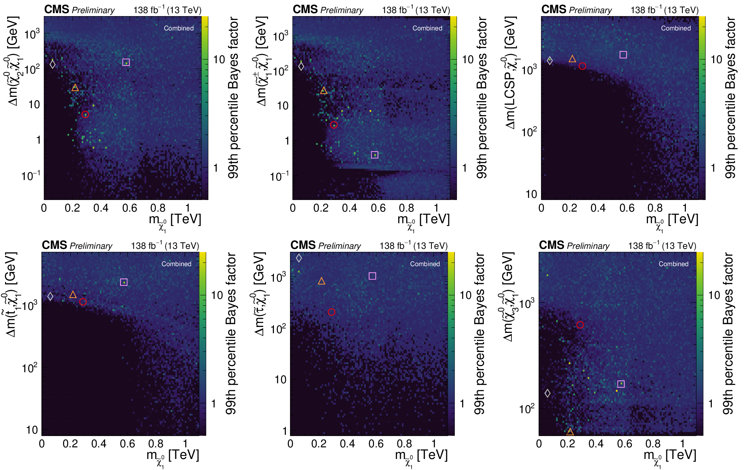
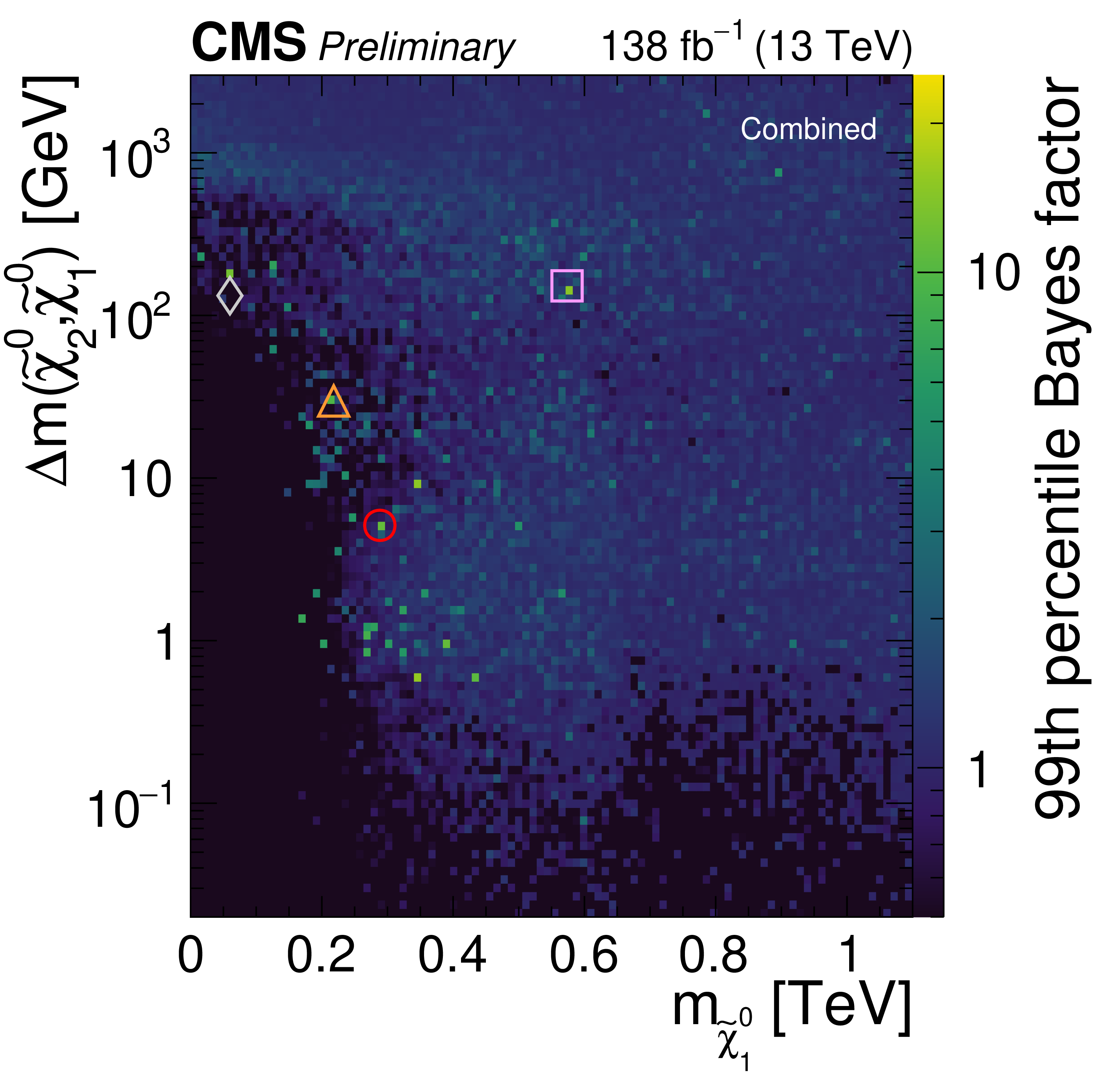
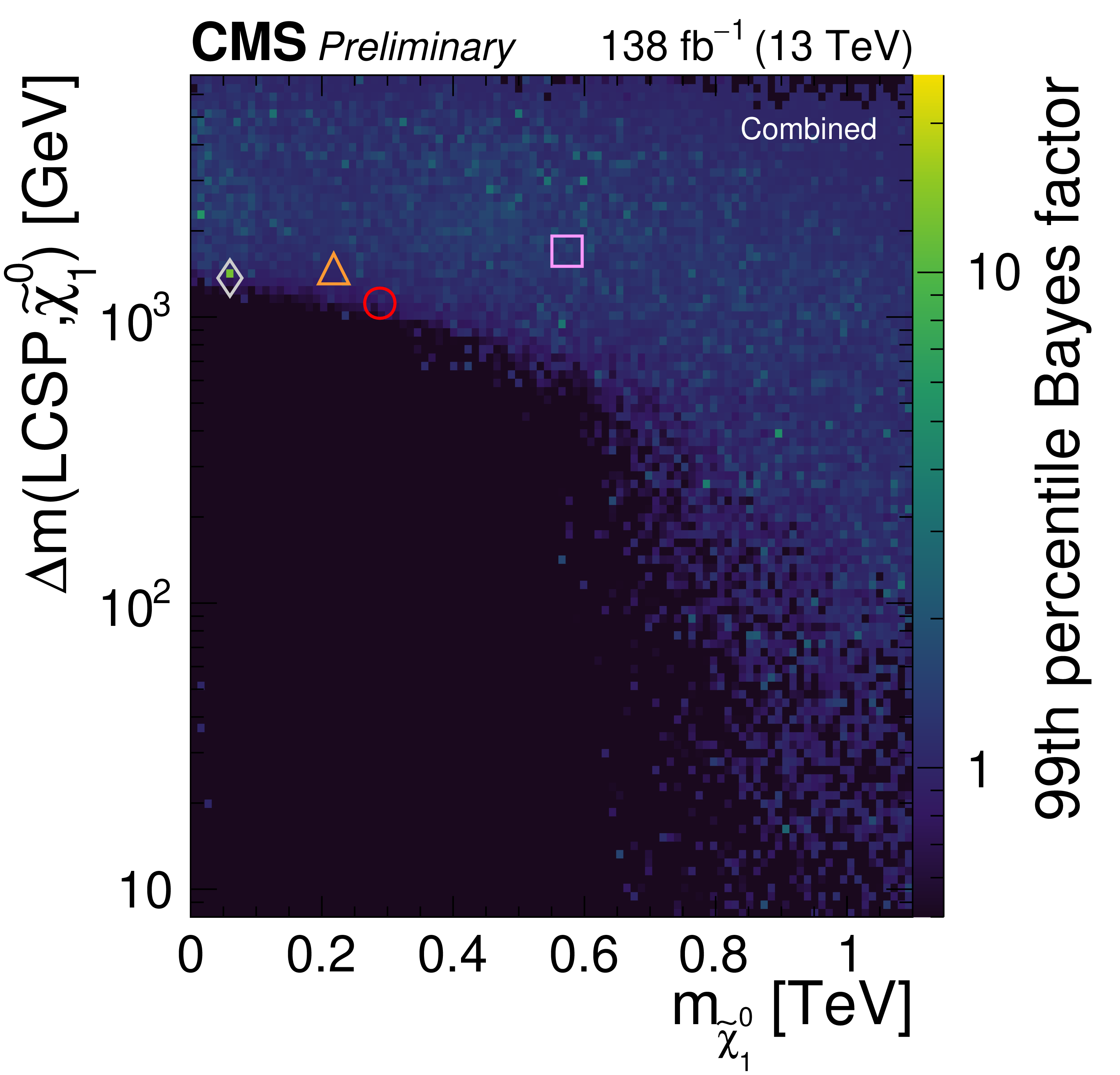
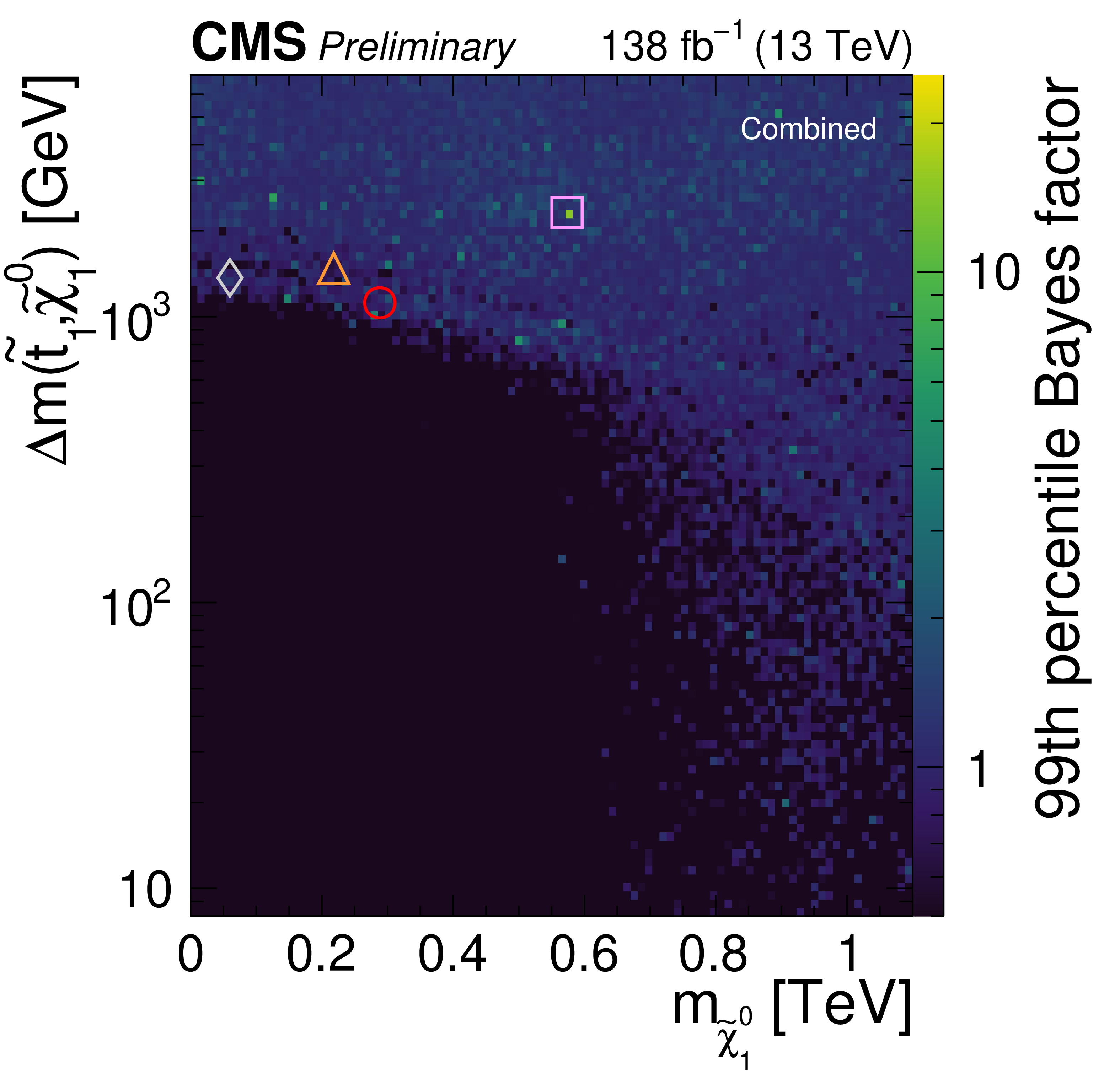
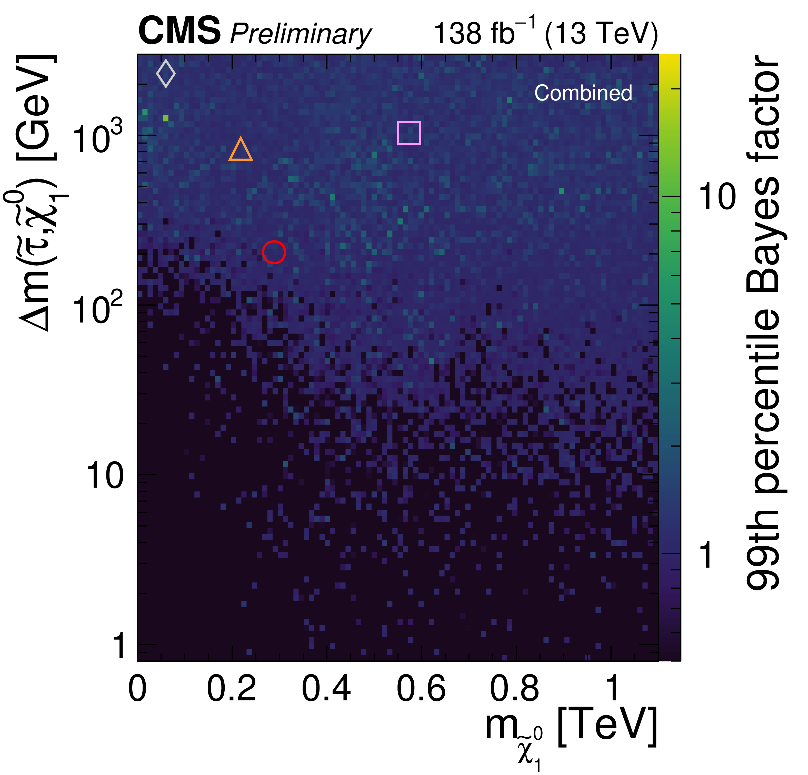
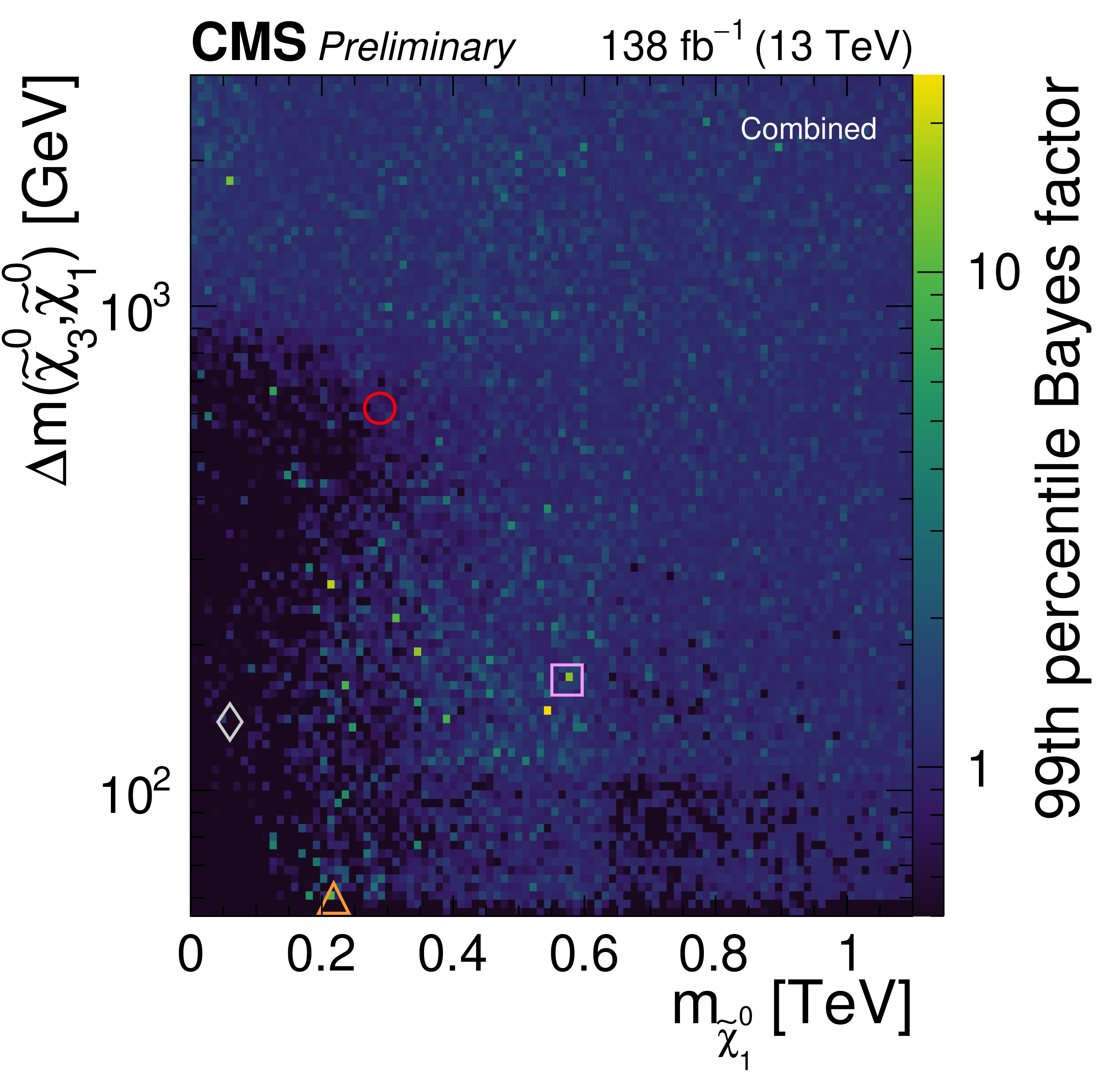
Figure 7:
99% upper percentiles on the BF in bins of various projections of superpartner mass differences and the LSP mass. Also shown as symbols are the projections of four high significance model points with (run number, iteration number): red circle (550, 52206), gray triangle (136, 33723), pink square (132, 73754), and orange triangle (449, 65877). |
png pdf |
Figure 7-a:
99% upper percentiles on the BF in bins of various projections of superpartner mass differences and the LSP mass. Also shown as symbols are the projections of four high significance model points with (run number, iteration number): red circle (550, 52206), gray triangle (136, 33723), pink square (132, 73754), and orange triangle (449, 65877). |

png pdf |
Figure 7-b:
99% upper percentiles on the BF in bins of various projections of superpartner mass differences and the LSP mass. Also shown as symbols are the projections of four high significance model points with (run number, iteration number): red circle (550, 52206), gray triangle (136, 33723), pink square (132, 73754), and orange triangle (449, 65877). |
png pdf |
Figure 7-c:
99% upper percentiles on the BF in bins of various projections of superpartner mass differences and the LSP mass. Also shown as symbols are the projections of four high significance model points with (run number, iteration number): red circle (550, 52206), gray triangle (136, 33723), pink square (132, 73754), and orange triangle (449, 65877). |
png pdf |
Figure 7-d:
99% upper percentiles on the BF in bins of various projections of superpartner mass differences and the LSP mass. Also shown as symbols are the projections of four high significance model points with (run number, iteration number): red circle (550, 52206), gray triangle (136, 33723), pink square (132, 73754), and orange triangle (449, 65877). |
png pdf |
Figure 7-e:
99% upper percentiles on the BF in bins of various projections of superpartner mass differences and the LSP mass. Also shown as symbols are the projections of four high significance model points with (run number, iteration number): red circle (550, 52206), gray triangle (136, 33723), pink square (132, 73754), and orange triangle (449, 65877). |
png pdf |
Figure 7-f:
99% upper percentiles on the BF in bins of various projections of superpartner mass differences and the LSP mass. Also shown as symbols are the projections of four high significance model points with (run number, iteration number): red circle (550, 52206), gray triangle (136, 33723), pink square (132, 73754), and orange triangle (449, 65877). |
png pdf |
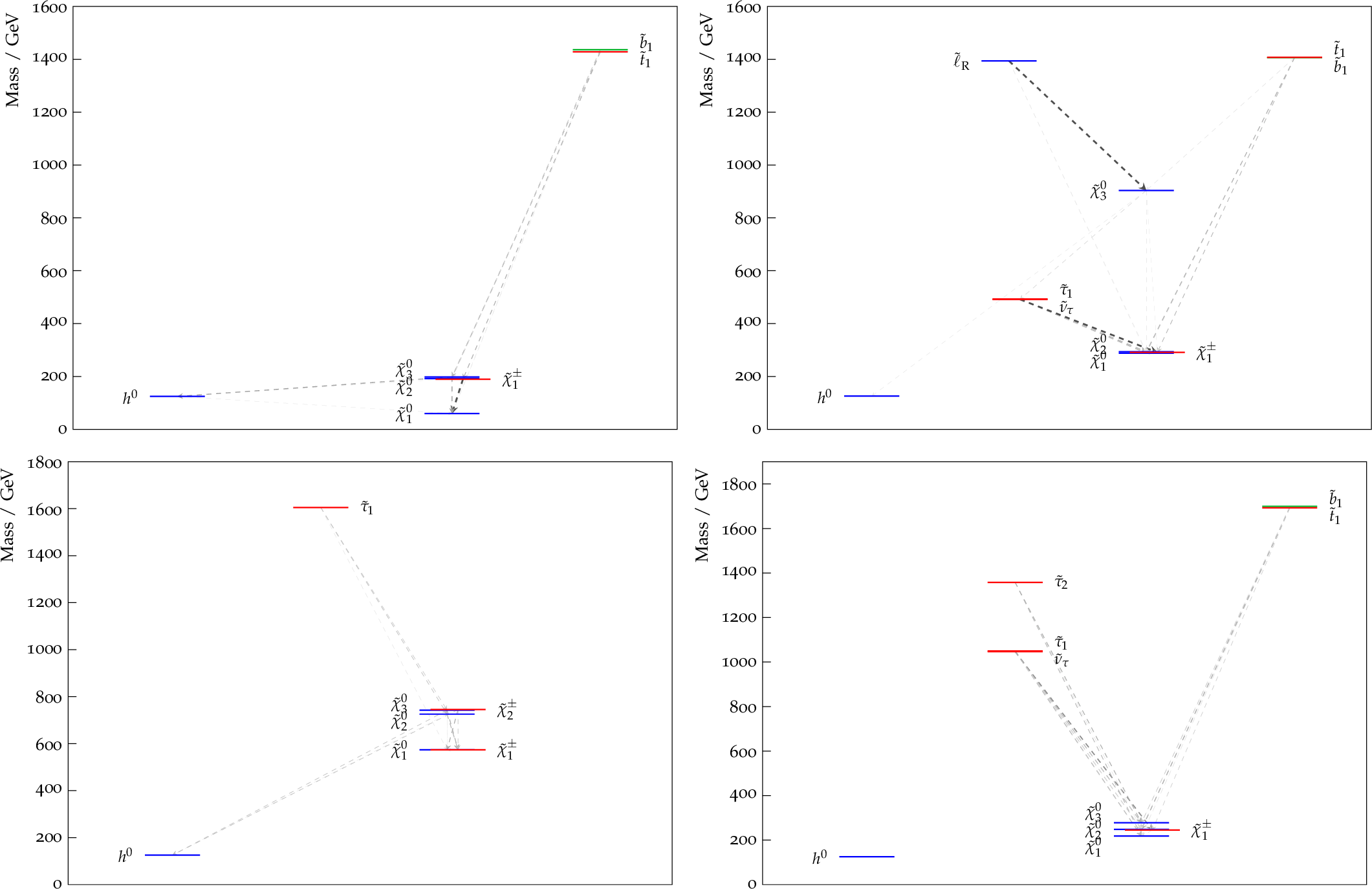
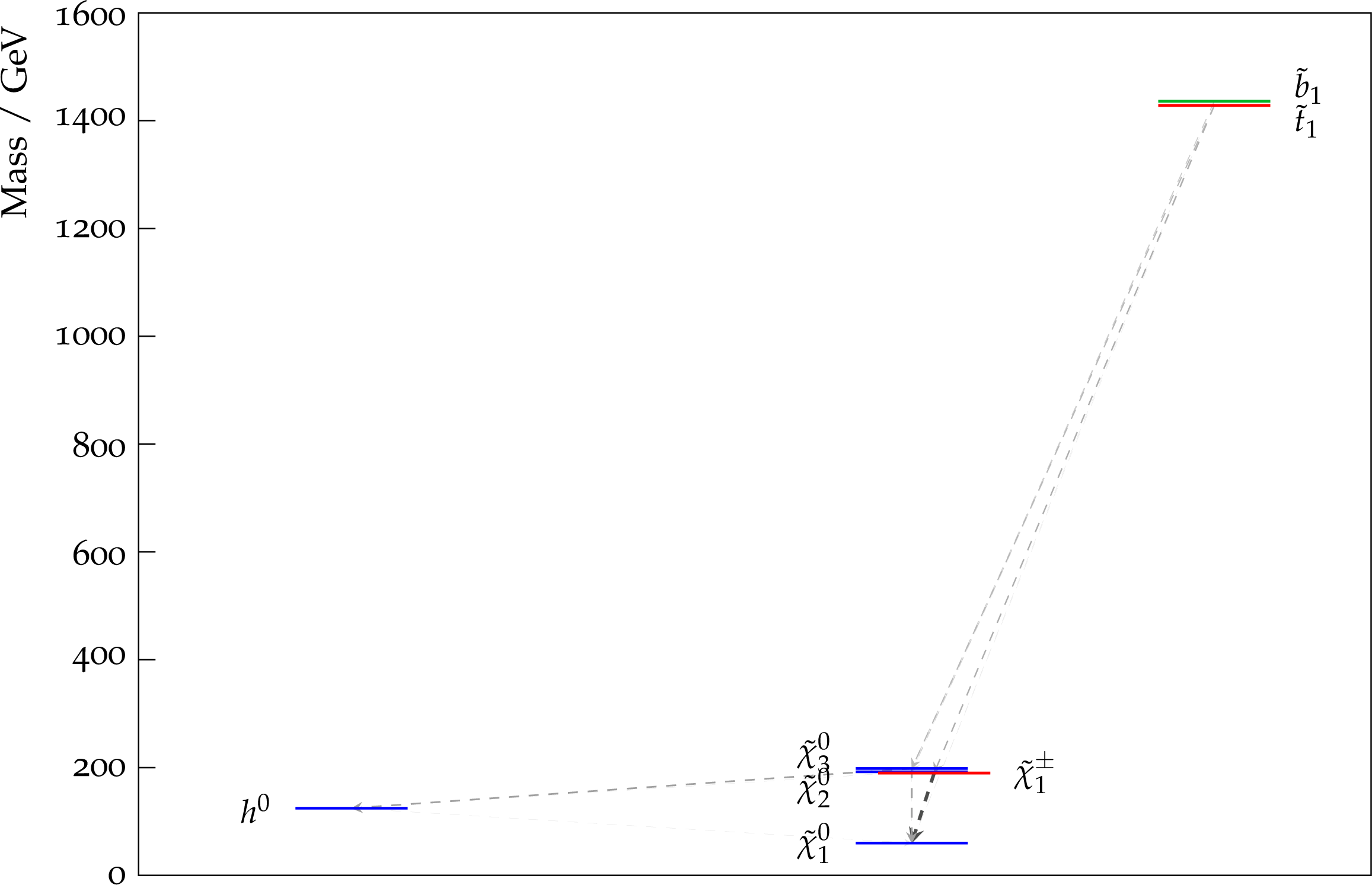
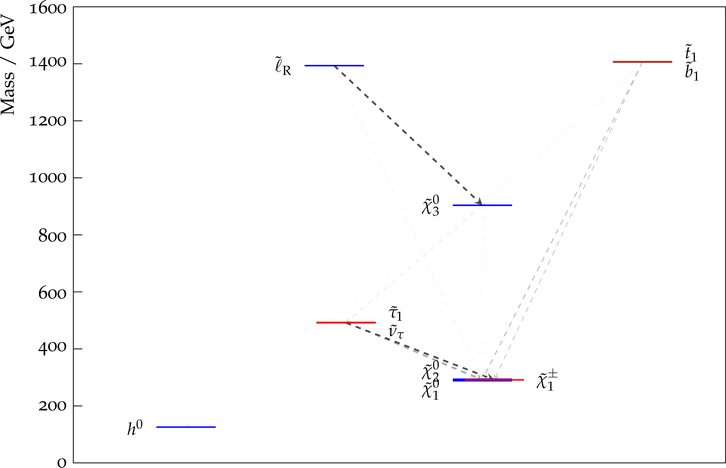
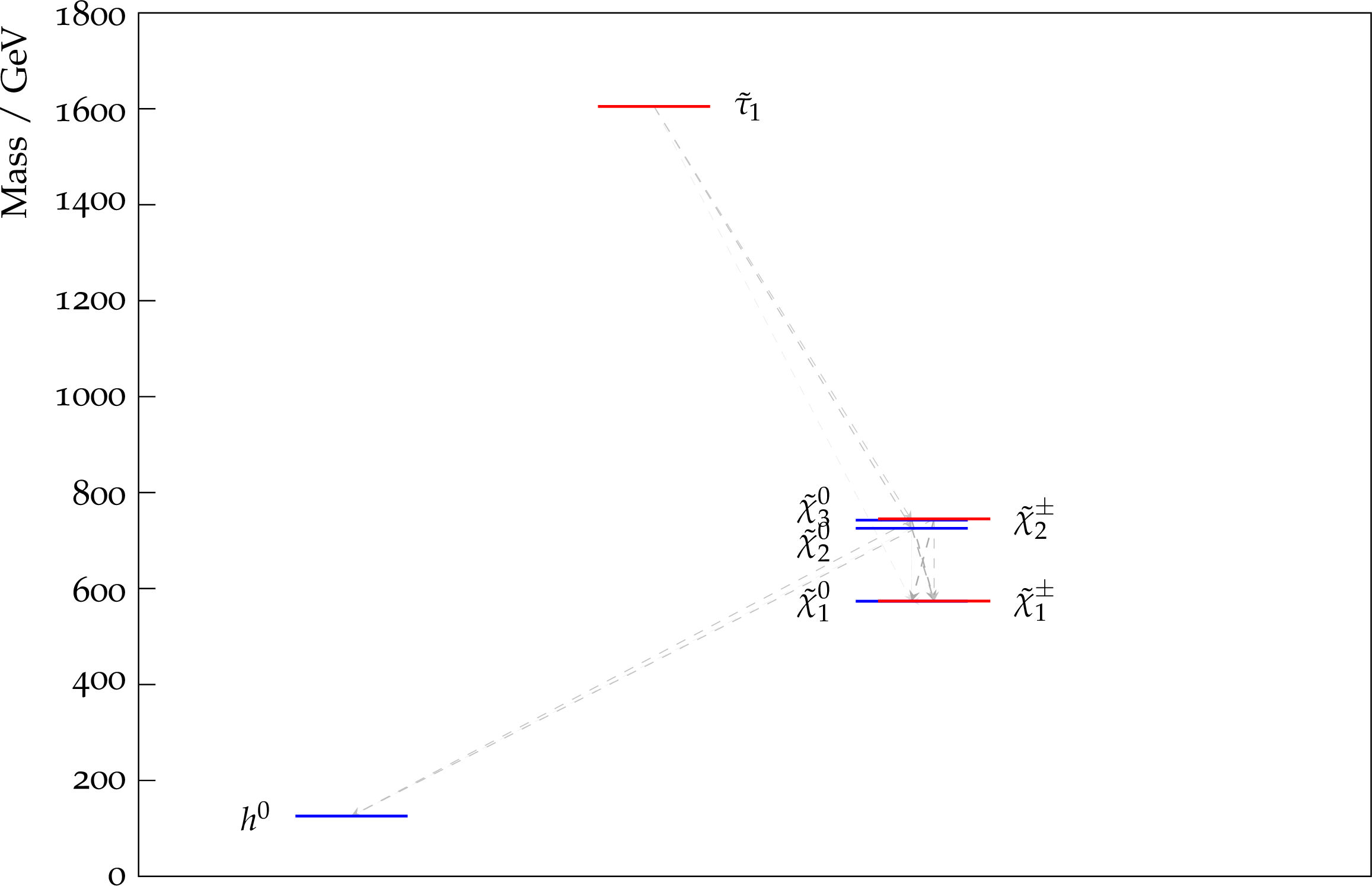
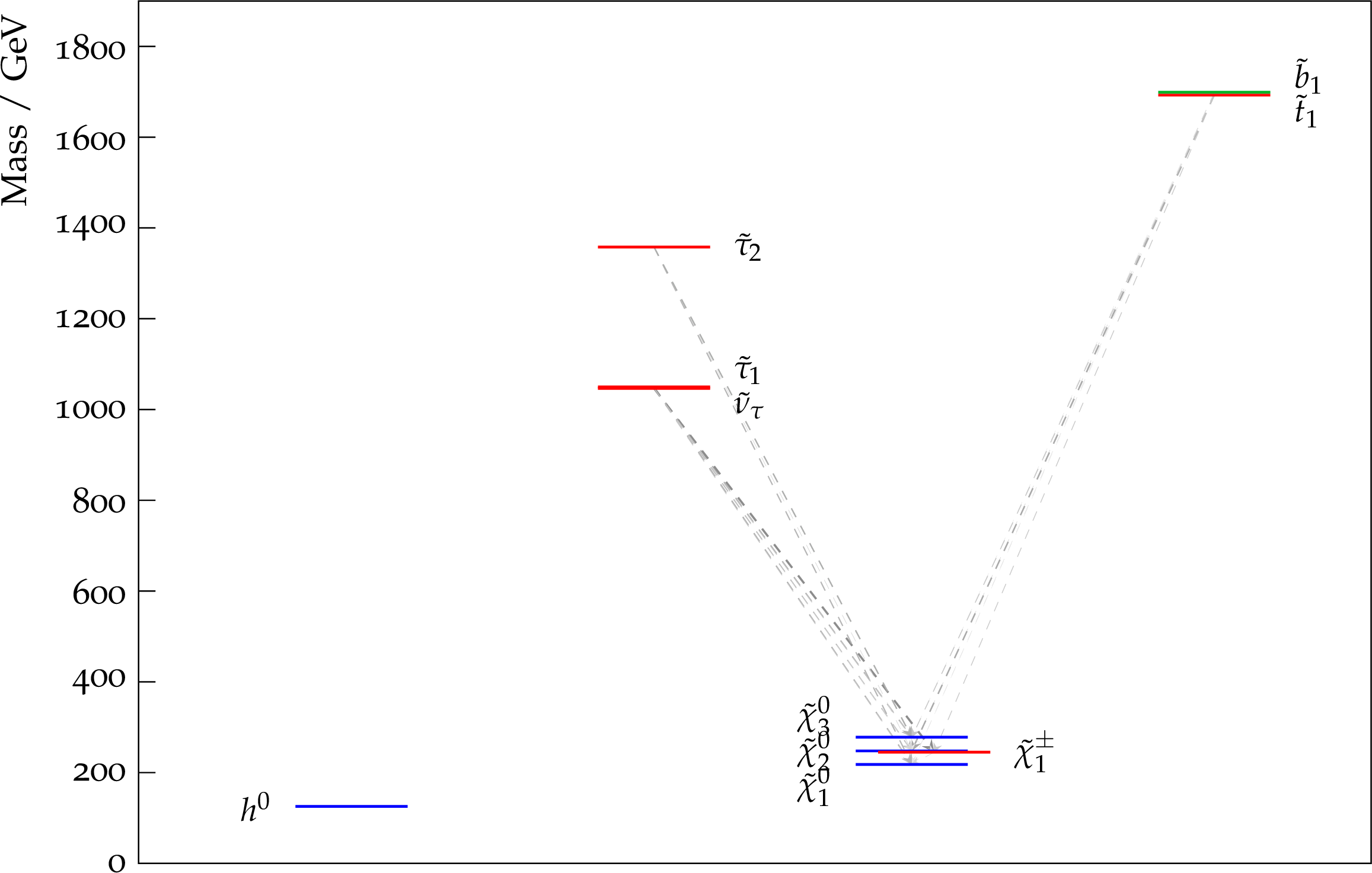
Figure 8:
Four pMSSM model points (run number, iteration number) with positive Z significance in reading order with symbols indicated as in: red circle (550, 52206), gray triangle (136, 33723), pink square (132, 73754), and orange triangle (449, 65877). The Z scores vary between 2 and 3. |
png pdf |
Figure 8-a:
Four pMSSM model points (run number, iteration number) with positive Z significance in reading order with symbols indicated as in: red circle (550, 52206), gray triangle (136, 33723), pink square (132, 73754), and orange triangle (449, 65877). The Z scores vary between 2 and 3. |
png pdf |
Figure 8-b:
Four pMSSM model points (run number, iteration number) with positive Z significance in reading order with symbols indicated as in: red circle (550, 52206), gray triangle (136, 33723), pink square (132, 73754), and orange triangle (449, 65877). The Z scores vary between 2 and 3. |
png pdf |
Figure 8-c:
Four pMSSM model points (run number, iteration number) with positive Z significance in reading order with symbols indicated as in: red circle (550, 52206), gray triangle (136, 33723), pink square (132, 73754), and orange triangle (449, 65877). The Z scores vary between 2 and 3. |
png pdf |
Figure 8-d:
Four pMSSM model points (run number, iteration number) with positive Z significance in reading order with symbols indicated as in: red circle (550, 52206), gray triangle (136, 33723), pink square (132, 73754), and orange triangle (449, 65877). The Z scores vary between 2 and 3. |
png pdf |
Figure 9:
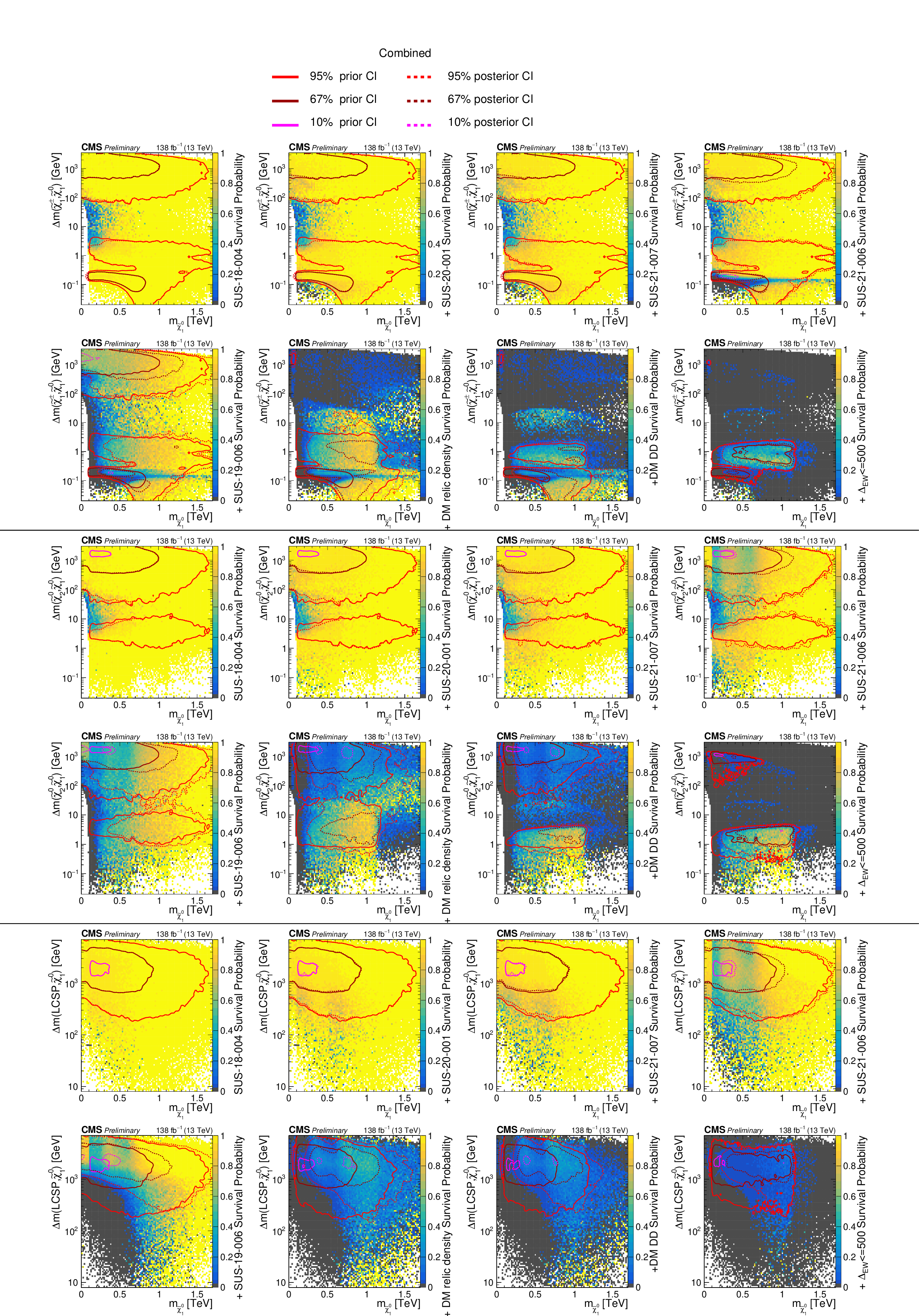
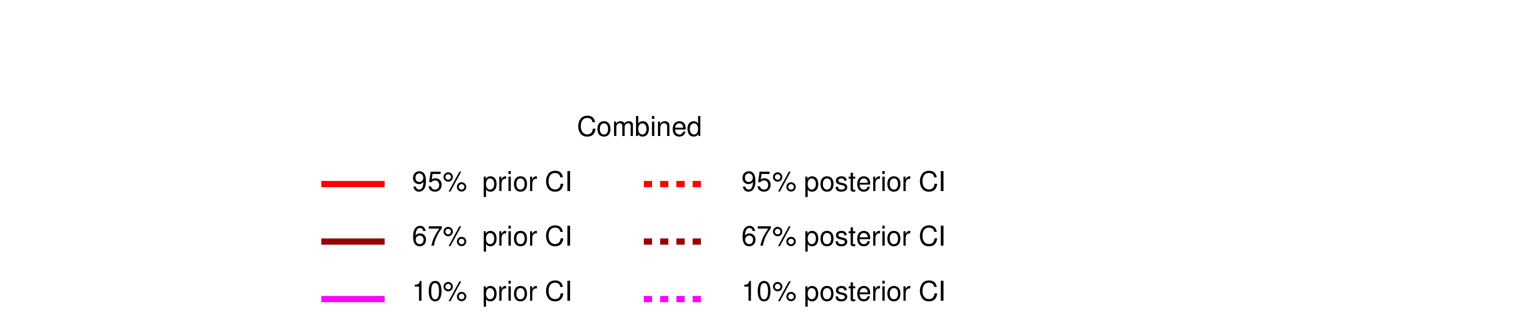
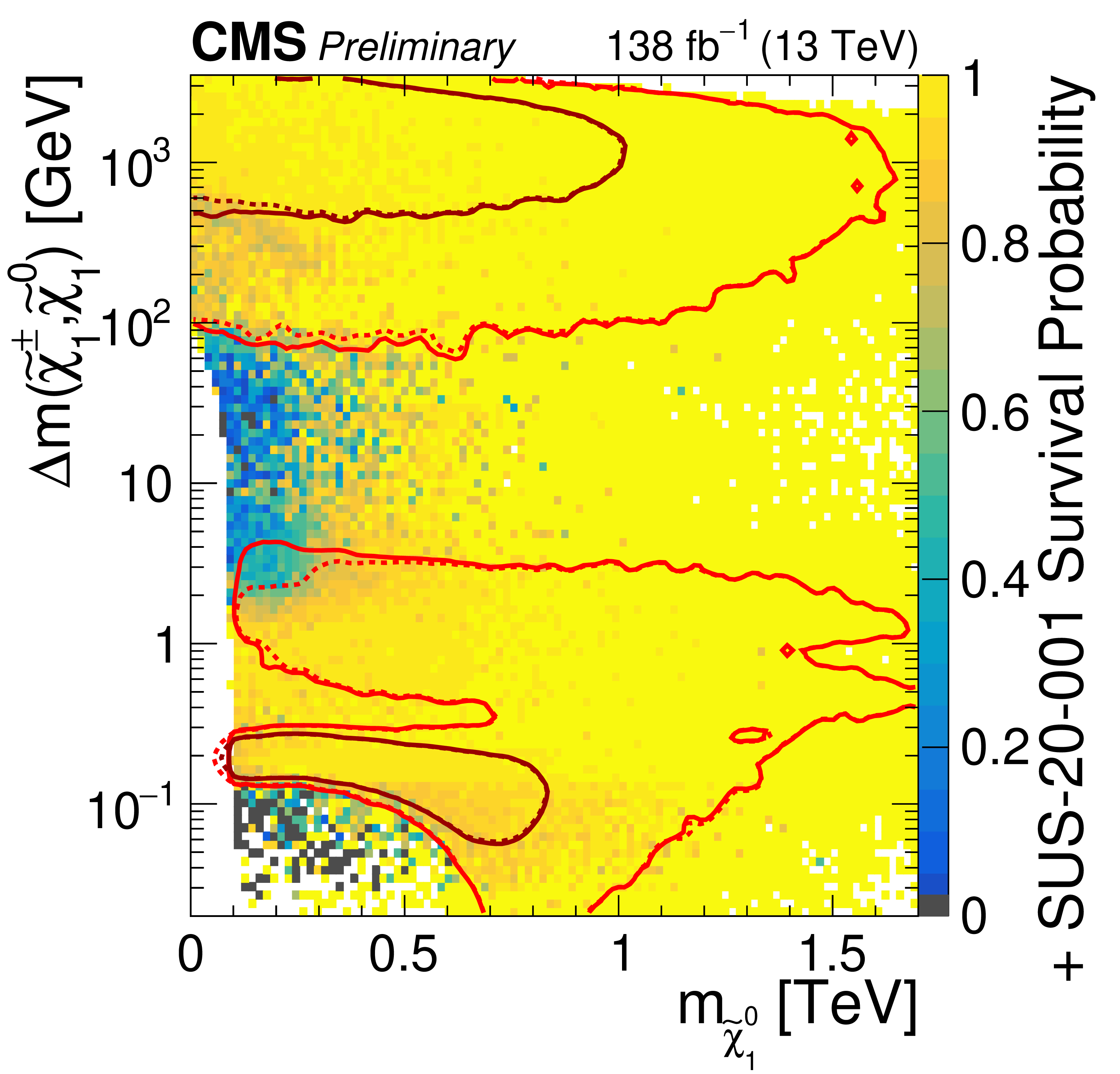
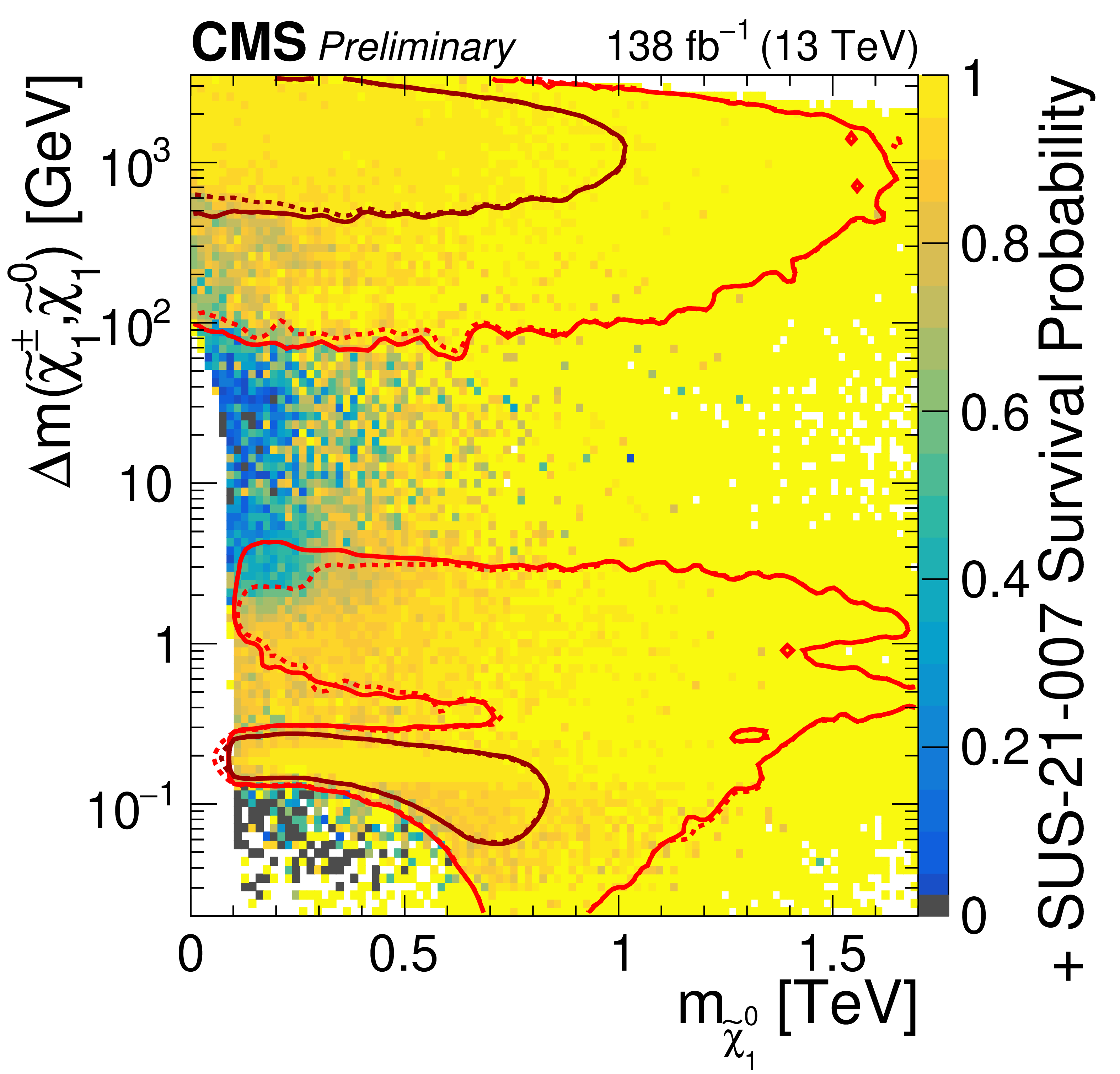
Progressive impact of individual searches on the pMSSM as a function of the LSP and mass differences between the LSP and lightest chargino (top two rows), the second-lightest neutralino (next two rows), and LCSP (bottom two rows). The order of the applied sequence of constraints is: SUS-18-004 [44], SUS-20-001 [47], SUS-21-007 [49], SUS-21-006 [48], SUS-19-006 [46], DM relic density, DM direct detection, $ \Delta_{\text{EW}} < $ 200. |
png pdf |
Figure 9-a:
Progressive impact of individual searches on the pMSSM as a function of the LSP and mass differences between the LSP and lightest chargino (top two rows), the second-lightest neutralino (next two rows), and LCSP (bottom two rows). The order of the applied sequence of constraints is: SUS-18-004 [44], SUS-20-001 [47], SUS-21-007 [49], SUS-21-006 [48], SUS-19-006 [46], DM relic density, DM direct detection, $ \Delta_{\text{EW}} < $ 200. |

png pdf |
Figure 9-b:
Progressive impact of individual searches on the pMSSM as a function of the LSP and mass differences between the LSP and lightest chargino (top two rows), the second-lightest neutralino (next two rows), and LCSP (bottom two rows). The order of the applied sequence of constraints is: SUS-18-004 [44], SUS-20-001 [47], SUS-21-007 [49], SUS-21-006 [48], SUS-19-006 [46], DM relic density, DM direct detection, $ \Delta_{\text{EW}} < $ 200. |
png pdf |
Figure 9-c:
Progressive impact of individual searches on the pMSSM as a function of the LSP and mass differences between the LSP and lightest chargino (top two rows), the second-lightest neutralino (next two rows), and LCSP (bottom two rows). The order of the applied sequence of constraints is: SUS-18-004 [44], SUS-20-001 [47], SUS-21-007 [49], SUS-21-006 [48], SUS-19-006 [46], DM relic density, DM direct detection, $ \Delta_{\text{EW}} < $ 200. |
png pdf |
Figure 9-d:
Progressive impact of individual searches on the pMSSM as a function of the LSP and mass differences between the LSP and lightest chargino (top two rows), the second-lightest neutralino (next two rows), and LCSP (bottom two rows). The order of the applied sequence of constraints is: SUS-18-004 [44], SUS-20-001 [47], SUS-21-007 [49], SUS-21-006 [48], SUS-19-006 [46], DM relic density, DM direct detection, $ \Delta_{\text{EW}} < $ 200. |

png pdf |
Figure 9-e:
Progressive impact of individual searches on the pMSSM as a function of the LSP and mass differences between the LSP and lightest chargino (top two rows), the second-lightest neutralino (next two rows), and LCSP (bottom two rows). The order of the applied sequence of constraints is: SUS-18-004 [44], SUS-20-001 [47], SUS-21-007 [49], SUS-21-006 [48], SUS-19-006 [46], DM relic density, DM direct detection, $ \Delta_{\text{EW}} < $ 200. |
png pdf |
Figure 9-f:
Progressive impact of individual searches on the pMSSM as a function of the LSP and mass differences between the LSP and lightest chargino (top two rows), the second-lightest neutralino (next two rows), and LCSP (bottom two rows). The order of the applied sequence of constraints is: SUS-18-004 [44], SUS-20-001 [47], SUS-21-007 [49], SUS-21-006 [48], SUS-19-006 [46], DM relic density, DM direct detection, $ \Delta_{\text{EW}} < $ 200. |
png pdf |
Figure 9-g:
Progressive impact of individual searches on the pMSSM as a function of the LSP and mass differences between the LSP and lightest chargino (top two rows), the second-lightest neutralino (next two rows), and LCSP (bottom two rows). The order of the applied sequence of constraints is: SUS-18-004 [44], SUS-20-001 [47], SUS-21-007 [49], SUS-21-006 [48], SUS-19-006 [46], DM relic density, DM direct detection, $ \Delta_{\text{EW}} < $ 200. |
png pdf |
Figure 9-h:
Progressive impact of individual searches on the pMSSM as a function of the LSP and mass differences between the LSP and lightest chargino (top two rows), the second-lightest neutralino (next two rows), and LCSP (bottom two rows). The order of the applied sequence of constraints is: SUS-18-004 [44], SUS-20-001 [47], SUS-21-007 [49], SUS-21-006 [48], SUS-19-006 [46], DM relic density, DM direct detection, $ \Delta_{\text{EW}} < $ 200. |
png pdf |
Figure 9-i:
Progressive impact of individual searches on the pMSSM as a function of the LSP and mass differences between the LSP and lightest chargino (top two rows), the second-lightest neutralino (next two rows), and LCSP (bottom two rows). The order of the applied sequence of constraints is: SUS-18-004 [44], SUS-20-001 [47], SUS-21-007 [49], SUS-21-006 [48], SUS-19-006 [46], DM relic density, DM direct detection, $ \Delta_{\text{EW}} < $ 200. |
png pdf |
Figure 9-j:
Progressive impact of individual searches on the pMSSM as a function of the LSP and mass differences between the LSP and lightest chargino (top two rows), the second-lightest neutralino (next two rows), and LCSP (bottom two rows). The order of the applied sequence of constraints is: SUS-18-004 [44], SUS-20-001 [47], SUS-21-007 [49], SUS-21-006 [48], SUS-19-006 [46], DM relic density, DM direct detection, $ \Delta_{\text{EW}} < $ 200. |
png pdf |
Figure 9-k:
Progressive impact of individual searches on the pMSSM as a function of the LSP and mass differences between the LSP and lightest chargino (top two rows), the second-lightest neutralino (next two rows), and LCSP (bottom two rows). The order of the applied sequence of constraints is: SUS-18-004 [44], SUS-20-001 [47], SUS-21-007 [49], SUS-21-006 [48], SUS-19-006 [46], DM relic density, DM direct detection, $ \Delta_{\text{EW}} < $ 200. |

png pdf |
Figure 9-l:
Progressive impact of individual searches on the pMSSM as a function of the LSP and mass differences between the LSP and lightest chargino (top two rows), the second-lightest neutralino (next two rows), and LCSP (bottom two rows). The order of the applied sequence of constraints is: SUS-18-004 [44], SUS-20-001 [47], SUS-21-007 [49], SUS-21-006 [48], SUS-19-006 [46], DM relic density, DM direct detection, $ \Delta_{\text{EW}} < $ 200. |
png pdf |
Figure 9-m:
Progressive impact of individual searches on the pMSSM as a function of the LSP and mass differences between the LSP and lightest chargino (top two rows), the second-lightest neutralino (next two rows), and LCSP (bottom two rows). The order of the applied sequence of constraints is: SUS-18-004 [44], SUS-20-001 [47], SUS-21-007 [49], SUS-21-006 [48], SUS-19-006 [46], DM relic density, DM direct detection, $ \Delta_{\text{EW}} < $ 200. |
png pdf |
Figure 9-n:
Progressive impact of individual searches on the pMSSM as a function of the LSP and mass differences between the LSP and lightest chargino (top two rows), the second-lightest neutralino (next two rows), and LCSP (bottom two rows). The order of the applied sequence of constraints is: SUS-18-004 [44], SUS-20-001 [47], SUS-21-007 [49], SUS-21-006 [48], SUS-19-006 [46], DM relic density, DM direct detection, $ \Delta_{\text{EW}} < $ 200. |
png pdf |
Figure 9-o:
Progressive impact of individual searches on the pMSSM as a function of the LSP and mass differences between the LSP and lightest chargino (top two rows), the second-lightest neutralino (next two rows), and LCSP (bottom two rows). The order of the applied sequence of constraints is: SUS-18-004 [44], SUS-20-001 [47], SUS-21-007 [49], SUS-21-006 [48], SUS-19-006 [46], DM relic density, DM direct detection, $ \Delta_{\text{EW}} < $ 200. |
png pdf |
Figure 9-p:
Progressive impact of individual searches on the pMSSM as a function of the LSP and mass differences between the LSP and lightest chargino (top two rows), the second-lightest neutralino (next two rows), and LCSP (bottom two rows). The order of the applied sequence of constraints is: SUS-18-004 [44], SUS-20-001 [47], SUS-21-007 [49], SUS-21-006 [48], SUS-19-006 [46], DM relic density, DM direct detection, $ \Delta_{\text{EW}} < $ 200. |
png pdf |
Figure 9-q:
Progressive impact of individual searches on the pMSSM as a function of the LSP and mass differences between the LSP and lightest chargino (top two rows), the second-lightest neutralino (next two rows), and LCSP (bottom two rows). The order of the applied sequence of constraints is: SUS-18-004 [44], SUS-20-001 [47], SUS-21-007 [49], SUS-21-006 [48], SUS-19-006 [46], DM relic density, DM direct detection, $ \Delta_{\text{EW}} < $ 200. |
png pdf |
Figure 9-r:
Progressive impact of individual searches on the pMSSM as a function of the LSP and mass differences between the LSP and lightest chargino (top two rows), the second-lightest neutralino (next two rows), and LCSP (bottom two rows). The order of the applied sequence of constraints is: SUS-18-004 [44], SUS-20-001 [47], SUS-21-007 [49], SUS-21-006 [48], SUS-19-006 [46], DM relic density, DM direct detection, $ \Delta_{\text{EW}} < $ 200. |
png pdf |
Figure 9-s:
Progressive impact of individual searches on the pMSSM as a function of the LSP and mass differences between the LSP and lightest chargino (top two rows), the second-lightest neutralino (next two rows), and LCSP (bottom two rows). The order of the applied sequence of constraints is: SUS-18-004 [44], SUS-20-001 [47], SUS-21-007 [49], SUS-21-006 [48], SUS-19-006 [46], DM relic density, DM direct detection, $ \Delta_{\text{EW}} < $ 200. |

png pdf |
Figure 9-t:
Progressive impact of individual searches on the pMSSM as a function of the LSP and mass differences between the LSP and lightest chargino (top two rows), the second-lightest neutralino (next two rows), and LCSP (bottom two rows). The order of the applied sequence of constraints is: SUS-18-004 [44], SUS-20-001 [47], SUS-21-007 [49], SUS-21-006 [48], SUS-19-006 [46], DM relic density, DM direct detection, $ \Delta_{\text{EW}} < $ 200. |

png pdf |
Figure 9-u:
Progressive impact of individual searches on the pMSSM as a function of the LSP and mass differences between the LSP and lightest chargino (top two rows), the second-lightest neutralino (next two rows), and LCSP (bottom two rows). The order of the applied sequence of constraints is: SUS-18-004 [44], SUS-20-001 [47], SUS-21-007 [49], SUS-21-006 [48], SUS-19-006 [46], DM relic density, DM direct detection, $ \Delta_{\text{EW}} < $ 200. |
png pdf |
Figure 9-v:
Progressive impact of individual searches on the pMSSM as a function of the LSP and mass differences between the LSP and lightest chargino (top two rows), the second-lightest neutralino (next two rows), and LCSP (bottom two rows). The order of the applied sequence of constraints is: SUS-18-004 [44], SUS-20-001 [47], SUS-21-007 [49], SUS-21-006 [48], SUS-19-006 [46], DM relic density, DM direct detection, $ \Delta_{\text{EW}} < $ 200. |
png pdf |
Figure 9-w:
Progressive impact of individual searches on the pMSSM as a function of the LSP and mass differences between the LSP and lightest chargino (top two rows), the second-lightest neutralino (next two rows), and LCSP (bottom two rows). The order of the applied sequence of constraints is: SUS-18-004 [44], SUS-20-001 [47], SUS-21-007 [49], SUS-21-006 [48], SUS-19-006 [46], DM relic density, DM direct detection, $ \Delta_{\text{EW}} < $ 200. |
png pdf |
Figure 9-x:
Progressive impact of individual searches on the pMSSM as a function of the LSP and mass differences between the LSP and lightest chargino (top two rows), the second-lightest neutralino (next two rows), and LCSP (bottom two rows). The order of the applied sequence of constraints is: SUS-18-004 [44], SUS-20-001 [47], SUS-21-007 [49], SUS-21-006 [48], SUS-19-006 [46], DM relic density, DM direct detection, $ \Delta_{\text{EW}} < $ 200. |

png pdf |
Figure 9-y:
Progressive impact of individual searches on the pMSSM as a function of the LSP and mass differences between the LSP and lightest chargino (top two rows), the second-lightest neutralino (next two rows), and LCSP (bottom two rows). The order of the applied sequence of constraints is: SUS-18-004 [44], SUS-20-001 [47], SUS-21-007 [49], SUS-21-006 [48], SUS-19-006 [46], DM relic density, DM direct detection, $ \Delta_{\text{EW}} < $ 200. |
| Summary |
| The CMS experiment has conducted various searches for BSM physics during the 2016-2018 data taking period at the CERN LHC, which have been interpreted using a 19-parameter scan of the phenomenological minimal supersymmetric standard model (pMSSM). Using previously published results from search analyses data from pp collisions at 13 TeV, corresponding to an integrated luminosity of 138 fb$ ^{-1} $, the study has provided a comprehensive analysis of the pMSSM. This model, a general realization of the MSSM with parameters defined at the supersymmetry scale, captures most observable features of the R-parity conserving weak scale MSSM. A global Bayesian analysis has been performed, incorporating CMS data along with pre-CMS measurements and indirect probes of supersymmetry. As a result of the CMS analyses, the posterior probability density generally shifts towards higher masses compared to the prior, consistent with the reduced experimental sensitivity at higher masses. A peak in the posterior density around an LSP mass of 400 GeV suggests that significant phase space remains consistent with experimental data even at low LSP mass. Lightest chargino, second-lightest neutralino, gluino, and top squark masses are heavily disfavored below approximately 200, 200, 700, and 1100 GeV, respectively, but certain phase space regions remain allowed. The survival probability indicates the likelihood of phase space exclusion by the data, highlighting the allowed regions. Additionally, the upper quantiles of the Bayes Factor reveal phase space regions that align most consistently with observed data, indicating regions of interest for further study. A small number of pMSSM points have a high Bayes Factor where the model phase space is consistent with bins within the studied analyses that have the observed data above the background predictions; examples of these points were discussed to illustrate such compatible pMSSM scenarios. The lightest chargino, second-lightest neutralino, gluino, and top squark are heavily disfavored for masses less than around 200, 200, 700, and 1100 GeV, respectively. Considerable MSSM phase space capable of solving the small hierarchy problem or explaining the known DM relic density remain non-excluded by the CMS searches. However, only a very small number of models that are consistent with low-fine tuning and the relic density remain viable. Most such models correspond to a roughly pure Higgsino-like dark matter candidate. |
| Additional Figures | |
png pdf |
Additional Figure 1:
Marginalized prior and posterior density, survival probability, and upper quantiles of the BF for the masses of the lowest-mass electroweakino states and the stau (May 2026 update of PAS Fig. 1). |

png pdf |
Additional Figure 1-a:
Marginalized prior and posterior density, survival probability, and upper quantiles of the BF for the masses of the lowest-mass electroweakino states and the stau (May 2026 update of PAS Fig. 1). |

png pdf |
Additional Figure 1-b:
Marginalized prior and posterior density, survival probability, and upper quantiles of the BF for the masses of the lowest-mass electroweakino states and the stau (May 2026 update of PAS Fig. 1). |

png pdf |
Additional Figure 1-c:
Marginalized prior and posterior density, survival probability, and upper quantiles of the BF for the masses of the lowest-mass electroweakino states and the stau (May 2026 update of PAS Fig. 1). |

png pdf |
Additional Figure 1-d:
Marginalized prior and posterior density, survival probability, and upper quantiles of the BF for the masses of the lowest-mass electroweakino states and the stau (May 2026 update of PAS Fig. 1). |

png pdf |
Additional Figure 1-e:
Marginalized prior and posterior density, survival probability, and upper quantiles of the BF for the masses of the lowest-mass electroweakino states and the stau (May 2026 update of PAS Fig. 1). |

png pdf |
Additional Figure 1-f:
Marginalized prior and posterior density, survival probability, and upper quantiles of the BF for the masses of the lowest-mass electroweakino states and the stau (May 2026 update of PAS Fig. 1). |

png pdf |
Additional Figure 1-g:
Marginalized prior and posterior density, survival probability, and upper quantiles of the BF for the masses of the lowest-mass electroweakino states and the stau (May 2026 update of PAS Fig. 1). |

png pdf |
Additional Figure 1-h:
Marginalized prior and posterior density, survival probability, and upper quantiles of the BF for the masses of the lowest-mass electroweakino states and the stau (May 2026 update of PAS Fig. 1). |

png pdf |
Additional Figure 1-i:
Marginalized prior and posterior density, survival probability, and upper quantiles of the BF for the masses of the lowest-mass electroweakino states and the stau (May 2026 update of PAS Fig. 1). |

png pdf |
Additional Figure 1-j:
Marginalized prior and posterior density, survival probability, and upper quantiles of the BF for the masses of the lowest-mass electroweakino states and the stau (May 2026 update of PAS Fig. 1). |

png pdf |
Additional Figure 1-k:
Marginalized prior and posterior density, survival probability, and upper quantiles of the BF for the masses of the lowest-mass electroweakino states and the stau (May 2026 update of PAS Fig. 1). |

png pdf |
Additional Figure 1-l:
Marginalized prior and posterior density, survival probability, and upper quantiles of the BF for the masses of the lowest-mass electroweakino states and the stau (May 2026 update of PAS Fig. 1). |

png pdf |
Additional Figure 2:
Marginalized prior and posterior density, survival probability, and upper quantiles of the BF for third-generation squarks, gluino, and lightest colored superpartner masses (May 2026 update of PAS Fig. 2). |

png pdf |
Additional Figure 2-a:
Marginalized prior and posterior density, survival probability, and upper quantiles of the BF for third-generation squarks, gluino, and lightest colored superpartner masses (May 2026 update of PAS Fig. 2). |

png pdf |
Additional Figure 2-b:
Marginalized prior and posterior density, survival probability, and upper quantiles of the BF for third-generation squarks, gluino, and lightest colored superpartner masses (May 2026 update of PAS Fig. 2). |

png pdf |
Additional Figure 2-c:
Marginalized prior and posterior density, survival probability, and upper quantiles of the BF for third-generation squarks, gluino, and lightest colored superpartner masses (May 2026 update of PAS Fig. 2). |

png pdf |
Additional Figure 2-d:
Marginalized prior and posterior density, survival probability, and upper quantiles of the BF for third-generation squarks, gluino, and lightest colored superpartner masses (May 2026 update of PAS Fig. 2). |

png pdf |
Additional Figure 2-e:
Marginalized prior and posterior density, survival probability, and upper quantiles of the BF for third-generation squarks, gluino, and lightest colored superpartner masses (May 2026 update of PAS Fig. 2). |
png pdf |
Additional Figure 2-f:
Marginalized prior and posterior density, survival probability, and upper quantiles of the BF for third-generation squarks, gluino, and lightest colored superpartner masses (May 2026 update of PAS Fig. 2). |
png pdf |
Additional Figure 2-g:
Marginalized prior and posterior density, survival probability, and upper quantiles of the BF for third-generation squarks, gluino, and lightest colored superpartner masses (May 2026 update of PAS Fig. 2). |
png pdf |
Additional Figure 2-h:
Marginalized prior and posterior density, survival probability, and upper quantiles of the BF for third-generation squarks, gluino, and lightest colored superpartner masses (May 2026 update of PAS Fig. 2). |

png pdf |
Additional Figure 2-i:
Marginalized prior and posterior density, survival probability, and upper quantiles of the BF for third-generation squarks, gluino, and lightest colored superpartner masses (May 2026 update of PAS Fig. 2). |

png pdf |
Additional Figure 2-j:
Marginalized prior and posterior density, survival probability, and upper quantiles of the BF for third-generation squarks, gluino, and lightest colored superpartner masses (May 2026 update of PAS Fig. 2). |

png pdf |
Additional Figure 2-k:
Marginalized prior and posterior density, survival probability, and upper quantiles of the BF for third-generation squarks, gluino, and lightest colored superpartner masses (May 2026 update of PAS Fig. 2). |

png pdf |
Additional Figure 2-l:
Marginalized prior and posterior density, survival probability, and upper quantiles of the BF for third-generation squarks, gluino, and lightest colored superpartner masses (May 2026 update of PAS Fig. 2). |

png pdf |
Additional Figure 3:
Marginalized prior and posterior density, survival probability, and upper quantiles of the BF for dark-matter observables and fine-tuning criteria (May 2026 update of PAS Fig. 3). |

png pdf |
Additional Figure 3-a:
Marginalized prior and posterior density, survival probability, and upper quantiles of the BF for dark-matter observables and fine-tuning criteria (May 2026 update of PAS Fig. 3). |

png pdf |
Additional Figure 3-b:
Marginalized prior and posterior density, survival probability, and upper quantiles of the BF for dark-matter observables and fine-tuning criteria (May 2026 update of PAS Fig. 3). |

png pdf |
Additional Figure 3-c:
Marginalized prior and posterior density, survival probability, and upper quantiles of the BF for dark-matter observables and fine-tuning criteria (May 2026 update of PAS Fig. 3). |
png pdf |
Additional Figure 3-d:
Marginalized prior and posterior density, survival probability, and upper quantiles of the BF for dark-matter observables and fine-tuning criteria (May 2026 update of PAS Fig. 3). |

png pdf |
Additional Figure 3-e:
Marginalized prior and posterior density, survival probability, and upper quantiles of the BF for dark-matter observables and fine-tuning criteria (May 2026 update of PAS Fig. 3). |
png pdf |
Additional Figure 3-f:
Marginalized prior and posterior density, survival probability, and upper quantiles of the BF for dark-matter observables and fine-tuning criteria (May 2026 update of PAS Fig. 3). |
png pdf |
Additional Figure 3-g:
Marginalized prior and posterior density, survival probability, and upper quantiles of the BF for dark-matter observables and fine-tuning criteria (May 2026 update of PAS Fig. 3). |
png pdf |
Additional Figure 3-h:
Marginalized prior and posterior density, survival probability, and upper quantiles of the BF for dark-matter observables and fine-tuning criteria (May 2026 update of PAS Fig. 3). |

png pdf |
Additional Figure 3-i:
Marginalized prior and posterior density, survival probability, and upper quantiles of the BF for dark-matter observables and fine-tuning criteria (May 2026 update of PAS Fig. 3). |
png pdf |
Additional Figure 3-j:
Marginalized prior and posterior density, survival probability, and upper quantiles of the BF for dark-matter observables and fine-tuning criteria (May 2026 update of PAS Fig. 3). |

png pdf |
Additional Figure 3-k:
Marginalized prior and posterior density, survival probability, and upper quantiles of the BF for dark-matter observables and fine-tuning criteria (May 2026 update of PAS Fig. 3). |

png pdf |
Additional Figure 3-l:
Marginalized prior and posterior density, survival probability, and upper quantiles of the BF for dark-matter observables and fine-tuning criteria (May 2026 update of PAS Fig. 3). |
png pdf |
Additional Figure 4:
Survival probability based on the full scan (left), based on the subset of the scan respecting dark-matter constraints (center), and based on the natural dark-matter subset (right), as a function of LSP mass and mass differences between the LSP and the lightest neutralino states or the stau mass. Black bins indicate where no pMSSM points survived the CMS analyses, and white indicate where no pMSSM points are present in the prior. Also shown are the prior and posterior density contours corresponding to the respective constraints (May 2026 update of PAS Fig. 4). |

png pdf |
Additional Figure 4-a:
Survival probability based on the full scan (left), based on the subset of the scan respecting dark-matter constraints (center), and based on the natural dark-matter subset (right), as a function of LSP mass and mass differences between the LSP and the lightest neutralino states or the stau mass. Black bins indicate where no pMSSM points survived the CMS analyses, and white indicate where no pMSSM points are present in the prior. Also shown are the prior and posterior density contours corresponding to the respective constraints (May 2026 update of PAS Fig. 4). |
png pdf |
Additional Figure 4-b:
Survival probability based on the full scan (left), based on the subset of the scan respecting dark-matter constraints (center), and based on the natural dark-matter subset (right), as a function of LSP mass and mass differences between the LSP and the lightest neutralino states or the stau mass. Black bins indicate where no pMSSM points survived the CMS analyses, and white indicate where no pMSSM points are present in the prior. Also shown are the prior and posterior density contours corresponding to the respective constraints (May 2026 update of PAS Fig. 4). |

png pdf |
Additional Figure 4-c:
Survival probability based on the full scan (left), based on the subset of the scan respecting dark-matter constraints (center), and based on the natural dark-matter subset (right), as a function of LSP mass and mass differences between the LSP and the lightest neutralino states or the stau mass. Black bins indicate where no pMSSM points survived the CMS analyses, and white indicate where no pMSSM points are present in the prior. Also shown are the prior and posterior density contours corresponding to the respective constraints (May 2026 update of PAS Fig. 4). |

png pdf |
Additional Figure 4-d:
Survival probability based on the full scan (left), based on the subset of the scan respecting dark-matter constraints (center), and based on the natural dark-matter subset (right), as a function of LSP mass and mass differences between the LSP and the lightest neutralino states or the stau mass. Black bins indicate where no pMSSM points survived the CMS analyses, and white indicate where no pMSSM points are present in the prior. Also shown are the prior and posterior density contours corresponding to the respective constraints (May 2026 update of PAS Fig. 4). |
png pdf |
Additional Figure 4-e:
Survival probability based on the full scan (left), based on the subset of the scan respecting dark-matter constraints (center), and based on the natural dark-matter subset (right), as a function of LSP mass and mass differences between the LSP and the lightest neutralino states or the stau mass. Black bins indicate where no pMSSM points survived the CMS analyses, and white indicate where no pMSSM points are present in the prior. Also shown are the prior and posterior density contours corresponding to the respective constraints (May 2026 update of PAS Fig. 4). |

png pdf |
Additional Figure 4-f:
Survival probability based on the full scan (left), based on the subset of the scan respecting dark-matter constraints (center), and based on the natural dark-matter subset (right), as a function of LSP mass and mass differences between the LSP and the lightest neutralino states or the stau mass. Black bins indicate where no pMSSM points survived the CMS analyses, and white indicate where no pMSSM points are present in the prior. Also shown are the prior and posterior density contours corresponding to the respective constraints (May 2026 update of PAS Fig. 4). |
png pdf |
Additional Figure 4-g:
Survival probability based on the full scan (left), based on the subset of the scan respecting dark-matter constraints (center), and based on the natural dark-matter subset (right), as a function of LSP mass and mass differences between the LSP and the lightest neutralino states or the stau mass. Black bins indicate where no pMSSM points survived the CMS analyses, and white indicate where no pMSSM points are present in the prior. Also shown are the prior and posterior density contours corresponding to the respective constraints (May 2026 update of PAS Fig. 4). |
png pdf |
Additional Figure 4-h:
Survival probability based on the full scan (left), based on the subset of the scan respecting dark-matter constraints (center), and based on the natural dark-matter subset (right), as a function of LSP mass and mass differences between the LSP and the lightest neutralino states or the stau mass. Black bins indicate where no pMSSM points survived the CMS analyses, and white indicate where no pMSSM points are present in the prior. Also shown are the prior and posterior density contours corresponding to the respective constraints (May 2026 update of PAS Fig. 4). |
png pdf |
Additional Figure 4-i:
Survival probability based on the full scan (left), based on the subset of the scan respecting dark-matter constraints (center), and based on the natural dark-matter subset (right), as a function of LSP mass and mass differences between the LSP and the lightest neutralino states or the stau mass. Black bins indicate where no pMSSM points survived the CMS analyses, and white indicate where no pMSSM points are present in the prior. Also shown are the prior and posterior density contours corresponding to the respective constraints (May 2026 update of PAS Fig. 4). |

png pdf |
Additional Figure 4-j:
Survival probability based on the full scan (left), based on the subset of the scan respecting dark-matter constraints (center), and based on the natural dark-matter subset (right), as a function of LSP mass and mass differences between the LSP and the lightest neutralino states or the stau mass. Black bins indicate where no pMSSM points survived the CMS analyses, and white indicate where no pMSSM points are present in the prior. Also shown are the prior and posterior density contours corresponding to the respective constraints (May 2026 update of PAS Fig. 4). |
png pdf |
Additional Figure 4-k:
Survival probability based on the full scan (left), based on the subset of the scan respecting dark-matter constraints (center), and based on the natural dark-matter subset (right), as a function of LSP mass and mass differences between the LSP and the lightest neutralino states or the stau mass. Black bins indicate where no pMSSM points survived the CMS analyses, and white indicate where no pMSSM points are present in the prior. Also shown are the prior and posterior density contours corresponding to the respective constraints (May 2026 update of PAS Fig. 4). |
png pdf |
Additional Figure 4-l:
Survival probability based on the full scan (left), based on the subset of the scan respecting dark-matter constraints (center), and based on the natural dark-matter subset (right), as a function of LSP mass and mass differences between the LSP and the lightest neutralino states or the stau mass. Black bins indicate where no pMSSM points survived the CMS analyses, and white indicate where no pMSSM points are present in the prior. Also shown are the prior and posterior density contours corresponding to the respective constraints (May 2026 update of PAS Fig. 4). |

png pdf |
Additional Figure 4-m:
Survival probability based on the full scan (left), based on the subset of the scan respecting dark-matter constraints (center), and based on the natural dark-matter subset (right), as a function of LSP mass and mass differences between the LSP and the lightest neutralino states or the stau mass. Black bins indicate where no pMSSM points survived the CMS analyses, and white indicate where no pMSSM points are present in the prior. Also shown are the prior and posterior density contours corresponding to the respective constraints (May 2026 update of PAS Fig. 4). |
png pdf |
Additional Figure 5:
Survival probability based on the full scan (left), based on the subset of the scan respecting dark-matter constraints (center), and based on the natural dark-matter subset (right), as a function of LSP mass and mass differences between the LSP and the lighter top and bottom squark, gluino, and LCSP masses. Black bins indicate where no pMSSM points survived the CMS analyses, and white indicate where no pMSSM points are present in the prior. Also shown are the prior and posterior density contours corresponding to the respective constraints (May 2026 update of PAS Fig. 5). |

png pdf |
Additional Figure 5-a:
Survival probability based on the full scan (left), based on the subset of the scan respecting dark-matter constraints (center), and based on the natural dark-matter subset (right), as a function of LSP mass and mass differences between the LSP and the lighter top and bottom squark, gluino, and LCSP masses. Black bins indicate where no pMSSM points survived the CMS analyses, and white indicate where no pMSSM points are present in the prior. Also shown are the prior and posterior density contours corresponding to the respective constraints (May 2026 update of PAS Fig. 5). |
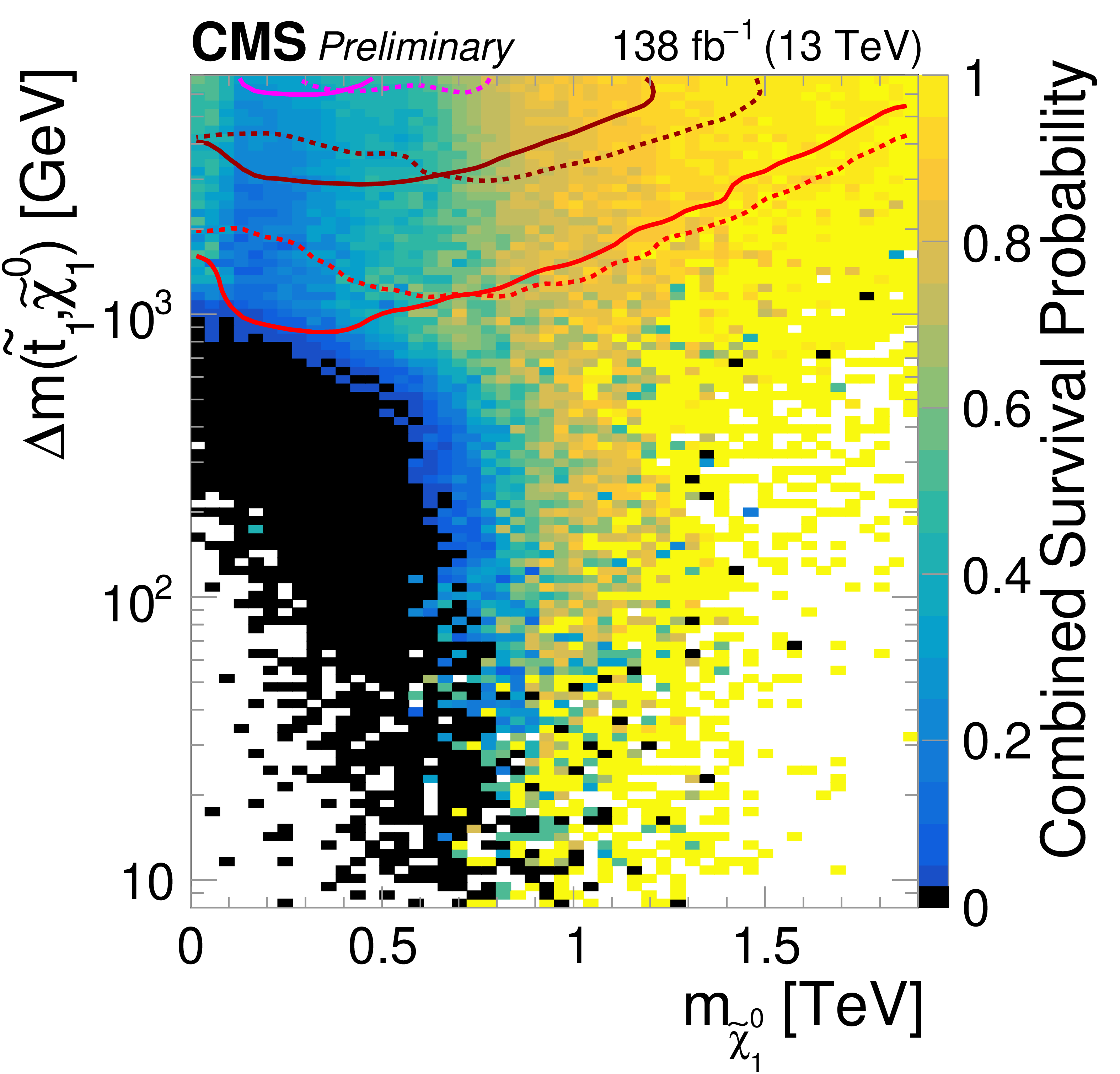
png pdf |
Additional Figure 5-b:
Survival probability based on the full scan (left), based on the subset of the scan respecting dark-matter constraints (center), and based on the natural dark-matter subset (right), as a function of LSP mass and mass differences between the LSP and the lighter top and bottom squark, gluino, and LCSP masses. Black bins indicate where no pMSSM points survived the CMS analyses, and white indicate where no pMSSM points are present in the prior. Also shown are the prior and posterior density contours corresponding to the respective constraints (May 2026 update of PAS Fig. 5). |

png pdf |
Additional Figure 5-c:
Survival probability based on the full scan (left), based on the subset of the scan respecting dark-matter constraints (center), and based on the natural dark-matter subset (right), as a function of LSP mass and mass differences between the LSP and the lighter top and bottom squark, gluino, and LCSP masses. Black bins indicate where no pMSSM points survived the CMS analyses, and white indicate where no pMSSM points are present in the prior. Also shown are the prior and posterior density contours corresponding to the respective constraints (May 2026 update of PAS Fig. 5). |

png pdf |
Additional Figure 5-d:
Survival probability based on the full scan (left), based on the subset of the scan respecting dark-matter constraints (center), and based on the natural dark-matter subset (right), as a function of LSP mass and mass differences between the LSP and the lighter top and bottom squark, gluino, and LCSP masses. Black bins indicate where no pMSSM points survived the CMS analyses, and white indicate where no pMSSM points are present in the prior. Also shown are the prior and posterior density contours corresponding to the respective constraints (May 2026 update of PAS Fig. 5). |

png pdf |
Additional Figure 5-e:
Survival probability based on the full scan (left), based on the subset of the scan respecting dark-matter constraints (center), and based on the natural dark-matter subset (right), as a function of LSP mass and mass differences between the LSP and the lighter top and bottom squark, gluino, and LCSP masses. Black bins indicate where no pMSSM points survived the CMS analyses, and white indicate where no pMSSM points are present in the prior. Also shown are the prior and posterior density contours corresponding to the respective constraints (May 2026 update of PAS Fig. 5). |

png pdf |
Additional Figure 5-f:
Survival probability based on the full scan (left), based on the subset of the scan respecting dark-matter constraints (center), and based on the natural dark-matter subset (right), as a function of LSP mass and mass differences between the LSP and the lighter top and bottom squark, gluino, and LCSP masses. Black bins indicate where no pMSSM points survived the CMS analyses, and white indicate where no pMSSM points are present in the prior. Also shown are the prior and posterior density contours corresponding to the respective constraints (May 2026 update of PAS Fig. 5). |

png pdf |
Additional Figure 5-g:
Survival probability based on the full scan (left), based on the subset of the scan respecting dark-matter constraints (center), and based on the natural dark-matter subset (right), as a function of LSP mass and mass differences between the LSP and the lighter top and bottom squark, gluino, and LCSP masses. Black bins indicate where no pMSSM points survived the CMS analyses, and white indicate where no pMSSM points are present in the prior. Also shown are the prior and posterior density contours corresponding to the respective constraints (May 2026 update of PAS Fig. 5). |

png pdf |
Additional Figure 5-h:
Survival probability based on the full scan (left), based on the subset of the scan respecting dark-matter constraints (center), and based on the natural dark-matter subset (right), as a function of LSP mass and mass differences between the LSP and the lighter top and bottom squark, gluino, and LCSP masses. Black bins indicate where no pMSSM points survived the CMS analyses, and white indicate where no pMSSM points are present in the prior. Also shown are the prior and posterior density contours corresponding to the respective constraints (May 2026 update of PAS Fig. 5). |

png pdf |
Additional Figure 5-i:
Survival probability based on the full scan (left), based on the subset of the scan respecting dark-matter constraints (center), and based on the natural dark-matter subset (right), as a function of LSP mass and mass differences between the LSP and the lighter top and bottom squark, gluino, and LCSP masses. Black bins indicate where no pMSSM points survived the CMS analyses, and white indicate where no pMSSM points are present in the prior. Also shown are the prior and posterior density contours corresponding to the respective constraints (May 2026 update of PAS Fig. 5). |

png pdf |
Additional Figure 5-j:
Survival probability based on the full scan (left), based on the subset of the scan respecting dark-matter constraints (center), and based on the natural dark-matter subset (right), as a function of LSP mass and mass differences between the LSP and the lighter top and bottom squark, gluino, and LCSP masses. Black bins indicate where no pMSSM points survived the CMS analyses, and white indicate where no pMSSM points are present in the prior. Also shown are the prior and posterior density contours corresponding to the respective constraints (May 2026 update of PAS Fig. 5). |
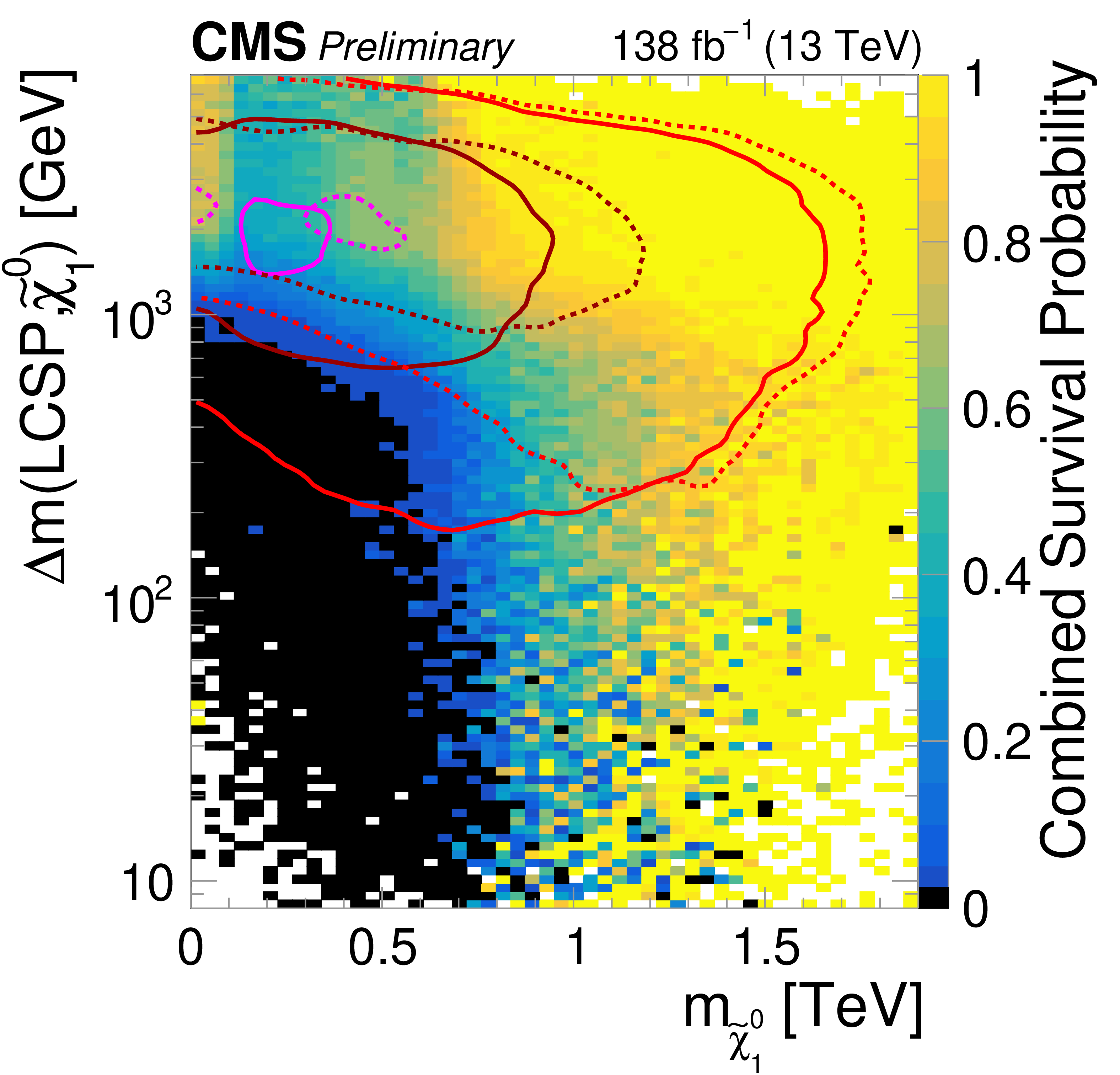
png pdf |
Additional Figure 5-k:
Survival probability based on the full scan (left), based on the subset of the scan respecting dark-matter constraints (center), and based on the natural dark-matter subset (right), as a function of LSP mass and mass differences between the LSP and the lighter top and bottom squark, gluino, and LCSP masses. Black bins indicate where no pMSSM points survived the CMS analyses, and white indicate where no pMSSM points are present in the prior. Also shown are the prior and posterior density contours corresponding to the respective constraints (May 2026 update of PAS Fig. 5). |

png pdf |
Additional Figure 5-l:
Survival probability based on the full scan (left), based on the subset of the scan respecting dark-matter constraints (center), and based on the natural dark-matter subset (right), as a function of LSP mass and mass differences between the LSP and the lighter top and bottom squark, gluino, and LCSP masses. Black bins indicate where no pMSSM points survived the CMS analyses, and white indicate where no pMSSM points are present in the prior. Also shown are the prior and posterior density contours corresponding to the respective constraints (May 2026 update of PAS Fig. 5). |

png pdf |
Additional Figure 5-m:
Survival probability based on the full scan (left), based on the subset of the scan respecting dark-matter constraints (center), and based on the natural dark-matter subset (right), as a function of LSP mass and mass differences between the LSP and the lighter top and bottom squark, gluino, and LCSP masses. Black bins indicate where no pMSSM points survived the CMS analyses, and white indicate where no pMSSM points are present in the prior. Also shown are the prior and posterior density contours corresponding to the respective constraints (May 2026 update of PAS Fig. 5). |
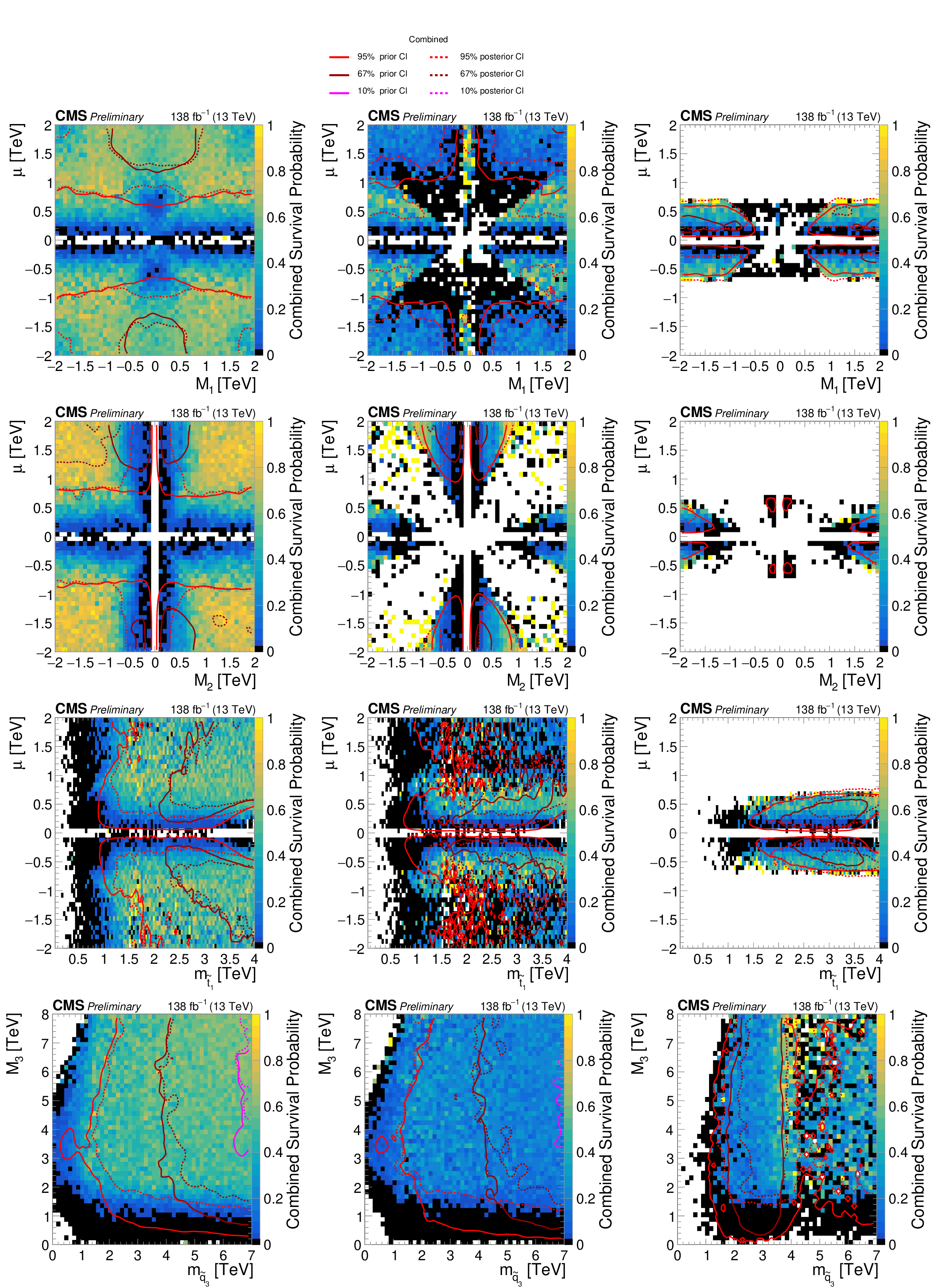
png pdf |
Additional Figure 6:
Survival probability based on the full scan (left), based on the subset of the scan respecting dark-matter constraints (center), and based on the natural dark-matter subset (right), as a function of representative pMSSM Lagrangian parameters. Black indicates bins where no pMSSM points survived the CMS analyses, and white indicates bins where no pMSSM points are present in the prior (May 2026 update of PAS Fig. 6). |

png pdf |
Additional Figure 6-a:
Survival probability based on the full scan (left), based on the subset of the scan respecting dark-matter constraints (center), and based on the natural dark-matter subset (right), as a function of representative pMSSM Lagrangian parameters. Black indicates bins where no pMSSM points survived the CMS analyses, and white indicates bins where no pMSSM points are present in the prior (May 2026 update of PAS Fig. 6). |
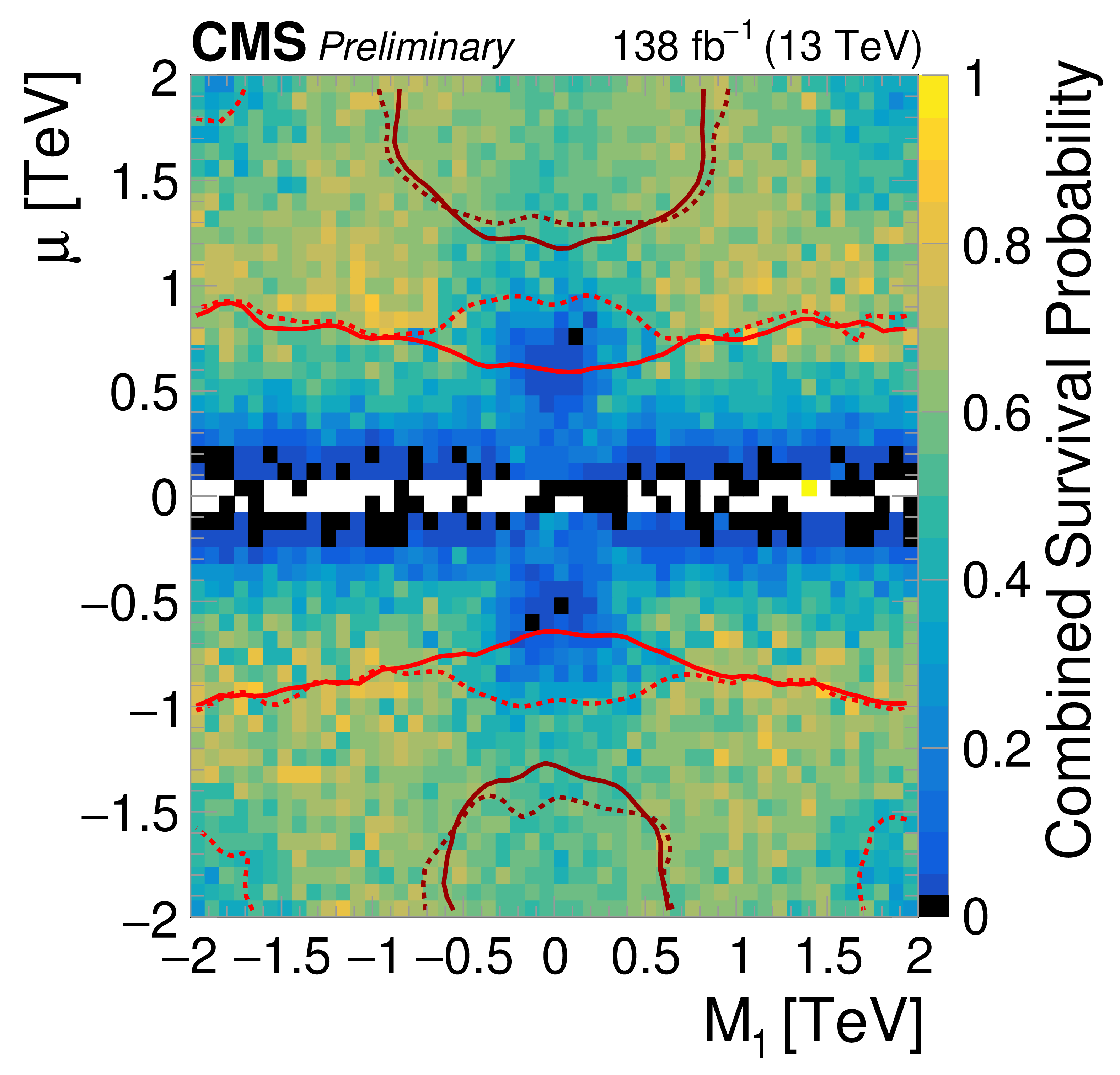
png pdf |
Additional Figure 6-b:
Survival probability based on the full scan (left), based on the subset of the scan respecting dark-matter constraints (center), and based on the natural dark-matter subset (right), as a function of representative pMSSM Lagrangian parameters. Black indicates bins where no pMSSM points survived the CMS analyses, and white indicates bins where no pMSSM points are present in the prior (May 2026 update of PAS Fig. 6). |

png pdf |
Additional Figure 6-c:
Survival probability based on the full scan (left), based on the subset of the scan respecting dark-matter constraints (center), and based on the natural dark-matter subset (right), as a function of representative pMSSM Lagrangian parameters. Black indicates bins where no pMSSM points survived the CMS analyses, and white indicates bins where no pMSSM points are present in the prior (May 2026 update of PAS Fig. 6). |
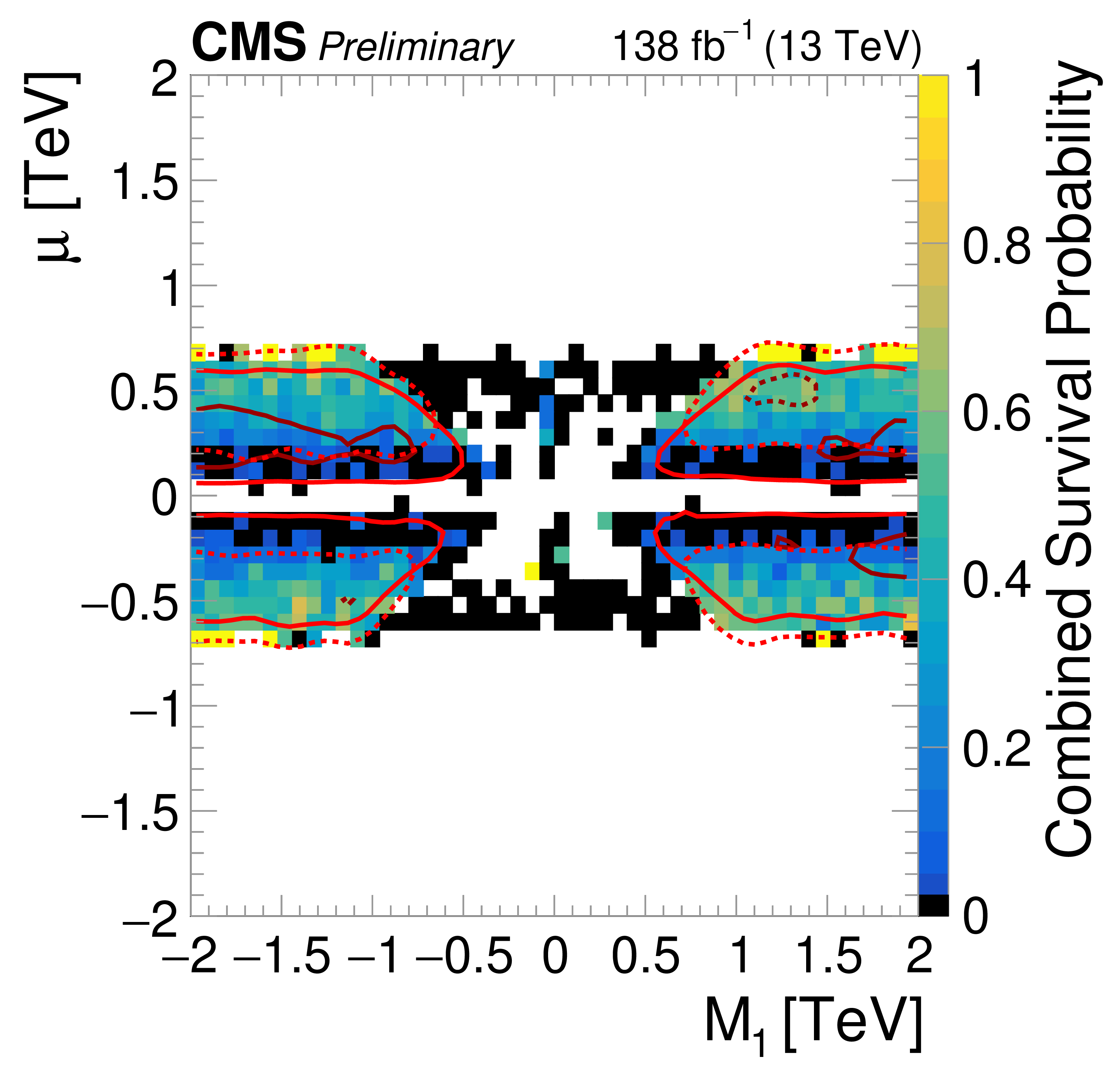
png pdf |
Additional Figure 6-d:
Survival probability based on the full scan (left), based on the subset of the scan respecting dark-matter constraints (center), and based on the natural dark-matter subset (right), as a function of representative pMSSM Lagrangian parameters. Black indicates bins where no pMSSM points survived the CMS analyses, and white indicates bins where no pMSSM points are present in the prior (May 2026 update of PAS Fig. 6). |

png pdf |
Additional Figure 6-e:
Survival probability based on the full scan (left), based on the subset of the scan respecting dark-matter constraints (center), and based on the natural dark-matter subset (right), as a function of representative pMSSM Lagrangian parameters. Black indicates bins where no pMSSM points survived the CMS analyses, and white indicates bins where no pMSSM points are present in the prior (May 2026 update of PAS Fig. 6). |
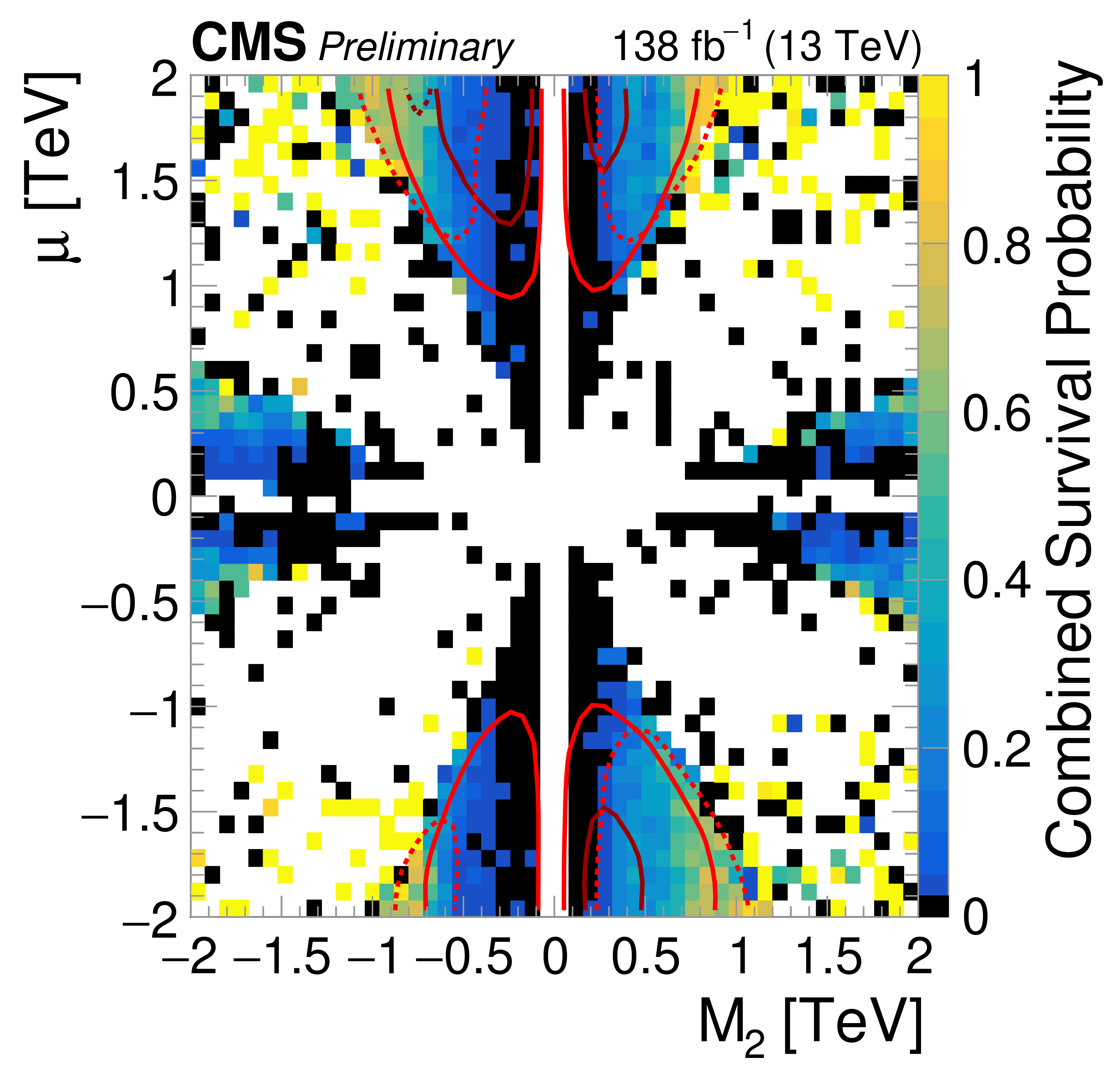
png pdf |
Additional Figure 6-f:
Survival probability based on the full scan (left), based on the subset of the scan respecting dark-matter constraints (center), and based on the natural dark-matter subset (right), as a function of representative pMSSM Lagrangian parameters. Black indicates bins where no pMSSM points survived the CMS analyses, and white indicates bins where no pMSSM points are present in the prior (May 2026 update of PAS Fig. 6). |

png pdf |
Additional Figure 6-g:
Survival probability based on the full scan (left), based on the subset of the scan respecting dark-matter constraints (center), and based on the natural dark-matter subset (right), as a function of representative pMSSM Lagrangian parameters. Black indicates bins where no pMSSM points survived the CMS analyses, and white indicates bins where no pMSSM points are present in the prior (May 2026 update of PAS Fig. 6). |
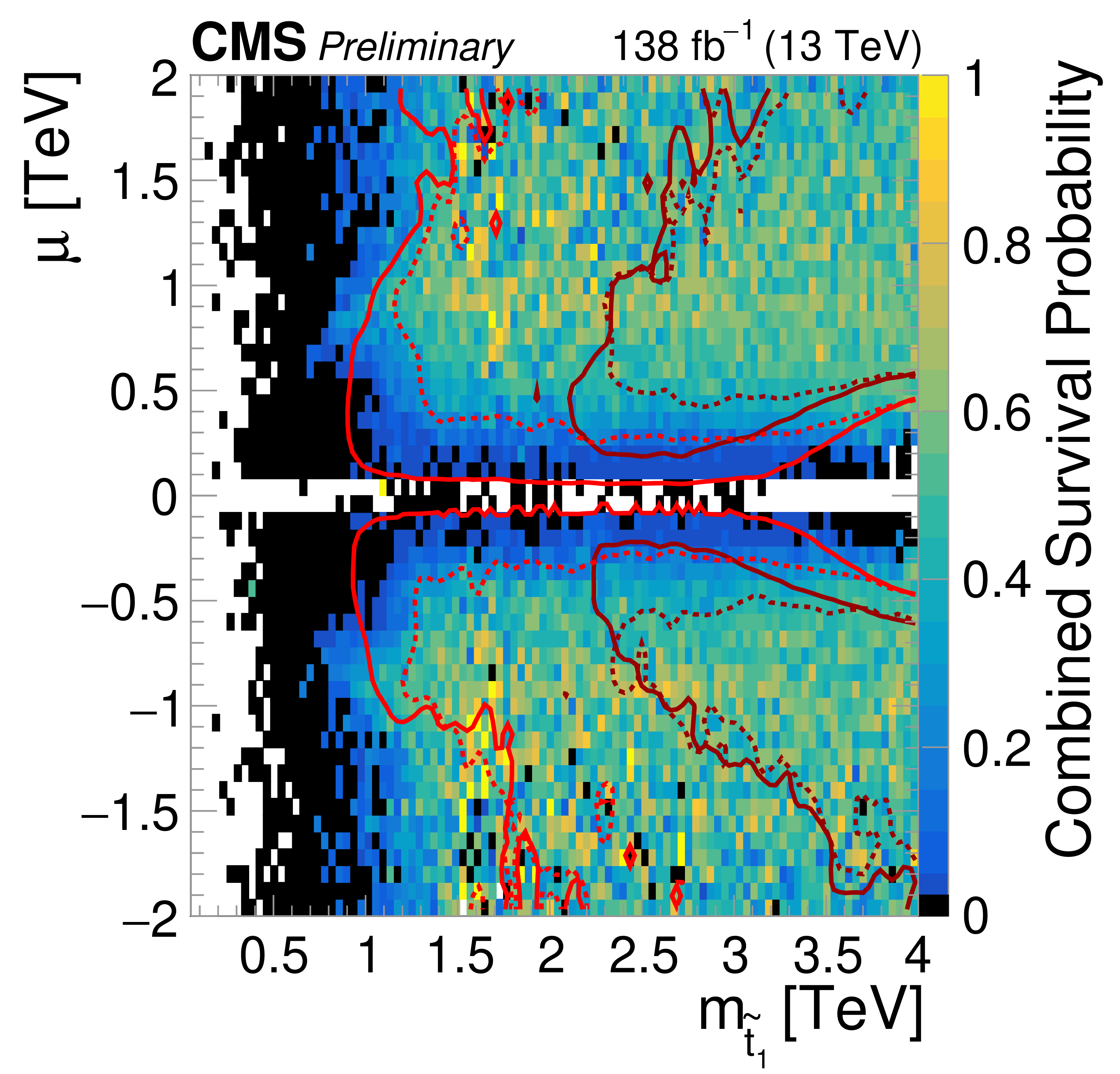
png pdf |
Additional Figure 6-h:
Survival probability based on the full scan (left), based on the subset of the scan respecting dark-matter constraints (center), and based on the natural dark-matter subset (right), as a function of representative pMSSM Lagrangian parameters. Black indicates bins where no pMSSM points survived the CMS analyses, and white indicates bins where no pMSSM points are present in the prior (May 2026 update of PAS Fig. 6). |

png pdf |
Additional Figure 6-i:
Survival probability based on the full scan (left), based on the subset of the scan respecting dark-matter constraints (center), and based on the natural dark-matter subset (right), as a function of representative pMSSM Lagrangian parameters. Black indicates bins where no pMSSM points survived the CMS analyses, and white indicates bins where no pMSSM points are present in the prior (May 2026 update of PAS Fig. 6). |
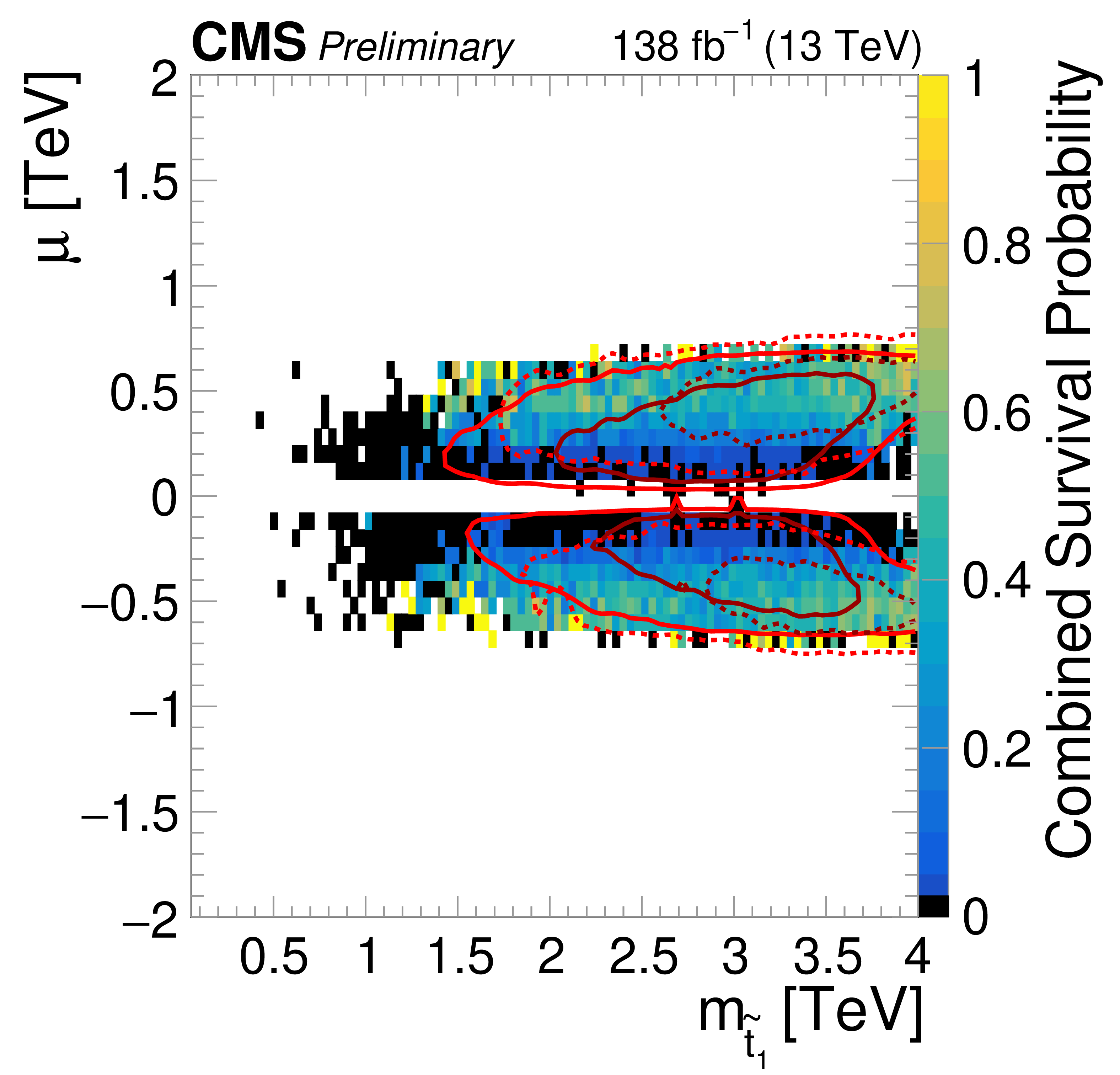
png pdf |
Additional Figure 6-j:
Survival probability based on the full scan (left), based on the subset of the scan respecting dark-matter constraints (center), and based on the natural dark-matter subset (right), as a function of representative pMSSM Lagrangian parameters. Black indicates bins where no pMSSM points survived the CMS analyses, and white indicates bins where no pMSSM points are present in the prior (May 2026 update of PAS Fig. 6). |

png pdf |
Additional Figure 6-k:
Survival probability based on the full scan (left), based on the subset of the scan respecting dark-matter constraints (center), and based on the natural dark-matter subset (right), as a function of representative pMSSM Lagrangian parameters. Black indicates bins where no pMSSM points survived the CMS analyses, and white indicates bins where no pMSSM points are present in the prior (May 2026 update of PAS Fig. 6). |

png pdf |
Additional Figure 6-l:
Survival probability based on the full scan (left), based on the subset of the scan respecting dark-matter constraints (center), and based on the natural dark-matter subset (right), as a function of representative pMSSM Lagrangian parameters. Black indicates bins where no pMSSM points survived the CMS analyses, and white indicates bins where no pMSSM points are present in the prior (May 2026 update of PAS Fig. 6). |
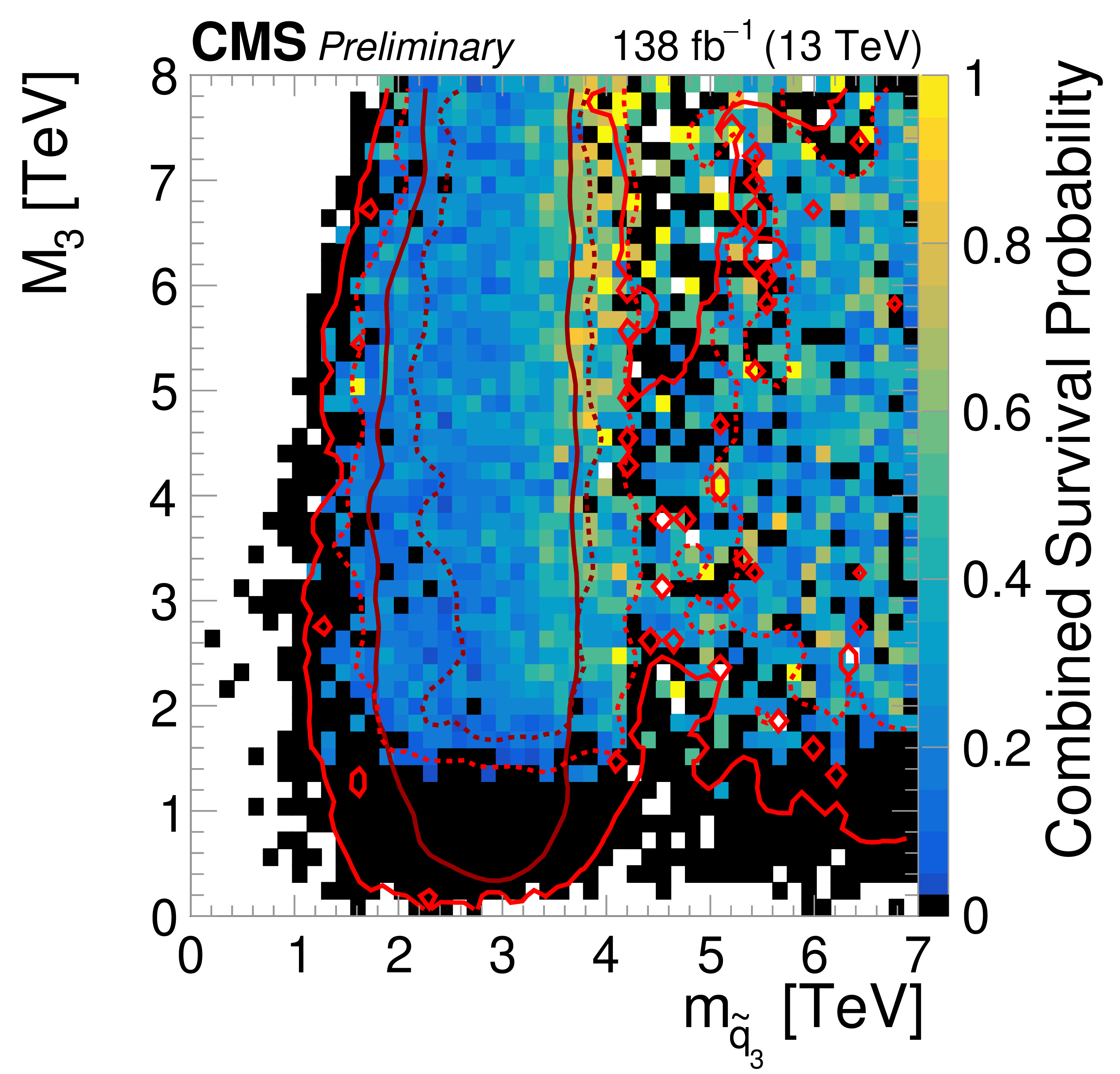
png pdf |
Additional Figure 6-m:
Survival probability based on the full scan (left), based on the subset of the scan respecting dark-matter constraints (center), and based on the natural dark-matter subset (right), as a function of representative pMSSM Lagrangian parameters. Black indicates bins where no pMSSM points survived the CMS analyses, and white indicates bins where no pMSSM points are present in the prior (May 2026 update of PAS Fig. 6). |

png pdf |
Additional Figure 7:
99% upper percentiles on the BF in bins of various projections of superpartner mass differences and the LSP mass (May 2026 update of PAS Fig. 7). |
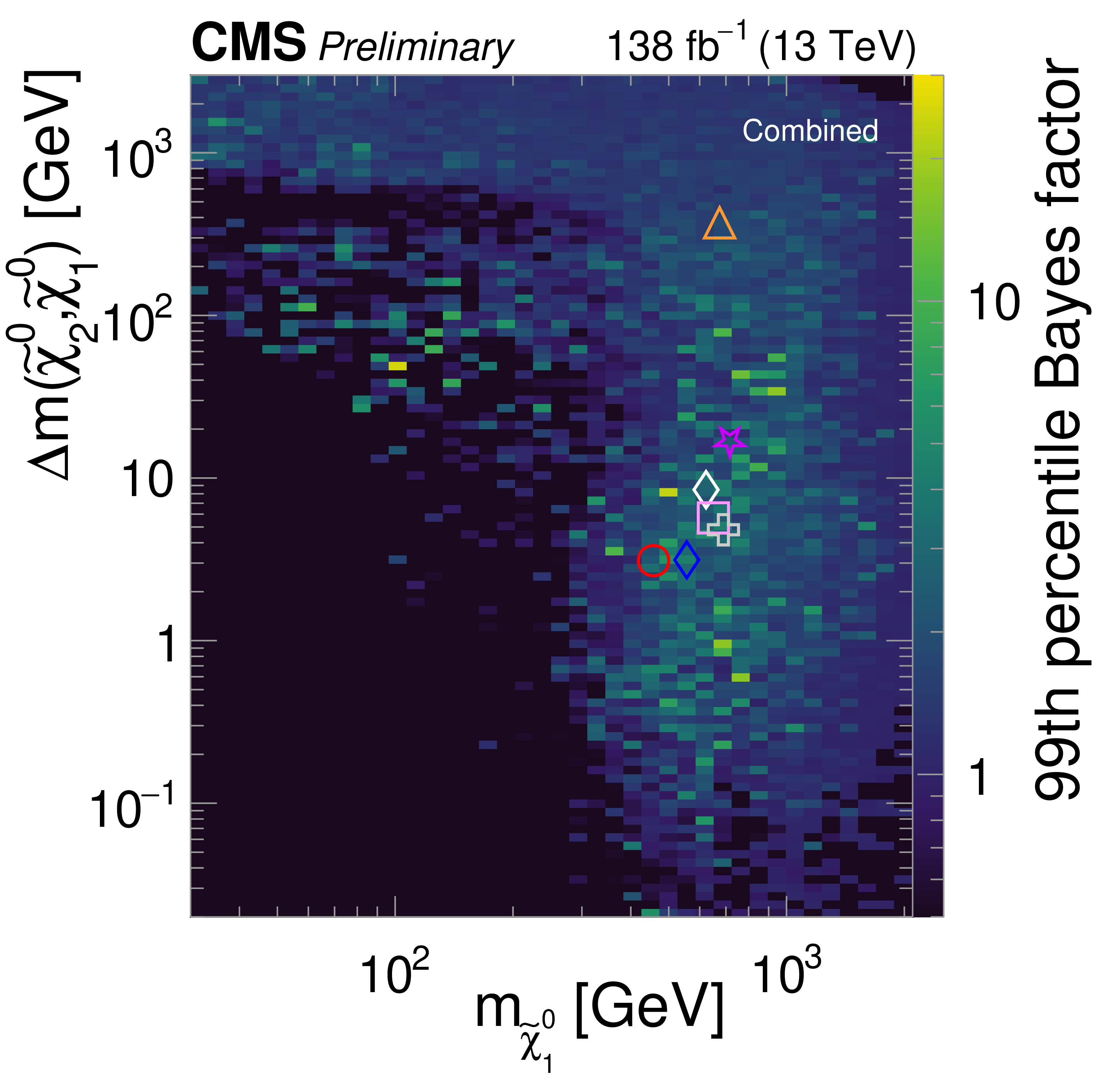
png pdf |
Additional Figure 7-a:
99% upper percentiles on the BF in bins of various projections of superpartner mass differences and the LSP mass (May 2026 update of PAS Fig. 7). |
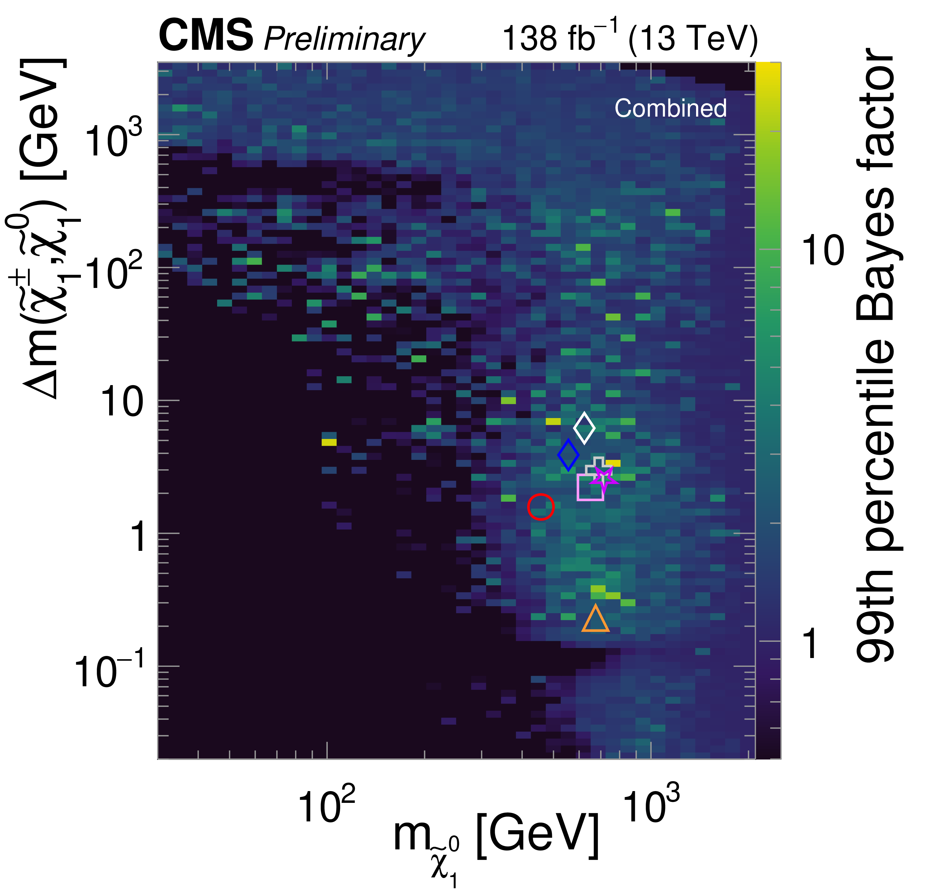
png pdf |
Additional Figure 7-b:
99% upper percentiles on the BF in bins of various projections of superpartner mass differences and the LSP mass (May 2026 update of PAS Fig. 7). |

png pdf |
Additional Figure 7-c:
99% upper percentiles on the BF in bins of various projections of superpartner mass differences and the LSP mass (May 2026 update of PAS Fig. 7). |

png pdf |
Additional Figure 7-d:
99% upper percentiles on the BF in bins of various projections of superpartner mass differences and the LSP mass (May 2026 update of PAS Fig. 7). |
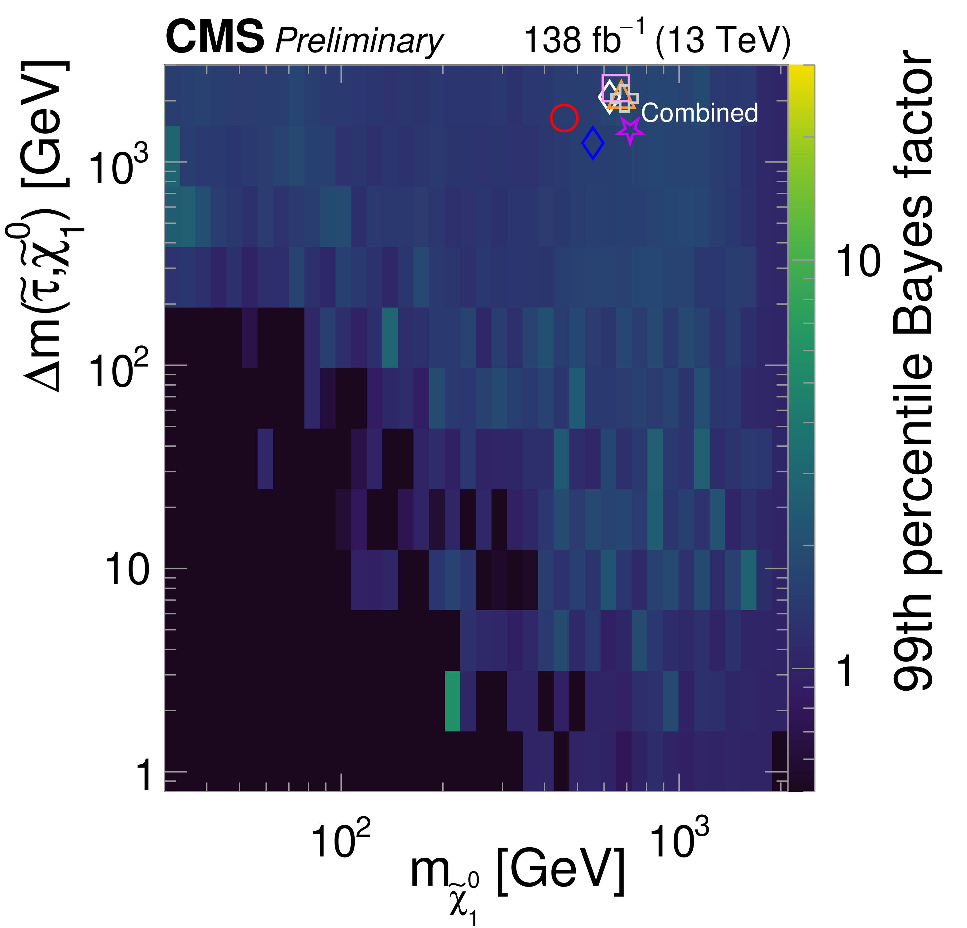
png pdf |
Additional Figure 7-e:
99% upper percentiles on the BF in bins of various projections of superpartner mass differences and the LSP mass (May 2026 update of PAS Fig. 7). |
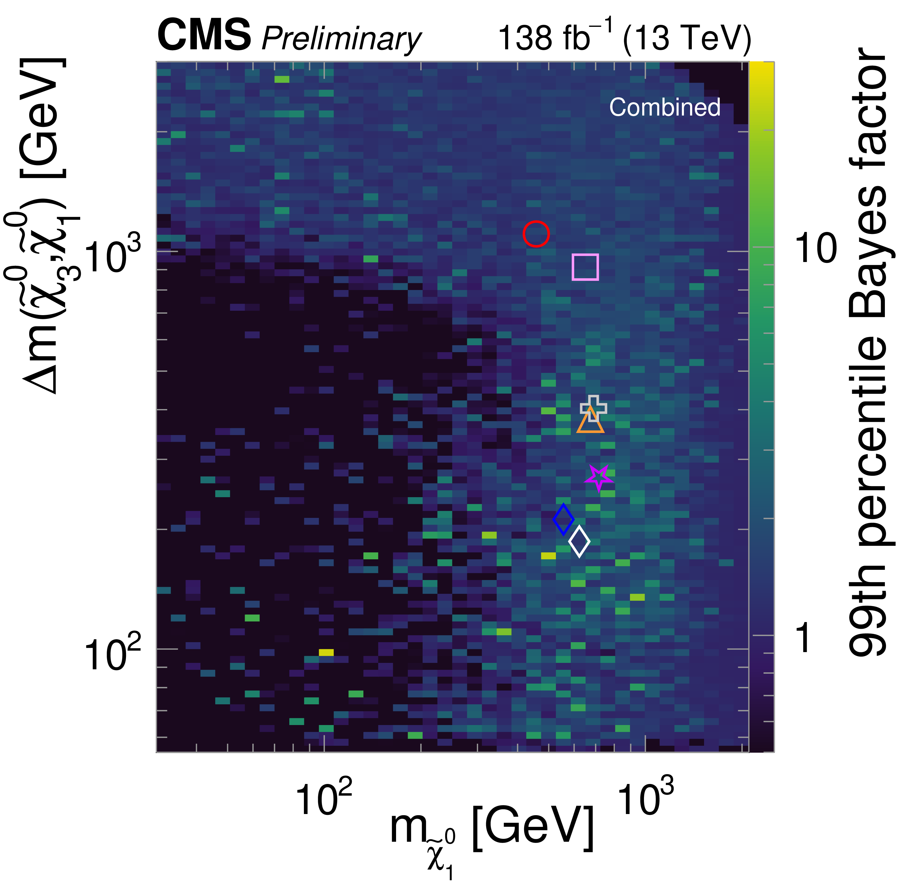
png pdf |
Additional Figure 7-f:
99% upper percentiles on the BF in bins of various projections of superpartner mass differences and the LSP mass (May 2026 update of PAS Fig. 7). |
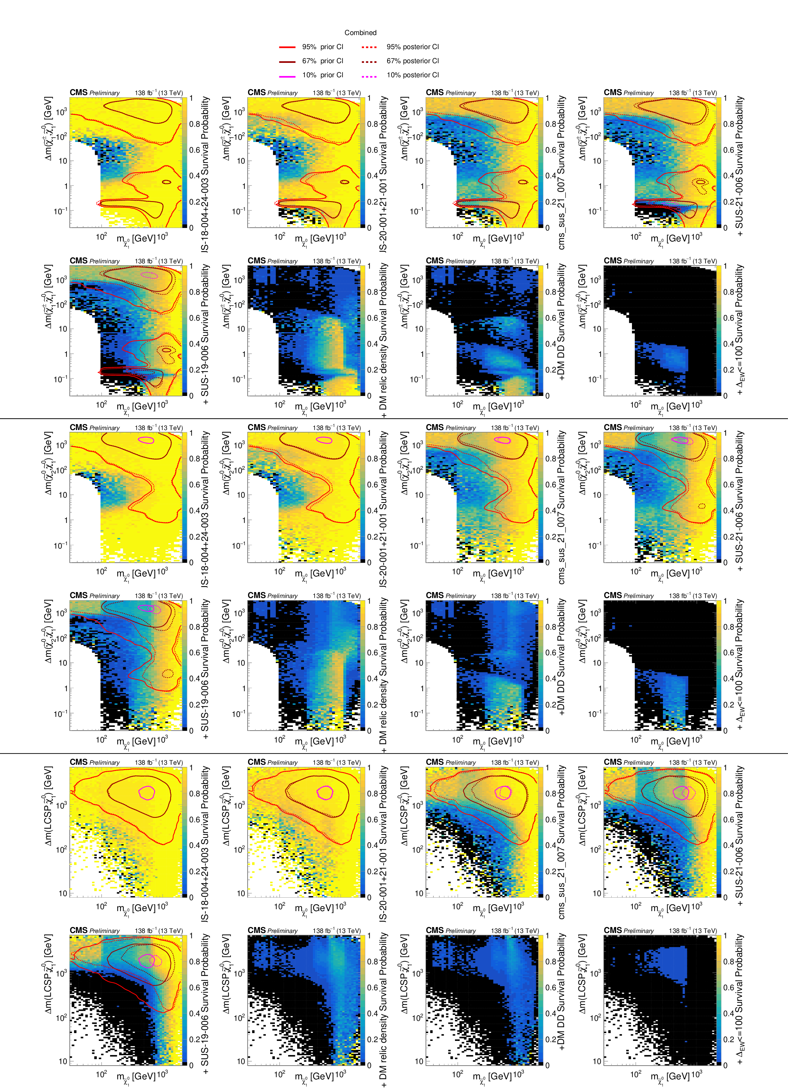
png pdf |
Additional Figure 8:
Progressive impact of individual searches on the pMSSM as a function of the LSP and mass differences between the LSP and lightest chargino (top two rows), the second-lightest neutralino (next two rows), and LCSP (bottom two rows). The order of the applied sequence of constraints, where semi-colons indicate changes in frame, is: SUS-20-001, SUS-21-001, SUS-21-007; SUS-18-004, SUS-24-003; SUS-19-006; SUS-21-006; EXO-18-002, SUS-23-002, SUS-23-014; dark-matter relic density; dark-matter direct detection; and $\Delta_{\text{EW}}<200$ (May 2026 update of PAS Fig. 9). |

png pdf |
Additional Figure 8-a:
Progressive impact of individual searches on the pMSSM as a function of the LSP and mass differences between the LSP and lightest chargino (top two rows), the second-lightest neutralino (next two rows), and LCSP (bottom two rows). The order of the applied sequence of constraints, where semi-colons indicate changes in frame, is: SUS-20-001, SUS-21-001, SUS-21-007; SUS-18-004, SUS-24-003; SUS-19-006; SUS-21-006; EXO-18-002, SUS-23-002, SUS-23-014; dark-matter relic density; dark-matter direct detection; and $\Delta_{\text{EW}}<200$ (May 2026 update of PAS Fig. 9). |
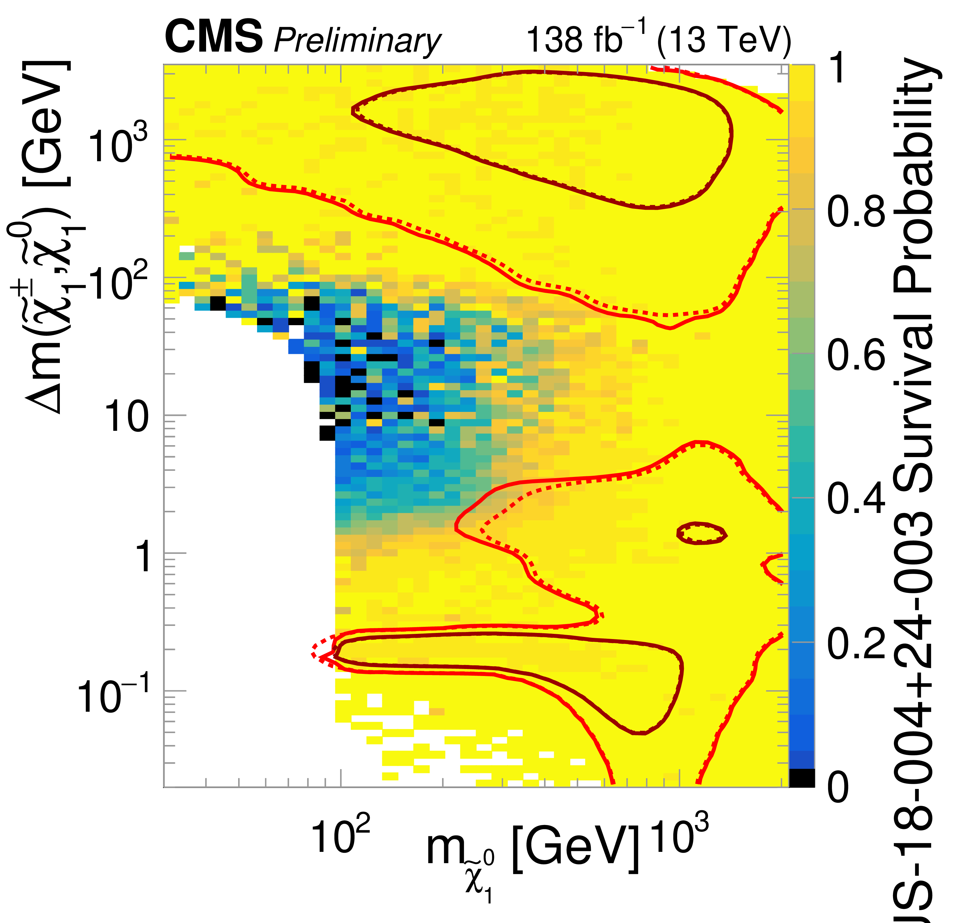
png pdf |
Additional Figure 8-b:
Progressive impact of individual searches on the pMSSM as a function of the LSP and mass differences between the LSP and lightest chargino (top two rows), the second-lightest neutralino (next two rows), and LCSP (bottom two rows). The order of the applied sequence of constraints, where semi-colons indicate changes in frame, is: SUS-20-001, SUS-21-001, SUS-21-007; SUS-18-004, SUS-24-003; SUS-19-006; SUS-21-006; EXO-18-002, SUS-23-002, SUS-23-014; dark-matter relic density; dark-matter direct detection; and $\Delta_{\text{EW}}<200$ (May 2026 update of PAS Fig. 9). |

png pdf |
Additional Figure 8-c:
Progressive impact of individual searches on the pMSSM as a function of the LSP and mass differences between the LSP and lightest chargino (top two rows), the second-lightest neutralino (next two rows), and LCSP (bottom two rows). The order of the applied sequence of constraints, where semi-colons indicate changes in frame, is: SUS-20-001, SUS-21-001, SUS-21-007; SUS-18-004, SUS-24-003; SUS-19-006; SUS-21-006; EXO-18-002, SUS-23-002, SUS-23-014; dark-matter relic density; dark-matter direct detection; and $\Delta_{\text{EW}}<200$ (May 2026 update of PAS Fig. 9). |
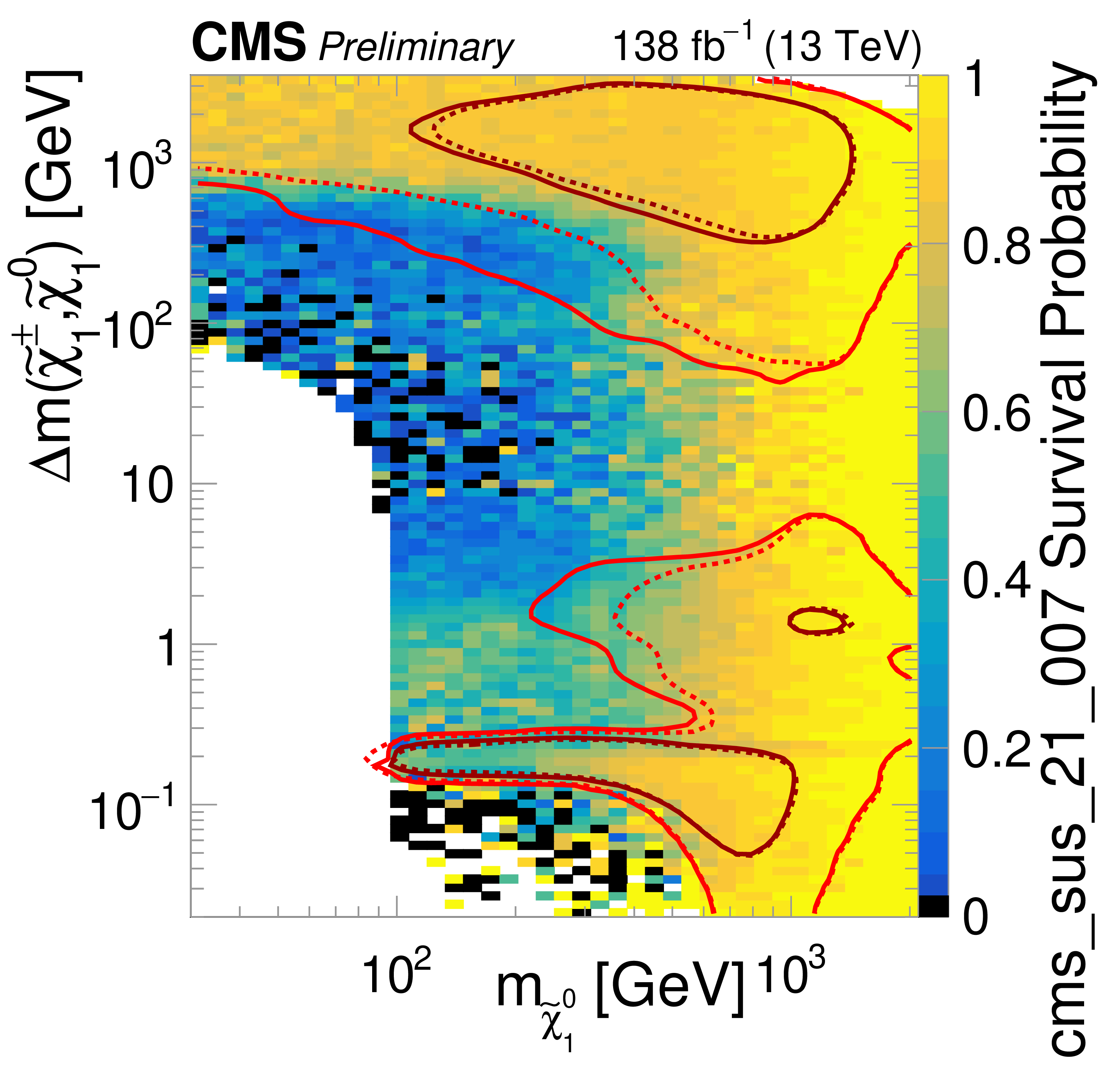
png pdf |
Additional Figure 8-d:
Progressive impact of individual searches on the pMSSM as a function of the LSP and mass differences between the LSP and lightest chargino (top two rows), the second-lightest neutralino (next two rows), and LCSP (bottom two rows). The order of the applied sequence of constraints, where semi-colons indicate changes in frame, is: SUS-20-001, SUS-21-001, SUS-21-007; SUS-18-004, SUS-24-003; SUS-19-006; SUS-21-006; EXO-18-002, SUS-23-002, SUS-23-014; dark-matter relic density; dark-matter direct detection; and $\Delta_{\text{EW}}<200$ (May 2026 update of PAS Fig. 9). |

png pdf |
Additional Figure 8-e:
Progressive impact of individual searches on the pMSSM as a function of the LSP and mass differences between the LSP and lightest chargino (top two rows), the second-lightest neutralino (next two rows), and LCSP (bottom two rows). The order of the applied sequence of constraints, where semi-colons indicate changes in frame, is: SUS-20-001, SUS-21-001, SUS-21-007; SUS-18-004, SUS-24-003; SUS-19-006; SUS-21-006; EXO-18-002, SUS-23-002, SUS-23-014; dark-matter relic density; dark-matter direct detection; and $\Delta_{\text{EW}}<200$ (May 2026 update of PAS Fig. 9). |

png pdf |
Additional Figure 8-f:
Progressive impact of individual searches on the pMSSM as a function of the LSP and mass differences between the LSP and lightest chargino (top two rows), the second-lightest neutralino (next two rows), and LCSP (bottom two rows). The order of the applied sequence of constraints, where semi-colons indicate changes in frame, is: SUS-20-001, SUS-21-001, SUS-21-007; SUS-18-004, SUS-24-003; SUS-19-006; SUS-21-006; EXO-18-002, SUS-23-002, SUS-23-014; dark-matter relic density; dark-matter direct detection; and $\Delta_{\text{EW}}<200$ (May 2026 update of PAS Fig. 9). |

png pdf |
Additional Figure 8-g:
Progressive impact of individual searches on the pMSSM as a function of the LSP and mass differences between the LSP and lightest chargino (top two rows), the second-lightest neutralino (next two rows), and LCSP (bottom two rows). The order of the applied sequence of constraints, where semi-colons indicate changes in frame, is: SUS-20-001, SUS-21-001, SUS-21-007; SUS-18-004, SUS-24-003; SUS-19-006; SUS-21-006; EXO-18-002, SUS-23-002, SUS-23-014; dark-matter relic density; dark-matter direct detection; and $\Delta_{\text{EW}}<200$ (May 2026 update of PAS Fig. 9). |
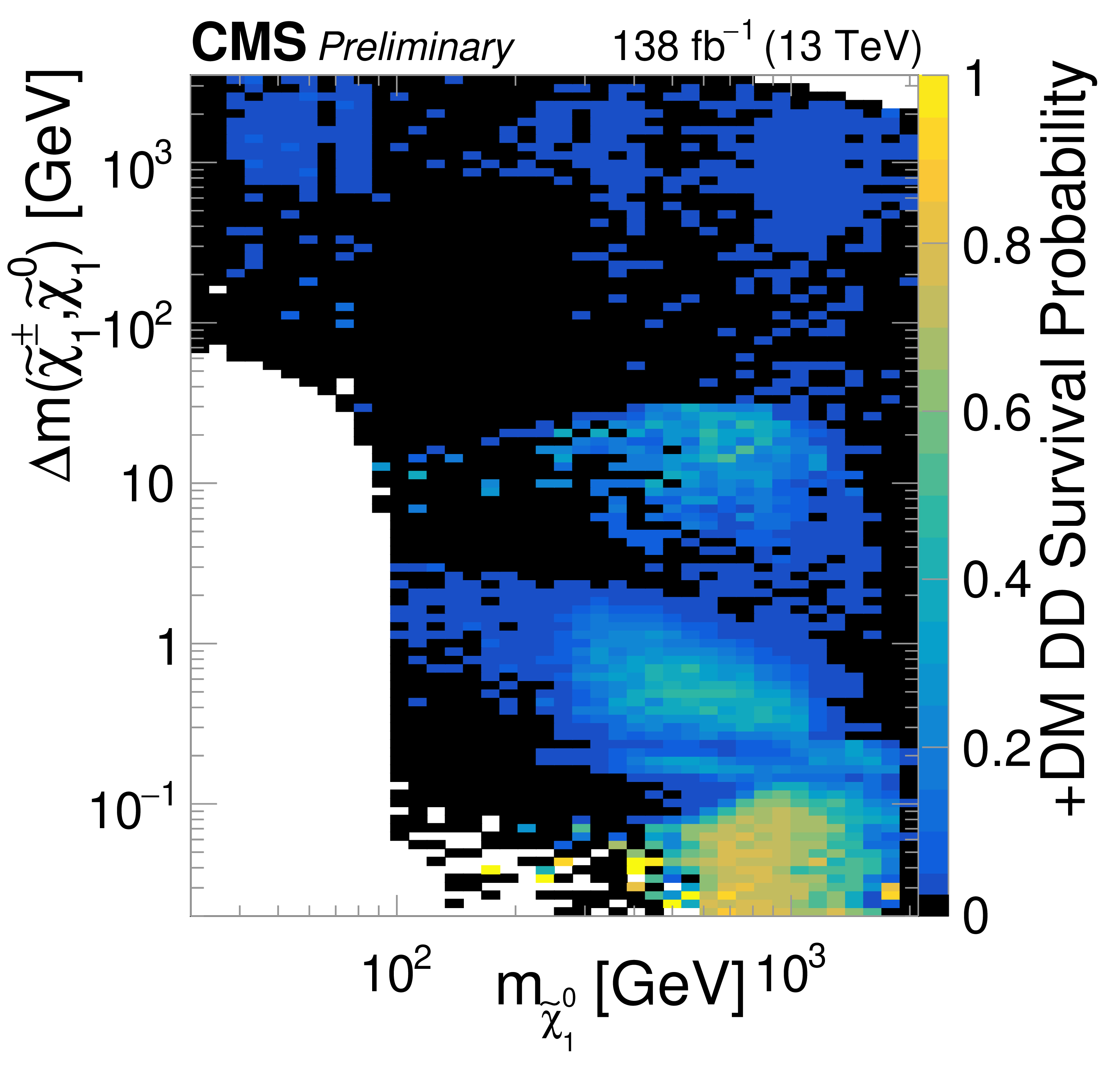
png pdf |
Additional Figure 8-h:
Progressive impact of individual searches on the pMSSM as a function of the LSP and mass differences between the LSP and lightest chargino (top two rows), the second-lightest neutralino (next two rows), and LCSP (bottom two rows). The order of the applied sequence of constraints, where semi-colons indicate changes in frame, is: SUS-20-001, SUS-21-001, SUS-21-007; SUS-18-004, SUS-24-003; SUS-19-006; SUS-21-006; EXO-18-002, SUS-23-002, SUS-23-014; dark-matter relic density; dark-matter direct detection; and $\Delta_{\text{EW}}<200$ (May 2026 update of PAS Fig. 9). |

png pdf |
Additional Figure 8-i:
Progressive impact of individual searches on the pMSSM as a function of the LSP and mass differences between the LSP and lightest chargino (top two rows), the second-lightest neutralino (next two rows), and LCSP (bottom two rows). The order of the applied sequence of constraints, where semi-colons indicate changes in frame, is: SUS-20-001, SUS-21-001, SUS-21-007; SUS-18-004, SUS-24-003; SUS-19-006; SUS-21-006; EXO-18-002, SUS-23-002, SUS-23-014; dark-matter relic density; dark-matter direct detection; and $\Delta_{\text{EW}}<200$ (May 2026 update of PAS Fig. 9). |
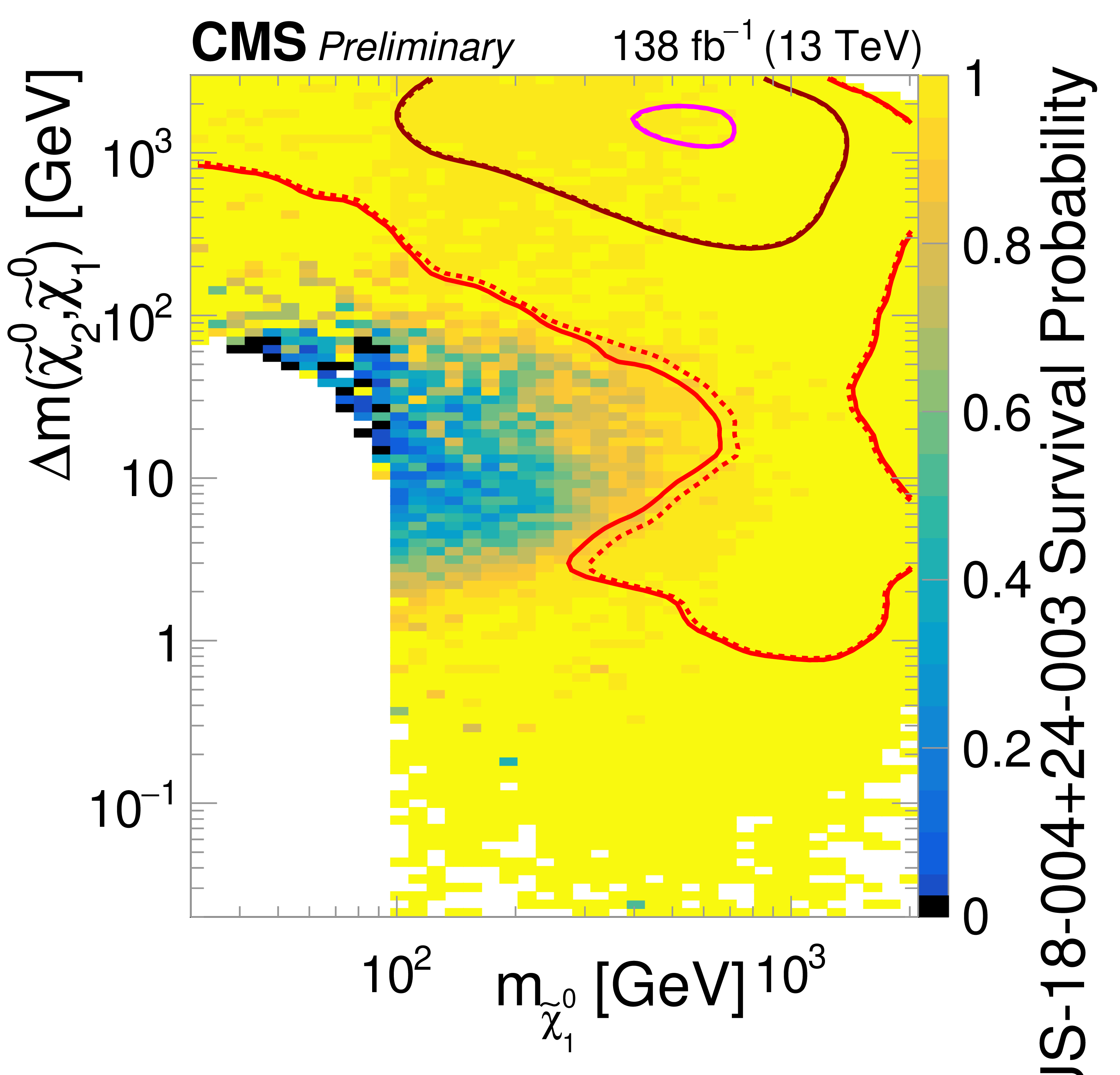
png pdf |
Additional Figure 8-j:
Progressive impact of individual searches on the pMSSM as a function of the LSP and mass differences between the LSP and lightest chargino (top two rows), the second-lightest neutralino (next two rows), and LCSP (bottom two rows). The order of the applied sequence of constraints, where semi-colons indicate changes in frame, is: SUS-20-001, SUS-21-001, SUS-21-007; SUS-18-004, SUS-24-003; SUS-19-006; SUS-21-006; EXO-18-002, SUS-23-002, SUS-23-014; dark-matter relic density; dark-matter direct detection; and $\Delta_{\text{EW}}<200$ (May 2026 update of PAS Fig. 9). |

png pdf |
Additional Figure 8-k:
Progressive impact of individual searches on the pMSSM as a function of the LSP and mass differences between the LSP and lightest chargino (top two rows), the second-lightest neutralino (next two rows), and LCSP (bottom two rows). The order of the applied sequence of constraints, where semi-colons indicate changes in frame, is: SUS-20-001, SUS-21-001, SUS-21-007; SUS-18-004, SUS-24-003; SUS-19-006; SUS-21-006; EXO-18-002, SUS-23-002, SUS-23-014; dark-matter relic density; dark-matter direct detection; and $\Delta_{\text{EW}}<200$ (May 2026 update of PAS Fig. 9). |

png pdf |
Additional Figure 8-l:
Progressive impact of individual searches on the pMSSM as a function of the LSP and mass differences between the LSP and lightest chargino (top two rows), the second-lightest neutralino (next two rows), and LCSP (bottom two rows). The order of the applied sequence of constraints, where semi-colons indicate changes in frame, is: SUS-20-001, SUS-21-001, SUS-21-007; SUS-18-004, SUS-24-003; SUS-19-006; SUS-21-006; EXO-18-002, SUS-23-002, SUS-23-014; dark-matter relic density; dark-matter direct detection; and $\Delta_{\text{EW}}<200$ (May 2026 update of PAS Fig. 9). |
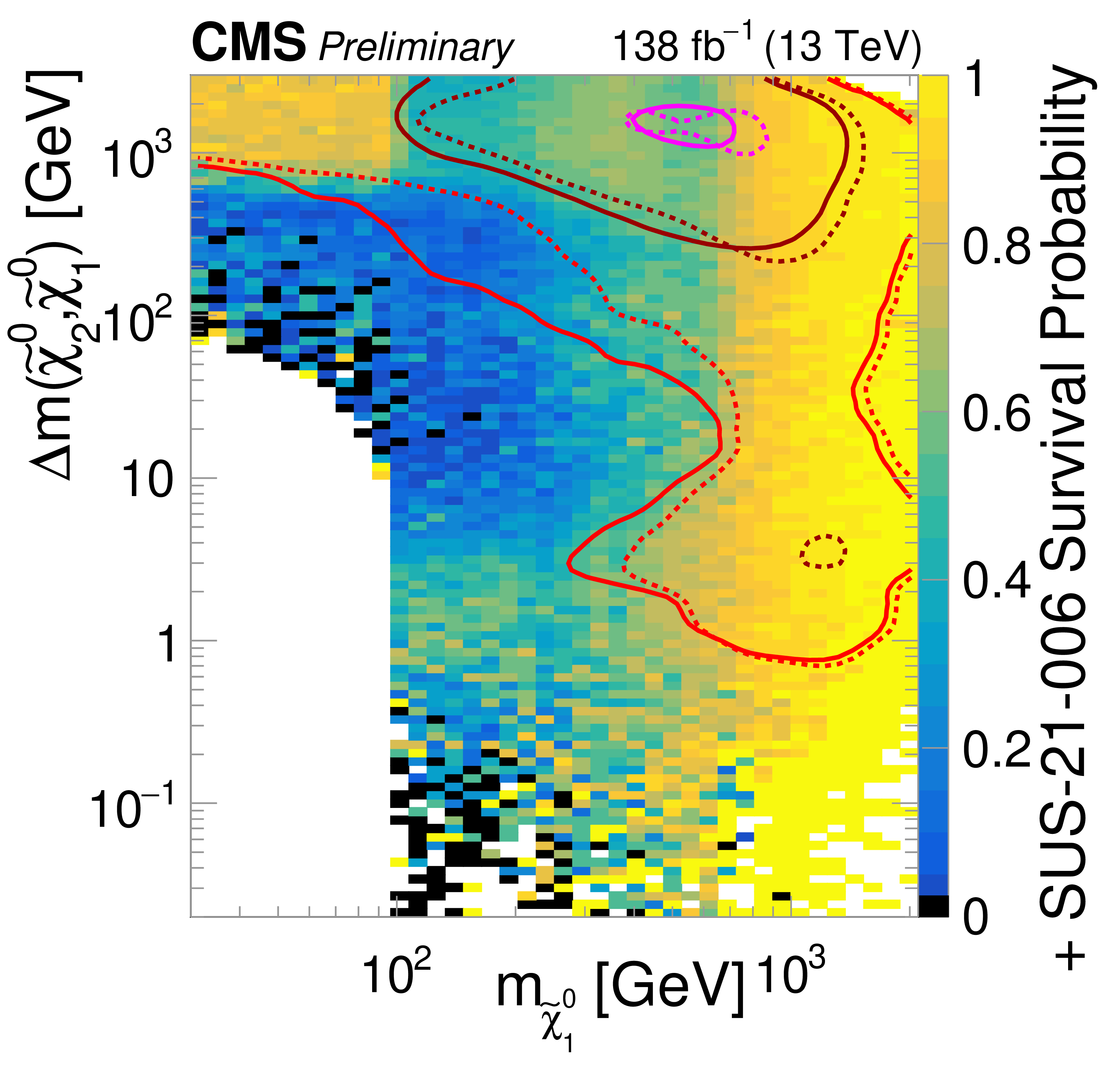
png pdf |
Additional Figure 8-m:
Progressive impact of individual searches on the pMSSM as a function of the LSP and mass differences between the LSP and lightest chargino (top two rows), the second-lightest neutralino (next two rows), and LCSP (bottom two rows). The order of the applied sequence of constraints, where semi-colons indicate changes in frame, is: SUS-20-001, SUS-21-001, SUS-21-007; SUS-18-004, SUS-24-003; SUS-19-006; SUS-21-006; EXO-18-002, SUS-23-002, SUS-23-014; dark-matter relic density; dark-matter direct detection; and $\Delta_{\text{EW}}<200$ (May 2026 update of PAS Fig. 9). |

png pdf |
Additional Figure 8-n:
Progressive impact of individual searches on the pMSSM as a function of the LSP and mass differences between the LSP and lightest chargino (top two rows), the second-lightest neutralino (next two rows), and LCSP (bottom two rows). The order of the applied sequence of constraints, where semi-colons indicate changes in frame, is: SUS-20-001, SUS-21-001, SUS-21-007; SUS-18-004, SUS-24-003; SUS-19-006; SUS-21-006; EXO-18-002, SUS-23-002, SUS-23-014; dark-matter relic density; dark-matter direct detection; and $\Delta_{\text{EW}}<200$ (May 2026 update of PAS Fig. 9). |

png pdf |
Additional Figure 8-o:
Progressive impact of individual searches on the pMSSM as a function of the LSP and mass differences between the LSP and lightest chargino (top two rows), the second-lightest neutralino (next two rows), and LCSP (bottom two rows). The order of the applied sequence of constraints, where semi-colons indicate changes in frame, is: SUS-20-001, SUS-21-001, SUS-21-007; SUS-18-004, SUS-24-003; SUS-19-006; SUS-21-006; EXO-18-002, SUS-23-002, SUS-23-014; dark-matter relic density; dark-matter direct detection; and $\Delta_{\text{EW}}<200$ (May 2026 update of PAS Fig. 9). |
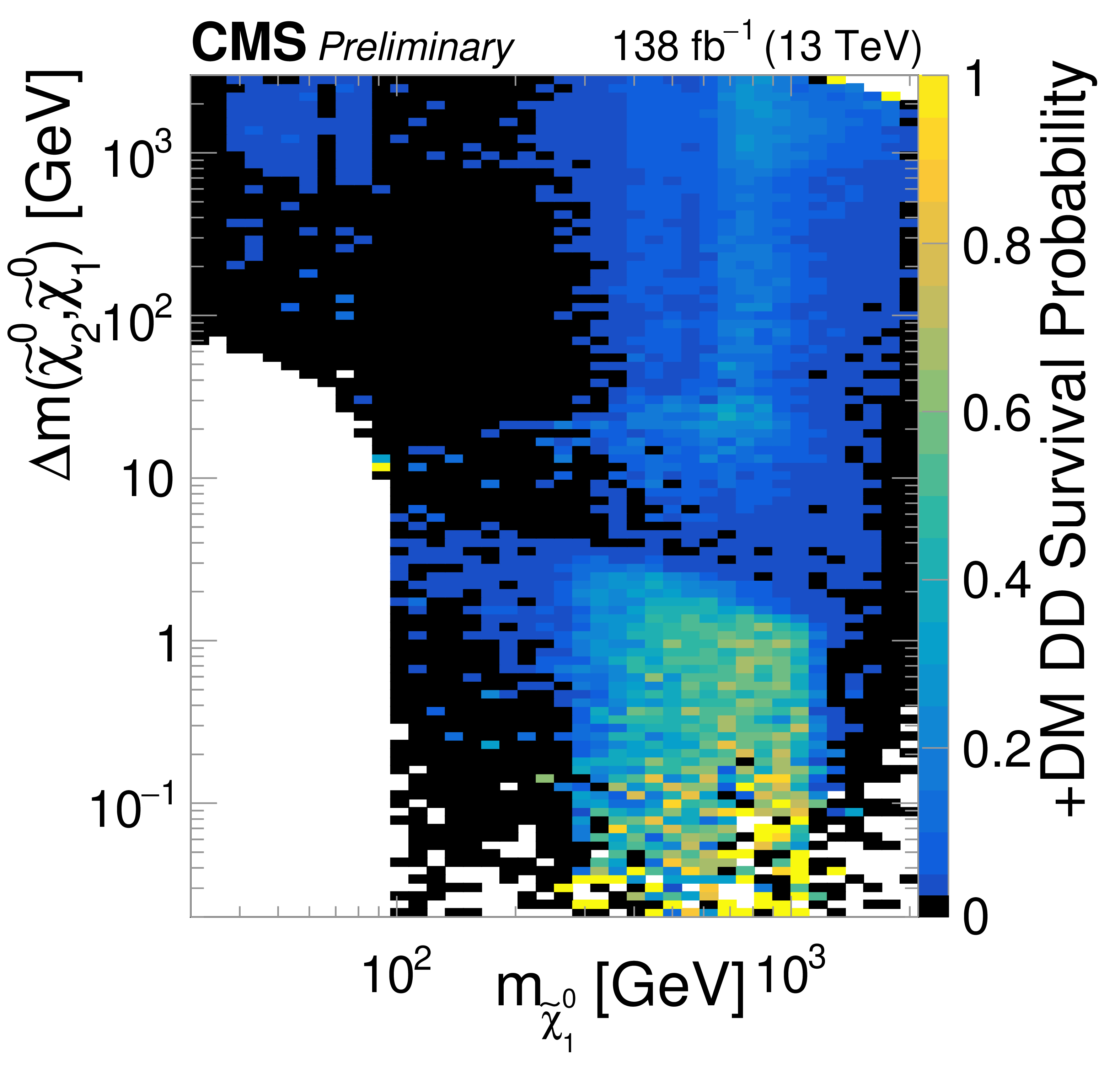
png pdf |
Additional Figure 8-p:
Progressive impact of individual searches on the pMSSM as a function of the LSP and mass differences between the LSP and lightest chargino (top two rows), the second-lightest neutralino (next two rows), and LCSP (bottom two rows). The order of the applied sequence of constraints, where semi-colons indicate changes in frame, is: SUS-20-001, SUS-21-001, SUS-21-007; SUS-18-004, SUS-24-003; SUS-19-006; SUS-21-006; EXO-18-002, SUS-23-002, SUS-23-014; dark-matter relic density; dark-matter direct detection; and $\Delta_{\text{EW}}<200$ (May 2026 update of PAS Fig. 9). |

png pdf |
Additional Figure 8-q:
Progressive impact of individual searches on the pMSSM as a function of the LSP and mass differences between the LSP and lightest chargino (top two rows), the second-lightest neutralino (next two rows), and LCSP (bottom two rows). The order of the applied sequence of constraints, where semi-colons indicate changes in frame, is: SUS-20-001, SUS-21-001, SUS-21-007; SUS-18-004, SUS-24-003; SUS-19-006; SUS-21-006; EXO-18-002, SUS-23-002, SUS-23-014; dark-matter relic density; dark-matter direct detection; and $\Delta_{\text{EW}}<200$ (May 2026 update of PAS Fig. 9). |

png pdf |
Additional Figure 8-r:
Progressive impact of individual searches on the pMSSM as a function of the LSP and mass differences between the LSP and lightest chargino (top two rows), the second-lightest neutralino (next two rows), and LCSP (bottom two rows). The order of the applied sequence of constraints, where semi-colons indicate changes in frame, is: SUS-20-001, SUS-21-001, SUS-21-007; SUS-18-004, SUS-24-003; SUS-19-006; SUS-21-006; EXO-18-002, SUS-23-002, SUS-23-014; dark-matter relic density; dark-matter direct detection; and $\Delta_{\text{EW}}<200$ (May 2026 update of PAS Fig. 9). |
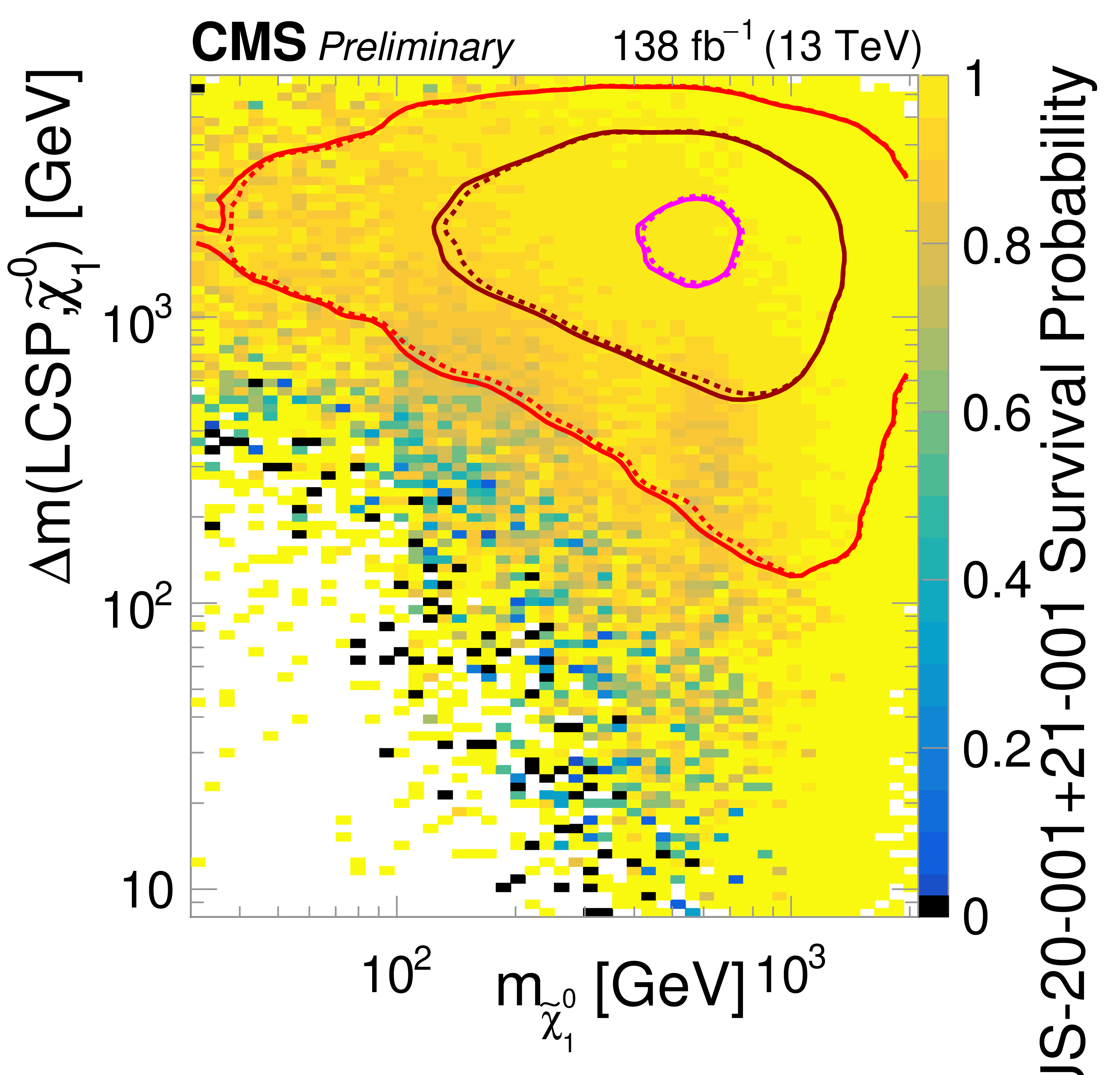
png pdf |
Additional Figure 8-s:
Progressive impact of individual searches on the pMSSM as a function of the LSP and mass differences between the LSP and lightest chargino (top two rows), the second-lightest neutralino (next two rows), and LCSP (bottom two rows). The order of the applied sequence of constraints, where semi-colons indicate changes in frame, is: SUS-20-001, SUS-21-001, SUS-21-007; SUS-18-004, SUS-24-003; SUS-19-006; SUS-21-006; EXO-18-002, SUS-23-002, SUS-23-014; dark-matter relic density; dark-matter direct detection; and $\Delta_{\text{EW}}<200$ (May 2026 update of PAS Fig. 9). |

png pdf |
Additional Figure 8-t:
Progressive impact of individual searches on the pMSSM as a function of the LSP and mass differences between the LSP and lightest chargino (top two rows), the second-lightest neutralino (next two rows), and LCSP (bottom two rows). The order of the applied sequence of constraints, where semi-colons indicate changes in frame, is: SUS-20-001, SUS-21-001, SUS-21-007; SUS-18-004, SUS-24-003; SUS-19-006; SUS-21-006; EXO-18-002, SUS-23-002, SUS-23-014; dark-matter relic density; dark-matter direct detection; and $\Delta_{\text{EW}}<200$ (May 2026 update of PAS Fig. 9). |

png pdf |
Additional Figure 8-u:
Progressive impact of individual searches on the pMSSM as a function of the LSP and mass differences between the LSP and lightest chargino (top two rows), the second-lightest neutralino (next two rows), and LCSP (bottom two rows). The order of the applied sequence of constraints, where semi-colons indicate changes in frame, is: SUS-20-001, SUS-21-001, SUS-21-007; SUS-18-004, SUS-24-003; SUS-19-006; SUS-21-006; EXO-18-002, SUS-23-002, SUS-23-014; dark-matter relic density; dark-matter direct detection; and $\Delta_{\text{EW}}<200$ (May 2026 update of PAS Fig. 9). |
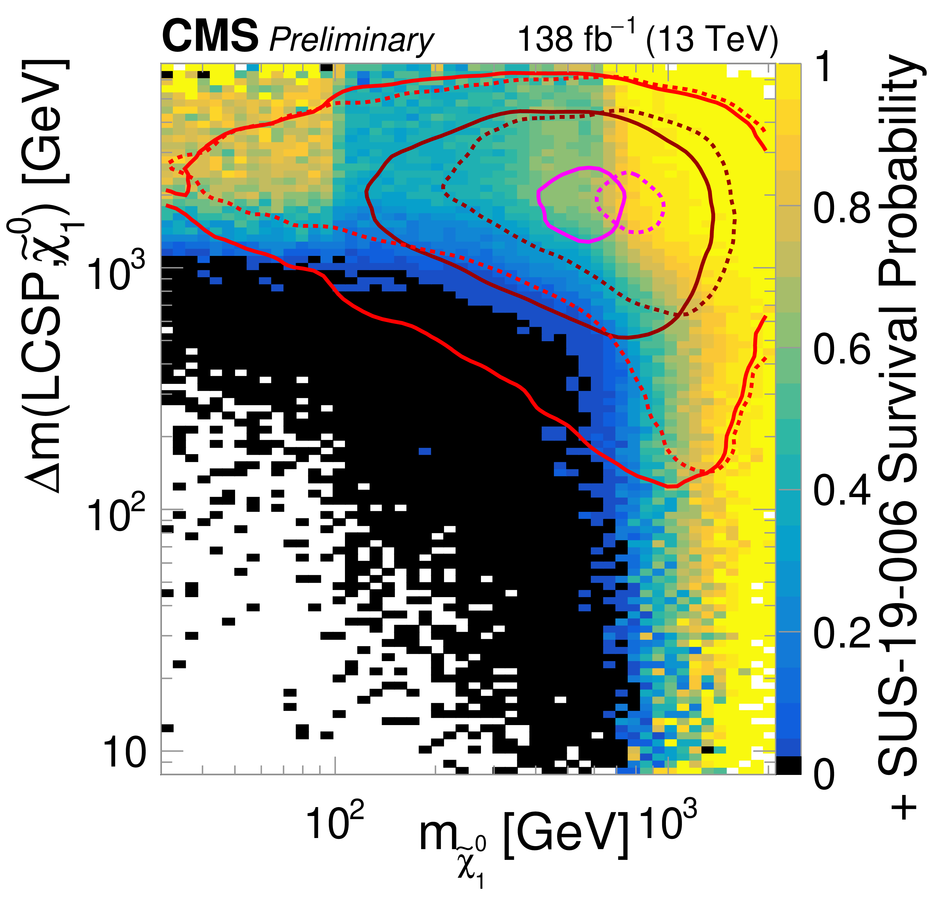
png pdf |
Additional Figure 8-v:
Progressive impact of individual searches on the pMSSM as a function of the LSP and mass differences between the LSP and lightest chargino (top two rows), the second-lightest neutralino (next two rows), and LCSP (bottom two rows). The order of the applied sequence of constraints, where semi-colons indicate changes in frame, is: SUS-20-001, SUS-21-001, SUS-21-007; SUS-18-004, SUS-24-003; SUS-19-006; SUS-21-006; EXO-18-002, SUS-23-002, SUS-23-014; dark-matter relic density; dark-matter direct detection; and $\Delta_{\text{EW}}<200$ (May 2026 update of PAS Fig. 9). |

png pdf |
Additional Figure 8-w:
Progressive impact of individual searches on the pMSSM as a function of the LSP and mass differences between the LSP and lightest chargino (top two rows), the second-lightest neutralino (next two rows), and LCSP (bottom two rows). The order of the applied sequence of constraints, where semi-colons indicate changes in frame, is: SUS-20-001, SUS-21-001, SUS-21-007; SUS-18-004, SUS-24-003; SUS-19-006; SUS-21-006; EXO-18-002, SUS-23-002, SUS-23-014; dark-matter relic density; dark-matter direct detection; and $\Delta_{\text{EW}}<200$ (May 2026 update of PAS Fig. 9). |

png pdf |
Additional Figure 8-x:
Progressive impact of individual searches on the pMSSM as a function of the LSP and mass differences between the LSP and lightest chargino (top two rows), the second-lightest neutralino (next two rows), and LCSP (bottom two rows). The order of the applied sequence of constraints, where semi-colons indicate changes in frame, is: SUS-20-001, SUS-21-001, SUS-21-007; SUS-18-004, SUS-24-003; SUS-19-006; SUS-21-006; EXO-18-002, SUS-23-002, SUS-23-014; dark-matter relic density; dark-matter direct detection; and $\Delta_{\text{EW}}<200$ (May 2026 update of PAS Fig. 9). |
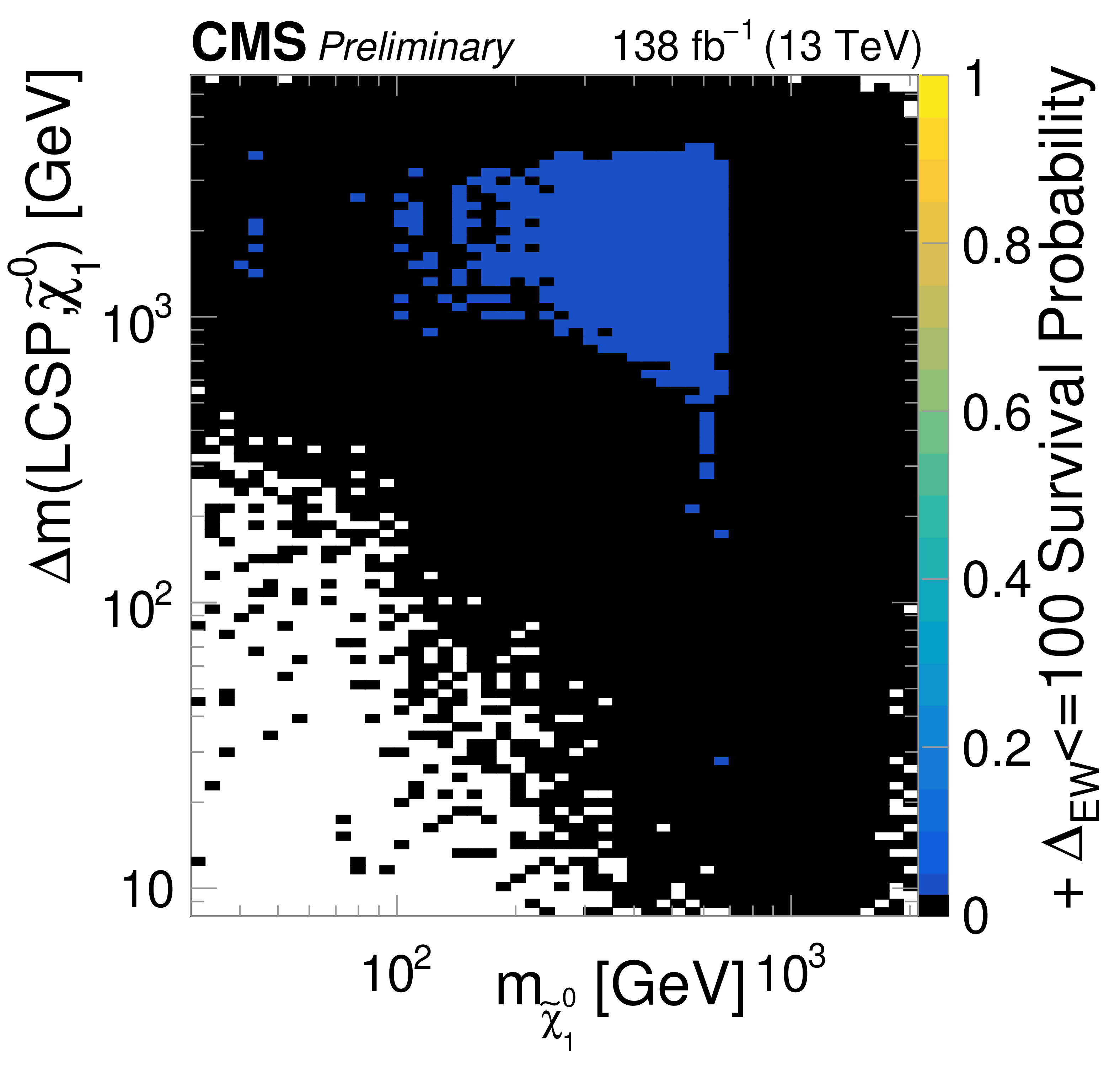
png pdf |
Additional Figure 8-y:
Progressive impact of individual searches on the pMSSM as a function of the LSP and mass differences between the LSP and lightest chargino (top two rows), the second-lightest neutralino (next two rows), and LCSP (bottom two rows). The order of the applied sequence of constraints, where semi-colons indicate changes in frame, is: SUS-20-001, SUS-21-001, SUS-21-007; SUS-18-004, SUS-24-003; SUS-19-006; SUS-21-006; EXO-18-002, SUS-23-002, SUS-23-014; dark-matter relic density; dark-matter direct detection; and $\Delta_{\text{EW}}<200$ (May 2026 update of PAS Fig. 9). |
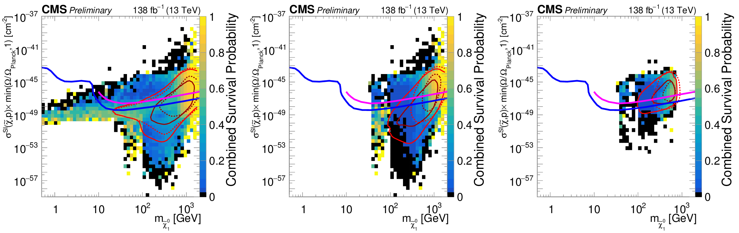
png pdf |
Additional Figure 9:
Survival probability based on the full scan (left), based on the subset of the scan respecting the relic-density upper bound (center), and based on the natural dark-matter subset (right), shown as a function of the LSP mass and the spin-independent proton scattering cross section. Black indicates bins where no pMSSM points survived the CMS analyses, and white indicates bins where no pMSSM points are present in the prior. Also shown are the latest dark-matter direct-detection limits in pink and the neutrino floor in blue (May 2026 update). |

png pdf |
Additional Figure 9-a:
Survival probability based on the full scan (left), based on the subset of the scan respecting the relic-density upper bound (center), and based on the natural dark-matter subset (right), shown as a function of the LSP mass and the spin-independent proton scattering cross section. Black indicates bins where no pMSSM points survived the CMS analyses, and white indicates bins where no pMSSM points are present in the prior. Also shown are the latest dark-matter direct-detection limits in pink and the neutrino floor in blue (May 2026 update). |
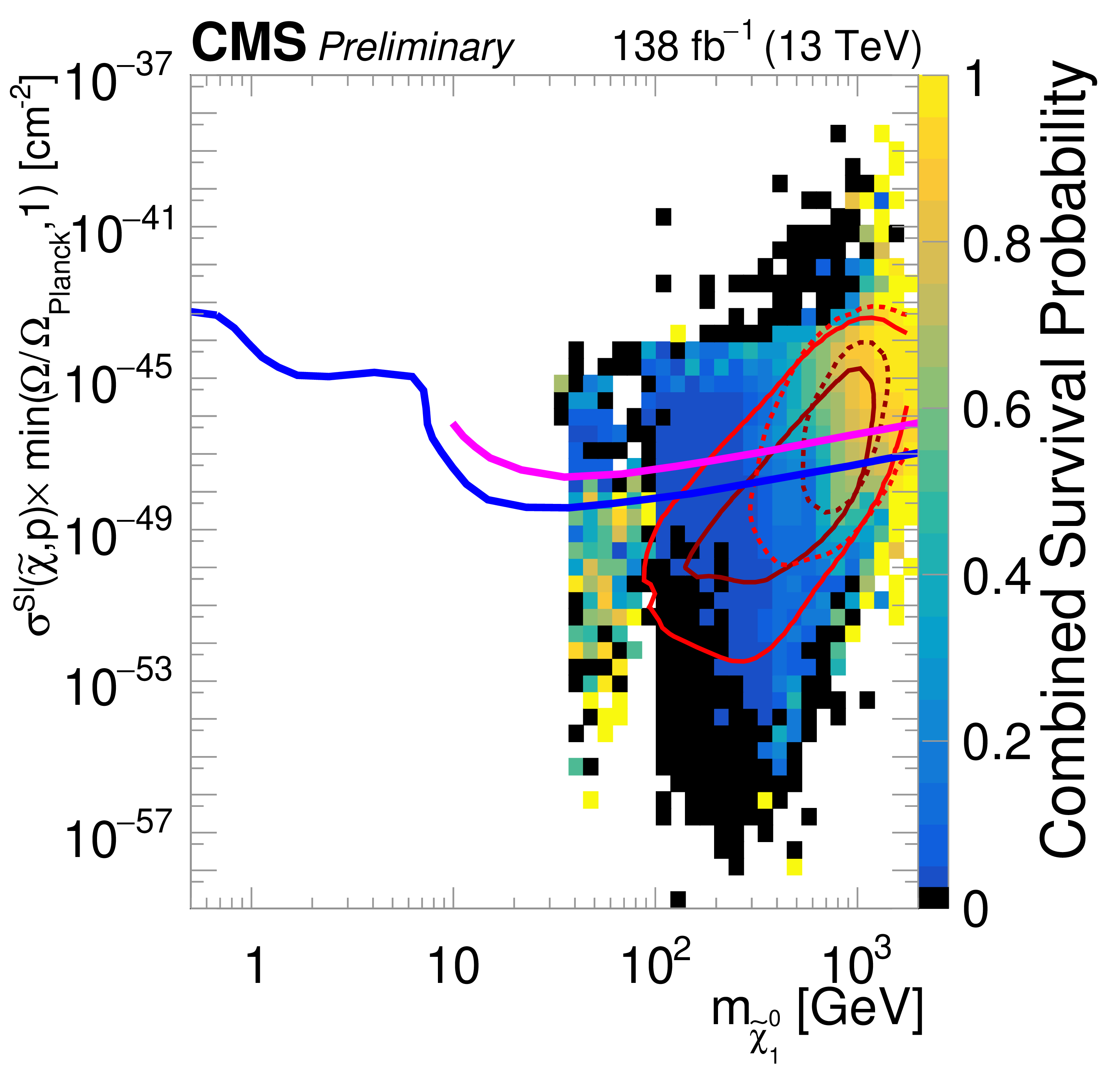
png pdf |
Additional Figure 9-b:
Survival probability based on the full scan (left), based on the subset of the scan respecting the relic-density upper bound (center), and based on the natural dark-matter subset (right), shown as a function of the LSP mass and the spin-independent proton scattering cross section. Black indicates bins where no pMSSM points survived the CMS analyses, and white indicates bins where no pMSSM points are present in the prior. Also shown are the latest dark-matter direct-detection limits in pink and the neutrino floor in blue (May 2026 update). |

png pdf |
Additional Figure 9-c:
Survival probability based on the full scan (left), based on the subset of the scan respecting the relic-density upper bound (center), and based on the natural dark-matter subset (right), shown as a function of the LSP mass and the spin-independent proton scattering cross section. Black indicates bins where no pMSSM points survived the CMS analyses, and white indicates bins where no pMSSM points are present in the prior. Also shown are the latest dark-matter direct-detection limits in pink and the neutrino floor in blue (May 2026 update). |
| References | ||||
| 1 | P. Ramond | Dual theory for free fermions | PRD 3 (1971) 2415 | |
| 2 | Y. A. Golfand and E. P. Likhtman | Extension of the algebra of poincare group generators and violation of p invariance | JETP Lett. 13 (1971) 323 | |
| 3 | D. V. Volkov and V. P. Akulov | Possible universal neutrino interaction | JETP Lett. 16 (1972) 438 | |
| 4 | J. Wess and B. Zumino | Supergauge transformations in four-dimensions | NPB 70 (1974) 39 | |
| 5 | P. Fayet | Supergauge invariant extension of the higgs mechanism and a model for the electron and its neutrino | NPB 90 (1975) 104 | |
| 6 | D. J. H. Chung et al. | The soft supersymmetry breaking lagrangian: Theory and applications | Phys. Rept. 407 (2005) 1 | hep-ph/0312378 |
| 7 | CMS Collaboration | Phenomenological MSSM interpretation of CMS searches in pp collisions at sqrt(s) = 7 and and 8 tev | JHEP 201 (2016) 6 | |
| 8 | ATLAS Collaboration | Atlas run 2 searches for electroweak production of supersymmetric particles interpreted within the pmssm | JHEP 05 (2024) 106 | 2402.01392 |
| 9 | M. Donadoni et al. | Scalable atlas pmssm computational workflows using containerised reana reusable analysis platform | EPJ Web Conf. 295 (2024) 04035 | 2403.03494 |
| 10 | A. Djouadi et al. | The minimal supersymmetric standard model: Group summary report | MSSM Working Group, in GDR (Groupement de recherche), 1998 | hep-ph/9901246 |
| 11 | W. K. Hastings | Monte carlo sampling methods using markov chains and their applications | Biometrika 57 (1970) 97 | |
| 12 | W. Porod | Spheno, a program for calculating supersymmetric spectra, susy particle decays and susy particle production at e+ e- colliders | Comput. Phys. Commun. 153 (2003) 275 | hep-ph/0301101 |
| 13 | W. Porod and F. Staub | Spheno 3.1: Extensions including flavour, cp-phases and models beyond the mssm | Comput. Phys. Commun. 183 (2012) 2458 | 1104.1573 |
| 14 | H. Bahl et al. | Precision calculations in the mssm higgs-boson sector with feynhiggs 2.14 | Comput. Phys. Commun. 249 (2020) 107099 | 1811.09073 |
| 15 | H. Bahl et al. | Reconciling EFT and hybrid calculations of the light MSSM higgs-boson mass | EPJC 78 (2018) | |
| 16 | H. Bahl and W. Hollik | Precise prediction for the light MSSM higgs-boson mass combining effective field theory and fixed-order calculations | EPJC 76 (2016) | |
| 17 | T. Hahn et al. | High-precision predictions for the light cp-even higgs boson mass of the minimal supersymmetric standard model | PRL 112 (2014) | |
| 18 | M. Frank et al. | The higgs boson masses and mixings of the complex MSSM in the feynman-diagrammatic approach | JHEP 047 (2007) | |
| 19 | G. Degrassi et al. | Towards high-precision predictions for the MSSM higgs sector | EPJC 28 (2003) | |
| 20 | S. Heinemeyer et al. | The masses of the neutral cp-even higgs bosons in the MSSM: Accurate analysis at the two-loop level | EPJC 9 (1999) 343 | |
| 21 | S. Heinemeyer et al. | FeynHiggs: a program for the calculation of the masses of the neutral cp-even higgs bosons in the MSSM | Computer Physics Communications 124 (2000) 76 | |
| 22 | H. Bahl et al. | Theoretical uncertainties in the MSSM higgs boson mass calculation | EPJC 80 (2020) | |
| 23 | CMS Collaboration | A portrait of the higgs boson by the cms experiment ten years after the discovery. | Nature 607 (2022) 60 | CMS-HIG-22-001 2207.00043 |
| 24 | G. Bélanger et al. | Recasting direct detection limits within micrOMEGAs and implication for non-standard dark matter scenarios | EPJC 81 (2021) | |
| 25 | F. Mahmoudi | Superiso v2.3: A program for calculating flavor physics observables in supersymmetry | Comput. Phys. Commun. 180 (2009) 1579 | 0808.3144 |
| 26 | HFLAV Collaboration, E. Barberio et al. | Averages of $ b- $hadron and $ c- $hadron Properties at the End of 2007 | 0808.1297 | |
| 27 | CMS Collaboration | Measurement of the $ B^0_s \to \mu^+ \mu^- $ branching fraction and search for $ B^0 \to \mu^+ \mu^- $ with the CMS experiment | PRL 111 (2013) 101804 | CMS-BPH-13-004 1307.5025 |
| 28 | LHCb Collaboration | Measurement of the $ B^0_s \to \mu^+ \mu^- $ branching fraction and search for $ B^0 \to \mu^+ \mu^- $ decays at the LHCb experiment | PRL 111 (2013) 101805 | 1307.5024 |
| 29 | CMS and LHCb Collaboration | Combination of results on the rare decays $ B^0_{(s)} \to \mu^+\mu^- $ from the CMS and LHCb experiments | Technical report, CERN, Geneva, 2013 | |
| 30 | Belle Collaboration | Improved measurement of the electroweak penguin process $ B \to X_s \ell^+ \ell^- $ | PRD 72 (2005) 092005 | hep-ex/0503044 |
| 31 | BaBar Collaboration | Measurement of the $ B \to X_s \ell^+ \ell^- $ branching fraction and search for direct cp violation from a sum of exclusive final states | PRL 112 (2014) 211802 | 1312.5364 |
| 32 | LHCb Collaboration | Measurement of form-factor-independent observables in the decay $ B^{0} \to K^{*0} \mu^+ \mu^- $ | PRL 111 (2013) 191801 | 1308.1707 |
| 33 | HFLAV Collaboration | Averages of B-Hadron, C-Hadron, and tau-lepton properties as of early 2012 | 1207.1158 | |
| 34 | B. Aubert et al. | Measurement of branching fractions and cp and isospin asymmetries in $ B \to K^{*} \gamma $ | BaBar Collaboration, in 34th International Conference on High Energy Physics. 8, 2008 | 0808.1915 |
| 35 | Belle Collaboration | Measurement of the $ B \to K^* \gamma $ branching fractions and asymmetries | PRD 69 (2004) 112001 | hep-ex/0402042 |
| 36 | Particle Data Group Collaboration | Review of particle physics | Chinese Physics C 38 (2014) 090001 | |
| 37 | Y. Amhis et al. | Averages of $ b $-hadron, $ c $-hadron, and $ \tau $-lepton properties as of 2021 | We are using the tables from May for this work, 2023 PRD 107 (2023) 052008 |
2206.07501 |
| 38 | Particle Data Group Collaboration | Review of particle physics | PRD 98 (2018) 030001 | |
| 39 | P. Z. Skands et al. | Susy les houches accord: Interfacing susy spectrum calculators, decay packages, and event generators | JHEP 07 (2004) 036 | hep-ph/0311123 |
| 40 | H. Baer et al. | Electroweak versus high scale finetuning in the 19-parameter sugra model | PRD 88 (2013) 055026 | 1304.6732 |
| 41 | Planck Collaboration | Planck 2018 results - vi. cosmological parameters | A&A 641 (2020) A6 | |
| 42 | T. Sjöstrand et al. | An introduction to PYTHIA 8.2 | Comput. Phys. Commun. 191 (2015) 159 | 1410.3012 |
| 43 | CMS Collaboration | The fast simulation of the CMS detector at LHC | Journal of Physics: Conference Series 331 (2011) 032049 | |
| 44 | CMS Collaboration | Search for supersymmetry in final states with two or three soft leptons and missing transverse momentum in proton-proton collisions at $\sqrt{s} =$ 13 TeV | JHEP 2204 (2022) 91 | CMS-SUS-18-004 2111.06296 |
| 45 | CMS Collaboration | Search for electroweak production of charginos and neutralinos in proton-proton collisions at $\sqrt{s} =$ 13 TeV | JHEP 04 (2022) 147 | CMS-SUS-19-012 2106.14246 |
| 46 | CMS Collaboration | Search for supersymmetry in proton-proton collisions at 13 TeV in final states with jets and missing transverse momentum | JHEP 10 (2019) 244 | |
| 47 | CMS Collaboration | Search for supersymmetry in final states with two oppositely charged same-flavor leptons and missing transverse momentum in proton-proton collisions at $\sqrt{s} = $ 13 TeV | JHEP 04 (2021) 123 | CMS-SUS-20-001 2012.08600 |
| 48 | CMS Collaboration | Search for supersymmetry in final states with disappearing tracks in proton-proton collisions at $\sqrt{s} =$ 13 TeV | CMS-SUS-21-006 2309.16823 |
|
| 49 | CMS Collaboration | Search for supersymmetry in final states with a single electron or muon using angular correlations and heavy-object identification in proton-proton collisions at $\sqrt{s} =$ 13 TeV | JHEP 09 (2023) 149 | CMS-SUS-21-007 2211.08476 |
| 50 | S. S. Wilks | The large-sample distribution of the likelihood ratio for testing composite hypotheses | The Annals of Mathematical Statistics 9 (1938) 60 | |
| 51 | LZ Collaboration | First dark matter search results from the Lux-Zeplin (LZ) experiment | PRL 131 (2023) 041002 | 2207.03764 |
|
|
Compact Muon Solenoid LHC, CERN |
|

|

|

|

|

|