

Compact Muon Solenoid
LHC, CERN
| CMS-PAS-SUS-17-002 | ||
| Search for supersymmetry in events with tau leptons and missing transverse momentum in proton-proton collisions at $\sqrt{s}= $ 13 TeV | ||
| CMS Collaboration | ||
| December 2017 | ||
| Abstract: A search for supersymmetry is performed using events with $\tau$ leptons in the final state with 13 TeV data recorded in 2016, corresponding to an integrated luminosity of 35.9 fb$^{-1}$. Models of direct $\widetilde{\tau}$-pair production, where each $\widetilde{\tau}$ is expected to decay to a $\tau$ lepton and the lightest supersymmetric particle, the $\widetilde{\chi}^{0}_1$, as well as neutralino-chargino and chargino pair production with decays to $\tau$ leptons are investigated. Several exclusive search regions are defined to maximize the sensitivity to various new physics topologies, based on final states with one hadronically decaying $\tau$ lepton and an electron or muon from the decay of the second $\tau$, as well as final states with one electron and one muon from the decay of the $\tau$ leptons. The data are consistent with the standard model expectation, and 95% CL limits are set for several scenarios. For neutralino-chargino production with mass-degenerate chargino ($\widetilde{\chi}^{\pm}_1$) or neutralino ($\widetilde{\chi}^{0}_2$), exclusion limits on the $\widetilde{\chi}^{\pm}_1$ and $\widetilde{\chi}^{0}_2$ masses can reach up to 560 GeV, depending on the masses of the intermediate $\widetilde{\tau}$ and the $\widetilde{\chi}^{0}_1$. The upper limit on cross section times the square of the branching fraction for direct $\widetilde{\tau}$-pair production is set to be 0.66 pb for a $\widetilde{\tau}$ mass of 90 GeV and a $\widetilde{\chi}^{0}_1$ mass of 1 GeV. | ||
| Links: CDS record (PDF) ; inSPIRE record ; CADI line (restricted) ; | ||
| Figures | |
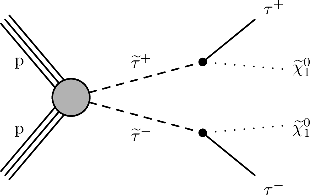
png pdf |
Figure 1-a:
Diagrams showing the investigated models for (left) direct $ \tilde{ \tau} $ -pair production and (right) $ {\tilde{\chi}^0_2} {\tilde{\chi}^{\pm}_1} $ production. |
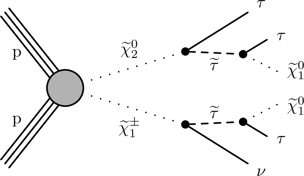
png pdf |
Figure 1-b:
Diagrams showing the investigated models for (left) direct $ \tilde{ \tau} $ -pair production and (right) $ {\tilde{\chi}^0_2} {\tilde{\chi}^{\pm}_1} $ production. |

png pdf |
Figure 2:
Relative composition of background processes to the total prediction for the (left) $ {\mathrm {e}\tau _{\mathrm h}} $, (middle) $ {\mu \tau _{\mathrm h}} $, and (right) $ {\mathrm {e}\mu} $ channel after the SR selection. |

png pdf |
Figure 2-a:
Relative composition of background processes to the total prediction for the (left) $ {\mathrm {e}\tau _{\mathrm h}} $, (middle) $ {\mu \tau _{\mathrm h}} $, and (right) $ {\mathrm {e}\mu} $ channel after the SR selection. |
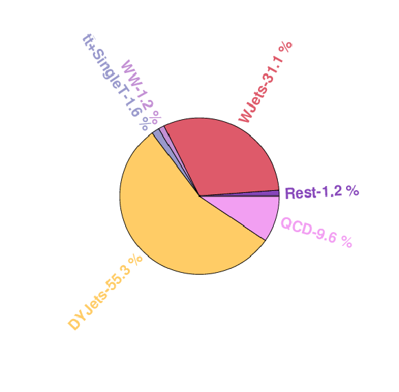
png pdf |
Figure 2-b:
Relative composition of background processes to the total prediction for the (left) $ {\mathrm {e}\tau _{\mathrm h}} $, (middle) $ {\mu \tau _{\mathrm h}} $, and (right) $ {\mathrm {e}\mu} $ channel after the SR selection. |
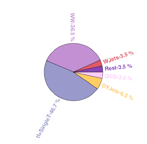
png pdf |
Figure 2-c:
Relative composition of background processes to the total prediction for the (left) $ {\mathrm {e}\tau _{\mathrm h}} $, (middle) $ {\mu \tau _{\mathrm h}} $, and (right) $ {\mathrm {e}\mu} $ channel after the SR selection. |

png pdf |
Figure 3:
Estimation of the DY+jets background: comparison of simulation to data after the shape corrections and the normalization to data. Shown are (left) the invariant di-muon mass, (middle) $ {{p_{\mathrm {T}}} ^\text {miss}} $, and (right) $\Delta R(\mu,\mu $). |
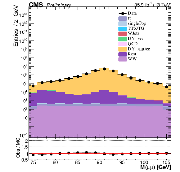
png pdf |
Figure 3-a:
Estimation of the DY+jets background: comparison of simulation to data after the shape corrections and the normalization to data. Shown are (left) the invariant di-muon mass, (middle) $ {{p_{\mathrm {T}}} ^\text {miss}} $, and (right) $\Delta R(\mu,\mu $). |
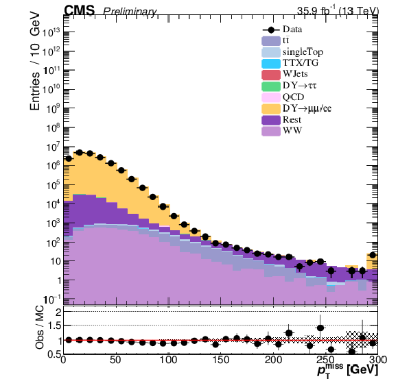
png pdf |
Figure 3-b:
Estimation of the DY+jets background: comparison of simulation to data after the shape corrections and the normalization to data. Shown are (left) the invariant di-muon mass, (middle) $ {{p_{\mathrm {T}}} ^\text {miss}} $, and (right) $\Delta R(\mu,\mu $). |
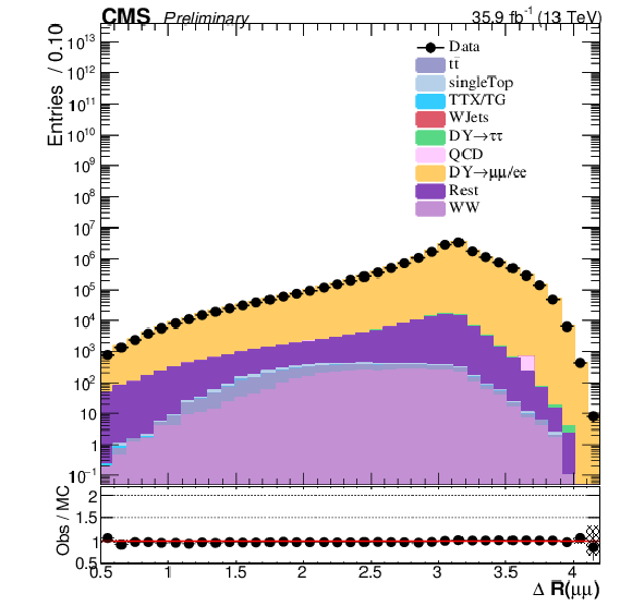
png pdf |
Figure 3-c:
Estimation of the DY+jets background: comparison of simulation to data after the shape corrections and the normalization to data. Shown are (left) the invariant di-muon mass, (middle) $ {{p_{\mathrm {T}}} ^\text {miss}} $, and (right) $\Delta R(\mu,\mu $). |
png pdf |
Figure 4:
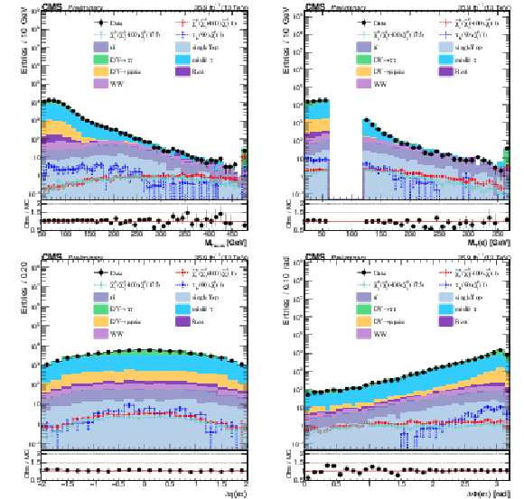
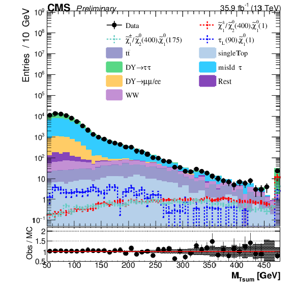
Control plots for the $ {\mathrm {e}\tau _{\mathrm h}} $ channel after the SR selection. Shown is (top left) $ {M_\mathrm {T}} _{\rm sum}$, (top right) $ {M_\mathrm {T}} $(e), (bottom left) $\Delta \eta (e,\tau)$, and (bottom right) $\Delta \mathrm{h}i (e,\tau)$. The black points show the data, the filled histograms represent the stacked SM background events, and three open histograms represent signal models (not stacked), where the numbers in the brackets represent the masses of the corresponding sparticles in GeV. |
png pdf |
Figure 4-a:
Control plots for the $ {\mathrm {e}\tau _{\mathrm h}} $ channel after the SR selection. Shown is (top left) $ {M_\mathrm {T}} _{\rm sum}$, (top right) $ {M_\mathrm {T}} $(e), (bottom left) $\Delta \eta (e,\tau)$, and (bottom right) $\Delta \mathrm{h}i (e,\tau)$. The black points show the data, the filled histograms represent the stacked SM background events, and three open histograms represent signal models (not stacked), where the numbers in the brackets represent the masses of the corresponding sparticles in GeV. |
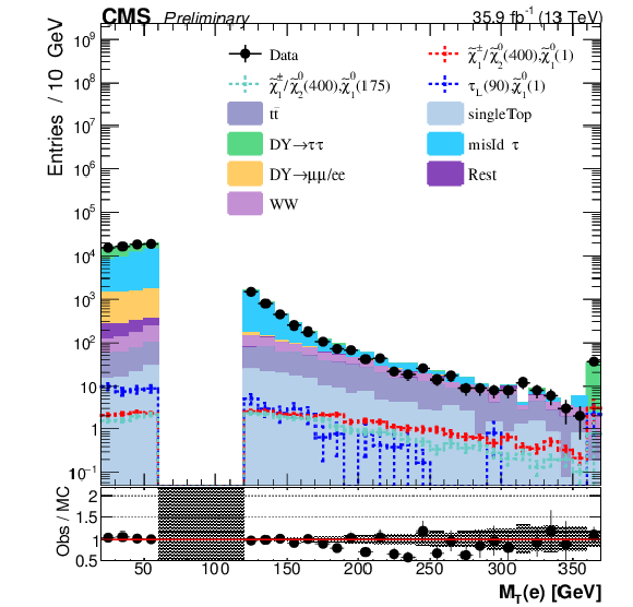
png pdf |
Figure 4-b:
Control plots for the $ {\mathrm {e}\tau _{\mathrm h}} $ channel after the SR selection. Shown is (top left) $ {M_\mathrm {T}} _{\rm sum}$, (top right) $ {M_\mathrm {T}} $(e), (bottom left) $\Delta \eta (e,\tau)$, and (bottom right) $\Delta \mathrm{h}i (e,\tau)$. The black points show the data, the filled histograms represent the stacked SM background events, and three open histograms represent signal models (not stacked), where the numbers in the brackets represent the masses of the corresponding sparticles in GeV. |
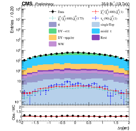
png pdf |
Figure 4-c:
Control plots for the $ {\mathrm {e}\tau _{\mathrm h}} $ channel after the SR selection. Shown is (top left) $ {M_\mathrm {T}} _{\rm sum}$, (top right) $ {M_\mathrm {T}} $(e), (bottom left) $\Delta \eta (e,\tau)$, and (bottom right) $\Delta \mathrm{h}i (e,\tau)$. The black points show the data, the filled histograms represent the stacked SM background events, and three open histograms represent signal models (not stacked), where the numbers in the brackets represent the masses of the corresponding sparticles in GeV. |
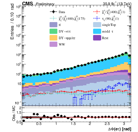
png pdf |
Figure 4-d:
Control plots for the $ {\mathrm {e}\tau _{\mathrm h}} $ channel after the SR selection. Shown is (top left) $ {M_\mathrm {T}} _{\rm sum}$, (top right) $ {M_\mathrm {T}} $(e), (bottom left) $\Delta \eta (e,\tau)$, and (bottom right) $\Delta \mathrm{h}i (e,\tau)$. The black points show the data, the filled histograms represent the stacked SM background events, and three open histograms represent signal models (not stacked), where the numbers in the brackets represent the masses of the corresponding sparticles in GeV. |
png pdf |
Figure 5:
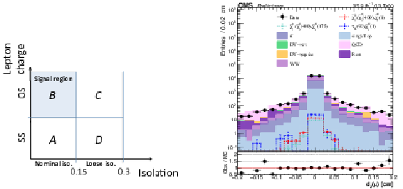
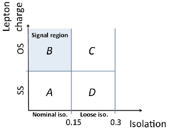
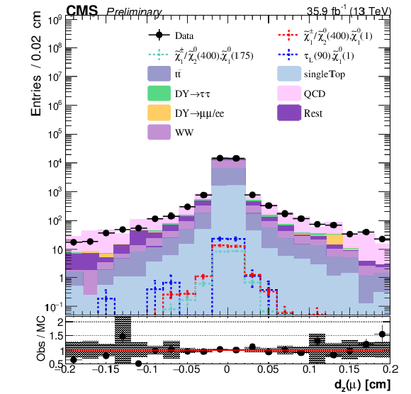
QCD multijet background estimate in the $ {\mathrm {e}\mu} $ channel: (left) sketch of the four regions used for the matrix method to determine the QCD background (relative isolation values refer to those of the $\mu $ candidate) and (right) distance of the reconstructed muon track to the primary vertex in $z$ direction ($d_z$) with the QCD multijet background determined with the matrix method from data, and with corrected simulations of the other backgrounds. The black points show the data, the filled histograms represent the stacked SM background events, and three open histograms represent signal models (not stacked), where the numbers in the brackets represent the masses of the corresponding sparticles in GeV. |
png pdf |
Figure 5-a:
QCD multijet background estimate in the $ {\mathrm {e}\mu} $ channel: (left) sketch of the four regions used for the matrix method to determine the QCD background (relative isolation values refer to those of the $\mu $ candidate) and (right) distance of the reconstructed muon track to the primary vertex in $z$ direction ($d_z$) with the QCD multijet background determined with the matrix method from data, and with corrected simulations of the other backgrounds. The black points show the data, the filled histograms represent the stacked SM background events, and three open histograms represent signal models (not stacked), where the numbers in the brackets represent the masses of the corresponding sparticles in GeV. |
png pdf |
Figure 5-b:
QCD multijet background estimate in the $ {\mathrm {e}\mu} $ channel: (left) sketch of the four regions used for the matrix method to determine the QCD background (relative isolation values refer to those of the $\mu $ candidate) and (right) distance of the reconstructed muon track to the primary vertex in $z$ direction ($d_z$) with the QCD multijet background determined with the matrix method from data, and with corrected simulations of the other backgrounds. The black points show the data, the filled histograms represent the stacked SM background events, and three open histograms represent signal models (not stacked), where the numbers in the brackets represent the masses of the corresponding sparticles in GeV. |
png pdf |
Figure 6:
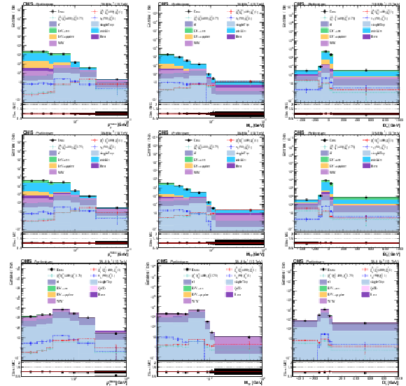
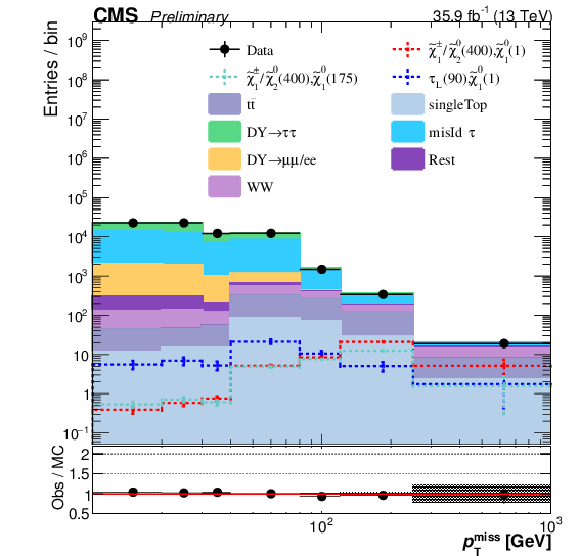
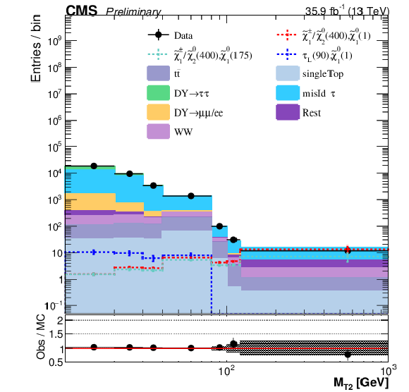
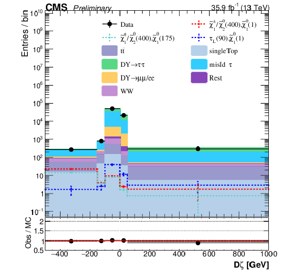
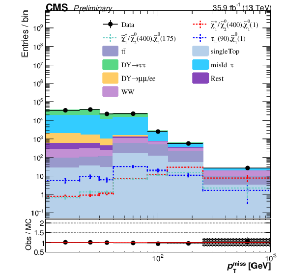
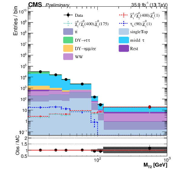
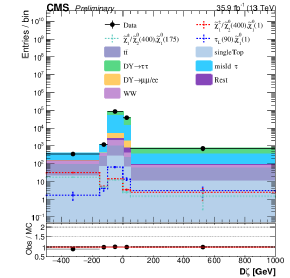
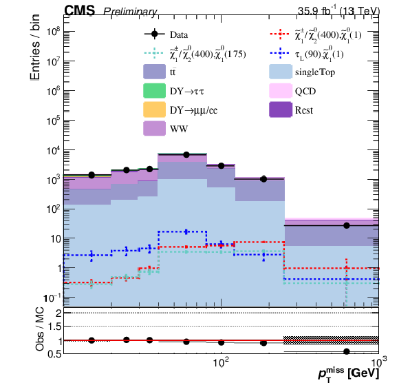
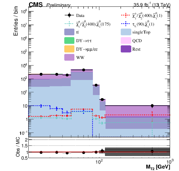
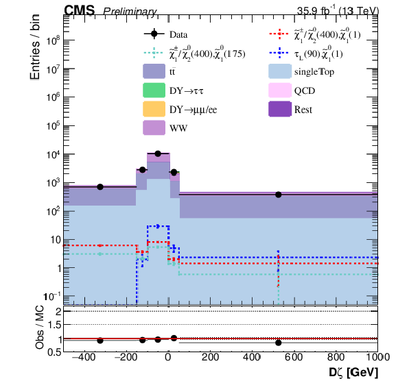
Comparison of several signals with background for the main search variables for the three different channels, (top) $ {\mathrm {e}\tau _{\mathrm h}} $, (middle) $ {\mu \tau _{\mathrm h}} $, and (bottom) $ {\mathrm {e}\mu} $ for $ {{p_{\mathrm {T}}} ^\text {miss}} $ (left column), $ {M_{\rm T2}} $ (middle column) and $ {D\zeta} $ (right column) after applying the SR selection. The black points show the data, the filled histograms represent the stacked SM background events, and three open histograms represent signal models (not stacked), where the numbers in the brackets represent the masses of the corresponding sparticles. |
png pdf |
Figure 6-a:
Comparison of several signals with background for the main search variables for the three different channels, (top) $ {\mathrm {e}\tau _{\mathrm h}} $, (middle) $ {\mu \tau _{\mathrm h}} $, and (bottom) $ {\mathrm {e}\mu} $ for $ {{p_{\mathrm {T}}} ^\text {miss}} $ (left column), $ {M_{\rm T2}} $ (middle column) and $ {D\zeta} $ (right column) after applying the SR selection. The black points show the data, the filled histograms represent the stacked SM background events, and three open histograms represent signal models (not stacked), where the numbers in the brackets represent the masses of the corresponding sparticles. |
png pdf |
Figure 6-b:
Comparison of several signals with background for the main search variables for the three different channels, (top) $ {\mathrm {e}\tau _{\mathrm h}} $, (middle) $ {\mu \tau _{\mathrm h}} $, and (bottom) $ {\mathrm {e}\mu} $ for $ {{p_{\mathrm {T}}} ^\text {miss}} $ (left column), $ {M_{\rm T2}} $ (middle column) and $ {D\zeta} $ (right column) after applying the SR selection. The black points show the data, the filled histograms represent the stacked SM background events, and three open histograms represent signal models (not stacked), where the numbers in the brackets represent the masses of the corresponding sparticles. |
png pdf |
Figure 6-c:
Comparison of several signals with background for the main search variables for the three different channels, (top) $ {\mathrm {e}\tau _{\mathrm h}} $, (middle) $ {\mu \tau _{\mathrm h}} $, and (bottom) $ {\mathrm {e}\mu} $ for $ {{p_{\mathrm {T}}} ^\text {miss}} $ (left column), $ {M_{\rm T2}} $ (middle column) and $ {D\zeta} $ (right column) after applying the SR selection. The black points show the data, the filled histograms represent the stacked SM background events, and three open histograms represent signal models (not stacked), where the numbers in the brackets represent the masses of the corresponding sparticles. |
png pdf |
Figure 6-d:
Comparison of several signals with background for the main search variables for the three different channels, (top) $ {\mathrm {e}\tau _{\mathrm h}} $, (middle) $ {\mu \tau _{\mathrm h}} $, and (bottom) $ {\mathrm {e}\mu} $ for $ {{p_{\mathrm {T}}} ^\text {miss}} $ (left column), $ {M_{\rm T2}} $ (middle column) and $ {D\zeta} $ (right column) after applying the SR selection. The black points show the data, the filled histograms represent the stacked SM background events, and three open histograms represent signal models (not stacked), where the numbers in the brackets represent the masses of the corresponding sparticles. |
png pdf |
Figure 6-e:
Comparison of several signals with background for the main search variables for the three different channels, (top) $ {\mathrm {e}\tau _{\mathrm h}} $, (middle) $ {\mu \tau _{\mathrm h}} $, and (bottom) $ {\mathrm {e}\mu} $ for $ {{p_{\mathrm {T}}} ^\text {miss}} $ (left column), $ {M_{\rm T2}} $ (middle column) and $ {D\zeta} $ (right column) after applying the SR selection. The black points show the data, the filled histograms represent the stacked SM background events, and three open histograms represent signal models (not stacked), where the numbers in the brackets represent the masses of the corresponding sparticles. |
png pdf |
Figure 6-f:
Comparison of several signals with background for the main search variables for the three different channels, (top) $ {\mathrm {e}\tau _{\mathrm h}} $, (middle) $ {\mu \tau _{\mathrm h}} $, and (bottom) $ {\mathrm {e}\mu} $ for $ {{p_{\mathrm {T}}} ^\text {miss}} $ (left column), $ {M_{\rm T2}} $ (middle column) and $ {D\zeta} $ (right column) after applying the SR selection. The black points show the data, the filled histograms represent the stacked SM background events, and three open histograms represent signal models (not stacked), where the numbers in the brackets represent the masses of the corresponding sparticles. |
png pdf |
Figure 6-g:
Comparison of several signals with background for the main search variables for the three different channels, (top) $ {\mathrm {e}\tau _{\mathrm h}} $, (middle) $ {\mu \tau _{\mathrm h}} $, and (bottom) $ {\mathrm {e}\mu} $ for $ {{p_{\mathrm {T}}} ^\text {miss}} $ (left column), $ {M_{\rm T2}} $ (middle column) and $ {D\zeta} $ (right column) after applying the SR selection. The black points show the data, the filled histograms represent the stacked SM background events, and three open histograms represent signal models (not stacked), where the numbers in the brackets represent the masses of the corresponding sparticles. |
png pdf |
Figure 6-h:
Comparison of several signals with background for the main search variables for the three different channels, (top) $ {\mathrm {e}\tau _{\mathrm h}} $, (middle) $ {\mu \tau _{\mathrm h}} $, and (bottom) $ {\mathrm {e}\mu} $ for $ {{p_{\mathrm {T}}} ^\text {miss}} $ (left column), $ {M_{\rm T2}} $ (middle column) and $ {D\zeta} $ (right column) after applying the SR selection. The black points show the data, the filled histograms represent the stacked SM background events, and three open histograms represent signal models (not stacked), where the numbers in the brackets represent the masses of the corresponding sparticles. |
png pdf |
Figure 6-i:
Comparison of several signals with background for the main search variables for the three different channels, (top) $ {\mathrm {e}\tau _{\mathrm h}} $, (middle) $ {\mu \tau _{\mathrm h}} $, and (bottom) $ {\mathrm {e}\mu} $ for $ {{p_{\mathrm {T}}} ^\text {miss}} $ (left column), $ {M_{\rm T2}} $ (middle column) and $ {D\zeta} $ (right column) after applying the SR selection. The black points show the data, the filled histograms represent the stacked SM background events, and three open histograms represent signal models (not stacked), where the numbers in the brackets represent the masses of the corresponding sparticles. |
png pdf |
Figure 7:
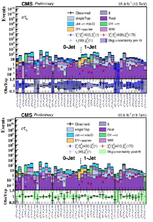
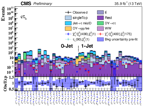
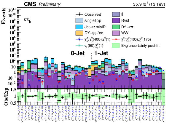
Results for the $ {\mathrm {e}\tau _{\mathrm h}} $ channel for pre-fit (top) and post-fit (bottom) in the search bins. The black points show the data, the filled histograms represent the stacked SM background events, and three star-shaped markers represent signal models (not stacked), where the numbers in the brackets represent the masses of the corresponding sparticles in GeV. The filled error bars represent the pre-fit predictions, while the light blue (green) band in the ratio plot represent the pre-fit (post-fit) results. In the lower panels, the black solid points represent the pre-fit (post-fit) comparison of observation over unmodified (fitted) expectation. |
png pdf |
Figure 7-a:
Results for the $ {\mathrm {e}\tau _{\mathrm h}} $ channel for pre-fit (top) and post-fit (bottom) in the search bins. The black points show the data, the filled histograms represent the stacked SM background events, and three star-shaped markers represent signal models (not stacked), where the numbers in the brackets represent the masses of the corresponding sparticles in GeV. The filled error bars represent the pre-fit predictions, while the light blue (green) band in the ratio plot represent the pre-fit (post-fit) results. In the lower panels, the black solid points represent the pre-fit (post-fit) comparison of observation over unmodified (fitted) expectation. |
png pdf |
Figure 7-b:
Results for the $ {\mathrm {e}\tau _{\mathrm h}} $ channel for pre-fit (top) and post-fit (bottom) in the search bins. The black points show the data, the filled histograms represent the stacked SM background events, and three star-shaped markers represent signal models (not stacked), where the numbers in the brackets represent the masses of the corresponding sparticles in GeV. The filled error bars represent the pre-fit predictions, while the light blue (green) band in the ratio plot represent the pre-fit (post-fit) results. In the lower panels, the black solid points represent the pre-fit (post-fit) comparison of observation over unmodified (fitted) expectation. |
png pdf |
Figure 8:
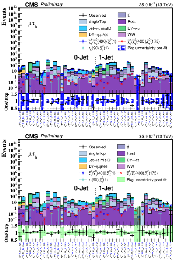
Results for the $ {\mu \tau _{\mathrm h}} $ channel for pre-fit (top) and post-fit (bottom) in the search bins. The black points show the data, the filled histograms represent the stacked SM background events, and three star-shaped markers represent signal models (not stacked), where the numbers in the brackets represent the masses of the corresponding sparticles in GeV. The filled error bars represent the pre-fit predictions, while the light blue (green) band in the ratio plot represent the pre-fit (post-fit) results. In the lower panels, the black solid points represent the pre-fit (post-fit) comparison of observation over unmodified (fitted) expectation. |

png pdf |
Figure 8-a:
Results for the $ {\mu \tau _{\mathrm h}} $ channel for pre-fit (top) and post-fit (bottom) in the search bins. The black points show the data, the filled histograms represent the stacked SM background events, and three star-shaped markers represent signal models (not stacked), where the numbers in the brackets represent the masses of the corresponding sparticles in GeV. The filled error bars represent the pre-fit predictions, while the light blue (green) band in the ratio plot represent the pre-fit (post-fit) results. In the lower panels, the black solid points represent the pre-fit (post-fit) comparison of observation over unmodified (fitted) expectation. |

png pdf |
Figure 8-b:
Results for the $ {\mu \tau _{\mathrm h}} $ channel for pre-fit (top) and post-fit (bottom) in the search bins. The black points show the data, the filled histograms represent the stacked SM background events, and three star-shaped markers represent signal models (not stacked), where the numbers in the brackets represent the masses of the corresponding sparticles in GeV. The filled error bars represent the pre-fit predictions, while the light blue (green) band in the ratio plot represent the pre-fit (post-fit) results. In the lower panels, the black solid points represent the pre-fit (post-fit) comparison of observation over unmodified (fitted) expectation. |
png pdf |
Figure 9:
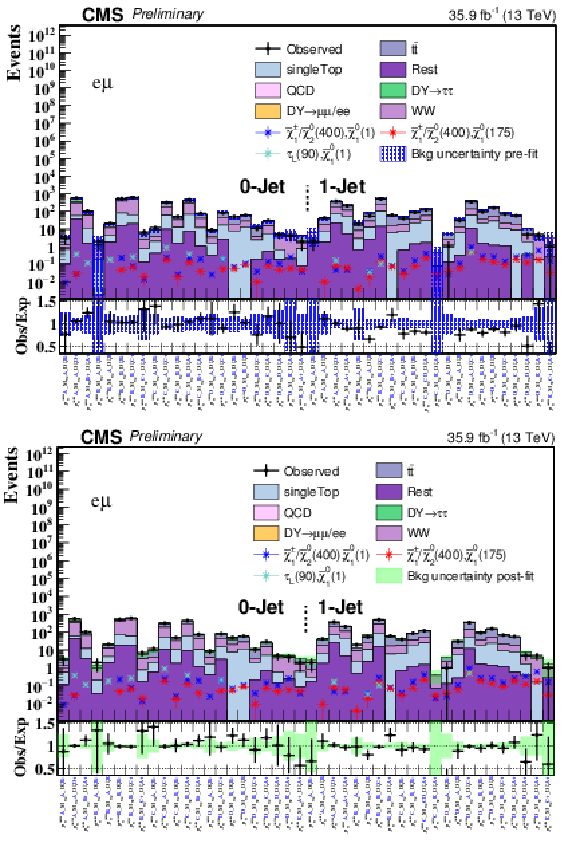
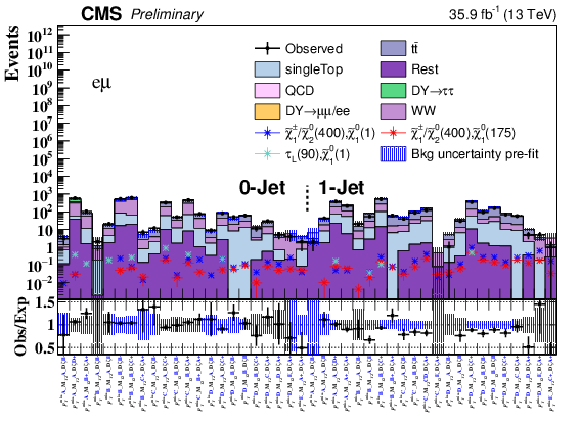
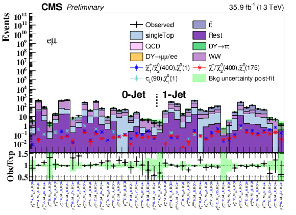
Results for the $ {\mathrm {e}\mu} $ channel for pre-fit (top) and post-fit (bottom) in the search bins. The black points show the data, the filled histograms represent the stacked SM background events, and three star-shaped markers represent signal models (not stacked), where the numbers in the brackets represent the masses of the corresponding sparticles in GeV. The filled error bars represent the pre-fit predictions, while the light blue (green) band in the ratio plot represent the pre-fit (post-fit) results. In the lower panels, the black solid points represent the pre-fit (post-fit) comparison of observation over unmodified (fitted) expectation. |
png pdf |
Figure 9-a:
Results for the $ {\mathrm {e}\mu} $ channel for pre-fit (top) and post-fit (bottom) in the search bins. The black points show the data, the filled histograms represent the stacked SM background events, and three star-shaped markers represent signal models (not stacked), where the numbers in the brackets represent the masses of the corresponding sparticles in GeV. The filled error bars represent the pre-fit predictions, while the light blue (green) band in the ratio plot represent the pre-fit (post-fit) results. In the lower panels, the black solid points represent the pre-fit (post-fit) comparison of observation over unmodified (fitted) expectation. |
png pdf |
Figure 9-b:
Results for the $ {\mathrm {e}\mu} $ channel for pre-fit (top) and post-fit (bottom) in the search bins. The black points show the data, the filled histograms represent the stacked SM background events, and three star-shaped markers represent signal models (not stacked), where the numbers in the brackets represent the masses of the corresponding sparticles in GeV. The filled error bars represent the pre-fit predictions, while the light blue (green) band in the ratio plot represent the pre-fit (post-fit) results. In the lower panels, the black solid points represent the pre-fit (post-fit) comparison of observation over unmodified (fitted) expectation. |
png pdf |
Figure 10:
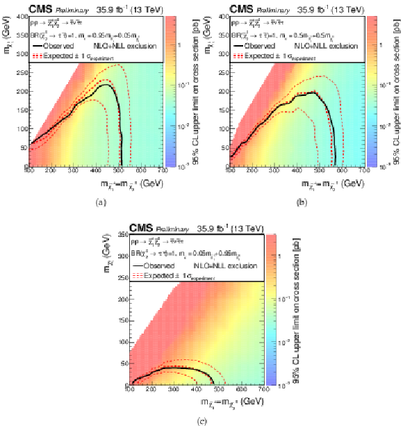
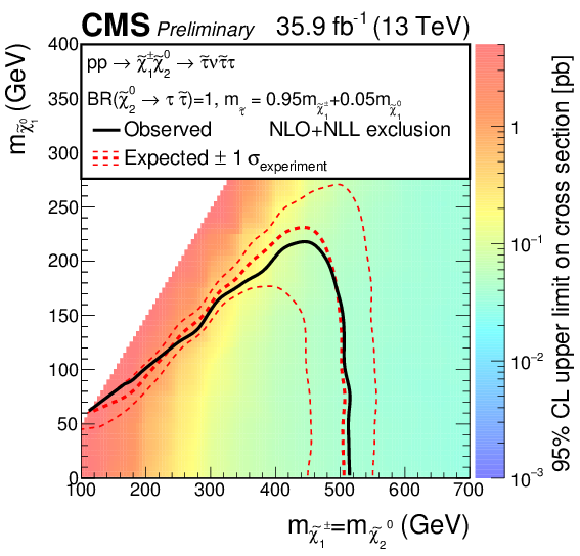
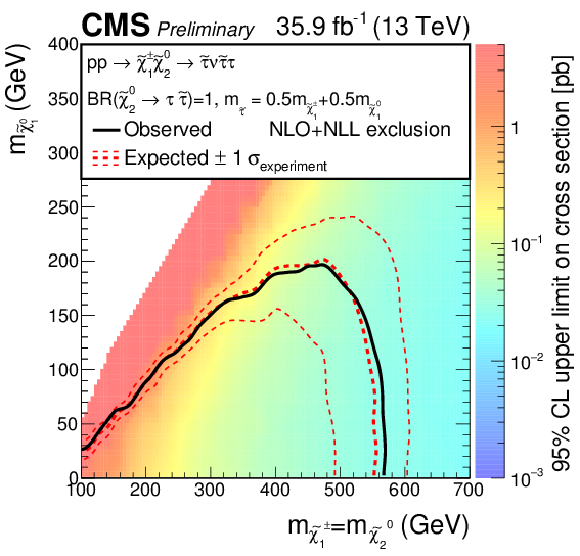
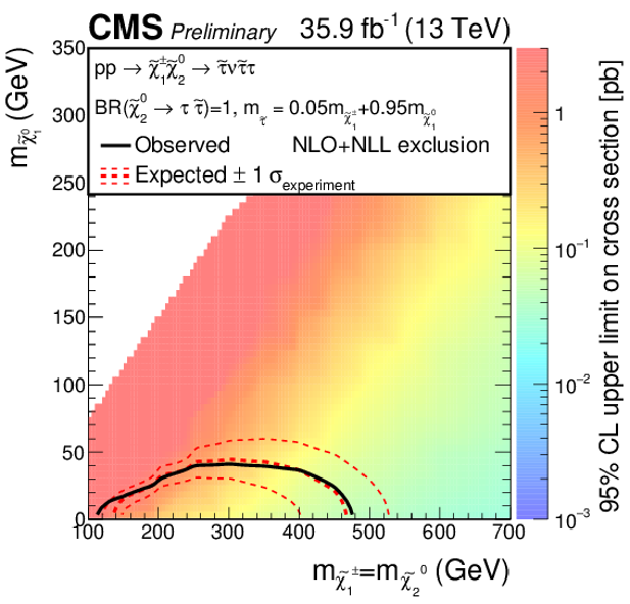
Expected and observed limits on the cross section for neutralino-chargino production with decay through $ \tilde{ \tau} $ with (top left) $x=0.95$, (top right) $x=0.5$, and (bottom) $x=0.05$, where $m_{\tilde{ \tau}} = m_{{\tilde{\chi}^0_1}} + x(m_{{\tilde{\chi}^0_2}} -m_{{\tilde{\chi}^0_1}})$. The branching ratio of the $ {\tilde{\chi}^0_2} $ is assumed to be BR($ {\tilde{\chi}^0_2} \to \tilde{ \tau} \tau)=1$. The area enclosed by the thick black curve represents the observed exclusion region, while the dashed red lines indicate the expected limits and their $ \pm 1 \sigma $ standard deviation ranges. |
png pdf |
Figure 10-a:
Expected and observed limits on the cross section for neutralino-chargino production with decay through $ \tilde{ \tau} $ with (top left) $x=0.95$, (top right) $x=0.5$, and (bottom) $x=0.05$, where $m_{\tilde{ \tau}} = m_{{\tilde{\chi}^0_1}} + x(m_{{\tilde{\chi}^0_2}} -m_{{\tilde{\chi}^0_1}})$. The branching ratio of the $ {\tilde{\chi}^0_2} $ is assumed to be BR($ {\tilde{\chi}^0_2} \to \tilde{ \tau} \tau)=1$. The area enclosed by the thick black curve represents the observed exclusion region, while the dashed red lines indicate the expected limits and their $ \pm 1 \sigma $ standard deviation ranges. |
png pdf |
Figure 10-b:
Expected and observed limits on the cross section for neutralino-chargino production with decay through $ \tilde{ \tau} $ with (top left) $x=0.95$, (top right) $x=0.5$, and (bottom) $x=0.05$, where $m_{\tilde{ \tau}} = m_{{\tilde{\chi}^0_1}} + x(m_{{\tilde{\chi}^0_2}} -m_{{\tilde{\chi}^0_1}})$. The branching ratio of the $ {\tilde{\chi}^0_2} $ is assumed to be BR($ {\tilde{\chi}^0_2} \to \tilde{ \tau} \tau)=1$. The area enclosed by the thick black curve represents the observed exclusion region, while the dashed red lines indicate the expected limits and their $ \pm 1 \sigma $ standard deviation ranges. |
png pdf |
Figure 10-c:
Expected and observed limits on the cross section for neutralino-chargino production with decay through $ \tilde{ \tau} $ with (top left) $x=0.95$, (top right) $x=0.5$, and (bottom) $x=0.05$, where $m_{\tilde{ \tau}} = m_{{\tilde{\chi}^0_1}} + x(m_{{\tilde{\chi}^0_2}} -m_{{\tilde{\chi}^0_1}})$. The branching ratio of the $ {\tilde{\chi}^0_2} $ is assumed to be BR($ {\tilde{\chi}^0_2} \to \tilde{ \tau} \tau)=1$. The area enclosed by the thick black curve represents the observed exclusion region, while the dashed red lines indicate the expected limits and their $ \pm 1 \sigma $ standard deviation ranges. |
png pdf |
Figure 11:
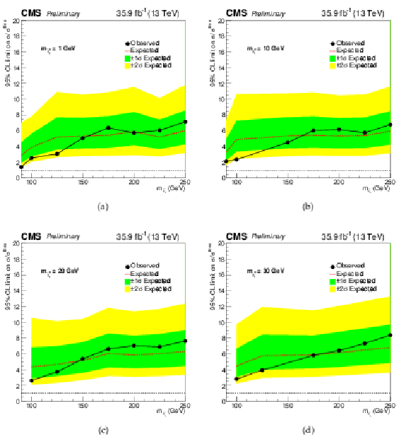
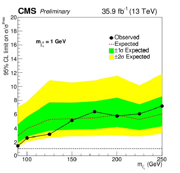
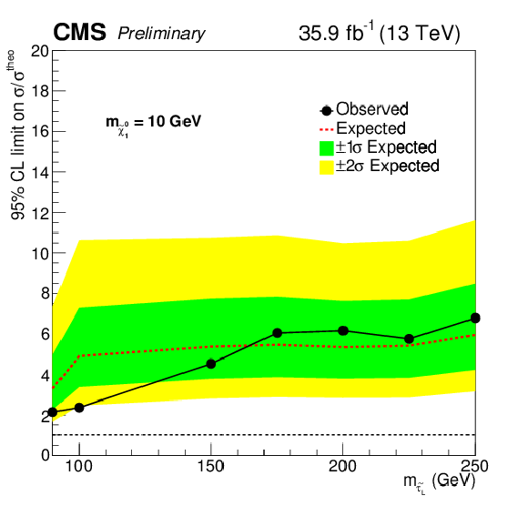
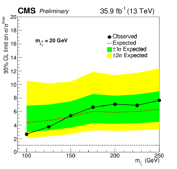
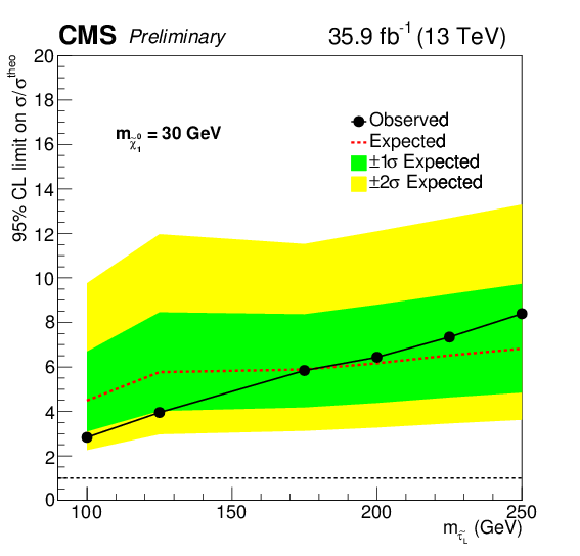
Excluded and observed exclusion limits on the cross section of direct $\tilde{ \tau} _{\rm L}$ production. The expected limits (dashed red line) and their $ \pm 1 \sigma $ and $ \pm 2 \sigma $ standard variations are shown as green and yellow bands, respectively. The observed limit is shown by the solid line with dots. |
png pdf |
Figure 11-a:
Excluded and observed exclusion limits on the cross section of direct $\tilde{ \tau} _{\rm L}$ production. The expected limits (dashed red line) and their $ \pm 1 \sigma $ and $ \pm 2 \sigma $ standard variations are shown as green and yellow bands, respectively. The observed limit is shown by the solid line with dots. |
png pdf |
Figure 11-b:
Excluded and observed exclusion limits on the cross section of direct $\tilde{ \tau} _{\rm L}$ production. The expected limits (dashed red line) and their $ \pm 1 \sigma $ and $ \pm 2 \sigma $ standard variations are shown as green and yellow bands, respectively. The observed limit is shown by the solid line with dots. |
png pdf |
Figure 11-c:
Excluded and observed exclusion limits on the cross section of direct $\tilde{ \tau} _{\rm L}$ production. The expected limits (dashed red line) and their $ \pm 1 \sigma $ and $ \pm 2 \sigma $ standard variations are shown as green and yellow bands, respectively. The observed limit is shown by the solid line with dots. |
png pdf |
Figure 11-d:
Excluded and observed exclusion limits on the cross section of direct $\tilde{ \tau} _{\rm L}$ production. The expected limits (dashed red line) and their $ \pm 1 \sigma $ and $ \pm 2 \sigma $ standard variations are shown as green and yellow bands, respectively. The observed limit is shown by the solid line with dots. |
| Tables | |

png pdf |
Table 1:
Summary of the required lepton properties. |

png pdf |
Table 2:
Requirements for additional leptons. Events with a third lepton (or a second same-flavor lepton) passing these conditions are rejected. |

png pdf |
Table 3:
Definition of the search bin labelling. |

png pdf |
Table 6:
The transfer factors as a function of $ {p_{\mathrm {T}}},\eta $ derived from the sideband. The uncertainties are statistical only. |
png pdf |
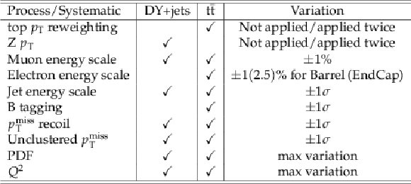
Table 7:
Contributions to the systematic uncertainty considered for the DY+jets and $ {\mathrm{t} {}\mathrm{\bar{t}}} $ processes in order to assess systematic uncertainties on the extracted normalization. |
png pdf |
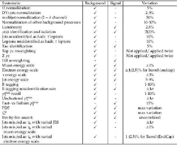
Table 8:
Systematic uncertainties considered for background and signal. |

png pdf |
Table 9:
Definition of combined search bins to be used for easier reinterpretation of the results. |
| Summary |
|
A search for supersymmetry has been performed with proton-proton collisions at a center-of-mass energy of 13 TeV recorded in 2016, corresponding to 35.9 fb$^{-1}$. Events are required to contain either one hadronically decaying $\tau$ lepton and an electron or muon, or and electron and a muon. The data are consistent with the standard model expectation, and 95% CL limits are set for several signal models. One model describes direct $ \tilde{ \tau} $ pair production, with each $ \tilde{ \tau} $ decaying to a $\tau$ lepton and the ${\widetilde{\chi}^0_1} $. For a $ \tilde{ \tau} $ mass of 90 GeV and a $ {\widetilde{\chi}^0_1} $ mass of 1 GeV, an upper limit on cross section times the square of the branching fraction is set to be 0.66 pb. Limits for neutralino ($ {\widetilde{\chi}^0_2} $ ) - chargino ($ {\widetilde{\chi}^0{\pm}_1} $) production are determined for decays of $ {\widetilde{\chi}^0_2} $ decays to a $\tau^+\tau^-$ pair and a $ {\widetilde{\chi}^0_1} $ , and the $ {\widetilde{\chi}^0{\pm}_1} $ decays to a $\tau^{\pm}$ and a $ {\widetilde{\chi}^0_1} $ , assuming mass degeneracy between $ {\widetilde{\chi}^0_2} $ and $ {\widetilde{\chi}^0{\pm}_1} $. Three different $m_{\tilde{ \tau}}$ mass scenarios have been defined: $m_{\tilde{ \tau}} = m_{{\widetilde{\chi}^0_1} } + x(m_{{\widetilde{\chi}^0_2} } -m_{{\widetilde{\chi}^0_1} })$ and $x=0.95$, 0.5 and 0.05. For $x=0.95$, $ {\widetilde{\chi}^0{\pm}_1} $ and $ {\widetilde{\chi}^0_2} $ masses can be excluded below 510 GeV for neutralino ($ {\widetilde{\chi}^0_1} $ ) masses below 200 GeV. For $x=0.5$, the limit on the $ {\widetilde{\chi}^0{\pm}_1} $ and $ {\widetilde{\chi}^0_2} $ mass can be extended to 560 GeV, while for $x=0.05$ the limit the $ {\widetilde{\chi}^0{\pm}_1} $ and $ {\widetilde{\chi}^0_2} $ mass reaches from 120-480 GeV. |
| References | ||||
| 1 | P. Ramond | Dual theory for free fermions | PRD 3 (1971) 2415 | |
| 2 | Y. A. Golfand and E. P. Likhtman | Extension of the algebra of Poincar$ \'e $ group generators and violation of P invariance | JEPTL 13 (1971)323 | |
| 3 | A. Neveu and J. H. Schwarz | Factorizable dual model of pions | NPB 31 (1971) 86 | |
| 4 | D. V. Volkov and V. P. Akulov | Possible universal neutrino interaction | JEPTL 16 (1972)438 | |
| 5 | J. Wess and B. Zumino | A Lagrangian model invariant under supergauge transformations | PLB 49 (1974) 52 | |
| 6 | J. Wess and B. Zumino | Supergauge transformations in four dimensions | NPB 70 (1974) 39 | |
| 7 | P. Fayet | Supergauge invariant extension of the Higgs mechanism and a model for the electron and its neutrino | NPB 90 (1975) 104 | |
| 8 | H. P. Nilles | Supersymmetry, supergravity and particle physics | Phys. Rep. 110 (1984) 1 | |
| 9 | G. R. Farrar and P. Fayet | Phenomenology of the production, decay, and detection of new hadronic states associated with supersymmetry | PLB 76 (1978) 575 | |
| 10 | ATLAS Collaboration | Search for the direct production of charginos, neutralinos and staus in final states with at least two hadronically decaying taus and missing transverse momentum in $ pp $ collisions at $ \sqrt{s} = $ 8 TeV with the ATLAS detector | JHEP 10 (2014) 096 | 1407.0350 |
| 11 | CMS Collaboration | Search for electroweak production of charginos in final states with two τ leptons in pp collisions at $ \sqrt{s}= $ 8 ~TeV | JHEP 04 (2017) 018 | CMS-SUS-14-022 1610.04870 |
| 12 | B. Fuks, M. Klasen, D. R. Lamprea, and M. Rothering | Revisiting slepton pair production at the Large Hadron Collider | JHEP 01 (2014) 168 | 1310.2621 |
| 13 | B. Fuks, M. Klasen, D. R. Lamprea, and M. Rothering | Gaugino production in proton-proton collisions at a center-of-mass energy of 8 TeV | JHEP 10 (2012) 081 | 1207.2159 |
| 14 | B. Fuks, M. Klasen, D. R. Lamprea, and M. Rothering | Precision predictions for electroweak superpartner production at hadron colliders with Resummino | EPJC73 (2013) 2480 | 1304.0790 |
| 15 | DELPHI Collaboration | Searches for supersymmetric particles in e+ e- collisions up to 208-GeV and interpretation of the results within the MSSM | EPJC31 (2003) 421 | hep-ex/0311019 |
| 16 | L3 Collaboration | Search for charginos and neutralinos in $ e^{+} e^{-} $ collisions at $ \sqrt{s} = $ 189-GeV | PLB472 (2000) 420 | hep-ex/9910007 |
| 17 | N. Arkani-Hamed et al. | MARMOSET: The path from LHC data to the new standard model via on-shell effective theories | hep-ph/0703088 | |
| 18 | J. Alwall, P. Schuster, and N. Toro | Simplified models for a first characterization of new physics at the LHC | PRD 79 (2009) 075020 | 0810.3921 |
| 19 | J. Alwall, M.-P. Le, M. Lisanti, and J. G. Wacker | Model-independent jets plus missing energy searches | PRD 79 (2009) 015005 | 0809.3264 |
| 20 | D. Alves et al. | Simplified models for LHC new physics searches | JPG 39 (2012) 105005 | 1105.2838 |
| 21 | CMS Collaboration | The CMS experiment at the CERN LHC | JINST 3 (2008) S08004 | CMS-00-001 |
| 22 | CMS Collaboration | Description and performance of track and primary-vertex reconstruction with the CMS tracker | JINST 9 (2014) P10009 | CMS-TRK-11-001 1405.6569 |
| 23 | CMS Collaboration | Determination of jet energy calibration and transverse momentum resolution in CMS | JINST 6 (2011) P11002 | CMS-JME-10-011 1107.4277 |
| 24 | CMS Collaboration | Performance of electron reconstruction and selection with the CMS detector in proton-proton collisions at $ \sqrt{s} = $ 8 ~TeV | JINST 10 (2015) P06005 | CMS-EGM-13-001 1502.02701 |
| 25 | CMS Collaboration | Performance of CMS muon reconstruction in $ pp $ collision events at $ \sqrt{s} = $ 7 TeV | JINST 7 (2012) P10002 | CMS-MUO-10-004 1206.4071 |
| 26 | CMS Collaboration | Particle-flow reconstruction and global event description with the CMS detector | JINST 12 (2017) P10003 | CMS-PRF-14-001 1706.04965 |
| 27 | M. Cacciari and G. P. Salam | Pileup subtraction using jet areas | PLB 659 (2008) 119 | 0707.1378 |
| 28 | CMS Collaboration | Reconstruction and identification of $ \tau $ lepton decays to hadrons and $ \nu_{\tau} $ at CMS | JINST 11 (2016) P01019 | CMS-TAU-14-001 1510.07488 |
| 29 | CMS Collaboration | Identification of b-quark jets with the CMS experiment | JINST 8 (2013) P04013 | CMS-BTV-12-001 1211.4462 |
| 30 | CMS Collaboration | Identification of b quark jets at the cms experiment in the lhc run 2 | CMS-PAS-BTV-15-001 | CMS-PAS-BTV-15-001 |
| 31 | CMS Collaboration | Performance of b tagging at $ \sqrt{s}= $ 8 ~TeV in multijet, $ \mathrm{t\bar{t}} $ and boosted topology events | CMS-PAS-BTV-13-001 | CMS-PAS-BTV-13-001 |
| 32 | M. Cacciari, G. P. Salam, and G. Soyez | The anti-$ k_t $ jet clustering algorithm | JHEP 04 (2008) 063 | 0802.1189 |
| 33 | M. Cacciari, G. P. Salam, and G. Soyez | FastJet user manual | EPJC 72 (2012) 1896 | 1111.6097 |
| 34 | J. Alwall et al. | The automated computation of tree-level and next-to-leading order differential cross sections, and their matching to parton shower simulations | JHEP 07 (2014) 079 | 1405.0301 |
| 35 | J. Alwall et al. | MadGraph5: going beyond | JHEP 06 (2011) 128 | 1106.0522 |
| 36 | NNPDF Collaboration | Parton distributions for the LHC Run II | JHEP 04 (2015) 040 | 1410.8849 |
| 37 | E. Re | Single-top Wt-channel production matched with parton showers using the POWHEG method | EPJC71 (2011) 1547 | 1009.2450 |
| 38 | S. Alioli, P. Nason, C. Oleari, and E. Re | NLO single-top production matched with shower in POWHEG: s- and t-channel contributions | JHEP 09 (2009) 111 | 0907.4076 |
| 39 | S. Agostinelli et al. | GEANT4 --- a simulation toolkit | Nucl. Instr. and Meth. A 506 (2003) 250 | |
| 40 | CMS Collaboration | The fast simulation of the CMS detector at LHC | J. Phys. Conf. Ser. 331 (2011) 032049 | |
| 41 | C. G. Lester and B. Nachman | Bisection-based asymmetric M$ _{T2} $ computation: a higher precision calculator than existing symmetric methods | JHEP 03 (2015) 100 | 1411.4312 |
| 42 | CMS Collaboration | Measurement of differential top-quark pair production cross sections in $ pp $ colisions at $ \sqrt{s}= $ 7 TeV | EPJC73 (2013) 2339 | CMS-TOP-11-013 1211.2220 |
| 43 | CMS Collaboration | Measurement of the differential cross section for top quark pair production in pp collisions at $ \sqrt{s} = $ 8 TeV | EPJC75 (2015) 542 | CMS-TOP-12-028 1505.04480 |
| 44 | CMS Collaboration | Measurement of normalized differential t$ \bar{\rm t} $ cross sections in the dilepton channel from pp collisions at $ \sqrt{s} = $ 13 ~TeV | Submitted to JHEP | CMS-TOP-16-007 1708.07638 |
| 45 | M. Czakon, D. Heymes, and A. Mitov | High-precision differential predictions for top-quark pairs at the LHC | PRL 116 (2016) 082003 | 1511.00549 |
| 46 | N. Kidonakis | NNLL threshold resummation for top-pair and single-top production | Phys. Part. Nucl. 45 (2014) 714 | 1210.7813 |
| 47 | T. Junk | Confidence level computation for combining searches with small statistics | Nucl. Instr. and Meth. A 434 (1999) 435 | hep-ex/9902006 |
| 48 | A. L. Read | Presentation of search results: the $ {CL}_s $ technique | JPG 28 (2002) 2693 | |
| 49 | ATLAS and CMS Collaborations, LHC Higgs Combination Group | Procedure for the LHC Higgs boson search combination in Summer 2011 | ATL-PHYS-PUB 2011-11, CMS NOTE 2011/005 | |
| 50 | G. Cowan, K. Cranmer, E. Gross, and O. Vitells | Asymptotic formulae for likelihood-based tests of new physics | EPJC 71 (2011) 1554 | 1007.1727 |

|
Compact Muon Solenoid LHC, CERN |

|

|

|

|

|

|