

Compact Muon Solenoid
LHC, CERN
| CMS-PAS-HIG-18-030 | ||
| Measurement of $\mathrm{t\overline{t}H}$ production in the $\mathrm{H\rightarrow b\overline{b}}$ decay channel in 41.5 fb$^{-1}$ of proton-proton collision data at $\sqrt{s}=$ 13 TeV | ||
| CMS Collaboration | ||
| May 2019 | ||
| Abstract: A measurement of the associated production of a standard model Higgs boson with a top quark-antiquark pair ($\mathrm{t\overline{t}H}$) in proton-proton collisions at $\sqrt{s}=$ 13 TeV is presented. The result is based on data recorded with the CMS detector at the CERN LHC in 2017 and corresponds to an integrated luminosity of 41.5 fb$^{-1}$ Candidate $\mathrm{t\overline{t}H}$ events are selected based on the number of leptons in the event, targeting all $\mathrm{t\overline{t}}$ decay channels, and are categorised according to the number of jets. Multivariate analysis techniques are employed to further categorise the events and eventually discriminate between signal and background. A combined fit of multivariate discriminant distributions in all categories results in a best fit value of the $\mathrm{t\overline{t}H}$ signal strength relative to the standard model cross section, $\mu = \sigma/\sigma_{\mathrm{SM}}$, of $\hat{\mu} = $ 1.49 $^{+0.21}_{-0.20}$(stat) $^{+0.39}_{-0.35}$ (syst), corresponding to an observed (expected) significance of 3.7 (2.6) standard deviations. Combined with previous results obtained with 36.9 fb$^{-1}$ of data recorded in 2016, a best-fit value of $\hat{\mu} = $ 1.15 $^{+0.15}_{-0.15}$ (stat) $^{+0.28}_{-0.25}$ (syst) is found, corresponding to an observed (expected) significance of 3.9 (3.5) standard deviations above the background-only hypothesis. | ||
| Links: CDS record (PDF) ; inSPIRE record ; CADI line (restricted) ; | ||
| Figures & Tables | Summary | Additional Figures & Tables | References | CMS Publications |
|---|
| Figures | |
png pdf |
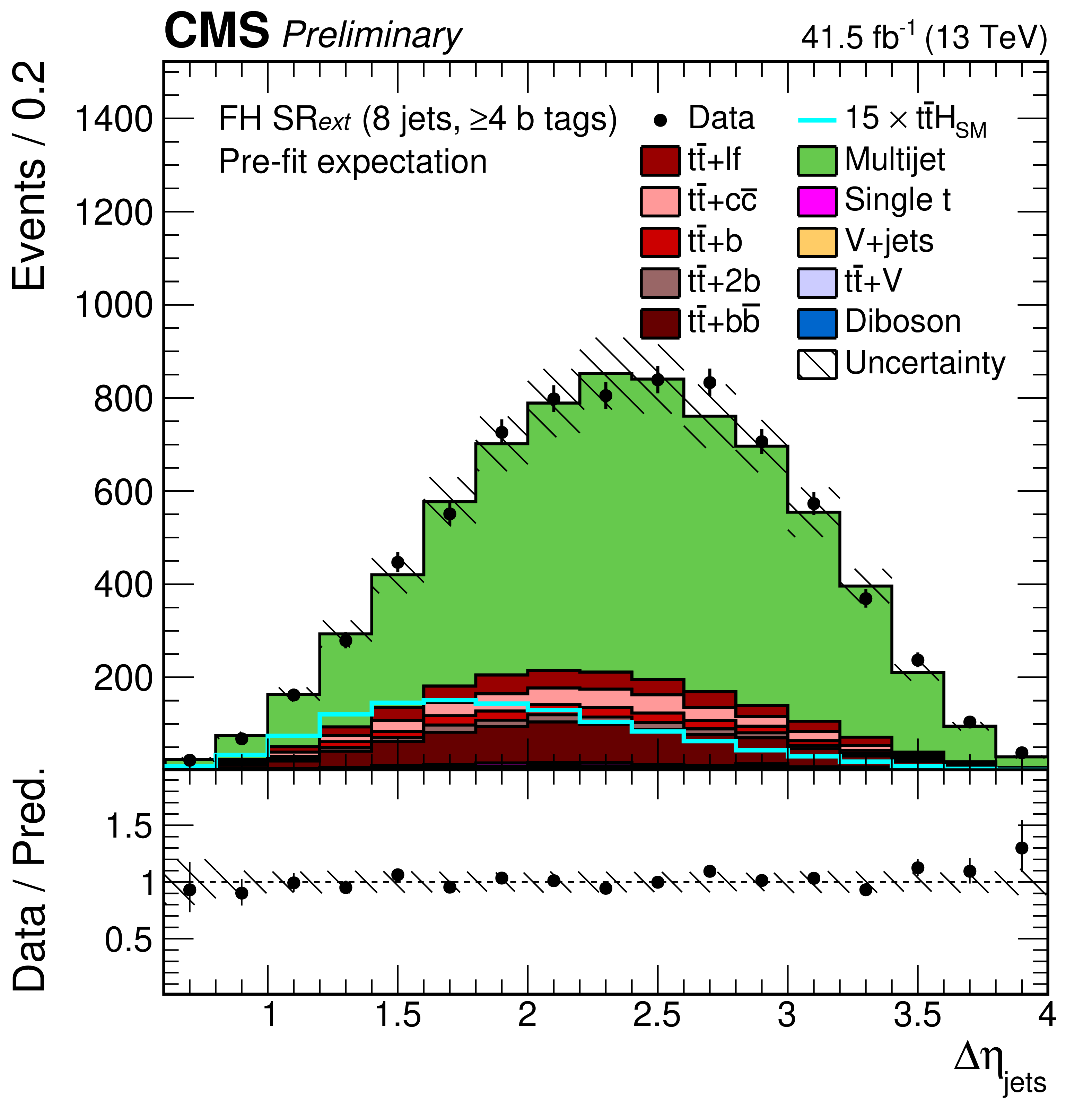
Figure 1:
Distribution of the $\Delta \eta _{\text {jets}}$ for events with 8 jets and $\geq $4 b-tags in an extended signal region (SRext), which corresponds to the regular SR but excluding the requirement of $\Delta \eta _{\text {jets}} \leq $ 2.52 for this category. The expected background contributions (filled histograms) are stacked, and the expected signal distribution (line) is superimposed. Each contribution is normalised to an integrated luminosity of 41.5 fb$^{-1}$, and the signal distribution is additionally scaled by a factor of 15 for better visibility. The hatched uncertainty bands correspond to the total statistical and systematic uncertainties. The distributions observed in data (markers) are overlayed. The lower plots show the ratio of the data to the background prediction. |
png pdf |
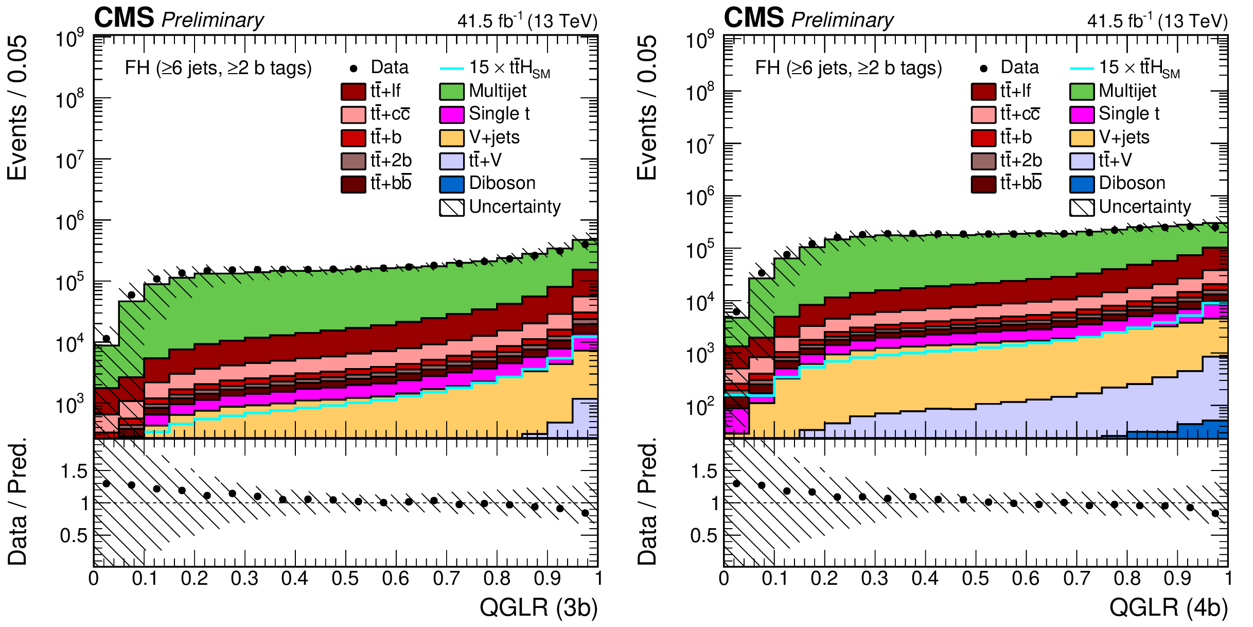
Figure 2:
Distributions of the QGLR after excluding the first three (left) and first four (right) b-tagged jets (ranked by the DeepCSV output value) for the calculation in the fully-hadronic channel after the baseline selection. The expected background contributions (filled histograms) are stacked, and the expected signal distribution (line) is superimposed. Each contribution is normalised to an integrated luminosity of 41.5 fb$^{-1}$, and the signal distribution is additionally scaled by a factor of 15 for better visibility. The hatched uncertainty bands correspond to the total statistical and systematic uncertainties (excluding the 50% uncertainties on the normalisation of the ${\mathrm{t} {}\mathrm{\bar{t}}}$+hf processes) added in quadrature. The distributions observed in data (markers) are overlayed. The last bin includes overflow events. The lower plots show the ratio of the data to the background prediction. |
png pdf |
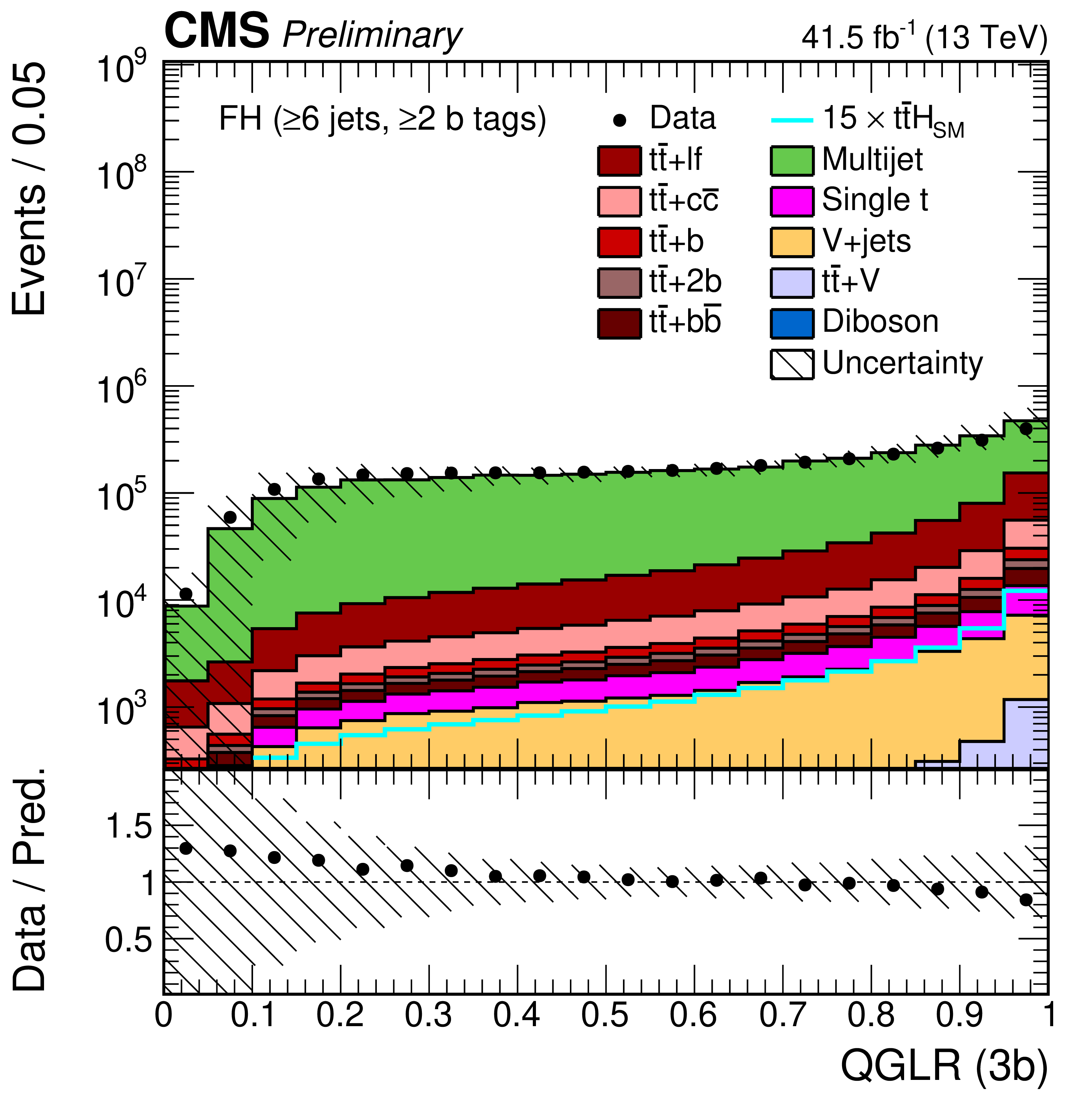
Figure 2-a:
Distribution of the QGLR after excluding the first three b-tagged jets (ranked by the DeepCSV output value) for the calculation in the fully-hadronic channel after the baseline selection. The expected background contributions (filled histograms) are stacked, and the expected signal distribution (line) is superimposed. Each contribution is normalised to an integrated luminosity of 41.5 fb$^{-1}$, and the signal distribution is additionally scaled by a factor of 15 for better visibility. The hatched uncertainty bands correspond to the total statistical and systematic uncertainties (excluding the 50% uncertainties on the normalisation of the ${\mathrm{t} {}\mathrm{\bar{t}}}$+hf processes) added in quadrature. The distribution observed in data (markers) is overlayed. The last bin includes overflow events. The lower plot shows the ratio of the data to the background prediction. |
png pdf |
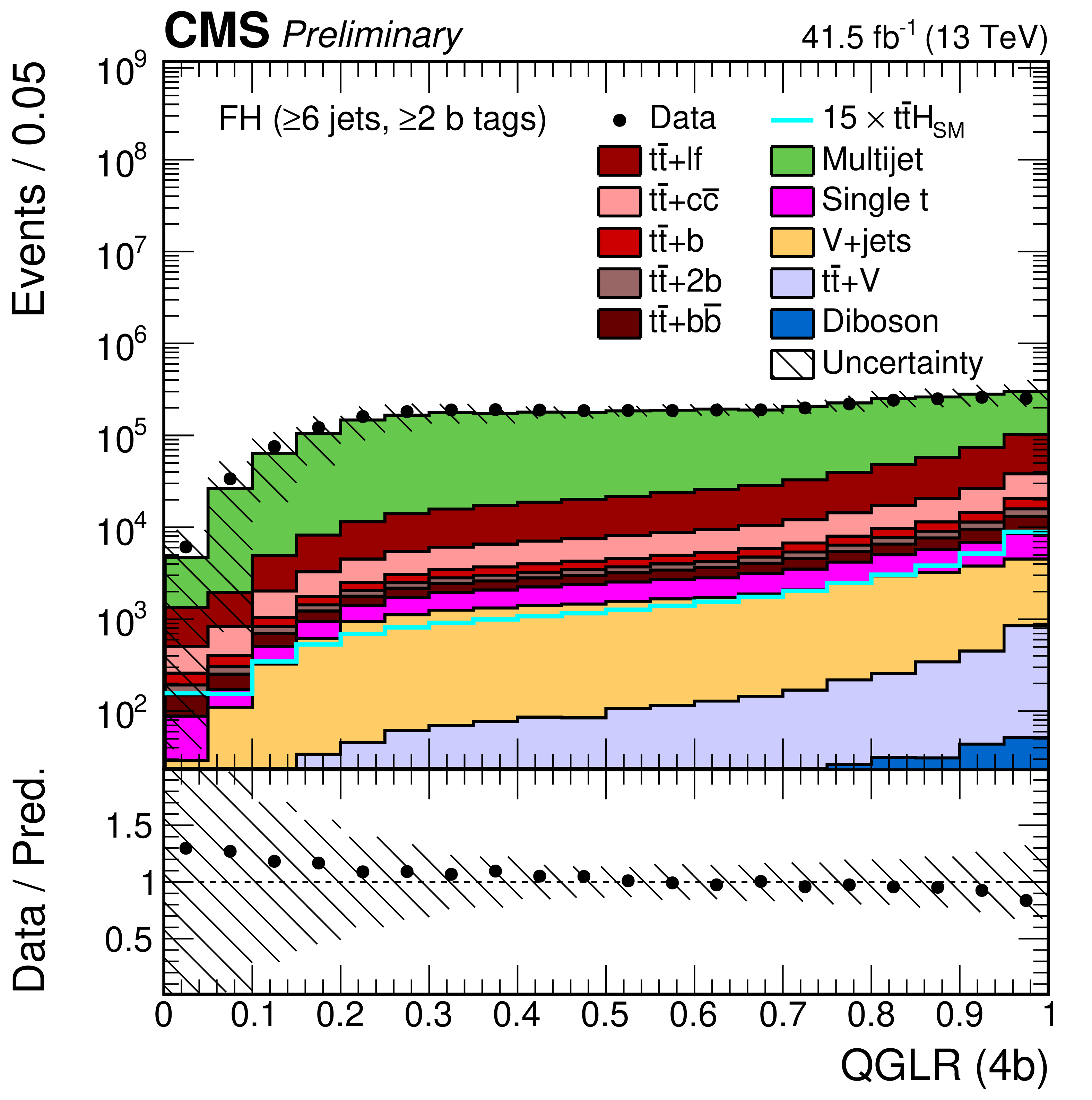
Figure 2-b:
Distribution of the QGLR after excluding the first four b-tagged jets (ranked by the DeepCSV output value) for the calculation in the fully-hadronic channel after the baseline selection. The expected background contributions (filled histograms) are stacked, and the expected signal distribution (line) is superimposed. Each contribution is normalised to an integrated luminosity of 41.5 fb$^{-1}$, and the signal distribution is additionally scaled by a factor of 15 for better visibility. The hatched uncertainty bands correspond to the total statistical and systematic uncertainties (excluding the 50% uncertainties on the normalisation of the ${\mathrm{t} {}\mathrm{\bar{t}}}$+hf processes) added in quadrature. The distribution observed in data (markers) is overlayed. The last bin includes overflow events. The lower plot shows the ratio of the data to the background prediction. |
png pdf |
Figure 3:
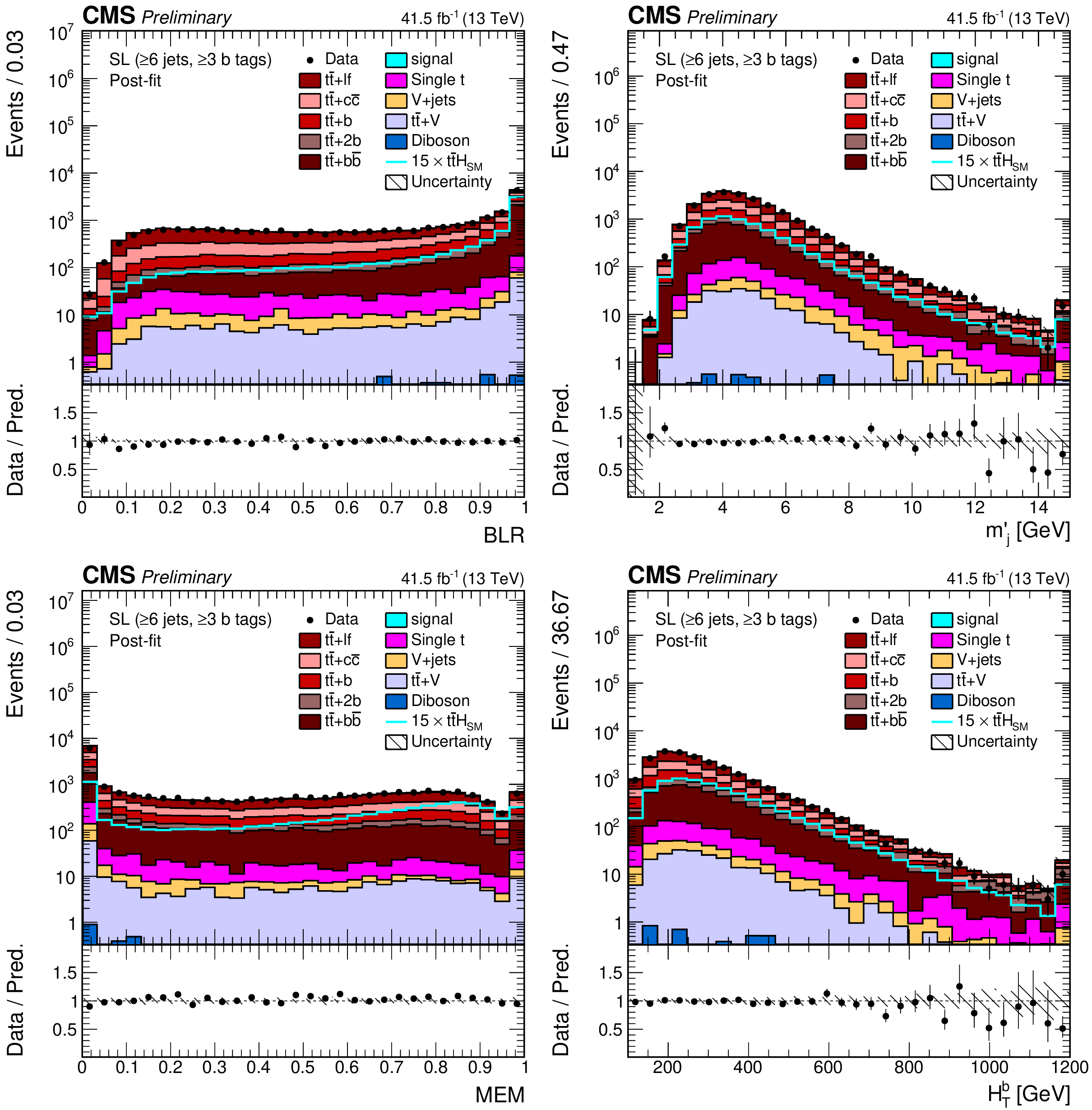
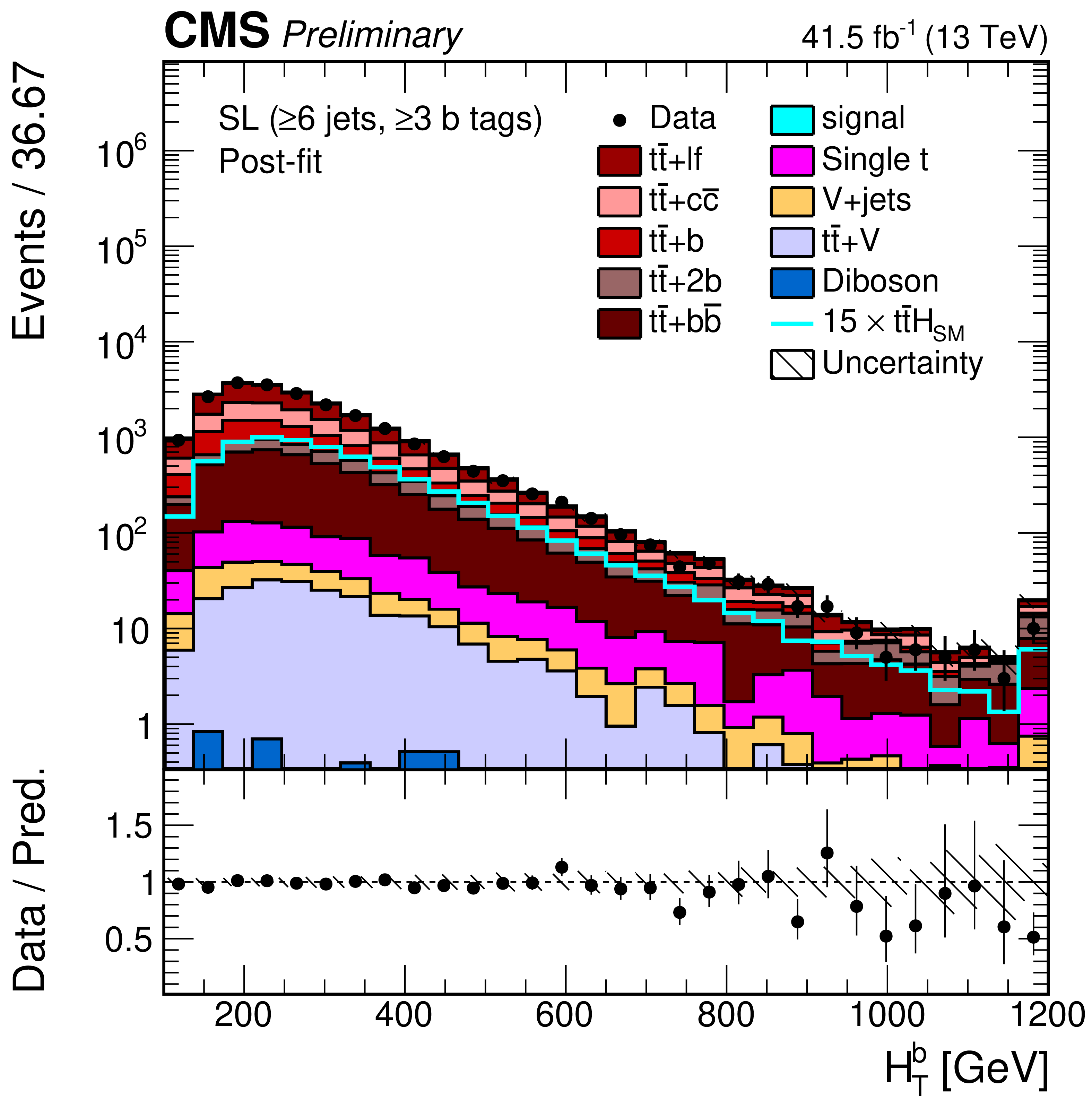
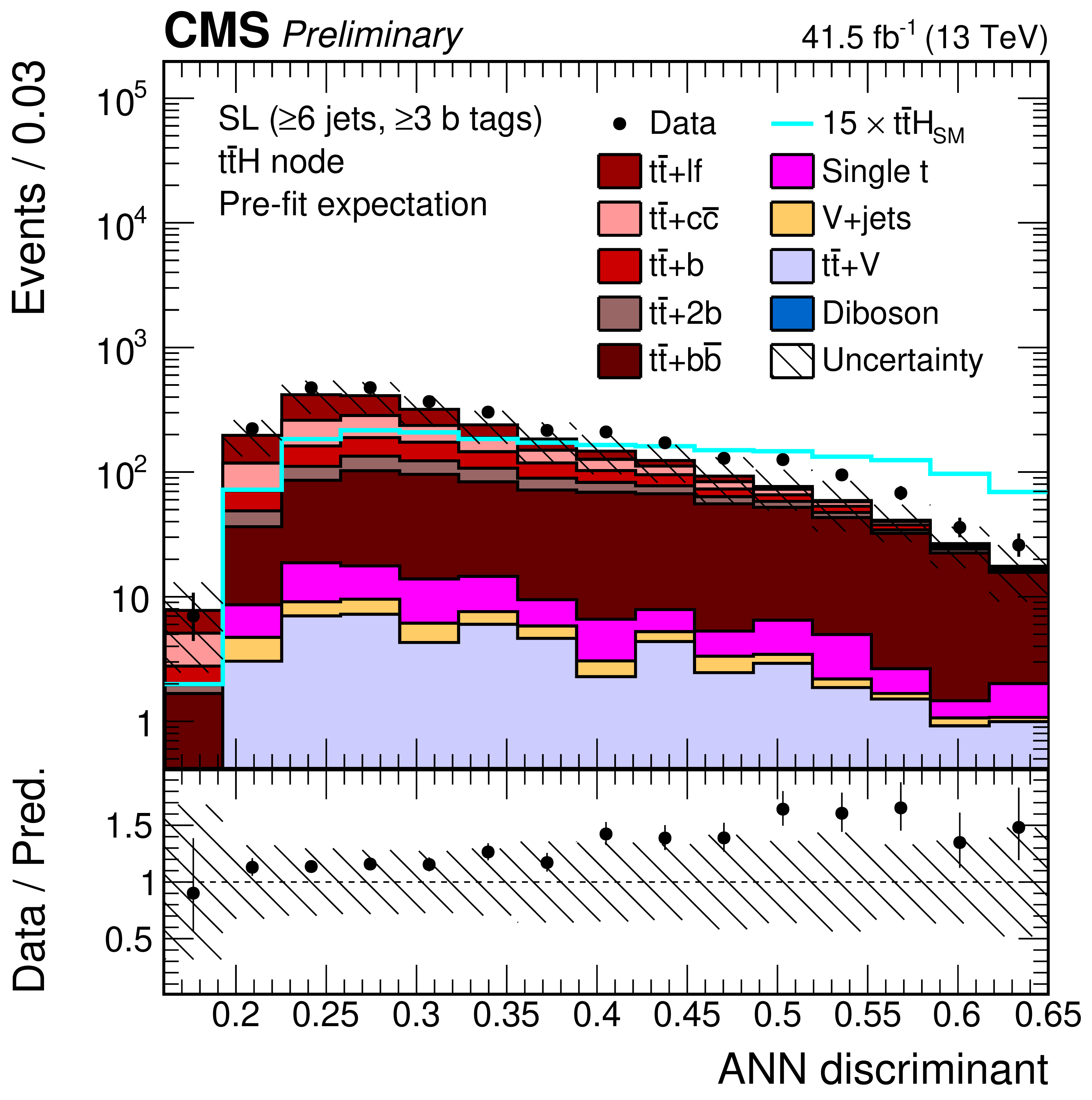
Distributions of representative variables used as input to the ANN in the $\geq $6 jets, $\geq $3 jets category of the single-lepton (SL) channel: likelihood ratio discriminating between events with 4 b quark jets and b quark jets (BLR), sum of the masses of all jets normalised to the number of dijet pairs in the event (${m'_{\text {j}}}$), MEM discriminant (MEM), and scalar sum of ${p_{\mathrm {T}}}$ of b-tagged jets (${H_{\text {T}}^{\text {b}}}$). The background and signal contributions (filled histograms) are stacked, and the hatched uncertainty bands correspond to the total statistical and systematic uncertainties. Shown are the post-fit contributions, where the model parameters are obtained from the final fit of the discriminant distributions to data, described in Section 7, and applied to the shown input variable distributions. The distributions observed in data (markers) are overlayed. In addition, the SM ${{\mathrm{t} {}\mathrm{\bar{t}}} \mathrm{H}}$ signal expectation (line) is overlayed (scaled by a factor 15 for better visibility). The first and the last bins include underflow and overflow events, respectively. The lower plots show the ratio of the data to the background prediction. |
png pdf |
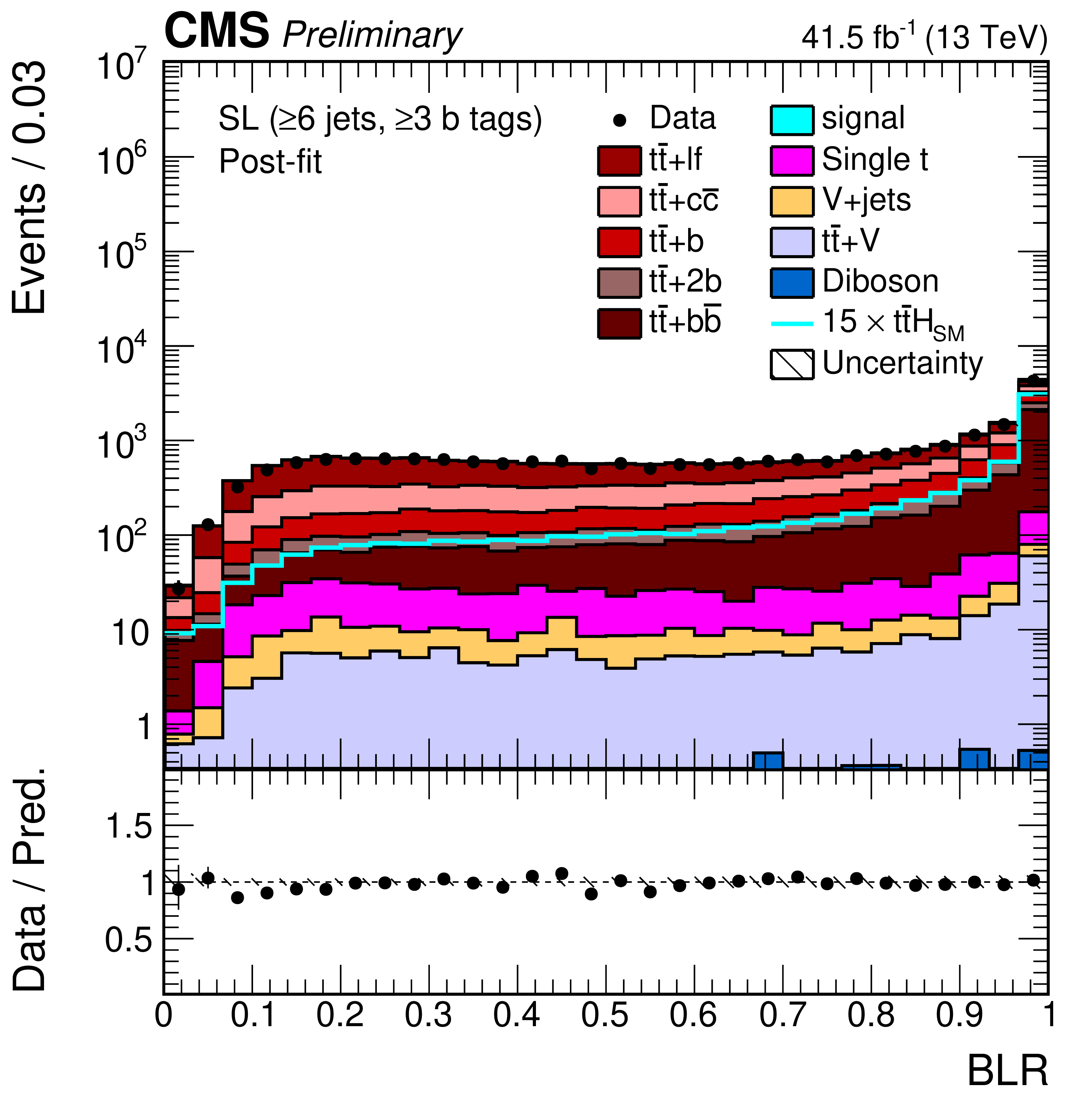
Figure 3-a:
Distribution of the likelihood ratio discriminating between events with 4 b quark jets and b quark jets (BLR) in the $\geq $6 jets, $\geq $3 jets category of the single-lepton (SL) channel. The background and signal contributions (filled histograms) are stacked, and the hatched uncertainty bands correspond to the total statistical and systematic uncertainties. Shown are the post-fit contributions, where the model parameters are obtained from the final fit of the discriminant distributions to data, described in Section 7, and applied to the shown input variable distributions. The distribution observed in data (markers) is overlayed. In addition, the SM ${{\mathrm{t} {}\mathrm{\bar{t}}} \mathrm{H}}$ signal expectation (line) is overlayed (scaled by a factor 15 for better visibility). The first and the last bins include underflow and overflow events, respectively. The lower plot shows the ratio of the data to the background prediction. |
png pdf |
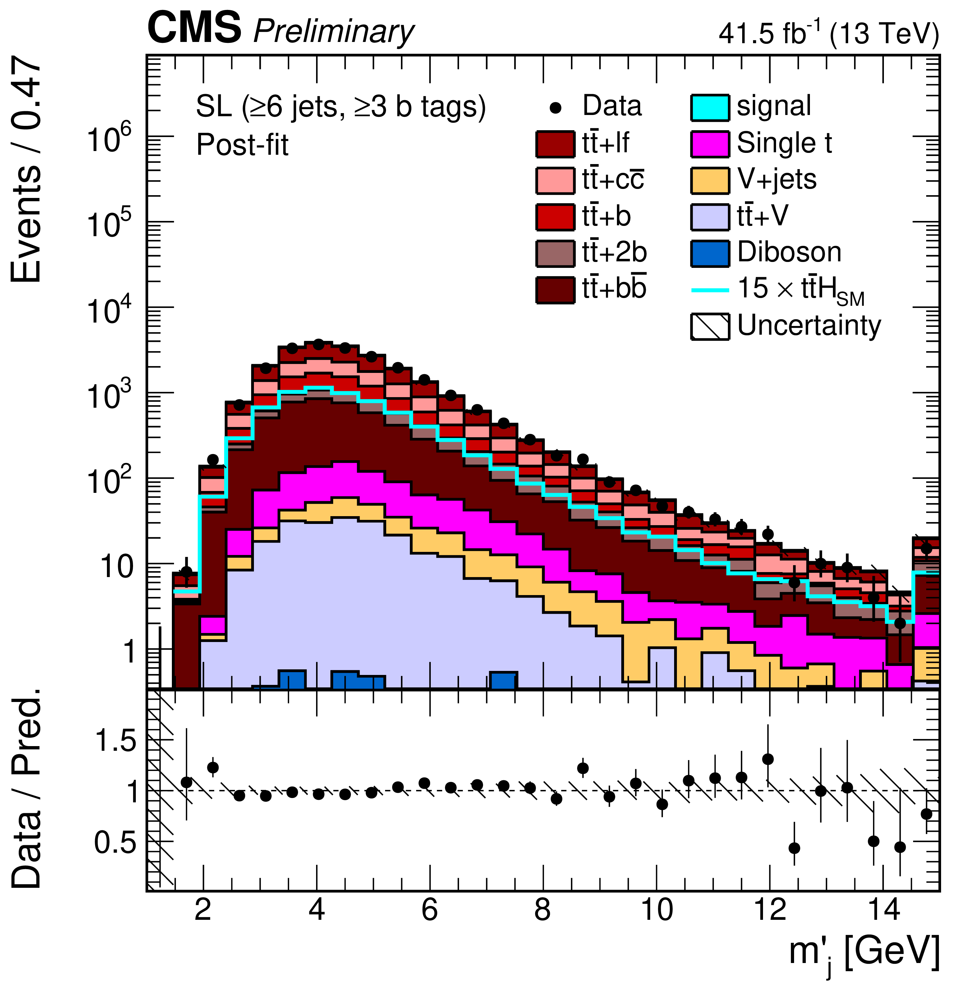
Figure 3-b:
Distribution of the sum of the masses of all jets normalised to the number of dijet pairs in the event (${m'_{\text {j}}}$) in the $\geq $6 jets, $\geq $3 jets category of the single-lepton (SL) channel. The background and signal contributions (filled histograms) are stacked, and the hatched uncertainty bands correspond to the total statistical and systematic uncertainties. Shown are the post-fit contributions, where the model parameters are obtained from the final fit of the discriminant distributions to data, described in Section 7, and applied to the shown input variable distributions. The distribution observed in data (markers) is overlayed. In addition, the SM ${{\mathrm{t} {}\mathrm{\bar{t}}} \mathrm{H}}$ signal expectation (line) is overlayed (scaled by a factor 15 for better visibility). The first and the last bins include underflow and overflow events, respectively. The lower plot shows the ratio of the data to the background prediction. |
png pdf |
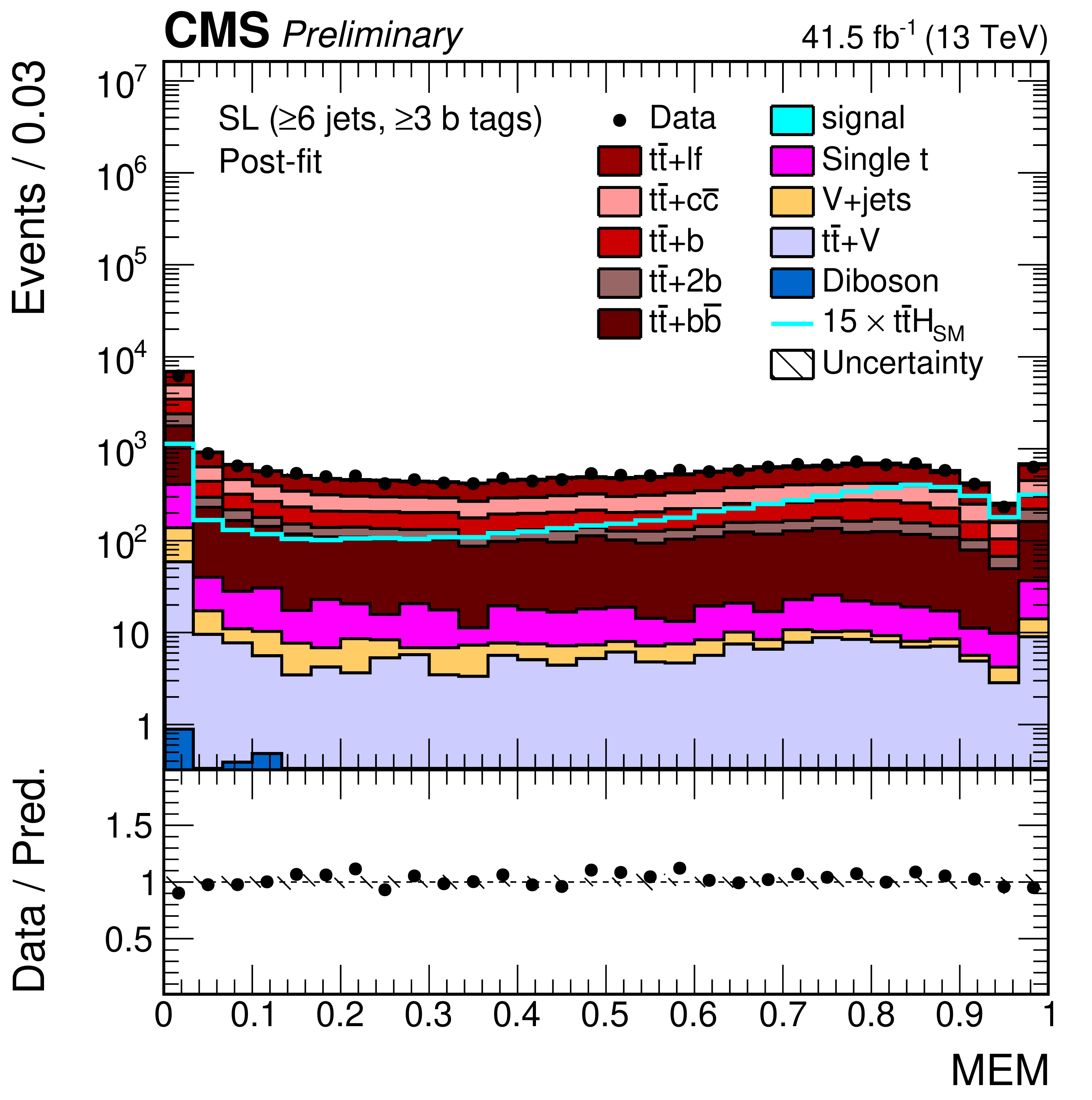
Figure 3-c:
Distribution of the MEM discriminant (MEM) in the $\geq $6 jets, $\geq $3 jets category of the single-lepton (SL) channel. The background and signal contributions (filled histograms) are stacked, and the hatched uncertainty bands correspond to the total statistical and systematic uncertainties. Shown are the post-fit contributions, where the model parameters are obtained from the final fit of the discriminant distributions to data, described in Section 7, and applied to the shown input variable distributions. The distribution observed in data (markers) is overlayed. In addition, the SM ${{\mathrm{t} {}\mathrm{\bar{t}}} \mathrm{H}}$ signal expectation (line) is overlayed (scaled by a factor 15 for better visibility). The first and the last bins include underflow and overflow events, respectively. The lower plot shows the ratio of the data to the background prediction. |
png pdf |
Figure 3-d:
Distribution of the scalar sum of ${p_{\mathrm {T}}}$ of b-tagged jets (${H_{\text {T}}^{\text {b}}}$) in the $\geq $6 jets, $\geq $3 jets category of the single-lepton (SL) channel. The background and signal contributions (filled histograms) are stacked, and the hatched uncertainty bands correspond to the total statistical and systematic uncertainties. Shown are the post-fit contributions, where the model parameters are obtained from the final fit of the discriminant distributions to data, described in Section 7, and applied to the shown input variable distributions. The distribution observed in data (markers) is overlayed. In addition, the SM ${{\mathrm{t} {}\mathrm{\bar{t}}} \mathrm{H}}$ signal expectation (line) is overlayed (scaled by a factor 15 for better visibility). The first and the last bins include underflow and overflow events, respectively. The lower plot shows the ratio of the data to the background prediction. |
png pdf |
Figure 4:
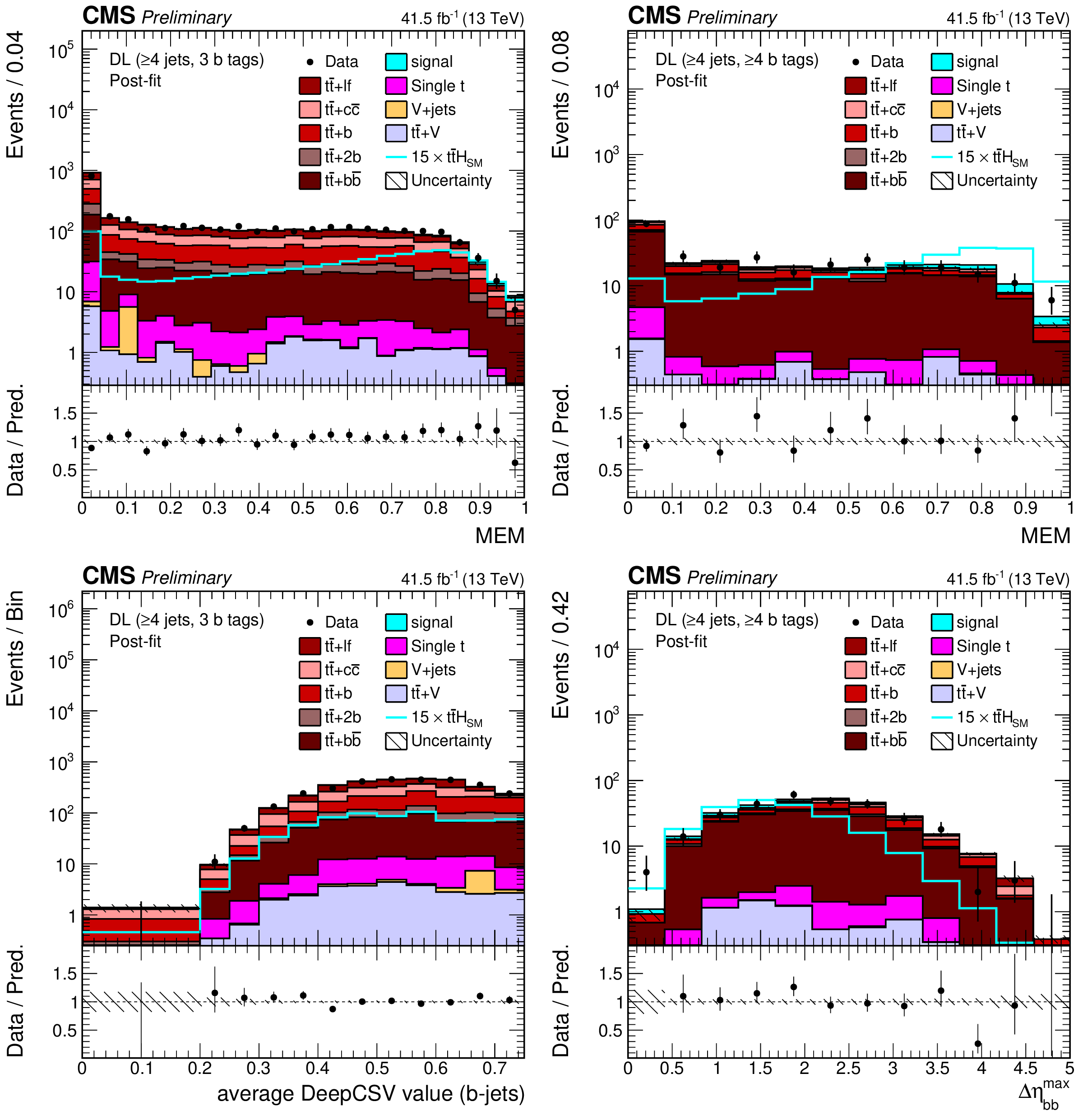
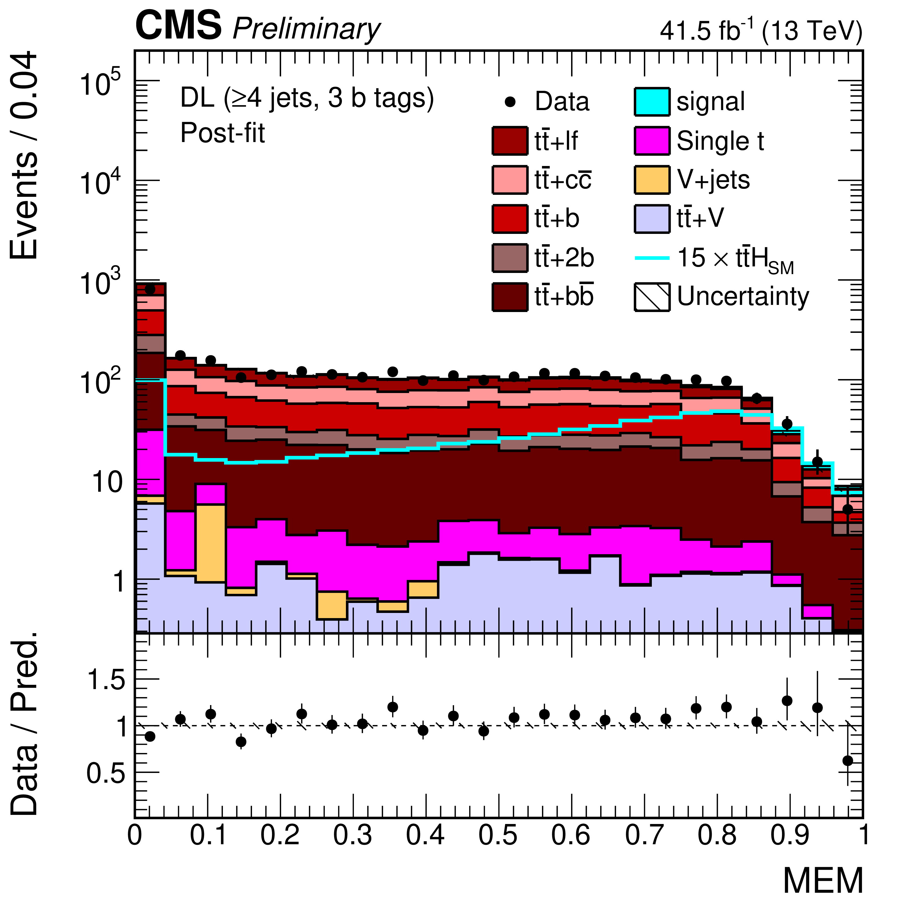
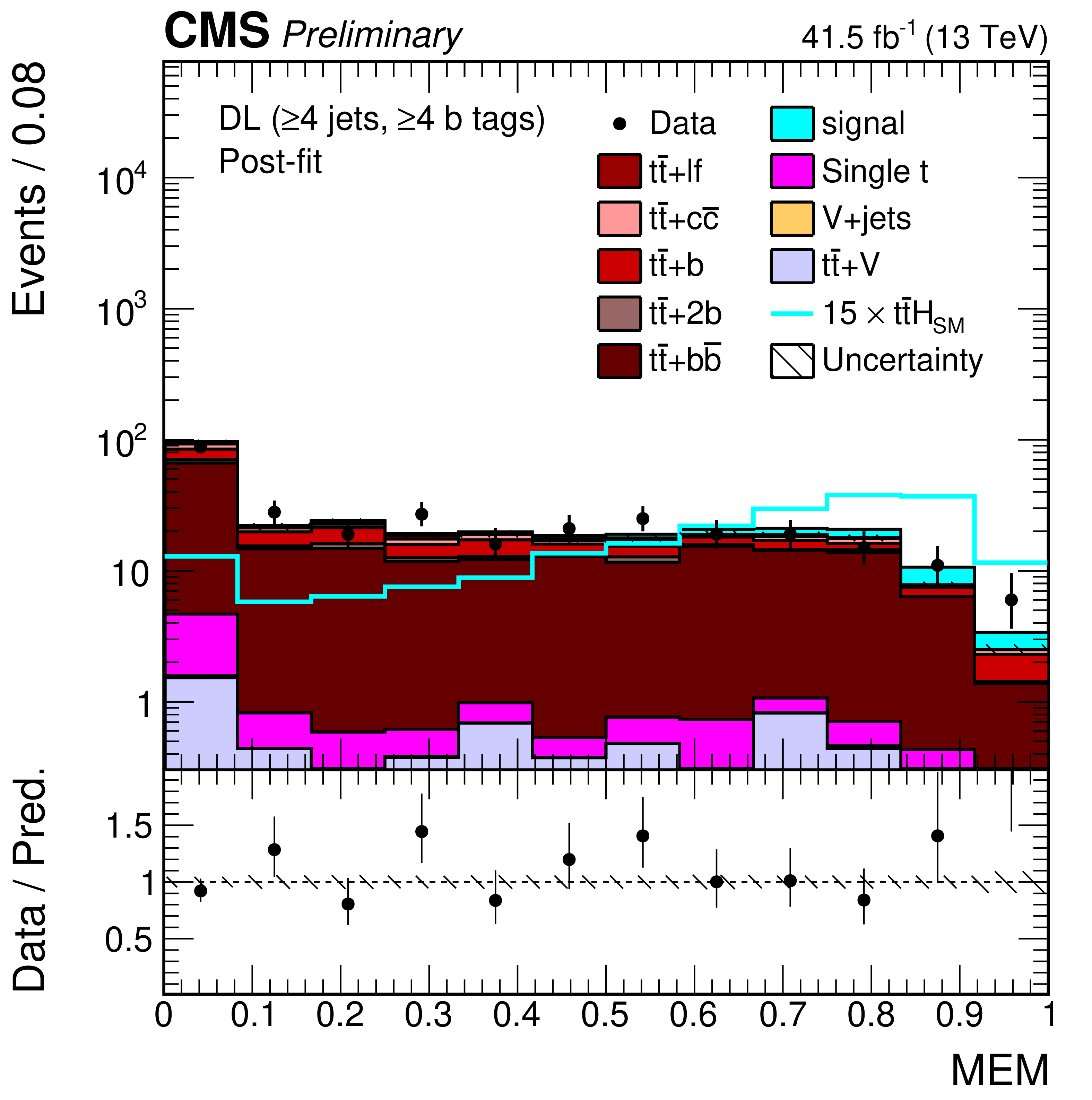
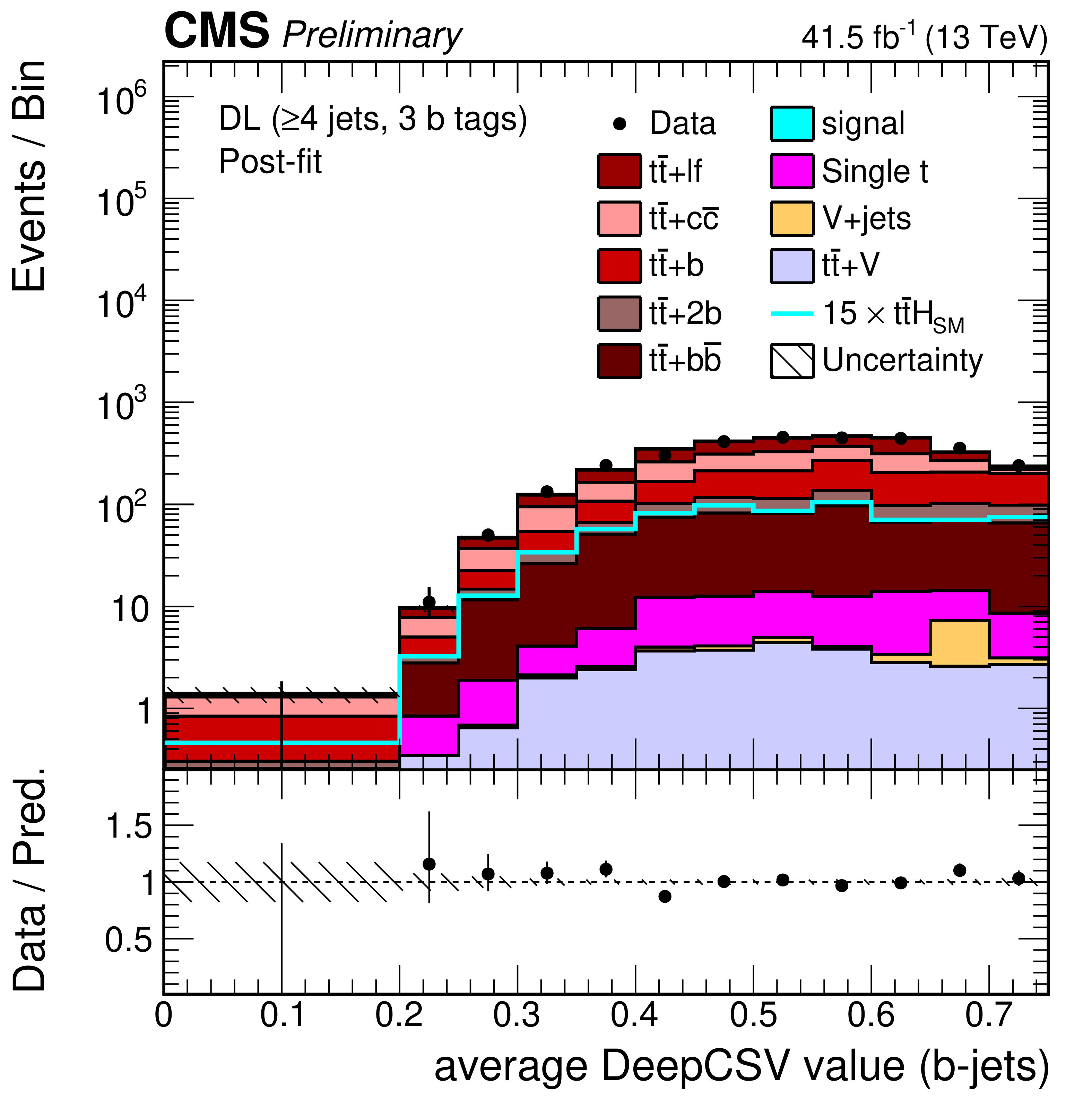
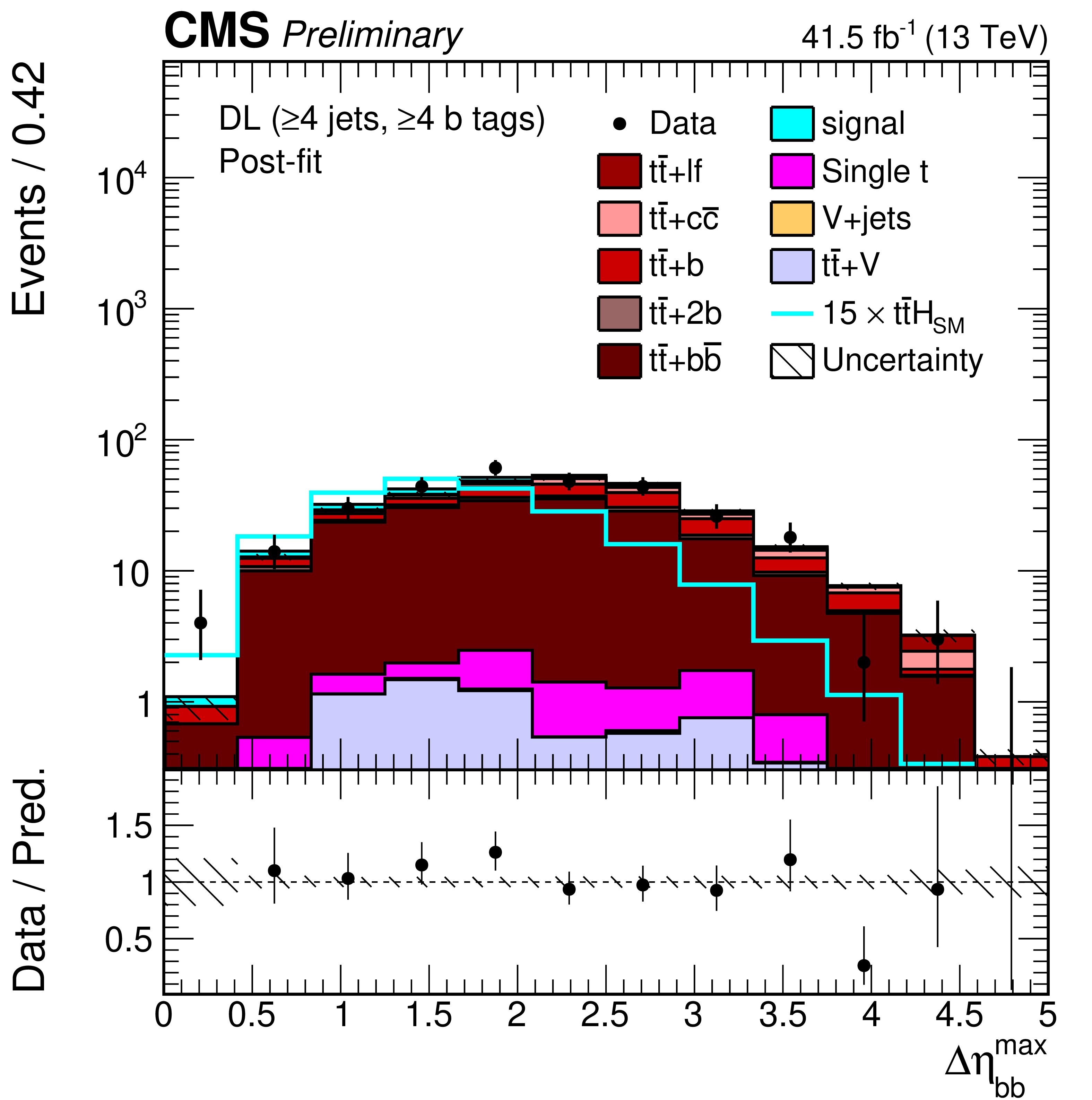
Distributions of representative variables used as input to the BDT in the $\geq $4 jets, 3 b-tags (left) and $\geq $4 jets, $\geq$4 b-tags (right) categories of the dilepton channel: MEM discriminant (MEM), average b-tagging discriminant value of all b-tagged jets normalised to the total number of jets (average DeepCSV value (b-jets)), and maximum $\Delta \eta $ between any two b-tagged jets ($\Delta \eta ^{\text {max}}_{\text {b},\text {b}}$). The background and signal contributions (filled histograms) are stacked, and the hatched uncertainty bands correspond to the total statistical and systematic uncertainties. Shown are the post-fit contributions, where the model parameters are obtained from the final fit of the discriminant distributions to data, described in Section 7, and applied to the shown input variable distributions. The distributions observed in data (markers) are overlayed. In addition, the SM ${{\mathrm{t} {}\mathrm{\bar{t}}} \mathrm{H}}$ signal expectation (line) is overlayed (scaled by a factor 15 for better visibility). The first and the last bins include underflow and overflow events, respectively. The lower plots show the ratio of the data to the background prediction. |
png pdf |
Figure 4-a:
Distributions of representative variables used as input to the BDT in the $\geq $4 jets, 3 b-tags (left) and $\geq $4 jets, $\geq$4 b-tags (right) categories of the dilepton channel: MEM discriminant (MEM), average b-tagging discriminant value of all b-tagged jets normalised to the total number of jets (average DeepCSV value (b-jets)), and maximum $\Delta \eta $ between any two b-tagged jets ($\Delta \eta ^{\text {max}}_{\text {b},\text {b}}$). The background and signal contributions (filled histograms) are stacked, and the hatched uncertainty bands correspond to the total statistical and systematic uncertainties. Shown are the post-fit contributions, where the model parameters are obtained from the final fit of the discriminant distributions to data, described in Section 7, and applied to the shown input variable distributions. The distributions observed in data (markers) are overlayed. In addition, the SM ${{\mathrm{t} {}\mathrm{\bar{t}}} \mathrm{H}}$ signal expectation (line) is overlayed (scaled by a factor 15 for better visibility). The first and the last bins include underflow and overflow events, respectively. The lower plots show the ratio of the data to the background prediction. |
png pdf |
Figure 4-b:
Distributions of representative variables used as input to the BDT in the $\geq $4 jets, 3 b-tags (left) and $\geq $4 jets, $\geq$4 b-tags (right) categories of the dilepton channel: MEM discriminant (MEM), average b-tagging discriminant value of all b-tagged jets normalised to the total number of jets (average DeepCSV value (b-jets)), and maximum $\Delta \eta $ between any two b-tagged jets ($\Delta \eta ^{\text {max}}_{\text {b},\text {b}}$). The background and signal contributions (filled histograms) are stacked, and the hatched uncertainty bands correspond to the total statistical and systematic uncertainties. Shown are the post-fit contributions, where the model parameters are obtained from the final fit of the discriminant distributions to data, described in Section 7, and applied to the shown input variable distributions. The distributions observed in data (markers) are overlayed. In addition, the SM ${{\mathrm{t} {}\mathrm{\bar{t}}} \mathrm{H}}$ signal expectation (line) is overlayed (scaled by a factor 15 for better visibility). The first and the last bins include underflow and overflow events, respectively. The lower plots show the ratio of the data to the background prediction. |
png pdf |
Figure 4-c:
Distributions of representative variables used as input to the BDT in the $\geq $4 jets, 3 b-tags (left) and $\geq $4 jets, $\geq$4 b-tags (right) categories of the dilepton channel: MEM discriminant (MEM), average b-tagging discriminant value of all b-tagged jets normalised to the total number of jets (average DeepCSV value (b-jets)), and maximum $\Delta \eta $ between any two b-tagged jets ($\Delta \eta ^{\text {max}}_{\text {b},\text {b}}$). The background and signal contributions (filled histograms) are stacked, and the hatched uncertainty bands correspond to the total statistical and systematic uncertainties. Shown are the post-fit contributions, where the model parameters are obtained from the final fit of the discriminant distributions to data, described in Section 7, and applied to the shown input variable distributions. The distributions observed in data (markers) are overlayed. In addition, the SM ${{\mathrm{t} {}\mathrm{\bar{t}}} \mathrm{H}}$ signal expectation (line) is overlayed (scaled by a factor 15 for better visibility). The first and the last bins include underflow and overflow events, respectively. The lower plots show the ratio of the data to the background prediction. |
png pdf |
Figure 4-d:
Distributions of representative variables used as input to the BDT in the $\geq $4 jets, 3 b-tags (left) and $\geq $4 jets, $\geq$4 b-tags (right) categories of the dilepton channel: MEM discriminant (MEM), average b-tagging discriminant value of all b-tagged jets normalised to the total number of jets (average DeepCSV value (b-jets)), and maximum $\Delta \eta $ between any two b-tagged jets ($\Delta \eta ^{\text {max}}_{\text {b},\text {b}}$). The background and signal contributions (filled histograms) are stacked, and the hatched uncertainty bands correspond to the total statistical and systematic uncertainties. Shown are the post-fit contributions, where the model parameters are obtained from the final fit of the discriminant distributions to data, described in Section 7, and applied to the shown input variable distributions. The distributions observed in data (markers) are overlayed. In addition, the SM ${{\mathrm{t} {}\mathrm{\bar{t}}} \mathrm{H}}$ signal expectation (line) is overlayed (scaled by a factor 15 for better visibility). The first and the last bins include underflow and overflow events, respectively. The lower plots show the ratio of the data to the background prediction. |
png pdf |
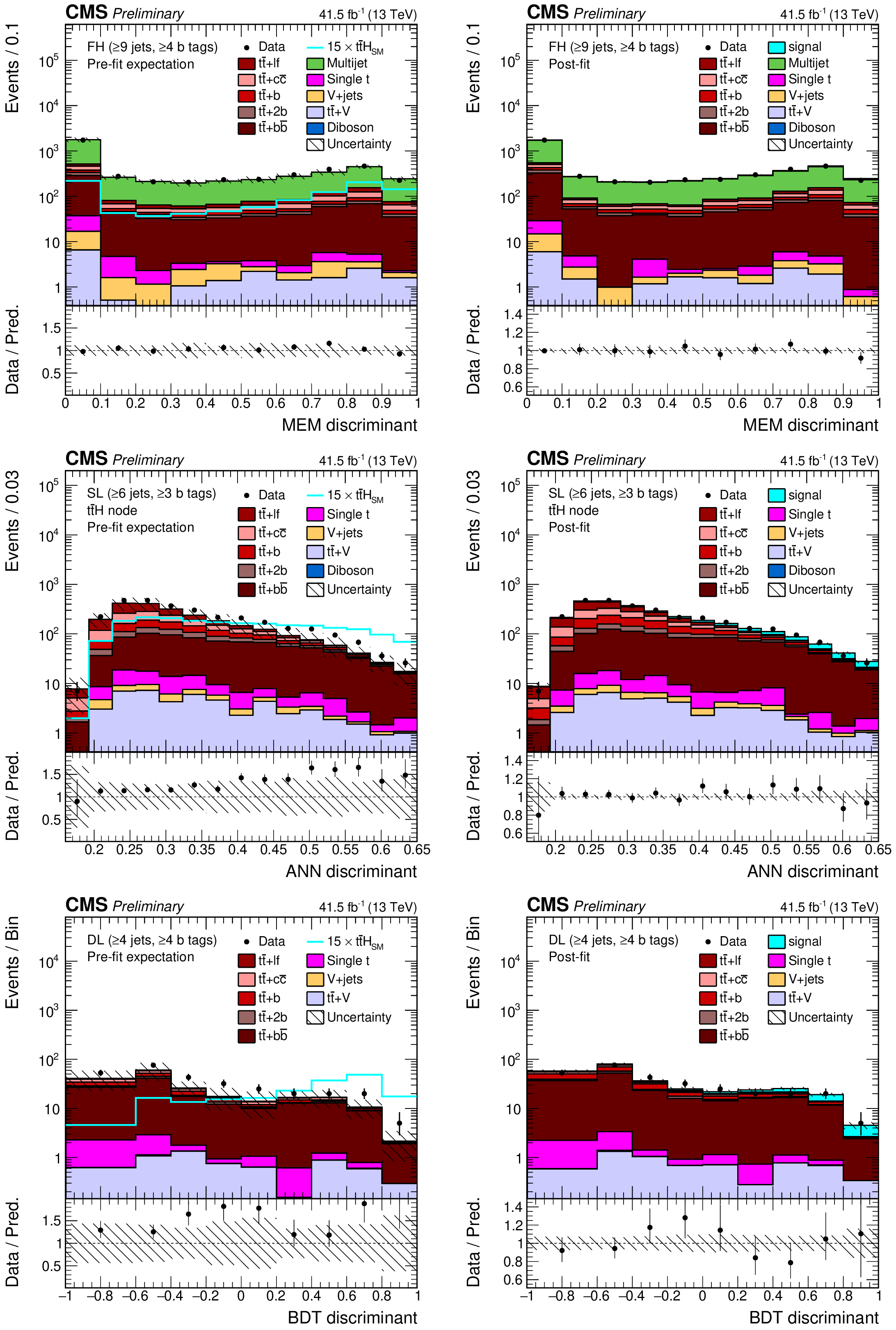
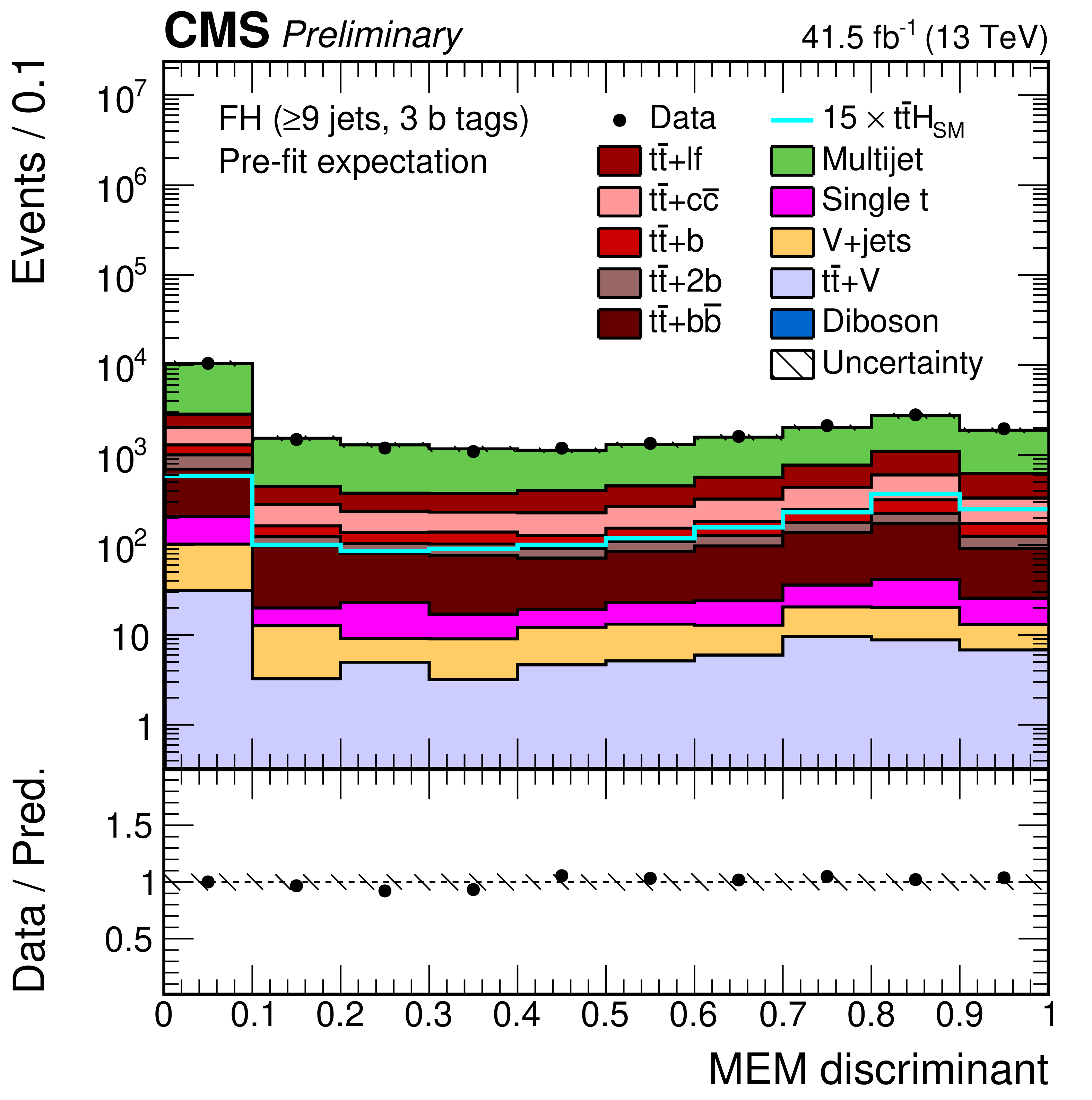
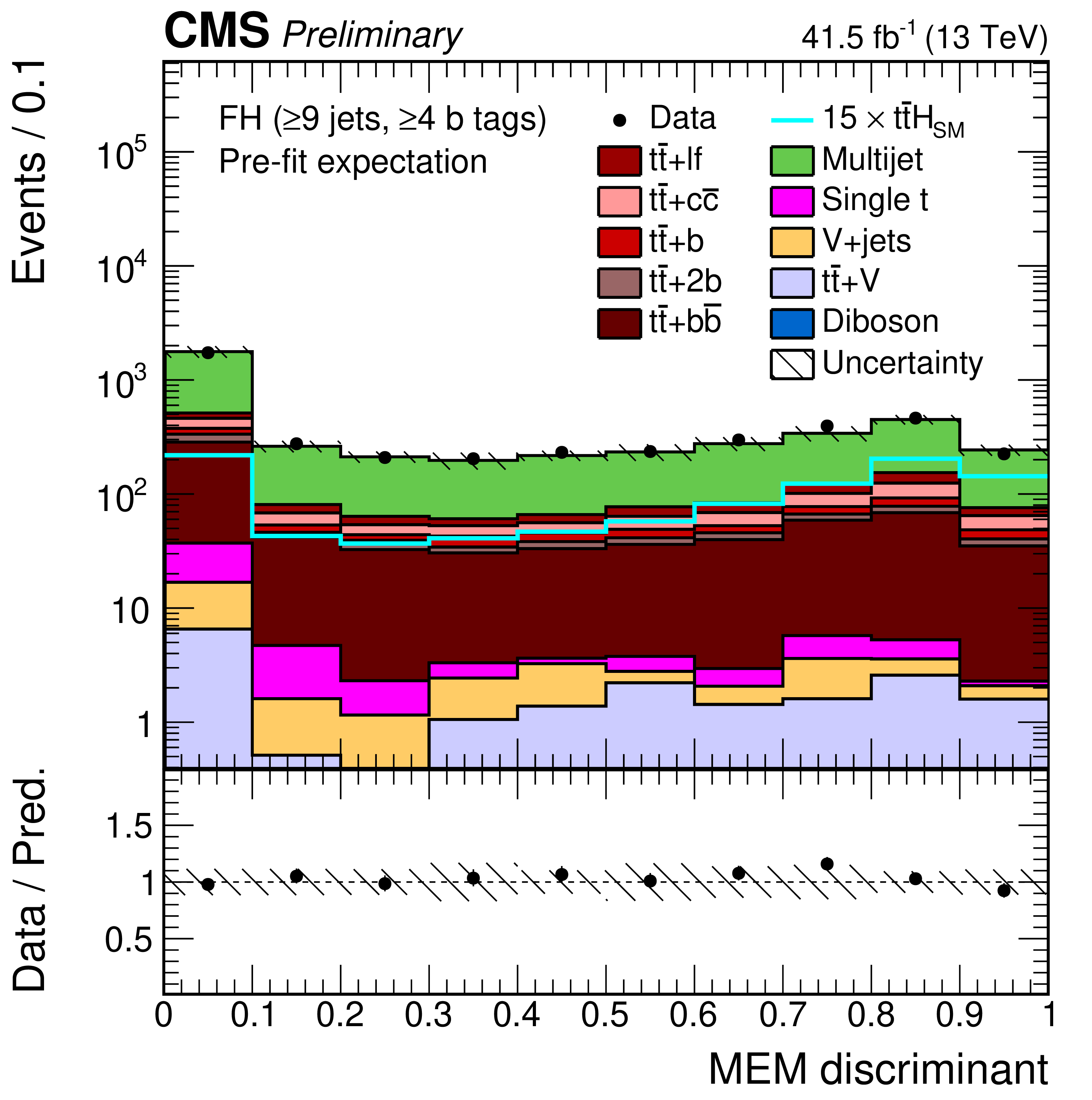
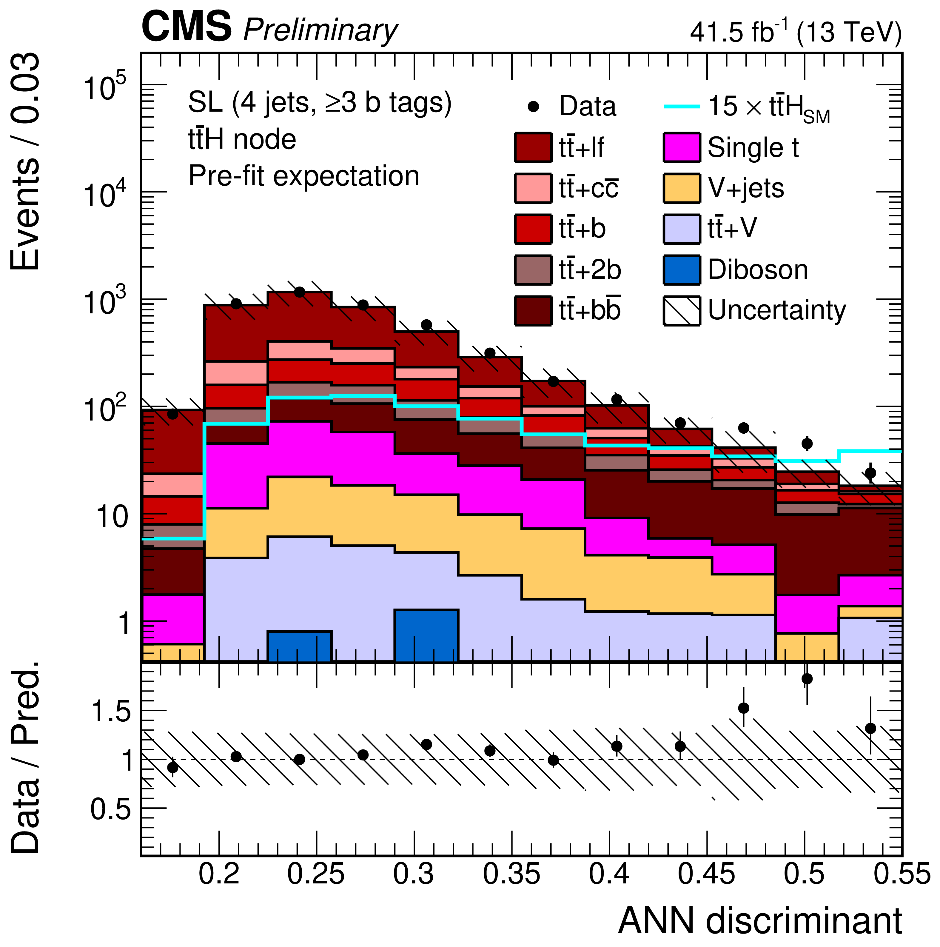
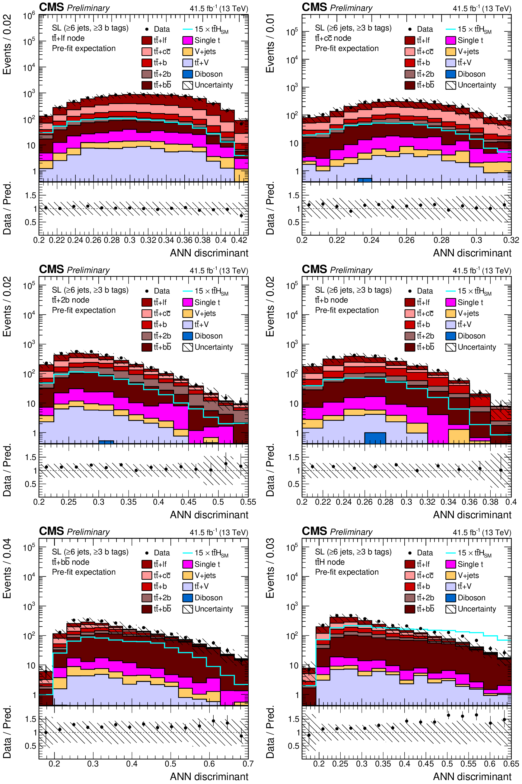
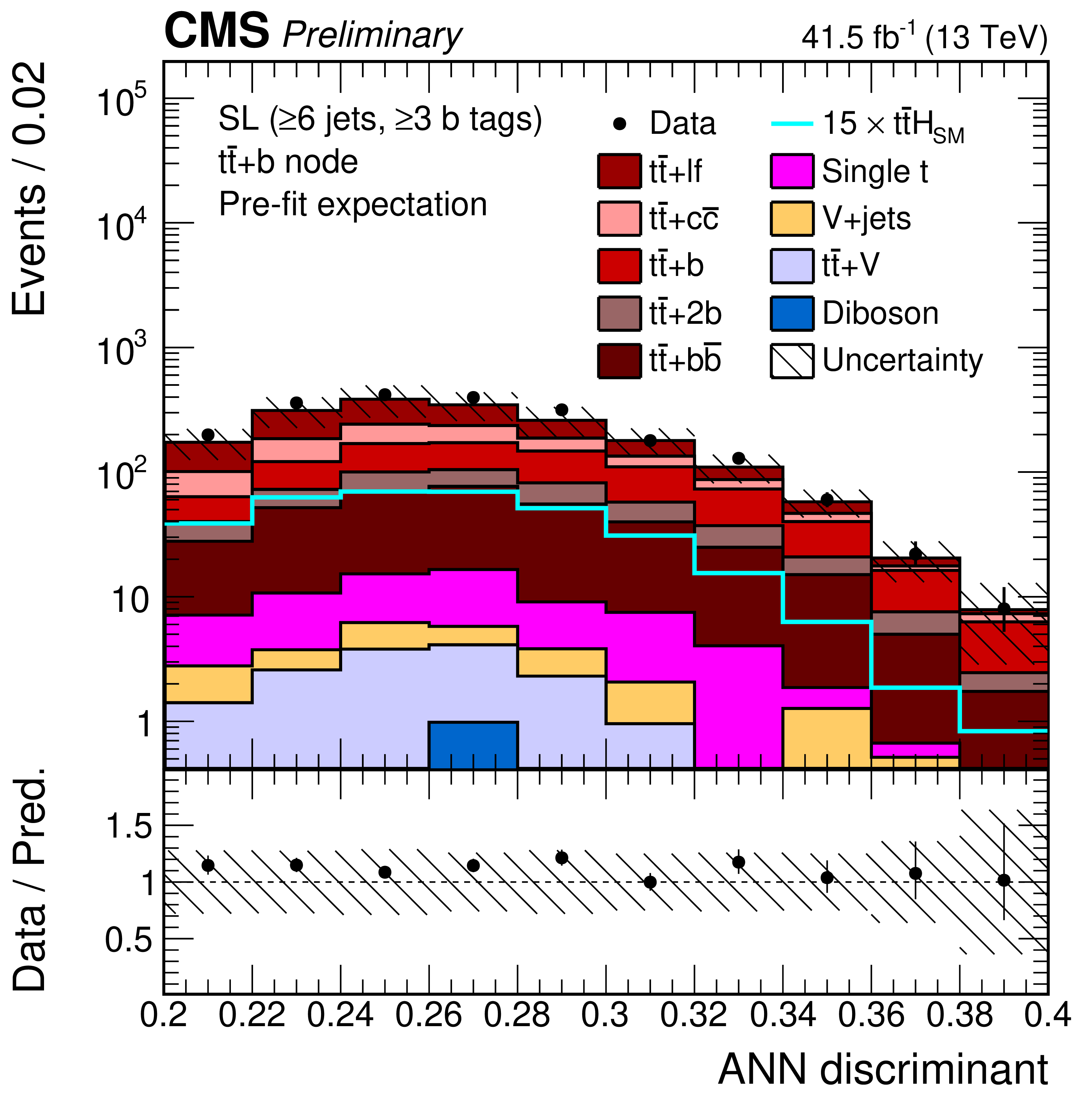
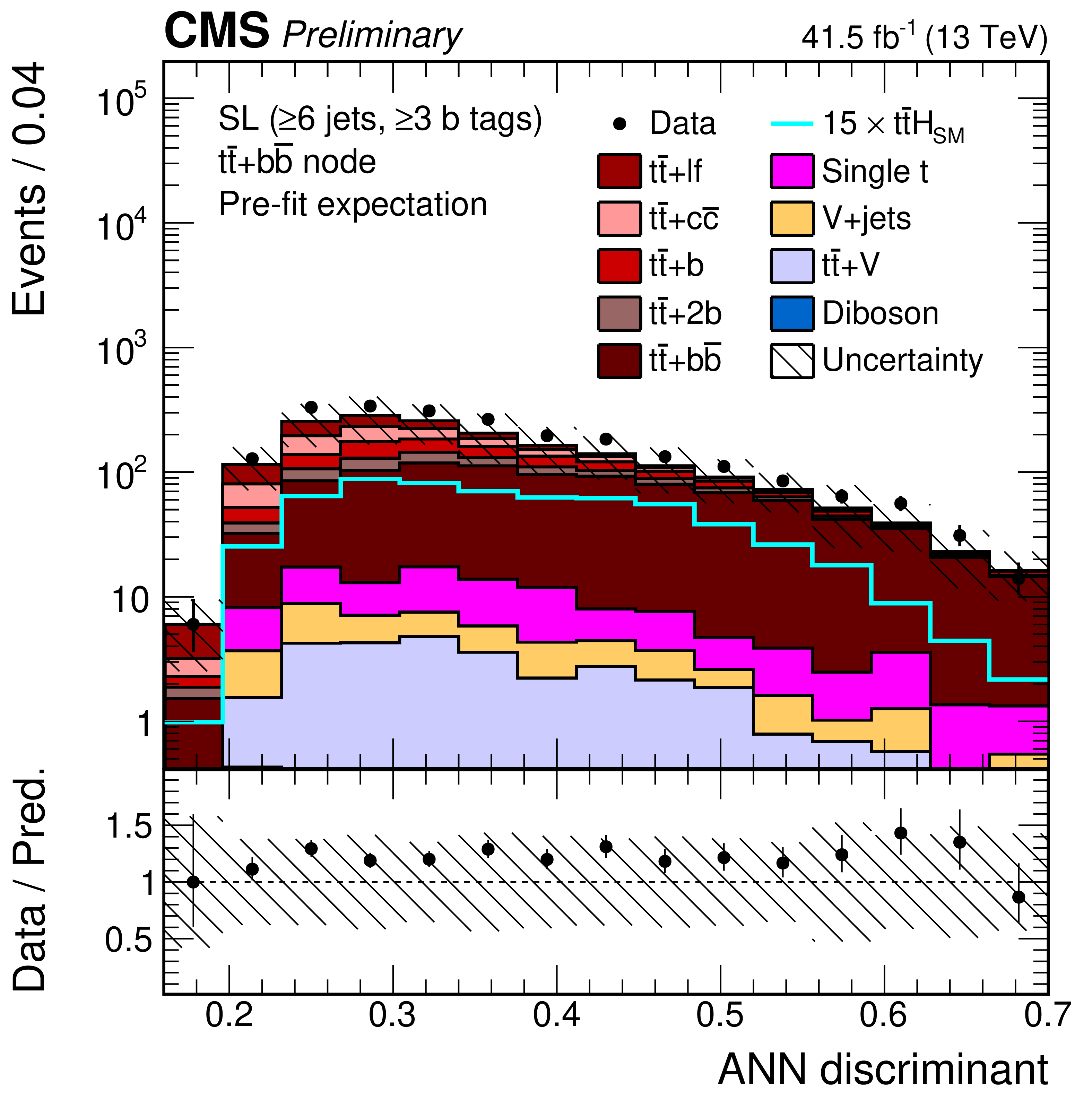
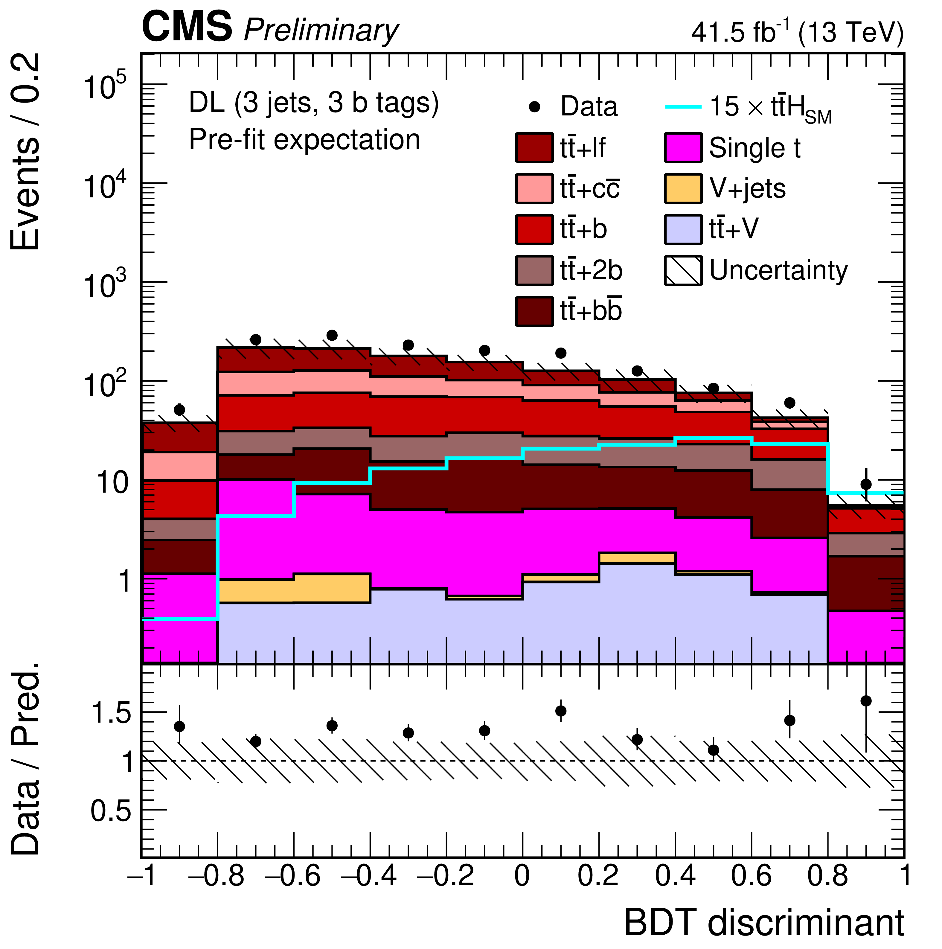
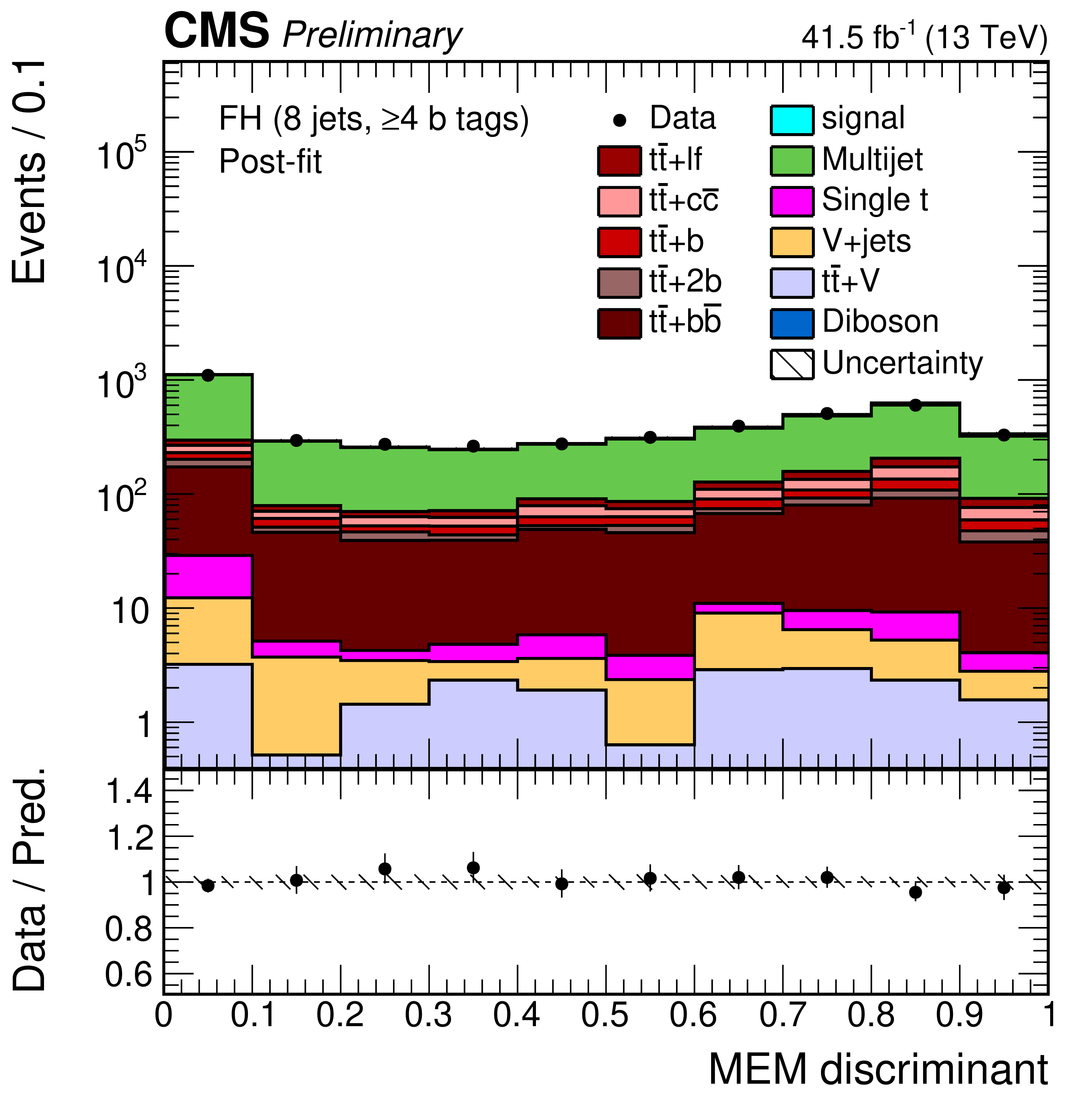
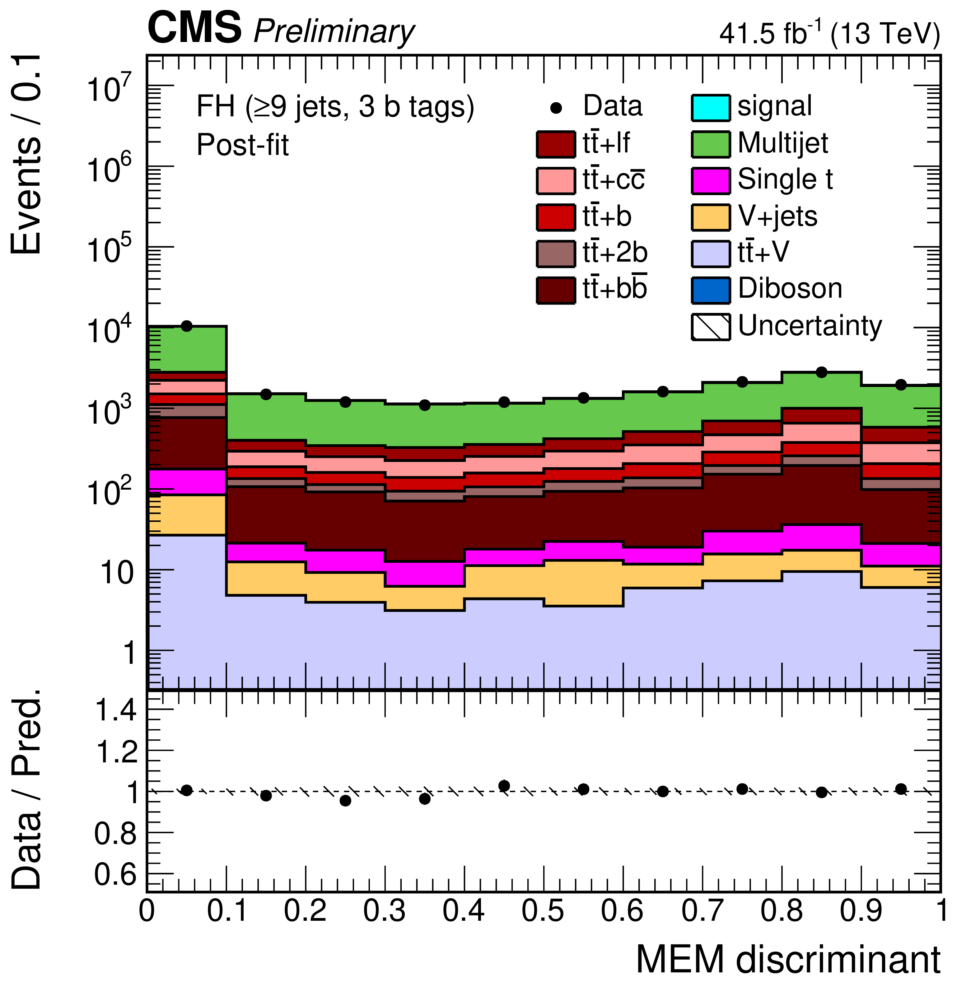
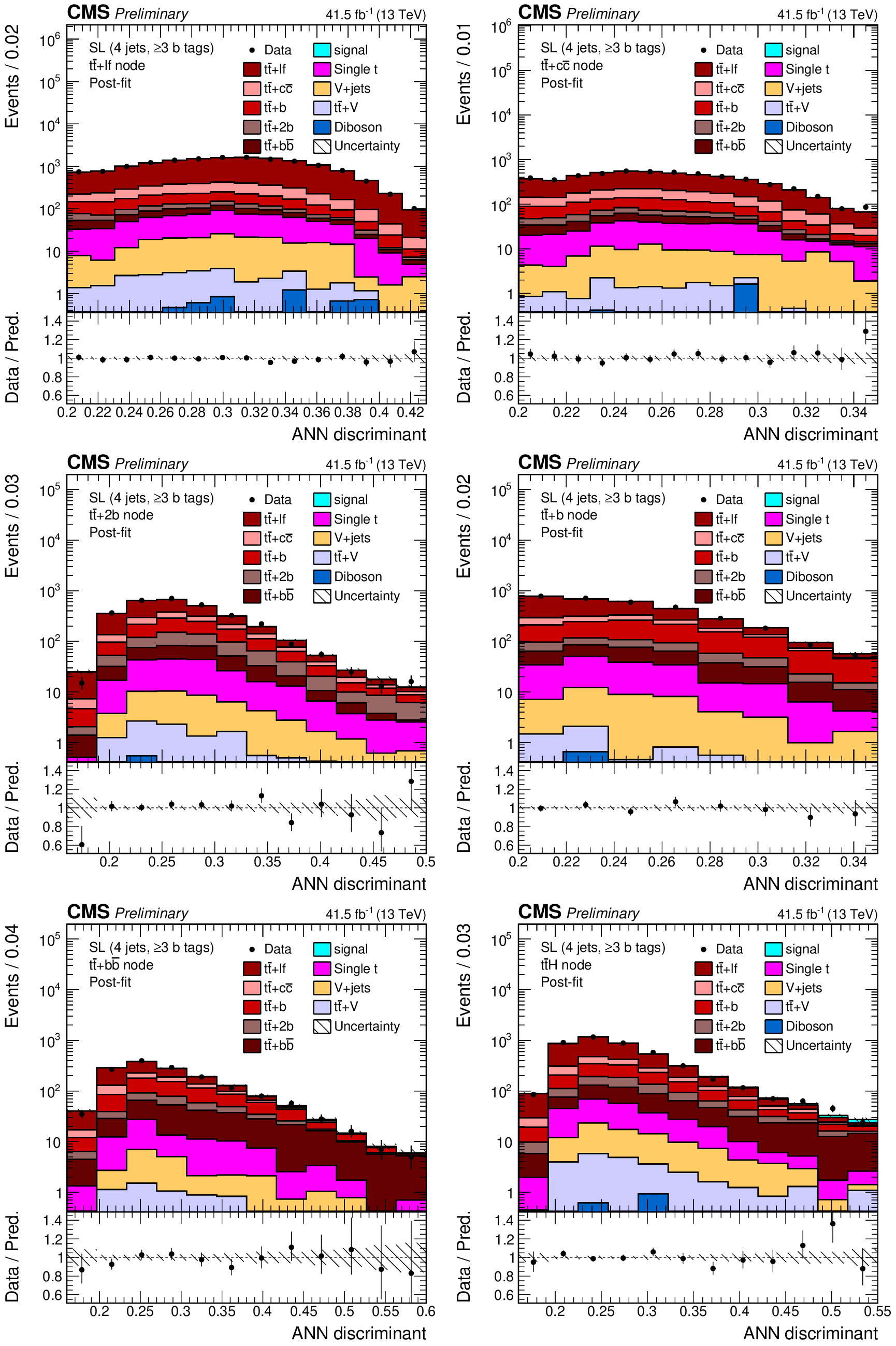
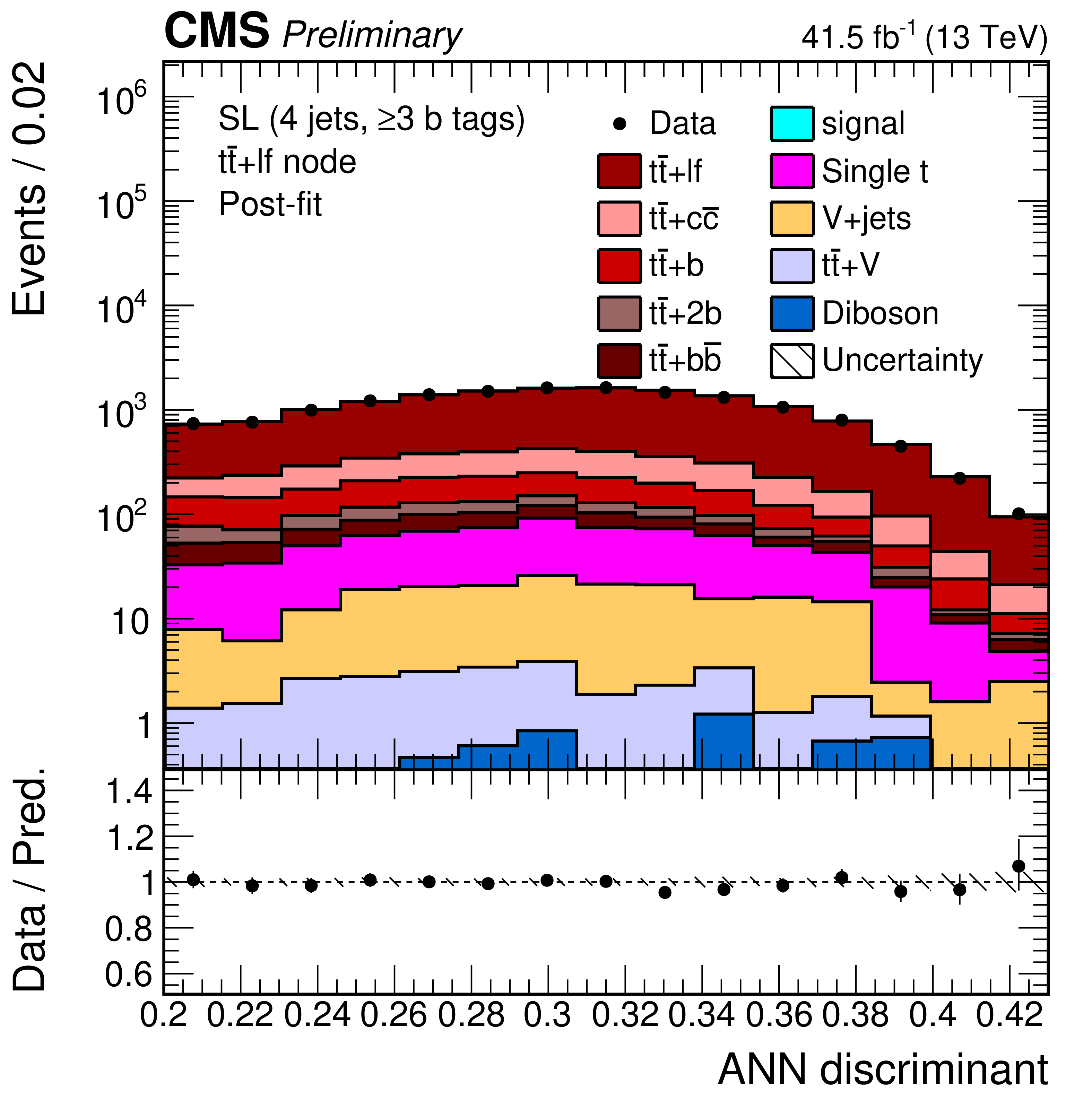
Figure 5:
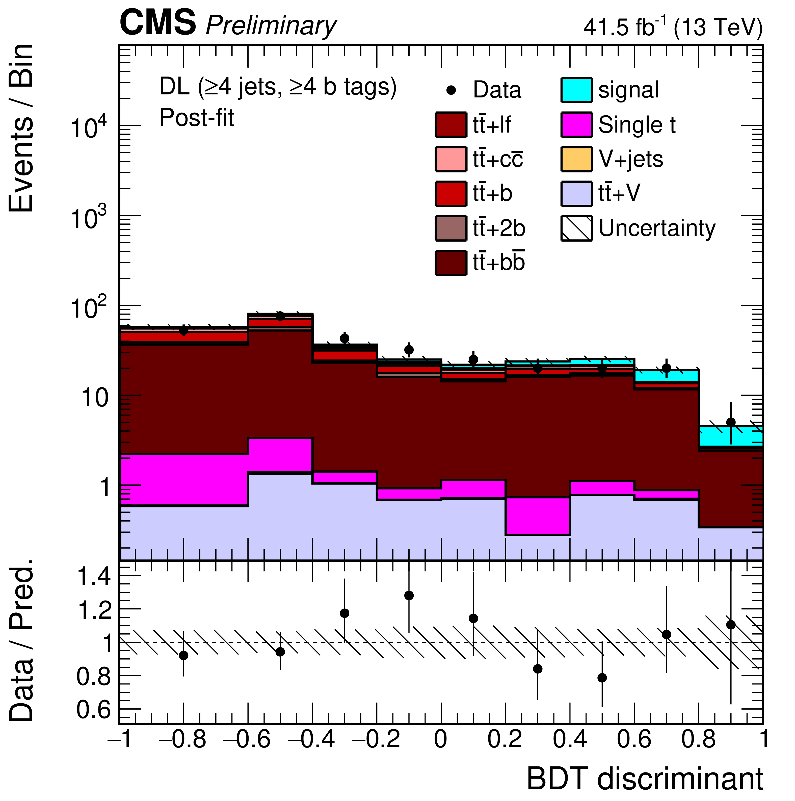
Final discriminant shapes in the categories with the highest sensitivity in fully-hadronic (top), semi-leptonic (middle), and dilepton (bottom) channels before (left) and after (right) the fit to data. The expected background contributions (filled histograms) are stacked. In the pre-fit case, the expected signal contribution (line), scaled by a factor 15, is superimposed. In the post-fit case, the fitted signal contribution is also stacked. The hatched uncertainty bands include the total uncertainty of the fit model. The distributions observed in data (markers) are overlayed. The first and the last bins include underflow and overflow events, respectively. The lower plots show the ratio of the data to the background prediction. |

png pdf |
Figure 5-a:
Final discriminant shapes in the categories with the highest sensitivity in fully-hadronic (top), semi-leptonic (middle), and dilepton (bottom) channels before (left) and after (right) the fit to data. The expected background contributions (filled histograms) are stacked. In the pre-fit case, the expected signal contribution (line), scaled by a factor 15, is superimposed. In the post-fit case, the fitted signal contribution is also stacked. The hatched uncertainty bands include the total uncertainty of the fit model. The distributions observed in data (markers) are overlayed. The first and the last bins include underflow and overflow events, respectively. The lower plots show the ratio of the data to the background prediction. |
png pdf |
Figure 5-b:
Final discriminant shapes in the categories with the highest sensitivity in fully-hadronic (top), semi-leptonic (middle), and dilepton (bottom) channels before (left) and after (right) the fit to data. The expected background contributions (filled histograms) are stacked. In the pre-fit case, the expected signal contribution (line), scaled by a factor 15, is superimposed. In the post-fit case, the fitted signal contribution is also stacked. The hatched uncertainty bands include the total uncertainty of the fit model. The distributions observed in data (markers) are overlayed. The first and the last bins include underflow and overflow events, respectively. The lower plots show the ratio of the data to the background prediction. |
png pdf |
Figure 5-c:
Final discriminant shapes in the categories with the highest sensitivity in fully-hadronic (top), semi-leptonic (middle), and dilepton (bottom) channels before (left) and after (right) the fit to data. The expected background contributions (filled histograms) are stacked. In the pre-fit case, the expected signal contribution (line), scaled by a factor 15, is superimposed. In the post-fit case, the fitted signal contribution is also stacked. The hatched uncertainty bands include the total uncertainty of the fit model. The distributions observed in data (markers) are overlayed. The first and the last bins include underflow and overflow events, respectively. The lower plots show the ratio of the data to the background prediction. |

png pdf |
Figure 5-d:
Final discriminant shapes in the categories with the highest sensitivity in fully-hadronic (top), semi-leptonic (middle), and dilepton (bottom) channels before (left) and after (right) the fit to data. The expected background contributions (filled histograms) are stacked. In the pre-fit case, the expected signal contribution (line), scaled by a factor 15, is superimposed. In the post-fit case, the fitted signal contribution is also stacked. The hatched uncertainty bands include the total uncertainty of the fit model. The distributions observed in data (markers) are overlayed. The first and the last bins include underflow and overflow events, respectively. The lower plots show the ratio of the data to the background prediction. |

png pdf |
Figure 5-e:
Final discriminant shapes in the categories with the highest sensitivity in fully-hadronic (top), semi-leptonic (middle), and dilepton (bottom) channels before (left) and after (right) the fit to data. The expected background contributions (filled histograms) are stacked. In the pre-fit case, the expected signal contribution (line), scaled by a factor 15, is superimposed. In the post-fit case, the fitted signal contribution is also stacked. The hatched uncertainty bands include the total uncertainty of the fit model. The distributions observed in data (markers) are overlayed. The first and the last bins include underflow and overflow events, respectively. The lower plots show the ratio of the data to the background prediction. |
png pdf |
Figure 5-f:
Final discriminant shapes in the categories with the highest sensitivity in fully-hadronic (top), semi-leptonic (middle), and dilepton (bottom) channels before (left) and after (right) the fit to data. The expected background contributions (filled histograms) are stacked. In the pre-fit case, the expected signal contribution (line), scaled by a factor 15, is superimposed. In the post-fit case, the fitted signal contribution is also stacked. The hatched uncertainty bands include the total uncertainty of the fit model. The distributions observed in data (markers) are overlayed. The first and the last bins include underflow and overflow events, respectively. The lower plots show the ratio of the data to the background prediction. |
png pdf |
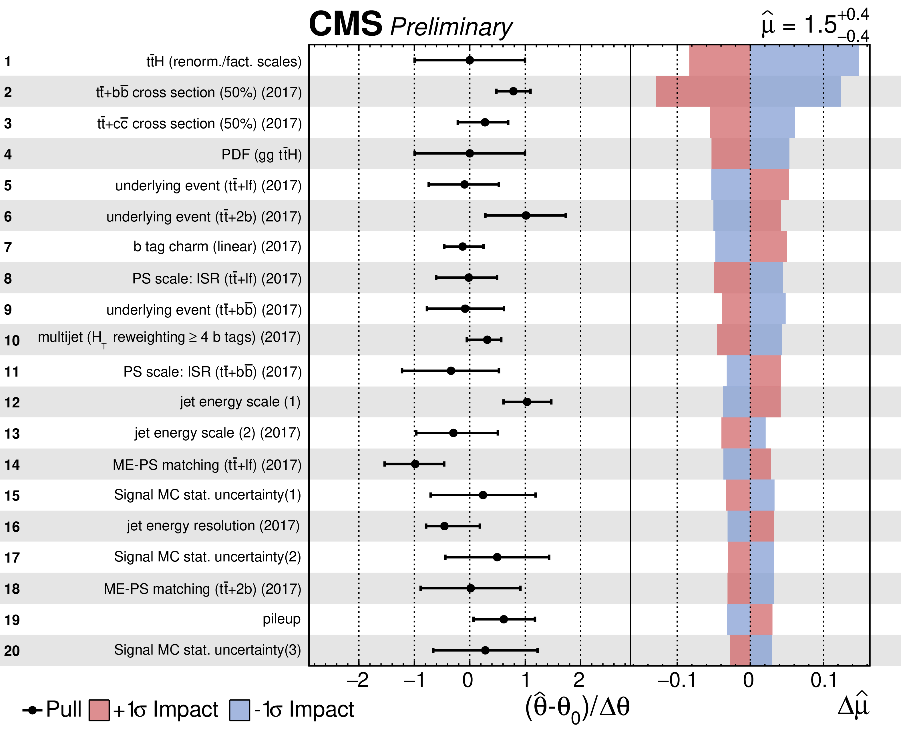
Figure 6:
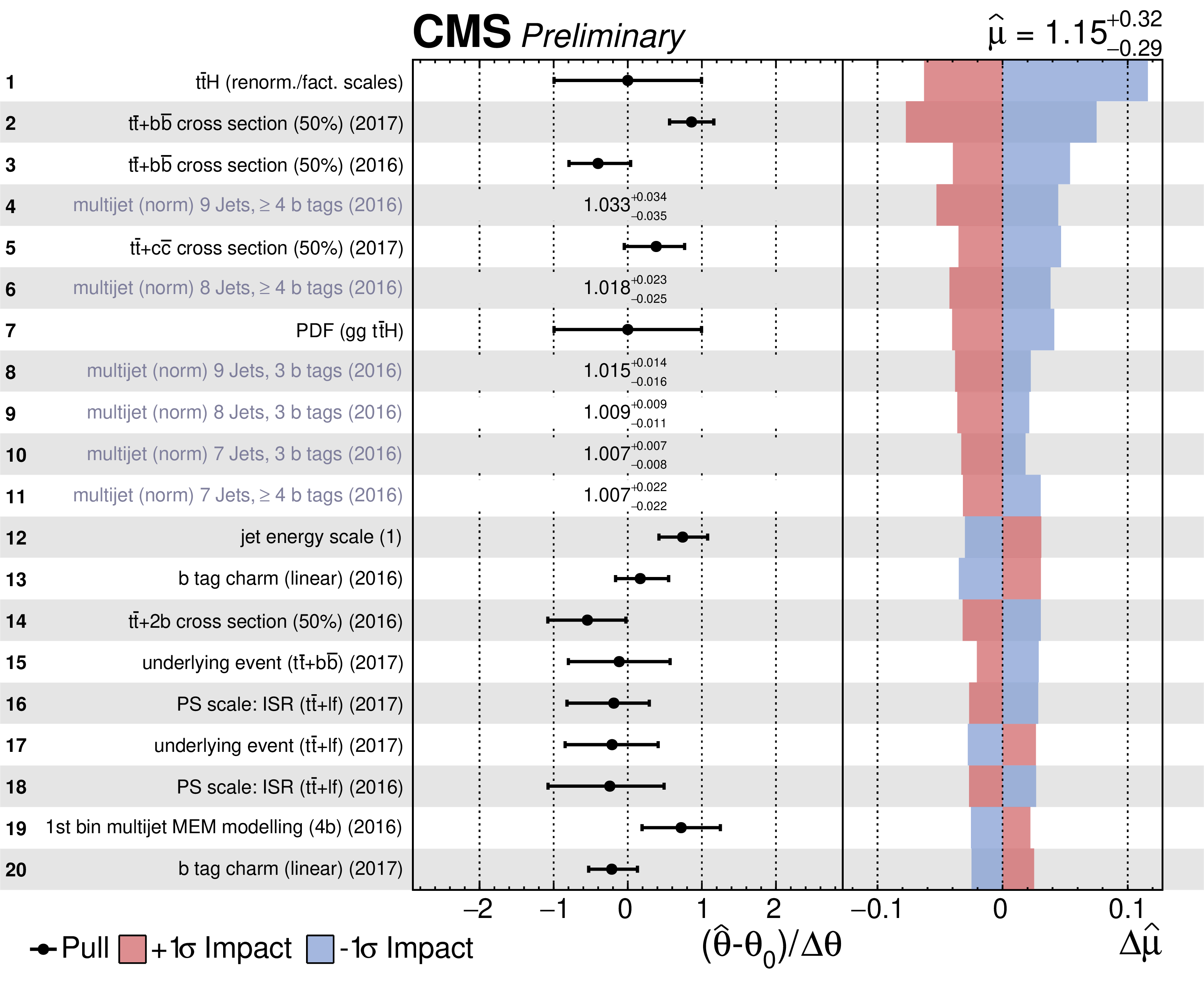
Post-fit pull and best-fit value of the nuisance parameters included in the fit to the 2017 data as well as their impact on the signal strength $\mu $, ordered by their impact. Only the 20 highest ranked parameters are shown. The two highest-ranked nuisance parameters related to the jet energy scale uncertainty sources are shown as indicated in parentheses. The pulls of the nuisance parameters (black markers) are computed relative to their pre-fit values $\theta _{0}$ and uncertainties $\Delta \theta $. The impact $\Delta \hat{\mu}$ is computed as the difference of the nominal best fit value of $\mu $ and the best fit value obtained when fixing the nuisance parameter under scrutiny to its best fit value $\hat{\theta}$ plus/minus its post-fit uncertainty (coloured areas). |
png pdf |
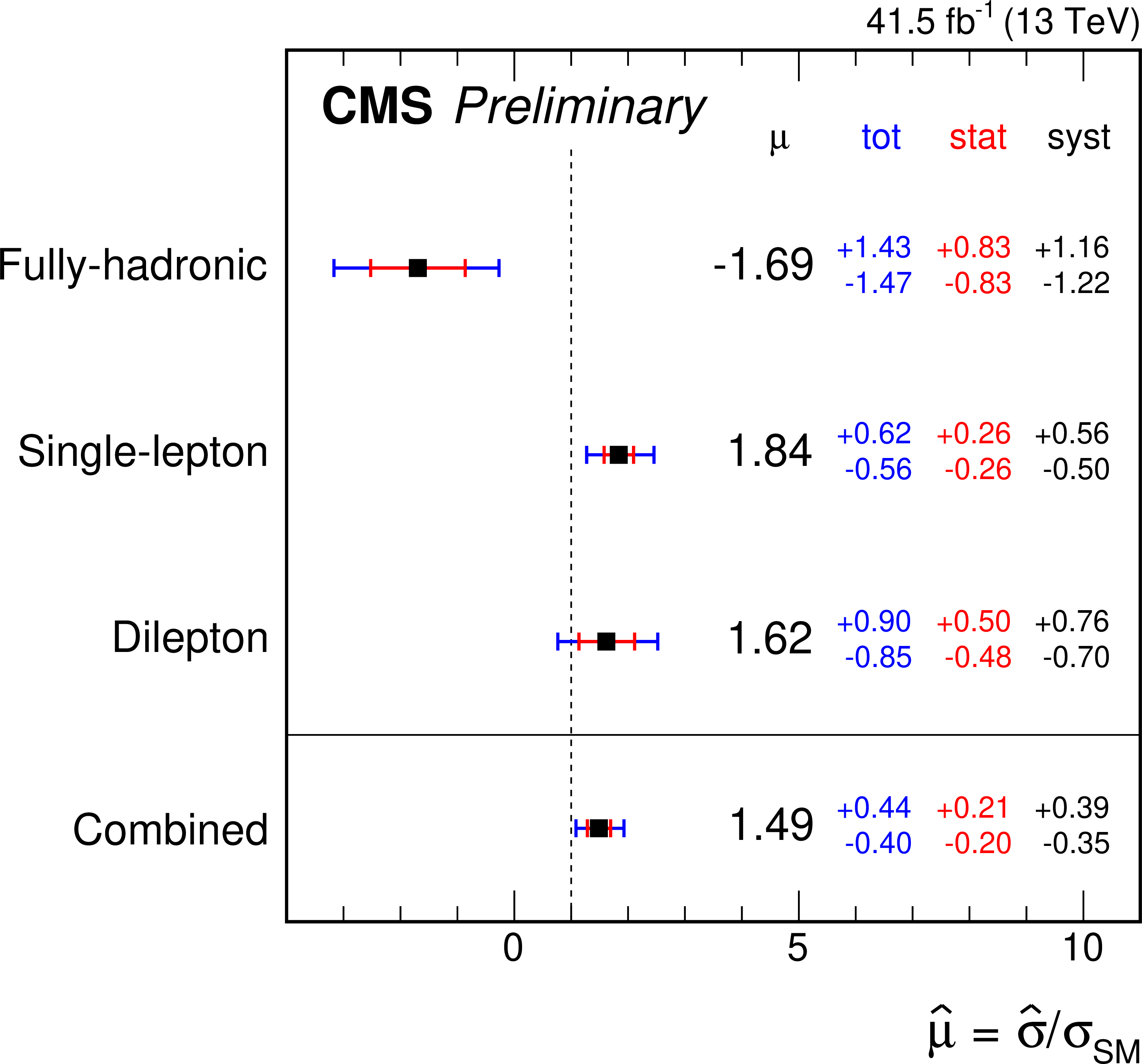
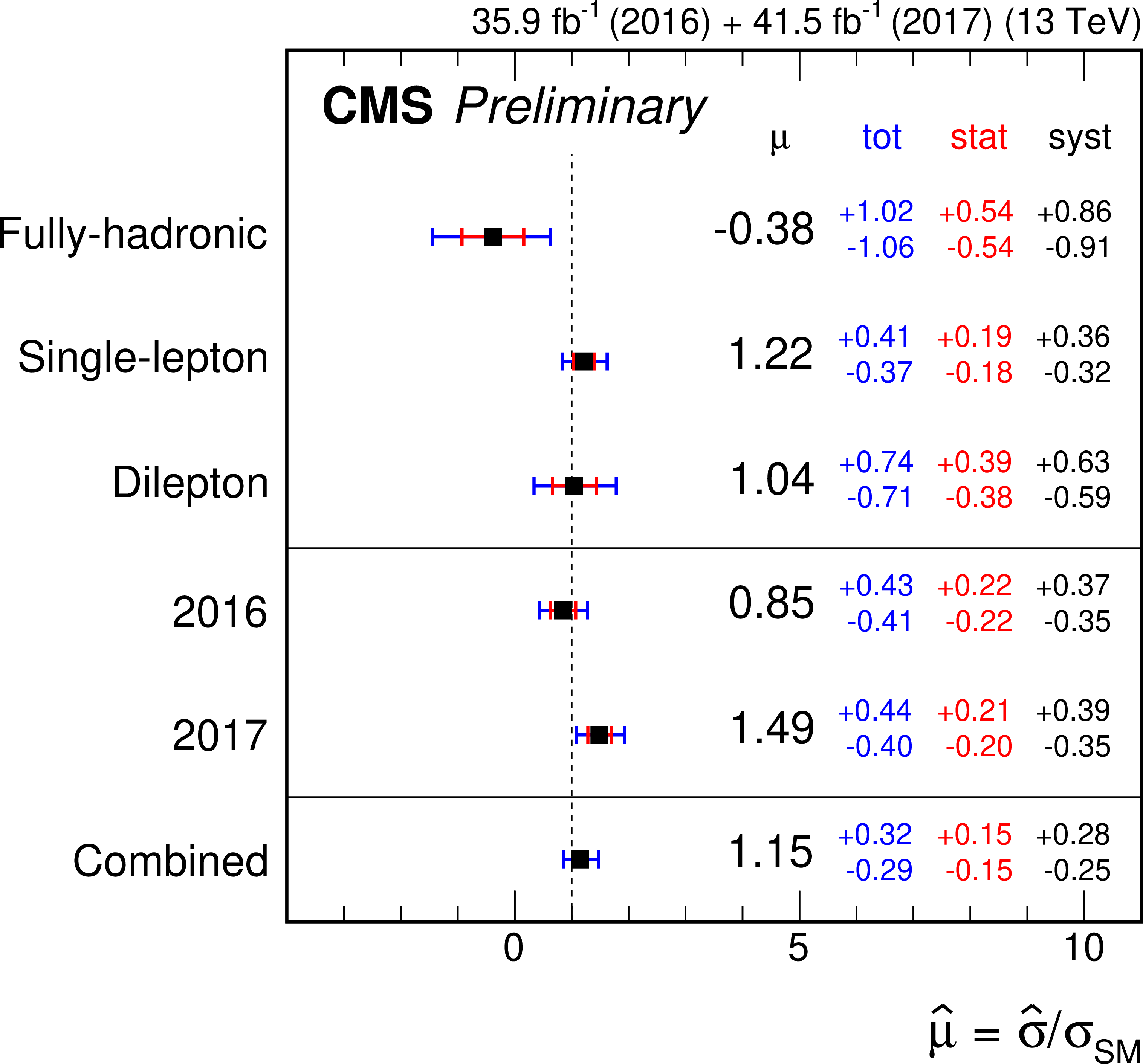
Figure 7:
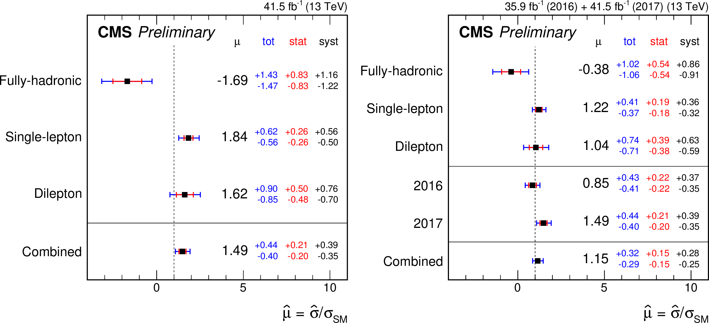
Best fit values of the signal strength modifiers $\mu $ obtained in the fit of the 2017 dataset (left) and in the combined fit of the 2016 and 2017 datasets (right) per channel and dataset and in the full combination. Also shown are the 68% expected confidence intervals (outer error bar), also split into their statistical (inner error bar) and systematic components. |
png pdf |
Figure 7-a:
Best fit values of the signal strength modifiers $\mu $ obtained in the fit of the 2017 dataset (left) and in the combined fit of the 2016 and 2017 datasets (right) per channel and dataset and in the full combination. Also shown are the 68% expected confidence intervals (outer error bar), also split into their statistical (inner error bar) and systematic components. |
png pdf |
Figure 7-b:
Best fit values of the signal strength modifiers $\mu $ obtained in the fit of the 2017 dataset (left) and in the combined fit of the 2016 and 2017 datasets (right) per channel and dataset and in the full combination. Also shown are the 68% expected confidence intervals (outer error bar), also split into their statistical (inner error bar) and systematic components. |
png pdf |
Figure 8:
Post-fit pull and best-fit value of the constrained (text in black) and unconstrained (text in grey) nuisance parameters included in the fit to the 2016 plus 2017 data as well as their impact on the signal strength $\mu $, ordered by their impact. Only the 20 highest ranked parameters are shown. The pulls of the nuisance parameters (black markers) are computed relative to their pre-fit values $\theta _{0}$ and uncertainties $\Delta \theta $. The impact $\Delta \hat{\mu}$ is computed as the difference of the nominal best fit value of $\mu $ and the best fit value obtained when fixing the nuisance parameter under scrutiny to its best fit value $\hat{\theta}$ plus/minus its post-fit uncertainty (coloured areas). |
| Tables | |
png pdf |
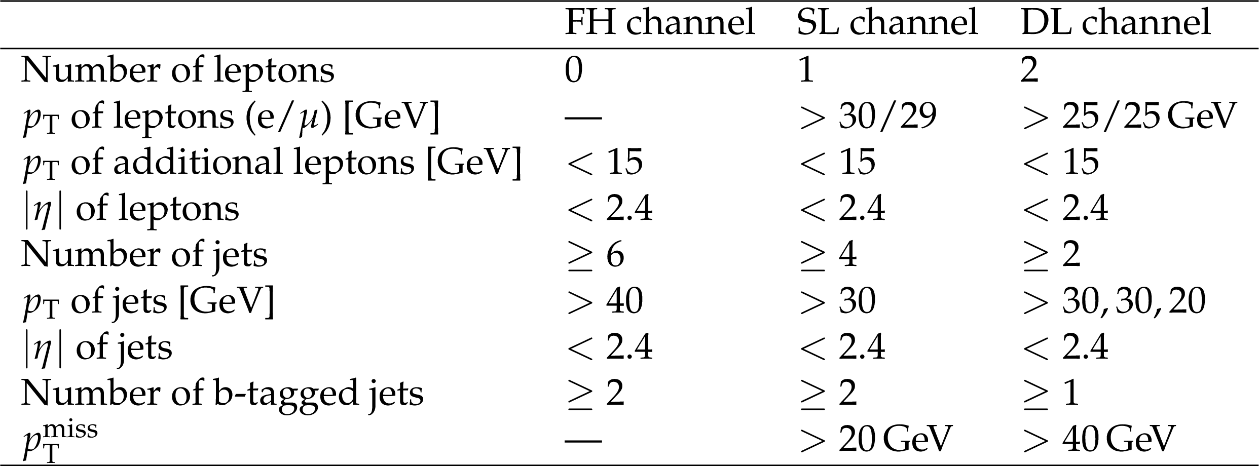
Table 1:
Baseline event selection criteria in the fully-hadronic (FH), single-lepton (SL), and dilepton (DL) channels. |
png pdf |
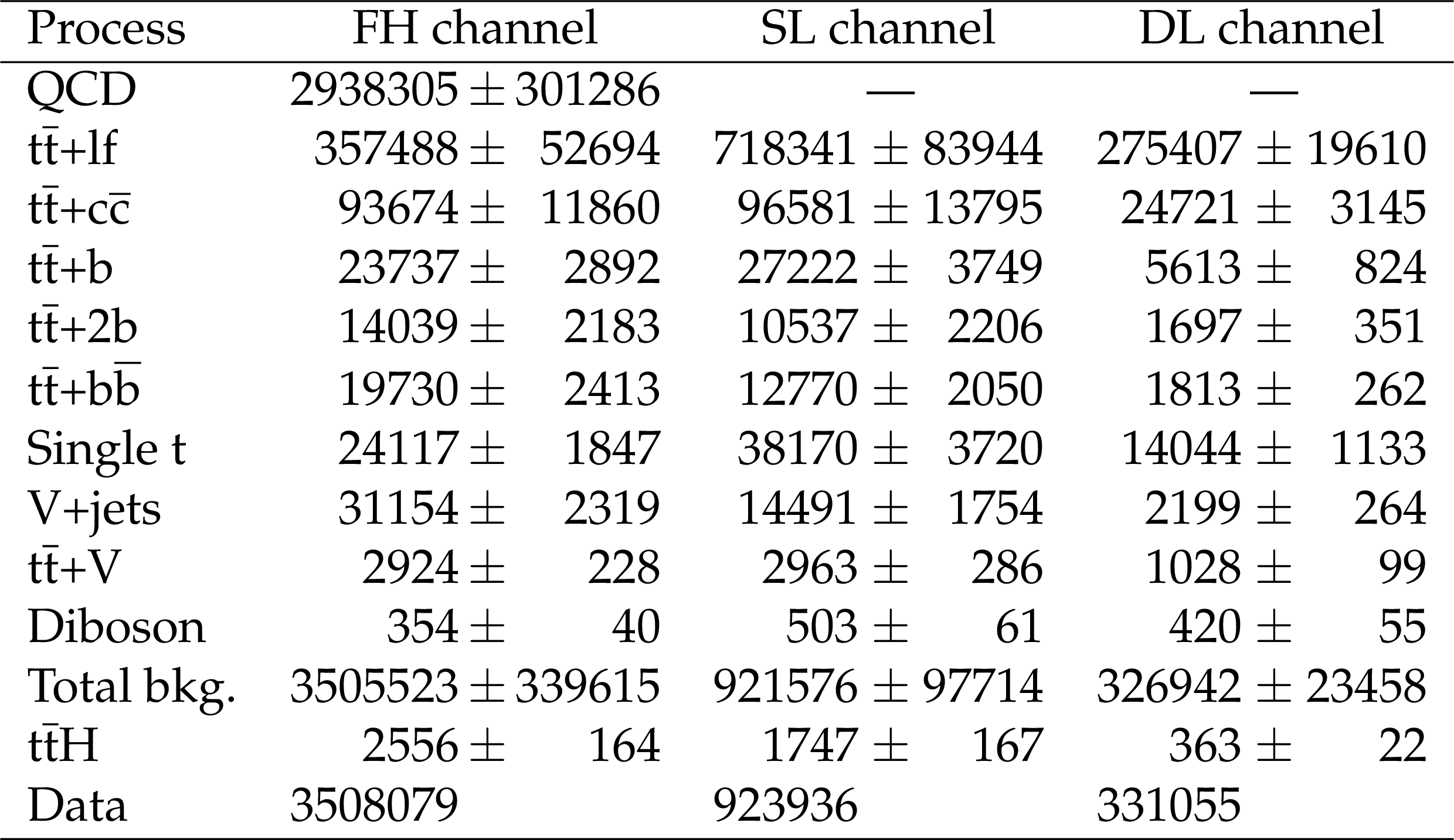
Table 2:
Event yields observed in data and predicted by the simulation after the baseline selection in the fully-hadronic (FH), single-lepton (SL), and dilepton (DL) channels prior to the fit to data. Here, the QCD prediction is taken from simulation. The quoted uncertainties correspond to the total statistical and systematic uncertainties (excluding the 50% uncertainties on the normalisation of the ${\mathrm{t} {}\mathrm{\bar{t}}}$+hf processes). |
png pdf |
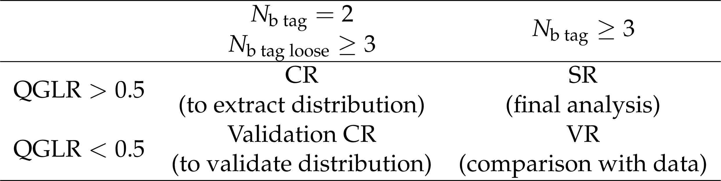
Table 3:
Definition and description of the four mutually exclusive regions in the analysis. |
png pdf |
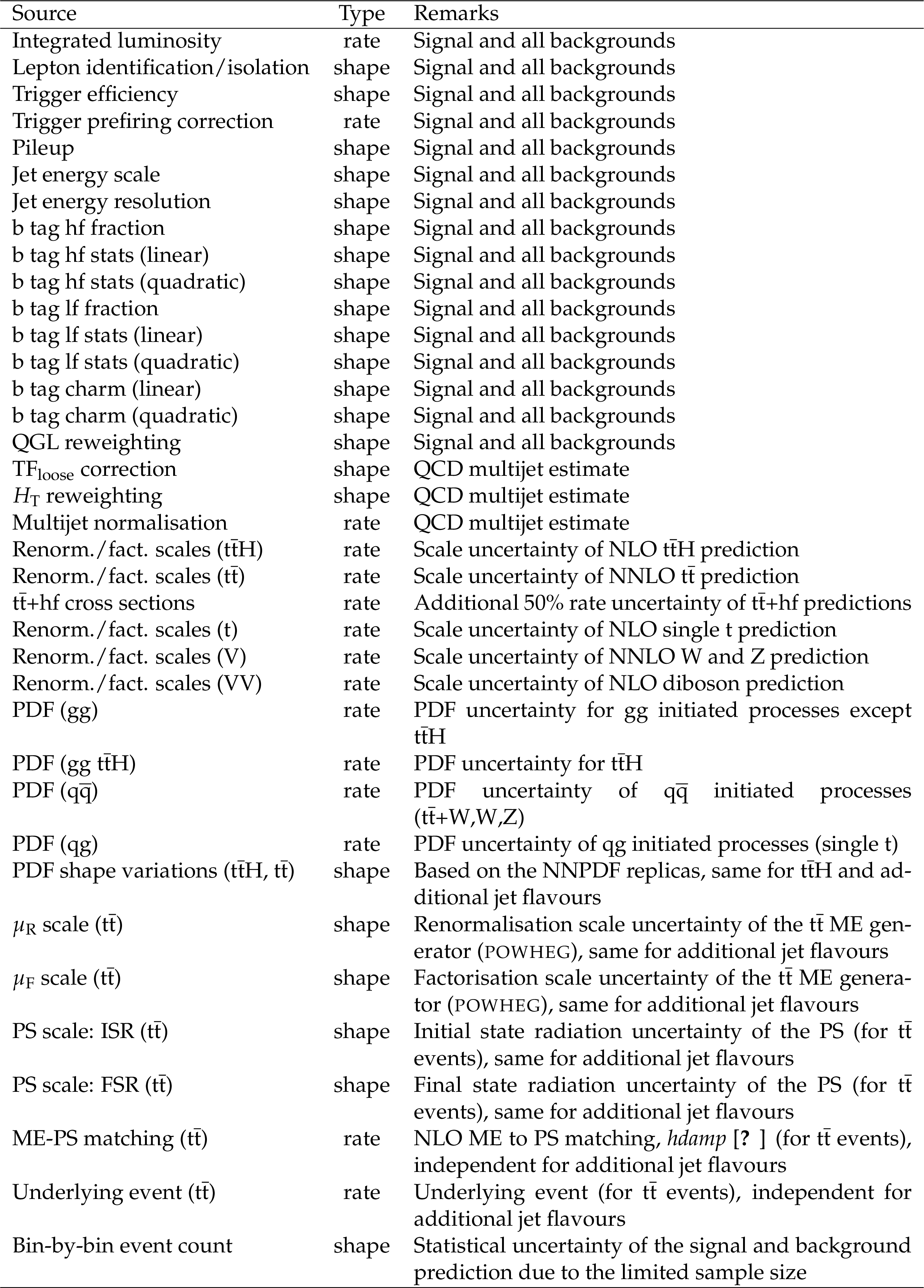
Table 4:
Systematic uncertainties considered in the analysis. |
png pdf |
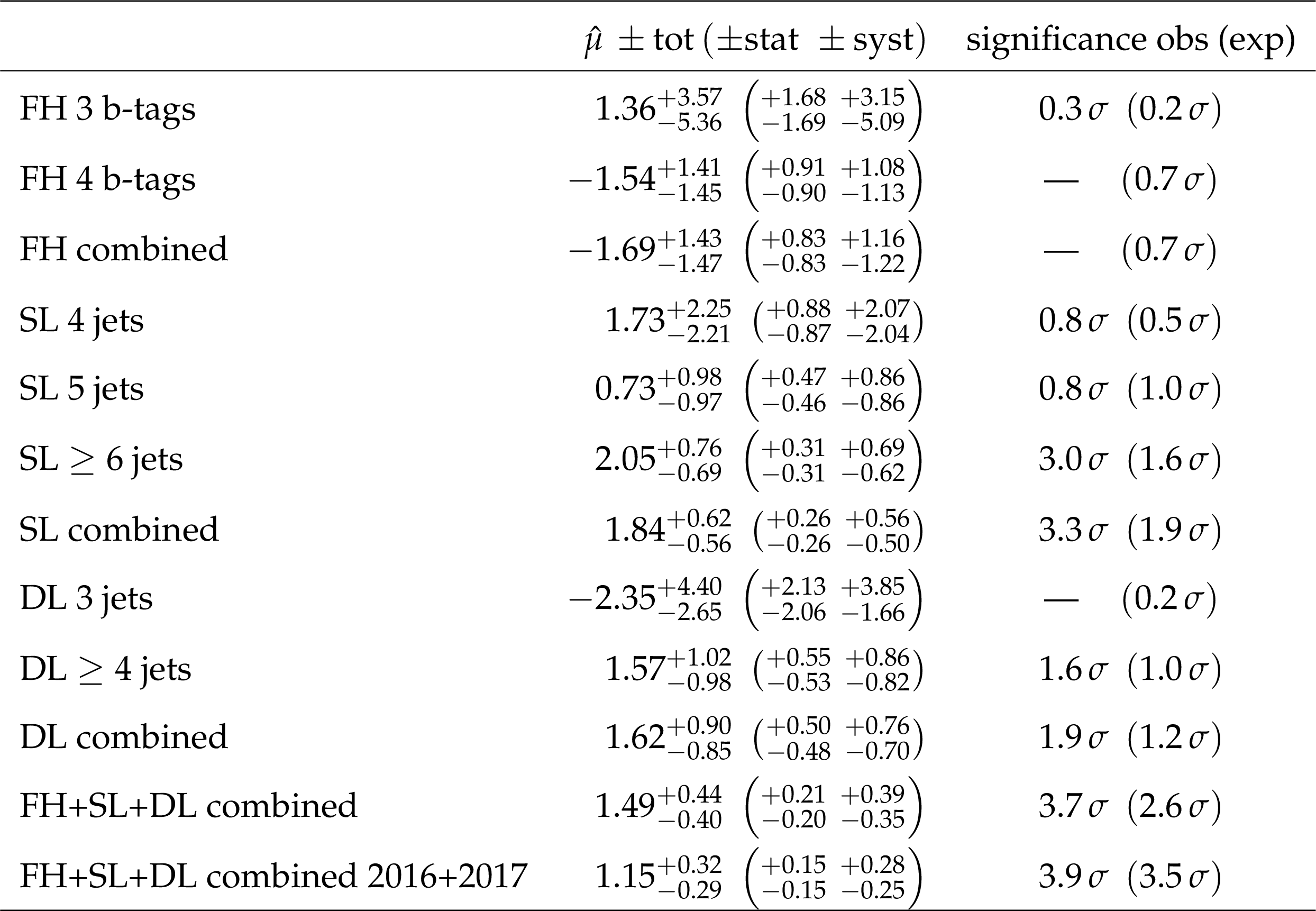
Table 5:
Best fit value of the signal strength modifier $\mu $ and the corresponding observed (obs) and expected (exp) significance in standard deviations in the fully-hadronic (FH), single-lepton (SL), and dilepton (DL) channels and in the channel combination. |
png pdf |
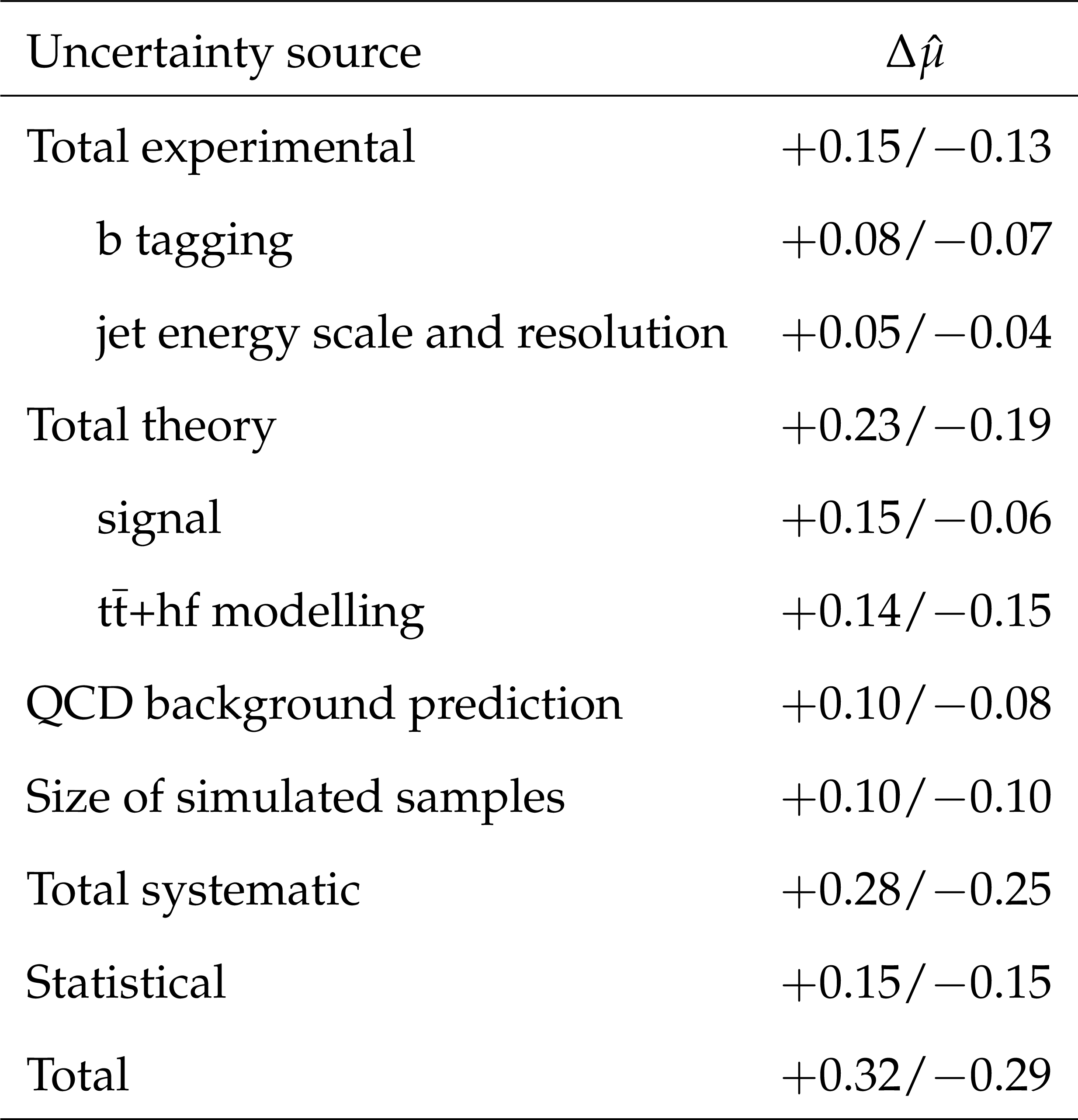
Table 6:
Contributions of different sources of uncertainties to the result for the combined fit to the 2016 and 2017 datasets (observed) and to the expectation from simulation (expected). The quoted uncertainties $\Delta \hat{\mu}$ in $\hat{\mu}$ are obtained by fixing the listed sources of uncertainties to their post-fit values in the fit and subtracting the obtained result in quadrature from the result of the full fit. The statistical uncertainty is evaluated by fixing all nuisance parameters to their post-fit values. The quadratic sum of the contributions is different from the total uncertainty because of correlations between the nuisance parameters. |
| Summary |
|
A measurement of the associated production of a Higgs boson and a top quark-antiquark pair (${\mathrm{t\bar{t}}\mathrm{H}}$) in the $\mathrm{b\bar{b}}$ final state of the Higgs boson has been presented. All decay channels of the $\mathrm{t\bar{t}}$ system are considered. The analysis has been performed in 41.5 fb$^{-1}$ of pp collision data recorded with the CMS detector at a centre-of-mass energy of 13 TeV in 2017. Candidate events are selected in mutually exclusive categories according to the $\mathrm{t\bar{t}}$ decay channel and jet multiplicity. Multivariate discriminants are used to further categorise the events and to separate the ${\mathrm{t\bar{t}}\mathrm{H}}$ signal from the $\mathrm{t\bar{t}}$-dominated background contributions. The signal is extracted in a simultaneous fit of the classifier distributions to the data across all categories and channels. The best fit value of the ${\mathrm{t\bar{t}}\mathrm{H}}$ signal cross-section on the 2017 dataset is $\hat{\mu} = $ 1.49 $^{+0.21}_{-0.20}$(stat) $^{+0.39}_{-0.35}$ (syst) relative to the SM expectation, corresponding to an observed (expected) significance of 3.7 (2.6) standard deviations above the background-only hypothesis. Combined with previous results obtained with 36.9 fb$^{-1}$ of data recorded in 2016, a best-fit value of $\hat{\mu} = $ 1.15 $^{+0.15}_{-0.15}$ (stat) $^{+0.28}_{-0.25}$ (syst) is found, corresponding to an observed (expected) significance of 3.9 (3.5) standard deviations above the background-only hypothesis. The presented result, which improves on previous CMS measurements in this channel owing to the increase in integrated luminosity and the usage of a more performant b tagging algorithm as well as refined analysis methods, constitutes the first evidence for ${\mathrm{t\bar{t}}\mathrm{H}}$ production in the $\mathrm{b\bar{b}}$ decay mode of the Higgs boson. |
| Additional Figures | |
png pdf |
Additional Figure 1:
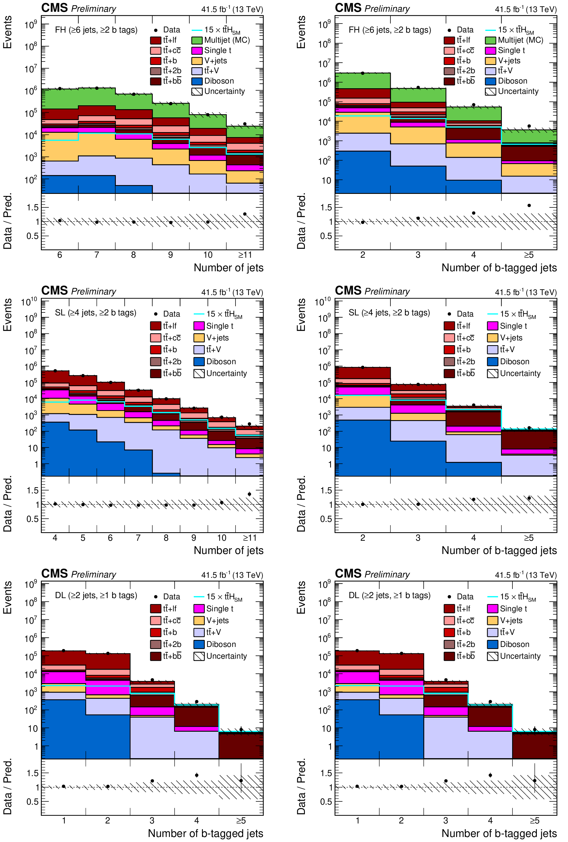
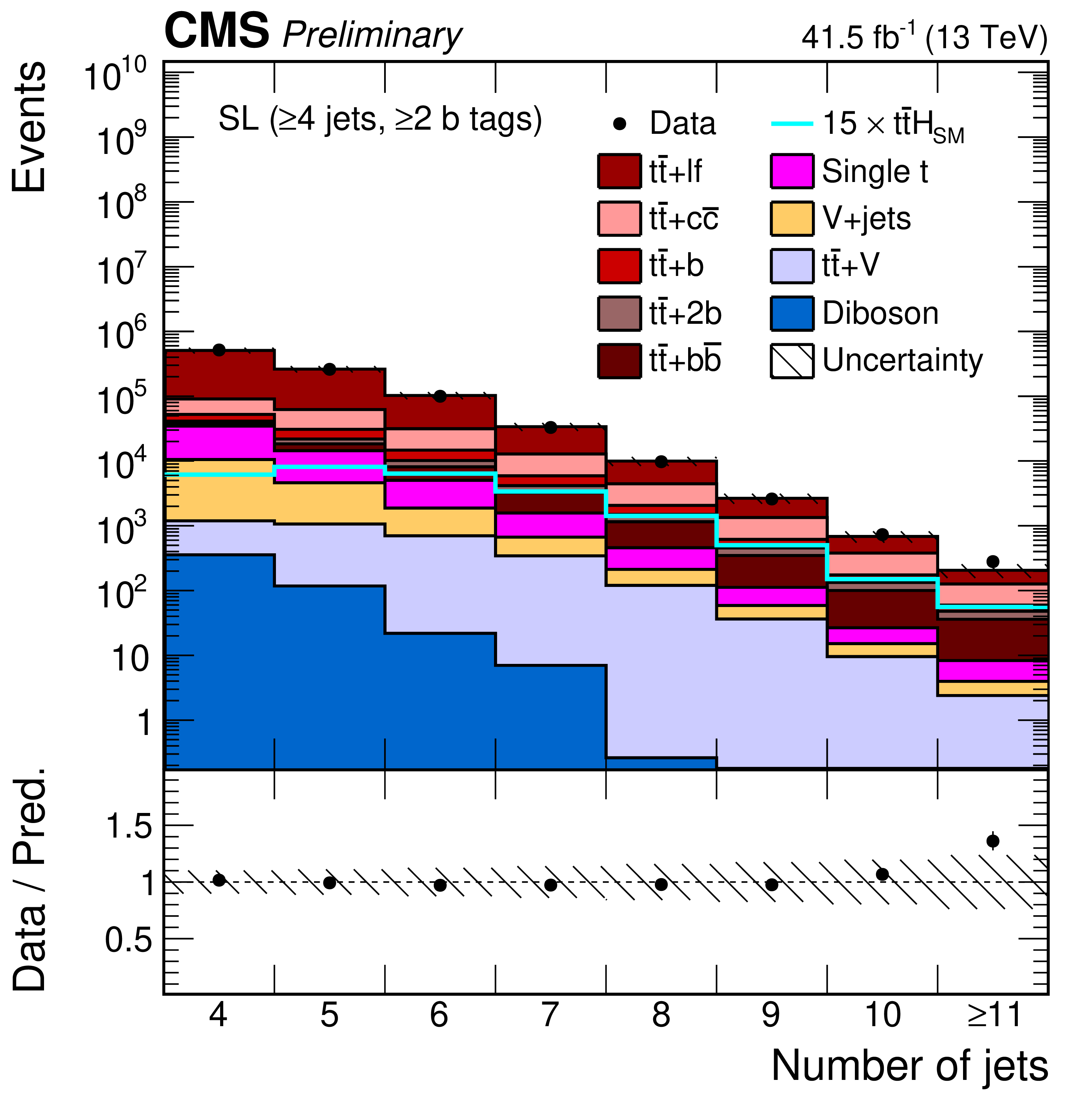
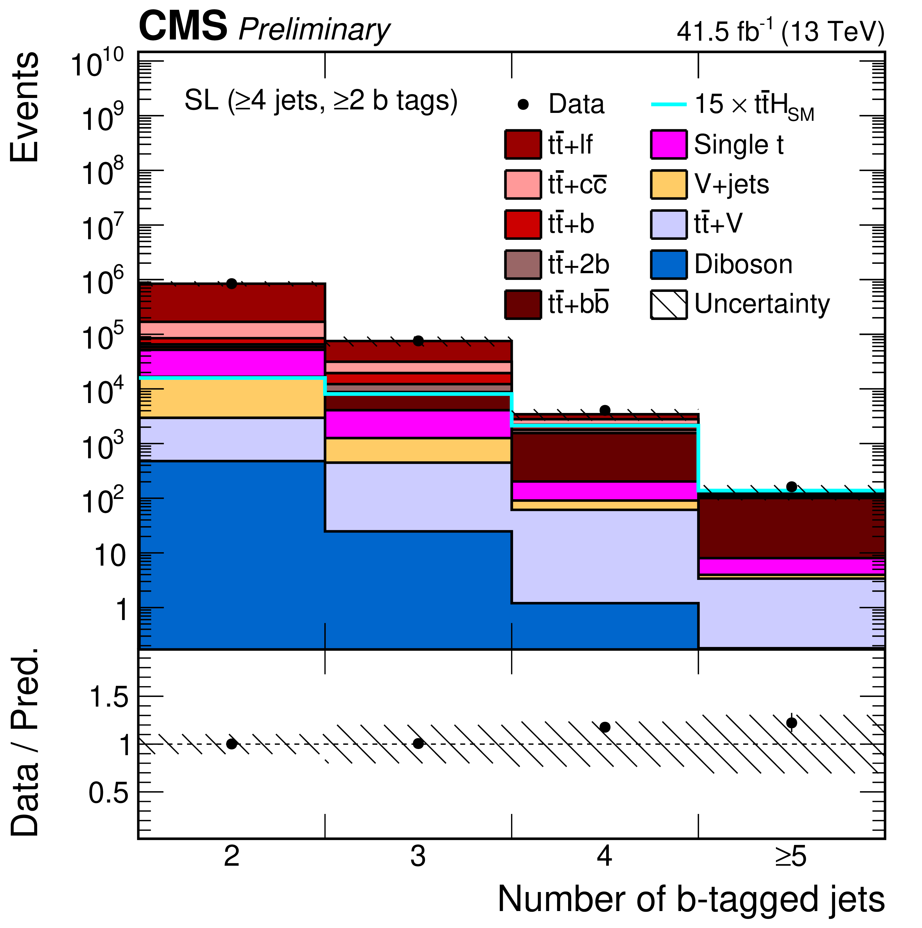
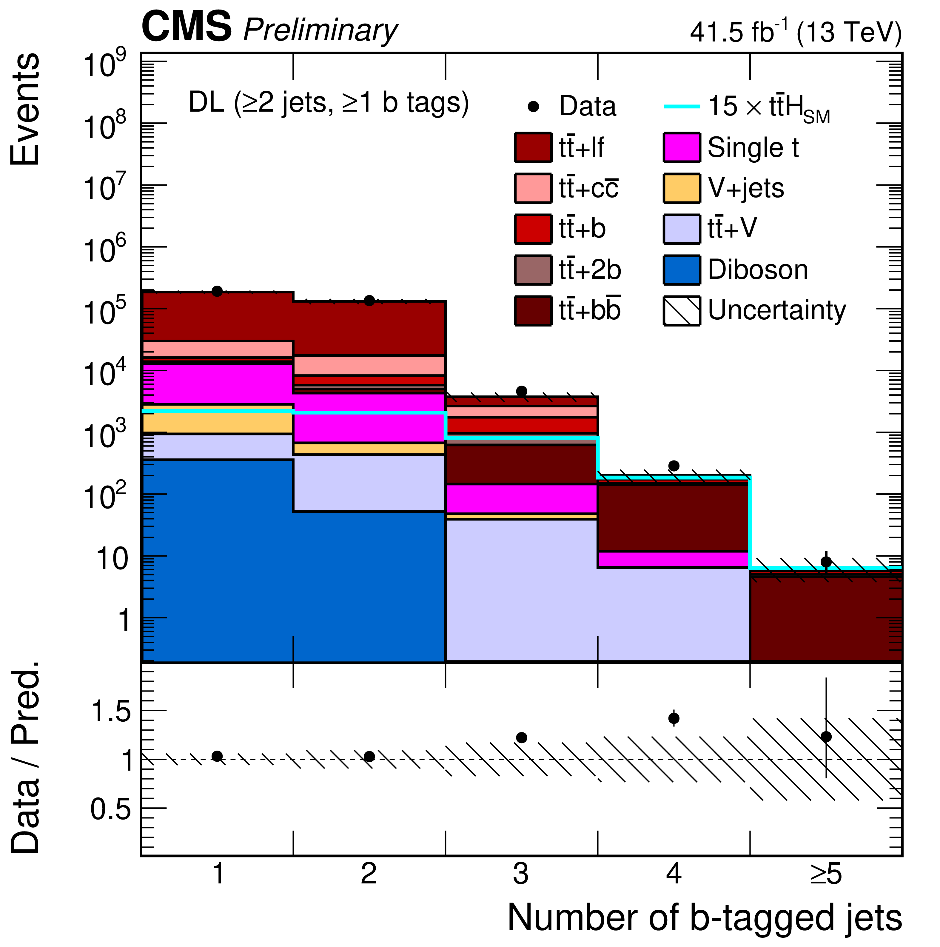
Jet (left) and b-tagged jet (right) multiplicity in the fully-hadronic (top), single-lepton (middle), and dilepton (bottom) channel after the baseline selection. The expected background contributions (filled histograms) are stacked, and the expected signal distribution (line) is superimposed. Here, the QCD-multijet prediction is taken from simulation. Each contribution is normalised to an integrated luminosity of 41.5 fb$^{-1}$, and the signal distribution is additionally scaled by for better visibility. The hatched uncertainty bands correspond to the total statistical and systematic uncertainties (excluding the 50% uncertainties on the normalisation of the ${{\mathrm {t}\overline {\mathrm {t}}}}$+hf processes) added in quadrature. The distributions observed in data (markers) are overlayed. The last bin includes overflow events. The lower plots show the ratio of the data to the background prediction. |
png pdf |
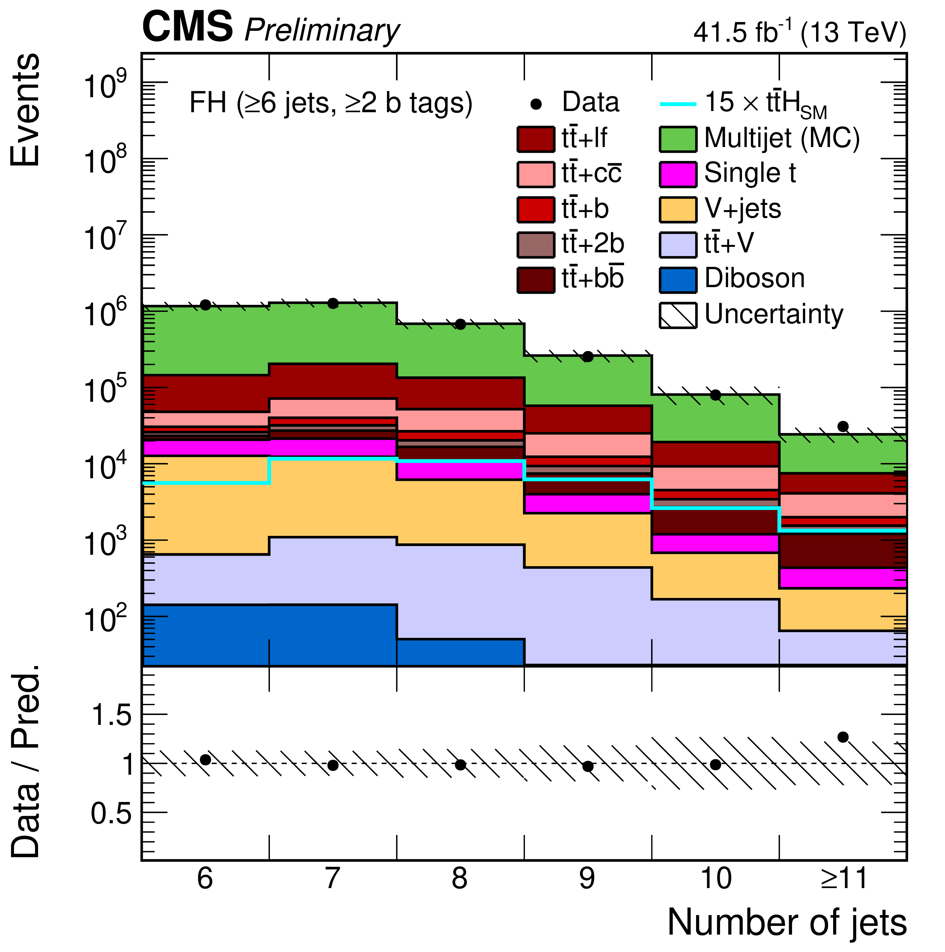
Additional Figure 1-a:
Jet multiplicity in the fully-hadronic channel after the baseline selection. The expected background contributions (filled histograms) are stacked, and the expected signal distribution (line) is superimposed. Here, the QCD-multijet prediction is taken from simulation. Each contribution is normalised to an integrated luminosity of 41.5 fb$^{-1}$, and the signal distribution is additionally scaled by for better visibility. The hatched uncertainty bands correspond to the total statistical and systematic uncertainties (excluding the 50% uncertainties on the normalisation of the ${{\mathrm {t}\overline {\mathrm {t}}}}$+hf processes) added in quadrature. The distribution observed in data (markers) is overlayed. The last bin includes overflow events. The lower plot shows the ratio of the data to the background prediction. |
png pdf |
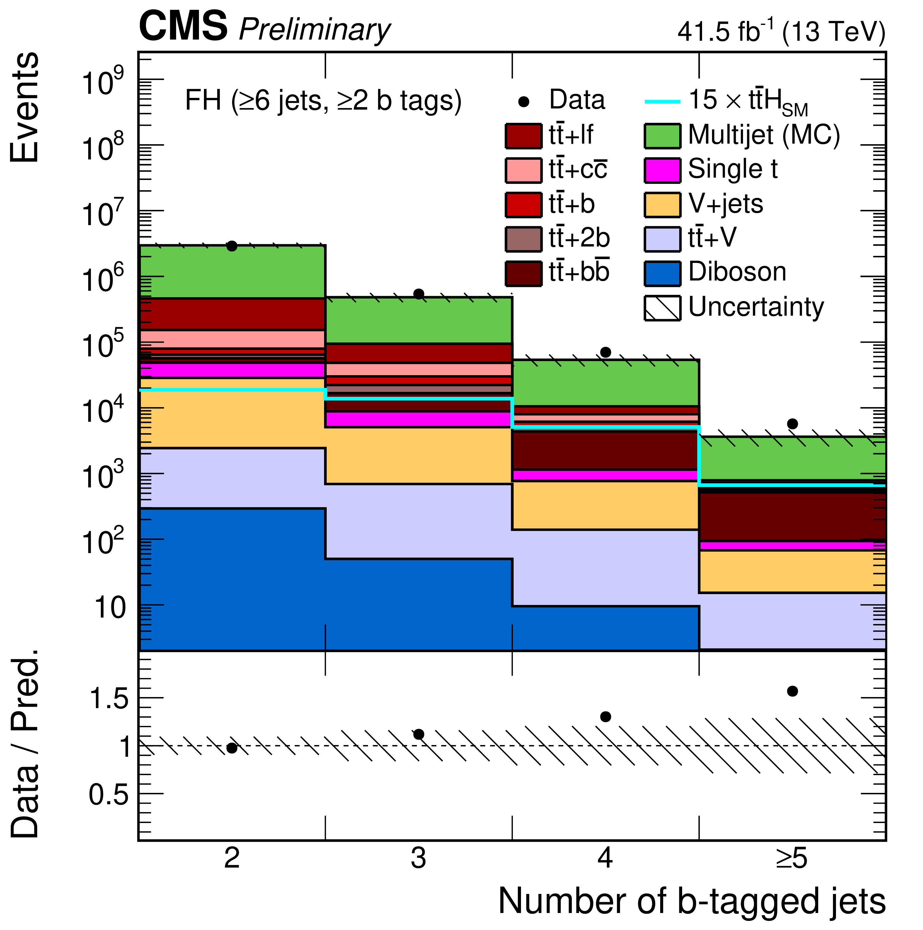
Additional Figure 1-b:
b-tagged jet multiplicity in the fully-hadronic channel after the baseline selection. The expected background contributions (filled histograms) are stacked, and the expected signal distribution (line) is superimposed. Here, the QCD-multijet prediction is taken from simulation. Each contribution is normalised to an integrated luminosity of 41.5 fb$^{-1}$, and the signal distribution is additionally scaled by for better visibility. The hatched uncertainty bands correspond to the total statistical and systematic uncertainties (excluding the 50% uncertainties on the normalisation of the ${{\mathrm {t}\overline {\mathrm {t}}}}$+hf processes) added in quadrature. The distribution observed in data (markers) is overlayed. The last bin includes overflow events. The lower plot shows the ratio of the data to the background prediction. |
png pdf |
Additional Figure 1-c:
Jet multiplicity in the single-lepton channel after the baseline selection. The expected background contributions (filled histograms) are stacked, and the expected signal distribution (line) is superimposed. Here, the QCD-multijet prediction is taken from simulation. Each contribution is normalised to an integrated luminosity of 41.5 fb$^{-1}$, and the signal distribution is additionally scaled by for better visibility. The hatched uncertainty bands correspond to the total statistical and systematic uncertainties (excluding the 50% uncertainties on the normalisation of the ${{\mathrm {t}\overline {\mathrm {t}}}}$+hf processes) added in quadrature. The distribution observed in data (markers) is overlayed. The last bin includes overflow events. The lower plot shows the ratio of the data to the background prediction. |
png pdf |
Additional Figure 1-d:
b-tagged jet multiplicity in the single-lepton channel after the baseline selection. The expected background contributions (filled histograms) are stacked, and the expected signal distribution (line) is superimposed. Here, the QCD-multijet prediction is taken from simulation. Each contribution is normalised to an integrated luminosity of 41.5 fb$^{-1}$, and the signal distribution is additionally scaled by for better visibility. The hatched uncertainty bands correspond to the total statistical and systematic uncertainties (excluding the 50% uncertainties on the normalisation of the ${{\mathrm {t}\overline {\mathrm {t}}}}$+hf processes) added in quadrature. The distribution observed in data (markers) is overlayed. The last bin includes overflow events. The lower plot shows the ratio of the data to the background prediction. |
png pdf |
Additional Figure 1-e:
Jet multiplicity in the dilepton channel after the baseline selection. The expected background contributions (filled histograms) are stacked, and the expected signal distribution (line) is superimposed. Here, the QCD-multijet prediction is taken from simulation. Each contribution is normalised to an integrated luminosity of 41.5 fb$^{-1}$, and the signal distribution is additionally scaled by for better visibility. The hatched uncertainty bands correspond to the total statistical and systematic uncertainties (excluding the 50% uncertainties on the normalisation of the ${{\mathrm {t}\overline {\mathrm {t}}}}$+hf processes) added in quadrature. The distribution observed in data (markers) is overlayed. The last bin includes overflow events. The lower plot shows the ratio of the data to the background prediction. |

png pdf |
Additional Figure 1-f:
b-tagged jet multiplicity in the dilepton channel after the baseline selection. The expected background contributions (filled histograms) are stacked, and the expected signal distribution (line) is superimposed. Here, the QCD-multijet prediction is taken from simulation. Each contribution is normalised to an integrated luminosity of 41.5 fb$^{-1}$, and the signal distribution is additionally scaled by for better visibility. The hatched uncertainty bands correspond to the total statistical and systematic uncertainties (excluding the 50% uncertainties on the normalisation of the ${{\mathrm {t}\overline {\mathrm {t}}}}$+hf processes) added in quadrature. The distribution observed in data (markers) is overlayed. The last bin includes overflow events. The lower plot shows the ratio of the data to the background prediction. |
png pdf |
Additional Figure 2:
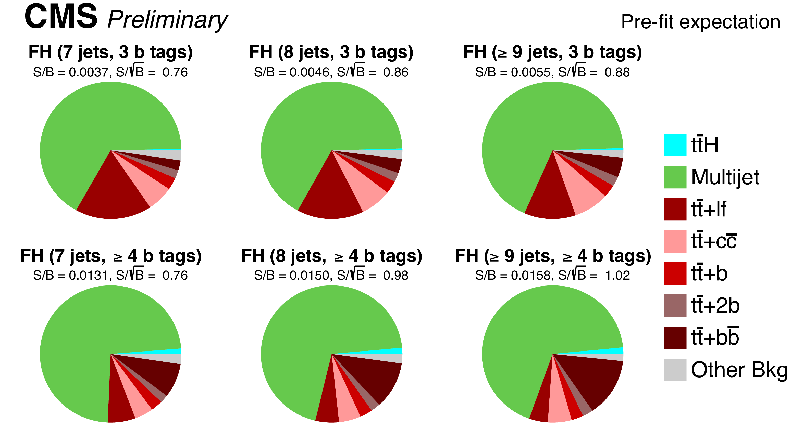
Expected fraction of signal and background events contributing to the analysis categories in the fully-hadronic (FH) channel before the fit to data. The QCD-multijet contribution is estimated from data. |

png pdf |
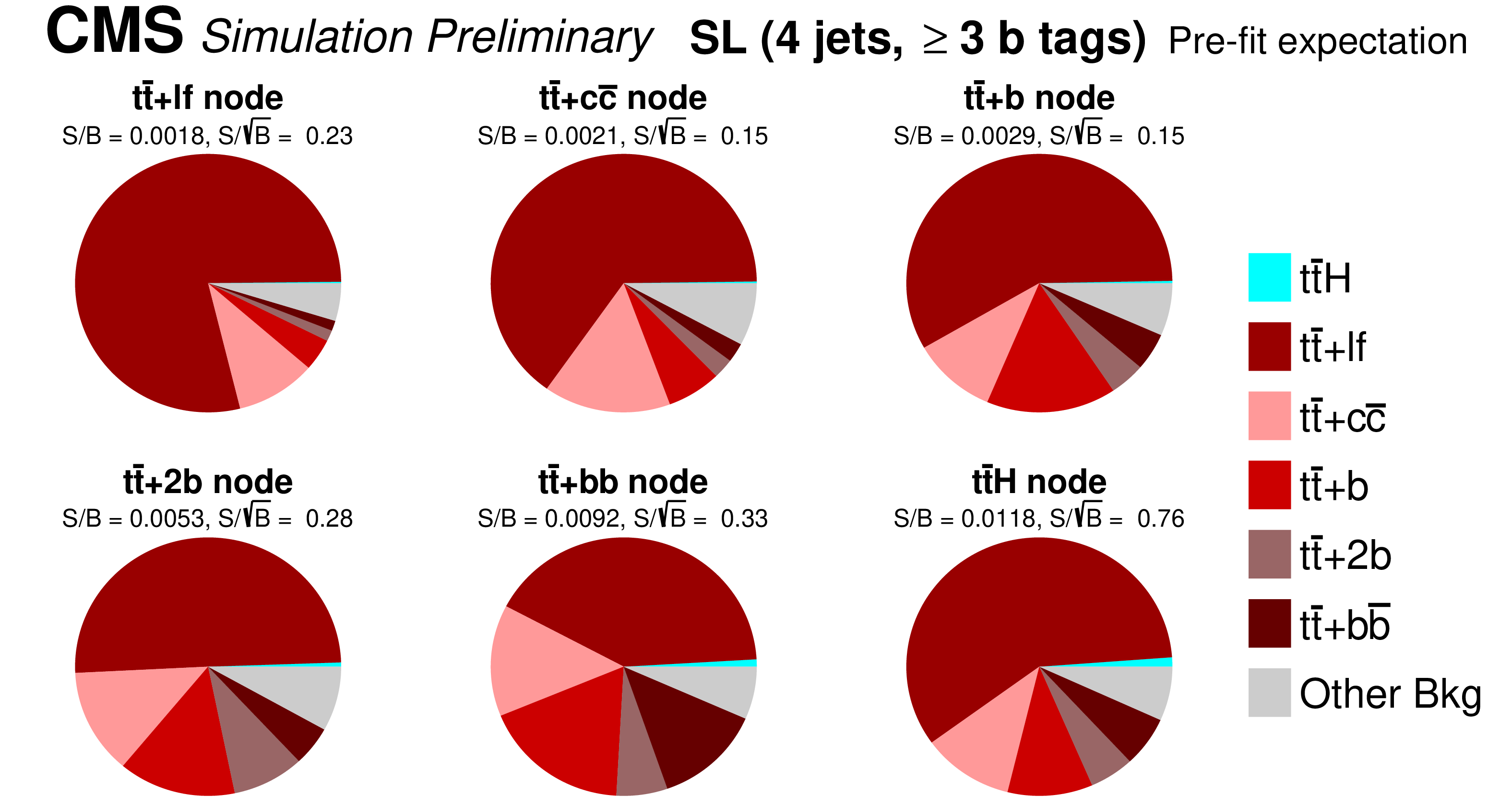
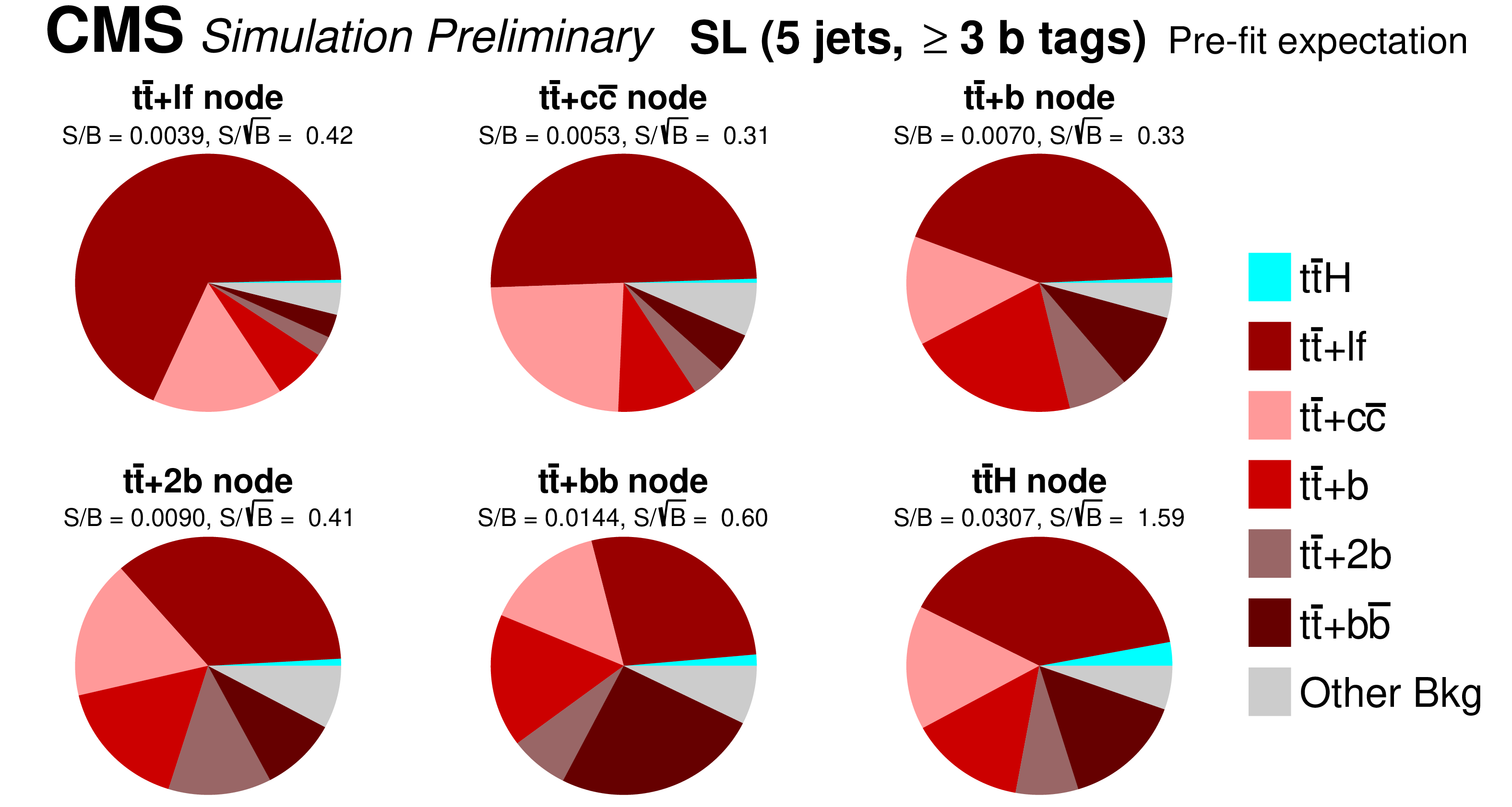
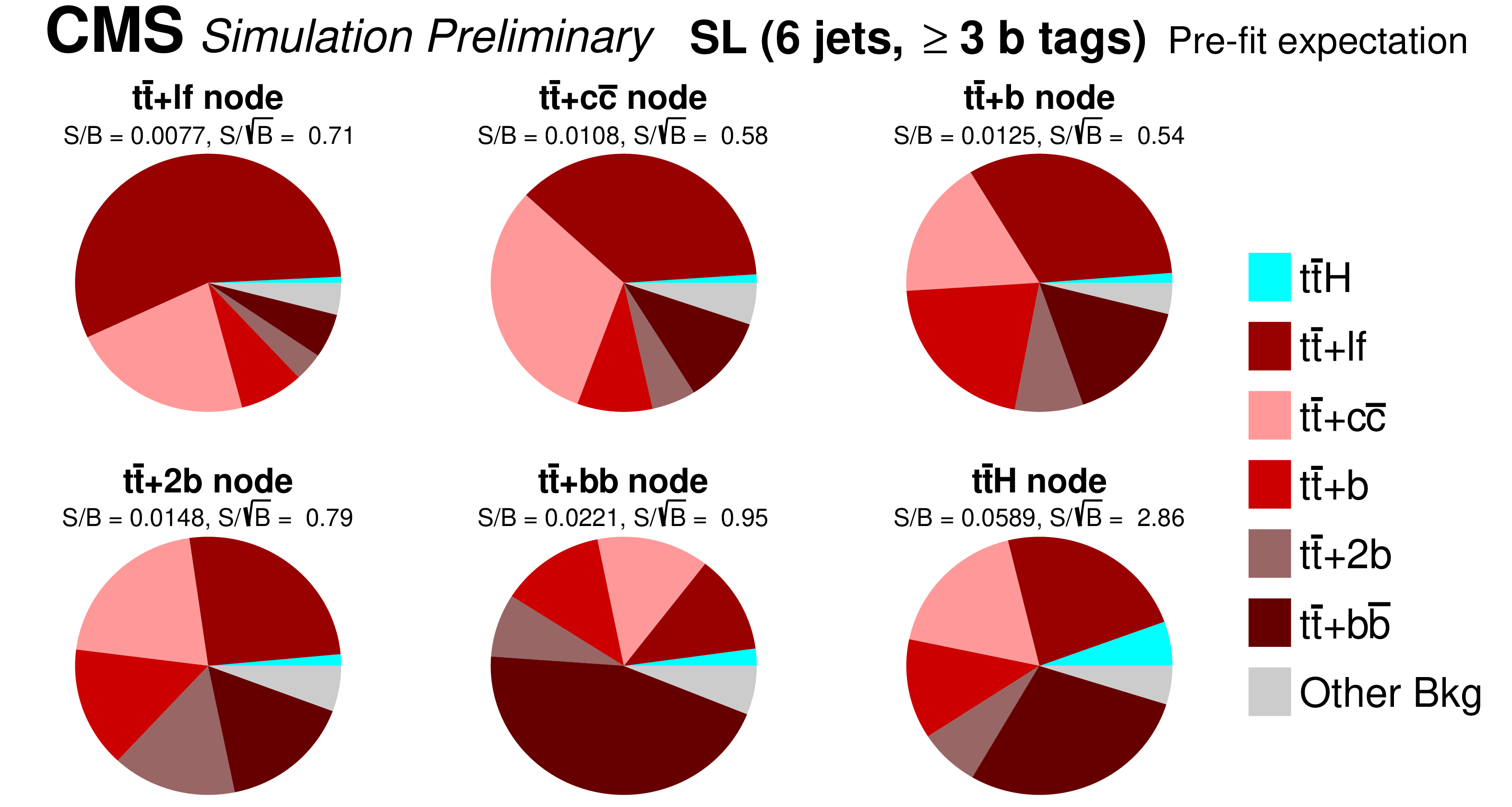
Additional Figure 3:
Expected fraction of signal and background events contributing to the analysis categories in the single-lepton (SL) channel before the fit to data. |
png pdf |
Additional Figure 3-a:
Expected fraction of signal and background events contributing to the analysis categories in the single-lepton (SL) channel before the fit to data. |
png pdf |
Additional Figure 3-b:
Expected fraction of signal and background events contributing to the analysis categories in the single-lepton (SL) channel before the fit to data. |
png pdf |
Additional Figure 3-c:
Expected fraction of signal and background events contributing to the analysis categories in the single-lepton (SL) channel before the fit to data. |
png pdf |
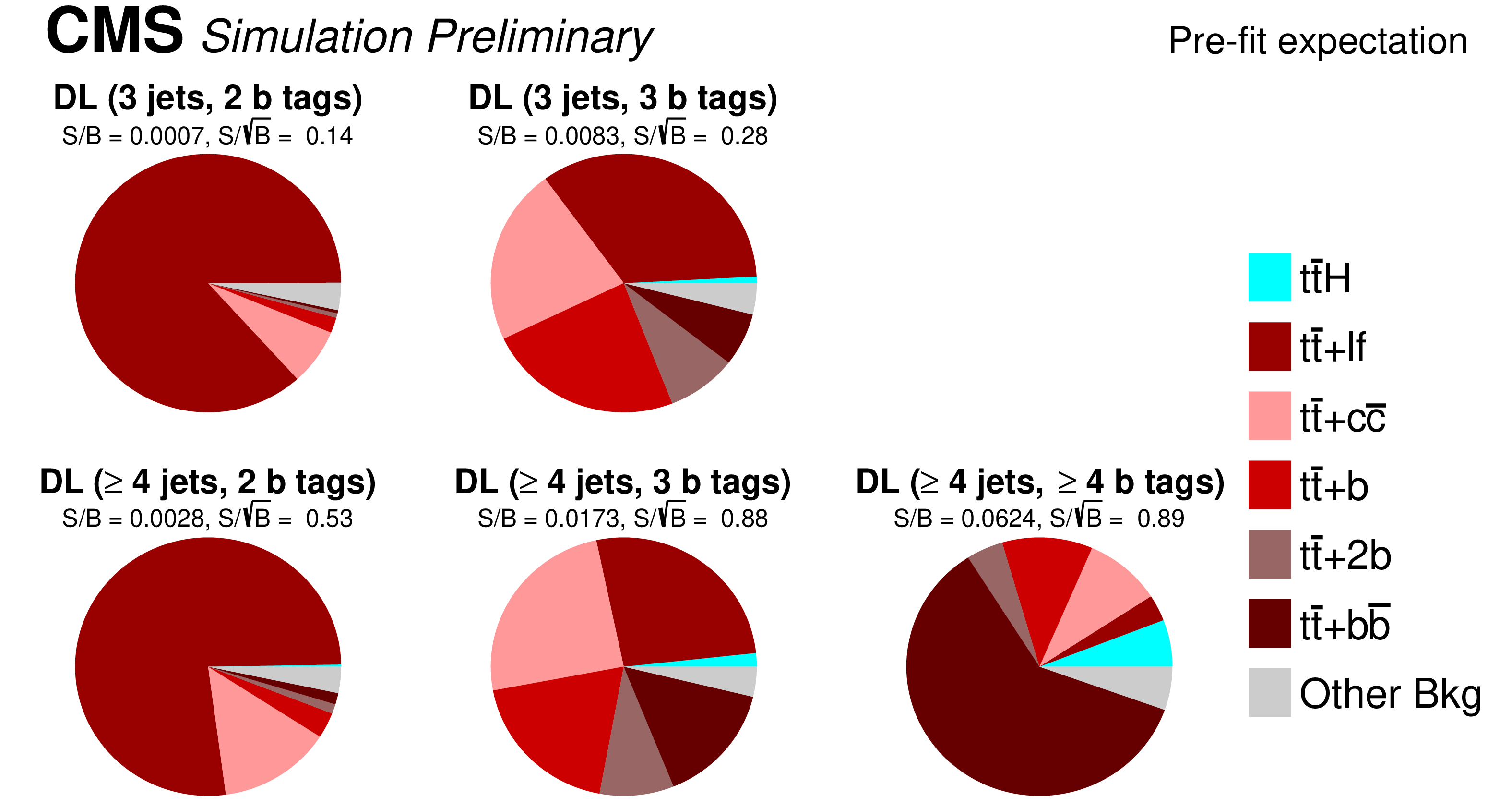
Additional Figure 4:
Expected fraction of signal and background events contributing to the analysis categories in the dilepton (DL) channel before the fit to data. |
png pdf |
Additional Figure 5:
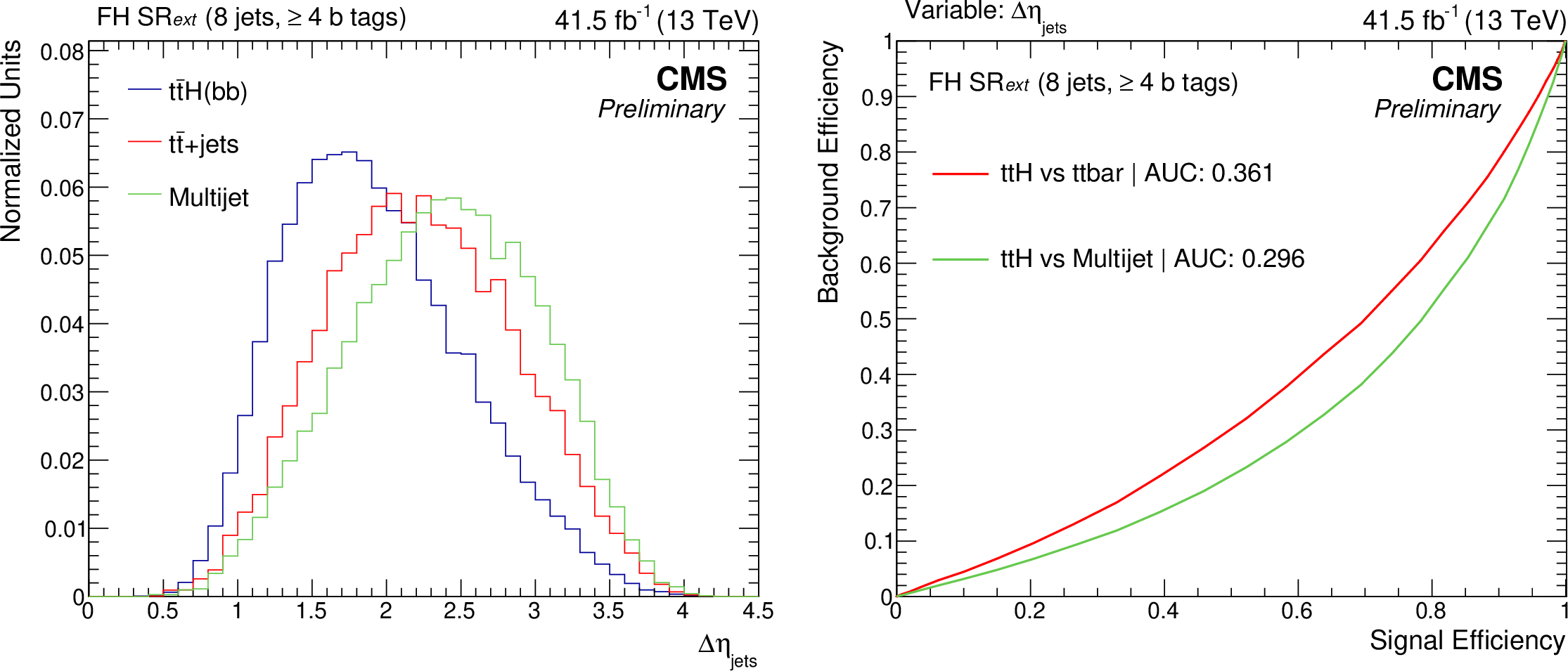
Normalised distribution of $\Delta \eta _{\text {jets}}$ used for QCD rejection in the fully-hadronic (FH) channel for ${{{\mathrm {t}\overline {\mathrm {t}}}} {\mathrm {H}}}$, ${{\mathrm {t}\overline {\mathrm {t}}}}$+jets, and QCD multijet events (left) and background vs. signal selection efficiency for different requirements on $\Delta \eta _{\text {jets}}$, evaluated with ${{\mathrm {t}\overline {\mathrm {t}}}}$+jets or multijet events as background (right) in the 8 jets, $\geq $4 b-tags category in an extended signal region (SR ext) corresponding to the analysis signal region but without the requirement on $\Delta \eta _{\text {jets}}$ itself. The distributions for ${{{\mathrm {t}\overline {\mathrm {t}}}} {\mathrm {H}}}$ and ${{\mathrm {t}\overline {\mathrm {t}}}}$+jets are taken from simulation while the QCD-multijet background is estimated from data. |
png pdf |
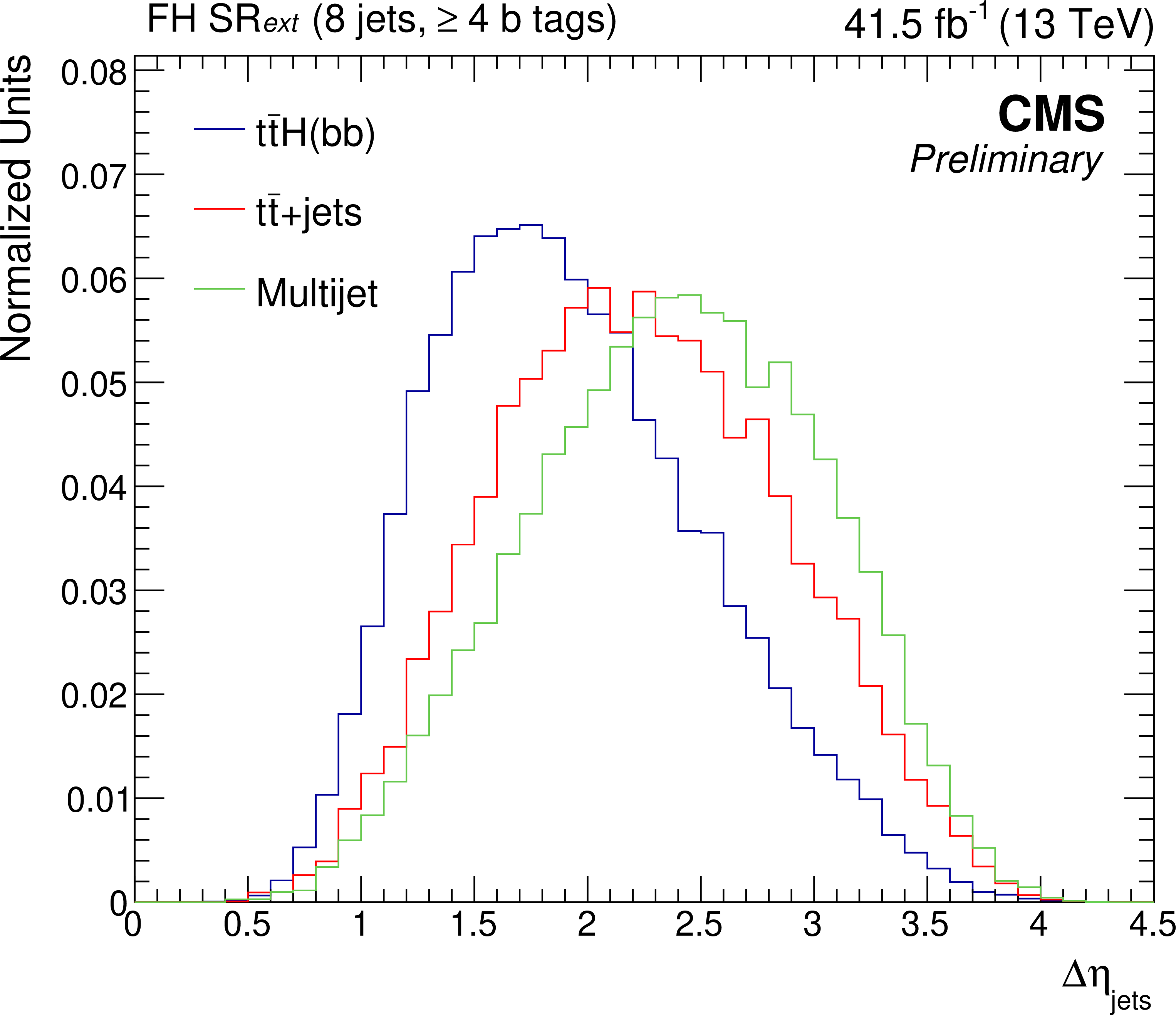
Additional Figure 5-a:
Normalised distribution of $\Delta \eta _{\text {jets}}$ used for QCD rejection in the fully-hadronic (FH) channel for ${{{\mathrm {t}\overline {\mathrm {t}}}} {\mathrm {H}}}$, ${{\mathrm {t}\overline {\mathrm {t}}}}$+jets, and QCD multijet events in the 8 jets, $\geq $4 b-tags category in an extended signal region (SR ext) corresponding to the analysis signal region but without the requirement on $\Delta \eta _{\text {jets}}$ itself. The distributions for ${{{\mathrm {t}\overline {\mathrm {t}}}} {\mathrm {H}}}$ and ${{\mathrm {t}\overline {\mathrm {t}}}}$+jets are taken from simulation while the QCD-multijet background is estimated from data. |
png pdf |
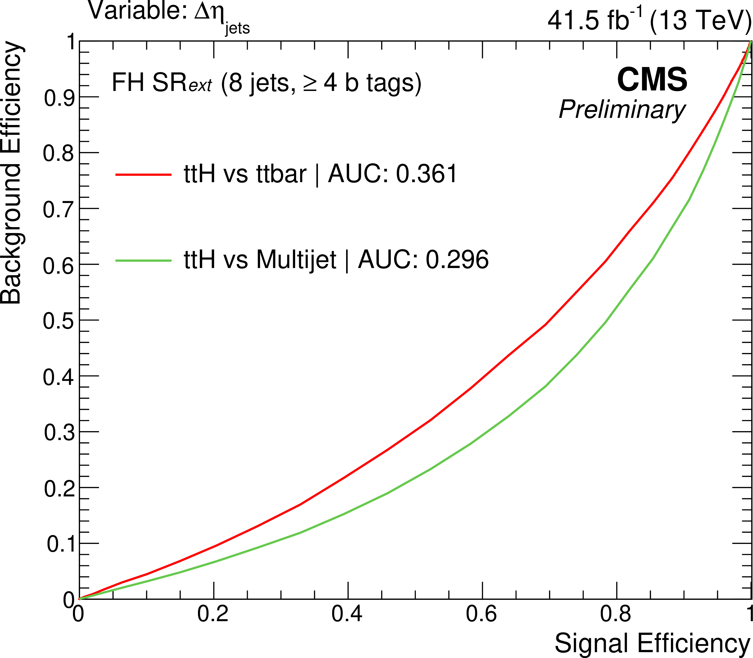
Additional Figure 5-b:
Background vs. signal selection efficiency for different requirements on $\Delta \eta _{\text {jets}}$, evaluated with ${{\mathrm {t}\overline {\mathrm {t}}}}$+jets or multijet events as background in the 8 jets, $\geq $4 b-tags category in an extended signal region (SR ext) corresponding to the analysis signal region but without the requirement on $\Delta \eta _{\text {jets}}$ itself. The distributions for ${{{\mathrm {t}\overline {\mathrm {t}}}} {\mathrm {H}}}$ and ${{\mathrm {t}\overline {\mathrm {t}}}}$+jets are taken from simulation while the QCD-multijet background is estimated from data. |
png pdf |
Additional Figure 6:
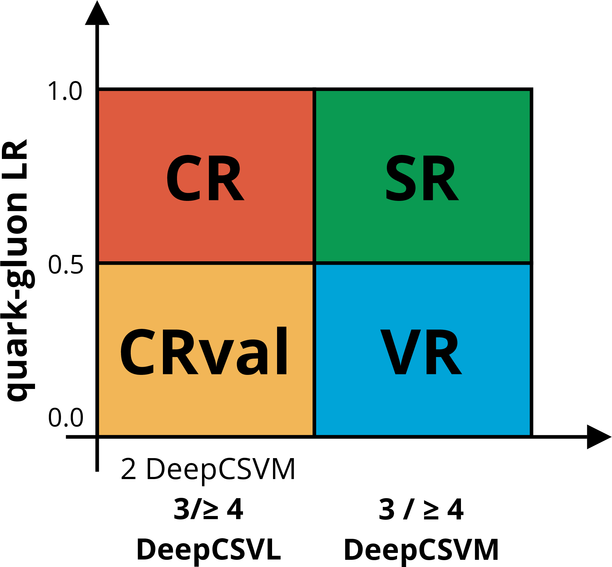
Illustration of the defintion of the signal (SR) and control (CR) regions used to determine the QCD-multijet background shapes in the fully-hadronic channel, as well as the validation regions (CRval, VR). |
png pdf |
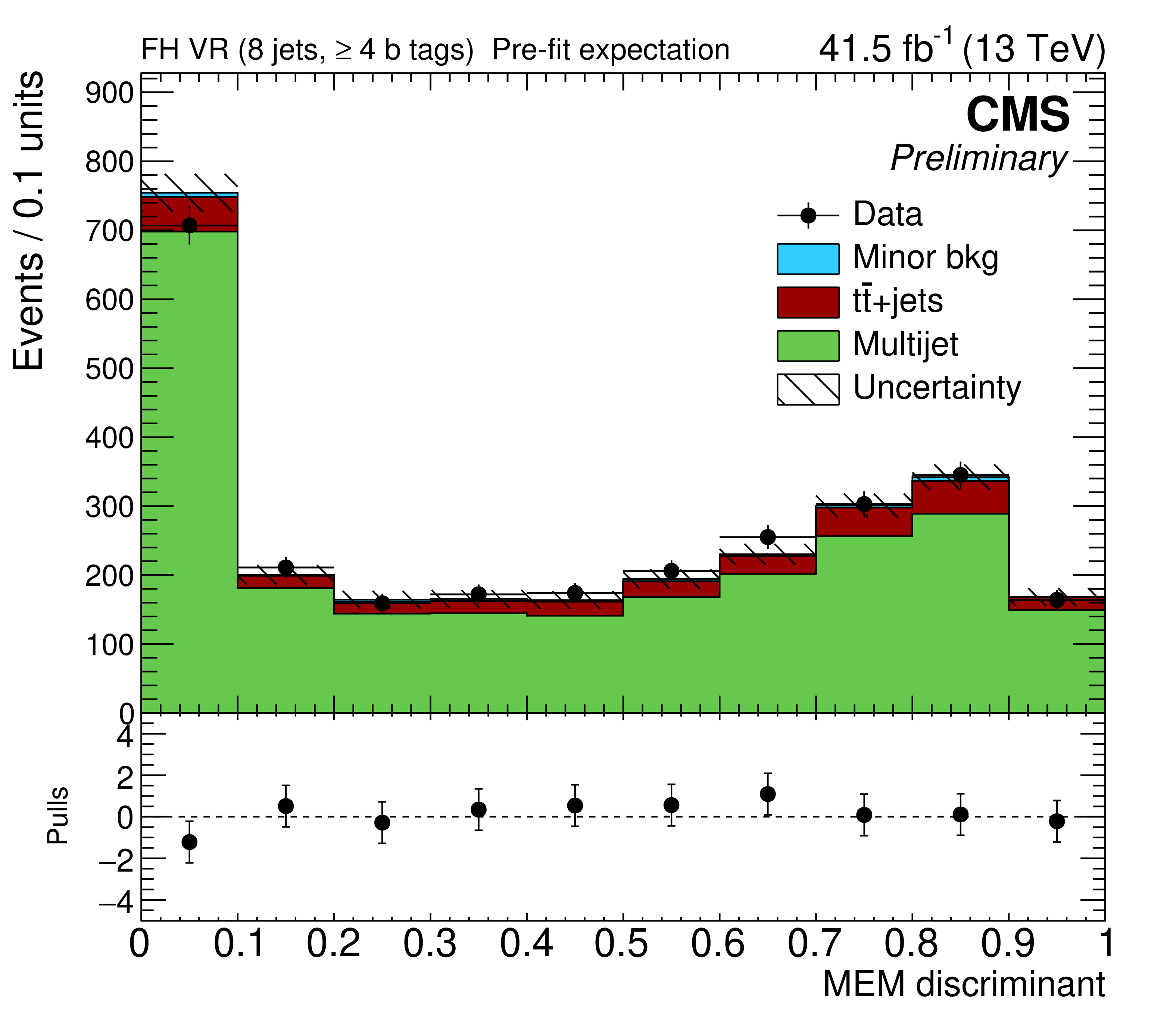
Additional Figure 7:
MEM discriminant distribution in the validation region of the fully-hadronic channel (FH VR) in the 8 jets, $\geq $4 b-tags category for data (markers) and backgrounds (stacked distributions). The QCD-multijet background is estimated from data while the other backgrounds are taken from the simulation. The difference between data and the total background estimate divided by the quadratic sum of the statistical and systematic uncertainties (pulls) are shown below the main panel. The last bin includes overflows. |
png pdf |
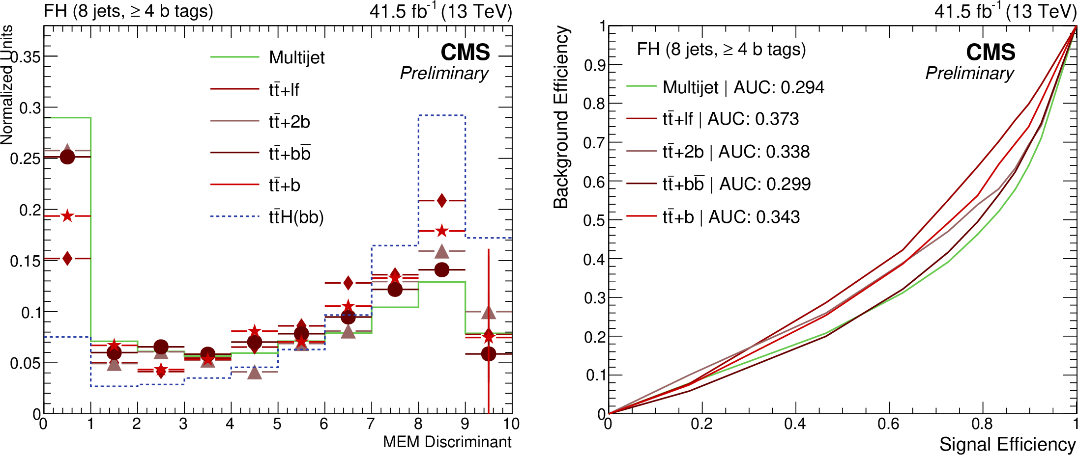
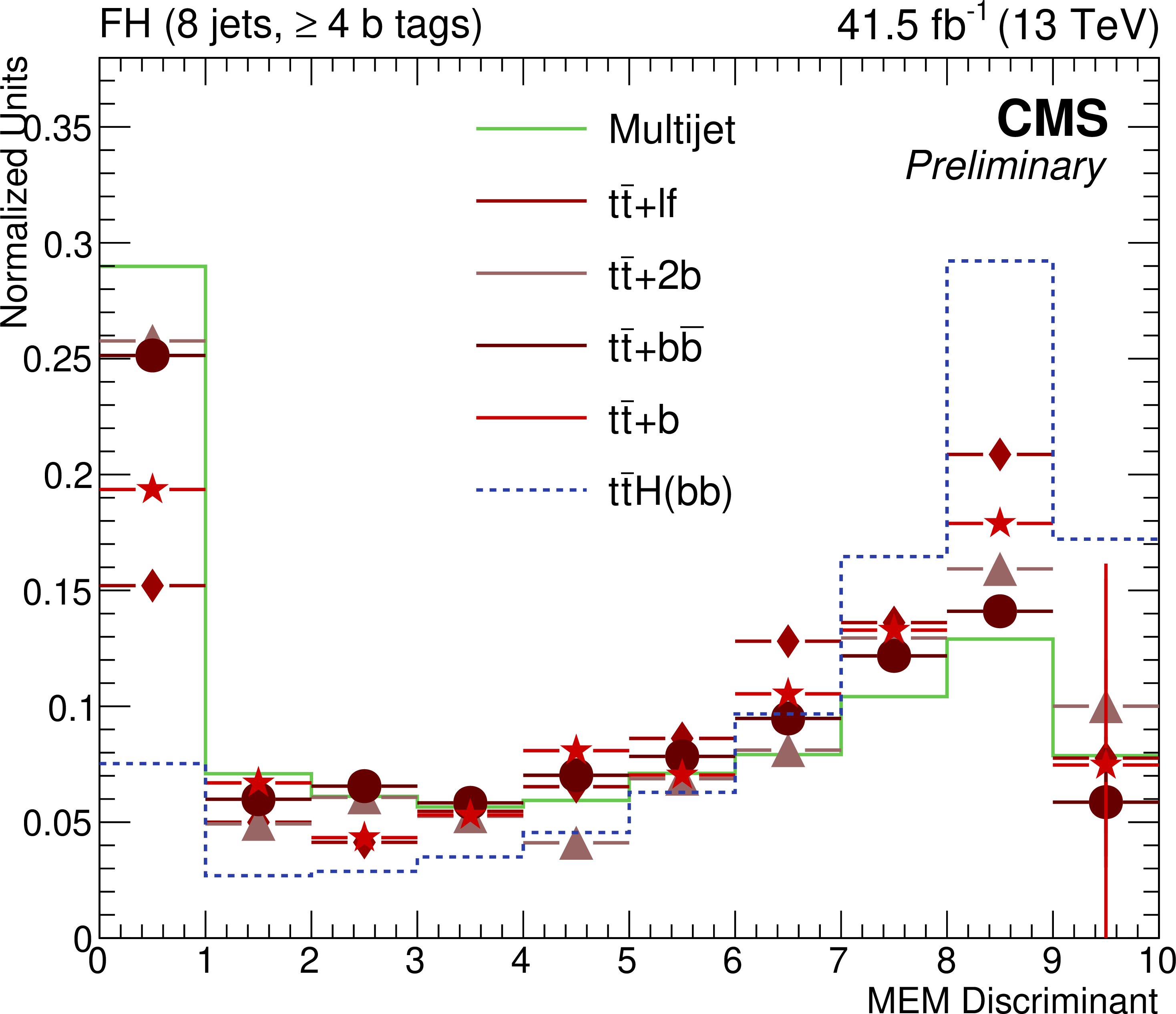
Additional Figure 8:
Normalised MEM discriminant distribution for ${{{\mathrm {t}\overline {\mathrm {t}}}} {\mathrm {H}}}$ and different background processes (left) and background vs. ${{{\mathrm {t}\overline {\mathrm {t}}}} {\mathrm {H}}}$ signal selection efficiency for different requirements on the MEM discriminant output, evaluated for different background processes (right) in the 8 jets, $\geq $4 b-tags category of the fully-hadronic (FH) channel. The distributions for ${{{\mathrm {t}\overline {\mathrm {t}}}} {\mathrm {H}}}$ and ${{\mathrm {t}\overline {\mathrm {t}}}}$+jets are taken from simulation while the QCD-multijet background is estimated from data. |
png pdf |
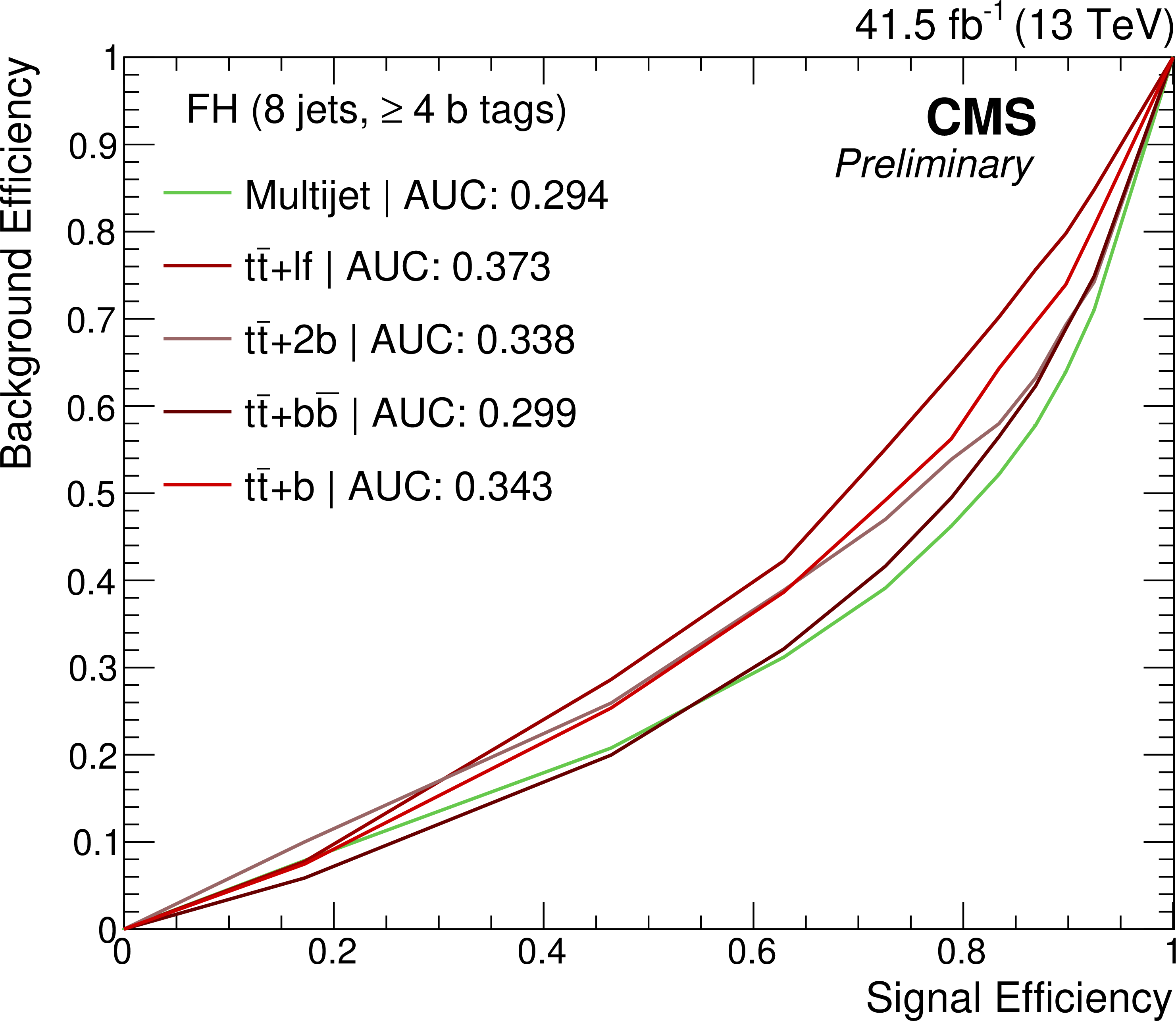
Additional Figure 8-a:
Background vs. ${{{\mathrm {t}\overline {\mathrm {t}}}} {\mathrm {H}}}$ signal selection efficiency for different requirements on the MEM discriminant output, evaluated for different background processes in the 8 jets, $\geq $4 b-tags category of the fully-hadronic (FH) channel. The distributions for ${{{\mathrm {t}\overline {\mathrm {t}}}} {\mathrm {H}}}$ and ${{\mathrm {t}\overline {\mathrm {t}}}}$+jets are taken from simulation while the QCD-multijet background is estimated from data. |
png pdf |
Additional Figure 8-b:
Background vs. ${{{\mathrm {t}\overline {\mathrm {t}}}} {\mathrm {H}}}$ signal selection efficiency for different requirements on the MEM discriminant output, evaluated for different background processes in the 8 jets, $\geq $4 b-tags category of the fully-hadronic (FH) channel. The distributions for ${{{\mathrm {t}\overline {\mathrm {t}}}} {\mathrm {H}}}$ and ${{\mathrm {t}\overline {\mathrm {t}}}}$+jets are taken from simulation while the QCD-multijet background is estimated from data. |
png pdf |
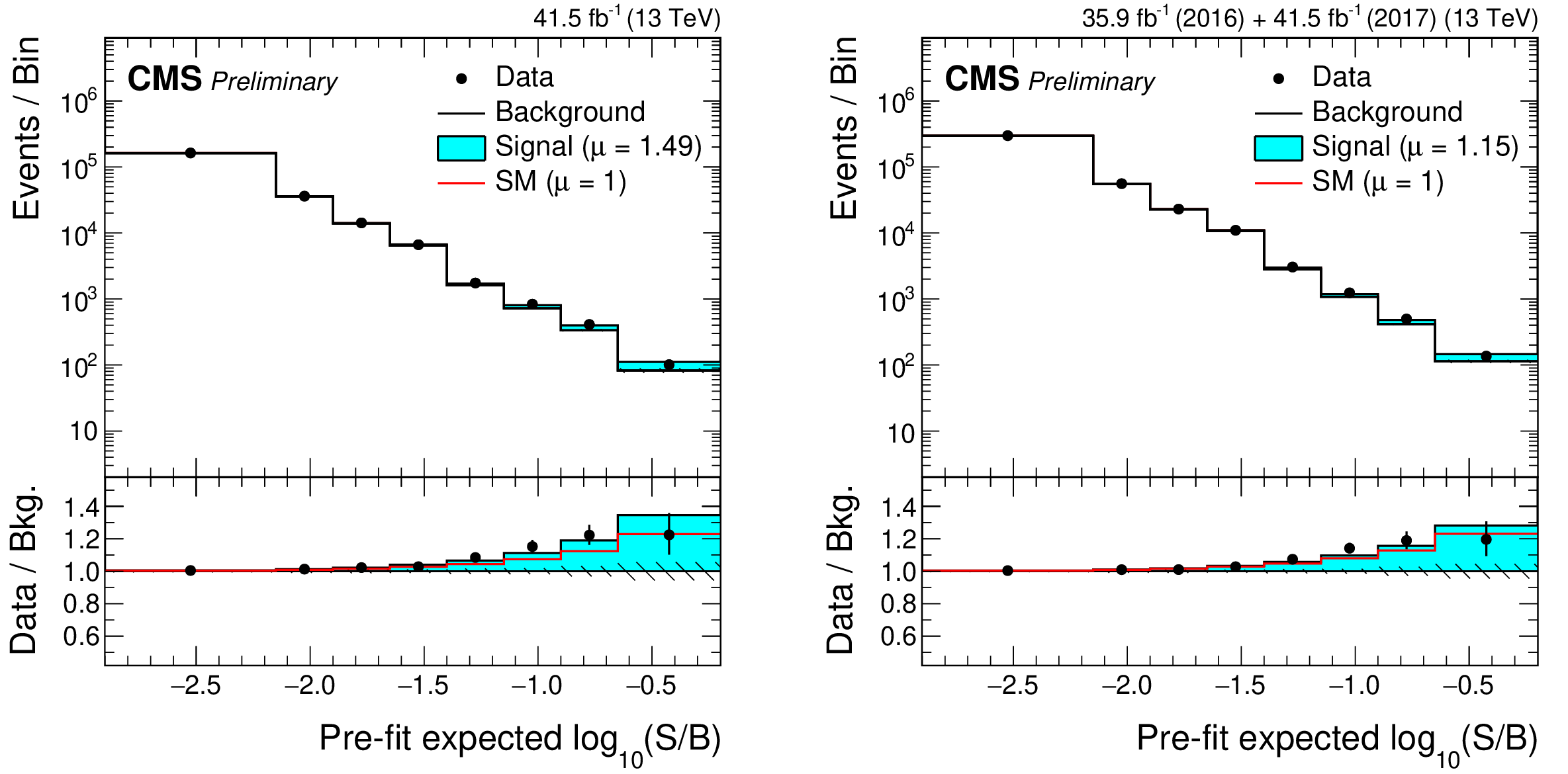
Additional Figure 9:
Bins of the final discriminants as used in the fit of the 2017 dataset (left) and in the combined fit of the 2016 and 2017 datasets (right), reordered by the pre-fit expected signal-to-background ratio (S/B). Each of the shown bins includes multiple bins of the final discriminants with similar S/B. The fitted signal (cyan) is compared to the expectation for the SM Higgs boson $\mu = $ 1 (red). |
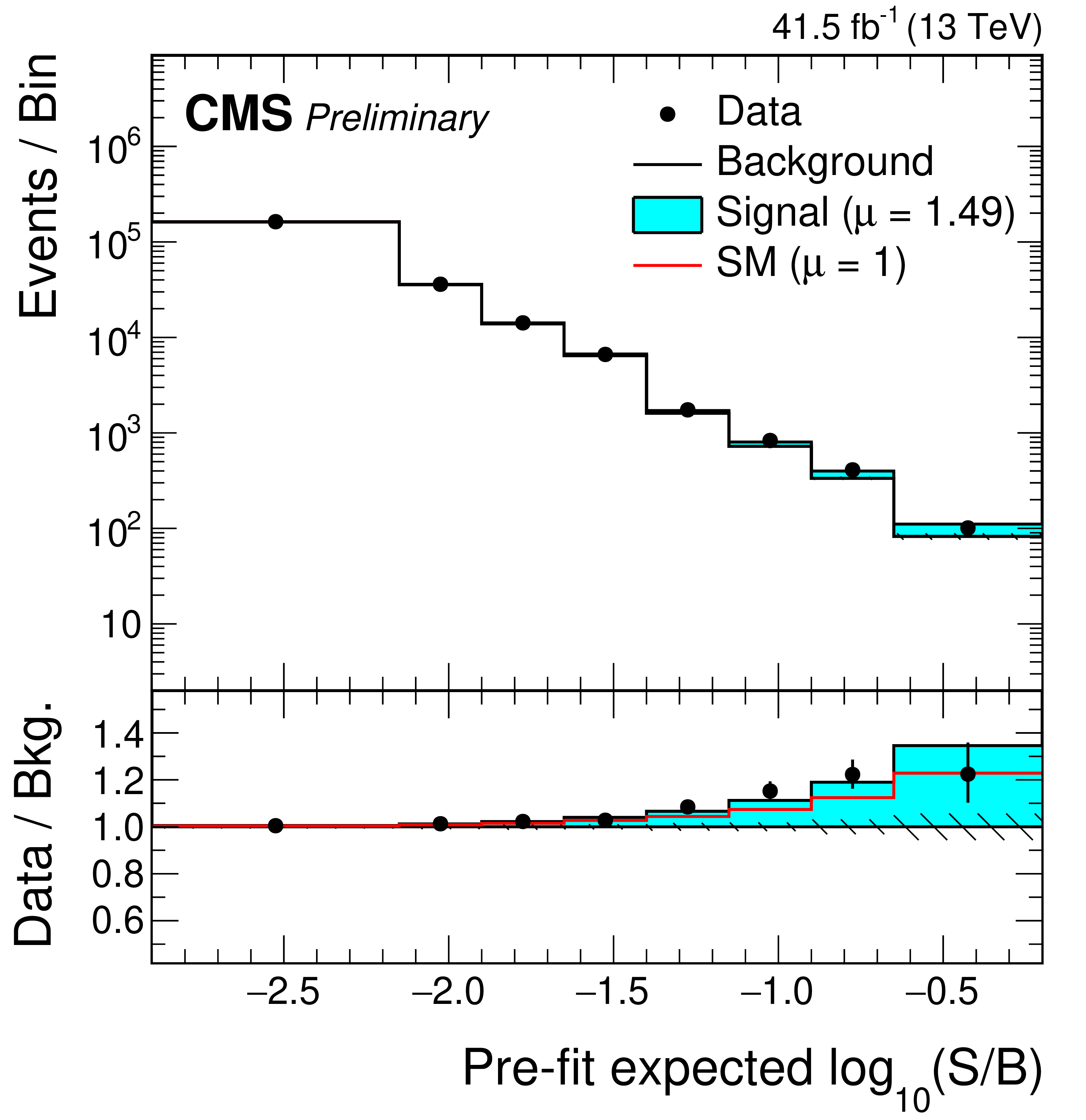
png pdf |
Additional Figure 9-a:
Bins of the final discriminants as used in the fit of the 2017 dataset, reordered by the pre-fit expected signal-to-background ratio (S/B). Each of the shown bins includes multiple bins of the final discriminants with similar S/B. The fitted signal (cyan) is compared to the expectation for the SM Higgs boson $\mu = $ 1 (red). |
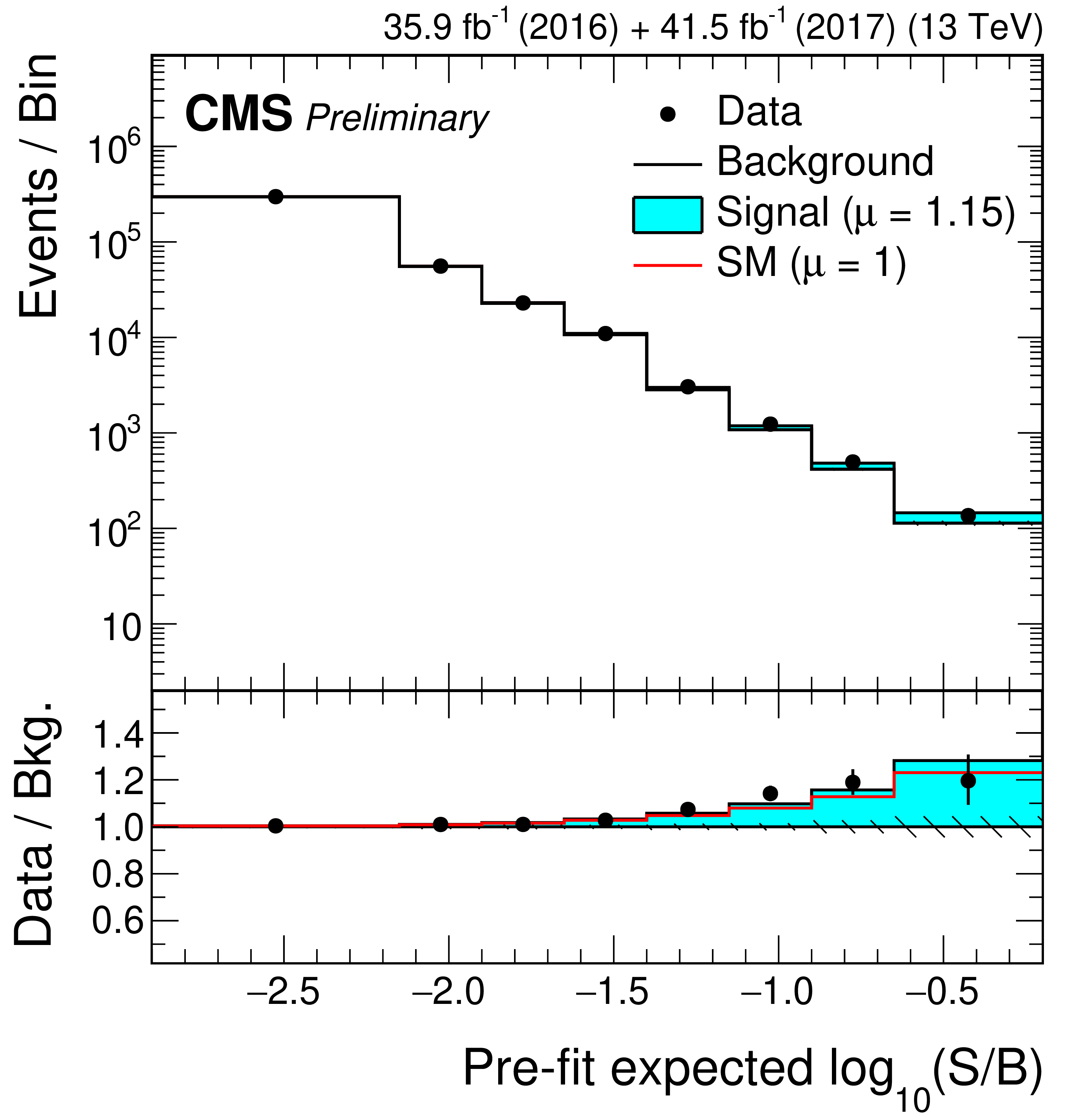
png pdf |
Additional Figure 9-b:
Bins of the final discriminants as used in the combined fit of the 2016 and 2017 datasets, reordered by the pre-fit expected signal-to-background ratio (S/B). Each of the shown bins includes multiple bins of the final discriminants with similar S/B. The fitted signal (cyan) is compared to the expectation for the SM Higgs boson $\mu = $ 1 (red). |
png pdf |
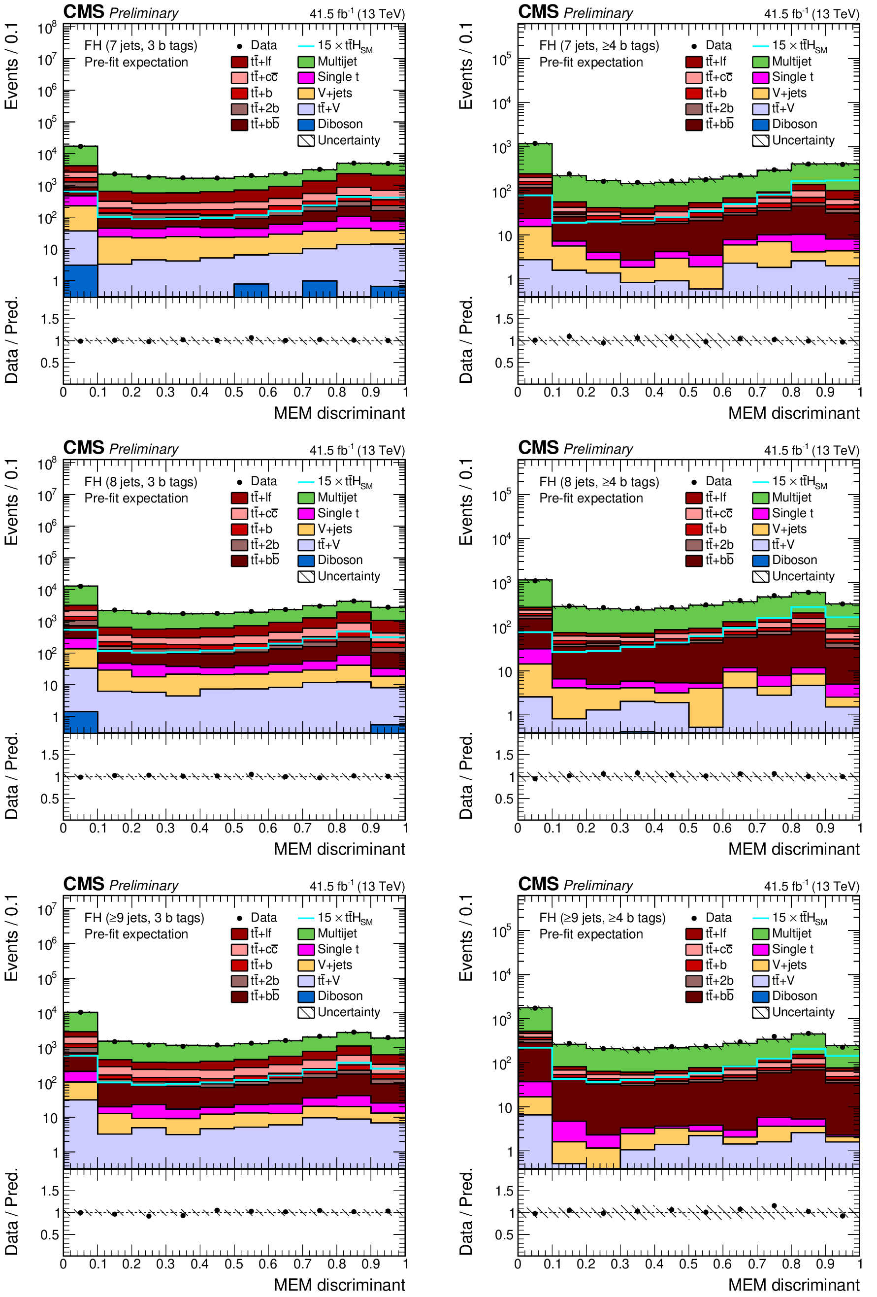
Additional Figure 10:
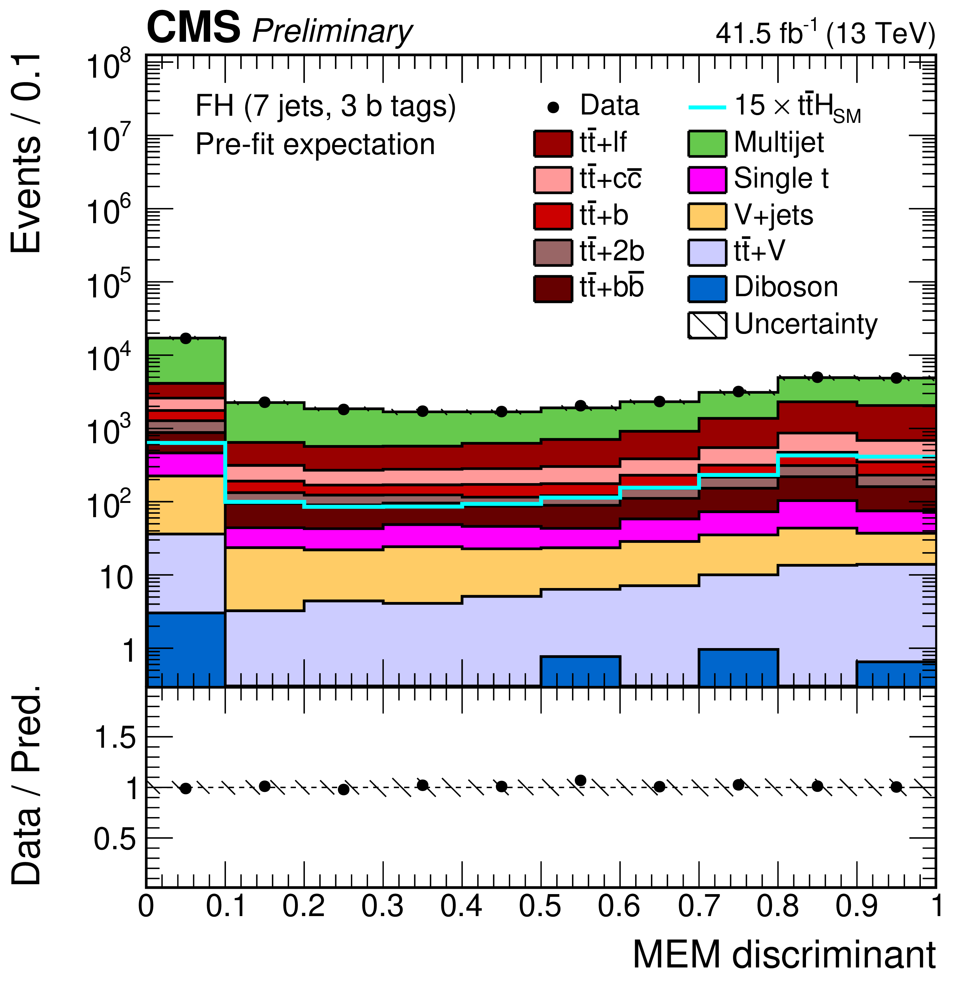
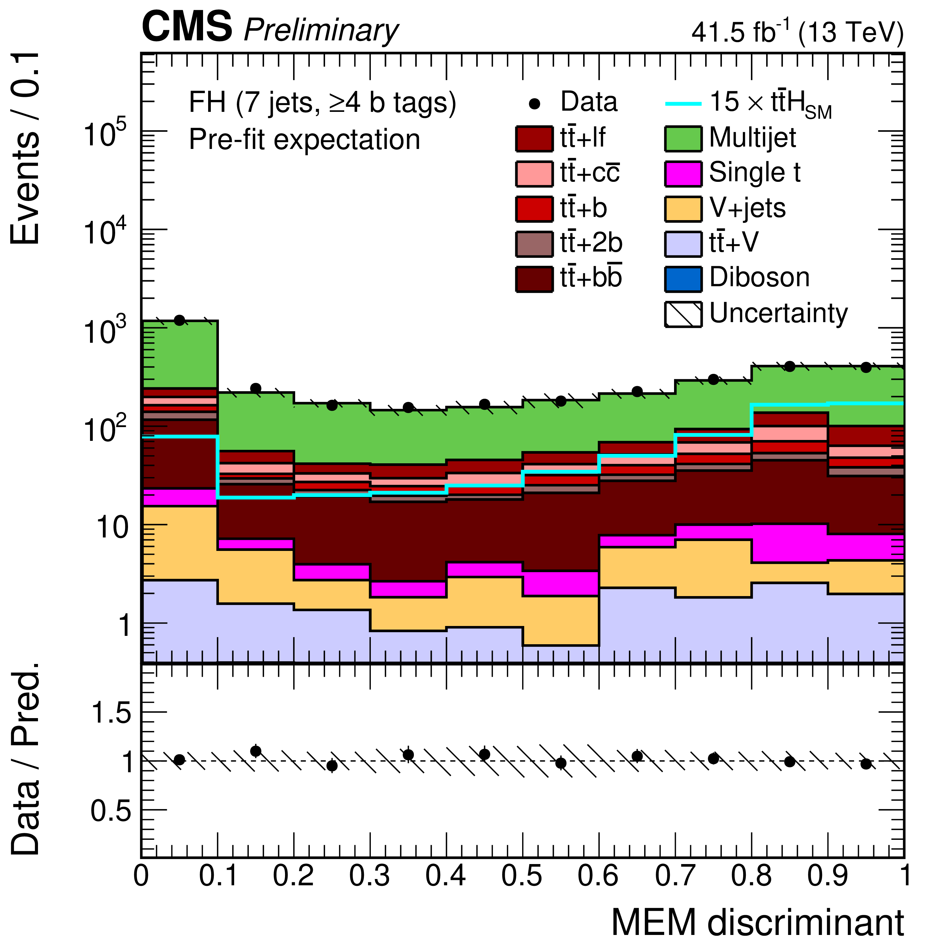
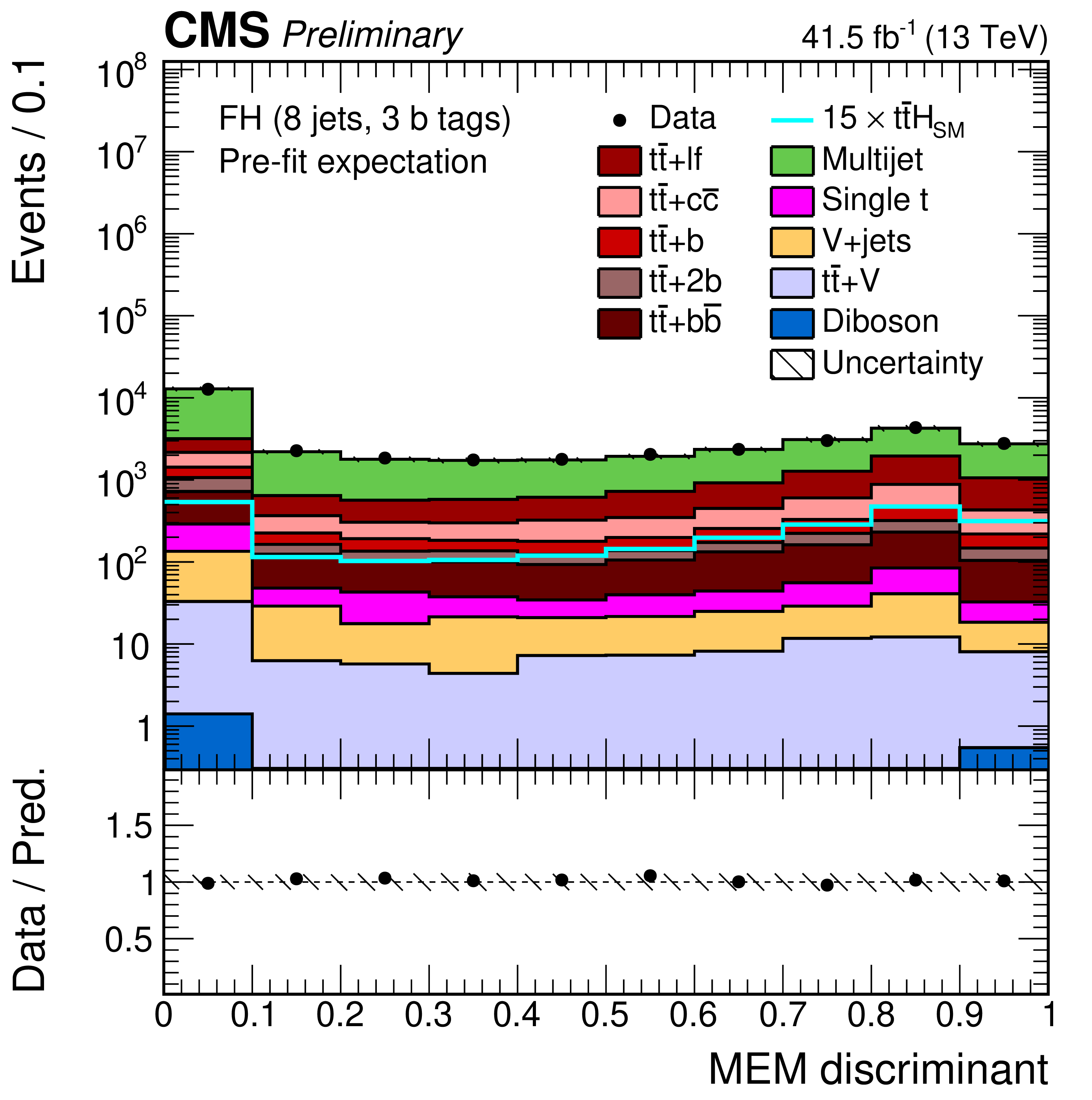
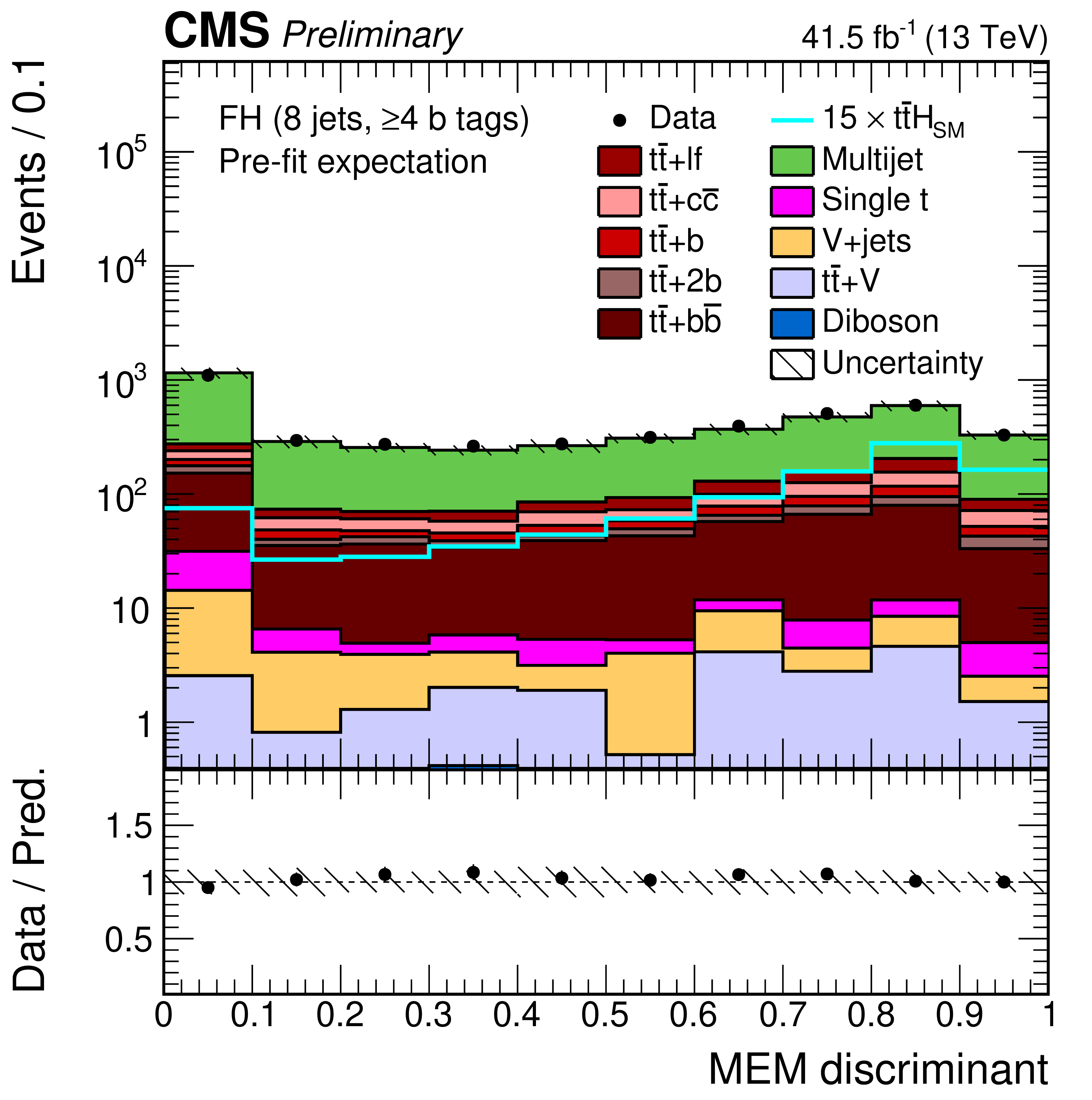
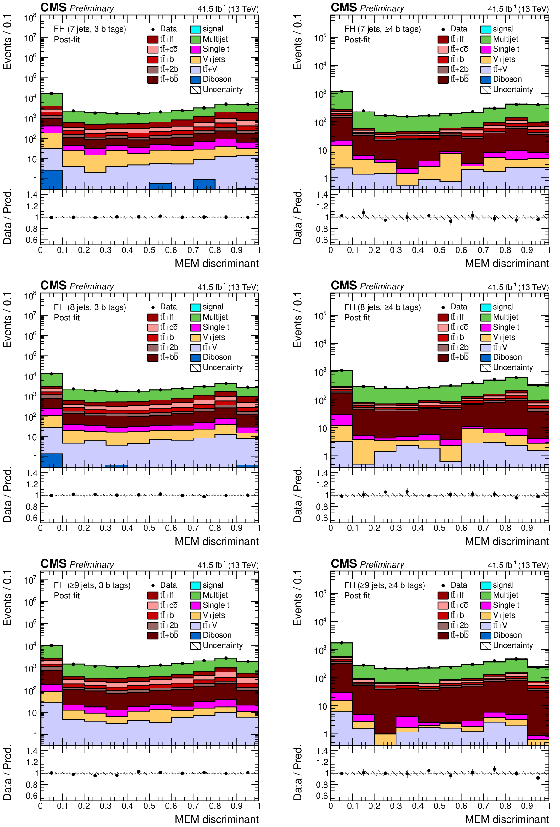
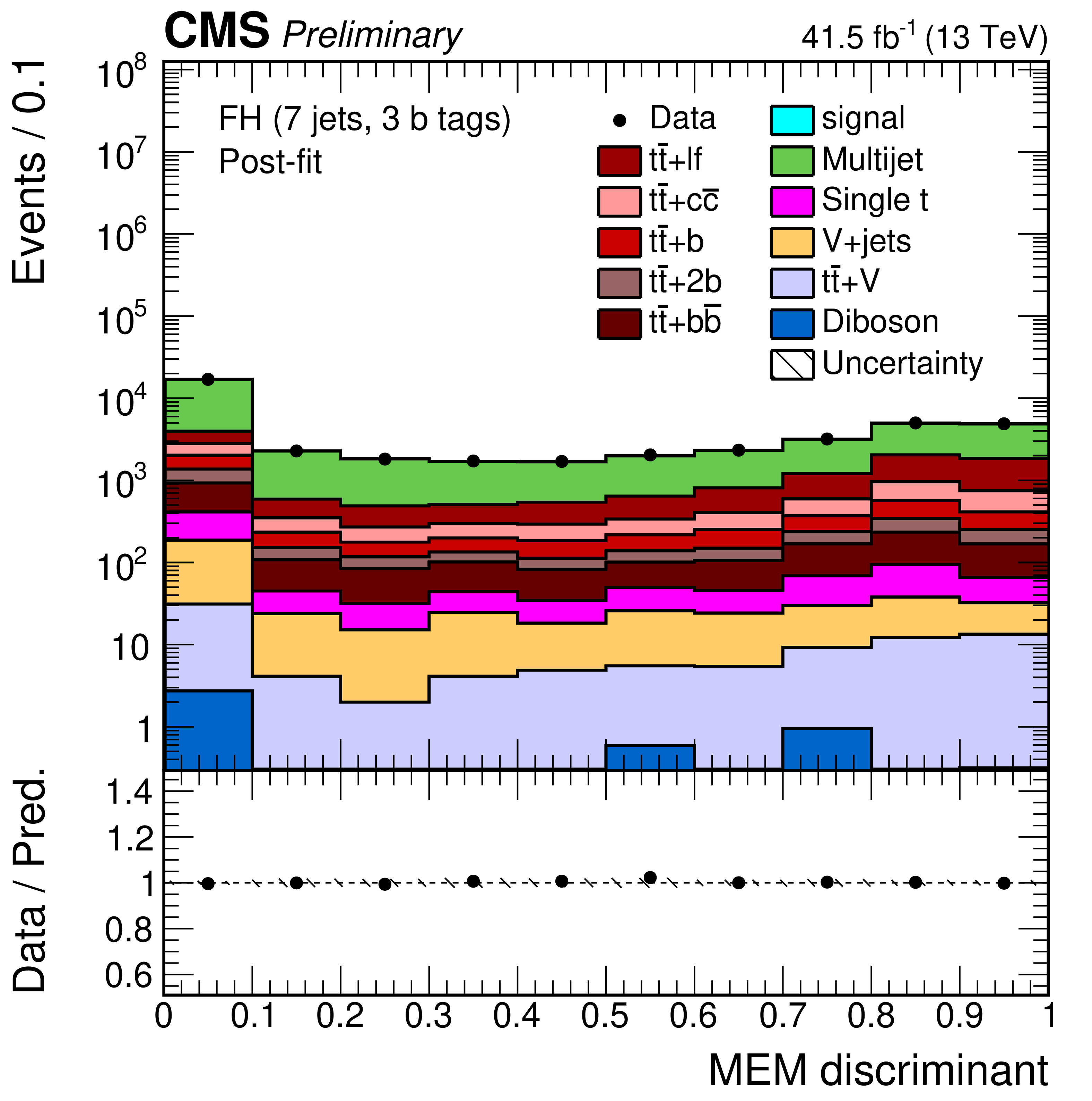
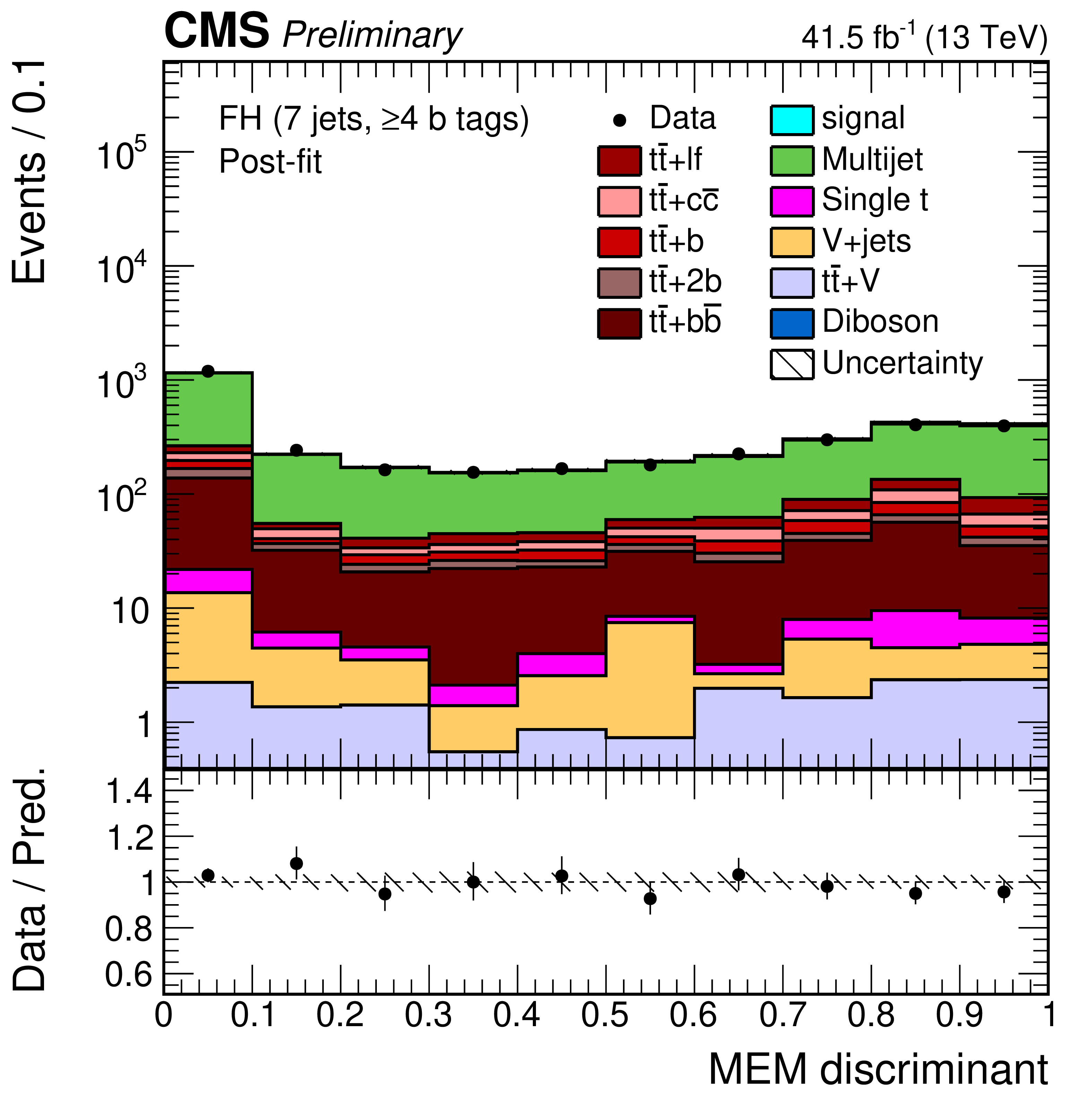
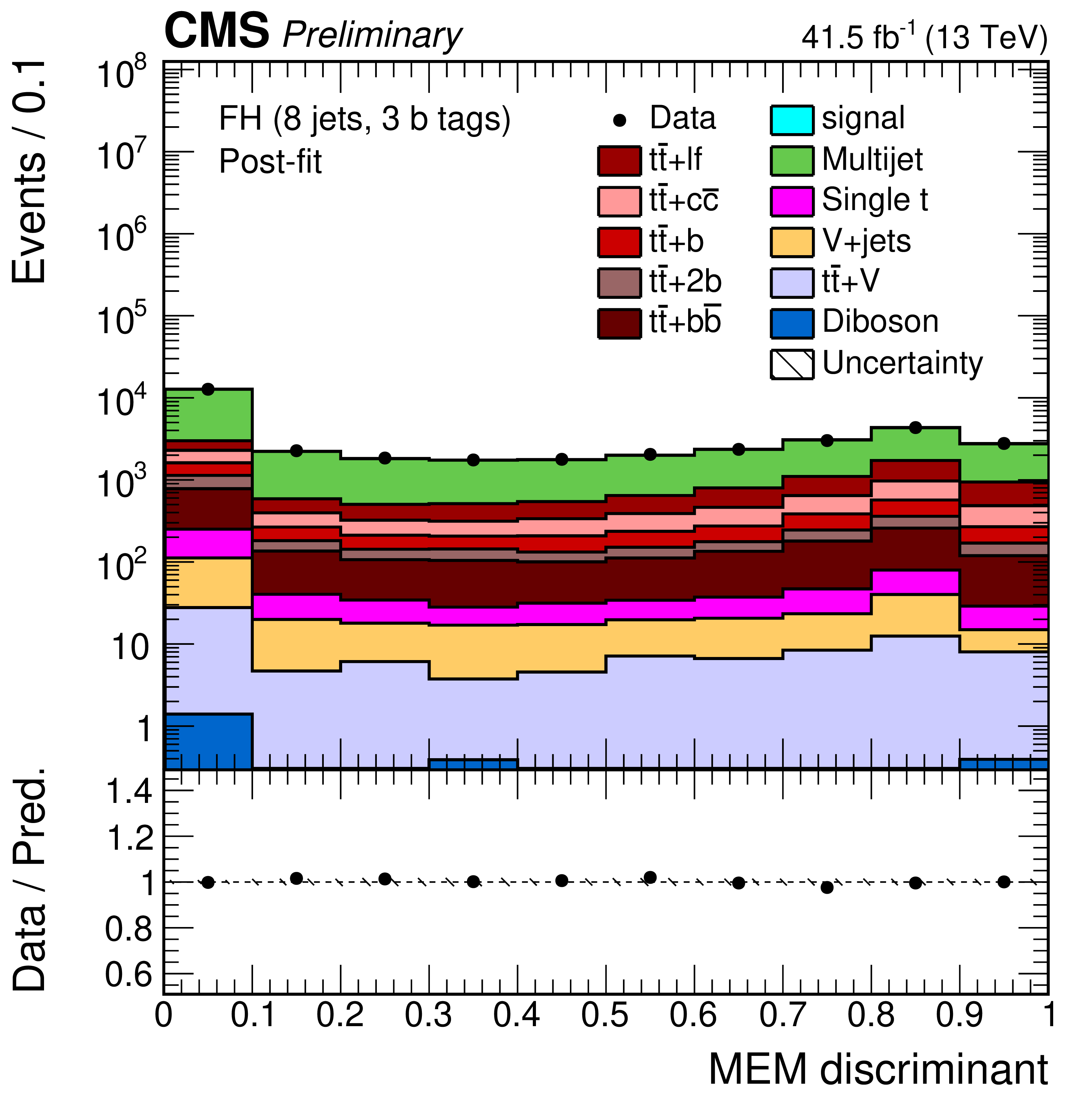
Final discriminant shapes in the fully-hadronic (FH) channel before the fit to data: MEM discriminant in the jet-tag categories with 3 b-tagged jets (left) and $\geq $4 b-tagged jets (right) with 7, 8, and $\geq $9 jets (from top to bottom). The expected background contributions (filled histograms) are stacked, and the expected signal distribution (line) is superimposed. Each contribution is normalised to an integrated luminosity of 41.5 fb$^{-1}$, and the signal distribution is additionally scaled by a factor of 15 for better visibility. The hatched uncertainty bands include the total uncertainty of the fit model except the effect due to the freely-floating QCD-background normalisation. The distributions observed in data (markers) are overlayed. The first and the last bins include underflow and overflow events, respectively. The lower plots show the ratio of the data to the background prediction. |
png pdf |
Additional Figure 10-a:
Final discriminant shapes in the fully-hadronic (FH) channel before the fit to data: MEM discriminant in the jet-tag categories with 3 b-tagged jets with 7 jets. The expected background contributions (filled histograms) are stacked, and the expected signal distribution (line) is superimposed. Each contribution is normalised to an integrated luminosity of 41.5 fb$^{-1}$, and the signal distribution is additionally scaled by a factor of 15 for better visibility. The hatched uncertainty bands include the total uncertainty of the fit model except the effect due to the freely-floating QCD-background normalisation. The distribution observed in data (markers) is overlayed. The first and the last bins include underflow and overflow events, respectively. The lower plot shows the ratio of the data to the background prediction. |
png pdf |
Additional Figure 10-b:
Final discriminant shapes in the fully-hadronic (FH) channel before the fit to data: MEM discriminant in the jet-tag categories with $\geq $4 b-tagged jets with 7 jets. The expected background contributions (filled histograms) are stacked, and the expected signal distribution (line) is superimposed. Each contribution is normalised to an integrated luminosity of 41.5 fb$^{-1}$, and the signal distribution is additionally scaled by a factor of 15 for better visibility. The hatched uncertainty bands include the total uncertainty of the fit model except the effect due to the freely-floating QCD-background normalisation. The distribution observed in data (markers) is overlayed. The first and the last bins include underflow and overflow events, respectively. The lower plot shows the ratio of the data to the background prediction. |
png pdf |
Additional Figure 10-c:
Final discriminant shapes in the fully-hadronic (FH) channel before the fit to data: MEM discriminant in the jet-tag categories with 3 b-tagged jets with 8 jets. The expected background contributions (filled histograms) are stacked, and the expected signal distribution (line) is superimposed. Each contribution is normalised to an integrated luminosity of 41.5 fb$^{-1}$, and the signal distribution is additionally scaled by a factor of 15 for better visibility. The hatched uncertainty bands include the total uncertainty of the fit model except the effect due to the freely-floating QCD-background normalisation. The distribution observed in data (markers) is overlayed. The first and the last bins include underflow and overflow events, respectively. The lower plot shows the ratio of the data to the background prediction. |
png pdf |
Additional Figure 10-d:
Final discriminant shapes in the fully-hadronic (FH) channel before the fit to data: MEM discriminant in the jet-tag categories with $\geq $4 b-tagged jets with 8 jets. The expected background contributions (filled histograms) are stacked, and the expected signal distribution (line) is superimposed. Each contribution is normalised to an integrated luminosity of 41.5 fb$^{-1}$, and the signal distribution is additionally scaled by a factor of 15 for better visibility. The hatched uncertainty bands include the total uncertainty of the fit model except the effect due to the freely-floating QCD-background normalisation. The distribution observed in data (markers) is overlayed. The first and the last bins include underflow and overflow events, respectively. The lower plot shows the ratio of the data to the background prediction. |
png pdf |
Additional Figure 10-e:
Final discriminant shapes in the fully-hadronic (FH) channel before the fit to data: MEM discriminant in the jet-tag categories with 3 b-tagged jets with $\geq $9 jets. The expected background contributions (filled histograms) are stacked, and the expected signal distribution (line) is superimposed. Each contribution is normalised to an integrated luminosity of 41.5 fb$^{-1}$, and the signal distribution is additionally scaled by a factor of 15 for better visibility. The hatched uncertainty bands include the total uncertainty of the fit model except the effect due to the freely-floating QCD-background normalisation. The distribution observed in data (markers) is overlayed. The first and the last bins include underflow and overflow events, respectively. The lower plot shows the ratio of the data to the background prediction. |
png pdf |
Additional Figure 10-f:
Final discriminant shapes in the fully-hadronic (FH) channel before the fit to data: MEM discriminant in the jet-tag categories with $\geq $4 b-tagged jets with $\geq $9 jets. The expected background contributions (filled histograms) are stacked, and the expected signal distribution (line) is superimposed. Each contribution is normalised to an integrated luminosity of 41.5 fb$^{-1}$, and the signal distribution is additionally scaled by a factor of 15 for better visibility. The hatched uncertainty bands include the total uncertainty of the fit model except the effect due to the freely-floating QCD-background normalisation. The distribution observed in data (markers) is overlayed. The first and the last bins include underflow and overflow events, respectively. The lower plot shows the ratio of the data to the background prediction. |
png pdf |
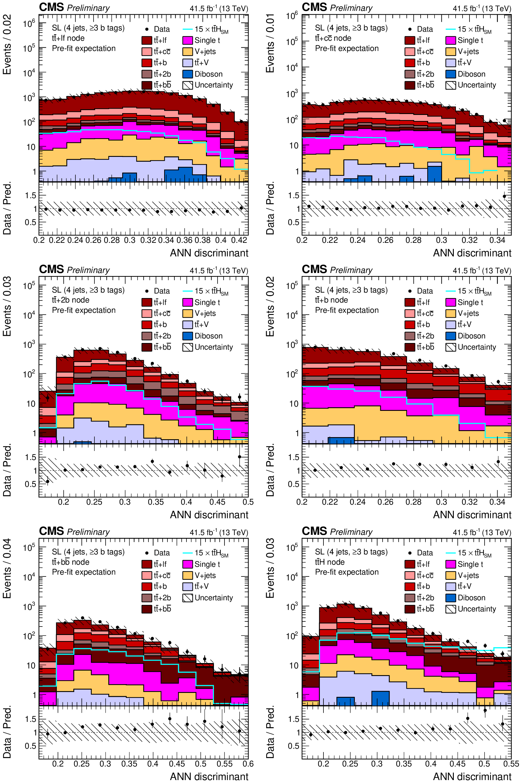
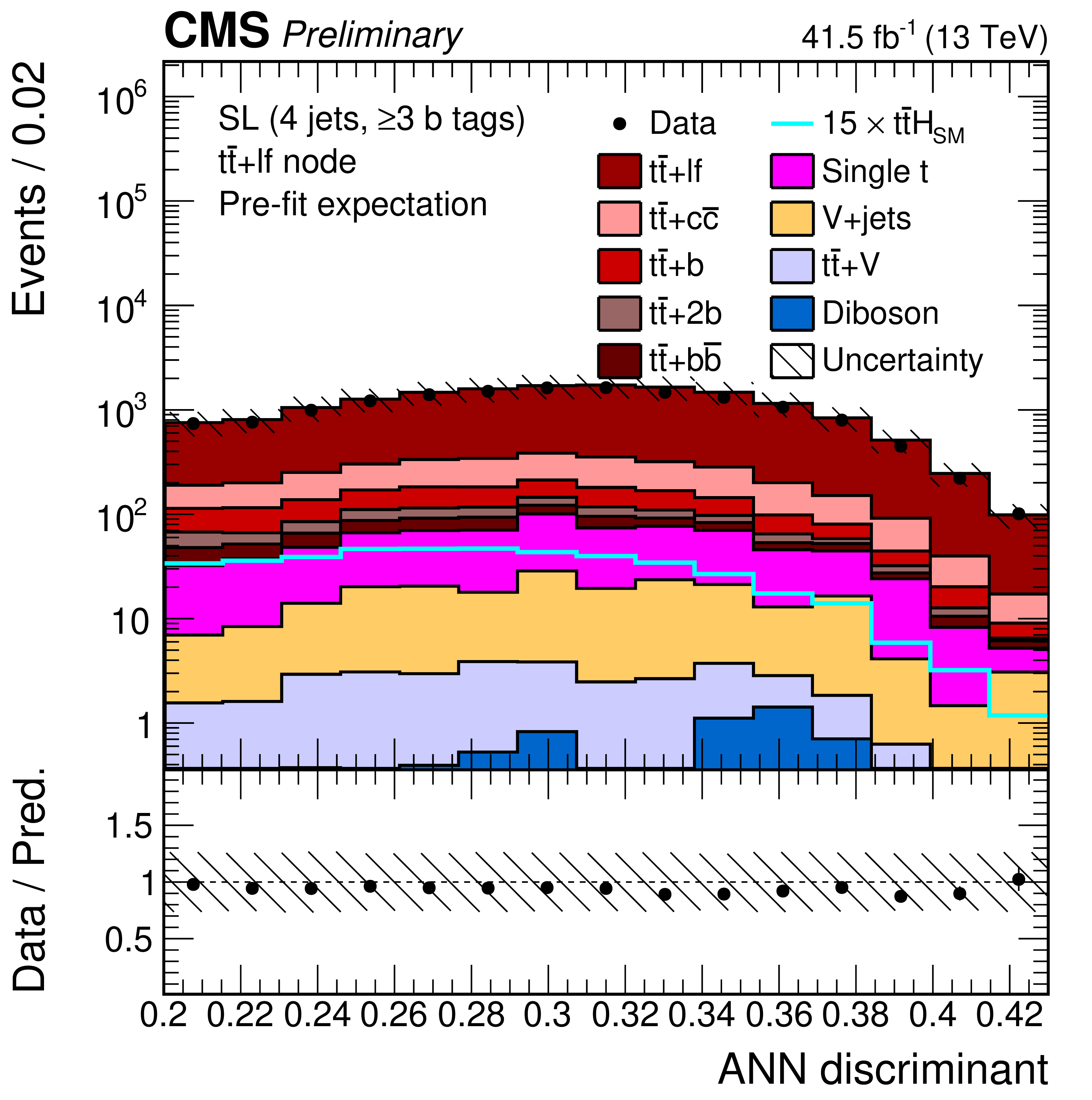
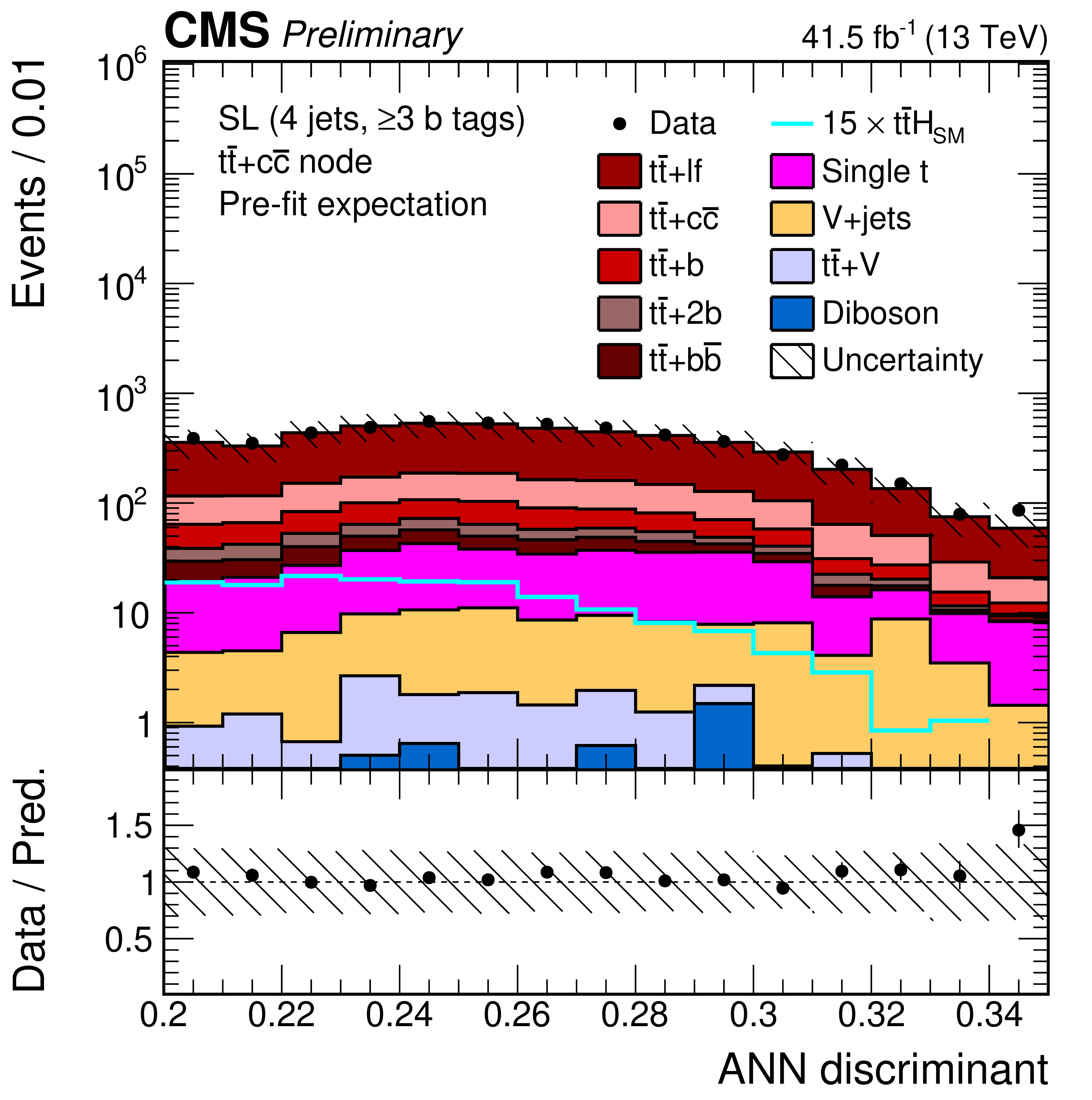
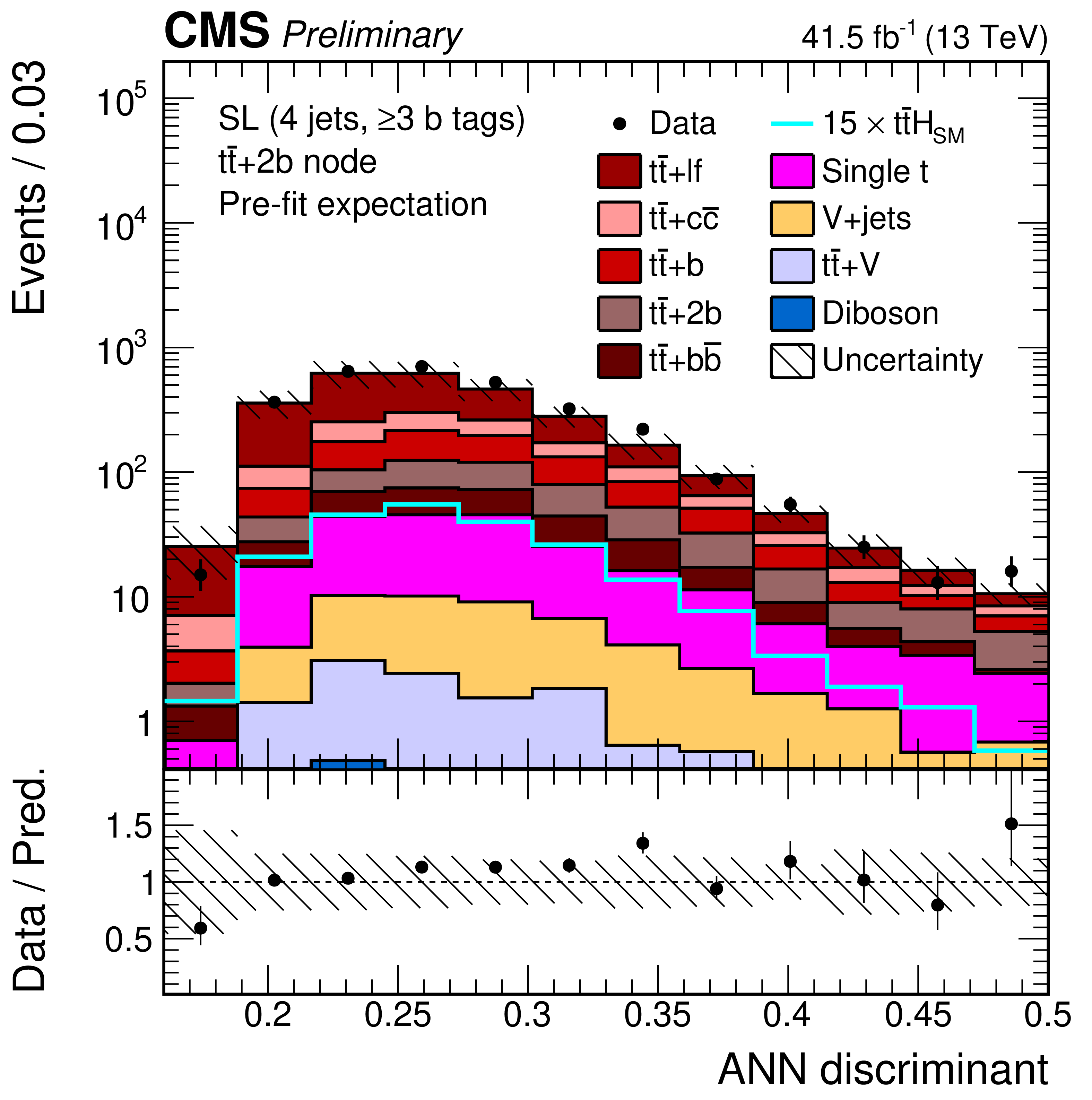
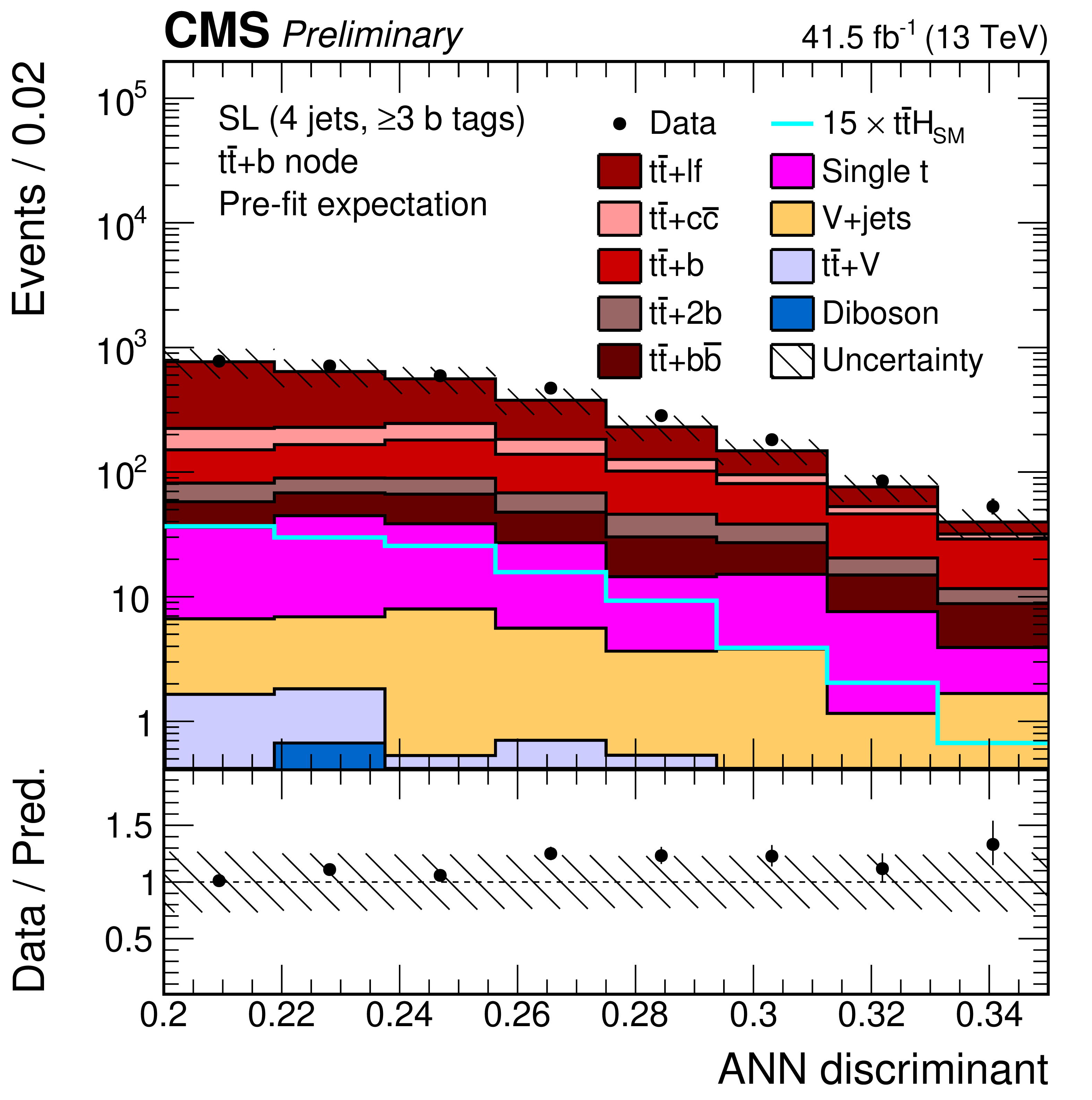
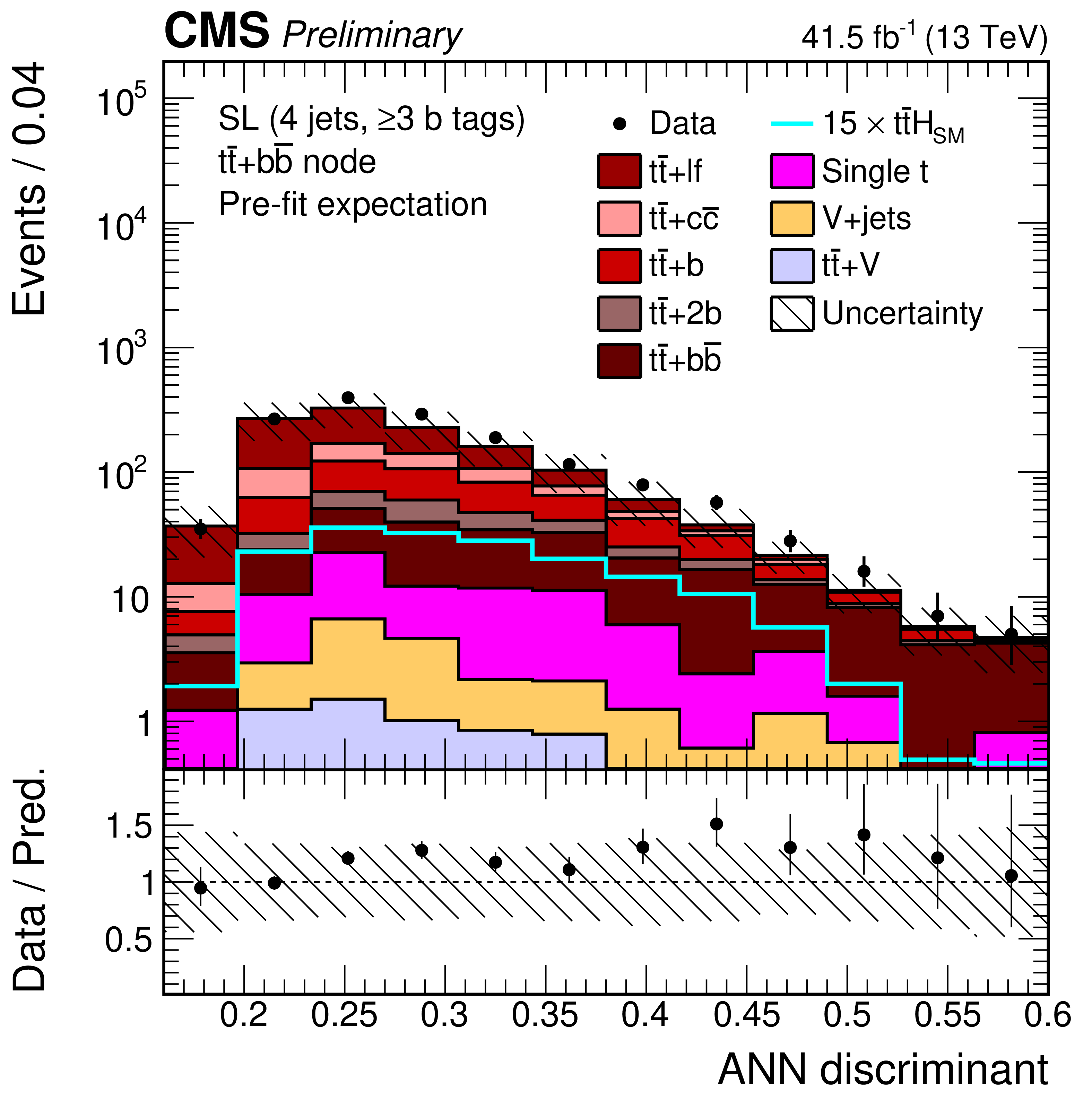
Additional Figure 11:
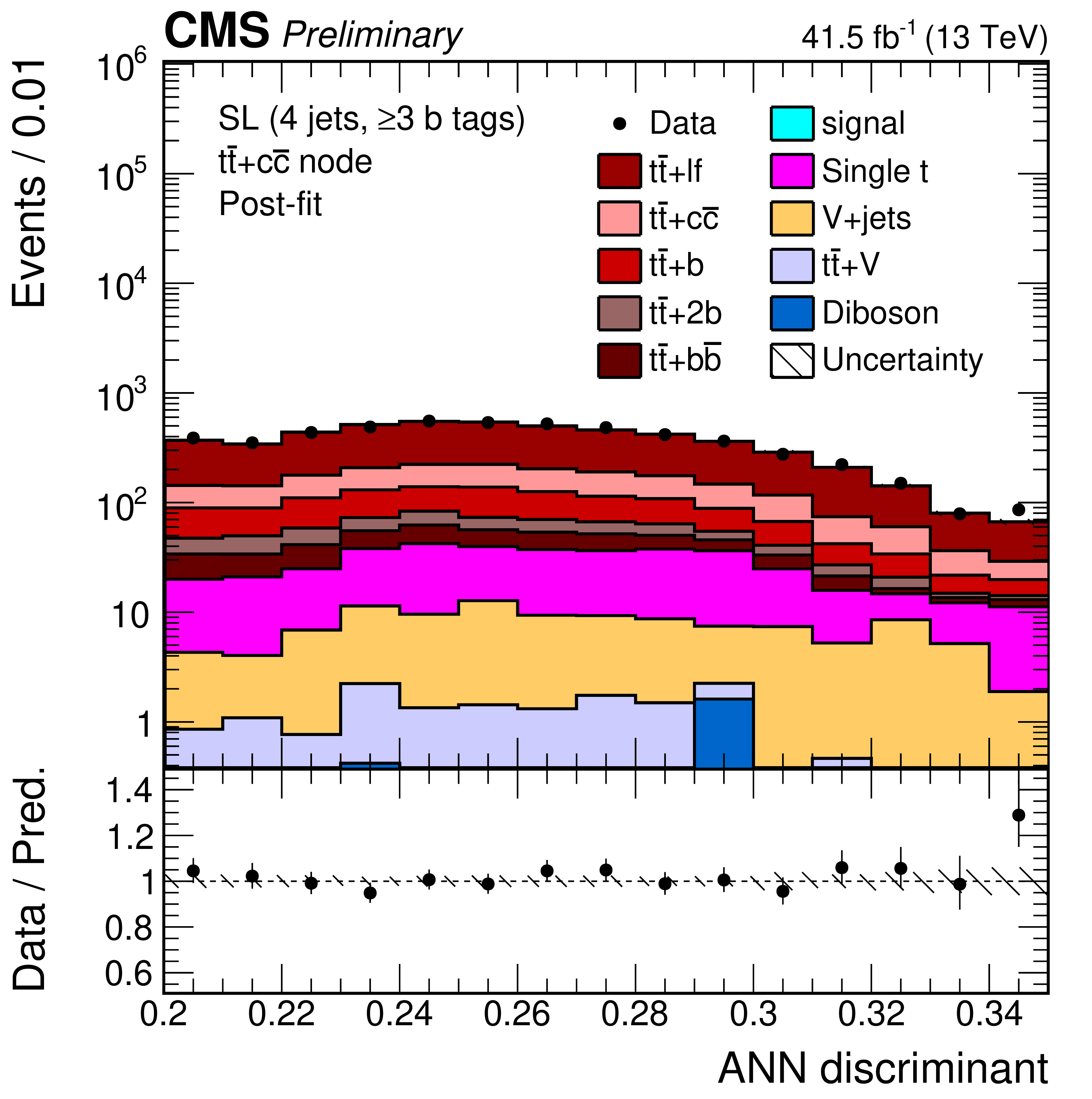
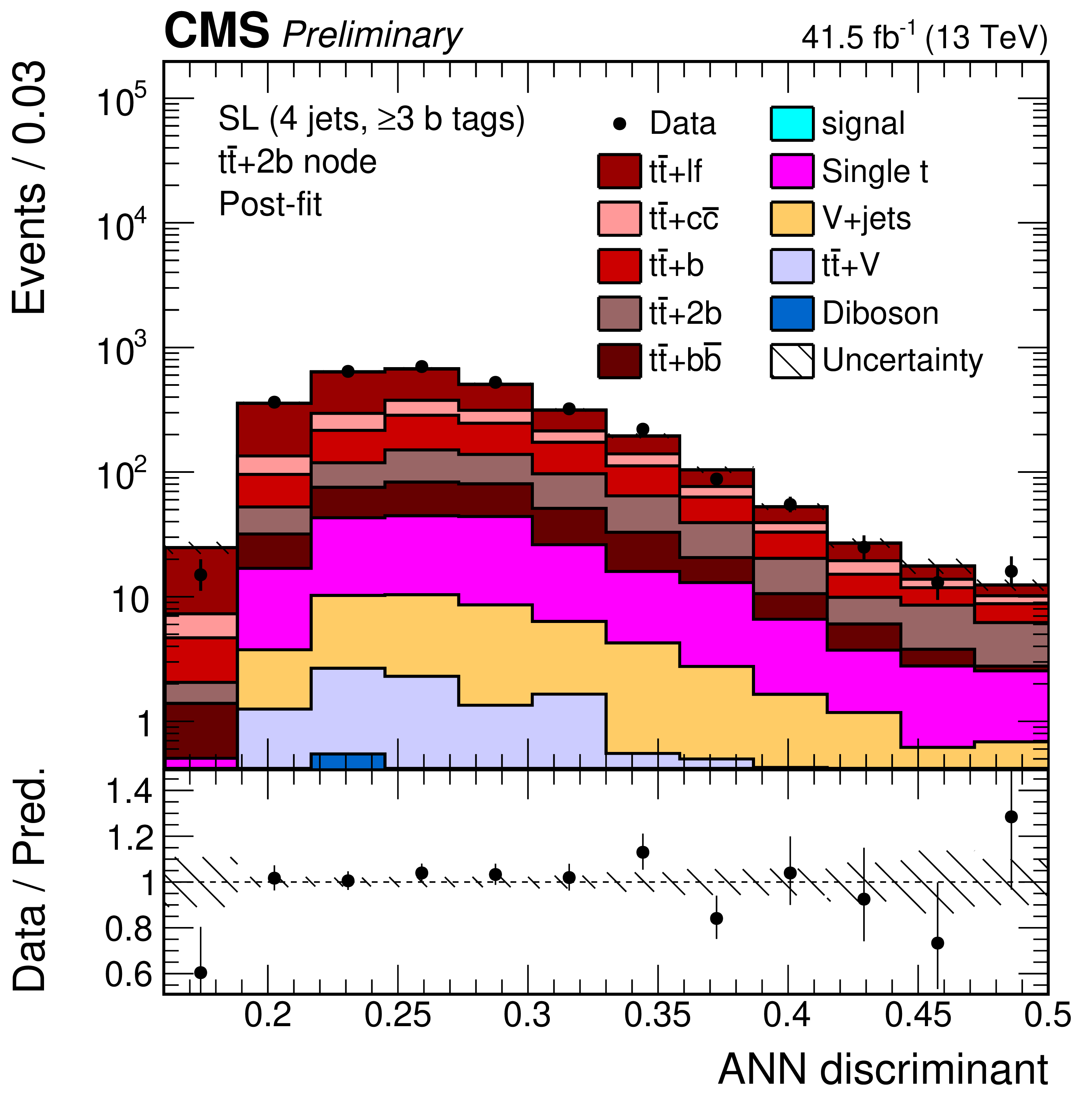
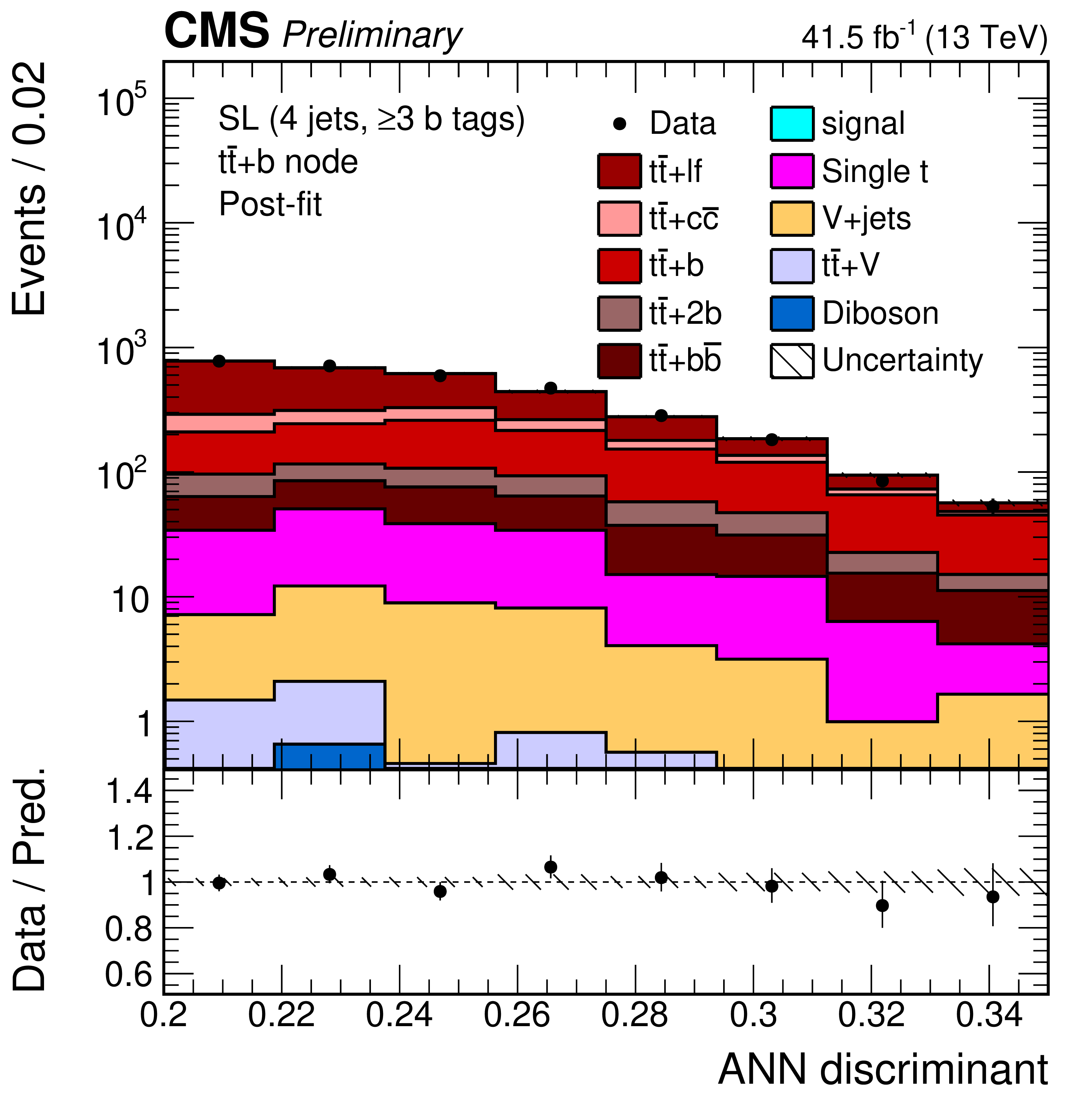
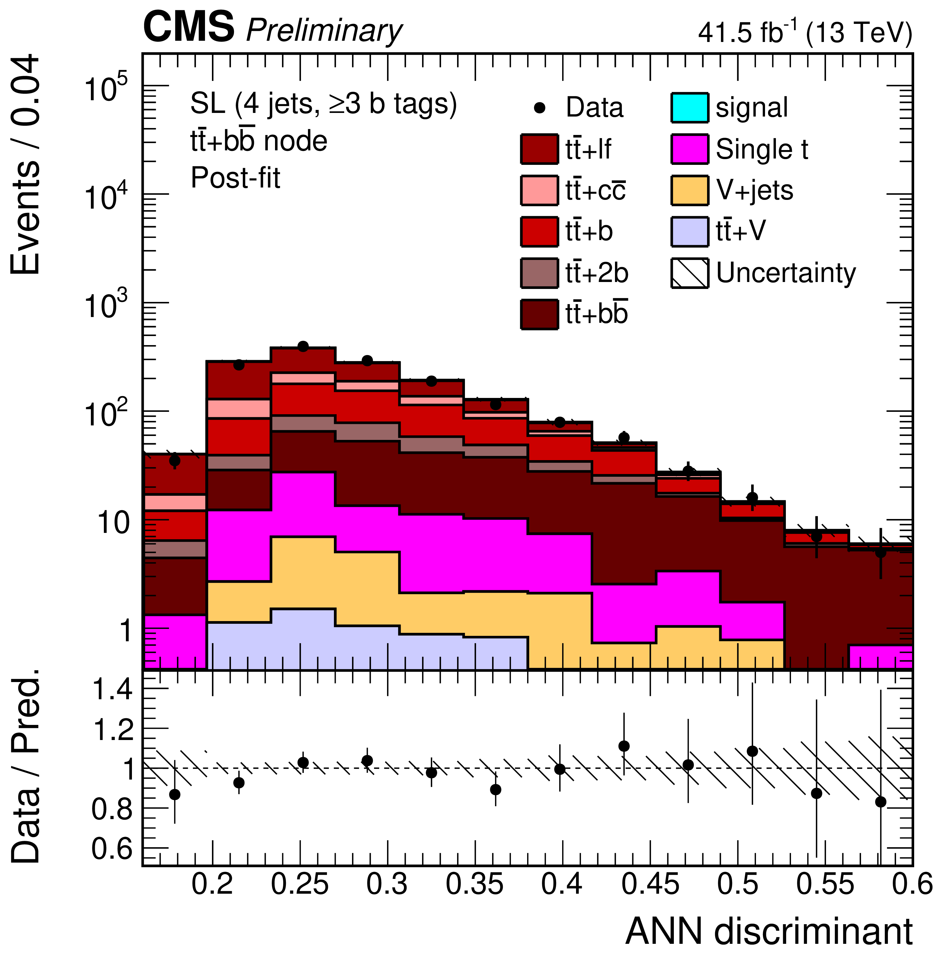
ANN discriminant shapes in the semi-leptonic (SL) channel before the fit to data in the jet-process categories with 4 jets, $\geq $3 b-tags. The expected background contributions (filled histograms) are stacked, and the expected signal distribution (line) is superimposed. Each contribution is normalised to an integrated luminosity of 41.5 fb$^{-1}$, and the signal distribution is additionally scaled by a factor of 15 for better visibility. The hatched uncertainty bands include the total uncertainty of the fit model. The distributions of the signal+background SM prediction (markers) are overlayed. The first and the last bins include underflow and overflow events, respectively. The lower plots show the ratio of the data to the background prediction. |
png pdf |
Additional Figure 11-a:
ANN discriminant shapes in the semi-leptonic (SL) channel before the fit to data in the jet-process categories with 4 jets, $\geq $3 b-tags. The expected background contributions (filled histograms) are stacked, and the expected signal distribution (line) is superimposed. Each contribution is normalised to an integrated luminosity of 41.5 fb$^{-1}$, and the signal distribution is additionally scaled by a factor of 15 for better visibility. The hatched uncertainty bands include the total uncertainty of the fit model. The distributions of the signal+background SM prediction (markers) are overlayed. The first and the last bins include underflow and overflow events, respectively. The lower plots show the ratio of the data to the background prediction. |
png pdf |
Additional Figure 11-b:
ANN discriminant shapes in the semi-leptonic (SL) channel before the fit to data in the jet-process categories with 4 jets, $\geq $3 b-tags. The expected background contributions (filled histograms) are stacked, and the expected signal distribution (line) is superimposed. Each contribution is normalised to an integrated luminosity of 41.5 fb$^{-1}$, and the signal distribution is additionally scaled by a factor of 15 for better visibility. The hatched uncertainty bands include the total uncertainty of the fit model. The distributions of the signal+background SM prediction (markers) are overlayed. The first and the last bins include underflow and overflow events, respectively. The lower plots show the ratio of the data to the background prediction. |
png pdf |
Additional Figure 11-c:
ANN discriminant shapes in the semi-leptonic (SL) channel before the fit to data in the jet-process categories with 4 jets, $\geq $3 b-tags. The expected background contributions (filled histograms) are stacked, and the expected signal distribution (line) is superimposed. Each contribution is normalised to an integrated luminosity of 41.5 fb$^{-1}$, and the signal distribution is additionally scaled by a factor of 15 for better visibility. The hatched uncertainty bands include the total uncertainty of the fit model. The distributions of the signal+background SM prediction (markers) are overlayed. The first and the last bins include underflow and overflow events, respectively. The lower plots show the ratio of the data to the background prediction. |
png pdf |
Additional Figure 11-d:
ANN discriminant shapes in the semi-leptonic (SL) channel before the fit to data in the jet-process categories with 4 jets, $\geq $3 b-tags. The expected background contributions (filled histograms) are stacked, and the expected signal distribution (line) is superimposed. Each contribution is normalised to an integrated luminosity of 41.5 fb$^{-1}$, and the signal distribution is additionally scaled by a factor of 15 for better visibility. The hatched uncertainty bands include the total uncertainty of the fit model. The distributions of the signal+background SM prediction (markers) are overlayed. The first and the last bins include underflow and overflow events, respectively. The lower plots show the ratio of the data to the background prediction. |
png pdf |
Additional Figure 11-e:
ANN discriminant shapes in the semi-leptonic (SL) channel before the fit to data in the jet-process categories with 4 jets, $\geq $3 b-tags. The expected background contributions (filled histograms) are stacked, and the expected signal distribution (line) is superimposed. Each contribution is normalised to an integrated luminosity of 41.5 fb$^{-1}$, and the signal distribution is additionally scaled by a factor of 15 for better visibility. The hatched uncertainty bands include the total uncertainty of the fit model. The distributions of the signal+background SM prediction (markers) are overlayed. The first and the last bins include underflow and overflow events, respectively. The lower plots show the ratio of the data to the background prediction. |
png pdf |
Additional Figure 11-f:
ANN discriminant shapes in the semi-leptonic (SL) channel before the fit to data in the jet-process categories with 4 jets, $\geq $3 b-tags. The expected background contributions (filled histograms) are stacked, and the expected signal distribution (line) is superimposed. Each contribution is normalised to an integrated luminosity of 41.5 fb$^{-1}$, and the signal distribution is additionally scaled by a factor of 15 for better visibility. The hatched uncertainty bands include the total uncertainty of the fit model. The distributions of the signal+background SM prediction (markers) are overlayed. The first and the last bins include underflow and overflow events, respectively. The lower plots show the ratio of the data to the background prediction. |
png pdf |
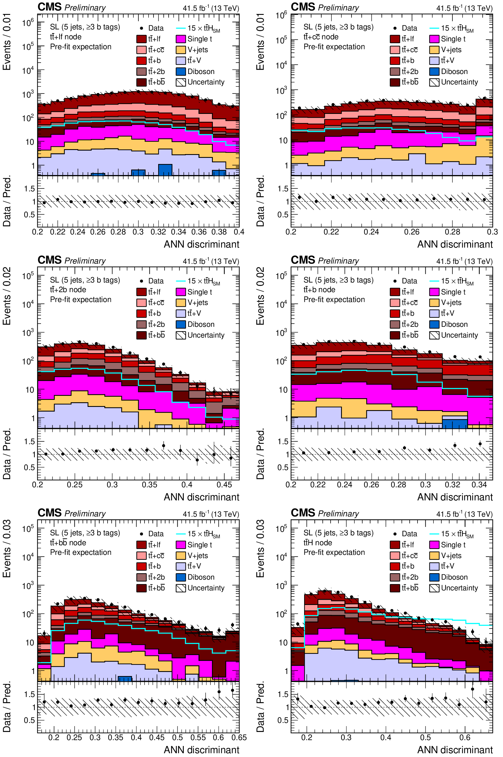
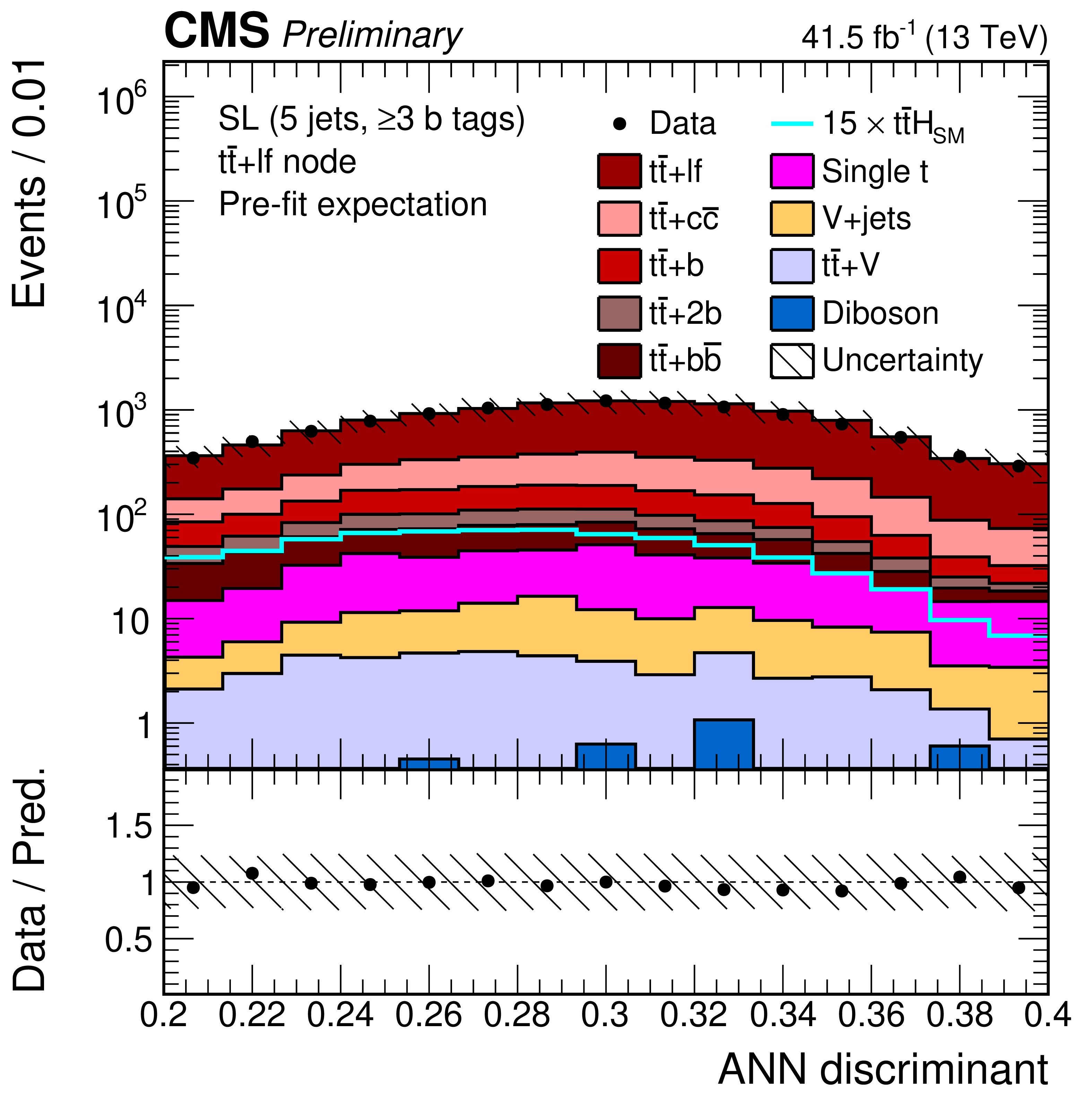
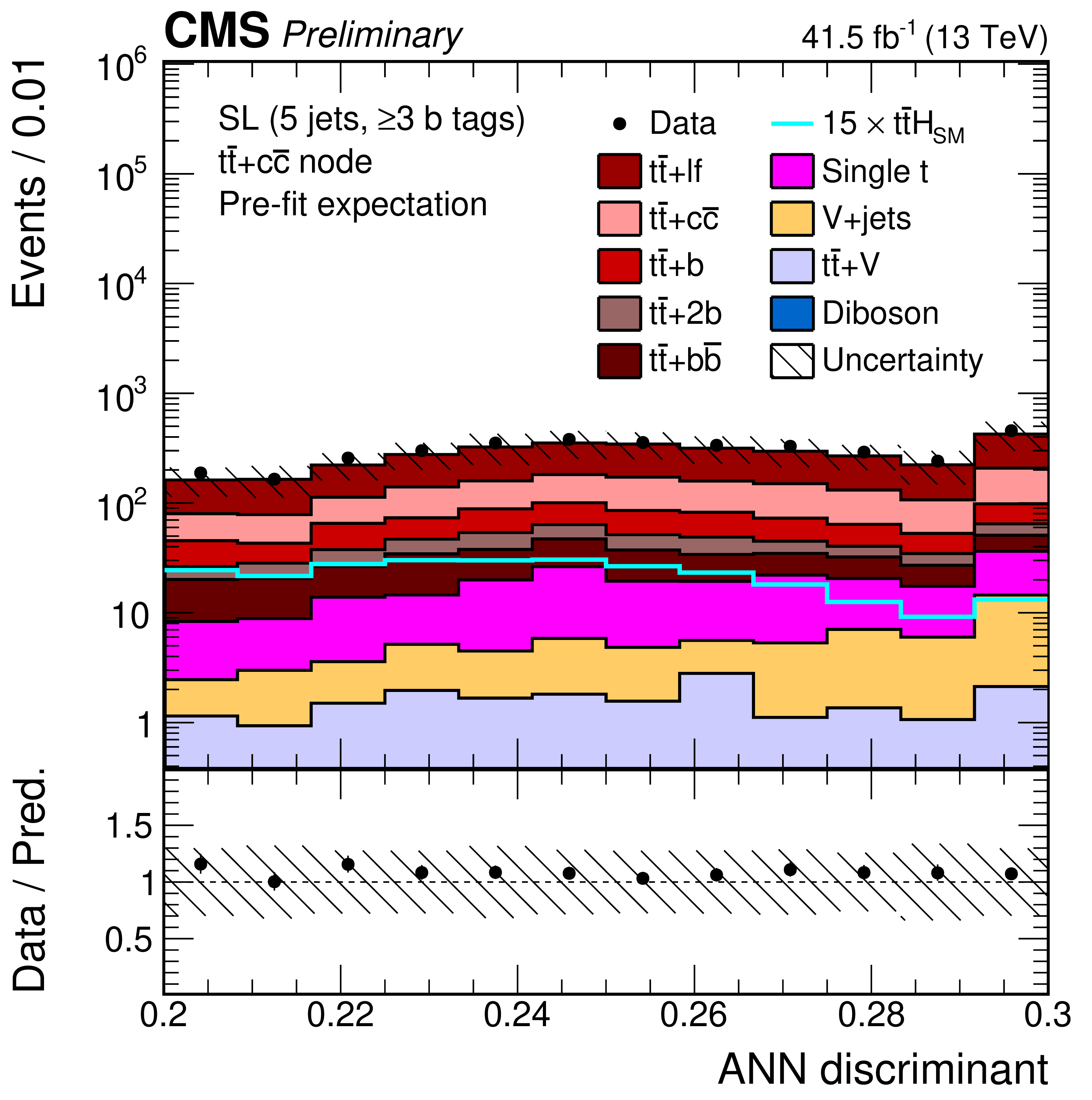
Additional Figure 12:
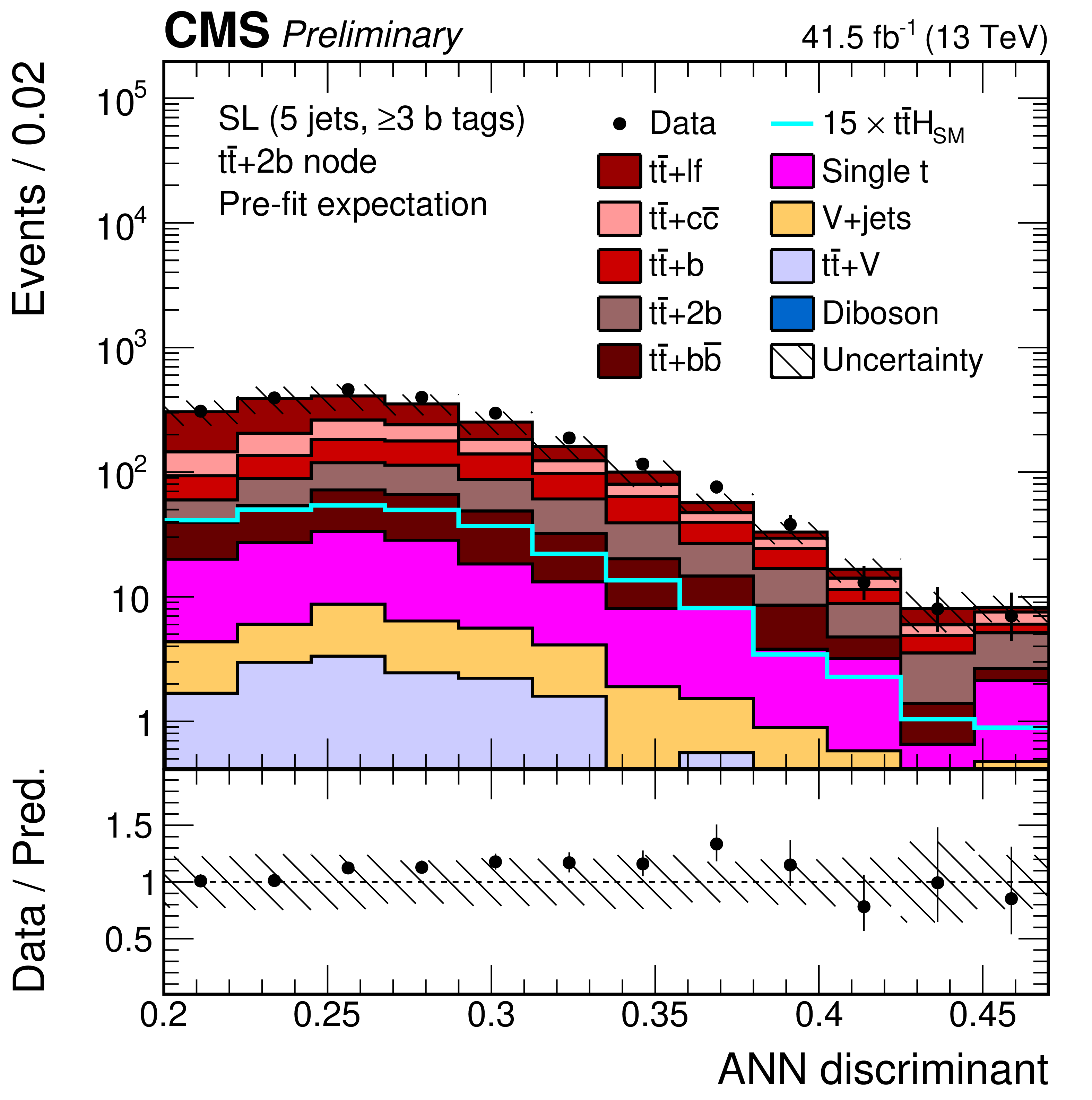
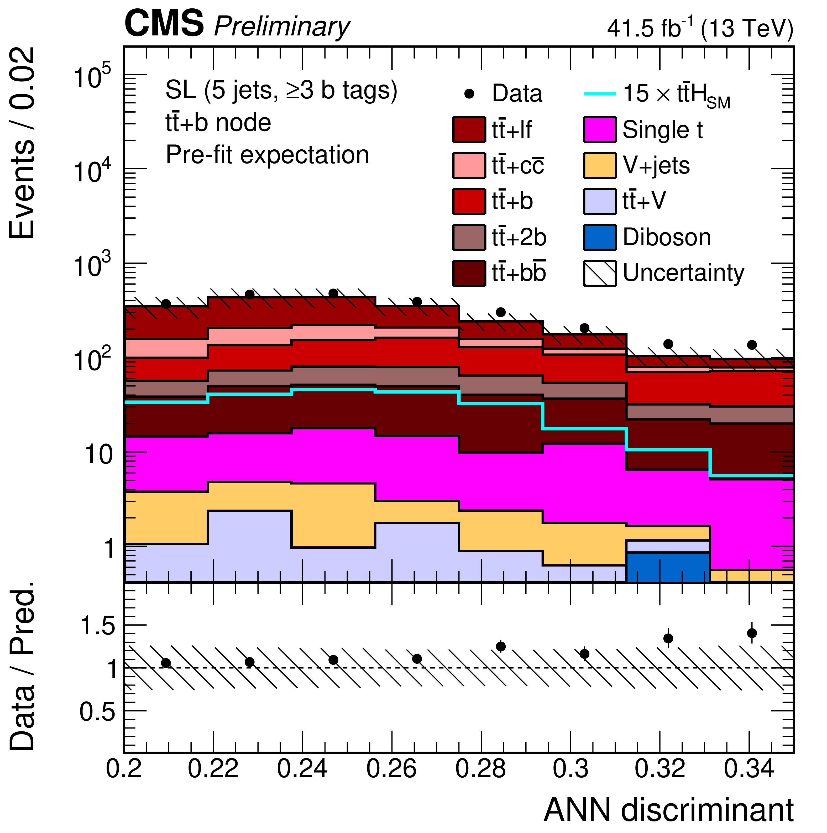
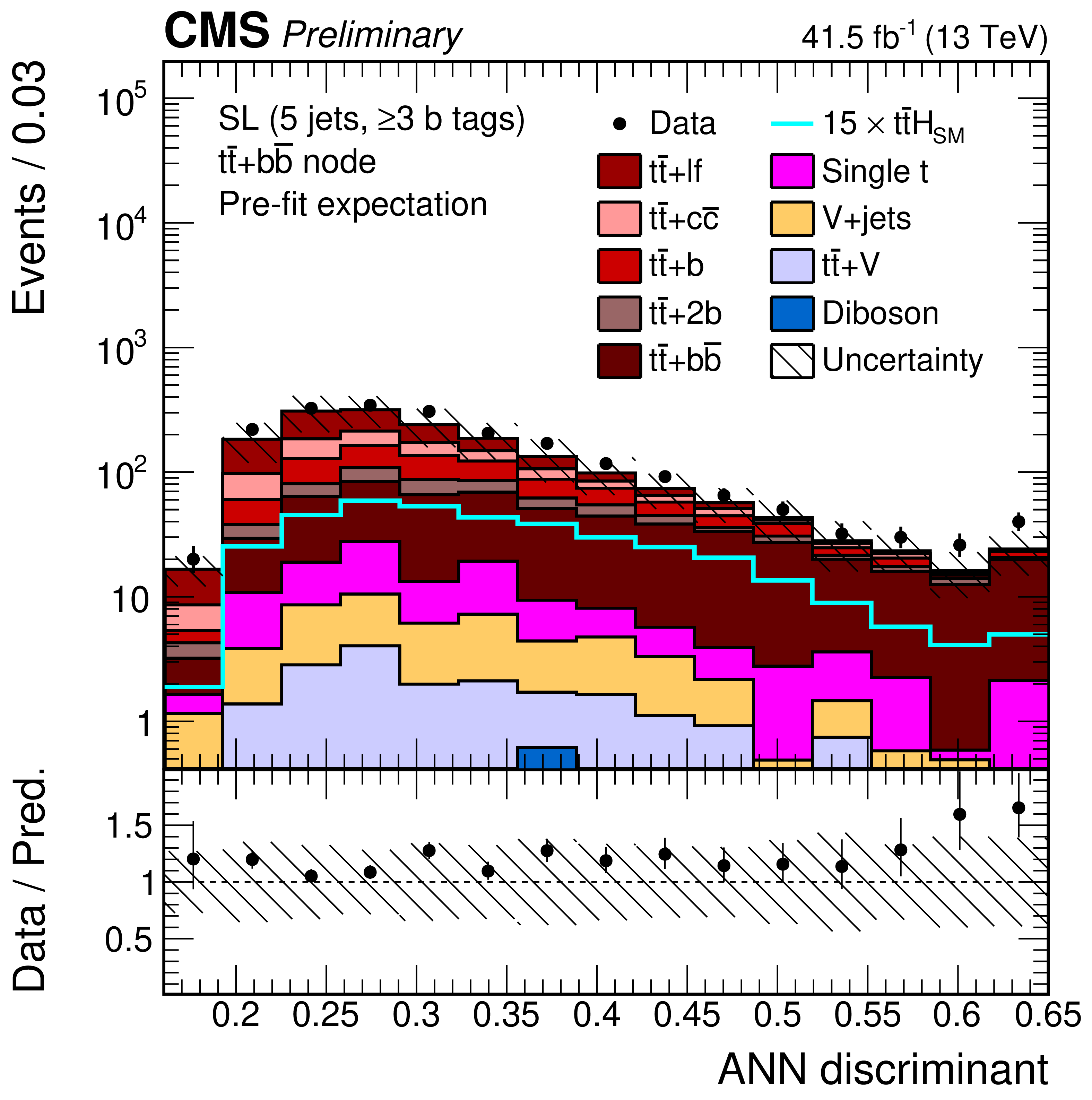
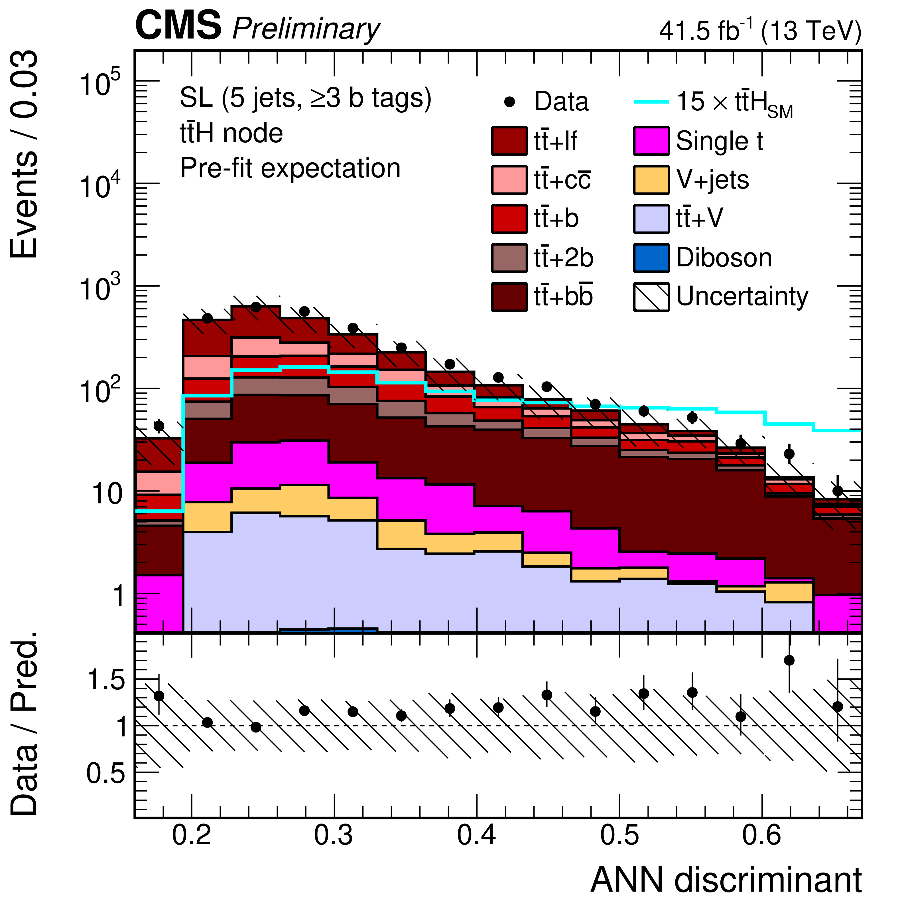
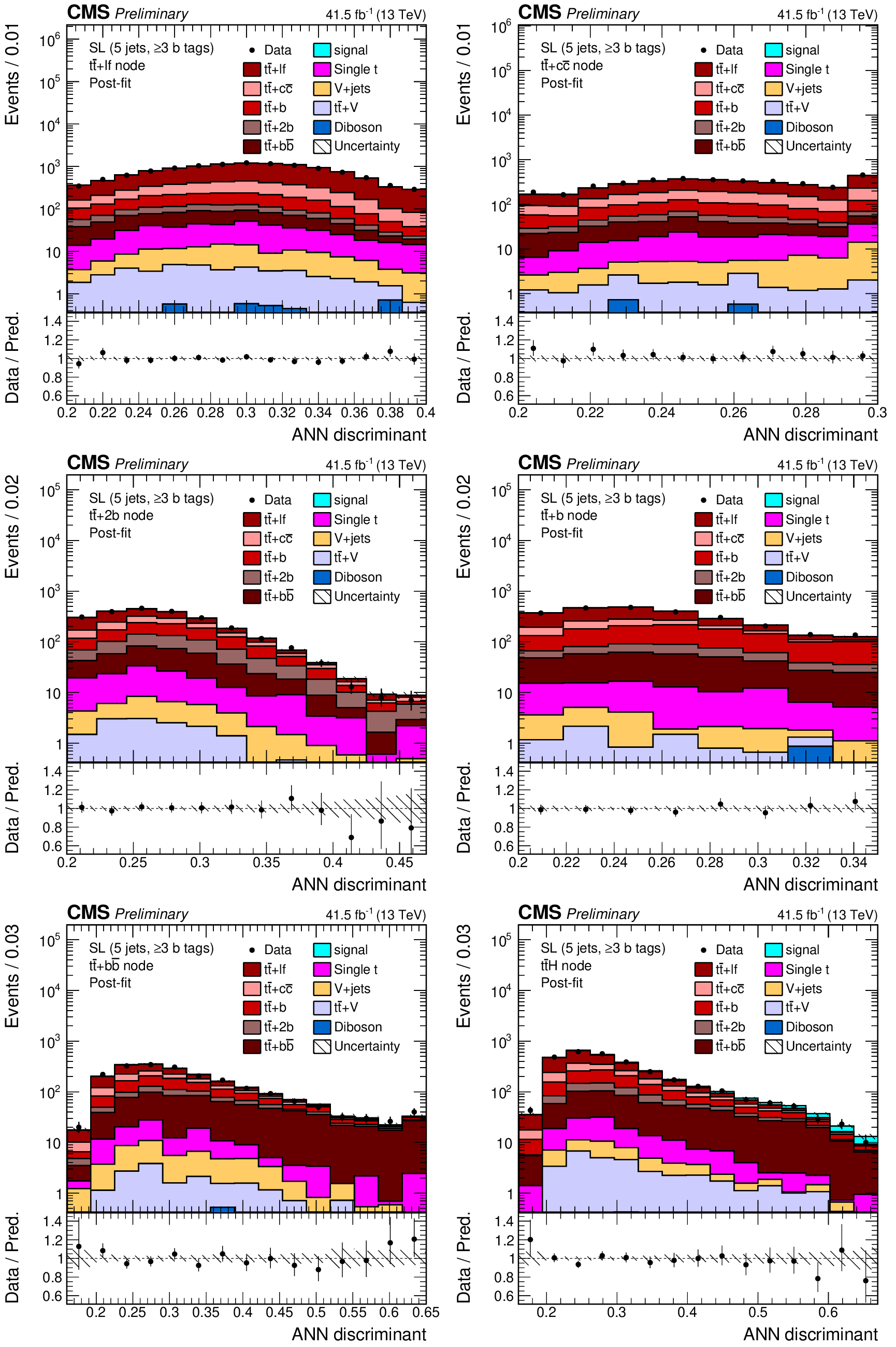
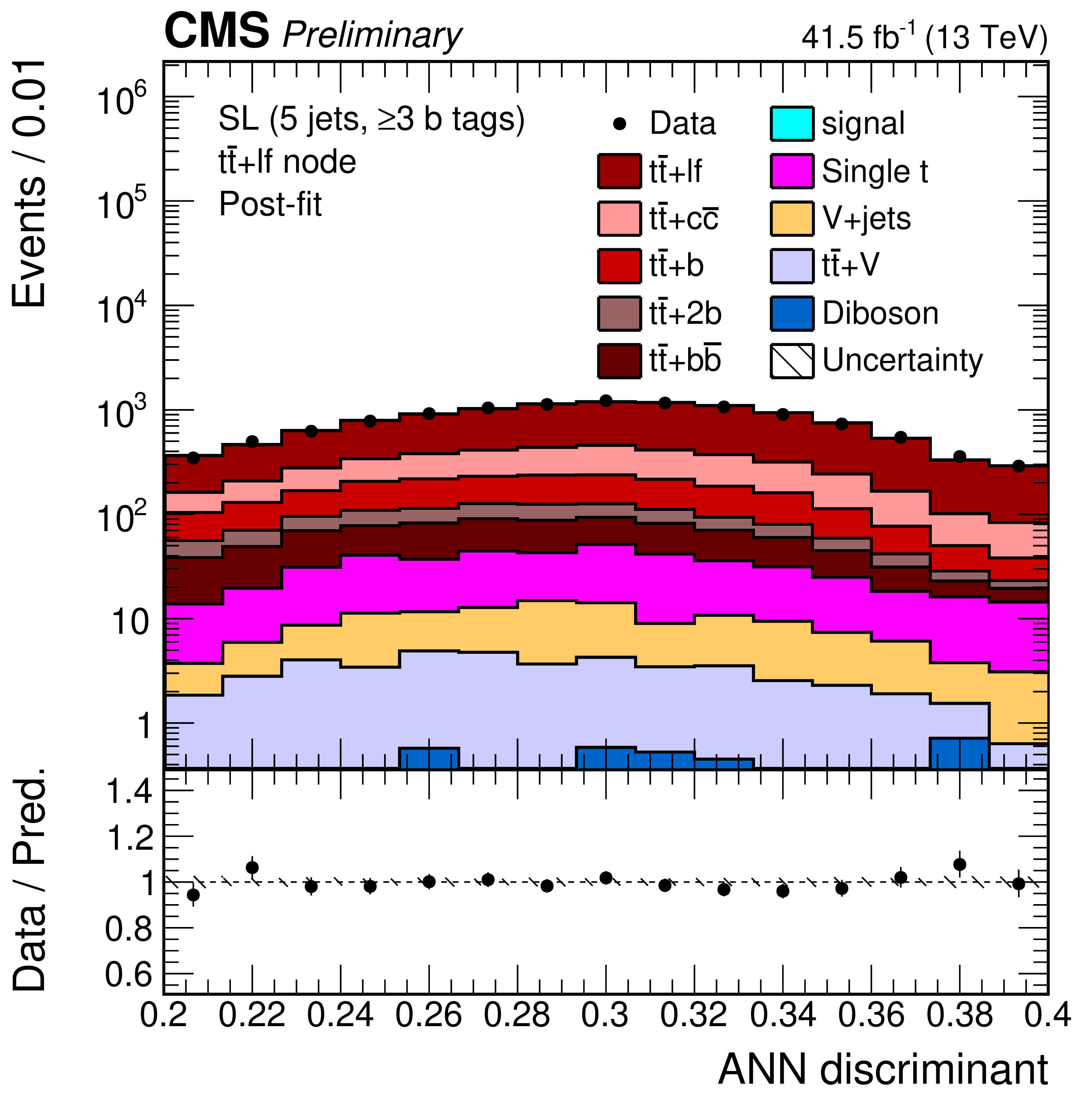
ANN discriminant shapes in the semi-leptonic (SL) channel before the fit to data in the jet-process categories with 5 jets, $\geq $3 b-tags. The expected background contributions (filled histograms) are stacked, and the expected signal distribution (line) is superimposed. Each contribution is normalised to an integrated luminosity of 41.5 fb$^{-1}$, and the signal distribution is additionally scaled by a factor of 15 for better visibility. The hatched uncertainty bands include the total uncertainty of the fit model. The distributions of the signal+background SM prediction (markers) are overlayed. The first and the last bins include underflow and overflow events, respectively. The lower plots show the ratio of the data to the background prediction. |
png pdf |
Additional Figure 12-a:
ANN discriminant shapes in the semi-leptonic (SL) channel before the fit to data in the jet-process categories with 5 jets, $\geq $3 b-tags. The expected background contributions (filled histograms) are stacked, and the expected signal distribution (line) is superimposed. Each contribution is normalised to an integrated luminosity of 41.5 fb$^{-1}$, and the signal distribution is additionally scaled by a factor of 15 for better visibility. The hatched uncertainty bands include the total uncertainty of the fit model. The distributions of the signal+background SM prediction (markers) are overlayed. The first and the last bins include underflow and overflow events, respectively. The lower plots show the ratio of the data to the background prediction. |
png pdf |
Additional Figure 12-b:
ANN discriminant shapes in the semi-leptonic (SL) channel before the fit to data in the jet-process categories with 5 jets, $\geq $3 b-tags. The expected background contributions (filled histograms) are stacked, and the expected signal distribution (line) is superimposed. Each contribution is normalised to an integrated luminosity of 41.5 fb$^{-1}$, and the signal distribution is additionally scaled by a factor of 15 for better visibility. The hatched uncertainty bands include the total uncertainty of the fit model. The distributions of the signal+background SM prediction (markers) are overlayed. The first and the last bins include underflow and overflow events, respectively. The lower plots show the ratio of the data to the background prediction. |
png pdf |
Additional Figure 12-c:
ANN discriminant shapes in the semi-leptonic (SL) channel before the fit to data in the jet-process categories with 5 jets, $\geq $3 b-tags. The expected background contributions (filled histograms) are stacked, and the expected signal distribution (line) is superimposed. Each contribution is normalised to an integrated luminosity of 41.5 fb$^{-1}$, and the signal distribution is additionally scaled by a factor of 15 for better visibility. The hatched uncertainty bands include the total uncertainty of the fit model. The distributions of the signal+background SM prediction (markers) are overlayed. The first and the last bins include underflow and overflow events, respectively. The lower plots show the ratio of the data to the background prediction. |
png pdf |
Additional Figure 12-d:
ANN discriminant shapes in the semi-leptonic (SL) channel before the fit to data in the jet-process categories with 5 jets, $\geq $3 b-tags. The expected background contributions (filled histograms) are stacked, and the expected signal distribution (line) is superimposed. Each contribution is normalised to an integrated luminosity of 41.5 fb$^{-1}$, and the signal distribution is additionally scaled by a factor of 15 for better visibility. The hatched uncertainty bands include the total uncertainty of the fit model. The distributions of the signal+background SM prediction (markers) are overlayed. The first and the last bins include underflow and overflow events, respectively. The lower plots show the ratio of the data to the background prediction. |
png pdf |
Additional Figure 12-e:
ANN discriminant shapes in the semi-leptonic (SL) channel before the fit to data in the jet-process categories with 5 jets, $\geq $3 b-tags. The expected background contributions (filled histograms) are stacked, and the expected signal distribution (line) is superimposed. Each contribution is normalised to an integrated luminosity of 41.5 fb$^{-1}$, and the signal distribution is additionally scaled by a factor of 15 for better visibility. The hatched uncertainty bands include the total uncertainty of the fit model. The distributions of the signal+background SM prediction (markers) are overlayed. The first and the last bins include underflow and overflow events, respectively. The lower plots show the ratio of the data to the background prediction. |
png pdf |
Additional Figure 12-f:
ANN discriminant shapes in the semi-leptonic (SL) channel before the fit to data in the jet-process categories with 5 jets, $\geq $3 b-tags. The expected background contributions (filled histograms) are stacked, and the expected signal distribution (line) is superimposed. Each contribution is normalised to an integrated luminosity of 41.5 fb$^{-1}$, and the signal distribution is additionally scaled by a factor of 15 for better visibility. The hatched uncertainty bands include the total uncertainty of the fit model. The distributions of the signal+background SM prediction (markers) are overlayed. The first and the last bins include underflow and overflow events, respectively. The lower plots show the ratio of the data to the background prediction. |
png pdf |
Additional Figure 13:
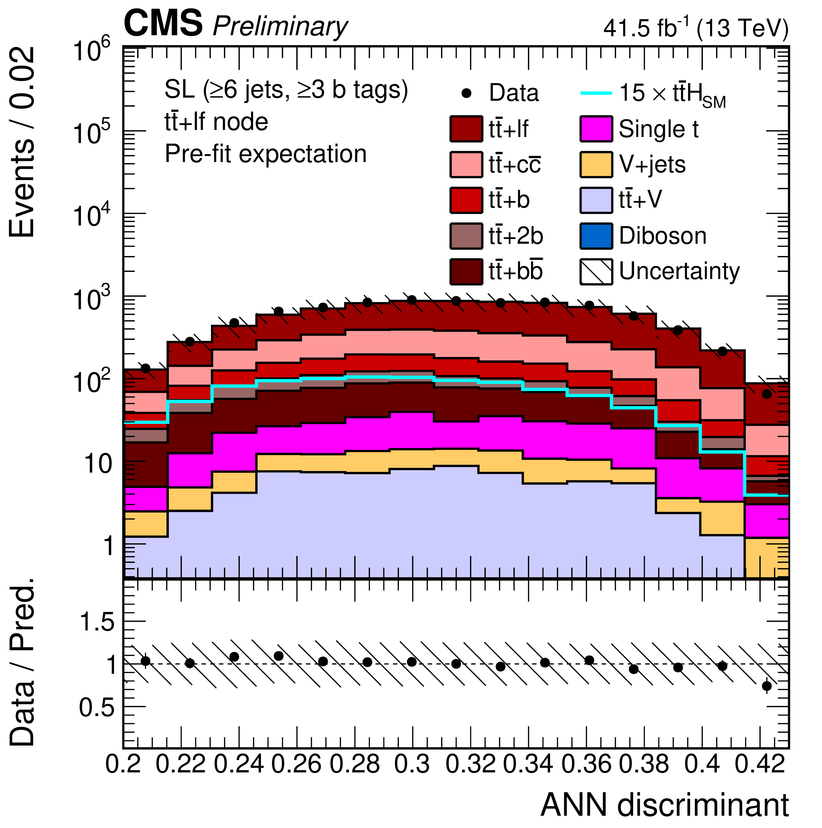
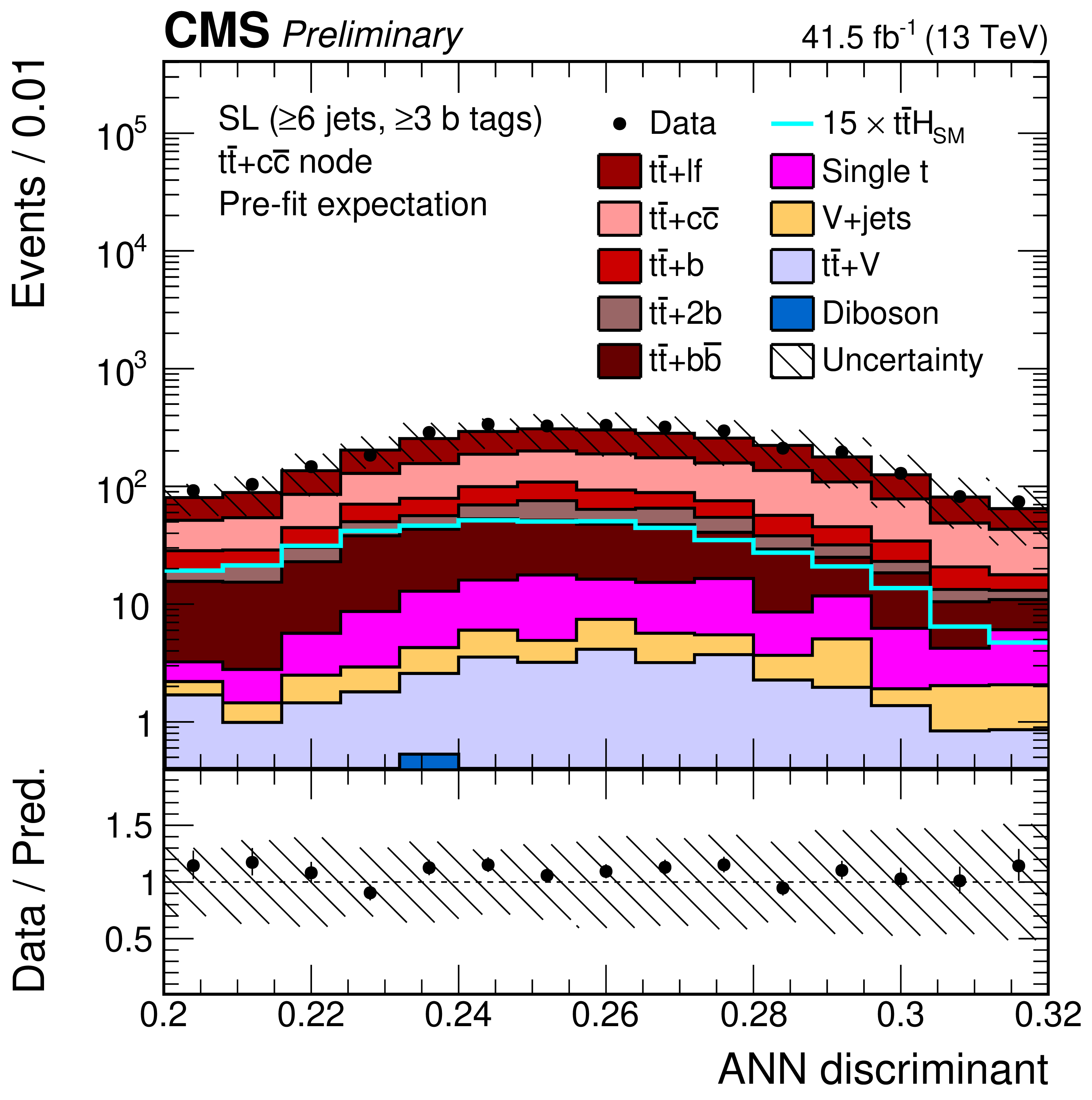
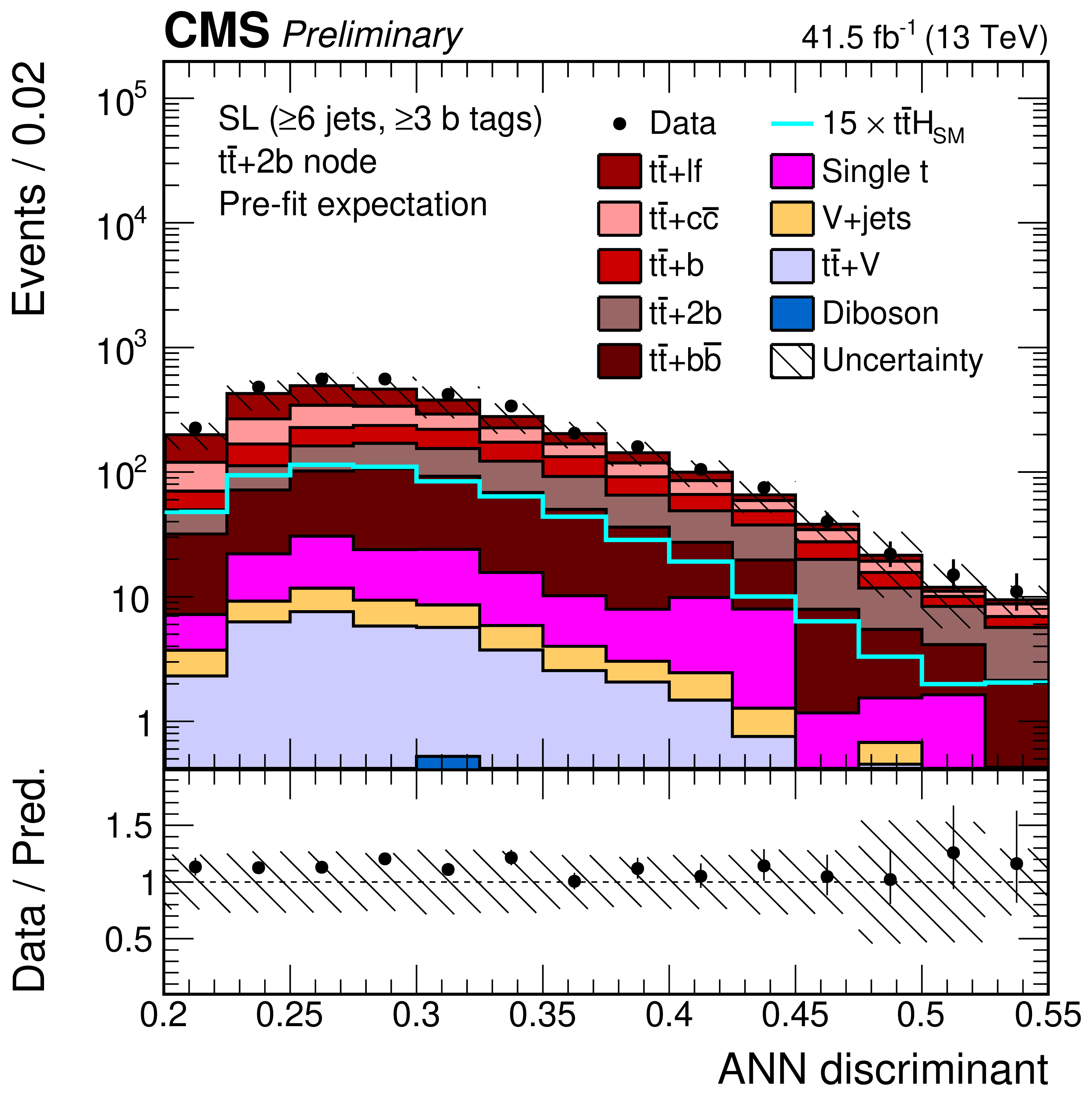
ANN discriminant shapes in the semi-leptonic (SL) channel before the fit to data in the jet-process categories with 6 jets, $\geq $3 b-tags. The expected background contributions (filled histograms) are stacked, and the expected signal distribution (line) is superimposed. Each contribution is normalised to an integrated luminosity of 41.5 fb$^{-1}$, and the signal distribution is additionally scaled by a factor of 15 for better visibility. The hatched uncertainty bands include the total uncertainty of the fit model. The distributions of the signal+background SM prediction (markers) are overlayed. The first and the last bins include underflow and overflow events, respectively. The lower plots show the ratio of the data to the background prediction. |
png pdf |
Additional Figure 13-a:
ANN discriminant shapes in the semi-leptonic (SL) channel before the fit to data in the jet-process categories with 6 jets, $\geq $3 b-tags. The expected background contributions (filled histograms) are stacked, and the expected signal distribution (line) is superimposed. Each contribution is normalised to an integrated luminosity of 41.5 fb$^{-1}$, and the signal distribution is additionally scaled by a factor of 15 for better visibility. The hatched uncertainty bands include the total uncertainty of the fit model. The distributions of the signal+background SM prediction (markers) are overlayed. The first and the last bins include underflow and overflow events, respectively. The lower plots show the ratio of the data to the background prediction. |
png pdf |
Additional Figure 13-b:
ANN discriminant shapes in the semi-leptonic (SL) channel before the fit to data in the jet-process categories with 6 jets, $\geq $3 b-tags. The expected background contributions (filled histograms) are stacked, and the expected signal distribution (line) is superimposed. Each contribution is normalised to an integrated luminosity of 41.5 fb$^{-1}$, and the signal distribution is additionally scaled by a factor of 15 for better visibility. The hatched uncertainty bands include the total uncertainty of the fit model. The distributions of the signal+background SM prediction (markers) are overlayed. The first and the last bins include underflow and overflow events, respectively. The lower plots show the ratio of the data to the background prediction. |
png pdf |
Additional Figure 13-c:
ANN discriminant shapes in the semi-leptonic (SL) channel before the fit to data in the jet-process categories with 6 jets, $\geq $3 b-tags. The expected background contributions (filled histograms) are stacked, and the expected signal distribution (line) is superimposed. Each contribution is normalised to an integrated luminosity of 41.5 fb$^{-1}$, and the signal distribution is additionally scaled by a factor of 15 for better visibility. The hatched uncertainty bands include the total uncertainty of the fit model. The distributions of the signal+background SM prediction (markers) are overlayed. The first and the last bins include underflow and overflow events, respectively. The lower plots show the ratio of the data to the background prediction. |
png pdf |
Additional Figure 13-d:
ANN discriminant shapes in the semi-leptonic (SL) channel before the fit to data in the jet-process categories with 6 jets, $\geq $3 b-tags. The expected background contributions (filled histograms) are stacked, and the expected signal distribution (line) is superimposed. Each contribution is normalised to an integrated luminosity of 41.5 fb$^{-1}$, and the signal distribution is additionally scaled by a factor of 15 for better visibility. The hatched uncertainty bands include the total uncertainty of the fit model. The distributions of the signal+background SM prediction (markers) are overlayed. The first and the last bins include underflow and overflow events, respectively. The lower plots show the ratio of the data to the background prediction. |
png pdf |
Additional Figure 13-e:
ANN discriminant shapes in the semi-leptonic (SL) channel before the fit to data in the jet-process categories with 6 jets, $\geq $3 b-tags. The expected background contributions (filled histograms) are stacked, and the expected signal distribution (line) is superimposed. Each contribution is normalised to an integrated luminosity of 41.5 fb$^{-1}$, and the signal distribution is additionally scaled by a factor of 15 for better visibility. The hatched uncertainty bands include the total uncertainty of the fit model. The distributions of the signal+background SM prediction (markers) are overlayed. The first and the last bins include underflow and overflow events, respectively. The lower plots show the ratio of the data to the background prediction. |

png pdf |
Additional Figure 13-f:
ANN discriminant shapes in the semi-leptonic (SL) channel before the fit to data in the jet-process categories with 6 jets, $\geq $3 b-tags. The expected background contributions (filled histograms) are stacked, and the expected signal distribution (line) is superimposed. Each contribution is normalised to an integrated luminosity of 41.5 fb$^{-1}$, and the signal distribution is additionally scaled by a factor of 15 for better visibility. The hatched uncertainty bands include the total uncertainty of the fit model. The distributions of the signal+background SM prediction (markers) are overlayed. The first and the last bins include underflow and overflow events, respectively. The lower plots show the ratio of the data to the background prediction. |
png pdf |
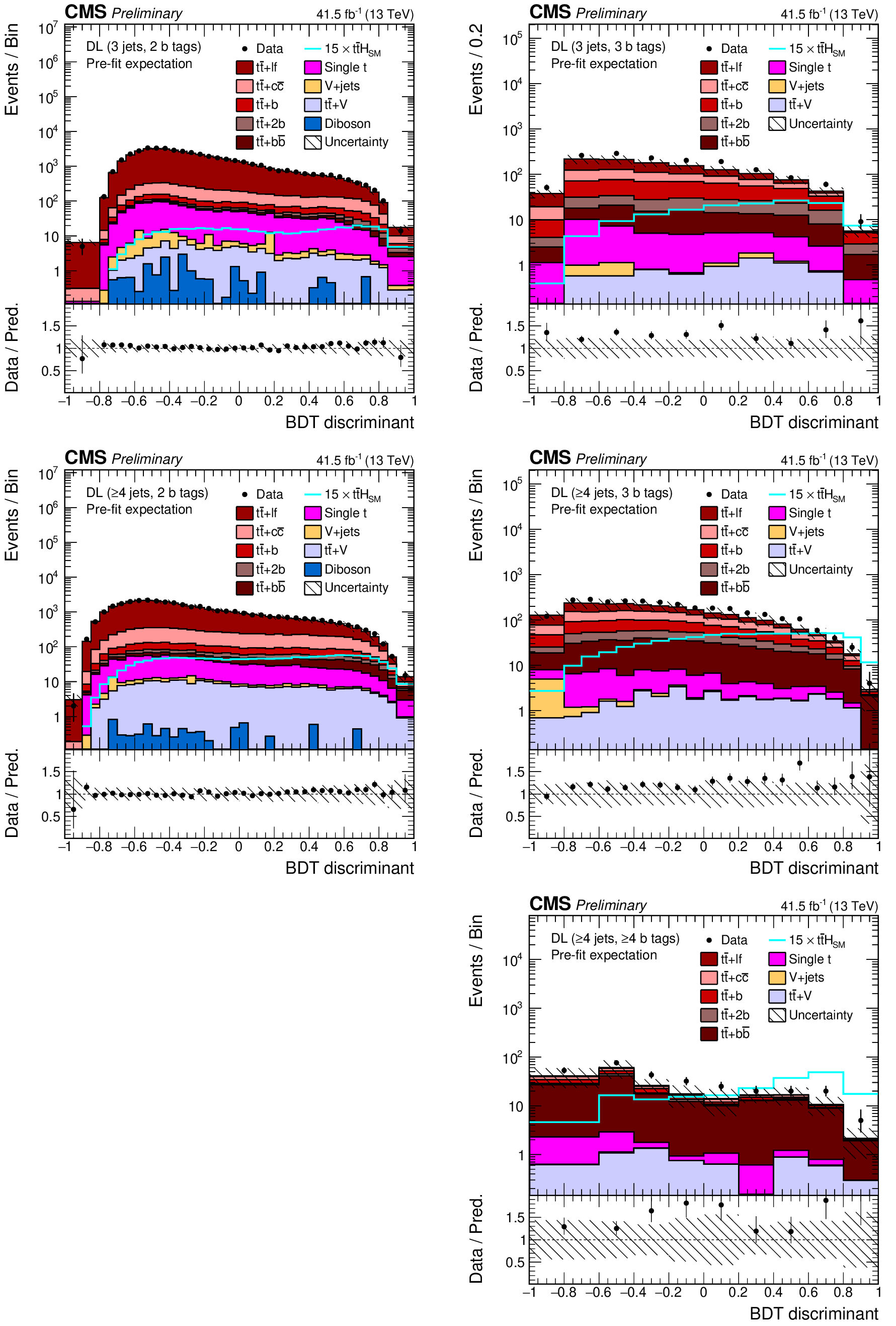
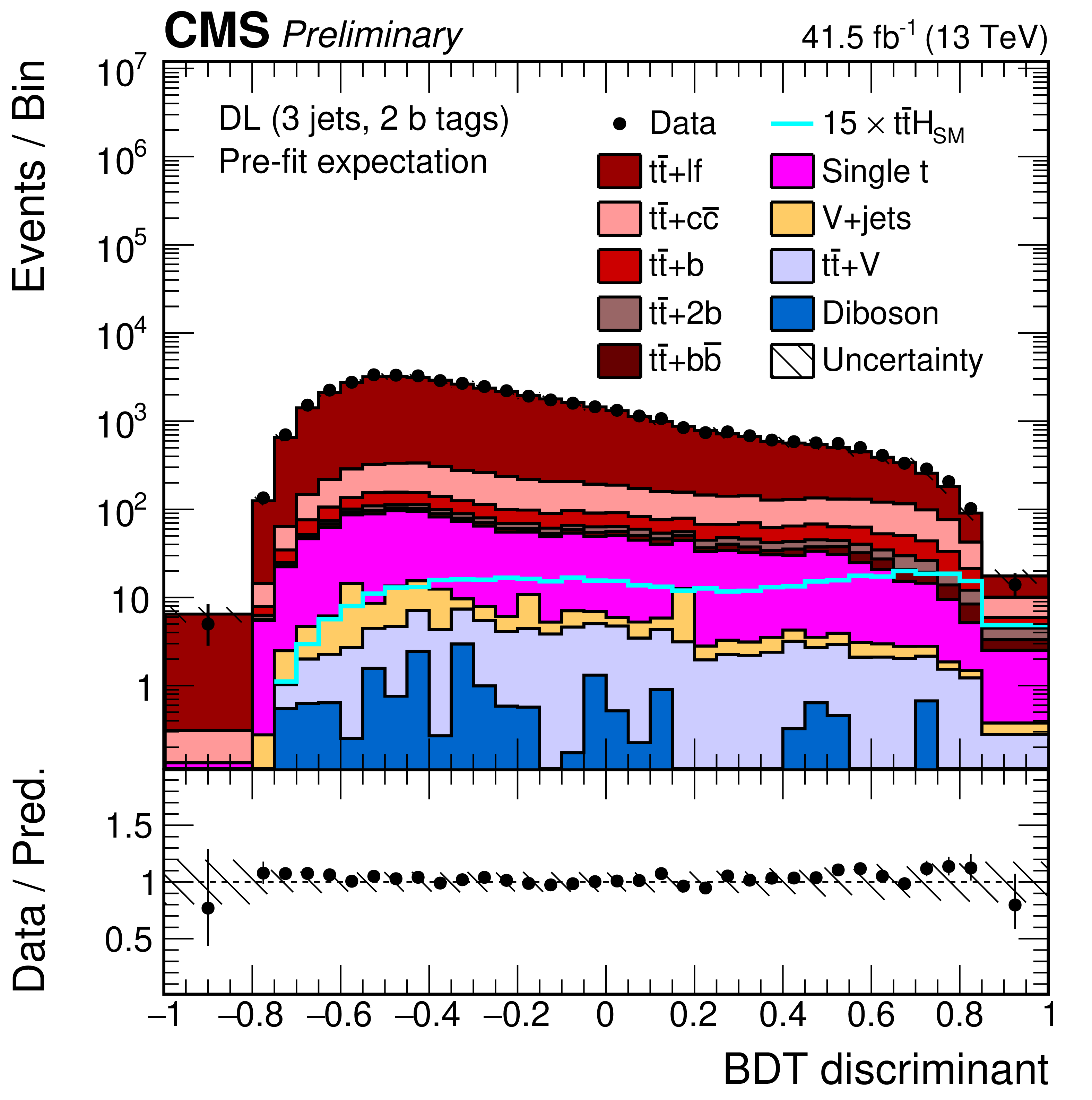
Additional Figure 14:
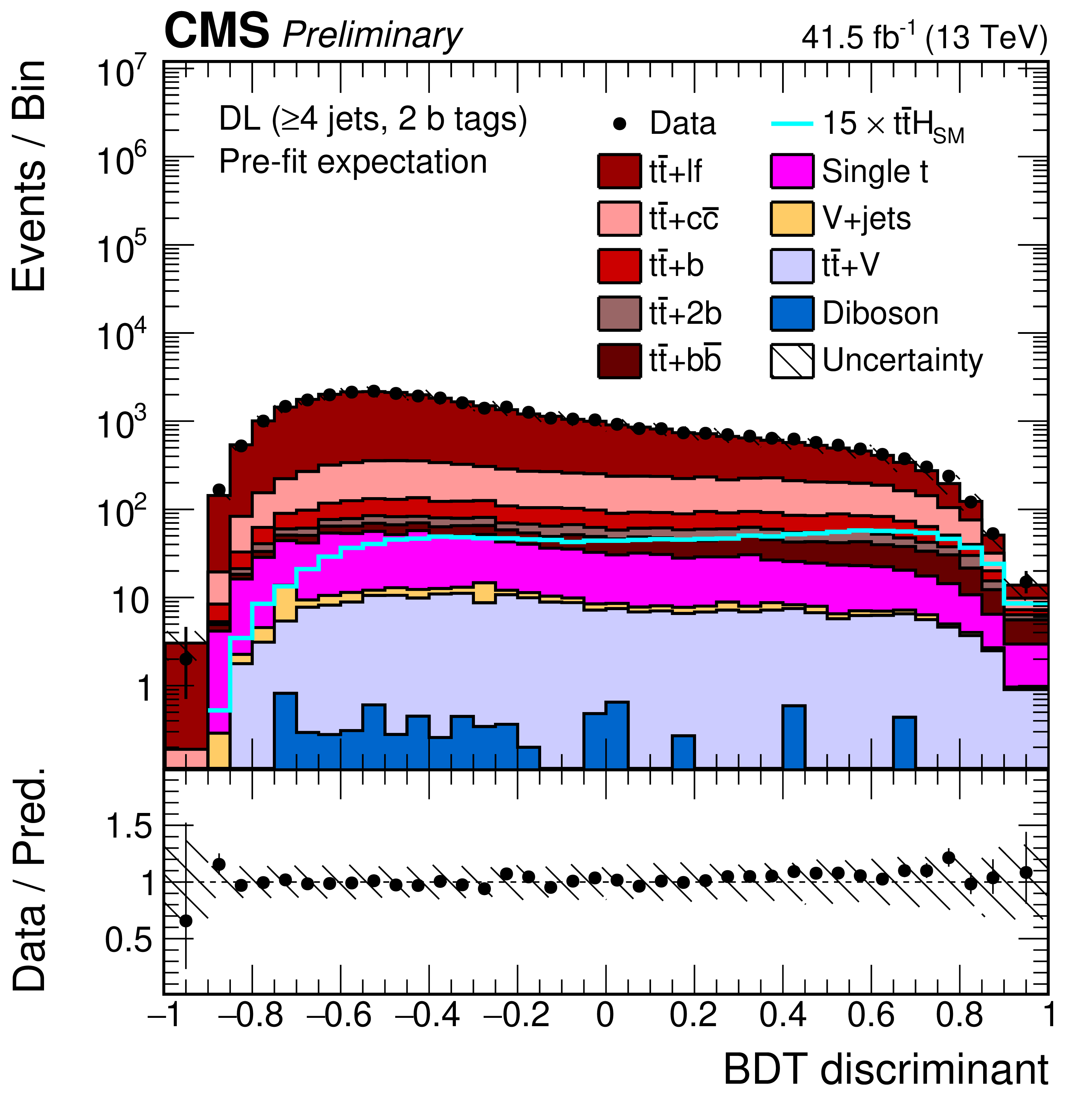
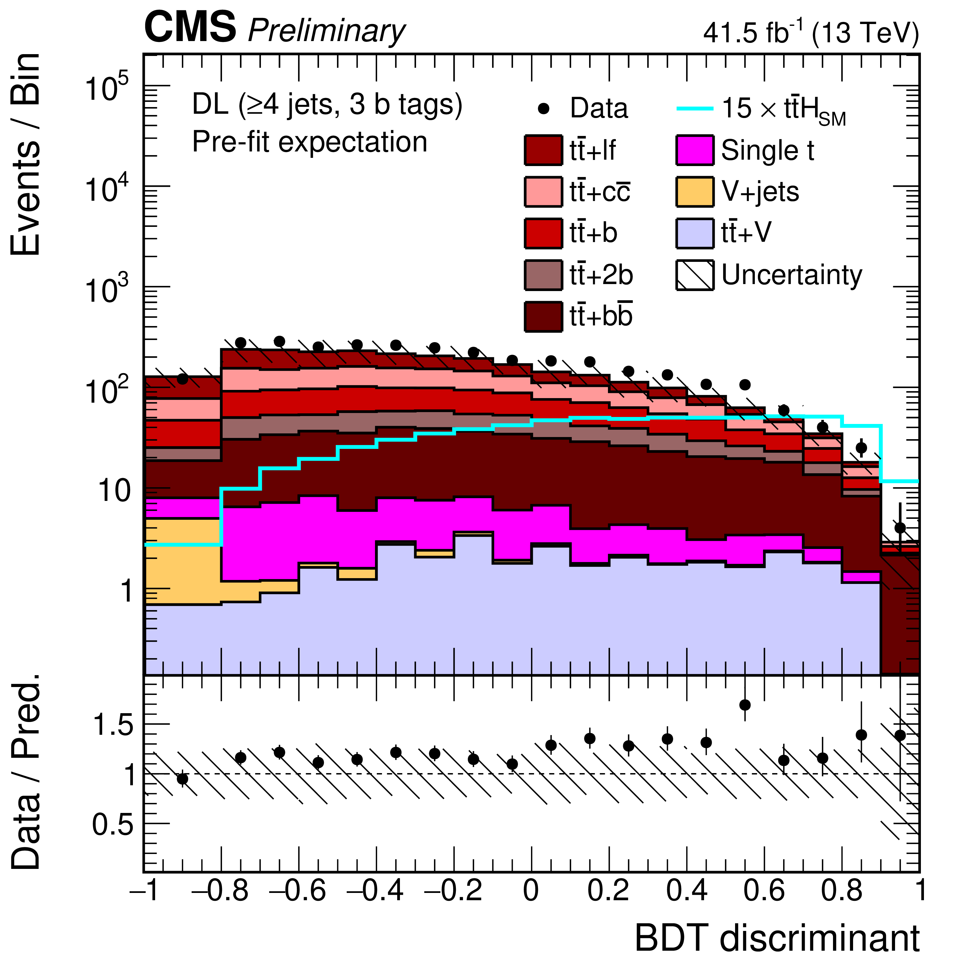
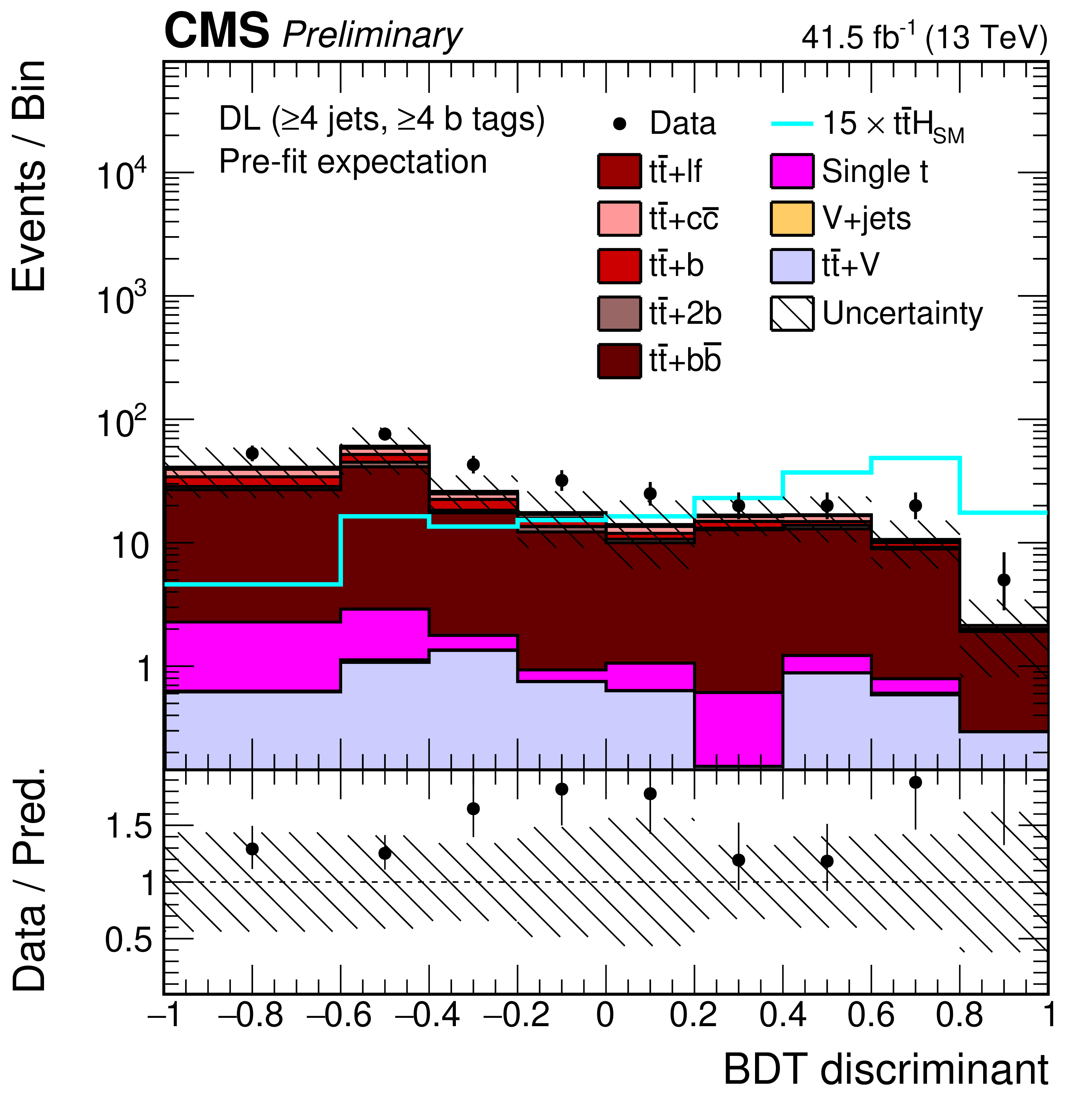
Final discriminant shapes in the dilepton (DL) channel before the fit to data: BDT discriminant in the jet-tag categories with 3 jets (left) and $\geq $4 jets (right) with 2, 3, and $\geq $4 b-tagged jets (from top to bottom). The expected background contributions (filled histograms) are stacked, and the expected signal distribution (line) is superimposed. Each contribution is normalised to an integrated luminosity of 41.5 fb$^{-1}$, and the signal distribution is additionally scaled by a factor of 15 for better visibility. The hatched uncertainty bands include the total uncertainty of the fit model. The distributions observed in data (markers) are overlayed. The first and the last bins include underflow and overflow events, respectively. The lower plots show the ratio of the data to the background prediction. |
png pdf |
Additional Figure 14-a:
Final discriminant shapes in the dilepton (DL) channel before the fit to data: BDT discriminant in the jet-tag categories with 3 jets with 2 b-tagged jets. The expected background contributions (filled histograms) are stacked, and the expected signal distribution (line) is superimposed. Each contribution is normalised to an integrated luminosity of 41.5 fb$^{-1}$, and the signal distribution is additionally scaled by a factor of 15 for better visibility. The hatched uncertainty bands include the total uncertainty of the fit model. The distribution observed in data (markers) is overlayed. The first and the last bins include underflow and overflow events, respectively. The lower plots show the ratio of the data to the background prediction. |
png pdf |
Additional Figure 14-b:
Final discriminant shapes in the dilepton (DL) channel before the fit to data: BDT discriminant in the jet-tag categories with $\geq $4 jets with 2 b-tagged jets. The expected background contributions (filled histograms) are stacked, and the expected signal distribution (line) is superimposed. Each contribution is normalised to an integrated luminosity of 41.5 fb$^{-1}$, and the signal distribution is additionally scaled by a factor of 15 for better visibility. The hatched uncertainty bands include the total uncertainty of the fit model. The distribution observed in data (markers) is overlayed. The first and the last bins include underflow and overflow events, respectively. The lower plots show the ratio of the data to the background prediction. |
png pdf |
Additional Figure 14-c:
Final discriminant shapes in the dilepton (DL) channel before the fit to data: BDT discriminant in the jet-tag categories with 3 jets with 3 b-tagged jets. The expected background contributions (filled histograms) are stacked, and the expected signal distribution (line) is superimposed. Each contribution is normalised to an integrated luminosity of 41.5 fb$^{-1}$, and the signal distribution is additionally scaled by a factor of 15 for better visibility. The hatched uncertainty bands include the total uncertainty of the fit model. The distribution observed in data (markers) is overlayed. The first and the last bins include underflow and overflow events, respectively. The lower plots show the ratio of the data to the background prediction. |
png pdf |
Additional Figure 14-d:
Final discriminant shapes in the dilepton (DL) channel before the fit to data: BDT discriminant in the jet-tag categories with $\geq $4 jets with 3 b-tagged jets. The expected background contributions (filled histograms) are stacked, and the expected signal distribution (line) is superimposed. Each contribution is normalised to an integrated luminosity of 41.5 fb$^{-1}$, and the signal distribution is additionally scaled by a factor of 15 for better visibility. The hatched uncertainty bands include the total uncertainty of the fit model. The distribution observed in data (markers) is overlayed. The first and the last bins include underflow and overflow events, respectively. The lower plots show the ratio of the data to the background prediction. |
png pdf |
Additional Figure 14-e:
Final discriminant shapes in the dilepton (DL) channel before the fit to data: BDT discriminant in the jet-tag categories with $\geq $4 jets with $\geq $4 b-tagged jets. The expected background contributions (filled histograms) are stacked, and the expected signal distribution (line) is superimposed. Each contribution is normalised to an integrated luminosity of 41.5 fb$^{-1}$, and the signal distribution is additionally scaled by a factor of 15 for better visibility. The hatched uncertainty bands include the total uncertainty of the fit model. The distribution observed in data (markers) is overlayed. The first and the last bins include underflow and overflow events, respectively. The lower plots show the ratio of the data to the background prediction. |
png pdf |
Additional Figure 15:
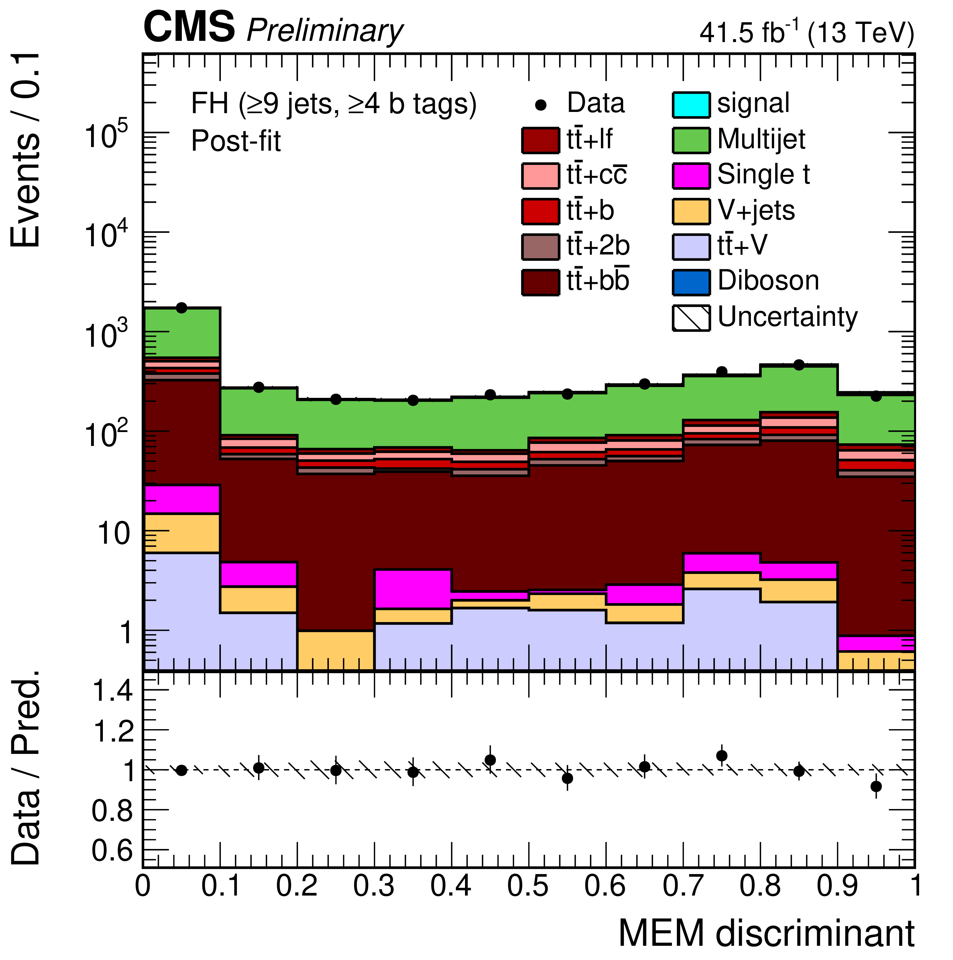
Final discriminant shapes in the fully-hadronic (FH) channel after the fit to data: MEM discriminant in the jet-tag categories with 3 b-tagged jets (left) and $\geq $4 b-tagged jets (right) with 7, 8, and $\geq $9 jets (from top to bottom). The expected signal and background contributions (filled histograms) are stacked. The hatched uncertainty bands include the total uncertainty of the fit model. The distributions observed in data (markers) are overlayed. The first and the last bins include underflow and overflow events, respectively. The lower plots show the ratio of the data to the background prediction. |
png pdf |
Additional Figure 15-a:
Final discriminant shapes in the fully-hadronic (FH) channel after the fit to data: MEM discriminant in the jet-tag categories with 3 b-tagged jets with 7 jets. The expected signal and background contributions (filled histograms) are stacked. The hatched uncertainty bands include the total uncertainty of the fit model. The distribution observed in data (markers) is overlayed. The first and the last bins include underflow and overflow events, respectively. The lower plot shows the ratio of the data to the background prediction. |
png pdf |
Additional Figure 15-b:
Final discriminant shapes in the fully-hadronic (FH) channel after the fit to data: MEM discriminant in the jet-tag categories with $\geq $4 b-tagged jets with 7 jets. The expected signal and background contributions (filled histograms) are stacked. The hatched uncertainty bands include the total uncertainty of the fit model. The distribution observed in data (markers) is overlayed. The first and the last bins include underflow and overflow events, respectively. The lower plot shows the ratio of the data to the background prediction. |
png pdf |
Additional Figure 15-c:
Final discriminant shapes in the fully-hadronic (FH) channel after the fit to data: MEM discriminant in the jet-tag categories with 3 b-tagged jets with 8 jets. The expected signal and background contributions (filled histograms) are stacked. The hatched uncertainty bands include the total uncertainty of the fit model. The distribution observed in data (markers) is overlayed. The first and the last bins include underflow and overflow events, respectively. The lower plot shows the ratio of the data to the background prediction. |
png pdf |
Additional Figure 15-d:
Final discriminant shapes in the fully-hadronic (FH) channel after the fit to data: MEM discriminant in the jet-tag categories with $\geq $4 b-tagged jets with 8 jets. The expected signal and background contributions (filled histograms) are stacked. The hatched uncertainty bands include the total uncertainty of the fit model. The distribution observed in data (markers) is overlayed. The first and the last bins include underflow and overflow events, respectively. The lower plot shows the ratio of the data to the background prediction. |
png pdf |
Additional Figure 15-e:
Final discriminant shapes in the fully-hadronic (FH) channel after the fit to data: MEM discriminant in the jet-tag categories with 3 b-tagged jets with $\geq $9 jets. The expected signal and background contributions (filled histograms) are stacked. The hatched uncertainty bands include the total uncertainty of the fit model. The distribution observed in data (markers) is overlayed. The first and the last bins include underflow and overflow events, respectively. The lower plot shows the ratio of the data to the background prediction. |

png pdf |
Additional Figure 15-f:
Final discriminant shapes in the fully-hadronic (FH) channel after the fit to data: MEM discriminant in the jet-tag categories with $\geq $4 b-tagged jets with $\geq $9 jets. The expected signal and background contributions (filled histograms) are stacked. The hatched uncertainty bands include the total uncertainty of the fit model. The distribution observed in data (markers) is overlayed. The first and the last bins include underflow and overflow events, respectively. The lower plot shows the ratio of the data to the background prediction. |
png pdf |
Additional Figure 16:
ANN discriminant shapes in the semi-leptonic (SL) channel after the fit to data in the jet-process categories with 4 jets, $\geq $3 b-tags. The expected signal and background contributions (filled histograms) are stacked. The hatched uncertainty bands include the total uncertainty of the fit model. The distributions observed in data (markers) are overlayed. The first and the last bins include underflow and overflow events, respectively. The lower plots show the ratio of the data to the background prediction. |
png pdf |
Additional Figure 16-a:
ANN discriminant shapes in the semi-leptonic (SL) channel after the fit to data in the jet-process categories with 4 jets, $\geq $3 b-tags. The expected signal and background contributions (filled histograms) are stacked. The hatched uncertainty bands include the total uncertainty of the fit model. The distributions observed in data (markers) are overlayed. The first and the last bins include underflow and overflow events, respectively. The lower plots show the ratio of the data to the background prediction. |
png pdf |
Additional Figure 16-b:
ANN discriminant shapes in the semi-leptonic (SL) channel after the fit to data in the jet-process categories with 4 jets, $\geq $3 b-tags. The expected signal and background contributions (filled histograms) are stacked. The hatched uncertainty bands include the total uncertainty of the fit model. The distributions observed in data (markers) are overlayed. The first and the last bins include underflow and overflow events, respectively. The lower plots show the ratio of the data to the background prediction. |
png pdf |
Additional Figure 16-c:
ANN discriminant shapes in the semi-leptonic (SL) channel after the fit to data in the jet-process categories with 4 jets, $\geq $3 b-tags. The expected signal and background contributions (filled histograms) are stacked. The hatched uncertainty bands include the total uncertainty of the fit model. The distributions observed in data (markers) are overlayed. The first and the last bins include underflow and overflow events, respectively. The lower plots show the ratio of the data to the background prediction. |
png pdf |
Additional Figure 16-d:
ANN discriminant shapes in the semi-leptonic (SL) channel after the fit to data in the jet-process categories with 4 jets, $\geq $3 b-tags. The expected signal and background contributions (filled histograms) are stacked. The hatched uncertainty bands include the total uncertainty of the fit model. The distributions observed in data (markers) are overlayed. The first and the last bins include underflow and overflow events, respectively. The lower plots show the ratio of the data to the background prediction. |
png pdf |
Additional Figure 16-e:
ANN discriminant shapes in the semi-leptonic (SL) channel after the fit to data in the jet-process categories with 4 jets, $\geq $3 b-tags. The expected signal and background contributions (filled histograms) are stacked. The hatched uncertainty bands include the total uncertainty of the fit model. The distributions observed in data (markers) are overlayed. The first and the last bins include underflow and overflow events, respectively. The lower plots show the ratio of the data to the background prediction. |

png pdf |
Additional Figure 16-f:
ANN discriminant shapes in the semi-leptonic (SL) channel after the fit to data in the jet-process categories with 4 jets, $\geq $3 b-tags. The expected signal and background contributions (filled histograms) are stacked. The hatched uncertainty bands include the total uncertainty of the fit model. The distributions observed in data (markers) are overlayed. The first and the last bins include underflow and overflow events, respectively. The lower plots show the ratio of the data to the background prediction. |
png pdf |
Additional Figure 17:
ANN discriminant shapes in the semi-leptonic (SL) channel before the fit to data in the jet-process categories with 5 jets, $\geq $3 b-tags. The expected signal and background contributions (filled histograms) are stacked. The hatched uncertainty bands include the total uncertainty of the fit model. The distributions observed in data (markers) are overlayed. The first and the last bins include underflow and overflow events, respectively. The lower plots show the ratio of the data to the background prediction. |
png pdf |
Additional Figure 17-a:
ANN discriminant shapes in the semi-leptonic (SL) channel before the fit to data in the jet-process categories with 5 jets, $\geq $3 b-tags. The expected signal and background contributions (filled histograms) are stacked. The hatched uncertainty bands include the total uncertainty of the fit model. The distributions observed in data (markers) are overlayed. The first and the last bins include underflow and overflow events, respectively. The lower plots show the ratio of the data to the background prediction. |
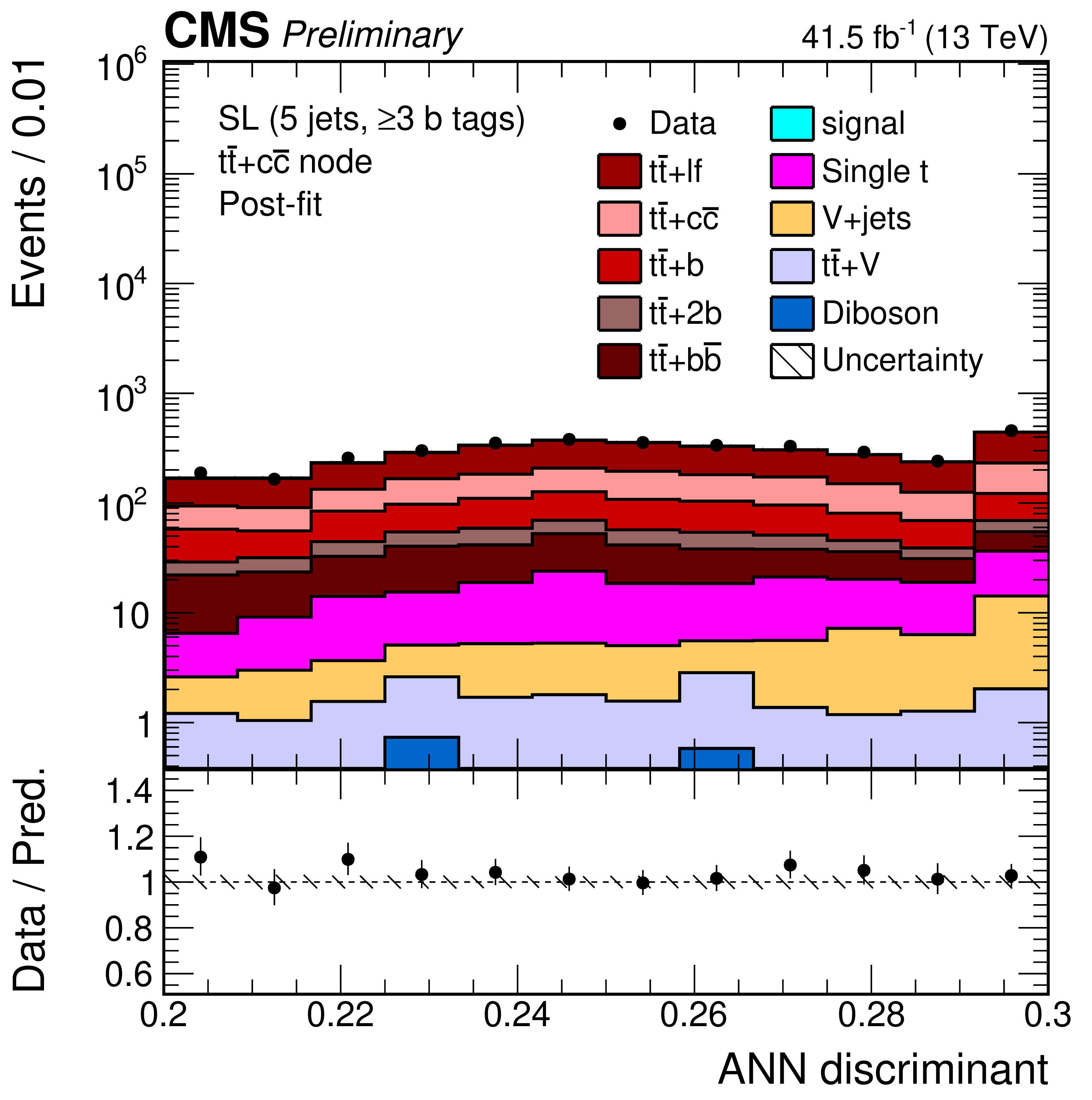
png pdf |
Additional Figure 17-b:
ANN discriminant shapes in the semi-leptonic (SL) channel before the fit to data in the jet-process categories with 5 jets, $\geq $3 b-tags. The expected signal and background contributions (filled histograms) are stacked. The hatched uncertainty bands include the total uncertainty of the fit model. The distributions observed in data (markers) are overlayed. The first and the last bins include underflow and overflow events, respectively. The lower plots show the ratio of the data to the background prediction. |
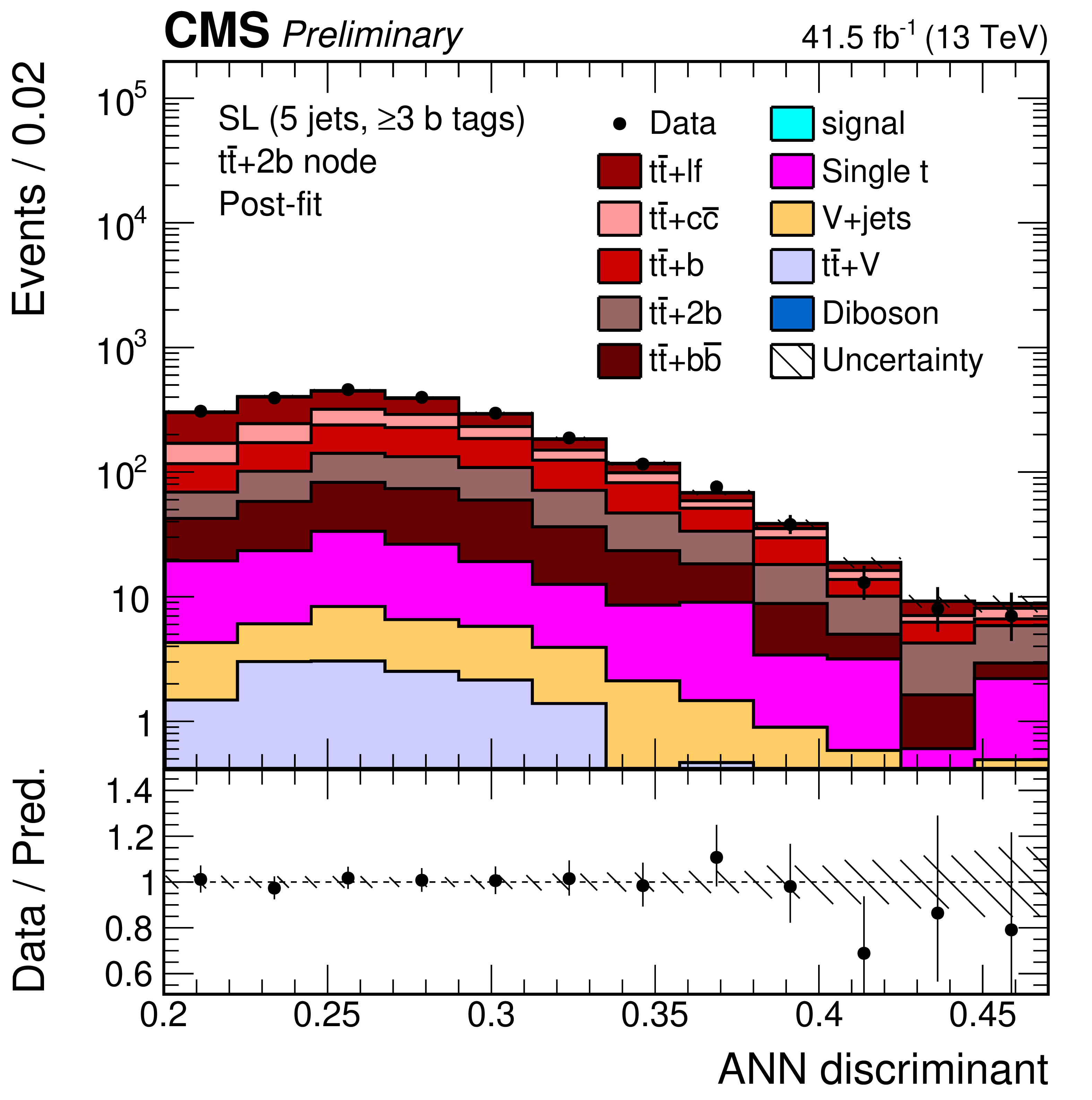
png pdf |
Additional Figure 17-c:
ANN discriminant shapes in the semi-leptonic (SL) channel before the fit to data in the jet-process categories with 5 jets, $\geq $3 b-tags. The expected signal and background contributions (filled histograms) are stacked. The hatched uncertainty bands include the total uncertainty of the fit model. The distributions observed in data (markers) are overlayed. The first and the last bins include underflow and overflow events, respectively. The lower plots show the ratio of the data to the background prediction. |
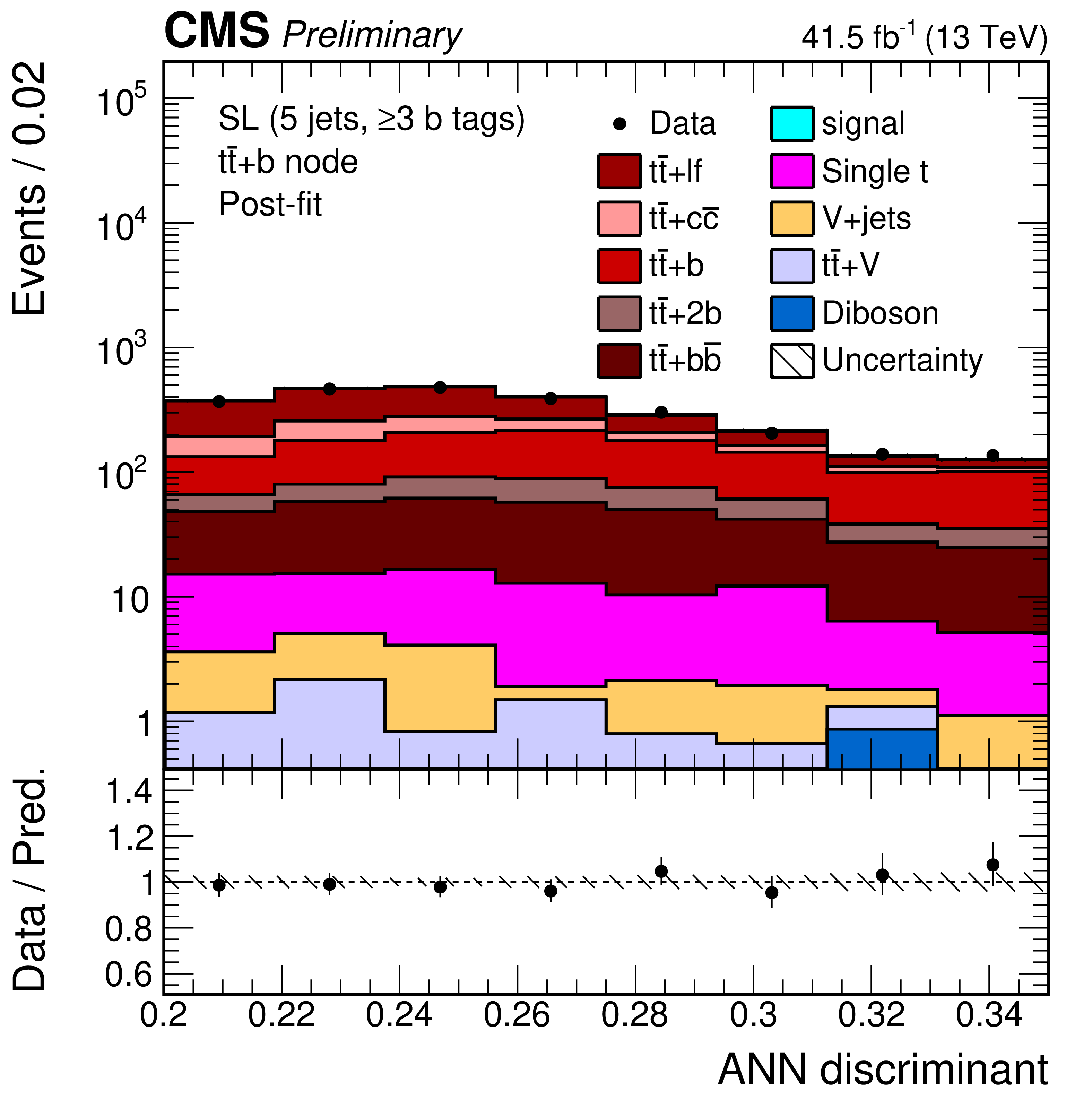
png pdf |
Additional Figure 17-d:
ANN discriminant shapes in the semi-leptonic (SL) channel before the fit to data in the jet-process categories with 5 jets, $\geq $3 b-tags. The expected signal and background contributions (filled histograms) are stacked. The hatched uncertainty bands include the total uncertainty of the fit model. The distributions observed in data (markers) are overlayed. The first and the last bins include underflow and overflow events, respectively. The lower plots show the ratio of the data to the background prediction. |
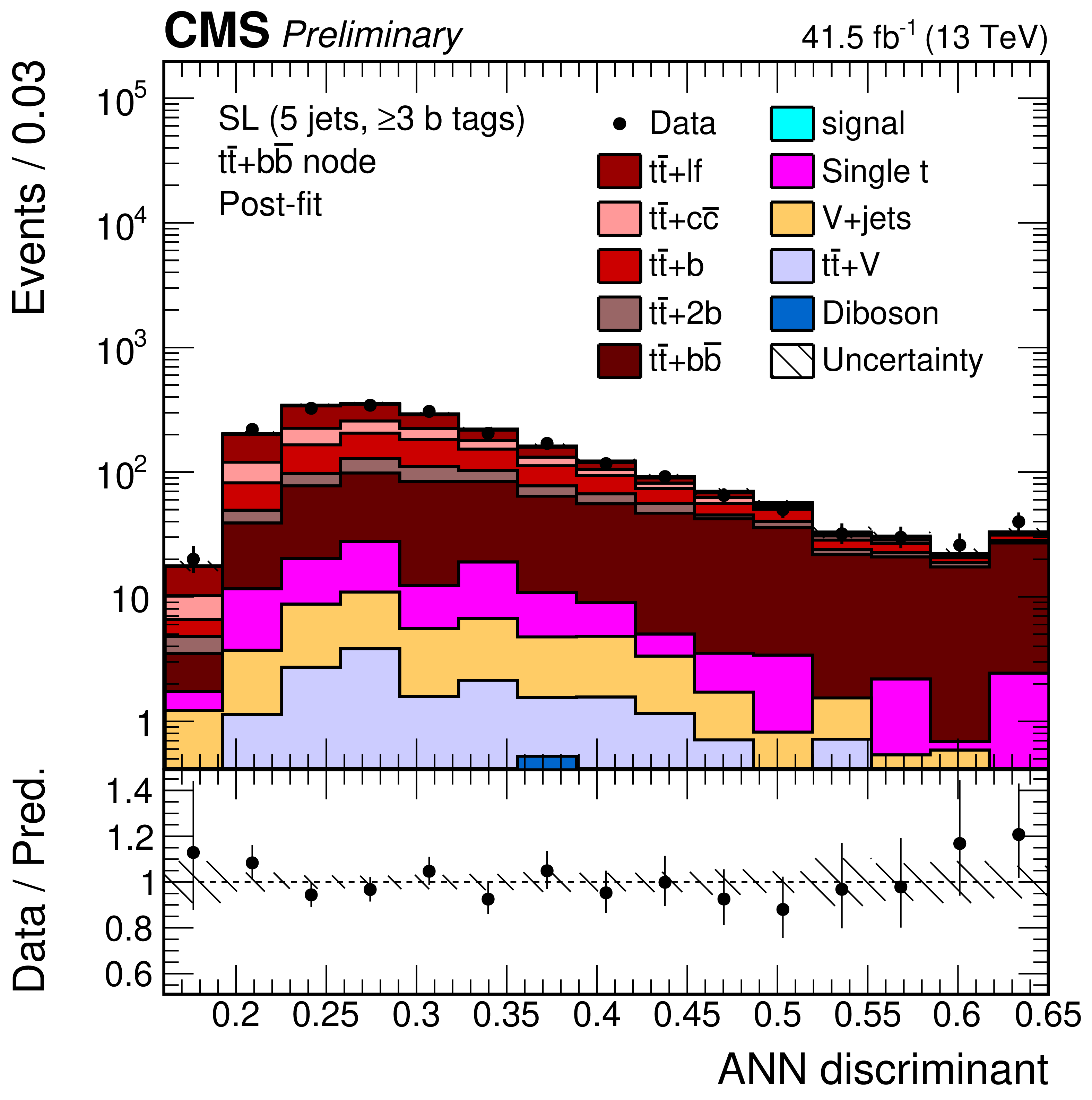
png pdf |
Additional Figure 17-e:
ANN discriminant shapes in the semi-leptonic (SL) channel before the fit to data in the jet-process categories with 5 jets, $\geq $3 b-tags. The expected signal and background contributions (filled histograms) are stacked. The hatched uncertainty bands include the total uncertainty of the fit model. The distributions observed in data (markers) are overlayed. The first and the last bins include underflow and overflow events, respectively. The lower plots show the ratio of the data to the background prediction. |
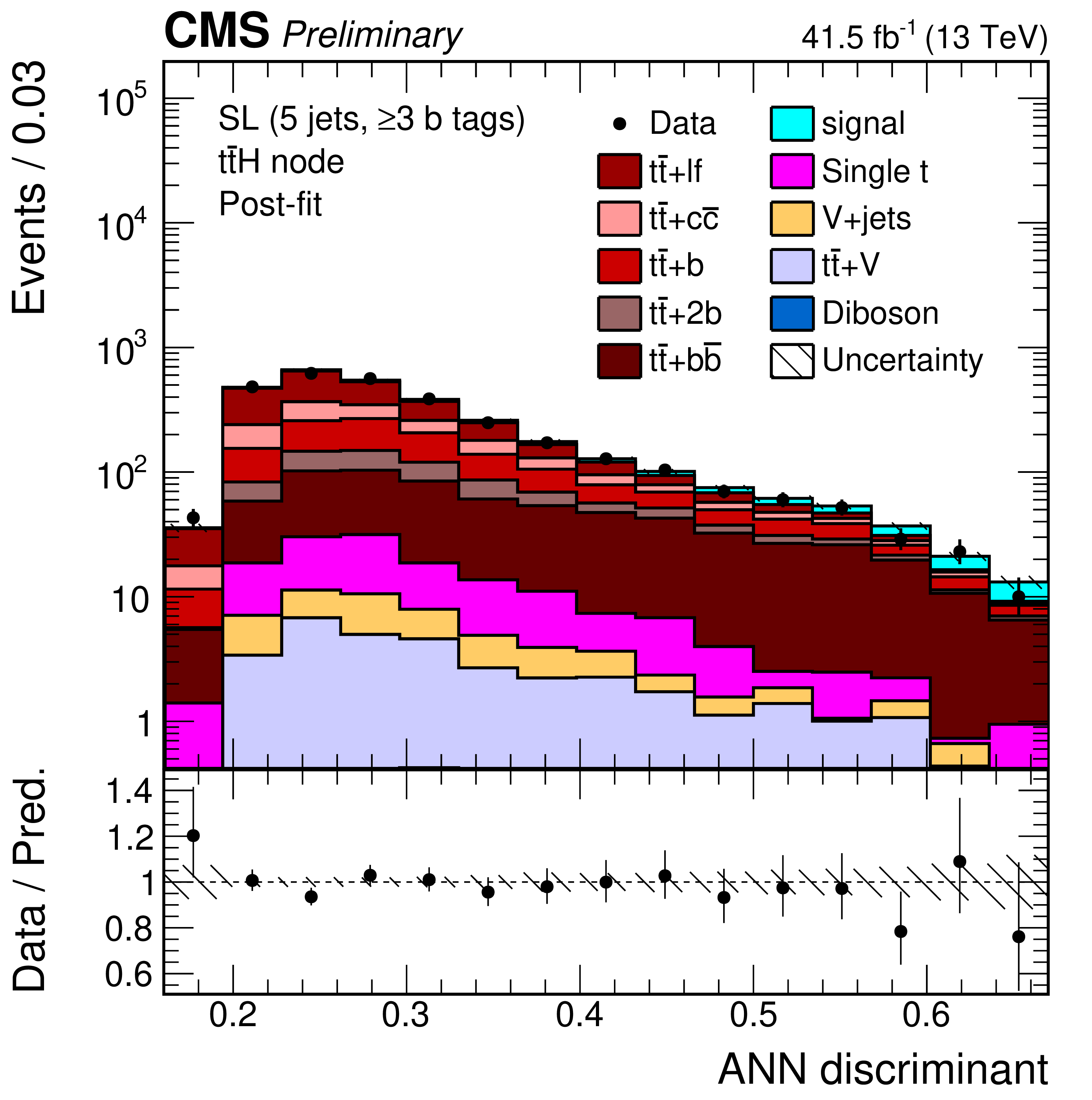
png pdf |
Additional Figure 17-f:
ANN discriminant shapes in the semi-leptonic (SL) channel before the fit to data in the jet-process categories with 5 jets, $\geq $3 b-tags. The expected signal and background contributions (filled histograms) are stacked. The hatched uncertainty bands include the total uncertainty of the fit model. The distributions observed in data (markers) are overlayed. The first and the last bins include underflow and overflow events, respectively. The lower plots show the ratio of the data to the background prediction. |
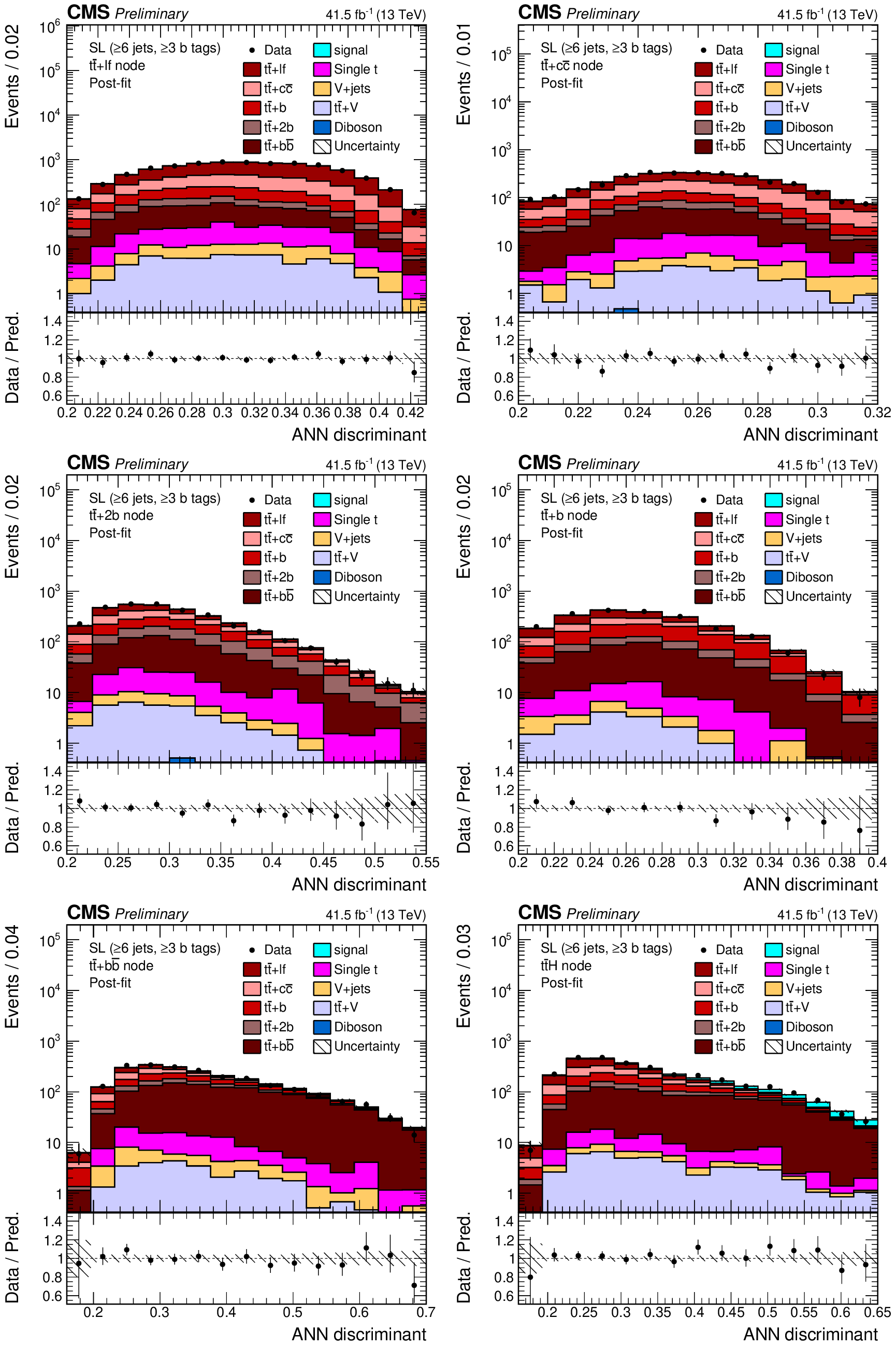
png pdf |
Additional Figure 18:
ANN discriminant shapes in the semi-leptonic (SL) channel before the fit to data in the jet-process categories with 6 jets, $\geq $3 b-tags. The expected signal and background contributions (filled histograms) are stacked. The hatched uncertainty bands include the total uncertainty of the fit model. The distributions observed in data (markers) are overlayed. The first and the last bins include underflow and overflow events, respectively. The lower plots show the ratio of the data to the background prediction. |
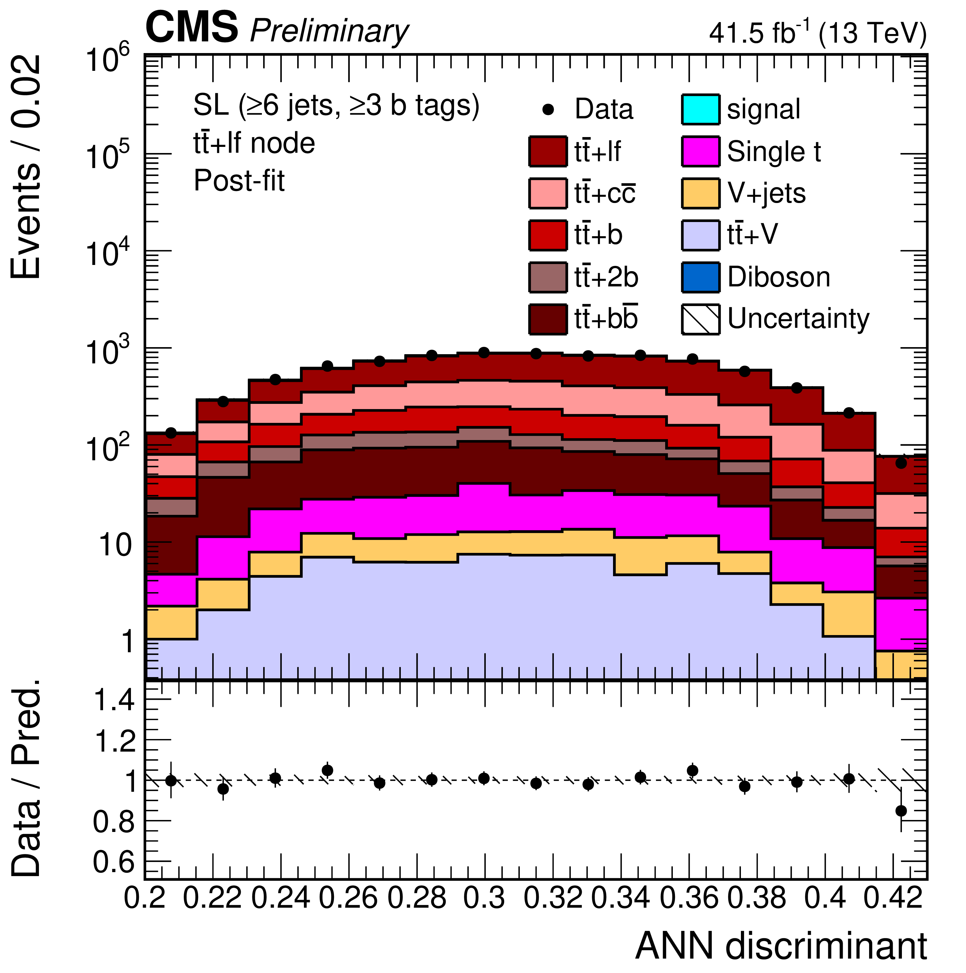
png pdf |
Additional Figure 18-a:
ANN discriminant shapes in the semi-leptonic (SL) channel before the fit to data in the jet-process categories with 6 jets, $\geq $3 b-tags. The expected signal and background contributions (filled histograms) are stacked. The hatched uncertainty bands include the total uncertainty of the fit model. The distributions observed in data (markers) are overlayed. The first and the last bins include underflow and overflow events, respectively. The lower plots show the ratio of the data to the background prediction. |
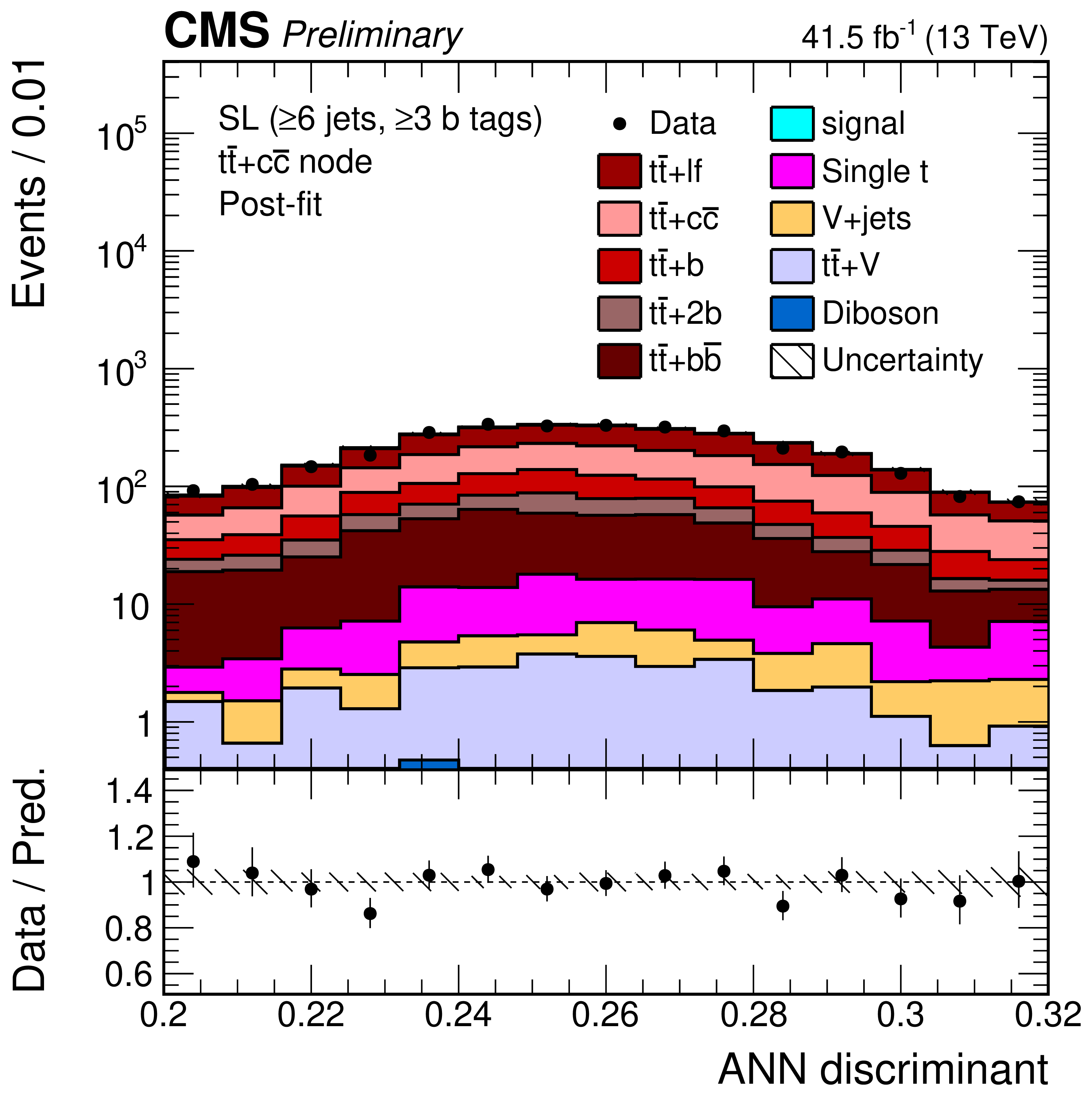
png pdf |
Additional Figure 18-b:
ANN discriminant shapes in the semi-leptonic (SL) channel before the fit to data in the jet-process categories with 6 jets, $\geq $3 b-tags. The expected signal and background contributions (filled histograms) are stacked. The hatched uncertainty bands include the total uncertainty of the fit model. The distributions observed in data (markers) are overlayed. The first and the last bins include underflow and overflow events, respectively. The lower plots show the ratio of the data to the background prediction. |
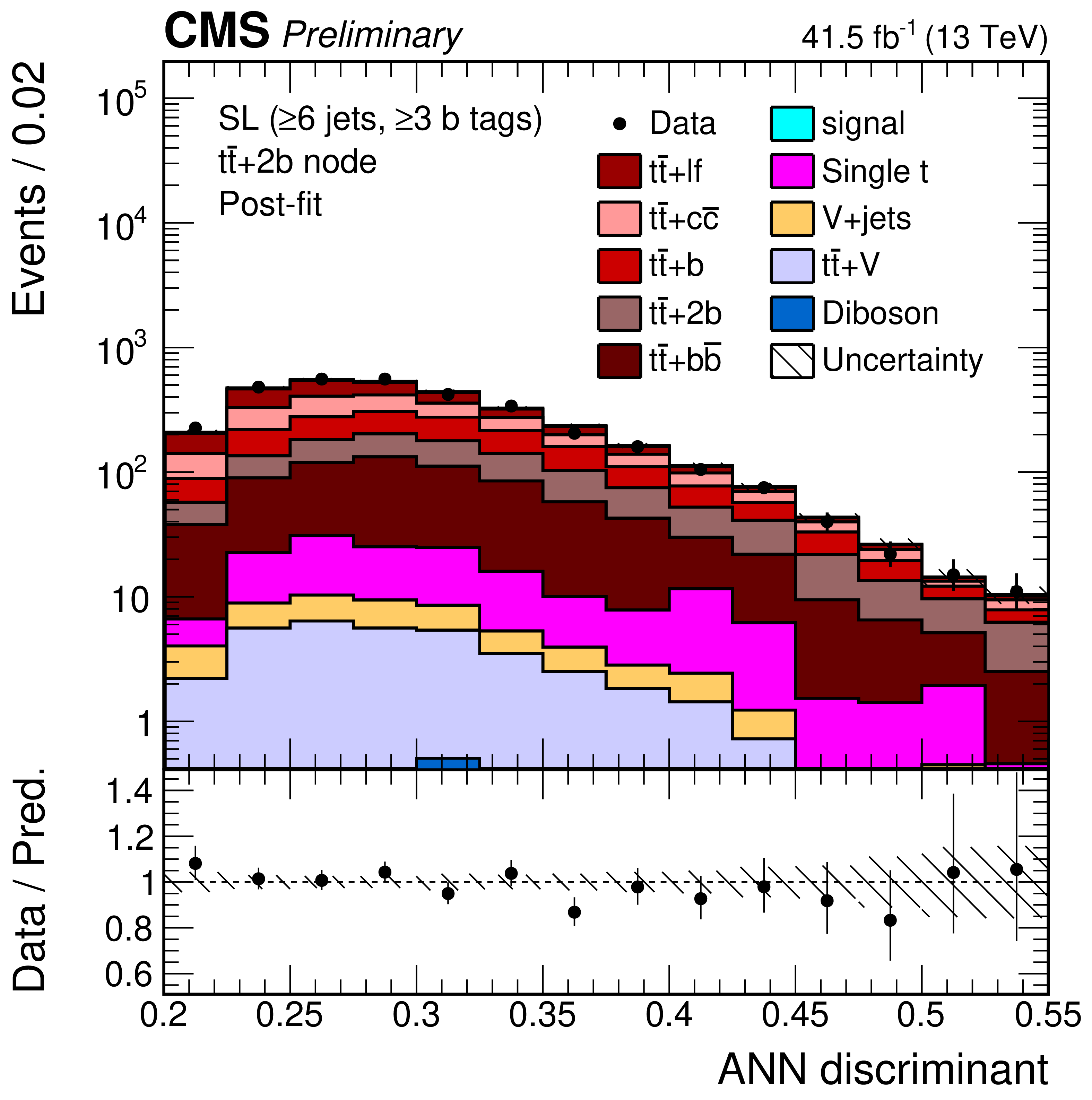
png pdf |
Additional Figure 18-c:
ANN discriminant shapes in the semi-leptonic (SL) channel before the fit to data in the jet-process categories with 6 jets, $\geq $3 b-tags. The expected signal and background contributions (filled histograms) are stacked. The hatched uncertainty bands include the total uncertainty of the fit model. The distributions observed in data (markers) are overlayed. The first and the last bins include underflow and overflow events, respectively. The lower plots show the ratio of the data to the background prediction. |
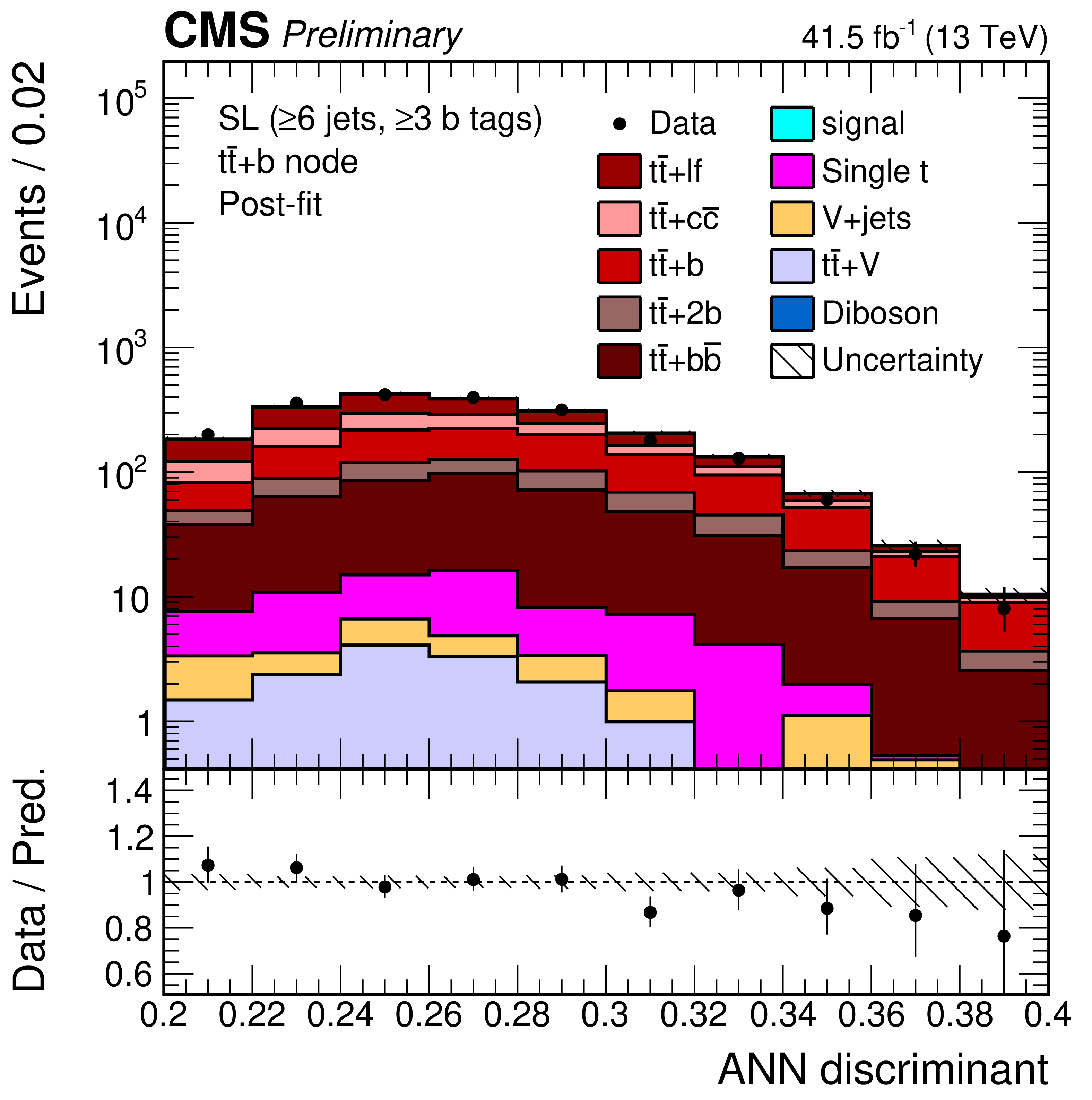
png pdf |
Additional Figure 18-d:
ANN discriminant shapes in the semi-leptonic (SL) channel before the fit to data in the jet-process categories with 6 jets, $\geq $3 b-tags. The expected signal and background contributions (filled histograms) are stacked. The hatched uncertainty bands include the total uncertainty of the fit model. The distributions observed in data (markers) are overlayed. The first and the last bins include underflow and overflow events, respectively. The lower plots show the ratio of the data to the background prediction. |
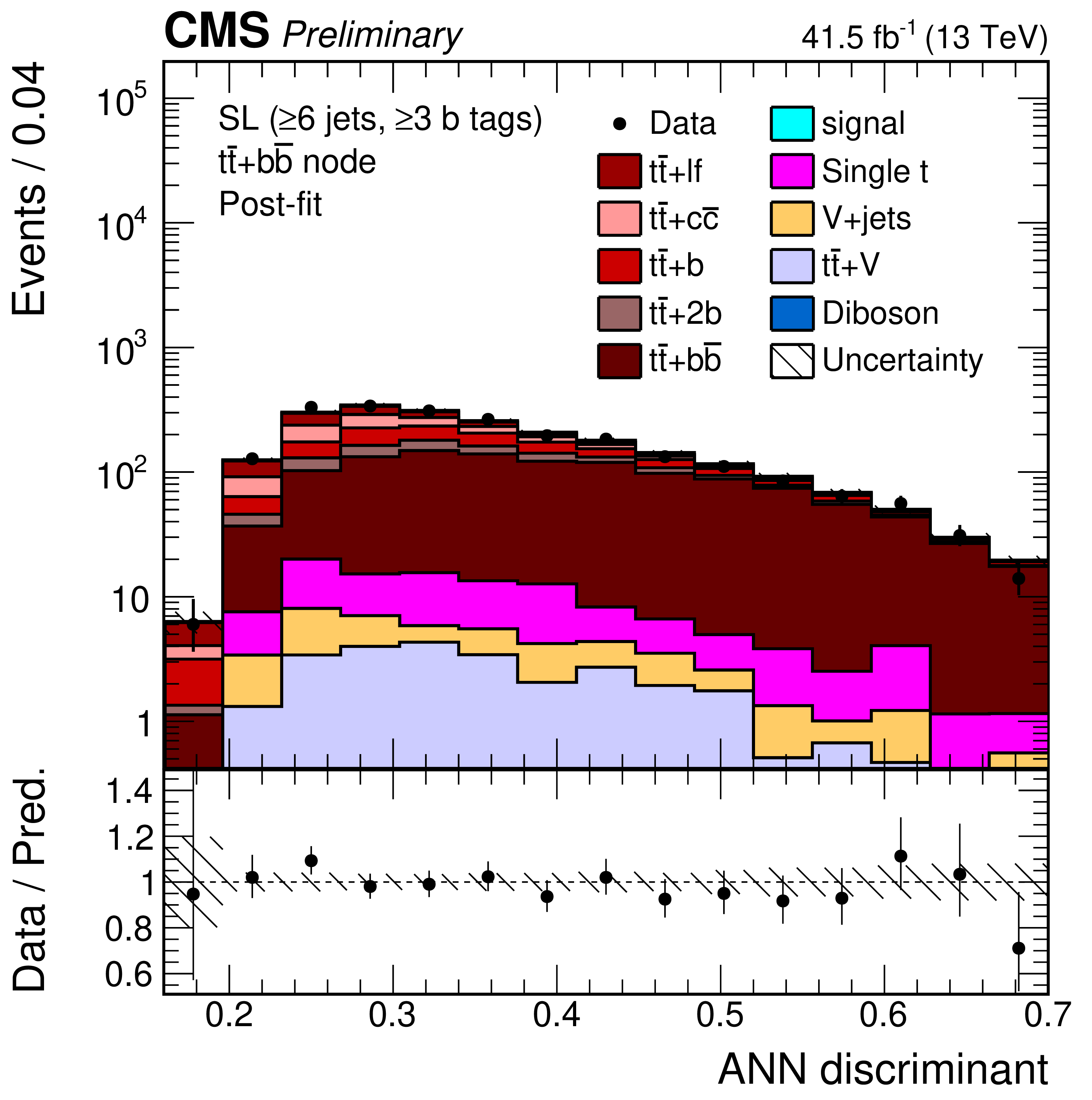
png pdf |
Additional Figure 18-e:
ANN discriminant shapes in the semi-leptonic (SL) channel before the fit to data in the jet-process categories with 6 jets, $\geq $3 b-tags. The expected signal and background contributions (filled histograms) are stacked. The hatched uncertainty bands include the total uncertainty of the fit model. The distributions observed in data (markers) are overlayed. The first and the last bins include underflow and overflow events, respectively. The lower plots show the ratio of the data to the background prediction. |
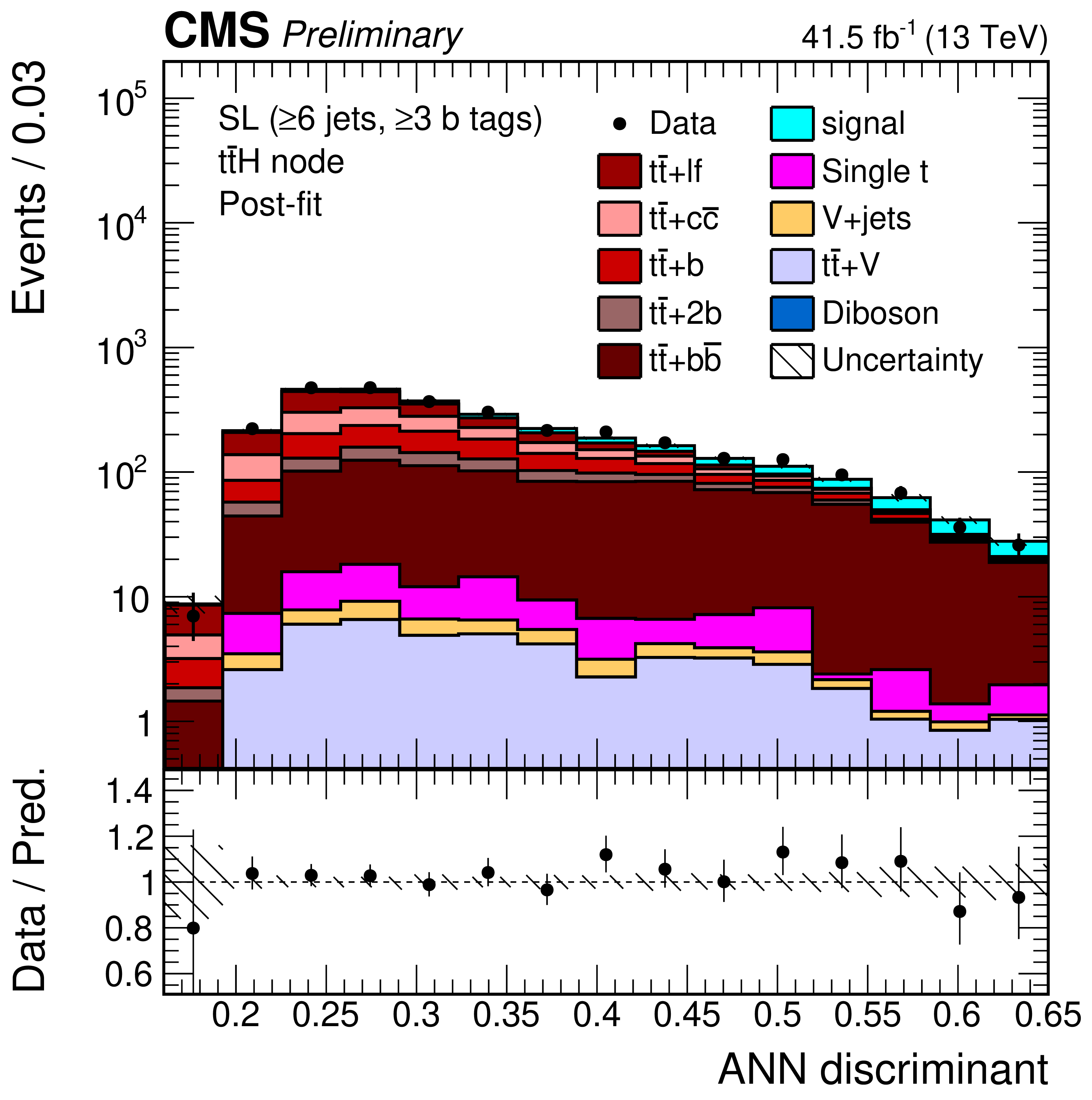
png pdf |
Additional Figure 18-f:
ANN discriminant shapes in the semi-leptonic (SL) channel before the fit to data in the jet-process categories with 6 jets, $\geq $3 b-tags. The expected signal and background contributions (filled histograms) are stacked. The hatched uncertainty bands include the total uncertainty of the fit model. The distributions observed in data (markers) are overlayed. The first and the last bins include underflow and overflow events, respectively. The lower plots show the ratio of the data to the background prediction. |
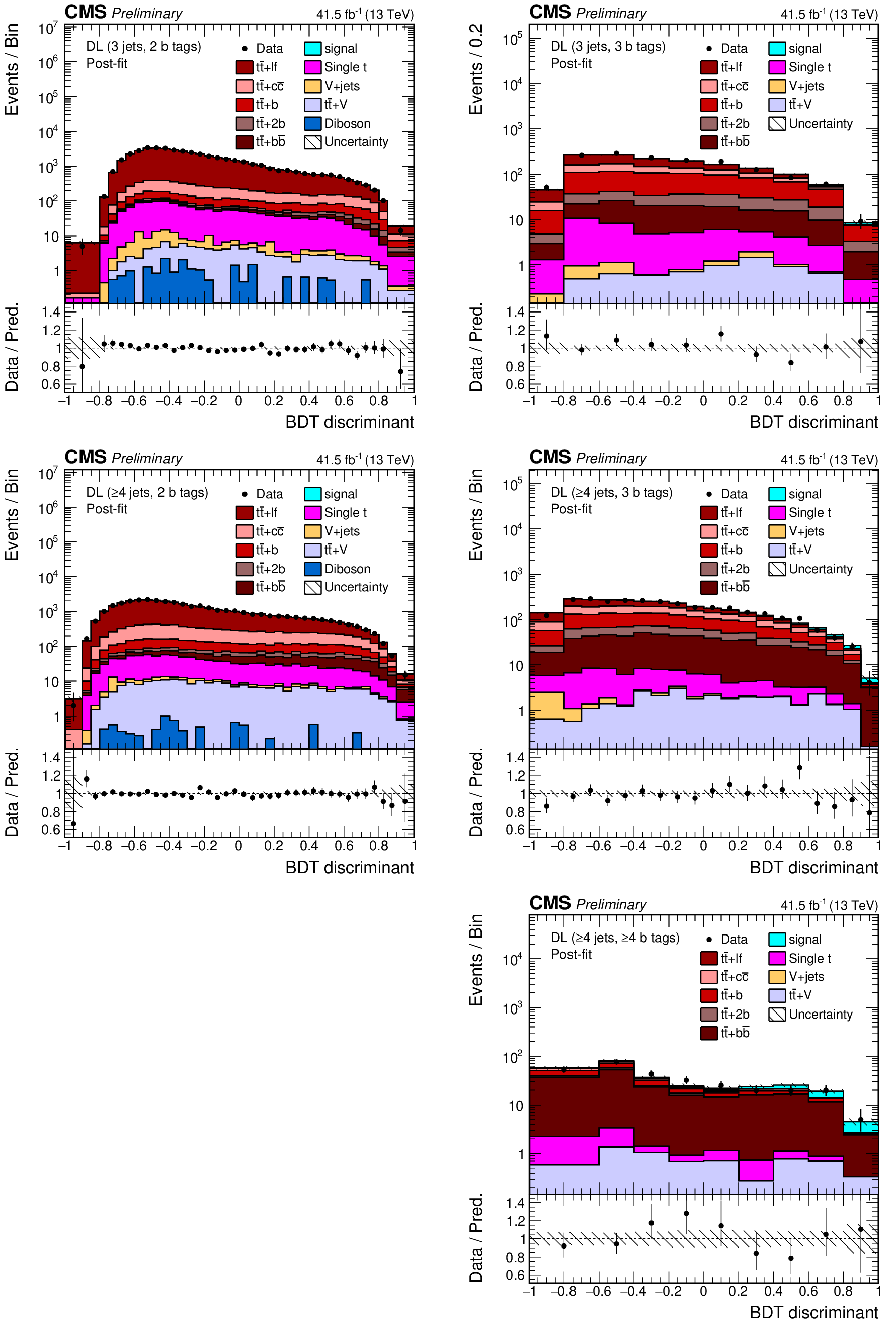
png pdf |
Additional Figure 19:
Final discriminant shapes in the dilepton (DL) channel after the fit to data: BDT discriminant in the jet-tag categories with 3 jets (left) and $\geq $4 jets (right) with 2, 3, and $\geq $4 b-tagged jets (from top to bottom). The expected signal and background contributions (filled histograms) are stacked. The hatched uncertainty bands include the total uncertainty of the fit model. The distributions observed in data (markers) are overlayed. The first and the last bins include underflow and overflow events, respectively. The lower plots show the ratio of the data to the background prediction. |
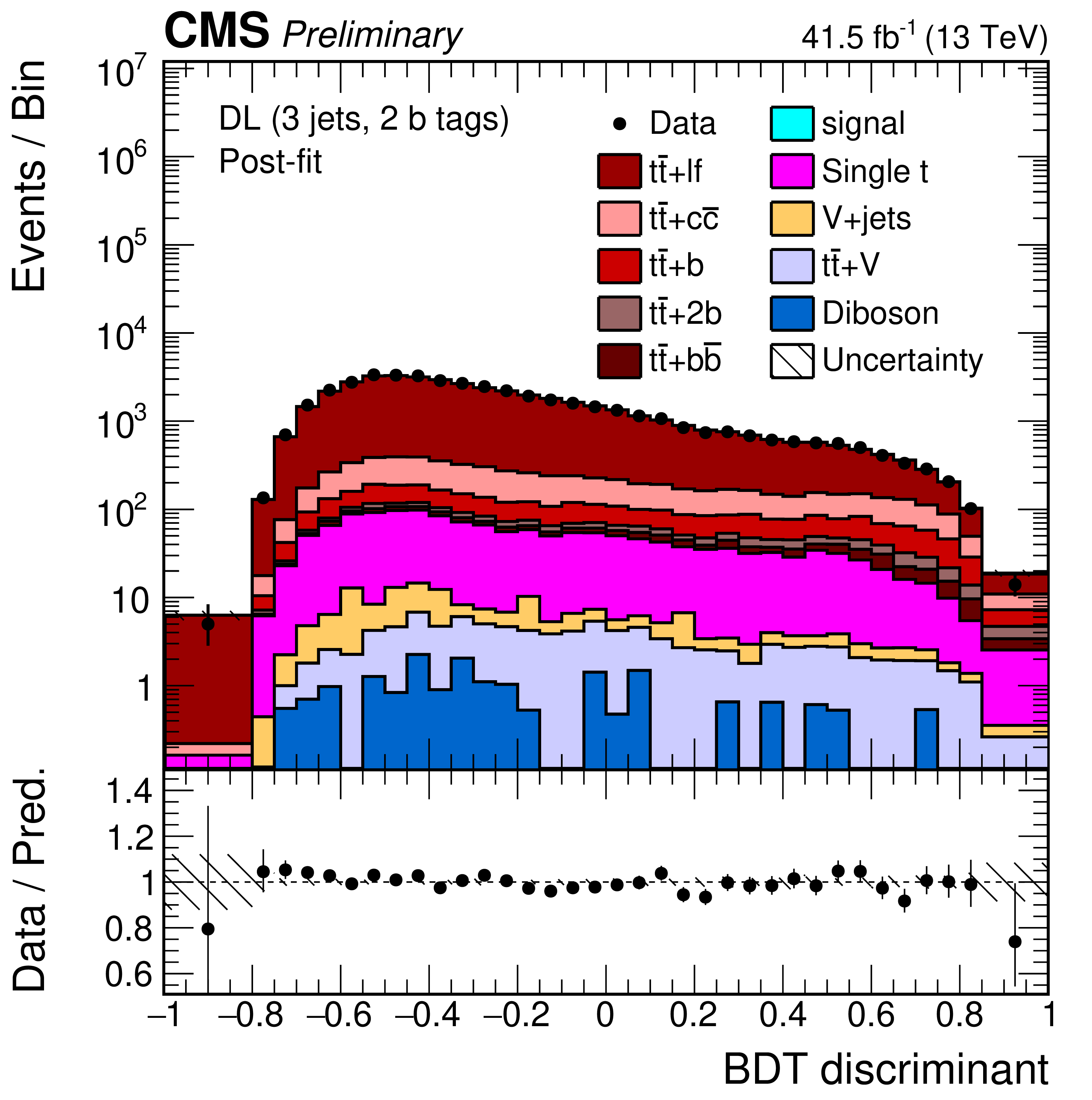
png pdf |
Additional Figure 19-a:
Final discriminant shapes in the dilepton (DL) channel after the fit to data: BDT discriminant in the jet-tag categories with 3 jets with 2 b-tagged jets. The expected signal and background contributions (filled histograms) are stacked. The hatched uncertainty bands include the total uncertainty of the fit model. The distribution observed in data (markers) is overlayed. The first and the last bins include underflow and overflow events, respectively. The lower plot shows the ratio of the data to the background prediction. |
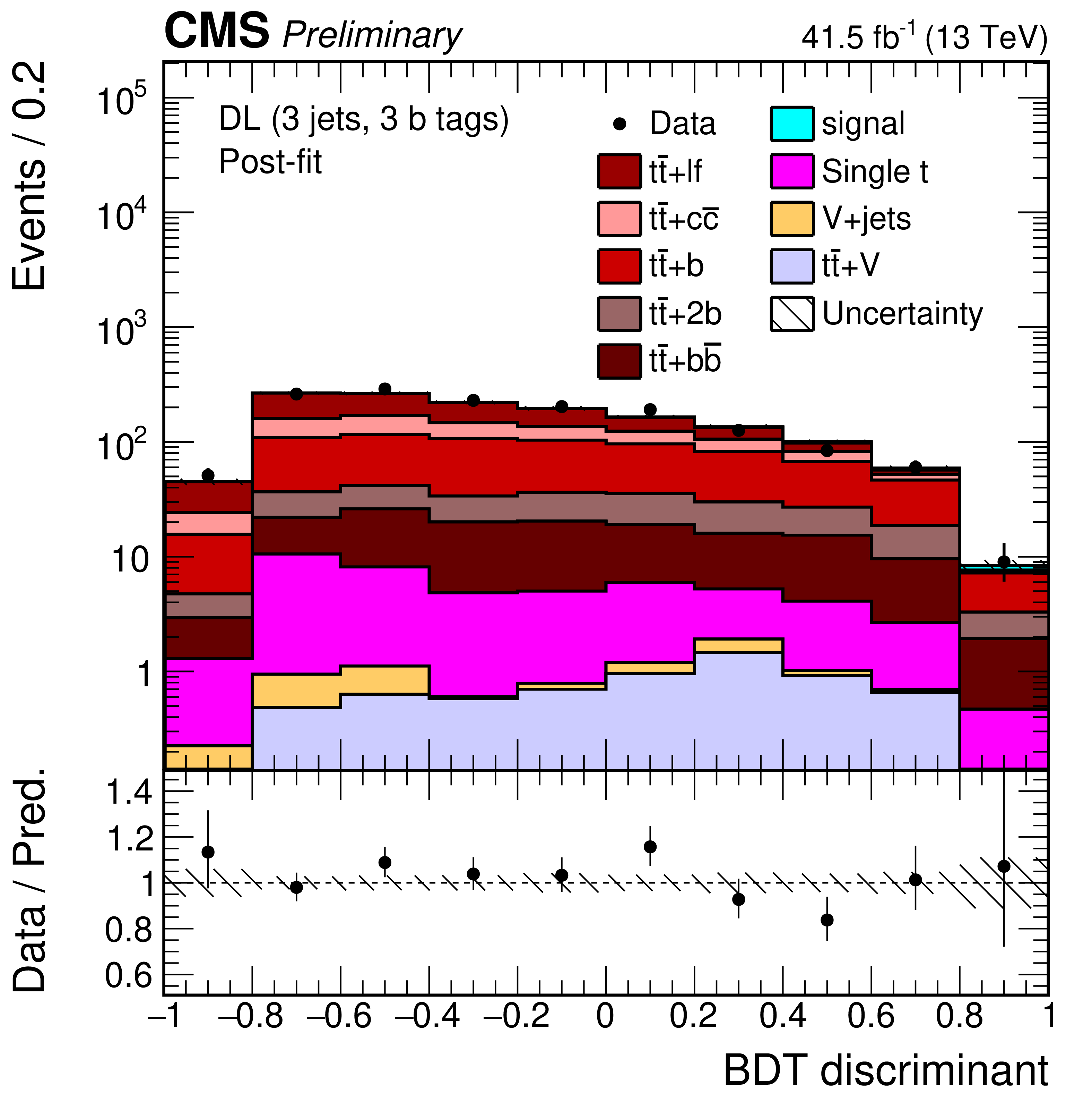
png pdf |
Additional Figure 19-b:
Final discriminant shapes in the dilepton (DL) channel after the fit to data: BDT discriminant in the jet-tag categories with 2 jets with $\geq $4 b-tagged jets. The expected signal and background contributions (filled histograms) are stacked. The hatched uncertainty bands include the total uncertainty of the fit model. The distribution observed in data (markers) is overlayed. The first and the last bins include underflow and overflow events, respectively. The lower plot shows the ratio of the data to the background prediction. |

png pdf |
Additional Figure 19-c:
Final discriminant shapes in the dilepton (DL) channel after the fit to data: BDT discriminant in the jet-tag categories with 3 jets with 3 b-tagged jets. The expected signal and background contributions (filled histograms) are stacked. The hatched uncertainty bands include the total uncertainty of the fit model. The distribution observed in data (markers) is overlayed. The first and the last bins include underflow and overflow events, respectively. The lower plot shows the ratio of the data to the background prediction. |
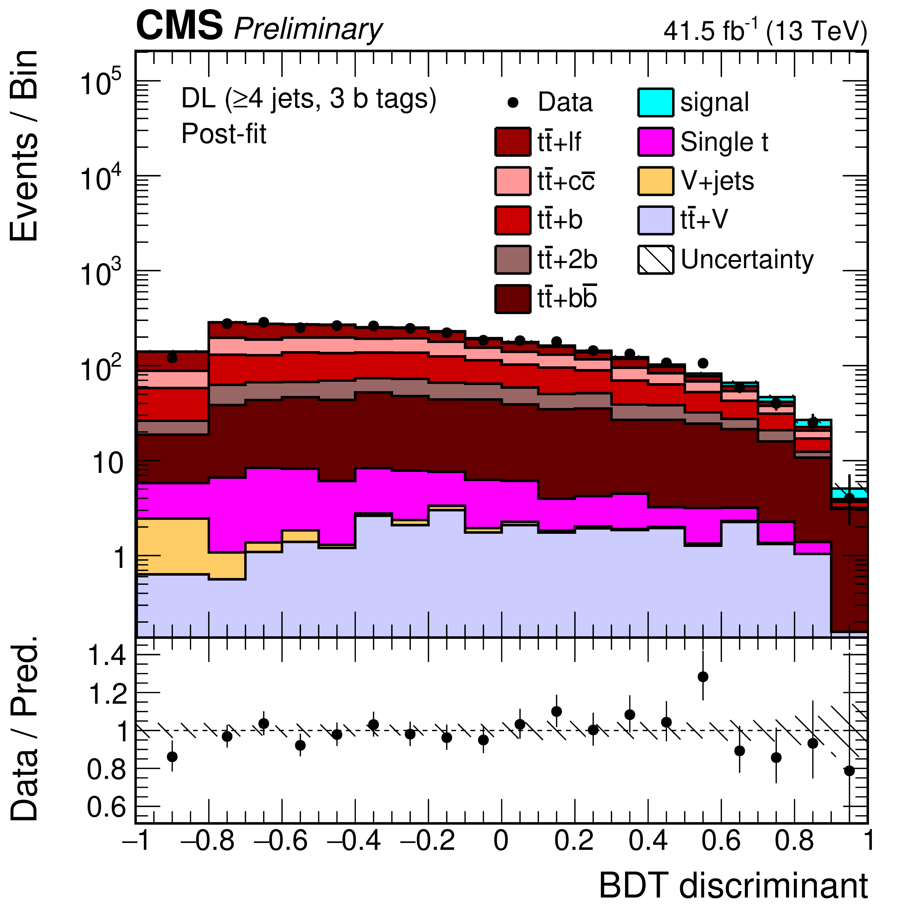
png pdf |
Additional Figure 19-d:
Final discriminant shapes in the dilepton (DL) channel after the fit to data: BDT discriminant in the jet-tag categories with 3 jets with $\geq $4 b-tagged jets. The expected signal and background contributions (filled histograms) are stacked. The hatched uncertainty bands include the total uncertainty of the fit model. The distribution observed in data (markers) is overlayed. The first and the last bins include underflow and overflow events, respectively. The lower plot shows the ratio of the data to the background prediction. |

png pdf |
Additional Figure 19-e:
Final discriminant shapes in the dilepton (DL) channel after the fit to data: BDT discriminant in the jet-tag categories with 3 jets with $\geq $4 b-tagged jets. The expected signal and background contributions (filled histograms) are stacked. The hatched uncertainty bands include the total uncertainty of the fit model. The distribution observed in data (markers) is overlayed. The first and the last bins include underflow and overflow events, respectively. The lower plot shows the ratio of the data to the background prediction. |
| Additional Tables | |
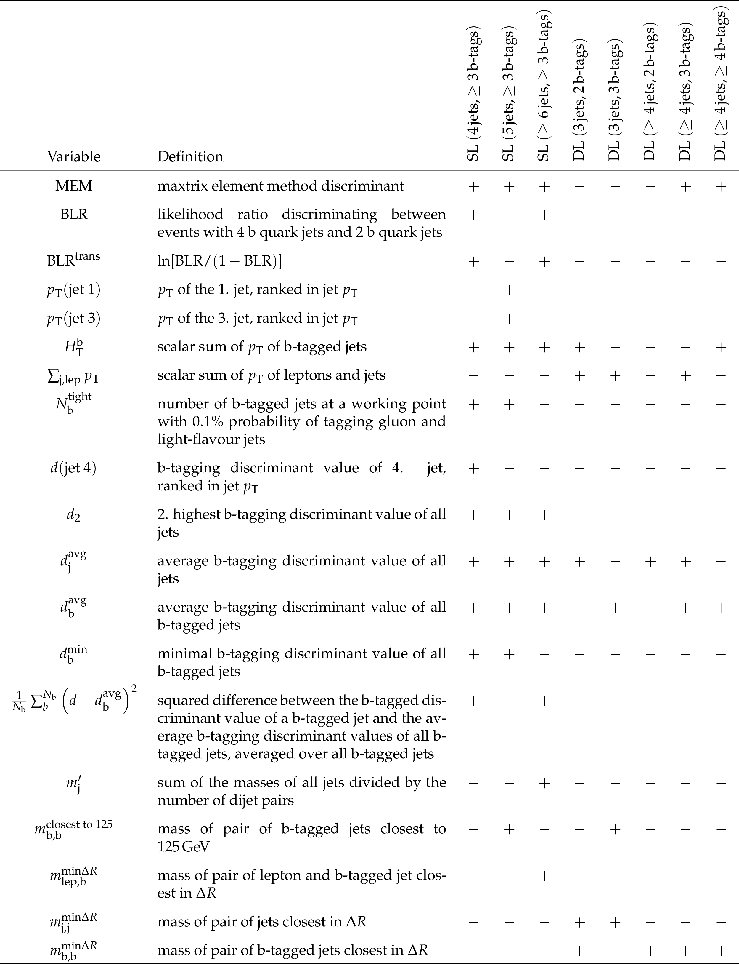
png pdf |
Additional Table 1:
Input variables used in the ANNs or BDTs in the different categories of the single-lepton (SL) and dilepton (DL) channels. Variables used in a specific multivariate method and analysis category are denoted by a "$+$'' and unused variables by a "$-$''. (Continued in Additional Table 2.) |
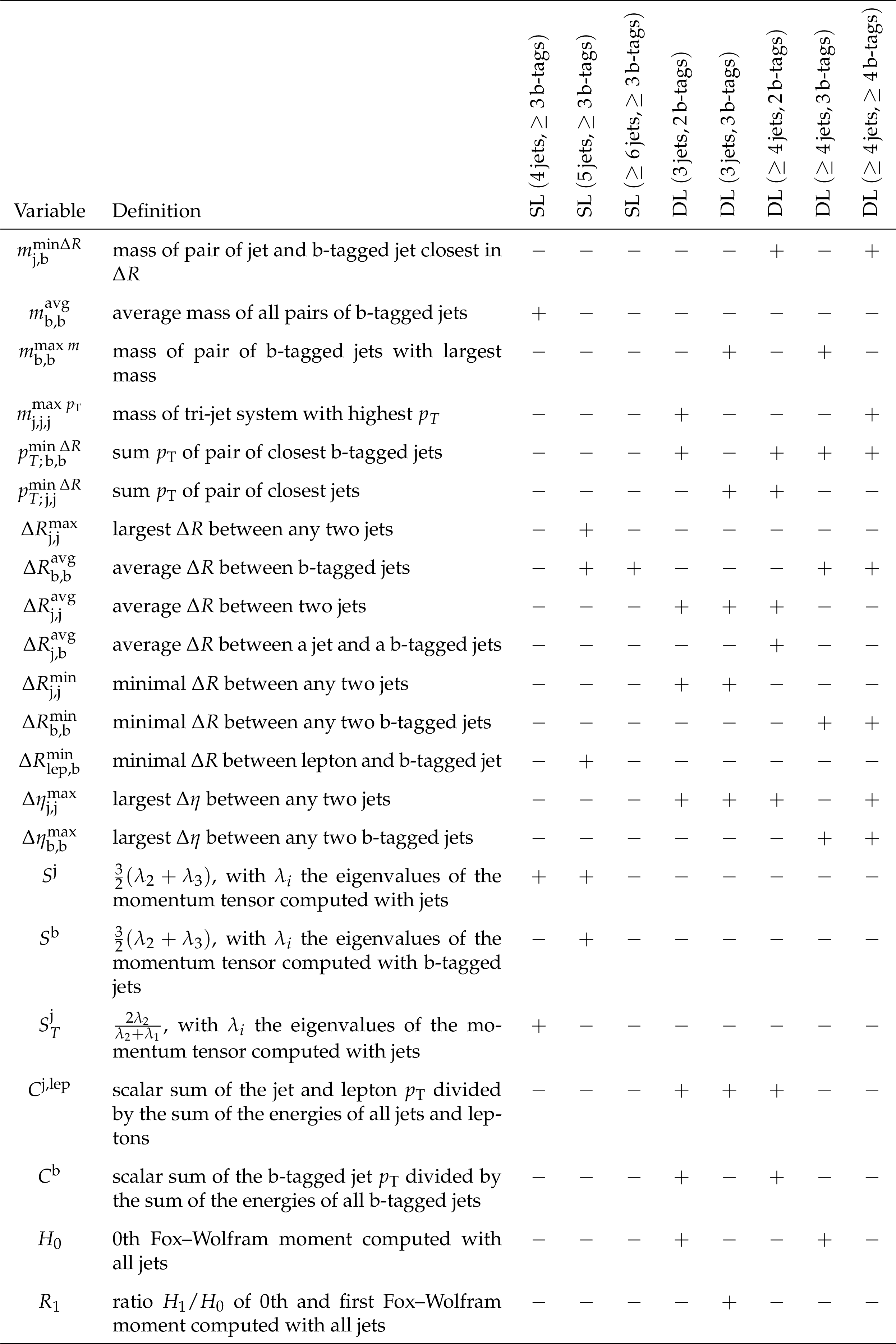
png pdf |
Additional Table 2:
Continued from Additional Table 1 and continued in Additional Table 3. |
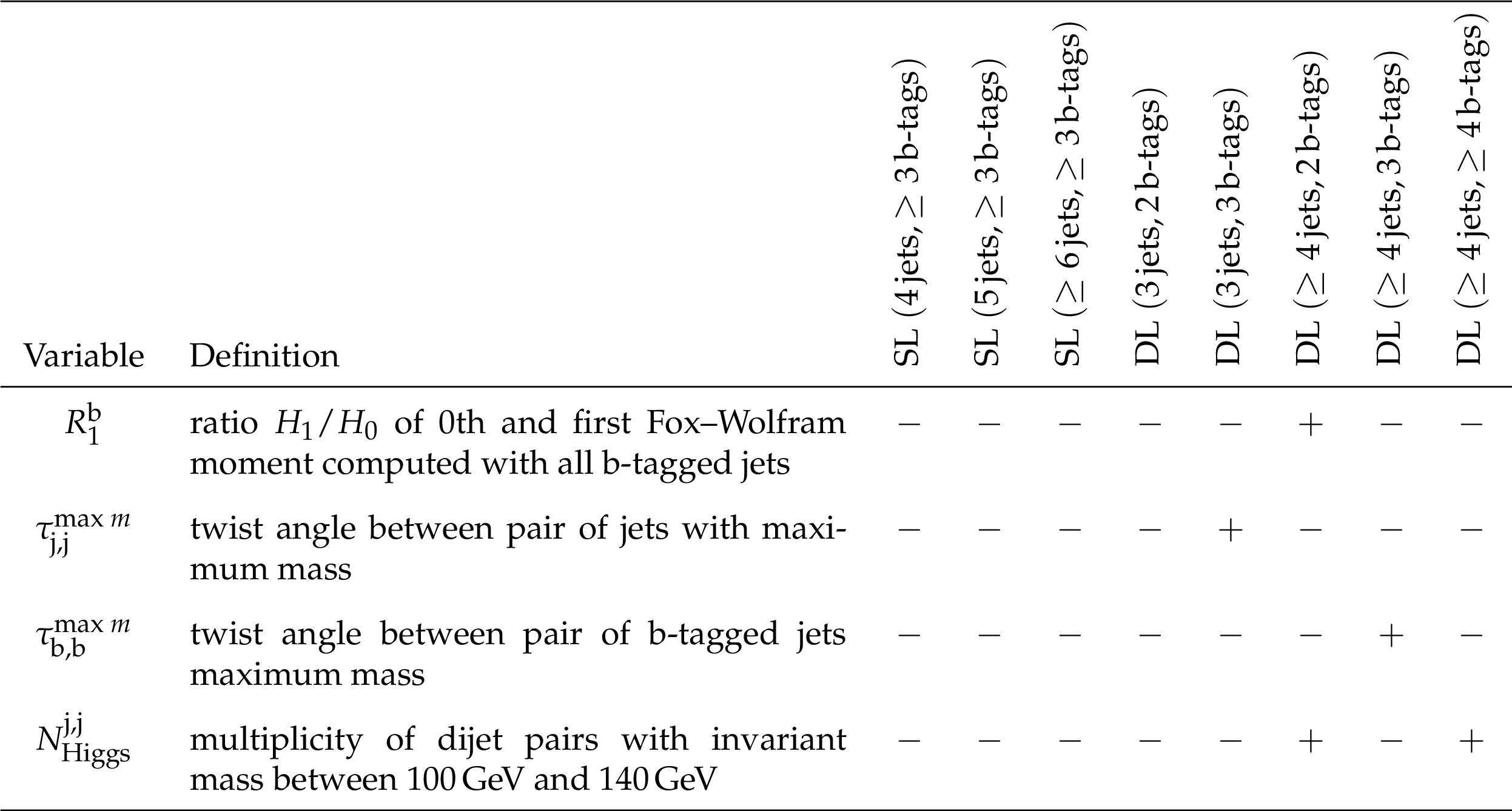
png pdf |
Additional Table 3:
Continued from Additional Table 2. |
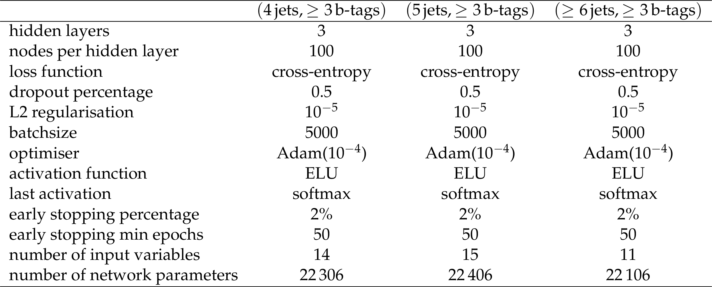
png pdf |
Additional Table 4:
Hyperparameters and number of input variables of the neural networks per jet-multiplicity category in the single-lepton channel. |
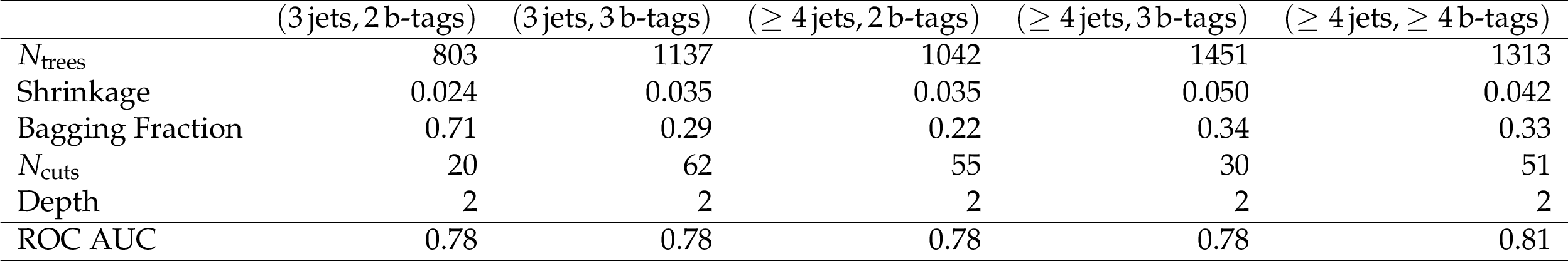
png pdf |
Additional Table 5:
BDT hyperparameters used in the five categories of the dilepton channel, followed by the AUC values of the corresponding ROC curves. |
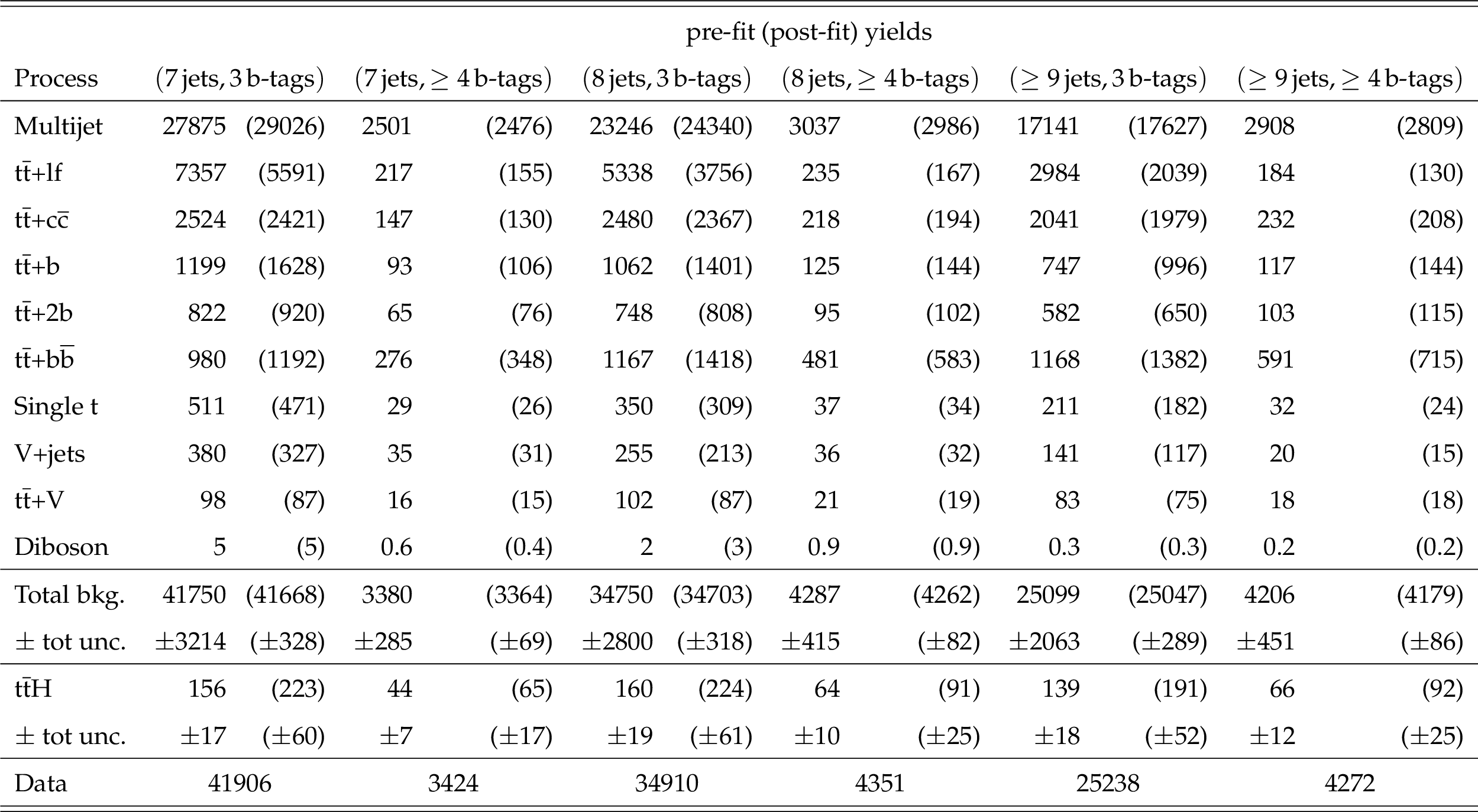
png pdf |
Additional Table 6:
Observed and expected event yields per jet-tag category in the fully-hadronic channel, prior to the fit to data (after the fit to data). The quoted uncertainties denote the total statistical and systematic uncertainty. |
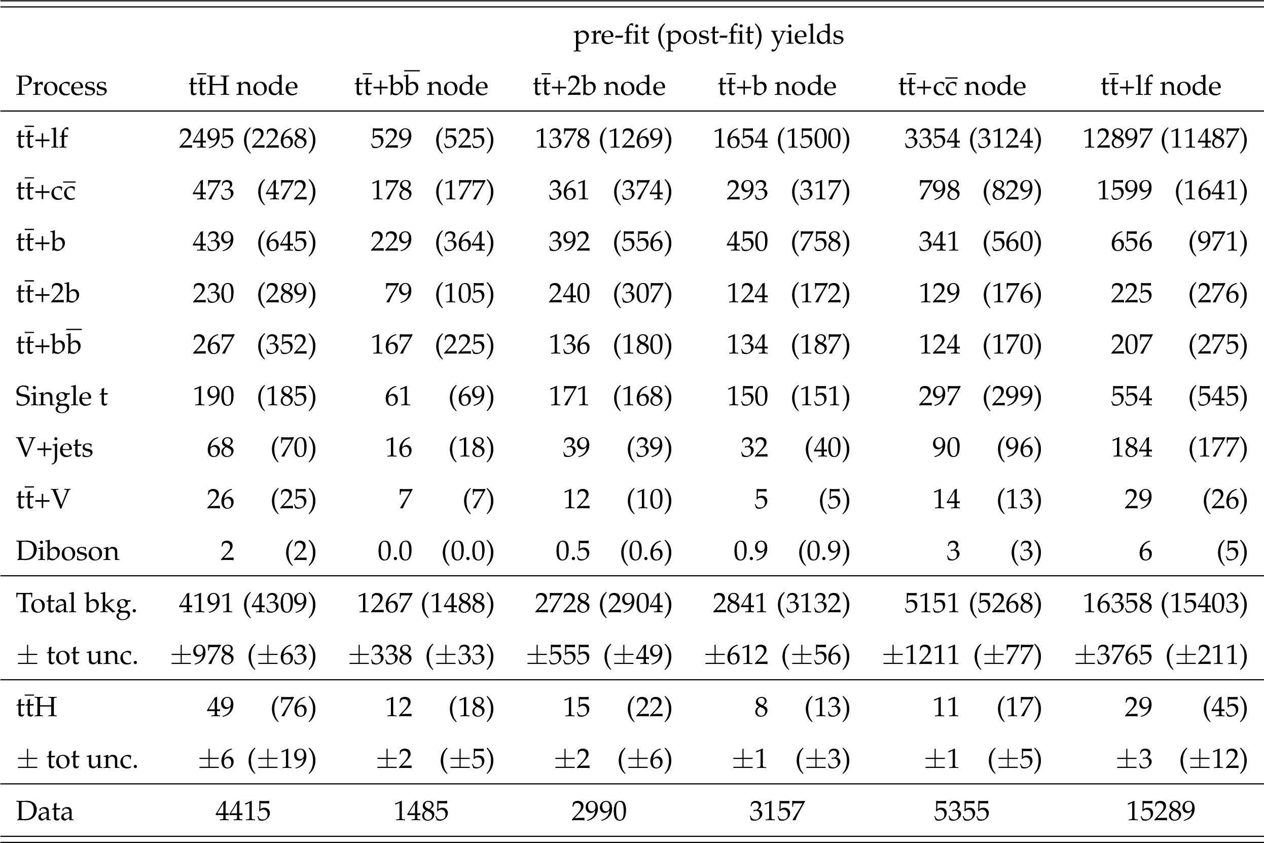
png pdf |
Additional Table 7:
Observed and expected event yields per jet-process category (node) in the single-lepton channel in the 4 jets, $\geq $3 b-tags category, prior to the fit to data (after the fit to data). The quoted uncertainties denote the total statistical and systematic components. |
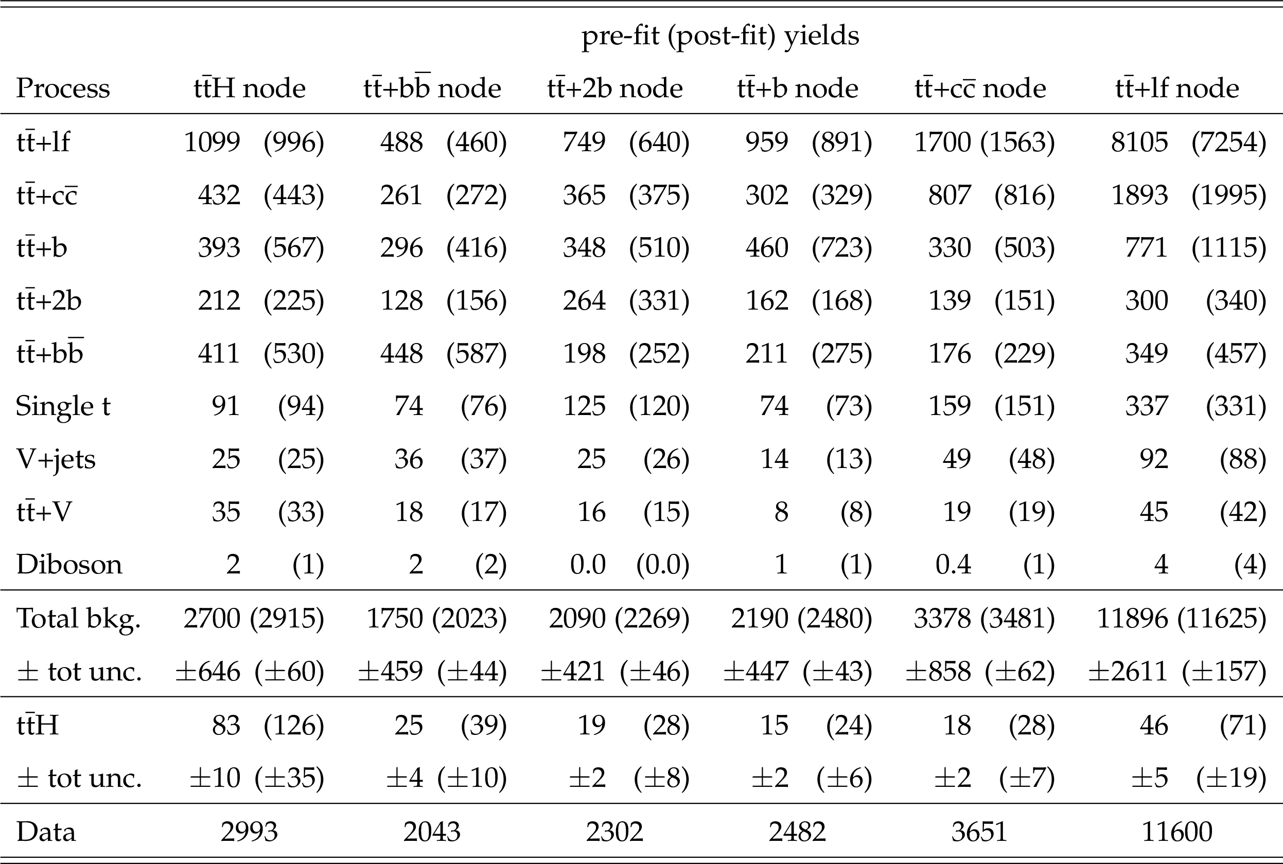
png pdf |
Additional Table 8:
Observed and expected event yields per jet-process category (node) in the single-lepton channel in the 5 jets, $\geq $3 b-tags category, prior to the fit to data (after the fit to data). The quoted uncertainties denote the total statistical and systematic components. |
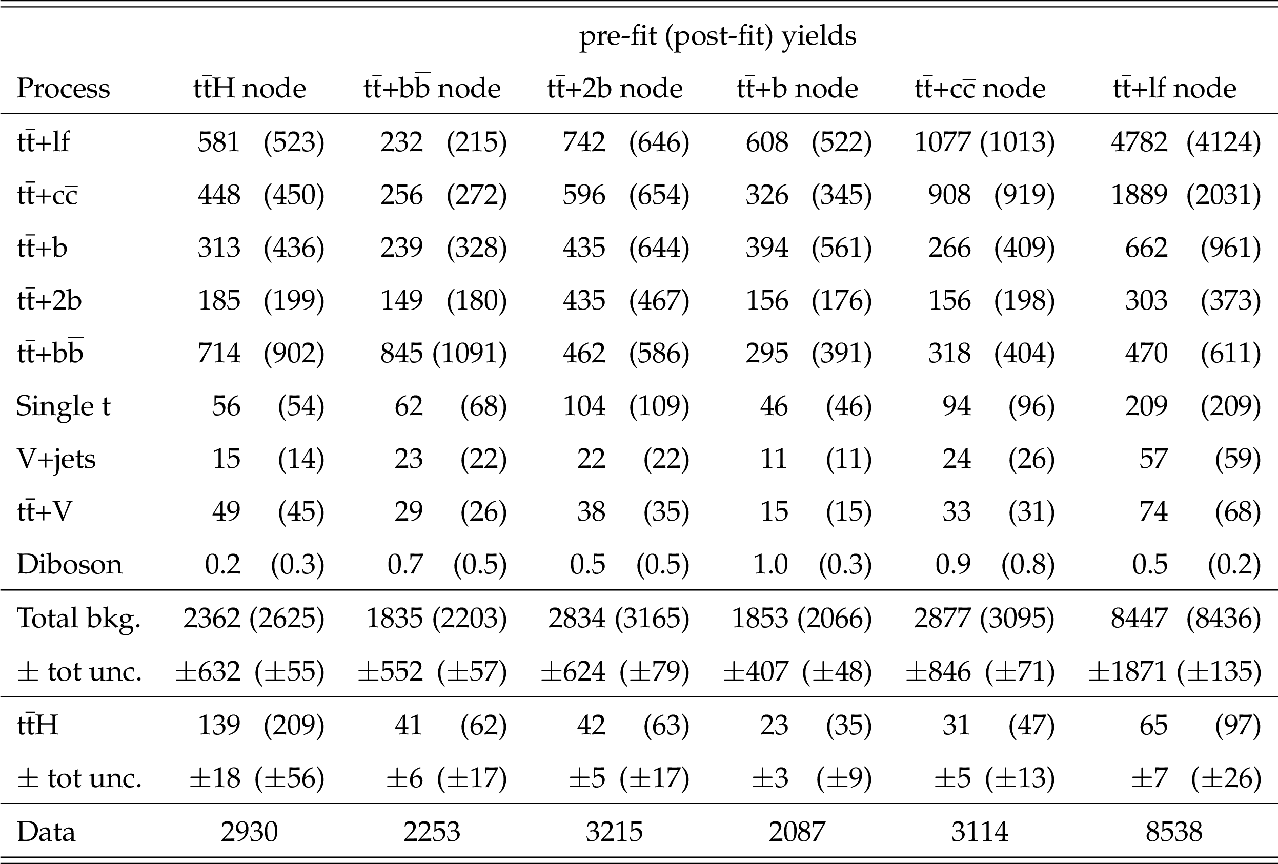
png pdf |
Additional Table 9:
Observed and expected event yields per jet-process category (node) in the single-lepton channel in the 6 jets, $\geq $3 b-tags category, prior to the fit to data (after the fit to data). The quoted uncertainties denote the total statistical and systematic components. |
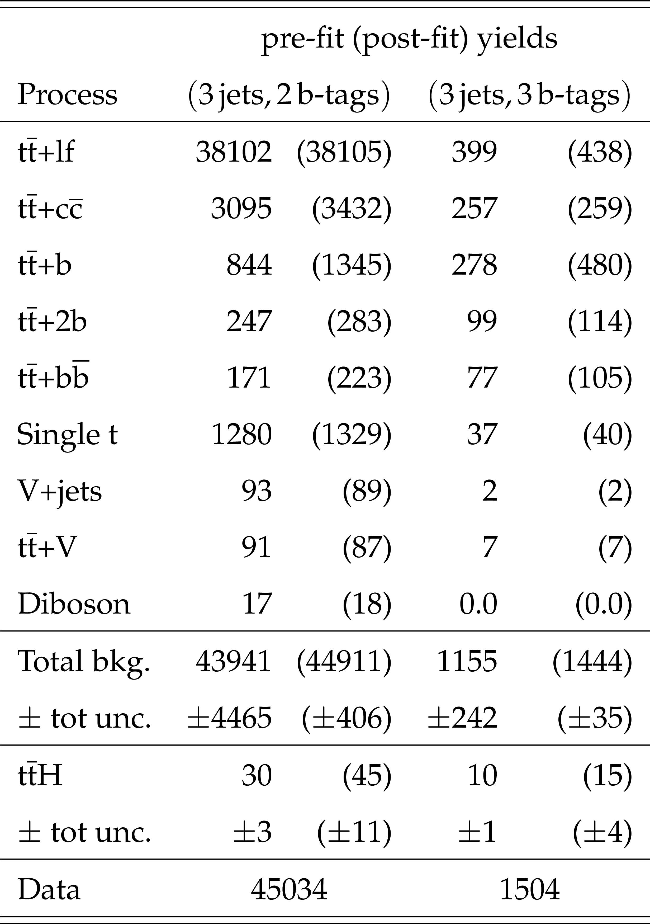
png pdf |
Additional Table 10:
Observed and expected event yields in the 3 jets, 2 b-tags and 3 jets, 3 b-tags categories of the dilepton channel, prior to the fit to data (after the fit to data). The quoted uncertainties denote the total statistical and systematic uncertainty. |
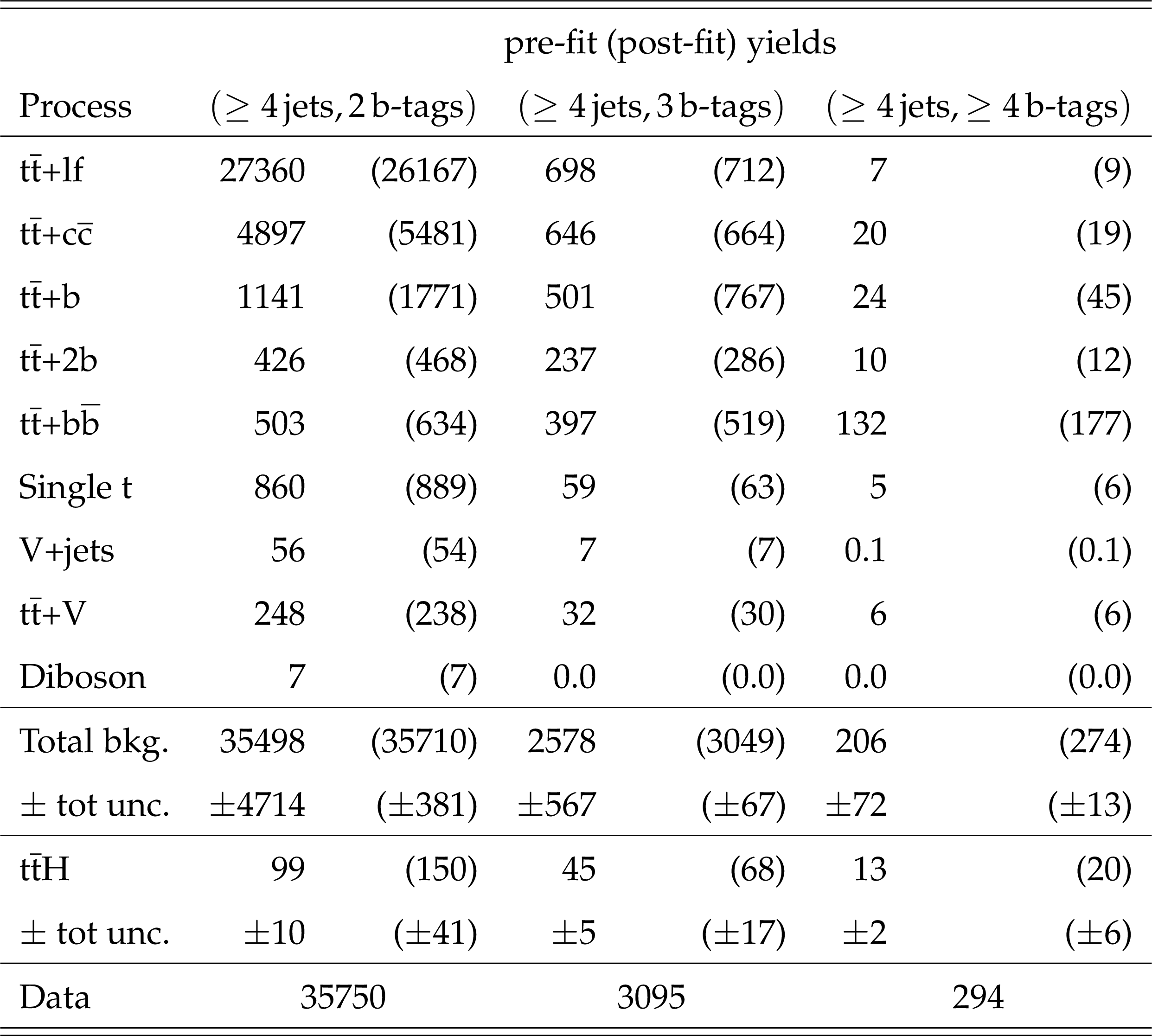
png pdf |
Additional Table 11:
Observed and expected event yields in the $\geq $4 jets, 2 b-tags, $\geq $4 jets, 3 b-tags and $\geq $4 jets, $\geq $4 b-tags categories of the dilepton channel, prior to the fit to data (after the fit to data). The quoted uncertainties denote the total statistical and systematic uncertainty. |
| References | ||||
| 1 | ATLAS Collaboration | Observation of Higgs boson production in association with a top quark pair at the LHC with the ATLAS detector | PLB784 (2018) 159 | 1806.00425 |
| 2 | CMS Collaboration | Observation of $ \mathrm{t\overline{t}} $H production | PRL 120 (2018) 231801 | CMS-HIG-17-035 1804.02610 |
| 3 | LHC Higgs Cross Section Working Group | Handbook of LHC Higgs cross sections: 4. deciphering the nature of the Higgs sector | CERN (2016) | 1610.07922 |
| 4 | ATLAS Collaboration | Search for the standard model Higgs boson produced in association with top quarks and decaying into a $ b\bar{b} $ pair in $ pp $ collisions at $ \sqrt{s} = $ 13 TeV with the ATLAS detector | PRD97 (2018) 072016 | 1712.08895 |
| 5 | CMS Collaboration | Search for $ \mathrm{t\overline{t}} $H production in the $ H\to\mathrm{b\overline{b}} $ decay channel with leptonic $ \mathrm{t\overline{t}} $ decays in proton-proton collisions at $ \sqrt{s}= $ 13 TeV | CMS-HIG-17-026 1804.03682 |
|
| 6 | CMS Collaboration | Search for $ \mathrm{t}\overline{\mathrm{t}} $H production in the all-jet final state in proton-proton collisions at $ \sqrt{s}= $ 13 TeV | JHEP 06 (2018) 101 | CMS-HIG-17-022 1803.06986 |
| 7 | GEANT4 Collaboration | GEANT4--a simulation toolkit | NIMA 506 (2003) 250 | |
| 8 | P. Nason | A new method for combining NLO QCD with shower Monte Carlo algorithms | JHEP 11 (2004) 040 | hep-ph/0409146 |
| 9 | S. Frixione, P. Nason, and C. Oleari | Matching NLO QCD computations with parton shower simulations: the POWHEG method | JHEP 11 (2007) 070 | 0709.2092 |
| 10 | S. Alioli, P. Nason, C. Oleari, and E. Re | A general framework for implementing NLO calculations in shower Monte Carlo programs: the POWHEG BOX | JHEP 06 (2010) 043 | 1002.2581 |
| 11 | H. B. Hartanto, B. Jager, L. Reina, and D. Wackeroth | Higgs boson production in association with top quarks in the POWHEG BOX | PRD 91 (2015) 094003 | 1501.04498 |
| 12 | J. Alwall et al. | The automated computation of tree-level and next-to-leading order differential cross sections, and their matching to parton shower simulations | JHEP 07 (2014) 079 | 1405.0301 |
| 13 | T. Sjostrand et al. | An Introduction to PYTHIA 8.2 | CPC 191 (2015) 159 | 1410.3012 |
| 14 | NNPDF Collaboration | Parton distributions from high-precision collider data | EPJC 77 (2017) 663 | 1706.00428 |
| 15 | CMS Collaboration | Extraction and validation of a new set of CMS PYTHIA8 tunes from underlying-event measurements | Submitted to EPJC | CMS-GEN-17-001 1903.12179 |
| 16 | S. Alioli, P. Nason, C. Oleari, and E. Re | NLO single-top production matched with shower in POWHEG: $ s $- and $ t $-channel contributions | JHEP 09 (2009) 111 | 0907.4076 |
| 17 | E. Re | Single-top Wt-channel production matched with parton showers using the POWHEG method | EPJC 71 (2011) 1547 | 1009.2450 |
| 18 | R. Frederix and S. Frixione | Merging meets matching in MC@NLO | JHEP 12 (2012) 061 | 1209.6215 |
| 19 | M. Cacciari et al. | Top-pair production at hadron colliders with next-to-next-to-leading logarithmic soft-gluon resummation | PLB 710 (2012) 612 | 1111.5869 |
| 20 | P. Barnreuther, M. Czakon, and A. Mitov | Percent-level-precision physics at the Tevatron: next-to-next-to-leading order QCD corrections to $ \mathrm{q}\mathrm{\bar{q}}\to\mathrm{t\bar{t}}\text{+X} $ | PRL 109 (2012) 132001 | 1204.5201 |
| 21 | M. Czakon and A. Mitov | NNLO corrections to top-pair production at hadron colliders: the all-fermionic scattering channels | JHEP 12 (2012) 054 | 1207.0236 |
| 22 | M. Czakon and A. Mitov | NNLO corrections to top pair production at hadron colliders: the quark-gluon reaction | JHEP 01 (2013) 080 | 1210.6832 |
| 23 | M. Beneke, P. Falgari, S. Klein, and C. Schwinn | Hadronic top-quark pair production with NNLL threshold resummation | NPB 855 (2012) 695 | 1109.1536 |
| 24 | M. Czakon, P. Fiedler, and A. Mitov | Total top-quark pair-production cross section at hadron colliders through $ o({\alpha_s}^4) $ | PRL 110 (2013) 252004 | 1303.6254 |
| 25 | M. Czakon and A. Mitov | Top++: a program for the calculation of the top-pair cross-section at hadron colliders | CPC 185 (2014) 2930 | 1112.5675 |
| 26 | N. Kidonakis | Two-loop soft anomalous dimensions for single top quark associated production with $ \mathrm{W^-} $ or $ \mathrm{H^-} $ | PRD 82 (2010) 054018 | 1005.4451 |
| 27 | M. Aliev et al. | HATHOR: HAdronic Top and Heavy quarks crOss section calculatoR | CPC 182 (2011) 1034 | 1007.1327 |
| 28 | P. Kant et al. | HatHor for single top-quark production: Updated predictions and uncertainty estimates for single top-quark production in hadronic collisions | CPC 191 (2015) 74 | 1406.4403 |
| 29 | F. Maltoni, D. Pagani, and I. Tsinikos | Associated production of a top-quark pair with vector bosons at NLO in QCD: impact on $ \mathrm{t}\overline{\mathrm{t}}\mathrm{H} $ searches at the LHC | JHEP 02 (2016) 113 | 1507.05640 |
| 30 | J. M. Campbell, R. K. Ellis, and C. Williams | Vector boson pair production at the LHC | JHEP 07 (2011) 018 | 1105.0020 |
| 31 | CMS Collaboration | Particle-flow reconstruction and global event description with the CMS detector | JINST 12 (2017) P10003 | CMS-PRF-14-001 1706.04965 |
| 32 | CMS Collaboration | Description and performance of track and primary-vertex reconstruction with the CMS tracker | JINST 9 (2014) P10009 | CMS-TRK-11-001 1405.6569 |
| 33 | CMS Collaboration | Performance of electron reconstruction and selection with the CMS detector in proton-proton collisions at $ \sqrt{s} = $ 8 TeV | JINST 10 (2015) P06005 | CMS-EGM-13-001 1502.02701 |
| 34 | CMS Collaboration | Performance of the CMS muon detector and muon reconstruction with proton-proton collisions at $ \sqrt{s} = $ 13 TeV | JINST 13 (2018) P06015 | CMS-MUO-16-001 1804.04528 |
| 35 | M. Cacciari, G. P. Salam, and G. Soyez | The anti-$ {k_{\mathrm{T}}} $ jet clustering algorithm | JHEP 04 (2008) 063 | 0802.1189 |
| 36 | M. Cacciari, G. P. Salam, and G. Soyez | FastJet user manual | EPJC 72 (2012) 1896 | 1111.6097 |
| 37 | M. Cacciari, G. P. Salam, and G. Soyez | The catchment area of jets | JHEP 04 (2008) 005 | 0802.1188 |
| 38 | CMS Collaboration | Jet energy scale and resolution in the CMS experiment in pp collisions at 8 TeV | JINST 12 (2017) P02014 | CMS-JME-13-004 1607.03663 |
| 39 | CMS Collaboration | Identification of heavy-flavour jets with the CMS detector in pp collisions at 13 TeV | JINST 13 (2018) P05011 | CMS-BTV-16-002 1712.07158 |
| 40 | CMS Collaboration | Performance of b tagging algorithms in proton-proton collisions at 13 TeV with Phase 1 CMS detector | CDS | |
| 41 | CMS Collaboration | Performance of quark/gluon discrimination in 8 TeV pp data | CMS-PAS-JME-13-002 | CMS-PAS-JME-13-002 |
| 42 | CMS Collaboration | Performance of quark/gluon discrimination in 13 TeV data | CDS | |
| 43 | F. Chollet et al. | Keras | link | |
| 44 | I. Goodfellow, Y. Bengio, and A. Courville | Deep Learning | MIT Press | |
| 45 | A. Hocker et al. | TMVA: Toolkit for multivariate data analysis | PoS ACAT (2007) 040 | physics/0703039 |
| 46 | J. Kennedy and R. Eberhart | Particle swarm optimization | in Proceedings of the IEEE International Conference on neural networks, volume 4, p. 1942 1995 | |
| 47 | K. El Morabit | A study of the multivariate analysis of Higgs boson production in association with a top quark-antiquark pair in the boosted regime at the CMS experiment | Master's thesis, Karlsruher Institut f\"ur Technologie (KIT), 2015 EKP-2016-00035 | |
| 48 | CMS Collaboration | CMS luminosity measurement for the 2017 data-taking period at $ \sqrt{s} = $ 13 ~ TeV | CMS-PAS-LUM-17-004 | CMS-PAS-LUM-17-004 |
| 49 | ATLAS Collaboration | Measurement of the inelastic proton-proton cross section at $ \sqrt{s} = $ 13 TeV with the ATLAS detector at the LHC | PRL 117 (2016) 182002 | 1606.02625 |
| 50 | P. Skands, S. Carrazza, and J. Rojo | Tuning PYTHIA 8.1: the Monash 2013 tune | EPJC 74 (2014) 3024 | 1404.5630 |
| 51 | CMS Collaboration | Investigations of the impact of the parton shower tuning in Pythia 8 in the modelling of $ \mathrm{t\bar{t}} $ at $ \sqrt{s}= $ 8 and 13 TeV | CMS-PAS-TOP-16-021 | CMS-PAS-TOP-16-021 |
| 52 | NNPDF Collaboration | Parton distributions for the LHC Run II | JHEP 04 (2015) 040 | 1410.8849 |
| 53 | R. J. Barlow and C. Beeston | Fitting using finite Monte Carlo samples | CPC 77 (1993) 219 | |
| 54 | J. S. Conway | Incorporating nuisance parameters in likelihoods for multisource spectra | in Proceedings, PHYSTAT 2011 Workshop on Statistical Issues Related to Discovery Claims in Search Experiments and Unfolding, CERN 2011 | 1103.0354 |
|
|
Compact Muon Solenoid LHC, CERN |
|

|

|

|

|

|