CMS-PAS-HIG-18-019

CMS-PAS-HIG-18-019
Measurement of the associated production of a Higgs boson with a top quark pair in final states with electrons, muons and hadronically decaying $\tau$ leptons in data recorded in 2017 at $\sqrt{s} =$ 13 TeV
CMS Collaboration
November 2018

Abstract: The production of a Higgs boson in association with a top quark pair ( $\mathrm{t}\overline{\mathrm{t}}\mathrm{H}$ ) is measured in final states with electrons, muons and hadronically decaying $\tau$ leptons. Events are selected from a sample of proton-proton collisions at a $\sqrt{s} =$ 13 TeV center-of-mass energy, recorded by the CMS experiment in 2017 and corresponding to an integrated luminosity of 41.5 fb $^{-1}$ . Machine learning and matrix element methods are used to optimize the analysis sensitivity. The observed (expected) $\mathrm{t}\overline{\mathrm{t}}\mathrm{H}$ production rate is 0.75 $^{+0.46}_{-0.43}$ (1.00 $^{+0.39}_{-0.35}$ ) times the expected rate in the standard model, which corresponds to an observed (expected) significance of 1.7 $\sigma$ (2.9 $\sigma$ ). In addition, these results are combined with those previously obtained from the data set collected in 2016 and corresponding to an integrated luminosity of 35.9 fb $^{-1}$ . The observed (expected) signal rate for the combined fit is 0.96 $^{+0.34}_{-0.31}$ (1.00 $^{+0.30}_{-0.27}$ ) times the expected rate in the standard model, which corresponds to an observed (expected) significance of 3.2 $\sigma$ (4.0 $\sigma$ ).
Links: CDS record (PDF) ; inSPIRE record ; CADI line (restricted) ;

Figures & Tables	Summary	References	CMS Publications

Figures
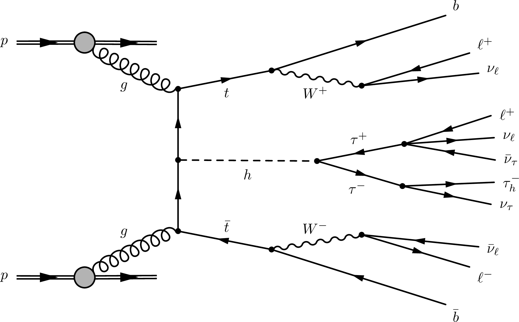
png pdf	Figure 1: An example Feynman diagram for ${\mathrm {t}} {\overline {\mathrm {t}}} {{\mathrm {H}}}$ production, followed by ${{\mathrm {H}}}$ boson decay into a ${\tau}$ pair [6].
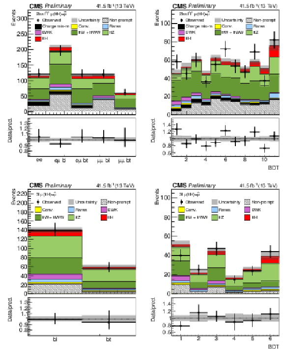
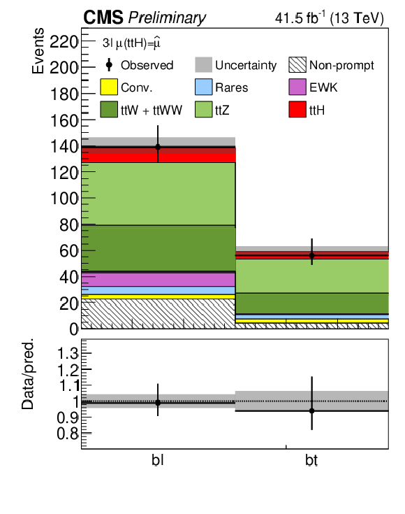
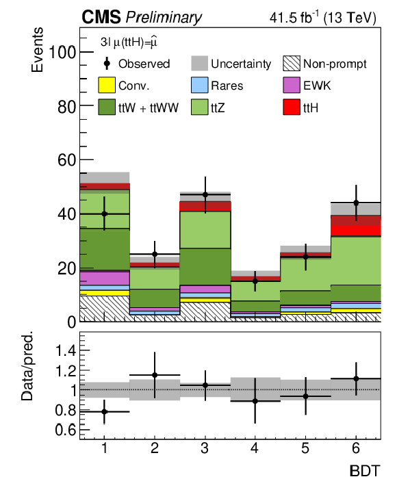
png pdf	Figure 2: Distributions in the discriminating observables used for the signal extraction in the $2 {\ell} {\text {ss}}$ and $3 {\ell}$ categories. Post-fit yields and uncertainties for the ${{{\mathrm {t}}} {{\overline {\mathrm {t}}}} {{\mathrm {H}}}}$ signal and the background processes are shown. In (a) and (c) the distributions for the $2 {\ell} {\text {ss}}$ and $3 {\ell}$ sub-categories are shown; the x-axis labels "bl'' and "bt'' stand for "b-tag loose'' and "b-tag tight'', respectively. Further details are given in Section 7.2.1.
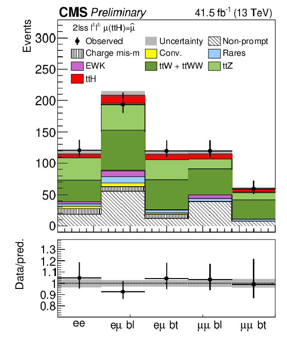
png pdf	Figure 2-a: The distributions for the $2 {\ell} {\text {ss}}$ sub-categories are shown. Further details are given in Section 7.2.1.
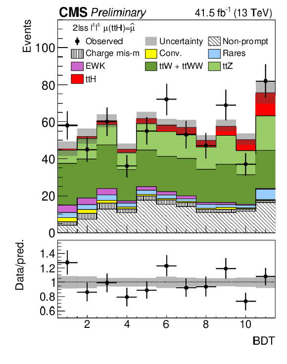
png pdf	Figure 2-b: Distribution in the discriminating observable used for the signal extraction in the $2 {\ell} {\text {ss}}$ categories. Post-fit yields and uncertainties for the ${{{\mathrm {t}}} {{\overline {\mathrm {t}}}} {{\mathrm {H}}}}$ signal and the background processes are shown. Further details are given in Section 7.2.1.
png pdf	Figure 2-c: The $3 {\ell}$ sub-categories are shown; the x-axis labels "bl'' and "bt'' stand for "b-tag loose'' and "b-tag tight'', respectively. Further details are given in Section 7.2.1.
png pdf	Figure 2-d: Distribution in the discriminating observables used for the signal extraction in the $3 {\ell}$ categories. Post-fit yields and uncertainties for the ${{{\mathrm {t}}} {{\overline {\mathrm {t}}}} {{\mathrm {H}}}}$ signal and the background processes are shown. Further details are given in Section 7.2.1.
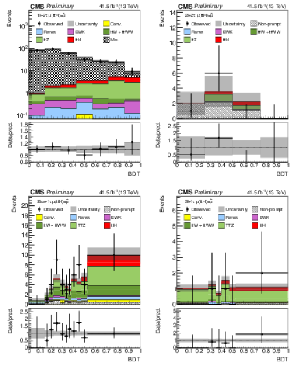
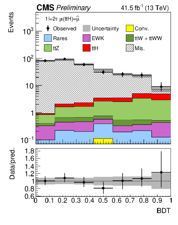
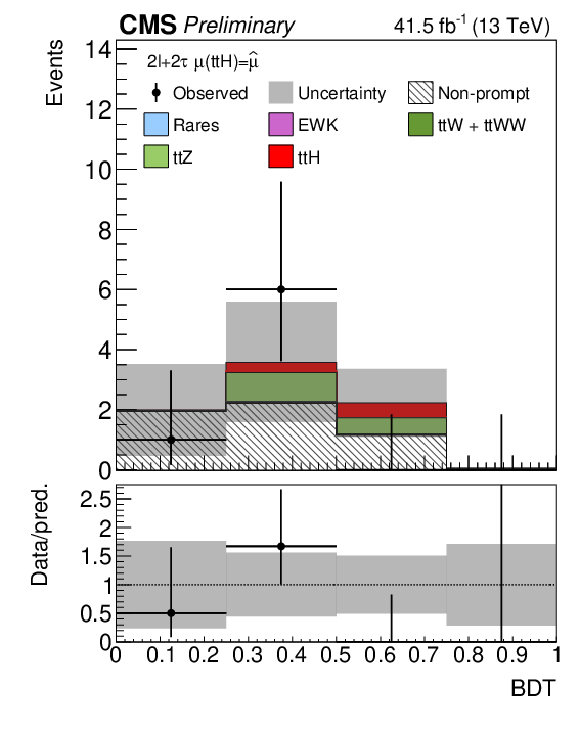
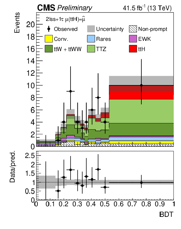
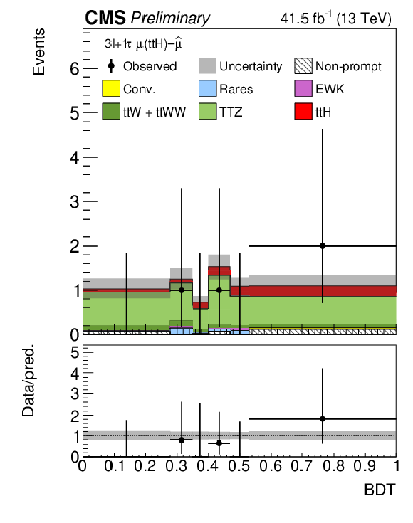
png pdf	Figure 3: Distributions in the discriminating observables used for the signal extraction in (a) the $1 {\ell}+2 {{\tau}_{\mathrm {h}}}$ , (b) the $2 {\ell}+2 {{\tau}_{\mathrm {h}}}$ , (c) the $2 {\ell}ss+1 {{\tau}_{\mathrm {h}}}$ , and (d) $3 {\ell}+1 {{\tau}_{\mathrm {h}}}$ categories. Post-fit yields and uncertainties for the ${{{\mathrm {t}}} {{\overline {\mathrm {t}}}} {{\mathrm {H}}}}$ signal and the background processes are shown.
png pdf	Figure 3-a: Distributions in the discriminating observables used for the signal extraction in the $1 {\ell}+2 {{\tau}_{\mathrm {h}}}$ category. Post-fit yields and uncertainties for the ${{{\mathrm {t}}} {{\overline {\mathrm {t}}}} {{\mathrm {H}}}}$ signal and the background processes are shown.
png pdf	Figure 3-b: Distributions in the discriminating observables used for the signal extraction in the $2 {\ell}+2 {{\tau}_{\mathrm {h}}}$ category. Post-fit yields and uncertainties for the ${{{\mathrm {t}}} {{\overline {\mathrm {t}}}} {{\mathrm {H}}}}$ signal and the background processes are shown.
png pdf	Figure 3-c: Distributions in the discriminating observables used for the signal extraction in the $2 {\ell}ss+1 {{\tau}_{\mathrm {h}}}$ category. Post-fit yields and uncertainties for the ${{{\mathrm {t}}} {{\overline {\mathrm {t}}}} {{\mathrm {H}}}}$ signal and the background processes are shown.
png pdf	Figure 3-d: Distributions in the discriminating observables used for the signal extraction in the $3 {\ell}+1 {{\tau}_{\mathrm {h}}}$ category. Post-fit yields and uncertainties for the ${{{\mathrm {t}}} {{\overline {\mathrm {t}}}} {{\mathrm {H}}}}$ signal and the background processes are shown.
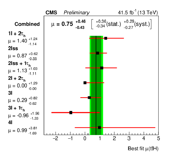
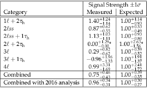
png pdf	Figure 4: Measured signal rates, normalized to the SM ${\mathrm {t}} {\overline {\mathrm {t}}} {{\mathrm {H}}}$ production rate, for the individual categories and for the combination of all seven categories.
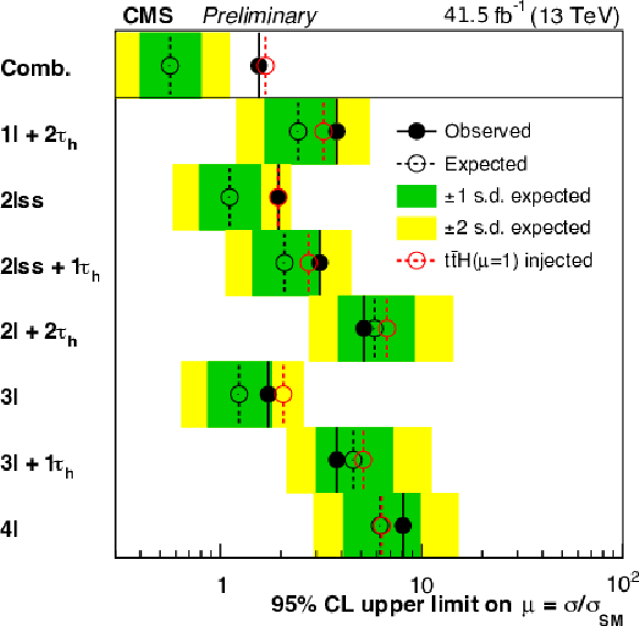
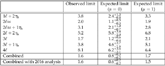
png pdf	Figure 5: 95% CL upper limits on the signal-rate multiplier, $\mu$ , obtained for the individual categories and for the combination of all seven categories.

Tables
png pdf	Table 1: List of event generators used to produce samples for signal and background processes.
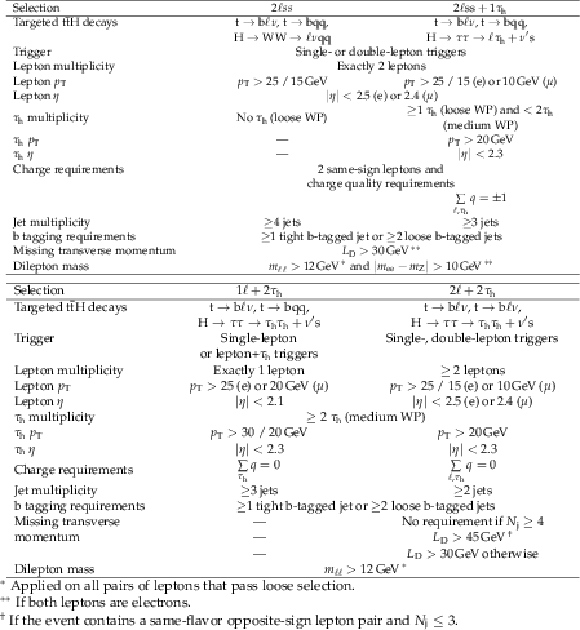
png pdf	Table 2: Event selections applied in the $2 {\ell} {\text {ss}}$ , $2 {\ell} {\text {ss}}+ 1 {{\tau}_{\mathrm {h}}}$ , $1 {\ell}+ 2 {{\tau}_{\mathrm {h}}}$ and $2 {\ell}+ 2 {{\tau}_{\mathrm {h}}}$ categories.
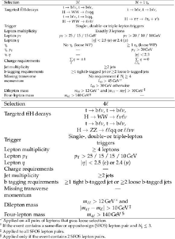
png pdf	Table 3: Event selections applied in the $3 {\ell}$ , $3 {\ell}+1 {{\tau}_{\mathrm {h}}}$ and $4 {\ell}$ categories.
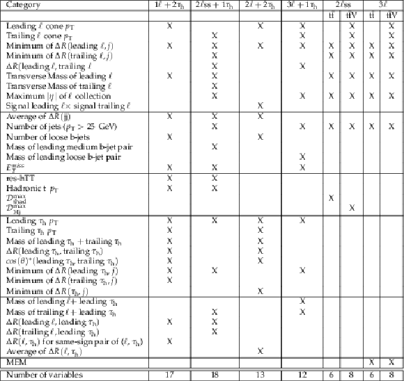
png pdf	Table 4: Variables used in the multivariate discriminators for the channels with and without taus. Only one multivariate discriminant is used in categories with ${{\tau}_{\mathrm {h}}}$ . For the categories without ${{\tau}_{\mathrm {h}}}$ , two different multivariate discriminants are constructed, each one providing better discrimination against a specific background process. The $cos(\theta)^*$ between leading and trailing ${{{\tau}_{\mathrm {h}}}}$ s is measured in the rest frame of the ${{\tau}_{\mathrm {h}}}$ pair. Masses of ${{\ell}}$ s $+$ leading ${{\tau}_{\mathrm {h}}}$ , in the $3 {\ell}+ 1 {{\tau}_{\mathrm {h}}}$ category, are constructed based on the leptons that have opposite signs to ${{\tau}_{\mathrm {h}}}$ .
png pdf	Table 5: Summary of the main sources of systematic uncertainty and their impact on the measured signal rate. The $\Delta \mu$ / $\mu$ column shows the approximate relative shift in signal rate when varying the systematic uncertainty source by its value. Impacts are shown both for the 2017 analysis and for the 2016 + 2017 combined analysis. A general indication on the treatment of their correlations between the 2016 and 2017 samples in the combined analysis is also given.
png pdf	Table 6: The selected number of events in categories based on leptons and hadronic $\tau$ s ( ${{\tau}_{\mathrm {h}}}$ ). The numbers in row "SM expectation'' also include ${{{\mathrm {t}}} {{\overline {\mathrm {t}}}} {{\mathrm {H}}}}$ process. The rates are adjusted using the maximum-likelihood fit (post-fit).
png pdf	Table 7: The measured and expected signal rates are presented as signal-rate multipliers, $\mu$ , which are normalized to the SM ${\mathrm {t}} {\overline {\mathrm {t}}} {{\mathrm {H}}}$ production rate, for the individual categories and for the combination of all seven categories. In addition, a combination with the results obtained from the 2016 dataset [6] is made and added to the table. The * indicates that a lower boundary was introduced in the allowed $\mu$ range to improve the fit convergence properties in the low-yield $2 {\ell}+ 2 {{\tau}_{\mathrm {h}}}$ category.
png pdf	Table 8: 95% CL upper limits on the signal-rate multiplier, $\mu$ , obtained for the individual categories and for the combination of all seven categories. In addition, a combination with the results obtained from the 2016 dataset [6] is made and added to the table. The observed limit is compared to the expected limits for the background-only hypothesis ( $\mu =$ 0) and for the hypothesis where the SM ${{{\mathrm {t}}} {{\overline {\mathrm {t}}}} {{\mathrm {H}}}}$ process is expected ( $\mu =$ 1).
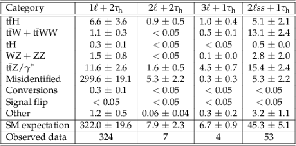
png pdf	Table 9: Selected number of events in the $1 {\ell}+ 2 {{\tau}_{\mathrm {h}}}$ , $2 {\ell}ss + 1 {{\tau}_{\mathrm {h}}}$ , $2 {\ell}+ 2 {{\tau}_{\mathrm {h}}}$ , and $3 {\ell}+ 1 {{\tau}_{\mathrm {h}}}$ categories. The "SM expectation'' row also includes the ${{{\mathrm {t}}} {{\overline {\mathrm {t}}}} {{\mathrm {H}}}}$ process. The rates are adjusted using the maximum-likelihood fit (post-fit).
png pdf	Table 10: Selected number of events in the $2 {\ell}ss$ subcategories. The "SM expectation'' row also includes the ${{{\mathrm {t}}} {{\overline {\mathrm {t}}}} {{\mathrm {H}}}}$ process. The rates are adjusted using the maximum-likelihood fit (post-fit).
png pdf	Table 11: Selected number of events in the $2 {\ell}ss$ control regions. The "SM expectation'' row also includes the ${{{\mathrm {t}}} {{\overline {\mathrm {t}}}} {{\mathrm {H}}}}$ process. The rates are adjusted using the maximum-likelihood fit (post-fit).
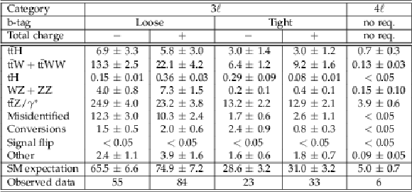
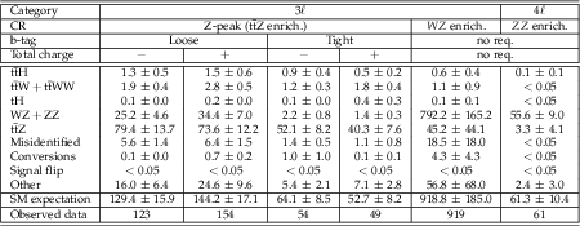
png pdf	Table 12: Selected number of events in the $3 {\ell}$ and $4 {\ell}$ categories. The "SM expectation'' row also includes the ${{{\mathrm {t}}} {{\overline {\mathrm {t}}}} {{\mathrm {H}}}}$ process. The rates are adjusted using the maximum-likelihood fit (post-fit).
png pdf	Table 13: Selected number of events in the $3 {\ell}$ and $4 {\ell}$ control regions. The "SM expectation'' row also includes the ${{{\mathrm {t}}} {{\overline {\mathrm {t}}}} {{\mathrm {H}}}}$ process. The rates are adjusted using the maximum-likelihood fit (post-fit).

Summary

A measurement of the production of a Higgs boson in association with a top quark pair in final states with electrons, muons and hadronically decaying

$\tau$ leptons has been presented. Events from the sample of proton-proton collisions recorded by the CMS experiment in 2017 are categorized according to the number of leptons and

${\tau_\mathrm{h}}$ . Machine learning and matrix element methods are used to optimize the analysis sensitivity. A

$\mathrm{t}\overline{\mathrm{t}}\mathrm{H}$ production rate of 0.75

$^{+0.46}_{-0.43}$ (1.00

$^{+0.39}_{-0.35}$ ) times the SM expectation is observed (expected), corresponding to a significance of 1.7

$\sigma$ (

$2.9\sigma$ ). These results are combined with those obtained from the data set collected in 2016 and reported in Ref. [6]. The combined fit yields an observed (expected) signal rate of 0.96

$^{+0.34}_{-0.31}$ (1.00

$^{+0.30}_{-0.27}$ ) times the SM expectation, which corresponds to a significance of 3.2

$\sigma$ (4.0

$\sigma$ ). All results are consistent with the SM expectation.

References
1	CMS Collaboration	Observation of a new boson at a mass of 125 GeV with the CMS experiment at the LHC	PLB 716 (2012) 30	CMS-HIG-12-028 1207.7235
2	ATLAS Collaboration	Observation of a new particle in the search for the standard model Higgs boson with the ATLAS detector at the LHC	PLB 716 (2012) 1	1207.7214
3	ATLAS and CMS Collaborations	Combined measurement of the Higgs boson mass in ${\mathrm{p}}{\mathrm{p}}$ collisions at $\sqrt{s}=$ 7 and 8~ TeV with the ATLAS and CMS experiments	PRL 114 (2015) 191803	1503.07589
4	ATLAS Collaboration	Observation of Higgs boson production in association with a top quark pair at the LHC with the ATLAS detector	PLB784 (2018) 173--191	1806.00425
5	CMS Collaboration	Observation of $\mathrm{t\overline{t}}$ H production	PRL 120 (2018) 231801	CMS-HIG-17-035 1804.02610
6	CMS Collaboration	Evidence for associated production of a Higgs boson with a top quark pair in final states with electrons, muons, and hadronically decaying $\tau$ leptons at $\sqrt{s} =$ 13 TeV	JHEP 08 (2018) 066	CMS-HIG-17-018 1803.05485
7	A. Hoecker et al.	TMVA --- toolkit for multivariate data analysis	PoS ACAT (2007) 040	physics/0703039
8	F. Pedregosa et al.	Scikit-learn: Machine learning in Python	JMLR 12 (2011) 2825	1201.0490
9	K. Kondo	Dynamical likelihood method for reconstruction of events with missing momentum. 1: method and toy models	J. Phys. Soc. Jap. 57 (1988) 4126
10	K. Kondo	Dynamical likelihood method for reconstruction of events with missing momentum. 2: mass spectra for $2 \to 2$ processes	J. Phys. Soc. Jap. 60 (1991) 836
11	CMS Collaboration	Description and performance of track and primary-vertex reconstruction with the CMS tracker	JINST 9 (2014) P10009	CMS-TRK-11-001 1405.6569
12	CMS Collaboration	The CMS trigger system	JINST 12 (2017) P01020	CMS-TRG-12-001 1609.02366
13	CMS Collaboration	The CMS experiment at the CERN LHC	JINST 3 (2008) S08004	CMS-00-001
14	J. Alwall et al.	The automated computation of tree-level and next-to-leading order differential cross sections, and their matching to parton shower simulations	JHEP 07 (2014) 079	1405.0301
15	R. Frederix and S. Frixione	Merging meets matching in MC@NLO	JHEP 12 (2012) 061	1209.6215
16	J. Alwall et al.	Comparative study of various algorithms for the merging of parton showers and matrix elements in hadronic collisions	EPJC53 (2008) 473--500	0706.2569
17	P. Nason	A new method for combining NLO QCD with shower Monte Carlo algorithms	JHEP 11 (2004) 040	hep-ph/0409146
18	S. Frixione, P. Nason, and C. Oleari	Matching NLO QCD computations with parton shower simulations: the POWHEG method	JHEP 11 (2007) 070	0709.2092
19	S. Alioli, P. Nason, C. Oleari, and E. Re	A general framework for implementing NLO calculations in shower Monte Carlo programs: the POWHEG BOX	JHEP 06 (2010) 043	1002.2581
20	R. Frederix, E. Re, and P. Torrielli	Single-top t-channel hadroproduction in the four-flavour scheme with POWHEG and aMC@NLO	JHEP 09 (2012) 130	1207.5391
21	E. Re	Single-top Wt-channel production matched with parton showers using the POWHEG method	EPJC71 (2011) 1547	1009.2450
22	T. Melia, P. Nason, R. Rontsch, and G. Zanderighi	W+W-, WZ and ZZ production in the POWHEG BOX	JHEP 11 (2011) 078	1107.5051
23	S. Frixione, P. Nason, and G. Ridolfi	A Positive-weight next-to-leading-order Monte Carlo for heavy flavour hadroproduction	JHEP 09 (2007) 126	0707.3088
24	T. Sjostrand, S. Mrenna, and P. Z. Skands	A brief introduction to PYTHIA 8.1	CPC 178 (2008) 852	0710.3820
25	LHC Higgs Cross Section Working Group Collaboration	Handbook of LHC Higgs Cross Sections: 4. Deciphering the Nature of the Higgs Sector		1610.07922
26	P. Kant et al.	HATHOR for single top-quark production: Updated predictions and uncertainty estimates for single top-quark production in hadronic collisions	CPC 191 (2015) 74	1406.4403
27	M. Aliev et al.	HATHOR: HAdronic Top and Heavy quarks crOss section calculatoR	CPC 182 (2011) 1034	1007.1327
28	N. Kidonakis	Two-loop soft anomalous dimensions for single top quark associated production with a $\mathrm{W}^{-}$ or $\mathrm{H}^{-}$	PRD 82 (2010) 054018	1005.4451
29	J. M. Campbell, R. K. Ellis, and C. Williams	Vector boson pair production at the LHC	JHEP 07 (2011) 018	1105.0020
30	K. Melnikov and F. Petriello	Electroweak gauge boson production at hadron colliders through O( $\alpha_{s}^{2}$ )	PRD 74 (2006) 114017	hep-ph/0609070
31	M. Czakon and A. Mitov	Top++: A program for the calculation of the top-pair cross section at hadron colliders	CPC 185 (2014) 2930	1112.5675
32	\GEANTfour Collaboration	GEANT4--a simulation toolkit	NIMA 506 (2003) 250
33	CMS Collaboration	Particle-flow reconstruction and global event description with the CMS detector	JINST 12 (2017) P10003	CMS-PRF-14-001 1706.04965
34	E. Chabanat and N. Estre	Deterministic annealing for vertex finding at CMS	in Computing in high energy physics and nuclear physics. Proceedings, Conference, CHEP'04, Interlaken, Switzerland, September 27-October 1, 2004, pp. 287--290 CERN, Geneva
35	W. Waltenberger, R. Fruhwirth, and P. Vanlaer	Adaptive vertex fitting	JPG 34 (2007) N343
36	M. Cacciari, G. P. Salam, and G. Soyez	The anti- ${k_{\mathrm{T}}}$ jet clustering algorithm	JHEP 04 (2008) 063	0802.1189
37	M. Cacciari, G. P. Salam, and G. Soyez	$FastJet$ user manual	EPJC 72 (2012) 1896	1111.6097
38	CMS Collaboration	Performance of electron reconstruction and selection with the CMS detector in ${\mathrm{p}}{\mathrm{p}}$ collisions at $\sqrt{s} =$ 8 TeV	JINST 10 (2015) P06005	CMS-EGM-13-001 1502.02701
39	CMS Collaboration	Performance of CMS muon reconstruction in ${\mathrm{p}}{\mathrm{p}}$ collision events at $\sqrt{s} =$ 7 TeV	JINST 7 (2012) P10002	CMS-MUO-10-004 1206.4071
40	CMS Collaboration	Reconstruction and identification of $\tau$ lepton decays to hadrons and ${\mathrm{n}}ut$ at CMS	JINST 11 (2016) P01019	CMS-TAU-14-001 1510.07488
41	CMS Collaboration	Performance of reconstruction and identification of $\tau$ leptons in their decays to hadrons and ${\mathrm{n}}ut$ in LHC Run 2	CMS-PAS-TAU-16-002	CMS-PAS-TAU-16-002
42	M. Cacciari, G. P. Salam, and G. Soyez	The catchment area of jets	JHEP 04 (2008) 005	0802.1188
43	M. Cacciari and G. P. Salam	Pileup subtraction using jet areas	PLB 659 (2008) 119	0707.1378
44	CMS Collaboration	Jet algorithms performance in 13 TeV data	CMS-PAS-JME-16-003	CMS-PAS-JME-16-003
45	CMS Collaboration	Determination of jet energy calibration and transverse momentum resolution in CMS	JINST 6 (2011) P11002	CMS-JME-10-011 1107.4277
46	CMS Collaboration	Identification of b quark jets with the CMS experiment	JINST 8 (2013) P04013	CMS-BTV-12-001 1211.4462
47	CMS Collaboration	Identification of b quark jets at the CMS experiment in the LHC Run 2	CMS-PAS-BTV-15-001	CMS-PAS-BTV-15-001
48	CMS Collaboration	Identification of heavy-flavour jets with the cms detector in pp collisions at 13 tev	Journal of Instrumentation 13 (2018), no. 05, P05011	CMS-BTV-16-002 1712.07158
49	CMS Collaboration	Performance of the CMS missing transverse momentum reconstruction in ${\mathrm{p}}{\mathrm{p}}$ data at $\sqrt{s} =$ 8 TeV	JINST 10 (2015) P02006	CMS-JME-13-003 1411.0511
50	CMS Collaboration	Performance of missing energy reconstruction in 13 TeV pp collision data using the CMS detector	CMS-PAS-JME-16-004	CMS-PAS-JME-16-004
51	Particle Data Group	Review of particle physics	CPC 38 (2014) 090001
52	CMS Collaboration	Measurements of properties of the Higgs boson decaying into the four-lepton final state in pp collisions at $\sqrt{s}=$ 13 TeV	JHEP 11 (2017) 047	CMS-HIG-16-041 1706.09936
53	M. Cacciari et al.	The $\mathrm{ t \bar{t} }$ cross-section at $1.8$ ~ TeV and $1.96$ ~ $TeV:$ a study of the systematics due to parton densities and scale dependence	JHEP 04 (2004) 068	hep-ph/0303085
54	S. Catani, D. de Florian, M. Grazzini, and P. Nason	Soft gluon resummation for Higgs boson production at hadron colliders	JHEP 07 (2003) 028	hep-ph/0306211
55	R. Frederix et al.	Four-lepton production at hadron colliders: aMC@NLO predictions with theoretical uncertainties	JHEP 02 (2012) 099	1110.4738
56	CMS Collaboration	Jet energy scale and resolution at $\sqrt{s} =$ 13 TeV
57	CMS Collaboration	Measurement of the cross section for top quark pair production in association with a W or Z boson in proton-proton collisions at $\sqrt{s} =$ 13 TeV	JHEP 08 (2018) 011	CMS-TOP-17-005 1711.02547