

Compact Muon Solenoid
LHC, CERN
| CMS-PAS-HIG-17-013 | ||
| Search for new resonances in the diphoton final state in the mass range between 70 and 110 GeV in pp collisions at $\sqrt{s}=$ 8 and 13 TeV | ||
| CMS Collaboration | ||
| September 2017 | ||
| Abstract: The results of a search for a new resonance decaying into two photons are presented for a diphoton invariant mass in the range between 70 and 110 GeV. The analysis uses the entire dataset collected by the CMS experiment in proton-proton collisions during the 2012 and 2016 LHC running periods. The data samples correspond to integrated luminosities of 19.7 fb$^{-1}$ at $\sqrt{s}= $ 8 TeV and 35.9 fb$^{-1}$ at $\sqrt{s}= $ 13 TeV. The expected and observed 95% confidence level upper limits on the product of the cross section times branching ratio into two photons are presented. No significant excess with respect to the expected limits is observed. The observed upper limit for the 2012 (2016) dataset ranges from approximately 133 (161) fb at the mass hypothesis of 91.1 (89.9) GeV to 31 (26) fb at a mass of 102.8 (103.0) GeV. The statistical combination of the results from the analysis of the two datasets in the mass range between 80 and 110 GeV yields a minimum (maximum) observed upper limit on the production cross section times branching ratio normalized to the Standard Model-like expectation of approximately 0.17 (1.15) corresponding to a mass hypothesis of 103.0 (90.0) GeV. | ||
|
Links:
CDS record (PDF) ;
inSPIRE record ;
CADI line (restricted) ;
These preliminary results are superseded in this paper, PLB 793 (2019) 320. The superseded preliminary plots can be found here. |
||
| Figures & Tables | Summary | Additional Figures | References | CMS Publications |
|---|
| Figures | |
png pdf |
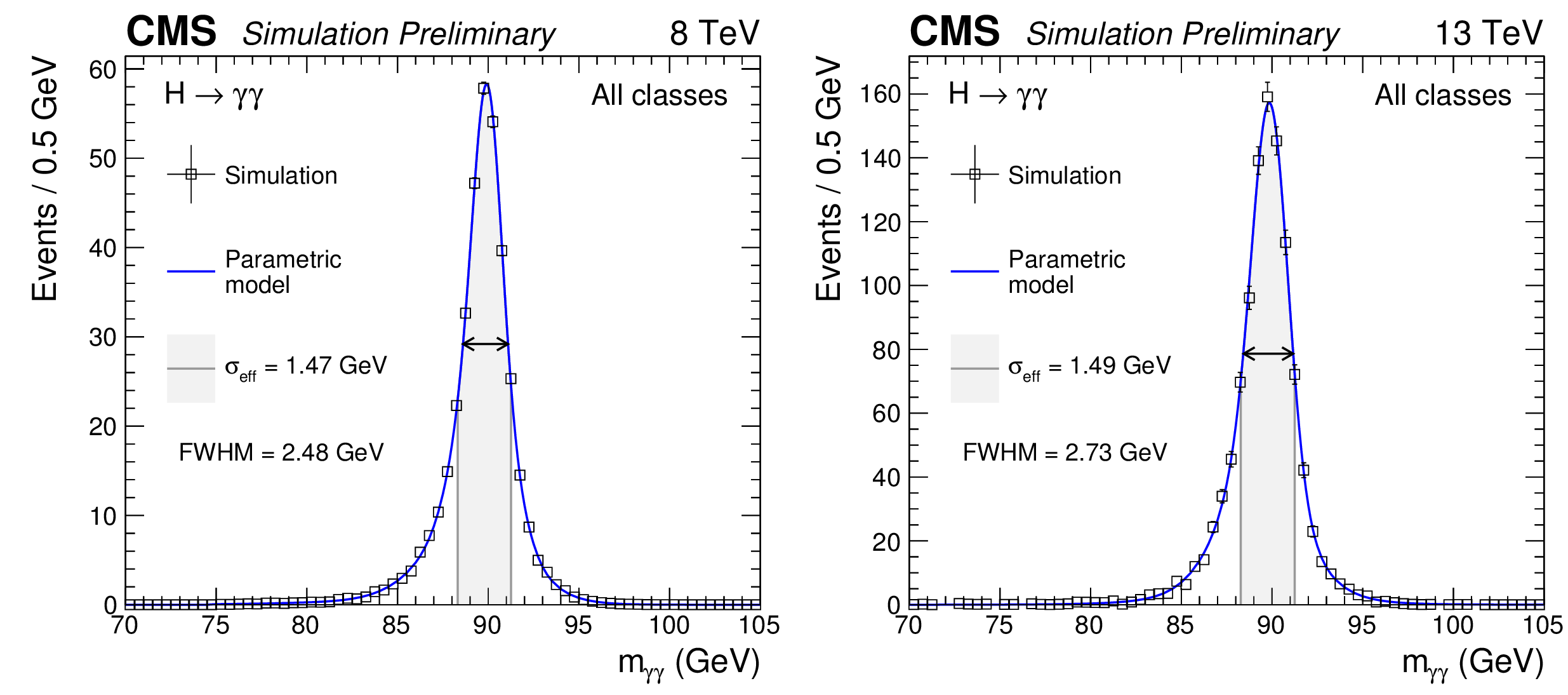
Figure 1:
Full parameterized signal shape integrated over all event classes, in simulated signal events with $ {m_{\mathrm {H}}} = $ 90 GeV at $\sqrt {s} = $ 8 TeV (left) and at $\sqrt {s} = $ 13 TeV (right). The open points are the weighted MC events and the blue lines are the corresponding parametric models. Also shown are the effective $\sigma $ ($\sigma _{\text {eff}}$) values and the corresponding full width at half-maximum (FWHM), indicated by the position of the arrows on each distribution. |
png pdf |
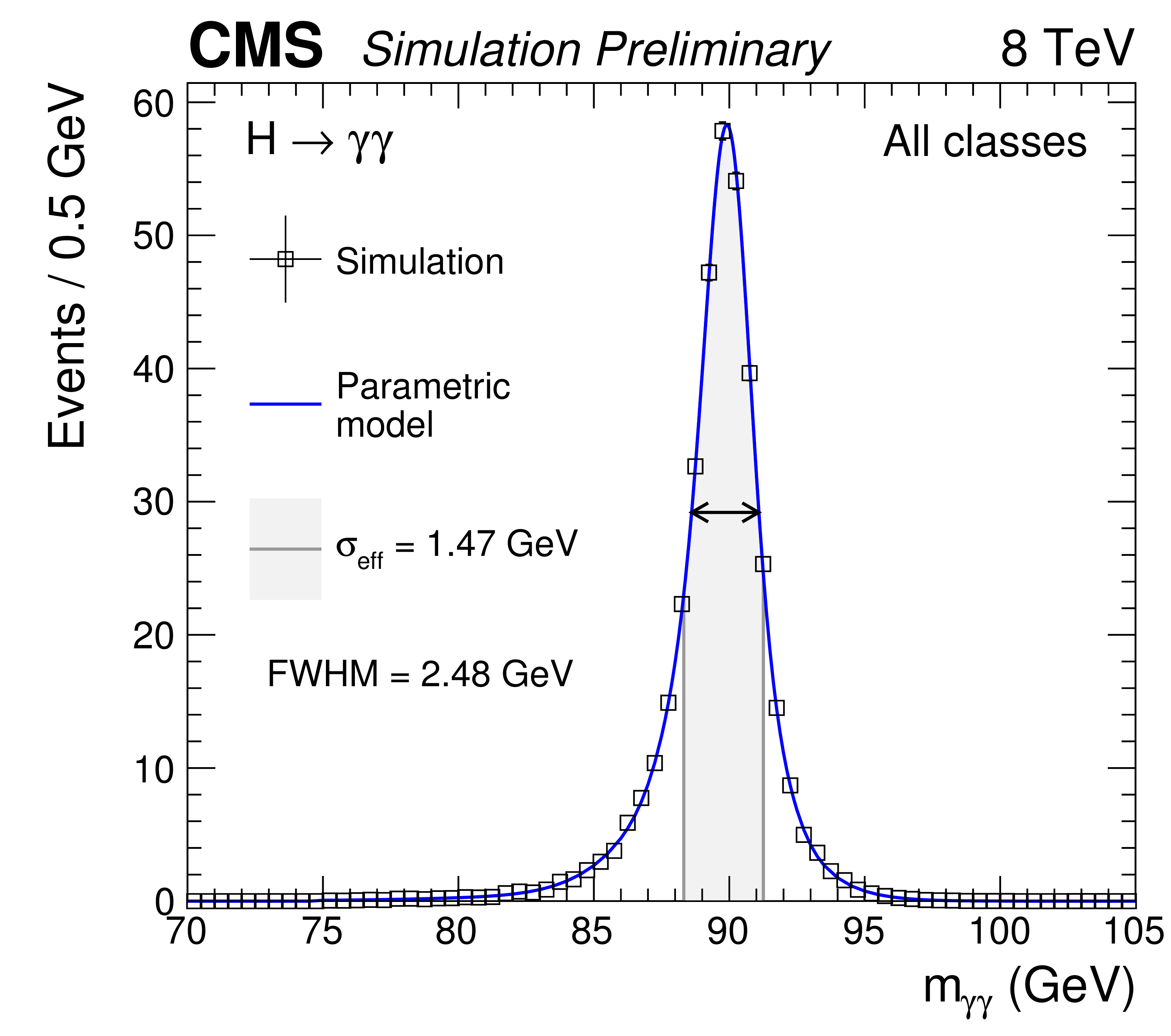
Figure 1-a:
Full parameterized signal shape integrated over all event classes, in simulated signal events with $ {m_{\mathrm {H}}} = $ 90 GeV at $\sqrt {s} = $ 8 TeV. The open points are the weighted MC events and the blue lines are the corresponding parametric models. Also shown are the effective $\sigma $ ($\sigma _{\text {eff}}$) values and the corresponding full width at half-maximum (FWHM), indicated by the position of the arrows on each distribution. |
png pdf |
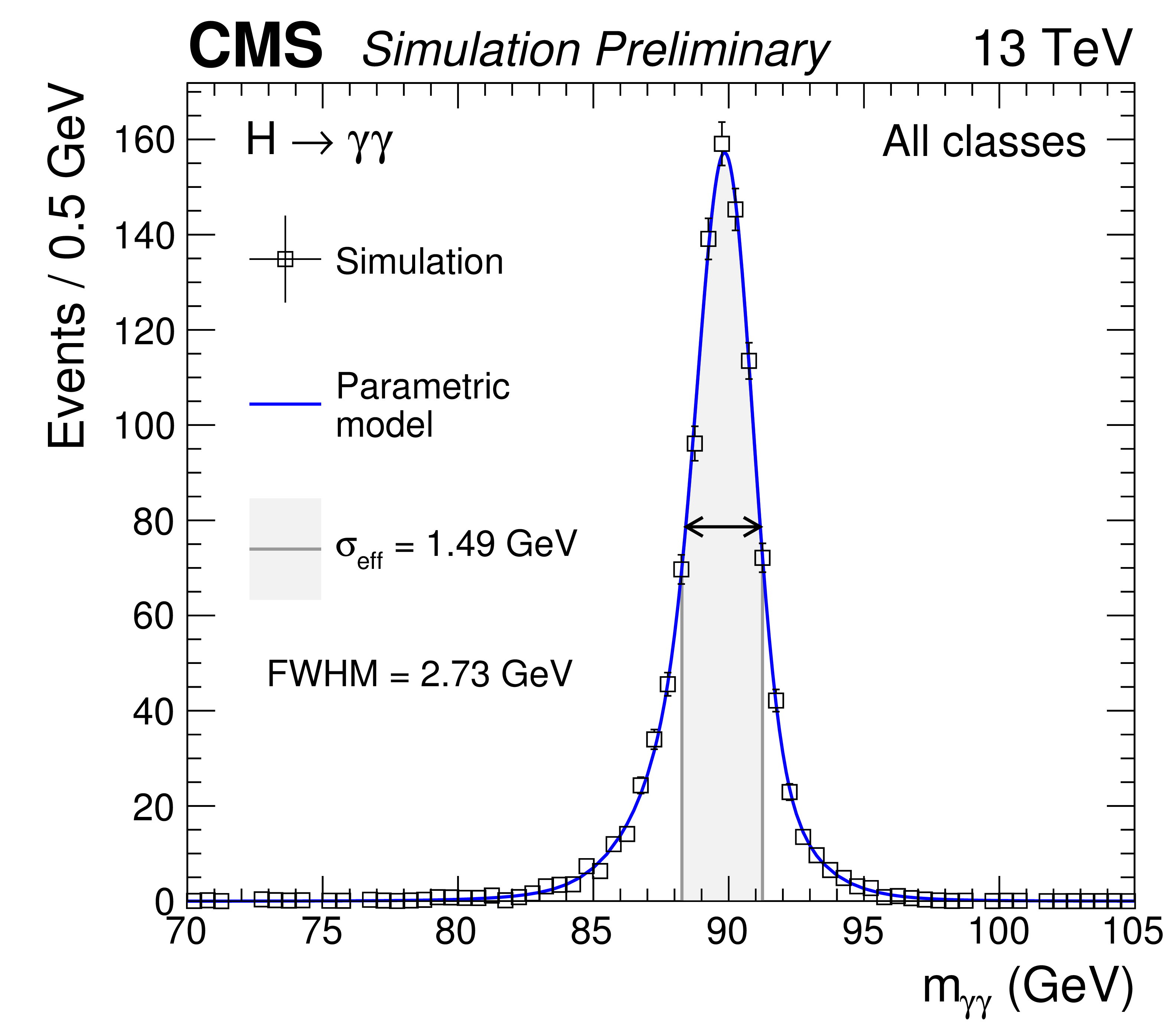
Figure 1-b:
Full parameterized signal shape integrated over all event classes, in simulated signal events with $ {m_{\mathrm {H}}} = $ 90 GeV at $\sqrt {s} = $ 13 TeV. The open points are the weighted MC events and the blue lines are the corresponding parametric models. Also shown are the effective $\sigma $ ($\sigma _{\text {eff}}$) values and the corresponding full width at half-maximum (FWHM), indicated by the position of the arrows on each distribution. |
png pdf |
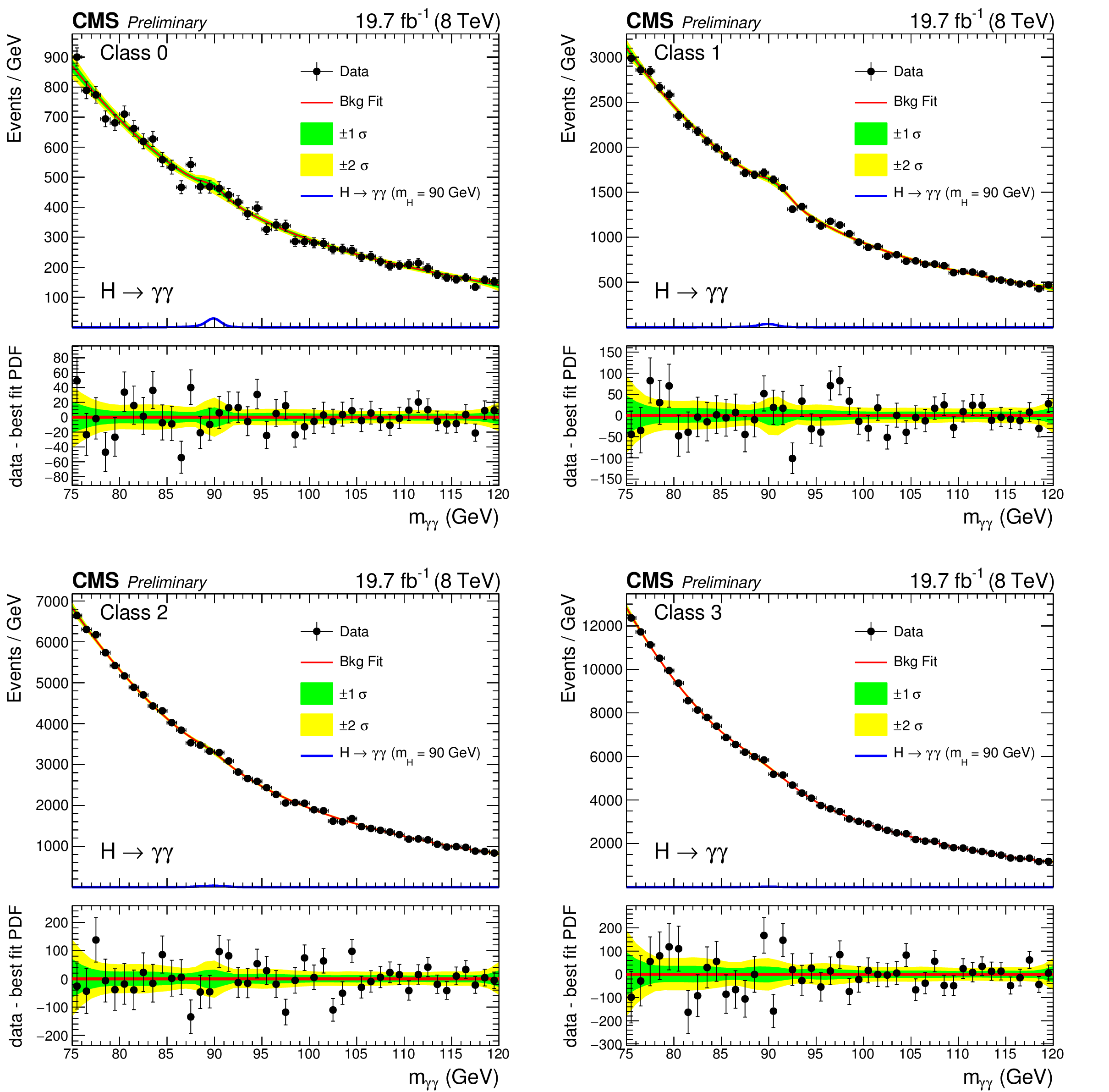
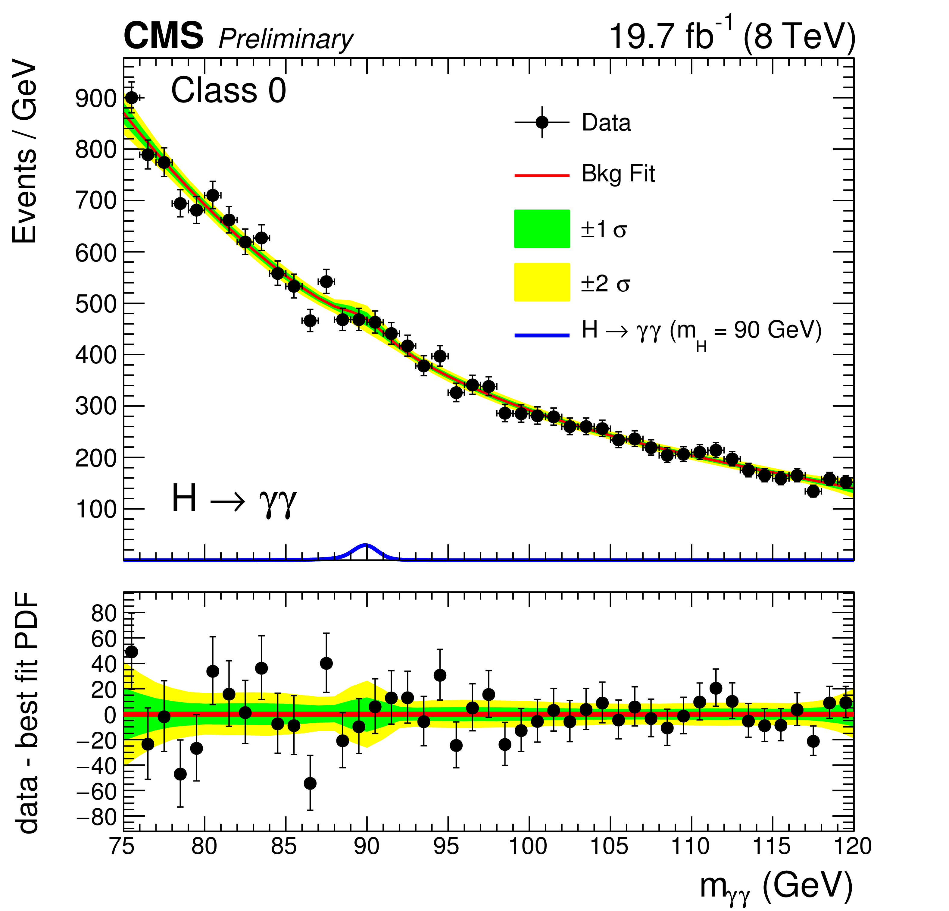
Figure 2:
Background model fits using the chosen 'best-fit' parametrization (PDF) to data in the four event classes at $\sqrt {s} = $ 8 TeV. The deviations from monotonically decreasing behavior in the neighborhood of $m_{\gamma \gamma} = $ 90 GeV are consistent with surviving double-fake events from the $\mathrm{Z} \to {\mathrm{e^{+}} \mathrm{e^{-}}} $ Drell-Yan process. The corresponding signal model for each class for $ {m_{\mathrm {H}}} = $ 90 GeV is also shown. The error bands, shown for illustration purposes only, reflect the uncertainty on the background model normalization associated with the statistical uncertainties of the fits. The difference between the data and the best-fit PDF is shown below. |
png pdf |
Figure 2-a:
Background model fits using the chosen 'best-fit' parametrization (PDF) to data in class 0 at $\sqrt {s} = $ 8 TeV. The deviations from monotonically decreasing behavior in the neighborhood of $m_{\gamma \gamma} = $ 90 GeV are consistent with surviving double-fake events from the $\mathrm{Z} \to {\mathrm{e^{+}} \mathrm{e^{-}}} $ Drell-Yan process. The corresponding signal model for $ {m_{\mathrm {H}}} = $ 90 GeV is also shown. The error bands, shown for illustration purposes only, reflect the uncertainty on the background model normalization associated with the statistical uncertainties of the fits. The difference between the data and the best-fit PDF is shown below. |
png pdf |
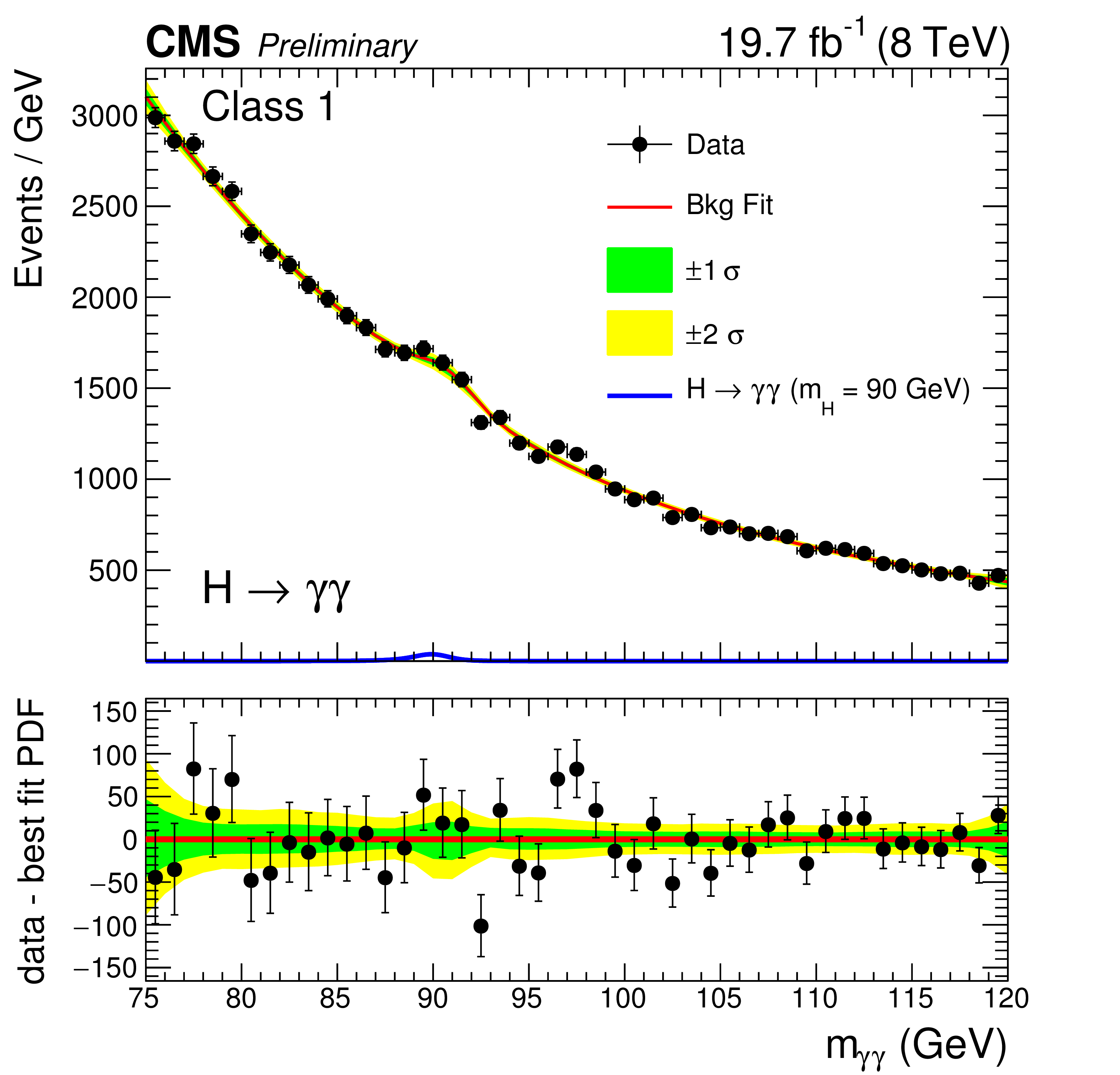
Figure 2-b:
Background model fits using the chosen 'best-fit' parametrization (PDF) to data in class 1 at $\sqrt {s} = $ 8 TeV. The deviations from monotonically decreasing behavior in the neighborhood of $m_{\gamma \gamma} = $ 90 GeV are consistent with surviving double-fake events from the $\mathrm{Z} \to {\mathrm{e^{+}} \mathrm{e^{-}}} $ Drell-Yan process. The corresponding signal model for $ {m_{\mathrm {H}}} = $ 90 GeV is also shown. The error bands, shown for illustration purposes only, reflect the uncertainty on the background model normalization associated with the statistical uncertainties of the fits. The difference between the data and the best-fit PDF is shown below. |
png pdf |
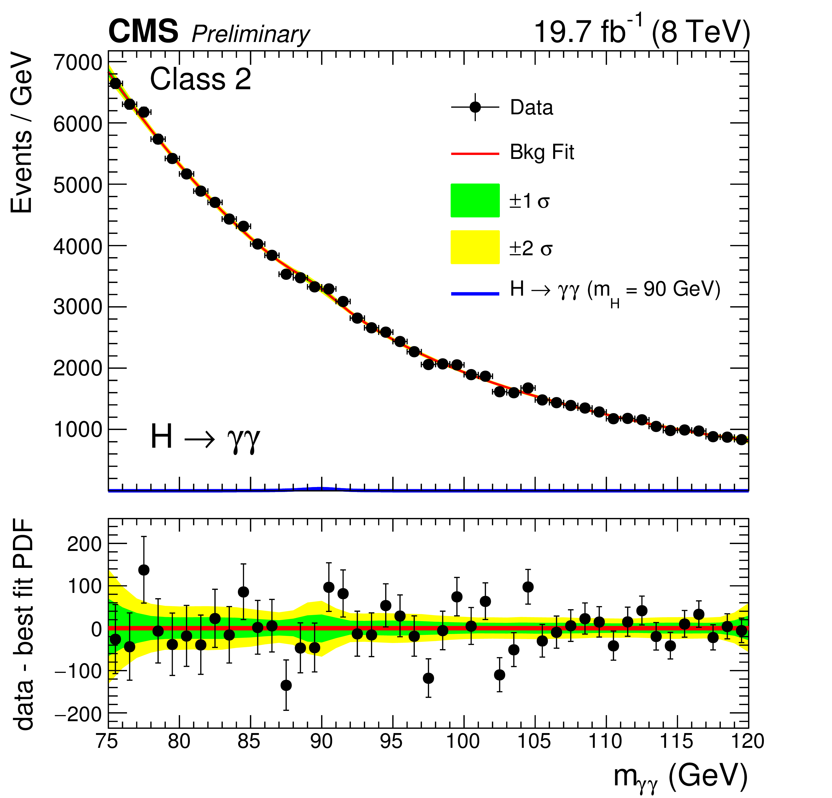
Figure 2-c:
Background model fits using the chosen 'best-fit' parametrization (PDF) to data in class 2 at $\sqrt {s} = $ 8 TeV. The deviations from monotonically decreasing behavior in the neighborhood of $m_{\gamma \gamma} = $ 90 GeV are consistent with surviving double-fake events from the $\mathrm{Z} \to {\mathrm{e^{+}} \mathrm{e^{-}}} $ Drell-Yan process. The corresponding signal model for $ {m_{\mathrm {H}}} = $ 90 GeV is also shown. The error bands, shown for illustration purposes only, reflect the uncertainty on the background model normalization associated with the statistical uncertainties of the fits. The difference between the data and the best-fit PDF is shown below. |
png pdf |
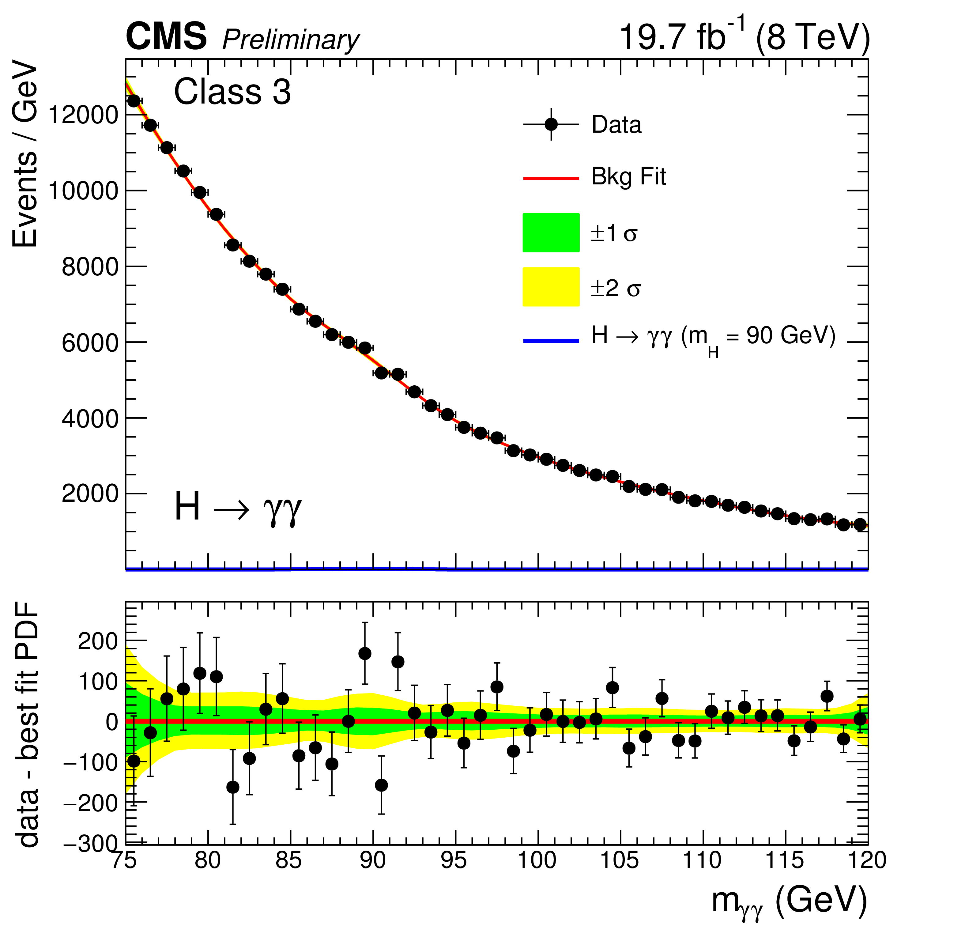
Figure 2-d:
Background model fits using the chosen 'best-fit' parametrization (PDF) to data in class 3 at $\sqrt {s} = $ 8 TeV. The deviations from monotonically decreasing behavior in the neighborhood of $m_{\gamma \gamma} = $ 90 GeV are consistent with surviving double-fake events from the $\mathrm{Z} \to {\mathrm{e^{+}} \mathrm{e^{-}}} $ Drell-Yan process. The corresponding signal model for $ {m_{\mathrm {H}}} = $ 90 GeV is also shown. The error bands, shown for illustration purposes only, reflect the uncertainty on the background model normalization associated with the statistical uncertainties of the fits. The difference between the data and the best-fit PDF is shown below. |
png pdf |
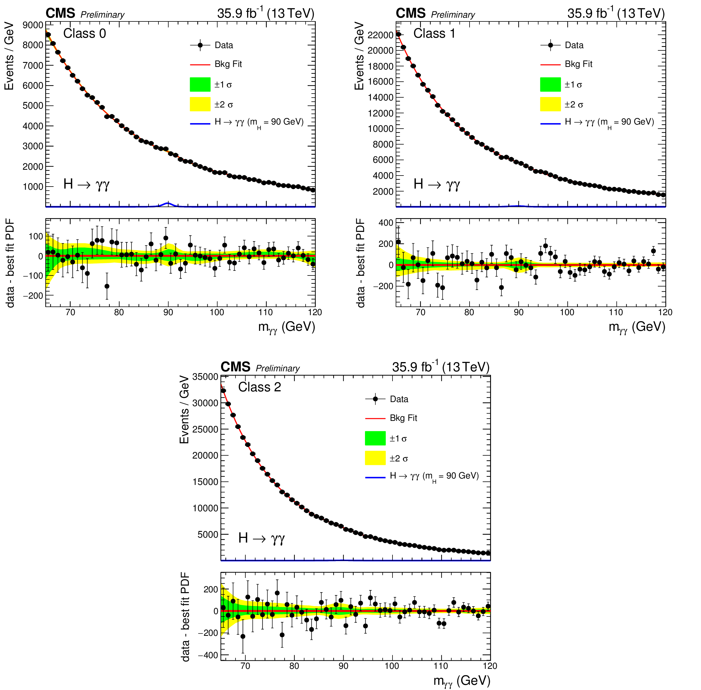
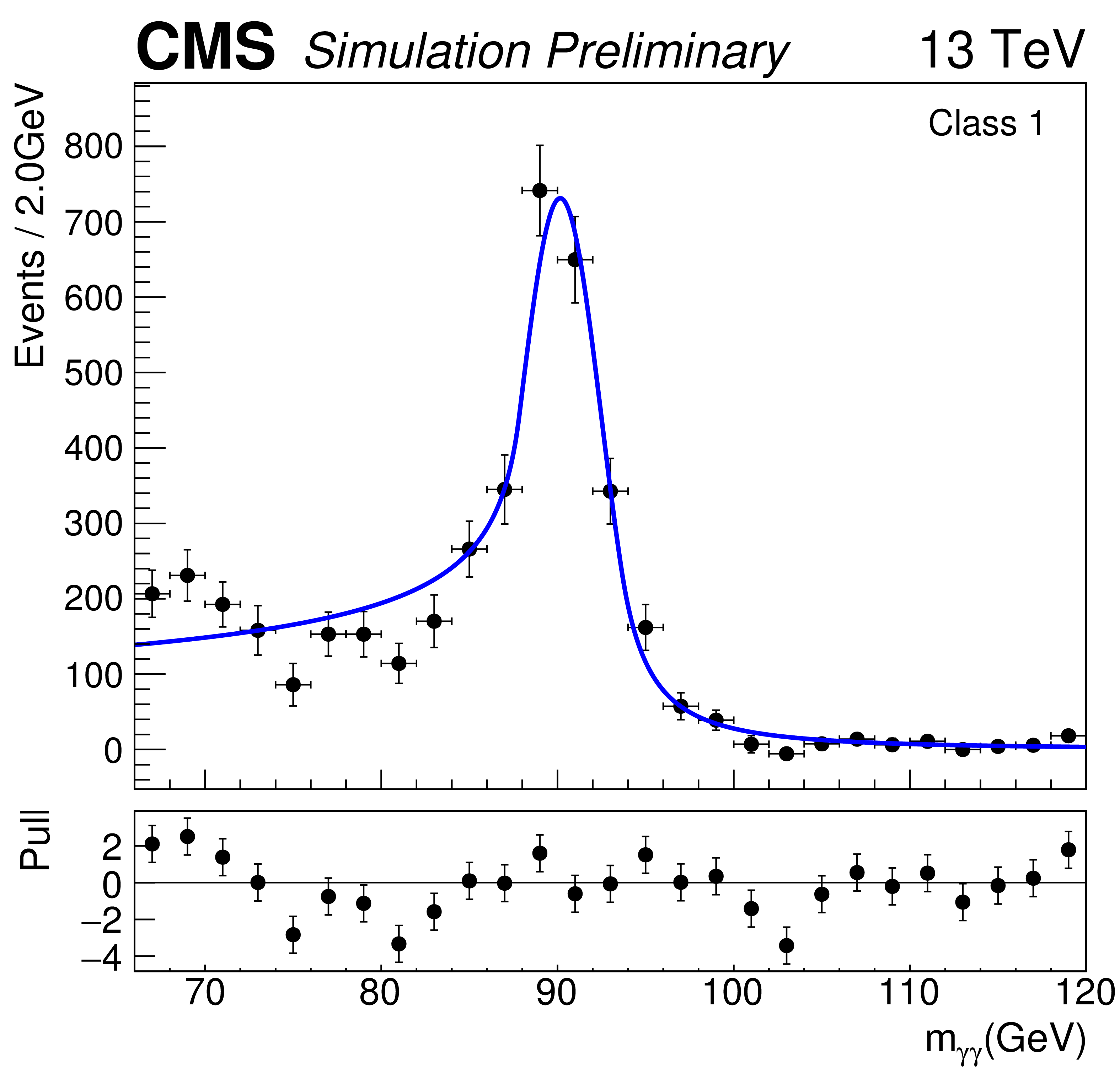
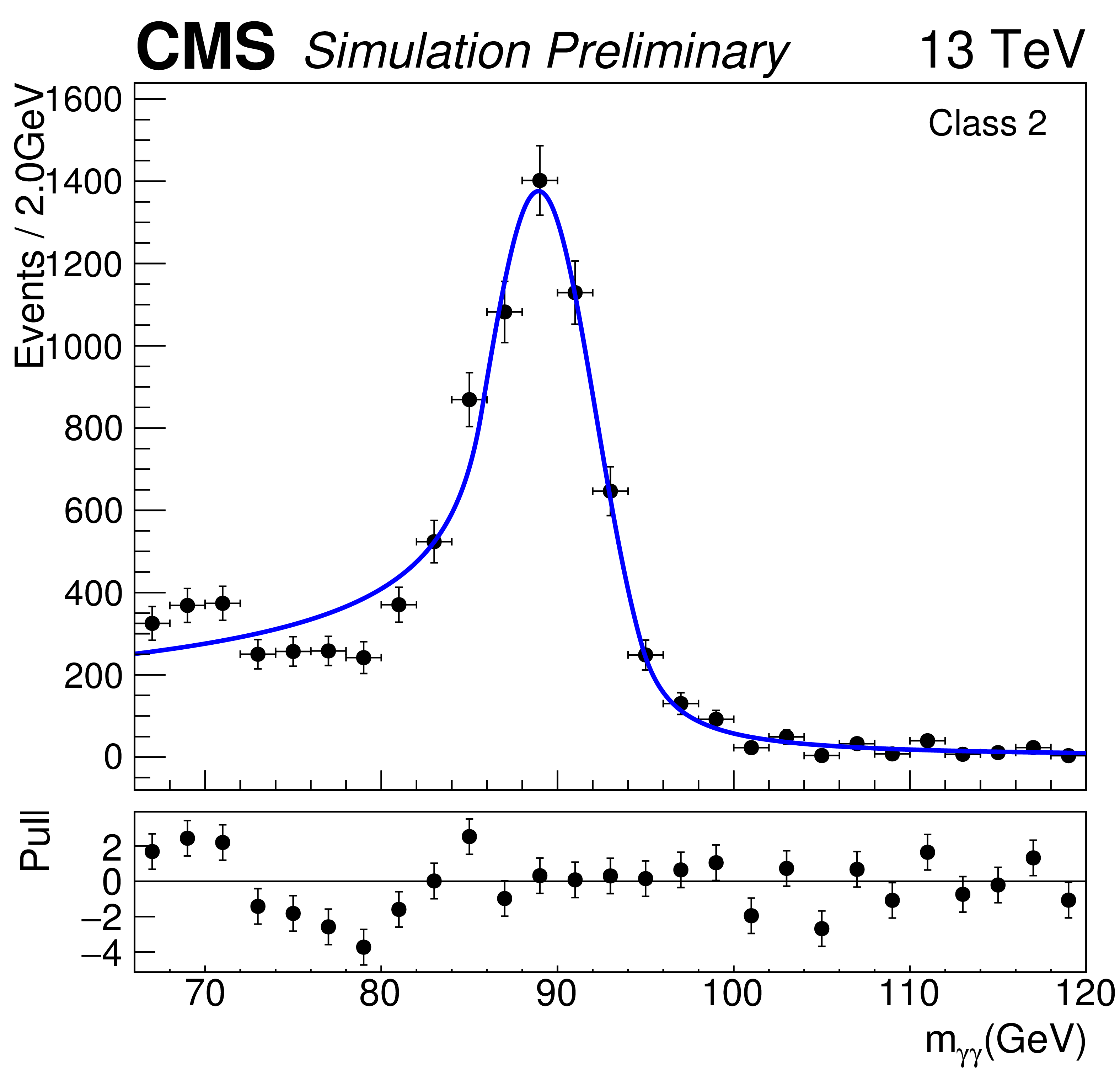
Figure 3:
Background model fits using the chosen 'best-fit' parametrization (PDF) to data in the three event classes at $\sqrt {s} = $ 13 TeV. The deviations from monotonically decreasing behavior in the neighborhood of $m_{\gamma \gamma} = $ 90 GeV are consistent with surviving double-fake events from the $\mathrm{Z} \to {\mathrm{e^{+}} \mathrm{e^{-}}} $ Drell-Yan process. The corresponding signal model for each class for $ {m_{\mathrm {H}}} = $ 90 GeV is also shown. The error bands, shown for illustration purposes only, reflect the uncertainty on the background model normalization associated with the statistical uncertainties of the fits. The difference between the data and the best-fit PDF is shown below. |
png pdf |
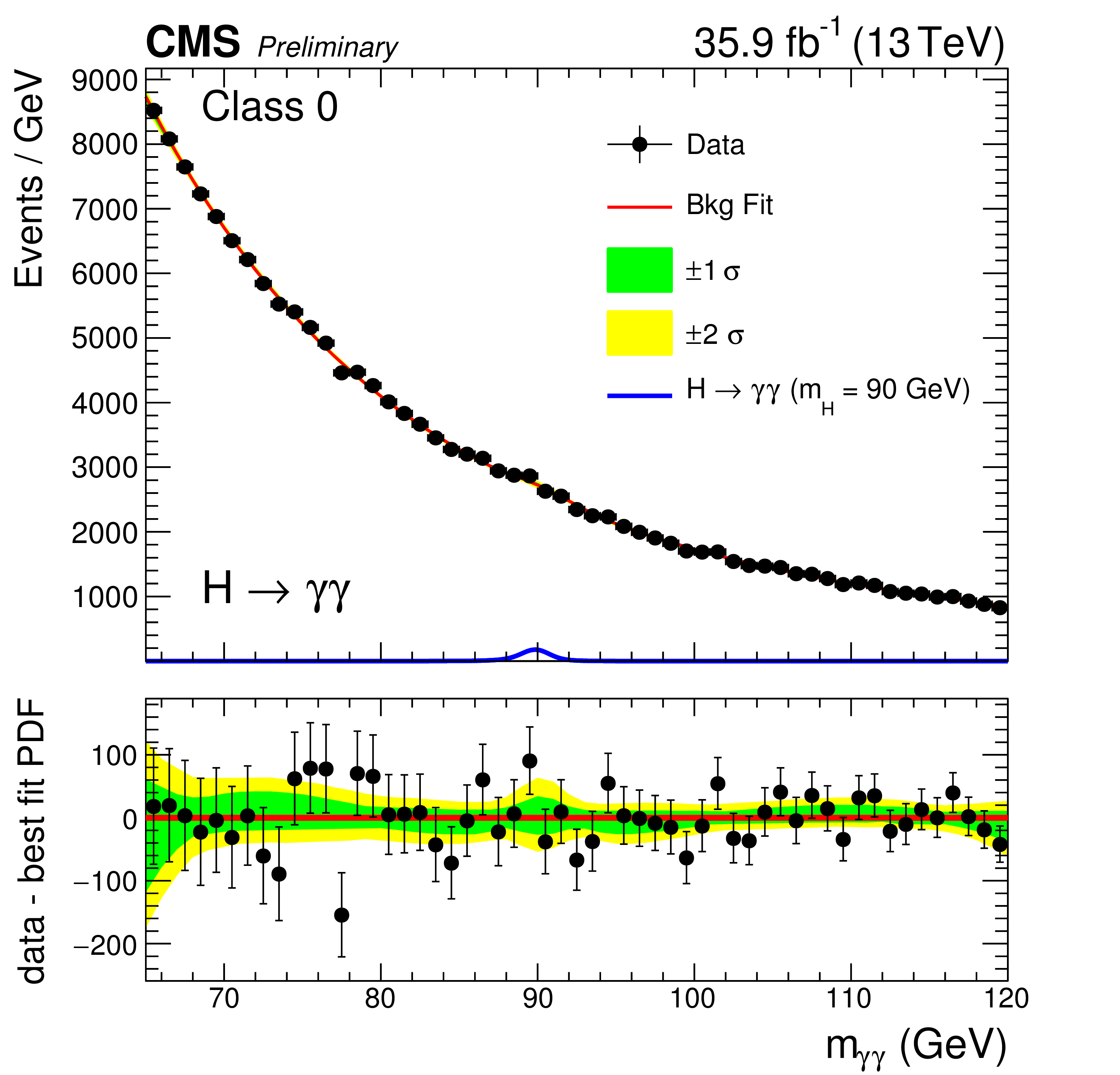
Figure 3-a:
Background model fits using the chosen 'best-fit' parametrization (PDF) to data in class 0 at $\sqrt {s} = $ 13 TeV. The deviations from monotonically decreasing behavior in the neighborhood of $m_{\gamma \gamma} = $ 90 GeV are consistent with surviving double-fake events from the $\mathrm{Z} \to {\mathrm{e^{+}} \mathrm{e^{-}}} $ Drell-Yan process. The corresponding signal model for $ {m_{\mathrm {H}}} = $ 90 GeV is also shown. The error bands, shown for illustration purposes only, reflect the uncertainty on the background model normalization associated with the statistical uncertainties of the fits. The difference between the data and the best-fit PDF is shown below. |
png pdf |
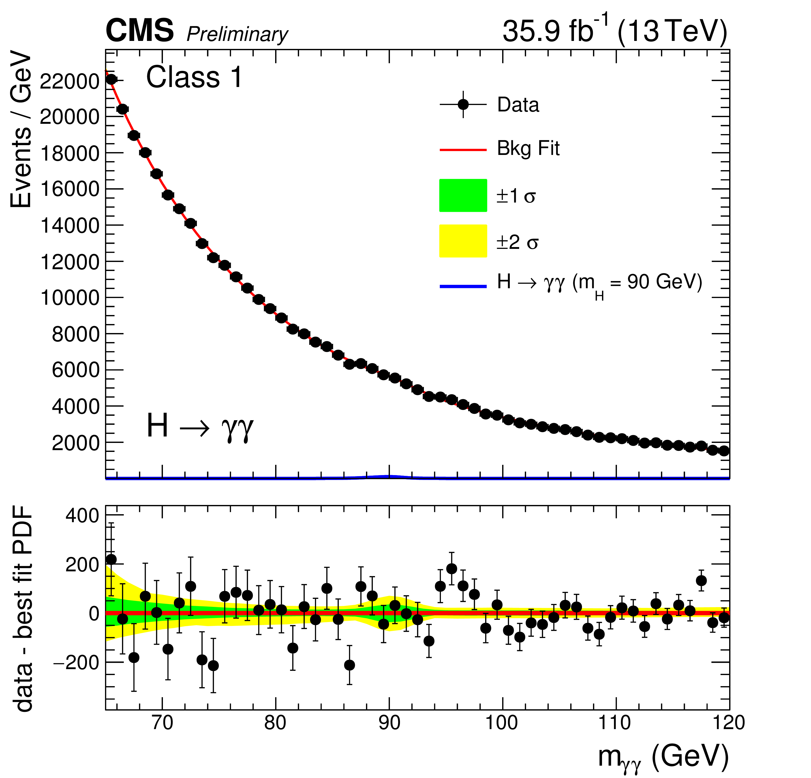
Figure 3-b:
Background model fits using the chosen 'best-fit' parametrization (PDF) to data in class 1 at $\sqrt {s} = $ 13 TeV. The deviations from monotonically decreasing behavior in the neighborhood of $m_{\gamma \gamma} = $ 90 GeV are consistent with surviving double-fake events from the $\mathrm{Z} \to {\mathrm{e^{+}} \mathrm{e^{-}}} $ Drell-Yan process. The corresponding signal model for $ {m_{\mathrm {H}}} = $ 90 GeV is also shown. The error bands, shown for illustration purposes only, reflect the uncertainty on the background model normalization associated with the statistical uncertainties of the fits. The difference between the data and the best-fit PDF is shown below. |
png pdf |
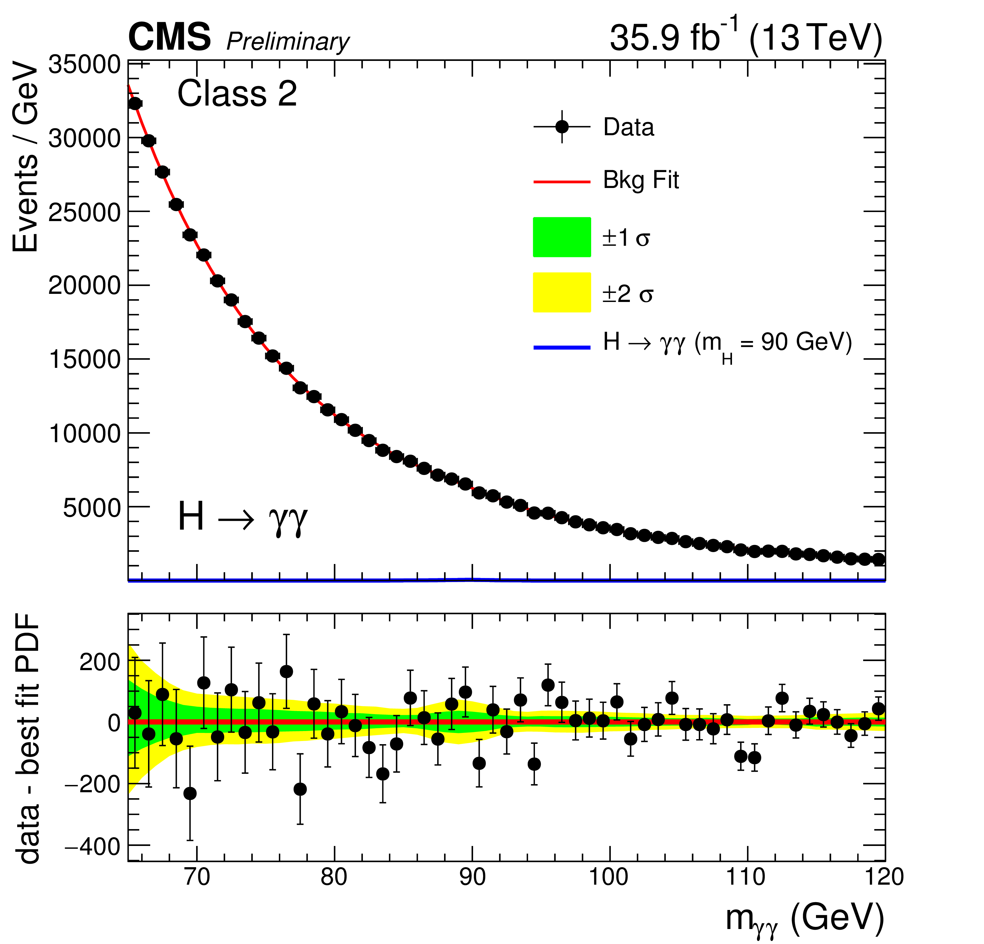
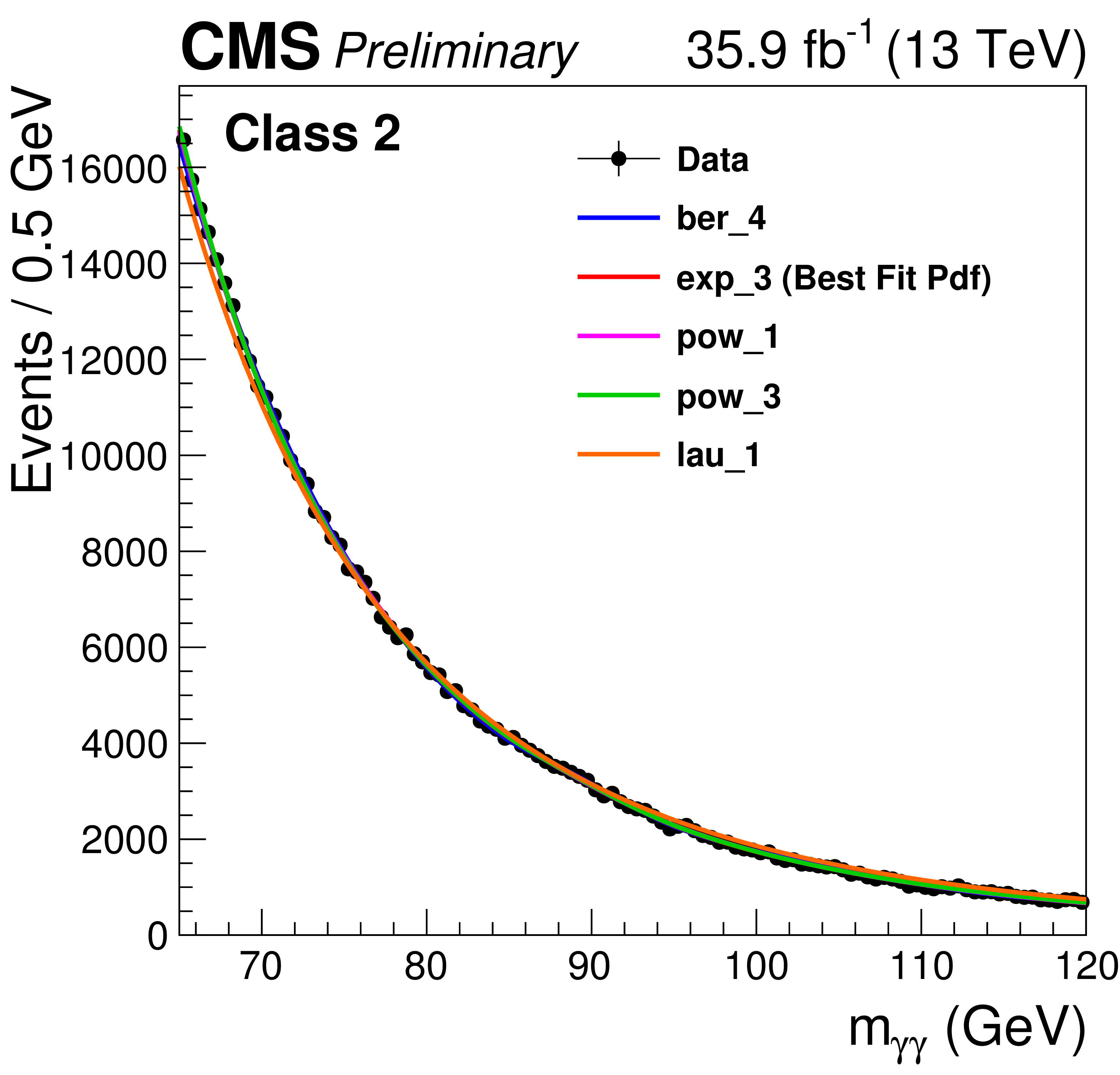
Figure 3-c:
Background model fits using the chosen 'best-fit' parametrization (PDF) to data in class 2 at $\sqrt {s} = $ 13 TeV. The deviations from monotonically decreasing behavior in the neighborhood of $m_{\gamma \gamma} = $ 90 GeV are consistent with surviving double-fake events from the $\mathrm{Z} \to {\mathrm{e^{+}} \mathrm{e^{-}}} $ Drell-Yan process. The corresponding signal model for $ {m_{\mathrm {H}}} = $ 90 GeV is also shown. The error bands, shown for illustration purposes only, reflect the uncertainty on the background model normalization associated with the statistical uncertainties of the fits. The difference between the data and the best-fit PDF is shown below. |
png pdf |
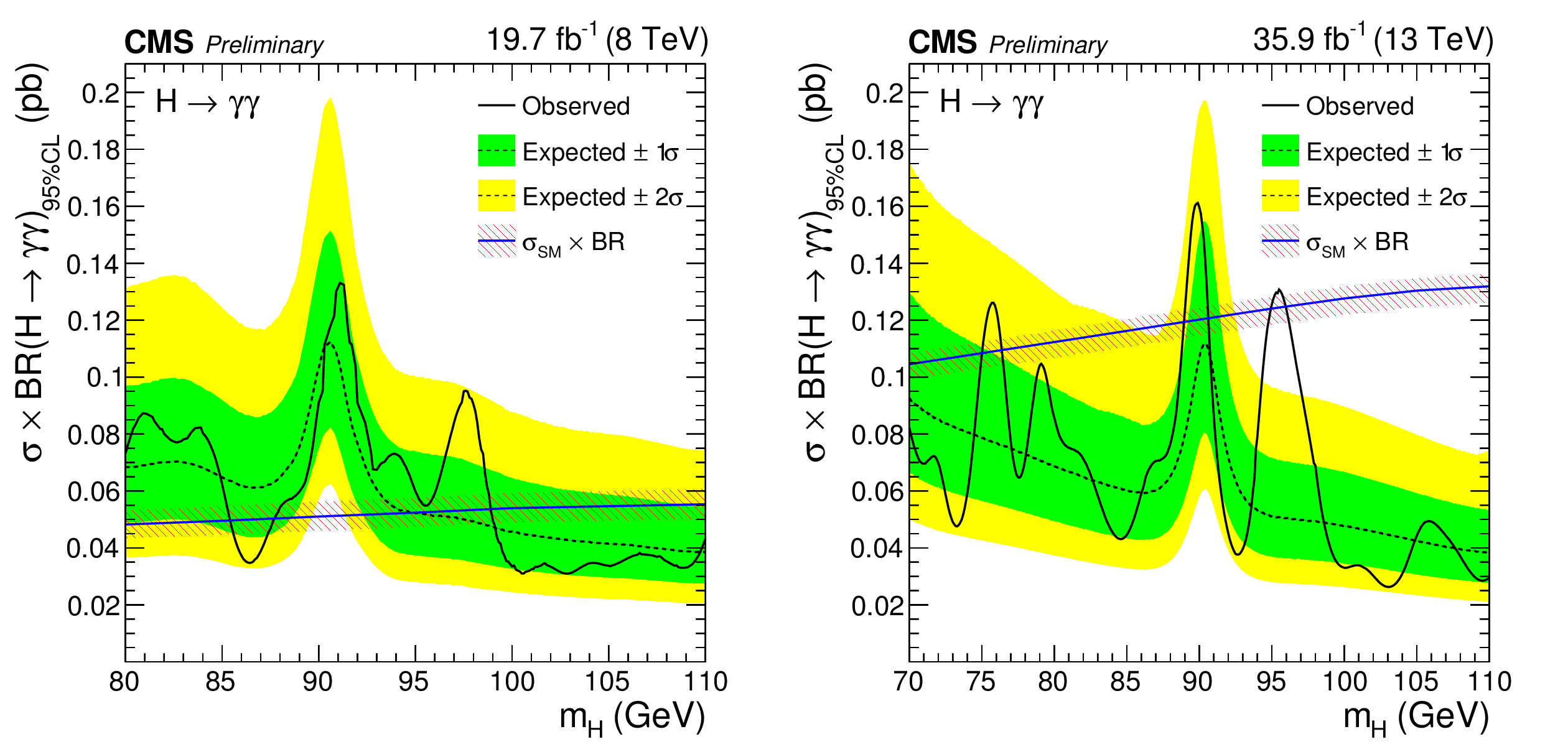
Figure 4:
Expected and observed exclusion limits (95% CL) on the production cross section times branching ratio into two photons for an SM-like second Higgs boson in the asymptotic CLs approximation, from the analysis of the 8 TeV (left) and 13 TeV (right) datasets. The inner (green) bands and the outer (yellow) bands indicate the regions containing 68 and 95%, respectively, of the distribution of limits expected under the background-only hypothesis. The theoretical prediction for the cross-section times branching ratio into two photons of an SM-like Higgs boson, $\sigma _{\text {SM}}\times \text {BR}$ is shown as a blue line, with the red-hatched band indicating its uncertainty [47,48]. |
png pdf |
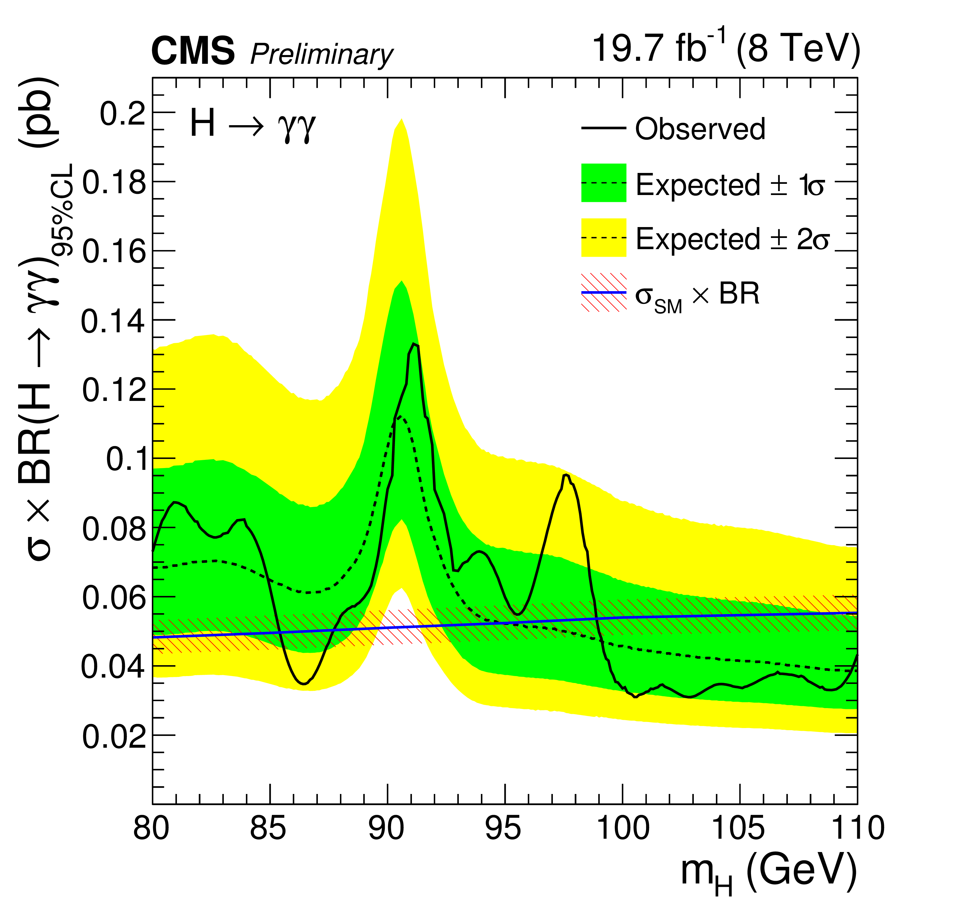
Figure 4-a:
Expected and observed exclusion limits (95% CL) on the production cross section times branching ratio into two photons for an SM-like second Higgs boson in the asymptotic CLs approximation, from the analysis of the 8 TeV dataset. The inner (green) bands and the outer (yellow) bands indicate the regions containing 68 and 95%, respectively, of the distribution of limits expected under the background-only hypothesis. The theoretical prediction for the cross-section times branching ratio into two photons of an SM-like Higgs boson, $\sigma _{\text {SM}}\times \text {BR}$ is shown as a blue line, with the red-hatched band indicating its uncertainty [47,48]. |
png pdf |
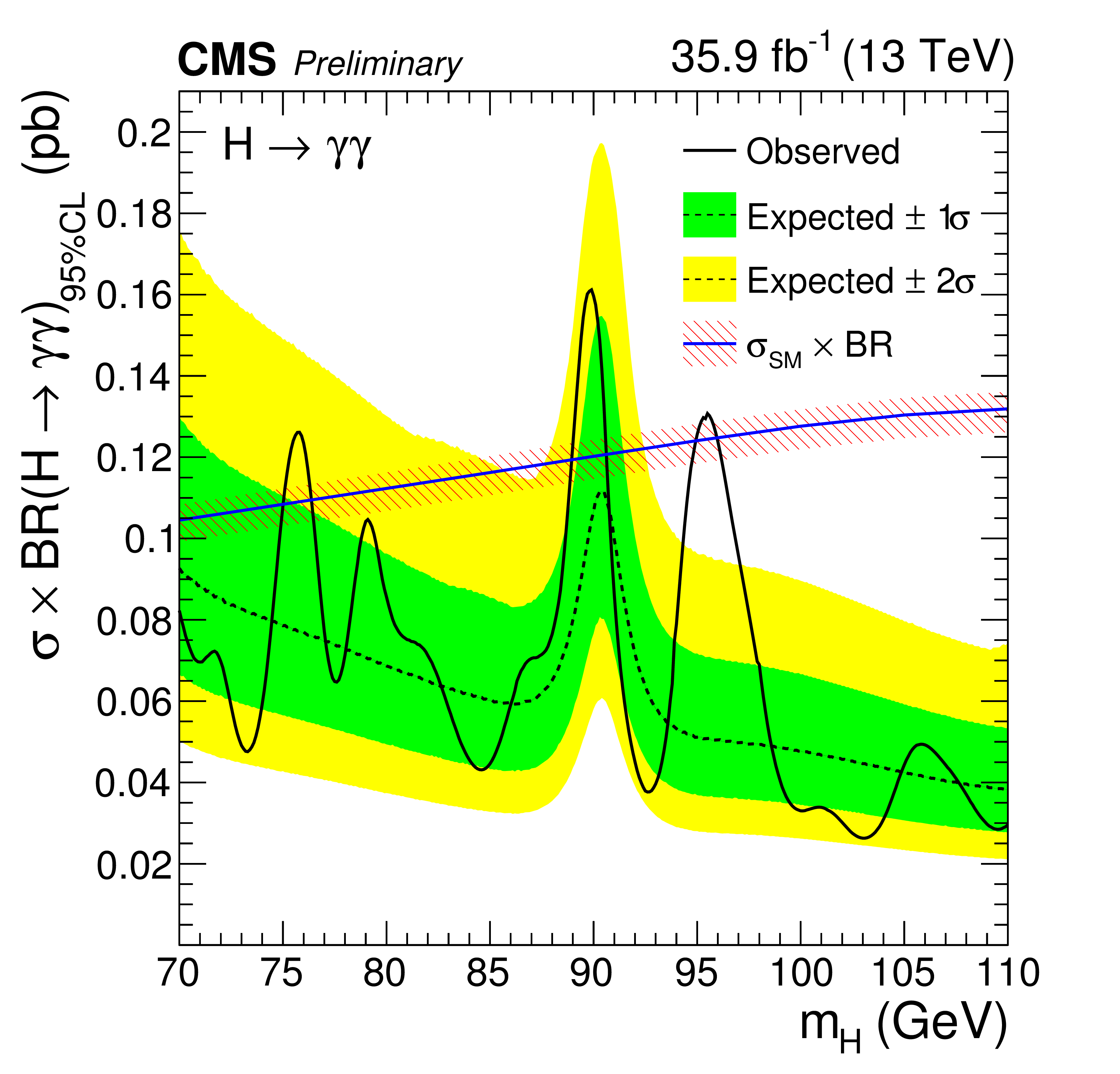
Figure 4-b:
Expected and observed exclusion limits (95% CL) on the production cross section times branching ratio into two photons for an SM-like second Higgs boson in the asymptotic CLs approximation, from the analysis of the 13 TeV dataset. The inner (green) bands and the outer (yellow) bands indicate the regions containing 68 and 95%, respectively, of the distribution of limits expected under the background-only hypothesis. The theoretical prediction for the cross-section times branching ratio into two photons of an SM-like Higgs boson, $\sigma _{\text {SM}}\times \text {BR}$ is shown as a blue line, with the red-hatched band indicating its uncertainty [47,48]. |
png pdf |
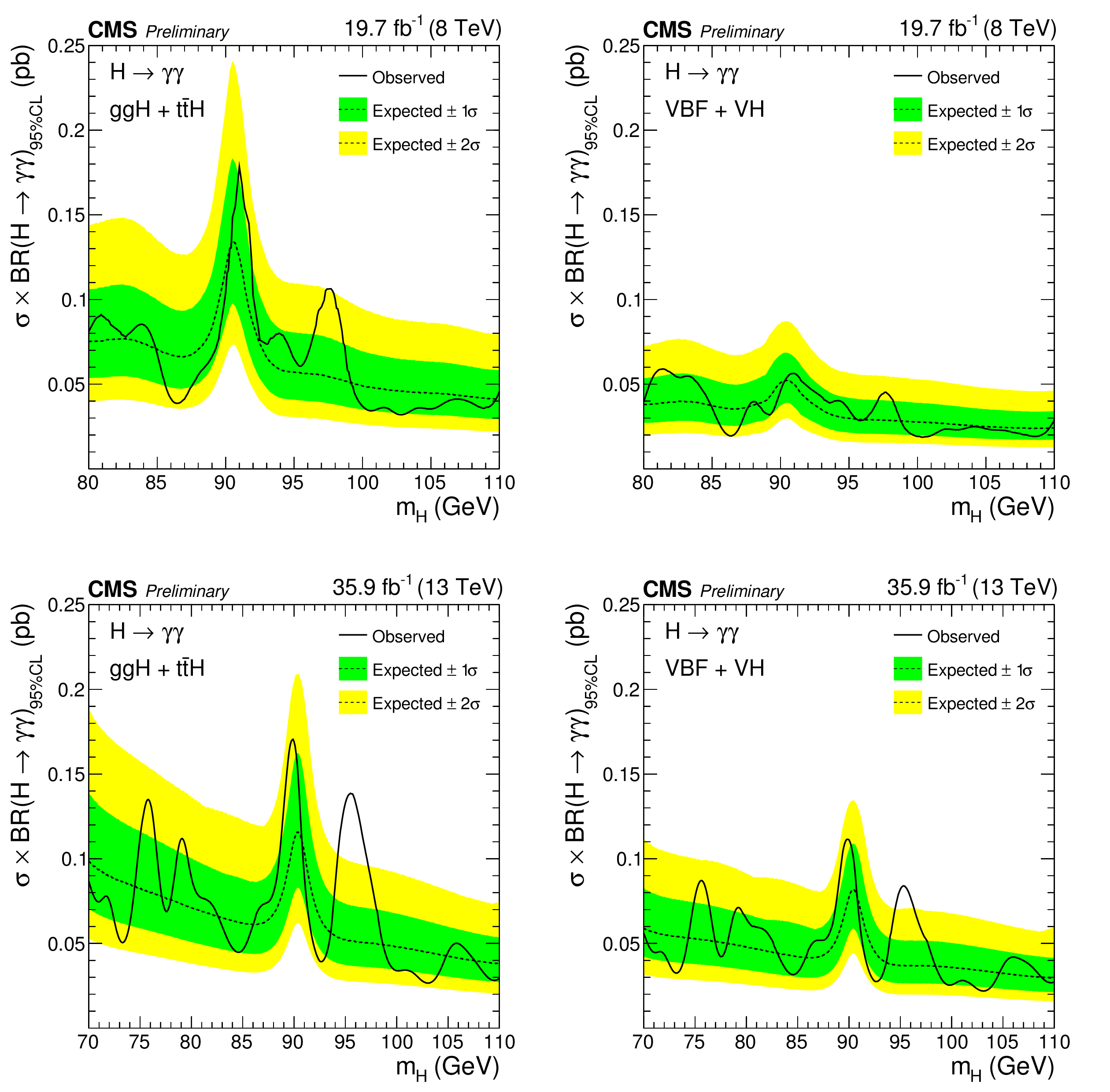
Figure 5:
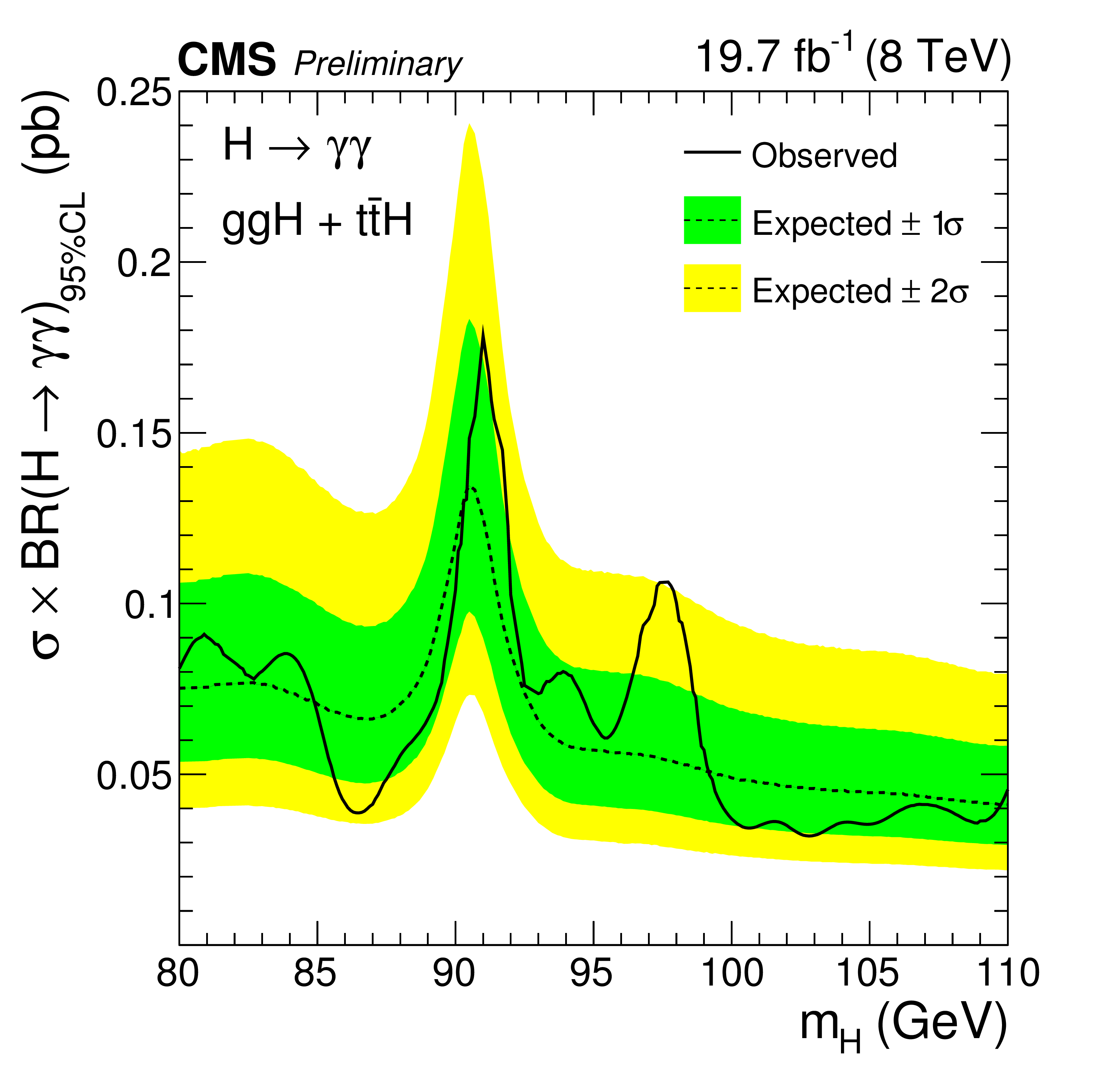
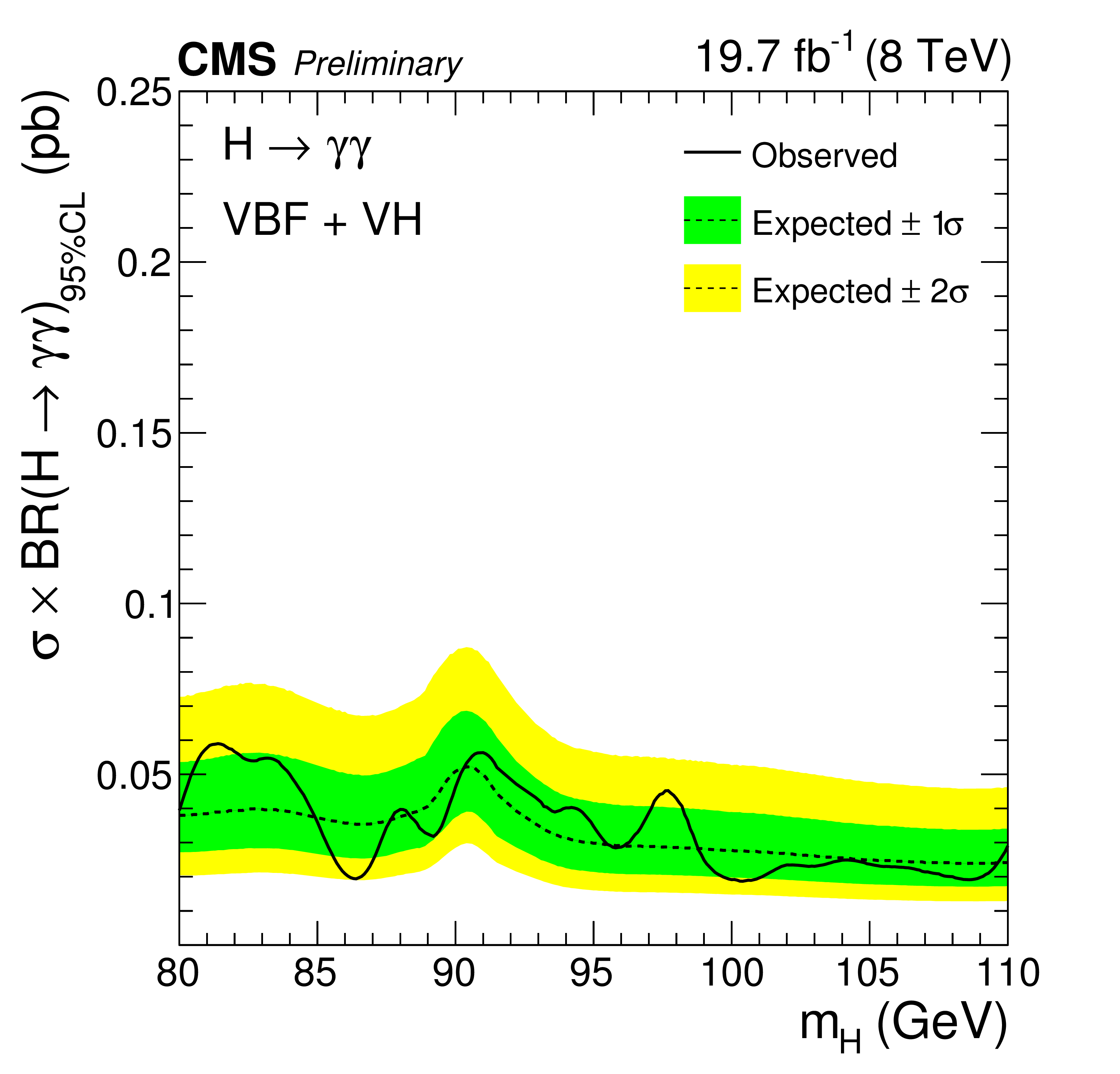
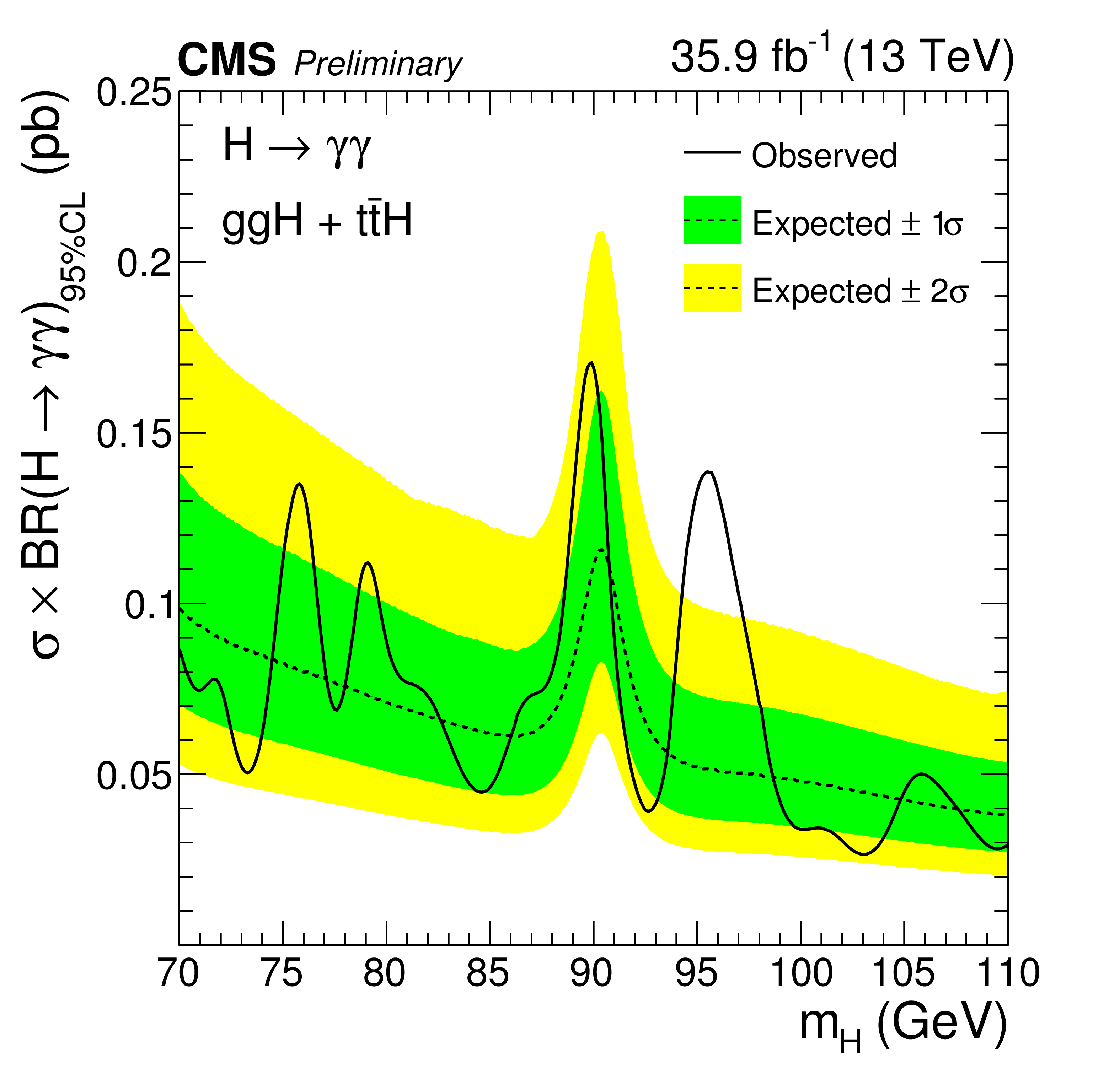
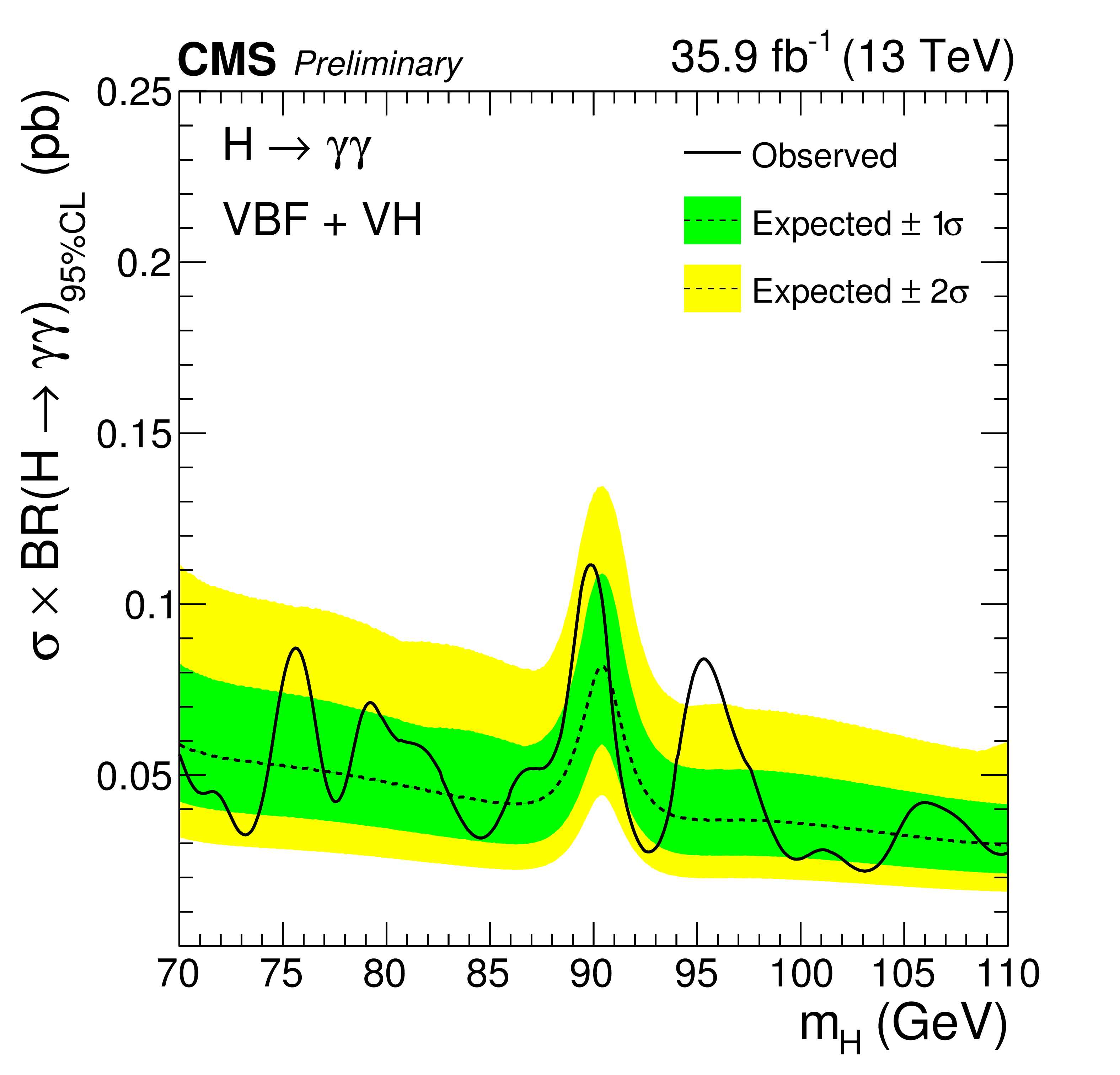
Expected and observed exclusion limits (95% CL) on the production cross section times branching ratio into two photons for a second Higgs boson in the asymptotic CLs approximation for the ggH plus $\text {t}\overline {\text {t}}$H (left) and VBF plus VH (right) processes, from the analysis of the 8 TeV (top) and 13 TeV (bottom) datasets. The inner (green) bands and the outer (yellow) bands indicate the regions containing 68 and 95%, respectively, of the distribution of limits expected under the background-only hypothesis. |
png pdf |
Figure 5-a:
Expected and observed exclusion limits (95% CL) on the production cross section times branching ratio into two photons for a second Higgs boson in the asymptotic CLs approximation for the ggH plus $\text {t}\overline {\text {t}}$H processes, from the analysis of the 8 TeV dataset. The inner (green) bands and the outer (yellow) bands indicate the regions containing 68 and 95%, respectively, of the distribution of limits expected under the background-only hypothesis. |
png pdf |
Figure 5-b:
Expected and observed exclusion limits (95% CL) on the production cross section times branching ratio into two photons for a second Higgs boson in the asymptotic CLs approximation for the VBF plus VH processes, from the analysis of the 8 TeV dataset. The inner (green) bands and the outer (yellow) bands indicate the regions containing 68 and 95%, respectively, of the distribution of limits expected under the background-only hypothesis. |
png pdf |
Figure 5-c:
Expected and observed exclusion limits (95% CL) on the production cross section times branching ratio into two photons for a second Higgs boson in the asymptotic CLs approximation for the ggH plus $\text {t}\overline {\text {t}}$H processes, from the analysis of the 13 TeV dataset. The inner (green) bands and the outer (yellow) bands indicate the regions containing 68 and 95%, respectively, of the distribution of limits expected under the background-only hypothesis. |
png pdf |
Figure 5-d:
Expected and observed exclusion limits (95% CL) on the production cross section times branching ratio into two photons for a second Higgs boson in the asymptotic CLs approximation for the VBF plus VH processes, from the analysis of the 13 TeV dataset. The inner (green) bands and the outer (yellow) bands indicate the regions containing 68 and 95%, respectively, of the distribution of limits expected under the background-only hypothesis. |
png pdf |
Figure 6:
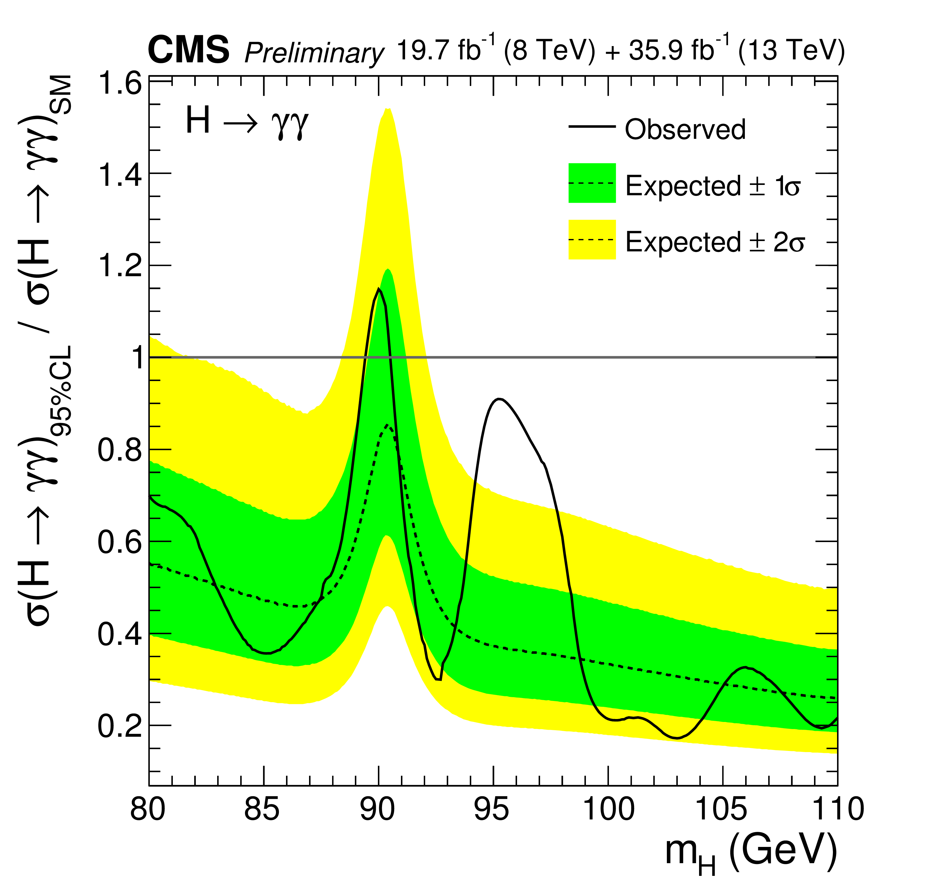
Expected and observed exclusion limits (95% CL) on the production cross section times branching ratio into two photons for a second Higgs boson relative to the expected SM-like expectation, in the asymptotic CLs approximation, from the analysis of the 8 and 13 TeV datasets. The inner (green) band and the outer (yellow) band indicate the regions containing 68 and 95%, respectively, of the distribution of limits expected under the background-only hypothesis. |
png pdf |
Figure 7:
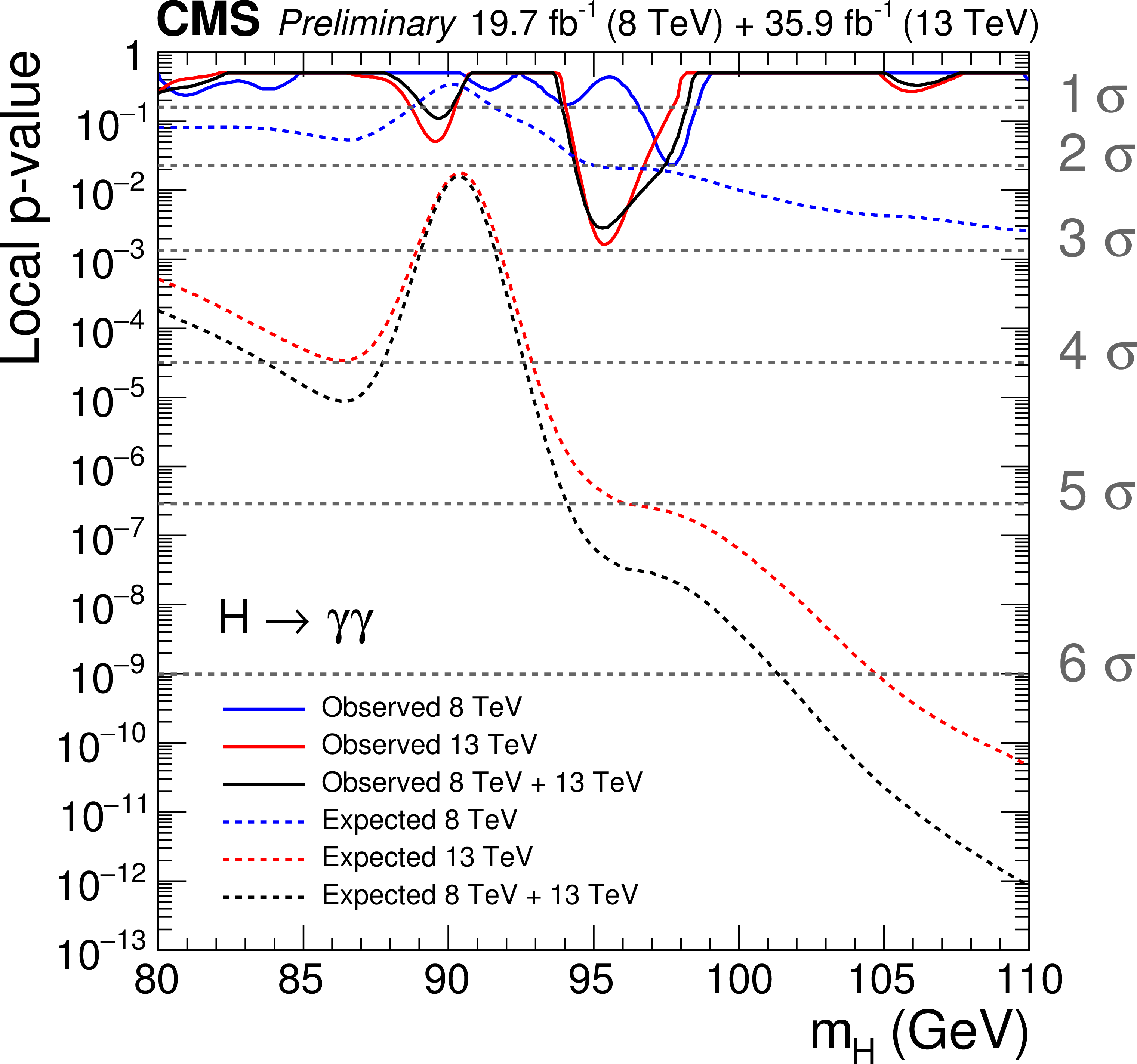
Observed local p-values as a function of $ {m_{\mathrm {H}}} $ for the 8 and 13 TeV datasets and their combination (solid curves) plotted together with the relevant expectations for an SM-like second Higgs boson (dotted curves). |
| Tables | |
png pdf |
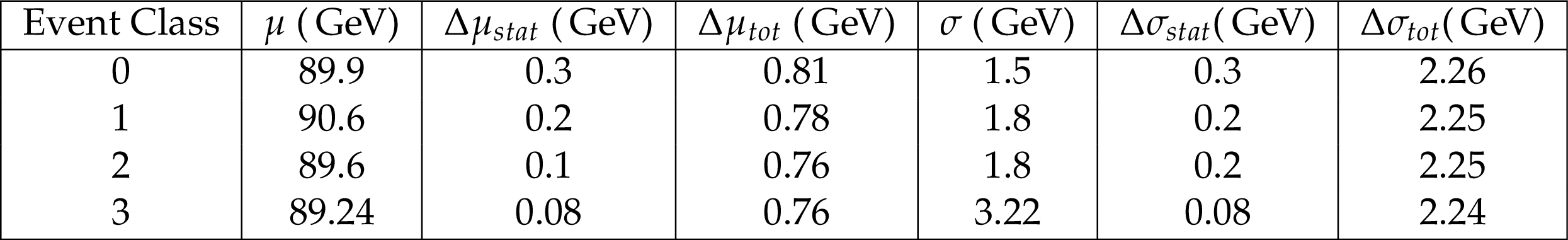
Table 1:
Values of $\mu $, $\sigma $ and their uncertainties from statistical errors on the double-fake fits, and the total uncertainty in each event class used in the final statistical analysis of the 8 TeV dataset. |
png pdf |
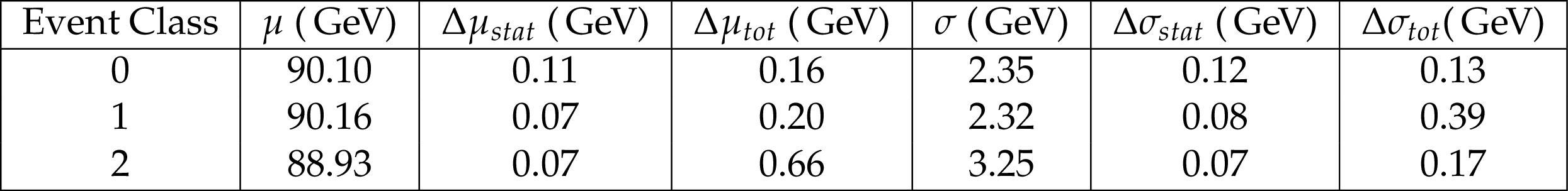
Table 2:
Values of $\mu $, $\sigma $ and their uncertainties from statistical errors on the double-fake fits, and the total uncertainty in each event class used in the final statistical analysis of the 13 TeV dataset. |
png pdf |
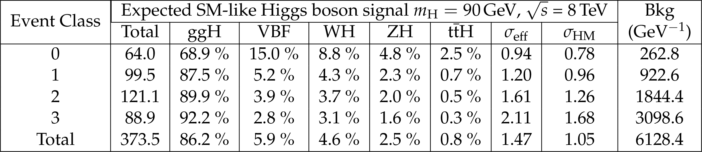
Table 3:
The expected number of signal events per event class and the corresponding percentage breakdown per production process, for the 8 TeV dataset. The values of $\sigma _{\text {eff}}$ and $\sigma _{\text {HM}}$ are also shown, as are the expected number of background events per GeV in a $\sigma _{\text {eff}}$ window centered on $ {m_{\mathrm {H}}} = $ 90 GeV. |
png pdf |
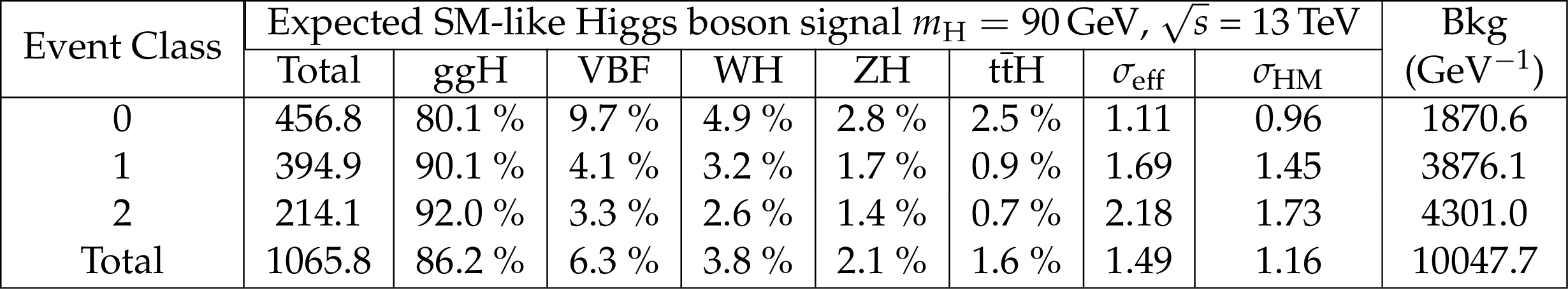
Table 4:
The expected number of signal events per event class and the corresponding percentage breakdown per production process, for the 13 TeV dataset. The values of $\sigma _{\text {eff}}$ and $\sigma _{\text {HM}}$ are also shown, as are the expected number of background events per GeV in a $\sigma _{\text {eff}}$ window centered on $ {m_{\mathrm {H}}} = $ 90 GeV. |
| Summary |
| A search for new low-mass resonances decaying to two photons has been presented. It is based upon data samples corresponding to integrated luminosities of 19.7 fb$^{-1}$ and 35.9 fb$^{-1}$ collected respectively at center-of-mass energies of 8 TeV in 2012 and 13 TeV in 2016. The search is performed in a mass range between 70 and 110 GeV. The expected and observed 95% confidence level upper limits on the product of the cross section times branching ratio into two photons for a second Higgs boson as well as the expected and observed local p-values are presented. No significant excess with respect to the expected limits is observed. For the 8 TeV dataset, the minimum(maximum) observed upper limit on the production cross section times branching ratio is approximately 31(133) fb corresponding to a mass hypothesis of 102.8(91.1) GeV. For the 13 TeV dataset, the minimum(maximum) observed upper limits are 26(161) fb corresponding to a mass hypothesis of 103.0(89.9) GeV. The statistical combination of the results from the analysis of the two datasets in the mass range between 80 and 110 GeV yields a minimum(maximum) observed upper limit on the production cross section times branching ratio normalized to the SM-like expectation of approximately 0.17 (1.15) corresponding to a mass hypothesis of 103.0(90.0) GeV. In the case of the 8 TeV dataset, one excess with approximately 2.0$\sigma$ local significance is observed for an hypothesis mass of 97.6 GeV. For the 13 TeV dataset, one excess with approximately 2.9$\sigma$ local (1.47$\sigma$ global) significance is observed for an hypothesis mass of 95.3 GeV. When combined statistically, these yield an excess with approximately 2.8$\sigma$ local (1.3$\sigma$ global) significance for the same hypothesis mass as for the 13 TeV dataset alone, 95.3 GeV. More data are required to ascertain the origin of this excess. These are the first LHC results to appear for a search for new resonances in the diphoton final state in this mass range, which include analysis of data at the center-of-mass energy of 13 TeV. |
| Additional Figures | |
png pdf |
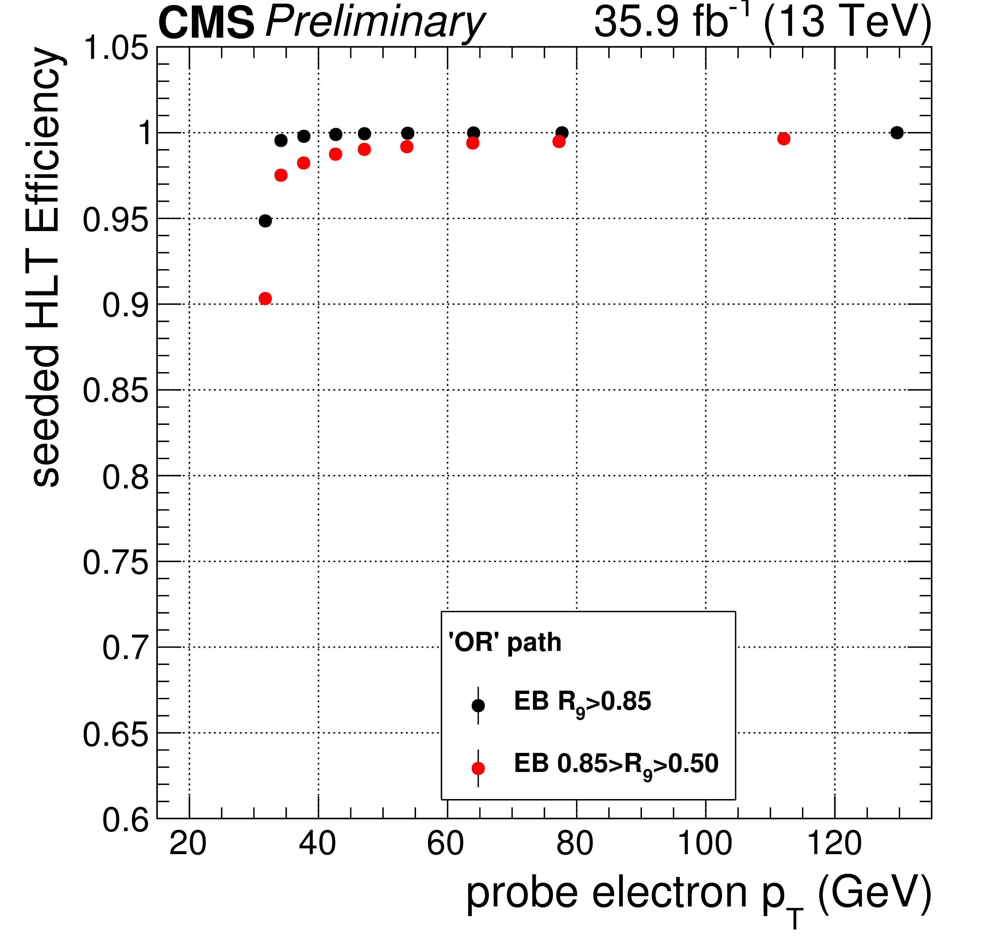
Additional Figure 1:
Efficiency for the seeded leg measured on data for $\mathrm{ Z\to ee }$ events using the tag-and-probe method, for the 'OR' high-level trigger (HLT) path used for the analysis of the 13 TeV dataset, with respect to offline probe electron $p_{\mathrm{T}}$, for ECAL barrel photons with $ {R_\mathrm {9}} > $ 0.85 (black) and 0.5 $ < {R_\mathrm {9}} < $ 0.85 (red). Variable bin widths have been used. |
png pdf |
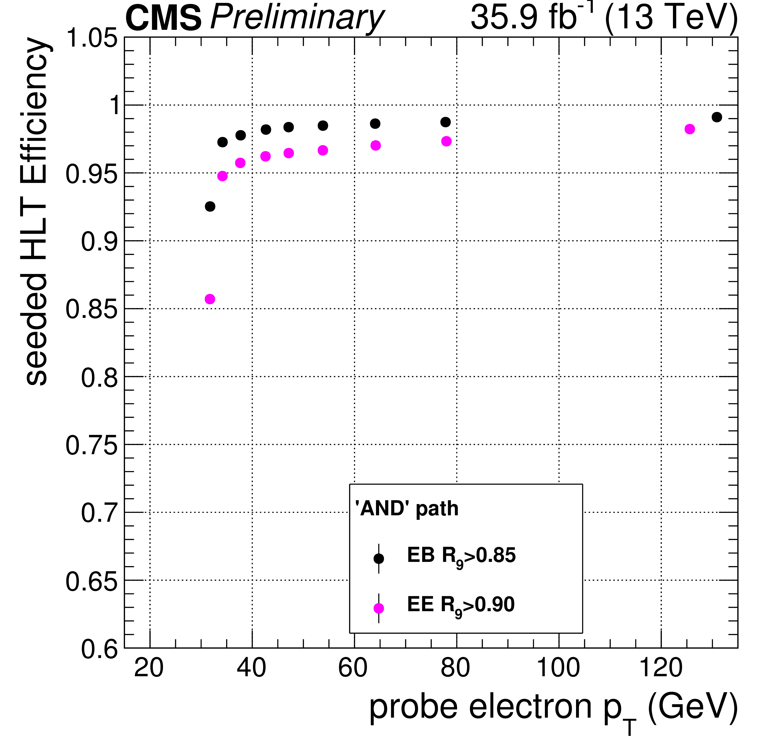
Additional Figure 2:
Efficiency for the seeded leg measured on data for $\mathrm{ Z\to ee }$ events using the tag-and-probe method, for the 'AND' high-level trigger (HLT) path used for the analysis of the 13 TeV dataset, with respect to offline probe electron $p_{\mathrm{T}}$, for ECAL barrel photons with $ {R_\mathrm {9}} > $ 0.85 (black) and endcap photons with $ {R_\mathrm {9}} > $ 0.9 (magenta). Variable bin widths have been used. |
png pdf |
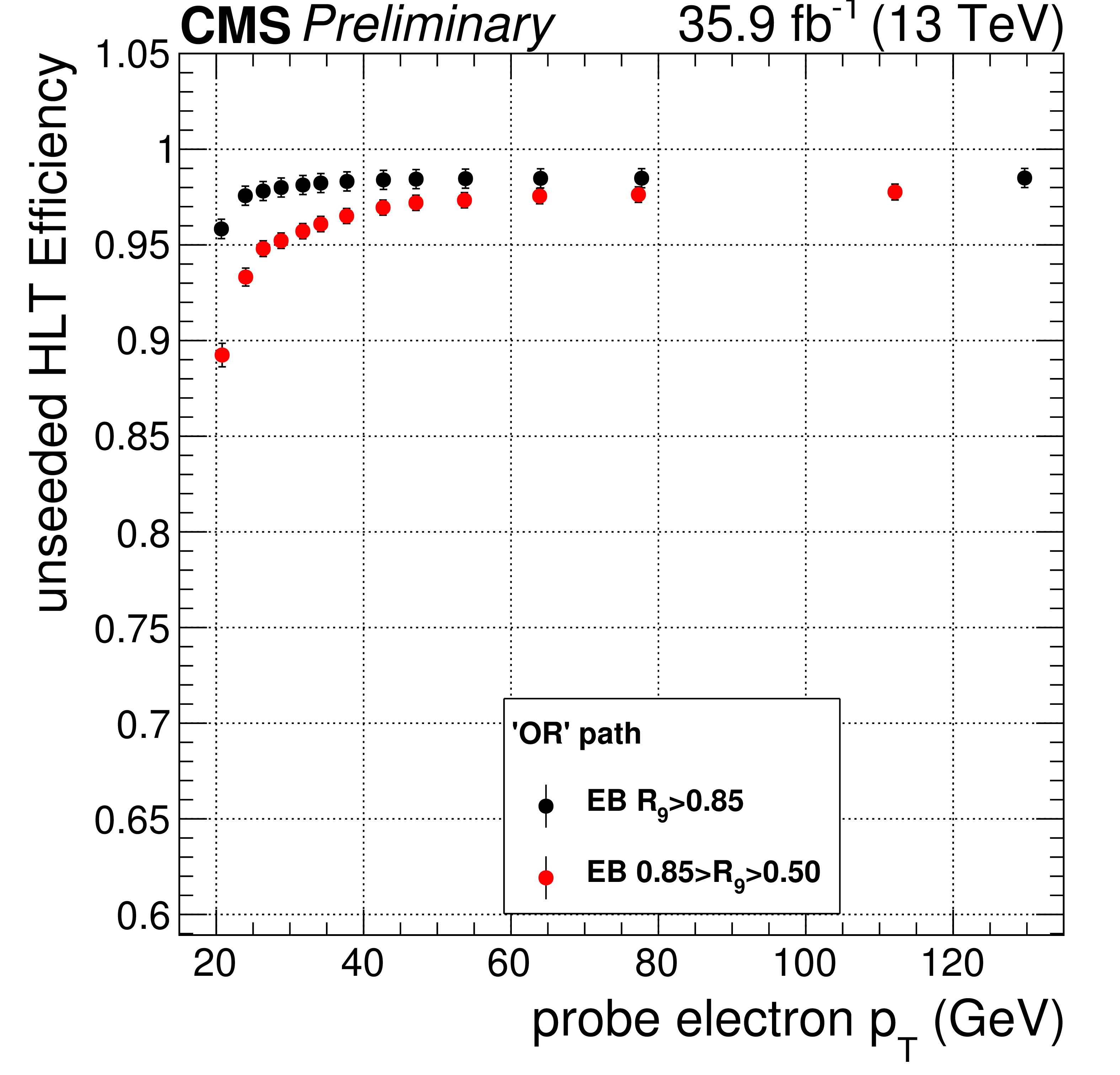
Additional Figure 3:
Efficiency for the unseeded leg measured on data for the 'OR' high-level trigger (HLT) path used for the analysis of the 13 TeV dataset, with respect to offline probe electron $p_{\mathrm{T}}$, for ECAL barrel photons with $ {R_\mathrm {9}} > $ 0.85 (black) and 0.5 $ < {R_\mathrm {9}} < $ 0.85 (red). Variable bin widths have been used. |
png pdf |
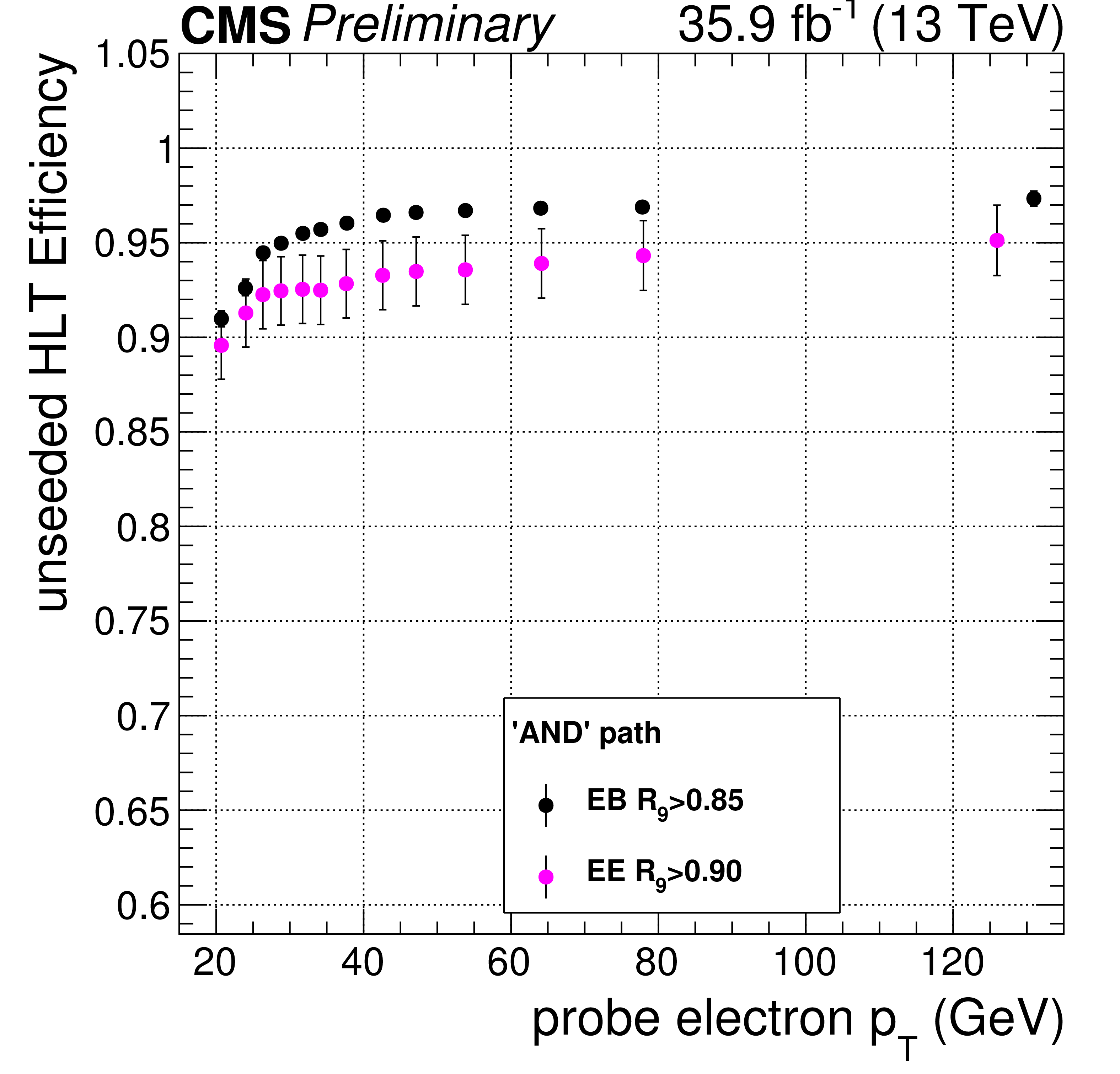
Additional Figure 4:
Efficiency for the unseeded leg measured on data for the 'AND' high-level trigger (HLT) path used for the analysis of the 13 TeV dataset, with respect to offline probe electron $p_{\mathrm{T}}$, for ECAL barrel photons with $ {R_\mathrm {9}} > $ 0.85 (black) and endcap photons with $ {R_\mathrm {9}} > $ 0.9 (magenta). Variable bin widths have been used. |
png pdf |
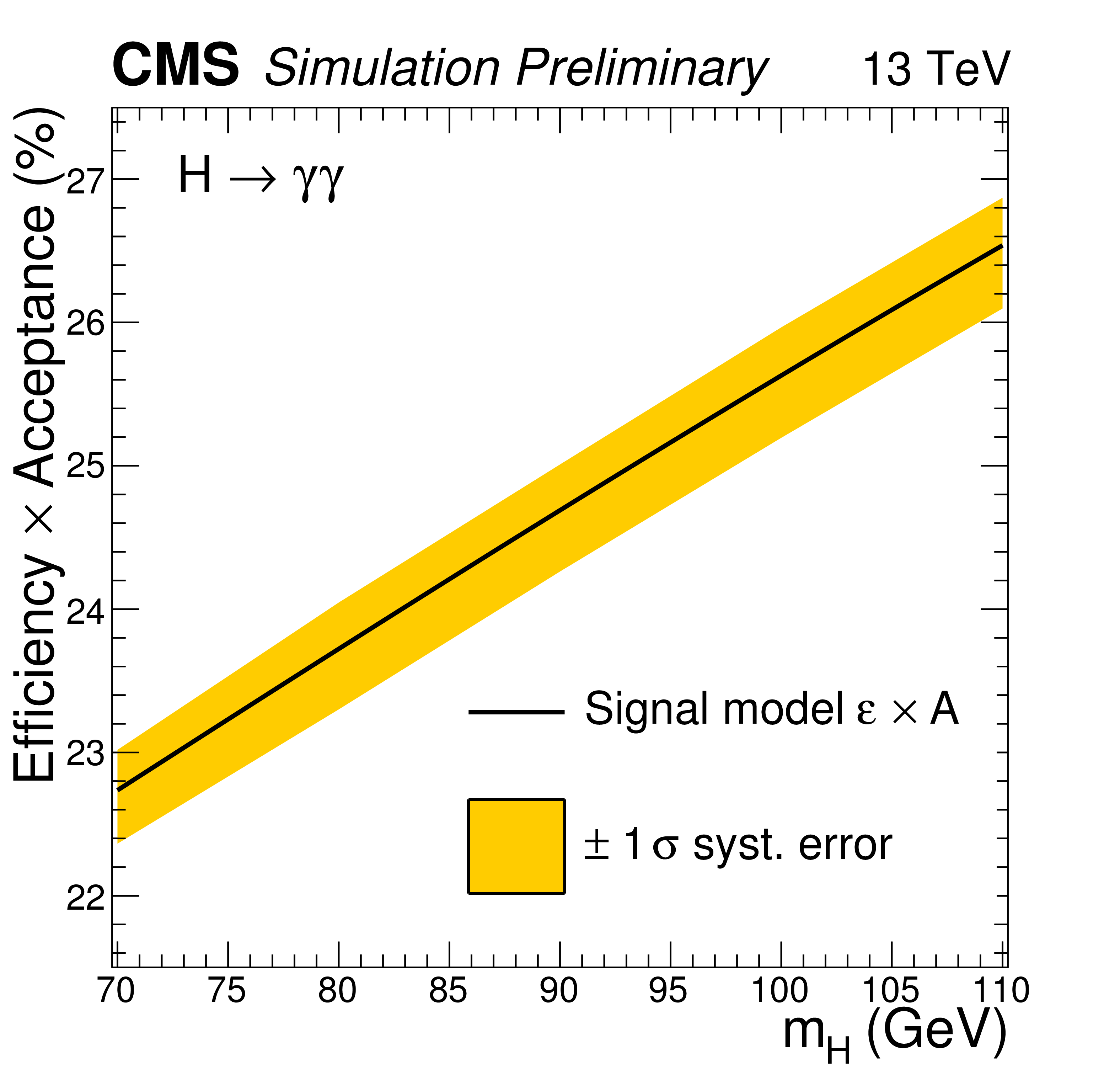
Additional Figure 5:
Signal efficiency$\times $acceptance for the analysis of the 13 TeV dataset, as a function of mass hypothesis. |
png pdf |
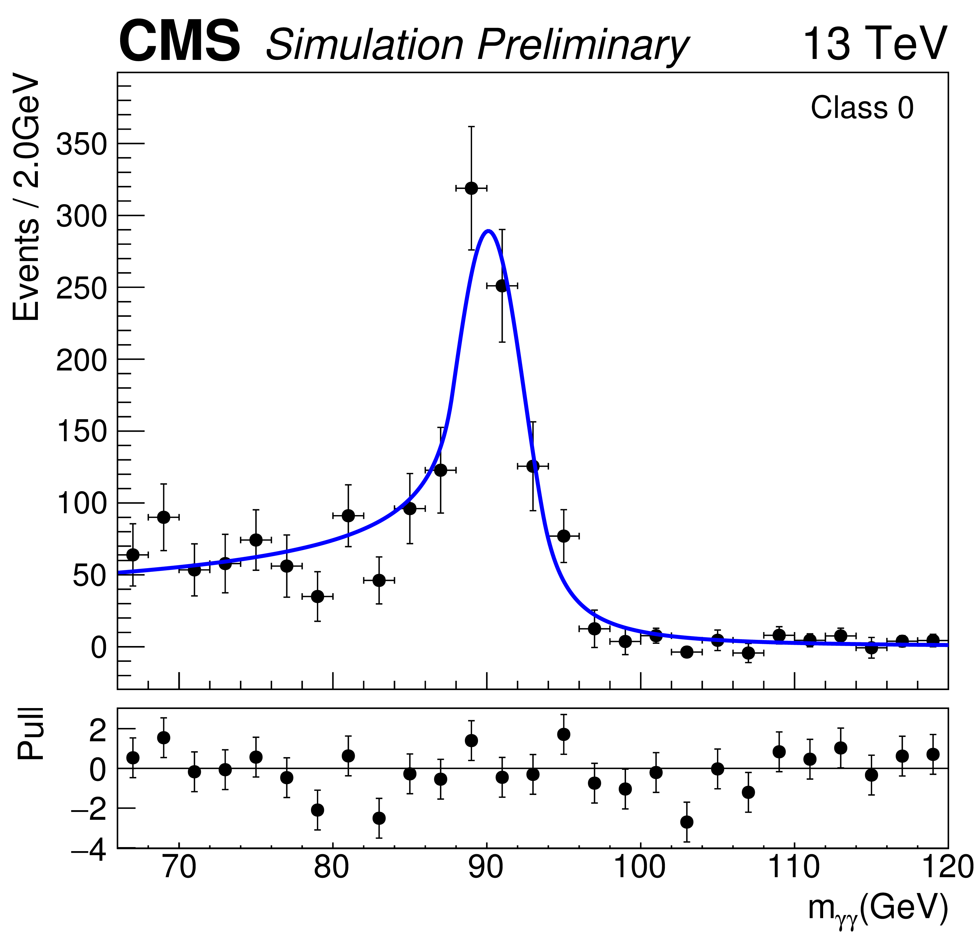
Additional Figure 6:
Double-sided Crystal Ball function fit to the dielectron invariant mass distribution from Drell-Yan 'double-fake' events for class 0, used for the analysis of the 13 TeV dataset. |
png pdf |
Additional Figure 7:
Double-sided Crystal Ball function fit to the dielectron invariant mass distribution from Drell-Yan 'double-fake' events for class 1, used for the analysis of the 13 TeV dataset. |
png pdf |
Additional Figure 8:
Double-sided Crystal Ball function fit to the dielectron invariant mass distribution from Drell-Yan 'double-fake' events for class 2, used for the analysis of the 13 TeV dataset. |
png pdf |
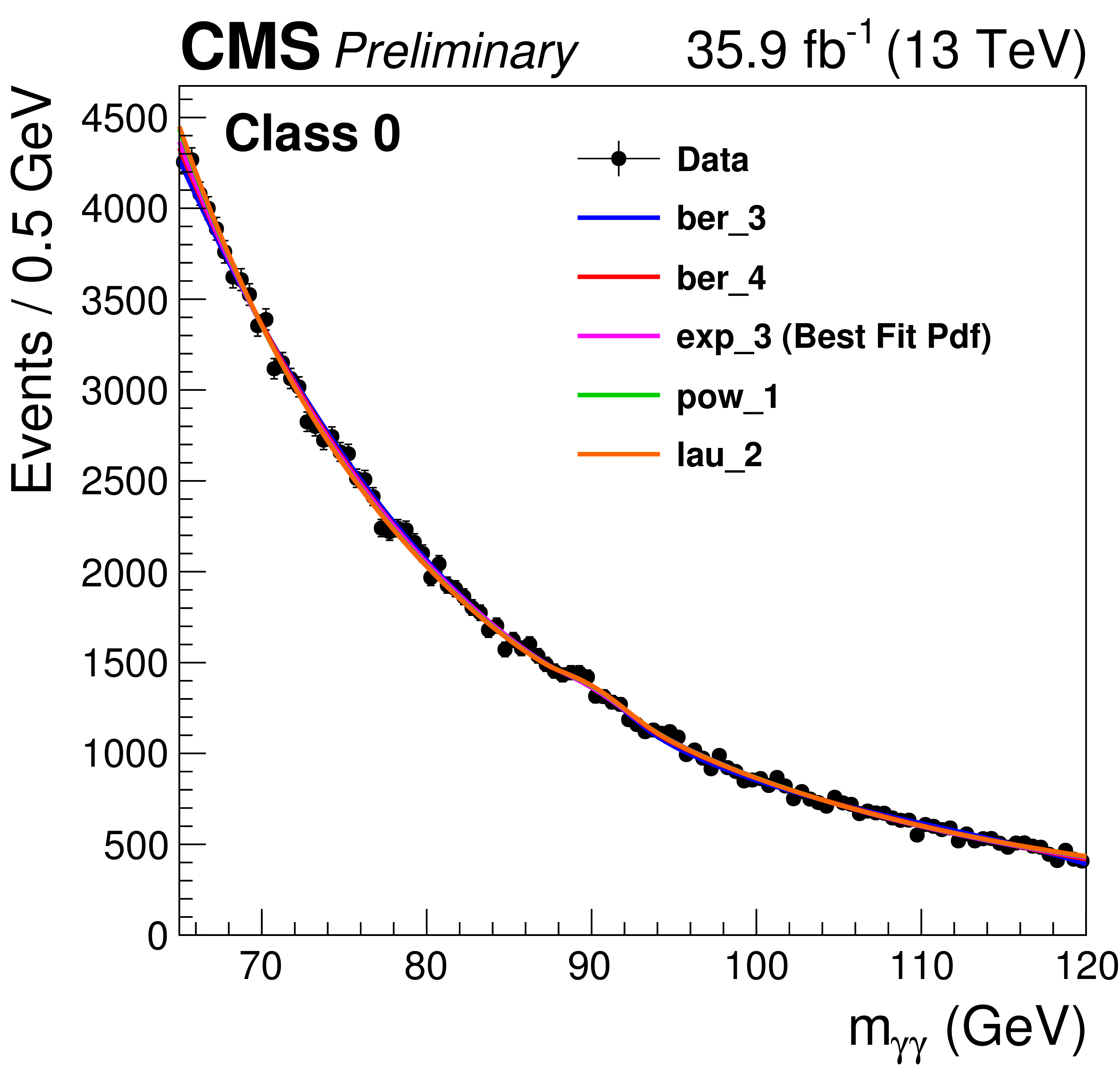
Additional Figure 9:
The set of functions chosen to fit the background using the discrete profiling method for the event class 0 in the analysis of the 13 TeV dataset. Four families of functions summed with the DCB function are considered: sums of exponentials, polynomials in the Bernstein basis, Laurent series and sums of power laws. |
png pdf |
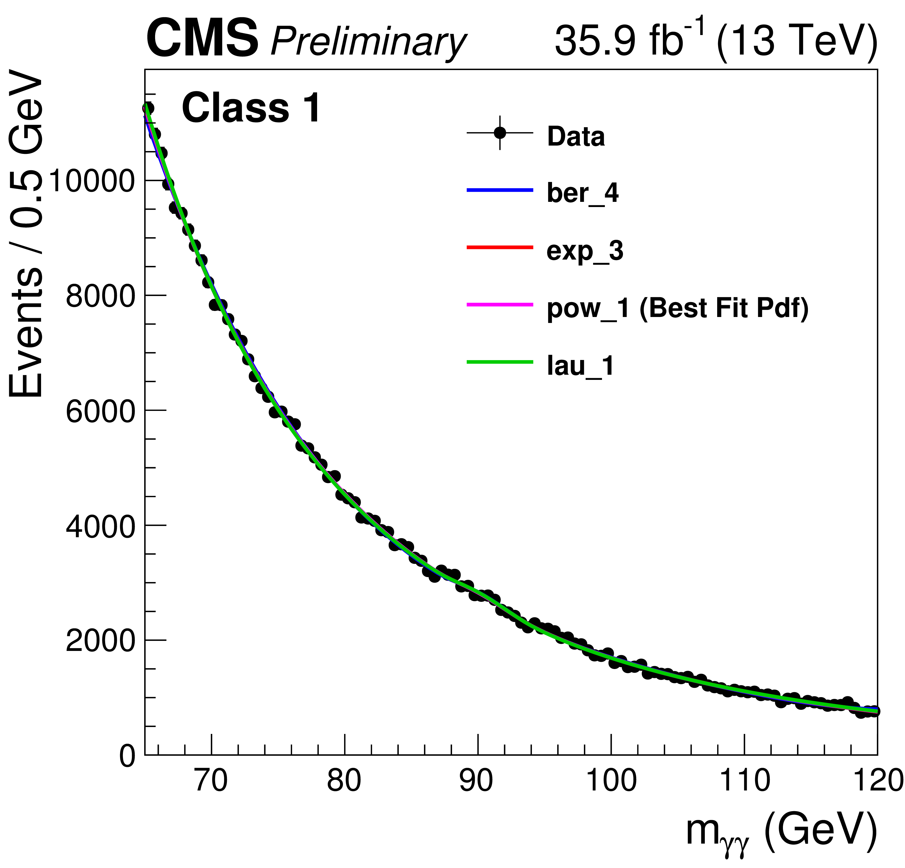
Additional Figure 10:
The set of functions chosen to fit the background using the discrete profiling method for the event class 1 in the analysis of the 13 TeV dataset. Four families of functions summed with the DCB function are considered: sums of exponentials, polynomials in the Bernstein basis, Laurent series and sums of power laws. |
png pdf |
Additional Figure 11:
The set of functions chosen to fit the background using the discrete profiling method for the event class 2 in the analysis of the 13 TeV dataset. Four families of functions summed with the DCB function are considered: sums of exponentials, polynomials in the Bernstein basis, Laurent series and sums of power laws. |
png pdf |
Additional Figure 12:
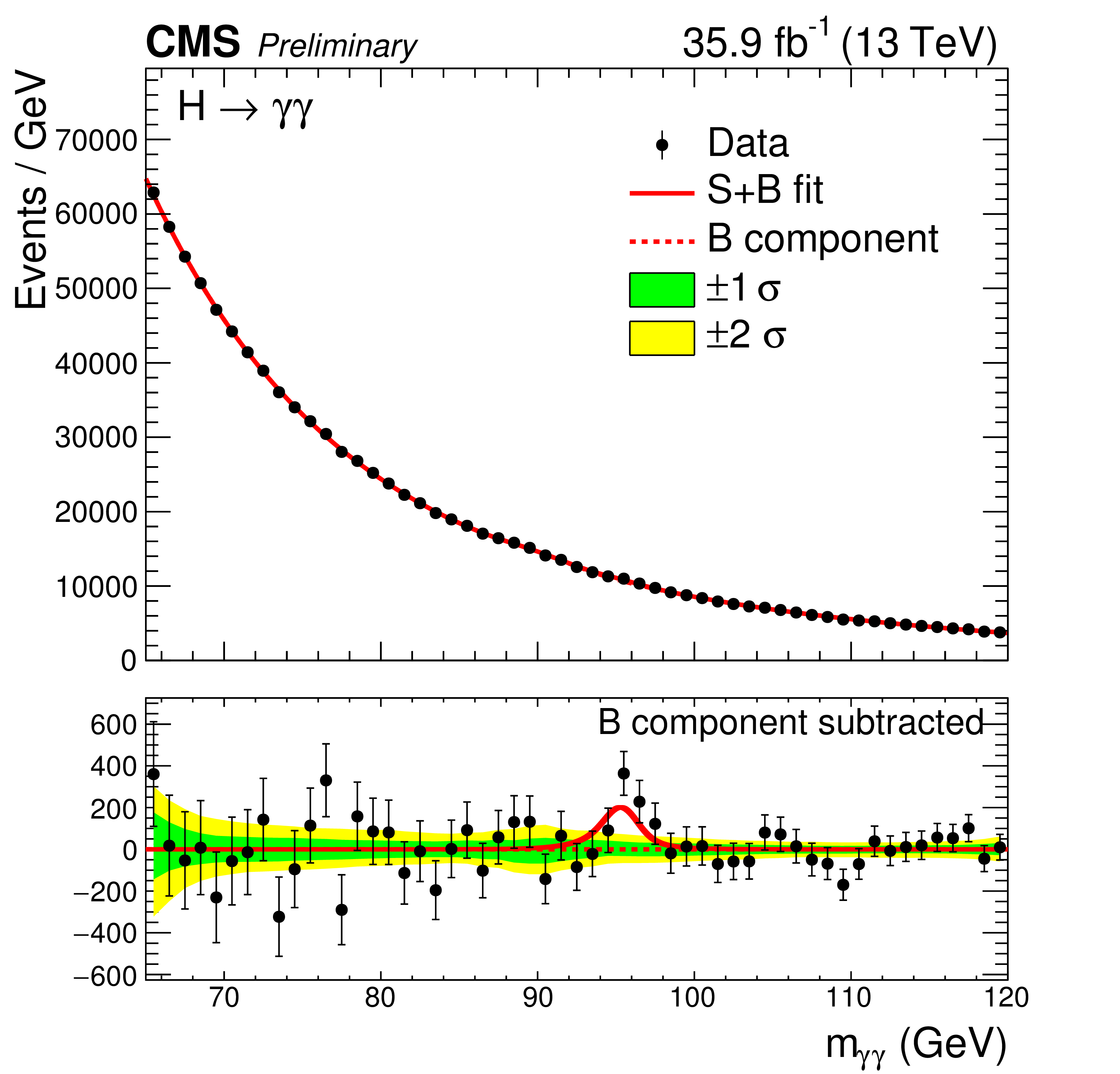
Events in the three classes of the 13 TeV dataset, binned as a function of $ {m_{\gamma \gamma}} $, together with the result of a fit of the signal-plus-background model. The 1$\sigma $ and 2$\sigma $ uncertainty bands shown for the background component of the fit include the uncertainty due to the choice of fit function and the uncertainty in the fitted parameters. The distribution of the residual data after subtracting the fitted background component is shown below. |
png pdf |
Additional Figure 13:
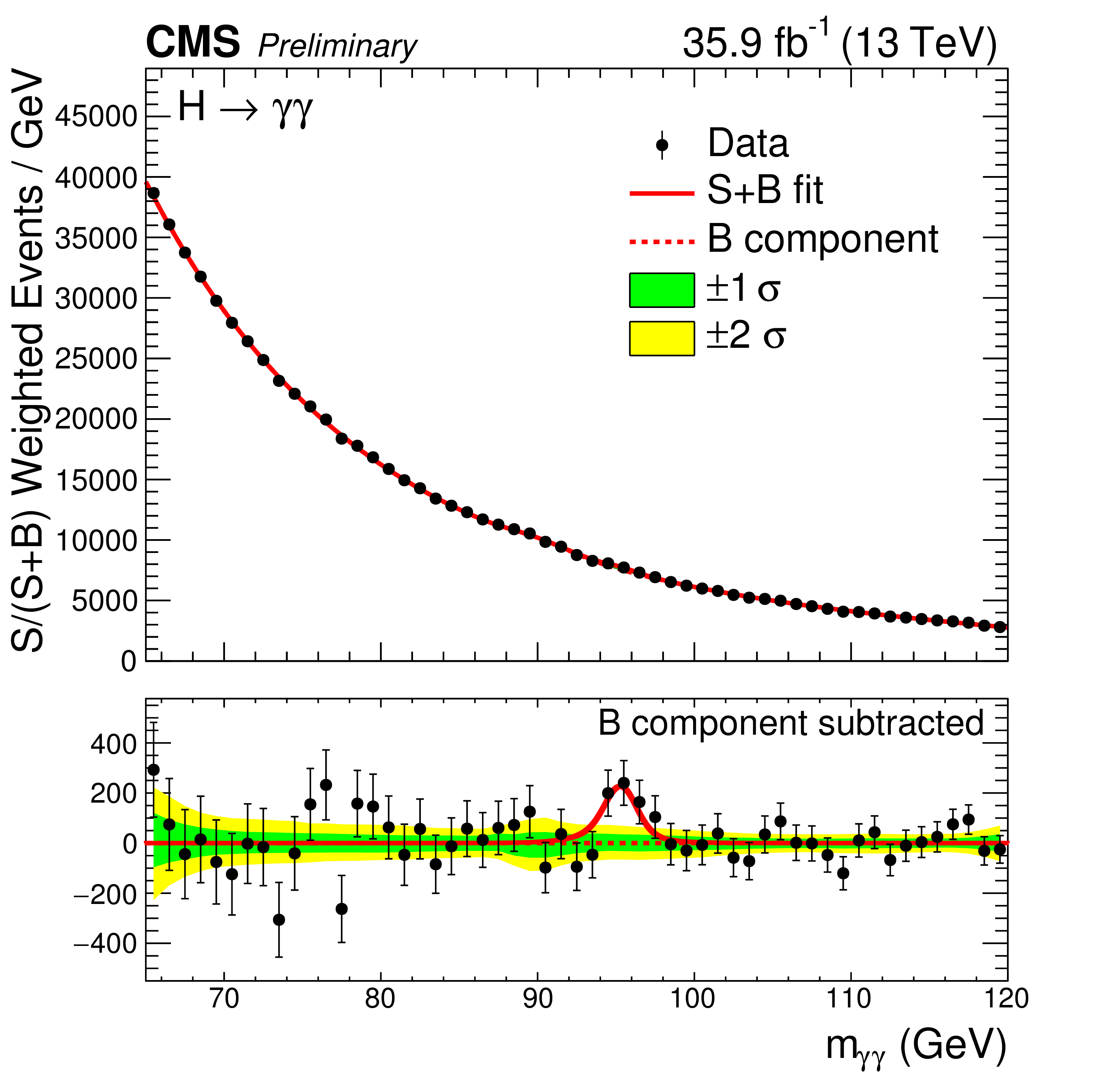
Events in the three classes of the 13 TeV dataset, binned as a function of $ {m_{\gamma \gamma}} $, where each event is weighted by the ratio S/(S+B) for its event class, together with the result of a fit of the signal-plus-background model. The 1$\sigma $ and 2$\sigma $ uncertainty bands shown for the background component of the fit include the uncertainty due to the choice of fit function and the uncertainty in the fitted parameters. The distribution of the residual weighted data after subtracting the fitted background component is shown below. |
png pdf |
Additional Figure 14:
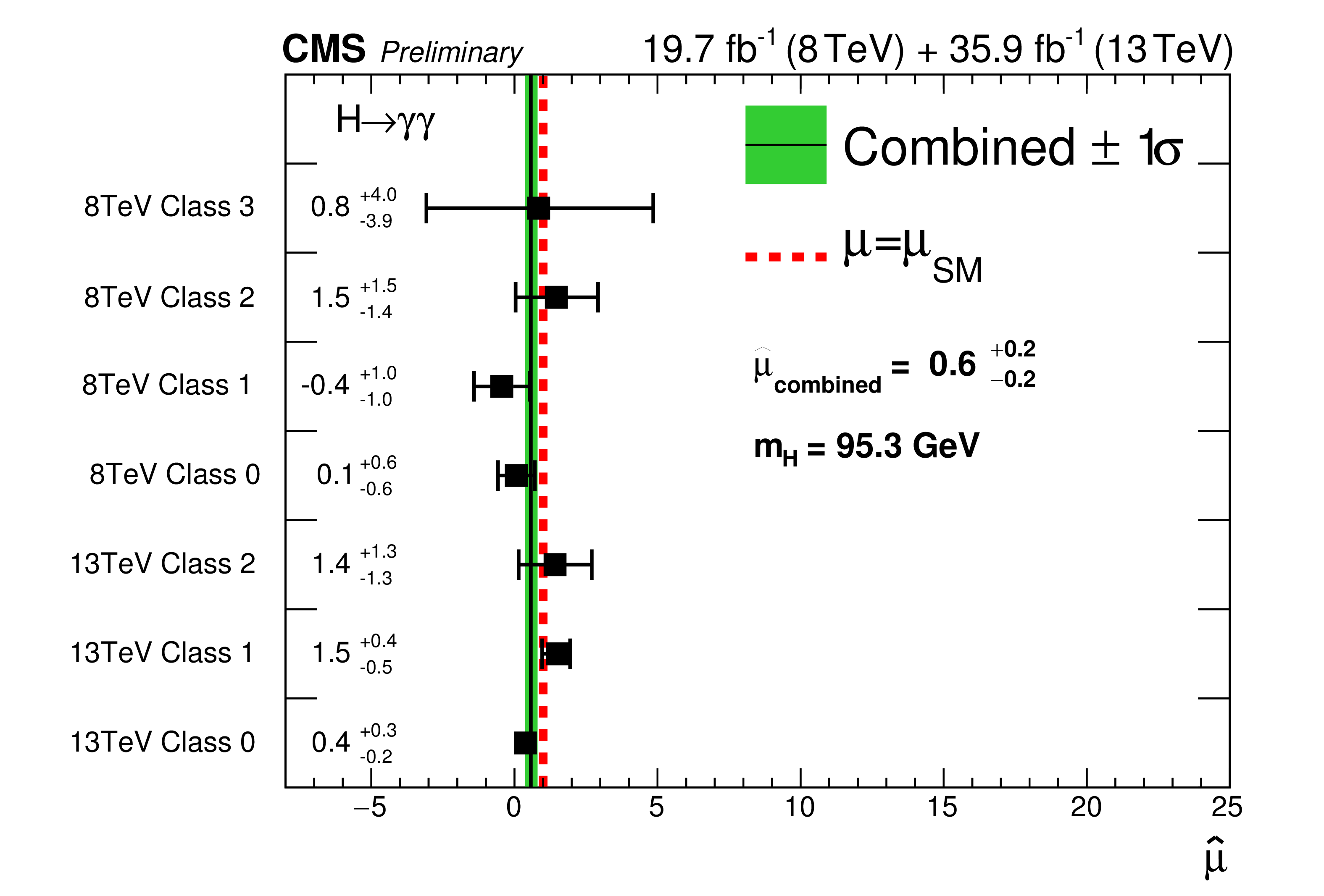
Values of the signal strength $\hat{\mu}$ measured individually for the seven event classes in the combination of the 8 and 13 TeV datasets, and the overall combined value, with $m_H$ fixed to that of the largest local p-value excess. The horizontal bars indicate $ \pm 1 \sigma $ uncertainties in the values, and the vertical line and band indicate the value of the combined $\hat{\mu}$ in the fit to the data and its uncertainty. The $\chi ^2$ probability of the values for the seven classes being compatible with the overall best-fit signal strength is 41%. |
| References | ||||
| 1 | S. L. Glashow | Partial-symmetries of weak interactions | NP 22 (1961) 579 | |
| 2 | S.Weinberg | A model of leptons | PRL 19 (1967) 1264 | |
| 3 | A. Salam | Weak and electromagnetic interactions | Elementary particle physics (1968) | |
| 4 | F. Englert and R. Brout | Broken symmetry and the mass of gauge vector mesons | PRL 13 (1964) 321 | |
| 5 | P.W. Higgs | Broken symmetries, massless particles and gauge fields | PL12 (1964) 132 | |
| 6 | P.W. Higgs | Broken symmetries and the masses of gauge bosons | PRL 13 (1964) 508 | |
| 7 | G. S. Guralnik, C. R. Hagen, and T. W. B. Kibble | Global conservation laws and massless particles | PRL 13 (Nov, 1964) 585--587 | |
| 8 | P. W. Higgs | Spontaneous symmetry breakdown without massless bosons | PR145 (May, 1966) 1156--1163 | |
| 9 | T. W. B. Kibble | Symmetry breaking in non-abelian gauge theories | PR155 (Mar, 1967) 1554--1561 | |
| 10 | ATLAS Collaboration | Observation of a new particle in the search for the Standard Model Higgs boson with the ATLAS detector at the LHC | PLB716 (2012) 1--29 | 1207.7214 |
| 11 | CMS Collaboration | Observation of a new boson at a mass of 125 GeV with the CMS experiment at the LHC | PLB716 (2012) 30--61 | CMS-HIG-12-028 1207.7235 |
| 12 | P. Fayet | Supergauge Invariant Extension of the Higgs Mechanism and a Model for the electron and Its Neutrino | NPB90 (1975) 104--124 | |
| 13 | R. Barbieri, S. Ferrara, and C. A. Savoy | Gauge Models with Spontaneously Broken Local Supersymmetry | PLB119 (1982) 343 | |
| 14 | M. Dine, W. Fischler, and M. Srednicki | A Simple Solution to the Strong CP Problem with a Harmless Axion | PLB104 (1981) 199 | |
| 15 | H. P. Nilles, M. Srednicki, and D. Wyler | Weak Interaction Breakdown Induced by Supergravity | PLB120 (1983) 346 | |
| 16 | J. M. Frere, D. R. T. Jones, and S. Raby | Fermion Masses and Induction of the Weak Scale by Supergravity | NPB222 (1983) 11 | |
| 17 | J. P. Derendinger and C. A. Savoy | Quantum Effects and SU(2) x U(1) Breaking in Supergravity Gauge Theories | NPB237 (1984) 307 | |
| 18 | J. Ellis et al. | Higgs bosons in a nonminimal supersymmetric model | PRD 39 (Feb, 1989) 844--869 | |
| 19 | M. Drees | Supersymmetric Models with Extended Higgs Sector | Int. J. Mod. Phys. A4 (1989) 3635 | |
| 20 | U. Ellwanger, M. Rausch de Traubenberg, and C. A. Savoy | Particle spectrum in supersymmetric models with a gauge singlet | PLB315 (1993) 331--337 | hep-ph/9307322 |
| 21 | U. Ellwanger, M. Rausch de Traubenberg, and C. A. Savoy | Higgs phenomenology of the supersymmetric model with a gauge singlet | Z. Phys. C67 (1995) 665--670 | hep-ph/9502206 |
| 22 | U. Ellwanger, M. Rausch de Traubenberg, and C. A. Savoy | Phenomenology of supersymmetric models with a singlet | NPB492 (1997) 21--50 | hep-ph/9611251 |
| 23 | T. Elliott, S. F. King, and P. L. White | Unification constraints in the next-to-minimal supersymmetric standard model | PLB351 (1995) 213--219 | hep-ph/9406303 |
| 24 | S. F. King and P. L. White | Resolving the constrained minimal and next-to-minimal supersymmetric standard models | PRD52 (1995) 4183--4216 | hep-ph/9505326 |
| 25 | F. Franke and H. Fraas | Neutralinos and Higgs bosons in the next-to-minimal supersymmetric standard model | Int. J. Mod. Phys. A12 (1997) 479--534 | hep-ph/9512366 |
| 26 | M. Maniatis | The Next-to-Minimal Supersymmetric extension of the Standard Model reviewed | Int. J. Mod. Phys. A25 (2010) 3505--3602 | 0906.0777 |
| 27 | U. Ellwanger, C. Hugonie, and A. M. Teixeira | The Next-to-Minimal Supersymmetric Standard Model | PR 496 (2010) 1--77 | 0910.1785 |
| 28 | A. Celis, V. Ilisie, and A. Pich | LHC constraints on two-Higgs doublet models | JHEP 07 (2013) 053 | 1302.4022 |
| 29 | B. Coleppa, F. Kling, and S. Su | Constraining Type II 2HDM in Light of LHC Higgs Searches | JHEP 01 (2014) 161 | 1305.0002 |
| 30 | S. Chang et al. | Two Higgs doublet models for the LHC Higgs boson data at $ \sqrt{s}= $ 7 and 8 TeV | JHEP 09 (2014) 101 | 1310.3374 |
| 31 | CMS Collaboration | Observation of the diphoton decay of the Higgs boson and measurement of its properties | EPJC74 (2014), no. 10 | CMS-HIG-13-001 1407.0558 |
| 32 | CMS Collaboration | Higgs to diphoton with 13 TeV with full 2016 dataset | CMS-PAS-HIG-16-040, CERN, Geneva | CMS-PAS-HIG-16-040 |
| 33 | CMS Collaboration | Search for new resonances in the diphoton final state in the mass range between 80 and 110 GeV in pp collisions at $ \sqrt{s}= $ 8 TeV | CMS-PAS-HIG-14-037 | CMS-PAS-HIG-14-037 |
| 34 | ATLAS Collaboration | Search for Scalar Diphoton Resonances in the Mass Range $ 65-600 $ GeV with the ATLAS Detector in $ pp $ Collision Data at $ \sqrt{s} = $ 8 TeV | PRL 113 (2014), no. 17, 171801 | 1407.6583 |
| 35 | CMS Collaboration | The CMS experiment at the CERN LHC | JINST 3 (2008) S08004 | CMS-00-001 |
| 36 | CMS Collaboration | Performance of photon reconstruction and identification with the CMS detector in proton-proton collisions at $ \sqrt{s} = $ 8 TeV | JINST 10 (2015) P08010 | CMS-EGM-14-001 1502.02702 |
| 37 | CMS Collaboration | The CMS trigger system | JINST 12 (2017) P01020 | CMS-TRG-12-001 1609.02366 |
| 38 | CMS Collaboration | Measurement of the inclusive W and Z production cross sections in pp collisions at $ \sqrt {s} = $ 7 TeV with the CMS experiment | JHEP 2011 (2011) 1 | |
| 39 | S. Alioli, P. Nason, C. Oleari, and E. Re | NLO Higgs boson production via gluon fusion matched with shower in POWHEG | JHEP 04 (2009) 002 | 0812.0578 |
| 40 | P. Nason and C. Oleari | NLO Higgs boson production via vector-boson fusion matched with shower in POWHEG | JHEP 02 (2010) 037 | 0911.5299 |
| 41 | T. Sjostrand, S. Mrenna, and P. Skands | PYTHIA 6.4 physics and manual | JHEP 05 (2006) 026 | hep-ph/0603175 |
| 42 | J. Alwall et al. | The automated computation of tree-level and next-to-leading order differential cross sections, and their matching to parton shower simulations | JHEP 07 (2014) 079 | 1405.0301 |
| 43 | R. Frederix and S. Frixione | Merging meets matching in MC@NLO | JHEP 12 (2012) 061 | 1209.6215 |
| 44 | T. Sjostrand, S. Mrenna, and P. Z. Skands | A Brief Introduction to PYTHIA 8.1 | CPC 178 (2008) 852--867 | 0710.3820 |
| 45 | CMS Collaboration | Measurement of the Underlying Event Activity at the LHC with $ \sqrt{s}= $ 7 TeV and Comparison with $ \sqrt{s} = $ 0.9 TeV | JHEP 09 (2011) 109 | CMS-QCD-10-010 1107.0330 |
| 46 | CMS Collaboration | Event generator tunes obtained from underlying event and multiparton scattering measurements | CMS-GEN-14-001 1512.00815 |
|
| 47 | LHC Higgs Cross Section Working Group Collaboration | Handbook of LHC Higgs Cross Sections: 3. Higgs Properties | 1307.1347 | |
| 48 | LHC Higgs Cross Section Working Group Collaboration | Handbook of LHC Higgs Cross Sections: 4. Deciphering the Nature of the Higgs Sector | 1610.07922 | |
| 49 | GEANT4 Collaboration | GEANT4---a simulation toolkit | NIMA 506 (2003) 250 | |
| 50 | T. Gleisberg et al. | Event generation with SHERPA 1.1 | JHEP 02 (2009) 007 | 0811.4622 |
| 51 | J. Alwall et al. | MadGraph 5 : Going Beyond | JHEP 06 (2011) 128 | 1106.0522 |
| 52 | P. D. Dauncey, M. Kenzie, N. Wardle, and G. J. Davies | Handling uncertainties in background shapes: the discrete profiling method | JINST 10 (2015), no. 04, P04015 | 1408.6865 |
| 53 | CMS Collaboration | CMS Luminosity Based on Pixel Cluster Counting - Summer 2013 Update | CMS-PAS-LUM-13-001 | CMS-PAS-LUM-13-001 |
| 54 | CMS Collaboration | CMS Luminosity Measurements for the 2016 Data Taking Period | CMS-PAS-LUM-17-001 | CMS-PAS-LUM-17-001 |
|
|
Compact Muon Solenoid LHC, CERN |
|

|

|

|

|

|